1

On the Dispersive Nature of the Power Dissipatedinto a Lossy Half-Space Close to a Radiating

SourceAndrea Cozza,Member, IEEE, and Benoît Derat,Member, IEEE

Abstract— In this paper, we study how the power dissipatedinto a lossy medium excited by a nearby antenna is affectedby drifts in the electrical parameters of the lossy medium.The statistical distribution of the sensitivity of the dissipatedpower is determined by means of a spectral analysis of thetransmission of electromagnetic energy from air into the lossyhalf-space. A clear link is drawn between the reactive contentof the field excited by the source and the dispersiveness of thesensitivity. The case of a stratified structure is also addressed,by defining a modification factor representing the alteration ofthe transmissivity and of its sensitivity when a buffer layer isintroduced. All of the results provided point out that, in general,the sensitivity of the total amount of power dissipated intothehalf-space cannot be predicted independently from a preciseknowledge of the source characteristics, unless under a paraxialpropagation approximation or in a far-field configuration.

Index Terms— Antennas, Lossy Media, Near Field, Plane-Wave Spectrum, Sensitivity Analysis, Specific Absorption Rate,Stratified Media.

I. I NTRODUCTION

In many practical configurations antennas stand near toa lossy half-space; an example of historical importance isthat of radiating sources placed over a lossy soil [1]. Manyother applications involve a similar scenario: radio-frequencyhyperthermia [2] and Specific Absorption-Rate (SAR) assess-ment [3] are but two examples. All of these configurationsshare a common concern, that of being able to estimate theamount of power that will be dissipated into the lossy medium.In the context of the present discussion, we will refer tothe concept of Total Dissipate Power (TDP). Depending onthe actual application, the TDP needs to be maximized orminimized, but all the same its value closely depends on theelectrical properties of the concerned medium, namely theelectric conductivityσ and the relative permittivityǫr. Thebasic need of a proper estimation of these parameters thusappears as a potential difficulty in the computation of theTDP; hence, it is fundamental to investigate how the TDPcan be affected by a variation of the electrical parameters ofthe medium, be that due to a drift in time or rather to anuncertainty in their knowledge.

The primary aim of this paper is twofold: 1) to providea model capable of predicting the sensitivity of the TDP

A. Cozza is with SUPELEC, Département de Recherche en Électromag-nétism, Gif-sur-Yvette, France, e-mail: andrea.cozza@supelec.fr.

B. Derat is with Field-Imaging, Meudon, France, e-mail:benoit.derat@field-imaging.com.

Manuscript received ..., 2008; revised ...

xz

y

S

s,er

Pin

0

Einc Etx

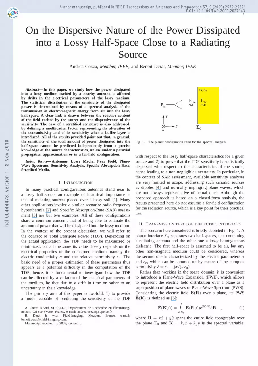
Fig. 1. The planar configuration used for the spectral analysis.

with respect to the lossy half-space characteristics for a givensource and 2) to prove that the TDP sensitivity is statisticallydispersed with respect to the characteristics of the source,hence leading to a non-negligible uncertainty. In particular, inthe context of SAR assessment, available sensitivity analysesare very limited in scope, addressing such canonic sourcesas dipoles [4] and normally impinging plane waves, whichare not always representative of actual ones. Although theproposed approach is based on a closed-form analysis, theresults presented here do not assume a far-field configurationfor the radiation source, which is a key point for their practicaluse.

II. T RANSMISSION THROUGH DIELECTRIC INTERFACES

The scenario here considered is briefly depicted in Fig. 1. Aplanar interfaceΣ0 separates two half-spaces, one containinga radiating antenna and the other one a lossy homogeneousdielectric. The first half-space is assumed to be air, but anyother non-magnetic medium could be considered, whereasthe second one is characterized by the electric parametersσand ǫr, which can be summed up by means of the complexpermittivity ǫ = ǫr − jσ/(ωǫ0).

Rather than working in the space domain, it is convenientto introduce a Plane-Wave Expansion (PWE), which allowsto represent the electric field distribution over a plane as asuperposition of plane waves or Plane-Wave Spectrum (PWS).Considering the electric fieldE(R) over a plane, its PWSE(K) is defined as [5]:

E(K, 0) =

∫

Σ0

E(R, 0)ejK·RdR , (1)

whereR = xx + yy spans the entire field topography overthe planeΣ0 and K = kxx + ky y is the spectral variable;

hal-0

0444

478,

ver

sion

1 -

8 N

ov 2

010

Author manuscript, published in "IEEE Transactions on Antennas and Propagation 57, 9 (2009) 2572-2582" DOI : 10.1109/TAP.2009.2027143

2

hereafter, capital hatted quantities will stand for PWSs. Therationale for this approach is that in the spectral domain itis much easier to represent the propagation of complex fieldtopographies through stratified media. The PWS over planesat other distancesz at the right ofΣ0 can be easily computedintroducing the propagatorP (K, z) = exp(−jkzz):

E(K, z) = E(K, 0)P (K, z) , (2)

with kz =√

k2 − ‖K‖2 as the longitudinal propagationconstant, andk the propagation constant for the consideredmedium. The norms used throughout this work are to beintended asL2 norms applied to complex vectors, unlessexplicitly declared otherwise.

The PWE formalism can be defined just over the tangentialcomponents of the vectors involved; for this reason, we willdecompose the electric field PWS as

E = E‖ + Ez z , (3)

having defined the tangential part of the PWS asE‖ =

Exx + Ey y. The overall PWSE can be derived by recallingthat Gauss law in a homogeneous medium in absence of localsources reads ask · E = 0, i.e.,

Ez = −K · E‖

kz, (4)

where k = K + kz z is the propagation vector for a planewave. Thus, (3) can be recast as

E =

1 00 1

−kx

kz−ky

kz

E

‖ = TE‖ . (5)

Let us now consider the interfaceΣ0: for each plane waveimpinging from the left side, there will be a transmitted planewave. Imposing the continuity of the tangential componentsofthe electric field through the air-dielectric interface, the PWSE

‖inc(K) of the incident electric field overΣ−

0 (i.e., on the airside) and the PWSE‖

tx(K) of the field overΣ+0 (on the right

side) are related by [5]:

E‖tx(K) = Π0(K)E

‖inc(K) , (6)

whereΠ0(K) is the spectral transmission operator for a planarinterface, as recalled in Appendix I. Hereafter, theR andK-dependency of, respectively, the spatial and spectral functionswill be omitted most of the time for the sake of simplicity.

The TDP is related to the transmitted field by

TDP = σ

∫

Ω

‖Etx(R, z)‖2dV , (7)

where Ω is the volume occupied by the lossy half-space.Thanks to Parseval theorem (as applied overΣ+

0 ), we can statethat

TDP = σ

∫ ‖Etx‖2

−2Im kzdK . (8)

We will now introduce the only two major assumptions usedthroughout this work: 1) the spatial bandwidthkBW of theelectric field PWS, satisfies the conditionkBW . k0|χ|, whereχ =

√ǫ is the dielectric contrast of the lossy medium and 2)

the medium can be described as a lossy dielectric, i.e.,σ ≪ωǫ0ǫr. The first requirement is necessary so that the propagatormodulus|P (K, z)| be almost flat over the entire bandwidth ofthe source PWS, allowing the approximationkz ≃ k0χ; thesecond assumption is needed in order to simplify the finalresults, although closed-form expressions could be given evenin a more general case. Under such conditions, (8) becomes

TDP ≃√

ǫr

ζ

∫

‖Etx‖2dK =

√ǫr

ζE . (9)

whereζ is the free-space wave impedance, and having definedas in signal analysis thesignal energy E = ‖Etx(R)‖2

L2 as thesquare of theL2 norm of the field distribution overΣ+

0 .A major issue in this approach is that whenever the dielectric

interface is in the near-field region of the source, couplingmechanisms will likely ensue. For a given distanced betweenthe source and the half-space, the field impinging on thedielectric interface may differ from the one that would be mea-sured at the same distance in a free-space configuration. Thesephenomena notwithstanding, the approach here proposed canalso be applied to near-field configurations, without any lossof generality. Indeed, the coupling between one source anda passive scatterer can be regarded as given by an infiniteseries of separate interactions. This can be referred to as themultiple-interaction paradigm, and it has been applied, amongother scenarios, in the definition of probe-correction modelsfor near-field measurement techniques [6].

The basic idea is that the time-domain evolution of thecoupling is naturally represented through a series of simpleinteractions, that can be divided into scattering, transmittingand receiving events. The actual fieldE

‖inc impinging over the

half-space is thus generally not the one that would be radiatedin a free-space configuration, e.g. in a far-field scenario,but rather the superposition of all the multiple-interactioncontributions, i.e. the steady-state field including the actualcoupling. This approach is completely general, with the far-field scenario as a special case.

III. SENSITIVITY ANALYSIS

We proceed by deriving a sensitivity model for the TDP, asdiscussed in Section III-A.A; subsequently, this model will beused in order to investigate how the TDP sensitivity is linked tothe PWS of the source (and ultimately to the field it radiates),proving in Section III-B.B that for a given configuration thesensitivity is, in general, not a deterministic value, but rathera random variable.

A. Perturbation model

The sensitivity of the TDP to variations ofǫ can be assessedby applying a perturbation approach to the transmission equa-tion (6). While a perturbation ofǫ has a direct impact on theTDP, it will have a higher-order effect on the reflectivity ofthe medium interface, as seen from free-space. In other words,it will be hardly noticed by the source: it will be shown inSection VI that this idea is viable, as long as the dielectriccontrast|χ| stays high. This conclusion is intuitively justifiedby the fact that the fundamental quantity in source-half-space

hal-0

0444

478,

ver

sion

1 -

8 N

ov 2

010

3

interactions is the dielectric contrast between the two media,which is negligibly affected by the lossy medium perturbation;this phenomenon was already pointed out in [7]. Therefore, itwill be assumed that the total incident electric fieldEinc(R)fulfills the condition‖∂Einc/∂ǫ‖ ≪ ‖∂Etx/∂ǫ‖.

The second order Taylor expansion of (9) with respect tothe complex dielectric permittivityǫ reads:

δTDP

TDP=

δEE +

δ√

ǫr√ǫr

+δ2E2E +

δ2√ǫr

2√

ǫr+

δ√

ǫr√ǫr

δEE . (10)

with:

δ√

ǫr√ǫr

=1

2

δǫr

ǫr(11)

δ2√ǫr√ǫr

= − 1

4ǫr

δǫr

ǫr(12)

The TDP sensitivity depends onδE/E andδǫr/ǫr sensitivityterms; since the latter are trivial, we will focus our analysison the former. Moreover, in the subsequent statistical analysisof the sensitivity,δǫr/ǫr introduces a mere offset, withoutaccounting for the statistical dispersion of the TDP sensitivity.

We will detail here the proposed analysis method for thefirst-order termδE/E , the second-order being derived fun-damentally in the same way. Knowing that the first-orderdifferential of the norm of a complex vectorv is related tothe differential of a complex variablep by

d‖v(p)‖2 = 2Re

vH ∂v

∂pdp

, (13)

where the apexH stands for the Hermitian transpose, we canwrite:

δE = 2Re

δǫ

∫

EHtx

∂Etx

∂ǫdK

. (14)

Using (5) and (6), together with the hypothesis of a weaklysensitive source, the following quadratic form is obtained:

δE = 2Re

δǫ

∫

E‖Htx D1E

‖txdK

, (15)

having defined matrixD1 as follows:

D1 = THD

′1 (16)

D′1 =

∂T

∂ǫ+ T

∂Π0

∂ǫΠ

−10 . (17)

A great part of the results dealing with the sensitivity willbeexpressed as functions of the transmitted PWS. The rationalefor this choice is that the PWS ofEtx is more regularthan the one in air, so that its envelope is more easilydescribed and reproduced. This is important for the subsequentstatistical analysis. Moreover, the mathematical analysis is alsosimplified thanks to this formalism, since the properties ofthedifferent operators are more readily applicable. In any case, theresults are not affected by this choice, since the PWSEinc andEtx are biunivocally related through the transmission operator.

All the derivatives involving the transmission matrices arereported in Appendix I. It is sensible to define the operator

S : C2×2 → C, hereafter referred to as the sensitivity operator:

S(A) =

∫

E‖Htx A E

‖txdK

∫

∥

∥

∥TE

‖tx

∥

∥

∥

2

dK

. (18)

Therefore, we can now provide the following fundamentalresult:

δEE = 2Re S(D1)δǫ . (19)

This formulation has the advantage of pointing out the factthat the sensitivity is of course dependent on the PWS of theexcitation, but that in fact its behavior is controlled by a kernel,modeled through the matrixD1, that is common to everysource. In other words,D1 represents the transfer functionbetween the PWS of the impinging wave and the sensitivitythat its components will experience while being transmittedinto the lossy medium.

The development applied to the linear term can also beapplied to the quadratic term in (10), the only differencebeing that it is now necessary to consider the second-orderdifferential of the norm of a vectorv:

d2‖v‖2 = 2

∥

∥

∥

∥

∂v

∂pdp

∥

∥

∥

∥

2

+ 2Re

vH ∂2

v

∂p2(dp)2

, (20)

hence

δ2E2E = Re

(δǫ)2S(D2)

+ |δǫ|2S(D3) , (21)

having introduced the following matrices:

D2 = TH

(

∂2T

∂ǫ2+ T

∂2Π0

∂ǫ2Π

−10 +

+ 2∂T

∂ǫ

∂Π0

∂ǫΠ

−10

)

(22)

D3 = D′H1 D

′1 . (23)

The model thus derived allows computing the TDP sensi-tivity for a given source, just requiring as an input the PWSof the field impinging on the lossy half-space. An interestingby-product of the proposed analysis is that the frequencydependency of the TDP sensitivity is dominated by the termδǫ = δǫr − jδσ/(ωǫ0), as seen in (19) and (21). The factthat this term contains a1/f associated to the electricalconductivity term means that any model approximating itthrough a polynomial expansion is bound to need high-orderterms. This is actually the case, as proved by the choice madein [4], where a third-order frequency polynomial had beennecessary. The proposed representation, being derived from aphysical analysis, thus leads to a more effective definitionofthe sensitivity.

B. Statistical analysis

The previous results can be used for investigating thefollowing problem: how does the TDP sensitivity depend onthe PWS of the source? We will here describe the PWSE

‖tx

as a stationary random process and study how the energy

hal-0

0444

478,

ver

sion

1 -

8 N

ov 2

010

4

10−1

100

101

102−0.06

−0.04

−0.02

0

0.02

0.04

0.06

0.08

0.1

kx/k

0

λ H

0 1 2−0.015

−0.01

−0.005

0

10−1

100

101

102−0.2

−0.15

−0.1

−0.05

0

0.05

kx/k

0

λ S

0 1 2−0.01

−0.005

0

0.005

0.01

Fig. 2. Eigenvalues of the Hermitian and skew-Hermitian parts of operatorD1 associated to the linear sensitivity term, at 0.9 GHz (solidline), 2.5 GHz(dash line) and 6 GHz (dotted line). The results here shown regard the cutky = 0.

sensitivity δE/E is statistically distributed as a consequenceof the randomness of the source PWS.

This problem can be solved easily by means of (18), sinceall the quantities involved can be computed directly withoutany need of actual simulations or measurements. Nevertheless,(18) requires to impose a certain PWS distribution; it ispossible to prove that the sensitivity actually depends juston the envelope of the PWS, since (18) involves quadraticexpressions [8] (see Appendix II). For this reason, the energy-normalized spectrum envelopew(K) will be considered, asdefined by:

w(K) =‖E‖

tx‖2

∫

‖E‖tx‖2dK

. (24)

In the context of a statistical analysis, the sensitivity oper-ator defined in (18) can be evaluated directly; the focus willbe put on studying the first two statistical moments of thesensitivity for a given PWS energy-density spectrum〈w(K)〉.Since all the quantities in (19) and (21) are deterministic butfor the sensitivity operator, the statistical analysis will focuson this last term.

In particular, the following approximation holds (see Ap-pendix II) as long as the spatial bandwidthkBW of thenormalized energy-density spectrum〈w(K)〉 of the averagesource is smaller thank0|χ|:

〈S(A)〉 ≃∫

[

λH(K) + λS(K)]

〈w(K)〉dK , (25)

where λH and λS are the arithmetic means of, respectively,the eigenvalues of the Hermitian and the skew-Hermitian parts

10−1

100

101

102−0.025

−0.02

−0.015

−0.01

−0.005

0

0.005

kx/k

0

λ H

0 1 20

2

4

6

8x 10−4

10−1

100

101

102−0.02

−0.015

−0.01

−0.005

0

0.005

0.01

kx/k

0λ S

0 1 2−5

0

5

10

15x 10−4

10−1

100

101

1020

0.002

0.004

0.006

0.008

0.01

kx/k

0

λ

0 1 20

1

2

x 10−4

Fig. 3. Eigenvalues of the Hermitian and skew-Hermitian parts of operatorD2 and D3 (last picture) associated to the quadratic sensitivity term, at0.9 GHz (solid line), 2.5 GHz (dash line) and 6 GHz (dotted line). The resultshere shown regard the cutky = 0.

of matrix A, where this last stands for any of the derivativeoperatorsDi. This result is noteworthy, since it states that theaverage of the sensitivity over all the possible sources dependsexclusively on the properties of the lossy medium and theaverage spectral content of the source.

The dispersion of the TDP sensitivity around its average canbe assessed by studying the eigenvalues of the three derivativeoperatorsDi. Indeed:

∫

min λHwdK ≤ S(AH) ≤∫

maxλHwdK (26)∫

min λSwdK ≤ S(AS) ≤∫

maxλSwdK , (27)

so that, the distance between the eigenvalue pairs is a directmeasure of the dispersive nature of the sensitivity.

In order to test these ideas, we will hereafter consider aplanar SAR assessment configuration as a practical applica-tion, since it is an interesting example of high-contrast lossyconfiguration; the nominal electrical parameters of the lossy

hal-0

0444

478,

ver

sion

1 -

8 N

ov 2

010

5

Freq. (GHz) ǫr σ (S/m) |χ|

0.9 41.5 0.97 6.772.5 39.2 1.8 6.426 36.2 4.45 6.23

TABLE I

THE ELECTRICAL CHARACTERISTICS OF TISSUE-EQUIVALENT LIQUIDS

FOR SAR ASSESSMENT CONFIGURATIONS, AS SET IN [9].

medium are thus imposed by international standards, suchas [9], and are reported in Table I.

Therefore, the associated eigenvalues are shown in Fig. 2and 3, as computed for the three half-space configurations ofTable I. The spectral variable was normalized with respect tothe free-space wave-numberk0. MatricesD1 andD2 were ex-panded into their Hermitian and skew-Hermitian components,as explained in Appendix II, whereasD3 is already Hermitian.

Figures 2 and 3 show that each pair of eigenvalues coincidesaround the originK = 0, i.e., for normal paraxial incidence.The L2-integrable discontinuities aroundk0 are due to thebranch singularity in the spectrum of Green’s function [10];a similar behavior is present aroundk0|χ|, fundamentallydue to the same phenomena, but mitigated by losses. Con-versely, it can be noticed that the distance between each pairof eigenvalues widens with the time and space frequency.This trend gets much stronger when getting beyondk0, i.e.,when considering reactive components of the source PWS.More specifically, the skew-Hermitian components present anincreased distance with respect to the purely Hermitian onesfor a givenK. Looking at (19), the skew-Hermitian componentoperates over the variations in the conductivityσ: this meansthat the reactive components of the source PWS will beaffected in a more variable way in response to variationsof the conductivity than equal-strength modifications of thepermittivity. These simple conclusions already show that thesensitivity will present an higher degree of variability for near-field sources, richer in reactive energy, than far-field ones,where no reactive component is available; this is coherent withthe common-sense perception that the TDP sensitivity is notdispersed for a far-field configuration.

In order to assess these findings, the sensitivity operatorswere studied in several ways: 1) equation (25) was used forassessing the average sensitivity, 2) a deterministic estimatewas given assuming a paraxial propagation, thus consideringthe approximationS(D)(K) ≃ S(D)(0); and finally 3) equa-tion (18) was directly evaluated by considering a population often thousand random realizations for the transmitted PWS. Forthis last case, we considered a Gaussian energy-density spec-trum with a−3 dB bandwidthkBW = k0, with a zero-meanGaussian distribution. This choice is justified in the context ofSAR assessment tests for telecommunications, where sourcesare usually not highly directive. Table II shows the resultsofthis analysis. It turns out that the paraxial approximationis notvery effective when compared to (25); nevertheless, it allowsto introduce a very simple model for the average sensitivity, as

D1H jD1S D2H jD2S D3

〈S〉 −94 38 3.6 −3.9 1.0

0.9 GHzeq. (25) −94 41 3.6 −4.1 1.1paraxial −88 38 3.3 −3.7 0.91〈S2〉 9.2 3.8 0.36 0.38 0.10

〈S〉 −113 36 5.7 −4.2 1.4

2.5 GHzeq. (25) −108 34 5.5 −4.0 1.3paraxial −100 31 4.9 −3.4 1.1〈S2〉 11.0 3.4 0.53 0.39 0.13

〈S〉 −113 39 −5.8 4.8 1.5

6.0 GHzeq. (25) −114 40 −5.9 4.9 1.5paraxial −106 36 −5.4 4.3 1.3〈S2〉 11 3.9 0.58 0.47 0.14

TABLE II

SENSITIVITY OPERATORS FOR AGAUSSIAN-ENVELOPEPWS,WITH

BANDWIDTH k0 . ALL THE RESULTS MUST BE MULTIPLIED BY A FACTOR

10−4 .

reported in Section VI. Much worse is the fact that the paraxialapproximation fails to acknowledge the intrinsic variability ofthe sensitivity with respect to the source PWS; the sensitivityis indeed collapsed into a deterministic value, rather thanastatistical distribution.

Statistical distributions for the five operators are shownin Fig. 4 for the same Gaussian PWS envelope, but for achanging spectral bandwidthkBW, for a frequency of 6 GHz.It appears that the casekBW = k0/2, i.e., with very littlereactive components, is indeed well described by the paraxialapproximation; but as soon as the reactive content increases,the sensitivity moves away and spreads. This trend is inaccordance with the results presented in Fig. 2 and 3 and theprevious considerations about the distance between the eigen-values. It is therefore not possible to neglect the variability ofthe sensitivity due to the source characteristics. The spread isquantified in Table II forkBW = k0, showing that consideringa 95 % margin of confidence implies an uncertainty of±20 %for the sensitivity, approximating the distributions as Gaussianones.

IV. I NCLUDING THE PRESENCE OF BUFFER LAYERS

In many practical cases the lossy dielectric may not facedirectly the air half-space, but buffer layers of complex dielec-tric permittivity ǫsi and thicknesssi are interposed betweenthe two half-spaces, fori ∈ [1, Nb] whereNb is the numberof buffer layers. Although the previous model was developedunder a half-space assumption, it can be promptly extended toa stratified configuration; in the following discussion, we willassume that all the media have negligible losses with respectto the inner medium. Therefore, for the sake of computing theTDP, the only important quantity is the PWSE‖

tx of the fieldtransmitted into the lossy dielectric. This can be computeddirectly in the case of a stratified structure, by cascading therelationships reported in Appendix I. In order to simplify thenotations, hereafter all of the quantities related to the electricfield will refer to the tangential component.

hal-0

0444

478,

ver

sion

1 -

8 N

ov 2

010

6

−0.0116 −0.0114 −0.0112 −0.011 −0.0108 −0.0106 −0.0104 −0.01020

0.02

0.04

0.06

0.08

0.1

0.12

0.14

S(D1H

)

Fre

quen

cy o

f occ

urre

nce

kBW

=k0/2

kBW

=k0

kBW

=2 k0

3 3.5 4 4.5 5 5.5 6 6.5 7x 10

−3

0

0.05

0.1

0.15

0.2

0.25

0.3

0.35

0.4

jS(D1S

)

Fre

quen

cy o

f occ

urre

nce

3 3.5 4 4.5 5 5.5 6 6.5x 10

−4

0

0.05

0.1

0.15

0.2

0.25

0.3

0.35

0.4

S(D2H

)

Fre

quen

cy o

f occ

urre

nce

−8.5 −8 −7.5 −7 −6.5 −6 −5.5 −5 −4.5 −4x 10

−4

0

0.05

0.1

0.15

0.2

0.25

0.3

0.35

0.4

jS(D2S

)

Fre

quen

cy o

f occ

urre

nce

1.2 1.4 1.6 1.8 2 2.2 2.4 2.6x 10

−4

0

0.1

0.2

0.3

0.4

0.5

0.6

0.7

S(D3)

Fre

quen

cy o

f occ

urre

nce

Fig. 4. Statistical distributions of the sensitivity operators for the Hermitianand skew-Hermitian components of the three derivative matrices Di, ascomputed for a Gaussian-distributed PWS with a Gaussian-envelope energy-density function with−3 dB spatial bandwidthkBW/k0 equal to 0.5, 1 and2. The working frequency is 6 GHz and the lossy medium is specified inTable I.

e~

P1

P2

G11

G2

Einc

s

es

Etx

Fig. 5. A stratified configuration with a lossless buffer layer of thicknesss.

In this Section we first investigate how the presence of abuffer layer affects the TDP, in particular by extending theanalysis of the role of the reactive energy of the source. Then,we focus on the modification of the TDP sensitivity.

A. Impact on the TDP

The PWSEtx of the field transmitted into the lossy mediumcan be regarded as having been generated in a configurationinvolving just two media, i.e., the right half-space made ofthe lossy dielectric and the left one in air, as in the originaldescription. To this end, an equivalent source needs to beintroduced, much in the same way as for a Thevenin equivalentcircuit. For the case of a single additional layer as depicted inFig. 5, we can write:

Etx = Π2R−1

Π1e−jkzss

Einc , (28)

withR = 1 + e−2jkzss

Γ1Γ2 . (29)

Matrices Γ1 and Γ2 are the reflection matrices at the twodielectric interfaces, as given in Appendix I, whereaskz0 andkzs are the longitudinal propagation constants for, respectively,the free-space and the shell media.

The PWS transmitted in the non-stratified configuration wasgiven by (6):

Etx = Π0Eince−jkz0s . (30)

By comparing (28) and (30), it is possible to define anequivalent PWSEeq impinging from the air side (with noshell) as :

Etx = Π0Eeqe−jkz0s = Π0ΞEince

−jkz0s , (31)

having introduced the correction matrixΞ

Ξ = Π−10 Π2R

−1Π1e

−j(kz2−kz0)s . (32)

Under a weakly-sensitive source assumption, the impact of theshell on the TDP can be assessed by computing the ratio of thesignal energyEs for the shell configuration and the originalone E0, that are related to the definition of the TDP givenin (9), while expressing all the spectral quantities as functionsof the transmitted PWS:

TDPs

TDP0=

Es

E0=

‖Π0ΞΠ−10 Etx,0‖2

L2

‖Etx,0‖2L2

, (33)

hal-0

0444

478,

ver

sion

1 -

8 N

ov 2

010

7

0 0.5 1 1.5 2 2.5 3 3.5 41

1.1

1.2

1.3

1.4

1.5

1.6

1.7

kx/k

0

|| Π

0 Ξ Π

0−1 ||

0.9 GHz2.5 GHz6.0 GHz

Fig. 6. The norm of matrixΞ for a 2 mm thick buffer withǫs = 4. Theinner lossy dielectric are tissue-equivalent liquids as described in Table I.

whereEtx,0 is the PWS transmitted with no shell present. Theprevious expression can be bound as

Es

E0≤∫

‖Π0ΞΠ−10 ‖2w(K)dK . (34)

This formulation can be usefully employed in assessing theoverall effect of a buffer layer on the TDP. Indeed, the matrixΠ0ΞΠ

−10 accounts for the modification of the transmissivity

of the PWS from the air side to the lossy medium in thepresence of a buffer layer; again, its effect is weighted by theenergy-normalized spectrumw(K).

The norm ofΞ is related to

‖Ξ‖ ≤ ‖Π1‖‖Π2‖‖R−1‖ ; (35)

the first two norms are bound to have a finite value, due totheir physical meaning: they account for the transmissivity. Onthe other hand,‖R−1‖ may be unbounded, since it representsstanding-wave phenomena. This can lead to a strong increasein the TDP as soon as a resonance can be physically instatedinside the shell region.

An example of the behavior of‖Π0ΞΠ−10 ‖ is given in

Fig. 6, for the case of SAR tissue-equivalent liquids witha shell 2 mm thick, with a relative permittivityǫs = 4.These results clearly prove that the TDP is indeed modifiedby the presence of the buffer, especially (as expected) atthose frequencies where its thickness is comparable withthe wavelength. These conclusions support and complete thefindings reported in [12], [13].

Fig. 6 shows that the shell affects the TDP in two ways: 1) inthe visible region (with respect to air), the shell operatesas animpedance transformer, providing a better matching betweenthe wave-impedances in air and in the lossy dielectric; 2) inthe reactive region, it allows the transmission of more reactiveenergy (‖K‖ > k0) if 1 < ǫs < ǫr, since it behaves as alens focusing PWS components towards the direction normalto the dielectric interfaces. It is this last phenomenon thatgives the strongest contribution to the TDP modification. Asa consequence, modification of the reactive part may have anon negligible effect on the topography of the electric fieldinside the lossy medium.

As in the case treated in Section III-B.B, the impact ofa shell on the TDP depends on the reactive content of the

1.05 1.1 1.15 1.2 1.25 1.3 1.350

0.05

0.1

0.15

0.2

0.25

Es/E

0

Fre

quen

cy o

f occ

urre

nce

kBW

=k0/2

kBW

=k0

kBW

=2 k0

Fig. 7. Statistical distributions of the modification factor Es/E0 for the TDP,due to the presence of a dielectric shell for a 6 GHz SAR configuration.

impinging PWS. This same approach yields the results shownin Fig. 7 : although the average modification of the TDPis not strongly affected, the more reactive the source, themore statistically dispersed is the TDP. It is fundamental tobear in mind that the scenario here considered presents aperfect knowledge of the electrical characteristics of thelossymedium.

The effectiveness of the bound given in (34) is proven inTable III, where for the 6 GHz configuration, withkBW =k0, the maximum modification of 1.41 well represents thedispersiveness shown in Figure 7.

B. Impact on the TDP sensitivity

The equivalent-source approach can now be applied toderive the sensitivity of the TDP in the stratified configuration,yielding

∂Etx

∂ǫ=

∂Π2

∂ǫR

−1Π1e

−jkzssEinc +

− Π2e−jkzss

R−1

Γ1∂Γ2

∂ǫR

−1e−2jkzssΠ1Einc .(36)

As shown in Section VI, the sensitivity of the reflectionmatrices is one order of magnitude smaller than that of thetransmission ones. Hence, we can claim that:

∂Etx

∂ǫ≃ ∂Π2

∂ǫR

−1Π1e

−jkzssEinc . (37)

Comparing this result to the sensitivity obtained in the firstplace with no buffer yields:

∂Etx

∂ǫ≃ ∂Π0

∂ǫΞ

′Eince

−jkzss , (38)

where

Ξ′ =

(

∂Π0

∂ǫ

)−1∂Π2

∂ǫR

−1Π1e

−j(kz2−kz0)s . (39)

Plugging (31) and (38) into (14) provides a tool for com-puting the new linear sensitivities as in the case with no shell.The fundamental quantity that dominates the modification ofthe sensitivities is the product of the norms of the two matricesΞ and Ξ

′. An example of the spectral behaviour of‖Ξ′‖ isshown in Fig. 8: as opposed to the modification of the TDP, the

hal-0

0444

478,

ver

sion

1 -

8 N

ov 2

010

8

0 0.5 1 1.5 2 2.5 3 3.5 4

0.8

1

1.2

1.4

1.6

kx/k

0

|| Ξ′ ||

0.9 GHz2.5 GHz6.0 GHz

Fig. 8. The norm of matrixΞ′ for a 2 mm thick buffer withǫs = 4.

norm of the first derivative of the transmitted PWS is generallynot strongly affected when compared to the case with no shell,especially for sources with a poor reactive content. Again,thestatistical distributions related to the source PWS have beencomputed and are shown in Fig. 9. These results give a betterinsight into the modification of the linear sensitivities; indeed,the sensitivity to the conductivity (imaginary part ofS) is morestrongly affected than the one to the permittivity. In particular,its average value decreases for a more reactive source and itspreads over a quite larger support.

The derivation of a closed-form upper-bound is not feasiblefor the modification of the linear sensitivities. Nevertheless,the following bound provides some information:

|S(D1H) + jS(D1S)|s|S(D1H) + jS(D1S)|0

≤

≤∫

‖Π0ΞΠ−10 ‖2‖Ξ′‖2w(K)dK , (40)

where the indices stands for “shell” and “no shell”.

The statistical results for the modification of the TDP andits sensitivities are summarized in Table III forkBW = k0,together with the value of the correction factors evaluatedfora paraxial propagation and the upper bounds given in (34)and (40). As for the results shown in Table II, though theparaxial model provides a fairly good estimate for the averagemodifications, it is unable to account for the dispersion theyinduce. Moreover, it cannot explain neither the stronger impactfor more reactive sources, nor the shift in the linear sensitivityrelated to the conductivity (see Fig. 9).

For the sake of brevity, we will not derive here the second-order sensitivity in the case of a shell. Nevertheless, the sameapproach can be extended to include such analysis. We canconclude that, in the case of SAR applications, the presenceof a shell has not a fundamental impact on how the TDP reactsto modifications in the permittivityǫr, whereas the sensitivityto the conductivityσ is more strongly spread and lowered.Moreover, the shell can indeed strongly increase the transferof energy between the two half-spaces, as well as lead to afurther uncertainty in the evaluation of the TDP for a givennear-field source.

0.9 0.95 1 1.05 1.1 1.150

0.05

0.1

0.15

0.2

0.25

0.3

0.35

0.4

(Re Ss)/(Re S

0)

Fre

quen

cy o

f occ

urre

nce

kBW

=k0/2

kBW

=k0

kBW

=2 k0

0.2 0.3 0.4 0.5 0.6 0.7 0.8 0.9 1 1.1 1.20

0.05

0.1

0.15

0.2

0.25

0.3

0.35

0.4

(Im Ss)/(Im S

0)

Fre

quen

cy o

f occ

urre

nce

kBW

=k0/2

kBW

=k0

kBW

=2 k0

Fig. 9. Statistical distributions of the modification of thelinear sensitivityoperator due to the presence of a dielectric shell for a 6 GHz SAR configu-ration. The real part is related to the sensitivity to the dielectric permittivityǫr, while the imaginary part deals with the sensitivity to the conductivity σ.

TDP S(D1H ) S(D1S)

〈·〉 1.008 0.87 0.80

0.9 GHz〈·2〉 0.0034 0.0066 0.02

paraxial 1.01 0.92 0.86upper bound 1.009 (1.07) -

〈·〉 1.04 0.88 0.79

2.5 GHz〈·2〉 0.010 0.0074 0.034

paraxial 1.03 0.92 0.88upper bound 1.03 (1.13) -

〈·〉 1.19 0.99 0.89

6.0 GHz〈·2〉 0.03 0.02 0.05

paraxial 1.16 1.02 0.98upper bound 1.41 (1.33) -

TABLE III

MODIFICATION OF THE TDP AND ITS LINEAR SENSITIVITIES IN PRESENCE

OF A DIELECTRIC SHELL, WITH s = 2 MM AND ǫs = 4, FOR A

GAUSSIAN-ENVELOPEPWSWITH kBW = k0 . THE BOUND FOR THETDP

MODIFICATION IS GIVEN BY (34),WHEREAS THE VALUES IN

PARENTHESES CORRESPOND TO THE BOUND(40).

hal-0

0444

478,

ver

sion

1 -

8 N

ov 2

010

9

10−1

100

101

1021

1.5

2

2.5

3

3.5

4

4.5

||K||/k0

ν(K

)

0.9 GHz2.5 GHz6.0 GHz

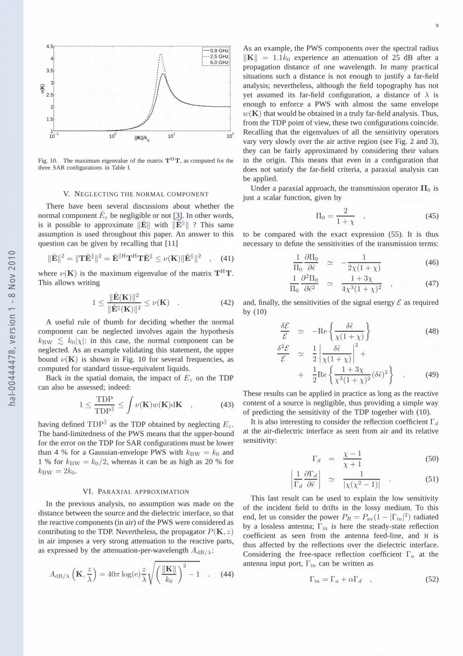
Fig. 10. The maximum eigenvalue of the matrixTHT, as computed for the

three SAR configurations in Table I.

V. NEGLECTING THE NORMAL COMPONENT

There have been several discussions about whether thenormal componentEz be negligible or not [3]. In other words,is it possible to approximate‖E‖ with ‖E‖‖ ? This sameassumption is used throughout this paper. An answer to thisquestion can be given by recalling that [11]

‖E‖2 = ‖TE‖‖2 = E

‖HT

HTE

‖ ≤ ν(K)‖E‖‖2 , (41)

whereν(K) is the maximum eigenvalue of the matrixTHT.

This allows writing

1 ≤ ‖E(K)‖2

‖E‖(K)‖2≤ ν(K) . (42)

A useful rule of thumb for deciding whether the normalcomponent can be neglected involves again the hypothesiskBW . k0|χ|: in this case, the normal component can beneglected. As an example validating this statement, the upperboundν(K) is shown in Fig. 10 for several frequencies, ascomputed for standard tissue-equivalent liquids.

Back in the spatial domain, the impact ofEz on the TDPcan also be assessed; indeed:

1 ≤ TDP

TDP‖≤∫

ν(K)w(K)dK , (43)

having definedTDP‖ as the TDP obtained by neglectingEz.The band-limitedness of the PWS means that the upper-boundfor the error on the TDP for SAR configurations must be lowerthan 4 % for a Gaussian-envelope PWS withkBW = k0 and1 % for kBW = k0/2, whereas it can be as high as 20 % forkBW = 2k0.

VI. PARAXIAL APPROXIMATION

In the previous analysis, no assumption was made on thedistance between the source and the dielectric interface, so thatthe reactive components (in air) of the PWS were considered ascontributing to the TDP. Nevertheless, the propagatorP (K, z)in air imposes a very strong attenuation to the reactive parts,as expressed by the attenuation-per-wavelengthAdB/λ:

AdB/λ

(

K,z

λ

)

= 40π log(e)z

λ

√

(‖K‖k0

)2

− 1 . (44)

As an example, the PWS components over the spectral radius‖K‖ = 1.1k0 experience an attenuation of 25 dB after apropagation distance of one wavelength. In many practicalsituations such a distance is not enough to justify a far-fieldanalysis; nevertheless, although the field topography has notyet assumed its far-field configuration, a distance ofλ isenough to enforce a PWS with almost the same envelopew(K) that would be obtained in a truly far-field analysis. Thus,from the TDP point of view, these two configurations coincide.Recalling that the eigenvalues of all the sensitivity operatorsvary very slowly over the air active region (see Fig. 2 and 3),they can be fairly approximated by considering their valuesin the origin. This means that even in a configuration thatdoes not satisfy the far-field criteria, a paraxial analysiscanbe applied.

Under a paraxial approach, the transmission operatorΠ0 isjust a scalar function, given by

Π0 =2

1 + χ, (45)

to be compared with the exact expression (55). It is thusnecessary to define the sensitivities of the transmission terms:

1

Π0

∂Π0

∂ǫ≃ − 1

2χ(1 + χ)(46)

1

Π0

∂2Π0

∂ǫ2≃ 1 + 3χ

4χ3(1 + χ)2, (47)

and, finally, the sensitivities of the signal energyE as requiredby (10)

δEE ≃ −Re

δǫ

χ(1 + χ)

(48)

δ2EE ≃ 1

2

∣

∣

∣

∣

δǫ

χ(1 + χ)

∣

∣

∣

∣

2

+

+1

2Re

1 + 3χ

χ3(1 + χ)2(δǫ)2

. (49)

These results can be applied in practice as long as the reactivecontent of a source is negligible, thus providing a simple wayof predicting the sensitivity of the TDP together with (10).

It is also interesting to consider the reflection coefficientΓd

at the air-dielectric interface as seen from air and its relativesensitivity:

Γd =χ − 1

χ + 1(50)

∣

∣

∣

∣

1

Γd

∂Γd

∂ǫ

∣

∣

∣

∣

≃ 1

|χ(χ2 − 1)| . (51)

This last result can be used to explain the low sensitivityof the incident field to drifts in the lossy medium. To thisend, let us consider the powerPR = Pav(1 − |Γin|2) radiatedby a lossless antenna;Γin is here the steady-state reflectioncoefficient as seen from the antenna feed-line, and it isthus affected by the reflections over the dielectric interface.Considering the free-space reflection coefficientΓa at theantenna input port,Γin can be written as

Γin = Γa + αΓd , (52)

hal-0

0444

478,

ver

sion

1 -

8 N

ov 2

010

10

where α is related to the transmitting properties of the an-tenna [14]; the finite directivity of the antenna implies that|α| < 1. These considerations lead to the following result:

1

PR

∣

∣

∣

∣

∂PR

∂ǫ

∣

∣

∣

∣

=2|αΓin|

1 − |Γin|2∣

∣

∣

∣

∂Γd

∂ǫ

∣

∣

∣

∣

(53)

and finally to

1

PR

∣

∣

∣

∣

∂PR

∂ǫ

∣

∣

∣

∣

<|Γin|

1 − |Γin|21

|χ(1 + χ)2| . (54)

Therefore, the relative sensitivity of the power radiated bythe antenna is approximately bounded by|Γin|/|χ|3, whichis at least one order of magnitude smaller than the signal-energy sensitivity. This result proves that, unless in a verynear-field configuration, the power radiated by the antennais less strongly affected by changes in the lossy half-spacecharacteristics than the TDP, as reported in [7].

VII. C ONCLUSIONS

We have introduced a spectral approach for the analysis ofthe sensitivity of the TDP to drifts of the electrical propertiesof a lossy half-space. The definition of a sensitivity operatorand of the derivative matrices has shown that their eigenvaluesdistribution leads to a clear understanding of complex phenom-ena, such as the dispersiveness of the TDP sensitivity and inparticular the fact that the sensitivity to the conductivity ismore critical. The same approach was extended to the caseof a stratified structure, in order to investigate how a losslessshell modifies the TDP and its sensitivity.

In all these scenarios, the fundamental role played by thereactive content of the source PWS was highlighted, pointingout how it gives rise to a statistically dispersive behaviour ofthe TDP and its sensitivity to drifts in the electrical parametersof the lossy medium. Hence, the very idea of characterizingthe sensitivity in a deterministic way, independently fromthe source, is not physically sound, especially for near-fieldsources. These results should thus lead to a better understand-ing of the phenomena involved in near-field configurations,such as in SAR applications.

APPENDIX IDEFINITION OF THE SPECTRAL TRANSMISSION OPERATOR

AND RELATED DERIVATIVES

The transmission and the reflection operators, respectivelyΠ and Γ, for a dielectric interface between two media aredefined as [5]:

Π = 2X−1(Y1 + Y2)−1

Y1X (55)

Γ = X−1(Y1 + Y2)

−1(Y1 − Y2)X (56)

Yi = − 1

ωµ0kz,i

[

k2i − k2

x −kxky

−kxky k2i − k2

y

]

(57)

X =

[

0 1−1 0

]

, (58)

beingkz,i =√

k2i − ‖K‖2, i ∈ [1, 2].

By applying the derivative chain-rule, the first derivative∂Π/∂ǫ is given by:

∂Π

∂ǫ=

∂Π

∂k2

∂k2

∂ǫ, (59)

where

∂Π

∂k2= −2X−1

B∂Y2

∂k2BY1X (60)

B = (Y1 + Y2)−1 (61)

∂Y2

∂k2= − k2

kz,2

[

Y2

kz,2+

2

ωµ01

]

(62)

∂k2

∂ǫ=

k1

2√

ǫ. (63)

In the same way, the second derivative is given by:

∂2Π

∂ǫ2=

∂2Π

∂k22

(

∂k2

∂ǫ

)2

+∂Π

∂k2

∂2k2

∂ǫ2, (64)

where

∂2Π

∂k22 = 2X−1

B

(

2∂Y2

∂k2B

∂Y2

∂k2+

− ∂2Y2

∂k22

)

BY1X (65)

∂2Y2

∂k22 = Y2

‖K‖2

k4z,2

+ 12

ωµ0kz,2

(

2‖K‖2

k2z,2

+ 1

)

(66)

∂2k2

∂ǫ2= − k1

4ǫ3/2. (67)

Concerning the derivatives of theT operator, we get:

∂T

∂ǫ=

0 00 0kx ky

1

2

k21

k3z,2

(68)

and

∂2T

∂ǫ2= −

0 00 0kx ky

3

4

k41

k5z,2

. (69)

APPENDIX IIPROOF OF(25)

The sensitivity operator defined in (18) operates over amatrix A ∈ C2×2. We consider at first the fact that anymatrix can be decomposed into the sum of an Hermitian partAH and a skew-Hermitian oneAS . Hence, the matrixAH

is orthonormal, i.e., with eigenvaluesλHi ∈ R, as well asjAS ; this last claim implies that the eigenvaluesλSi of AS

are purely imaginary. Furthermore, thanks to their symmetryproperties the diagonalization matrices are orthonormal too,so that one can write:

AH = XHΛHXHH (70)

AS = XSΛSXHS , (71)

whereΛH,S are diagonal matrices containing the eigenvaluesof, respectively, the Hermitian and the skew-Hermitian com-ponent ofA. Imposingv = E

‖tx, we are able to write the

hal-0

0444

478,

ver

sion

1 -

8 N

ov 2

010

11

integrand of the numerator of (18) as:

vHAv = e

HHΛHeH + e

HSΛSeS

=∑

i

λHi|eHi|2 +∑

i

λSi|eSi|2 , (72)

having introduced the representation of the vectorv into thenew basis given by the diagonalization matricesAH andAS

as:

eH = XHHv (73)

eS = XHS v , (74)

where the termsλHi andλSi are the eigenvalues of, respec-tively, matricesAH andAS .

As shown in Section V, matrixTHT ≃ 1 for any source

with kBW . k0|χ|. Recalling thatXHXHH = XSX

HS = 1, we

can state that

vHT

HTv ≃

∑

i

|eHi|2 =∑

i

|eSi|2 , (75)

leading to

S(A) ≃∑

i

∫

λHi|eHi|2

∑

m

∫

|eHm|2dKdK +

+∑

i

∫

λSi|eSi|2

∑

m

∫

|eSm|2dKdK . (76)

In order to compute the statistical average ofS(A), thefollowing functions need to be studied

wi

2=

|ei|2∑

m

∫

|em|2dK, (77)

where e stands foreH or eS . This function represents theenergy distribution of the PWS normalized to its total energy;it can thus be regarded as a function describing an envelope.Only one component of the PWS, as represented over thediagonalized basis, is considered, according to the value of theindex i. It is reasonable to assume that the two componentsof this function are identically distributed; therefore, theiraverages are identical too. Hence, the energy-density spectrum〈w〉 = 〈wi〉, ∀i can be defined, yielding

〈S(A)〉 ≃∫

[

λH(K) + λS(K)]

〈w(K)〉dK , (78)

where λH and λS are the arithmetic means of, respectively,the eigenvalues of matricesAH and AS . The fact that thesame envelope has been used for the Hermitian and theskew-Hermitian parts is due to the unitary property of thediagonalization matrices. The energy content of the PWS istherefore not modified passing from one basis to the other.No assumption has been made in order to come to this result;it is therefore independent of the probability distribution ofthe energy-density spectrum.

REFERENCES

[1] A. Baños,Dipole Radiation in the Presence of a Conducting Halfspace,Pergamon, 1966.

[2] K.L. Carr, “Antenna: the critical element in successfulmedical technol-ogy,” Microwave Symposium Digest, 1990., IEEE MTT-S International,8-10 May 1990.

[3] N. Kuster, Q. Balzano, “Energy absorption mechanism by biologicalbodies in the near field of dipole antennas above 300 MHz,”IEEETransactions on Vehicular Technology, Vol. 41, Issue 1, Febraury 1992.

[4] M.G. Douglas, C.-K. Chou, “Enabling the use of broadbandtissueequivalent liquids for specific absorption rate measurements,” IEEEInternational Symposium on Electromagnetic Compatibility, EMC 2007,9-13 July 2007.

[5] C. Scott, The Spectral Domain Method in Electromagnetics, ArtechHouse, 1989.

[6] J.E. Hansen,Spherical Near-Field Antenna Measurements, IEE Electro-magnetic Waves Series 26, 1988.

[7] L.M. Correia, “Mobile Broadband Multimedia Networks: Techniques,Models and Tools for 4G,” Academic Press, June 2006.

[8] D.A. Harville, Matrix algebra from a statistician’s perspective, Springer,2000.

[9] International Electrotechnical Commission, “Human Exposure to RadioFrequency Fields From Handheld and Body-Mounted Wireless Commu-nication Devices - Human Models, Instrumentation and Procedures, Part2: Procedure to Determine the Specific Absorption Rate (SAR)in theHead and Body for 30 MHz to 6 GHz Handheld and Body-MountedDevices Used in Close Proximity to the Body,” IEC 62209, pt. 2, June2008 (committee draft).

[10] D.R. Rhodes, “On a fundamental principle in the theory of planarantennas,”Proceedings of the IEEE, Vol. 52, Issue 9, September 1964.

[11] G.H. Golub, C.F. Van Loan,Matrix Computations, The John HopkinsUniversity Press, Third Edition, 1996.

[12] T. Onishi, S. Uebayshi, “Influence of phantom shell on SAR measure-ment in 3-6 GHz frequency range,”IEICE Trans. Commun., Vol. E88-B,No.8, August 2005.

[13] A. Christ, A. Klingenböck, T. Samaras, C. Goiceanu, N. Kuster, “Thedependence of electromagnetic far-field absorption on bodytissue com-position in the frequency range from 300 MHz to 6 GHz,”IEEETransactions on Microwave Theory and Techniques, vol. 54, No. 5, May2006.

[14] D.M. Kerns, Plane-Wave Scattering-Matrix Theory of Antennas andAntenna-Antenna Interactions, National Bureau of Standards, 1981.

hal-0

0444

478,

ver

sion

1 -

8 N

ov 2

010