Empirical Economics (2003) 28:75–100EMPIRICALECONOMICS( Springer-Verlag 2003

On the choice of functional form in stochastic frontiermodeling

Konstantinos Giannakas1, Kien C. Tran*2, Vangelis Tzouvelekas3

1Department of Agricultural Economics, University of Nebraska-Lincoln, 216 H. C. Filley Hall,Lincoln, NE 68583-0922, USA (E-mail: kgiannakas@unl.edu)2Department of Economics, University of Saskatchewan, 9 Campus Drive, Saskatoon,Saskatchewan, S7N 5A5, Canada (E-mail: trank@sask.usask.ca)3Department of Economics, University of Crete, University Campus, Rethymno, Crete, 74 100,Greece (E-mail: Vangelis@cha.forthnet.gr)

First version received: November 1999/Final version received: July 2001

Abstract. This paper examines the e¤ect of functional form specification on theestimation of technical e‰ciency using a panel data set of 125 olive-growingfarms in Greece for the period 1987–93. The generalized quadratic Box-Coxtransformation is used to test the relative performance of alternative, widelyused, functional forms and to examine the e¤ect of prior choice on final e‰-ciency estimates. Other than the functional specifications nested within theBox-Cox transformation, the comparative analysis includes the minflex Lau-rent translog and generalized Leontief that possess desirable approximationproperties. The results indicate that technical e‰ciency measures are very sen-sitive to the choice of functional specification. Perhaps most importantly, thechoice of functional form a¤ects the identification of the factors a¤ecting in-dividual performance – the sources of technical ine‰ciency. The analysis alsoshows that while specification searches do narrow down the set of feasible al-ternatives, the identification of the most appropriate functional specificationmight not always be (statistically) feasible.

Key words: Stochastic frontiers, functional specifications, Box-Cox transfor-mation, technical e‰ciency, Greek olive oil.

JEL Classification System Numbers: C12, C13, C23, C52, Q12

* The authors wish to thank Almas Heshmati, Robert Romain, and an anonymous referee forinsightful comments and suggestions. Special thanks go to the associate editor who handled thepaper, and whose careful reading and suggestions have improved the paper substantially. Thesecond author wishes to acknowledge the financial support from ‘‘President SSHRC’’ from theUniversity of Saskatchewan. The usual caveats with respect to opinions expressed in the paperapply. Senior authorship is shared. This is University of Nebraska-Lincoln Agricultural ResearchDivision Article No. 13270.

1. Introduction

The stochastic production frontier model, which was proposed independentlyby Aigner, Lovell and Schmidt and Meeusen and van den Broeck in 1977, hasdominated the empirical literature of e‰ciency measurement. Within thisframework, several alternative models for estimating productive e‰ciencyhave been progressively developed, extending the stochastic production fron-tier methodology to account for di¤erent theoretical issues in frontier model-ing. Comparative studies to date have mainly focused on estimates of the de-gree of ine‰ciency in the samples under study within di¤erent productionfrontier model specifications (for detailed reviews of the theoretical and em-pirical work in this area see Coelli, Rao and Battese (1998), Greene (1999),and Kumbhakar and Lovell (2000)).Apart from the choice of the appropriate production frontier model how-

ever, an important issue that arises, which is not unique to e‰ciency studies,concerns the functional specification of the estimated frontier – the featuresof the technology employed. Interestingly, empirical applications for the mea-surement of e‰ciency have traditionally focused on a single ad hoc imposedfunctional specification, mostly translog and Cobb-Douglas.The choice of the appropriate functional form is not a trivial matter how-

ever. It is well known that functional forms are both data and model specific,and di¤er in their convergence properties and their ability to approximate al-ternative technologies. Simply put, there is no functional form that dominatesunder all circumstances – the appropriate functional specification is case spe-cific. If the empirical estimates are contaminated with the imposition of aninappropriate functional form, predicted responses arising from the modelmay be biased and inaccurate, posing serious problems for policy design and/or policy implications. Therefore, when there are no strong theoretical or priorempirical reasons in favor of a specific functional specification, the explorationof the sensitivity of the economic optima, including e‰ciency, to the choice offunctional form becomes crucial.The objective of this study is to empirically evaluate the performance of

di¤erent functional specifications in the estimation of technical e‰ciency for apanel data set of 125 olive-growing farms in Greece. The paper explores thesensitivity of obtained e‰ciency estimates to the choice of functional specifi-cation while maintaining an identical data set and retaining the same assump-tions about the underlying technology and the structure of farm e‰ciencies.The e¤ects of the choice of functional form on the estimates of productionstructure (such as production elasticities, returns to scale, and technologi-cal change) and the determination of the factors influencing farm e‰ciencyare also examined. The latter is particularly important since determining thesources of technical e‰ciency provides policy makers with insight on thecauses of ine‰ciency and can suggest potential policies that enhance the pro-ductivity of the sector under study.The estimation of farm-specific technical e‰ciency is based on the sto-

chastic frontier model of Battese and Coelli (1993; 1995). This stochastic fron-tier model allows for a more flexible intertemporal variation in e‰ciency rat-ings, and identifies the factors influencing the e‰ciency of sample participantsdirectly from the estimated production frontier. The production frontiers uti-lized in this comparative study belong primarily to the generalized quadraticfamily of flexible functional forms. More specifically, technical e‰ciency mea-

76 K. Giannakas et al.

sures obtained from the transcendental logarithmic, the generalized Leontief,the normalized quadratic, the squared-root quadratic, the non-homotheticconstant elasticity of substitution (CES) and the Cobb-Douglas functionalforms are analyzed and compared using the generalized quadratic Box-Coxtransformation function that nests all these functional specifications (Appel-baum, 1979; Berndt and Khaled, 1979). In addition to the above functionalforms, the comparative analysis includes the minflex Laurent translog andgeneralized Leontief functional specifications due to their attractive propertiesin approximating the production technology (Barnett, 1983; 1985).The rest of the paper is organized as follows. Section 2 provides a review of

studies on the e¤ect of functional choice on e‰ciency measures derived fromeconometric frontier models. Section 3 presents the functional specification ofthe production frontiers used in the analysis. Section 4 outlines the stochasticproduction frontier model utilized for the measurement of technical e‰ciency.Section 5 provides data descriptions while empirical results are presented inSection 6. Section 7 summarizes and concludes the paper.

2. Background

To our knowledge, there are only few studies that examine the e¤ect of func-tional choice on e‰ciency measures derived from econometric stochastic fron-tier models. Kopp and Smith (1980) compared e‰ciency estimates derivedfrom the translog, the non-homothetic CES, and the Cobb-Douglas functionalspecifications using cross-sectional data from steam generating electric plantsin the US. They found that plant level productive e‰ciency is less sensitive tothe choice of functional form. Several years later, Gong and Sickles (1992)examined the relative performance of translog, CES-translog, and generalizedLeontief functions under di¤erent model specifications using a Monte-Carlosimulation approach and panel data. Disagreeing with the earlier findings ofKopp and Smith (1980) they concluded that the ‘‘choice of functional form instochastic frontier model appears to be crucial.’’Zhu, Ellinger and Shumway (1995) applied the generalized quadratic Box-

Cox transformation model to examine the relative performance of normalizedquadratic, translog and generalized Leontief functions using cross-sectionaldata from rural US banks in the context of a stochastic cost frontier. In ac-cordance with the earlier findings of Gong and Sickles (1992), Zhu, Ellingerand Shumway (1995) suggested that ‘‘the choice of inappropriate functionalspecification would substantially alter conclusions about both scale elastic-ities and ine‰ciencies.’’ Finally, Battese and Broca (1997) compared the trans-log and Cobb-Douglas functional forms using panel data from wheat farmsin Pakistan. They also concluded that the final e‰ciency measures are sen-sitive to the choice of both functional specification and ine‰ciency e¤ectsmodel.When compared with Zhu, Ellinger and Shumway (1995) (who also uti-

lized a generalized quadratic Box-Cox transformation), our study has four dis-tinct features. First, it proceeds to the estimation of a production frontier andthe subsequent measures of technical e‰ciency. Zhu, Ellinger and Shumway(1995) estimated a cost frontier assuming that any deviation from that frontieris due to technical ine‰ciency. However, this is questionable in the dualapproach of estimation since such a specification assumes that individuals are

Choice of functional form in stochastic frontier modeling 77

allocativelly perfectly e‰cient.1 Second, the stochastic frontier model of Bat-tese and Coelli (1993; 1995) used in this paper does away with the need to im-pose restrictive assumptions regarding the inter- and intra-farm variation ine‰ciency ratings.2 Third, the current study relies on a panel data set of 125olive-growing farms observed in seven consecutive years. E‰ciency measuresderived from cross-sectional data (i.e., a single production period) may bedistorted by period specific abnormalities, which questions the accuracy of theestimates and, perhaps more importantly, the relevance of the analysis (Daw-son, Lingard and Woodford, 1991). Finally, our comparative analysis includestwo more flexible functional forms with desirable approximation properties(i.e., the minflex translog and generalized Leontief ) that are not nested withinthe generalized quadratic Box-Cox transformation.

3. Functional specifications

Appelbaum (1979) and Berndt and Khaled (1979) generalized the applicationof the Box-Cox transformation function to allow for a variety of functionalforms to be nested within this function and performed parametric tests todiscriminate among them. Ever since, generalized quadratic Box-Cox modelshave been widely applied in problems of selecting among nested functionalspecifications in applied production analysis. The generalized quadratic Box-Cox model, assuming input-biased technical change, can be written as:

YðdÞit ¼ a0 þ

XJj¼1

ajXðlÞjit þ 1

2

XJj¼1

XJk¼1

ajkXðlÞjit X

ðlÞkit þ b1t

þ 12b2t

2 þXJj¼1

gjXðlÞjit tþ eit ð1Þ

where i ¼ 1; . . . ;N represents cross sectional units; t ¼ 1; . . . ;T denotes time;j; k ¼ 1; . . . ; J are the applied inputs, and eit is a random error. The variables

YðdÞit and X

ðlÞit are the Box-Cox transformations of output and inputs, respec-

tively, defined as (Box and Cox, 1964):

YðdÞit ¼ Y 2d

it � 12d

and XðlÞjit ¼

X ljit � 1l

ð2Þ

where d and l are the transformation parameters to be estimated. Under ap-propriate parametric restrictions for the values of d and l, the generalizedquadratic Box-Cox transformation yields the four locally flexible functionalforms (i.e., translog, generalized Leontief, normalized quadratic, squared-rootquadratic) as well as the non-homothetic CES and Cobb-Douglas specifica-tions.

1 The estimation of technical e‰ciency in the context of the production frontier is conditional onthe input combination. Whether that combination is allocativelly e‰cient or not is a side issue,although an important one (Greene, 1993), i.e., a technically e‰cient producer could still use aninappropriate (for given input prices) input mix.2 The model of Battese and Coelli (1993; 1995) was also used by Battese and Broca (1997).

78 K. Giannakas et al.

More specifically, by utilizing l’Hopital’s rule the power transformationsare continuous around zero. Thus, for d ¼ l ¼ 0 the generalized quadraticBox-Cox becomes the non-homothetic translog functional form:

lnYit ¼ a0 þXJj¼1

aj lnXjit þ1

2

XJj¼1

XJk¼1

ajk lnXjit lnXkit þ b1tþ1

2b2t

2

þXJj¼1

gj lnXjittþ eit ð3Þ

It becomes the non-homothetic generalized Leontief when d ¼ l ¼ 0:5:

Yit ¼ ða0 þ 1Þ þ 2XJj¼1

XJk¼1

ajk � aj

!þ 2

XJj¼1

aj � 2XJk¼1

ajk

!X 0:5

jit

þ 2XJj¼1

XJk¼1

ajkX0:5jit X 0:5

kit þ b1 � 2XJj¼1

gj

!t

þ 12b2t

2 þ 2XJj¼1

gjX0:5jit tþ eit ð4Þ

The generalized quadratic Box-Cox results in the non-homothetic normalizedquadratic when d ¼ 0:5 and l ¼ 1:

Yit ¼ ða0 þ 1Þ þXJj¼1

XJk¼1

ajk

2� aj

!þXJj¼1

aj �XJk¼1

ajk

!Xjit

þ 12

XJj¼1

XJk¼1

ajkXjitXkit þ b1�XJj¼1

gj

!tþ 1

2b2t

2 þXJj¼1

gjXjittþ eit ð5Þ

and becomes the squared-root quadratic when d ¼ l ¼ 1:

Yit ¼"2ða0 þ 1Þ þ 2

XJj¼1

XJk¼1

ajk

2� aj

!þ 2

XJj¼1

aj �XJk¼1

ajk

!Xjit

þXJj¼1

XJk¼1

ajkXjitXkit þ 2 b1 �XJj¼1

gj

!t

þ b2t2 þ 2

XJj¼1

gjXjittþ 2eit

#0:5ð6Þ

Choice of functional form in stochastic frontier modeling 79

All the above functional forms are second-order Taylor series expansions3and provide equally plausible a priori approximations of a true but unknownproduction technology. However, all four functions maintain important re-strictions in modeling production relationships. More specifically, the gener-alized Leontief, normalized quadratic and squared-root quadratic maintainquasi-homotheticity of the underlying technology even at the point of approx-imation. Even though the translog does not maintain this restriction, it is lessseparable flexible than the other three functional forms. Nevertheless, thesefunctional specifications do satisfy the requirement of parametric parsimonysince the number of free parameters is adequate for ensuring flexibility (for adetailed discussion on the properties of several functional specifications usedin applied production analysis see Fuss, McFadden and Mundlak (1978),Gri‰n, Montgomery and Rister (1987) and Thompson (1988) among others).Since all parametric models display these features, there is no a priori reasonto favor any one of them.Apart from these locally flexible functional specifications, the generalized

quadratic Box-Cox also nests the restrictive but widely applied non-homotheticCES and Cobb-Douglas. More specifically, the generalized quadratic Box-Coxproduction function in equation (1) becomes a non-homothetic CES functionwhen the second-order parameters (ajk) equal zero E j; k, i.e.,

Yit ¼"ð2da0 þ 1Þ �

2d

l

XJj¼1

aj þ 2db1 �2d

l

XJj¼1

gj

!tþ db2t

2

þ 2dl

XJj¼1

ajXljit þ

2d

l

XJj¼1

gjXljittþ 2deit

#1=2dð7Þ

Finally, the familiar Cobb-Douglas functional form (or, equivalently, astrongly separable translog when input-biased technical change is maintained)is obtained either from the CES function when d ¼ l ¼ 0 (by utilizing l’Hopi-tal’s rule) or from the translog by setting ajk ¼ 0 E j; k.The selection of the appropriate functional form within the generalized

quadratic Box-Cox transformation function can be based on nested hypothe-sis testing (i.e., likelihood ratio test). Whereas the alternative specifications canbe tested by likelihood support against the generalized quadratic Box-Cox, theycannot be tested against each other however. This problem can be surmountedusing the likelihood dominance criterion that ranks models based on their ad-justed likelihood values (Pollak and Wales, 1991). Specifically, the likelihooddominance criterion assures an unambiguous ordering of the functional formsnested within the generalized quadratic Box-Cox no matter the number of es-timated parameters in each model (Anderson et al., 1996).Recognizing certain deficiencies in the ability of Taylor-series expansion to

generate flexible functional forms, Barnett (1983, 1985) utilized the Laurent-series expansion to provide more desirable approximations of the underlyingproduction technology. The clear advantage of the Laurent-series expansion is

3 The concept of linear-in-parameters functional forms and the property of second-order approxi-mation at a point are due to Diewert (1971), who introduced the generalized linear and generalizedLeontief forms.

80 K. Giannakas et al.

the fact that its remainder term varies less over the interval of convergence forthe same fixed order of expansion. A special case of a second-order Laurentseries expansion that includes both the translog and generalized Leontief func-tional specifications is:

Y �it ¼ a0 þ 2

XJj¼1

ajX�jit þ

XJj¼1

ajjX�2jit

þXJj¼1

XJk¼1

ðajkX �jitX

�kit � zjkX

��1jit X ��1

kit Þ þ eit ð8Þ

Specifically, equation (8) becomes the minflex Laurent generalized Leontief

when X �jit ¼X

1=2jit while when Y �

it ¼ lnYit and X�jit ¼ lnXjit equation (8) generates

the minflex Laurent translog. Whereas both minflex Laurent translog andgeneralized Leontief are flexible functional forms they do not possess greaterparametric freedom than is needed to attain local flexibility. Note that thespecification in equation (8) is not nested within the generalized quadraticBox-Cox model, and the statistical discrimination among these non-nestedmodels can be performed by means of non-nested hypothesis testing. In ourcase we use the PE test developed by MacKinnon, White and Davidson(1983).4 While the PE test follows the same analytical approach as the An-drews test (1971), it is based on a Gauss-Newton artificial regression (for de-tails on non-nested hypothesis testing see Davidson and MacKinnon, 1993,pp. 505–7).

4. Modeling technical e‰ciency

Each functional specification presented in the previous section is used to esti-mate technical ine‰ciency by utilizing the stochastic production frontier modelof Battese and Coelli (1993; 1995). Technical ine‰ciency is expressed as alinear function of explanatory variables associated with farm specific charac-teristics (ine‰ciency e¤ects) to allow for the investigation of inter-farm e‰-ciency variation. In this formulation every farm in the sample faces its ownfrontier (given the current state of technology and the physical endowmentsof the farm) rather than a sample norm. In addition, modeling technical inef-ficiency as a function of farm specific characteristics allows for the consistentestimation of the stochastic frontier and the ine‰ciency e¤ects model in asingle stage (Reifschneider and Stevenson, 1991; Battese and Coelli, 1995).5

4 We choose the PE test because it is simple to compute and more importantly, it has su‰cientpower for applied research.5 Other than simultaneously predicting and explaining technical ine‰ciency, this model formula-tion has two important advantages: (a) it identifies separately time-varying output-oriented tech-nical e‰ciency and technical change as long as the ine‰ciency e¤ects are stochastic and have aknown distribution; and (b) it does not require that technical e‰ciencies follow a specific timepattern common to all farms in the sample.

Choice of functional form in stochastic frontier modeling 81

Specifically, the model of Battese and Coelli (1993; 1995) in the presence oftechnical change and panel data has the following general form:

yit ¼ f ðxit; t;BÞ � expðeitÞ ð9Þ

where yit is the output of farm i ði ¼ 1; 2; . . . ;NÞ at time t ðt ¼ 1; 2; . . . ;TÞ; xitis the corresponding matrix of J inputs; t is a time index that serves as a proxyfor technical change; B is the vector of parameters to be estimated; and eit isthe error term composed of two independent elements vit and uit such thateit 1 vit � uit. The component vit is a symmetric identically and independentlydistributed (iid ) error term that represents random variation in output due tofactors outside the control of the farmer (weather, diseases etc.) as well as thee¤ects of measurement errors, left-out explanatory variables, and statisticalnoise.The component uit is a non-negative error term representing the stochastic

shortfall of farm i ’s output from its production frontier due to technical inef-ficiency. Thus, technical e‰ciency is defined in an output-expanding manner(Debreu-type) and reveals the maximum amount by which output can be in-creased using the same level of inputs.6 It is obtained by truncation of thenormal distribution with mean mit ¼ y0 þ

PMm ymzmit and variance s

2m, where

zmit is the mth explanatory variable associated with technical ine‰cienciesof farm i over time and y0 and ym are the unknown coe‰cients to be esti-mated.7The parameters of both the stochastic frontier and the ine‰ciency e¤ects

model can be consistently estimated by the maximum likelihood procedure.The likelihood function and estimation issues are explicitly discussed in Bat-tese and Coelli (1993). The variance parameters of the likelihood function areestimated in terms of s21 s2v þ s2u and g1 s2u=s

2. Farm- and time-specificestimates of output-based technical e‰ciency are obtained using the expecta-tion of uit (or function of uit, depending on whether the dependent variable isin level or in logs), conditional upon the observed value of eit.A ð1� aÞ100 percent confidence interval for the predicted technical e‰-

ciencies can be determined as (Horrace and Schmidt, 1996, pp. 261–2):8

expð�m0it � s0ZUit ÞaTEit a expð�m0it � s0Z

Lit Þ ð10Þ

6 In a similar manner, an input-conserving measure of technical ine‰ciency (Shephard-type) isdefined as the ratio of best practice input usage to actual usage, with output held constant(Kumbhakar and Lovell, 2000, p. 6). Fare and Lovell (1978) have shown that these two measuresof technical ine‰ciency are equal only under constant returns to scale. Under decreasing (in-creasing) returns to scale the output-oriented measure is greater (less) than the input-orientedmeasure of technical ine‰ciency. Output-oriented measures of technical e‰ciency are more ap-propriate in agricultural frontier modeling, since input choices are made prior to farm production.7 Exclusion of the intercept parameter y0 may result in biased estimates of ym since in such a casethe shape of the distribution of the ine‰ciency e¤ects is being unnecessarily restricted (see Batteseand Coelli (1995)).8 These confidence intervals are based on monotonic transformations of the a=2 and (1� a=2)quantiles of the distribution (uitjeit). Since, however, these intervals are conditioned on knownvalues of the parameters (ignoring therefore any variation in the parameter estimates used toconstruct them), they should be regarded as minimal width intervals (Greene, 1999, p. 108).

82 K. Giannakas et al.

where

ZLit ¼ F�1ð1� ð1� a=2Þð1�Fð�m0it=s0ÞÞÞ ð10aÞ

and

ZUit ¼ F�1ð1� ða=2Þð1�Fð�m0it=s0ÞÞÞ ð10bÞ

are the lower and upper limits of the standard normal variable Z respectively.Obviously, the variables introduced to explain inter-farm e‰ciency di¤erentialshave an e¤ect on the range of the confidence interval; they a¤ect the vari-ability of the conditional mean of uit which, in turn, influences the spread ofthe lower and upper limits of technical e‰ciency (Hjalmarsson Kumbhakarand Heshmati, 1996, p. 320).

5. Data and variables definition

The data used in this study were extracted from a survey undertaken by theInstitute of Agricultural Economics and Rural Sociology in Greece. Our anal-ysis focuses on a sample of 125 olive-growing farms, located in the four mostproductive olive-growing regions of Greece (Peloponissos, Crete, StereaEllada and Aegean Islands). The sample was selected with respect to produc-tion area, the total number of farms within the area, the number of olive treeson the farm, the area of cultivated land, and the share of olive oil productionin farm output. Observations were obtained on an annual basis for the period1987–93.The dependent variable is annual olive-oil production measured in kilo-

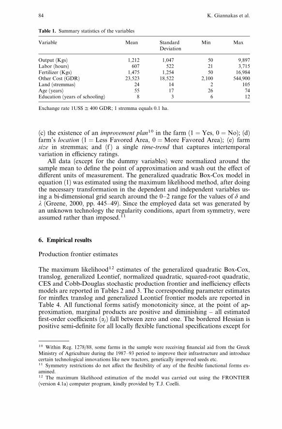
grams (kgs). The aggregate inputs included as explanatory variables are: (a)total labor, comprising hired (permanent and casual), family and contract la-bor which includes all farm activities such as plowing, fertilization, chemicalspraying, harvesting, irrigation, pruning, transportation, administration andother services and is measured in working hours; (b) fertilizers, including ni-trogenous, phosphate, potash, complex and others, measured in kgs; (c) othercost expenses, consisting of pesticides, fuel and electric power, irrigation taxes,depreciation,9 interest payments, fixed assets interest, taxes and other miscel-laneous expenses, measured in Greek drachmas (GDR) (constant 1990 prices);and (d) land, including only the area devoted to olive-tree cultivation, mea-sured in stremmas (one stremma equals 0.1 ha). Summary statistics of thesevariables are presented in Table 1. Aggregation over the various componentsof the above input categories was conducted using Divisia indices with costshares serving as weights (Vogt and Barta, 1997, pp. 29–33). Finally, the ex-planatory variables in the ine‰ciency e¤ects model include: (a) farmer’s age(in years) and age squared; (b) farmer’s formal education in years of schooling;

9 The rate of depreciation applied to machinery was between 10 and 13% depending on the size ofthe farm, while for buildings and inventories it was 7% of the stock value.

Choice of functional form in stochastic frontier modeling 83

(c) the existence of an improvement plan10 in the farm (1 ¼ Yes, 0 ¼ No); (d)farm’s location (1 ¼ Less Favored Area, 0 ¼More Favored Area); (e) farmsize in stremmas; and (f ) a single time-trend that captures intertemporalvariation in e‰ciency ratings.All data (except for the dummy variables) were normalized around the

sample mean to define the point of approximation and wash out the e¤ect ofdi¤erent units of measurement. The generalized quadratic Box-Cox model inequation (1) was estimated using the maximum likelihood method, after doingthe necessary transformation in the dependent and independent variables us-ing a bi-dimensional grid search around the 0–2 range for the values of d andl (Greene, 2000, pp. 445–49). Since the employed data set was generated byan unknown technology the regularity conditions, apart from symmetry, wereassumed rather than imposed.11

6. Empirical results

Production frontier estimates

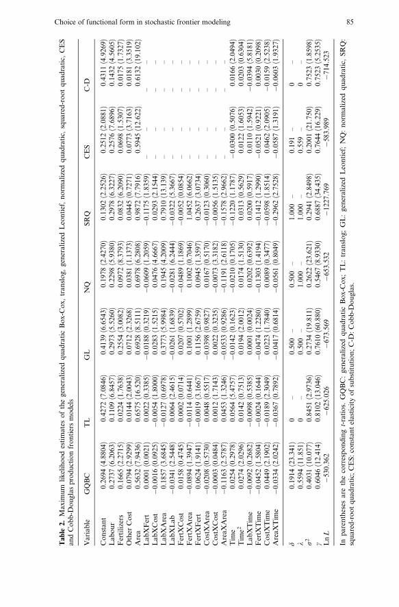
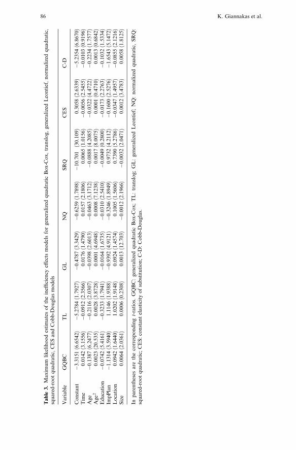
The maximum likelihood12 estimates of the generalized quadratic Box-Cox,translog, generalized Leontief, normalized quadratic, squared-root quadratic,CES and Cobb-Douglas stochastic production frontier and ine‰ciency e¤ectsmodels are reported in Tables 2 and 3. The corresponding parameter estimatesfor minflex translog and generalized Leontief frontier models are reported inTable 4. All functional forms satisfy monotonicity since, at the point of ap-proximation, marginal products are positive and diminishing – all estimatedfirst-order coe‰cients (aj) fall between zero and one. The bordered Hessian ispositive semi-definite for all locally flexible functional specifications except for

10 Within Reg. 1278/88, some farms in the sample were receiving financial aid from the GreekMinistry of Agriculture during the 1987–93 period to improve their infrastructure and introducecertain technological innovations like new tractors, genetically improved seeds etc.11 Symmetry restrictions do not a¤ect the flexibility of any of the flexible functional forms ex-amined.12 The maximum likelihood estimation of the model was carried out using the FRONTIER(version 4.1a) computer program, kindly provided by T.J. Coelli.

Table 1. Summary statistics of the variables

Variable Mean StandardDeviation

Min Max

Output (Kgs) 1,212 1,047 50 9,897Labor (hours) 607 522 21 3,715Fertilizer (Kgs) 1,475 1,254 50 16,984Other Cost (GDR) 23,523 18,522 2,100 544,900Land (stremmas) 24 14 2 105Age (years) 55 17 26 74Education (years of schooling) 8 3 6 12

Exchange rate 1US$G 400 GDR; 1 stremma equals 0.1 ha.

84 K. Giannakas et al.

Table

2.MaximumlikelihoodestimatesofthegeneralizedquadraticBox-Cox,translog,generalizedLeontief,normalizedquadratic,squared-rootquadratic,CES

andCobb-Douglasproductionfrontiersmodels

Variable

GQBC

TL

GL

NQ

SRQ

CES

C-D

Constant

0.2694(4.8804)

0.4272(7.0846)

0.4139(6.6543)

0.1978(2.4270)

0.1302(2.2526)

0.2512(2.0881)

0.4311(4.9269)

Labour

0.2737(6.2063)

0.1109(6.8457)

0.2973(5.5260)

0.2298(5.9380)

0.2978(6.3227)

0.2576(7.6896)

0.1432(4.5605)

Fertilizers

0.1665(2.2715)

0.0224(1.7638)

0.2554(3.0082)

0.0972(8.3793)

0.0832(6.2090)

0.0698(1.5307)

0.0175(1.7327)

OtherCost

0.0794(2.9299)

0.0144(2.0043)

0.0712(2.3268)

0.0381(1.1373)

0.0445(0.7271)

0.0773(3.7163)

0.0181(3.3519)

Area

0.5632(7.9436)

0.6575(16.520)

0.6928(8.5111)

0.6978(6.2808)

0.9872(7.7916)

0.5945(12.622)

0.6132(19.102)

LabXFert

0.0001(0.0021)

0.0022(0.3385)

�0.0188(0.3219)

�0.0609(1.2059)

�0.1175(1.8359)

––

––

LabXCost

�0.0016(0.0925)

�0.0054(1.8000)

0.0283(1.5215)

0.0476(4.6667)

0.0293(2.1544)

––

––

LabXArea

0.1857(3.6845)

�0.0127(0.6978)

0.3773(5.9984)

0.1945(4.2009)

0.7910(13.139)

––

––

LabXLab

�0.0341(2.5448)

0.0064(2.4615)

�0.0261(1.6839)

�0.0281(6.2444)

�0.0322(5.3667)

––

––

FertXCost

0.0158(0.4745)

0.0002(0.0714)

0.0207(0.5702)

�0.0489(1.1869)

�0.0052(0.0854)

––

––

FertXArea

�0.0894(1.3947)

�0.0114(0.6441)

0.1001(1.2899)

0.1002(0.7046)

1.0452(6.0662)

––

––

FertXFert

0.0624(1.9141)

�0.0019(3.1667)

0.1156(2.6759)

0.0945(1.3597)

0.2637(3.0734)

––

––

CostXArea

�0.0208(0.5730)

0.0048(0.5517)

�0.0398(0.9827)

0.0167(0.5170)

�0.0123(0.3060)

––

––

CostXCost

�0.0003(0.0484)

0.0012(1.7143)

0.0022(0.3235)

�0.0073(3.3182)

�0.0056(1.5135)

––

––

AreaXArea

�0.1163(2.5787)

0.0453(1.3246)

�0.0533(0.9286)

�0.1191(2.6118)

�0.1578(2.9662)

––

––

Time

0.0254(0.2978)

0.0564(5.4757)

�0.0142(0.1623)

�0.0210(0.1705)

�0.1220(1.1787)

�0.0300(0.5076)

0.0166(2.0494)

Time2

0.0274(2.0296)

0.0142(0.7513)

0.0194(2.0012)

0.0174(1.5130)

0.0313(0.5629)

0.0122(1.6053)

0.0203(0.6304)

LabXTime

�0.0092(0.2682)

�0.0098(0.5385)

0.0001(0.0024)

0.0202(0.6392)

0.0200(0.5917)

0.0110(1.5942)

�0.0394(5.8181)

FertXTime

�0.0452(1.5804)

�0.0024(0.1644)

�0.0474(1.2280)

�0.1303(1.4194)

�0.1412(1.2990)

�0.0521(0.9221)

0.0030(0.2098)

CostXTime

0.0449(2.1902)

�0.0189(2.3049)

0.0223(1.7840)

0.0089(0.3477)

�0.0598(1.8514)

0.0462(2.0905)

�0.0159(2.5238)

AreaXTime

�0.0334(2.0242)

�0.0367(0.7892)

�0.0417(0.6814)

�0.0561(0.8049)

�0.2962(2.7528)

�0.0587(1.3191)

�0.0603(1.9327)

d0.1914(23.341)

0–

0.500–

0.500–

1.000–

0.191–

0–

l0.5594(11.851)

0–

0.500–

1.000–

1.000–

0.559–

0–

s2

0.4031(10.077)

0.8451(2.9736)

0.2734(19.811)

0.2622(23.621)

0.2941(2.8498)

0.2001(21.750)

0.7523(1.8598)

g0.6046(12.414)

0.8102(13.046)

0.7610(60.880)

0.5467(8.9330)

0.6887(34.435)

0.7644(16.229)

0.7523(5.2535)

LnL

�530.362

�625.026

�673.569

�653.532

�1227.769

�583.989

�714.523

Inparenthesesarethecorrespondingt-ratios.GQBC:generalizedquadraticBox-Cox;TL:translog;GL:generalizedLeontief;NQ:normalizedquadratic,SRQ:

squared-rootquadratic;CES:constantelasticityofsubstitution;C-D:Cobb-Douglas.

Choice of functional form in stochastic frontier modeling 85

Table

3.Maximumlikelihoodestimatesoftheine‰ciencye¤ectsmodelsforgeneralizedquadraticBox-Cox,translog,generalizedLeontief,normalizedquadratic,

squared-rootquadratic,CESandCobb-Douglasmodels

Variable

GQBC

TL

GL

NQ

SRQ

CES

C-D

Constant

�3.3151(6.6542)

�5.2784(1.7927)

�0.4787(3.3429)

�0.6259(1.7898)

�10.701(30.109)

0.3058(2.6339)

�5.2354(6.8670)

Time

0.0142(3.1556)

�0.0912(2.3566)

0.0176(1.4790)

0.0157(2.1806)

0.0065(1.0156)

�0.0056(2.5455)

�0.0103(0.9196)

Age

�0.1387(6.2477)

�0.2116(2.0307)

�0.0398(2.6013)

�0.0463(3.1712)

�0.0888(4.2085)

�0.0322(4.4722)

�0.2234(1.7577)

Age2

0.0023(20.535)

0.0028(3.8728)

0.0001(4.6948)

0.0008(7.1238)

0.0017(8.0075)

0.0001(0.4710)

0.0013(0.6842)

Education

�0.0742(5.4161)

�0.3233(1.7941)

�0.0164(1.6735)

�0.0310(2.5410)

�0.0049(0.2800)

�0.0173(2.2763)

�0.1032(1.5334)

ImpPlan

�1.1314(3.5940)

1.1146(1.9388)

�0.9392(4.9121)

�0.3246(1.8949)

0.9732(4.2112)

�0.1600(2.5276)

�1.6543(5.1472)

Location

0.0942(1.6440)

1.0202(1.9148)

0.0924(1.4574)

0.1005(1.5606)

0.7390(5.2786)

�0.0347(1.4957)

�0.0855(2.1216)

Size

0.0064(2.0361)

0.0006(0.2308)

0.0013(12.703)

�0.0012(2.1966)

�0.0032(2.0471)

0.0012(3.4783)

0.0058(1.8125)

Inparenthesesarethecorrespondingt-ratios.GQBC:generalizedquadraticBox-Cox;TL:translog;GL:generalizedLeontief;NQ:normalizedquadratic,SRQ:

squared-rootquadratic;CES:constantelasticityofsubstitution;C-D:Cobb-Douglas.

86 K. Giannakas et al.

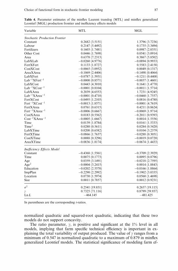
normalized quadratic and squared-root quadratic, indicating that these twomodels do not support concavity.The ratio parameter, g, is positive and significant at the 1% level in all

models, implying that farm specific technical e‰ciency is important in ex-plaining the total variability of output produced. The value of g ranges from aminimum of 0.547 in normalized quadratic to a maximum of 0.879 in minflexgeneralized Leontief models. The statistical significance of modeling farm ef-

Table 4. Parameter estimates of the minflex Laurent translog (MTL) and minflex generalizedLeontief (MGL) production frontier and ine‰ciency e¤ects models

Variable MTL MGL

Stochastic Production Frontier

Constant 0.2682 (3.5151) 1.3796 (3.7236)Labour 0.2147 (5.4492) 0.1735 (3.3494)Fertilizers 0.1603 (1.7481) 0.0987 (2.0351)Other Cost 0.0446 (1.7698) 0.0541 (3.0914)Area 0.6378 (7.2313) 0.3867 (5.8502)LabXLab �0.0260 (4.9776) �0.0894 (0.9933)FertXFert 0.1133 (1.8727) 0.5583 (2.4158)CostXCost �0.0065 (3.0952) 0.0049 (0.1317)AreaXArea �0.1069 (2.4406) �0.1498 (0.4064)LabXFert �0.0787 (1.5931) �0.1211 (0.4408)Lab�1XFert�1 �0.0000 (0.8571) �0.0037 (1.4601)LabXCost 0.0443 (4.3010) 0.1641 (1.4770)Lab�1XCost�1 �0.0001 (0.8104) �0.0011 (1.5714)LabXArea 0.2039 (4.6553) 1.7231 (4.9245)Lab�1XArea�1 �0.0001 (0.4710) �0.0460 (1.7557)FertXCost �0.0495 (1.2103) 0.0816 (0.4780)Fert�1XCost�1 �0.0013 (1.8571) �0.0001 (4.7619)FertXArea 0.0761 (0.6315) 0.4211 (0.8624)Fert�1XArea�1 �0.0006 (0.6667) �0.0069 (1.9714)CostXArea 0.0183 (0.5562) �0.2011 (0.9393)Cost�1XArea�1 �0.0005 (1.6667) 0.0014 (1.5556)Time 0.0139 (1.8784) 0.0161 (1.5333)Time2 0.0280 (0.5611) 0.0284 (0.5420)LabXTime 0.0208 (0.6582) 0.0104 (3.2379)FertXTime �0.0866 (1.7637) �0.0288 (0.3051)CostXTime 0.0088 (0.3296) �0.0019 (0.0720)AreaXTime �0.0836 (1.8174) �0.0674 (1.4433)

Ine‰ciency E¤ects Model

Constant �0.4368 (1.5561) �0.3709 (2.3929)Time 0.0075 (0.1773) 0.0095 (0.8796)Age 0.0359 (3.1491) �0.0218 (2.7595)Age2 �0.0004 (3.2415) 0.0014 (1.8843)Education �0.0202 (2.5570) �0.0166 (1.8864)ImpPlan �0.2290 (2.2992) �0.1902 (3.0335)Location 0.0730 (1.5974) 0.0560 (1.4698)Size 0.0011 (0.7857) 0.0012 (0.9231)

s2 0.2541 (19.851) 0.2657 (19.115)g 0.7325 (71.116) 0.8799 (59.937)LnL �464.145 �481.425

In parentheses are the corresponding t-ratios.

Choice of functional form in stochastic frontier modeling 87

fects within the stochastic frontier model is further examined using likelihoodratio tests (the results of statistical testing are presented in Table 5).13The null hypothesis that the traditional average response model adequately

represents the structure of Greek olive-growing farms is rejected. This is trueregardless of whether farm ine‰ciency e¤ects are present or absent from theproduction frontier model.14 The hypothesis that ine‰ciency e¤ects are nota linear function of the variables considered herein is rejected at the 5% levelof significance. As well, the specification of the model in equation (9) cannotbe reduced to neither Aigner, Lovell and Schmidt (1977) nor Stevenson’s(1980) formulations, as the null hypotheses of y0 ¼ ym ¼ 0 and ym ¼ 0 (form ¼ 1; 2; . . . ;M), respectively, are rejected at 5% level of significance. Finally,the hypothesis that technical ine‰ciency is time-invariant (yT ¼ 0) is rejectedfor all but the square-root quadratic and the minflex model specifications.Hence, no sub-hypothesis of the stochastic frontier model is justified apart ofthe temporal patterns of technical ine‰ciencies in squared-root quadratic, min-flex translog and minflex generalized Leontief models.Several hypotheses concerning the structure of the underlying technology

were also examined using likelihood ratio test. Both homogeneity and linearhomogeneity (constant returns to scale) are rejected by all functional specifi-cations at the 5% level of significance. Technical change is present in almostall models. The hypothesis of zero technical change is not rejected at the 5%level of significance for the normalized quadratic and minflex generalized

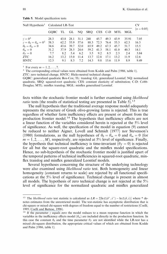
Table 5. Model specification tests

Calculated LR-TestNull Hypothesis1

GQBC TL GL NQ SRQ CES C-D MTL MGL

CV(a ¼ 0:05)

g ¼ 02 28.3 43.8 28.1 31.1 248 45.7 49.3 43.9 35.91 7.05g ¼ y0 ¼ ym ¼ 02 58.3 62.2 55.9 57.6 88.3 72.3 76.4 55.3 62.3 16.3y0 ¼ ym ¼ 0 34.6 43.6 39.7 32.0 65.9 49.2 67.3 45.7 51.7 15.5ym ¼ 0 31.2 37.9 28.5 24.6 59.2 41.3 58.1 41.0 40.3 14.1yT ¼ 0 7.7 8.2 5.4 6.2 3.5 9.2 8.5 2.3 2.4 3.84ZTC 16.2 13.2 15.0 11.4 13.7 12.8 17.1 13.2 11.9 12.6HNTC 12.3 9.1 8.3 7.2 14.3 9.8 15.6 11.9 8.9 9.49

1 For every m ¼ 1; 2; . . . ; 7.2 The corresponding critical values were obtained from Kodde and Palm (1986, table 1).ZTC: zero technical change, HNTC: Hicks-neutral technical change.GQBC: generalized quadratic Box-Cox; TL: translog; GL: generalized Leontief; NQ: normalizedquadratic, SRQ: squared-root quadratic; CES: constant elasticity of substitution; C-D: Cobb-Douglas; MTL: minflex translog; MGL: minflex generalized Leontief.

13 The likelihood ratio test statistic is calculated as LR ¼ 2½lnLðd�; l�Þ � lnLðd; lÞ where * de-notes estimates from the unrestricted model. The test-statistic has asymptotic distribution that ischi-square or mixed chi-square with degrees of freedom equal to the number of restrictions (Coelli,1995; Coelli and Battese, 1996).14 If the parameter g equals zero the model reduces to a mean response function in which thevariables in the ine‰ciency e¤ects model (ym) are included directly in the production function. Inthis case the constant y0 and the time parameter yT are not identified while the LR-test has amixed chi-square distribution, the appropriate critical values of which are obtained from Koddeand Palm (1986, table 1).

88 K. Giannakas et al.

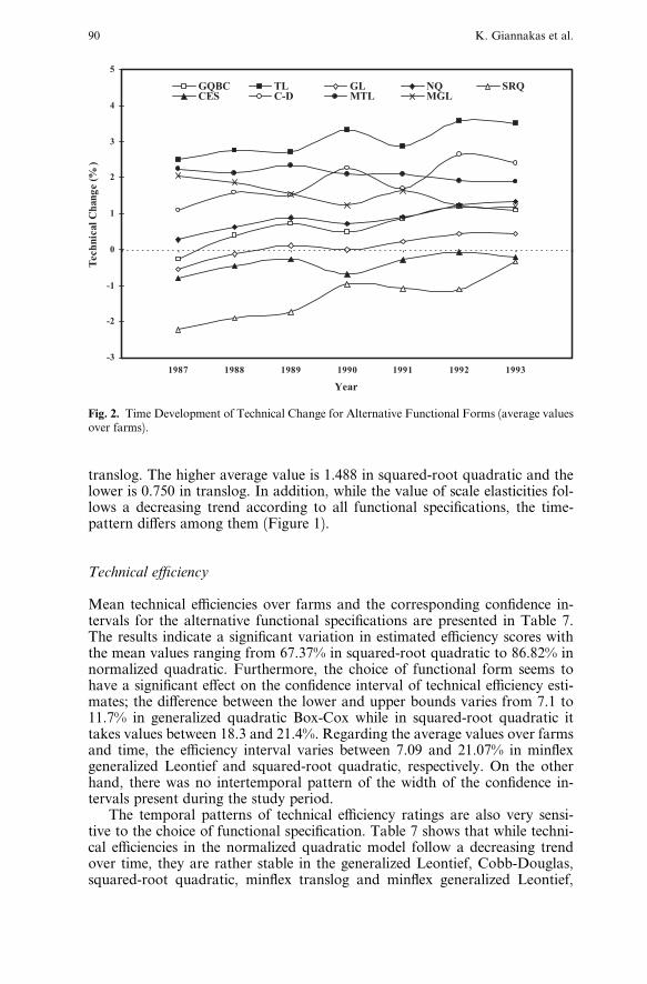
Leontief models (see Table 5). There is no consistency regarding the nature oftechnical change. While the underlying technological change is characterizedas Hicks-neutral according to translog, generalized Leontief and normalizedquadratic models, this hypothesis is rejected under all other functional speci-fications. The rate of technical change follows an increasing trend over time,with the time-pattern being model specific (Figure 2).Average estimates over farms and time of production elasticities, returns to

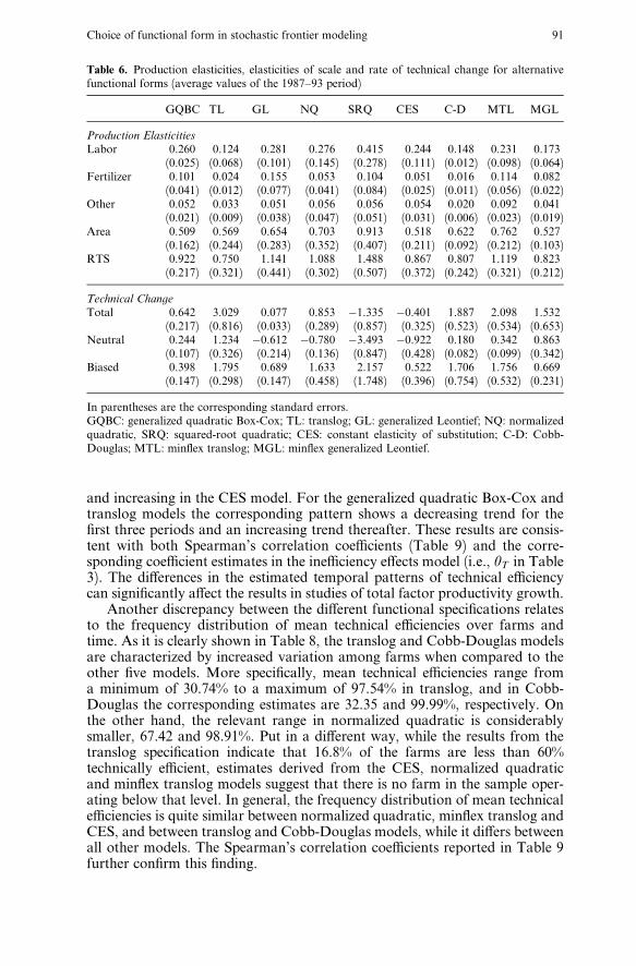
scale (RTS), and the rate of technical change are presented in Table 6. Esti-mates of production elasticities indicate that land has contributed the most toolive-oil production, followed by labor, according to all functional specifica-tions.15 However, the relative contributions of fertilizers and other capital in-puts di¤er across models. Whereas point elasticity estimates in translog, nor-malized quadratic, CES and Cobb-Douglas are very close, the rest of themodels generate significantly di¤erent average values. For instance, the landelasticity takes values between 0.509 and 0.913 in generalized quadratic Box-Cox and squared-root quadratic respectively, and labor elasticity varies be-tween 0.124 in translog and 0.415 in squared-root quadratic.The time development of production elasticities is also similar across mod-

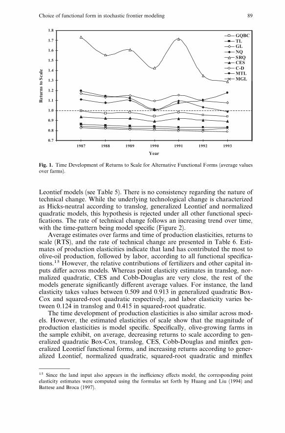
els. However, the estimated elasticities of scale show that the magnitude ofproduction elasticities is model specific. Specifically, olive-growing farms inthe sample exhibit, on average, decreasing returns to scale according to gen-eralized quadratic Box-Cox, translog, CES, Cobb-Douglas and minflex gen-eralized Leontief functional forms, and increasing returns according to gener-alized Leontief, normalized quadratic, squared-root quadratic and minflex

Fig. 1. Time Development of Returns to Scale for Alternative Functional Forms (average valuesover farms).

15 Since the land input also appears in the ine‰ciency e¤ects model, the corresponding pointelasticity estimates were computed using the formulas set forth by Huang and Liu (1994) andBattese and Broca (1997).

Choice of functional form in stochastic frontier modeling 89

translog. The higher average value is 1.488 in squared-root quadratic and thelower is 0.750 in translog. In addition, while the value of scale elasticities fol-lows a decreasing trend according to all functional specifications, the time-pattern di¤ers among them (Figure 1).

Technical e‰ciency

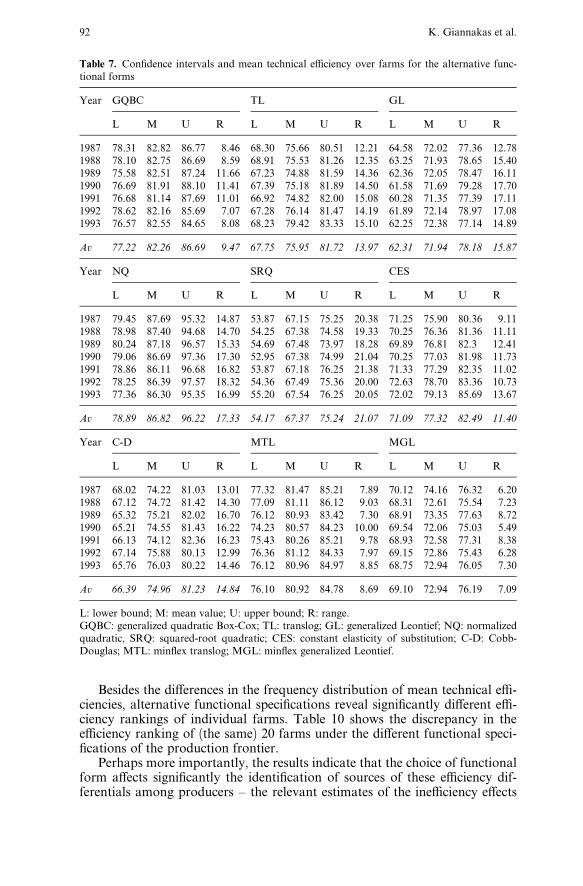
Mean technical e‰ciencies over farms and the corresponding confidence in-tervals for the alternative functional specifications are presented in Table 7.The results indicate a significant variation in estimated e‰ciency scores withthe mean values ranging from 67.37% in squared-root quadratic to 86.82% innormalized quadratic. Furthermore, the choice of functional form seems tohave a significant e¤ect on the confidence interval of technical e‰ciency esti-mates; the di¤erence between the lower and upper bounds varies from 7.1 to11.7% in generalized quadratic Box-Cox while in squared-root quadratic ittakes values between 18.3 and 21.4%. Regarding the average values over farmsand time, the e‰ciency interval varies between 7.09 and 21.07% in minflexgeneralized Leontief and squared-root quadratic, respectively. On the otherhand, there was no intertemporal pattern of the width of the confidence in-tervals present during the study period.The temporal patterns of technical e‰ciency ratings are also very sensi-

tive to the choice of functional specification. Table 7 shows that while techni-cal e‰ciencies in the normalized quadratic model follow a decreasing trendover time, they are rather stable in the generalized Leontief, Cobb-Douglas,squared-root quadratic, minflex translog and minflex generalized Leontief,

Fig. 2. Time Development of Technical Change for Alternative Functional Forms (average valuesover farms).

90 K. Giannakas et al.

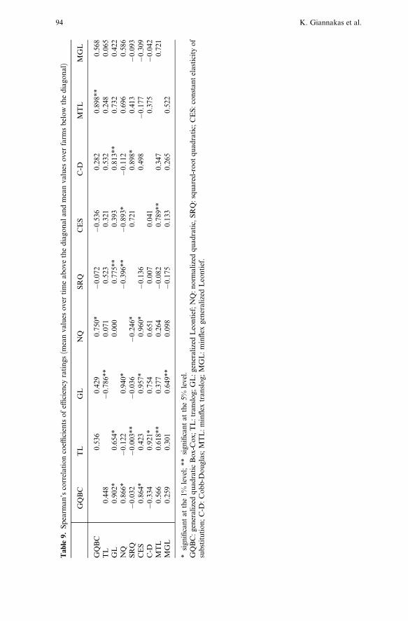
and increasing in the CES model. For the generalized quadratic Box-Cox andtranslog models the corresponding pattern shows a decreasing trend for thefirst three periods and an increasing trend thereafter. These results are consis-tent with both Spearman’s correlation coe‰cients (Table 9) and the corre-sponding coe‰cient estimates in the ine‰ciency e¤ects model (i.e., yT in Table3). The di¤erences in the estimated temporal patterns of technical e‰ciencycan significantly a¤ect the results in studies of total factor productivity growth.Another discrepancy between the di¤erent functional specifications relates

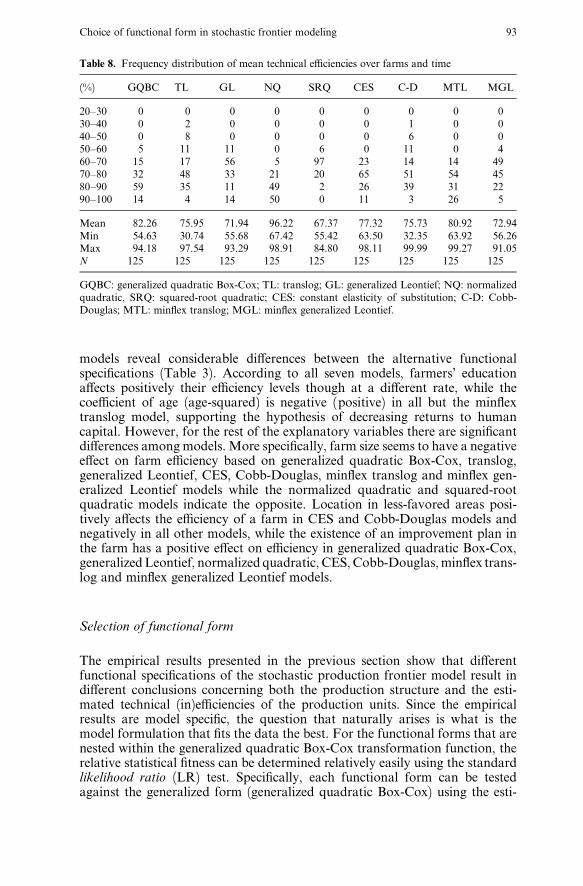
to the frequency distribution of mean technical e‰ciencies over farms andtime. As it is clearly shown in Table 8, the translog and Cobb-Douglas modelsare characterized by increased variation among farms when compared to theother five models. More specifically, mean technical e‰ciencies range froma minimum of 30.74% to a maximum of 97.54% in translog, and in Cobb-Douglas the corresponding estimates are 32.35 and 99.99%, respectively. Onthe other hand, the relevant range in normalized quadratic is considerablysmaller, 67.42 and 98.91%. Put in a di¤erent way, while the results from thetranslog specification indicate that 16.8% of the farms are less than 60%technically e‰cient, estimates derived from the CES, normalized quadraticand minflex translog models suggest that there is no farm in the sample oper-ating below that level. In general, the frequency distribution of mean technicale‰ciencies is quite similar between normalized quadratic, minflex translog andCES, and between translog and Cobb-Douglas models, while it di¤ers betweenall other models. The Spearman’s correlation coe‰cients reported in Table 9further confirm this finding.

Table 6. Production elasticities, elasticities of scale and rate of technical change for alternativefunctional forms (average values of the 1987–93 period)

GQBC TL GL NQ SRQ CES C-D MTL MGL

Production Elasticities

Labor 0.260(0.025)

0.124(0.068)

0.281(0.101)

0.276(0.145)

0.415(0.278)

0.244(0.111)

0.148(0.012)

0.231(0.098)

0.173(0.064)

Fertilizer 0.101(0.041)

0.024(0.012)

0.155(0.077)

0.053(0.041)

0.104(0.084)

0.051(0.025)

0.016(0.011)

0.114(0.056)

0.082(0.022)

Other 0.052(0.021)

0.033(0.009)

0.051(0.038)

0.056(0.047)

0.056(0.051)

0.054(0.031)

0.020(0.006)

0.092(0.023)

0.041(0.019)

Area 0.509(0.162)

0.569(0.244)

0.654(0.283)

0.703(0.352)

0.913(0.407)

0.518(0.211)

0.622(0.092)

0.762(0.212)

0.527(0.103)

RTS 0.922(0.217)

0.750(0.321)

1.141(0.441)

1.088(0.302)

1.488(0.507)

0.867(0.372)

0.807(0.242)

1.119(0.321)

0.823(0.212)

Technical Change

Total 0.642(0.217)

3.029(0.816)

0.077(0.033)

0.853(0.289)

�1.335(0.857)

�0.401(0.325)

1.887(0.523)

2.098(0.534)

1.532(0.653)

Neutral 0.244(0.107)

1.234(0.326)

�0.612(0.214)

�0.780(0.136)

�3.493(0.847)

�0.922(0.428)

0.180(0.082)

0.342(0.099)

0.863(0.342)

Biased 0.398(0.147)

1.795(0.298)

0.689(0.147)

1.633(0.458)

2.157(1.748)

0.522(0.396)

1.706(0.754)

1.756(0.532)

0.669(0.231)

In parentheses are the corresponding standard errors.GQBC: generalized quadratic Box-Cox; TL: translog; GL: generalized Leontief; NQ: normalizedquadratic, SRQ: squared-root quadratic; CES: constant elasticity of substitution; C-D: Cobb-Douglas; MTL: minflex translog; MGL: minflex generalized Leontief.

Choice of functional form in stochastic frontier modeling 91

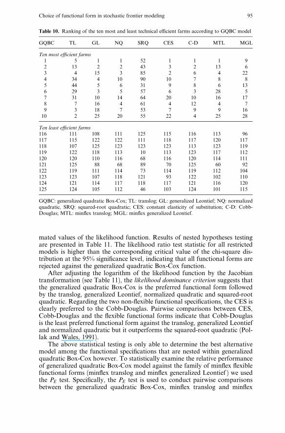
Besides the di¤erences in the frequency distribution of mean technical e‰-ciencies, alternative functional specifications reveal significantly di¤erent e‰-ciency rankings of individual farms. Table 10 shows the discrepancy in thee‰ciency ranking of (the same) 20 farms under the di¤erent functional speci-fications of the production frontier.Perhaps more importantly, the results indicate that the choice of functional

form a¤ects significantly the identification of sources of these e‰ciency dif-ferentials among producers – the relevant estimates of the ine‰ciency e¤ects

Table 7. Confidence intervals and mean technical e‰ciency over farms for the alternative func-tional forms

GQBC TL GLYear

L M U R L M U R L M U R

1987 78.31 82.82 86.77 8.46 68.30 75.66 80.51 12.21 64.58 72.02 77.36 12.781988 78.10 82.75 86.69 8.59 68.91 75.53 81.26 12.35 63.25 71.93 78.65 15.401989 75.58 82.51 87.24 11.66 67.23 74.88 81.59 14.36 62.36 72.05 78.47 16.111990 76.69 81.91 88.10 11.41 67.39 75.18 81.89 14.50 61.58 71.69 79.28 17.701991 76.68 81.14 87.69 11.01 66.92 74.82 82.00 15.08 60.28 71.35 77.39 17.111992 78.62 82.16 85.69 7.07 67.28 76.14 81.47 14.19 61.89 72.14 78.97 17.081993 76.57 82.55 84.65 8.08 68.23 79.42 83.33 15.10 62.25 72.38 77.14 14.89

Av 77.22 82.26 86.69 9.47 67.75 75.95 81.72 13.97 62.31 71.94 78.18 15.87

NQ SRQ CESYear

L M U R L M U R L M U R

1987 79.45 87.69 95.32 14.87 53.87 67.15 75.25 20.38 71.25 75.90 80.36 9.111988 78.98 87.40 94.68 14.70 54.25 67.38 74.58 19.33 70.25 76.36 81.36 11.111989 80.24 87.18 96.57 15.33 54.69 67.48 73.97 18.28 69.89 76.81 82.3 12.411990 79.06 86.69 97.36 17.30 52.95 67.38 74.99 21.04 70.25 77.03 81.98 11.731991 78.86 86.11 96.68 16.82 53.87 67.18 76.25 21.38 71.33 77.29 82.35 11.021992 78.25 86.39 97.57 18.32 54.36 67.49 75.36 20.00 72.63 78.70 83.36 10.731993 77.36 86.30 95.35 16.99 55.20 67.54 76.25 20.05 72.02 79.13 85.69 13.67

Av 78.89 86.82 96.22 17.33 54.17 67.37 75.24 21.07 71.09 77.32 82.49 11.40

C-D MTL MGLYear

L M U R L M U R L M U R

1987 68.02 74.22 81.03 13.01 77.32 81.47 85.21 7.89 70.12 74.16 76.32 6.201988 67.12 74.72 81.42 14.30 77.09 81.11 86.12 9.03 68.31 72.61 75.54 7.231989 65.32 75.21 82.02 16.70 76.12 80.93 83.42 7.30 68.91 73.35 77.63 8.721990 65.21 74.55 81.43 16.22 74.23 80.57 84.23 10.00 69.54 72.06 75.03 5.491991 66.13 74.12 82.36 16.23 75.43 80.26 85.21 9.78 68.93 72.58 77.31 8.381992 67.14 75.88 80.13 12.99 76.36 81.12 84.33 7.97 69.15 72.86 75.43 6.281993 65.76 76.03 80.22 14.46 76.12 80.96 84.97 8.85 68.75 72.94 76.05 7.30

Av 66.39 74.96 81.23 14.84 76.10 80.92 84.78 8.69 69.10 72.94 76.19 7.09

L: lower bound; M: mean value; U: upper bound; R: range.GQBC: generalized quadratic Box-Cox; TL: translog; GL: generalized Leontief; NQ: normalizedquadratic, SRQ: squared-root quadratic; CES: constant elasticity of substitution; C-D: Cobb-Douglas; MTL: minflex translog; MGL: minflex generalized Leontief.

92 K. Giannakas et al.

models reveal considerable di¤erences between the alternative functionalspecifications (Table 3). According to all seven models, farmers’ educationa¤ects positively their e‰ciency levels though at a di¤erent rate, while thecoe‰cient of age (age-squared) is negative (positive) in all but the minflextranslog model, supporting the hypothesis of decreasing returns to humancapital. However, for the rest of the explanatory variables there are significantdi¤erences among models. More specifically, farm size seems to have a negativee¤ect on farm e‰ciency based on generalized quadratic Box-Cox, translog,generalized Leontief, CES, Cobb-Douglas, minflex translog and minflex gen-eralized Leontief models while the normalized quadratic and squared-rootquadratic models indicate the opposite. Location in less-favored areas posi-tively a¤ects the e‰ciency of a farm in CES and Cobb-Douglas models andnegatively in all other models, while the existence of an improvement plan inthe farm has a positive e¤ect on e‰ciency in generalized quadratic Box-Cox,generalizedLeontief, normalized quadratic, CES,Cobb-Douglas,minflex trans-log and minflex generalized Leontief models.

Selection of functional form

The empirical results presented in the previous section show that di¤erentfunctional specifications of the stochastic production frontier model result indi¤erent conclusions concerning both the production structure and the esti-mated technical (in)e‰ciencies of the production units. Since the empiricalresults are model specific, the question that naturally arises is what is themodel formulation that fits the data the best. For the functional forms that arenested within the generalized quadratic Box-Cox transformation function, therelative statistical fitness can be determined relatively easily using the standardlikelihood ratio (LR) test. Specifically, each functional form can be testedagainst the generalized form (generalized quadratic Box-Cox) using the esti-

Table 8. Frequency distribution of mean technical e‰ciencies over farms and time

(%) GQBC TL GL NQ SRQ CES C-D MTL MGL

20–30 0 0 0 0 0 0 0 0 030–40 0 2 0 0 0 0 1 0 040–50 0 8 0 0 0 0 6 0 050–60 5 11 11 0 6 0 11 0 460–70 15 17 56 5 97 23 14 14 4970–80 32 48 33 21 20 65 51 54 4580–90 59 35 11 49 2 26 39 31 2290–100 14 4 14 50 0 11 3 26 5

Mean 82.26 75.95 71.94 96.22 67.37 77.32 75.73 80.92 72.94Min 54.63 30.74 55.68 67.42 55.42 63.50 32.35 63.92 56.26Max 94.18 97.54 93.29 98.91 84.80 98.11 99.99 99.27 91.05N 125 125 125 125 125 125 125 125 125

GQBC: generalized quadratic Box-Cox; TL: translog; GL: generalized Leontief; NQ: normalizedquadratic, SRQ: squared-root quadratic; CES: constant elasticity of substitution; C-D: Cobb-Douglas; MTL: minflex translog; MGL: minflex generalized Leontief.

Choice of functional form in stochastic frontier modeling 93

Table

9.Spearman’scorrelationcoe‰cientsofe‰ciencyratings(meanvaluesovertimeabovethediagonalandmeanvaluesoverfarmsbelowthediagonal)

GQBC

TL

GL

NQ

SRQ

CES

C-D

MTL

MGL

GQBC

0.536

0.429

0.750*

�0.072

�0.536

0.282

0.898**

0.568

TL

0.448

�0.786**

0.071

0.523

0.321

0.532

0.248

0.065

GL

0.902*

0.654*

0.000

0.775**

0.393

0.813**

0.732

0.422

NQ

0.866*

�0.122

0.940*

�0.396**

�0.893*

�0.112

0.696

0.586

SRQ

�0.032

�0.003**

�0.036

�0.246*

0.721

0.898*

0.413

�0.093

CES

0.864*

0.423

0.957*

0.960*

�0.136

0.498

�0.177

�0.309

C-D

�0.334

0.921*

0.754

0.651

0.007

0.041

0.375

�0.042

MTL

0.566

0.618**

0.377

0.264

�0.082

0.789**

0.347

0.721

MGL

0.259

0.301

0.649**

0.098

�0.175

0.133

0.265

0.522

*significantatthe1%level;**significantatthe5%level.

GQBC:generalizedquadraticBox-Cox;TL:translog;GL:generalizedLeontief;NQ:normalizedquadratic,SRQ:squared-rootquadratic;CES:constantelasticityof

substitution;C-D:Cobb-Douglas;MTL:minflextranslog;MGL:minflexgeneralizedLeontief.

94 K. Giannakas et al.

mated values of the likelihood function. Results of nested hypotheses testingare presented in Table 11. The likelihood ratio test statistic for all restrictedmodels is higher than the corresponding critical value of the chi-square dis-tribution at the 95% significance level, indicating that all functional forms arerejected against the generalized quadratic Box-Cox function.After adjusting the logarithm of the likelihood function by the Jacobian

transformation (see Table 11), the likelihood dominance criterion suggests thatthe generalized quadratic Box-Cox is the preferred functional form followedby the translog, generalized Leontief, normalized quadratic and squared-rootquadratic. Regarding the two non-flexible functional specifications, the CES isclearly preferred to the Cobb-Douglas. Pairwise comparisons between CES,Cobb-Douglas and the flexible functional forms indicate that Cobb-Douglasis the least preferred functional form against the translog, generalized Leontiefand normalized quadratic but it outperforms the squared-root quadratic (Pol-lak and Wales, 1991).The above statistical testing is only able to determine the best alternative

model among the functional specifications that are nested within generalizedquadratic Box-Cox however. To statistically examine the relative performanceof generalized quadratic Box-Cox model against the family of minflex flexiblefunctional forms (minflex translog and minflex generalized Leontief ) we usedthe PE test. Specifically, the PE test is used to conduct pairwise comparisonsbetween the generalized quadratic Box-Cox, minflex translog and minflex

Table 10. Ranking of the ten most and least technical e‰cient farms according to GQBC model

GQBC TL GL NQ SRQ CES C-D MTL MGL

Ten most e‰cient farms

1 5 1 1 52 1 1 1 92 13 2 2 43 3 2 13 63 4 15 3 85 2 6 4 224 34 4 10 90 10 7 8 85 44 5 6 31 9 8 6 136 29 3 5 57 6 3 28 57 31 10 14 64 20 10 16 178 7 16 4 61 4 12 4 79 3 18 7 53 7 9 9 1610 2 25 20 55 22 4 25 28

Ten least e‰cient farms

116 111 108 111 125 115 116 113 96117 115 122 122 111 118 117 120 117118 107 125 123 123 123 113 123 119119 122 118 113 10 113 123 117 112120 120 110 116 68 116 120 114 111121 125 88 68 89 70 125 60 92122 119 111 114 73 114 119 112 104123 123 107 118 121 93 122 102 110124 121 114 117 118 117 121 116 120125 124 105 112 46 103 124 101 115

GQBC: generalized quadratic Box-Cox; TL: translog; GL: generalized Leontief; NQ: normalizedquadratic, SRQ: squared-root quadratic; CES: constant elasticity of substitution; C-D: Cobb-Douglas; MTL: minflex translog; MGL: minflex generalized Leontief.

Choice of functional form in stochastic frontier modeling 95

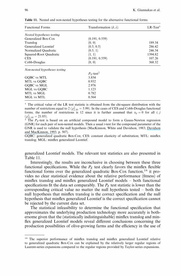
generalized Leontief models. The relevant test statistics are also presented inTable 11.Interestingly, the results are inconclusive in choosing between these three

functional specifications. While the PE test clearly favors the minflex flexiblefunctional forms over the generalized quadratic Box-Cox function,16 it pro-vides no clear statistical evidence about the relative performance (fitness) ofminflex translog and minflex generalized Leontief models – both functionalspecifications fit the data set comparably. The PE test statistic is lower than thecorresponding critical value no matter the null hypothesis tested – both thenull hypothesis that minflex translog is the correct specification and the nullhypothesis that minflex generalized Leontief is the correct specification cannotbe rejected by the current data set.The statistical infeasibility to determine the functional specification that

approximates the underlying production technology more accurately is both-ersome given that the (statistically indistinguishable) minflex translog and min-flex generalized Leontief models reveal di¤erent conclusions concerning theproduction possibilities of olive-growing farms and the e‰ciency in the use of

Table 11. Nested and non-nested hypotheses testing for the alternative functional forms

Functional Forms Transformation ðd; lÞ LR-Test1

Nested hypotheses testing

Generalized Box-Cox (0.191, 0.559)Translog (0, 0) 189.34Generalized Leontief (0.5, 0.5) 286.42Normalized Quadratic (0.5, 1) 246.34Squared-Root Quadratic (1, 1) 1394.82CES (0.191, 0.559) 107.26Cobb-Douglas (0, 0) 368.32

Non-nested hypotheses testing

PE-test2

GQBC vs MTL 3.854MTL vs GQBC 0.932GQBC vs MGL 2.976MGL vs GQBC 1.123MTL vs MGL 0.782MGL vs MTL 0.564

1 The critical value of the LR test statistic is obtained from the chi-square distribution with thenumber of restrictions equal to 2 ðw22; 95 ¼ 5:99Þ. In the cases of CES and Cobb-Douglas functionalforms, the number of restrictions is 12 since it is further assumed that aij ¼ 0 for all i; jðw212; 95 ¼ 21:03Þ.2 The PE-test is based on an artificial compound model to form a Gauss-Newton regression(GNR) for each pair of non-nested models. Then a usual t-test for the compound parameter of theGNR is used to validate the null hypothesis (MacKinnon, White and Davidson, 1983; Davidsonand MacKinnon, 1993, p. 507).GQBC: generalized quadratic Box-Cox; CES: constant elasticity of substitution; MTL: minflextranslog; MGL: minflex generalized Leontief.

16 The superior performance of minflex translog and minflex generalized Leontief relativeto generalized quadratic Box-Cox can be explained by the relatively larger regular regions ofLaurent-series expansions compared to the regular regions provided by Taylor-series expansions.

96 K. Giannakas et al.

their resources.17 One possible explanation for this counterintuitive findingis that, albeit both the minflex translog and the minflex generalized Leontiefmodels fit the data equally well, they can have very di¤erent disturbance dis-tributions. Since the technical e‰ciency predictor is conditioned upon specificdistribution of the disturbances, di¤erent distributional assumptions can resultin di¤erent technical e‰ciency measures.Lau (1986) and Thompson (1988) suggest that a choice among the various

flexible functional specifications available for applied production analysis canbe made on either theoretical or empirical grounds. The former refers to apriori restrictions regarding the algebraic form and the assumptions on theunderlying production technology, while the latter refers to an ex post evalu-ation of functional specifications given the peculiarities of any particular em-pirical application. However, as Gri‰n, Montgomery and Rister (1987) pointout, theoretical criteria could lead to contradictory conclusions about thechoice between the currently available functional forms. On the other hand,our comparative analysis reveals that the empirical ex post evaluation doesnot always lead to the determination of ‘‘the superior’’ functional specification.Put in a di¤erent way, unless a more general composite model is developed,the search for the appropriate functional specification will always involve non-nested hypothesis testing which, however, entails the possibility of statisticallyindistinguishable results.The inability to achieve the ‘‘first best’’ should not be perceived as an

anathema to specification searches. Since the e‰ciency estimates are sensitiveto the choice of functional form, one should always attempt to statisticallydiscriminate among the viable alternatives. Despite its drawbacks, in our casestatistical testing did narrow down the set of suitable alternatives from eight totwo functional specifications.The natural question that arises is then what is the best way to proceed in

cases where the determination of the appropriate functional form is not sta-tistically feasible. A potential solution can be borrowed from the time-seriesforecasting literature where many authors suggest that composite predictionsquite often outperform any particular predictive model (see Coelli and Perel-man (1999)). Palm and Zellner (1992, p. 699) argue that ‘‘in many cases a sim-ple average of forecasts achieves a substantial reduction in variance and bias.’’On this basis, when di¤erent functional specifications are statistically indis-tinguishable and give di¤erent predictions of technical e‰ciency and inferenceon its determinants, a composite measure can provide a solution reducing thebias of the obtained e‰ciency estimates.18

7. Summary and concluding remarks

In recent years several attempts have been made to measure technical e‰ciencyin both developed and developing countries. Since policy recommendationscould be drawn from such studies, the design of the employed methodology

17 We would like to thank the associate editor for pointing out this issue.18 Coelli and Perelman (1999) used a similar approach in analyzing technical e‰ciency estimatesobtained from the non-parametric and parametric estimation of an output distance function.Specifically, they argued that since there is no a priori reason for choosing among these two tech-niques, one should construct geometric means of the obtained technical e‰ciency estimates foreach data point.

Choice of functional form in stochastic frontier modeling 97

is of great importance. Although several studies have examined the impactof estimation techniques on final e‰ciency estimates, only a few can be pin-pointed as dealing with the e¤ect that the choice of functional specificationhas on these estimates.This paper utilizes recent advances in stochastic production frontier mod-

eling and a panel data set of 125 olive growing farms in Greece during theperiod 1987–93 to examine the e¤ect that the choice of functional form hason measures of farm e‰ciency. The relative performance of six popular func-tional specifications (i.e., translog, normalized quadratic, squared-root qua-dratic, generalized Leontief, non-homothetic CES, and Cobb-Douglas) wasevaluated using the generalized quadratic Box-Cox transformation model. Inaddition, our comparative analysis included the minflex translog and general-ized Leontief flexible functional specifications due to their desirable approxi-mation properties.The results show that both estimates of production structure and measures

of farm e‰ciency are sensitive to the functional form used. The choice offunctional specification significantly a¤ects the measures obtained, implyingthat the selection of a particular parametric specification cannot be a matterof indi¤erence. Not only are estimation results of overall ine‰ciency sensi-tive to functional choice, but di¤erent functional specifications also rendersignificantly di¤erent conclusions regarding the potential sources of these in-e‰ciencies. The latter is crucial for the design of policies aimed at improvingthe economic performance of the farms.To the extent that an empirical analysis seeks to be relevant, these results

strongly reject the ad hoc imposition of a (any) functional specification andunderline the importance of specification searches. When estimation proce-dures and the data set are adequate, formal empirical hypotheses may be testedto help narrow the range of viable alternatives; that is, one may proceed witha general-to-specific modeling approach to determine the appropriate func-tional specification. When data and/or estimation/testing procedures are notadequate, a range of relevant alternative functional specifications should atleast be explored to determine how sensitive empirical findings, such as e‰-ciency, are to these specifications. The current study shows that the inappro-priate choice of functional form could result in significantly biased e‰ciencyestimates and misleading policy recommendations regarding e‰ciency im-provements.Finally, a potential solution for cases where statistically indistinguishable

functional specifications yield significantly di¤erent results could involve theconstruction of composite e‰ciency measures that reduce the bias of the finale‰ciency predictions.

References

Aigner D, Lovell CAK, Schmidt P (1977) Formulation and estimation of stochastic frontier pro-duction function models. Journal of Econometrics 6:21–37

Anderson DP, Chaisantikulawat T, Tan Khee Guan A, Kebbeh M, Lin N, Shumway CR (1996)Choice of functional form for agricultural production analysis. Review of Agricultural Eco-nomics 18:223–231

Andrews DF (1971) A note on the selection of data transformations. Biometrika 58:249–54Appelbaum E (1979) On the choice of functional forms. International Economic Review 20:449–

458

98 K. Giannakas et al.

Barnett WA (1983) New indices of money supply and the flexible Laurent demand system. Jour-nal of Business and Economic Statistics 1:7–23

Barnett WA (1985) The minflex Laurent translog flexible functional form. Journal of Econo-metrics 30:33–44

Battese GE, Broca SS (1997) Functional forms of stochastic frontier production functions andmodels for technical ine‰ciency e¤ects: A comparative study for wheat farmers in Pakistan.Journal of Productivity Analysis 8:395–414

Battese GE, Coelli TJ (1988) Prediction of firm-level technical e‰ciencies with a generalizedfrontier production function and panel data. Journal of Econometrics 38:387–399

Battese GE, Coelli TJ (1993) A stochastic frontier production function incorporating a model fortechnical ine‰ciency e¤ects. Working Paper in Econometrics and Applied Statistics No 69,Department of Econometrics, University of New England, Armidale, Australia

Battese GE, Coelli TJ (1995) A model for technical ine‰ciency e¤ects in a stochastic frontierproduction function for panel data. Empirical Economics 20:325–332

Berndt ER, Khaled MS (1979) Parametric productivity measurement and choice among flexiblefunctional forms. Journal of Political Economy 87:1220–1245

Box GEP, Cox DR (1964) An analysis of transformations. Journal of the Royal Statistical Soci-ety, Series B 26:211–252

Coelli TJ, Rao DSP, Battese GE (1998) An introduction to e‰ciency and productivity analysis.Kluwer Academic Publishers, Boston

Coelli TJ (1995) Recent developments in frontier modeling and e‰ciency measurement. Austra-lian Journal of Agricultural Economics 39:219–245

Coelli TJ, Battese GE (1996) Identification of factors which influence the technical e‰ciency ofIndian farmers. Australian Journal of Agricultural Economics 40:19–44

Coelli TJ, Perelman S (1999) A comparison of parametric and non-parametric distance functions:With application to European railways. European Journal of Operational Research 117:326–339

Davidson R, MacKinnon JG (1993) Estimation and inference in econometrics. New York: Ox-ford University Press

Dawson PJ, Lingard J, Woodford CH (1991) A generalized measure of farm-specific technicale‰ciency. American Journal of Agricultural Economics 73:1098–1104

Diewert WE (1971) An application of the Shephard duality theorem: A generalized Leontiefproduction function. American Economic Review 67:404–418

Fare R, Lovell CAK (1978) Measuring the technical e‰ciency of production. Journal of Eco-nomic Theory 19:150–62

Fuss M, McFadden D, Mundlak Y (1978) A survey of functional forms in the economic analysisof production. In: Fuss M, McFadden D (eds) Production economics: A dual approach totheory and application, Amsterdam: North Holland

Giannakas K, Tran KC, Tzouvelekas V (2000) On the choice of functional form in stochasticfrontier models: A Box-Cox approach. Working Paper, Department of Economics, Universityof Saskatchewan

Gong BH, Sickles RC (1992) Finite sample evidence on the performance of stochastic frontiersand data envelopment analysis using panel data. Journal of Econometrics 51:259–284

Greene WH (1993) The econometric approach to e‰ciency analysis. In: Fried HO, Lovell CAK,Schmidt P (eds) The measurement of productive e‰ciency: Techniques and applications, NewYork: Oxford University Press

Greene WH (1999) Frontier production functions. In: Pesaran H, Schmidt P (eds) Handbook ofApplied Econometrics, Vol. II, Microeconomics. Oxford: Blackwell

Greene WH (2000) Econometric analysis. New York: Prentice Hall IncGri‰n RC, Montgomery JM, Rister ME (1987) Selecting functional form in production function

analysis. Western Journal of Agricultural Economics 12:216–227Hjalmarsson L, Kumbhakar SC, Heshmati A (1996) DEA, DFA and SFA: A comparison. Jour-

nal of Productivity Analysis 7:303–327Horrace WC, Schmidt P (1996) Confidence statements for e‰ciency estimates from stochastic

frontier models. Journal of Productivity Analysis 7:303–327Huang CJ, Liu JT (1994) Estimation of a non-neutral stochastic frontier production function.

Journal of Productivity Analysis 5:171–180Kodde DA, Palm FC (1986) Wald criteria for jointly testing equality and inequality restrictions.

Econometrica 54:1243–1248

Choice of functional form in stochastic frontier modeling 99

Kopp RJ, Smith K (1980) Frontier production function estimates for steam electric generation: Acomparative analysis. Southern Economic Journal 47:1049–1059

Kumbhakar SC, Lovell CAK (2000) Stochastic frontier analysis. Cambridge: Cambridge Uni-versity Press

Lau LJ (1986) Functional forms in econometric model building. In: Griliches Z, Intriligator MD(eds) Handbook of Econometrics, Vol III, Amsterdam: North Holland

MacKinnon JG, White H, Davidson R (1983) Tests for model specification in the presence of al-ternative hypotheses: Some further results. Journal of Econometrics 21:53–70

Meeusen W, van den Broeck J (1977) E‰ciency estimation from Cobb-Douglas productionfunctions with composed error. International Economic Review 18:435–444

Palm FC, Zellner A (1992) To combine or not to combine? Issues of combining forecasts. Journalof Forecasting 11:687–701

Pollak RA, Wales TJ (1991) The likelihood dominance criterion: A new approach to model se-lection. Journal of Econometrics 47:227–242

Reifschneider D, Stevenson R (1991) Systematic departures from the frontier: A framework forthe analysis of firm ine‰ciency. International Economic Review 32:715–723

Stevenson RE (1980) Likelihood functions for generalized stochastic frontier estimation. Journalof Econometrics 13:58–66

Thompson GD (1988) Choice of flexible functional forms: Review and appraisal. Western Journalof Agricultural Economics 13:169–183

Vogt A, Barta J (1997) The making of tests for index numbers: Mathematical methods of de-scriptive statistics. Heidelberg: Physica-Verlag

Zhu S, Ellinger PN, Shumway CR (1995) The choice of functional form and estimation of bank-ing ine‰ciency. Applied Economics Letters 2:375–379.

100 K. Giannakas et al.