on the bounded variation of the flow of stochastic differential equation
TRANSCRIPT
Springer Proceedings in Mathematics
Volume 7
For further volumes:http://www.springer.com/series/8806

Springer Proceedings in Mathematics
The book series will feature volumes of selected contributions from workshops andconferences in all areas of current research activity in mathematics. Besides anoverall evaluation, at the hands of the publisher, of the interest, scientific quality,and timeliness of each proposal, every individual contribution will be refereed tostandards comparable to those of leading mathematics journals. It is hoped that thisseries will thus propose to the research community well-edited and authoritativereports on newest developments in the most interesting and promising areas ofmathematical research today.

Mounir Zili � Darya V. FilatovaEditors
Stochastic DifferentialEquations and Processes
SAAP, Tunisia, October 7-9, 2010
123
EditorsMounir ZiliPreparatory Instituteto the Military AcademiesDepartment of MathematicsAvenue Marechal Tito4029 [email protected]
Darya V. FilatovaJan Kochanowski University in Kielceul. Krakowska 1125-029 KielcePolanddaria [email protected]
ISSN 2190-5614ISBN 978-3-642-22367-9 e-ISBN 978-3-642-22368-6DOI 10.1007/978-3-642-22368-6Springer Heidelberg Dordrecht London New York
Library of Congress Control Number: 2011938117
Mathematical Subject Classification (2010): 60HXX, 60GXX, 60FXX, 91BXX, 93BXX, 92DX
c� Springer-Verlag Berlin Heidelberg 2012This work is subject to copyright. All rights are reserved, whether the whole or part of the material isconcerned, specifically the rights of translation, reprinting, reuse of illustrations, recitation, broadcasting,reproduction on microfilm or in any other way, and storage in data banks. Duplication of this publicationor parts thereof is permitted only under the provisions of the German Copyright Law of September 9,1965, in its current version, and permission for use must always be obtained from Springer. Violationsare liable to prosecution under the German Copyright Law.The use of general descriptive names, registered names, trademarks, etc. in this publication does notimply, even in the absence of a specific statement, that such names are exempt from the relevant protectivelaws and regulations and therefore free for general use.
Cover design: deblik, Berlin
Printed on acid-free paper
Springer is part of Springer Science+Business Media (www.springer.com)

Preface
Stochastic analysis is currently undergoing a period of intensive research andvarious new developments, motivated in part by the need to model, understand,forecast, and control the behavior of many natural phenomena that evolve in time ina random way. Such phenomena appear in the fields of finance, telecommunications,economics, biology, geology, demography, physics, chemistry, signal processing,and modern control theory, to mention just a few.
Often, it is very convenient to use stochastic differential equations and stochasticprocesses to study stochastic dynamics. In such cases, research needs the guaranteeof some theoretical properties, such as the existence and uniqueness of the stochasticequation solution. Without a deep understanding of the nature of the stochastic pro-cess this is seldom possible. The theoretical background of both stochastic processesand stochastic differential equations are therefore very important.
Nowadays, quite a few stochastic differential equations can be solved by meansof exact methods. Even if this solution exists, it cannot necessarily be used forcomputer simulations, in which the continuous model is replaced by a discrete one.The problems of “ill-posed” tasks, the “stiffness” or “stability” of the system limitnumerical approximations of the stochastic differential equation. As a result, newapproaches for the numerical solution and, consequently, new numerical algorithmsare also very important.
This volume contains 8 refereed papers dealing with these topics, chosen fromamong the contributions presented at the international conference on StochasticAnalysis and Applied Probability (SAAP 2010), which was held at Yasmine-Hammamet, Tunisia, from 7 to 9 October 2010. This conference was organized bythe “Applied Mathematics & Mathematical Physics” research unit of the preparatoryinstitute to the military academies of Sousse, Tunisia. It brought together some 60researchers and PhD students, from 14 countries and 5 continents. Through lectures,communications, and posters, these researchers reported on theoretical, numerical,or application work as well as on significant results obtained for several topicswithin the field of stochastic analysis and probability, particularly for “Stochasticprocesses and stochastic differential equations.” The conference program wasplanned by an international committee chaired by Mounir Zili (Preparatory Institute
v
vi Preface
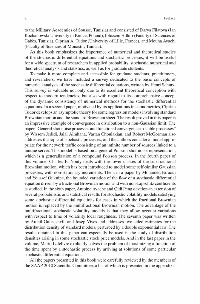
to the Military Academies of Sousse, Tunisia) and consisted of Darya Filatova (JanKochanowski University in Kielce, Poland), Ibtissem Hdhiri (Faculty of Sciences ofGabes, Tunisia), Ciprian A. Tudor (University of Lille, France), and Mouna Ayachi(Faculty of Sciences of Monastir, Tunisia).
As this book emphasizes the importance of numerical and theoretical studiesof the stochastic differential equations and stochastic processes, it will be usefulfor a wide spectrum of researchers in applied probability, stochastic numerical andtheoretical analysis and statistics, as well as for graduate students.
To make it more complete and accessible for graduate students, practitioners,and researchers, we have included a survey dedicated to the basic concepts ofnumerical analysis of the stochastic differential equations, written by Henri Schurz.This survey is valuable not only due to its excellent theoretical conception withrespect to modern tendencies, but also with regard to its comprehensive conceptof the dynamic consistency of numerical methods for the stochastic differentialequations. In a second paper, motivated by its applications in econometrics, CiprianTudor develops an asymptotic theory for some regression models involving standardBrownian motion and the standard Brownian sheet. The result proved in this paper isan impressive example of convergence in distribution to a non-Gaussian limit. Thepaper “General shot noise processes and functional convergence to stable processes”by Wissem Jedidi, Jalal Almhana, Vartan Choulakian, and Robert McGorman alsoaddresses the topic of stochastic processes, and the authors consider a model appro-priate for the network traffic consisting of an infinite number of sources linked to aunique server. This model is based on a general Poisson shot noise representation,which is a generalization of a compound Poisson process. In the fourth paper ofthis volume, Charles El-Nouty deals with the lower classes of the sub-fractionalBrownian motion, which has been introduced to model some self-similar Gaussianprocesses, with non-stationary increments. Then, in a paper by Mohamed Erraouiand Youssef Ouknine, the bounded variation of the flow of a stochastic differentialequation driven by a fractional Brownian motion and with non-Lipschitz coefficientsis studied. In the sixth paper, Antoine Ayache and Qidi Peng develop an extension ofseveral probabilistic and statistical results for stochastic volatility models satisfyingsome stochastic differential equations for cases in which the fractional Brownianmotion is replaced by the multifractional Brownian motion. The advantage of themultifractional stochastic volatility models is that they allow account variationswith respect to time of volatility local roughness. The seventh paper was writtenby Archil Gulisashvili and Josep Vives and addresses two-sided estimates for thedistribution density of standard models, perturbed by a double exponential law. Theresults obtained in this paper can especially be used in the study of distributiondensities arising in some stochastic stock price models. And in the last paper in thevolume, Mario Lefebvre explicitly solves the problem of maximizing a function ofthe time spent by a stochastic process by arriving at solutions of some particularstochastic differential equations.
All the papers presented in this book were carefully reviewed by the members ofthe SAAP 2010 Scientific Committee, a list of which is presented in the appendix.

Preface vii
We would like to thank the anonymous reviewers for their reports and manyothers who contributed enormously to the high standards for publication in theseproceedings by carefully reviewing the manuscripts that were submitted.
Finally, we want to express our gratitude to Marina Reizakis for her invaluablehelp in the process of preparing this volume edition.
Tunisia Mounir ZiliSeptember 2011 Daria Filatova

�
Contents
1 Basic Concepts of Numerical Analysis of StochasticDifferential Equations Explained by BalancedImplicit Theta Methods . . . . . . . . . . . . . . . . . . . . . . . . . . . . . . . . . . . . . . . . . . . . . . . . . . . . . 1Henri Schurz
2 Kernel Density Estimation and Local Time . . . . . . . . . . . . . . . . . . . . . . . . . . . . . . . 141Ciprian A. Tudor
3 General Shot Noise Processes and Functional Convergenceto Stable Processes . . . . . . . . . . . . . . . . . . . . . . . . . . . . . . . . . . . . . . . . . . . . . . . . . . . . . . . . . . . 151Wissem Jedidi, Jalal Almhana, Vartan Choulakian, and RobertMcGorman
4 The Lower Classes of the Sub-Fractional Brownian Motion. . . . . . . . . . . . 179Charles El-Nouty
5 On the Bounded Variation of the Flow of StochasticDifferential Equation . . . . . . . . . . . . . . . . . . . . . . . . . . . . . . . . . . . . . . . . . . . . . . . . . . . . . . . . 197Mohamed Erraoui and Youssef Ouknine
6 Stochastic Volatility and Multifractional Brownian Motion . . . . . . . . . . . . 211Antoine Ayache and Qidi Peng
7 Two-Sided Estimates for Distribution Densities in Modelswith Jumps . . . . . . . . . . . . . . . . . . . . . . . . . . . . . . . . . . . . . . . . . . . . . . . . . . . . . . . . . . . . . . . . . . . . 239Archil Gulisashvili and Josep Vives
8 Maximizing a Function of the Survival Time of a WienerProcess in an Interval . . . . . . . . . . . . . . . . . . . . . . . . . . . . . . . . . . . . . . . . . . . . . . . . . . . . . . . . 255Mario Lefebvre
Appendix ASAAP 2010 Scientific Committee . . . . . . . . . . . . . . . . . . . . . . . . . . . . . . . . . . . . . . . . . . . 263
ix

�
Contributors
Jalal Almhana GRETI Group, University of Moncton, Moncton, NB E1A3E9,Canada, [email protected]
Antoine Ayache U.M.R. CNRS 8524, Laboratory Paul Painleve, UniversityLille 1, 59655 Villeneuve d’Ascq Cedex, France, [email protected]
Vartan Choulakian GRETI Group, University of Moncton, Moncton, NBE1A3E9, Canada, [email protected]
Charles El-Nouty UMR 557 Inserm/ U1125 Inra/ Cnam/ Universite Paris XIII,SMBH-Universite Paris XIII, 74 rue Marcel Cachin, 93017 Bobigny Cedex, France,[email protected]
Mohamed Erraoui Faculte des Sciences Semlalia Departement de Mathematiques,Universite Cadi Ayyad BP 2390, Marrakech, Maroc, [email protected]
Archil Gulisashvili Department of Mathematics, Ohio University, Athens, OH45701, USA, [email protected]
Wissem Jedidi Department of Mathematics, Faculty of Sciences of Tunis, CampusUniversitaire, 1060 Tunis, Tunisia, [email protected]
Mario Lefebvre Departement de Mathematiques et de Genie Industriel, EcolePolytechnique, C.P. 6079, Succursale Centre-ville, Montreal, PQ H3C 3A7, Canada,[email protected]
Robert McGorman NORTEL Networks, 4001 E. Chapel Hill-Nelson Hwy,Research Triangle Park, NC 27709, USA, [email protected]
Youssef Ouknine Faculte des Sciences Semlalia Departement de Mathematiques,Universite Cadi Ayyad BP 2390, Marrakech, Maroc, [email protected]
Qidi Peng U.M.R. CNRS 8524, Laboratory Paul Painleve, University Lille 1,59655 Villeneuve d’Ascq Cedex, France, [email protected]
xi

xii Contributors
Henry Schurz Department of Mathematics, Southern Illinois University, 1245Lincoln Drive, Carbondale, IL 62901, USA, [email protected]
Ciprian A. Tudor Laboratoire Paul Painleve, Universite de Lille 1, F-59655Villeneuve d’Ascq, France, [email protected]
Josep Vives Departament de Probabilitat, Logica i Estadıstica, Universitat deBarcelona, Gran Via 585, 08007-Barcelona (Catalunya), Spain, [email protected]
Chapter 1Basic Concepts of Numerical Analysisof Stochastic Differential Equations Explainedby Balanced Implicit Theta Methods
Henri Schurz
Abstract We present the comprehensive concept of dynamic consistency ofnumerical methods for (ordinary) stochastic differential equations. The conceptis illustrated by the well-known class of balanced drift-implicit stochastic Thetamethods and relies on several well-known concepts of numerical analysis toreplicate the qualitative behaviour of underlying continuous time systems underadequate discretization. This involves the concepts of consistency, stability,convergence, positivity, boundedness, oscillations, contractivity and energybehaviour. Numerous results from literature are reviewed in this context.
1.1 Introduction
Numerous monographs and research papers on numerical methods of stochasticdifferential equations are available. Most of them concentrate on the constructionand properties of consistency. A few deal with stability and longterm properties.However, as commonly known, the replication of qualitative properties of numericalmethods in its whole is the most important issue for modeling and real-worldapplications. To evaluate numerical methods in a more comprehensive manner,we shall discuss the concept of dynamic consistency of numerical methods forstochastic differential equations. For the sake of precise illustration, we will treat theexample class of balanced implicit outer Theta methods. This class is defined by
H. Schurz (�)Southern Illinois University, Department of Mathematics, 1245 Lincoln Drive, Carbondale,IL 62901, USAe-mail: [email protected]
M. Zili and D.V. Filatova (eds.), Stochastic Differential Equations and Processes,Springer Proceedings in Mathematics 7, DOI 10.1007/978-3-642-22368-6 1,© Springer-Verlag Berlin Heidelberg 2012
1
2 H. Schurz
XnC1 D
8ˆˆ<
ˆˆ:
XnC Œ�na.tnC1; XnC1/C.I��n/a.tn; Xn/� hnCmX
jD1bj .tn; Xn/�W
jn
CmX
jD0cj .tn; Xn/.Xn � XnC1/j�W j
n j(1.1)
with appropriate (bounded) matrices cj with continuous entries, where I is the unitmatrix in IRd�d and
�W 0n D hn; �W j
n D W j .tnC1/�W j .tn/
along partitions
0 D t0 < t1 < : : : < tn < tnC1 < : : : < tnT D T < C1
of finite time-intervals Œ0; T �. These methods are discretizations of d -dimensionalordinary stochastic differential equations (SDEs), [3, 14, 32, 33, 81, 86, 102, 108]
dX.t/Da.t; X.t//dtCmX
jD1bj .t; X.t//dW j .t/
0
@DmX
jD0bj .t; X.t//dW j .t/
1
A (1.2)
(with b0 D a, W 0.t/D t), driven by i.i.d. Wiener processes W j and started atadapted initial values X.0/ D x0 2 IRd . The vector fields a and bj are supposedto be sufficiently smooth throughout this survey. All stochastic processes areconstructed on the complete probability basis .˝;F ; .Ft /t�0; IP /.
The aforementioned Theta methods (1.1) represent a first natural generalizationof explicit and implicit Euler methods. Indeed, they are formed by a convexlinear combinations of explicit and implicit Euler increment functions of thedrift part, whereas the diffusion part is explicitly treated due to the problem ofadequate integration within one and the same stochastic calculus. The balancedterms cj are appropriate matrices and useful to control the pathwise (i.e. almostsure) behaviour and uniform boundedness of those approximations. The parametermatrices .�n/n2IN 2 IRd�d determine the degree of implicitness and simplectivebehaviour (energy- and area-preserving character) of related approximations. Mostpopular representatives are those with simple scalar choices �n D �nI where Idenotes the unit matrix in IRd�d and �n 2 IR1. Originally, without balanced termscj , they were invented by Talay [138] in stochastics, who proposed �n D �I withautonomous scalar choices � 2 Œ0; 1�. This family with matrix-valued parameters� 2 IRd�d has been introduced by Ryashko and Schurz [116] who also provedtheir mean square convergence with an estimate of worst case convergence rate 0:5.If � D 0 then its scheme reduces to the classical (forward) Euler method (seeMaruyama [90], Golec et al. [35–38], Guo [39, 40], Gyongy [41, 42], Protter and
1 Basic Concepts of Numerical Analysis Stochastic Differential Equations Explained 3
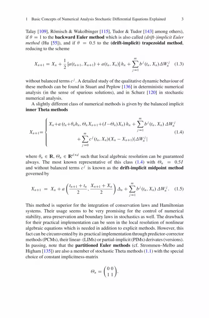
Talay [109], Romisch & Wakolbinger [115], Tudor & Tudor [143] among others),if � D 1 to the backward Euler method which is also called (drift-)implicit Eulermethod (Hu [55]), and if � D 0:5 to the (drift-implicit) trapezoidal method,reducing to the scheme
XnC1 D Xn C 1
2Œa.tnC1; XnC1/C a.tn; Xn/� hn C
mX
jD1bj .tn; Xn/�W
jn (1.3)
without balanced terms cj . A detailed study of the qualitative dynamic behaviour ofthese methods can be found in Stuart and Peplow [136] in deterministic numericalanalysis (in the sense of spurious solutions), and in Schurz [120] in stochasticnumerical analysis.
A slightly different class of numerical methods is given by the balanced implicitinner Theta methods
XnC1D
8ˆˆ<
ˆˆ:
XnCa .tnC�nhn;�nXnC1C.I��n/Xn/ hn CmX
jD1bj .tn; Xn/�W
jn
CmX
jD0cj .tn; Xn/.Xn � XnC1/j�W j
n j(1.4)
where �n 2 IR, �n 2 IRd�d such that local algebraic resolution can be guaranteedalways. The most known representative of this class (1.4) with �n D 0:5I
and without balanced terms cj is known as the drift-implicit midpoint methodgoverned by
XnC1 D Xn C a
�tnC1 C tn
2;XnC1 CXn
2
�
�n CmX
jD1bj .tn; Xn/�W
jn : (1.5)
This method is superior for the integration of conservation laws and Hamiltoniansystems. Their usage seems to be very promising for the control of numericalstability, area-preservation and boundary laws in stochastics as well. The drawbackfor their practical implementation can be seen in the local resolution of nonlinearalgebraic equations which is needed in addition to explicit methods. However, thisfact can be circumvented by its practical implementation through predictor-correctormethods (PCMs), their linear- (LIMs) or partial-implicit (PIMs) derivates (versions).In passing, note that the partitioned Euler methods (cf. Strommen–Melbo andHigham [135]) are also a member of stochastic Theta methods (1.1) with the specialchoice of constant implicitness-matrix
�n D�0 0
1 1
�
:

4 H. Schurz
In passing, note that stochastic Theta methods (1.1) represent the simplest class ofstochastic Runge-Kutta methods. Despite their simplicity, they are rich enough tocover many aspects of numerical approximations in an adequate manner.
The purpose of this survey is to compile some of the most important factson representatives of classes (1.1) and (1.4). Furthermore, we shall reveal thegoodness of these approximation techniques in view of their dynamic consistency.In the following sections we present and discuss several important key conceptsof stochastic numerical analysis explained by Theta methods. At the end wefinalize our presentation with a summary leading to the governing concept ofdynamic consistency unifying the concepts presented before in a complex fashion.The paper is organized in 12 sections. The remaining part of our introductionreports on auxiliary tools to construct, derive, improve and justify consistency ofrelated numerical methods for SDEs. Topics as consistency in Sect. 1.2, asymptoticstability in Sect. 1.3, convergence in Sect. 1.4, positivity in Sect. 1.5, boundednessin Sect. 1.6, oscillations in Sect. 1.7, energy in Sect. 1.8, order bounds in Sect. 1.9,contractivity in Sect. 1.10 and dynamic consistency in Sect. 1.11 are treated. Finally,the related references are listed alphabetically, without claiming to refer to allrelevant citations in the overwhelming literature on those subjects. We recommendalso to read the surveys of Artemiev and Averina [5], Kanagawa and Ogawa [66],Pardoux and Talay [106], S. [125] and Talay [140] in addition to our paper. A goodintroduction to related basic elements is found in Allen [1] and [73] too.
1.1.1 Auxiliary tool: Ito Formula (Ito Lemma)with Operators L j
Define linear partial differential operators
L 0 D @
@tC < a.t; x/;rx >d C1
2
mX
jD1
dX
i;kD1bji .t; x/b
j
k .t; x/@2
@xk@xi(1.6)
and L jD < bj .t; x/;rx >d where jD1; 2; : : : ; m. Then, thanks to the fundamen-tal contribution of Ito [56] and [57], we have the following lemma.
Lemma 1.1.1 (Stopped Ito Formula in Integral Operator Form). Assume thatthe given deterministic mapping V 2 C1;2.Œ0; T � � IRd ; IRk/. Let � be a finite Ft -adapted stopping time with 0 � t � � � T .Then, we have
V.�;X.�// D V.t; X.t//CmX
jD0
Z �
t
L j V .s; X.s// dW j .s/ : (1.7)

1 Basic Concepts of Numerical Analysis Stochastic Differential Equations Explained 5
1.1.2 Auxiliary Tool: Derivation of Stochastic Ito-TaylorExpansions
By iterative application of Ito formula we gain the family of stochastic Taylorexpansions. This idea is due to Wagner and Platen [144]. Suppose we have enoughsmoothness of V and of coefficients a; bj of the Ito SDE. Remember, thanks to Ito’sformula, for t � t0
V .t; X.t// D V.t0; X.t0//CZ t
t0
L 0V .s; X.s//dsCmX
jD1
Z t
t0
L j V .s; X.s// dW j .s/:
Now, take V.t; x/ D x at the first step, and set b0.t; x/ � a.t; x/;W 0.t/ � t . Thenone derives
X.t/ D X.t0/CZ t
t0
a.s; X.s//ds CmX
jD1
Z t
t0
bj .s; X.s// dW j .s/
V � bj
D X.t0/CZ t
t0
"
a.t0; X.t0//CmX
kD0
Z s
t0
L ka.u; X.u//dW k.u/
#
ds
CmX
jD1
Z t
t0
"
bj .t0; X.t0//CmX
kD0
Z s
t0
L ka.u; X.u//dW k.u/
#
dW j .s/
b0 � a
D X.t0/CmX
jD0bj .t0; X.t0//
Z t
t0
dW j .s/
„ ƒ‚ …
Euler Increment
CmX
j;kD0
Z t
t0
Z s
t0
L kbj .u; X.u// dW k.u/dW j .s/
„ ƒ‚ …
Remainder Term RE
V � L kbj
D X.t0/
CmX
jD0bj .t0; X.t0//
Z t
t0
dWj .s/CmX
j;kD1L kbj .t0; X.t0//
Z t
t0
Z s
t0
dW k.u/dWj.s/
„ ƒ‚ …
Increment of Milstein Method

6 H. Schurz
CmX
jD1
Z t
t0
Z s
t0
L 0bj .u; X.u// du dW j .s/
CmX
kD1
Z t
t0
Z s
t0
L ka.u; X.u// dW k.u/ds
CmX
j;kD1;lD0
Z t
t0
Z s
t0
Z u
t0
L lL kbj .z; X.z// dW l .z/dW k.u/dW j .s/
„ ƒ‚ …
Remainder Term RM
V � L kbj
D X.t0/
CmX
jD0bj .t0; X.t0//
Z t
t0
dW j .s/CmX
j;kD0L kbj .t0; X.t0//
Z t
t0
Z s
t0
dWk.u/dW j .s/
„ ƒ‚ …
Increment of 2nd order Taylor Method
CmX
j;k;lD0
Z t
t0
Z s
t0
Z u
t0
L lL kbj .z; X.z// dW l.z/dW k.u/dW j .s/
„ ƒ‚ …
Remainder Term RTM2
V � L rL kbj
D X.t0/
CmX
jD0bj .t0; X.t0//
Z t
t0
dW j .s/CmX
j;kD0L kbj .t0; X.t0//
Z t
t0
Z s
t0
dWk.u/dWj .s/
„ ƒ‚ …
Increment of 3rd order Taylor Method
CmX
j;k;rD0L rL kbj .t0; X.t0//
Z t
t0
Z s
t0
Z u
t0
dW r.v/dW k.u/dW j .s/
„ ƒ‚ …
Increment of 3rd order Taylor Method
CmX
j;k;r;lD0
Z t
t0
Z s
t0
Z u
t0
Z v
t0
L lL rL kbj .z; X.z//dW l.z/dW r.v/dW k.u/dW j .s/
„ ƒ‚ …
Remainder Term RTM3
: : : : : : : : : : : : : : :
1 Basic Concepts of Numerical Analysis Stochastic Differential Equations Explained 7
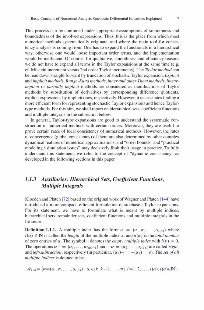
This process can be continued under appropriate assumptions of smoothness andboundedness of the involved expressions. Thus, this is the place from which mostnumerical methods systematically originate, and where the main tool for consis-tency analysis is coming from. One has to expand the functionals in a hierarchicalway, otherwise one would loose important order terms, and the implementationwould be inefficient. Of course, for qualitative, smoothness and efficiency reasonswe do not have to expand all terms in the Taylor expansions at the same time (e.g.cf. Milstein increment versus 2nd order Taylor increments). The Taylor method canbe read down straight forward by truncation of stochastic Taylor expansion. Explicitand implicit methods, Runge-Kutta methods, inner and outer Theta methods, linear-implicit or partially implicit methods are considered as modifications of Taylormethods by substitution of derivatives by corresponding difference quotients,explicit expressions by implicit ones, respectively. However, it necessitates finding amore efficient form for representing stochastic Taylor expansions and hence Taylor-type methods. For this aim, we shall report on hierarchical sets, coefficient functionsand multiple integrals in the subsection below.
In general, Taylor-type expansions are good to understand the systematic con-struction of numerical methods with certain orders. Moreover, they are useful toprove certain rates of local consistency of numerical methods. However, the ratesof convergence (global consistency) of them are also determined by other complexdynamical features of numerical approximations, and “order bounds” and “practicalmodeling / simulation issues” may decisively limit their usage in practice. To fullyunderstand this statement, we refer to the concept of “dynamic consistency” asdeveloped in the following sections in this paper.
1.1.3 Auxiliaries: Hierarchical Sets, Coefficient Functions,Multiple Integrals
Kloeden and Platen [72] based on the original work of Wagner and Platen [144] haveintroduced a more compact, efficient formulation of stochastic Taylor expansions.For its statement, we have to formulate what is meant by multiple indices,hierarchical sets, remainder sets, coefficient functions and multiple integrals in theIto sense.
Definition 1.1.1. A multiple index has the form ˛ D .˛1; ˛2; : : : ; ˛l.˛// wherel.˛/ 2 IN is called the length of the multiple index ˛, and n.˛/ is the total numberof zero entries of ˛. The symbol � denotes the empty multiple index with l.�/ D 0.The operations ˛� D .˛1; : : : ; ˛l.˛/�1/ and �˛ D .˛2; : : : ; ˛l.˛// are called right-and left-subtraction, respectively (in particular, .˛1/� D �.˛1/ D �). The set of allmultiple indices is defined to be
Mk;mD ˚˛D.˛1; ˛2; : : : ; ˛l.˛// W ˛i2fk; kC1; : : : ; mg; iD1; 2; : : : ; l.˛/; l.˛/2IN
�:

8 H. Schurz
A hierarchical set Q � M0;m is any set of multiple indices ˛ 2 M0;m such that� 2 Q and ˛ 2 Q implies �˛ 2 Q. The hierarchical set Qk denotes the set of allmultiple indices ˛ 2 M0;m with length smaller than k 2 IN, i.e.
Qk D f˛ 2 M0;m W l.˛/ � kg :
The setR.Q/ D f˛ 2 M0;m nQ W ˛� 2 Qg
is called the remainder set R.Q/ of the hierarchical set Q. A multiple (Ito) integralI˛;s;t ŒV .:; :/� is defined to be
I˛;s;t ŒV .: ; :/� D� R t
sI�˛;s;uŒV .: ; :/� dW ˛1 .u/ if l.˛/ > 1
R tsV .u; Xu/ dW
˛l.˛/ .u/ otherwise
for a given process V.t; X.t//where V 2 C0;0 and fixed ˛ 2 M0;mnf�g. A multiple(Ito) coefficient function V˛ 2 C0;0 for a given mapping V D V.t; x/ 2 C l.˛/;2l.˛/
is defined to be
V˛.t; x/ D�
L l.˛/V˛�.t; x/ if l.˛/ > 0
V.t; x/ otherwise:
Similar notions can be introduced with respect to Stratonovich calculus (in fact, ingeneral with respect to any stochastic calculus), see [72] for Ito and Stratonovichcalculus.
1.1.4 Auxiliary Tool: Compact Formulation of Wagner-PlatenExpansions
Now we are able to state a general form of Ito-Taylor expansions. Stochastic Taylor-type expansions for Ito diffusion processes have been introduced and studied byWagner and Platen [144] (cf. also expansions in Sussmann [137], Arous [4], andHu [54]). Stratonovich Taylor-type expansions can be found in Kloeden and Platen[72]. We will follow the original main idea of Wagner and Platen [144].
An Ito-Taylor expansion for an Ito SDE (1.2) is of the form
V.t; X.t// DX
˛2QV˛.s; X.s//I˛;s;t C
X
˛2R.Q/I˛;s;t ŒV˛.: ; :/� (1.8)
for a given mapping V D V.t; x/ W Œ0; T � � IRd �! IRk which is smooth enough,where I˛;s;t without the argument Œ�� is understood to be I˛;s;t D I˛;s;t Œ1�. Sometimesthis formula is also referred to as Wagner-Platen expansion. Now, for completeness,let us restate the Theorem 5.1 of Kloeden and Platen [72].
1 Basic Concepts of Numerical Analysis Stochastic Differential Equations Explained 9
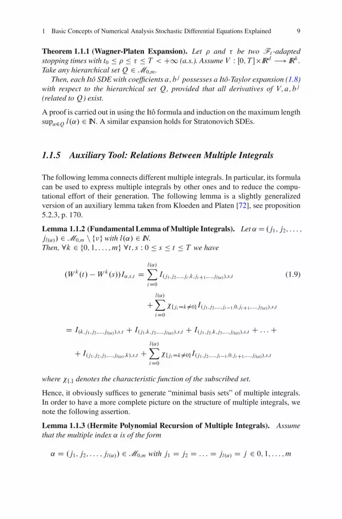
Theorem 1.1.1 (Wagner-Platen Expansion). Let � and � be two Ft -adaptedstopping times with t0 � � � � � T < C1 (a.s.). Assume V W Œ0; T ��IRd �! IRk .Take any hierarchical set Q 2 M0;m.
Then, each Ito SDE with coefficients a; bj possesses a Ito-Taylor expansion (1.8)with respect to the hierarchical set Q, provided that all derivatives of V; a; bj
(related to Q) exist.
A proof is carried out in using the Ito formula and induction on the maximum lengthsup˛2Q l.˛/ 2 IN. A similar expansion holds for Stratonovich SDEs.
1.1.5 Auxiliary Tool: Relations Between Multiple Integrals
The following lemma connects different multiple integrals. In particular, its formulacan be used to express multiple integrals by other ones and to reduce the compu-tational effort of their generation. The following lemma is a slightly generalizedversion of an auxiliary lemma taken from Kloeden and Platen [72], see proposition5.2.3, p. 170.
Lemma 1.1.2 (Fundamental Lemma of Multiple Integrals). Let ˛D .j1; j2; : : : ;
jl.˛// 2 M0;m n f�g with l.˛/ 2 IN.Then, 8k 2 f0; 1; : : : ; mg 8t; s W 0 � s � t � T we have
.W k.t/ �W k.s//I˛;s;t Dl.˛/X
iD0I.j1;j2;:::;ji ;k;jiC1;:::;jl.˛//;s;t (1.9)
Cl.˛/X
iD0fjiDk¤0gI.j1;j2;:::;ji�1;0;jiC1;:::;jl.˛//;s;t
D I.k;j1;j2;:::;jl.˛//;s;t C I.j1;k;j2;:::;jl.˛//;s;t C I.j1;j2;k;j3;:::;jl.˛//;s;t C : : :C
C I.j1;j2;j3;:::;jl.˛/;k/;s;t Cl.˛/X
iD0fjiDk¤0gI.j1;j2;:::;ji�1;0;jiC1;:::;jl.˛//;s;t
where f:g denotes the characteristic function of the subscribed set.
Hence, it obviously suffices to generate “minimal basis sets” of multiple integrals.In order to have a more complete picture on the structure of multiple integrals, wenote the following assertion.
Lemma 1.1.3 (Hermite Polynomial Recursion of Multiple Integrals). Assumethat the multiple index ˛ is of the form
˛ D .j1; j2; : : : ; jl.˛// 2 M0;m with j1 D j2 D : : : D jl.˛/ D j 2 0; 1; : : : ; m
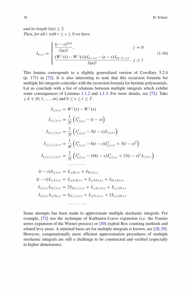
10 H. Schurz
and its length l.˛/ � 2.Then, for all t with t � s � 0 we have
I˛;s;t D
8ˆ<
ˆ:
.t � s/l.˛/
l.˛/Š; j D 0
.W j .t/ �W j .s//I˛�;s;t � .t � s/I.˛�/�;s;tl.˛/Š
; j � 1
(1.10)
This lemma corresponds to a slightly generalized version of Corollary 5.2.4(p. 171) in [72]. It is also interesting to note that this recursion formula formultiple Ito integrals coincides with the recursion formula for hermite polynomials.Let us conclude with a list of relations between multiple integrals which exhibitsome consequences of Lemmas 1.1.2 and 1.1.3. For more details, see [72]. Takej; k 2 f0; 1; : : : ; mg and 0 � s � t � T .
I.j /;s;t D W j .t/ �W j .s/
I.j;j /;s;t D 1
2Š
�I 2.j /;s;t � .t � s/
�
I.j;j;j /;s;t D 1
3Š
�I 3.j /;s;t � 3.t � s/I.j /;s;t
�
I.j;j;j;j /;s;t D 1
4Š
�I 4.j /;s;t � 6.t � s/I 2.j /;s;t C 3.t � s/2
�
I.j;j;j;j;j /;s;t D 1
5Š
�I 5.j /;s;t � 10.t � s/I 3.j /;s;t C 15.t � s/2I.j /;s;t
�
: : : : : : : : : :
.t � s/I.j /;s;t D I.j;0/;s;t C I.0;j /;s;t
.t � s/I.j;k/;s;t D I.j;k;0/;s;t C I.j;0;k/;s;t C I.0;j;k/;s;t
I.j /;s;t I.0;j /;s;t D 2I.0;j;j /;s;t C I.j;0;j /;s;t C I.j;j;0/;s;t
I.j /;s;t I.j;0/;s;t D I.0;j;j /;s;t C I.j;0;j /;s;t C 2I.j;j;0/;s;t
: : : : : : : : : ::
Some attempts has been made to approximate multiple stochastic integrals. Forexample, [72] use the technique of Karhunen-Loeve expansion (i.e. the Fourierseries expansion of the Wiener process) or [30] exploit Box counting methods andrelated levy areas. A minimal basis set for multiple integrals is known, see [28, 29].However, computationally more efficient approximation procedures of multiplestochastic integrals are still a challenge to be constructed and verified (especiallyin higher dimensions).
1 Basic Concepts of Numerical Analysis Stochastic Differential Equations Explained 11
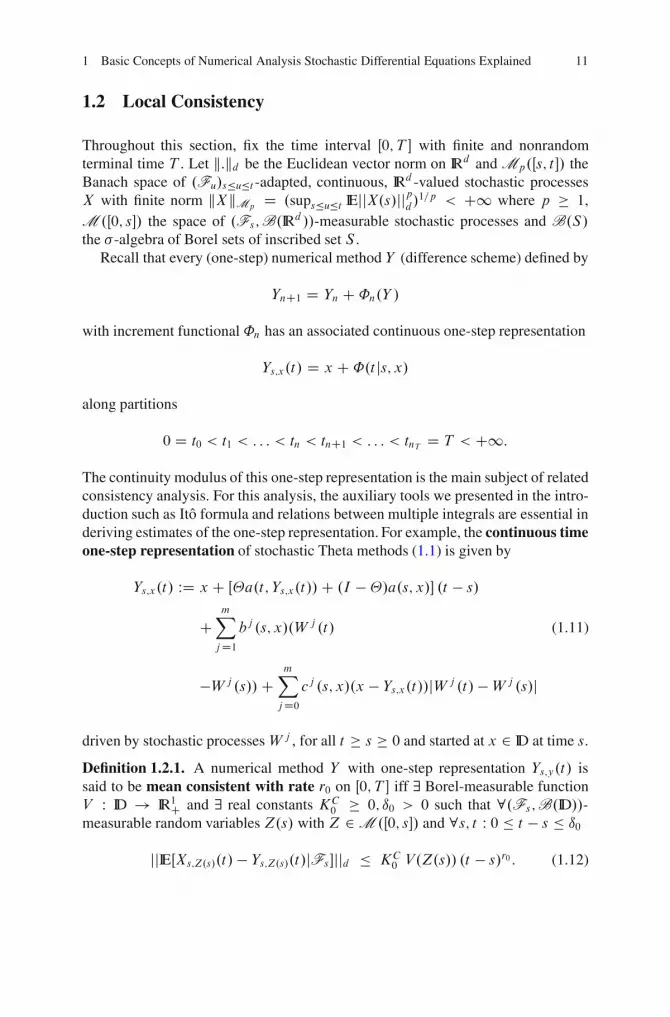
1.2 Local Consistency
Throughout this section, fix the time interval Œ0; T � with finite and nonrandomterminal time T . Let k:kd be the Euclidean vector norm on IRd and Mp.Œs; t �/ theBanach space of .Fu/s�u�t -adapted, continuous, IRd -valued stochastic processesX with finite norm kXkMp D .sups�u�t IEjjX.s/jjpd/1=p < C1 where p � 1,M .Œ0; s�/ the space of .Fs;B.IRd //-measurable stochastic processes and B.S/the -algebra of Borel sets of inscribed set S .
Recall that every (one-step) numerical method Y (difference scheme) defined by
YnC1 D Yn C ˚n.Y /
with increment functional˚n has an associated continuous one-step representation
Ys;x.t/ D x C ˚.t js; x/
along partitions
0 D t0 < t1 < : : : < tn < tnC1 < : : : < tnT D T < C1:
The continuity modulus of this one-step representation is the main subject of relatedconsistency analysis. For this analysis, the auxiliary tools we presented in the intro-duction such as Ito formula and relations between multiple integrals are essential inderiving estimates of the one-step representation. For example, the continuous timeone-step representation of stochastic Theta methods (1.1) is given by
Ys;x.t/ WD x C Œ�a.t; Ys;x.t//C .I ��/a.s; x/� .t � s/
CmX
jD1bj .s; x/.W j .t/ (1.11)
�W j .s//CmX
jD0cj .s; x/.x � Ys;x.t//jW j .t/ �W j .s/j
driven by stochastic processesW j , for all t � s � 0 and started at x 2 ID at time s.
Definition 1.2.1. A numerical method Y with one-step representation Ys;y.t/ issaid to be mean consistent with rate r0 on Œ0; T � iff 9 Borel-measurable functionV W ID ! IR1C and 9 real constants KC
0 � 0; ı0 > 0 such that 8.Fs;B.ID//-measurable random variablesZ.s/ with Z 2 M .Œ0; s�/ and 8s; t W 0 � t � s � ı0
jjIEŒXs;Z.s/.t/ � Ys;Z.s/.t/jFs �jjd � KC0 V.Z.s// .t � s/r0 : (1.12)

12 H. Schurz
Remark 1.2.1. In the subsections below, we shall show that the balanced Thetamethods (1.1) with uniformly bounded weights cj and uniformly bounded param-eters �n are mean consistent with worst case rate r0 � 1:5 and moment controlfunction V.x/ D .1C jjxjj2d /1=2 for SDEs (1.2) with global Holder-continuous andlinear growth-bounded coefficients bj 2F �C1;2.Œ0; T �� ID/ (j D 0; 1; 2; : : : ; m).
Definition 1.2.2. A numerical method Y with one-step representation Ys;y.t/ issaid to be p-th mean consistent with rate r2 on Œ0; T � iff 9 Borel-measurablefunction V W ID ! IR1C and 9 real constants KC
p � 0; ı0 > 0 such that8.Fs;B.ID//-measurable random variables Z.s/ with Z 2 Mp.Œ0; s�/ and 8s; t W0 � t � s � ı0
�IEŒjjXs;Z.s/.t/ � Ys;Z.s/.t/jjpd jFs�
�1=p � KCp V.Z.s// .t � s/rp : (1.13)
If p D 2 then we also speak of mean square consistency with local mean squarerate r2.
Remark 1.2.2. Below, we shall prove that the balanced Theta methods (1.1) aremean square consistent with worst case rate r2 � 1:0 and moment control functionV.x/ D .1C jjxjj2/1=2d for SDEs (1.2) with global Lipschitz-continuous and lineargrowth-bounded coefficients bj 2 F � C1;2.Œ0; T � � ID/ (j D 0; 1; 2; : : : ; m).
In the proofs of consistency of balanced Theta methods (1.1) below, it is crucialthat one exploits the explicit identity
Ys;x.t/ � xD M�1s;x.t/ Œ�a.t; Ys;x.t// � .I ��/a.s; x/� .t � s/
CM�1s;x.t/mX
jD1bj .s; x/.W j.t/�W j.s//
D M�1s;x .t/� Œa.t; Ys;x.t//� a.s; x/�
Z t
s
du CM�1s;x .t/mX
jD0bj .s; x/
Z t
s
dW j .u/
where I is the d�d unit matrix in IRd�d , b0.s; x/ D a.s; x/;W 0.t/ D t;W 0.s/ D s
and
Ms;x.t/ D I CmX
jD0cj .s; x/jW j .t/�W j .s/j:
1.2.1 Main Assumptions for Consistency Proofs
Let jj:jjd�d denote a matrix norm on IRd�d which is compatible to the Euclideanvector norm jj:jjd on IRd , and h:; :id the Euclidean scalar product on IRd .

1 Basic Concepts of Numerical Analysis Stochastic Differential Equations Explained 13
Furthermore we have to assume that the coefficients a and bj are Caratheodoryfunctions such that a strong, unique solution X D .X.t//0�t�T exists. Recallthat ID IRd is supposed to be a nonrandom set. Let ID be simply connected.To guarantee certain rates of consistency of the BTMs (and also its rates ofconvergence) the following conditions have to be satisfied:
(A0) 8s; t 2 Œ0; T � W s < t H) IP .fX.t/ 2 IDjX.s/ 2 IDg/DIP .fYs;y.t/2IDjy2IDg/D1
(A1) 9 constantsKB D KB.T /;KV D KV .T / � 0 such that
8t 2 Œ0; T � 8x 2 ID WmX
jD0jjbj .t; x/jj2d � .KB/
2 ŒV .x/�2 (1.14)
sup0�t�T
IEŒV .X.t//�2 � .KV /2IEŒV .X.0//�2 < C1 (1.15)
with appropriate Borel-measurable function V W ID ! IR1C satisfying
8x 2 ID W jjxjjd � V.x/
(A2) Holder continuity of .a; bj /, i.e. 9 real constants La and Lb such that
8s; t W 0 � t � s � ı0;8x; y 2 ID W jja.t; y/� a.s; x/jjd � La.jt � sj1=2
Cjjy � xjjd / (1.16)mX
jD1jjbj .t; y/ � bj .s; x/jj2d � .Lb/
2.jt�sjCjjy�xjj2d / (1.17)
(A3) 9 real constantsKM D KM.T / � 0 such that, for the chosen weight matricescj 2 IRd�d of balanced Theta methods (1.1), we have
8s; t W 0�t�s�ı0;8x2ID W 9M�1s;x .t/ with jjM�1s;x .t/jjd�d�KM (1.18)
(A4) 9 real constants Kca D Kca.T / � 0 and Kcb D Kcb.T / � 0 such that, forthe chosen weight matrices cj 2 IRd�d of BTMs (1.1), we have
8s 2 Œ0; T � 8x 2 ID WmX
jD0jjcj .s; x/a.s; x/jjd � KcaV.x/ (1.19)
mX
kD0
mX
jD0jjck.s; x/bj .s; x/jj2d�K2
cbŒV .x/�2 (1.20)
14 H. Schurz
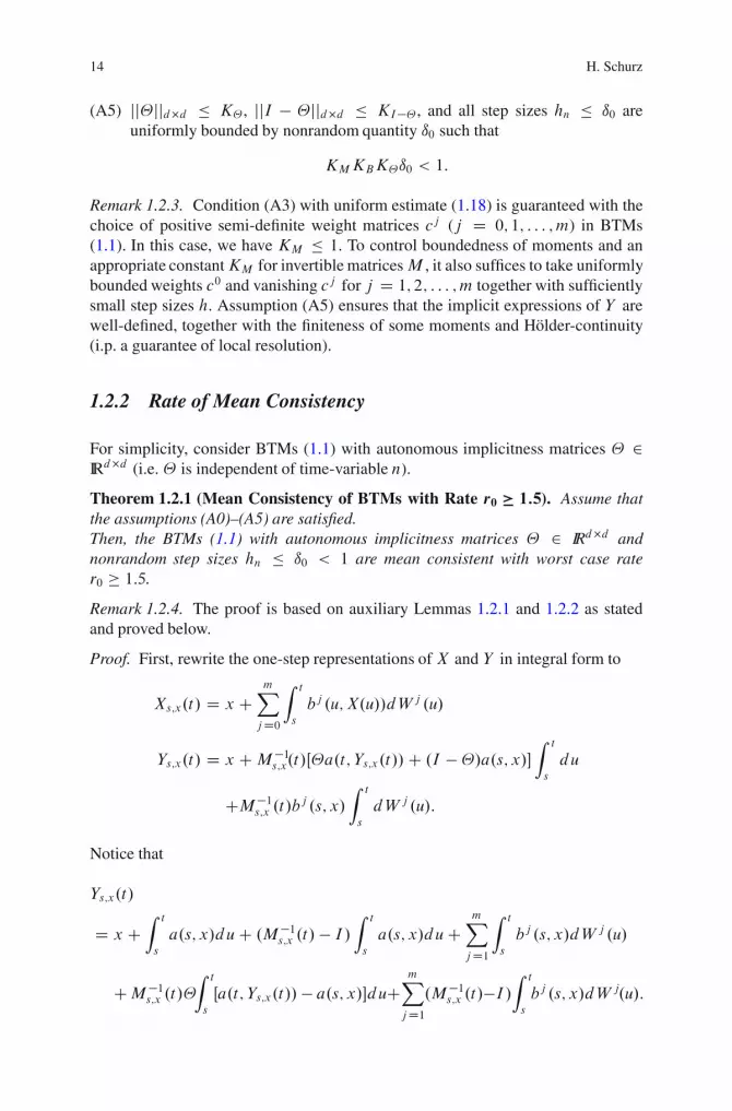
(A5) jj�jjd�d � K�, jjI � �jjd�d � KI�� , and all step sizes hn � ı0 areuniformly bounded by nonrandom quantity ı0 such that
KMKBK�ı0 < 1:
Remark 1.2.3. Condition (A3) with uniform estimate (1.18) is guaranteed with thechoice of positive semi-definite weight matrices cj (j D 0; 1; : : : ; m) in BTMs(1.1). In this case, we have KM � 1. To control boundedness of moments and anappropriate constantKM for invertible matricesM , it also suffices to take uniformlybounded weights c0 and vanishing cj for j D 1; 2; : : : ; m together with sufficientlysmall step sizes h. Assumption (A5) ensures that the implicit expressions of Y arewell-defined, together with the finiteness of some moments and Holder-continuity(i.p. a guarantee of local resolution).
1.2.2 Rate of Mean Consistency
For simplicity, consider BTMs (1.1) with autonomous implicitness matrices � 2IRd�d (i.e. � is independent of time-variable n).
Theorem 1.2.1 (Mean Consistency of BTMs with Rate r0 � 1:5). Assume thatthe assumptions (A0)–(A5) are satisfied.Then, the BTMs (1.1) with autonomous implicitness matrices � 2 IRd�d andnonrandom step sizes hn � ı0 < 1 are mean consistent with worst case rater0 � 1:5.
Remark 1.2.4. The proof is based on auxiliary Lemmas 1.2.1 and 1.2.2 as statedand proved below.
Proof. First, rewrite the one-step representations of X and Y in integral form to
Xs;x.t/ D x CmX
jD0
Z t
s
bj .u; X.u//dW j .u/
Ys;x.t/ D x CM�1s;x.t/Œ�a.t; Ys;x.t//C .I ��/a.s; x/�Z t
s
du
CM�1s;x .t/bj .s; x/Z t
s
dW j .u/:
Notice that
Ys;x.t/
D x CZ t
s
a.s; x/du C .M�1s;x .t/ � I /Z t
s
a.s; x/du CmX
jD1
Z t
s
bj .s; x/dW j .u/
CM�1s;x .t/�Z t
s
Œa.t; Ys;x.t// � a.s; x/�duCmX
jD1.M�1s;x .t/�I /
Z t
s
bj .s; x/dW j.u/:

1 Basic Concepts of Numerical Analysis Stochastic Differential Equations Explained 15
Second, subtracting both representations gives
Xs;x.t/ � Ys;x.t/
DZ t
s
Œa.u; X.u//� a.s; x/�du CmX
jD1
Z t
s
Œbj .u; X.u//� bj .s; x/�dW j .u/
C .M�1s;x .t/ � I /Z t
s
a.s; x/du CM�1s;x .t/�Z t
s
Œa.t; Ys;x.t// � a.s; x/�du
CmX
jD1.M�1s;x .t/ � I /
Z t
s
bj .s; x/dW j .u/:
Recall that the above involved stochastic integrals driven by W j form martingaleswith vanishing first moment.Third, pulling the expectation IE over the latter identity and applying triangleinequality imply that
jjIEŒXs;x.t/ � Ys;x.t/�jjd
�Z t
s
IEjja.u; X.u//� a.s; x/jjd du C IEjjM�1s;x .t/ � I jjdZ t
s
jja.s; x/jjd du
C IEŒjjM�1s;x .t/�jjdZ t
s
jja.t; Ys;x.t//� a.s; x/jjddu�
CmX
jD1IEŒjjM�1s;x .t/ � I jj � jj
Z t
s
bj .s; x/dW j .u/jjd �
� La
Z t
s
Œju � sj1=2 C .IEjjXs;x.u/� xjj2d /1=2�du
CKM.t � s/
mX
jD0jjcj .s; x/a.s; x/jjd IEŒj
Z t
s
dW j .u/j�
CKM.t � s/jj�jjLaŒjt � sj1=2 C .IEjjYs;x.t/ � xjj2d /1=2�:
Note that we used the facts that
M�1s;x .t/ � I D �M�1s;x .t/mX
kD0ck.s; x/
ˇˇˇˇ
Z t
s
dW k.u/
ˇˇˇˇ
and
IE
2
4mX
kD0
mX
jD1M�1s;x .t/ck.s; x/bj .s; x/
ˇˇˇˇ
Z t
s
dW k.u/
ˇˇˇˇ
Z t
s
dW j .v/
3
5 D 0

16 H. Schurz
since all W k are independent and symmetric about 0 (i.e. odd moments of them arevanishing to zero).Fourth, we apply Lemma 1.2.2 in order to arrive at
jjIEŒXs;x.t/ � Ys;x.t/�jjd � LaŒ1CKHX V.x/�
Z t
s
.u � s/1=2du
CKM.t�s/mX
jD0jjcj .s; x/a.s; x/jjd
IE
"
jZ t
s
dW j .u/j2#!1=2
CKMK�LaŒ1CKHY V.x/�.t � s/3=2
� Œ2
3La CKM.Kca CK�La/�.1CKH
X /V.x/.t � s/3=2
D O..t � s/3=2/
under the assumptions (A0)–(A5). Consequently, this confirms the estimate of localrate r0 � 1:5 of mean consistency of BTMs (1.1) with autonomous implicitnessmatrices � 2 IRd�d along any nonrandom partitions of fixed time-intervals Œ0; T �with step sizes h < 1, and hence the conclusion of Theorem 1.2.1 is verified. ˘Remark 1.2.5. Moreover, returning to the proof and extracted from its final estima-tion process, the leading mean error constantKC
0 can be estimated by
KC0 � Œ
2
3La CKM.Kca CK�La/�.1CKH
X /
where KHX is as in (1.23) (see also Remark 1.2.7). For uniformly Lipschitz-
continuous coefficients bj (j D 0; 1; : : : ; m), the functional V of consistency istaken as
V.x/ D .1C jjxjj2d /1=2
which represents the functional of linear polynomial growth (as it is common in thecase with globally Holder-continuous coefficients bj ).
Lemma 1.2.1 (Local uniform boundedness of L2-norms of X and Y ).Assume that
8x 2 ID W jjxjj2d � ŒV .x/�2 � 1C jjxjj2d ;
the assumptions (A1) and (A3) are satisfied, and both X and Y are ID-invariant fordeterministic set ID IRd (i.e. assumption (A0)). Furthermore, for well-definednessof Y , let (A5) hold, i.e.
KMKBK�ı0 < 1
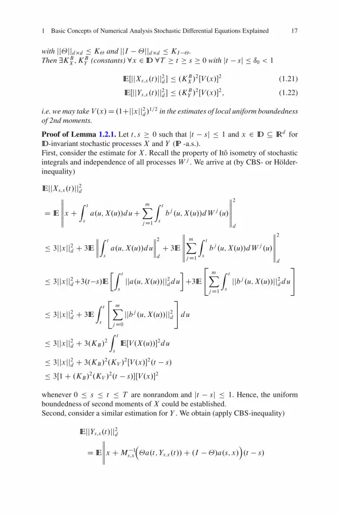
1 Basic Concepts of Numerical Analysis Stochastic Differential Equations Explained 17
with jj�jjd�d � K� and jjI ��jjd�d � KI��.Then 9KB
X ;KBY (constants) 8x 2 ID 8T � t � s � 0 with jt � sj � ı0 < 1
IEŒjjXs;x.t/jj2d � � .KBX /
2ŒV .x/�2 (1.21)
IEŒjjYs;x.t/jj2d � � .KBY /
2ŒV .x/�2; (1.22)
i.e. we may take V.x/D .1Cjjxjj2d /1=2 in the estimates of local uniform boundednessof 2nd moments.
Proof of Lemma 1.2.1. Let t; s � 0 such that jt � sj � 1 and x 2 ID IRd forID-invariant stochastic processes X and Y (IP -a.s.).First, consider the estimate for X . Recall the property of Ito isometry of stochasticintegrals and independence of all processes W j . We arrive at (by CBS- or Holder-inequality)
IEjjXs;x.t/jj2d
D IE
������x C
Z t
s
a.u; X.u//du CmX
jD1
Z t
s
bj .u; X.u//dW j .u/
������
2
d
� 3jjxjj2d C 3IE
����
Z t
s
a.u; X.u//du
����
2
d
C 3IE
������
mX
jD1
Z t
s
bj .u; X.u//dW j .u/
������
2
d
� 3jjxjj2dC3.t�s/IEZ t
s
jja.u; X.u//jj2ddu
C3IE
2
4mX
jD1
Z t
s
jjbj .u; X.u//jj2ddu
3
5
� 3jjxjj2d C 3IEZ t
s
2
4mX
jD0jjbj .u; X.u//jj2d
3
5du
� 3jjxjj2d C 3.KB/2
Z t
s
IEŒV .X.u//�2du
� 3jjxjj2d C 3.KB/2.KV /
2ŒV .x/�2.t � s/
� 3Œ1C .KB/2.KV /
2.t � s/�ŒV .x/�2
whenever 0 � s � t � T are nonrandom and jt � sj � 1. Hence, the uniformboundedness of second moments of X could be established.Second, consider a similar estimation for Y . We obtain (apply CBS-inequality)
IEjjYs;x.t/jj2d
D IE
�����x CM�1s;x
��a.t; Ys;x.t//C .I ��/a.s; x/
�.t � s/

18 H. Schurz
CmX
jD1
Z t
s
M�1s;x .t/bj .s; x/dW j .u/
�����
2
d
� 4jjxjj2dC4K2MK
2�IEjja.t; Ys;x.t//jj2d .t � s/2
C 4K2MK
2I��jja.s; x/jj2d .t � s/2 C 4K2
M
mX
jD1jjbj .s; x/jj2d .t � s/
� 4ŒV .x/�2 C 4K2MK
2�.KB/
2IEŒV .Ys;x.t//�2.t � s/2
C 4K2M.1CK2
I��/mX
jD1jjbj .s; x/jj2d .t � s/
� 4ŒV .x/�2 C 4K2MK
2�.KB/
2IEŒV .Ys;x.t//�2.t � s/2
C 4K2M.1CK2
I��/.KB/2ŒV .x/�2.t � s/
� 41CK2
M .KB/2K2
�.t � s/2 C 1CK2I��.t � s/
1 �K2M.KB/2K
2�.ı0/
2ŒV .x/�2
� 41CK2
M .KB/2K2
�.ı0/2 C 1CK2
I��ı01 �K2
M.KB/2K2�.ı0/
2ŒV .x/�2;
where ŒV .x/�2 � 1C jjxjj2d and K2M.KB/
2K2�.ı0/
2 < 1 are additionally supposedin the latter estimation. Therefore, the uniform boundedness of second moments ofY is verified. ˘Remark 1.2.6. Indeed, while returning to the proof of Lemma 1.2.1, under theassumptions (A0)–(A1), (A3) and (A5) with V.x/ D .1 C jjxjj2d /1=2 we find thatKBX can be estimated by
KBX � 3Œ1C .KB/
2.KV /2�:
as long as jt � sj � 1. Similarly,KBY is bounded by
KBY � 4
1CK2M.KB/
2K2�.ı0/
2 C 1CK2I��ı0
1 �K2M .KB/2K
2�.ı0/
2
whenever K2M.KB/
2K2�.ı0/
2 < 1 and jt � sj � ı0 � 1, jjxjj2d � ŒV .x/�2 � 1Cjjxjj2d for all x 2 ID.
Lemma 1.2.2 (Local mean square Holder continuity of X and Y ). Assume that
8x 2 ID W jjxjj2d � ŒV .x/�2 � 1C jjxjj2d ;

1 Basic Concepts of Numerical Analysis Stochastic Differential Equations Explained 19
the assumptions (A1)–(A3) and (A5) are satisfied, and both X and Y areID-invariant for deterministic set ID IRd (i.e. assumption (A0)).Then 9KH
X ;KHY (constants) 8T � t � s � 0 with jt � sj < 1
IEŒjjXs;x.t/ � xjj2d � � .KHX /
2ŒV .x/�2.t � s/ (1.23)
IEŒjjYs;x.t/ � xjj2d � � .KHY /
2ŒV .x/�2.t � s/ (1.24)
for all nonrandom x 2 ID IRd , i.e. we may take V.x/ � .1 C jjxjj2d /1=2 in theestimates of Holder-continuity modulus of 2nd moments.
Proof of Lemma 1.2.2. Let t; s � 0 such that jt � sj � 1 and x 2 ID IRd forID-invariant stochastic processes X and Y (IP -a.s.).First, consider the estimate for X . Recall the property of Ito isometry of stochasticintegrals and independence of all processes W j . We arrive at
IEjjXs;x.t/� xjj2d D IE
������
Z t
s
a.u; X.u//du CmX
jD1
Z t
s
bj .u; X.u//dW j .u/
������
2
d
D IE
����
Z t
s
a.u; X.u//du
����
2
CmX
jD1IE
����
Z t
s
bj .u; X.u//dW j .u/
����
2
d
�Z t
s
IE
2
4.t � s/jja.u; X.u//jj2d CmX
jD1jjbj .u; X.u//jj2d
3
5du
�Z t
s
IE
2
4mX
jD0jjbj .u; X.u//jj2d
3
5 du � .KB/2
Z t
s
IEŒV .X.u//�2du
� .KB/2.KV /
2IEŒV .Xs;x.s//�2jt�sjD.KB/2.KV /
2ŒV .x/�2.t�s/
whenever 0 � s � t � T are nonrandom and jt � sj � 1.Second, consider a similar estimation for Y . We obtain (apply CBS-inequality)
IEjjYs;x.t/� xjj2d
D IE
�����M�1s;x
��a.t; Ys;x.t//C .I ��/a.s; x/
�.t � s/
CmX
jD1
Z t
s
M�1s;x .t/bj .s; x/dW j .u/
�����
2
d
� 3K2MK
2�IEjja.t; Ys;x.t//jj2d .t � s/2 C 3K2
MK2I��jja.s; x/jj2d .t � s/2

20 H. Schurz
C3K2M
mX
jD1jjbj .s; x/jj2d .t � s/
� 3K2M.KB/
2.K2�IEŒV .Ys;x.t//�2
CK2I��ŒV .x/�2/.t�s/2C3K2
M.KB/2ŒV .x/�2.t�s/
� 3K2M.KB/
2ŒK2�.K
BY /
2 CK2I�� C 1�ŒV .x/�2.t � s/
whenever 0 � s � t � T are nonrandom and jt � sj � 1. This completes the proofof Lemma 1.2.2. ˘Remark 1.2.7. Indeed, while returning to the proof of Lemma 1.2.2, under theassumptions (A0)–(A5) with V.x/ D .1 C jjxjj2
d /1=2 we find that KH
X can beestimated by
KHX � .KB/
2.KV /2:
Similarly,KHY is bounded by
KHY � 3K2
M.KB/2ŒK2
�.KBY /
2 CK2I�� C 1�:
1.2.3 Mean Square Consistency
For simplicity, consider BTMs (1.1) with autonomous implicitness matrices � 2IRd�d .
Theorem 1.2.2 (Mean Square Consistency of BTMs with Rate r2�1:0). Assumethat the assumptions (A0) - (A5) are satisfied, together with
8x 2 ID W V.x/ D .1C jjxjj2d /1=2:
Then, the BTMs (1.1) with autonomous implicitness matrices � 2 IRd�d andnonrandom step sizes hn � ı0 < 1 are mean square consistent with worst caserate r2 � 1:0 along V on ID IRd .
Remark 1.2.8. The proof is based on auxiliary Lemmas 1.2.1 and 1.2.2 as stated inprevious subsection.
Proof. First, from the proof of Theorem 1.2.1, recall the difference of one-steprepresentations of X and Y in integral form is given by
Xs;x.t/ � Ys;x.t/
DZ t
s
Œa.u; X.u//� a.s; x/�du CmX
jD1
Z t
s
Œbj .u; X.u//� bj .s; x/�dW j .u/

1 Basic Concepts of Numerical Analysis Stochastic Differential Equations Explained 21
C .M�1s;x .t/ � I /Z t
s
a.s; x/du CM�1s;x .t/�Z t
s
Œa.t; Ys;x .t// � a.s; x/�du
CmX
jD1.M�1s;x .t/ � I /
Z t
s
bj .s; x/dW j .u/:
Second, take the square norm and apply Holder-inequality (CBS-inequality) in orderto encounter the estimation
IEjjXs;x.t/� Ys;x.t/jj2d
D IE
������
Z t
s
Œa.u; X.u//� a.s; x/�du CmX
jD1
Z t
s
Œbj .u; X.u//� bj .s; x/�dW j .u/
C.M�1s;x .t/ � I /
Z t
s
a.s; x/du CM�1s;x .t/�Z t
s
Œa.t; Ys;x.t// � a.s; x/�du
CmX
jD1.M�1s;x .t/ � I /
Z t
s
bj .s; x/dW j .u/
������
2
d
� 5IE
����
Z t
s
Œa.u; X.u//�a.s; x/�du
����
2
d
C5mX
jD1IE
����
Z t
s
Œbj .u; X.u//�bj .s; x/�dW j .u/
����
2
d
C 5IE
����.M
�1s;x .t/�I /
Z t
s
a.s; x/du
����
2
d
C5IE
����M
�1s;x .t/�
Z t
s
Œa.t;Ys;x.t//�a.s; x/�du
����
2
d
C 5
mX
jD1IE
����.M
�1s;x .t/ � I /
Z t
s
bj .s; x/dW j .u/
����
2
d
:
Third, recall Ito isometry and the facts that
M�1s;x .t/ � I D �M�1s;x .t/mX
kD0ck.s; x/
ˇˇˇˇ
Z t
s
dW k.u/
ˇˇˇˇ
and
IE
2
4mX
kD0
mX
jD1M�1s;x .t/ck.s; x/bj .s; x/
ˇˇˇˇ
Z t
s
dW k.u/
ˇˇˇˇ
Z t
s
dW j .v/
3
5 D 0
since all W k are independent and symmetric about 0 (i.e. odd moments of them arevanishing to zero). Therefore, we may simplify our latter estimation to
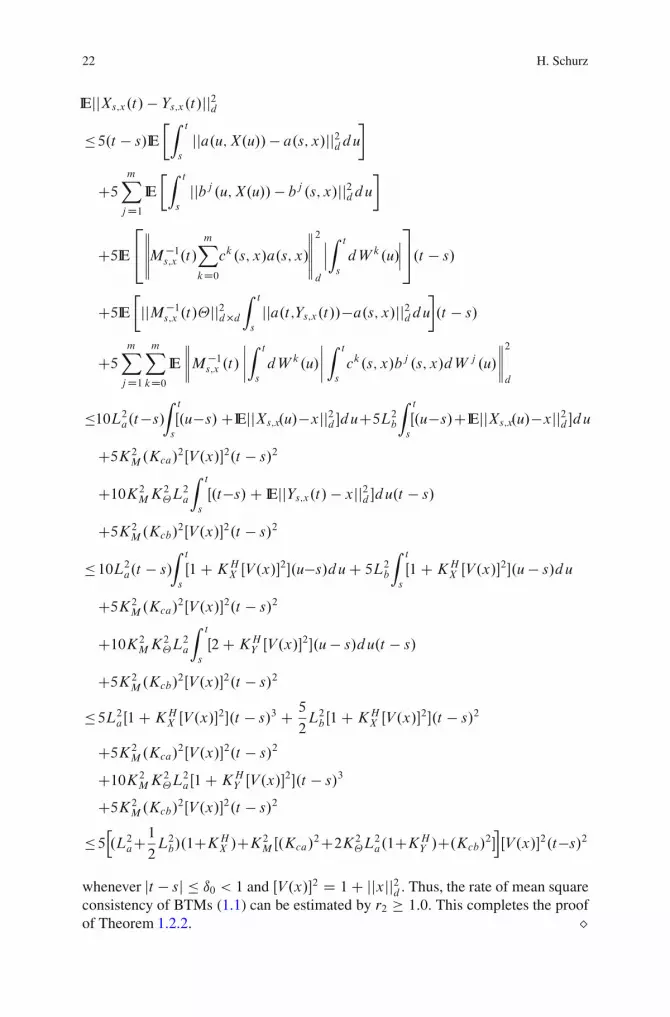
22 H. Schurz
IEjjXs;x.t/� Ys;x.t/jj2d�5.t � s/IE
Z t
s
jja.u; X.u//� a.s; x/jj2d du
C5mX
jD1IE
Z t
s
jjbj .u; X.u//� bj .s; x/jj2d du
C5IE
2
4
�����M�1s;x .t/
mX
kD0ck.s; x/a.s; x/
�����
2
d
ˇˇˇ
Z t
s
dW k.u/ˇˇˇ
3
5.t � s/
C5IE
jjM�1s;x .t/�jj2d�dZ t
s
jja.t;Ys;x.t//�a.s; x/jj2ddu
.t � s/
C5mX
jD1
mX
kD0IE
����M
�1s;x .t/
ˇˇˇˇ
Z t
s
dW k.u/
ˇˇˇˇ
Z t
s
ck.s; x/bj .s; x/dW j .u/
����
2
d
�10L2a.t�s/Z t
s
Œ.u�s/CIEjjXs;x.u/�xjj2d �duC5L2bZ t
s
Œ.u�s/CIEjjXs;x.u/�xjj2d �du
C5K2M.Kca/
2ŒV .x/�2.t � s/2
C10K2MK
2�L
2a
Z t
s
Œ.t�s/C IEjjYs;x.t/ � xjj2d �du.t � s/
C5K2M.Kcb/
2ŒV .x/�2.t � s/2
�10L2a.t � s/
Z t
s
Œ1CKHX ŒV.x/�
2�.u�s/du C 5L2b
Z t
s
Œ1CKHX ŒV.x/�
2�.u � s/du
C5K2M.Kca/
2ŒV .x/�2.t � s/2
C10K2MK
2�L
2a
Z t
s
Œ2CKHY ŒV .x/�
2�.u � s/du.t � s/
C5K2M.Kcb/
2ŒV .x/�2.t � s/2
�5L2aŒ1CKHX ŒV.x/�
2�.t � s/3 C 5
2L2bŒ1CKH
X ŒV.x/�2�.t � s/2
C5K2M.Kca/
2ŒV .x/�2.t � s/2
C10K2MK
2�L
2aŒ1CKH
Y ŒV .x/�2�.t � s/3
C5K2M.Kcb/
2ŒV .x/�2.t � s/2
�5h.L2aC
1
2L2b/.1CKH
X /CK2MŒ.Kca/
2C2K2�L
2a.1CKH
Y /C.Kcb/2�iŒV .x/�2.t�s/2
whenever jt � sj � ı0 < 1 and ŒV .x/�2 D 1C jjxjj2d . Thus, the rate of mean squareconsistency of BTMs (1.1) can be estimated by r2 � 1:0. This completes the proofof Theorem 1.2.2. ˘
1 Basic Concepts of Numerical Analysis Stochastic Differential Equations Explained 23
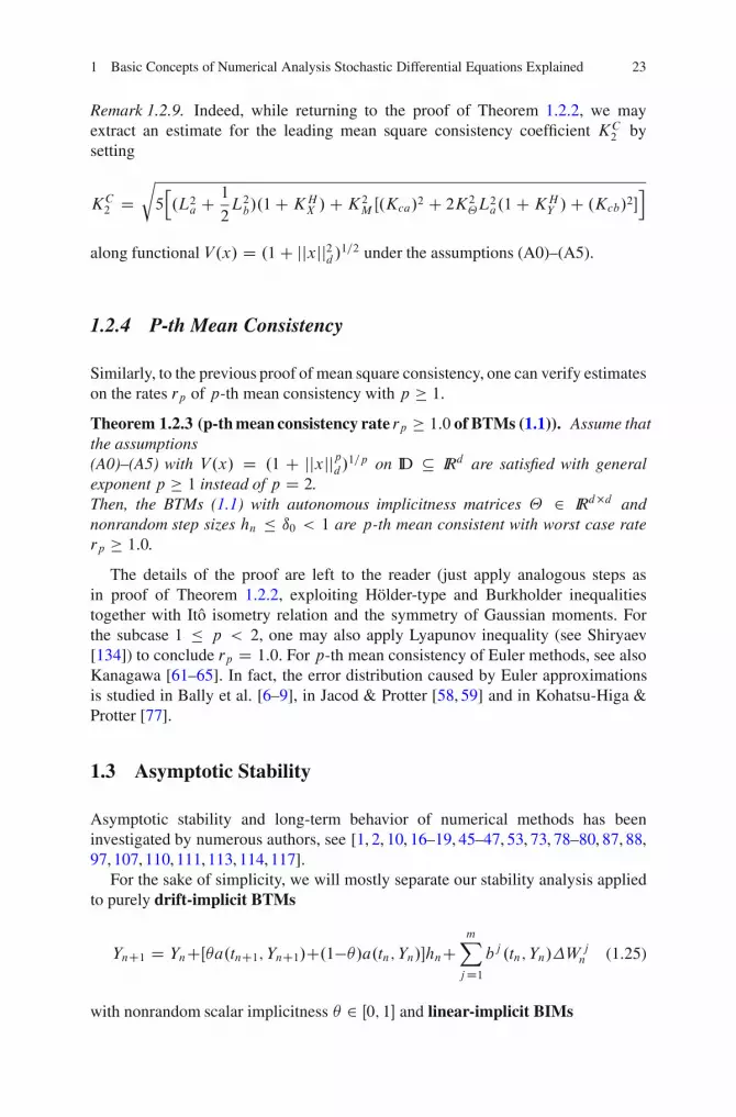
Remark 1.2.9. Indeed, while returning to the proof of Theorem 1.2.2, we mayextract an estimate for the leading mean square consistency coefficient KC
2 bysetting
KC2 D
r
5h.L2a C 1
2L2b/.1CKH
X /CK2M Œ.Kca/2 C 2K2
�L2a.1CKH
Y /C .Kcb/2�i
along functional V.x/ D .1C jjxjj2d /1=2 under the assumptions (A0)–(A5).
1.2.4 P-th Mean Consistency
Similarly, to the previous proof of mean square consistency, one can verify estimateson the rates rp of p-th mean consistency with p � 1.
Theorem 1.2.3 (p-th mean consistency rate rp � 1:0 of BTMs (1.1)). Assume thatthe assumptions(A0)–(A5) with V.x/ D .1 C jjxjjpd/1=p on ID IRd are satisfied with generalexponent p � 1 instead of p D 2.Then, the BTMs (1.1) with autonomous implicitness matrices � 2 IRd�d andnonrandom step sizes hn � ı0 < 1 are p-th mean consistent with worst case raterp � 1:0.
The details of the proof are left to the reader (just apply analogous steps asin proof of Theorem 1.2.2, exploiting Holder-type and Burkholder inequalitiestogether with Ito isometry relation and the symmetry of Gaussian moments. Forthe subcase 1 � p < 2, one may also apply Lyapunov inequality (see Shiryaev[134]) to conclude rp D 1:0. For p-th mean consistency of Euler methods, see alsoKanagawa [61–65]. In fact, the error distribution caused by Euler approximationsis studied in Bally et al. [6–9], in Jacod & Protter [58, 59] and in Kohatsu-Higa &Protter [77].
1.3 Asymptotic Stability
Asymptotic stability and long-term behavior of numerical methods has beeninvestigated by numerous authors, see [1, 2, 10, 16–19, 45–47, 53, 73, 78–80, 87, 88,97, 107, 110, 111, 113, 114, 117].
For the sake of simplicity, we will mostly separate our stability analysis appliedto purely drift-implicit BTMs
YnC1 D YnCŒ�a.tnC1; YnC1/C.1��/a.tn; Yn/�hnCmX
jD1bj .tn; Yn/�W
jn (1.25)
with nonrandom scalar implicitness � 2 Œ0; 1� and linear-implicit BIMs

24 H. Schurz
YnC1 D Yn CmX
jD0bj .tn; Yn/�W
jn C
mX
jD0cj .tn; Yn/.Yn � YnC1/j�W j
n j (1.26)
with appropriate weight matrices cj .
1.3.1 Weak V -Stability of Numerical Methods
Definition 1.3.1. A numerical method Y with one-step representation Ys;y.t/ issaid to be weakly V -stable with real constant KS D KS.T / on Œ0; T � iff V WIRd!IR1C is Borel-measurable and 9 real constant ı0 > 0 such that 8.Fs;B.IRd //-measurable random variablesZ.s/ and 8s; t W 0 � t � s � ı0 � 1
IEŒV .Ys;Z.s/.t//jFs � � exp.KS.t � s// V .Z.s//: (1.27)
A weakly V -stable numerical method Y is called weakly exponential V -stable iffKS < 0. A numerical method Y is exponential p-th mean stable iff Y is weaklyexponential V -stable with V.x/ D jjxjjp
dand KS < 0. In the case p D 2, we speak
of exponential mean square stability.
Remark 1.3.1. Exponential stability is understood with respect to the trivial solution(equilibrium or fixed point 0) throughout this paper.
Theorem 1.3.1. Assume that the numerical method Y started at a .F0;B.IRd //-measurableY0 and constructed along any .Ft /-adapted time-discretization of Œ0; T �with maximum step size hmax � ı0 is weakly V -stable with ı0 and stability constantKS on Œ0; T �. Then
8t 2 Œ0; T � W IEŒV .Y0;Y0 .t//� � exp.KSt/IEŒV .Y0/�; (1.28)
sup0�t�T
IEŒV .Y0;Y0 .t//� � exp.ŒKS�CT /IEŒV .Y0/� (1.29)
where Œ:�C denotes the positive part of the inscribed expression.
Proof. Suppose that tk � t � tkC1 with hk � ı0. If IEŒV .Y0/� D C1 then nothingis to prove. Now, suppose that IEŒV .Y0/� < C1. Using elementary properties ofconditional expectations, we estimate
IEŒV .Y0;Y0 .t//� D IEŒIEŒV .Ytk;Yk .t/jFtk ��
� exp.KS.t � tk// � IEŒV .Yk/�
D exp.KS.t � tk// � IEŒV .Ytk�1;Yk�1.tk//� � : : :
� exp.KSt/ � IEŒV .Y0/� � exp.ŒKS �Ct/ � IEŒV .Y0/�

1 Basic Concepts of Numerical Analysis Stochastic Differential Equations Explained 25
� exp.ŒKS �CT / � IEŒV .Y0/�
by induction. Hence, taking the supremum confirms the claim of Theorem 1.3.1. ˘Remark. Usually V plays the role of a Lyapunov functional for controlling thestability of the numerical method Y .
Theorem 1.3.2. Assume that .A1/ and .A3/ with V.x/ D �2 C jjxjj2d (� 2 IR1
some real constant) hold. Then the BIMs (1.26) with hmax � ı0 � min.1; T / areweakly V -stable with stability constant
KS � KM �KB � .2CKM �KB/ (1.30)
and they satisfy global weak V -stability estimates (1.28) and (1.29).
Proof. Suppose that .A1/ and .A3/ hold with V.x/ D �2 C jjxjj2. Recall that0 � t � s � ı0 � 1. Let Z.s/ be any .Fs;B.IRd //-measurable random variable.Then
IEŒ�2 C jjYs;Z.s/jj2d jFs � D IEŒ�2 C jjZ.s/CM�1s;Z.s/.t/mX
jD0bj .s; Z.s//.W j .t/
�W j .s//jj2d jFs�
D IEŒ�2 C jjZ.s/CM�1s;Z.s/.t/a.s;Z.s//.t � s/
CM�1s;Z.s/.t/mX
jD1bj .s; Z.s//.W j .t/ �W j .s//jj2d jFs�
D �2 C 1
2IEŒjjz CM�1s;z .t/a.s; z/.t�s/
CM�1s;z .t/mX
jD1bj .s; z/.W j .t/�W j .s//jj2d �
ˇˇˇzDZ.s/
C1
2IEŒjjz CM�1s;z .t/a.s; z/.t � s/
�M�1s;z .t/mX
jD1bj .s; z/.W j .t/�W j .s//jj2d �
ˇˇˇzDZ.s/
D �2 C IEŒjjz CM�1s;z .t/a.s; z/.t � s/jj2d �ˇˇzDZ.s/
CIEŒjjM�1s;z .t/mX
jD1bj .s; z/.W j .t/ �W j .s//jj2d �
ˇˇˇzDZ.s/
D �2CjjZ.s/jj2dC2 ŒIE<z;M�1s;z .t/a.s; z/>d �ˇˇzDZ.s/ .t�s/
C IEŒjjM�1s;z .t/a.s; z/jj2d �ˇˇzDZ.s/.t�s/2

26 H. Schurz
CmX
jD1IEŒjjM�1s;z .t/bj .s; z/jj2d .W j .t/�W j .s//2�
ˇˇzDZ.s/
� .1C Œ2KMKB CK2MK
2B�.t � s// � .�2 C jjZ.s/jj2d /
� exp.Œ2KMKB CK2MK
2B�.t � s// � .�2 C jjZ.s/jj2d /;
hence the BIMs (1.26) are weakly V -stable with V.x/ D �2 C jjxjj2d . It obviouslyremains to apply Theorem 1.3.1 in order to complete the proof. ˘Remark 1.3.2. Interestingly, by setting � D 0, we gain also a result on numericalmean square stability. However, for results on asymptotic mean square stability ofBTMs and BIMs, see below or [120].
1.3.2 Asymptotic Mean Square Stability for Bilinear TestEquations
Consider (autonomous) linear systems of Ito SDEs with stationary solutionX1 D 0
dX.t/ D AX.t/ dt CmX
jD1BjX.t/dW j .t/ (1.31)
started in .F0;B.IRd //-measurable initial data X.0/ at time t D 0. Let p 2.0;C1/ be a nonrandom constant.
Definition 1.3.2. Assume X � 0 is an equilibrium (fixed point, steady state). Thetrivial solution X � 0 of SDE (1.2) is called globally (asymptotically) p-th meanstable iff 8X0 W IEkX.0/kp
d< C1 H) limt!C1 IEkX.t/kp
dD 0: In the case
p D 2 we speak of global (asymptotic) mean square stability. Moreover, thetrivial solution X � 0 of SDE (1.2) is said to be locally (asymptotically) p-thmean stable iff 8" > 09ı W 8X0 W IEkX.0/kp
d< ı H) 8t > 0 W IEkX.t/kp
d< ":
In the case p D 2 we speak of local (asymptotic) mean square stability.
Remark 1.3.3. To recall some well-known facts from general stability theory, anexponentially p-th mean stable process is also asymptotically p-th mean stable.However, not vice versa in general. Furthermore, a globally (asymptotically) p-thmean stable trivial solution is also locally (asymptotically) p-th mean stable. Fornonlinear systems of SDEs (1.2), the concepts of local and global stability do notcoincide. For linear autonomous systems, these concepts coincide.
Let Y0 be .F0;B.IRd //-measurable in all statements in what follows.
Definition 1.3.3. Assume Y � 0 is an equilibrium (fixed point, steady state). Thetrivial solution Y � 0 of BTMs (1.1) is called globally (asymptotically)p-th meanstable iff 8Y0 W IEkY0kpd < C1 H) limn!C1 IEkYnkpd D 0: In the case p D 2
1 Basic Concepts of Numerical Analysis Stochastic Differential Equations Explained 27
we speak of global (asymptotic) mean square stability of Y . Moreover, the trivialsolution Y � 0 of BTMs (1.1) is said to be locally (asymptotically) p-th meanstable iff 8" > 09ı W 8Y0 W IEkY0kpd < ı H) 8n > 0 W IEkYnkpd < ": In the casep D 2 we speak of local (asymptotic) mean square stability of Y .
Now, consider the family of drift-implicit Theta methods
YnC1 D Yn C .�AYnC1 C .1 � �/AYn/hn CmX
jD1BjYn�W
jn (1.32)
applied to autonomous systems of SDEs (1.31) with scalar implicitness parameter� 2 IR1 (i.e. � D �I , all cj D 0 in (1.1)).
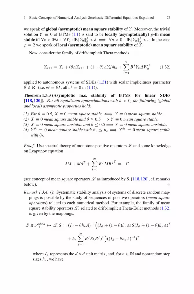
Theorem 1.3.3 (Asymptotic m.s. stability of BTMs for linear SDEs[118, 120]). For all equidistant approximations with h > 0, the following (globaland local) asymptotic properties hold:
(1) For � D 0:5, X � 0 mean square stable ” Y � 0 mean square stable.(2) X � 0 mean square stable and � � 0:5 H) Y � 0 mean square stable.(3) X � 0 mean square unstable and � � 0:5 H) Y � 0 mean square unstable.(4) Y �1 � 0 mean square stable with �1 � �2 H) Y �2 � 0mean square stable
with �2.
Proof. Use spectral theory of monotone positive operators L and some knowledgeon Lyapunov equation
AM C MAT CmX
jD1BjMBj
T D �C
(see concept of mean square operators L as introduced by S. [118,120], cf. remarksbelow). ˘Remark 1.3.4. (i) Systematic stability analysis of systems of discrete random map-
pings is possible by the study of sequences of positive operators (mean squareoperators) related to each numerical method. For example, the family of meansquare stability operators Ln related to drift-implicit Theta-Euler methods (1.32)is given by the mappings.
S 2 S d�dC 7! LnS D .Id � �hnA/�1�.Id C .1 � �/hnA/S.Id C .1� �/hnA/
T
Chn
mX
jD1BjS.Bj /T
�..Id � �hnA/
�1/T
where Id represents the d �d unit matrix, and, for n 2 IN and nonrandom stepsizes hn, we have
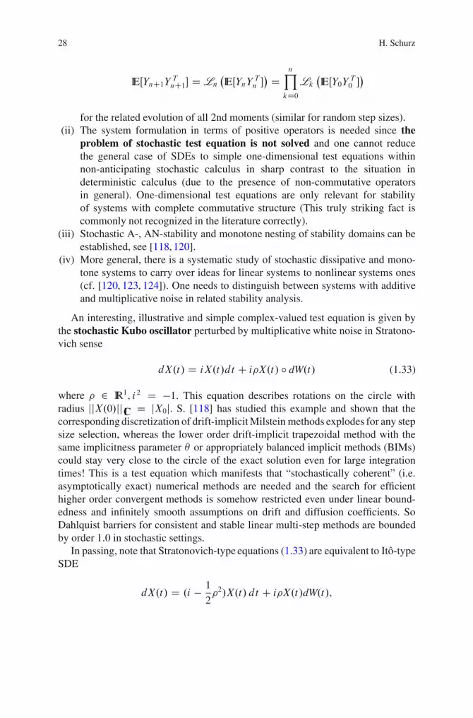
28 H. Schurz
IEŒYnC1Y TnC1� D Ln
�IEŒYnY
Tn �� D
nY
kD0Lk
�IEŒY0Y
T0 ��
for the related evolution of all 2nd moments (similar for random step sizes).(ii) The system formulation in terms of positive operators is needed since the
problem of stochastic test equation is not solved and one cannot reducethe general case of SDEs to simple one-dimensional test equations withinnon-anticipating stochastic calculus in sharp contrast to the situation indeterministic calculus (due to the presence of non-commutative operatorsin general). One-dimensional test equations are only relevant for stabilityof systems with complete commutative structure (This truly striking fact iscommonly not recognized in the literature correctly).
(iii) Stochastic A-, AN-stability and monotone nesting of stability domains can beestablished, see [118, 120].
(iv) More general, there is a systematic study of stochastic dissipative and mono-tone systems to carry over ideas for linear systems to nonlinear systems ones(cf. [120, 123, 124]). One needs to distinguish between systems with additiveand multiplicative noise in related stability analysis.
An interesting, illustrative and simple complex-valued test equation is given bythe stochastic Kubo oscillator perturbed by multiplicative white noise in Stratono-vich sense
dX.t/ D iX.t/dt C i�X.t/ ı dW.t/ (1.33)
where � 2 IR1; i 2 D �1. This equation describes rotations on the circle withradius jjX.0/jj IC D jX0j. S. [118] has studied this example and shown that thecorresponding discretization of drift-implicit Milstein methods explodes for any stepsize selection, whereas the lower order drift-implicit trapezoidal method with thesame implicitness parameter � or appropriately balanced implicit methods (BIMs)could stay very close to the circle of the exact solution even for large integrationtimes! This is a test equation which manifests that “stochastically coherent” (i.e.asymptotically exact) numerical methods are needed and the search for efficienthigher order convergent methods is somehow restricted even under linear bound-edness and infinitely smooth assumptions on drift and diffusion coefficients. SoDahlquist barriers for consistent and stable linear multi-step methods are boundedby order 1:0 in stochastic settings.
In passing, note that Stratonovich-type equations (1.33) are equivalent to Ito-typeSDE
dX.t/ D .i � 1
2�2/X.t/ dt C i�X.t/dW.t/;

1 Basic Concepts of Numerical Analysis Stochastic Differential Equations Explained 29
thereby SDEs (1.33) belong to following subclass (1.34). A more general bilineartest equation is studied in the following example.
Example of one-dimensional complex-valued test SDE. Many authors (e.g.Mitsui and Saito [98] or Schurz [118]) have studied the SDE
dX.t/ D �X.t/ dt C �X.t/ dW.t/; (1.34)
with X.0/ D x0; �; � 2 IC1, representing a test equation for the class of completelycommutative systems of linear SDEs with multiplicative white noise. This stochasticprocess has the unique exact solutionX.t/ D X.0/ �exp..���2=2/tC�W.t// withsecond moment
IEŒX.t/X�.t/� D IEjX.t/j2 D IE exp.2.� � �2=2/r t C 2�rW.t// � jx0j2D jx0j2 � exp.2.�r � �2r =2C �2i =2/t C 2�2r t/
D jx0j2 � exp..2�r C j� j2/t/
where x0 2 IC1 is nonrandom (zr is the real part, zi the imaginary part of z 2 IC1)and denotes the complex conjugate value. The trivial solution X � 0 of (1.34)is mean square stable for the process fX.t/ W t � 0g iff 2�r C j� j2 < 0. Now, letus compare the numerical approximations of families of (drift-)implicit Theta andMilstein methods. Applied to (1.34), the drift-implicit Milstein and drift-implicitTheta methods are given by
Y.M/nC1 D 1C .1 � �/�hC � n
phC �2. 2n � 1/h=2
1 � ��h � Y .M/n (1.35)
and
Y.E/nC1 D 1C .1� �/�hC � n
ph
1� ��h� Y .E/n ; (1.36)
respectively. Their second moments P .E=M/n D IEŒY .E=M/
n Y.E=M/*�n satisfy
P.M/nC1 D
IEj1C .1 � �/�hC � nph
1 � ��h j2 C IEj�2. 2n � 1/1 � ��h
j2 � h2=4!
� P .M/n
D P.M/0 �
� j1C .1 � �/�hj2 C j� j2hC j� j4h2=2j1 � ��hj2
�nC1
> P.E/0 �
� j1C .1 � �/�hj2 C j� j2hj1 � ��hj2
�nC1D P
.E/nC1 .n D 0; 1; 2; : : :/;
provided that P .M/0 D IEŒY .M/
0 Y.M/*
0 � � IEŒY .E/0 Y.E/*
0 � D P.E/0 , and
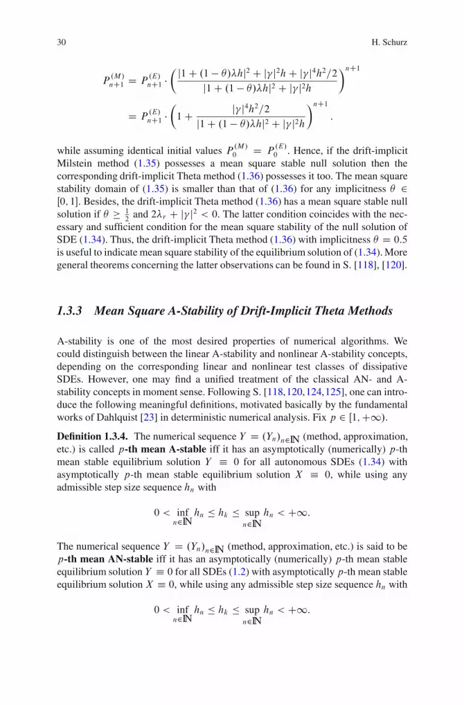
30 H. Schurz
P.M/nC1 D P
.E/nC1 �
� j1C .1 � �/�hj2 C j� j2hC j� j4h2=2j1C .1 � �/�hj2 C j� j2h
�nC1
D P.E/nC1 �
�
1C j� j4h2=2j1C .1 � �/�hj2 C j� j2h
�nC1:
while assuming identical initial values P.M/0 D P
.E/0 . Hence, if the drift-implicit
Milstein method (1.35) possesses a mean square stable null solution then thecorresponding drift-implicit Theta method (1.36) possesses it too. The mean squarestability domain of (1.35) is smaller than that of (1.36) for any implicitness � 2Œ0; 1�. Besides, the drift-implicit Theta method (1.36) has a mean square stable nullsolution if � � 1
2and 2�r C j� j2 < 0. The latter condition coincides with the nec-
essary and sufficient condition for the mean square stability of the null solution ofSDE (1.34). Thus, the drift-implicit Theta method (1.36) with implicitness � D 0:5
is useful to indicate mean square stability of the equilibrium solution of (1.34). Moregeneral theorems concerning the latter observations can be found in S. [118], [120].
1.3.3 Mean Square A-Stability of Drift-Implicit Theta Methods
A-stability is one of the most desired properties of numerical algorithms. Wecould distinguish between the linear A-stability and nonlinear A-stability concepts,depending on the corresponding linear and nonlinear test classes of dissipativeSDEs. However, one may find a unified treatment of the classical AN- and A-stability concepts in moment sense. Following S. [118,120,124,125], one can intro-duce the following meaningful definitions, motivated basically by the fundamentalworks of Dahlquist [23] in deterministic numerical analysis. Fix p 2 Œ1;C1/.
Definition 1.3.4. The numerical sequence Y D .Yn/n2IN (method, approximation,etc.) is called p-th mean A-stable iff it has an asymptotically (numerically) p-thmean stable equilibrium solution Y � 0 for all autonomous SDEs (1.34) withasymptotically p-th mean stable equilibrium solution X � 0, while using anyadmissible step size sequence hn with
0 < infn2IN
hn � hk � supn2IN
hn < C1:
The numerical sequence Y D .Yn/n2IN (method, approximation, etc.) is said to bep-th mean AN-stable iff it has an asymptotically (numerically) p-th mean stableequilibrium solution Y � 0 for all SDEs (1.2) with asymptotically p-th mean stableequilibrium solution X � 0, while using any admissible step size sequence hn with
0 < infn2IN
hn � hk � supn2IN
hn < C1:

1 Basic Concepts of Numerical Analysis Stochastic Differential Equations Explained 31
In case of p D 2, we speak of mean square A- and mean square AN-stability.
Remark 1.3.5. Recall, from literature, that the bilinear real-valued test SDE (1.34)possesses an asymptotically mean square stable trivial solution X � 0 iff
2�C j� j2 < 0:
Theorem 1.3.4 (M.s. A-stability of drift-implicit Theta methods [120]). Assumethat Y0 D X0 is independent of all -algebras .W j .t/ W t � 0/ and IEŒX0�2 < 1.Then the drift-implicit Theta method (1.25) applied to SDEs (1.34) with � � 0:5
provides mean square A-stable numerical approximations (i.e. when p D 2).
Proof. For simplicity, let �; � 2 IR1. Suppose that .hn/n2IN is nonrandom andadmissible with
0 < infn2IN
hn � hk � supn2IN
hn < C1:
First, note that the drift-implicit Theta methods (1.25) applied to SDEs (1.34) withscalar � 2 Œ0; 1� is governed by the scheme (with i.i.d. n with IEŒ n� D 0 andIEŒ n�2 D 1)
Y �nC1 D 1C .1 � �/�hn C � nphn
1 � ��hn� Y �n :
Second, its temporal second moment evolution P �n D IEŒY �n �
2 can be rewritten to as
P�nC1 D P�
0 �nY
kD0
j1C .1 � �/�hk j2 C j� j2hkj1 � ��hk j2
D P�0 �
nY
kD0
�
1C 2�C j� j2 C .1 � 2�/j�j2hkj1 � ��hkj2 hk
�
� P�0 �
nY
kD0
�
1C 2�C j� j2j1� ��hkj2 hk
�
� P �0 �
nY
kD0
�
1C 2�C j� j2j1� �� supl2IN hl j2
hk
�
where P�0 D IEŒY0�2, � � 0:5 and 2� C j� j2 � 0. Third, one shows that there are
real constants c1 and c2 such that
exp
c1
nX
kD0hk
!
P�0 D exp.c1tnC1/P �
0 � P�nC1 � exp.c2tnC1/P �
0

32 H. Schurz
D exp
c2
nX
kD0hk
!
P�0 (1.37)
for all n 2 IN. Fourth, it remains to verify that c2 < 0 whenever 2�C �2 < 0 and� � 0:5. In fact, one finds that
P �nC1 � P�
0 �nY
kD0exp
�2�C j� j2
j1 � �� supl2IN hl j2hk
�
D P �0 � exp
2�C j� j2
j1� �� supl2IN hl j2nX
kD0hk
!
D P�0 � exp
�2�C j� j2
j1 � �� supl2IN hl j2tnC1
�
;
hence
c2 � 2�C �2
.1 � �� supn2IN hn/2
since 2�C �2 < 0 and � � 0:5. Consequently, limn!C1P �n D 0 for all P0 with
adapted Y0 2 L2.!;F0; IP / and for all admissible step sizes hn if 2� C �2 < 0
and � � 0:5. This fact establishes mean square A-stability of drift-implicit Thetamethods (1.25) with � � 0:5, hence the proof is complete. ˘
A warning. The drift-implicit Theta methods with � > 0:5 such as backwardEuler methods are on the “sure numerically stable” side. However, we must noticethat they provide so-called “superstable” numerical approximations. Superstabilityis a property which may lead to undesired stabilization effects of numericaldynamics whereas the underlying SDE does not have stable behaviour. Of course, itwould be better to make use of asymptotically exact numerical methods such asmidpoint-type or trapezoidal methods (cf. explanations in sections below).
Remark 1.3.6. Artemiev and Averina [5], Mitsui and Saito [98], and Higham[47], [48] have also established mean square A-stability, however exclusively forequidistant partitions only. They analyze the more standard concept of stabilityfunction which is only adequate for equidistant discretizations and test classes oflinear SDEs (for stability regions for 1D linear test SDEs, see also [15]). There isalso an approach using the concept of weak A-stability, i.e. the A-stability of relateddeterministic parts of numerical dynamics discretizing linear SDEs. However, thisconcept does not lead to new insights into the effects of stochasticity with respect tostability (cf. [95] or [72]).
1 Basic Concepts of Numerical Analysis Stochastic Differential Equations Explained 33
1.3.4 Asymptotic Mean Square Stability for Nonlinear TestEquations
Let Xs;x.t/ denote the value of the stochastic processX at time t � s, provided thatit has started at the value Xs;x.s/ D x at prior time s. x and y are supposed to beadapted initial values. Let ˘ denote an ordered time-scale (discrete (˘ D IN) orcontinuous (˘ D Œ0;C1/)) and p ¤ 0 be a nonrandom constant.
Definition 1.3.5. A stochastic processXD.X.t//t2˘ with basis .˝;F ; .Ft /t2˘;IP/ is said to be uniformly p-th mean (forward) dissipative on IRd iff 9KX
D 2IR 8t � s 2 ˘ 8x 2 IRd
IEhjjXs;x.t/jjpd
ˇˇˇFs
i� exp
�pKX
D.t � s/�jjxjjp
d(1.38)
with p-th mean dissipativity constant KXD . X is said to be a process with p-th
mean non-expansive norms iff 8t � s 2 ˘ 8x 2 IRd
IEhjjXs;x.t/jjpd
ˇˇˇFs
i� jjxjjp
d: (1.39)
If p D 2 then we speak of mean square dissipativity and mean square non-expansive norms, resp.
For dissipative processes with adapted initial data, one can re-normalize p-thpower norms to be uniformly bounded and find uniformly bounded p-th momentLyapunov exponents by KX
D . Hence, its p-th mean longterm dynamic behaviour isunder some control. Processes with non-expansivep-th mean norms have uniformlybounded Lp-norms even without renormalization along the entire time-scale ˘ .These concepts are important for the uniform boundedness and stability of valuesof numerical methods. They are also meaningful to test numerical methods whileapplying to SDEs with uniformly p-th norm bounded coefficient systems.
Let p > 0 be a nonrandom constant.
Definition 1.3.6. A coefficient system .a; bj / of SDEs (1.2) and its SDE are said tobe strictly uniformly p-th mean bounded on IRd iff 9KOB 2 IR8t 2 IR8x 2 IRd
< a.t; x/; x >d C1
2
mX
jD1jjbj .t; x/jj2dCp�2
2
mX
jD1
< bj .t; x/; x >2d
jjxjj2d� KOB jjxjj2d :
(1.40)
If p D 2 then we speak of mean square boundedness.
Lemma 1.3.1 (Dissipativity of SDE (1.2), S.[120, 124]). Assume that X satisfiesSDE (1.2) with p-th mean bounded coefficient system .a; bj /.Then X is p-th mean dissipative for all p � 2 and its p-th mean dissipativity
34 H. Schurz
constantKXD can be estimated by
KXD � KOB:
This lemma can be proved by Dynkin’s formula (averaged Ito formula). Let usdiscuss the possible “worst case effects” on the temporal evolution of p-th meannorms related to numerical methods under condition (1.40) with p D 2. It turns outthat the drift-implicit backward Euler methods are mean square dissipative underthis condition and mean square stable if additionallyKOB < 0.
Theorem 1.3.5 (Dissipativity + expo. m.s. stability of backward EM[120, 124]).Assume that
(i) �n D 1.(ii) 0 < infn2IN hn � supn2IN hn < C1, all hn nonrandom (i.e. only admissible
step sizes).(iii) 9Ka � 08x 2 Rd 8t � 0 W < a.t; x/; x >� Kajjxjj2d .(iv) 9Kb8x 2 Rd 8t � 0 W Pm
jD1 jjbj .t; x/jj2d � Kbjjxjj2d .
Then, the drift-implicit Euler methods (1.1) with scalar implicitness �n D 1 andvanishing cj D 0 are mean square dissipative when applied to SDEs (1.2) withmean square bounded coefficients .a; bj / with dissipativity constant
KXD D sup
n2IN
2Ka CKb
1 � 2hnKa
: (1.41)
If additionally 2Ka CKb � 0 then they are mean square non-expansive and
KXD D 2Ka CKb
1 � 2Ka supn2IN
hn(1.42)
and hence exponentially mean square stable if 2Ka CKb < 0
Proof. Rearrange the scheme (1.1) for the drift-implicit Theta methods withnonrandom scalar implicitness .�n/ D �nI to separate implicit from explicit partsuch that
XnC1 � �nhna.tnC1; XnC1/ D Xn C .1 � �n/hna.tn; Xn/
CmX
jD1bj .tn; Xn/�W
jn : (1.43)
Recall that X denotes the value of the iteration scheme (1.1) started at values X0 2L2.˝;F0; IP /. Now, take the square of Euclidean norms on both sides. By takingthe expectation on both sides we arrive at
1 Basic Concepts of Numerical Analysis Stochastic Differential Equations Explained 35
IEjjXnC1jj2d � 2�nhnIE < XnC1; a.tnC1; XnC1/ >d C�2nh2nIEjja.tnC1; XnC1/jj2dD IEjjXnjj2d C 2.1� �n/hnIE < Xn; a.tn; Xn/ >d C.1 � �n/
2h2nIEjja.tn; Xn/jj2d
Chn
mX
jD1IEjjbj .tn; Xn/jj2d :
Under the assumption .i i i/ we have
�2�nhn < a.t; x/; x >d � �2�nhnKajjxjj2d � 0
for all x 2 IRd and t � 0. Consequently, under .i i i/ and .iv/, we may estimate
.1 � 2�nhnKa/IEjjXnC1jj2d� Œ1C .2.1� �n/Ka CKb/hn�CIEjjXnjj2d C .1 � �n/2h2nIEjja.tn; Xn/jj2d :
for all n 2 IN. This leads to the estimate
IEjjXnC1jj2d � Œ1C .2.1� �n/Ka CKb/hn�C1 � 2�nhnKa
IEjjXnjj2d
D�
1C .2Ka CKb/hn
1 � 2�nhnKa
�
IEjjXnjj2d C .1 � �n/2h2n1 � 2�nhnKa
IEjja.tn; Xn/jj2d
� exp
�.2Ka CKb/hn
1 � 2�nhnKa
�
IEjjXnjj2d C .1 � �n/2h2n
1 � 2�nhnKa
IEjja.tn; Xn/jj2d (1.44)
since 1 C z � exp.z/ for z � �1. Now, set all parameters �n D 1 in the aboveinequality. In this case one encounters
IEjjXnC1jj2d � exp
�2Ka CKb
1 � 2hnKa
hn
�
IEjjXnjj2d :
Therefore, the drift-implicit backward Euler methods are mean square dissipativewith dissipativity constant
KXD D sup
n2IN
2Ka CKb
1 � 2hnKa
D 2Ka CKb
1 � 2 supn2IN
hnKa
if 2Ka CKb � 0:
If additionally 2Ka C Kb � 0, then their norms are mean square non-expansive.Exponential mean square stability follows from estimate (1.44) with setting �n D1:0 under the hypothesis 2Ka CKb < 0. This completes the proof. ˘
36 H. Schurz
Theorem 1.3.6 (Local m.s. stability of drift-implicit BTMs for dissipativeSDEs). Assume that:
(i) �n � 0:5.(ii) 0 < infn2IN hn � supn2IN hn < C1, all hn nonrandom (i.e. only admissible
step sizes), .�nhn/n2IN is non-increasing in n.(iii) 9Ka � 08x 2 Rd 8t � 0 W < a.t; x/; x >� Kajjxjj2d .(iv) 9Kb8x 2 Rd 8t � 0 W Pm
jD1 jjbj .t; x/jj2d � Kbjjxjj2d .(v) 2Ka CKb � 0.
(vi) a.0; 0/ D 0 and a.0; �/ 2 C0.N.0/; IRd / for a neighborhood N.0/ around0 2 IRd .
Then, the drift-implicit BTMs (1.25) with scalar implicitness �n � 0:5 (andvanishing cj D 0) are locally (asymptotically) mean square stable when appliedto SDEs (1.2) with mean square bounded coefficients .a; bj /.
Proof. As before, rearrange the scheme (1.1) for the drift-implicit Theta methodswith nonrandom scalar implicitness .�n/ D �nI to separate implicit from explicitpart such that
XnC1 � �nhna.tnC1; XnC1/ D Xn C .1 � �n/hna.tn; Xn/
CmX
jD1bj .tn; Xn/�W
jn : (1.45)
Recall that X denotes the value of the iteration scheme (1.1) started at values X0 2L2.˝;F0; IP /. Now, take the square of Euclidean norms on both sides. By takingthe expectation on both sides we arrive at
IEjjXnC1jj2d � 2�nhnIE < XnC1; a.tnC1; XnC1/ >d C�2nh2nIEjja.tnC1; XnC1/jj2dD IEjjXnjj2d C 2.1� �n/hnIE < Xn; a.tn; Xn/ >d C.1 � �n/
2h2nIEjja.tn; Xn/jj2d
ChnmX
jD1IEjjbj .tn; Xn/jj2d :
Under the assumption .i i i/ we have
�2�nhn < a.t; x/; x >d � �2�nhnKajjxjj2d � 0
for all x 2 IRd and t � 0. Consequently, under the requirements .i/–.iv/, we mayestimate
.1 � 2�nhnKa/IEjjXnC1jj2d C �2nh2nIEjja.tnC1; XnC1/jj2d
� Œ1C .2.1� �n/Ka CKb/hn�CIEjjXnjj2d C .1 � �n/2h2nIEjja.tn; Xn/jj2d

1 Basic Concepts of Numerical Analysis Stochastic Differential Equations Explained 37
D Œ1C .2.1� �n/Ka CKb/hn�CIEjjXnjj2d C .1 � 2�n/h2nIEjja.tn; Xn/jj2d
C�2nh2nIEjja.tn; Xn/jj2d� Œ1C .2.1� �n/Ka CKb/hn�CIEjjXnjj2d C �2n�1h2n�1IEjja.tn; Xn/jj2d :
for all n 2 IN. This leads to the estimate
IEjjXnC1jj2d C �2nh2n
1 � 2�nhnKa
IEjja.tnC1; XnC1/jj2d
� Œ1C .2.1� �n/Ka CKb/hn�C1� 2�nhnKa
IEjjXnjj2d C �2n�1h2n�11 � 2�nhnKa
IEjja.tn; Xn/jj2d
� Œ1C .2.1� �n/Ka CKb/hn�C1� 2�nhnKa
IEjjXnjj2d C �2n�1h2n�11 � 2�n�1hn�1Ka
IEjja.tn; Xn/jj2d
D�
1C .2Ka CKb/hn
1 � 2�nhnKa
�
IEjjXnjj2d C �2n�1h2n�11� 2�n�1hn�1Ka
IEjja.tn; Xn/jj2d
� exp
�.2Ka CKb/hn
1 � 2�nhnKa
�
IEjjXnjj2d C �2n�1h2n�11 � 2�n�1hn�1Ka
IEjja.tn; Xn/jj2d
� IEjjXnjj2d C �2n�1h2n�11 � 2�n�1hn�1Ka
IEjja.tn; Xn/jj2d
since 1 C z � exp.z/ for z � �1, Ka � 0, �n � 0:5, �nhn > 0 non-increasing inn and .v/. Now, it remains to apply the principle of complete induction in order toconclude that
IEjjXnC1jj2d C �2nh2n
1 � 2�nhnKa
IEjja.tnC1; XnC1/jj2d
� IEjjX0jj2d C �2�1h2�11 � 2��1h�1Ka
IEjja.t0; X0/jj2d
D IEjjX0jj2d C �20h20
1 � 2�0h0Ka
IEjja.0;X0/jj2d
for all n 2 IN (recall the convention t0 D 0, h�1 WD h0 and ��1 D �0).Eventually, the continuity hypothesis .vi/ on a w.r.t. x in the neighborhood of0 together with a.0; 0/ D 0 guarantees that the drift-implicit BTMs (1.25) arelocally (asymptotically) mean square stable for nonlinear SDEs (1.2) with p-thmean bounded coefficient systems .a; bj /, provided that .i/–.v/. This conclusioncompletes the proof. ˘
In contrast to backward Euler methods and drift-implicit Theta methods with� � 0:5, we may establish expansivity of p-th norms for norm-expansive nonlinearSDEs. To see this fact, consider the concept of expansive norms in what follows.

38 H. Schurz
Definition 1.3.7. A stochastic processXD.X.t//t2˘ with basis .˝; F ; .Ft /t2˘;IP / is said to be p-th mean (forward) expansive on IRd iff 8t � s 2 ˘ 8x 2 IRd
(adapted)
IEhjjXs;x.t/jjpd
ˇˇˇFs
i� jjxjjp
d : (1.46)
X is said to be a process with strictly p-th mean expansive norms iff 8t > s 2˘ 8x 2 IRd .x ¤ 0/ (adapted)
IEhjjXs;x.t/jjpd
ˇˇˇFs
i> jjxjjp
d : (1.47)
If pD 2 then we speak of mean square expansivity and strict mean squareexpansivity, respectively.
For expansive processes, p-th mean norms of the initial data may significantlyenlarge as time t advances. The Lp-norms of adapted initial data of strict expansiveprocesses may even show an non-controllable or exponential growth, hence explo-sions as t tends to C1. These concepts are important for testing and control of thetemporal evolution of Lp-norms through numerical methods applied to SDEs withexpansive coefficient systems.
Let p > 0 be a nonrandom constant.
Definition 1.3.8. A coefficient system .a; bj / of SDEs (1.2) and its SDE are said tobe (uniformly) p-th mean expansive on IRd iff 9KOB � 0 2 IR 8t 2 IR 8x 2 IRd
< a.t; x/; x >d C1
2
mX
jD1jjbj .t; x/jj2d C p � 2
2
mX
jD1
< bj .t; x/; x >2d
jjxjj2d� KOB jjxjj2d : (1.48)
If KOB > 0 in (1.48) then the coefficient system .a; bj / is said to be strictly p-thmean expansive and its SDE has p-th mean expansive norms. Moreover, if p D 2
then we speak of mean square expansivity and strictly mean square expansivenorms and systems, respectively.
Lemma 1.3.2. Assume that X satisfies SDE (1.2) with p-th mean expansivecoefficient system .a; bj /.Then X has p-th mean expansive norms for all p � 2. If additionally KOB > 0 in(1.48) then X possesses strict p-th mean expansive norms.
This lemma can be proved by Dynkin’s formula (averaged Ito formula). Letus discuss the possible “worst case effects” on Lp-norms of numerical methodsunder condition (1.48) with p D 2. It turns out that the drift-implicit forward Eulermethods have mean square expansive norms under this condition and may evenpossess strict mean square expansive norms.

1 Basic Concepts of Numerical Analysis Stochastic Differential Equations Explained 39
Theorem 1.3.7 (Mean square expansivity of forward Euler methods). Assumethat
(i) �n D 0.(ii) 0 < infn2IN hn � supn2IN hn < C1, all hn nonrandom (i.e. only admissible
step sizes).(iii) 9Ka 8x 2 Rd 8t � 0 W < a.t; x/; x >d � Kajjxjj2d .(iv) 9Kb 8x 2 Rd 8t � 0 W Pm
jD1 jjbj .t; x/jj2d � Kbjjxjj2d .
Then, the drift-implicit (forward) Euler methods (1.1) with scalar implicitness �nD0(and vanishing cj D 0) have mean square expansive norms when applied to SDEs(1.2) with mean square expansive coefficients .a; bj / satisfying 2Ka C Kb � 0. Ifadditionally 2Ka CKb > 0 then their norms are strictly mean square expansive.
Proof. Consider the scheme (1.1) for the drift-implicit Theta methods with nonran-dom scalar implicitness .�n/ D �nI and separate implicit from explicit part suchthat
XnC1 � �nhna.tnC1; XnC1/ D Xn C .1 � �n/hna.tn; Xn/
CmX
jD1bj .tn; Xn/�W
jn : (1.49)
Recall that X denote the value of the scheme (1.1) started at values X0 2L2.˝;F0; IP /. Now, take the square of Euclidean norms on both sides. By takingthe expectation on both sides we arrive at
IEjjXnC1jj2d � 2�nhnIE < XnC1; a.tnC1; XnC1/ >d C�2nh2nIEjja.tnC1; XnC1/jj2dD IEjjXnjj2d C 2.1� �n/hnIE < Xn; a.tn; Xn/ >d C.1 � �n/2h2nIEjja.tn; Xn/jj2d
ChnmX
jD1IEjjbj .tn; Xn/jj2d :
Under the assumption .i i i/ and �n � 1 we have
2.1� �n/hn < a.t; x/; x >d ChnmX
jD1jjbj .t; x/jj2d � Œ2.1� �n/Ka CKb�hnjjxjj2d
for all x 2 IRd and t � 0. Consequently, under .i i/–.iv/, �n � 1 and 2KaCKb � 0,we may estimate
.1 � 2�nhnKa/IEjjXnC1jj2d C �2nh2nIEjja.tnC1; XnC1/jj2d
� Œ1C .2.1� �n/Ka CKb/hn�IEjjXnjj2d C .1 � �n/2h2nIEjja.tn; Xn/jj2d :

40 H. Schurz
for all n 2 IN. Now, set �n D 0. This leads to the estimate
IEjjXnC1jj2d � Œ1C .2Ka CKb/hn�IEjjXnjj2d � IEjjXnjj2d :
Therefore, the forward Euler methods have mean square expansive norms under thecondition 2Ka CKb � 0. After returning to the latter inequality above, one clearlyrecognizes that, if additionally 2Ka C Kb > 0, then their norms are strictly meansquare expansive. ˘
1.3.5 Asymptotic Almost Sure Stability for BilinearSystems in IRd
In the following two subsections we discuss the almost sure stability behavior ofnumerical methods (and sequences of random variables) with both constant h andvariable step sizes hn with respect to the trivial equilibrium 0 2 IRd . Let k:kd be avector norm of IRd which is compatible with the matrix norm k:kd�d of IRd�d.
Definition 1.3.9. A random sequence Y D .Yn/n2IN of real-valued randomvariables Yn W .˝;Fn; IP / ! .IRd ;B.IRd // is called (globally) asymptoticallystable with probability one (or (globally) asymptotically a.s. stable) iff
limn!C1 kYnkd D 0 .a:s:/
for all Y0 D y0 2 IRd nf0g, where y0 2 IRd is nonrandom, otherwise asymptoticallya.s. unstable.
Remark 1.3.7. One may introduce a similar definition of local asymptotic stabilitywith probability one (i.e. a.s.). However, we omit this here, and we leave this andrelated investigations to the interested reader. We shall follow the concept of globalasymptotic a.s. stability in what follows.
Throughout this subsection, consider the real-valued system of bilinear stochasticTheta methods
YnC1 D Yn C��nAnC1YnC1 C .1 � �n/AnYn
�hn
Cphn
mX
jD1Bj;nYn
jn 2 IRd ; n 2 IN (1.50)
driven by independent random variables n with centered first moments IEŒ n� D 0
and finite second moments 2n D IEŒ n�2 < C1. Here, An and Bj;n are nonrandommatrices in IRd�d . Recall that hn D tnC1 � tn > 0 represents the current step size ofnumerical integration. We suppose that the initial value Y0 2 IRd is independent of
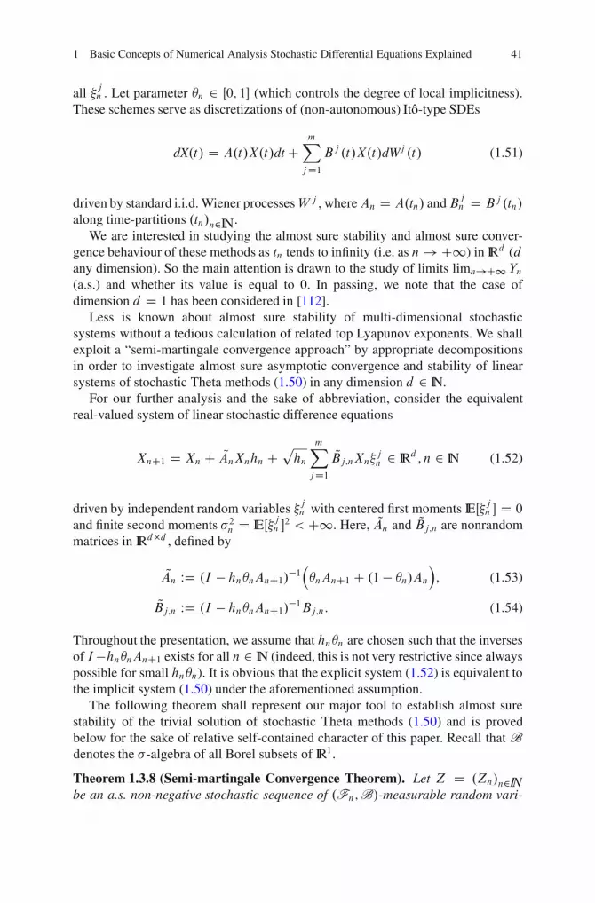
1 Basic Concepts of Numerical Analysis Stochastic Differential Equations Explained 41
all jn . Let parameter �n 2 Œ0; 1� (which controls the degree of local implicitness).These schemes serve as discretizations of (non-autonomous) Ito-type SDEs
dX.t/ D A.t/X.t/dt CmX
jD1Bj .t/X.t/dWj .t/ (1.51)
driven by standard i.i.d. Wiener processesW j , whereAn D A.tn/ andBjn D Bj .tn/
along time-partitions .tn/n2IN.We are interested in studying the almost sure stability and almost sure conver-
gence behaviour of these methods as tn tends to infinity (i.e. as n ! C1) in IRd (dany dimension). So the main attention is drawn to the study of limits limn!C1 Yn(a.s.) and whether its value is equal to 0. In passing, we note that the case ofdimension d D 1 has been considered in [112].
Less is known about almost sure stability of multi-dimensional stochasticsystems without a tedious calculation of related top Lyapunov exponents. We shallexploit a “semi-martingale convergence approach” by appropriate decompositionsin order to investigate almost sure asymptotic convergence and stability of linearsystems of stochastic Theta methods (1.50) in any dimension d 2 IN.
For our further analysis and the sake of abbreviation, consider the equivalentreal-valued system of linear stochastic difference equations
XnC1 D Xn C QAnXnhn Cphn
mX
jD1QBj;nXn jn 2 IRd ; n 2 IN (1.52)
driven by independent random variables jn with centered first moments IEŒ jn � D 0
and finite second moments 2n D IEŒ jn �2 < C1. Here, QAn and QBj;n are nonrandommatrices in IRd�d , defined by
QAn WD .I � hn�nAnC1/�1��nAnC1 C .1 � �n/An
�; (1.53)
QBj;n WD .I � hn�nAnC1/�1Bj;n: (1.54)
Throughout the presentation, we assume that hn�n are chosen such that the inversesof I�hn�nAnC1 exists for all n 2 IN (indeed, this is not very restrictive since alwayspossible for small hn�n). It is obvious that the explicit system (1.52) is equivalent tothe implicit system (1.50) under the aforementioned assumption.
The following theorem shall represent our major tool to establish almost surestability of the trivial solution of stochastic Theta methods (1.50) and is provedbelow for the sake of relative self-contained character of this paper. Recall that Bdenotes the -algebra of all Borel subsets of IR1.
Theorem 1.3.8 (Semi-martingale Convergence Theorem). Let Z D .Zn/n2INbe an a.s. non-negative stochastic sequence of .Fn;B/-measurable random vari-
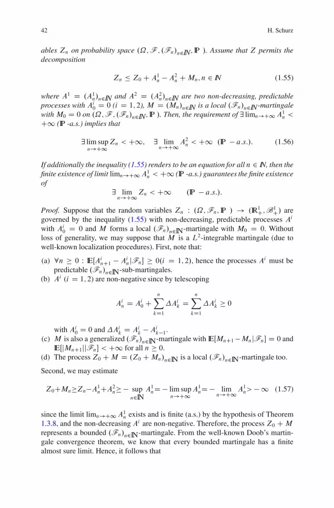
42 H. Schurz
ables Zn on probability space .˝;F ; .Fn/n2IN; IP /. Assume that Z permits thedecomposition
Zn � Z0 C A1n � A2n CMn; n 2 IN (1.55)
where A1 D .A1n/n2IN and A2 D .A2n/n2IN are two non-decreasing, predictableprocesses with Ai0 D 0 (i D 1; 2), M D .Mn/n2IN is a local .Fn/n2IN-martingalewith M0 D 0 on .˝;F ; .Fn/n2IN; IP /. Then, the requirement of 9 limn!C1A1n <C1 (IP -a.s.) implies that
9 lim supn!C1
Zn < C1; 9 limn!C1A
2n < C1 .IP � a:s:/: (1.56)
If additionally the inequality (1.55) renders to be an equation for all n 2 IN, then thefinite existence of limit limn!C1A1n < C1 (IP -a.s.) guarantees the finite existenceof
9 limn!C1Zn < C1 .IP � a:s:/:
Proof. Suppose that the random variables Zn W .˝;Fn; IP / ! .IR1C;B1C/ aregoverned by the inequality (1.55) with non-decreasing, predictable processes Ai
with Ai0 D 0 and M forms a local .Fn/n2IN-martingale with M0 D 0. Withoutloss of generality, we may suppose that M is a L2-integrable martingale (due towell-known localization procedures). First, note that:
(a) 8n � 0 W IEŒAinC1 � AinjFn� � 0.i D 1; 2/, hence the processes Ai must bepredictable .Fn/n2IN-sub-martingales.
(b) Ai (i D 1; 2) are non-negative since by telescoping
Ain D Ai0 CnX
kD1�Aik D
nX
kD1�Aik � 0
with Ai0 D 0 and�Aik D Aik � Aik�1.(c) M is also a generalized .Fn/n2IN-martingale with IEŒMnC1�MnjFn� D 0 and
IEŒjMnC1jjFn� < C1 for all n � 0.(d) The process Z0 CM D .Z0 CMn/n2IN is a local .Fn/n2IN-martingale too.
Second, we may estimate
Z0CMn�Zn�A1nCA2n� � supn2IN
A1nD � lim supn!C1
A1nD � limn!C1A
1n> � 1 (1.57)
since the limit limn!C1A1n exists and is finite (a.s.) by the hypothesis of Theorem1.3.8, and the non-decreasing Ai are non-negative. Therefore, the process Z0 CM
represents a bounded .Fn/n2IN-martingale. From the well-known Doob’s martin-gale convergence theorem, we know that every bounded martingale has a finitealmost sure limit. Hence, it follows that

1 Basic Concepts of Numerical Analysis Stochastic Differential Equations Explained 43
9 limn!C1Z0 CMn < C1.IP � a:s:/
and9M1 WD lim
n!C1Mn < C1.IP � a:s:/
with IEŒjMC1j� < C1. Consequently, the sequence Y D .Yn/n2IN of bounded,non-negative random variables Yn satisfying
0 � Yn WD Zn C A2n � Z0 C A1n CMn (1.58)
for all n 2 IN must have a finite limit YC1 WD lim supn!C1 Yn which is boundedby
lim supn!C1
Yn � Z0 C lim supn!C1
A1n C lim supn!C1
Mn D Z0 C limn!C1A
1n
C limn!C1Mn < C1 (1.59)
(IP -a.s.) (just pull the limit lim sup as n ! C1 over the inequality (1.58) and usethe fact that the limits of bothA1 andM exist, and are finite a.s.). Furthermore, notethat
0 � Zn � Yn; 0 � A2n � Yn; n 2 IN:
This fact implies that the non-decreasing process A2 must have a finite limit and
0 � lim supn!C1
Zn � lim supn!C1
Yn < C1; 0 � limn!C1A
2n � lim sup
n!C1Yn < C1
by applying the Bounded Monotone Sequence Theorem from calculus. Eventually,the identity
Zn D Z0 C A1n � A2n CMn
for all n 2 IN yields that
Yn D Zn C A2n D Z0 C A1n CMn
for all n 2 IN. Hence, the process Z D .Yn � A2n/n2IN satisfies
0 � lim infn!C1Yn D Z0 C lim inf
n!C1A1n C lim inf
n!C1Mn D Z0 C limn!C1A
1n C lim
n!C1Mn
D Z0 C A1C1 CMC1 D lim supn!D1
Yn < C1
in view of the identity in (1.59), Consequently, the process Z D .Yn � A2n/n2INconverges (a.s.) too since the finite limits of Y and A2 exist (a.s.) from previousargumentation. This completes the proof of Theorem 1.3.8. ˘
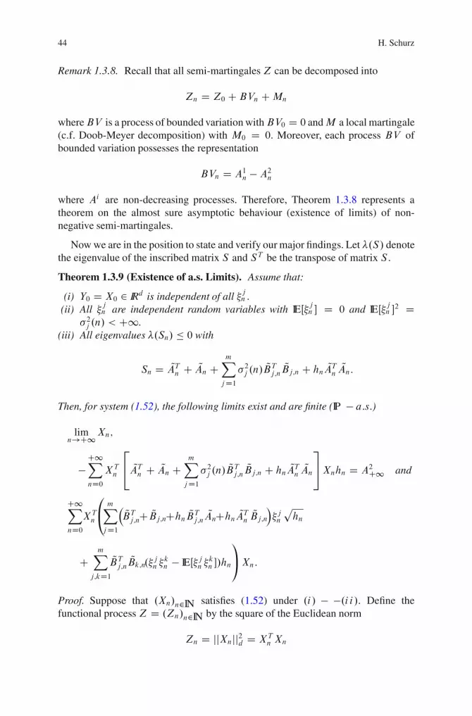
44 H. Schurz
Remark 1.3.8. Recall that all semi-martingalesZ can be decomposed into
Zn D Z0 CBVn CMn
whereBV is a process of bounded variation withBV0 D 0 andM a local martingale(c.f. Doob-Meyer decomposition) with M0 D 0. Moreover, each process BV ofbounded variation possesses the representation
BVn D A1n � A2n
where Ai are non-decreasing processes. Therefore, Theorem 1.3.8 represents atheorem on the almost sure asymptotic behaviour (existence of limits) of non-negative semi-martingales.
Now we are in the position to state and verify our major findings. Let �.S/ denotethe eigenvalue of the inscribed matrix S and ST be the transpose of matrix S .
Theorem 1.3.9 (Existence of a.s. Limits). Assume that:
(i) Y0 D X0 2 IRd is independent of all jn .(ii) All jn are independent random variables with IEŒ jn � D 0 and IEŒ jn �2 D
2j .n/ < C1.(iii) All eigenvalues �.Sn/ � 0 with
Sn D QATn C QAn CmX
jD12j .n/
QBTj;n
QBj;n C hn QATn QAn:
Then, for system (1.52), the following limits exist and are finite (IP � a:s:)
limn!C1Xn;
�C1X
nD0XTn
2
4 QATn C QAn CmX
jD12j .n/
QBTj;n
QBj;n C hn QATn QAn3
5Xnhn D A2C1 and
C1X
nD0XTn
0
@mX
jD1
� QBTj;nC QBj;nChn QBTj;n QAnChn QATn QBj;n� jn
phn
CmX
j;kD1QBTj;n
QBk;n. jn kn � IEŒ jn kn �/hn
1
AXn:
Proof. Suppose that .Xn/n2IN satisfies (1.52) under .i/ � �.i i/. Define thefunctional process Z D .Zn/n2IN by the square of the Euclidean norm
Zn D jjXnjj2d D XTn Xn
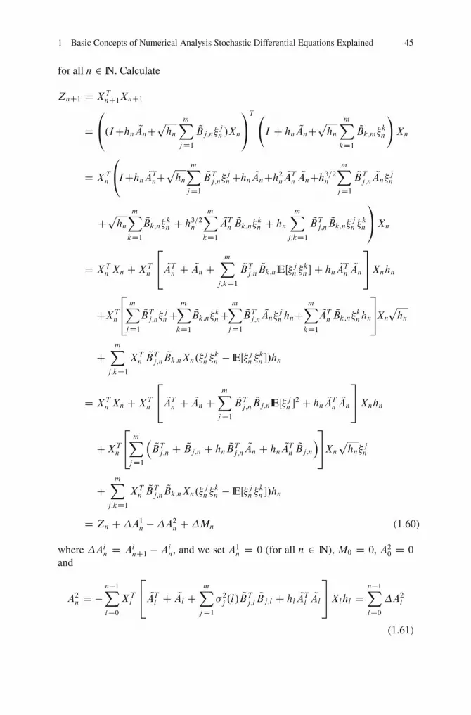
1 Basic Concepts of Numerical Analysis Stochastic Differential Equations Explained 45
for all n 2 IN. Calculate
ZnC1 D XTnC1XnC1
D0
@.IChn QAnCphn
mX
jD1QBj;n jn /Xn
1
A
T
I C hn QAnCphn
mX
kD1QBk;m kn
!
Xn
D XTn
0
@IChn QATnCphn
mX
jD1QBTj;n
jnChn QAnCh2n QATn QAnCh3=2n
mX
jD1QBTj;n
QAn jn
Cphn
mX
kD1QBk;n kn C h3=2n
mX
kD1QATn QBk;n kn C hn
mX
j;kD1QBTj;n QBk;n jn kn
1
AXn
D XTn Xn CXT
n
2
4 QATn C QAn CmX
j;kD1QBTj;n QBk;nIEΠjn
kn �C hn QATn QAn
3
5Xnhn
CXTn
2
4mX
jD1QBTj;n jnC
mX
kD1QBk;n knC
mX
jD1QBTj;n QAn jn hnC
mX
kD1QATn QBk;n knhn
3
5Xnphn
CmX
j;kD1XTn
QBTj;n
QBk;nXn. jn kn � IEŒ jn kn �/hn
D XTn Xn CXT
n
2
4 QATn C QAn CmX
jD1QBTj;n
QBj;nIEŒ jn �2 C hn QATn QAn3
5Xnhn
CXTn
2
4mX
jD1
� QBTj;n C QBj;n C hn QBTj;n QAn C hn QATn QBj;n
�3
5Xnphn
jn
CmX
j;kD1XTn
QBTj;n
QBk;nXn. jn kn � IEŒ jn kn �/hn
D Zn C�A1n ��A2n C�Mn (1.60)
where �Ain D AinC1 � Ain, and we set A1n D 0 (for all n 2 IN), M0 D 0, A20 D 0
and
A2n D �n�1X
lD0XTl
2
4 QATl C QAl CmX
jD12j .l/
QBTj;l
QBj;l C hl QATl QAl3
5Xlhl Dn�1X
lD0�A2l
(1.61)

46 H. Schurz
Mn Dn�1X
lD0XTl
0
@mX
jD1
� QBTj;l C QBj;l C QBTj;lQlhl C QATl QBj;lhl
� j
l
phl
CmX
j;kD1QBTj;l QBk;l . jl kl � IEŒ jl
kl �/hl
1
AXl (1.62)
for all n � 1. Recall the definitions of differences�Ajn D AjnC1 � A
jn and �Mn D
MnC1 � Mn for all n 2 IN. Next, telescoping and summing up over n in (1.60)implies that
Zn D Z0 C A1n � A2n CMn
with A1 � 0. Now, recall the assumption .i i i/. This guarantees that A2n � 0 forall values of xl and A2n is non-decreasing in n. Consequently, all assumptions ofTheorem 1.3.8 with A1 � 0 are fulfilled. Hence, a direct application of Theorem1.3.8 to the non-negative sequence Z D .Zn/n2IN yields that
9 limn!C1Zn D lim
n!C1 jjXnjj2d < C1 .IP � a:s:/:
From the continuity of the Euclidean norm jj:jjd , we conclude that
�1 < 9 limn!C1Xn < C1 .IP � a:s:/
– a fact which confirms the main assertion of Theorem 1.3.9 together with thebounded martingale inequality Z0 CMn � 0 (a.s.) for all n 2 IN. ˘Theorem 1.3.10 (A.s. Stability). Assume that:
(i) x0 2 IRd is independent of all jn .(ii) All jn are independent random variables with IEŒ jn � D 0, IEŒ jn �2 D 2j .n/ <
C1.(iii) 9c > 0 constant such that 8n 2 IN we have all eigenvalues �. OSn/ � �c < 0
with
OSn D0
@ QATn C QAn CmX
jD12j .n/
QBTj;n
QBj;n C hn QATn QAn1
Ahn:
Then, limn!C1Xn D 0, i.e. the trivial solution x D 0 of the system (1.52) isglobally a.s. asymptotically stable.
Proof. First, apply previous Theorem 1.3.9 to get the a.s. convergence and existenceof the limit limn!C1Xn since all eigenvalues also satisfy �. OSn/ � 0 under .i i i/.From the proof of Theorem 1.3.9 based on Theorem 1.3.8, we also know that

1 Basic Concepts of Numerical Analysis Stochastic Differential Equations Explained 47
limn!C1
QA2n D �C1X
lD0XTl
2
4 QATl C QAlCmX
jD12j .l/
QBTj;l
QBj;lChl QATl QAl3
5XlhlDC1X
lD0�A2l :
From calculus of series, the convergence of a series requires that each series member�A2l must converge to zero (IP -a.s.). Therefore, we arrive at the estimation
0 � c limn!C1 jjXnjj2d � lim
n!C1min ��. OSn/jjXnjj2d D � limn!C1max�. OSn/jjXnjj2d
� limn!C1�
QA2n D 0: (1.63)
Consequently, squeezing yields that
limn!C1 jjXnjj2d D 0 .IP � a:s:/:
This leads us to the conclusion that
limn!C1Xn D 0 .IP � a:s:/;
thanks to the continuity and definiteness of the Euclidean norm in IRd . ˘Note that above (see (1.63)) we have used the known facts from linear algebra
that all symmetric matrices S 2 IRd�d have real eigenvalues, a complete set ofeigenvalues which form an orthogonal basis in IRd and, for such matrices, we havethe uniform estimation
min�.S/jjxjj2d � xT Sx � max�.S/jjxjj2dwhere �.S/ are the eigenvalues of inscribed matrix S .
A two-dimensional example (Systems with diagonal-noise terms). Consider thetwo-dimensional system of stochastic difference equations
xnC1 D xnCŒ�n.anC1xnC1 C bnC1ynC1/C.1 � �n/.anxn C bnyn/�hn (1.64)
C 1n
phnxn n
ynC1 D yn C Œ�n.cnC1xnC1 C dnC1ynC1/C.1 � �n/.cnxnCdnyn/�hn (1.65)
C 2n
phnyn n
where an; bn; cn; in are real constants and n are independent standardized randomvariables with moments IEŒ n� D 0 and IEŒ n�2 D 1 for all n 2 IN. (e.g. take i.i.d. n 2 N .0; 1/, but the property of being Gaussian is not essential for the validityof our findings, however the fact of independence and properties of finite first two

48 H. Schurz
moments does). Obviously, system (1.64)–(1.65) has the form (1.50) with d D 2,m D 1, and matrices
An D�an bn
cn dn
�
; Bn D�1n 0
0 2n
�
: (1.66)
To apply Theorem 1.3.9, we need to calculate Sn D QATn C QAn C QBTn
QBn C hn QATn QAn.For this purpose, we study the equivalent system (1.52) with matrices
QAn D�pn qn
rn sn
�
;
QBn D
0
BB@
� .�1C �nhndnC1/1ndetn
�nhnbnC12ndetn
�nhncnC11ndetn
� .�1C �nhnanC1/2ndetn
1
CCA : (1.67)
where
detn D 1��nhndnC1 � �nhnanC1C�2nh2nanC1dnC1��2nh2nbnC1cnC1; (1.68)
pn D � .�1C�n hndnC1/ .�n anC1C .1��n/ an/C �n hnbnC1 .�n cnC1C .1��n/ cn/
1 � �n hndnC1 � �n hnanC1 C �2nh2nanC1 dnC1 � �2nh2nbnC1 cnC1
;
qn D � .�1C�nhndnC1/ .�n bnC1C .1��n/ bn/C�n hnbnC1 .�n dnC1 C .1��n/ dn/
1 � �n hndnC1 � �n hnanC1 C �2nh2nanC1 dnC1 � �2nh2nbnC1 cnC1
;
rn D �n hncnC1 .�n anC1C .1��n/ an/� .�1C�n hnanC1/ .�n cnC1C .1 � �n/ cn/
1 � �n hndnC1 � �n hnanC1C�2nh2nanC1 dnC1 � �2nh2nbnC1 cnC1
;
sn D �n hncnC1 .�n bnC1C .1��n/ bn/ � .�1C�n hnanC1/ .�n dnC1C .1 � �n/ dn/
1 � �n hndnC1 � �n hnanC1 C �2nh2nanC1 dnC1 � �2nh2nbnC1 cnC1
:
Thus, one obtains
Sn D�
un wnwn vn
�
(1.69)
with
un D �2 .�1C �n hndnC1/ .�n anC1 C .1 � �n/ an/
1��n hndnC1��n hnanC1 C �2nh2nanC1dnC1 � �2nh2nbnC1 cnC1
(1.70)
C 2�n hnbnC1 .�n cnC1 C .1 � �n/ cn/
1 � �n hndnC1 � �n hnanC1 C �2nh2nanC1 dnC1 � �2nh2nbnC1 cnC1
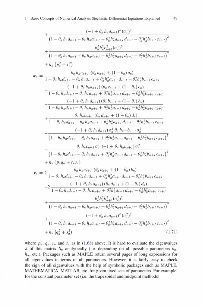
1 Basic Concepts of Numerical Analysis Stochastic Differential Equations Explained 49
C .�1C �n hndnC1/2 .1n /
2
�1 � �n hndnC1 � �n hnanC1 C �2nh
2nanC1 dnC1 � �2nh
2nbnC1 cnC1
�2
C �2nh2nc2nC1.1n/2
�1 � �n hndnC1 � �n hnanC1 C �2nh
2nanC1 dnC1 � �2nh
2nbnC1 cnC1
�2
Chn�p2n C r2n
�
wn D �n hncnC1 .�n anC1 C .1 � �n/ an/
1 � �n hndnC1 � �n hnanC1 C �2nh2nanC1 dnC1 � �2nh
2nbnC1 cnC1
� .�1C �n hnanC1/ .�n cnC1 C .1 � �n/ cn/
1 � �n hndnC1 � �n hnanC1 C �2nh2nanC1 dnC1 � �2nh2nbnC1 cnC1
� .�1C �n hndnC1/ .�n bnC1 C .1 � �n/ bn/
1 � �n hndnC1 � �n hnanC1 C �2nh2nanC1 dnC1 � �2nh2nbnC1 cnC1
C �n hnbnC1 .�n dnC1 C .1 � �n/ dn/
1 � �n hndnC1 � �n hnanC1 C �2nh2nanC1 dnC1 � �2nh2nbnC1 cnC1
� .�1C �n hndnC1/ 1n �n hn�bnC1
2n
�1 � �n hndnC1 � �n hnanC1 C �2nh
2nanC1 dnC1 � �2nh
2nbnC1 cnC1
�2
� �n hncnC1 1n .�1C �n hnanC1/
2n
�1 � �n hndnC1 � �n hnanC1 C �2nh
2nanC1 dnC1 � �2nh
2nbnC1 cnC1
�2
Chn .pnqn C rnsn/
vn D 2�n hncnC1 .�n bnC1 C .1 � �n/ bn/
1 � �n hndnC1 � �n hnanC1 C �2nh2nanC1 dnC1 � �2nh2nbnC1 cnC1
�2 .�1C �n hnanC1/ .�n dnC1 C .1 � �n/ dn/
1 � �n hndnC1 � �n hnanC1 C �2nh2nanC1 dnC1 � �2nh2nbnC1 cnC1
C �2nh2nb
2nC1.2n /2
�1 � �n hndnC1 � �n hnanC1 C �2nh
2nanC1 dnC1 � �2nh
2nbnC1 cnC1
�2
C .�1C �n hnanC1/2 .2n /
2
�1 � �n hndnC1 � �n hnanC1 C �2nh
2nanC1 dnC1 � �2nh
2nbnC1 cnC1
�2
Chn�q2n C s2n
�(1.71)
where pn, qn, rn and sn as in (1.68) above. It is hard to evaluate the eigenvalues� of this matrix Sn analytically (i.e. depending on all possible parameters �n,hn, etc.). Packages such as MAPLE return several pages of long expressions forall eigenvalues in terms of all parameters. However, it is fairly easy to checkthe sign of all eigenvalues with the help of symbolic packages such as MAPLE,MATHEMATICA, MATLAB, etc. for given fixed sets of parameters. For example,for the constant parameter set (i.e. the trapezoidal and midpoint methods)
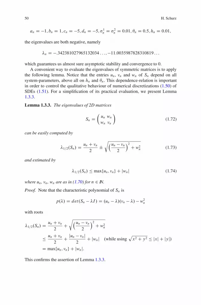
50 H. Schurz
an D �1; bn D 1; cn D �5; dn D �5; 1n D 2n D 0:01; �n D 0:5; hn D 0:01;
the eigenvalues are both negative, namely
�n D �:342381027965132034 : : : ;�11:0035987828310819 : : :
which guarantees us almost sure asymptotic stability and convergence to 0.A convenient way to evaluate the eigenvalues of symmetric matrices is to apply
the following lemma. Notice that the entries un, vn and wn of Sn depend on allsystem-parameters, above all on hn and �n. This dependence-relation is importantin order to control the qualitative behaviour of numerical discretizations (1.50) ofSDEs (1.51). For a simplification of its practical evaluation, we present Lemma1.3.3.
Lemma 1.3.3. The eigenvalues of 2D matrices
Sn D�
un wnwn vn
�
(1.72)
can be easily computed by
�1=2.Sn/ D un C vn2
˙r�un � vn
2
�2 C w2n (1.73)
and estimated by
�1=2.Sn/ � maxfun; vng C jwnj (1.74)
where un, vn, wn are as in (1.70) for n 2 IN.
Proof. Note that the characteristic polynomial of Sn is
p.�/ D det.Sn � �I/ D .un � �/.vn � �/� w2n
with roots
�1=2.Sn/ D un C vn2
Cr�un � vn
2
�2 C w2n
� un C vn2
C jun � vnj2
C jwnj .while usingpx2 C y2 � jxj C jyj/
D maxfun; vng C jwnj:
This confirms the assertion of Lemma 1.3.3.

1 Basic Concepts of Numerical Analysis Stochastic Differential Equations Explained 51
Therefore, the direct evaluation of these eigenvalues by Lemma 1.3.3 and anapplication of Theorem 1.3.9 provide the following immediate consequence underthe assumptions of this subsection.
Corollary 1.3.1 (Corollary to Theorem 1.3.9). Assume that, for all n 2 IN, wehave
maxfun; vng C jwnj � 0
where un; vn and wn are defined as in (1.70).Then, for all adapted initial values .x0y0/T , the following limits for system
(1.64)-(1.65) with QAn, QBn defined by (1.67) exist and are finite (IP -a.s.)
lim supn!C1
xn; lim supn!C1
yn; lim infn!C1xn; lim inf
n!C1yn;
limn!C1
�xn yn
� QATn C QAn C QBTn
QBn C hn QATn QAn��xnyn
�
D 0;
limn!C1
�xn yn
�h. QBT
n C QBn C hn QBTn QAn C hn QATn QBn/ nphn
C QBTn
QBn. 2n � 1/hni�
xn
yn
�
D 0:
Note that the main assumption of Corollary 1.3.1 requires that at least unCvn � 0
for all n 2 IN, where un and vn are defined by (1.70). As an immediate consequenceof Theorem 1.3.10 applied to OSn D Snhn and Lemma 1.3.3, we are able to find thefollowing corollary on a.s. asymptotic stability.
Corollary 1.3.2 (Corollary to Theorem 1.3.10). Assume that 9c D constant > 0such that 8n 2 IN
.maxfun; vng C jwnj/ hn � �c < 0
where un; vn and wn are defined by (1.70).Then, for all adapted initial values .x0y0/T , the limits satisfy
limn!C1xn D 0; lim
n!C1yn D 0 .IP � a:s:/;
i.e. global almost sure asymptotic stability of the trivial solution for system (1.64)-(1.65) is observed.
Remark 1.3.9. Moreover, the conditions of Corollaries 1.3.1 and 1.3.2 need to befulfilled only for all n � n0 where n0 2 IN is sufficiently large (due to the asymptoticcharacter of main assertion).
Remark 1.3.10. To summarize our findings, an evaluation of eigenvalues � in ourexample shows a strong dependence of � on the determinants detn determined

52 H. Schurz
by (1.68). Stabilizing effects of these determinants on the fluctuation of � can beobserved and maximized whenever
dn � 0; an � 0; bncn � 0 (1.75)
for all n � n0. In this case, one can show that detn > 1 for all n � n0 and“fluctuations of eigenvalues” � are also under some control and the choice of stepsizes hn is not very sensitive for qualitative behavior of Theta methods. Moreover,an increase of implicitness � � 0 leads to stabilization of numerical dynamics under(1.75).
Remark 1.3.11. In order to avoid “unwanted spurious” oscillations through Theta-methods in our example we recommend to use only step sizes hn and implicitness�n which guarantee that
�nhn maxfdnC1; anC1g < 1
for all n 2 IN. There are some hints to prefer the choice �n D 0:5 to circumvent theproblem of over- or under-stabilization through Theta-methods (cf. [118,120–122]).
This subsection has shown how to exploit semi-martingale convergence theorems(cf. Theorem 1.3.8) to discuss the existence of finite almost sure limits and globalasymptotic stability for stochastic Theta methods applied to systems of stochasticdifferential equations. Sufficient conditions (cf. Theorems 1.3.9, 1.3.10) for almostsure stability and convergence of their solutions could be verified in terms of allparameters of non-autonomous systems such as variable step sizes hn and variableimplicitness �n. These conditions are applicable (see Sect. 1.3.5) and can be easilyevaluated by computer packages such as MAPLE, MATHEMATICA, MATLAB,etc. It would be interesting to extend the main results to other type of noisesources (i.e. non-martingale-type or noise with infinite moments). Our conditionson the noise are fairly general (since we only asked for existence of first andsecond moments). However, a key assumption is the complete independence ofall noise terms jn . The relaxation of this major assumption is a potential subjectfor further research. It is also possible to extend the presented results to othernumerical methods or to systems of nonlinear stochastic differential equationsunder appropriate conditions (recall that balanced Theta methods (1.1) representthe simplest parametric family of stochastic Runge-Kutta methods), thanks to thegenerality of Semimartingale Convergence Theorem 1.3.8).
1.3.6 Asymptotic Almost Sure Stability for Pure DiffusionProcesses
This subsection is devoted to the analysis of discretizations of pure diffusionprocesses as the simplest class of stochastic test equations in IR1.

1 Basic Concepts of Numerical Analysis Stochastic Differential Equations Explained 53
Theorem 1.3.11. Let V D .V .n//n2IN be a sequence of non-negative randomvariables V.n/ W .˝;Fn; IP / ! IR1C with V.0/ > 0 satisfying the recursive scheme
V.nC 1/ D V.n/G.n/ (1.76)
where G.n/ W .˝;Fn; IP / ! IR1C are i.i.d. random variables with the momentproperty IEj lnŒG.n/�j < C1. Then
V (globally) asymptotically a.s. stable iff IE lnŒG.0/� < 0 .
Proof. This result is already found in [48] and in [125]. The main idea is to usethe strong law of large numbers (SLLN) in conjunction with the law of iteratedlogarithm (LIL). Note that V possesses the explicit representation
V.nC 1/ D
nY
kD0G.k/
!
V.0/ (1.77)
for all n 2 IN. Now, suppose that G.k/ are i.i.d. random variables and define
�0 WD IEŒln.G.0//�; Sn WDn�1X
kD0lnG.k/;
hence V.nC1/ D exp.SnC1/V .0/ and IEŒSn� D n� for n 2 IN. By SLLN, concludethat
limn!C1
Sn
nD �0 .a:s:/
thanks to the IP -integrability of G.k/. This fact implies that if �0 < 0 then Sn !�1, i.e. V.n/ ! 0 as n tends to C1 and if � > 0 then Sn ! C1, i.e. V.n/ !C1 as n tends to C1. Moreover, in the case �0 D 0, we may use LIL (at first,under 2 D Var.lnG.k// D IEŒlnG.k/ � IE lnG.k/�2 < C1, later we may drop2 < C1 by localization procedures) to get
lim infn!C1
Snp2n ln lnn
D �j j; lim supn!C1
Snp2n ln ln n
D j j;
hence Sn oscillates with growing amplitude and limn!C1 Sn does not exist.Therefore
limn!C1V.n/ D lim
n!C1 exp.Sn/V .0/
does not exist either (a.s.). Thus, limn!C1 V.n/ ¤ 0 and the proof is complete. ˘Now, consider the one-dimensional test class of pure diffusion equations
(a Girsanov SDE of Ito-type)
dX.t/ D X.t/ dW.t/ (1.78)

54 H. Schurz
discretized by BIMs
YnC1 D Yn C Yn�Wn C .c0hn C c1j�Wnj/.Yn � YnC1/ (1.79)
as suggested by Milstein, Platen and Schurz [96]. Then, the following resultprovides a mathematical evidence that their numerical experiments for BIMs (1.79)led to the correct observation of numerical stability due to its asymptotic a.s.stability. It extends results which are found in [48, 120] and [125].
Theorem 1.3.12 (A.s. asymptotic stability of BIMs with constant h,[127]). The BIMs (1.79) with scalar weights c0 D 0 and c1 D j j applied tomartingale test (1.78) for any parameter 2 IR1 n f0g with any equidistant step sizeh provide (globally) asymptotically a.s. stable sequences Y D .Yn/n2IN.
Proof. Suppose j j > 0. Then, the proof is an application of Theorem 1.3.11. Forthis purpose, consider the sequenceV D .V .n//n2IN D .jYnj/n2IN. Note that V.nC1/ D G.n/V.n/, IEj lnG.n/j < C1 and IEŒlnG.n/� < 0 since
IEŒj lnG.n/j� � .IEŒlnG.n/�2/1=2 � ln.2/C j jph and
IEŒlnG.n/� D IE
lnˇˇˇ1C j�Wnj C �Wn
1C j�Wnjˇˇˇ
D IE
lnˇˇˇ1C �Wn
1C j�Wnjˇˇˇ
D 1
2IE
lnˇˇˇ1C �Wn
1C j�Wnjˇˇˇ
C 1
2IE
lnˇˇˇ1 � �Wn
1C j�Wnjˇˇˇ
D 1
2IE
"
lnˇˇˇ1 �
��Wn
1C j�Wnj�2 ˇˇˇ
#
<�12
IE
"� j�Wnj1C j�Wnj
�2#
<0
with independently identically Gaussian distributed increments �Wn 2 N .0; h/
(In fact, note that, for all ¤ 0 and Gaussian �Wn, we have
0 < 1 ��
�Wn
1C j�Wnj�2
< 1
with probability one, hence, that�Wn has a non-degenerate probability distributionwith nontrivial support is essential here!). Therefore, the assumptions of Theorem1.3.11 are satisfied and an application of Theorem 1.3.11 yields the claim ofTheorem 1.3.12. Thus, the proof is complete. ˘Remark 1.3.12. The increments �Wn 2 N .0; hn/ can also be replaced by multi-point discrete probability distributions such as
IPn�Wn D ˙
phn
oD 1
2
or IP f�Wn D 0g D 2
3; IP
n�Wn D ˙
p3hn
oD 1
6

1 Basic Concepts of Numerical Analysis Stochastic Differential Equations Explained 55
as commonly met in weak approximations. In this case, the almost sure stabilityof the BIMs as chosen by Theorem 1.3.12 is still guaranteed, as seen by our proofabove (due to the inherent symmetry of �Wn with respect to 0).
For variable step sizes, we can also formulate and prove a general assertion withrespect to asymptotic a.s. stability. Let Var.Z/ denote the variance of the inscribedrandom variableZ.
Theorem 1.3.13 (A.s. asymptotic stability of linear recursions, S. [127]). Let VD.V .n//n2IN be a sequence of non-negative random variables V.n/ W .˝;Fn; IP / !IR1C with V.0/ > 0 satisfying the recursive scheme
V.nC 1/ D V.n/G.n/; (1.80)
where G.n/ W .˝;Fn; IP / ! IR1C are independent random variables such that 9nonrandom sequence b D .bn/n2IN with bn ! C1 as n ! C1
C1X
kD0
Var.ln.G.k///
b2k< C1; lim
n!C1
Pn�1kD0 IE ln.G.k//
bn< 0: (1.81)
Then V D .V .n//n!C1 is (globally) asymptotically a.s. stable sequence, i.e. wehave limn!C1 V.n/ D 0 (a.s.).Moreover, if
C1X
kD0
Var.ln.G.k///
b2k
< C1; limn!C1
Pn�1kD0 IE ln.G.k//
bn> 0 (1.82)
then V D .V .n//n!C1 is (globally) asymptotically a.s. unstable sequence, i.e. wehave limn!C1 V.n/ D C1 (a.s.) for all nonrandom y0 ¤ 0.
Proof. The main idea is to apply Kolmogorov’s SLLN, see Shiryaev [134] (p. 389).Recall that V possesses the explicit representation (1.77). Now, define
Sn WDn�1X
kD0lnG.k/;
hence V.n C 1/ D exp.SnC1/V .0/ for n 2 IN. By Kolmogorov’s SLLN we mayconclude that
limn!C1
Sn
bnD lim
n!C1IESnbn
D limn!C1
Pn�1kD0 IE ln.G.k//
bn< 0.a:s:/
thanks to the assumptions (1.81) of IP -integrability of G.k/. This fact togetherwith bn ! C1 implies that Sn ! �1 (a.s.), i.e. V.n/ ! 0 as n tends to C1.

56 H. Schurz
The reverse direction under (1.82) is proved analogously to previous proof-steps.Thus, the proof is complete. ˘
Now, let us apply this result to BIMs (1.79) applied to test (1.78). For k D0; 1; : : : ; nT , define
G.k/ WDˇˇˇ1C j�Wk j C �Wk
1C j�Wk jˇˇˇ: (1.83)
Theorem 1.3.14 (A.s. asymptotic stability I of BIMs with variable hn, [127]).Assume that 9 nonrandom sequence b D .bn/n2IN with bn ! C1 as n ! C1 fora fixed choice of step sizes hn > 0 such that
C1X
kD0
Var.ln.G.k///
b2k< C1; lim
n!C1
Pn�1kD0 IE ln.G.k//
bn< 0:
Then the BIMs (1.79) with scalar weights c0 D 0 and c1 D j j applied to martingaletest (1.78) with parameter 2 IR1 nf0g with the fixed sequence of variable step sizeshn provide (globally) asymptotically a.s. stable sequences Y D .Yn/n2IN.
Proof. We may apply Theorem 1.3.13 with V.n/ D jYnj since the assumptions aresatisfied for the BIMs (1.26) with scalar weights c0 D 0 and c1 D j j applied tomartingale test (1.78). Hence, the proof is complete. ˘Theorem 1.3.15 (A.s. asymptotic stability II of BIMs with variable hn, S.[127]).The BIMs (1.79) with scalar weights c0 D 0 and c1 D j j applied to martingaletest (1.78) with parameter 2 IR1 n f0g with any nonrandom variable step sizeshk satisfying 0 < hmin � hk � hmax provide (globally) asymptotically a.s. stablesequences Y D .Yn/n2IN.
Proof. We may again apply Theorem 1.3.13 with V.n/D jYnj. For this purpose,we check the assumptions. Define bn WDn. Note that the variance Var.ln.G.k///is uniformly bounded since �Wn 2 N .0; hn/ and 0 < hmin � hk � hmax. Moreprecisely, we have
Var.ln.G.k///
� IEŒln.G.k//�2 D IEŒIf�Wn>0g ln.G.k//�2 C IEŒIf�Wn<0g ln.G.k//�2
< pnŒln.2/�2 C IEŒln.1C j�Wnj/�2 � pnŒln.2/�
2 C IEŒln.exp.j�Wnj//�2� pnŒln.2/�
2 C IEŒ�Wn�2 D pnŒln.2/�
2 C 2hn � pnŒln.2/�2 C 2hmax
for G.k/ as defined in (1.83), where IfQg denotes the indicator function of theinscribed set Q and pn D p
IP f�Wn > 0g. Note that 0<pnDp2=2<1 if �Wn
is Gaussian distributed. Therefore, there is a finite real constant KG2 < .ln.2//2 C
2hmax such that
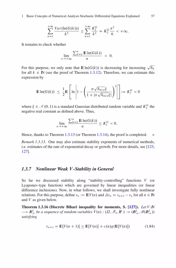
1 Basic Concepts of Numerical Analysis Stochastic Differential Equations Explained 57
C1X
kD1
Var.ln.G.k///
k2�C1X
kD1
KG2
k2D KG
2
�2
6< C1:
It remains to check whether
limn!C1
PnkD1 IE ln.G.k//
n< 0:
For this purpose, we only note that IE ln.G.k// is decreasing for increasingphk
for all k 2 IN (see the proof of Theorem 1.3.12). Therefore, we can estimate thisexpression by
IE ln.G.k// � 1
2IE
2
4ln
ˇˇˇˇˇˇ1�
phmin
1C jphmin j
!2ˇˇˇˇˇˇ
3
5 WD KG1 < 0
where 2 N .0; 1/ is a standard Gaussian distributed random variable and KG1 the
negative real constant as defined above. Thus,
limn!C1
PnkD1 IE ln.G.k//
n� KG
1 < 0:
Hence, thanks to Theorem 1.3.13 (or Theorem 1.3.14), the proof is completed. ˘Remark 1.3.13. One may also estimate stability exponents of numerical methods,i.e. estimates of the rate of exponential decay or growth. For more details, see [123,127].
1.3.7 Nonlinear Weak V -Stability in General
So far we discussed stability along “stability-controlling” functions V (orLyaponuv-type function) which are governed by linear inequalities (or lineardifference inclusions). Now, in what follows, we shall investigate fully nonlinearrelations. For this purpose, define vn WD IEV.n/ and�vn D vnC1 � vn for all n 2 INand V as given below.
Theorem 1.3.16 (Discrete Bihari inequality for moments, S. [127]). LetV WIN�! IR1C be a sequence of random variables V.n/ W .˝;Fn; IP / ! .IR1C;B.IR1C//satisfying
vnC1 D IEŒV .nC 1/� � IEŒV .n/�C c.n/g.IEŒV .n/�/ (1.84)
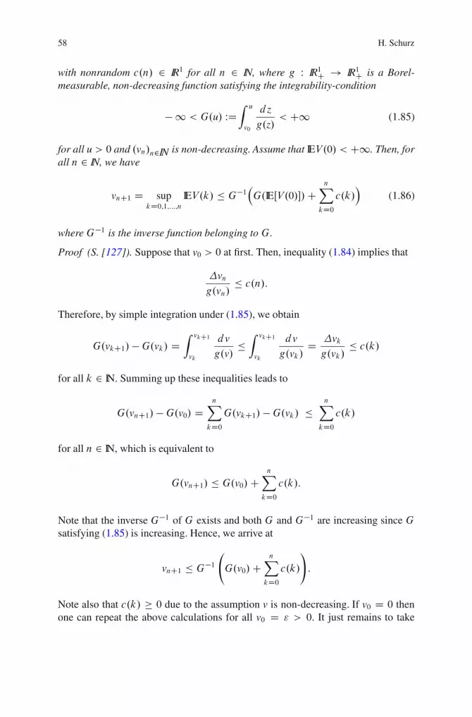
58 H. Schurz
with nonrandom c.n/ 2 IR1 for all n 2 IN, where g W IR1C ! IR1C is a Borel-measurable, non-decreasing function satisfying the integrability-condition
� 1 < G.u/ WDZ u
v0
d z
g.z/< C1 (1.85)
for all u > 0 and .vn/n2IN is non-decreasing. Assume that IEV.0/ < C1. Then, forall n 2 IN, we have
vnC1 D supkD0;1;:::;n
IEV.k/ � G�1�G.IEŒV .0/�/C
nX
kD0c.k/
�(1.86)
where G�1 is the inverse function belonging to G.
Proof (S. [127]). Suppose that v0 > 0 at first. Then, inequality (1.84) implies that
�vng.vn/
� c.n/:
Therefore, by simple integration under (1.85), we obtain
G.vkC1/�G.vk/ DZ vkC1
vk
dv
g.v/�Z vkC1
vk
dv
g.vk/D �vkg.vk/
� c.k/
for all k 2 IN. Summing up these inequalities leads to
G.vnC1/�G.v0/ DnX
kD0G.vkC1/ �G.vk/ �
nX
kD0c.k/
for all n 2 IN, which is equivalent to
G.vnC1/ � G.v0/CnX
kD0c.k/:
Note that the inverse G�1 of G exists and both G and G�1 are increasing since Gsatisfying (1.85) is increasing. Hence, we arrive at
vnC1 � G�1
G.v0/CnX
kD0c.k/
!
:
Note also that c.k/ � 0 due to the assumption v is non-decreasing. If v0 D 0 thenone can repeat the above calculations for all v0 D " > 0. It just remains to take

1 Basic Concepts of Numerical Analysis Stochastic Differential Equations Explained 59
the limit as " tends to zero in the obtained estimates. Thus, the proof of (1.86) iscomplete. ˘Remark 1.3.14. Theorem 1.3.16 can be understood as a discrete version of thecontinuous time Lemma of Bihari [12] and is due to S. [127].
1.3.8 Girsanov’s Equation to Test Moments and Positivity
The simplest test equation for asymptotic stability, boundedness of moments,monotonicity and positivity of numerical methods is the one-dimensional GirsanovSDE (originating from Girsanov [34]) of Ito type
dX.t/ D .ŒX.t/�C/˛ dW.t/ (1.87)
with X.0/ D X0 � 0 (a.s.) in view of its solutions and strong uniqueness. Withoutloss of generality, we may suppose that � 0. If ˛ 2 Œ0; 1� and IEX2
0 < C1we obtain continuous time solutions which are martingales with respect to the -algebra generated by the driving Wiener process W D .W.t//t�0. If ˛ D 0 or ˛ 2Œ1=2; 1� these (non-anticipating) martingale-solutions are unique with probabilityone (by the help of Osgood-Yamada-Watanabe results, cf. Karatzas and Shreve[70]). Due to the pathwise continuity, the non-negative cone IRC D fx 2 IR1 Wx � 0g is left invariant (a.s.). A nontrivial question is whether related numericalapproximations are stable, converge to the underlying analytic solution and have thesame invariance property. We are able to answer these problems. Here, we are onlyinterested in stability and invariance of “appropriately balanced discretizations” (forconvergence, see also in Sect. 1.4 below). For this purpose, consider the balancedimplicit methods (BIMs)
YnC1 D Yn C .ŒYn�C/˛�Wn C .ŒYn�C/˛�1j�Wnj.Yn � YnC1/ (1.88)
as a linear-implicit member of the more general class of BTMs (1.1).
Theorem 1.3.17 (Stability of 2nd Moments of BIMs, S.[127]). The BIMs (1.88)applied to Girsanov’s SDE (1.87) with 0 < ˛ < 1 leave the non-negative coneIRC invariant (a.s.) and provide polynomially stable numerical sequences. Moreprecisely, if > 0, 0 < IEY 20 < C1 and Y0 is independent of the -algebra F DfW.t/ W t � 0g then their second moments are strictly increasing as n increasesand they are governed by
IEŒY 2n � ��.IEŒY 20 �/
1�˛ C .1 � ˛/2.tnC1 � t0/�1=.1�˛/
(1.89)

60 H. Schurz
Proof. Suppose that 0 < ˛ < 1. At first we rewrite (1.88) as the explicit scheme
YnC1 D Yn1C .ŒYn�C/˛�1�Wn C .ŒYn�C/˛�1j�Wnj
1C .ŒYn�C/˛�1j�Wnj (1.90)
which immediately gives the a.s. invariance with respect to the non-negative coneIRC, provided that Y0 � 0 (a.s.). Therefore, we may drop the taking of positive partby Œ:�C in the above form. Now, rewrite (1.90) as
YnC1 D Yn C .Yn/˛�Wn
1C .Yn/˛�1j�Wnj : (1.91)
Taking the square and expectation yields
vnC1 WD IEŒY 2nC1� D IEŒYn�2 C IE
.Yn/
˛�Wn
1C .Yn/˛�1j�Wnj2
: (1.92)
Thus, due to the positivity of all summands at the right hand side, we may concludethat the second moments .vn/n2IN are non-decreasing and, in fact if > 0, vn isstrictly increasing. It remains to apply Theorem 1.3.16. For this purpose, estimate(1.92) by Jensen’s inequality for concave functions in order to obtain
vnC1 � vn C 2IEŒ.Yn/2˛�Wn� D vn C 2IEŒ.Yn/2˛IEŒ�WnjFn�� (1.93)
D vn C 2IEŒ.Yn/2˛IEŒ�Wn�� � vn C 2.vn/˛hn: (1.94)
Therefore, we may take V.x/ D x2, g.z/ D z˛ , c.n/ D 2hn and apply Theorem1.3.16 with the conclusion (1.86) in order to get to (1.89). Note also that
G.u/ DZ u
v0
d z
g.z/DZ u
v0
d z
z˛D z1�˛
1 � ˛ˇˇˇzDu
zDv0D u1�˛ � .v0/1�˛
1 � ˛;
G�1.z/ D�
z.1 � ˛/C v1�˛0
�1=.1�˛/:
If v0 D 0 then one can repeat the above calculations for v0 D " > 0. It just remainsto take the limit as " tends to zero in the obtained estimates. Thus, the proof iscomplete. ˘
One could also compare the moment evolutions of the explicit Euler methodY E D .Y En /n2IN with that of BIMs Y B D .Y Bn /n2IN governed by (1.26). Then,it is fairly easy to recognize that IE.Y Bn /
2� � IE.Y En /2� for all integers � 2 IN,
provided that IE.Y B0 /2� � IE.Y E0 /
2� . It is also interesting to note that the explicitEuler methods cannot preserve the a.s. invariance property with respect to thenon-negative cone IRC. In fact, they exit that cone with positive probability,independently of the choice of any nonrandom step sizes �n. Summarizing,
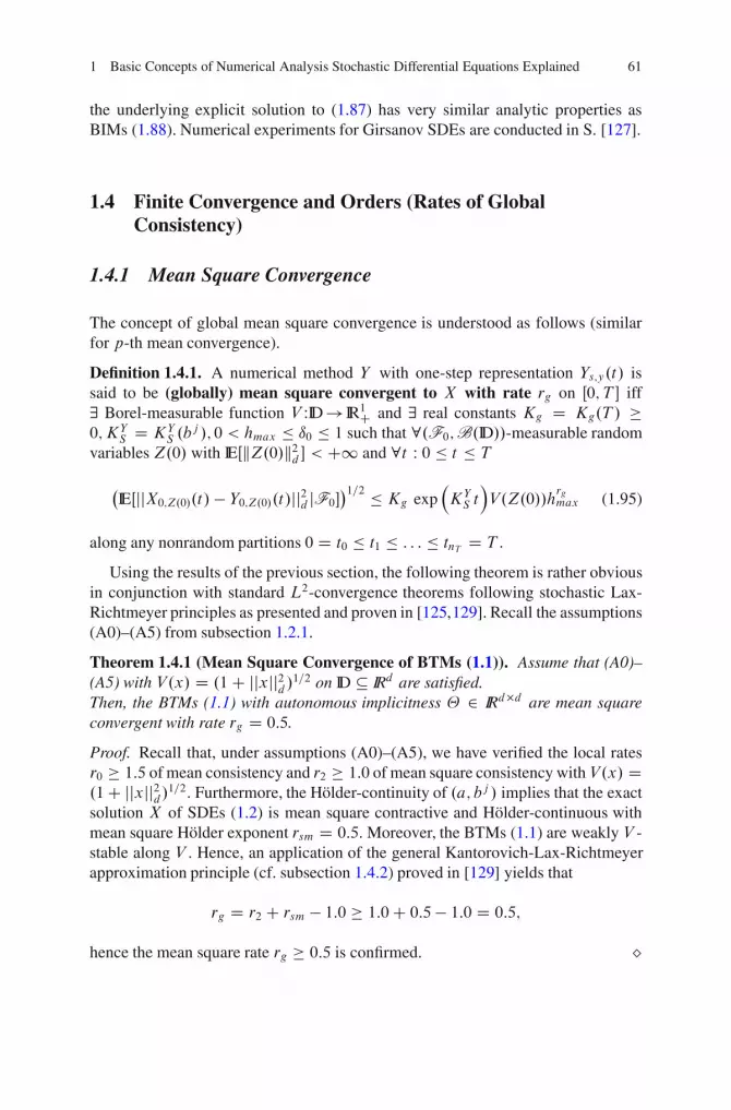
1 Basic Concepts of Numerical Analysis Stochastic Differential Equations Explained 61
the underlying explicit solution to (1.87) has very similar analytic properties asBIMs (1.88). Numerical experiments for Girsanov SDEs are conducted in S. [127].
1.4 Finite Convergence and Orders (Rates of GlobalConsistency)
1.4.1 Mean Square Convergence
The concept of global mean square convergence is understood as follows (similarfor p-th mean convergence).
Definition 1.4.1. A numerical method Y with one-step representation Ys;y.t/ issaid to be (globally) mean square convergent to X with rate rg on Œ0; T � iff9 Borel-measurable function V WID ! IR1C and 9 real constants Kg D Kg.T / �0;KY
S D KYS .b
j /; 0 < hmax � ı0 � 1 such that 8.F0;B.ID//-measurable randomvariablesZ.0/ with IEŒkZ.0/k2d � < C1 and 8t W 0 � t � T
�IEŒjjX0;Z.0/.t/ � Y0;Z.0/.t/jj2d jF0�
�1=2 � Kg exp�KYS t�V.Z.0//h
rgmax (1.95)
along any nonrandom partitions 0 D t0 � t1 � : : : � tnT D T .
Using the results of the previous section, the following theorem is rather obviousin conjunction with standard L2-convergence theorems following stochastic Lax-Richtmeyer principles as presented and proven in [125,129]. Recall the assumptions(A0)–(A5) from subsection 1.2.1.
Theorem 1.4.1 (Mean Square Convergence of BTMs (1.1)). Assume that (A0)–(A5) with V.x/ D .1C jjxjj2
d /1=2 on ID IRd are satisfied.
Then, the BTMs (1.1) with autonomous implicitness � 2 IRd�d are mean squareconvergent with rate rg D 0:5.
Proof. Recall that, under assumptions (A0)–(A5), we have verified the local ratesr0 � 1:5 of mean consistency and r2 � 1:0 of mean square consistency with V.x/ D.1C jjxjj2d /1=2. Furthermore, the Holder-continuity of .a; bj / implies that the exactsolution X of SDEs (1.2) is mean square contractive and Holder-continuous withmean square Holder exponent rsm D 0:5. Moreover, the BTMs (1.1) are weakly V -stable along V . Hence, an application of the general Kantorovich-Lax-Richtmeyerapproximation principle (cf. subsection 1.4.2) proved in [129] yields that
rg D r2 C rsm � 1:0 � 1:0C 0:5 � 1:0 D 0:5;
hence the mean square rate rg � 0:5 is confirmed. ˘
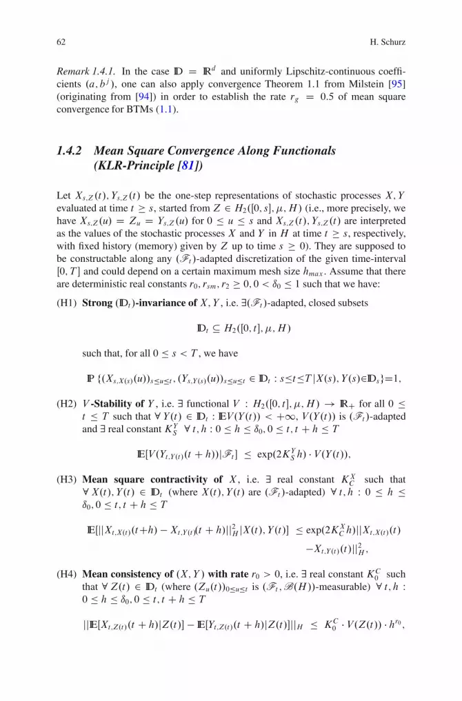
62 H. Schurz
Remark 1.4.1. In the case ID D IRd and uniformly Lipschitz-continuous coeffi-cients .a; bj /, one can also apply convergence Theorem 1.1 from Milstein [95](originating from [94]) in order to establish the rate rg D 0:5 of mean squareconvergence for BTMs (1.1).
1.4.2 Mean Square Convergence Along Functionals(KLR-Principle [81])
Let Xs;Z.t/; Ys;Z.t/ be the one-step representations of stochastic processes X; Yevaluated at time t � s, started from Z 2 H2.Œ0; s�; �;H/ (i.e., more precisely, wehave Xs;Z.u/ D Zu D Ys;Z.u/ for 0 � u � s and Xs;Z.t/; Ys;Z.t/ are interpretedas the values of the stochastic processes X and Y in H at time t � s, respectively,with fixed history (memory) given by Z up to time s � 0). They are supposed tobe constructable along any .Ft /-adapted discretization of the given time-intervalŒ0; T � and could depend on a certain maximum mesh size hmax . Assume that thereare deterministic real constants r0; rsm; r2 � 0; 0 < ı0 � 1 such that we have:
(H1) Strong .IDt /-invariance of X; Y , i.e. 9.Ft /-adapted, closed subsets
IDt H2.Œ0; t �; �;H/
such that, for all 0 � s < T , we have
IP f.Xs;X.s/.u//s�u�t ; .Ys;Y.s/.u//s�u�t 2 IDt W s�t�T jX.s/; Y.s/2IDsgD1;
(H2) V -Stability of Y , i.e. 9 functional V W H2.Œ0; t �; �;H/ ! IRC for all 0 �t � T such that 8Y.t/ 2 IDt : IEV.Y.t// < C1, V.Y.t// is .Ft /-adaptedand 9 real constantKY
S 8 t; h W 0 � h � ı0; 0 � t; t C h � T
IEŒV .Yt;Y.t/.t C h//jFt � � exp.2KYS h/ � V.Y.t//;
(H3) Mean square contractivity of X , i.e. 9 real constant KXC such that
8X.t/; Y.t/ 2 IDt (where X.t/; Y.t/ are .Ft /-adapted) 8 t; h W 0 � h �ı0; 0 � t; t C h � T
IEŒjjXt;X.t/.tCh/ �Xt;Y.t/.t C h/jj2H jX.t/; Y.t/� � exp.2KXC h/jjXt;X.t/.t/
�Xt;Y.t/.t/jj2H ;
(H4) Mean consistency of .X; Y / with rate r0 > 0, i.e. 9 real constant KC0 such
that 8Z.t/ 2 IDt (where .Zu.t//0�u�t is .Ft ;B.H//-measurable) 8 t; h W0 � h � ı0; 0 � t; t C h � T
jjIEŒXt;Z.t/.t C h/jZ.t/� � IEŒYt;Z.t/.t C h/jZ.t/�jjH � KC0 � V.Z.t// � hr0 ;
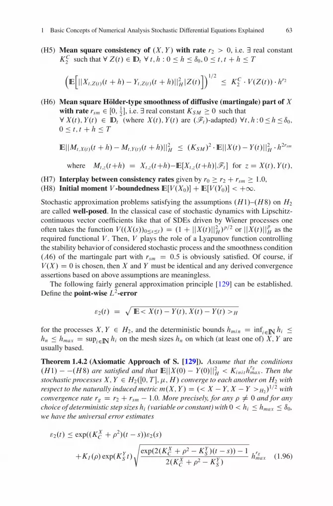
1 Basic Concepts of Numerical Analysis Stochastic Differential Equations Explained 63
(H5) Mean square consistency of .X; Y / with rate r2 > 0, i.e. 9 real constantKC2 such that 8Z.t/ 2 IDt 8 t; h W 0 � h � ı0; 0 � t; t C h � T
�IEhjjXt;Z.t/.t C h/ � Yt;Z.t/.t C h/jj2H jZ.t/
i�1=2 � KC2 � V.Z.t// � hr2
(H6) Mean square Holder-type smoothness of diffusive (martingale) part of Xwith rate rsm 2 Œ0; 1
2�, i.e. 9 real constantKSM � 0 such that
8X.t/; Y.t/ 2 IDt (where X.t/; Y.t/ are .Ft /-adapted) 8t; h W 0�h� ı0;0 � t; t C h � T
IEjjMt;X.t/.t C h/�Mt;Y.t/.t C h/jj2H � .KSM /2 � IEjjX.t/� Y.t/jj2H � h2rsm
where Mt;z.tCh/ D Xt;z.tCh/�IEŒXt;z.tCh/jFt � for z D X.t/; Y.t/;
(H7) Interplay between consistency rates given by r0 � r2 C rsm � 1:0,(H8) Initial moment V -boundedness IEŒV .X0/�C IEŒV .Y0/� < C1.
Stochastic approximation problems satisfying the assumptions .H1/–.H8/ on H2
are called well-posed. In the classical case of stochastic dynamics with Lipschitz-continuous vector coefficients like that of SDEs driven by Wiener processes oneoften takes the function V..X.s//0�s�t / D .1 C jjX.t/jj2H /p=2 or jjX.t/jjpH as therequired functional V . Then, V plays the role of a Lyapunov function controllingthe stability behavior of considered stochastic process and the smoothness condition.A6/ of the martingale part with rsm D 0:5 is obviously satisfied. Of course, ifV.X/ D 0 is chosen, then X and Y must be identical and any derived convergenceassertions based on above assumptions are meaningless.
The following fairly general approximation principle [129] can be established.Define the point-wise L2-error
"2.t/ D pIE< X.t/ � Y.t/; X.t/� Y.t/ >H
for the processes X; Y 2 H2, and the deterministic bounds hmin D infi2IN hi �hn � hmax D supi2IN hi on the mesh sizes hn on which (at least one of) X; Y areusually based.
Theorem 1.4.2 (Axiomatic Approach of S. [129]). Assume that the conditions.H1/ � �.H8/ are satisfied and that IEjjX.0/ � Y.0/jj2H < Kinith
rgmax: Then the
stochastic processes X; Y 2 H2.Œ0; T �; �;H/ converge to each another onH2 withrespect to the naturally induced metric m.X; Y / D .< X � Y;X � Y >H2/
1=2 withconvergence rate rg D r2 C rsm � 1:0. More precisely, for any � ¤ 0 and for anychoice of deterministic step sizes hi (variable or constant) with 0 < hi � hmax � ı0,we have the universal error estimates
"2.t/ � exp..KXC C �2/.t � s//"2.s/
CKI.�/ exp.KYS t/
sexp.2.KX
C C �2 �KYS /.t � s// � 1
2.KXC C �2 �KY
S /hrgmax (1.96)
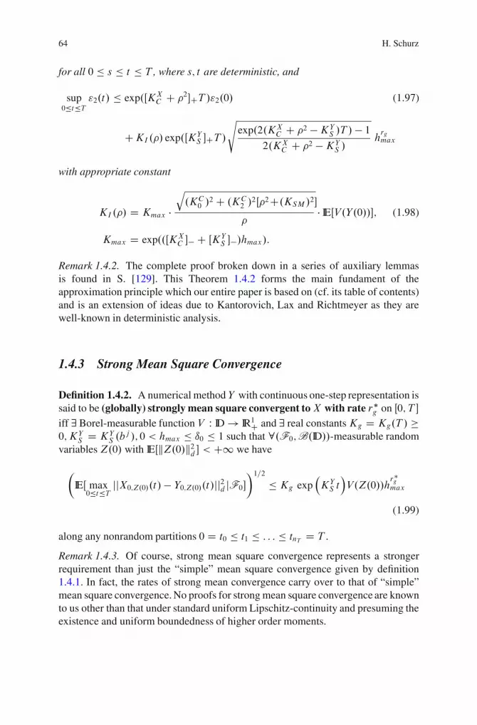
64 H. Schurz
for all 0 � s � t � T , where s; t are deterministic, and
sup0�t�T
"2.t/ � exp.ŒKXC C �2�CT /"2.0/ (1.97)
CKI .�/ exp.ŒKYS �CT /
sexp.2.KX
C C �2 �KYS /T /� 1
2.KXC C �2 �KY
S /hrgmax
with appropriate constant
KI .�/ D Kmax �q
.KC0 /
2 C .KC2 /
2Œ�2C.KSM /2�
�� IEŒV .Y.0//�; (1.98)
Kmax D exp..ŒKXC �� C ŒKY
S ��/hmax/:
Remark 1.4.2. The complete proof broken down in a series of auxiliary lemmasis found in S. [129]. This Theorem 1.4.2 forms the main fundament of theapproximation principle which our entire paper is based on (cf. its table of contents)and is an extension of ideas due to Kantorovich, Lax and Richtmeyer as they arewell-known in deterministic analysis.
1.4.3 Strong Mean Square Convergence
Definition 1.4.2. A numerical method Y with continuous one-step representation issaid to be (globally) strongly mean square convergent toX with rate r�g on Œ0; T �iff 9 Borel-measurable function V W ID ! IR1C and 9 real constantsKg D Kg.T / �0;KY
S D KYS .b
j /; 0 < hmax � ı0 � 1 such that 8.F0;B.ID//-measurable randomvariablesZ.0/ with IEŒkZ.0/k2d � < C1 we have
�
IEŒ max0�t�T jjX0;Z.0/.t/ � Y0;Z.0/.t/jj2d jF0�
�1=2
� Kg exp�KYS t�V.Z.0//h
r�gmax
(1.99)
along any nonrandom partitions 0 D t0 � t1 � : : : � tnT D T .
Remark 1.4.3. Of course, strong mean square convergence represents a strongerrequirement than just the “simple” mean square convergence given by definition1.4.1. In fact, the rates of strong mean convergence carry over to that of “simple”mean square convergence. No proofs for strong mean square convergence are knownto us other than that under standard uniform Lipschitz-continuity and presuming theexistence and uniform boundedness of higher order moments.

1 Basic Concepts of Numerical Analysis Stochastic Differential Equations Explained 65
The proof of following theorem is left to interested reader, but it can be carriedout in a similar fashion as previous convergence proofs by applying a theorem dueto Milstein [94, 95].
Theorem 1.4.3. Assume that all coefficients a and bj are uniformly Lipschitzcontinuous and assumptions (A0)–(A5) hold with V.x/ D .1C jjxjj4d /1=4.Then, the BTMs (1.1) with equidistant step sizes h � ı0 < 1 are strongly meansquare convergent with rate r�g D 0:5.
This theorem is proved by Milstein’s Theorem stated as follows. We leave thework out of related details to the interest of our readership.
Theorem 1.4.4 (Milstein’s strong mean square convergence theorem [95]).Assume that all coefficients a and bj are uniformly Lipschitz continuous on Œ0; T ��IRd and the local rates of consistency r0 and r2 satisfy
r2 � 3
4; r0 � r2 C 1
2:
Moreover, let 9K4 8t 2 Œ0; T �8h W 0 < h � ı0 8z 2 IRd
IE kXt;z.t C h/ � Yt;z.t C h/k4d � .K4/4.1C kzk4d /h4r2�1:
Then, equidistant numerical methods Y with nonrandom initial values X.0/ DY0 D x0 2 IRd permit estimates
Fundamental Strong Mean Square Convergence Relation
"�2 .T / D
IE sup0�t�T
kX0;x0.t/ � Y0;x0.t/k2d!1=2
� KSC2 .1C kx0k4d /1=4hr2�
12
where KSC2 is a real constant, and h � 1, i.e. ��g .2/ D r2 � 1
2.
1.4.4 Milstein’s Weak Convergence Theorem
Sometimes one is only interested in moments of solutions of SDEs. This conceptrather corresponds to the concept of weak convergence from functional analysis.A numerical version of that concept is introduced and studied independently byMilstein [93] and Talay [139]. Let F denote a nonempty class of sufficiently smoothtest functions f W IRd ! IR1 (or functionals) and ID IRd .
Definition 1.4.3. A numerical method Y with one-step representation Ys;y.t/ issaid to be (globally) weakly convergent toX with rate rw 2 .0;C1/ on Œ0; T ��ID

66 H. Schurz
(with respect to the test class F ) iff 9 Borel-measurable function V W ID ! IR1C and9 real constantsKw D Kw.F; T; b
j / � 0 and ı0 with 0 < hmax � ı0 � 1 such that
8x 2 ID W supf 2F
sup0�t�T
ˇˇˇIE f .X0;x.t// � IE f .Y h0;x.t//
ˇˇˇ � KwV.x/ � hrw (1.100)
where Y h is constructed along any nonrandom partitions 0 D t0 � t1 � : : : � tnT DT with maximum step size h based on scheme-values .Yn/n2IN at discrete instantstn.
Usually one investigates weak convergence with respect to continuous functionsf 2 F . However, step functions (elementary functions) such as indicator functionsIS of certain sets S or convex functions are also common to guarantee convergenceof related probabilities. However, the main result on weak convergence is borrowedfrom Milstein [95] and reads as follows. Let PG.r/ be the set of functionsf W IRd ! IR1 which does not possess polynomial growth more than power r 2 IN.
Theorem 1.4.5 (Milstein’s weak convergence theorem [95]). Assume that a; bj
are uniformly Lipschitz continuous on Œ0; T �� IRd , f W IRd ! IR and a; bj togetherwith their derivatives up to degree 2r C 2 are polynomially bounded of degree 2p,r 2 IN, X is governed by SDE (1.2) and:
(i) X0;x0.0/Dx02IRd independent of F jD.W j .s/; s�0/with IEŒkx0k2pd �< C1.
(ii) sup.hn/n2INWhn�ı0�1 supn2IN IEkY .hn/0;x0
.tn/k2pd � Kb < C1.
(iii) 9K0 8t 2 Œ0; T � 8x 2 IR : ka.t; x/k2d CmX
jD1kbj .t; x/k2d � .KB/
2.1Ckxk2d /.
(iv) 9Kc 8t 2 Œ0; T � 8x; y 2 IR : ka.t; x/ � a.t; y/k2d CmX
jD1kbj .t; x/ �
bj .t; y/k2d � .KL/2kx � yk2d .
(v) 9g D g.x/ 2 F PG.2p/ 8h � hmax 8Œt; t C h� � Œ0; T � 8l D1; 2; : : : ; 2r C 1
ˇˇˇˇˇIE
lY
kD1.Xt;x.t C h/� x/ik �
lY
kD1.Yt;x.t C h/� x/ik
!ˇˇˇˇˇ
� g.x/hrC1
IE2rC2Y
kD1jYt;x.t C h/� xjik � g.x/hrC1
Then, weak convergence of Y to X with rate rw D r with respect to the test classf 2 F PG.2p/\C2.IRd / with V.x/ D .1Cjjxjj2pd on ID D IRd is established,i.e. more precisely
"w0.T / D sup
f 2Fsup0�t�T
kIEŒf .X0;x0.t//� � IEŒf .Y0;x0 .t//�kd

1 Basic Concepts of Numerical Analysis Stochastic Differential Equations Explained 67
� K.T;a;bj /.1CIEkx0k2pd /hrmaxwhere all K represent real constants (only depending on T , a, bj ), and hmax � 1.
The proof is found in Milstein [95]. Forward and backward Euler, stochasticTheta methods with vanishing weight matrices cj (j D 1; 2; : : : ; m) as well asfamilies of implicit Milstein and Theta-Milstein methods have weak convergenceorder rw D 1:0. There are other methods such as Talay-Tubaro’s extrapolationmethod which can achieve weak order 2:0 or even higher order of weak convergencefor moments of functions of solutions of SDEs at fixed deterministic terminal timeT . The situation is more complicated for approximation of functionals depending onthe past or even whole memory of trajectories. Then it may happen that the orders(rates) shrink to much lower orders. A similar reduction of orders can happen iffunctions are not very smooth or a control at all times T up to infinity is necessary.For some analysis of convex functionals, see S. [133]. In this case and when non-smoothness is given, one can exploit the more robust Lp-convergence analysis tojustify a minimum rate of convergence (an at least guaranteed order).
1.4.5 Weak Convergence of BTMs (1.1) with Nonrandom Weights
For simplicity, set F D C2b.�/.IR
d ; IR1/ and consider the subclass of linear-implicitBTMs (by putting� D 0 in (1.1))
YkC1 D Yk CmX
jD0bj .tk; Yk/�W
j
kC
mX
jD0cj .tk; Yk/j�W j
kj.Yk � YkC1/ (1.101)
which we also abbreviate by BIMs.For approximations in the weak sense w.r.t. test class F , one should rather take
the weights cj � O for j D 1; 2; : : : ; m to guarantee the maximum rate of weakconvergence. More degree of freedom is in the choice of c0. A preferable choice isc0.t; x/ D 0:5ra.t; x/ due to a reasonable replication of the p-th moment stabilitybehavior of such BIMs compared to the underlying SDEs. This choice would alsocoincide with linearly drift-implicit midpoint and trapezoidal methods for bilinearSDEs. Let C l
b.�/.IRd ; IR1/ denote the set of all l-times (l 2 IN) continuously
differentiable functions f W IRd ! IR1 with uniformly bounded derivatives up tol-th order such that
maxfjf .x/j; jjrf .x/jjd ; kr2f .x/kd�d ; : : :g � Kf � .1C kxk�d /
for all x 2 IRd , whereKf and � are appropriate real constants.

68 H. Schurz
Theorem 1.4.6 (Weak Convergence of BIMs, S.[128]). Assume that .A1/–.A4/with V 2 C2
b.�/.IRd ;IR1C/ with V.x/ � .1 C jjxjj2d /1=2 hold, IEkY0k4� < C1 for
an integer � � 1, all coefficients a; bj 2 C 2b.�/.Œ0; T � � IRd ; IRd / of SDE (1.2) are
uniformly Lipschitz-continuous with Lipschitz constantsKjL with respect to x and
8t 2 Œ0; T �8x 2 IRdmX
jD0kc0.t; x/bj .t; x/k4d � .K4c/
4.1C kxk4�d /: (1.102)
Then the subclass of BIMs (1.101) with weights cj .t; x/ � O for j D 1; 2; : : : ; m
(i.e. BIMs with nonrandom weights) is weakly converging with rate rw D 1:0 withrespect to the test class f 2 C2
b.�/.IRd ; IR1/. More precisely, for all test functions
f 2C2b.�/.IR
d ; IR1/ for which the standard Euler method weakly converges with rate
rEw D 1:0, there is a real constantKw D Kw.T;Kf ; bj / (for its estimate, see at the
end of following proof) such that
jIEf .X.T // � IEf .YnT /j � Kw ��
maxkD0;1;:::;nT
IE.1C kYkk4�d /�
� hmax (1.103)
where the maximum step size hmax satisfies the condition
2�.4� � 1/mK2M.K
j
b.2//2hmax < 1 (1.104)
with constantsKj
b.2/ chosen as in (1.107) for all j D1; 2; : : : ; m (i.e. for bj insteadof f ).
Proof. Recall that the forward Euler methods weakly converge with worst caseglobal rate rEw D 1:0 and error-constants KE
w D KEw .T / � 0 under the given
assumptions (see Milstein [95] and Talay [140]). Let f 2 C2b.�/.IR
d ; IR1/ haveuniformly bounded derivatives satisfying
max�jf .x/j; krf .x/kd ; kr2f .x/kd�d
�� Kf .1Ckxk4� /1=4 � Kf .1Ckxk� /
with constant Kf . Moreover, for such functions f , one can find an appropriate realconstant KE
w D KEw .T; f; b
j / such that it satisfies the conditional estimates of thelocal weak error
ˇˇˇIEŒf .Xs;x.t// � f .Y Es;x.t//�
ˇˇˇ � KE
w � .1C kxk4�d / � .t � s/2
for sufficiently small 0 � t � s � hmax � ı0 and x 2 IRd , and the global weak error
ˇˇˇIEŒf .X0;x.T // � f .Y E0;x.T //�
ˇˇˇ � KE
w � .1C kxk4�d / � T � hmax;
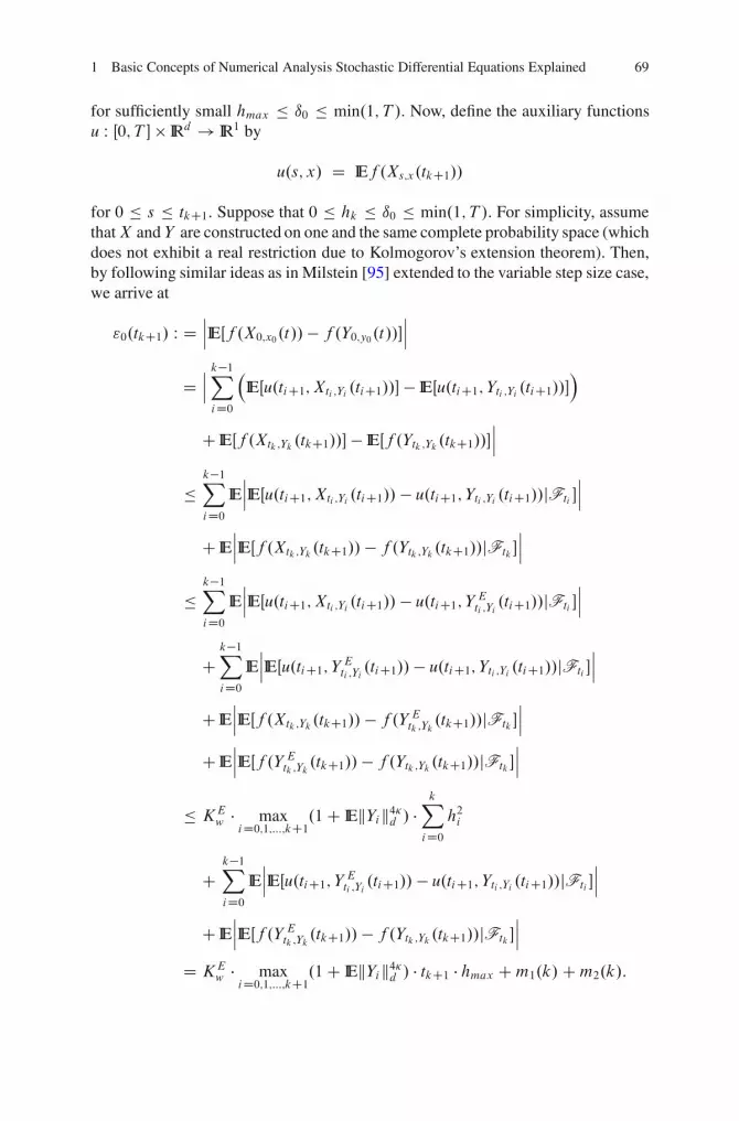
1 Basic Concepts of Numerical Analysis Stochastic Differential Equations Explained 69
for sufficiently small hmax � ı0 � min.1; T /. Now, define the auxiliary functionsu W Œ0; T � � IRd ! IR1 by
u.s; x/ D IEf .Xs;x.tkC1//
for 0 � s � tkC1. Suppose that 0 � hk � ı0 � min.1; T /. For simplicity, assumethatX and Y are constructed on one and the same complete probability space (whichdoes not exhibit a real restriction due to Kolmogorov’s extension theorem). Then,by following similar ideas as in Milstein [95] extended to the variable step size case,we arrive at
"0.tkC1/ W DˇˇˇIEŒf .X0;x0 .t//� f .Y0;y0 .t//�
ˇˇˇ
Dˇˇˇ
k�1X
iD0
�IEŒu.tiC1; Xti ;Yi .tiC1//� � IEŒu.tiC1; Yti ;Yi .tiC1//�
�
C IEŒf .Xtk;Yk .tkC1//� � IEŒf .Ytk ;Yk .tkC1//�ˇˇˇ
�k�1X
iD0IEˇˇˇIEŒu.tiC1; Xti ;Yi .tiC1// � u.tiC1; Yti ;Yi .tiC1//jFti �
ˇˇˇ
C IEˇˇˇIEŒf .Xtk;Yk .tkC1// � f .Ytk ;Yk .tkC1//jFtk �
ˇˇˇ
�k�1X
iD0IEˇˇˇIEŒu.tiC1; Xti ;Yi .tiC1// � u.tiC1; Y Eti ;Yi .tiC1//jFti �
ˇˇˇ
Ck�1X
iD0IEˇˇˇIEŒu.tiC1; Y Eti ;Yi .tiC1//� u.tiC1; Yti ;Yi .tiC1//jFti �
ˇˇˇ
C IEˇˇˇIEŒf .Xtk;Yk .tkC1// � f .Y Etk ;Yk .tkC1//jFtk �
ˇˇˇ
C IEˇˇˇIEŒf .Y Etk ;Yk .tkC1// � f .Ytk ;Yk .tkC1//jFtk �
ˇˇˇ
� KEw � max
iD0;1;:::;kC1.1C IEkYik4�d / �kX
iD0h2i
Ck�1X
iD0IEˇˇˇIEŒu.tiC1; Y Eti ;Yi .tiC1// � u.tiC1; Yti ;Yi .tiC1//jFti �
ˇˇˇ
C IEˇˇˇIEŒf .Y Etk ;Yk .tkC1// � f .Ytk ;Yk .tkC1//jFtk �
ˇˇˇ
D KEw � max
iD0;1;:::;kC1.1C IEkYik4�d / � tkC1 � hmax Cm1.k/Cm2.k/:
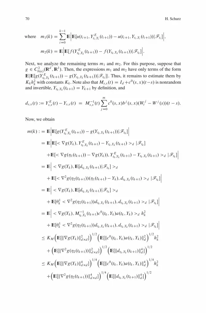
70 H. Schurz
where m1.k/ Dk�1X
iD0IEˇˇˇIEŒu.tiC1; Y Eti ;Yi .tiC1//� u.tiC1; Yti ;Yi .tiC1//jFti �
ˇˇˇ;
m2.k/ D IEˇˇˇIEŒf .Y Etk ;Yk .tkC1//� f .Ytk;Yk .tkC1//jFtk �
ˇˇˇ:
Next, we analyze the remaining terms m1 and m2. For this purpose, suppose thatg 2 C2
b.�/.IRd ; IR1/. Then, the expressions m1 and m2 have only terms of the form
IEjIEŒg.Y Etk;Yk .tkC1// � g.Ytk ;Yk .tkC1//jFtk �j. Thus, it remains to estimate them byKkh
2k with constantsKk . Note also thatMs;x.t/ D IdCc0.s; x/.t�s/ is nonrandom
and invertible, Ytk;Yk .tkC1/ D YkC1 by definition, and
ds;x.t/ WD Y Es;x.t/� Ys;x.t/ D M�1s;x .t/mX
jD0c0.s; x/bj .s; x/.W
jt �W j .s//.t � s/:
Now, we obtain
m.k/ W D IEˇˇˇIEŒg.Y Etk ;Yk .tkC1// � g.Ytk ;Yk .tkC1//jFtk �
ˇˇˇ
D IEˇˇˇIEŒ< rg.Yk/; Y Etk;Yk .tkC1/� Ytk;Yk .tkC1/ >d jFtk �
CIEŒ< rg.�1.tkC1//� rg.Yk//; Y Etk;Yk .tkC1/ � Ytk ;Yk .tkC1/ >d jFtk �ˇˇˇ
D IEˇˇˇ < rg.Yk/; IEŒdtk ;Yk .tkC1/jFtk � >d
C IEŒ< r2g.�2.tkC1//.�1.tkC1/� Yk/; dtk ;Yk .tkC1/ >d jFtk �ˇˇˇ
D IEˇˇˇ < rg.Yk/; IEŒdtk ;Yk .tkC1/jFtk � >d
C IEŒ�1k < r2g.�2.tkC1//dtk;Yk .tkC1/; dtk;Yk .tkC1/ >d jFtk �ˇˇˇ
D IEˇˇˇ < rg.Yk/;M�1tk;Yk .tkC1/c0.tk ; Yk/a.tk ; Yk/ >d h2k
C IEŒ�1k < r2g.�2.tkC1//dtk;Yk .tkC1/; dtk;Yk .tkC1/ >d jFtk �ˇˇˇ
� KM
�IEŒkrg.Yk/k2d�d �
�1=2�IEŒkc0.tk; Yk/a.tk; Yk/k2d
�1=2h2k
C�
IEŒkr2g.�2.tkC1//k2d�d ��1=2�
IEŒkdtk ;Yk .tkC1/k4d ��1=2
� KM
�IEŒkrg.Yk/k4d�d �
�1=4�IEŒkc0.tk; Yk/a.tk ; Yk/k4d
�1=4h2k
C�
IEŒkr2g.�2.tkC1//k4d�d ��1=4�
IEŒkdtk ;Yk .tkC1/k4d ��1=2
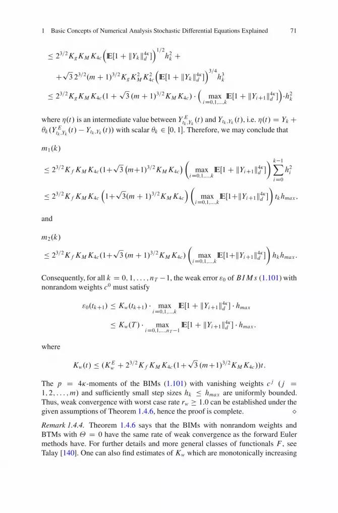
1 Basic Concepts of Numerical Analysis Stochastic Differential Equations Explained 71
� 23=2KgKMK4c
�IEŒ1C kYkk4�d �
�1=2h2k C
Cp3 23=2.mC 1/3=2KgK
2MK
24c
�IEŒ1C kYkk4�d �
�3=4h3k
� 23=2KgKMK4c.1C p3 .mC 1/3=2KMK4c/ �
�max
iD0;1;:::;kIEŒ1C kYiC1k4�d ��
�h2k
where �.t/ is an intermediate value between Y Etk;Yk .t/ and Ytk ;Yk .t/, i.e. �.t/ D Yk C�k.Y
Etk;Yk
.t/ � Ytk;Yk .t// with scalar �k 2 Œ0; 1�. Therefore, we may conclude that
m1.k/
� 23=2Kf KMK4c.1Cp3�mC1/3=2KMK4c
��
maxiD0;1;:::;kIEŒ1C kYiC1k4�d �
� k�1X
iD0h2i
� 23=2Kf KMK4c
�1Cp
3.mC 1/3=2KMK4c
��
maxiD0;1;:::;kIEŒ1CkYiC1k4�d �
�
tkhmax;
and
m2.k/
� 23=2Kf KMK4c.1Cp3 .mC 1/3=2KMK4c/
�
maxiD0;1;:::;kIEŒ1CkYiC1k4�d �
�
hkhmax:
Consequently, for all k D 0; 1; : : : ; nT �1, the weak error "0 of BIMs (1.101) withnonrandom weights c0 must satisfy
"0.tkC1/ � Kw.tkC1/ � maxiD0;1;:::;k IEŒ1C kYiC1k4�d � � hmax
� Kw.T / � maxiD0;1;:::;nT�1
IEŒ1C kYiC1k4�d � � hmax:
where
Kw.t/ � .KEw C 23=2Kf KMK4c.1Cp
3 .mC1/3=2KMK4c//t:
The p D 4�-moments of the BIMs (1.101) with vanishing weights cj .j D1; 2; : : : ; m/ and sufficiently small step sizes hk � hmax are uniformly bounded.Thus, weak convergence with worst case rate rw � 1:0 can be established under thegiven assumptions of Theorem 1.4.6, hence the proof is complete. ˘Remark 1.4.4. Theorem 1.4.6 says that the BIMs with nonrandom weights andBTMs with � D 0 have the same rate of weak convergence as the forward Eulermethods have. For further details and more general classes of functionals F , seeTalay [140]. One can also find estimates of Kw which are monotonically increasing
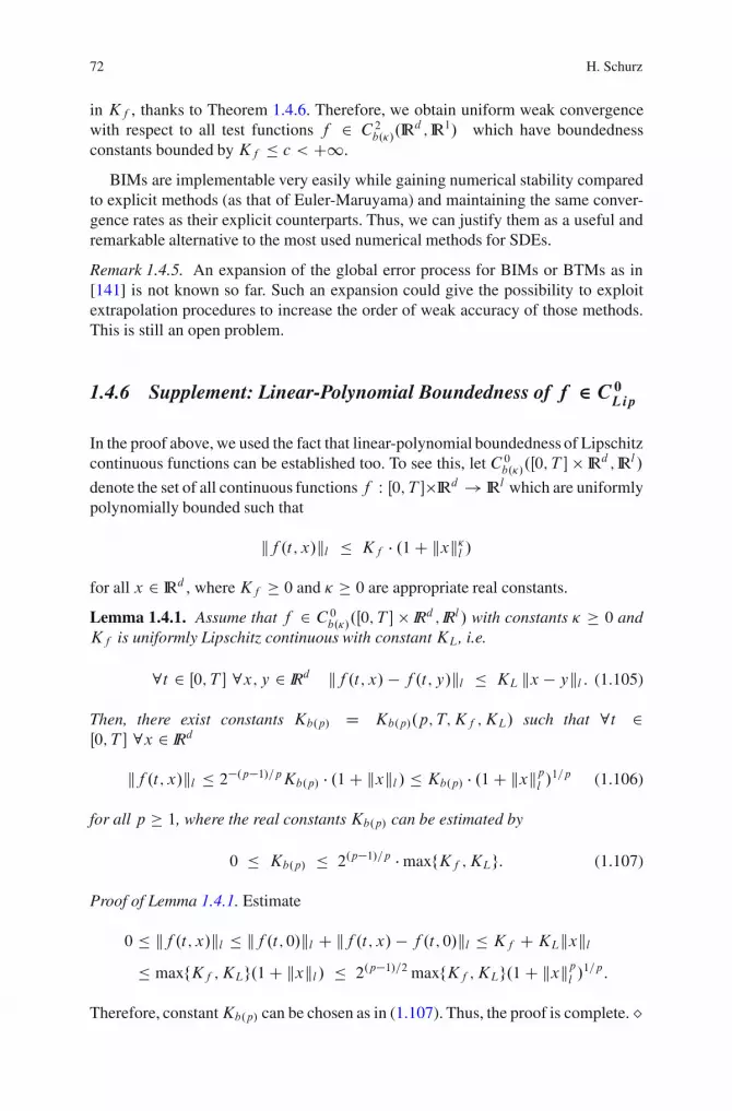
72 H. Schurz
in Kf , thanks to Theorem 1.4.6. Therefore, we obtain uniform weak convergencewith respect to all test functions f 2 C2
b.�/.IRd ; IR1/ which have boundedness
constants bounded by Kf � c < C1.
BIMs are implementable very easily while gaining numerical stability comparedto explicit methods (as that of Euler-Maruyama) and maintaining the same conver-gence rates as their explicit counterparts. Thus, we can justify them as a useful andremarkable alternative to the most used numerical methods for SDEs.
Remark 1.4.5. An expansion of the global error process for BIMs or BTMs as in[141] is not known so far. Such an expansion could give the possibility to exploitextrapolation procedures to increase the order of weak accuracy of those methods.This is still an open problem.
1.4.6 Supplement: Linear-Polynomial Boundedness of f 2 C 0Lip
In the proof above, we used the fact that linear-polynomial boundedness of Lipschitzcontinuous functions can be established too. To see this, let C0
b.�/.Œ0; T � � IRd ; IRl /
denote the set of all continuous functions f W Œ0; T ��IRd ! IRl which are uniformlypolynomially bounded such that
kf .t; x/kl � Kf � .1C kxk�l /
for all x 2 IRd , whereKf � 0 and � � 0 are appropriate real constants.
Lemma 1.4.1. Assume that f 2 C0b.�/.Œ0; T � � IRd ; IRl / with constants � � 0 and
Kf is uniformly Lipschitz continuous with constantKL, i.e.
8t 2 Œ0; T � 8x; y 2 IRd kf .t; x/ � f .t; y/kl � KL kx � ykl : (1.105)
Then, there exist constants Kb.p/ D Kb.p/.p; T;Kf ;KL/ such that 8t 2Œ0; T � 8x 2 IRd
kf .t; x/kl � 2�.p�1/=pKb.p/ � .1C kxkl / � Kb.p/ � .1C kxkpl/1=p (1.106)
for all p � 1, where the real constantsKb.p/ can be estimated by
0 � Kb.p/ � 2.p�1/=p � maxfKf ;KLg: (1.107)
Proof of Lemma 1.4.1. Estimate
0 � kf .t; x/kl � kf .t; 0/kl C kf .t; x/ � f .t; 0/kl � Kf CKLkxkl� maxfKf ;KLg.1C kxkl / � 2.p�1/=2 maxfKf ;KLg.1C kxkpl /1=p:
Therefore, constantKb.p/ can be chosen as in (1.107). Thus, the proof is complete. ˘

1 Basic Concepts of Numerical Analysis Stochastic Differential Equations Explained 73
Remark 1.4.6. In fact, it suffices that sup0�t�T kf .t; x�/kl < C1 for some x� 2IRd and f is Lipschitz continuous in x 2 IRd with Lipschitz constant KL.t/ whichis uniformly bounded with respect to t 2 Œ0; T �. However, Kb.p/ may depend on� too. Now, we can apply Lemma 1.4.1 in order to recognize that the requirement(A2) of Holder continuity of system .a; bj / yields linear-polynomial boundednessof both a and all bj coefficients of diffusion processes X .
Remark 1.4.7. Weak approximations and weak rates of convergence of Euler-typemethods are also studied in Kohatsu-Higa et al. [75,76], in Kannan et al. [67,68], inKushner et al. [84, 85], in Ogawa [103–105], or in Talay [140].
Remark 1.4.8. Strong convergence under nonclassical conditions has been inves-tigated in Deelstra & Delbaen [24], Gyongy [42], Higham et al. [49], Hu [55],Ogawa [104], Tudor [142]. Moreover, asymptotic efficiency of classes of Runge-Kutta methods is considered in Newton [101].
1.5 Positivity
It is well-known that the geometric Brownian motion X satisfying the Ito SDE
dX.t/ D �X.t/ dt C � X.t/ dW.t/ (1.108)
driven by the Wiener process W possesses the exact solution (with constants �,� 2 IR1)
X.t/ D exp..� � �2=2/t C �W.t// �X.0/ (1.109)
for F0-adapted initial data X.0/ 2 IR1. Remarkable facts are that X remains non-negative for non-negative initial values X.0/ D x0, X remains strictly positive forstrictly positive initial values, and X with X.0/ < 0 or X.0/ > 0 does not changeits sign as time t advances. Let us investigate the behaviour of representatives ofTheta methods (1.1) with respect to this observation of sign-preservation. For thispurpose, we suppose � > 0 for the further consideration.
1.5.1 Non-Positivity of Standard Euler Methodsfor Linear ODEs
In deterministic numerical analysis a very simple example is well–known. Considerthe equation (ODE)
Px D �x with x.0/ D x0 � 0
74 H. Schurz
and its non-negative exact solution x.t/ D exp.�t/ �x0. Then the Euler scheme (1.1)gives
ynC1 D yn C �ynhn D .1C �hn/yn D y0
nY
iD0.1C �hi/: (1.110)
Obviously, started at y0 > 0, this solution is always positive if � � 0 or j�jhi < 1
for all i D 0; 1; : : : ; n. Thus negative values may occur under the assumption y0 >0, � < 0 and hi large enough (indeed infinitely often). This step size restriction evengets worse for large values of � and a uniform restriction of h is not possible for allparameters � < 0 in order to guarantee (strict) positivity (or sign-preservation).
1.5.2 Positivity of Balanced Theta Methods for Linear ODEs
In contrast to the standard Euler scheme, in the case y0 > 0 and � < 0, we canalways prevent negative outcomes or even “explosions” in numerical methods witharbitrary step sizes hi for linear differential equations. For this purpose we introducethe family of implicit Euler-type schemes (1.1) with
ynC1 D yn C .�ynC1 C .1 � �/yn/�hn
D 1C .1 � �/�hn1 � ��hn
yn D y0
nY
iD0
1C .1 � �/�hi1 � ��hi ; (1.111)
hence it gives exclusively positive values under y0 > 0 if 1C.1��/�hi > 0 for alli 2 IN. A generalization of these schemes is presented by the deterministic balancedmethods
ynC1 D yn C �ynhn C chn.yn � ynC1/
D 1C .�C c/hn
1C chnyn D y0
nY
iD0
1C .�C c/hi
1C chi(1.112)
for an appropriate constant c > 0. Consequently, numerical solutions generated by(1.112) with c � j�j or by (1.111) with � D 1 are positive and monotonicallydecreasing for all y0 > 0, � < 0 and arbitrary step sizes hi � 0. They do nothave any explosions, and do not vanish for positive start values as well. Indeedthey provide sign-preserving approximations. All these properties are features ofthe underlying SDE. Hence, BIMs possess adequate realizations.
1.5.3 Negativity of Drift-Implicit Theta Methods for Linear SDEs
After previous elementary illustrations with ODEs, we return to the stochasticcase. For the sake of simplicity, we confine ourselves to equidistant partitions with

1 Basic Concepts of Numerical Analysis Stochastic Differential Equations Explained 75
uniform step size h (a similar result can be formulated for partitions with variable,nonrandom step sizes hi , but with “some care”).
Theorem 1.5.1 (Non-adequate Negativity of BTMs without Balanced Terms).Suppose X satisfies (1.108) with X.0/ > 0 (a.s.), � ¤ 0 and .1 � ��h/ > 0. Thenthe drift-implicit Theta approximation (1.1) applied to the linear SDE (1.108) andstarted in Y �0 D X.0/with nonrandom equidistant step size h > 0, non-autonomousnonrandom implicitness � 2 IR1 and without balanced terms cj � 0 has negativevalues with positive probability, i.e. there is a stopping time � D �.!/ W ˝ ! INsuch that
IP .f! 2 ˝ W Y �� .!/ < 0g/ > 0:
Proof. The family of drift-implicit Theta schemes (1.1) applied to (1.108) withcj � 0 and autonomous scalar implicitness � D �n is governed by
Y �nC1 D Y �n C ��Y �nC1hC .1� �/�Y �n hC �Y �n �Wn
D 1C .1 � �/�hC ��Wn
1 � ��hY �n D Y �0
nY
iD0
1C .1 � �/�hC �
ph i
1 � ��h
!
:
Define the events Ei ˝ on .˝;F ; IP / (for i 2 IN) by
Ei WD f! 2 ˝ W 1C .1� �/�hC �ph i .!/ < 0g
for i.i.d. i 2 N .0; 1/ (standard Gaussian distributed). Then the event
E WD f! 2 ˝ W 9�.!/ < C1; �.!/ 2 IN W Y ��.!/ < 0g
can be substituted by the events Ei .
IP .E0/ D IP
f! 2 ˝ W 0.!/ < �1C .1 � �/�h
�ph
g!
DW p
Notice that
IP .E0/ D IP
f! 2 ˝ W 0.!/ < �1C .1 � �/�h
j� jph g!
D p
as 0 is symmetric about 0 (recall the assumption of Gaussian distribution of 0).Thus, one obtains
IP .E/ D IP .E \ .E0 [E0// D IP .EjE0/IP .E0/C IP .EjE0/IP .E0/
D p C .1 � p/IP .EjE0/ D p C .1 � p/IP .E \ .E1 [E1/jE0/
76 H. Schurz
D p C .1 � p/�IP .EjE0;E1/IP .E1/C IP .EjE0;E1/IP .E1/
�
D p C p.1 � p/C .1 � p/2IP .EjE0;E1/
D p C p.1 � p/C p.1 � p/2 C .1 � p/3IP .EjE0;E1;E2/
� � �
D p
1X
iD0.1 � p/i D p
�1
1 � .1 � p/
�
D p
pD 1:
Note that 0 < p < 1. Thus it must exist (a.s.) a finite stopping time �n D n.w/hsuch that Y �.�n/ D Y �n < 0.
Alternatively, with the help of the well–known Lemma of Borel–Cantelli (orKolmogorov’s 0�1–law, see Shiryaev [134]) one also finds a short proof of Theorem1.5.1 (see original idea with � D 0 in S. [119]). For this purpose, we define
An D f! 2 ˝ W 9i � n W Y �i < 0g
for n 2 INC. Then it follows that
E D \1nD1 [1kDn Ak D [1nD1 \1kDn Ak :
Because of IP .An/ D .1 � IP .E0//n .n D 1; 2; : : :/, we obtain
1X
nD0IP .An/ D 1
IP .E0/< C1
where
1 > IP .E0/ D IP .f! 2 ˝ W 1C .1 � �/�hC j� jph 0.!/ < 0g/
D 1p2�
Z�
� 1C.1��/�h
j� jph
�
�1exp.�x2=2/dx
D ˚
�1C .1 � �/�hj� jph
!
> 0 8h 2 .0;1/
and ˚ denotes the probability distribution function of the standard Gaussiandistribution N .0; 1/, hence the assertion IP .E/ D 0 is true. Thus, drift-implicitTheta schemes with any � 2 IR1 and without balanced terms always possess atrajectory with negative outcome under the assumptions of Theorem 1.5.1.
1 Basic Concepts of Numerical Analysis Stochastic Differential Equations Explained 77
1.5.4 Positivity of Balanced Theta Methods for Linear SDEs
In contrast to the Euler methods, we find numerical methods which only have non-negative values and are sign-preserving. A corresponding assertion is formulated byTheorem 1.5.2.
Theorem 1.5.2 (A.s. Positivity of Balanced Methods, S.[119]). Assume that pro-cess X satisfies (1.108) and X.0/ � 0 (a.s.).Then the balanced methods with non-negative constants c0 and c1 exclusively havepositive outcomes at all instants n 2 IN, provided that
1C .c0 C �/h � 0 and c1 � j� j : (1.113)
Proof. This claim follows immediately from the structure of the balanced methods(1.1) applied to the (1.108) with � D 0, appropriate weights c0 and c1 satisfying(1.113). One encounters
Y BnC1 D Y Bn C �Y Bn hC �Y Bn �Wn C .c0hC c1j�Wnj/.Y Bn � Y BnC1/
D 1C .c0 C �/hC ��Wn C c1j�Wnj1C c0hC c1j�Wnj Y Bn :
Thereby, Y BiC1 � 0 iff
1C .c0 C �/hC ��Wi C c1j�Wi j � 0
for all i 2 IN. Obviously, this is true under (1.113). ˘Remark 1.5.1. An optimal choice of weights cj to maintain positivity under � < 0is given by c1 D j� j and c0 D Œ���C where Œz�C is the positive part of inscribedexpression z (for optimality, see also exact contraction-monotone and energy-exactmethods below). Numerical methods with variable step sizes could also preventnegativity, however this may lead to inefficient implementations in random settingsand throws out the nontrivial question of convergence of random instants tn to T asn ! C1. Moreover, the predictable measurability of instants tn is given up (i.e.one deals with another category of stochastic approximations!).
1.5.5 Positivity of Balanced Theta Methods for Nonlinear SDEs
Consider nonlinear autonomous SDEs (1.2) of the form
dX.t/ D2
4f .X.t//dt CmX
jD1gj .X.t//dW
j .t/
3
5X.t/ (1.114)

78 H. Schurz
with a.t; x/ D xf .x/ and bj .t; x/ D xgj .x/ where f and gj are nonrandommatrices in IRd�d . Such (1.114) are met in biology and ecology (see Lotka-Volterraequations or logistic Pearl-Verhulst models). There X approximates the numberof populations of certain species such as fish, flies, rabbits, fox, mice and owls orthe dynamic evolution of offspring-to-parents ratios. Naturally, X must have onlypositive outcomes for its practical meaningful modeling character.
Let us discretize SDEs (1.114) by the balanced methods (1.1) of the form
XnC1 D2
4I C f .Xn/hn CmX
jD1gj .Xn/�W
jn
3
5Xn
C2
4jjf .Xn/jjmaxhnCmX
jD1jjgj .Xn/jjmaxj�W j
n j3
5 .Xn�XnC1/ (1.115)
where jj:jjmax is the maximum norm of all entries of inscribed matrices and I is theunit matrix in IRd�d .
Theorem 1.5.3 (Positivity of BIMs for Nonlinear SDE). The balanced implicitmethods (1.115) applied to SDEs (1.114) with same initial value X.0/ > 0 and anystep sizes hn maintain the positivity at all instants n 2 IN.
Proof. Rewrite scheme (1.115) to equivalent expression
CnXnC1 D"
I C .f .Xn/C jjf .Xn/jjmaxI /hn
CmX
jD1.gj .Xn/�W
jn C jjgj .Xn/jjmaxj�W j
n j/#
Xn (1.116)
where Cn represents the invertible d � d diagonal matrix
Cn D2
41C jjf .Xn/jjmaxhn CmX
jD1jjgj .Xn/jjmaxj�W j
n j3
5 I:
Now, apply complete induction on n 2 IN and exploit the positivity of both the righthand side of (1.116) and the matrix Cn to conclude the assertion of Theorem 1.5.3.It is worth noting that the choice of step sizes hn > 0 does not play a role in keepingpositivity as n advances in our previous argumentation. ˘Remark 1.5.2. A slightly more general theorem on positivity of convergent multi-dimensional BIMs is found in S. [119, 120].
1 Basic Concepts of Numerical Analysis Stochastic Differential Equations Explained 79
1.5.6 Positivity of Balanced Milstein Methods
The lack of preservation of positivity can not be removed by the use of “higherorder methods” such as standard Milstein or Taylor-type methods (while noting thatthe probabilities of negative outcomes can be reduced by using them). However,by appropriate introduction of further balancing terms in them, one may achievethe goal of positivity (and sign-preservation) and higher order of convergence(and consistency as well). This fact is demonstrated by the following discussionwhich is related to higher order numerical methods applied to SDEs drivenexclusively by diagonal noise (for the sake of simplicity). Recall that systemswith diagonal noise are characterized by L i bj .t; x/ D 0 for all i ¤ j wherei; j D 1; : : : ; m. In this case the balanced Milstein methods (BMMs) withdiagonal noise follow the scheme
YnC1 D Yn CmX
jD0bj .tn; Yn/I.j /;tn;tnC1
CmX
jD1L j bj .tn; Yn/I.j;j /;tn;tnC1
C0
@d0.tn; Yn/I.0/;tn;tnC1C
mX
jD1d j .tn; Yn/I.j;j /;tn;tnC1
1
A .Yn � YnC1/ :
(1.117)
This class has been introduced and studied in Kahl and S. [60] in a more generalform referring to multiple Ito integrals I˛;tn;tnC1
.
Theorem 1.5.4 (Positivity of Balanced Milstein Methods [60]). The one-dimen-sional BMMs (1.117) applied to one-dimensional SDEs (1.2) with diagonal noisealong partitions
t0 < t1 < : : : < tn < tnC1 < : : :
and applied to SDEs (1.2) with diagonal noise maintain positivity of initialconditionsX.0/ 2 IRC if the following conditions hold
(A6) 8t 2 Œ0; T � 8x 2 IRC W d0.t; x/� 12
PmjD1 d j .t; x/ is positive semi-definite.
(A7) 8j D 1; 2; : : : ; m 8t 2 Œ0; T � 8x 2 IRC W dj .t; x/ is positive semi-definite.(A8) 8j D 1; : : : ; m 8tn 2 Œ0; T � and 8x 2 IRC.
bj .tn; x/@
@xbj .tn; x/C dj .tn; x/x > 0; (1.118)
(A9) 8tn 2 Œ0; T � and 8x 2 IRC.
x �mX
jD1
.bj .tn; x//2
2bj .tn; x/@@xbj .tn; x/C 2dj .tn; x/x
> 0; (1.119)

80 H. Schurz
(A10) IfD.tn; x/D a.tn; x/� 1
2
mX
jD1bj .tn; x/
@
@xbj .tn; x/Cd0.tn; x/x � 1
2
mX
jD1d j
.tn; x/x<0 for a value x 2 IRC at time-instant tn 2 Œ0; T � then the currentstep size hn is chosen such that 8tn 2 Œ0; T �, 8x 2 IRC.
hn <x CN.tn; x/
�D.tn; x/ (1.120)
where
N.tn; x/ D �mX
jD1
.bj .tn; x//2
2bj .tn; x/@@xbj .tn; x/C 2dj .tn; x/x
:
Remark 1.5.3. The assumption (A8) guarantees that the BMMs inherit the posi-tivity preserving structure of the underlying Milstein method. Condition (A9) ismore technical, but in many applications this is valid without the use of the weightfunction d1. (A10) is only necessary if D.tn; x/ < 0, otherwise we can drop thisrestriction for positivity. So, we obtain a first idea to apply BMMs as advancedMilstein-type methods to preserve positivity by choosing d 0 and d1 in such a waythatD.tn; x/ is greater than zero and we do not have to restrict the step size through(1.120) in this case. Furthermore, for global mean square convergence of BMMswith worst case rate 1:0 and positivity at the same time, we need to require thatD.t; x/ � 0. Note that the adapted, but random step size selection depending oncurrent random outcomes Yn by condition (A10) in the case of D.t; x/ < 0 wouldcontradict to the exclusive use of nonrandom step sizes as exploited in standardconvergence proofs. Moreover, a restricted step size selection as given by (A10)throws out the problem of proving that any terminal time T can be reached in afinite time with probability one. So it is advantageous to requireD.t; x/ � 0 for allx � 0 and 0 � t � T for meaningful and practically relevant approximations.
Proof. Set x D Yn. Using the one-step representation of the BMM (1.117) weobtain
0
@1C d0.tn; x/C 1
2
mX
jD1d j .tn; x/
�.�W j
n /2 � hn
�
1
A YnC1
D
x C a.tn; x/hn CmX
jD1bj .tn; x/�W
jn
C 1
2
mX
jD1bj .tn; x/
@
@xbj .tn; x/
�.�W j
n /2 � hn
�
Cd0.tn; x/xhn C 1
2
mX
jD1d j .tn; x/x
�.�W j
n /2 � hn
�!
D R.tn; Yn/:
1 Basic Concepts of Numerical Analysis Stochastic Differential Equations Explained 81
The expression .: : :/ in-front of YnC1 at the left hand side of this equation is positivedue to (A6) and (A7). Rewriting the right hand side leads to
R.tn; x/ D x C0
@a.tn; x/ � 1
2
mX
jD1bj .tn; x/
@
@xbj .tn; x/C d0.tn; x/x
�12
mX
jD1d j .tn; x/x
1
A hn C g.�W 1n ; : : : ; �W
mn /
with
g.�W 1n ; : : : ; �W
mn / D
mX
jD1bj .tn; x/�W
jn
C1
2
mX
jD1
�
bj .tn; x/@
@xbj .tn; x/C dj .tn; x/x
�
.�W jn /
2:
The function g W IRm ! IR1 possesses a global minimum due to (A8). Moreprecisely, an obvious calculation shows that
minz2IRm
g.z/ D �mX
jD1
.bj .tn; x//2
2�bj .tn; x/
@@xbj .tn; x/C dj .tn; x/x
� : (1.121)
This enables us to estimate R from below by replacing the value of g.�W 1n ; : : : ;
�W mn / by its minimum. So we arrive at
R.tn; x/ � x C0
@a.tn; x/ � 1
2
mX
jD1bj .tn; x/
@
@xbj .tn; x/C d0.tn; x/x
�12
mX
jD1d j .tn; x/x
1
A�n �mX
jD1
.bj .tn; x//2
2�bj .tn; x/
@@xbj .tn; x/C dj .tn; x/x
�
D xCN.tn; x/CD.tn; x/hnWe can clearly see that (A9)–(A10) under (A8) are needed to get positive valuesYnC1 > 0 whenever Yn > 0 for all n 2 IN. More precisely, if
D.tn; x/ D0
@a.tn; x/ � 1
2
mX
jD1bj .tn; x/
@
@xbj .tn; x/
Cd0.tn; x/x � 1
2
mX
jD1d j .tn; x/x
1
A � 0

82 H. Schurz
then R.tn; x/ > 0 and we do not need any restriction of the step size hn by (A10) atall. IfD.tn; x/ < 0 then xCN.tn; x/CD.tn; x/hn � 0 guarantees thatR.tn; x/ > 0,hence condition (A10) is needed in this case. Therefore, assumptions (A8)-(A10)imply the property of positivity of BMMs (1.117). ˘Remark 1.5.4. The proof of Theorem 1.5.4 shows that the condition (A9) can berelaxed to
x �mX
jD1
.bj .tn; x//2
2bj .tn; x/@@xbj .tn; x/C 2dj .tn; x/x
� 0 (1.122)
under the assumptionD.tn; x/ > 0.
Moreover, in some cases it is more efficient to verify the following conditionsinstead of restrictions (A9) and (A10) known from Theorem 1.5.4.
Corollary 1.5.1 (Kahl and S. [60]). The one-dimensional BMM (1.117) satisfying(A6)–(A8) along partitions
t0 < t1 < � � � < tn < tnC1 < � � �
maintains positivity if additionally
(A11) 8j D 1; : : : ; m 8tn 2 Œ0; T � and 8x 2 IRC W xCN.tn; x/CD.tn; x/hn > 0;where the functions N and D are defined in Theorem 1.5.4.
Example 6.1. Consider the one-dimensional geometric Brownian motion
dX.t/ DmX
jD1jX.t/ dW
j .t/; X.0/ D x0 > 0 (1.123)
without any drift which is a standard example for stability analysis for numericalintegration schemes for SDEs (e.g. see [120, 127]) where the standard numericalmethods possess serious step size restrictions or even fail to preserve stability andpositivity. Using any BMM with
d0.tn; x/ � m
2
mX
jD12j ;
8l D 1; : : : ; m d l.tn; x/ D .m � 1/2l
can solve this problem with higher order of accuracy very easily since
D.tn; x/ D �12
mX
jD12j x C d0.tn; x/x � m � 1
2
mX
jD12j x

1 Basic Concepts of Numerical Analysis Stochastic Differential Equations Explained 83
� �m2
mX
jD12j x C m
2
mX
jD12j x D 0 and
N.tn; x/ D �mX
jD1
2j x2
22j x C 2.m� 1/2j xD �x
2< 0
for x 2 IRC D .0;C1/. Hence, the restriction (A10) on the step size hn is notrelevant here. However, notice that a restriction of the form D.tn; x/ � �K Dconstant is important for the finiteness of related numerical algorithm (i.e. inparticular in order to reach any desired terminal time T > 0 with probability one).Moreover, all assumptions (A6)–(A9) are satisfied. Consequently, the related BMMsprovide positive-invariant numerical approximations to test SDE (1.123) with anychoice of step sizes hn and any F0-adapted initial data X.0/. Moreover, one canshow that they are consistent, convergent and stable (i.e. dynamically consistent).
Example 6.2. Consider the mean-reverting process (ECIRM)
dR.t/ D �.� � R.t//dt C ŒR.t/�pdW.t/ (1.124)
with �; �; > 0 which is of great importance in financial mathematics as well as inother areas of applied science. Focusing on the financial meaning of this equationwe obtain the well known Cox-Ingersoll-Ross model with exponent p D 0:5,describing the short-rate R in the interest rate market. Furthermore this SDE canbe used to model stochastic volatility. As commonly known, these dynamics mustbe positive for practically meaningful models. Indeed one can show that for theabove process X with exponents p 2 Œ0:5; 1/ and positive initial data R.0/ (e.g. byusing Fellers classification of boundary values). Then Kahl and S. [60] have shownthat the BMM (1.117) satisfying (A6)-(A7) with 2 > 0 along partitions
t0 < t1 < � � � < tn < tnC1 < � � �
has exclusively positive outcomes when applied to the mean-reverting process(1.124) with diffusion exponentp 2 .0:5; 1�with the following choice of the weightfunctions
d0.x/ D ˛� C 1
22pjxj.2p�2/; d 1.x/ D 0: (1.125)
with relaxation parameter ˛ 2 Œ0; 1� such that
hn <2p � 1
2p�.1 � ˛/ : (1.126)
Here, the relaxation parameter ˛ is similar to the implicitness parameter � in theclass of Theta methods (1.1) and gives some flexibility to adjust the BMM to specificproblem issues. The fully implicit case ˛ D 1 is a safe choice as we do not have to
84 H. Schurz
restrict the step size in that case. On the other hand, numerical tests have indicatedthat a reduced level of implicitness leads to better approximation results. Therefore,we would recommend to use ˛ D 0:5 whenever the parameter configuration allowsthis choice, also supported by results from [120]. Similarly, but with some care, onemay circumvent the problem of negative outcomes by BMMs in the critical casep D 0:5 of model (1.124). For more details, see [60].
Remark 1.5.5. An alternative numerical method to prevent inadequate negativity isgiven by splitting techniques of Moro and Schurz [99].
1.5.7 Non-positivity of Standard Euler Methodsfor Nonlinear SDE
Again, for simplicity, we confine ourselves to equidistant partitions of Eulerapproximations with step size h (e.g. h D T=N ) and possibly state-dependent noiseterm
XnC1 D Xn C ha.Xn/Cphb.Xn/ nC1; n D 1; 2; : : : ; X.0/ D x0 > 0;
(1.127)where f ngn2IN are independent identically distributed (i.i.d.) random variables on.˝;Ftn ; IP /. Then one is able to prove the following Theorem (see [2]) whichextends the results from [119, 120] to nonlinear equations (1.127). As usual, let
.˝;F ; .Ftn /n2IN; IP /
be a complete filtered probability space and the filtration .Ftn/n2IN be naturallygenerated, namely that Ftn D f 0; 1; : : : ng.
Theorem 1.5.5 (Non-positivity of Euler Methods for Nonlinear SDEs in 1D).Assume that:
(o) h >, x0 > 0 are nonrandom and fixed(i) a W IR ! IR and b W IR ! IR are continuous, nonrandom functions with
a.0/ D b.0/ D 0; (1.128)
(ii) G is well-defined by
G.u/ D u C ha.u/phjb.u/j (1.129)
for all u ¤ 0 and satisfies
infu>0
f�G.u/g > �1; (1.130)
(iii) diffusion function b is positive-definite on IR1C, i.e.

1 Basic Concepts of Numerical Analysis Stochastic Differential Equations Explained 85
8x > 0 W b.x/ > 0; (1.131)
(iv) . n/n2IN are i.i.d. Gaussian N .0; 1/-distributed random variables on thefiltered probability space .˝;F ; .Ftn /n2IN; IP /.
Then, for the standard Euler method (1.127) with equidistant step size h and positiveinitial value X.0/ D x0 > 0, there exists an a.s. finite stopping time � W ˝ ! INsuch that
X� < 0: (a.s.)
Remark 1.5.6. In fact, our main results are also valid when all n are i.i.d. randomvariables with symmetric continuous probability distribution F satisfying
8n 2 IN W F n D F� n ; supp.F n/ D IR1: (1.132)
Proof. In the proof we use a technique which was suggested by [119] and which isbased on the Borel-Cantelli Lemma (for latter, see, e.g. [134]). For this purpose andfixed step size h, introduce the nonrandom real constantM by setting
infu>0
f�G.u/g D infu>0
(
�u C ha.u/phjb.u/j
)
DW M > �1: (1.133)
Furthermore, define
NEn D f! 2 ˝ W Xi.!/ > 0;8i � ng ; (1.134)
thenEn D f! 2 ˝ W 9i � n W Xi.!/ � 0g : (1.135)
From the Borel-Cantelli Lemma we conclude that the solutionX to equation (1.127)becomes non-positive with probability one if
1X
nD0IP . NEn/ < 1: (1.136)
To prove (1.136) we estimate IP . NEn/ from above. Set X.0/ D X0. Since
IP . NEn/ D IP f! 2 ˝ W Xi.!/ > 0;8i � ng
DnY
jD1IP f! 2 ˝ W Xj .!/ > 0jXj�1 > 0; : : : ; X0 > 0g;
we need to estimate IP f! 2 ˝ W Xj .!/ > 0jXj�1 > 0; : : : ; X0 > 0g. We have forj > 1
86 H. Schurz
IP˚! 2 ˝ W Xj .!/ > 0
ˇˇXj�1 > 0; : : : ; X0 > 0
�
D IPn! 2 ˝ W Xj�1 C ha.Xj�1/C
phb.Xj�1/ j .!/ > 0
ˇˇ NEj�1
o
D IPn! 2 ˝ W
phb.Xj�1/ j .!/ > �Xj�1 � ha.Xj�1/
ˇˇ NEj�1
o
D IP
(
! 2 ˝ W j .!/ > �Xj�1 C ha.Xj�1/phb.Xj�1/
ˇˇˇˇXj�1 > 0
)
� IP˚! 2 ˝ W j .!/ > M
ˇˇXj�1 > 0
� D IP˚! 2 ˝ W j .!/ > M
�
under b.u/ > 0 for u > 0. The last equality in the above estimation holds sinceXj�1 is defined by 0; 1; : : : ; j�1 and j is independent of 0; 1; : : : ; j�1, andtherefore j is independent of Xj�1.
Now, put
IP˚! 2 ˝ W j .!/ > M
� D qM ;
and note that qM does not depend on j and qM < 1. The former statement istrue since M > �1 and n are all N .0; 1/–distributed, and therefore all n arecontinuously distributed with support .�1;C1/. Therefore,
IP . NEn/ � .qM /n;
1X
nD0IP . NEn/ � 1
1 � qM< 1:
Furthermore, define
�.!/ D inf fi 2 IN W Xi.!/ � 0g ; (1.137)
and note that, by the above argumentation, the random variable �0 is a.s. finite andall events f� D ng are .Ftn ;P.IN//-measurable, where P.IN/ is the power set ofall natural numbers IN (i.e. f� D ng 2 Ftn for all n 2 IN and � is a finite Markovtime). We also note that we actually haveX� < 0 (a.s.). This last statement is correctsince Xn has a continuous probability distribution and, therefore, it cannot take onthe value 0 with positive probability. ˘Remark 1.5.7. Condition (1.131) is not so essential for the validity of the aboveproof. Indeed, one can proceed without imposing condition (1.131), but this is notin the scope of this survey.
Remark 1.5.8. Condition (1.130) is fulfilled in particular if, for some Ka;Kb > 0
and all u 2 IR, we have
a.u/ � Kau if u � 0; a.u/ � Kbu if u � 0 and jb.u/j � Kbjuj if u 2 IR:(1.138)
1 Basic Concepts of Numerical Analysis Stochastic Differential Equations Explained 87
Moreover, for example thanks to Theorem 1.5.5, if there are constants p>0, Ka>0
andKb > 0 such that
a.u/ D �Kajujpu and b.u/ D Kbu; for all u 2 IR; (1.139)
then every solution X of (1.127) started at X.0/ D x0 > 0 will eventually possessnegative values as the integration time tn advances.
Remark 1.5.9. In passing, we note that the fact of non-positivity of numericalmethods is not so a bad property for some classes of SDEs. For example, systemswith additive noise (see e.g. discretizations of Ornstein-Uhlenbeck processes) musthave that feature of changing signs infinitely. This stems from the inherent propertyof underlying Wiener processes to cross zero levels after some finite time always(cf. the law of iterated logarithm of Wiener processes). All in all, we recommendsome care with requiring positivity in only adequate situations.
1.6 Boundedness (Finite Stability)
In this section, we shall study the topic of uniform boundedness of numericalapproximations which is mostly omitted in the literature. The property of bounded-ness can be interpreted as stability on finite intervals or the absence of “inadequateexplosions”. This is also an important requirement in view of meaningful modelingunder the absence of blow-ups. We can only indicate some results on the fairlycomplex property of boundedness.
1.6.1 Almost Sure Boundedness for Logistic Equations
Meaningful stochastic generalizations of logistic equations lead to the nonlinearSDEs of Ito-type
dX.t/ D Œ.�C�X.t//.K�X.t//��X.t/� dtCX.t/˛ jK�X.t/jˇdW.t/ (1.140)
driven by a standard Wiener process .W.t/ W t � 0/, started at X0 2 ID D Œ0;K� �IR1, where �; �;K;�; are positive and ˛; ˇ non-negative real parameters. There� can be understood as coefficient of transition (self-innovation), � as coefficient ofimitation depending on the contact intensity with its environment,K as a somewhat“optimal” environmental carrying capacity and � as natural death rate. However,in view of issues of practical meaningfulness, model (1.140) makes only sensewithin deterministic algebraic constraints, either given by extra boundary conditionsor self-inherent properties resulting into natural barriers at 0 at least. This factis supported by the limited availability of natural resources as known from the

88 H. Schurz
evolution of species in population ecology. In what follows we study almost sureregularity (boundedness on ID) of both exact and numerical solutions of (1.140).
Theorem 1.6.1 ([120, 130]). Let X.0/ 2 ID D Œ0;K� be independent of -algebra.W.t/; t � 0/. Then, under the conditions that ˛ � 1; ˇ � 1; K � 1; � � 0; � �0; � � 0, the stochastic process fX.t/; t � 0g governed by equation (1.140) isregular on ID D Œ0;K�, i.e. we have IP .X.t/ 2 Œ0;K�/ D 1 for all t � 0.Moreover, regularity on ID implies boundedness, uniqueness, continuity and Markovproperty of the strong solution process fX.t/; t � 0g of SDE (1.140) wheneverX.0/ D 0 (a.s.), X.0/ D K (a.s.) or
IEŒln.X.0/.K � X.0///� > �1:
Remark 1.6.1. The proof of Theorem 1.6.1 is found in S. [130]. To avoid technicalcomplications, define the diffusion coefficient b.x/ to be zero outside Œ0;K�. Notethat the requirement ˛ � 1 is a reasonable one in ecology, marketing and finance.This can be seen from the fact that modeling in population models is motivated bymodeling per-capita-growth rates (cf. S. [130]). Similar argumentation applies tomodels in finance (asset pricing) and marketing (innovation diffusion).
Proof. Define the drift function
a.x/ D .�C �x/.K � x/ � �x
and diffusion functionb.x/ D x˛.K � x/ˇ
for x 2 Œ0;K�. Take the sequence of open domains
IDn WD .exp.�n/;K � exp.�n//; n 2 IN:
Then, equation (1.140) is well–defined, has unique, bounded and Markoviansolution up to random time �s;x.IDn/, due to Lipschitz continuity and (linear)boundedness of drift a.x/ and diffusion b.x/ on IDn. Now, use Lyapunov functionV 2 C2.ID/ defined on ID D .0;K/ via
V.x/ D K � ln.x.K � x// :
Note that V.x/ D K � ln.x.K � x// D x � ln.x/ C K � x � ln.K � x/ � 2
for x 2 ID D .0;K/. Now, fix initial time s � 0, introduce a new LyapunovfunctionW 2 C1;2.Œs;C1/xID/ byW.t; x/ D exp.�c.t�s//V .x/ for all .t; x/ 2Œs;C1/ x ID, where
c D �C �K C 2K2˛C2ˇ�2 C �
2:
1 Basic Concepts of Numerical Analysis Stochastic Differential Equations Explained 89
Then V 2 C2.ID/ and W 2 C 1;2.Œs;C1/ x IDn/. Define L D L 0 as infinitesimalgenerator as in (1.6). Calculate
L V.x/D�.�C�x/.K�x/��x
��1x
C 1
K�x
C2
2x2˛.K�x/2ˇ
1
x2C 1
.K�x/2
for x 2 ID D .0;K/. An elementary calculus-based estimate leads to L V.x/ �c � V.x/ on ID. Consequently, we have
V.x/ � 2; infy2IDnIDn
V .y/ > 1C n; L V.x/ � c � V.x/ 8x 2 ID:
Therefore one may conclude that LW.t; x/ � 0, since L V.x/ � c � V.x/.Introduce �n WD min.�s;x.IDn/; t/. After applying Dynkin’s formula (averaged Itoformula), one finds that IEW.�n;X�n/ � V.x/ .X.s/ D x is deterministic!), hence
IEh
exp.c.t � �n//V .X�n/i
� exp.c.t � s//V .x/:
Using this fact, x 2 IDn (n large enough), one estimates
0 � IP .�s;x..0;K// < t/ � IP .�s;x.IDn/ < t/ D IP .�n < t/ D IEII�n<t
� IE
exp.c.t � �n// � V.X�s;x.IDn//
infy2IDnIDn V .y/� II�n<t
� exp.c.t � s// � V.x/
infy2IDnIDn V .y/� exp.c.t � s// � V.x/
1C n
�!n ! C10;
for all fixed t 2 Œs;C1/, where II.:/ represents the indicator function of subscribedrandom set. Consequently
IP .�s;x.ID/ < t/ D limn!C1 IP .�s;x.IDn/ < t/ D 0;
for x 2 .0;K/. After discussion of the trivial invariance behavior of X.t/ whenX0 D 0 or X0 D K , (almost sure) regularity of X.t/ on Œ0;K� follows immediately.Eventually, uniqueness, continuity and Markov property is obtained by a result fromKhas’minskii [71] (see Theorem 4.1, p. 84). ˘
Numerical regularization (the preservation of invariance of certain subsets underdiscretization while keeping convergence orders of related standard methods) isgenerally aiming at the construction of convergent and appropriately boundednumerical approximations for SDEs. First, we introduce the notion of regulardiscrete time processes.
Definition 1.6.1. A random sequence .Zi /i2IN is called regular on (or invariantwith respect to given domain) ID � IRd iff IP .Zi 2 ID/ D 1 for all i 2 IN;otherwise non-regular (not invariant with respect to ID).
90 H. Schurz
The following BIM solves the problem of numerical regularization on boundeddomain ID D Œ0;K�, at least in the case of ˛ � 1; ˇ � 1. Take
YnC1 D8<
:
Yn C�.�C �Yn/.K � Yn/� �Yn
�hn C Y ˛n .K � Yn/
ˇ�Wn
C��hn C C.K/Y ˛�1n .K � Yn/
ˇ�1j�Wnj�.Yn � YnC1/;
(1.141)
where C D C.K/ is an appropriate positive constant and Y0 2 ID D Œ0;K� (a.s.).Then one finds the following assertion.
Theorem 1.6.2. Assume that the initial value Y0 2 Œ0;K� (a.s.) is independent of-algebra .W.t/; t � 0/ andK > 0, � � 0, � � 0, � � 0. The numerical solution.Yn/n2IN governed by (1.141) is regular on ID D Œ0;K� if additionally
C1 > C.K/ � K > 0; ˛ � 1; ˇ � 1; 0 < hn � 1
�C �K.8n 2 IN/ :
Remark 1.6.2. It is rather obvious that standard Euler methods or Theta methodswithout using balancing terms can not provide almost surely bounded numericalapproximations on ID D Œ0;K� for the logistic (1.140). (One can even estimatetheir positive local probability of exiting ID – an exercise we leave to the interestedreader).
Proof. Use induction on n 2 IN. Then, after explicit rewriting of (1.141), one finds
YnC1 D Yn Ch.�C �Yn/hn C Y ˛n .K � Yn/ˇ�1�Wn
i.K � Yn/� �Ynhn
1C �hn C C.K/Y ˛�1n .K � Yn/ˇ�1j�Wnj
� Yn C ın � .K � Yn/ � K
where
ın D .� C �Yn/hn C Y ˛n .K � Yn/ˇ�1�Wn
1C �hn C C.K/Y ˛�1n .K � Yn/ˇ�1j�Wnj ;
since ın � 1 if Yn 2 Œ0;K�, C.K/ � K and hn � 1=.� C �K/. Otherwise, non-negativity of YnC1 follows from the identity
YnC1DYnC.�C�Yn/.K�Yn/hnCY ˛n .K�Yn/ˇ�1..K�Yn/�Wn C C.K/j�Wnj/1C �hn C C.K/Y ˛�1n .K�Yn/ˇ�1j�Wnj
if C D C.K/ � K . Consequently, we have IP . 0 � Yn � K / D 1 for alln 2 IN. ˘
Note, a stochastic adaptation of step sizes would form an alternative to deter-ministic step size selection as above. For example, for regularity, it suffices to
1 Basic Concepts of Numerical Analysis Stochastic Differential Equations Explained 91
require hn < 1=Œ� C �Yn � ��C for all n 2 IN. However, then one has tofind a truncation procedure to guarantee finiteness of corresponding algorithms toreach given terminal times T ! This is particularly important for adequate long termsimulations on computers.
The sequence Y D .Yn/n2IN following (1.141) is also regular on ID under otherconditions than those of Theorem 1.6.2. For example, if the condition ˛ � 1 isreplaced by ˛ 2 Œ0; 1/, the weights c.x/ D j jC.K/x˛�1.K � x/ˇ�1 of BIMs(1.141) guarantee the a.s. invariance of ID D Œ0;K�. However, they are unbounded inthis case. One even obtains regularity and boundedness of all numerical incrementsYnC1�Yn here, but we may suspect to loose convergence speed with such methods.So the open question arises how to maintain standard convergence rates and almostsure regularity of numerical methods on ID when ˛ 2 Œ0; 1/. Who knows the rightanswer? (At least, the case 0:5 � ˛ < 1 would be physically relevant.)
Remark 1.6.3. The rates of mean square consistency and convergence of BIMs(1.141) to the strong solutions of logistic SDE (1.140) is studied in S. [120, 130].
1.6.2 P-th Mean Boundedness of Theta Methods for MonotoneSystems
Consider nonlinear SDEs (1.2) discretized by drift-implicit Theta methods (1.1)with slightly modified class of schemes
XnC1 D Xn C Œ�na.t�nC1; XnC1/C .1 � �n/a.t�n ; Xn/�hn
CmX
jD1bj .t�n ; Xn/�W j
n (1.142)
where �n 2 IR1 and t�nC1 2 Œtn; tnC1� are nonrandom. Let ˘ be a time-scale (i.e.discrete (˘ D IN) or continuous (˘ D Œ0; T /)) and p 2 IR1 n f0g.
Definition 1.6.2. A stochastic process X D .X.t//t2˘ is said to be (uncondition-ally) uniformly p-th mean bounded along ˘ iff
supt2˘
IEjjX.t/jjp < C1:
If p D 2 we also speak of (uniform) mean square boundedness along ˘ .
SDEs (1.2) with p-th monotone coefficient systems .a; bj / have uniformlybounded solutions X (see S. [120]). Let us investigate this aspect for numericalapproximations. For technical reasons, set ��1 D �0, h�1 D h0, t��1 D 0. jj:jjdenotes the Euclidean norm in IRd and < :; : > the Euclidean scalar product.

92 H. Schurz
Theorem 1.6.3 (Uniform M.S. Boundedness of Theta Methods with �n � 0:5).Assume that p D 2 and 9Ka � 0;Kb (constants) 8t � 0 8x 2 IRd
< a.t; x/; x > � Kajjxjj2; (1.143)mX
jD1jjbj .t; x/jj2 � Kb; (1.144)
2Ka CKb � 0; (1.145)
8n 2 IN W �nhn � �n�1hn�1: (1.146)
Then the drift-implicit Theta methods with non-increasing, nonrandom sequence.�nhn/n2IN and non-increasing, nonrandom step sizes hn are uniformly mean squarebounded along˘ D IN and
VnC1 WD .1 � 2�nhnKa/IEjjXnC1jj2 C �2nh2nIEŒjja.t�nC1; XnC1/jj2�
� IEjjX0jj2 C h20.1 � �20 /IEŒjja.t�0 ; X0/jj2� D V0 < C1 (1.147)
for all n 2 IN, whenever IEŒjja.0;X0/jj2� < C1 and started at X0 2 L2.˝;
F0; IP /.
Proof. First, separate the terms with indices nC 1 and n to obtain
XnC1 � �na.t�nC1; XnC1/hn D Xn C .1� �n/a.t�n ; Xn/hn C
mX
jD1bj .t�n ; Xn/�W j
n :
Second, one takes the square of the Euclidean norm on both sides, leading to
jjXnC1��na.t�nC1; XnC1/hnjj2DjjXnC.1��n/a.t�n ; Xn/hnCmX
jD1bj .t�n ; Xn/�W j
n jj2:
Third, taking the expectation on both sides and using the independence of all �W jn
from Xn yield that
IEjjXnC1jj2 � 2�nhnIE < XnC1; a.t�nC1; XnC1/ > C�2nh2nIEjja.t�nC1; XnC1/jj2
D IEjjXnjj2 C"
2.1� �n/IE < Xn; a.t�n ; Xn/ > CIE
mX
jD1jjbj .t�n ; Xn/jj2
#
hn
Ch2nh.1 � 2�n/IEjja.t�n ; Xn/jj2 C �2n IEjja.t�n ; Xn/jj2
i
� .1C hnŒ2.1� �n/Ka CKb�/IEjjXnjj2 C �2nh2nIEjja.t�n ; Xn/jj2
1 Basic Concepts of Numerical Analysis Stochastic Differential Equations Explained 93
for all n 2 IN, provided that �n � 0:5. Notice that both �n and hn are supposed to benonrandom. Fourth, the assumption of non-increasing products �nhn is equivalentto
�2�nhnKa � �2�n�1hn�1Ka
for all n 2 IN, since Ka � 0. This gives the estimation
1 � 2�nhnKa CKbhn � 1 � 2�n�1hn�1Ka CKbhn�1;
hence (recall the assumptionsKa � 0, hn > 0)
1C Œ2.1 � �n/Ka CKb�hn � 1 � 2�n�1hn�1Ka CKbhn�1:
Fifth, applying this latter estimation to the final estimation in step “Third” impliesthat
.1 � 2�nKahn/IEjjXnC1jj2 C �2nh2nIEjja.t�nC1; XnC1/jj2
� .1 � �n�1Kahn�1/IEjjXnjj2 C �2n�1h2n�1IEjja.t�n ; Xn/jj2:
Sixth, define the functional V by
Vn WD .1 � �n�1Kahn�1/IEjjXnjj2 C �2n�1h2n�1IEjja.t�n ; Xn/jj2
for all n 2 IN. By complete induction on n 2 IN while using the estimate from“Fifth” step, we find that
Vn � V0 D .1 � ��1Kah�1/IEjjX0jj2 C �2�1h2�1IEjja.t��1; X0/jj2D .1 � �0Kah0/IEjjX0jj2 C �20 h
20IEjja.0;X0/jj2 < C1
for all n 2 IN. Recall the conventions ��1 D �0 and h�1 WD h0. This concludes theproof of Theorem 1.6.3 for �n 2 Œ0:5; 1�. ˘
A similar theorem for the estimation from below can be found for �n 2 Œ0; 0:5�.So Theta methods have uniformly bounded moments. This justifies also to studythe longterm convergence of all moments jjXnjjp for 0 < p � 2 as n advances toC1 (e.g. as a consequence, lim infn!C1 and lim supn!C1 of those expressionsmust exist). Moreover, one has some reason for the preference of Theta methodswith all parameters �n D 0:5 and midpoints t�n D .tnC1 � tn/=2 (i.e. trapezoidal inspace, midpoint in time, cf. also exact norm-monotone methods below). For linearsystems and constant �n, some of the above estimates are exact. For example, takea.t; x/ D �jjxjjp�2x with Ka D �1 and b.t; x/ D jjxjj.p�2/=2x with Kb D 2
for p D 2, and consider the drift-implicit Theta methods with all �n D 0:5 andequidistant step sizes hn D h > 0.
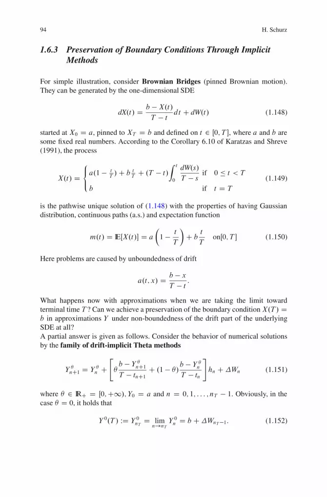
94 H. Schurz
1.6.3 Preservation of Boundary Conditions Through ImplicitMethods
For simple illustration, consider Brownian Bridges (pinned Brownian motion).They can be generated by the one-dimensional SDE
dX.t/ D b � X.t/
T � tdt C dW.t/ (1.148)
started at X0 D a, pinned to XT D b and defined on t 2 Œ0; T �, where a and b aresome fixed real numbers. According to the Corollary 6.10 of Karatzas and Shreve(1991), the process
X.t/ D8<
:
a.1 � tT/C b t
TC .T � t/
Z t
0
dW.s/
T � sif 0 � t < T
b if t D T
(1.149)
is the pathwise unique solution of (1.148) with the properties of having Gaussiandistribution, continuous paths (a.s.) and expectation function
m.t/ D IEŒX.t/� D a
�
1 � t
T
�
C bt
TonŒ0; T � (1.150)
Here problems are caused by unboundedness of drift
a.t; x/ D b � x
T � t :
What happens now with approximations when we are taking the limit towardterminal time T ? Can we achieve a preservation of the boundary conditionX.T / Db in approximations Y under non-boundedness of the drift part of the underlyingSDE at all?A partial answer is given as follows. Consider the behavior of numerical solutionsby the family of drift-implicit Theta methods
Y �nC1 D Y �n C"
�b � Y �nC1T � tnC1
C .1 � �/b � Y �nT � tn
#
hn C�Wn (1.151)
where � 2 IRC D Œ0;C1/; Y0 D a and n D 0; 1; : : : ; nT � 1. Obviously, in thecase � D 0, it holds that
Y 0.T / WD Y 0nT D limn!nT
Y 0n D b C�WnT�1: (1.152)

1 Basic Concepts of Numerical Analysis Stochastic Differential Equations Explained 95
Thus, the explicit Euler method ends in random terminal values, which is acontradiction to the behavior of exact solution (1.149)! Otherwise, in the case � > 0,rewrite (1.151) as Y �nC1 D
T � tnC1T � tnC1 C �hn
Y �n � .1 � �/.T � tnC1/hn.T � tn/.T � tnC1 C �hn/
Y �n C T � tnC1T � tnC1 C �hn
�Wn
C .1 � �/.T � tnC1/hn.T � tn/.T � tnC1 C �hn/
b C �hn
T � tnC1 C �hnb (1.153)
which impliesY � .T / WD Y �nT D lim
n!nTY �n D b: (1.154)
Thus, the drift-implicit Theta methods with positive implicitness � > 0 can preserve(a.s.) the boundary conditions!
Theorem 1.6.4 (S. [119]). For any choice of step sizes hn > 0; n D 0; 1; : : : ; nT�1,we haveŒ1�: IEY �nT D b if � � 0
Œ2�: IE.Y �nT � b/2 D hnT�1 if � D 0
Œ3�: IP .Y �nT D b/ D 0 if � D 0
Œ4�: IP .Y �nT D b/ D 1 if � > 0
where the random sequence .Y �n /nD0;1;:::;nT is generated by drift-implicit Thetamethod (1.151) with step size �Wn 2 N .0; hn/ where N .0; hn/ denotes theGaussian distribution with mean 0 and variance hn (supposing deterministic stepsize).
Remark 1.6.4. The proof of Theorem 1.6.4 is carried out in [119].
Remark 1.6.5. As we clearly recognize, discontinuities in the drift part of SDEsmay destroy rates of convergence. A guarantee of algebraic constraints at the endsof time-intervals through implicit stochastic numerical methods can be observed.The example of Brownian Bridges supports the preference of implicit techniques,not only in so-called stiff problems as often argued with in literature.
Remark 1.6.6. A practical and efficient alternative to preserve boundary conditionsis given by the splitting-step algorithm of Moro and Schurz [99].
1.7 Oscillations
Unfortunately, there is not much known on oscillatory behaviour of stochasticnumerical methods so far. So this section gives a first excursion into this important,but very complex field. For this purpose, consider the following definitions.

96 H. Schurz
Definition 1.7.1. A numerical methodZ with values .Zn/n2IN at instants .tn/n2INof partitions of Œ0; T � is called strictly oscillatory about c iff
8n 2 IN W ZnC1 � c
Zn � c< 0: (1.155)
A numerical method Z with values .Zn/n2IN at instants .tn/n2IN of partitions ofŒ0; T � is called quasi-oscillatory about c iff
ZnC1 � cZn � c
< 0 (1.156)
for infinitely many n 2 IN.Moreover, a numerical method Z with values .Zn/n2IN at instants .tn/n2IN ofpartitions of Œ0; T � is called (asymptotically) oscillatory about c in the wide senseiff
8n 2 IN W lim infn!C1
ZnC1 � cZn � c < 0 and lim sup
n!C1ZnC1 � cZn � c
> 0: (1.157)
If none of above conditions is true then we say Z is non-oscillatory.
We shall study the most important case of oscillation about c D 0 throughoutthis section. Oscillations in the wide sense and quasi-oscillations mean that thenumerical method has outcomes infinitely often above and below the level c. Oscil-lations in the wide sense can not belong to asymptotically stable approximations atequilibrium 0, whereas quasi-oscillations can be a feature of asymptotically stableones.
Definition 1.7.2. A methodZ is said to have spurious oscillations iff it has (quasi-) oscillations of any kind from above and the underlying SDE (1.2) does not showany oscillatory behaviour at all.
It is well-known that the geometric Brownian motionX satisfying the Ito SDE(1.108) does not show any oscillations for all F0-adapted initial data X.0/ 2 IR1.In fact, this process preserves the sign of F0-adapted initial data X.0/ (a.s) asintegration time advances. Now, let us study the oscillatory behaviour of relatednumerical methods applied to this simple test (1.108) and some further nonlinearequations. For this purpose, we suppose that � > 0 for the further consideration.
1.7.1 Spurious Oscillations of Standard Euler Methodsfor Linear ODE
In deterministic numerical analysis a very simple example is well–known. Considerthe equations (ODEs)

1 Basic Concepts of Numerical Analysis Stochastic Differential Equations Explained 97
Px D �x with x.0/ D x0 2 IR1 (1.158)
and its sign-preserving exact solution x.t/ D exp.�t/ � x0. Then the standard Eulerscheme (1.1) gives
ynC1 D yn C �ynhn D .1C �hn/yn D y0
nY
iD0.1C �hi/ : (1.159)
Obviously, started at y0 ¤ 0, we have that yn ¤ 0 for all n 2 IN provided that�hi ¤ �1 for all i 2 IN and
ynC1yn
D 1C �hn:
This expression is always positive if �hi > �1 for all i D 0; 1; : : : ; n. However,negative values may occur under the assumption that � < 0 and hi large enough(indeed always), i.e. we observe no sign changes whenever �hi < �1. This stepsize restriction for oscillations about 0 even gets less restrictive for large negativevalues of � < 0 and a uniform restriction of hi is not possible for all possibleparameters � < 0 in order to guarantee (strict) positivity of ratios ynC1=yn andhence no strict oscillations at all. In contrast to that, the underlying exact solutionX(as exponentials do not either) does not show any oscillatory behaviour at all. Thisargumentation proves the following theorem on existence of spurious oscillationsthrough Euler-type discretizations.
Theorem 1.7.1 (Spurious Strict Oscillations of Euler Methods in 1D). Assumethat
8n 2 IN W �hn < �1: (1.160)
Then the forward Euler method applied to linear ODEs (1.158) with step sizes hnpossesses strict spurious oscillations for any initial data x.0/ D y0.Assume that, for infinitely many n 2 IN, we have
�hn < �1: (1.161)
Then the forward Euler method applied to linear ODEs (1.158) with step sizes hnpossesses spurious quasi-oscillations for any initial data x.0/ D y0.
Remark 1.7.1. If �hn � �1 for all n 2 IN then the Euler method has no oscillationsat all. However, this might be very restrictive for long-term simulations withnegative values of � << �1. At least, for nonlinear equations, the situation becomeseven worse (here thresholds imposed on hn for the absence of spurious oscillationsare not known in general).

98 H. Schurz
1.7.2 Non-oscillations of (Balanced) Theta Methodsfor Linear ODEs
In contrast to the standard Euler scheme, in the case � < 0, we can always preventoscillations in numerical methods with arbitrary step sizes hi for linear differentialequations in 1D. For this purpose we return to the deterministic family of Euler-typeTheta schemes (1.1) with implicitness �n 2 IR1
ynC1 D yn C .�nynC1 C .1 � �n/yn/�hn
D 1C .1 � �n/�hn
1 � �n�hnyn D y0
nY
iD0
1C .1 � �i /�hi1 � �i�hi : (1.162)
Thus, we find that
ynC1yn
D 1C .1 � �n/�hn
1 � �n�hn
whenever �n�hn ¤ 1. Hence, when � < 0 and all �i�hi < 1, these schemespossess strict oscillations if 1C .1��i/�hi < 0 for all i 2 IN and quasi-oscillationsif 1C .1 � �n/�hn < 0 for infinitely many n 2 IN.
A generalization of these schemes is presented by the deterministic balancedmethods (as a subclass of (1.1))
ynC1 D yn C �ynhn C c0hn.yn � ynC1/
D 1C .�C c0/hn
1C c0hnyn D y0
nY
iD0
1C .�C c0/hi
1C c0hi(1.163)
for an appropriate constant c0 > 0. This leads to the identity
ynC1yn
D 1C .�C c0/hn
1C c0hn
for all n 2 IN. Consequently, as a summary, we gain the following theorem.
Theorem 1.7.2. Numerical approximations generated by balanced methods(1.163) with c0 � Œ���C or by drift-implicit Theta methods (1.162) with parameterssatisfying �n D 1 or .1 � �n/�hn > 0 are non-oscillatory for all test (1.158) withany � � 0 along any choice of arbitrary step sizes hn � 0. Therefore, they possessadequate realizations without spurious oscillations along any partition.
Remark 1.7.2. Suppose that � � 0. Then, the balanced methods (1.163) with theweight c0 D Œ���C coincide with drift-implicit backward Euler methods (1.1) with�n D 1 for all n 2 IN while applying to ODEs. Hence, there are drift-implicit

1 Basic Concepts of Numerical Analysis Stochastic Differential Equations Explained 99
Theta methods (1.1) without any spurious oscillations for any choice of step sizeshn. However, the situation changes in stochastic settings where nontrivial weightscj are needed in order to limit the possibility of inadequate oscillations (see below).
1.7.3 Spurious Oscillations of Theta Methods for Linear SDEs
After previous elementary illustrations with ODEs, we return to the stochastic case.For the sake of simplicity, we confine ourselves to partitions with nonrandom stepsizes hn. Note that
8t � s � 0 W IP
��
! 2 ˝ W X.t/.!/X.s/.!/
< 0
��
D 0
for the stochastic process X satisfying (1.110).
Theorem 1.7.3. Assume that X satisfies (1.108) with X.0/ ¤ 0 (a.s.), � ¤ 0 and
8n 2 IN W 1 ¤ �n�hn; n 2 N .0; 1/:
Then the drift-implicit Theta methods (1.1) applied to the linear SDE (1.108) andstarted in Y �0 D X.0/ with nonrandom step sizes hn, nonrandom parameters �n 2IR1 and values .Y �n /n2IN have oscillations about 0 with positive probability, i.e.
8n 2 IN W IP
(
! 2 ˝ W Y�nC1.!/Y �n .!/
< 0
)!
> 0: (1.164)
Proof. The family of drift-implicit Euler-Theta schemes (1.1) applied to one-dimensional linear SDE (1.108) with cj � 0 and implicitness �n is governed by
Y �nC1 D Y �n C �n�Y�nC1hn C .1 � �n/�Y �n hn C �Y �n �Wn
D 1C .1 � �n/�hn C ��Wn
1 � �n�hn Y �n D Y �0
nY
iD0
1C .1 � �i/�hi C �
phi i
1 � �i�hi
!
:
Therefore we have
Y �nC1Y �n
D 1C .1 � �n/�hn C �phn n
1 � �n�hnD 1C .1 � �n/�hn
1 � �n�hnC �
phn
1 � �n�hn n
for all N 2 IN. Recall that 1 � �n�hn ¤ 0, � ¤ 0 and n are Gaussian N .0; 1/-distributed. That means that
Y �nC1Y �n
2 N
�1C .1 � �n/�hn
1 � �n�hn;
�2
.1 � �n�hn/2 hn�
:

100 H. Schurz
Consequently, under � ¤ 0 and 1 � �n�hn ¤ 0, this fact implies that (1.164). ˘Remark 1.7.3. After, returning to the proof above, one may extract the probabilityof local sign changes of Theta methods Y � and obtains
IP
(Y �nC1Y �n
< 0
)!
D IP
��
n < �1C .1 � �n/hn
j� jphn
��
D 1
2�
Z � 1C.1��n/hn
j� jphn
�1exp
�
�x2
2
�
dx
which tends to 0 as hn ! 0 since n is Gaussian distributed, provided that
infn2IN
.1 � �n/phn > �1:
1.7.4 Non-oscillatory Behaviour by Balanced Methodsfor Linear SDE
Consider the balanced methods
Y BnC1DY Bn C �Y Bn hn C �Y Bn �Wn C .c0hn C c1j�Wnj/.Y Bn � Y BnC1/: (1.165)
Theorem 1.7.4. Suppose X satisfies (1.108) with adapted initial values X.0/ � 0.Then the balanced methods (1.165) with constants c0, c1 � 0 and step sizes hn,started at Y B0 D X.0/ do not allow any sign changes as n advances, provided that
1C .c0 C �/hn � 0 and c1 � j� j : (1.166)
for all n 2 IN. Therefore, they do not possess any spurious oscillations in contrastto all solutionsX of linear SDEs (1.108).
Proof. This claim follows immediately from the construction of the balancedmethods (1.165) applied to the linear equation (1.108). One receives then
Y BnC1 D Y Bn C �Y Bn hn C �Y Bn �Wn C .c0hn C c1j�Wnj/.Y Bn � Y BnC1/
D 1C .c0 C �/hn C ��Wn C c1j�Wnj1C c0hn C c1j�Wnj Y Bn :
Thereby, Y BiC1 � 0 for all i 2 IN iff
1C .c0 C �/hn C ��Wi C c1j�Wi j � 0
for all i 2 IN. Obviously, this is the case under (1.166). ˘
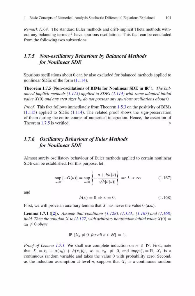
1 Basic Concepts of Numerical Analysis Stochastic Differential Equations Explained 101
Remark 1.7.4. The standard Euler methods and drift-implicit Theta methods with-out any balancing terms cj have spurious oscillations. This fact can be concludedfrom the following two subsections.
1.7.5 Non-oscillatory Behaviour by Balanced Methodsfor Nonlinear SDE
Spurious oscillations about 0 can be also excluded for balanced methods applied tononlinear SDEs of the form (1.114).
Theorem 1.7.5 (Non-oscillations of BIMs for Nonlinear SDE in IRd ). The bal-anced implicit methods (1.115) applied to SDEs (1.114) with same adapted initialvalue X.0/ and any step sizes hn do not possess any spurious oscillations about 0.
Proof. This fact follows immediately from Theorem 1.5.3 on the positivity of BIMs(1.115) applied to SDEs (1.114). The related proof shows the sign-preservationof them during the entire course of numerical integration. Hence, the assertion ofTheorem 1.7.5 is verified. ˘
1.7.6 Oscillatory Behaviour of Euler Methodsfor Nonlinear SDE
Almost surely oscillatory behaviour of Euler methods applied to certain nonlinearSDE can be established. For this purpose, let
supu<0
f�G.u/g D supu<0
(
�u C ha.u/phjb.u/j
)
DW L < 1 (1.167)
andb.x/ D 0 ) x D 0: (1.168)
First, we will prove an auxiliary lemma that X has never the value 0 (a.s.).
Lemma 1.7.1 ([2]). Assume that conditions (1.128), (1.133), (1.167) and (1.168)hold. Then the solutionX to (1.127) with arbitrary nonrandom initial valueX.0/ Dx0 ¤ 0 obeys
IP fXn ¤ 0 for all n 2 INg D 1:
Proof of Lemma 1.7.1. We shall use complete induction on n 2 IN. First, notethat X1 Dx0 C a.x0/ C b.x0/ 1; so as x0 ¤ 0, and supp 1 D IR, X1 is acontinuous random variable and takes the value 0 with probability zero. Second,as the induction assumption at level n, suppose that Xn is a continuous random
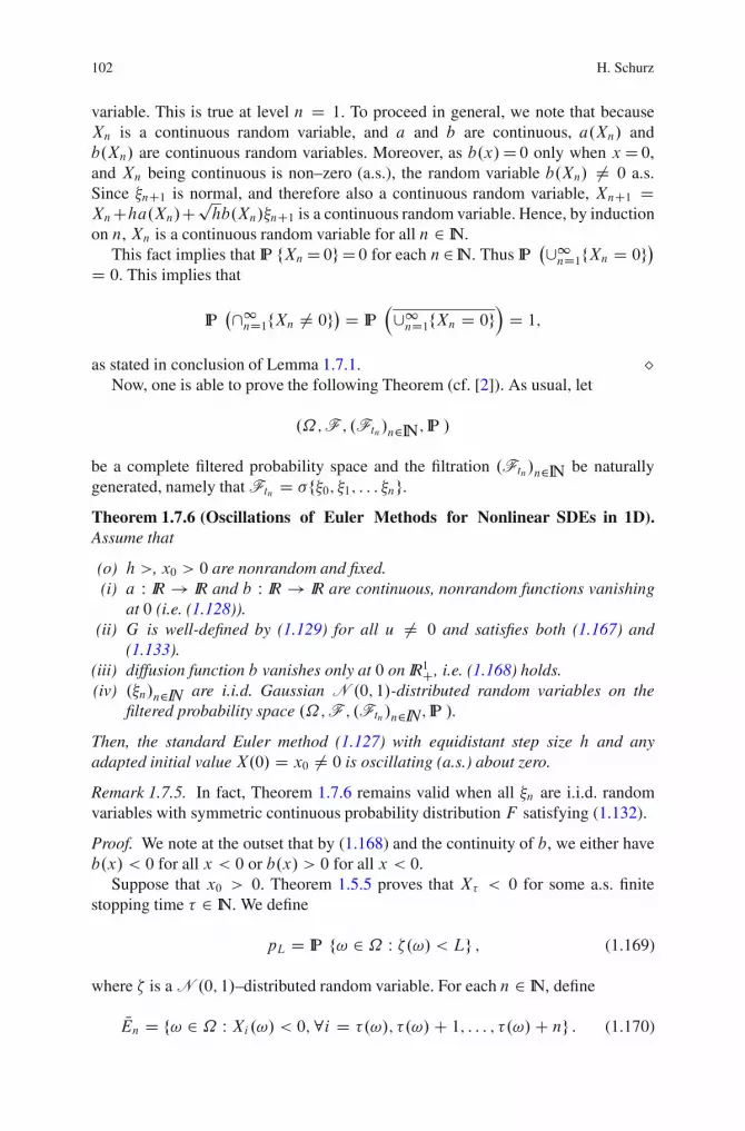
102 H. Schurz
variable. This is true at level n D 1. To proceed in general, we note that becauseXn is a continuous random variable, and a and b are continuous, a.Xn/ andb.Xn/ are continuous random variables. Moreover, as b.x/D 0 only when xD 0,and Xn being continuous is non–zero (a.s.), the random variable b.Xn/ ¤ 0 a.s.Since nC1 is normal, and therefore also a continuous random variable, XnC1 DXnCha.Xn/C
phb.Xn/ nC1 is a continuous random variable. Hence, by induction
on n, Xn is a continuous random variable for all n 2 IN.This fact implies that IP fXn D 0g D 0 for each n2 IN. Thus IP
�[1nD1fXn D 0g�D 0. This implies that
IP�\1nD1fXn ¤ 0g� D IP
�[1nD1fXn D 0g
�D 1;
as stated in conclusion of Lemma 1.7.1. ˘Now, one is able to prove the following Theorem (cf. [2]). As usual, let
.˝;F ; .Ftn /n2IN; IP /
be a complete filtered probability space and the filtration .Ftn/n2IN be naturallygenerated, namely that Ftn D f 0; 1; : : : ng.
Theorem 1.7.6 (Oscillations of Euler Methods for Nonlinear SDEs in 1D).Assume that
(o) h >, x0 > 0 are nonrandom and fixed.(i) a W IR ! IR and b W IR ! IR are continuous, nonrandom functions vanishing
at 0 (i.e. (1.128)).(ii) G is well-defined by (1.129) for all u ¤ 0 and satisfies both (1.167) and
(1.133).(iii) diffusion function b vanishes only at 0 on IR1C, i.e. (1.168) holds.(iv) . n/n2IN are i.i.d. Gaussian N .0; 1/-distributed random variables on the
filtered probability space .˝;F ; .Ftn /n2IN; IP /.
Then, the standard Euler method (1.127) with equidistant step size h and anyadapted initial value X.0/ D x0 ¤ 0 is oscillating (a.s.) about zero.
Remark 1.7.5. In fact, Theorem 1.7.6 remains valid when all n are i.i.d. randomvariables with symmetric continuous probability distribution F satisfying (1.132).
Proof. We note at the outset that by (1.168) and the continuity of b, we either haveb.x/ < 0 for all x < 0 or b.x/ > 0 for all x < 0.
Suppose that x0 > 0. Theorem 1.5.5 proves that X� < 0 for some a.s. finitestopping time � 2 IN. We define
pL D IP f! 2 ˝ W �.!/ < Lg ; (1.169)
where � is a N .0; 1/–distributed random variable. For each n 2 IN, define
NEn D f! 2 ˝ W Xi.!/ < 0;8i D �.!/; �.!/C 1; : : : ; �.!/C ng : (1.170)
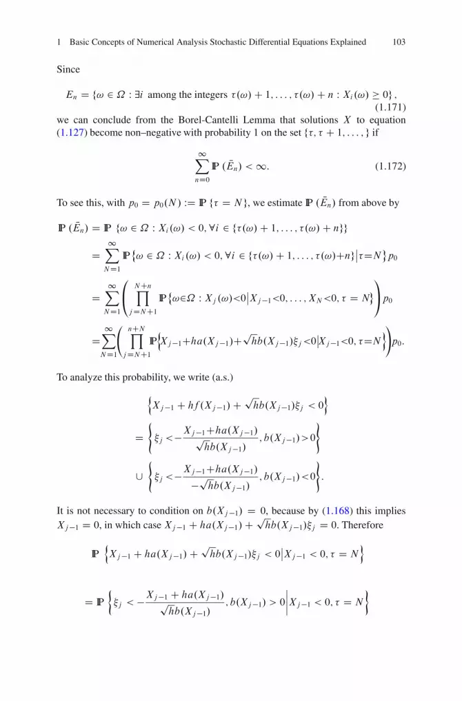
1 Basic Concepts of Numerical Analysis Stochastic Differential Equations Explained 103
Since
En D f! 2 ˝ W 9i among the integers �.!/C 1; : : : ; �.!/C n W Xi.!/ � 0g ;(1.171)
we can conclude from the Borel-Cantelli Lemma that solutions X to equation(1.127) become non–negative with probability 1 on the set f�; � C 1; : : : ; g if
1X
nD0IP . NEn/ < 1: (1.172)
To see this, with p0 D p0.N / WD IP f� D N g, we estimate IP . NEn/ from above by
IP . NEn/ D IP f! 2 ˝ W Xi.!/ < 0;8i 2 f�.!/C 1; : : : ; �.!/C ngg
D1X
ND1IP˚! 2 ˝ W Xi.!/ < 0;8i 2 f�.!/C 1; : : : ; �.!/Cngˇˇ�DN �p0
D1X
ND1
0
@NCnY
jDNC1IP˚!2˝ W Xj .!/<0
ˇˇXj�1<0; : : : ; XN<0; � D N
�
1
Ap0
D1X
ND1
nCNY
jDNC1IPnXj�1Cha.Xj�1/C
phb.Xj�1/ j<0
ˇXj�1<0; �DN
o!
p0:
To analyze this probability, we write (a.s.)
nXj�1 C hf .Xj�1/C
phb.Xj�1/ j < 0
o
D(
j <�Xj�1Cha.Xj�1/phb.Xj�1/
; b.Xj�1/>0)
[(
j <�Xj�1Cha.Xj�1/�phb.Xj�1/
; b.Xj�1/<0)
:
It is not necessary to condition on b.Xj�1/ D 0, because by (1.168) this impliesXj�1 D 0, in which case Xj�1 C ha.Xj�1/C p
hb.Xj�1/ j D 0. Therefore
IPnXj�1 C ha.Xj�1/C
phb.Xj�1/ j < 0
ˇˇXj�1 < 0; � D N
o
D IP
�
j < �Xj�1 C ha.Xj�1/phb.Xj�1/
; b.Xj�1/ > 0ˇˇˇˇXj�1 < 0; � D N
�
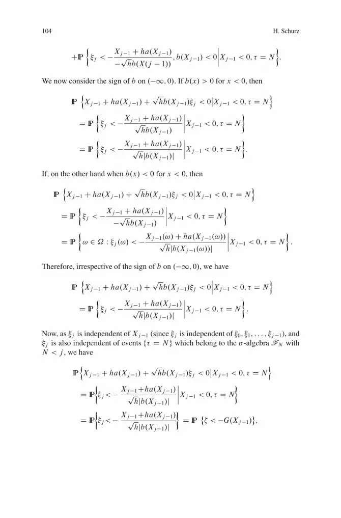
104 H. Schurz
CIP
�
j < �Xj�1 C ha.Xj�1/�p
hb.X.j � 1// ; b.Xj�1/ < 0ˇˇˇˇXj�1 < 0; � D N
�
:
We now consider the sign of b on .�1; 0/. If b.x/ > 0 for x < 0, then
IPnXj�1 C ha.Xj�1/C
phb.Xj�1/ j < 0
ˇˇXj�1 < 0; � D N
o
D IP
�
j < �Xj�1 C ha.Xj�1/phb.Xj�1/
ˇˇˇˇXj�1 < 0; � D N
�
D IP
�
j < �Xj�1 C ha.Xj�1/phjb.Xj�1/j
ˇˇˇˇXj�1 < 0; � D N
�
:
If, on the other hand when b.x/ < 0 for x < 0, then
IPnXj�1 C ha.Xj�1/C
phb.Xj�1/ j < 0
ˇˇXj�1 < 0; � D N
o
D IP
�
j < �Xj�1 C ha.Xj�1/�p
hb.Xj�1/
ˇˇˇˇXj�1 < 0; � D N
�
D IP
�
! 2 ˝ W j .!/ < �Xj�1.!/C ha.Xj�1.!//phjb.Xj�1.!//j
ˇˇˇˇXj�1 < 0; � D N
�
:
Therefore, irrespective of the sign of b on .�1; 0/, we have
IPnXj�1 C ha.Xj�1/C
phb.Xj�1/ j < 0
ˇˇˇXj�1 < 0; � D N
o
D IP
�
j < �Xj�1 C ha.Xj�1/phjb.Xj�1/j
ˇˇˇˇXj�1 < 0; � D N
�
:
Now, as j is independent of Xj�1 (since j is independent of 0; 1; : : : ; j�1), and j is also independent of events f� D N g which belong to the -algebra FN withN < j , we have
IPnXj�1 C ha.Xj�1/C
phb.Xj�1/ j < 0
ˇˇXj�1 < 0; � D N
o
D IP
�
j< � Xj�1Cha.Xj�1/phjb.Xj�1/j
ˇˇˇˇXj�1 < 0; � D N
�
D IP
�
j< � Xj�1Cha.Xj�1/phjb.Xj�1/j
�
D IP˚� < �G.Xj�1/
�;

1 Basic Concepts of Numerical Analysis Stochastic Differential Equations Explained 105
where � is a standard normal random variable. Hence
IPnXj�1 C ha.Xj�1/C
phb.Xj�1/ j < 0
ˇˇXj�1 < 0; � D N
o� IP f�<Lg DpL:
Thus
nCNY
jDNC1IPnXj�1 C ha.Xj�1/C
phb.Xj�1/ j < 0
ˇˇXj�1 < 0; � D N
o� pnL:
Therefore, we have
IP . NEn/ �1X
ND1
0
@nCNY
jDNC1IP f� < Lg
1
A IP f� D N g � pnL
1X
ND1IP f� D N g D pnL:
Thus, 1X
nD0IP . NEn/ � 1
1 � pL < 1;
and we conclude that there exists an a.s. finite stopping time �1 > �0 WD � suchthat X�1 � 0 a.s. But by Lemma 1.7.1, it follows that we must have X�1 > 0
(a.s.). By repeating the same approach while requiring (1.133) and (1.167), andusing mathematical induction, we obtain that Xn changes its sign infinitely oftenand with probability 1. Similarly, we verify the assertion for the case X.0/ < 0 (juststart with the event f�0 D 0g of negative initial values and proceed as above). Thus,the proof of Theorem 1.7.6 is complete. ˘Example 8.1. Consider Ito SDE
dX.t/ D �ŒX.t/�3dt CX.t/dW.t/
with initial value X.0/ D x0 > 0 and its Euler discretization
Y EnC1 D Y En .1 � hŒY En �2 C�Wn/
started at the same value Y E0 D X.0/ D x0 > 0, where �Wn are independent andidentically distributed increments. It can be shown that the exact solution X is a.s.positive for all times t � 0 and never oscillates. However, an application of Theorem1.7.6 gives that the related standard Euler method is quasi-oscillatory (a.s.), henceit shows spurious oscillations. However, an application of balanced methods withc0.x/ D x2 and c1.x/ D 1 governed by
Y BnC1 D Y Bn .1 � hŒY Bn �2 C�Wn/C .ŒY Bn �
2hC j�Wnj/.Y Bn � Y BnC1/
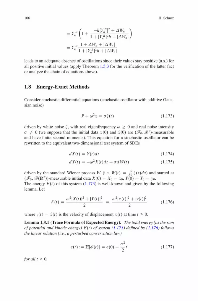
106 H. Schurz
D Y Bn
�
1C �hŒY Bn �2 C�Wn
1C ŒY Bn �2hC j�Wnj
�
D Y Bn1C�Wn C j�Wnj1C ŒY Bn �
2hC j�Wnjleads to an adequate absence of oscillations since their values stay positive (a.s.) forall positive initial values (apply Theorem 1.5.3 for the verification of the latter factor analyze the chain of equations above).
1.8 Energy-Exact Methods
Consider stochastic differential equations (stochastic oscillator with additive Gaus-sian noise)
Rx C !2x D .t/ (1.173)
driven by white noise , with real eigenfrequency ! � 0 and real noise intensity ¤ 0 (we suppose that the initial data x.0/ and Px.0/ are .F0;B1/-measurableand have finite second moments). This equation for a stochastic oscillator can berewritten to the equivalent two-dimensional test system of SDEs
dX.t/ D Y.t/dt (1.174)
dY.t/ D �!2X.t/dt C dW.t/ (1.175)
driven by the standard Wiener process W (i.e. W.t/ D R t0 .s/ds) and started at
.F0;B.IR2//-measurable initial data X.0/ D X0 D x0, Y.0/ D Y0 D y0.The energy E.t/ of this system (1.173) is well-known and given by the followinglemma. Let
E .t/ D !2ŒX.t/�2 C ŒY.t/�2
2D !2Œx.t/�2 C Œv.t/�2
2(1.176)
where v.t/ D Px.t/ is the velocity of displacement x.t/ at time t � 0.
Lemma 1.8.1 (Trace Formula of Expected Energy). The total energy (as the sumof potential and kinetic energy) E.t/ of system (1.173) defined by (1.176) followsthe linear relation (i.e., a perturbed conservation law)
e.t/ WD IEŒE .t/� D e.0/C 2
2t (1.177)
for all t � 0.

1 Basic Concepts of Numerical Analysis Stochastic Differential Equations Explained 107
Let us test numerical methods whether they can follow this perturbed conserva-tion law for its discretized energy functional. In particular, for the sake of simplicity,consider the drift-implicit �-methods applied to the system (1.174)–(1.175) andgoverned by the scheme
XnC1 D Xn C .�nYnC1 C .1 � �n/Yn/hn
YnC1 D Yn � !2.�nXnC1 C .1 � �n/Xn/hn C �Wn (1.178)
with nonrandom parameter-sequence .�n/n2IN, where
�n 2 IR1; hn D tnC1 � tn; �Wn D W.tnC1/�W.tn/ 2 N .0; hn/
along nonrandom partitions (or adapted partitions) of Œ0; T � of the form
0 D t0 � t1 � : : : � tn � : : : � tnT D T:
Definition 1.8.1. A numerical method Z based on instants .Zn/n2IN is calledenergy-exact for the SDE (1.173) iff its expected energy e D e.t/ satisfies theperturbed conservation law (1.177) at all instants .tn/n2IN along any nonrandompartition of non-random time-intervals Œ0; T �. Otherwise, Z is said to be non-energy-exact.
1.8.1 Non-energy-Exact Methods
The following theorem shows that the simplest choice of stochastic Runge-Kuttamethods such as forward and backward Euler methods as well as trapezoidalmethods fail to preserve simple energy laws (despite of their asymptoticallyconsistent behaviour).
Theorem 1.8.1. Assume that initial data X.0/ D x0, Y.0/ D Px0 areL2.˝;F0; IP /-integrable. Then the drift-implicit �-methods (1.178) appliedto (1.173) are not energy-exact for any sequence of nonrandom implicitnessparameters .�n/n2IN and any nonrandom step-sizes .hn/n2IN. More precisely,their expected energy e.t/ D IEŒE .tn/� is finite for all n 2 IN, e can beuniformly estimated by linear functions in t from below and above, and it satisfies8!; 2 IR1 8X0; Y0 2 L2.˝;F0; IP /
0 � IEŒE .0/�C 2
2tn minkD0;1;:::;n�1
1
1C!2h2k=4
� IEŒE .tn/�C!2
2
n�1X
kD0.1�2�k/IEŒYkXkC1 � YkC1Xk�hk

108 H. Schurz
D IEŒE .0/�C2
2
n�1X
kD0
hk
1C!2h2k=4
� IEŒE .0/�C 2
2tn maxkD0;1;:::;n�1
1
1C !2h2k=4� IEŒE .0/�C 2
2tn < C1
which renders to be a chain of equations for equidistant partitions (i.e. we mayreplace � by D signs above).
Proof. Define the statistical average values
NXn D XnC1 CXn
2; NYn D YnC1 C Yn
2: (1.179)
First, rewrite the system (1.178) of equations for .X; Y / to as
XnC1 D Xn C .2�n NYn C .1 � 2�n/Yn/hn
YnC1 D Yn � !2.2�n NXn C .1 � 2�n/Xn/hn C �Wn:
Second, multiply the components of these equations by !2 NXn and NYn (resp.) toarrive at
!2
2.X2
nC1 � X2n/ D .2�n!
2 NYn NXn C .1 � 2�n/!2Yn NXn/hn1
2
�Y 2nC1�Y 2n
� D �!2 �2�n NYn NXn C .1�2�n/ NYnXn�hnC NYn�Wn:
Third, adding both equations leads to
EnC1 D En � !2.1 � 2�n/ŒYn NXn � NYnXn�hn C NYn�Wn: (1.180)
Fourth, note that
ŒYn NXn � NYnXn� D 1
2ŒYnXnC1 � YnC1Xn�;
NYn D 2Yn � !2.Xn C �n.1 � 2�n/Ynhn/hn C �Wn
2.1C !2�2nh2n/
;
IEŒ NYn�Wn� D 2
2.1C !2�2nh2n/hn:
Fifth, pulling over expectations and summing over n in equation (1.180) for thepathwise evolution of related energy yield that
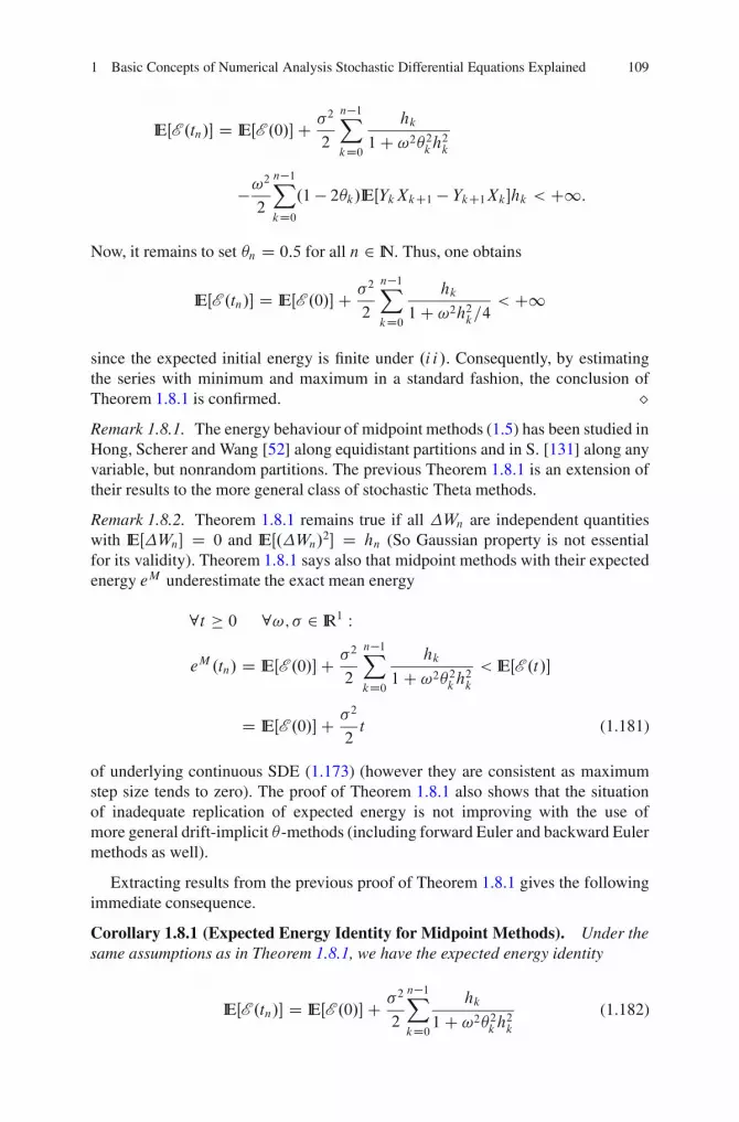
1 Basic Concepts of Numerical Analysis Stochastic Differential Equations Explained 109
IEŒE .tn/� D IEŒE .0/�C 2
2
n�1X
kD0
hk
1C !2�2kh2k
�!2
2
n�1X
kD0.1 � 2�k/IEŒYkXkC1 � YkC1Xk�hk < C1:
Now, it remains to set �n D 0:5 for all n 2 IN. Thus, one obtains
IEŒE .tn/� D IEŒE .0/�C 2
2
n�1X
kD0
hk
1C !2h2k=4< C1
since the expected initial energy is finite under .i i/. Consequently, by estimatingthe series with minimum and maximum in a standard fashion, the conclusion ofTheorem 1.8.1 is confirmed. ˘Remark 1.8.1. The energy behaviour of midpoint methods (1.5) has been studied inHong, Scherer and Wang [52] along equidistant partitions and in S. [131] along anyvariable, but nonrandom partitions. The previous Theorem 1.8.1 is an extension oftheir results to the more general class of stochastic Theta methods.
Remark 1.8.2. Theorem 1.8.1 remains true if all �Wn are independent quantitieswith IEŒ�Wn� D 0 and IEŒ.�Wn/
2� D hn (So Gaussian property is not essentialfor its validity). Theorem 1.8.1 says also that midpoint methods with their expectedenergy eM underestimate the exact mean energy
8t � 0 8!; 2 IR1 W
eM .tn/ D IEŒE .0/�C 2
2
n�1X
kD0
hk
1C !2�2kh2k
< IEŒE .t/�
D IEŒE .0/�C 2
2t (1.181)
of underlying continuous SDE (1.173) (however they are consistent as maximumstep size tends to zero). The proof of Theorem 1.8.1 also shows that the situationof inadequate replication of expected energy is not improving with the use ofmore general drift-implicit �-methods (including forward Euler and backward Eulermethods as well).
Extracting results from the previous proof of Theorem 1.8.1 gives the followingimmediate consequence.
Corollary 1.8.1 (Expected Energy Identity for Midpoint Methods). Under thesame assumptions as in Theorem 1.8.1, we have the expected energy identity
IEŒE .tn/� D IEŒE .0/�C 2
2
n�1X
kD0
hk
1C !2�2kh2k
(1.182)

110 H. Schurz
along any nonrandom partition .tn/n2IN for the drift-implicit �-methods (1.178)with all implicitness parameters �k D 0:5, any nonrandom constants !; 2 IR1
and any random initial data X0; Y0 2 L2.˝;F0; IP /.
Remark 1.8.3. It is obvious that the standard midpoint methods (1.178) with�n D 0:5 do not possess an exact evolution of the energy. In fact, they underestimatethe exact mean energy functional for any choice of parameters and any adaptedinitial conditions. This is in strong contrast to the deterministic situation with D 0
where midpoint methods are known to be exact-energy integrators (see simplecticmethods) obeying the law of conservation of energy.
1.8.2 Existence of Energy-Exact Methods
Indeed, there exist numerical methods which can exactly preserve energy andconservation laws. These are nonstandard numerical methods. In stochastics, thiswas firstly noted and proved by S. [131]. The observed bias in the energy-evolutionunder discretization can be even removed by the energy-exact improved midpointmethods
XnC1 D Xn C NYnhn; YnC1 D Yn � !2 NXnhn C
q
1C !2h2n=4�Wn (1.183)
where the involved quantities are defined as in (1.179). In passing, we note thatthis numerical method is fairly new to the best of our knowledge. Moreover, it is aconsistent one with an exact replication of the temporal evolution of underlyingcontinuous time energy and represents a stochastic correction of widely knownstandard midpoint methods.
Theorem 1.8.2 (Exact Energy Identity for Improved Midpoint Methods).Under the same assumptions as in Theorem 1.8.1, we have the exact energy identity(also called trace formula in a more general context, see S. [132])
IEŒE .tn/� D IEŒE .0/�C 1
22tn (1.184)
along any nonrandom partition .tn/n2IN for the methods (1.183) with any nonran-dom constants !; 2 IR1 and any random initial data X0; Y0 2 L2.˝;F0; IP/.
Proof. More general, consider the improved implicit �-methods
XnC1 D Xn C .�nYnC1 C .1 � �n/Yn/hnYnC1 D Yn � !2.�nXnC1 C .1 � �n/Xn/hn C n�Wn (1.185)
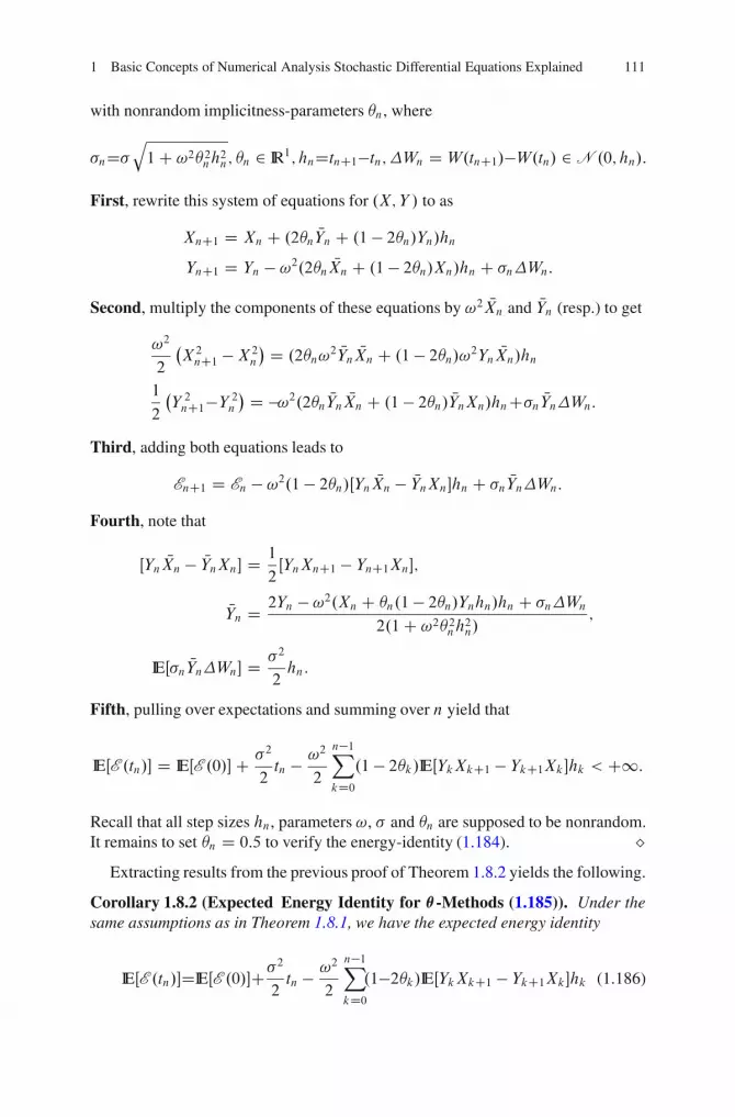
1 Basic Concepts of Numerical Analysis Stochastic Differential Equations Explained 111
with nonrandom implicitness-parameters �n, where
nDq
1C !2�2nh2n; �n 2 IR1; hnDtnC1�tn; �Wn D W.tnC1/�W.tn/ 2 N .0; hn/:
First, rewrite this system of equations for .X; Y / to as
XnC1 D Xn C .2�n NYn C .1 � 2�n/Yn/hnYnC1 D Yn � !2.2�n NXn C .1 � 2�n/Xn/hn C n�Wn:
Second, multiply the components of these equations by !2 NXn and NYn (resp.) to get
!2
2
�X2nC1 �X2
n
� D .2�n!2 NYn NXn C .1 � 2�n/!2Yn NXn/hn
1
2
�Y 2nC1�Y 2n
� D �!2.2�n NYn NXn C .1 � 2�n/ NYnXn/hnCn NYn�Wn:
Third, adding both equations leads to
EnC1 D En � !2.1 � 2�n/ŒYn NXn � NYnXn�hn C n NYn�Wn:
Fourth, note that
ŒYn NXn � NYnXn� D 1
2ŒYnXnC1 � YnC1Xn�;
NYn D 2Yn � !2.Xn C �n.1 � 2�n/Ynhn/hn C n�Wn
2.1C !2�2nh2n/
;
IEŒn NYn�Wn� D 2
2hn:
Fifth, pulling over expectations and summing over n yield that
IEŒE .tn/� D IEŒE .0/�C 2
2tn � !2
2
n�1X
kD0.1 � 2�k/IEŒYkXkC1 � YkC1Xk�hk < C1:
Recall that all step sizes hn, parameters !, and �n are supposed to be nonrandom.It remains to set �n D 0:5 to verify the energy-identity (1.184). ˘
Extracting results from the previous proof of Theorem 1.8.2 yields the following.
Corollary 1.8.2 (Expected Energy Identity for �-Methods (1.185)). Under thesame assumptions as in Theorem 1.8.1, we have the expected energy identity
IEŒE .tn/�DIEŒE .0/�C2
2tn � !2
2
n�1X
kD0.1�2�k/IEŒYkXkC1 � YkC1Xk�hk (1.186)

112 H. Schurz
along any nonrandom partition .tn/n2IN for the improved implicit �-methods(1.185) with any nonrandom parameters �k 2 IR1, any nonrandom constants!; 2 IR1 and any random initial data X0; Y02L2.˝;F0; IP/.
Remark. Notice that relations (1.181) for continuous energy of SDE (1.173) and(1.184) for discrete energy of numerical methods (1.183) are indeed identicalat the partition-instants tn for all parameters !, and initial values X0; Y0 2L2.˝;F0; IP /! Thus we answer the question that such numerical methods indeedexist (which are consistent too). The conclusions of Theorems 1.8.1, 1.8.2 andCorollaries 1.8.1, 1.8.2 are still valid if all �Wn are independent random variableswith IEŒ�Wn� D 0 and IEŒ.�Wn/
2� D hn.
1.8.3 General Energy Identity of Numerical Methodsand Monotonicity
One is able to establish a general energy balance identity for numerical methods.This will show that midpoint-type methods are designed to adequately replicate theincreasing or decreasing evolution of energy balance for random initial data. Recallthat any difference method for the approximation of any differential equation isconstructed from general scheme-structure
XnC1 D Xn C ˚n.X/ (1.187)
where ˚n.X/ represents the increment functional of related numerical method.Recall NXn D .XnC1 CXn/=2 and let jj:jj be the Euclidean norm in IRd , < : ; : > theEuclidean scalar product.
Theorem 1.8.3 (General Energy Identity). For all numerical methods in IRd
satisfying (1.187) with increment functional ˚n, we have
jjXnC1jj2 D jjXnjj2 C 2 < NXn;˚n.X/ > (1.188)
where jj:jj is the Euclidean norm in IRd and < :; : > the Euclidean scalar product.
Proof. First, for the Euclidean norm jj:jj and scalar product < : ; : >, recall theidentity
jju C vjj2 D jjujj2 C 2 < u; v > Cjjvjj2
for all vectors u; v 2 IRd . Now, set
u WD NXn; v WD ˚n.X/:
Note that, for numerical methods (1.187) with increment functional ˚n, we have
v D XnC1 � Xn:

1 Basic Concepts of Numerical Analysis Stochastic Differential Equations Explained 113
Second, after returning to the norm-identity (1.189), we get to
2 < NXn;˚n.X/ > D jj NXn C ˚n.X/jj2 � jj NXnjj2 � jj˚n.X/jj2D jj NXn CXnC1 �Xnjj2 � jj NXnjj2 � jjXnC1 � Xnjj2D jj NXnjj2 C 2 < NXn;XnC1 � Xn > CjjXnC1 � Xnjj2 � jj NXnjj2
�jjXnC1 � Xnjj2D < XnC1 CXn;XnC1 � Xn > D jjXnC1jj2 � jjXnjj2:
This is equivalent to the energy identity (1.188). ˘Remark 1.8.4. For stochastic numerical methods, the energy identity (1.188) holdsalmost surely too since their increment functional ˚n is random. This identity(1.188) also explains why midpoint-type numerical integrators with ˚n D ˚n. NXn/form a preferable base for adequate construction of numerical methods from adynamical point of view. They may preserve the monotone character of norms alongscalar products.
Definition 1.8.2. A numerical method Z is called exact norm-monotone iffthe following implications while discretizing ODEs dx=dt D f .t; x/ withCaratheodory functions f can be established
8x 2 IRd ; t 2 IR1 W< f .t; x/; x >� 0
H) 8n 2 IN W jjX0jj � jjX1jj � : : : � jjXnjj � jjXnC1jj � : : :
and8x 2 IRd ; t 2 IR1 W< f .t; x/; x >� 0
H) 8n 2 IN W jjX0jj � jjX1jj � : : : � jjXnjj � jjXnC1jj � : : :
for all adapted random initial values X0 2 IRd .
Theorem 1.8.4 (Exact Monotonicity of Midpoint Methods). All midpoint-typemethods X with increments ˚. NXn/ D f .t�n ; NXn/hn and any sample time-pointst�n 2 IR1 are exact norm-monotone for all ODEs with adapted random initial valuesX0 and any choice of step sizes hn.
Proof. Apply the energy identity (1.188) to midpoint methods with increments˚. NXn/ D f .t�n ; NXn/hn and any sample time-points t�n 2 IR1. For them, this identityreads as
jjXnC1jj2 D jjXnjj2 C 2 < NXn; f .t�n ; NXn/ > hn:
Obviously, by taking the square root, this relation is equivalent to
jjXnC1jj Dq
jjXnjj2 C 2 < NXn; f .t�n ; NXn/ > hn:

114 H. Schurz
Now, the uniform monotonicity of Euclidean scalar product < x; f .t; x/ > withrespect to x and positivity of hn imply the exact norm-monotonicity of relatedmidpoint methods X . For example, if < x; f .t; x/ >� 0 then we have
jjXnC1jj � jjXnjj
for all n 2 IN. Complete induction on n 2 IN yields the non-increasing evolutionof Euclidean norms jjXnjj in n. Similarly, we can verify the monotonicity for <x; f .t; x/ >� 0. Thus, the proof of Theorem 1.8.4 is completed. ˘Remark 1.8.5. The situation with fully random increment functionals˚n (e.g. with˚n.X/ D a.tn; Xn/hn C b.tn; Xn/�Wn for Euler methods) is somewhat morecomplicated (due to the non-monotone character of Wiener processes W ) andrequires further research.
1.8.4 Asymptotically Exact Methods
To relax the requirement of being exact at finite times, we may only require thatnumerical methods provide exact values as the integration time tn tends to infinity orstep sizes hn tend to 0. In view of S. [118,120–122], midpoint and trapezoidal meth-ods are good candidates. Consider (for brevity, autonomous) linear system of SDEs
dX.t/ D AX.t/dt CmX
jD1bjdWj .t/ (1.189)
with additive noise and constant drift matrix A 2 IRd�d Assume that there is astationary solution X1 of (1.189). Then, for stationarity of autonomous systems(1.189) with additive white noise, it is a necessary and sufficient requirement thatall eigenvalues Re.�i .A// < 0. Under this condition, we also find the almost surelimit limt!C1X.t/ D X1.
Definition 1.8.3. The random sequence .Yn/n2IN is said to be asymptotically p-thmean preserving iff
limn!C1 IEkYnkp D IEkX1kp;
(asymptotically) mean preserving iff
limn!C1 IEYn D IEX1;
(asymptotically) in-law preserving iff
L aw.Y1/ D L aw.X1/;
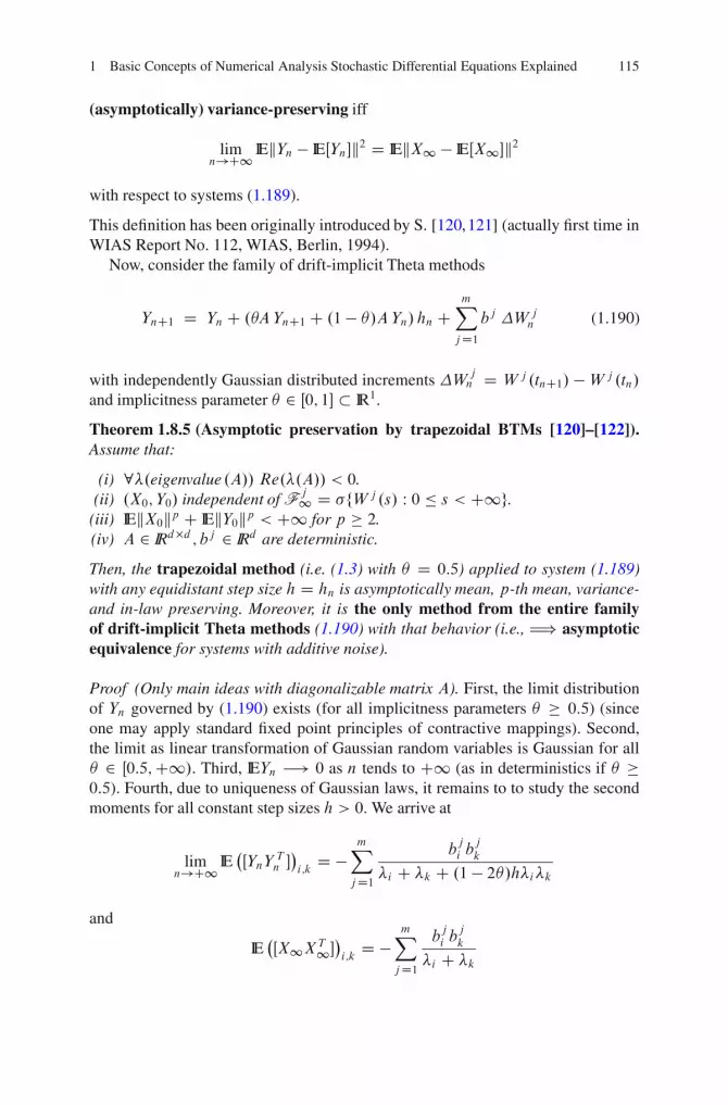
1 Basic Concepts of Numerical Analysis Stochastic Differential Equations Explained 115
(asymptotically) variance-preserving iff
limn!C1 IEkYn � IEŒYn�k2 D IEkX1 � IEŒX1�k2
with respect to systems (1.189).
This definition has been originally introduced by S. [120,121] (actually first time inWIAS Report No. 112, WIAS, Berlin, 1994).
Now, consider the family of drift-implicit Theta methods
YnC1 D Yn C .�AYnC1 C .1 � �/AYn/ hn CmX
jD1bj �W j
n (1.190)
with independently Gaussian distributed increments �W jn D W j .tnC1/ � W j .tn/
and implicitness parameter � 2 Œ0; 1� � IR1.
Theorem 1.8.5 (Asymptotic preservation by trapezoidal BTMs [120]–[122]).Assume that:
(i) 8�.eigenvalue .A// Re.�.A// < 0.(ii) .X0; Y0/ independent of F
j1 D fW j .s/ W 0 � s < C1g.(iii) IEkX0kp C IEkY0kp < C1 for p � 2.(iv) A 2 IRd�d ; bj 2 IRd are deterministic.
Then, the trapezoidal method (i.e. (1.3) with � D 0:5) applied to system (1.189)with any equidistant step size h D hn is asymptotically mean, p-th mean, variance-and in-law preserving. Moreover, it is the only method from the entire familyof drift-implicit Theta methods (1.190) with that behavior (i.e., H) asymptoticequivalence for systems with additive noise).
Proof (Only main ideas with diagonalizable matrix A). First, the limit distributionof Yn governed by (1.190) exists (for all implicitness parameters � � 0:5) (sinceone may apply standard fixed point principles of contractive mappings). Second,the limit as linear transformation of Gaussian random variables is Gaussian for all� 2 Œ0:5;C1/. Third, IEYn �! 0 as n tends to C1 (as in deterministics if � �0:5). Fourth, due to uniqueness of Gaussian laws, it remains to to study the secondmoments for all constant step sizes h > 0. We arrive at
limn!C1 IE
�ŒYnY
Tn ��
i;kD �
mX
jD1
bji b
j
k
�i C �k C .1 � 2�/h�i�k
and
IE�ŒX1XT1�
�
i;kD �
mX
jD1
bji b
j
k
�i C �k

116 H. Schurz
Thenlim
n!C1 IE�ŒYnY
Tn ��
i;kD IE
�ŒX1XT1�
�
i;k” � D 0:5:
Thus, the stationarity with exact stationary Gaussian probability law including thepreservation of all moments and variance under discretization is obvious. ˘Remark 1.8.6. For the proof with non-diagonalizable matrices A, one may applyfixed point principles to verify the same conclusion of Theorem 1.8.5. Note that,for linear autonomous systems of SDEs (1.189), the schemes of trapezoidal andmidpoint methods coincide. Thus, midpoint methods possess the same preservingcharacter of asymptotic exactness under discretization.
1.9 Order Bounds: Why Not Higher Order Methods?
As commonly known from deterministic numerical analysis, there are order boundsfor convergence of numerical methods. Sometimes they are also called Dahlquistbarriers.
1.9.1 Order Bounds of Clark-Cameron
Clark and Cameron [22] could prove the following very remarkable result onmaximum order bounds of partition FN
T -measurable approximations.
Definition 1.9.1. The stochastic process Y D .Y.t//0�t�T is called partition FNT -
measurable iff all values Y.tn/ (tn 2 Œ0; T �; 0 � n � N ) are FNtn
-measurable with
FNtn
D nW j .tk/ W k D 0; 1; : : : ; nI j D 1; 2; : : : ; m
o
for all n D 0; 1; : : : ; N , along a given FNtn
-measurable discretization 0 D t0 � t1 �: : : � tN D T for the fixed deterministic time-interval Œ0; T �.
Remark 1.9.1. The conditional expectations IEŒX.tnC1/jFNtn� provide the partition
FNT -measurable stochastic approximations with the minimal mean square error due
to their inherent projection property in Hilbert spaces L2.˝;F ; IP /. Thus it isnatural to study their error and practical implementation at first.
Theorem 1.9.1 (Clark-Cameron Order-Bound Theorem). Assume that XD.X.t//0 � t � T satisfies the one-dimensional autonomous SDE
dX.t/ D a.X.t//dt C dW.t/ (1.191)
where a 2 C3.IR/ and all derivatives of a are uniformly bounded. Then

1 Basic Concepts of Numerical Analysis Stochastic Differential Equations Explained 117
IEŒ.X.T / � IEŒX.T /jFNT �/
2� D cT
N 2C o
�1
N 2
�
where
c D T 3
12
Z T
0
IE
exp
�
2
Z T
s
a0.X.u//du
�
Œa0.X.s//�2
ds:
Thus, for systems with additive noise, we obtain the general mean square orderbound 1:0 for numerical approximations using only the increments of underlyingWiener process. A similar result holds also for diffusions with variable diffusioncoefficients b.x/ when
c.x/ WD a.x/ � 1
2b.x/b0.x/ 6� Kb.x/
for any real constant K , see Clark and Cameron [22]. They also provide aconstructive example with multiplicative noise. Consider the two-dimensional SDE
dX.1/.t/ D dW 1.t/
dX.2/.t/ D X.1/.t/ dW 2.t/
driven by two independent scalar Wiener processesW 1;W 2. This system obviouslyhas the solutions X.1/.t/ D W 1.t/ and
X.2/.t/ DZ t
0
W 1.s/dW 2.s/ DZ t
0
Z s
0
dW 1.u/ dW 2.s/
(in fact it is an one-dimensional example with multi-dimensional “Wiener processdifferentials” (i.e. m D 2)). Then they compute the best convergence rate �2 D 0:5
(in mean square sense) for partition FNT -measurable approximations using any set
of N equidistant, FNtn
-measurable time-instants tn D n TN
, and the mean squareminimally attainable approximation error
�
IE
ˇˇˇX.2/.T / � IEŒX.2/.T /jFN
T �ˇˇˇ2� 1
2
D T
2
h 1
N
i 12:
It is worth noting that X.2/ represents the simplest nontrivial multiple integral withlength l.˛/ > 1. Liske [89] has studied its joint distribution with .W 1.t/;W 2.t//. Inthis case the error order bound for FN
T -measurable approximations ofX2T is already
attained with 0:5, since X2 cannot be expanded in a linear combination ofW 1;W 2.This system also exhibits an interesting test equation for the qualitative behavior ofnumerical methods (e.g. compare the numerically estimated distribution with that ofthe exact solution derived by Liske [89]). Since in the L2 sense one cannot providebetter partition FN
T -measurable approximations than that of the projection doneby conditional expectations, there are natural (convergence) order restrictions for
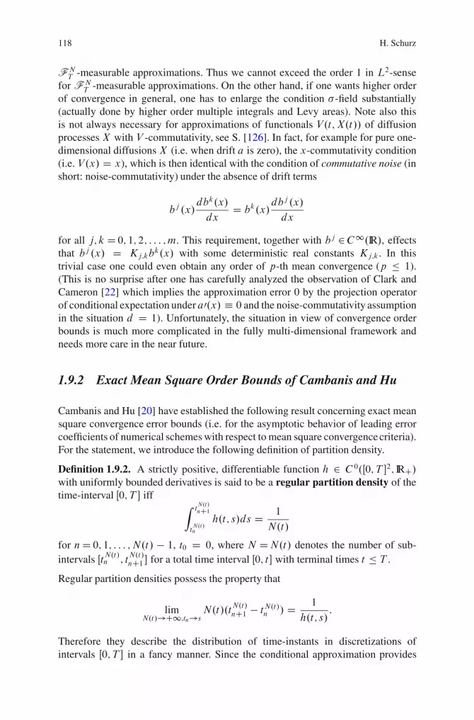
118 H. Schurz
FNT -measurable approximations. Thus we cannot exceed the order 1 in L2-sense
for FNT -measurable approximations. On the other hand, if one wants higher order
of convergence in general, one has to enlarge the condition -field substantially(actually done by higher order multiple integrals and Levy areas). Note also thisis not always necessary for approximations of functionals V.t; X.t// of diffusionprocesses X with V -commutativity, see S. [126]. In fact, for example for pure one-dimensional diffusions X (i.e. when drift a is zero), the x-commutativity condition(i.e. V.x/ D x), which is then identical with the condition of commutative noise (inshort: noise-commutativity) under the absence of drift terms
bj .x/dbk.x/
dxD bk.x/
dbj .x/
dx
for all j; kD 0; 1; 2; : : : ; m. This requirement, together with bj 2C1.IR/, effectsthat bj .x/ D Kj;kb
k.x/ with some deterministic real constants Kj;k . In thistrivial case one could even obtain any order of p-th mean convergence (p � 1).(This is no surprise after one has carefully analyzed the observation of Clark andCameron [22] which implies the approximation error 0 by the projection operatorof conditional expectation under a0.x/ � 0 and the noise-commutativity assumptionin the situation d D 1). Unfortunately, the situation in view of convergence orderbounds is much more complicated in the fully multi-dimensional framework andneeds more care in the near future.
1.9.2 Exact Mean Square Order Bounds of Cambanis and Hu
Cambanis and Hu [20] have established the following result concerning exact meansquare convergence error bounds (i.e. for the asymptotic behavior of leading errorcoefficients of numerical schemes with respect to mean square convergence criteria).For the statement, we introduce the following definition of partition density.
Definition 1.9.2. A strictly positive, differentiable function h 2 C 0.Œ0; T �2; IRC/with uniformly bounded derivatives is said to be a regular partition density of thetime-interval Œ0; T � iff
Z tN.t/
nC1
tN.t/n
h.t; s/ds D 1
N.t/
for nD 0; 1; : : : ; N.t/ � 1, t0 D 0, where N DN.t/ denotes the number of sub-intervals ŒtN.t/n ; t
N.t/nC1 � for a total time interval Œ0; t � with terminal times t � T .
Regular partition densities possess the property that
limN.t/!C1;tn!s
N.t/.tN.t/nC1 � tN.t/n / D 1
h.t; s/:
Therefore they describe the distribution of time-instants in discretizations ofintervals Œ0; T � in a fancy manner. Since the conditional approximation provides
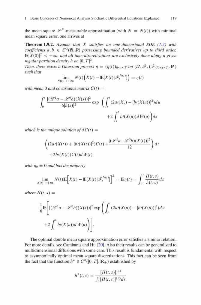
1 Basic Concepts of Numerical Analysis Stochastic Differential Equations Explained 119
the mean square FN -measurable approximation (with N D N.t/) with minimalmean square error, one arrives at
Theorem 1.9.2. Assume that X satisfies an one-dimensional SDE (1.2) withcoefficients a; b 2 C3.IR; IR/ possessing bounded derivatives up to third order,IEjX.0/j2 < C1, and all time-discretizations are exclusively done along a givenregular partition density h on Œ0; T �2.Then, there exists a Gaussian process � D .�.t//0�t�T on .˝;F ; .Ft /0�t�T ; IP /such that
limN.t/!C1N.t/
�X.t/ � IEŒX.t/jFN.t/
t ��
D �.t/
with mean 0 and covariance matrix C.t/ DZ t
0
Œ.L 1a � L 0b/.X.s//�2
6Œh.s/�2exp
�Z t
s
.2a0.Xu/� Œb0.X.u//�2/du
C2Z t
s
b0.X.u//dW.u/�
ds
which is the unique solution of dC.t/ D�
.2a0.X.t//C Œb0.X.t//�2/C.t/C Œ.L 1a�L 0b/.X.t//�2
12
�
dt
C2b0.X.t//C.t/dW.t/
with �0 D 0 and has the property
limN.t/!C1N.t/IE
hX.t/ � IEŒX.t/jFN.t/
t �i2 D IE�.t/ D
Z t
0
H.t; s/
h.t; s/ds
where H.t; s/ D
1
6IE
"
Œ.L 1a � L 0b/.X.s//�2 exp
Z t
s
.2a0.X.u//� Œb0.X.u//�2/du
C2Z t
s
b0.X.u//dW.u/!#
:
The optimal double mean square approximation error satisfies a similar relation.For more details, see Cambanis and Hu [20]. Also their results can be generalized tomultidimensional diffusions with some care. This result is fundamental with respectto asymptotically optimal mean square discretizations. This fact can be seen fromthe fact that the function h� 2 C0.Œ0; T �; IRC/ established by
h�.t; s/ D ŒH.t; s/�1=3R t0ŒH.t; s/�1=3ds

120 H. Schurz
minimizes the functionalR ts
H.t;s/
Œh.t;s/�2ds whereH.t; s/ � 0 among all regular partition
densities h with h.t; s/ > 0 andR t0h.t; s/ds D 1. Therefore, any asymptotically
mean square optimal approximation has to use a discretization following thatoptimal partition law. However, the practical value is still in doubt, since it willbe hard to evaluate those expressions in the fully multidimensional framework orhas any reader another suggestion in the case m; d > 1?
1.9.3 Lower Order Bounds of Hofmann-Gronbach-Ritter
Hofmann, Muller-Gronbach and Ritter [50] have noticed in one dimension (i.e.d DmD 1) that, for continuously differentiable b and fixed terminal time T D 1,there are efficient estimates for the lower bounds of order of strong (mean square)convergence for all FN
tn-measurable approximations Y � for SDEs in IR1 with
additive noise. More precisely, for the error e2 of mean square convergence andpartitions with maximum step size � and N C 1 time-instants, we have
lim�!0
pN inf
Y �e2.Y
�; a; b;X0; T / D K2jjbjjL1
with constants K2 D 1p6
and T D 1. Therefore, the standard forward Euler methodwith an adaptive strategy of step size selection already produces asymptoticallymean square optimal FN
tn-measurable numerical approximations. Note that the
number N of observations of the underlying driving noise W may be determinedby any measurable termination criterion. Moreover, one can carry the qualitativeassertion on lower order bounds over to d -dimensional SDEs with additive noiseandLp-integrable b as well (i.e.p� 1). It is worth noting that that step size selectionsuggested originally by Hofmann, Muller-Gronbach and Ritter [50] is only designedto control large diffusion fluctuations, and it does not seem to be very appropriate asone takes the limit as b goes to zero (i.e. incomplete adaptability is obtained in thepresence of significant drift parts - an approach which leads to inconsistent resultsin view of deterministic limit equations, however a procedure which indeed mightbe appropriate for pure diffusion processes with very large diffusion coefficientsb.t/ >> 1). Furthermore, they did not study the dependence of the order and errorbounds on variable terminal times T or as T tends to C1. Such as study would beimportant for adequate asymptotic analysis through numerical dynamical systemsas discretizations.
In the paper [51], the authors Hofmann, Muller-Gronbach and Ritter analyzethe double L2.Œ0; 1�/-error associated to the approximation of a scalar stochasticdifferential equation by numerical methods based on multiple Ito integrals assuggested in Kloeden and Platen [72]. Namely, for a scalar diffusion process XX,they consider approximations of the type X D f .I˛1;s1;t1 ; : : : ; I˛k;sk ;tk / wheref W IRk ! L2.Œ0; 1�/ is assumed to be measurable and I˛;s;t denotes the multiple
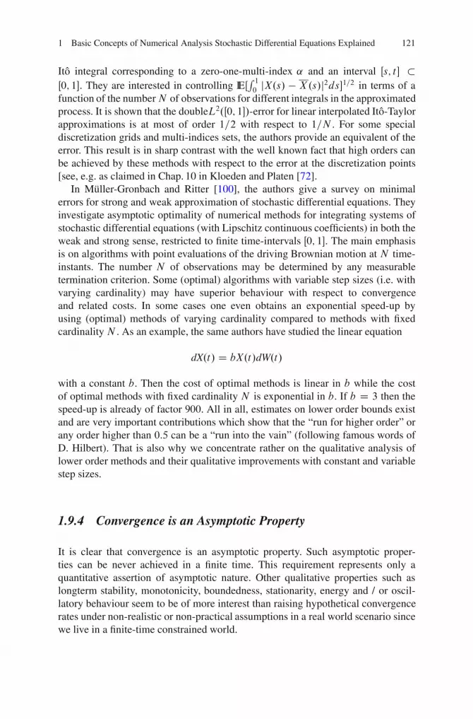
1 Basic Concepts of Numerical Analysis Stochastic Differential Equations Explained 121
Ito integral corresponding to a zero-one-multi-index ˛ and an interval Œs; t � �Œ0; 1�. They are interested in controlling IEŒ
R 10
jX.s/ � X.s/j2ds�1=2 in terms of afunction of the numberN of observations for different integrals in the approximatedprocess. It is shown that the doubleL2.Œ0; 1�/-error for linear interpolated Ito-Taylorapproximations is at most of order 1=2 with respect to 1=N . For some specialdiscretization grids and multi-indices sets, the authors provide an equivalent of theerror. This result is in sharp contrast with the well known fact that high orders canbe achieved by these methods with respect to the error at the discretization points[see, e.g. as claimed in Chap. 10 in Kloeden and Platen [72].
In Muller-Gronbach and Ritter [100], the authors give a survey on minimalerrors for strong and weak approximation of stochastic differential equations. Theyinvestigate asymptotic optimality of numerical methods for integrating systems ofstochastic differential equations (with Lipschitz continuous coefficients) in both theweak and strong sense, restricted to finite time-intervals Œ0; 1�. The main emphasisis on algorithms with point evaluations of the driving Brownian motion at N time-instants. The number N of observations may be determined by any measurabletermination criterion. Some (optimal) algorithms with variable step sizes (i.e. withvarying cardinality) may have superior behaviour with respect to convergenceand related costs. In some cases one even obtains an exponential speed-up byusing (optimal) methods of varying cardinality compared to methods with fixedcardinality N . As an example, the same authors have studied the linear equation
dX.t/ D bX.t/dW.t/
with a constant b. Then the cost of optimal methods is linear in b while the costof optimal methods with fixed cardinality N is exponential in b. If b D 3 then thespeed-up is already of factor 900. All in all, estimates on lower order bounds existand are very important contributions which show that the “run for higher order” orany order higher than 0:5 can be a “run into the vain” (following famous words ofD. Hilbert). That is also why we concentrate rather on the qualitative analysis oflower order methods and their qualitative improvements with constant and variablestep sizes.
1.9.4 Convergence is an Asymptotic Property
It is clear that convergence is an asymptotic property. Such asymptotic proper-ties can be never achieved in a finite time. This requirement represents only aquantitative assertion of asymptotic nature. Other qualitative properties such aslongterm stability, monotonicity, boundedness, stationarity, energy and / or oscil-latory behaviour seem to be of more interest than raising hypothetical convergencerates under non-realistic or non-practical assumptions in a real world scenario sincewe live in a finite-time constrained world.

122 H. Schurz
1.10 Contractivity and Two-Point Behaviour
For simplicity, we shall exclusively illustrate the concepts of contractivity and non-expansivity by the drift-implicit Theta methods (1.1) without balancing terms cj ,i.e. all weight matrices cj � 0.
1.10.1 Two-Point Motion Process and GeneralContraction-Identity
One is able to establish a general contraction identity for numerical methods. Thiswill show that midpoint-type methods are designed to adequately replicate theincreasing or decreasing evolution of perturbations for random initial data. Recallthat any difference method for the approximation of any differential equation isconstructed from general scheme-structure (1.187) (i.e. XnC1 D Xn C˚n.X/) with˚n.X/ representing the increment functional of related numerical method. RecallNXn D .XnC1CXn/=2. LetX and Y denote the stochastic processes belonging to the
same numerical scheme (1.187) and started at X0 2 IRd and Y0 2 IRd , respectively.We shall study the dynamic behaviour of the two-point motion process .X; Y /along the same numerical method governed by the schemes
XnC1 D Xn C ˚n.X/
YnC1 D Yn C ˚n.Y /
with one and the same increment functional ˚n along one and the same partition.tn/n2IN. Recall that jj:jj denotes the Euclidean vector norm in IRd and < : ; : > theEuclidean scalar product.
Theorem 1.10.1 (General Contraction Identity). For all numerical methods inIRd satisfying (1.187) with increment functional ˚n, we have
jjXnC1 � YnC1jj2 D jjXn � Ynjj2 C 2 < NXn � NYn;˚n.X/ �˚n.Y / > (1.192)
where jj:jj is the Euclidean norm in IRd and < : ; : > the Euclidean scalar product.
Proof. First, for the Euclidean norm jj:jj and scalar product < : ; : >, recall theidentity jju C vjj2 D jjujj2 C 2 < u; v > Cjjvjj2 for all vectors u; v 2 IRd . Note that,for numerical methods (1.187) with increment functional ˚n, we have
˚n.X/ D XnC1 �Xn:
Second, analyzing the Euclidean norm of the two-point motion process gives theidentities
1 Basic Concepts of Numerical Analysis Stochastic Differential Equations Explained 123
jjXnC1 � YnC1jj2 D jjXn � Yn C˚n.X/ � ˚n.Y /jj2D jjXn � Ynjj2 C 2 < Xn � Yn;˚n.X/ � ˚n.Y / >
Cjj˚n.X/ �˚n.Y /jj2D jjXn � Ynjj2C < Xn � Yn;˚n.X/ �˚n.Y / >
C < XnC1�˚n.X/ � YnC1C˚n.Y /; ˚n.X/�˚n.Y / >Cjj˚n.X/ �˚n.Y /jj2
D jjXn � Ynjj2C < XnC1CXn � YnC1�Yn;˚n.X/�˚n.Y / >� < ˚n.X/�˚n.Y /; ˚n.X/ �˚n.Y />Cjj˚n.X/�˚n.Y /jj2
D jjXn � Ynjj2 C 2 < NXn � NYn;˚n.X/ � ˚n.Y / >
which confirm the validity of contraction identity (1.192). ˘Remark 1.10.1. For stochastic numerical methods, the contraction identity (1.192)holds almost surely too (with their increment functional ˚n which is random).This identity (1.192) also explains why midpoint-type numerical integrators with˚n D ˚n. NXn/ form a preferable base for adequate construction of numericalmethods from a dynamical point of view. They may preserve the monotone characterof contractions (perturbations) of two-point motion process along scalar products.
Definition 1.10.1. A numerical method Z is called exact contraction-monotoneiff the following implications while discretizing ODEs dx=dt D f .t; x/ with Cara-theodory functions f can be established
8x; y 2 IRd ; t 2 IR1 W< f .t; x/ � f .t; y/; x � y >� 0
H)8n 2 INWjjX0�Y0jj�jjX1�Y1jj� : : :�jjXn�Ynjj � jjXnC1 � YnC1jj � : : :
and
8x; y 2 IRd ; t 2 IR1 W< f .t; x/ � f .t; y/; x � y > � 0
H) 8n 2 IN W jjX0�Y0jj�jjX1�Y1jj� : : :�jjXn � Ynjj � jjXnC1 � YnC1jj � : : :
for all adapted random initial values X0; Y0 2 IRd .
Theorem 1.10.2 (Exact Contraction-Property of Midpoint Methods). All mid-point-type methodsX with increments˚. NXn/ D f .t�n ; NXn/hn and any sample time-points t�n 2 IR1 are exact contraction-monotone for all ODEs with adapted randominitial values X0 and any choice of step sizes hn.
Proof. Apply the contraction identity (1.192) to midpoint methods with incrementfunctional ˚. NXn/ D f .t�n ; NXn/hn and any sample time-points t�n 2 IR1. For them,this identity reads as
jjXnC1 � YnC1jj2 D jjXn � Ynjj2 C 2 < NXn � NYn; f .t�n ; NXn/� f .t�n ; NYn > hn:

124 H. Schurz
Obviously, by taking the square root, this relation is equivalent to
jjXnC1 � Ynjj Dq
jjXn � Ynjj2 C 2 < NXn � NYn; f .t�n ; NXn/� f .t�n ; NYn/ > hn:
Now, the uniform monotonicity of Euclidean scalar product
< x � y; f .t; x/ � f .t; y/ >
with respect to x; y 2 IRd and positivity of hn imply the exact contraction-monotonicity of related midpoint methods X . For example, if < x � y; f .t; x/ �f .t; y/ >� 0 for all x; y 2 IRd then we have
jjXnC1 � YnC1jj � jjXn � Ynjj
for all n 2 IN. Complete induction on n 2 IN yields the non-increasing evolutionof Euclidean norms jjXn � Ynjj in n. Similarly, we can verify the monotonicity for< x � y; f .t; x/ � f .t; y/ >� 0 for all x; y 2 IRd . Thus, the proof of Theorem1.10.2 is completed. ˘Remark 1.10.2. The situation with fully random increment functionals ˚n (e.g.with ˚n.X/ D a.tn; Xn/hn C b.tn; Xn/�Wn for Euler methods) is somewhatmore complicated (due to the non-monotone character of Wiener processes W )and requires further research. However, an extension to p-th mean contractions(appropriate for the concept of B-stability) gives some more insight for stochasticTheta methods (see next subsections).
1.10.2 P-th Mean Contractivity and Non-expansivityof Backward Euler Methods
Let Xs;x.t/ denote the value of the stochastic processX at time t � s, provided thatit has started at the value Xs;x.s/ D x at prior time s. x and y are supposed to beadapted initial values. Let ˘ denote an ordered time-scale (discrete (˘ D IN) orcontinuous (˘ D Œ0;C1/)) and p ¤ 0 be a nonrandom constant.
Definition 1.10.2. A stochastic processX D .X.t//t2˘ with basis .˝;F ; .Ft /t2˘;IP / is said to be uniformly p-th mean (forward) contractive on IRd iff9KX
C 2 IR 8t � s 2 ˘ 8x; y 2 IRd
IEhjjXs;x.t/ � Xs;y.t/jjp
ˇˇˇFs
i� exp
�pKX
C .t � s/�jjx � yjjp (1.193)
with p-th mean contractivity constant KXC . In the case KX
C < 0, we speak ofstrict p-th mean contractivity. Moreover, X is said to be a process with p-th
1 Basic Concepts of Numerical Analysis Stochastic Differential Equations Explained 125
mean non-expansive perturbations iff 8t � s 2 ˘ 8x; y 2 IRd
IEhjjXs;x.t/ � Xs;y.t/jjp
ˇˇˇFs
i� jjx � yjjp: (1.194)
If p D 2 then we speak of mean square contractivity and mean square non-expansivity.
For strictly contractive processes, adapted perturbations in the initial data haveno significant impact on its longterm dynamic behaviour. Adapted perturbations ofnon-expansive processes are under control along the entire time-scale ˘ . Theseconcepts are important for the control of error propagation through numericalmethods. They are meaningful to test numerical methods while applying to SDEswith monotone coefficient systems.
Let p > 0 be a nonrandom constant.
Definition 1.10.3. A coefficient system .a; bj / of SDEs (1.2) and its SDEare said to be strictly uniformly p-th mean monotone on IRd iff 9KUC 2IR 8t2 IR8x; y2 IRd
< a.t; x/ � a.t; y/; x � y >d C1
2
mX
jD1jjbj .t; x/ � bj .t; y/jj2
C p � 2
2
mX
jD1
< bj .t; x/ � bj .t; y/; x � y >2djjx � yjj2 � KUC jjx � yjj2: (1.195)
If p D 2 then we speak of mean square monotonicity.
Lemma 1.10.1. Assume that X satisfies SDE (1.2) with p-th mean monotonecoefficient system .a; bj /.Then X is p-th mean contractive for all p � 2 and its p-th mean contractivityconstantKX
C can be estimated by
KXC � KUC :
This lemma can be proved by Dynkin’s formula (averaged Ito formula). Let usdiscuss the possible “worst case effects” on perturbations of numerical methodsunder condition (1.195) with p D 2. It turns out that the drift-implicit backwardEuler methods are mean square contractive.
Theorem 1.10.3. Assume that
(i) �n D 1.(ii) 0 < infn2IN hn � supn2IN hn < C1, all hn nonrandom (i.e. only admissible
step sizes).(iii) 9Ka � 08x; y 2 Rd 8t � 0 W < a.t; x/ � a.t; y/; x � y >� Kajjx � yjj2.(iv) 9Kb8x; y 2 Rd 8t � 0 W Pm
jD1 jjbj .t; x/ � bj .t; y/jj2 � Kbjjx � yjj2.
126 H. Schurz
Then, the drift-implicit Euler methods (1.1) with scalar implicitness �n D 1 andvanishing cj D 0 have mean square contractive perturbations when applied to SDEs(1.2) with mean square monotone coefficients .a; bj / with contractivity constant
KXC D sup
n2IN
2Ka CKb
1 � 2hnKa
: (1.196)
If additionally 2Ka CKb � 0 then they are mean square non-expansive and
KXC D 2Ka CKb
1 � 2Ka supn2IN
hn: (1.197)
Proof. Rearrange the scheme (1.1) for the drift-implicit Theta methods withnonrandom scalar implicitness .�n/ D �nI to separate implicit from explicit partsuch that
XnC1 � �nhna.tnC1; XnC1/ D Xn C .1 � �n/hna.tn; Xn/
CmX
jD1bj .tn; Xn/�W
jn : (1.198)
Recall that X and Y denote the values of the same scheme (1.1) started at valuesX0 and Y0, respectively. Now, take the square of Euclidean norms on both sides. Bytaking the expectation on both sides we arrive at
IEjjXnC1 � YnC1jj2 � 2�nhnIE < XnC1 � YnC1; a.tnC1; XnC1/ � a.tnC1; YnC1/ >C�2nh2nIEjja.tnC1; XnC1/ � a.tnC1; YnC1/jj2
D IEjjXn � Ynjj2 C 2.1� �n/hnIE < Xn � Yn; a.tn; Xn/� a.tn; Yn/ >
C.1��n/2h2nIEjja.tn; Xn/�a.tn; Yn/jj2ChnmX
jD1IEjjbj .tn; Xn/� bj .tn; Yn/jj2:
Under the assumption .i i i/ we have
�2�nhn < a.t; x/ � a.t; y/; x � y > � �2�nhnKajjx � yjj2 � 0
for all x; y 2 IRd and t � 0. Consequently, under .i i i/ and .iv/, we may estimate
.1 � 2�nhnKa/IEjjXnC1 � YnC1jj2� Œ1C.2.1��n/KaCKb/hn�CIEjjXn�Ynjj2
C.1��n/2h2nIEjja.tn; Xn/�a.tn; Yn/jj2:

1 Basic Concepts of Numerical Analysis Stochastic Differential Equations Explained 127
for all n 2 IN. This leads to the estimate
IEjjXnC1 � YnC1jj2
� Œ1C .2.1 � �n/Ka CKb/hn�C1 � 2�nhnKa
IEjjXn � Ynjj2
D�
1C .2KaCKb/hn
1 � 2�nhnKa
�
IEjjXn�Ynjj2C .1��n/2h2n1�2�nhnKa
IEjja.tn; Xn/� a.tn; Yn/jj2
� exp
�.2KaCKb/hn
1 � 2�nhnKa
�
IEjjXn�Ynjj2C .1��n/2h2n1�2�nhnKa
IEjja.tn; Xn/�a.tn; Yn/jj2
since 1 C z � exp.z/ for z � �1. Now, set all parameters �n D 1 in the aboveinequality. In this case one encounters
IEjjXnC1 � YnC1jj2 � exp
�2Ka CKb
1� 2hnKa
hn
�
IEjjXn � Ynjj2:
Therefore, the drift-implicit backward Euler methods have mean square contractiveperturbations with contractivity constant
KXC D sup
n2IN
2Ka CKb
1 � 2hnKa
D 2Ka CKb
1 � 2 supn2IN
hnKa
if 2Ka CKb � 0:
If additionally 2Ka CKb � 0, then the perturbations are mean square non-expansive. ˘
1.10.3 P-th Mean Non-contractivity and Expansivityof Euler Methods
Let Xs;x.t/ denote the value of the stochastic processX at time t � s, provided thatit has started at the value Xs;x.s/ D x at prior time s. x and y are supposed to beadapted initial values. Let ˘ denote an ordered time-scale (discrete (˘ D IN) orcontinuous (˘ D Œ0;C1/)) and p > 0 be a nonrandom constant.
Definition 1.10.4. A stochastic processXD.X.t//t2˘ with basis .˝;F ; .Ft /t2˘;IP / is said to be p-th mean (forward) non-contractive (in the strict sense) on IRd
iff 8t � s 2 ˘ 8x; y 2 IRd (adapted)
IE jjXs;x.t/ �Xs;y.t/jjp
ˇˇFs
� � jjx � yjjp: (1.199)
128 H. Schurz
X is said to be a process with p-th mean expansive perturbations iff 8t > s 2˘ 8x; y 2 IRd .x ¤ y/ (adapted)
IEhjjXs;x.t/ � Xs;y.t/jjp
ˇˇˇFs
i> jjx � yjjp: (1.200)
If p D 2 then we speak of mean square non-contractivity and mean squareexpansivity, respectively.
For non-contractive processes, perturbations in the initial data may have signifi-cant impact on its longterm dynamic behaviour. Adapted perturbations of expansiveprocesses lead to chaotic, sensitive dynamic behaviour along the entire time-scale ˘ . These concepts are important for the control of error propagation throughnumerical methods. They are meaningful to test numerical methods while applyingto SDEs with non-contractive coefficient systems.
Let p > 0 be a nonrandom constant.
Definition 1.10.5. A coefficient system .a; bj / of SDEs (1.2) and its SDE are saidto be strictly uniformly p-th mean non-decreasing on IRd iff 9KUC � 0 2IR 8t 2 IR 8x; y 2 IRd
< a.t; x/ � a.t; y/; x � y >d C1
2
mX
jD1jjbj .t; x/ � bj .t; y/jj2
Cp � 2
2
mX
jD1
< bj .t; x/ � bj .t; y/; x � y >2djjx � yjj2
� KUC jjx � yjj2: (1.201)
If KUC > 0 in (1.201) then the coefficient system .a; bj / is said to be p-th meanexpansive and its SDE has p-th mean expansive perturbations. Moreover, if p D2 then we speak of mean square non-decreasing and mean square expansiveperturbations and systems, respectively.
Lemma 1.10.2. Assume that X satisfies SDE (1.2) with p-th mean non-decreasingcoefficient system .a; bj /.Then X has p-th mean non-decreasing perturbations for all p � 2. If additionallyKUC > 0 in (1.201) then X possesses p-th mean expansive perturbations.
This lemma can be proved by Dynkin’s formula (averaged Ito formula). Let usdiscuss the possible “worst case effects” on perturbations of numerical methodsunder condition (1.201) with p D 2. It turns out that the drift-implicit forwardEuler methods are mean square non-contractive under this condition and may haveeven mean square expansive perturbations.
1 Basic Concepts of Numerical Analysis Stochastic Differential Equations Explained 129
Theorem 1.10.4. Assume that:
(i) �n D 0.(ii) 0 < infn2IN hn � supn2IN hn < C1, all hn nonrandom (i.e. only admissible
step sizes).(iii) 9Ka8x; y 2 Rd8t � 0 W< a.t; x/ � a.t; y/; x � y >� Kajjx � yjj2.(iv) 9Kb 8x; y 2 Rd 8t � 0 W Pm
jD1 jjbj .t; x/ � bj .t; y/jj2 � Kbjjx � yjj2.Then, the drift-implicit (forward) Euler methods (1.1) with scalar implicitness�n D 0 and vanishing cj D 0 have mean square non-contractive perturbationswhen applied to SDEs (1.2) with coefficients .a; bj / satisfying 2Ka C Kb � 0. Ifadditionally 2Ka CKb > 0 then they are mean square expansive.
Proof. Consider the scheme (1.1) for the drift-implicit Theta methods with nonran-dom scalar implicitness .�n/ D �nI and separate implicit from explicit part suchthat
XnC1 � �nhna.tnC1; XnC1/ D Xn C .1 � �n/hna.tn; Xn/
CmX
jD1bj .tn; Xn/�W
jn : (1.202)
Recall that X and Y denote the values of the same scheme (1.1) started at valuesX0 and Y0, respectively. Now, take the square of Euclidean norms on both sides. Bytaking the expectation on both sides we arrive at
IEjjXnC1 � YnC1jj2 � 2�nhnIE < XnC1 � YnC1; a.tnC1; XnC1/ � a.tnC1; YnC1/ >C �2nh
2nIEjja.tnC1; XnC1/ � a.tnC1; YnC1/jj2
D IEjjXn � Ynjj2 C 2.1� �n/hnIE < Xn � Yn; a.tn; Xn/ � a.tn; Yn/ >
C .1��n/2h2nIEjja.tn; Xn/�a.tn; Yn/jj2ChnmX
jD1IEjjbj .tn; Xn/�bj .tn; Yn/jj2:
Under the assumption .i i i/ and �n � 1 we have
2.1� �n/hn < a.t; x/ � a.t; y/; x � y > Chn
mX
jD1jjbj .t; x/ � bj .t; y/jj2
� Œ2.1 � �n/Ka CKb�hnjjx � yjj2
for all x; y 2 IRd and t � 0. Consequently, under .i i/–.iv/, �n � 1 and 2KaCKb �0, we may estimate
130 H. Schurz
.1 � 2�nhnKa/IEjjXnC1 � YnC1jj2 C �2nh2nIEjja.tnC1; XnC1/� a.tnC1; YnC1/jj2
� Œ1C.2.1��n/KaCKb/hn�IEjjXn�Ynjj2C.1��n/2h2nIEjja.tn; Xn/� a.tn; Yn/jj2:
for all n 2 IN. Now, set �n D 0. This leads to the estimate
IEjjXnC1 � YnC1jj2 � Œ1C .2Ka CKb/hn�IEjjXn � Ynjj2 � IEjjXn � Ynjj2:
Therefore, the forward Euler methods have mean square non-contractive perturba-tions under the condition 2Ka C Kb � 0. After returning to the latter inequalityabove, one clearly recognizes that, if additionally 2Ka C Kb > 0, then theperturbations are mean square expansive. ˘
1.10.4 Mean Square BN- and B-stability of BackwardEuler Methods
It is natural to ask for transferring the deterministic concept of B-stability to thestochastic case. This can be done in the p-th mean moment sense fairly straight–forward, and it has been studied by S. [120] at first.
Definition 1.10.6. A numerical sequence Z D .Zn/n2IN (method, scheme,approximation, etc.) is called p-th mean B-stable iff it is p-th mean contractive forall autonomous SDEs (1.2) with p-th mean monotone coefficient systems .a; bj /and for all admissible step sizes. It is said to be p-th mean BN-stable iff it is p-thmean contractive for all non-autonomous SDEs (1.2) with p-th mean monotonecoefficient systems .a; bj / for all admissible step sizes. If p D 2 then we also speakof mean square B- and BN-stability.
Indeed, the drift-implicit backward Euler methods are appropriate to controlthe growth of its perturbations as long as the underlying SDE does. This factis documented by the mean square B-stability of these methods in the followingTheorem.
Theorem 1.10.5 (Mean Square BN-, B-Stability of Backward Euler Methods).Assume that
8n 2 IN W �n D �nI; 8j D 1; 2; : : : ; m W cj � 0:
Then, the drift-implicit backward Euler method (1.1) applied to Ito SDEs (1.2) withscalar implicitness parameters �n D 1 and nonrandom step sizes hn is mean squareBN-stable and B-stable.
Proof. Combine the main assertions of Lemma 1.10.1 and Theorem 1.10.3 ˘

1 Basic Concepts of Numerical Analysis Stochastic Differential Equations Explained 131
1.11 On a First Definition of Dynamic Consistencyin Stochastics
The previous course of sections presenting several concepts is unified in thefollowing concept of dynamic consistency.
1.11.1 The Definition of Dynamic Consistency
Definition 1.11.1. A class of numerical methods Y discretizing SDEs (1.2) issaid to be dynamically consistent iff the following properties hold for theirrepresentatives:
(1) Y is p-th mean consistent.(2) Y is p-th mean stable for all nonrandom step sizes hn whenever the underlying
SDE has a p-th mean stable fixed point.(3) Y is p-th mean contractive for all nonrandom step sizes hn whenever the
underlying SDE is p-th mean contractive.(4) The limit limn!C1 Yn D limt!C1X.t/ whenever the latter limit exist (in
the sense of moments or in the sense of probability law).(5) Y has positive outcomes for all nonrandom step sizes hn whenever the
underlying SDE has positive solutions (a.s.).(6) Y is p-th mean convergent to the unique solution of underlying SDE with
Lipschitz-continuous coefficients.(7) Y is an energy-exact numerical method for all nonrandom step sizes hn and
all adapted initial data.(8) Y is exact norm-monotone for all nonrandom step sizes hn and all adapted
initial data.(9) Y is exact contraction-monotone for all nonrandom step sizes hn and all
adapted initial data.(10) Y does not admit spurious solutions of any kind.
Remark 1.11.1. This list of requirements for dynamic consistency can be easilyextended, hence it can be considered as incomplete at this stage. These requirementsact like those requirements in statistical hypothesis testing which leads to anacceptance or non-acceptance of test objects (here numerical methods). Theserequirements should be understood as a sort of minimum fair requirements for“qualitative goodness of numerical approximations”.
The concept of dynamic consistency leads to the problem of construction andverification of nonstandard numerical methods (as initiated in Mickens [92] indeterministic analysis).

132 H. Schurz
1.11.2 Class of Balanced Theta Methods is DynamicallyConsistent
As we could recognize from previous sections, the class of balanced (improved)Theta methods provides us dynamically consistent numerical approximations ofSDEs. In fact, it is rich enough to replicate qualitatively the dynamic behaviourof underlying SDEs. We gain control on stability (cf. Sect. 1.3), positivity (cf.Sect. 1.5), boundedness (cf. Sect. 1.6), oscillations (cf. Sect. 1.7), contractivity(cf. Sect. 1.10), consistency (cf. Sect. 1.2) and convergence (cf. Sect. 1.4) throughtheir representatives. The balanced terms cj with j � 1 are needed to controlthe pathwise behaviour of Theta methods (1.1) (e.g. for almost sure positivity,boundedness and absence of oscillations). The parameters � or balanced terms c0
in them are used to control the moment behaviour of Theta methods (1.1) (e.g. formoment contractivity, moment stability, moment boundedness, etc.). In the previoussections we have reported numerous facts supporting the preference of midpoint-type numerical methods (or trapezoidal methods) since they avoid spurioussolutions, are simplectic, exact norm-monotone, exact contraction-monotone anda stochastically improved version of them are energy- and asymptotically exact.They can practically be implemented by predictor-corrector procedures, linear-or partial-implicit versions to avoid the time-consuming resolution of implicitalgebraic equations at each integration step. Dynamically consistent methods ofhigher order of convergence than midpoint-type methods are not known so far. Thisis a challenging subject for further research.
1.11.3 Remarks and Practical Guideline on Optimal Choiceof �; cj
The optimal choice of implicitness parameters � and weights cj is a fairlycomplex problem. Its choice depends on the qualitative properties which oneis aiming at to be guaranteed by numerical approximations. Here a shortlist ofmain recommendations and conclusion on its choice is given, based on the priorobservations in previous sections:
1. � D 0:5 is optimal for linear systems (see S. [121, 122]) with respect to stability(cf. Sect. 1.3), contractivity (cf. Sect. 1.10), monotonicity, energy-exactness (cf.Sect. 1.8), etc.
2. Equivalent choices with appropriate c0 are possible (see S. [120]).3. Positive semi-definite matrices cj are preferrable since they imply no additional
step size restrictions (guaranteeing the inverses of “stabilizers” M (matrices) inlocal one step representation).
1 Basic Concepts of Numerical Analysis Stochastic Differential Equations Explained 133
4. � > 0 and positive negative-definite part c0 D 12Œ� @a.t;x/
@x�C of Jacobian matrix
@a.t;x/
@xare recommendable choices to achieve “optimal numerical stabilization”
based on standard linearization techniques.5. cj D 0.j D 1; 2; : : : ; m/ suffices to control p-th moments (stability, bounded-
ness of moments).6. cj ¤ 0.j D 1; 2; : : : ; m/ is needed to control pathwise behaviour such as a.s.
stability, a.s. boundedness or a.s. positivity (cf. Sect. 1.5).7. cj D bj .t; x/=x (componentwise) is recommended to be chosen for systems
with bj .t; x/ D Bj .t; x/x as commonly met in population models in ecology,biology, finance, marketing.
Of course, this represents an incomplete list of observations and further studies areneeded. As commonly known, optimal choices must depend on the specific structureof drift and diffusion coefficients, and, above all, on the goal one is aiming at by theapproximation. This clearly depends on the knowledge on qualitative behaviour ofunderlying class of SDEs.
Acknowledgements We sincerely thank the anonymous reviewers for their useful comments andMounir Zili for his continuous support.
References
1. Allen, E.: Modeling with Ito Stochastic Differential Equations. Springer, New York (2007)2. Appleby, J.A.D., Rodkina, A., Schurz, H.: Non-positivity and oscillations of solutions of
nonlinear stochastic difference equations. J. Difference Equ. Appl. 16(7), 807–830 (2010)3. Arnold, L.: Random Dynamical Systems. Springer, Berlin (1998)4. Arous, G.B.: Flots et series de taylor stochastiques. Probab. Theory Rel. 81(1), 29–77 (1989)5. Artemiev, S.S., Averina, T.A.: Numerical Analysis of Systems of Ordinary and Stochastic
Differential Equations. VSP, Utrecht (1997)6. Bally, V., Protter, P., Talay, D.: The law of the Euler scheme for stochastic differential
equations, Z. Angew. Math. Mech. 76(3), 207–210 (1996)7. Bally, V., Talay, D.: The Euler scheme for stochastic differential equations: Error analysis
with Malliavin calculus. Math. Comput. Simul. 38(1–3), 35–41 (1995)8. Bally, V., Talay, D.: The law of the Euler scheme for stochastic differential equations I.
Convergence rate of the distribution function. Probab. Theory Relat. Fields 104, 43–60 (1996)9. Bally, V., Talay, D.: The law of the Euler scheme for stochastic differential equations. II:
Convergence rate of the density. Monte Carlo Methods Appl. 2(2), 93–128 (1996)10. Bashkirtseva, I., Ryashko, L., Schurz, H.: Analysis of noise-induced transitions for Hopf
system with additive and multiplicative random disturbances. Chaos Solitons Fractals 39(1),72–82 (2009)
11. Bernard, P., Fleury, G.: Convergence of numerical schemes for stochastic differentialequations. Monte Carlo Methods Appl. 7(1–2), 35–44 (2001)
12. Bihari, T.: A generalization of a lemma of Bellman and its application to uniqueness problemsof differential equations. Acta Math. Acad. Sci. Hung. 7, 81–94 (1956)
13. Biscay, R., Jimenez, J.C., Riera, J.J., Valdes, P.A.: Local linearization method for thenumerical solution of stochastic differential equations. Ann. Inst. Statist. Math. 48(4), 631–644 (1996)
14. Bouleau, N., Lepingle, D.: Numerical Methods for Stochastic Processes. Wiley, New York(1993)
134 H. Schurz
15. Bryden, A., Higham, D.J.: On the boundedness of asymptotic stability regions for thestochastic theta method. BIT 43(1), 1–6 (2003)
16. Burrage, K., Platen, E.: Runge-Kutta methods for stochastic differential equations. Ann.Numer. Math. 1, 63–78 (1994)
17. Burrage, K., Burrage, P.M., Mitsui, T.: Numerical solutions of stochastic differentialequations – implementation and stability issues. J. Comput. Appl. Math. 125(1–2), 171–182(2000)
18. Burrage, K., Tian, T.: A note on the stability properties of the Euler methods for solvingstochastic differential equations. New Zealand J. Math. 29(2), 115–127 (2000)
19. Burrage, K., Tian, T.: The composite Euler method for stiff stochastic differential equations.J. Comput. Appl. Math. 131(1-2), 407–426 (2001)
20. Cambanis, S., Hu, Y.: Exact convergence rate of the Euler-Maruyama scheme with applicationto sampling design. Stochastics Stochastics Rep. 59, 211–240 (1996)
21. Chang, C.C.: Numerical solution of stochastic differential equations with constant diffusioncoefficients. Math. Comp. 49(180), 523–542 (1987)
22. Clark, J.M.C., Cameron, R.J.: The maximum rate of convergence of discrete approximationsfor stochastic differential equations. In: Stochastic Differential Systems (Proc. IFIP-WG 7/1Working Conf., Vilnius, 1978), pp. 162–171, Lecture Notes in Control and Information Sci.25, Springer, Berlin-New York (1980)
23. Dahlquist, G.: A special stability problem for linear multistep methods. BIT 3, 27–43 (1963)24. Deelstra, G., Delbaen, F.: Convergence of discretized stochastic (interest rate) processes with
stochastic drift term. Appl. Stochastic Models Data Anal. 14(1), 77–84 (1998)25. Del Moral, P.: A uniform convergence theorem for the numerical solving of the nonlinear
filtering problem. J. Appl. Probab. 35(4), 873–884 (1998)26. Ermakov, S.M., Mikhajlov, G.A.: Statistical Simulation (in Russian). Nauka, Moscow (1982)27. Faure, O.: Simulation de mouvement brownien et des diffusions. These ENPC, Paris (1992)28. Gaines, J.G.: The algebra of iterated stochastic integrals. Stochastics Stoch. Reports 49, 169–
179 (1994)29. Gaines, J.G.: A basis for iterated stochastic integrals. Math. Comput. Simulation 38(1–3),
7–11 (1995)30. Gaines, J.G., Lyons, T.J.: Random generation of stochastic area integrals. SIAM J. Appl.
Math. 54(4), 1132–1146 (1994)31. Gaines, J.G., Lyons, T.J.: Variable step size control in the numerical solution of stochastic
differential equations. SIAM J. Appl. Math. 57(5), 1455–1484 (1997)32. Gard, T.C.: Introduction to Stochastic Differential Equations. Marcel Dekker, Basel (1988)33. Gikhman, I.I., Skorochod, A.V.: Stochastische Differentialgleichungen. Akademie-Verlag,
Berlin (1971)34. Girsanov, I.V.: An example of non-uniqueness of the solution of the stochastic equation of K.
Ito. Theor. Probab. Appl. 7, 325–331 (1962)35. Golec, J.: Averaging Euler-type difference schemes. Stochastic Anal. Appl. 15(5), 751–758
(1997)36. Golec, J., Ladde, G.S.: Euler–type approximation for systems of stochastic differential
equations. J. Appl. Math. Simul. 28, 357–385 (1989)37. Golec, J., Sathananthan, S.: Sample path approximation for stochastic integro-differential
equations. Stoch. Anal. Appl. 17(4), 579–588 (1999)38. Golec, J., Sathananthan, S.: Strong approximations of stochastic integro-differential equa-
tions, Dyn. Contin. Discrete Impuls. Syst. Ser. B Appl. Algorithms 8(1), 139–151 (2001)39. Guo, S.J.: On the mollifier approximation for solutions of stochastic differential equations.
J. Math. Kyoto Univ. 22, 243–254 (1982)40. Guo, S.J.: Approximation theorems based on random partitions for stochastic differential
equations and applications. Chinese Ann. Math. 5, 169–183 (1984)41. Gyongy, I.: On approximation of Ito stochastic equations. Math. SSR Sbornik. 70, 165–173
(1991)42. Gyongy, I.: A note on Euler’s approximations. Potential Anal. 8(3), 205–216 (1998)
1 Basic Concepts of Numerical Analysis Stochastic Differential Equations Explained 135
43. Gyongy, I., Nualart, D.: Implicit scheme for quasi-linear parabolic partial differentialequations perturbed by space-time white noise. Stoch. Processes Appl. 58(1), 57–72 (1995)
44. Gyongy, I., Nualart, D.: Implicit scheme for stochastic partial differential equations driven byspace-time white noise. Potential Anal. 7, 725–757 (1997)
45. Hernandez, D.B., Spigler, R.: A–stability of implicit Runge–Kutta methods for systems withadditive noise. BIT 32, 620–633 (1992)
46. Hernandez, D.B., Spigler, R.: Convergence and stability of implicit Runge–Kutta methods forsystems with multiplicative noise. BIT 33, 654–669 (1993)
47. Higham, D.J.: A-stability and stochastic mean-square stability. BIT 40(2), 404–409 (2000)48. Higham, D.J.: Mean-square and asymptotic stability of the stochastic Theta method. SIAM J.
Numer. Anal. 38(3), 753–769 (2000)49. Higham, D.J., Mao, X., Stuart, A.M.: Strong convergence of Euler-type methods for nonlinear
stochastic differential equations. SIAM J. Numer. Anal. 40(3), 1041–1063 (2002)50. Hofmann, N., Muller-Gronbach, T., Ritter, K.: Optimal approximation of stochastic differen-
tial equations by adaptive step-size control. Math. Comp. 69(231), 1017–1034 (2000)51. Hofmann, N., Muller-Gronbach, T., Ritter, K.: On the global error of Ito-Taylor schemes for
strong approximation of scalar stochastic differential equations. J. Complexity 20(5), 732–752 (2004)
52. Hong, J., Scherer, R., Wang, L.: Midpoint rule for a linear stochastic oscillator with additivenoise. Neural, Parallel Sci. Comput. 14(1), 1–12 (2006)
53. Horvath-Bokor, R.: Convergence and stability properties for numerical approximations ofstochastic ordinary differential equations. Ph.D. thesis, University of Zagreb, Zagreb (2000)
54. Hu, Y.Z.: Series de Taylor stochastique et formule de Campbell-Hausdorff d’apres Ben Arous.In: Seminaire de Probabilites XXVI; Lecture Notes in Math. 1526, pp. 579–586, Springer,New York (1992)
55. Hu, Y.: Semi-implicit Euler-Maruyama scheme for stiff stochastic equations, In: Koerezlioglu(ed.) Stochastic Analysis and Related Topics V: The Silvri Workshop, Progr. Probab. 38, pp.183–202, Birkhauser, Boston (1996)
56. Ito, K.: Stochastic integral, Proc. Imp. Acad. Tokyo 20, 519–524 (1944)57. Ito, K.: On a formula concerning stochastic differential equations. Nagoya Math. J. 3, 55–65
(1951)58. Jacod, J., Protter, P.: Asymptotic error distributions for the Euler method for stochastic
differential equations. Ann. Probab. 26(1), 267–307 (1998)59. Jacod, J., Jakubowski, A., Memin, J.: About asymptotic errors in discretization of processes.
PMA 661, Preprint, University of Paris 6 & 7, Paris (2001)60. Kahl, C., Schurz, H.: Balanced implicit Milstein methods for SDEs. Monte Carlo Meth. Appl.
12(2), 143–170 (2006)61. Kanagawa, S.: On the rate of convergence for Maruyama’s approximation solutions of
stochastic differential equations. Yokohama Math. J. 36(1), 79–86 (1988)62. Kanagawa, S.: The rate of convergence for approximate solutions of stochastic differential
equations. Tokyo J. Math. 12, 33–48 (1989)63. Kanagawa, S.: Error estimations for the Euler-Maruyama approximate solutions of stochastic
differential equations. Monte Carlo Meth. Appl. 1(3), 165–171 (1995)64. Kanagawa, S.: Convergence rates for the Euler-Maruyama type approximate solutions of
stochastic differential equations. In: Probability Theory and Mathematical Statistics (Tokyo,1995), pp. 183–192, World Sci. Publishing, River Edge, NJ (1996)
65. Kanagawa, S.: Confidence intervals of discretized Euler-Maruyama approximate solutions ofSDE’s. In: Proceedings of the Second World Congress of Nonlinear Analysts, Part 7 (Athens,1996), Nonlinear Anal. 30(7), 4101–4104 (1997)
66. Kanagawa, S., Ogawa, S.: Numerical solution of stochastic differential equations and theirapplications. Sugaku Expositions 18(1), 75–99 (2005)
67. Kannan, D., De Ting Wu: A numerical study of the additive functionals of solutions ofstochastic differential equations. Dynam. Syst. Appl. 2(3), 291–310 (1993)

136 H. Schurz
68. Kannan, D., Zhang, Q.: Nonlinear filtering of an interactive multiple model with smallobservation noise: Numerical methods. Stoch. Anal. Appl. 16(4), 631–659 (1998)
69. Kantorovic, L.V.: Functional analysis and applied mathematics (in Russian). Uspehi Matem.Nauk (N.S.) 3(6 (28)), 89–185 (1948) and Vestnik Leningrad. Univ. 3(6), 3–18 (1948)
70. Karatzas, I., Shreve, S.: Brownian motion and stochastic calculus. Springer, New York (1988)71. Khas’minskii, R.Z.: Stochastic Stability of Differential equations. Sijthoff & Noordhoff,
Alphen aan den Rijn (1980)72. Kloeden, P.E., Platen, E.: Numerical Solution of Stochastic Differential Equations. Springer,
Berlin (1992)73. Kloeden, P.E., Platen, E., Schurz, H.: Numerical Solution of Stochastic Differential Equations
through Computer Experiments. Universitext, Springer, New York (1994)74. Kohatsu-Higa, A.: High order Ito-Taylor approximations to heat kernels. J. Math. Kyoto Univ.
37, 129–150 (1997)75. Kohatsu-Higa, A.: Weak approximations. A Malliavin calculus approach. Math. Comput.
70(233), 135–172 (2001)76. Kohatsu-Higa, A., Ogawa, S.: Weak rate of convergence for an Euler scheme of nonlinear
SDE’s. Monte Carlo Meth. Appl. 3(4), 327–345 (1997)77. Kohatsu-Higa, A., Protter, P.P.: The Euler scheme for SDE’s driven by semimartingales, In:
Kunita, H. and Kuo, H.H. (eds.) Stochastic Analysis on Infinite-dimensional Spaces (BatonRouge, LA, 1994), pp. 141–151, Pitman Res. Notes Math. Ser. 310, Longman Sci. Tech.,Harlow (1994)
78. Komori, Y., Mitsui, T.: Stable ROW-type weak scheme for stochastic differential equations.Monte Carlo Meth. Appl. 1(4), 279–300 (1995)
79. Komori, Y., Saito, Y., Mitsui, T.: Some issues in discrete approximate solution for stochasticdifferential equations. Surikaisekikenkyusho Kokyuroku 850, 1–13 (1993)
80. Korzeniowski, A.: Stability of stochastic differential equations under discretization. Stoch.Anal. Appl. 26(6), 1267–1273 (2008)
81. Krylov, N.: Introduction to the Theory of Diffusion Processes. AMS, Providence (1995)82. Kuchler, U., Platen, E.: Strong discrete time approximation of stochastic differential equations
with time delay. Math. Comput. Simulation 54(1–3), 189–205 (2000)83. Kurtz, T., Protter, P.: Wong–Zakai corrections, random evolutions and numerical schemes for
SDE’s, in Meyer-Wolf, E.M.E. and Schwartz, A. (eds.) Stochastic Analysis: Liber Amicorumfor Moshe Zakai, pp. 331–346, Academic Press, Boston (1991)
84. Kushner, H.J.: On the weak convergence of interpolated Markov chains to a diffusion. Ann.Probab. 2, 40–50 (1974)
85. Kushner, H.J., Dupuis, P.G.: Numerical Methods for Stochastic Control Problems in Contin-uous Time. Springer, New York (1992)
86. Kuznetzov, D.F.: Stochastic Differential Equations: Theory and Practice of NumericalSolutions (in Russian). Polytechnical State University, St. Petersburg (2010)
87. Ladde, G.S., Lawrence, B.A.: Stability and convergence of stochastic approximation proce-dures under Markovian structural perturbations. Dynam. Syst. Appl. 10(2), 145–175 (2001)
88. Ladde, G.S., Sathananthan, S.: Error estimates and stability of Ito-type systems of nonlinearstochastic integro-differential equations. Appl. Anal. 43(3–4), 163–189 (1992)
89. Liske, H.: On the distribution of some functional of the Wiener process (in Russian). Theoryof Random Processes 10, 50–54 (1982)
90. Maruyama, G.: Continuous Markov processes and stochastic equations. Rend. Circ. Mat.Palermo 4, 48–90 (1955)
91. Medhin, N.G., Sambandham, M.: A numerical study of random integro-differential equations.Dynam. Syst. Appl. 1(2), 171–185 (1992)
92. Mickens, R.E.: Nonstandard Finite Difference Models of Differential Equations. WorldScientific, Singapore (1994)
93. Milstein, G.N.: Weak approximation of solutions of systems of stochastic differentialequations. Theor. Probab. Applic. 30, 750–766 (1985)
1 Basic Concepts of Numerical Analysis Stochastic Differential Equations Explained 137
94. Milstein, G.N.: A theorem on the order of convergence of mean square approximations ofsolutions of systems of stochastic differential equations. Theor. Probab. Applic. 32, 738–741(1988)
95. Milstein, G.N.: Numerical Integration of Stochastic Differential Equations. Kluwer,Dordrecht (1995)
96. Milstein, G.N., Platen, E., Schurz, H.: Balanced implicit methods for stiff stochastic systems.SIAM J. Numer. Anal. 35(3), 1010–1019 (1998)
97. Mitsui, T.: Computational issues in numerical solution of stochastic differential equations.In: Kawarada, H. et al. (eds.) Advances in Numerical Mathematics. Proceedings of the 4thJapan-China Joint Seminar on Numerical Mathematics, Chiba Univ., Chiba, Japan, August24–28, 1998, Gakkotosho, Tokyo, GAKUTO Int. Ser., Math. Sci. Appl. 12, 75–84 (1999)
98. Mitsui, T., Saito, Y.: Stability analysis of numerical schemes for stochastic differentialequations. SIAM J. Numer. Anal. 33(6), 2254–2267 (1996)
99. Moro, E., Schurz, H.: Boundary preserving semi-analytical numerical algorithms for stochas-tic differential equations. SIAM J. Sci. Comput. 29(4), 1525–1549 (2007)
100. Muller-Gronbach, T., Ritter, K.: Minimal errors for strong and weak approximation ofstochastic differential equations. In: Monte Carlo and quasi-Monte Carlo Methods 2006, pp.53–82, Springer, Berlin (2008)
101. Newton, N.J.: Asymptotically efficient Runge–Kutta methods for a class of Ito and Stra-tonovich equations. SIAM J. Appl. Math. 51(2), 542–567 (1991)
102. Øksendal, B.: Stochastic Differential Equations. Springer, New York (1985)103. Ogawa, S.: Monte Carlo simulation of nonlinear diffusion processes. Jpn. J. Ind. Appl. Math.
9(1), 22–33 (1992)104. Ogawa, S.: Some problems in the simulation of nonlinear diffusion processes. Math. Comput.
Simul. 38, 217–223 (1995)105. Ogawa, S.: On a deterministic approach to the numerical solution of the SDE. Math. Comput.
Simul. 55(1–3), 209–214 (2001)106. Pardoux, E., Talay, D.: Discretization and simulation of stochastic differential equations. Acta
Appl. Math. 3(1), 23–47 (1985)107. Petersen, W.P.: Some experiments on numerical simulations of stochastic differential equa-
tions and a new algorithm. J. Comput. Phys. 113(1), 75–81 (1994) (see also Petersen, W.P.:Stability and accuracy of simulations for stochastic differential equations. IPS Report 90-02,ETH, Zurich (1990))
108. Protter, P.: Stochastic Integration and Differential Equations. Springer, New York (1990)109. Protter, P., Talay, D.: The Euler scheme for Levy driven stochastic differential equations. Ann.
Probab. 25(1), 393–423 (1997)110. Rodkina, A., Schurz, H.: A theorem on global asymptotic stability of solutions to nonlinear
stochastic difference equations with Volterra type noises. Stab. Control Theory Appl.(SACTA) 6(1), 23–34 (2004)
111. Rodkina, A., Schurz, H.: Global asymptotic stability of solutions to cubic stochastic differenceequations. Adv. Diff. Equat. 1(3), 249–260 (2004)
112. Rodkina, A., Schurz, H.: Almost sure asymptotic stability of drift-implicit theta-methodsfor bilinear ordinary stochastic differential equations in IR1. J. Comput. Appl. Math. 180(1),13–31 (2005)
113. Rodkina, A., Schurz, H.: On global asymptotic stability of solutions to some in-arithmetic-mean-sense drift-monotone stochastic difference equations. Int. J. Numer. Anal. Model. 2(3),355–366 (2005)
114. Rodkina, A., Schurz, H., Shaikhet, L.: Almost sure stability of some stochastic dynamicalsystems with memory. Discrete Contin. Dyn. Syst. Ser. A. 21(2), 571–593 (2008)
115. Romisch, W., Wakolbinger, A.: On the convergence rates of approximate solutions ofstochastic equations. Lect. Notes Contr. Inform. Sci. 96, 204–212 (1987)
116. Ryashko, L.B., Schurz, H.: Mean square stability analysis of some linear stochastic systems.Dynam. Syst. Appl. 6(2), 165–190 (1997)
138 H. Schurz
117. Saito, Y., Mitsui, T.: T -stability of numerical scheme for stochastic differential equations.In: “Contributions in Numerical Mathematics”, pp. 333–344, World Sci. Ser. Appl. Anal. 2,World Sci. Publishing, River Edge, NJ (1993)
118. Schurz, H.: Asymptotical mean square stability of an equilibrium point of some linearnumerical solutions with multiplicative noise, Stochastic Anal. Appl. 14(3), 313–354 (1996)
119. Schurz, H.: Numerical regularization for SDEs: construction of nonnegative solutions.Dynam. Syst. Appl. 5(1), 323–352 (1996)
120. Schurz, H.: Stability, Stationarity, and Boundedness of Some Implicit Numerical Methods forStochastic Differential Equations and Applications. Logos-Verlag, Berlin (1997)
121. Schurz, H.: Preservation of asymptotical laws through Euler methods for Ornstein-Uhlenbeckprocess. Stoch. Anal. Appl. 17(3), 463–486 (1999)
122. Schurz, H.: The invariance of asymptotic laws of linear stochastic systems under discretiza-tion. Z. Angew. Math. Mech. 79(6), 375–382 (1999)
123. Schurz, H.: Moment attractivity, stability and contractivity exponents of stochastic dynamicalsystems. Discrete Cont. Dynam. Syst. 7(3), 487–515 (2001)
124. Schurz, H.: On moment-dissipative stochastic dynamical systems. Dynam. Syst. Appl. 10(1),11–44 (2001)
125. Schurz, H.: Numerical Analysis of SDEs without tears, In: Kannan, D., Lakshmikantham, V.:(eds.) Handbook of Stochastic Analysis and Applications, pp. 237–359, Marcel Dekker, Basel(2002) (see also Schurz, H.: Applications of numerical methods and its analysis for systemsof stochastic differential equations. Bull. Karela Math. Soc. 4(1), 1–85 (2007))
126. Schurz, H.: Remarks on Taylor series expansions and conditional expectations for Stratono-vich SDEs with complete V -commutativity. Stoch. Anal. Appl. 21(4), 865–894 (2003)
127. Schurz, H.: Stability of numerical methods for ordinary SDEs along Lyapunov-type and otherfunctions with variable step sizes. Electron. Trans. Numer. Anal. 20, 27–49 (2005)
128. Schurz, H.: Convergence and stability of balanced implicit methods for SDEs with variablestep sizes. Int. J. Numer. Anal. Model. 2(2), 197–220 (2005)
129. Schurz, H.: An axiomatic approach to numerical approximations of stochastic processes. Int.J. Numer. Anal. Model. 3(4), 459–480 (2006)
130. Schurz, H.: Modeling, analysis and discretization of stochastic logistic equations. Int. J.Numer. Anal. Model. 4(2), 180–199 (2007)
131. Schurz, H.: New stochastic integrals, oscillation theorems and energy identities. Preprint m-07-005, Department of Mathematics, SIU, Carbondale, 2007 (Revised version published inCommun. Appl. Anal. 13(2), 181–194 (2009))
132. Schurz, H.: Nonlinear stochastic wave equations in IR1 with power-law nonlinearity andadditive space-time noise. Contemp. Math. 440, 223–242 (2007)
133. Schurz, H.: How rates of Lp-convergence carry over to numerical approximations of someconvex, non-smooth functionals of SDEs. Int. J. Numer. Anal. Model. 5(1), 55–72 (2008)
134. Shiryaev, A.N.: Probability (2nd Ed.). Springer, New York (1996)135. Strmmen–Melb, A.H., Higham, D.J.: Numerical simulation of a linear stochastic oscillator
with additive noise, Appl. Numer. Math. 51(1), 89–99 (2004)136. Stuart, A.M., Peplow, A.T.: The dynamics of the theta method. SIAM J. Sci. Statist. Comput.
12(6), 1351–1372 (1991)137. Sussmann, H.J.: Product expansions of exponential Lie series and the discretization of
stochastic differential equations. In: Fleming, W., Lions, J.: (eds.) Stochastic DifferentialSystems, Stochastic Control Theory, and Applications (Minneapolis, Minn., 1986), IMA Vol.Math. Appl. 10, 563–582. Springer, New York 563–582 (1988)
138. Talay, D.: Analyse Numerique des Equations Differentielles Stochastiques. These 3emeCycle, Universite de Provence, Centre Saint Charles (1982)
139. Talay, D.: Efficient numerical schemes for the approximation of expectations of functionalsof the solution of an SDE and applications. Springer Lect. Notes Contr. Inf. Sci. 61, 294–313(1984)
1 Basic Concepts of Numerical Analysis Stochastic Differential Equations Explained 139
140. Talay, D.: Simulation of stochastic differential systems. In: “Probabilistic Methods in AppliedPhysics” (P. Kre and W. Wedig, Eds.), Lecture Notes in Physics 451, pp. 54–96, Springer,Berlin (1995)
141. Talay, D., Tubaro, L.: Expansion of the global error for numerical schemes solving stochasticdifferential equations. Stoch. Anal. Appl. 8, 483–509 (1990)
142. Tudor, M.: Approximation schemes for two-parameter stochastic equations. Probab. Math.Statist. 13(2), 177–189 (1992)
143. Tudor, C., Tudor, M.: Approximation schemes for Ito-Volterra stochastic equations. Bol. Soc.Mat. Mexicana 3(1), 73–85 (1995)
144. Wagner, W., Platen, E.: Approximation of Ito integral equations. Preprint ZIMM, Akad. Wiss.DDR, Berlin (1978)

�

Chapter 2Kernel Density Estimation and Local Time
Ciprian A. Tudor
Abstract In this paper we develop an asymptotic theory for some regressionmodels involving standard Brownian motion and standard Brownian sheet.
2.1 Introduction
The motivation of our work comes from the econometric theory. Consider aregression model of the form
yi D f .xi / C ui ; i � 0 (2.1)
where .ui /i�0 is the “error” and .xi /i�0 is the regressor. The purpose is to estimatethe function f based on the observation of the random variables yi , i � 0. Theconventional kernel estimate of f .x/ is
Of .x/ DPn
iD0 Kh.xi � x/yiPn
iD0 Kh.xi � x/
where K is a nonnegative real kernel function satisfyingRR
K2.y/dy D 1 andR
RyK.y/dy D 0 and Kh.s/ D 1
hK. s
n/. The bandwidth parameter h � hn satisfies
hn ! 0 as n ! 1. We will choose in our work hn D n˛ with 0 < ˛ < 12.
The asymptotic behavior of the estimator Of is usually related to the behavior of thesequence
Vn DnX
iD1
Kh.xi � x/ui :
C.A. Tudor (�)Laboratoire Paul Painleve, Universite de Lille 1, F-59655 Villeneuve d’Ascq, Francee-mail: [email protected].
M. Zili and D.V. Filatova (eds.), Stochastic Differential Equations and Processes,Springer Proceedings in Mathematics 7, DOI 10.1007/978-3-642-22368-6 2,© Springer-Verlag Berlin Heidelberg 2012
141

142 C.A. Tudor
The limit in distribution as n ! 1 of the sequence Vn has been widely studied inthe literature in various situations. We refer, among others, to [5] and [6] for the casewhere xt is a recurrent Markov chain, to [12] for the case where xt is a partial sum ofa general linear process, and [13] for a more general situation. See also [9] or [10].An important assumption in the main part of the above references is the fact thatui is a martingale difference sequence. In our work we will consider the followingsituation: first the error ui is chosen to be ui D WiC1 � Wi for every i � 0, where.Wt/t�0 denotes a standard Wiener process and xi D Wi for i � 0. Note that in thiscase, although for every i the random variables ui and xi are independent, there isnot global independence between the regressor .xi /i�0 and .ui /i�0. However, thiscase has been already treated in previous works (see e.g. [12, 13]). See also [2]for models related with fractional Brownian motion. In this case, the sequence Vn
reduces to (we will also restrict to the case x D 0 because the estimation part is notaddressed in this paper)
Sn Dn�1X
iD0
K.n˛Wi/ .WiC1 � Wi / : (2.2)
The second case we consider concerns a two-parameter model:
yi;j D f .xi;j / C ei;j ; i; j � 0 (2.3)
where ei;j D W.2/
iC1;jC1 � W.2/
iC1;j � W.2/
i;jC1 C W.2/
i;j are the rectangular increments
of a Wiener sheet W .2/ (see Sect. 2 for the definition of the Wiener sheet). This caseseems to be new in the literature. But in this situation, because of the complexityof the stochastic calculus for two-parameter processes, we will restrict ourselves tocase when the regressor xi;j is independent by the error ui;j . That is, we assume that
xi;j D W.1/
i;j where W .1/ is a Wiener sheet independent by W .2/. The model (2.3)leads to the study of the sequence
Tn Dn�1X
i;jD0
K�n˛W
.1/i;j
� �W
.2/iC1;jC1 � W
.2/iC1;j � W
.2/i;jC1 C W
.2/i;j
�:
We will assume that the kernel K is the standard Gaussian kernel
K.x/ D 1p2�
e�x2
2 : (2.4)
The limits in distribution of Sn and Tn will be c1ˇLW .1;0/ and c2ˇLW .1/
.1;0/respec-
tively, where LW and LW .1/denote the local time of W and W .1/ respectively, ˇ
is a Brownian motion independent by W and W .1/ and c1; c2 are explicit positiveconstants.
2 Kernel Density Estimation and Local Time 143
2.2 The One Parameter Case
Let .Wt/t�0 be a standard Brownian motion on a standard probability space.˝; F ; P / and let us consider the sequence Sn given by (2.2) with 0 < ˛ < 1
2
and the kernel function K given by (2.4). Denote by Ft the filtration generatedby W: Our first step is to estimate the L2 mean of Sn.
Lemma 2.1. As n ! 1 it holds that
n˛� 12 ES2
n ! C Dp
2
2�:
Proof. Recall that, if Z is a standard normal random variable, and if 1 C 2c > 0
E�e�cZ2
�D 1p
1 C 2c: (2.5)
Since the increments of the Brownian motion are independent and WiC1 � Wi isindependent by Fi for every i , it holds that (here Z denotes a standard normalrandom variable)
ES2n D E
n�1X
iD0
K2.n˛Wi/ .WiC1 � Wi/2 D E
n�1X
iD0
K2.n˛Wi/
D 1
2�
n�1X
iD0
Ee�n2˛iZ2 D 1
2�
n�1X
iD0
�1 C 2n2˛i
�� 12
and this behaves asp
22�
n�˛C 12 when n tends to infinity. ut
In the following our aim is to prove that the sequence n� 14C ˛
2 Sn converges indistribution to a non-trivial limit. Note that the sequence Sn can be written as
Sn Dn�1X
iD0
K.n˛Wi /.WiC1 � Wi/ Dn�1X
iD0
Z iC1
i
K.n˛Wi /dWs
Dn�1X
iD0
Z iC1
i
K.n˛WŒs�/dWs DZ n
0
K.n˛WŒs�/dWs
where Œs� denotes the integer part of the real number s. Define, for every t � 0,
Snt D
Z t
0
K.n˛WŒs�/dWs: (2.6)
144 C.A. Tudor
Then for every n � 1 the process .Snt /t�0 is a Ft martingale (recall that Ft
denotes the sigma algebra generated by the Wiener process W ). The bracket ofthe martingale .St /t�0 will be given by, for every t � 0
hSnit DZ t
0
K2.n˛WŒs�/ds:
This bracket plays a key role in order to understand the behavior of Sn. Let us firstunderstand the limit of the sequence hSnin. Its asymptotic behavior is related to thelocal time of the Brownian motion. We recall its definition. For any t � 0 and x 2 R
we define LW .t; x/ as the density of the occupation measure (see [1, 21])
�t.A/ DZ t
0
1A.Ws/ds; A 2 B.R/:
The local time LW .t; x/ satisfies the occupation time formula
Z t
0
f .Ws/ds DZ
R
LW .t; x/f .x/dx (2.7)
for any measurable function f . The local time is Holder continuous with respect tot and with respect to x. Moreover, it admits a bicontinuous version with respect to.t; x/.
We will denote by p" the Gaussian kernel with variance " > 0 given by p".x/ D1p2�"
e� x2
2" : Note that
n˛C 12 K2.n˛C 1
2 Wt / D 1
2p
�p
12 n�˛� 1
2.Wt /
and by the scaling property of the Brownian motion
n�12C˛hSnin D n�
12C˛
n�1X
iD0
K2.n˛Wi/
D .d/n� 1
2C˛
n�1X
iD0
K2�n˛C 1
2 W in
�D 1
n
n�1X
iD0
1
2p
�p 1
2 n�2˛�1
�W i
n
�:
where D.d/ means the equality in distribution. A key point of our paper is thefollowing result which gives the convergence of the “bracket.”
Lemma 2.2. The sequence 1n
Pn�1iD0 p
12n�˛� 1
2.W i
n/ converges in L2.˝/, as n ! 1
to LW .1; 0/.
2 Kernel Density Estimation and Local Time 145
Proof. Let us recall thatR 1
0p".Ws/ds converges as " ! 0 to LW .1; 0/ in L2.˝/
and almost surely (see e.g. [8]). Using this fact, it suffices to show that the quantity
In WD E�Z 1
0
�p˛n.Ws/ � p˛n
�W Œns�
n
��ds
�2
(2.8)
converges to zero as n ! 1, where we denoted by ˛n D 12n�˛� 1
2 : We have
In D EZ 1
0
Z 1
0
dsdt�p˛n
.Ws/ � p˛n
�W Œns�
n
�� �p˛n
.Wt / � p˛n
�W Œnt�
n
��
D 2EZ 1
0
dt
Z t
0
ds�p˛n.Ws/ � p˛n
�W Œns�
n
�� �p˛n.Wt / � p˛n
�W Œnt�
n
��:
Notice that for every s; t 2 Œ0; 1�, s � t ,
Ep".Ws/p".Wt/ D E .E Œp".Ws/p".Wt/jFs �/
D E .p".Ws/E Œp".Wt/jFs �/
D E .p".Ws/E Œp".Wt � Ws C Ws/jFs�/ :
By the independence of Wt � Ws and FWs we get
E Œp".Wt � Ws C Ws/jFs� D .Ep".Wt � Ws C x//xDWsD p"Ct�s.Ws/:
We will obtain
Ep".Ws/p".Wt/ D Ep".Ws/p"Ct�s.Ws/
D 1p2�
�s
"s C ".t � s C "/ C s.t � s C "/
� 12
: (2.9)
This sequence converges to 1p2�s.t�s/
as " ! 0. If we replace s or t by Œns�
sor Œnt �
n
respectively, we get the same limit.As a consequence of the Lemma 2.2 we obtain
Proposition 1. The sequence n� 12C˛hSnin converges in distribution, as n ! 1, to
�Z
R
K2.y/dy
�
LW .1; 0/ D 1
2p
�LW .1; 0/
where LW denotes the local time of the Brownian motion W .
146 C.A. Tudor
Proof. The conclusion follows because
n� 12C˛hSnin D n� 1
2C˛
n�1X
iD0
K2.n˛Wi/ D.d/ n� 12C˛
n�1X
iD0
K2.n˛C 12 W i
n/
and this converges to LW .1; 0/ in L2.˝/ from Lemma 2.2.
Remark 2.1. Intuitively, the result in Proposition 1 follows because
n�12C˛
n�1X
iD0
K2.n˛Wi/ D.d/ n�12C˛
n�1X
iD0
K2.n˛C 12 W i
n/
� n12C˛
Z 1
0
K2.n˛C 12 Ws/ds D
Z
R
K2.n˛C 12 x/LW .1; x/dx
DZ
R
dyK2.y/LW
�
1;y
n˛C 12
�
where we used the occupation time formula (2.7). The bicontinuity of the local timeimplies that this last expression converges to the limit in Proposition 1.
We state the main result of this part.
Theorem 2.1. Let Sn be given by (2.2). Then as n ! 1, the sequence n˛2� 1
4 Sn
converges in distribution to
��Z
R
K2.y/dy
�
LW .1; 0/
� 12
Z
where Z is a standard normal random variable independent by LW .1; 0/.
Proof. A similar argument has already been used in [4]. Obviously,
Sn D.d/ n14C ˛
2
Z 1
0
K�n˛C 1
2 W Œns�n
�dWs WD Tn:
Let
T nt D n
14C ˛
2
Z t
0
K�n˛C 1
2 W Œns�n
�dWs:
Then T nt is a martingale with respect to the filtration of W . We can show that
hT n; W i converges to zero in probability as n ! 1. Indeed,
hT n; W it D n14C ˛
2
Z t
0
K�n˛C 1
2 W Œns�n
�ds
2 Kernel Density Estimation and Local Time 147
and this clearly goes to zero using formula (2.5). It is not difficult to see that theconvergence is uniform on compact sets. On the other hand hT ni1 converges to�R
RK2.y/dy
�LW .1; 0/ in L2.˝/ from Lemma 2. The result follows immediately
from the asymptotic Knight theorem (see [11], Theorem 2.3 page 524, see also [4]).ut
2.3 The Multiparameter Settings
This part concerns the two-parameter model (2.3) defined in the introduction.Let W .1/ and W .2/ denote two independent Wiener sheets on a probability space.˝; F ; P /. Recall that a Brownian sheet .Wu;v/u;v�0 is defined as a centered two-parameter Gaussian process with covariance function
E .Ws;t Wu;v/ D .s ^ u/.t ^ v/
for every s; t; u; v � 0. The model (2.3) leads to the study of the sequence
Tn Dn�1X
i;jD0
K�n˛W
.1/i;j
� �W
.2/iC1;jC1 � W
.2/iC1;j � W
.2/i;jC1 C W
.2/i;j
�: (2.10)
As in the previous section, we will first give the renormalization of the L2 normof Tn as n ! 1.
Proposition 2. We have
E�n˛�1Tn
�2 !n!1p
2
�:
Proof. By the independence of W .1/ and W .2/ and by the independence of theincrements of the Brownian sheet W .2/ we have, using (2.5)
ET 2n D
n�1X
i;jD0
E�K2.n˛W
.1/i;j /
�D 1
2�
n�1X
i;jD0
E�e�n2˛.W
.1/i;j /2
�D 1
2�
n�1X
i;jD0
1p1C2n2˛ij
and the conclusion follows becausePn�1
iD01pi
behaves, when n ! 1 as 2p
n.ut
We will first study the “bracket” hT in D Pn�1i;jD0 K2.n˛W
.1/i;j / which is in some
sense the analogous of the bracket of Sn defined in the one-dimensional model.For simplicity, we will still use the notation hT in even if it is not anymore a truemartingale bracket (the stochastic calculus for two parameter martingales is more
148 C.A. Tudor
complex, see e.g. [7]). By the scaling property of the Brownian sheet, the sequencen˛�1hT in has the same distribution as
n˛�1
n�1X
i;jD0
K2
�
n˛C1W.1/in ;
jn
�
:
Note that for every u; v � 0 we can write
p�n˛C1K2
�n˛C1W .1/
u;v
� D 1
2p 1
2n2.1C˛/.W .1/
u;v /:
As a consequence n˛�1hT in has the same law as
1
2p
�
1
n2
n�1X
i;jD0
p 1
2n2.1C˛/
�
W.1/in
;jn
�
:
In the limit of the above sequence, the local time of the Brownian sheet W .1/ willbe involved. This local time can be defined as in the one-dimensional case. Moreprecisely, for any s; t � 0 and x 2 R the local time LW .1/
..s; t/; x/ is defined as thedensity of the occupation measure (see [1, 21])
�s;t .A/ DZ t
0
Z s
0
1A.Wu;v/dudv; A 2 B.R/:
and it satisfies the occupation time formula: for any measurable function f
Z t
0
Z s
0
f .W .1/u;v /dudv D
Z
R
LW .1/
..s; t/; x/f .x/dx: (2.11)
The following lemma is the two-dimensional counterpart of Lemma 2.2.
Lemma 2.3. The sequence 1n2
Pn�1i;jD0 p 1
2n2˛C2
�
W.1/in ;
jn
�
converges in L2.˝/ an
n ! 1 to LW .1/.1; 0/ where LW .1/
.1; 0/ denotes the local time of the Browniansheet W .1/, where 1 D .1; 1/.
Proof. This proof follows the lines of the proof of Lemma 2.2. SinceR 1
0
R 1
0
p".Wu;v/duv converges to LW .1/.1; 0/ as " ! 0 (in L2.˝/ and almost surely, it
suffices to check that
Jn WD E�Z 1
0
Z 1
0
�p˛n.Wu;v/ � p˛n
�W Œun�
n ;Œvn�n
��dudv
�2

2 Kernel Density Estimation and Local Time 149
converges to zero as n ! 1 with ˛n D 12n�2˛�2 . This follows from the formula,
for every a � u and b � v
E .p".Wa;b � Wu;v/p".Wu;v// D E .p".Wu;v/p"Cab�uv.Wu;v//
and relation (2.9). utLet us now state our main result of this section.
Theorem 2.2. As n ! 1, the sequence n˛2� 1
2 Tn converges in distribution to�c0L
W .1/.1; 0/
� 12
Z where LW .1; 0/ is the local time of the Brownian sheet W .1/,
c0 D 1
2p
�and Z is a standard normal random variable independent by W .1/.
Proof. We will compute the characteristic function of the Tn. Let � 2 R. Since the
conditional law of Tn given W .1/ is Gaussian with variancePn�1
i;jD0 K2�n˛W
.1/i;j
�
we can write
E�
ei�n˛2 � 1
2 Tn
�
D E�
E�
ei�n˛2 � 1
2 Tn jW .1/
��
D E�
e� �2
2 n˛�1Pn�1
i;j D0 K2�n˛W
.1/i;j
��
D E�
e� �2
2 n˛�1hT in�
:
By the scaling property of the Brownian sheet, the sequence
n˛�1hT in D.d/ n˛�1
n�1X
i;jD0
K2
�
n˛C1W.1/in ;
jn
�
D 1
2p
�
1
n2
n�1X
i;jD0
p 1
2n2.1C˛/
�
W.1/in ;
jn
�
:
The result follows from Lemma 2.3. utRemark 2.2. A similar remark as Remark 1 is available in the two-parametersettings. Indeed, the basic idea of the result is that
n˛�1Tn D .d/n˛�1
n�1X
i;jD0
K2
�
n˛C1W.1/in ;
jn
�
� n˛C1
Z 1
0
Z 1
0
K2�n˛C1W .1/
u;v
�dudv
D n˛C1
Z
R
K2�n˛C1x
�LW .1/
.1; x/dx
DZ
R
K2.y/LW .1/�1;
y
n˛C1
�dy !n!1
Z
R
K2.y/dyLW .1/
.1; 0/
by using (2.11) and the bicontinuity of the local time.
150 C.A. Tudor
As a final remark, let us mention that above result (and) the model (2.3) canbe relatively easily extended to the case of N -parameter Brownian motion, withN � 2.
References
1. Berman, S. Local nondeterminism and local times of Gaussian processes. Indiana Univ. Math.J. 23, 69–94 (1973)
2. Bourguin, S., Tudor, C.A.: Asymptotic theory for fractional regression models via Malliavincalculus. J. Theoretical Probab., to appear (2010)
3. Geman, D., Horowitz, J.: Occupation densities. Ann. Probab. 8, 1-67 (1980)4. Hu, Y., Nualart, D.: Stochastic integral representation of the L2 modulus of local time and a
centram limit theorem. Electron. Comm. Probab. 14, 529–539 (2009)5. Karlsen, H.A., Tjostheim, D.: Nonparametric estimation in null recurrent time series. Ann.
Stat. 29, 372–416 (2001)6. Karlsen, H.A., Mykklebust, T., Tjostheim, D.: Non parametric estimation in a nonlinear
cointegrated model. Ann. Stat. 35, 252–299 (2007)7. Nualart, D.: On the Quadratic Variation of Two-Parameter Continuous Martingales. Ann.
Probab. 12(2), 445–457 (1984)8. Nualart, D., Vives, J.: Chaos expansion and local time. Publications Matematiques. 36,
827–836 (1992b)9. Park, J.Y., Phillips, P.C.B. Nonlinear regression with integrated time series. Economet. 74,
117–161 (2001)10. Phillips, P.C.B.: Regression theory for near-integrated time series. Economet. 56, 1021–1044
(1988)11. Revuz, D., Yor, M.: Continuous martingales and Brownian motion. 3rd edn. Springer, Berlin
(1999)12. Wang, Q., Phillips, P.: Asymptotic theory for the local time density estimation and nonpara-
metric cointegrated regression. Economet. Theor. 25, 710–738 (2009)13. Wang, Q., Phillips, P.: Structural nonparametric cointegrating regression. Economet. 77(6),
1901–1948 (2009)
Chapter 3General Shot Noise Processes and FunctionalConvergence to Stable Processes
Wissem Jedidi, Jalal Almhana, Vartan Choulakian, and Robert McGorman
Abstract In traffic modeling theory, many authors present models based on partic-ular shot noise representations. We propose here a model based on a general Poissonshot noise representation. Under minimal assumptions, we obtain an approximationof the cumulative input process by a stable Levy motion via a functional limittheorem.
3.1 Introduction
In the present paper, we consider a unique server dealing with an infinite sizedsource. The source sends data to the server over independent transmissions andaccording to a Poisson process. Our aim is to study the traffic generated by thetransmissions over an interval of time Œ0; t � and denoted byAt . The cumulative inputprocess A D .At/t�0 has a structure of a Poisson shot noise (see [3] and [13]) thatis a natural generalization of the compound Poisson process when the summandsare stochastic processes starting at the points of the underlying Poisson process.This has become popular in modeling traffic, computer failure times, geophysicalphenomena and finance. Here, we do not assume any particular mechanism of
W. Jedidi (�)Department of Mathematics, Faculty of Sciences of Tunis, Campus Universitaire, 1060 Tunis,Tunisiae-mail: [email protected]
J. Almhana � V. ChoulakianGRETI group, University of Moncton, Moncton, NB E1A3E9, Canadae-mail: [email protected]; [email protected]
R. McGormanNORTEL Networks, 4001 E. Chapel Hill-Nelson Hwy, research Triangle Park, North Carolina,USA 27709e-mail: [email protected]
M. Zili and D.V. Filatova (eds.), Stochastic Differential Equations and Processes,Springer Proceedings in Mathematics 7, DOI 10.1007/978-3-642-22368-6 3,© Springer-Verlag Berlin Heidelberg 2012
151
152 W. Jedidi et al.
evolution in time of this process (i.e. on the summands). In Sect. 3.5, we willcompare with the specialized literature where some mechanisms are assumed : Kaj[11], Konstantopoulos and Lin [14] Maulik et al. [15], Maulik and Resnick [16],Mikosch et al. [18], Resnick and Van den Berg [20]. Of course, when specifyingthe mechanism, some random quantities take a particular importance. We will showlater that only two data are relevant for us, namely:
1. The size of each transmission (denoted X1 in the sequel).2. The length (i.e. the duration) of each transmission (denoted � in the sequel).
in order to show that the cumulative process A is approximated in a strong senseby a stable process. The strong sense means that the process A, when adequatelydrifted, rescaled in time and normalized, functionally converges in law to a stable(non-Gaussian) process (see Sect. 3.2 below) for the precise definition of functionalconvergence in law for stochastic processes). This convergence is obtained undertwo crucial assumptions: (1) the size of each transmission has a distribution tailregularly varying and (2) an assumption very close (and sometimes weaker) to whatis called, in the literature cited below, a slow connection rate or slow input ratecondition on the length of the transmission. Notice that if condition (3) is substitutedby (4) a fast connection rate (resp. intermediate connection rate), the limit is nolonger stable but selfsimilar Gaussian (resp. non-Gaussian and non-stable stochasticprocess with stationary increments). See Caglar [4], Kaj [11], Kaj and Taqqu [12],Maulik and Resnick [16], K. Maulik and Resnick [17], Mikosch et al. [18] for non-Stable limits. Some extensions in the context of cluster Poisson point processesare studied in Fasen and Samorodnitsky [7] and Fasen [6] (with superpositions ofinput processes) and analogous results are shown. A generalization of the popularON/OFF model can be found in [19] and also analogous results are shown.
We stress, here, that we are only interested by a simple formalism leading tostable limits. The main idea of the paper is simple and is stated in theorem 5: weobserve that if the total traffic of sessions which have been active up to time t istaken into account, then the cumulative input process would be compound Poisson.In the scaling we consider, we prove that the difference goes to 0 and the compoundPoisson is approximated by a stable process totally skewed to the right with indexof stability in ˛ 2 .0; 2/.
To the best of our knowledge, apart the model of Resnick and Van Den Berg [20],all the results available in the literature only treat the finite-dimensional part of theattraction (expressed in 3.21 below) by a stable process totally skewed to the rightwith index of stability ˛ 2 .1; 2/.
The model proposed by Kluppelberg et al. [13] deals with the Poisson shot noiseprocess B in (3.2) below. Their main result says that the convergence of the finite-dimensional distributions of a (rescaled) Poisson shot noise process to a stableprocess S with index in ˛ 2 Œ1; 2/ is equivalent to what they call a condition ofregular variation in the mean. The limiting stable process S is not necessarily astable Levy motion (we relax the independence of the increments in S ) and onehas to describe it according to the mechanism of B . We consider that our approach

3 General Shot Noise Processes and Functional Convergence to Stable Processes 153
intercepts the one of [13], but only on the finite-dimensional point of view. Then wereinforce the result of [13] when S is a stable Levy motion.
As already announced, the main result is stated in theorem 5. Surprisingly,the assumptions required in theorem 5 are weaker than those required in theliterature (see Sect. 3.5 for a comparison), but they provide a stronger conclusion:the functional convergence to a stable process totally skewed to the right with indexof stability ˛ 2 .0; 2/.
3.2 The Topology
All the convergence of processes shown in this paper hold in the functional (or weak)mode i.e. in the space D D D.RC;R/ of cadlag functions equipped with the M1-Skorohod topology. We will not get into details about Skorohod topologies, we justsay that, according to 3.20 p.350 [8], a sequence Zn of stochastic processes is saidto functionally (or weakly) converge in law to a process Z (we denote Zn H) Z)if and only if we have the two statements: .1/ the limit process Z is well identifiedvia finite-dimensional convergence, i.e. for all d � 1 and t1; t2; � � � ; td � 0, wehave convergence of the d -dimensional random variable .Zn
t1; Zn
t2; � � �Zn
td/ �!
.Zt1 ; Zt2 ; � � �Ztd / and .2/ the sequence of processesZn is tight which is a technicalcondition (strongly related to the modulus of continuity of the topology) ensuringthe existence of the limit. This paper mostly uses the powerful tools on the M1
topology presented in the book of Jacod and Shiryaev [8]. Another importantreference on the topic is the book of Whitt [22]. Notice that many natural andimportant functionals on D (like the supremum functional) are continuous in M1
and for the other stronger Skorohod topology namely J1 (see Billingsley [1]). Ourchoice to use M1 topology relies on this fact that it is desirable to use as weaktopology as possible, since it requires weak conditions for tightness. We are going tomake some significant discontinuous element of (D;M1) (namely, the processes "1
and "2 introduced in (3.6) and (3.7) below) converge to 0. See also remark 6 below.Observe that finite-dimensional convergence of a sequenceZn to 0 is equivalent
to the unidimensional convergence .Znt ! 0; 8t > 0). In the following, this
simple constatation will be useful.
3.3 The Model
Through all the following, we assume that a unique server deals with an infinitenumber of sources. Following Resnick’s formalism [20], the transmissions arrive tothe server according to an homogeneous Poisson process on R labeled by its points.Tk/k2Z so that � � �T�1 < T0 < 0 < T1 � � � and hence f�T0; T1; .TkC1�Tk; k ¤ 0/gare i.i.d. exponential random variables with parameter �.
Tk is considered as the time of initiation of the k-th transmission:

154 W. Jedidi et al.
Let the counting measure N.du/ D Pk2Z "Tk .du/ and define the Poisson process
N byNt D NŒ0; t � if t � 0 and Nt D NŒ t; 0/ if t < 0:
The quantityNt represents the number of transmissions started between time s D 0
and time s D t .We are interested in the cumulative input of work to the server (also called totalaccumulated work) over an interval of time Œ0; t � and denoted by At . It correspondsto the size of the files transmitted by the source. There are many ways to model it(from the most trivial way to the most sophisticated). Specification of the sourcebehavior could be taken into account adding more and more parameters. In order toavoid this intricacy, most authors (Kaj [11], Konstantopoulos and Lin [14] Mauliket al. [15], Maulik and Resnick [16], Maulik and Resnick [17], Mikosch et al. [18],Resnick and Van den Berg [20]) have a macroscopic approach strongly connectedwith times of initiation of the transmissions, their duration and their rate. As wewill see, this paper confirms the pertinence of this approach, and we show that it issufficient for having the required control on the cumulative input process.
Our aim is to describe, in the more general setting, the cumulative input processand to give an approximation of its law. Notice that the cumulative input processdescribes the work generated over the interval Œ0; t �. Time s D 0 is when our“observation starts” and s D t is when our “observation finishes.” Observe thattimes of initiation of transmissions are either negative or positive (before orafter our observation starts, respectively). The k-th transmission starts at timeTk and continues over the interval of time ŒTk;C1/. Suppose we observed thetransmissions for all times and until time s and we want to calculate the workgenerated by the k-th transmission. This work occurs over the random interval.�1; s� \ ŒTk;C1/. The length of this interval is the r.v.
.s � Tk/C D Maxf0; s � Tkg:
We deduce that the work generated by the k-th transmission is given by a quantitywhich depends on the length .s � Tk/C. We will denote this work
Xk.s � Tk/
where�Xk.r//r2R is a stochastic process, the random variable Xk.r/ is an increas-
ing function of r , vanishing if r � 0 and describing the quantity of work potentiallygenerated by the k-th transmission over an interval of time of length r > 0.If we had observed only over the interval .s0; s� (instead of .�1; s�), the workpotentially generated by the k-th transmission should be written as the difference
Xk.s � Tk/ �Xk.s0 � Tk/:
Notice that t � Tl � Tk � 0 � Tj � Ti is equivalent to Nt � l � k�0�j�i .Because of the above considerations, we propose the following general model
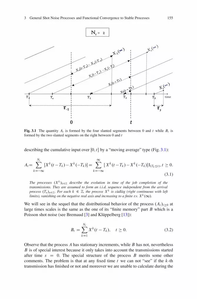
3 General Shot Noise Processes and Functional Convergence to Stable Processes 155
Fig. 3.1 The quantity At is formed by the four slanted segments between 0 and t while Bt isformed by the two slanted segments on the right between 0 and t
describing the cumulative input over Œ0; t � by a “moving average” type (Fig. 3.1):
AtDNtX
kD�1ŒXk.t �Tk/�Xk.�Tk/�D
1X
kD�1Œ Xk.t �Tk/�Xk.�Tk/�1l.Tk�t /; t � 0:
(3.1)
The processes .Xk/k2Z describe the evolution in time of the job completion of thetransmissions. They are assumed to form an i.i.d. sequence independent from the arrivalprocess .Tn/n2Z. For each k 2 Z, the process Xk is cadlag (right continuous with leftlimits), vanishing on the negative real axis and increasing to a finite r.v. Xk.1/.
We will see in the sequel that the distributional behavior of the process .At /t�0 atlarge times scales is the same as the one of its “finite memory” part B which is aPoisson shot noise (see Bremaud [3] and Kluppelberg [13]):
Bt DNtX
kD1Xk.t � Tk/; t � 0: (3.2)
Observe that the process A has stationary increments, while B has not, neverthelessB is of special interest because it only takes into account the transmissions startedafter time s D 0. The special structure of the process B merits some othercomments. The problem is that at any fixed time t we can not “see” if the k-thtransmission has finished or not and moreover we are unable to calculate during the

156 W. Jedidi et al.
time t �Tk the accumulated workXk.t �Tk/. The only available information is thequantity
Xk.1/ which is the total work required by the k-th transmission.
It is then natural to introduce the process
Ct DNtX
kD1Xk.1/; t � 0; (3.3)
which characterizes the total work required by all the transmissions started withinthe interval Œ0; t �. This process enjoys a very special property: it is a Levy process,i.e. it has independent and stationary increments and, more precisely, is a compoundPoisson process (see the book of Sato [21] for an account of Levy processes orappendix 3.7). This process turns out to be the principal component of the processesA and B , a component which will give the right approximation by a stable process,as stated in theorem 5 below.
Observe that the processes B and C defined in (3.2) and (8.5) are very welldefined because they are finite sums while the process A introduces in (3.1) mayhave problems of definition, since the r.v. At ; t > 0, could be infinite. We will seein lemma 2 that they are actually finite under our assumptions. There are many waysto represent these processes. Recall the random Poisson measure N.du/ associatedwith the sequence .Tk/k2Z and define the integer random measure M on .R � D;
B ˝ D/ by
M.du; dy/ WDX
k2Z�.Tk;Xk/.du; dy/; (3.4)
which is actually a marked Poisson measure. Then, the process A has a Poissonintegral representation of the moving average type
At DZ
.�1;t ��D�y..t � u/C/� y..�u/C/
�M.du; dy/:
Notice also that the process A is increasing and, as shown later on, is locallyintegrable if 1 < ˛ < 2. Then, the process A may have the structure of a specialsemimartingale (see definition 4.21 p. 43 [8]). We will only invoke some morefamiliar aspects in the structure of the processA, namely, it is represented as follows:
At DNtX
kD�1Œ Xk.t � Tk/ �Xk.�Tk/ � D Bt C �1t (3.5)

3 General Shot Noise Processes and Functional Convergence to Stable Processes 157
where
Bt DNtX
kD1Xk.t � Tk/; �1t D
0X
kD�1Œ Xk.t � Tk/ �Xk.�Tk/ �: (3.6)
We can also decompose B in B D C � �2 with
Ct DNtX
kD1Xk.1/; �2t D
NtX
kD1Œ Xk.1/�Xk.t � Tk/ �: (3.7)
All the processes presented above are closely connected to the load of the transmis-sions, this is the reason why we will call them load processes. The lemma 2 belowunveils some of their properties.
3.4 The Results
We will show that the processZ D A; B or C , after being correctly drifted rescaledand normalized, satisfy a limit theorem and share a common limiting process, a strictstable Levy motion totally skewed to the right (see appendix 3.7 for more on stableLevy motions).
3.4.1 Assumptions and Notations
Through all the following we adopt the following notations for all real numbers a; b
a^b D minfa; bg; a_b D maxfa; bg and .a�b/C D .a�b/_0 D a�.a^b/:
Recall the processes Xk are i.i.d. Let
.Xt /t�0 WD .X1.t//t�0; X1 WD limt!1Xt ; (3.8)
and assume the stopping time
� WD inff t W Xt D X1g is finite: (3.9)
Notice that the event .X1 > Xu/; u � 0; is given by .� > u/. Then, the behaviorof the r.v. � describes the way the cumulative process of each transmission reachesits maximum, or in other words the way each transmission is completed. The r.v.X1 and � are actually versions of the size and of the length of any transmissions.

158 W. Jedidi et al.
3.4.1.1 Assumption on the Size of the Transmissions
The r.v. X1 is finite and has a distribution with regularly varying tail of order �˛;with ˛ 2 .0; 2/ i.e. there exists a deterministic increasing function r such that foreach x > 0,
limu!1 uP.X1 > r.u/ x/ D 1
x˛(3.10)
which is equivalent to r.u/ D u1˛ l.u/ for some slowly varying function l i.e.
satisfying limu!1l.u x/=l.u/ D 1; for all x > 0. It is commonly said that X1 hasheavy tails. The reader is referred to the book of Bingham et al. [2] or to appendix3.7 for more details on regular variation theory.
3.4.1.2 Assumption on the Arrivals
Notice that the intensity parameter � of the arrival process N is not necessarilyconstant,
it may depend on a scale c and � D �c may depend on a parameter c > 0 as studied inMikosch et al. [17] and Kaj [11]. Through all the following, we consider the case where�c increases to a value �1 2 .0;1� as c goes to infinity. Of course, the constant case�c D �1 is included in the latter. Sometimes, we will simply write � instead of �c .
3.4.1.3 Technical Assumptions on the Length of the Transmissions:Connection with the Intensity and with the Size
At large scales, we will need one of these four assumptions expressed with afunction r W .0;1/ ! .0;1/ such that:
limc!1�c E
�
.� ^ c/�X1r.c�c/
^ 1��
D 0 (3.11)
or
limc!1�c E
�
�
�X1r.c�c/
^ 1��
D 0 (3.12)
or
EŒX1� < 1 and limc!1
�c
r.c �c/
Z c
0
EŒX1 �Xu� du D 0 (3.13)
or
EŒX1� < 1 and limc!1
�c
r.c �c/
Z ct
0
EŒX1 � Xu� du D 0; 8t > 0: (3.14)
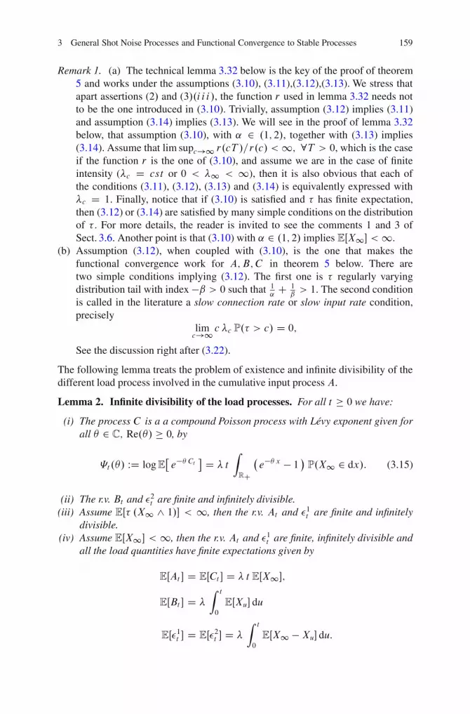
3 General Shot Noise Processes and Functional Convergence to Stable Processes 159
Remark 1. (a) The technical lemma 3.32 below is the key of the proof of theorem5 and works under the assumptions (3.10), (3.11),(3.12),(3.13). We stress thatapart assertions (2/ and (3/.i i i/, the function r used in lemma 3.32 needs notto be the one introduced in (3.10). Trivially, assumption (3.12) implies (3.11)and assumption (3.14) implies (3.13). We will see in the proof of lemma 3.32below, that assumption (3.10), with ˛ 2 .1; 2/, together with (3.13) implies(3.14). Assume that lim supc!1 r.cT /=r.c/ < 1; 8T > 0, which is the caseif the function r is the one of (3.10), and assume we are in the case of finiteintensity (�c D cst or 0 < �1 < 1), then it is also obvious that each ofthe conditions (3.11), (3.12), (3.13) and (3.14) is equivalently expressed with�c D 1. Finally, notice that if (3.10) is satisfied and � has finite expectation,then (3.12) or (3.14) are satisfied by many simple conditions on the distributionof � . For more details, the reader is invited to see the comments 1 and 3 ofSect. 3.6. Another point is that (3.10) with ˛ 2 .1; 2/ implies EŒX1� < 1.
(b) Assumption (3.12), when coupled with (3.10), is the one that makes thefunctional convergence work for A;B;C in theorem 5 below. There aretwo simple conditions implying (3.12). The first one is � regularly varyingdistribution tail with index �ˇ > 0 such that 1
˛C 1
ˇ> 1. The second condition
is called in the literature a slow connection rate or slow input rate condition,precisely
limc!1 c �c P.� > c/ D 0;
See the discussion right after (3.22).
The following lemma treats the problem of existence and infinite divisibility of thedifferent load process involved in the cumulative input process A.
Lemma 2. Infinite divisibility of the load processes. For all t � 0 we have:
(i) The process C is a a compound Poisson process with Levy exponent given forall � 2 C; Re.�/ � 0, by
�t.�/ WD logE�e�� Ct
� D � t
Z
RC
�e�� x � 1 P.X1 2 dx/: (3.15)
(ii) The r.v. Bt and �2t are finite and infinitely divisible.(iii) Assume EŒ� .X1 ^ 1/� < 1, then the r.v. At and �1t are finite and infinitely
divisible.(iv) Assume EŒX1� < 1, then the r.v. At and �1t are finite, infinitely divisible and
all the load quantities have finite expectations given by
EŒAt � D EŒCt � D � t EŒX1�;
EŒBt � D �
Z t
0
EŒXu� du
EŒ�1t � D EŒ�2t � D �
Z t
0
EŒX1 � Xu� du:
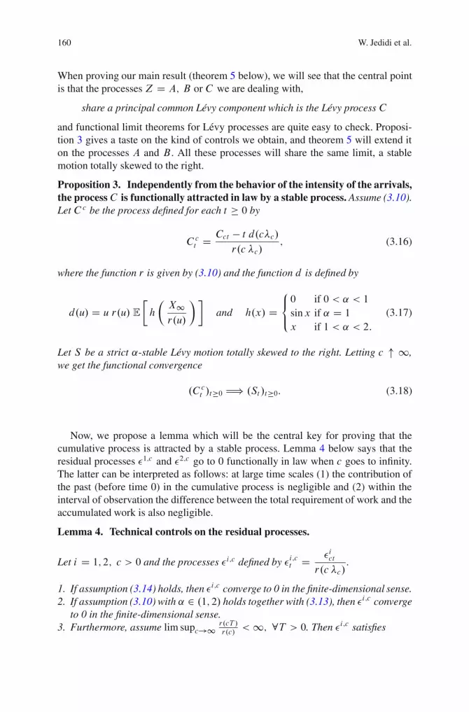
160 W. Jedidi et al.
When proving our main result (theorem 5 below), we will see that the central pointis that the processes Z D A; B or C we are dealing with,
share a principal common Levy component which is the Levy process C
and functional limit theorems for Levy processes are quite easy to check. Proposi-tion 3 gives a taste on the kind of controls we obtain, and theorem 5 will extend iton the processes A and B . All these processes will share the same limit, a stablemotion totally skewed to the right.
Proposition 3. Independently from the behavior of the intensity of the arrivals,the process C is functionally attracted in law by a stable process. Assume (3.10).Let C c be the process defined for each t � 0 by
C ct D Cct � t d.c�c/
r.c �c/; (3.16)
where the function r is given by (3.10) and the function d is defined by
d.u/ D u r.u/ E
�
h
�X1r.u/
��
and h.x/ D8<
:
0 if 0 < ˛ < 1sinx if ˛ D 1
x if 1 < ˛ < 2:(3.17)
Let S be a strict ˛-stable Levy motion totally skewed to the right. Letting c " 1,we get the functional convergence
.C ct /t�0 H) .St /t�0: (3.18)
Now, we propose a lemma which will be the central key for proving that thecumulative process is attracted by a stable process. Lemma 4 below says that theresidual processes �1;c and �2;c go to 0 functionally in law when c goes to infinity.The latter can be interpreted as follows: at large time scales (1) the contribution ofthe past (before time 0) in the cumulative process is negligible and (2) within theinterval of observation the difference between the total requirement of work and theaccumulated work is also negligible.
Lemma 4. Technical controls on the residual processes.
Let i D 1; 2; c > 0 and the processes �i;c defined by �i;ct D �ictr.c �c/
.
1. If assumption (3.14) holds, then �i;c converge to 0 in the finite-dimensional sense.2. If assumption (3.10) with ˛ 2 .1; 2/ holds together with (3.13), then �i;c converge
to 0 in the finite-dimensional sense.3. Furthermore, assume lim supc!1
r.cT /
r.c/< 1; 8T > 0. Then �i;c satisfies

3 General Shot Noise Processes and Functional Convergence to Stable Processes 161
8T; � > 0; limc!1P
supt�T
�i;ct > �
!
D 0 (3.19)
(which certainly implies the �i;c functionally converges in law to the null process) inany of the following situations:
(i) i D 1; and assumption (3.13) holds;(ii) i D 1 and assumption (3.12) holds;
(iii) i D 2 and assumption (3.10) holds together with (3.11)�recall (3.11) is
implied by (3.12).
After the previous preliminaries, we tackle our main result dealing with theattraction of the load processes by a stable process.
Theorem 5. The processesA; B; C are attracted functionally in law by a commonstable process. Assume (3.10). Let Z D A; B or C and define for each t � 0
Zct D Zct � t d.c�c/
r.c�c/; (3.20)
where r.c�c/ is given by (3.10) and d.c�c/ is defined in (3.17). Let S be a strict ˛-stable Levy motion totally skewed to the right. Letting c " 1, we get the functionalconvergence
.Zct /t�0 H) .St /t�0; (3.21)
in any of the following situations:
(a) Z D C ;(b) Z D B and (3.11) holds;(c) Z D A and (3.12) holds;(d) Z D A;B; ˛ 2 .1; 2/ and (3.13) holds. Then, the convergence (3.21) is true in
the finite-dimensional sense, and the drift “t d.c�c/ D c �c t EŒX1�” in (3.20)can be replaced by the expectation EŒBct �.
Remark 6. Our main result stated in the las theorem merits some comments:
(i) We would like to call the attention of the reader that we had allowed theintensity of the arrival process �c to increase to infinity with the time scale.The condition ˛ 2 .1; 2/ in the statement d) of theorem 5 is connected to thefiniteness of the moments EŒZt �; t > 0.
(ii) The reader should also notice that in the case that the intensity �c ! �1 2.0;1/ and � has a finite expectation then the functional convergence intheorem 5 simply holds under condition (3.10) (See the details in Sect. 3.6–3below).
(iii) As already noticed in Sect. 3.2, the mode of convergence (functional in.D;M1/) is extremely useful because it implies that some special functionals ofthe sequence of processes in D converge to the functionals of the limit process.For instance, consider the inverse in time of Z
162 W. Jedidi et al.
�.Z/a D infft � 0 W; Zt > ag; a � 0:
It corresponds to the first time the cumulative input crosses the critical barriera. Correctly normalized, and with convergence (3.21), it is easy to show thatthe distribution of the process �.Z/ can be approximated by �.S/ whichis well studied in probability literature. Functionals such as supremum andreflection maps are treated similarly. See the monograph of Whitt [23] for theseconsiderations.
3.5 Overview of Some Related Work
We will describe the different infinite source Poisson models we encountered in theliterature according to their chronological order of appearance. Of course, our listis not exhaustive. We will see that all the models we present are particular formsof (3.1) or (3.2) when the processes Xk is specified. In what follows, we denote by�k D infft W Xk.t/ D Xk.1/g the length (or duration) of the k-th transmission andRk its rate (Rk could be interpreted as the size of the transmission per time unit,i.e. Rk D Xk.1/=�k). In all the following models, the sequence .�k; Rk/k2Z isassumed to be i.i.d. and independent from the arrival processN . As done previously,we denote .�; R/ D .�1; R1/ andX D X1. The assumptions used in the works citedbelow imply (3.10) and (3.11) according to the discussions in Sect. 3.6 below. Atthe end of each model presented, we explain why the last claim is true by referringto the corresponding argument in Sect. 3.6.
1. Konstantopoulos et Lin [14]:The intensity � is constant. The model is in the form(3.1) with
Xk.r/ D .r ^ �k/where .:/ is a deterministic regularly varying function with index a > 0 and �has regularly varying tails with index �ˇ where ˇ 2 .1; 2/ and ˇ > a, so thatEŒ� � < 1 and X1 D .�/ has a regularly varying tail of index ˛ D ˇ=a 2.1; 2/. The authors assumed many other constraints on the indexes a and ˇ andon the increments of the function . They also conjectured that the convergencemight hold with the M1 topology for their model. See Sect. 3.6–3 below.
2. Resnick and Van Den Berg [20]: The intensity � is constant. The modelof Konstantopoulos et al. [14] is revisited under the form (3.2) by keepingsome identical assumptions cited in [14] and relaxing the extraneous ones. Theconvergence (3.21) is shown to hold in the weak Skorohod sense, i.e. in .D;M1/.See Sect. 3.6–3 below.
3. Mikosch et al. [18]: The intensity � is constant. Assuming that � has a regularlyvarying tail with index �˛; ˛ 2 .1; 2/, the authors proposed a model in the form(3.2) with
Xk.r/ D .rC ^ �k/:Then X1 D � and EŒ� � < 1. See Sect. 3.6–3 below.
3 General Shot Noise Processes and Functional Convergence to Stable Processes 163
4. Maulik et al. [15]: The intensity � is constant. The model is of the form (3.2)with
Xk.r/ D .rC ^ �k/Rk:The authors imposed a kind of asymptotic independence with a bivariate regu-larly varying nature on the tails of the pair .�; R/: � and R have both regularlyvarying distribution tail with indexes �˛� ; �˛R; 1 < ˛� ; ˛R < 2. There existstwo regularly varying function r� .c/; rR.c/ with indexes 1=˛� ; 1=˛R and aprobability measure G on RC with ˛� -th finite moment such that the followingvague convergence holds: if ˛� < ˛R , then
c P
���
r� .c/; R
�
2 :�
�! dx
x˛�C1 �G.:/ on .0;1� � Œ0;1�;
and
lim�!0 lim sup
c!1E
"��
r� .c/; R
�ı
1l.�<r� .c/ �/
#
D 0 for some ı > 0:
If ˛� > ˛R the same convergence hold when exchanging � by R MutatisMutandis. It is shown in this paper that these assumptions imply: X1 D � R
has a regularly varying distribution tail with index �˛; ˛ D ˛� ^ ˛R 2 .1; 2/
and because � has a regularly varying distribution tail with index �˛; ˛ > 1 wehave EŒ� � < 1. See Sect. 3.6–3 below.
5. Maulik and Resnick [16]: The intensity � is constant. The model has the form(3.2) withXk.t/ D Y k.t/^Xk.1/ and .Yk;Xk.1//k independent formN . Theauthors assumed a kind of asymptotic independence type between the processesY k and the r.v. Xk.1/ with regularly varying nature on the tails: denotingYc;t D Y 1ct , the authors assumed the existence of a regularly varying function.c/ with index H > 1 and a process � in D with stationary increments suchthat EŒ.�1/�˛� < 1 for some ˛ 2 .1; 2/ and for each � > 0, the followingconvergence of finite measures is true
1
P.X1 > .c//P
�X1.c/
> �;Yc;:
.c/2 :�
�! 1
�˛P.� 2 :/
and for each � > 0
lim�!0 lim sup
c!11
P.X1 > .c//P
�X1.c/
� �;�
c> �
�
D 0:
It is shown in this paper that these assumptions imply: � is self-similar, X1has regularly varying distribution tail with index �˛ and � has regularly varyingdistribution tail with index �ˇ; ˇ D H˛ > 1 which implies EŒ� � < 1. SeeSect. 3.6–3 below.

164 W. Jedidi et al.
6. Maulik and Resnick [17]: The model partly extends [16] by �c ! 1 by letting� D �c ! 1 but Y 1 isH -self-similar. The authors studied two rates of growth:a slow connection growth condition (limc!1 c �c P.� > c/ D 0 giving a stablelimit process) and a fast connection growth condition (limc!1 c �c P.�>c/D1)giving a self-similar Gaussian limit process). We compare only with the slowconnection setting. The authors assumed (3.10) with ˛ 2 .1; 2/, EŒ.Y 11 /�˛� < 1,EŒ.Y 1
1 /2Cı�˛� < 1 for some ı > 0 and ˇ D H˛ > 1 satisfies 1
˛C 1
ˇ> 3�˛
˛_1.
It is shown in this paper that these assumptions imply: � has a regularly varyingdistribution tail with index ˇ. See Sect. 3.6–4 below.
7. Kaj [11]: The intensity � D �c ! 1. The model is expressed with the processesB in (3.2) with
Xk.r/ D rC ^ �kand the cumulative process A is expressed as the sum A D B C �1 where �1
is build in order to have a stationary version of the process A. Namely, �1t DPM
kD1 t ^e�k , where M is a Poisson r.v with intensity parameter D EŒ��
independent from .�k/k�1, the sequence .e�k/k�1 is i.i.d., independent from M
and .�k/k�1 ande�1 has the equilibrium distribution P.e�1 � u/ D 1
R u0P.�>z/ dz:
Trivial calculations show that the process �1 introduced by the author has thesame law as the process �1 defined in (3.6) by
�1t D0X
kD�1.t � Tk/ ^ �k � .�Tk/ ^ �k:
The author assumed that the right tail of X1 D � is regularly varying withindex �˛; ˛ 2 .1; 2/, and connection rate holds: there exists a function a.c/such that a.c/ �c P.� > a.c/ / ! K 2 Œ0;1�: The slow (resp. intermediate,resp. fast) connection rate is for K D 0 (resp. > 0, resp D 1), In theintermediate case, when, replacing the functions r.c �c / and d.c �c / in (3.20)by a.c/, the author show that (3.21) holds but the limit is a non-Gaussian andnon-stable stochastic process with stationary increments Y . The limit process is aH -fractional Brownian motion (resp. stable Levy motion) in the fast (resp.slow)connection rates and can be recovered from the new intermediate regime limitprocess by applying two different (extreme) rescaling options: taking Y c Dc�H Y.ct/ (resp. Y c D c�1=˛ Y.ct/), then Y c converges functionally to the H -fractional Brownian motion when c ! 0 (resp. finite-dimensionally to a totallyskewed to the right stable motion when c ! 1).
3.6 Comments on Our Assumptions
The regular variation condition (3.10) is familiar in probability theory and will be themain argument for approximating the Levy measure of the processesZ D A;B;C .It is explicitly assumed in this section. For more details on regular variation theory
3 General Shot Noise Processes and Functional Convergence to Stable Processes 165
we refer to [2] or to appendix 3.7. Actually, the conditions leading to assumptions(3.11), (3.12) and (3.13) are simple and numerous. Some of them are presentedhere:
1. Assumptions (3.11) or (3.12) simply hold if we take any function t 7! f .t/
which is strictly increasing, less than 1 for all t, has limit 1 and
Xt D f .t/X1; with X1 satisfying (3.10):
Furthermore, since ˛ 2 .1; 2/, we have EŒX1� < 1 and assumption (3.13)works if
limc!1
�c
r.c �c/
Z c
0
Œ1 � f .u/� du D 0:
2. In the finite intensity case (�c D cst D � or �1 2 .0;1/), assumptions(3.11) and (3.12) are also simply implied by EŒ� � < 1. Recall we have chosenan increasing version of the regularly varying function r.u/, then applying themonotone convergence theorem (decreasing version) we have
E
�
�
�
1 ^ X1r.c �/
��
�! 0:
In the infinite intensity case (�1 D 1), and in order to have (3.12) it sufficesthat � is a bounded r.v or even if there exists ˇ 2 .1; c˛/,
c˛ D C11l.˛�1/ C ˛
˛ � 11l.˛>1/;
such that EŒ�ˇ� < 1 and �c=cˇ�1 ! 0. Indeed, the Holder inequality and (3.42)in appendix 3.7 yield
�cE
�
�
�X1r.c�c/
^ 1��
� E��ˇ�1=ˇ
�c E
"�X1r.c�c/
�ˇ=.ˇ�1/^ 1
#.ˇ�1/=ˇ
C1� E��ˇ�1=ˇ�c.c�c/
.1�ˇ/=ˇDE��ˇ�1=ˇ.�c=c
ˇ�1/1=ˇ!0:
3. Assume the length � has also a regularly varying distribution tail with index �ˇsuch that 1
˛C 1
ˇ> 1. Assume also the slow connection rate condition
limc!1 c �c P.� > c/ D 0; (3.22)
then, assumption (3.11) is satisfied. Indeed, using the Holder inequality with p >ˇ; q > ˛, we have
�cE
�
.�^c/�X1r.c�c/
^1��
�c�cE
h�
c
�p^1i� 1
pc�cE
��X1r.c�c/
�q
^1� � 1
q:
166 W. Jedidi et al.
Now, using (3.42,3.43, appendix 3.7), we have:
c�cE
h�
c
�p ^ 1i� 1
p
�
c�cE
��X1r.c�c/
�q
^ 1�� 1
q
C1��
p
p � ˇc�cP.� > c/
� 1p�
q
q � ˛
� 1q
:
4. Assume we have a fixed intensity � (the case � D �c ! �1 2 .0;1/ beingtreated similarly). Recall that 1 < ˛ < 2 implies EŒX1� < 1. Then necessarily
limt!1
1
t
Z t
0
EŒX1 � Xu� du D 0
which this is weaker than assumption (3.13). Condition (3.13) is easily checkedif the length � satisfies EŒ�� � < 1 for some � > 1 (of course the right tail ofthe distribution of � can also be regularly varying with index �ˇ; ˇ > � ). In thiscase, necessarily y 7! y� P.� > y/ is a bounded function (by some bound K).Indeed, choose
� < q < �˛=.˛ � 1/ .which implies 1 � 1=˛ < �=q < 1/
and take p D q=.q � 1/. By the Holder inequality, we have
0 �Z t
0
EŒX1 �Xu�du D EŒ
Z �^t
0
.X1 �Xu/du� � EŒ.� ^ t/X1�
� EŒXp1�1p EŒ.� ^ t/q � 1q :
Now, write
EŒ.� ^ t/q� D tqZ 1
0
P.� > t y1=q/ dy D tq��Z 1
0
.t y1=q/� P.� > t y1=q/
y�=qdy
� K tq��Z 1
0
1
y�=qdu D K 0 t q�� ;
and finally because rt D t1=˛ l.t/, we get for some constantK 00 > 0
0 � 1
rt
Z t
0
EŒX1 � Xu� du � K 00t1�1=˛��=q
l.t/�! 0:
Assumption (3.13) is also obviously implied by EŒ� X1� < 1.5. Example of a non trivial candidate for the process X describing the evolution in
time of the job completion of the transmissions

3 General Shot Noise Processes and Functional Convergence to Stable Processes 167
Take any positive r.v. X1 satisfying (3.10) and an independent increasing H -self-similar process Y such that EŒY ��1 � < 1 when � is in the neighborhood of˛. Then form the process
Xt D Yt ^ X1:We know according to (3.44, appendix 3.7) that P.� > u/
C1� EŒY �˛1 �
P.X1 > uH/. Then, going through the preceding situations for example, theadequate choice of H leads to our assumptions (3.11), (3.12) or (3.13). In thefinite intensity case (�c D cst or �1 2 .0;1/), a candidate for Y could be astrictH–stable subordinatorSH with 0 < H < ˛^1. See appendix 3.7 below fora precise definition of stable subordinators, and for their distributional properties,the reader is referred to the to the book of Zolotarev [24] or to Jedidi [9, 10]. Forself-similar processes, we suggest the book of Embrecht and Maejima [5].
3.7 Proofs of the Results
We start by proving lemma 2 justifying the existence of the load processes.Proof of lemma 2. Recall the integer Poisson measure M defined in (3.4). For anypositive measurable function f defined in RC �R�D, the process .Zt /t�0 definedby
Zt DZ
.u;y/2R�Df .t; u; y/M.du; dy/ D
X
k2Zf .t; Tk; X
k/
admits a Levy-Khintchine representation: for all � 2 R, Re.�/ � 0 we have
logEŒe�� Zt � D �
Z
R
EŒe�� f .t;u;X/ � 1� du: (3.23)
Due to the Poisson representation of the load processes, we deduce that if Z DA;B;C; �1; �2 then for all t � 0 and � 2 R, Re.�/ � 0 we have a Levy-Khintchinerepresentation
logEŒe�� Zt � D �
Z
.0;1/.e�� x � 1/ Zt .dx/; (3.24)
where
Zt .dx/ D
8ˆˆˆˆˆ<
ˆˆˆˆˆ:
R1�t P.XtCu �Xu 2 dx/ du if Z D AZ t
0
P.Xu 2 dx/ du if Z D B
tP.X1 2 dx/ if Z D CZ 1
0
P.XtCu �Xu 2 dx/ du if Z D �1
Z t
0
P.X1 �Xu 2 dx/ du if Z D �2:

168 W. Jedidi et al.
We recall the following useful and easily checkable inequality
je�� x �1j � .2^j� j x/ � .2_j� j/.x^1/; 8x � 0; � 2 C; Re.�/ � 0: (3.25)
Since x2 ^ 1 � x ^ 1, then proving that Zt .dx/ integrates x ^ 1 will insure that itis a Levy measure and the r.v. Zt is finite and infinitely divisible. For more accounton infinite divisibility and Levy processes, the reader is referred to appendix 3.7 orto the book of Sato [21].
.i/ and .i i/: If Z D B;C; �2, the result is obvious since in these cases
Z
.0;1/.x ^ 1/ Zt .dx/ � t EŒX1 ^ 1�:
We make a special emphasis on the r.v.Ct . The process .Ct /t�0 has stationaryand independent increments. This is easily seen from its Poisson integralrepresentation: 8 0 � s � t , we have
Ct � Cs DZ
.s;t ��Dy.1/ M.du; dy/
DZ
.s;t ��RCyX
k�0�.Tk ;Xk.1//.du; dy/
and because the sequence .Tk;Xk.1//k�0 forms a marked Poisson process..i i i/: Since At .dx/ D Bt .dx/ C �
1
t .dx/, it suffices to check when �1
t .dx/ is aLevy measure, but this is easy since
Z
.0;1/x ^ 1 �1t .dx/ D
Z 1
0
EŒ.XtCu � Xu/ ^ 1� du
DZ 1
0
EŒ1l.�>u/ .XtCu�Xu/^1�du � EŒ� .X1 ^ 1/�<1:
.iv/: The assumption EŒX1� < 1 impliesR.0;1/ x Zt .dx/ < 1 for Z D
B; C; �2 and allows to differentiate the Levy-Khintchine formula (3.24).Then,
EŒBt �DZ t
0
EŒXu� du; EŒCt �D tEŒX1� and EŒ�2t �DZ t
0
EŒX1�Xu� du:
Now, we tackle the processes A and �1. Noticing that x2 ^ 1 � x ^ 1 � x, wewill show the stronger result:
R.0;1/ x At .dx/ < 1. This result will provide in the
same time two results: (1) finiteness and then infinite divisibility of At ; �1t and (2)the equality EŒAt � D � t EŒX1�. Write

3 General Shot Noise Processes and Functional Convergence to Stable Processes 169
Z
.0;1/x At .dx/ D
Z 1
�tEŒXtCu �Xu� du D
Z t
0
EŒXu� du CZ 1
0
EŒXtCu � Xu� du:
Denote the Stieljes function EŒXu� by f .u/. We have f .1/ WD limu!1 f .u/ DEŒX1� < 1. It is then obvious that
limt!1
1
t
Z t
0
.f .1/� f .u// du D 0:
Applying the Tonelli-Fubini result, we get
Z 1
0
.f .t C u/� f .u//du DZ 1
0
Z
Œu;tCu�df .r/du D
Z
.0;1/.r ^ t/df .r/
D t Œf .1/ � f .t/�CZ
.0;t �
rdf .r/:
Then, integrating by parts the last integral, we get
Z 1
0
.f .t C u/� f .u// du DZ t
0
.f .1/ � f .u// du (3.26)
and the last quantity is finite. We conclude by saying that the infinitely divisible r.v.At has finite expectation if its Levy measure t .x/ integrates x in the neighborhoodon 1 (see theorem 25.3 [21]). Then, 8t > 0;
EŒAt �D�Z
.0;1/x At .dx/ D �
˚Z t
0
f .u/duCZ 1
0
.f .tCu/�f .u//du� D �tEŒX1�:
Notice that this is an expected result since At has stationary increments, and then,its expectation is linear in t . We have also proved that
EŒ�2t � D �
Z t
0
EŒX1 �Xu� du D �
Z 1
0
EŒXtCu � Xu� du D EŒ�1t �: (3.27)
utProof of proposition 3. Proving the convergence functional in law (3.18) is an easyproblem since the process C and then Cc are Levy processes. Due to corollary 3.6p.415 [8], it is enough to show that
the r.v. Cc1 D Cc � d.c �c/
r.c �c/converges in distribution to S1
a strict totally skewed to the right ˛-stable variable. Thanks to (3.15), for all � > 0,the Laplace exponent of Cc is defined by
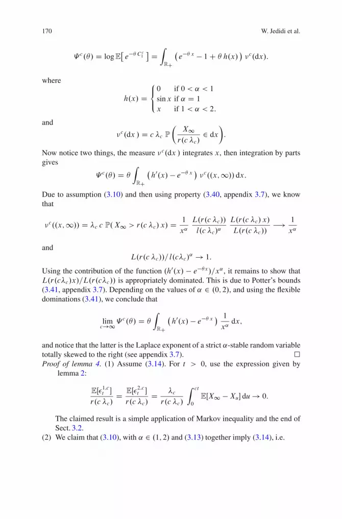
170 W. Jedidi et al.
�c.�/ D logE�e�� Cc1
� DZ
RC
�e�� x � 1C � h.x/
c.dx/:
where
h.x/ D8<
:
0 if 0 < ˛ < 1sinx if ˛ D 1
x if 1 < ˛ < 2:
and
c.dx / D c �c P
�X1r.c �c/
2 dx
�
:
Now notice two things, the measure c.dx / integrates x, then integration by partsgives
�c.�/ D �
Z
RC
�h0.x/ � e�� x c..x;1// dx:
Due to assumption (3.10) and then using property (3.40, appendix 3.7), we knowthat
c..x;1// D �c c P.X1 > r.c �c/ x/ D 1
x˛L.r.c �c//
l.c �c/˛L.r.c �c/ x/
L.r.c �c//�! 1
x˛
andL.r.c �c//= l.c�c/
˛ ! 1:
Using the contribution of the function .h0.x/ � e��x/=x˛, it remains to show thatL.r.c�c/x/=L.r.c�c// is appropriately dominated. This is due to Potter’s bounds(3.41, appendix 3.7). Depending on the values of ˛ 2 .0; 2/, and using the flexibledominations (3.41), we conclude that
limc!1�
c.�/ D �
Z
RC
�h0.x/ � e�� x
1
x˛dx;
and notice that the latter is the Laplace exponent of a strict ˛-stable random variabletotally skewed to the right (see appendix 3.7). �Proof of lemma 4. (1) Assume (3.14). For t > 0, use the expression given by
lemma 2:
EŒ�1;ct �
r.c �c/D EŒ�
2;ct �
r.c �c/D �c
r.c �c/
Z ct
0
EŒX1 �Xu� du ! 0:
The claimed result is a simple application of Markov inequality and the end ofSect. 3.2.
(2) We claim that (3.10), with ˛ 2 .1; 2/ and (3.13) together imply (3.14), i.e.

3 General Shot Noise Processes and Functional Convergence to Stable Processes 171
limc!1
�c
r.c �c/
Z ct
0
EŒX1 �Xu� du D 0; 8t > 0: (3.28)
Indeed, (3.28) is immediate for t � 1. For t > 1, we have �c�ct
� 1 (�: is
increasing). Now, choose � < 1 � 1˛
and use Potter’s bounds (3.41, appendix3.7) in order to write
�c;t D �c
r.c �c/
Z ct
0
EŒX1 � Xu�du D �c;1�c
�ct
r.ct�ct /
r.c�c/
� �c;1 K.�/t�C 1
˛� �c
�ct
1��� 1˛
� �c;1 K.�/t�C 1
˛ ! 0; as c ! 1;
then, conclude by 1/.(3) Observe that �1;c is an increasing process while �2;c is not. In order to control
the quantities P.supt�T �i;ct > �/ for i D 1; 2 and T > 0, observe also that
supt�T
�i;ct D supt�T
�ic tr.c �c/
D sups�1
�ic T sr.c �c/
D r.c �c T /
r.c �c/sups�1
�ic T sr.c �c T /
: (3.29)
Since lim supc!1
r.c�cT /
r.c�c/< 1; 8T > 0; it is enough to show that
P.sups�1
�i;cs > �/!0:
(3)(i ): The control of �1;c is easier than the one of �2;c because it is increasingand then
sups�1
�1;cs D �1;c1 D �1c =r.c �c/:
It is enough to reproduce the argument of (1/.
(3)(i i ) and (2/.i i i/: Recall �k is the length of the k-th transmission: �k Dinfft W Xk.t/ D Xk.1/g: Due to the Levy-Khintchine representation(3.24), the following stochastic inequality holds:
�1cr.c �c/
dD 1
r.c �c/
1X
kD1.Xk.c C Tk/� Xk.Tk// 1l.Tk��k/
� ı1c WD 1
r.c �c/
1X
kD1Xk.1/ 1l.Tk��k/: (3.30)
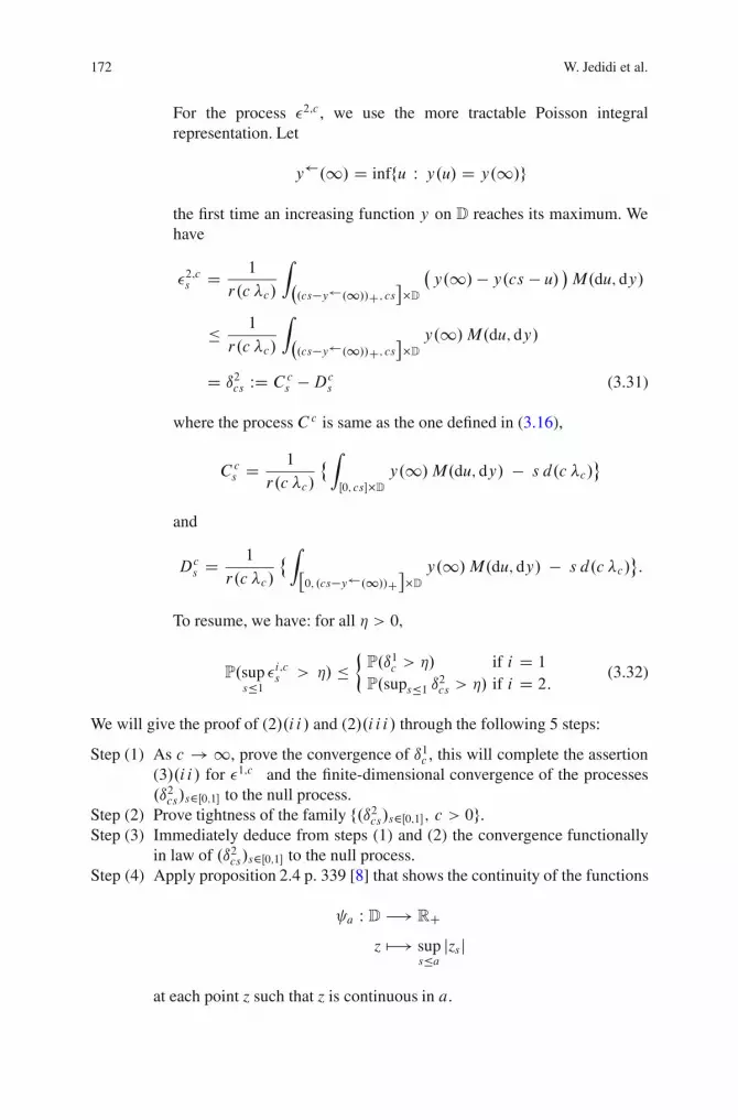
172 W. Jedidi et al.
For the process �2;c , we use the more tractable Poisson integralrepresentation. Let
y .1/ D inffu W y.u/ D y.1/g
the first time an increasing function y on D reaches its maximum. Wehave
�2;cs D 1
r.c �c/
Z
�.cs�y .1//C; cs
��D�y.1/ � y.cs � u/
M.du; dy/
� 1
r.c �c/
Z
�.cs�y .1//C; cs
��Dy.1/M.du; dy/
D ı2cs WD C cs �Dc
s (3.31)
where the process C c is same as the one defined in (3.16),
Ccs D 1
r.c �c/
˚Z
Œ0; cs��Dy.1/M.du; dy/ � s d.c �c/
�
and
Dcs D 1
r.c �c/
˚Z
�0; .cs�y .1//C
��Dy.1/M.du; dy/ � s d.c �c/
�:
To resume, we have: for all � > 0,
P.sups�1
�i;cs > �/ � P.ı1c > �/ if i D 1
P.sups�1 ı2cs > �/ if i D 2:(3.32)
We will give the proof of (2/.i i/ and (2/.i i i/ through the following 5 steps:
Step (1) As c ! 1, prove the convergence of ı1c , this will complete the assertion(3/.i i/ for �1;c and the finite-dimensional convergence of the processes.ı2cs/s2Œ0;1� to the null process.
Step (2) Prove tightness of the family f.ı2cs/s2Œ0;1�; c > 0g.Step (3) Immediately deduce from steps (1) and (2) the convergence functionally
in law of .ı2cs/s2Œ0;1� to the null process.Step (4) Apply proposition 2.4 p. 339 [8] that shows the continuity of the functions
a W D �! RCz 7�! sup
s�ajzsj
at each point z such that z is continuous in a.
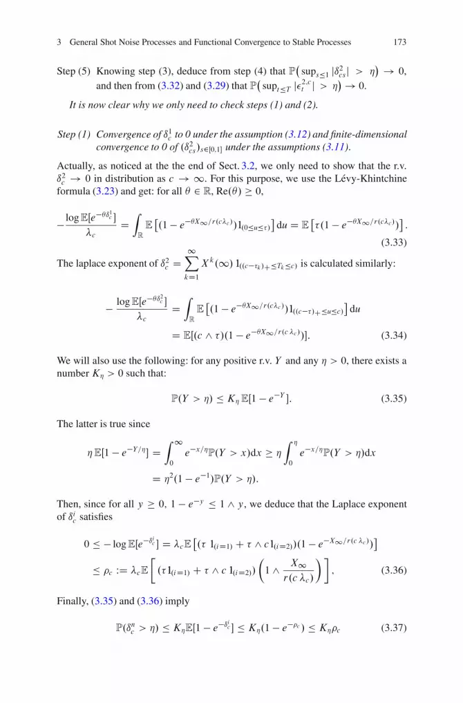
3 General Shot Noise Processes and Functional Convergence to Stable Processes 173
Step (5) Knowing step (3), deduce from step (4) that P�
sups�1 jı2csj > � ! 0,
and then from (3.32) and (3.29) that P�
supt�T j�2;ct j > � ! 0.
It is now clear why we only need to check steps (1) and (2).
Step (1) Convergence of ı1c to 0 under the assumption (3.12) and finite-dimensionalconvergence to 0 of .ı2cs/s2Œ0;1� under the assumptions (3.11).
Actually, as noticed at the the end of Sect. 3.2, we only need to show that the r.v.ı2c ! 0 in distribution as c ! 1. For this purpose, we use the Levy-Khintchineformula (3.23) and get: for all � 2 R, Re.�/ � 0,
� logEŒe��ı1c ��c
DZ
R
E�.1� e��X1=r.c�c//1l.0�u��/
�du D E
��.1 � e��X1=r.c�c//
�:
(3.33)
The laplace exponent of ı2c D1X
kD1Xk.1/ 1l..c��k/C�Tk�c/ is calculated similarly:
� logEŒe��ı2c ��c
DZ
R
E�.1 � e��X1=r.c�c //1l..c��/C�u�c/
�du
D EŒ.c ^ �/.1 � e��X1=r.c �c //�: (3.34)
We will also use the following: for any positive r.v. Y and any � > 0, there exists anumberK� > 0 such that:
P.Y > �/ � K� EŒ1 � e�Y �: (3.35)
The latter is true since
�EŒ1 � e�Y=�� DZ 1
0
e�x=�P.Y > x/dx � �
Z �
0
e�x=�P.Y > �/dx
D �2.1 � e�1/P.Y > �/:
Then, since for all y � 0; 1 � e�y � 1 ^ y, we deduce that the Laplace exponentof ıic satisfies
0 � � logEŒe�ıic � D �cE�.� 1l.iD1/ C � ^ c1l.iD2//.1 � e�X1=r.c �c //�
� �c WD �cE
�
.�1l.iD1/ C � ^ c 1l.iD2//�
1 ^ X1r.c �c/
��
; (3.36)
Finally, (3.35) and (3.36) imply
P.ınc > �/ � K�EŒ1 � e�ıic � � K�.1 � e��c / � K��c (3.37)
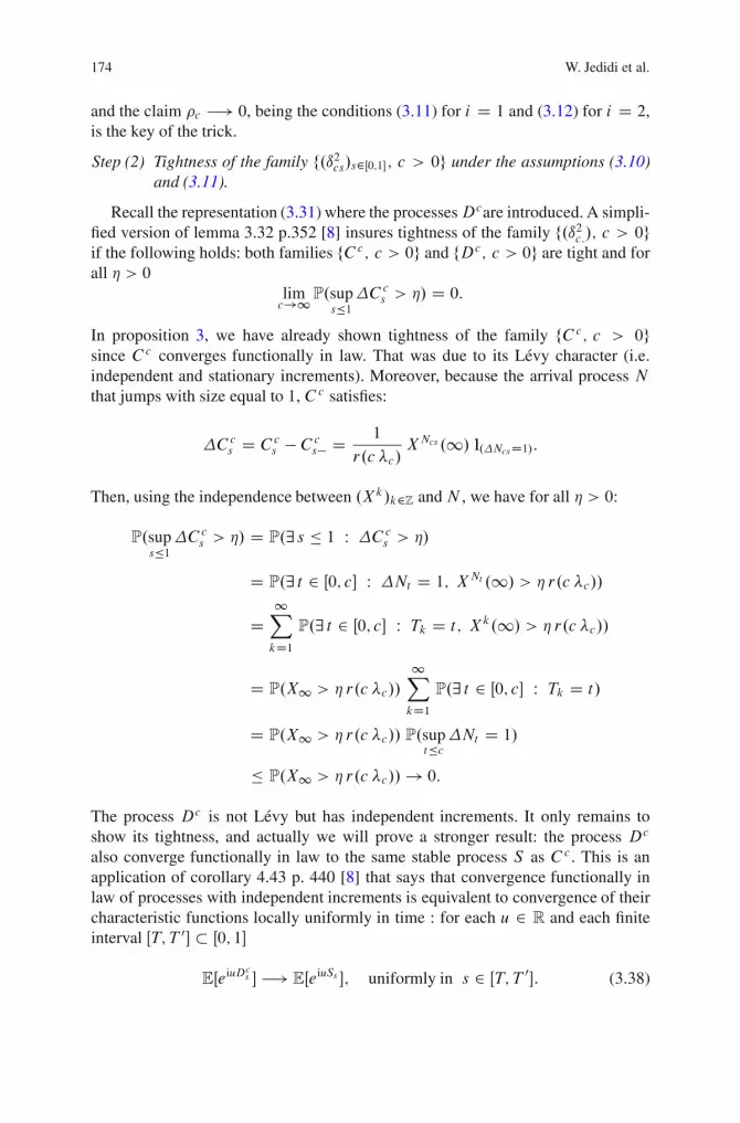
174 W. Jedidi et al.
and the claim �c �! 0, being the conditions (3.11) for i D 1 and (3.12) for i D 2,is the key of the trick.
Step (2) Tightness of the family f.ı2cs/s2Œ0;1�; c > 0g under the assumptions (3.10)and (3.11).
Recall the representation (3.31) where the processesDcare introduced. A simpli-fied version of lemma 3.32 p.352 [8] insures tightness of the family f.ı2c:/; c > 0gif the following holds: both families fCc; c > 0g and fDc; c > 0g are tight and forall � > 0
limc!1P.sup
s�1�C c
s > �/ D 0:
In proposition 3, we have already shown tightness of the family fCc; c > 0gsince Cc converges functionally in law. That was due to its Levy character (i.e.independent and stationary increments). Moreover, because the arrival process Nthat jumps with size equal to 1, C c satisfies:
�Ccs D Cc
s � C cs� D 1
r.c �c/XNcs .1/ 1l.�NcsD1/:
Then, using the independence between .Xk/k2Z and N , we have for all � > 0:
P.sups�1
�C cs > �/ D P.9 s � 1 W �Cc
s > �/
D P.9 t 2 Œ0; c� W �Nt D 1; XNt .1/ > � r.c �c//
D1X
kD1P.9 t 2 Œ0; c� W Tk D t; Xk.1/ > � r.c �c//
D P.X1 > � r.c �c//
1X
kD1P.9 t 2 Œ0; c� W Tk D t/
D P.X1 > � r.c �c// P.supt�c
�Nt D 1/
� P.X1 > � r.c �c// ! 0:
The process Dc is not Levy but has independent increments. It only remains toshow its tightness, and actually we will prove a stronger result: the process Dc
also converge functionally in law to the same stable process S as Cc . This is anapplication of corollary 4.43 p. 440 [8] that says that convergence functionally inlaw of processes with independent increments is equivalent to convergence of theircharacteristic functions locally uniformly in time : for each u 2 R and each finiteinterval ŒT; T 0� � Œ0; 1�
EŒeiuDcs � �! EŒeiuSs �; uniformly in s 2 ŒT; T 0�: (3.38)
3 General Shot Noise Processes and Functional Convergence to Stable Processes 175
Levy-Khintchine representation (3.23) and then (3.17) imply
logEŒeiuDcs � D �c
Z
R
EŒ.ei uX1=r.c �c / � 1/1lu�.cs��/C � du � i u sd.c �c/
r.c �c/
D �c EŒ.cs � �/C .ei uX1=r.c �c/ � 1/� � i u c �c s E
�
h
�X1r.c �c/
��
D logEŒeiuCcs � C �c EŒ.� ^ cs/ .1 � ei uX1=r.c �c //�:
Denoting zc;s D �c EŒ .� ^ cs/ .ei uX1=r.c �c / � 1/ � and using (3.25) we have
jzc;sj � .2 _ juj/ �c E�
.� ^ c/�
X1r.c �c/
^ 1��
:
Using assumption (3.11) or (3.12), we see that zc;s go 0 uniformly in s. Now, write
EŒeiuDcs � � EŒeiuSs � D �
EŒeiuCcs �� EŒeiuSs �ezc;s C .ezc;s � 1/ EŒeiuSs �
ˇˇEŒeiuDc
s � � EŒeiuSs �ˇˇ � ˇ
ˇEŒeiuCcs � � EŒeiuSs �ˇˇ ejzc;s j C jzc;s j ejzc;s j:
Since C c has independent increments and using again corollary 4.43 p. 440 [8], weget that the quantity
ˇˇEŒeiuDc
s � � EŒeiuSs �ˇˇ goes to 0 with the required uniformity.
We conclude that (3.38) is true. �
Proof of theorem 5. We have all the ingredients for this proof. Recall Ac DCc C �1;c � �2;c and Bc D C c � �2;c . The process Cc converges functionally inlaw to a stable process and the processes �1;c ; �2;c satisfy lemma 4. Assertion a) intheorem 5 has already been proved in proposition 3. Assertions b) and c) are a directapplication of lemma 3.31 p.352 [8] (which is kind of Slutzy theorem). The weakerassertion d) is proved using Slutzky theorem. �
Acknowledgements The authors would like to thank the referees for pointing out the obscurepoints and for their helpful comments, which improved the presentation of this paper. This workwas funded by Atlantic Canada Opportunity Agency (ACOA) and through grant from the NationalScience and Engineering Research Council of Canada (NSERC) to Dr. Vartan Choulakian.
Appendix : Regular Variation
In this appendix, the r.v U has a regularly varying distribution tail with index�˛; ˛ > 0 and could play the rule of the r.v. X1 and also of the r.v � : there existsa deterministic function r such that for each x > 0,
limu!1 uP.U > r.u/ x/ D 1
x˛: (3.39)
176 W. Jedidi et al.
Condition (3.39) is equivalent to one of the the definitions: (1) existence of aslowly varying function L (i.e. for all x > 0; limu!1L.u x/=L.u/ D 1) suchthat P.U>x/ D L.x/x�˛ ; .2/ dilation of the right tail of U gives limu!1 P.U >
u x/=P.U > u/ D x�˛: It also implies the existence of moments of any order0 < � < ˛ for the r.v. U : EŒU �� < 1. When ˛ 2 .0; 2/, it is said in the literaturethat U has a heavy tail.In regular variation theory, the function r.u/ is the asymptotic inverse of the functionx˛=L.x/ and necessarily r.u/ is regularly varying with index 1=˛; i.e
limu!1
L.r.u//
l.u/˛D 1 and r.u/ D u1=˛ l.u/ (3.40)
for some slowly varying function l . Furthermore, it is known that there exits anincreasing function r 0.u/ which is equivalent to r.u/ when u ! 1. This is thereason why we can take an increasing version for the function r.u/. A useful resultfor dominating slowly varying functions is known as Potter’s bounds and is givenby theorem 1.5.6 [2]: If L is a slowly varying function bounded away from 0 and 1on each interval ŒA;1/, then for all �; �0 > 0, there exits K.�/ < 1 < K.�0/ suchthat
K.�/.x=y/� � L.x/=L.y/ � K.�0/.x=y/��0 ; .0 < x � y/: (3.41)
Proposition 3.1. Assume (3.39) and let u ! 1, then
E
��U
r.u/
�q
^ 1�C1� q
q � ˛1
ufor all q > ˛ (3.42)
E
��U
u
�q
^ 1�C1�
8ˆ<
ˆ:
q
q � ˛ P.U > u/ for all q > ˛
EŒU q�
uqfor all q < ˛:
(3.43)
Proof. Equivalence (3.42) is a direct application of (3.43) and (3.39). For (3.43),q > ˛ just write
E
��U
u
�q
^ 1�
DZ 1
0
P
�U
u> v1=q
�
dv D q
Z 1
0
u
v
��q1l. u
v�1/ P.U > v/dv
v:
For q < ˛, write E� �U
u
q ^ 1� D q
Z 1
0
v�q 1l.v�1/ P.U >u
v/
dv
v: Then apply
ARANDELOVIC’s theorem 4.1.6 [2]. �
Proposition 3.2. Assume (3.39). Let U a r.v. with regularly varying distribution tailof order �˛ < 0 and Y be an increasing H–self-similar process independent from
3 General Shot Noise Processes and Functional Convergence to Stable Processes 177
U and � D infft W Yt � U g. Assume that Y1 admits a density f and EŒY ��1 � < 1if � is in the neighborhood of ˛. Then � regularly varying distribution tail of order�˛H and, more precisely, as u ! 1,
P.� > u/C1� EŒY �˛1 � P.U > uH/: (3.44)
Proof. The result is obvious since
P.� > u/ D P.Yu < U/ D P.Y1 uH < U / DZ
.0;1/P.Y1 uH < v/P.U 2 dv/
D 1
uH
Z 1
0
f v
uH
�P.U > v/dv D
Z 1
0
h v
uHf v
uH
�iP.U > v/
dv
v:
Then apply again ARANDELOVIC’s theorem 4.1.6. �
Appendix : Levy Processes and Stable Levy Motions
Let .˝;F ; .Ft /t>0;P/ be a stochastic basis. We say that a process X on thisbasis is a Levy process, if it has independent and stationary increments. It isentirely characterized by its Levy-Khintchine exponent: for all u 2 R, '.u/ DlogE Œ ei uX1 � D i u d � b2 u2
2C R
Œ ei ux � 1 � i u g.x/ � .dx/ where d 2 R; b � 0
and the Levy measure is a positive measure giving no mass to 0, integratingx2 ^ 1: The truncation function g could be any real bounded function such thatlimx!0 .g.x/ � x/=x2 D 0. A process S is called stable process with index˛ 2 .0; 2�, if it is a Levy process and (i) ˛ D 2 and D 0 (drifted and scaledBrownian motion) or (ii) b D 0 and 0 < ˛ < 2 and .dx/ D .cC1l.x > 0/Cc�1l.x <0//x�˛�1dx/; cC; c� � 0. A standard totally skewed to the right stable process(0 < ˛ < 2) has d D c� D 0; cC D 1 with the truncation function equal tog.x/ D sin x. A standard stable subordinator (0 < ˛ < 1) has d D c� D 0; cC D 1
with the truncation function equal g.x/ D 0.
References
1. Billingsley P.: Convergence of Probability Measures, 2nd edn. Wiley, New York (1999)2. Bingham N.H., Goldie C.M., Teugels J.L.: Regular Variation. Cambridge University Press,
Cambridge (1987)3. Bremaud P.: An insensitivity property of Lindberg’s estimate for delayed claims. J. Appl.
Probab. 37, 914–917 (2000)4. Caglar M.: A Long-Range Dependent Workload Model for Packet Data Traffic. Math. Oper.
Res. 29(1), 92-105 (2004)
178 W. Jedidi et al.
5. Embrecht P., Maejima M.: Selfsimilar Processes. Princeton Univ Press, Princeton and Oxford(2002)
6. Fasen V.: Modeling network traffic by a cluster Poisson input process with heavy and light-tailed file sizes. Queueing Systems: Theory and Applications 66(4), 313–350 (2010)
7. Fasen V., Samorodnitsky G.: A fluid cluster Poisson input process can look like a fractionalBrownian motion even in the slow growth aggregation regime. Adv. in App. Probab. 41(2),393–427 (2009)
8. Jacod J., Shiryaev A.N.: Limit Theorems for Stochastic Processes. New York, Springer (1987)9. Jedidi W.: Stable Processes, Mixing, and Distributional Properties. I. Theory Probab. Appl.
52(4), 580–593 (2008)10. Jedidi W.: Stable Processes, Mixing, and Distributional Properties. II. Theory Probab. Appl.
53(1), 81–105 (2009)11. Kaj I.: The long-memory infinite source Poisson model: scaling limit and its representation.
Technical report, Uppsala, 19 (2003)12. Kaj I., Taqqu M.S.: Convergence to fractional Brownian motion and to the Telecom process:
the integral representation approach. In: In and Out of Equilibrium 2. Sidoravicius V., VaresM.E.: (eds.) Series: Progress in Probability, 60. pp. 383-427. Birkhauser (2008)
13. Kluppelberg C., Mikosch T., Scharf A.: Regular variation in the mean and stable limits forPoisson shot noise. Bernoulli 9, 467–496 (2003)
14. Konstantopoulos T., Lin S.J.: Macroscopic models for long-range dependent network traffic.Queueing Sys. Th. Appl. 28(1-3), 215–243 (1998)
15. Maulik K., Resnick S., Rootzen H.: Asymptotic independence and a network traffic model.J. of App. Prob. 39, 671–699 (2002)
16. Maulik K., Resnick, S.: Small and large time scale analysis of a network traffic model.Queueing Systems, 43(3), 221–250 (2002)
17. Maulik K., Resnick, S.: The self-similar and multifractal nature of a network traffic model.Stoch. Models. 19(4), 549–577, Dekker (2003)
18. Mikosch T., Resnick, S., Rootzen, H., Stegeman, A.W.: Is network traffic approximated bystable Levy motion or fractional Brownian motion?. Ann. Appl. Probab. 12(1), 23–68 (2002)
19. Mikosch T., Samorodnitsky, G.: Scaling limits for cumulative input processes. Math. Oper.Res. 32, 890-919 (2007)
20. Resnick S., Van Den Berg, E.: Weak Convergence of high-speed network traffic models.J. Appl. Probab. 37(2), 575-597 (2000)
21. Sato K.I.: Levy Processes and Infinitely Divisible Distributions. Cambridge University Press,Camrbridge (1999)
22. Whitt W.: Limits for cumulative input processes to queues. Probab. Engrg. Inform. Sci.14, 123–150 (2000)
23. Whitt, W.: Stochastic-Process Limits: An Introduction to Stochastic-Process Limits and theirApplication to Queues. Springer Series in Op. Res. and Fin. Eng. Hardcover (2002)
24. Zolotarev, V.M.: One Dimensional Stable Laws. Trans. Math. Mono. Am. Math. Soc. 31(2),424–425 (1986)

Chapter 4The Lower Classes of the Sub-FractionalBrownian Motion
Charles El-Nouty
Abstract Let fBH.t/; t 2 IRg be a fractional Brownian motion with Hurst index0 < H < 1. Consider the sub-fractional Brownian motion XH defined as follows :
XH.t/ D BH .t/CBH.�t/p2
; t � 0:
We characterize the lower classes of the sup-norm statistic ofXH by an integral test.
4.1 Introduction and Main Results
Let fBH.t/; t 2 IRg be a fractional Brownian motion (fBm) with Hurst index0 < H < 1, i.e. a centered Gaussian process with stationary increments satisfyingBH.0/ D 0, with probability 1, and IE.BH.t//
2 D j t j2H ; t 2 IR.Consider the sub-fractional Brownian motion (sfBm)
XH.s/ D BH .s/C BH.�s/p2
; s � 0;
and define its sup-norm statistic
Y.t/ D sup0�s�t
j XH.s/ j; t � 0:
We have for any t � s
C. El-Nouty (�)UMR 557 Inserm/ U1125 Inra/ Cnam/ Universite Paris XIII, SMBH-Universite Paris XIII,74 rue Marcel Cachin, 93017 Bobigny Cedex, FRANCEe-mail: [email protected]
M. Zili and D.V. Filatova (eds.), Stochastic Differential Equations and Processes,Springer Proceedings in Mathematics 7, DOI 10.1007/978-3-642-22368-6 4,© Springer-Verlag Berlin Heidelberg 2012
179
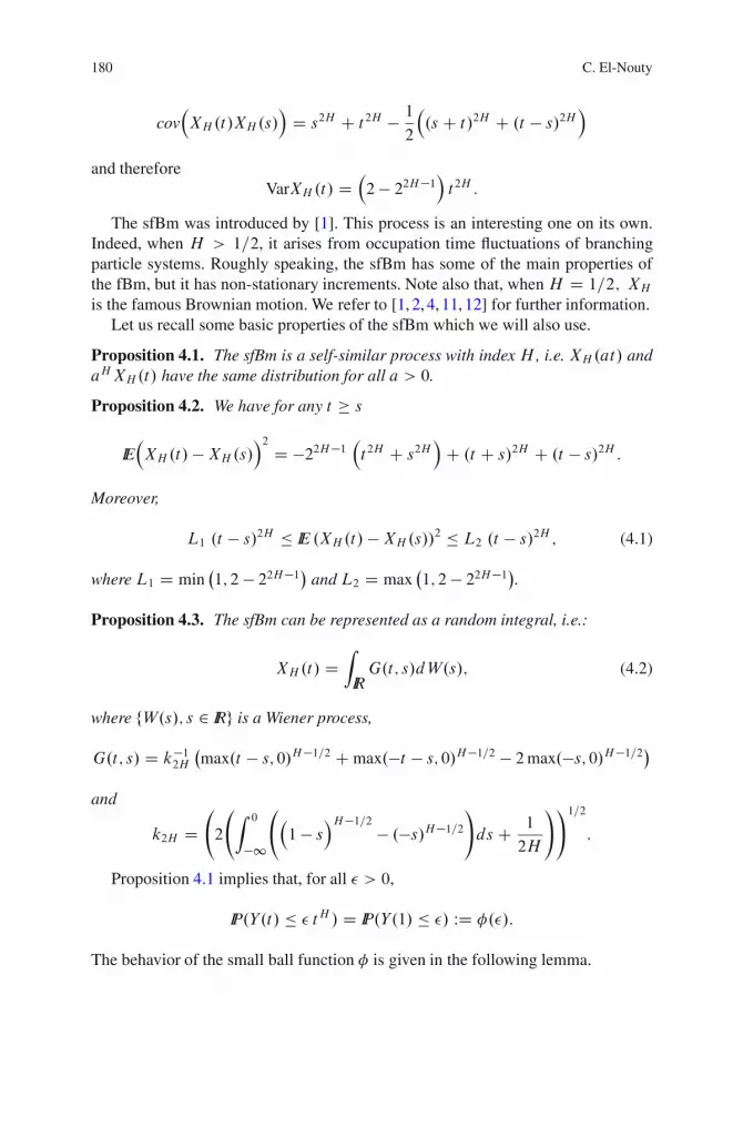
180 C. El-Nouty
cov�XH.t/XH.s/
�D s2H C t2H � 1
2
�.s C t/2H C .t � s/2H
�
and thereforeVarXH.t/ D
�2 � 22H�1
�t2H :
The sfBm was introduced by [1]. This process is an interesting one on its own.Indeed, when H > 1=2, it arises from occupation time fluctuations of branchingparticle systems. Roughly speaking, the sfBm has some of the main properties ofthe fBm, but it has non-stationary increments. Note also that, when H D 1=2; XHis the famous Brownian motion. We refer to [1, 2, 4, 11, 12] for further information.
Let us recall some basic properties of the sfBm which we will also use.
Proposition 4.1. The sfBm is a self-similar process with index H , i.e. XH.at/ andaHXH.t/ have the same distribution for all a > 0.
Proposition 4.2. We have for any t � s
IE�XH.t/ �XH.s/
�2 D �22H�1�t 2H C s2H
�C .t C s/2H C .t � s/2H :
Moreover,
L1 .t � s/2H � IE .XH.t/ �XH.s//2 � L2 .t � s/2H ; (4.1)
where L1 D min�1; 2 � 22H�1� and L2 D max
�1; 2� 22H�1
�.
Proposition 4.3. The sfBm can be represented as a random integral, i.e.:
XH.t/ DZ
IRG.t; s/dW.s/; (4.2)
where fW.s/; s 2 IRg is a Wiener process,
G.t; s/ D k�12H�max.t � s; 0/H�1=2 C max.�t � s; 0/H�1=2 � 2max.�s; 0/H�1=2�
and
k2H D
2
Z 0
�1
�1 � s
�H�1=2 � .�s/H�1=2!
ds C 1
2H
!!1=2
:
Proposition 4.1 implies that, for all � > 0,
IP.Y.t/ � � tH / D IP.Y.1/ � �/ WD �.�/:
The behavior of the small ball function � is given in the following lemma.
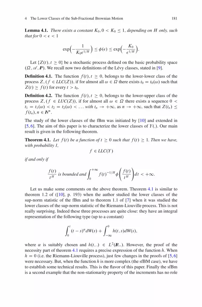
4 The Lower Classes of the Sub-Fractional Brownian Motion 181
Lemma 4.1. There exists a constant K0; 0 < K0 � 1; depending on H only, suchthat for 0 < � < 1
exp�� 1
K0�1=H
�� �.�/ � exp
�� K0
�1=H
�:
Let fZ.t/; t � 0g be a stochastic process defined on the basic probability space.˝;A ; IP/. We recall now two definitions of the Levy classes, stated in [9].
Definition 4.1. The function f .t/; t � 0; belongs to the lower-lower class of theprocessZ; .f 2 LLC.Z//; if for almost all ! 2 ˝ there exists t0 D t0.!/ such thatZ.t/ � f .t/ for every t > t0.
Definition 4.2. The function f .t/; t � 0; belongs to the lower-upper class of theprocess Z; .f 2 LUC.Z//; if for almost all ! 2 ˝ there exists a sequence 0 <t1 D t1.!/ < t2 D t2.!/ < : : : with tn ! C1; as n ! C1; such that Z.tn/ �f .tn/; n 2 IN�.
The study of the lower classes of the fBm was initiated by [10] and extended in[5, 6]. The aim of this paper is to characterize the lower classes of Y.:/. Our mainresult is given in the following theorem.
Theorem 4.1. Let f .t/ be a function of t � 0 such that f .t/ � 1. Then we have,with probability 1,
f 2 LLC.Y /
if and only if
f .t/
tHis bounded and
Z C1
0
f .t/�1=H� f .t/
tH
!
dt < C1:
Let us make some comments on the above theorem. Theorem 4.1 is similar totheorem 1.2 of ([10], p. 193) when the author studied the lower classes of thesup-norm statistic of the fBm and to theorem 1.1 of [7] when it was studied thelower classes of the sup-norm statistic of the Riemann-Liouville process. This is notreally surprising. Indeed these three processes are quite close: they have an integralrepresentation of the following type (up to a constant)
Z t
0
.t � s/˛dW.s/CZ 0
�1h.t; s/dW.s/;
where ˛ is suitably chosen and h.t; :/ 2 L2.IR�/. However, the proof of thenecessity part of theorem 4.1 requires a precise expression of the function h. Whenh D 0 (i.e. the Riemann-Liouville process), just few changes in the proofs of [5, 6]were necessary. But, when the function h is more complex (the sfBM case), we haveto establish some technical results. This is the flavor of this paper. Finally the sfBmis a second example that the non-stationarity property of the increments has no role

182 C. El-Nouty
in the study in the lower classes, as soon as the methodology introduced by [10]works. The first example was given in [7].
Although theorem 4.1 depends on an unknown function �, it is sharp. Indeed, set
f .t/ D �tH
.log log t/H; t � 3; � > 0:
Combining lemma 4.1 with a careful computation, we get that, if � < KH0 then
f 2 LLC.Y /, else if � � K�H0 , then f 2 LUC.Y /.In Sect. 4.2, we prove lemma 4.1 and state some basic results on �. The
main steps of the sufficiency are given in Sect. 4.3. The proof of the necessity ispostponed to Sects. 4.4 and 4.5. Section 4.4 consists in constructing some well-chosen sequences and a suitable set whereas we end the proof of the necessity inSect. 4.5 by establishing some key small ball estimates. The proofs which are similarto those in [5–7] will consequently be omitted.
In the sequel, there is no loss of generality to assume H ¤ 1=2.
For notational convenience, we define at D f .t/
tHand bt D �.at / D �
�f .t/
tH
�.
4.2 Proof of Lemma 4.1 and Preliminary Results
Before stating some preliminary results, we have to prove lemma 4.1.
Proof of Lemma 4.1. By using (4.1), we have for any h > 0
Var�XH.t Ch/�XH.t/
�D IE
�XH.t Ch/�XH.t/
�2 � L2 h2H � 2 h2H : (4.3)
Moreover, we deduce from (4.2) that
Var .XH .t C h/ j XH.s/; 0 � s � t/
� Var�k�12H
Z tCh
t
.t C h � s/H�1=2 dW.s/�
D k�22H1
2Hh2H : (4.4)
Since (4.3) and (4.4) hold, we can apply theorem 2.1 of [8]. The proof oflemma 4.1 is therefore complete. �Set D � log�. Thus, is positive and nonincreasing. A straight consequence oflemma 4.1 is given in the following lemma.
Lemma 4.2. We have for 0 < � < 1
1
K1�1=H� .�/ � K1
�1=H;
where K1 � 1=K0:

4 The Lower Classes of the Sub-Fractional Brownian Motion 183
Lemma 4.3. is convex.
Lemma 4.3 (see [3]) implies the existence of the right derivative 0
of . Thus,
0 � 0 and j 0 j is nonincreasing.
Lemma 4.4. There exists a constant K2 � sup�21C1=HK1; 2.2K
21/HK1
�, such
that we have for 0 < � < 1=K2
1
K2 �1C1=H� j 0
.�/ j � K2
�1C1=H:
Lemma 4.5. We have for �1 > �=2
exp
�
�K3
j �1 � � j�1C1=H
�
� �.�1/
�.�/� exp
�
K3
j �1 � � j�1C1=H
�
; (4.5)
where K3 � K2 21C1=H :
Lemma 4.6. There exists ˇ D .H=K2/H > 0; such that for � < ˇ; the function
��1=H�.�/ increases.
4.3 Sufficiency
Suppose here that at is bounded andRC10
a�1=Ht bt
dtt< C1. We want to prove
that f .t/ � Y.t/ for t large enough.
Lemma 4.7. limt!C1 at D 0.
In order to prove the sufficiency, we need to construct some special sequencesftn; n � 1g; fun; n � 1g and fvn; n � 1g. This will be done by recursion as follows,where L is a parameter depending onH only, such that L� 2H > 0. We start witht1 D 1. Having constructed tn, we set
unC1 D tn
�1C a
1=Htn
�;
vnC1 D inffu > tn; f .u/ � f .tn/.1C La1=Htn
/g;
andtnC1 D min.unC1; vnC1/:
Lemma 4.8. limn!C1 tn D C1.
The key part of the proof of the sufficiency is stated in the following lemma.
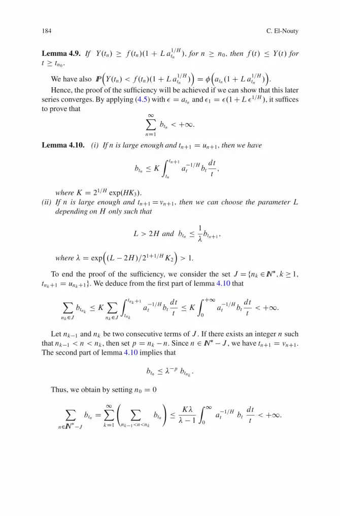
184 C. El-Nouty
Lemma 4.9. If Y.tn/ � f .tn/.1 C La1=Htn
/; for n � n0; then f .t/ � Y.t/ fort � tn0 :
We have also IP�Y.tn/ < f .tn/.1CLa
1=Htn
/�
D ��atn .1C La
1=Htn
/�
.
Hence, the proof of the sufficiency will be achieved if we can show that this laterseries converges. By applying (4.5) with � D atn and �1 D �.1CL�1=H /, it sufficesto prove that
1X
nD1btn < C1:
Lemma 4.10. (i) If n is large enough and tnC1 D unC1; then we have
btn � K
Z tnC1
tn
a�1=Ht bt
dt
t;
where K D 21=H exp.HK3/:(ii) If n is large enough and tnC1 D vnC1; then we can choose the parameter L
depending onH only such that
L > 2H and btn � 1
�btnC1
;
where � D exp�.L � 2H/=21C1=HK2
�> 1.
To end the proof of the sufficiency, we consider the set J D fnk 2 IN�; k� 1;tnkC1 D unkC1g. We deduce from the first part of lemma 4.10 that
X
nk2Jbtnk � K
X
nk2J
Z tnkC1
tnk
a�1=Ht bt
dt
t� K
Z C1
0
a�1=Ht bt
dt
t< C1:
Let nk�1 and nk be two consecutive terms of J . If there exists an integer n suchthat nk�1 < n < nk , then set p D nk �n. Since n 2 IN��J , we have tnC1 D vnC1.The second part of lemma 4.10 implies that
btn � ��p btnk :
Thus, we obtain by setting n0 D 0
X
n2IN��Jbtn D
1X
kD1
X
nk�1<n<nk
btn
!
� K�
� � 1Z 1
0
a�1=Ht bt
dt
t< C1:

4 The Lower Classes of the Sub-Fractional Brownian Motion 185
4.4 Necessity 1
Suppose here that, with probability 1, f .t/ � Y.t/ for all t large enough. We wantto prove that at is bounded and
R10a�1=Ht bt
dtt< C1.
In the sequel, there is no loss of generality to assume that f is a continuousfunction of t � 0.
Lemma 4.11. at is bounded and limt!C1 at D 0.
To prove the necessity, we will show that f 2 LUC.Y /whenR10a�1=Ht bt
dtt
DC1 and limt!C1 at D 0. The first step consists in constructing a suitable sequence.
Lemma 4.12. WhenR10
a�1=Ht bt
dtt
D C1 and limt!C1 at D 0; we can finda sequence ftn; n � 1g with the three following properties
tnC1 � tn.1C a1=Htn /;
For n large enough, m � n ) atmtHm
� 2atntHn;
and
1X
nD1btn D C1:
To continue the proof of the necessity, we need the following definition.
Definition 4.3. Consider the interval Ak D Œ2k; 2kC1Œ; k 2 IN: If a�1=Hti2 Ak; i 2
IN�; then we note u.i/ D k:
Set Ik D fi; u.i/ D kg which is finite by lemma 4.11 and Nk D exp.K0 2k�1/,
whereK0 was defined in lemma 4.1 and depends on H only.
Lemma 4.13. There exist a constantK4 depending onH only and a set J with thefollowing properties
X
n2Jbtn D C1:
Given n 2 J;m 2 J; n < m and an integer k such that k � min.u.n/; u.m// andcard.Ik \ Œn;m�/ > Nk; we have
tm
tn� exp
�exp
�K4 2
min.u.n/;u.m//��:
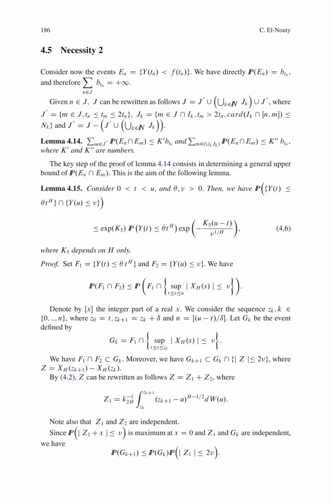
186 C. El-Nouty
4.5 Necessity 2
Consider now the events En D fY.tn/ < f .tn/g. We have directly IP.En/ D btn ,
and thereforeX
n2Jbtn D C1.
Given n 2 J; J can be rewritten as follows J D J0 [�S
k2IN Jk
�[J ”, where
J0 D fm 2 J; tn � tm � 2tng; Jk D fm 2 J \ Ik; tm > 2tn; card.Ik \ Œn;m�/ �
Nkg and J ” D J ��J
0 [�S
k2IN Jk
��.
Lemma 4.14.P
m2J 0 IP.En\Em/ � K 0btn andP
m2.[kJk/ IP.En\Em/ � K” btn ;where K 0 andK” are numbers.
The key step of the proof of lemma 4.14 consists in determining a general upperbound of IP.En \Em/. This is the aim of the following lemma.
Lemma 4.15. Consider 0 < t < u; and �; � > 0: Then, we have IP�fY.t/ �
� tH g \ fY.u/ � �g�
� exp.K5/ IP�Y.t/ � � tH
�exp
�
�K5.u � t/�1=H
�
; (4.6)
where K5 depends on H only.
Proof. Set F1 D fY.t/ � � tH g and F2 D fY.u/ � �g. We have
IP.F1 \ F2/ � IP
�
F1 \�
supt�s�u
j XH.s/ j � �
�
:
Denote by Œx� the integer part of a real x. We consider the sequence zk; k 2f0; ::; ng, where z0 D t; zkC1 D zk C ı and n D Œ.u � t/=ı�. Let Gk be the eventdefined by
Gk D F1 \�
supt�s�zk
j XH.s/ j � �
:
We have F1 \ F2 � Gk . Moreover, we have GkC1 � Gk \ fj Z j� 2�g, whereZ D XH.zkC1/� XH.zk/.
By (4.2), Z can be rewritten as follows Z D Z1 CZ2, where
Z1 D k�12HZ zkC1
zk
.zkC1 � u/H�1=2dW.u/:
Note also that Z1 and Z2 are independent.
Since IP�j Z1 Cx j � �
�is maximum at x D 0 andZ1 andGk are independent,
we haveIP.GkC1/ � IP.Gk/IP
�j Z1 j � 2�
�:

4 The Lower Classes of the Sub-Fractional Brownian Motion 187
The integral representation ofZ1 implies that IE.Z1/ D 0 and
VarZ1 D k�22HZ zkC1
zk
.zkC1 � u/2H�1du D 1
2Hk22Hı2H :
So, we have IP .j Z1 j� 2�/ D ˚�2p2Hk2H�
ıH
�, where˚ denotes the distribution
function of the absolute value of a standard Gaussian random variable. Then, weobtain
IP.GkC1/ � IP.Gk/˚
2p2Hk2H�
ıH
!
;
and therefore IP.F1 \ F2/ � IP.F1/˚�2p2Hk2H �ıH
�n.
Choosing ı D �1=H , we get K5 D � log˚�2
p2H k2H
�. (4.6) is proved. �
To prove lemma 4.14, just apply inequality (4.6) by setting u D tm; t D tn; � Datn and � D f .tm/.
Lemma 4.16. There exists an integer p such that, if n > sups�p .sup Is/ ; then, form 2 J ”; m > n; given � > 0; we have IP.En \Em/ � .1C �/ btnbtm .
The proof of lemma 4.16 is based on the two following lemmas. The first oneis a general result on Gaussian processes, whereas the second one gives a specificproperty on some probabilities of the sfBm.
Lemma 4.17. Let fX.t/; 0� t � 1g be a separable, centered, real-valued Gaussianprocess such that X.0/ D 0 with probability 1, and satisfying
�IE.X.t C h/� X.t//2
�1=2 � .h/ � c hˇ; ˇ > 0:
Then, we have for c�1 ı > 1
IP
sup0�s�1
j X.s/ j� ı
!
� 1
Cexp
��C.c�1 ı/
2�;
where C is a positive constant independent of c and ı:
Lemma 4.18. Let ˛ be a real number such that 1=2 < ˛ < 1. Set r D min�1�H3;
.1�˛/H3
�: Then, we have for u � 2t
IP�Y.t/ � � tH ; Y.u/ � �uH
�
� �.�/�.�/ exp
�
2� t
u
�rK3
� 1
�1C1=HC 1
�1C1=H��
C 6
Cexp
�
� C
K2
�u
t
�r�
;
(4.7)
where K > 0 depends on H only, K3 was defined in lemma 4.5 and C in lemma4.17.
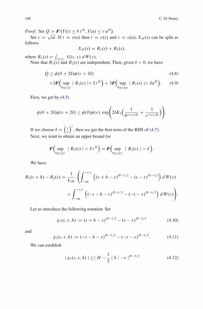
188 C. El-Nouty
Proof. Set Q D IP�Y.t/ � � tH ; Y.u/ � � uH
�.
Set v D put . If t D o.u/ then t D o.v/ and v D o.u/: XH.s/ can be split as
followsXH.s/ D R1.s/CR2.s/;
where R1.s/ D Rjxj�v G.s; x/ dW.x/.
Note that R1.s/ and R2.s/ are independent. Then, given ı > 0, we have
Q � �.� C 2ı/�.� C 2ı/ (4.8)
C3IP�
sup0�s�t
j R2.s/ j> ı tH�
C 3IP�
sup0�s�u
j R1.s/ j> ıuH�: (4.9)
First, we get by (4.5)
�.� C 2ı/�.� C 2ı/ � �.�/�.�/ exp
2ıK3
� 1
�1C1=HC 1
�1C1=H�!
:
If we choose ı D�tu
�r, then we get the first term of the RHS of (4.7).
Next, we want to obtain an upper bound for
IP�
sup0�s�t
j R2.s/ j > ı tH�
D IP�
sup0�s�1
j R2.s/ j > ı�:
We have
R2.s C h/� R2.s/ D 1
k2H
Z �v=t
�1
�.s C h � x/H�1=2 � .s � x/H�1=2
�dW.x/
CZ �v=t
�1
�.�s � h � x/H�1=2 � .�s � x/H�1=2
�dW.x/
!
:
Let us introduce the following notation. Set
g1.s; x; h/ WD .s C h� x/H�1=2 � .s � x/H�1=2 (4.10)
andg2.s; x; h/ WD .�s � h� x/H�1=2 � .�s � x/H�1=2: (4.11)
We can establish
j g1.s; x; h/ j � j H � 1
2j h j �x jH�3=2 (4.12)
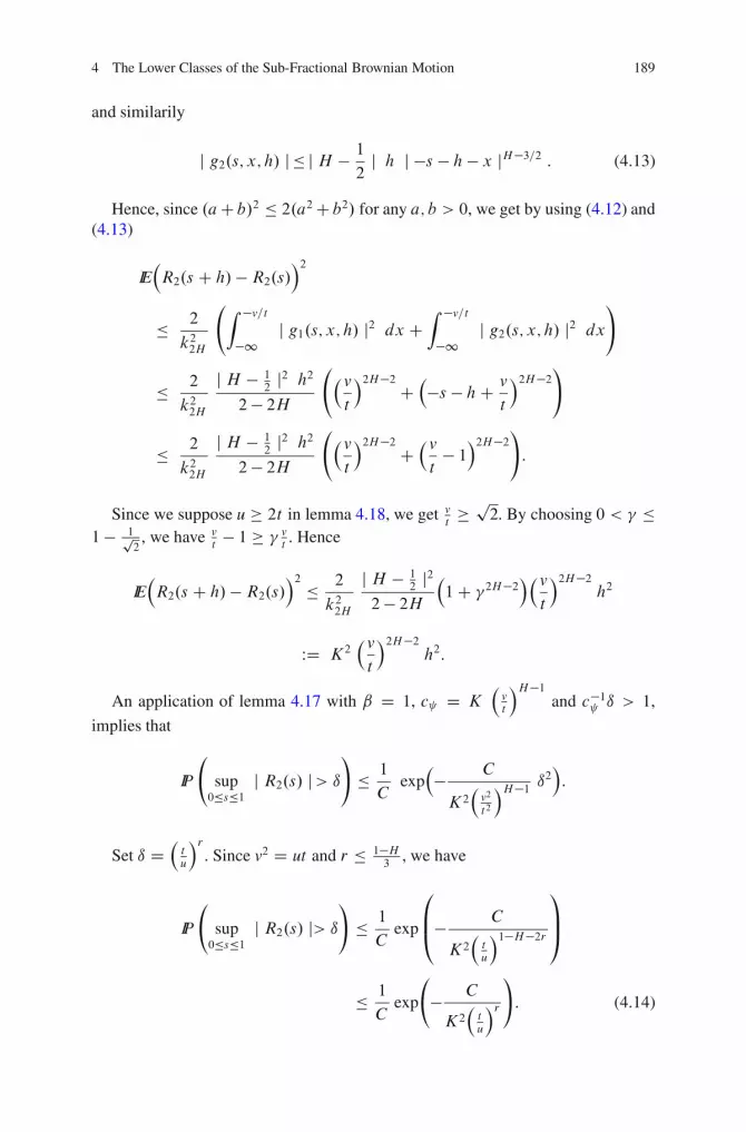
4 The Lower Classes of the Sub-Fractional Brownian Motion 189
and similarily
j g2.s; x; h/ j � j H � 1
2j h j �s � h� x jH�3=2 : (4.13)
Hence, since .aC b/2 � 2.a2 C b2/ for any a; b > 0, we get by using (4.12) and(4.13)
IE�R2.s C h/� R2.s/
�2
� 2
k22H
Z �v=t
�1j g1.s; x; h/ j2 dx C
Z �v=t
�1j g2.s; x; h/ j2 dx
!
� 2
k22H
j H � 12
j2 h22 � 2H
�v
t
�2H�2 C��s � hC v
t
�2H�2!
� 2
k22H
j H � 12
j2 h22 � 2H
�v
t
�2H�2 C�v
t� 1
�2H�2!
:
Since we suppose u � 2t in lemma 4.18, we get vt
� p2. By choosing 0 < � �
1 � 1p2, we have v
t� 1 � � v
t. Hence
IE�R2.s C h/� R2.s/
�2 � 2
k22H
j H � 12
j22 � 2H
�1C �2H�2
��v
t
�2H�2h2
WD K2�v
t
�2H�2h2:
An application of lemma 4.17 with ˇ D 1, c D K�
vt
�H�1and c�1 ı > 1,
implies that
IP
sup0�s�1
j R2.s/ j> ı!
� 1
Cexp
�� C
K2
�v2
t 2
�H�1 ı2�:
Set ı D�tu
�r. Since v2 D ut and r � 1�H
3, we have
IP
sup0�s�1
j R2.s/ j> ı!
� 1
Cexp
0
B@� C
K2�tu
�1�H�2r
1
CA
� 1
Cexp
� C
K2
�tu
�r
!
: (4.14)
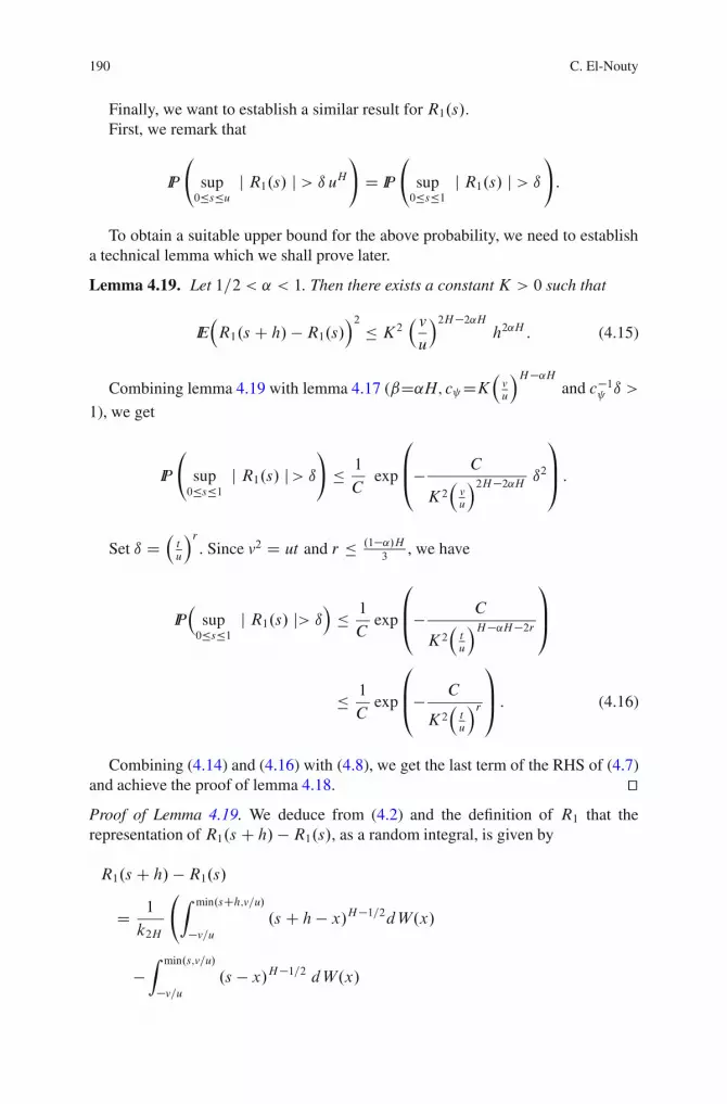
190 C. El-Nouty
Finally, we want to establish a similar result for R1.s/.First, we remark that
IP
sup0�s�u
j R1.s/ j > ı uH!
D IP
sup0�s�1
j R1.s/ j > ı!
:
To obtain a suitable upper bound for the above probability, we need to establisha technical lemma which we shall prove later.
Lemma 4.19. Let 1=2 < ˛ < 1. Then there exists a constantK > 0 such that
IE�R1.s C h/ �R1.s/
�2 � K2� v
u
�2H�2˛Hh2˛H : (4.15)
Combining lemma 4.19 with lemma 4.17 (ˇD˛H; c DK�
vu
�H�˛Hand c�1 ı >
1), we get
IP
sup0�s�1
j R1.s/ j> ı!
� 1
Cexp
0
B@� C
K2
�vu
�2H�2˛H ı2
1
CA :
Set ı D�tu
�r. Since v2 D ut and r � .1�˛/H
3, we have
IP�
sup0�s�1
j R1.s/ j> ı�
� 1
Cexp
0
B@� C
K2�tu
�H�˛H�2r
1
CA
� 1
Cexp
0
B@� C
K2�tu
�r
1
CA : (4.16)
Combining (4.14) and (4.16) with (4.8), we get the last term of the RHS of (4.7)and achieve the proof of lemma 4.18. utProof of Lemma 4.19. We deduce from (4.2) and the definition of R1 that therepresentation of R1.s C h/ � R1.s/, as a random integral, is given by
R1.s C h/ �R1.s/
D 1
k2H
Z min.sCh;v=u/
�v=u.s C h� x/H�1=2dW.x/
�Z min.s;v=u/
�v=u.s � x/H�1=2 dW.x/
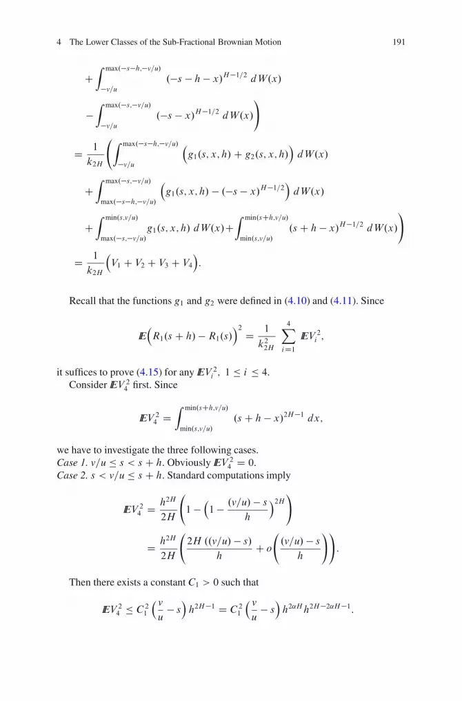
4 The Lower Classes of the Sub-Fractional Brownian Motion 191
CZ max.�s�h;�v=u/
�v=u.�s � h� x/H�1=2 dW.x/
�Z max.�s;�v=u/
�v=u.�s � x/H�1=2 dW.x/
!
D 1
k2H
Z max.�s�h;�v=u/
�v=u
�g1.s; x; h/C g2.s; x; h/
�dW.x/
CZ max.�s;�v=u/
max.�s�h;�v=u/
�g1.s; x; h/ � .�s � x/H�1=2
�dW.x/
CZ min.s;v=u/
max.�s;�v=u/g1.s; x; h/ dW.x/C
Z min.sCh;v=u/
min.s;v=u/.s C h � x/H�1=2 dW.x/
!
D 1
k2H
�V1 C V2 C V3 C V4
�:
Recall that the functions g1 and g2 were defined in (4.10) and (4.11). Since
IE�R1.s C h/� R1.s/
�2 D 1
k22H
4X
iD1IEV 2
i ;
it suffices to prove (4.15) for any IEV 2i ; 1 � i � 4.
Consider IEV 24 first. Since
IEV 24 D
Z min.sCh;v=u/
min.s;v=u/.s C h � x/2H�1 dx;
we have to investigate the three following cases.Case 1. v=u � s < s C h. Obviously IEV 2
4 D 0.Case 2. s < v=u � s C h. Standard computations imply
IEV 24 D h2H
2H
1 ��1 � .v=u/� s
h
�2H!
D h2H
2H
2H ..v=u/� s/
hC o
.v=u/� s
h
!!
:
Then there exists a constant C1 > 0 such that
IEV 24 � C2
1
� v
u� s�h2H�1 D C2
1
� v
u� s
�h2˛Hh2H�2˛H�1:
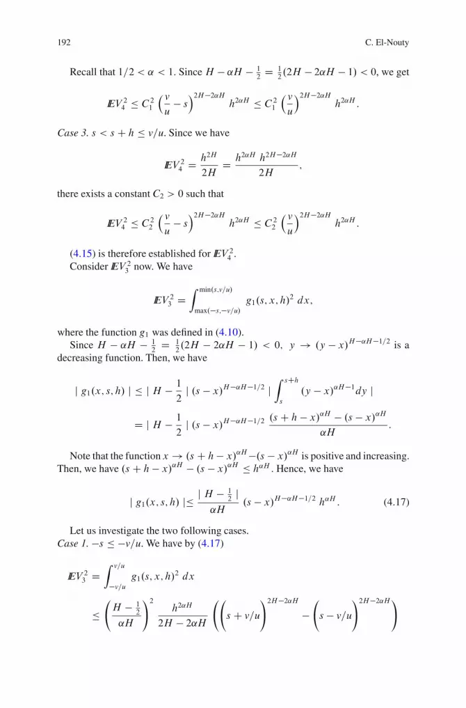
192 C. El-Nouty
Recall that 1=2 < ˛ < 1. Since H � ˛H � 12
D 12.2H � 2˛H � 1/ < 0, we get
IEV 24 � C2
1
� v
u� s
�2H�2˛Hh2˛H � C2
1
� v
u
�2H�2˛Hh2˛H :
Case 3. s < s C h � v=u. Since we have
IEV 24 D h2H
2HD h2˛H h2H�2˛H
2H;
there exists a constant C2 > 0 such that
IEV 24 � C2
2
� v
u� s
�2H�2˛Hh2˛H � C2
2
� v
u
�2H�2˛Hh2˛H :
(4.15) is therefore established for IEV 24 .
Consider IEV 23 now. We have
IEV 23 D
Z min.s;v=u/
max.�s;�v=u/g1.s; x; h/
2 dx;
where the function g1 was defined in (4.10).Since H � ˛H � 1
2D 1
2.2H � 2˛H � 1/ < 0; y ! .y � x/H�˛H�1=2 is a
decreasing function. Then, we have
j g1.x; s; h/ j � j H � 1
2j .s � x/H�˛H�1=2 j
Z sCh
s
.y � x/˛H�1dy j
D j H � 1
2j .s � x/H�˛H�1=2
.s C h � x/˛H � .s � x/˛H
˛H:
Note that the function x ! .s C h� x/˛H�.s � x/˛H is positive and increasing.Then, we have .s C h� x/˛H � .s � x/˛H � h˛H . Hence, we have
j g1.x; s; h/ j� j H � 12
j˛H
.s � x/H�˛H�1=2 h˛H : (4.17)
Let us investigate the two following cases.Case 1. �s � �v=u. We have by (4.17)
IEV 23 D
Z v=u
�v=ug1.s; x; h/
2 dx
� H � 1
2
˛H
!2h2˛H
2H � 2˛H
s C v=u
!2H�2˛H�
s � v=u
!2H�2˛H!

4 The Lower Classes of the Sub-Fractional Brownian Motion 193
� H � 1
2
˛H
!2h2˛H
2H � 2˛H s2H�2˛H
2.2H � 2˛H/ v
usC o
v
us
!2!
:
Then there exists a constant C3 > 0 such that
IEV 23 � C2
3 h2˛H s2H�2˛H�1
v
u� C2
3
� v
u
�2H�2˛Hh2˛H :
Case 2. �v=u < �s. We have
IEV 23 �
H � 1
2
˛H
!2
h2˛HZ s
�s
�s � x
�2H�2˛H�1dx
� H � 1
2
˛H
!2h2˛H
2H � 2˛H .2s/2H�2˛H
and consequently (4.15).(4.15) is therefore established for IEV 2
3 .Let us turn to IEV 2
2 . Since .a � b/2 � 2.a2 C b2/ for any a; b > 0, we get
IEV 22 � 2
Z max.�s;�v=u/
max.�s�h;�v=u/g1.s; x; h/
2 dx CZ max.�s;�v=u/
max.�s�h;�v=u/.�s � x/2H�1 dx
!
:
(4.18)
Set I1 WDZ max.�s;�v=u/
max.�s�h;�v=u/.�s � x/2H�1 dx and
I2 WDZ max.�s;�v=u/
�v=ug1.s; x; h/
2 dx
DZ max.�s�h;�v=u/
�v=ug1.s; x; h/
2 dx CZ max.�s;�v=u/
max.�s�h;�v=u/g1.s; x; h/
2 dx:
To prove (4.15) for IEV 22 , it suffices by (4.18) to show it for I1 and I2.
Consider I1 first. We have to investigate the two following cases.Case 1. �v=u � �s � h < �s. We have
I1 DZ �s
�s�h.�s � x/2H�1 dx D h2H
2HD h2˛H h2H�2˛H
2H
� 1
2H.v=u � s/2H�2˛H h2˛H � 1
2H.v=u/2H�2˛H h2˛H :

194 C. El-Nouty
Case 2. �s � h < �v=u. When �s < �v=u; I1 D 0. So assume �v=u < �s. Wehave
I1 DZ �s
�v=u.�s � x/2H�1 dx D 1
2H.v=u � s/2H
D 1
2H.v=u � s/2˛H .v=u � s/2H�2˛H
� 1
2Hh2˛H .v=u � s/2H�2˛H � K2 .v=u/2H�2˛H h2˛H :
Consider I2 now. We have by (4.17)
I2 � .H � 1=2/2.˛H/2
h2˛HZ max.�s;�v=u/
�v=u.s � x/2H�2˛H�1 dx: (4.19)
Let us investigate the two following cases.Case 1. �s � �v=u. Obviously I2 D 0.Case 2. �v=u < �s. We deduce from (4.19)
I2 � .H � 1=2/2
.˛H/2h2˛H
2H � 2˛H
�s C v=u
�2H�2˛H
� .H � 1=2/2
.˛H/222H�2˛H
2H � 2˛H
�v=u
�2H�2˛Hh2˛H ;
that proves (4.15) for I2.Finally let us consider IEV 2
1 . We have
IEV 21 � 2
Z max.�s�h;�v=u/
�v=ug1.s; x; h/
2 dx CZ max.�s�h;�v=u/
�v=ug2.s; x; h/
2 dx
!
� 2
I2 CZ max.�s�h;�v=u/
�v=ug2.s; x; h/
2 dx
!
;
where the function g2 was defined in (4.11).To establish (4.15) for IEV 2
1 , it suffices to show it for
Z max.�s�h;�v=u/
�v=ug2.s; x; h/
2 dx:
When max.�s � h;�v=u/ D �v=u, the above integral equals 0. So let us assume�v=u < �s � h. We have
j g2.s; x; h/ j D j .H � 1=2/Z �s�h
�s.y � x/H�3=2dy j

4 The Lower Classes of the Sub-Fractional Brownian Motion 195
D j H � 1=2 j jZ �s�h
�s.y � x/H�˛H�1=2 .y � x/˛H�1 dy j
� j H � 1=2 j .�s � h � x/H�˛H�1=2 .�s � x/˛H � .�s � h� x/˛H
˛H:
Note that the function x! .�s � x/˛H � .�s � h � x/˛H is positive andincreasing. Then, since �v=u<x <�s�h, we get .�s � x/˛H�.�s � h � x/˛H �h˛H . Hence, we have
j g2.x; s; h/ j� j H � 12
j˛H
.�s � h � x/H�˛H�1=2 h˛H : (4.20)
We get by (4.20)
Z �s�h
�v=ug2.s; x; h/
2dx � .H � 1=2/2.˛H/2
h2˛H
2H � 2˛H .�s � hC v=u/2H�2˛H
� K2 .v=u/2H�2˛H h2˛H :
The proof of lemma 4.19 is now complete. �Let us end the proof of theorem 4.1. Combining lemma 4.14 with lemma 4.16,
we show that, given � > 0, there exists a real numberK > 0 and an integer p suchthat
8n 2 J; n � p )X
m2J;m>nIP.En \ Em/ � btn
K C .1C �/X
m2J;m>nbtm
!
:
Since (4.6) holds, an application of corollary (2.3) of ([10], p. 198) yields
1
1C 2�� IP
[
n2JEn
!
D IP
[
n2JfY.tn/ � f .tn/g
!
;
and consequently f 2 LUC.Y /. The proof of theorem 4.1 is now complete. ut
References
1. Bojdecki, T., Gorostiza, L.G., Talarczyk, A.: Sub-fractional Brownian motion and its relationto occupation times. Statist. Probab. Lett. 69, 405–419 (2004)
2. Bojdecki, T., Gorostiza, L.G., Talarczyk, A.: Some extensions of fractional Brownian motionand sub-fractional Brownian motion related to particle systems. Electron. Comm. Probab. 12,161–172 (2007)
3. Borell, C.: Convex measures on locally convex spaces. Ark. Math. 12, 239–252 (1974)
196 C. El-Nouty
4. Dzhaparidze, K., Van Zanten, H.: A series expansion of fractional Brownian motion. Probab.Th. Rel. Fields 103, 39–55 (2004)
5. El-Nouty, C.: On the lower classes of fractional Brownian motion. Studia Sci. Math. Hungar.37, 363–390 (2001)
6. El-Nouty, C.: Lower classes of fractional Brownian motion under Holder norms. LimitTheorems in Probability and Statistics, Balatonlelle, 1999, (I. Berkes, E. Csaki, M. Csorgo,eds.) Janos Bolyai Mathematical Society, Budapest (2002)
7. El-Nouty, C.: Lower classes of the Riemann-Liouville process. Bull. Sci. Math. 135, 113–123(2011)
8. Monrad, D., Rootzen, H.: Small values of Gaussian processes and functional laws of theiterated logarithm. Probab. Th. Rel. Fields 101, 173–192 (1995)
9. Revesz, P.: Random walk in random and non-random environments. World Scientific Publish-ing Co., Teaneck, NJ (1990)
10. Talagrand, M.: Lower classes of fractional Brownian motion. J. Theoret. Probab. 9, 191–213(1996)
11. Tudor, C.: Some properties of the sub-fractional Brownian motion. Stochastics 79, 431–448(2007)
12. Tudor, C.: On the Wiener integral with respect to a sub-fractional Brownian motion on aninterval. J. Math. Anal. Appl. 351, 456–468 (2009)
Chapter 5On the Bounded Variation of the Flowof Stochastic Differential Equation
Mohamed Erraoui and Youssef Ouknine
Abstract We consider a stochastic differential equation, driven by a Brownianmotion, with non Lipschitz coefficients. We consider the class BV which is largerthan Sobolev space and got a sufficient condition for a solution of stochasticdifferential equation to belong to the class BV. As a consequence we prove that thecorresponding flow is, almost surely, almost every where derivable with respect toinitial data. The result is a partial extension of the result of N. Bouleau and F. Hirschon the derivability, with respect to the initial data, of the solution of a stochasticdifferential equation with Lipschitz coefficients.
5.1 Introduction
Let us consider the 1-dimensional stochastic differential equation
X.t/ D X0 CZ t
0
�.X.s//dB.s/CZ t
0
b.X.s//ds; (5.1)
where � and b are R-valued measurables functions, fB.t/; t � 0g is a 1-dimensionalBrownian motion on the filtered space .˝;F ; .Ft /t�0; P / and X0 is the initialcondition independent of B . We assume that:
M. Erraoui (�) � Y. OuknineFaculte des Sciences Semlalia, Departement de Mathematiques, Universite Cadi AyyadBP 2390, Marrakech, Maroce-mail: [email protected]; [email protected]
M. Zili and D.V. Filatova (eds.), Stochastic Differential Equations and Processes,Springer Proceedings in Mathematics 7, DOI 10.1007/978-3-642-22368-6 5,© Springer-Verlag Berlin Heidelberg 2012
197

198 M. Erraoui and Y. Ouknine
A.1 � and b are continuous on R with linear growth condition
j�.x/j C jb.x/j � L.1C jxj/;
for every x 2 R, where L is a positive constant.A.2 The equation (5.1) has pathwise uniqueness in the sense that if whenever
.X;B/ and .X 0; B 0/ are two solutions defined on the same filtered space withB D B 0 and X0 D X 00 a.s., then X and X 0 are indistinguishable.
In the sequel we will abbreviate “stochastic differential equation” to SDE. Fur-thermore, we use the notation Xx.�/ if we impose the condition X0 D x a.s. onthe solution. It is well-known that assumption (A.1) ensures the existence of weaksolution fXx.t/; t � 0g, for every x 2 R, which becomes strong under assumption(A.2), cf. [6].
For x � y fixed, we define stopping time,
S D infft > 0 W Xx.t/ > Xy.t/g:
It is well known that on the set ŒS < C1� the process f QB.t/ D B.S C t/ �B.S/; t � 0g is again a Brownian motion. Moreover the processes fXx.SC t/ ; t �0g and fXy.S C t/ ; t � 0g satisfy the following SDEs:
Xx.S C t/ D Xx.S/CZ t
0
�.Xx.S C s//d QB.s/CZ t
0
b.Xx.S C s//ds;
and
Xy.S C t/ D Xy.S/CZ t
0
�.Xy.S C s//d QB.s/CZ t
0
b.Xy.S C s//ds:
Since Xx.S/ D Xy.S/ a.s. on ŒS < C1� then thanks to pathwise uniqueness, wehave
P ŒXx.S C t/1ŒS<C1� D Xy.S C t/1ŒS<C1�; 8 t � 0� D 1:
It follows thatP ŒXx.t/ � Xy.t/; 8 t � 0� D 1:
We conclude that P -almost all w, for any t � 0 the Borel function x 7! Xx.t/.w/ isincreasing and consequently is differentiable a.e. with respect to Lebesgue measurein the sense of classical differentiation. It should be noted that this result is obtainedwithout assuming the Lipschitz condition on the coefficients. The main tool used isthe comparison theorem which is no longer valid in higher dimensions. A questionarises: What remains of the above conclusion for SDE in R
n?The main result of this note provides a partial answer to this question. First,
it is important to recall the differentiability result for SDE in Rn with Lipschitz
coefficients due to Bouleau and Hirsch [1]. Precisely they have shown that the
5 On the Bounded Variation of the Flow of Stochastic Differential Equation 199
corresponding flow is, almost surely, almost everywhere derivable with respect tothe initial data for any time. Their proof is based on the fact that the solutionlives in a subspace, which is a Dirichlet space, of the Sobolev space H1
loc.Rn/.
Unfortunately when the diffusion coefficient is not necessary Lipschitz the solutionswould not belong to Sobolev space in general. Indeed we give sufficient conditionsfor solutions of stochastic differential equations to belong a larger class which ismerely the class of functions of bounded variation which we denote by BV. Wenote that this idea was recently used by Kusuoka in [5] to show the existence ofdensity for SDE with non Lipschitz coefficients. Finally we use the relation betweendifferentiability and the class BV to prove differentiability of the solutions withrespect to the initial data.
5.2 Class BV
For d � 1, we denote by .˝;F ; .Ft /t�0; P; .Bt /t�0/ the standard Brownianmotion in R
d starting from 0. That is ˝ D C0.Œ0;C1/;Rd / is the Banach spaceof continuous functions, null at time 0, equipped with the Borel �-field F . Thecanonical process B D fBt W t � 0g is defined by Bt.!/ D !.t/, the probabilitymeasure P on .˝;F / is the Wiener measure and Ft is the �-field �fBs; 0 � s � tg.Let h be a fixed continuous positive function on R
n such that
Z
Rn
h.x/dx D 1 andZ
Rn
jxj2 h.x/dx < C1:
Let O be the product space Rn � ˝ , which is also a Frechet space. We endow O
with the measure . OF ; OP / where OF denotes the Borel �-field on O and OP denotesthe product measure h.x/ dx � P . For simplicity we choose h the form of
h.x/ D h.x1; : : : ; xn/ D 1
.p2�/n
e�PniD1 x
2i =2 D
nY
iD1h.xi /
where h.xi / D 1p2�e�x2i =2.
Now we give the definition of class BV as follows
Definition 5.1. We define BV.Rn � ˝/ the total set of Borel functions F on. O ; OF ; OP / such that there exists a Borel function OF on . O ; OF ; OP / satisfying that:
(i) F D OF OP -a.s.(ii) 8 w 2 ˝ , x ! OF .x;w/ is a function of bounded variation on each compact
in Rn.
Now we give a criterion that a Borel function belongs to the class V.Rn �˝/.
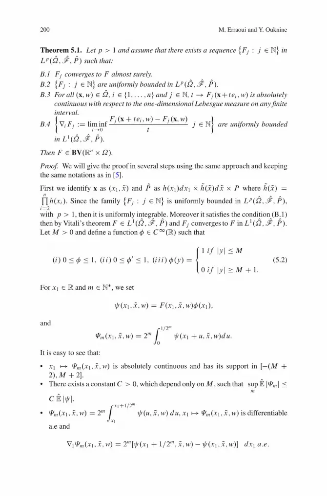
200 M. Erraoui and Y. Ouknine
Theorem 5.1. Let p > 1 and assume that there exists a sequence˚Fj W j 2 N
�in
Lp. O ; OF ; OP / such that:
B.1 Fj converges to F almost surely.B.2
˚Fj W j 2 N
�are uniformly bounded in Lp. O ; OF ; OP /.
B.3 For all .x;w/ 2 O , i 2 f1; : : : ; ng and j 2 N, t ! Fj .xC tei ;w/ is absolutelycontinuous with respect to the one-dimensional Lebesgue measure on any finiteinterval.
B.4
�
riFj WD lim inft!0
Fj .x C tei ;w/ � Fj .x;w/t
j 2 N
�
are uniformly bounded
in L1. O ; OF ; OP/.Then F 2 BV.Rn �˝/.Proof. We will give the proof in several steps using the same approach and keepingthe same notations as in [5].
First we identify x as .x1; Qx/ and OP as h.x1/dx1 � Qh. Qx/d Qx � P where Qh. Qx/ DnQ
iD2h.xi /. Since the family
˚Fj W j 2 N
�is uniformly bounded in Lp. O ; OF ; OP /,
with p > 1, then it is uniformly integrable. Moreover it satisfies the condition (B.1)then by Vitali’s theoremF 2 L1. O ; OF ; OP / andFj converges toF inL1. O ; OF ; OP /.Let M > 0 and define a function � 2 C1.R/ such that
.i/ 0 � � � 1; .i i/ 0 � �0 � 1; .i i i/ �.y/ D8<
:
1 if jyj � M
0 if jyj � M C 1:
(5.2)
For x1 2 R and m 2 N�, we set
.x1; Qx;w/ D F.x1; Qx;w/�.x1/;
and
�m.x1; Qx;w/ D 2mZ 1=2m
0
.x1 C u; Qx;w/du:
It is easy to see that:
• x1 7! �m.x1; Qx;w/ is absolutely continuous and has its support in Œ�.M C2/;M C 2�.
• There exists a constantC > 0, which depend only onM , such that supm
OE j�mj �C OE j j.
• �m.x1; Qx;w/ D 2mZ x1C1=2m
x1
.u; Qx;w/ du, x1 7! �m.x1; Qx;w/ is differentiable
a.e and
r1�m.x1; Qx;w/ D 2mŒ .x1 C 1=2m; Qx;w/ � .x1; Qx;w/� dx1 a:e:
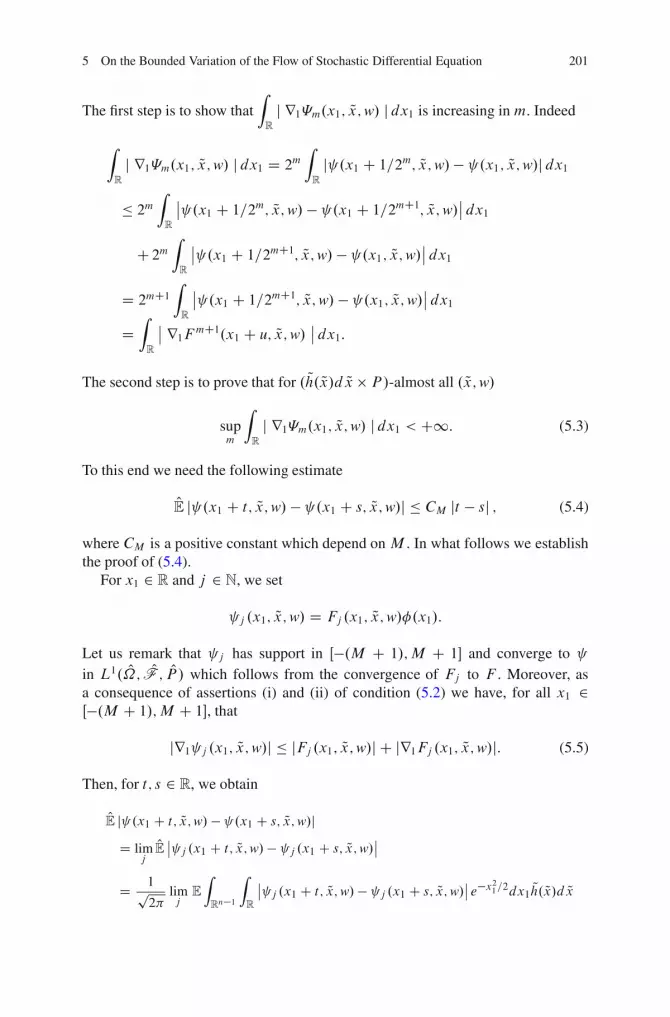
5 On the Bounded Variation of the Flow of Stochastic Differential Equation 201
The first step is to show thatZ
R
j r1�m.x1; Qx;w/ j dx1 is increasing in m. Indeed
Z
R
j r1�m.x1; Qx;w/ j dx1 D 2mZ
R
j .x1 C 1=2m; Qx;w/� .x1; Qx;w/j dx1
� 2mZ
R
ˇˇ .x1 C 1=2m; Qx;w/ � .x1 C 1=2mC1; Qx;w/ˇˇ dx1
C 2mZ
R
ˇˇ .x1 C 1=2mC1; Qx;w/ � .x1; Qx;w/ˇˇ dx1
D 2mC1Z
R
ˇˇ .x1 C 1=2mC1; Qx;w/ � .x1; Qx;w/ˇˇ dx1
DZ
R
ˇˇ r1F
mC1.x1 C u; Qx;w/ ˇˇ dx1:
The second step is to prove that for . Qh. Qx/d Qx � P/-almost all . Qx;w/
supm
Z
R
j r1�m.x1; Qx;w/ jdx1 < C1: (5.3)
To this end we need the following estimate
OE j .x1 C t; Qx;w/ � .x1 C s; Qx;w/j � CM jt � sj ; (5.4)
where CM is a positive constant which depend on M . In what follows we establishthe proof of (5.4).
For x1 2 R and j 2 N, we set
j .x1; Qx;w/ D Fj .x1; Qx;w/�.x1/:
Let us remark that j has support in Œ�.M C 1/;M C 1� and converge to in L1. O ; OF ; OP / which follows from the convergence of Fj to F . Moreover, asa consequence of assertions (i) and (ii) of condition (5.2) we have, for all x1 2Œ�.M C 1/;M C 1�, that
jr1 j .x1; Qx;w/j � jFj .x1; Qx;w/j C jr1Fj .x1; Qx;w/j: (5.5)
Then, for t; s 2 R, we obtain
OE j .x1 C t; Qx;w/ � .x1 C s; Qx;w/jD lim
j
OE ˇˇ j .x1 C t; Qx;w/� j .x1 C s; Qx;w/ˇˇ
D 1p2�
limj
E
Z
Rn�1
Z
R
ˇˇ j .x1 C t; Qx;w/� j .x1 C s; Qx;w/ˇˇ e�x21=2dx1 Qh. Qx/d Qx

202 M. Erraoui and Y. Ouknine
� 1p2�
lim infj
E
Z
Rn�1
Z
R
ˇˇˇˇ
Z t
sr1 j .x1 C u; Qx;w/du
ˇˇˇˇ dx1
Qh. Qx/d Qx
� 1p2�
lim infj
E
Z t
s
Z
Rn�1
Z
R
ˇˇr1 j .x1 C u; Qx;w/ˇˇdx1 Qh. Qx/d Qxdu
� 1p2�
jt � sj e.MC2/2=2 supj
OE.ˇˇFj .x1; Qx;w/ jCj r1Fj .x1; Qx;w/ˇˇ/;
where the last inequality is a consequence of (5.5). Now using (B.2) and (B.4) weobtain
OE j .x1 C t; Qx;w/ � .x1 C s; Qx;w/j � CM jt � sj ;
where CM D 1p2�e.MC2/
2=2 supj
OE.ˇˇFj .x1; Qx;w/ jCj r1Fj .x1; Qx;w/ˇˇ/:Now we are able to make out (5.3). By monotone convergence theorem we have
E
Z
Rn�1
supm
Z
R
jr1�m.x1; Qx;w/j dx1 Qh. Qx/d Qx
D supm
E
Z
Rn�1
Z
R
jr1�m.x1; Qx;w/j dx1 Qh. Qx/d Qx
Since �m has support in Œ�.M C 2/;M C 2� then
E
Z
Rn�1
supm
Z
R
jr1�m.x1; Qx;w/j dx1 Qh. Qx/d Qx � p2� e.MC2/
2=2 OE jr1�m.x1; Qx;w/j
� p2� e.MC2/2=2 sup
m2m OE j .x1 C 1=2m; Qx;w/� .x1; Qx;w/j :
Now using (5.4) we obtain
E
Z
Rn�1
supm
Z
R
jr1�m.x1; Qx;w/j dx1 Qh. Qx/d Qx � p2� e.MC2/
2=2CM : (5.6)
Therefore, for . Qh. Qx/d Qx � P/-almost all . Qx;w/,
supm
Z
R
jr1�m.x1; Qx;w/j dx1 < C1:
On the other hand, by the definition of �m, for all . Qx;w/ there exists a functionNF1.�; Qx;w/ so that
limm�m.x1; Qx;w/ D NF1.x1; Qx;w/�.x1/
NF1.:; Qx;w/ D F.:; Qx;w/; dx1 � a:e:

5 On the Bounded Variation of the Flow of Stochastic Differential Equation 203
Hence, by Corollary 5.3.4 of [7], we have NF1.:; Qx;w/�.:/ is a function of boundedvariation on R for . Qh. Qx/d Qx � P/-almost all . Qx;w/. So, for . Qh. Qx/d Qx � P/-almostall . Qx;w/, and for all M > 0, NF1.:; Qx;w/ is a function of bounded variation onŒ�M;M� such that
VŒ�M;M�NF1.:; Qx;w/ � sup
m
Z
R
jr1�m.x1; Qx;w/j dx1;
where VŒ�M;M�.f / denotes the total variation of the function f on Œ�M;M�. Itfollows from (5.6) that
E
Z
Rn�1
VŒ�M;M�NF1.:; Qx;w/ Qh. Qx/d Qx � E
Z
Rn�1
supm
Z
R
jr1�m.x1; Qx;w/j dx1 Qh. Qx/d Qx
� p2� e.MC2/2=2CM :
Thus for P -almost all w and for each rectangular cell R of the formnQ
iD2Œ�M;M�
we have Z
R
VŒ�M;M�NF1.:; Qx;w/d Qx < C1: (5.7)
Now for 2 � i � n, we write x as .xi ; Qx/ where Qx 2 Rn�1. Then using the same
procedure as that used above we obtain that there exists a function NFi .�; Qx;w/ so that
NFi .:; Qx;w/ D F.:; Qx;w/; dxi � a:e:
Moreover for P -almost all w and for each rectangular cell R in Rn�1 we have
Z
R
VŒ�M;M�NFi .xi ; Qx;w/d Qx < C1: (5.8)
Therefore, we conclude by Theorem 5.3.5 of [7] that F 2 BV.Rn �˝/.Let F is in BV.Rn �˝/ and OF its associated according to the above definition.
Then for each 1 � i � n the function t ! OF .x C tei ;w/ is a function of boundedvariation on any finite interval. Consequently it is differentiable a.e and for all w 2˝
riOF .x;w/ D lim inf
t!0OF .x C tei ;w/ � OF .x;w/
t:
We can prove as in Bouleau-Hirsch [2] that riF is well defined OP -a.s. and thisdefinition does not depend on the representative OF , up to OP -a.s. equality. This isgiven in the following proposition
Proposition 5.1. If F 2 BV.Rn � ˝/ then for P -almost all w 2 ˝ and for alli 2 f1; : : : : : : ; ng we have:
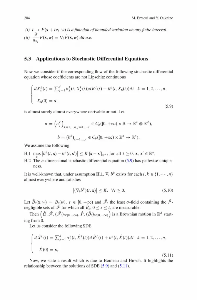
204 M. Erraoui and Y. Ouknine
(i) t ! F.x C tei ;w/ is a function of bounded variation on any finite interval.
(ii)@
@xiF.x;w/ D ri
OF .x;w/ dx-a.e.
5.3 Applications to Stochastic Differential Equations
Now we consider if the corresponding flow of the following stochastic differentialequation whose coefficients are not Lipschitz continuous
8
<
:
dXkx .t/ D Pd
jD1 �kj .t; Xkx .t//dB
j .t/C bk.t; Xx.t//dt k D 1; 2; : : : ; n;
Xx.0/ D x;(5.9)
is almost surely almost everywhere derivable or not. Let
� D��kj
�
kD1;:::;n;jD1;:::;d 2 Cb.Œ0;C1/ � R ! Rn ˝ R
d /;
b D �bk�
kD1;:::;n 2 Cb.Œ0;C1/ � Rn ! R
n/;
We assume the following
H.1 maxk
ˇˇbk.t; x/ � bk.t; x0/ˇˇ � K jx � x0j
Rn; for all t � 0; x; x0 2 R
n.
H.2 The n-dimensional stochastic differential equation (5.9) has pathwise unique-ness.
It is well-known that, under assumption H.1, ri bk exists for each i; k 2 f1; � � � ; ng
almost everywhere and satisfies
ˇˇ.ri b
k/.t; x/ˇˇ � K; 8t � 0: (5.10)
Let OBt.x;w/ D Bt.w/; t 2 Œ0;C1/ and OFt the least �-field containing the OP -negligible sets of OF for which all OBs , 0 � s � t , are measurable.
Then� O ; OF ; . OFt /t2Œ0;C1/; OP ; . OBt /t2Œ0;C1/
�is a Brownian motion in R
d start-
ing from 0.Let us consider the following SDE
8
<
:
d OXk.t/ D PdjD1 �kj .t; OXk.t//d OBj .t/C bk.t; OX.t//dt k D 1; 2; : : : ; n;
OX.0/ D x;(5.11)
Now, we state a result which is due to Bouleau and Hirsch. It highlights therelationship between the solutions of SDE (5.9) and (5.11).

5 On the Bounded Variation of the Flow of Stochastic Differential Equation 205
Proposition 5.2. There exists a OP -negligible set ON such that
8.x;w/ 2 ONc 8t � 0 OX.t/.x;w/ D Xx.t/.w/
For the first, we will show a lemma which makes the most important role in thispaper.
Lemma 5.1. Let f D .fj /jD1;2;:::;d be an Rd – valued measurable function on
Œ0;C1/ � O , and g be a measurable function on Œ0;C1/ � O . We assume that a1-dimensional Ft -adapted continuous process OY D . OY .t// on . O ; OF ; OP / satisfiesthe stochastic differential equation
OY .t/ D y CdX
jD1
Z t
0
fj .s; y;w/ OY .s/d OBjs C
Z t
0
g.s; y;w/ds; (5.12)
where y 2 R. Moreover, we assume that
maxj
supt;y;w
ˇˇfj .t; y;w/
ˇˇ < 1; (5.13)
and there exists a constant L satisfying that
jg.t; y;w/j � Lˇˇˇ OY .t/
ˇˇˇ ; for all .t; .y;w// 2 Œ0;C1/ � O : (5.14)
Then, for each T � 0 there exists a constant C which depends on only T;L suchthat
supt2Œ0;T �
OEˇˇˇ OY .t/
ˇˇˇ � C:
Proof. For .t; .y;w// 2 Œ0;C1/ � O , define:
Og.t; y;w/ D
8ˆ<
ˆ:
g.t; y;w/OY .t/ if OY .t/ ¤ 0;
0 if OY .t/ D 0:
Then it follows from (5.14) that
j Og.s; y;w/j � L; for all .t; .y;w// 2 Œ0;C1/ � O :
Moreover it is easy to see that OY satisfies the following Linear stochastic differentialequation
OY .t/ D y CdX
jD1
Z t
0
fj .s; y;w/ OY .s/d OBjs C
Z t
0
Og.s; y;w/ OY .s/ds: (5.15)

206 M. Erraoui and Y. Ouknine
Thus we have
OY .t/ D y exp
0
@dX
jD1
Z t
0
fj .s; y;w/d OBjs CZ t
0
Og.s; y;w/ds
� 1
2
dX
jD1
Z t
0
fj .s; y;w/2ds
1
A : (5.16)
Since Og is bounded by L we deduce the following estimate
j OY .t/j � jyjeLT exp
0
@dX
jD1
Z t
0
fj .s; y;w/d OBjs � 1
2
dX
jD1
Z t
0
fj .s; y;w/2ds
1
A
for all t 2 Œ0; T �.Using condition (5.13), yields that the exponential
exp
0
@dX
jD1
Z t
0
fj .s; y;w/d OBjs � 1
2
dX
jD1
Z t
0
fj .s; y;w/2ds
1
A
is a . OFt � OP/-martingale. Therefore, for all t 2 Œ0; T �, we obtain
OEˇˇˇ OY .t/
ˇˇˇ � jyjeLT :
This establishes the lemma.
The next lemma is a version of the above lemma about derivative of a stochasticdifferential equation.
Lemma 5.2. We assume that
� D��kj
�
kD1;:::;n;jD1;:::;d 2 Cb.Œ0;C1/ � R ! Rn ˝ R
d /;
�kj .t; �/ 2 C1.R/; t 2 Œ0;C1/ and @x�kj .�; �/ is bounded on compact subsets ofŒ0;C1/ � R;
b D �bk�
kD1;:::;n 2 Cb.Œ0;C1/ � Rn ! R
n/;
bk.t; �/ 2 C1.Rn ! Rn//; t 2 Œ0;C1/;
and assumptions (H.1)–(H.2) hold. Then, for each T � 0, the solution OX on. O ; OF ; OP / of the stochastic differential equation (5.11) satisfies
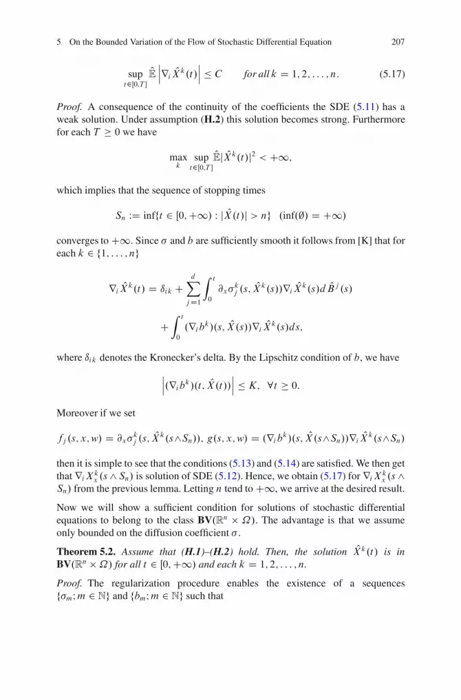
5 On the Bounded Variation of the Flow of Stochastic Differential Equation 207
supt2Œ0;T �
OEˇˇˇri
OXk.t/ˇˇˇ � C for all k D 1; 2; : : : ; n: (5.17)
Proof. A consequence of the continuity of the coefficients the SDE (5.11) has aweak solution. Under assumption (H.2) this solution becomes strong. Furthermorefor each T � 0 we have
maxk
supt2Œ0;T �
OEj OXk.t/j2 < C1;
which implies that the sequence of stopping times
Sn WD infft 2 Œ0;C1/ W j OX.t/j > ng .inf.;/ D C1/
converges to C1. Since � and b are sufficiently smooth it follows from [K] that foreach k 2 f1; : : : ; ng
riOXk.t/ D ıik C
dX
jD1
Z t
0
@x�kj .s;
OXk.s//riOXk.s/d OBj .s/
CZ t
0
.ri bk/.s; OX.s//ri
OXk.s/ds;
where ıik denotes the Kronecker’s delta. By the Lipschitz condition of b, we have
ˇˇˇ.ri b
k/.t; OX.t//ˇˇˇ � K; 8t � 0:
Moreover if we set
fj .s; x;w/ D @x�kj .s;
OXk.s^Sn//; g.s; x;w/ D .ri bk/.s; OX.s^Sn//ri
OXk.s^Sn/
then it is simple to see that the conditions (5.13) and (5.14) are satisfied. We then getthat riX
kx .s ^Sn/ is solution of SDE (5.12). Hence, we obtain (5.17) for riX
kx .s^
Sn/ from the previous lemma. Letting n tend to C1, we arrive at the desired result.
Now we will show a sufficient condition for solutions of stochastic differentialequations to belong to the class BV.Rn � ˝/. The advantage is that we assumeonly bounded on the diffusion coefficient � .
Theorem 5.2. Assume that (H.1)–(H.2) hold. Then, the solution OXk.t/ is inBV.Rn �˝/ for all t 2 Œ0;C1/ and each k D 1; 2; : : : ; n.
Proof. The regularization procedure enables the existence of a sequencesf�mIm 2 Ng and fbmIm 2 Ng such that

208 M. Erraoui and Y. Ouknine
�m D��kj;m
�
kD1;:::;n;jD1;:::;d 2 Cb.Œ0;C1/ � R ! Rn ˝ R
d /;
�kj;m.t; �/ 2 C1.R/; t 2 Œ0;C1/;
bm D �bkm�
kD1;:::;n 2 Cb.Œ0;C1/ � Rn ! R
n/;
bkm.t; �/ 2 C1.Rn ! Rn//; t 2 Œ0;C1/;
supm
ˇˇ.ri b
kn/.t; x/
ˇˇ � K; 8 t � 0; x 2 R
n:
limm
supt2Œ0;T �
supx2K
j�m.t; x/ � �.t; x/jRn˝Rd C jbm.t; x/ � b.t; x/jRn D 0
for each compact K in Rn. Let fZn
x In 2 Ng be the strong solutions of the SDE(5.9) with coefficients �n and bn and the Brownian motion B . Then, by a standardmethod of stochastic differential equations and (5.17) of Lemma 5.2 we have for alli 2 f1; � � � ; ng and t 2 Œ0;C1/
supm
E jZmx .t/j2Rn < 1 and sup
m
E jri .Zmx .t/jRn < 1: (5.18)
On the other hand we have from [3] that
limn!C1 sup
x2KE . max
t2Œ0;T � jZnx .t/ �Xx.t/j2Rn / D 0: (5.19)
Let M > 0 and ˚ be a fixed function in C1.Rn/ satisfying
˚.x/ D 1 if x 2nQ
iD1Œ�M;M�;
˚.x/ D 0 if x …nQ
iD1Œ�M C 1;M C 1�;
jri˚.x/j � C (constant) for all x 2 Rn:
Letn OZmIm 2 N
obe the strong solution of the SDE (5.11) with coefficients �m and
bm and the Brownian motion OB . It follows from (5.18–5.19) and Proposition 5.2that
supm
OEˇˇˇ OZm.t/ ˚.x/
ˇˇˇ2
Rn< 1 and sup
m
OEˇˇˇri . OZm.t/ ˚.x//
ˇˇˇRn< 1; (5.20)
andlim
m!C1OE . max
t2Œ0;T � j OZm.t/˚.x/� OX.t/˚.x/j2Rn/ D 0: (5.21)
5 On the Bounded Variation of the Flow of Stochastic Differential Equation 209
It is easy to see that (5.20) means that the family f OZm˚;m 2 Ng satisfies condition(B.2) and (B.4) of Theorem 7.1. Furthermore, for each m 2 N, OZm ˚ satisfies thesmoothness property (B.3), cf. Kunita [4]. It follows from (5.21) that there existsa subsequence of f OZm˚;m 2 Ng which converges OP -almost surely to OX˚ . Forsimplicity, we also denote the subsequence by f OZm˚;m 2 Ng again. Thus, wecan use Theorem 2.2, and we have OX.t/˚.x/ is in BV.Rn � ˝/ and consequentlyOX.t/ 2 BV.Rn �˝/ for all t 2 Œ0;C1/.
Now as a consequence of the foregoing we obtain the following result
Theorem 5.3. Assume that (H.1)–(H.2) hold. Then, for almost all w the flow x 7!Xx.t;w/ is a function of bounded variation on each compact in R
n.
Acknowledgements The authors wish to thank the anonymous referee for the suggestion of asimple proof of Lemma 1. This work was supported by the Academy Hassan II of Sciences andTechnology
References
1. Bouleau, N. Hirsch, F.: On the derivability with respect to the initial data of the solution of astochastic differential equation with lipschitz coefficients. In: Seminaire de Theorie du PotentialParis, 9, 39–57. Springer, Berlin (1989)
2. Bouleau, N. Hirsch, F.: Proprietes d’absolue continuite dans les espaces de Dirichlet etapplication aux equations differentielles stochastiques. In: Seminaire de Probabilites, XX,131–161. Springer, Berlin (1986)
3. Kaneko, H., Nakao, S.: A note on approximation for stochastic differential equations. In:Seminaire de Probabilites, XXII, 155–162. Springer, Berlin (1988)
4. Kunita, H.: Stochastic differential equations and stochastic flows of diffeomorphisms. In: Ecoled’ete de probabilites de Saint-Flour, XII-1982, 143–303. Springer, Berlin (1984)
5. Kusuoka, S.: Existence of densities of solutions of stochastic differential equations by Malliavincalculus. J. Funct. Anal. 258, 758–784 (2010)
6. Revuz, D. Yor, M.: Continuous martingales and Brownian motion. Springer-Verlag, Berlin(1999)
7. Ziemer William, P.: Weakly differentiable functions. Sobolev spaces and functions of boundedvariation. Springer-Verlag, New York (1989)

�
Chapter 6Stochastic Volatility and MultifractionalBrownian Motion
Antoine Ayache and Qidi Peng
Abstract In order to make stochastic volatility models more realistic some authors(see for example Comte and Renault J. Econom. 73:101–150, 1996; Comte andRenault Math. Financ. 8:291–323, 1998; Gloter, A., Hoffmann, M.: Stochasticvolatility and fractional Brownian motion Stoch. Proc. Appl. 113:143–172, 2004;Rosenbaum Stoch. Proc. Appl. 118:1434–1462, 2008) have proposed to replace theBrownian motion governing the volatility by a more flexible stochastic process.This is why, we introduce multifractional stochastic volatility models; their mainadvantage is that they allow to account variations with respect to time of volatilitylocal roughness. Our definition of multifractional stochastic volatility models isinspired by that of the fractional stochastic volatility models previously introducedby Gloter and Hoffmann (Gloter, A., Hoffmann, M.: Stochastic volatility and frac-tional Brownian motion, Stoch. Proc. 502 Appl. 113:143–172, 2004). The main goalof our article is to extend to these new models some theoretical results concerningstatistical inference which were obtained in (Gloter, A., Hoffmann, M.: Stochasticvolatility and fractional Brownian motion, Stoch. Proc. Appl. 113:143–172, 2004).More precisely, assuming that the functional parameter H.�/ of multifractionalBrownian motion is known, we construct, in a general framework, an estimator ofintegrated functional of the volatility, and we derive from it, in the linear case, anestimator of a parameter � related to the volatility.
A. Ayache (�)U.M.R. CNRS 8524, Laboratory Paul Painleve, University Lille 1, 59655 Villeneuve d’AscqCedex, Francee-mail: [email protected]
Q. PengU.M.R. CNRS 8524, Laboratory Paul Painleve, University Lille 1, 59655 Villeneuve d’AscqCedex, Francee-mail: [email protected]
M. Zili and D.V. Filatova (eds.), Stochastic Differential Equations and Processes,Springer Proceedings in Mathematics 7, DOI 10.1007/978-3-642-22368-6 6,© Springer-Verlag Berlin Heidelberg 2012
211
212 A. Ayache and Q. Peng
6.1 Introduction and Motivation
Stochastic volatility models are extensions of the well-known Black and Scholesmodel. Hull and White [22] and other authors in mathematical finance (see forinstance [30] and [25]) introduced them in the eighties in order to account thevolatility effects of exogenous arrivals of information. Our article is inspired froma work of Gloter and Hoffmann [21, 22] which concerns statistical inference in aparametric stochastic volatility model driven by a fractional Brownian motion (fBmfor short). Namely, the model considered in [21, 22] can be expressed as:
�Z.t/ D z0 C R t
0�.s/ dW.s/
�.s/ D �0 C ˚.�;B˛.s//;(6.1)
where:
• Z.t/ denotes logarithm of the price of the underlying asset, the original price z0is supposed to be deterministic and known.
• fW.s/gs2Œ0;1� denotes a standard Brownian motion (Bm for short).• f�.s/gs2Œ0;1� denotes the volatility process (�0 is real-valued and known); the
deterministic function x 7! ˚.�; x/, through which it is defined, is known upto a real-valued parameter � . For the sake of convenience, one sets for everyx 2 R,
f .x/ WD .�0 C ˚.�; x//2 (6.2)
and throughout this article one assumes that the function f belongs to the setC2pol .R/. Observe that for every integer l � 0, C l
pol .R/ denotes the vector spaceof l-times continuously differentiable functions over the real line, which slowlyincrease at infinity as well as their derivative of any order, more formally,
C lpol .R/ WD
nh 2 C l.R/ W 9c;K > 0 ;8 x 2 R;
lX
kD0jh.k/.x/j � c
�1C jxjK�
o:
(6.3)• fB˛.s/gs2Œ0;1� denotes a fractional Brownian motion (fBm for short) with Hurst
parameter ˛ (see e.g. [15,16,29]), which is assumed to be independent on the BmfW.s/gs2Œ0;1�; one makes the latter independence assumption for the stochasticintegral
R t0�.s/ dW.s/ to be well-defined. Note that the idea of replacing the Bm
governing the volatility by a fBm is due to Comte and Renault (see [13,14]), whohave proposed to do so in order to account some long memory effects.
In order to clearly explain the main goal of our article, we need to brieflypresent some of the main results obtained in [21, 22]. In the latter articles, it isassumed that one observes a discretized trajectory of the process fZ.t/gt2Œ0;1�,namely the high frequency data Z.j=n/, j D 0; : : : ; n. Also, it is assumed that

6 Stochastic Volatility and Multifractional Brownian Motion 213
the fBm B˛ governing the volatility is hidden; however one knows the value of itsHurst parameter ˛, moreover ˛ 2 .1=2; 1/. Though, the hypothesis that the Hurstparameter is known may seem to be restrictive from a practical point of view, it hasalready been made by other authors (see for example [35]), in some settings moreor less related to that of the model (6.1). Under additional technical assumptions,we will not give here for the sake of simplicity, Gloter and Hoffmann [21, 22] haveobtained the following results .1/ and .2/:
1: By using the notion of generalized quadratic variation, one can con-struct estimators of integrated functional of the volatility of the form:R 10 f0.B˛.s//2h.�2.s// ds, where f 0 is the derivative of f and h 2 C1
pol .R/
is arbitrary and fixed. Note that the problem of the estimation of such quantitiesis of some importance in its own right, since more or less similar integrals appearin some option pricing formulas (see for instance [22]).
2: Thanks to the result .1/, it is possible to build a minimax optimal estimator ofthe unknown parameter � . Also, it is worth noticing that, it has been shown in[21, 22] that the minimax rate of convergence for estimating � , in the setting ofthe model (6.1), is not the usual rate n�1=2 but the slower rate n�1=.4˛C2/, whichdeteriorates when the Hurst parameter ˛ increases; basically, the reason for thisunusual phenomenon is that the volatility is hidden and the Brownian motion Wmakes the approximation of the volatility more noisy.
Let us now present the main motivation behind the introduction of multifractionalstochastic volatility models. To this end, first we need to introduce the notionof pointwise Holder exponent. Let fX.s/gs2Œ0;1� be a stochastic process whosetrajectories are with probability 1, continuous and nowhere differentiable functions(this is the case of fBm and of multifractional Brownian motion which will soon beintroduced), �X.t/ the pointwise Holder exponent of the process fX.s/gs2Œ0;1� at anarbitrary time t , is defined as,
�X.t/ D supn� 2 Œ0; 1� W lim sup
�!0X.t C �/ �X.t/
j� j� D 0o:
The quantity of �X.t/ provides a measure of fX.s/gs2Œ0;1� roughness (i.e. of themaximum of the fluctuations amplitudes of fX.s/gs2Œ0;1�) in a neighborhood of t ;the smaller �X.t/ is the rougher (i.e. the more fluctuating) is fX.s/gs2Œ0;1� in tneighborhood. In [1] numerical evidences have shown that for a better understand-ing of stock price dynamics, it is important to analyze volatility local roughness.With this respect, fractional stochastic volatility model has a serious limitation: itsvolatility local roughness cannot evolve with time; more precisely, when ˚.�; �/is a continuously differentiable function with a nowhere vanishing derivative, thenone has, almost surely, at any time t , ��.t/ D ˛, where ˛ is the constant Hurstparameter of the fBm fB˛.s/gs2Œ0;1� and ��.t/ the pointwise Holder exponent at t ,of the volatility process f�.s/gs2Œ0;1� defined in (6.1). The latter limitation is due to

214 A. Ayache and Q. Peng
the fact that the local roughness of fB˛.s/gs2Œ0;1� itself cannot change from time totime, namely one has almost surely, for all t , �B˛ .t/ D ˛ (see e.g. [23]). In orderto overcome this drawback, we propose to replace in (6.1), the fBm fB˛.s/gs2Œ0;1�by a multifractional Brownian motion (mBm for short), denoted in all the sequelby fX.s/gs2Œ0;1�, which is independent on fW.s/gs2Œ0;1�. Thus, we obtain a newstochastic volatility model we call multifractional stochastic volatility model. Itsprecise definition is the following:
�Z.t/ D z0 C R t
0�.s/ dW.s/
�.s/ D �0 C ˚.�;X.s//;(6.4)
where z0, �0, � , ˚.�; �/ and fW.s/gs2Œ0;1� satisfy the same assumptions as before;note that the stochastic integral
R t0 �.s/ dW.s/ is well-defined since the mBm
fX.s/gs2Œ0;1� is assumed to be independent on the Bm fW.s/gs2Œ0;1�. In order toclearly explain the reason why multifractional stochastic volatility model allowsto overcome the limitation of fractional volatility model we have already pointedout we need to make some brief recalls concerning mBm. The latter non stationaryincrements centered Gaussian process was introduced independently in [8] and [26],in order to avoid some drawbacks coming from the fact that the Hurst parameter offBm cannot evolve with time. The mBm fX.s/gs2Œ0;1� can be obtained by substitutingto the constant Hurst parameter ˛ in the harmonizable representation of fBm:
B˛.s/ DZ
R
eis� � 1j�j˛C1=2 dbB.�/; (6.5)
a function H.�/ depending continuously on time and with values in .0; 1/. Theprocess fX.s/gs2Œ0;1� can therefore be expressed as,
X.s/ WDZ
R
eis� � 1j�jH.s/C1=2 dbB.�/: (6.6)
Throughout our article not only we assume that H.�/ is continuous but also that itis a C2-function, actually we need to impose this condition in order to be able toestimate the correlations between the generalized increments of local averages ofmBm (see Proposition 6.3.6). Moreover, to obtain Part .i i/ of Lemma 6.3.2, weneed to assume that H.�/ is with values in .1=2; 1/.
For the sake of clarity, notice that dbB is defined as the unique complex-valuedstochastic Wiener measure which satisfies for all f 2 L2.R/,
Z
R
f .s/ dB.s/ DZ
R
bf .�/ dbB.�/; (6.7)
6 Stochastic Volatility and Multifractional Brownian Motion 215
where fB.s/gs2R denotes a real-valued Wiener process and bf the Fourier transformof f . Observe that it follows from (6.7) that, one has up to a negligible deterministicsmooth real-valued multiplicative function (see [12, 34]), for all s 2 Œ0; 1�,
Z
R
njs C xjH.s/�1=2 � jxjH.s/�1=2
odB.x/ D
Z
R
eis� � 1
j�jH.s/C1=2 dbB.�/;
which implies that the process fX.s/gs2Œ0;1� is real-valued.Since several years, there is an increasing interest in the study of mBm and
related processes (see for instance [2–7, 9–11, 17–19, 31–34]). The usefulness ofsuch processes as models in financial frame has been emphasized by several authors(see for example [9–11,23,24]). Generally speaking, mBm offers a larger spectrumof applications than fBm, mainly because its local roughness can be prescribedvia its functional parameter H.�/ and thus is allowed to change with time; moreprecisely, one has almost surely, for all t , �X.t/ D H.t/, where �X.t/ denotes thepointwise Holder exponent at t of the mBm fX.s/gs2Œ0;1�. It is worth noticing thatthe latter result, in turn, implies that in the model (6.4) the volatility local roughnesscan evolve with time, namely when ˚.�; �/ is a continuously differentiable functionwith a nowhere vanishing derivative, then one has, almost surely, at any time t ,��.t/ D H.t/, where ��.t/ is the pointwise Holder exponent at t , of the volatilityprocess f�.s/gs2Œ0;1� defined in (6.4).
Having given the main motivation behind multifractional stochastic volatilitymodels, let us now clearly explain the goal of our article. Our aim is to studyto which extent it is possible to extend to the setting of these new models Gloterand Hoffmann results (1) and (2) stated above. Basically, we use some techniqueswhich are reminiscent to those in [21, 22]; however new difficulties appear in ourmultifractional setting. These new difficulties are essentially due to the fact thatlocal properties of mBm change from one time to another.
Throughout our article we assume that the functional parameter H.�/ of themBm fX.s/gs2Œ0;1� is known. We show that the result (1) can be stated in a moregeneral form and can be extended to multifractional stochastic volatility models.The challenging problem of extending the result (2) to these models remains open;the major difficulty in it, consists in precisely determining the minimax rate ofconvergence for estimating � . Yet, in the linear case, that is for a model of the form:
�Z.t/ D z0 C R t
0�.s/ dW.s/
�.s/ D �0 C �X.s/;(6.8)
assuming that there exists t0 2 .0; 1/ such that H.t0/ D mint2Œ0;1� H.t/, we givea partial solution to this problem; namely, we show that by localizing Gloter andHoffmann estimator in a well-chosen neighborhood of t0, it is possible to obtainan estimator of �2 whose rate of convergence can be bounded in probability by
n�1=.4H.t0/C2/�
logn�1=4
.

216 A. Ayache and Q. Peng
6.2 Statement of the Main Results
Let us consider an integrated functional of the volatility of the form:
Z 1
0
�f 0.X.s//
�2h.Y.s// ds; (6.9)
where, fX.s/gs2Œ0;1� denotes the mBm, fY.s/gs2Œ0;1� is the process defined as
Y.s/ WD f .X.s// WD �2.s/ WD ��0 C ˚.�;X.s//
�2; (6.10)
and h an arbitrary function of C1pol .R/. An important difficulty in the problem of the
nonparametric estimation of the integral (6.9) comes from the fact that the processfY.s/gs2Œ0;1� is hidden; as we have mentioned before, we only observe the sample.Z.0/;Z.1=n/; : : : ; Z.1//, where fZ.t/gt2Œ0;1� is the process defined in (6.4). Letus first explain how to overcome this difficulty. Y i;N , i D 0; : : : ; N � 1, the localaverage values of the process fY.s/gs2Œ0;1� over a grid f0; 1=N; : : : ; 1g,N � 1 beingan arbitrary integer, are defined, for all i D 0; : : : ; N � 1, as
Y i;N WD N
Z iC1N
iN
Y.s/ ds: (6.11)
Let us now assume that N is a well chosen integer depending on n (this choice willbe made more precise in the statements of Theorems 6.2.2 and 6.2.3 given below),such an N is denoted by Nn; moreover, we set
mn WD Œn=Nn� and for every i D 0; : : : ; Nn,ji WD Œin=Nn�; (6.12)
with the convention that Œ�� is the integer part function. The key idea to overcomethe difficulty, we have already pointed out, consists in using the fact that for n bigenough, Y i;Nn can be approximated by
bY i;Nn;n WD Nn
jiC1�ji�1X
kD0
�
Z
�ji C k C 1
n
�
�Z�ji C k
n
��2
: (6.13)
The rigorous proof of the latter approximation result relies on Ito formula, it is givenin [22] page 157 in the case of fBm and it can be easily extended to the case of mBm.This is why we will only give here a short heuristic proof. Using (6.13), (6.4), thefact that n is big enough, and (6.10), one has
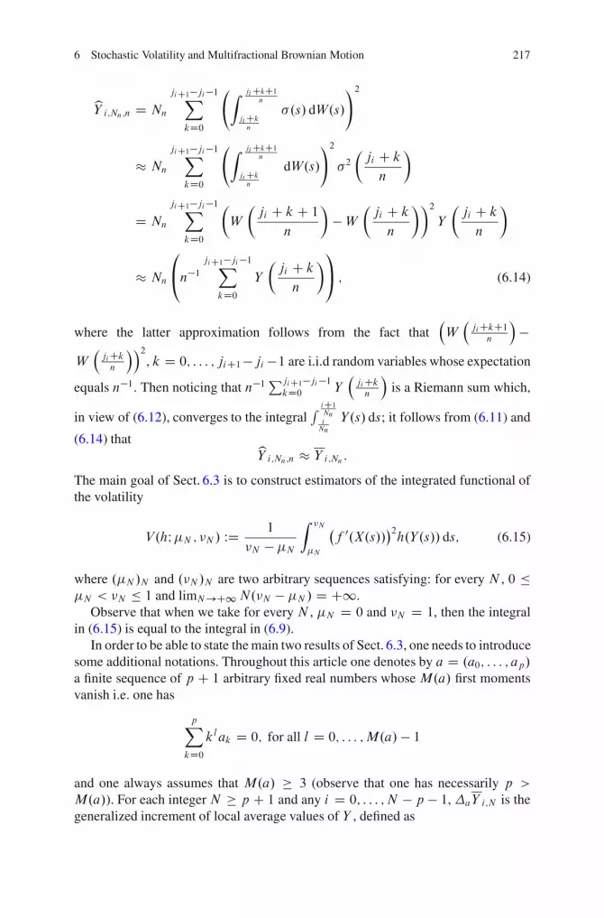
6 Stochastic Volatility and Multifractional Brownian Motion 217
bY i;Nn;n D Nn
jiC1�ji�1X
kD0
Z jiCkC1
n
jiCkn
�.s/ dW.s/
!2
� Nn
jiC1�ji�1X
kD0
Z jiCkC1n
jiCkn
dW.s/
!2
�2�ji C k
n
�
D Nn
jiC1�ji�1X
kD0
�
W
�ji C k C 1
n
�
�W�ji C k
n
��2
Y
�ji C k
n
�
� Nn
0
@n�1jiC1�ji�1X
kD0Y
�ji C k
n
�1
A ; (6.14)
where the latter approximation follows from the fact that�W�jiCkC1
n
��
W�jiCkn
��2, k D 0; : : : ; jiC1�ji �1 are i.i.d random variables whose expectation
equals n�1. Then noticing that n�1PjiC1�ji�1
kD0 Y�jiCkn
�is a Riemann sum which,
in view of (6.12), converges to the integralR iC1
NniNn
Y.s/ ds; it follows from (6.11) and
(6.14) thatbY i;Nn;n � Y i;Nn :
The main goal of Sect. 6.3 is to construct estimators of the integrated functional ofthe volatility
V.hI�N ; N / WD 1
N � �NZ N
�N
�f 0.X.s//
�2h.Y.s// ds; (6.15)
where .�N /N and .N /N are two arbitrary sequences satisfying: for every N , 0 ��N < N � 1 and limN!C1N.N � �N / D C1.
Observe that when we take for every N , �N D 0 and N D 1, then the integralin (6.15) is equal to the integral in (6.9).
In order to be able to state the main two results of Sect. 6.3, one needs to introducesome additional notations. Throughout this article one denotes by a D .a0; : : : ; ap/
a finite sequence of p C 1 arbitrary fixed real numbers whose M.a/ first momentsvanish i.e. one has
pX
kD0klak D 0; for all l D 0; : : : ;M.a/� 1
and one always assumes that M.a/ � 3 (observe that one has necessarily p >
M.a/). For each integer N � p C 1 and any i D 0; : : : ; N � p � 1, aY i;N is thegeneralized increment of local average values of Y , defined as

218 A. Ayache and Q. Peng
aY i;N WDpX
kD0akY iCk;N (6.16)
andaXi;N is the generalized increment of local average values of mBmX , definedas
aXi;N WDpX
kD0akXiCk;N ; (6.17)
where
Xi;N WD N
Z iC1N
iN
X.s/ ds: (6.18)
At last, for each integer n big enough and any i D 0; : : : ; Nn � p � 1, one denotesby a
bY i;Nn;n the generalized increment defined as
abY i;Nn;n WDpX
kD0akbY iCk;Nn;n: (6.19)
One is now in position to state the two main results of Sect. 6.3. The following theo-rem provides an estimator of the integrated functional of the volatility V.hI�N ; N /starting from Y i;N , �N � i=N � N , the local average values of the processfY.s/gs2Œ0;1� over the grid f0; 1=N; : : : ; 1g \ Œ�N ; N �. It also provides an upperbound of the rate of convergence.
Theorem 6.2.1. For every integer N � p C 1 and for every function h 2 C1pol .R/
one sets
V .hI�N ; N / WD 1
N.N � �N /X
i2J .�N ;N /
.aY i;N /2
C.i=N /N�2H.i=N/h.Y i;N /; (6.20)
where:
• J .�N ; N / denotes the set of indices,
J .�N ; N / D ˚i 2 f0; : : : ; N � p � 1g W �N � i=N � N
I (6.21)
• For all s 2 Œ0; 1�,
C.s/ WDZ
R
jei� � 1j2jPp
kD0 akeik�j2j�j2H.s/C3 d�: (6.22)
Then there exists a constant c > 0, such that one has for each integer N � p C 1,
E
nˇˇV .hI�N ; N / � V.hI�N ; N /
ˇˇo
� c�N.N � �N /
��1=2: (6.23)
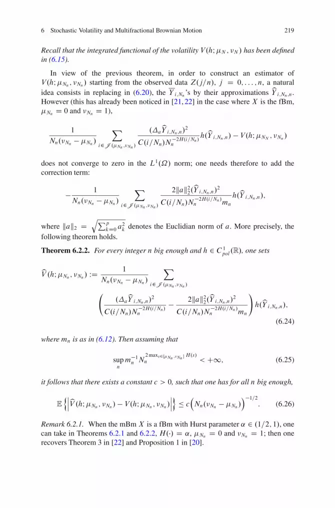
6 Stochastic Volatility and Multifractional Brownian Motion 219
Recall that the integrated functional of the volatility V.hI�N ; N / has been definedin (6.15).
In view of the previous theorem, in order to construct an estimator ofV.hI�Nn ; Nn/ starting from the observed data Z.j=n/, j D 0; : : : ; n, a naturalidea consists in replacing in (6.20), the Y i;Nn ’s by their approximations bY i;Nn;n.However (this has already been noticed in [21, 22] in the case where X is the fBm,�Nn D 0 and Nn D 1),
1
Nn.Nn � �Nn/
X
i2J .�Nn ;Nn /
.abY i;Nn;n/2
C.i=Nn/N�2H.i=Nn/n
h.bY i;Nn;n/ � V.hI�NN ; Nn/
does not converge to zero in the L1.˝/ norm; one needs therefore to add thecorrection term:
� 1
Nn.Nn � �Nn/X
i2J .�Nn ;Nn/
2kak22.bY i;Nn;n/2C.i=Nn/N
�2H.i=Nn/n mn
h.bY i;Nn;n/;
where kak2 DqPp
kD0 a2k denotes the Euclidian norm of a. More precisely, thefollowing theorem holds.
Theorem 6.2.2. For every integer n big enough and h 2 C1pol.R/, one sets
bV .hI�Nn; Nn/ WD 1
Nn.Nn � �Nn/
X
i2J .�Nn ;Nn /
.a
bY i;Nn;n/2
C.i=Nn/N�2H.i=Nn/n
� 2kak22.bY i;Nn;n/2C.i=Nn/N
�2H.i=Nn/n mn
!
h.bY i;Nn;n/;
(6.24)
where mn is as in (6.12). Then assuming that
supn
m�1n N2maxs2Œ�Nn ;Nn � H.s/n < C1; (6.25)
it follows that there exists a constant c > 0, such that one has for all n big enough,
E
nˇˇˇbV .hI�Nn ; Nn/� V.hI�Nn ; Nn/
ˇˇˇ
o� c
�Nn.Nn � �Nn/
��1=2: (6.26)
Remark 6.2.1. When the mBm X is a fBm with Hurst parameter ˛ 2 .1=2; 1/, onecan take in Theorems 6.2.1 and 6.2.2, H.�/ D ˛, �Nn D 0 and Nn D 1; then onerecovers Theorem 3 in [22] and Proposition 1 in [20].
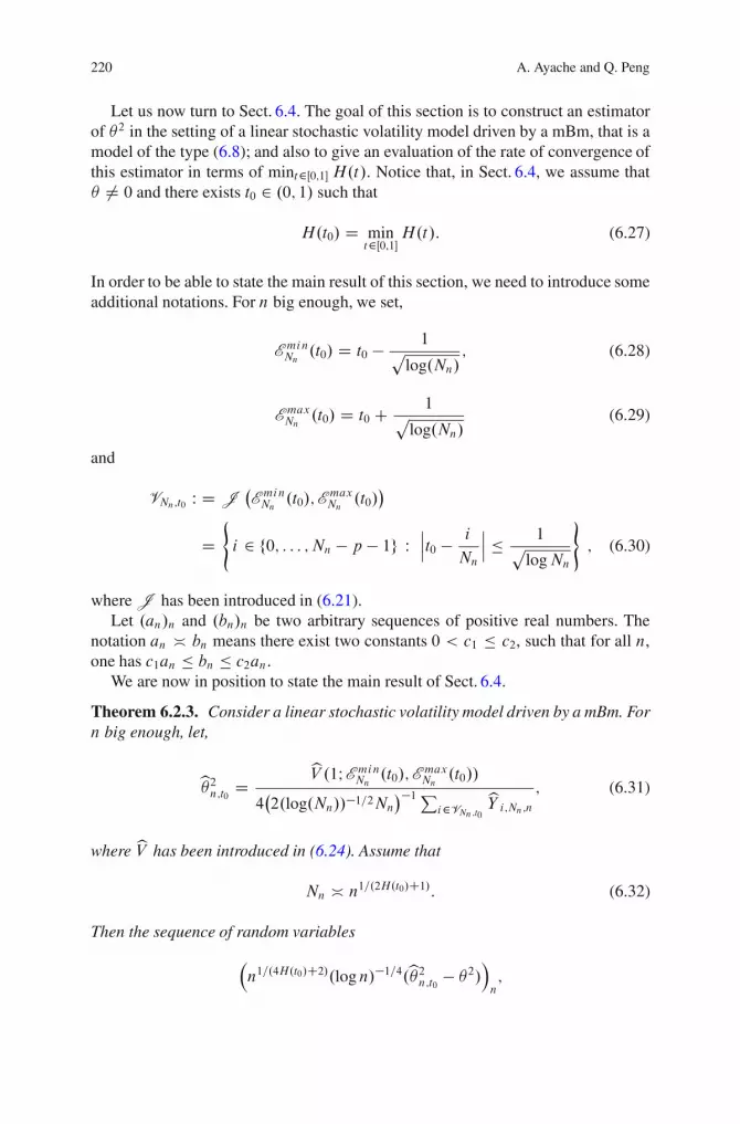
220 A. Ayache and Q. Peng
Let us now turn to Sect. 6.4. The goal of this section is to construct an estimatorof �2 in the setting of a linear stochastic volatility model driven by a mBm, that is amodel of the type (6.8); and also to give an evaluation of the rate of convergence ofthis estimator in terms of mint2Œ0;1� H.t/. Notice that, in Sect. 6.4, we assume that� ¤ 0 and there exists t0 2 .0; 1/ such that
H.t0/ D mint2Œ0;1� H.t/: (6.27)
In order to be able to state the main result of this section, we need to introduce someadditional notations. For n big enough, we set,
E minNn
.t0/ D t0 � 1p
log.Nn/; (6.28)
E maxNn
.t0/ D t0 C 1p
log.Nn/(6.29)
and
VNn;t0 W D J�E minNn
.t0/;EmaxNn
.t0/�
D(
i 2 f0; : : : ; Nn � p � 1g Wˇˇˇt0 � i
Nn
ˇˇˇ � 1
plogNn
)
; (6.30)
where J has been introduced in (6.21).Let .an/n and .bn/n be two arbitrary sequences of positive real numbers. The
notation an � bn means there exist two constants 0 < c1 � c2, such that for all n,one has c1an � bn � c2an.
We are now in position to state the main result of Sect. 6.4.
Theorem 6.2.3. Consider a linear stochastic volatility model driven by a mBm. Forn big enough, let,
b�2n;t0 DbV .1I E min
Nn.t0/;E max
Nn.t0//
4�2.log.Nn//�1=2Nn
��1Pi2VNn;t0
bY i;Nn;n; (6.31)
where bV has been introduced in (6.24). Assume that
Nn � n1=.2H.t0/C1/: (6.32)
Then the sequence of random variables
�n1=.4H.t0/C2/.logn/�1=4.b�2n;t0 � �2/
�
n;
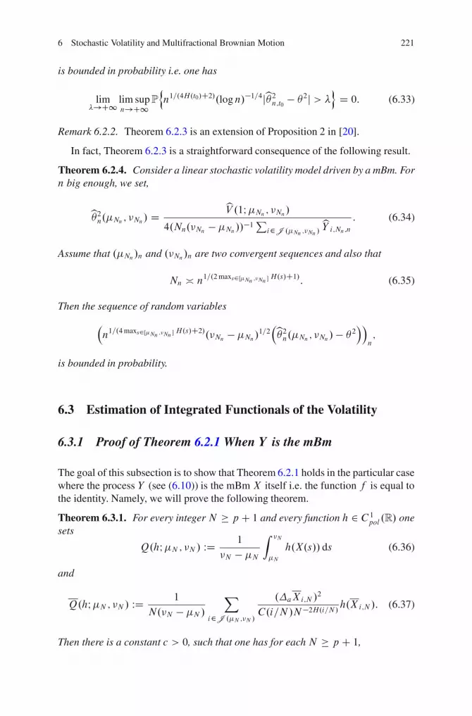
6 Stochastic Volatility and Multifractional Brownian Motion 221
is bounded in probability i.e. one has
lim�!C1 lim sup
n!C1P
nn1=.4H.t0/C2/.logn/�1=4jb�2n;t0 � �2j > �
oD 0: (6.33)
Remark 6.2.2. Theorem 6.2.3 is an extension of Proposition 2 in [20].
In fact, Theorem 6.2.3 is a straightforward consequence of the following result.
Theorem 6.2.4. Consider a linear stochastic volatility model driven by a mBm. Forn big enough, we set,
b�2n.�Nn ; Nn/ DbV .1I�Nn ; Nn/
4.Nn.Nn � �Nn//�1P
i2J .�Nn ;Nn /bY i;Nn;n
: (6.34)
Assume that .�Nn/n and .Nn/n are two convergent sequences and also that
Nn � n1=.2maxs2Œ�Nn ;Nn � H.s/C1/: (6.35)
Then the sequence of random variables
�n1=.4maxs2Œ�Nn ;Nn � H.s/C2/.Nn � �Nn/1=2
�b�2n.�Nn; Nn/� �2
��
n;
is bounded in probability.
6.3 Estimation of Integrated Functionals of the Volatility
6.3.1 Proof of Theorem 6.2.1 When Y is the mBm
The goal of this subsection is to show that Theorem 6.2.1 holds in the particular casewhere the process Y (see (6.10)) is the mBm X itself i.e. the function f is equal tothe identity. Namely, we will prove the following theorem.
Theorem 6.3.1. For every integer N � pC 1 and every function h 2 C1pol .R/ one
sets
Q.hI�N ; N / WD 1
N � �N
Z N
�N
h.X.s// ds (6.36)
and
Q.hI�N ; N / WD 1
N.N � �N /
X
i2J .�N ;N /
.aXi;N /2
C.i=N /N�2H.i=N/h.Xi;N /: (6.37)
Then there is a constant c > 0, such that one has for each N � p C 1,
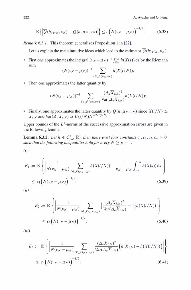
222 A. Ayache and Q. Peng
E
nˇˇˇQ.hI�N ; N /�Q.hI�N ; N /
ˇˇˇ
o� c
�N.N � �N /
��1=2: (6.38)
Remark 6.3.1. This theorem generalizes Proposition 1 in [22].
Let us explain the main intuitive ideas which lead to the estimatorQ.hI�N ; N /.• First one approximates the integral .N ��N /�1
R N�Nh.X.s// ds by the Riemann
sum.N.N � �N//
�1 X
i2J .�N ;N /
h.X.i=N //I
• Then one approximates the latter quantity by
.N.N � �N //�1X
i2J .�N ;N /
.aXi;N /2
Var.aXi;N /h.X.i=N //I
• Finally, one approximates the latter quantity by Q.hI�N ; N / since X.i=N / 'Xi;N and Var.aXi;N / ' C.i=N /N�2H.i=N/.
Upper bounds of the L1-norms of the successive approximation errors are given inthe following lemma.
Lemma 6.3.2. Let h 2 C1pol.R/, then there exist four constants c1; c2; c3; c4 > 0,
such that the following inequalities hold for every N � p C 1.
(i)
E1 WD E
8<
:
ˇˇˇˇ
1
N.N � �N /
X
i2J .�N ;N /
h.X.i=N //� 1
N � �N
Z N
�N
h.X.s// ds
ˇˇˇˇ
9=
;
� c1
�N.N � �N /
��1=2I (6.39)
(ii)
E2 WD E
8<
:
ˇˇˇˇ
1
N.N � �N /
X
i2J .�N ;N /
n .aXi;N /2
Var.aXi;N /� 1
oh.X.i=N //
ˇˇˇˇ
9=
;
� c2
�N.N � �N /
��1=2I (6.40)
(iii)
E3 WD E
8<
:
ˇˇˇˇ
1
N.N � �N /
X
i2J .�N ;N /
.aXi;N /2
Var.aXi;N /
�h.Xi;N /� h.X.i=N //
�ˇˇˇˇ
9=
;
� c3
�N.N � �N /
��1=2I (6.41)
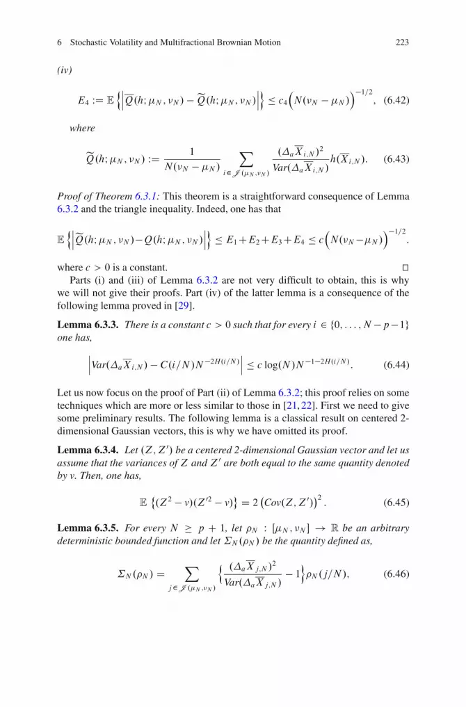
6 Stochastic Volatility and Multifractional Brownian Motion 223
(iv)
E4 WD E
nˇˇˇQ.hI�N ; N / � eQ.hI�N ; N /
ˇˇˇ
o� c4
�N.N � �N /
��1=2; (6.42)
where
eQ.hI�N ; N / WD 1
N.N � �N /X
i2J .�N ;N /
.aXi;N /2
Var.aXi;N /h.Xi;N /: (6.43)
Proof of Theorem 6.3.1: This theorem is a straightforward consequence of Lemma6.3.2 and the triangle inequality. Indeed, one has that
E
nˇˇˇeQ.hI�N ; N /�Q.hI�N ; N /
ˇˇˇ
o� E1CE2CE3CE4 � c
�N.N ��N /
��1=2:
where c > 0 is a constant. utParts (i) and (iii) of Lemma 6.3.2 are not very difficult to obtain, this is why
we will not give their proofs. Part (iv) of the latter lemma is a consequence of thefollowing lemma proved in [29].
Lemma 6.3.3. There is a constant c > 0 such that for every i 2 f0; : : : ; N �p�1gone has,
ˇˇˇVar.aXi;N / � C.i=N /N�2H.i=N/
ˇˇˇ � c log.N /N�1�2H.i=N/: (6.44)
Let us now focus on the proof of Part (ii) of Lemma 6.3.2; this proof relies on sometechniques which are more or less similar to those in [21, 22]. First we need to givesome preliminary results. The following lemma is a classical result on centered 2-dimensional Gaussian vectors, this is why we have omitted its proof.
Lemma 6.3.4. Let .Z;Z0/ be a centered 2-dimensional Gaussian vector and let usassume that the variances of Z and Z0 are both equal to the same quantity denotedby v. Then, one has,
E˚.Z2 � v/.Z02 � v/
D 2�Cov.Z;Z0/
�2: (6.45)
Lemma 6.3.5. For every N � p C 1, let �N W Œ�N ; N � ! R be an arbitrarydeterministic bounded function and let ˙N.�N / be the quantity defined as,
˙N .�N / DX
j2J .�N ;N /
n .aXj;N /2
Var.aXj;N /� 1
o�N .j=N /; (6.46)
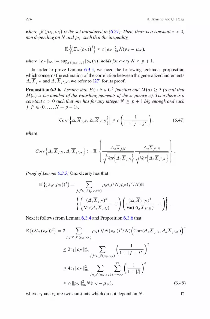
224 A. Ayache and Q. Peng
where J .�N ; N / is the set introduced in (6.21). Then, there is a constant c > 0,non depending on N and �N , such that the inequality,
E
n�˙N .�N /
�2o
� ck�N k21N.N � �N /;
where k�N k1 WD supx2Œ�N ;N � j�N .x/j holds for every N � p C 1.
In order to prove Lemma 6.3.5, we need the following technical propositionwhich concerns the estimation of the correlation between the generalized incrementsaXj;N andaXj 0;N ; we refer to [27] for its proof.
Proposition 6.3.6. Assume that H.�/ is a C2-function and M.a/ � 3 (recall thatM.a/ is the number of the vanishing moments of the sequence a). Then there is aconstant c > 0 such that one has for any integer N � p C 1 big enough and eachj; j 0 2 f0; : : : ; N � p � 1g,
ˇˇˇCorr
naXj;N ;aXj 0;N
oˇˇˇ � c
�1
1C jj � j 0j�
; (6.47)
where
CorrnaXj;N ;aXj 0;N
oWD E
8ˆ<
ˆ:
aXj;Nr
VarnaXj;N
oaXj 0;N
r
VarnaXj 0;N
o
9>>=
>>;
:
Proof of Lemma 6.3.5: One clearly has that
E˚.˙N .�N //
2 D
X
j;j 02J .�N ;N /
�N .j=N /�N .j0=N/E
( .aXj;N /
2
Var.aXj;N /� 1
! .aXj 0;N /
2
Var.aXj 0;N /� 1
!)
:
Next it follows from Lemma 6.3.4 and Proposition 6.3.6 that
E˚.˙N .�N //
2 D 2
X
j;j 02J .�N ;N /
�N .j=N /�N .j0=N/
�Corr.aXj;N ;aXj 0;N /
�2
� 2c1k�N k21X
j;j 02J .�N ;N /
�1
1C jj � j 0j�2
� 4c1k�N k21X
j2J .�N ;N /
1X
lD�1
�1
1C jl j�2
� c2k�N k21N.N � �N /; (6.48)
where c1 and c2 are two constants which do not depend onN . ut
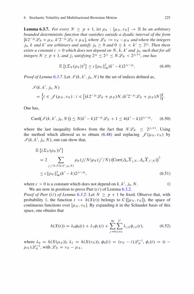
6 Stochastic Volatility and Multifractional Brownian Motion 225
Lemma 6.3.7. For every N � p C 1, let �N W Œ�N ; N � ! R be an arbitrarybounded deterministic function that vanishes outside a dyadic interval of the formŒk2�j0LN C�N ; k
02�j0LN C�N �, where LN WD N ��N and where the integersj0, k and k0 are arbitrary and satisfy j0 � 0 and 0 � k < k0 � 2j0 . Then thereexists a constant c > 0 which does not depend on N , k, k0 and j0, such that for allintegers N � p C 1, and j1 satisfying 2j0 � 2j1 � NLN < 2
j1C1, one has
E˚.˙N .�N //
2 � ck�N k21.k0 � k/2j1�j0 : (6.49)
Proof of Lemma 6.3.7. Let I .k; k0; j0; N / be the set of indices defined as,
I .k; k0; j0; N /
Dni 2 J .�N ; N / W i 2 .k2�j0LN C �N/N; .k
02�j0LN C �N /N�o:
One has,
Card�I .k; k0; j0; N /
� � N.k0 � k/2�j0LN C 1 � 4.k0 � k/2j1�j0 ; (6.50)
where the last inequality follows from the fact that NLN � 2j1C1. Usingthe method which allowed us to obtain (6.48) and replacing J .�N ; N / byI .k; k0; j0; N /, one can show that,
E˚.˙N .�N //
2
D 2X
j;j 02I .k;k0;j0;N /
�N .j=N /�N .j0=N/
�Corr.aXj;N ;aXj 0;N /
�2
� ck�N k21.k0 � k/2j1�j0 ; (6.51)
where c > 0 is a constant which does not depend on k; k0; j0; N . utWe are now in position to prove Part .i i/ of Lemma 6.3.2.
Proof of Part .i i/ of Lemma 6.3.2: Let N � p C 1 be fixed. Observe that, withprobability 1, the function t 7! h.X.t// belongs to C
�Œ�N ; N �
�, the space of
continuous functions over Œ�N ; N �. By expanding it in the Schauder basis of thisspace, one obtains that
h.X.t// D �0 0.t/C �1 1.t/C1X
jD0
2jX
kD1�j;k j;k.t/; (6.52)
where �0 D h.X.�N //, �1 D h.X.N //, 0.t/ D .N � t/L �1N , 1.t/ D .t ��N /L
�1N , with LN D N � �N ,

226 A. Ayache and Q. Peng
�j;k D 2�j2
n2h�X�2k � 1
2jC1LN C �N
��� h
�X� 2k
2jC1LN C �N
��
�h�X�2k � 22jC1
LN C �N
��o;
and
j;k.t/ D 23j=2L �1NZ t
�N
�
1h .2k�2/LN
2jC1 C�N ; .2k�1/LN
2jC1 C�Ni.s/
�1h .2k�1/LN
2jC1 C�N ; 2kLN
2jC1 C�Ni.s/
�
ds:
(6.53)
Observe that the series in (6.52) is, with probability 1, uniformly convergent inŒ�N ; N �. Now let us show that there is a constant c > 0 such that
E f�20 C �21g � c; (6.54)
and
E f�2j;kg � c2�j.1C2mins2Œ�N ;N � H.s//; for every j; k. (6.55)
By using the fact that h 2 C1pol .R/ as well as the fact that all the moments of the
random variable kXk1 WD sups2Œ0;1� jX.s/j are finite, one gets,
E j�0j2 D E
�h.X.�N //
�2 � E
�c.1C kXk1/K
�2< C1: (6.56)
Similarly, one can show that
E j�1j2 < C1: (6.57)
Combining (6.56) and (6.57), one obtains (6.54). Let us now show that (6.55) holds.Using, the expression of �j;k , the inequality .aC b/2 � 2a2 C 2b2 for all a; b 2 R
and the triangle inequality one gets,
E j�j;kj2
D E
ˇˇˇˇˇ2�
j2
(
2h
X
2k � 1
2jC1LN C �N
!!
� h
X
2k
2jC1LN C �N
!!
�h
X
2k � 22jC1
LN C �N
!!) ˇˇˇˇˇ
2

6 Stochastic Volatility and Multifractional Brownian Motion 227
� 2�j(
2E
ˇˇˇˇˇh
X
2k � 1
2jC1LN C �N
!!
� h
X
2k
2jC1LN C �N
!!ˇˇˇˇˇ
2
C2Eˇˇˇˇˇh
X
2k � 12jC1
LN C �N
!!
� h
X
2k � 22jC1
LN C �N
!!ˇˇˇˇˇ
2)
: (6.58)
Thus, in view of (6.58), for proving (6.55), it suffices to show that there is a constantc > 0 (which does not depend on N , j and k) such that one has,
E
ˇˇˇh�X�2k � 12jC1
LN C �N
��� h
�X� 2k
2jC1LN C �N
��ˇˇˇ2 � c2�2j mins2Œ�N ;N � H.s/
(6.59)and
E
ˇˇˇh�X�2k � 12jC1
LN C�N��
�h�X�2k � 22jC1
LN C�N��ˇˇˇ2 � c2�2j mins2Œ�N ;N � H.s/
(6.60)We will only prove that (6.59) holds since (6.60) can be obtained in the same way.By using the fact that h 2 C1
pol .R/, the Mean Value Theorem and Cauchy-Schwarzinequality, one has
E
ˇˇˇh
�
X
�2k � 1
2jC1LN C �N
��
� h�
X
�2k
2jC1LN C �N
�� ˇˇˇ2
� E
sups2Œ�kXk1;kXk1�
jh0.s/j! ˇˇˇˇX
�2k � 1
2jC1LN C �N
�
�X�2k
2jC1LN C �N
�ˇˇˇˇ
�2
��E�c.1C kXk1/K
�4�1=2
�
E
ˇˇˇˇX
�2k � 1
2jC1LN C �N
�
�X�2k
2jC1LN C �N
�ˇˇˇˇ
4!1=2
:
(6.61)
On the other hand, standard computations (see e.g. [6]) allow to show that, there isa constant c > 0 (non depending on N ) such that for all t; t 0 2 Œ�N ; N �, one has
E jX.t/ � X.t 0/j2 � cjt � t 0j2mins2Œ�N ;N � H.s/:
228 A. Ayache and Q. Peng
Then the latter inequality, the equivalence of the Gaussian moments and (6.61)implies that (6.59) holds; recall that (6.60) can be obtained in the same way. Nextcombining (6.58) with (6.59) and (6.60) one gets (6.55).
Now observe that (6.52) and (6.46), entail that
X
i2J .�N ;N /
(.aXi;N /
2
Var.aXi;N /� 1
)
h.X.i=N //
D �0˙N . 0/C �1˙N . 1/C1X
jD0
2jX
kD1�j;k˙N . j;k/: (6.62)
Also observe that by using the triangle inequality, Cauchy-Schwarz inequality,Lemma 6.3.5, (6.54) and the fact that k 0k1 D k 1k1 D 1, one gets that thereis a constant c > 0 such that for all N ,
Eˇˇ�0˙N . 0/C �1˙N . 1/
ˇˇ � E
ˇˇ�0˙N . 0/
ˇˇC E
ˇˇ�1˙N . 1/
ˇˇ
��Eˇˇ�0ˇˇ2�1=2�
Eˇˇ˙N . 0/
ˇˇ2�1=2
C�Eˇˇ�1ˇˇ2�1=2�
Eˇˇ˙N . 1/
ˇˇ2�1=2
� c�N.N � �N /
�1=2: (6.63)
Thus in view of (6.62) and (6.63), in order to finish our proof, it remains to showthat there exists a constant c > 0 such that for all N � p C 1, one has,
E
ˇˇˇ
1X
jD0
2jX
kD1�j;k˙N . j;k/
ˇˇˇ � c.N.N � �N //1=2: (6.64)
Let j1 � 1 be the unique integer such that
2j1 � NLN < 2j1C1:
It follows from the triangle inequality, Cauchy-Schwarz inequality, (6.55), the factthat for all j; k,
supp j;k �hk � 12j
LN C �N ;k
2jLN C �N
i; (6.65)
and Lemma 6.3.7 in which one takes j0 D j , that
6 Stochastic Volatility and Multifractional Brownian Motion 229
E
ˇˇˇ
j1X
jD0
2jX
kD1�j;k˙N . j;k/
ˇˇˇ
�j1X
jD0
2jX
kD1
�E j�j;kj2
�1=2�E j˙N . j;k/j2
�1=2
� c
j1X
jD0
2jX
kD12�j.1C2mins2Œ�N ;N � H.s//=2
�k j;kk21.k � .k � 1//2j1�j
�1=2
D c
j1X
jD0
2jX
kD12�j.1Cmins2Œ�N ;N � H.s//Cj1=2k j;kk1; (6.66)
where c > 0 is a constant. Then using (6.66), the fact that k j;kk1 � 2j=2, theinequalities mins2Œ�N ;N � H.s/ � mins2Œ0;1� H.s/ > 1=2 and 2j1 � NLN , one getsthat
E
ˇˇˇ
j1X
jD0
2jX
kD1�j;k˙N . j;k/
ˇˇˇ � c
j1X
jD0
2jX
kD12�j.1=2Cmins2Œ�N ;N � H.s//Cj1=2
� c2j1=2C1X
jD02j.1=2�mins2Œ�N ;N � H.s//
� c1.N.N � �N//1=2; (6.67)
where c1 D cPC1
jD0 2j.1=2�mins2Œ0;1� H.s// < C1. Let us now show that there is aconstant c2 > 0 non depending on j1 and N , such that
E
ˇˇˇ
1X
jDj1C1
2jX
kD1�j;k˙N . j;k/
ˇˇˇ � c2.N.N � �N //1=2: (6.68)
First observe that, for every fixed .j; k/, (6.65) and the inequalities 2�j � 2�j1�1 <.NLN /
�1 imply that there is at most one index i 2 J .�N ; N / such that j;k.i=N / ¤ 0. Therefore, in view of (6.46), one has
E j˙N. j;k/j2 � k j;kk21E
.aXi;N /
2
Var.aXi;N /� 1
!2
:
(6.69)
230 A. Ayache and Q. Peng
Then noticing that k j;kk1 � 2j=2 and that E
�.aXi;N /
2
Var.aXi;N /� 1
�2 D E�Z2 � 1
�2,
where Z is a standard Gaussian random variable. It follows that
E j˙N. j;k/j2 � c2j ; (6.70)
where c > 0 is a constant non depending on N; j and k. Now, for every fixedj � j1 C 1, let us denote by Kj;N the set of indices k 2 f0; : : : ; 2j g defined as
Kj;N Dnk 2 f1; : : : ; 2j g W 9 i 2 J .�N ; N / such that j;k.i=N / ¤ 0
o:
Observe that when k … Kj;N then for every i 2 J .�N ; N /, one has j;k.i=N / D0 and as a consequence,
˙N . j;k/ D 0: (6.71)
On the other hand, by using (6.65) and the fact that for all k and k0 satisfying k ¤ k0,one has�k � 12j
LN C �N ;k
2jLN C �N
�
\�k0 � 12j
LN C �N ;k0
2jLN C �N
�
D ;;
it follows that
Card.Kj;N / � CardJ .�N ; N / � 2N.N � �N /: (6.72)
Next it follows from, (6.71), the triangle inequality, Cauchy-Schwarz inequal-ity, (6.55), (6.70), (6.72), and the inequalities mins2Œ0;1� H.s/ > 1=2, 2�j1 <
2.NLN /�1, that
E
ˇˇˇ
C1X
jDj1C1
2jX
kD1�j;k˙N . j;k/
ˇˇˇ
�C1X
jDj1C1
X
k2Kj;N
�E j�j;k j2
�1=2�E j˙N . j;k/j2
�1=2
� c
C1X
jDj1C1
X
k2Kj;N
2�j.1C2mins2Œ�N ;N � H.s//=22j=2
� 2cN.N � �N /
C1X
jDj12�j mins2Œ0;1� H.s/
D 2cN.N � �N / 2�j1 mins2Œ0;1� H.s/
1 � 2�mins2Œ0;1� H.s/

6 Stochastic Volatility and Multifractional Brownian Motion 231
� c0�NLN
�1�mins2Œ0;1� H.s/
� c0.N.N � �N //1=2; (6.73)
where the constant c0 D 4c�1 � 2�mins2Œ0;1� H.s/
��1and thus we obtain (6.68).
Moreover combining (6.68) with (6.67) one gets (6.64).Finally, Part (ii) of Lemma 6.3.2 results from (6.62), (6.63) and (6.64). ut
6.3.2 Proof of Theorem 6.2.1 When Y is Arbitrary
We need the following lemmas.
Lemma 6.3.8. For all N � p C 1 and j 2 f0; : : : ; N � p � 1g, one sets
ej;N D aY j;N � f 0.Xj;N /aXj;N and e0j;N D h.Y j;N /� h.f .Xj;N //:
Then for all real k � 1 there exists a constant c D c.k/ > 0, such that theinequalities,
E fjej;N jkg � cN�2H.j=N/k and E fje0j;N jkg � cN�H.j=N/k;
hold for every N � p C 1 and j 2 f0; : : : ; N � p � 1g.
Proof of Lemma 6.3.8: The first inequality can be obtained similarly to Relation(34) in [22], by using a second order Taylor expansion for f . The second inequalityfollows from the regularity properties of f and h and its proof is very close to thatof Relation (35) in [22]. utLemma 6.3.9. For all N � p C 1, one sets
e.1/N D 1
N.N � �N /X
j2J .�N ;N /
�e2j;N C 2aXj;Nf
0.Xj;N /ej;N
�
C.j=N/N�2H.j=N/h.Y j;N /
and
e.2/N D 1
N.N � �N /X
j2J .�N ;N /
�aXj;Nf
0.Xj;N /�2
C.j=N /N�2H.j=N/e0j;N :
Then there is a constant c > 0, such that the inequality
E
nje.1/N j
oC E
nje.2/N j
o� cN�1=2;
holds for every N � p C 1.

232 A. Ayache and Q. Peng
Proof of Lemma 6.3.9. The lemma can be obtained by using Lemmas 6.3.8, 6.3.3and standard computations. utLemma 6.3.10. For every function h 2 C1
pol .R/ one has
V.hI�N ; N / D Q..f 0/2 h ı f I�N ; N /:
Moreover, for each N � p C 1 one has
V .hI�N ; N / D Q..f 0/2 h ı f I�N ; N /C e.1/N C e
.2/N :
Proof of Lemma 6.3.10: The lemma can be obtained by using standardcomputations. ut
We are now in position to prove Theorem 6.2.1.Proof of Theorem 6.2.1: We use Lemmas 6.3.8, 6.3.9 and 6.3.10 as well as Theorem6.3.1 and we follow the same lines as in the proof of Theorem 3 in [22]. ut
6.3.3 Proof of Theorem 6.2.2
Theorem 6.2.2 is a straightforward consequence of Theorem 6.2.1 and the followingproposition which allows to control the L1.˝/ norm of the error one makes whenone replaces the estimator V .hI�Nn ; Nn/ by the estimator bV .hI�Nn ; Nn/.Proposition 6.3.11. For any n big enough one sets
v.Nn;mn/ D .N�1=2n Cm�1=2n /�1Cm�1n N
2maxs2Œ�Nn ;Nn � H.s/n
�:
Recall that mn has been defined in (6.12). Let us assume that (6.25) is satisfied.Then there exists a constant c > 0 such that for any n big enough, one has
E
nˇˇˇbV .hI�Nn; Nn/� V .hI�Nn ; Nn/
ˇˇˇ
o� cv.Nn;mn/ D O.N�1=2n / (6.74)
The proposition can be obtained similarly to Proposition 2 in [22]. ut
6.4 Estimation of the Unknown Parameter in the Linear Case
The goal of this section is to prove Theorem 6.2.4. One needs the following twolemmas. We will not give the proof of the first lemma since it is not difficult.

6 Stochastic Volatility and Multifractional Brownian Motion 233
Lemma 6.4.1. Assume that .�Nn/n and .Nn/n are two convergent sequences.Then, when n goes to infinity, the random variableTNn WD .Nn��Nn/�1
R Nn�Nn
Y.s/ dsalmost surely converges to an almost surely strictly positive random variable T .
Lemma 6.4.2. Assume that (6.25) holds. Then the sequence
0
@1
Nn.Nn � �Nn/X
i2J .�Nn ;Nn /
bY i;Nn;n � 1
Nn � �Nn
Z Nn
�Nn
Y.s/ ds
1
A
n
converges to 0 in L1.˝;F ;P/ with the rate .Nn.Nn � �Nn//�1=2 when n goes to
infinity. Note that in this lemma we do not necessarily suppose that ˚ is of the form˚.x; �/ D �x.
Proof of Lemma 6.4.2: It follows from (6.11) that for any n big enough one has
E
ˇˇˇ.Nn.Nn � �Nn//
�1 X
i2J .�Nn ;Nn /
bY i;Nn;n � .Nn � �Nn/�1Z Nn
�Nn
Y.s/ dsˇˇˇ
� Mn C O�.Nn.Nn � �Nn//�1
�; (6.75)
where
Mn WD 1
Nn.Nn � �Nn/
X
i2J .�Nn ;Nn/
E
ˇˇˇbY i;Nn;n � Y i;Nn
ˇˇˇ: (6.76)
Next Cauchy-Schwarz inequality, a result similar to Part (ii) of Lemma 7 in [20],(6.25), the inequalities 0 � Nn � �Nn � 1 and the fact that H.�/ is with values in.1=2; 1/, imply that for all n big enough,
Mn � 1
Nn.Nn � �Nn/
X
i2J .�Nn ;Nn/
q
E .jbY i;Nn;n � Y i;Nn j2/
D O.m�1=2n / D O�N�maxs2Œ�Nn ;Nn � H.s/n
� D O�.Nn.Nn � �Nn//�1=2
�: (6.77)
Finally putting together (6.75), (6.76) and (6.77), one obtains the lemma. utWe are now in position to prove Theorem 6.2.4.
Proof of Theorem 6.2.4: Let us set
TNn D .Nn � �Nn/�1Z Nn
�Nn
Y.s/ ds; (6.78)
T n D .Nn.Nn � �Nn//�1 X
i2J .�Nn ;Nn /
bY i;Nn;n; (6.79)
un D bV .1I�Nn; Nn/� V.1I�Nn; Nn/; (6.80)
234 A. Ayache and Q. Peng
andvn D T n � TNn: (6.81)
Moreover, observe that (6.2), (6.15), the fact that ˚.x; �/ D �x, and (6.78) implythat
V.1I�Nn; Nn/ D 4�2.Nn � �Nn/�1Z Nn
�Nn
Y.s/ ds D 4�2TNn : (6.82)
Then it follows from (6.34), (6.78), (6.79), (6.80), (6.81) and (6.82) that
b�2n.�Nn; Nn/ � �2 D un � 4�2vn4TNn C 4vn
: (6.83)
Therefore, one has for any real � > 1 and any integer n big enough
P
�.Nn.Nn � �Nn//
1=2jb�2n.�Nn ; Nn// � � j > ��
� P
�n.Nn.Nn � �Nn//1=2jun � 4�2vnj
4TNn C 4vn> �
o\nTNn � ��1=2
o
\ ˚jvnj � 4�1��1=2�
C P
�TNn < �
�1=2�C P
�jvnj > 4�1��1=2
�
� P
�.Nn.Nn � �Nn//1=2jun � 4�2vnj > 3�3=2
�
C P
�TNn < �
�1=2�C P
�jvnj > 4�1��1=2
�:
Next the latter inequality, (6.78), (6.79), (6.80), (6.81), Theorem 6.2.2, Lemma 6.4.2and Markov inequality, imply that there is a constant c > 0 such that for all real� > 1, one has
lim supn!C1
P
�.Nn.Nn � �Nn//1=2
ˇˇˇb�2n.�Nn ; Nn//� �2
ˇˇˇ > �
�
� 3�1c��3=2 C P
�T < ��1=2
�; (6.84)
where T WD limn!C1 TNn . Thus, it follows from (6.35), (6.84), (6.78) and Lemma6.4.1, that Theorem 6.2.4 holds. ut
6.5 Histograms of the Estimated Values
We have tested our estimator of �2 on simulated data and our numerical results aresummarized in the following two histograms:
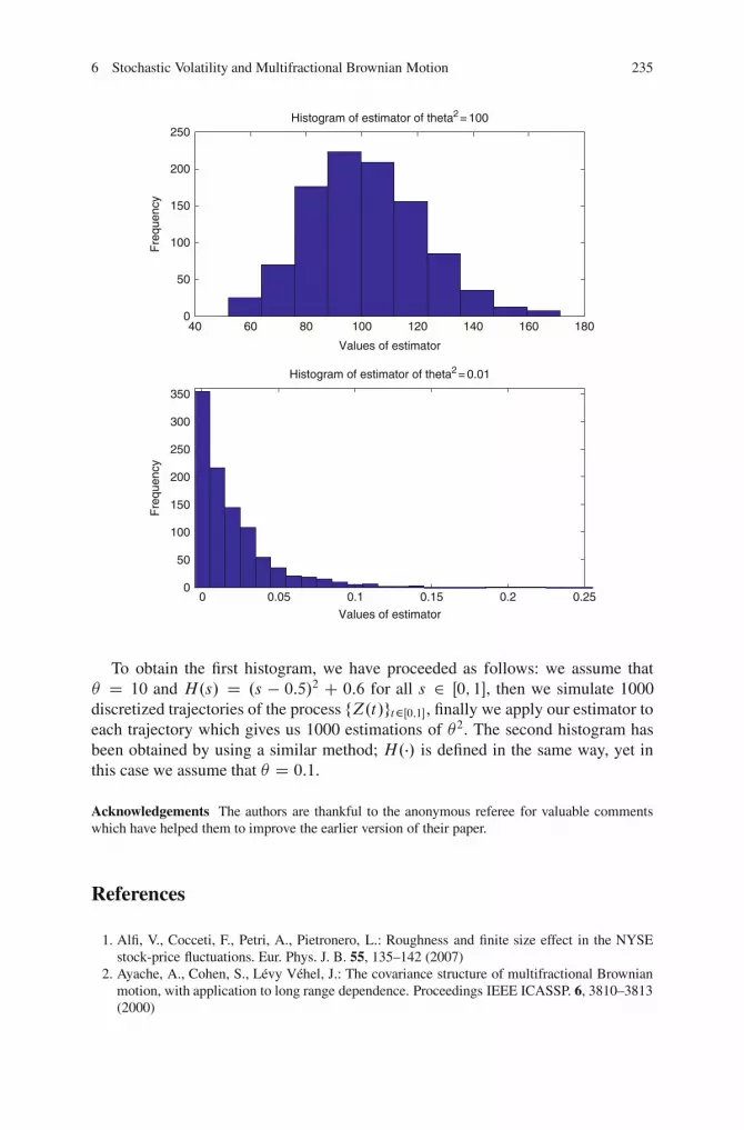
6 Stochastic Volatility and Multifractional Brownian Motion 235
40 60 80 100 120 140 160 1800
50
100
150
200
250
Values of estimator
Fre
quen
cy
Histogram of estimator of theta2= 100
0 0.05 0.1 0.15 0.2 0.250
50
100
150
200
250
300
350
Values of estimator
Fre
quen
cy
Histogram of estimator of theta2= 0.01
To obtain the first histogram, we have proceeded as follows: we assume that� D 10 and H.s/ D .s � 0:5/2 C 0:6 for all s 2 Œ0; 1�, then we simulate 1000discretized trajectories of the process fZ.t/gt2Œ0;1�, finally we apply our estimator toeach trajectory which gives us 1000 estimations of �2. The second histogram hasbeen obtained by using a similar method; H.�/ is defined in the same way, yet inthis case we assume that � D 0:1.
Acknowledgements The authors are thankful to the anonymous referee for valuable commentswhich have helped them to improve the earlier version of their paper.
References
1. Alfi, V., Cocceti, F., Petri, A., Pietronero, L.: Roughness and finite size effect in the NYSEstock-price fluctuations. Eur. Phys. J. B. 55, 135–142 (2007)
2. Ayache, A., Cohen, S., Levy Vehel, J.: The covariance structure of multifractional Brownianmotion, with application to long range dependence. Proceedings IEEE ICASSP. 6, 3810–3813(2000)
236 A. Ayache and Q. Peng
3. Ayache, A.: Du mouvement brownien fractionnaire au mouvement brownien multifraction-naire. Technique et science informatiques 20–29, 1133–1152 (2001)
4. Ayache, A.: The generalized multifractional field: A nice tool for the study of the GeneralizedMultifractional Brownian Motion. J. Four. Anal. Appl. 8, 581–601 (2002)
5. Ayache, A., El-Nouty, C.: The small ball behavior of a non stationary increments process: Themultifractional Brownian motion. Preprint CMLA. 08, (2004)
6. Ayache, A., Taqqu, M.S.: Multifractional processes with random exponent. Publ. Mat. 49(2),459–486 (2005)
7. Ayache, A., Jaffard, S., Taqqu, M.S.: Wavelet construction of generalized multifractionalprocesses. Rev. Mat. Iberoam. 23(1), 327–370 (2007)
8. Benassi, A., Jaffard, S., Roux, D.: Gaussian processes and pseudodifferential elliptic operators.Rev. Mat. Iberoam. 13(1), 19–81 (1997)
9. Bianchi, S.: Pathwise identification of the memory function of multifractional Brownianmotion with application to finance. Int. J. Theoret. Appl. Financ. 8(2), 255–281 (2005)
10. Bianchi, S., Pianese, A.: Multifractional properties of stock indices decomposed by filteringtheir pointwise holder regularity. Int. J. Theoret. Appl. Financ. 11(6), 567–595 (2008)
11. Bianchi, S., Pianese, A., Pantanella, A.: Modeling Stock Prices by Multifractional BrownianMotion: An Improved Estimation of the Pointwise Regularity. Quantitative Finance, Forth-coming. Available at SSRN: http://ssrn.com/abstract=1888288 (2011)
12. Cohen, S.: From self-similarity to local self-similarity: the estimation problem, Fractal inEngineering, ed. by Levy Vehel and C. Tricot. Springer, 3–16 (1999)
13. Comte, F., Renault, E.: Long memory continuous time models. J. Econom. 73, 101–150 (1996)14. Comte, F., Renault, E.: Long memory in continuous-time stochastic volatility models. Math.
Financ. 8, 291–323 (1998)15. Doukhan, P., Oppenheim, G., Taqqu, M.S.: Theory and applications of long-Range depen-
dence. Birkhauser, Boston (2003)16. Embrechts, P., Maejima, M.: Selfsimilar Processes. Princeton University Press, Princeton and
Oxford (2002)17. Falconer, K.: Tangent fields and the local structure of random fields. J. Theoret. Probab. 15,
731–750 (2002)18. Falconer, K.: The local structure of random processes, J. London Math. Soc. 67, 657–672
(2003)19. Falconer, K., Le Guevel, R., Levy Vehel, J.: Localisable moving average stable and multistable
processes. Stochastic Models. 25, 648–672 (2009)20. Gloter, A., Hoffmann, M.: Stochastic volatility and fractional Brownian motion.
Prepublication du laboratoire de Probabilites & Modeles Aleatoires des Universites Paris 6& Paris 7, 746 (2002)
21. Gloter, A., Hoffmann, M.: Stochastic volatility and fractional Brownian motion. Stoch. Proc.Appl. 113, 143–172 (2004)
22. Hull, J., White, A.: The pricing of options on assets with stochastic volatilities. J. Financ. 3,281–300 (1987)
23. Mandelbrot, B.B.: Fractales, hasard et finance. Paris, Flammarion (1997)24. Mandelbrot, B.B.: Fractals and scaling in finance: Discontinuity, concentration, risk. New
York, Springer (1997)25. Melino, A., Turnbull, S.M.: Pricing foreign currency options with stochastic volatility.
J. Econom. 45, 239–265 (1990)26. Peltier, R.F., Levy Vehel, J.: Multifractional Brownian motion: Definition and preliminary
results. Rapport de recherche de l’INRIA, 2645 (1995)27. Peng, Q.: Statistical inference for hidden multifractional processes in a setting of stochastic
volatility models. PhD Thesis, University Lille 1 (2011)28. Rosenbaum, M.: Estimation of the volatility persitence in a discretely observed diffusion
model. Stoch. Proc. Appl. 118, 1434–1462 (2008)29. Samorodnitsky, G., Taqqu, M.S.: Stable non-Gaussian random processes. Chapman and Hall,
New York, London (1994)
6 Stochastic Volatility and Multifractional Brownian Motion 237
30. Scott, L.: Option pricing when the variance changes randomly: Estimation and an application.J. Finan. Quantit. Anal. 22, 419–438 (1987)
31. Surgailis, D.: Nonhomogeneous fractional integration and multifractional processes. Stoch.Proc. Appl. 118, 171–198 (2008)
32. Stoev, S., Taqqu, M.S.: Path properties of the linear multifractional stable motion. Fractals13(2), 157–178 (2005)
33. Stoev, S., Taqqu, M.S.: Stochastic properties of the linear multifractional stable motion. Adv.Appl. Probab. 36(4), 1085–1115 (2004)
34. Stoev, S., Taqqu, M.S.: How rich is the class of multifractional Brownian motions? Stoch.Process Appl. 116, 200–221 (2006)
35. Tudor, C., Viens, F.: Statistical aspects of the fractional stochastic calculus. Ann. Statist. 35,1183–1212 (2007)

�

Chapter 7Two-Sided Estimates for Distribution Densitiesin Models with Jumps
Archil Gulisashvili and Josep Vives*
Abstract The present paper is devoted to applications of mathematical analysisto the study of distribution densities arising in stochastic stock price models.We consider uncorrelated Stein-Stein, Heston, and Hull-White models and theirperturbations by compound Poisson processes with jump amplitudes distributedaccording to a double exponential law. Similar perturbations of the Black-Scholesmodel were studied by S. Kou. For perturbed models, we obtain two-sided estimatesfor the stock price distribution density and compare the rate of decay of this densityin the original and the perturbed model. It is shown that if the value of the parameter,characterizing the rate of decay of the right tail of the double exponential law, issmall, then the stock price density in the perturbed model decays slower than thedensity in the original model. On the other hand, if the value of this parameteris large, then there are no significant changes in the behavior of the stock pricedistribution density.
7.1 Introduction
In this paper, we use methods of mathematical analysis to find two-sided estimatesfor the distribution density of the stock price in stochastic models with jumps. Weconsider perturbations of the Hull-White, the Stein-Stein, and the Heston models
� The research of Josep Vives is partially supported by grant MTM2009-07203
A. Gulisashvili (�)Department of Mathematics, Ohio University, Athens, OH 45701, USAe-mail: [email protected]
J. VivesDepartament de Probabilitat, Logica i Estadıstica, Universitat de Barcelona, Gran Via 585,08007-Barcelona (Catalunya), Spaine-mail: [email protected]
M. Zili and D.V. Filatova (eds.), Stochastic Differential Equations and Processes,Springer Proceedings in Mathematics 7, DOI 10.1007/978-3-642-22368-6 7,© Springer-Verlag Berlin Heidelberg 2012
239
240 A. Gulisashvili and J. Vives
by compound Poisson processes. In these models, the volatility processes are ageometric Brownian motion, the absolute value of an Ornstein-Uhlenbeck process,and a Cox-Ingersoll-Ross process, respectively. For more information on stochasticvolatility models, see [5] and [7].
A stock price model with stochastic volatility is called uncorrelated if standardBrownian motions driving the stock price equation and the volatility equation areindependent. In [8, 10], and [11], sharp asymptotic formulas were found for thedistribution density of the stock price in uncorrelated Hull-White, Stein-Stein, andHeston models. Various applications of these formulas were given in [9] and [12].The results obtained in [10] and [11] will be used in the present paper.
It is known that the stock price distribution density in an uncorrelated stochasticvolatility model possesses a certain structural symmetry (see formula (7.14) below).This implies a similar symmetry in the Black-Scholes implied volatility, which doesnot explain the volatility skew observed in practice. To improve the performanceof an uncorrelated model, one can either assume that the stock price process andthe volatility process are correlated, or add a jump component to the stock priceequation or to the volatility equation. The stock price distribution in the resultingmodel fits the empirical stock price distribution better than in the uncorrelatedcase. However, passing to a correlated model or adding a jump component maysometimes lead to similar effects or may have different consequences (see e.g. [1]and [2]). Examples of stock price models with jumps can be found in [3, 17], and[18]. We refer the reader to [4] for more information about stock price models withjumps. An interesting discussion of the effect of adding jumps to the Heston modelin contained in [16].
An important jump-diffusion model was introduced and studied by Kou in [17]and by Kou and Wang in [18]. This model can be described as a perturbation ofthe Black-Scholes model by a compound Poisson process with double-exponentiallaw for the jump amplitudes. In the present paper, we consider similar perturbationsof stochastic volatility models. Our main goal is to determine whether significantchanges may occur in the tail behavior of the stock price distribution after sucha perturbation. We show that the answer depends on the relations between theparameters defining the original model and the characteristics of the jump process.For instance, no significant changes occur in the behavior of the distribution densityof the stock price in a perturbed Heston or Stein-Stein model if the value of theparameter characterizing the right tail of the double exponential law is large. On theother hand, if this value is small, then the distribution density of the stock price inthe perturbed model decreases slower than in the original model. For the Hull-Whitemodel, there are no significant changes in the tail behavior of the stock price density,since this density decays extremely slowly.
We will next briefly overview the structure of the present paper. In Sect. 7.2, wedescribe classical stochastic volatility models and their perturbations by a compoundPoisson process. In Sect. 7.3 we formulate the main results of the paper and discusswhat follows from them. Finally, in Sect. 7.4, we prove the theorems formulated inSect. 7.3.

7 Two-Sided Estimates for Distribution Densities in Models with Jumps 241
7.2 Preliminaries
In the present paper, we consider perturbations of uncorrelated Stein-Stein, Heston,and Hull-White models by compound Poisson processes. Our goal is to determinewhether the behavior of the stock price distribution density in the original modelschanges after such a perturbation.
The stock price process X and the volatility process Y in the Stein-Stein modelsatisfy the following system of stochastic differential equations:
�dXt D �Xtdt C jYt jXtdWt
dYt D q .m � Yt/ dt C �dZt :(7.1)
This model was introduced and studied in [20]. The process Y , solving the secondequation in (7.1), is called an Ornstein-Uhlenbeck process. We assume that � 2 R,q � 0, m � 0, and � > 0.
The Heston model was developed in [14]. In this model, the processes X and Ysatisfy
�dXt D �Xtdt C p
YtXtdWt
dYt D q .m � Yt/ dt C cpYtdZt ;
(7.2)
where � 2 R; q � 0, m � 0, and c > 0. The volatility equation in (7.2) is uniquelysolvable in the strong sense, and the solution Y is a non-negative stochastic process.This process is called a Cox-Ingersoll-Ross process.
The stock price process X and the volatility process Y in the Hull-White modelare determined from the following system of stochastic differential equations:
�dXt D �Xtdt C YtXtdWt
dYt D �Ytdt C �YtdZt :(7.3)
In (7.3), � 2 R; � 2 R, and � > 0. The Hull-White model was introduced in [15].The volatility process in this model is a geometric Brownian motion.
It will be assumed throughout the paper that standard Brownian motions W andZ in (7.1), (7.2), and (7.3) are independent. The initial conditions for the processesX and Y will be denoted by x0 and y0, respectively.
We will next discuss perturbations of the models defined above by a compoundPoisson process with jump amplitudes distributed according to a double exponentiallaw. Perturbations of the Black-Scholes model by such jump processes were studiedby Kou in [17] and by Kou and Wang in [18]. Some of the methods developed in[17] will be used in the present paper.
Let N be a standard Poisson process with intensity � > 0, and consider acompound Poisson process defined by
Jt DNtX
iD1.Vi � 1/; t � 0; (7.4)
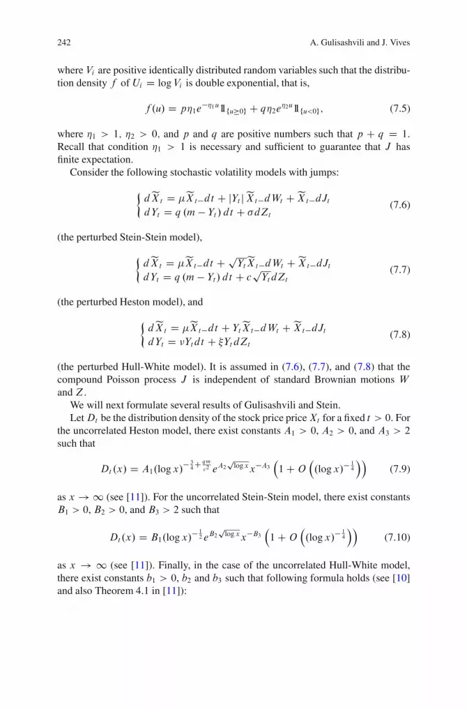
242 A. Gulisashvili and J. Vives
where Vi are positive identically distributed random variables such that the distribu-tion density f of Ui D logVi is double exponential, that is,
f .u/ D p�1e��1u11fu�0g C q�2e
�2u11fu<0g; (7.5)
where �1 > 1; �2 > 0; and p and q are positive numbers such that p C q D 1:
Recall that condition �1 > 1 is necessary and sufficient to guarantee that J hasfinite expectation.
Consider the following stochastic volatility models with jumps:
�deXt D �eXt�dt C jYt jeXt�dWt C eXt�dJtdYt D q .m � Yt / dt C �dZt
(7.6)
(the perturbed Stein-Stein model),
�deXt D �eXt�dt C p
YteXt�dWt C eXt�dJtdYt D q .m � Yt/ dt C c
pYtdZt
(7.7)
(the perturbed Heston model), and
�deXt D �eXt�dt C YteXt�dWt C eXt�dJtdYt D �Ytdt C �Yt dZt
(7.8)
(the perturbed Hull-White model). It is assumed in (7.6), (7.7), and (7.8) that thecompound Poisson process J is independent of standard Brownian motions Wand Z.
We will next formulate several results of Gulisashvili and Stein.LetDt be the distribution density of the stock price priceXt for a fixed t > 0: For
the uncorrelated Heston model, there exist constants A1 > 0, A2 > 0, and A3 > 2
such that
Dt .x/ D A1.logx/�34C qm
c2 eA2p
logxx�A3�1CO
�.logx/�
14
��(7.9)
as x ! 1 (see [11]). For the uncorrelated Stein-Stein model, there exist constantsB1 > 0, B2 > 0, and B3 > 2 such that
Dt.x/ D B1.logx/�12 eB2
plog xx�B3
�1CO
�.logx/�
14
��(7.10)
as x ! 1 (see [11]). Finally, in the case of the uncorrelated Hull-White model,there exist constants b1 > 0, b2 and b3 such that following formula holds (see [10]and also Theorem 4.1 in [11]):
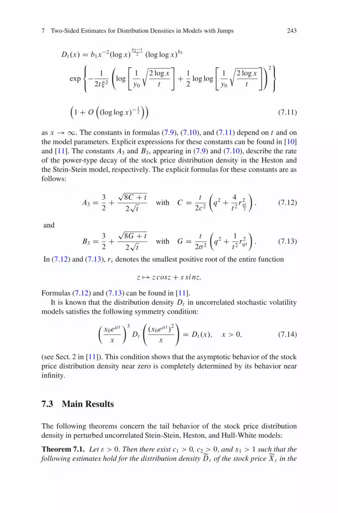
7 Two-Sided Estimates for Distribution Densities in Models with Jumps 243
Dt.x/ D b1x�2.logx/
b2�1
2 .log logx/b3
exp
8<
:� 1
2t�2
log
"1
y0
r2 logx
t
#
C 1
2log log
"1
y0
r2 logx
t
#!29=
;
�1CO
�.log logx/�
12
��(7.11)
as x ! 1: The constants in formulas (7.9), (7.10), and (7.11) depend on t and onthe model parameters. Explicit expressions for these constants can be found in [10]and [11]. The constants A3 and B3, appearing in (7.9) and (7.10), describe the rateof the power-type decay of the stock price distribution density in the Heston andthe Stein-Stein model, respectively. The explicit formulas for these constants are asfollows:
A3 D 3
2C
p8C C t
2pt
with C D t
2c2
�
q2 C 4
t2r2qt2
�
; (7.12)
and
B3 D 3
2C
p8G C t
2pt
with G D t
2�2
�
q2 C 1
t2r2qt
�
: (7.13)
In (7.12) and (7.13), rs denotes the smallest positive root of the entire function
z 7! z cosz C s sinz:
Formulas (7.12) and (7.13) can be found in [11].It is known that the distribution density Dt in uncorrelated stochastic volatility
models satisfies the following symmetry condition:
�x0e
�t
x
�3
Dt
.x0e
�t /2
x
!
D Dt.x/; x > 0; (7.14)
(see Sect. 2 in [11]). This condition shows that the asymptotic behavior of the stockprice distribution density near zero is completely determined by its behavior nearinfinity.
7.3 Main Results
The following theorems concern the tail behavior of the stock price distributiondensity in perturbed uncorrelated Stein-Stein, Heston, and Hull-White models:
Theorem 7.1. Let " > 0: Then there exist c1 > 0, c2 > 0; and x1 > 1 such that thefollowing estimates hold for the distribution density eDt of the stock price eXt in the
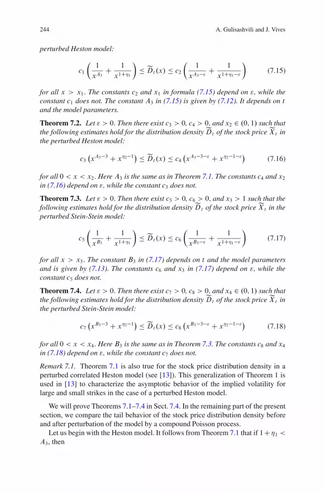
244 A. Gulisashvili and J. Vives
perturbed Heston model:
c1
�1
xA3C 1
x1C�1
�
� eDt.x/ � c2
�1
xA3�"C 1
x1C�1�"
�
(7.15)
for all x > x1: The constants c2 and x1 in formula (7.15) depend on "; while theconstant c1 does not. The constant A3 in (7.15) is given by (7.12). It depends on tand the model parameters.
Theorem 7.2. Let " > 0: Then there exist c3 > 0, c4 > 0; and x2 2 .0; 1/ such thatthe following estimates hold for the distribution density eDt of the stock price eXt inthe perturbed Heston model:
c3�xA3�3 C x�2�1
� � eDt.x/ � c4�xA3�3�" C x�2�1�"
�(7.16)
for all 0 < x < x2: Here A3 is the same as in Theorem 7.1. The constants c4 and x2in (7.16) depend on "; while the constant c3 does not.
Theorem 7.3. Let " > 0: Then there exist c5 > 0, c6 > 0; and x3 > 1 such that thefollowing estimates hold for the distribution density eDt of the stock price eXt in theperturbed Stein-Stein model:
c5
�1
xB3C 1
x1C�1
�
� eDt.x/ � c6
�1
xB3�"C 1
x1C�1�"
�
(7.17)
for all x > x3: The constant B3 in (7.17) depends on t and the model parametersand is given by (7.13). The constants c6 and x3 in (7.17) depend on "; while theconstant c5 does not.
Theorem 7.4. Let " > 0: Then there exist c7 > 0, c8 > 0; and x4 2 .0; 1/ such thatthe following estimates hold for the distribution density eDt of the stock price eXt inthe perturbed Stein-Stein model:
c7�xB3�3 C x�2�1
� � eDt.x/ � c8�xB3�3�" C x�2�1�"
�(7.18)
for all 0 < x < x4: Here B3 is the same as in Theorem 7.3. The constants c8 and x4in (7.18) depend on "; while the constant c7 does not.
Remark 7.1. Theorem 7.1 is also true for the stock price distribution density in aperturbed correlated Heston model (see [13]). This generalization of Theorem 1 isused in [13] to characterize the asymptotic behavior of the implied volatility forlarge and small strikes in the case of a perturbed Heston model.
We will prove Theorems 7.1–7.4 in Sect. 7.4. In the remaining part of the presentsection, we compare the tail behavior of the stock price distribution density beforeand after perturbation of the model by a compound Poisson process.
Let us begin with the Heston model. It follows from Theorem 7.1 that if 1C�1 <A3, then

7 Two-Sided Estimates for Distribution Densities in Models with Jumps 245
Nc1x1C�1
� eDt.x/ � Nc2x1C�1�"
for large enough values of x. Therefore, formula (7.9) shows that that if thecondition 1 C �1 < A3 holds, then the tail of the distribution of the stock pricein the perturbed Heston model is heavier than in the original model.
On the other hand, if 1 C �1 � A3, then Theorem 7.1 implies the followingestimate: Qc1
xA3� eDt.x/ � Qc2
xA3�"for large enough values of x. Now formula (7.9) shows that if 1 C �1 � A3, thenthere are no significant changes in the tail behavior of the distribution density ofthe stock price after perturbation. Similar assertions hold for the Stein-Stein model.This can be established using Theorem 7.3 and formula (7.10).
Next, suppose x ! 0. Then we can compare the behavior of the distributiondensity of the stock price in unperturbed and perturbed models, taking into accountTheorem 7.2, Theorem 7.4, formula (7.9), formula (7.10), and the symmetrycondition (7.14). For instance, if �2 < A3 � 2 in the perturbed Heston model, then
Nc3x�2�1 � eDt.x/ � Nc4x�2�1�"
for small enough values of x. On the other hand if �2 � A3 � 2, then
Qc3xA3�3 � eDt.x/ � Qc4xA3�3�"
for small enough values of x. Similar results hold for the Stein-Stein model.
Remark 7.2. For the Hull-White model, there are no significant changes in the tailbehavior of the stock price distribution after perturbation. This statement followsfrom the assumption �1 > 1 and from the fact that the stock price density in theunperturbed Hull-White model decays like x�2 (see formula (7.11)).
7.4 Proofs of the Main Results
The proofs of Theorems 7.1–7.4 are based on an explicit formula for the distributiondensity eDt of the stock price eXt in perturbed Heston, Stein-Stein, and Hull-Whitemodels (see formula (7.22) below). Note that the stock price process eX in theperturbed Stein-Stein and Hull-White models is given by
eXt D x0 exp
(
�t � 1
2
Z t
0
Y 2s ds CZ t
0
YsdWs CNtX
iD1Ui
)
; (7.19)

246 A. Gulisashvili and J. Vives
while for the perturbed for Heston model we have
eXt D x0 exp
(
�t � 1
2
Z t
0
Ysds CZ t
0
pYsdWs C
NtX
iD1Ui
)
: (7.20)
Formulas (7.19) and (7.20) can be established using the Doleans-Dade formula (see,for example, [19]). Put Tt D PNt
iD1 Ui and denote by �t its probability distribution.Clearly, we have:
�t .A/ D �0ı0.A/C1X
nD1�n
Z
A
f �.n/.u/du (7.21)
where �0 D e��t , �n D e��t .nŠ/�1.�t/n for n � 1, A is a Borel subset of R, andf is given by (7.5). The star in (7.21) denotes the convolution.
The distribution density Dt of the stock price Xt in uncorrelated models of ourinterest is related to the law of the following random variable:
˛t D�1
t
Z t
0
Y 2s ds
12
for the Stein-Stein and the Hull-White model, and
˛t D�1
t
Z t
0
Ysds
12
for the Heston model (see [10] and [11]). The distribution density of the randomvariable ˛t is called the mixing distribution density and is denoted by mt . We referthe reader to [10, 11], and [20] for more information on the mixing distributiondensity.
The next lemma establishes a relation between the mixing distribution densitymt in the uncorrelated model and the distribution density eDt of the stock price eXt
in the corresponding perturbed model.
Lemma 7.1. The density eDt in perturbed Stein-Stein, Heston and Hull-Whitemodels is given by the following formula:
eDt.x/ D 1p2�tx
Z 1
0
0
@
Z 1
�1exp
8<
:� .log x
x0e�tC ty2
2� u/2
2ty2
9=
;�t .du/
1
Amt.y/dy
y;
where mt is the mixing distribution density and �t is defined by (7.21).
Proof. We will prove Lemma 7.1 for the Heston model. The proof for the Stein-Stein and the Hull-White model is similar. For the latter models, we use formula(7.19) instead of formula (7.20).
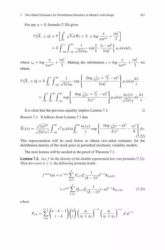
7 Two-Sided Estimates for Distribution Densities in Models with Jumps 247
For any � > 0, formula (7.20) gives
P�eXt � �
� D P
Z t
0
pYsdWs C Tt � log
�
x0e�tC t˛2t
2
�
D E
Z z�
�1
Z 1
�11p2�t˛t
exp
�
� .z � u/2
2t˛2t
�t .du/d z;
where z� D log�
x0e�tC t˛2t
2. Making the substitution z D log
x
x0e�tC t˛2t
2, we
obtain
P�eXt � �
� D E
Z �
0
Z 1
�11p2�t˛t
exp
8<
:� .log x
x0e�tC t˛2t
2� u/2
2t˛2t
9=
;�t.du/
dx
x
DZ �
0
Z 1
0
Z 1
�1exp
8<
:� .log x
x0e�tC ty2
2� u/2
2ty2
9=
;�t .du/
mt .y/p2�ty
dydx
x:
It is clear that the previous equality implies Lemma 7.1. utRemark 7.3. It follows from Lemma 7.1 that
eDt.x/ Dpx0e�tp2�tx
32
Z 1
�1e
u2 �t .du/
Z 1
0
mt .y/
yexp
(
� .log xx0e�t
� u/2
2ty2� ty2
8
)
dy:
(7.22)This representation will be used below to obtain two-sided estimates for thedistribution density of the stock price in perturbed stochastic volatility models.
The next lemma will be needed in the proof of Theorem 7.1.
Lemma 7.2. Let f be the density of the double exponential law (see formula (7.5)).Then for every n � 1, the following formula holds:
f �.n/.u/ D e��1unX
kD1Pn;k�
k1
1
.k � 1/Šuk�111fu�0g
C e�2unX
kD1Qn;k�
k2
1
.k � 1/Š.�u/k�111fu<0g; (7.23)
where
Pn;k Dn�1X
iDk
n � k � 1i � k
! n
i
!��1
�1 C �2
�i�k ��2
�1 C �2
�n�ipi qn�i
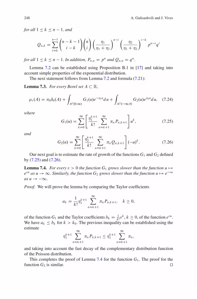
248 A. Gulisashvili and J. Vives
for all 1 � k � n � 1; and
Qn;k Dn�1X
iDk
n � k � 1i � k
! n
i
!��1
�1 C �2
�n�i ��2
�1 C �2
�i�kpn�i qi
for all 1 � k � n � 1: In addition, Pn;n D pn andQn;n D qn:
Lemma 7.2 can be established using Proposition B.1 in [17] and taking intoaccount simple properties of the exponential distribution.
The next statement follows from Lemma 7.2 and formula (7.21):
Lemma 7.3. For every Borel set A � R;
�t .A/ D �0ı0.A/CZ
A\Œ0;1/G1.u/e
��1udu CZ
A\.�1;0/G2.u/e
�2udu; (7.24)
where
G1.u/ D1X
kD0
"�kC11
kŠ
1X
nDkC1�nPn;kC1
#
uk; (7.25)
and
G2.u/ D1X
kD0
"�kC12
kŠ
1X
nDkC1�nQn;kC1
#
.�u/k: (7.26)
Our next goal is to estimate the rate of growth of the functionsG1 andG2 definedby (7.25) and (7.26).
Lemma 7.4. For every " > 0 the function G1 grows slower than the function u 7!e"u as u ! 1: Similarly, the function G2 grows slower than the function u 7! e�"uas u ! �1:
Proof. We will prove the lemma by comparing the Taylor coefficients
ak D 1
kŠ�kC11
1X
nDkC1�nPn;kC1; k � 0;
of the functionG1 and the Taylor coefficients bk D 1kŠ"k , k � 0, of the function e"u:
We have ak � bk for k > k0. The previous inequality can be established using theestimate
�kC11
1X
nDkC1�nPn;kC1 � �kC11
1X
nDkC1�n;
and taking into account the fast decay of the complementary distribution functionof the Poisson distribution.
This completes the proof of Lemma 7.4 for the function G1. The proof for thefunctionG2 is similar. ut
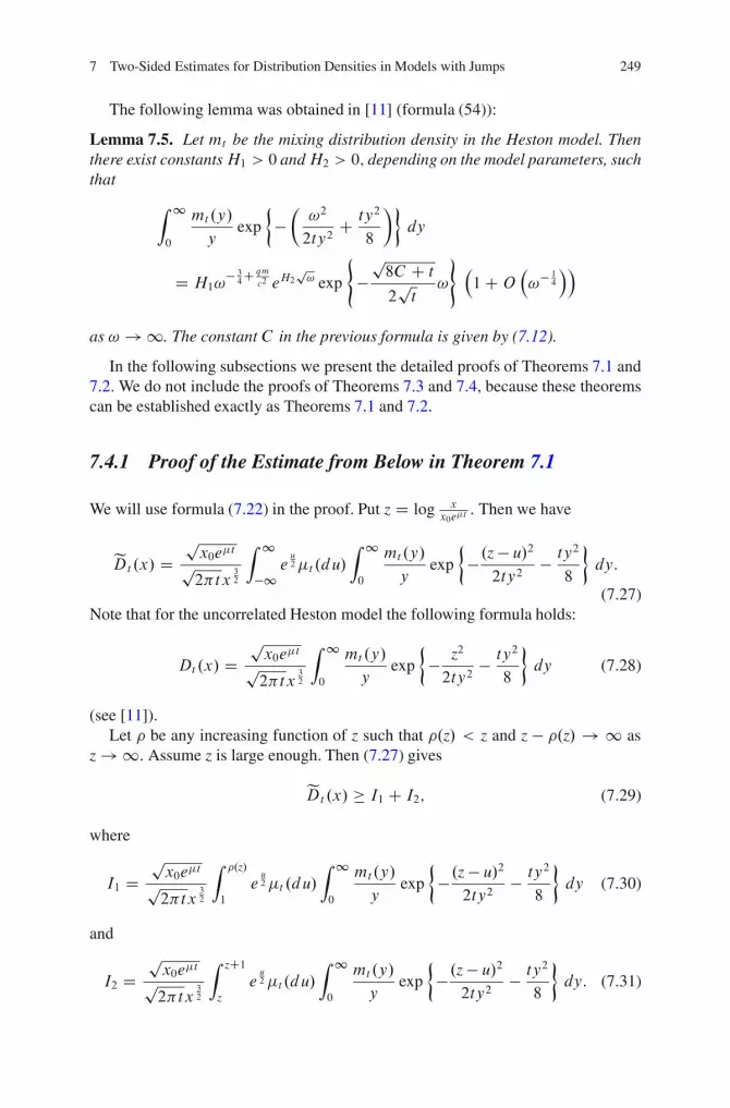
7 Two-Sided Estimates for Distribution Densities in Models with Jumps 249
The following lemma was obtained in [11] (formula (54)):
Lemma 7.5. Let mt be the mixing distribution density in the Heston model. Thenthere exist constantsH1 > 0 andH2 > 0; depending on the model parameters, suchthat
Z 1
0
mt .y/
yexp
�
��!2
2ty2C ty2
8
�
dy
D H1!� 34C qm
c2 eH2p! exp
(
�p8C C t
2pt
!
)�1CO
�!�
14
��
as ! ! 1. The constant C in the previous formula is given by (7.12).
In the following subsections we present the detailed proofs of Theorems 7.1 and7.2. We do not include the proofs of Theorems 7.3 and 7.4, because these theoremscan be established exactly as Theorems 7.1 and 7.2.
7.4.1 Proof of the Estimate from Below in Theorem 7.1
We will use formula (7.22) in the proof. Put z D log xx0e�t
: Then we have
eDt.x/ Dpx0e�tp2�tx
32
Z 1
�1e
u2 �t .du/
Z 1
0
mt .y/
yexp
�
� .z � u/2
2ty2� ty2
8
dy:
(7.27)Note that for the uncorrelated Heston model the following formula holds:
Dt.x/ Dpx0e�tp2�tx
32
Z 1
0
mt .y/
yexp
�
� z2
2ty2� ty2
8
dy (7.28)
(see [11]).Let be any increasing function of z such that .z/ < z and z � .z/ ! 1 as
z ! 1: Assume z is large enough. Then (7.27) gives
eDt.x/ � I1 C I2; (7.29)
where
I1 Dpx0e�tp2�tx
32
Z .z/
1
eu2 �t .du/
Z 1
0
mt.y/
yexp
�
� .z � u/2
2ty2� ty2
8
dy (7.30)
and
I2 Dpx0e�tp2�tx
32
Z zC1
ze
u2 �t .du/
Z 1
0
mt .y/
yexp
�
� .z � u/2
2ty2� ty2
8
dy: (7.31)

250 A. Gulisashvili and J. Vives
Throughout the remaining part of the section, we will denote by ˛ a positiveconstant which may differ from line to line. Since the function G1 is increasing on.0;1/ and (7.24) and (7.25) hold, we have
I2 � ˛x� 32Z zC1
ze
u2 e��1udu
Z 1
0
mt.y/
yexp
�
� 1
2ty2� ty2
8
dy; x > x1:
It is known thatZ 1
0
y�1mt .y/dy < 1 (see [11]). Therefore, the second integral in
the previous estimate converges. It follows that
I2 � ˛x� 32Z zC1
ze
u2 e��1udu D ˛x�1��1
for x > x1. It is not hard to see using the inequality QDt.x/ � I2 that the estimatefrom below in (7.15) holds in the case where 1C �1 � A3:
It remains to prove the estimate from below under the assumption 1C �1 > A3:
We will use the inequality QDt.x/ � I1 in the proof. To estimate I1 we notice thatz�u � z�.z/ ! 1 as x ! 1: Therefore, Lemma 7.5 can be applied to estimatethe second integral on the right-hand side of (7.30). This gives
I1 � ˛x�32
Z .z/
1
eu2 G1.u/e
��1u.z�u/�34C qm
c2 eH2p
z�u exp
(
�p8C C t
2pt
.z � u/
)
du:
Since the function G1 is increasing on .0;1/ and the function
y 7! y� 34C qm
c2 eH2py
is eventually increasing, the previous inequality gives
I1 � ˛x�32
Z .z/
1
eu2 e��1u exp
(
�p8C C t
2pt
.z � u/
)
du
D ˛x�A3Z .z/
1
exp f.A3 � 1 � �1/ ugdu:
Here we used the equality A3 D 32
Cp8CCt2pt
(see (7.12)). Since A3 < 1C �1 we get
I1 � ˛x�A3 ; x > x1: This establishes the estimate from below in Theorem 7.1 inthe case where A3 < 1C �1.

7 Two-Sided Estimates for Distribution Densities in Models with Jumps 251
7.4.2 Proof of the Estimate from Above in Theorem 7.1
Let " be a sufficiently small positive number. Denote by t.z; u/ the followingintegral:
Z 1
0
mt.y/
yexp
�
� .z � u/2
2ty2� ty2
8
dy;
Then formula (7.27) can be rewritten as follows:
eDt.x/ Dpx0e�tp2�tx
32
Z 1
�1e
u2 t .z; u/�t .du/ D J1 C J2 C J3; (7.32)
where
J1 Dpx0e�tp2�tx
32
Z 0�
�1e
u2 t .z; u/�t .du/;
J2 Dpx0e�tp2�tx
32
Z sz
0
eu2t .z; u/�t .du/;
and
J3 Dpx0e�tp2�tx
32
Z 1
sze
u2 t .z; u/�t .du/:
The number s in the previous equalities satisfies 0 < s < 1. The value of s will bechosen below.
To estimate J2, we notice that if x is large, then z � u in the expression for J2 isalso large. Using Lemma 7.3 and Lemma 7.5, we see that
J2 � ˛Dt .x/C ˛x� 32
Z sz
0
eu2 G1.u/e
��1u.z � u/�34C qm
c2 eH2p
z�u
exp
(
�p8C C t
2pt
.z � u/
)
du:
Since the functions G1.y/ and y 7! y� 34C qm
c2 eH2py grow slower than the function
y 7! exp˚"2y�
(see Lemma 7.4), the previous inequality and formula (7.9) implythat
J2 � ˛x�A3C" C ˛x� 32Z sz
0
exp
��1
2� �1 C "
2
�
u
exp
(
�p8C C t
2pt
C "
2
!
.z � u/
)
du

252 A. Gulisashvili and J. Vives
� ˛x�A3C" C ˛x�A3C "2
Z z
0
exp f.A3 � 1 � �1/ ugdu
� ˛
�1
xA3�"C 1
x1C�1�"
�
(7.33)
for x > x1.The function t is bounded (this has already been established in the previous
part of the proof). Therefore,
J3 � ˛x� 32
Z 1
sze
u2 G1.u/e
��1udu: (7.34)
Since the function G1.u/ grows slower than the function y 7! exp f�ug for any� > 0 (see Lemma 7.4), estimate (7.34) implies that
J3 � ˛x� 32Cs. 12C���1/; x > x1:
Now using the fact that � can be any close to 0 and s any close to 1, we see that
J3 � ˛1
x1C�1�"; x > x1: (7.35)
We will next estimate J1. It follows from Lemma 7.3 that
J1 D ˛x� 32Z 0�
�1e
u2 t .z; u/G2.u/e
�2udu:
Since u < 0, we see that z � u is large if x is large. Using Lemma 7.5, we obtain
J1 � ˛x� 32Z 0�
�1e
u2 .z � u/�
34C qm
c2 eH2p
z�u
exp
(
�p8C C t
2pt
.z � u/
)
G2.u/e�2udu: (7.36)
The function y 7! y� 34C qm
c2 eH2py is eventually increasing. Moreover, it grows
slower than e�2 y . Since z � u > z in (7.36), we have
J1 � ˛x� 32
Z 0�
�1e
u2 exp
(
�p8C C t
2pt
C "
2
!
.z � u/
)
G2.u/e�2udu
� ˛x�A3C"2
Z 0�
�1e
u2 exp
( p8C C t
2pt
� "
2
!
u
)
G2.u/e�2udu

7 Two-Sided Estimates for Distribution Densities in Models with Jumps 253
D ˛x�A3C "2
Z 1
0
exp
(
�12
� �2 �p8C C t
2pt
C "
2
!
u
)
G2.�u/du: (7.37)
If " is sufficiently small, then the integral in (7.37) converges (use Lemma 7.4). Itfollows from (7.37) that
J1 � ˛1
xA3�"; x > x1: (7.38)
Finally, combining (7.32), (7.33), (7.35), and (7.38), we establish the estimatefrom above in Theorem 7.1.
7.4.3 Proof of Theorem 7.2
The following formula can be obtained from (7.22):
�x0e
�t
x
�3eDt
.x0e
�t /2
x
!
Dpx0e�tp2�tx
32
Z
R
eu2 �t .du/
Z 1
0
mt.y/
yexp
(
� .log xx0e�t
C u/2
2ty2� ty2
8
)
dy: (7.39)
It follows from (7.39) and (7.24) that
�x0e
�t
x
�3eDt
.x0e
�t /2
x
!
Dpx0e�tp2�tx
32
Z 1
�1e
u2 Q�t .du/
Z 1
0
mt.y/
yexp
(
� .log xx0e�t
� u/2
2ty2� ty2
8
)
dy; (7.40)
where
Q�t .A/ D �0ı0.A/CZ
A\.0;1/G2.�u/e�.�2C1/udu C
Z
A\.�1;0/G1.�u/e.�1�1/udu
(7.41)for all Borel sets A � R. In (7.41), G1 and G2 are defined by (7.25) and (7.26),respectively. Now it is clear that we can use the proof of Theorem 7.1 with the pairs.�1; p/ and .�2; q/ replaced by the pairs .�2 C 1; q/ and .�1 � 1; p/, respectively. Itis not hard to see using (7.39) that for every " > 0, there exist constants Qc1 > 0,Qc2 > 0, and Qx > 0 such that the following estimates hold:
Qc1�1
xA3C 1
x�2C2
�
� x�3eDt
.x0e
�t /2
x
!
� Qc2�
1
xA3�"C 1
x�2C2�"
�
(7.42)

254 A. Gulisashvili and J. Vives
for all x > Qx. The constants Qc2 and Qx depend on ". Now it is clear that (7.16) followsfrom (7.42).
This completes the proof of Theorem 7.2.
References
1. Alos, E., Leon, J., Vives,J.: On the short time behavior of the implied volatility for jumpdiffusion models with stochastic volatility. Finance Stochast. 11, 571–589 (2007)
2. Alos, E., Leon, J., Pontier, M., Vives, J.: A Hull and White formula for a general stochasticvolatility jump-diffusion model with applications to the study of the short-time behavior of theimplied volatility. J. Appl. Math. Stoch. Anal. Vol. 2008 (2008), ID 359142, 17 pages.
3. Bates, D.S.: Jumps and stochastic volatility: exchange rate processes implicit in Deutsche Markoptions. Rev. Financ. Stud. 9, 69–107 (1996)
4. Cont, R., Tankov, P.: Financial Modeling with Jump Processes. Chapman and Hall – CRC,Boca Raton (2004)
5. Fouque, J.P., Papanicolaou, G., Sircar, K.R.: Derivatives in Financial Markets with StochasticVolatility. Cambridge University Press, Cambridge (2000)
6. Friz, P., Gerhold, S., Gulisashvili, A., Sturm, S.: On refined volatility smile expansion in theHeston model. Quant Finanace, 11, 1151–1164 (2011)
7. Gatheral, J.: The Volatility Surface: A Practitioner’s Guide. Wiley, Hoboken, NJ (2006)8. Gulisashvili, A., Stein, E.M.: Asymptotic behavior of distribution densities in models with
stochastic volatility: The Hull-White model. Comptes Rendus de l’Academie des Sciences deParis I 343, 519–523 (2006)
9. Gulisashvili, A., Stein, E.M.: Implied volatility in the Hull-White model. Math. Finance. 19,303–327 (2009)
10. Gulisashvili, A., Stein, E.M.: Asymptotic behavior of distribution densities in models withstochastic volatility I. Math. Finance. 20, 447–477 (2010)
11. Gulisashvili, A., Stein, E.M.: Asymptotic behavior of the stock price distribution density andimplied volatility in stochastic volatility models. Appl. Math. Optim. 61, 287–315 (2010)
12. Gulisashvili, A.: Asymptotic formulas with error estimates for call pricing functions and theimplied volatility at extreme strikes. SIAM J. Financ. Math. 1, 609–641 (2010)
13. Gulisashvili, A.: Asymptotic equivalence in Lee’s moment formulas for the implied volatilityand Piterbarg’s conjecture. Submitted for publication; available at arxiv.org, arXiv:1007.5353
14. Heston, S.L.: A closed-form solution for options with stochastic volatility with applications tobond and currency options. Rev. Financ. Stud. 6, 327–343 (1993)
15. Hull, J., White, A.: The pricing of options on assets with stochastic volatilities. J. Finance 42,281–300 (1987)
16. Keller-Ressel, M.: Moment explosions and long-term behavior of affine stochastic volatilitymodels. Math. Finance, 21, 73–98 (2011)
17. Kou, S.: A jump-diffusion model for option pricing. Manag. Sci. 48, 1086–1101 (2002)18. Kou, S., Wang, H.: Option pricing under a double exponential jump diffusion model. Manag.
Sci. 50, 1178–1192 (2003)19. Protter, P.: Stochastic Integration and Differential Equations, 2nd ed. Springer, Berlin (2005)20. Stein, E.M., Stein, J.C.: Stock price distributions with stochastic volatility: An analytic
approach. Rev. Financ. Stud. 4, 727–752 (1991)

Chapter 8Maximizing a Function of the Survival Timeof a Wiener Process in an Interval
Mario Lefebvre
Abstract Let X.t/ be a controlled one-dimensional Wiener process with positivedrift. The problem of maximizing a function of the time spent by X.t/ in a giveninterval is solved explicitly. The process is controlled at most until a fixed time t1.The same type of problem is considered for a two-dimensional degenerate diffusionprocess .X.t/; Y.t//.
8.1 Introduction
We consider the one-dimensional controlled Wiener process fX.t/; t � 0g definedby the stochastic differential equation
dX.t/ D �dt C b u.t/dt C � dB.t/; (8.1)
where fB.t/; t � 0g is a standard Brownian motion, u.t/ is the control variable, and�, b and � are positive constants.
Assume that the process starts from X.0/ D x < d .> 0/, and define
T .xI d/ D infft > 0 W X.t/ D d j X.0/ D xg:
That is, T .xI d/ is the first time the controlled process X.t/ takes on the value d .Next, let
T1.xI d/ D minfT .xI d/; t1g;
M. Lefebvre (�)Departement de mathematiques et de genie industriel, Ecole Polytechnique,C.P. 6079, Succursale Centre-ville, Montreal, Quebec H3C 3A7, Canadae-mail: [email protected]
M. Zili and D.V. Filatova (eds.), Stochastic Differential Equations and Processes,Springer Proceedings in Mathematics 7, DOI 10.1007/978-3-642-22368-6 8,© Springer-Verlag Berlin Heidelberg 2012
255
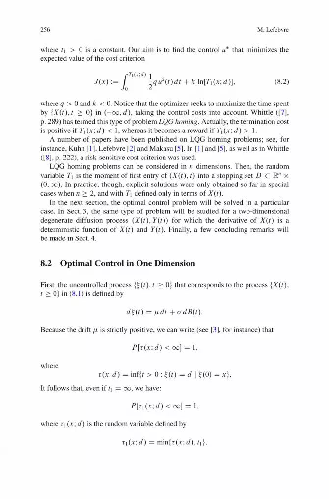
256 M. Lefebvre
where t1 > 0 is a constant. Our aim is to find the control u� that minimizes theexpected value of the cost criterion
J.x/ WDZ T1.xId/
0
1
2q u2.t/dt C k lnŒT1.xI d/�; (8.2)
where q > 0 and k < 0. Notice that the optimizer seeks to maximize the time spentby fX.t/; t � 0g in .�1; d /, taking the control costs into account. Whittle ([7],p. 289) has termed this type of problem LQG homing. Actually, the termination costis positive if T1.xI d/ < 1, whereas it becomes a reward if T1.xI d/ > 1.
A number of papers have been published on LQG homing problems; see, forinstance, Kuhn [1], Lefebvre [2] and Makasu [5]. In [1] and [5], as well as in Whittle([8], p. 222), a risk-sensitive cost criterion was used.
LQG homing problems can be considered in n dimensions. Then, the randomvariable T1 is the moment of first entry of .X.t/; t/ into a stopping set D � R
n �.0; 1/. In practice, though, explicit solutions were only obtained so far in specialcases when n � 2, and with T1 defined only in terms of X.t/.
In the next section, the optimal control problem will be solved in a particularcase. In Sect. 3, the same type of problem will be studied for a two-dimensionaldegenerate diffusion process .X.t/; Y.t// for which the derivative of X.t/ is adeterministic function of X.t/ and Y.t/. Finally, a few concluding remarks willbe made in Sect. 4.
8.2 Optimal Control in One Dimension
First, the uncontrolled process f�.t/; t � 0g that corresponds to the process fX.t/;
t � 0g in (8.1) is defined by
d�.t/ D �dt C � dB.t/:
Because the drift � is strictly positive, we can write (see [3], for instance) that
P Œ�.xI d/ < 1� D 1;
where�.xI d/ D infft > 0 W �.t/ D d j �.0/ D xg:
It follows that, even if t1 D 1, we have:
P Œ�1.xI d/ < 1� D 1;
where �1.xI d/ is the random variable defined by
�1.xI d/ D minf�.xI d/; t1g:

8 Maximizing a Function of the Survival Time of a Wiener Process in an Interval 257
Moreover, because the quantities b, � and q in the problem formulation above areall positive constants, we can state that there exists a positive constant ˛ such that
˛�2 D b2
q: (8.3)
Then, we may appeal to a theorem in Whittle [7] to assert that the optimal controlu� .D u�.0// can be expressed in terms of the mathematical expectation
G.x/ WD E
�
exp
�
� b2
q �2k lnŒ�1.xI d/�
��
: (8.4)
Namely, we can write that
u� D �2
b
G 0.x/
G.x/:
Thus, making use of the theorem in [7], the stochastic optimal control problem setup above is reduced to the computation of the function G.x/.
Assume next that we choose the constant k D �q �2=b2. Then, the mathematicalexpectation G.x/ simplifies to
G.x/ D E ŒexpflnŒ�1.xI d/�g� D E Œ�1.xI d/� :
Now, if we assume further that the constant t1 is such that
EŒ�1.xI d/� D c EŒ�.xI d/�; (8.5)
where c 2 .0; 1/, then (see [3], p. 220)
G.x/ D cd � x
�:
Hence, the optimal control follows at once.
Proposition 8.1. Under the hypotheses above, the optimal control u� is given by
u� D �2
b
1
x � dfor x < d: (8.6)
Remarks. (i) Let fX�.t/; t � 0g denote the optimally controlled process. We deducefrom the proposition that
u�.t/ D �2
b
1
X�.t/ � d;

258 M. Lefebvre
where fX�.t/; t � 0g satisfies the stochastic differential equation
dX�.t/ D �dt C �2
X�.t/ � ddt C � dB.t/:
(ii) An application of the model considered in this paper is the following: supposethat X.t/ is the wear of a machine at time t , and that this machine is assumedto be worn out when X.t/ reaches the value d > 0. Then, the optimizer tries tomaximize the lifetime of the machine, taking the control costs into account. Bychoosing to stop controlling the process at most at time t1, with t1 being suchthat (8.5) holds, it is understood that the aim is to use the machine for a certainpercentage of its expected lifetime, in the case when no control is used at all.A reason for doing so is the fact that a machine can become obsolete before itis actually worn out. Also, when it is old, the maintenance costs can increaserapidly.
(iii) Notice that the optimal solution (8.6) depends neither on the constant c, nor onthe drift �. However, if we modify the cost criterion (8.2) to
J1.x/ WDZ T1.xId/
0
1
2q u2.t/dt C k lnŒ1 C T1.xI d/�;
so that the termination cost is always negative, then we find that
u� D ��2
b
c
� C c.d � x/for x < d;
which implies that
u�.t/ D ��2
b
c
� C cŒd � X�.t/�:
If t1 D 1, so that c D 1, we obtain that
u�.t/ D ��2
b
1
� C d � X�.t/:
(iv) The probability density function of the first passage time �.xI d/ is given by(see [3], p. 219)
f�.xId/.t/ D d � xp2� �2 t3
exp
�
� .d � x � �t/2
2�2 t
�
for t > 0.
When t1 < 1, we have:

8 Maximizing a Function of the Survival Time of a Wiener Process in an Interval 259
EŒ�1.xI d/� D EŒ�1.xI d/ j �.x/ � t1�P Œ�.x/ � t1�
C EŒ�1.xI d/ j �.x/ > t1�P Œ�.x/ > t1�
DZ t1
0
t f�.xId/.t/dt C t1
Z 1
t1
f�.xId/.t/dt:
From the previous formula, we can compute the value of c for any choice of t1:
c D �
d � xEŒ�1.xI d/�:
If we look for the value of t1 that corresponds to a given proportion c, then we canuse a mathematical software package to estimate the value of t1 from the aboveformula.
8.3 Optimal Control in Two Dimensions
We mentioned in Remark (ii) above that a possible application of the modelconsidered in Sect. 2 is obtained by assuming that X.t/ is the wear of a machine attime t . However, because wear should always increase with time, a better model isobtained by defining the two-dimensional controlled diffusion process .X.t/; Y.t//,starting from .X.0/; Y.0// D .x; y/, by the system (see Rishel [6])
dX.t/ D f ŒX.t/; Y.t/�dt;
dY.t/ D mŒX.t/; Y.t/�dt C b.t/u.t/dt C fvŒX.t/; Y.t/�g1=2 dB.t/; (8.7)
where f .> 0/, b .¤ 0/, m and v .� 0/ are real functions, and the random variableY.t/ is a variable that is closely correlated with the wear.
Let
T .x; y/ D infft > 0 W Y.t/ D 0 j X.0/ D x > 0; Y.0/ D y > 0gand define, as in Sect. 2, the random variable
T1.x; y/ D minfT .x; y/; t1g;where t1 > 0 is a constant.
We want to find the control u� that minimizes the expected value of the costcriterion
J.x; y/ WDZ T1.x;y/
0
1
2q u2.t/dt C k lnŒT1.x; y/�;
where q is a positive function, and k is a negative constant.Assume next that
f .x; y/ D m.x; y/x
y

260 M. Lefebvre
and thatv.x; y/ D 2xy:
Moreover, let us choose
b.t/ � b0 .¤ 0/ and q D q0
xy;
where q0 > 0 is a constant. Then, there exists a positive constant ˛ for which therelation
˛ v.x; y/ D b2
q” ˛ D b2
0
2q0
(8.8)
holds. Furthermore, at least when t1 is finite, we can write that
P Œ�1.x; y/ < 1� D 1;
where �1.x; y/ is the same as T1.x; y/, but for the uncontrolled process obtained bysetting u.t/ D 0 in (8.7). Similarly for the first passage time �.x; y/.
Then, making use of the theorem in [7], we deduce that
u� D 2xy
b0
Gy.x; y/
G.x; y/; (8.9)
whereG.x; y/ WD E Œexpf�˛k lnŒ�1.x; y/�g� D E
��1.x; y/�˛ k
�:
Remark. Let H.x; y/ D Gy.x; y/. We can write that
u�.t/ D 2X�.t/Y �.t/b0
HŒX�.t/; Y �.t/�GŒX�.t/; Y �.t/�
;
where .X�.t/; Y �.t// is the optimally controlled process defined by
dX�.t/ D mŒX�.t/; Y �.t/�X�.t/Y �.t/
dt;
dY �.t/ D mŒX�.t/; Y �.t/�dt C 2X�.t/Y �.t/HŒX�.t/; Y �.t/�GŒX�.t/; Y �.t/�
dt
C f2X�.t/Y �.t/�g1=2dB.t/:
Now, it can be shown (see [4]) that the probability density function of the randomvariable �.x; y/ is given by
f�.x;y/.t/ D y
x t2exp
n� y
x t
ofor t > 0.
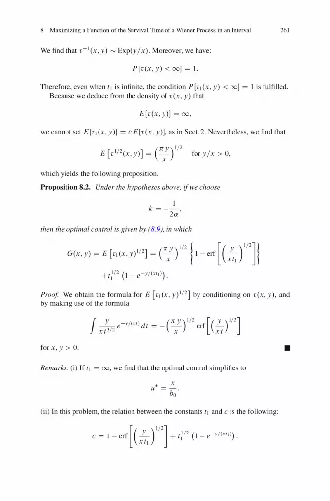
8 Maximizing a Function of the Survival Time of a Wiener Process in an Interval 261
We find that ��1.x; y/ � Exp.y=x/. Moreover, we have:
P Œ�.x; y/ < 1� D 1:
Therefore, even when t1 is infinite, the condition P Œ�1.x; y/ < 1� D 1 is fulfilled.Because we deduce from the density of �.x; y/ that
EŒ�.x; y/� D 1;
we cannot set EŒ�1.x; y/� D c EŒ�.x; y/�, as in Sect. 2. Nevertheless, we find that
E��1=2.x; y/
� D�� y
x
1=2
for y=x > 0,
which yields the following proposition.
Proposition 8.2. Under the hypotheses above, if we choose
k D � 1
2˛;
then the optimal control is given by (8.9), in which
G.x; y/ D E��1.x; y/1=2
� D�� y
x
1=2
(
1 � erf
"y
x t1
�1=2#)
Ct1=21
�1 � e�y=.xt1/
:
Proof. We obtain the formula for E��1.x; y/1=2
�by conditioning on �.x; y/, and
by making use of the formula
Zy
x t3=2e�y=.xt/ dt D �
�� y
x
1=2
erf
�� y
x t
1=2�
for x; y > 0.
Remarks. (i) If t1 D 1, we find that the optimal control simplifies to
u� D x
b0
:
(ii) In this problem, the relation between the constants t1 and c is the following:
c D 1 � erf
"y
x t1
�1=2#
C t1=21
�1 � e�y=.xt1/
:
262 M. Lefebvre
8.4 Concluding Remarks
We solved explicitly two optimal control problems involving diffusion processes,making use of a theorem that enables us to reduce them to purely probabilisticproblems. In each case, in order to obtain an exact and explicit expression forthe optimal control, we needed the probability density function of a first passagetime for the corresponding uncontrolled process. In Sect. 2, we used the well knowndensity function of the time it takes a one-dimensional Wiener process to hit a givenboundary. In Sect. 3, we made use of the density function computed in [4] of a firstpassage time defined in terms of a degenerate two-dimensional diffusion process.There are few such explicit expressions in the case of n-dimensional processes, withn � 2.
As mentioned above, the models considered in this note can be applied toreliability theory. The model presented in Sect. 3 is such that the wear of a certaindevice always increases with time, as it should. We could try to generalize the modelby incorporating a compound Poisson process in (8.7). However, then we couldno longer appeal to the theorem in [7] to transform the stochastic optimal controlproblem into a probability problem. Similarly, we could consider discrete processes,instead of diffusion processes. Again, we would have to solve the optimal controlproblems differently.
Finally, here we solved problems for which the optimizer tries to maximize afunction of the survival time of a diffusion process in a given continuation region.In the application presented, we assumed that a machine is used at most until a fixedtime t1. We could also assume that there is a warranty period, so that it will be usedat least during a given period of time.
Acknowledgements The author is grateful to the reviewers for their constructive comments.
References
1. Kuhn, J.: The risk-sensitive homing problem. J. Appl. Probab. 22, 796–803 (1985)2. Lefebvre, M.: A homing problem for diffusion processes with control-dependent variance. Ann.
Appl. Probab. 14, 786–795 (2004)3. Lefebvre, M.: Applied Stochastic Processes, Springer, New York (2007)4. Lefebvre, M.: Controlling a two-dimensional diffusion process at most until a fixed time.
(Submitted for publication)5. Makasu, C.: Risk-sensitive control for a class of homing problems. Automatica J. IFAC. 45,
2454–2455 (2009)6. Rishel, R.: Controlled wear processes: modeling optimal control. IEEE Trans. Automat. Contr.
36, 1100–1102 (1991)7. Whittle, P.: Optimization over Time, Vol. I, Wiley, Chichester (1982)8. Whittle, P.: Risk-sensitive Optimal Control, Wiley, Chichester (1990)

Appendix ASAAP 2010 Scientific Committee
Edward Allen (Texas Tech University, USA)Jean-marc Bardet (University Paris 1, France)Viacheslav Belavkin (University of Nottingham, United Kingdom)Kevin Burrage (University Queensland, Brisbane, Australia)Zhen-Qing Chen (University of Washington, USA)Nathalie Eisenbaum (University Paris 6, France)Vyacheslav Leonidovich Girko (Institute of Mathematics Kiev, Ukraine)Abdelhamid Hassairi (Faculty of sciences of Sfax, Tunisia)Shuya Kanagawa (Tokyo City University, Japan)Peter Kloeden (J.W.Goethe-Universitt Frankfurt, Germany)Sana Louhichi (University Paris- South, France)Habib Maagli (Faculty of sciences of Tunis, Tunisia)David Nualart (Kansas University, USA)Habib Ouerdiane (Faculty of sciences of Tunis, Tunisia)Youssef Ouknine (University of Marrakech, Morocco)Henri Schurz (Southern Illinois University, USA)Marta-Sanz Sole (Barcelona University, Spain)Constantin Tudor (University of Bucharest, Romania)Tusheng Zhang (University of Manchester, United Kingdom)
M. Zili and D.V. Filatova (eds.), Stochastic Differential Equations and Processes,Springer Proceedings in Mathematics 7, DOI 10.1007/978-3-642-22368-6,© Springer-Verlag Berlin Heidelberg 2012
263