on stick–slip phenomenon as primary mechanism behind structural damping in wind-resistant design...

J. Wind Eng. Ind. Aerodyn. 115 (2013) 121–136

Contents lists available at SciVerse ScienceDirect

Journal of Wind Engineeringand Industrial Aerodynamics

0167-61

http://d

n Corr

E-m

yukio@a1 Pe

Philippi

journal homepage: www.elsevier.com/locate/jweia

On stick–slip phenomenon as primary mechanism behind structuraldamping in wind-resistant design applications

Ronwaldo Emmanuel R. Aquino n,1, Yukio Tamura

School of Architecture and Wind Engineering, Tokyo Polytechnic University, 1583 Iiyama, Atsugi, Kanagawa, 243-0297, Japan

a r t i c l e i n f o

Article history:

Received 22 June 2012

Received in revised form

6 December 2012

Accepted 22 December 2012Available online 5 March 2013

Keywords:

Wind-resistant design

Wind loads

Structural damping models

Amplitude dependency

Stick–slip mechanism

05/$ - see front matter & 2013 Elsevier Ltd. A

x.doi.org/10.1016/j.jweia.2012.12.017

esponding author. Tel./fax: þ81 46 242 9658

ail addresses: [email protected], engg

rch.t-kougei.ac.jp (Y. Tamura).

rmanent Address: 4715 Ang Buhay Stree

nes.

a b s t r a c t

Structural damping, particularly in wind-resistant design applications where the main structure is

desired to generally remain within linear-elastic limits, has been widely attributed to a stick–slip

mechanism occurring at material interfaces between primary structural members and secondary

components. However, no one has yet proven this analytically using an appropriate mathematical

model and probabilistic considerations. A theoretical expression for damping due to one stick–slip

component (SSC) in a simple linear 1DOF system is thus first derived. In actual structures, there can be a

very large number of SSCs, so theoretical expressions are then derived to pursue the study for a number

of different cases, also considering different probability distributions to characterize the large number

of unknown parameters. One apparent result from all analyses carried out is found: damping increases

but eventually decreases with amplitude due to these SSCs. This amplitude dependency of structural

damping can be observed in measurements on actual structures, demonstrating that the stick–slip

phenomenon can indeed be a primary mechanism behind structural damping in wind-resistant design

applications. Finally, the implication on the design wind loads of using the derived model in contrast to

current models is discussed, illustrating a limitation in these damping models.

& 2013 Elsevier Ltd. All rights reserved.

1. Introduction

Wind loading codes typically characterize the design along-wind loads on a structure using the gust loading factor methodpioneered by Davenport (1967):

F̂r ¼ GFr ð1Þ

where Fr is the matrix of mean wind loads based on the localmeteorological conditions (associated with a certain return per-iod, r) and the aerodynamic characteristics of the structure, G isthe gust loading factor, and F̂r is the corresponding matrix of peakwind loads, also associated with r and consequently used indesign. Fr is generally proportional to the square of the basicwind speed, U. G is a non-dimensional number that represents theconsideration of dynamic response due to wind load fluctuationsin addition to the static response due to the mean wind loadcomponent:

G¼ 1þD ð2aÞ

ll rights reserved.

.

@ronjie.com (R.E.R. Aquino),

t, Sta. Mesa, Manila, 1016,

D¼ 2gI

ffiffiffiffiffiffiffiffiffiffiffiffiffiffiffiB2þR2

qð2bÞ

where D is the non-dimensional dynamic component, g is astatistical peak factor, I is the turbulence intensity, B is the non-dimensional background component which generally depends onthe size of the structure in relation to the eddy sizes, and R is thenon-dimensional resonant component. R can be defined by:

R¼SE

zð3Þ

where S accounts for spatial correlation effects, E represents thegust energy at the natural frequency of the structure, and z is thedamping ratio. z could be taken as the summation of structural,aerodynamic, and supplemental damping components (zs, za, andzd, respectively):

z¼ zsþzaþzd ð4Þ

In cases where za can be neglected and where it is yet to bedecided whether providing zd is necessary or not, such as in theearly design stages, the resonant component and ultimately thedesign wind loads depend upon structural damping, among otherparameters. Damping in general is widely recognized as one ofthe most important parameters in estimating structural responsesto wind loads, but ironically, it is found to have a high degree ofvariability, leading to lower reliability in wind-resistant design.It is also emphasized here that in wind-resistant design, in

www.elsevier.com/locate/jweia

www.elsevier.com/locate/jweia

http://dx.doi.org/10.1016/j.jweia.2012.12.017



mailto:[email protected]




R.E.R. Aquino, Y. Tamura / J. Wind Eng. Ind. Aerodyn. 115 (2013) 121–136122

contrast to earthquake-resistant design, structures are desired toremain within their linear elastic limit because of the longer-duration of wind loading, its having a non-fluctuating meancomponent, and when the response goes beyond the linear elasticlimit, the natural frequency will be significantly reduced whichexacerbates the resonant response component (Tamura, 2012).

Consider now the current structural damping models byJeary (1986, 1996, 1997), Davenport and Hill-Carroll (1986),Lagomarsino (1993), and Tamura et al. (2000), that are intendedto be used for wind-resistant design. These models all attributethe primary damping mechanism to the stick–slip phenomenonthat occurs at material interfaces between primary structuralmembers and secondary components. Consequently, all thesemodels consider damping amplitude dependency. The generalshape of these different current models is shown in Fig. 1 anddescribed in equation form as follows:

zsðXÞ ¼ zbþzcðXÞrzs,max ð5Þ

zcðXÞ ¼ bXarzc,max for XA/Xl,XmS ð6Þ

where zs(X) is the amplitude-dependent total structural dampingratio; X is displacement amplitude; zb is a constant baselinedamping ratio that could be set to zero; zc(X) is the amplitude-dependent component of structural damping; zs,max and zc,max areupper limits of zs and zc, respectively; Xl and Xm define the lowerand upper limits of the amplitude, respectively, at which zc(X)may be evaluated; and b and a are the coefficient and exponent ofamplitude, respectively. zb, b, and a are dependent on certain

Xm

Amplitude X Xl

ζs,max

ζb

linear-elasticlimit

StructuralDampingRatio ζs

Fig. 1. General shape of current damping predictor models.

Amplitude Level(as Tip Drift Ratio)

10-6 10-5

Most damping measurements

Applications

Current damping modeattributed to stick-slip

Damping

Fig. 2. Limitation of current damping predictor models

structural properties such as natural frequency, building dimen-sions, and primary structural material. a is an exponent that isusually taken as unity except in Davenport and Hill-Carroll(1986). Eqs. (5) and (6) and Fig. 1 basically suggest that initiallyat very low amplitudes, damping has a minimum, constant,‘‘baseline’’ value; starting from a certain point (i.e., Xl) it startsto increase with amplitude; and finally, when what Tamura(2012) refers to as a ‘‘critical’’ amplitude (i.e., Xm) is reached,damping stops increasing and instead maintains a maximum,constant value for larger amplitudes within the bounds of linear-elastic, wind-resistant design or that is, before structural non-linearity is reached and becomes the more dominant mechanismfor structural damping. In the case of Tamura et al.’s (2000)model, Xm corresponds to a tip drift ratio (ratio of displacementamplitude at the top or tip of a building to its height) of 2�10�5,based solely on the reliable range of amplitudes on the databaseof damping measurements they used to derive their model. Thatis, if there were a sufficient number of reliable measurementswith amplitudes beyond that, the model would possibly bedifferent. For now, the damping value at that point is assumedto extend to wind-resistant design levels, which are then applieda 20% and a further 30% reduction for use in design. Coinciden-tally, such an Xm value is between 10�5 and 10�4 that Tamura(2012) has identified as a range of critical tip drift ratios in actualbuildings.

In the development of the aforementioned damping models,stick–slip mechanism itself was not explicitly studied however,except in Lagomarsino (1993) where, as pointed out later, themodels used might not be representative though of actual build-ings and stick–slip action. Nonetheless, in the end, all thesecurrent models are based directly on empirical data. The firstobjective, therefore, is to study stick–slip mechanism and to see ifit could indeed characterize damping behaviour in actual struc-tures. The expression of damping following a stick–slip model isdiscussed in Sections 2 and 3.

Another important concern though is that the data used toderive the current models are from measurements at amplitudesthat are well below the amplitudes associated with wind-resistant design (Fig. 2). In some cases, damping has beenmeasured under high amplitudes close to wind-resistant designlevels, but these are typically under excitations (i.e., earthquakeexcitations) that might not be reflective of conditions under wind

10-4 10-3 10-2 10-1

Occupant comfort limits Strength

design (linear elastic) Strength

design (nonlinear / inelastic)

ls intended for wind-resistant design, mechanism

Some damping measurements

Wind-resistantdesign

in relation to wind-resistant design applications.

Fig. 3. Representative damping measurements (black data markers) superimposed with current model (orange line), and an indication of the critical amplitude (dashed

red line) and corresponding approximate critical tip drift ratio (red text). (a) 100 m-high steel building (Jeary, 1998), (b) 99m-high steel observatory building (Tamura et al.,

2000), (c) 3-storey steel building, showing results from 4 measurements (Fukuwa et al., 1996) and (d) 200m-high steel office building (Okada et al., 1993). (For

interpretation of the references to color in this figure legend, the reader is referred to the web version of this article.)

R.E.R. Aquino, Y. Tamura / J. Wind Eng. Ind. Aerodyn. 115 (2013) 121–136 123

excitations. These current models, meanwhile, assume dampingto increase with amplitude until a certain relatively low ampli-tude point at which damping is then assumed to remain constantwith amplitude, except in Davenport and Hill-Carroll’s (1986)model which assumes damping to constantly increase withamplitude, until the linear elastic limit of the structure. Somedamping measurements are shown in Fig. 3, showing results fromJeary (1998), Tamura et al. (2000), Fukuwa et al. (1996), andOkada et al. (1993), together with the general shape of currentdamping models superimposed and fitted to the data. Eqs. (5) and(6) and Fig. 1 appear to embody an appropriate model for themeasurements shown in Fig. 3a–c. However, as shown in Fig. 3d,the model does not account for the decrease in damping afterreaching the critical amplitude level. In Fig. 3c, we might observea somewhat constant maximum value of damping after thecritical amplitude, but at an amplitude of around 10 mm, damp-ing appears to decrease as well. The same might be said of Fig. 3bstarting around 50 mm/s2, but there are only two data points. Inany case, the decrease of damping with amplitude after reaching acritical amplitude level, such as in Fig. 3c and d, is something thatthe current models cannot account for. After studying stick–slipmechanism, and it can be shown that it can indeed reflect thesefull-scale conditions, the next question is on what the implicationof using current damping models might be on design wind loads.The second objective, therefore, is to compare the effect on windloads of using one of these current models and of using the stick–slip model developed herein that is supposedly the basis of suchmodels. This is illustrated in Section 4.

Before proceeding, some limitations in this study need to bediscussed and emphasized. First, in the derived stick–slip modeldiscussed in the succeeding chapters, there are two main para-meters. If there are an N number of stick–slip surfaces, there arethen 2N unknown parameters. Meanwhile, N itself is an unknownparameter, and N could be very large (Davenport and Hill-Carroll,

1986; Tamura, 2012). Second, measurement of the stiffnessparameter might be possible, but the displacement parameter isdirectly related to the friction capacity at different contactsurfaces, which in turn is related to the coefficients of frictionand normal forces at those surfaces. The coefficients of frictioncan be found to be within a specific range for the differentmaterials used in construction. But the normal forces, and con-sequently the friction capacities and displacement parameter, aredifficult to obtain directly from an experimental point of view. Inthis regard, the use of the model might only represent a blind bestfitting of data, in the same way that the current models also are,as pointed out earlier. That is, these models are mostly generatedfrom a set of measurements at low amplitudes, and they areintended to predict damping at higher amplitudes correspondingto wind-resistant design. It is then difficult to ascertain what isactually occurring at such higher amplitudes. For example, othermechanisms, including secondary element damage, mightincrease damping again before the main structure’s linear elasticlimit is reached. But, there is no clear evidence yet of such and it isalso not considered in wind-resistant design (Tamura, 2012).Lastly, by using the model introduced in this paper, it can beshown that it is of a more general and more flexible shape andform than the current ones described earlier, that is adaptable tonewer measurements when they become available. This is illu-strated by the comparisons made in Section 4.

2. Damping due to one stick–slip component

2.1. Principal model

The stick–slip phenomenon can be observed in something assimple as the friction behaviour at contact surfaces in a structure,for example between primary structural elements and secondary

Fig. 4. Simple model to illustrate stick–slip action. (a) base system, (b) basic

system with unattached non-structural wall; i.e. no stick-slip action, (c) basic

system in contact with non-structural wall and under small movement; i.e. ‘‘stuck

friction’’ phase and (d) basic system in contact with non-structural wall and under

large movement; i.e. ‘‘slipping’’ phase.

Fig. 5. Evolution of stick–slip model. (a) basic system, (b) basic system in contact

with non-structural wall, (c) simpler model of basic system in contact with non-

structural wall, represented by stick-slip component and (d) general model of

basic system with an N number of stick-slip components.


members such as partition walls, ceilings, cladding, secondarystructural elements, and the like. This could also occur in internalfriction elements at the material level, usually at microcracks thatare practically invisible to the human eye, as first suggested byJeary (1986), and at joints between two primary structuralelements as first suggested by Jacobsen (1965). To describestick–slip action, we first look at a simple case where we have avery simple shear structure composed of two columns carrying arigid mass, shown in Fig. 4a. The example is a 1DOF system that isassumed to model a single vibration mode of a structure, andcharacterized by this typical free vibration equation:

mb €xþcb _xþkbx¼ 0 ð7Þ

where mb¼basic system mass, cb¼basic system’s equivalentviscous damping coefficient (can be assumed to be zero), kb¼basicsystem stiffness, and x¼displacement response.

Now consider when a non-structural component is present asin actual structures. As a simple example, a wall with stiffness k0

is introduced. If this wall is not in contact with the frame (Fig. 4b),Eq. (7) still holds. If the wall is resting on the mass, obviously thesystem mass is increased. Consider now that it is in contact withand presumably carrying only a very small part of the mainstructure mass (Fig. 4c) and likewise presumably contributingnegligible mass to the whole system. When the frame startsmoving, there is a friction force Q that starts to be manifested atthat contact surface. Engineers are probably more familiar withwhat is referred to here as friction capacity and represented hereby Qc, which is equal to mN0 where m is the coefficient of frictionand N0 is the normal force at the surface. There are two possiblevalues for m corresponding to static/‘‘stuck’’ and sliding/‘‘slipping’’friction conditions, but for simplicity m and consequently Qc foreach surface are assumed constant between the two frictionconditions. It is likewise assumed that there is no loss of frictioncapacity at such a contact surface over time, even after manycycles of sticking and slipping, and that at motion reversals, thefriction characteristics remain constant. Note again that formaterials used in actual structures, m has already been studiedexhaustively and can be assigned certain values, while N0 isgenerally difficult to assess. Consequently, it is difficult to accu-rately model Qc and its derivative stick–slip parameter, dc, whichis discussed next.

What actually happens at the contact surface between mainstructure and secondary wall is two-fold. At low vibrationamplitudes of the system where displacement x is less than what

is referred to here as ‘‘slip trigger displacement’’ and denoted as dc

such that dc¼Qc/k0, Q is smaller than Qc and the stiffness of thewall, k0, is fully mobilized (Fig. 4c). The system equation thereforebecomes:

mb €xþcb _xþðkbþk0Þx¼ 0 for xodc ð8Þ

Eq. (8) and Fig. 4c actually represent the ‘‘stuck’’ frictioncondition. Next, when the frame movement is sufficiently largesuch that xZdc, Q remains constant at Qc and slipping at thefriction surface starts to occur (Fig. 4d). It is in this duality of thefriction condition that this surface is called a ‘‘stick–slip’’ frictionsurface. Now, while the stiffness k0 obviously remains constant,the wall’s effective contribution to the total system stiffness thengenerally starts to decrease when slipping occurs. In fact, at verylarge amplitudes, it approaches zero and the system equationbecomes closer to Eq. (7). The stiffness contribution from the wallis now represented as kc, and the system equation becomes:

mb €xþcb _xþðkbþkcÞx¼ 0 for xZdc ð9Þ

Eqs. (8) and (9) describe the same system, but now obviouslypresent a nonlinear problem—even as the main structure remainslinear (i.e., mb, kb, and cb remain constant) as in wind-resistantdesign applications. This is due to the nonlinearity of the effectivestiffness contribution kc from the non-structural wall at suffi-ciently large amplitudes, which in turn is due to the stick–slipaction at the contact surface and can be expressed by thefollowing definition:

kc ¼k0 for xodc

0 for xZdc

(ð10Þ

For convenience, particularly during derivation of theoreticalexpressions, it is desired to have Eq. (10) written in one line andthus the Heaviside step function H( ) is employed. Likewise, it isdesired to express displacement in terms of displacement ampli-tude X, thus:

kc ¼ k0Hðdc�XÞ ð11Þ

In terms of mass-spring-dashpot modelling, Fig. 5a shows ourbasic system model corresponding to either Fig. 4a or b. Fig. 5b,our model for Fig. 4c and d, includes the basic system (linear mainstructure), wall stiffness element, and the stick–slip contact sur-face represented as a Coulomb friction element that exhibits theforce–displacement relationship shown in Fig. 6a, which is typicalof a Coulomb friction damper. For simplification, the wall stiffnesselement and stick–slip contact surface can be combined into one


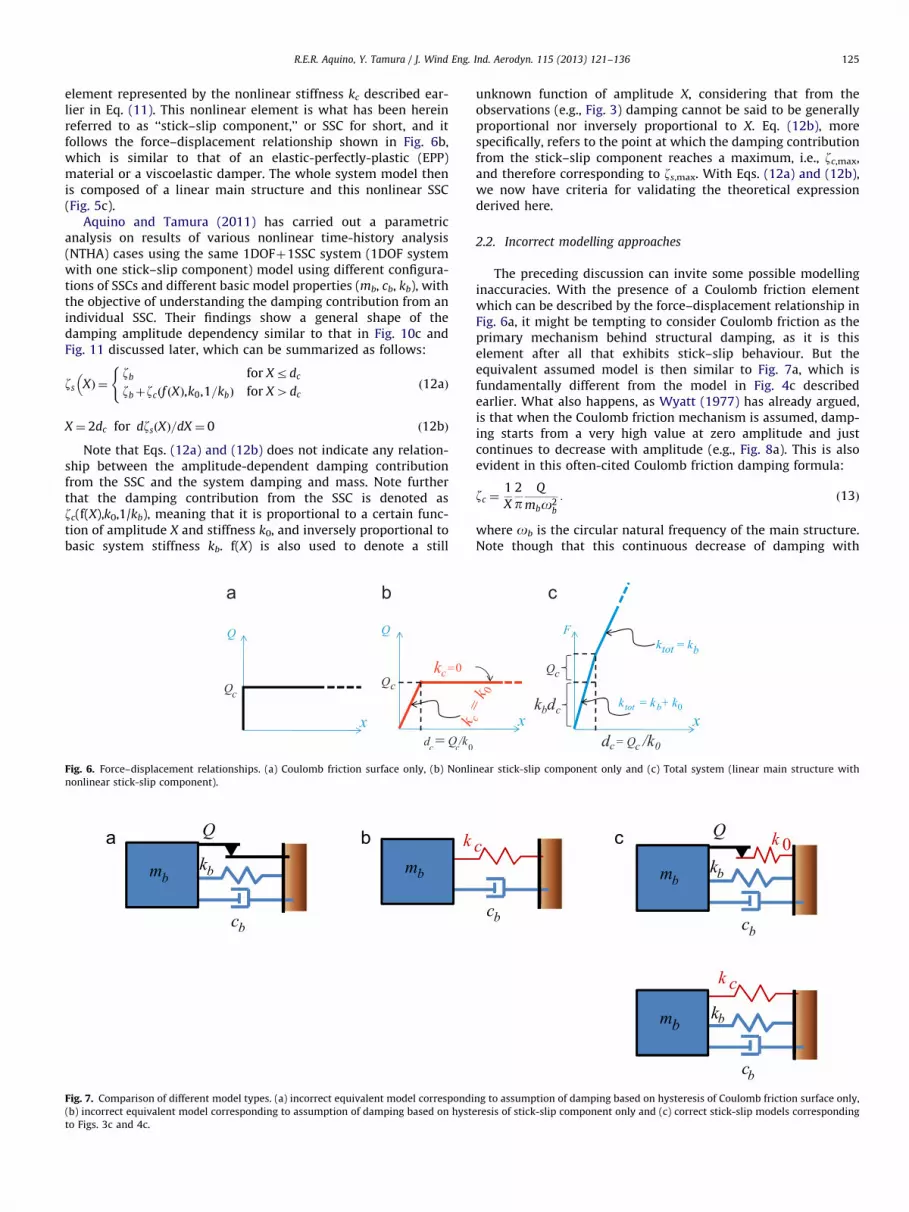
element represented by the nonlinear stiffness kc described ear-lier in Eq. (11). This nonlinear element is what has been hereinreferred to as ‘‘stick–slip component,’’ or SSC for short, and itfollows the force–displacement relationship shown in Fig. 6b,which is similar to that of an elastic-perfectly-plastic (EPP)material or a viscoelastic damper. The whole system model thenis composed of a linear main structure and this nonlinear SSC(Fig. 5c).

Aquino and Tamura (2011) has carried out a parametricanalysis on results of various nonlinear time-history analysis(NTHA) cases using the same 1DOFþ1SSC system (1DOF systemwith one stick–slip component) model using different configura-tions of SSCs and different basic model properties (mb, cb, kb), withthe objective of understanding the damping contribution from anindividual SSC. Their findings show a general shape of thedamping amplitude dependency similar to that in Fig. 10c andFig. 11 discussed later, which can be summarized as follows:

zs

�XÞ ¼

zb for Xrdc

zbþzcðf ðXÞ,k0,1=kbÞ for X4dc

(ð12aÞ

X ¼ 2dc for dzsðXÞ=dX ¼ 0 ð12bÞ

Note that Eqs. (12a) and (12b) does not indicate any relation-ship between the amplitude-dependent damping contributionfrom the SSC and the system damping and mass. Note furtherthat the damping contribution from the SSC is denoted aszc(f(X),k0,1/kb), meaning that it is proportional to a certain func-tion of amplitude X and stiffness k0, and inversely proportional tobasic system stiffness kb. f(X) is also used to denote a still

Fig. 6. Force–displacement relationships. (a) Coulomb friction surface only, (b) Nonli

nonlinear stick-slip component).

Fig. 7. Comparison of different model types. (a) incorrect equivalent model correspondi

(b) incorrect equivalent model corresponding to assumption of damping based on hyste

to Figs. 3c and 4c.

unknown function of amplitude X, considering that from theobservations (e.g., Fig. 3) damping cannot be said to be generallyproportional nor inversely proportional to X. Eq. (12b), morespecifically, refers to the point at which the damping contributionfrom the stick–slip component reaches a maximum, i.e., zc,max,and therefore corresponding to zs,max. With Eqs. (12a) and (12b),we now have criteria for validating the theoretical expressionderived here.

2.2. Incorrect modelling approaches

The preceding discussion can invite some possible modellinginaccuracies. With the presence of a Coulomb friction elementwhich can be described by the force–displacement relationship inFig. 6a, it might be tempting to consider Coulomb friction as theprimary mechanism behind structural damping, as it is thiselement after all that exhibits stick–slip behaviour. But theequivalent assumed model is then similar to Fig. 7a, which isfundamentally different from the model in Fig. 4c describedearlier. What also happens, as Wyatt (1977) has already argued,is that when the Coulomb friction mechanism is assumed, damp-ing starts from a very high value at zero amplitude and justcontinues to decrease with amplitude (e.g., Fig. 8a). This is alsoevident in this often-cited Coulomb friction damping formula:

zc ¼1

X

2

pQ

mbo2b

: ð13Þ

where ob is the circular natural frequency of the main structure.Note though that this continuous decrease of damping with

near stick-slip component only and (c) Total system (linear main structure with

ng to assumption of damping based on hysteresis of Coulomb friction surface only,

resis of stick-slip component only and (c) correct stick-slip models corresponding

Fig. 8. Stick–slip models employed by Lagomarsino (1993), reformatted for similarly to the models shown in Figs. 4 and 6. P represents an exterenally applied force.

A = area below secant stiffnessA = area of hysteresis loop

xX

F2

1

(X )( X )

( X )A

A

2

1

4

1

πζ =

Force-Displacement(Extension line)Hysteresis LoopSecant Stiffness

xX

(Force)F

Fig. 9. Hysteretic damping concept. (a) basic definitions and (b) equivalent viscous damping formula.

0

0.2

0.4

0.6

0.8

1

Nor

mal

ized

dam

ping

Normalizeddisplacement

0

0.2

0.4

0.6

0.8

1

Nor

mal

ized

dam

ping


0

0.2

0.4

0.6

0.8

1

1 10 100 1000 1 10 100 1000 1 10 100 1000

Nor

mal

ized

dam

ping


Fig. 10. General damping amplitude dependency using different models. (a) Coulomb friction only, (b) Nonlinear stick-slip component only and (c) Total system (linear

main structure with nonlinear stick-slip component).


amplitude is something that has not exactly been observed inactual measurements such as those shown in Fig. 3.

The seemingly more logical assumption is to apply the hys-teretic damping concept (Fig. 9) on the force–displacementrelationship of the nonlinear SSC (Fig. 6b). What this results inthough is a continuous increase of damping (Fig. 10b) foramplitudes beyond the slip displacement dc (i.e., once slippingis manifested, or when plasticity occurs in the case of EPPmaterials). The increase is at a rapid pace at lower amplitudes,later tapering to a slower pace but still continuously increasingthrough the much higher amplitude range. While the assumptionof stick–slip friction as opposed to simply Coulomb friction as thedamping mechanism is more correct, it is also possible that the

idea that damping continually increases with amplitude asdamage accumulates whether on a microscopic or on a structuralcomponent level stems from the picture painted in Fig. 10b. Inany case, Fig. 10b still does not reflect what has been observed insome full-scale measurements such as Fig. 3d. This modellingapproach is akin to neglecting the linear/constant stiffness con-tribution from the main structure and assuming a model such asin Fig. 7b, which is again fundamentally different from the modelthat has been discussed earlier (Fig. 5c), and not at all represen-tative of our simple system with SSC (Fig. 4c or d).

What is found though is that the nonlinearity of the totalsystem should be considered, i.e., that of the linear main structureplus the nonlinear SSC (Fig. 7c), and thus the force–displacement


relationship shown in Fig. 6c. This results now in a dampingamplitude dependency of the shape shown in Fig. 10c, which issimilar to those shown in Wyatt’s (1977) paper. The key differ-ence between the nonlinear-component-only approach (i.e.,Figs. 6, 7 and 10b, and discussed in the preceding paragraph)and the total system approach (Figs. 6, 7 and 10c) is that in theformer, all stiffness is unintentionally assumed lost after slippingoccurs whereas in the latter the stiffness from the linear compo-nent (in this case, the main structure) is still accounted for even asthe nonlinear component starts to have a degraded stiffnesscontribution. This is a very significant and very importantdifferentiator between the two. The end result then differs inthat in the latter, an increase in damping only occurs from thestart of slipping until a critical amplitude is reached; in theformer, the increase in damping theoretically lasts until infiniteamplitude. This already is justification for the stick–slip phenom-enon as the primary mechanism behind structural damping, but itis again emphasized that actual structures can have a largenumber of SSCs (hence, Fig. 5d) with unknown properties. Itcould be that after one SSC has slipped and initiates an increase indamping and then reaches a maximum level, a second SSC mightstart to slip and then continue to increase the system’s totaldamping, and so on.

For completeness of discussion, Lagomarsino’s (1993) pro-posed stick–slip models for wind-resistant design purposes arealso shown here in Fig. 8. Note their differences from the earlierestablished models (Fig. 5c or d), including that of Wyatt (1977)and Davenport and Hill-Carroll (1986), and how they might notrepresent the example system with stick–slip component dis-cussed earlier (Fig. 4c and d).

2.3. Derivation and validation of theoretical expression

The theoretical expression, as mentioned earlier, can bederived based on the hysteretic damping concept illustrated inFig. 9 and defined by:

z Xð Þ ¼1

4pA1ðXÞ

A2ðXÞ: ð14Þ

where z(X) is the equivalent viscous damping ratio for thesystem’s hysteresis occurring with amplitude X, and A1 and A2

are areas inside the hysteresis loop (i.e., from amplitude �X to X),and below a straight line (i.e., corresponding to the secantstiffness) from zero displacement to the point on the hysteresiscurve corresponding to the amplitude X, respectively. The ratioA1/A2 represents the ratio of the energy dissipated by the dampingmechanism over the total energy in the system. Likewise asmentioned, Eq. (14) should be applied to the force–displacement relationship of the total system. The resulting

0%

1%

10%

0.0001 0.001

Dam

ping

Rat

io ζ

s

Displacemen

Fig. 11. Validation against numerical results of derived theoretical expression (Eq. (18))

a 1DOF system.

formula is then:

zc Xð Þ ¼2

p1

1þðkb=k0ÞðX=dcÞ

� �1�

dc

X

� �H 1�

dc

X

� �ð15Þ

Eq. (15) meets the first of the three parts of the validatingequation in Eqs. (12a) and (12b) as it simply becomes zero whenXrdc. It also clearly suggests that zc(X)pk0/kb, meeting the 2ndof the three parts of Eqs. (12a) and (12b). To check if a maximaoccurs at X¼2dc, the derivative of Eq. (15) with respect toamplitude X equated to zero, or dzc(X)/dX¼0, is evaluated. Onewill find that for such a case, Xm¼X¼2dc, and additionally,zc,max¼zc(2dc)¼[p(1þ½kb/k0)]�1 which tells us that zc,max isproportional to k0/kb. All validation requirements depicted in Eq.(12) have now been met.

Fig. 11 likewise shows a validation of Eq. (15) against numer-ical results obtained using the same methodology in Aquino andTamura (2011). The figure does not show a perfect fit, which isattributed to errors generated in the numerical analyses thatgenerally occur in the low-amplitude range corresponding to theend of the NTHA output. In any case, Eq. (15) is now our finalderived expression for the amplitude-dependent damping con-tribution zc(X) from an individual SSC with initial stiffness k0 andslip displacement dc¼Qc/k0 acting on a 1DOF system of stiffnesskb. Eq. (15) can be viewed as a function with two simpleparameters: a stiffness parameter defined by k0/kb, and anamplitude parameter defined by dc/X. Eq. (15) also serves as amore general equation that covers both Coulomb friction (Figs. 6,7 and 10a) and nonlinear EPP/stick–slip-component-only (Figs. 6,7 and 10b) models. The former can be obtained by setting dc tozero and substituting k0dc with Qc. The latter can be obtained bysetting kb to zero, or by setting k0 to infinity.

3. Damping due to a large number of stick–slip componentswith unknown parameters

3.1. Principal model

The preceding chapter discussed the basic stick–slip dampingtheory due to an individual SSC in a 1DOF system. Systems with alarge number of stick–slip components are now analysed, as thesemight be more reflective of actual structures. A 1DOF systemmodel is still used, representing individual modes of vibration.But this time, multiple stick–slip components are considered. If N

SSCs are present, additional nonlinear spring elements are mod-elled in parallel, with each nonlinear stiffness element denoted bya subscript i, e.g., kci, and thus their stiffnesses are simply summedup (Fig. 5d). The principal model for 1DOFþNSSC systems (1DOFsystem with an N number of SSCs) is thus defined by this general

0.01 0.1 1t Amplitude X (m)

Theoretical

Numerical

for amplitude-dependent damping contribution from one stick–slip component in

0%

1%

10%

0.000001 0.00001 0.0001 0.001 0.01 0.1

TheoreticalNumerical

1%

10%

g Rat

io ζ s

Dam

ping

Rat

io ζ s

Displacement Amplitude X (m)

TheoreticalNumerical


system equation:

mb €xþcb _xþkbxþXN

i ¼ 1

kcix¼ 0 ð16aÞ

kci ¼ k0iHðdci�XÞ ð16bÞ

where dci is the trigger displacement for SSC i. From Eqs. (16a) and(16b), it is initially judged that the damping contribution fromindividual SSCs in a 1DOFþNSSC system will simply add up andthus:

zs

�XÞ ¼ zbþ

XN

i ¼ 1

zciðXÞ ð17Þ

3.2. Numerical experiment and theoretical validation

With Eq. (17) still subject to validation, a new numericalexperiment was carried out. A rather simple 1DOFþ6SSC systemwas analysed, using the same methodology as in Aquino andTamura (2011). In the numerical analyses, the individual SSC’s k0i

values were set to have a coefficient of variation (COV) of 0%,while their dci values followed a uniform distribution with around70% COV (Table 1). Individual 1DOFþ1SSC systems each usingone of the 6SSC system’s SSCs were also analysed for comparisonwith the results for the 1DOFþ6SSC system. A more complicated1DOFþ441SSC system was subsequently analysed to validate theupdated theoretical expression for a larger N. The value 441 was alimit imposed by the computational requirements on the desktopcomputer and software used for the numerical experiment. Atotal of eight numerical analysis cases were carried out, one1DOFþ6SSC system (‘‘Case J’’) and six 1DOFþ1SSC systems withSSC parameters (‘‘J-a’’ to ‘‘J-f’’) listed in Table 1, and one1DOFþ441SSC system with the SSCs having practically arbitraryk0i and dci values with a COV of 200% and 367%, respectively.Figs. 12 and 13 shows results for the 1DOFþ6SSC system (‘‘CaseJ’’) and the related six 1DOFþ1SSC systems (Cases ‘‘J-a’’ thru ‘‘J-f’’). The figure shows that as individual SSCs slip, they eachcontribute additional damping as postulated earlier in Eq. (17).

Table 1Properties of SSCs in Case J (N¼6, 1DOFþ6SSC system).

Stick–slip component k0i (kN/m) dc (m�10�4) Qc (kN)

J-a 10,000 0.06 0.06

J-b 10,000 0.44 0.44

J-c 10,000 0.81 0.81

J-d 10,000 1.19 1.19

J-e 10,000 1.56 1.56

J-f 10,000 1.94 1.94

0%

1%

2%

3%

4%

5%

6%

0.000001 0.00001 0.0001

Dam

ping

Rat

io ζ

s

Displacemen

Fig. 12. Results for Case J (1DOFþ6SSC system with SSC properties following Table 2)

corresponding to each of the 6 listed in Table 2).

Together with the derived equation for one SSC’s dampingcontribution in Eq. (15), Eq. (17) can thus now be updated forapplicability to 1DOFþNSSC systems by:

zc Xð Þ ¼XN

i ¼ 1

2

p1

1þðkb=k0iÞðX=dciÞ

� �1�

dci

X

� �H 1�

dci

X

� �ð18Þ

The numerical results for both the 6SSC and the 441SSCsystems again exhibit errors in the small amplitude range(Fig. 18). Ignoring such small errors, Fig. 18 suggests goodagreement between the theoretical and numerical results, vali-dating Eqs. (17) and (18).

The problem though is that a system with a very large numberof SSCs, say as many as N¼10,000 or more, and followingdifferent levels of variability (expressed by their COVs) andprobability distribution types should be analysed. But to carryout NTHA for a large number of cases is deemed quite cumber-some, and therefore development of purely theoretical expres-sions of damping based on the stick–slip mechanism, togetherwith theoretical expressions of inverse cumulative distributionfunctions is pursued next.

0.001 0.01 0.1

t Amplitude (m)

Case J-a Case J-bCase J-c Case J-dCase J-e Case J-fCase J

, and Cases J-a, J-b, J-c, J-d, J-e, and J-f (1DOFþ1SSC systems with SSC properties

0%0.000001 0.00001 0.0001 0.001 0.01 0.1 1

Dam

pin

Displacement Amplitude X (m)

Fig. 13. Validation against numerical results of derived theoretical expression (Eq.

(18)) for amplitude-dependent damping due to multiple stick–slip components in

a 1DOF system. (a) 1DOFþ6SSC system in Case J (i.e. with N¼6, constant k0i, and

uniformly distributed dci with COV of 20%) and (b) 1DOFþ441SSC system (i.e. with

N¼441, k0i with COV of 200%, and dci values with COV of 367%).

Table 2Inverse CDF functions.

Probability distribution Original CDF Inverse CDFs for substitution

in rki or rdi

Uniform i�1N�1

ðCDFi�0:5ÞaLog-normal 1

2 þ12 ERF lnri�mffiffiffiffiffiffi

2s2p

� �exp½1þ

ffiffiffiffiffiffiffiffiffiffiffiffiffiffiffi2COV2

pUERF�1

ð2CDFi�1Þ�

Normal ri�mþffiffi3p

s2ffiffi3p

s1þ

ffiffiffiffiffiffiffiffiffiffiffiffiffiffiffi2COV2

pUERF�1

ð2CDFi�1Þ

Weibull (k¼5, l¼1) 1�exp½�ðri=lÞk� l½�Inð1�CDFiÞ�

1=kaZ

Gamma (t¼1, y¼2) gðt,ri=yÞGðtÞ

�2½Inð1�CDFiÞ�aZ

Note: ri is a variable that could be replaced with either rki or rdidci as used in Eq.

(17); m is the mean of ri values; s is the standard deviation of ri values such that

the COV is s/m; k and l are Weibull distribution parameters; t and y are Gamma

distribution parameters; ERF denotes the Error Function; G and g indicate the

Gamma and the lower incomplete Gamma functions, respectively; a is a multiplier

that should adjust the COV (and mean) of the distribution; and CDFi are equally

spaced N numbers from 0 to 1.


3.3. Probabilistic analysis methodology

Eq. (18) is flexible such that if all SSCs in actual structures areidentified (i.e., N is known) and their properties (i.e., k0i and dci)are measurable or at least possible to estimate with acceptableaccuracy, these could just be plugged into Eq. (16) directly,thereby employing a deterministic approach. However, it isdifficult to determine such values, and even more so when N issignificantly large. A probabilistic approach, where probabilitydistributions as well as variability (defined by the COV) areconsidered for each of the parameters, is therefore necessary. Toaccommodate the probabilistic analysis, Eq. (18) is modified as:

zc Xð Þ ¼XN

i ¼ 1

2

p1

1þðkb=k0rkiÞðX=dc1rdiÞ

!1�

dc1rdi

X

� �H 1�

dc1rdi

X

� �

ð19Þ

where k0 is the mean of all k0i values, dc1 is the smallest of all dci

slip displacement values, rki is a set of random numbers withmean equal to unity following a certain probability distribution

and COV such that all k0rki values translate to all k0i values, rdi is

a set of random numbers with mean equal to 1=dci as a

dimensionless value (or that rdidci as a dimensionless value is a

set of random numbers with mean equal to unity) and following a

certain probability distribution and COV such that rdidci trans-

lates to dci, and dci is the mean value of all dci. The mean value dci

could have been used instead of dc1, but it is more difficult to

determine dci in real structures because it is a function of Qci,which in turn is a function of a normal force N0 (where Qci¼mNi

0),which is very difficult to determine in actual structures, incontrast to stiffness values k0i which are easier to estimate.Moreover, from damping amplitude dependency measurements,

it might be easier to detect dc1, because to arrive at dci all valuesof dci need to be detected, and current measurement techniquesare only able to observe damping amplitude dependency for alimited range of amplitudes much less than those correspondingto wind-resistant design.

To generate purely theoretical estimates of damping based onthe selected probability distributions, theoretical estimates of rki

and rdidci (i.e., ‘‘random numbers’’ with mean equal to unity)need to be generated. These numbers are a function of cumulativedensity functions (CDFs). Normally information on CDFs is readilyavailable, comprising functions of given random numbers such asrki and rdidci . But it is not usually necessary to generate ‘‘random’’numbers such as rki and rdidci that would theoretically andclosely follow a certain CDF. The inverse of these CDFs (or herein

Fig. 14. Illustration of derivation of iCDFs (i.e., ‘‘theoretical random numbers’’

given a CDF).

referred to as ‘‘iCDFs’’) are therefore derived. iCDFs for otherprobability distribution types can be obtained by interestedparties following the procedure illustrated in Fig. 14 anddescribed next.

Taking a (theoretical) CDF for a specific probability distributionand considering that an N number of ‘‘theoretical’’ randomnumbers were to be generated, an N number of horizontal lineswere projected towards the plot of the CDF (which theoreticallyranges from zero to unity) and from there projected downtowards the axis of ‘‘random numbers.’’ It was thus necessary toexpress first the CDF in terms of N values from zero to unity:

CDFi ¼i�1

N�1ð20Þ

Incidentally, Eq. (20) is the CDF for a uniform distribution, aslisted in Table 2, and from which it can be deduced that the CDFi

values are equally spaced. For the four other selected probabilitydistribution types, the CDF functions are likewise listed in Table 2together with the final set of derived iCDFs that could be used inconjunction with Eq. (19). The iCDF equations in Table 2 addi-tionally use a variable a that is meant to adjust the COV (andmean) of the distribution to that desired. At least for the uniformdistribution, it can be defined as:

a¼ffiffiffiffiffiffiffiffiffiffiffiffiffiffiffiffiffiffiffiffiffiffiffiffiffiffiffiffiffiffiffiffiffiffiffiffiffi

NPNj ¼ 1ðCDFj�0:5Þ

s� COV ð21Þ

where the term inside the square root operator is essentially theinverse of the mean of generated ‘‘theoretical’’ random numbers.Note that the term inside the parentheses is the same as the terminside the parentheses in the iCDF for the uniform distributionshown in Table 2. In the analysis, an algorithm has been usedinstead of calculating appropriate values of a for each case. Forvalidation, pseudo-random numbers has been generated andcompared with the equations in Table 2 (Fig. 15) for cases withN¼10,000, mean m¼1, and COV¼20%. The results show that thetwo sets of generated ‘‘random’’ numbers match satisfactorily.

Note that the 5 different probability distribution types (Fig. 15and Table 2) were selected, such that each had a very distinctshape; i.e., the uniform distribution was flat and had zero skew,the normal distribution had a bump and zero skew, the log-normal distribution had a bump and positive skew, the Weibulldistribution with k¼5 and l¼1 had a bump but with negativeskew, and the Gamma distribution with t¼1 and y¼2 hadpositive skew but with the statistical mode closer to the lowestvalues. At this time, it is pointed out that these theoreticalestimates evidently account for univariate probability distribu-tions only. It is left to interested parties to generate theoretical

Fig. 15. Validation of ‘‘theoretical random numbers’’ against numerically generated pseudo-random numbers, for five selected probability distributions. Both cumulative

density functions (CDFs) and histograms are shown. (a) uniform distribution, (b) normal distribution, (c) log-normal distribution, (d) Weibull distribution with k¼5 and

l¼1 and (e) Gamma distribution with t¼1 and y¼2.


estimates for multivariate cases. For this study, as mentioned,numerically-generated pseudo-random numbers following themultivariate normal distribution, and ‘‘pseudo-bivariate’’ caseswhere one univariate distribution is applied to two parameters ata time, are used as well. It is also important to note that inconsideration of the requirement that the generated properties

are positive-definite, only the log-normal distribution permitsCOV values of 200% and higher, and only in conjunction with N of100 or higher. In this sense, perhaps the log-normal or similarlyshaped probability distributions may be best suited to modellingactual conditions particularly for systems with very largevariability.


3.4. Probabilistic analysis cases

As mentioned, without knowledge of the actual stick–slipparameters in structures, including their quantity N, Eq. (18) byitself would be difficult to use in practice. What was done insteadis to analyse a large number of cases, each with different sets ofparameters that are defined using different probability distribu-tions. Using the updated theoretical expression, a total of 672cases with different 1DOFþNSSC systems were analysed withSSCs as follows:

�

Fig

N values of 10, 100, 1000, and 10,000;
� 5 selected univariate probability distributions (uniform, nor-
mal, log-normal, Gamma, Weibull);
� One multivariate distribution (multivariate normal); � for the univariate cases, COVs of 0%, 5%, 10%, 25%, 50%, 75%,
100%, 200%, and 500% where possible;
� for the univariate cases, 6 sub-cases as follows: constant dci,
constant k0i, constant k0idci but varying k0i, constant k0idci butvarying dci, varying k0i and dci similarly such that theircorrelation coefficient is unity, and varying k0i and dci similarlybut applied inversely such that their correlation coefficient isclose to negative one (�1);
� for multivariate cases, target correlation coefficients of 0%, 1%,
5%, 10%, 20%, 50%, 80%, and 95%, and their negative counter-parts, applied to two cases each except the 0% case.

The multivariate normal random numbers were numerically-generated, but one problem found with such was that each set ofthe generated numbers was different from the next, and so theend results for what was intended to be the same cases (sametarget correlation coefficient) were slightly different. Thus, foreach target correlation coefficient, two sets of numbers werenumerically generated. For the univariate sub-cases mentioned,note that only the first two were actual univariate cases, with therest being pseudo-bivariate cases, meaning that only one uni-variate probability distribution was used together with an estab-lished relationship for the two parameters. The multivariatenormal cases were likewise bivariate cases only. The basic systemproperties were similar to those of the earlier analysed 1DOFsystems, but in these 672 cases, the total of stiffness values Sk0i

and the mean of all slip displacement values dci were madeconstant for all cases. Again, the values assigned were notimportant, and instead these are later normalized so that thefindings might be applicable to structures with any basic dampingratio, basic natural frequency, or SSC parameter values. Further-more, a maximum COV of 500% was used in consideration of therange of coefficients of friction between materials typically usedin construction. COV values larger than 500% or other probabilitydistributions could be analysed in future studies if warranted,using the same procedure discussed in this paper.

1

2

4

0.1 1 10

Nor

mal

ized

Dam

ping

ζc/ζ

b

Normalized A

X=d c1 X=Xl

X=X

ζ c ≈1.05 ζb

. 16. Visual definitions of dc1, Xl, Xm, and zc,max, overlain on one example case with N

3.5. Results and discussion

The earlier definitions of zc,max (maximum added dampingratio), Xl (low amplitude level at which damping starts to increasewith amplitude), and Xm (moderate amplitude level correspond-ing to zc,max) are used in the succeeding discussion of the results.Refer to Fig. 16 for a visualization of these quantities in thecontext of 1DOFþNSSC systems. The definition of Xl is refined tobecome the amplitudes corresponding to total structural dampingvalues that are around 5% larger than the baseline damping (zb,here assumed to be 0.3%), or when the amplitude-dependentcomponent is 5% of the baseline level. This new definition takesinto account cases such as those shown in Fig. 16 where dampingvery gradually increases with amplitude over a large amplituderange after the initial dc1 before finally increasing more dramati-cally with amplitude. In some cases the ratio Xm/dc1 can be asmuch as around 4 orders of magnitude, but by using Xm/Xl

instead, maximum damping is seen to occur only within twoorders of magnitude from the start of significant dampingincrease with amplitude. The use of this redefined Xl is also moreuseful in that in actual measurements where it is practicallyimpossible to know true dci values, it might still be difficult tomeasure true dc1 values, particularly where damping only ever soslightly increases with amplitude as in Fig. 16, whereas it is easierto detect Xl values in full-scale measurements given this newdefinition as it more or less corresponds to when damping startsto more noticeably increase with amplitude.

From the 672 cases analyzed, nine representative results areshown in Figs. 17–20. The results are grouped into four, correspond-ing to the number of peaks. In these figures, the vertical axis isexpressed as a normalized damping value, and more specifically, zc/zc,max(all). zc,max(all) is the maximum zc,max from all 672 cases. Notethat Fig. 17a, for example, has a maximum normalized damping zc/zc,max(all) equal to unity, suggesting that this case resulted in thelargest maximum damping value compared to other cases. Thehorizontal axis of these figures is likewise in terms of a normalizedamplitude, X/Xl, where the amplitude is normalized against Xl, asdiscussed earlier, being the point at which damping more or lessstarts to significantly increase with amplitude.

Fig. 17 shows five different examples with one peak and withthe ratio Xm/Xl varying from around 2 to around 100 in conjunc-tion with a generally decreasing zc,max. Fig. 18 shows examplesthat could be considered to have two peaks while Fig. 19 showsone out of all 672 cases that could be considered to have resultedin three peaks. Figs. 18b and 19 show small peaks occurringbefore the absolute peak is reached, while Fig. 18a shows anexample where the larger peak occurs at smaller amplitudes thanthe lower peak. Figs. 18 and 19 highlight the fact that if dampingmeasurements are carried out for only a very narrow amplituderange at relatively very low levels, there are a number ofpossibilities for what might be happening in the actual amplitude

100 1000 10000mplitude X/dc1

m

ζc = ζ c,max

¼10,000, COV¼500% and log-normal distribution for k0i, and k0idci kept constant.

0

0.2

0.4

0.6

0.8

1

0.1 1 10 100 1000N

orm

aliz

edD

ampi

ng ζ

c/ζc,

max

(all)

Normalized Amplitude X/Xl

(a)(b)(c)(d)(e)

Fig. 17. Five sample results out of 672 analysis cases of different 1DOFþNSSC systems showing one peak: (a) N¼10,000, COV¼500% and log-normal distribution for k0i,

constant dci; (b) N¼10,000, COV¼25% and normal distribution for both k0i and dci, varied similarly such that they are fully correlated (c) N¼10, COV¼50% and Weibull

distribution for both k0i and dci, varied similarly such that they are fully correlated; (d) N¼100, COV¼500% and log-normal distribution for dci, k0idci kept constant; and

(e) N¼1,000, COV¼200% and log-normal distribution for k0i, k0idci kept constant.

0

0.2

0.4

0.6

0.8

1

0.1 1 10 100 1000 10000

Nor

mal

ized

Dam

ping

c/ c

,max

(all)


(a)(b)

ζζ

Fig. 18. Two sample results out of 672 analysis cases of different 1DOFþNSSC systems showing two peaks: (a) N¼100, COV¼500% and log-normal distribution for k0i,

constant dci; and (b) N¼10, COV¼100% and log-normal distribution for both k0i and dci, varied inversely such that their correlation coefficient approaches negative one.

0

0.2

0.4

0.6

0.8

1

0.1 1 10 100 1000 10000

Nor

mal

ized

Dam

ping

c/ c

,max

(all)


ζζ

Fig. 19. One sample result out of 672 analysis cases of different 1DOFþNSSC systems showing three peaks. (N¼100, COV¼500% and log-normal distribution for both k0i

and dci, varied similarly such that their correlation coefficient is unity.).

0

0.2

0.4

0.6

0.8

1

0.1 1 10 100 1000 10000

Nor

mal

ized

Dam

ping

c/ c

,max

(all)


ζζ

Fig. 20. One result out of 672 analysis cases of different 1DOFþNSSC systems showing no clear peak. (N¼100, COV¼200% and log-normal distribution for k0i, k0idci kept

constant.).


range of concern that might not be detected. In other words, thereis near-absolute uncertainty as to appropriate damping values forwind-resistant design applications unless measurements arecarried out specifically at the corresponding amplitudes.

Fig. 20 could be looked at as having two peaks, or as one withno clear peak and instead having practically constant maximumdamping over about one order of magnitude of the amplitudebefore decreasing. Fig. 20 shows that current damping models


such as that depicted in Fig. 1 can still be valid. But here it isqualified that it could be valid only up to a certain amplituderange. Note that this has occurred only for one out of the 672cases, with N¼100, log-normal distribution, and a COV of 200%(i.e., it did not occur for higher N nor higher COV values). Fig. 13bshows another example where the stiffness and amplitude para-meters had 200% and 367% as COV values, respectively, resultingin practically constant damping over around two orders ofmagnitude of the amplitude.

While in some cases (e.g., Figs. 18 and 19) there would be a‘‘roller coaster,’’ up and down, alternating increase and decreaseof damping with amplitude, note however that in all results,damping initially increased but eventually decreased with ampli-tude. This is perhaps the single most important conclusion thatcan be drawn from this analysis.

Additionally, it is found that in 92 cases where dci is constantor has low variability (say up to 10%), Xm/dc1 is close to 2, Xm/Xl

E1.8, and the amplitude dependency of damping is identical tothat in an equivalent 1DOFþ1SSC system with k0/kb¼Sk0i/kb anddc¼dci¼dc1¼any dci. This is logical as the maxima of the indivi-dual damping contributions coincide and simply add up. Fig. 17ais one such result with no dci variability, and shape-wise it looksvery similar to Figs. 10c or 11 for 1DOFþ1SSC systems. This resultbasically suggests that regardless of the number N of SSCs in themodel (1, 10, or 10,000), the COV (0%, 50%, or 500%), or distribu-tion type of k0i, the system would simply resemble a 1DOFþ1SSCsystem if there were constant or low-variability dci. As discussedearlier, the k0i values should also have some effect on thedamping levels, but such effect is only manifested more visiblyin conjunction with a variability in dci. In this sense, dci perhaps isa more important parameter in damping amplitude dependencythan k0i, and meanwhile dci values (as well as Qci since Qci¼k0i/dci)are generally more difficult to determine in real structures. k0i isperhaps more important only in determining absolute dampingvalues; i.e., if another set of similar cases had been analyzedwhere the k0i values were changed, only zc, zc,max, and zs,max

values would change but their amplitude dependency would

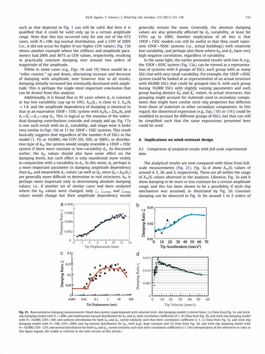
Fig. 21. Representative damping measurements (black data points) superimposed with

slip damping model with N¼1,000, and multivariate normal distribution for k0i and dci w

with N¼10,000, COV¼50% and uniform distribution for both k0i and dci, varied simila

damping model with N¼100, COV¼200% and log-normal distribution for k0i, with k0

N¼10,000, COV¼25% and normal distribution for both k0i and dci, varied similarly such t

this figure legend, the reader is referred to the web version of this article.)

generally remain the same. Generally, the absolute dampingvalues are also generally affected by dci variability, at least forCOVs up to 100%. Another implication of all this is that1DOFþ1SSC models can still be useful in that they could repre-sent 1DOFþNSSC systems (i.e., actual buildings) with relativelylow variability, and perhaps also those where k0i and dci have veryhigh negative correlation, regardless of variability.

In the same light, the earlier presented results with low N, e.g.,the 1DOFþ6SSC system (Fig. 13a), can be viewed as a representa-tion of systems with 6 groups of SSCs, each group with as manySSCs but with very small variability. For example, the 1DOFþ6SSCsystem could be looked at as representative of an actual structurewith 60,000 SSCs that could be grouped into 6, with each grouphaving 10,000 SSCs with slightly varying parameters and eachgroup having distinct k0i and dci values. In actual structures, thisgrouping might account for materials used in secondary compo-nents that might have similar stick–slip properties but differentfrom those of materials in other secondary components. In thisregard, the theoretical expression (e.g., Eqs. (18) or (19)) could bemodified to account for different groups of SSCs, but that can stillbe simplified such that the same expressions presented herecould be used.

4. Implications on wind-resistant design

4.1. Comparison of analytical results with full-scale experimental

data

The analytical results are now compared with those from full-scale measurements (Fig. 21). Fig. 3a–d show Xm/Xl values ofaround 4, 5, 30, and 3, respectively. These are all within the rangeof Xm/Xl values observed in the analyses. Likewise, Fig. 3a and bshow damping to be more or less constant for a certain amplituderange, and this has been shown to be a possibility if stick–slipmechanism was assumed, as illustrated by Fig. 20. Constantdamping can be observed in Fig. 3c for around 1 to 2 orders of

selected stick–slip damping models (colored lines). (a) Data from Fig. 3a, and stick-

ith correlation coefficient of 1, (b) Data from Fig. 3b, and stick-slip damping model

rly such that their correlation coefficient is 1, (c) Data from Fig. 3c, and stick-slip

idci kept constant and (d) Data from Fig. 3d, and stick-slip damping model with

hat their correlation coefficient is 1. (For interpretation of the references to color in


magnitude of the amplitude, and meanwhile, Fig. 20 and Fig. 13b(for the 1DOFþ441SSC system) suggests that damping could bemore or less constant for as much as 2 orders of magnitude.Fig. 17b has an Xm/Xl of around 3 and could be a model for Fig. 3d.Looking only at the amplitude range 7�10�5 m to 3�10�4 m inFig. 13a (for the 1DOFþ6SSC system) suggests an Xm/Xl of around4, and this could more or less be viewed as a possible model forFig. 3a, which has similar Xm/Xl. In any case, this again highlightshow damping measurements carried out for a limited amplituderange might not paint the whole picture. Conversely, thesecomparisons also show that the stick–slip phenomenon canindeed be a primary mechanism behind structural damping inwind-resistant design applications—where the main structureresponse is desired to remain within linear-elastic limits.

In general, the representative shapes shown in Figs. 17–20appear to be similar or better models for full-scale measurementsin Fig. 3 than the current model, depicted in Fig. 2 and super-imposed on the data in Fig. 3. Selected possible models are nowsuperimposed with these full-scale experimental data as shownin Fig. 21. The selected models do not perfectly fit the data,especially in the case where there is a scatter in the results suchas in Fig. 21c. Better fitting models could also be used, but for nowthese are sufficient to show the flexibility and appropriateness ofthe use of the model, because, in the case of Fig. 21d for example,there is better correlation with the data for the derived modelthan for the current model (Fig. 3d).

4.2. Estimation of differences in wind loads

The differences in wind loads using current models and usingthe derived stick–slip damping model are now presented, usingthe basic wind loading equations discussed earlier. More specifi-cally, two wind-resistant design applications are considered:‘‘habitability design’’ (design for occupant comfort, say, under

Table 3Different damping estimates and corresponding approximate differences in wind load

Model Habitability designa

Estimated damping ratio

a. Building data shown in Figs. 3a and 21a (assumed to be in non-cyclonic regionc)

Direct from data 0.5%

Current, as fitted to data 0.5%

Current, using Jeary (1986) formula 1.9%

Stick–slip, as fitted to data 0.5%

b. Building data shown in Figs. 3b and 21b (assumed to be in cyclonic regionf)

Direct from data –


Current, using Tamura et al. (2000) recommendation 0.7%

Stick–slip, as fitted to data 2%

c. Building data shown in Figs. 3c and 21c (assumed to be in cyclonic regionf)

Direct from data 11–13%

Current, as fitted to data 12%

Stick–slip, as fitted to data 13%

d. Building data shown in Figs. 3d and 21d (assumed to be in cyclonic regionf)

Direct from data 1%


Current, using Tamura et al. (2000) recommendation 0.7%

Stick–slip, as fitted to data 0.9%

a Approximately corresponding to 1-year return period winds, and an assumed tipb Approximately corresponding to 500-year return period winds, and an assumedc Assumed basic gust wind speeds of 15 m/s and 35 m/s for habitability design and Approximate difference in wind load is relative to this case for habitability desige Approximate difference in wind load is relative to this case for safety design.f Assumed basic gust wind speeds of 30 m/s and 70 m/s for habitability design and

1-year return period winds), and ‘‘safety design’’ (correspondingto structural design itself, say, under 500-year return periodwinds). For simplicity in this comparison and only for illustrativepurposes, these two design applications are associated withassumed tip drift ratios of 10�4 and 10�3, respectively; assumedmaximum basic gust wind speeds of 15 m/s and 35 m/s, respec-tively, for non-cyclonic regions; and assumed maximum basicgust wind speeds of 30 m/s and 70 m/s, respectively, for cyclonicregions. All other wind loading parameters, including the naturalfrequency (assumed as f¼46/H in all cases), are assumed to beconstant for each building. The estimated damping ratios usingcurrent models and the new models, and their differences in windloads are shown in Table 3. The differences in wind loads areexpressed in percentage relative to the wind loads correspondingto the cases when the current damping model is used. Note thatTamura et al.’s (2000) model is used for the data in Fig. 21b and d(Fig. 3b and d) since the model is intended for buildings in Japanbetween 30 m and 200 m in height, and meanwhile, the data inFig. 21b–d (Fig. 3b–d) are from buildings in Japan. Jeary’s (1986)model is used for Fig. 21a (Fig. 3a), which is one of the buildingsanalysed in the development of his model. When estimating thedifference in wind loads for the buildings in Japan, a cyclonicregion is assumed, while a non-cyclonic region is assumed for thebuilding in Fig. 21a (Fig. 3a). Table 3 also shows the approximatedamping ratios directly from the data, if the amplitude range of themeasurements are inclusive of the amplitude associated with thedesign application (habitability or safety).

4.3. Results and discussion

The results in Table 3 all show that with such amplitude-damping data available, even at generally low amplitudes, thedifferent models are able to approximate a damping value thatresults in not much differences in wind loads. Such data can only

s.

Safety designb

Approximate difference

in wind load

Estimated damping

ratio

Approximate difference

in wind load

0% – –

0%d 0.5% 0%e

Up to 2% lower 1.9% Up to 13% lower

0% 0.2% Up to 24% higher

– – –

0%d 2.5% 0%e

Up to 12% higher 1% Up to 22% higher

Up to 1% higher 1.6% Up to 9% higher

0% 11–14% 0%

0%d 12% 0%e

0% 13% 0%

Up to 3% higher – –

0%d 1.3% 0%e

Up to 7% higher 1% Up to 7% higher

Up to 4% higher 0.6% Up to 23% higher

drift ratio of around 10�4.

tip drift ratio of around 10�3.

d safety design, respectively.

n.

safety design, respectively.


be obtained by time-domain damping evaluation techniques (e.g.,see Jeary, 1996; Tamura and Suganuma, 1996; Tamura, 2012), andin the case of at least the first, third, and fourth buildings(Table 3a, c, and d), up to higher than usual amplitudes. Conse-quently, the differences in wind loads are also up to 12% underhabitability design, and up to 24% under safety design, suggestingthat with the amplitude of excitations under habitability designclose to those as measured, there could be higher reliability in thisdesign application than in safety design for wind. This begs theissue stated earlier in Section 1 on the lack of proper dampingmeasurements at such high amplitude levels (but not beyond themain structural system’s linear elastic limit) to be addressed, butthe impracticality of such measurements cannot be discounted.

In Table 3a, even with a large difference in damping estimates,the result is only as much as a 2% difference in wind loads underhabitability design, again due to measurements being actuallyavailable at the associated amplitude. But the difference is asmuch as around 40% under safety design. The selected stick–slipmodel (Fig. 21a) resulted in the lowest damping estimate undersafety design, having assumed damping to decrease with ampli-tude in the range without measurements; the fitted modelfollowing the current approach (Fig. 1) assumes it would still bearound the same as the maximum measured damping at thelower amplitudes; and the proposed model which is based on adatabase of buildings (Jeary, 1986) resulted in the highest damp-ing estimate. Even if another stick–slip model could have beenused, this large difference in results highlights the fact that nomodel could be considered as the accurate one, and the predicteddamping behaviour at such high amplitudes cannot be validated,until the proper measurements are carried out. This same con-clusion can be made from the results in Tables 3b–d. Table 3cshows a near perfect match for all models relative to the data, andtherefore practically no differences in wind load estimates, pre-cisely because the data is available, but also perhaps because thisis a small structure relative to the other examples.

Table 3b also shows that, using the selected stick–slip model,the estimated damping might not be as low as suggested byTamura et al. (2000). Of course, their model is based on a databaseof buildings, with some scatter in the data, for which this specificbuilding measurement might be an exception. Both Tables 3b andd, meanwhile, illustrate the reduction factors applied to dampingestimates recommended by Tamura et al. (2000). By their model,the estimated damping ratio is a very low 0.7% for both buildingsunder habitability design, and then it increases to 1% for safetydesign, which is contrary to stick–slip damping theory. The effecton the wind loads is not so much significant in Table 3d, but forthe safety design case in Table 3b, it is. Meanwhile, in Table 3b,the stick–slip damping model results in lower wind loads thanwhen using the current recommendation, but in Table 3d, itresults in higher wind loads. Table 3d also shows how the currentmodel cannot predict the decrease of damping with amplitude,resulting in higher damping estimates for wind-resistant design.

5. Concluding remarks

The importance of damping and wind loads was first dis-cussed, and current damping models intended for wind-resistantdesign were presented. These models are based on empirical data,and attributed to stick–slip mechanism. The mechanism itself hasnot been studied properly yet, and so this was performed, first, toarrive at a theoretical expression for one-stick–slip-componentsystems, and then for multiple-stick–slip-component systemsconsidering different probability distributions. Perhaps the mostimportant finding in the study was that in all cases analysed,damping initially increased but eventually decreased with

amplitude, which can be observed in full-scale measurementscarried out over a range of amplitudes wider than in usualmeasurements. It was therefore concluded that the stick–slipphenomenon could indeed be considered as the primary mechan-ism behind structural damping in wind-resistant designapplications.

The next target was to find out what are the implications ofusing this stick–slip damping model on wind-resistant design,relative to current models. Comparisons were then made, fromwhich it was concluded that it is difficult to ascertain whichmodels are accurate because of the lack of measurements at thehigher amplitudes associated with wind-resistant design (i.e.,within the linear elastic limit of the main structural system).The results also showed that using different models, especially forhabitability design with associated amplitudes close to the onesduring damping measurements, the effect on wind loads might beinsignificant. In the cases analysed, the wind load differencescould be as high as 40% under safety design.

The analysis carried out here was for a linear main system,which might not be representative of reinforced concrete struc-tures, where concrete cracking and reinforcement steel yielding –and thus nonlinearity – occurs at lower amplitudes than for steelstructures. The full-scale data shown are, themselves, all frommeasurements of steel structures only. It is believed though thatwith a stick–slip model represented by a force–displacementrelationship similar to EPP materials, these conclusions could beapplicable to concrete structures as well. In future studies,comparisons should be made between damping measurementsfrom full-scale concrete structures and similar models with SSCs.

It is again emphasized that secondary element damage andother damping mechanisms could manifest, introducing addi-tional damping near wind-resistant design-level amplitudes. Thisagain points to the issue of not much reliable measurements atsuch amplitudes, and precisely under wind excitations. At thispoint, it is recommended to consider the stick–slip dampingmodel derived here when evaluating damping from full-scalemeasurements, and when further developing structural dampingpredictor formulas particularly for wind-resistant design pur-poses where the main structural components are desired toremain linear-elastic and where material nonlinearity is not yeta significant driver behind structural damping. In this light, it islikewise recommended to use time domain or similar methods,such as the more general and more rational Multi-mode RandomDecrement Technique with Least Squares Approximation (Tamuraand Suganuma, 1996; Tamura, 2012), when evaluating dampingso that the amplitude dependency can be more properly char-acterized in full-scale structures.

Acknowledgment

The authors gratefully acknowledge the funding for this studyprovided by the Research Fellowships for Young Scientists of theJapan Society for the Promotion of Science (JSPS), and by theMinistry of Education, Culture, Sports, Science and Technology(MEXT), Japan, through the Global Centre of Excellence (GCOE)Program, 2008–2012. The authors also wish to thank thereviewers who provided valuable comments that helped improvethis paper.

References

Aquino, R.E.R., Tamura, Y., 2011. Damping based on EPP spring models of stick–slipsurfaces. In: Proceedings of the 13th International Conference on WindEngineering, Amsterdam, the Netherlands.

Davenport, A.G., 1967. Gust loading factors. Journal of the Structural Division,ASCE 93 (ST3), 11–34.


Davenport, A.G., Hill-Carroll, P., 1986. Damping in tall buildings: its variability andtreatment in design. In: Building Motion in Wind, Proceedings of the ASCESpring Convention, Seattle, Washington, pp. 42–57.

Fukuwa, N., Nishizawa, R., Yagi, S., Tanaka, K., Tamura, Y., 1996. Field measure-ment of damping and natural frequency of an actual steel-framed buildingover a wide range of amplitude. Journal of Wind Engineering and IndustrialAerodynamics 59 (2–3), 325–347.

Jacobsen, L.S., 1965. Damping in composite structures. In: Proceedings of theSecond World Conference on Earthquake Engineering, Tokyo and Kyoto, Japan.

Jeary, A.P., 1986. Damping in tall buildings—a mechanism and a predictor.Earthquake Engineering and Structural Dynamics 14 (5), 733–750.

Jeary, A.P., 1996. The description and measurement of nonlinear damping instructures. Journal of Wind Engineering and Industrial Aerodynamics 59,103–114.

Jeary, A.P., 1997. Damping in structures. Journal of Wind Engineering andIndustrial Aerodynamics 72, 345–355.

Jeary, A.P., 1998. The damping parameter as a descriptor of energy release instructures. In: Proceedings of the, Structural Engineers World Congress, SanFrancisco, CA.

Lagomarsino, S., 1993. Forecast models for damping and vibration periods ofbuildings. Journal of Wind Engineering and Industrial Aerodynamics 48 (2–3),221–239.

Okada, K., Nakamura, Y., Shiba, K., Hayakawa, T., Tsuji, E., Ukita, T., Yamaura, N.,1993. Forced vibration tests of ORC200 Symbol Tower, Part 1 Test methods

and results, In: summaries of technical papers of the annual meeting ofarchitectural institute of Japan. Structures 1, 875–876.

Tamura, Y., 2012. Amplitude dependency of damping in buildings and critical tipdrift ratio. International Journal of High-Rise Buildings 1 (1), 1–13.

Tamura, Y., Suganuma, S., 1996. Evaluation of amplitude-dependent damping and

natural frequency of buildings under strong winds. Journal of Wind Engineer-ing and Industrial Aerodynamics 59 (2–3), 115–130.

Tamura, Y., Suda, K., Sasaki, A., 2000. Damping in buildings for wind resistantdesign. In: Proceedings of the International Symposium on Wind and Struc-

tures for the 21st Century, 26–28 January 2000, Cheju, Korea, pp. 115–130.Wyatt, T.A., 1977. Mechanisms of damping. In: Proceedings of the Symposium on

Dynamic Behaviour of Bridges, Transport and Road Research Laboratory,Crowthorne, Berkshire, UK.

on stick–slip phenomenon as primary mechanism behind structural damping in wind-resistant design...

Documents