CE

UeT

DC

olle

ctio

n

Oil Refinery Maintenanceas a Strategic Decision

byAnar Yusifov

Submitted toCentral European UniversityDepartment of Economics

In partial fulfillment of the requirements for the degree of Master of Arts

Supervisor: Professor Andrzej Baniak

Budapest, Hungary2008

CE

UeT

DC

olle

ctio

n

ii

Abstract

In this thesis I construct a model of interaction of refinery firms which decide on their

maintenance and production levels. Both of these choices are considered strategic variables in my

model as they affect the probability of failure of refinery machinery. Using game theory tools and

simulations, I first analyze the competition of refineries in static one-shot game and identify their

strategies that lead to a unique equilibrium outcome. Further, to improve the assumptions on

maintenance and production choices, I model a simple 2-period dynamic game which is later

extended with an introduction of uncertainty. Dynamic model allows answering the question of

whether it is beneficial to take up maintenance at all. In each model simulations are used to simplify

the derivations and uncover the dependence of results on parameter values. The results of static

model suggest that refineries should produce at a low level with a less need for maintenance.

Dynamic model suggests that it is better to skip the production in the first period and take up

maintenance instead. However, after introducing uncertainty the results of dynamic model depend

on beliefs of refinery firms about future demand.

CE

UeT

DC

olle

ctio

n

iii

Acknowledgments

I would like to thank my supervisor, Professor Andrzej Baniak, for his valuable suggestions and

comments during my research. I am also grateful to Péter Simon Vargha and László Varró from

MOL Hungarian Oil & Gas Plc. for an opportunity of research internship. Finally, I thank my

parents for their never-ending support.

CE

UeT

DC

olle

ctio

n

iv

Table of Contents

Introduction....................................................................................................... 1

Chapter 1: Static Model and One-shot Games.......................................... 51.1 Oil Refinery Process in Detail.......................................................... 51.2 Simulation Method............................................................................ 61.3 Single Firm Analysis.......................................................................... 71.4 Duopoly Analysis ............................................................................ 10

1.4.1 Simultaneous Move Competition ...................................................111.4.2 Sequential Move Competition .........................................................13

1.5 Concluding Remarks....................................................................... 15

Chapter 2: Dynamic Model and Repeated Games ................................ 162.1 Dynamic Programming................................................................... 162.2 Single Firm Analysis........................................................................ 172.3 Duopoly Analysis ............................................................................ 20

2.3.1 Simultaneous Move Competition ...................................................202.3.2 Sequential Move Competition .........................................................23

2.4 Introducing Uncertainty ................................................................. 242.5 Concluding Remarks....................................................................... 27

Conclusions ..................................................................................................... 28

Appendix .......................................................................................................... 30

References ........................................................................................................ 40

CE

UeT

DC

olle

ctio

n

1

Introduction

Generally crude oil can not be consumed as a fuel or lubricant in its initial form. Changing its

structure to make it consumable is the middle step of the whole process. This significant position is

held by refinery industries which link crude oil extraction to sales of final refined products in

markets. The specificity of this position can be seen in its many differences from other parts of the

oil sector.

One of the most important of these differences is that refinery firms have to answer more

production questions in decision-making and therefore have a larger scope for optimization.

Refineries are constantly falling under the pressure of market demands due to the fact that the basic

refining process allows the firms to extract only a fixed amount of different products from a unit of

input (crude oil). So in order to satisfy the market demand, firms are compelled to apply more

complex processes, which demand costly investments1.

This pressure increases with the need for frequent maintenance works on refining machinery

and equipment. In the majority of cases these kinds of works incur not only costs but also demand

the stoppage of production for the period of maintenance. With growing demand on petroleum

products, refining firms have a strong incentive to produce at maximum production rates and

capacity possibilities. Refining facilities process several hundred thousand barrels of crude oil per

day. Taking this into consideration, one understands that the supply side of the market and the

prices of final products significantly depend on capacity possibilities, unexpected refinery outages

and decisions on frequency of maintenance works. It is clear that choosing the “right” time for

stoppage is a challenge for refinery firms.

1 For more detailed information about refining technologies see Manzano (2005).

CE

UeT

DC

olle

ctio

n

2

An importance of maintenance decisions can also be seen from the perspective of complexity

of refinery systems: the sophistication of the refining process has grown since the beginning of

technological revolution due to competition among firms and the need for frequent changes in the

fractions of different refined products to satisfy the constantly changing demand. As a result,

vulnerability of refinery system and machinery to breakdowns (even in small areas) has greatly

increased and brought up new reasons for increasing frequency and quality of machinery

maintenance.

There were numerous explosions and fires at oil refineries in different countries during the past

decades, majority of which happened due to the failure in machinery system or leakages. For

example, British Petroleum oil refinery explosion in Texas (March 2005) led to fifteen deaths, more

people were wounded. This event led to huge losses for society, environment and for the refinery

firm itself. The reports said that the explosion happened due to a breakdown in the system2.

Another example is the fire in Bombay High oil field in India (2005), when four people were killed

and the platform itself was completely destroyed in the fire. The reason for this event was a leakage

in a naphtha pipeline3. The maintenance decisions have become crucially important in preventing

these kinds of disasters and in safer cases – huge costs to the firm.

In my thesis I analyze decisions of competing refinery firms on quantity supplied to the market

and maintenance works in game theory context in order to answer the questions of how much effort

it is optimal to put in taking up maintenance and how to combine this choice with an optimal choice

of production level. Maintenance is assumed to be a strategic decision for a firm as it directly affects

the probability of machinery failure. Choice of maintenance will be first presented as a choice of

percentage of the whole refining machinery to be repaired or renewed in a static model, later

presented as a binary choice in a dynamic model. Making reasonable assumptions about the

2 URL: http://www.popularmechanics.com/technology/industry/1758242.html3 URL: http://news.bbc.co.uk/2/hi/south_asia/6319459.stm

CE

UeT

DC

olle

ctio

n

3

behavior and choices available to firm, I will first model the problem of one firm and its actions

assuming no competition. Later, using game theory I will model and analyze the interaction of two

refinery firms in particular situations in order to identify their strategies and responses to the actions

of rival firm. Numerical simulations will be used in all analyzed problems both for simplification of

derivations and quantitative evaluation of results.

Generally, known from MOL experience4, refinery firms do not optimize, but iterate their

profits using different combinations of strategic variables and choosing the ones yielding the highest

value for the profits. This particular way of maximization can sometimes be useful; however

iteration does not necessarily yield maximizing results and there is a scope for optimization.

Little research has been devoted to an optimal choice of maintenance and optimization of

production shut down. Muehlegger (1997) in his doctoral thesis models a choice of oil refinery

between output and maintenance to find out whether change in ownership affects the probability of

outage. He addresses the problem of unexpected outages and their possible correlation to the

immediate price increases, which can create an incentive for aimed (and sometimes unnecessary)

shutdowns. Fudenberg and Tirole (1984) analyze similar to Muehlegger`s (1997) two-step game with

capacity and entry decisions. A game of simultaneous and sequential choice of road maintenance

and tolling decision for competing road firms is analyzed in de Palma et al. (2006). Even though

there are major differences between road and refinery sectors, their model is able to identify optimal

maintenance levels and together with Muehlegger`s (1997) model will serve as a basis for a static

model analyzed in my thesis.

As a science, game theory can be considered “young” in comparison with other branches of

math and economics. The main concept of game theory – Nash Equilibrium – has been introduced

less than 60 years ago. Nevertheless it has already created a lot of different branches in itself

4 From a personal discussion with Mr. Györfi János – SCM Optimization Manager of MOL Hungarian Oil & GasCompany.

CE

UeT

DC

olle

ctio

n

4

(Evolutionary, Experimental Game Theory, etc.) and is widely used in different kinds of researches.

I chose game theory as a tool for this research because it proved to be a powerful and convenient

tool for analyzing and predicting actions of individuals and firms (as entities controlled by

individuals). With the help of classical game theory, I will model the interaction of rational self-

regarding refinery firms, which (according to this theory) will arrive at their equilibrium choices – a

state which appears as a result of best response of each firm to the actions of others.

This thesis is constructed as follows: Chapter 1 develops a static model of interaction of refinery

firms with an assumption about simultaneous choice of maintenance and production levels and

identifies equilibrium strategies of refinery firms; Chapter 2 repeats the same analysis for a dynamic

model with different assumptions about the choices available to refinery firms and later extends the

model with uncertainty about demand.

CE

UeT

DC

olle

ctio

n

5

Chapter 1: Static Model and One-shot Games

In the first chapter I concentrate on building a static refinery model following Muehlegger

(1997) and de Palma et al. (2006). I apply it to simultaneous and sequential one-shot games by

introducing two competing refinery firms and specific demand function. Even though the analysis

of a static model has its drawbacks (which will be discussed later) it will help to understand the

actions of refinery firm under specific conditions. The chapter begins with the introduction to a

more detailed refinery process and complicated choices which the firms face. It then continues with

a step-by-step construction of interaction of refinery firms.

1.1 Oil Refinery Process in Detail

The choice of the crude oil type is the first step of refinery process. The price of crude oil

differs mainly according to its density (light, medium or heavy), content of sulfur (sweet or sour) and

acids. Light sweet crude is processed more easily and yields a greater amount of light products.

Hence, this type of crude oil is more expensive due to an increased demand for lighter fuels during

the last decades. Acid content is important in the sense that corrosion of refinery equipment

increases with its level5.

Initially the crude oil has to be separated by distillation into different parts, which are later

improved with different refining technologies to match the quality of market demand. Refinery firms

have to adjust the supply of different types of products to seasonality of their consumption. This

5 See Manzano (2005) for more detailed information.

CE

UeT

DC

olle

ctio

n

6

adjustment is done either through the choice of crude oil type or technology (or both) subject to

capacity constraints of the firm.

Refining machinery and equipment have become much more sophisticated since the beginnings

of the refinery industry. The reason for this sophistication is technological innovations that

introduced new possibilities for firms to quickly adapt to market demand and increase efficiency. On

the other hand, these new options came with greater vulnerability of refinery systems to breakdowns

even in small areas. Such incidences as leakage or machinery failure could lead to fires and

explosions with tragic consequences. Hence, the frequent maintenance of refining machinery and

equipment works are necessary to avoid the costs of failure.

Maintenance decisions become strategic when a refinery firm chooses the time, frequency,

length and quality of maintenance. Due to the changes in demand (especially seasonally) and

competition these choices along with the choice of output determine the profits of the refineries.

Optimization of maintenance is thus crucial for a survival of the firm.

Maintenance works in reality could be taken up simultaneously with production, however

majority of works demand stoppage of production because of complex interconnection of all parts

of refining machinery. With static model it is impossible to put restrictions that would allow

accounting for stoppage of production. In this sense this model is less realistic than dynamic one;

however it allows defining a unique equilibrium and greatly simplifies the analysis.

1.2 Simulation Method

Simulation methods have become very popular in all branches of economics. Even though they

are used more often in empirical researches, here I use simulation with base values of parameters in

order to simplify burdensome derivations and arrive at an equilibrium outcome. Simulations are

CE

UeT

DC

olle

ctio

n

7

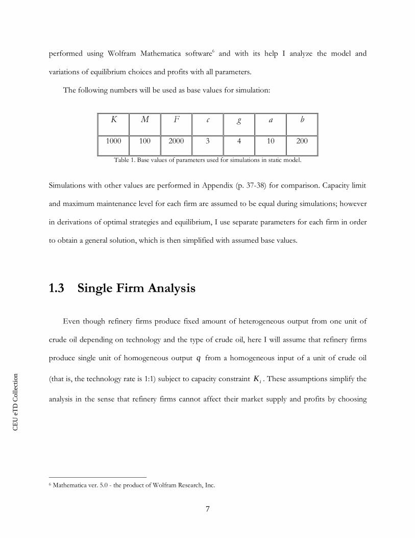
performed using Wolfram Mathematica software6 and with its help I analyze the model and

variations of equilibrium choices and profits with all parameters.

The following numbers will be used as base values for simulation:

K M F c g a b

1000 100 2000 3 4 10 200

Table 1. Base values of parameters used for simulations in static model.

Simulations with other values are performed in Appendix (p. 37-38) for comparison. Capacity limit

and maximum maintenance level for each firm are assumed to be equal during simulations; however

in derivations of optimal strategies and equilibrium, I use separate parameters for each firm in order

to obtain a general solution, which is then simplified with assumed base values.

1.3 Single Firm Analysis

Even though refinery firms produce fixed amount of heterogeneous output from one unit of

crude oil depending on technology and the type of crude oil, here I will assume that refinery firms

produce single unit of homogeneous output q from a homogeneous input of a unit of crude oil

(that is, the technology rate is 1:1) subject to capacity constraint iK . These assumptions simplify the

analysis in the sense that refinery firms cannot affect their market supply and profits by choosing

6 Mathematica ver. 5.0 - the product of Wolfram Research, Inc.

CE

UeT

DC

olle

ctio

n

8

different types of crude oil or technologies. So the choices of refinery firms are limited to the

choices of homogeneous output and maintenance7.

The cost functions for the two variables of main interest are given respectively by:

2)()(

mgmgqcqc

In my analysis I assume that capacities of refineries affect the choices of output through the

probability of failure function and do not affect the cost function, thus allowing producing with

constant marginal cost.

The probability of failure for a refinery firm is defined as a function of q (quantity produced)

and m (quality of maintenance) with cost F incurred in case of failure. It is reasonable to assume

that q and m independently affect (even though in reality their effects can be somehow

correlated), so that the probability function is represented by a linear function of two increasing and

convex probability functions:

( , ) ( ) ( )

( ), ( ) 0 ; ( ), ( ) 0

q m

q m q m

q m q m

In cases of optimal choice derivation a simple linear probability function mqmq ),( will be

used instead of the general form, with 1 1 ; =K M

, where K is the capacity limit of refinery

firm and M is the maximum possible maintenance level8. With this construction the effect of

production level on probability of failure reaches 100% as production level approaches capacity

7 Relaxing these assumptions will not change the outcome of the analysis. It is possible to redefine:j

jqq , where j

is the number of different types of products. The result will be the same since the analysis does not involve upgradingtechnologies that would change the fractions of output yields.8M can be thought of as a maintenance of the whole refining machinery and equipment, i.e. choosing maintenance levelM/2 means maintaining half of the refinery system. During simulations M will be assumed to be equal to 100 and thusthe choice of maintenance will be basically a choice of percentage of refining machinery to be renewed or repaired.

CE

UeT

DC

olle

ctio

n

9

limit. It is obvious that ( ) decreases with K and increases with M (the more complex is the

refining machinery, the more danger there is for a failure in one of its parts). These assumptions also

assure that probability of failure stays in the zero-one interval with an additional condition that

q mK M

(which is satisfied for all following results).

Assuming there are N firms operating on the market, the price is determined from total output

supplied by all firms: )(Qpp and the problem of the firm i is:

,

1

max [ ( ) ( )] (1 ( , )) ( , ) ( )

subject to: , and Q=

i ii i i i i i i iq m

N

i i i i jj

p Q q c q q m F q m g m

q K m M q (1)

Optimal simultaneous choice of output and quality of maintenance can be found from the first order

conditions for the problem:

direct effect (increase in due to an increase in output produced)

indirect effect (decrease in

[ ( ) ( ) ( )] (1 ( , ))

( , ) ( , )[ ( ) ( )]

ii i i i

i

i i i ii i

i i

q p Q p Q c q q mq

q m q mp Q q c q Fq q

due to an increase in probability of failure)

0 (2)

this effect is positive due to decrease in probability of failure

( , ) ( , )[ ( ) ( )] ( ) 0i i i i ii i i

i i i

q m q mp Q q c q F g mm m m (3)

In this part of analysis demand will be treated as fixed at high enough level (so that whatever is

produced by the firm is sold), hence the refinery is a price-taker. Using assumed functional forms of

production and maintenance costs and probability of failure function, one can find an optimal

CE

UeT

DC

olle

ctio

n

10

choice of output and maintenance for refinery firm as functions of fixed price fp and costs. Graph

G28 in Appendix shows how profit function changes with main variables of choice.

Solving first order conditions simultaneously optimal choices are defined as (see A1 in

Appendix):

2 2* *

2( )( 2 ) 2 ( ( ) ) ;( )(4 ( )) 4 ( )

f fi i i i i

i if f fi i i i

K p c F gM FgM M K p c Fq mp c gM K p c gM K p c

An increase in capacity leads to an increase both in optimal output and maintenance levels. After

differentiating both results with respect to iM it is obvious that both *iq and *

im decrease with

maximum possible maintenance level. Using reasonable assumption about an increase in optimal

choice of maintenance with an increase in failure (and implied necessary conditions for it), the

necessary condition for *iq to decrease with F is: 22 ( ))f

i igM K p c 9 (see A1 in Appendix).

1.4 Duopoly Analysis

This part of the Chapter deals with the interaction of two independent competing firms in a

world of perfect information. Refinery firms choose quantities that all-together define the final price;

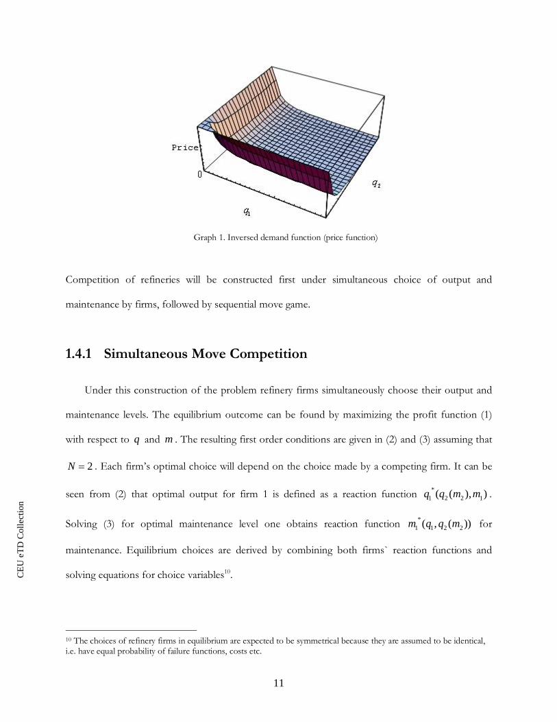
hence the competition is a la Cournot. Price is determined according to the following functional

form: 1 21 2

( , ) b bp q q aq q

, which reflects the weak response of price to supply changes if

quantity supplied is large enough and strong response if supply is on low level. This function has a

constant elasticity coefficient of minus one and is depicted in Graph 1.

9 This condition holds for assumed base values of parameters unless fixed price is incredibly high.

CE

UeT

DC

olle

ctio

n

11

Graph 1. Inversed demand function (price function)

Competition of refineries will be constructed first under simultaneous choice of output and

maintenance by firms, followed by sequential move game.

1.4.1 Simultaneous Move Competition

Under this construction of the problem refinery firms simultaneously choose their output and

maintenance levels. The equilibrium outcome can be found by maximizing the profit function (1)

with respect to q and m . The resulting first order conditions are given in (2) and (3) assuming that

2N . Each firm’s optimal choice will depend on the choice made by a competing firm. It can be

seen from (2) that optimal output for firm 1 is defined as a reaction function *1 2 2 1( ( ), )q q m m .

Solving (3) for optimal maintenance level one obtains reaction function *1 1 2 2( , ( ))m q q m for

maintenance. Equilibrium choices are derived by combining both firms` reaction functions and

solving equations for choice variables10.

10 The choices of refinery firms in equilibrium are expected to be symmetrical because they are assumed to be identical,i.e. have equal probability of failure functions, costs etc.

CE

UeT

DC

olle

ctio

n

12

With assumed functional forms of probability and cost functions, the problem of firm 1

becomes:

1 1

21 1 1 11 1 1 1,

1 2 1 1 1 1

1 1 1 1

max [( ) ] (1 )) ( )

subject to: and

q m

b b q m q ma q cq F gmq q K M K M

q K m M (4)

After solving an equivalent problem for reaction functions of firm 2 analysis of simultaneous choice

game comes down to four equations with four unknowns (see A2 in Appendix). The output and

maintenance reaction functions of firm 1 are respectively:

* 1 1 1 1 2 2 1 1 1 11 2 1

1 2

( ( ) ) ( ( )( ))( , )2 ( ( ))

b K M m M q q FM K a c M mq q mM b q a c

(5)

* 2 1 11 1 2

1 2

( ( ) )( , )2

q F q a c b bqm q qgM q

(6)

Simultaneous solution of (5) and (6) leads to a reaction function )( 2*

1 qq (see A2 in Appendix).

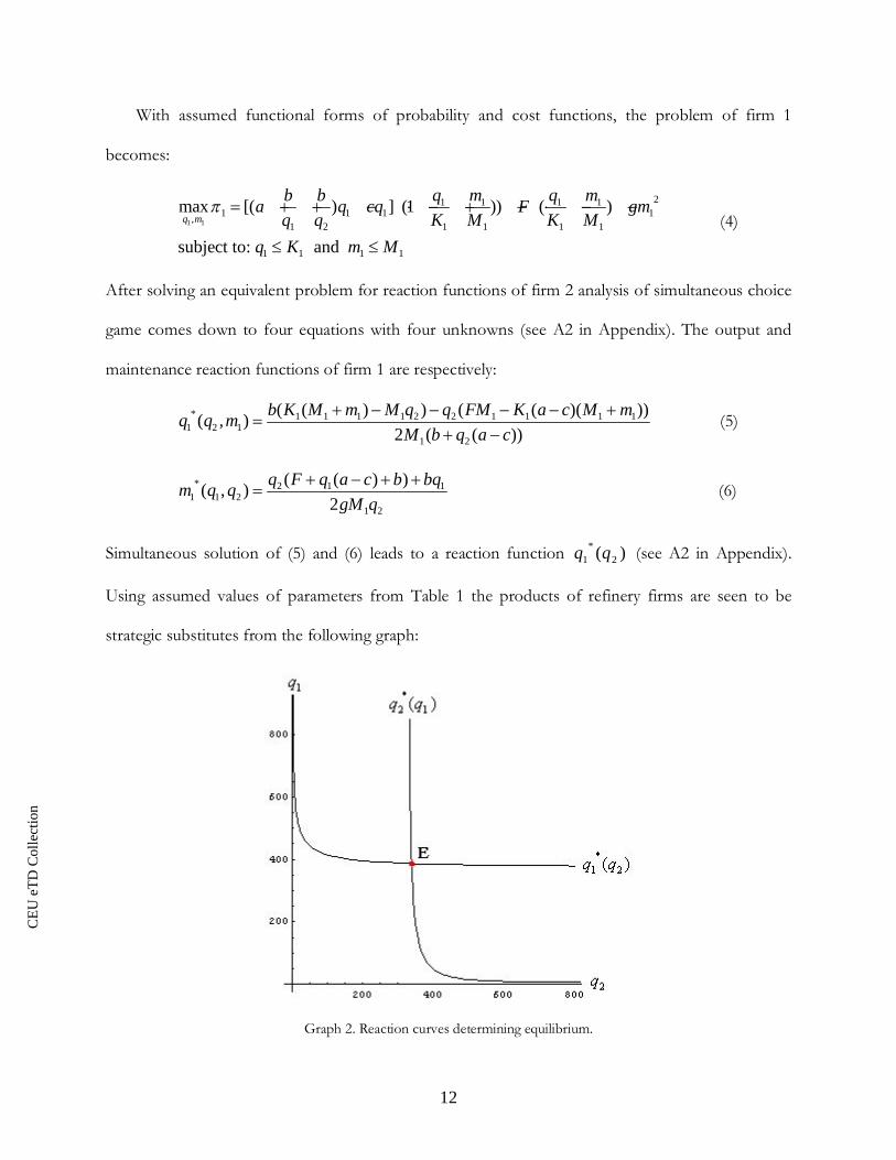
Using assumed values of parameters from Table 1 the products of refinery firms are seen to be

strategic substitutes from the following graph:

Graph 2. Reaction curves determining equilibrium.

CE

UeT

DC

olle

ctio

n

13

Reaction curves of refinery firms intersect at equilibrium point E (at this point * *1 2 386q q and

* *1 2 6.37 (%)m m ). Maintenance reaction curve of firm 1 is depicted in Graph G29 in

Appendix.

The resulting choice of production and maintenance levels states that firms in equilibrium will

prefer to produce only at 40% of their capacity possibilities. This choice has a logical explanation: by

doing so firms both decrease their need for more intensive maintenance (only about 7% of the total

maintenance possible) and increase the price. These results are supported by additional simulations

performed in Appendix, except for simulation of Table 6 in which refineries choose production

level at more than 50% of their capacity limit and maintain 15% of the whole system11.

Graphs G4-G9 in Appendix depict the variation of equilibrium output choice with all

parameters of the model: for this purpose explanatory parameter varies in some range around its

base value, while all other parameters are held constant at their base values. The resulting curves are

pretty intuitive: it turns out that equilibrium choice of output increases only with an increase in

capacity and parameters of price function12.

Variation of equilibrium profits with output and maintenance choices are shown respectively in

Graphs G30 and G31 in Appendix. These curves show the variation with one strategic variable

while holding another constant (hence the maximum points in these graphs are not equilibrium

values).

1.4.2 Sequential Move Competition

It is possible that in a regional market firms are not equal in timing of taking actions and hence

make their choices one after another. With sequential move setting, the competition among firms

11 Comparing to Table 1, Table 6 in Appendix assumes higher capacity and price, lower failure and production costs.This explains the choice of higher production level by refineries.12 It can be seen from Graph G9 in Appendix that the effect of an increase in a is much larger in magnitude than that ofb. This is explained by specificity of price function and its elasticity coefficient.

CE

UeT

DC

olle

ctio

n

14

consists of 2 stages: in the first stage first-moving refinery firm chooses its optimal maintenance and

production levels; after observing the choice of its rival, second-moving firm decides on its

production and maintenance levels in the second stage. Equilibrium outcome is found as usually by

backward induction.

Assuming that refinery firm 1 moves first, derivation of optimal solutions for both firms starts

with analysis of second stage (firm 2 actions). As before, maximizing profits with respect to 2q and

2m and solving first order conditions reaction function 2 1( )q q is obtained for firm 2 (same as 11A in

Appendix, but for 2q ). Going back to first stage refinery firm 1 maximizes:

1 1

21 1 1 11 1 1 1,

1 2 1 1 1 1 1

1 1 1 1

max [( ) ] (1 )) ( )( )

subject to: and

q m

b b q m q ma q cq F gmq q q K M K M

q K m M

At this stage derivations are becoming laborious and there is a need for simulation. Using base

values of parameters equilibrium output and maintenance are obtained for each firm: *1 387.32q ,

*2 385.54q , *

1 6.39 (%)m , *2 6.37 (%)m . As was expected, first-moving refinery firm

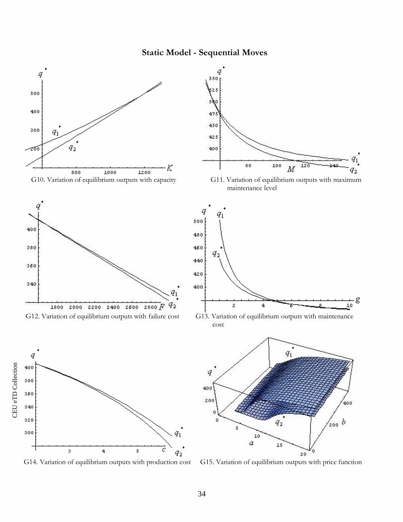
produces more output, but has a need for more maintenance. Graphs G10-G15 in Appendix show

the dependence of optimal output choices on parameter values. The difference between two firms’

choices decreases as capacity and maintenance cost increase.

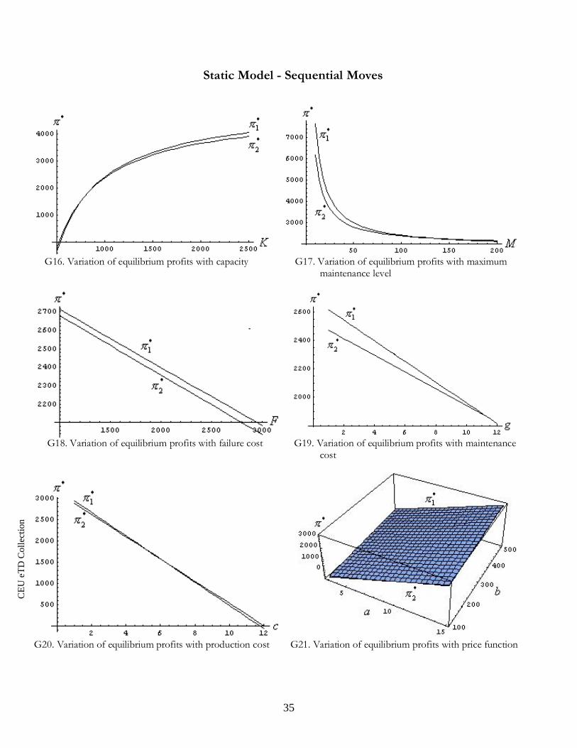
Profits of competing firms are depicted in Graphs G16-G21 in Appendix. As maintenance cost

increases, profit of first-moving refinery firm is approaching that of second moving firm. This is

explained by the choice of first-moving firm – greater level of production demands greater level of

maintenance and incurs higher maintenance costs.

Additional simulations in Appendix (p. 37-38) show the same results for different parameter

values.

CE

UeT

DC

olle

ctio

n

15

1.5 Concluding Remarks

In this Chapter interaction of refinery firms has been modeled as a static game, in which

maintenance works and production have been assumed to be taken up simultaneously. This

assumption can be considered as an unrealistic one for majority of maintenance works which

demand stoppage of production. Nevertheless, the model has allowed identifying unique strategies

of refinery firms that define Nash equilibrium.

Both simultaneous and sequential move competitions have showed similar results in simulations

that used base values of parameters given in Table 1: it has turned out that it is better for each

refinery firm to produce at about 40% of its capacity limit. This strategy has two benefits – low

production (supply) implies higher price and decreases the need for more intensive maintenance.

Sequential move game has showed that firm 1 chooses to produce slightly more than in

simultaneous case, but still sticks to the optimal strategy of producing less than half of capacity

possibilities.

Next Chapter develops this model further to a dynamic case which allows making more strict

assumptions about maintenance and constructing interaction of refinery firms in a more realistic

model.

CE

UeT

DC

olle

ctio

n

16

Chapter 2: Dynamic Model and RepeatedGames

In this chapter I develop previous model by introducing time periods. Such an extension has its

benefits as well as drawbacks. The main advantage of this addition lies in the possibility of making

more realistic assumptions. The refinery model of previous chapter has assumed that maintenance

and production can be taken up at the same time. With the introduction of dynamic model it is

feasible to make a reasonable assumption about maintenance being a time consuming event, i.e.

refinery firms need to put the production off line in order to take up maintenance. In this context it

will be possible to answer the question of whether it is optimal to take up the maintenance and stop

the production or to continue producing no matter what.

Dynamic model has its disadvantage in comparison with static model in finding equilibrium.

According to folk theorem, repeated games have a problem of multiple equilibria13. However the

model will be extended to two periods only and equilibrium will still be defined as a unique one in

this context. Hence the model allows analyzing the interaction of competing refineries in a more

realistic construction.

2.1 Dynamic Programming

Dynamic programming is a method that allows solving a problem with overlapping sub-

problems, i.e. a problem that can be divided into separate parts and optimized step-by-step. Here

this problem is defined as maximizing total profits of refinery firms. A simple finite horizon model

13 Folk Theorem states that sufficient condition for an outcome to be equilibrium in a repeated game is to satisfyminimax conditions, i.e. if the choice minimizes maximum possible loss for a player.

CE

UeT

DC

olle

ctio

n

17

with 2 periods without discounting is analyzed. Profits of refinery firms are assumed to be time

separable. Since one of the choice variables is assumed to be binary, it is impossible to use usual

dynamic programming methods for solution and a simpler approach of comparison of the outcomes

will be used.

For simulation purposes the following numbers will be used as base values:

K F c G a b

1500 2000 3 500 10 200 0.25 0.1

Table 2. Base values of parameters used for simulations in dynamic model.

Other assumed values of parameters are used for additional simulations in Appendix (p. 39).

2.2 Single Firm Analysis

In this part of the Chapter demand is treated as fixed in order to determine the actions of

refinery firm as a price taker. Dynamic programming allows putting restrictions on maintenance and

production choices: maintenance decision will be treated as a binary choice variable with a fixed

cost; if maintenance in some period is taken up, the production stops; if refinery decides to produce

in some period it cannot take up maintenance. Basically the firm faces the problem of choosing

between two options – either to produce or take up maintenance.

The cost of maintenance is fixed and equal to G. Firm starts making its choice in first period

with initial )failure(P . If in some period maintenance has been taken up, profits from

production in that period are equal to zero and probability of failure decreases by some constant

amount . Assuming that firm takes actions for two periods without discounting, it has two

choices: either to take up maintenance in the first period and produce in the second or to produce in

CE

UeT

DC

olle

ctio

n

18

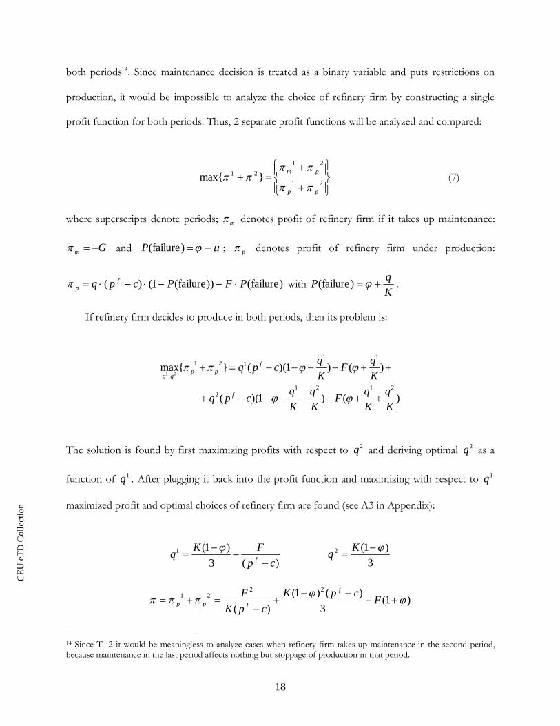
both periods14. Since maintenance decision is treated as a binary variable and puts restrictions on

production, it would be impossible to analyze the choice of refinery firm by constructing a single

profit function for both periods. Thus, 2 separate profit functions will be analyzed and compared:

21

2121 }max{

pp

pm (7)

where superscripts denote periods; m denotes profit of refinery firm if it takes up maintenance:

Gm and )failure(P ; p denotes profit of refinery firm under production:

)failure())failure(1()( PFPcpq fp with

KqP )failure( .

If refinery firm decides to produce in both periods, then its problem is:

1 2

1 11 2 1

,

1 2 1 22

max{ } ( )(1 ) ( )

( )(1 ) ( )

fp p

q q

f

q qq p c FK K

q q q qq p c FK K K K

The solution is found by first maximizing profits with respect to 2q and deriving optimal 2q as a

function of 1q . After plugging it back into the profit function and maximizing with respect to 1q

maximized profit and optimal choices of refinery firm are found (see A3 in Appendix):

)(3)1(1

cpFKq f 3

)1(2 Kq

)1(3

)()1()(

2221 FcpK

cpKF f

fpp

14 Since T=2 it would be meaningless to analyze cases when refinery firm takes up maintenance in the second period,because maintenance in the last period affects nothing but stoppage of production in that period.

CE

UeT

DC

olle

ctio

n

19

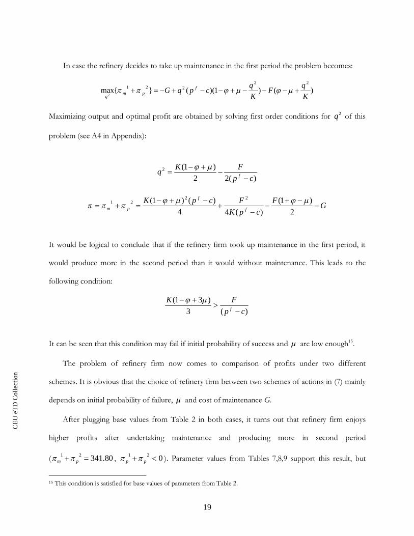
In case the refinery decides to take up maintenance in the first period the problem becomes:

)()1)((}{max22

2212 K

qFKqcpqG f

pmq

Maximizing output and optimal profit are obtained by solving first order conditions for 2q of this

problem (see A4 in Appendix):

)(22)1(2

cpFKq f

GFcpK

FcpKf

f

pm 2)1(

)(44)()1( 22

21

It would be logical to conclude that if the refinery firm took up maintenance in the first period, it

would produce more in the second period than it would without maintenance. This leads to the

following condition:

)(3)31(

cpFK

f

It can be seen that this condition may fail if initial probability of success and are low enough15.

The problem of refinery firm now comes to comparison of profits under two different

schemes. It is obvious that the choice of refinery firm between two schemes of actions in (7) mainly

depends on initial probability of failure, and cost of maintenance G.

After plugging base values from Table 2 in both cases, it turns out that refinery firm enjoys

higher profits after undertaking maintenance and producing more in second period

( 80.34121pm , 021

pp ). Parameter values from Tables 7,8,9 support this result, but

15 This condition is satisfied for base values of parameters from Table 2.

CE

UeT

DC

olle

ctio

n

20

using values from Table 10 changes the outcome in favor of producing in both periods

( 3440.6321pm , 3992.5021

pp ). Parameter values from Table 10 decrease the need for

maintenance by assuming: lower failure cost and higher maintenance cost; lower cost of production

and higher capacity and price.

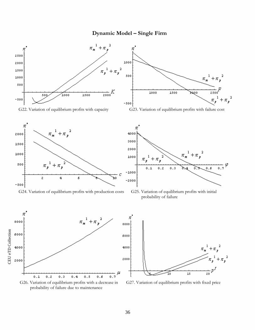
Graphs G22-G27 in Appendix show how overall equilibrium profits under both schemes

change with all parameters. It is important to notice in G25 that under these base values profit of

refinery firm when producing in both periods decreases to zero as initial probability of failure

approaches the threshold value of about 33%. Graph G23 shows that equilibrium profits are higher

under production in both periods when failure costs are low enough and the benefits of taking up

maintenance decrease.

2.3 Duopoly Analysis

Demand function is assumed to be given in the same form as in previous Chapter. In Duopoly

case each firm has a choice in form of (7). If one firm decides to take up maintenance in the first

period, the other firm gets all the residual demand. I will analyze interaction of refinery firms again

under simultaneous and sequential move games, later introducing uncertainty.

2.3.1 Simultaneous Move Competition

Using assumed functional forms for costs and probability function, each firm maximizes sum of

its time-separable profits. As before, each refinery decides whether to take up maintenance in the

first period or to skip it. In case of duopoly this means that there are 4 possible states in which firms

CE

UeT

DC

olle

ctio

n

21

may end up: both firms always produce; both firms take up maintenance in the first period; one of

the firms takes up maintenance in the first period, the other supplies the market. Optimal solutions

are obtained by backward induction for each case.

Again, since maintenance is a binary choice variable it is impossible to analyze actions of

refinery firms by constructing a single production function, and hence all cases should be compared

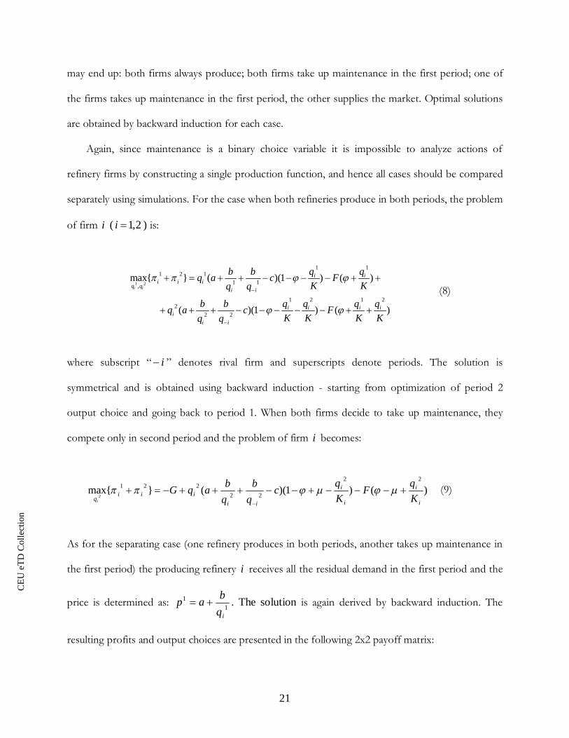
separately using simulations. For the case when both refineries produce in both periods, the problem

of firm i ( 2,1i ) is:

1 2

1 11 2 1

1 1,

1 2 1 22

2 2

max{ } ( )(1 ) ( )

( )(1 ) ( )

i i

i ii i i

q qi i

i i i ii

i i

q qb bq a c FK Kq q

q q q qb bq a c FK K K Kq q

(8)

where subscript “ i ” denotes rival firm and superscripts denote periods. The solution is

symmetrical and is obtained using backward induction - starting from optimization of period 2

output choice and going back to period 1. When both firms decide to take up maintenance, they

compete only in second period and the problem of firm i becomes:

)()1)((}{max22

22221

2i

i

i

i

iiiii

q KqF

Kqc

qb

qbaqG

i

(9)

As for the separating case (one refinery produces in both periods, another takes up maintenance in

the first period) the producing refinery i receives all the residual demand in the first period and the

price is determined as: 11

iqbap . The solution is again derived by backward induction. The

resulting profits and output choices are presented in the following 2x2 payoff matrix:

CE

UeT

DC

olle

ctio

n

22

Firm 2

Firm 1Produce-Produce Maintain-Produce

Produce-Produce

317.3211

32.1511q 375.212

1q

317.3212

32.1512q 375.212

2q

984.1371

49.3911q 394.302

1q

513.0562

012q 603.512

2q

Maintain-Produce

513.0561

011q 603.512

1q

984.1372

49.3912q 394.302

2q

551.2451

011q 489.032

1q

551.2452

012q 489.032

2q

where “Produce-Produce” stands for producing in both periods and “Maintain-Produce” - for

taking up maintenance in the first period. This game may seem similar to Prisoner`s Dilemma,

however it is obvious from this matrix that Maintain-Produce is a dominant strategy for both firms.

Optimal choices of output levels state the strategies of refinery firms. It turns out that if a firm

decides to produce in both periods, it prefers to keep the production on low level in the first one to

compete more harshly in the second. Much higher level of production in the second period is also

explained by the limitation of model to two periods: the choice of output in the last period can

increase the probability of failure in that period, but it does not affect the future probability of

failure since the game is terminated at that point. However extension of the model to T periods is

predicted to yield the same results: firms will produce on low levels until the last period and in

period T the production level will greatly increase.

CE

UeT

DC

olle

ctio

n

23

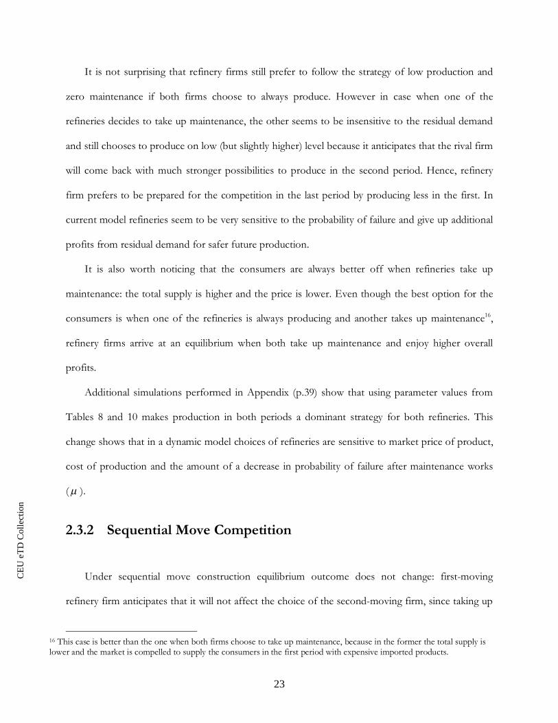
It is not surprising that refinery firms still prefer to follow the strategy of low production and

zero maintenance if both firms choose to always produce. However in case when one of the

refineries decides to take up maintenance, the other seems to be insensitive to the residual demand

and still chooses to produce on low (but slightly higher) level because it anticipates that the rival firm

will come back with much stronger possibilities to produce in the second period. Hence, refinery

firm prefers to be prepared for the competition in the last period by producing less in the first. In

current model refineries seem to be very sensitive to the probability of failure and give up additional

profits from residual demand for safer future production.

It is also worth noticing that the consumers are always better off when refineries take up

maintenance: the total supply is higher and the price is lower. Even though the best option for the

consumers is when one of the refineries is always producing and another takes up maintenance16,

refinery firms arrive at an equilibrium when both take up maintenance and enjoy higher overall

profits.

Additional simulations performed in Appendix (p.39) show that using parameter values from

Tables 8 and 10 makes production in both periods a dominant strategy for both refineries. This

change shows that in a dynamic model choices of refineries are sensitive to market price of product,

cost of production and the amount of a decrease in probability of failure after maintenance works

( ).

2.3.2 Sequential Move Competition

Under sequential move construction equilibrium outcome does not change: first-moving

refinery firm anticipates that it will not affect the choice of the second-moving firm, since taking up

16 This case is better than the one when both firms choose to take up maintenance, because in the former the total supply islower and the market is compelled to supply the consumers in the first period with expensive imported products.

CE

UeT

DC

olle

ctio

n

24

maintenance is a dominant strategy for both firms. This conclusion is resulting from the choice of

specific values of parameters from Table 2. It is possible to readjust them in such a way that taking

up maintenance is no longer a dominant strategy. Additional simulations in Appendix (p. 39) have

showed that the equilibrium outcome changes to production in both periods after assuming: higher

price and maintenance cost; lower and production cost.

The next subsection introduces uncertainty and demonstrates how equilibrium depends on

beliefs of refinery firms about demand and shows an example when producing in both periods

becomes a dominant strategy.

2.4 Introducing Uncertainty

In a world of perfect information choices of refinery firms are based on their knowledge about

costs and demand. This part of the Chapter extends the previous model by introducing uncertainty

about demand and hence – price of the product. Firms are assumed to have identical beliefs about

the future price: the demand will be low with probability 1 in the first period and with probability

2 in the second. Therefore the problems of refineries are unchanged with the only difference in

their beliefs about price. Using probabilities that refinery firms put on low demand, prices in first

and second period respectively are expected to be:

)()1()( 11

11

11

11

1

11

qb

qba

qb

qbap HH

HLL

L

)()1()( 21

21

22

12

1

22

qb

qba

qb

qbap HH

HLL

L

CE

UeT

DC

olle

ctio

n

25

where subscripts L and H stand for Low and High respectively and: HL aa , HL bb . The

results obtained without uncertainty do not change if 1 2 : that is, if refinery firm believes that

demand will be high or low with the same probability in each period, it will still stick to its previous

strategy of taking up maintenance.

The following graph shows how maximized profits change with beliefs (probabilities) about

demand for a single price-taking firm case when HL ppp )1( 111 and

HL ppp )1( 222 :

Graph 3. Optimal profits changing with beliefs (probabilities of low demand)

It can be seen from Graph 3 that producing in both periods can be optimal for a refinery firm if

demand is likely to be high in the first period and low in the second ( 5.01 and 0.52 ). It is

also obvious that taking up maintenance is always better when 21 , i.e. when demand in the first

period is expected to be low with a probability at least as great as probability of low demand in the

second period.

CE

UeT

DC

olle

ctio

n

26

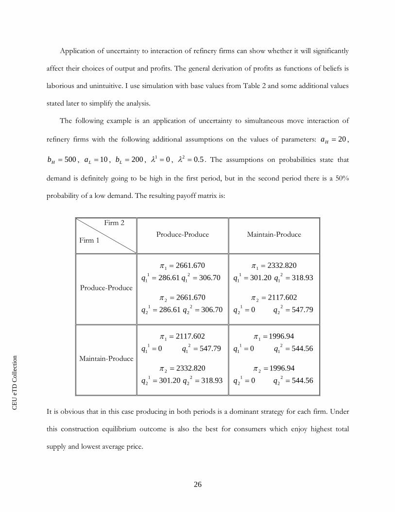
Application of uncertainty to interaction of refinery firms can show whether it will significantly

affect their choices of output and profits. The general derivation of profits as functions of beliefs is

laborious and unintuitive. I use simulation with base values from Table 2 and some additional values

stated later to simplify the analysis.

The following example is an application of uncertainty to simultaneous move interaction of

refinery firms with the following additional assumptions on the values of parameters: 20Ha ,

500Hb , 10La , 200Lb , 01 , 5.02 . The assumptions on probabilities state that

demand is definitely going to be high in the first period, but in the second period there is a 50%

probability of a low demand. The resulting payoff matrix is:

Firm 2

Firm 1Produce-Produce Maintain-Produce

Produce-Produce

2661.6701

286.6111q 306.702

1q

2661.6702

61.86212q 306.702

2q

2332.8201

301.2011q 318.932

1q

2117.6022

012q 547.792

2q

Maintain-Produce

2117.6021

011q 79.5472

1q

820.23322

301.2012q 318.932

2q

1996.941

011q 544.562

1q

1996.942

012q 544.562

2q

It is obvious that in this case producing in both periods is a dominant strategy for each firm. Under

this construction equilibrium outcome is also the best for consumers which enjoy highest total

supply and lowest average price.

CE

UeT

DC

olle

ctio

n

27

2.5 Concluding Remarks

This Chapter has developed a simple but useful dynamic model of interaction of refinery firms.

Dynamic approach has allowed me to analyze the actions of refinery firms under more realistic

assumptions about maintenance decisions: production and maintenance works have been assumed

to be exclusive decision variables.

The results derived with the help of simulations have identified the optimal strategies of refinery

firms. Construction of 2x2 payoff matrix has showed that taking up maintenance is a dominant

strategy under assumed values of parameters. In cases when refinery decides to produce in both

periods, it should stick to the strategy derived in the previous Chapter: produce less and enjoy higher

prices with lower probability of failure. The model has also demonstrated insensitivity of refinery

firms to residual demand and high sensitivity to probability of failure.

The surprising difference between optimal production choice in the first and second periods

comes from the fact that the choice game is terminated after production in the second period.

Extension of the model to more periods should not change the general result of this outcome,

because the firms will still produce at an optimal low level until the last period and boost the

production right when the game terminates and probability of failure is no longer affected.

Later introducing uncertainty the model has showed that the equilibrium outcome depends on

beliefs of refinery firms about demand. The result has turned out pretty intuitive: when demand is

expected to be high in the first period and low in the second, it is optimal to produce in both

periods. This change of equilibrium from maintenance to production is also welcomed by customers

because they enjoy higher total supply and lower average price.

CE

UeT

DC

olle

ctio

n

28

Conclusions

Harsh competition and a constantly changing demand for oil require refineries to produce at

full capacity possibilities and create bad incentives to skip production stoppage for maintenance

works. This, in turn, can lead to a system failure, which creates a danger of explosions (fires) and

incurs huge costs of restoration of refining machinery. In my thesis, I have analyzed the choices of

production and maintenance levels chosen by refinery firms. Besides defining profits, production

and maintenance were assumed to be strategic decisions which affect the probability of failure.

Using classical game theory tools and simulations of parameters, I have identified the optimal

strategies for refinery firms in static and dynamic models under different situations: single refinery

firm being a price taker; competition of two refinery firms that make their choices of strategic

variables` levels simultaneously; competition of two refinery firms deciding on strategic variables

sequentially, one after another.

Static model in Chapter 1 has allowed optimizing refineries` optimal (simultaneous) choices of

output and maintenance levels in a convenient and simple way. In this model, the result of

interaction of the refinery firms under different constructions (simultaneous and sequential moves)

has turned out to be surprising but intuitive: in all cases, refineries have been involved in a kind of

tacit collusion by supplying the regional market with considerably less quantity of refined products

than possible. By doing so, refinery firms have been enjoying higher prices and have decreased their

need for maintenance (less than 10% of total refinery system demands maintenance in this

equilibrium). The advantage of the static model lies in the simplicity and the possibility of defining a

unique equilibrium. However, this model makes it impossible to put realistic restrictions on the

choices of maintenance and production. The majority of maintenance works in oil refinery sector

CE

UeT

DC

olle

ctio

n

29

demands production stoppage for the period of maintenance, mainly because of complex

interconnection of all parts of the refinery system.

Introduction of dynamic model in Chapter 2 has allowed for necessary restrictions: maintenance

has been assumed to be a binary variable with fixed costs of implementation and fixed fraction of a

decrease in probability of failure; production and maintenance have been exclusive events. Despite

this advantage, dynamic models and repeated games come with their problem of multiple equilibria.

Intuitively, this means that in an infinite horizon model, both firms can end up in any of the

situations when they are both better off. This disadvantage, however, has been overcome by the

introduction of finite horizon (2 periods) model. The results of the dynamic model have showed

that refineries are sensitive to any possibilities of failure and both of the competing refineries end up

taking up maintenance in the first period. In choosing production levels, firms still follow the

optimal strategy of static model: producing less and enjoying safety with higher prices. Later,

extending the model with uncertainty, I have showed that decisions of refineries can switch to

production in both periods depending on their beliefs about demand.

Both models presented in my thesis are simple but informative. Further extensions can help to

understand the interaction and choices of oil refineries. Among possible ones, I would suggest:

analyzing in static model the interaction of non-identical refineries that differ in their capacities,

market power etc.; extending dynamic model to more periods (finite) or infinite horizon and

studying more in-depth decisions of refineries on optimal frequency of maintenance; testing both

dynamic and static models empirically on whether the equilibrium outcome is supported by data.

CE

UeT

DC

olle

ctio

n

30

Appendix

Static Model

A1. Single Firm Choice with Fixed Demand

Using assumed functional forms of probability and cost functions, firm maximizes its profit withrespect to output and maintenance:

( )(1 ) [ ] 0f

fi i i

i i i i i

q m q p c Fp cq K M K K

(1A)

( ) 2 0f

ii

i i

p c q F gmm M

(2A)

Solving (1A) and (2A) for q and m respectively brings the problem to:

* ( )2 2( )

i i ii f

i

K m M FqM p c

(3A)

* ( )2

fi

ii

p c q FmgM

(4A)

Profit maximizing output and maintenance choices are found in terms of parameters by solvingsimultaneously equations (3A) and (4A).

Dependence of optimal maintenance and output choices on different parameters is found bydifferentiation:

* 2 *

2 2

(4 )( ) 0(4 ( ))

fi i i i

fi ii i

m M gM F p c mK KgM K p c

* 2 2 *

2 2

2 (4 ) 0(4 ( ))

i i i if

i ii i

q gM gM F qK KgM K p c

* 2 *

2 2

(4 ( ))( ( )) 0(4 ( ))

f fi i i i i

fi ii i

m gM K p c F K p c mM MgM K p c

CE

UeT

DC

olle

ctio

n

31

* *

2 2

4 ( ( )) 0(4 ( ))

fi i i i i

fi ii i

q gK M F K p c qM MgM K p c

* *2

2 0 4 ( )4 ( )

fi i ii if

i i

m M m gM K p cF FgM K p c

(5A)

* 2 *2

2

2 ( )) 0 2 ( ))( )(4 ( ))

ffi i i i

i if fii i

q gM K p c q gM K p cF Mp c gM K p c

Last condition is necessary for the optimal output to decrease with F and is sufficient for optimalmaintenance choice to increase with F .

A2. Simultaneous Choice Game in Duopoly

First order conditions for the problem are:

11 1 1 2

1 1 1 2 1 1

[ ](1 ) [ ] 0

b bq a cq m b Fq qa c

q K M q K K (7A)

11 2

11 1

[ ]2 0

b bq a c Fq q gm

m M (8A)

The first one leads to the output reaction function of firm 1:

* 1 1 1 1 2 2 1 1 1 11 2 1

1 2

( ( ) ) ( ( )( ))( , )2 ( ( ))

b K M m M q q FM K a c M mq q mM b q a c

(9A)

FOC for maintenance level defines optimal choice of maintenance as:

* 2 1 11 1 2

1 2

( ( ) )( , )2

q F q a c b bqm q qgM q

(10A)

Reaction function *1 2( )q q is obtained by solving (9A) and (10A) simultaneously for optimal choice

of output:

CE

UeT

DC

olle

ctio

n

32

2 2 22* 2 1 2 1 1 1 1 1 1 2 1 2

1 2 22 2 1 1 1

( ( ( )( 2 ) 2 ) ( 2 ( ) ( )))( )( ( ))( (4 ( )) )

q b K q K a c F gM FgM b FK gM K q K q a cq qb q a c q gM K a c bK

(11A)

Equilibrium outcome is found by solving the same problem for firm 2 in a similar way andcombining the 2 reaction functions for output of both firms. The solution is burdensome and hasno intuitive value without using simulations.

Dynamic Model

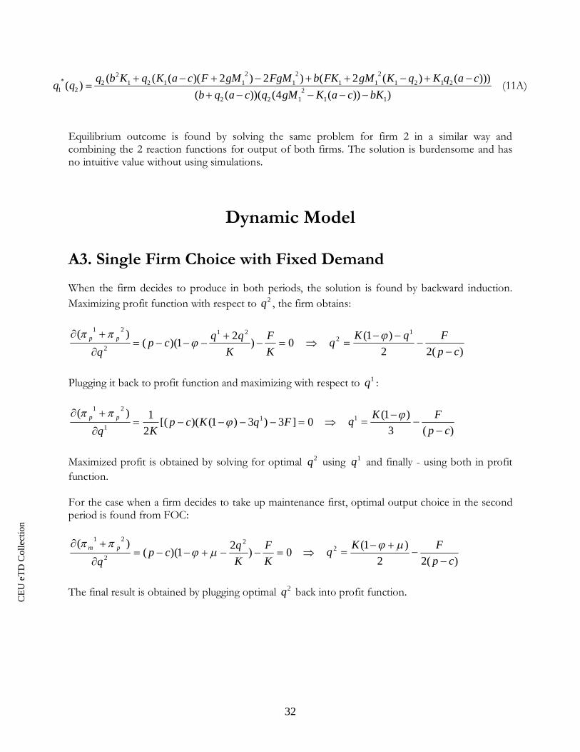
A3. Single Firm Choice with Fixed DemandWhen the firm decides to produce in both periods, the solution is found by backward induction.Maximizing profit function with respect to 2q , the firm obtains:

0)21)(()( 21

2

21

KF

Kqqcp

qpp

)(22)1( 1

2

cpFqKq

Plugging it back to profit function and maximizing with respect to 1q :

0]3)3)1()([(21)( 1

1

21

FqKcpKq

pp

)(3)1(1

cpFKq

Maximized profit is obtained by solving for optimal 2q using 1q and finally - using both in profitfunction.

For the case when a firm decides to take up maintenance first, optimal output choice in the secondperiod is found from FOC:

0)21)(()( 2

2

21

KF

Kqcp

qpm

)(22)1(2

cpFKq

The final result is obtained by plugging optimal 2q back into profit function.

CE

UeT

DC

olle

ctio

n

33

Static Model – Simultaneous Moves

G4. Variation of equilibrium output with capacity G5. Variation of equilibrium output with maximum maintenance level

G6. Variation of equilibrium output with failure cost G7. Variation of equilibrium output with maintenance Cost

G8. Variation of equilibrium output with production cost G9. Variation of equilibrium output with price function

CE

UeT

DC

olle

ctio

n

34

Static Model - Sequential Moves

G10. Variation of equilibrium outputs with capacity G11. Variation of equilibrium outputs with maximum maintenance level

G12. Variation of equilibrium outputs with failure cost G13. Variation of equilibrium outputs with maintenance cost

G14. Variation of equilibrium outputs with production cost G15. Variation of equilibrium outputs with price function

CE

UeT

DC

olle

ctio

n

35

Static Model - Sequential Moves

G16. Variation of equilibrium profits with capacity G17. Variation of equilibrium profits with maximum maintenance level

G18. Variation of equilibrium profits with failure cost G19. Variation of equilibrium profits with maintenance cost

G20. Variation of equilibrium profits with production cost G21. Variation of equilibrium profits with price function

CE

UeT

DC

olle

ctio

n

36

Dynamic Model – Single Firm

G22. Variation of equilibrium profits with capacity G23. Variation of equilibrium profits with failure cost

G24. Variation of equilibrium profits with production costs G25. Variation of equilibrium profits with initial probability of failure

G26. Variation of equilibrium profits with a decrease in G27. Variation of equilibrium profits with fixed price probability of failure due to maintenance

CE

UeT

DC

olle

ctio

n

37

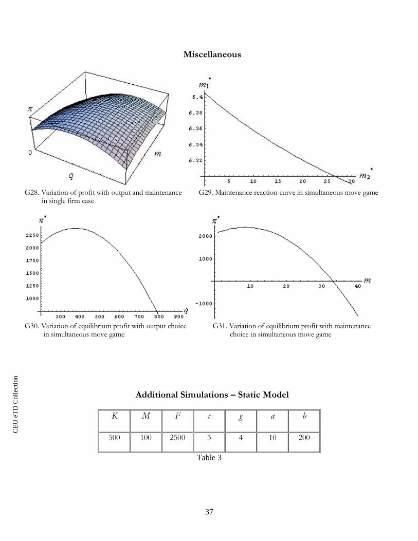
Miscellaneous

G28. Variation of profit with output and maintenance G29. Maintenance reaction curve in simultaneous move game in single firm case

G30. Variation of equilibrium profit with output choice G31. Variation of equilibrium profit with maintenance in simultaneous move game choice in simultaneous move game

Additional Simulations – Static Model

K M F c g a b

500 100 2500 3 4 10 200

Table 3

CE

UeT

DC

olle

ctio

n

38

K M F c g a b

500 100 2500 2 6 20 500

Table 4

K M F c g a b

1500 100 1500 3 4 10 200

Table 5

K M F c g a b

1500 100 1500 2 6 20 500

Table 6

Type of Game Simultaneous Moves Sequential Moves

Firm

ValuesFirms 1 & 2 First-mover (Firm 1) Second-mover (Firm 2)

Table 3* *

1 2 108.72q q* *

1 2 4.58 (%)m m* *

1 2 448.76

*1 122.98q*

1 4.74 (%)m*

1 452.11

*2 104.76q*

2 4.50 (%)m*

2 429.81

Table 4* *

1 2 191.69q q* *

1 2 5.79 (%)m m* *

1 2 1987.05

*1 192.94q*

1 5.81 (%)m*

1 1987.12

*1 191.62q*

1 5.79 (%)m*

1 1984.87

Table 5* *

1 2 696.9q q* *

1 2 8.47 (%)m m* *

1 2 2416.26

*1 697.10q*

1 8.47 (%)m*

1 2416.26

*1 696.90q*

1 8.46 (%)m*

1 2416.23

Table 6* *

1 2 802.17q q* *

1 2 14.12 (%)m m* *

1 2 7575.94

*1 802.30q

*1 14.12 (%)m

*1 7575.94

*1 802.17q

*1 14.11 (%)m

*1 7575.89

CE

UeT

DC

olle

ctio

n

39

Additional Simulations – Dynamic Model

K F c G a b

1000 2500 3 300 10 200 0.2 0.15

Table 7

K F c G a b

1000 2500 2 700 20 500 0.3 0.05

Table 8

K F c G a b

2000 1500 3 300 10 200 0.2 0.15

Table 9

K F c G a b

2000 1500 2 700 20 500 0.3 0.05

Table 10

Choice

Values

F1 Produce-ProduceF2 Produce-Produce

F1 Maintain-ProduceF2 Produce-Produce

F1 Maintain-ProduceF2 Maintain-Produce

Table 7 * *1 2 14.76 *

1 450.46 ; *1 0 * *

1 2 457.23

Table 8 * *1 2 1070.56 *

1 800.72 ; *1 701.87 * *

1 2 813.89

Table 9 * *1 2 1764.52 *

1 2072.46 ; *1 1603.34 * *

1 2 2325.71

Table 10 * *1 2 4803.61 *

1 3466.16 ; *1 4489.11 * *

1 2 3843.40

CE

UeT

DC

olle

ctio

n

40

References

De Palma, A., Kilani, M., and Lindsey, R. (2006) “Maintenance, service quality andcongestion pricing with competing roads”, working paper:URL: http://www.uofaweb.ualberta.ca/economics/WorkingPapers.cfm ;

Fudenberg, D. and Tirole, J. (1984) “The fat cat effect, the puppy-dog ploy and the leanand hungry look”, American Economic Review: Papers and Proceedings;

Manzano, F. (2005) “Supply Chain Practices in the Petroleum Downstream”, MastersThesis submitted to the department of Engineering Systems Division of MassachusettsInstitute of Technology;

Muehlegger, E. J. (2005) “Essays on gasoline price spikes, environmental regulation ofgasoline content, and incentives for refinery operation”, Doctoral Thesis submitted tothe department of Economics of B.A. Williams College;

Wellin, P (2008) “Computer Simulations With Mathematica And Java” book, publisher:Springer-Verlag New York Inc.

BBC News: “Four die in India refinery fire”, last view date 03/06/08URL: http://news.bbc.co.uk/2/hi/south_asia/6319459.stm

Popular Mechanics: “What Went Wrong: Oil Refinery Disaster”, last view date 03/06/08URL: http://www.popularmechanics.com/technology/industry/1758242.html