oil prices and current account deficits: analysis of causality in the usa

Applied Econometrics and International Development Vol. 10-1 (2010)

OIL PRICES AND CURRENT ACCOUNT DEFICITS: ANALYSIS OF CAUSALITY IN THE USA

BILDIRICI, Melike* ALP, Elcin

BAKIRTAS, Tahsin Abstract In this discussion, the theoretical structure of the great depression and the historical dimension of the crisis were taken into consideration and while we examine the depression within the framework of oil prices and financial crisis, we will use mortgage credit and current account deficits. Depression will be tested with TVAR and Granger Causality analysis. Key word; Threshold VAR, Granger Causality, Financial Crisis, Depression, Oil Prices JEL Classification: C32, C52, E32, G21 1. Introduction Capitalist economies face crisis often. The crisis lived contributed to the economy literature and a lot of financial crisis models were developed. In last depression, economists was forward different point. As many economist, 2007-08 depression is related with credit channel that is, in this framework, mortgage credits are in the leading position and current account deficit. The approaches developed from credit channel take H. Minsky (1977), and C. Kindleberger (1989) as the basis and these studies carry important inspirations from W. Mitchell (1913), I. Fisher(1933). Among these studies concentrated on credit channel, J.Taylor (2009), Mian, Sufi and Trebbi (2008) Dell’Aricci, Igan and Laeven (2008) Mizen (2008) Arrow (2008) can be listed. We examine 2007-08 depression within the framework of oil prices, we will use mortgage and current account and budget deficits as a tool. In this scope, 1974-75 crisis and 2007-08 depression carries similarities. Both in 1974-75 crisis and before 2007-08 depression, there was USA military intervention. This caused the loss value of dollar. If we examine 1974 crisis and 2008 depression comparatively, the subject becomes clear. After USA intervention to Vietnam in 1965, with the effect of the increase in military spending, there was a huge current account and budget deficit. The high price of Vietnam War led to expansion and final expansion led to the increase of general price level and melting of USA’s payments deficit balance surplus. Although in the beginning, a contractionary monetary policy was adopted, the negative effect of high interest rates on construction sector caused Federal Reserve Bank to adopt more expansionary monetary policies between 1967-68. In 15 August 1971, USA declared that it left the gold standard. In 19 March 1973, Japan and fundamental monetary units left to free fluctuation against US Dollar. In 1973-74, oil prices started to increase. At this time, the high oil prices made

Prof.Dr. Melike E. Bildirici, [email protected], Dr. Elçin A. Alp, [email protected] Department of Economics, Yildiz Technical University, Istanbul, and Asist. Prf. Dr. Tahsin Bakirtaş [email protected] Department of Economics, Sakarya University, Turkey Acknowledgement: Helpful comments by the Editor, Maria Carmen Guisan, are gratefully acknowledged.


138

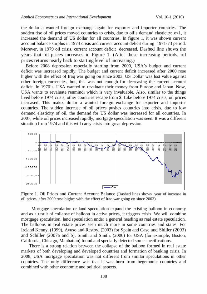
the dollar a wanted foreign exchange again for exporter and importer countries. The sudden rise of oil prices moved countries to crisis, due to oil’s demand elasticity; e<1, it increased the demand of US dollar for all countries. In figure 1, it was shown current account balance surplus in 1974 crisis and current account deficit during 1971-73 period. Morever, in 1979 oil crisis, current account deficit decreased. Dashed line shows the years that oil prices increases in Figure 1. (After these increasing periods, oil prices returns nearly back to starting level of increasing.) Before 2008 depression especially starting from 2000, USA’s budget and current deficit was increased rapidly. The budget and current deficit increased after 2000 rose higher with the effect of Iraq war going on since 2003. US Dollar was lost value against other foreign currencies, but, this was not enough for decreasing the current account deficit. In 1970’s, USA wanted to revaluate their money from Europe and Japan. Now, USA wants to revaluate renmindi which is very invaluable. Also, similar to the things lived before 1974 crisis, other countries escape from $. Like before 1974 crisis, oil prices increased. This makes dollar a wanted foreign exchange for exporter and importer countries. The sudden increase of oil prices pushes countries into crisis, due to low demand elasticity of oil, the demand for US dollar was increased for all countries. In 2007, while oil prices increased rapidly, mortgage speculation was seen. It was a different situation from 1974 and this will carry crisis into great depression.

Figure 1. Oil Prices and Current Account Balance (Dashed lines shows year of increase in oil prices, after 2000 rose higher with the effect of Iraq war going on since 2003) Mortgage speculation or land speculation expand the existing balloon in economy and as a result of collapse of balloon in active prices, it triggers crisis. We will combine mortgage speculation, land speculation under a general heading as real estate speculation. The balloons in real estate prices seen much more in some countries and states. For Ireland Kenny, (1999), Ayuso and Restoy, (2003) for Spain and Case and Shiller (2003) and Schiller (2007a and b), Smith and Smith, (2006) for USA (for example, Boston, California, Chicago, Manhattan) found and specially detected some specifications. There is a strong relation between the collapse of the balloon formed in real estate markets of both developing and developed countries and formation of banking crisis. In 2008, USA mortgage speculation was not different from similar speculations in other countries. The only difference was that it was born from hegemonic countries and combined with other economic and political aspects.

Bildirici,M.,Alp,E.,Bakirtas,T. Oil Prices and Current Account Deficits: Causality in the USA

139

We can say that, like in 1974-75, the increase of oil prices in 2007-08 bears two important results. First one is that by the increase of oil prices US Dollar demand increases and USA’s current account deficit decreases. Second result is that, Arab countries transferred money to banks in USA and this money relaxed both USA banks and EU countries. In this study, to be able to test the above views, TVAR analysis we will used. 2. Data and Econometric Methodology

a. Data: GDP data used in the study was taken from U.S. Department of Commerce Bureau of

Economic Analysis, oil prices (OP) was taken from Energy Information Administration, USA exchange rate (E), USA current account deficit (CA) data were taken from Federal Reserve Bank of St. Louis and Global Financial Data and mortgage rates (M) were taken from Federal Reserve Bank of St. Louis. Budget deficit data (BD) were taken from Federal Reserve Bank of St. Louis. In the analysis, GDP;(GDPt/GDPt-1), CA;(CAt/CAt-1), OP;(OPt/OPt-1), BD;(BDt/BDt-1), E;(Et/Et-1) and M;(Mt/Mt-1) data are used. GDP, CA, OP, BD, E were analyzed for 1968:01-2008:04 and and CA, OP, M and E for 1971:01-2008:04. Firstly threshold will be determined and TVAR analysis will be used. While making crisis analysis, VAR is a preferred method but to us since crisis create threshold linear analysis can not be used to analyze the crisis in this period. At this stage, the existence of threshold is very important for us. For this reason, by using Threshold VAR (TVAR) analysis we will find impulse responses.

b. Econometric Methodology TVAR Analysis The purpose of this paper is to investigate the effect of the crisis of oil and mortgage on USA economy. The testing strategy follows Balke (2000) and consists of: selecting and estimating a threshold VAR model, and testing formally for the presence of threshold effects; and than analyzing whether impulse responses reveal signs of asymmetric propagation of shocks across the separate regimes identified by the threshold model. (Cazla and Sousa:2005:9) The first step to study the potential role of oil prices in the non-linear propagation of shocks is to estimate a two-regime threshold VAR model following the specification: Y = µ1 + A1 Yt + B’( L) Yt-1 + (µ2 + A2 Yt + B2 (L) Yt-1) I +εt Yt variable is a vector composed of endogenous (yit) and exogenous (njt) variables:

1

2

1

2

t

t

itt

t

t

jt

yy

yY

nn

n

where i=1,…,n, j=1,…,m. (3.16)


140

where Yt is a vector of endogenous variables, It [.] is an indicator that takes the value 1 when the d-lagged threshold variable ct is lower than the threshold critical value γ and 0 otherwise. The indicator It [.] is a transitional variable identifying two separate regimes on the basis of the value of ct-d relative to γ. Asymmetry is introduced by allowing for the coefficients of the VAR – the vector of constant terms µ , the matrix A and the matrix polynomial in the lag operator B(L) – to vary across the two separate regimes: µ1 , A1 and B1 (L) represent the parameters of the VAR in the regime defined by It [.] = 0 , while µ1 +µ2 , A1 + A2 and B1 (L) + B2 (L) are the parameters in the regime identified by It [.] = 1. By specifying ct as a function of one of the variables in Yt, it is possible to model regime switching as an endogenous process determined by movements in the variables forming the model. This implies that shocks to any of the variables in Yt may - via their impact on the variable underlying ct induce a shift to a different regime. t=1,…,T and I{.} is indicator function (Cazla and Sousa:2005:9). Because the distributions of the test statistics are non-standard, the p-values are use Hansen (1996) the simulation technique to calculate the unknown asymptotic distributions. The reaction of GDP, BD and CA to oil and mortage shocks, differ across regimes by means of two complementary sets of impulse response functions: (1) regime-dependent impulse responses and (2) non-linear impulse responses. The first set of impulse responses describe the reaction of the system to a shock within each of the regimes identified by the estimated threshold. A sufficiently large shock to a variable may lead to the economy switching away from the starting regime once its direct and indirect effect feed through and, over time, responses may potentially switch repeatedly between the two regimes.

As suggested by Balke (2000), in this paper also, generalized impulse responses (GI) under alternative regimes are numerically computed by using bootstrap simulations and GI relies on the definition of an impulse response as a revision in conditional expectations. The response of variable Y to a shock at time t (ut), at horizon k (k = 1,…, h) is given by the difference between the expected value of variable Y given the shock and conditional on a particular history (Ωt−1) of the shocks at time t-1 and the expected value of Y in the case of no such shocks:

GIk = E( Yt+h |ut, Ωt-1)- E( Yt+h | Ωt-1 ) (3.17)

In order to compute each of the expectations an iterative procedure is used. Hansen (1996) was used for P-values, which is the simulation technique for

calculating the unknown asymptotic distributions, since the distributions of the test statistics are non-standard. The reaction of GDP, budget deficit and current account deficit to oil shocks vary across regimes due to two complementary sets of impulse response functions, the first of which is formed by regime-dependent impulse responses and the second is a set of non-linear impulse responses. The first set of impulse responses describe the reaction of the system to a shock within each of the regimes identified by the estimated threshold. A sufficiently large shock to a variable may lead to a switching of the economy, away from the starting regime. Once its direct and indirect effects feed through and over time, responses may potentially switch repeatedly between the two regimes.


141

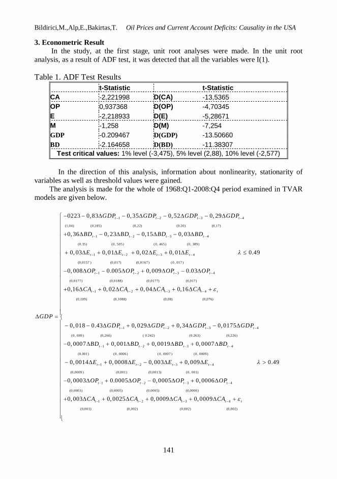
3. Econometric Result In the study, at the first stage, unit root analyses were made. In the unit root analysis, as a result of ADF test, it was detected that all the variables were I(1). Table 1. ADF Test Results

t-Statistic t-Statistic CA -2,221998 D(CA) -13,5365 OP 0,937368 D(OP) -4,70345 E -2,218933 D(E) -5,28671 M -1,258 D(M) -7,254 GDP -0.209467 D(GDP) -13.50660 BD -2.164658 D(BD) -11.38307

Test critical values: 1% level (-3,475), 5% level (2,88), 10% level (-2,577)

In the direction of this analysis, information about nonlinearity, stationarity of variables as well as threshold values were gained. The analysis is made for the whole of 1968:Q1-2008:Q4 period examined in TVAR models are given below.

1 2 3 4

(1,04) (0,185) (0,22) (0.20) (0,17)

1 2 3

0223 0,83 0,35 0,52 0, 29

0,36 0, 23 0,15

t t t t

t t t

GDP GDP GDP GDP

BD BD BD

GDP

4

(0.35) (0 , 505) ( 0, 465) (0 , 389)

1 2 3 4

(0,0157 ) (0,017) (0,0167) ( 0 , 017 )

1 2 3 4

(0,0177) (0,0188) (0,

0, 03

0, 03 0,01 0, 02 0, 01 0.49

0, 008 0.005 0,009 0.03

t

t t t t

t t t t

BD

E E E E

OP OP OP OP

0177) (0,017)

1 2 3 4

(0,109) (0,1088) (0,08) (0,076)

1 2 3 4

(0, 009 ) (0,266) ( 0.242)

0,16 0, 02 0, 04 0,16

0, 018 0.43 0, 029 0,34 0,0175

t t t t t

t t t t

CA CA CA CA

GDP GDP GDP GDP

(0.263) (0,226)

1 2 3 4

(0.001) (0 , 0006) ( 0 , 0007 ) (0 , 0009)

1 2 3

0, 0007 0,001 0, 0019 0, 0007

0, 0014 0, 0008 0, 003 0, 009

t t t t

t t t

BD BD BD BD

E E E

4

(0,0009 ) (0,001) (0,0013) (0 , 001)

1 2 3 4

(0,0003) (0,0005) (0,0005) (0,0006)

1 2 3 4

(0,003) (0,002) (0,002)

0.49

0, 0003 0.0005 0,0005 0, 0006

0, 003 0, 0025 0, 0009 0,0009

t

t t t t

t t t t t

E

OP OP OP OP

CA CA CA CA

(0,002)


142

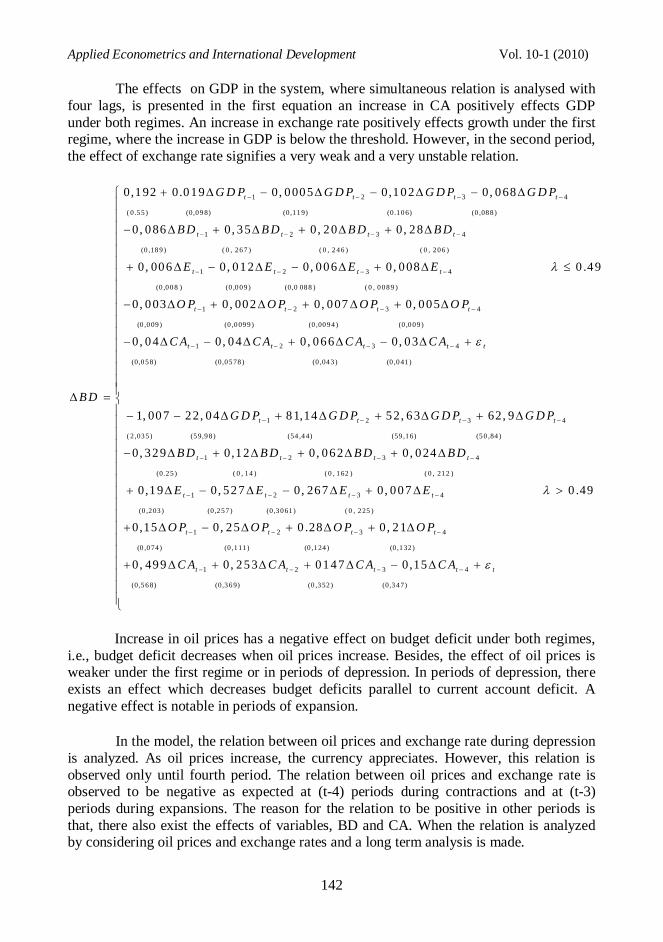
The effects on GDP in the system, where simultaneous relation is analysed with four lags, is presented in the first equation an increase in CA positively effects GDP under both regimes. An increase in exchange rate positively effects growth under the first regime, where the increase in GDP is below the threshold. However, in the second period, the effect of exchange rate signifies a very weak and a very unstable relation.

1 2 3 4

( 0 .5 5 ) (0,0 9 8) (0,1 1 9) (0.1 0 6) (0 ,08 8 )

1 2

0,192 0.019 0, 0005 0,102 0, 068

0, 086 0, 35 0,

t t t t

t t

G D P G D P G D P G D P

B D B D

B D

3 4

(0 ,18 9 ) ( 0 , 2 6 7 ) ( 0 , 2 4 6 ) ( 0 , 2 0 6 )

1 2 3 4

(0 ,0 0 8 ) (0 ,0 0 9 ) (0,0 08 8 ) ( 0 , 0 0 8 9 )

1 2 3 4

(0 ,0 09

20 0, 28

0, 006 0, 012 0, 006 0, 008 0 .49

0, 003 0, 002 0, 007 0, 005

t t

t t t t

t t t t

B D B D

E E E E

O P O P O P O P

) (0 ,0 09 9 ) (0 ,00 9 4 ) (0 ,0 0 9 )

1 2 3 4

(0,0 5 8) (0,0 5 78 ) (0 ,04 3 ) (0 ,0 41 )

1 2 3 4

( 2 ,03 5 ) (5 9,9 8 ) (54

0, 04 0, 04 0, 066 0, 03

1, 007 22, 04 81,14 52, 63 62, 9

t t t t t

t t t t

C A C A C A C A


,4 4) (59 ,1 6) (5 0 ,84 )

1 2 3 4

(0.2 5 ) ( 0 , 1 4 ) ( 0 , 1 62 ) ( 0 , 21 2 )

1 2 3

0, 329 0,12 0, 062 0, 024

0,19 0, 527 0, 267 0, 007

t t t t

t t t

B D B D B D B D

E E E

4

(0 ,2 03 ) (0 ,2 5 7 ) (0,3 0 61 ) ( 0 , 2 25 )

1 2 3 4

(0 ,0 74 ) (0 ,1 11 ) (0 ,1 24 ) (0 ,1 32 )

1 2 3 4

(0,5 6 8) (0,3 6 9) (0 ,3 52 ) (0,3 4 7)

0 .49

0,15 0, 25 0 .28 0, 21

0, 499 0, 253 0147 0,15

t

t t t t

t t t t t

E

O P O P O P O P

C A C A C A C A

Increase in oil prices has a negative effect on budget deficit under both regimes,

i.e., budget deficit decreases when oil prices increase. Besides, the effect of oil prices is weaker under the first regime or in periods of depression. In periods of depression, there exists an effect which decreases budget deficits parallel to current account deficit. A negative effect is notable in periods of expansion.

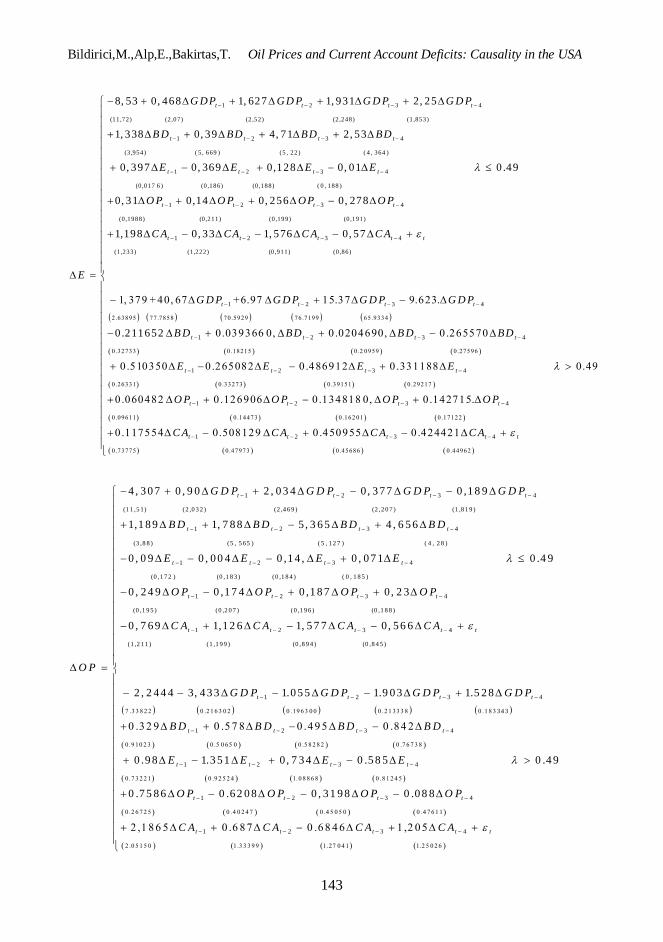
In the model, the relation between oil prices and exchange rate during depression

is analyzed. As oil prices increase, the currency appreciates. However, this relation is observed only until fourth period. The relation between oil prices and exchange rate is observed to be negative as expected at (t-4) periods during contractions and at (t-3) periods during expansions. The reason for the relation to be positive in other periods is that, there also exist the effects of variables, BD and CA. When the relation is analyzed by considering oil prices and exchange rates and a long term analysis is made.


143

1 2 3 4

(11,72) (2 ,07) (2 ,52) (2 ,248) (1 ,853)

1 2

8, 53 0, 468 1, 627 1, 931 2, 25

1, 338 0, 39 4, 71

t t t t

t t

G DP GD P G D P G D P

B D BD B

E

3 4

(3 ,954) ( 5 , 669 ) (5 , 22 ) ( 4 , 364 )

1 2 3 4

(0,017 6 ) (0 ,186) (0 ,188) ( 0 , 188 )

1 2 3 4

(0,1988) (0 ,211

2, 53

0, 397 0, 369 0,128 0, 01 0 .49

0, 31 0,14 0, 256 0, 278

t t

t t t t

t t t t

D BD

E E E E

O P O P OP O P

) (0 ,199) (0 ,191)

1 2 3 4

(1,233) (1 ,222) (0 ,911) (0 ,86)

1 2 3 4

2.63895 77.7858 70.5929 76.7199 65.9334

1,198 0, 33 1, 576 0, 57

1, 379 + 40, 67 +6.97 15.37 9.623.

0.211652

t t t t t

t t t t

C A CA C A C A


1 2 3 4

0 .32733 0 .18215 0 .2 0959 0 .27596

1 2 3 4

0 .26331 0 .33273 0 .39151 0 .29217

0.039366 0, 0 .0204690, 0 .265570

0.510350 0 .265082 0.486912 0.331188 0.49

0 .060482

t t t t

t t t t

B D BD B D BD

E E E E

O P

1 2 3 4

0 .09611 0 .14473 0 .162 01 0 .17122

1 2 3 4

0 .73775 0 .47973 0 .45686 0 .44962

0.126906 0.134818 0, 0 .142715.

0 .117554 0.508129 0 .450955 0.424421

t t t t

t t t t t

O P O P O P

C A C A C A C A

1 2 3 4

(1 1 ,5 1) (2 ,0 3 2 ) (2 ,4 6 9 ) (2 ,2 0 7 ) (1 ,8 1 9 )

1 2

4 , 3 0 7 0 , 9 0 2 , 0 3 4 0, 3 7 7 0 ,1 8 9

1,1 8 9 1, 7 8 8 5

t t t t

t t


B D B D

O P

3 4

(3 ,8 8 ) (5 , 5 65 ) ( 5 , 1 2 7 ) ( 4 , 2 8 )

1 2 3 4

(0 ,1 7 2 ) (0 ,1 8 3 ) (0 ,1 8 4 ) ( 0 , 1 8 5 )

1 2 3 4

(0 ,1 9 5 ) (0

, 3 6 5 4 , 6 5 6

0 , 0 9 0 , 0 0 4 0 ,1 4 , 0 , 0 7 1 0 .4 9

0 , 2 4 9 0 ,1 7 4 0 ,1 8 7 0, 2 3

t t

t t t t

t t t t

B D B D

E E E E

O P O P O P O P

,2 0 7 ) (0 ,1 9 6 ) (0 ,1 8 8 )

1 2 3 4

(1 ,2 1 1 ) (1 ,1 9 9 ) (0 ,8 9 4 ) (0 ,8 4 5 )

1 2 3 4

7 .3 3 8 2 2 0 .2 1 6 3 0 2 0 .19 6 3 0 0 0 .2 1 33 3 8 0 .1 8 3 34

0 , 7 6 9 1,1 2 6 1, 5 7 7 0, 5 6 6

2 , 2 4 4 4 3, 4 3 3 1.0 5 5 1.9 0 3 1.5 2 8

t t t t t

t t t t

C A C A C A C A


3

1 2 3 4

0 .9 10 2 3 0 .5 0 65 0 0 .5 8 2 8 2 0 .7 6 7 3 8

1 2 3 4

0 .7 3 2 2 1 0 .9 2 5 2 4 1.0 8 8 6 8 0 .8 1 2 4 5

1 2

0 .3 2 9 0 .5 7 8 0 .4 9 5 0 .8 4 2

0 .9 8 1.3 5 1 0, 7 3 4 0 .5 8 5 0 .4 9

0 .7 5 8 6 0 .6 2 0 8 0 , 3 1 9 8

t t t t

t t t t

t t

B D B D B D B D

E E E E

O P O P

3 4

0 .2 6 7 2 5 0 .4 0 2 4 7 0 .4 5 0 5 0 0 .4 7 6 1 1

1 2 3 4

2 .0 5 1 5 0 1.3 3 3 9 9 1.27 0 4 1 1.2 5 0 2 6

0 .0 8 8

2 ,1 8 6 5 0 .6 8 7 0 .6 8 4 6 1 ,2 0 5

t t

t t t t t

O P O P

C A C A C A C A


144

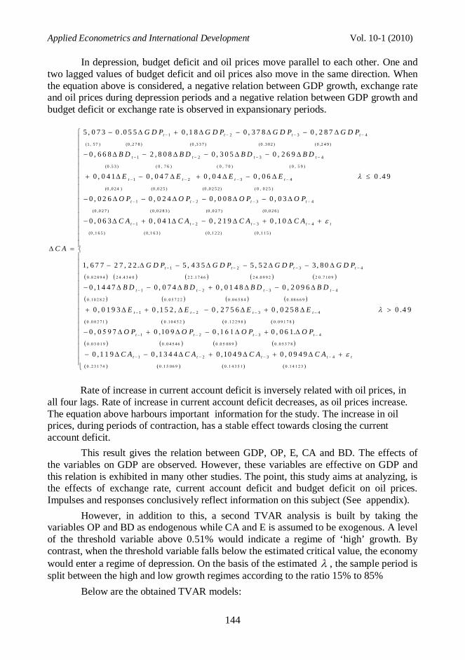
In depression, budget deficit and oil prices move parallel to each other. One and two lagged values of budget deficit and oil prices also move in the same direction. When the equation above is considered, a negative relation between GDP growth, exchange rate and oil prices during depression periods and a negative relation between GDP growth and budget deficit or exchange rate is observed in expansionary periods.

1 2 3 4

(1 , 5 7 ) (0 ,2 7 8 ) (0 ,3 3 7 ) (0 .3 0 2 ) ( 0 ,2 4 9 )

1 2

5 , 0 7 3 0 .0 5 5 0 ,1 8 0 , 3 7 8 0 , 2 8 7

0 , 6 6 8 2 , 8 0 8 0 , 3

t t t t

t t


B D B D

C A

3 4

(0 .5 3 ) ( 0 , 7 6 ) ( 0 , 7 0 ) ( 0 , 5 9 )

1 2 3 4

(0 ,0 2 4 ) (0 ,0 2 5 ) (0 ,0 2 5 2 ) ( 0 , 0 2 5 )

1 2 3 4

(0 ,0 2 7 ) ( 0 ,0 2

0 5 0 , 2 6 9

0 , 0 4 1 0 , 0 4 7 0 , 0 4 0 , 0 6 0 .4 9

0 , 0 2 6 0 , 0 2 4 0 , 0 0 8 0 , 0 3

t t

t t t t

t t t t

B D B D

E E E E

O P O P O P O P

8 3 ) (0 ,0 2 7 ) (0 ,0 2 6 )

1 2 3 4

(0 ,1 6 5 ) ( 0 ,1 6 3 ) ( 0 ,1 2 2 ) ( 0 ,1 1 5 )

1 2 3 4

0 .8 2 8 9 4 2 4 .4 3 4 0 2 2 .1 7 4 6 2 4 .0 9 9 2 2 0 .7 1 0 9

0 , 0 6 3 0 , 0 4 1 0 , 2 1 9 0 ,1 0

1, 6 7 7 2 7 , 2 2 . 5 , 4 3 5 5 , 5 2 3, 8 0

0 ,1 4 4 7

t t t t t

t t t t

C A C A C A C A


B D

1 2 3 4

0 .1 0 2 8 2 0 .0 5 7 2 2 0 .0 6 5 8 4 0 .0 8 6 6 9

1 2 3 4

0 .0 8 2 7 1 0 .1 0 4 5 2 0 .1 2 2 9 8 0 .0 9 1 7 8

1 2 3

0 , 0 7 4 0 , 0 1 4 8 0 , 2 0 9 6

0 , 0 1 9 3 0 ,1 5 2 , 0 , 2 7 5 6 0 , 0 2 5 8 0 .4 9

0 , 0 5 9 7 0 ,10 9 0 ,1 6 1

t t t t

t t t t

t t t

B D B D B D

E E E E

O P O P O P

4

0 .0 3 0 1 9 0 .0 4 5 4 6 0 .0 5 0 8 9 0 .0 5 3 7 8

1 2 3 4

0 .2 3 1 7 4 0 .1 5 0 6 9 0 .1 4 3 5 1 0 .1 4 1 2 3

0 , 0 6 1.

0 ,1 1 9 0 ,1 3 4 4 0 ,10 4 9 0 , 0 9 4 9

t

t t t t t

O P

C A C A C A C A

Rate of increase in current account deficit is inversely related with oil prices, in

all four lags. Rate of increase in current account deficit decreases, as oil prices increase. The equation above harbours important information for the study. The increase in oil prices, during periods of contraction, has a stable effect towards closing the current account deficit.

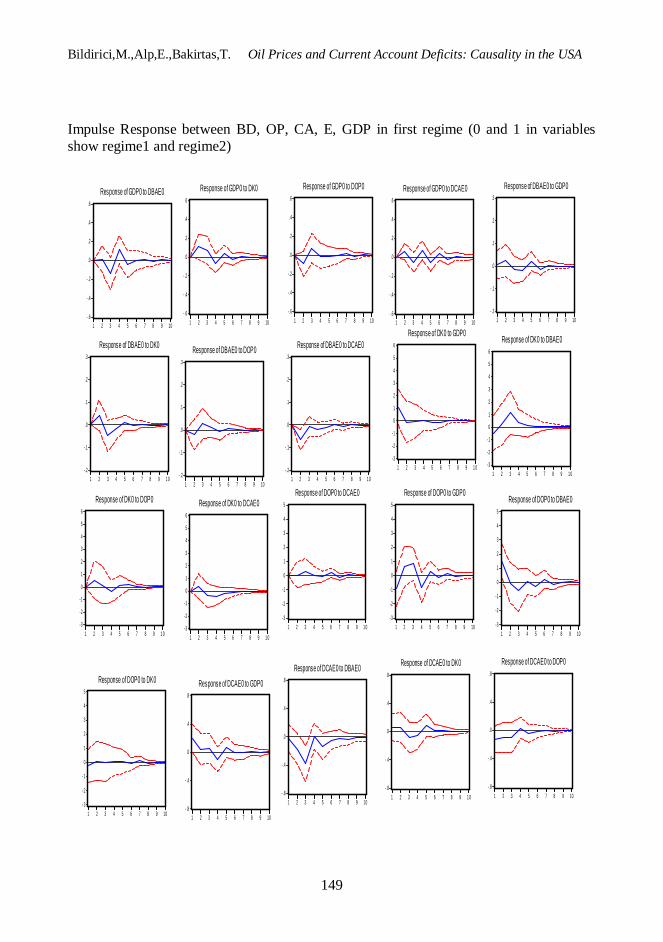
This result gives the relation between GDP, OP, E, CA and BD. The effects of the variables on GDP are observed. However, these variables are effective on GDP and this relation is exhibited in many other studies. The point, this study aims at analyzing, is the effects of exchange rate, current account deficit and budget deficit on oil prices. Impulses and responses conclusively reflect information on this subject (See appendix).

However, in addition to this, a second TVAR analysis is built by taking the variables OP and BD as endogenous while CA and E is assumed to be exogenous. A level of the threshold variable above 0.51% would indicate a regime of ‘high’ growth. By contrast, when the threshold variable falls below the estimated critical value, the economy would enter a regime of depression. On the basis of the estimated , the sample period is split between the high and low growth regimes according to the ratio 15% to 85%

Below are the obtained TVAR models:


145

1 2 3 4

(0.163) ( 0.168) ( 0.159) (0.163)

1 2 3

0.149 0.376 0.009 0.190

5.519 1.287 0.402

t t t t

t t t

OP OP OP OP

BD BD BD

OP

4

(7.243) (6.497) (6.865 ) (6.975)

1 1

(0.456) (0.494)

1 2 3 4

(0.102) ( 0.1

5.316 0.51

0.508 0.1

0.482 0.117 0.086 0.167

t

t t t t

t t t t

BD

CA E

OP OP OP OP

13) ( 0.112) (0.114)

1 2 3 4

(0.403) (0.363) (0.370 ) (0.346)

1 1

(0.482)

0.499 0.689 0.380 0.328 0.51

0.783 0.506

t t t t

t t t t

BD BD BD BD

CA E

(0.251)

1 2 3 4

( 0.002) ( 0.003) ( 0 .002) ( 0 .002)

1 2

0.002 0.003 0.001 0.00003

0.132 0.325 0.492

t t t t

t t

O P O P O P O P

B D B D

BD

3 4

(0 .110) (0 .099 ) (0.105) ( 0 .106 )

1 1

(0.007) (0.008)

1 2 3 4

( 0.027) ( 0.029)

0.003 0.51

0.043 0.007

0.051 0.039 0.110 0.30

t t

t t t t

t t t t

BD B D

CA E

O P O P O P O P

( 0 .0295) (0.30)

1 2 3 4

(0 .106 ) (0 .096) ( 0.097 ) (0 .091)

1 1

(0.127) (0.066

0.007 0.042 0.0310 0.086 0.51

0.028 0.066

t t t t

t t t t

BD B D B D BD

C A E

)

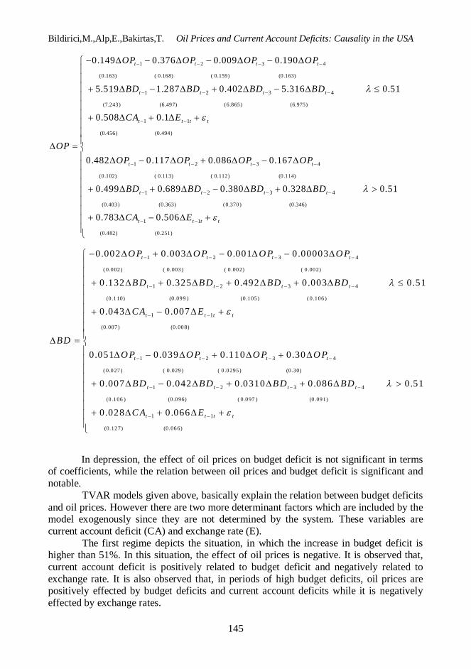
In depression, the effect of oil prices on budget deficit is not significant in terms of coefficients, while the relation between oil prices and budget deficit is significant and notable.

TVAR models given above, basically explain the relation between budget deficits and oil prices. However there are two more determinant factors which are included by the model exogenously since they are not determined by the system. These variables are current account deficit (CA) and exchange rate (E).

The first regime depicts the situation, in which the increase in budget deficit is higher than 51%. In this situation, the effect of oil prices is negative. It is observed that, current account deficit is positively related to budget deficit and negatively related to exchange rate. It is also observed that, in periods of high budget deficits, oil prices are positively effected by budget deficits and current account deficits while it is negatively effected by exchange rates.


146

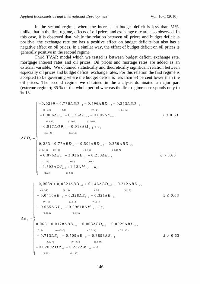
In the second regime, where the increase in budget deficit is less than 51%, unlike that in the first regime, effects of oil prices and exchange rate are also observed. In this case, it is observed that, while the relation between oil prices and budget deficit is positive, the exchange rate too has a positive effect on budget deficits but also has a negative effect on oil prices. In a similar way, the effect of budget deficit on oil prices is generally positive in the second regime.

Third TVAR model which we tested is between budget deficit, exchange rate, mortgage interest rates and oil prices. Oil prices and mortage rates are added as an external variable. We obtained statistically and theoretically significant relation between especially oil prices and budget deficit, exchange rates. For this relation the first regime is accepted to be governing where the budget deficit is less than 63 percent lower than the oil prices. The second regime we obtained in the analysis dominated a major part (extreme regime); 85 % of the whole period whereas the first regime corresponds only to % 15.

1 2 3

( 0 , 33 ) ( 0 .11) ( 0 .12 ) ( 0 .11 2)

1 2 3

(0 .065 ) (0 .0

0, 0 2 9 9 0 .7 7 6 0 .5 9 6 0 .3 5 3

0 .0 0 6 0 .1 2 5 0 .0 0 5 0 .6 3

t t t

t t t

t

B D B D B D

E E E

B D

6 7 ) (0 .0 66 8)

1 1

(0 .0 149 ) (0 .06 8)

1 2 3

(1 0 , 11) ( 0 .1 3) ( 0 .15 ) ( 0 .15 7)

0 .0 1 7 0 .0 1 8

0, 2 3 3 0 .7 7 0 .5 0 1 0 .3 5 9

t t t

t t t

O P M

B D B D B D

1 2 3

(1 .7 3) (1 .94 4 ) (1 .95 6)

1 1

(1 .2 3) (1 .82 )

0 .8 7 6 3 .0 2 0 .2 3 3 0 .6 3

1 .5 0 2 1 .1 3

t t t

t t t

E E E

O P M

1 2 3

( 0 , 55 ) ( 0 .1 9) ( 0 .2 1) ( 0 .1 9)

1 2 3

(0 .10 9) (0 .1

0, 0 6 8 9 0 , 0 8 2 1 0 .1 4 6 0 .2 1 2

0 .0 4 1 6 0 .3 2 8 0 .3 2 1 0 .6 3

t t t

t t t

t

B D B D B D

E E E

E

1 1 ) (0 .11 1)

1 1

(0 .02 4) (0 .115 )

1 2 3

( 0 , 74 ) ( 0 .00 97 ) ( 0 .01 1) ( 0 .01 15 )

0 .0 6 5 0 .0 9 6 1 8

0 .0 6 3 0 .0 1 2 8 0 .0 0 3 0 .0 0 2 5

t t t

t t t

O P M

B D B D B D

1 2 3

(0 .12 7) (0 .14 3 ) (0 .1 44 )

1 1

(0 .09 ) (0 .1 33)

0 .7 1 3 0 .5 0 9 0 .3 8 9 8 0 .6 3

0 .0 2 0 9 0 .2 3 2

t t t

t t t

E E E

O P M


147

In first regime (in depression) oil prices shows negative and significant relation between exchange rate and budget deficit however in second regime (expansion) this relation insignificant with exchange rate but significant with budget deficit. This shows the impression of oil prices on budget deficit especially in depression periods. Moreover the mortgage rates are insignificant in this third analyze. Conclusion In the analysis, the relation between GDP, budget deficit, current account deficit, exchange rate, mortage rate and oil prices were tested with three TVAR models and it was stated that GDP, oil prices, current account deficit, mortage rate, exchange rate and budget deficits are related. As the results of our models, when current account and budget deficits increase, oil prices are effected by this. In the period analyzed during 1968:Q1-2008:Q4, in situations where US budget deficits and current account deficits increase above threshold, increases in oil prices are observed. In periods where the increase in budget deficit is below threshold (second regime), oil prices and exchange rate are observed to be positively related with budget and current account deficit. These effects are observed and experienced before and during the crises in 1974 (1979) and 2008. Reference Arrow K. (2008), “Risky business”, http://www.guardian.co.uk/commentisfree/cifamerica/2008/oct/15/kenneth-arrow-economy-crisis Ayuso and Restoy, (2003) “House prices and rents: an asset pricing approach”, Banco de España, Documento de trabajo. Azariadis, C., Smith, B. (1998), “Financial intermediaries and regime switching in business Cycles”, American Economic Review, Vol. 88, No. 3, pp. 516-536. Balke, N.S. (2000) , “Credit and economic activity: credit regimes and nonlinear propagation of Shocks”, Review of Economics and Statistics, Vol. 82, No. 2, pp. 344-349. Bernanke, B. S., Lown, C. S.(1991), “The Credit Crunch.” Brookings Papers on Economic Activity, (2), pp. 205-47. Calza A., Sousa J. (2005), Output And Inflatıon Responses To Credit Shocks Are There Threshold Effects In The Euro Area? European Central Bank Working Paper, No. 481 / Aprıl 2005 Case K E & Shiller R J, (2003), "Is There a Bubble in the Housing Market?" Brookings Papers on Economic Activity, Vol 2003, No 2, pp 299-342 Dell’Aricci G., Igan D. and Laeven L. (2008), “Credit Booms and Lending Standards: Evidence from the Subprime Mortgage Market”, 11 th Annual Research Conference,Amsterdam, October 30, 2008. Dornbusch, R., (1986), Dollars, Debts, and Deficits. Cambridge, MA: MIT Press Fisher, I. (1933), "The debt-deflation theory of great depressions", Econometrica, Vol. 1 No.4, pp.337-57.


148

Guisan, M.C.(2001). “Causality and Cointegration between Consumption and GDP in 25 OECD countries: Limitations of Cointegration Approach”, Applied Econometrics and International Development, Vol.1-1, pp. 39-61.

Guisan, M.C. (2003). “Causality Tests, Interdependence and Model Selection: Aplication to OECD countries 1960-97”, Workinp paper Series Economic Development, free on line.1

Hansen, B. E. (1996), “Inference When a Nuisance Parameter Is Not Identified Under the Null Hypothesis”, Econometrica. c.64. s.2: 413-430. Kenny, G., (1999), “Modelling the demand and supply sides of the housing market;evidence from Ireland”, Economic Modelling Vol:16, pp. 389-409. Kindleberger, C. P(1989)., Manias, Panics and Crashes: A History of Financial Crises, New York: Basic Books. Mian A., Sufi A., and Trebbi F. (2008),”The Political Economy of the U.S. Mortgage Default Crisis”NBER Working Paper No. 14468 Mian, Atif R. and Sufi A., (2008), “The Consequences of Mortgage Credit Expansion: Evidence from the 2007 Mortgage Default Crisis”, University of Chicago Working Paper. Minsky, H. (1977), "The financial instability hypothesis: an interpretation of Keynes and an alternative to ‘Standard’ theory", Nebraska Journal of Economics and Business, Vol. 16 No.1, pp.5-16. Mitchell W.(1913), Business Cycle, Berkeley: University of California Press Mizen Paul (2008), “The Credit Crunch of 2007-2008: A Discussion of the Background, Market Reactions, and Policy Responses” Federal Reserve Bank of St. Louis Review, 90(5), pp. 531-67. Shiller R J (2007a), "Understanding Recent Trends in House Prices and Home Ownership." Working Paper no 28. Department of Economics, Yale University. Shiller R J (2007b), "Low Interest Rates and High Asset Prices: An Interpretation in Term of Changing Popular Models". Cowles Discussion Paper No 1632. Yale University. Smith M W & Smith G (2006), "Bubble, bubble, Where´s the Housing Bubble?" Brookings Panel of Economic Activity, March 2006 Taylor, J. B.( 2009), “The Financial Crisis and the Policy Responses: An Empirical Analysis of What Went Wrong”, NBER Working Paper No. 14631 Newspapers:Arrow, K. (2008), “Risky business”, The Guardian http://www.guardian.co.uk/commentisfree/cifamerica/2008/oct/15/kenneth-arrow-economy-crisis

1 http://ideas.repec.org/s/eaa/ecodev.html Annex on line at the journal Website: http://www.usc.es/economet/aeid.htm


149

Impulse Response between BD, OP, CA, E, GDP in first regime (0 and 1 in variables show regime1 and regime2)

- .6

- .4

- .2

.0

.2

.4

.6

1 2 3 4 5 6 7 8 9 10

Response of GDP0 to DBAE0

- .6

- .4

- .2

.0

.2

.4

.6

1 2 3 4 5 6 7 8 9 10

Response of GDP0 to DK0

-.6

-.4

-.2

.0

.2

.4

.6

1 2 3 4 5 6 7 8 9 10

Response of GDP0 to DOP0

- .6

- .4

- .2

.0

.2

.4

.6

1 2 3 4 5 6 7 8 9 10

Response of GDP0 to DCAE0

- .2

- .1

.0

.1

.2

.3

1 2 3 4 5 6 7 8 9 10

Response of DBAE0 to GDP0

-.2

-.1

.0

.1

.2

.3

1 2 3 4 5 6 7 8 9 1 0

Response of DBAE0 to DK0

- .2

- .1

.0

.1

.2

.3

1 2 3 4 5 6 7 8 9 10

Response of DBAE0 to DOP0

-.2

-.1

.0

.1

.2

.3

1 2 3 4 5 6 7 8 9 1 0

Response of DBAE0 to DCAE0

-3

-2

-1

0

1

2

3

4

5

6

1 2 3 4 5 6 7 8 9 1 0

Response of DK0 to GDP0

-3

-2

-1

0

1

2

3

4

5

6

1 2 3 4 5 6 7 8 9 1 0

Response of DK0 to DBAE0

-3

-2

-1

0

1

2

3

4

5

6

1 2 3 4 5 6 7 8 9 1 0

Response of DK0 to DOP0

-3

-2

-1

0

1

2

3

4

5

6

1 2 3 4 5 6 7 8 9 1 0

Response of DK0 to DCAE0

-3

-2

-1

0

1

2

3

4

5

1 2 3 4 5 6 7 8 9 10

Response of DOP0 to GDP0

-3

-2

-1

0

1

2

3

4

5

1 2 3 4 5 6 7 8 9 10

Response of DOP0 to DBAE0

- 3

- 2

- 1

0

1

2

3

4

5

1 2 3 4 5 6 7 8 9 10

Response of DOP0 to DK0

-3

-2

-1

0

1

2

3

4

5

1 2 3 4 5 6 7 8 9 1 0

Response of DOP0 to DCAE0

- .8

- .4

.0

.4

.8

1 2 3 4 5 6 7 8 9 10

Response of DCAE0 to GDP0

- .8

- .4

.0

.4

.8

1 2 3 4 5 6 7 8 9 10

Response of DCAE0 to DBAE0

- .8

- .4

.0

.4

.8

1 2 3 4 5 6 7 8 9 1 0

Response of DCAE0 to DK0

- .8

- .4

.0

.4

.8

1 2 3 4 5 6 7 8 9 10

Response of DCAE0 to DOP0


150

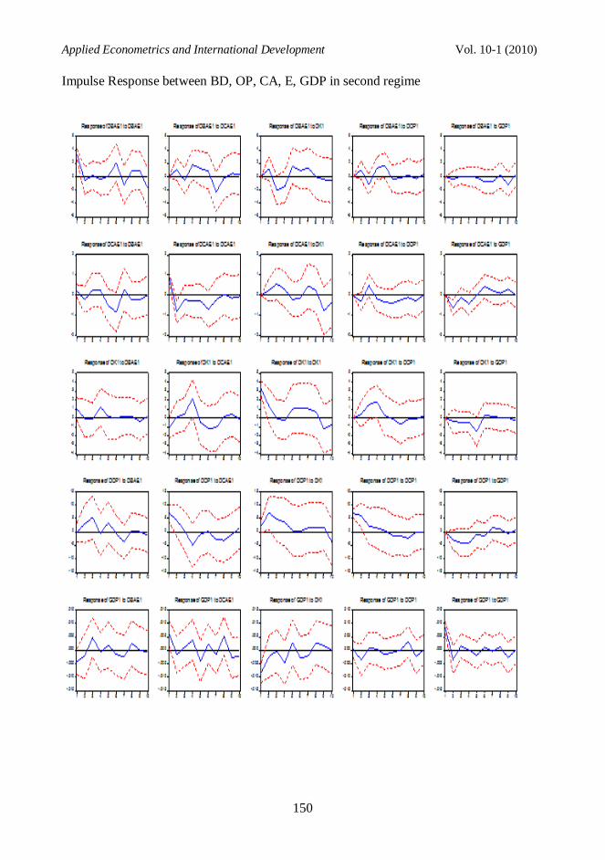
Impulse Response between BD, OP, CA, E, GDP in second regime

oil prices and current account deficits: analysis of causality in the usa

Documents