octane blending and oxidation chemistry of ethanol

Octane Blending and Oxidation Chemistry of

Ethanol-Hydrocarbon Mixtures

Hao Yuan

March 2018

Submitted in total fulfilment of the requirements of the degree of

Doctor of Philosophy

Supervised by

A/Prof. Yi Yang

Co-Supervised by

Prof. Michael Brear

Department of Mechanical Engineering

THE UNIVERSITY OF MELBOURNE

Produced on archival quality paper

Copyright © 2018 Hao Yuan

All rights reserved. No part of the publication may be reproduced in any form by print,

photoprint, microfilm or any other means without written permission from the author.

Abstract

The strong anti-knock property of ethanol makes it a preferred blending component for gasoline to

improve spark ignition (SI) engine performance. Despite its widespread use, understanding several,

particular aspects of ethanol’s interaction with different components of gasoline is still lacking.

This work therefore performs the following three studies to investigate the interactions among

ethanol and hydrocarbon fuels. First, a method for correlating octane numbers is developed for

toluene reference fuels (TRFs) blended with ethanol. This method combines linear regression and

exhaustive (or brute-force) searching for optimal correlations. The proposed correlations reproduce

the measured RON and MON with a maximum absolute error smaller than two octane numbers. De-

spite the empirical nature, the correlations demonstrate the significance of linear by mole blending

rules for TRF fuels and provide insights on the chemical interactions between ethanol and different

hydrocarbons. The work of the optimal octane number correlations has been published in Fuel [Yuan

et al., Fuel, 188 (2017), p.408].

Second, a five-component gasoline surrogate is developed to emulate the octane blending be-

haviours of gasoline and ethanol. The surrogate contains iso-pentane, n-pentane, cyclohexane, 1-

hexene, and 1,2,4-trimethylbenzene and is developed using extensive Cooperative Fuel Research (CFR)

engine testing. The formulated surrogate captures the synergistic RON blending behavior between the

target gasoline and ethanol over the entire blending range, with a hydrocarbon composition similar

to the target fuel.

Lastly, a Pressurised Flow Reactor (PFR) experimental study is carried out to study oxidation

chemistry of a fuel matrix including neat fuels, binaries, gasoline surrogates, and gasoline surro-

gates/ethanol mixtures. The measured species profiles are simulated with published kinetic models.

The result indicates that further investigations on toluene and its interaction chemistries with other

compounds are needed for understanding the oxidation of surrogate fuels.

iii

Declaration

This is to certify that:

1. the thesis comprises only my original work towards the PhD,

2. due acknowledgement has been made in the text to all other material used,

3. the thesis is fewer than 100,000 words in length, exclusive of tables, maps, bibliographies and

appendices.

Hao Yuan, March 2018

v

Acknowledgements

I would like to express my gratitude the following people for their supports during my PhD study.

This thesis would not have been possible without them.

• Yi Yang and Michael Brear (my academic supervisors)

Their constructive advice and insightful guidance have been of tremendous help to me during the

past four years of my PhD study.

• Zhongyuan Chen and Zhewen Lu

Zhongyuan helped me with the CFR engine experiments and we worked together for the past four

years. Zhewen helped to build the PFR and worked together with me on the PFR experiments.

• Tien Mun Foong and Al Knox

Tien Mun offered me great help in starting the CFR engine experiment and modelling at the beginning

of my PhD. Al provided technical supports in the CFR engine overhaul.

• James Anderson and Thomas Leone (research engineers at Ford)

James and Thomas provided the data for the engine modelling work and offered valuable suggestions

for my PhD research.

• Monica Pater

Thanks Monica for her help with purchasing of research equipment and chemicals.

• My friends within the Thermodynamics Group

Thank all of you for making the past four years such an enjoyable experience.

• My beloved family and girlfriend

Foremost, I wish to extend thanks to my family for the continuous and unquestioning support over the

last 30 years. I also would like to thank my girlfriend, Jie Jian, who shared all my sadness, happiness,

failure and success during my PhD study and wish her every success in her own PhD project.

vii

To my mum

ix

Contents

1 Introduction 1

1.1 Energy consumption and climate change . . . . . . . . . . . . . . . . . . . . . . . . . . . 1

1.2 Biofuels for transportation . . . . . . . . . . . . . . . . . . . . . . . . . . . . . . . . . . . . 2

1.2.1 Increased biofuels production . . . . . . . . . . . . . . . . . . . . . . . . . . . . . . 2

1.2.2 Ethanol as a fuel additive . . . . . . . . . . . . . . . . . . . . . . . . . . . . . . . . 2

1.3 Octane blending of ethanol and hydrocarbons . . . . . . . . . . . . . . . . . . . . . . . . 4

2 Literature Review 5

2.1 Overview of Knock . . . . . . . . . . . . . . . . . . . . . . . . . . . . . . . . . . . . . . . . 5

2.1.1 Essence of knock . . . . . . . . . . . . . . . . . . . . . . . . . . . . . . . . . . . . . 5

2.1.2 Characteristics of knock . . . . . . . . . . . . . . . . . . . . . . . . . . . . . . . . . 7

2.2 Anti-knock Characteristics of Ethanol/Hydrocarbon Blends . . . . . . . . . . . . . . . . 8

2.2.1 Octane numbers of ethanol/hydrocarbon blends . . . . . . . . . . . . . . . . . . . 8

2.2.2 Charge cooling effect . . . . . . . . . . . . . . . . . . . . . . . . . . . . . . . . . . . 10

2.3 Chemistries of Ethanol and Hydrocarbons . . . . . . . . . . . . . . . . . . . . . . . . . . . 13

2.3.1 Experimental techniques . . . . . . . . . . . . . . . . . . . . . . . . . . . . . . . . . 13

2.3.1.1 Shock tube . . . . . . . . . . . . . . . . . . . . . . . . . . . . . . . . . . . 13

2.3.1.2 Rapid compression machine . . . . . . . . . . . . . . . . . . . . . . . . . 14

2.3.1.3 Well-stirred reactor . . . . . . . . . . . . . . . . . . . . . . . . . . . . . . 14

2.3.1.4 Pressurised flow reactor . . . . . . . . . . . . . . . . . . . . . . . . . . . 15

2.3.2 Combustion chemistry of hydrocarbons and alcohol . . . . . . . . . . . . . . . . . 16

2.3.2.1 Combustion chemistry of alkanes . . . . . . . . . . . . . . . . . . . . . . 16

2.3.2.2 Combustion chemistry of aromatics . . . . . . . . . . . . . . . . . . . . . 19

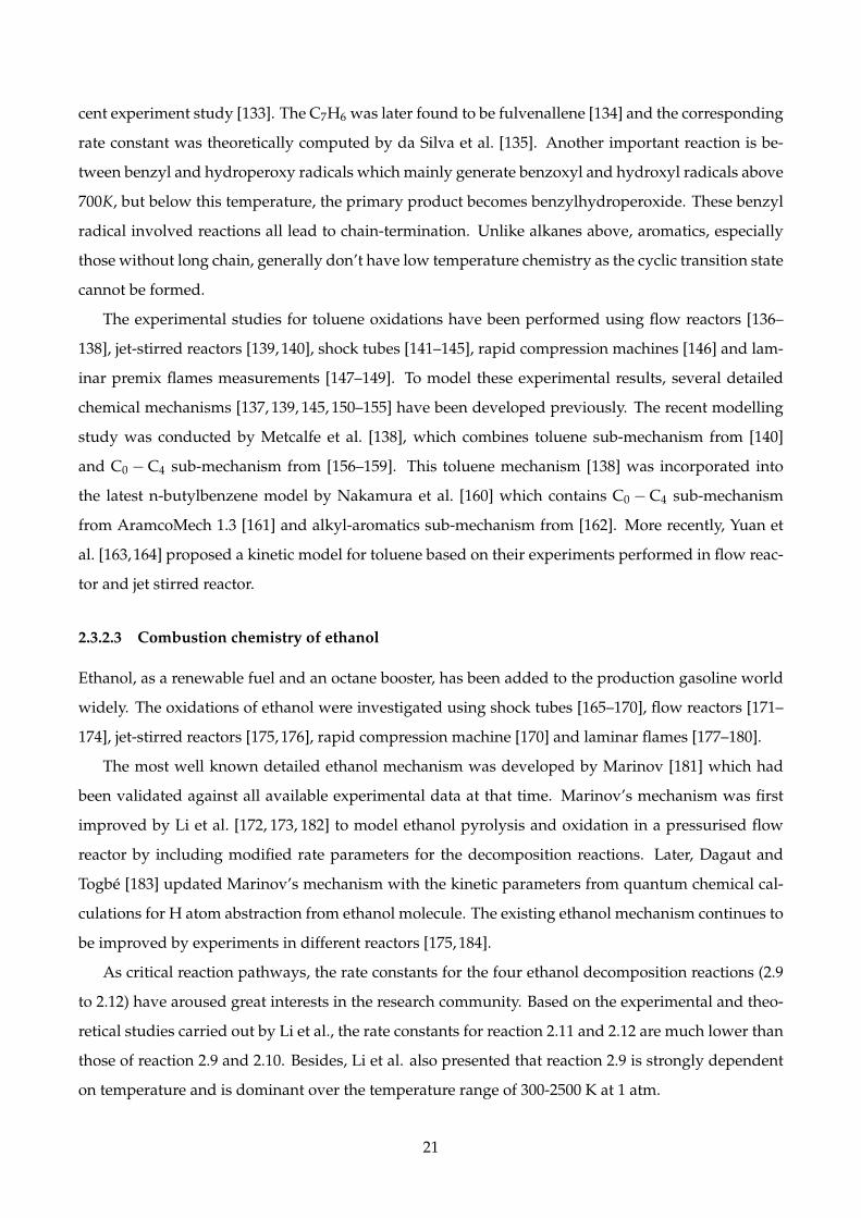
2.3.2.3 Combustion chemistry of ethanol . . . . . . . . . . . . . . . . . . . . . . 21

2.4 Chemical Interactions of Fuel Mixtures . . . . . . . . . . . . . . . . . . . . . . . . . . . . . 22

2.4.1 Interactions between alkanes . . . . . . . . . . . . . . . . . . . . . . . . . . . . . . 22

2.4.2 Interactions between PRF and toluene . . . . . . . . . . . . . . . . . . . . . . . . . 23

xi

2.4.2.1 Cross reactions via large radicals . . . . . . . . . . . . . . . . . . . . . . 23

2.4.2.2 Cross reactions via radical pool . . . . . . . . . . . . . . . . . . . . . . . 25

2.4.3 Interactions between ethanol and hydrocarbons . . . . . . . . . . . . . . . . . . . 27

2.5 Summary and research questions . . . . . . . . . . . . . . . . . . . . . . . . . . . . . . . . 28

3 Experimental Methods 30

3.1 Overview . . . . . . . . . . . . . . . . . . . . . . . . . . . . . . . . . . . . . . . . . . . . . . 30

3.2 CFR engine . . . . . . . . . . . . . . . . . . . . . . . . . . . . . . . . . . . . . . . . . . . . . 30

3.2.1 Overview . . . . . . . . . . . . . . . . . . . . . . . . . . . . . . . . . . . . . . . . . 30

3.2.2 The Structure of the CFR engine . . . . . . . . . . . . . . . . . . . . . . . . . . . . 30

3.2.3 Methods for standard octane number tests . . . . . . . . . . . . . . . . . . . . . . 33

3.3 Pressurised flow reactor . . . . . . . . . . . . . . . . . . . . . . . . . . . . . . . . . . . . . 34

3.3.1 Overview . . . . . . . . . . . . . . . . . . . . . . . . . . . . . . . . . . . . . . . . . 34

3.3.2 Reactor structure . . . . . . . . . . . . . . . . . . . . . . . . . . . . . . . . . . . . . 35

3.3.3 Mixer . . . . . . . . . . . . . . . . . . . . . . . . . . . . . . . . . . . . . . . . . . . . 37

3.3.4 Sampling probe . . . . . . . . . . . . . . . . . . . . . . . . . . . . . . . . . . . . . . 38

3.3.5 Experimental conditions . . . . . . . . . . . . . . . . . . . . . . . . . . . . . . . . . 39

3.4 Gas chromatography . . . . . . . . . . . . . . . . . . . . . . . . . . . . . . . . . . . . . . . 41

3.4.1 Overview of the gas chromatography . . . . . . . . . . . . . . . . . . . . . . . . . 41

3.4.2 Identification and quantification of species . . . . . . . . . . . . . . . . . . . . . . 43

4 Optimal Octane Number Correlations for Toluene Reference Fuels (TRFs) Blended with

Ethanol 48

4.1 Introduction . . . . . . . . . . . . . . . . . . . . . . . . . . . . . . . . . . . . . . . . . . . . 48

4.2 Algorithm for correlation development . . . . . . . . . . . . . . . . . . . . . . . . . . . . 49

4.2.1 The Scheffe polynomial based correlation . . . . . . . . . . . . . . . . . . . . . . . 49

4.2.2 Linear regression . . . . . . . . . . . . . . . . . . . . . . . . . . . . . . . . . . . . . 50

4.2.3 Data for correlation development and validation . . . . . . . . . . . . . . . . . . . 51

4.2.4 Criterion for correlation development . . . . . . . . . . . . . . . . . . . . . . . . . 52

4.2.5 Procedures for optimal correlation development and validation . . . . . . . . . . 53

4.3 Optimal correlations . . . . . . . . . . . . . . . . . . . . . . . . . . . . . . . . . . . . . . . 54

4.3.1 Optimal RON correlation for TRF/ethanol mixtures . . . . . . . . . . . . . . . . . 55

4.3.1.1 Development of the optimal correlation . . . . . . . . . . . . . . . . . . 55

4.3.1.2 Validation of the optimal correlation . . . . . . . . . . . . . . . . . . . . 57

4.3.2 Optimal MON correlation for TRF/ethanol mixtures . . . . . . . . . . . . . . . . 58

xii

4.3.2.1 Development of the optimal correlation . . . . . . . . . . . . . . . . . . 58

4.3.2.2 Validation of the optimal correlation . . . . . . . . . . . . . . . . . . . . 58

4.4 Summary . . . . . . . . . . . . . . . . . . . . . . . . . . . . . . . . . . . . . . . . . . . . . . 60

5 The Octane Numbers of Binary Mixtures and Gasoline Surrogates Blended with Ethanol 62

5.1 Introduction . . . . . . . . . . . . . . . . . . . . . . . . . . . . . . . . . . . . . . . . . . . . 62

5.2 The RONs of binary mixtures . . . . . . . . . . . . . . . . . . . . . . . . . . . . . . . . . . 63

5.2.1 Binary mixtures of hydrocarbons . . . . . . . . . . . . . . . . . . . . . . . . . . . . 63

5.2.2 Binary mixtures containing ethanol . . . . . . . . . . . . . . . . . . . . . . . . . . 72

5.3 The RONs of gasoline surrogates blended with ethanol . . . . . . . . . . . . . . . . . . . 73

5.3.1 Detailed hydrocarbon analysis for the Australian production gasoline . . . . . . 74

5.3.2 Strategy for emulating the octane number of the gasoline . . . . . . . . . . . . . . 76

5.3.3 Comparison between production gasoline and its surrogates when blended with

ethanol . . . . . . . . . . . . . . . . . . . . . . . . . . . . . . . . . . . . . . . . . . . 77

5.4 Summary . . . . . . . . . . . . . . . . . . . . . . . . . . . . . . . . . . . . . . . . . . . . . . 81

6 Oxidation of Ethanol and Hydrocarbon Mixtures in a Flow Reactor 82

6.1 Introduction . . . . . . . . . . . . . . . . . . . . . . . . . . . . . . . . . . . . . . . . . . . . 82

6.2 Kinetic modelling approach . . . . . . . . . . . . . . . . . . . . . . . . . . . . . . . . . . . 84

6.3 Neat fuels . . . . . . . . . . . . . . . . . . . . . . . . . . . . . . . . . . . . . . . . . . . . . 84

6.3.1 Isooctane . . . . . . . . . . . . . . . . . . . . . . . . . . . . . . . . . . . . . . . . . . 84

6.3.2 Ethanol . . . . . . . . . . . . . . . . . . . . . . . . . . . . . . . . . . . . . . . . . . . 89

6.3.3 Toluene . . . . . . . . . . . . . . . . . . . . . . . . . . . . . . . . . . . . . . . . . . 92

6.4 Test mechanism . . . . . . . . . . . . . . . . . . . . . . . . . . . . . . . . . . . . . . . . . . 94

6.4.1 Sensitivity analysis . . . . . . . . . . . . . . . . . . . . . . . . . . . . . . . . . . . . 94

6.4.2 Updated toluene sub-mechanism . . . . . . . . . . . . . . . . . . . . . . . . . . . . 95

6.5 Binary mixtures . . . . . . . . . . . . . . . . . . . . . . . . . . . . . . . . . . . . . . . . . . 98

6.5.1 Ethanol and isooctane . . . . . . . . . . . . . . . . . . . . . . . . . . . . . . . . . . 98

6.5.2 Toluene and isooctane . . . . . . . . . . . . . . . . . . . . . . . . . . . . . . . . . . 99

6.5.3 Ethanol and toluene . . . . . . . . . . . . . . . . . . . . . . . . . . . . . . . . . . . 101

6.6 Gasoline surrogates . . . . . . . . . . . . . . . . . . . . . . . . . . . . . . . . . . . . . . . . 102

6.6.1 PRF91 . . . . . . . . . . . . . . . . . . . . . . . . . . . . . . . . . . . . . . . . . . . 102

6.6.2 TRF91-30 . . . . . . . . . . . . . . . . . . . . . . . . . . . . . . . . . . . . . . . . . . 105

6.7 Gasoline surrogates/ethanol mixtures . . . . . . . . . . . . . . . . . . . . . . . . . . . . . 108

6.7.1 PRF91 and ethanol . . . . . . . . . . . . . . . . . . . . . . . . . . . . . . . . . . . . 108

xiii

6.7.2 TRF91-30 and ethanol . . . . . . . . . . . . . . . . . . . . . . . . . . . . . . . . . . 111

6.8 Comparison of fuel reactivities . . . . . . . . . . . . . . . . . . . . . . . . . . . . . . . . . 118

6.9 Summary . . . . . . . . . . . . . . . . . . . . . . . . . . . . . . . . . . . . . . . . . . . . . . 122

7 Conclusions and Recommendations for Future Research 123

7.1 Conclusions . . . . . . . . . . . . . . . . . . . . . . . . . . . . . . . . . . . . . . . . . . . . 123

7.2 Recommendations for future research . . . . . . . . . . . . . . . . . . . . . . . . . . . . . 125

References 127

A Octane number data used for optimal correlation development 151

B Liquid volume based correlations 155

C Modelling of Trace Knock in a Modern SI Engine Fuelled by Ethanol and Gasoline Blends 157

C.1 Introduction . . . . . . . . . . . . . . . . . . . . . . . . . . . . . . . . . . . . . . . . . . . . 157

C.2 Numerical methods . . . . . . . . . . . . . . . . . . . . . . . . . . . . . . . . . . . . . . . . 158

C.3 Formulation of gasoline surrogates . . . . . . . . . . . . . . . . . . . . . . . . . . . . . . . 159

C.4 NO sub-model . . . . . . . . . . . . . . . . . . . . . . . . . . . . . . . . . . . . . . . . . . . 160

C.5 GT-Power modelling . . . . . . . . . . . . . . . . . . . . . . . . . . . . . . . . . . . . . . . 162

C.5.1 Full flow model . . . . . . . . . . . . . . . . . . . . . . . . . . . . . . . . . . . . . . 162

C.5.2 Reverse run model . . . . . . . . . . . . . . . . . . . . . . . . . . . . . . . . . . . . 164

C.6 Two-zone model of autoignition . . . . . . . . . . . . . . . . . . . . . . . . . . . . . . . . 167

C.7 Modelling of trace knock . . . . . . . . . . . . . . . . . . . . . . . . . . . . . . . . . . . . . 168

C.7.1 Raw pressure data . . . . . . . . . . . . . . . . . . . . . . . . . . . . . . . . . . . . 168

C.7.2 Approach for modelling trace knock . . . . . . . . . . . . . . . . . . . . . . . . . . 170

C.7.3 Example of modelling approach . . . . . . . . . . . . . . . . . . . . . . . . . . . . 171

C.8 Modelling results and discussion . . . . . . . . . . . . . . . . . . . . . . . . . . . . . . . . 172

C.8.1 UFI engine results . . . . . . . . . . . . . . . . . . . . . . . . . . . . . . . . . . . . 172

C.8.1.1 Non-kinetic factors . . . . . . . . . . . . . . . . . . . . . . . . . . . . . . 172

C.8.1.2 Effect of ethanol content . . . . . . . . . . . . . . . . . . . . . . . . . . . 173

C.8.2 DI engine results . . . . . . . . . . . . . . . . . . . . . . . . . . . . . . . . . . . . . 176

C.8.3 The effect of NO . . . . . . . . . . . . . . . . . . . . . . . . . . . . . . . . . . . . . 177

C.9 Summary . . . . . . . . . . . . . . . . . . . . . . . . . . . . . . . . . . . . . . . . . . . . . . 179

D The kinetic model for the flow reactor 180

xiv

List of Figures

1.1 The outlook for (a) energy consumption and (b) oil demand before 2035 [1] . . . . . . . 2

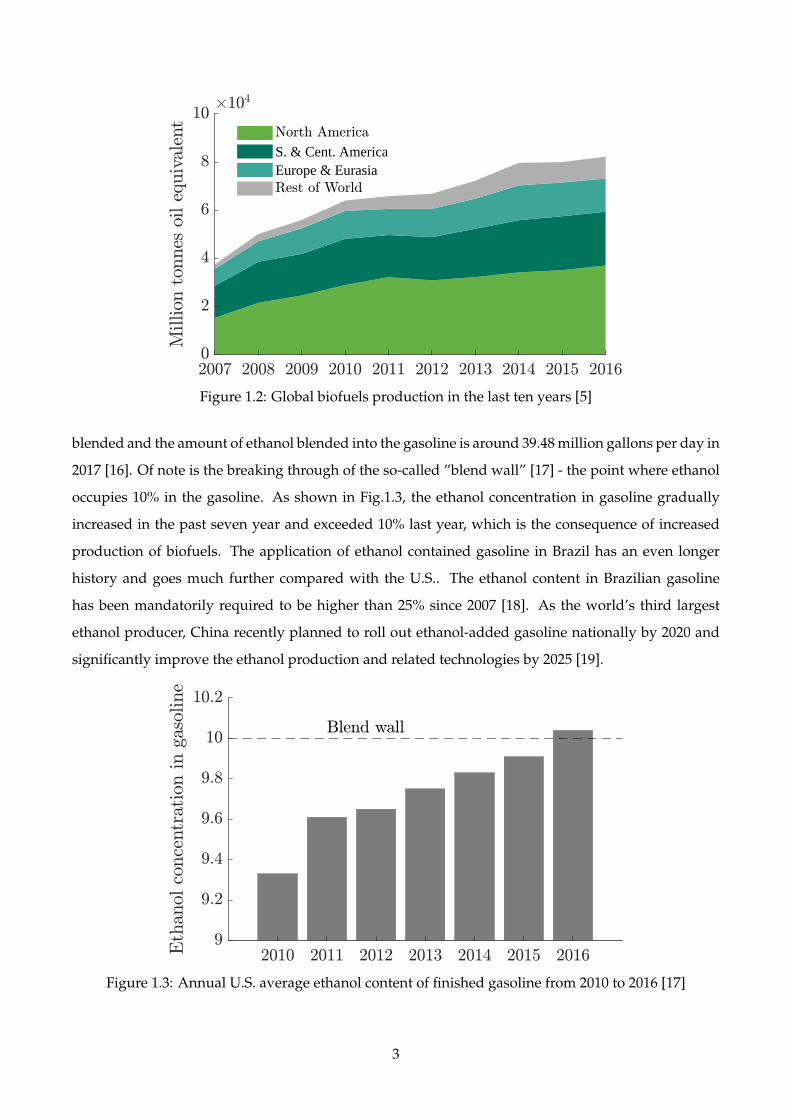
1.2 Global biofuels production in the last ten years [5] . . . . . . . . . . . . . . . . . . . . . . 3

1.3 Annual U.S. average ethanol content of finished gasoline from 2010 to 2016 [17] . . . . . 3

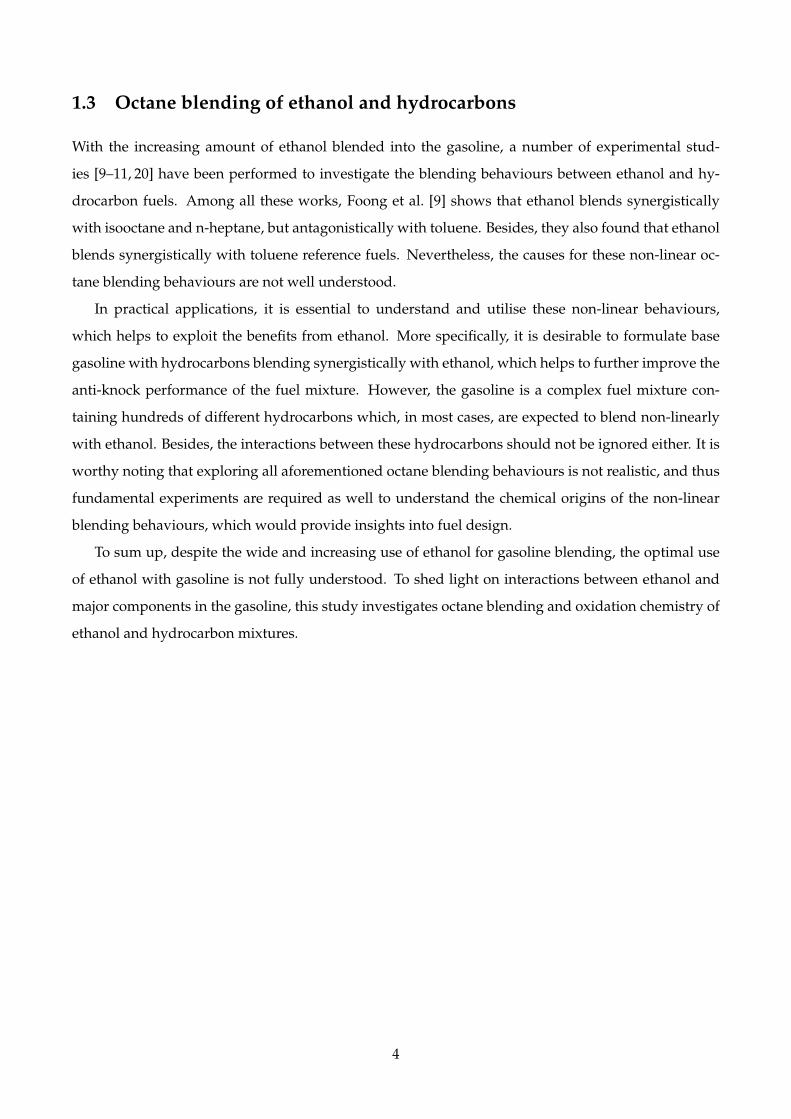
2.1 The pressure trace of a knocking cycle and its corresponding non-knocking cycle sup-

pressed by tetraethyl lead [23] . . . . . . . . . . . . . . . . . . . . . . . . . . . . . . . . . . 6

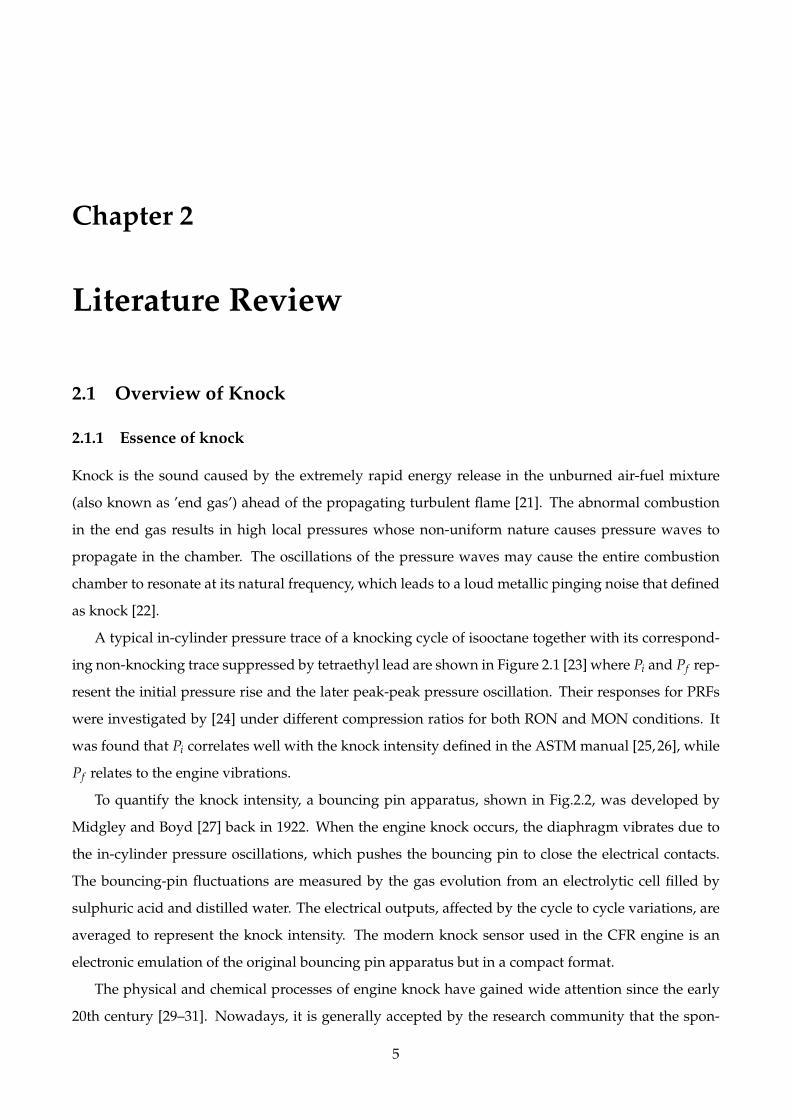
2.2 The Midgley and Boyd bouncing pin apparatus for knock detection [28] . . . . . . . . . 6

2.3 Image series for both non-knocking and knocking engine cycles [32] . . . . . . . . . . . 7

2.4 Measured (a) RONs and (b) MONs for the ethanol and gasoline blends . . . . . . . . . . 9

2.5 Measured (a) RONs and (b) MONs for ethanol blended with isooctane, n-heptane and

toluene . . . . . . . . . . . . . . . . . . . . . . . . . . . . . . . . . . . . . . . . . . . . . . . 10

2.6 Measured RON values for ethanol/gasoline blends under standard and modified con-

ditions [13] . . . . . . . . . . . . . . . . . . . . . . . . . . . . . . . . . . . . . . . . . . . . . 11

2.7 CAD model of the combustion chamber [45] . . . . . . . . . . . . . . . . . . . . . . . . . 12

2.8 The comparison between overall and effective octane numbers [14] . . . . . . . . . . . . 12

2.9 Separation of chemical octane and charge cooling effects on knock limit [11] . . . . . . . 13

2.10 Schematic of a shock tube/rapid compression machine . . . . . . . . . . . . . . . . . . . 14

2.11 Schematic of a well-stirred reactor [47] . . . . . . . . . . . . . . . . . . . . . . . . . . . . . 15

2.12 Structure of a pressurised flow reactor . . . . . . . . . . . . . . . . . . . . . . . . . . . . . 16

2.13 Simplified scheme for the primary mechanism of oxidation of alkanes at low tempera-

tures [51] . . . . . . . . . . . . . . . . . . . . . . . . . . . . . . . . . . . . . . . . . . . . . . 17

2.14 Simplified scheme for the oxidations of benzene and toluene [132] . . . . . . . . . . . . . 20

2.15 Measured MONs of toluene blended with isooctane [187] . . . . . . . . . . . . . . . . . . 24

2.16 Comparisons of cool flame (open symbols) and autoignition delay times (filled sym-

bols) of neat isooctane and isooctane/toluene mixture [190] . . . . . . . . . . . . . . . . . 26

3.1 The system of the CFR engine . . . . . . . . . . . . . . . . . . . . . . . . . . . . . . . . . . 31

3.2 The structure of the CFR engine . . . . . . . . . . . . . . . . . . . . . . . . . . . . . . . . . 32

xv

3.3 The piston head (a) before and (b) after overhaul . . . . . . . . . . . . . . . . . . . . . . . 33

3.4 Schematic of the Pressurised Flow Reactor system . . . . . . . . . . . . . . . . . . . . . . 35

3.5 Structure of the Pressurised Flow Reactor . . . . . . . . . . . . . . . . . . . . . . . . . . . 36

3.6 The mixer a) cutaway view and b) orifices distribution . . . . . . . . . . . . . . . . . . . 37

3.7 CO2 concentrations at 10 bar and 900 K in the flow reactor with air flow rate of 6.02 g/s

and CO2 flow rate of 0.71 g/s . . . . . . . . . . . . . . . . . . . . . . . . . . . . . . . . . . 38

3.8 The sampling probe a) cutaway view b) three thermocouples . . . . . . . . . . . . . . . 38

3.9 Reactor temperature profiles for isooctane oxidation at 10 bar and 900 K with equiva-

lence ratio of 0.058 . . . . . . . . . . . . . . . . . . . . . . . . . . . . . . . . . . . . . . . . 40

3.10 Gas Chromatography-2010ATF plus from Shimadzu . . . . . . . . . . . . . . . . . . . . . 41

3.11 Flow chart of Gas Chromatography . . . . . . . . . . . . . . . . . . . . . . . . . . . . . . . 42

3.12 The temperature program for GC analysis . . . . . . . . . . . . . . . . . . . . . . . . . . . 44

3.13 The spectrum of isooctane oxidation at 900 mm under 900 K and 10 bar . . . . . . . . . . 44

3.14 The spectrum of ethanol oxidation at 500 mm under 900 K and 10 bar . . . . . . . . . . . 45

3.15 The spectrum of toluene oxidation at 700 mm under 930 K and 10 bar . . . . . . . . . . . 45

3.16 The GC calibrations for (a) isooctane, (b) n-heptane, (c) toluene and (d) ethanol . . . . . 46

4.1 Data distribution on simplex lattices with filled circles representing development data

and open ones for validation data . . . . . . . . . . . . . . . . . . . . . . . . . . . . . . . . 52

4.2 Residual error between the development data and correlated RON from (a) linear by-

mole correlation, (b) five terms correlation, (c) six terms correlation and (d) seven terms

correlation . . . . . . . . . . . . . . . . . . . . . . . . . . . . . . . . . . . . . . . . . . . . . 56

4.3 Variation of a) R2 and b) MAE with optimal combination of terms in RON correlations

of increasing length . . . . . . . . . . . . . . . . . . . . . . . . . . . . . . . . . . . . . . . . 57

4.4 Residual error between the validation data and a) 7 and b) 8 term RON correlations on

a molar basis . . . . . . . . . . . . . . . . . . . . . . . . . . . . . . . . . . . . . . . . . . . . 58

4.5 Residual error between the development data and correlated MON from (a) linear by-

mole correlation, and (b) seven terms correlation . . . . . . . . . . . . . . . . . . . . . . . 59

4.6 Variation of a) R2 and b) MAE with optimal combination of terms in MON correlations

of increasing length . . . . . . . . . . . . . . . . . . . . . . . . . . . . . . . . . . . . . . . . 59

4.7 Residual error between the validation data and a) 7 and b) 8 term MON correlations on

a molar basis . . . . . . . . . . . . . . . . . . . . . . . . . . . . . . . . . . . . . . . . . . . . 60

5.1 Measured RONs for Australian production gasoline, PRF91, and TRF91s blended with

ethanol [9] . . . . . . . . . . . . . . . . . . . . . . . . . . . . . . . . . . . . . . . . . . . . . 63

xvi

5.2 RONs of isooctane blended with toluene on a a) volume basis and b) mole basis from

this study. RONs of isooctane blended with ethylbenzene on a c) volume basis and d)

mole basis from [208] . . . . . . . . . . . . . . . . . . . . . . . . . . . . . . . . . . . . . . . 65

5.3 RONs of n-heptane blended with toluene on a a) volume basis and b) mole basis from

this study. RONs of n-heptane blended with ethylbenzene on a c) volume basis and d)

mole basis from [208] . . . . . . . . . . . . . . . . . . . . . . . . . . . . . . . . . . . . . . . 66

5.4 RONs of cyclohexane blended with toluene on a a) volume basis and b) mole basis from

this study. RONs of cyclopentane blended with ethylbenzene on a c) volume basis and

d) mole basis from [208] . . . . . . . . . . . . . . . . . . . . . . . . . . . . . . . . . . . . . 68

5.5 RONs of 1-hexene blended with toluene on a a) volume basis and b) mole basis from

this study. RONs of diisobutylene blended with ethylbenzene on a c) volume basis and

d) mole basis from [208] . . . . . . . . . . . . . . . . . . . . . . . . . . . . . . . . . . . . . 69

5.6 RONs of cyclohexane blended with isooctane on a a) volume basis and b) mole basis

from this study. RONs of methylcyclohexane blended with isooctane on a c) volume

basis and d) mole basis from [208] . . . . . . . . . . . . . . . . . . . . . . . . . . . . . . . 70

5.7 RONs of 1-hexene blended with isooctane on a a) volume basis and b) mole basis from

this study. RONs of 2-heptene blended with isooctane on a c) volume basis and d) mole

basis from [208] . . . . . . . . . . . . . . . . . . . . . . . . . . . . . . . . . . . . . . . . . . 71

5.8 RONs of cyclohexane and 1-hexene blended with ethanol on a a) volume basis and b)

mole basis . . . . . . . . . . . . . . . . . . . . . . . . . . . . . . . . . . . . . . . . . . . . . 72

5.9 The comparisons of the gasoline/ethanol mixture and different gasoline surrogates

blended with ethanol . . . . . . . . . . . . . . . . . . . . . . . . . . . . . . . . . . . . . . . 79

6.1 The measurements of (a) CO and CO2, and (b) isooctane from the neat isooctane oxida-

tion experiment at 900 K and 10 bar, and the modelling results from Mehl et al. (solid

lines), Andrae (dashed lines) and Atef et al. (dotted lines) using the corrected tempera-

ture profile from the three-thermocouple method (c) . . . . . . . . . . . . . . . . . . . . . 86

6.2 The measured intermediate species profiles from the neat isooctane oxidation exper-

iment at 900 K and 10 bar, and the modelling results from Mehl et al. (solid lines),

Andrae (dashed lines) and Atef et al. (dotted lines) . . . . . . . . . . . . . . . . . . . . . . 87

6.3 The reaction pathways for IC4H8, XC7H14, and YC7H14 from the isooctane experiment

at 900mm . . . . . . . . . . . . . . . . . . . . . . . . . . . . . . . . . . . . . . . . . . . . . . 88

6.4 The reaction pathway for IC3H5CHO from the isooctane experiment at 900mm . . . . . 88

xvii

6.5 The measurements of (a) CO and CO2, and (b) ethanol from the neat ethanol oxidation

at 900 K and 10 bar, and the modelling results from Mehl et al. (solid lines), Mittal et al.

(dotted lines), Marinov (dashdot lines) and Andrae (dashed lines) using the corrected

temperature profile from the three-thermocouple method (c) . . . . . . . . . . . . . . . . 90

6.6 The measured intermediate species profiles from the neat ethanol oxidation at 900 K

and 10 bar, and the modelling results from Mehl et al. (solid lines), Mittal et al. (dotted

lines), Marinov (dashdot lines) and Andrae (dashed lines) . . . . . . . . . . . . . . . . . 91

6.7 The reaction pathway for CH3CHO from the ethanol experiment at 500mm . . . . . . . 92

6.8 The measurements of CO and toluene (a) from the neat toluene oxidation at 930 K and

10 bar, and the modelling results from Mehl et al. (solid lines), Yuan et al. (dashdot

lines), Metcalfe et al. (dotted lines), Andrae (dashed lines), Zhang et al. (large dashed

lines), and Pelucchi et al. (large dashdot lines) using the corrected temperature profile

from the three-thermocouple method (b) . . . . . . . . . . . . . . . . . . . . . . . . . . . . 93

6.9 The measured benzene profile from the neat toluene oxidation at 930 K and 10 bar, and

the modelling results from Mehl et al. (solid line), Yuan et al. (dashdot line), Metcalfe et

al. (dotted line), Andrae (dashed line), Zhang et al. (large dashed lines), and Pelucchi

et al. (large dashdot lines) . . . . . . . . . . . . . . . . . . . . . . . . . . . . . . . . . . . . 94

6.10 The brute-force sensitivity analysis of CO for the toluene oxidation at 930 K and 10 bar . 96

6.11 The measurements of CO and toluene from the neat toluene oxidation at 930 K and 10

bar, and the modelling results from Mehl et al. (solid lines) and TestMech (dashed lines) 98

6.12 The measured CO profiles of different binary mixtures (a-c) of isooctane and ethanol at

900 K and 10 bar, and the modelling results from Mehl et al. (solid lines) and TestMech

(dashed lines, overlapping with the solid lines) using the corrected temperature profile

from the three-thermocouple method (d) . . . . . . . . . . . . . . . . . . . . . . . . . . . 99

6.13 The measured CO profiles of different binary mixtures (a-c) of isooctane and toluene at


(dashed lines) using the corrected temperature profile from the three-thermocouple

method (d) . . . . . . . . . . . . . . . . . . . . . . . . . . . . . . . . . . . . . . . . . . . . . 100

6.14 The measured CO profiles of different binary mixtures (a-c) of ethanol and toluene at



method (d) . . . . . . . . . . . . . . . . . . . . . . . . . . . . . . . . . . . . . . . . . . . . . 101

xviii

6.15 The measurements of (a) CO and CO2, and (b) isooctane and n-heptane from the PRF91

oxidation at 900 K and 10 bar, and the modelling results from Mehl et al. (solid lines),

TestMech (dashed lines) and TestMech without chemical interactions between parent

fuels or fuel-like species (dotted lines) using the corrected temperature profile from the

three-thermocouple method (c) . . . . . . . . . . . . . . . . . . . . . . . . . . . . . . . . . 103

6.16 The measured intermediate species profiles from the PRF91 oxidation experiment at


(dashed lines) . . . . . . . . . . . . . . . . . . . . . . . . . . . . . . . . . . . . . . . . . . . 104

6.17 The measured species profiles: (a) CO, CO2, and toluene, (b) isooctane and n-heptane

from the oxidation of TRF91-30 at 900 K and 10 bar, and the modelling results from Mehl

et al. (solid lines), TestMech (dashed lines) and TestMech without chemical interactions

between parent fuels or fuel-like species (dotted lines) using the corrected temperature

profile from the three-thermocouple method (c) . . . . . . . . . . . . . . . . . . . . . . . 106

6.18 The measured intermediate species profiles from the TRF91 oxidation experiment at

900 K and 10 bar, and the modelling results from Mehl et al. (solid lines) and Test-

Mech(dashed lines) . . . . . . . . . . . . . . . . . . . . . . . . . . . . . . . . . . . . . . . . 107

6.19 The measured species profiles: (a) CO, CO2 and ethanol, (b) isooctane and n-heptane

from the oxidation of PRF91 blended with 73.7% ethanol by mole (50% by volume) at



method (c) . . . . . . . . . . . . . . . . . . . . . . . . . . . . . . . . . . . . . . . . . . . . . 109

6.20 The measured intermediate species profiles from the oxidation of PRF91 blended with

73.7% ethanol by mole (50% by volume) at 900 K and 10 bar, and the modelling results

from Mehl et al. (solid lines) and TestMech (dotted lines) . . . . . . . . . . . . . . . . . . 110

6.21 The measured species profiles: (a) CO, isooctane, and n-heptane, (b) CO2, toluene, and

ethanol from the oxidation of TRF91-30 blended with 87.7% ethanol by mole (75% by

volume) at 900 K and 10 bar, and the modelling results from Mehl et al. (solid lines)

and TestMech (dashed lines) using the corrected temperature profile from the three-

thermocouple method (c) . . . . . . . . . . . . . . . . . . . . . . . . . . . . . . . . . . . . 112

6.22 The measured intermediate species profiles the oxidation of TRF91-30 blended with



xix

6.23 The measured species profiles: (a) CO, isooctane, and n-heptane, (b) CO2, toluene, and

ethanol from the oxidation of TRF91-30 blended with 70.5% ethanol by mole (50% by







6.25 The measured species profiles: (a) CO, isooctane, and n-heptane, (b) CO2, ethanol, and

toluene from the oxidation of TRF91-30 blended with 44.3% ethanol by mole (25% by







6.27 The CO and corrected temperature comparisons among isooctane and ethanol . . . . . 118

6.28 The CO and corrected temperature comparisons for two binary mixtures: ethanol plus

isooctane and ethanol plus toluene . . . . . . . . . . . . . . . . . . . . . . . . . . . . . . . 120

6.29 The measured CO profiles of PRF91 and TRF91-30: (a) without ethanol and (c) with

ethanol. The corrected temperature profiles of PRF91 and TRF91-30: (b) without ethanol

and (d) with ethanol . . . . . . . . . . . . . . . . . . . . . . . . . . . . . . . . . . . . . . . 121

B.1 Residual error between the development data and correlated RON from (a) linear by-

volume correlation, (b) seven terms correlation . . . . . . . . . . . . . . . . . . . . . . . . 155

B.2 Residual error between the development data and correlated MON from (a) linear by-

volume correlation, (b) seven terms correlation . . . . . . . . . . . . . . . . . . . . . . . . 156

C.1 Comparison of the simulated ignition delay of the formulated gasoline surrogate (Table

C.1) using the original LLNL model and the extended model containing NO in a con-

stant volume reactor without NO present initially. Equivalence ratio = 1, 30bar, 700-1200K161

C.2 Experimental CA50 vs. NMEP for ethanol/gasoline blends at 10:1 CR and 1500 rpm

with DI [11] . . . . . . . . . . . . . . . . . . . . . . . . . . . . . . . . . . . . . . . . . . . . 163

C.3 The full flow GT-Power model for the single cylinder engine in [11] . . . . . . . . . . . . 163

xx

C.4 The sensitivity analysis for the convection multiplier, to the cylinder wall temperature,

Twall . Dashed lines represent the minimal RMSE at each wall temperature. RMSE values

(×104) are indicated by the numbers on the contours . . . . . . . . . . . . . . . . . . . . . 166

C.5 Unburned gas temperature profiles at different wall temperatures from the GT-Power

reverse run . . . . . . . . . . . . . . . . . . . . . . . . . . . . . . . . . . . . . . . . . . . . . 166

C.6 Measured and simulated pressure traces from the GT-Power reverse run . . . . . . . . . 167

C.7 Raw and band pass filtered pressure traces (left), and power spectra from Fast Fourier

Transform (FFT) analysis (right) for the most advanced pressure traces under standard

knocking for isooctane in a CFR engine (a and b), and under trace knocking for E0, UFI,

NMEP=402kPa (c and d) and E50, UFI, NMEP=1324kPa (e and f) in a single-cylinder

engine from the experimental study [11] . . . . . . . . . . . . . . . . . . . . . . . . . . . . 169

C.8 Modelled results for E50 and UFI at NMEP=1324kPa with the MFB profile being swept 171

C.9 Comparison of measured and modelled spark timing for trace knock using different

representative traces for E0, E20 and E50. All cases are with UFI fueling . . . . . . . . . 174

C.10 Variation of modelled (using the 95th percentile advanced trace) and measured spark

timing for trace knock for E0, E20 and E50 . . . . . . . . . . . . . . . . . . . . . . . . . . . 175

C.11 MFB at autoignition for spark timings that are one degree earlier than the spark timing

for trace knock . . . . . . . . . . . . . . . . . . . . . . . . . . . . . . . . . . . . . . . . . . . 175

C.12 Comparison of modelled and experimental spark timing for trace knock with DI and

UFI for E50. Modelling results are from 95th percentile most advanced pressure traces . 177

C.13 Modelled spark timings for trace knock without residual NO compared to equivalent

results with residual NO for different fuel mixtures and injection methods . . . . . . . . 178

D.1 The comparison between the modelled results of the neat isooctane oxidation at 900 K

and 10 bar in the PFR using Chemkin and the model developed in this study . . . . . . 181

xxi

List of Tables

3.1 Operating conditions for the RON and MON measurements [25, 26] . . . . . . . . . . . . 34

3.2 The composition of the dilute TEL [25, 26] . . . . . . . . . . . . . . . . . . . . . . . . . . . 34

3.3 Experimental conditions for the PFR study . . . . . . . . . . . . . . . . . . . . . . . . . . 40

3.4 Response factors for gaseous fuels . . . . . . . . . . . . . . . . . . . . . . . . . . . . . . . 47

3.5 Response factors for intermediate species in liquid phase . . . . . . . . . . . . . . . . . . 47

4.1 Terms of the Scheffe polynomial with four variables . . . . . . . . . . . . . . . . . . . . . 50

4.2 Coefficients of first order terms in the Scheffe polynomial . . . . . . . . . . . . . . . . . . 50

5.1 RONs of cyclohexane and 1-hexene from different studies [20, 207] . . . . . . . . . . . . 67

5.2 Interactions of binary mixtures on a mole basis . . . . . . . . . . . . . . . . . . . . . . . . 73

5.3 Volume fractions of hydrocarbon groups in the Australian production gasoline . . . . . 74

5.4 Top ten most abundant species in iso-, n- and cyclo-paraffins . . . . . . . . . . . . . . . . 75

5.5 Top ten most abundant species in aromatics and olefins . . . . . . . . . . . . . . . . . . . 75

5.6 Formulated gasoline surrogates . . . . . . . . . . . . . . . . . . . . . . . . . . . . . . . . . 77

5.7 Equivalence ratios of gasoline/ethanol and GS11/ethanol at standard knocking condi-

tions . . . . . . . . . . . . . . . . . . . . . . . . . . . . . . . . . . . . . . . . . . . . . . . . . 80

5.8 The physical properties of the gasoline and the gasoline surrogates . . . . . . . . . . . . 80

6.1 Test fuels and reaction mechanisms for modelling . . . . . . . . . . . . . . . . . . . . . . 83

6.2 Experimental conditions for the PFR study . . . . . . . . . . . . . . . . . . . . . . . . . . 84

6.3 Reaction changes to LLNL’s toluene sub-mechanism . . . . . . . . . . . . . . . . . . . . . 97

A.1 Octane number data used for developing the optimal correlations for TRF/ethanol mix-

tures . . . . . . . . . . . . . . . . . . . . . . . . . . . . . . . . . . . . . . . . . . . . . . . . 151

A.2 Octane number data used for validating the optimal correlations for TRF/ethanol mix-

tures . . . . . . . . . . . . . . . . . . . . . . . . . . . . . . . . . . . . . . . . . . . . . . . . 153

C.1 Gasoline and surrogate fuel compositions (%vol) . . . . . . . . . . . . . . . . . . . . . . . 160

xxii

C.2 Gasoline and surrogate fuel properties . . . . . . . . . . . . . . . . . . . . . . . . . . . . . 160

C.3 Specifications for the single cylinder SI engine [11] . . . . . . . . . . . . . . . . . . . . . . 162

C.4 Experimental conditions for modelled trace knocking cases . . . . . . . . . . . . . . . . . 164

C.5 Vibration mode frequencies from [266] . . . . . . . . . . . . . . . . . . . . . . . . . . . . . 170

C.6 Comparison between peak frequencies from the FFT result and the prediction . . . . . . 170

C.7 Inputs to the two-zone modelling obtained from GT-Power for the UFI cases in Table

C.4 and their corresponding 95th percentile raw pressure traces . . . . . . . . . . . . . . 172

C.8 Inputs to the two-zone modelling obtained from GT-Power for the DI cases in Table C.4

and the 95th percentile raw pressure traces . . . . . . . . . . . . . . . . . . . . . . . . . . 176

xxiii

Chapter 1

Introduction

1.1 Energy consumption and climate change

With the growth of the world economy, more energy is required in the future. Based on the estimations

of the BP Energy Outlook in 2017 [1], the growth of the total energy consumption in the next 20

years is over 30% with the world economy to double in this period, as shown in Fig.1.1. Half of the

growth is expected to come from renewables, nuclear, and hydroelectric power, but the fossil energy

sources, such as coal, gas, and oil, still provide over three-quarters of total energy supplies. Among

all these conventional energies, the oil consumption is predicted to be the largest. Meanwhile, more

than half of the oil demands come from transportations, as shown in Fig.1.1(b). In the foreseeable

future, it is expected that Internal Combustion Engines (ICEs), which predominantly rely on oil, will

serve as the main propulsion systems for transportations [2] owing to low cost, high reliability, long

durability, and fast refuelling. The deep understanding and accurate control of combustion process

have enabled the emergence of novel engine technologies for higher efficiencies and lower emissions,

such as direct injection, turbocharging, and downsizing. New types of engine utilising advanced

combustion modes, such as spark assisted homogeneous charge compression ignition technology, are

emerging [3].

The predominant use of fossil fuels in ICEs produces a significant amount of carbon dioxide (CO2)

which accounts for approximately 25% of global greenhouse gas emissions responsible for global

warming [4] and other pollutants such as nitrogen oxides (NOx), carbon monoxide (CO), particulate

matter (PM), and soot. Compared with the fossil fuels, biofuels produced from biomass are renewable

and produce less CO2, soot, and unburned hydrocarbon (HC) emissions, which have been widely

used as alternative neat fuels or fuel additives.

1

0

2

4

6

8

10

12

14

16

18

1965 1975 1985 1995 2005 2015 2025 2035

Renewables Hydro Nuclear Coal

Gas

Oil

Billion toe

(a)

0

20

40

60

80

100

120

2000 2005 2010 2015 2020 2025 2030 2035

Mb/d

Non-combusted

Buildings

Industry

Ships, trains & planes

Trucks

Cars

Power

Transport

(b)

Figure 1.1: The outlook for (a) energy consumption and (b) oil demand before 2035 [1]

1.2 Biofuels for transportation

1.2.1 Increased biofuels production

To reduce the GHG emissions, biofuels have been used as, in most cases, fuel blending components

in nowadays transportations due to their cleaner emissions compared with the conventional fuels.

Fig.1.2 shows the global biofuels production in the past ten years [5]. The overall amount is twice of

the value from ten years ago, indicating increasing importance of biofuels. The increased production

enables higher levels of biofuels blending in the fossil fuels.

1.2.2 Ethanol as a fuel additive

Among all biofuels productions, ethanol is the predominant compound and has been extensively used

as a transportation fuel. Generally, renewable ethanol fuel can be sustainably produces in many coun-

tries [6, 7]. Besides, when blended with gasoline, ethanol reduces the emissions of CO and unburned

hydrocarbon in exhaust [8]. Finally, ethanol is known to have high octane numbers [9–12] and signifi-

cant charge cooling effect [9, 11–15], which suppress the knock in spark-ignition (SI) engines and thus

improves the engine efficiencies.

Ethanol has been widely used as a fuel additive in the gasoline with the blending ratios of 10%

or 85% by volume (known as E10 and E85) in most cases. As the largest ethanol production country,

U.S. blends ethanol extensively in the gasoline and nearly all their gasoline are sold with ethanol

2

S. & Cent. AmericaEurope & Eurasia

Figure 1.2: Global biofuels production in the last ten years [5]

blended and the amount of ethanol blended into the gasoline is around 39.48 million gallons per day in

2017 [16]. Of note is the breaking through of the so-called ”blend wall” [17] - the point where ethanol

occupies 10% in the gasoline. As shown in Fig.1.3, the ethanol concentration in gasoline gradually

increased in the past seven year and exceeded 10% last year, which is the consequence of increased

production of biofuels. The application of ethanol contained gasoline in Brazil has an even longer

history and goes much further compared with the U.S.. The ethanol content in Brazilian gasoline

has been mandatorily required to be higher than 25% since 2007 [18]. As the world’s third largest

ethanol producer, China recently planned to roll out ethanol-added gasoline nationally by 2020 and

significantly improve the ethanol production and related technologies by 2025 [19].

Figure 1.3: Annual U.S. average ethanol content of finished gasoline from 2010 to 2016 [17]

3

1.3 Octane blending of ethanol and hydrocarbons

With the increasing amount of ethanol blended into the gasoline, a number of experimental stud-

ies [9–11, 20] have been performed to investigate the blending behaviours between ethanol and hy-

drocarbon fuels. Among all these works, Foong et al. [9] shows that ethanol blends synergistically

with isooctane and n-heptane, but antagonistically with toluene. Besides, they also found that ethanol

blends synergistically with toluene reference fuels. Nevertheless, the causes for these non-linear oc-

tane blending behaviours are not well understood.

In practical applications, it is essential to understand and utilise these non-linear behaviours,

which helps to exploit the benefits from ethanol. More specifically, it is desirable to formulate base

gasoline with hydrocarbons blending synergistically with ethanol, which helps to further improve the

anti-knock performance of the fuel mixture. However, the gasoline is a complex fuel mixture con-

taining hundreds of different hydrocarbons which, in most cases, are expected to blend non-linearly

with ethanol. Besides, the interactions between these hydrocarbons should not be ignored either. It is

worthy noting that exploring all aforementioned octane blending behaviours is not realistic, and thus

fundamental experiments are required as well to understand the chemical origins of the non-linear

blending behaviours, which would provide insights into fuel design.

To sum up, despite the wide and increasing use of ethanol for gasoline blending, the optimal use

of ethanol with gasoline is not fully understood. To shed light on interactions between ethanol and

major components in the gasoline, this study investigates octane blending and oxidation chemistry of

ethanol and hydrocarbon mixtures.

4

Chapter 2

Literature Review

2.1 Overview of Knock

2.1.1 Essence of knock

Knock is the sound caused by the extremely rapid energy release in the unburned air-fuel mixture

(also known as ’end gas’) ahead of the propagating turbulent flame [21]. The abnormal combustion

in the end gas results in high local pressures whose non-uniform nature causes pressure waves to

propagate in the chamber. The oscillations of the pressure waves may cause the entire combustion

chamber to resonate at its natural frequency, which leads to a loud metallic pinging noise that defined

as knock [22].

A typical in-cylinder pressure trace of a knocking cycle of isooctane together with its correspond-

ing non-knocking trace suppressed by tetraethyl lead are shown in Figure 2.1 [23] where Pi and Pf rep-

resent the initial pressure rise and the later peak-peak pressure oscillation. Their responses for PRFs

were investigated by [24] under different compression ratios for both RON and MON conditions. It

was found that Pi correlates well with the knock intensity defined in the ASTM manual [25,26], while

Pf relates to the engine vibrations.

To quantify the knock intensity, a bouncing pin apparatus, shown in Fig.2.2, was developed by

Midgley and Boyd [27] back in 1922. When the engine knock occurs, the diaphragm vibrates due to

the in-cylinder pressure oscillations, which pushes the bouncing pin to close the electrical contacts.

The bouncing-pin fluctuations are measured by the gas evolution from an electrolytic cell filled by

sulphuric acid and distilled water. The electrical outputs, affected by the cycle to cycle variations, are

averaged to represent the knock intensity. The modern knock sensor used in the CFR engine is an

electronic emulation of the original bouncing pin apparatus but in a compact format.

The physical and chemical processes of engine knock have gained wide attention since the early

20th century [29–31]. Nowadays, it is generally accepted by the research community that the spon-

5

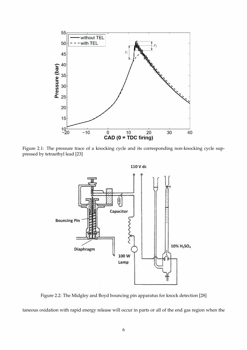
Figure 2.1: The pressure trace of a knocking cycle and its corresponding non-knocking cycle sup-pressed by tetraethyl lead [23]

Figure 2.2: The Midgley and Boyd bouncing pin apparatus for knock detection [28]

taneous oxidation with rapid energy release will occur in parts or all of the end gas region when the

6

pressure and temperatures of one or several gas pockets in the end gas are adequately high [21]. Dur-

ing the autoignition, the pressure trace first has a rapid increase and then oscillates with decaying

amplitude due to the pressure waves generated from the auto-ignited hot spots.

2.1.2 Characteristics of knock

With high-speed imaging, knocking combustion can be observed photographically. Figure 2.3 shows

the time series images for non-knocking and knocking cycles [32]. The normal flame front can be

clearly observed in the non-knocking cycle and the first image of the knocking cycle. The dark

crescent-shaped region ahead of the flame front is the unburned gas zone where autoignition occurs

(in frame G). Then the unburned gas zone becomes brighter and hotter with the propagation of the

autoignition region. Finally, the end gas gets burned completely in frame J.

Figure 2.3: Image series for both non-knocking and knocking engine cycles [32]

Autoignition occurs at places with the most favourable conditions for the low temperature oxi-

dations, and reaction propagation depends on the inhomogeneity of temperature and compositions

of the unburned gas. Based on the temperature gradients, the end gas autoignition could propagate

from the hot gas pocket in three modes [33]:

• With low temperature and steep temperature gradients, the end gas will produce a weak pres-

sure propagating from the centre and is attenuated. In this phase, combustion undergoes a

gradual transition to knock and is regarded as non-knocking combustion.

• With high temperature and small temperature gradients, the end gas will generate simultaneous

chemical reactions following the occurrence of the autoignition. The knock intensity is positively

correlated with the propagation speed of the reaction front. Moderate knock occurs under this

condition.

7

• With intermediate temperature and temperature gradients, the end gas will create strong shock

waves after the initiation of the chemical reactions. Strong pressure waves coupled with very

reactive end gas will generate an intensely illuminating flame. In this case, autoignition ends up

with a severe and damaging knock.

Knock detection techniques can generally be categorised into two types: direct measurements

based on in-cylinder parameters and indirect measurements such as sound, pressure or cylinder block

vibrations [34–36].

• The peak-peak value of the pressure oscillations after band pass filtering was applied to define

the knock intensity by [37].

• Fast Fourier transform (FFT) and power spectral density (PSD) of raw pressure trace were used

to characterise knock in [38, 39].

• The third derivative of the pressure trace, which generates a much higher absolute value when

knock happens, could also be applied to determine the knock onset point [40, 41].

• The occurrence of knock can be determined by engine vibration whose oscillation frequencies

depend on the size and shape of the chamber [42].

2.2 Anti-knock Characteristics of Ethanol/Hydrocarbon Blends

Ethanol, as an oxygenated gasoline blending component, has aroused worldwide interests in the last

two decades. Beneficial results have been reported in numerous studies related to ethanol fuelled SI

engine. Among all these studies, this review summarises ethanol’s two most important features: high

octane number and charge cooling effect.

2.2.1 Octane numbers of ethanol/hydrocarbon blends

In 1927, Graham Edgar [43] proposed an octane rating scale which defines the knock-limited com-

pression ratios for the blend fraction of the two Primary Reference Fuels (PRFs), namely iso-octane

and n-heptane. For instance, a PRF with an octane number of 80 is comprised of 80% iso-octane and

20% n-heptane by volume. Octane rating experiments are conducted in the Cooperative Fuel Re-

search Committee (CFR) engine with standard testing procedures [25, 26]. Research octane number

(RON) and motored octane number (MON) are two types of octane numbers associated with different

operating conditions.

8

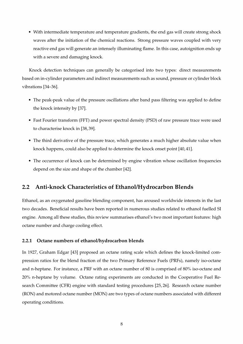
The RONs and MONs of different ethanol/gasoline blends on a volume basis are shown in Fig.2.4,

based on the studies from Foong [9] and Anderson [44]. The measured RONs show a non-linear

relationship with the volume fraction of ethanol. Although both of them exhibit similar trends, the

results reported by Anderson [44] are more synergistic (octane number deviates more from the linear

blending to the higher octane number side). Fig.2.4(b) shows the synergistic blending behaviours

observed in the corresponding MON tests. The differences between these two works are probably

caused by the different gasolines used in the experiments.

0 10 20 30 40 50 60 70 80 90 100

Ethanol content %(v/v)

90

95

100

105

110

RON

Foong et al.,2014Anderson et al., 2012

(a)

0 20 40 60 80 100


80

82

84

86

88

90

92

MON

Foong et al.,2014Anderson et al., 2012

(b)

Figure 2.4: Measured (a) RONs and (b) MONs for the ethanol and gasoline blends

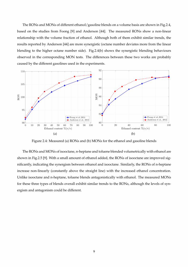
The RONs and MONs of isooctane, n-heptane and toluene blended volumetrically with ethanol are

shown in Fig.2.5 [9]. With a small amount of ethanol added, the RONs of isooctane are improved sig-

nificantly, indicating the synergism between ethanol and isooctane. Similarly, the RONs of n-heptane

increase non-linearly (constantly above the straight line) with the increased ethanol concentration.

Unlike isooctane and n-heptane, toluene blends antagonistically with ethanol. The measured MONs

for these three types of blends overall exhibit similar trends to the RONs, although the levels of syn-

ergism and antagonism could be different.

9

0 20 40 60 80 100


60

70

80

90

100

110

120

RON

isooctanen-heptanetoluene

(a)

0 20 40 60 80 100


60

70

80

90

100

110

MON

isooctanen-heptanetoluene

(b)

Figure 2.5: Measured (a) RONs and (b) MONs for ethanol blended with isooctane, n-heptane andtoluene

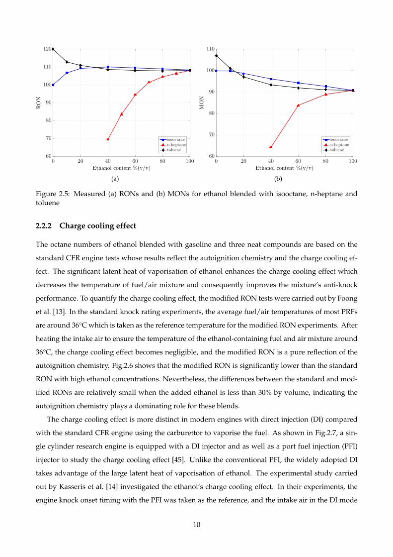
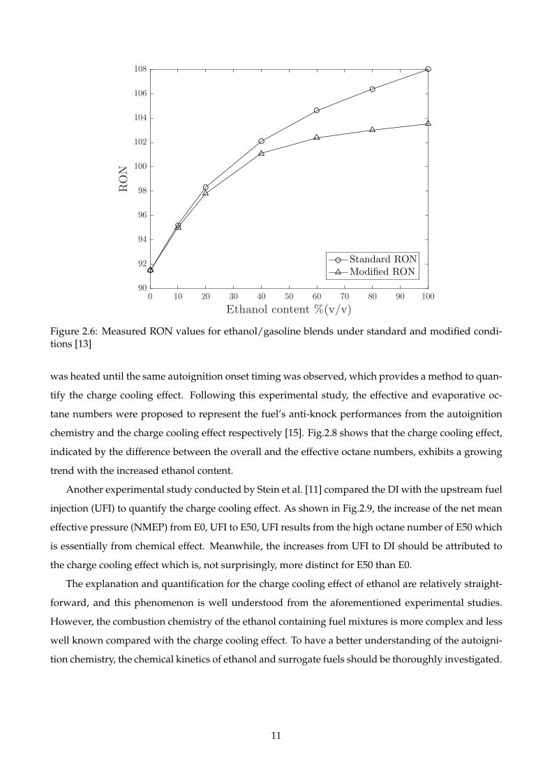
2.2.2 Charge cooling effect

The octane numbers of ethanol blended with gasoline and three neat compounds are based on the

standard CFR engine tests whose results reflect the autoignition chemistry and the charge cooling ef-

fect. The significant latent heat of vaporisation of ethanol enhances the charge cooling effect which

decreases the temperature of fuel/air mixture and consequently improves the mixture’s anti-knock

performance. To quantify the charge cooling effect, the modified RON tests were carried out by Foong

et al. [13]. In the standard knock rating experiments, the average fuel/air temperatures of most PRFs

are around 36°C which is taken as the reference temperature for the modified RON experiments. After

heating the intake air to ensure the temperature of the ethanol-containing fuel and air mixture around

36°C, the charge cooling effect becomes negligible, and the modified RON is a pure reflection of the

autoignition chemistry. Fig.2.6 shows that the modified RON is significantly lower than the standard

RON with high ethanol concentrations. Nevertheless, the differences between the standard and mod-

ified RONs are relatively small when the added ethanol is less than 30% by volume, indicating the

autoignition chemistry plays a dominating role for these blends.

The charge cooling effect is more distinct in modern engines with direct injection (DI) compared

with the standard CFR engine using the carburettor to vaporise the fuel. As shown in Fig.2.7, a sin-

gle cylinder research engine is equipped with a DI injector and as well as a port fuel injection (PFI)

injector to study the charge cooling effect [45]. Unlike the conventional PFI, the widely adopted DI

takes advantage of the large latent heat of vaporisation of ethanol. The experimental study carried

out by Kasseris et al. [14] investigated the ethanol’s charge cooling effect. In their experiments, the

engine knock onset timing with the PFI was taken as the reference, and the intake air in the DI mode

10

0 10 20 30 40 50 60 70 80 90 100


90

92

94

96

98

100

102

104

106

108

RON

Standard RONModified RON

Figure 2.6: Measured RON values for ethanol/gasoline blends under standard and modified condi-tions [13]

was heated until the same autoignition onset timing was observed, which provides a method to quan-

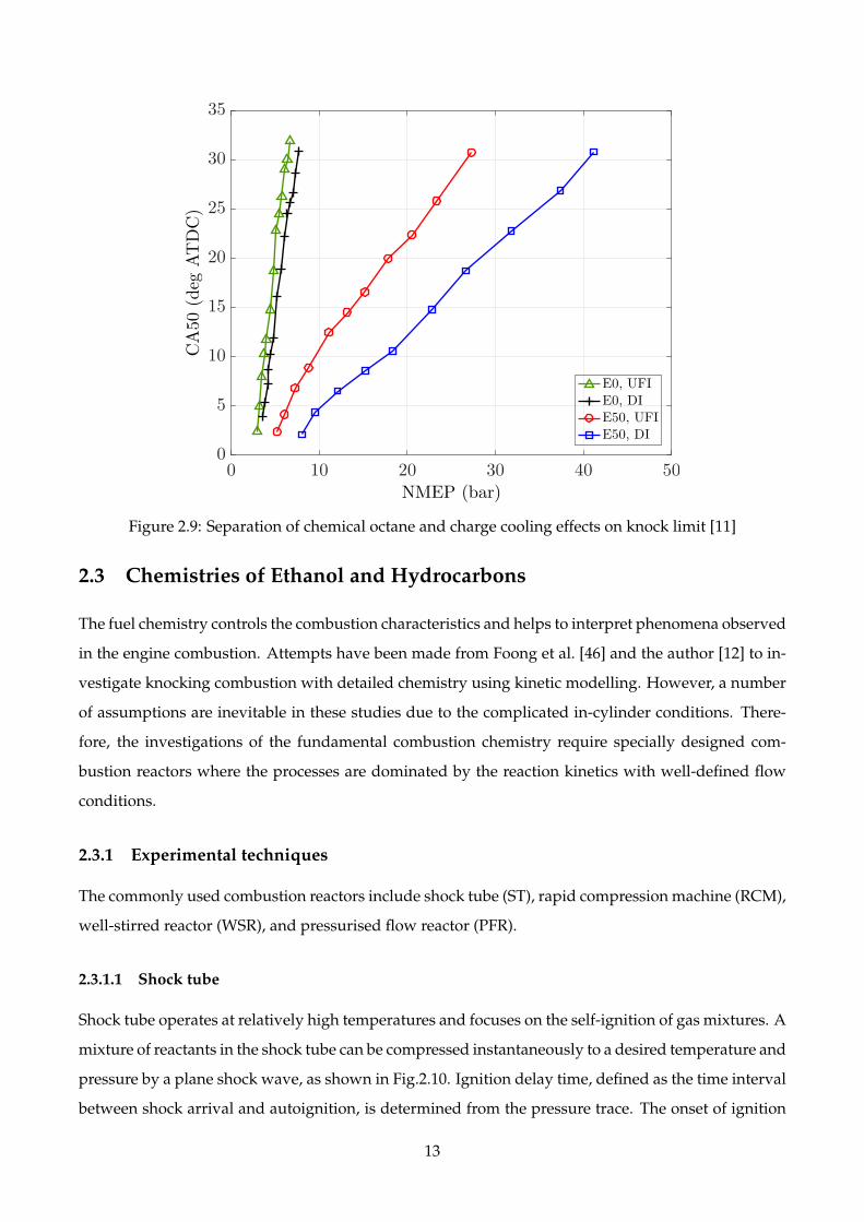
tify the charge cooling effect. Following this experimental study, the effective and evaporative oc-

tane numbers were proposed to represent the fuel’s anti-knock performances from the autoignition

chemistry and the charge cooling effect respectively [15]. Fig.2.8 shows that the charge cooling effect,

indicated by the difference between the overall and the effective octane numbers, exhibits a growing

trend with the increased ethanol content.

Another experimental study conducted by Stein et al. [11] compared the DI with the upstream fuel

injection (UFI) to quantify the charge cooling effect. As shown in Fig.2.9, the increase of the net mean

effective pressure (NMEP) from E0, UFI to E50, UFI results from the high octane number of E50 which

is essentially from chemical effect. Meanwhile, the increases from UFI to DI should be attributed to

the charge cooling effect which is, not surprisingly, more distinct for E50 than E0.

The explanation and quantification for the charge cooling effect of ethanol are relatively straight-

forward, and this phenomenon is well understood from the aforementioned experimental studies.

However, the combustion chemistry of the ethanol containing fuel mixtures is more complex and less

well known compared with the charge cooling effect. To have a better understanding of the autoigni-

tion chemistry, the chemical kinetics of ethanol and surrogate fuels should be thoroughly investigated.

11

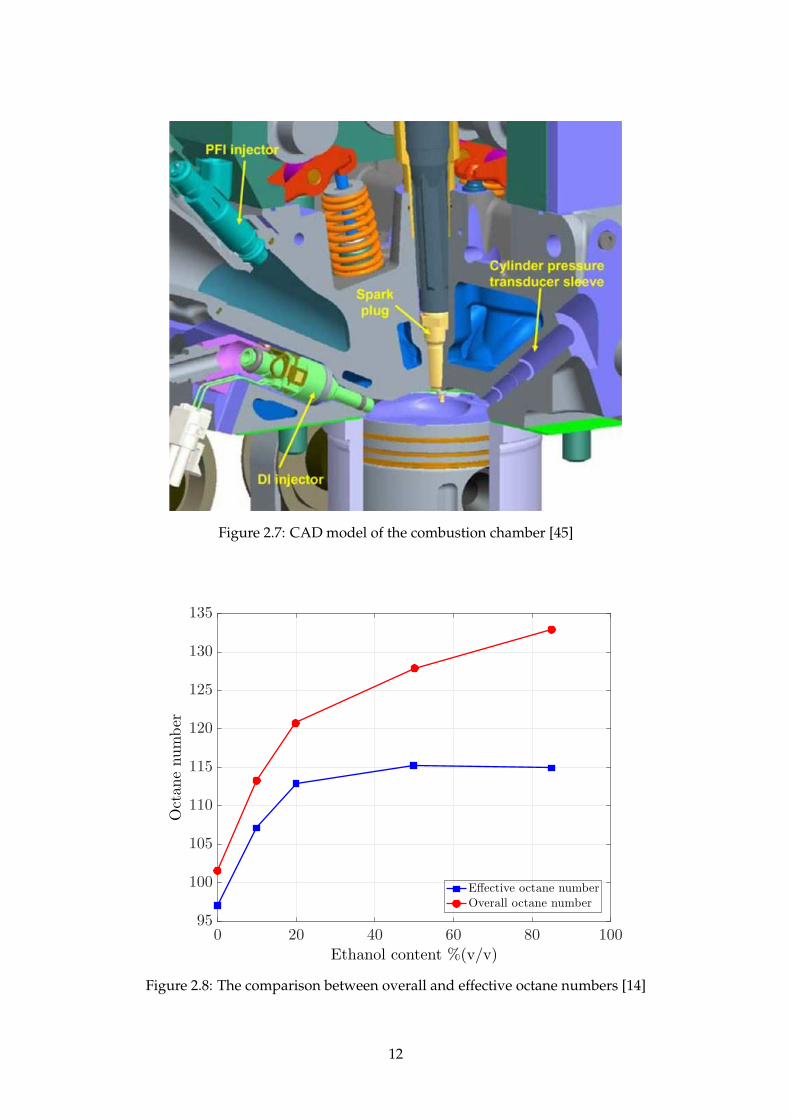
Figure 2.7: CAD model of the combustion chamber [45]

0 20 40 60 80 100


95

100

105

110

115

120

125

130

135

Octan

enumber

Effective octane numberOverall octane number

Figure 2.8: The comparison between overall and effective octane numbers [14]

12

0 10 20 30 40 50

NMEP (bar)

0

5

10

15

20

25

30

35

CA50

(deg

ATDC)

E0, UFIE0, DIE50, UFIE50, DI

Figure 2.9: Separation of chemical octane and charge cooling effects on knock limit [11]

2.3 Chemistries of Ethanol and Hydrocarbons

The fuel chemistry controls the combustion characteristics and helps to interpret phenomena observed

in the engine combustion. Attempts have been made from Foong et al. [46] and the author [12] to in-

vestigate knocking combustion with detailed chemistry using kinetic modelling. However, a number

of assumptions are inevitable in these studies due to the complicated in-cylinder conditions. There-

fore, the investigations of the fundamental combustion chemistry require specially designed com-

bustion reactors where the processes are dominated by the reaction kinetics with well-defined flow

conditions.

2.3.1 Experimental techniques

The commonly used combustion reactors include shock tube (ST), rapid compression machine (RCM),

well-stirred reactor (WSR), and pressurised flow reactor (PFR).

2.3.1.1 Shock tube

Shock tube operates at relatively high temperatures and focuses on the self-ignition of gas mixtures. A

mixture of reactants in the shock tube can be compressed instantaneously to a desired temperature and

pressure by a plane shock wave, as shown in Fig.2.10. Ignition delay time, defined as the time interval

between shock arrival and autoignition, is determined from the pressure trace. The onset of ignition

13

can be obtained from the emission/absorption spectra of intermediate combustion species. However,

the non-ideal conditions, i.e. the formation of boundary layers in reflected shock tube experiment,

limit the observation times to hundred of microseconds. Thus, experiment conditions are constrained

to pressure and temperature regimes with short chemical induction times.

Figure 2.10: Schematic of a shock tube/rapid compression machine

2.3.1.2 Rapid compression machine

With the similar schematic to the shock tube, the rapid compression machine is designed to emulate

the combustion process in reciprocating engines, which makes it a relatively complicated system. The

movement of a piston compresses premixed mixture in the combustion chamber to a small volume,

high pressure, and temperature, which initiates the ignition. The pressure and temperature histories

are controlled by the compression ratio, initial pressure and mixture composition. Similar to engines,

the physical phenomena inside the rapid compression machine are complicated. Unknown wall heat

transfer, blow-by due to piston crevices and large-scale disturbances of reacting mixture caused by

piston movement complicate the interpretation of the experimental results of the rapid compression

machine. Besides, it is challenging to use extractive sampling method to measure mixture composi-

tion. Normally, the data from rapid compression machine are modelled with a homogeneous reaction

condition and empirically determined heat loss function.

2.3.1.3 Well-stirred reactor

The well-stirred, or perfectly-stirred reactor is assumed to have entirely homogeneous mixing inside

the control volume, as shown in Fig.2.11 [47]. A common type of well stirred reactor is called jet-stirred

reactor which uses high velocity inlet jets to facilitate the mixing process.

An essential characteristics of the well-stirred reactor is the perfect mixing assumption which con-

siders the time required for the mixing is much shorter than the mean residence time of the fluid in the

reactor. However, the actual residence time in a WSR is less defined, which is supposed to follow a res-

idence time function, not a single value. This has to be assumed in the modelling. The WSR operates

with less dilution, short residence times, and higher temperatures. However, the non-ideal conditions

14

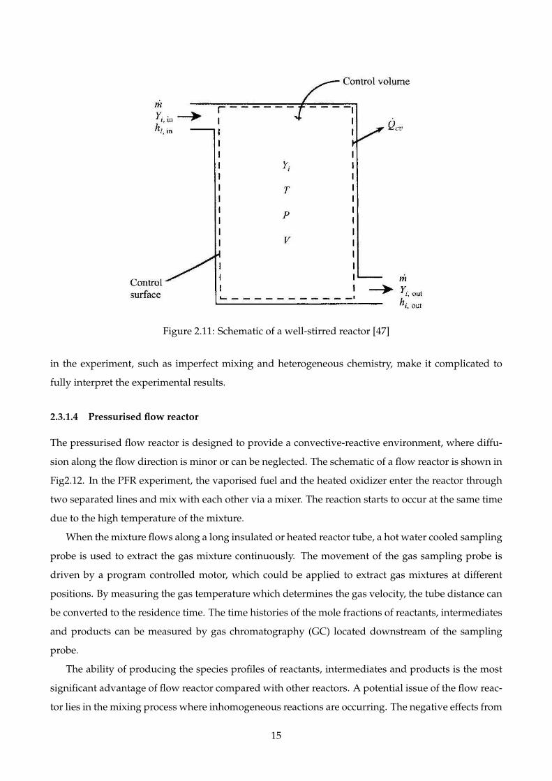
Figure 2.11: Schematic of a well-stirred reactor [47]

in the experiment, such as imperfect mixing and heterogeneous chemistry, make it complicated to

fully interpret the experimental results.

2.3.1.4 Pressurised flow reactor

The pressurised flow reactor is designed to provide a convective-reactive environment, where diffu-

sion along the flow direction is minor or can be neglected. The schematic of a flow reactor is shown in

Fig2.12. In the PFR experiment, the vaporised fuel and the heated oxidizer enter the reactor through

two separated lines and mix with each other via a mixer. The reaction starts to occur at the same time

due to the high temperature of the mixture.

When the mixture flows along a long insulated or heated reactor tube, a hot water cooled sampling

probe is used to extract the gas mixture continuously. The movement of the gas sampling probe is

driven by a program controlled motor, which could be applied to extract gas mixtures at different

positions. By measuring the gas temperature which determines the gas velocity, the tube distance can

be converted to the residence time. The time histories of the mole fractions of reactants, intermediates

and products can be measured by gas chromatography (GC) located downstream of the sampling

probe.

The ability of producing the species profiles of reactants, intermediates and products is the most

significant advantage of flow reactor compared with other reactors. A potential issue of the flow reac-

tor lies in the mixing process where inhomogeneous reactions are occurring. The negative effects from

15

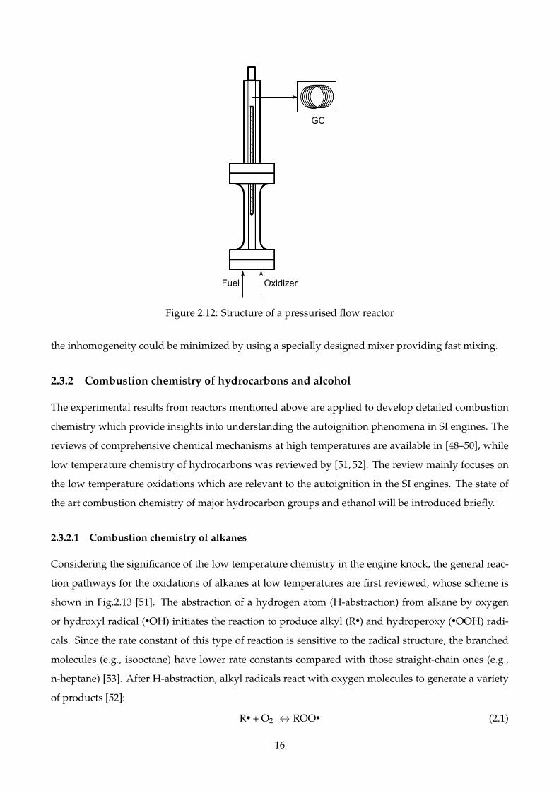
Figure 2.12: Structure of a pressurised flow reactor

the inhomogeneity could be minimized by using a specially designed mixer providing fast mixing.

2.3.2 Combustion chemistry of hydrocarbons and alcohol

The experimental results from reactors mentioned above are applied to develop detailed combustion

chemistry which provide insights into understanding the autoignition phenomena in SI engines. The

reviews of comprehensive chemical mechanisms at high temperatures are available in [48–50], while

low temperature chemistry of hydrocarbons was reviewed by [51, 52]. The review mainly focuses on

the low temperature oxidations which are relevant to the autoignition in the SI engines. The state of

the art combustion chemistry of major hydrocarbon groups and ethanol will be introduced briefly.

2.3.2.1 Combustion chemistry of alkanes

Considering the significance of the low temperature chemistry in the engine knock, the general reac-

tion pathways for the oxidations of alkanes at low temperatures are first reviewed, whose scheme is

shown in Fig.2.13 [51]. The abstraction of a hydrogen atom (H-abstraction) from alkane by oxygen

or hydroxyl radical (•OH) initiates the reaction to produce alkyl (R•) and hydroperoxy (•OOH) radi-

cals. Since the rate constant of this type of reaction is sensitive to the radical structure, the branched

molecules (e.g., isooctane) have lower rate constants compared with those straight-chain ones (e.g.,

n-heptane) [53]. After H-abstraction, alkyl radicals react with oxygen molecules to generate a variety

of products [52]:

(2.1)R• + O2 ↔ ROO•

16

(2.2)R• + O2 → alkene + HO2•

The products from R• + O2 reaction change with pressure and temperature. Typically, at low tempera-

ture and moderate pressures, alkyl peroxy radical (•ROO) is the primary product, as shown in reaction

2.1.

•QOOH

HO2

• + alkeneRH

ROOH + O2

degeneratebranching

RO• + •OH

steps

RH •OH + cyclic ethers,aldehydes or ketones

R•

keto-hydroperoxides + • OH

R’• + H2 O2 ROO•degeneratebranching

steps

•OOQOOH

•U(OOH)2

O2

XO• + •OH

O2

R’• + alkene

(2)(1)

HO2•

RH + O2 or • OH

O2

R’• + H2O

initiation steps

H abstractions

(3)

Figure 2.13: Simplified scheme for the primary mechanism of oxidation of alkanes at low temperatures[51]

The thermally unstable alkyl peroxy radical may undergo different reaction paths, which results

in the varied progresses of autoignition. Firstly, the alkyl peroxy radical can dissociate back to the

alkyl radical and oxygen molecule. If at the same time, the temperature increases to favour reac-

tion 2.2, the overall reaction rate will be reduced, which leads to the so-called negative temperature

coefficient (NTC) regime. Secondly, with the low energy threshold, the alkyl peroxy radical decom-

poses to alkene and hydroperoxy radical even at room temperatures [54], as shown in reaction 2.3.

Both theoretical [55] and experimental [56] studies showed that this type of reaction is significant

for hydroperoxy radical production. However, hydroperoxy radical is not reactive, which slows or

effectively terminates the low temperature reactions.

(2.3)ROO• → alkene + HO2•

(2.4)ROO• ↔ •QOOH

17

The most important reaction path for alkyl peroxy radical, which leads to chain-propagating re-

actions, is the isomerization via internal H-atom abstraction to form hydroperoxy alkyl (•QOOH)

radical, as shown in reaction 2.4. This type of reaction undergoes a cyclic transition state, whose ac-

tivation energies for isomerization comprising the activation energy for H-abstraction and the strain

energy of the cyclic transition state. In this case, both the ring strain energy barriers and the type of

abstracted H atom affect the rate constants of these reactions. Then, the unstable hydroperoxy alkyl

radical decomposes to cyclic ether and highly reactive hydroxyl radical (•OH).

The unpaired electron of the carbon atom of hydroperoxy alkyl radical is vulnerable to the attack

from oxygen molecule, as shown in reaction 2.5, which is quite similar to the reaction between alkyl

radical and oxygen molecule.

(2.5)•QOOH + O2 ↔ •OOQOOH

Afterwards, the •OOQOOH radical goes through a second internal H-abstractions, similar to

ROO•, and forms the •Q(OOH)2 radical. The decomposition of this radical gives hydroxyl radical,

which is a chain-branching reaction:

(2.6)•OOQOOH ↔ •Q(OOH)2 → ketohydroperoxides + •OH→ •OQO + 2•OH

Another chain-branching reaction pathway in Fig.2.13 related to reaction 2.7 and 2.8. However, the

alkyl hydroperoxide is relatively stable, especially at low temperatures, which results in slow chain

branching reactions and thus contributes little to the production of hydroxyl radicals.

(2.7)ROO• + HO2• → ROOH + O2

(2.8)ROOH → RO• + •OH

The low temperature combustion chemistry of the alkanes provides fundamentals for the devel-

opment of the state of the art chemical mechanisms for various hydrocarbons of interest to practical

fuels. Among all these hydrocarbons, isooctane, n-heptane and pentanes are considered as important

in the production gasoline, and their chemical mechanisms are critical in terms of understanding the

engine knock.

As a representative branched alkane, isooctane is widely used as a surrogate gasoline fuel for

engine combustion research. The most well known detailed combustion model of isooctane at both

low and high temperatures was developed by Curran et al. [57] based on the experimental results

from a jet-stirred reactor [58], flow reactors [59–61], shock tubes [62–64] and motored engines [65, 66],

which cover the pressure range from 1 atm to 45 atm and temperature from 550 K to 1700 K with

equivalence ratio from 0.3 to 1.5. The model shows good agreements when compared with different

experimental results. Then, a gasoline surrogate mechanism developed by Mehl et al. [67] speeds up

18

the low temperature oxidation processes with updated rate constants and thermal properties, which

produces better agreements to experiments in various operating conditions. A very recent update for

isooctane mechanism comes from Atef et al. [68], which is motivated by matching the experimental

results [69–73] causing problems for previous mechanisms. With the implementations of the recent

results from computational studies in isooctane thermochemistry [74–77], low temperature oxidation

kinetics of normal and branched alkanes [78–81], and new alternative isomerization pathways, the

latest isooctane mechanism produces improved agreements to the existing experiments, especially

those at lower equivalence ratios.

N-heptane is a representative fuel for normal alkane, whose combustion chemistry is relatively

well understood. Numerous experimental studies were performed in shock tubes [62, 82–86], rapid

compression machines [87–90], jet-stirred reactors [58, 91–94], flow reactors [60, 95–97], flame exper-

iments [98–106], and engines [107–111] to study the oxidations of n-heptane over a wide range of

conditions. A detailed combustion mechanism of n-heptane was proposed by Curran et al. [112],

which not only perform well when matching experimental data but also provides a kinetic frame for

the mechanism development. This mechanism was modified by Mehl et al. [67] to incorporate the

updated decomposition rates of the alkyl and alkoxy radicals [113], the isomerization rates at low

temperature oxidation recommended by [114], and the new reaction pathways from [115, 116]. The

most recent update [117] for the mechanism includes AramcoMech 2.0 [118] for the C0 −C4 species,

the latest chemistry for three pentan isomers [119–121], and the base n-heptane sub-smechanism [112].

Although isooctane and n-heptane are normally considered as surrogate gasoline fuels, their frac-

tions in the Australia production gasoline are much less than iso-pentane and n-pentane. Several

experimental studies were conducted to investigate the oxidations of pentane isomers in rapid com-

pression machines [120, 122–125], shock tubes [120, 126, 127], a well-stirred reactor [128], an annular

flow reactor [129], and a CFR engine [130]. The state of the art chemical mechanism of pentane isomers

was developed by Bugler et al. [120] and very recently updated based on experimental results from

two jet-stirred reactors [131].

The chemical mechanisms for most alkanes have been renewed in recent two years with constantly

emerging experimental, theoretical and modelling studies. However, alkanes alone are not sufficient

to emulate the production gasoline with a significant amount of aromatics as octane boosters.

2.3.2.2 Combustion chemistry of aromatics

As important components in petroleum-derived fuels, aromatics typically show much slower oxida-

tion rates than alkanes, particularly at low temperatures. Understanding the detailed chemical kinet-

ics of aromatics is necessary to interpret the combustion characteristics of the production gasoline.

19

Toluene, a representative hydrocarbon in the aromatics family, has been used as a surrogate gaso-

line fuel along with n-heptane and isooctane to emulate the production gasoline. The major reaction

pathways and the state of the art chemical mechanisms for toluene will be reviewed.

Fig.2.14 presents the main reaction pathways of toluene and benzene oxidations proposed by

Brezinsky [132]. As a very important product of toluene oxidation, benzene may form phenyl rad-

ical, phenol, and phenoxy radical after being attacked by those small and reactive radicals. Besides,

the former two products, phenyl radical and phenol, react with small radicals to produce phenoxy

radical which decomposes to CO and cyclopentadienyl radical. The free electron of cyclopentadienyl

radical may combine an H atom to form cyclopentadiene or reacts with those oxygenated radicals to

generate cyclopentadionyl radical which produces butadienyl radical and CO.

Figure 2.14: Simplified scheme for the oxidations of benzene and toluene [132]

Toluene oxidation mechanism can be found on the right part of Fig.2.14. At the beginning, toluene

reacts with small radicals to form benzyl radical, cresol, cresoxy radical and benzene. Benzyl radical is

most abundant product from the first step oxidation. Although benzyl radical is very stable, especially

at low temperatures, it has several reaction pathways at relatively high temperatures. The benzyl rad-

ical may combine with itself to generate bibenzyl and react with small radicals to form other stable

molecules, such as benzyl alcohol, ethylbenzene and benzaldehyde. Apart from the reaction pathways

proposed in [132], a C7H6 molecule was observed from the decomposition of benzyl radical by the re-

20

cent experiment study [133]. The C7H6 was later found to be fulvenallene [134] and the corresponding

rate constant was theoretically computed by da Silva et al. [135]. Another important reaction is be-

tween benzyl and hydroperoxy radicals which mainly generate benzoxyl and hydroxyl radicals above

700K, but below this temperature, the primary product becomes benzylhydroperoxide. These benzyl

radical involved reactions all lead to chain-termination. Unlike alkanes above, aromatics, especially

those without long chain, generally don’t have low temperature chemistry as the cyclic transition state

cannot be formed.

The experimental studies for toluene oxidations have been performed using flow reactors [136–

138], jet-stirred reactors [139, 140], shock tubes [141–145], rapid compression machines [146] and lam-

inar premix flames measurements [147–149]. To model these experimental results, several detailed

chemical mechanisms [137, 139, 145, 150–155] have been developed previously. The recent modelling

study was conducted by Metcalfe et al. [138], which combines toluene sub-mechanism from [140]

and C0 −C4 sub-mechanism from [156–159]. This toluene mechanism [138] was incorporated into

the latest n-butylbenzene model by Nakamura et al. [160] which contains C0 −C4 sub-mechanism

from AramcoMech 1.3 [161] and alkyl-aromatics sub-mechanism from [162]. More recently, Yuan et

al. [163,164] proposed a kinetic model for toluene based on their experiments performed in flow reac-

tor and jet stirred reactor.

2.3.2.3 Combustion chemistry of ethanol

Ethanol, as a renewable fuel and an octane booster, has been added to the production gasoline world

widely. The oxidations of ethanol were investigated using shock tubes [165–170], flow reactors [171–

174], jet-stirred reactors [175, 176], rapid compression machine [170] and laminar flames [177–180].

The most well known detailed ethanol mechanism was developed by Marinov [181] which had

been validated against all available experimental data at that time. Marinov’s mechanism was first

improved by Li et al. [172, 173, 182] to model ethanol pyrolysis and oxidation in a pressurised flow

reactor by including modified rate parameters for the decomposition reactions. Later, Dagaut and

Togbe [183] updated Marinov’s mechanism with the kinetic parameters from quantum chemical cal-

culations for H atom abstraction from ethanol molecule. The existing ethanol mechanism continues to

be improved by experiments in different reactors [175, 184].

As critical reaction pathways, the rate constants for the four ethanol decomposition reactions (2.9

to 2.12) have aroused great interests in the research community. Based on the experimental and theo-

retical studies carried out by Li et al., the rate constants for reaction 2.11 and 2.12 are much lower than

those of reaction 2.9 and 2.10. Besides, Li et al. also presented that reaction 2.9 is strongly dependent

on temperature and is dominant over the temperature range of 300-2500 K at 1 atm.

21

(2.9)C2H5OH ↔ C2H4 + H2O

(2.10)C2H5OH ↔ •CH3 + •CH2OH

(2.11)C2H5OH ↔ •CH2CH3 + •OH

(2.12)C2H5OH ↔ •C•HCH3 + H2O

The reactions between ethanol and hydroxyl radical generate different products (2.13 to 2.15)

whose relative fractions are determined by the branching ratios. The ratios applied by both Mari-

nov [181] and Li et al. [172, 173, 182] are from empirical approaches. While a more recent study per-

formed by Mittal et al. [184] adopted the rate constants from Sivaramaskrishnan et al. [185] and tuned

the branching ratios to match the experimental results.

(2.13)C2H5OH + •OH ↔ CH3•CHOH + H2O

(2.14)C2H5OH + •OH ↔ •CH2CH2OH + H2O

(2.15)C2H5OH + •OH ↔ CH3CH2O• + H2O

Understanding the chemical mechanisms of the neat compounds is the prerequisite to explain the

behaviours of production gasoline and gasoline surrogates over a wide range of conditions. However,

the interactions among different components in these mixtures do exist and may play a significant role

concerning affecting the overall performances. In this regard, there has been an increasing awareness

of the necessity to investigate the chemical interactions.

2.4 Chemical Interactions of Fuel Mixtures

Although the oxidation kinetics for neat fuel compounds is relatively well understood, it is often chal-

lenging to predict the autoignition of fuel mixtures due to chemical interactions. These interactions

are typically divided into two types: the first is via large fuel-like radicals, and the second is via small

radicals.

2.4.1 Interactions between alkanes

The cross reactions for alkane mixtures have been studied by Andrae et al. [152, 186]. In their earlier

publication [186], the cross reactions between fuel-like radicals were incorporated in the mechanism to

explain the experimental results that PRF84 ignites much earlier than toluene/n-heptane mixture with

similar RON in HCCI engine at high intake pressure and low intake temperature, since the ignition

delays of these fuel mixtures are similar at low intake pressure and high intake temperature. They

22

argued that with the added cross reactions, the PRF mixture would be more reactive than toluene/n-

heptane mixture before the NTC regime. While at low intake pressure and high intake temperature,

which is within the NTC regime, the reactivity of toluene/n-heptane mixture was less affected by

the NTC effects compared with PRFs. It seems that the addition of the cross reactions increases the

reactivity of PRF before the NTC regime and thus improves the predictions of autoignition delays in

HCCI engine.

However, in their later experimental study [152], the rate constants of the cross reactions have

been re-evaluated. When validating the TRF mechanism against the shock tube autoignition delays,

the rate constants of the cross reactions were too high, which lead to significantly shorter predicted

ignition times than the measurements below 1000 K. Besides, excluding those cross reactions had little

influence to the modelling results, which suggests that the cross reactions may not be significant in the

PRF autoignition. The studies from Andrae et al. [152, 186] showed that the cross reactions between

fuel-like radicals are not significant at least when predicting the autoignition delays from the shock

tube. However, the cross reactions related to the small radicals are supposed to be important, which

are more likely to occur and even affect the overall reactivity.

2.4.2 Interactions between PRF and toluene

The measured MONs of isooctane and toluene mixtures are plotted in Fig.2.15, which indicate the fuel

interactions do occur as the MON of 75% isooctane and 25% toluene is lower than those of both neat

compounds [187]. It is necessary to understand the fuel interactions before interpreting the complex

behaviours of fuel mixtures.

2.4.2.1 Cross reactions via large radicals

The chemical interactions between PRF and toluene have been studied when developing the com-

prehensive kinetic mechanism for surrogate fuels [67, 152, 186]. At high temperatures, numerous in-

termediates, like alkenes and benzyl radical, coexist at the beginning of oxidation and tend to react

with each other. The cross reactions between large fuel-like radicals are divided into three groups, as

proposed by [188].

The first type is H-abstraction reaction, which was incorporated by Andrae et al. [152,186] in their

kinetic mechanisms. In reaction 2.16, RH represents toluene, benzene and benzaldehyde, while QH

denotes n-heptane, isooctane, C3H6 and iC4H8. The rate constants of this type of reactions are from

the studies by Bounaceur et al. [140] and Da Costa et al. [189].

(2.16)RH + Q ↔ R + QH

23

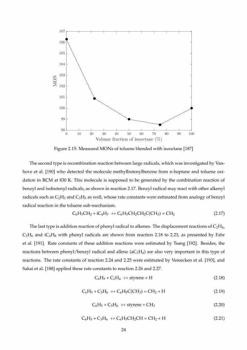
0 10 20 30 40 50 60 70 80 90 100

Volume fraction of isooctane (%)

98

99

100

101

102

103

104

105

106

107

MON

Figure 2.15: Measured MONs of toluene blended with isooctane [187]

The second type is recombination reaction between large radicals, which was investigated by Van-

hove et al. [190] who detected the molecule methylbutenylbenzne from n-heptane and toluene oxi-

dation in RCM at 830 K. This molecule is supposed to be generated by the combination reaction of

benzyl and isobutenyl radicals, as shown in reaction 2.17. Benzyl radical may react with other alkenyl

radicals such as C2H3 and C3H5 as well, whose rate constants were estimated from analogy of benzyl

radical reaction in the toluene sub-mechanism.

(2.17)C6H5CH2 + iC4H7 ↔ C6H5CH2CH2C(CH3) = CH2

The last type is addition reaction of phenyl radical to alkenes. The displacement reactions of C2H4,

C3H6 and iC4H8 with phenyl radicals are shown from reaction 2.18 to 2.23, as presented by Fahr

et al. [191]. Rate constants of these addition reactions were estimated by Tsang [192]. Besides, the

reactions between phenyl/benzyl radical and allene (aC3H4) are also very important in this type of

reactions. The rate constants of reaction 2.24 and 2.25 were estimated by Vereecken et al. [193], and

Sakai et al. [188] applied these rate constants to reaction 2.26 and 2.27.

(2.18)C6H5 + C2H4 ↔ styrene + H

(2.19)C6H5 + C3H6 ↔ C6H5C(CH3) = CH2 + H

(2.20)C6H5 + C3H6 ↔ styrene + CH3

(2.21)C6H5 + C3H6 ↔ C6H5CH2CH = CH2 + H

24

(2.22)C6H5 + iC4H8 ↔ C6H5C(CH3) = CH2 + CH3

(2.23)C6H5 + iC4H8 ↔ C6H5CH2C(CH3) = CH2 + H

(2.24)C6H5 + aC3H4 ↔ C6H5CH2 + C2H2

(2.25)C6H5 + aC3H4 ↔ C9H8 + H

(2.26)C6H5CH2 + aC3H4 ↔ C6H5CH2CH2 + C2H2

(2.27)C6H5CH2 + aC3H4 ↔ C10H10 + H

Although the fuel interactions on the large radical level have been observed in multiple studies,

their impacts on the fuel mixture performances could be limited as the associated elementary reactions

normally have very small rate constants. Note that the chemical interactions related to parent fuels

and parent fuel-like radicals were incorporated in the gasoline surrogate mechanisms developed by

Mehl et al. [67] and Andrae [187] respectively.

2.4.2.2 Cross reactions via radical pool

According to Vanhove et al. [193] and Andrae et al. [152], the cross reactions via radical pool may have

greater significance than those between large molecules and/or radicals. The ignition delays of neat

isooctane and isooctane/toluene mixtures are shown in Fig.2.16. Both the cool flame and the main

ignition delay times increase when toluene is added. Besides, the autoignition delay times of fuel

mixture decreases sharply above 830 K, suggesting the promoting effect of toluene on the reactivity

at high temperatures. The interactions between toluene and isooctane are of great significance com-

pared with those between toluene and n-heptane because both aromatics and iso-paraffins account

for significant fractions of gasoline. Based on the species analysis, Vanhove et al. [190] concluded that

toluene is unlikely to change the reaction pathways of isooctane oxidation, but may react with active

radicals from isooctane and produce stable benzyl radical to deactivate the reaction pool.

The investigation of fuel interactions via the radical pool is challenging, as it requires rigorous

species analysis to interpret how the elementary reactions related to the radical pool affect the mix-

ture’s performance. To predict the fuel mixture behaviours over a wide range of conditions, more

fundamental experimental and computational studies are required to provide accurate rate constants

and species profiles to better calibrate the existing chemical mechanisms.

25

isooctane/toluene

isooctane

isooctane/toluene

isooctane

Figure 2.16: Comparisons of cool flame (open symbols) and autoignition delay times (filled symbols)of neat isooctane and isooctane/toluene mixture [190]

26

2.4.3 Interactions between ethanol and hydrocarbons

The interactions between ethanol and hydrocarbons are known to be significant in the SI engines from

the experimental study performed by Foong et al. [9]. Meanwhile, several kinetic experimental studies

[86, 183, 194–198] were conducted to investigate the interactions between alcohols and hydrocarbons.

All these studies focused on the radical pool level competitions between alcohols and hydrocarbons.

Ethanol and n-heptane have very different reactivities, and their competition for small radicals

have been recently investigated by many groups. At low temperatures, both ethanol and n-heptane

undergo H abstraction to generate α-hydroxyethyl and heptyl respectively. The calculation from da

Silva et al. [199] suggested that, due to the influence of the OH group, the reaction of α-hydroxyethyl

and oxygen molecule proceeds almost exclusively to acetaldehyde and hydroperoxyl radical. As the

dominant product from H abstraction, α-hydroxyethyl prohibits ethanol’s chain-branching reaction,

which results in less OH radicals. At the beginning of the oxidation, n-heptane produces much more

OH radicals than ethanol. Later, the two fuels compete for the limited OH radicals at the same time.

Consequently, the consumption of n-heptane is decreased during this stage due to less OH radicals

available comparing with neat n-heptane oxidation; while ethanol gets relatively more OH radicals

and is consumed more rapidly than neat ethanol oxidation. After NTC regime, the decomposition of

hydrogen peroxide produces a significant amount of OH radicals consuming remaining fuels. Gener-

ally, for ethanol/hydrocarbon mixtures, ethanol acts as OH radical scavenger and therefore suppresses

the overall oxidation process. As two common alcohol compounds, ethanol and n-butanol have dif-

ferent lengths of the carbon chain. According to HCCI engine experiment by Saisirirat et al. [196],

both ethanol and n-butanol retard the start of combustion, but ethanol has a more pronounced effect

regarding suppressing combustion.

The oxidations of ethanol/gasoline surrogates were carried out by Dagaut and Togbe [183] and

Cancino et al. [200]. The kinetic models proposed by both groups can reproduce the experimental

results from the jet-stirred reactor and shock tube respectively. The chemical interactions involved in

these studies are still at the radical pool level.

Although the studies above all successfully reproduced their own experimental results by the

blended mechanisms, these kinetic models haven’t been validated for the complex fuel mixtures con-

taining practical gasoline surrogates and ethanol. Further experimental and modelling studies fo-

cusing on the oxidations of ethanol and hydrocarbon mixtures are necessary to understand the fuel

interactions.

27

2.5 Summary and research questions

As an abnormal combustion phenomenon in the engine, knock is a consequence of end gas autoigni-

tion. To suppress knock, ethanol is often added to production gasoline as an octane enhancer. Nu-

merous experimental studies show that ethanol increases both RON and MON of gasoline, and thus

improves anti-knock performance. However, the interactions between ethanol and production gaso-

line in the CFR engine are complicated. Foong et al . [9] carried out the initial experimental study

to understand the complex interactions. They formulated three TRF-based gasoline surrogates with

different amounts of toluene added to emulate the blending behaviours between ethanol and the

production gasoline. The results showed that the TRF-based gasoline surrogates blend more synergis-

tically with ethanol compared with the production gasoline at a similar RON and aromatic content..

Therefore, more engine tests are required to fully understand the interactions between ethanol and

the production gasoline.

Ethanol’s anti-knock behaviour has been extensively investigated mainly from two aspects: charge

cooling effect and chemical kinetics. The high latent heat of vaporisation of ethanol improves the

charge cooling effect which increases the knock onset limits and thus the engine efficiency. The chem-

ical effect of ethanol needs to be further clarified, especially when interacting with hydrocarbon fuels.

Although the interactions among larger species have been incorporated into the widely used gasoline

surrogate mechanisms developed by Mehl et al. [67] and Andrae [187], their impacts on the overall be-

haviours of fuel mixtures might not be significant due to the small rate constants of these elementary

reactions. Therefore, fuel interactions are expected to be more likely to occur with the involvement of

small reactive radicals. To predict the fuel interaction, the kinetic model should therefore have accu-

rate rate constants for these reactions involving small radicals, and more kinetic experiments for the

fuel mixtures are needed to calibrate the existing models.

This study, therefore, aims to investigate the fuel interactions in a CFR engine and combustion

chemistry of ethanol containing gasoline surrogates in a PFR. The following research questions are

proposed.

1. How should the non-linear octane blending of ethanol and toluene reference fuels (TRFs) be

represented?

Ethanol is known to blend non-linearly with surrogate fuels under standard knocking conditions

in the CFR engine [9]. This study proposes a statistical model to quantify these non-linearities

and predict the octane numbers of fuel mixtures containing ethanol and TRFs.

2. What is the gasoline surrogate that best emulates the anti-knock behaviours of production

gasoline when blended with ethanol?

28

As shown in the prior standard octane number test [9], ethanol blends more synergistically with

the TRF-based gasoline surrogates than with gasoline, suggesting that TRFs are not good enough

to emulate gasoline. Besides, the octane number blending behaviours between ethanol and the

hydrocarbon fuels other than TRF components are not known. Therefore, this study formu-

lates new gasoline surrogates to better emulate the knocking behaviours of the gasoline when

blended with ethanol.

3. How does ethanol interact with gasoline surrogates under engine representative conditions in

the PFR, and do existing mechanisms reproduce the measured species profiles?

Numerous kinetic experiments have been carried out by different groups to study the combus-

tion chemistry for neat fuels and fuel mixtures. However, no systematic experimental study has

been carried out to investigate how ethanol interacts with surrogate fuels and more importantly,

gasoline surrogates in flow reactors. Also, state of the art gasoline surrogate mechanisms haven’t

been fully calibrated to predict the behaviours of the fuel mixtures containing ethanol and gaso-

line surrogates. Therefore, this study performs PFR experiments to study the impacts of ethanol

on the reactivities of gasoline surrogates and validates the state of the art chemical mechanisms

using these measurements.

29

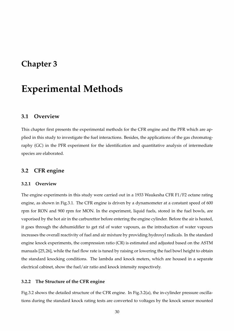
Chapter 3

Experimental Methods

3.1 Overview

This chapter first presents the experimental methods for the CFR engine and the PFR which are ap-

plied in this study to investigate the fuel interactions. Besides, the applications of the gas chromatog-

raphy (GC) in the PFR experiment for the identification and quantitative analysis of intermediate

species are elaborated.

3.2 CFR engine

3.2.1 Overview

The engine experiments in this study were carried out in a 1933 Waukesha CFR F1/F2 octane rating

engine, as shown in Fig.3.1. The CFR engine is driven by a dynamometer at a constant speed of 600

rpm for RON and 900 rpm for MON. In the experiment, liquid fuels, stored in the fuel bowls, are

vaporised by the hot air in the carburettor before entering the engine cylinder. Before the air is heated,

it goes through the dehumidifier to get rid of water vapours, as the introduction of water vapours

increases the overall reactivity of fuel and air mixture by providing hydroxyl radicals. In the standard

engine knock experiments, the compression ratio (CR) is estimated and adjusted based on the ASTM

manuals [25,26], while the fuel flow rate is tuned by raising or lowering the fuel bowl height to obtain

the standard knocking conditions. The lambda and knock meters, which are housed in a separate

electrical cabinet, show the fuel/air ratio and knock intensity respectively.

3.2.2 The Structure of the CFR engine

Fig.3.2 shows the detailed structure of the CFR engine. In Fig.3.2(a), the in-cylinder pressure oscilla-

tions during the standard knock rating tests are converted to voltages by the knock sensor mounted

30

Figure 3.1: The system of the CFR engine

on the top of the cylinder, and the dial indicator is applied to adjust the compression ratios specified

in [25, 26]. The condenser on the right upper part of the engine body uses the pressurised tap water

to dissipate heat away from the coolant flowing in the engine jacket. The CFR engine body is shown

in Fig.3.2(b), (c) and (d) from three different views with all auxiliary parts removed. The cylinder

inlet and outlet locate on the left and right side of the engine body respectively. The condenser inlet,

sitting on the right upper corner of the exhaust side, guides the engine coolant to the condenser and

get cooled.

Before starting the standard octane number measurements in this study, the CFR engine went

through a top overhaul to clean deposits on the cylinder wall and piston head. The comparison of

piston head before and after deposits cleaning is shown in Fig.3.3. The deposits act as an insulation

layer reducing the overall heat loss from the gas mixtures to the cylinder wall and piston head, which

makes test fuels more prone to knock and thus results in a lower octane number. In this study, all

knock rating tests are carried out right after the top overhaul when the CFR engine is in the good

condition.

31

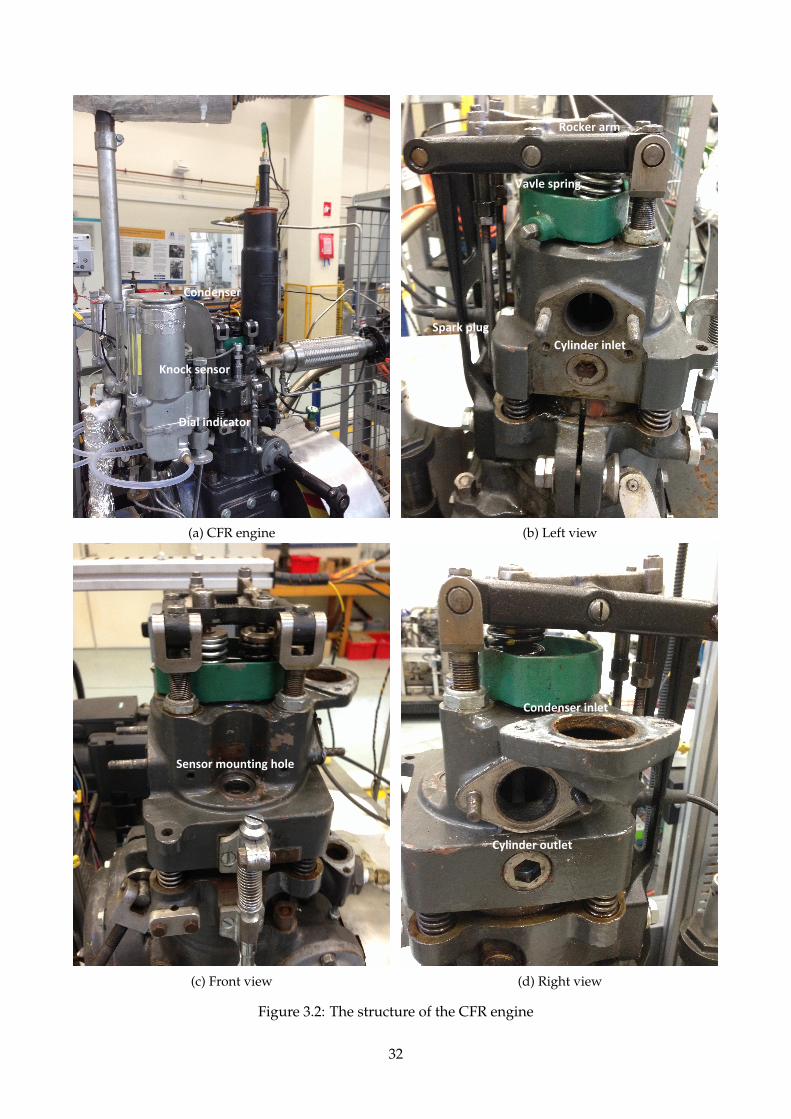
(a) CFR engine (b) Left view

(c) Front view (d) Right view

Figure 3.2: The structure of the CFR engine

32

(a) (b)

Figure 3.3: The piston head (a) before and (b) after overhaul

3.2.3 Methods for standard octane number tests

The CFR engine test methods for the standard RON and MON have been specified in [25] and [26]

respectively, and their test conditions are listed in Table 3.1. Both methods determine the octane num-

bers of the sample fuel by comparing its standard knock intensity with those of two PRFs whose

octane numbers are known by definition. To obtain the standard knock intensity for the sample fuel

during the knock rating tests, the cylinder height representing the compression ratio needs to be first

estimated and gradually tuned based on the [25, 26]. Although it is desirable to measure both RON

and MON of the sample fuels to have comprehensive understandings of their knocking behaviours,

the measurements conducted in this study are mostly for RON, since MON is not as important as

RON in modern engines, especially under high loads.

To ensure the engine’s compliance with the ASTM standards [25, 26], the so-called ’Fit-for-Use’

tests were conducted using the toluene standardisation fuels with known octane numbers. If the dif-

ference between the known and measured octane numbers is within the allowed tolerance, the engine

is considered fit for knock ratings in a certain octane number range. Note that the PRFs are not capable

of rating any sample fuels with RON larger than 100, and different amounts of the dilute tetraethyl

lead (TEL) are blended into isooctane as bracket fuels for RON tests above 100. The compositions of

the dilute TEL are listed in Table 3.2.

33

Table 3.1: Operating conditions for the RON and MON measurements [25, 26]

Operating parameters RON MON

Engine speed 600±6 rpm 900±9 rpm

Intake air temperature 52±1.0 °Ca 38±2.8 °C

Mixture intake temperaturea N/A 149±1.0 °C

Intake air pressure Barometric Barometric

Intake air humidity 25-50g H2O/kg dry air 25-50g H2O/kg dry air

Coolant temperature 100±1.5 °C 100±1.5 °C

Oil pressure 172-207 kPa(g) 172-207 kPa(g)

Oil temperature 57±8.0 °C 57±8.0 °C

Spark timing 13 °BTDC 14-26 °BTDCc

a varied with barometric pressureb temperature measured right before engine inletc varied with the compression ratio

Table 3.2: The composition of the dilute TEL [25, 26]

Component TEL Ethylene dibromide Xylene N-heptane Other

Mass fraction (%) 18.2 10.6 52.5 17.8 0.9

3.3 Pressurised flow reactor

3.3.1 Overview

The schematic drawing of the PFR system is shown in Fig.3.4. The air comes from an oil-free com-

pressor and goes into the flow reactor after heated to a specified temperature. The air flow rate is

controlled by a needle valve and measured by a flow meter. A balanced air stream goes to the gap be-

tween reaction tube and wall heater to equalise pressures inside and outside of the reaction tube. The

nitrogen is divided into two streams: one is to pressurise liquid fuel out of the cylindrical tank, and

another one is used to vaporise the pressurised liquid fuel. These two lines, together with the subse-

quently merged line are all wrapped with tube heaters to ensure that the liquid fuel is fully vaporised

before entering the flow reactor. A strain gauge is used to measure the fuel tank weight to derive the

fuel flow rate which is confirmed by the Coriolis flow meter. The gas mixture in the flow reactor is

collected by a sampling probe and analysed by a Gas Chromatography, and the remaining mixture

is purged into the exhaust system. The reactor pressure is controlled by a back-pressure valve. More

detailed information are available in [201].

Although the reactor is designed to run at 50 bar and 1000 K, low pressure of 10 bar is used in this

34

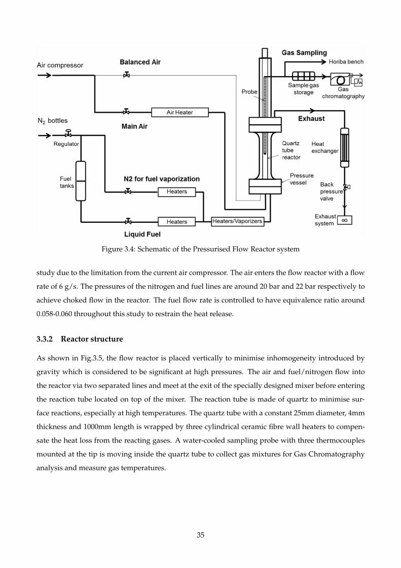
Figure 3.4: Schematic of the Pressurised Flow Reactor system

study due to the limitation from the current air compressor. The air enters the flow reactor with a flow

rate of 6 g/s. The pressures of the nitrogen and fuel lines are around 20 bar and 22 bar respectively to

achieve choked flow in the reactor. The fuel flow rate is controlled to have equivalence ratio around

0.058-0.060 throughout this study to restrain the heat release.

3.3.2 Reactor structure

As shown in Fig.3.5, the flow reactor is placed vertically to minimise inhomogeneity introduced by

gravity which is considered to be significant at high pressures. The air and fuel/nitrogen flow into

the reactor via two separated lines and meet at the exit of the specially designed mixer before entering

the reaction tube located on top of the mixer. The reaction tube is made of quartz to minimise sur-

face reactions, especially at high temperatures. The quartz tube with a constant 25mm diameter, 4mm

thickness and 1000mm length is wrapped by three cylindrical ceramic fibre wall heaters to compen-

sate the heat loss from the reacting gases. A water-cooled sampling probe with three thermocouples

mounted at the tip is moving inside the quartz tube to collect gas mixtures for Gas Chromatography

analysis and measure gas temperatures.

35

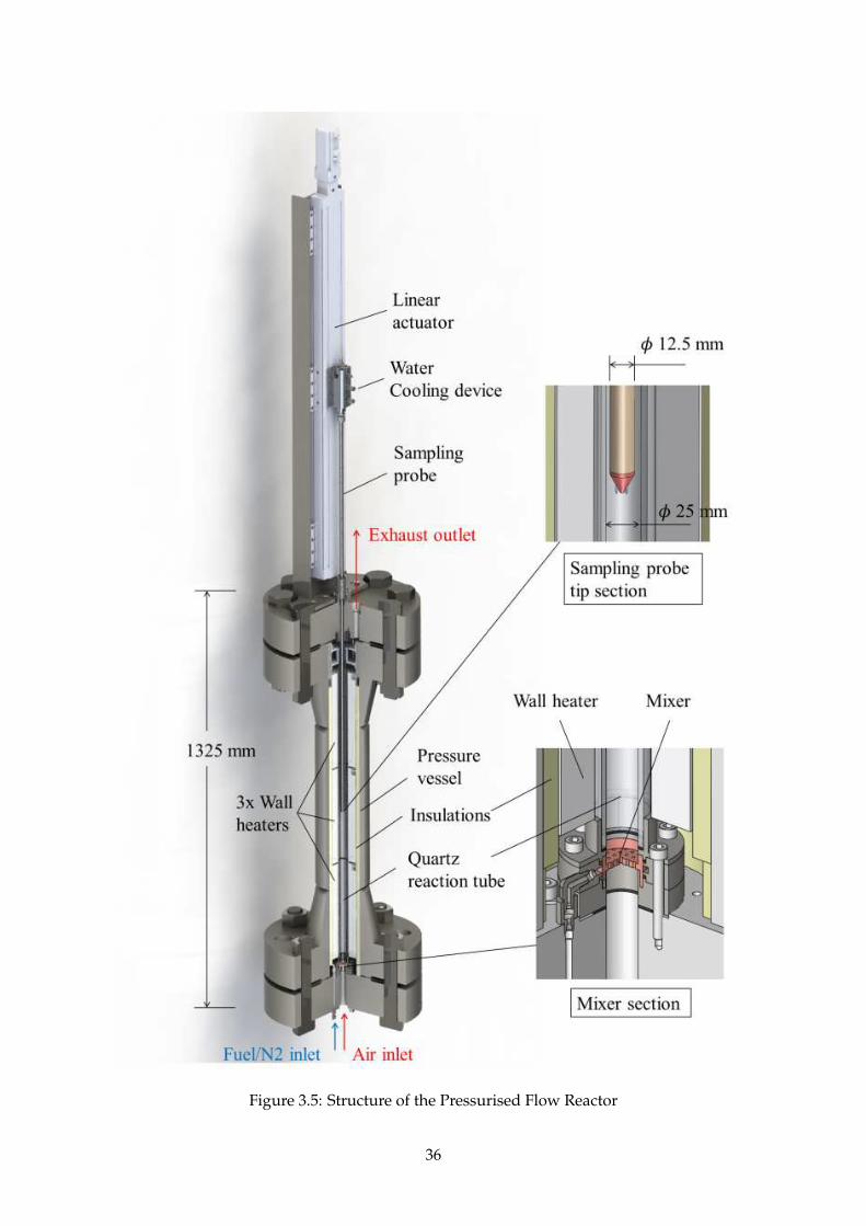
Figure 3.5: Structure of the Pressurised Flow Reactor

36

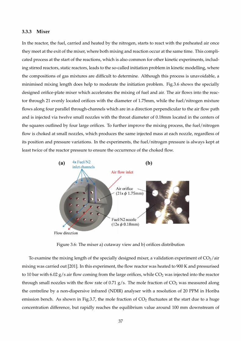
3.3.3 Mixer

In the reactor, the fuel, carried and heated by the nitrogen, starts to react with the preheated air once

they meet at the exit of the mixer, where both mixing and reaction occur at the same time. This compli-

cated process at the start of the reactions, which is also common for other kinetic experiments, includ-

ing stirred reactors, static reactors, leads to the so-called initiation problem in kinetic modelling, where

the compositions of gas mixtures are difficult to determine. Although this process is unavoidable, a

minimised mixing length does help to moderate the initiation problem. Fig.3.6 shows the specially

designed orifice-plate mixer which accelerates the mixing of fuel and air. The air flows into the reac-

tor through 21 evenly located orifices with the diameter of 1.75mm, while the fuel/nitrogen mixture

flows along four parallel through-channels which are in a direction perpendicular to the air flow path

and is injected via twelve small nozzles with the throat diameter of 0.18mm located in the centers of

the squares outlined by four large orifices. To further improve the mixing process, the fuel/nitrogen

flow is choked at small nozzles, which produces the same injected mass at each nozzle, regardless of

its position and pressure variations. In the experiments, the fuel/nitrogen pressure is always kept at

least twice of the reactor pressure to ensure the occurrence of the choked flow.

Figure 3.6: The mixer a) cutaway view and b) orifices distribution

To examine the mixing length of the specially designed mixer, a validation experiment of CO2/air

mixing was carried out [201]. In this experiment, the flow reactor was heated to 900 K and pressurised

to 10 bar with 6.02 g/s air flow coming from the large orifices, while CO2 was injected into the reactor

through small nozzles with the flow rate of 0.71 g/s. The mole fraction of CO2 was measured along

the centreline by a non-dispersive infrared (NDIR) analyser with a resolution of 20 PPM in Horiba

emission bench. As shown in Fig.3.7, the mole fraction of CO2 fluctuates at the start due to a huge

concentration difference, but rapidly reaches the equilibrium value around 100 mm downstream of

37

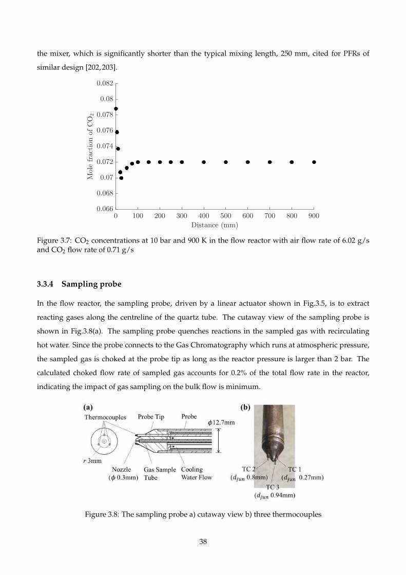
the mixer, which is significantly shorter than the typical mixing length, 250 mm, cited for PFRs of

similar design [202, 203].

0 100 200 300 400 500 600 700 800 900

Distance (mm)

0.066

0.068

0.07

0.072

0.074

0.076

0.078

0.08

0.082Mole

fractionofCO

2

Figure 3.7: CO2 concentrations at 10 bar and 900 K in the flow reactor with air flow rate of 6.02 g/sand CO2 flow rate of 0.71 g/s

3.3.4 Sampling probe

In the flow reactor, the sampling probe, driven by a linear actuator shown in Fig.3.5, is to extract

reacting gases along the centreline of the quartz tube. The cutaway view of the sampling probe is

shown in Fig.3.8(a). The sampling probe quenches reactions in the sampled gas with recirculating

hot water. Since the probe connects to the Gas Chromatography which runs at atmospheric pressure,

the sampled gas is choked at the probe tip as long as the reactor pressure is larger than 2 bar. The

calculated choked flow rate of sampled gas accounts for 0.2% of the total flow rate in the reactor,

indicating the impact of gas sampling on the bulk flow is minimum.

Figure 3.8: The sampling probe a) cutaway view b) three thermocouples

38

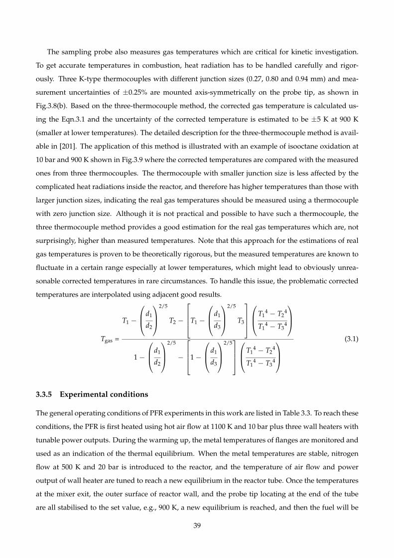
The sampling probe also measures gas temperatures which are critical for kinetic investigation.

To get accurate temperatures in combustion, heat radiation has to be handled carefully and rigor-

ously. Three K-type thermocouples with different junction sizes (0.27, 0.80 and 0.94 mm) and mea-

surement uncertainties of ±0.25% are mounted axis-symmetrically on the probe tip, as shown in

Fig.3.8(b). Based on the three-thermocouple method, the corrected gas temperature is calculated us-

ing the Eqn.3.1 and the uncertainty of the corrected temperature is estimated to be ±5 K at 900 K

(smaller at lower temperatures). The detailed description for the three-thermocouple method is avail-

able in [201]. The application of this method is illustrated with an example of isooctane oxidation at

10 bar and 900 K shown in Fig.3.9 where the corrected temperatures are compared with the measured

ones from three thermocouples. The thermocouple with smaller junction size is less affected by the

complicated heat radiations inside the reactor, and therefore has higher temperatures than those with

larger junction sizes, indicating the real gas temperatures should be measured using a thermocouple

with zero junction size. Although it is not practical and possible to have such a thermocouple, the

three thermocouple method provides a good estimation for the real gas temperatures which are, not

surprisingly, higher than measured temperatures. Note that this approach for the estimations of real

gas temperatures is proven to be theoretically rigorous, but the measured temperatures are known to

fluctuate in a certain range especially at lower temperatures, which might lead to obviously unrea-

sonable corrected temperatures in rare circumstances. To handle this issue, the problematic corrected

temperatures are interpolated using adjacent good results.

(3.1)Tgas =

T1 −

d1

d2

2/5

T2 −

T1 −

d1

d3

2/5

T3

T1

4 − T24

T14 − T3

4

1−

d1

d2

2/5

−

1−

d1

d3

2/5

T1

4 − T24

T14 − T3

4

3.3.5 Experimental conditions

The general operating conditions of PFR experiments in this work are listed in Table 3.3. To reach these

conditions, the PFR is first heated using hot air flow at 1100 K and 10 bar plus three wall heaters with

tunable power outputs. During the warming up, the metal temperatures of flanges are monitored and

used as an indication of the thermal equilibrium. When the metal temperatures are stable, nitrogen

flow at 500 K and 20 bar is introduced to the reactor, and the temperature of air flow and power

output of wall heater are tuned to reach a new equilibrium in the reactor tube. Once the temperatures

at the mixer exit, the outer surface of reactor wall, and the probe tip locating at the end of the tube

are all stabilised to the set value, e.g., 900 K, a new equilibrium is reached, and then the fuel will be

39

0 100 200 300 400 500 600 700 800 900 1000

Distance (mm)

820

840

860

880

900

920

940

960

Tem

perature

(K)

T1 with junction size of 0.27mmT2 with junction size of 0.80mmT3 with junction size of 0.94mmCorrected Temperature

Figure 3.9: Reactor temperature profiles for isooctane oxidation at 10 bar and 900 K with equivalenceratio of 0.058

injected into hot nitrogen flow at a slightly higher pressure around 23 bar. The fuel rate is measured

by the strain gauge and the Coriolis flow meter. The difference between these two measurements are

generally below 5%.

Table 3.3: Experimental conditions for the PFR study

PFR parameter Set value

Reactor pressure (bar) 10

Reactor nominal temperature (K) 900-930

Equivalence ratio 0.058-0.060

Air flow rate (g/s) 6

Nitrogen flow rate (g/s) 0.32

Reynolds number in the reactor tube 8000

Fuel/nitrogen pressure (bar) 20-21

Fuel/nitrogen temperature (K) 500

40

3.4 Gas chromatography

3.4.1 Overview of the gas chromatography

The reacting gases collected by the sampling probe go to the gas loops of the GC for quantitative

species analysis. Fig.3.10 shows the picture of GC used in this study, which contains GC itself and

an auxiliary sampling system installed on the left plate. The inlet and outlet of the sampling system

locate on top of the insulation container which accommodates rotator 94 and 93. On the upper left

of the container locates a manual controller for rotator 92 which connects ten sampling loops and is

placed in another insulation container mounted on the back of the plate (not shown in Fig.3.10). Each

rotator has a motor to drive it, and the motor for rotator 92 is installed on the lower middle part of

the front, while the other two motors for rotator 94 and 93 are attached on the back. The positions of

these rotators are shown on the indicators and controller. Besides the loop based sampling system,

two injectors are installed on the top of the GC for the typical manual injections.

Figure 3.10: Gas Chromatography-2010ATF plus from Shimadzu

The connection between the GC and the aforementioned auxiliary system is shown in Fig.3.11.

During the PFR experiments, gas samples are introduced into the GC via a sampling loop system,

which involves two working modes: sampling and analysis. In the sampling process, the rotator 94

stays in the current position, specified as position A, which guides the gas sample flow from point 1 to

6, and then to the inlet of the rotator 92. As shown in Fig.3.11, the rotator 92 has both inner and outer

41

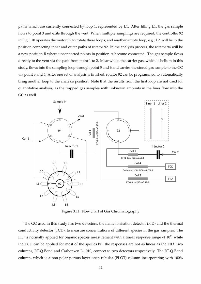
paths which are currently connected by loop 1, represented by L1. After filling L1, the gas sample

flows to point 3 and exits through the vent. When multiple samplings are required, the controller 92

in Fig.3.10 operates the motor 92 to rotate these loops, and another empty loop, e.g., L2, will be in the

position connecting inner and outer paths of rotator 92. In the analysis process, the rotator 94 will be

a new position B where unconnected points in position A become connected. The gas sample flows

directly to the vent via the path from point 1 to 2. Meanwhile, the carrier gas, which is helium in this

study, flows into the sampling loop through point 5 and 6 and carries the stored gas sample to the GC

via point 3 and 4. After one set of analysis is finished, rotator 92 can be programmed to automatically

bring another loop to the analysis position. Note that the results from the first loop are not used for

quantitative analysis, as the trapped gas samples with unknown amounts in the lines flow into the

GC as well.

Figure 3.11: Flow chart of Gas Chromatography

The GC used in this study has two detectors, the flame ionisation detector (FID) and the thermal

conductivity detector (TCD), to measure concentrations of different species in the gas samples. The

FID is normally applied for organic species measurement with a linear response range of 107, while

the TCD can be applied for most of the species but the responses are not as linear as the FID. Two

columns, RT-Q-Bond and Carbonxen L-1010, connect to two detectors respectively. The RT-Q-Bond

column, which is a non-polar porous layer open tubular (PLOT) column incorporating with 100%

42

divinylbenzene, performs excellently in term of separating hydrocarbons up to C12 and works fine

for oxygenated compounds. The other column, Carbonxen L-1010, is ideal for separating small com-

pounds, such as nitrogen, oxygen, carbon monoxide, carbon dioxide and light hydrocarbons up to C3.

In this study, only the FID was used for quantifying the compositions of the sampled reacting gases.

Although the FID cannot detect inorganic compounds, the NDIR analyser with a resolution of 20 PPM

in the Horiba emission bench was applied for CO and CO2 measurements. The reason for not using

the TCD was due to the excessive amounts oxygen and nitrogen in the sampled gases. Their large

concentrations produce huge peaks with long tails which affect the detection of other species with

small amounts.

Although the PFR experiments only necessitate the sampling loop system in quantitative analysis,

the GC has been equipped with two injectors containing different liners for calibration purpose, as

shown in Fig.3.11. The Injector 1, which contains Liner 1 with small volume, is essentially applied

as a pathway to the Col 1 for the gas samples coming from the sampling loop system, while the

Liner 2 with a large volume of 0.83 ml has been installed in Injector 2 is commonly used for manual

injections whose results are applied for the calibrations of loop volumes and concentrations of large

intermediates.

3.4.2 Identification and quantification of species

The most significant advantage of PFR is its capability of measuring the temporal species profiles

which provide insights into the fundamental fuel chemistry. Therefore, the species identification and

quantification are critical to obtain accurate profiles for combustion chemistry study.

In the PFR experiment, the sampled reacting gas was transferred in a heated sampling pipe to the

sampling loop system of GC. The temperatures of both pipe and loop system were kept at 200 °C to

prevent condensation. Besides, a specially designed temperature program, as shown in Fig.3.12, was

used for GC analysis to achieve efficient separations. Finally, the loop injection volumes were used to

calculate the total moles of reacting gases which quantify the mole fractions of detected species. Note

that no split was applied to the GC analysis performed in this study.

The detected peaks on the spectrum need to be identified before the quantitative analysis. The

identification of the parent fuels and small gaseous species are relatively straightforward. The react-

ing gas collected at the start of the reactor contains mainly parent fuels whose peaks stand out on the

spectrum. A gas standard containing 27 species from C1 to C6 was applied for the identification of

the small gaseous species by comparing their retention times. Nevertheless, it is difficult to identify

the large and uncommon intermediates which are not likely to be included in the gas standards. In

this case, the literature results under similar conditions, together with the predictions from kinetic

43

Figure 3.12: The temperature program for GC analysis

modellings were combined to speculate those unknown intermediates. Then, the vapours of the spec-

ulated compounds were introduced to the GC whose retention times can be compared with those from

the PFR experiments. If the retention times agree well, the identifications are considered to be success-

ful. Note that the vapours of the guessed compounds were carried by a gas standard containing 1000

PPM propane balanced by nitrogen. The introduction of the propane standard provides an internal

standard for identification to take care of the retention time drifts. The identified intermediate species

for isooctane, ethanol, and toluene oxidations are shown in Fig.3.13, 3.14, and 3.15 respectively.

CH4C2H4

C3H6

CH3CHO

IC4H8

CH3COCH3

IC3H5CHO

XC7H14YC7H14

IC8H18

5.0 10.0 15.0 20.0 25.0 30.0 35.0 40.0 45.0 50.0 min0

25

50

75

100

125

150

175

200mV

Figure 3.13: The spectrum of isooctane oxidation at 900 mm under 900 K and 10 bar

The intermediate species can be divided into three groups: the parent fuels, the large intermedi-

ates in the liquid phase and the small molecules in the gaseous phase. Each group has its unique

quantification method.

44

5.0 10.0 15.0 20.0 25.0 30.0 35.0 40.0 45.0 50.0 min

0

250

500

750

1000

1250mV

CH4C2H4

CH3CHO

C2H5OH

Figure 3.14: The spectrum of ethanol oxidation at 500 mm under 900 K and 10 bar

5.0 10.0 15.0 20.0 25.0 30.0 35.0 40.0 45.0 50.0 55.0 60.0 65.0 min0

250

500

750

1000

1250

1500

1750

2000mV

C6H5CH3

C6H6

Figure 3.15: The spectrum of toluene oxidation at 700 mm under 930 K and 10 bar

45

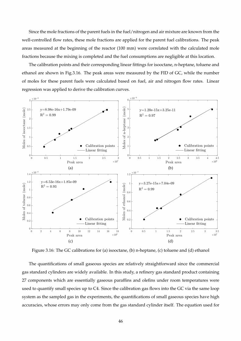
Since the mole fractions of the parent fuels in the fuel/nitrogen and air mixture are known from the

well-controlled flow rates, these mole fractions are applied for the parent fuel calibrations. The peak

areas measured at the beginning of the reactor (100 mm) were correlated with the calculated mole

fractions because the mixing is completed and the fuel consumptions are negligible at this location.

The calibration points and their corresponding linear fittings for isooctane, n-heptane, toluene and

ethanol are shown in Fig.3.16. The peak areas were measured by the FID of GC, while the number

of moles for these parent fuels were calculated based on fuel, air and nitrogen flow rates. Linear

regression was applied to derive the calibration curves.

(a) (b)

(c) (d)

Figure 3.16: The GC calibrations for (a) isooctane, (b) n-heptane, (c) toluene and (d) ethanol

The quantifications of small gaseous species are relatively straightforward since the commercial

gas standard cylinders are widely available. In this study, a refinery gas standard product containing

27 components which are essentially gaseous paraffins and olefins under room temperatures were

used to quantify small species up to C4. Since the calibration gas flows into the GC via the same loop

system as the sampled gas in the experiments, the quantifications of small gaseous species have high

accuracies, whose errors may only come from the gas standard cylinder itself. The equation used for

46

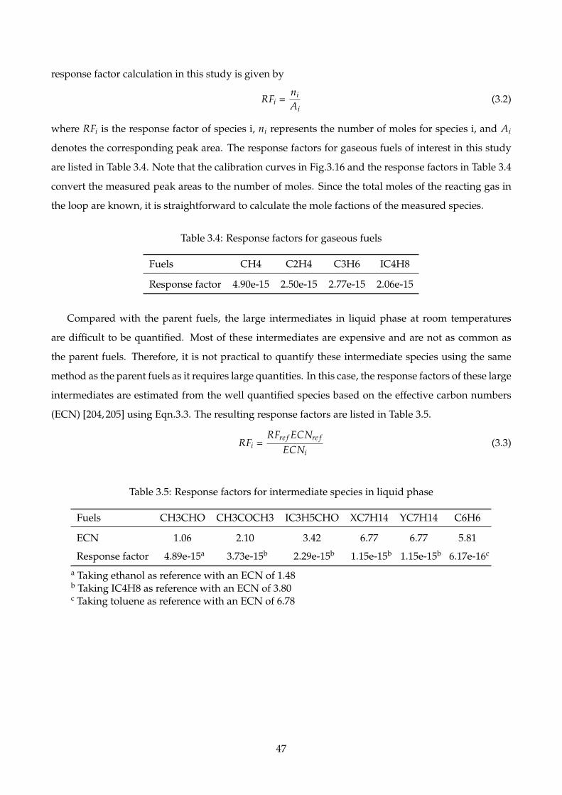
response factor calculation in this study is given by

(3.2)RFi =ni

Ai

where RFi is the response factor of species i, ni represents the number of moles for species i, and Ai

denotes the corresponding peak area. The response factors for gaseous fuels of interest in this study

are listed in Table 3.4. Note that the calibration curves in Fig.3.16 and the response factors in Table 3.4

convert the measured peak areas to the number of moles. Since the total moles of the reacting gas in

the loop are known, it is straightforward to calculate the mole factions of the measured species.

Table 3.4: Response factors for gaseous fuels

Fuels CH4 C2H4 C3H6 IC4H8

Response factor 4.90e-15 2.50e-15 2.77e-15 2.06e-15

Compared with the parent fuels, the large intermediates in liquid phase at room temperatures

are difficult to be quantified. Most of these intermediates are expensive and are not as common as

the parent fuels. Therefore, it is not practical to quantify these intermediate species using the same

method as the parent fuels as it requires large quantities. In this case, the response factors of these large

intermediates are estimated from the well quantified species based on the effective carbon numbers

(ECN) [204, 205] using Eqn.3.3. The resulting response factors are listed in Table 3.5.

(3.3)RFi =RFre f ECNre f

ECNi

Table 3.5: Response factors for intermediate species in liquid phase

Fuels CH3CHO CH3COCH3 IC3H5CHO XC7H14 YC7H14 C6H6

ECN 1.06 2.10 3.42 6.77 6.77 5.81

Response factor 4.89e-15a 3.73e-15b 2.29e-15b 1.15e-15b 1.15e-15b 6.17e-16c

a Taking ethanol as reference with an ECN of 1.48b Taking IC4H8 as reference with an ECN of 3.80c Taking toluene as reference with an ECN of 6.78

47

Chapter 4

Optimal Octane Number Correlations for

Toluene Reference Fuels (TRFs) Blended

with Ethanol

4.1 Introduction

Ethanol is known to interact non-linearly with isooctane, n-heptane, toluene, and PRF-, TRF-based

gasoline surrogates in the CFR engine under the standard knocking conditions [9], but the quantita-

tive understanding of these interaction behaviours is not complete. Therefore, this chapter proposes

optimal octane number correlations to quantify these interactions based on a systematically and rig-

orously statistical approach, which provides basis for ethanol blending into the gasoline and octane

number estimations for TRF-based gasoline surrogates. Note that this chapter is revised from a re-

cently published paper by the author [206].

The octane numbers of neat compounds were extensively measured in the 1950s by the American

Petroleum Institute [207]. Publications that present the octane numbers of mixtures are relatively

sparse. The octane blending of mixtures can be quite complicated [9, 208], particularly when ethanol

is involved. The use of ethanol in SI engines has received significant attention in recent years [9,

10, 12, 44, 209, 210], and it is commonly blended with gasoline for its low autoignition reactivity and

high heat of vaporisation, both of which result in ethanol’s relatively high octane number. Octane

number measurements have been conducted for ethanol blended with different commercial gasoline

[10,44], primary reference fuels (PRFs) (mixtures of n-heptane and isooctane) [9,211–213], and toluene

reference fuels (TRFs) (mixtures of PRF and toluene) [9, 211–213]. Significant non-linear blending

has been reported in some cases. Proper account of such non-linear and sometimes non-monotonic

behaviours is essential for optimal blending of ethanol into gasoline of different compositions, as well

48

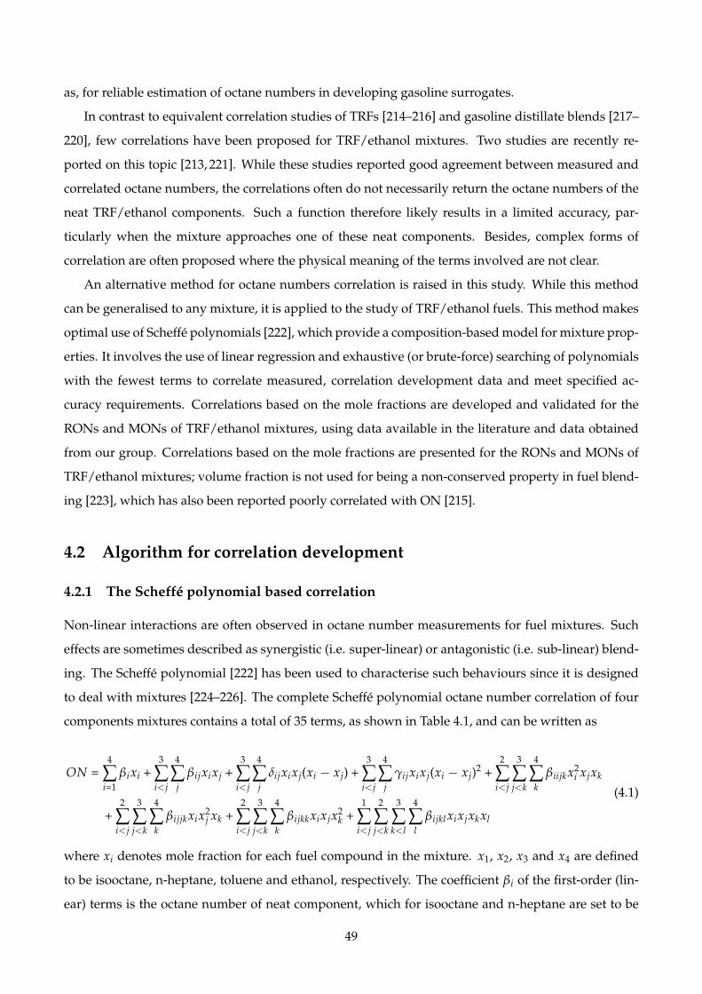
as, for reliable estimation of octane numbers in developing gasoline surrogates.

In contrast to equivalent correlation studies of TRFs [214–216] and gasoline distillate blends [217–

220], few correlations have been proposed for TRF/ethanol mixtures. Two studies are recently re-

ported on this topic [213, 221]. While these studies reported good agreement between measured and

correlated octane numbers, the correlations often do not necessarily return the octane numbers of the

neat TRF/ethanol components. Such a function therefore likely results in a limited accuracy, par-

ticularly when the mixture approaches one of these neat components. Besides, complex forms of

correlation are often proposed where the physical meaning of the terms involved are not clear.

An alternative method for octane numbers correlation is raised in this study. While this method

can be generalised to any mixture, it is applied to the study of TRF/ethanol fuels. This method makes

optimal use of Scheffe polynomials [222], which provide a composition-based model for mixture prop-

erties. It involves the use of linear regression and exhaustive (or brute-force) searching of polynomials

with the fewest terms to correlate measured, correlation development data and meet specified ac-

curacy requirements. Correlations based on the mole fractions are developed and validated for the

RONs and MONs of TRF/ethanol mixtures, using data available in the literature and data obtained

from our group. Correlations based on the mole fractions are presented for the RONs and MONs of

TRF/ethanol mixtures; volume fraction is not used for being a non-conserved property in fuel blend-

ing [223], which has also been reported poorly correlated with ON [215].

4.2 Algorithm for correlation development

4.2.1 The Scheffe polynomial based correlation

Non-linear interactions are often observed in octane number measurements for fuel mixtures. Such

effects are sometimes described as synergistic (i.e. super-linear) or antagonistic (i.e. sub-linear) blend-

ing. The Scheffe polynomial [222] has been used to characterise such behaviours since it is designed

to deal with mixtures [224–226]. The complete Scheffe polynomial octane number correlation of four

components mixtures contains a total of 35 terms, as shown in Table 4.1, and can be written as

(4.1)

ON =4

∑i=1

βixi +3

∑i<j

4

∑j

βijxixj +3

∑i<j

4

∑j

δijxixj(xi − xj) +3

∑i<j

4

∑j

γijxixj(xi − xj)2 +2

∑i<j

3

∑j<k

4

∑k

βiijkx2i xjxk

+2

∑i<j

3

∑j<k

4

∑k

βijjkxix2j xk +

2

∑i<j

3

∑j<k

4

∑k

βijkkxixjx2k +

1

∑i<j

2

∑j<k

3

∑k<l

4

∑l

βijklxixjxkxl

where xi denotes mole fraction for each fuel compound in the mixture. x1, x2, x3 and x4 are defined

to be isooctane, n-heptane, toluene and ethanol, respectively. The coefficient βi of the first-order (lin-

ear) terms is the octane number of neat component, which for isooctane and n-heptane are set to be

49

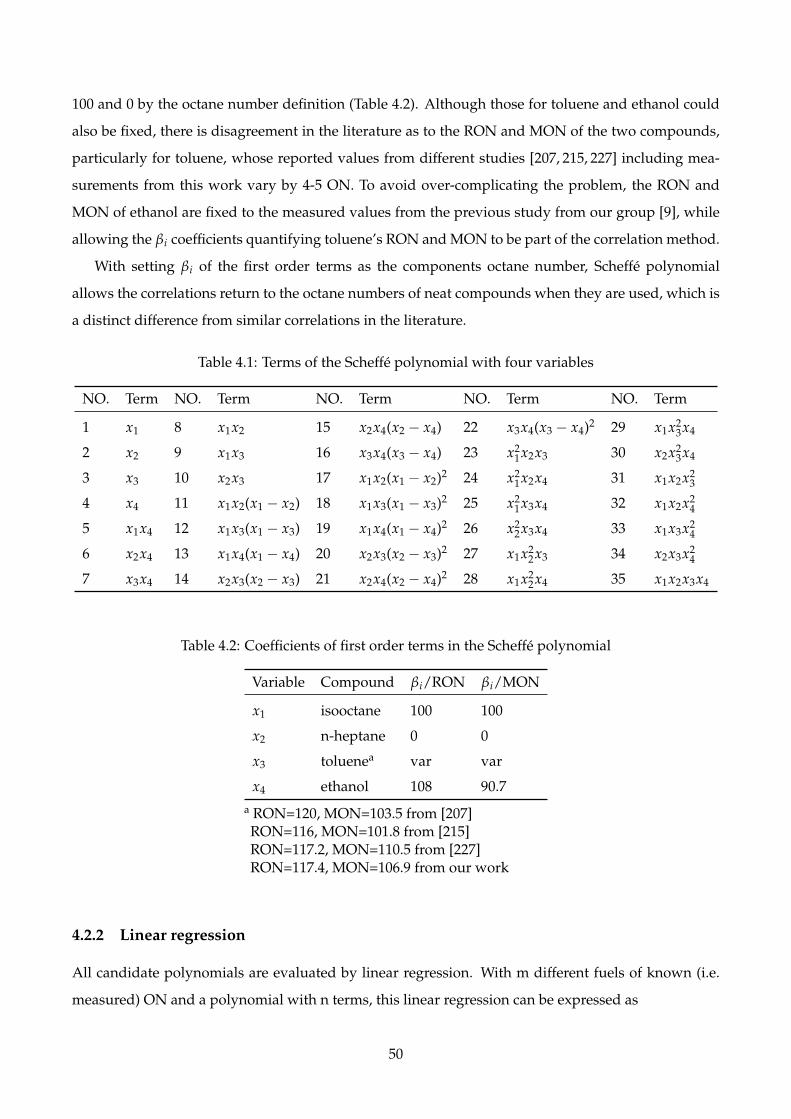
100 and 0 by the octane number definition (Table 4.2). Although those for toluene and ethanol could

also be fixed, there is disagreement in the literature as to the RON and MON of the two compounds,

particularly for toluene, whose reported values from different studies [207, 215, 227] including mea-

surements from this work vary by 4-5 ON. To avoid over-complicating the problem, the RON and

MON of ethanol are fixed to the measured values from the previous study from our group [9], while

allowing the βi coefficients quantifying toluene’s RON and MON to be part of the correlation method.

With setting βi of the first order terms as the components octane number, Scheffe polynomial

allows the correlations return to the octane numbers of neat compounds when they are used, which is

a distinct difference from similar correlations in the literature.

Table 4.1: Terms of the Scheffe polynomial with four variables

NO. Term NO. Term NO. Term NO. Term NO. Term

1 x1 8 x1x2 15 x2x4(x2 − x4) 22 x3x4(x3 − x4)2 29 x1x23x4

2 x2 9 x1x3 16 x3x4(x3 − x4) 23 x21x2x3 30 x2x2

3x4

3 x3 10 x2x3 17 x1x2(x1 − x2)2 24 x21x2x4 31 x1x2x2

3

4 x4 11 x1x2(x1 − x2) 18 x1x3(x1 − x3)2 25 x21x3x4 32 x1x2x2

4

5 x1x4 12 x1x3(x1 − x3) 19 x1x4(x1 − x4)2 26 x22x3x4 33 x1x3x2

4

6 x2x4 13 x1x4(x1 − x4) 20 x2x3(x2 − x3)2 27 x1x22x3 34 x2x3x2

4

7 x3x4 14 x2x3(x2 − x3) 21 x2x4(x2 − x4)2 28 x1x22x4 35 x1x2x3x4

Table 4.2: Coefficients of first order terms in the Scheffe polynomial

Variable Compound βi/RON βi/MON

x1 isooctane 100 100

x2 n-heptane 0 0

x3 toluenea var var

x4 ethanol 108 90.7a RON=120, MON=103.5 from [207]RON=116, MON=101.8 from [215]RON=117.2, MON=110.5 from [227]RON=117.4, MON=106.9 from our work

4.2.2 Linear regression

All candidate polynomials are evaluated by linear regression. With m different fuels of known (i.e.

measured) ON and a polynomial with n terms, this linear regression can be expressed as

50

y = Xβ (4.2)

where y is a vector representing the measured ONs for the m fuels, X is an m× n matrix containing

the value of the indeterminate of each of the n polynomial terms for these m fuels (i.e. x1, x2,..., x1x2,...,

x1x2(x1− x2),...), and β is a vector denoting n coefficients of these polynomial terms. To solve for vector

β, the rank of X must be no less than n, i.e. the number of fuels of linearly independent composition

must be at least equal to the number of polynomial terms. Otherwise, the rank deficiency problem will

appear. Given the number of fuels (m > 50) is considerably larger than the number of terms (n < 10),

rank deficiency is not an issue for correlations reported here.

4.2.3 Data for correlation development and validation

This section used the following, independent data sets, which are also presented in full tabular form

in Appendix A.

• The data for developing the correlations

TRF - ASTM standards [25, 26], Morgan et al. [214] and Knop et al. [215]

TRF/ethanol - Foong et al. [9]

• The data for validating the correlations

TRF - this work, and Lund [211–213]

TRF/ethanol - Lund [211–213]

It is noted that the development data used in this study is restricted to a range of 80 to 120 regarding

RON, since this spans a plausible range of production gasoline, while avoiding excessive polynomial

complexity that arises from fitting data at low ONs and which is of limited, practical interest. These

limits could, of course, be relaxed, with longer, optimal polynomials then inevitably resulting. The

distributions of development and validation data are plotted in four simplex lattices as shown in

Fig.4.1, each with one component omitted. Note that quaternary mixtures are not shown in Fig.4.1,

but are listed in Appendix A. The contour line representing RON = 80 is drawn in Fig.4.1(a), (c)

and (d), and no contour line is plotted in Fig.4.1(b), as the entire surface has octane number higher

than 100. It is clear that both the development and validation data are located in the regions with

octane number above 80. Considering that octane number tests are normally carried out in a range of

application interests, and coordinated efforts have not been made to map these surfaces systematically,

it is not surprising to find unevenly distributed data points on these simplex lattices, which might

make developed correlations perform poorly in the regions where data points are scarce. In this case,

51

RON=80

0.2 0.4 0.6 0.8

0.8

0.6

0.4

0.2 0.8

0.6

0.4

0.2

n−heptane

toluene ethanol

(a) toluene/n-heptane/ethanol

0.2 0.4 0.6 0.8

0.8

0.6

0.4

0.2 0.8

0.6

0.4

0.2

ethanol

isooctane toluene

(b) isooctane/toluene/ethanol

RON=80

0.2 0.4 0.6 0.8

0.8

0.6

0.4

0.2 0.8

0.6

0.4

0.2

n−heptane

isooctane ethanol

(c) isooctane/n-heptane/ethanol

RON=80

0.2 0.4 0.6 0.8

0.8

0.6

0.4

0.2 0.8

0.6

0.4

0.2

n−heptane

isooctane toluene

(d) isooctane/n-heptane/toluene

Figure 4.1: Data distribution on simplex lattices with filled circles representing development data andopen ones for validation data

the selection of the criterion for correlation development has to be careful to avoid over-constraining

the correlation, as discussed in the following.

4.2.4 Criterion for correlation development

The optimal correlations should be accurate enough to constrain the residual errors within an accept-

able range, but should not over-constrain the data, because measurements from different sources have

different uncertainties, and correlations may get involved with these experimental errors if containing

52

more terms than necessary. That is, an over-constrained correlation may correlate the development

data very well but perform poorly with independent, validation data, due to excessive terms pro-

ducing erratic results. Therefore, a balance needs to be maintained between accurate correlation and

over-fitting. In this work, the Scheffe polynomial starts from the four linear first-order terms and is

increased by adding one term a time. The coefficient of determination (R2) and the maximum abso-

lute error (MAE) between the measured and correlated values are examined in parallel for all cases.

Both R2 and MAE are used with the consideration that R2 reflects the statistical performance of the

correlations, and MAE indicates how individual datasets are correlated. The latter apparently rep-

resents a more practical measure of accuracy but is subject to the experimental uncertainties specific

to the dataset used. During the correlation development, if R2 and MAE are improved significantly

with adding one term, more term(s) is added. If the improvement is minor and the highest R2 and the

lowest MAE don’t yield the same correlation, the process then stops, with the consideration that the

statistical measure and dataset specific measure of the correlation quality start to deviate, suggesting

that over-constraint may occur. In this case, the last polynomial is called the optimal correlation which

should contain the fewest terms that can correlate the development data reasonably well.

4.2.5 Procedures for optimal correlation development and validation

The method for determining the optimal octane number correlation of any fuel mixture places three

requirements.

1. The candidate polynomials must only depend on some measure of the fuel composition and

must return the octane numbers of the neat mixture components.

2. The polynomial selected must belong to the sub-set of candidate polynomials with the fewest

terms that meet the criterion mentioned above.

3. The polynomial selected must have the highest R2 or smallest MAE with the development data

amongst all of those belonging to the sub-set of candidate polynomial.

The first requirement ensures that correlation can be determined from physically meaningful quan-

tities and can be expected to be accurate over a wide range of mixtures, e.g. from neat compounds

to quaternary TRF/ethanol mixtures. Scheffe polynomials [222], which provide a composition-based

model for mixture properties, meet this requirement. The second requirement recognises that differ-

ences with data generally decrease with more polynomial terms, and that we should, therefore, seek

the polynomial with the fewest terms that is acceptably accurate. The third requirement then sim-

ply states that the final, selected polynomial should be most accurate of those simplest polynomials

considered.

53

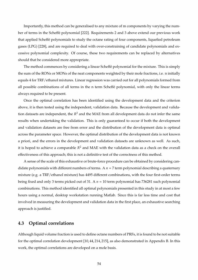
Importantly, this method can be generalised to any mixture of m components by varying the num-

ber of terms in the Scheffe polynomial [222]. Requirements 2 and 3 above extend our previous work

that applied Scheffe polynomials to study the octane rating of four components, liquefied petroleum

gases (LPG) [228], and are required to deal with over-constraining of candidate polynomials and ex-

cessive polynomial complexity. Of course, these two requirements can be replaced by alternatives

should that be considered more appropriate.

The method commences by considering a linear Scheffe polynomial for the mixture. This is simply

the sum of the RONs or MONs of the neat components weighted by their mole fractions, i.e. n initially

equals 4 for TRF/ethanol mixtures. Linear regression was carried out for all polynomials formed from

all possible combinations of all terms in the n term Scheffe polynomial, with only the linear terms

always required to be present.

Once the optimal correlation has been identified using the development data and the criterion

above, it is then tested using the independent, validation data. Because the development and valida-

tion datasets are independent, the R2 and the MAE from all development data do not infer the same

results when undertaking the validation. This is only guaranteed to occur if both the development

and validation datasets are free from error and the distribution of the development data is optimal

across the parameter space. However, the optimal distribution of the development data is not known

a priori, and the errors in the development and validation datasets are unknown as well. As such,

it is hoped to achieve a comparable R2 and MAE with the validation data as a check on the overall

effectiveness of this approach; this is not a definitive test of the correctness of this method.

A sense of the scale of this exhaustive or brute-force procedure can be obtained by considering can-

didate polynomials with different numbers of terms. A n = 7 term polynomial describing a quaternary

mixture (e.g. a TRF/ethanol mixture) has 4495 different combinations, with the four first-order terms

being fixed and only 3 terms picked out of 31. A n = 10 term polynomial has 736281 such polynomial

combinations. This method identified all optimal polynomials presented in this study in at most a few

hours using a normal, desktop workstation running Matlab. Since this is far less time and cost that

involved in measuring the development and validation data in the first place, an exhaustive searching

approach is justified.

4.3 Optimal correlations

Although liquid volume fraction is used to define octane numbers of PRFs, it is found to be not suitable

for the optimal correlation development [10, 44, 214, 215], as also demonstrated in Appendix B. In this

work, the optimal correlations are developed on a mole basis.

54

4.3.1 Optimal RON correlation for TRF/ethanol mixtures

4.3.1.1 Development of the optimal correlation

The linear-by-mole correlation (Eq.4.3), which contains four first order terms for isooctane, n-heptane,

toluene and ethanol, was first demonstrated with the octane number of toluene allowed to vary (as

discussed in Section 4.2.1). The residual errors between the development data and linear blending are

shown in Fig.4.2(a), indicating an overall poor correlation. This is in sharp contrast to the neat TRF

cases for which the linear-by-mole rule was reported working satisfactorily [215]. It is noted that in

Fig.4.2(a) that a significant proportion of residual errors are above 0, because the fuels used here are

mostly synergistic blending mixtures, causing the linear-by-mole rule underestimating RON.

(4.3)RON4,terms = 100x1 + 0x2 + 116.4x3 + 108x4

Non-linear terms are then added one at a time to improve the correlation through the exhaustive

searching described in Section 4.2.5. The first term identified, i.e. that produces the highest R2 and

smallest MAE for 5-term Scheffe polynomials, is 63.2x2x4, as shown in Eq.4.4. The positive coefficient

for this term is consistent with the synergistic octane blending between n-heptane (x2) and ethanol (x4)

observed in the recent study from our group [9]. With this term added, distribution of the residual

errors shifts closer to 0 as a whole, as shown in Figs.4.2(b), confirming that the added term accounts

for synergisms in the fuel mixtures.

(4.4)RON5,terms = 100x1 + 0x2 + 115.9x3 + 108x4 + 63.2x2x4

To further improve the correlation, a second non-linear term, 26.1x1x4, is identified and added

to the polynomial (Eq.4.5). This positive coefficient is also consistent with the synergism observed

between isooctane and ethanol in octane blending [9]. Meanwhile, the 63.2x2x4 term previously found

in Eq.4.4 is replaced by a term composed of the same molar fractions but a negative coefficient, -

97.8x2x4(x2 − x4). Since x2 is smaller than x4 for all development data used here, this term is always

positive and thus still captures the synergism between n-heptane and ethanol. With the two terms

added, the positive residual errors, resulted from synergistic blending, are constrained to 2 ON as in

Fig.4.2(c).

(4.5)RON6,terms = 100x1 + 0x2 + 115.7x3 + 108x4 + 26.1x1x4 − 97.8x2x4(x2 − x4)

A third term is further identified, −9.1x3x4, and added to the polynomial (Eq.4.6). The negative

contribution to the mixture octane numbers by this term is also consistent with the antagonistic blend-

ing between toluene and ethanol as reported in [9]. With this term, residual errors below 0 are mostly

corrected, as shown in Fig.4.2(d).

(4.6)RON7,terms = 100x1 + 0x2 + 116.2x3 + 108x4 + 27.0x1x4 − 9.1x3x4 − 98.4x2x4(x2 − x4)

55

RON

80 85 90 95 100 105 110 115 120

Residual

-10

-8

-6

-4

-2

0

2

4

6

8

10

(a)

RON

80 85 90 95 100 105 110 115 120

Residual

-10

-8

-6

-4

-2

0

2

4

6

8

10

(b)

RON

80 85 90 95 100 105 110 115 120

Residual

-6

-4

-2

0

2

4

6

(c)

RON

80 85 90 95 100 105 110 115 120

Residual

-6

-4

-2

0

2

4

6

(d)

Figure 4.2: Residual error between the development data and correlated RON from (a) linear by-molecorrelation, (b) five terms correlation, (c) six terms correlation and (d) seven terms correlation

Apparently, as more non-linear terms are added, the development data can be better correlated

with significantly improved R2 and MAE. However, the improvement starts to diminish at some point

and the risk of over-constraining the correlation to measurement uncertainties increases, as discussed

in Section 4.2.4. Fig.4.3(a) and (b) show the variations of the R2 and MAE with the number of terms. In

each figure, results from searching by the highest R2 and by the smallest MAE are plotted. It is noted

that after 7 terms, R2 only increases slightly for both searching methods. Besides, from 7-term to 8-

term, the two searching methods result in different polynomials, as shown in the locally magnified

plots in Fig.4.3. In particular, the MAE produced by searching the highest R2 is larger with the 8-term

correlation than with the 7-term correlation (Fig.4.3(b)). These observations indicate that the statistics-

based measure (R2) and dataset specific measure (MAE) for correlation quality start to deviate and

thus suggest over-constraining of the correlation. The correlation development thus stops at 7 terms,

and Eq.4.6 is called the optimal correlation for RON of TRF/ethanol mixtures, with respect to the

56

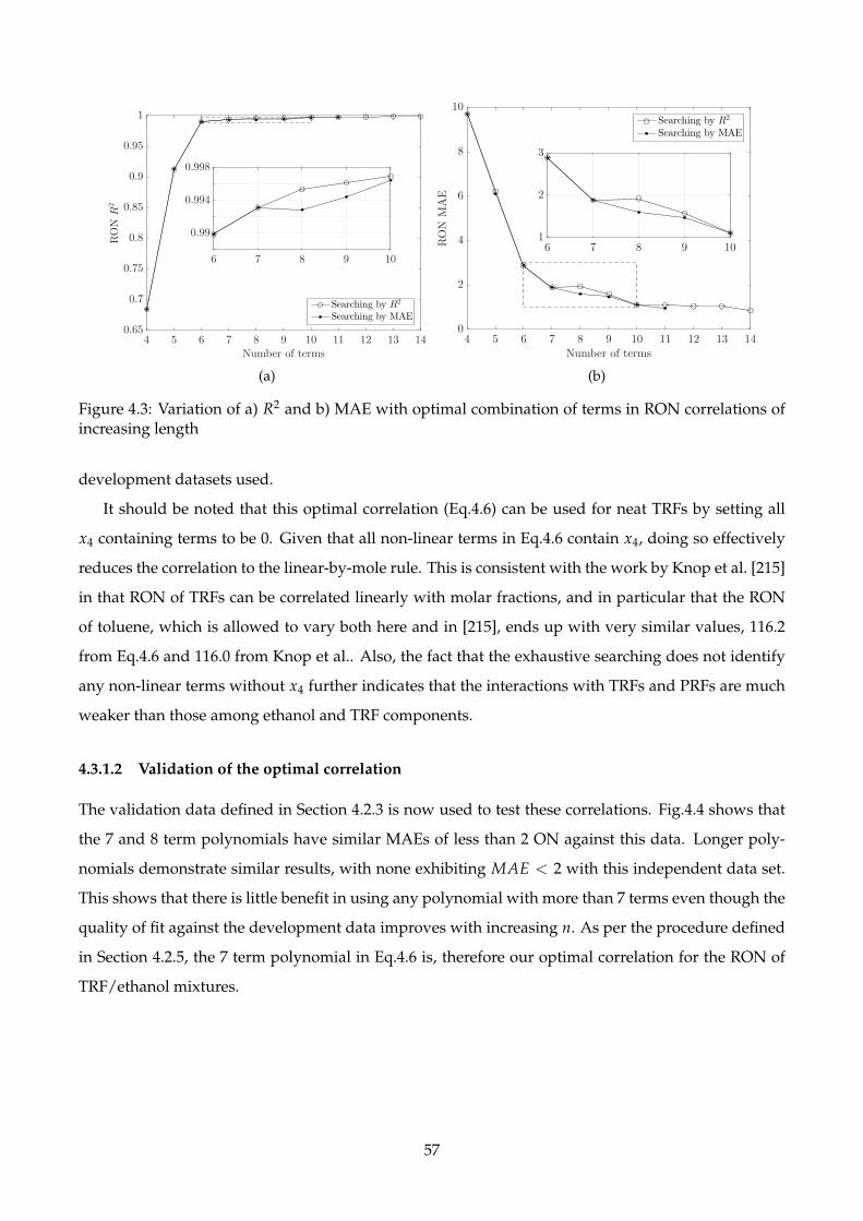
Number of terms

4 5 6 7 8 9 10 11 12 13 14

RON

R2

0.65

0.7

0.75

0.8

0.85

0.9

0.95

1

Searching by R2

Searching by MAE

6 7 8 9 10

0.99

0.994

0.998

(a)

Number of terms

4 5 6 7 8 9 10 11 12 13 14

RON

MAE

0

2

4

6

8

10

Searching by R2

Searching by MAE

6 7 8 9 101

2

3

(b)

Figure 4.3: Variation of a) R2 and b) MAE with optimal combination of terms in RON correlations ofincreasing length

development datasets used.

It should be noted that this optimal correlation (Eq.4.6) can be used for neat TRFs by setting all

x4 containing terms to be 0. Given that all non-linear terms in Eq.4.6 contain x4, doing so effectively

reduces the correlation to the linear-by-mole rule. This is consistent with the work by Knop et al. [215]

in that RON of TRFs can be correlated linearly with molar fractions, and in particular that the RON

of toluene, which is allowed to vary both here and in [215], ends up with very similar values, 116.2

from Eq.4.6 and 116.0 from Knop et al.. Also, the fact that the exhaustive searching does not identify

any non-linear terms without x4 further indicates that the interactions with TRFs and PRFs are much

weaker than those among ethanol and TRF components.

4.3.1.2 Validation of the optimal correlation

The validation data defined in Section 4.2.3 is now used to test these correlations. Fig.4.4 shows that

the 7 and 8 term polynomials have similar MAEs of less than 2 ON against this data. Longer poly-

nomials demonstrate similar results, with none exhibiting MAE < 2 with this independent data set.

This shows that there is little benefit in using any polynomial with more than 7 terms even though the

quality of fit against the development data improves with increasing n. As per the procedure defined

in Section 4.2.5, the 7 term polynomial in Eq.4.6 is, therefore our optimal correlation for the RON of

TRF/ethanol mixtures.

57

RON

80 90 100 110 120

Residual

-6

-4

-2

0

2

4

6

(a)

RON

80 90 100 110 120

Residual

-6

-4

-2

0

2

4

6

(b)

Figure 4.4: Residual error between the validation data and a) 7 and b) 8 term RON correlations on amolar basis

4.3.2 Optimal MON correlation for TRF/ethanol mixtures

4.3.2.1 Development of the optimal correlation

The optimal MON correlation was developed using the same method as for RON. Here the MON

range extends to lower than 80 because of the non-zero octane sensitivity of the fuels used in the RON

correlation. The linear-by-mole blending rule was first attempted, and the correlation and residual er-

rors are shown in Eq.4.7 and Fig.4.5(a) respectively. Three higher order terms: 76.7x2x4, 12.8x1x4, and

−6.4x3x4 were added consecutively from exhaustive searching to account for the non-linear blending

behaviours, as shown in Eq.4.8 and Fig.4.5(b). Coefficients of these terms again suggest the synergis-

tic blending of ethanol/n-heptane and ethanol/isooctane, and antagonistic blending between ethanol

and toluene, which are all similar to the RON case. As shown in Fig.4.6, adding another higher or-

der term to Eq.4.8 doesn’t increase R2 significantly, whereas the correlation with the maximum R2

becomes different from the one with the minimum MAE, suggesting that the seven terms polynomial

in Eq.4.8 is the optimal correlation.

(4.7)MON4,terms = 100x1 + 0x2 + 102.4x3 + 90.7x4

(4.8)MON7,terms = 100x1 + 0x2 + 102.0x3 + 90.7x4 + 12.8x1x4 + 76.7x2x4 − 6.4x3x4

4.3.2.2 Validation of the optimal correlation

The validation data defined in Section 4.2.3 is again used to test these correlations. As with the RON,

Fig.4.7 shows that the 7 and 8 term polynomials have similar MAEs of less than 2 ON against the

validation data. Longer polynomials again demonstrate similar results, with none exhibiting MAE <

58

MON

70 75 80 85 90 95 100 105

Residual

-15

-10

-5

0

5

10

15

(a)

MON

70 75 80 85 90 95 100 105

Residual

-6

-4

-2

0

2

4

6

(b)

Figure 4.5: Residual error between the development data and correlated MON from (a) linear by-molecorrelation, and (b) seven terms correlation

Number of terms4 5 6 7 8 9 10 11

MON

R2

0.7

0.75

0.8

0.85

0.9

0.95

1

Searching by R2

Searching by MAE

6 7 8 90.98

0.985

0.99

0.995

(a)

Number of terms

4 5 6 7 8 9 10 11

MON

MAE

0

2

4

6

8

10

12

14

Searching by R2

Searching by MAE

6 7 8 91

1.5

2

2.5

(b)

Figure 4.6: Variation of a) R2 and b) MAE with optimal combination of terms in MON correlations ofincreasing length

2 with this independent data set. The procedure defined in Section 4.2.5 therefore now infers that the

7 term polynomial in Eq.4.8 is the optimal correlation for the MON of TRF/ethanol mixtures.

59

MON

80 85 90 95

Residual

-6

-4

-2

0

2

4

6

(a)

MON

80 85 90 95

Residual

-6

-4

-2

0

2

4

6

(b)

Figure 4.7: Residual error between the validation data and a) 7 and b) 8 term MON correlations on amolar basis

4.4 Summary

This chapter proposed a systematic method for correlating the octane numbers of fuel mixtures. While

this method can be generalised to any such mixture, it was applied to the study of TRF/ethanol fuels

in this work.

The method made optimal use of Scheffe polynomials [222], which provide a composition-based

model for mixture properties. It combined linear regression and exhaustive (or brute-force) searching

for polynomials that met specified requirements with the fewest terms. The data used to develop these

correlations included measurements on TRFs by other groups [25, 26, 214, 215] and TRF/ethanol mix-

tures [9]. These correlations were then validated using independent datasets of TRFs and TRF/ethanol

mixtures from other groups [211–213] as well new measurements for TRFs that were undertaken for

this work.

Correlations using mole fractions were presented for the RONs and MONs of TRF/ethanol mix-

tures. These were compared with equivalent, linear correlations obtained from the same data. Al-

though the residual errors of these correlations can be further tightened by adding more terms, they

are likely to be affected by unknown measurement errors and lose their physical significance. The fol-

lowing two correlations were found to be optimal (i.e. have the fewest terms) satisfying the searching

criterion.

RON7,terms,optimal = 100x1 + 0x2 + 116.2x3 + 108x4 + 27.0x1x4 − 9.1x3x4 − 98.4x2x4(x2 − x4)

MON7,terms,optimal = 100x1 + 0x2 + 102.0x3 + 90.7x4 + 12.8x1x4 + 76.7x2x4 − 6.4x3x4

where x1, x2, x3, and x4 denote the mole fractions of isooctane, n-heptane, toluene and ethanol re-

spectively. These optimal correlations are the shortest polynomials that can correlate the RON and

60

MON of both the development data and validation data with MAE < 2ON, obtained by employing

two goodness-of-fit indicators, R2 and MAE. The non-linear terms identified from the correlation de-

velopment are well represented by the interactions observed in binary mixtures of ethanol and TRF

components, imparting physical significance for these terms selected from exhaustive searching. Nev-

ertheless, these correlations can return the linear-by-mole blending rules for neat TRF mixtures with

the fitted RON and MON of toluene agreeing excellently with the literature values. This demonstrates

the consistency of these correlations over a wide range of fuel compositions, an attribute lacking for

most fuel properties correlations previously reported.

61

Chapter 5

The Octane Numbers of Binary Mixtures

and Gasoline Surrogates Blended with

Ethanol

5.1 Introduction

The work from Chapter 4, together with the prior experimental study [9] explore the blending be-

haviours between ethanol and the TRF-based gasoline surrogates. Nevertheless, the interactions be-

tween ethanol and gasoline should be more complex due to the composition of practical fuels. In this

regard, it is necessary to add more hydrocarbons to the test matrix, which extends the understand-

ings of ethanol/hydrocarbon and hydrocarbon/hydrocarbon interactions and provides fundamental

information to formulate more practical gasoline surrogates.

Australian production gasoline with approximately 30% aromatics by volume blends slightly syn-

ergistically with ethanol, as shown in Fig.5.1. In comparison, the TRF-based gasoline surrogates,

which have a fixed RON of 91 and varied toluene fractions, exhibit significant synergistic behaviours

when blended with ethanol as shown in Fig.5.1, indicating that the TRFs are not sufficient to emulate

the production gasoline.

To develop the gasoline surrogates which better emulate the gasoline’s blending behaviours with

ethanol, systematic studies of the octane numbers for binary fuel mixtures and multi-component gaso-

line surrogates were carried out in the CFR engine. These mixtures were formulated by hydrocarbons

which were selected based on the detailed hydrocarbon analysis (DHA) results of the Australian regu-

lar grade unleaded gasoline with RON of 91. The study has two steps. In the first step, binary mixtures

containing the selected hydrocarbons and ethanol were tested to investigate how neat fuels interact

with each other, which provides the foundation for the following complicated gasoline surrogates for-

62

Volume fraction of ethanol (%)0 20 40 60 80 100

RON

90

95

100

105

110

Gasoline

PRF91

TRF91-15

TRF91-30

TRF91-45

Figure 5.1: Measured RONs for Australian production gasoline, PRF91, and TRF91s blended withethanol [9]

mulation. In the second step, various gasoline surrogates were formulated and tested to develop a

surrogate that can reproduce the interactions between production gasoline and ethanol. Note that this

surrogate only focuses on reproducing the octane number blending with ethanol and other properties

are not used as targets or constraints, although it turns out that some properties of the surrogate match

reasonably well with the gasoline.

5.2 The RONs of binary mixtures

Before formulating new gasoline surrogates, it is necessary to understand the blending behaviours

of binary mixtures, which provides the required basis for more complex gasoline surrogate formula-

tion. Considering that the gasoline contains hundreds of hydrocarbons, the interactions among these

hydrocarbons are critical to formulate gasoline surrogates. Therefore, this section first investigates

how isooctane, n-heptane, cyclohexane, and 1-hexene interact with toluene, and then the blending

behaviours of isooctane/cyclohexane and isooctane/1-hexene mixtures. Lastly, the octane number

measurements of ethanol blended with cyclohexane and 1-hexene were carried out in this study to

supplement the prior experimental study focusing on blending ethanol with isooctane, n-heptane,

and toluene [9].

5.2.1 Binary mixtures of hydrocarbons

Although the octane numbers of neat hydrocarbons have been measured extensively in the API Re-

search Project 45 [207], practical fuels are complex mixtures in which the interactions among hydro-

63

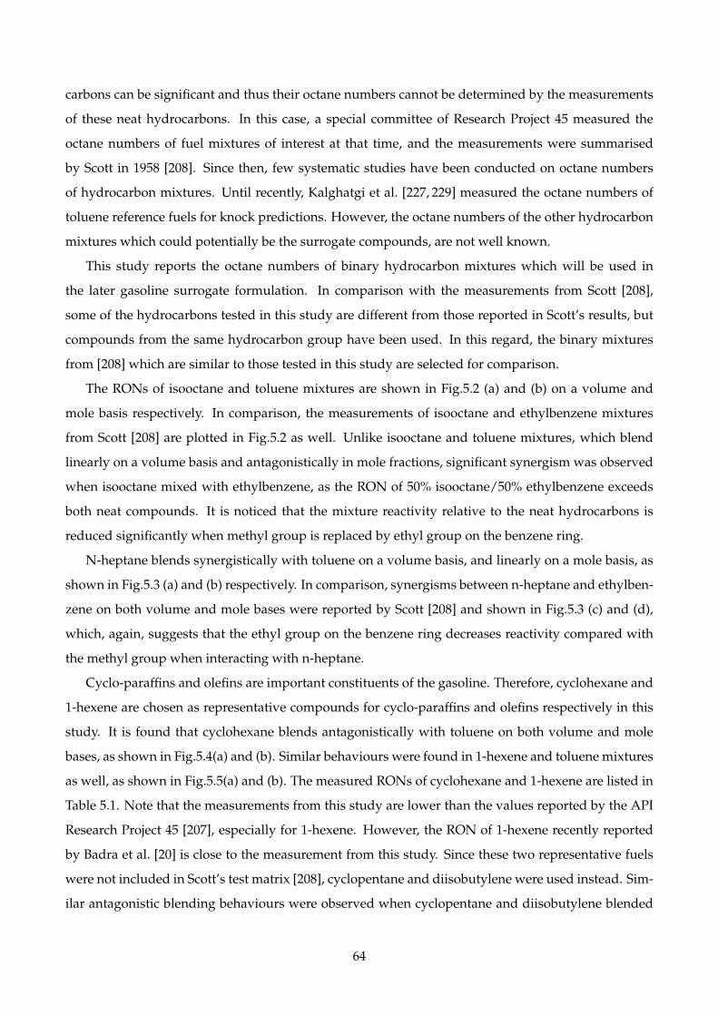
carbons can be significant and thus their octane numbers cannot be determined by the measurements

of these neat hydrocarbons. In this case, a special committee of Research Project 45 measured the

octane numbers of fuel mixtures of interest at that time, and the measurements were summarised

by Scott in 1958 [208]. Since then, few systematic studies have been conducted on octane numbers

of hydrocarbon mixtures. Until recently, Kalghatgi et al. [227, 229] measured the octane numbers of

toluene reference fuels for knock predictions. However, the octane numbers of the other hydrocarbon

mixtures which could potentially be the surrogate compounds, are not well known.

This study reports the octane numbers of binary hydrocarbon mixtures which will be used in

the later gasoline surrogate formulation. In comparison with the measurements from Scott [208],

some of the hydrocarbons tested in this study are different from those reported in Scott’s results, but

compounds from the same hydrocarbon group have been used. In this regard, the binary mixtures

from [208] which are similar to those tested in this study are selected for comparison.

The RONs of isooctane and toluene mixtures are shown in Fig.5.2 (a) and (b) on a volume and

mole basis respectively. In comparison, the measurements of isooctane and ethylbenzene mixtures

from Scott [208] are plotted in Fig.5.2 as well. Unlike isooctane and toluene mixtures, which blend

linearly on a volume basis and antagonistically in mole fractions, significant synergism was observed

when isooctane mixed with ethylbenzene, as the RON of 50% isooctane/50% ethylbenzene exceeds

both neat compounds. It is noticed that the mixture reactivity relative to the neat hydrocarbons is

reduced significantly when methyl group is replaced by ethyl group on the benzene ring.

N-heptane blends synergistically with toluene on a volume basis, and linearly on a mole basis, as

shown in Fig.5.3 (a) and (b) respectively. In comparison, synergisms between n-heptane and ethylben-

zene on both volume and mole bases were reported by Scott [208] and shown in Fig.5.3 (c) and (d),

which, again, suggests that the ethyl group on the benzene ring decreases reactivity compared with

the methyl group when interacting with n-heptane.

Cyclo-paraffins and olefins are important constituents of the gasoline. Therefore, cyclohexane and

1-hexene are chosen as representative compounds for cyclo-paraffins and olefins respectively in this

study. It is found that cyclohexane blends antagonistically with toluene on both volume and mole

bases, as shown in Fig.5.4(a) and (b). Similar behaviours were found in 1-hexene and toluene mixtures

as well, as shown in Fig.5.5(a) and (b). The measured RONs of cyclohexane and 1-hexene are listed in

Table 5.1. Note that the measurements from this study are lower than the values reported by the API

Research Project 45 [207], especially for 1-hexene. However, the RON of 1-hexene recently reported

by Badra et al. [20] is close to the measurement from this study. Since these two representative fuels

were not included in Scott’s test matrix [208], cyclopentane and diisobutylene were used instead. Sim-

ilar antagonistic blending behaviours were observed when cyclopentane and diisobutylene blended

64

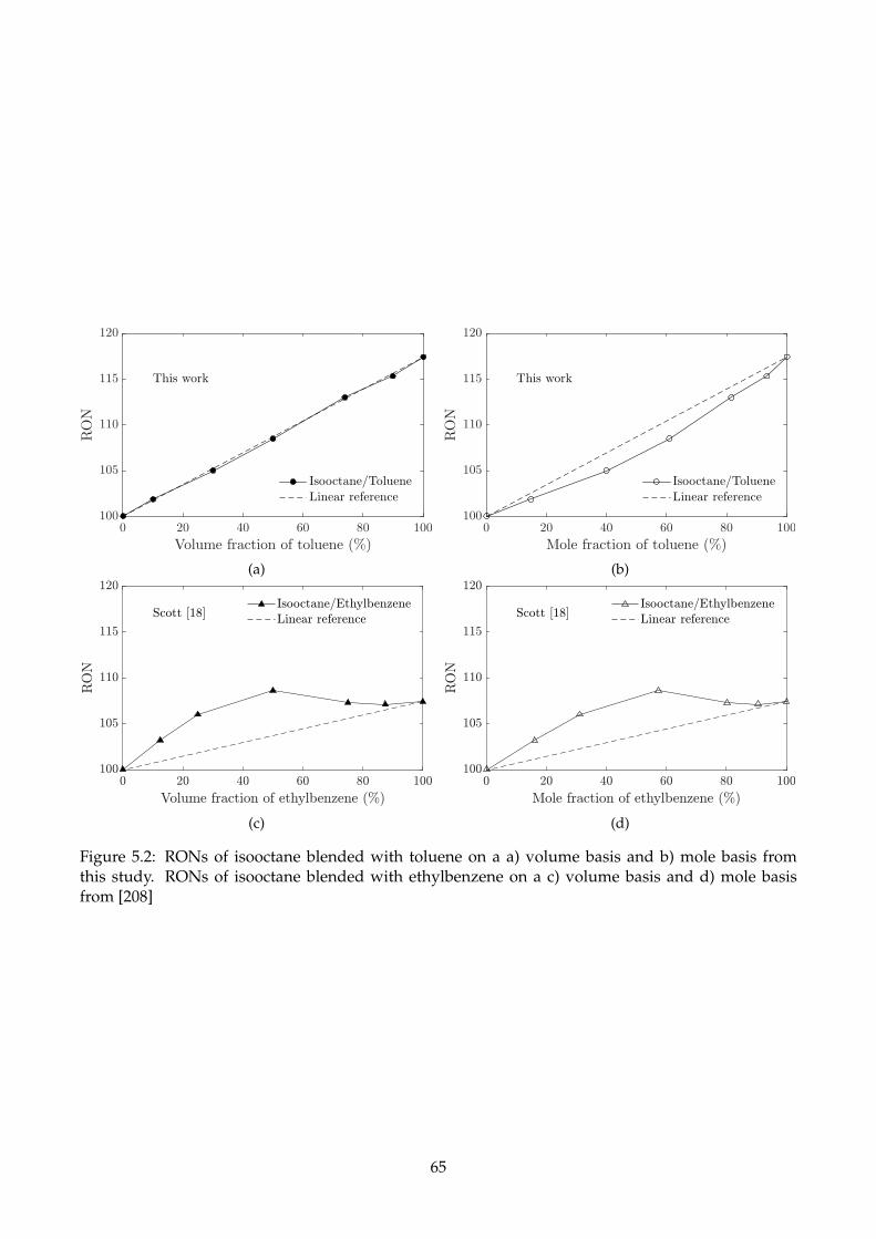
Volume fraction of toluene (%)0 20 40 60 80 100

RON

100

105

110

115

120

This work

Isooctane/Toluene

Linear reference

(a)

Mole fraction of toluene (%)0 20 40 60 80 100

RON

100

105

110

115

120

This work

Isooctane/Toluene

Linear reference

(b)

(c) (d)

Figure 5.2: RONs of isooctane blended with toluene on a a) volume basis and b) mole basis fromthis study. RONs of isooctane blended with ethylbenzene on a c) volume basis and d) mole basisfrom [208]

65

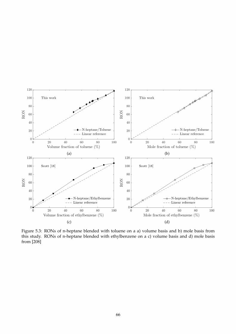
Volume fraction of toluene (%)0 20 40 60 80 100

RON

0

20

40

60

80

100

120

This work

N-heptane/Toluene

Linear reference

(a)

Mole fraction of toluene (%)0 20 40 60 80 100

RON

0

20

40

60

80

100

120

This work

N-heptane/Toluene

Linear reference

(b)

(c) (d)

Figure 5.3: RONs of n-heptane blended with toluene on a a) volume basis and b) mole basis fromthis study. RONs of n-heptane blended with ethylbenzene on a c) volume basis and d) mole basisfrom [208]

66

with ethylbenzene, as shown in Fig.5.4 and 5.5 respectively. Although ethylbenzene exhibits more

complex blending behaviours with other hydrocarbons, it is of interest to find that toluene blends

antagonistically with most representative fuels (except n-heptane) on a mole basis in this study.

Table 5.1: RONs of cyclohexane and 1-hexene from different studies [20, 207]

Fuel This study API Project 45 [207] Badra et al. [20]

1-hexene 72.7 76.4 73.6

Cyclohexane 82.2 83.0 -

The RONs of cyclohexane and 1-hexene blended with isooctane were measured in this study as

well. As shown in Fig.5.6 (a) and (b), cyclohexane blends linearly with isooctane on a volume basis

and synergistically on a mole basis. In comparison, similar trends were found when blending methyl-

cyclohexane with isooctane [208], as shown in Fig.5.6(c) and (d). Synergistic blending behaviours were

observed for 1-hexene/isooctane and 2-heptene/isooctane [208] mixtures, as shown in Fig.5.7.

67

(a) (b)

(c) (d)

Figure 5.4: RONs of cyclohexane blended with toluene on a a) volume basis and b) mole basis fromthis study. RONs of cyclopentane blended with ethylbenzene on a c) volume basis and d) mole basisfrom [208]

68

(a) (b)

(c) (d)

Figure 5.5: RONs of 1-hexene blended with toluene on a a) volume basis and b) mole basis from thisstudy. RONs of diisobutylene blended with ethylbenzene on a c) volume basis and d) mole basisfrom [208]

69

(a) (b)

(c) (d)

Figure 5.6: RONs of cyclohexane blended with isooctane on a a) volume basis and b) mole basis fromthis study. RONs of methylcyclohexane blended with isooctane on a c) volume basis and d) mole basisfrom [208]

70

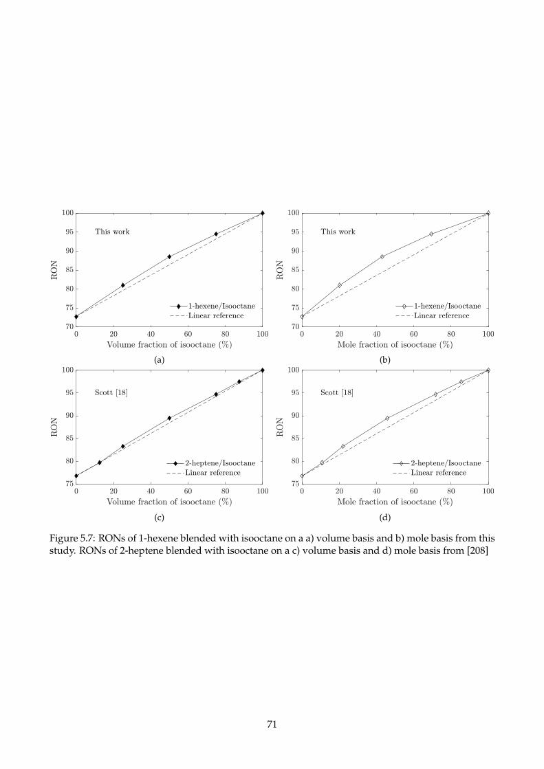
(a) (b)

(c) (d)

Figure 5.7: RONs of 1-hexene blended with isooctane on a a) volume basis and b) mole basis from thisstudy. RONs of 2-heptene blended with isooctane on a c) volume basis and d) mole basis from [208]

71

5.2.2 Binary mixtures containing ethanol

The blending behaviours of isooctane, n-heptane, and toluene with ethanol have been systematically

studied in Foong’s work [9]. However, the interactions of other hydrocarbon groups, such as cyclo-

paraffins and olefins, with ethanol are not known. Fig.5.8 shows the RONs of cyclohexane and 1-

hexene blended with ethanol. The synergistic blending behaviours were observed from these two

binary mixtures, which are more evident on a volume basis than on a mole basis.

Volume fraction of ethanol (%)0 20 40 60 80 100

RON

70

80

90

100

110

This work

Cyclohexane1-hexeneLinear reference

(a)

Mole fraction of ethanol (%)0 20 40 60 80 100

RON

70

80

90

100

110

This work

Cyclohexane1-hexeneLinear reference

(b)

Figure 5.8: RONs of cyclohexane and 1-hexene blended with ethanol on a a) volume basis and b) molebasis

Combining Foong’s work [9] and the results of this study, it is found that the commonly used rep-

resentative fuels of different hydrocarbon groups (except toluene) blend synergistically with ethanol.

On the other hand, toluene blends antagonistically with all studied components (except n-heptane)

on a mole basis.

The octane number interactions among hydrocarbons and ethanol are known to be complicated

and, often non-linear, which are summarised in Table 5.2. It is difficult to draw definitive conclusions

for octane number predictions of complex fuel mixtures, especially when the uncommon components

get involved. The RON tests for the binary mixtures here obtained thus provide the foundations for

the more complex gasoline surrogate formulation.

72

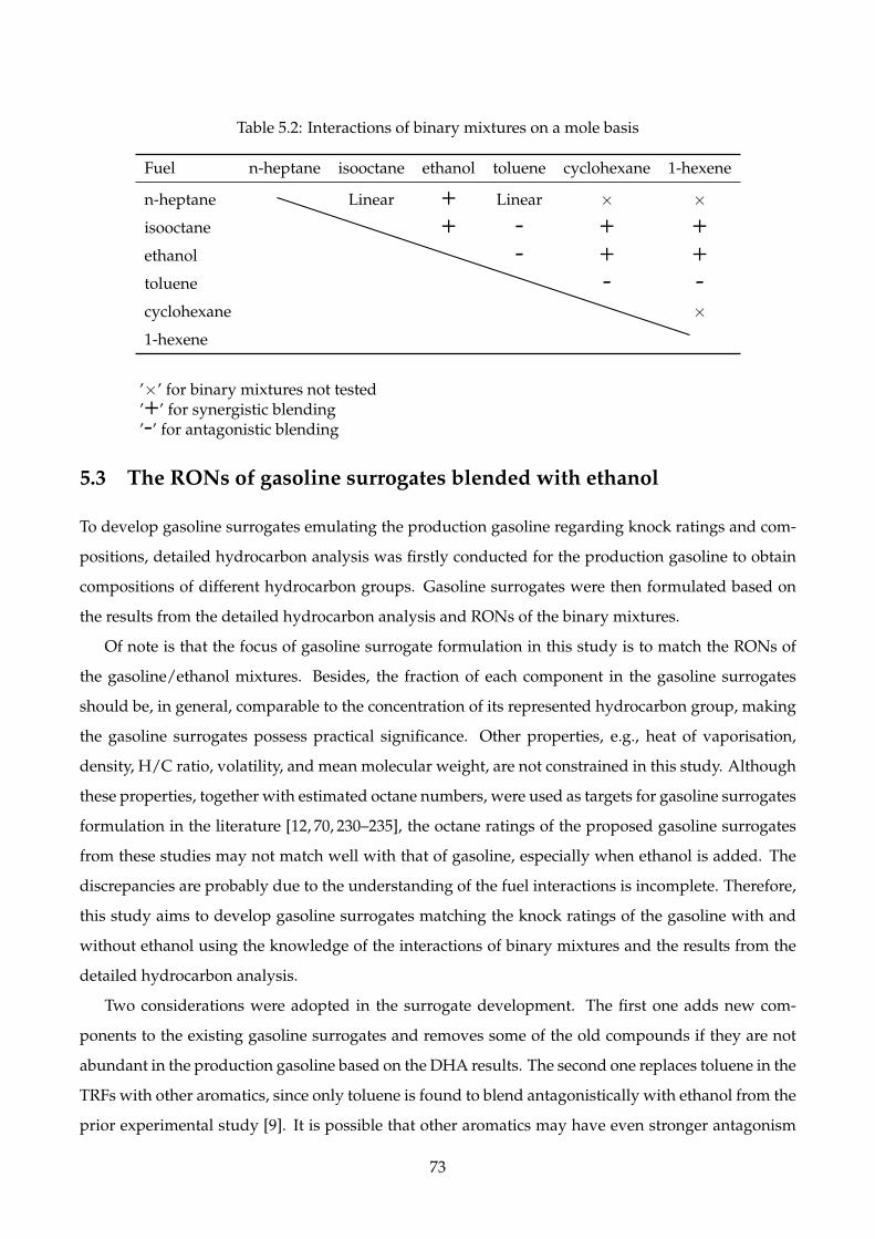
Table 5.2: Interactions of binary mixtures on a mole basis

Fuel n-heptane isooctane ethanol toluene cyclohexane 1-hexene

n-heptane Linear + Linear × ×isooctane + - + +ethanol - + +toluene - -cyclohexane ×1-hexene

’×’ for binary mixtures not tested’+’ for synergistic blending’-’ for antagonistic blending

5.3 The RONs of gasoline surrogates blended with ethanol

To develop gasoline surrogates emulating the production gasoline regarding knock ratings and com-

positions, detailed hydrocarbon analysis was firstly conducted for the production gasoline to obtain

compositions of different hydrocarbon groups. Gasoline surrogates were then formulated based on

the results from the detailed hydrocarbon analysis and RONs of the binary mixtures.

Of note is that the focus of gasoline surrogate formulation in this study is to match the RONs of

the gasoline/ethanol mixtures. Besides, the fraction of each component in the gasoline surrogates

should be, in general, comparable to the concentration of its represented hydrocarbon group, making

the gasoline surrogates possess practical significance. Other properties, e.g., heat of vaporisation,

density, H/C ratio, volatility, and mean molecular weight, are not constrained in this study. Although

these properties, together with estimated octane numbers, were used as targets for gasoline surrogates

formulation in the literature [12, 70, 230–235], the octane ratings of the proposed gasoline surrogates

from these studies may not match well with that of gasoline, especially when ethanol is added. The

discrepancies are probably due to the understanding of the fuel interactions is incomplete. Therefore,

this study aims to develop gasoline surrogates matching the knock ratings of the gasoline with and

without ethanol using the knowledge of the interactions of binary mixtures and the results from the

detailed hydrocarbon analysis.

Two considerations were adopted in the surrogate development. The first one adds new com-

ponents to the existing gasoline surrogates and removes some of the old compounds if they are not

abundant in the production gasoline based on the DHA results. The second one replaces toluene in the

TRFs with other aromatics, since only toluene is found to blend antagonistically with ethanol from the

prior experimental study [9]. It is possible that other aromatics may have even stronger antagonism

73

than toluene when blended with ethanol, which may help to decrease the octane number difference.

The gasoline surrogates proposed in this study all perform better than the simple TRFs, which sug-

gests the added surrogate compounds are critical in terms of emulating the blending behaviours of

the gasoline and ethanol. The experimental results reported in this chapter together with the optimal

correlations developed in Chapter 4 provide implications for fuel surrogate design.

5.3.1 Detailed hydrocarbon analysis for the Australian production gasoline

The Australian gasoline with RON of 91 was analysed by Independent Petroleum Laboratory (IPL)

in New Zealand and categorized into five groups: iso-, n-, cyclo- paraffins, aromatics and olefins

using the PIANO method which considers cyclo-olefins as olefins and is thus different from the more

commonly used PIONA method. The volume fraction of each group is summarised in Table 5.3 which

shows that iso-paraffins, n-paraffins and aromatics are major constituents in the gasoline, while cyclo-

paraffins and olefins, whose volume fractions are slightly less than n-paraffins, should be considered

as important constituents as well.

Table 5.3: Volume fractions of hydrocarbon groups in the Australian production gasoline

Group iso-paraffins n-paraffins cyclo-paraffins aromatics olefins others

vol (%) 39.9 10.7 9.1 24.8 9.9 5.6

The result of DHA test contains more than 300 species which have been sorted into different hy-

drocarbon groups. Table 5.4 and 5.5 list top ten most abundant species in these five groups and the

species with the largest fraction in each group is marked in bold. Although isooctane and n-heptane

are commonly used as the representative compounds of iso-paraffins and n-paraffins respectively,

their contents in the gasoline are much lower than iso-pentane and n-pentane. Besides, cyclohexane

and toluene are important surrogate compounds as well owing to their absolute concentrations. Un-

like other hydrocarbon groups, olefins don’t have a single species which has a significantly higher

volume fraction than the rest. Since most olefins in the gasoline are C6, the simplest C6 olefin, 1-

hexene, is a reasonable choice to represent olefins.

74

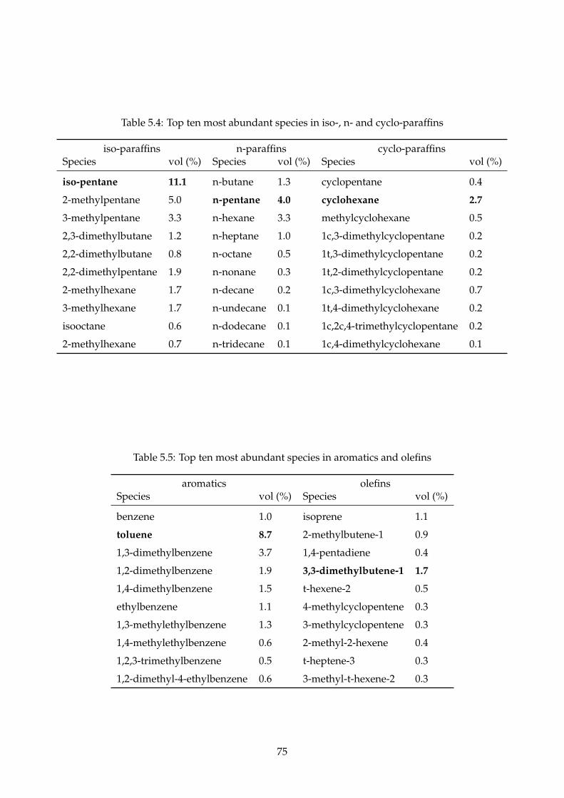
Table 5.4: Top ten most abundant species in iso-, n- and cyclo-paraffins

iso-paraffins n-paraffins cyclo-paraffinsSpecies vol (%) Species vol (%) Species vol (%)

iso-pentane 11.1 n-butane 1.3 cyclopentane 0.4

2-methylpentane 5.0 n-pentane 4.0 cyclohexane 2.7

3-methylpentane 3.3 n-hexane 3.3 methylcyclohexane 0.5

2,3-dimethylbutane 1.2 n-heptane 1.0 1c,3-dimethylcyclopentane 0.2

2,2-dimethylbutane 0.8 n-octane 0.5 1t,3-dimethylcyclopentane 0.2

2,2-dimethylpentane 1.9 n-nonane 0.3 1t,2-dimethylcyclopentane 0.2

2-methylhexane 1.7 n-decane 0.2 1c,3-dimethylcyclohexane 0.7

3-methylhexane 1.7 n-undecane 0.1 1t,4-dimethylcyclohexane 0.2

isooctane 0.6 n-dodecane 0.1 1c,2c,4-trimethylcyclopentane 0.2

2-methylhexane 0.7 n-tridecane 0.1 1c,4-dimethylcyclohexane 0.1

Table 5.5: Top ten most abundant species in aromatics and olefins

aromatics olefinsSpecies vol (%) Species vol (%)

benzene 1.0 isoprene 1.1

toluene 8.7 2-methylbutene-1 0.9

1,3-dimethylbenzene 3.7 1,4-pentadiene 0.4

1,2-dimethylbenzene 1.9 3,3-dimethylbutene-1 1.7

1,4-dimethylbenzene 1.5 t-hexene-2 0.5

ethylbenzene 1.1 4-methylcyclopentene 0.3

1,3-methylethylbenzene 1.3 3-methylcyclopentene 0.3

1,4-methylethylbenzene 0.6 2-methyl-2-hexene 0.4

1,2,3-trimethylbenzene 0.5 t-heptene-3 0.3

1,2-dimethyl-4-ethylbenzene 0.6 3-methyl-t-hexene-2 0.3

75

5.3.2 Strategy for emulating the octane number of the gasoline

A good gasoline should match RON, MON, heat of vaporisation, etc, which are important for SI engine

combustion. In the prior study, Foong et al. [9] formulated the three TRF-based gasoline surrogates

with 15%, 30% and 45% toluene by volume. To make these mixtures have RONs around 91, the

base PRF composition was adjusted. The same method is applied in this study to formulate the new

gasoline surrogates.

As shown in Fig.5.1, the TRF-based gasoline surrogates have higher octane numbers than the pro-

duction gasoline when blended with ethanol. Although this difference can be reduced by increasing

the fraction of toluene and decreasing the isooctane in the mixture using the optimal correlations in

Chapter 4 to estimate the octane number, the toluene content becomes too high relative to the aromat-

ics content typically found in production gasoline (25% in this study and 32% from Foong [23]). The

purpose of this study is to find the gasoline surrogates similar to the production gasoline regarding

both compositions and octane numbers when blended with ethanol.

Several strategies have been applied to formulate better gasoline surrogates.

• Cyclohexane and 1-hexene were added into TRFs, and three different gasoline surrogates named

GS1, GS2, and GS3 were developed, as shown in Table 5.6. The volume fractions of toluene in

these three mixtures are fixed to be 30%, which is similar to the concentration of aromatics in the

gasoline. Since the volume fractions of both cyclo-paraffins and olefins are around 10%, the GS3

is developed to meet these compositional requirements. In comparison, GS1 and GS2 have 20%

cyclohexane and 1-hexene respectively.

• Since toluene is known to have antagonistic blending behaviours with most hydrocarbons from

the previous binary mixtures experiments, other aromatics, including p-, m-, o-xylene, ethyl-

benzene, and 1,2,4-trimethylbenzene, were used to replace toluene to test whether they exhibit

stronger antagonism when blended with ethanol, and these mixtures are denoted by GS6 to

GS10.

• Based on the study of aromatics, 1,2,4-trimethylbenzene was selected to represent aromatics.

Besides, iso-pentane and n-pentane were also chosen for being the most abundant compound in

their respective class. Note that the additions of C5 components with low boiling points could

help to emulate the gasoline’s volatility (quantified by reid vapour pressure).

Note that all surrogate fuel were formulated to have the RON of 91. This was achieved by adjusting

the ratio of iso-paraffins and n-paraffins via trial-and-error method.

76

Table 5.6: Formulated gasoline surrogates

Surrogate Detailed compositions (vol %)

GS1 30% toluene+20% cyclohexane+50% PRF77

GS2 30% toluene+20% 1-hexene+50% PRF78

GS3 30% toluene+10% cyclohexane+10% 1-hexene+50% PRF77.5

GS4 30% toluene+10% cyclohexane+10% 1-hexene+32% i-C5+18% n-C5

GS5 30% 1,2,4-trimethylbenzene+10% cyclohexane+10% 1-hexene+50% PRF78

GS6 30% p-xylene+70% PRF70

GS7 30% m-xylene+70% PRF72

GS8 30% o-xylene+70% PRF81

GS9 30% 1,2,4-trimethylbenzene+70% PRF76

GS10 30% ethylbenzene+70% PRF74

GS11 30% 1,2,4-trimethylbenzene+10% cyclohexane+10% 1-hexene+38% i-C5+12% n-C5

5.3.3 Comparison between production gasoline and its surrogates when blended with

ethanol

Since the largest octane number difference between gasoline and its TRF-based surrogates appears

when approximately 40% (by volume) ethanol is added, the formulated eleven gasoline surrogates

listed in Table 5.6 were blended with the same amount of ethanol to compare their knock propensities

with the gasoline.

The effects of adding cyclohexane and 1-hexene into TRFs with 30% toluene by volume are shown

in Fig.5.9 (a). With 20% cyclohexane added, the mixture of GS1 and 40% ethanol has RON of 104.0

which is lower than the result of 105.1 from TRF91-30 reported in the prior experimental study [9].

The octane number is further decreased by 0.6 with GS2 which has 20% 1-hexene instead of cyclohex-

ane. However, production gasolines generally don’t contain such a large amount of cyclo-paraffins or

olefins, and the more reasonable surrogate is GS3 which has 10% cyclohexane and 10% 1-hexene re-

spectively. The octane number from GS3 is right in the middle of GS1 and GS2, indicating apparently

a linear trend when varying the concentrations of 1-hexene and cyclohexane.

Although GS1, GS2, and GS3 reduce the octane number difference, it is still not close to the target

value 101.6 which is the octane number of the production gasoline blended with 40% ethanol. In this

case, other aromatic hydrocarbons, including p-xylene, m-xylene, o-xylene, 1,2,4-trimethylbenzene,

and ethylbenzene, were used to replace toluene in TRF91-30. The results are plotted in Fig.5.9 (b). Of

interest is GS9 containing 30% 1,2,4-trimethylbenzene, whose octane number is 103.6 with 40% ethanol

added, while the measurements for the other four surrogates range from 104.2 to 104.7, suggesting

77

1,2,4-trimethylbenzene produces a stronger antagonistic effect with ethanol than other aromatics re-

garding decreasing the octane number gap.

Considering the strong antagonistic effect of 1,2,4-trimethylbenzene, this aromatic compound is

applied to replace toluene in GS3 to formulate GS5 which has RON of 103.0 with 40% ethanol added,

as shown in Fig.5.9(c). Also, another attempt is to use iso-pentane and n-pentane instead of isooc-

tane and n-heptane in the gasoline surrogates, as the former two have much higher concentrations in

the gasoline. Therefore, another five-component gasoline surrogate GS4 is formed, and the resulting

octane number is 103.1. GS4 and GS5 are thus two gasoline surrogates having the lowest octane num-

bers than the other mixtures with 40% ethanol added. Considering that 1,2,4-trimethylbenzene and

C5 paraffins both reduce the octane number difference effectively, another gasoline surrogate, GS11,

containing all aforementioned favourable compounds, is formulated, which has RON of 102.1 with

40% ethanol blended. With GS11, the RON difference has been reduced to 0.5 which is smaller than

the tolerance of 0.9 for RON measurements of this octane number range. To have a comprehensive

comparison between GS11 and the gasoline, different amounts of ethanol were added into GS11 and

the resulting RONs are plotted in Fig.5.9(c). Although the largest RON difference across the entire

range is 0.7 with 60% ethanol addition, it is found that the differences are very small at lower ethanol

concentrations which are practical range of current ethanol blending.

Due to the nature of octane number tests, the equivalence ratios had to be varied to achieve

the standard knocking conditions. The equivalence ratios of gasoline/ethanol and GS11/ethanol at

standard knocking conditions are listed in Table 5.7 which includes previous measurements from

Foong [23] as well. It is apparent that the equivalence ratios of gasoline/ethanol mixtures reported in

this study are similar to Foong’s results [23] and comparable to those of GS11 and ethanol mixtures.

This study also compares other physical properties between the gasoline and the formulated gasoline

surrogates, as shown in Table 5.8. Note that the heat of vaporisation is quantified by the mixture tem-

perature which is measured downstream of the carburettor and right before the intake port. Table 5.8

shows that the mixture temperatures of both the gasoline and GS11 are 291 K, indicating the similar

level of heat of vaporisation. Besides, the contents of iso-pentane and n-pentane in GS11 are very sim-

ilar to the volume fractions of iso-paraffins and n-paraffins which are 39.9% and 10.7% respectively in

the gasoline. In the following MON tests, the MONs of GS11 with and without 40% ethanol are 88.0

and 81.6 respectively, which are higher than the values of 85.4 and 80.3 from the gasoline. This is not

totally unexpected, as the formulation is focused on RON instead of MON.

The above results indicate that although isooctane, n-heptane, and toluene are commonly regarded

as useful surrogate compounds, they cannot match the anti-knock behaviours of the production gaso-

line when blended with ethanol if their concentrations are constrained by the hydrocarbon class dis-

78

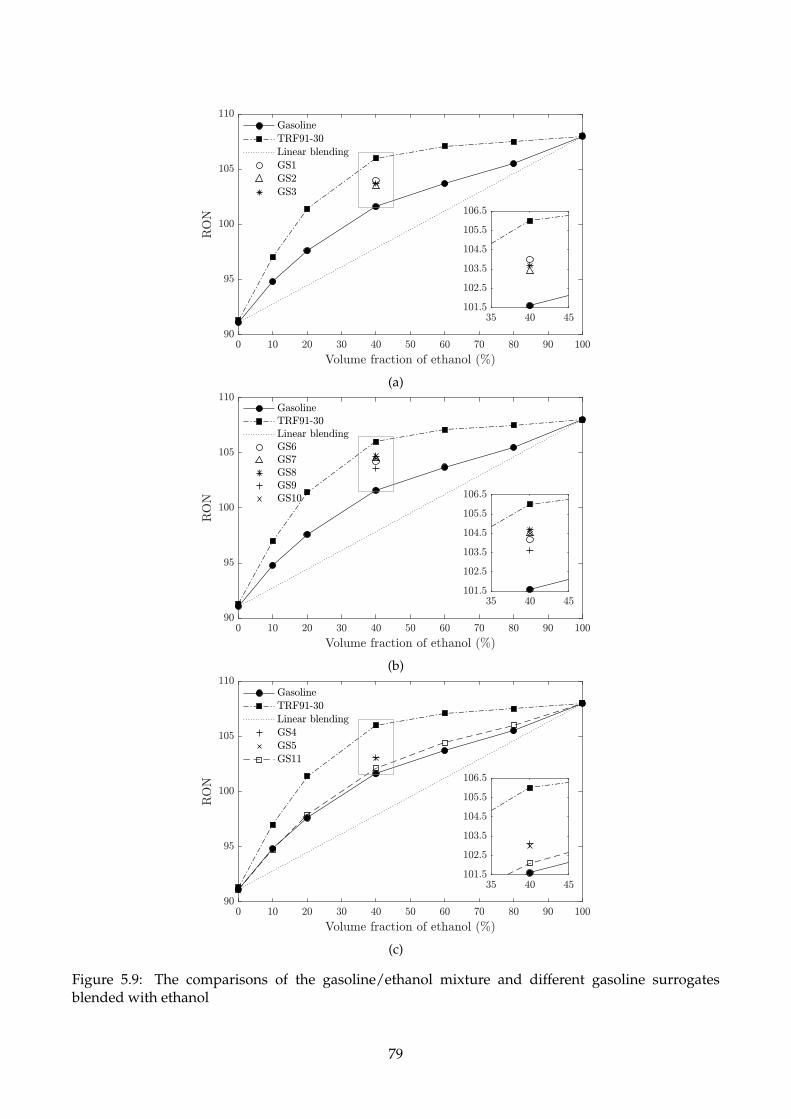
(a)

(b)

(c)

Figure 5.9: The comparisons of the gasoline/ethanol mixture and different gasoline surrogatesblended with ethanol

79

Table 5.7: Equivalence ratios of gasoline/ethanol and GS11/ethanol at standard knocking conditions

Mixtures E0 E10 E20 E40 E60 E80 E100

Gasoline/ethanol a 1.05 1.03 1.03 0.98 0.99 1.02 1.03

Gasoline/ethanol b 1.06 1.04 1.04 1.02 1.01 1.01 1.03

GS11/ethanol a 1.14 1.07 1.03 0.99 1.00 1.05 1.03a Data from this studyb Data from Foong’s experiments [23]

Table 5.8: The physical properties of the gasoline and the gasoline surrogates

Fueldensity(g/ml)

H/C ratioMW(g/mol)

RON(+40% EtOH)

Mixture T atRON test (K)

Gasoline 0.73 1.87 92.06 101.6 291

GS1 0.61 1.81 97.48 104 -

GS2 0.61 1.80 97.98 103.4 -

GS3 0.75 1.80 97.73 103.7 289

GS4 0.72 1.84 80.71 103.1 291

GS5 0.75 1.87 107.00 103.0 -

GS6 1.16 1.89 108.21 104.2 -

GS7 1.17 1.89 108.40 104.5 -

GS8 1.25 1.88 109.22 104.7 -

GS9 1.21 1.92 113.55 103.6 -

GS10 1.20 1.89 108.58 104.5 -

GS11 0.72 1.91 87.28 102.1 291

80

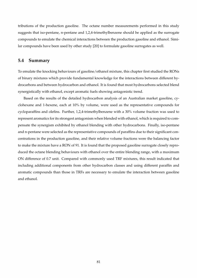
tributions of the production gasoline. The octane number measurements performed in this study

suggests that iso-pentane, n-pentane and 1,2,4-trimethylbenzene should be applied as the surrogate

compounds to emulate the chemical interactions between the production gasoline and ethanol. Simi-

lar compounds have been used by other study [20] to formulate gasoline surrogates as well.

5.4 Summary

To emulate the knocking behaviours of gasoline/ethanol mixture, this chapter first studied the RONs

of binary mixtures which provide fundamental knowledge for the interactions between different hy-

drocarbons and between hydrocarbon and ethanol. It is found that most hydrocarbons selected blend

synergistically with ethanol, except aromatic fuels showing antagonistic trend.

Based on the results of the detailed hydrocarbon analysis of an Australian market gasoline, cy-

clohexane and 1-hexene, each at 10% by volume, were used as the representative compounds for

cycloparaffins and olefins. Further, 1,2,4-trimethylbenzene with a 30% volume fraction was used to

represent aromatics for its strongest antagonism when blended with ethanol, which is required to com-

pensate the synergism exhibited by ethanol blending with other hydrocarbons. Finally, iso-pentane

and n-pentane were selected as the representative compounds of paraffins due to their significant con-

centrations in the production gasoline, and their relative volume fractions were the balancing factor

to make the mixture have a RON of 91. It is found that the proposed gasoline surrogate closely repro-

duced the octane blending behaviours with ethanol over the entire blending range, with a maximum

ON difference of 0.7 unit. Compared with commonly used TRF mixtures, this result indicated that

including additional components from other hydrocarbon classes and using different paraffin and

aromatic compounds than those in TRFs are necessary to emulate the interaction between gasoline

and ethanol.

81

Chapter 6

Oxidation of Ethanol and Hydrocarbon

Mixtures in a Flow Reactor

6.1 Introduction

Octane rating is closely related to autoignition chemistry of the unburned fuel/air mixtures in SI

engines. Kinetic modelling of SI engines autoignition has been attempted for gasoline and ethanol

mixtures by Foong et al. [46] and the author ([Yuan et al., SAE Paper 2015-01-1242], reported in Ap-

pendix C). These efforts suggested that the existing chemistry models are unable to reproduce the

octane behaviours observed in the CFR engine experiments. Therefore, this chapter uses a recently

built PFR which is designed to operate at up to 1000 K and 50 bar in Thermodynamics Laboratory,

the University of Melbourne, to investigate the autoignition chemistry of hydrocarbon and ethanol

mixtures. The PFR experiments in this study were carried out at a nominal temperature around 900 K

which is related to the autoignition temperature in the CFR engine [46]. Note that the knock related

chemistry may occur at lower temperatures. However, not all fuels tested in this study have low tem-

perature chemistry, and the purpose of this study is to systematically check the existing models with

a comprehensive fuel matrix. Therefore, the intermediate temperature of 900 K is chosen in this study.

This PFR study focuses on evaluating the existing chemical mechanisms that can be used to reproduce

the engine measurements.

Neat fuels, binary mixtures, gasoline surrogates and their mixtures with ethanol were tested in

the PFR at 900 K (except 930 K for neat toluene) and 10 bar. The fuel matrix and the PFR operating

conditions in this work are listed in Table 6.1 and 6.2 respectively. The Horiba emission bench was

used to measure the CO concentration with a non-dispersive infrared (NDIR) analyser with a resolu-

tion of 20 PPM. Other intermediate species including the parent fuels were measured using the gas

chromatography (GC) discussed in Chapter 3, whose measurement uncertainties are around 10%. As

82

mentioned in Chapter 3, the reacting gas temperatures are calculated based on measurements from

three K-type thermocouples using the so called three-thermocouple method [201].

Table 6.1: Test fuels and reaction mechanisms for modelling

Fuel Mechanism Composition

IsooctaneAtef et al. [68]Mehl et al. [67]Andrae [187]

isooctanegasoline surrogate and ethanolgasoline surrogate and ethanol

Ethanol

Marinov [181]Mittal et al. [184]Mehl et al . [67]Andrae [187]

ethanolethanolgasoline surrogate and ethanolgasoline surrogate and ethanol

Toluene

Metcalfe et al. [138]Yuan et al. [163]Mehl et al . [67]Andrae [187]

toluenetoluenegasoline surrogate and ethanolgasoline surrogate and ethanol

Isooctane/ethanolIsooctane/tolueneEthanol/toluene

Mehl et al. [67]TestMecha

gasoline surrogate and ethanolgasoline surrogate and ethanol

PRF91b

TRF91-30cMehl et al. [67]TestMech


PRF91/ethanolTRF91-30/ethanol

Mehl et al. [67]TestMech


a TestMech: the mechanism from this studyb PRF91: 91% isooctane and 9% n-heptanec TRF91-30: 53.2% isooctane, 17.0% n-heptane, and 29.8% toluene [9]

83

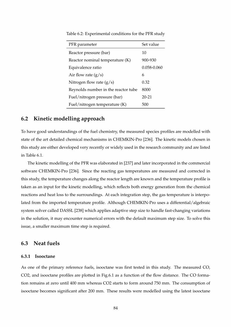
Table 6.2: Experimental conditions for the PFR study

PFR parameter Set value

Reactor pressure (bar) 10

Reactor nominal temperature (K) 900-930

Equivalence ratio 0.058-0.060

Air flow rate (g/s) 6

Nitrogen flow rate (g/s) 0.32

Reynolds number in the reactor tube 8000

Fuel/nitrogen pressure (bar) 20-21

Fuel/nitrogen temperature (K) 500

6.2 Kinetic modelling approach

To have good understandings of the fuel chemistry, the measured species profiles are modelled with

state of the art detailed chemical mechanisms in CHEMKIN-Pro [236]. The kinetic models chosen in

this study are either developed very recently or widely used in the research community and are listed

in Table 6.1.

The kinetic modelling of the PFR was elaborated in [237] and later incorporated in the commercial

software CHEMKIN-Pro [236]. Since the reacting gas temperatures are measured and corrected in

this study, the temperature changes along the reactor length are known and the temperature profile is

taken as an input for the kinetic modelling, which reflects both energy generation from the chemical

reactions and heat loss to the surroundings. At each integration step, the gas temperature is interpo-

lated from the imported temperature profile. Although CHEMKIN-Pro uses a differential/algebraic

system solver called DASSL [238] which applies adaptive step size to handle fast-changing variations

in the solution, it may encounter numerical errors with the default maximum step size. To solve this

issue, a smaller maximum time step is required.

6.3 Neat fuels

6.3.1 Isooctane

As one of the primary reference fuels, isooctane was first tested in this study. The measured CO,

CO2, and isooctane profiles are plotted in Fig.6.1 as a function of the flow distance. The CO forma-

tion remains at zero until 400 mm whereas CO2 starts to form around 750 mm. The consumption of

isooctane becomes significant after 200 mm. These results were modelled using the latest isooctane

84

mechanisms from Atef et al. [68] and two gasoline surrogate mechanisms from Mehl et al. [67] and

Andrae [187]. The modelling results are also shown in Fig.6.1. Among these mechanisms, the one

from Mehl et al. [67] best reproduces the measured species profiles, while Andrae’s mechanism [187]

and Atef et al.’s mechanism [68] under-predicts and over-predicts the isooctane oxidation reactivity

respectively in the PFR.

The profiles of intermediate species are plotted separately with the corresponding modelling re-

sults in Fig.6.2. Note that the flame ionization detector used in this study cannot detect inorganic

substances and highly oxygenated species. This is why some common intermediates from isooc-

tane oxidation, like hydrogen and formaldehyde, are not included in Fig.6.2. The most significant

and abundant intermediate species is isobutylene (IC4H8) whose profile is well predicted by Mehl et

al. [67], slightly over-predicted by Andrae [187], and significantly under-predicted by the most recent

mechanism from Atef et al. [68]. The reaction pathways for IC4H8 are shown in Fig.6.3. As for the

predictions of the small species, such as methane, ethylene, and propylene, the model from Mehl et

al. [67], again, performs the best, while the other two models [68, 187] reasonably reproduce the pro-

files. It is noticed that these models all under-predict the profiles for the oxygenated compounds, but

Mehl et al.’s model [67] exhibits good fidelity to the measurements in terms of matching the posi-

tions where the peak values appear. The reaction pathway for one of these oxygenated compounds,

IC3H5CHO, is show in Fig.6.4. The largest intermediate species detected from the isooctane oxidation

are XC7H14 (2,4-dimethyl-1-pentene) and YC7H14 (2,4-dimethyl-2-pentene) whose concentrations are

much smaller than the others’. The mechanism developed by Mehl et al. [67] over-estimates the con-

centration of XC7H14 and under-estimates YC7H14. The reaction pathways for XC7H14 and YC7H14

are shown in Fig.6.3.

The intermediate species shown in Fig.6.2 have been reported by previous experimental studies

[58, 59, 61, 239] as well. Among all these works, the flow reactor experiments from Chen et al. [61]

have the closest experimental conditions to this study. The peak values of different hydrocarbon

species from these two experiments are similar, except for the oxygenated compounds. The measured

oxygenated compounds from this study have higher concentrations than those from Chen et al. [61].

Since the isooctane sub-model from the gasoline surrogate mechanism [67] was developed based on

the measurements from Chen et al. [61], this is why the existing model under-estimates the profiles of

the oxygenated compounds from this study. Currently, the causes for the discrepancies between the

measured oxygenated compounds from this study and Chen et al. [61] are not known, and thus more

kinetic experiments are required to explain the differences, which could be a future work of this study.

85

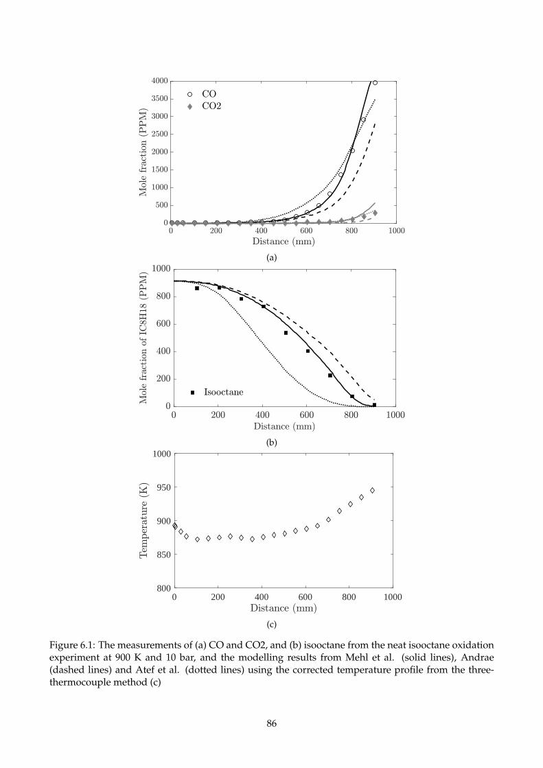
(a)

(b)

0 200 400 600 800 1000800

850

900

950

1000

(c)

Figure 6.1: The measurements of (a) CO and CO2, and (b) isooctane from the neat isooctane oxidationexperiment at 900 K and 10 bar, and the modelling results from Mehl et al. (solid lines), Andrae(dashed lines) and Atef et al. (dotted lines) using the corrected temperature profile from the three-thermocouple method (c)

86

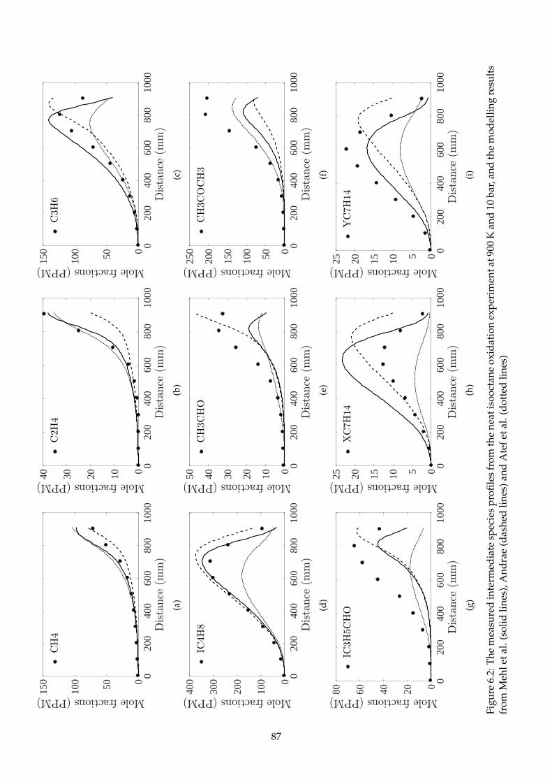
020

040

060

080

010

00050100

150

(a)

020

040

060

080

010

00010203040

(b)

020

040

060

080

010

00050100

150

(c)

020

040

060

080

010

000

100

200

300

400

(d)

020

040

060

080

010

0001020304050

(e)

020

040

060

080

010

00050100

150

200

250

(f)

020

040

060

080

010

00020406080

(g)

020

040

060

080

010

000510152025

(h)

020

040

060

080

010

000510152025

(i)

Figu

re6.

2:Th

em

easu

red

inte

rmed

iate

spec

ies

profi

les

from

the

neat

isoo

ctan

eox

idat

ion

expe

rim

enta

t900

Kan

d10

bar,

and

the

mod

ellin

gre

sult

sfr

omM

ehle

tal.

(sol

idlin

es),

And

rae

(das

hed

lines

)and

Ate

feta

l.(d

otte

dlin

es)

87

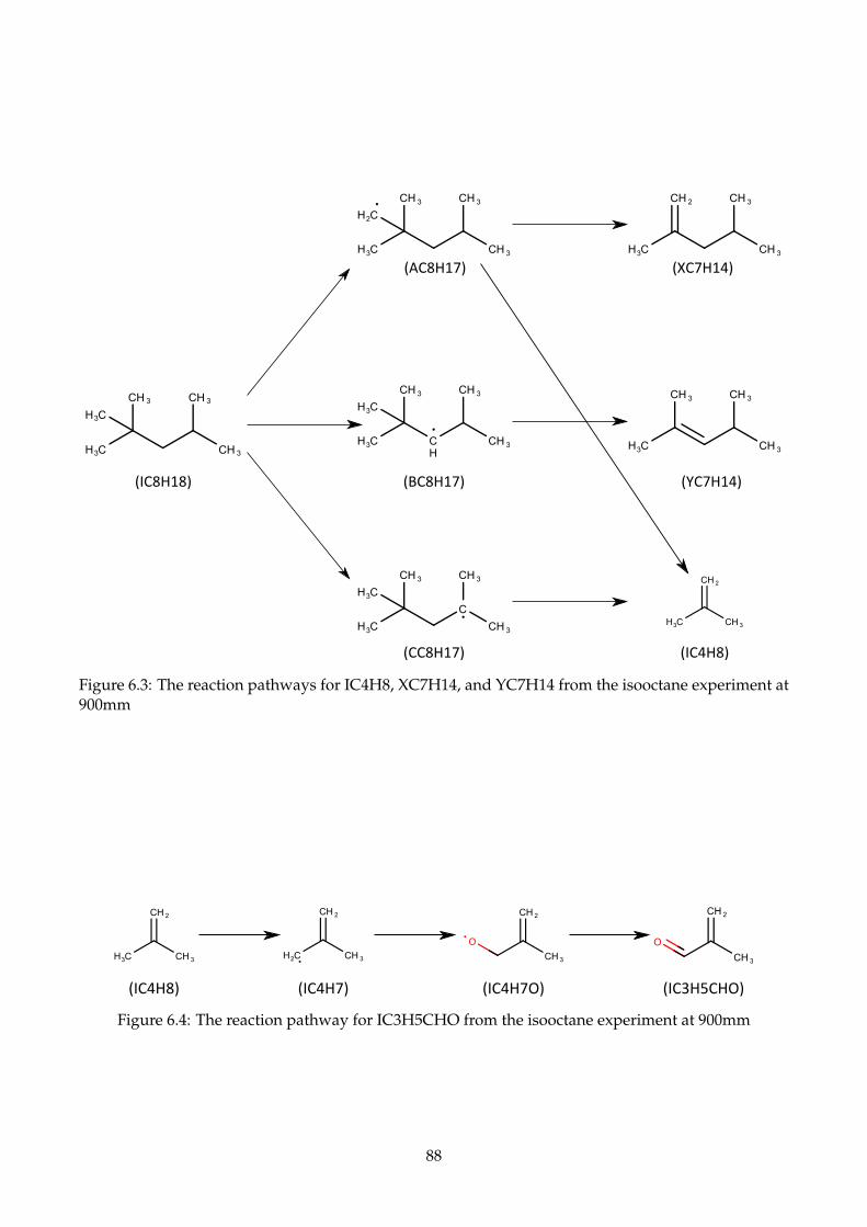
Figure 6.3: The reaction pathways for IC4H8, XC7H14, and YC7H14 from the isooctane experiment at900mm

(IC4H8) (IC4H7) (IC4H7O) (IC3H5CHO)

Figure 6.4: The reaction pathway for IC3H5CHO from the isooctane experiment at 900mm

88

6.3.2 Ethanol

The CO, CO2, and fuel profiles for ethanol, together with the modelling results are shown in Fig.6.5.

Marinov’s mechanism [181] is one of the earliest comprehensive mechanisms for ethanol, which under-

predicts the ethanol’s reactivity in this study. Three more recent mechanisms from Mehl et al. [67],

Andrae [187], and Mittal et al. [184] perform similarly, which produce excellent agreements for CO

and ethanol profiles but fail to match the CO plateau. The agreements suggest that the models accu-

rately capture the chemistry where ethanol converts to CO. The discrepancies in the CO plateau are

significant, which are probably caused by the problematic kinetics of CO to CO2 conversion as the

CO2 profile is over-predicted by all these three mechanisms.

The measured intermediate species from the ethanol oxidation are methane, ethylene, and ac-

etaldehyde, as shown in Fig.6.6. The most abundant intermediate species is acetaldehyde whose pro-

file is overall well-predicted by Mehl et al. [67] and the reaction pathways for acetaldehyde are shown

in Fig.6.7. Besides, the methane profile is well captured with the same mechanism as well. However,

this mechanism has difficulty to reproduce the ethylene profile and the level of over-prediction is sig-

nificant. In comparison, the predictions from Andrae’s model [187] match well with the measured

ethylene profile but not with the other species. The discrepancies between the measurements and

modellings are likely due to the super lean experimental conditions, against which the existing kinetic

models may not be fully validated.

The intermediates shown in Fig.6.6 were also reported in a flow reactor [202], a jet-stirred reac-

tor [175], and a rapid compression machine [240]. Although it is difficult to compare the measure-

ments from the different reactors due to different experimental conditions, the relative concentrations

of the major intermediate, acetaldehyde, from these experiments are overall comparable with the mea-

surement in this study, especially when taking their initial contents of ethanol into account. Note that

in the most recent rapid compression machine study [240], the initial mole fraction of ethanol is one

order of magnitude higher than those of the aforementioned experiments, making its results not com-

parable with others.

89

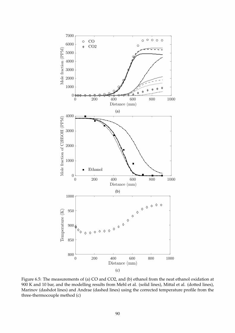
(a)

(b)

0 200 400 600 800 1000800

850

900

950

1000

(c)

Figure 6.5: The measurements of (a) CO and CO2, and (b) ethanol from the neat ethanol oxidation at900 K and 10 bar, and the modelling results from Mehl et al. (solid lines), Mittal et al. (dotted lines),Marinov (dashdot lines) and Andrae (dashed lines) using the corrected temperature profile from thethree-thermocouple method (c)

90

0 200 400 600 800 10000

100

200

300

400

500

600

700

(a)

0 200 400 600 800 10000

200

400

600

800

(b)

0 200 400 600 800 10000

200

400

600

800

(c)

Figure 6.6: The measured intermediate species profiles from the neat ethanol oxidation at 900 K and10 bar, and the modelling results from Mehl et al. (solid lines), Mittal et al. (dotted lines), Marinov(dashdot lines) and Andrae (dashed lines)

91

Figure 6.7: The reaction pathway for CH3CHO from the ethanol experiment at 500mm

6.3.3 Toluene

Comparing with isooctane and ethanol, toluene has much lower reactivity and barely reacts at 900 K.

Therefore, the experiment was conducted at a higher temperature, 930 K. Even at this temperature,

the measured CO concentrations are significantly lower than those of isooctane and ethanol, as shown

in Fig.6.8. The modelling results show that only the predictions from the mechanisms of Metcalfe

et al. [138] and Zhang et al. [241] agree reasonably well with the measurements. The other three

mechanisms from Mehl et al. [67], Yuan et al. [163] and, in particular, Andrae [187] and Pelucchi et

al. [242] substantially over-predict the toluene’s reactivity. Therefore, it is necessary to examine the

existing toluene sub-model to reproduce the measured species profiles in this study.

Since the reactivity of toluene at 930 K is low, benzene is the only intermediate detected by the

GC and has a much smaller fraction compared with toluene. The comparison between the measured

benzene profile and the modelling results from the aforementioned mechanisms is shown in Fig.6.9.

Although the kinetic models from Mehl et al. [67] and Yuan et al. [163] over-predict the overall reac-

tivity, their predictions on the benzene formation are lower than the measurement. This inconsistency

may come from the mechanisms themselves or the measurement uncertainties of species with small

amounts.

As one of the most important intermediate species, benzene was detected in two recent experi-

mental studies performed in the flow reactor [138] and the jet-stirred reactor [163] respectively. Under

comparable conditions to our experiments, similarly small levels of benzene concentrations were ob-

served in these experiments.

92

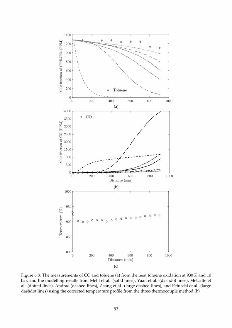
(a)

(b)

0 200 400 600 800 1000800

850

900

950

1000

(c)

Figure 6.8: The measurements of CO and toluene (a) from the neat toluene oxidation at 930 K and 10bar, and the modelling results from Mehl et al. (solid lines), Yuan et al. (dashdot lines), Metcalfe etal. (dotted lines), Andrae (dashed lines), Zhang et al. (large dashed lines), and Pelucchi et al. (largedashdot lines) using the corrected temperature profile from the three-thermocouple method (b)

93

Figure 6.9: The measured benzene profile from the neat toluene oxidation at 930 K and 10 bar, and themodelling results from Mehl et al. (solid line), Yuan et al. (dashdot line), Metcalfe et al. (dotted line),Andrae (dashed line), Zhang et al. (large dashed lines), and Pelucchi et al. (large dashdot lines)

6.4 Test mechanism

In order to improve the modelling of species profiles from the neat toluene oxidation, a test mechanism

is proposed based on the toluene sub-model from Mehl et al.’s gasoline surrogate mechanism [67].

6.4.1 Sensitivity analysis

In this study, an in-house PFR model was developed in Python with the VODE solver and designed

to run in parallel on a high performance computing (HPC) system for the sensitivity analysis. The

details of this in-house model can be found in Appendix D.

A sensitivity analysis was carried out for the toluene oxidation at 930 K and 10 bar using the gaso-

line surrogate mechanism from Mehl et al. [67]. When conducting the analysis, each pre-exponential

factor, A, was increased by two times to produce a temporary chemical mechanism, and the total

number of the temporary mechanisms is over 10,000. All these generated mechanisms were applied

to model the neat toluene oxidation, and their resulting maximum CO concentrations, denoted by

COi, were compared with the CO concentration from the original gasoline surrogate mechanism, rep-

resented by COref. Therefore, the sensitivity coefficient (SC) is given by:

(6.1)SC =COi − COre f

COre f

The elementary reactions having the top 30 largest absolute sensitivity coefficients for the toluene

oxidation at 930 K and 10 bar are shown in Fig.6.10 where positive sensitivity coefficients indicate that

increasing the rate constants of the corresponding elementary reactions enhances the CO formation

94

and negative coefficients suggest the opposite trend. It is noticed that the high-sensitivity elementary

reactions mostly contain toluene or toluene-like species.

6.4.2 Updated toluene sub-mechanism

To update the existing toluene sub-mechanism, the rate constants of those most sensitive elementary

reactions require careful investigations. Considering the sparsity of the accurate rate constants for

these high-sensitivity reactions, either from experimental measurements or theoretical computations,

only the top eight most sensitive elementary reactions are analysed for updates in their rate constants.

Since Metcalfe et al.’s mechanism [138] performs the best as shown in Fig.6.8, the rate constants from

Mehl et al’s model [67] were replaced by those from [138], if related fundamental experiments and

theoretical computations are not available.

Reaction 6.2 is found to be the most sensitive elementary reaction from the sensitivity analysis

as shown in Fig.6.10. Both Mehl et al. [67] and Metcalfe et al. [138] only assigned pre-exponential

factors as the rate constants for this elementary reaction, indicating the reaction is independent of

temperature and pressure in their mechanisms. However, the quantum chemical study of da Silva

and Bozzelli [243] proposed a more complex and lower rate constant for Reaction 6.2 compared with

the values used by those two mechanisms. Note that the rate constants from da Silva and Bozzelli [243]

are at atmospheric pressure. Zhang et al. [241] extended the rate constants to different pressures with

Quantum-Rice˙Ramsperger-Kassel theory. Therefore, this study uses the updated rate constants from

Zhang et al. [241] for Reaction 6.2.

(6.2)C6H5CH2J + HO2 = C6H5CH2OJ + OH

The rate constants of Reaction 6.3 and 6.4 from Mehl et al. [67] were updated by the values from

Baulch et al. [244] and Metcalfe et al. [138]. The updated rate constants were used in Metcalfe et al.’s

toluene mechanism [138] which produce good agreements with the measurements from this study, as

shown in Fig.6.8. The changes made to the toluene sub-model in the gasoline surrogate model [67] are

listed in Table 6.3.

(6.3)C6H5CH3 + HO2 = C6H5CH2J + H2O2

(6.4)C6H5OJ + HO2 = RODC6JDO + OH

Although Reaction 6.5 to 6.9 have high sensitivities, this study keeps the original rate constants

from Mehl et al. [67] for these reactions due to the following reasons. First, the rate constants of these

five reactions haven’t been investigated by fundamental experiments or theoretical computations. It

is difficult to figure out whether the original rate constants from Mehl et al. [67] need to be updated.

Second, Reaction 6.5 and 6.6 don’t appear in Metcalfe et al.’s model [138], while the rate constants of

95

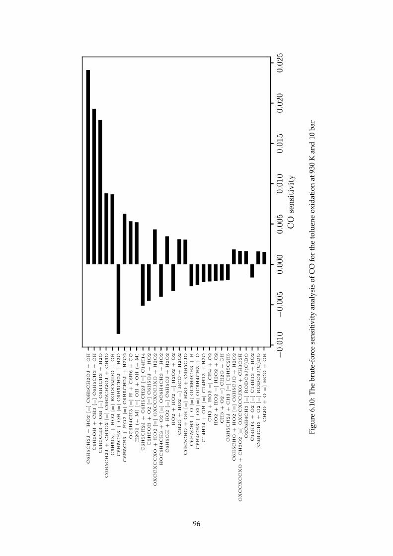
−0.0

10

−0.0

050.

000

0.00

50.

010

0.01

50.

020

0.02

5

CO

sen

siti

vit

y

C6H

5C

H2J

+H

O2

[=]

C6H

5C

H2O

J+

OH

C6H

5O

H+

CH

3[=

]C

6H

5C

H3

+O

H

C6H

5C

H3

+O

H[=

]C

6H

4C

H3

+H

2O

C6H

5C

H2J

+C

H3O

2[=

]C

6H

5C

H2O

J+

CH

3O

C6H

5O

J+

HO

2[=

]R

OD

C6JD

O+

OH

C6H

5C

H3

+O

H[=

]C

6H

5C

H2J

+H

2O

C6H

5C

H3

+H

O2

[=]

C6H

5C

H2J

+H

2O

2

OC

6H

4C

H3

[=]

H+

C6H

6+

CO

H2O

2(+

M)

[=]

OH

+O

H(+

M)

C6H

5C

H2J

+C

6H

5C

H2J

[=]

C14H

14

C6H

5O

H+

O2

[=]

C6H

5O

J+

HO

2

OX

CC

XC

CX

O+

HO

2[=

]O

XC

CX

CC

JX

O+

H2O

2

HO

C6H

4C

H3

+O

2[=

]O

C6H

4C

H3

+H

O2

C6H

5O

H+

HO

2[=

]C

6H

5O

J+

H2O

2

HO

2+

HO

2=

]H

2O

2+

O2

CH

2O

+H

O2

=]

HC

O+

H2O

2

C6H

5C

HO

+O

H[=

]H

2O

+C

6H

5C

JO

C6H

5C

H3

+O

[=]

OC

6H

4C

H3

+H

C6H

4C

H3

+O

2[=

]O

C6H

4C

H3

+O

C14H

14

+O

H[=

]C

14H

13

+H

2O

CH

3+

HO

2=

]C

H4

+O

2

HO

2+

HO

2=

]H

2O

2+

O2

CH

3+

O2

=]

CH

2O

+O

H

C6H

5C

H2J

+C

H3

[=]

C6H

5C

2H

5

C6H

5C

HO

+H

O2

[=]

C6H

5C

JO

+H

2O

2

OX

CC

XC

CX

O+

CH

3O

2[=

]O

XC

CX

CC

JX

O+

CH

3O

2H

O2C

6H

4C

H3

[=]

RO

DC

6J(C

)D

O

C14H

14

+O

2[=

]C

14H

13

+H

O2

C6H

4C

H3

+O

2[=

]R

OD

C6J(C

)D

O

CH

2O

+O

=]

HC

O+

OH

Figu

re6.

10:T

hebr

ute-

forc

ese

nsit

ivit

yan

alys

isof

CO

for

the

tolu

ene

oxid

atio

nat

930

Kan

d10

bar

96

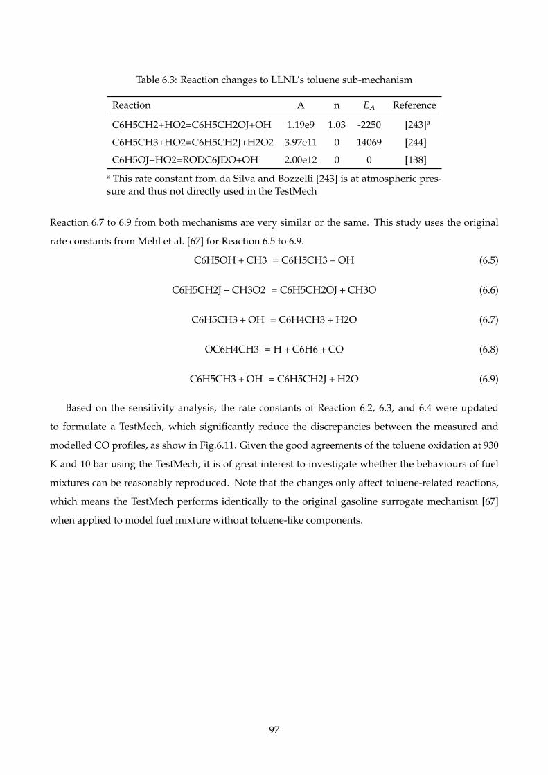
Table 6.3: Reaction changes to LLNL’s toluene sub-mechanism

Reaction A n EA Reference

C6H5CH2+HO2=C6H5CH2OJ+OH 1.19e9 1.03 -2250 [243]a

C6H5CH3+HO2=C6H5CH2J+H2O2 3.97e11 0 14069 [244]

C6H5OJ+HO2=RODC6JDO+OH 2.00e12 0 0 [138]a This rate constant from da Silva and Bozzelli [243] is at atmospheric pres-sure and thus not directly used in the TestMech

Reaction 6.7 to 6.9 from both mechanisms are very similar or the same. This study uses the original

rate constants from Mehl et al. [67] for Reaction 6.5 to 6.9.

(6.5)C6H5OH + CH3 = C6H5CH3 + OH

(6.6)C6H5CH2J + CH3O2 = C6H5CH2OJ + CH3O

(6.7)C6H5CH3 + OH = C6H4CH3 + H2O

(6.8)OC6H4CH3 = H + C6H6 + CO

(6.9)C6H5CH3 + OH = C6H5CH2J + H2O

Based on the sensitivity analysis, the rate constants of Reaction 6.2, 6.3, and 6.4 were updated

to formulate a TestMech, which significantly reduce the discrepancies between the measured and

modelled CO profiles, as show in Fig.6.11. Given the good agreements of the toluene oxidation at 930

K and 10 bar using the TestMech, it is of great interest to investigate whether the behaviours of fuel

mixtures can be reasonably reproduced. Note that the changes only affect toluene-related reactions,

which means the TestMech performs identically to the original gasoline surrogate mechanism [67]

when applied to model fuel mixture without toluene-like components.

97

Figure 6.11: The measurements of CO and toluene from the neat toluene oxidation at 930 K and 10bar, and the modelling results from Mehl et al. (solid lines) and TestMech (dashed lines)

6.5 Binary mixtures

The proposed TestMech is capable of predicting the measurements of all neat fuels tested in this study.

However, practical fuels are all mixtures. In this regard, it is critical to understand the behaviours

of fuel mixtures in the PFR, which are good tests for the state of the art surrogate mechanisms as

well. Therefore, binary mixtures were studied in this subsection, which includes ethanol/isooctane,

toluene/isooctane, and ethanol/toluene. Apart from the TestMech, the gasoline surrogate mechanism

from Mehl et al. [67] is also applied in the following kinetic modellings for fuel mixtures. This mecha-

nism [67] was used by several recent experimental studies [245–248] to model ignition delays in shock

tubes and rapid compression machines. It was found that the mechanism [67] performs reasonably

well in terms of predicting experimental results but requires improvements for TRF mixtures with

high toluene fraction [246], which is consistent with the results from the experiments of the neat com-

pounds in this study. To the knowledge of the author, the mechanism [67] has not been systematically

validated with the species profiles from fuel mixtures in either flow reactors or jet-stirred reactors.

6.5.1 Ethanol and isooctane

Ethanol and isooctane mixtures were first tested in this study at 900 K and 10 bar. The mole frac-

tions of ethanol in these mixtures are 25%, 50%, and 74%. The measured CO profiles and corrected

temperature profiles using the three-thermocouple method are shown in Fig.6.12. Both Mehl et al.’s

gasoline surrogate model [67] and the TestMech proposed by this study were applied to model the CO

profiles. The modelling results well reproduced the measured CO profiles as shown in Fig.6.12, indi-

cating the interactions between isooctane and ethanol are well taken care of by the existing chemical

98

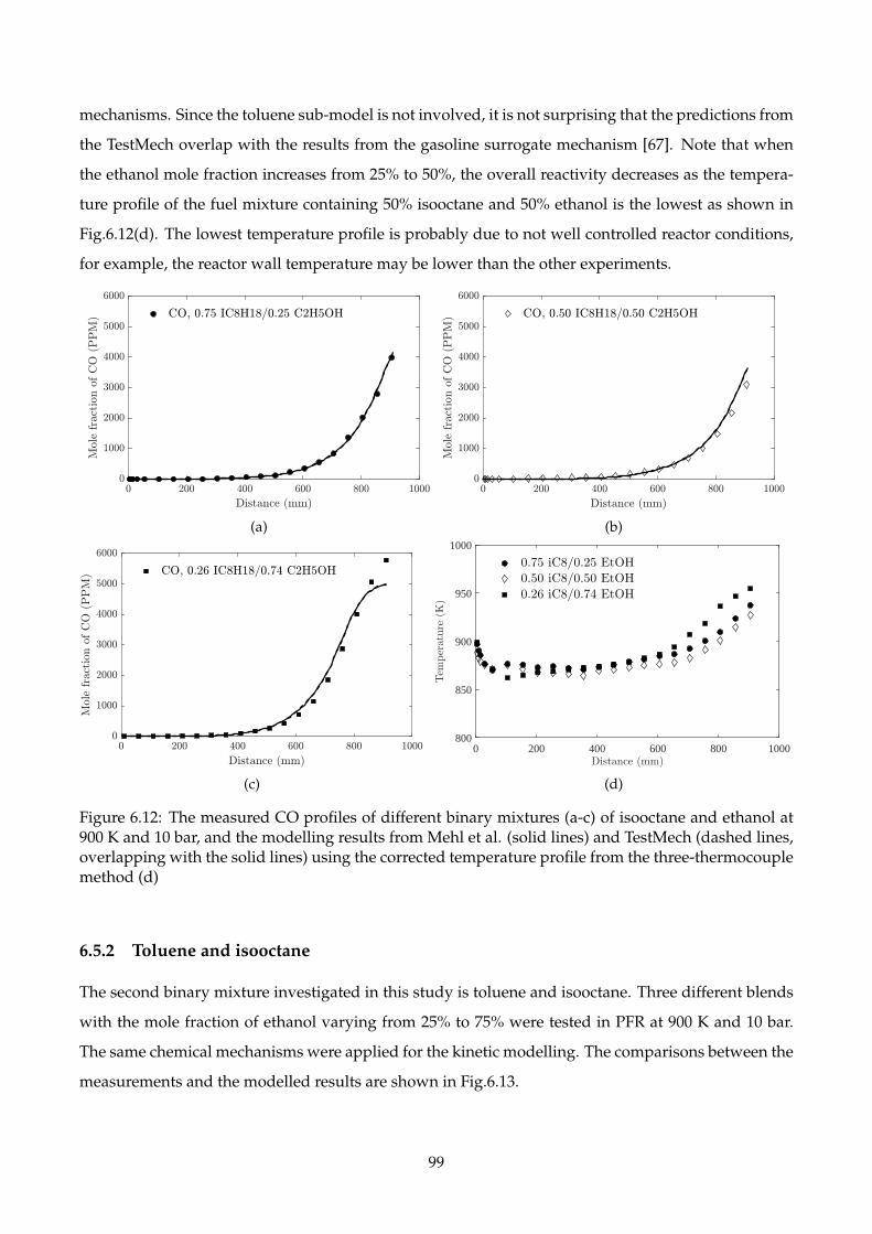
mechanisms. Since the toluene sub-model is not involved, it is not surprising that the predictions from

the TestMech overlap with the results from the gasoline surrogate mechanism [67]. Note that when

the ethanol mole fraction increases from 25% to 50%, the overall reactivity decreases as the tempera-

ture profile of the fuel mixture containing 50% isooctane and 50% ethanol is the lowest as shown in

Fig.6.12(d). The lowest temperature profile is probably due to not well controlled reactor conditions,

for example, the reactor wall temperature may be lower than the other experiments.

(a) (b)

(c)

Distance (mm)0 200 400 600 800 1000

Tem

perature

(K)

800

850

900

950

1000

0.75 iC8/0.25 EtOH0.50 iC8/0.50 EtOH0.26 iC8/0.74 EtOH

(d)

Figure 6.12: The measured CO profiles of different binary mixtures (a-c) of isooctane and ethanol at900 K and 10 bar, and the modelling results from Mehl et al. (solid lines) and TestMech (dashed lines,overlapping with the solid lines) using the corrected temperature profile from the three-thermocouplemethod (d)

6.5.2 Toluene and isooctane

The second binary mixture investigated in this study is toluene and isooctane. Three different blends

with the mole fraction of ethanol varying from 25% to 75% were tested in PFR at 900 K and 10 bar.

The same chemical mechanisms were applied for the kinetic modelling. The comparisons between the

measurements and the modelled results are shown in Fig.6.13.

99

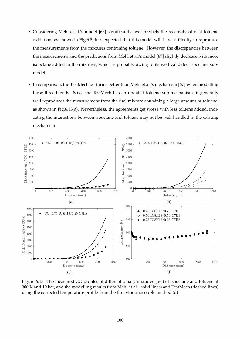
• Considering Mehl et al.’s model [67] significantly over-predicts the reactivity of neat toluene

oxidation, as shown in Fig.6.8, it is expected that this model will have difficulty to reproduce

the measurements from the mixtures containing toluene. However, the discrepancies between

the measurements and the predictions from Mehl et al.’s model [67] slightly decrease with more

isooctane added in the mixtures, which is probably owing to its well validated isooctane sub-

model.

• In comparison, the TestMech performs better than Mehl et al.’s mechanism [67] when modelling

these three blends. Since the TestMech has an updated toluene sub-mechanism, it generally

well reproduces the measurement from the fuel mixture containing a large amount of toluene,

as shown in Fig.6.13(a). Nevertheless, the agreements get worse with less toluene added, indi-

cating the interactions between isooctane and toluene may not be well handled in the existing

mechanism.

(a) (b)

(c) (d)

Figure 6.13: The measured CO profiles of different binary mixtures (a-c) of isooctane and toluene at900 K and 10 bar, and the modelling results from Mehl et al. (solid lines) and TestMech (dashed lines)using the corrected temperature profile from the three-thermocouple method (d)

100

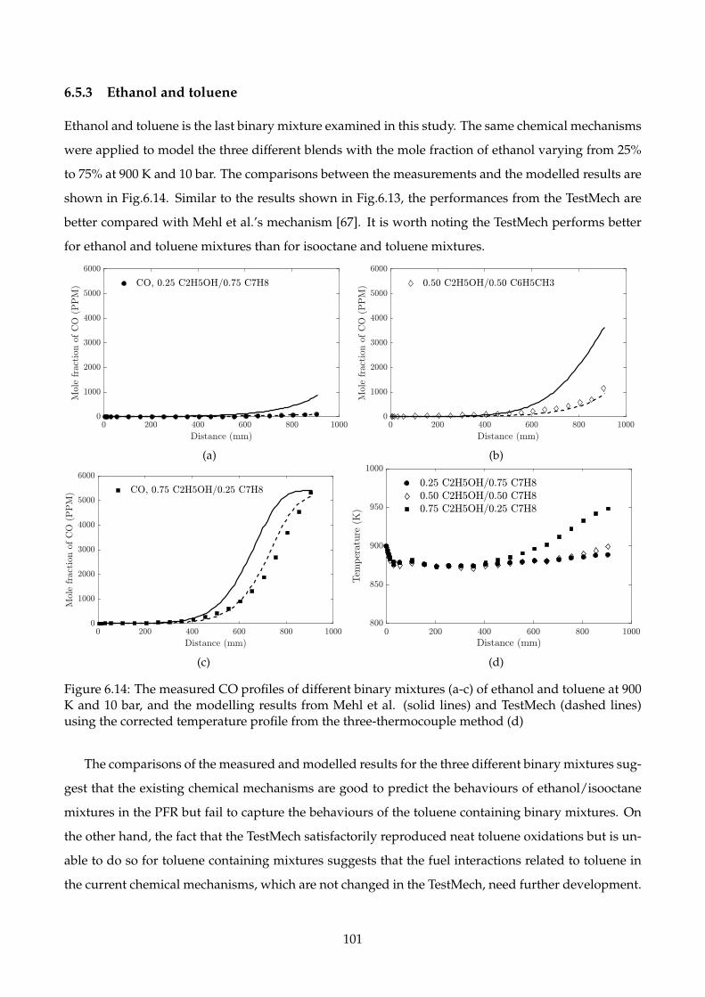
6.5.3 Ethanol and toluene

Ethanol and toluene is the last binary mixture examined in this study. The same chemical mechanisms

were applied to model the three different blends with the mole fraction of ethanol varying from 25%

to 75% at 900 K and 10 bar. The comparisons between the measurements and the modelled results are

shown in Fig.6.14. Similar to the results shown in Fig.6.13, the performances from the TestMech are

better compared with Mehl et al.’s mechanism [67]. It is worth noting the TestMech performs better

for ethanol and toluene mixtures than for isooctane and toluene mixtures.

(a) (b)

(c) (d)

Figure 6.14: The measured CO profiles of different binary mixtures (a-c) of ethanol and toluene at 900K and 10 bar, and the modelling results from Mehl et al. (solid lines) and TestMech (dashed lines)using the corrected temperature profile from the three-thermocouple method (d)

The comparisons of the measured and modelled results for the three different binary mixtures sug-

gest that the existing chemical mechanisms are good to predict the behaviours of ethanol/isooctane

mixtures in the PFR but fail to capture the behaviours of the toluene containing binary mixtures. On

the other hand, the fact that the TestMech satisfactorily reproduced neat toluene oxidations but is un-

able to do so for toluene containing mixtures suggests that the fuel interactions related to toluene in

the current chemical mechanisms, which are not changed in the TestMech, need further development.

101

6.6 Gasoline surrogates

Comparing with the binary mixtures, the gasoline surrogates have more implications for the practi-

cal applications. This study chooses PRF91 and TRF91-30 with 30% toluene proposed by [9] as the

gasoline surrogates, which were tested in the PFR under 900 K and 10 bar.

6.6.1 PRF91

PRFs are known as the simplest gasoline surrogates which can match the RON of the production

gasoline. In this study, PRF91 is blended to emulate the gasoline with RON of 91. The compar-

isons between the measured profiles from the PRF91 oxidation and the modelling results are shown

in Fig.6.15. Both the gasoline surrogate mechanism [67] and the TestMech well predict the profiles

of CO, CO2, and the parent fuels. Since toluene is not included in PRF91, it is not surprising that

the TestMech behaves exactly the same as the original mechanism from Mehl et al. [67]. In order to

quantify the impact of the chemical interactions between the parent fuels or fuel-like species to the

reactivity, the related elementary reactions (Reaction 5724 to 5935 from the original gasoline surrogate

model [67]) were deleted from the TestMech. The predictions from the mechanism excluding these

chemical interactions are also shown in Fig.6.15. It is found that removing chemical interactions has

negligible impact on the reactivity.

The profiles of the intermediate species from the PRF91 oxidation and the corresponding mod-

elling results are compared in Fig.6.16. The major species measured from the PRF91 oxidation are

similar to those from isooctane since isooctane is the major component of PRF91. Generally, the pro-

files of the hydrocarbon intermediates are well captured by these two mechanisms. However, the

maximum concentrations of the two oxygenated compounds, acetone and methacrolein, are under-

predicted. It is noticed that the mechanisms exhibit good fidelity in terms of reproducing the overall

trends for these two oxygenated compounds.

102

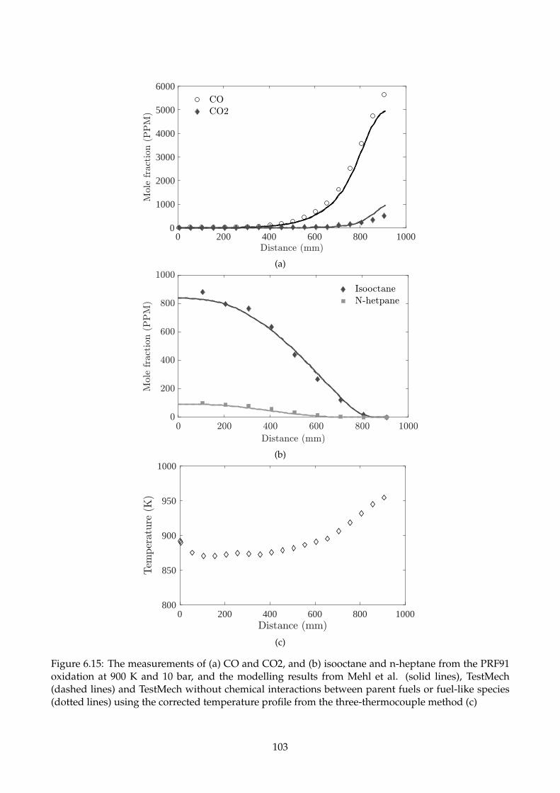
0 200 400 600 800 10000

1000

2000

3000

4000

5000

6000

(a)

(b)

0 200 400 600 800 1000800

850

900

950

1000

(c)

Figure 6.15: The measurements of (a) CO and CO2, and (b) isooctane and n-heptane from the PRF91oxidation at 900 K and 10 bar, and the modelling results from Mehl et al. (solid lines), TestMech(dashed lines) and TestMech without chemical interactions between parent fuels or fuel-like species(dotted lines) using the corrected temperature profile from the three-thermocouple method (c)

103

020

040

060

080

010

00020406080100

(a)

020

040

060

080

010

00020406080100

(b)

020

040

060

080

010

00050100

150

(c)

020

040

060

080

010

00050100

150

200

250

300

350

(d)

020

040

060

080

010

00050100

150

200

250

(e)

020

040

060

080

010

00010203040506070

(f)

020

040

060

080

010

000510152025

(g)

020

040

060

080

010

000510152025

(h)

Figu

re6.

16:T

hem

easu

red

inte

rmed

iate

spec

ies

profi

les

from

the

PRF9

1ox

idat

ion

expe

rim

enta

t900

Kan

d10

bar,

and

the

mod

ellin

gre

sult

sfr

omM

ehle

tal.

(sol

idlin

es)a

ndTe

stM

ech

(das

hed

lines

)

104

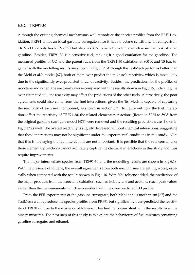
6.6.2 TRF91-30

Although the existing chemical mechanisms well reproduce the species profiles from the PRF91 ox-

idation, PRF91 is not an ideal gasoline surrogate since it has no octane sensitivity. In comparison,

TRF91-30 not only has RON of 91 but also has 30% toluene by volume which is similar to Australian

gasoline. Besides, TRF91-30 is a sensitive fuel, making it a good emulation for the gasoline. The

measured profiles of CO and the parent fuels from the TRF91-30 oxidation at 900 K and 10 bar, to-

gether with the modelling results are shown in Fig.6.17. Although the TestMech performs better than

the Mehl et al.’s model [67], both of them over-predict the mixture’s reactivity, which is most likely

due to the significantly over-predicted toluene reactivity. Besides, the predictions for the profiles of

isooctane and n-heptane are clearly worse compared with the results shown in Fig.6.15, indicating the

over-estimated toluene reactivity may affect the predictions of the other fuels. Alternatively, the poor

agreements could also come from the fuel interactions, given the TestMech is capable of capturing

the reactivity of each neat compound, as shown in section 6.3. To figure out how the fuel interac-

tions affect the reactivity of TRF91-30, the related elementary reactions (Reaction 5724 to 5935 from

the original gasoline surrogate model [67]) were removed and the resulting predictions are shown in

Fig.6.17 as well. The overall reactivity is slightly decreased without chemical interactions, suggesting

that these interactions may not be significant under the experimental conditions in this study. Note

that this is not saying the fuel interactions are not important. It is possible that the rate constants of

these elementary reactions cannot accurately capture the chemical interactions in this study and thus

require improvements.

The major intermediate species from TRF91-30 and the modelling results are shown in Fig.6.18.

With the presence of toluene, the overall agreements from both mechanisms are getting worse, espe-

cially when compared with the results shown in Fig.6.16. With 30% toluene added, the predictions of

the major products from the isooctane oxidation, such as isobutylene and acetone, reach peak values

earlier than the measurements, which is consistent with the over-predicted CO profile.

From the PFR experiments of the gasoline surrogates, both Mehl et al.’s mechanism [67] and the

TestMech well reproduce the species profiles from PRF91 but significantly over-predicted the reactiv-

ity of TRF91-30 due to the existence of toluene. This finding is consistent with the results from the

binary mixtures. The next step of this study is to explore the behaviours of fuel mixtures containing

gasoline surrogates and ethanol.

105

(a)

(b)

0 200 400 600 800 1000800

850

900

950

1000

(c)

Figure 6.17: The measured species profiles: (a) CO, CO2, and toluene, (b) isooctane and n-heptanefrom the oxidation of TRF91-30 at 900 K and 10 bar, and the modelling results from Mehl et al. (solidlines), TestMech (dashed lines) and TestMech without chemical interactions between parent fuels orfuel-like species (dotted lines) using the corrected temperature profile from the three-thermocouplemethod (c)

106

020

040

060

080

010

000102030405060

(a)

020

040

060

080

010

00020406080100

120

(b)

020

040

060

080

010

00020406080100

(c)

020

040

060

080

010

00050100

150

200

(d)

020

040

060

080

010

00050100

150

200

(e)

020

040

060

080

010

0001020304050

(f)

020

040

060

080

010

00024681012

(g)

020

040

060

080

010

0002468101214

(h)

Figu

re6.

18:T

hem

easu

red

inte

rmed

iate

spec

ies

profi

les

from

the

TRF9

1ox

idat

ion

expe

rim

enta

t900

Kan

d10

bar,

and

the

mod

ellin

gre

sult

sfr

omM

ehle

tal.

(sol

idlin

es)a

ndTe

stM

ech(

dash

edlin

es)

107

6.7 Gasoline surrogates/ethanol mixtures

6.7.1 PRF91 and ethanol

Ethanol was first blended into the simplest gasoline surrogate PRF91 with a mole fraction of 73.7%

(50% by volume). The fuel mixture was tested in the PFR at 900 K and 10 bar. The species profiles of

CO and the parent fuels from the oxidation of PRF91 blended with 73.7% ethanol by mole (50% by

volume), together with the modelling results using Mehl et al.’s mechanism [67] and the TestMech are

shown in Fig.6.19. Without the presence of toluene, both mechanisms well predict the profiles of CO

and three parent fuels and the TestMech performs exactly the same as Mehl et al.’s mechanism [67].

More importantly, the good agreements suggest that the interactions among isooctane, n-heptane, and

ethanol are well modelled, although the predicted ethanol profile has an earlier plateau compared

with the measurement. The mismatched plateau is less likely due to the fuel interactions since the

modelling of neat ethanol has the same issue, as shown in Fig.6.5.

With 73.7% (50% by volume) ethanol added, acetaldehyde becomes the most abundant interme-

diate species whose profile is well captured by both Mehl et al.’s mechanism [67] and the TestMech,

as shown in Fig.6.20. Note that acetaldehyde is the common product from both isooctane and ethanol

oxidations. The gasoline surrogate mechanism [67] well captures the acetaldehyde profile from the

ethanol oxidation, as shown in Fig.6.6(c), but has difficulty to match the peak value of acetaldehyde

profile from the isooctane oxidation which is shown in Fig.6.2(e). Since ethanol is much more abun-

dant than isooctane in the mixture, the formation of acetaldehyde mainly comes from the ethanol

oxidation, which is known to be well predicted by the mechanism [67]. For the same reason, most

of ethylene comes from ethanol as well and the over-predicted ethylene profile is consistent with

the result shown in Fig.6.6(b). Apart from acetaldehyde, the other two oxygenated compounds from

isooctane oxidation are under-predicted, which were also observed in the neat isooctane experiment.

Other than predicting these two oxygenates and ethylene, the existing mechanisms perform overall

satisfactorily.

108

(a)

(b)

0 200 400 600 800 1000800

850

900

950

1000

(c)

Figure 6.19: The measured species profiles: (a) CO, CO2 and ethanol, (b) isooctane and n-heptanefrom the oxidation of PRF91 blended with 73.7% ethanol by mole (50% by volume) at 900 K and 10bar, and the modelling results from Mehl et al. (solid lines) and TestMech (dashed lines) using thecorrected temperature profile from the three-thermocouple method (c)

109

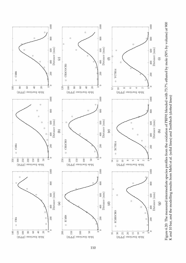
020

040

060

080

010

00020406080100

120

140

(a)

020

040

060

080

010

00050100

150

200

250

300

350

(b)

020

040

060

080

010

00020406080100

(c)

020

040

060

080

010

00050100

150

200

(d)

020

040

060

080

010

00050100

150

200

250

(e)

020

040

060

080

010

00020406080100

120

(f)

020

040

060

080

010

0005101520253035

(g)

020

040

060

080

010

0002468101214

(h)

020

040

060

080

010

00024681012

(i)

Figu

re6.

20:T

hem

easu

red

inte

rmed

iate

spec

ies

profi

les

from

the

oxid

atio

nof

PRF9

1bl

ende

dw

ith

73.7

%et

hano

lby

mol

e(5

0%by

volu

me)

at90

0K

and

10ba

r,an

dth

em

odel

ling

resu

lts

from

Meh

leta

l.(s

olid

lines

)and

Test

Mec

h(d

otte

dlin

es)

110

6.7.2 TRF91-30 and ethanol

To study the ethanol’s effects on the reactivity of TRF91-30, different amounts of ethanol were added

into the gasoline surrogates, and these mixtures were tested in PFR at 900 K and 10 bar. The same

chemical mechanisms were applied for the kinetic modellings.

The species profiles of CO and the parent fuels from the oxidation of TRF91-30 blended with 87.7%

ethanol by mole (75% by volume), together with the modelling results are shown in Fig.6.21. The

plateau from the measured CO profile indicates that the overall reactivity has been significantly im-

proved by the ethanol addition. With such a large ethanol content, the toluene sub-models in both

chemical mechanisms play a much less significant role, as the mole fraction of toluene in the fuel

mixture is less than 5%. Of interest is that the modelled isooctane and n-heptane profiles agree much

better with the measurements than in the neat TRF91 case, as shown in Fig.6.17.

Consistent with the reactivity measurements, the addition of 87.7% ethanol makes the mixture be-

have more like ethanol, which is embodied by the over-predicted ethylene profiles from both Mehl et

al.’s model [67] and the TestMech, as shown in Fig.6.22. Meanwhile, the profiles of the oxygenated

compounds are still under-estimated. Note that the absolute amounts of the C7 olefins become negli-

gible due to the small content of isooctane in the mixture, and thus these species are not included in

Fig.6.22.

With the addition of 70.5% ethanol by mole (50% by volume), the overall performances of the

gasoline surrogate mechanisms become worse, as shown in Fig.6.23. Compared with the predictions

of isooctane and n-heptane profiles, the consumption rates of toluene and ethanol are significantly

over-estimated, resulting in an over-predicted CO profile. The profiles of intermediate species and

the modelling results of the TRF mixture with 70.5% ethanol by mole (50% by volume) are shown

in Fig.6.24. The overall agreements are consistent with the results shown in Fig.6.22, suggesting that

ethanol still plays a significant role during the oxidation process. With the decreased ethanol content,

the fraction of isooctane increases accordingly, which produces detectable amounts of C7 olefins.

When the ethanol concentration drops to 44.3% by mole (25% by volume), the predictions become

the worst among all ethanol-containing TRF91-30 mixtures. The consumption rates of all parent fuels

are over-estimated, as shown in Fig.6.25, which are probably due to the problematic toluene sub-

mechanism. The intermediates’ profiles and the modelling results are shown in Fig.6.26. The predicted

profiles reach peaks earlier than the measurements, which is similar to the results shown in Fig.6.18.

It is probably because both cases have significant amounts of toluene in the fuel mixtures, and the

problematic toluene sub-mechanisms over-predict the reactivity, making the modelled profiles reach

peaks values earlier.

In summary, the gasoline surrogate mechanism from Mehl et al. [67] performs satisfactorily in

111

(a)

(b)

0 200 400 600 800 1000800

850

900

950

1000

(c)

Figure 6.21: The measured species profiles: (a) CO, isooctane, and n-heptane, (b) CO2, toluene, andethanol from the oxidation of TRF91-30 blended with 87.7% ethanol by mole (75% by volume) at 900 Kand 10 bar, and the modelling results from Mehl et al. (solid lines) and TestMech (dashed lines) usingthe corrected temperature profile from the three-thermocouple method (c)

112

020

040

060

080

010

00050100

150

(a)

020

040

060

080

010

000

100

200

300

400

500

600

(b)

020

040

060

080

010

00010203040

(c)

020

040

060

080

010

00010203040506070

(d)

020

040

060

080

010

000

100

200

300

400

(e)

020

040

060

080

010

00020406080100

(f)

020

040

060

080

010

0002468101214

(g)

Figu

re6.

22:T

hem

easu

red

inte

rmed

iate

spec

ies

profi

les

the

oxid

atio

nof

TRF9

1-30

blen

ded

wit

h87

.7%

etha

nolb

ym

ole

(75%

byvo

lum

e)at

900

Kan

d10

bar,

and

the

mod

ellin

gre

sult

sfr

omM

ehle

tal.

(sol

idlin

es)a

ndTe

stM

ech

(dot

ted

lines

)

113

(a)

(b)

0 200 400 600 800 1000800

850

900

950

1000

(c)

Figure 6.23: The measured species profiles: (a) CO, isooctane, and n-heptane, (b) CO2, toluene, andethanol from the oxidation of TRF91-30 blended with 70.5% ethanol by mole (50% by volume) at 900 Kand 10 bar, and the modelling results from Mehl et al. (solid lines) and TestMech (dashed lines) usingthe corrected temperature profile from the three-thermocouple method (c)

114

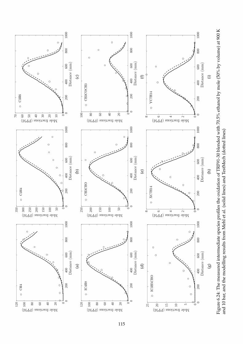
020

040

060

080

010

00020406080100

120

(a)

020

040

060

080

010

00050100

150

200

250

300

350

(b)

020

040

060

080

010

00010203040506070

(c)

020

040

060

080

010

00020406080100

120

(d)

020

040

060

080

010

00050100

150

200

250

(e)

020

040

060

080

010

00020406080100

(f)

020

040

060

080

010

000510152025

(g)

020

040

060

080

010

0002468

(h)

020

040

060

080

010

0002468

(i)

Figu

re6.

24:T

hem

easu

red

inte

rmed

iate

spec

ies

profi

les

the

oxid

atio

nof

TRF9

1-30

blen

ded

wit

h70

.5%

etha

nolb

ym

ole

(50%

byvo

lum

e)at

900

Kan

d10

bar,

and

the

mod

ellin

gre

sult

sfr

omM

ehle

tal.

(sol

idlin

es)a

ndTe

stM

ech

(dot

ted

lines

)

115

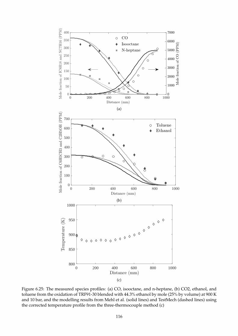
(a)

(b)

0 200 400 600 800 1000800

850

900

950

1000

(c)

Figure 6.25: The measured species profiles: (a) CO, isooctane, and n-heptane, (b) CO2, ethanol, andtoluene from the oxidation of TRF91-30 blended with 44.3% ethanol by mole (25% by volume) at 900 Kand 10 bar, and the modelling results from Mehl et al. (solid lines) and TestMech (dashed lines) usingthe corrected temperature profile from the three-thermocouple method (c)

116

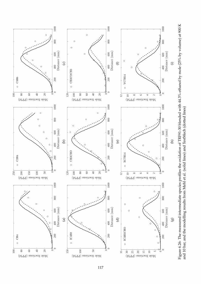
020

040

060

080

010

00020406080100

(a)

020

040

060

080

010

00050100

150

200

250

(b)

020

040

060

080

010

00020406080100

(c)

020

040

060

080

010

00050100

150

(d)

020

040

060

080

010

00020406080100

120

(e)

020

040

060

080

010

00020406080100

120

(f)

020

040

060

080

010

0005101520253035

(g)

020

040

060

080

010

00024681012

(h)

020

040

060

080

010

00024681012

(i)

Figu

re6.

26:T

hem

easu

red

inte

rmed

iate

spec

ies

profi

les

the

oxid

atio

nof

TRF9

1-30

blen

ded

wit

h44

.3%

etha

nolb

ym

ole

(25%

byvo

lum

e)at

900

Kan

d10

bar,

and

the

mod

ellin

gre

sult

sfr

omM

ehle

tal.

(sol

idlin

es)a

ndTe

stM

ech

(dot

ted

lines

)

117

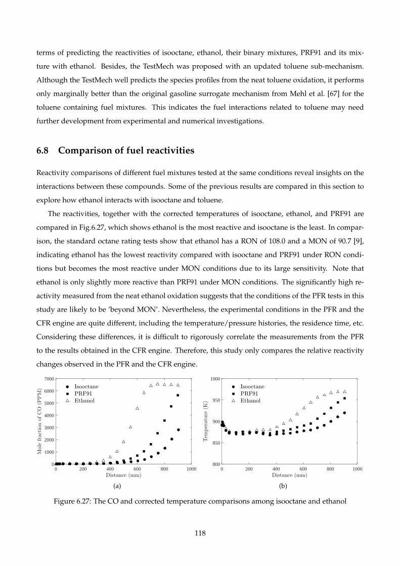
terms of predicting the reactivities of isooctane, ethanol, their binary mixtures, PRF91 and its mix-

ture with ethanol. Besides, the TestMech was proposed with an updated toluene sub-mechanism.

Although the TestMech well predicts the species profiles from the neat toluene oxidation, it performs

only marginally better than the original gasoline surrogate mechanism from Mehl et al. [67] for the

toluene containing fuel mixtures. This indicates the fuel interactions related to toluene may need

further development from experimental and numerical investigations.

6.8 Comparison of fuel reactivities

Reactivity comparisons of different fuel mixtures tested at the same conditions reveal insights on the

interactions between these compounds. Some of the previous results are compared in this section to

explore how ethanol interacts with isooctane and toluene.

The reactivities, together with the corrected temperatures of isooctane, ethanol, and PRF91 are

compared in Fig.6.27, which shows ethanol is the most reactive and isooctane is the least. In compar-

ison, the standard octane rating tests show that ethanol has a RON of 108.0 and a MON of 90.7 [9],

indicating ethanol has the lowest reactivity compared with isooctane and PRF91 under RON condi-

tions but becomes the most reactive under MON conditions due to its large sensitivity. Note that

ethanol is only slightly more reactive than PRF91 under MON conditions. The significantly high re-

activity measured from the neat ethanol oxidation suggests that the conditions of the PFR tests in this

study are likely to be ’beyond MON’. Nevertheless, the experimental conditions in the PFR and the

CFR engine are quite different, including the temperature/pressure histories, the residence time, etc.

Considering these differences, it is difficult to rigorously correlate the measurements from the PFR

to the results obtained in the CFR engine. Therefore, this study only compares the relative reactivity

changes observed in the PFR and the CFR engine.

0 200 400 600 800 10000

1000

2000

3000

4000

5000

6000

7000

(a)

0 200 400 600 800 1000800

850

900

950

1000

(b)

Figure 6.27: The CO and corrected temperature comparisons among isooctane and ethanol

118

The reactivity comparisons between ethanol/isooctane and ethanol/toluene are shown in Fig.6.28.

Although the measured CO profiles from the PFR are not directly comparable with the octane numbers

from the CFR engine, they do reflect the reactivities of different fuels and their mixtures. As shown in

Fig.6.28(a), isooctane is much more reactive than toluene which barely reacts at 900 K. With ethanol

added, the reactivity difference between these two fuels are diminishing, as shown in Fig.6.28(c) and

(e). When the ethanol concentration reaches approximately 75%, the reactivity of ethanol and isooc-

tane mixture is only slightly higher than that of the mixture containing ethanol and toluene, suggesting

that the impact of ethanol is more significant on toluene than on isooctane in terms of improving the

mixture’s reactivity, especially when considering isooctane is much more reactive than toluene.

Similar impact was also found with gasoline surrogates, as shown in Fig.6.29. Although both

PRF91 and TRF91-30 have RON of 91, PRF91 has a higher CO concentration compared with TRF91-30

in the PFR experiment. After adding ethanol with a volume fraction of 50% (73.7% by mole in PRF91

and 70.5% by mole in TRF91-30) to these two gasoline surrogates, their reactivities become very similar

and the reactivity increment of PRF91 is not significant, indicating that the interaction between ethanol

and isooctane (the major component in PRF91) does not contribute much to improve the mixture’s

reactivity, but the interaction between ethanol and toluene does. The results from both Fig.6.28 and

6.29 are consistent with the conclusion from the prior study [9] that ethanol blends synergistically

with isooctane but antagonistically with toluene in terms of the octane rating, as shown in Fig.2.5(a).

Although it is not intended to use the PFR results to explain the octane number blending behaviours

reported in [9] due to the different conditions in the two experiments, it is interesting to find the

relative reactivity changes in the PFR and the CFR engine are consistent, suggesting the combustion

chemistry behind these experiments may be similar.

The motivation of the reactivity comparisons for different fuels and fuel mixtures is trying to fig-

ure out how hydrocarbons interact with ethanol under simple and well-controlled thermodynamic

conditions in the PFR.

119

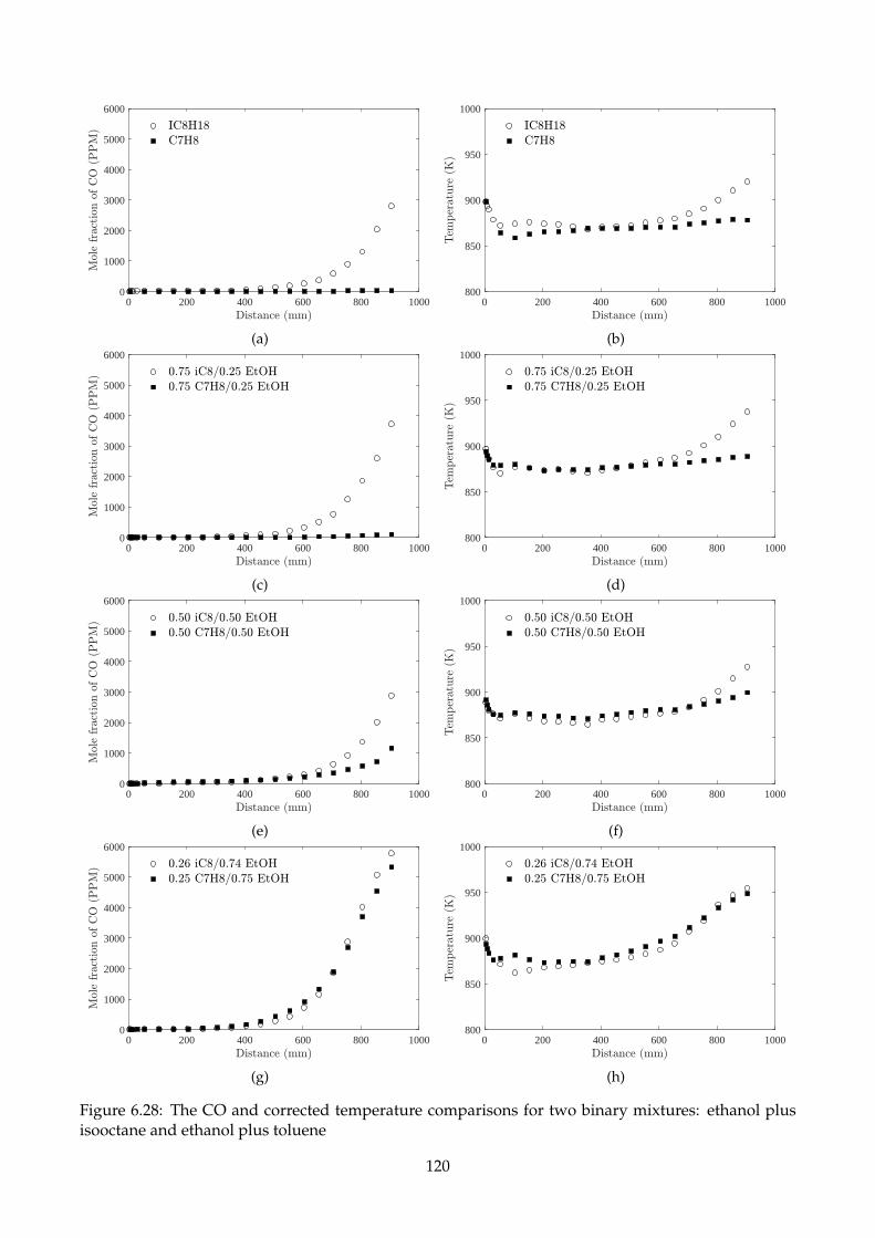
0 200 400 600 800 10000

1000

2000

3000

4000

5000

6000

(a)

0 200 400 600 800 1000800

850

900

950

1000

(b)

0 200 400 600 800 10000

1000

2000

3000

4000

5000

6000

(c)

0 200 400 600 800 1000800

850

900

950

1000

(d)

0 200 400 600 800 10000

1000

2000

3000

4000

5000

6000

(e)

0 200 400 600 800 1000800

850

900

950

1000

(f)

0 200 400 600 800 10000

1000

2000

3000

4000

5000

6000

(g)

0 200 400 600 800 1000800

850

900

950

1000

(h)

Figure 6.28: The CO and corrected temperature comparisons for two binary mixtures: ethanol plusisooctane and ethanol plus toluene

120

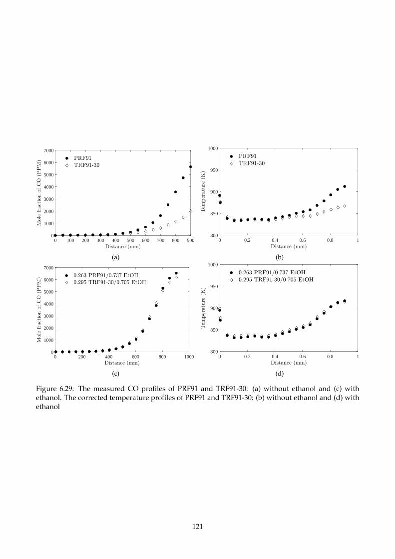
0 100 200 300 400 500 600 700 800 9000

1000

2000

3000

4000

5000

6000

7000

(a)

0 0.2 0.4 0.6 0.8 1800

850

900

950

1000

(b)

0 200 400 600 800 10000

1000

2000

3000

4000

5000

6000

7000

(c)

0 0.2 0.4 0.6 0.8 1800

850

900

950

1000

(d)

Figure 6.29: The measured CO profiles of PRF91 and TRF91-30: (a) without ethanol and (c) withethanol. The corrected temperature profiles of PRF91 and TRF91-30: (b) without ethanol and (d) withethanol

121

6.9 Summary

The PFR experiments for isooctane, ethanol, toluene, and their mixtures were performed at 900 K

(except toluene at 930 K) and 10 bar. CO, the parent fuels, and the intermediate species were measured

along the reactor length and modelled with the state of the art chemical mechanisms.

First, these mechanisms, in general, well reproduce the reactivities of isooctane and ethanol (except

CO plateau), their binary mixtures, PRF and PRF/ethanol mixture. Overall, the profiles of the major

intermediate species are well matched, but some improvements are needed for certain intermediate

species, e.g., oxygenates for isooctane and ethylene for ethanol. However, the existing chemical mech-

anisms become problematic when applied to model the neat toluene oxidation. Except the Princeton’s

mechanism [138], the other mechanisms significantly over-estimate the reactivity of toluene. As for

the toluene containing fuel mixtures, the problematic toluene sub-model in the gasoline surrogate

mechanism [67] results in larger discrepancies with a higher concentration of toluene in the mixture.

Second, the TestMech with an updated toluene sub-model was proposed to have close agreements

with the species profiles from the neat toluene experiment. However, the TestMech only performs

marginally better than the gasoline surrogate mechanism [67] for fuel mixtures, suggesting the inter-

action chemistry needs further development.

Lastly, the reactivity comparisons show that the impact of ethanol is more evident on toluene than

on isooctane in terms of improving the mixture’s reactivity, which is consistent with the conclusions

from the prior octane number study [9] despite the major differences between the two experiments.

122

Chapter 7

Conclusions and Recommendations for

Future Research

7.1 Conclusions

This thesis studied the octane blending and oxidation chemistry of ethanol-hydrocarbon mixtures. It

makes three contributions to our understanding of this problem.

1. This study quantifies the non-linear octane blending between ethanol and the surrogate fuels.

A systematic method for quantifying non-linear octane blending behaviours observed in fuel

mixtures was proposed. The method made use of Scheffe polynomials, which provide a com-

position based model for mixture properties, including octane numbers. It combined linear

regression and exhaustive (or brute-force) searching for polynomials that met specified require-

ments with the fewest terms. The following optimal correlations for the RON and MON of

TRF/ethanol mixtures were found, which achieve maximum absolute error of less than two

octane numbers across TRF/ethanol mixtures with a RON between 80 and 120.

RON = 100x1 + 0x2 + 116.2x3 + 108x4 + 27.0x1x4 − 98.4x2x4(x2 − x4)− 9.1x3x4MON = 100x1 + 0x2 + 102.0x3 + 90.7x4 + 12.8x1x4 + 76.7x2x4 − 6.4x3x4

where x1, x2, x3 and x4 denote the mole fractions of isooctane, n-heptane, toluene and ethanol

respectively. These correlations were obtained from a systematic method and reveal some signif-

icant results. For example, the significance of the linear by mole blending rule for TRF mixtures

is reconfirmed by correlations, since the non-linear terms are all binary and all contain ethanol

(x4). Furthermore, the coefficients of these non-linear terms correspond to the levels of synergis-

tic or antagonistic blending of different binary mixtures, as previously reported in the literature.

123

2. This work develops a gasoline surrogate that more accurately emulates the octane blending be-

haviours of production gasoline with ethanol.

To emulate the knocking behaviours of gasoline/ethanol mixtures, this work first measured the

RONs of binary mixtures to gain fundamental understanding for the interactions between dif-

ferent hydrocarbons and between hydrocarbon and ethanol. It is found that most hydrocarbons

selected blend synergistically with ethanol, except aromatic fuels showing antagonistic trend.

Based on the results of the detailed hydrocarbon analysis of an Australian market gasoline, cy-

clohexane and 1-hexene, each at 10% by volume, were used as the representative compounds

for cycloparaffins and olefins. Further, 1,2,4-trimethylbenzene with a 30% volume fraction was

used to represent aromatics for its strongest antagonism when blended with ethanol, which is re-

quired to compensate the synergism exhibited by ethanol blending with other hydrocarbons. Fi-

nally, iso-pentane and n-pentane were selected as the representative compounds of paraffins due

to their significant concentrations in the production gasoline, and their relative volume fractions

were the balancing factor to make the mixture have a RON of 91. It is found that the proposed

gasoline surrogate closely reproduced the octane blending behaviours with ethanol over the en-

tire blending range, with a maximum ON difference of 0.7 unit. Compared with commonly used

TRF mixtures, this surrogate formulation indicates that including additional components from

other hydrocarbon classes and using different paraffin and aromatic compounds than those in

TRFs are necessary to emulate the interaction between gasoline and ethanol. The developed

gasoline surrogate is the first of its kind in attempt to emulate the octane blending behaviour of

the gasoline and ethanol. In addition to capture the blending behaviours, the compositions of

the gasoline surrogate match with the hydrocarbon class distributions in the gasoline.

3. This work studied ethanol interaction with different hydrocarbons in the pressurised flow re-

actor, finding that whilst current mechanisms often captured the measured trends, those for

toluene and toluene-rich mixtures are lacking.

A systematic PFR experimental study was carried out at 900 K (except toluene at 930 K) and

10 bar to study oxidation chemistry of a comprehensive fuel matrix including neat fuels, bi-

nary mixtures, gasoline surrogates, and gasoline surrogates/ethanol mixtures. GC with an FID

analyser was applied for species measurements. The measurements are consistent with those

reported previously from jet-stirred reactors and rapid compression machines, and other flow

reactors on the relevant fuels.

The measured detailed species profiles are used to systematically validate the existing chemi-

cal mechanisms. The gasoline surrogate mechanism from Mehl et al. [67] reproduces most of

the species profiles from the oxidations of ethanol, isooctane, their binary mixtures, PRF, and

124

PRF/ethanol mixtures. Large discrepancies were observed between the measured profiles and

the modelled results for neat toluene and toluene-containing fuel mixtures. Revising some mis-

used elementary reactions rate constants (TestMech) improved the modelling of the neat toluene

but was still unable to capture the behaviours of the mixtures, indicating that the toluene mech-

anism, and probably its interactions with other compounds need major improvements, which

are required to develop a valid gasoline surrogate mechanism.

Under the experimental conditions in this study, it is found that ethanol promotes toluene oxi-

dation more than it does to isooctane, which is consistent with the results from the prior octane

blending behaviours in the CFR engine [9].

7.2 Recommendations for future research

1. Experimental studies for toluene oxidation under various conditions and development of a de-

tailed toluene mechanism

This study shows that the existing toluene sub-model significantly over-estimates the reactiv-

ity of toluene and toluene-containing fuel mixtures, which indicates that the understanding of

the toluene oxidation is not complete. Therefore, more kinetic experiments are requires to in-

vestigate the oxidation of toluene at different temperatures, pressures, and equivalence ratios.

With more experimental results, a new detailed toluene mechanism can be proposed, which is

required for further gasoline surrogate mechanism development.

2. Experimental studies for binary mixtures to understand fuel interactions

It has been shown in this work that the TestMech can reproduce the species profiles from neat

toluene but didn’t perform well for toluene containing binary mixtures, indicating the chemical

interactions related to toluene need improvement. Besides, it is also found ethanol promotes

toluene oxidation more than does to isooctane, but the combustion chemistry behind this ob-

servation is not clear. Hence, more kinetic experiments are required to understand the fuel

interactions of these binary mixtures, which is essential to develop a detailed gasoline surrogate

mechanism.

3. Experimental studies for neat fuels and their mixtures at lower temperatures

The reactivity comparison between ethanol and PRF91 suggests that the experimental condi-

tion in this study is ’beyond MON’. To have comprehensive understandings of the combustion

chemistry, it is necessary to carry out these experiments at lower temperatures where the low

temperature chemistry is more significant.

125

4. Experimental studies for the oxidations of isooctane and ethanol

Although the existing chemical mechanisms capture most of the species profiles from isooctane

and ethanol oxidation, the oxygenated compounds from isooctane and ethylene from ethanol

are not well reproduced. Also, the CO plateau issue near the end of the reactor at high reactivity

conditions should be resolved. Thus, it is necessary to carry out more kinetic experiments for

isooctane and ethanol under different conditions in the PFR to improve the existing mechanisms.

126

References

[1] BP Global. BP Energy Outlook, 2017 edition, 2017.

[2] Jose Ramon Serrano. Imagining the Future of the Internal Combustion Engine for Ground Trans-

port in the Current Context. Applied Sciences, 7:1001, 2017.

[3] Mazda announces breakthrough in long-coveted engine technology. Yahoo finance, 2017.

[4] J. Hansen, D. Johnson, A. Lacis, S. Lebedeff, P. Lee, D. Rind, and G. Russell. Climate Impact of

Increasing Atmospheric Carbon Dioxide. Science, 213(4511):957–966, 1981.

[5] BP Global. BP Statistical Review of World Energy, 2017.

[6] Alexander E. Farrell, Richard J. Plevin, Brian T. Turner, Andrew D. Jones, Michael O’Hare, and

Daniel M. Kammen. Ethanol Can Contribute to Energy and Environmental Goals. Science,

311(5760):506–508, 2006.

[7] Jose Goldemberg. Ethanol for a Sustainable Energy Future. Science, 315(5813):808–810, 2007.

[8] Avinash Kumar Agarwal. Biofuels (alcohols and biodiesel) applications as fuels for internal

combustion engines. Progress in Energy and Combustion Science, 33(3):233–271, 2007.

[9] Tien Mun Foong, Kai J. Morganti, Michael J. Brear, Gabriel da Silva, Yi Yang, and Frederick L.

Dryer. The octane numbers of ethanol blended with gasoline and its surrogates. Fuel, 115:727–

739, 2014.

[10] J. E. Anderson, U. Kramer, S. A. Mueller, and T. J. Wallington. Octane numbers of ethanol- and

methanol- gasoline blends estimated from molar concentrations. Energy Fuels, 24(12):6576–6585,

2010-12-16.

[11] Robert A. Stein, Dusan Polovina, Kevin Roth, Michael Foster, Michael Lynskey, Todd Whiting,

James E. Anderson, Michael H. Shelby, Thomas G. Leone, and Steven VanderGriend. Effect of

Heat of Vaporization, Chemical Octane, and Sensitivity on Knock Limit for Ethanol - Gasoline

Blends. SAE Int. J. Fuels Lubr., 5(2):823–843, 2012.

127

[12] Hao Yuan, Tien Mun Foong, Zhongyuan Chen, Yi Yang, Michael Brear, Thomas Leone, and

James E. Anderson. Modeling of trace knock in a modern SI engine fuelled by ethanol/gasoline

blends. SAE Technical Paper, 2015-01-1242, 2015.

[13] Tien Mun Foong, Kai J. Morganti, Michael J. Brear, Gabriel da Silva, Yi Yang, and Frederick L.

Dryer. The effect of charge cooling on the RON of ethanol/gasoline blends. SAE Int. J. Fuels

Lubr., 6(1):31–43, 2013.

[14] Emmanuel Kasseris and John Heywood. Charge cooling effects on knock limits in SI DI engines

using Gasoline/Ethanol blends: Part 1-quantifying charge cooling. SAE Technical Paper, 2012-

01-1275, 2012.

[15] Emmanuel Kasseris and John Heywood. Charge cooling effects on knock limits in SI DI engines

using Gasoline/Ethanol blends: Part 2-effective octane numbers. SAE Int. J. Fuels Lubr., 5(2):844–

854, 2012.

[16] Renewable Fuel Association. 2017 Ethanol Industry Outlook, 2017.

[17] Renewable Fuel Association. Ethanol Consumption Breaks Through the ”Blend Wall” in 2016,

2017.

[18] Livestock Ministry of Agriculture and Food Supply. This decree fixed the mandatory blend at

25% starting july 1st, 2007, 2007.

[19] Chinese Government. The Implementation of the Expansion of Ethanol Production and the

Promotion of Ethanol-added Gasoline, 2017.

[20] Jihad Badra, Abdullah S. AlRamadan, and S. Mani Sarathy. Optimization of the octane response

of gasoline/ethanol blends. Applied Energy, 203:778–793, 2017.

[21] John B. Heywood. Internal combustion engine fundamentals. McGraw-Hill, 1988.

[22] J. M. Towers and R. L. Hoekstra. Engine knock, a renewed concern in motorsports - a literature

review. SAE Technical Paper, 983026, 1998.

[23] Tien Mun Foong. On the Autoignition of Ethanol/Gasoline Blends in Spark-Ignition Engines. Ph.D.

thesis, The University of Melbourne, 2013.

[24] V. Arrigoni, G. M. Cornetti, Spallanzani G., Calvi F., and A. Tontodonati. High speed knock in

s.i. engines. SAE Technical Paper, 741056, 1974.

128

[25] ASTM International. Standard test method for research octane number of spark-ignition engine

fuel, 2011. ASTM D2699-11.

[26] ASTM International. Standard test method for motor octane number of spark-ignition engine

fuel, 2011. ASTM D2700-11.

[27] T. Midgley and T. Boyd. Methods of measuring detonation in engines. SAE Technical Paper,

220004, 1922.

[28] H.R. Ricardo. The influence of various fuels on the performance of internal combustion engines.

Report of the Empire Motor Fuels Committee, The Institution of Automobile Engineers vol XVIII Pt

I, 1924.

[29] Dugald Clerk. Investigations on gaseous explosions. part II. explosive reactions considered in

reference to internal combustion engines. introductory survey. Trans. Faraday Soc., 22(0):338–340,

1926.

[30] D. Downs, A. D. Walsh, and R. W. Wheeler. A study of the reactions that lead to ’Knock’ in the

spark-ignition engine. Phil. Trans. R. Soc. Lond. A, 243(870):463–524, 1951.

[31] Charles K. Westbrook, Yasuhiro Mizobuchi, Thierry J. Poinsot, Phillip J. Smith, and Jurgen War-

natz. Computational combustion. Proceedings of the Combustion Institute, 30(1):125–157, 2005.

[32] Nobuyuki Kawahara, Eiji Tomita, and Yoshitomo Sakata. Auto-ignited kernels during knocking

combustion in a spark-ignition engine. Proceedings of the Combustion Institute, 31(2):2999–3006,

2007.

[33] M. Poschl and T. Sattelmayer. Influence of temperature inhomogeneities on knocking combus-

tion. Combustion and Flame, 153(4):562–573, 2008.

[34] R. Worret, S. Bernhardt, F. Schwarz, and U. Spicher. Application of different cylinder pressure

based knock detection methods in spark ignition engines. SAE Technical Paper, 2002-01-1668,

2002.

[35] Enrico Corti and Claudio Forte. Statistical analysis of indicating parameters for knock detection

purposes. SAE Technical Paper, 2009-01-0237, 2009.

[36] F. Millo and C. V. Ferraro. Knock in S.I. engines: A comparison between different techniques for

detection and control. SAE Technical Paper, 982477, 1998.

[37] Kwang Min Chun and John B. Heywood. Characterization of knock in a spark-ignition engine.

SAE Technical Paper, 890156, 1989.

129

[38] Gao Xiaofeng, Richard Stone, Chris Hudson, and Ian Bradbury. The detection and quantification

of knock in spark ignition engines. SAE Technical Paper, 932759, 1993.

[39] Michael F. J. Brunt, Christopher R. Pond, and John Biundo. Gasoline engine knock analysis

using cylinder pressure data. SAE Technical Paper, 980896, 1998.

[40] M. D. Checkel and J. D. Dale. Computerized knock detection from engine pressure records. SAE

Technical Paper, 860028, 1986.

[41] Tassos H. Valtadoros, Victor W. Wong, and John B. Heywood. Engine knock characteristics at

the audible level. SAE Technical Paper, 910567, 1991.

[42] Kwang Min Chun and Kyung Woon Kim. Measurement and analysis of knock in a SI engine

using the cylinder pressure and block vibration signals. SAE Technical Paper, 940146, 1994.

[43] G. Edgar. Measurement of knock characteristics of gasoline in terms of a standard fuel. Ind.

Engg. Chem., pages 145–146, 1927.

[44] James E. Anderson, Thomas G. Leone, Michael H. Shelby, Timothy J. Wallington, Jeffrey J. Bizub,

Michael Foster, Michael G. Lynskey, and Dusan Polovina. Octane numbers of ethanol-gasoline

blends: Measurements and novel estimation method from molar composition. SAE Technical

Paper, 2012-01-1274, 2012.

[45] Paul Whitaker, Yuan Shen, Christian Spanner, Heribert Fuchs, Apoorv Agarwal, and Kevin

Byrd. Development of the combustion system for a flexible fuel turbocharged direct injection

engine. SAE Int. J. Engines, 3(1)(2010-01-0585):326–354, 2010.

[46] Tien Mun Foong, Michael J. Brear, Kai J. Morganti, Gabriel da Silva, Yi Yang, and Frederick L.

Dryer. Modeling End-Gas Autoignition of Ethanol/Gasoline Surrogate Blends in the Coopera-

tive Fuel Research Engine. Energy & Fuels, 31(3):2378–2389, 2017.

[47] Stephen Turns. An Introduction to Combustion: Concepts and Applications. McGraw-Hill Educa-

tion, 2011.

[48] Charles K. Westbrook and Frederick L. Dryer. Chemical kinetic modeling of hydrocarbon com-

bustion. Progress in Energy and Combustion Science, 10(1):1–57, 1984.

[49] Charles K. Westbrook. Chemical kinetics of hydrocarbon ignition in practical combustion sys-

tems. Proceedings of the Combustion Institute, 28(2):1563–1577, 2000.

[50] John M. Simmie. Detailed chemical kinetic models for the combustion of hydrocarbon fuels.

Progress in Energy and Combustion Science, 29(6):599–634, 2003.

130

[51] F. Battin-Leclerc. Detailed chemical kinetic models for the low-temperature combustion of hy-

drocarbons with application to gasoline and diesel fuel surrogates. Progress in Energy and Com-

bustion Science, 34(4):440–498, August 2008.

[52] Judit Zador, Craig A. Taatjes, and Ravi X. Fernandes. Kinetics of elementary reactions in low-

temperature autoignition chemistry. Progress in Energy and Combustion Science, 37(4):371–421,

August 2011.

[53] Zhengkai Xi, Wha Jin Han, and Kyle D. Bayes. Temperature dependence of the rate constant for

the reaction of neopentyl radicals with oxygen. J. Phys. Chem., 92(12):3450–3453, 1988.

[54] E. W. Kaiser. Formation of C3H6 from the reaction C3H7 + o2 between 450 and 550 k. J. Phys.

Chem. A, 102(29):5903–5906, 1998.

[55] James A. Miller, Stephen J. Klippenstein, and Struan H. Robertson. A theoretical analysis of the

reaction between ethyl and molecular oxygen. Proceedings of the Combustion Institute, 28(2):1479–

1486, 2000.

[56] Edgar G. Estupinan, Stephen J. Klippenstein, and Craig A. Taatjes. Measurements and modeling

of HO2 formation in the reactions of n-C3H7 and i-C3H7 radicals with o2†. J. Phys. Chem. B,

109(17):8374–8387, 2005.

[57] H. J. Curran, P. Gaffuri, W. J. Pitz, and C. K. Westbrook. A comprehensive modeling study of

iso-octane oxidation. Combustion and Flame, 129(3):253–280, 2002.

[58] Philippe Dagaut, Marcelline Reuillon, and Michel Cathonnet. High Pressure Oxidation of Liq-

uid Fuels From Low to High Temperature. 1. n-Heptane and iso-Octane. Combustion Science and

Technology, 95(1-6):233–260, 1993.

[59] F. L. DRYER and K. BREZINSKY. A Flow Reactor Study of the Oxidation of n-Octane and Iso-

Octane. Combustion Science and Technology, 45(3-4):199–212, 1986.

[60] C. V. Callahan, T. J. Held, F. L. Dryer, R. Minetti, M. Ribaucour, L. R. Sochet, T. Faravelli,

P. Gaffuri, and E. Rani. Experimental data and kinetic modeling of primary reference fuel mix-

tures. Symposium (International) on Combustion, 26(1):739–746, 1996.

[61] J.-S. CHEN, T. A. LITZINGER, and H. J. CURRAN. The Lean Oxidation of Iso-Octane in the

Intermediate Temperature Regime at Elevated Pressures. Combustion Science and Technology,

156(1):49–79, 2000.

131

[62] D. J. Vermeer, J. W. Meyer, and A. K. Oppenheim. Auto-ignition of hydrocarbons behind re-

flected shock waves. Combustion and Flame, 18(3):327–336, 1972.

[63] K. Fieweger, R. Blumenthal, and G. Adomeit. Shock-tube investigations on the self-ignition

of hydrocarbon-air mixtures at high pressures. Symposium (International) on Combustion,

25(1):1579–1585, 1994.

[64] K. Fieweger, R. Blumenthal, and G. Adomeit. Self-ignition of S.I. engine model fuels: A shock

tube investigation at high pressure. Combustion and Flame, 109(4):599–619, 1997.

[65] Willaim R. Leppard. The autoignition chemistries of primary reference fuels, olefin/paraffin

binary mixtures, and non-linear octane blending. SAE Technical Paper, 922325, 1992.

[66] H. Li, S. Prabhu, D. Miller, and N. Cernansky. Autoignition chemistry studies on primary refer-

ence fuels in a motored engine. SAE Technical Paper, 942062, 1994.

[67] Marco Mehl, William J. Pitz, Charles K. Westbrook, and Henry J. Curran. Kinetic modeling of

gasoline surrogate components and mixtures under engine conditions. Proceedings of the Com-

bustion Institute, 33(1):193–200, 2011.

[68] Nour Atef, Goutham Kukkadapu, Samah Y. Mohamed, Mariam Al Rashidi, Colin Banyon,

Marco Mehl, Karl Alexander Heufer, Ehson F. Nasir, A. Alfazazi, Apurba K. Das, Charles K.

Westbrook, William J. Pitz, Tianfeng Lu, Aamir Farooq, Chih-Jen Sung, Henry J. Curran, and

S. Mani Sarathy. A comprehensive iso-octane combustion model with improved thermochem-

istry and chemical kinetics. Combustion and Flame, 178:111–134, April 2017.

[69] M. Hartmann, I. Gushterova, M. Fikri, C. Schulz, R. Schießl, and U. Maas. Auto-ignition of

toluene-doped n-heptane and iso-octane/air mixtures: High-pressure shock-tube experiments

and kinetics modeling. Combustion and Flame, 158(1):172–178, 2011.

[70] S. Mani Sarathy, Goutham Kukkadapu, Marco Mehl, Weijing Wang, Tamour Javed, Sungwoo

Park, Matthew A. Oehlschlaeger, Aamir Farooq, William J. Pitz, and Chih-Jen Sung. Ignition

of alkane-rich FACE gasoline fuels and their surrogate mixtures. Proceedings of the Combustion

Institute, 35(1):249–257, 2015.

[71] M. Mehl, W. Pitz, M. Sjoberg, , and J. Dec. Autoignition chemistry studies on primary reference

fuels in a motored engine. SAE Technical Paper, 2009-01-1806, 2009.

[72] Wontae Hwang, John Dec, and Magnus Sjoberg. Spectroscopic and chemical-kinetic analysis

of the phases of HCCI autoignition and combustion for single- and two-stage ignition fuels.

Combustion and Flame, 154(3):387–409, 2008.

132

[73] D. Vuilleumier, H. Selim, R. Dibble, and M. Sarathy. Exploration of heat release in a homoge-

neous charge compression ignition engine with primary reference fuels. SAE Technical Paper,

2013-01-2622, 2013.

[74] Suarwee Snitsiriwat and Joseph W. Bozzelli. Thermochemical Properties for Isooctane and Car-

bon Radicals: Computational Study. The Journal of Physical Chemistry A, 117(2):421–429, 2013.

[75] Itsaso Auzmendi-Murua and Joseph W. Bozzelli. Thermochemistry, Reaction Paths, and Ki-

netics on the Secondary Isooctane Radical Reaction with 3O2. International Journal of Chemical

Kinetics, 46(2):71–103, 2014.

[76] Suarwee Snitsiriwat and Joseph W. Bozzelli. Thermochemistry, Reaction Paths, and Kinetics on

the tert-Isooctane Radical Reaction with O2. The Journal of Physical Chemistry A, 118(26):4631–

4646, 2014.

[77] HongBo Ning, ChunMing Gong, ZeRong Li, and XiangYuan Li. Pressure-Dependent Kinetics of

Initial Reactions in Iso-octane Pyrolysis. The Journal of Physical Chemistry A, 119(18):4093–4107,

2015.

[78] Stephanie M. Villano, Lam K. Huynh, Hans-Heinrich Carstensen, and Anthony M. Dean. High-

Pressure Rate Rules for Alkyl + O2 Reactions. 1. The Dissociation, Concerted Elimination,

and Isomerization Channels of the Alkyl Peroxy Radical. The Journal of Physical Chemistry A,

115(46):13425–13442, 2011.

[79] Stephanie M. Villano, Lam K. Huynh, Hans-Heinrich Carstensen, and Anthony M. Dean. High-

Pressure Rate Rules for Alkyl + O2 Reactions. 2. The Isomerization, Cyclic Ether Formation,

and β-Scission Reactions of Hydroperoxy Alkyl Radicals. The Journal of Physical Chemistry A,

116(21):5068–5089, 2012.

[80] Akira Miyoshi. Systematic Computational Study on the Unimolecular Reactions of Alkylper-

oxy (RO2), Hydroperoxyalkyl (QOOH), and Hydroperoxyalkylperoxy (O2qooh) Radicals. The

Journal of Physical Chemistry A, 115(15):3301–3325, 2011.

[81] Sandeep Sharma, Sumathy Raman, and William H. Green. Intramolecular Hydrogen Migration

in Alkylperoxy and Hydroperoxyalkylperoxy Radicals: Accurate Treatment of Hindered Rotors.

The Journal of Physical Chemistry A, 114(18):5689–5701, 2010.

[82] C. M. Coats and Alan Williams. Investigation of the ignition and combustion of n-heptane-

oxygen mixtures. Symposium (International) on Combustion, 17(1):611–621, 1979.

133

[83] H. K. Ciezki and G. Adomeit. Shock-tube investigation of self-ignition of n-heptane-air mixtures

under engine relevant conditions. Combustion and Flame, 93(4):421–433, 1993.

[84] J. Herzler, L. Jerig, and P. Roth. Shock tube study of the ignition of lean n-heptane/air mixtures at

intermediate temperatures and high pressures. Proceedings of the Combustion Institute, 30(1):1147–

1153, 2005.

[85] D. F. Davidson, Z. Hong, G. L. Pilla, A. Farooq, R. D. Cook, and R. K. Hanson. Multi-species

time-history measurements during n-heptane oxidation behind reflected shock waves. Combus-

tion and Flame, 157(10):1899–1905, 2010.

[86] Jiaxiang Zhang, Shaodong Niu, Yingjia Zhang, Chenglong Tang, Xue Jiang, Erjiang Hu, and

Zuohua Huang. Experimental and modeling study of the auto-ignition of n-heptane/n-butanol

mixtures. Combustion and Flame, 160(1):31–39, 2013.

[87] R. Minetti, M. Carlier, M. Ribaucour, E. Therssen, and L. R. Sochet. A rapid compression ma-

chine investigation of oxidation and auto-ignition of n-Heptane: Measurements and modeling.

Combustion and Flame, 102(3):298–309, 1995.

[88] A. Cox, J. F. Griffiths, C. Mohamed, H. J. Curran, W. J. Pitz, and C. K. Westbrook. Extents of

alkane combustion during rapid compression leading to single-and two-stage ignition. Sympo-

sium (International) on Combustion, 26(2):2685–2692, 1996.

[89] Emma J. Silke, Henry J. Curran, and John M. Simmie. The influence of fuel structure on combus-

tion as demonstrated by the isomers of heptane: a rapid compression machine study. Proceedings

of the Combustion Institute, 30(2):2639–2647, 2005.

[90] J. F. Griffiths, K. J. Hughes, M. Schreiber, and C. Poppe. A unified approach to the reduced

kinetic modeling of alkane combustion. Combustion and Flame, 99(3):533–540, 1994.

[91] A. Chakir, M. Bellimam, J. C. Boettner, and M. Cathonnet. Kinetic study of n-heptane oxidation.

International Journal of Chemical Kinetics, 24(4):385–410, 1992.

[92] Philippe Dagaut, Marcelline Reuillon, and Michel Cathonnet. Experimental study of the oxida-

tion of n-heptane in a jet stirred reactor from low to high temperature and pressures up to 40

atm. Combustion and Flame, 101(1):132–140, 1995.

[93] Olivier Herbinet, Benoit Husson, Zeynep Serinyel, Maximilien Cord, Valerie Warth, Rene Four-

net, Pierre-Alexandre Glaude, Baptiste Sirjean, Frederique Battin-Leclerc, Zhandong Wang,

Mingfeng Xie, Zhanjun Cheng, and Fei Qi. Experimental and modeling investigation of the

low-temperature oxidation of n-heptane. Combustion and Flame, 159(12):3455–3471, 2012.

134

[94] H. M. Hakka, R. F. Cracknell, A. Pekalski, P. A. Glaude, and F. Battin-Leclerc. Experimental and

modeling study of ultra-rich oxidation of n-heptane. Fuel, 144:358–368, 2015.

[95] T. J. Held, A. J. Marchese, and F. L. Dryer. A Semi-Empirical Reaction Mechanism for n-Heptane

Oxidation and Pyrolysis. Combustion Science and Technology, 123(1-6):107–146, 1997.

[96] David B. Lenhert, David L. Miller, Nicholas P. Cernansky, and Kevin G. Owens. The oxidation

of a gasoline surrogate in the negative temperature coefficient region. Combustion and Flame,

156(3):549–564, 2009.

[97] P.S. Veloo, S. Jahangirian, and F.L. Dryer. An experimental and kinetic modeling study of the

two stage autoignition kinetic behavior of c7, c10, c12, and c14 n-alkanes. Proceedings of the

Spring Technical MEtting of the Central States Section of the Combustion Institute, Dayton, OH, 2012.

[98] A. J. Smallbone, W. Liu, C. K. Law, X. Q. You, and H. Wang. Experimental and modeling study

of laminar flame speed and non-premixed counterflow ignition of n-heptane. Proceedings of the

Combustion Institute, 32(1):1245–1252, 2009.

[99] Chunsheng Ji, Enoch Dames, Yang L. Wang, Hai Wang, and Fokion N. Egolfopoulos. Propaga-

tion and extinction of premixed C5–C12 n-alkane flames. Combustion and Flame, 157(2):277–287,

2010.

[100] A. P. Kelley, A. J. Smallbone, D. L. Zhu, and C. K. Law. Laminar flame speeds of C5 to C8

n-alkanes at elevated pressures: Experimental determination, fuel similarity, and stretch sensi-

tivity. Proceedings of the Combustion Institute, 33(1):963–970, 2011.

[101] L. Sileghem, V. A. Alekseev, J. Vancoillie, K. M. Van Geem, E. J. K. Nilsson, S. Verhelst, and

A. A. Konnov. Laminar burning velocity of gasoline and the gasoline surrogate components

iso-octane, n-heptane and toluene. Fuel, 112:355–365, 2013.

[102] P. Dirrenberger, P. A. Glaude, R. Bounaceur, H. Le Gall, A. Pires da Cruz, A. A. Konnov, and

F. Battin-Leclerc. Laminar burning velocity of gasolines with addition of ethanol. Fuel, 115:162–

169, 2014.

[103] Chunde Yao, Chuanhui Cheng, Shiyu Liu, Zhenyu Tian, and Jing Wang. Identification of in-

termediates in an n-heptane/oxygen/argon low-pressure premixed laminar flame using syn-

chrotron radiation. Fuel, 88(9):1752–1757, 2009.

[104] Jinou Song, Chunde Yao, Shiyu Liu, Zhenyu Tian, and Jing Wang. Experiment study of oxy-

genates impact on n-heptane flames with tunable synchrotron vacuum UV photoionization.

Fuel, 88(11):2297–2302, 2009.

135

[105] Gen Chen, Wu Yu, Jin Fu, Jun Mo, Zuohua Huang, Jiuzhong Yang, Zhandong Wang, Hanfeng

Jin, and Fei Qi. Experimental and modeling study of the effects of adding oxygenated fuels to

premixed n-heptane flames. Combustion and Flame, 159(7):2324–2335, 2012.

[106] Lars Seidel, Kai Moshammer, Xiaoxiao Wang, Thomas Zeuch, Katharina Kohse-Hoinghaus, and

Fabian Mauss. Comprehensive kinetic modeling and experimental study of a fuel-rich, pre-

mixed n-heptane flame. Combustion and Flame, 162(5):2045–2058, 2015.

[107] A. Cavaliere, A. Ciajolo, A. D’Anna, R. Mercogliano, and R. Ragucci. Autoignition of n-heptane

and n-tetradecane in engine-like conditions. Combustion and Flame, 93(3):279–286, 1993.

[108] Dae Sik Kim and Chang Sik Lee. Improved emission characteristics of HCCI engine by various

premixed fuels and cooled EGR. Fuel, 85(5):695–704, 2006.

[109] Xing-Cai Lu, Wei Chen, and Zhen Huang. A fundamental study on the control of the HCCI

combustion and emissions by fuel design concept combined with controllable EGR. Part 1. The

basic characteristics of HCCI combustion. Fuel, 84(9):1074–1083, 2005.

[110] Xing-Cai Lu, Wei Chen, and Zhen Huang. A fundamental study on the control of the HCCI

combustion and emissions by fuel design concept combined with controllable EGR. Part 2. Effect

of operating conditions and EGR on HCCI combustion. Fuel, 84(9):1084–1092, 2005.

[111] James P. Szybist, Andre L. Boehman, Daniel C. Haworth, and Hibiki Koga. Premixed ignition

behavior of alternative diesel fuel-relevant compounds in a motored engine experiment. Com-

bustion and Flame, 149(1):112–128, 2007.

[112] H. J. Curran, P. Gaffuri, W. J. Pitz, and C. K. Westbrook. A Comprehensive Modeling Study of

n-Heptane Oxidation. Combustion and Flame, 114(1):149–177, 1998.

[113] H. J. Curran. Rate constant estimation for C1 to C4 alkyl and alkoxyl radical decomposition.

International Journal of Chemical Kinetics, 38(4):250–275, 2006.

[114] Li Zhu, Joseph W. Bozzelli, and Lisa M. Kardos. Thermochemical Properties, δ f h°(298), S°(298),

and Cp°(T), for n-Butyl and n-Pentyl Hydroperoxides and the Alkyl and Peroxy Radicals, Tran-

sition States, and Kinetics for Intramolecular Hydrogen Shift Reactions of the Peroxy Radicals.

The Journal of Physical Chemistry A, 111(28):6361–6377, 2007.

[115] Marco Mehl, Guillaume Vanhove, William J. Pitz, and Eliseo Ranzi. Oxidation and combus-

tion of the n-hexene isomers: A wide range kinetic modeling study. Combustion and Flame,

155(4):756–772, 2008.

136

[116] Marco Mehl, William J. Pitz, Charles K. Westbrook, Kenji Yasunaga, Christine Conroy, and

Henry J. Curran. Autoignition behavior of unsaturated hydrocarbons in the low and high tem-

perature regions. Proceedings of the Combustion Institute, 33(1):201–208, 2011.

[117] Kuiwen Zhang, Colin Banyon, John Bugler, Henry J. Curran, Anne Rodriguez, Olivier Herbinet,

Frederique Battin-Leclerc, Christine B’Chir, and Karl Alexander Heufer. An updated experi-

mental and kinetic modeling study of n-heptane oxidation. Combustion and Flame, 172:116–135,

2016.

[118] Chong-Wen Zhou, Yang Li, Eoin O’Connor, Kieran P. Somers, Sebastien Thion, Charles Keesee,

Olivier Mathieu, Eric L. Petersen, Trent A. DeVerter, Matthew A. Oehlschlaeger, Goutham

Kukkadapu, Chih-Jen Sung, Majed Alrefae, Fathi Khaled, Aamir Farooq, Patricia Dirrenberger,

Pierre-Alexandre Glaude, Frederique Battin-Leclerc, Jeffrey Santner, Yiguang Ju, Timothy Held,

Francis M. Haas, Frederick L. Dryer, and Henry J. Curran. A comprehensive experimental and

modeling study of isobutene oxidation. Combustion and Flame, 167:353–379, 2016.

[119] John Bugler, Kieran P. Somers, Emma J. Silke, and Henry J. Curran. Revisiting the Kinetics and

Thermodynamics of the Low-Temperature Oxidation Pathways of Alkanes: A Case Study of the

Three Pentane Isomers. The Journal of Physical Chemistry A, 119(28):7510–7527, 2015.

[120] John Bugler, Brandon Marks, Olivier Mathieu, Rachel Archuleta, Alejandro Camou, Claire

Gregoire, Karl A. Heufer, Eric L. Petersen, and Henry J. Curran. An ignition delay time and

chemical kinetic modeling study of the pentane isomers. Combustion and Flame, 163:138–156,

2016.

[121] Kuiwen Zhang, Colin Banyon, Casimir Togbe, Philippe Dagaut, John Bugler, and Henry J. Cur-

ran. An experimental and kinetic modeling study of n-hexane oxidation. Combustion and Flame,

162(11):4194–4207, 2015.

[122] C. K. Westbrook, H. J. Curran, W. J. Pitz, J. F. Griffiths, C. Mohamed, and S. K. Wo. The effects

of pressure, temperature, and concentration on the reactivity of alkanes: Experiments and mod-

eling in a rapid compression machine. Symposium (International) on Combustion, 27(1):371–378,

1998.

[123] M. Ribaucour, R. Minetti, L. R. Sochet, H. J. Curran, W. J. Pitz, and C. K. Westbrook. Ignition of

isomers of pentane: An experimental and kinetic modeling study. Proceedings of the Combustion

Institute, 28(2):1671–1678, 2000.

[124] R Minetti, A Roubaud, E Therssen, M Ribaucour, and L. R Sochet. The chemistry of pre-ignition

of n-pentane and 1-pentene. Combustion and Flame, 118(1):213–220, 1999.

137

[125] R. MINETTI, M. RIBAUCOUR, M. CARLIER, and L. R. SOCHET. Autoignition Delays of a

Series of Linear and Branched Chain Alkanes in the Intermediate Range of Temperature. Com-

bustion Science and Technology, 113(1):179–192, 1996.

[126] Alexander Burcat, Karl Scheller, and Assa Lifshitz. Shock-tube investigation of comparative

ignition delay times for C1-C5 alkanes. Combustion and Flame, 16(1):29–33, 1971.

[127] V. P. Zhukov, V. A. Sechenov, and A. Yu. Starikovskii. Self-ignition of a lean mixture of n-pentane

and air over a wide range of pressures. Combustion and Flame, 140(3):196–203, 2005.

[128] Charles K. Westbrook, William J. Pitz, Mark M. Thornton, and Philip C. Malte. A kinetic mod-

eling study of n-pentane oxidation in a well-stirred reactor. Combustion and Flame, 72(1):45–62,

1988.

[129] F. S. Gonzalez and S. Sandler. An experimental study of the oxidation of n-pentane in the high

temperature pre-ignition region. Combustion and Flame, 26:35–44, 1976.

[130] Song Cheng, Yi Yang, Michael J. Brear, Dongil Kang, Stanislav Bohac, and Andre L. Boehman.

Autoignition of pentane isomers in a spark-ignition engine. Proceedings of the Combustion Insti-

tute, 36(3):3499–3506, 2017.

[131] John Bugler, Anne Rodriguez, Olivier Herbinet, Frederique Battin-Leclerc, Casimir Togbe, Guil-

laume Dayma, Philippe Dagaut, and Henry J. Curran. An experimental and modelling study of

n-pentane oxidation in two jet-stirred reactors: The importance of pressure-dependent kinetics

and new reaction pathways. Proceedings of the Combustion Institute, 36(1):441–448, 2017.

[132] Kenneth Brezinsky. The high-temperature oxidation of aromatic hydrocarbons. Progress in En-

ergy and Combustion Science, 12(1):1–24, 1986.

[133] Matthew A. Oehlschlaeger, David F. Davidson, and Ronald K. Hanson. Investigation of the reac-

tion of toluene with molecular oxygen in shock-heated gases. Combustion and Flame, 147(3):195–

208, 2006.

[134] Carlo Cavallotti, Marco Derudi, and Renato Rota. On the mechanism of decomposition of the

benzyl radical. Proceedings of the Combustion Institute, 32(1):115–121, 2009.

[135] Gabriel da Silva, John A. Cole, and Joseph W. Bozzelli. Thermal decomposition of the benzyl

radical to fulvenallene (C7H6) + h. J. Phys. Chem. A, 113(21):6111–6120, 2009.

[136] K. Brezinsky, T. A. Litzinger, and I. Glassman. The high temperature oxidation of the methyl

side chain of toluene. International Journal of Chemical Kinetics, 16(9):1053–1074, 1984.

138

[137] Stephen D. Klotz, Kenneth Brezinsky, and Irvin Glassman. Modeling the combustion of toluene-

butane blends. Symposium (International) on Combustion, 27(1):337–344, 1998.

[138] W. K. Metcalfe, S. Dooley, and F. L. Dryer. Comprehensive Detailed Chemical Kinetic Modeling

Study of Toluene Oxidation. Energy & Fuels, 25(11):4915–4936, 2011.

[139] P. Dagaut, G. Pengloan, and A. Ristori. Oxidation, ignition and combustion of toluene: Experi-

mental and detailed chemical kinetic modeling. Physical Chemistry Chemical Physics, 4(10):1846–

1854, 2002.

[140] Experimental and modeling study of the oxidation of toluene. International Journal of Chemical

Kinetics, 37(1).

[141] D. F. Davidson, B. M. Gauthier, and R. K. Hanson. Shock tube ignition measurements of iso-

octane/air and toluene/air at high pressures. Proceedings of the Combustion Institute, 30(1):1175–

1182, 2005.

[142] Subith S. Vasu, David F. Davidson, and Ronald K. Hanson. Shock-Tube Experiments and Kinetic

Modeling of Toluene Ignition. Journal of Propulsion and Power, 26(4):776–783, 2010.

[143] Y. Sakai, T. Inamura, T. Ogura, M. Koshi, and W. Pitz. Detailed kinetic modeling of toluene

combustion over a wide range of temperature and pressure. SAE Technical Paper, 2007-01-1885,

2007.

[144] Hsi-Ping S. Shen, Jeremy Vanderover, and Matthew A. Oehlschlaeger. A shock tube study of the

auto-ignition of toluene/air mixtures at high pressures. Proceedings of the Combustion Institute,

32(1):165–172, 2009.

[145] R. Sivaramakrishnan, R. S. Tranter, and K. Brezinsky. High-pressure, high-temperature oxida-

tion of toluene. Combustion and Flame, 139(4):340–350, 2004.

[146] A. Roubaud, R. Minetti, and L. R. Sochet. Oxidation and combustion of low alkylbenzenes at

high pressure: comparative reactivity and auto-ignition. Combustion and Flame, 121(3):535–541,

2000.

[147] S. G. Davis, H. Wang, K. Breinsky, and C. K. Law. Laminar flame speeds and oxidation kinetics

of benene-air and toluene-air flames. Symposium (International) on Combustion, 26(1):1025–1033,

1996.

[148] Taichang Zhang, Lidong Zhang, Xin Hong, Kuiwen Zhang, Fei Qi, Chung K. Law, Taohong Ye,

Pinghui Zhao, and Yiliang Chen. An experimental and theoretical study of toluene pyrolysis

139

with tunable synchrotron VUV photoionization and molecular-beam mass spectrometry. Com-


[149] Yuyang Li, Lidong Zhang, Zhenyu Tian, Tao Yuan, Jing Wang, Bin Yang, and Fei Qi. Experimen-

tal Study of a Fuel-Rich Premixed Toluene Flame at Low Pressure. Energy & Fuels, 23(3):1473–

1485, 2009.

[150] J. L. Emdee, K. Brezinsky, and I. Glassman. A kinetic model for the oxidation of toluene near

1200 K. The Journal of Physical Chemistry, 96(5):2151–2161, 1992.

[151] R. P. LINDSTEDT and L. Q. MAURICE. Detailed Kinetic Modelling of Toluene Combustion.

Combustion Science and Technology, 120(1-6):119–167, 1996.

[152] J. C. G. Andrae, P. Bjornbom, R. F. Cracknell, and G. T. Kalghatgi. Autoignition of toluene

reference fuels at high pressures modeled with detailed chemical kinetics. Combustion and Flame,

149(1):2–24, 2007.

[153] Y. Sakai, H. Ozawa, T. Ogura, A. Miyoshi, M. Koshi, and W. Pitz. Effects of toluene addition to

primary reference fuel at high temperature. SAE Technical Paper, 2007-01-4104, 2007.

[154] K. Narayanaswamy, G. Blanquart, and H. Pitsch. A consistent chemical mechanism for oxida-

tion of substituted aromatic species. Combustion and Flame, 157(10):1879–1898, 2010.

[155] Zhenyu Tian, William J. Pitz, Rene Fournet, Pierre-Alexander Glaude, and Frederique Battin-

Leclerc. A detailed kinetic modeling study of toluene oxidation in a premixed laminar flame.

Proceedings of the Combustion Institute, 33(1):233–241, 2011.

[156] Juan Li, Zhenwei Zhao, Andrei Kazakov, Marcos Chaos, Frederick L. Dryer, and James J. Scire. A

comprehensive kinetic mechanism for CO, CH2o, and CH3oh combustion. International Journal

of Chemical Kinetics, 39(3):109–136, 2007.

[157] D. Healy, H. J. Curran, J. M. Simmie, D. M. Kalitan, C. M. Zinner, A. B. Barrett, E. L. Petersen,

and G. Bourque. Methane/ethane/propane mixture oxidation at high pressures and at high,

intermediate and low temperatures. Combustion and Flame, 155(3):441–448, 2008.

[158] S. G. Davis, C. K. Law, and H. Wang. Propene pyrolysis and oxidation kinetics in a flow reactor

and laminar flames. Combustion and Flame, 119(4):375–399, 1999.

[159] Alexander Laskin, Hai Wang, and Chung K. Law. Detailed kinetic modeling of 1,3-butadiene

oxidation at high temperatures. International Journal of Chemical Kinetics, 32(10):589–614, 2000.

140

[160] Hisashi Nakamura, Daniel Darcy, Marco Mehl, Colin J. Tobin, Wayne K. Metcalfe, William J.

Pitz, Charles K. Westbrook, and Henry J. Curran. An experimental and modeling study of shock

tube and rapid compression machine ignition of n-butylbenzene/air mixtures. Combustion and

Flame, 161(1):49–64, 2014.

[161] Wayne K. Metcalfe, Sinead M. Burke, Syed S. Ahmed, and Henry J. Curran. A hierarchical and

comparative kinetic modeling study of c1-c2 hydrocarbon and oxygenated fuels. International

Journal of Chemical Kinetics, 45(10):638–675, 2013.

[162] D. Darcy, M. Mehl, J. M. Simmie, J. Wurmel, W. K. Metcalfe, C. K. Westbrook, W. J. Pitz, and

H. J. Curran. An experimental and modeling study of the shock tube ignition of a mixture

of n-heptane and n-propylbenzene as a surrogate for a large alkyl benzene. Proceedings of the


[163] Wenhao Yuan, Yuyang Li, Philippe Dagaut, Jiuzhong Yang, and Fei Qi. Investigation on the

pyrolysis and oxidation of toluene over a wide range conditions. I. Flow reactor pyrolysis and

jet stirred reactor oxidation. Combustion and Flame, 162(1):3–21, 2015.

[164] Wenhao Yuan, Yuyang Li, Philippe Dagaut, Jiuzhong Yang, and Fei Qi. Investigation on the

pyrolysis and oxidation of toluene over a wide range conditions. II. A comprehensive kinetic

modeling study. Combustion and Flame, 162(1):22–40, 2015.

[165] K. Natarajan and K. A. Bhaskaran. Experimental and analytical investigation of high tempera-

ture ignition of ethanol. Int. Symp. Shock Waves, 13:834, 1981.

[166] Mary P. Dunphy and John M. Simmie. High-temperature oxidation of ethanol. Part 1.—Ignition

delays in shock waves. Journal of the Chemical Society, Faraday Transactions, 87(11):1691–1696,

1991.

[167] Henry J. Curran, Mary P. Dunphy, John M. Simmie, Charles K. Westbrook, and William J. Pitz.

Shock tube ignition of ethanol, isobutene and MTBE: Experiments and modeling. Symposium

(International) on Combustion, 24(1):769–776, 1992.

[168] K. A. Heufer and H. Olivier. Determination of ignition delay times of different hydrocarbons in

a new high pressure shock tube. Shock Waves, 20(4):307–316, 2010.

[169] L. R. Cancino, M. Fikri, A. A. M. Oliveira, and C. Schulz. Measurement and Chemical Kinetics

Modeling of Shock-Induced Ignition of Ethanol-Air Mixtures. Energy & Fuels, 24(5):2830–2840,

2010.

141

[170] Changyoul Lee, Stijn Vranckx, Karl A. Heufer, Sergey V. Khomik, Yasar Uygun, Herbert

Olivier, and Ravi X. Fernandez. On the Chemical Kinetics of Ethanol Oxidation: Shock Tube,

Rapid Compression Machine and Detailed Modeling Study. Zeitschrift fur Physikalische Chemie,

226(1):1–28, 2011.

[171] T. S. Norton and F. L. Dryer. An experimental and modeling study of ethanol oxidation kinetics

in an atmospheric pressure flow reactor. Int. J. Chem. Kinet., 24(4):319–344, 1992.

[172] Juan Li, Andrei Kazakov, and Frederick L. Dryer. Ethanol pyrolysis experiments in a variable

pressure flow reactor. International Journal of Chemical Kinetics, 33(12):859–867, 2001.

[173] Juan Li, Andrei Kazakov, and Frederick L. Dryer. Experimental and Numerical Studies of

Ethanol Decomposition Reactions. The Journal of Physical Chemistry A, 108(38):7671–7680, 2004.

[174] Francis M. Haas, Marcos Chaos, and Frederick L. Dryer. Low and intermediate temperature

oxidation of ethanol and ethanol–PRF blends: An experimental and modeling study. Combustion

and Flame, 156(12):2346–2350, 2009.

[175] N. Leplat, P. Dagaut, C. Togbe, and J. Vandooren. Numerical and experimental study of ethanol

combustion and oxidation in laminar premixed flames and in jet-stirred reactor. Combustion and

Flame, 158(4):705–725, 2011.

[176] A. Frassoldati, A. Cuoci, T. Faravelli, and E. Ranzi. Kinetic Modeling of the Oxidation of Ethanol

and Gasoline Surrogate Mixtures. Combustion Science and Technology, 182(4-6):653–667, 2010.

[177] Omer L. Gulder. Laminar burning velocities of methanol, ethanol and isooctane-air mixtures.

Symposium (International) on Combustion, 19(1):275–281, 1982.

[178] F. N. Egolfopoulos, D. X. Du, and C. K. Law. A study on ethanol oxidation kinetics in lami-

nar premixed flames, flow reactors, and shock tubes. Symposium (International) on Combustion,

24(1):833–841, 1992.

[179] T. S. Kasper, P. Oßwald, M. Kamphus, and K. Kohse-Hoinghaus. Ethanol flame structure inves-

tigated by molecular beam mass spectrometry. Combustion and Flame, 150(3):220–231, 2007.

[180] Priyank Saxena and Forman A. Williams. Numerical and experimental studies of ethanol flames.

Proceedings of the Combustion Institute, 31(1):1149–1156, 2007.

[181] Nick M. Marinov. A detailed chemical kinetic model for high temperature ethanol oxidation.

Int. J. Chem. Kinet., 31(3):183–220, 1999.

142

[182] J. Li, A. Kazakov, M. Chaos, and F.L. Dryer. Chemical kinetics of ethanol oxidation. 5th US

combustion meeting, 2007.

[183] Philippe Dagaut and Casimir Togbe. Experimental and modeling study of the kinetics of oxida-

tion of ethanol−gasoline surrogate mixtures (e85 surrogate) in a jet-stirred reactor. Energy Fuels,

22(5):3499–3505, 2008.

[184] Gaurav Mittal, Sinead M. Burke, Varun A. Davies, Bikash Parajuli, Wayne K. Metcalfe, and

Henry J. Curran. Autoignition of ethanol in a rapid compression machine. Combustion and

Flame, pages 1164–1171, 2013.

[185] R. Sivaramakrishnan, M.-C. Su, J. V. Michael, S. J. Klippenstein, L. B. Harding, and B. Ruscic.

Rate constants for the thermal decomposition of ethanol and its bimolecular reactions with OH

and d: Reflected shock tube and theoretical studies. J. Phys. Chem. A, 114(35):9425–9439, 2010.

[186] Johan Andrae, David Johansson, Pehr Bjornbom, Per Risberg, and Gautam Kalghatgi. Co-

oxidation in the auto-ignition of primary reference fuels and n-heptane/toluene blends. Com-


[187] J. C. G. Andrae. Development of a detailed kinetic model for gasoline surrogate fuels. Fuel,

87(10–11):2013–2022, 2008.

[188] Yasuyuki Sakai, Akira Miyoshi, Mitsuo Koshi, and William J. Pitz. A kinetic modeling study

on the oxidation of primary reference fuel–toluene mixtures including cross reactions between

aromatics and aliphatics. Proceedings of the Combustion Institute, 32(1):411–418, 2009.

[189] I. Da Costa, R. Fournet, F. Billaud, and F. Battin-Leclerc. Experimental and modeling study of

the oxidation of benzene. Int. J. Chem. Kinet., 35(10):503–524, 2003.

[190] G. Vanhove, G. Petit, and R. Minetti. Experimental study of the kinetic interactions in the low-

temperature autoignition of hydrocarbon binary mixtures and a surrogate fuel. Combustion and

Flame, 145(3):521–532, 2006.

[191] Askar Fahr and Stephen E. Stein. Gas-phase reactions of phenyl radicals with aromatic

molecules. J. Phys. Chem., 92(17):4951–4955, 1988.

[192] Wing Tsang. Chemical kinetic data base for combustion chemistry part v. propene. Journal of

Physical and Chemical Reference Data, 20(2):221–273, 1991.

[193] Luc Vereecken and Jozef Peeters. Reactions of chemically activated C9H9 species II: the reaction

of phenyl radicals with allene and cyclopropene, and of benzyl radicals with acetylene. Phys.

Chem. Chem. Phys., 5(13):2807–2817, 2003.

143

[194] Philippe Dagaut and Casimir Togbe. Experimental and modeling study of the kinetics of ox-

idation of butanol−n-heptane mixtures in a jet-stirred reactor. Energy Fuels, 23(7):3527–3535,

2009.

[195] Philippe Dagaut and Casimir Togbe. Experimental and modeling study of the kinetics of oxida-

tion of ethanol-n-heptane mixtures in a jet-stirred reactor. Fuel, 89(2):280–286, 2010.

[196] P. Saisirirat, C. Togbe, S. Chanchaona, F. Foucher, C. Mounaim-Rousselle, and P. Dagaut.

Auto-ignition and combustion characteristics in HCCI and JSR using 1-butanol/n-heptane and

ethanol/n-heptane blends. Proceedings of the Combustion Institute, 33(2):3007–3014, 2011.

[197] Darshan M. A. Karwat, Scott W. Wagnon, Margaret S. Wooldridge, and Charles K. West-

brook. On the combustion chemistry of n-heptane and n-butanol blends. J. Phys. Chem. A,

116(51):12406–12421, 2012.

[198] Zheng Yang, Yong Qian, Xin Yang, Yue Wang, Ya Wang, Zhen Huang, and Xingcai Lu. Autoigni-

tion of n-butanol/n-heptane blend fuels in a rapid compression machine under low-to-medium

temperature ranges. Energy Fuels, 27(12):7800–7808, 2013.

[199] Gabriel da Silva, Joseph W. Bozzelli, Long Liang, and John T. Farrell. Ethanol Oxidation: Ki-

netics of the alpha-Hydroxyethyl Radical + O2 Reaction. The Journal of Physical Chemistry A,

113(31):8923–8933, 2009.

[200] L. R. Cancino, M. Fikri, A. A. M. Oliveira, and C. Schulz. Ignition delay times of ethanol-

containing multi-component gasoline surrogates: Shock-tube experiments and detailed model-

ing. Fuel, 90(3):1238–1244, 2011.

[201] Zhewen Lu, Julien Cochet, Nicolas Leplat, Yi Yang, and Michael J. Brear. A high-pressure plug

flow reactor for combustion chemistry investigations. Measurement Science and Technology, 2017.

[202] Juan Li. Experimental and numerical studies of ethanol chemical kinetics. Ph.D. thesis, Princeton

University, 2004.

[203] T.J. Held. The oxidation of methanol, isobutene and methyl tertiary-butyl ether. Ph.D. thesis, Princeton

University, 1993.

[204] James T. Scanlon and Donald E. Willis. Calculation of Flame Ionization Detector Relative Re-

sponse Factors Using the Effective Carbon Number Concept. Journal of Chromatographic Science,

23(8):333–340, 1985.

144

[205] Andrew D. Jorgensen, Kurt C. Picel, and Vassilis C. Stamoudis. Prediction of gas chromatogra-

phy flame ionization detector response factors from molecular structures. Analytical Chemistry,

62(7):683–689, 1990.

[206] Hao Yuan, Yi Yang, Michael J. Brear, Tien Mun Foong, and James E. Anderson. Optimal octane

number correlations for mixtures of toluene reference fuels (TRFs) and ethanol. Fuel, 188:408–

417, 2017.

[207] American Petroleum Institute. A.P.I. Research Project 45. ASTM Special Technical Publication

No. 225, 1941.

[208] ESY Scott. Knock characteristics of hydrocarbon mixtures. Proc. API Div. refin., 38(III):90–111,

1958.

[209] Raymond L. Speth, Eric W. Chow, Robert Malina, Steven R. H. Barrett, John B. Heywood, and

William H. Green. Economic and environmental benefits of higher-octane gasoline. Environ. Sci.

Technol., 48(12):6561–6568, 2014.

[210] Thomas G. Leone, Edward D. Olin, James E. Anderson, Hosuk H. Jung, Michael H. Shelby, and

Robert A. Stein. Effects of fuel octane rating and ethanol content on knock, fuel economy, and

CO2 for a turbocharged DI engine. SAE Int. J. Fuels Lubr, 7(1):9–28, 2014.

[211] Hadeel Solaka, Martin Tuner, and Bengt Johansson. Analysis of surrogate fuels effect on ignition

delay and low temperature reaction during partially premixed combustion. SAE Technical Paper,

2013-01-0903, 2013.

[212] Ida Truedsson, Martin Tuner, Bengt Johansson, and William Cannella. Pressure sensitivity of

hcci auto-ignition temperature for gasoline surrogate fuels. SAE Technical Paper, 2013-01-1669,

2013.

[213] Solaka Aronsson, Martin Tuner, and Bengt Johansson. Using oxygenated gasoline surrogates

compositions to map ron and mon. SAE Technical Paper, 2014-01-1303, 2014.

[214] Neal Morgan, Andrew Smallbone, Amit Bhave, Markus Kraft, Roger Cracknell, and Gautam

Kalghatgi. Mapping surrogate gasoline compositions into RON/MON space. Combustion and

Flame, 157(6):1122–1131, 2010.

[215] Vincent Knop, Melanie Loos, Cecile Pera, and Nicolas Jeuland. A linear-by-mole blending rule

for octane numbers of n-heptane/iso-octane/toluene mixtures. Fuel, 115:666–673, 2014.

145

[216] Jihad A. Badra, Nehal Bokhumseen, Najood Mulla, S. Mani Sarathy, Aamir Farooq, Gautam

Kalghatgi, and Patrick Gaillard. A methodology to relate octane numbers of binary and ternary

n-heptane, iso-octane and toluene mixtures with simulated ignition delay times. Fuel, 160:458–

469, 2015.

[217] Prasenjeet Ghosh, Karlton J. Hickey, and Stephen B. Jaffe. Development of a detailed gasoline

composition-based octane model. Ind. Eng. Chem. Res., 45(1):337–345, 2005.

[218] N. Nikolaou, C. E. Papadopoulos, I. A. Gaglias, and K. G. Pitarakis. A new non-linear calculation

method of isomerisation gasoline research octane number based on gas chromatographic data.

Fuel, 83(4):517–523, 2004.

[219] C. MORLEY. A Fundamentally Based Correlation Between Alkane Structure and Octane Num-

ber. Combustion Science and Technology, 55(4-6):115–123, October 1987.

[220] Gorana Protic-Lovasic, Nada Jambrec, Djurdja Deur-Siftar, and Mladen V. Prostenik. Determi-

nation of catalytic reformed gasoline octane number by high resolution gas chromatography.

Fuel, 69(4):525–528, April 1990.

[221] Abdullah S. AlRamadan, S. Mani Sarathy, Muneeb Khurshid, and Jihad Badra. A blending rule

for octane numbers of PRFs and TPRFs with ethanol. Fuel, 180:175–186, September 2016.

[222] Henry Scheffe. Experiments with mixtures. Journal of the Royal Statistical Society. Series B (Method-

ological), 20(2):344–360, 1958.

[223] Francis M. Haas and Frederick L. Dryer. Application of blending rules for ignition quality

metrics: A comment on “a linear-by-mole blending rule for octane numbers of n-heptane/iso-

octane/toluene mixtures”. Fuel, 120:240–242, 2014.

[224] N.G. Becker. Models for the response of a mixture. Journal of the Royal Statistical Society. Series B

(Methodological), 30(2):349–358, 1968.

[225] S.D. Dimitrov and D.I. Kamenski. Binary mixture properties: fitting with canonical rational

functions. Computer and Chemical Engineering, 23(8):1011–1019, 1999.

[226] Norman R. Draper and Friedrich Pukelsheim. Mixture models based on homogeneous polyno-

mials. Journal of Statistical Planning and Inference, 71(1-2):303–311, 1998.

[227] Gautam Kalghatgi, Hassan Babiker, and Jihad Badra. A simple method to predict knock using

toluene, n-heptane and iso-octane blends (TPRF) as gasoline surrogates. SAE Int. J. Engines,

8(2):505–519, 2015.

146

[228] Kai J. Morganti, Tien Mun Foong, Michael J. Brear, Gabriel da Silva, Yi Yang, and Frederick L.

Dryer. The research and motor octane numbers of liquefied petroleum gas (LPG). Fuel, 108:797–

811, 2013.

[229] Gautam Kalghatgi, Robert Head, Junseok Chang, Yoann Viollet, Hassan Babiker, and Amer

Amer. An alternative method based on toluene/n-heptane surrogate fuels for rating the anti-

knock quality of practical gasolines. SAE Int. J. Fuels Lubr., 7(3):663–672, 2014.

[230] M. Mehl, J. Y. Chen, W. J. Pitz, S. M. Sarathy, and C. K. Westbrook. An Approach for Formulat-

ing Surrogates for Gasoline with Application toward a Reduced Surrogate Mechanism for CFD

Engine Modeling. Energy & Fuels, 25(11):5215–5223, 2011.

[231] Goutham Kukkadapu, Kamal Kumar, Chih-Jen Sung, Marco Mehl, and William J. Pitz. Au-

toignition of gasoline and its surrogates in a rapid compression machine. Proceedings of the


[232] Combustion and emissions modeling of a gasoline hcci engine using model fuels. 2009-01-0669,

pages = , journal = SAE Technical Paper, author = Puduppakkam, Karthick V. and Liang, Long

and Naik, Chitralkumar V. and Meeks, Ellen and Bunting, Bruce G., year = 2009.

[233] Vincent Knop, Cecile Pera, and Florence Duffour. Validation of a ternary gasoline surrogate in

a CAI engine. Combustion and Flame, 160(10):2067–2082, 2013.

[234] Cecile Pera and Vincent Knop. Methodology to define gasoline surrogates dedicated to auto-

ignition in engines. Fuel, 96:59–69, 2012.

[235] Ahfaz Ahmed, Gokop Goteng, Vijai S. B. Shankar, Khalid Al-Qurashi, William L. Roberts, and

S. Mani Sarathy. A computational methodology for formulating gasoline surrogate fuels with

accurate physical and chemical kinetic properties. Fuel, 143:290–300, 2015.

[236] CHEMKIN-PRO. CHEMKIN-PRO 15131, Reaction Design: San Diego, 2013.

[237] Richard S. Larson. Plug: a fortran program for the analysis of plug flow reactors with gas-phase

and surface chemistry, January 1996.

[238] Linda R. Petzold. A description of DASSL: a differential/algebraic system solver, August 1982.

[239] X. He, S. M. Walton, B. T. Zigler, M. S. Wooldridge, and A. Atreya. Experimental investiga-

tion of the intermediates of isooctane during ignition. International Journal of Chemical Kinetics,

39(9):498–517, 2007.

147

[240] Cesar L. Barraza-Botet, Scott W. Wagnon, and Margaret S. Wooldridge. Combustion Chemistry

of Ethanol: Ignition and Speciation Studies in a Rapid Compression Facility. The Journal of

Physical Chemistry A, 120(38):7408–7418, 2016.

[241] Yingjia Zhang, Kieran P. Somers, Marco Mehl, William J. Pitz, Roger F. Cracknell, and Henry J.

Curran. Probing the antagonistic effect of toluene as a component in surrogate fuel models at

low temperatures and high pressures. A case study of toluene/dimethyl ether mixtures. Pro-

ceedings of the Combustion Institute, 36(1):413–421, January 2017.

[242] M. Pelucchi, C. Cavallotti, T. Faravelli, and S. J. Klippenstein. H-Abstraction reactions by OH,

HO2, O, O2 and benzyl radical addition to O2 and their implications for kinetic modelling of

toluene oxidation. Physical Chemistry Chemical Physics, 2018.

[243] Gabriel da Silva and Joseph W. Bozzelli. Kinetic modeling of the benzyl+HO2 reaction. Proceed-

ings of the Combustion Institute, 32(1):287–294, 2009.

[244] D. L. Baulch, C. J. Cobos, R. A. Cox, P. Frank, G. Hayman, Th. Just, J. A. Kerr, T. Murrells, M. J.

Pilling, J. Troe, R. W. Walker, and J. Warnatz. Evaluated Kinetic Data for Combustion Modeling.

Supplement I. Journal of Physical and Chemical Reference Data, 23(6):847–848, 1994.

[245] Goutham Kukkadapu, Kamal Kumar, Chih-Jen Sung, Marco Mehl, and William J. Pitz. Au-

toignition of gasoline surrogates at low temperature combustion conditions. Combustion and

Flame, 162(5):2272–2285, 2015.

[246] Tamour Javed, Changyoul Lee, Mohammed AlAbbad, Khalil Djebbi, Mohamed Beshir, Jihad

Badra, Henry Curran, and Aamir Farooq. Ignition studies of n-heptane/iso-octane/toluene

blends. Combustion and Flame, 171:223–233, September 2016.

[247] Abdullah S. AlRamadan, Jihad Badra, Tamour Javed, Mohammed Al-Abbad, Nehal Bokhum-

seen, Patrick Gaillard, Hassan Babiker, Aamir Farooq, and S. Mani Sarathy. Mixed butanols

addition to gasoline surrogates: Shock tube ignition delay time measurements and chemical

kinetic modeling. Combustion and Flame, 162(10):3971–3979, 2015.

[248] Edirin Agbro, Alison S. Tomlin, Malcolm Lawes, Sungwoo Park, and S. Mani Sarathy. The

influence of n-butanol blending on the ignition delay times of gasoline and its surrogate at high

pressures. Fuel, 187(Supplement C):211–219, 2017.

[249] O. Stenlaas, P. Einewall, R. Egnell, and B. Johansson. Measurement of Knock and Ion Current

in a Spark Ignition Engine with and without NO Addition to the Intake Air. Technical report,

2003.

148

[250] P.J. Roberts and C.G.W. Sheppard. The Influence of Residual Gas NO Content on Knock Onset

of Iso-Octane, PRF, TRF and ULG Mixtures in SI Engines. SAE Int. J. Engines, 6(4):2028–2043,

2013.

[251] Kai J. Morganti, Michael J. Brear, Gabriel da Silva, Yi Yang, and Frederick L. Dryer. The autoigni-

tion of Liquefied Petroleum Gas (LPG) in spark-ignition engines. Proceedings of the Combustion

Institute, 2014.

[252] J. S. Cowart, J. C. Keck, J. B. Heywood, C. K. Westbrook, and W. J. Pitz. Engine knock predictions

using a fully-detailed and a reduced chemical kinetic mechanism. Symposium (International) on

Combustion, 23(1):1055–1062, 1991.

[253] Henry J. Curran, Paolo Gaffuri, William J. Pitz, Charles K. Westbrook, and William R. Leppard.

Autoignition chemistry in a motored engine: An experimental and kinetic modeling study. Sym-

posium (International) on Combustion, 26(2):2669–2677, 1996.

[254] Iltesham Zameer Syed, Abhijit Mukherjee, and Jeffrey D. Naber. Numerical Simulation of Au-

toignition of Gasoline-Ethanol/Air Mixtures under Different Conditions of Pressure, Tempera-

ture, Dilution, and Equivalence Ratio. Technical report, 2011.

[255] Marlan Perumal and Gareth Floweday. An Investigation of Cascading Autoignition and Octane

Number using a Multi-zone Model of the CFR Engine. Technical Report 2011-01-0850, 2011.

[256] L. Sileghem, T. Wallner, and S. Verhelst. A quasi-dimensional model for SI engines fueled with

gasoline–alcohol blends: Knock modeling. Fuel, 140:217–226, 2015.

[257] Shahrokh Hajireza, Bengt Sunden, and Fabian Mauss. A Three-Zone Model for Investigation

of Gas Behavior in the Combustion Chamber of SI Engines in Relation to Knock. SAE Technical

Paper, 1999-01-0219, 1999.

[258] G. D’Errico, T. Lucchini, A. Onorati, M. Mehl, T. Faravelli, E. Ranzi, S. Merola, and B. M.

Vaglieco. Development and Experimental Validation of a Combustion Model with Detailed

Chemistry for Knock Predictions. SAE Technical Paper, 2007-01-0938, 2007.

[259] Shahrokh Hajireza, Fabian Mauss, and Bengt Sunden. Two-zone model of gas thermodynamic

state in SI engines with relevance for knock. COMODIA, pages 203–208, 1998.

[260] A. Gogan, B. Sunden, L. Montorsi, S. S. Ahmedand, and F. Mauss. Knock Modeling: an Inte-

grated Tool for Detailed Chemistry and Engine Cycle Simulation. SAE Technical Paper, 2003-01-

3122, 2003.

149

[261] Gamma Technologies. GT-Power user’s manual, version 7.3, 2012.

[262] Philippe Dagaut and Andre Nicolle. Experimental study and detailed kinetic modeling of the

effect of exhaust gas on fuel combustion: mutual sensitization of the oxidation of nitric oxide

and methane over extended temperature and pressure ranges. Combustion and Flame, 140(3):161–

171, 2005.

[263] David G. Goodwin, Harry K. Moffat, and Raymond L. Speth. Cantera: An object-oriented soft-

ware toolkit for chemical kinetics, thermodynamics, and transport processes, 2016.

[264] G. Woschni. A Universally Applicable Equation for the Instantaneous Heat Transfer Coefficient

in the Internal Combustion Engine. SAE Technical Paper, 670931, 1967.

[265] D. G. Goodwin. An open source, extensible software suite for CVD process simulation. Technical

report, 2003.

[266] C. Draper. Pressure waves accompanying detonation in the internal combustion engine. J.

Aeronaut. Sci., 5(6):219–226, 1938.

[267] Zhongyuan Chen, Hao Yuan, Yi Yang, and Michael Brear. The Effect of Nitric Oxide on Knock

Onset of iso-Octane in a CFR Spark-Ignition Engine. The 10th Asia-Pacific Conference on Com-

bustion, Beijing, July 2015.

[268] P. Brown, G. Byrne, and A. Hindmarsh. VODE: A Variable-Coefficient ODE Solver. SIAM Journal

on Scientific and Statistical Computing, 10(5):1038–1051, 1989.

150

Appendix A

Octane number data used for optimal

correlation development

Table A.1: Octane number data used for developing the optimal correlations for TRF/ethanol mixtures

NO.iC8H18

(mol%)

iC8H18

(vol%)

nC7H16

(mol%)

nC7H16

(vol%)

C7H8

(mol%)

C7H8

(vol%)

C2H6O

(mol%)

C2H6O

(vol%)RON MON Ref.

1 0.0 0.0 27.2 34.0 72.8 66.0 0.0 0.0 85.2 74.8 [25, 26]

2 0.0 0.0 23.7 30.0 76.3 70.0 0.0 0.0 89.3 78.2 [25, 26]

3 0.0 0.0 20.3 26.0 79.7 74.0 0.0 0.0 93.4 81.5 [25, 26]

4 3.5 5.0 16.5 21.0 80.0 74.0 0.0 0.0 96.9 85.2 [25, 26]

5 7.0 10.0 12.6 16.0 80.4 74.0 0.0 0.0 99.8 88.7 [25, 26]

6 10.5 15.0 8.7 11.0 80.8 74.0 0.0 0.0 103.3 92.6 [25, 26]

7 14.1 20.0 4.8 6.0 81.1 74.0 0.0 0.0 107.6 96.6 [25, 26]

8 18.4 26.0 0.0 0.0 81.6 74.0 0.0 0.0 113.0 100.8 [25, 26]

9 66.0 73.0 13.0 12.0 21.0 15.0 0.0 0.0 91.0 88.4 [9]

10 45.0 53.0 16.0 17.0 39.0 30.0 0.0 0.0 91.4 86.1 [9]

11 27.0 35.0 18.0 20.0 55.0 45.0 0.0 0.0 91.0 83.5 [9]

12 12.0 16.7 13.5 16.7 74.5 66.7 0.0 0.0 98.0 87.4 [214]

13 59.9 66.7 16.9 16.7 23.2 16.7 0.0 0.0 87.0 84.0 [214]

14 39.2 50.0 0.0 0.0 60.8 50.0 0.0 0.0 110.0 99.3 [214]

15 0.0 0.0 20.8 26.6 79.2 73.4 0.0 0.0 92.3 80.7 [215]

16 65.0 72.2 10.0 9.9 25.0 17.9 0.0 0.0 93.7 90.3 [215]

17 35.0 43.5 15.0 16.5 50.0 40.0 0.0 0.0 93.0 85.8 [215]

18 42.8 51.5 13.7 14.7 43.5 33.8 0.0 0.0 93.0 86.7 [215]

19 0.0 0.0 16.0 20.8 84.0 79.2 0.0 0.0 97.7 86.2 [215]

151

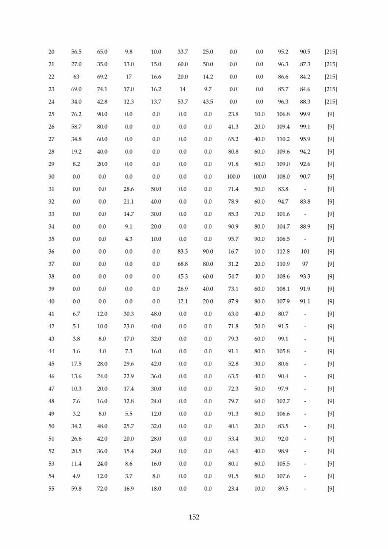
20 56.5 65.0 9.8 10.0 33.7 25.0 0.0 0.0 95.2 90.5 [215]

21 27.0 35.0 13.0 15.0 60.0 50.0 0.0 0.0 96.3 87.3 [215]

22 63 69.2 17 16.6 20.0 14.2 0.0 0.0 86.6 84.2 [215]

23 69.0 74.1 17.0 16.2 14 9.7 0.0 0.0 85.7 84.6 [215]

24 34.0 42.8 12.3 13.7 53.7 43.5 0.0 0.0 96.3 88.3 [215]

25 76.2 90.0 0.0 0.0 0.0 0.0 23.8 10.0 106.8 99.9 [9]

26 58.7 80.0 0.0 0.0 0.0 0.0 41.3 20.0 109.4 99.1 [9]

27 34.8 60.0 0.0 0.0 0.0 0.0 65.2 40.0 110.2 95.9 [9]

28 19.2 40.0 0.0 0.0 0.0 0.0 80.8 60.0 109.6 94.2 [9]

29 8.2 20.0 0.0 0.0 0.0 0.0 91.8 80.0 109.0 92.6 [9]

30 0.0 0.0 0.0 0.0 0.0 0.0 100.0 100.0 108.0 90.7 [9]

31 0.0 0.0 28.6 50.0 0.0 0.0 71.4 50.0 83.8 - [9]

32 0.0 0.0 21.1 40.0 0.0 0.0 78.9 60.0 94.7 83.8 [9]

33 0.0 0.0 14.7 30.0 0.0 0.0 85.3 70.0 101.6 - [9]

34 0.0 0.0 9.1 20.0 0.0 0.0 90.9 80.0 104.7 88.9 [9]

35 0.0 0.0 4.3 10.0 0.0 0.0 95.7 90.0 106.5 - [9]

36 0.0 0.0 0.0 0.0 83.3 90.0 16.7 10.0 112.8 101 [9]

37 0.0 0.0 0.0 0.0 68.8 80.0 31.2 20.0 110.9 97 [9]

38 0.0 0.0 0.0 0.0 45.3 60.0 54.7 40.0 108.6 93.3 [9]

39 0.0 0.0 0.0 0.0 26.9 40.0 73.1 60.0 108.1 91.9 [9]

40 0.0 0.0 0.0 0.0 12.1 20.0 87.9 80.0 107.9 91.1 [9]

41 6.7 12.0 30.3 48.0 0.0 0.0 63.0 40.0 80.7 - [9]

42 5.1 10.0 23.0 40.0 0.0 0.0 71.8 50.0 91.5 - [9]

43 3.8 8.0 17.0 32.0 0.0 0.0 79.3 60.0 99.1 - [9]

44 1.6 4.0 7.3 16.0 0.0 0.0 91.1 80.0 105.8 - [9]

45 17.5 28.0 29.6 42.0 0.0 0.0 52.8 30.0 80.6 - [9]

46 13.6 24.0 22.9 36.0 0.0 0.0 63.5 40.0 90.4 - [9]

47 10.3 20.0 17.4 30.0 0.0 0.0 72.3 50.0 97.9 - [9]

48 7.6 16.0 12.8 24.0 0.0 0.0 79.7 60.0 102.7 - [9]

49 3.2 8.0 5.5 12.0 0.0 0.0 91.3 80.0 106.6 - [9]

50 34.2 48.0 25.7 32.0 0.0 0.0 40.1 20.0 83.5 - [9]

51 26.6 42.0 20.0 28.0 0.0 0.0 53.4 30.0 92.0 - [9]

52 20.5 36.0 15.4 24.0 0.0 0.0 64.1 40.0 98.9 - [9]

53 11.4 24.0 8.6 16.0 0.0 0.0 80.1 60.0 105.5 - [9]

54 4.9 12.0 3.7 8.0 0.0 0.0 91.5 80.0 107.6 - [9]

55 59.8 72.0 16.9 18.0 0.0 0.0 23.4 10.0 89.5 - [9]

152

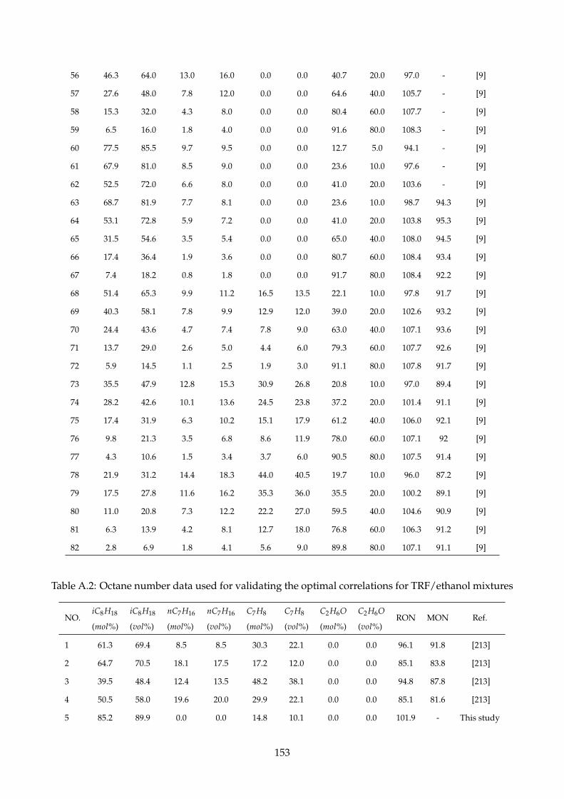
56 46.3 64.0 13.0 16.0 0.0 0.0 40.7 20.0 97.0 - [9]

57 27.6 48.0 7.8 12.0 0.0 0.0 64.6 40.0 105.7 - [9]

58 15.3 32.0 4.3 8.0 0.0 0.0 80.4 60.0 107.7 - [9]

59 6.5 16.0 1.8 4.0 0.0 0.0 91.6 80.0 108.3 - [9]

60 77.5 85.5 9.7 9.5 0.0 0.0 12.7 5.0 94.1 - [9]

61 67.9 81.0 8.5 9.0 0.0 0.0 23.6 10.0 97.6 - [9]

62 52.5 72.0 6.6 8.0 0.0 0.0 41.0 20.0 103.6 - [9]

63 68.7 81.9 7.7 8.1 0.0 0.0 23.6 10.0 98.7 94.3 [9]

64 53.1 72.8 5.9 7.2 0.0 0.0 41.0 20.0 103.8 95.3 [9]

65 31.5 54.6 3.5 5.4 0.0 0.0 65.0 40.0 108.0 94.5 [9]

66 17.4 36.4 1.9 3.6 0.0 0.0 80.7 60.0 108.4 93.4 [9]

67 7.4 18.2 0.8 1.8 0.0 0.0 91.7 80.0 108.4 92.2 [9]

68 51.4 65.3 9.9 11.2 16.5 13.5 22.1 10.0 97.8 91.7 [9]

69 40.3 58.1 7.8 9.9 12.9 12.0 39.0 20.0 102.6 93.2 [9]

70 24.4 43.6 4.7 7.4 7.8 9.0 63.0 40.0 107.1 93.6 [9]

71 13.7 29.0 2.6 5.0 4.4 6.0 79.3 60.0 107.7 92.6 [9]

72 5.9 14.5 1.1 2.5 1.9 3.0 91.1 80.0 107.8 91.7 [9]

73 35.5 47.9 12.8 15.3 30.9 26.8 20.8 10.0 97.0 89.4 [9]

74 28.2 42.6 10.1 13.6 24.5 23.8 37.2 20.0 101.4 91.1 [9]

75 17.4 31.9 6.3 10.2 15.1 17.9 61.2 40.0 106.0 92.1 [9]

76 9.8 21.3 3.5 6.8 8.6 11.9 78.0 60.0 107.1 92 [9]

77 4.3 10.6 1.5 3.4 3.7 6.0 90.5 80.0 107.5 91.4 [9]

78 21.9 31.2 14.4 18.3 44.0 40.5 19.7 10.0 96.0 87.2 [9]

79 17.5 27.8 11.6 16.2 35.3 36.0 35.5 20.0 100.2 89.1 [9]

80 11.0 20.8 7.3 12.2 22.2 27.0 59.5 40.0 104.6 90.9 [9]

81 6.3 13.9 4.2 8.1 12.7 18.0 76.8 60.0 106.3 91.2 [9]

82 2.8 6.9 1.8 4.1 5.6 9.0 89.8 80.0 107.1 91.1 [9]

Table A.2: Octane number data used for validating the optimal correlations for TRF/ethanol mixtures

NO.iC8H18

(mol%)

iC8H18

(vol%)

nC7H16

(mol%)

nC7H16

(vol%)

C7H8

(mol%)

C7H8

(vol%)

C2H6O

(mol%)

C2H6O

(vol%)RON MON Ref.

1 61.3 69.4 8.5 8.5 30.3 22.1 0.0 0.0 96.1 91.8 [213]

2 64.7 70.5 18.1 17.5 17.2 12.0 0.0 0.0 85.1 83.8 [213]

3 39.5 48.4 12.4 13.5 48.2 38.1 0.0 0.0 94.8 87.8 [213]

4 50.5 58.0 19.6 20.0 29.9 22.1 0.0 0.0 85.1 81.6 [213]

5 85.2 89.9 0.0 0.0 14.8 10.1 0.0 0.0 101.9 - This study

153

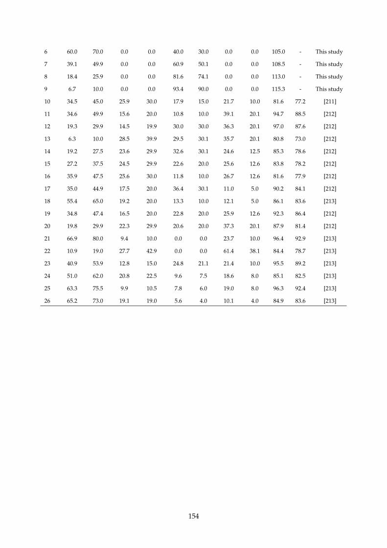
6 60.0 70.0 0.0 0.0 40.0 30.0 0.0 0.0 105.0 - This study

7 39.1 49.9 0.0 0.0 60.9 50.1 0.0 0.0 108.5 - This study

8 18.4 25.9 0.0 0.0 81.6 74.1 0.0 0.0 113.0 - This study

9 6.7 10.0 0.0 0.0 93.4 90.0 0.0 0.0 115.3 - This study

10 34.5 45.0 25.9 30.0 17.9 15.0 21.7 10.0 81.6 77.2 [211]

11 34.6 49.9 15.6 20.0 10.8 10.0 39.1 20.1 94.7 88.5 [212]

12 19.3 29.9 14.5 19.9 30.0 30.0 36.3 20.1 97.0 87.6 [212]

13 6.3 10.0 28.5 39.9 29.5 30.1 35.7 20.1 80.8 73.0 [212]

14 19.2 27.5 23.6 29.9 32.6 30.1 24.6 12.5 85.3 78.6 [212]

15 27.2 37.5 24.5 29.9 22.6 20.0 25.6 12.6 83.8 78.2 [212]

16 35.9 47.5 25.6 30.0 11.8 10.0 26.7 12.6 81.6 77.9 [212]

17 35.0 44.9 17.5 20.0 36.4 30.1 11.0 5.0 90.2 84.1 [212]

18 55.4 65.0 19.2 20.0 13.3 10.0 12.1 5.0 86.1 83.6 [213]

19 34.8 47.4 16.5 20.0 22.8 20.0 25.9 12.6 92.3 86.4 [212]

20 19.8 29.9 22.3 29.9 20.6 20.0 37.3 20.1 87.9 81.4 [212]

21 66.9 80.0 9.4 10.0 0.0 0.0 23.7 10.0 96.4 92.9 [213]

22 10.9 19.0 27.7 42.9 0.0 0.0 61.4 38.1 84.4 78.7 [213]

23 40.9 53.9 12.8 15.0 24.8 21.1 21.4 10.0 95.5 89.2 [213]

24 51.0 62.0 20.8 22.5 9.6 7.5 18.6 8.0 85.1 82.5 [213]

25 63.3 75.5 9.9 10.5 7.8 6.0 19.0 8.0 96.3 92.4 [213]

26 65.2 73.0 19.1 19.0 5.6 4.0 10.1 4.0 84.9 83.6 [213]

154

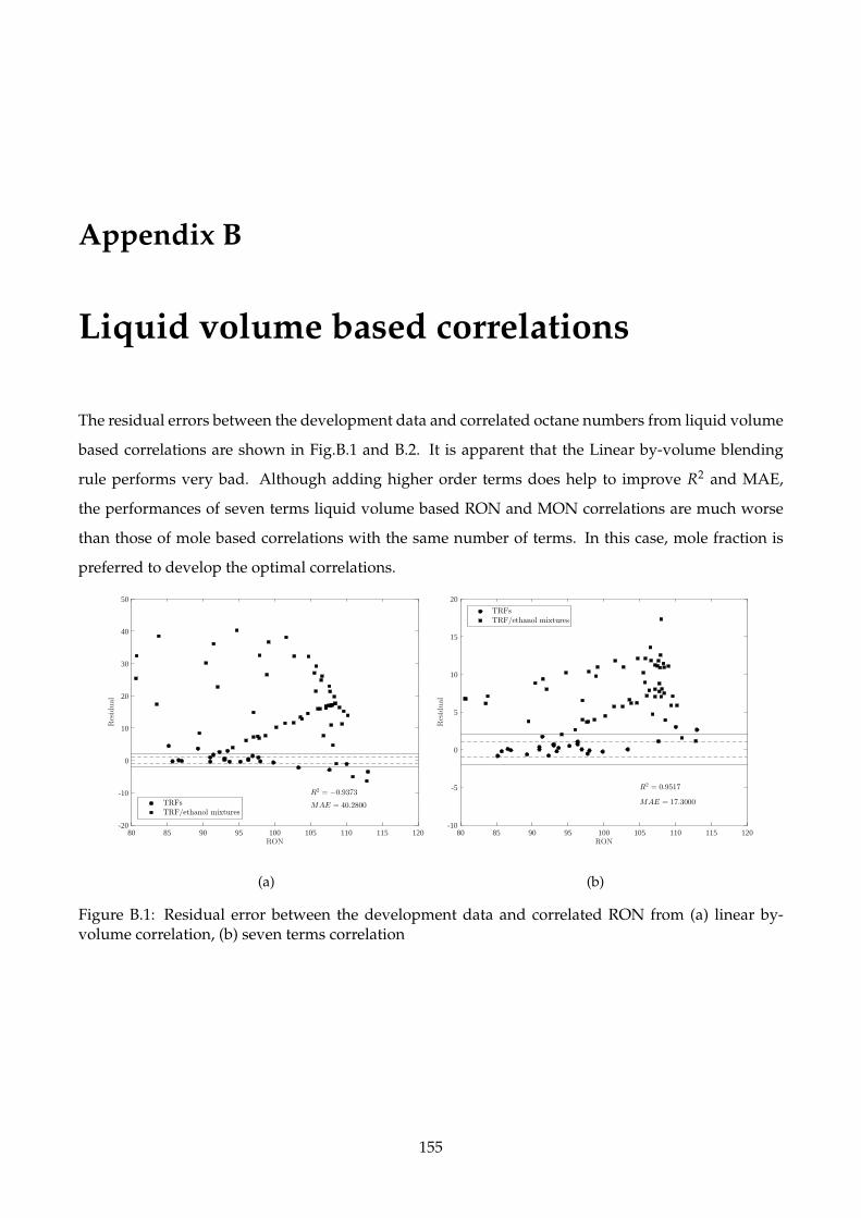
Appendix B

Liquid volume based correlations

The residual errors between the development data and correlated octane numbers from liquid volume

based correlations are shown in Fig.B.1 and B.2. It is apparent that the Linear by-volume blending

rule performs very bad. Although adding higher order terms does help to improve R2 and MAE,

the performances of seven terms liquid volume based RON and MON correlations are much worse

than those of mole based correlations with the same number of terms. In this case, mole fraction is

preferred to develop the optimal correlations.

RON80 85 90 95 100 105 110 115 120

Residual

-20

-10

0

10

20

30

40

50

R2 = −0.9373

MAE = 40.2800TRFsTRF/ethanol mixtures

(a)

RON80 85 90 95 100 105 110 115 120

Residual

-10

-5

0

5

10

15

20

R2 = 0.9517

MAE = 17.3000

TRFsTRF/ethanol mixtures

(b)

Figure B.1: Residual error between the development data and correlated RON from (a) linear by-volume correlation, (b) seven terms correlation

155

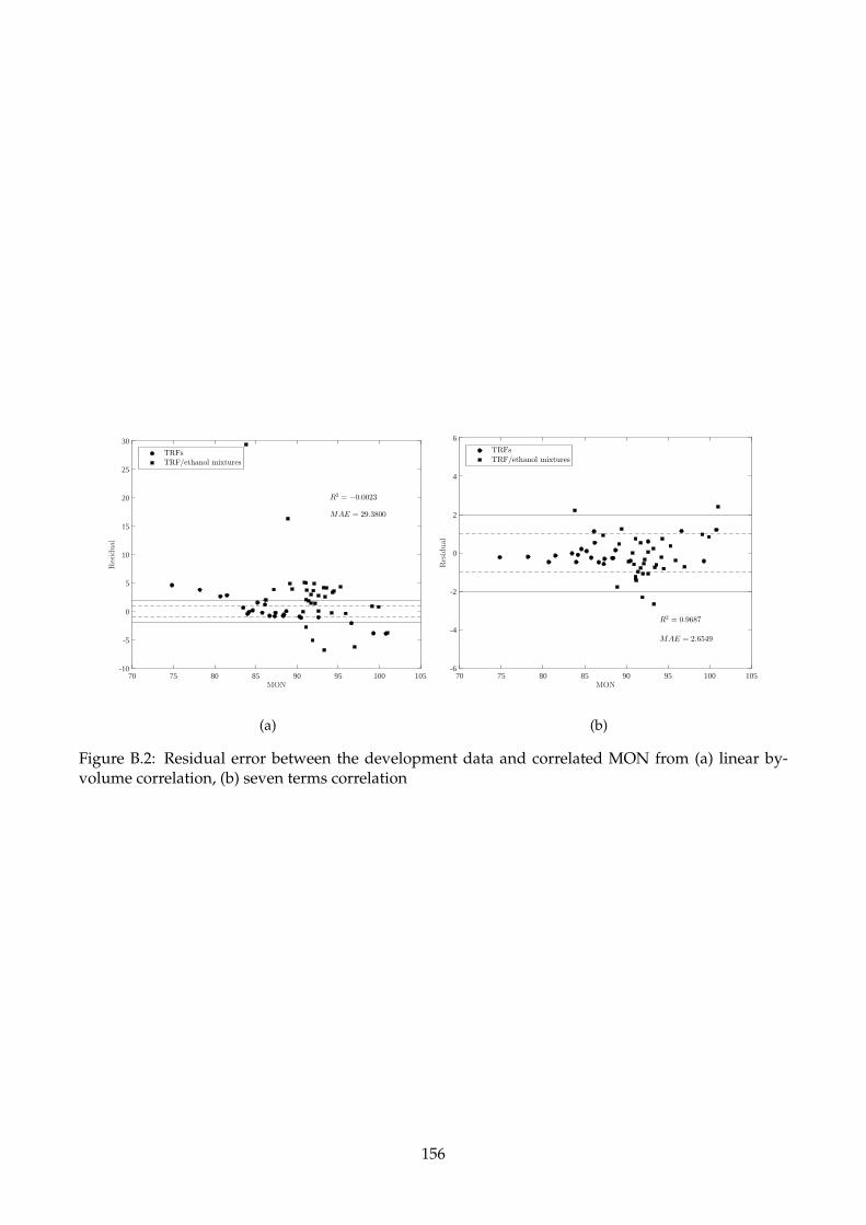
MON70 75 80 85 90 95 100 105

Residual

-10

-5

0

5

10

15

20

25

30

R2 = −0.0023

MAE = 29.3800


(a)

MON70 75 80 85 90 95 100 105

Residual

-6

-4

-2

0

2

4

6

R2 = 0.9687

MAE = 2.6549


(b)

Figure B.2: Residual error between the development data and correlated MON from (a) linear by-volume correlation, (b) seven terms correlation

156

Appendix C

Modelling of Trace Knock in a Modern SI

Engine Fuelled by Ethanol and Gasoline

Blends

C.1 Introduction

A systematic method has been proposed in [23] to model the knocking behaviours in spark ignition

engines using two-zone kinetic model coupled with detailed chemistry. However, in most scenarios,

engine knocks are not as strong as reported in [23] and, most likely, occur intermittently in real pro-

duction engines, which is commonly known as trace knock. The trace knock is the borderline between

non-knocking and knocking combustions. If the spark timing is advanced, there will be a larger heat

release inside the engine cylinder, resulting in knocking combustion, and vice versa. Unlike those

strong knocking behaviours, no distinct incipient jump, indicating autoignition, can be seen on the

pressure traces from trace knock. This complicates the numerical modelling since the autoignition

is insignificant and no clear clue is available from the pressure traces suggesting the occurrence of

autoignition.

Hence, this study is aiming to model the trace knocks from a single-cylinder research engine [11].

The objectives of this study are as follows.

• To propose a systematic method for trace knock modelling in SI engines

• To model the effect of ethanol on trace knock with the proposed method and an existing kinetic

model for gasoline surrogates

• To model the effect of DI on trace knock

157

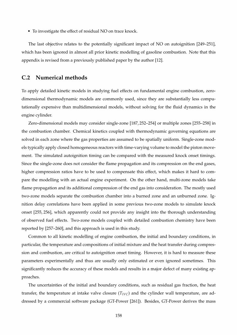
• To investigate the effect of residual NO on trace knock.

The last objective relates to the potentially significant impact of NO on autoignition [249–251],

which has been ignored in almost all prior kinetic modelling of gasoline combustion. Note that this

appendix is revised from a previously published paper by the author [12].

C.2 Numerical methods

To apply detailed kinetic models in studying fuel effects on fundamental engine combustion, zero-

dimensional thermodynamic models are commonly used, since they are substantially less compu-

tationally expensive than multidimensional models, without solving for the fluid dynamics in the

engine cylinder.

Zero-dimensional models may consider single-zone [187, 252–254] or multiple zones [255–258] in

the combustion chamber. Chemical kinetics coupled with thermodynamic governing equations are

solved in each zone where the gas properties are assumed to be spatially uniform. Single-zone mod-

els typically apply closed homogeneous reactors with time-varying volume to model the piston move-

ment. The simulated autoignition timing can be compared with the measured knock onset timings.

Since the single-zone does not consider the flame propagation and its compression on the end gases,

higher compression ratios have to be used to compensate this effect, which makes it hard to com-

pare the modelling with an actual engine experiment. On the other hand, multi-zone models take

flame propagation and its additional compression of the end gas into consideration. The mostly used

two-zone models separate the combustion chamber into a burned zone and an unburned zone. Ig-

nition delay correlations have been applied in some previous two-zone models to simulate knock

onset [255, 256], which apparently could not provide any insight into the thorough understanding

of observed fuel effects. Two-zone models coupled with detailed combustion chemistry have been

reported by [257–260], and this approach is used in this study.

Common to all kinetic modelling of engine combustion, the initial and boundary conditions, in

particular, the temperature and compositions of initial mixture and the heat transfer during compres-

sion and combustion, are critical to autoignition onset timing. However, it is hard to measure these

parameters experimentally and thus are usually only estimated or even ignored sometimes. This

significantly reduces the accuracy of these models and results in a major defect of many existing ap-

proaches.

The uncertainties of the initial and boundary conditions, such as residual gas fraction, the heat

transfer, the temperature at intake valve closure (TIVC) and the cylinder wall temperature, are ad-

dressed by a commercial software package (GT-Power [261]). Besides, GT-Power derives the mass

158

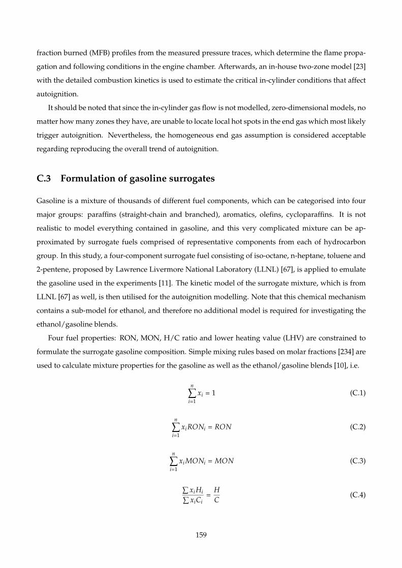
fraction burned (MFB) profiles from the measured pressure traces, which determine the flame propa-

gation and following conditions in the engine chamber. Afterwards, an in-house two-zone model [23]

with the detailed combustion kinetics is used to estimate the critical in-cylinder conditions that affect

autoignition.

It should be noted that since the in-cylinder gas flow is not modelled, zero-dimensional models, no

matter how many zones they have, are unable to locate local hot spots in the end gas which most likely

trigger autoignition. Nevertheless, the homogeneous end gas assumption is considered acceptable

regarding reproducing the overall trend of autoignition.

C.3 Formulation of gasoline surrogates

Gasoline is a mixture of thousands of different fuel components, which can be categorised into four

major groups: paraffins (straight-chain and branched), aromatics, olefins, cycloparaffins. It is not

realistic to model everything contained in gasoline, and this very complicated mixture can be ap-

proximated by surrogate fuels comprised of representative components from each of hydrocarbon

group. In this study, a four-component surrogate fuel consisting of iso-octane, n-heptane, toluene and

2-pentene, proposed by Lawrence Livermore National Laboratory (LLNL) [67], is applied to emulate

the gasoline used in the experiments [11]. The kinetic model of the surrogate mixture, which is from

LLNL [67] as well, is then utilised for the autoignition modelling. Note that this chemical mechanism

contains a sub-model for ethanol, and therefore no additional model is required for investigating the

ethanol/gasoline blends.

Four fuel properties: RON, MON, H/C ratio and lower heating value (LHV) are constrained to

formulate the surrogate gasoline composition. Simple mixing rules based on molar fractions [234] are

used to calculate mixture properties for the gasoline as well as the ethanol/gasoline blends [10], i.e.

n

∑i=1

xi = 1 (C.1)

n

∑i=1

xiRONi = RON (C.2)

n

∑i=1

xi MONi = MON (C.3)

∑ xi Hi

∑ xiCi=

HC

(C.4)

159

n

∑i=1

xiLHVi = LHV (C.5)

where n is the number of representative components, xi is the molar fraction, Hi and Ci are the number

of hydrogen and carbon atoms respectively, RONi and MONi are research and motor octane numbers,

and LHVi is the lower heating value of the ith component in the surrogate mixture.

Since autoignition is of primary concern, priority was given to matching the RON MON, when

considering these constraints. In addition, the gasoline compositions reported in the original single-

cylinder, research engine experiments [11, 44] were considered to make the surrogate fuels have a

similar hydrocarbon type distribution to the actual test fuels. Table C.1 shows the compositions of

the original and resulting gasoline surrogates. The properties of the two fuels are shown in Table

C.2. It is clear that the RON and MON are matched closely, and the H/C ratio and LHV are matched

reasonably well. The naphthenes, whose composition is less than 5 vol% in the test gasoline, are not

considered in the surrogates.

Table C.1: Gasoline and surrogate fuel compositions (%vol)

Fuel iso-paraffins n-paraffins naphthenes olefins aromatics

Gasoline 42.4 21.2 4.9 5.8 25.7

surrogate 44.6 21.0 0.0 6.5 27.9

Table C.2: Gasoline and surrogate fuel properties

Parameters RON MON H/C ratio LHV (MJ/kg)

Gasoline 87.7 81.5 1.94 42.4

surrogate 87.7 81.5 1.85 43.4

C.4 NO sub-model

NO has been identified as a particularly significant trace species that affect autoignition in spark igni-

tion engines [249–251]. The NO sub-model, however, is not available in most chemical mechanisms,

including the one used in this study [67]. In this case, the NO mechanism proposed by [262] was incor-

porated into the four-component LLNL gasoline mechanism for this study. One repeated elementary

reaction (appearing in both mechanisms) was removed from the NO sub-model, which means the

original gasoline surrogate model remained intact. To confirm this, the ignition delay of the new

160

NO-containing gasoline mechanism and the original LLNL mechanism was modelled in a constant

volume reactor.

The governing equations for a constant volume reactor [47] are expressed as

dTdt

=(Q/V) + RuT ∑ wi −∑ (hiwi)

∑ [[Xi](cp,i − Ru)](C.6)

dPdt

= RuT ∑ wi + Ru ∑ [Xi]dTdt

(C.7)

where T, P, Q, V, and Ru are temperature, pressure, rate of heat transferred to the system, reactor

volume and gas constant, [Xi] represents mole concentration for species i, cp,i and hi denote molar

constant-pressure specific heat and molar enthalpy of species i, and wi is the net production rate for

species i, which can be derived from chemical kinetics. These equations are solved in Matlab using

ode15s solver with kinetic parameters provided by Cantera [263]. Whilst the ignition delay timing

is indicated by the rapid temperature increase, e.g. 400K increase in one time step. The modelled

ignition delays with the original and blended mechanisms are compared in Fig.C.1, which confirms

the integrity of the original mechanism.

1000K/T

0.8 0.9 1 1.1 1.2 1.3 1.4 1.5

Ignitiondelay

time(m

s)

10−1

100

101

102

Blended mechanismOriginal mechanism

Figure C.1: Comparison of the simulated ignition delay of the formulated gasoline surrogate (TableC.1) using the original LLNL model and the extended model containing NO in a constant volumereactor without NO present initially. Equivalence ratio = 1, 30bar, 700-1200K

161

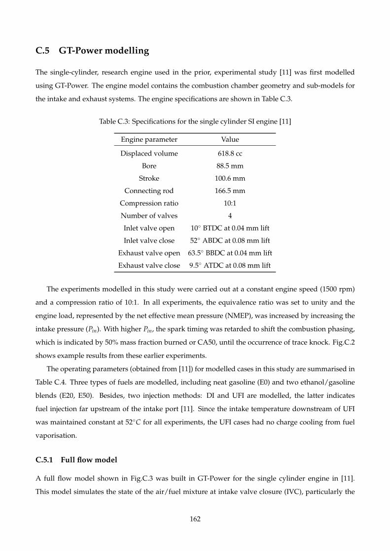
C.5 GT-Power modelling

The single-cylinder, research engine used in the prior, experimental study [11] was first modelled

using GT-Power. The engine model contains the combustion chamber geometry and sub-models for

the intake and exhaust systems. The engine specifications are shown in Table C.3.

Table C.3: Specifications for the single cylinder SI engine [11]

Engine parameter Value

Displaced volume 618.8 cc

Bore 88.5 mm

Stroke 100.6 mm

Connecting rod 166.5 mm

Compression ratio 10:1

Number of valves 4

Inlet valve open 10◦ BTDC at 0.04 mm lift

Inlet valve close 52◦ ABDC at 0.08 mm lift

Exhaust valve open 63.5◦ BBDC at 0.04 mm lift

Exhaust valve close 9.5◦ ATDC at 0.08 mm lift

The experiments modelled in this study were carried out at a constant engine speed (1500 rpm)

and a compression ratio of 10:1. In all experiments, the equivalence ratio was set to unity and the

engine load, represented by the net effective mean pressure (NMEP), was increased by increasing the

intake pressure (Pin). With higher Pin, the spark timing was retarded to shift the combustion phasing,

which is indicated by 50% mass fraction burned or CA50, until the occurrence of trace knock. Fig.C.2

shows example results from these earlier experiments.

The operating parameters (obtained from [11]) for modelled cases in this study are summarised in

Table C.4. Three types of fuels are modelled, including neat gasoline (E0) and two ethanol/gasoline

blends (E20, E50). Besides, two injection methods: DI and UFI are modelled, the latter indicates

fuel injection far upstream of the intake port [11]. Since the intake temperature downstream of UFI

was maintained constant at 52◦C for all experiments, the UFI cases had no charge cooling from fuel

vaporisation.

C.5.1 Full flow model

A full flow model shown in Fig.C.3 was built in GT-Power for the single cylinder engine in [11].

This model simulates the state of the air/fuel mixture at intake valve closure (IVC), particularly the

162

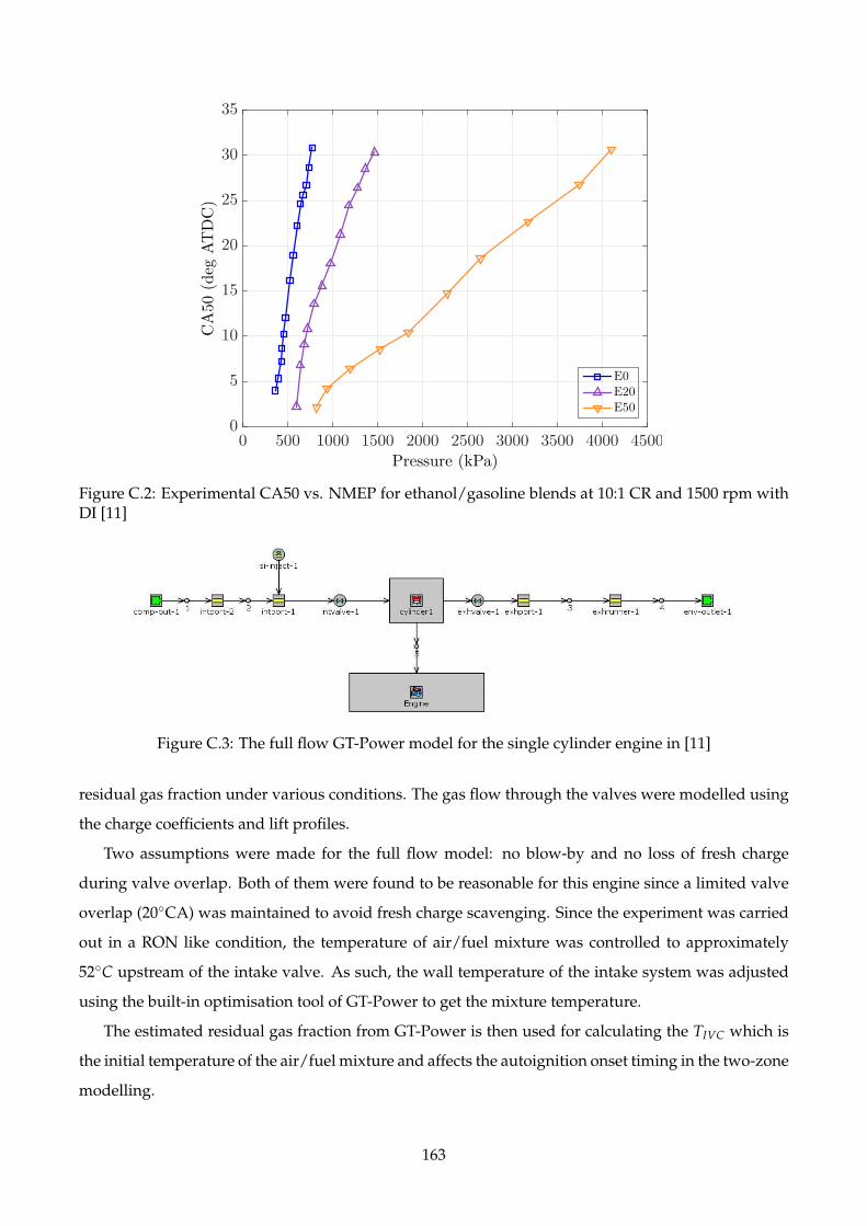
Pressure (kPa)

0 500 1000 1500 2000 2500 3000 3500 4000 4500

CA50(deg

ATDC)

0

5

10

15

20

25

30

35

E0E20E50

Figure C.2: Experimental CA50 vs. NMEP for ethanol/gasoline blends at 10:1 CR and 1500 rpm withDI [11]

Figure C.3: The full flow GT-Power model for the single cylinder engine in [11]

residual gas fraction under various conditions. The gas flow through the valves were modelled using

the charge coefficients and lift profiles.

Two assumptions were made for the full flow model: no blow-by and no loss of fresh charge

during valve overlap. Both of them were found to be reasonable for this engine since a limited valve

overlap (20◦CA) was maintained to avoid fresh charge scavenging. Since the experiment was carried

out in a RON like condition, the temperature of air/fuel mixture was controlled to approximately

52◦C upstream of the intake valve. As such, the wall temperature of the intake system was adjusted

using the built-in optimisation tool of GT-Power to get the mixture temperature.

The estimated residual gas fraction from GT-Power is then used for calculating the TIVC which is

the initial temperature of the air/fuel mixture and affects the autoignition onset timing in the two-zone

modelling.

163

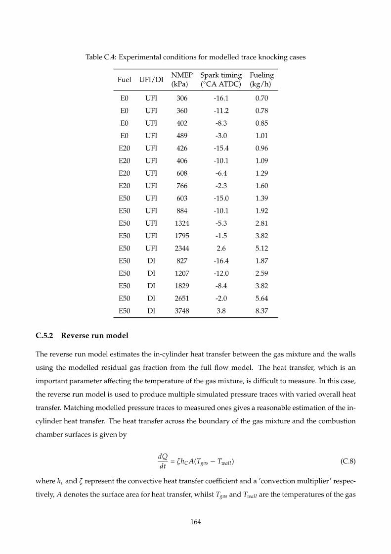
Table C.4: Experimental conditions for modelled trace knocking cases

Fuel UFI/DINMEP(kPa)

Spark timing(◦CA ATDC)

Fueling(kg/h)

E0 UFI 306 -16.1 0.70

E0 UFI 360 -11.2 0.78

E0 UFI 402 -8.3 0.85

E0 UFI 489 -3.0 1.01

E20 UFI 426 -15.4 0.96

E20 UFI 406 -10.1 1.09

E20 UFI 608 -6.4 1.29

E20 UFI 766 -2.3 1.60

E50 UFI 603 -15.0 1.39

E50 UFI 884 -10.1 1.92

E50 UFI 1324 -5.3 2.81

E50 UFI 1795 -1.5 3.82

E50 UFI 2344 2.6 5.12

E50 DI 827 -16.4 1.87

E50 DI 1207 -12.0 2.59

E50 DI 1829 -8.4 3.82

E50 DI 2651 -2.0 5.64

E50 DI 3748 3.8 8.37

C.5.2 Reverse run model

The reverse run model estimates the in-cylinder heat transfer between the gas mixture and the walls

using the modelled residual gas fraction from the full flow model. The heat transfer, which is an

important parameter affecting the temperature of the gas mixture, is difficult to measure. In this case,

the reverse run model is used to produce multiple simulated pressure traces with varied overall heat

transfer. Matching modelled pressure traces to measured ones gives a reasonable estimation of the in-

cylinder heat transfer. The heat transfer across the boundary of the gas mixture and the combustion

chamber surfaces is given by

dQdt

= ζhC A(Tgas − Twall) (C.8)

where hc and ζ represent the convective heat transfer coefficient and a ’convection multiplier’ respec-

tively, A denotes the surface area for heat transfer, whilst Tgas and Twall are the temperatures of the gas

164

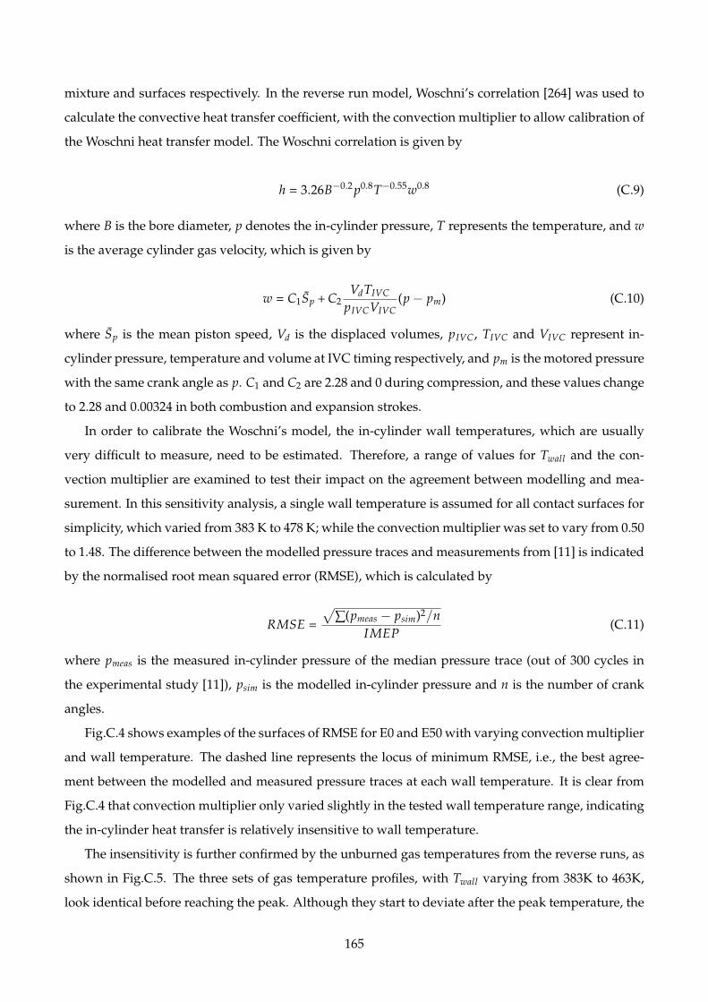
mixture and surfaces respectively. In the reverse run model, Woschni’s correlation [264] was used to

calculate the convective heat transfer coefficient, with the convection multiplier to allow calibration of

the Woschni heat transfer model. The Woschni correlation is given by

h = 3.26B−0.2 p0.8T−0.55w0.8 (C.9)

where B is the bore diameter, p denotes the in-cylinder pressure, T represents the temperature, and w

is the average cylinder gas velocity, which is given by

w = C1Sp + C2VdTIVC

pIVCVIVC(p− pm) (C.10)

where Sp is the mean piston speed, Vd is the displaced volumes, pIVC, TIVC and VIVC represent in-

cylinder pressure, temperature and volume at IVC timing respectively, and pm is the motored pressure

with the same crank angle as p. C1 and C2 are 2.28 and 0 during compression, and these values change

to 2.28 and 0.00324 in both combustion and expansion strokes.

In order to calibrate the Woschni’s model, the in-cylinder wall temperatures, which are usually

very difficult to measure, need to be estimated. Therefore, a range of values for Twall and the con-

vection multiplier are examined to test their impact on the agreement between modelling and mea-

surement. In this sensitivity analysis, a single wall temperature is assumed for all contact surfaces for

simplicity, which varied from 383 K to 478 K; while the convection multiplier was set to vary from 0.50

to 1.48. The difference between the modelled pressure traces and measurements from [11] is indicated

by the normalised root mean squared error (RMSE), which is calculated by

RMSE =

√∑(pmeas − psim)2/n

IMEP(C.11)

where pmeas is the measured in-cylinder pressure of the median pressure trace (out of 300 cycles in

the experimental study [11]), psim is the modelled in-cylinder pressure and n is the number of crank

angles.

Fig.C.4 shows examples of the surfaces of RMSE for E0 and E50 with varying convection multiplier

and wall temperature. The dashed line represents the locus of minimum RMSE, i.e., the best agree-

ment between the modelled and measured pressure traces at each wall temperature. It is clear from

Fig.C.4 that convection multiplier only varied slightly in the tested wall temperature range, indicating

the in-cylinder heat transfer is relatively insensitive to wall temperature.

The insensitivity is further confirmed by the unburned gas temperatures from the reverse runs, as

shown in Fig.C.5. The three sets of gas temperature profiles, with Twall varying from 383K to 463K,

look identical before reaching the peak. Although they start to deviate after the peak temperature, the

165

1.5

1.5

2

2

2.5

2.5

3

3

3.5

3.54

4.55

5.5

6 6

Temperature (K)

383 393 403 413 423 433 443 453 463 473

Convectionmultiplier

0.5

0.6

0.7

0.8

0.9

1

1.1

1.2

1.3

1.4

(a) E0.UFI, NMEP=402kPa

1

1

1.5

1.5

2

2

2.5

2.5

3

3

3.5

3.5

4

4

4.5

4.5

5

5

Temperature (K)

383 393 403 413 423 433 443 453 463 473

Convectionmultiplier

0.5

0.6

0.7

0.8

0.9

1

1.1

1.2

1.3

1.4

(b) E50.UFI, NMEP=1324kPa

Figure C.4: The sensitivity analysis for the convection multiplier, to the cylinder wall temperature,Twall . Dashed lines represent the minimal RMSE at each wall temperature. RMSE values (×104) areindicated by the numbers on the contours

absolute differences are still quite small at the end of combustion.

Crank Angle (deg)

-20 0 20 40 60 80

Tem

perature

(K)

550

600

650

700

750

800

850

900

950

1000383K423K463K


Crank Angle (deg)

-20 0 20 40 60 80 100

Tem

perature

(K)

550

600

650

700

750

800

850

900

950383K423K463K


Figure C.5: Unburned gas temperature profiles at different wall temperatures from the GT-Powerreverse run

Based on the results from Fig.C.4 and C.5, it is reasonable to assume a constant wall temperature

of 423K for all modelling in this work, with the convection multiplier optimised for a given measured

pressure trace. This assumption significantly simplifies the reverse run modelling, since the only pa-

rameter needs to be varied is the convection multiplier when estimating the in-cylinder heat transfer.

Fig.C.6 then shows the close agreement between the resulting modelled pressure traces and those

measured over the range of fuels in this study. Besides, the mass fraction burned (MFB) profiles were

derived from the matched modelled pressure trace. Therefore, a systematic approach estimating the

166

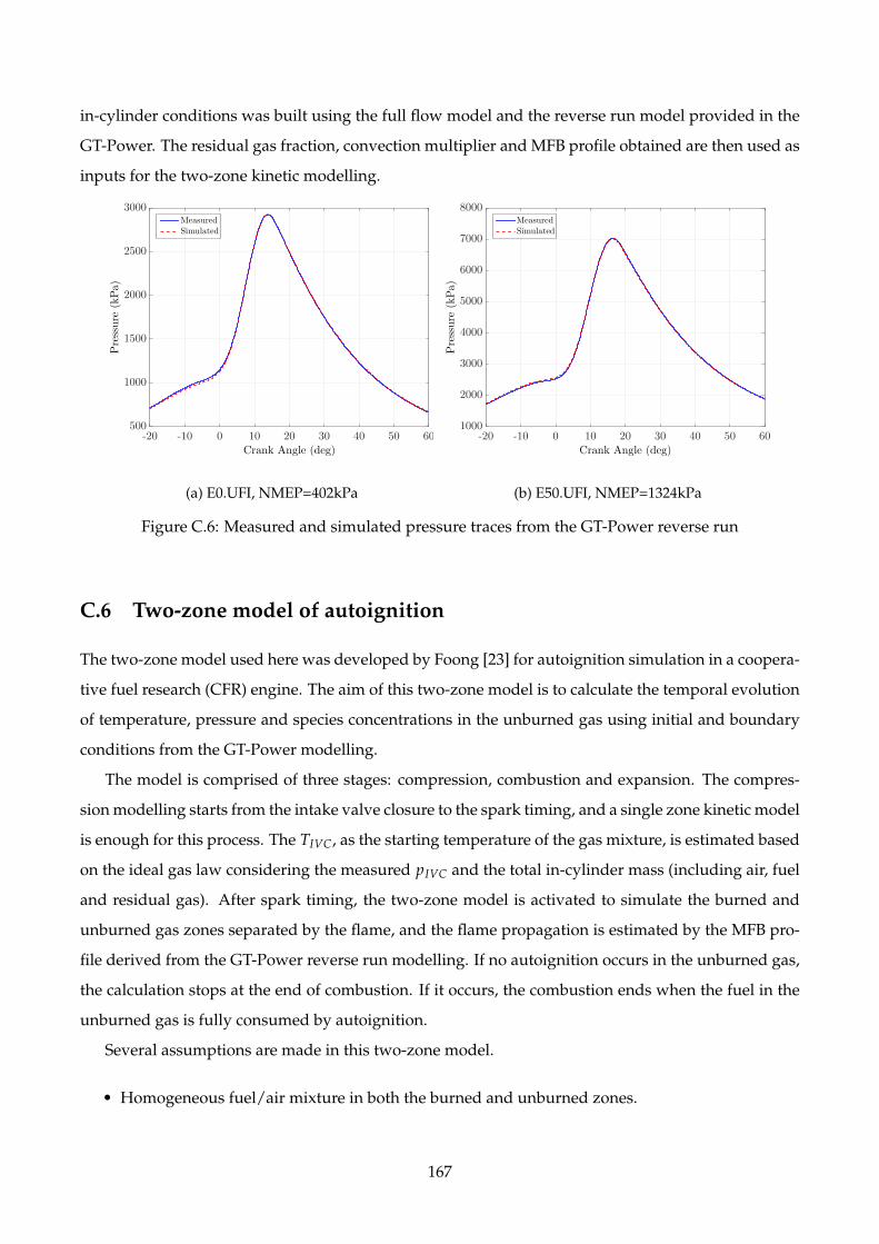
in-cylinder conditions was built using the full flow model and the reverse run model provided in the

GT-Power. The residual gas fraction, convection multiplier and MFB profile obtained are then used as

inputs for the two-zone kinetic modelling.

Crank Angle (deg)

-20 -10 0 10 20 30 40 50 60

Pressure

(kPa)

500

1000

1500

2000

2500

3000MeasuredSimulated


Crank Angle (deg)

-20 -10 0 10 20 30 40 50 60Pressure

(kPa)

1000

2000

3000

4000

5000

6000

7000

8000MeasuredSimulated


Figure C.6: Measured and simulated pressure traces from the GT-Power reverse run

C.6 Two-zone model of autoignition

The two-zone model used here was developed by Foong [23] for autoignition simulation in a coopera-

tive fuel research (CFR) engine. The aim of this two-zone model is to calculate the temporal evolution

of temperature, pressure and species concentrations in the unburned gas using initial and boundary

conditions from the GT-Power modelling.

The model is comprised of three stages: compression, combustion and expansion. The compres-

sion modelling starts from the intake valve closure to the spark timing, and a single zone kinetic model

is enough for this process. The TIVC, as the starting temperature of the gas mixture, is estimated based

on the ideal gas law considering the measured pIVC and the total in-cylinder mass (including air, fuel

and residual gas). After spark timing, the two-zone model is activated to simulate the burned and

unburned gas zones separated by the flame, and the flame propagation is estimated by the MFB pro-

file derived from the GT-Power reverse run modelling. If no autoignition occurs in the unburned gas,

the calculation stops at the end of combustion. If it occurs, the combustion ends when the fuel in the

unburned gas is fully consumed by autoignition.

Several assumptions are made in this two-zone model.

• Homogeneous fuel/air mixture in both the burned and unburned zones.

167

• The volume of the flame is neglected, and therefore mass transfer and enthalpy exchange be-

tween the two zones occur instantaneously.

• The flame is at chemical equilibrium.

• No heat transfer between the two zones.

The two-zone model was implemented in MATLAB, with kinetic information derived from Can-

tera 1.8 [265].

C.7 Modelling of trace knock

C.7.1 Raw pressure data

Trace knock, which has no distinct pressure jump, is the borderline between knocking and non-

knocking combustion. If the spark timing is advanced slightly, e.g. 1 ◦CA, the engine combustion

may transfer from non-knocking to knocking and vice versa. To have a good understanding on trace

knock, the raw pressure data from trace knocking conditions are compared a ’typical’ knocking pres-

sure trace. Fig.C.7(a) shows a typical knocking raw pressure trace for isooctane at so-called ’standard

knock intensity’ condition in our CFR engine, which is from [23] and represents a condition in which

autoignition and knock occur in all cycles. The trace knock results in Fig.C.7(c) and (e) are for the

E0 and E50 cases as shown in Fig.C.6. The pressure traces selected for trace knock conditions are

the most advanced ones, which have the most intensive autoignition comparing to other relatively

retarded traces. It would be interesting to investigate whether the characteristics of typical knock-

ing pressure trace repeat themselves on trace knocks. Band-pass filtering and Fast Fourier Transform

(FFT) are two common techniques used to characterise knocking pressure traces, and their results are

shown in Fig.C.7 as well. The band-pass filter has high-pass and cut-off frequencies of 4kHz and

25kHz respectively.

Fig.C.7(a) shows the commonly observed rapid change in the pressure rise rate and the resulting

pressure oscillations for the knocking of isooctane in the CFR engine. Nevertheless, such oscillations

cannot be seen for the trace knocking cycles for both E0, UFI, NMEP=402kPa (Fig.C.7(c)) and E50,

UFI, NMEP=1324kPa (Fig.C.7(e)) in the single-cylinder Ford engine, most likely because trace knock is

intermittent. Meanwhile, the FFT result of the typical knocking pressure trace of isooctane has several

clear peaks at different frequencies, as shown in Fig.C.7(b), which correspond to various vibration

modes reported by [266].The equation used to predict these peak frequencies is given by

fm,n =Cρm,n

πB(C.12)

168

(a)

Frequency (kHz)

4 6 8 10 12 14 16 18

Magnitude

0

0.2

0.4

0.6

0.8

1

1.2

1.4

1.6

(b)

(c)

Frequency (kHz)

4 6 8 10 12 14 16 18 20 22 24

Magnitude

0

0.1

0.2

0.3

0.4

0.5

(d)

(e)

Frequency (kHz)

4 6 8 10 12 14 16 18 20 22 24

Magnitude

0

0.1

0.2

0.3

0.4

0.5

(f)

Figure C.7: Raw and band pass filtered pressure traces (left), and power spectra from Fast FourierTransform (FFT) analysis (right) for the most advanced pressure traces under standard knocking forisooctane in a CFR engine (a and b), and under trace knocking for E0, UFI, NMEP=402kPa (c and d)and E50, UFI, NMEP=1324kPa (e and f) in a single-cylinder engine from the experimental study [11]

169

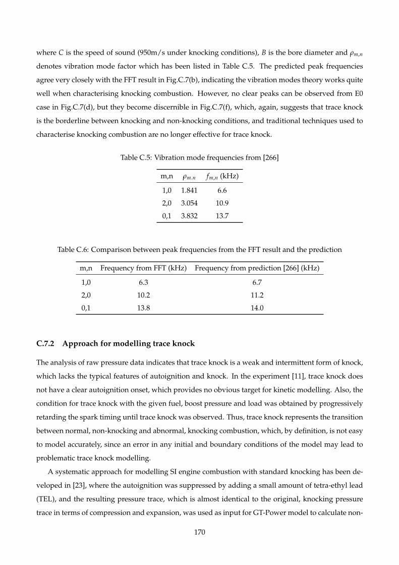
where C is the speed of sound (950m/s under knocking conditions), B is the bore diameter and ρm,n

denotes vibration mode factor which has been listed in Table C.5. The predicted peak frequencies

agree very closely with the FFT result in Fig.C.7(b), indicating the vibration modes theory works quite

well when characterising knocking combustion. However, no clear peaks can be observed from E0

case in Fig.C.7(d), but they become discernible in Fig.C.7(f), which, again, suggests that trace knock

is the borderline between knocking and non-knocking conditions, and traditional techniques used to

characterise knocking combustion are no longer effective for trace knock.

Table C.5: Vibration mode frequencies from [266]

m,n ρm.n fm,n (kHz)

1,0 1.841 6.6

2,0 3.054 10.9

0,1 3.832 13.7

Table C.6: Comparison between peak frequencies from the FFT result and the prediction

m,n Frequency from FFT (kHz) Frequency from prediction [266] (kHz)

1,0 6.3 6.7

2,0 10.2 11.2

0,1 13.8 14.0

C.7.2 Approach for modelling trace knock

The analysis of raw pressure data indicates that trace knock is a weak and intermittent form of knock,

which lacks the typical features of autoignition and knock. In the experiment [11], trace knock does

not have a clear autoignition onset, which provides no obvious target for kinetic modelling. Also, the

condition for trace knock with the given fuel, boost pressure and load was obtained by progressively

retarding the spark timing until trace knock was observed. Thus, trace knock represents the transition

between normal, non-knocking and abnormal, knocking combustion, which, by definition, is not easy

to model accurately, since an error in any initial and boundary conditions of the model may lead to

problematic trace knock modelling.

A systematic approach for modelling SI engine combustion with standard knocking has been de-

veloped in [23], where the autoignition was suppressed by adding a small amount of tetra-ethyl lead

(TEL), and the resulting pressure trace, which is almost identical to the original, knocking pressure

trace in terms of compression and expansion, was used as input for GT-Power model to calculate non-

170

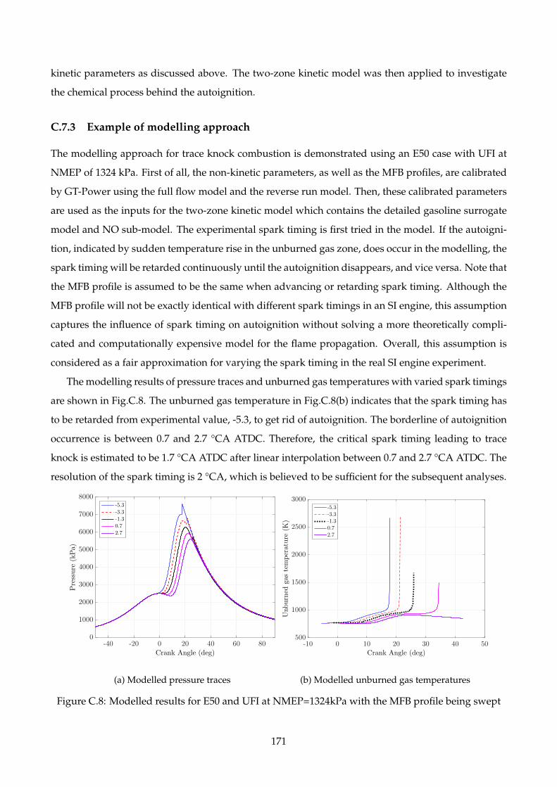
kinetic parameters as discussed above. The two-zone kinetic model was then applied to investigate

the chemical process behind the autoignition.

C.7.3 Example of modelling approach

The modelling approach for trace knock combustion is demonstrated using an E50 case with UFI at

NMEP of 1324 kPa. First of all, the non-kinetic parameters, as well as the MFB profiles, are calibrated

by GT-Power using the full flow model and the reverse run model. Then, these calibrated parameters

are used as the inputs for the two-zone kinetic model which contains the detailed gasoline surrogate

model and NO sub-model. The experimental spark timing is first tried in the model. If the autoigni-

tion, indicated by sudden temperature rise in the unburned gas zone, does occur in the modelling, the

spark timing will be retarded continuously until the autoignition disappears, and vice versa. Note that

the MFB profile is assumed to be the same when advancing or retarding spark timing. Although the

MFB profile will not be exactly identical with different spark timings in an SI engine, this assumption

captures the influence of spark timing on autoignition without solving a more theoretically compli-

cated and computationally expensive model for the flame propagation. Overall, this assumption is

considered as a fair approximation for varying the spark timing in the real SI engine experiment.

The modelling results of pressure traces and unburned gas temperatures with varied spark timings

are shown in Fig.C.8. The unburned gas temperature in Fig.C.8(b) indicates that the spark timing has

to be retarded from experimental value, -5.3, to get rid of autoignition. The borderline of autoignition

occurrence is between 0.7 and 2.7 °CA ATDC. Therefore, the critical spark timing leading to trace

knock is estimated to be 1.7 °CA ATDC after linear interpolation between 0.7 and 2.7 °CA ATDC. The

resolution of the spark timing is 2 °CA, which is believed to be sufficient for the subsequent analyses.

Crank Angle (deg)

-40 -20 0 20 40 60 80

Pressure

(kPa)

0

1000

2000

3000

4000

5000

6000

7000

8000-5.3

-3.3

-1.3

0.7

2.7

(a) Modelled pressure traces

Crank Angle (deg)

-10 0 10 20 30 40 50

Unburned

gastemperature

(K)

500

1000

1500

2000

2500

3000-5.3

-3.3

-1.3

0.7

2.7

(b) Modelled unburned gas temperatures

Figure C.8: Modelled results for E50 and UFI at NMEP=1324kPa with the MFB profile being swept

171

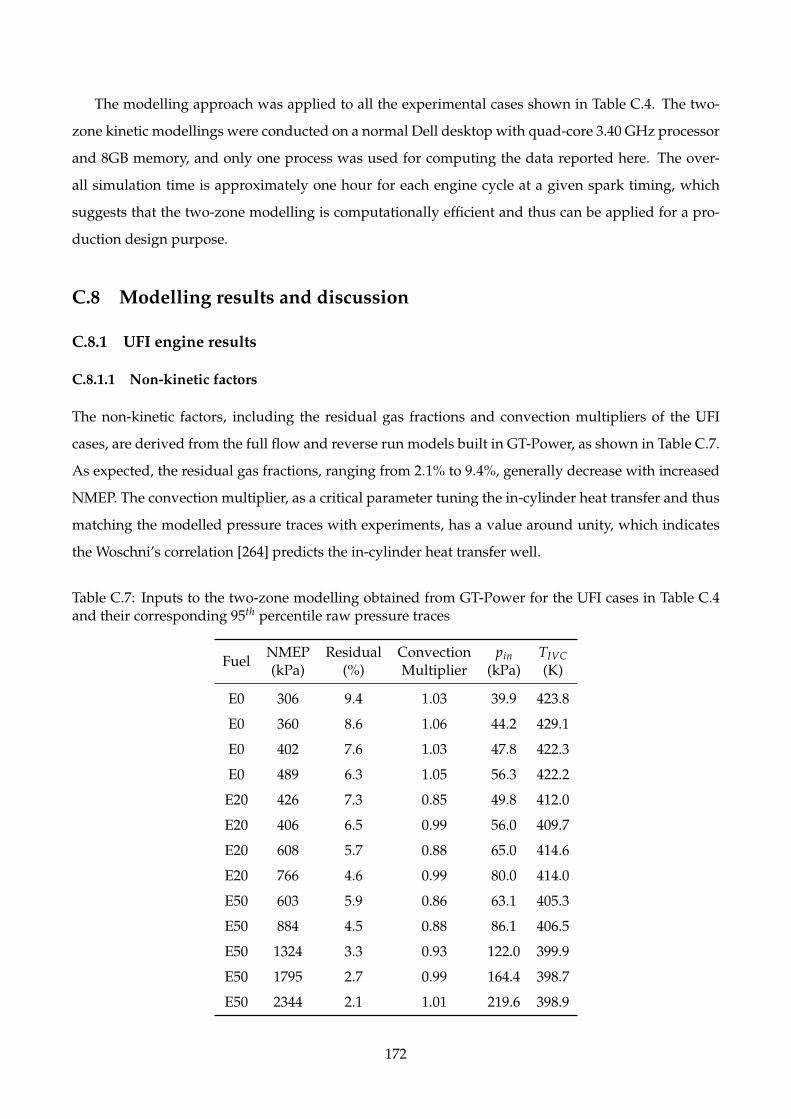
The modelling approach was applied to all the experimental cases shown in Table C.4. The two-

zone kinetic modellings were conducted on a normal Dell desktop with quad-core 3.40 GHz processor

and 8GB memory, and only one process was used for computing the data reported here. The over-

all simulation time is approximately one hour for each engine cycle at a given spark timing, which

suggests that the two-zone modelling is computationally efficient and thus can be applied for a pro-

duction design purpose.

C.8 Modelling results and discussion

C.8.1 UFI engine results

C.8.1.1 Non-kinetic factors

The non-kinetic factors, including the residual gas fractions and convection multipliers of the UFI

cases, are derived from the full flow and reverse run models built in GT-Power, as shown in Table C.7.

As expected, the residual gas fractions, ranging from 2.1% to 9.4%, generally decrease with increased

NMEP. The convection multiplier, as a critical parameter tuning the in-cylinder heat transfer and thus

matching the modelled pressure traces with experiments, has a value around unity, which indicates

the Woschni’s correlation [264] predicts the in-cylinder heat transfer well.

Table C.7: Inputs to the two-zone modelling obtained from GT-Power for the UFI cases in Table C.4and their corresponding 95th percentile raw pressure traces

FuelNMEP(kPa)

Residual(%)

ConvectionMultiplier

pin(kPa)

TIVC(K)

E0 306 9.4 1.03 39.9 423.8

E0 360 8.6 1.06 44.2 429.1

E0 402 7.6 1.03 47.8 422.3

E0 489 6.3 1.05 56.3 422.2

E20 426 7.3 0.85 49.8 412.0

E20 406 6.5 0.99 56.0 409.7

E20 608 5.7 0.88 65.0 414.6

E20 766 4.6 0.99 80.0 414.0

E50 603 5.9 0.86 63.1 405.3

E50 884 4.5 0.88 86.1 406.5

E50 1324 3.3 0.93 122.0 399.9

E50 1795 2.7 0.99 164.4 398.7

E50 2344 2.1 1.01 219.6 398.9

172

C.8.1.2 Effect of ethanol content

The critical spark timings for trace knocks of all UFI cases listed in Table C.7 were modelled by the

two-zone kinetic model, and the results were plotted against NMEP for E0, E20 and E50, as shown in

Fig.C.9. The most advanced, the 95th percentile and the median pressure traces were modelled for all

cases in Table C.7. In general, similar trends are observed from the three different raw pressure traces

regarding the variation of spark timing for knock limited combustion with NMEP. However, absolute,

systematic differences between experimental and modelling exist in all cases.

The largest systematic differences between the modelled and measured spark timings come from

the most advanced traces, which is probably due to two factors: the burning rates are faster with the

most advanced traces, leading to more rapid compression of the unburned gas, and the convection

multipliers for more advanced cycles are smaller, resulting in less heat loss, both of which increase

the unburned gas temperature and thus more retarded critical spark timing is required to get rid of

autoignition. Although the autoignition in the unburned gas zone is used to infer the critical spark

timing for the trace knock, it may not necessarily lead to knocking combustion, since the mass in the

unburned gas zone may not be sufficient to produce knock if the autoignition event occurs too late.

In this regard, some additional constrains should be imposed to guarantee the occurrence of knock,

which helps to reduce the gap between the modelling and experiment. An example given by [256]

suggests that the autoignition should occur early enough and the mass left in the end gas should be

sufficient to produce engine knock. However, it can be arbitrary and subjective to quantify ’early

timing’ and ’sufficient mass’, which will not be explored in this work.

Note that the differences of critical spark timings between the three types of raw pressure traces

are overall consistent across the NMEP range. However, larger discrepancies are found at relatively

low loads, which might result from greater randomness in those most advanced pressure traces under

such conditions. Considering the similar and systematic differences in the modelled critical spark

timing for trace knock using the most advanced, 95th percentile and the median pressure traces, the

95th percentile trace, unaffected by the randomness and representative of the advanced cycles having

trace knock, is applied in the rest modelling of this study.

The modelled critical spark timings using the 95th percentile advanced pressure traces are com-

pared with measurements in Fig.C.10. It is evident that the modelled spark timings are consistently

later than measured ones. Besides the choice of the representative trace and aforementioned non-

kinetic modelling assumptions, two possible causes will be elaborated here.

First, the experiment [11] used a pressure-based criterion to determine trace knock, which might be

less stringent than the one used in the two-zone kinetic modelling. As mentioned before and shown

in Fig.C.8(b), the critical spark timing in the modelling was obtained by analysing the temperature

173

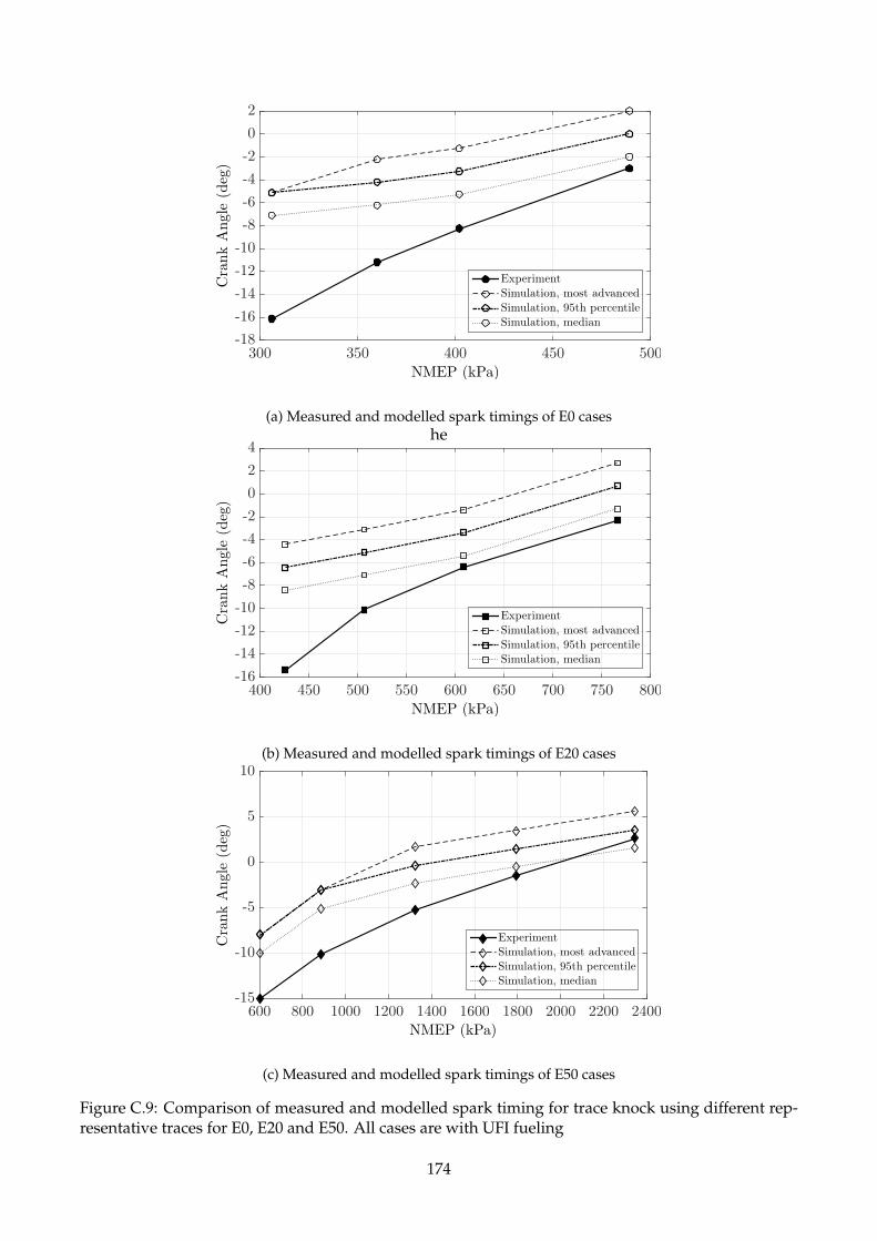
NMEP (kPa)

300 350 400 450 500

CrankAngle

(deg)

-18

-16

-14

-12

-10

-8

-6

-4

-2

0

2

Experiment

Simulation, most advanced

Simulation, 95th percentile

Simulation, median

(a) Measured and modelled spark timings of E0 caseshe

NMEP (kPa)

400 450 500 550 600 650 700 750 800

CrankAngle

(deg)

-16

-14

-12

-10

-8

-6

-4

-2

0

2

4

Experiment



Simulation, median

(b) Measured and modelled spark timings of E20 cases

NMEP (kPa)

600 800 1000 1200 1400 1600 1800 2000 2200 2400

CrankAngle

(deg)

-15

-10

-5

0

5

10

Experiment



Simulation, median

(c) Measured and modelled spark timings of E50 cases

Figure C.9: Comparison of measured and modelled spark timing for trace knock using different rep-resentative traces for E0, E20 and E50. All cases are with UFI fueling

174

NMEP (kPa)

0 500 1000 1500 2000 2500

CrankAngle

(deg)

-20

-15

-10

-5

0

5

E0, experiment

E0, simulation

E20, experiment

E20, simulation

E50, experiment

E50, simulation

Figure C.10: Variation of modelled (using the 95th percentile advanced trace) and measured sparktiming for trace knock for E0, E20 and E50

rise in the unburned gas zone. However, the comparison between Fig.C.8(a) and (b) suggests that a

temperature rise in the unburned gas zone may not always lead to a discernible pressure jump when

the mass left in the unburned gas zone at autoignition is not enough. Fig.C.11 shows that the MFB at

autoignition timing is approximately 90% for all cases modelled in this work.

NMEP (kPa)

0 500 1000 1500 2000 2500 3000 3500 4000

MFB

atautoignitiontiming

0.5

0.55

0.6

0.65

0.7

0.75

0.8

0.85

0.9

0.95

1

E0, UFI

E20, UFI

E50, UFI

E50, DI

Figure C.11: MFB at autoignition for spark timings that are one degree earlier than the spark timingfor trace knock

175

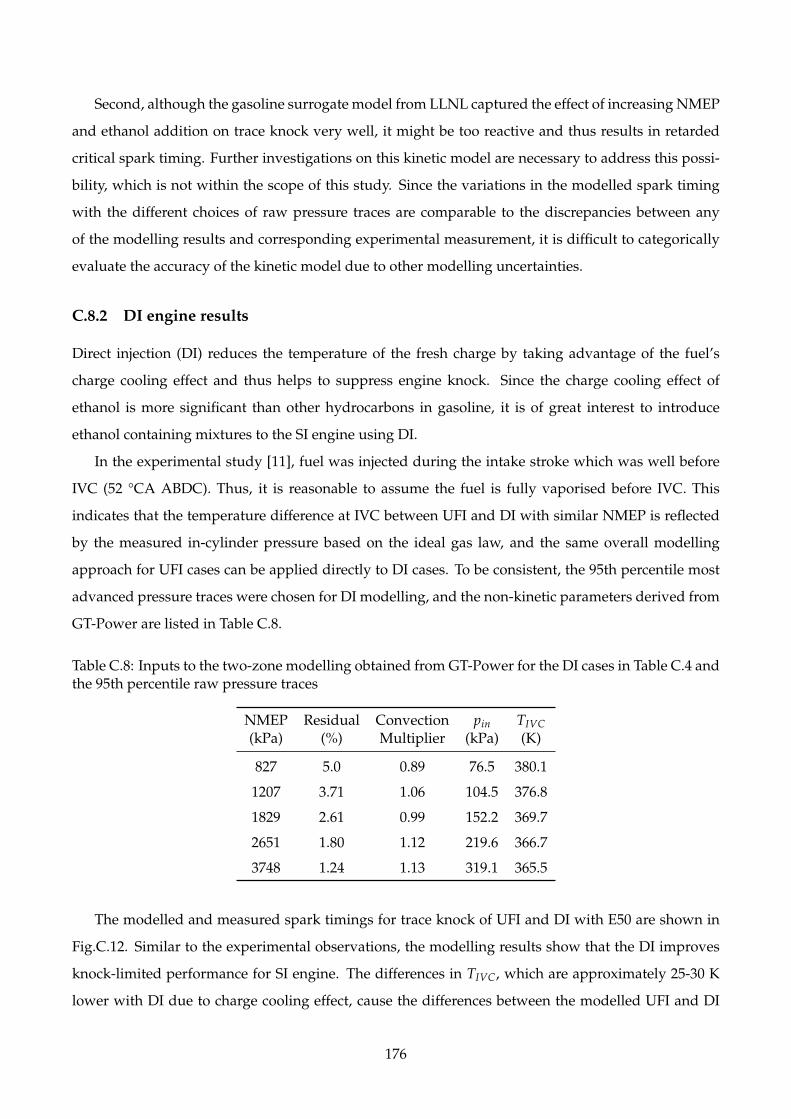
Second, although the gasoline surrogate model from LLNL captured the effect of increasing NMEP

and ethanol addition on trace knock very well, it might be too reactive and thus results in retarded

critical spark timing. Further investigations on this kinetic model are necessary to address this possi-

bility, which is not within the scope of this study. Since the variations in the modelled spark timing

with the different choices of raw pressure traces are comparable to the discrepancies between any

of the modelling results and corresponding experimental measurement, it is difficult to categorically

evaluate the accuracy of the kinetic model due to other modelling uncertainties.

C.8.2 DI engine results

Direct injection (DI) reduces the temperature of the fresh charge by taking advantage of the fuel’s

charge cooling effect and thus helps to suppress engine knock. Since the charge cooling effect of

ethanol is more significant than other hydrocarbons in gasoline, it is of great interest to introduce

ethanol containing mixtures to the SI engine using DI.

In the experimental study [11], fuel was injected during the intake stroke which was well before

IVC (52 °CA ABDC). Thus, it is reasonable to assume the fuel is fully vaporised before IVC. This

indicates that the temperature difference at IVC between UFI and DI with similar NMEP is reflected

by the measured in-cylinder pressure based on the ideal gas law, and the same overall modelling

approach for UFI cases can be applied directly to DI cases. To be consistent, the 95th percentile most

advanced pressure traces were chosen for DI modelling, and the non-kinetic parameters derived from

GT-Power are listed in Table C.8.

Table C.8: Inputs to the two-zone modelling obtained from GT-Power for the DI cases in Table C.4 andthe 95th percentile raw pressure traces

NMEP(kPa)

Residual(%)

ConvectionMultiplier

pin(kPa)

TIVC(K)

827 5.0 0.89 76.5 380.1

1207 3.71 1.06 104.5 376.8

1829 2.61 0.99 152.2 369.7

2651 1.80 1.12 219.6 366.7

3748 1.24 1.13 319.1 365.5

The modelled and measured spark timings for trace knock of UFI and DI with E50 are shown in

Fig.C.12. Similar to the experimental observations, the modelling results show that the DI improves

knock-limited performance for SI engine. The differences in TIVC, which are approximately 25-30 K

lower with DI due to charge cooling effect, cause the differences between the modelled UFI and DI

176

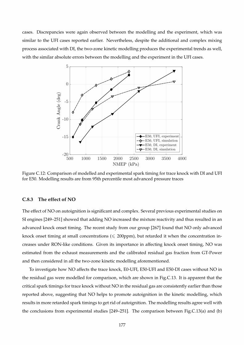
cases. Discrepancies were again observed between the modelling and the experiment, which was

similar to the UFI cases reported earlier. Nevertheless, despite the additional and complex mixing

process associated with DI, the two-zone kinetic modelling produces the experimental trends as well,

with the similar absolute errors between the modelling and the experiment in the UFI cases.

NMEP (kPa)

500 1000 1500 2000 2500 3000 3500 4000

CrankAngle

(deg)

-20

-15

-10

-5

0

5

E50, UFI, experiment

E50, UFI, simulation

E50, DI, experiment

E50, DI, simulation

Figure C.12: Comparison of modelled and experimental spark timing for trace knock with DI and UFIfor E50. Modelling results are from 95th percentile most advanced pressure traces

C.8.3 The effect of NO

The effect of NO on autoignition is significant and complex. Several previous experimental studies on

SI engines [249–251] showed that adding NO increased the mixture reactivity and thus resulted in an

advanced knock onset timing. The recent study from our group [267] found that NO only advanced

knock onset timing at small concentrations (6 200ppm), but retarded it when the concentration in-

creases under RON-like conditions. Given its importance in affecting knock onset timing, NO was

estimated from the exhaust measurements and the calibrated residual gas fraction from GT-Power

and then considered in all the two-zone kinetic modelling aforementioned.

To investigate how NO affects the trace knock, E0-UFI, E50-UFI and E50-DI cases without NO in

the residual gas were modelled for comparison, which are shown in Fig.C.13. It is apparent that the

critical spark timings for trace knock without NO in the residual gas are consistently earlier than those

reported above, suggesting that NO helps to promote autoignition in the kinetic modelling, which

results in more retarded spark timings to get rid of autoignition. The modelling results agree well with

the conclusions from experimental studies [249–251]. The comparison between Fig.C.13(a) and (b)

177

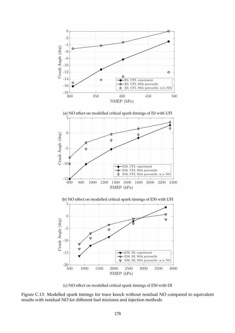
NMEP (kPa)

300 350 400 450 500

CrankAngle

(deg)

-18

-16

-14

-12

-10

-8

-6

-4

-2

0

E0, UFI, experimentE0, UFI, 95th percentileE0, UFI, 95th percentile, w/o NO

(a) NO effect on modelled critical spark timings of E0 with UFI

NMEP (kPa)

600 800 1000 1200 1400 1600 1800 2000 2200 2400

CrankAngle

(deg)

-15

-10

-5

0

5

E50, UFI, experimentE50, UFI, 95th percentileE50, UFI, 95th percentile, w/o NO

(b) NO effect on modelled critical spark timings of E50 with UFI

NMEP (kPa)

500 1000 1500 2000 2500 3000 3500 4000

CrankAngle

(deg)

-20

-15

-10

-5

0

5

E50, DI, experimentE50, DI, 95th percentileE50, DI, 95th percentile, w/o NO

(c) NO effect on modelled critical spark timings of E50 with DI

Figure C.13: Modelled spark timings for trace knock without residual NO compared to equivalentresults with residual NO for different fuel mixtures and injection methods

178

shows that the effect of NO is more significant for E0 than E50, as the spark advance is approximately

11-12 °CA for E0 but only 2 °CA for E50, which indicates that the interactions between NO and the

hydrocarbon fuels may be weakened by ethanol at low temperatures. In general, it is necessary to

include the NO sub-model for accurate autoignition modelling.

C.9 Summary

This study proposed a systematic numerical approach for trace knock modelling in a modern, single-

cylinder SI engine fuelled by ethanol/gasoline mixture. GT-Power and two-zone model were used

for the calibration of non-kinetic parameters and the prediction of autoignition onset timing respec-

tively. The modelling results agreed well with the experimental data [11] in terms of the trend of the

critical spark timings for trace knock under various conditions. The two-zone kinetic model used an

ethanol-containing gasoline surrogate mechanism [67] coupled with a NO sub-model [262] to simulate

autoignition in the unburned gas zone. For the purpose of modelling trace knock, the mass fraction

burned (MFB) profile from GT-Power was shifted accordingly with the change of the spark timing

until no autoignition occurred, and the critical spark timing was then obtained for trace knock.

The influence of ethanol on the autoignition, including its low autoignition reactivity and high

charge cooling, was first investigated by modelling upstream, pre-vaporized fuel injection (UFI) and

direct injection (DI) cases. As expected, the charge cooling effects of ethanol significantly improve

knock-limited performance with DI. Although some systematic, absolute differences do exist when

comparing modelled critical spark timings with those from the measurements, the relative trends

with engine load and ethanol content were well captured. Also, the effect of NO on knock-limited

combustion was investigated. The results are consistent with the experimental findings from the liter-

ature, but ethanol appears to weaken the interactions between NO and the hydrocarbon fuels at low

temperatures.

179

Appendix D

The kinetic model for the flow reactor

The governing equations for the PFR, ignoring heat loss and surface chemistry for simplicity, are

expressed in the format of the ODE system [47], as shown from Eqn.D.1 to D.3.

(D.1)dρ

dx=

1−Ru

cpMWmix

ρ2v2x

1

A

dA

dx

+ρRu

vxcp MWmix∑N

i=1 MWiωi

hi −MWmix

MWicpT

P

1 +v2

x

cpT

− ρv2x

(D.2)dT

dx=

v2x

ρcp

dρ

dx+

v2x

cp

1

A

dA

dx

− 1

vxρcp

N

∑i=1

hiωi MWi −Q′′C

mcp

(D.3)dYi

dx=

ωi MWi

ρvx

where ρ, T, Yi and x indicate the mixture density, temperature, mass fraction of species i and reactor

length, P is the reactor pressure, cp is the constant-pressure specific heat, MWmix is molecular weight

of the mixture, Ru is the universal gas constant, A is the cross section area of the reactor tube (constant

in our PFR), vx is the axial gas velocity, hi is the specific enthalpy of species i, Q′′

is the heat loss to

the surrounding, C is the circumference of the reactor tube, m is the total mass flow rate, and ωi is the

molar net production rate.

In this study, Eqn.D.1 and D.3 are solved with the VODE solver [268] in Python when carrying out

the global sensitivity analysis on a high performance computing (HPC) system named FIREBOX in our

group. Note that the temperature change with reactor length is provided from the experiments and

thus Eqn.D.2 is no longer needed. It generally takes twelve hours to analyse a chemical mechanism

containing approximately 10,000 elementary reactions using 30 cores and 100 GB memory. To validate

180

this in-house model, the modelled results for isooctane oxidation in the PFR using Chemkin and the

developed model are compared in Fig.D.1. The almost identical results suggest that the in-house

model is good enough to replace Chemkin in the PFR modelling.

0 200 400 600 800 10000

1

2

3

4

510-3

Figure D.1: The comparison between the modelled results of the neat isooctane oxidation at 900 K and10 bar in the PFR using Chemkin and the model developed in this study

181

octane blending and oxidation chemistry of ethanol

Documents