blending chem-bio dispersion forecasts and sensor data
TRANSCRIPT

REPORT DOCUMENTATION PAGE Form Approved
OMB No. 0704-0188 The public reporting burden for this collection of information is estimated to average 1 hour per response, including the time for reviewing instructions, searching existing data sources, gathering and maintaining the data needed, and completing and reviewing this collection of information. Send comments regarding this burden estimate or any other aspect of this collection of information, including suggestions for reducing the burden, to the Department of Defense, Executive Services and Communications Directorate (0704-0188). Respondents should be aware that notwithstanding any other provision of law, no person shall be subject to any penalty for failing to comply with a collection of information if it does not display a currently valid OMB control number. PLEASE DO NOT RETURN YOUR FORM TO THE ABOVE ADDRESS. 1. REPORT DATE (DD-MM-YYYY) 31-12-2008
2. REPORT TYPEFinal
3. DATES COVERED (From - To)Aug 2006 – Dec 2008
4. TITLE AND SUBTITLE Blending Chem-Bio Dispersion Forecasts and Sensor Data
5a. CONTRACT NUMBER W911NF-06-C-0162 5b. GRANT NUMBER N/A 5c. PROGRAM ELEMENT NUMBER N/A
6. AUTHOR(S) Tarunraj Singh, Peter Scott, Puneet Singla, Yang Cheng, Uma Konda, Gabriel Terejanu, Alex James, Sue Ellen Haupt, George Young, Anke Beyer-Lout, Kerrie Long.
5d. PROJECT NUMBER N/A 5e. TASK NUMBER N/A 5f. WORK UNIT NUMBERN/A
7. PERFORMING ORGANIZATION NAME(S) AND ADDRESS(ES) CUBRC, Inc.; 4455 Genesee Street Buffalo, NY 14225 University at Buffalo; 402 Crofts Hall, Buffalo NY 14260 Pennsylvania State University; P. O. Box 30, State College, PA 16804-0030
8. PERFORMING ORGANIZATION REPORT NUMBER N/A
9. SPONSORING / MONITORING AGENCY NAME(S) AND ADDRESS(ES) 10. SPONSOR/MONITOR’S ACRONYM(S)U. S. Army Research Office P.O. Box 12211, Research Triangle Park, NC 27709-2211 Defense Threat Reduction Agency Joint Science & Technology Office for Chemical & Biological Defense 8725 John J. Kingman Road Fort Belvoir, VA 22060-6201
ARO, DTRA 11. SPONSOR/MONITOR’S REPORT NUMBER(S)
12. DISTRIBUTION / AVAILABILITY STATEMENT Approved for public release; distribution unlimited.
13. SUPPLEMENTARY NOTES The views, opinions and/or findings contained in this report are those of the author(s) and should not be construed as an official Department of the Army position, policy or decision, unless so designated by other documentation. 14. ABSTRACT In a chemical release incident, two important questions in hazard prediction and assessment are: Where are the sources located? and, What is the plumes dispersion profile? This report details the development, and testing of algorithms to address the two questions. SCIPUFF is the model of choice for forecasting the dispersion which is used in conjunction with sensor data and meteorological data for improving the forecast and the identification of the source parameters. The authors of this report have exploited simple models based on RIMPUFF and a shallow water model to initially test their algorithms prior to using them with SCIPUFF. The data assimilation algorithms illustrate the improved quality of the forecast of the plume profile and the source identification algorithms based on Genetic Algorithms has been tested to identify source characteristics and meteorological parameters with encouraging results.
15. SUBJECT TERMS Data Assimilation, Source Identification, Plume dispersion, Puff based models.
16. SECURITY CLASSIFICATION OF: UNCLASSIFIED
17. LIMITATION OF ABSTRACT
18. NUMBER OF PAGES
19a. NAME OF RESPONSIBLE PERSONTarunraj Singh
a. REPORT UNCLASSIFIED
b. ABSTRACT UNCLASSIFIED
c. THIS PAGEUNCLASSIFIED
Same as report 204 19b. TELEPHONE NUMBER (include area code) 716-645-2593 x2235
Standard Form 298 (Re . 8/98)vPrescribed by ANSI Std. Z39.18

Blending Chem-Bio Dispersion Forecasts and Sensor Data
Contract No. W911NF-06-C-0162
Final Report
December, 2008
Submitted to: Defense Threat Reduction Agency
Joint Science & Technology Office for Chemical & Biological Defense 8725 John J. Kingman Road
Fort Belvoir, VA 22060-6201
Principal Investigator: Dr. Tarunraj Singh Department of Mechanical and Aerospace Engineering University at Buffalo Buffalo NY 14260-2000
Approved for public release; distribution is unlimited

Acknowlegments
I gratefully acknowledge the efforts of the team of faculty, consultants and graduate students
from CUBRC, the University at Buffalo, the Pennsylvania State University and beyond who
worked on this project. Over its two year lifetime, these scholars gave unstintingly of their time
and expertise to support a common vision of scientific excellence and technical relevance.
Whatever achievements may be noted in this work is theirs, wherever we came up short I take
responsibility. I also acknowledge the support given us by our sponsor DTRA, and the guidance
of our program director Dr. John Hannan.
Many sections of this final report were distilled from reports and publications authored by
project team members cited in Section 4 Personnel Supported by the Grant, and I thank them for
the opportunity to use their work here. All should be considered co-authors of this report.
Tarunraj Singh December 31, 2008
-A-- 1 --
DTRA W911NF-06-C-0162

1. Table of Contents
Page
Acknowledgments 1
1. Table of Contents (this page) 2
2. Program Goals and Achievements 3
3. Personnel Supported by the Grant 5
4. Theses/Dissertations Produced 8
5. Publications Produced Under the Grant 18
6. Technical Summary of Results (UB) 22
7. Technical Summary of Results (PSU) 144
Appendix A: RIMPUFF Source Code
Appendix B: Shallow Water Model Source
-A-- 2 --
DTRA W911NF-06-C-0162

2. Program Goals and Achievements
Here an executive summary of the principal goals, objectives, achievements and new findings
are presented. Extended technical development of each item can be found in Section 6 of this
report.
2.1 Goals
The primary goals and program objectives of this project are related to integrating sensor data
with dispersion models for forecasting, nowcasting and hindcasting. Nowcasting is also referred
to as filtering, which endeavors to determine the optimal estimate of the state given the set of all
measurements and dispersion model estimate. Hind-casting, also called smoothing, is intended to
determine an optimal estimate of the states at a specified time including data from the future. The
CB dispersion process is represented using a puff based model such as SCIPUFF which is
characterized by a time-varying number of Gaussian puffs that are used to represent the
concentration distribution as a function of time. Typical sensors used in the field to measure
concentrations are bar sensors, which provide a coarse quantization of the range of
concentrations. The nonlinearity of the model in conjunction with the time-varying system order
precludes using the standard Kalman paradigm for filtering and smoothing. The primary
objective of this project is the development of new algorithms for data assimilation for systems
with time-varying model order. Another objective of the project is characterization of the source
by exploiting all the measurements, dispersion model and atmospheric data. Determination of the
source location in the presence of sparse measurements that are perturbed by noise, and by low
fidelity nonlinear models make the source identification a difficult problem. In performing this
project, a paradigm for data assimilation for contaminant dispersion and for source term
estimation was also sought.
-A-- 3 --
DTRA W911NF-06-C-0162

2.2 Achievements
Progress was made in the two focus areas: data assimilation for forecasting and source
estimation. MATLAB based testbeds were developed for test and evaluation of the proposed
algorithms.
2.2.1 New Methodologies
Here we list the highlights of the data assimilation tools that were developed for forecasting and
source identification. The details are provided in Section 6 of this report.
1. Development of a particle filter for data assimilation for systems with time-varying order. The
class of models referred to as puff based models are characterized by varying numbers of puffs
as a function of time requiring the development of new algorithms for integrating sensor data
with model outputs.
2. Development of an Extended Kalman Filter for puff based dispersion models accounting for
puff splitting and puff merging.
3. Development of a Bayesian based algorithm for the integration of highly quantized CB sensor
models with continuous spatiotemporal dispersion models.
4. Development of a convex algorithm for source localization. A L1 norm minimizing approach
is used to determine a sparse solution to the source identification problem exploiting the
knowledge that on a rectangular (or other kind) grid, where the sources are required to lie on a
grid point, the number of grid points where the sources reside will be small compared to the
number of grids.
5. A new Gaussian Mixture model was developed for the propagation of non-Gaussian
uncertainties through nonlinear systems.
-A-- 4 --
DTRA W911NF-06-C-0162

6. Development of a Gaussian Mixture model for high fidelity estimation of the state probability
density function in conjunction with sensor data.
7. Development of a procedure for extracting features of a contaminant puff and then nudging it
toward the observed state in the model.
8. Development of a genetic algorithm-based method for comparing a field of contaminant
concentrations to a modeled field for the purpose of determining the underlying wind field and
predicting the future transport and dispersion.
9. Development of several data assimilation techniques for using observed contaminant
concentrations to infer meteorological conditions and to assimilate those values into transport
and dispersion models. These assimilation techniques include nudging, extended Kalman
filtering, ensemble Kalman filtering, and Four Dimensional Variational Data assimilation.
10. Development of a genetic algorithm-based methodology that when given observations of
contaminant concentrations is capable of back-calculating source parameters (such as location,
source strength, height of release, and time of release) as well as required meteorological
parameters (such as wind speed, wind direction, and boundary layer depth). This algorithm
considers sensor characteristics such as minimum detection limits and saturation values. The
general methodology has been validated in the context of several different dispersion models:
Gaussian plume, Gaussian puff, and the SCIPUFF model.
10. Development of a back-trajectory model to back-calculate source terms such as location and
emission rate. This model can be applied to determine multiple sources.
11. Development of a theoretical and numerical framework for comparing and contrasting
engineering style sensor data fusion with meteorological data assimilation for the purposes of
determining best practices for integrating monitored observations into a model forecast.
12. Development of a paradigm for considering problems in data assimilation and sensor data
fusion and for applying techniques from each to the source term estimation problem.
-A-- 5 --
DTRA W911NF-06-C-0162

2.2.2 The Puff-Model based Dispersion Test Bed for Data Assimilation
1. A RIMPUFF based two dimensional dispersion model has been programmed in the MATLAB
environment to permit rapid prototyping of data assimilation and source identification
algorithms.
2. A shallow water model to characterize spatiotemporal wind dynamics over topography has
been programmed in MATLAB to permit testing of data assimilation algorithms and to provide
the exogenous input to the RIMPUFF based dispersion model.
3. The particle filter based data assimilation algorithm has been tested on the RIMPUFF based
testbed.
4. A basic Gaussian puff model interfaces with the shallow water model for the purposes of
dispersion. Data assimilation algorithms that have been tested with this coupled formulation
include nudging, extended Kalman Filtering, Ensemble Kalman Filtering, and Four Dimensional
Variational Data Assimilation.
5. A basic gridded flat terrain testbed for studying a meandering wind field coupled to a
Gaussian puff dispersion model. Assimilation algorithms applied with this testbed are the
Lagrangian entity approach of feature extraction with nudging as well as the Eulerian field-based
approach of applying a genetic algorithm based field approach.
6. A gridded flat terrain testbed for source and meteorological characterization. Field-based
approaches using a genetic algorithm were applied to back-calculate source characteristics and
meteorological parameters. A three dimensional version was used to determine the impact of
boundary layer depth on the back-calculation. This testbed was also configured similar to the
FFT07 experiment for testing the source term estimation algorithms.
7. Ion Mobility Spectrometer (IMS) sensor Bar-sensor models.
8. Sensor models that incorporate minimum detection limits and saturation levels.
-A-- 6 --
DTRA W911NF-06-C-0162

3. Personnel Supported by the Grant
3.1 Faculty
Dr. Sue Ellen Haupt, Dept. of Atmospheric & Oceanic Physics/Applied Research Laboratory &
Meteorology Department, The Pennsylvania State University
Dr. Peter Scott, Computer Science and Engineering Dept., University at Buffalo
Dr. Tarunraj Singh, Dept. of Mechanical & Aerospace Engineering, University at Buffalo
Dr. Puneet Singla, Dept. of Mechanical & Aerospace Engineering, University at Buffalo
Dr. George Young, Meteorology Department, The Pennsylvania State University
3.2 Post-Doctoral Fellows
Dr. Yang Cheng, Dept. of Mechanical & Aerospace Engineering, University at Buffalo
3.4 Professional staff
Mike Moskal, CUBRC
Alex James, CUBRC
3.5 Graduate Students
Umamaheswara Reddy, Dept. Mechanical Engineering, University at Buffalo
Gabriel Terejanu, Dept. Computer Sci. and Eng., University at Buffalo
Anke Beyer-Lout, Meteorology Department, The Pennsylvania State University
Kerrie Long, Meteorology Department and Applied Research Laboratory, The Pennsylvania
State University
Christopher Allen, Meteorology Department and Applied Research Laboratory, The
Pennsylvania State University
-A-- 7 --
DTRA W911NF-06-C-0162

Luna Rodriguez, Meteorology Department and Applied Research Laboratory, The Pennsylvania
State University
Andrew Annunzio, Meteorology Department and Applied Research Laboratory, The
Pennsylvania State University
James Limbacher, Meteorology Department, The Pennsylvania State University
4. Theses and Dissertations Produced Under the Grant
4.1 MS Theses
4.1.1 Reddy, Umamaheswara, Data Assimilation for Dispersion Models. A thesis presented to
the faculty of the Mechanical Engineering Department of the University at Buffalo in partial
fulfillment of the requirements for the MS Degree.
Abstract: The design of an effective data assimilation environment for dispersion models is
studied. These models are usually described by nonlinear partial differential equations
which lead to large scale state space models. The linear Kalman filter theory fails to meet the
requirements of such applications due to high dimensionality leading to high computational
costs, strong non-linearities, non-Gaussian driving disturbances and model parameter
uncertainties. Application of Kalman filter to these large scale models is computationally
expensive and real time estimation is not possible with the present resources. Various sampling
based filtering techniques are studied for implementation in the case of dispersion models,
focusing on Ensemble filtering and Particle filtering approaches. The filters are compared with
the full Kalman filter estimates on a one dimensional spherical diffusion model for illustrative
purposes. The sampling based techniques show a considerable improvement in computational
time compared to the full Kalman filter, while giving comparable estimates.
4.1.2 Terejanu, Gabriel., A project presented to the faculty of the Computer Science and
Engineering Department of the University at Buffalo in partial fulfillment of the requirements for
the MS Degree.
-A-- 8 --
DTRA W911NF-06-C-0162
4.1.3 Long, Kerrie J., Improving Contaminant Source Characterization and Meteorological
Data Forcing with a Genetic Algorithm, A thesis in Meteorology submitted in partial fulfillment
of the Requirements for the Degree of Master of Science, May 2007.
Abstract: The release of harmful contaminants is a potentially devastating threat to homeland
security. In order to minimize the effects of such a release, emergency management agencies
need accurate identification of the source so that they can better predict which areas will require
evacuation and take steps to mitigate the source. Insufficient spatial and temporal resolution in
the meteorological data as well as inherent uncertainty in the wind field data make characterizing
the source and predicting subsequent transport and dispersion extremely difficult. A robust
technique such as a genetic algorithm (GA) may be used to characterize the source precisely and
to obtain the required wind information. The method presented here uses a GA to find the
combination of source location, source height, source strength, surface wind direction, surface
wind speed, and time of release that best matches the monitored receptor data with the forecast
pollutant dispersion model output. The approach is validated using the Gaussian puff equation as
the dispersion model in identical twin numerical experiments. The limits of the model are further
tested by incorporating additive and multiplicative noise into the synthetic data. The minimum
requirements for data quantity and quality are determined by sensitivity analysis.
4.1.4 Beyer-Lout, Anke, Concentration Assimilation into Wind Field Models for Dispersion Modeling, A thesis in Meteorology submitted in partial fulfillment of the Requirements for the Degree of Master of Science, December 2007. Abstract: In case of a chemical, biological, radiological, or nuclear (CBRN) release, emergency
managers need to draw on all the available data to create the most accurate concentration
forecast possible. Traditionally, a numerical weather prediction (NWP) model provides the
bridge between the raw meteorological observations and the meteorological forcing fields for a
transport and dispersion model. This approach has two shortcomings: sparse meteorological
observations can lead to inaccurate wind fields and the source information for the contaminant
must be estimated outside of the modeling framework. These two problems can be addressed
together by assimilating concentration and wind observations into a coupled NWP and dispersion
modeling system. Assimilating wind observations into the coupled model is straightforward
using traditional data assimilation methods such as a Kalman filter, Nudging, or four-
-A-- 9 --
DTRA W911NF-06-C-0162
dimensional variational data assimilation (4D-Var). Two aspects of assimilating concentration
data into the model complicate the process however: 1) the observations are likely to be sparser
than of the wind because the contaminant is localized, and 2) the evolving concentration field
does not feed back to the meteorology. The impact of these differences on the implementation
and success of traditional data assimilation techniques is assessed through a series of numerical
experiments with a two-dimensional shallow water equation forced dispersion model. The results
are compared and data needs are considered.
4.1.5 Annunzio, Andrew J., Source Characterization with Atmospheric Boundary Layer Depth, A thesis in Meteorology submitted in partial fulfillment of the Requirements for the Degree of Master of Science, August 2008.
Abstract: Characterizing the source of a contaminant is a contemporary issue in atmospheric
transport and dispersion modeling. In addition to the source parameters, it is also necessary to
back-calculate meteorological forcing parameters because they govern the subsequent transport
of a contaminant. One aspect that has not been addressed previously is ascertaining the height of
the atmospheric boundary layer. The capping inversion at the top of the boundary layer traps the
puff by reflecting contaminants back towards the surface, directly impacting surface
concentrations. Because the depth of the atmospheric boundary layer varies with time of day,
stability, and the horizontal and vertical wind, it is generally difficult to determine. In the
Gaussian puff model, a rigid lid is added to the top of the boundary layer to reflect contaminants
back towards the surface. From time dependent concentration observations of the puff a Genetic
Algorithm characterizes the source strength and location, boundary layer height, wind speed, and
wind direction. It is shown that the Genetic Algorithm can back-calculate all these parameters
working solely from concentration observations.
4.1.6 Rodriguez, Luna R., Source Term Estimation Using a Genetic Algorithm and Incorporating Sensor Characteristics, A thesis in Meteorology submitted in partial fulfillment of the Requirements for the Degree of Master of Science, August 2008.
Abstract: An accidental or intentional release of hazardous chemical, biological, nuclear, or
radioactive material into the atmosphere requires characterizing the source of an airborne
contaminant from remote measurements of the resulting concentration field. The genetic
algorithm (GA) method used here has proved to be successful in back-calculating not only these
-A-- 10 --
DTRA W911NF-06-C-0162

source characteristics but also the meteorological parameters necessary to predict the transport
and dispersion of a contaminant. Previous validation studies have utilized identical twin
experiments wherein the synthetic validation data were created using the same transport and
dispersion models that were used for the back-calculations. The same identical twin approach is
used here with the Gaussian Puff model as the dispersion model, then a solution is optimized by
means of a GA, and finally a global minimum is found with the Nelder-Mead downhill simplex
algorithm. The model incorporated sensor detection limits and saturation levels.
4.2 Ph.D. Dissertations
4.2.1. Reddy, Umamaheswara, Stochastic scheduling problems for minimizing tardy jobs with
application to emergency vehicle dispatching on unreliable road networks, Ongoing dissertation
in the Mechanical and Aerospace Engineering Department of the University at Buffalo.
4.2.2 Terejanu, Gabriel, Responding to casualties in a disaster relief operation: Initial
ambulance allocation and reallocation, and switching of casualty priorities, Ongoing
dissertation in the Computer Science and Engineering Department of the University at Buffalo.
5. Publications Produced Under the Grant
1. Cheng, Y. & Singh, T., “Identification of Multiple Radioactive Sources Using Convex Optimization”, Submitted for review to the IEEE Transaction on Aerospace and Electronic Systems.
2. Cheng, Y., Reddy, K. V. U., Singh, T., Scott, P., “Fusion of Discrete-Valued CBRN Sensor Data”, Submitted for review to the IEEE Transaction on Aerospace and Electronic Systems.
3. G. Terejanu, P. Singla, T. Singh, and P. D. Scott, “Uncertainty Propagation for Nonlinear Dynamical Systems using Gaussian Mixture Models,” AIAA Journal of Guidance, Control and Dynamics, 31(6), 1623-1633.
4. Reddy , K.V. Umamaheswara, Cheng, Yang, Singh, Tarunraj and Scott, Peter, “Source Estimation in CBRN Incidents Using Convex Optimization”, To be presented at the Chemical and Biological Defense Physical Science and Technology (CBD PS&T) Conference, New Orleans, LA, November 17-21, 2008. (Student Scholarship Award).
-A-- 11 --
DTRA W911NF-06-C-0162
5. Terejanu, G., Cheng, Y., Singh, T., and Scott, P., “Comparison of SCIPUFF Plume
Prediction With Particle Filter Assimilated Prediction for Dipole 26 Data”, To be presented at the Chemical and Biological Defense Physical Science and Technology (CBD PS&T) Conference, New Orleans, LA, November 17-21, 2008. (Student Scholarship Award).
6. G. Terejanu, P. Singla, T. Singh, and P. Scott, “Uncertainty Propagataion for Nonlinear Dynamical Systems using Gaussian Mixture Models”, Presented at the AIAA Guidance, Navigation and Control Conference, Honolulu, Hawaii, Aug. 18-21, 2008.
7. Y. Cheng, and T. Singh, “Source Term Estimation using Convex Optimization,” Presented at The 11th International Conference on Information Fusion, Cologne, Germany, June 30- July 3, 2008.
8. G. Terejanu, P. Singla, T. Singh, and P. Scott, “A Novel Gaussian Sum Filter Method for Accurate Solution to Nonlinear Filtering Problem,” Presented at The 11th International Conference on Information Fusion, Cologne, Germany, June 30- July 3, 2008.
9. Singla, P., & Singh. T., “A Gaussian FunctionNetwork for Uncertainty Propagation
Through Nonlinear Dynamical System”, Presented at the 2008 AAS, Galveston, TX, January 27-31, 2008.
10. Singla, P., & Singh. T., “A Gaussian FunctionNetwork for Uncertainty Propagation Through Nonlinear Dynamical System”, Presented at the 2008 AAS, Galveston, TX, January 27-31, 2008.
11. Tarunraj Singh, Peter Scott, Puneet Singla., Gabriel Terajanu, Yang Cheng, and K. V.
Umamaheswara Reddy, "Data Assimilation for Forecasting Plume Dispersion" by authors Presented at the Geo Hazard Conference, Buffalo, NY, March 29-30, 2008.
12. P. Singla, T. Singh, P. Scott, G. Terejanu, Y. Cheng and U. K. V. Reddy, “Accurate
Uncertainty Propagation through Nonlinear Systems,” First Annual Conference of Center for GeoHazards Studies, Natural Disasters in Small Communities: How Can We Help?, Mar. 29-30, 2008.
13. Haupt, S.E., A. Beyer-Lout, K.J. Long, and G.S. Young, 2008, “Assimilating
concentration Observations for Transport and Dispersion Modeling in a Meandering
Wind Field”, submitted to Atmospheric Environment.
14. Rodriguez, L.M., S.E. Haupt, and G.S. Young, 2008, “Impact of Sensor Characteristics
on Source Characterization for Dispersion Modeling”, submitted to Measurement.
-A-- 12 --
DTRA W911NF-06-C-0162
15. Beyer-Lout, A., G.S. Young, and S.E. Haupt, 2008, “Assimilation of Concentration and
Wind Data into a Coupled Wind and Dispersion System", submitted to Monthly Weather
Review.
16. Haupt, S.E., R.L. Haupt, and G.S. Young, 2008, “A Mixed Integer Genetic Algorithm
used in Chem-Bio Defense Applications”, accepted by Journal of Soft Computing.
17. Annunzio, A.J., S.E. Haupt, and G.S. Young, 2008, “Source Characterization including
Impact of Atmospheric Boundary Layer Depth”, to be submitted to Boundary Layer
Meteorology.
18. Annunzio, A.J., S.E. Haupt, and G.S. Young, 2008, “Comparing Sensor Data Fusion and
Data Assimilation for Contaminant Transport and Dispersion”, in preparation.
19. Haupt, S.E., A. Beyer-Lout, G.S. Young, and K..J. Long, 2008: On Assimilating
Concentration Data into Wind Field Models, 12th Annual George Mason University
Conference on Atmospheric Transport and Dispersion Modeling, July 9, 2008.
20. Long, K.J., S.E. Haupt, G.S. Young, 2008, “Coupling a Genetic Algorithm with
SCIPUFF to Extract Source and Meteorological Information”, 12th Annual George
Mason University Conference on Atmospheric Transport and Dispersion Modeling, July
8, 2008.
21. Annunzio, A.J., S.E. Haupt, and G.S. Young, 2008, “Source Characterization
Considering Atmospheric Boundary Layer Depth as a Variable”, 12th Annual George
Mason University Conf
22. Rodriguez, L.M., S.E. Haupt, and G.S. Young, 2008, “Source Term Estimation
Incorporating Sensor Characteristics”, 12th Annual George Mason University Conference
on Atmospheric Transport and Dispersion Modeling, July 8, 2008.
23. Haupt, S.E., K.J. Long, G.S. Young, and A. Beyer-Lout, 2008, “Data Requirements for Assimilating Concentration Data with a Genetic Algorithm”, Sixth Conference on Artificial Intelligence Application to Environmental Science, New Orleans, LA, Jan. 20-24.
-A-- 13 --
DTRA W911NF-06-C-0162

24. Beyer-Lout, A., G.S. Young, and S.E. Haupt, 2008, “Concentration Assimilation into
Wind Field Models for Dispersion Modeling”, 15th Joint Conference on the Applications of Air Pollution Meteorology with the A&WMA, New Orleans, LA, Jan. 20-24.
25. Annunzio, A.J., S.E. Haupt, and G.S. Young, 2008, “Source Characterization and
Meteorology Retrieval Including Atmospheric Boundary Layer Depth using a Genetic Algorithm”, 15th Joint Conference on the Applications of Air Pollution Meteorology with the A&WMA, New Orleans, LA, Jan. 20-24.
26. Haupt, S.E. and G.S. Young, 2008, “Paradigms for Source Characterization”, 15th Joint
Conference on the Applications of Air Pollution Meteorology with the A&WMA, New Orleans, LA, Jan. 20-24.
27. Long, K.J., S.E. Haupt, G.S. Young, 2008, “Source Characterization and Meteorology
Retrieval using a Genetic Algorithm with SCIPUFF”, 15th Joint Conference on the Applications of Air Pollution Meteorology with the A&WMA, New Orleans, LA, Jan. 20-24.
28. Rodriguez, L.M., S.E. Haupt, and G.S. Young, 2008, “Adding Realism to Source
Characterization with a Genetic Algorithm”, 15th Joint Conference on the Applications of Air Pollution Meteorology with the A&WMA, New Orleans, LA, Jan. 20-24.
29. Annunzio, A.J., S.E. Haupt, and G.S. Young, 2008, “Similarities and Differences
between Multi-sensor Data Fusion and Data Assimilation: Implications for Over-determined vs. Under-determined Systems”, 15th Joint Conference on the Applications of Air Pollution Meteorology with the A&WMA, New Orleans, LA, Jan. 20-24.
30. “Data Requirements for Data Assimilation and Source Estimation”, TTCP-CBD
Technical Panel 9 Annual Meeting, Montreal, QC, CA, Feb. 6, 2008.
31. Haupt, S.E., G.S. Young, K.J. Long, A. Beyer-Lout, and A. Annunzio, 2008, “Data Fusion and Prediction for CBRN Transport and Dispersion for Security”, 2008 IEEE Aerospace Conference with AIAA, Big Sky, MT, March 1-8.
32. Long, K.J., S.E. Haupt, and G.S. Young, 2008, “Optimizing Source Characteristics and
Meteorological Data Describing a Contaminant Release with a Genetic Algorithm”. Submitted to Optimization and Engineering
33. Y. Cheng, K. V. U. Reddy, T. Singh, and P. Scott, “CBRN Data Fusion Using Puff-
Based Model and Bar-Reading Sensor Data,” Presented at The 10th International Conference on Information Fusion, Quebec City, Quebec, July 9-12, 2007
-A-- 14 --
DTRA W911NF-06-C-0162

34. K. V. U. Reddy, Y. Cheng, T. Singh, and P. Scott, “Data Assimilation in Variable Dimension Dispersion Models using Particle Filters,” Presented at The 10th International Conference on Information Fusion, Quebec City, Quebec, July 9-12, 2007
35. G. Terejanu, T. Singh, and P. Scott, “Unscented Kalman Filter/Smoother for a CBRN
Puff-Based Dispersion Model,” Presented at The 10th International Conference on Information Fusion, Quebec City, Quebec, July 9-12, 2007
36. Reddy, K. V. U., Cheng, Y., Singh, T., and Scott, P., “Data Assimilation for Puff-Model-
Based Chem-Bio Dispersion”, Presented at the 2007 CBIS Conference, Austin, Tx, Jan. 8-12, 2007
37. Haupt, S.E., G.S. Young, A. Beyer, and K.J. Long, 2007, “Assimilating Sensor
Concentration Data into a Dispersion Model in a Meandering Flow Field”, GMU Conference on Atmospheric Transport and Dispersion, Fairfax, VA, July 10-12.
38. Long, K.J., S.E. Haupt, and G.S. Young, 2007, “Applying a Genetic Algorithm to
Identify Source and Meteorological Data Characteristics”, GMU Conference on Atmospheric Transport and Dispersion, Fairfax, VA, July 10-12.
39. Beyer, A., G.S. Young, and S.E. Haupt, 2007, “Dispersion Modeling with Uncertain
Wind Conditions”, GMU Conference on Atmospheric Transport and Dispersion, Fairfax, VA, July 10-12.
40. Annunzio, A.J., S.E. Haupt, G.S. Young, 2007: Comparing Assimilation and Sensor Data
Fusion Techniques for Dispersion Modeling, GMU Conference on Atmospheric Transport and Dispersion, Fairfax, VA, July 10-12, (Poster presentation).
41. Haupt, S.E., R.L. Haupt, and G.S. Young, 2007, “Using Genetic Algorithms in Chem-Bio
Defense Applications”, ECSIS Symposium on Bio-inspired, Learning, and Intelligent Systems for Security (BLISS-2007), Edinburgh, UK, Aug. 9-10.
42. Haupt, S.E., G.S. Young, and C.T. Allen, 2007, “A Genetic Algorithm Method to
Assimilate Sensor Data for a Toxic Contaminant Release”, Journal of Computers, 2, 85-
93.
43. Haupt, S.E., G.S. Young, K.J. Long, and A. Beyer, 2007, “Data Requirements from Evolvable Sensor Networks for Homeland Security Problems”, NASA/ESA Conference on Adaptive Hardware and Systems (AHS-2007), Edinburgh, UK, Aug. 5-9.
44. Haupt, S.E., G.S. Young, and L.J. Peltier, 2007, “Assimilating Monitored Data into Dispersion Models”, Fifth Conference on Artificial Intelligence Applications to Environmental Science at AMS Annual Meeting, San Antonio, TX, Jan. 16, Paper number 4.3.
-A-- 15 --
DTRA W911NF-06-C-0162
45. Beyer, A., G.S. Young, and S.E. Haupt, 2007, “On using Data Assimilation in Dispersion Modeling”, 11th Symposium on Integrated Observing and Assimilation Systems for the Atmosphere, Oceans, and Land Surface (IOAS-AOLS) at AMS Annual Meeting, San Antonio, TX, Jan. 16, Paper number 3.13.
46. Long, K.J., C.T. Allen, S.E. Haupt, and G.S. Young, 2007, “Characterizing Contaminant Source and Meteorological Forcing using Data Assimilation with a Genetic Algorithm”, Fifth Conference on Artificial Intelligence Applications to Environmental Science at AMS Annual Meeting, San Antonio, TX, Jan. 16, Paper number 4.3.
47. Young, G.S and S.E. Haupt, 2007, “Going Nonlinear: Towards Automated Puff Intercept”, Fifth Conference on Artificial Intelligence Applications to Environmental Science at AMS Annual Meeting, San Antonio, TX, Jan. 15-16, Paper number P1.1.
48. Reddy, K. V. U., Cheng, Y., Singh, T., and Scott, P., “Data Assimilation for Dispersion
Models”, Presented at the 2006 Fusion Conference, Florence, Italy, July 10-13, 2006.
49. Haupt, S.E., G.S. Young, and K.J. Long, 2008, “ A Paradigm for Source Term
Estimation”, Chemical and Biological Defense Physical Science and Technology
Conference, New Orleans, LA, Nov. 17-21.
50. Long, K.J., S.E. Haupt, G.S. Young, and A. Beyer-Lout, 2008, “Data Assimilation to
Improve the Forecast of Chemical and Biological Contaminant Transport and
Dispersion”, Chemical and Biological Defense Physical Science and Technology
Conference, New Orleans, LA, Nov. 17-21. (poster presentation, student travel
scholarship)
51. Annunzio, A.J., S.E. Haupt, and G.S. Young, 2008, “Comparison of Data Assimilation
and Multi-sensor Data Fusion Techniques in Atmospheric Transport and Dispersion”,
Chemical and Biological Defense Physical Science and Technology Conference, New
Orleans, LA, Nov. 17-21. (poster presentation, student travel scholarship)
52. Rodriguez, L.M., S.E. Haupt, and G.S. Young, 2008, “Source Term Estimation with
Realistic Sensor Data”, Chemical and Biological Defense Physical Science and
-A-- 16 --
DTRA W911NF-06-C-0162
Technology Conference, New Orleans, LA, Nov. 17-21. (poster presentation, student
travel scholarship)
Conference Papers accepted for presentation but not yet presented:
53. Young, G.S., Y. Kuroki, and S.E. Haupt, 2009, “Rule-based UAV Navigation for
Contaminant Mapping”, Seventh Conference on Artificial Intelligence and its
Applications to the Environmental Sciences at AMS Annual Meeting, Phoenix, AZ, Jan.
11-15.
54. Young, G.S., J. Limbacher, and S.E. Haupt, 2009, “Back Trajectories for Hazard Origin
Estimation: BackHOE”, Seventh Conference on Artificial Intelligence and its
Applications to the Environmental Sciences at AMS Annual Meeting, Phoenix, AZ, Jan.
11-15.
55. Long, K.J., S.E. Haupt, G.S. Young, and L.M. Rodriguez, 2009, “Source
Characterization using a Genetic Algorithm and SCIPUFF”, Seventh Conference on
Artificial Intelligence and its Applications to the Environmental Sciences at AMS Annual
Meeting, Phoenix, AZ, Jan. 11-15.
56. Rodriguez, L.M., A.J. Annunzio, S.E. Haupt, and G.S. Young, 2009, “Sheared Gaussian
Coupled with Hybrid Genetic Algorithm for Source Characterization using CFD and
FFT07 Data”, Seventh Conference on Artificial Intelligence and its Applications to the
Environmental Sciences at AMS Annual Meeting, Phoenix, AZ, Jan. 11-15.
57. Haupt, S.E., K.J. Long, A. Beyer-Lout, G.S. Young, 2009, “Assimilating Chem-Bio Data
into Dispersion Models with a Genetic Algorithm”, Seventh Conference on Artificial
Intelligence and its Applications to the Environmental Sciences at AMS Annual
Meeting, Phoenix, AZ, Jan. 11-15.
58. Annunzio, A.J., S.E. Haupt, and G.S. Young, 2009, “Sheared Gaussian Coupled with
Hybrid Genetic Methods of Mitigating Uncertainty in Contaminant Dispersion in a
-A-- 17 --
DTRA W911NF-06-C-0162

Turbulent Flow: Data Assimilation vs. Multisensor Data Fusion”, 13th Conference on
Integrated Observing and Assimilation Systems for Atmosphere, Oceans, and Land
Surface at AMS Annual Meeting, Phoenix, AZ, Jan. 11-15.
-A-- 18 --
DTRA W911NF-06-C-0162

-A-- 19 --
DTRA W911NF-06-C-0162
Dept. of Mechanical and Aerospace Engineering Dept. of Computer Science and Engineering
University at Buffalo
Buffalo, New York

6: Technical Summary of Results (UB)Blending Chem-Bio Dispersion Forecasts and Sensor Data

Abstract
In a chemical release incident, two important questions in hazard prediction and assessmentare: Where are the sources? Where are the plumes going? The two sources for predictiveinference with which to address these questions are the relevant models and data: models of thedispersion, meteorology and sensors, and data supplied by chemical and meteorological sensors.Data assimilation is the integration of information from models and data to derive estimates of thesources and the spatio-temporal states of the release incident. This work is primarily concernedwith data assimilation solutions to the second question, that is, forecasting of the movement ofthe toxic plume.
The prediction of the transport and dispersion of chemical materials in the atmosphererelies on numerical prediction models. For example, SCIPUFF is the dispersion engine incorpo-rated into the Hazard Prediction and Assessment Capability (HPAC) and the Joint Warning andReporting Network (JWARN) tools for situation assessment of CBRN incidents. Because of thelimited knowledge about the dispersion process, for example, turbulence, the imperfection of me-teorological station measurements, and constraints in model accuracy imposed by computationalcomplexity, SCIPUFF can at best provide ensemble-averaged concentration prediction with theprediction errors accumulating with time.
While the idea of blending the numerical model forecasts with the sensor data to improve orrefine the model forecasts is simple, data assimilation for puff-based atmospheric release dispersionneeds to deal with such difficult problems as high nonlinearity, high state dimensionality, andtime-varying state dimensionality. Additionally, nonlinearities in the concentration-sensor readingrelation pose significant challenges for data assimilation techniques.
In this report, nonlinear filters, smoothers, and propagators for data assimilation are de-veloped under the Bayesian framework. They enhance the model prediction capacities by moreaccurate or more balanced approximation to the optimal estimation solutions. In addition, asoftware chemical sensor model that simulates the behavior of an Ion Mobility Spectrometer anddata fusion algorithms for discrete-valued sensors, for example, bar sensors, are developed.

Contents
Preamble 4
List of Figures . . . . . . . . . . . . . . . . . . . . . . . . . . . . . . . . . . . . . . 6
List of Tables . . . . . . . . . . . . . . . . . . . . . . . . . . . . . . . . . . . . . . 7
1 Introduction 8
1.1 Motivation . . . . . . . . . . . . . . . . . . . . . . . . . . . . . . . . . . . . . 8
1.2 Transport and Dispersion Models . . . . . . . . . . . . . . . . . . . . . . . . . 9
1.3 Data Assimilation Methods . . . . . . . . . . . . . . . . . . . . . . . . . . . . 12
1.3.1 Estimation Theory Basis of Data Assimilation . . . . . . . . . . . . . . 12
1.3.2 Data Assimilation Methods . . . . . . . . . . . . . . . . . . . . . . . . 13
1.4 Challenges . . . . . . . . . . . . . . . . . . . . . . . . . . . . . . . . . . . . . 15
1.5 Outline . . . . . . . . . . . . . . . . . . . . . . . . . . . . . . . . . . . . . . . 16
2 Ensemble and Particle Filtering with a Spherical Diffusion Model 17
2.1 Spherical Diffusion Model . . . . . . . . . . . . . . . . . . . . . . . . . . . . . 17
2.1.1 Numerical Solution and Model Simulation . . . . . . . . . . . . . . . . . 21
2.1.2 State Space Description . . . . . . . . . . . . . . . . . . . . . . . . . . 22
2.2 Recursive Filters . . . . . . . . . . . . . . . . . . . . . . . . . . . . . . . . . . 22
2.2.1 Linear Kalman Filter . . . . . . . . . . . . . . . . . . . . . . . . . . . . 23
2.2.2 Ensemble Kalman Filter . . . . . . . . . . . . . . . . . . . . . . . . . . 23
2.2.3 Ensemble Square Root Kalman Filter . . . . . . . . . . . . . . . . . . . 25
2.2.4 Particle Filter . . . . . . . . . . . . . . . . . . . . . . . . . . . . . . . 27
2.3 Numerical Results . . . . . . . . . . . . . . . . . . . . . . . . . . . . . . . . . 28
2.4 Remarks . . . . . . . . . . . . . . . . . . . . . . . . . . . . . . . . . . . . . . 31
3 Particle Filtering with Puff-Based Dispersion Models 33
3.1 Particle Filtering with Simplified Puff Model . . . . . . . . . . . . . . . . . . . 34
2

December 2008
3.1.1 Simplified Dispersion Model . . . . . . . . . . . . . . . . . . . . . . . . 34
3.1.2 Sensor Model . . . . . . . . . . . . . . . . . . . . . . . . . . . . . . . 38
3.1.3 State Space Model Description . . . . . . . . . . . . . . . . . . . . . . 39
3.1.4 Extended Kalman Filter and Particle Filter . . . . . . . . . . . . . . . . 40
3.1.5 Numerical Results . . . . . . . . . . . . . . . . . . . . . . . . . . . . . 43
3.1.6 Remarks . . . . . . . . . . . . . . . . . . . . . . . . . . . . . . . . . . 47
3.2 Particle Filtering with SCIPUFF . . . . . . . . . . . . . . . . . . . . . . . . . . 49
3.2.1 Dipole Pride 26 and SCIPUFF . . . . . . . . . . . . . . . . . . . . . . . 49
3.2.2 Particle Filter Implementation . . . . . . . . . . . . . . . . . . . . . . . 51
3.2.3 Numerical Results . . . . . . . . . . . . . . . . . . . . . . . . . . . . . 52
3.2.4 Remarks . . . . . . . . . . . . . . . . . . . . . . . . . . . . . . . . . . 54
4 Nonlinear Smoothing with Puff-Based Dispersion Models 55
4.1 Unscented Kalman Smoothers . . . . . . . . . . . . . . . . . . . . . . . . . . . 56
4.1.1 Square Root Unscented Kalman Filter (SRUKF) . . . . . . . . . . . . . 56
4.1.2 Unscented Kalman Smoother - two filter formulation . . . . . . . . . . . 57
4.1.3 Square Root Unscented Kalman Smoother - RTS form . . . . . . . . . . 60
4.2 Variable Dimensionality . . . . . . . . . . . . . . . . . . . . . . . . . . . . . . 61
4.3 High Dimensionality . . . . . . . . . . . . . . . . . . . . . . . . . . . . . . . . 62
4.4 Numerical Results . . . . . . . . . . . . . . . . . . . . . . . . . . . . . . . . . 63
4.4.1 Simulation Environment . . . . . . . . . . . . . . . . . . . . . . . . . . 63
4.4.2 Results . . . . . . . . . . . . . . . . . . . . . . . . . . . . . . . . . . . 63
4.5 Remarks . . . . . . . . . . . . . . . . . . . . . . . . . . . . . . . . . . . . . . 65
5 Uncertainty Propagation Using Gaussian Mixture Models 67
5.1 Update Scheme for Discrete-Time Dynamic Systems . . . . . . . . . . . . . . . 68
5.2 Update Scheme for Continuous-Time Dynamic Systems . . . . . . . . . . . . . 73
5.3 Numerical Results . . . . . . . . . . . . . . . . . . . . . . . . . . . . . . . . . 77
5.4 Application to Data Assimilation . . . . . . . . . . . . . . . . . . . . . . . . . 86
5.5 Numerical results on Data Assimilation Simulations . . . . . . . . . . . . . . . . 87
5.6 Remarks . . . . . . . . . . . . . . . . . . . . . . . . . . . . . . . . . . . . . . 93
6 Chemical Sensor Modeling and Data Fusion 95
6.1 Sensor Modeling . . . . . . . . . . . . . . . . . . . . . . . . . . . . . . . . . . 95
6.1.1 Computing Probabilities . . . . . . . . . . . . . . . . . . . . . . . . . . 96
University at Buffalo, The State University of New York
3

December 2008
6.1.2 State-Based Modeling . . . . . . . . . . . . . . . . . . . . . . . . . . . 96
6.1.3 Application Programming Interface . . . . . . . . . . . . . . . . . . . . 98
6.1.4 Scope and Limitations . . . . . . . . . . . . . . . . . . . . . . . . . . . 98
6.1.5 Remarks . . . . . . . . . . . . . . . . . . . . . . . . . . . . . . . . . . 99
6.2 Data Fusion . . . . . . . . . . . . . . . . . . . . . . . . . . . . . . . . . . . . 100
6.2.1 Problem Statement . . . . . . . . . . . . . . . . . . . . . . . . . . . . 100
6.2.2 Probabilistic Sensor Model . . . . . . . . . . . . . . . . . . . . . . . . . 103
6.2.3 Updating c . . . . . . . . . . . . . . . . . . . . . . . . . . . . . . . . . 104
6.2.4 Numerical Results . . . . . . . . . . . . . . . . . . . . . . . . . . . . . 110
6.2.5 Remarks . . . . . . . . . . . . . . . . . . . . . . . . . . . . . . . . . . 113
7 Summary 115
University at Buffalo, The State University of New York
4

List of Figures
1.1 Data assimilation for dispersion process . . . . . . . . . . . . . . . . . . . . . 9
2.1 Control volume schematic . . . . . . . . . . . . . . . . . . . . . . . . . . . . . 18
2.2 Spherical diffusion: coarse grid simulation . . . . . . . . . . . . . . . . . . . . 21
2.3 Spherical diffusion: fine grid simulation . . . . . . . . . . . . . . . . . . . . . . 22
2.4 RMS error in all states . . . . . . . . . . . . . . . . . . . . . . . . . . . . . . 29
2.5 RMS error in all states for PF schemes . . . . . . . . . . . . . . . . . . . . . . 29
2.6 Estimates of the mass fraction . . . . . . . . . . . . . . . . . . . . . . . . . . 30
2.7 1σ band of the ensemble estimate . . . . . . . . . . . . . . . . . . . . . . . . 31
2.8 1σ band of the SQRT estimate . . . . . . . . . . . . . . . . . . . . . . . . . . 32
2.9 1σ band of the PF estimate . . . . . . . . . . . . . . . . . . . . . . . . . . . . 32
3.1 Model illustration . . . . . . . . . . . . . . . . . . . . . . . . . . . . . . . . . 35
3.2 Puff-splitting illustration [1] . . . . . . . . . . . . . . . . . . . . . . . . . . . . 37
3.3 Sensor locations on the grid . . . . . . . . . . . . . . . . . . . . . . . . . . . 43
3.4 Wind field over the grid . . . . . . . . . . . . . . . . . . . . . . . . . . . . . . 44
3.5 Number of puffs . . . . . . . . . . . . . . . . . . . . . . . . . . . . . . . . . . 45
3.6 RMS error in the concentrations . . . . . . . . . . . . . . . . . . . . . . . . . . 47
3.7 Concentration contours . . . . . . . . . . . . . . . . . . . . . . . . . . . . . . 48
3.8 Process model: chemical dosage plot after 3hr at 1.5m . . . . . . . . . . . . . . 50
3.9 Process model with nominal wind field . . . . . . . . . . . . . . . . . . . . . . 53
3.10 Particle Filter with perturbed wind field (best run) . . . . . . . . . . . . . . . . 54
4.1 Process model . . . . . . . . . . . . . . . . . . . . . . . . . . . . . . . . . . . 61
4.2 Gridwise dosage after one hour . . . . . . . . . . . . . . . . . . . . . . . . . . 63
4.3 Numerical results . . . . . . . . . . . . . . . . . . . . . . . . . . . . . . . . . . 64
5.1 Numerical results: example 1 . . . . . . . . . . . . . . . . . . . . . . . . . . . 78
5

December 2008
5.2 Numerical results: example 2 . . . . . . . . . . . . . . . . . . . . . . . . . . . 79
5.3 Numerical results: example 3 . . . . . . . . . . . . . . . . . . . . . . . . . . . 81
5.4 Numerical results: example 4 . . . . . . . . . . . . . . . . . . . . . . . . . . . 83
5.5 Numerical results: example 5 . . . . . . . . . . . . . . . . . . . . . . . . . . . 85
5.6 Example 1: A posteriori pdf comparison for one particular run . . . . . . . . . . 89
5.7 Example 1: RMSE Comparison (avg. over 100 runs) . . . . . . . . . . . . . . . 90
5.8 Example 1: Log probability of the particles (avg. over 100 runs) . . . . . . . . . 91
5.9 Example 2: RMSE Comparison (avg. over 100 runs) . . . . . . . . . . . . . . . 92
5.10 Example 2: Log probability of the particles (avg. over 100 runs) . . . . . . . . . 92
6.1 Baseline probable bar level detection . . . . . . . . . . . . . . . . . . . . . . . 96
6.2 Baseline detection with increased humidity . . . . . . . . . . . . . . . . . . . . 97
6.3 Baseline detection with increased humidity . . . . . . . . . . . . . . . . . . . . 97
6.4 Output of the IMS model . . . . . . . . . . . . . . . . . . . . . . . . . . . . . 98
6.5 Cumulative distribution function . . . . . . . . . . . . . . . . . . . . . . . . . . 102
6.6 Likelihood function of the chemical sensor . . . . . . . . . . . . . . . . . . . . 104
6.7 Likelihood function . . . . . . . . . . . . . . . . . . . . . . . . . . . . . . . . . 111
6.8 Posterior density function . . . . . . . . . . . . . . . . . . . . . . . . . . . . . 111
6.9 Contributions of the Gaussian components . . . . . . . . . . . . . . . . . . . . 112
6.10 Approximation error of the likelihood function . . . . . . . . . . . . . . . . . . 113
University at Buffalo, The State University of New York
6

List of Tables
3.1 Numerical results: 50 Monte Carlo runs . . . . . . . . . . . . . . . . . . . . . . 53
4.1 Selection of sigma points . . . . . . . . . . . . . . . . . . . . . . . . . . . . . 56
4.2 Square Root Unscented Kalman Filter . . . . . . . . . . . . . . . . . . . . . . . 58
4.3 Backward Sigma-Point Information Filter . . . . . . . . . . . . . . . . . . . . . 59
4.4 Smoother update for the two filter formulation . . . . . . . . . . . . . . . . . . 60
4.5 Square Root Unscented Kalman Smoother . . . . . . . . . . . . . . . . . . . . 60
5.1 Numerical approximation of the integral of the absolute error . . . . . . . . . . 84
5.2 Adaptive Gaussian Sum Filter for Continuous-Time Dynamical Systems . . . . . 88
5.3 Adaptive Gaussian Sum Filter for Discrete-Time Dynamical Systems . . . . . . . 94
6.1 Gaussian sum approximation parameters . . . . . . . . . . . . . . . . . . . . . 113
6.2 Posterior means and variances using Hermite-Gaussian method . . . . . . . . . . 114
7
Chapter 1
Introduction
1.1 Motivation
There is an increasing requirement for accuracy and computational performance in atmospherictransport and dispersion models used in critical decision making in the context of chemical,biological, radiological, and nuclear (CBRN) incidents. The output (field concentrations anddosages) of the dispersion models is used directly to guide decision-makers, and as an input forhigher fusion levels, such as situation and threat assessment. Therefore the accuracy of themodels as well as the time of delivery of the forecasts plays an important part in decision making.
Chemical transport and dispersion is a complex nonlinear physical process with numerousuncertainties in model order, model parameters, meteorological inputs, and initial and boundaryconditions. The application of various transport and dispersion models in hazard prediction andassessment is limited by the lack of complete knowledge about the physical process and the variousuncertainties. Even the best models are of limited forecast capabilities without measurements tocorrect the forecast errors which accumulate over time. This is especially true for transport anddispersion models developed for near real-time applications.
Interpolation or extrapolation of measurements of chemical concentrations at sensor lo-cations is also not enough to describe the dispersion process and the concentration field to asatisfactory extent, because the measurements are often asynchronous, incomplete, imperfect,unevenly distributed, and spatially and temporally sparse.
Because of the uncertainties of the dispersion model and the typically limited coverageof the sensors in time and space, it is beneficial to combine information in the dispersion modelforecast and the sensor data. This synergistic process will provide better estimate of the currentstates, e.g., the current concentration field, and/or various model parameters, along with criticalterm parameters.
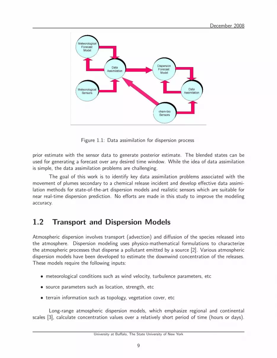
Data assimilation is the science and art of fusing the observations with the model predic-tions. Figure 1.1 illustrates schematically the data flow and the processes involved in the dataassimilation problem. The meteorological and dispersion forecast models recursively determinethe system states with current states modified by the data assimilation process which blends the
8
December 2008
Figure 1.1: Data assimilation for dispersion process
prior estimate with the sensor data to generate posterior estimate. The blended states can beused for generating a forecast over any desired time window. While the idea of data assimilationis simple, the data assimilation problems are challenging.
The goal of this work is to identify key data assimilation problems associated with themovement of plumes secondary to a chemical release incident and develop effective data assimi-lation methods for state-of-the-art dispersion models and realistic sensors which are suitable fornear real-time dispersion prediction. No efforts are made in this study to improve the modelingaccuracy.
1.2 Transport and Dispersion Models
Atmospheric dispersion involves transport (advection) and diffusion of the species released intothe atmosphere. Dispersion modeling uses physico-mathematical formulations to characterizethe atmospheric processes that disperse a pollutant emitted by a source [2]. Various atmosphericdispersion models have been developed to estimate the downwind concentration of the releases.These models require the following inputs:
• meteorological conditions such as wind velocity, turbulence parameters, etc
• source parameters such as location, strength, etc
• terrain information such as topology, vegetation cover, etc
Long-range atmospheric dispersion models, which emphasize regional and continentalscales [3], calculate concentration values over a relatively short period of time (hours or days).
University at Buffalo, The State University of New York
9

December 2008
Models of this type are often used to deal with accidental releases [4].
Two categories of atmospheric dispersion models can be distinguished, Eulerian and La-grangian. Eulerian models describe the dispersion of pollutants in a fixed frame of reference (fixedwith respect to a point on the earth surface). In Lagrangian models, the evolution of a pollutantair parcel (or puff) is described relative to a mobile reference system associated with the pufffrom its initial position as it moves along its trajectory. Both descriptions are equivalent, sincethe wind velocity u(x,t) in the Eulerian frame of reference is equal to the Lagrangian velocitydx/dt (if, for simplicity, only one dimension is considered) [4].
In the Eulerian approach, advection, diffusion, transformation and removal are simulatedin each grid cell by a set of mathematical expressions. Ideally, initial conditions are specifiedfor each cell, and new output data (such as emissions) are injected into the appropriate cells.In the Lagrangian approach, diffusion, transformation and removal calculations are performedfor the moving puffs [3]. The choice of model category depends on the various aspects of thedesired application, such as the numerical facilities available. Both Eulerian and Lagrangianmodels are based on the mass conservation equation. The Eulerian approach is burdened by highcomputational complexity and computer storage requirements, while the Lagrangian models arerelatively easy and inexpensive to run on a computer. Hence, the Lagrangian models have beenwidely used for problems of regional-to-continental scales.
The atmospheric dispersion models are also known as atmospheric diffusion models, airdispersion models, air quality models, and air pollution dispersion models. These dispersionmodels have several important applications. They provide useful knowledge about the hazardousreleases due to chemical/biological incidents, and radiological incidents like the Chernobyl nuclearaccident in 1986. These are also used to estimate or predict the downwind concentration of airpollutants emitted from sources such as industrial plants and vehicular traffic.
These models are addressed in Appendix A of EPA’s Guideline on Air Quality Models [2].Some of them are listed below:
• CALPUFF is a multi-layer, multi-species non-steady-state puff dispersion model that simu-lates the effects of time- and space-varying meteorological conditions on pollution transport,transformation and removal. CALPUFF can be applied on scales of tens to hundreds ofkilometers. It includes algorithms for subgrid scale effects (such as terrain impingement),as well as, longer range effects (such as pollutant removal due to wet scavanging and drydeposition, chemical transformation, and visibility effects of particulate matter concentra-tions).
• CAL3QHC is a roadway dispersion model that predicts air pollutant concentrations nearhighways and arterial streets due to emissions from motor vehicles operating under free-flowconditions and idling vehicles. In addition, CAL3QHC incorporates methods for estimatingtraffic queue lengths at roadway intersections.
• HOTMAC is a model for weather forecasting used in conjunction with RAPTAD which isa puff model for pollutant transport and dispersion. These models are used for complexterrain, coastal regions, urban areas, and around buildings where other models fail.
University at Buffalo, The State University of New York
10
December 2008
• SLAB is a model for denser-than-air gaseous plume releases that utilizes the one-dimensionalequations of momentum, conservation of mass and energy, and the equation of state.SLAB handles point source ground-level releases, elevated jet releases, releases from volumesources and releases from the evaporation of volatile liquid spill pools.
• OBODM is a model for evaluating the air quality impacts of the open burning and deto-nation (OB/OD) of obsolete munitions and solid propellants.
• PLUVUEII is a model used for estimating visual range reduction and atmospheric discol-oration caused by plumes resulting from the emissions of particles, nitrogen oxides, andsulfur oxides from a single source.
• RIMPUFF (Riso Mesoscale PUFF model) is a Lagrangian mesoscale atmospheric dispersionpuff model designed for calculating the concentration and doses resulting from the dispersionof airborne materials. The model can cope well with the in-stationary and inhomogeneousmeteorological situations, which are often of interest in connection with calculations usedto estimate the consequences of the short-term (accidental) release of airborne materialsinto atmosphere [1].
• SCIPUFF is a Lagrangian puff dispersion model that uses a collection of Gaussian puffsto predict three-dimensional, time-dependent pollutant concentrations. In addition to theaverage concentration value in each cell, SCIPUFF provides a prediction of the statisticalvariance in the concentration field resulting from the random fluctuations in the windfield [5]. SCIPUFF is a component of DTRA’s HPAC and the Joint Command’s JWARN.
The European Topic Centre on Air and Climate Change, which is part of the European En-vironment Agency (EEA), maintains an online Model Documentation System (MDS) [6] thatincludes descriptions and other information for several additional dispersion models developed bythe countries of Europe.
Most available practical atmospheric dispersion models predict only the ensemble-averageconcentration (that is, the average over a large number of realizations of a given dispersionsituation). In particular, single-event uncertainties in atmospheric dispersion models are not wellbounded, and current models are not well designed for complex natural topographies or built urbanenvironments [7]. At the other end of the spectrum, supercomputer solutions of the Navier-Stokesequations with LES (Large Eddy Simulation) turbulence modeling (e.g., FAST3D-CT [8]) havevery high resolution but are presently considered too slow to serve the emergency responder’sneeds [9].
Hence, the challenge is to add to the atmospheric dispersion models, the capability ofassimilating the measurements that are obtained from a variety of sensors, with information ofuneven quality and quantity, collected over irregular time periods. This will help in a betterprediction of the evolution of the dispersed species and a better evaluation of the hazard zones.
University at Buffalo, The State University of New York
11
December 2008
1.3 Data Assimilation Methods
1.3.1 Estimation Theory Basis of Data Assimilation
In Data Assimilation, the estimation of the unknown system states and/or model parametersgiven the underlying dynamics of the system and a set of observations may be framed as afiltering, smoothing or prediction problem. Given a fixed discrete time interval, t1, t2, . . . tN,over which observations are available, the problem of filtering is to find the best states at timetk given all the observations up to and including tk. The smoothing problem is to find the beststates at time tk given all the observations up to time tN , where tk ≤ tN . For tk > tN theprediction problem is to forecast the states of the system to time tk through system dynamics.Filtering and smoothing are inverse problems; prediction is a forward problem. Prediction isconcerned with uncertainty evolution through dynamic systems with stochastic excitation anduncertain initial conditions [10,11]. Prediction does not involve incorporating measurement databut filtering and smoothing do. Compared with filtering, smoothing provides better estimates andlower uncertainties but is computationally more expensive and involves time delay. The two-filterform of a recursive smoother has a forward pass and a backward pass. The forward pass is givenby a filter.
Because the states and the state estimates incorporate aleatoric uncertainty, the completedescription of them is the probability density function (pdf). In practice, the pdf is approximatedanalytically, for example, as a Gaussian pdf or Gaussian mixture, or numerically with grid pointsor random samples in the state space.
For continuous dynamics, the exact description of the pdf evolution is provided by a linearpartial differential equation (pde) known as the Fokker Planck Kolmogorov Equation (FPKE) [11].Analytical solutions exists only for stationary pdf and are restricted to a limited class of dynamicalsystems [10, 11]. Thus researchers are looking actively at numerical approximations to solve theFPKE [12–15], generally using the variational formulation of the problem. The Finite DifferenceMethod (FDM) and the Finite Element Method (FEM) have been used successfully for twoand even three dimensional systems. However, these methods are severely handicapped forhigher dimensions because the generation of meshes for spaces beyond three dimensions is stillimpractical. Furthermore, since these techniques rely on the FPKE, they can only be applied tocontinuous-time dynamical systems. For discrete-time dynamical systems, solving for the exactforecast pdf, which is given by the Chapman-Kolmogorov Equation [16] (CKE), yields the sameproblems as in the continuous-time case.
Several other techniques exist in the literature to approximate the pdf evolution, the mostpopular being Monte Carlo (MC) methods [17], Gaussian Closure [18] (or higher order momentclosure), Equivalent Linearization [19], and Stochastic Averaging [20,21]. Monte Carlo methodsrequire extensive computational resources and effort, and becomes increasingly infeasible for high-dimensional dynamic systems. All of these algorithms except Monte Carlo methods are similar inseveral respects, and are suitable only for linear or weakly nonlinear systems, because the effect ofhigher order terms can lead to significant errors. Furthermore, all these approaches provide onlyan approximate description of the uncertainty propagation problem by restricting the solution to
University at Buffalo, The State University of New York
12
December 2008
a small number of parameters - for instance, the first N moments of the sought pdf.
Adopting a Bayesian approach, the optimal data assimilation or data fusion is based onBayes’ rule:
posterior =likelihood × prior
normalizing constant(1.1)
In the above formula, the prior come from the model forecast, and the likelihood from themeasurement model and the measurement data. The posterior distribution is the pdf after theinformation contained in the measurement data is assimilated into the model forecast.
The ultimate objective of optimal estimation is to obtain the posterior distribution of thestates. It includes the optimal propagation and update of the pdf. The Kalman Filtering theoryplays an important role in optimal estimation. For linear stochastic models whose uncertainty ismodeled as Gaussian noise, the posterior distribution is also Gaussian, which is fully parameterizedby its mean vector and covariance matrix (the first two moments), and the optimal Bayesianestimator for this case is the Kalman Filter [22]. The Kalman Filter may also be derived as anoptimal linear least-squares estimator, without introducing probability distributions.
Most data assimilation problems of practical interest, however, involve nonlinear mod-els. In general, the exact solution for the state posterior distribution of a nonlinear model isintractable, even if the nonlinear model is of low order and simple. Various approximate nonlinearfiltering approaches are used in practice, many of which aim to recursively estimate the meanand covariance of the states instead of the much more complex posterior distribution.
1.3.2 Data Assimilation Methods
Classical Methods
Classical data assimilation methods include the polynomial approximation method, the Tikhonovregularization method, the successive correction methods, and the optimum interpolation method[23]. The polynomial approximation method rests upon the least squares fit of a general third-order polynomial of two independent coordinates to a set of observations. Because the polynomialcannot be expected to represent the variation of the meteorological variable over spatial dimensionthat is large compared to important smaller-scale structure, the domain of interest is divided intosub-domains where separate polynomial fits are found. The Tikhonov regularization methodinvolves adding a quadratic penalty or regularization term to the original least-squares cost. Insuccessive correction methods, an example of which is Cressman’s Method, the central variable isthe observation increment or difference between observation and forecast at the station and theproblem is solved iteratively. The essence of the Optimal Interpolation method is to express theanalysis increment as a linear combination of the observation increments weighted by the optimalweights under certain assumptions.
University at Buffalo, The State University of New York
13

December 2008
Variational Methods
Modern data assimilation methods include variational methods such as 3DVAR and 4DVAR, whichare based on least square estimation and can be formulated using the Bayesian framework [23].They are solved using the adjoint method. The objective of 3DVAR method is to find the bestparameter estimate that minimizes a quadratic cost of the form Jb(x) + Jo(x,y), where x isthe parameter vector of interest, y is the observation vector at a time point, and Jb and Jo
represent how far away the estimate deviates from the background (prior) knowledge and theobservations, respectively. The best estimate fits the background knowledge about x as wellas the observations. The 3DVAR method does not take the time evolution of the system intoaccount, leading to difficulties when the sensor data may be asynchronous with the state temporalgrid. This limitation is overcome by 4DVAR. The 4DVAR method finds the best fit over timeand space.
Recursive Nonlinear Estimators
Here we limit ourselves to a brief discussion of recursive nonlinear filters. The extension torecursive smoothers is straightforward in most cases.
The Extended Kalman Filter [22] is one of the most widely used nonlinear filters. Ofthe infinite moments that characterize the posterior distribution only the mean and the errorcovariance are computed. The model is linearized around the most recent estimate; the gradientsassociated with the linear error model have to be computed. The Extended Kalman Filter issufficient for many applications. However, when the state estimates are poorly initialized, themeasurement sampling rate is low, the noise is large, and/or the model is highly nonlinear, themethod will frequently fail. In such cases it may be worthwhile to use filters with higher ordertruncations, which require second or higher order derivatives [22].
The Unscented Filter [24] avoids computation of any derivatives while still attaining secondorder accuracy in mean and covariance estimates, but is also computationally more expensive thanthe Extended Kalman Filter. It works on the premise that with a fixed number of parameters itshould be easier to approximate a Gaussian distribution than to approximate an arbitrary nonlinearfunction.
A common characteristic of numerical atmospheric dispersion models is high dimensional-ity and high complexity, directly resulting from discretization of the governing partial differentialequations. For grid-based models, the size n of the state vector of an operational model can be ofthe order of thousands or even larger, depending on the grid resolution and size. In the ExtendedKalman Filter, the computational complexity of the update of the error covariance alone is of theorder of O(n3) [23]. The standard Unscented Filter formulation has computational complexityof the same order as the EKF [25]. Given the excessive or prohibitively large computationalrequirements, the Extended Kalman Filter and the more advanced methods cannot be applieddirectly [23].
Reduced-rank filters, which employ reduced-rank approximation to the full-rank covari-ance matrix, are becoming popular for large-scale data assimilation applications in atmospheric
University at Buffalo, The State University of New York
14
December 2008
dispersion, weather forecast, and so on [23]. The Ensemble Kalman Filters [26, 27] are a typicalexample, with the error covariance matrix approximated by the ensemble covariance around theensemble mean. The main operations of the Ensemble Kalman Filters are the dynamical propa-gation and transformation of the ensemble members. The transformation at measurement timesmay be preformed stochastically by treating observations as random variables, or deterministi-cally by requiring that the updated analysis perturbations satisfy the Kalman Filter analysis errorcovariance equation [28]. Compared with the extended Kalman Filter, these methods are easyto implement and computationally inexpensive. Besides, the Ensemble Kalman Filters need nolinearization or computation of the Jacobian matrices. Since the ensemble members are propa-gated with the fully nonlinear forecast model, the Ensemble Kalman Filter may do better in theforecast step than the Extended Kalman Filter [29].
It is not unusual to find in the data assimilation literature that 100 ensemble members aresufficient for data assimilation on systems of thousands of or more state variables [27]. However,it should not be interpreted as suggesting that the Ensemble Kalman Filters are able to defeat thecurse of dimensionality. The justification for using such a limited number of ensemble members liesnot in the magic of the Ensemble Kalman Filters, which are inferior to the full Extended KalmanFilter in estimation performance in many cases, but in the fact that the short-term uncertainty ofthe sophisticated dynamical models for atmospheric dispersion can often be described with muchlower-order models. As a result, working in a subspace of much lower dimension does not causesevere performance degradation.
Particle Filters [30] approximate the posterior distribution of the states with weightedparticles, ie., a superposition of weighted Dirac delta functions, being able to provide highermoment estimates and not requiring the posterior distribution to be Gaussian. The ParticleFilters are most suitable for the most general, highly nonlinear non-Gaussian models, but areamong the computationally most expensive nonlinear filters. The computational complexity ofa Particle Filter is closely related to the importance function employed to compose the proposaldistribution. Daum recently showed that a carefully designed Particle Filter should mitigate thecurse of dimensionality for certain filtering problems, but the Particle Filter does not avoid thecurse of dimensionality in general [31].
1.4 Challenges
The puff-based SCIPUFF is the transport and dispersion prediction tool used in HPAC andJWARN. Hence, one of our important goals is to develop data assimilation algorithms that aresuitable for puff-based transport and dispersion models including SCIPUFF. Data assimilationfor atmospheric release dispersion using puff models need to resolve three main problems: non-linearity, variable and high state dimensionality. Nonlinearities in the dispersion model and theobservation model pose significant challenges for data assimilation techniques based on linear op-timal or linearized estimation techniques. Furthermore, since pollutant release extended over timeis modeled as a sequence of puff releases, and potential subsequent puff splitting and merging,the number of puffs and therefore the length of the state vector is not constant, but changes withtime. In the case of a release extended over many discrete time steps, or a cascade of repeated
University at Buffalo, The State University of New York
15

December 2008
puff splitting, the state dimension may become so high that estimating all the states from thesensor data becomes impossible.
Another challenge comes from the fact that the CBRN sensors typically output discrete-valued measurements in the form of bar readings or particle counts, which in general meanscoarse quatization of the material concentration or radiation intensity. Many coarse sensors areonly capable of detecting whether the concentration exceeds a certain threshold or not.
1.5 Outline
Our efforts to meet the challenges of data assimilation for puff-based transport and dispersionmodels include: nonlinear filters (Chapters 2 and 3) and smoothers (Chapter 4) for data assim-ilation with puff-based transport and dispersion models, adaptive Gaussian sum propagator fordispersion forecasting (Chapter 5), chemical sensor modeling and data fusion algorithms (Chapter6).
University at Buffalo, The State University of New York
16

Chapter 2
Ensemble and Particle Filtering with aSpherical Diffusion Model
A common characteristic of numerical atmospheric dispersion models is high dimensionality andhigh complexity, directly resulting from discretization of the governing partial differential equa-tions. For grid-based models, the size n of the state vector of an operational model can be ofthe order of millions or even larger.
On the other hand, it is not unusual to find in the data assimilation literature that 100ensemble members are sufficient for data assimilation on systems of thousands of or more statevariables [27], which is in sharp contrast with the typical nonlinear Particle Filtering applicationsin which hundreds of or thousands of particles are used with as low as one- or three-dimensionalnonlinear systems. However, that should not be interpreted as that the Ensemble Kalman Filtersare able to beat the curse of dimensionality. The justification for using such a limited number ofensemble members lies not in the magic of the Ensemble Kalman Filters, which are inferior tothe full Extended Kalman Filter in estimation performance in many cases, but in the fact thatthe short-term uncertainty of the sophisticated dynamical models for atmospheric dispersion canoften be described with much lower-order models. As a result, working in a subspace of muchlower dimension does not cause severe performance degradation.
The efficacy of the ensemble filtering and particle filtering schemes is illustrated using theexample of a one-dimensional diffusion model. First, a diffusion model is introduced as a partialdifferential equation which is solved using the finite-difference approach. Then, the ensembleand Particle Filtering schemes as well as the full linear Kalman Filter are described in detail andimplemented on the diffusion model and the results are compared. For this example, the KalmanFilter provides the optimal solution to the data assimilation problem.
2.1 Spherical Diffusion Model
The model used is a one-dimensional spherical diffusion model to simulate the diffusion of aspecies expelled at a radial velocity uR from a spherical source of radius R.
17

December 2008
The equation for conservation of a diffusing species for any control volume can be writtenas
mass accumulation rate = (mass in − mass out)advection
+(mass in − mass out)diffusion
+generation rate (2.1)
Figure 2.1: Control volume schematic
Consider a thin spherical shell of thickness dr as the control volume (figure 2.1). Assumingthe generation rate in this volume to be zero, equation 2.1 can be written as:
(4πr2dr)∂
∂t(ρf) = −∆(ρfur4πr2) − ∆(Jr4πr2) (2.2)
where, ∆(ρfur4πr2) = (ρf)ur(4πr2)|r+dr − (ρf)ur(4πr2)|r∆(Jr4πr2) = (Jr4πr2)|r+dr − (Jr4πr2)|r
where ur is the radial velocity at distance r and Jr is the Diffusion Flux, given by Fick’s law
Jr = −Dm∂
∂r(ρf) (2.3)
where, Dm is Diffusivity.
University at Buffalo, The State University of New York
18

December 2008
This reduces to the following partial differential equation, representing the conservationof species:
∂
∂t(ρf) +
1
r2
∂
∂r(r2ρurf) =
1
r2
∂
∂r(r2Dm
∂(ρf)
∂r) (2.4)
where ρ is the density of the mixture and f represents the mass fraction of the species. If ρis constant, then it follows, from the application of law of conservation of mass to the controlvolume, that
m = ρ(4πr2ur) (2.5)
where, m is the mass of the mixture. Since m = ρ(4πR2uR) which is a constant, it can be seenfrom the above equation that ρr2ur is a constant and is given by m
4π.
The equation for conservation of species is now given by,
ρ∂f
∂t+
m
4πr2
∂f
∂r=
1
r2
∂
∂r(ρr2Dm
∂f
∂r) (2.6)
Initially, f(r, t) = 0 everywhere. The boundary conditions are stated below. At r = R(surface of emission), we have
m
4πR2=
m
4πR2fs − ρDm
∂f
∂r r=R(2.7)
where, fs is the value of f at the surface r = R. This equation can be rewritten as follows:
m
4πR2ρDm=
1
fs − 1
∂f
∂r r=R(2.8)
Also, as r → ∞, f → 0.
Note that equation 2.6 is singular as r → 0. This causes singularity problems whensolving numerically. To avoid this, the following variable transformations and standard notationare introduced.
η =( r
R
)3
and t∗ = t/
(R
uR
)(2.9)
Sc =ν
Dmand Re =
uRR
ν(2.10)
where, ν is the kinematic viscosity of the diffusing species. In the above notation, Sc is thedimensionless Schmidt number and Re is the dimensionless Reynolds number [32]. Using these,we have:
∂f
∂t=
uR
R
∂f
∂t∗
∂f
∂r=
3r2
R3
∂f
∂η
University at Buffalo, The State University of New York
19

December 2008
Equation (2.6) now reduces to:
m
4πR3
∂f
∂t∗+
3m
4πR3
∂f
∂η=
3ρDm
r2R3
∂
∂r(r4∂f
∂η)
=9ρDm
R2
∂
∂η(η
43∂f
∂η)
∂f
∂t∗+ 3
∂f
∂η=
36πρDmR
m
∂
∂η(η4/3 ∂f
∂η)
Further,
36πρDmR
m=
36πρDmR
4πR2ρuR
=9Dm
RuR
= 9Dm
ν
ν
uRR
=9
Sc · Re
The above calculations reduce equation (2.6) to the following:
∂f
∂t∗+ 3
∂f
∂η=
9
Sc · Re
∂
∂η(η4/3∂f
∂η) (2.11)
Now we have,
∂
∂η(η4/3∂f
∂η) =
[4η1/3
3
∂f
∂η+ η4/3∂2f
∂η2
]
Using this, equation (2.11) can be further simplified as follows, which is useful for devel-oping numerical solutions.
∂f
∂t∗+ 3
∂f
∂η
[1 − 4
Sc · Reη1/3
]=
9
Sc · Reη4/3 ∂2f
∂η2(2.12)
The boundary conditions in terms of the new variables are as follows.
As η → ∞, f → 0 (2.13)
At η = 1,∂f
∂η η=1
=Sc · Re
3(fs − 1) (2.14)
University at Buffalo, The State University of New York
20

December 2008
2.1.1 Numerical Solution and Model Simulation
The Crank-Nicholson method [33] is used for developing the numerical solution. Introducing thenotation
β = 3
[1 − 4
Sc · Reη1/3
]
α =9
Sc · Reη4/3
the finite difference approximation of the model is given below:
fk+1m −fk
m
∆t∗= 1
2
(−β
fkm+1−fk
m−1
2∆η− β
fk+1m+1−fk+1
m−1
2∆η
)
+12
(α
fkm+1−2fk
m+fkm−1
∆η2 + αfk+1
m+1−2fk+1m +fk+1
m−1
∆η2
)(2.15)
The above system of equations can be solved by LU decomposition, i.e. by forming atridiagonal system of equations which is solved using the Thomas algorithm [33].
The model is simulated using a coarse grid as well as a fine grid. A high resolution finegrid model is used for simulating the truth and obtaining the simulated measurements at thesensor locations. A low resolution coarse grid model is used for the purpose of testing the dataassimilation techniques.
0 20 40 60 80 100 1200.1
0.2
0.3
0.4
0.5
0.6
0.7
0.8
0.9
eta
f
1
3
10 num.ss
ss
Coarse Grid (21 points)
t* = 1t* = 3t* = 10num ssTrue ss
Figure 2.2: Spherical diffusion: coarse grid simulation
University at Buffalo, The State University of New York
21
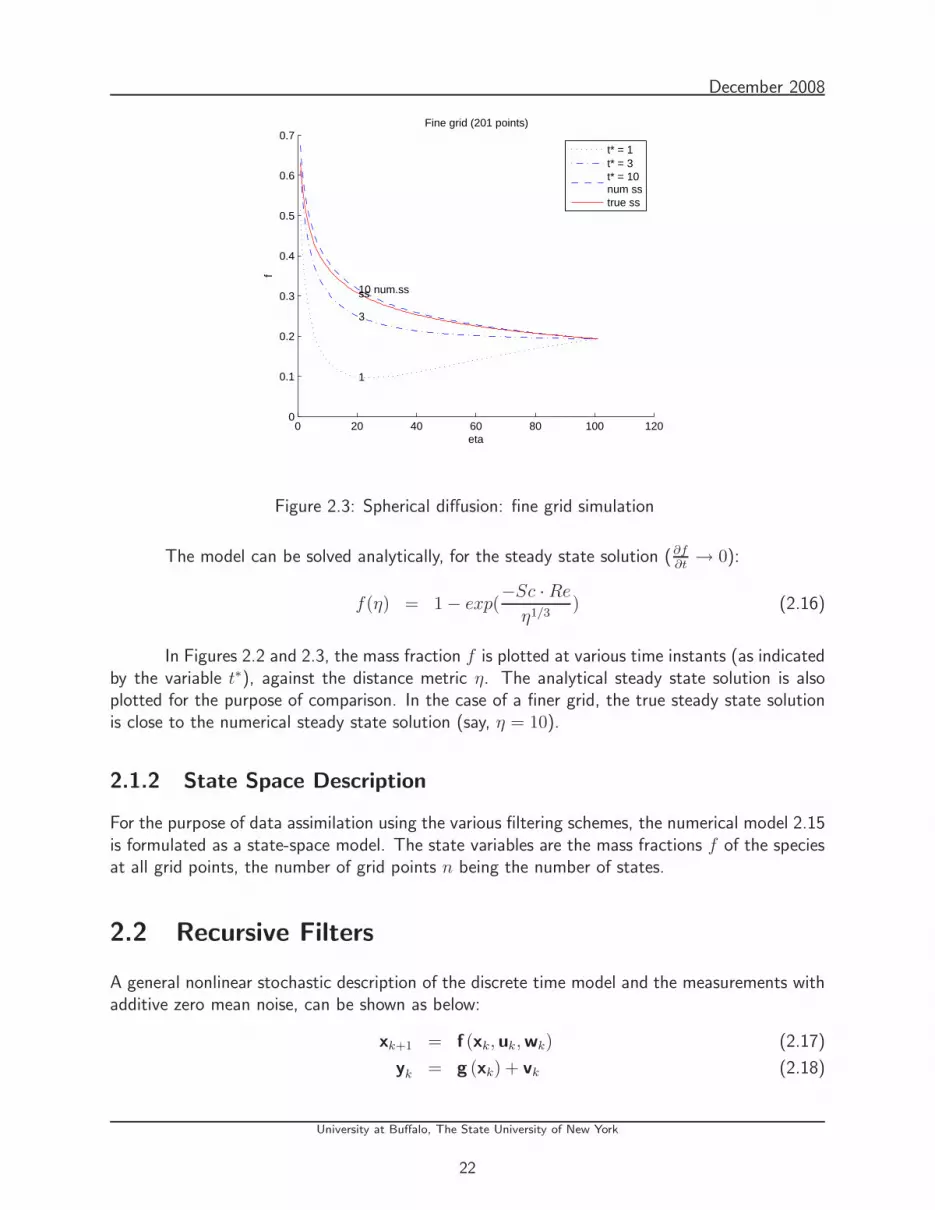
December 2008
0 20 40 60 80 100 1200
0.1
0.2
0.3
0.4
0.5
0.6
0.7
eta
f
1
3
10 num.ssss
Fine grid (201 points)
t* = 1t* = 3t* = 10num sstrue ss
Figure 2.3: Spherical diffusion: fine grid simulation
The model can be solved analytically, for the steady state solution (∂f∂t
→ 0):
f(η) = 1 − exp(−Sc · Re
η1/3) (2.16)
In Figures 2.2 and 2.3, the mass fraction f is plotted at various time instants (as indicatedby the variable t∗), against the distance metric η. The analytical steady state solution is alsoplotted for the purpose of comparison. In the case of a finer grid, the true steady state solutionis close to the numerical steady state solution (say, η = 10).
2.1.2 State Space Description
For the purpose of data assimilation using the various filtering schemes, the numerical model 2.15is formulated as a state-space model. The state variables are the mass fractions f of the speciesat all grid points, the number of grid points n being the number of states.
2.2 Recursive Filters
A general nonlinear stochastic description of the discrete time model and the measurements withadditive zero mean noise, can be shown as below:
xk+1 = f (xk, uk,wk) (2.17)
yk = g (xk) + vk (2.18)
University at Buffalo, The State University of New York
22

December 2008
2.2.1 Linear Kalman Filter
When a stochastic description of model and measurements of the form
xk+1 = Akxk + Bkuk + Fkwk (2.19)
yk = Ckxk + vk (2.20)
is available, it is possible to incorporate the measurements into the model to obtain an optimalestimate of the system. For this linear model with the assumption of Gaussian noise, the KalmanFilter provides the optimal estimate. The main advantage of using a linear model driven byGaussian noise is that the state and output will also be Gaussian. Furthermore, a Gaussiandistribution is characterized by its mean and covariance only. The Kalman Filter therefore hasonly first moment (mean) and second moment (error covariance) equations. The Kalman Filterequations are given by:
xk+1|k = Akxk|k + Bkuk (2.21)
Pk+1|k = AkPk|kATk + FkQkF
Tk (2.22)
xk+1|k+1 = xk+1|k + Kk+1(yk+1 − Ck+1xk+1|k) (2.23)
Kk+1 = Pk+1|kCTk+1(Ck+1Pk+1|kC
Tk+1 + Rk+1)
−1
(2.24)
Pk+1|k+1 = Pk+1|k −Kk+1Ck+1Pk+1|k (2.25)
x0|0 = x0 (2.26)
P0|0 = P0 (2.27)
An equivalent but more numerically stable substitute for covariance update is as follows:
Pk+1|k+1 = [I − Kk+1Ck+1]Pk+1|k [I − Kk+1Ck+1]T
+ Kk+1Rk+1KTk+1 (2.28)
Although these Kalman Filter equations can in principle be used to solve many dataassimilation problems the actual implementation for real life problems is far from transparent.
2.2.2 Ensemble Kalman Filter
The Ensemble Kalman Filter [26] is a data assimilation method that approximates the conditionaldensity using a Monte Carlo method. The data is assimilated using the analysis step of theKalman Filter, whereas the error covariance matrix is replaced by the sample error covariance.The ensemble filtering approaches are slightly modified to include nonlinearity in the observationoperator as well as the process model.
In this filter, the forecast error covariance is computed by integrating an ensemble ofrandomly perturbed initial analysis states in time with random perturbations added to the forcing.This Monte Carlo type approach based on the full nonlinear model allows for consistent statistics
University at Buffalo, The State University of New York
23
December 2008
in the case of nonlinear dynamics. The analysis of the perturbed states, known as ensemblemembers, is carried out with perturbed observations.
The propagation equations are given by:
ξik+1|k = f(ξik|k, uk,wik
)(2.29)
xk+1|k =1
N
N∑
i=1
ξik+1|k (2.30)
Let X be the matrix holding the ensemble members ξik+1|k ∈ ℜn×N ,
Xk+1|k = (ξ1k+1|k, ξ2k+1|k, . . . , ξNk+1|k) (2.31)
where N is the number of ensemble members and n is the size of the model state vector. Theensemble mean xk+1|k is stored in each column of Xk+1|k , which is of size n × N . The ensemblecovariance matrix Pe ∈ ℜn×n is defined as
Pe =X′X′T
N − 1(2.32)
where, X′ = Xk+1|k − Xk+1|k (2.33)
Given a vector of measurements d ∈ ℜm at the (k + 1)th time step, with m being thenumber of measurements, we can define the N vectors of perturbed observations as
dj = d + ǫj , j = 1, . . . , N, (2.34)
where d is the actual measurement vector and ǫj is the measurement error vector that is ran-domly generated from a predefined distribution with zero mean and covariance matrix R. Theseperturbed observations can be stored in the columns of a matrix
D = (d1, d2, . . . ,dN ) ∈ ℜm×N , (2.35)
while the ensemble of perturbations, with ensemble mean equal to zero, can be stored in thematrix
Υ = (ǫ1, ǫ2, . . . , ǫN) ∈ ℜm×N , (2.36)
from which we can construct the ensemble representation of the measurement error covariancematrix
Re =ΥΥT
N − 1(2.37)
The ensemble of innovations vectors defined as:
D′ = D −Yk+1 (2.38)
where, Yk+1 = g(Xk+1|k
)(2.39)
and the mean yk+1 is stored in each column of Yk+1 , which is of size m × N .
Y′ = Yk+1 − Yk+1 (2.40)
University at Buffalo, The State University of New York
24

December 2008
Using the above notations, the standard analysis equation can be expressed as:
Xk+1|k+1 = Xk+1|k + X′Y′T (Y′Y′T + ΥΥT )−1D′ (2.41)
The potential singularity of the inverse computation may require the use of a pseudoin-verse.
2.2.3 Ensemble Square Root Kalman Filter
The Ensemble Kalman Filter (EnKF) as described above uses pure Monte Carlo sampling whengenerating the initial ensemble, the process noise and the measurement perturbations. By se-lecting the initial ensemble, the process noise and the measurement perturbations wisely, it ispossible to achieve a significant improvement in the EnKF results, using the same number of en-semble members. The measurement perturbations introduce sampling errors which can be fullyeliminated when the square root analysis algorithm is used. Potential loss of rank may occur inthe case when random measurement perturbations are used to represent the measurement errorcovariance matrix. This can be avoided by a proper sampling of measurement perturbations oravoiding the perturbations as such. The algorithm described here solves for the analysis avoidingthe perturbation of measurements, and without imposing any additional approximations, such asthe assumption of uncorrelated measurement errors. This is discussed in detail in Evensen [27].
The algorithm is used to update the ensemble perturbations and is derived starting fromthe traditional analysis equation for the covariance update [34] given below, which reduces to2.25 in the case of Kalman Filter.
Pk+1|k+1 = Pk+1|k − Pxyk+1|k(P
yyk+1|k)
−1PxyTk+1|k (2.42)
where, Pxyk+1|k is the cross covariance between the state and the measurement errors and Pyy
k+1|k
is the innovation covariance. When using the ensemble representation, these covariances can beapproximated as follows:
Pxyk+1|k =
X′Y′T
N − 1(2.43)
Pyyk+1|k =
Y′Y′T
N − 1+ R (2.44)
Using these combined with 2.32, equation 2.42 can be rewritten as
Xa′
Xa′T = X′(I − Y′TG−1Y′)X′T (2.45)
where, Xa′
= Xk+1|k+1 − Xk+1|k+1 (2.46)
G = Y′Y′T + (N − 1)R (2.47)
Note that the equation for the ensemble analysis is derived by defining a factorization of thecovariance 2.45, where G is written so that no reference is made to the measurements or mea-surement perturbations.
University at Buffalo, The State University of New York
25

December 2008
The analyzed ensemble mean is computed from the standard analysis 2.41, as follows:
xk+1|k+1 = xk+1|k + X′Y′T G−1(d − yk+1) (2.48)
Assume that G is of full rank such that G−1 exists. Compute the eigenvalue decompositionand obtain
G−1 = ZΛ−1ZT (2.49)
Substituting this in 2.45, we obtain
Xa′Xa′T = X′(I − Y′T ZΛ−1ZT Y′)X′T
= X′[I − (Λ− 1
2 ZT Y′)T (Λ− 12 ZT Y′)
]X′T
= X′(I − XT
1 X1
)X′T (2.50)
where, X1 = Λ− 12 ZT Y′ (2.51)
Compute the singular value decomposition (SVD) of X1 and obtain
X1 = U1Σ1VT1 (2.52)
Substituting back, we get
Xa′Xa′T = X′
(I −[U1Σ1V
T1
]T [U1Σ1V
T1
])X′T
= X′(I − V1Σ
T1 Σ1V
T1
)X′T
= X′V1
(I − ΣT
1 Σ1
)VT
1 X′T
=(X′V1
√I − ΣT
1 Σ1
)(X′V1
√I − ΣT
1 Σ1
)T
(2.53)
In the above equation,√· denotes the matrix square root:
√P√
PT
= P .
Thus, a solution for the analysis ensemble perturbations is given by,
Xa′
= X′V1
√I − ΣT
1 Σ1ΘT (2.54)
This is added to the updated ensemble mean to get the ensemble update X(k + 1|k + 1) (2.46).
The additional multiplication with a random orthogonal matrix ΘT also results in a validsolution and is necessary to preserve zero mean for the analysis ensemble perturbations. Notethat by definition, we should have X′ · 1 = Xa′ · 1 = 0 with 1 a column vector of 1’s. Such arandom redistribution of the variance reduction among the ensemble members is used by default.The matrix ΘT is easily constructed, e.g., by using the right singular vectors from an SVD of arandom N × N matrix [27]. This approximately preserves zero mean for smaller N and as Nincreases, the accuracy increases.
University at Buffalo, The State University of New York
26

December 2008
2.2.4 Particle Filter
In Particle Filters, the posterior distribution p(xk|Yk) is approximated with N weighted particles
x(i)k , w
(i)k N
i=1, given by
PN(dxk|Yk) ≈N∑
i=1
w(i)k δ
x(i)k
(dxk) (2.55)
where x(i)k are the particles drawn from the importance function or proposal distribution, w
(i)k
are the normalized importance weights, satisfying∑N
i=1 w(i)k = 1, and δ
x(i)k
(dxk) denotes the
Dirac-delta mass located in x(i)k . We use Xk and Yk to denote the state trajectory xjk
j=0
and measurement history yjkj=1, respectively. The expectation of a known function f(xk) with
respect to p(xk|Yk) is then approximated by
∫f(xk)p(xk)dxk ≈
N∑
i=1
w(i)k f(x
(i)k ) (2.56)
For example, the approximation to the arithmetic mean of xk is∑N
i=1 w(i)x(i).
A Particle Filter updates the particle representation x(i)k , w
(i)k N
i=1 in a recursive manner.A cycle of a generic Particle Filter includes [30]
• Sequential Importance Sampling
– For i = 1, . . . N , sample x(i)k+1 from the importance function q(xk+1|X(i)
k ,Yk+1)
– For i = 1, . . . N , evaluate and normalize the importance weights
w(i)k+1 ∝ w
(i)k
p(yk+1|x(i)k+1)p(x
(i)k+1|x
(i)k )
q(x(i)k+1|X
(i)k ,Yk+1)
(2.57)
• Resampling: Multiply/Discard particles x(i)k+1N
i=1 with respect to high/low importance
weights w(i)k+1 to obtain N new particles x(i)
k+1Ni=1 with equal weights.
It should be noted that the computation of the mean and covariance is not required for theprocess of the Particle Filter.
The importance function plays a significant role in the particle filter. One of the simplestimportance function is given by q(xk+1|X(i)
k ,Yk+1) = p(xk+1|x(i)k ). The corresponding impor-
tance weights are w(i)k+1 ∝ w
(i)k p(yk+1|x(i)
k+1). Sampling x(i)k+1 from p(xk+1|x(i)
k ) is equivalent to
the dynamic propagation of x(i)k to time tk+1 and estimating the state pdf before any new obser-
vation. The optimal importance function that minimizes the variance of the importance weightw
(i)k+1 conditional upon x
(i)k and yk+1 is given by q(xk+1|X(i)
k ,Yk) = p(xk+1|x(i)k ,yk+1). The
corresponding importance weights are w(i)k+1 ∝ w
(i)k p(yk+1|x(i)
k ). The optimal Particle Filter givesthe limiting performance of particle filters.
University at Buffalo, The State University of New York
27
December 2008
When the state model is linear Gaussian as given in the previous section, all the above-mentioned probability density functions are Gaussian. In the simple Particle Filter, the meanand covariance of p(xk+1|x(i)
k ) are given by xk+1|k = Akx(i)k + Bkuk and Pk+1|k = FkQkF
Tk
respectively; the mean and covariance of p(yk+1|x(i)k+1) are given by Ck+1x
(i)k+1 and Rk+1 respec-
tively. In the optimal Particle Filter, the mean and covariance of p(xk+1|x(i)k ,yk+1) are given
by xk+1|k + Kk+1(yk+1 − Ck+1xk+1|k) and (I − Kk+1Ck+1)Pk+1|k respectively; the mean and
covariance of p(yk+1|x(i)k ) are given by Ck+1xk+1|k and Ck+1Pk+1|kC
Tk+1 + Rk+1 respectively.
It is well known that the simple Particle Filter with the prior p(xk+1|x(i)k ) as the importance
function does not work well when the overlap between the prior and the likelihood is small, forexample, when the measurement is very accurate [17]. A simple trick is applied in the simpleParticle Filter. Basically, the measurement update of the particle weights are done twice perfilter cycle. First, a large measurement noise variance 25R is used to calculate the Gaussianlikelihood and update the weights. Then, the particles are resampled. Finally, 25/24R is usedto do the same update again. That is based on the factorization e−1/R = e−1/25/R · e−24/25/R.The procedure will not change the weight associated with a particle but will have more particlesbe selected in the resampling steps. The more systematic, adpative treatment is known as“progressive corrections [17].”
2.3 Numerical Results
For the purpose of data assimilation using the various filtering schemes, the numerical model 2.15is formulated as a state-space model. The state variables are the mass fractions f of the speciesat all grid points, the number of grid points n being the number of states. A grid with n = 31 isused for the model used for testing the various filtering schemes. A finer grid (n = 301) is usedto simulate the measurements at sensor locations. The uncertainties in the process model andthe measurement model are modeled as Gaussian white noise processes.
In the simulations, the distance from the source and the simulation time are given by thenon-dimensional variables η and t∗ respectively, as described in equation 2.9. The value of η variesfrom 1 to 100 in these simulations, while the simulation time t∗ is 20. The model is simulated forthe fine grid (n = 301) and the values of f are taken as the truth at each time-step. The valuesof the measurement at the simulated sensor locations ηSenloc = [20 40 60] is obtained by linearinterpolation of the values of f at each grid point of the fine grid, and adding measurement noisewith a covariance R.
The coarse model (n = 31) is taken as an approximate model to simulate the abovetrue model and the filtering schemes are applied to estimate the states using the measurementsobtained as described before. The Ensemble Kalman Filter, the ensemble square root filter andthe simple Particle Filter are applied to the spherical diffusion problem, and the plots are comparedwith the truth and the full Kalman estimates. Note that the number of states in this model isn = 31. The measurement noise standard deviation at all the three sensor locations is 0.1. Thenumber of ensemble members used is 20 in both the ensemble filtering schemes and the numberof particles used is also 20 in the Particle Filter. Since Monte Carlo filtering schemes are used for
University at Buffalo, The State University of New York
28

December 2008
estimation, the results plotted are the values averaged over 50 Monte Carlo simulations.
0 5 10 15 20 250
0.2
0.4
0.6
0.8
1
1.2
1.4
Time
rms
erro
r
Nens = 20; Senloc = [20 40 60]; runs = 50
no filterensenSQRTpfkalman
Figure 2.4: RMS error in all states
0 5 10 15 20 250
0.05
0.1
0.15
0.2
0.25
0.3
0.35
Time
rms
erro
r
Nens = 20; Senloc = [20 40 60]; runs = 50
pfpfo
Figure 2.5: RMS error in all states for PF schemes
In Figure 2.4, the root mean square error in all the states is calculated and is plottedvs. time, for the ensemble filters and the Particle Filter. These are compared against the errorcalculated using just the model propagation and using the full kalman Filter. It can be observedthat the full Kalman Filter gives the best results as expected, while the ensemble square rootfilter has a significant advantage over the ensemble filter. The simple Particle Filter gives resultssimilar to the full Kalman Filter. Also the model error grows in time (to a steady state) as theerror keeps propagating through the coarse model, while the estimates in all the schemes improvewith time as the filters acquire more information. In Figure 2.5, the results of the simple Particle
University at Buffalo, The State University of New York
29

December 2008
0 5 10 15 20 25−0.1
0
0.1
0.2
0.3
0.4
0.5
0.6
Time
Mas
s F
ract
ion
f
Nens = 20; Senloc = [20 40 60]; location = 67.6667; runs = 50
kalmanensenSQRTpfTruthModel
Figure 2.6: Estimates of the mass fraction
Filter are compared with that of the optimal particle filter. It can be noticed that in our case,both the results are comparable in terms of accuracy while the optimal Particle Filter takes a verylong time (7519.6s) compared to the simple particle filter (445.3s).
In Figure 2.6, the estimates of the mass fraction of the species at two-thirds (η = 66.67)of the diffusion domain are plotted for various schemes, for the purpose of illustration. Theseestimates are compared with the truth as obtained from the simulation of the fine grid model, thefull Kalman Filter estimates and the values as predicted by the coarse model. It can be observedthat the model propagated state differs considerably from the truth, which is corrected using thevarious filtering techniques. Also, the Particle Filter estimate is as good as the Kalman estimate.The square root filter estimate is comparable to the Kalman estimate and shows a very goodimprovement over the standard ensemble filter. In Figure 2.7 and Figure 2.8, the one standarddeviation bands are plotted for both the ensemble filtering methods. The same is plotted for thesimple Particle Filtering scheme in Figure 2.9.
For the same number of representations of the states (N = 20), it has been shown thatthe simple Particle Filter gives better results in terms of accuracy than the two ensemble filters,for the model considered. However, it has been noticed that the computational time required forthe simple Particle Filter is also the highest among the three sub-optimal filters considered. TheCPU time required for the simple Particle Filter for 50 Monte Carlo runs is 445.28s whereas thesame for the ensemble and the square root filters are 342.47s and 364.31s respectively. Notethat the full Kalman Filter takes 713.15s for the same. Thus, it can be observed that the sub-optimal filters considered, offer significant improvement over the full Kalman Filter in terms ofcomputational time, while giving comparable estimates.
University at Buffalo, The State University of New York
30

December 2008
0 5 10 15 20 25−0.1
0
0.1
0.2
0.3
0.4
0.5
0.6
Time
Mas
s F
ract
ion
f
Nens = 20; Senloc = [20 40 60]; location = 67.6667; runs = 50
1σ bandensTruthModel
Figure 2.7: 1σ band of the ensemble estimate
2.4 Remarks
The ensemble and Particle Filters offer much advantage in terms of estimation time and computa-tional power used, as they avoid the storage and propagation of the state covariance matrix. Theensemble square root filter offers significant improvement over the standard Ensemble KalmanFilter in terms of the estimation error. While the simple Particle Filter gives the best results interms of accuracy, it is also computationally expensive and takes longer than the two ensemblefilters.
University at Buffalo, The State University of New York
31
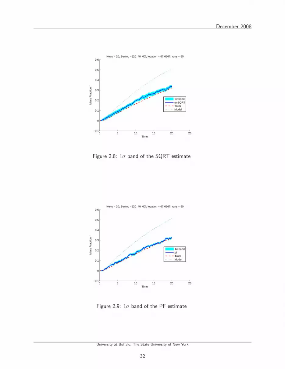
December 2008
0 5 10 15 20 25−0.1
0
0.1
0.2
0.3
0.4
0.5
0.6
Time
Mas
s F
ract
ion
f
Nens = 20; Senloc = [20 40 60]; location = 67.6667; runs = 50
1σ bandenSQRTTruthModel
Figure 2.8: 1σ band of the SQRT estimate
0 5 10 15 20 25−0.1
0
0.1
0.2
0.3
0.4
0.5
0.6
Time
Mas
s F
ract
ion
f
Nens = 20; Senloc = [20 40 60]; location = 67.6667; runs = 50
1σ bandpfTruthModel
Figure 2.9: 1σ band of the PF estimate
University at Buffalo, The State University of New York
32
Chapter 3
Particle Filtering with Puff-BasedDispersion Models
Gaussian puff-based models [1, 35] are often used to make fast release concentration prediction,in which a series of Gaussian shaped puffs (pollutant atmospheric parcels with a Gaussian distri-bution of the concentration field for each puff) are released at the sources and propagated in theatmosphere. DTRA’s HPAC and the Joint Commanders’ JWARN rely on SCIPUFF to computeconcentration prediction.
Because pollutant release extended over time is modeled as a sequence of puff releases,and potential subsequent puff splitting and merging, the number of puffs and therefore the lengthof the state vector is not constant, but changes with time. In the case of a release extendedover many discrete time steps, or a cascade of repeated puff splittings, the state dimension maybecome so high that estimating all the states from the sensor data becomes impossible.
The variable state dimension poses unique challenges for many recursive data assimilationmethods. The application of EKF and reduced-rank EKF requires complete knowledge of thedispersion modeling package, for mean and covariance propagation. The EnKF cannot be usedwith the puff-based models due to the inherent variable state dimensionality in these models.At each measurement update time, the ensemble members, the puff components of which mayhave been emitted at different source locations (to account for source location uncertainty) andmay have undergone different advection and splitting processes, may have different dimensions.For example, at a time instant one ensemble member may consist of ten puffs while anothermay consist of fifteen. Even if all the ensemble members have the same number of puffs, thecorrespondence among the puffs of different ensemble members is often unavailable. As a result,the ensemble mean and covariance as well as the cross correlation matrix between concentrationand puffs cannot be computed and the measurement update required to complete each step ofthe EnKF cannot be carried out. The same is true for the Unscented Filter.
Particle Filters [30] provide an attractive solution for such non-standard dynamical mod-els. Particle Filters are capable of providing useful estimates of the higher moments even innon-Gaussian cases, and are mostly suitable for strongly nonlinear and non-Gaussian models.The variable and high dimensionality of the state vector, which poses a problem to standard
33

December 2008
nonlinear assimilation techniques, can be overcome using Particle Filters. [31] showed that acarefully designed Particle Filter should mitigate the curse of dimensionality for certain filteringproblems. The efficacy of Particle Filter and Ensemble based filters, for data assimilation in a highdimensional linear diffusion model, is discussed in our earlier work [36]. Further, the Monte Carlonature of Particle Filtering techniques provides the potential for predicting multiple hypothesesscenarios in case of large uncertainty and multi-modal distributions, typical of such large models.Conveying multiple hypotheses to the decision-maker, rather than a single optimal hypothesis,is a more complete and useful characterization of risk in case of potentially lethal releases andwhen significant uncertainties exist in the source and the atmospheric data.
3.1 Particle Filtering with Simplified Puff Model
In this section, a simplified nonlinear puff-based dispersion model is used for the purpose of testingdata assimilation techniques. This model incorporates the characteristic features of change instate dimensionality with time and high state dimensionality. The performance of Particle Filteris studied, using a realistic nonlinear sensor model which measures concentration at the sensorlocation, and the various advantages and limitations are discussed. The result of the ParticleFilter is compared with that of the EKF.
3.1.1 Simplified Dispersion Model
The atmospheric dispersion model used is based on the RIMPUFF [1] (Riso Mesoscale PUFF)model which was designed to calculate the concentration and doses resulting from the dispersion ofairborne particles. It is a Lagrangian mesoscale atmospheric dispersion puff model, which appliesboth to homogeneous and inhomogeneous terrain with moderate topography on a horizontalscale of up to 50 km, and responds to changing (non-stationary) meteorological conditions. Themodel simulates the time varying release (source emission) of airborne materials by sequentiallyreleasing a series of Gaussian shaped puffs at a fixed rate on a specified spatio-temporal grid. Theamount of airborne materials allocated to individual puffs equals the release rate multiplied by thetime elapsed between puff releases. At each time step, the model advects, diffuses and depositsthe individual puffs according to local meteorological and physico-chemical parameter values. Asimilar model is used in [37] for experimental data assimilation studies using a variational approach.This model is used as a basis for the present dispersion model, which can be used to benchmarkvarious data assimilation techniques for dispersion models. Also, to reduce the computationalcomplexity of the simulations, the present model is restricted to the two dimensional horizontalspread of the plume. The vertical dimension, and thus the vertical effects on dispersion areignored. While this limits the direct applicability of the results to the target chemical dispersionapplication, it represents a simple testbed upon which prediction methods may be convenientlycompared.
University at Buffalo, The State University of New York
34
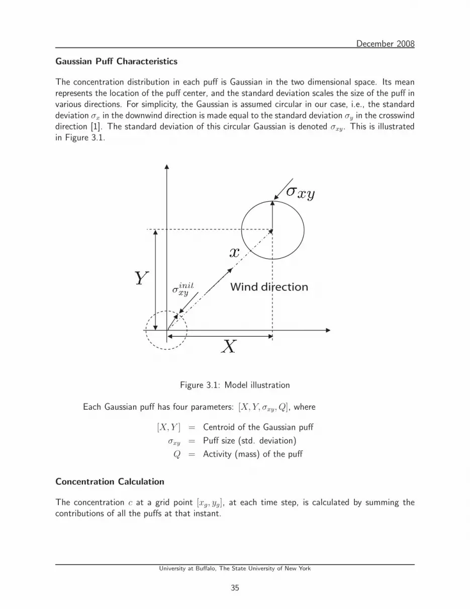
December 2008
Gaussian Puff Characteristics
The concentration distribution in each puff is Gaussian in the two dimensional space. Its meanrepresents the location of the puff center, and the standard deviation scales the size of the puff invarious directions. For simplicity, the Gaussian is assumed circular in our case, i.e., the standarddeviation σx in the downwind direction is made equal to the standard deviation σy in the crosswinddirection [1]. The standard deviation of this circular Gaussian is denoted σxy. This is illustratedin Figure 3.1.
Wind direction
Figure 3.1: Model illustration
Each Gaussian puff has four parameters: [X, Y, σxy, Q], where
[X, Y ] = Centroid of the Gaussian puff
σxy = Puff size (std. deviation)
Q = Activity (mass) of the puff
Concentration Calculation
The concentration c at a grid point [xg, yg], at each time step, is calculated by summing thecontributions of all the puffs at that instant.
University at Buffalo, The State University of New York
35

December 2008
c(xg, yg) =N∑
j=1
Qj
2πσjxy
2 exp
[−1
2
((Xj − xg)
2 + (Y j − yg)2
σjxy
2
)]
(3.1)
where, N is the number of puffs.
Puff Dynamics
The advection and diffusion of each puff takes place according to local meteorological parametervalues. In this model, the advection of each puff is calculated according to the wind vector, u atthe puff center and the time step, ∆T used to determine the next position of the puff center.
Xk+1 = Xk + uX∆T (3.2)
Yk+1 = Yk + uY ∆T (3.3)
where, u = [uX , uY ]T (3.4)
Expansion with time of a single puff is fundamentally related to the relative diffusionprocess. It is computed from simultaneous measurements or specifications of the atmosphericturbulence intensity and/or stability in the dispersion area. For the current model, standardplume dispersion information is used. Pasquill parameterisation, using a modified Karlsruhe-Julich system [1], is employed.
This parameterization is valid for limited cases of near ground level releases and dispersionover flat terrains. The growth of each puff is described by
σxy = pyxqy (3.5)
where, x = downwind distance given by,
xk+1 = xk +√
u2X + u2
Y ∆T
and py, qy = stability dependent parameters
(Karlsruhe-Julich diffusion coefficients)
py = 0.466 and qy = 0.866 are used in our reported simulation experiments to determinethe growth of each puff. Deposition and target species chemical reactivity (reactions in whichthe target species are components) are neglected for the present model and hence the mass ofeach puff remains constant during the dispersion process.
Puff Splitting
A puff splitting scheme is usually employed in the puff-based dispersion models such as RIMPUFF,to account for dispersion over complex terrains which might result in plume splitting. This scheme
University at Buffalo, The State University of New York
36

December 2008
is included in the present model to represent a similar structure for testing purposes. When aninitially small puff is grown to the size comparable with the grid spacing of the flow model, localeffects begin to dominate puff evolution and make a single puff a poor fit to its future evolution.In this circumstance, the original puff is replaced with five new smaller Gaussian puffs, under thefollowing constraints [1]:
1.∑5
j=1 Qj = Q
2.∑5
j=1 Qj(dj2+ σj
xy2) = Qσ2
xy
3.∑5
j=1 cj(X,Y ) = c(X,Y ) where cj
(X,Y ) is the concentration at [X, Y ] due to puff j.
4. σjxy = 1
2σxy for j = 1 to 5 (arbitrarily assigned)
Figure 3.2: Puff-splitting illustration [1]
The solution corresponding to these constraints is illustrated in Figure 3.2. Conservationof the puff moments is ensured in the splitting process. It can be noted from the solution thatthe new split puff parameters can be obtained through a linear transformation of the original puffparameters. After splitting, the new puffs can set off in individual directions in response to theinformation of divergence now explicitly contained in the flow field.
Puff Merging
It can be seen that as time progresses, there can be a rapid increase in the number of puffs dueto the splitting process, with a significant overlap between puffs. To reduce the extent of this
University at Buffalo, The State University of New York
37

December 2008
exponentially bounded increase in the number of puffs with time, several of the available puff-based dispersion models such as SCIPUFF (Second Order Closure Integrated Puff) model [5]include puff merging based on the degree of overlap between several puffs. . If they can besufficiently well modeled by a single Gaussian, overlapping puffs can be merged to form a singlepuff, thereby reducing the total number of puffs approximating the concentration distribution.
In the present model, we choose to preserve circularity of the merged puff. Two puffs,which are sufficiently close to each other, are merged according to the following equations, whichconserve the mass and the moments of the circular Gaussians:
1. Q =∑2
j=1 Qj
2. X =∑2
j=1 QjXj
Q
3. Y =∑2
j=1 QjY j
Q
4. σxy =
√∑2
j=1 Qj[σj
xy2+(X−Xj)2+(Y −Y j)2
]
Q
The new merged puff parameters can be obtained through a nonlinear transformation ofthe parameters of the two original puffs. The closeness of two puffs i and j is decided using thedimensionless measure δm, between the two puffs, which is a function of the separation distanceas well as their sizes:
δm =∆ij2
(σixy
2 + σjxy
2)
(3.6)
where, ∆ij is the separation distance between the centroids of the puffs. The puffs are mergedif δm is less than a certain value.
The model described in this section, is used as a representative atmospheric dispersionmodel for demonstrating the data assimilation methodologies.
3.1.2 Sensor Model
A nonlinear observation model is used to derive sensor data necessary for studying the dataassimilation performance. Each sensor measures concentration according to equation (3.1), andgives a noisy output due to additive zero mean Gaussian noise with a certain variance R at itslocation:
cv(xs, ys) =
N∑
j=1
Qj
2πσjxy
2 exp
[−1
2
((Xj − xs)
2 + (Y j − ys)2
σjxy
2
)]+ ν (3.7)
where cv is the measured concentration and ν is the observation noise of the sensor. Theconcentration at a location is the sum of the contributions, due to all the Gaussian puffs, at thelocation.
University at Buffalo, The State University of New York
38

December 2008
3.1.3 State Space Model Description
A general nonlinear stochastic state space description of the discrete time model and the mea-surements with additive zero mean noise, can be shown as below:
xk+1 = f (xk, uk,wk) (3.8)
yk = h (xk) + vk (3.9)
When such a stochastic description of model and measurements is available, it is theo-retically possible to incorporate the measurements into the model to obtain an optimal estimateof the system theoretically. The standard assignment of states for the dispersion problem usesconcentrations measured on a spatial grid. Using a puff model, the opportunity exists to dramat-ically reduce the dimensionality of the state space by replacing gridded concentrations by puffparameters. Specifically, the atmospheric dispersion model described in the previous section isinterpreted as a state space model as follows:
Define a state vector for each Gaussian puff as zj =[
Xj Y j σjxy Qj
]T, which
captures all the information of the jth Gaussian. The dynamics of each puff is governed by thefollowing equations as discussed before:
Xjk+1 = Xj
k + uXj∆T
Y jk+1 = Y j
k + uY j∆T
σjxyk+1
= py
[(σj
xyk
py
)1/qy
+√
u2Xj + u2
Y j∆T
]qy
Qjk+1 = Qj
k (3.10)
Combining, the state vector for the overall dynamic process is given by Z, the orderedconcatenation of the puff state vectors. The state space model of the discrete time atmosphericdispersion model is then given by
Zk+1 = f(Zk,uk,wk) (3.11)
uk, being the wind velocity vector and wk, being the process noise characterizing the uncertaintyin the wind velocity, at the time instant k.
When a puff splits at time k + 1, the original puff parameters are replaced by the newparameters obtained using the linear transformation corresponding to the splitting process, asdescribed in the earlier section. Let A be the corresponding linear operator of size 20× 4. Then,the new puff parameters are given by:
zk+1 = Azk+1BS (3.12)
where, zk+1BS represents the 4 × 1 state vector corresponding to the puff before splitting, andzk+1 represents the 20 × 1 state vector corresponding to the five new puffs after splitting.
University at Buffalo, The State University of New York
39

December 2008
Similarly, when two puffs merge at the instant k + 1, the original puff parameters arereplaced by the new parameters obtained using the nonlinear transformation corresponding tothe merging process. Let g(.) be the corresponding nonlinear operator. Then, the new puffparameters are given by:
zk+1 = g(zk+1BM) (3.13)
where, zk+1BM represents the 8×1 state vector corresponding to the two puff parameters beforemerging, and zk+1 represents the 4 × 1 state vector corresponding to the merged puff.
The spatio-temporal gridded concentrations induced by the puff states Zk are given byEquation (3.1). The length of the state vector Z changes whenever the number of puffs changeswith time as new source puffs are released, or existing puffs split, or merge. Thus we have anonlinear state space description, with variable state dimensionality and, in many cases such asextended releases, high state dimensionality as well. With puff parameters as states, the statespace dimensionality is much less than if the gridded concentration values were selected as states,but typically in the range of tens or hundreds for practical mesoscale applications.
3.1.4 Extended Kalman Filter and Particle Filter
Extended Kalman Filter
The Extended Kalman Filter (EKF) is one of the most widely used nonlinear filters. It employsmodel linearization around the most recent estimate. Use of the EKF in the case of variable statedimensionality necessitates certain block operations on the state covariance matrix at each timestep.
At each time k, if there is a new puff release, its covariance is initialized with P0. Thepropagation equations for the puffs, when there is no splitting, are as follows:
x0|0 = x0 (3.14)
P0|0 = P0 (3.15)
xk+1|k = f(xk|k,uk
)(3.16)
Pk+1|k = FkPk|kFTk + Qk (3.17)
where, F = ∂f∂x
. For a single puff, the Jacobian F is a 4× 4 identity matrix except for the (3, 3)element which is given by,
F33 =
(σxy
py
) 1qy
−1[(
σxy
py
) 1qy
+√
u2X + u2
Y ∆T
]qy−1
(3.18)
For the whole state-space model with more than a single puff, the Jacobian matrix F is calculatedin a similar fashion.
University at Buffalo, The State University of New York
40

December 2008
When there is puff splitting, the state mean and error covariance propagation occurs asabove, and they change according to the following equations due to splitting:
xk+1|k = Axk+1|k,BS (3.19)
Pk+1|k = APk+1|k,BSAT (3.20)
where A is the linear operator corresponding to the puff splitting process, xk+1|k,BS and Pk+1|k,BS
are the propagated state mean and the propagated state error covariance matrix before splitting.To ensure that the eigenvalues of the transformed state error covariance matrix are positive, thesmallest eigenvalue is set to a specified constant 10−6 in the simulations to be reported. Thepropagated state mean and error covariances for all the puffs are then concatenated appropriately.In this step, the cross-covariance terms between the split puffs are set so that the block diagonalstructure of P is maintained for computational ease, each block being a 4 × 4 error covariancematrix corresponding to each puff.
When puffs merge, the propagated state mean and error covariance are transformed ac-cording to the following equations:
xk+1|k = g(xk+1|k,BM) (3.21)
Pk+1|k = GPk+1|k,BMGT (3.22)
where g(.) is the nonlinear operator corresponding to the puff merging process, G is the 4×8 lin-earized Jacobian matrix corresponding to the nonlinear transformation, xk+1|k,BM and Pk+1|k,BM
are the propagated state mean and the propagated state error covariance matrix before merging.It is again ensured that the eigenvalues of the state error covariance matrix are positive duringthis transformation, by fixing the smallest eigenvalue as above. The propagated state mean anderror covariances for all the puffs are concatenated appropriately.
The propagated state mean and error covariances for all the puffs are then updated withthe sensor measurements as follows:
xk+1|k+1 = xk+1|k + Kk+1(yk+1 − h(xk+1|k)) (3.23)
Kk+1 = Pk+1|kHTk+1(Hk+1Pk+1|kH
Tk+1
+Rk+1)−1 (3.24)
Pk+1|k+1 = Pk+1|k − Kk+1Hk+1Pk+1|k (3.25)
where, H = ∂h∂x
is the measurement Jacobian.
For the observation model given by (3.7), the measurement Jacobian can be calculated asfollows. The elements of the measurement Jacobian at a sensor location [xs, ys] corresponding
University at Buffalo, The State University of New York
41

December 2008
to the states of jth Gaussian puff are given by:
∂h
∂Xj= −cj
[Xj − xs
σjxy
2
]
∂h
∂Y j= −cj
[Y j − ys
σjxy
2
]
∂h
∂σjxy
= cj
[(Xj − xs)
2 + (Y j − ys)2
σjxy
3 − 2
σjxy
]
∂h
∂Qj=
cj
Qj(3.26)
where, cj is the concentration at [xs, ys] due to the jth Gaussian puff. The measurement Jacobianfor the states of all the puffs and for all the sensor locations can be similarly calculated andconcatenated appropriately, to obtain the full measurement Jacobian matrix. The block diagonalstructure of the process and measurement Jacobians is maintained throughout.
The EKF involves the tedious calculation of process and measurement model Jacobians,storage and propagation of large state error covariance matrices. The state error covariancematrix rapidly increases in size due to increase in the state dimension with time. This increasesthe complexity of the EKF. Particle Filters provide a good alternative for such non-standarddynamical and observation models. The Bootstrap Particle Filter is implemented on the repre-sentative atmospheric dispersion model using the sensor model discussed in the earlier section.The implementation of this Particle Filter, as applicable to our present models, is outlined below:
Particle Filter
The Bootstrap Filter [30] is used. The measurement likelihood, in the Bootstrap Filter, for thechosen observation model, is given by:
P (cv|c) =1√2πR
e−(cv−c)2
2R (3.27)
The updated weight of each particle is proportional to this particle likelihood.
Particle Filter does not involve the calculation of Jacobians, the storage of large stateerror covariance matrices and associated block operations due to varying state dimensions. In thepresent application, each of the particles, in general, may have different state dimensions. In thecase of the Bootstrap Particle Filter, only the weights of the different particles are updated basedon the likelihood for each particle. The likelihood for each particle is calculated in the griddedconcentration space using Equation 3.27. Each particle, regardless of its state dimensionality,maps to a particular distribution of the release concentration field in the two-dimensional gridspace of interest. Therefore, the mean representation of the particles is the mean concentrationfield in the fixed two-dimensional grid space. This mean can be used as a single point estimateof the concentration at various grid locations. Thus, Particle Filter provides a unified approachto the case of variable state dimensionality.
University at Buffalo, The State University of New York
42

December 2008
3.1.5 Numerical Results
The performance of the estimation techniques, is studied for these models using simulated at-mospheric dispersion and concentration measurements. In the simulations, the grid resolutionover the dispersion region is 200m and sensors are located every other grid point along both thespatial axes as shown in Figure 3.3.
0 500 1000 1500 2000 2500 30000
500
1000
1500
2000
2500
3000
X (m)
Y (
m)
Sensor placement
Figure 3.3: Sensor locations on the grid
The total simulated elapsed time is 3600s using sampling interval 20s. The source locationis assumed to be in the vicinity of the origin. Source release duration and location are modeledparametrically. The exact location is modeled as a Gaussian random variable with 5m standarddeviation in each direction. The release occurs for 20% of the simulated elapsed time, with a 10%standard deviation on the cut-off time. This is implemented as a dimensionless fraction of thetotal number of time steps and is modeled as a random variable α with mean 0.2 and a standarddeviation of 0.02. There is a puff release every three time steps. The activity of each puff isassumed to be 5×10⁵. The units of activity can be chosen according to the species under study.Note that the units of concentration (as well as concentration error) are then ActivityUnits/m2
in the following. A puff is split into five new puffs when the size of the puff σxy is greater than1500m. The wind speed is 4m/s and the nominal wind field is as shown in Figure 3.4. Thewind blows at θ in the lower left corner of the grid near the source location. This θ is modeled
University at Buffalo, The State University of New York
43
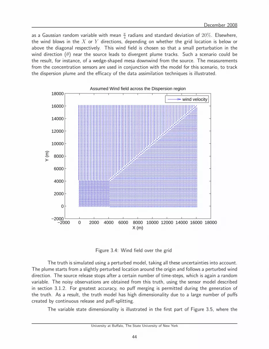
December 2008
as a Gaussian random variable with mean π4
radians and standard deviation of 20%. Elsewhere,the wind blows in the X or Y directions, depending on whether the grid location is below orabove the diagonal respectively. This wind field is chosen so that a small perturbation in thewind direction (θ) near the source leads to divergent plume tracks. Such a scenario could bethe result, for instance, of a wedge-shaped mesa downwind from the source. The measurementsfrom the concentration sensors are used in conjunction with the model for this scenario, to trackthe dispersion plume and the efficacy of the data assimilation techniques is illustrated.
−2000 0 2000 4000 6000 8000 10000 12000 14000 16000 18000−2000
0
2000
4000
6000
8000
10000
12000
14000
16000
18000
X (m)
Y (
m)
Assumed Wind field across the Dispersion region
wind velocity
Figure 3.4: Wind field over the grid
The truth is simulated using a perturbed model, taking all these uncertainties into account.The plume starts from a slightly perturbed location around the origin and follows a perturbed winddirection. The source release stops after a certain number of time-steps, which is again a randomvariable. The noisy observations are obtained from this truth, using the sensor model describedin section 3.1.2. For greatest accuracy, no puff merging is permitted during the generation ofthe truth. As a result, the truth model has high dimensionality due to a large number of puffscreated by continuous release and puff-splitting.
The variable state dimensionality is illustrated in the first part of Figure 3.5, where the
University at Buffalo, The State University of New York
44

December 2008
0 50 100 150 2000
20
40
60
80
Num
ber
of p
uffs
Sample truth simulation
0 50 100 150 2000
5
10
15
time−step
Num
ber
of p
uffs
Model simulation
Figure 3.5: Number of puffs
number of puffs is plotted against the time step, during the simulation of a sample truth. Aconstant increase in the number of puffs, due to constant source release, can be seen till thetime-step k = 39. A new puff is added every three time steps during the source release. Followingk = 39, there are no subsequent new puffs released at the source. The number of puffs remainsconstant for a certain duration, during which the puffs disperse, causing them to grow in size.There is again an increase in the state dimension beginning at time step k ≈ 140, as the largepuffs begin splitting 5 : 1.
For the observation model, the concentration variance at each sensor location is chosen tobe 0.01. The nominal dispersion model, which also includes puff-merging, is used for the purposeof testing the estimation algorithms using these noisy observations. In this model, the puffs aremerged if δm is less than 0.05. This way, the number of puffs are reduced, but still quite high forthe purpose of data assimilation. The variable state dimensionality for the process model usedfor data assimilation, is shown in the second part of Figure 3.5. Note the decrease in the numberof puffs at various time steps due to the merging of overlapping puffs.
The Extended Kalman Filter and the Bootstrap Particle Filter are implemented on thisrepresentative 2D puff-based atmospheric dispersion model, and the results are compared withsimulated truths. The number of particles used in the Particle Filter, is 50, which is comparable to
University at Buffalo, The State University of New York
45
December 2008
the final number of states (60) in the nominal process model as seen in Figure 3.5. The particlesin the Particle Filter are sampled from the initial uncertain source location and the initial winddirection for each particle is also sampled from uncertain wind direction θ. Then, each of theseparticles is propagated according to the dispersion model with splitting and merging. In the EKF,the uncertainty in the cut-off time is being accounted for by having a larger state error covariancematrix for the puffs released around the cut-off time, so that the EKF corrects the discrepancybetween its prediction and the true plume by adjusting the parameters of the existing puffs basedon the sensor data. In the Particle Filter, different particles have different cut-off times sampledfrom the Gaussian distribution of its uncertainty, and the correct plume trajectory is selected byproportionately weighing its samples according to their likelihoods. In the calculation of likelihoodvalues of the particles, very small positive numbers are added to them to overcome numericaldifficulties caused by near zero values.
These particles are used to estimate the posterior distribution of concentrations at variousgrid points in the dispersion region, using the sensor measurements along with the process modeldynamics in the puff parameter space whose dimension is varying with the number of puffs. Whilethe number of particles (50) used here is relatively less than the maximum state dimensionality( 60) of the process model, the effective number of degrees of freedom in the process noiseis much smaller than the number of actual states. The uncertainty in the states is effectivelycaptured by the prevailing wind velocity, source location and source duration. Thus increasingthe number of particles by a factor of 2 − 5 was not found to materially improve the estimationperformance.
During the process of data assimilation, the differences between the predicted concentra-tions and the sensor measurements are used to update the model states in the case of EKF andthe weights of the particles in the case of Bootstrap Particle Filter. The sensor locations whereboth the predicted concentrations and the measured concentrations are below 3σ are neglected,σ being the standard deviation of the noise in the sensors. The results are averaged over 50Monte Carlo runs.
For error calculations, a grid domain of 16×16 km2 is used. In Figure 3.6, the root meansquared (RMS) error in concentrations across all grid points in the domain is calculated and isplotted vs. time, for the filters as well as for the nominal model without data assimilation. Thedecrease in the RMS error for the nominal model without data assimilation starting at about timestep 125 can be explained by the fact that with time, all concentrations decay to zero. The spikesin the error graph for the model, EKF and PF around time-step 42 is due to the uncertainty inthe source cut-off time which occurs around time-step 36 as explained earlier. The source cut-offmight occur at a different time in the truth compared to the model used for prediction. Thisresults in a sudden increase in error due to the different number of puffs in the true plume andthe predicted plumes. From the figure, it can be seen that on an average, both the filters areable to predict the plume with much less error. It can also be observed that the Particle Filterperformance is comparable to that of the EKF.
In Figure 3.7, the predicted and the true tracks are shown for two of the sample runs, byplotting concentration contours of C = 0.2 for every 10 time steps, in the dispersion region. Itcan be seen from the figure that both the Particle Filter and the EKF predictions are quite close
University at Buffalo, The State University of New York
46

December 2008
0 50 100 150 2000
2
4
6
8
10
12
time−step
RM
S e
rror
RMS error in concentrations over 50 Monte Carlo runs
PFModelEKF
Figure 3.6: RMS error in the concentrations
to the true plume even in this highly unstable case in which the model predictions diverge rapidlyfrom the assimilated estimates.
3.1.6 Remarks
While the two filters are comparable in terms of estimation performance, the Bootstrap ParticleFilter offers significant advantages in terms of ease of implementation for practical (black-box)models and memory requirements. The application potential of Particle Filter, in the contextof variable state dimensionality, puff-based dispersion modeling packages, non-linearities in theprocess and observation models, is thus demonstrated.
University at Buffalo, The State University of New York
47

December 2008
Sample run 1: C = 0.2
Y (
m)
0 5000 10000 150000
5000
10000
15000
Sample run 2: C = 0.2
0 5000 10000 150000
5000
10000
15000TruthEKFModel
Y (
m)
X (m)0 5000 10000 15000
0
5000
10000
15000
X (m)
0 5000 10000 150000
5000
10000
15000TruthPFModel
Figure 3.7: Concentration contours
University at Buffalo, The State University of New York
48
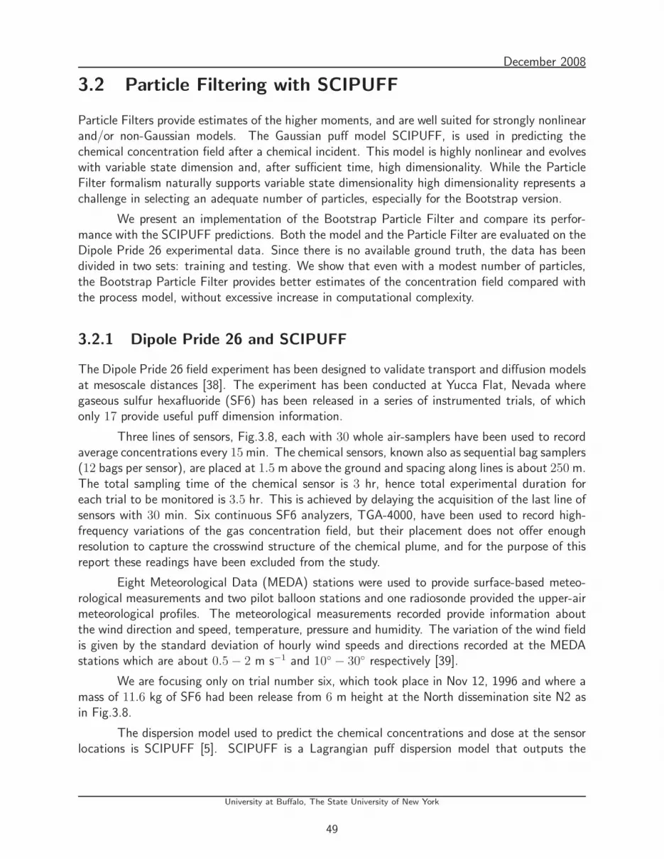
December 2008
3.2 Particle Filtering with SCIPUFF
Particle Filters provide estimates of the higher moments, and are well suited for strongly nonlinearand/or non-Gaussian models. The Gaussian puff model SCIPUFF, is used in predicting thechemical concentration field after a chemical incident. This model is highly nonlinear and evolveswith variable state dimension and, after sufficient time, high dimensionality. While the ParticleFilter formalism naturally supports variable state dimensionality high dimensionality represents achallenge in selecting an adequate number of particles, especially for the Bootstrap version.
We present an implementation of the Bootstrap Particle Filter and compare its perfor-mance with the SCIPUFF predictions. Both the model and the Particle Filter are evaluated on theDipole Pride 26 experimental data. Since there is no available ground truth, the data has beendivided in two sets: training and testing. We show that even with a modest number of particles,the Bootstrap Particle Filter provides better estimates of the concentration field compared withthe process model, without excessive increase in computational complexity.
3.2.1 Dipole Pride 26 and SCIPUFF
The Dipole Pride 26 field experiment has been designed to validate transport and diffusion modelsat mesoscale distances [38]. The experiment has been conducted at Yucca Flat, Nevada wheregaseous sulfur hexafluoride (SF6) has been released in a series of instrumented trials, of whichonly 17 provide useful puff dimension information.
Three lines of sensors, Fig.3.8, each with 30 whole air-samplers have been used to recordaverage concentrations every 15 min. The chemical sensors, known also as sequential bag samplers(12 bags per sensor), are placed at 1.5 m above the ground and spacing along lines is about 250 m.The total sampling time of the chemical sensor is 3 hr, hence total experimental duration foreach trial to be monitored is 3.5 hr. This is achieved by delaying the acquisition of the last line ofsensors with 30 min. Six continuous SF6 analyzers, TGA-4000, have been used to record high-frequency variations of the gas concentration field, but their placement does not offer enoughresolution to capture the crosswind structure of the chemical plume, and for the purpose of thisreport these readings have been excluded from the study.
Eight Meteorological Data (MEDA) stations were used to provide surface-based meteo-rological measurements and two pilot balloon stations and one radiosonde provided the upper-airmeteorological profiles. The meteorological measurements recorded provide information aboutthe wind direction and speed, temperature, pressure and humidity. The variation of the wind fieldis given by the standard deviation of hourly wind speeds and directions recorded at the MEDAstations which are about 0.5 − 2 m s−1 and 10 − 30 respectively [39].
We are focusing only on trial number six, which took place in Nov 12, 1996 and where amass of 11.6 kg of SF6 had been release from 6 m height at the North dissemination site N2 asin Fig.3.8.
The dispersion model used to predict the chemical concentrations and dose at the sensorlocations is SCIPUFF [5]. SCIPUFF is a Lagrangian puff dispersion model that outputs the
University at Buffalo, The State University of New York
49
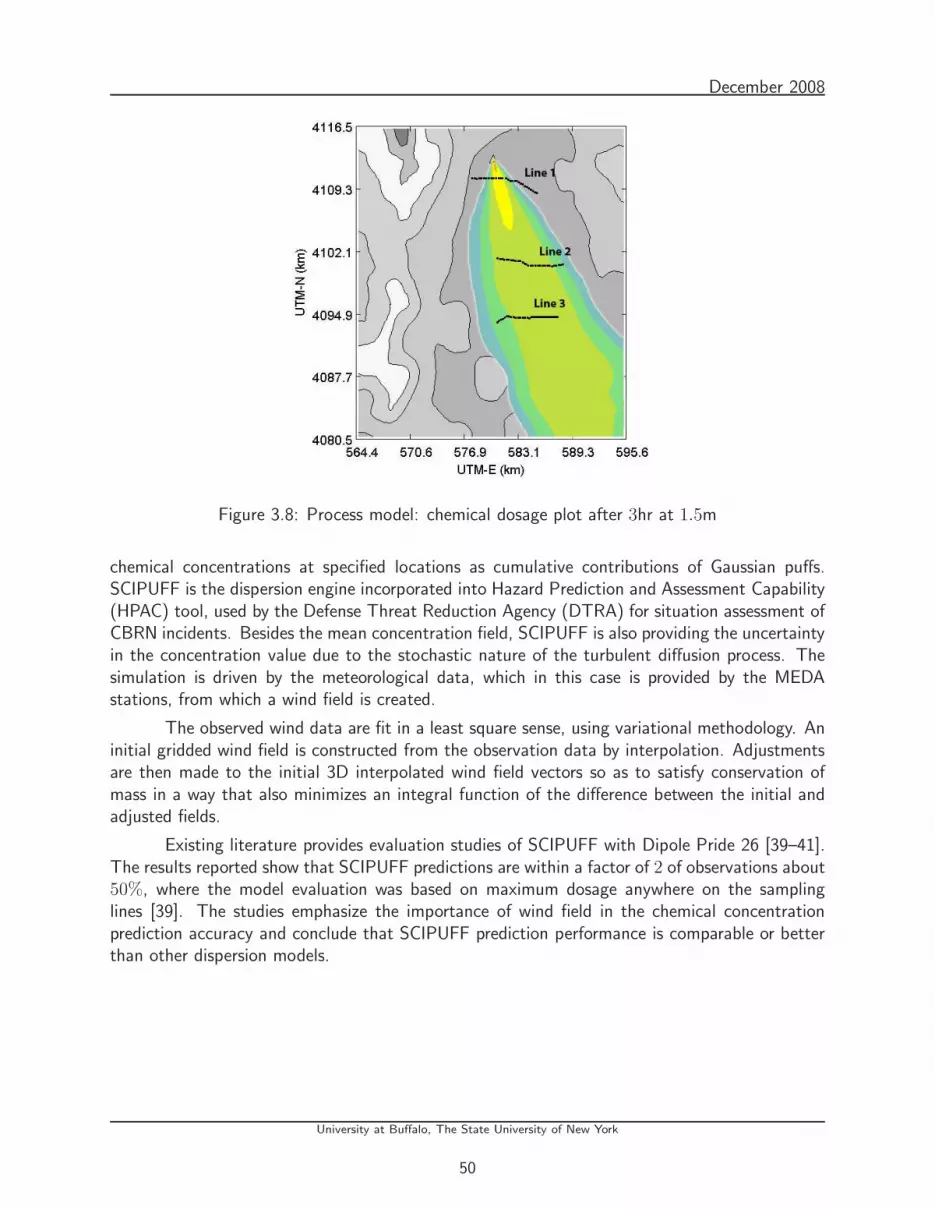
December 2008
Figure 3.8: Process model: chemical dosage plot after 3hr at 1.5m
chemical concentrations at specified locations as cumulative contributions of Gaussian puffs.SCIPUFF is the dispersion engine incorporated into Hazard Prediction and Assessment Capability(HPAC) tool, used by the Defense Threat Reduction Agency (DTRA) for situation assessment ofCBRN incidents. Besides the mean concentration field, SCIPUFF is also providing the uncertaintyin the concentration value due to the stochastic nature of the turbulent diffusion process. Thesimulation is driven by the meteorological data, which in this case is provided by the MEDAstations, from which a wind field is created.
The observed wind data are fit in a least square sense, using variational methodology. Aninitial gridded wind field is constructed from the observation data by interpolation. Adjustmentsare then made to the initial 3D interpolated wind field vectors so as to satisfy conservation ofmass in a way that also minimizes an integral function of the difference between the initial andadjusted fields.
Existing literature provides evaluation studies of SCIPUFF with Dipole Pride 26 [39–41].The results reported show that SCIPUFF predictions are within a factor of 2 of observations about50%, where the model evaluation was based on maximum dosage anywhere on the samplinglines [39]. The studies emphasize the importance of wind field in the chemical concentrationprediction accuracy and conclude that SCIPUFF prediction performance is comparable or betterthan other dispersion models.
University at Buffalo, The State University of New York
50

December 2008
3.2.2 Particle Filter Implementation
The Bootstrap Filter in the previous section is used. Three types of uncertainties [42] are presentin the model predictions: model uncertainty due to the inaccurate representation of the chemicaland dynamical processes, data uncertainty due to the errors in data used to drive the modeland random turbulence of the atmosphere.
The model uncertainty is not completely reducible, and in the SCIPUFF prediction case it isestimated. The uncertainty due to the variability of the atmosphere cannot be further reduced andthe uncertainty due to data errors it is usually high, more than 50% of the total uncertainty [43],but it can be minimized. The data errors considered in this report are meteorological data: windspeed and wind direction. The errors are due to the unrepresentative sitting of the wind sensorsin the field and sensor accuracy and calibration [41]. This information is rarely available and forthis study a standard deviation of 0.5 m s−1 for the wind speed and 5 for the wind direction hasbeen considered.
A FORTRAN implementation of the Particle Filter has been specially created for SCIPUFFto run in parallel on the cluster hosted at the Center for Computational Research at University atBuffalo. This implementation of the Particle Filter is designed to account for the uncertainty inthe wind sensor readings while coping with the challenges of the data assimilation for the CBRNincidents using Gaussian puff models: variable dimensionality and high dimensionality [44].
Compared with the maximum dosage approach [39], the evaluation method used in thisreport is to compare the predicted dosage after every 15 min with the corresponding observeddosage.
Since there is no ground truth, the samples provided in the DP26 have been divided totwo sets: the training set used to perform the data assimilation, composed of Line 1 and Line2 of sensors, and the testing set, Line 3 of sensors, used for performance evaluation.
Due to the spatial and temporal distance between the wind readings all the consideredindependent random variables described by a Gaussian distribution with mean given by the nominalsensor reading and uncertainty given by the standard deviation mentioned above. Hence theparticles, each representing a SCIPUFF instance, are propagated using wind field generated fromdata sampled from this distribution. Each particle outputs a dose field di
j which depends on thewind field; here j is the sensor number, i is the particle number and k is the time step. Theestimated dosage dj is given by the following relation:
di(k) =
N∑
i=1
wikd
ij(k) (3.28)
Here wik is given by wi
k+1 ∝ wikp(zk+1|xi
k+1). The conditional probability p(zk+1|xik+1) is unknown
since the authors could not find information regarding the uncertainty in the concentration read-ings for the whole air-samplers. The concentration readings of the sensors have been assumed tobe independent random variables due to the spatial and temporal distances. The likelihood havebeen approximated with a Gaussian function given by:
p(dj(k)|dij(k)) = N
(di
j(k)∣∣dj(k), v(k)
)(3.29)
University at Buffalo, The State University of New York
51
December 2008
Here dj(k) is the observed dosage at the jth sensor at time k and v(k) is the sample variance ofthe difference between observed dosages and predicted ones over all the particles. Any predicteddosage less than 1 ppt-hr (including zero) has been set to 1 ppt-hr and all the observed dosagesless than 10 ppt-hr have been ignored. Hence the total number of dosage values to be comparedis 47.
3.2.3 Numerical Results
Both the process model predictions, using nominal wind sensor readings, and the Particle Filterpredictions with perturbed wind field have been compared against the observed dosages on thethird line of sensors.
To evaluate the performance of the Particle Filter compared with the process model, weconsider the following statistical measures [45]: FB - fractional bias, MG - geometric meanbias, NMSE - normalized mean square error, VG - geometric variance, FAC2 - fraction ofpredictions within a factor 2 of observations and FAC3 - fraction of predictions within a factor 3of observations.
FB =Do − Dp
0.5(Do + Dp)(3.30)
MG = exp(lnDo − lnDp) (3.31)
NMSE =(Do − Dp)2
Do Dp
(3.32)
VG = exp((lnDo − lnDp)2
)(3.33)
FAC2 = #Dp such that1
2≤ Dp
Do
≤ 2 (3.34)
FAC3 = #Dp such that1
3≤ Dp
Do
≤ 3 (3.35)
Here Do represents the observed dosage and Dp the predicted dosage. Since we are dealingwith random samples, 50 Monte Carlo runs have been performed in assessing the performance ofthe Particle Filter. The numerical results based on the performance metrics have been tabulatedin Table 3.1.
Overall the Particle Filter provides improved estimates compared to the process model andall the performance measures are better on average. Since the predicted and observed values varyby several orders of magnitude, MG, VG, FAC2 and FAC3 are more appropriate. While wedo not see a significant reduction in the geometric bias, the geometric variance and the fractionof factor 2 and 3 give a significant improvement of the Particle Filter over the process model.This is consistent with the scatter plots shown in Fig.3.9 and Fig.3.10. The Particle Filter is ableto alleviate the under-prediction and over-prediction problem present in the dispersion models.
The result reiterates the need of accurate meteorological observations and provides supportfor the use of data assimilation in the CBRN incidents.
University at Buffalo, The State University of New York
52

December 2008
Table 3.1: Numerical results: 50 Monte Carlo runs
Process Model Particle Filter PF 95% CI
FB 1.426 1.405 1.390 − 1.419
MG 0.456 0.443 0.402 − 0.484
NMSE 8.658 8.466 8.249 − 8.683
VG 86.75 61.20 53.65 − 68.74
FAC2 6.38% 11.45% 9.31% − 13.58%
FAC3 6.38% 22.17% 19.45% − 24.89%
Figure 3.9: Process model with nominal wind field
University at Buffalo, The State University of New York
53
December 2008
Figure 3.10: Particle Filter with perturbed wind field (best run)
3.2.4 Remarks
Due to the high uncertainty in the meteorological input, the CBRN dispersion models shouldbe accompanied by a data assimilation step to account for this uncertainty and improve thepredictions. For the Dipole Pride 26 the Particle Filter has doubled the number of predictionswithin a factor of 2 of the observations and it has tripled the ones within a factor of 3 of theobservations. Observe that the geometric mean (MG) and the normalized mean squared error(NMSE) are not statistically significant at 5% significance level. This is happening due to theinitial assumption that the measurement noise is considered additive and not multiplicative. Theincorporation of the multiplicative noise assumption is considered to improve the performance ofthe filter especially for the over predicted dosage values.
University at Buffalo, The State University of New York
54
Chapter 4
Nonlinear Smoothing with Puff-BasedDispersion Models
The nonlinear smoothing problem, especially for Gaussian puff based dispersion models, hasreceived less attention than the filtering problem in the literature. In certain critical applicationssuch as CBRN scenarios, however, its potential benefit compared to filtering mandates its carefulconsideration. A significantly better estimate of concentrations and cumulative dosages can oftenbe made by waiting for data from subsequent observations. In this class of applications, the trade-off between state estimation accuracy and decision latency may favor this delay. Decisions suchas specifying the level of safety gear to be employed by emergency responders or the boundariesof evacuation regions require careful trade-off between latency and accuracy. In CBRN dispersionscenarios, the problem of source determination (localization and characterization) is also of thischaracter. Additionally, CBRN or meteorological sensor readings with low confidence at time tkmay result in misleading assessment of the plume dynamics until corroborated or contradictedby smoothing from later readings. The fixed-interval smoothing problem is the most importantof the three basic smoothing forms, the other two being fixed-point and fixed-lag, and can beused to derive the other two [46]. For that reason, we will limit discussion to the fixed-intervalsmoothing problem.
The main focus of this chapter is to examine the benefits that smoothing may bring todata assimilation applications of CBRN puff-based dispersion models. We have used a 2D puff-dispersion model based on RIMPUFF [1,44] which capture the main characteristics of puff-baseddispersion models. High dimensionality and variable state dimension are two main features of thistype of model. The square root version of the UKF and the Unscented Kalman Smoother (UKS)have been implemented to deal with these challenges and valuable lessons are drawn in order toprepare the transition to the more complex puff-based dispersion model SCIPUFF [5].
55

December 2008
4.1 Unscented Kalman Smoothers
4.1.1 Square Root Unscented Kalman Filter (SRUKF)
“The UKF is founded on the intuition that it is easier to approximate a probability distributionthat it is to approximate an arbitrary nonlinear function or transformation” [47]. The sigma pointsare a deterministic sample set, or cloud, of states chosen so that their mean and covariance areexactly x+
k and P+k . Each sigma point is propagated through the nonlinear state equations yielding
a cloud of transformed points. The estimated mean and covariance of the predicted state arethen computed based on the statistics of this set of propagated sigma points. This process isreferred to as the Unscented Transformation. The Unscented Transformation is a general methodfor estimating the statistics of a random vector which undergoes a nonlinear transformation [25].
Let Xfk be a set of 2n + 1 sigma points (where n is the dimension of the state space)and their associated weights:
Xfk =(
X ifk,W i(m)
fk ,W i(c)fk
)|i = 0 . . . 2n
(4.1)
The first set of weights, W i(m)fk , is used to compute the first order moment (the mean)
and the second set of weights, W i(c)fk , is used to compute the second order moment (the
covariance). The subscript f indicates a forward pass.
The sigma points are selected to capture the first and the second order moments of theprior distribution [25,48]. In Table 4.1 the point selection scheme to provide a scaled UnscentedTransformation is shown.
Table 4.1: Selection of sigma points
X 0fk = x+
fk W0(m)fk = λ
n+λ
W0(c)fk = λ
n+λ+ (1 − α2 + β)
X ifk = x+
fk +(√
(n + λ)P+fk
)i W i(m)
fk = 12(n+λ)
W i(c)fk = 1
2(n+λ)
λ = α2(n + κ) − n
i = 1 . . . n
X ifk = x+
fk −(√
(n + λ)P+fk
)
i
i = n + 1 . . . 2n
Where(√
(n + λ)P+fk
)
iis the ith column of the matrix. The scaling parameter α controls
the position of sigma points and usually 10−4 ≤ α ≤ 1. While any selection of scaling parametersmatches the second-order statistics of the state, larger values of α set the sigma points further
University at Buffalo, The State University of New York
56
December 2008
from the mean. The scaling parameter κ is usually set either to 0 (for state estimation) or to3−n (for parameter estimation [25]). With no special assumptions about the nonlinear functionor Gaussian distributions the optimal value [47] for β is set to 2.
The likelihoods of the predicted states are determined using the generally nonlinear mea-surement mapping and the sample statistics once again computed. Given the innovation zk
extracted from the new observation, the data assimilation step is derived as in the Kalman Filterwhere the best state estimate is computed as a linear combination of the forecast estimate andthe innovation as shown in Table 4.2.
For Gaussian inputs, the Unscented Transformation gives accuracy to the third ordermoment and for non-Gaussian uncertainties the approximations are accurate at least to thesecond order with partially higher order moment matching based on the choice of the scalingparameters [47, 49].
Note that in order to compute each new set of sigma points we need the square root ofthe posterior covariance matrix P+
fk = S+fk(S
+fk)
T . Since the update is applied to the full posterior
covariance the algorithm can be reframed to propagate the square root matrix directly, S+fk.
A square root version of the UKF, based on Cholesky factorization, Cholesky rank 1 updateand QR decomposition, is reported by R. van der Merwe and E. Wan [50]. In Table 4.2 the squareroot version of the Unscented Kalman Filter is presented.
Since QR-decomposition and Cholesky factorization tend to control better the round offerrors and there are no matrix inversions, the SRUKF has better numerical properties than theUKF and it also guarantees positive semi-definiteness of each updated error covariance matrix.
4.1.2 Unscented Kalman Smoother - two filter formulation
In a fixed-interval smoothing problem, the entire batch of observations over the interval are usedto estimate the entire batch of states. A two filter formulation [51] and a compact formulation, theRauch-Tung-Striebel (RTS) form [52], are the two classical flavors of the fixed-interval smoothing.
The two filter formulation consists of one filter running forwards and another one runningbackwards. The smoothed estimate may be expressed as a linear combination of the forwardestimate and the backward estimate [51]. For our problem the forward filter is UKF and thebackward filter is selected to be a Backward Sigma-Point Information Filter [53] (BSIF). Thischoice is governed by the lack of information with which to initialize the backward filter at theend of the fixed interval.
The Kalman filter recursively propagates the covariance of the state estimate, while theinformation filter propagates its inverse. This is a useful substitution when little or no initialinformation is available to begin filter recursions, as for the backward pass of a smoother.
In Table 4.3 is presented the Backward Sigma-Point Information Filter derived usingWeighted Statistical Linearization [53]. The derivation employs a simplified inverse process modelbased on Kailath’s formulation [54] assuming the forecast error covariance grows rapidly enoughto replace its final inverse with the zero matrix. For the current application this is plausible sincethere are a significant number of heterogeneous uncertainties that act on the process model and
University at Buffalo, The State University of New York
57

December 2008
Table 4.2: Square Root Unscented Kalman Filter
Propagate through process model
X ∗ifk+1 = f(X i
fk) for all i
x−fk+1 =∑2n
i=0 Wi(m)fk X ∗i
fk+1
Px+fk
x−fk+1
=∑2n
i=0 Wi(c)fk
(X i
fk − x+fk
) (X ∗i
fk+1 − x−fk+1
)T
S−fk+1 = QR
([√W i(c)
fk (X ∗ifk+1 − x−fk+1)
√Qk
])i 6= 0
S−fk+1 = CHOLUPDATE
(S−
fk+1 , X ∗0fk+1 − x−fk+1 , W0(c)
fk
)
Xfk+1 =[x−fk+1 x−fk+1 + γS−
fk+1 x−fk+1 − γS−fk+1
]
where γ =√
n + λ
Propagate through measurement model
Z ifk+1 = h(X i
fk+1) for all i
z−fk+1 =∑2n
i=0 Wi(m)fk Z i
fk+1
Szz−fk+1 = QR
([√W i(c)
fk (Z ifk+1 − z−fk+1)
√Rk
])i 6= 0
Szz−fk+1 = CHOLUPDATE
(Szz−
fk+1 , Z0fk+1 − z−fk+1 , W0(c)
fk
)
Pxz−fk+1 =
∑2ni=0 W
i(c)fk
(X i
fk+1 − x−fk+1
) (Z i
fk+1 − z−fk+1
)T
Data Assimilation Step
Kfk+1 =(Pxz−
fk+1/(Szz−fk+1)
T)/Szz−
fk+1
x+fk+1 = x−fk+1 + Kfk+1(zk+1 − z−fk+1)
S+fk+1 = CHOLUPDATE
(S−
fk+1 , Kfk+1Szz−fk+1 , −1
)
University at Buffalo, The State University of New York
58
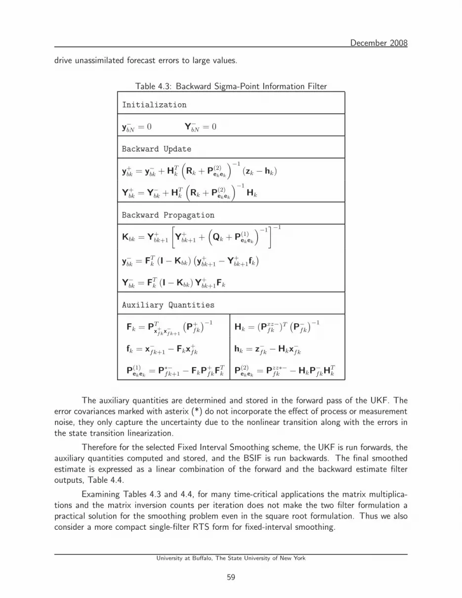
December 2008
drive unassimilated forecast errors to large values.
Table 4.3: Backward Sigma-Point Information Filter
Initialization
y−bN = 0 Y−bN = 0
Backward Update
y+bk = y−bk + HT
k
(Rk + P(2)
ekek
)−1
(zk − hk)
Y+bk = Y−
bk + HTk
(Rk + P(2)
ekek
)−1
Hk
Backward Propagation
Kbk = Y+bk+1
[Y+
bk+1 +(Qk + P(1)
ekek
)−1]−1
y−bk = FTk (I − Kbk)
(y+
bk+1 − Y+bk+1fk
)
Y−bk = FT
k (I −Kbk)Y+bk+1Fk
Auxiliary Quantities
Fk = PTx+fk
x−fk+1
(P+
fk
)−1Hk = (Pxz−
fk )T(P−
fk
)−1
fk = x−fk+1 − Fkx+fk hk = z−fk −Hkx
−fk
P(1)ekek
= P∗−fk+1 − FkP
+fkF
Tk P(2)
ekek= Pzz∗−
fk −HkP−fkH
Tk
The auxiliary quantities are determined and stored in the forward pass of the UKF. Theerror covariances marked with asterix (*) do not incorporate the effect of process or measurementnoise, they only capture the uncertainty due to the nonlinear transition along with the errors inthe state transition linearization.
Therefore for the selected Fixed Interval Smoothing scheme, the UKF is run forwards, theauxiliary quantities computed and stored, and the BSIF is run backwards. The final smoothedestimate is expressed as a linear combination of the forward and the backward estimate filteroutputs, Table 4.4.
Examining Tables 4.3 and 4.4, for many time-critical applications the matrix multiplica-tions and the matrix inversion counts per iteration does not make the two filter formulation apractical solution for the smoothing problem even in the square root formulation. Thus we alsoconsider a more compact single-filter RTS form for fixed-interval smoothing.
University at Buffalo, The State University of New York
59

December 2008
Table 4.4: Smoother update for the two filter formulation
Ksk = P+
fkY−bk
(I + P+
fkY−bk
)−1
Psk = (I − Ks
k)P+fk
xsk = (I − Ks
k) x+fk + Ps
ky−bk
4.1.3 Square Root Unscented Kalman Smoother - RTS form
A more computationally efficient form for fixed interval smoothing in the linear case was intro-duced by Rauch, Tung and Striebel [52]. The RTS smoother combines the backward filter andthe smoother update into a single-step correction to the forward filter estimate which is basedon the information gain in the forward pass.
One way to derive the RTS formulation of the Unscented Smoother is by trying to elimi-nate the backward information from the two filter equations [53, 55]: The Forward Sigma PointInformation Filter [56] and The Backward Sigma Point Information Filter.
Psiaki and Wada [57] present a derivation of the RTS form of the Unscented Smootherwhere the formulation is mathematically similar with the two filter formulation [53], but with alower computational complexity.
In Table 4.5 is presented the square root version of the RTS Unscented Smoother in asimilar formulation, that uses the Cholesky factorization, as in the SRUKF.
Table 4.5: Square Root Unscented Kalman Smoother
Initialization
xsN = x+
fN SsN = S+
fN
Smoother Update
Ksk =
(Px+
fkx−
fk+1/(S−
fk+1)T)
/S−fk+1
xsk = x+
fk + Ksk(x
sk+1 − x−fk+1)
U = CHOLUPDATE(S−
fk+1 , Ssk+1 , −1
)
Ssk = CHOLUPDATE
(S+
fk , KskU , −1
)
For this form of Fixed Interval Smoothing we run the UKF forward, compute and storethe quantities required in Table 4.5, obtaining the smoothed estimates by employing backwardscorrections to the filtered estimates.
University at Buffalo, The State University of New York
60

December 2008
4.2 Variable Dimensionality
A challenge in implementing both the filter and the smoother in the present application settingsis that the model evolves with variable state dimension due to the splitting and releasing of puffs.
Even with the Unscented Transformation the process model can no longer be consideredas a black box. We need additional knowledge about puff splitting and the release sequences thatcause the process state dimension to increase over time. Therefore the process model may beusefully divided into three modules: Puff Dynamics, Splitting and Release as illustrated in Figure4.1.
Figure 4.1: Process model
Puff Dynamics Splitting Release
sigma points
prior forecast
mean
covariance
redraw sigma points
for the measurementmean
covariance
The Puff Dynamics reflects the advection and diffusion of each Gaussian puff. Because itdoes not change the dimensionality of the state vector, the Puff Dynamics process model moduleacts as a black box, though with the other modules, the overall process model becomes a graybox.
To accommodate the variable dimensionality, more precisely sigma points with differentdimensions, we propagate the sigma points only through the Puff Dynamics module, after whichthey are recombined to obtain the ensemble mean and the error covariance.
Splitting may be formulated as a linear operation and is applied to the resulting mean andcovariance.
xsplitfk+1 = T20×4x
dynfk+1
Here T20×4 is a 20× 4 matrix which converts a spatially overextended puff into 5 more spatiallycompact puffs. Since T20×4 is a rank deficient matrix the resulting error covariance is semi-definite. For numerical stability we choose to increase the error covariance by adding the processnoise again to the resulting puffs.
Since the new puffs released are uncorrelated with the rest, we just augment the new puffsto the resulting mean and build the new block diagonal error covariance.
After the forecast the new sigma points are redrawn in order to count both for the processnoise and the new state dimension, and the following steps of UKF are performed.
To perform the smoothing update, the time steps when the release has occurred as well asthe number of puffs released are marked, such that when running the smoother update backwardsto be able to remove those puffs from the state space. The splitting phenomena is captured inthe smoother Kalman gain, more precisely in the Px+
fkx−
fk+1cross-covariance.
University at Buffalo, The State University of New York
61
December 2008
4.3 High Dimensionality
In this approach, a linear increase in computational complexity occurs because the number ofsigma points increases linearly with the number of puffs. Usually puff-based dispersion mod-els have a puff-merging scheme, which may alleviate the computational burden for short-rangeforecasts. Merging has not been implemented here.
In the forecast step, since the puff dynamics depends solely on past history and weatherdata at the center of the puff, one may form uncoupled systems and create sigma points for eachone of them reducing the computational complexity.
In the measurement propagation, having a puff statistically independent with the rest ofthe puffs, its contribution to the measurement concentration will be independent with the rest ofthe contributions. Therefore we may treat the independent puffs as uncoupled systems, propagatesigma points for each of them through the measurement equation, and compute the statistics ofthe measurement concentration based on the individual statistics of the contributions.
One example is the release of new puffs. Consider that the state dimension before puffrelease is Nold and the new puffs released bring an extra Nnew states. Just to forecast theNold + Nnew states through nonlinearity requires the following number of elementary operationsto compute the error covariance:
(Nold + Nnew)2 × [2(Nold + Nnew) + 1]
For a decoupled system the number of operations is given by:
2N3old + 2N3
new + N2old + N2
new
therefore a reduction of:6N2
oldNnew + 6NoldN2new + 2NoldNnew
which asymptotically it translates in a reduction in the coefficient of the cubic term.
Since the measurement equation computes the concentration at each grid point as a sumof the contribution of all the puffs, after measurement update the decoupling of the systemvanishes.
A reduced number of puffs can be selected to be updated based on their distance fromthe grid point where the concentration has to be computed. Puffs further away from the sensorlocation bring negligible contribution with respect to the sensor concentration. This way we tryto keep as many puffs as possible correlated only with a smaller number of puffs.
By carefully bookkeeping the correlation between the puffs, given by puff splitting/mergingand measurement update, we are able to decrease the number of sigma points and make the dataassimilation appropriate for parallel computing.
University at Buffalo, The State University of New York
62

December 2008
4.4 Numerical Results
4.4.1 Simulation Environment
The performance of Square Root Unscented Kalman Filter / Smoother is tested on a represen-tative atmospheric dispersion puff-based model, based on RIso Mesoscale PUFF (RIMPUFF) [1],and compared with a Particle Filter (PF) data assimilation technique reported by Reddy et al. [44].
To explore the results for SRUKF and SRUKS, we have used the same model to createthe measurements and the truth and perform the filtering. Simulations reported here used the 2Dpuff-based dispersion model and a modeled dispersion region of 15× 15 km2 with 200 m spatialresolution and sensors assumed to be located every 1 km within the grid. The simulated durationwas 60 min with sampling interval 20 sec. The simulated source, located at the origin, releasedequal masses every 1 min for the first 15 min and the wind direction was changed after one halfhour from 15 to 60. The wind speed chosen was 5 m/sec with 20% standard deviation [44].
Given this parametrization the dosage (time-integrated concentration) yielded by the truthmodel after one hour is illustrated in Figure 4.2.
Figure 4.2: Gridwise dosage after one hour
x [m]
y [m
]
0 5000 10000 15000
0
5000
10000
15000
50
100
150
200
250
The difficulty of the problem is significantly increased by the five sources of uncertaintypresent: duration of the chemical release from the source, initial puff parameters, uncertainparameters (wind fluctuations, modeling deficiencies), puff splitting and observation uncertainty.The model evolves with variable dimension, caused by accumulation of source puffs and puff-splitting. The results presented in the next subsection have been Monte-Carlo averaged over 50runs and do not contain the concentrations/doses near the source.
4.4.2 Results
In Figure 4.3a we compare the Pure Model Forecast, the SRUKF, the SRUKS and the BootstrapParticle Filter in estimating the Instantaneously Plume Concentration at each time step. TheRMS error is obtained by averaging all the gridwise concentration errors in the 15 × 15 km2
domain.
University at Buffalo, The State University of New York
63

December 2008
0 6.6 13.3 20 26.6 33.3 40 46.6 53.3 600
0.01
0.02
0.03
0.04
0.05
0.06
0.07
0.08
time [min]
RM
S E
rror
ModelPFUKFUKS
0 6.6 13.3 20 26.6 33.3 40 46.6 53.3 600
0.5
1
1.5
2
2.5
3
3.5
4
4.5
5x 10
7
time [min]
norm
aliz
ed e
rror
cov
aria
nce
trac
e
UKFUKS
(a) Instantaneous plume concentration RMS error (b) Covariance trace
0 6.6 13.3 20 26.6 33.3 40 46.6 53.3 600
0.2
0.4
0.6
0.8
1
1.2
1.4
1.6
1.8
time [min]
RM
S E
rror
ModelPFUKFUKS
0 16.6 33.30
0.5
1
1.5
2
2.5
3
3.5
RM
S E
rror
40 46.6 53.3 603.6
3.65
3.7
3.75
3.8
3.85
3.9
3.95
4
time [min]
RM
S E
rror
UKFUKS
(c) Dosage RMS error (d) Dosage RMS error (smaller region)
Figure 4.3: Numerical results
University at Buffalo, The State University of New York
64

December 2008
Comparing the SRUKF and the PF, their performance is broadly similar and the Filterperformed better for few time intervals. Since no systematic effort was made to tune the pa-rameters of either algorithm, no clear conclusion can be drawn from this observed performancedifference, except that neither scheme demonstrated a clear advantage in this test environment.
Comparing the SRUKF and SRUKS performance in Figure 4.3a, it may be noted thatsharp error peaks occasionally experienced by the Filter are significantly reduced by the Smoother.It is characteristic of statistical estimation that sudden excursions into difficult-to-estimate statedomains are better tolerated when they can be smoothed by data acquired after a given estimationtime as well as before. This means that the Smoother is better estimating the shape and locationof the plume.
In Figure 4.3b we compare the trace of the error covariance, of both SRUKF and SRUKS,that has been normalized by the number of puffs.
The Smoother indeed reduces the uncertainty giving better confidence in its estimates.This suggests that in the CBRN response setting, smoothing may be worth the computationaland decision-latency costs where lower uncertainties are mission-relevant.
Even in the data assimilation settings, the trace of the normalized error covariance reaches107. This means that the assumption in deriving the backward Markovian process for the BSPIFmay be justified for this application.
By integrating the concentration over time we obtain the gridwise dose. A comparison inestimating the dose for the entire dispersion domain is given in Figure 4.3c.
Even though in the earlier comparison in estimating the instantaneously plume concen-tration the PF performed somehow worse that the SRUKF, here its later performance is better.This suggests error cancellation in the integration process.
Even in this case the Smoother performs better than both the SRUKF and PF. Sincehere we have also obtained the RMS by averaging the dosage error over the entire domain theimprovement brought by the Smoother does not seem to be significant.
To see better the difference between the SRUKF and SRUKS we have computed the RMSError over a smaller patch of interest of 1.4 × 1.4 km2, from the given domain, which has theorigin at (3900, 900), Figure 4.3d.
Such a small region may be a military unit or a civil neighborhood which in criticalsituations might be evacuated. This suggests that the Smoother is more suited for situationassessment or alarm triggering.
4.5 Remarks
The fixed-interval Sigma-Point Kalman Smoother has been studied in a CBRN scenario simulationenvironment. The UKF and the UKS has been applied on a model which evolves with both variableand high state dimension. Valuable lessons are drawn how to lower the number of sigma pointsand how to deal with the variable dimensionality by exploiting the model, in order to prepare thetransition to a more complex puff-based dispersion model SCIPUFF.
University at Buffalo, The State University of New York
65

December 2008
Two solutions to this nonlinear smoothing problem are presented based on the weightedstatistical linearization: the forward-backward two-filter formulation and the RTS formulation.While these results are not novel, derivation from this basis is a contribution of the presentpaper.
The RTS formulation is computationally more efficient than the two filter formulation andits square root version is easily derived. The Smoother avoids sudden large errors experienced bythe Filter and overall provides better estimates for both instantaneous plume concentration anddosage, and a better confidence in estimates which makes the Smoother suitable for situationassessment or alarm triggering.
University at Buffalo, The State University of New York
66
Chapter 5
Uncertainty Propagation Using GaussianMixture Models
This chapter is concerned with improving an arbitrary approximation to the forecast densityfunction using a finite Gaussian mixture. With a sufficient number of Gaussian components, anypdf may be approximated as closely as desired. Many algorithms [58, 59] have been discussed inthe literature for time evolution of the initial state pdf through a nonlinear dynamical system indiscrete-time or continuous-time. In conventional methods, the weights of different componentsof a Gaussian mixture are kept constant while propagating the uncertainty through a nonlinearsystem and are updated only in the presence of measurement data [58, 59]. This assumption isvalid if the underlying dynamics is linear or the system is weakly nonlinear. The same is not truefor the general nonlinear case and new estimates of weights are required for accurate propagationof the state pdf. However, the existing literature provides no means for adaptation of the weightsof different Gaussian components in the mixture model during the propagation of state pdf.The lack of adaptive algorithms for the weights of the Gaussian mixture are felt to be a seriousdisadvantage of existing algorithms and provides the motivation for the work presented in thischapter.
Two different schemes are introduced to update the weights corresponding to differentcomponents of Gaussian mixture model during pure propagation. The first method updates theforecast weights by minimizing the integral square difference between the true forecast pdf andits Gaussian sum approximation. The second method updates the weights by constraining theGaussian sum approximation to satisfy the Fokker-Planck equation for continuous-time dynam-ical systems. Both the methods leads to a convex quadratic programming problem which iscomputationally efficient to solve.
67

December 2008
5.1 Update Scheme for Discrete-Time Dynamic Systems
Problem Statement
Consider the following nonlinear discrete-time dynamical system driven by white noise (ηk),
xk+1 = f(k,xk) + ηk (5.1)
ηk ∼ N (0,Qk) (5.2)
with the probability density function of the initial conditions given by the following Gaussian sum,
p(tk,xk) =
N∑
i=1
wikN (xk | µ
ik,P
ik) (5.3)
where N (x | µ,P) = |2πP|−1/2 exp
[−1
2(x − µ)T
P−1 (x − µ)
](5.4)
We are interested in approximating the probability density function p(tk+1,xk+1) as aGaussian mixture. The true forecast pdf is given by the Chapman-Kolmogorov equation [16]:
p(tk+1,xk+1) =
∫p(tk+1,xk+1|tk,xk)p(tk,xk)dxk (5.5)
where, p(tk+1,xk+1|tk,xk) is the conditional state transition pdf which corresponds to the pdffor the process noise variable ηk, generally modeled as Gaussian white noise of covariance Qk,i.e. p(tk+1,xk+1|tk,xk) = N (xk+1 | f(k,xk),Qk).
A linear mapping will transform a Gaussian mixture into another Gaussian mixture with-out changing the weights of different Gaussian components, where the parameters (mean andcovariance) of the resulting mixands can be easily computed. But the outcome of a Gaussianthat undergoes a nonlinear transformation is generally non-Gaussian. Conventionally, a Gaussiansum approximation to the forecast density function p(tk+1,xk+1) is obtained by linearizing thenonlinear transformation and assuming weights of different components to be constant.
p(tk+1,xk+1) =
N∑
i=1
wik+1N (xk+1 | µ
ik+1,P
ik+1) (5.6)
where, the reference values of the parameters of the Gaussian components are given by theprediction step of the Extended Kalman filter (EKF):
wik+1 = wi
k (5.7a)
µik+1 = f(k, µi
k) (5.7b)
Pik+1 = Ak(µ
ik)P
ikA
Tk (µi
k) + Qk, where Ak(xk) =∂f(k,xk)
∂xk
(5.7c)
Evolution schemes other than linearization using Taylor series, such as statistical linearization[60], may be used for obtaining the moments of the Gaussian components. Since they imply
University at Buffalo, The State University of New York
68

December 2008
linearizations, such approximations are computational convenient and may be easily used in linearapplications and have been intensively studied.
The reason that the weights are not changed in Eq. (5.7a) is because it is assumed thatthe covariances are small enough and there is a sufficient number of Gaussian components [16,58]such that the linearizations become representative for the dynamics around the means. To betterunderstand this assumption, let us substitute Eq. (5.3) into (5.5), and further, one can derivethe following relationships by following the steps presented in Ref. [16]:
p(tk+1,xk+1) =
N∑
i=1
wik
∫N (xk | µ
ik,P
ik)N (xk+1 | f(k,xk),Qk)dxk (5.8a)
=
N∑
i=1
wik
∫N (xk | µ
ik,P
ik)N (xk+1 | Ak(µ
ik)(xk − µ
ik) + f(k, µi
k),Qk)dxk
+N∑
i=1
wik
∫ǫkdxk (5.8b)
where,
ǫk = N (xk|µik,P
ik)
[N (xk+1|f(k,xk),Qk) −N (xk+1|Ak(µ
ik)(xk − µ
ik) + f(k,µi
k),Qk)
](5.9)
Assuming that all covariances, Pik, of the Gaussian components are small enough such
that the linearization around a mean is representative for the dynamics in the vicinity of therespective mean and there are sufficient number of Gaussian components, then Pi
k → 0 implies∫ǫkdxk → 0. Using this assumption and the fact that the product of two Gaussian densities
yields another Gaussian density function, Eq. (5.8b) becomes, after some algebraic manipulations:
p(tk+1,xk+1) ≈N∑
i=1
wik
∫N (xk|µi
k,Pik)N (xk+1|Ak(µ
ik)(xk − µ
ik) + f(k, µi
k),Qk)dxk
(5.10a)
=
N∑
i=1
wikN (xk+1 | f(k, µi
k),Ak(µik)P
ikA
Tk (µi
k) + Qk) (5.10b)
=N∑
i=1
wikN (xk+1 | µ
ik+1,P
ik+1) (5.10c)
= p(tk+1,xk+1) (5.10d)
In practice this assumption,
∀i Pik → 0 implies
∫ǫkdxk → 0 implies wi
k+1 = wik (5.11)
may be easily violated resulting in a poor approximation of the forecast pdf. Practically, thedynamic system may exhibit strong nonlinearities and the total number of Gaussian components,
University at Buffalo, The State University of New York
69

December 2008
needed to represent the pdf, may be restricted due to computational requirements. The existingliterature provides no means for adaption of the weights of different Gaussian components in themixture model during the propagation of the state pdf. The lack of adaptive means for updatingthe weights of Gaussian mixture are felt to be a serious disadvantage of existing algorithms andprovide the main motivation for this paper.
Weight Update I
In this section, we present a novel scheme to better approximate the forecast pdf by developingthe update laws for the forecast weights. The new weights can be obtained by minimizing thefollowing integral square difference between the true pdf (p(tk+1,xk+1)) and its approximation(p(tk+1,xk+1)) in the least square sense:
minwi
k+1
1
2
∫ ∣∣p(tk+1,xk+1) − p(tk+1,xk+1)∣∣2dxk+1 (5.12a)
s.t.
N∑
i=1
wik+1 = 1 (5.12b)
wik+1 ≥ 0, i = 1, · · · , N (5.12c)
Notice that Eqs. (5.12b) and (5.12c) are introduced to account for the normality and positivityconstraint for the state pdf. Here, the true density function p(tk+1,xk+1), is given by Eq. (5.5).By substituting Eq. (5.6) in Eq. (5.12a) and expanding and grouping the terms in the costfunction w.r.t. the weights, the new cost function is given by,
J =1
2wT
k+1Mwk+1 − wTk+1y (5.13)
where wk+1 = [w1k+1 w2
k+1 . . . wNk+1]
T , and M ∈ RN×N is a symmetric matrix given by:
M =
∫M(xk+1)M
T (xk+1)dxk+1 (5.14)
where M is a N × 1 vector that contains all the Gaussian components at time k + 1:
M(xk+1) =
[N (xk+1|µ1
k+1,P1k+1) N (xk+1|µ2
k+1,P2k+1) . . . N (xk+1|µN
k+1,PNk+1)
]T
(5.15)
Thus, the components of matrix M are easily given by the product rule of two Gaussiandensity functions which yields another Gaussian density function [61]. By integrating the productwe are left only with the normalization constant as illustrated below:
University at Buffalo, The State University of New York
70
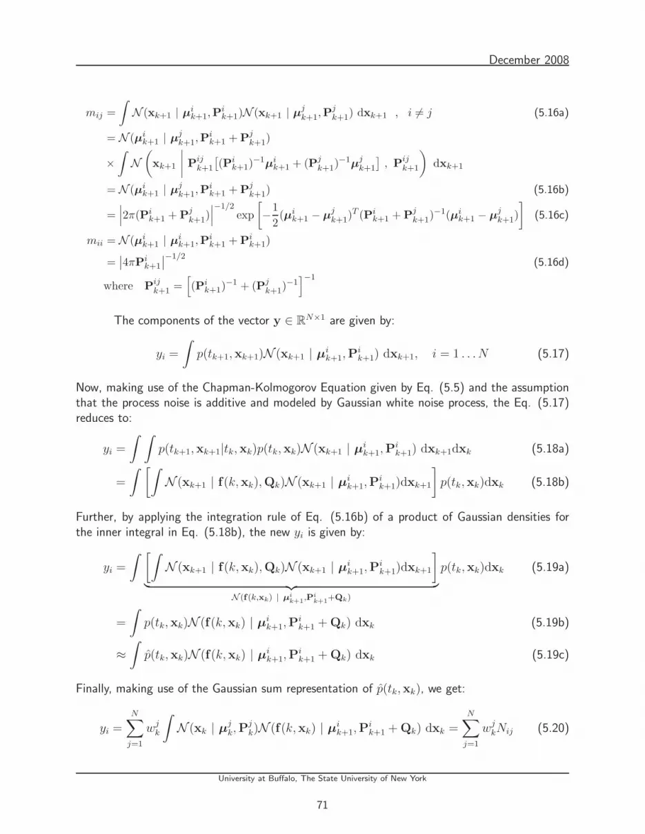
December 2008
mij =
∫N (xk+1 | µ
ik+1,P
ik+1)N (xk+1 | µ
jk+1,P
jk+1) dxk+1 , i 6= j (5.16a)
= N (µik+1 | µ
jk+1,P
ik+1 + P
jk+1)
×∫
N(xk+1
∣∣∣∣ Pijk+1
[(Pi
k+1)−1
µik+1 + (Pj
k+1)−1
µjk+1
], P
ijk+1
)dxk+1
= N (µik+1 | µ
jk+1,P
ik+1 + P
jk+1) (5.16b)
=∣∣∣2π(Pi
k+1 + Pjk+1)
∣∣∣−1/2
exp
[−1
2(µi
k+1 − µjk+1)
T (Pik+1 + P
jk+1)
−1(µik+1 − µ
jk+1)
](5.16c)
mii = N (µik+1 | µ
ik+1,P
ik+1 + Pi
k+1)
=∣∣4πPi
k+1
∣∣−1/2(5.16d)
where Pijk+1 =
[(Pi
k+1)−1 + (Pj
k+1)−1]−1
The components of the vector y ∈ RN×1 are given by:
yi =
∫p(tk+1,xk+1)N (xk+1 | µ
ik+1,P
ik+1) dxk+1, i = 1 . . . N (5.17)
Now, making use of the Chapman-Kolmogorov Equation given by Eq. (5.5) and the assumptionthat the process noise is additive and modeled by Gaussian white noise process, the Eq. (5.17)reduces to:
yi =
∫ ∫p(tk+1,xk+1|tk,xk)p(tk,xk)N (xk+1 | µ
ik+1,P
ik+1) dxk+1dxk (5.18a)
=
∫ [∫N (xk+1 | f(k,xk),Qk)N (xk+1 | µ
ik+1,P
ik+1)dxk+1
]p(tk,xk)dxk (5.18b)
Further, by applying the integration rule of Eq. (5.16b) of a product of Gaussian densities forthe inner integral in Eq. (5.18b), the new yi is given by:
yi =
∫ [∫N (xk+1 | f(k,xk),Qk)N (xk+1 | µ
ik+1,P
ik+1)dxk+1
]
︸ ︷︷ ︸N (f(k,xk) | µi
k+1,Pik+1+Qk)
p(tk,xk)dxk (5.19a)
=
∫p(tk,xk)N (f(k,xk) | µ
ik+1,P
ik+1 + Qk) dxk (5.19b)
≈∫
p(tk,xk)N (f(k,xk) | µik+1,P
ik+1 + Qk) dxk (5.19c)
Finally, making use of the Gaussian sum representation of p(tk,xk), we get:
yi =
N∑
j=1
wjk
∫N (xk | µ
jk,P
jk)N (f(k,xk) | µ
ik+1,P
ik+1 + Qk) dxk =
N∑
j=1
wjkNij (5.20)
University at Buffalo, The State University of New York
71

December 2008
where,
Nij =
∫N (f(k,xk) | µ
ik+1,P
ik+1 + Qk)N (xk | µ
jk,P
jk) dxk (5.21)
The result is a sum of expectations of composite functions. Notice that, we assume that we havea good Gaussian sum approximation at time tk such that p(tk,xk) ≈ p(tk,xk).
Further, substitution of Eq. (5.20) into Eq. (5.13) leads to the following expression forthe cost function:
J =1
2wT
k+1Mwk+1 − wTk+1Nwk (5.22)
where wk = [w1k w2
k . . . wNk ]T is the prior weight vector, and the matrix N ∈ R
N×N has thefollowing components:
Nij =
∫N (f(k,xk) | µ
ik+1,P
ik+1 + Qk)N (xk | µ
jk,P
jk) dxk (5.23a)
= EN (xk|µj
k,Pj
k)
[N (f(k,xk) | µ
ik+1,P
ik+1 + Qk)
](5.23b)
The expectations (5.23b) may be computed using Gaussian Quadrature, Monte Carlo integrationor Unscented Transformation [47]. While in lower dimensions the Unscented Transformation ismostly equivalent with Gaussian quadrature, in higher dimensions the Unscented Transformationis computational more appealing in evaluating integrals since the number of points grows onlylinearly with the number of dimensions. However, this comes with a loss in accuracy [62], hencethe need for a larger number of points [63] to capture additional information.
In the case of linear transformation, f(k, ·) = Fk, using the integration rule of two Gaussiandensities in Eq.(5.21), and after some algebraic manipulations, the elements Mij = Nij , thereforeM = N. Hence, as expected weights vector will be kept constant. However, the numericalapproximations made in computing the expectation integrals involved in Eq. (5.23b) may resultsin some change in the value of the weight vector.
The final formulation of the optimization (5.12a) can be posed in the quadratic program-ming framework and solved using readily available solvers:
minwk+1
J =1
2wT
k+1Mwk+1 −wTk+1Nwk (5.24)
s.t. 1Twk+1 = 1
wk+1 ≥ 0
Here 1 ∈ RN×1 is a vector of ones and 0 ∈ R
N×1 is a vector of zeros. Now, if we show that thematrix M is a positive semi-definite and the cost function J is lower bounded, then the aforemen-tioned optimization problem can be posed as a convex optimization problem and we are guaran-teed to have a unique solution [64]. Notice that the integrand M(xi
k+1)MT (xi
k+1) is a rank onesymmetric positive semi-definite matrix with non-zero eigenvalue equal to M
T (xik+1)M(xi
k+1).Further, we write the integral (5.14) as a infinite sum as follows:
M =∑
i
M(xik+1)M
T (xik+1) (5.25)
University at Buffalo, The State University of New York
72

December 2008
Making use of the fact that summation of two positive semi-definite matrix is also a positivesemi-definite matrix, we conclude that matrix M is a positive semi-definite matrix since M is asum of positive semi-definite matrices. Further, notice that the linear term wT
k+1Nwk in costfunction J is lower bounded since N ≥ 0 and both wk+1 and wk has to lie between 0 and 1.Hence, we can conclude that the cost function J is always bounded below and we are guaranteedto have a unique solution.
5.2 Update Scheme for Continuous-Time Dynamic Sys-
tems
Problem Statement
Consider a general n-dimensional noise driven nonlinear dynamic system with uncertain initialconditions, given by the equation:
x = f(t,x) + g(t,x)Γ(t) (5.26)
where, Γ(t) represents a Gaussian white noise process with the correlation function Qδ(t1 − t2),and the initial state uncertainty is captured by the pdf p(t0,x). Then, the time evolution ofp(t0,x) is described by the following FPKE, which is a second order pde in p(t,x):
∂
∂tp(t,x) = LFP [p(t,x)] (5.27)
where,
LFP =
[−
n∑
i=1
∂
∂xiD
(1)i (t,x)[.] +
n∑
i=1
n∑
j=1
∂2
∂xi∂xjD
(2)ij (t,x)[.]
](5.28a)
D(1)(t,x) = f(t,x) +1
2
∂g(t,x)
∂xQg(t,x) (5.28b)
D(2)(t,x) =1
2g(t,x)QgT(t,x) (5.28c)
We mention that Eqs. (5.27)-(5.28a) represent the Stratonovich interpretation for the FPKE andis more popular among engineers and physicists. An alternative interpretation (Ito interpretation)for the FPKE is also commonly used among mathematicians and leads to the same equation ifg(.) is constant in Eq. (5.26). In this paper, we use the Stratonovich interpretation for the FPKEto illustrate the main idea of updating the weights corresponding to different component of theGaussian mixture model. However, one can use the Ito interpretation for the FPKE equationwithout compromising the formulation presented in the next section. Irrespective of the form(Stratonovich or Ito), the FPKE is a formidable problem to solve, because of the following issues:
1. Positivity of the pdf: p(t,x) ≥ 0, ∀t & x
University at Buffalo, The State University of New York
73

December 2008
2. Normalization constraint of the pdf:∫
Rn
p(t,x)dx = 1.
3. No fixed Solution Domain: how to impose boundary conditions in a finite region and restrictnumerical computation to regions where p >∼ 10−9.
Let us assume that underlying pdf can be approximated by a finite sum of Gaussian pdfs
p(t,x) =
N∑
i=1
wipgiwhere pgi
= N (x(t) | µi,Pi) (5.29)
where µi and Pi represent the mean and covariance of the ith component of the Gaussianpdf, respectively and wi denotes the amplitude of ith Gaussian in the mixture. The positivityand normalization constraint on the mixture pdf, p(t,x), leads to following constraints on theamplitude vector:
N∑
i=1
wi = 1, wi ≥ 0 (5.30)
Since all the components of the mixture pdf (5.29) are Gaussian and thus, only estimates of theirmean and covariance need to be maintained in order to obtain the optimal state estimates whichcan be propagated using the Extended Kalman filter time update equations:
µi = f(µi) (5.31)
Pi = AiPi + PiATi + g(t, µi)QgT (t, µi) (5.32)
where Ai =∂f(t,x)
∂x
∣∣∣∣x=µi
(5.33)
Notice that the weights wi corresponding to each Gaussian component are unknown. Inconventional Gaussian sum filter the weights are initialized such that initial mixture pdf approx-imates the given initial pdf and it is assumed that weights does not change over time. Thisassumption is valid if the underlying dynamics is linear or the system is marginally nonlinear. Thesame is not true for the general nonlinear case and new estimates of weights are required foraccurate propagation of the state pdf.
Weight Update II
In this section, a novel method is described to update the weights of different components of theGaussian mixture of Eq. (5.29). The main idea is that the mixture pdf of Eq. (5.29), p(t,x),should satisfy the Fokker-Planck equation (5.28a) and the Fokker-Planck equation error can beused as a feedback to update the weights of different Gaussian components in the mixture pdf [65].In other words, we seek to minimize the Fokker-Planck equation error under the assumption ofEqs. (5.29), (5.31) and (5.32).
University at Buffalo, The State University of New York
74

December 2008
Substituting Eq. (5.29) in Eq. (5.28a) leads to
e(t,x) =∂p(t,x)
∂t−LFP [p(t,x)] (5.34)
=∂p(t,x)
∂t−[−
n∑
i=1
∂D(1)i (t,x)
∂xi
+n∑
i=1
n∑
j=1
∂2D(2)ij (t,x)
∂xi∂xj
][p(t,x)] (5.35)
where LFP(·) is the so called Fokker-Planck operator, and,
∂p(t,x)
∂t=
N∑
i=1
wi
[∂pgi
∂µi
T
µi +n∑
j=1
n∑
k=1
∂pgi
∂Pijk
Pijk
](5.36)
where Pijkis the jkth element of the ith covariance matrix Pi. Further, substitution of Eqs.
(5.28b) and (5.28c) along with Eq. (5.36) in Eq. (5.35) leads to
e(t,x) =
N∑
i=1
wiLi(t,x) = LT w (5.37)
where w is a N × 1 vector of Gaussian weights, and Li is given by
Li(t,x) =
[∂pgi
∂µi
T
f(t, µi) +n∑
j=1
n∑
k=1
∂pgi
∂Pijk
Pijk+
n∑
j=1
(fj(t,x)
∂pgi
∂xj+ pgi
∂fj(t,x)
∂xj
+1
2
∂d(1)j (t,x)pgi
∂xj− 1
2
n∑
k=1
∂2d(2)jk (t,x)pgi
xjxk
)](5.38a)
d(1)(t,x) and d(2)(t,x) are given as:
d(1)(t,x) =1
2
∂g(t,x)
∂xQg(t,x) (5.39a)
d(2)(t,x) =1
2g(t,x)QgT (t,x) (5.39b)
Further, different derivatives in the above equation can be computed using the following analyticalformulas:
∂pgi
∂µi= P−1
i (x − µi) pgi(5.40a)
∂pgi
∂Pi
= − pgi
2|Pi|∂|Pi|∂Pi
− pgi
2
∂(x − µi)TP−1
i (x − µi)
∂Pi
= −pgi
2P−1
i − pgi
2
∂(x − µi)TP−1
i (x − µi)
∂Pi
= −pgi
2P−1
i +pgi
2P−1
i (x − µi) (x − µi)TP−1
i (5.40b)
∂pgi
∂x= −P−1
i (x − µi) pgi(5.40c)
∂2pgi
∂xxT= −P−1
i
[I + (x − µi) (x − µi)
TP−1
i
]pgi
(5.40d)
University at Buffalo, The State University of New York
75
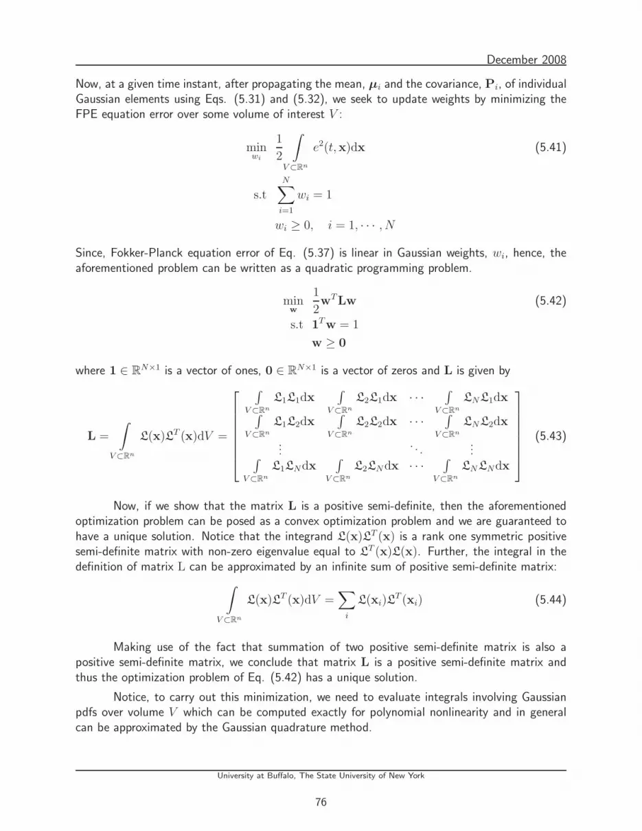
December 2008
Now, at a given time instant, after propagating the mean, µi and the covariance, Pi, of individualGaussian elements using Eqs. (5.31) and (5.32), we seek to update weights by minimizing theFPE equation error over some volume of interest V :
minwi
1
2
∫
V ⊂Rn
e2(t,x)dx (5.41)
s.t
N∑
i=1
wi = 1
wi ≥ 0, i = 1, · · · , N
Since, Fokker-Planck equation error of Eq. (5.37) is linear in Gaussian weights, wi, hence, theaforementioned problem can be written as a quadratic programming problem.
minw
1
2wTLw (5.42)
s.t 1Tw = 1
w ≥ 0
where 1 ∈ RN×1 is a vector of ones, 0 ∈ R
N×1 is a vector of zeros and L is given by
L =
∫
V ⊂Rn
L(x)LT (x)dV =
∫V ⊂Rn
L1L1dx∫
V ⊂Rn
L2L1dx · · ·∫
V ⊂Rn
LNL1dx∫
V ⊂Rn
L1L2dx∫
V ⊂Rn
L2L2dx · · ·∫
V ⊂Rn
LNL2dx
.... . .
...∫V ⊂Rn
L1LNdx∫
V ⊂Rn
L2LNdx · · ·∫
V ⊂Rn
LNLNdx
(5.43)
Now, if we show that the matrix L is a positive semi-definite, then the aforementionedoptimization problem can be posed as a convex optimization problem and we are guaranteed tohave a unique solution. Notice that the integrand L(x)LT (x) is a rank one symmetric positivesemi-definite matrix with non-zero eigenvalue equal to L
T (x)L(x). Further, the integral in thedefinition of matrix L can be approximated by an infinite sum of positive semi-definite matrix:
∫
V ⊂Rn
L(x)LT (x)dV =∑
i
L(xi)LT (xi) (5.44)
Making use of the fact that summation of two positive semi-definite matrix is also apositive semi-definite matrix, we conclude that matrix L is a positive semi-definite matrix andthus the optimization problem of Eq. (5.42) has a unique solution.
Notice, to carry out this minimization, we need to evaluate integrals involving Gaussianpdfs over volume V which can be computed exactly for polynomial nonlinearity and in generalcan be approximated by the Gaussian quadrature method.
University at Buffalo, The State University of New York
76

December 2008
5.3 Numerical Results
The two update schemes presented in this paper has been tested on a variety of benchmarkproblems studied extensively in the literature [12–14]. In this section, we present results fromthese tests. For discrete-time update scheme, we represent the system dynamics by convertingthe continuous-time differential equations to discrete-time difference equations. The selection ofthe examples presented in assessing the performance of the proposed methods, has been madesuch that they cover a wide spectrum of scenarios including 1D and 2D dynamical systems anddifferent initial conditions for the Gaussian components: equally weighted, randomly weighted aswell as having particular weight assignments. The two update schemes are compared with theusual procedure of not updating the weights on several dynamical systems where either a closedform solution for the stationary pdf is available or a Monte Carlo simulation is carried out. Forthe examples where an analytical solution is available, the following integral of the absolute errorhas been used for quantitative comparison of the methods:
E =
∫ ∣∣p(t,x) − p(t,x)∣∣dx (5.45)
The different expectation integrals which appear in the cost function of the two methods havecompact support and have been numerically approximated using the Gaussian quadrature method.
Example 1
The first update method has been applied on the following nonlinear discrete-time dynamicalsystem with uncertain initial condition given by Eq. (5.47):
xk+1 =1
2xk + 10
xk
1 + x2k
+ ηk where ηk ∼ N (0, 1) (5.46)
x0 ∼ 0.1N (−0.5, 0.1) + 0.9N (0.5, 1) (5.47)
The moments of the two Gaussian components are propagated for 20 time steps usingEqs. (5.7b) and (5.7c). Since there is no analytical solution for the forecast pdf, we run a MonteCarlo simulation using 10000 samples and compute the histogram of the samples at each timestep as shown in Fig. 5.1(a). Fig. 5.1(b) shows the pdf approximation without updating theweights and in Fig. 5.1(c) is plotted the pdf approximation with updated weights. By updatingthe weights, we are able to better capture the two modes presented in Fig. 5.1(a). In addition tothis, log probability of the monte carlo sample points was computed according to the followingrelationship:
L =
M∑
j=1
log
N∑
i=1
wiN (xj | µi,Pi) (5.48)
Here, M is the total number of samples used in the Monte Carlo approximation. The higher valueof L represents a better pdf approximation. Fig. 5.1(d) shows the plot of log probability of the
University at Buffalo, The State University of New York
77
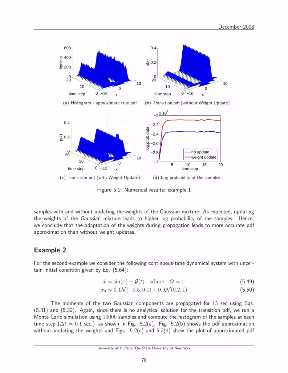
December 2008
−100
10
0
10
200
200
400
600
xtime step
#poi
nts
(a) Histogram - approximate true pdf
−100
10
0
10
200
0.2
0.4
xtime step
p(x)
(b) Transition pdf (without Weight Update)
−100
10
0
10
200
0.2
0.4
xtime step
p(x)
(c) Transition pdf (with Weight Update)
5 10 15 20−3
−2.8
−2.6
−2.4
−2.2
−2x 10
4
time step
log.
prob
.dat
ano updateweight update
(d) Log probability of the samples
Figure 5.1: Numerical results: example 1
samples with and without updating the weights of the Gaussian mixture. As expected, updatingthe weights of the Gaussian mixture leads to higher log probability of the samples. Hence,we conclude that the adaptation of the weights during propagation leads to more accurate pdfapproximation than without weight updates.
Example 2
For the second example we consider the following continuous-time dynamical system with uncer-tain initial condition given by Eq. (5.64):
x = sin(x) + G(t) where Q = 1 (5.49)
x0 ∼ 0.1N (−0.5, 0.1) + 0.9N (0.2, 1) (5.50)
The moments of the two Gaussian components are propagated for 15 sec using Eqs.(5.31) and (5.32). Again, since there is no analytical solution for the transition pdf, we run aMonte Carlo simulation using 10000 samples and compute the histogram of the samples at eachtime step (∆t = 0.1 sec.) as shown in Fig. 5.2(a). Fig. 5.2(b) shows the pdf approximationwithout updating the weights and Figs. 5.2(c) and 5.2(d) show the plot of approximated pdf
University at Buffalo, The State University of New York
78
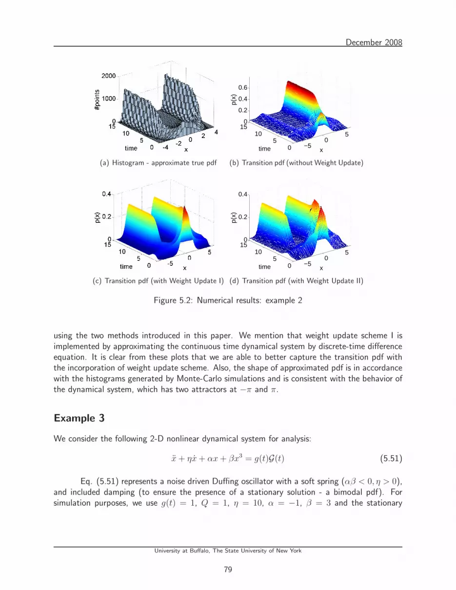
December 2008
(a) Histogram - approximate true pdf
−50
5
05
1015
0
0.2
0.4
0.6
xtime
p(x)
(b) Transition pdf (without Weight Update)
(c) Transition pdf (with Weight Update I)
−50
5
05
1015
0
0.2
0.4
xtime
p(x)
(d) Transition pdf (with Weight Update II)
Figure 5.2: Numerical results: example 2
using the two methods introduced in this paper. We mention that weight update scheme I isimplemented by approximating the continuous time dynamical system by discrete-time differenceequation. It is clear from these plots that we are able to better capture the transition pdf withthe incorporation of weight update scheme. Also, the shape of approximated pdf is in accordancewith the histograms generated by Monte-Carlo simulations and is consistent with the behavior ofthe dynamical system, which has two attractors at −π and π.
Example 3
We consider the following 2-D nonlinear dynamical system for analysis:
x + ηx + αx + βx3 = g(t)G(t) (5.51)
Eq. (5.51) represents a noise driven Duffing oscillator with a soft spring (αβ < 0, η > 0),and included damping (to ensure the presence of a stationary solution - a bimodal pdf). Forsimulation purposes, we use g(t) = 1, Q = 1, η = 10, α = −1, β = 3 and the stationary
University at Buffalo, The State University of New York
79

December 2008
probability density function given by Eq. (5.52) is plotted in Fig. 5.3(b).
p(x, x) ∝ exp
(−2
η
g2Q
(α
2x2 +
β
4x4 +
1
2x2
))(5.52)
Notice that the stationary pdf is an exponential function of the steady state systemHamiltonian, scaled by the parameter −2 η
g2Q[10].
To approximate the stationary pdf given by Eq. (5.52), we assume the initial pdf to bea mixture of 10 Gaussian pdfs with centers uniformly distributed between (−5,−5) and (5, 5).The covariance matrix for each Gaussian component is chosen to be P = 10 × I, where I is the2 × 2 identity matrix and the initial weights of the Gaussian components are randomly assigneda number between 0 and 1. The weights have been randomly generated in 20 different runs (seeFig. 5.3(i) for weights/run), and the initial pdf for the last run is plotted in Fig. 5.3(a).
The center and corresponding covariance matrices of the Gaussian components are linearlypropagated for 100 seconds. Fig. 5.3(c) shows the plot of the approximated pdf without updatingthe weights of Gaussian mixture and Fig. 5.3(f) shows the corresponding approximation errorplot for the weights of the last run. As expected, the final pdf is biased towards one of the modeof the true pdf due to the fact that initial weights of those components were large.
It is clear that although the approximated pdf did capture some of non-Gaussian behavior,it fails to capture both the modes accurately. Further, Figs. 5.3(d) and 5.3(h) show the plot of theapproximated stationary pdfs after updating the weights of different components of the Gaussianmixture using weight update schemes I and II, respectively. It is clear that both methods (UpdateI and Update II) yield approximately the same pdf with corresponding approximation error givenin Figs. 5.3(g) and 5.3(h). The integral absolute error of Eq. (5.45) for the updated Gaussiansum is lower than the one without weight update. This result is consistent in all 20 runs as shownin Fig. 5.3(j), where for different initial weights both methods are able to yield approximately thesame approximation error and lower than without updating the weights.
The first method has been applied recursively every second to update the weights and thesecond method has been applied only once at the end of the simulation. The results of the 20runs have been averaged and tabulated at the end of the section in Table 5.1. As expected, withthe adaptation of the weights, the approximation error has been reduced.
Example 4
For the fourth example we have considered the following the 2D noise driven quintic oscillatorgiven by Eq. (5.53):
x + ηx + x(ǫ1 + ǫ2x2 + ǫ3x
4) = g(t)G(t) (5.53)
For simulation purposes, we choose the following parameters: g(t) = 1, Q = 1, η = 10,ǫ1 = 1, ǫ2 = −3.065, ǫ3 = 1.825. The true stationary pdf [10] given by Eq. (5.54), plotted inFig. 5.4(b), is trimodal in this case with each of the mode centered at three equilibrium points
University at Buffalo, The State University of New York
80

December 2008
(a) Initial pdf (b) True pdf
(c) Final pdf (without WeightUpdate - run #20)
(d) Final pdf (with WeightUpdate I - run #20)
(e) Final pdf (with Weight Up-date II - run #20)
(f) Error pdf (without WeightUpdate - run #20)
(g) Error pdf (with WeightUpdate I - run #20)
(h) Error pdf (with WeightUpdate II - run #20)
0 5 10 15 200
0.05
0.1
0.15
0.2
0.25
# random run
rand
om w
eigh
ts
(i) Random Weights Run
5 10 15 200.45
0.5
0.55
0.6
0.65
# random run
int.a
bs.e
rr.
No UpdateUpdate IUpdate II
(j) Integral Absolute Error Run
Figure 5.3: Numerical results: example 3
University at Buffalo, The State University of New York
81
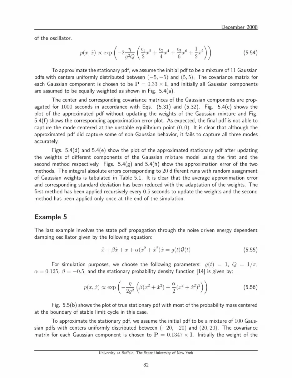
December 2008
of the oscillator.
p(x, x) ∝ exp
(−2
η
g2Q
(ǫ1
2x2 +
ǫ2
4x4 +
ǫ3
6x6 +
1
2x2
))(5.54)
To approximate the stationary pdf, we assume the initial pdf to be a mixture of 11 Gaussianpdfs with centers uniformly distributed between (−5,−5) and (5, 5). The covariance matrix foreach Gaussian component is chosen to be P = 0.33 × I, and initially all Gaussian componentsare assumed to be equally weighted as shown in Fig. 5.4(a).
The center and corresponding covariance matrices of the Gaussian components are prop-agated for 1000 seconds in accordance with Eqs. (5.31) and (5.32). Fig. 5.4(c) shows theplot of the approximated pdf without updating the weights of the Gaussian mixture and Fig.5.4(f) shows the corresponding approximation error plot. As expected, the final pdf is not able tocapture the mode centered at the unstable equilibrium point (0, 0). It is clear that although theapproximated pdf did capture some of non-Gaussian behavior, it fails to capture all three modesaccurately.
Figs. 5.4(d) and 5.4(e) show the plot of the approximated stationary pdf after updatingthe weights of different components of the Gaussian mixture model using the first and thesecond method respectively. Figs. 5.4(g) and 5.4(h) show the approximation error of the twomethods. The integral absolute errors corresponding to 20 different runs with random assignmentof Gaussian weights is tabulated in Table 5.1. It is clear that the average approximation errorand corresponding standard deviation has been reduced with the adaptation of the weights. Thefirst method has been applied recursively every 0.5 seconds to update the weights and the secondmethod has been applied only once at the end of the simulation.
Example 5
The last example involves the state pdf propagation through the noise driven energy dependentdamping oscillator given by the following equation:
x + βx + x + α(x2 + x2)x = g(t)G(t) (5.55)
For simulation purposes, we choose the following parameters: g(t) = 1, Q = 1/π,α = 0.125, β = −0.5, and the stationary probability density function [14] is given by:
p(x, x) ∝ exp
(− η
2g2
(β(x2 + x2) +
α
2(x2 + x2)2
))(5.56)
Fig. 5.5(b) shows the plot of true stationary pdf with most of the probability mass centeredat the boundary of stable limit cycle in this case.
To approximate the stationary pdf, we assume the initial pdf to be a mixture of 100 Gaus-sian pdfs with centers uniformly distributed between (−20,−20) and (20, 20). The covariancematrix for each Gaussian component is chosen to P = 0.1347 × I. Initially the weight of the
University at Buffalo, The State University of New York
82

December 2008
(a) Initial pdf (b) True pdf
(c) Final pdf (without WeightUpdate)
(d) Final pdf (with Weight Up-date I)
(e) Final pdf (with Weight Up-date II)
(f) Error pdf (without WeightUpdate)
(g) Error pdf (with Weight Up-date I)
(h) Error pdf (with Weight Up-date II)
Figure 5.4: Numerical results: example 4
University at Buffalo, The State University of New York
83

December 2008
first Gaussian component is w1 = 0.5 and the rest of the 99 Gaussian components have equalweights, w2...100 = 0.0051.
The center and corresponding covariance matrices of the Gaussian components are prop-agated for 1000 seconds using Eqs. (5.31) and (5.32). Fig. 5.5(c) shows the plot of theapproximated pdf without updating the weights of the Gaussian mixture and Fig. 5.5(f) showsthe corresponding approximation error plot. As expected, the final pdf is not able to capture thenon-Gaussian behavior in this case.
Figs. 5.5(d) and 5.5(e) show the plot of the approximated stationary pdf after updatingthe weights of different components of the Gaussian mixture model using the first and thesecond method respectively. Figs. 5.5(g) and 5.5(h) show the approximation error of the twomethods. The integral absolute errors corresponding to 20 different runs with random assignmentof Gaussian weights is tabulated in Table 5.1. It is clear that the average approximation errorand corresponding standard deviation has been reduced with the adaptation of the weights. Thefirst method has been applied recursively every 0.5 seconds to update the weights and the secondmethod has been applied only once at the end of the simulation.
Table 5.1: Numerical approximation of the integral of the absolute error
No Update Update I Update II
Example 3 (avg. 20 runs) 0.50 ± 0.02 0.47 ± 10−15 0.47 ± 10−15
Example 4 (avg. 20 runs) 0.86 ± 0.07 0.74 ± 10−14 0.50 ± 10−15
Example 5 (avg. 20 runs) 0.75 ± 0.01 0.19 ± 10−15 0.26 ± 10−15
For continuous time dynamical systems, the overall computational complexity in applyingthe second method is small since it is used to update the weights only when an estimate orapproximation of the conditional pdf has to be computed. In the continuous time case, the firstmethod has to be applied sequentially on the discretized equations of the dynamical system,making the method more computational expensive than the second one. Therefore discretizationerrors may be propagated in the update formulation of the weights.
Finally, we mention that the numerical results presented in this section reiterates ourobservation and support the conclusion that the better performance of proposed algorithms canbe attributed to the adaptation of amplitude corresponding to different components of Gaussianmixture. These dramatic advantages from five different problems provide compelling evidence forthe merits of proposed algorithms.
University at Buffalo, The State University of New York
84

December 2008
(a) Initial pdf (b) True pdf
(c) Final pdf (without WeightUpdate)
(d) Final pdf (with Weight Up-date I)
(e) Final pdf (with Weight Up-date II)
(f) Error pdf (without WeightUpdate)
(g) Error pdf (with Weight Up-date I)
(h) Error pdf (with Weight Up-date II)
Figure 5.5: Numerical results: example 5
University at Buffalo, The State University of New York
85
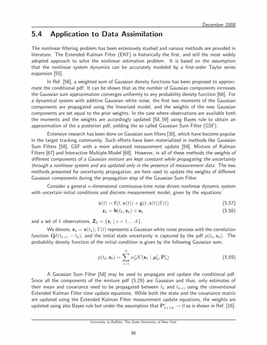
December 2008
5.4 Application to Data Assimilation
The nonlinear filtering problem has been extensively studied and various methods are provided inliterature. The Extended Kalman Filter (EKF) is historically the first, and still the most widelyadopted approach to solve the nonlinear estimation problem. It is based on the assumptionthat the nonlinear system dynamics can be accurately modeled by a first-order Taylor seriesexpansion [55].
In Ref. [58], a weighted sum of Gaussian density functions has been proposed to approxi-mate the conditional pdf. It can be shown that as the number of Gaussian components increasesthe Gaussian sum approximation converges uniformly to any probability density function [66]. Fora dynamical system with additive Gaussian white noise, the first two moments of the Gaussiancomponents are propagated using the linearized model, and the weights of the new Gaussiancomponents are set equal to the prior weights. In the case where observations are available boththe moments and the weights are accordingly updated [58, 59] using Bayes rule to obtain anapproximation of the a posteriori pdf, yielding the so called Gaussian Sum Filter (GSF).
Extensive research has been done on Gaussian sum filters [30], which have become popularin the target tracking community. Such efforts have been materialized in methods like GaussianSum Filters [58], GSF with a more advanced measurement update [59], Mixture of KalmanFilters [67] and Interactive Multiple-Model [68]. However, in all of these methods the weights ofdifferent components of a Gaussian mixture are kept constant while propagating the uncertaintythrough a nonlinear system and are updated only in the presence of measurement data. The twomethods presented for uncertainty propagation, are here used to update the weights of differentGaussian components during the propagation step of the Gaussian Sum Filter.
Consider a general n-dimensional continuous-time noise driven nonlinear dynamic systemwith uncertain initial conditions and discrete measurement model, given by the equations:
x(t) = f(t,x(t)) + g(t,x(t))Γ(t) (5.57)
zk = h(tk, xk) + vk (5.58)
and a set of k observations, Zk = zi | i = 1 . . . k.We denote, xk = x(tk), Γ(t) represents a Gaussian white noise process with the correlation
function Qδ(tk+1 − tk), and the initial state uncertainty is captured by the pdf p(t0,x0). Theprobability density function of the initial condition is given by the following Gaussian sum,
p(t0, x0) =
N∑
i=1
wi0N (x0 | µ
i0,P
i0) (5.59)
A Gaussian Sum Filter [58] may be used to propagate and update the conditional pdf.Since all the components of the mixture pdf (5.29) are Gaussian and thus, only estimates oftheir mean and covariance need to be propagated between tk and tk+1 using the conventionalExtended Kalman Filter time update equations. While both the state and the covariance matrixare updated using the Extended Kalman Filter measurement update equations, the weights areupdated using also Bayes rule but under the assumption that Pi
k+1|k → 0 as is shown in Ref. [16].
University at Buffalo, The State University of New York
86

December 2008
Notice that it is assumed that weights wit|k do not change between measurement updates. In
practice this assumption may be easily violated resulting in a poor approximation of the forecastpdf. Practically, the dynamic system may exhibit strong nonlinearities and the total numberof Gaussian components, needed to represent the pdf, may be restricted due to computationalrequirements.
Our minimization problem will substitute the equation wik+1|k = wi
k|k whenever an estimatehas to be computed, even between measurements. The summary of the Gaussian Sum Filterwith forecast weight update for the continuous-time nonlinear dynamical systems and discretemeasurement model is presented in Table 5.2.
For discrete-time case, consider the following nonlinear dynamic system with uncertaininitial conditions given by the Gaussian mixture pdf (5.59) and discrete measurement model:
xk+1 = f(tk,xk) + ηk (5.60)
zk = h(tk, xk) + vk (5.61)
and a set of k observations, Zk = zi | i = 1 . . . k. Here ηk ∼ N (0,Qk) represents theprocess noise. The same assumptions on process and measurement noise are made as in thecontinuous-time case.
The Gaussian Sum Filter used to propagate the conditional pdf, p(tk,xk|Zk) is very similarwith the filter used in continuous-time case, except the time-update step.
The same argument is made here regarding the forecast weights, that are not changedduring propagation. A better approximation of the forecast pdf and a more accurate estimatemay be obtained by updating these weights.
The final formulation of the optimization may be posed in the quadratic programmingframework as shown in Table 5.3 and solved using readily available solvers.
5.5 Numerical results on Data Assimilation Simulations
Example 1
To evaluate the performance of the forecast weight update scheme we consider the followingcontinuous-time dynamical system with uncertain initial condition and discrete measurementmodel given by (5.64):
x = sin(x) + Γ(t) where Q = 1 (5.62)
zk = x2k + vk where R = 1 (5.63)
x0 ∼ 0.1N (−0.2, 1) + 0.9N (0.2, 1) (5.64)
The moments of the two Gaussian components are propagated for eight seconds using(5.31) and (5.32), using a sampling time of ∆t = 0.25 sec and measurements available every1 sec. Both methods have been applied for this example and every time step the estimate has
University at Buffalo, The State University of New York
87
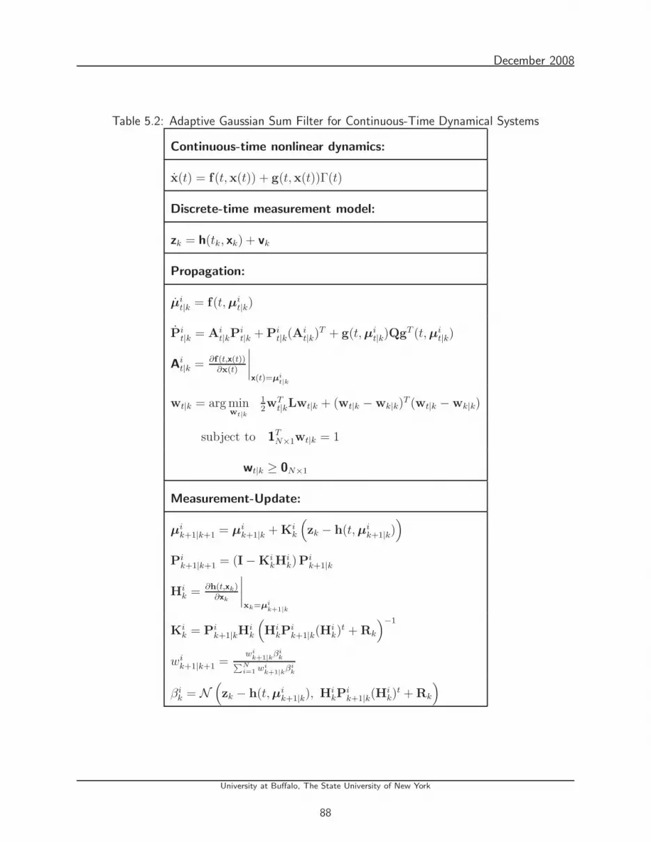
December 2008
Table 5.2: Adaptive Gaussian Sum Filter for Continuous-Time Dynamical Systems
Continuous-time nonlinear dynamics:
x(t) = f(t,x(t)) + g(t,x(t))Γ(t)
Discrete-time measurement model:
zk = h(tk, xk) + vk
Propagation:
µit|k = f(t, µi
t|k)
Pit|k = Ai
t|kPit|k + Pi
t|k(Ait|k)
T + g(t, µit|k)QgT (t, µi
t|k)
Ait|k = ∂f(t,x(t))
∂x(t)
∣∣∣∣x(t)=µi
t|k
wt|k = arg minwt|k
12wT
t|kLwt|k + (wt|k − wk|k)T (wt|k − wk|k)
subject to 1TN×1wt|k = 1
wt|k ≥ 0N×1
Measurement-Update:
µik+1|k+1 = µ
ik+1|k + Ki
k
(zk − h(t, µi
k+1|k))
Pik+1|k+1 = (I − Ki
kHik)P
ik+1|k
Hik = ∂h(t,xk)
∂xk
∣∣∣∣xk=µi
k+1|k
Kik = Pi
k+1|kHik
(Hi
kPik+1|k(H
ik)
t + Rk
)−1
wik+1|k+1 =
wik+1|k
βik∑N
i=1 wik+1|k
βik
βik = N
(zk − h(t, µi
k+1|k), HikP
ik+1|k(H
ik)
t + Rk
)
University at Buffalo, The State University of New York
88
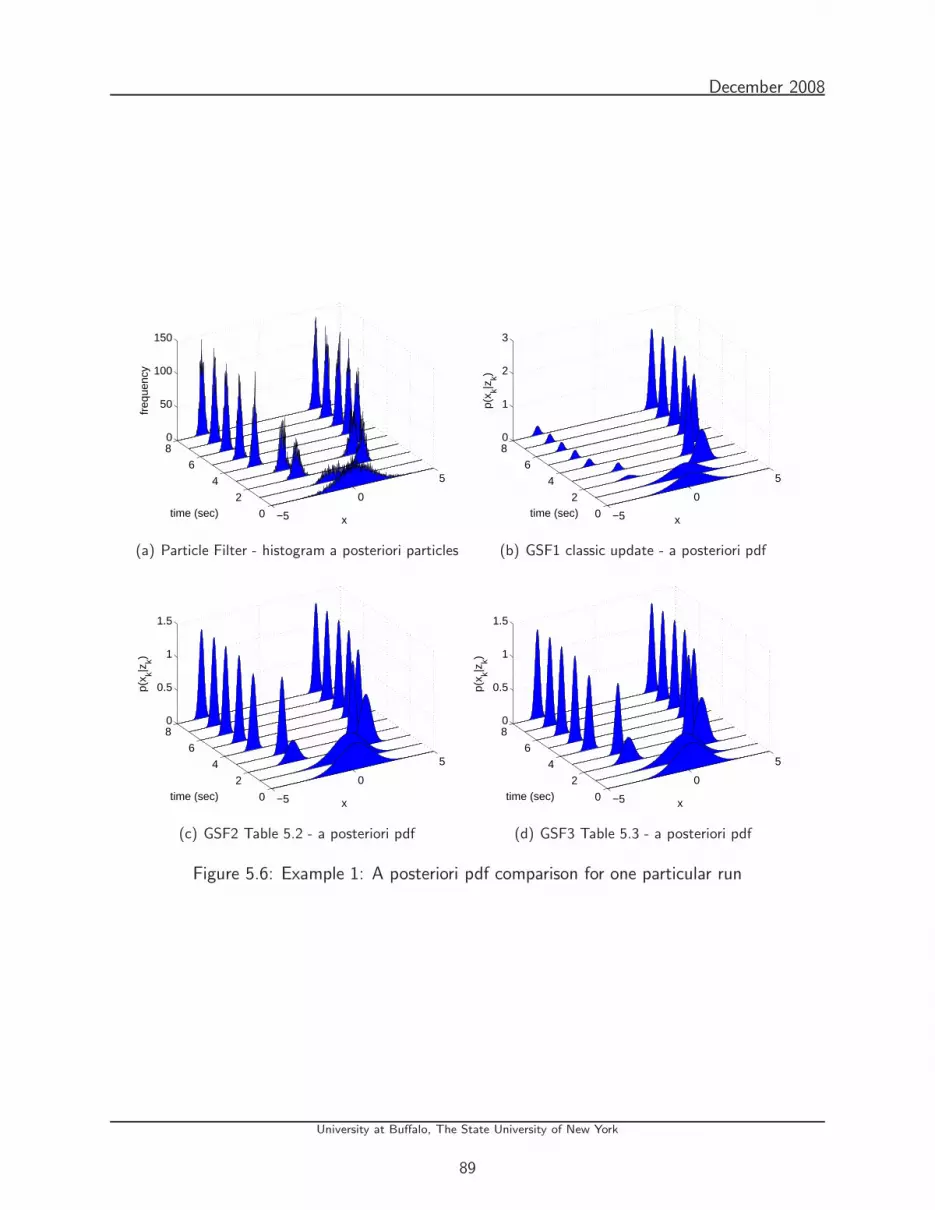
December 2008
−5
0
5
0
2
4
6
80
50
100
150
xtime (sec)
freq
uenc
y
(a) Particle Filter - histogram a posteriori particles
−5
0
5
0
2
4
6
80
1
2
3
xtime (sec)
p(x k|z
k)
(b) GSF1 classic update - a posteriori pdf
−5
0
5
0
2
4
6
80
0.5
1
1.5
xtime (sec)
p(x k|z
k)
(c) GSF2 Table 5.2 - a posteriori pdf
−5
0
5
0
2
4
6
80
0.5
1
1.5
xtime (sec)
p(x k|z
k)
(d) GSF3 Table 5.3 - a posteriori pdf
Figure 5.6: Example 1: A posteriori pdf comparison for one particular run
University at Buffalo, The State University of New York
89

December 2008
0 2 4 6 80
1
2
3
4
5
time (sec)
RM
SE
GSF1 − classic updateGSF2 − w.upd.IGSF3 − w.upd.IIParticle Filter
Figure 5.7: Example 1: RMSE Comparison (avg. over 100 runs)
been computed and compared with the truth. The estimates of the two methods have beencompared with the classical Gaussian Sum Filter using the root mean square error, RMSE -Eq.(5.65), averaged over 100 runs. Every run a different truth and afferent measurements havebeen generated.
RMSE(t) =
√√√√ 1
R
R∑
j=1
(xjt − µj
t|k)2 (5.65)
Where xjt is the true value of the state at time t for the jth run and R is the total number
of runs. In Fig. 5.7 we have computed the RMSE for all three methods. It is clear from thisplot that we are able to better estimate the state with the incorporation of the weight updateschemes.
Due to the multimodal nature of the a posteriori pdf, the RMSE is not an appropriateperformance measure to compare different filters. A Boostrap Particle Filter with 10, 000 particles,has also been implemented in order to have a proxy for the true a posteriori pdf. In Fig.5.6 we cansee that by updating the weights of the Gaussian Sum during propagation we can better capturethe true a posteriori pdf. In addition to this, log probability of the particles was computedaccording to the following relationship:
L =
M∑
j=1
log
N∑
i=1
wiN (xj | µi,Pi) (5.66)
Here, M is the total number of particles used in the Boostrap Particle Filter. The highervalue of L represents a better pdf approximation. Fig.5.8 shows the plot of log probability of theparticles with and without updating the weights of the Gaussian mixture. As expected, updatingthe weights of the Gaussian mixture leads to higher log probability of the particles. Hence,
University at Buffalo, The State University of New York
90

December 2008
0 1 2 3 4 5 6 7 8−2.5
−2
−1.5
−1
−0.5
0x 10
4
time (sec)
log.
prob
.dat
a.
GSF1 − classic updateGSF2 − w.upd.IGSF3 − w.upd.II
Figure 5.8: Example 1: Log probability of the particles (avg. over 100 runs)
we conclude that the adaptation of the weights during propagation leads to a more accuratea posteriori pdf approximation than without weight update. Due to the squared form of themeasurement model, and bimodal nature of the forecast pdf, our measurements are not ableto offer sufficient information to choose one mode of the conditional pdf, thus maintaining itsbimodal nature. In such situation an accurate propagation makes the difference in providingbetter estimates and a more accurate conditional pdf.
While updating the forecast weights we obtain more accurate estimate of the state, itcan be shown [53] that we also obtain a better conditional density function that agrees with thebimodal nature of the underlying true pdf, which can be used in applications that require morethan just estimates.
Example 2
We have also considered the following continuous-time dynamical system with uncertain initialcondition and discrete measurement model given by (5.69):
x = 5x(1 − x2) + Γ(t) where Q = 0.25 (5.67)
zk = x2k + vk where R = 0.01 (5.68)
x0 ∼ 0.1N (−0.5, 2) + 0.9N (0.5, 2) (5.69)
The moments of the two Gaussian components are propagated for 1 sec using (5.31) and(5.32), with a sampling time of ∆t = 0.01 sec and measurements available every 0.1 sec. Bothmethods have been applied for this example and every time step the estimate has been computedand compared with the truth.
In Fig.5.9 and Fig.5.10 we compare the three methods using the RMSE (5.65) and logprobability of the particles (5.66) averaged over 100 runs.
University at Buffalo, The State University of New York
91

December 2008
0 0.2 0.4 0.6 0.8 1
0.6
0.7
0.8
0.9
1
time (sec)
RM
SE
GSF1 − classic updateGSF2 − w.upd.IGSF3 − w.upd.IIParticle Filter
Figure 5.9: Example 2: RMSE Comparison (avg. over 100 runs)
0 0.2 0.4 0.6 0.8 1−2
−1.5
−1
−0.5
0
0.5
1x 10
4
time (sec)
log.
prob
.dat
a.
GSF1 − classic updateGSF2 − w.upd.IGSF3 − w.upd.II
Figure 5.10: Example 2: Log probability of the particles (avg. over 100 runs)
University at Buffalo, The State University of New York
92

December 2008
As in the previous example, a reduction in the error between the estimates and the truthis obtained and we better capture the a posteriori pdf when the forecast weights are updatedduring propagation.
5.6 Remarks
Two update schemes for the forecast weights are presented in order to obtain a better Gaussiansum approximation to the forecast pdf. The difference between the two methods comes from theparticularities of their derivations. The first method updates the weights such that they minimizethe integral square difference between the true probability density function and its approximation.The derivation of the first method indicates that it is more appropriate for discrete time systems.The second method is derived such that the Gaussian sum is satisfying the FPKE, which indicatethat it is more appropriate for continuous time systems. The weights are updated such that theyminimize the FPKE error. Both the method leads to two different convex quadratic minimizationproblems which are guaranteed to have a unique solution.
Several benchmark problems have been provided to compare the two methods with theusual procedure of not updating the weights in pure propagation settings. In all of these diversetest problems, the proposed two algorithms are found to produce considerably smaller errors ascompared to existing methods. The results presented in this paper serve to illustrate the usefulnessof adaptation of weights corresponding to different components of Gaussian sum model.
By updating the forecast weights, not only do we obtain a more accurate estimate butalso a better approximation to the conditional probability density function. The update methodspresented are very useful when the measurement model offer limited or no information in updatingthe states of the system. Such situation arise when we are doing pure forecast, the frequencyof the measurements is low, the uncertainty in the measurements is large or the measurementmodel is ambiguous, hence incapable of selecting one mode from the conditional probabilitydensity function. In these situations, when the measurements give little or no information inupdating our uncertainty, a more accurate propagation of the conditional pdf is required.
We anticipate that major advances are possible in numerous engineering applications suchas studying the chemical-bio plume propagation using uncertain meteorological data.
University at Buffalo, The State University of New York
93

December 2008
Table 5.3: Adaptive Gaussian Sum Filter for Discrete-Time Dynamical Systems
Discrete-time nonlinear dynamics:
xk+1 = f(tk,xk) + ηk
Discrete-time measurement model:
zk = h(tk, xk) + vk
Propagation:
µik+1|k = f(k, µi
k|k)
Pik+1|k = Ai
kPik|k(A
ik)
T + Qk
Aik = ∂f(k,xk)
∂xk
∣∣∣∣xk=µi
k|k
wk+1|k = arg minwk+1|k
12wT
k+1|kMwk+1|k −wTk+1|kNwk|k
subject to 1TN×1wk+1|k = 1
wk+1|k ≥ 0N×1
Measurement Update:
µik+1|k+1 = µ
ik+1|k + Ki
k
(zk − h(t, µi
k+1|k))
Pik+1|k+1 = (I − Ki
kHik)P
ik+1|k
Hik = ∂h(t,xk)
∂xk
∣∣∣∣xk=µi
k+1|k
Kik = Pi
k+1|kHik
(Hi
kPik+1|k(H
ik)
t + Rk
)−1
wik+1|k+1 =
wik+1|k
βik∑N
i=1 wik+1|k
βik
βik = N
(zk − h(t, µi
k+1|k), HikP
ik+1|k(H
ik)
t + Rk
)
University at Buffalo, The State University of New York
94
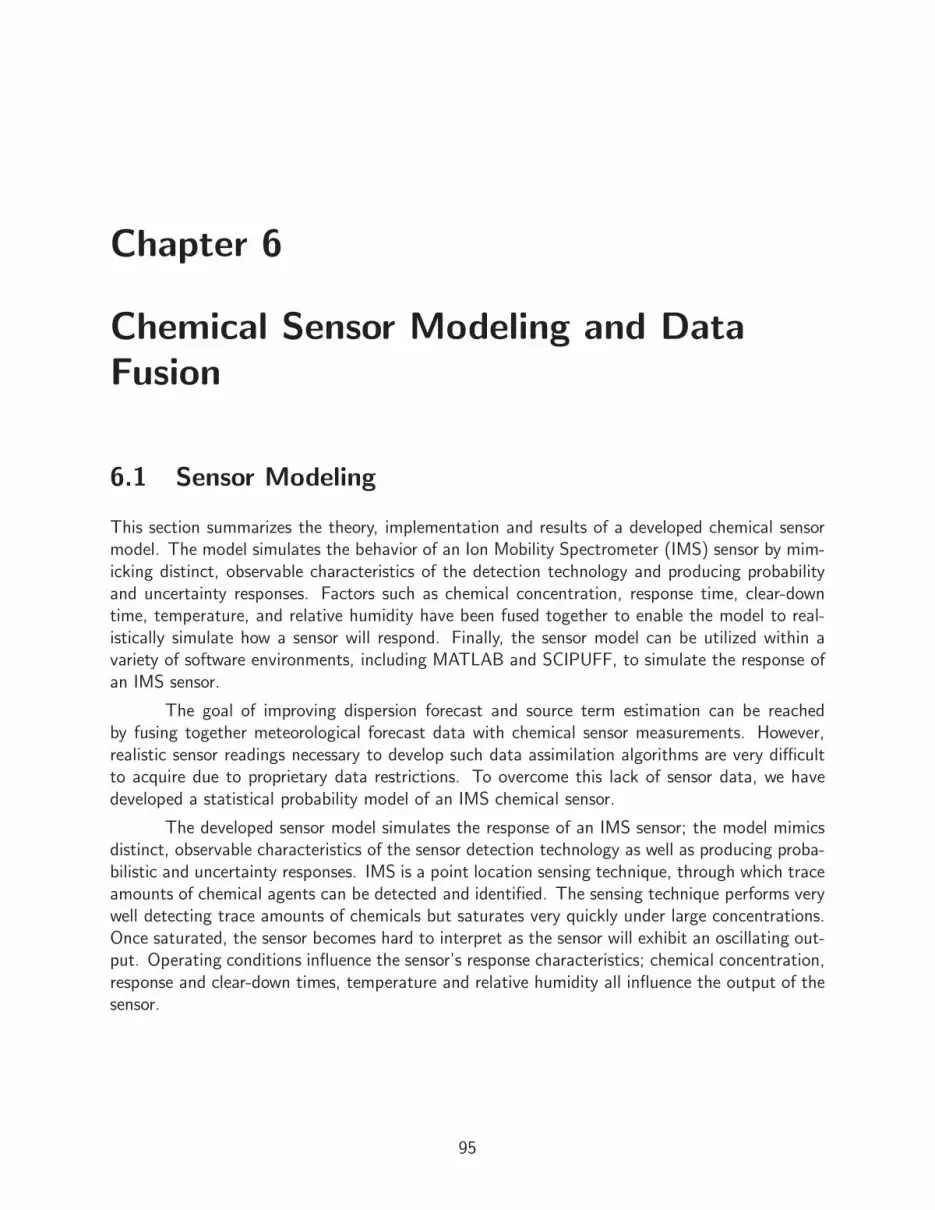
Chapter 6
Chemical Sensor Modeling and DataFusion
6.1 Sensor Modeling
This section summarizes the theory, implementation and results of a developed chemical sensormodel. The model simulates the behavior of an Ion Mobility Spectrometer (IMS) sensor by mim-icking distinct, observable characteristics of the detection technology and producing probabilityand uncertainty responses. Factors such as chemical concentration, response time, clear-downtime, temperature, and relative humidity have been fused together to enable the model to real-istically simulate how a sensor will respond. Finally, the sensor model can be utilized within avariety of software environments, including MATLAB and SCIPUFF, to simulate the response ofan IMS sensor.
The goal of improving dispersion forecast and source term estimation can be reachedby fusing together meteorological forecast data with chemical sensor measurements. However,realistic sensor readings necessary to develop such data assimilation algorithms are very difficultto acquire due to proprietary data restrictions. To overcome this lack of sensor data, we havedeveloped a statistical probability model of an IMS chemical sensor.
The developed sensor model simulates the response of an IMS sensor; the model mimicsdistinct, observable characteristics of the sensor detection technology as well as producing proba-bilistic and uncertainty responses. IMS is a point location sensing technique, through which traceamounts of chemical agents can be detected and identified. The sensing technique performs verywell detecting trace amounts of chemicals but saturates very quickly under large concentrations.Once saturated, the sensor becomes hard to interpret as the sensor will exhibit an oscillating out-put. Operating conditions influence the sensor’s response characteristics; chemical concentration,response and clear-down times, temperature and relative humidity all influence the output of thesensor.
95
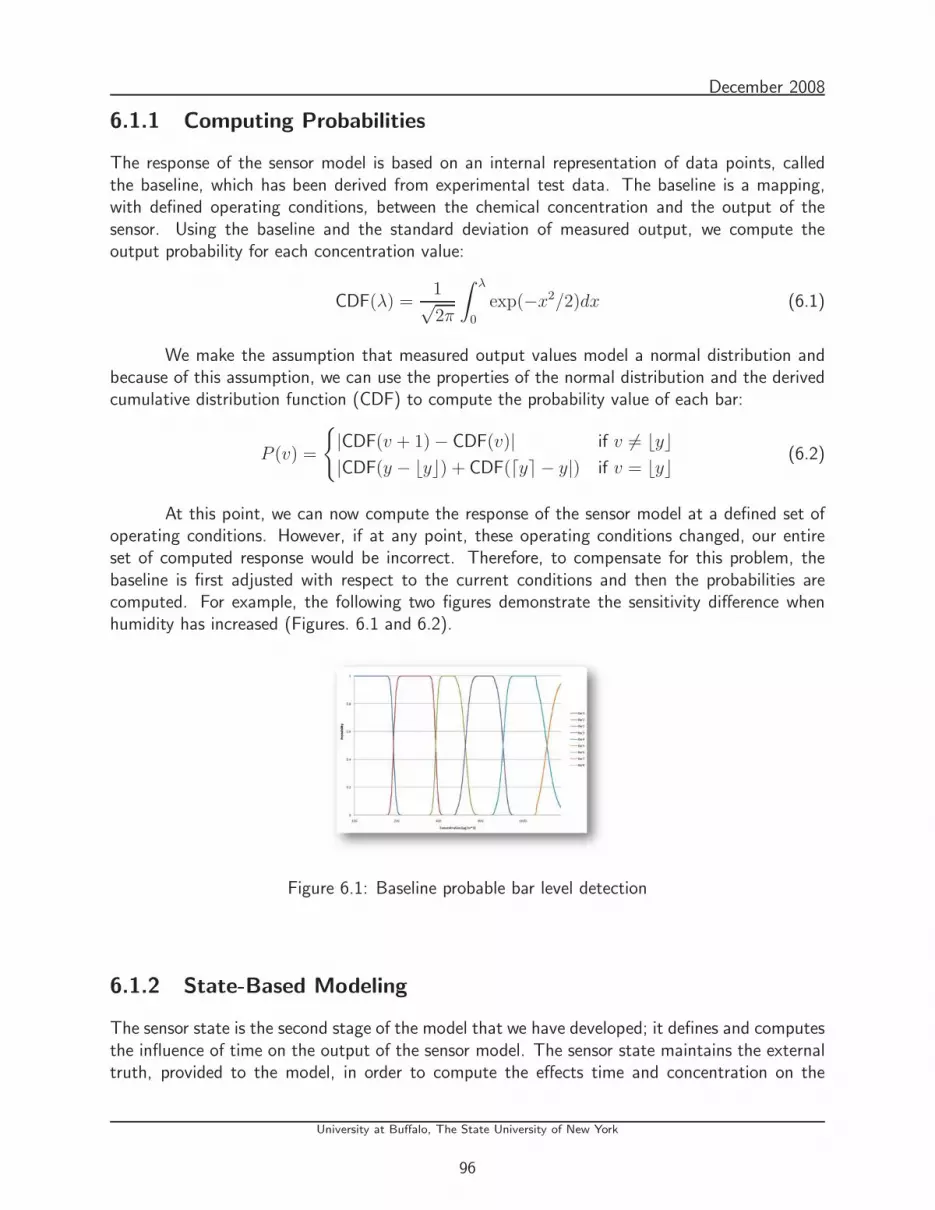
December 2008
6.1.1 Computing Probabilities
The response of the sensor model is based on an internal representation of data points, calledthe baseline, which has been derived from experimental test data. The baseline is a mapping,with defined operating conditions, between the chemical concentration and the output of thesensor. Using the baseline and the standard deviation of measured output, we compute theoutput probability for each concentration value:
CDF(λ) =1√2π
∫ λ
0
exp(−x2/2)dx (6.1)
We make the assumption that measured output values model a normal distribution andbecause of this assumption, we can use the properties of the normal distribution and the derivedcumulative distribution function (CDF) to compute the probability value of each bar:
P (v) =
|CDF(v + 1) − CDF(v)| if v 6= ⌊y⌋|CDF(y − ⌊y⌋) + CDF(⌈y⌉ − y|) if v = ⌊y⌋ (6.2)
At this point, we can now compute the response of the sensor model at a defined set ofoperating conditions. However, if at any point, these operating conditions changed, our entireset of computed response would be incorrect. Therefore, to compensate for this problem, thebaseline is first adjusted with respect to the current conditions and then the probabilities arecomputed. For example, the following two figures demonstrate the sensitivity difference whenhumidity has increased (Figures. 6.1 and 6.2).
Figure 6.1: Baseline probable bar level detection
6.1.2 State-Based Modeling
The sensor state is the second stage of the model that we have developed; it defines and computesthe influence of time on the output of the sensor model. The sensor state maintains the externaltruth, provided to the model, in order to compute the effects time and concentration on the
University at Buffalo, The State University of New York
96

December 2008
Figure 6.2: Baseline detection with increased humidity
output of the sensor. The reader should note that the model is never responding to the trueoperating conditions, rather, it is responding to the internally perceived state of the sensor. Theinternal concentration of the model is modeled after the rates observed in electronic devices;specifically, the charging and discharging rate of a capacitor.
In Figure 6.3, the input concentration is a simple square wave example. When using theSensor Model, more complex inputs of concentration would be expected from simulation softwaresuch as SCIPUFF. From Figure 6.4, we can see that the output of the Sensor Model is drivenover time - that is, both the probabilistic and state based sections of the model are combinedto emulate the output of a sensor over time. In this case, it can be observed that the sensortakes a small amount of time to output its highest value, becomes saturated and then starts tocleardown - thus reducing the output over time. When the sensor has reached an acceptableinternal concentration, the sensor will again redetect and respond by increasing its output value.Finally, as the truth concentration is brought down to zero, the sensors output will follow thusresulting in a cleardown to zero.
Figure 6.3: Baseline detection with increased humidity
University at Buffalo, The State University of New York
97
December 2008
Figure 6.4: Output of the IMS model
6.1.3 Application Programming Interface
The sensor model requires several inputs of ’truth’ data, which the model processes and utilizes,in order to return an output similar to that of a real sensor. The sensor model provides severaloutputs, all of which are not provided by a real sensor, that can be utilized within the dataassimilation algorithm; the probability of getting an output bar at a current time during thesimulation, the uncertainty related to the current output, and the likelihood of a concentrationvalue provided an output bar value. The source code for the sensor model was written in C♯and ran atop of the Microsoft.NET framework. However, due to the requirements of the dataassimilation project, the sensor model was required to run in MATLAB and on a Linux clusterwithin SCIPUFF. In order to enable these capabilities, the sensor model utilized the open-source.NET framework project, Mono, to run atop Linux and within SCIPUFF. To run the sensor modelwithin MATLAB, the .NET code was compiled into a Java Archive (JAR) file and was thenutilized with the native Java Runtime Environment (JRE) capabilities embedded into MATLAB.
6.1.4 Scope and Limitations
The sensor model that has been developed has several known limitations; these limitations couldbe eliminated with further testing and validation efforts. The most important of these limitationsis that the sensor represents and computes its internal concentration using exponential growth anddecay functions. The internal concentrations, themselves, are not mapped in a linear fashion tothe output of the sensor model, may have a more accurate representation. The second limitationis that no experimentally derived test data was reported over varying operating conditions ofatmospheric pressure. Thus, no correlation can be made in the sensor model for this condition.Other limitations of the sensor model consist of measurement drift as the sensor is continuallyexposed to chemical agents. While the sensor has not been cleaned, its abilities to correlate theexposed concentration and operating conditions to a valid output value will decrease; the abilitiesof the current sensor model will never degrade. Additionally, when the IMS sensor is exposed todifferent chemical agents, the sensor will respond to multiple different chemical types as opposedto the sensor model, which will only respond to the correct chemical type.
University at Buffalo, The State University of New York
98

December 2008
6.1.5 Remarks
The model is now currently being used in the development of data assimilation and fusion algo-rithms that can be used to better identify the source and forecasted dispersion of a chemical re-lease. Many different factors, such as chemical concentration, temperature and relative humidity,are taken into account to create realistic responses. However, the most important characteristicof the model is its ability to dynamically model and simulate the response of the sensor overtime.
University at Buffalo, The State University of New York
99

December 2008
6.2 Data Fusion
6.2.1 Problem Statement
In this section, the problem of sensor-aided chemical transport and dispersion prediction, the roleof data fusion in this problem, and the outline of a two-step data fusion procedure are introduced.Note, however, that the focus of this chapter is the formulation and numerical solutions of the datafusion problem. The introduction of the complete sensor-aided chemical transport and dispersionprediction problem helps explain the practical constraint to which the data fusion methods inCBRN applications are subject.
In the chemical transport and dispersion prediction problem, the state vector, denoted byx (with the time index dropped), represents a set of Gaussian puffs released from the sourcesand transported by the wind (or the concentrations over a region of interest computed from thepuffs using a known model). A puff is characterized by its mass, centroid, size, and orientation.The state vector is large because the number of puffs in a SCIPUFF run can be hundreds,thousands, or more. The probability distribution of the state vector, p(x), is typically representedby an ensemble of x, with each ensemble member time-updated with the nonlinear transport anddispersion model. The functional form of the density p(x) can be obtained from the ensembleof x using approximation theory. Owing to errors in the transport and dispersion model and arange of parameters, p(x) or the ensemble of x is an inaccurate representation of the probabilitydistribution of the puffs or the material concentrations.
The objective of data fusion is to integrate sensor measurements into model forecast usingBayes rule. The sensor measurements contain information about local concentrations, whichhelp improve the prediction precision. The sensor model will be presented in a later section.We assume that the sensor measurements are conditionally independent, thus facilitating thesequential processing of them. Given the sequential processing structure, we only need to considerthe problem of data fusion with a scalar discrete sensor measurement I. According to Bayes rule,
p(x|I) =p(I|x)p(x)
p(I)(6.3)
where p(x|I) is the posterior density of x, p(I) is the probability of I, p(I|x) is the probabilityof I conditional on x, also known as the likelihood function of x. The information obtained fromthe sensor enters the posterior density through the likelihood function, which is determined bythe sensor characteristics.
The ultimate goal of optimal estimation is to compute p(x|I). In general, the densityfunction p(x|I) requires an infinite-dimensional representation and an exact analytic solution toit is impossible. The key question of interest here is how to solve the problem approximatelyand efficiently. Computationally efficient suboptimal methods are needed because the size ofthe state vector is large. The methods presented in this chapter are focused on the estimationof the first two moments of p(x|I), that is, the conditional mean and covariance, under theGaussian fit approximation that p(x) is Gaussian. Of course, the methods can still be appliedwith degradation of accuracy when the Gaussian fit approximation is invalid.
University at Buffalo, The State University of New York
100
December 2008
Two-Step Update
A two-step procedure outlined below will be used to update the mean and covariance of x.
First, some quantities are defined. Suppose I is the discrete-valued measurement to befused with p(x). Let c be the continuous-valued concentration at the same location. Let the
mean and covariance of[xT , c
]T(before fusion) be
[x−
c−
]and
[P−
x P−xc
(P−xc)
TP−
c
]
These quantities are computed from the puff ensemble. The mean and covariance of[xT , c
]T(after fusion) is denoted by [
x+
c+
]and
[P+
x P+xc
(P +xc)
TP+
c
]
The two-step procedure is as follows. In the first step, the continuous-valued concentrationestimate is updated with I from c− to c+ assuming p(c) is a Gaussian distribution. In the secondstep, the state estimate is updated from x− to x+ based on the correlation between x and c andusing the following formulae [34]:
x+ = x− + K(c+ − c−) (6.4)
P+x = P−
x + K(P +c − P−
c )KT (6.5)
withK = P−
xc(P−c )−1 (6.6)
The issue with discrete-valued sensor data is addressed in the first step and is totally separatedfrom the second step. Were the update method of the same form used to update c with themeasurement, the two-step procedure would yield the same x+ and P+
x as updating the stateestimate directly with the measurement. The simple linear update method is used in the secondstep mainly because the size of x is large and the higher order update is computationally tooexpensive. The linear update has the same form as the update of the estimator with quantizedmeasurements in [69] and the Kalman filter and its variants. Note that the linear update givenby Eqs. (6.4),(6.5),(6.6) is optimal, that is, it is equivalent to the Bayes rule, when x and c arejointly Gaussian. In other cases, the linear update is suboptimal.
Since all the complexities of the data fusion method lie in the update of c, after thissection we will focus on the method for updating c with I under the assumption that c is aGaussian random variable. Because both c and I are one dimensional, more accurate update ofc than a linear update can be used without significantly increasing the computational load.
Approximations
The assumption that x and c are jointly Gaussian is only approximately true because of thenonlinearity of the sensor model and the transport and dispersion model. Furthermore, because
University at Buffalo, The State University of New York
101

December 2008
a concentration is nonnegative the underlying distribution p(c) and p(c|I) of the material con-centration is approximated by a clipped normal distribution in SCIPUFF [5]. More details of thedistribution model and the comparisons between this model and the log-normal model and otherscan be found in [70, 71]. If c and Pc are the mean and variance of a Gaussian distribution, thedensity function of the corresponding clipped Gaussian distribution is given by [5]
p(c|c, Pc) =1
2
[1 − erf(
c√2Pc
)
]δ(c)
+1√
2πPc
exp
[−(c − c)2
2Pc
], c ≥ 0
(6.7)
where δ(c) is Dirac’s δ function. The corresponding cumulative distribution function F (c|, c, Pc)is
F (c|, c, Pc) =1
2
[1 + erf
(c − c√
2Pc
)], c ≥ 0 (6.8)
Note that F (c|, c, Pc) is right continuous for c ≥ 0. A plot of F (c|, c, Pc) with Pc = 1 andc = 0, 1, 2, 3 is shown in Figure. 6.5. The mean c∗ and variance P ∗
c of the clipped Gaussian
0 1 2 3 4 5 6 7 80
0.1
0.2
0.3
0.4
0.5
0.6
0.7
0.8
0.9
1
concentration
cdf
c = 0 c = 1 c = 2 c = 3
Figure 6.5: Cumulative distribution function
distribution are [5]
c∗ =
√Pc
2πexp
[− c2
2Pc
]+
c
2
[1 + erf
(c√2Pc
)](6.9)
and
P ∗c = −c2 +
Pc
2
[1 + erf
(c√2Pc
)]+ c∗ · c (6.10)
where erf is the error function, which is defined in a later section. SCIPUFF assumes that theconcentration distribution is clipped Gaussian with outputs c and Pc instead of c∗ and P ∗
c . For
c = 0, c∗ =√
Pc
2πand P ∗
c = Pc/2. However, for c ≫ 0, the difference between c and c∗ and the
difference between Pc and P ∗c become negligible.
University at Buffalo, The State University of New York
102

December 2008
Neither the Gaussianity nor the clipped Gaussianity is preserved in the data fusion pro-cess. Even if p(c) is a clipped Gaussian distribution, p(c|I) is not. In the proposed data fusionmethods, the parameters we choose to compute are c and P instead of c∗ and P ∗. That is,when the estimate of c is updated, p(c) will be treated as an un-clipped Gaussian distributionwith appropriate mean and variance; the proposed data fusion methods compute c+ and P+
c asif the underlying posterior distribution is not clipped. These parameters are then adjusted toaccount for the clipping effect using Eqs. (6.9) and (6.10), assuming that p(c|I) is approximatelya clipped Gaussian distribution and that c+ and P+
c are the moments of the un-clipped Gaussiandistribution.
6.2.2 Probabilistic Sensor Model
Given a set of M puffs, with each of them being parameterized by the mass Q(j), the centroidvector x
(j)c , and the spread matrix P (j), the state vector x is the collection of all the puff
parameters. The concentration of the material at a given location xg is computed by
c , c(xg) =M∑
j=1
Q(j)
√det (2π · P (j))
· exp
[−1
2(∆x(j))T P (j)−1(∆x(j))
] (6.11)
where det denotes the matrix determinant, and ∆x(j) = x(j)c − xg. The sensor model describes
the relation between the concentration and the sensor reading. The outputs of a bar sensorare discrete numbers of bars. In [72], the number of bars ranges from zero to seven. Thesebar readings indicate the concentration magnitude at the sensor location at the “instant”; thesensor displays I = 0, . . . , 7, bars when the internal continuous-valued concentration magnitudecv is between thresholds TI and TI+1, where TI+1 > TI ≥ 0. The thresholds are assumedto be exactly known. The properties of the sensor are determined by the thresholds and theproperties of cv, which is assumed normally distributed about the true concentration c [72]. Themeasurement model is given by
cv = c + v (6.12)
where the noise v may be considered a combination of multiplicative noise and additive noisewith mean zero and variance
R , R(c) = αc + J (6.13)
where α is the proportionality constant and J accounts for the thermal motion of the electronsin the components [72]. The probability density function of cv conditional on c is
p(cv|c) =1√
2πR(c)exp
[−(cv − c)2
2R(c)
](6.14)
Because the dependency of R on c, p(cv|c) is an asymmetric function of c (with cv fixed).Following Eq. (6.14), the likelihood function of the concentration c given the output I, or the
University at Buffalo, The State University of New York
103
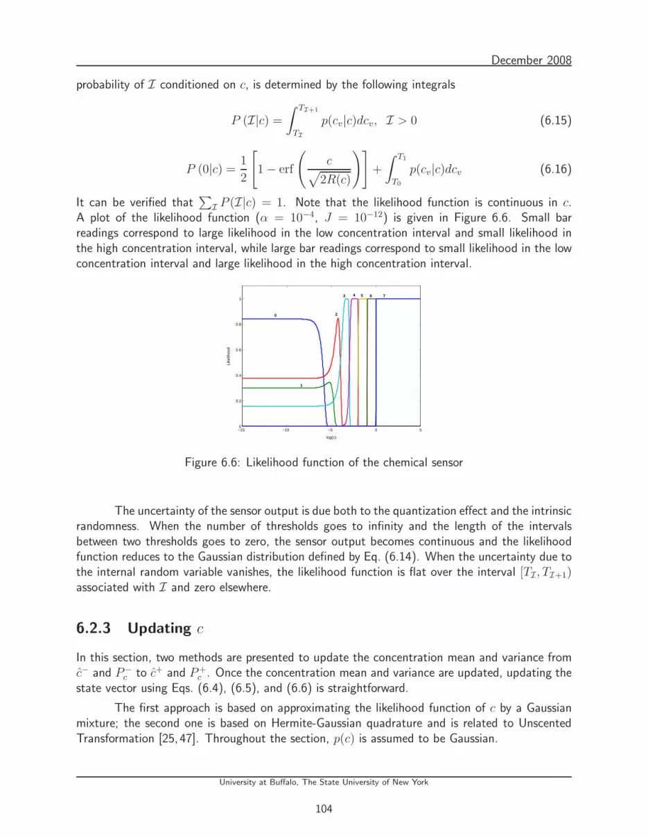
December 2008
probability of I conditioned on c, is determined by the following integrals
P (I|c) =
∫ TI+1
TI
p(cv|c)dcv, I > 0 (6.15)
P (0|c) =1
2
[1 − erf
(c√
2R(c)
)]+
∫ T1
T0
p(cv|c)dcv (6.16)
It can be verified that∑
I P (I|c) = 1. Note that the likelihood function is continuous in c.A plot of the likelihood function (α = 10−4, J = 10−12) is given in Figure 6.6. Small barreadings correspond to large likelihood in the low concentration interval and small likelihood inthe high concentration interval, while large bar readings correspond to small likelihood in the lowconcentration interval and large likelihood in the high concentration interval.
−15 −10 −5 0 50
0.2
0.4
0.6
0.8
1
log(c)
Like
lihoo
d
0 2
1
3 4 5 6 7
Figure 6.6: Likelihood function of the chemical sensor
The uncertainty of the sensor output is due both to the quantization effect and the intrinsicrandomness. When the number of thresholds goes to infinity and the length of the intervalsbetween two thresholds goes to zero, the sensor output becomes continuous and the likelihoodfunction reduces to the Gaussian distribution defined by Eq. (6.14). When the uncertainty due tothe internal random variable vanishes, the likelihood function is flat over the interval [TI , TI+1)associated with I and zero elsewhere.
6.2.3 Updating c
In this section, two methods are presented to update the concentration mean and variance fromc− and P−
c to c+ and P+c . Once the concentration mean and variance are updated, updating the
state vector using Eqs. (6.4), (6.5), and (6.6) is straightforward.
The first approach is based on approximating the likelihood function of c by a Gaussianmixture; the second one is based on Hermite-Gaussian quadrature and is related to UnscentedTransformation [25, 47]. Throughout the section, p(c) is assumed to be Gaussian.
University at Buffalo, The State University of New York
104
December 2008
Gaussian Sum Method
Using Bayes rule, the posterior distribution of c is given by
p(c|I) =P (I|c)p(c)
P (I)
=
∫ TI+1
TIp(cv|c)p(c)dcv
∫ TI+1
TI
∫∞
−∞ p(cv|c)p(c)dc dcv
=
∫ TI+1
TIp(cv)p(c|cv)dcv
∫ TI+1
TIp(cv)dcv
(6.17)
wherep(cv|c)p(c) = p(c|cv)p(cv) (6.18)
and
p(cv) =
∫ ∞
−∞
p(cv|c)p(c) dc (6.19)
have been used. The posterior mean and variance are given by
c+ = Ep(c|I)[c]
=
∫ ∞
−∞
c p(c|I)dc
=
∫ TI+1
TI
[∫∞
−∞ c · p(c|cv)dc]p(cv)dcv
∫ TI+1
TIp(cv)dcv
(6.20)
and
P+c = Ep(c|I)
[(c − Ep(c|I)[c])
2]
= Ep(c|I)[c2] −
Ep(c|I)[c]
2
=
∫ ∞
−∞
c2p(c|I)dc − (c+)2
=
∫ TI+1
TI
[∫∞
−∞c2 · p(c|cv)dc
]p(cv)dcv
∫ TI+1
TIp(cv)dcv
− (c+)2
(6.21)
where Ep(c|I) denotes the expectation with respect to p(c|I). Define
c(cv) =
∫ ∞
−∞
c · p(c|cv)dc (6.22)
Pc(cv) =
∫ ∞
−∞
(c − c(cv))2 · p(c|cv)dc (6.23)
University at Buffalo, The State University of New York
105

December 2008
and
β(cv) =p(cv)∫ TI+1
TIp(cv)dcv
(6.24)
Obviously, ∫ TI+1
TI
β(cv)dcv = 1 (6.25)
The posterior mean and variance can now be rewritten as
c+ =
∫ TI+1
TI
c(cv)β(cv)dcv (6.26)
and
P+c =
∫ TI+1
TI
[Pc(cv) + (c(cv) − c+)2]β(cv)dcv (6.27)
These equations holds for any form of p(cv|c).Now we will show how to compute the posterior mean and variance numerically. The
numerical approximation begins with a Gaussian sum approximation of the likelihood function
P (I|c) =
∫ TI+1
TI
p(cv|c)dcv ≈L∑
l=1
αlN (c(l)v ; c, R(l)) (6.28)
where αl are the coefficients and N (c(l)v ; c, R(l)) is a Gaussian density function with mean c and
variance R(l). Here R(l) is not a function of c. Note that in the above equation the likelihoodfunction P (I|c) is a function of c and I is the known measurement.
Approximation theory is used to obtain the Gaussian sum parameters αl, c(l)v , and R(l),
for example, by requiring them to minimize
∫ TI+1
TI
(P (I|c) −
L∑
l=1
αlN (c(l)v ; c, R(l))
)2
dc
subject to R(l) > 0 and αl > 0. The latter constraint can be relaxed to allow some of αl to benegative, as long as
∑Ll=1 αlN (c
(l)v ; c, R(l)) is positive or zero at all values of c. The integral is
over an interesting, finite interval of c, which is not identical to [Ti, Ti+1) in general. In practice,the cost function is approximated by
∑
k
(P (I|ck) −
L∑
l=1
αlN (c(l)v ; ck, R
(l))
)2
(6.29)
The number of components of the Gaussian mixture depends on the closeness of the likelihood tothe Gaussian function as well as the accuracy and complexity requirements. This approximationmethod is valid for any likelihood function.
University at Buffalo, The State University of New York
106

December 2008
Because the likelihood function P (I|c) (I > 0) is an integration of the Gaussian function,
a simpler way is to choose N (c(l)v ; c, R(l)) = p(c
(l)v |c). The variance parameter R(l) is set to
αc∗ + J , where c∗ is an approximation to the unknown true value, given by c−, a point in[TI , TI+1), or a combination of the two. The coefficients in this case satisfies
∑l αl = TI+1−TI .
The problem with this approximation is that when R(l) is much smaller than TI+1 − TI , a lotof Gaussian components are needed by this method in order to represent the likelihood functionaccurately.
Because p(c) is Gaussian and the likelihood function is a Gaussian mixture, p(c|c(l)v ) and
p(c(l)v ), denoted by N
(c; c(l)+, P
(l)+c
)and N
(c(l)v ; c−, P−
c + R(l)), respectively, are Gaussian.
The posterior estimate c(l)+ and the associated error variance P(l)+c are available from standard
Kalman filter measurement updates:
c(l)+ =R(l) · c− + P−
c · c(l)v
P−c + R(l)
(6.30)
and
P (l)+c =
P−c · R(l)
P−c + R(l)
(6.31)
It follows that ∫ TI+1
TI
p(cv)p(c|cv)dcv ≈L∑
l=1
αlp(c(l)v )p(c|c(l)
v ) (6.32)
∫ TI+1
TI
p(cv)dcv ≈L∑
l=1
αlp(c(l)v ) (6.33)
Substituting the above numerical approximations into Eq. (6.17) gives
p(c|I) ≈∑L
l=1 αjp(c(l)v )p(c|c(l)
v )∑L
l=1 αlp(c(l)v )
=
L∑
l=1
βlp(c|c(l)v )
(6.34)
where
βl =αlp(c
(l)v )
∑Ll=1 αlp(c
(l)v )
(6.35)
That is, p(c|I) is approximated by a finite sum of Gaussian distributions with the weights βl
satisfyingL∑
l=1
βl = 1 (6.36)
Finally, the mean and variance of p(c|I) are
c+ =L∑
l=1
βlc(l)+ (6.37)
University at Buffalo, The State University of New York
107

December 2008
and
P+c =
L∑
l=1
βl
[P (l)+
c + (c(l)+ − c+)2]
(6.38)
respectively.
When the upper limit of the integral in Eq. (6.28) is Ti+1 = ∞, an infinite number ofGaussian components is needed to accurately approximate the integral or the likelihood over[Ti,∞). However, only a relatively small number of them will contribute significantly to thecomputation of the posterior mean and variance. By checking the weights βl defined by Eq. (6.35),
we can determine the small set of effective c(l)v for Ti+1 = ∞.
The Gaussian sum approach is now summarized as follows:
1. Approximate the likelihood function P (I|c) as∑L
l=1 αlN (c(l)v ; c, R(l)).
2. Compute c(l)+ (using Eq. (6.30)), P(l)+c (using Eq. (6.31)), and βl (using Eq. (6.35)).
3. Compute c+ (using Eq. (6.37)) and P+ (using Eq. (6.38)).
Hermite-Gaussian Approach
DefineII(c) = P (I|c) (6.39)
Under the Gaussian assumption for p(cv|c), II(c) can be calculated as the difference of two errorfunctions or that of two complementary error functions. An error function for a standard Gaussiandistribution with zero mean and unity variance is defined by [73]
erf(c) =2√π
∫ c
0
exp(−t2)dt (6.40)
A complementary error function for standard Gaussian distribution with zero mean and unityvariance is defined by [73]
cerf(c) =2√π
∫ ∞
c
exp(−t2)dt (6.41)
Hence,
II(c) =1√2πR
∫ TI+1
TI
exp
[−(cv − c)2
2R
]dcv
=1
2
[erf
(TI+1 − c√
2R
)− erf
(Ti − c√
2R
)]
=1
2
[cerf
(Ti − c√
2R
)− cerf
(TI+1 − c√
2R
)](6.42)
where R is a function of c. In terms of II(c), the posterior distribution can be rewritten as
p(c|I) =II(c)p(c)∫II(c)p(c)dc
(6.43)
University at Buffalo, The State University of New York
108
December 2008
Accordingly, the posterior mean and variance of p(c|I) are
c+ =
∫cII(c)p(c)dc∫II(c)p(c)dc
(6.44)
and
P+c =
∫c2II(c)p(c)dc∫II(c)p(c)dc
− (c+)2 (6.45)
Noting that p(c) is a Gaussian distribution, we use the Hermite-Gaussian quadrature method [73]to approximate the above integrals.
The basic idea of the Hermite-Gaussian quadrature method is to approximate
∫ ∞
−∞
f(c) exp(−c2)dc
byL∑
l=1
αlf(cl)
The points cl are the L roots of the Hermite polynomial of degree L. The coefficients αl are theassociated weights on the points. The quadrature is exact if f(c) is a polynomial up to degree2L + 1. The Hermite polynomials are defined by [73]
HL(x) = (−1)nex2 dL
dxLe−x2
(6.46)
For example,
H1(x) = 2x
H2(x) = 4x2 − 2
H3(x) = 8x3 − 12x
H4(x) = 14x4 − 48x2 + 12
(6.47)
The associated weights are given by [73]
αl =2L−1L!
√π
L2[HL−1(xl)]2(6.48)
with L! the factorial of L. Close relation between the Hermite-Gaussian quadrature and theUnscented Transformation [25] has been noted ( [59] and [74]). For L = 3, the three points ofcl are 0 and ±
√3/2 and the associated weights are 2/3
√π and 1/6
√π. With the three points,
University at Buffalo, The State University of New York
109
December 2008
the expectation of f(c) with respect to Gaussian p(c) is given by
∫ ∞
−∞
f(c)p(c)dc
=1√
2πP−c
∫ ∞
−∞
f(c) exp
[−(c − c−)2
2P−c
]dc
=1√π
∫ ∞
−∞
f(c− +
√2P−
c c)
exp[−c2
]dc
≈ 1
6
[4f(c−) + f
(c− +
√3P−
c
)+ f
(c− −
√3P−
c
)]
(6.49)
Given cl and αl, we have the approximations:
∫II(c)p(c)dc ≈
∑
l
αlII(cl) (6.50)
∫cII(c)p(c)dc ≈
∑
l
αlclII(cl) (6.51)
∫c2II(c)p(c)dc ≈
∑
l
αlc2l II(cl) (6.52)
Following these equations,
c+ =
∑l αlclII(cl)∑l αlII(cl)
(6.53)
and
P+c =
∑l αlc
2l II(cl)∑
l αlII(cl)− (c+)2 (6.54)
Higher moments can be computed similarly. The higher moments is informative on how well theunderlying distribution p(c|I) is approximated by a single Gaussian distribution.
The Hermite-Gaussian method is summarized as follows:
1. Determine the number L of nodes to be used.
2. Find out the weights αl and the nodes cl.
3. Compute c+ and P+c using Eqs. (6.53) and (6.54).
6.2.4 Numerical Results
A binary chemical sensor displays one bar when its internal measurement cv ≥ 1 and zero barotherwise. The variance of cv is R = 0.09. The objective of the problem is to combine thepredicted concentration and the sensor reading.
University at Buffalo, The State University of New York
110

December 2008
The reading of the sensor is one bar and the likelihood function over [0, 20] is shown inFigure 6.7. The prior p(c) is a Gaussian distribution with mean c− = 1.5 and variance P−
c = 4.The posterior distribution, obtained using Bayes rule and 500,001 uniformly-spaced points in[0, 20], is shown in Figure 6.8. The posterior mean c+ and variance P+ computed directly fromthe 500,001 points are 2.7806 and 1.7339, respectively. These values are used as the exact values.Comparing the prior and posterior means and variances, we note thata large update needs to beapplied to the mean and variance.
0 2 4 6 8 10 12 14 16 18 200
0.1
0.2
0.3
0.4
0.5
0.6
0.7
0.8
0.9
1
Concentration
Like
lihoo
d
Figure 6.7: Likelihood function
0 2 4 6 8 10 12 14 16 18 200
0.05
0.1
0.15
0.2
0.25
0.3
0.35
Concentration
Pos
terio
r
Figure 6.8: Posterior density function
The Gaussian sum approach begins with the approximation of the likelihood function.Two ways of approximating the likelihood function have been presented. The first way is toapproximate the likelihood function by equally-weighted Gaussian components using Eq. (6.28),
of which c(l)v are evenly spaced in [1, 50], an approximation to [1,∞) over which the integral for
the likelihood function is defined, and R(l) = 0.09. That is,
P (I|c) =
∫ TI+1
TI
p(cv|c)dcv ≈ 49
L
L∑
l=1
N (c(l)v ; c, 0.09) (6.55)
University at Buffalo, The State University of New York
111
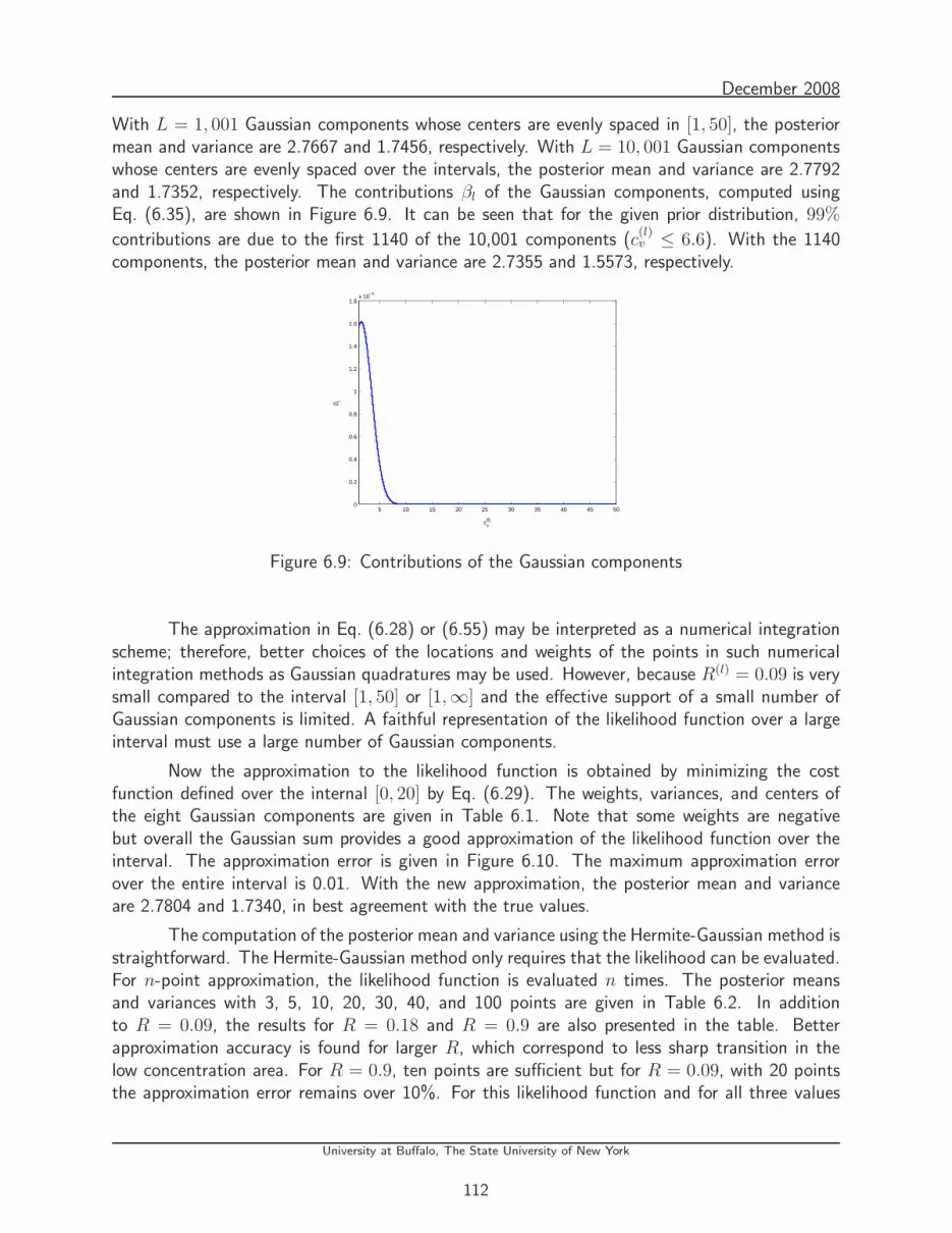
December 2008
With L = 1, 001 Gaussian components whose centers are evenly spaced in [1, 50], the posteriormean and variance are 2.7667 and 1.7456, respectively. With L = 10, 001 Gaussian componentswhose centers are evenly spaced over the intervals, the posterior mean and variance are 2.7792and 1.7352, respectively. The contributions βl of the Gaussian components, computed usingEq. (6.35), are shown in Figure 6.9. It can be seen that for the given prior distribution, 99%
contributions are due to the first 1140 of the 10,001 components (c(l)v ≤ 6.6). With the 1140
components, the posterior mean and variance are 2.7355 and 1.5573, respectively.
5 10 15 20 25 30 35 40 45 500
0.2
0.4
0.6
0.8
1
1.2
1.4
1.6
1.8x 10
−3
cv(l)
β l
Figure 6.9: Contributions of the Gaussian components
The approximation in Eq. (6.28) or (6.55) may be interpreted as a numerical integrationscheme; therefore, better choices of the locations and weights of the points in such numericalintegration methods as Gaussian quadratures may be used. However, because R(l) = 0.09 is verysmall compared to the interval [1, 50] or [1,∞] and the effective support of a small number ofGaussian components is limited. A faithful representation of the likelihood function over a largeinterval must use a large number of Gaussian components.
Now the approximation to the likelihood function is obtained by minimizing the costfunction defined over the internal [0, 20] by Eq. (6.29). The weights, variances, and centers ofthe eight Gaussian components are given in Table 6.1. Note that some weights are negativebut overall the Gaussian sum provides a good approximation of the likelihood function over theinterval. The approximation error is given in Figure 6.10. The maximum approximation errorover the entire interval is 0.01. With the new approximation, the posterior mean and varianceare 2.7804 and 1.7340, in best agreement with the true values.
The computation of the posterior mean and variance using the Hermite-Gaussian method isstraightforward. The Hermite-Gaussian method only requires that the likelihood can be evaluated.For n-point approximation, the likelihood function is evaluated n times. The posterior meansand variances with 3, 5, 10, 20, 30, 40, and 100 points are given in Table 6.2. In additionto R = 0.09, the results for R = 0.18 and R = 0.9 are also presented in the table. Betterapproximation accuracy is found for larger R, which correspond to less sharp transition in thelow concentration area. For R = 0.9, ten points are sufficient but for R = 0.09, with 20 pointsthe approximation error remains over 10%. For this likelihood function and for all three values
University at Buffalo, The State University of New York
112

December 2008
Table 6.1: Gaussian sum approximation parameters
αl c(l)v R(l)
1 -1.0789 0.2530 3.4970
2 2.4323 0.3016 0.2509
3 1.4780 1.7946 1.8556
4 -5.4721 0.5602 0.3516
5 2.7054 0.9121 0.2982
6 3.8470 3.8091 8.1734
7 6.5080 9.0844 18.6352
8 16.9385 19.8336 48.9650
0 2 4 6 8 10 12 14 16 18 20−0.01
−0.005
0
0.005
0.01
0.015
Concentration
App
roxi
mat
ion
Err
or
Figure 6.10: Approximation error of the likelihood function
of R, the Hermite-Gaussian method with three points does not yield satisfactory accuracy. Arelatively large number of points is needed in the integral approximation partly because the pointsare chosen solely based on the prior distribution.
6.2.5 Remarks
The data fusion methods are used to combine the predicted concentration with the binary chem-ical sensor measurements. The results of the Hermite-Gaussian method contain relatively largeerrors when the likelihood function has a sharp transition. This is not surprising because theHermite-Gaussian method chooses the points where the likelihood function is evaluated solelybased on the prior distribution. In the Gaussian sum method, two approaches to approximatingthe likelihood function are considered. In the first approach, the variances of the Gaussian com-ponents are predetermined to be 0.09, the variance from the chemical sensor model. Becausethe supports of all the Gaussian components are small, hundreds of Gaussian components areneeded to achieve good approximation of the likelihood function and good estimates of the pos-
University at Buffalo, The State University of New York
113
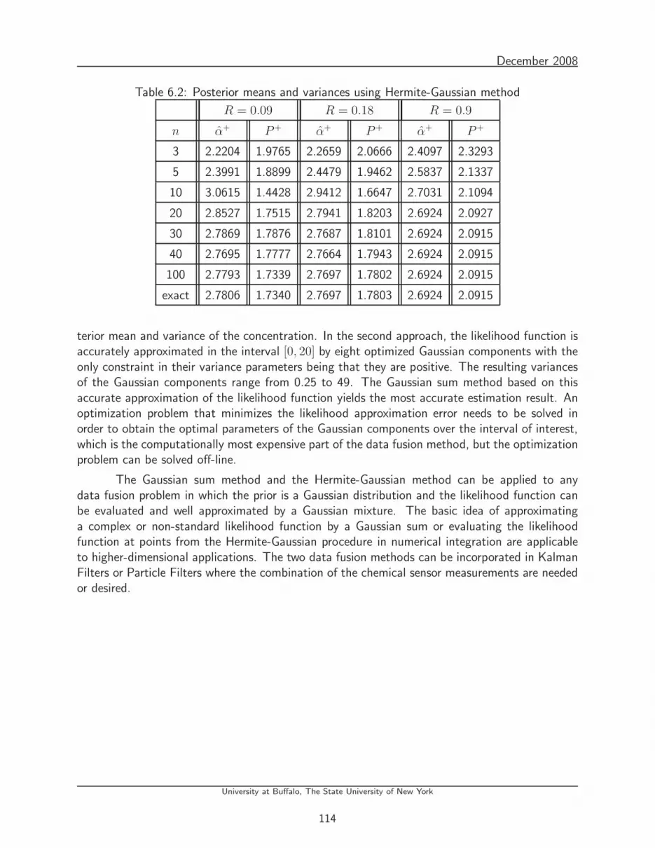
December 2008
Table 6.2: Posterior means and variances using Hermite-Gaussian method
R = 0.09 R = 0.18 R = 0.9
n α+ P+ α+ P+ α+ P+
3 2.2204 1.9765 2.2659 2.0666 2.4097 2.3293
5 2.3991 1.8899 2.4479 1.9462 2.5837 2.1337
10 3.0615 1.4428 2.9412 1.6647 2.7031 2.1094
20 2.8527 1.7515 2.7941 1.8203 2.6924 2.0927
30 2.7869 1.7876 2.7687 1.8101 2.6924 2.0915
40 2.7695 1.7777 2.7664 1.7943 2.6924 2.0915
100 2.7793 1.7339 2.7697 1.7802 2.6924 2.0915
exact 2.7806 1.7340 2.7697 1.7803 2.6924 2.0915
terior mean and variance of the concentration. In the second approach, the likelihood function isaccurately approximated in the interval [0, 20] by eight optimized Gaussian components with theonly constraint in their variance parameters being that they are positive. The resulting variancesof the Gaussian components range from 0.25 to 49. The Gaussian sum method based on thisaccurate approximation of the likelihood function yields the most accurate estimation result. Anoptimization problem that minimizes the likelihood approximation error needs to be solved inorder to obtain the optimal parameters of the Gaussian components over the interval of interest,which is the computationally most expensive part of the data fusion method, but the optimizationproblem can be solved off-line.
The Gaussian sum method and the Hermite-Gaussian method can be applied to anydata fusion problem in which the prior is a Gaussian distribution and the likelihood function canbe evaluated and well approximated by a Gaussian mixture. The basic idea of approximatinga complex or non-standard likelihood function by a Gaussian sum or evaluating the likelihoodfunction at points from the Hermite-Gaussian procedure in numerical integration are applicableto higher-dimensional applications. The two data fusion methods can be incorporated in KalmanFilters or Particle Filters where the combination of the chemical sensor measurements are neededor desired.
University at Buffalo, The State University of New York
114

Chapter 7
Summary
The main accomplishments of the work are summarized as follows:
1. Nonlinear filters, in particular Particle Filters, are developed that are suitable for puff-baseddispersion models whose state dimension varies with time such as SCIPUFF.
2. Unscented Kalman smoothers are developed for puff-based dispersion models, permittingmore accurate offline dosage estimation than available with online filters.
3. Gaussian mixture-based methods are developed for accurate model propagation of highlynonlinear systems using a novel weight-adaptation scheme.
4. A software model for chemical sensors with bar readings is developed and data fusionalgorithms for bar sensors are developed.
As a consequence of this work, practical real time data assimilation for chemical incidentplume prediction using modern Monte Carlo techniques which are tolerant of severe nonlinearities,high dimensionality and variable state dimension are feasible. Further work in this direction isunderway.
115

Bibliography
[1] Thykier-Nielsen, S., S.Deme, and Mikkelsen, T., “Description of the Atmospheric Disper-sion Module RIMPUFF,” Tech. Rep. RODOS(WG2)-TN(98)-02, Riso National Laboratory,Roskilde, Denmark, 1999.
[2] http://www.epa.gov/scram001/dispersionindex.htm.
[3] Whelpdale, D. M., Methods for Assessing Exposure of Human and Non-Human Biota, chap.Geographically-Placed Atmospheric Models, John Wiley and Sons Ltd., 1991.
[4] European Union Joint Research Centre (JRC), “Features of Dispersion Models,” 2004.
[5] Sykes, R., Parker, S., Henn, D., and Chowdhury, B., “SCIPUFF Version 2.2 TechnicalDocumentation,” Tech. Rep. 729, L-3 Titan Corporation, 2006.
[6] http://pandora.meng.auth.gr/mds/strquery.php?wholedb.
[7] Committee on the Atmospheric Dispersion of Hazardous Material Releases and National Re-search Council, Tracking and Predicting the Atmospheric Dispersion of Hazardous MaterialReleases: Implications for Homeland Security , The National Academies Press, US, 2003.
[8] Boris, J., “The Threat of Chemical and Biological Terrorism: Preparing a Response,” Com-puting in Science and Engineering , Vol. 4, No. 2, 2002, pp. 22–32.
[9] Settles, G. S., “Fluid Mechanics and Homeland Security,” Annual Review in Fluid Mechanics,Vol. 38, 2006, pp. 87–110.
[10] Fuller, A. T., “Analysis of Nonlinear Stochastic Systems by Means of the Fokker-PlanckEquation,” International Journal of Control , Vol. 9, 1969, pp. 6.
[11] Risken, H., The Fokker-Planck Equation: Methods of Solution and Applications, Springer,1989, 1-12, 32-62.
[12] Kumar, M., Singla, P., Chakravorty, S., and Junkins, J. L., “A Multi-Resolution Approachfor Steady State Uncertainty Determination in Nonlinear Dynamical Systems,” 38th South-eastern Symposium on System Theory , 2006.
[13] Kumar, M., Singla, P., Chakravorty, S., and Junkins, J. L., “The Partition of Unity FiniteElement Approach to the Stationary Fokker-Planck Equation,” 2006 AIAA/AAS Astrody-namics Specialist Conference and Exhibit, Keystone, CO , Aug. 21-24, 2006.
116

December 2008
[14] Muscolino, G., Ricciardi, G., and Vasta, M., “Stationary and Non-stationary ProbabilityDensity Function for Nonlinear Oscillators,” International Journal of Non-Linear Mechanics,Vol. 32, 1997, pp. 1051–1064.
[15] Paola, M. D. and Sofi, A., “Approximate Solution of the Fokker-Planck-Kolmogorov Equa-tion,” Probabilistic Engineering Mechanics, Vol. 17, 2002, pp. 369–384.
[16] Anderson, B. D. and Moore, J. B., Optimal Filtering , Prentice-Hall, 1979, 193-222.
[17] Doucet, A., Godsill, S., and Andrieu, C., “On Sequential Monte Carlo Sampling Methodsfor Bayesian Filtering,” Statistics and Computing , Vol. 10, 2000, pp. 197–208.
[18] Iyengar, R. N. and Dash, P. K., “Study of the Random Vibration of Nonlinear Systems by theGaussian Closure Technique,” Journal of Applied Mechanics, Vol. 45, 1978, pp. 393–399.
[19] Roberts, J. B. and Spanos, P. D., Random Vibration and Statistical Linearization, Wiley,1990, 122-176.
[20] Lefebvre, T., Bruyninckx, H., and Schutter, J. D., “Kalman Filters of Non-Linear Systems:A Comparison of Performance,” International Journal of Control , Vol. 77, No. 7, 2004,pp. 639–653.
[21] Lefebvre, T., Bruyninckx, H., and Schutter, J. D., “Comment on A New Method for theNonlinear Transformations of Means and Covariances in Filters and Estimators,” IEEE Trans-actions on Automatic Control , Vol. 47, No. 8, 2002.
[22] Jazwinski, A. H., Stochastic Processes and Filtering Theory , chap. 4-7, Academic Press,San Diego, CA, 1970.
[23] Lewis, J., Lakshmivarahan, S., and Dhall, S., Dynamic Data Assimilation: A Least SquaresApproach, Cambridge University Press, Cambridge, UK, 2006.
[24] Julier, S. J., Uhlmann, J. K., and Durrant-Whyte, H. F., “A New Approach for FilteringNonlinear Systems,” Proceedings of the American Control Conference, Seattle, WA, June1995, pp. 1628–1632.
[25] Wan, E. and van der Merwe, R., “The Unscented Kalman Filter,” Kalman Filtering andNeural Networks, edited by S. Haykin, chap. 7, John Wiley & Sons, New York, NY, 2001.
[26] Evensen, G., “The Ensemble Kalman Filter: Theoretical Formulation and Practical Imple-mentation,” Ocean Dynamics, Vol. 53, 2003, pp. 343–367.
[27] Evensen, G., “Sampling Strategies and Square Root Analysis Schemes for the EnKF,” OceanDynamics, Vol. 54, 2004, pp. 539–560.
[28] Tippett, M. K., Anderson, J. L., Bishop, C. H., Hamill, T. M., and Whitaker, J. S., “En-semble Square-Root Filters,” Monthly Weather Review , Vol. 131, 2002, pp. 1485–1490.
University at Buffalo, The State University of New York
117
December 2008
[29] Hamill, T. M., Whitaker, J. S., and Snyder, C., “Distance-Dependent Filtering of Back-ground Error Covariance Estimates in an Ensemble Kalman Filter,” Monthly Weather Re-view , Vol. 129, 2001, pp. 2776–2790.
[30] Ristic, B., Arulampalam, S., and Gordon, N., Beyond the Kalman Filter: Particle Filters forTracking Applications, chap. 3, Artech House, Boston, MA, 2004.
[31] Daum, F. and Huang, J., “Curse of Dimensionality and Particle Filters,” Proceedings of theIEEE Aerospace Conference, Vol. 4, Big Sky, MT, March 2003, pp. 1979–1993.
[32] Incropera, F. P. and Dewitt, D. P., Fundamentals of Heat and Mass Transfer, Third Edition,John Wiley and Sons Ltd., US, 1990.
[33] Kolditz, O., Computational Methods in Environmental Fluid Mechanics, chap. 6, Springer,Berlin, 2002.
[34] Bar-Shalom, Y., Li, X. R., and Kirubarajan, T., Estimation with Applications to Trackingand Navigation, John Wiley & Sons, 2001.
[35] Holmes, N. and Morawska, L., “A Review Of Dispersion Modelling And Its ApplicationTo The Dispersion Of Particles: An Overview Of Different Dispersion Models Available,”Atmospheric Environment, Vol. 40, No. 30, 2006, pp. 5902–5928.
[36] Reddy, K., Y.Cheng, T.Singh, and P.D.Scott, “Data Assimilation For Dispersion Models,”The 9th International Conference on Information Fusion, Florence, Italy , 2006.
[37] Krysta, M., Bocquet, M., Sportisse, B., and Isnard, O., “Data Assimilation for Short-Range Dispersion Of Radionuclides: An Application To Wind Tunnel Data,” AtmosphericEnvironment, Vol. 40, No. 38, 2006, pp. 7267–7279.
[38] Biltoft, C. A., “Dipole Pride 26: Phase II of Defense Special Weapons Agency Transport andDispersion Model Validation,” Tech. rep., Army Dugway Proving Ground, UT, Jan 1998.
[39] Chang, J. C., Franzese, P., Chayantrakom, K., and Hanna, S. R., “Evaluations of CALPUFF,HPAC, and VLSTRACK with Two Mesoscale Field Datasets,” Journal of Applied Meteorol-ogy , Vol. 42, 2003, pp. 453–466.
[40] Cox, R. M., Sontowski, J., and Dougherty, C. M., “An Evaluation of Three Diagnostic WindModels (CALMET, MCSCIPUF, and SWIFT) with Wind Data from the Dipole Pride 26Field Experiments,” Meteorological Applications, Vol. 12, 2006, pp. 329–341.
[41] Chang, J. C., Uncertainty and Sensitivity of Dispersion Model Results to MeteorologicalInputs, Two Case Studies, chap. 9, Springer-Verlag, 2002.
[42] Rao, S. K., “Uncertainty Analysis in Atmospheric Dispersion Modeling,” Pure and AppliedGeophysics, Vol. 162, 2005, pp. 1893–1917.
[43] Lewellen, W. and Sykes, R., “Meteorological Data Needs for Modeling Air Quality Uncer-tainties,” Journal of Atmospheric and Oceanic Technology , Vol. 6, 1989, pp. 759–768.
University at Buffalo, The State University of New York
118

December 2008
[44] Reddy, K., Y.Cheng, T.Singh, and P.D.Scott, “Data Assimilation in Variable DimensionDispersion Models using Particle Filters,” The 10th International Conference on InformationFusion, Quebec City, Canada, 2007.
[45] Hanna, S., Chang, J., and Strimaitis, D., “Hazardous Gas Model Evaluation with FieldObservations,” Atmospheric Environment, Vol. 27A, 1993, pp. 2265–2285.
[46] Briers, M., Doucet, A., and Maskell, S., “Smoothing Algorithms for State-Space Models,”Submission IEEE Trans. on Signal Processing , 2004.
[47] Julier, S. and Uhlmann, J., “Unscented filtering and nonlinear estimation,” Proceedings ofthe IEEE , Vol. 92, No. 3, Mar 2004, pp. 401–422.
[48] Julier, S., “The Scaled Unscented Transformation,” American Control Conference, Vol. 6,2002, pp. 4555– 4559.
[49] van der Merwe, R., “Sigma-Point Kalman Filters for Probabilistic Inference in DynamicState-Space Models,” Tech. rep., In Workshop on Advances in Machine Learning, Montreal,2003.
[50] van der Merwe, R. and Wan, E., “The Square-Root Unscented Kalman Filter for State andParameter-Estimation,” International Conference on Acoustics, Speech, and Signal Process-ing (ICASSP), Salt Lake City, Utah,, 2001.
[51] Fraser, D. and Potter, J., “The Optimum Linear Smoother as a Combination of Two Opti-mum Linear Filters,” Automatic Control, IEEE Transactions on, Vol. 14, No. 4, Aug 1969,pp. 387–390.
[52] Rauch, H., Tung, F., and Striebel, C., “Maximum Likelihood Estimates of Linear DynamicSystems,” J. Amer. Inst. Aeronautics and Astronautics, Vol. 3 (8), 1965, pp. 1445–1450.
[53] Terejanu, G., Singh, T., and Scott, P., “Unscented Kalman Filter/Smoother for a CBRNPuff-Based Dispersion Model,” The 10th International Conference on Information Fusion,Quebec City, Canada, 2007.
[54] Kailath, T., Sayed, A., and Hassibi, B., Linear Estimation, Prentice Hall, 2000.
[55] Crassidis, J. and Junkins, J., Optimal Estimation of Dynamic Systems, CRC Press, 2004.
[56] Vercauteren, T. and Wang, X., “Decentralized Sigma-Point Information Filters for Tar-get Tracking in Collaborative Sensor Networks,” IEEE Transactions on Signal Processing ,Vol. 53, 2005, pp. 2997– 3009.
[57] Psiaki, M. and Wada, M., “Derivation and Simulation Testing of a Sigma-Points Smoother,”Journal of Guidance, Control, and Dynamics, Vol. 30, 2007, pp. 78–86.
[58] Alspach, D.; Sorenson, H., “Nonlinear Bayesian Estimation Using Gaussian Sum Approxi-mations,” Automatic Control, IEEE Transactions on, Vol. 17, No. 4, 1972, pp. 439–448.
University at Buffalo, The State University of New York
119
December 2008
[59] Ito, K. and Xiong, K., “Gaussian Filters for Nonlinear Filtering Problems,” IEEE Transactionson Automatic Control , Vol. 45, No. 5, May 2000, pp. 910–927.
[60] Gelb, A., Applied Optimal Estimation, M.I.T. Press, 1974.
[61] Petersen, K. B. and Pedersen, M. S., “The Matrix Cookbook,”http://matrixcookbook.com/, Technical Report, 2008.
[62] Honkela, A., “Approximating Nonlinear Transformations of Probability Distributions for Non-linear Independent Component Analysis,” IEEE International Joint Conference on NeuralNetworks, 2004.
[63] Wu, Y., Wu, M., Hu, D., and Hu, X., “An Improvement to Unscented Transformation,”17th Australian Joint Conference on Artificial Intelligence, 2004.
[64] Boyd, S. and Vandenberghe, L., Convex Optimization, Cambridge University Press, 2004,67-78, 152-159.
[65] Singla, P. and Singh, T., “A Gaussian Function Network for Uncertainty PropagationThrough Nonlinear Dynamical System,” 18th AAS/AIAA Spaceflight Mechanics Meeting,Galveston, TX , Jan. 27-31, 2008.
[66] Sorenson, H. W. and Alspach, D. L., “Recursive Bayesian estimation using Gaussian sums,”Automatica, Vol. 7, 1971, pp. 465–479.
[67] Chen, R. and Liu, J., “Mixture Kalman filters,” Journal of the Royal Statistical Society:Series B , Vol. 62, 2000, pp. 493–508.
[68] Bar-Shalom, Y., Li, X. R., and Kirubarajan, T., Estimatio with Applications to Tracking andNavigation, John Wiley & Sons, Inc., 2001.
[69] Curray, R. E., Estimation and Control with Quantized Measurements, chap. 2, MIT Press,Cambridge, MA, 1970.
[70] Lewellen, W. S. and Sykes, R. I., “Analysis of Concentration Fluctuations from Lidar Ob-servations of Atmospheric Plumes,” Journal of Climate and Applied Meteorology , Vol. 25,1986, pp. 1145–1154.
[71] Yee, E., “The Shape of the Probability Density Function of Short-Term Concentration Fluc-tuations of Plumes in The Atmospheric Boundary Layer,” Boundary-Layer Meteorology ,Vol. 51, 1990, pp. 269–298.
[72] Robins, P., Rapley, V., and Thomas, P., “A Probabilistic Chemical Sensor Model for DataFusion,” The Eighth International Conference on Information Fusion, Philadelphia, PA, 2005.
[73] Abramowitz, M. and Stegun, I. A., editors, Handbook of Mathematical Functions withFormulas, Graphs, and Mathematical Tables, chap. 7, 22, 25, Dover, New York, NY, 1965.
University at Buffalo, The State University of New York
120

December 2008
[74] Zoeter, O., Ypma, A., and Heskes, T., “Improved Unscented Kalman Smoothing for StockVolatility Estimation,” 2004 IEEE Workshop on Machine Learning for Signal Processing ,2004, pp. 143–152.
University at Buffalo, The State University of New York
121

Dept. of Atmospheric & Oceanic Physics/Applied Research Laboratory & Meteorology Department
The Pennsylvania State University
University Park, Pennsylvania
1
7: Technical Summ
1. INTRODUCTION
ary of Results (PSU)
Most atmospheric transport and dispersion (AT&D) applications focus on modeling the statistics of the transport and dispersion. That approach recognizes that it is impossible to accurately forecast the details of a particular turbulent flow: atmospheric motion is governed by nonlinear physics that displays sensitivity to initial conditions, leading to unpredictable chaotic flow (Lorenz 1963). Thus, only the stochastic approach is practical if one cannot determine the flow details by other means. This approach predicts the statistics of an ensemble of a large number of realizations, including means, variances, and likely maximum concentrations. The statistical approach is appropriate for traditional regulatory purposes that emphasize meeting standards over a long time period. There are cases, however, where it is critical to instead model the particular realization that is occurring. An example is a scenario where a toxic contaminant is released, either accidentally or intentionally, and it is necessary to predict its transport and dispersion in order to evacuate people in harm’s way and to minimize the impact (NRC 2003). Incorrect concentration predictions could lead to evacuating the wrong areas. In such cases, we need to determine the specific realization from the available data so that the subsequent prediction is as accurate as possible. Although this objective sounds formidable, if there are field sensors to monitor contaminant concentrations, one can use those data to 1) determine the characteristics of the turbulent scenario and 2) assimilate the concentration data into a flow-aware transport and dispersion model. The assimilation process is well documented in meteorology applications where a variety of data assimilation methods are used operationally to improve the quality of the forecast (Daley 1991, Kalnay 2003, Ide et al. 1997). Most of those methods assimilate either the same quantity as observed or ones that are easily derived from the observed quantities. The situation is more complex for assimilating concentration data, however, due to the one-way coupling. In contrast to numerical weather prediction (NWP) models, the system of equations used in the transport and dispersion context is not fully coupled. Although, the wind field drives the concentration field, the contaminant concentration field has no direct influence on the wind field.1 Therefore, the goal is not only to assimilate concentration data into the model to improve the concentration forecast, but also to derive the time dependent wind field from observations of the dispersed contaminant and assimilate them as well. Thus, we require an indirect data assimilation method to infer the wind field from concentration observations. Much of the uncertainty in atmospheric transport and dispersion modeling is due to large scale variations in the wind direction (Peltier et al. 2008). Uncertainty in the wind direction is acknowledged as a source of error when applying an atmospheric transport and dispersion 1 The simplification of one-way coupling assumes that the contaminant particles are sufficiently small to neglect entrainment effects on the flow or gravitational settling, have non-inertial initial conditions, and that it is nonreactive.
2

system in an attempt to match measured field data (Chang et al. 2003) and even in experimental wind tunnel data (Krysta et al. 2006). In fact, even in wind tunnel studies, wind direction can vary sufficiently that it becomes a large source of error in modeling dispersion (Zheng et al. 2007). Therefore, groups who are using sensor concentration data to back-calculate source characteristics are also finding it necessary to additionally back-calculate the wind information (Krysta et al. 2006, Allen et al. 2007, Haupt et al. 2007, Long et al. 2008). Deng et al. (2004), Davakis et al. (2007), and Lee et al. (2008) showed that when meteorological data assimilation is incorporated into a numerical weather prediction model that forces a transport and dispersion model, the concentration predictions agree better with field monitored values. Several recent studies additionally used assimilation methods to incorporate observations of a chemical species into a dispersion model (Constantiscu et al. 2007, Cheng et al. 2007, Reddy et al. 2007, Terejanu et al. 2007). Stuart et al. (2007) found that assimilating concentration observations into a simple model of sea breeze dynamics coupled with a diffusion equation reduced errors in both the concentration field and in the meteorological fields. Most of this previous work on assimilating concentration data to deduce a meteorological field assumed that the meteorological conditions are constant in time and space. If the wind field varies spatially or temporally, however, as is usually the case, one would infer a wind that is not appropriate to the current time or locale. Then a dynamic data assimilation scheme is required to infer a temporally evolving or spatially varying field. The objectives of this work are to
• review the literature for best practices in multi-sensor data fusion and meteorological data assimilation to determine what methods are most applicable for blending concentration measurements with atmospheric transport and dispersion models,
• analyze the fundamental similarities and differences between multi-sensor data fusion and meteorological data assimilation,
• apply the most promising methods to AT&D problems to test which can be adapted to the one-way coupled problems,
• evaluate and develop methods for reconstructing unknown model input parameters given concentration measurements, and
• develop a paradigm for using assimilation techniques for source term estimation.
The remainder of this technical report describes our progress. Section 2 describes the forward assimilation problem by introducing a mathematical framework, demonstrating the feasibility of assimilating concentration data into a variable wind field, then summarizes a study of several different assimilation methods applied to the TusseyPuff system. The source characterization problem is detailed in section 3. We show how not only can a method be formulated to back-calculate source parameters, but we can also back-calculate unknown meteorological parameters. We analyze the behavior of the model in the presence of noise and when data is sparse, look at dependence on sensor characteristics, and study the impact of boundary layer depth on the model’s ability to compute the input parameters. Finally, an alternate method, BackHOE is detailed. Section 4 compares and contrasts the techniques of data assimilation and sensor data fusion. That section presents an analytical framework for the problem then gives a numerical analysis of the workings of both types of methods. A paradigm for data assimilation developed in
3

tshe context of the source term estimation problem is described in section 5. Section 6 provides a ummary and discussion of the relevance of our findings.
2. FORWARD ASSIMILATION OF CONCENTRATION DATA INTO ATMOSPHERIC TRANSPORT AND DISPERSION MODELS 2.1 Mathematical description The simplest way to pose the time rate of change of a dynamical system (our transport and dispersion model in this case) is:
∂
t= +
∂x Mx η
(1)
where x represents the predictands (concentration and wind), t
∂∂x
η
is their time rate of change or
tendency, M is a linearized operator based on the potentially nonlinear dynamics, and is a stochastic noise term representing the errors in the model and the unresolved subgrid processes. One way to look at incorporating observations into the model is:
∂ ( )G
t= + +
∂0 fx Mx η x , x
0x x
(2)
where is the observed value of the field and is the forecast field. G is an adjustment function that specifies how the field is to be “nudged” toward the observations. If G is applied sufficiently gradually, the dynamical system has a chance to adjust toward an equilibrium state that is consistent with the observations. Note the implications if M is replaced or augmented by a nonlinear operator as is the case for most fluid dynamics models. In that case, nonlinear dynamical systems theory applies, meaning that there may be system behaviors such as bifurcations, multiple equilibria, and sensitivity to initial conditions.
f
Our goal is to define an optimal G for problems in atmospheric transport and dispersion. There are numerous ways to do that. This is the problem that both NWP assimilation techniques and sensor data fusion techniques strive to solve. Our objectives are to: 1) define the essential dynamics, M, of Eq. (1) for this problem and 2) find ways of computing the functional operator
4
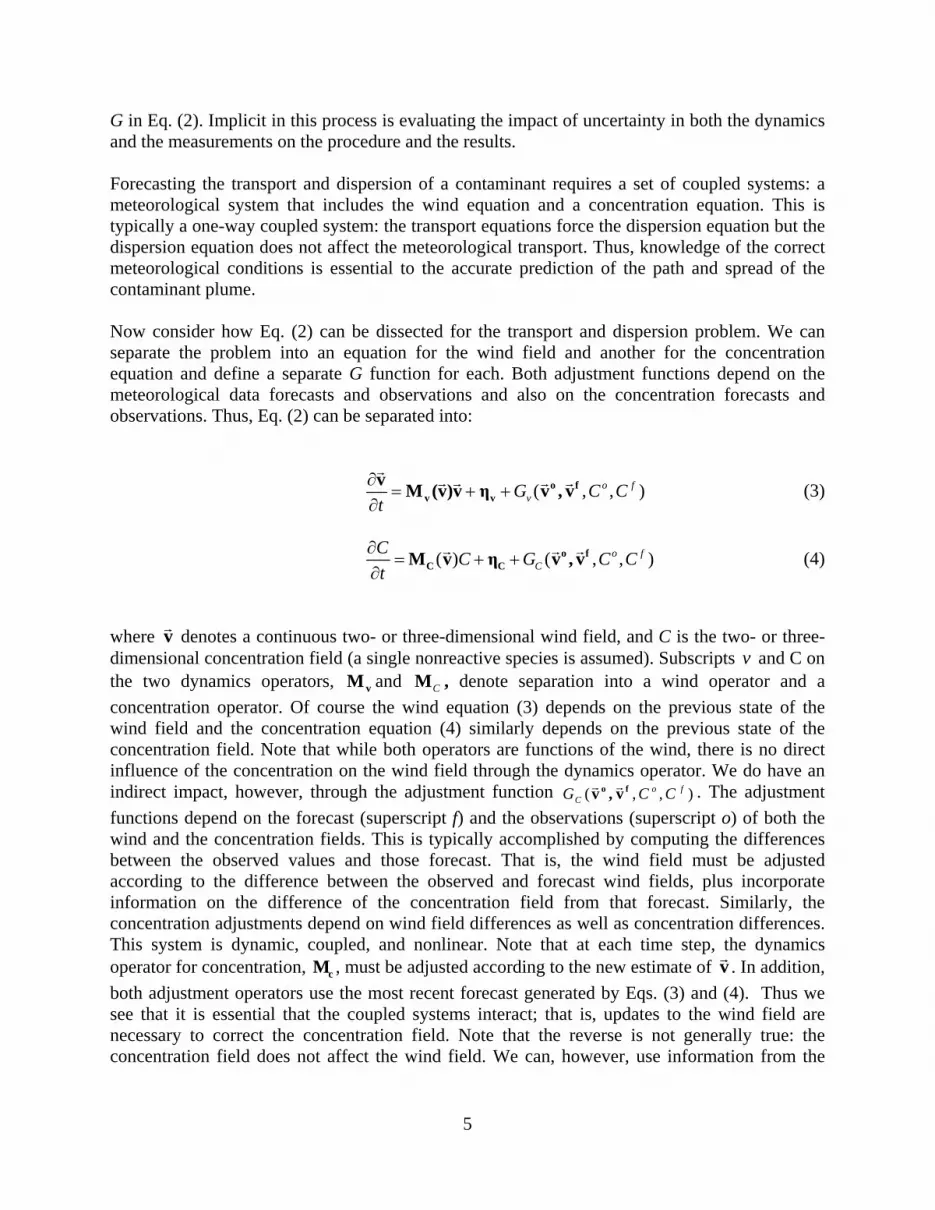
G in Eq. (2). Implicit in this process is evaluating the impact of uncertainty in both the dynamics and the measurements on the procedure and the results. Forecasting the transport and dispersion of a contaminant requires a set of coupled systems: a meteorological system that includes the wind equation and a concentration equation. This is typically a one-way coupled system: the transport equations force the dispersion equation but the dispersion equation does not affect the meteorological transport. Thus, knowledge of the correct meteorological conditions is essential to the accurate prediction of the path and spread of the contaminant plume. Now consider how Eq. (2) can be dissected for the transport and dispersion problem. We can separate the problem into an equation for the wind field and another for the concentration equation and define a separate G function for each. Both adjustment functions depend on the meteorological data forecasts and observations and also on the concentration forecasts and observations. Thus, Eq. (2) can be separated into:
( , ,o fvG C C
t∂
= + +∂
o fv v
v M (v)v η v , v )r
r r r r (3)
( ) ( , , )o fC
C C G C Ct
∂= + +
∂o f
C CM v η v , vr r r (4)
where denotes a continuous two- or three-dimensional wind field, and C is the two- or three-dimensional concentration field (a single nonreactive species is assumed). Subscripts v and C on the two dynamics operators, and , denote separation into a wind operator and a concentration operator. Of course the wind equation (3) depends on the previous state of the wind field and the concentration equation (4) similarly depends on the previous state of the concentration field. Note that while both operators are functions of the wind, there is no direct influence of the concentration on the wind field through the dynamics operator. We do have an indirect impact, however, through the adjustment function
vr
vM CM
( , ,o fCG Co fv , v )Cr r . The adjustment
functions depend on the forecast (superscript f) and the observations (superscript o) of both the wind and the concentration fields. This is typically accomplished by computing the differences between the observed values and those forecast. That is, the wind field must be adjusted according to the difference between the observed and forecast wind fields, plus incorporate information on the difference of the concentration field from that forecast. Similarly, the concentration adjustments depend on wind field differences as well as concentration differences. This system is dynamic, coupled, and nonlinear. Note that at each time step, the dynamics operator for concentration, , must be adjusted according to the new estimate of . In addition, both adjustment operators use the most recent forecast generated by Eqs. (3) and (4). Thus we see that it is essential that the coupled systems interact; that is, updates to the wind field are necessary to correct the concentration field. Note that the reverse is not generally true: the concentration field does not affect the wind field. We can, however, use information from the
cM vr
5

concentration field to infer the wind field then adjust it through ( , ,o fvG C Co fv , v )r r , the topic
addressed in this work. 2.2 Meandering plume example Gaussian dispersion in a meandering wind field is used as a first testbed for our assimilation methods here. Such a configuration is simple, it varies smoothly in time and space, and it represents an important realizable state of the atmosphere. Meandering wind conditions are particularly common during nocturnal stable boundary layer conditions (Hanna 1983, Mahrt 1999, among others). It is also analogous to vertical plume meandering observed in unstable direct numerical simulations in the convective boundary layer (Liu and Leung 2005). Here two methods are demonstrated for this problem. The first represents the concentration puff as an entity and extracts its features to use in nudging the wind field to that observed. The second models the concentration observations as a field variable then applies a genetic algorithm to produce a forecast that best matches those observed.
2.2.1 Feature Extraction with Nudging One data assimilation technique frequently used in NWP applications is Newtonian Relaxation or Nudging (Hoke and Anthes 1976). Nudging provides one of the simplest possible implementations of the adjustment function G in Eqs. (3) and (4). The difference between the forecast and observations, weighted by a nudging coefficient is added to the model budget equations. Thus, observations are inserted directly into the model and the model state is slowly relaxed towards these observations. Nudging is easily applied to those variables that are modeled explicitly. It is a bit more difficult for our application, however, because concentration data is to be used to improve the wind field. Thus, we require a method to couple the concentration field back to the wind field. Here this coupling is achieved by applying feature extraction to the concentration observations to infer errors in the wind field. As applied here, feature extraction assumes that the concentration field can be represented by a single Gaussian puff. We must fit the location of the maximum concentration, the maximum concentration value, and the spread to the observed field. The wind field error estimates are extracted by taking the difference between the forecast and observed concentration field. The steepest gradient in this difference field provides a direction that is used as the observation of the wind direction in the assimilation scheme. This feature extraction method is a crude, but nonetheless, effective way to couple the concentration field to the wind field. Combining Feature Extraction With Nudging (FEWN) provides a strategy that is both simple to implement and computationally efficient. The wind forecast is nudged at each assimilation step by:
ff
1−=
ττvv rr (5)
6
)( 11of
nudgeff G θθθθ τττ −+= −− (6)
where the wind speed, vr , is assumed constant at every time step τ . The forecast of the wind direction, , is based on the wind direction forecast of the previous time step, , and the adjustment function – the weighted difference between the forecast, , and the observation,
, that is determined by feature extraction. The relaxation timescale or nudging coefficient, , which acts as a proportionality constant in the adjustment term, is always positive and is
chosen so that the nudging tendencies are relatively small compared to the other terms in the prognostic equations (Stauffer and Seaman 1993). In this study G is taken to be fixed in space and time. A sensitivity study was conducted to determine an appropriate value for the nudging coefficient.
fτθ
f1−τθ
f1−τθ
oθGnudge
nudge
2.2.2 Assimilation with a Genetic Algorithm In the second assimilation method, we seek to directly optimize the wind direction to produce a predicted concentration field closest to that monitored. This method is most akin to the variational approaches to assimilation (for example see Sasaki 1970 or Kalnay 2003), but rather than using the variational formalism, it directly optimizes the match. We choose the continuous genetic algorithm (GA) as our optimization tool. The GA is an artificial intelligence optimization method inspired by the biological processes of genetic recombination and evolution. It begins with a population of potential solutions and evolves them closer to the correct solution through the implementation of mating and mutation operators. The GA in general and the continuous parameter version used here are described in detail in Haupt and Haupt (2004). As with the FEWN technique presented above, the GA-variational approach to assimilation is applied dynamically. We assume that we have already modeled the past dispersion history and seek to assimilate the most recent concentration observations into the transport and dispersion model. This is a two step process: 1) we use the current concentration measurements to compute the optimal wind direction and 2) we use that wind direction to forecast the location of the plume at the next observation time.
2.2.3 Results of Assimilation in Meandering Plume Both the FEWN method and the GA-variational approach are applied to a concentration puff model using the same model time step (20 s) and the full observational grid (41 x 41), plotted every fifth time step in Figure 1a. Puff concentration predicted for the meandering puff using FEWN appears as Figure 1b, and with the GA-variational technique in Figure 1c. The field-based technique (Figure 1c) is nearly indistinguishable from the original data. Although FEWN does not predict concentrations quite as closely, it is still remarkable in its ability to capture the wind direction shifts.
7

a) b) c)
Figure 1. Series of concentration puff locations in meandering wind field calculated with a time step of 20 s, plotted every 100 s for visualization for a total time of 1000 s. a) original data created for comparison, b)
puffs assimilated via FEWN, and c) puffs assimilated with the GA-variational technique. Figure 2a shows the true, FEWN, and GA computed wind direction (at each time step) for the same assimilation setup. The wind diagnosed by feature extraction is relatively close to the truth and nudging keeps the wind direction in tandem with the true wind direction. The GA approach produces smoother time trajectories than the FEWN method because the wind direction is computed directly from all observations rather than extracted by tracking a single feature. The solution is ill-posed at the first sample time because there is not yet sufficient puff spread to reach the sensor grid; hence, there is a large wind direction error at this time. After the first time step, the GA curve is indistinguishable from the truth curve. Figure 2b shows the locations of the puff centroid plotted as a trajectory in time. Despite the minor numerical oscillations about the truth, the puff centerline is tracked well in the FEWN analysis. The GA curve is smoother, however, and follows the truth more exactly than that for FEWN. Thus, the GA method is more precise than FEWN, but the computer time required to optimize the match is much greater. The biggest advantage of the GA method is that it does not rely on identifying features, but instead compares entire fields of concentration data. We conclude that the FEWN approach to assimilating concentration is successful, computationally fast, and shows promise in situations where we can define discrete features that can be tracked.
8

a) b)
Figure 2. a) Wind direction as a function of time for full spatial and temporal resolution for the truth (solid black), as computed from FEWN (dashed dot red), and the GA-variational technique (dashed blue) and b)
location of the puff centroid plotted as a trajectory in time for full spatial and temporal resolution comparing the three (same markings).
The results above have demonstrated success at using concentration observations to infer a meteorological variable, in this case wind direction, to assimilate into the wind equation (3). That assimilated variable then forces the prognostic concentration equation (4). Haupt et al. (2008) also addresses issues of how many concentration observations are necessary to correctly infer the wind direction in terms of both spatial and temporal data denial for both techniques studied here. These results, while preliminary, show promise for predicting the transport and dispersion of a contaminant in a time varying wind field. They also provide hope for being able to model elements of a specific realization of concentration dispersion if sufficient concentration observations are available. The data make it possible to determine the realization, allowing a more accurate prediction in spite of the one-way coupling of the wind and concentration models. Future work will extend the model to a more complex wind field. 2.3 Assimilating Concentration and Wind Data into a Coupled Shallow Water Wind and Dispersion System The second study of forward assimilation compares the performance of the conventional data assimilation techniques used in NWP applied in an unconventional framework introducing the assimilation of both wind and concentration observations (Beyer-Lout et al. 2008). For this purpose a simple two-dimensional wind model is coupled with a basic transport and dispersion model. The performance of the data assimilation techniques is assessed through a series of identical twin experiments. After the assimilation period, wind and concentration forecasts are compared for different observational network setups and densities. The goal is to find a data assimilation method that improves the forecast not only of the hazardous contaminant but also of the wind field. Moreover, it must do so in a timely enough fashion to be of use in CBRN emergency situations.
9
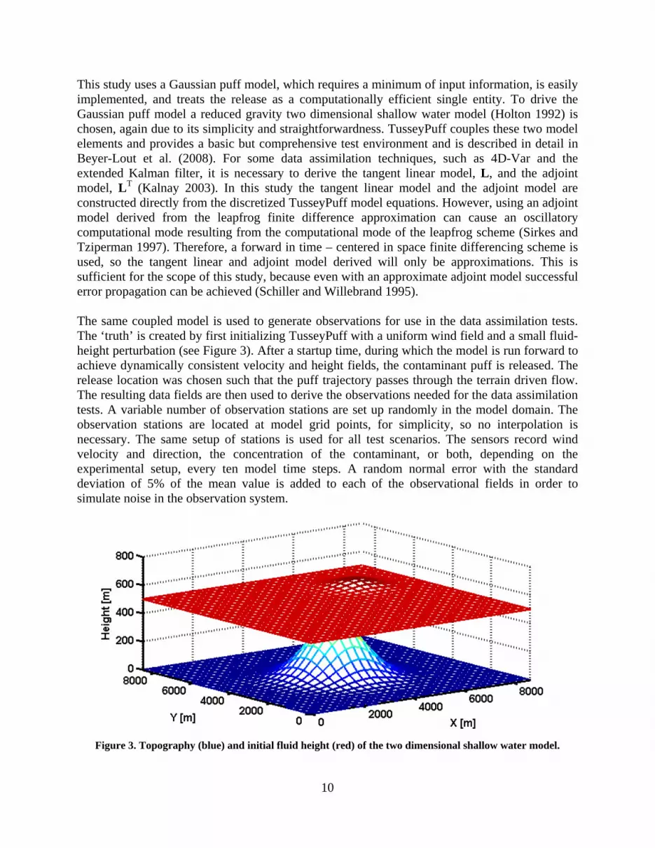
This study uses a Gaussian puff model, which requires a minimum of input information, is easily implemented, and treats the release as a computationally efficient single entity. To drive the Gaussian puff model a reduced gravity two dimensional shallow water model (Holton 1992) is chosen, again due to its simplicity and straightforwardness. TusseyPuff couples these two model elements and provides a basic but comprehensive test environment and is described in detail in Beyer-Lout et al. (2008). For some data assimilation techniques, such as 4D-Var and the extended Kalman filter, it is necessary to derive the tangent linear model, L, and the adjoint model, LT (Kalnay 2003). In this study the tangent linear model and the adjoint model are constructed directly from the discretized TusseyPuff model equations. However, using an adjoint model derived from the leapfrog finite difference approximation can cause an oscillatory computational mode resulting from the computational mode of the leapfrog scheme (Sirkes and Tziperman 1997). Therefore, a forward in time – centered in space finite differencing scheme is used, so the tangent linear and adjoint model derived will only be approximations. This is sufficient for the scope of this study, because even with an approximate adjoint model successful error propagation can be achieved (Schiller and Willebrand 1995). The same coupled model is used to generate observations for use in the data assimilation tests. The ‘truth’ is created by first initializing TusseyPuff with a uniform wind field and a small fluid-height perturbation (see Figure 3). After a startup time, during which the model is run forward to achieve dynamically consistent velocity and height fields, the contaminant puff is released. The release location was chosen such that the puff trajectory passes through the terrain driven flow. The resulting data fields are then used to derive the observations needed for the data assimilation tests. A variable number of observation stations are set up randomly in the model domain. The observation stations are located at model grid points, for simplicity, so no interpolation is necessary. The same setup of stations is used for all test scenarios. The sensors record wind velocity and direction, the concentration of the contaminant, or both, depending on the experimental setup, every ten model time steps. A random normal error with the standard deviation of 5% of the mean value is added to each of the observational fields in order to simulate noise in the observation system.
Figure 3. Topography (blue) and initial fluid height (red) of the two dimensional shallow water model.
10
This study does not assimilate the continuous concentration fields, but rather the four puff parameters, the puff center x and y , the puff spread σ, and the puff concentration amplitude, q. These puff parameters are derived from the continuous concentration field by fitting a Gaussian distribution to the observations. While computationally more efficient than assimilating the continuous concentration observations, this approach adds uncertainty when the puff is still small and only a few sensors detect concentration. Four different assimilation test scenarios are each assessed at varying sensor densities. For all four scenarios the same sensor array setup is used. In the first test scenario only concentration data is assimilated into the TusseyPuff model. The contaminant source parameters, such as source location and source strength are assumed to be known. In the second test scenario only wind observations are used in the assimilation, again, with known source parameters. For the third and fourth test scenarios both wind and concentration observations are assimilated into the TusseyPuff system. In the third scenario the source parameters are known. In contrast to the other scenarios, in the fourth scenario the source parameters are among those quantities sought. As with the other quantities being sought, the initial values of the source parameters are contaminated with errors that the assimilation methods must eliminate. The prescribed error in the source location is taken to be 2400 m and the source strength is overestimated by 100%. For our purposes, i.e. the prediction of transport and dispersion of a CBRN release, a flexible assimilation method is needed, not only to improve the accuracy of a forecast with time dependent observational data, but also to use the CBRN concentration data to modify and correct the predicted wind field and vice versa. Some of the more advanced, frequently used data assimilation techniques in NWP applications include optimal interpolation (Gandin 1963), three-dimensional (Sasaki 1970) and four dimensional variational analysis (3D and 4D-Var) (Lewis and Derber 1985), extended Kalman filtering (Kalman and Bucy 1961), ensemble Kalman filtering (Houtekamer and Mitchell 1998), and Newtonian relaxation (Nudging) (Hoke and Anthes 1976). Both of the Kalman filter techniques, 4D-Var, and Nudging are structured to fit our needs. Therefore, these four data assimilation techniques are tested with the TusseyPuff model. Nudging is a computationally efficient technique that relaxes the model state toward the observations by adding an artificial tendency term to the prognostic equations (Stauffer and Seaman 1993). The Kalman filter technique assimilates the observations sequentially each time step during the model run (Caya et al. 2005). However, instead of subtracting a fixed fraction of the model error at each assimilation step, the weight for the increment is calculated so that it minimizes the forecast error (Kalman and Bucy 1961). The extended Kalman filter is a variant of the Kalman filter that can be used for nonlinear problems (Miller et al. 1994) and is hence suitable for transport and dispersion applications. A promising simplification of the extended Kalman filter is the ensemble Kalman filter (Kalnay 2003). In this approach an ensemble of data assimilation cycles is carried out simultaneously. The ensemble Kalman filter does not specifically integrate the forecast error covariance forward in time, but instead computes it diagnostically from the spread of the model states across the ensemble (Houtekamer and Mitchell 1998). Unlike the Kalman filters and Nudging, four-dimensional variational analysis (4D-Var) does not assimilate observations sequentially each time step. 4D-Var tries instead to find the optimal analysis that best fits the background field and all the observations by minimizing a scalar cost function (Lewis and Derber 1985). The TusseyPuff prediction model is used as a strong constraint.
)( 0txa
11
The performance of the data assimilation techniques is studied for the coupled TusseyPuff model using observations from a variable number of observation stations randomly located in the model domain. In the first scenario tested, the source parameters are known and only concentration data is assimilated into the TusseyPuff model. Figure 4 shows the root mean squared errors of the puff center location (RP), the root mean squared errors of the final wind fields (RW), the normalized root mean squared errors of the final concentration fields (RC) depending on the number of observation stations for all four different data assimilation methods tested. The errors of the run without data assimilation (solid black line) serve as reference values. The most significant improvements of the wind and the concentration fields are achieved by the extended and the ensemble Kalman filter for a large number of observation stations (see Figure 4). However, the performance of the ensemble Kalman filter is inconsistent and it worsened the forecast in two cases. This result may suggest that a larger number of ensemble members are necessary to estimate the forecast error correctly. The Nudging technique, while enhancing the concentration prediction, cannot successfully improve the wind forecast for this test scenario. The same is true for the 4D-Var assimilation scheme. The performance of all data assimilation methods decreases with decreasing observational density. As the number of concentration observations decreases so does the quality of the puff parameter estimates, because there are fewer observations in the puff upon which to base the estimates. With a further decrease in the number of observation stations, the odds of the puff even hitting a sensor begin to fall. In the case of ten observation stations, for example, only one observation of the puff is available throughout the whole assimilation period. In the second test scenario, only wind observations are assimilated into the TusseyPuff system (not shown – see Beyer-Lout et al. 2008). The performance of the Kalman filters is not strongly affected by the number of observation stations. For high observational densities Nudging produces the best wind forecast, with the lowest root mean squared error of the wind field. The larger wind error of the extended Kalman filter can be explained by the fact that the tangent linear model and the adjoint model do not incorporate topographical effects. The performance of the 4D-Var scheme is comparable to the other data assimilation methods. In the third test scenario, both wind observations and puff parameters are assimilated into the TusseyPuff system. For this scenario the concentration and wind observations were taken at the same sensor sites. However, a sensitivity study shows that the performance of the data assimilation techniques is similar when the observation stations are not co-located. As before, the extended and the ensemble Kalman filters produce the best concentration and wind forecasts. The 4D-Var scheme, using 50 iterations in this case, did not perform well. In the fourth scenario, both wind observations and puff parameters are assimilated into the TusseyPuff system. However, in this scenario the release location and the source strength are among those quantities sought and that are contaminated with errors. Both the Nudging scheme and the extended Kalman filter show good improvement across all variables. The performance of the ensemble Kalman filter is again inconsistent. 4D-Var, again using 50 iterations, did not perform as well. In two cases the 4D-Var scheme was unable to find the correct source strength and therefore worsened the concentration forecast significantly.
12
a
b
c
Figure 4. First scenario: assimilation of concentration data; a) Root mean squared errors of the location of the puff center (RP) depending on the number of observation stations; b) Root mean squared errors of the final wind fields (RW) depending on the number of observation stations; c) Normalized root mean squared
errors of the final concentration fields (RC) depending on the number of observation stations.
13

This work has shown that wind and concentration fields can be successfully recovered from measurements of concentration provided that the observations are frequent and dense. Furthermore, it is shown that assimilation of wind data alone, or in combination with the assimilation of sparse observations of contaminant concentration, can improve the concentration and wind forecast significantly. The extended Kalman filter performed consistently well and had the lowest root mean squared errors throughout all of the tested scenarios. However, this technique is computationally expensive and therefore may not be appropriate for a rapid CBRN emergency response system. The ensemble Kalman filter and Nudging produced good results in terms of both the error values and the computer run time. Nudging the coupled model proved especially useful when either wind alone or a combination of wind and concentration data is available. The ensemble Kalman filter provides promising results when only concentration observations are available.
3. SOURCE CHARACTERIZATION AS A METRIC FOR ANALYZING ASSIMILATION METHODS 3.1 Motivation
America’s National Strategy for Homeland Security states that one of the nation’s goals is to respond to and recover from harmful incidents that occur (Homeland Security Office 2007). Such incidents include an intentional release of hazardous chemical, biological, radiological, or nuclear (CBRN) material into the atmosphere. To achieve this it is important to be able to predict the transport and dispersion of these materials. However, sometimes there is inadequate source information to perform those predictions; therefore it becomes necessary to characterize the source of an airborne contaminant from remote measurements of the resulting concentration field. Such characterization of a source involves back-calculating the source location and emission rate. Accurate identification of the source is essential to predicting subsequent transport and dispersion of the contaminant, thus minimizing the impact of a release. However, insufficient spatial and temporal resolution in the meteorological data as well as inherent uncertainty in the wind field makes source term estimation extremely difficult (Figure 5). In addition to characterizing the source, some studies back-calculate meteorological variables relevant to transport and dispersion, such as wind speed, wind direction, and stability.
14
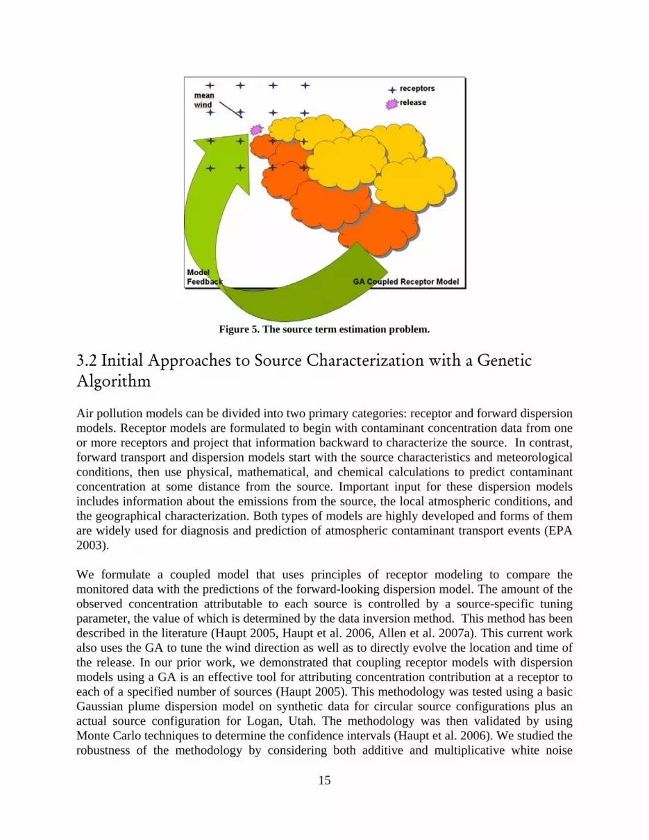
Figure 5. The source term estimation problem.
3.2 Initial Approaches to Source Characterization with a Genetic Algorithm
Air pollution models can be divided into two primary categories: receptor and forward dispersion models. Receptor models are formulated to begin with contaminant concentration data from one or more receptors and project that information backward to characterize the source. In contrast, forward transport and dispersion models start with the source characteristics and meteorological conditions, then use physical, mathematical, and chemical calculations to predict contaminant concentration at some distance from the source. Important input for these dispersion models includes information about the emissions from the source, the local atmospheric conditions, and the geographical characterization. Both types of models are highly developed and forms of them are widely used for diagnosis and prediction of atmospheric contaminant transport events (EPA 2003). We formulate a coupled model that uses principles of receptor modeling to compare the monitored data with the predictions of the forward-looking dispersion model. The amount of the observed concentration attributable to each source is controlled by a source-specific tuning parameter, the value of which is determined by the data inversion method. This method has been described in the literature (Haupt 2005, Haupt et al. 2006, Allen et al. 2007a). This current work also uses the GA to tune the wind direction as well as to directly evolve the location and time of the release. In our prior work, we demonstrated that coupling receptor models with dispersion models using a GA is an effective tool for attributing concentration contribution at a receptor to each of a specified number of sources (Haupt 2005). This methodology was tested using a basic Gaussian plume dispersion model on synthetic data for circular source configurations plus an actual source configuration for Logan, Utah. The methodology was then validated by using Monte Carlo techniques to determine the confidence intervals (Haupt et al. 2006). We studied the robustness of the methodology by considering both additive and multiplicative white noise
15
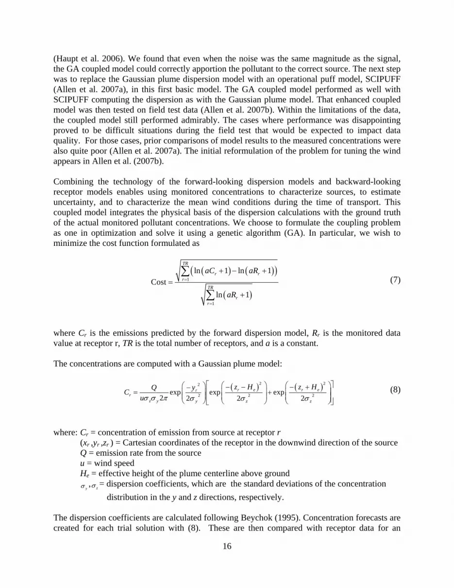
(Haupt et al. 2006). We found that even when the noise was the same magnitude as the signal, the GA coupled model could correctly apportion the pollutant to the correct source. The next step was to replace the Gaussian plume dispersion model with an operational puff model, SCIPUFF (Allen et al. 2007a), in this first basic model. The GA coupled model performed as well with SCIPUFF computing the dispersion as with the Gaussian plume model. That enhanced coupled model was then tested on field test data (Allen et al. 2007b). Within the limitations of the data, the coupled model still performed admirably. The cases where performance was disappointing proved to be difficult situations during the field test that would be expected to impact data quality. For those cases, prior comparisons of model results to the measured concentrations were also quite poor (Allen et al. 2007a). The initial reformulation of the problem for tuning the wind appears in Allen et al. (2007b). Combining the technology of the forward-looking dispersion models and backward-looking receptor models enables using monitored concentrations to characterize sources, to estimate uncertainty, and to characterize the mean wind conditions during the time of transport. This coupled model integrates the physical basis of the dispersion calculations with the ground truth of the actual monitored pollutant concentrations. We choose to formulate the coupling problem as one in optimization and solve it using a genetic algorithm (GA). In particular, we wish to minimize the cost function formulated as
( ) (( ))
( )
1
1
ln 1 ln 1Cost
ln 1
TR
r rr
TR
rr
aC aR
aR
=
=
+ − +=
+
∑
∑ (7)
where Cr is the emissions predicted by the forward dispersion model, Rr is the monitored data value at receptor r, TR is the total number of receptors, and a is a constant.
The concentrations are computed with a Gaussian plume model:
( ) ( )22
2 2 2exp exp exp2 2 2 2
r e r err
z y y z z
z H z HQ yCuσ σ π σ σ σ
2⎡ ⎤⎛ ⎞ ⎛⎛ ⎞ − − − +−= +
⎞⎢ ⎥⎜ ⎟ ⎜⎜ ⎟⎜ ⎟ ⎜ ⎟ ⎜ ⎟⎟⎢ ⎥⎝ ⎠ ⎝ ⎠ ⎝ ⎠⎣ ⎦
(8)
where: Cr = concentration of emission from source at receptor r (xr ,yr ,zr ) = Cartesian coordinates of the receptor in the downwind direction of the source
Q = emission rate from the source u = wind speed He = effective height of the plume centerline above ground
yσ ,zσ = dispersion coefficients, which are the standard deviations of the concentration
distribution in the y and z directions, respectively. The dispersion coefficients are calculated following Beychok (1995). Concentration forecasts are created for each trial solution with (8). These are then compared with receptor data for an
16

arbitrary number of sites. The GA optimizes the combination of source location, strength, and surface wind direction that provides the best match between the monitored receptor data and the expected concentrations as compared by (7). We wish to minimize the cost in (7) using a continuous parameter GA, that is, one in which the parameters are real numbers Here, we use a hybrid GA, which uses the GA to find the correct solution basin, then applies the Nelder-Mead Downhill Simplex (NMDS) method to complete finding the minimum point of that basin. The rationale for this combination is that the GA is sufficiently robust to usually find the basin of the global minima. Once that basin is identified, however, the NMDS finds the bottom of that basin more rapidly. As demonstrated in Haupt et al. (2007), the NMDS method alone is not reliable for finding the global minimum.
The first step is to demonstrate and validate the method of tuning meteorological data and source characteristics. We do this in the context of an identical twin experiment; that is, we generate synthetic data produced by (8) to compute contaminant concentration at the receptors. Using the same dispersion model to generate the synthetic data as is used in the coupled GA system to back-calculate the source parameters enables us to eliminate part of the potential source of variability for the purpose of validating the technique. The receptors are sited on a grid surrounding the source, each separated by 2000 meters. Model runs are performed using 2×2, 4 4, 8×8, 16×16, and 32×32 grids of receptors. For all five receptor configurations, the source is located in the center of the receptor domain at the point defined as the origin (0,0). Synthetic data is produced for each receptor configuration for two different wind directions, 180° and 225°. A wind direction of 180° places the plume centerline directly between receptors, and a wind direction of 225° places the plume centerline directly over some of the receptors.
×
Figure 6 shows the 8×8 receptor grid for the 225° wind direction.
Figure 6. Schematic of receptor grid, pictured with plume from 225°.
Table 1 gives results computed by the GA alone: wind directions, source strengths, source locations, and skill scores for six synthetic configurations. We used a population size of 1,200, mutation rate of 0.01, and 100 iterations for each GA run. The correct solution is θ = (180° or 225°) for our two cases, strength = 1.00, and (x, y) = 0, 0. Skill scores are designed to equally
17

weight the error in wind direction, source strength, and source location. The errors in each parameter are normalized to a [0,1] scale, with a score of 0 given to exact solution, and a score of 1 given when inaccuracy exceeds a predefined upper bound. These scores are then added up to give a final score from 0 to 3, with a score of 0 denoting an exact solution. The GA system was able to find the exact solution given a grid of at least 8×8 receptors. For fewer receptors, such as a 4×4 grid, performance was less satisfactory, as a smaller set of receptors does not provide enough information to distinguish the effect of wind direction from that of the source characteristics. Table 1. GA-produced wind directions, source strengths, source locations, and skill scores for six synthetic configurations using a population size of 1,200, mutation rate of 0.01, after 100 iterations, for one GA run. The correct solution is θ = (180 or 225), strength = 1.00, and (x, y) = (0.0,0.0).
Configuration Strength (x, y) m θ Skill score
8×8, θ=180° 2.96 -417,1346 184.12° 1.4581
8×8, θ=225° 1.06 -26, -56 223.95° 0.1952 16×16, θ=180° 1.00 -1, 0 180.01° 0.0029 16×16, θ=225° 1.00 -1, 1 225.01° 0.0019 32×32, θ=180° 1.00 0, 0 180.00° 0.0000 32×32, θ=225° 1.12 -123,519 220.27° 0.6870
3.3 Source Characterization in a Noisy Environment and with Limited Data The results shown to this point have assumed that the sensors provide perfectly accurate data, the remaining atmospheric variables (except for the wind direction) are exactly known, there is no unrepresented turbulence, and the Gaussian plume model is an accurate representation of the effects of atmospheric dispersion. Of course these assumptions are unreasonable. In reality, we would expect high variability in atmospheric state, the specific realization does not match the ensemble average Gaussian plume model, and the sensors have thresholds and are prone to errors. In addition, the success of the GA in matching the synthetic data runs is partially due to the nature of the identical twin experiment: the synthetic receptor data is computed with the same dispersion model as the expected concentrations. With real data, the dispersion model would not provide a perfect match to the receptor data, as there are discrepancies between ensemble-means being predicted and realization values that are measured. The match is compromised further by monitoring errors. Therefore, the next step in validating the GA model is to contaminate our synthetic data with white noise to simulate the variability and errors present in monitored receptor data. Here, we seek to optimize source term parameters: location, strength, effective height of puff centerline, time of release, as well as meteorological parameters: wind direction and wind speed and to evaluate how much data is necessary to accurately perform the back-claculation. We find that a random search method paired with a gradient descent algorithm is not sufficient to accurately solve this problem when sensor quantities and noise levels are set to realistic values.
18

Thus, a more sophisticated technique is required. Because this problem yields a complex cost surface with multiple local minima, the robustness of the GA is required to identify the basin of the global minimum. A gradient descent method such as the Nelder-Mead Downhill Simplex can then be used to fine tune the solution. We test the limits of the model’s capabilities by completing a comprehensive study of performance over a number of different sensor network setups in an effort to determine the number of sensors required to estimate the source term. For the noiseless studies, the GA model coupled with the Nelder-Mead downhill simplex algorithm is able to correctly identify the source location, strength, wind direction, wind speed, and time of release for grid sizes ranging from 6 x 6 to 64 x 64. Effective height of the puff centerline was found to be difficult to back-calculate. If we were to assume the correct quadrant for the wind, then the number of sensors required would likely be only a quarter of these values. The model is robust and can withstand additive and multiplicative signal-to-noise ratios of 100, 10, and 5. Figure 7 illustrates the skill scores for various model setups for a 180° wind. Note that skill scores of less than 0.01 indicate successful source term estimation.
Figure 7. Skill scores for various model configurations, averaged over 10 runs.
In addition, we have developed a statistic to describe how much noise can be incorporated into a model without compromising its ability to complete the back-calculation. That statistic indicates that the level of noise in the data is the most important factor determining data requirements. Using the Gaussian puff equation as the dispersion model in conjunction with a genetic algorithm, we estimate the source term describing a contaminant emission as well as the transporting wind direction and speed from sensor observations of the time-evolving concentration field. The ensemble average dispersion model, the Gaussian puff equation, is able to successfully assimilate concentration data to match one specific realization of a contaminant release. The basic meteorological data, wind speed and direction, and source information is now
19

available to drive transport and dispersion models to predict the future state of the puff, enhancing situational awareness. More detail is provided in Long et al. (2008). 3.4 Source Term Estimation with Sensor Constraints The goal of this portion of our study is to perform a sensitivity analysis of model enhancements designed to add an element of realism, including considering the likely sensor constraints. This sensitivity analysis is needed because sensor readings are often limited by saturation and detection thresholds. These thresholds censor the data and the effects are important because they distort the observed contaminant field. Thus, the GA must be aware of these thresholds so that it can model the observed data instead of the ideal Gaussian distribution. The Gaussian puff model is used to produce the synthetic concentration observations over five time steps for each of five grid sizes on a 16 km2 domain. Twin data is created by applying the Gaussian puff model to generate concentration observations at grid points. It is then thresholded to simulate detection and saturation levels. Figure 8 shows how the concentration strength varies over five time steps for a 16 x 16 receptor grid before the data is clipped to simulate the saturation and detection levels of the sensors for two different wind directions examined (180° and 270°).
Figure 8. Concentration pattern over five time steps on a 16 x 16 receptor grid. The panel on the left shows
the concentration for with a 180° wind direction and the panel on the right for a 225° wind direction.
20

The detection level is specified with respect to the maximum concentration strength value and any data under that level is set to zero. For a 1x10-16 cutoff, anything smaller than 1x10-16 of the maximum concentration is changed to 0 and the 1x10-12, 1x10⁻⁸, 1x10⁻⁴ thresholds are handled similarly. Saturation level is similarly defined for this study. Any value over a specified percentage of the maximum concentration is clipped to that threshold. For a saturation level of 100% of the maximum concentration, 1 is used as the cutoff value, and similarly for 50%, 10%, and 1%. Examples of the detection and saturation cutoff levels are given in Figure 9 where the maximum concentration in this illustration is 1 kg m-3. After the data is clipped they serve as our true observations.
Figure 9. Data fit to a Gaussian. The maximum concentration normalized to 1 kg m-3. Panel a indicates the threshold detection levels of 1x10-16, 1x10-12, 1x10⁻⁸, and 1x10⁻⁴. Panel b shows the saturation levels, set as a
percentage of the full (100%, 50%, 10%, 1%). After our true observations are made, the GA begins with a random population of “guesses” of the variables that fall within our criteria. They are then compared to our true observations by means of our cost function. We use a population of 40 chromosomes, 640 iterations, and a mutation rate of 0.32: these parameters were shown to converge in Kuroki (2008). The mean absolute errors (MAE) of ten Monte Carlo runs of the median of ten runs for each saturation level were evaluated for each detection level and grid size.
Figure 10 shows the MAE values of the 10 Monte Carlo runs. This figure reflects a 100% saturation level while varying detection levels across the abscissa and varying grid sizes indicated by the line color. In this figure the results for each parameter (wind direction, source strength, and x,y location) are plotted separately.
21

Figure 10. Results for all grid sizes (colored lines) and detection levels (x-axis) of the saturation level at 100%
of the maximum concentration value. Panel a shows the MAE of θ (wind direction, 180°), panel b indicates the MAE of the source strength (1 kg s-1), and panels c and d show the MAE of the location (0, 0) (in m) for x and y respectfully. All of these MAE results are of ten Monte Carlo runs of the median value of ten individual
runs. Figure 10 indicates that the GA retrieves the correct source characteristics for all the detection levels using the 8 x 8, 10 x 10, 12 x 12, and 16 x 16 observation grids. The results for the coarser grids were not as good and were inconsistent. Thresholding the data too severely eliminates so much information that retrieval quality degrades significantly, thus, more dynamic range in sensors leads to more accurate inversion for the variables. This dynamic range produces the most impact if it extends to the maximum concentration as is illustrated in Figure 11. In this figure the detection level is 1x10-16 and the saturation levels vary along the abscissa with the differing grid sizes indicated by the colored lines. In agreement with Figure 10, Figure 11 demonstrates that the larger grid sizes, 8 x 8, 10 x 10, 12 x 12, and 16 x 16, are successful in retrieving the correct parameter values up to the 50% saturation level. It also shows that only the two largest grid sizes (12 x 12 and 16 x 16) can successfully retrieve the parameters at the 10% saturation level. The smaller grid sizes are less reliable after the 50% cutoff and none of the grid sizes are able to correctly identify all of the parameters for the lowest saturation levels.
22

Figure 11. Results for all grid sizes (colored lines) and saturation levels (x-axis) of the detection level at 1x10-16
of the maximum concentration value. Panel a shows the MAE of θ (wind direction, 180°), panel b indicates the MAE of the source strength (1 kg s-1), and panels c and d show the MAE of the location (0, 0) (in m) for x and y respectfully. All of these MAE results are of ten Monte Carlo runs of the median value of ten individual
runs. The hybrid GA method used here (with NMDS) is successful in back-calculating source characteristics and wind direction with data that has been censored forming a clipped Gaussian concentration distribution. These thresholds simulate saturation and detection levels in sensors and, if applied too severely, they eliminate so much information that retrieval quality degrades significantly. The inversion is most successful if the sensor can detect the maximum concentrations, which means that the most effective sensors have this characteristic. More details appear in Rodriguez (2008) and Rodriguez et al. (2008). 3.5 Including the Effects of Boundary Layer Depth In our Genetic Algorithm back-calculation studies reported above, we retrieved source characteristics and relevant meteorological parameters such as mean wind speed and mean wind direction from surface concentration data. Another meteorological parameter that is also relevant in atmospheric transport and dispersion is Atmospheric Boundary Layer (ABL) depth. The ABL depth is an important meteorological parameter because the average depth of the boundary layer
23

gives the average mixing depth of the contaminant (Stull 1988). Further, in convective boundary layers, updrafts and downdrafts loft parcels of air, and the contaminants within the parcels, upwards and downwards. These updrafts and downdrafts have the effect of driving contaminants upward toward the top of the ABL and then sending the contaminants back towards the surface, such that contaminants are “reflected” back towards the surface. Therefore in our Gaussian puff model we add a rigid lid at the top of the boundary layer that reflects contaminants back towards the surface, which is mathematically given by:
(9)
( ) ( )
( )
( ) ( )
∑=
⎥⎥⎦
⎤⎟⎟⎠
⎞⎜⎜⎝
⎛ −+−+⎟⎟
⎠
⎞⎜⎜⎝
⎛ −−−+
⎟⎟⎠
⎞⎜⎜⎝
⎛ +−−+⎟⎟
⎠
⎞⎜⎜⎝
⎛ ++−
+
⎟⎟⎠
⎞⎜⎜⎝
⎛ +−+
⎢⎢⎣
⎡⎟⎟⎠
⎞⎜⎜⎝
⎛ −−×
⎟⎟⎠
⎞⎜⎜⎝
⎛ −−⎟⎟
⎠
⎞⎜⎜⎝
⎛ +−−
Δ=
N
n
z
io
z
io
z
io
z
io
z
o
z
o
y
o
x
o
zyx
σ)nzz(z
σ)nzz(z
σnzzz
σnzzz
zzzz
σyy
σut)(xx
π)(σσu σ
tQC
2
2
2
2
2
2
2
2
2
2
2
2
2
2
2
2
23
22exp
22exp
22exp
22exp
2)(exp
2exp
2exp
2exp
2
σσ
where is the boundary layer depth. N in the summation represents the number of reflections, and the reflection terms also include ground reflections. Notice that the product of n and boundary layer depth appears in the exponential terms implying that as n increases above five subsequent reflection terms will minimally impact surface concentration values.
iz
The ability to retrieve boundary layer depth depends on the length of our horizontal domain; if our domain is too small then the puff will move out of the domain before reflected contaminants affect surface concentration values. Back-calculating boundary layer depth is contingent on the impact of reflected contaminants at the sensor; if no reflected contaminants are present then back-calculating boundary layer depth is impossible. The optimal domain distance is a function of stability, which impacts the spread of the puff in the vertical, and boundary layer depth. When
the value of zσ is equivalent to 15.2
2 oi zz −, surface concentration values are significantly affected
by reflected contaminants (Beychok 1995). By inverting zσ one can then find an appropriate distance for horizontal domain length. It is of note that this distance can become very large for a slightly unstable or neutral atmosphere. Given an appropriate domain size that varies with atmospheric stability and boundary layer depth, we can back-calculate boundary layer depth as well as other parameters, including the latitudinal and longitudinal source location, source strength, mean wind speed and mean wind direction. Two GA configurations were implemented for the back-calculation: the first with population size of 640, a mutation rate of 0.04, and 80 iterations and second with a population size of 1200, a mutation rate of 0.02 or 0.04, and 80 iterations. Figure 12 contours skill scores for different boundary layer depths and varying signal to noise ratios (SNRs), which limit the amount of information the GA has to work with. Each panel in the figure represents a different stability state of the atmosphere.
24
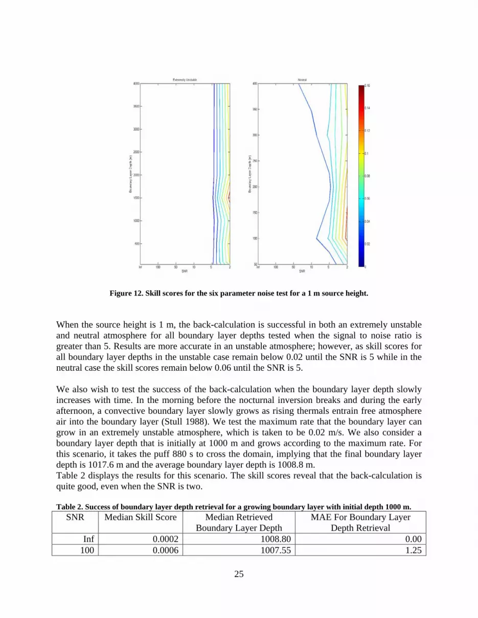
Figure 12. Skill scores for the six parameter noise test for a 1 m source height.
When the source height is 1 m, the back-calculation is successful in both an extremely unstable and neutral atmosphere for all boundary layer depths tested when the signal to noise ratio is greater than 5. Results are more accurate in an unstable atmosphere; however, as skill scores for all boundary layer depths in the unstable case remain below 0.02 until the SNR is 5 while in the neutral case the skill scores remain below 0.06 until the SNR is 5. We also wish to test the success of the back-calculation when the boundary layer depth slowly increases with time. In the morning before the nocturnal inversion breaks and during the early afternoon, a convective boundary layer slowly grows as rising thermals entrain free atmosphere air into the boundary layer (Stull 1988). We test the maximum rate that the boundary layer can grow in an extremely unstable atmosphere, which is taken to be 0.02 m/s. We also consider a boundary layer depth that is initially at 1000 m and grows according to the maximum rate. For this scenario, it takes the puff 880 s to cross the domain, implying that the final boundary layer depth is 1017.6 m and the average boundary layer depth is 1008.8 m. Table 2 displays the results for this scenario. The skill scores reveal that the back-calculation is quite good, even when the SNR is two. Table 2. Success of boundary layer depth retrieval for a growing boundary layer with initial depth 1000 m.
SNR Median Skill Score Median Retrieved Boundary Layer Depth
MAE For Boundary Layer Depth Retrieval
Inf 0.0002 1008.80 0.00100 0.0006 1007.55 1.25
25
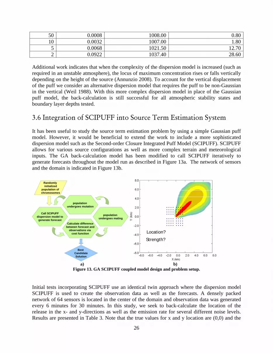
50 0.0008 1008.00 0.8010 0.0032 1007.00 1.805 0.0068 1021.50 12.702 0.0922 1037.40 28.60
Additional work indicates that when the complexity of the dispersion model is increased (such as required in an unstable atmosphere), the locus of maximum concentration rises or falls vertically depending on the height of the source (Annunzio 2008). To account for the vertical displacement of the puff we consider an alternative dispersion model that requires the puff to be non-Gaussian in the vertical (Weil 1988). With this more complex dispersion model in place of the Gaussian puff model, the back-calculation is still successful for all atmospheric stability states and boundary layer depths tested. 3.6 Integration of SCIPUFF into Source Term Estimation System It has been useful to study the source term estimation problem by using a simple Gaussian puff model. However, it would be beneficial to extend the work to include a more sophisticated dispersion model such as the Second-order Closure Integrated Puff Model (SCIPUFF). SCIPUFF allows for various source configurations as well as more complex terrain and meteorological inputs. The GA back-calculation model has been modified to call SCIPUFF iteratively to generate forecasts throughout the model run as described in Figure 13a. The network of sensors and the domain is indicated in Figure 13b.
Randomly initialized
population of chromosomes
Call SCIPUFFdispersion model to
generate forecastCalculate difference
between forecast and observations via
cost function
population undergoes mutation
population undergoes mating
Best CandidateSolution
Location?
Strength?
♦ ♦ ♦ ♦ ♦ ♦ ♦ ♦
♦ ♦ ♦ ♦ ♦ ♦ ♦ ♦
♦ ♦ ♦ ♦ ♦ ♦ ♦ ♦
♦ ♦ ♦ ♦ ♦ ♦ ♦ ♦
♦ ♦ ♦ ♦ ♦ ♦ ♦ ♦
♦ ♦ ♦ ♦ ♦ ♦ ♦ ♦
♦ ♦ ♦ ♦ ♦ ♦ ♦ ♦
♦ ♦ ♦ ♦ ♦ ♦ ♦ ♦
Location?
Strength?
♦ ♦ ♦ ♦ ♦ ♦ ♦ ♦
♦ ♦ ♦ ♦ ♦ ♦ ♦ ♦
♦ ♦ ♦ ♦ ♦ ♦ ♦ ♦
♦ ♦ ♦ ♦ ♦ ♦ ♦ ♦
♦ ♦ ♦ ♦ ♦ ♦ ♦ ♦
♦ ♦ ♦ ♦ ♦ ♦ ♦ ♦
♦ ♦ ♦ ♦ ♦ ♦ ♦ ♦
♦ ♦ ♦ ♦ ♦ ♦ ♦ ♦
a) b)
Figure 13. GA SCIPUFF coupled model design and problem setup. Initial tests incorporating SCIPUFF use an identical twin approach where the dispersion model SCIPUFF is used to create the observation data as well as the forecasts. A densely packed network of 64 sensors is located in the center of the domain and observation data was generated every 6 minutes for 30 minutes. In this study, we seek to back-calculate the location of the release in the x- and y-directions as well as the emission rate for several different noise levels. Results are presented in Table 3. Note that the true values for x and y location are (0,0) and the
26

true strength is 1 kg s-1. For low noise levels, the model is able to estimate the release location to within a few meters and the strength to within 1 % error.
Table 3. Results of the GA coupled SCIPUFF model.
SNR x (m) y (m) Strength (kg s-1) Cost function
Inf 0.2 0.3 0.999 1.6x10⁻⁵ 100 0.4 0.4 1.002 7.8x10⁻⁵ 10 2.4 1.7 1.001 7.3x10⁻⁴ 2 0.1 -0.9 0.819 5.4x10⁻³
The next phase of this task is to prepare the GA SCIPUFF coupled model for the inclusion of FFT07 field trial data. The sensor network and domain have been incorporated into a SCIPUFF case and a sensitivity test using an identical twin approach is being carried out. The optimal parameters determined by the sensitivity test will be used in the next phase of testing on CFD data. The final step is to test the GA SCIPUFF coupled model on the FFT07 data. This work is on-going. 3.7 Source Term Estimation using LES data Previous validation studies emphasized identical twin experiments; however, this portion of the study continues the research validation process and using concentration data created by a time-dependent computational fluid dynamics Large Eddy Simulation (LES) model, EULAG, as provided by colleagues at NCAR. Such data inherently include time-dependent behavior unique to each contaminant episode rather than the ensemble average predicted by the T&D model. The genetic algorithm coupled dispersion model technique then back-calculates source characteristics. A realistic sensor configuration is modeled based on the Fusing Sensor Information from Observing Networks (FUSION) Field Trial 2007 (FFT07). We analyze the features inherent in turbulence that make modeling a single realization with an ensemble average model difficult and suggest new approaches. This study uses the LES data to study the impact of turbulence on the accuracy of the source characterization. Such testing is necessary to simulate turbulence because it distorts the smoothed Gaussian shaped puff the model would predict. This distortion makes it difficult to fit data to a Gaussian model and thus retrieve the source characteristics. Using LES data is useful because although real observations should be used for maximum verisimilitude they are very difficult to come by as well as expensive. The resulting LES data simulate the transport and dispersion of a single puff during a daytime release with an unstable boundary layer for a five minute time period. The simulated concentration data are sampled over the domain, but the values used for this study are only taken from sensor locations. We use the mean concentration value between 0-20 meter heights. To use this dataset with a Gaussian puff model coupled to the Hybrid GA, a single value for wind speed and direction are required. To achieve this single value wind speed and direction fields were averaged over space (x,y) to view the variations in height over time. The mean wind
27

speed and direction profiles indicated 1) that the lowest 80 meters are where the largest variation in the wind speed occurs and 2) that there is minimal wind direction variation throughout the 290 meter vertical domain over time. Therefore, the relevant wind speed and direction are determined by taking the mean over the x,y and 0-80 meter vertical domain. These are then used as known parameters for the source term estimation model. With the identification of wind speed and direction, all of the parameters needed to back-calculate source location are known. The Hybrid GA is used to then back-calculate the source location. The median of ten Monte Carlo runs and the mean of ten ensemble runs are used to determine the mean absolute error (MAE) of the most likely location. The Hybrid GA with the Gaussian puff model as configured is not sufficient for back-calculating a reasonable solution. We hypothesize that wind shear significantly deforms the puff. Thus, another variation of the Gaussian puff model is considered, a Sheared Gaussian puff model that includes a nondimensional shear factor (Konopka 1995, Walcek 2004). The Sheared Gaussian puff model is then coupled with the Hybrid GA. The Sheared Gaussian puff model differs from the regular Gaussian model in that it more accurately accounts for the along wind dispersion improving the back-calculation of the “y” location. Unfortunately, computation of the “x” location has degraded. We do not consider either configuration adequate at the present time. Note that we may be discerning the inherent mismatch in modeling a specific realization (the LES data) with an ensemble average model (represented by the Gaussian puff model). Figure 14 was created of the along wind perspective of the CFD data and it displayed the non-Gaussian nature of this turbulent data. Thus, using a puff model such as SCIPUFF, which includes puff splitting, may be necessary to capture the behavior of realistic turbulent dispersion. This study has examined the impact of using LES generated concentration data for the sensor input. This aspect of the study adds realism by simulating a specific potential realization of turbulent dispersion in a fully three dimensional sheared wind field. Our initial numerical experiments reveal the difficulty of determining the source of a more realistic puff. Current experimental scenarios include altering GA and wind parameters to understand the dynamics between a Gaussian puff model and turbulent data. Another approach is to re-evaluate the physics of the shear Gaussian puff model and seek alterations that more closely simulate a sheared puff in a turbulent environment.
28
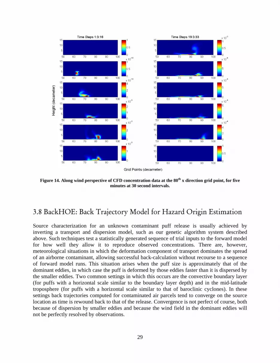
Figure 14. Along wind perspective of CFD concentration data at the 80th x direction grid point, for five minutes at 30 second intervals.
3.8 BackHOE: Back Trajectory Model for Hazard Origin Estimation Source characterization for an unknown contaminant puff release is usually achieved by inverting a transport and dispersion model, such as our genetic algorithm system described above. Such techniques test a statistically generated sequence of trial inputs to the forward model for how well they allow it to reproduce observed concentrations. There are, however, meteorological situations in which the deformation component of transport dominates the spread of an airborne contaminant, allowing successful back-calculation without recourse to a sequence of forward model runs. This situation arises when the puff size is approximately that of the dominant eddies, in which case the puff is deformed by those eddies faster than it is dispersed by the smaller eddies. Two common settings in which this occurs are the convective boundary layer (for puffs with a horizontal scale similar to the boundary layer depth) and in the mid-latitude troposphere (for puffs with a horizontal scale similar to that of baroclinic cyclones). In these settings back trajectories computed for contaminated air parcels tend to converge on the source location as time is rewound back to that of the release. Convergence is not perfect of course, both because of dispersion by smaller eddies and because the wind field in the dominant eddies will not be perfectly resolved by observations.
29

For these situations we have developed a new algorithm, a back trajectory model for hazard origin estimation (BackHOE). The essence of the method is to backtrack those air parcels known to be contaminated from sensor observations. The method is tested here in the boundary layer setting, with transport times on the scale of minutes and distances of less than a kilometer. In settings where deformation dominates dispersion these parcels should come together at the source location. We developed and tested several metrics for diagnosing maximum convergence of the cloud of contaminated parcels, thus deducing the source location. For a single source release the clumping of the parcels around their centroid indicates that the back trajectories have reached the source location. For a multi-source release, it is necessary to first apply cluster analysis, to associate each parcel with a particular cloud and then quantify the evolution of each cloud’s spread along its back trajectory. Since the number of sources is not known, a method was also developed for determining the true source location when the model happens to be run with too many clusters. This is achieved by ranking the clusters in order of their minimum spread, i.e. how well each converges to a single source location. The winds necessary to compute the back trajectories are obtained from surface observation stations. The frozen wave approximation is applied in those cases where the parcel trajectories leave the observation grid. The concentration data are generated by driving a Lagrangian parcel model with the horizontal wind field from a turbulence-resolving LES model run, the same EULAG LES simulation described in section 3.7. Results show that BackHOE can succeed in characterizing an unknown instantaneous source in those meteorological situations where puff deformation by the transporting wind field poses challenges for conventional forward-model-based techniques. Figure 15 depicts the particle cloud’s back trajectory for a single-source release. The wind field deformation pulls the particles together as they approach the source (going backward in time) and then apart again after they pass the source. Figure 16 shows this same information from a quantitative statistical perspective, plotting a time history of the spatial spread of each of two clusters of particles. The cluster that tracks to the release point achieves a much lower minimum spread than the other, thereby identifying it as the correct choice for source term estimation. The plot includes results from five BackHOE runs, each for a different start time, to demonstrate the repeatability of the results. For these same five runs, Figure 17 indicates the location of the cluster centroids at the time each cluster achieves minimum spread. The cluster with the smallest minimum was able to consistently locate the source to within a few decameters despite the source being located 15 decameters outside of the concentration sensor grid. Thus, we believe that BackHOE is a method to add to our arsenal of source term estimation methods that may be most successful when the puff size is similar to that of the dominant eddies. These are precisely the cases where the more prevalent methods are most likely to encounter difficulties.
30
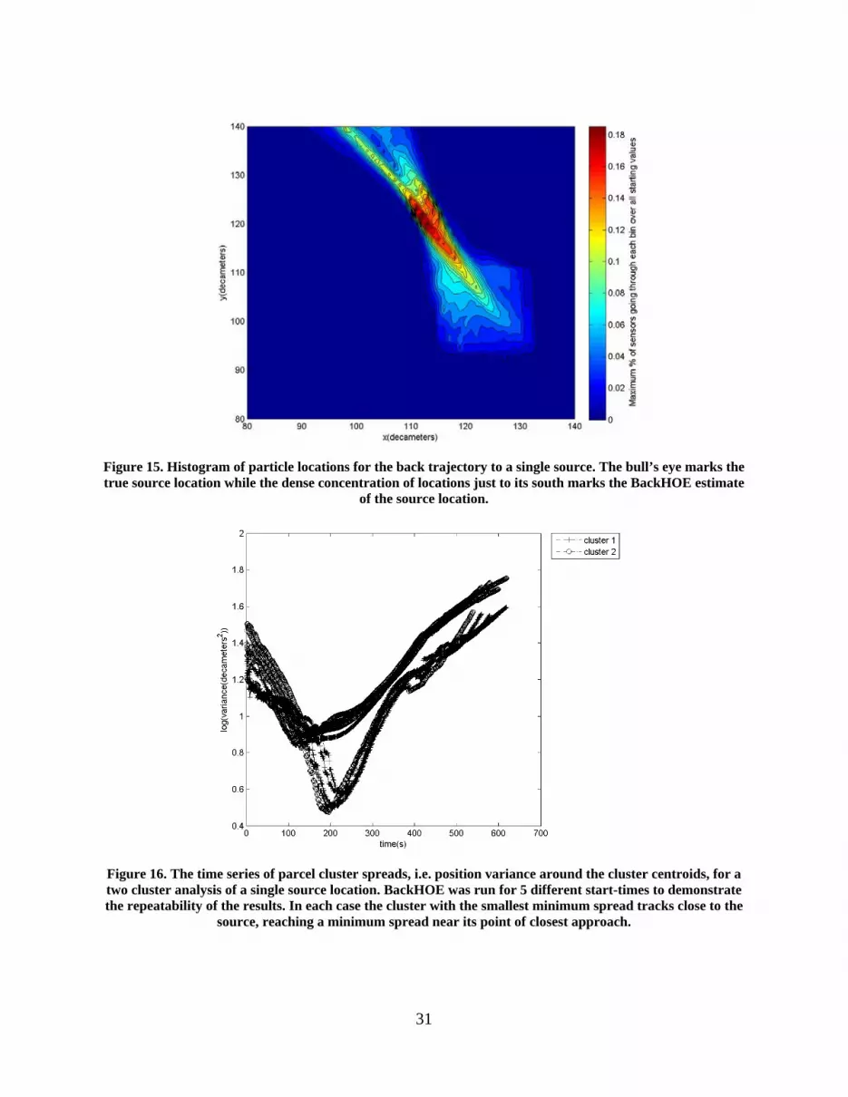
Figure 15. Histogram of particle locations for the back trajectory to a single source. The bull’s eye marks the true source location while the dense concentration of locations just to its south marks the BackHOE estimate
of the source location.
Figure 16. The time series of parcel cluster spreads, i.e. position variance around the cluster centroids, for a two cluster analysis of a single source location. BackHOE was run for 5 different start-times to demonstrate the repeatability of the results. In each case the cluster with the smallest minimum spread tracks close to the
source, reaching a minimum spread near its point of closest approach.
31

Figure 17. A map of the locations at which each cluster achieves its minimum spread. The true source
location is shown as a triangle. The cluster with the smallest minimum spread achieved that value within a few decameters of the true source location. In contrast, the other (large-spread) cluster suggests a source
position that is in error by almost 20 decameters. Thus, the magnitude of the intra-cluster spread correctly identifies both the cluster that tracks to the source and the position along that track at which the source is
located.
4. COMPARE AND CONTRAST DATA ASSIMILATION WITH MULTISENSOR DATA FUSION In AT&D there are two different methods of incorporating data into dispersion models: data assimilation (DA) and multi-sensor data fusion (MSDF). These methods rely on the premise that sensors report concentration data, wind data, or both types within the same domain as the model. DA and MSDF both have the same goal: to incorporate data from many sensors into a model to improve the prediction of an unknown (Daley 1991, Hall and McMullen 2004). Although these methods share a common goal, their approach to defining the unknown parameters differs. In DA, the unknown is a field variable, while in MSDF the unknown is an entity, and one can implement either method because contaminant concentration can be considered a field variable and a contaminant filled puff can be considered an entity. The specification of the unknown parameters as either a field or an entity changes the framework for incorporating data; with a contaminant puff, one takes a Lagrangian approach to assimilating data, while for contaminant concentration one uses an Eulerian approach to assimilating data. While both methods have been used extensively in AT&D, it is instructive to directly compare and contrast their use for modeling a contaminant release in a turbulent flow, which is the purpose of this study. Both MSDF and DA include several techniques by which data is incorporated into dispersion models. While the frameworks for the methods differ, the techniques available to incorporate the data are
32

strikingly similar. This overlap enables comparison, and here we compare the most basic DA technique, Newtonian relaxation (nudging), with the most basic MSDF technique, alpha filtering. These techniques are the most basic since model computation time increases marginally when augmenting the model concentration field prediction (DA) or puff characteristics (MSDF) with an observation. 4.1 Data Assimilation: Nudging For nudging, the specification of concentration as a field variable leads to the scalar conservation equation for turbulent flow. In order to simplify this analysis we require that the sensors lie on the grid points so that no interpolation technique is necessary. We allow the equation to match the partial differential equation (PDE) that produces the Gaussian puff model: however, in order to assimilate data we augment this equation with an assimilation term known as the innovation vector, which represents the difference of the observation from the prediction (Kalnay 2003).
( )),,,()(12
2
2
2
2
2tzyxgtCC
zCK
yCK
xCK
xCU
tC
obszyxv
−=∂
∂−
∂
∂−
∂
∂−
∂∂
+∂∂
τ (10)
where is the mean wind speed, , , and are eddy diffusivities in the x, y, and z
directions respectively, τ is the nudging coefficient, and
U xK yK zK
)(tCobs
vaccounts for all observations at a
certain time, and is a function that allows the observations to influence other grid points throughout the domain, and form the innovation. Note the parallel between this specific equation for concentration tendency with the basic general form given by (2) in section 2.1. These observations act as a source for concentration values at sensors throughout the domain. In order to solve (10) we first obtain a Green’s function from the homogeneous equation and then add the effects that the initial conditions and source terms have on the Green’s function to obtain the nudged concentration equation.
),,,( tzyxg
( ) ( ) ( )
( ) ( ) ( ) t'dx'dy'dz'dτ
t'tt')(tK
z'zt')(tK
y'yt')(tK
t')U(tx'xt')(tπ)()KK(K
tzyx(t)gC
dx'dy'dz'τt
tKz'z
tKy'y
tKUtx'x
)t(tπ)()KK(Kf(x,y,z)C
zyΩ
t
t x//
zyx
obs
zyΩ xo//
zyxn
f
ob
⎟⎠⎞
⎜⎝⎛ −
⎟⎟⎠
⎞⎜⎜⎝
⎛
−−
−⎟⎟⎠
⎞⎜⎜⎝
⎛
−−
−⎟⎟⎠
⎞⎜⎜⎝
⎛
−−−−
−−
+
⎟⎠⎞
⎜⎝⎛−⎟
⎟⎠
⎞⎜⎜⎝
⎛ −−⎟
⎟⎠
⎞⎜⎜⎝
⎛ −−⎟
⎟⎠
⎞⎜⎜⎝
⎛ −−−
−=
∫∫∫ ∫
∫∫∫
exp4
exp4
exp4
exp4
),,,(
exp4
exp4
exp4
exp4
2
2
2
22
2/32321
222
2/32321
v(11)
where Ω represents the spatial domain and all other variables are the same as previously defined. The unknowns in this problem are introduced through the initial condition which is given by:
),,(),,( ,, ououou zzyyxx
UM
zyxf −−−= δ (12)
where δ is the Kronecker delta function, and represent the guessed initial source location and represents the guessed mass of the puff. To complete the analytic formulation for Nudging, we then compute the first integral in (11) to obtain,
uox , uoy ,
uM
33

( ) ( ) ( ) ( )( ) ( ) ( ) ( ) '''''exp
)'(4
2'exp
)'(4
2'exp
)'(4
2)'('exp
2/3)'(2/3)4(2/1)(
),,,()(
exp4
2'exp
4
2,exp
4
2,exp2/3)(2/3)4(2/1)(
dtdzdydxttttzK
zz
ttyK
yyft
obt ttxK
ttUxx
ttzKyKxK
tzyxgtobsC
ttzK
zz
tyKuoyy
txK
Utuoxx
tzKyKxKuM
nC
τπ
τπ
−−
−−
−
−−∫∫∫
Ω∫
−
−−−−
−+
−−
−−
−−−
−=
⎟⎠⎞
⎜⎝⎛
⎟⎠⎞
⎜⎝⎛
⎟⎟⎠
⎞⎜⎜⎝
⎛
⎟⎠⎞
⎜⎝⎛⎟
⎠⎞
⎜⎝⎛
⎟⎠⎞
⎜⎝⎛
v (13)
he second integral is left alone for the present, as this may require some approximation that is
t from o
.2 Multi-Sensor Data Fusion: Alpha Filtering
or alpha filtering, one no longer has to solve a PDE. The problem is formulated as one in
Tdependent on the function ),,,( tzyxg . Equation (13) predicts surface concentration values via a decaying Gaussian with inpu bservations. 4 Foptimization: optimizing puff characteristics given contaminant concentrations. The characteristics of the puff that we wish to ascertain are total integrated mass of the puff and the two-dimensional puff location at each time step. In order to derive these characteristics, we fit a Gaussian puff to the data. Note that with the assumption of stationary, homogeneous turbulence, and aligning our x coordinate with the mean wind direction, we only need to find the downwind location of the puff when optimizing the two-dimensional location. We pose the optimization problem in terms of least squares by taking derivatives with respect to the unknowns of the squared difference of the observations and the Gaussian puff equation. Because the Gaussian puff equation involves exponential terms, it is easier to take the natural logarithm of both.
( )( ) ( ) ( )
( )( ) ( ) ( )0
444)()4(ln)ln(
)(
0444)()4(
ln)ln()(
2222
2/32/12/3
2222
2/32/12/3
=⎟⎟
⎠
⎞
⎜⎜
⎝
⎛ −−
−−
+−−⎟
⎟⎠
⎞⎜⎜⎝
⎛−
∂∂
=⎟⎟
⎠
⎞
⎜⎜
⎝
⎛ −−
−−
+−−⎟
⎟⎠
⎞⎜⎜⎝
⎛−
+∂∂
tKzz
tKyy
tKUtxx
tKKKMC
M
tKzz
tKyy
tKUtxx
tKKKMC
Utx
z
o
y
o
x
o
zyxobs
z
o
y
o
x
o
zyxobs
o
π
π(14)
The alpha filter updates the guessed characteristics with the ascertained characteristics at each time step with an equation given as a linear combination of the two (Hall and McMullen 2004).
( )( ) ( ) ( ) ( )( )goaogofo
gagf
UtxUtxUtxUtx
MMMM
+−+++=+
−+=
α
α (15)
where the subscript g denotes the guessed characteristic, the subscript a indicates the ascertained characteristic, and the subscript f designates the final characteristic, and α is a constant whose value is between zero and one and plays a similar role to the τ in nudging. To complete the analytic formulation for the Alpha Filter, we replace the unknowns in the Gaussian puff equation with (14) to obtain,
34
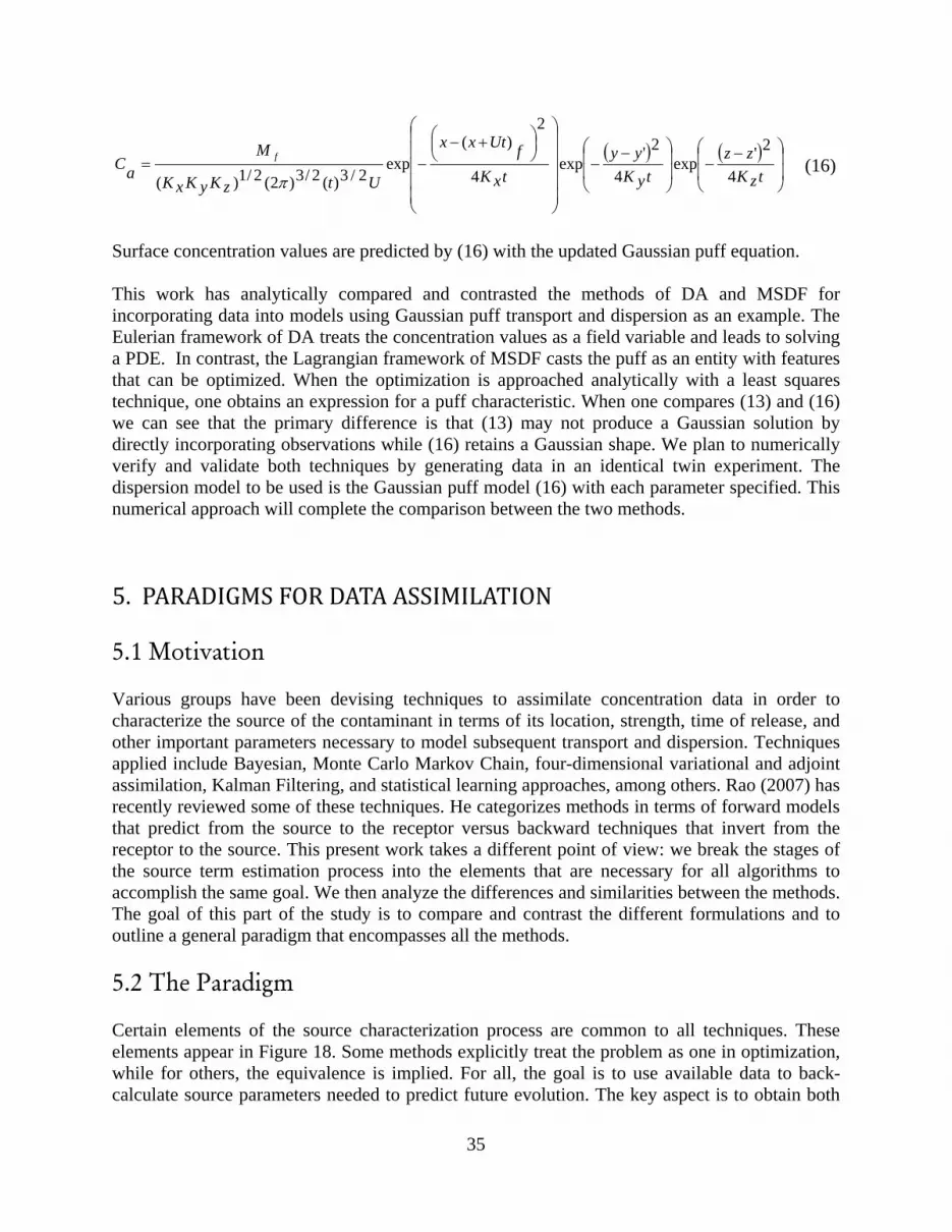
( ) ( )⎟⎟
⎠
⎞
⎜⎜
⎝
⎛ −−⎟
⎟
⎠
⎞
⎜⎜
⎝
⎛ −−
⎟⎟⎟⎟⎟
⎠
⎞
⎜⎜⎜⎜⎜
⎝
⎛⎟⎠⎞⎜
⎝⎛ +−
−=tzK
zztyK
yytxK
fUtxx
UtzKyKxK
MaC f
4
2'exp4
2'exp
4
2)(
exp2/3)(2/3)2(2/1)( π
(16)
Surface concentration values are predicted by (16) with the updated Gaussian puff equation. This work has analytically compared and contrasted the methods of DA and MSDF for incorporating data into models using Gaussian puff transport and dispersion as an example. The Eulerian framework of DA treats the concentration values as a field variable and leads to solving a PDE. In contrast, the Lagrangian framework of MSDF casts the puff as an entity with features that can be optimized. When the optimization is approached analytically with a least squares technique, one obtains an expression for a puff characteristic. When one compares (13) and (16) we can see that the primary difference is that (13) may not produce a Gaussian solution by directly incorporating observations while (16) retains a Gaussian shape. We plan to numerically verify and validate both techniques by generating data in an identical twin experiment. The dispersion model to be used is the Gaussian puff model (16) with each parameter specified. This numerical approach will complete the comparison between the two methods.
5. PARADIGMS FOR DATA ASSIMILATION 5.1 Motivation Various groups have been devising techniques to assimilate concentration data in order to characterize the source of the contaminant in terms of its location, strength, time of release, and other important parameters necessary to model subsequent transport and dispersion. Techniques applied include Bayesian, Monte Carlo Markov Chain, four-dimensional variational and adjoint assimilation, Kalman Filtering, and statistical learning approaches, among others. Rao (2007) has recently reviewed some of these techniques. He categorizes methods in terms of forward models that predict from the source to the receptor versus backward techniques that invert from the receptor to the source. This present work takes a different point of view: we break the stages of the source term estimation process into the elements that are necessary for all algorithms to accomplish the same goal. We then analyze the differences and similarities between the methods. The goal of this part of the study is to compare and contrast the different formulations and to outline a general paradigm that encompasses all the methods.
5.2 The Paradigm Certain elements of the source characterization process are common to all techniques. These elements appear in Figure 18. Some methods explicitly treat the problem as one in optimization, while for others, the equivalence is implied. For all, the goal is to use available data to back-calculate source parameters needed to predict future evolution. The key aspect is to obtain both
35

field monitored concentration values and estimates of the predicted concentration values at common times and locations. Sometimes interpolation is necessary to get the data on a common grid. The field monitored data are obtained from sensor(s) located in the field. A dispersion model produces the estimated predicted concentration field. That model requires input parameters including source information and meteorological data. Since source information is typically what the technique is designed to back-calculate, it is necessary to make “guesses” at such data to obtain a concentration estimate. The atmospheric transport and dispersion (AT&D) models also require information about the meteorological conditions as well as information about the site (terrain, land usage, etc.). Although such data are often assumed to be known, the AT&D model can be quite sensitive to errors or changes in those conditions as discussed below.
Figure 18. Flowchart of source inversion process.
The difference between the predicted concentration values and those observed are compared quantitatively by a cost function. This explicit comparison guides the algorithm to generate new, improved guesses of the input parameters. The ways to produce these new estimates are the primary differences in the various source estimation methods. Each method includes some algorithm to generate these improved source parameters.
5.3 Comparison of Techniques Quite a few research groups have formulated and tested methods for characterizing source parameters for dispersion modeling based on downwind concentration measurements. There is a wide range of complexity in the methods to match the range of applications. Some methods invert for only source strength but on a regional scale with sparse field data. Others seek several meteorological variables in addition to characterizing source strength, location, and time of release but on a smaller scale grid construed in the context of an identical twin numerical experiment (that is, synthetic test data is created using the same model filling the role of the AT&D model in the algorithm). The AT&D models range from simple back-trajectories and basic Gaussian plume models to high resolution Computational Fluid Dynamics (CFD) models. The inversion techniques themselves tend to be quite innovative. The main inversion categories include: 1) Bayesian methods coupled with statistical sampling (such as Monte Carlo Markov chains); 2) adjoint and variational methods that use a tangent linear version of the AT&D model; 3) Kalman Filter and similar analytic update approaches; and 4) statistical learning techniques such as genetic algorithms and simulated annealing. Each method has its own system for
36
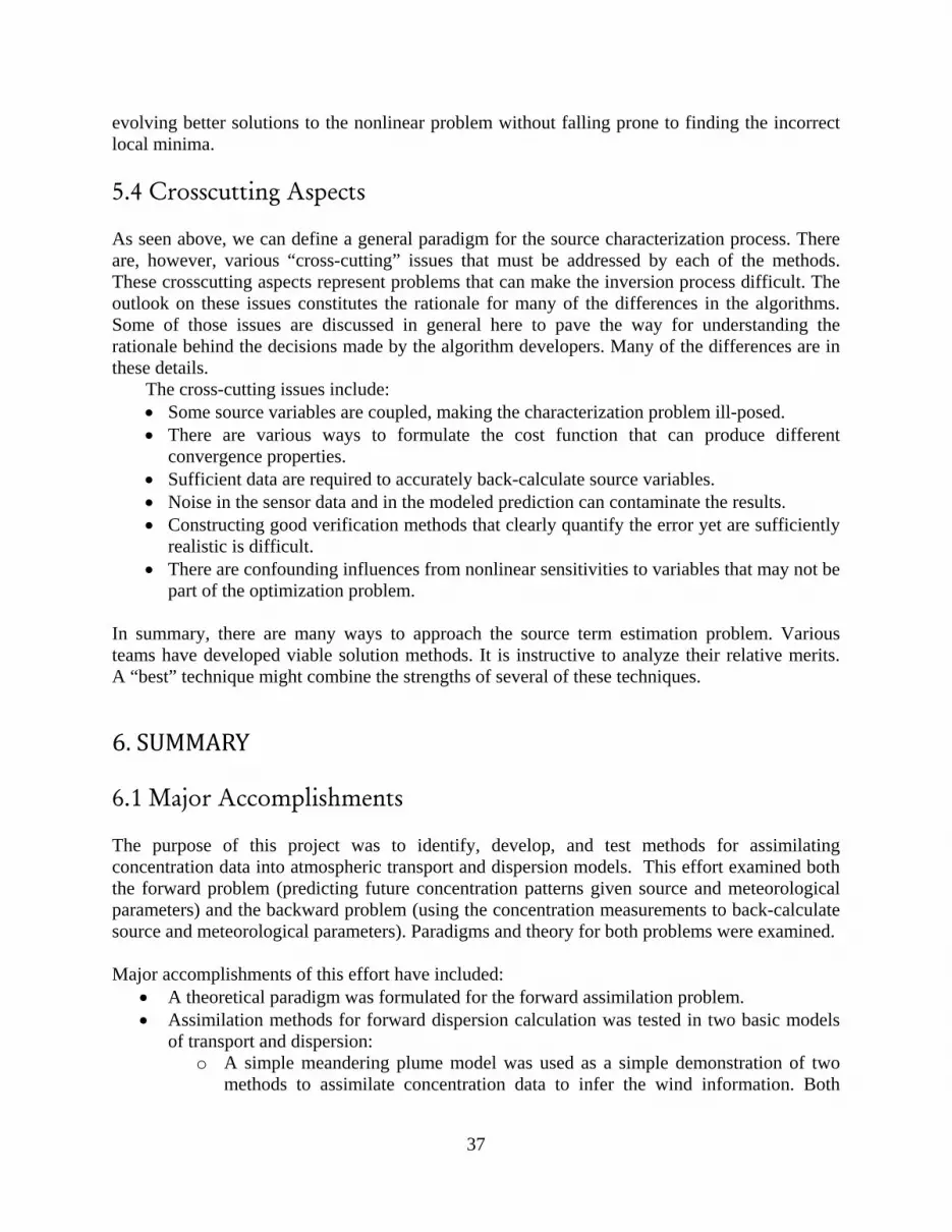
evolving better solutions to the nonlinear problem without falling prone to finding the incorrect local minima.
5.4 Crosscutting Aspects As seen above, we can define a general paradigm for the source characterization process. There are, however, various “cross-cutting” issues that must be addressed by each of the methods. These crosscutting aspects represent problems that can make the inversion process difficult. The outlook on these issues constitutes the rationale for many of the differences in the algorithms. Some of those issues are discussed in general here to pave the way for understanding the rationale behind the decisions made by the algorithm developers. Many of the differences are in these details.
The cross-cutting issues include: • Some source variables are coupled, making the characterization problem ill-posed. • There are various ways to formulate the cost function that can produce different
convergence properties. • Sufficient data are required to accurately back-calculate source variables. • Noise in the sensor data and in the modeled prediction can contaminate the results. • Constructing good verification methods that clearly quantify the error yet are sufficiently
realistic is difficult. • There are confounding influences from nonlinear sensitivities to variables that may not be
part of the optimization problem. In summary, there are many ways to approach the source term estimation problem. Various teams have developed viable solution methods. It is instructive to analyze their relative merits.
ues. A “best” technique might combine the strengths of several of these techniq
6. SUMMARY 6.1 Major Accomplishments The purpose of this project was to identify, develop, and test methods for assimilating concentration data into atmospheric transport and dispersion models. This effort examined both the forward problem (predicting future concentration patterns given source and meteorological parameters) and the backward problem (using the concentration measurements to back-calculate source and meteorological parameters). Paradigms and theory for both problems were examined. Major accomplishments of this effort have included:
• A theoretical paradigm was formulated for the forward assimilation problem. • Assimilation methods for forward dispersion calculation was tested in two basic models
of transport and dispersion: o A simple meandering plume model was used as a simple demonstration of two
methods to assimilate concentration data to infer the wind information. Both
37

methods showed success at dynamically assimilating that wind to predict transport and dispersion. Those two methods are:
Feature extraction with nudging Genetic algorithm variational method
o A two dimensional shallow water model with topography and Gaussian puff dispersion was used to evaluate four methods to assimilate noisy wind and concentration observations. Those methods include:
Newtonian relaxation or nudging Extended Kalman Filter Ensemble Kalman Filter Four dimensional variational data assimilation
The results indicate that some value is derived from each method. The nudging method is the most efficient in terms of computational time, followed by the ensemble Kalman Filter.
• New methods for testing assimilation in terms of the backward-looking source term estimation problem were developed and extensively tested, first in the context of identical twin experiments, then using data computed by an LES model. The methods include:
o Genetic algorithm to optimize the match. This model was tested in several contexts:
Gaussian plume and puff experiments, including adding noise. Even when noise of the same order of magnitude as the signal is added, the GA can reconstruct source and meteorological parameters with multiple runs. A first formulation required potential source locations to be input and only computed source parameters. A reformulation directly seeks any required parameter value, including three dimensional source location, time of release, source strength, and meteorological data. A full analysis of data requirements in the presence of noise was conducted.
SCIPUFF experiments, including noise. The results, even including noise are similar to those for the Gaussian puff studies for the initial model and that model was successful at estimating source parameters for the Dipole Pride 26 data. Current efforts incorporating SCIPUFF in the reformulated model show success at back-calculating source characteristics and runs in a reasonable amount of CPU time.
Gaussian plume experiments considering boundary depth as a parameter. The reflections from the boundary layer depth make a large impact on the computed results and is a critical parameter. The success at correctly identifying the boundary layer depth depends on atmospheric stability, with more unstable conditions proving easier for the back-calculation.
Gaussian puff experiments including sensitivity to sensor characteristics. When sensor detection level and saturation level were considered, we determined that it is most important to resolve the maximum concentrations for the purpose of easing the back-calculation of source location, source strength, and wind direction.
Parameters back-calculated using these methodologies include two-dimensional source location, source height, source strength, time of release, wind direction, wind speed, stability category, and boundary layer depth.
38
o Back trajectory model for hazard origin estimation (BackHOE). This method triangulates the source location and is most useful when the eddies are on the same scale as the size of the puff, such as may occur in the FFT07 data.
• A theoretical framework was used to compare and contrast the engineering approach to multi-sensor data fusion with the meteorological approach to data assimilation. MSDF emphasizes identifying entities and uses a Lagrangian framework while DA works with field variables in an Eulerian framework. A mathematical comparison is made of the DA method, nudging, with the MSDF method, alpha filtering.
• A paradigm was developed for the source term estimation solution methods and cross-cutting aspects were identified.
The work described herein has resulted in eight journal articles, five master’s theses, 32 conference presentations (with another 10 accepted for presentation in the next several months), and 10 student posters at local poster contests. Appendix A lists these publications and specifies which were directly funded by this project.
39
References Allen, C. T., S.E. Haupt, and G.S. Young, 2007a: Source Characterization with a Receptor/Dispersion Model Coupled with a Genetic Algorithm, Journal of Applied Meteorology and Climatology, 46, 273-287 Allen C.T., G.S. Young, and S.E. Haupt, 2007b: Improving Pollutant Source Characterization by Optimizing Meteorological Data with a Genetic Algorithm. Atmospheric Environment, 41, 2283-2289.
Annunzio, A.J., 2008: Source Characterization with Atmospheric Boundary Layer Depth. M.S. Thesis, Dept. of Meteorology, The Pennsylvania State University, 50 pp.
Beychok M.R., 1995: Fundamentals of Stack Gas Dispersion, 3rd Ed. Milton Beychok, pub., Irvine, CA, 193 pp. Beyer-Lout, A., G.S. Young, and S.E. Haupt, 2008: Assimilation of Concentration and Wind Data into a Coupled Wind and Dispersion System, submitted to Monthly Weather Review. Caya, A., J. Sun, and C. Snyder, 2005: A Comparison between 4D Var and the Ensemble Kalman Filter Technique for Radar Data Assimilation. Monthly Weather Review, 133, 3081-3093. Chang J.C., P. Franzese, K. Chayantrakom, and S. R. Hanna, 2003. Evaluations of CALPUFF, HPAC, and VLSTRACK with Two Mesoscale Field Datasets. Journal of Applied Meteorology 42, 453-466. Cheng Y., K.V. Umanaheswara Reddy, T. Singh, and P.D. Scott, 2007: CBRN Data Fusion Using Puff-Based Model and Bar-Reading Sensor Data. 10th International Conference on Information Fusion, Quebec City, Canada, July 9-12th, 2007. Constantinescu E.M., A. Sandu, T. Chai, and G.R. Carmichael, 2007: Assessment of ensemble-based chemical data assimilation in an idealized setting. Atmospheric Environment, 41, 18-36. Daley R., 1991: Atmospheric Data Assimilation. Cambridge University Press, Cambridge, 457 pp. Davakis E., S. Andronopoulos, I. Kovalets, N. Gounaris, J.G. Batzis, and S.G. Nychas, 2007: Data assimilation in meteorological pre-processors: Effects on atmospheric dispersion simulations. Atmospheric Environment, 41, 2917-2932. Defense Threat Reduction Agency, cited 2008: Mission statement. [Available online at http://www.dtra.mil/about/mission.cfm]
40
Deng A., N.L. Seman, G.K. Hunter, and D.R. Stauffer, 2004: Evaluation of interregional transport using the MM5-SCIPUFF system. Journal of Applied Meteorology, 43, 1864-1886. EPA, 2003: Revision to the Guidelines on Air Quality Models. Adoption of a Preferred Long Range Transport Model and Other Revisions. Federal Register, vol. 68, (72), 40 CFR Part 51. Gandin, L. S., 1963: Objective analysis of meteorological fields. Gidrometeor. Isdaty., Leningrad. [Israel Program for Scientific Translations, Jerusalem, 1965, 242 pp.] Hall, D. and S. McMullen, 2004: Mathematical Techniques in Multisensor Data Fusion. Artech House, Inc., Norwood, MA 02062. Hanna S.R., 1983: Lateral turbulence intensity and plume meandering during stable conditions. Journal of Climate and Applied Meteorology. 22, 1424-1430. Haupt R. L. and S. E. Haupt, 2004: Practical Genetic Algorithms, 2nd edition with CD. John Wiley & Sons, New York, NY. Haupt, S. E., 2005: A Demonstration of Coupled Receptor/Dispersion Modeling with a Genetic Algorithm. Atmospheric Environment, 39, 7181-7189. Haupt, S. E., G.S. Young, and C.T. Allen, 2006: Validation of a Receptor-Dispersion Model Coupled with a Genetic Algorithm Using Synthetic Data, Journal of Applied Meteorology and Climatology, 45, 476–490. Haupt S.E., G.S. Young, and C.T. Allen, 2007: A Genetic Algorithm Method to Assimilate Sensor Data for a Toxic Contaminant Release. Journal of Computers, 2, 85-93. Haupt, S.E., R.L. Haupt, and G.S. Young, 2008: A Mixed Integer Genetic Algorithm used in Chem-Bio Defense Applications, submitted to Journal of Soft Computing. Hoke J.E. and R.A. Anthes, 1976: The Initialization of Numerical Models by a Dynamic Initialization Technique. Monthly Weather Review, 104, 1551-1556. Holton, J.R. 1992: An introduction to dynamic meteorology. Volume 48 of International Geophysics Series. 3rd edition, Academic Press. Homeland Security Office, cited 2007: National Strategy for Homeland Security. [Available online at http://www.whitehouse.gov/infocus/homeland/nshs/NSHS.pdf.] Houtekamer, P.L. and H.L. Mitchell, 1998: Data Assimilation Using an Ensemble Kalman Filter Technique. Monthly Weather Review, 126, 796-811. Ide K., P. Courtier, M. Ghil, and A.C. Lorenc, 1997: Unified Notation for Data Assimilation: Operational, Sequential and Variational. Journal of the Meteorological Society of Japan, 75, 181-189.
41
Kalman, R. and R. Bucy, 1961: New results in linear prediction and filtering theory. Trans. AMSE, J. Basic Eng., 83D, 95–108. Kalnay E., 2003: Atmospheric Modeling, Data Assimilation and Predictability. Cambridge University Press, Cambridge, 136-204. Krysta M., M. Bocquet, B. Sportisse, and O. Isnard, 2006: Data assimilation for short-range dispersion of radionuclides: An application to wind tunnel data, Atmospheric Environment, 40, 7267-7279.
Konopka, P., 1995: Gaussian solutions for anisotropic diffusion in linear shear flow. J. Non-Equilib. Thermo-dyn., 20, 78-91.
Kuroki, Y., 2008: Source Characterization via Autonomous Aircraft. M.S. Thesis, Dept. of Meteorology, The Pennsylvania State University, 34 pp.
Lee J.A., L.J. Peltier, S.E. Haupt, J.C. Wyngaard, D.R. Stauffer, and A.J. Deng, 2008: Improving SCIPUFF dispersion forecasts with NWP Ensembles, to be submitted to the Journal of Applied Meteorology and Climatology. Lewis, J.M. and J.C. Derber, 1985: The use of adjoint equations to solve a variational adjustment problem with advective constraints. Tellus, 37, 309-327. Liu D.-H. and D.Y.C. Leung, 2005: On plume meandering in unstable stratification. Atmospheric Environment, 39, 2995-2999. Long K.J., S.E. Haupt, and G.S. Young, 2008: Optimizing Source Characteristics and Meteorological Data for a Contaminant Release with a Genetic Algorithm. Submitted to Optimization and Engineering. Lorenz, E.N., 1963: Deterministic Nonperiodic Flow, J. Atmos. Sci., 20, 130-141. Mahrt L., 1999: Stratified atmospheric boundary layers. Boundary Layer Meteorology, 90, 375-396. Miller, R.N., M. Ghil, and F. Gauthiez, 1994: Advanced Data Assimilation in Strongly Nonlinear Dynamical Systems. J. Atmos. Sci, 51, 1037-1056. National Research Council, 2003: Tracking and Predicting the Atmospheric Dispersion of Hazardous Material Releases. Implications for Homeland Security, The National Academies Press, Washington, D.C. Nelder, J. A. and R. Mead, 1965: A Simplex Method for Function Minimization. Computer Journal, 7, 308-313.
42
Peltier, L.J., J.C. Wyngaard, S.E. Haupt, D.R. Stauffer, A. Deng, and J.A. Lee, 2008: Parameterization of NWP Uncertainty for Dispersion Modeling, to be submitted to Journal of Applied Meteorology and Climatology. Rao, S., 2007: Source estimation methods for atmospheric dispersion, Atmospheric Environment, 41, 6963-6973.
Rodriguez, L.M, 2008: Source Term Estimation Using a Genetic Algorithm and Incorporating Sensor Characteristics, M.S. Thesis, Dept. of Meteorology, The Pennsylvania State University, 36 pp.
Rodriguez, L.M., S.E. Haupt, and G.S. Young, 2008: Impact of Sensor Characteristics on Source Characterization for Dispersion Modeling, submitted to Measurement. Reddy U.K.V., Y. Cheng, T. Singh, and P.D. Scott, 2007: Data Assimilation in Variable Dimension Dispersion Models using Particle Filters. 10th International Conference on Information Fusion, Quebec City, Canada, July 9-12th, 2007. Sasaki, Y., 1970: Some basic formalisms in numerical variational analysis. Monthly Weather Review, 98, 875-883. Schiller, A. and J. Willebrand, 1995: A technique for the determination of surface heat and freshwater fluxes from hydrographic observations, using an approximate adjoint ocean circulation model. J. Mar. Res., 53, 433-451. Sirkes, Z. and E. Tziperman, 1997: Finite Difference of Adjoint or Adjoint of Finite Difference? Monthly Weather Review, 125, 3373-3378. Stauffer D.R. and N.L. Seaman, 1993: Multiscale Four-Dimensional Data Assimilation. Journal of Applied Meteorology, 33, 416-434. Stuart A.L. A. Aksoy, F. Zhang, and J.W. Nielsen-Gammon, 2007: Ensemble-based data assimilation and targeted observation of a chemical tracer in a sea breeze model. Atmospheric Environment, 41, 3082-3094. Stull, R.B., 1988: An Introduction to Boundary Layer Meteorology. Kluwar Academic, The Netherlands, 666 pp. Terejanu G., T. Singh, and P.D. Scott, 2007: Unscented Kalman Filter/Smoother for a CBRN Puff-Based Dispersion Model. 10th International Conference on Information Fusion, Quebec City, Canada, July 9-12th, 2007. Walcek, L.C., 2004: A Gaussian dispersion/plume model explicitly accounting for wind shear, 13th Conference on the Applications of Air Pollution Meteorology with the Air and Waste Management Assoc, Vancouver/BC, Canada Amer. Meteor. Soc., CD-ROM, 79742.
43

44
Zheng D.Q., Leung J.K.C., Lee B.Y., and Lam H.Y., 2007: Data assimilation in the atmospheric dispersion model for nuclear accident assessments. Atmospheric Environment, 41, 2438-2446.
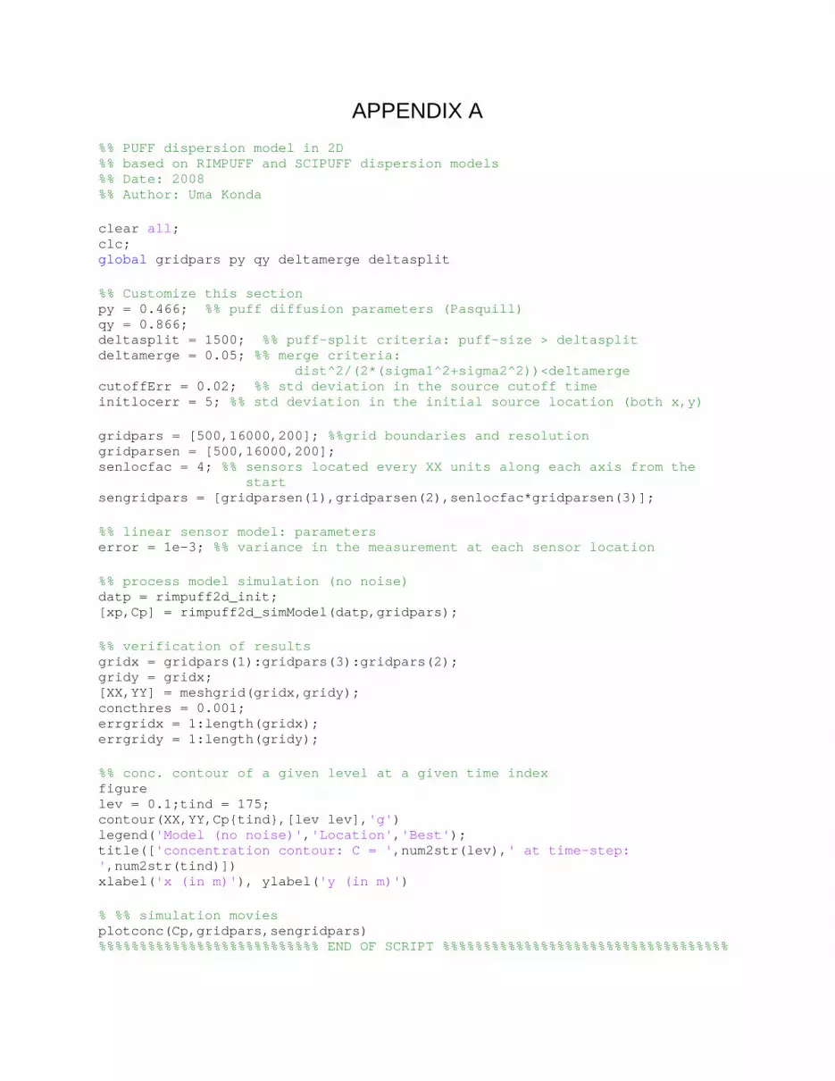
APPENDIX A %% PUFF dispersion model in 2D %% based on RIMPUFF and SCIPUFF dispersion models %% Date: 2008 %% Author: Uma Konda clear all; clc; global gridpars py qy deltamerge deltasplit %% Customize this section py = 0.466; %% puff diffusion parameters (Pasquill) qy = 0.866; deltasplit = 1500; %% puff-split criteria: puff-size > deltasplit deltamerge = 0.05; %% merge criteria: dist^2/(2*(sigma1^2+sigma2^2))<deltamerge cutoffErr = 0.02; %% std deviation in the source cutoff time initlocerr = 5; %% std deviation in the initial source location (both x,y) gridpars = [500,16000,200]; %%grid boundaries and resolution gridparsen = [500,16000,200]; senlocfac = 4; %% sensors located every XX units along each axis from the start sengridpars = [gridparsen(1),gridparsen(2),senlocfac*gridparsen(3)]; %% linear sensor model: parameters error = 1e-3; %% variance in the measurement at each sensor location %% process model simulation (no noise) datp = rimpuff2d_init; [xp,Cp] = rimpuff2d_simModel(datp,gridpars); %% verification of results gridx = gridpars(1):gridpars(3):gridpars(2); gridy = gridx; [XX,YY] = meshgrid(gridx,gridy); concthres = 0.001; errgridx = 1:length(gridx); errgridy = 1:length(gridy); %% conc. contour of a given level at a given time index figure lev = 0.1;tind = 175; contour(XX,YY,Cptind,[lev lev],'g') legend('Model (no noise)','Location','Best'); title(['concentration contour: C = ',num2str(lev),' at time-step: ',num2str(tind)]) xlabel('x (in m)'), ylabel('y (in m)') % %% simulation movies plotconc(Cp,gridpars,sengridpars) %%%%%%%%%%%%%%%%%%%%%%%%%%% END OF SCRIPT %%%%%%%%%%%%%%%%%%%%%%%%%%%%%%%%%%%

function dat = rimpuff2d_init; % initialize rimpuff2d model global py qy %======================================================== % model parameters %======================================================== dat.model.tStep = 20; %timestep diff (in s) dat.model.tStart = 0; %start time (in s) dat.model.tStop = 3600; %stop time (in s) dat.model.tpuffrel = 3; %puff released at every XX timesteps dat.model.sourceCutoff = 0.2; %fraction of nSteps after which puff release
stops dat.model.npar = 4; %no of parameters in each puff dat.model.puffinit = [0;0;1;5e5]; %init puff pars [x,y,sigxy,puffActivity] dat.model.unom = 5; % nominal wind speed Ts = dat.model.tStep;

function [x,C] = rimpuff2d_simModel(dat,gridpars) %% RIMPUFF process model simulation in 2D Ts = dat.model.tStep; tStart = dat.model.tStart; tStop = dat.model.tStop; npar = dat.model.npar; %no of puff parameters tpuffrel = dat.model.tpuffrel; alpha = dat.model.sourceCutoff; % uncertain alpha leads to variable state length unom = dat.model.unom; ustd = 0; %no noise for process model simulation nSteps = length(tStart:Ts:tStop)-1; puffRR = rimpuff2d_source(0,tpuffrel,alpha,nSteps); for j = 1:puffRR puffmat(:,j) = dat.model.puffinit; end; npuff = size(puffmat,2) ;x1.puffmat = puffmat; %% for output gridx = gridpars(1):gridpars(3):gridpars(2); gridy = gridx; lx = length(gridx); ly = length(gridy); [XX,YY] = meshgrid(gridx,gridy); C1 = zeros(size(XX)); for j = 1:nSteps, loc = xj.puffmat(1:2,:); u = rimpuff2d_u(unom,ustd,loc,j,nSteps); [xj+1] = rimpuff2d_f_process(dat,xj,u,j,nSteps); Cj+1 = rimpuff2d_output(xj+1.puffmat,XX,YY); end; function puffRR = rimpuff2d_source(tind,tpuffrel,alpha,nSteps) %%Source Design puffRR = 0; if (tind<alpha*nSteps)&&(mod(tind,tpuffrel)==0), puffRR = 1; end;

function u = rimpuff2d_u(unom,ustd,loc,tind,nSteps) % compute 2D windfield u as a 2*npuff matrix % tind : no of timestep unom = unom*ones(1,size(loc,2)); %nominal wind speed unoise1 = ustd*randn(1,size(loc,2)); %noise in each direction unoise2 = ustd*randn(1,size(loc,2)); %%change in wind direction after half the simulation time if tind<0.5*nSteps u = [(unom)*cos(pi/12)+unoise1; (unom)*sin(pi/12)+unoise2]; else u = [(unom)*cos(pi/3)+unoise1; (unom)*sin(pi/3)+unoise2]; end;

function [x_new] = rimpuff2d_f_process(dat,x_old,u_inp,tind,nSteps); Ts = dat.model.tStep; npar = dat.model.npar; tpuffrel = dat.model.tpuffrel; alpha = dat.model.sourceCutoff; puffmat = x_old.puffmat; npuff = size(puffmat,2); puffRR = rimpuff2d_source(tind,tpuffrel,alpha,nSteps); global py qy for j = 1:npuff u_inp(:,j) = u_inp(:,j); ux = u_inp(1,j); uy = u_inp(2,j); dx = norm(u_inp(:,j))*Ts; %dist. traversed in the downwind dist. during this instant puffmat(1,j) = puffmat(1,j)+ux*Ts; puffmat(2,j) = puffmat(2,j)+uy*Ts; tmp = (puffmat(3,j)/py)^(1/qy)+dx; %sigma in the downwind/crosswind
direction puffmat(3,j) = py*tmp^qy; puffmat(4,j) = puffmat(4,j); %puff activity doesn't change with time end; if puffRR ~= 0 %% new puff release for j = 1:puffRR puffmat(:,npuff+j) = dat.model.puffinit; end; npuff = npuff+puffRR; end; npuffb4split = npuff; %% puff splitting global splitcount deltasplit deltamerge for j = 1:npuff if puffmat(3,j)>deltasplit splitmat = puffsplit5(puffmat(:,j)); puffmat(:,j) = splitmat(:,1); %% center puff is retained at the same position puffmat = [puffmat splitmat(:,2:5)]; %% surround puffs added at the end d; enend; npuffaftersplit = size(puffmat,2); %%puff merging if (npuff > 1) && (deltamerge > 0) [puffmat] = puffmerge(puffmat); end; npuffaftermerge = size(puffmat,2); x_new.puffmat = puffmat;

function puffmat = puffsplit5(puff) %% when the puff grows to size comparable with the grid spacing of the flow %% model, it splits horizontally into five new gaussian puffs, each with half %% the std. dev of the original puff %% puff = [x,y,sig,Q]; signew = 0.5*puff(3); %% 0.5 is chosen arbitrarily Qcirc = .2353*puff(4); Qcen = puff(4)-4*Qcirc; xcen = puff(1); ycen = puff(2); xl = xcen-0.89*puff(3); xr = xcen+0.89*puff(3); yh = ycen; yu = ycen+0.89*puff(3); yd = ycen-0.89*puff(3); xv = xcen; puffmat(1:2,:) = [xcen xl xr xv xv; ycen yh yh yu yd]; puffmat(3,1:5) = signew; puffmat(4,:) = [Qcen Qcirc Qcirc Qcirc Qcirc];

function [puffmatnew] = puffmerge(puffmat) %% puff = [x,y,sig,Q]; %% puffmat: 4 x npuff matrix global gridpars py qy deltamerge puffmatnew = []; keep_merging = 1; npuff = size(puffmat,2); delta = zeros(npuff); for i = 1:npuff delta(i,i) = 1000; end; while numel(delta) > 1 puff1 = puffmat(:,1); for j = 2:size(puffmat,2) pufftmp = puffmat(:,j); sepdistsqrd = (puff1(1:2)-pufftmp(1:2))'*(puff1(1:2)-pufftmp(1:2)); maxsigsqrd = max(puff1(3),pufftmp(3))^2; delta(1,j) = sepdistsqrd/(2*(puff1(3)^2+pufftmp(3)^2)); elta(1,j) = sepdistsqrd/(4*maxsigsqrd); %d end; [mindelta,ind] = min(delta(1,:)); ind = ind(1); mindelta = mindelta(1); puff2 = puffmat(:,ind); if mindelta < deltamerge puff = puffmerge2(puff1,puff2); delta(:,ind) = []; delta(ind,:) = []; puffmat(:,ind) = []; puffmat(:,1) = puff; else puff = puff1; puffmatnew = [puffmatnew puff]; delta(1,:) = []; delta(:,1) = []; puffmat(:,1) = []; end; end; puffmatnew = [puffmatnew puffmat(:,1)];

function puffvec = puffmerge2(puff1,puff2) %% puff = [x,y,sig,Q]; puffvec(4,:) = puff1(4)+puff2(4); puffvec(1:2,:) = (puff1(4)*puff1(1:2)+puff2(4)*puff2(1:2))/puffvec(4); temp1 = puff1(3)^2+norm(puffvec(1:2)-puff1(1:2))^2; temp2 = puff2(3)^2+norm(puffvec(1:2)-puff2(1:2))^2; puffvec(3,:) = sqrt(1/puffvec(4)*(puff1(4)*temp1+puff2(4)*temp2));

function [] = plotconc(C,gridpars,sengridpars) gridx = gridpars(1):gridpars(3):gridpars(2); gridy = gridx; [XX,YY] = meshgrid(gridx,gridy); senx = sengridpars(1):sengridpars(3):sengridpars(2); seny = senx; [senXX,senYY] = meshgrid(senx,seny); gridlim = length(gridx); sengridlim = length(senx); figure set(gca,'xlim',[gridx(1) gridx(gridlim)],'ylim',[gridy(1) gridy(gridlim)],... 'clim',[0 0.2],'NextPlot','replace','Visible','on') set(gca,'nextplot','replacechildren') colormap('jet') colorbar for j = 1:1:length(C) plot(XX(1:gridlim,1:gridlim),YY(1:gridlim,1:gridlim),'w.','MarkerSize',5) hold on plot(senXX(1:sengridlim,1:sengridlim),senYY(1:sengridlim,1:sengridlim),
'r*','MarkerSize',15); plot(YY(xgridstart,:)',XX(xgridstart,:)') [Contour,h] = contour(XX,YY,Cj,[0.1 0.5 0.5*max(max(Cj)) 0.8*max(max(Cj))]); clabel(Contour,h); grid on title(['timestep = ',num2str(j),'; time = ',num2str(j*20),'s']) colorbar pause(0.1) Mctr(j) = getframe(gcf); hold off end; movie2avi(Mctr,'ctr.avi'); % movie2avi(Msurf,'surf.avi');

#include "mex.h" #include <math.h> /* C routine rimpuff2d_output.c to calculate rimpuff output concentration */ /* $Revision: 1.8 $ */ void rimpuff2d_output(double C[], double puffmat[], double X[], double Y[], int mX, int nX, int npuff) double chemin = 0.001; double tmp = -2.*log(chemin); int i, j, k; for (i=0;i<mX;i++) for (j=0;j<nX;j++) double xg = X[mX*j+i]; double yg = Y[mX*j+i]; C[j*mX+i] = 0.; for (k=0;k<npuff;k++) double xc = puffmat[4*k]; double yc = puffmat[4*k+1]; double sigxy = puffmat[4*k+2]; double puffQ = fabs(puffmat[4*k+3]); double exponent = (xg-xc)*(xg-xc)+(yg-yc)*(yg-yc); exponent /= (sigxy*sigxy); if (exponent<tmp) double temp = exp(-0.5*exponent); C[j*mX+i] += (puffQ*temp/2./3.14159265358979/sigxy/sigxy); void mexFunction( int nlhs, mxArray *plhs[], int nrhs, const mxArray *prhs[] ) double *puffmat,*X, *Y; double *C; int mX,nX,npuff; /* The input must be a noncomplex scalar double.*/ mX = mxGetM(prhs[1]); nX = mxGetN(prhs[1]); npuff = mxGetN(prhs[0]); /* Create matrix for the return argument. */ plhs[0] = mxCreateDoubleMatrix(mX,nX, mxREAL);
/* Assign pointers to each input and output. */ puffmat = mxGetPr(prhs[0]); X = mxGetPr(prhs[1]); Y = mxGetPr(prhs[2]); C = mxGetPr(plhs[0]); /* Call the rimpuff2d_output subroutine. */ rimpuff2d_output(C, puffmat, X, Y, mX, nX, npuff);
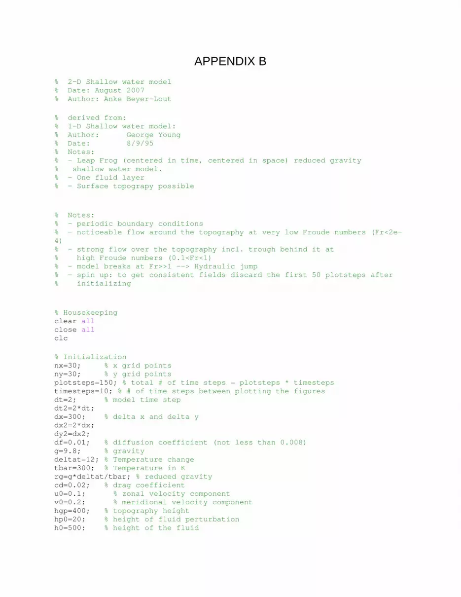
APPENDIX B % 2-D Shallow water model % Date: August 2007 % Author: Anke Beyer-Lout % derived from: % 1-D Shallow water model: % Author: George Young % Date: 8/9/95 % Notes: % - Leap Frog (centered in time, centered in space) reduced gravity % shallow water model. % - One fluid layer % - Surface topograpy possible % Notes: % - periodic boundary conditions % - noticeable flow around the topography at very low Froude numbers (Fr<2e-4) % - strong flow over the topography incl. trough behind it at % high Froude numbers (0.1<Fr<1) % - model breaks at Fr>>1 --> Hydraulic jump % - spin up: to get consistent fields discard the first 50 plotsteps after % initializing % Housekeeping clear all close all clc % Initialization nx=30; % x grid points ny=30; % y grid points plotsteps=150; % total # of time steps = plotsteps * timesteps timesteps=10; % # of time steps between plotting the figures dt=2; % model time step dt2=2*dt; dx=300; % delta x and delta y dx2=2*dx; dy2=dx2; df=0.01; % diffusion coefficient (not less than 0.008) g=9.8; % gravity deltat=12; % Temperature change tbar=300; % Temperature in K rg=g*deltat/tbar; % reduced gravity cd=0.02; % drag coefficient u0=0.1; % zonal velocity component v0=0.2; % meridional velocity component hgp=400; % topography height hp0=20; % height of fluid perturbation h0=500; % height of the fluid

% make the initial fluid height perturbation (a round hump) Rad=2; % radius of influence w1=zeros(6*Rad+1); for x=1:6*Rad+1 for y=1:6*Rad+1 r=(0-sqrt((x-3*Rad-1)^2+(y-3*Rad-1)^2)); % define w according to
distance between observation and analysis points if r==0 w1(x,y)=1; else w1(x,y)=exp(-r^2/(2*Rad^2)); end end end pert=w1*hp0; % make the topography (another round hump) Rad=3; % radius of influence w2=zeros(6*Rad+1); for x=1:6*Rad+1 for y=1:6*Rad+1 r=(0-sqrt((x-3*Rad-1)^2+(y-3*Rad-1)^2)); % define w according to
distance between observation and analysis points if r==0 w2(x,y)=1; else w2(x,y)=exp(-r^2/(2*Rad^2)); % Daley (1991) (3.6.4) end end end topo=w2*hgp; % initialize the fields xy=zeros(nx,ny); xaxis=0:dx:nx*dx-dx; yaxis=0:dx:ny*dx-dx; ustart=xy+u0; vstart=xy+v0; hstart=xy+h0; hgnd=xy; hstart(17:29,16:28)=hstart(17:29,16:28)+pert; % add initial perturbation to the fluid depth hgnd(6:24,6:24)=hgnd(6:24,6:24)+topo; % add topography to the hstart=hstart-hgnd; % initialize all the time steps % fluid height fields hvery=hstart; % very old: t-1 hnew=hstart; % new: t+1 htemp=hstart; % dummy variable for diffusion hol=hstart; % old: t % zonal momentum fields uvery=ustart; unew=ustart; utemp=ustart;
uold=ustart; udrag=unew*0; upgf=udrag; % meridional momentum fields vvery=vstart ;vnew=vstart; vtemp=vstart; vold=vstart; vdrag=vnew*0; vpgf=vdrag; % initialize output fields u=zeros(nx,ny,timesteps*plotsteps); v=zeros(nx,ny,timesteps*plotsteps); % calculate Froude number Fr=(u0^2+v0^2)/(rg*hgp/2); if Fr>=1 disp('Attention: Froude number critical!') disp('Aborting program!') disp('Please try again.') disp(' ') break end % plot initial fields figure(1) subplot(2,1,1); mesh(xaxis,yaxis,hgnd') hold on mesh(xaxis,yaxis,(hstart+hgnd)'); hold off axis([0 (nx-1)*dx 0 (ny-1)*dx 0 800]) xlabel('X [m]') ylabel('Y [m]') zlabel('H [m]') title('Initial field') subplot(2,1,2); contour(xaxis,yaxis,hgnd') title('topography and wind') axis equal xlabel('X [m]') ylabel('Y [m]') hold on quiver(xaxis,yaxis,ustart',vstart'); hold off axis tight % Itterate in time count=0; % counter for the output for bigtime=1:plotsteps for time=1:timesteps count=count+1; % % Loop over all the grid points %
for x=2:nx-1 for y=2:ny-1 % h advection and convergance hnew(x,y)=hvery(x,y)+(dt2/dx2)*uold(x,y)*(hol(x-1,y)-
hol(x+1,y))+(dt2/dy2)*vold(x,y)*(hol(x,y-1)-hol(x,y+1))+(dt2/dx2)*hol(x,y)*(uold(x-1,y)-uold(x+1,y))+(dt2/dy2)*hol(x,y)*(vold(x,y-1)-vold(x,y+1));
% v advection vnew(x,y)=(dt2/dx2)*uold(x,y)*(vold(x-1,y)- vold(x+1,y))+(dt2/dy2)*vold(x,y)*(vold(x-1,y)- vold(x+1,y))+vvery(x,y); % v p-gradient force (implicit) vpgf(x,y)=(dt2/dy2)*rg*((hol(x,y-1)+hgnd(x,y-1))- (hol(x,y+1)+hgnd(x,y+1))); vnew(x,y)=vnew(x,y)+vpgf(x,y); % v drag force
vdrag(x,y)=dt2*cd*vold(x,y)*(sqrt(vold(x,y)^2 +uold(x,y)^2))/hol(x,y);
vnew(x,y)=vnew(x,y)-vdrag(x,y); % u advection unew(x,y)=(dt2/dx2)*uold(x,y)*(uold(x-1,y)- uold(x+1,y))+(dt2/dy2)*vold(x,y)*(uold(x-1,y)- uold(x+1,y))+uvery(x,y); % u p-gradient force (implicit) upgf(x,y)=(dt2/dx2)*rg*((hol(x-1,y)+hgnd(x-1,y))- (hol(x+1,y)+hgnd(x+1,y))); unew(x,y)=unew(x,y)+upgf(x,y); % u drag force
udrag(x,y)=dt2*cd*uold(x,y)*(sqrt(vold(x,y)^2+ uold(x,y)^2))/hol(x,y);
unew(x,y)=unew(x,y)-udrag(x,y); nd e end for x=2:nx-1 for y=2:ny-1 % horizongal diffusion utemp(x,y)=(df*(unew(x+1,y)+unew(x,y+1)+unew(x-1,y)+unew(x,y- 1))+unew(x,y))/(1+4*df); vtemp(x,y)=(df*(vnew(x+1,y)+vnew(x,y+1)+vnew(x-1,y)+vnew(x,y- 1))+vnew(x,y))/(1+4*df); htemp(x,y)=(df*(hnew(x+1,y)+hnew(x,y+1)+hnew(x-1,y)+hnew(x,y- 1))+hnew(x,y))/(1+4*df); end end unew=utemp; vnew=vtemp; hnew=htemp; % % Impose the lateral boundary conditions % % periodic boundaries % x direction

vnew(nx,3:ny-2)=vnew(4,3:ny-2); unew(nx,3:ny-2)=unew(4,3:ny-2); hnew(nx,3:ny-2)=hnew(4,3:ny-2); vnew(nx-1,3:ny-2)=vnew(3,3:ny-2); unew(nx-1,3:ny-2)=unew(3,3:ny-2); hnew(nx-1,3:ny-2)=hnew(3,3:ny-2); vnew(1,3:ny-2)=vnew(nx-3,3:ny-2); unew(1,3:ny-2)=unew(nx-3,3:ny-2); hnew(1,3:ny-2)=hnew(nx-3,3:ny-2); vnew(2,3:ny-2)=vnew(nx-2,3:ny-2); unew(2,3:ny-2)=unew(nx-2,3:ny-2); hnew(2,3:ny-2)=hnew(nx-2,3:ny-2); % y direction vnew(3:nx-2,ny)=vnew(3:nx-2,4); unew(3:nx-2,ny)=unew(3:nx-2,4); hnew(3:nx-2,ny)=hnew(3:nx-2,4); vnew(3:nx-2,ny-1)=vnew(3:nx-2,3); unew(3:nx-2,ny-1)=unew(3:nx-2,3); hnew(3:nx-2,ny-1)=hnew(3:nx-2,3); vnew(3:nx-2,1)=vnew(3:nx-2,ny-3); unew(3:nx-2,1)=unew(3:nx-2,ny-3); hnew(3:nx-2,1)=hnew(3:nx-2,ny-3); vnew(3:nx-2,2)=vnew(3:nx-2,ny-2); unew(3:nx-2,2)=unew(3:nx-2,ny-2); hnew(3:nx-2,2)=hnew(3:nx-2,ny-2); % corners vnew(1:2,1:2)=vnew(nx-3:nx-2,ny-3:ny-2); unew(1:2,1:2)=unew(nx-3:nx-2,ny-3:ny-2); hnew(1:2,1:2)=hnew(nx-3:nx-2,ny-3:ny-2); vnew(nx-1:nx,1:2)=vnew(3:4,ny-3:ny-2); unew(nx-1:nx,1:2)=unew(3:4,ny-3:ny-2); hnew(nx-1:nx,1:2)=hnew(3:4,ny-3:ny-2); vnew(nx-1:nx,ny-1:ny)=vnew(3:4,3:4); unew(nx-1:nx,ny-1:ny)=unew(3:4,3:4); hnew(nx-1:nx,ny-1:ny)=hnew(3:4,3:4); vnew(1:2,ny-1:ny)=vnew(nx-3:nx-2,3:4); unew(1:2,ny-1:ny)=unew(nx-3:nx-2,3:4); hnew(1:2,ny-1:ny)=hnew(nx-3:nx-2,3:4); % % shift the arrays in time % htemp=hvery; utemp=uvery; vtemp=vvery; hvery=hol; uvery=uold; vvery=vold; hol=hnew; uold=unew; vold=vnew; % OUTPUT % save the new velocity fields every timestep for later use u(:,:,count)=unew; v(:,:,count)=vnew;

end % % Time filter the data to prevent time splitting (Asselin 1972) % uvery=(uvery+utemp)/2; vvery=(vvery+vtemp)/2; hvery=(hvery+htemp)/2; uold=(unew+uold)/2; vold=(vnew+vold)/2; hol=(hnew+hol)/2; hplot=hol-h0; % % Plot results % figure(3); subplot(2,1,1) mesh(xaxis,yaxis,(hol+hgnd)'); axis([0 (nx-1)*dx 0 (ny-1)*dx 450 550]) xlabel('X [m]') ylabel('Y [m]') zlabel('H [m]') title('fluid surface') subplot(2,1,2) contour(xaxis,yaxis,hgnd') title('topography and wind') axis equal xlabel('X [m]') ylabel('Y [m]') hold on quiver(xaxis,yaxis,uold',vold'); hold off axis tight end % OUTPUT % save the velocity fields to a .mat file save('SWM_output_velocity','u','v') % The End