ocean oxygen isotope constraints on mechanisms for millennial-scale climate variability

Ocean oxygen isotope constraints on mechanisms

for millennial-scale climate variability

Steffen Malskær OlsenDanish Meteorological Institute, Copenhagen, Denmark

Gary ShafferDanish Center for Earth System Science and Department of Geophysics, University of Copenhagen, Copenhagen, Denmark

Department of Geophysics, University of Concepcion, Concepcion, Chile

Christian J. BjerrumGeological Institute, University of Copenhagen, Copenhagen, Denmark

Received 23 June 2004; revised 27 October 2004; accepted 23 December 2004; published 26 February 2005.

[1] Millennial-scale climate variability pervades the last several million years of Earth history with largestamplitudes during moderate glacial conditions. However, the processes behind such variability remain unclear.Here we present results from a simplified, coupled climate model that includes an explicit treatment of theatmosphere-ocean cycle of oxygen-18 isotope. The model exhibits a relatively strong North Atlantic overturningcirculation for present day and last glacial maximum conditions. Self-sustained, millennial-scale oscillationswith strong and weak overturning states are found for moderate glacial conditions. These oscillations reproduceobserved features like ‘‘sawtooth’’ structure, Northern-Southern Hemisphere asynchrony, sensitivity to climatestate, and oxygen isotope signals in the ocean. Amplitudes, structures, and phasing of observed millennial-scalevariability in high-resolution, benthic oxygen isotope records from the North Atlantic Ocean are consistent withlarge heating/cooling cycles in the ocean interior, as found in the model. Glacial meltwater, changes in solarirradiance and high-frequency climate variability affect the timing, period, and persistence of the model climatecycles. However, the basic dynamics, structure, amplitude, and timescale of variability are due to internal, self-sustained oscillations in the model ocean-atmosphere system.

Citation: Olsen, S. M., G. Shaffer, and C. J. Bjerrum (2005), Ocean oxygen isotope constraints on mechanisms for millennial-scale

climate variability, Paleoceanography, 20, PA1014, doi:10.1029/2004PA001063.

1. Introduction

[2] Ice core records from Greenland and Antarctica haverevealed strong and pervasive, millennial-scale climatecycles during the last glacial period [Dansgaard et al.,1993; Blunier et al., 1998]. Ocean sediment records havedocumented significant millennial-scale variability duringthe last several million years with less, but persistent,variability during interglacial and maximum glacial condi-tions [McIntyre et al., 2001; McManus et al., 1999; Bond etal., 1997, 1999]. Greenland records of d18Ow (d18O inwater) show Dansgaard-Oeschger (DO) climate cycles,characterized by abrupt, decade-scale warming of 5�–10�C to a warm, interstadial state, subsequent slow coolingand then abrupt, decade-scale cooling back to a cold, stadialstate (Figure 1a). In contrast, Antarctic d18Ow recordsindicate slow warming, before initial, rapid, northern warm-ing, followed by slow cooling, simultaneous with slow,northern cooling (Figure 1b). This north-south structure andphasing is best defined during Heinrich (H) events (H1–H5in Figure 1d) of increased ice rafted debris from massiveiceberg discharges due to surging of the Laurentide ice sheet

[Bond et al., 1993]. However, the other DO cycles exhibitsimilar north-south structure and phasing. In Greenland,excursions to the warm state become shorter and lessfrequent toward the glacial maximum around 20 kyr beforepresent (B.P.; Figure 1a) [Schulz et al., 1999]. Any expla-nation for millennial-scale climate variability should be ableto account for these ice core observations [e.g., Ganopolskiand Rahmstorf, 2002; Schulz et al., 2002]. However, sincethe ocean is a key player in such variability [Stocker andJohnsen, 2003], it is equally important that any suchexplanation can also account for high-resolution, oceansediment observations.[3] Large decreases of 1% or more are found in plank-

tonic d18Oc (d18O in carbonate) in a high-resolution sedi-ment core from north of Iceland (62�N) during H eventstadials in Greenland (Figures 1a and 1c) [Rasmussen et al.,1996a]. A 1% decrease in d18Oc could reflect a temperatureincrease of about 4�C, a salinity decrease of about 2% orsome combination of the two. Smaller planktonic d18Oc

decreases less than 0.5% are found during other DOstadials. These d18Oc features have a symmetric shape overtime. Similar levels of millennial-scale, planktonic d18Oc

variability are found in high-resolution cores from north of40�N in the North Atlantic with less variability in cores to

PALEOCEANOGRAPHY, VOL. 20, PA1014, doi:10.1029/2004PA001063, 2005

Copyright 2005 by the American Geophysical Union.0883-8305/05/2004PA001063$12.00

PA1014 1 of 19

the south (Figure 2). An exception to this rule is strongvariability in a planktonic d18Oc record at 37�N off Portugal[Shackleton et al., 2000]. However, this may reflect strongzonal gradients in millennial-scale variability across theAtlantic Ocean in the 30�–40�N latitude band [Vautraverset al., 2004].[4] Large decreases of 1% or more are found in benthic

d18Oc at the �1000 m depth at 62�N during H eventstadials. However, quite large benthic d18Oc decreasesof 0.5–1% coincide with other DO stadials (Figures 1aand 1d) [Rasmussen et al., 1996a]. Most of these d18Oc

features exhibit sawtooth shape and terminate with rapid

increases tied to rapid Greenland warming events. FeaturesassociatedwithH3 andH4 are exceptions to this pattern. Slowbenthic d18Oc increases of 0.5% or less at the�3000 m depthof the 37�N core off Portugal track slow cooling inGreenland and Antarctica (Figure 1e) [Shackleton et al.,2000]. In both benthic records, d18Oc values decrease overabout 1 kyr before rapid northern warming. These inter-relationships are apparent for strong H events but also forweaker DO cycles, indicating similar dynamics for stron-ger and longer, millennial-scale climate cycles and weakerand shorter cycles [Bond et al., 1999]. Throughout theNorth Atlantic Ocean, millennial-scale benthic d18Oc var-iability in high-resolution cores greatly increases from thedeep ocean to intermediate depths (Figure 2).[5] Here we interpret both the ice and sediment core

records with the help of simulations from a simplified,coupled climate model that includes the ocean-atmosphered18Ow cycle. Ocean d18Oc is calculated explicitly from

Figure 2. Standard deviation (s) from high-resolution,filtered records (periods � 12 kyr retained) of planktonicand benthic d18Oc over the interval �50–20 kyr B.P. Theone-sided error bars show estimated s prior to smoothing bymoderate bioturbation, given core sedimentation rates[Anderson, 2001]. The records are from the North Atlanticsites, numbered as follows: 1, 6�N 44�W; 2, 5�N 44�W[Curry et al., 1999; 3, 37�N 10�W [Shackleton et al., 2000];4, 4�N 43�W; 5, 43�N 30�W; 6, 55�N 14�W [Vidal et al.,1998]; 7, 61�N 23�W, [Curry et al., 1999]; 8, 67�N 04�E[Dokken and Jansen, 1999]; 9, 63�N 04�W [Rasmussen etal., 1996a]; and 10, 26�N 78�W [Curry et al., 1999]. Alsoshown are vertical s profiles for d18Oc and d18Ow from amodel simulation shown in Figure 12. Model results werefiltered as above before calculating s.

Figure 1. Millennial-scale variability in ice and deep seasediment records. The d18Ow records are from (a) aGreenland ice core [Grootes and Stuiver, 1997] and (b) anAntarctic ice core [Johnsen et al., 1972]. The d18Oc recordsare from (c) high northern latitude planktonic foraminiferalcalcite [Rasmussen et al., 1996a], (d) intermediate depth,high northern latitude benthic foraminiferal calcite[Rasmussen et al., 1996a], and (e) deep, middle northernlatitude benthic foraminiferal calcite [Shackleton et al.,2000]. Figures 1a and 1b are on the GISP2 age scale[Blunier and Brook, 2001]. Figures 1c and 1d were fitted tothis scale using magnetic susceptibility [Dokken andJansen, 1999], and Figure 1e was fitted to this scale usingplanktonic d18Oc [Shackleton et al., 2000]. Several Heinrichevents are indicated (H2–H5) [Bond and Lotti, 1995].Stippled lines aid visual correlation. Freshening andwarming arrows are interpretations guided by our modeld18Oc calculations (see Figures 7 and 8).

PA1014 OLSEN ET AL.: MECHANISMS FOR CLIMATE VARIABILITY

2 of 19

PA1014

modeled ocean temperature and d18Ow distributions forcomparison with high-resolution ocean sediment records.The model reproduces observations and reconstructionsrather well for modern day and last glacial maximumforcing. Emphasis is placed on moderate glacial forcing,for which millennial-scale, self-sustained climate oscilla-tions are found that compare well with d18Oc from sedimentcores. We also investigate the sensitivity of such oscillationsto choices of model parameter values, climate noise andweak, periodic variations of solar irradiance. Model simu-lations are then carried out for the last glacial period,including simplified Heinrich events and slowly varyingclimate forcing. These simulations capture many importantfeatures from the ice and sediment core records. Finally, ourresults are discussed in the context of other recent work onmillennial-scale climate variability.

2. Model Description and Validation

2.1. Modern Day Simulation

[6] We use a simplified global climate model with atmo-sphere, ocean, land and sea ice components and four zonemeridional resolution (Figure 3) [Olsen, 2002]. Thismodel setup is similar to that of Gildor and Tziperman[2001]; however, our ocean submodel has fine (100 m)vertical resolution. This allows detailed treatment ofocean exchange and Southern Ocean processes, important

for ocean circulation and climate [Shaffer and Olsen, 2001;Toggweiler and Samuels, 1995]. Among the processes andfeatures we consider are ocean vertical diffusion dependenton stratification, deep water formation off Antarctica bybrine rejection and the seasonal cycle. We also include anovel explicit treatment of ocean-atmosphere d18Ow cycle.We choose model parameter values guided by observationsin the present day climate system and, for these parametervalues, consider model solutions for present and pastexternal forcing by atmospheric pCO2, icecap extent andinsolation changes due to orbital variations [Berger andLoutre, 1991]. A detailed model description is presented inAppendix A.[7] A modern day ‘‘on’’ mode is found for preanthropo-

genic forcing, including relatively weak horizontal mixingto account for relatively weak modern winds (Figure 4a and

Figure 3. Sketch of the geometry and components of thesimple global climate model. The vertical striped bar at40�S extends down to 2000 m depth and marks the model‘‘Drake Passage’’ (see Appendix A for a detailed modeldescription). Note that only the Atlantic Ocean circulation ismodeled.

Figure 4. Modeled modern day atmosphere and oceanconditions. (a) Meridional overturning circulation stream-lines in Sv (1 Sv = 106 m3s�1) and (b) comparison ofthe seasonal cycle of zone mean, model air temperature(black lines) with observed air temperatures (gray lines). InFigure 4a the upper overturning cell carries North AtlanticDeep Water and a lower overturning cell carries AntarcticBottom Water (positive contours: clockwise overturning).Yearly average sea ice extent is shown as white horizontalbars at the top. Note the brine rejection-driven circulation at70�S and the surface layer, Ekman transport at 40�S, bothinjected into appropriate density surfaces in adjacentmodel zones. In Figure 4b the observed air temperaturesat 1000 mbar are monthly means based on the last 40 yearsof the NCEP/NCAR CDAS/Reanalysis Project data.


3 of 19

PA1014

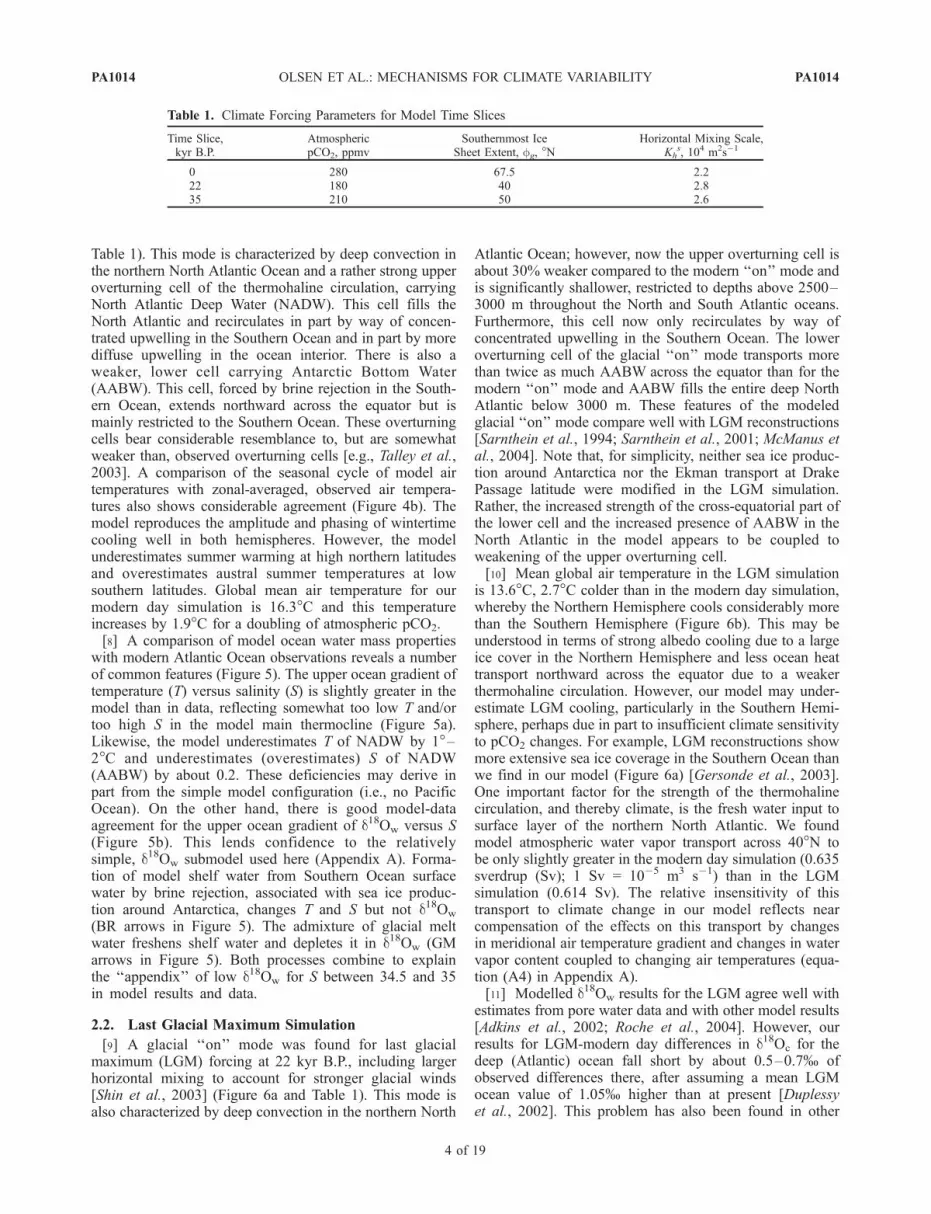
Table 1). This mode is characterized by deep convection inthe northern North Atlantic Ocean and a rather strong upperoverturning cell of the thermohaline circulation, carryingNorth Atlantic Deep Water (NADW). This cell fills theNorth Atlantic and recirculates in part by way of concen-trated upwelling in the Southern Ocean and in part by morediffuse upwelling in the ocean interior. There is also aweaker, lower cell carrying Antarctic Bottom Water(AABW). This cell, forced by brine rejection in the South-ern Ocean, extends northward across the equator but ismainly restricted to the Southern Ocean. These overturningcells bear considerable resemblance to, but are somewhatweaker than, observed overturning cells [e.g., Talley et al.,2003]. A comparison of the seasonal cycle of model airtemperatures with zonal-averaged, observed air tempera-tures also shows considerable agreement (Figure 4b). Themodel reproduces the amplitude and phasing of wintertimecooling well in both hemispheres. However, the modelunderestimates summer warming at high northern latitudesand overestimates austral summer temperatures at lowsouthern latitudes. Global mean air temperature for ourmodern day simulation is 16.3�C and this temperatureincreases by 1.9�C for a doubling of atmospheric pCO2.[8] A comparison of model ocean water mass properties

with modern Atlantic Ocean observations reveals a numberof common features (Figure 5). The upper ocean gradient oftemperature (T) versus salinity (S) is slightly greater in themodel than in data, reflecting somewhat too low T and/ortoo high S in the model main thermocline (Figure 5a).Likewise, the model underestimates T of NADW by 1�–2�C and underestimates (overestimates) S of NADW(AABW) by about 0.2. These deficiencies may derive inpart from the simple model configuration (i.e., no PacificOcean). On the other hand, there is good model-dataagreement for the upper ocean gradient of d18Ow versus S(Figure 5b). This lends confidence to the relativelysimple, d18Ow submodel used here (Appendix A). Forma-tion of model shelf water from Southern Ocean surfacewater by brine rejection, associated with sea ice produc-tion around Antarctica, changes T and S but not d18Ow

(BR arrows in Figure 5). The admixture of glacial meltwater freshens shelf water and depletes it in d18Ow (GMarrows in Figure 5). Both processes combine to explainthe ‘‘appendix’’ of low d18Ow for S between 34.5 and 35in model results and data.

2.2. Last Glacial Maximum Simulation

[9] A glacial ‘‘on’’ mode was found for last glacialmaximum (LGM) forcing at 22 kyr B.P., including largerhorizontal mixing to account for stronger glacial winds[Shin et al., 2003] (Figure 6a and Table 1). This mode isalso characterized by deep convection in the northern North

Atlantic Ocean; however, now the upper overturning cell isabout 30% weaker compared to the modern ‘‘on’’ mode andis significantly shallower, restricted to depths above 2500–3000 m throughout the North and South Atlantic oceans.Furthermore, this cell now only recirculates by way ofconcentrated upwelling in the Southern Ocean. The loweroverturning cell of the glacial ‘‘on’’ mode transports morethan twice as much AABW across the equator than for themodern ‘‘on’’ mode and AABW fills the entire deep NorthAtlantic below 3000 m. These features of the modeledglacial ‘‘on’’ mode compare well with LGM reconstructions[Sarnthein et al., 1994; Sarnthein et al., 2001; McManus etal., 2004]. Note that, for simplicity, neither sea ice produc-tion around Antarctica nor the Ekman transport at DrakePassage latitude were modified in the LGM simulation.Rather, the increased strength of the cross-equatorial part ofthe lower cell and the increased presence of AABW in theNorth Atlantic in the model appears to be coupled toweakening of the upper overturning cell.[10] Mean global air temperature in the LGM simulation

is 13.6�C, 2.7�C colder than in the modern day simulation,whereby the Northern Hemisphere cools considerably morethan the Southern Hemisphere (Figure 6b). This may beunderstood in terms of strong albedo cooling due to a largeice cover in the Northern Hemisphere and less ocean heattransport northward across the equator due to a weakerthermohaline circulation. However, our model may under-estimate LGM cooling, particularly in the Southern Hemi-sphere, perhaps due in part to insufficient climate sensitivityto pCO2 changes. For example, LGM reconstructions showmore extensive sea ice coverage in the Southern Ocean thanwe find in our model (Figure 6a) [Gersonde et al., 2003].One important factor for the strength of the thermohalinecirculation, and thereby climate, is the fresh water input tosurface layer of the northern North Atlantic. We foundmodel atmospheric water vapor transport across 40�N tobe only slightly greater in the modern day simulation (0.635sverdrup (Sv); 1 Sv = 10�5 m3 s�1) than in the LGMsimulation (0.614 Sv). The relative insensitivity of thistransport to climate change in our model reflects nearcompensation of the effects on this transport by changesin meridional air temperature gradient and changes in watervapor content coupled to changing air temperatures (equa-tion (A4) in Appendix A).[11] Modelled d18Ow results for the LGM agree well with

estimates from pore water data and with other model results[Adkins et al., 2002; Roche et al., 2004]. However, ourresults for LGM-modern day differences in d18Oc for thedeep (Atlantic) ocean fall short by about 0.5–0.7% ofobserved differences there, after assuming a mean LGMocean value of 1.05% higher than at present [Duplessyet al., 2002]. This problem has also been found in other

Table 1. Climate Forcing Parameters for Model Time Slices

Time Slice,kyr B.P.

AtmosphericpCO2, ppmv

Southernmost IceSheet Extent, fg, �N

Horizontal Mixing Scale,Kh

s, 104 m2s�1

0 280 67.5 2.222 180 40 2.835 210 50 2.6


4 of 19

PA1014

modeling work [Roche et al., 2004]. The data may beinterpreted as a cooling in the deep LGM Atlantic, 2�–3�C greater still than the cooling of about 1�C found in ourmodel there. Much of this discrepancy derives from the factthat our modern day NADW is 1�–2�C too cold. Thus whenNADW is replaced by AABW during the LGM in themodel, cooling is underestimated. It is also possible thatcolder, windier conditions around Antarctica during theLGM may have led to more sea ice production, more brinerejection and thus more AABW formation there. Theseaspects are outside our present focus on moderate glacialconditions but present prospects for future study.

3. Model Climate Oscillations

3.1. Oscillation Structure and Dynamics

[12] Millennial-scale climate oscillations are found in themodel for external forcing at 35 kyr B.P., an intermediatevalue of horizontal mixing, but no external periodic forcing(Table 1). These self-sustained oscillations are coupled tolarge variability in surface layer salinity and interior tem-perature (Figures 7 and 8). Such ‘‘deep-decoupling’’ oscil-lations are also found in other simple models as well as 3-D

Figure 5. Comparison of model ocean water massproperties for the modern day simulation with modernAtlantic Ocean observations. (a) Temperature (T) versussalinity (S). (b) The d18Owversus S. Heavy black lines aremodeled, zone mean profiles from ocean surface to bottom.Arrows mark the transition of Southern Ocean surface layerwater to shelf water (a precursor of Antarctic Bottom Water)by brine rejection during sea ice formation and export (BR)and by input of glacial meltwater (GM). Observational dataare for the Atlantic Ocean between 60�S and 70�N and weretaken from the Global Seawater Oxygen-18 Database(available at http://www.giss.nasa.gov/data/o18data). Notethe good correspondence between the mean slope of modeld18Ow versus S and the data.

Figure 6. Modeled last glacial maximum atmosphere andocean conditions. (a) LGM meridional overturning circula-tion streamlines in Sv (positive contours: clockwise over-turning). Yearly average sea ice extent is shown as whitehorizontal bars at the top. (b) Modeled, zone mean LGMtemperatures minus modern day temperatures for theatmosphere (dashed lines) and the ocean surface layer(solid lines).


5 of 19

PA1014

models [e.g., Winton and Sarachik, 1993; Winton, 1997;Sakai and Peltier, 1997; Oka et al., 2001; Schulz et al.,2002]. The behavior of our model demonstrates sensitivityto orbital forcing since pCO2, icecap extent and horizontal

mixing at 35 kyr B.P. lie between modern (preindustrial)and LGM values while simulations for both of these periodsyield steady states characterized by ‘‘on’’ mode conditions(Table 1). The results can be understood in terms of long

Figure 7


6 of 19

PA1014

term changes of low latitude (40�S–40�N) to high northernlatitude (40�N–90�N) difference in yearly mean solarinsolation (DQ; Figure 9). Whereas modern day and LGMorbital forcing are similar, DQ was 4–5% weaker at 35 kyrthan at present or during the LGM. This weaker insolationdifference leads to weaker thermal forcing of the thermo-haline circulation at 35 kyr B.P., tending to destabilizethe ‘‘on’’ mode. This new finding may help explain

greater observed millennial-scale variability around thistime (Figure 1) [see also Schulz et al., 1999].[13] Model oscillations exhibit many observed features

during DO cycles like rapid climate transitions, hemisphericasynchrony and, during stadials, warming of intermediatedepth water in the tropical and North Atlantic and theinvasion of the deep North Atlantic by Antarctic BottomWater [Dansgaard et al., 1993; Blunier et al., 1998; Curry

Figure 7. Model self-sustained climate oscillations for 35 kyr B.P. external forcing. (a) Time series versus depth oftemperature and salinity (contoured) in the 40�–90�N zone. Time slices of ocean distributions (b) after the onset of a coldphase, (c) during the off mode, (d) shortly before the onset of a warm phase, and (e) during a warm phase. Shown areoverturning streamlines in Sv (top row), vertical diffusion coefficient (second row; ongoing convection is shaded), andanomalies of temperature (third row), salinity (fourth row), d18Ow (fifth row), and d18Oc (bottom row). Anomalies arecalculated relative to local means over a complete oscillation (white contours mark zero anomaly). Sea ice extent is shownas white horizontal bars at the top of the second row. For clarity, only salinities above 34.0 are contoured and no glacialsalinity offset is applied in Figure 7a. The period of the oscillation is 1.31 kyr. A sensitivity analysis (see Figure 10) showsthat this period could be tuned toward the observed, �1.5 kyr period. Note how deep ocean temperature (Figure 7a) slowlyincreases during weak circulation conditions due to downward diffusion of heat into the low latitude ocean.

Figure 8. Evolution of model variables for selected model zones and water depths over a self-sustainedclimate oscillation for 35 kyr B.P. external forcing. (a) Air temperature, (b) surface layer salinity,(c) surface layer d18Oc, (d) surface layer d

18Ow, (e) intermediate and deep d18Oc, and (f) intermediate anddeep d18Ow. Zone and depth identifications in Figures 8a, 8c, and 8e also apply to Figures 8b, 8d, and 8f,respectively. Ocean mean d18Ow at 35 kyr B.P. is set to 0.75% but, for clarity, no glacial salinity offset isapplied. Dots on vertical axes in Figures 8a and 8b indicate modern day simulation values (open dots areSouthern Hemisphere values). Note that high latitude d18Oc at 1000 m (Figure 8e) is in phase with surfacelayer d18Oc (Figure 8c) due to temperature changes at 1000 m and salinity changes in the surface layer.


7 of 19

PA1014

et al., 1999; Oppo and Lehman, 1993; Rasmussen et al.,1996a]. When a halocline develops and convection ceasesin the northern North Atlantic, the upper overturning cellweakens and shoals, giving way to the lower overturningcell that fills the deep Atlantic with cold Antarctic BottomWater (Figures 7a and 7b). Without cooling by NorthAtlantic convection, the ocean interior above about 2500 mwarms slowly by downward diffusion of heat at lowlatitudes (Figures 7a and 7c) [cf. Ruhlemann et al., 2004].Some of this heat is transported poleward in subsurfacelayers by the weak, shallow upper overturning cell andhorizontal mixing. In the Southern Ocean, this heat isupwelled to the ocean surface, warming the atmosphere(Figures 7d and 8a). In the northern North Atlantic, thispoleward heat transport creates a growing temperatureinversion that weakens upper ocean stratification, promot-ing increased vertical mixing and, finally, the onset ofconvection there (Figures 7a, 7d, and 7e). The switch toconvection and strong overturning is self-reinforcing assaltier, warmer water brought to the surface from belowand from the south cools rapidly by air-sea exchange. Heataccumulated in the ocean interior is thereby released rapidlyto the atmosphere and the sea ice edge moves from 60�N to80�N within decades (Figure 7e). The heat output from themodel ocean and the albedo decrease quickly and raiseNorthern Hemisphere air temperature to near present daylevels despite low pCO2 and a large continental ice cover(Figure 8a). At the same time, convection cools the oceaninterior above about 2500 m and the upper overturning cellfills the deep North Atlantic (Figure 7e). The cell graduallyweakens because of cooling of the low latitude thermoclineas warmer water there is transported poleward and replacedby cooler water from the south and from below. Less

poleward salt transport in the weakened cell and continuedfresh water input from the atmosphere promote gradualhalocline buildup and, finally, convection shutdown in thenorthern North Atlantic. The oscillation period of order 1 kyrcan be related to a diffusive timescale for the oceanthermocline, L2/k, where L is the ocean thermocline depthand k is the vertical diffusion coefficient in the thermocline.For example, L = 1 � 103 m and k = 2 � 10�5 m2 s�1

[Ledwell et al., 1993] yields a timescale of about 1.5 kyr.

3.2. Comparisons With Observations

[14] Air temperature amplitude, structure and north-southasynchrony over model cycles compare favorably withGreenland and Antarctic data (Figures 1a, 1b, and 8a).Model d18Oc changes due to surface warming of �2�C inthe 0�–40�N model zone are consistent with low latitudeplanktonic d18Oc data [Curry et al., 1999]. Warming at highsouthern latitudes during cool, ‘‘off’’ mode conditions in thenorth is often explained by weaker cross-equatorial heattransport in a weaker thermohaline circulation [Crowley,1992]. Our results suggest that part of the observed Ant-arctic warming may also be explained by ocean interiorwarming at low latitudes, ocean transport to the SouthernOcean and upwelling into the surface layer there [cf.Ruhlemann et al., 2004]. Large, abrupt increases in d18Oc

within the cycles at 1000 m depth in the 40�–90�N zonereflect, in the model (Figure 8e) and likely in the data(Figure 1d), rapid cooling at the onset of convection(Figures 7a, 7d, and 7e). During the slow, interior ocean-warming phase of the cycles, model results show slowdecreases in d18Oc there. In general, data show a similartendency although specific events deviate from this pattern,probably in part due to sedimentation rate assumptions. Inthe surface layer of the 40�–90�N zone, d18Ow changes,associated with fresh water balance (salinity) changes,dominate the d18Oc signal (Figures 8b, 8c, and 8d).Thus, although model surface and intermediate depth d18Oc

in the northern North Atlantic are controlled in differentways, they vary in phase over the cycles (Figures 8c and 8e),as observed (Figures 1c and 1d) [Rasmussen et al., 1996a;Dokken and Jansen, 1999]. Slow increases and decreases ind18Oc are found at 3000 m depth with minimum values atthe onset of convection (Figure 8e). In the model, andpossibly in the data (Figure 1e), this reflects interior heatingand cooling cycles and, to a lesser extent, salinity andwater mass changes as Antarctic Bottom Water invades thedeep North Atlantic during the ‘‘off’’ phase of the cycles(Figures 7b–7d). Such circulation changes explain largeobserved, millennial-scale variability of benthic d13C in thedeep North Atlantic during glacial time [Sarnthein et al.,2001; Curry et al., 1999].

3.3. Sensitivity to Parameter Choices

[15] We performed extensive studies of the sensitivity ofour model results to choices of model parameter values forclimate forcing of 35 kyr B.P. Results are quite sensitive tovertical diffusion and wind-driven circulation (estimatedhere by horizontal diffusion concentrated in the upperocean), as in simpler and more complex, coupled models[Shaffer and Olsen, 2001; Oka et al., 2001]. For strongvertical and horizontal diffusion, the only model state is the

Figure 9. Time series of zone averaged, yearly mean solarinsolation difference between the 40�S–40�N low zone andthe 40�–90�N zone from 50 kyr B.P. to the present. Thevertical dashed lines mark the three different time slicesconsidered here. The reduced thermal torque at 35 kyr B.P.permits self-sustained oscillations in the model for theprescribed atmospheric pCO2 and ice cap extent.


8 of 19

PA1014

‘‘on’’ mode (Figure 10a). Downward diffusion of heat atlow latitudes enhances the thermal forcing of the upperoverturning cell and the wind-driven, horizontal diffusionlimits the meridional salinity gradient opposing this cell. Forweak vertical and horizontal mixing, the only model state isthe ‘‘off’’ mode. For sufficiently strong vertical but weakhorizontal diffusion, both modes are possible steady statesolutions. This multiple equilibrium behavior rests upon anadvective salinity feedback on the upper cell, as shown by asimilar result in a simpler coupled model [Shaffer andOlsen, 2001]. Model oscillations exist in a well-definedrange of upper ocean vertical and horizontal diffusivityscales. For example, these oscillations are only found forsmall, upper ocean vertical diffusivity scales of less thanabout 3.5 � 10�5 m2 s�1. Meridional overturning may besensitive to vertical diffusion parameterizations [Nilsson etal., 2003]. However, in additional sensitivity studies (notshown) we found similar sensitivities as in Figure 10a forfixed low vertical diffusivity and for a stronger dependenceof vertical diffusivity on stratification.[16] Oscillations are present in the model for a wide range

of Southern Ocean forcing, demonstrating relative modelinsensitivity to changes in the values of Southern Oceanparameters (Figure 10b). Increased Ekman transport tendsto favor the ‘‘on’’ mode while increased sea ice productionand associated brine rejection tend to favor the ‘‘off’’ mode.Poleward heat transport in the atmosphere also increaseswhen the atmospheric exchange coefficient for sensible heatis increased (Figure 10c). However, longwave radiationfeedbacks in the overall atmospheric heat balance act toreduce the meridional air temperature gradient in this case.This leads to less poleward water vapor transport, favoringthe ‘‘on’’ mode. The meridional air temperature gradientdecreases slightly when the atmospheric exchange coeffi-cient of water vapor/latent heat is increased; however, thenet effect is an increase in poleward water vapor transport,favoring the ‘‘off’’ mode. This explains why model oscil-lations are rather insensitive to coupled changes of theseexchange coefficients. Finally it should be noted that modeloscillations are found for atmospheric water vapor trans-

Figure 10. Sensitivity of model climate regimes toparameter value changes for 35 kyr B.P. forcing.(a) Sensitivity to upper ocean, vertical, and horizontaldiffusitivity scales, Kv and Kh, respectively, (b) sensitivity toEkman transport, E, and sea ice formation/ice shelf melting,Fi, and (c) sensitivity to exchange coefficients for sensibleand latent heat in the atmosphere, Kt and Kq, respectively,expressed as % changes from standard values (Table A1).Five different model regimes are an ‘‘on’’ mode with strongoverturning circulation in the North Atlantic, an ‘‘off’’mode with weak overturning circulation in the NorthAtlantic, both ‘‘on’’ and ‘‘off’’ modes possible, 50–70 yrperiod oscillations in North Atlantic convection in a weak‘‘on’’ mode situation (hatched area in Figure 10a) andmillennial-scale oscillations (white; oscillation periodscontoured in kyr). Other parameter values and forcing asfor 35 kyr B.P. in Tables 1 and A1; dots at the figure centersmark the standard case of Figures 7 and 8.


9 of 19

PA1014

ports across 40�N in the range of 0.58–0.72 Sv, for ourstandard parameters values and 35 kyr B.P. forcing.

3.4. Influence of Weak, External Forcing

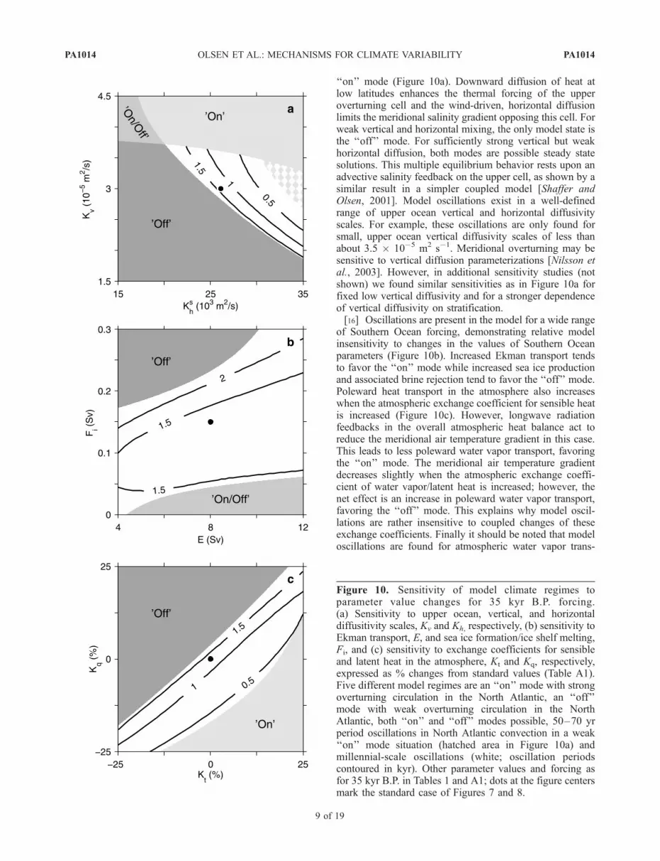
[17] Millennial-scale, climate change may be influencedby pervasive, interannual- to decadal-scale variability in thereal climate system. Such variability, when modeled asweak noise on the atmospheric water vapor transportacross 40�N, broadens the range of climate forcing forwhich millennial-scale oscillations occur in the model(Figures 11a and 11b). Model oscillation periods are some-what shorter in the presence of this noise, as ‘‘on’’ modesare triggered earlier in the cycles. Furthermore, other workhas raised the possibility of weak solar forcing on millennialtimescales [Bjorck et al., 2001; Bond et al., 2001]. Therange of climate forcing for which oscillations occur is alsobroadened by forcing with a weak, prescribed, 1.5 kyrperiod modulation of the solar constant (Figure 11c). Inaddition, this weak forcing acts to phase-lock the oscilla-tions into a 1.5 kyr period at the warm and cold ends of thisrange. Such phase-locking has also been found in other

studies [Ganopolski and Rahmstorf, 2002; Timmermann etal., 2003]. Forcing by a combination of weak noise andperiodic forcing leads to a still broader range of climateforcing for which oscillations occur. Again, phase-locking isfound at the ends of this range; however, there is a broaderinterior segment without phase-locking (Figure 11d). It isimportant to note that the presence of weak forcing has littleeffect on oscillation amplitude and period, which arebasically set by internal dynamics. System variables likeEkman transport and vertical and horizontal diffusion surelyalso vary over the real glacial-interglacial climate cycles andwould also have influenced the climate range for whichthese oscillations are possible. The ‘‘range-broadening’’effect of weak forcing may help explain the ubiquity ofthe millennium-scale climate variability in Quaternary cli-mate records.

4. Last Glacial Period Simulations

[18] A model simulation was carried out for the period50 kyr to 20 kyr B.P. with standard model parameters,

Figure 11. Behavior of the model North Atlantic overturning circulation during a slow 30 kyr transitionfrom warm to cold conditions forced by prescribed changes in atmospheric pCO2 and in fg, thesouthernmost latitude of ice cap extent. (a) Results for standard parameter values and 35 kyr orbitalforcing and horizontal exchange (‘‘wind-driven circulation’’), (b) including zero-mean Gaussian noise onwater vapor transport across 40�N with s = 0.0025 Sv, guided by observations over the Atlantic for arecent 40 year period [Walsh et al., 1994], otherwise as Figure 11a, (c) including a 1.5% modulation ofthe solar constant with a 1.5 kyr period, otherwise as Figure 11a, (d) including the weak forcings ofFigure 11b and 11c, otherwise as Figure 11a. The gray vertical bars in Figure 11c and 11d mark weaksolar forcing maxima. The range for which oscillations occur is broadened when noise (Figure 11b) orsolar modulation (Figure 11c) are imposed. Note also phase-locking of the oscillation to the solar cycle atthe perimeters of the oscillation range (Figures 11c and 11d).


10 of 19

PA1014

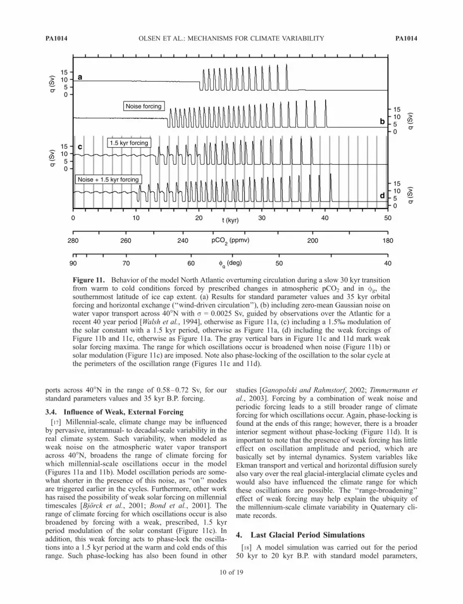
slowly varying pCO2 and continental ice cover extent fromobservations, orbital forcing, slowly increasing horizontalmixing and imposed H events (Figure 12; see caption fordetails). The simulation facilitates a more direct comparisonwith the last glacial period observations, summarized inFigures 1 and 2. Model results mimic well many of the

features in Figure 1 such as enhanced DO activity between30 and 40 kyr B.P. and long ‘‘on’’ mode periods followingH events. This enhanced DO activity in the simulation canbe explained by a low difference in solar insolation betweenlow latitudes and high northern latitudes during this period,as discussed above. Long ‘‘on’’ mode periods following Hevents in the model, and likely in the data, can be explainedby the stabilization of the ‘‘on’’ mode via decreased freshwater flux to the northern North Atlantic surface layer, dueto parameterized fresh water storage in growing ice caps.[19] Other observational features summarized in Figure 1

are also reproduced well in the simulation such as atmo-spheric warming at high southern latitudes during cold,‘‘off’’ mode conditions in the northern North Atlantic andlarger amplitudes in planktonic and benthic d18Oc for Hevents than for DO events (Figures 1 and 12). As shownabove, model atmospheric warming at high southern lat-itudes is largely associated with ocean interior warmingduring ‘‘off’’ mode conditions. Indeed, interior warmingand cooling cycles explain similar, millennium-scale evo-lution of atmospheric temperature around Antarctica anddeep, benthic d18Oc in the North Atlantic Ocean in themodel, and likely in the data (Figures 1b, 1e, 12b, and 12e).Larger planktonic d18Oc amplitudes for H events than forDO events in the northern North Atlantic reflect icebergmeltwater of the H events in the model and in the data(Figures 1c and 12c). However, in the model and arguablyin the data, greater benthic d18Oc amplitudes for H eventsthan for DO events in the North Atlantic are associated withlonger, and thus greater, interior warming as surface layerfreshening from iceberg melting during H events extends‘‘off’’ mode conditions by suppressing open ocean convec-tion (Figures 1d, 1e, 12d, and 12e). The model simulationalso captures features in the data like in-phase variability forplanktonic and benthic d18Oc over H and DO events,symmetric event structure for planktonic d18Oc and saw-tooth event structure for benthic d18Oc in the North Atlantic(Figures 1c–1e and 12c–12e). These features reflect inthe model, and probably in the data, control of northernNorth Atlantic planktonic d18Oc by surface layer salinityand control of North Atlantic benthic d18Oc by interiortemperature.[20] Model results show a strong increase in d18Oc vari-

ability from the deep ocean up into the thermocline in theNorth Atlantic, as was found in the observations (Figure 2).A comparison of model d18Ow and d18Oc variability showsclearly that this strong increase is explained by a strongincrease in model temperature variability. Model d18Oc

variability overestimates observed benthic d18Oc variabilitywithin the North Atlantic thermocline and shows very largevariability near 200–300 m, a depth range only in partcaptured by vertically migrating N. pachyderma (s) [Weineltet al., 2001]. However, observed d18Oc variability in thethermocline still greatly exceeds model d18Ow there, sug-gesting that observed d18Oc variability there reflects large,millennial-scale, temperature variability during the lastglacial period. In contrast, model surface layer variabilityof d18Oc in the northern North Atlantic is dominated by themeltwater signal from the H events and overestimatesobserved planktonic d18Oc there. Greater variability in the

Figure 12. Model simulation from 50 to 20 kyr B.P. of airtemperature (Ta) and ocean d18Oc. (a) Ta in the 40�–90�Nzone. (b) Ta in the 40�–90�S zone. (c) Ocean surface d18Oc

in the 40�–90�N zone. (d) The d18Oc at 1000 m depth in the40�–90�N zone. (e) The d18Oc at 3000 m depth in the 0�–40�N zone. For this calculation the horizontal diffusivityscale, Kh

s, was increased linearly over this period from 2.5to 2.8 � 104 m2 s�1 to account for increasing wind speeds,atmospheric pCO2 was decreased linearly from 220 to180 ppmv and the southernmost ice cap extent wasadvanced from 60 to 40�N such that ice cap area increasedlinearly with time over this period. Orbital forcing over thisperiod was calculated from Berger and Loutre [1991]. The40�–90�N zone was forced by Heinrich meltwater cycles(d18Ow = �30%) with 7 kyr buildup and 1 kyr releasephases (both decreasing linearly to zero), guided by an icecap surge model [MacAyeal, 1993]. Amplitudes were scaledto reflect an 8 m sea level change over the global ocean[Chappell, 2002]. The vertical stippled lines mark thetransition from release to buildup phases of this forcing. Forcomparison with Figure 1, ocean mean d18Ow was increasedlinearly from 0.5 to 1.0% over this period. Note how modelfluctuations (Figures 12c, 12d, and 12e) compare withocean sediment observations (Figures 1c–1e).


11 of 19

PA1014

model than in the observations in the surface layer mayreflect too large assumed H event amplitude, too lowassumed d18Ow in the iceberg meltwater, too weak nearsurface vertical exchange or some combination of thesefactors.

5. Discussion

[21] One leading explanation for millennial-scale cli-mate variability during glacial time involves switchesamong a modern ‘‘on’’ mode, a glacial ‘‘on’’ mode anda Heinrich ‘‘off’’ mode of the thermohaline circulation,forced by changes in the North Atlantic freshwater budget[Clark et al., 2002]. This explanation attributes DOcycles to switches between the modern and glacial‘‘on’’ modes, associated with large horizontal displace-ments of deep convection sites. In this view, DO cyclesare paced by millennial-scale, external forcing and per-haps amplified by stochastic resonance [Alley et al., 2001;Ganopolski and Rahmstorf, 2001]. However, for bothmodern and glacial ‘‘on’’ modes, deep convection wouldventilate the North Atlantic with cold, salty water to wellbelow 2000 m [Paul and Schafer-Neth, 2003]. Thereforeswitches between modern on and glacial ‘‘on’’ modeswould not lead to large d18Oc variation above 2000m inthe North Atlantic. Thus large benthic d18Oc variabilityobserved there over DO cycles need to be explainedotherwise (Figures 1 and 2).[22] In other work, such observed benthic d18Oc variabil-

ity has instead been ascribed to ‘‘off’’ mode, deep oceanventilation by d18Ow-depleted water formed by brine rejec-tion during sea ice formation in the northern North Atlantic[Vidal et al., 1998; Dokken and Jansen, 1999; van Kreveldet al., 2000]. However, the brine rejection hypothesisappears unlikely: In the formation of shelf water by brinerejection, surface layer salinity is raised by about 0.4–0.5[Muench and Gordon, 1995]. In the Southern Ocean,upwelling of deep, salty water helps maintain relativelyhigh, surface layer salinity (above 34 at present), facilitatingdeep water formation there by brine rejection. In the ArcticOcean where deep upwelling does not occur at present, amore brackish surface layer forms (salinity well below 34).Then brine rejection creates lighter water that enters theshallow halocline, not the deep basin there [Bauch andBauch, 2001]. Likewise, for an ‘‘off’’ mode with a brackishsurface layer in the northern North Atlantic, brine rejectionwould most likely force shallow recirculation, not deep-water formation.[23] Another possible contribution to the observed ben-

thic d18Oc variability during H events might be glacialmeltwater inputs associated with sea level changes of upto 10 m over these events [Chappell, 2002]. When spreadover the global ocean, such events would only lead to amean standard deviation of up to 0.03%. A vertical meanstandard deviation in d18Ow of up to 0.05% can be foundfor the North Atlantic Ocean in a simple two-box modelwith a conservative total exchange estimate of 10 Sv and theassumption that half of this meltwater enters the NorthAtlantic. In contrast, North Atlantic observations indicatea vertical mean variability of about 0.2% (Figure 2). Thus

glacial meltwater effects fall short of explaining the largebenthic d18Oc variability above 3000 m in the NorthAtlantic during the last glacial period.[24] It appears then that large temperature changes in the

interior of the North Atlantic Ocean are required to explainthe large benthic d18Oc variability observed there. To beconsistent with observations, such interior temperaturechanges must be out of phase with atmospheric temperaturechanges in Greenland (Figure 1). Indeed faunal evidencehas been interpreted as indicating significant warming atintermediate depths in the northern North Atlantic duringthe cold climate phase in Greenland [Rasmussen et al.,1996a, 1996b]. However, other interpretations in terms offood supply and oxygen content are possible, both probablyrelated to circulation and there by temperature changes. Inan ‘‘off’’ mode situation with a cold high latitude atmo-sphere, the ocean interior would warm as low latitudeheating is no longer opposed by high latitude convectivecooling [Ruhlemann et al., 2004], as shown by our modelresults (Figure 7). This situation becomes more complicatedbecause cold Antarctic Bottom Water invades the deeplayers of the North Atlantic during an ‘‘off’’ mode. How-ever, warming prevails above the influence of AntarcticBottom Water.[25] There is general agreement that large meltwater

pulses during H events forced ‘‘off’’ mode situations inthe North Atlantic. From our model results and the dis-cussion above, we interpret the large decreases in benthicd18Oc at intermediate depths in the northern North Atlanticduring these events to indicatewarmingof 4–5�C(Figure 1d).Furthermore, our model results and the above discussionalso suggest that the large, but somewhat weaker, decreasesin benthic d18Oc during DO events are likely explained bysomewhat weaker warming. Large warming-cooling cyclesin the interior of the North Atlantic over DO events areconsistent with transitions between states like ‘‘on’’ and‘‘off’’ modes, but do not seem consistent with transitionsbetween ‘‘on’’ modes with different convection sites [cf.Paul and Schafer-Neth, 2003]. Thus we propose thatmillennial-scale climate variability during glacial timeinvolves transitions among states like a glacial ‘‘on’’ mode,a glacial ‘‘off’’ mode and a Heinrich ‘‘off’’ mode of thethermohaline circulation. In this view, H events are essen-tially DO events that have been modified by changing freshwater forcing of the surface layer of the northern NorthAtlantic during iceberg discharge and subsequent ice capbuildup. Such an explanation of DO cycles in terms of‘‘deep-decoupling’’ oscillations (free or forced in part bynoise and weak solar forcing) is attractive since largetemperature changes in the ocean interior, implied bybenthic d18Oc data and faunal composition, are a keydynamical component of the oscillations: Interior warmingduring the ‘‘off’’ mode eventually helps to destabilize nearsurface stratification in the northern North Atlantic, leadingto increased vertical exchange and a rapid transition to openocean convection and the ‘‘on’’ mode.[26] Our results also suggest that variable orbital forcing

can significantly modulate the occurrence of millennial-scale climate variability by modulating the thermal forcingof the thermohaline circulation (Figure 9). On the other


12 of 19

PA1014

hand, our model may be too simplistic for a propertreatment of orbital forcing. For example, orbital forcingmay also influence continental ice volume around thenorthern North Atlantic and, thereby, the strength of thethermohaline circulation by modulating fresh water inputsto the ocean surface layer there. Also, mean air temperaturesin our model may be too sensitive to orbital forcing.Background air temperature in the 40�–90�S zone is morestrongly modulated than d18Ow in the Byrd ice core byorbital forcing (Figures 1b and 12b). This may reflect modeldeficiencies like insufficient climate sensitivity to pCO2

changes or insufficient sea ice extent and export aroundAntarctica or may reflect orbital-modulation of source waterfor Antarctic ice. Our results and our suggestion that orbitalforcing may significantly modulate thermal forcing of thethermohaline circulation should be further examined in thedata from earlier periods during glacial time and by carryingout long runs with more complex, coupled models andorbital forcing.[27] Internal, millennial-scale variability has not been

routinely found in coupled, 3-D ocean-atmosphere models.Our results suggest that this may reflect too strong verticaland/or horizontal diffusion in these models, often consider-ably higher than indicated by observations [Ledwell et al.,1993]. Overly diffusive models would smooth out the largetemperature and salinity anomalies that lie at the heart ofsuch oscillations. Sophisticated treatments of ocean diffu-sion and long coupled model runs without deep oceanacceleration of temperature and salinity are likely requiredfor more realistic climate simulations. Likewise, high-reso-lution records of geochemical proxies sensitive only totemperature [e.g., Rosenthal et al., 1997; Skinner et al.,2003] are needed to confirm large temperature cycles in theocean interior, proposed here as a hallmark of millennial-scale climate change.

6. Conclusions

[28] We conclude that millennial-scale climate variabilityduring the last glacial period is best explained by ‘‘deepdecoupling’’ oscillations, coupled to less frequent Heinrichevents, based on constraints from modeling oxygen isotopesin water and calcite. In this view, most observed, millennial-scale variability of benthic d18Oc at intermediate depths inthe North Atlantic Ocean during glacial time can beattributed to large temperature changes at these depths.Modulation of thermal forcing of the thermohaline circula-tion by orbital forcing may help explain why millennial-scale climate variability was particularly active during theintermediate glacial conditions of Marine Isotope Stage 3and why little such variability has been found during theHolocene or during the Last Glacial Maximum. The exis-tence of noise in the climate system broadens the range ofexternal forcing for which millennial-scale climate oscilla-tions may occur. Any weak, millennial-scale, periodicchanges in solar forcing would also broaden this rangeand also would tend to lock the oscillations into the periodof such forcing, as has been found in earlier studies.However, the basic structure and amplitude of variabilityare set by the internal, self-sustained oscillations in the

model ocean-atmosphere system and do not rely on externalforcing.

Appendix A

[29] The simplified, global climate model contains atmo-sphere, ocean, land and sea ice components and is divided intofour 360� wide zones bounded by 0�, 40�N,S and the poles(Figure 3). The 4500 m deep, model ocean is continuouslystratified with 100 m vertical resolution and consists of an‘‘Atlantic’’ (60� wide, from 90�N to 40�S) connected to a‘‘Southern Ocean’’ (SO) (180� wide, from 40�S to 70�S).PacificOceanheat transport is parameterizedby incorporationinto atmospheric transports. The model is designed for longintegrations, possibly with a large number of tracers [seeOlsen, 2002], and focuses on representing the vertical distri-butions of water masses. The division into high and lowlatitude zones only was motivated in part by the possibilityto use simple, robust parameterizations of midlatitude atmo-spheric transports [e.g.,Gildor and Tziperman, 2001].

A1. Atmosphere

[30] We use a simple, zone mean, energy balance modelfor the near surface atmospheric temperature, Ta (�C),forced by seasonally varying insolation, meridional trans-ports and air-sea exchange. In combination with a sea iceparameterization, the model includes the ice albedo feed-back, the insulating effect of sea ice and the seasonal cycle.The seasonal cycle permit variation in surface ocean densitythat leads to wintertime convection and deep water forma-tion with the properties of the wintertime surface layer.[31] Prognostic equations for mean Ta in the 0�–40� and

40�–90� zones, Tal and Ta

h, are obtained in each hemisphereby integrating the surface energy balance over the zones.Thus

Al;hr0Cpbl;h @T

l;ha

@t¼ �Fmerid � a2

Z 360

0

Z fm;90

0;fm

� Ftoa � FT� �

cos fð Þdfdl; ðA1Þ

where Al,h are surface areas and r0Cpbl,h are the heat

capacities for each atmospheric zone, expressed as waterequivalent capacities, whereby Cp is the specific heatcapacity [4 � 103 J (kg �C)�1], r0 is the reference density ofwater (1 � 103 kg m�3), and bl,h are thicknesses (bl = 5 m,bh = 20 m), chosen to yield observed seasonal cycles of Ta

l,h.Furthermore, fm is the latitude of the zone division(40�N,S), Fmerid is the loss (low latitude) or gain (highlatitude) of heat due to meridional transports across fm, a isthe Earth’s radius, and Ftoa and FT are the vertical fluxes ofheat through the top of the atmosphere and the oceansurface. Cross-equatorial, atmospheric heat transport hasbeen neglected in equation (A1) and a no flux boundarycondition has been applied at the poles.[32] Latitudinal variations of Ta in the model are repre-

sented by a second order Legendre polynomial in sine oflatitude [Wang et al., 1999],

Ta fð Þ ¼ T0 þT1

23 sin2 fð Þ � 1� �

ðA2Þ


13 of 19

PA1014

with T0 and T1 determined by matching the area-weighted,zone mean values of Ta(f) to the prognostic mean sectorvalues, Ta

l,h(f), in each hemisphere. The temperatures andtemperature gradients entering equations (A3)–(A6) beloware obtained via equation (A2).[33] Observations show that eddy heat fluxes in the

midlatitude atmosphere are much greater than advectiveheat fluxes there [Oort and Peixoto, 1983]. By neglectingthe advective heat fluxes, Wang et al. [1999] developedsuitable expressions for Fmerid and the associated moistureflux, Emerid, in terms of Ta and

@Ta@f at fm,

Fmerid ¼ � Kt þ LvKq exp �5420T�1a

� �� @Ta@f

��n�1 @Ta

@f

ðA3Þ

Emerid ¼ �Kq exp �5420T�1a

� � @Ta@f

��n�1@Ta

@f; ðA4Þ

where Kt is a sensible heat exchange coefficient, Kq is alatent heat exchange coefficient and Lv is the latent heat ofcondensation (2.25 * 109 J m�3). From observations, n isfound to vary with latitude [Stone and Miller, 1980] and hasa value of 2.5 at fm. In each hemisphere, half of Emerid

enters (leaves) the high (low) latitude, ocean surface layer.[34] Furthermore, we take

Ftoa ¼ Aþ BTa � 1� að ÞQs; ðA5Þ

where the outgoing longwave radiation at the top of theatmosphere is A + BTa [Budyko, 1969], whereby A and BTaare the flux at Ta = 0 and the deviation from this flux,respectively, and A depends on the (prescribed) atmosphericpCO2 and is equal to A0 + 5.35 ln [280 ppmv(pCO2)

�1][Myhre et al., 1998]. Furthermore, a is the planetary albedo,equal to 0.62 for ice and snow-covered areas and to 0.3 +0.0875[3sin2 (f) � 1] otherwise [Hartmann, 1994], and Qs

is the orbital-, seasonal-, and latitudinal-varying short-waveradiation [Berger and Loutre, 1991].[35] Finally, from Haney [1971],

FT ¼ �Lo � l Ta � Tl;ho

� �; ðA6Þ

where Lo is the direct heating of the ocean (andcorresponding cooling of the atmosphere), l is a constantbulk transfer coefficient, set to zero for areas covered by seaice, and To

l,h are the zone mean, ocean surface temperatures(see below).

A2. Ice and Snow Cover

[36] We use a simple dynamical formulation for theseasonal, equatorward extent of sea ice, which takes advan-tage of the meridional profile of Ta. Different heat fluximbalances may control sea ice formation (advance) andmelting (retreat). Ice formation occurs when the air-sea heatexchange at the ice-free ocean surface is large enough to

cool the mixed layer to the freezing point, Tf, in the presenceof layer heating via ocean exchanges. Melting of sea iceoccurs when when heating at the ice bottom exceeds cool-ing at the ice surface. Thus sea ice advance is taken to beproportional to the inverse timescale of cooling the oceanmixed layer to Tf by heat loss to the atmosphere and retreatis taken to be proportional to the inverse timescale ofmelting of a seasonal ice cover.[37] For sea ice cover to latitude fi, the rate of change of

Toh due to air-sea heat exchange at the ice edge is

@Tho

@t

��fi

¼ �lr0Cpdu

Ta fið Þ � Tho

� �; ðA7Þ

where du is the mixed layer depth (100 m). The inversetimescale for cooling of the mixed layer to Tf can then bedefined as

tadv � �1

Tho � Tf

@Tho

@t

��fi

for@Th

o

@t

��fi

< 0: ðA8Þ

Simple thermodynamic sea ice models [e.g., Semtner, 1976]determine the growth and decay rate of sea ice thickness bythe heat transfer through the air-sea and ice water interfaces,assuming uniform heat conduction. Thus the rate of changeof sea ice thickness di at the ice edge can be expressed as

@di@t

��fi

¼ � ki

diriLTa fið Þ � Tf� �

þ k0riL

Tf � Tho

� �; ðA9Þ

where ki is the thermal conductivity of ice (2.0 W m�2

�C�1), ri is the ice density (917 kg m�3), L is the latent heatof fusion (3.34 � 105 J kg�1) and k0 is the heat transfercoefficient between ice and water. It is assumed that thetemperature of the ice surface and ice bottom equals Ta andTf, respectively. The inverse timescale for melting sea ice ofthickness di due to heat convergence in the ice is thendefined as,

tret � �1

di

@di@t

��fi

for@di@t

��fi

< 0; ðA10Þ

Thus changes in ice line position are taken to be

@fi

@t

��fi

¼ �G tadv � tret� �

; ðA11Þ

where G is a scaling parameter chosen to yield observedseasonal variations of sea ice cover. The value of k0, whichexerts a strong control on the annual mean ice line position,is likewise guided by ice cover observations. Furthermore,di is taken to be 2 m. In the model, sea ice cover determinesthe part of the sea surface isolated from the atmosphere andwith a high albedo. Sea ice advance is rapid if oceantemperatures approach freezing. This isolates the oceansurface from further heat loss and sets the lower bound of Tfon ocean temperatures. In this case, wintertime sea ice cover


14 of 19

PA1014

will approach the latitude where Ta = Tf. If ocean exchanges,e.g., convection, act to maintain a high To

h during winter, seaice advance is slow, allowing strong heat loss to theatmosphere.[38] For simplicity, the snow line on land is assumed to

track fi(t). Ice caps are prescribed as constant areas with icealbedo, independent of season and snow cover. Bothmodern day Northern Hemisphere ice cover and recon-structed ice cover for the last glaciation can be approxi-mated by one ice cap characterized by a latitude ofsouthernmost ice cap extent, fg, and a zonal width thatincreases northward by 6� of latitude per 1� of latitude[Peltier, 1994]; see Figure 3. Antarctica (70�–90�S) iscovered by an ice cap in the model.

A3. Oxygen Isotope

[39] The atmospheric freshwater transports affect oceansalinity as well as ocean isotopic composition of oxygen,d18Ow, where

d18O �18O=16O

� �Sample

18O=16O� �

SMOW

� 1

264

375� 1000; ðA12Þ

and SMOW refers to Standard Mean Ocean Water.Fractionation during evaporation enriches the net evapora-tive, low latitude surface ocean and depletes low latitudeatmospheric moisture in d18Ow. Atmospheric moisture isfurther depleted via condensation as this moisture istransported poleward and cooled. Upon precipitation, thismoisture leaves the high-latitude ocean depleted in d18Ow.[40] Initial kinetic fractionation of the evaporated water at

low latitude is expressed as [Merlivat and Jouzel, 1979]

d18Ola þ 1 ¼ 1

ak

1þ K

1þ HKd18Ol

w þ 1� �

; ðA13Þ

where d18Oal and d18Ow

l are the compositions of low-latitude, atmospheric moisture and ocean surface layer, H isthe relative humidity (75%), K is a kinematic fractionationparameter (0.006) and ak is the temperature-dependent,equilibrium fractionation coefficient from water to watervapor, calculated from ak = (0.9884 + 1.025 * 10�4 T2)�1

[Gat and Gonfiantini, 1981] with T = Tol .

[41] Subsequent fractionation via Rayleigh condensationmay be expressed as [Johnsen et al., 1989]

d18Ofma ¼ Rak�1 d18Ol

a þ 1� �

� 1; ðA14Þ

where d18Oafm is the composition of the water vapor

crossing fm, ak is {ak(Tal) + ak[Ta(fm)]}/2, and R, the

mass fraction of water remaining at fm relative to the massinitially evaporated, is

R ¼ r Ta fmð Þ½ r T l

a

� � ; ðA15Þ

where r is the (mixing) ratio of water vapor mass to dry airmass. The saturation mixing ratio, rs, is given by e�1

es(T)p�1 where es(T) is the equilibrium water vapor

pressure at temperature T, e is the ratio of the molecularweight of water to the apparent molecular weight of dryair, and p is air pressure. Since H � rrs

�1, we have r =e�1[es(T)p

�1]H.[42] From the above and the assumption that moist air is

transported poleward at constant p and H, we obtain

R ¼ es Ta fmð Þ½ es T l

a

� � ; ðA16Þ

where es is calculated from log10 es = 9.4 � 2.35 � 103 T�1,an approximate formulation based on integration of theClausius-Clapeyron equation.[43] Isotopic composition of the atmospheric moisture

transport at fm is calculated from equation (A14) in eachhemisphere. From conservation requirements, the surfaceforcing of the ocean d18Ow distribution for each ocean basinis then given by ±0.5Emeridd18Oa

fm. Weak fractionationduring sea ice formation is neglected.[44] Finally, the d18O concentration in biogenic carbonate,

d18Oc, is calculated as

d18Oc ¼ d18Ow þ 16:5� Tð Þ 4:8ð Þ�1; ðA17Þ

where T(�C) is ocean temperature [Bemis et al., 1998].

A4. Ocean

[45] We take the meridional momentum equation to bea balance between the pressure gradient force andlinear (Rayleigh) friction acting on the meridional velocity[Winton, 1997]. Model flow is defined by this relation andthe hydrostatic and continuity equations,

0 ¼ �1

aro

@P

@f� rf v; 0 ¼ �1

ro

@P

@z� rr0g;

0 ¼ 1

a cos fð Þ@v cos fð Þ

@fþ @w

@z; ðA18Þ

where rf is a friction coefficient, v, w are the meridionaland vertical velocities, P is the pressure, g is gravity, and ris the water density, calculated as a simplified, nonlinearfunction of salinity (S) and temperature [Winton andSarachik, 1993].[46] Lack of meridional boundaries at the Drake Pas-

sage latitudes implies that geostrophic flow cannot bemaintained above the sill depth there. This feature isincluded in the model via a 2000 m deep barrier againstmeridional flow at 40�S (Figure 3). Equatorward Ekmantransport there, forced by prevailing westerly winds, isincluded by prescribing a net northward volume flux, E,in the surface layer at 40�S. This transport, with waterproperties of the Southern Ocean surface layer, is injectedinto the ‘‘South Atlantic’’ on the corresponding densitylevel, forming the model’s Antarctic Intermediate Water.At all other latitudes, meridional flow is set to zero in thesurface layer where exchanges rely entirely on horizontaland vertical mixing processes [see also Shaffer andOlsen, 2001].


15 of 19

PA1014

[47] The zonally averaged, interior flow at each meridio-nal zone boundary is related to the density field according toequation (A18),

v z > duð Þ ¼ �g

arf r0

Z z

0

@r@f

dz� g

arf

@h@f

; ðA19Þ

where h is the sea level and du is the depth of the mixedlayer or, for the Southern Ocean, the Drake Passage silldepth. Sea levels of the model zones are adjustedinstantaneously to conserve mass and to form sea levelgradients in equation (A19) that lead to ocean meridionaltransports needed to balance the Ekman transport (at 40�Sonly) and atmospheric freshwater forcing at the oceansurface, treated here explicitly as a volume flux. The verticalflow is calculated from continuity, given meridional flow,Ekman transport, atmospheric freshwater forcing and shelfexchange (see below).[48] The mixing effect of wind-driven gyres is parame-

terized by a surface intensified, horizontal diffusivity [seealso Stocker et al., 1992],

Kh zð Þ ¼ Ksh exp z=zg

� �; ðA20Þ

where Khs is a horizontal diffusivity scale at the ocean

surface and zg is an e-folding, gyre depth. The high verticalresolution in the model is motivated in part by the desire torepresent vertical diffusion with some sophistication. Wetake Kv � N�g, where Kv is the vertical diffusivity and N isthe Brunt-Vaisala frequency equal to [(g/r0)(@r/@z)]

0.5. Wechoose g to be 0.5, giving a relatively weak dependency onstratification, consistent with diapycnal mixing via breakingof internal waves [Gargett and Holloway, 1984]. Then,

Kv zð Þ ¼ min Kmaxv ;K0

v

N

N0

� ��0:5" #

for N > 0; ðA21Þ

where Kvmax is an upper (convective) limit (5 � 10�3 m2

s�1), Kv0 is a vertical diffusivity scale and N0 is a typical

thermocline N (10�2 s�1). For unstable stratification, Kv isequated with Kv

max, accounting for model convectiveadjustment.[49] In the Southern Ocean, wind-driven upwelling of

deep salty water, mainly of North Atlantic origin, causessurface waters to be relatively salty. In this setting, denseshelf water is produced by brine rejection as sea ice isformed and exported seaward. The shelf water flows downthe continental slope to become the source for AntarcticBottom Water [Orsi et al., 1999]. To address this process,we include a Southern Ocean shelf, 100 m deep andspanning one degree of latitude at 70�S. Net freshwaterexport from the shelf equals sea ice export to the SouthernOcean, Fi, minus glacial meltwater input, Fg. Model‘‘downslope’’ flow occurs when shelf water density, rshelf,exceeds the density of the adjacent Southern Ocean water,rSO, and has a flux, Fds, proportional to the densitydifference [Campin and Goosse, 1999],

Fds ¼1

rshr0rshelf � rSO z ¼ �duð Þ� �

; ðA22Þ

where rsh is a shelf exchange coefficient. The flow, which isreplaced by inflow of Southern Ocean water at the shelflevel, moves downward without mixing until it encountersand enters a layer of equal density. Air-sea exchanges areassumed to keep Tshelf fixed at Tf and heat lost in this way isadded to the atmosphere. The conservation equation for thetracer S or d18Ow on the model shelf is

@ysh

@t¼ 1

Vsh

Fgyg � Fiyi þ Fds þ Fi � Fg

� �ySO � Fdsysh

h i;

ðA23Þ

where Vsh is the shelf volume, yi and yg are the tracerconcentrations of sea ice (zero for S, shelf water value for

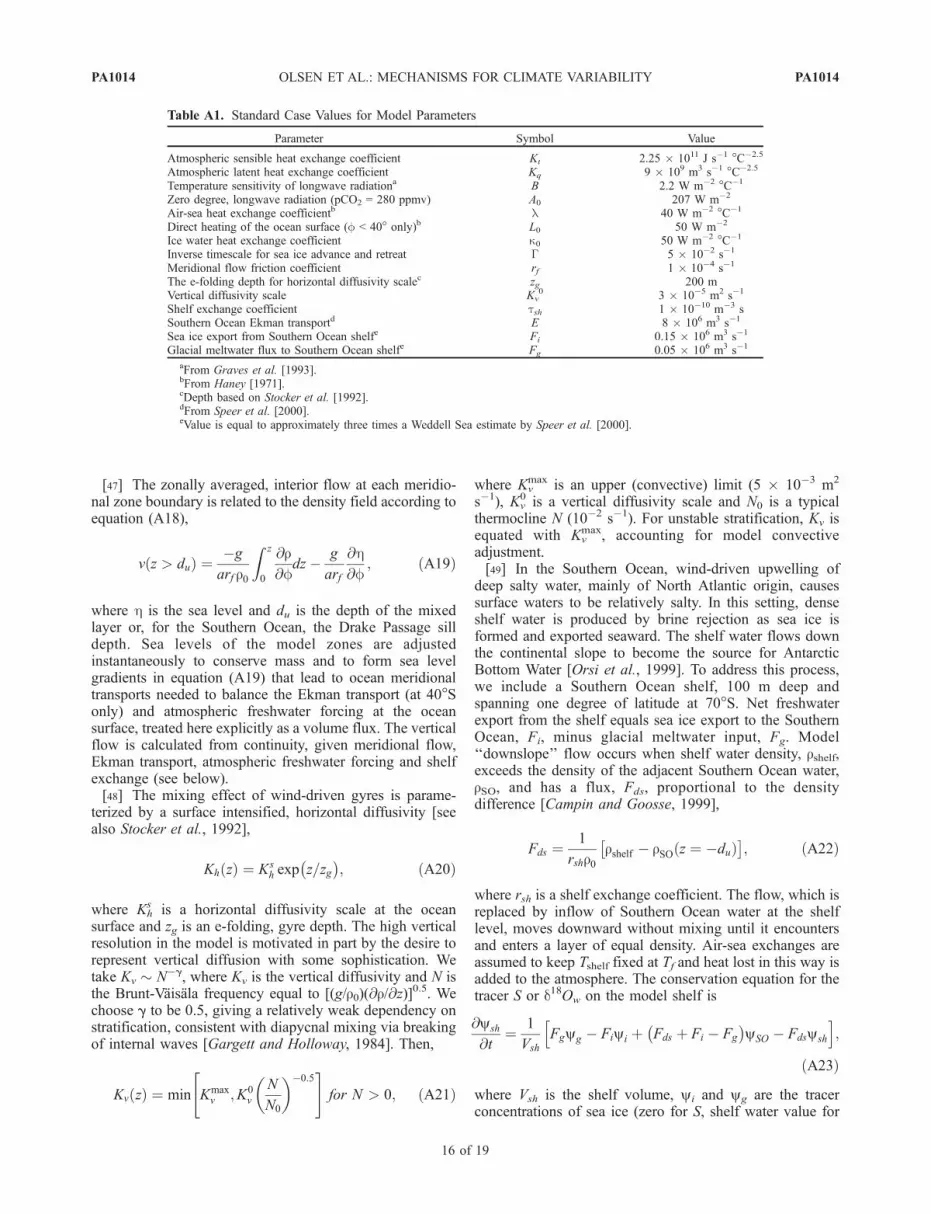
Table A1. Standard Case Values for Model Parameters

Parameter Symbol Value

Atmospheric sensible heat exchange coefficient Kt 2.25 � 1011 J s�1 �C�2.5

Atmospheric latent heat exchange coefficient Kq 9 � 109 m3 s�1 �C�2.5

Temperature sensitivity of longwave radiationa B 2.2 W m�2 �C�1

Zero degree, longwave radiation (pCO2 = 280 ppmv) A0 207 W m�2

Air-sea heat exchange coefficientb l 40 W m�2 �C�1

Direct heating of the ocean surface (f < 40� only)b L0 50 W m�2

Ice water heat exchange coefficient k0 50 W m�2 �C�1

Inverse timescale for sea ice advance and retreat G 5 � 10�2 s�1

Meridional flow friction coefficient rf 1 � 10�4 s�1

The e-folding depth for horizontal diffusivity scalec zg 200 mVertical diffusivity scale Kv

0 3 � 10�5 m2 s�1

Shelf exchange coefficient tsh 1 � 10�10 m�3 sSouthern Ocean Ekman transportd E 8 � 106 m3 s�1

Sea ice export from Southern Ocean shelfe Fi 0.15 � 106 m3 s�1

Glacial meltwater flux to Southern Ocean shelfe Fg 0.05 � 106 m3 s�1

aFrom Graves et al. [1993].bFrom Haney [1971].cDepth based on Stocker et al. [1992].dFrom Speer et al. [2000].eValue is equal to approximately three times a Weddell Sea estimate by Speer et al. [2000].


16 of 19

PA1014

d18Ow) and glacial meltwater (zero for S, �30% for d18Ow),and ySO is the Southern Ocean tracer concentration at z =�du(100 m). Tracer and volume fluxes for glacial meltwaterare transported to Antarctica by the atmosphere and thus aresubtracted from the surface forcing of the Southern Ocean.[50] The conservation equation for tracer T, S or d18Ow in

the rest of the ocean is

@y@t

þ 1

a cosf@ cosfvyð Þ

@fþ @ wyð Þ

@z

¼ 1

a2 cosf@

@fcosfKh

@y@f

� �þ @

@zKv

@y@z

� �þ Fs þ Fi;

ðA24Þ

where Fs denotes surface layer sources due to air-sea heatexchange and atmospheric moisture transport and Fi

denotes interior sources due to Ekman transport (40�S) orshelf water export (70�S). The discretized ocean modelequations are formulated on a staggered grid type, withtracer values defined at the center of boxes and velocitiesand diffusivities determined at box edges. Centereddifferences are used to evaluate derivatives, diffusion andvertical advection; an upwind scheme is applied for thecoarsely resolved, meridional advection. Prognostic equa-tions (A1), (A11), (A23), and (A24) are integratedsimultaneously using a fourth order Runge Kutta schemewith a 3-day time step. All diagnostic equations above forexchanges and fluxes are evaluated at each time step.

[51] We choose model parameter values guided byobservations in the modern climate system. Low levelsof vertical diffusion (1–3 10�5 m2 s�1) are found in theocean thermocline while considerably higher levels (1–5 �10�4 m2 s�1) are found deeper down, in particular nearrough bottom topography [Ledwell et al., 1993; Polzin etal., 1997]. There is a strong Atlantic thermohaline circu-lation (upper overturning cell), with a heat transport ofabout 0.6 PW across 40�N [Trenberth and Caron, 2001]and a weaker deep circulation originating in the SouthernOcean (lower overturning cell). Total ocean and atmo-sphere heat transports and total atmospheric fresh watertransports across 40�N,S are, respectively, about 5 �1015 W and 0.6–0.7 Sv [Trenberth and Caron, 2001;Wijffels et al., 1992]. At high northern latitudes, deep,open ocean convection takes place. In contrast, at highsouthern latitudes, deep water formation occurs mainly bybrine rejection during sea ice formation near Antarctica[Orsi et al., 1999]. Wind observations at the DrakePassage latitude yield an equatorward, surface layerEkman transport of about 8 Sv in the Atlantic [Sloyanand Rintoul, 2001]. Table A1 lists parameter valuesdetermined in this way for the modern climate system.

[52] Acknowledgments. We wish to thank Tine Rasmussen, BillCurry, Trond Dokken, and Laurence Vidal for supplying data presentedin Figures 1 and 2. This work was supported in part by the Danish NationalResearch Foundation.

ReferencesAdkins, J. F., K. McIntyre, and D. P. Schrag(2002), The salinity, temperature, and d18O ofthe glacial deep ocean, Science, 298, 1769–1773.

Alley, R. B., S. Anandakrishnan, and P. Jung(2001), Stochastic resonance in the NorthAtlantic, Paleoceanography, 16, 190–198.

Anderson, D. M. (2001), Attenuation of millen-nial-scale events by bioturbation in marinesediments, Paleoceanography, 16, 352–357.

Bauch, D., and H. Bauch (2001), Last glacialbenthic foraminiferal delta O-18 anomalies inthe polar North Atlantic: A modern analogueevaluation, J. Geophys. Res., 106, 9135–9143.

Bemis, B. E., H. J. Spero, J. Bijma, and D. W.Lea (1998), Reevaluation of the oxygen isoto-pic composition of planktonic foraminifera:Experimental results and revised paleotem-perature equations, Paleoceanography, 13,150–160.

Berger, A., and M. F. Loutre (1991), Insolationvalues for the climate of the last 10 millionyears, Quat. Sci. Rev., 11, 297–317.

Bjorck, S., et al. (2001), High-resolution ana-lyses of an early Holocene climate event mayimply decreased solar forcing as an importantclimate trigger, Geology, 29, 1107–1110.

Blunier, T., and E. J. Brook (2001), Timing ofmillennial-scale climate change in Antarcticaand Greenland during the last glacial period,Science, 291, 109–112.

Blunier, T., et al. (1998), Asynchrony of Antarc-tic and Greenland climate change during thelast glacial period, Nature, 394, 739–743.

Bond, G., and R. Lotti (1995), Iceberg dischargesinto the North Atlantic on millennial timescales during the last glaciation, Science,267, 1005–1010.

Bond, G., W. Broecker, S. Johnsen, J. McManus,L. Labeyrie, J. Jouzel, and G. Bonani (1993),Correlations between climate records fromNorth Atlantic sediments and Greenland ice,Nature, 365, 143–147.

Bond, G., et al. (1997), A pervasive millennial-scale cycle in North Atlantic Holocene andglacial climates, Science, 278, 1257–1266.

Bond, G., et al. (1999), The North Atlantic’s 1–2 kyr climate rhythm: Relation to Heinrichevents, Dansgaard/Oeschger cycles and theLittle Ice Age, in Mechanisms of Global Cli-mate Change at Millennial Time Scales, editedby P. U. Clark, R. S. Webb, and L. D. Keigwin,pp. 243–262, AGU, Washington D. C.

Bond, G., et al. (2001), Persistent solar influenceon North Atlantic climate during the Holocene,Science, 294, 2130–2136.

Budyko, M. I. (1969), The effect of solar radia-tion variations on the climate of the Earth,Tellus, 21, 611–619.

Campin, J. M., and H. Goosse (1999), Parame-terization of density-driven downsloping flowfor a coarse-resolution ocean model in z-coor-dinate, Tellus, Ser. A, 51, 412–430.

Chappell, J. (2002), Sea level changes forced byice breakouts in the Last Glacial cycle: Newresults from coral terraces, Quat. Sci. Rev., 21,1229–1240.

Clark, P. U., N. G. Pisias, T. F. Stocker, and A. J.Weaver (2002), The role of the thermohaline

circulation in abrupt climate change, Nature,415, 863–869.

Crowley, T. J. (1992), North Atlantic deep watercools the southern hemisphere, Paleoceano-graphy, 7, 489–497.

Curry, W. B., T. M. Marchitto, J. F. McManus,D. W. Oppo, and K. L. Laarkamp (1999),Millennial-scale changes in ventilation of thethermocline, intermediate and deep waters ofthe glacial North Atlantic, in Mechanisms ofGlobal Climate Change at Millennial TimeScales, Geophys. Monogr. Ser., vol. 112, editedby P. U. Clark, R. S. Webb, and L. D. Keigwin,pp. 59–76, AGU, Washington D. C.

Dansgaard, W., et al. (1993), Evidence for gen-eral instability of past climate from a 250-kyrice-core record, Nature, 364, 218–220.

Dokken, T. M., and E. Jansen (1999), Rapidchanges in the mechanism of ocean convectionduring the last glacial period, Nature, 401,458–461.

Duplessy, J. C., L. Labeyrie, and C. Waelbroeck(2002), Constraints on the ocean oxygen iso-topic enrichment between the Last GlacialMaximum and the Holocene: Paleoceano-graphic implications, Quat. Sci. Rev., 21,315–330.

Ganopolski, A., and S. Rahmstorf (2001), Rapidchanges of glacial climate simulated in acoupled climate model, Nature, 409, 153–158.

Ganopolski, A., and S. Rahmstorf (2002),Abrupt glacial climate changes due to stochas-tic resonance, Phys. Rev. Lett., 88, doi:10.1103/PhysRev.Lett.88.038501.


17 of 19

PA1014

Gargett, A. E., and G. Holloway (1984), Dissipa-tion and diffusion by internal wave breaking,J. Mar. Res., 42, 14–27.

Gat, J. R., and R. Gonfiantini (1981), Stable iso-tope hydrology: Deuterium and oxygen-18 inthe water cycle, Tech. Rep. Ser., 210, Int. At.Energy Agency, Vienna.

Gersonde, R., et al. (2003), Last glacial sea sur-face temperatures and sea-ice extent in theSouthern Ocean (Atlantic-Indian sector): Amultiproxy approach, Paleoceanography, 18,1061, doi:10.1029/2002PA000809.

Gildor, H., and E. Tziperman (2001), A sea iceclimate switch mechanism for the 100-kyr gla-cial cycles, J. Geophys. Res., 106, 9117–9133.

Graves, C. E., W.-H. Lee, and G. R. North(1993), New parameterizations and sensitiv-ities for simple climate models, J. Geophys.Res., 98, 5025–5036.

Grootes, P. M., and M. Stuiver (1997), Oxygen18/16 variability in Greenland snow and icewith 103 to 105-year time resolution, J. Geo-phys. Res., 102, 26,455–26,470.

Haney, R. L. (1971), Surface thermal boundaryconditions for ocean circulation models,J. Phys. Oceanogr., 1, 24–48.

Hartmann, D. L. (1994), Global Physical Clima-tology, Elsevier, New York.

Johnsen, S. J., W. Dansgaard, H. B. Clausen, andC. C. Langway (1972), Oxygen isotope pro-files through the Antarctic and Greenland icesheets, Nature, 235, 429–434.

Johnsen, S. J., W. Dansgaard, and J. W. C. White(1989), The origin of Arctic preciptation underpresent and glacial condition, Tellus, Ser. B,41, 452–468.

Ledwell, J. R., A. J. Watson, and C. S. Law(1993), Evidence for slow mixing across thepycnocline from an open-ocean tracer-releaseexperiment, Nature, 364, 701–703.

MacAyeal, D. R. (1993), Binge/purge oscilla-tions of the Laurentide ice-sheet as a causeof the North Atlantic Heinrich events, Paleo-ceanography, 8, 767–773.

McIntyre, K., M. L. Delaney, and A. C. Ravelo(2001), Millennial-scale climate change andoceanic processes in the late Pliocene and earlyPleistocene, Paleoceanography, 16, 535–543.

McManus, J. F., D. W. Oppo, and J. L. Cullen(1999), A 0. 5-million-year record of millen-nial-scale climate variability in the NorthAtlantic, Science, 283, 971–975.

McManus, J. F., R. Francois, J.-M. Gherardi,L. D. Keigwin, and S. Brown-Leger (2004),Collapse and rapid resumption of Atlanticmeridional circulation linked to deglacial cli-mate changes, Nature, 428, 834–837.

Merlivat, L., and J. Jouzel (1979), Globalclimatic interpretation of the Deuterium-Oxygen-18 relationship for precipitation,J. Geophys. Res., 84, 5029–5033.

Muench, R. D., and A. L. Gordon (1995), Cir-culation and transport of water along the wes-tern Weddell Sea margin, J. Geophys. Res.,100, 18,503–18,515.

Myhre, G., E. J. Highwood, K. P. Shine, andF. Stordal (1998), New estimates of radiativeforcing due to well mixed greenhouse gases,Geophys. Res. Lett., 25, 2715–2718.

Nilsson, J., G. Brostrom, and G. Walin (2003),The thermohaline circulation and vertical mix-ing: Does weaker density stratification givestronger overturning?, J. Phys. Oceanogr.,33, 2781–2795.

Oka, A., H. Hasumi, and N. Suginohara (2001),Stabilization of thermohaline circulation bywind-driven and vertical diffusive salt trans-port, Clim. Dyn., 18, 71–83.

Olsen, S. M. (2002), Stable and oscillating ther-mohaline circulation states in simple climatemodels validated against palodata, Ph.D. the-sis, 166 pp., Univ. of Copenhagen, Copenha-gen, Denmark.

Oort, A. A., and J. P. Peixoto (1983), Globalangular momentum and energy balancerequirements from observations, Adv. Geo-phys., 25, 355–490.

Oppo, D. W., and S. J. Lehman (1993), Mid-depth circulation of the subpolar North Atlan-tic during the last glacial maximum, Science,259, 1148–1152.

Orsi, A. H., G. C. Johnson, and J. L. Bullister(1999), Circulation, mixing, and production ofAntarctic bottom water, Prog. Oceanogr., 43,55–109.

Paul, A., and C. Schafer-Neth (2003), Modelingthe water masses of the Atlantic Ocean at theLast Glacial Maximum, Paleoceanography,18(3), 1058, doi:10.1029/2002PA000783.

Peltier, W. R. (1994), Ice-age paleotopography,Science, 265, 195–201.

Polzin, K. L., J. M. Toole, J. R. Ledwell, andR. W. Schmitt (1997), Spatial variability ofturbulent mixing in the abyssal ocean, Science,276, 93–96.

Rasmussen, T. L., E. Thomsen, L. Labeyrie, andT. C. E. van Weering (1996a), Circulationchanges in the Faeroe-Shetland Channel corre-lating with cold events during the last glacialperiod (58–10 ka), Geology, 24, 937–940.

Rasmussen, T. L., E. Thomsen, T. C. E. vanWeering, and L. Labeyrie (1996b), Rapidchanges in surface and deep water conditionsat the Faeroe margin during the last 58,000years, Paleoceanography, 11, 757–771.

Roche, D., D. Paillard, A. Ganopolski, andG. Hoffmann (2004), Oceanic oxygen-18at the present day and LGM: Equilibriumsimulations with a coupled climate modelof intermediate complexity, Earth Planet.Sci. Lett., 218, 317–330.

Rosenthal, Y., E. A. Boyle, and N. Slowey(1997), Temperature control on the incorpora-tion of magnesium, strontium, fluorine, andcadmium into benthic foraminiferal shellsfrom Little Bahama Bank: Prospects forthermocline paleoceanography, Geochim.Cosmochim. Acta, 61, 3633–3643.

Ruhlemann, C., S. Mulitza, G. Lohmann,A. Paul, M. Prange, and G. Wefer(2004), Intermediate depth warming inthe tropical Atlantic related to weakeningthermohaline circulation: Combining paleo-climate data and modelling results for thelast deglaciation, Paleoceanography, 19,PA1025, doi:10.1029/2003PA000948.

Sakai, K., and W. R. Peltier (1997), Dansgaard-Oeschger oscillations in a coupled atmosphere-ocean climate model, J. Clim., 10, 949–970.

Sarnthein, M., K. Winn, S. J. A. Jung, J.-C.Duplessy, L. Labeyrie, H. Erlenkeuser, andG. Ganssen (1994), Changes in east Atlan-tic deepwater circulation over the last30,000 years: Eight time slice reconstruc-tions, Paleoceanography, 9, 209–268.

Sarnthein, M. et al. (2001), Fundamental modesand abrupt changes in North Atlantic circula-tion and climate over the last 60 ky-Concepts,

reconstruction and numerical modeling, in TheNorthern North Atlantic: A Changing Environ-ment, edited by P. Schafer et al., pp. 365–410,Springer, New York.

Schulz, M., W. H. Berger, M. Sarnthein, andP. M. Grootes (1999), Amplitude variationsof 1470-year climate oscillations during thelast 100,000 years linked to fluctuations ofcontinental ice mass, Geophys. Res. Lett., 26,3385–3388.

Schulz, M., A. Paul, and A. Timmermann(2002), Relaxation oscillators in concert: Aframework for climate change at millennialtimescales during the late Pleistocene, Geo-phys. Res. Lett., 29(24), 2193, doi:10.1029/2002GL016144.

Semtner, A. J. (1976), A model for the thermo-dynamic growth of sea ice in numerical inves-tigations of climate, J. Phys. Oceanogr., 6,379–389.

Shackleton, N. J., M. A. Hall, and E. Vincent(2000), Phase relationships between millen-nial-scale events 64,000–24,000 years ago,Paleoceanography, 15, 565–569.

Shaffer, G., and S. M. Olsen (2001), Sensitivityof the thermohaline circulation and climate toocean exchanges in a simple coupled model,Clim. Dyn., 17, 433–444.

Shin, S.-I., Z. Liu, B. Otto-Bliesner, E. Brady,J. Kutzbach, and S. Harrison (2003), Asimulation of the Last Glacial Maximum cli-mate using the NCAR-CCSM, Clim. Dyn.,20, 127–151.

Skinner, L. C., N. J. Shackleton, and H. Elderfield(2003), Millennial-scale variability of deep-water temperature and d18Odw indicatingdeep-water source variations in the northeastAtlantic, 0–34 cal. ka BP, Geochem. Geo-phys. Geosyst., 4(12), 1098, doi:10.1029/2003GC000585.

Sloyan, B. M., and S. R. Rintoul (2001), Circu-lation, renewal, and modification of Antarcticmode and intermediate water, J. Phys. Ocean-ogr., 31, 1005–1030.

Speer, K., S. R. Rintoul, and B. Sloyan (2000),The diabatic Deacon Cell, J. Phys. Oceanogr.,30, 3212–3222.

Stocker, T. F., and S. J. Johnsen (2003), A mini-mum thermodynamic model for the bipolarseesaw, Paleoceanography, 18(4), 1087,doi:10.1029/2003PA000920.

Stocker, T. F., W. Broecker, and D. G. Wright(1992), A zonally averaged, coupled oceaat-mosphere model for paleoclimate studies,J. Clim., 5, 773–797.

Stone, P. H., and D. A. Miller (1980), Empiricalrelations between seasonal-changes in meridio-nal temperature-gradients and meridionalfluxes of heat, J. Atmos. Sci., 37, 1708–1721.

Talley, L. D., J. L. Reid, and P. E. Robbins(2003), Data-based meridional overturningstreamfunctions for the global ocean, J. Clim.,16, 3213–3226.

Timmermann, A., H. Gildor, M. Schulz, andE. Tziperman (2003), Coherent resonantmillennial-scale climate oscillations triggeredby massive meltwater pulses, J. Clim., 16,2569–2585.

Toggweiler, J. R., and B. Samuels (1995), Effectof the Drake Passage on the global thermoha-line circulation, Deep Sea Res., 42, 477–500.

Trenberth, K. E., and J. M. Caron (2001), Esti-mates of meridional atmosphere and oceanheat transports, J. Clim., 14, 3433–3443.


18 of 19

PA1014

van Kreveld, S., M. Sarnthein, H. Erlenkeuser,P.Grootes, S. Jung,M. J.Nadeau,U.Pflaumann,and A. Voelker (2000), Potential linksbetween surging ice sheets, circulation andthe Dansgaard-Oeschger cycles in the Irmin-ger Sea, 60–18 kyr, Paleoceanography, 15,425–442.

Vautravers, M. J., N. J. Shackleton, C. Lopez-Martinez, and J. O. Grimalt (2004), GulfStream variability during marine isotope stage3 , Pa l eo ceanog raphy, 19 , PA2011 ,doi:10.1029/2003PA000966.

Vidal, L., L. Labeyrie, and T. C. E. van Weering(1998), Benthic delta O-18 records in theNorth Atlantic over the last glacial period(60–10 kyr): Evidence for brine formation,Paleoceanography, 13, 245–251.

Walsh, J., X. Hou, P. Portis, and M. Serreze(1994), Atmospheric contribution to hydrolo-

gic variation in the Arctic, Atmos. Ocean, 34,733–755.

Wang, X. L., P. H. Stone, and J. Marotzke(1999), Global thermohaline circulation, PartII: Sensitivity with interactive atmospherictransports, J. Clim., 12, 83–91.

Weinelt, M., et al. (2001), Paleoceanographicproxies in the northern North Atlantic, inThe Northern North Atlantic, edited byP. Schafer et al., pp. 319–352, Springer, NewYork.

Wijffels, S. E., R. W. Schmitt, H. L. Bryden, andA. Stigebrandt (1992), Transport of fresh-water by the oceans, J. Phys. Oceanogr., 22,155–162.

Winton, M. (1997), The effect of cold climateupon North Atlantic Deep Water formation ina simple ocean-atmosphere model, J. Clim.,10, 37–51.

Winton, M., and E. S. Sarachik (1993), Thermo-haline oscillations induced by strong steadysalinity forcing of ocean general circulationmodels, J. Phys. Oceanogr., 23, 1389–1410.

��C. J. Bjerrum, Geological Institute, University

of Copenhagen, Øster Voldgade 10, 1350Copenhagen K, Denmark.S. M. Olsen, Danish Meteorological Institute,

Lyngbyvej 100, 2100 København Ø, Denmark.([email protected])G. Shaffer, Danish Center for Earth System

Science and Department of Geophysics, Uni-versity of Copenhagen, Juliane Maries Vej 30,2100 Copenhagen Ø, Denmark.


19 of 19

PA1014

ocean oxygen isotope constraints on mechanisms for millennial-scale climate variability

Documents