observing and modeling turbulence at a potential tidal energy site

Observing and Modeling Turbulence at a Potential

Tidal Energy Site

Katherine McCaffrey, PhDNational Oceanic and Atmospheric Administration Earth Systems Research Laboratory, Physical

Sciences Division

Climate and Global Dynamics SeminarTuesday, September 23, 2014

Acknowledgments• Baylor Fox-Kemper (Brown Univ.), Peter Hamlington (CU MechEng)

• Observations and model collaborators: Jim Thomson (UW-APL) , Levi Kilcher (NREL), Spencer Alexander (CU MechEng)

This work was supported by the CIRES/ESRL Graduate Research Fellowship.

2

Outline

1.Introduction to tidal energy– Technology and potential in the United States– Site characterization

2.Tidal turbulence from observations– Turbulence Metrics– Parameterization of Anisotropy and Coherence

3.Examination of tidal turbulence models– Stochastic Turbulence Generator: NREL TurbSim– Large-eddy Simulations: NCAR LES

4.Conclusions

3

1. Introduction to Tidal Energy

4

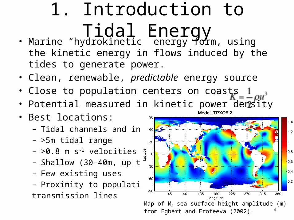
• Marine “hydrokinetic” energy form, using the kinetic energy in flows induced by the tides to generate power.

• Clean, renewable, predictable energy source • Close to population centers on coasts• Potential measured in kinetic power density• Best locations:

– Tidal channels and inlets– >5m tidal range– >0.8 m s-1 velocities– Shallow (30-40m, up to 80m)– Few existing uses– Proximity to populations and transmission lines

Map of M2 sea surface height amplitude (m) from Egbert and Erofeeva (2002).

5

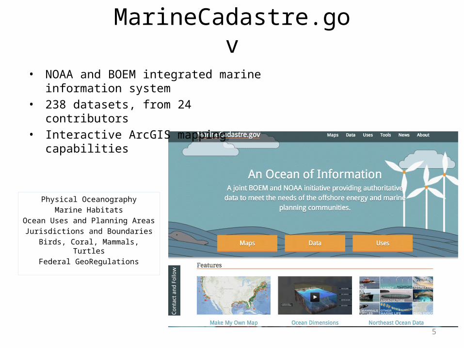
MarineCadastre.gov

• NOAA and BOEM integrated marine information system

• 238 datasets, from 24 contributors

• Interactive ArcGIS mapping capabilities

Physical OceanographyMarine Habitats

Ocean Uses and Planning AreasJurisdictions and Boundaries

Birds, Coral, Mammals, Turtles

Federal GeoRegulations

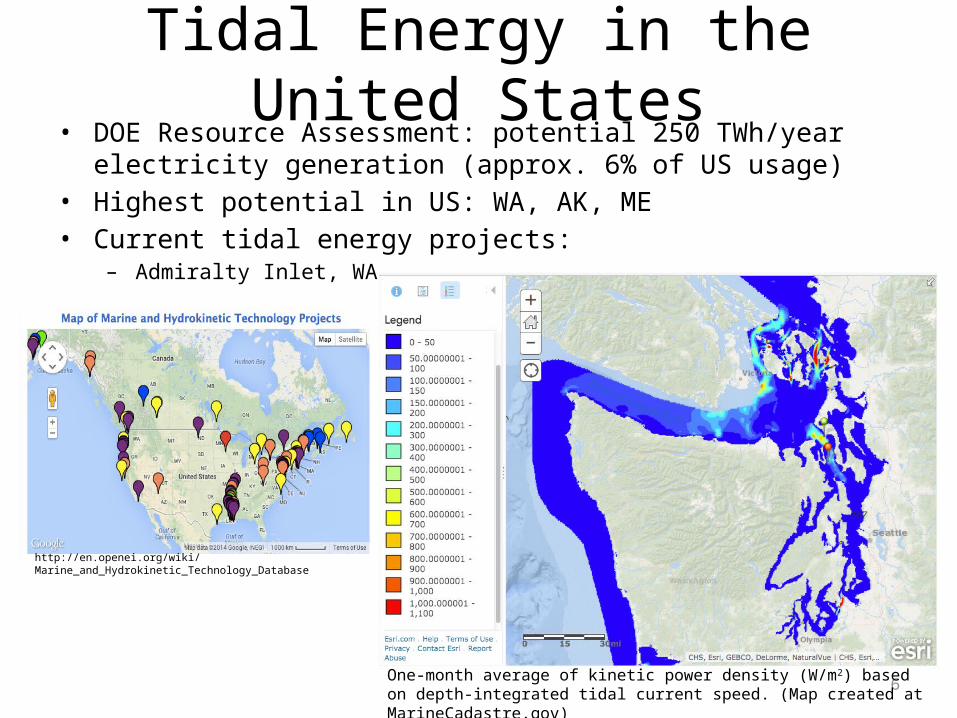
• DOE Resource Assessment: potential 250 TWh/year electricity generation (approx. 6% of US usage)

• Highest potential in US: WA, AK, ME• Current tidal energy projects:

– Admiralty Inlet, WA

6

Tidal Energy in the United States

One-month average of kinetic power density (W/m2) based on depth-integrated tidal current speed. (Map created at MarineCadastre.gov)

http://en.openei.org/wiki/Marine_and_Hydrokinetic_Technology_Database

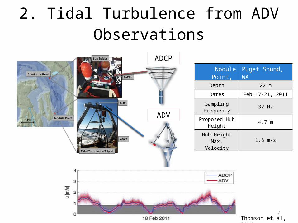
7Thomson et al, 2012

ADV

ADCP Nodule Point,

Puget Sound, WA

Depth 22 mDates Feb 17-21, 2011

Sampling Frequency 32 Hz

Proposed Hub Height 4.7 m

Hub Height Max.

Velocity1.8 m/s

2. Tidal Turbulence from ADV Observations

Definitions and notation:Perturbation velocity:Velocity components:Angle brackets and overline are 10-min mean

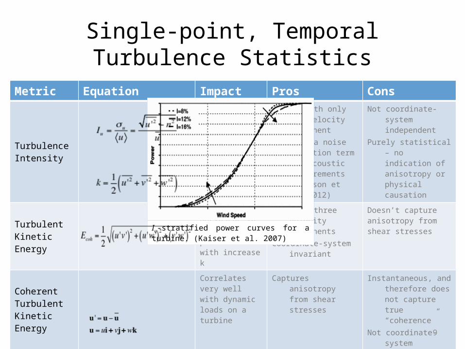
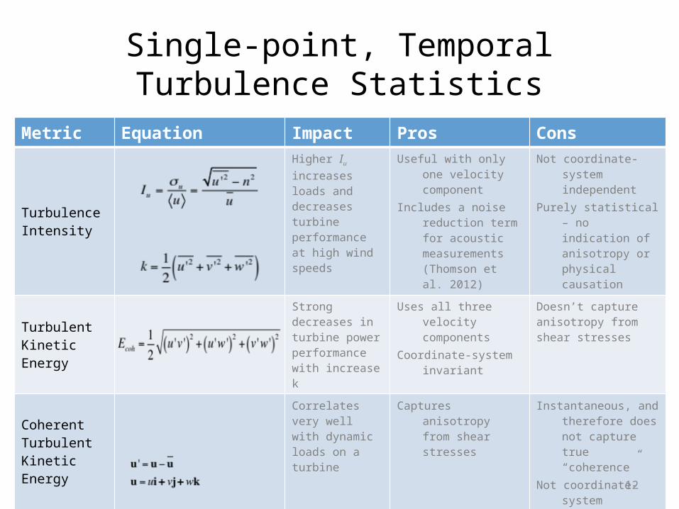
Single-point, Temporal Turbulence Statistics

Metric Equation Impact Pros Cons

Turbulence Intensity

Higher Iu increases loads and decreases turbine performance at high wind speeds

Useful with only one velocity component

Includes a noise reduction term for acoustic measurements (Thomson et al. 2012)

Not coordinate-system independent

Purely statistical – no indication of anisotropy or physical causation

Turbulent Kinetic Energy

Strong decreases in turbine power performance with increase k

Uses all three velocity components

Coordinate-system invariant

Doesn’t capture anisotropy from shear stresses

Coherent Turbulent Kinetic Energy

Correlates very well with dynamic loads on a turbine

Captures anisotropy from shear stresses

Instantaneous, and therefore does not capture true “coherence”


8




















9

Iu-stratified power curves for a turbine. (Kaiser et al. 2007)




















10




















11

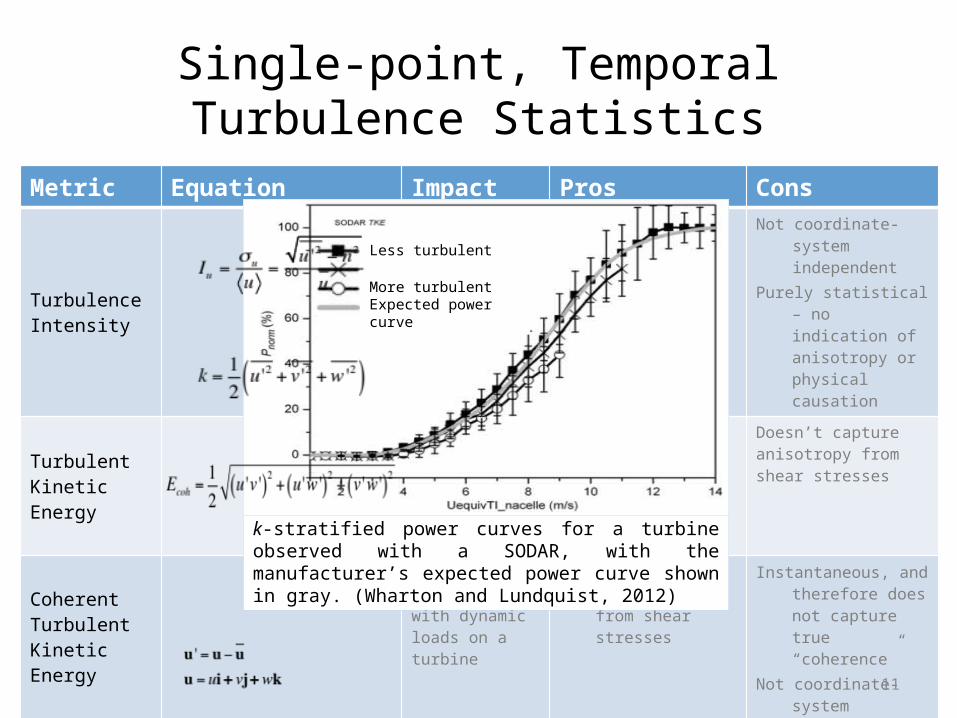
k-stratified power curves for a turbine observed with a SODAR, with the manufacturer’s expected power curve shown in gray. (Wharton and Lundquist, 2012)

Less turbulent

More turbulentExpected power curve




















12




















13

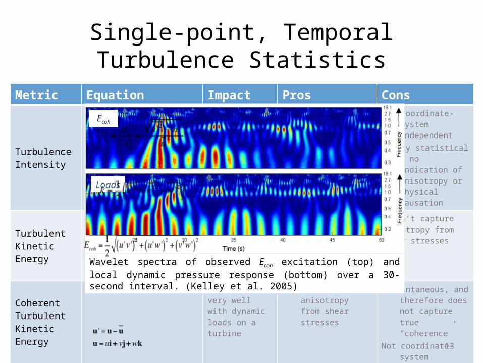
Wavelet spectra of observed Ecoh excitation (top) and local dynamic pressure response (bottom) over a 30-second interval. (Kelley et al. 2005)

Ecoh

Loads




















14

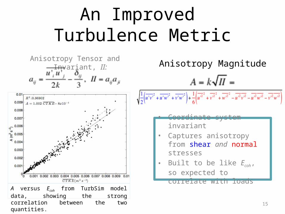
An Improved Turbulence Metric

Anisotropy Magnitude

15

• Coordinate-system invariant

• Captures anisotropy from shear and normal stresses

• Built to be like Ecoh, so expected to correlate with loads

Anisotropy Tensor and Invariant, II:

A versus Ecoh from TurbSim model data, showing the strong correlation between the two quantities.

Physical Characterization

What physical descriptors of coherent events (eddies) can be found from single-point, temporal data?– Shape – Anisotropy characteristics from anisotropy tensor

– Size – Coherence from autocorrelations

16

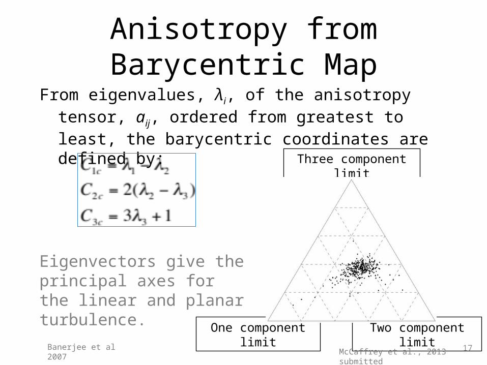
Anisotropy from Barycentric Map

From eigenvalues, λi, of the anisotropy tensor, aij, ordered from greatest to least, the barycentric coordinates are defined by:

17Banerjee et al 2007

Three component limit

Two component limit

One component limit

Eigenvectors give the principal axes for the linear and planar turbulence.

McCaffrey et al., 2013 submitted

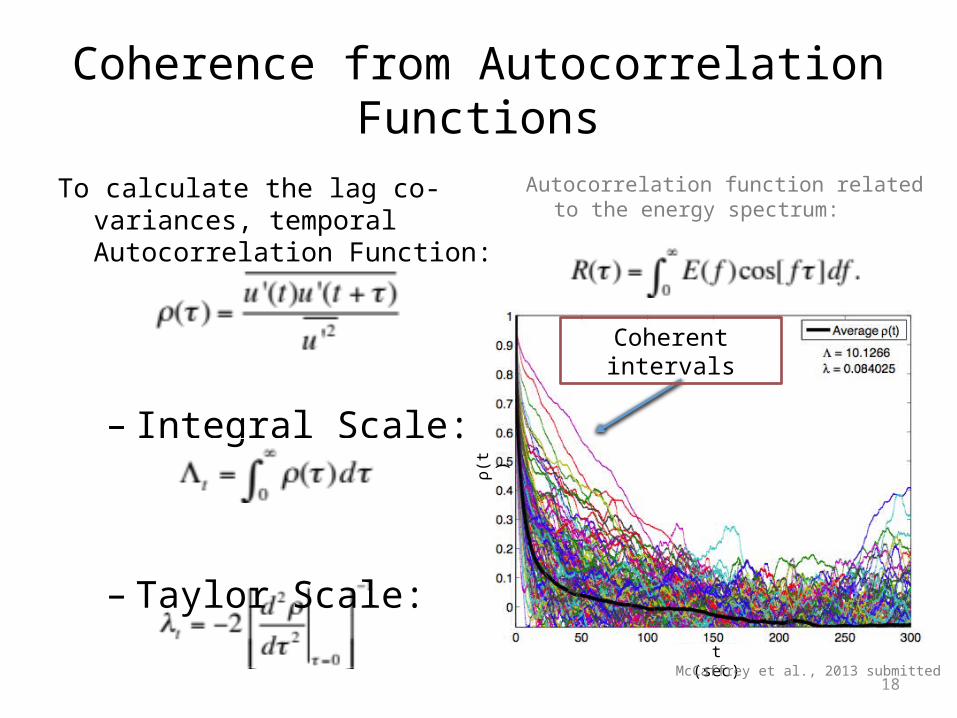
Coherence from Autocorrelation Functions

To calculate the lag co-variances, temporal Autocorrelation Function:

– Integral Scale:

– Taylor Scale:

18

t (sec)

ρ(t )

Coherent intervals

Autocorrelation function related to the energy spectrum:


Parameterizing Correlation with Turbulence Metrics

Instead of calculating a slew of physical properties and turbulence metrics, can we calculate only one metric to parameterize the anisotropic, coherent structures?

19

20

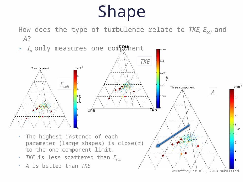
How does the type of turbulence relate to TKE, Ecoh and A?

• Iu only measures one component

TwoOne

Parameterization: Shape

• The highest instance of each parameter (large shapes) is close(r) to the one-component limit.

• TKE is less scattered than Ecoh

• A is better than TKE

Three

Ecoh

TKE

A


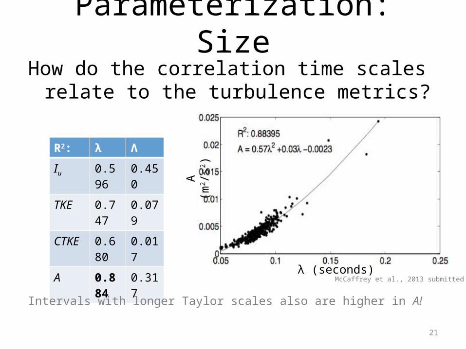
Parameterization: Size

How do the correlation time scales relate to the turbulence metrics?

21

R2: λ ΛIu 0.5

960.450

TKE 0.747

0.079

CTKE 0.680

0.017

A 0.884

0.317

A (m

2 /s2)

λ (seconds)

Intervals with longer Taylor scales also are higher in A!


Taylor’s Frozen Turbulence Hypothesis

• The only way that we can say anything about the spatial scales from the temporal ones is through Taylor’s hypothesis:

As the mean flow advects the turbulence, the properties of the turbulence are not changed, so the turbulence is considered “frozen.”– Good when u’/U<<1 (~Iu is small).

U~L/T becomes a good approximation, so we can use the mean flow speed with temporal scales, to estimate length scales

22

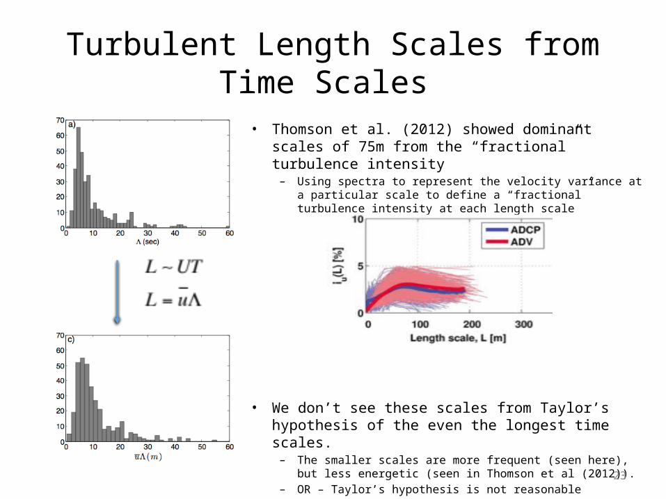
Turbulent Length Scales from Time Scales

• Thomson et al. (2012) showed dominant scales of 75m from the “fractional” turbulence intensity – Using spectra to represent the velocity variance at

a particular scale to define a “fractional” turbulence intensity at each length scale

• We don’t see these scales from Taylor’s hypothesis of the even the longest time scales.– The smaller scales are more frequent (seen here),

but less energetic (seen in Thomson et al (2012)).– OR – Taylor’s hypothesis is not reasonable

23

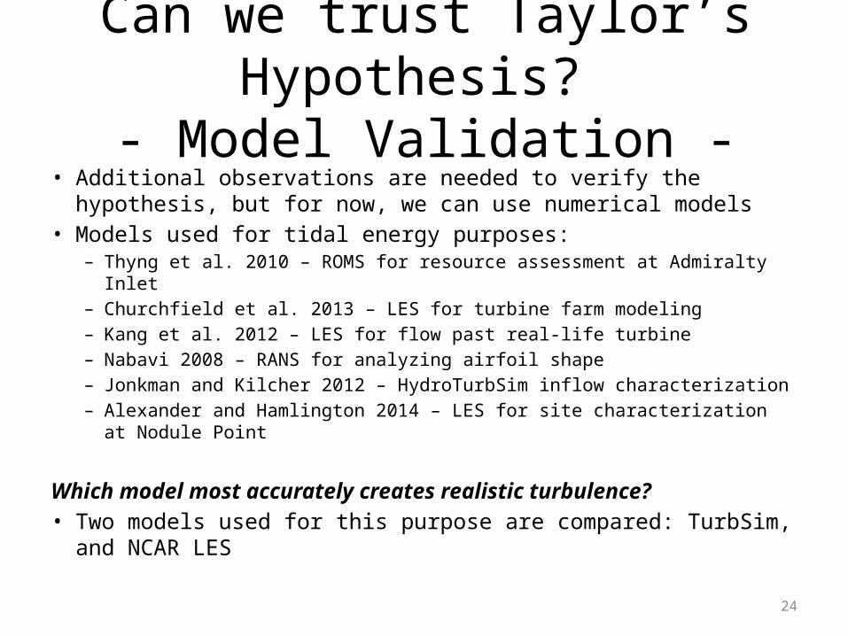
Can we trust Taylor’s Hypothesis?

- Model Validation -• Additional observations are needed to verify the hypothesis, but for now, we can use numerical models

• Models used for tidal energy purposes:– Thyng et al. 2010 – ROMS for resource assessment at Admiralty Inlet

– Churchfield et al. 2013 – LES for turbine farm modeling– Kang et al. 2012 – LES for flow past real-life turbine– Nabavi 2008 – RANS for analyzing airfoil shape– Jonkman and Kilcher 2012 – HydroTurbSim inflow characterization– Alexander and Hamlington 2014 – LES for site characterization at Nodule Point

Which model most accurately creates realistic turbulence?• Two models used for this purpose are compared: TurbSim, and NCAR LES

24

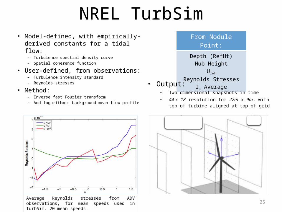
NREL TurbSim• Model-defined, with empirically-

derived constants for a tidal flow:– Turbulence spectral density curve– Spatial coherence function

• User-defined, from observations:– Turbulence intensity standard– Reynolds stresses

• Method:– Inverse fast Fourier transform– Add logarithmic background mean flow profile

25

From Nodule Point:

Depth (RefHt)Hub Height

Uref

Reynolds StressesIu Average• Output:

• Two-dimensional snapshots in time• 44 x 18 resolution for 22m x 9m, with

top of turbine aligned at top of grid

Average Reynolds stresses from ADV observations, for mean speeds used in TurbSim. 20 mean speeds.

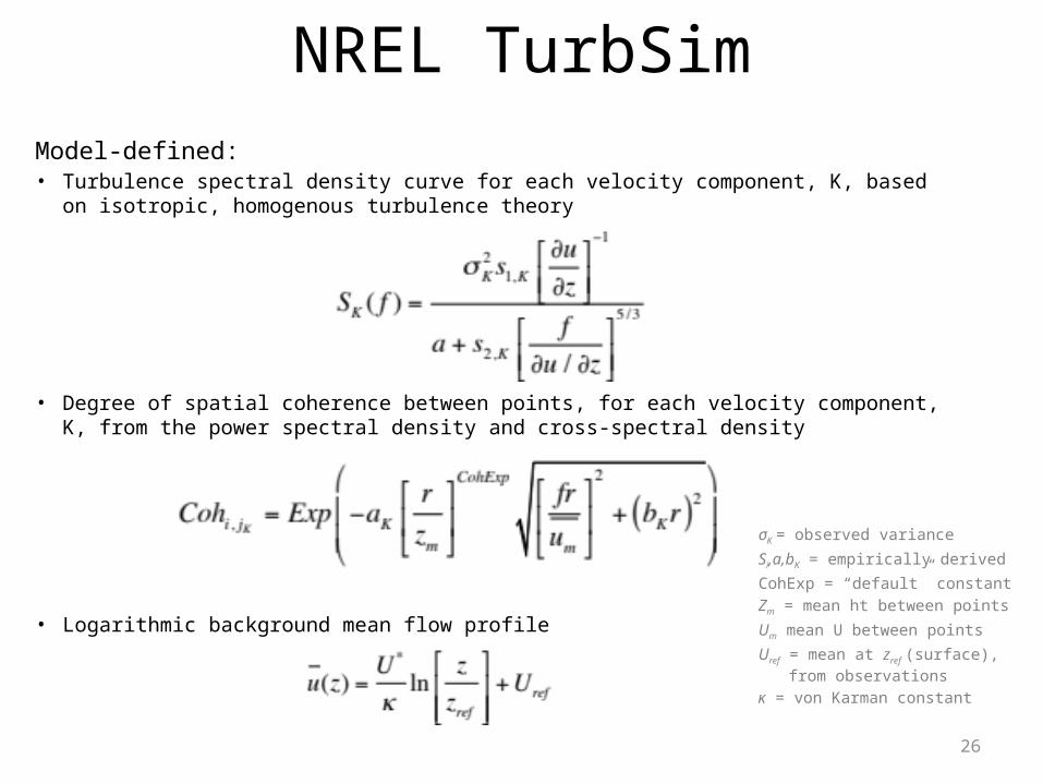
NREL TurbSimModel-defined:• Turbulence spectral density curve for each velocity component, K, based

on isotropic, homogenous turbulence theory

• Degree of spatial coherence between points, for each velocity component, K, from the power spectral density and cross-spectral density

• Logarithmic background mean flow profile

26

σK = observed varianceSi,a,bK = empirically derivedCohExp = “default” constantZm = mean ht between pointsUm mean U between pointsUref = mean at zref (surface),

from observationsκ = von Karman constant

NCAR LES

27

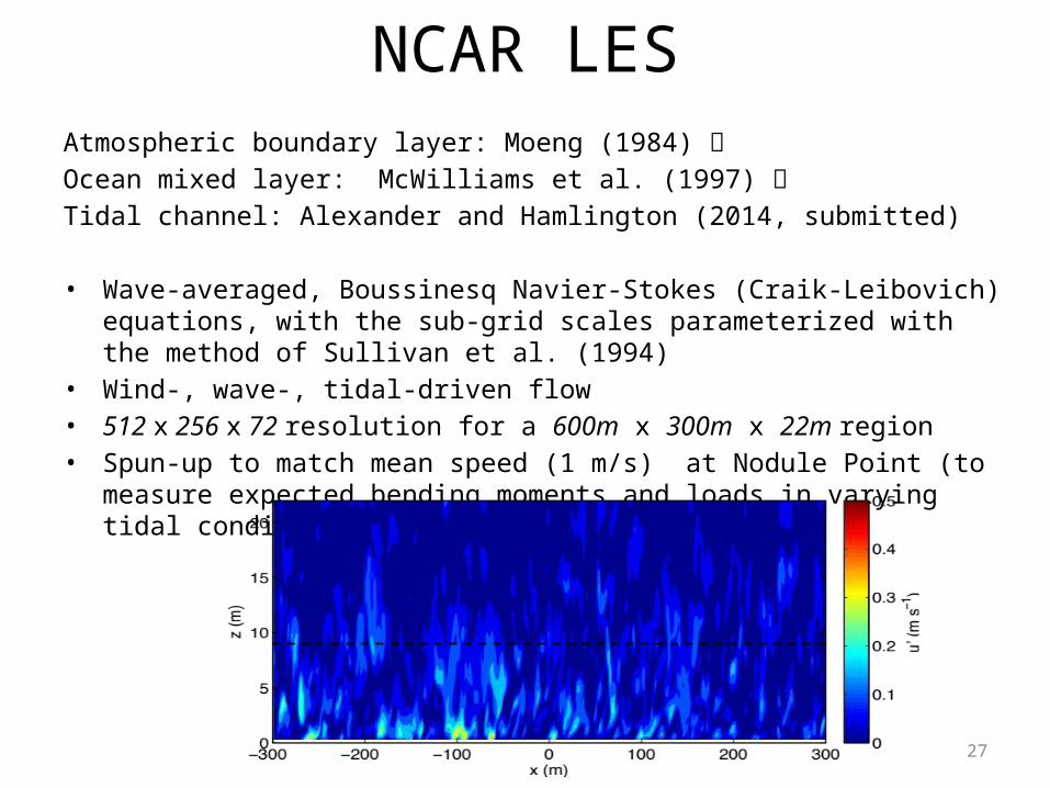
Atmospheric boundary layer: Moeng (1984) Ocean mixed layer: McWilliams et al. (1997) Tidal channel: Alexander and Hamlington (2014, submitted)

• Wave-averaged, Boussinesq Navier-Stokes (Craik-Leibovich) equations, with the sub-grid scales parameterized with the method of Sullivan et al. (1994)

• Wind-, wave-, tidal-driven flow• 512 x 256 x 72 resolution for a 600m x 300m x 22m region• Spun-up to match mean speed (1 m/s) at Nodule Point (to

measure expected bending moments and loads in varying tidal conditions)

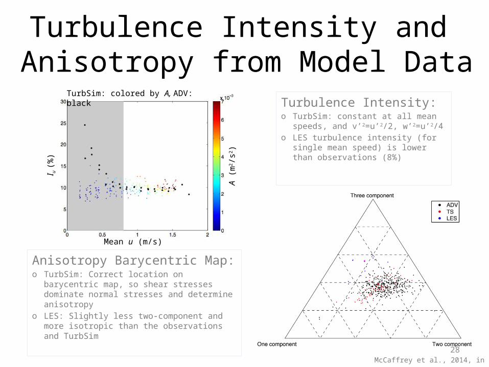
Turbulence Intensity and Anisotropy from Model Data

28

Turbulence Intensity:o TurbSim: constant at all mean

speeds, and v’2=u’2/2, w’2=u’2/4o LES turbulence intensity (for

single mean speed) is lower than observations (8%)

I u (%)

Mean u (m/s)A (m

2 /s2)

A (m

2 /s2)

Anisotropy Barycentric Map: o TurbSim: Correct location on

barycentric map, so shear stresses dominate normal stresses and determine anisotropy

o LES: Slightly less two-component and more isotropic than the observations and TurbSim

TurbSim: colored by A, ADV: black

McCaffrey et al., 2014, in prep

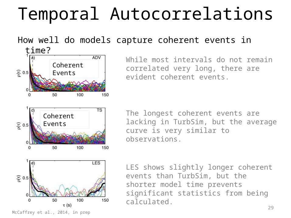
Temporal AutocorrelationsHow well do models capture coherent events in time?

29

While most intervals do not remain correlated very long, there are evident coherent events.

The longest coherent events are lacking in TurbSim, but the average curve is very similar to observations.

LES shows slightly longer coherent events than TurbSim, but the shorter model time prevents significant statistics from being calculated.

McCaffrey et al., 2014, in prep

Coherent Events

Coherent Events

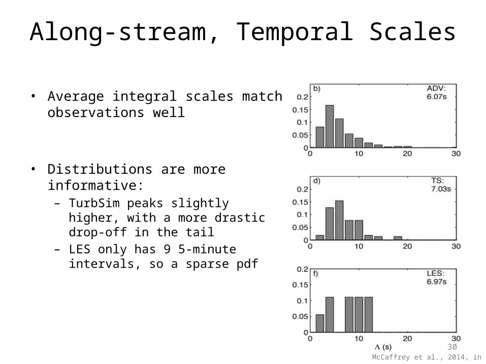
Along-stream, Temporal Scales

• Average integral scales match observations well

• Distributions are more informative:– TurbSim peaks slightly

higher, with a more drastic drop-off in the tail

– LES only has 9 5-minute intervals, so a sparse pdf

30McCaffrey et al., 2014, in prep

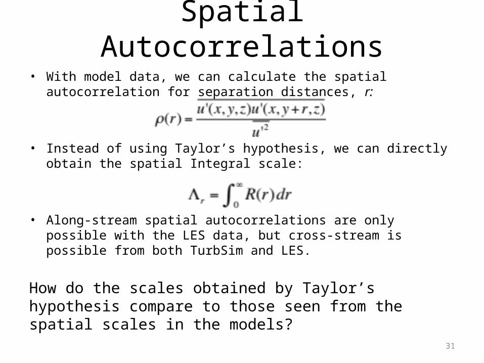
Spatial Autocorrelations

• With model data, we can calculate the spatial autocorrelation for separation distances, r:

• Instead of using Taylor’s hypothesis, we can directly obtain the spatial Integral scale:

• Along-stream spatial autocorrelations are only possible with the LES data, but cross-stream is possible from both TurbSim and LES.

How do the scales obtained by Taylor’s hypothesis compare to those seen from the spatial scales in the models?

31

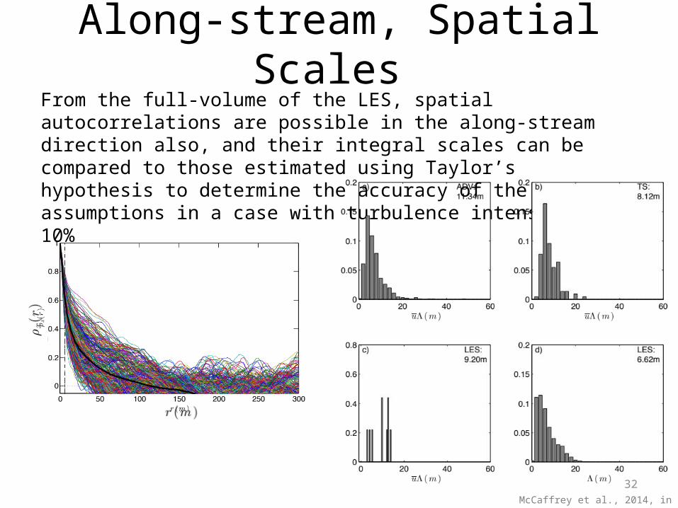
Along-stream, Spatial Scales

From the full-volume of the LES, spatial autocorrelations are possible in the along-stream direction also, and their integral scales can be compared to those estimated using Taylor’s hypothesis to determine the accuracy of the assumptions in a case with turbulence intensity of 10%

32McCaffrey et al., 2014, in prep

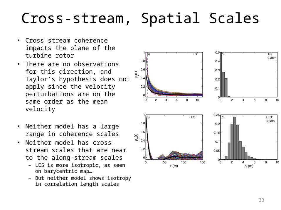
Cross-stream, Spatial Scales• Cross-stream coherence

impacts the plane of the turbine rotor

• There are no observations for this direction, and Taylor’s hypothesis does not apply since the velocity perturbations are on the same order as the mean velocity

• Neither model has a large range in coherence scales

• Neither model has cross-stream scales that are near to the along-stream scales– LES is more isotropic, as seen

on barycentric map…– But neither model shows isotropy

in correlation length scales

33

Conclusions and Hypotheses for Model Results

• TurbSim:– Does what it is meant to do well: lower-order statistics (mean velocities and turbulence intensity).

– Anisotropy is dominated by shear stresses. Hypothesis: Model-defined normal stresses are smaller than reality, and shear stresses are user-defined to be accurate, so they dominate the anisotropy.

– Coherence is lacking. Hypothesis: The spatial coherence function is not sufficient to recreate the physical coherence since it beings with a stochastic model. Statistically-defined, instead of physically-defined, turbulence limits the results that can be produced.

• LES:– A closer cut at simulating a realistic tidal channel.– Anisotropy is too isotropic. Hypothesis: There is a lack of planar eddies due to the flat bottom.

– Coherence scales are too small. Hypothesis: Need topography and realistic local geography to get longer scales, and potentially the planar eddies that are also missing. 34

4. Conclusions• Observational analysis:

– A simple ADV measurement allows a description of turbulence, though limited, using basic turbulence metrics and physical characteristics:

– A new, tensor-invariant metric, the anisotropy magnitude, is introduced to parameterize the physical properties of turbulence better than the previously-used turbulence intensity, TKE, and Ecoh.

• Model analysis:– The stochastic turbulence model, TurbSim, captures some aspects of the turbulence, but not the largest coherent features that are the most harmful to a turbine.

– The large-eddy simulations, NCAR LES, do create more coherent structures, but not accurate anisotropy.

– LES is more realistic, though neither model can capture the largest features that are generated by the local topography.

35

Turbulence intensityTurbulent kinetic energyCoherent turbulent

kinetic energyAnisotropy EigenvaluesIntermittencyCoherence/correlation

Looking Forward• Northwest National Marine Renewable Energy Center see the following as the key issues that must be resolved if MHK tidal energy is to be developed responsibly:– Uncertainty in the practically recoverable resource (balancing available power against competing uses, maximum device density, and environmental impacts).

– The effect of certain site-specific characteristics, such as turbulence and shear on device operation and survivability.

– Cumulative environmental effects of large arrays, including disruption of natural circulatory processes and migration routes for fish and marine mammals.

– Maximum packing density for devices, in order to make effective use of a localized resource.

– Long-term survivability of devices in a marine environment, including reduced performance due to bio-fouling.

• Large Eddy Simulations, with the ability to simulate turbines in the flow, and future abilities to create realistic bottom boundaries and geometry, shows great promise for site-specific characterization of turbulence. 36

Questions?

37

Extra Slides

38

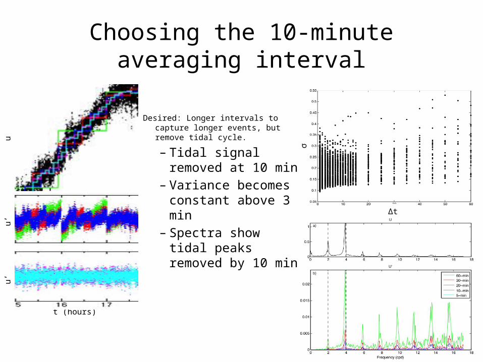
Choosing the 10-minute averaging interval

Desired: Longer intervals to capture longer events, but remove tidal cycle.

– Tidal signal removed at 10 min

– Variance becomes constant above 3 min

– Spectra show tidal peaks removed by 10 min

39

Δt

σt (hours)

uu’

u’

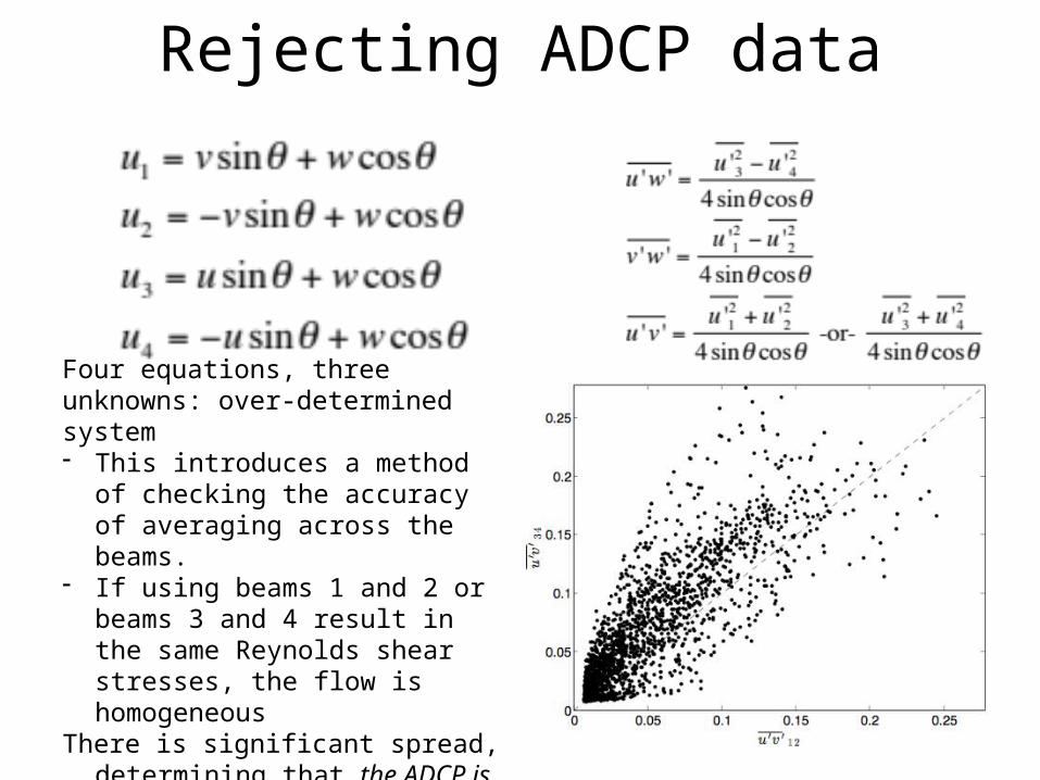
Rejecting ADCP data

40

Four equations, three unknowns: over-determined system- This introduces a method

of checking the accuracy of averaging across the beams.

- If using beams 1 and 2 or beams 3 and 4 result in the same Reynolds shear stresses, the flow is homogeneous

There is significant spread, determining that the ADCP is not sufficient for calculating Reynolds stresses!

Intermittency from Probability Density Functions

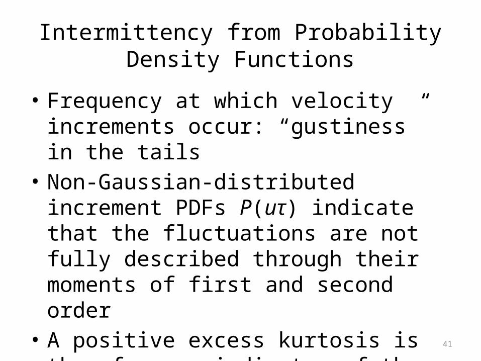
• Frequency at which velocity increments occur: “gustiness” in the tails

• Non-Gaussian-distributed increment PDFs P(uτ) indicate that the fluctuations are not fully described through their moments of first and second order

• A positive excess kurtosis is therefore an indicator of the degree of intermittency

41

Intermittency

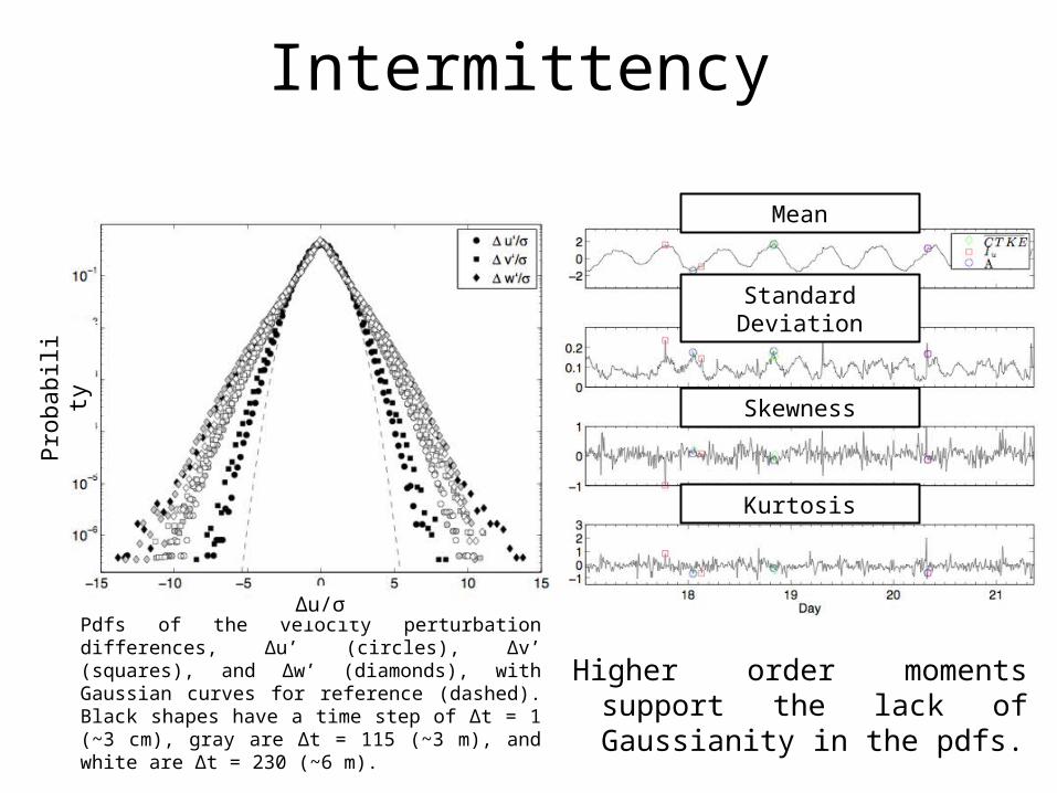
Higher order moments support the lack of Gaussianity in the pdfs.

Mean

Kurtosis

Skewness

Standard Deviation

Pdfs of the velocity perturbation differences, ∆u’ (circles), ∆v’ (squares), and ∆w’ (diamonds), with Gaussian curves for reference (dashed). Black shapes have a time step of ∆t = 1 (~3 cm), gray are ∆t = 115 (~3 m), and white are ∆t = 230 (~6 m).

Prob

abil

ity

Δu/σ

NCAR LES

43

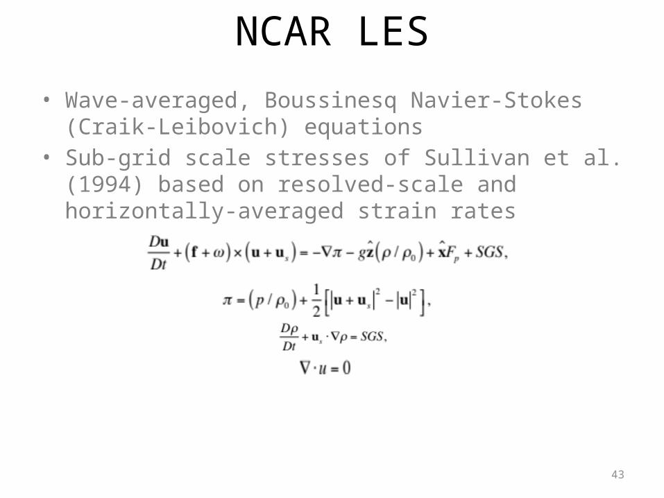
• Wave-averaged, Boussinesq Navier-Stokes (Craik-Leibovich) equations

• Sub-grid scale stresses of Sullivan et al. (1994) based on resolved-scale and horizontally-averaged strain rates

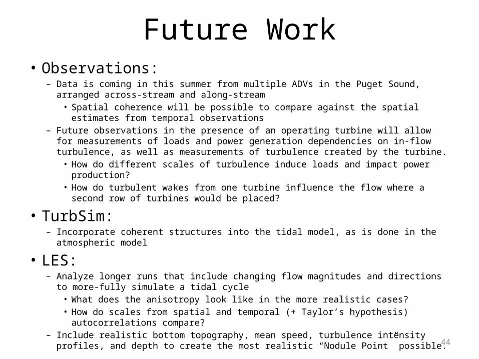
Future Work• Observations:

– Data is coming in this summer from multiple ADVs in the Puget Sound, arranged across-stream and along-stream• Spatial coherence will be possible to compare against the spatial estimates from temporal observations

– Future observations in the presence of an operating turbine will allow for measurements of loads and power generation dependencies on in-flow turbulence, as well as measurements of turbulence created by the turbine.• How do different scales of turbulence induce loads and impact power production?

• How do turbulent wakes from one turbine influence the flow where a second row of turbines would be placed?

• TurbSim:– Incorporate coherent structures into the tidal model, as is done in the atmospheric model

• LES:– Analyze longer runs that include changing flow magnitudes and directions to more-fully simulate a tidal cycle• What does the anisotropy look like in the more realistic cases?• How do scales from spatial and temporal (+ Taylor’s hypothesis) autocorrelations compare?

– Include realistic bottom topography, mean speed, turbulence intensity profiles, and depth to create the most realistic “Nodule Point” possible.44

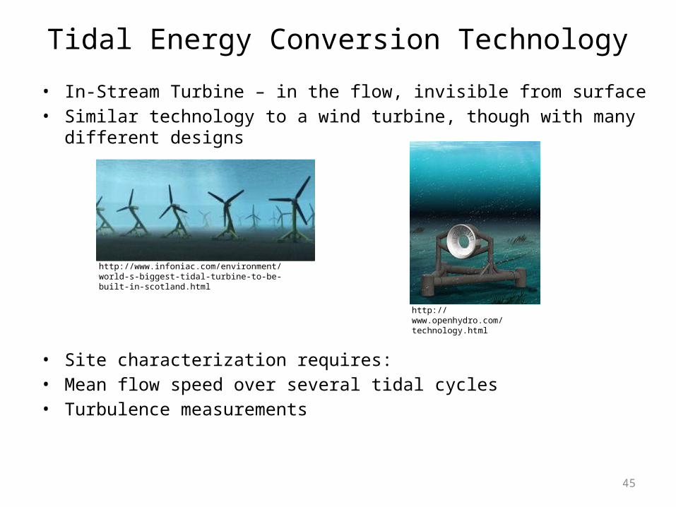
Tidal Energy Conversion Technology• In-Stream Turbine – in the flow, invisible from surface• Similar technology to a wind turbine, though with many

different designs

• Site characterization requires:• Mean flow speed over several tidal cycles• Turbulence measurements

45

http://www.infoniac.com/environment/world-s-biggest-tidal-turbine-to-be-built-in-scotland.html

http://www.openhydro.com/technology.html

observing and modeling turbulence at a potential tidal energy site

Documents