Science-Driven Optimization

of the LSST Observing Strategy

Prepared by the LSST Science Collaborations,

with support from the LSST Project.

Version 1.0

Most recent commit: fe3d2ad

(Mon, 14 Aug 2017 02:08:33 -0700)

arX

iv:1

708.

0405

8v1

[as

tro-

ph.I

M]

14

Aug

201

7

Contributing Authors

Phil Marshall,1 Timo Anguita,2 Federica B. Bianco,3 Eric C. Bellm,4 Niel Brandt,5 Will Clark-son,6 Andy Connolly,7 Eric Gawiser,8 Zeljko Ivezic,9 Lynne Jones,10 Michelle Lochner,11

Michael B. Lund,12 Ashish Mahabal,13 David Nidever,14 Knut Olsen,15 Stephen Ridgway,16

Jason Rhodes,17 Ohad Shemmer,18 David Trilling,19 Kathy Vivas,20 Lucianne Walkowicz,21

Beth Willman,22 Peter Yoachim,23 Scott Anderson,24 Pierre Antilogus,25 Ruth Angus,26 Iair Ar-cavi,27 Humna Awan,28 Rahul Biswas,29 Keaton J. Bell,30 David Bennett,31 Chris Britt,32

Derek Buzasi,33 Dana I. Casetti-Dinescu,34 Laura Chomiuk,35 Chuck Claver,36 Kem Cook,37

James Davenport,38 Victor Debattista,39 Seth Digel,40 Zoheyr Doctor,41 R. E. Firth,42 Ryan Fo-ley,43 Wen-fai Fong,44 Lluıs Galbany,45 Mark Giampapa,46 John E. Gizis,47 Melissa L. Gra-ham,48 Carl Grillmair,49 Phillipe Gris,50 Zoltan Haiman,51 Patrick Hartigan,52 Suzanne Haw-ley,53 Renee Hlozek,54 Saurabh W. Jha,55 C. Johns-Krull,56 Shashi Kanbur,57 Vassiliki Kalogera,58

Vinay Kashyap,59 Vishal Kasliwal,60 Richard Kessler,61 Alex Kim,62 Peter Kurczynski,63

Ofer Lahav,64 Michael C. Liu,65 Alex Malz,66 Raffaella Margutti,67 Tom Matheson,68 Jason D. McEwen,69

Peregrine McGehee,70 Søren Meibom,71 Josh Meyers,72 Dave Monet,73 Eric Neilsen,74 Jeffrey New-man,75 Matt O’Dowd,76 Hiranya V. Peiris,77 Matthew T. Penny,78 Christina Peters,79 Rados law Poleski,80

Kara Ponder,81 Gordon Richards,82 Jeonghee Rho,83 David Rubin,84 Samuel Schmidt,85

Robert L. Schuhmann,86 Avi Shporer,87 Colin Slater,88 Nathan Smith,89 Marcelles Soares-Santos,90 Keivan Stassun,91 Jay Strader,92 Michael Strauss,93 Rachel Street,94 Christopher Stubbs,95

Mark Sullivan,96 Paula Szkody,97 Virginia Trimble,98 Tony Tyson,99 Miguel de Val-Borro,100

Stefano Valenti,101 Robert Wagoner,102 W. Michael Wood-Vasey,103 Bevin Ashley Zauderer,104

A graphical representation of the contributions made to this white paper can be found on thispaper’s GitHub repository.

1drphilmarshall, SLAC National Accelerator Laboratory, 2575 Sand Hill Road, MS29, Menlo Park, CA 94025, USA2tanguita, Universidad Andres Bello, 13 Nte. 798, Vina del Mar, Regin de Valparaso, Chile3fedhere, Center for Cosmology and Particle Physics, Department of Physics, New York University, 726 Broadway, 9th

Floor, New York, NY 10003, USA4ebellm, California Institute of Technology, Pasadena, CA, USA5nielbrandt, Pennsylvania State University, 514A Davey Lab University Park, PA 16802, USA6willclarkson, University of MichiganDearborn, 4901 Evergreen Road, Dearborn, MI 48128, USA7connolly, University of Washington, Department of Astronomy, University of Washington, 3910 15th Avenue NE, Seattle,

WA, 98195, USA8egawiser, Department of Physics and Astronomy, Rutgers the State University of New Jersey, 136 Frelinghuysen Road,

Piscataway, NJ 08854 USA9ivezic, University of Washington, Department of Astronomy, University of Washington, 3910 15th Avenue NE, Seattle,

WA, 98195, USA10rhiannonlynne, University of Washington, Department of Astronomy, University of Washington, 3910 15th Avenue NE,

Seattle, WA, 98195, USA

3

11MichelleLochner, African Institute for Mathematical Sciences, 6 Melrose Road, Muizenberg 7945, South Africa; SKA SouthAfrica, 3rd Floor, The Park, Park Road, Pinelands 7405, South Africa; Department of Physics and Astronomy, UniversityCollege London, Gower Street, London WC1E 6BT, UK

12lundmb, Vanderbilt University, 2201 West End Ave, Nashville, TN 37235, USA13AshishMahabal, California Institute of Technology, Pasadena, CA, USA14dnidever, LSST, 933 N. Cherry Ave., Tucson, AZ 85721, USA15knutago, NOAO, 950 N. Cherry Ave., Tucson, AZ 8571916StephenRidgway, NOAO, 950 N. Cherry Ave., Tucson, AZ 8571917jasondrhodes, Jet Propulsion Laboratory, California Institute of Technology, 4800 Oak Grove Drive, Pasadena, CA 91109,

USA18ohadshemmer, University of North Texas, 1155 Union Cir, Denton, TX 76203, USA19davidtrilling, Dept. of Physics & Astronomy, Northern Arizona University, NAU Box 6010, Flagstaff, AZ, 86011, USA20akvivas, Cerro Tololo Inter-American Observatory, Casilla 603, La Serena, Chile21lmwalkowicz, Adler Planetarium, Chicago, IL, USA22bethwillman, LSST, 933 N. Cherry Ave., Tucson, AZ 85721, USA23yoachim, University of Washington, Department of Astronomy, University of Washington, 3910 15th Avenue NE, Seattle,

WA, 98195, USA24ScottAnderson, University of Washington, Department of Astronomy, University of Washington, 3910 15th Avenue NE,

Seattle, WA, 98195, USA25antilogus, LPNHE, Barre 12-22, 1er setage, 4 Place Jussieu, 75252 Paris Cedex 05, France26ruthangus, Department of Physics, University of Oxford, Keble Road, Oxford, UK27arcavi, LCOGT, University of California, Santa Barbara, CA, USA28humnaawan, Department of Physics and Astronomy, Rutgers the State University of New Jersey, 136 Frelinghuysen Road,

Piscataway, NJ 08854 USA29rbiswas4, University of Washington, Department of Astronomy, University of Washington, 3910 15th Avenue NE, Seattle,

WA, 98195, USA; The eScience Institute, University of Washington, Seattle, WA, 98195, USA30keatonb, University of Texas at Austin, Austin, TX, 78712, USA31davidpbennett, NASA Goddard Space Flight Center, 8800 Greenbelt Road, Greenbelt, MD 20771, USA32cbritt4, Department of Physics and Astronomy, Michigan State University, 5678 Wilson Road, Lansing, MI 48824, USA;

Department of Physics, Texas Tech University, Box 41051 Lubbock, TX 79409-1051, USA33derekbuzasi, Florida Gulf Coast University, Fort Meyers, FL, USA34DanaCD, Department of Physics, Southern Connecticut State University, 501 Crescent Street, New Haven, CT 06515,

USA; Department of Astronomy, Yale University, P.O. Box 208101, New Haven, CT 06520-8101, USA35chomiuk, Department of Physics and Astronomy, Michigan State University, 5678 Wilson Road, Lansing, MI 48824, USA36cclaver, LSST, 933 N. Cherry Ave., Tucson, AZ 85721, USA37kem0cook, Cook Astronomical Consulting, USA38jimdavenport, Western Washington University, 516 High Street, Bellingham, WA 98225, USA39vpdebattista, University of Central Lancashire, Preston PR1 2HE, UK40sethdigel, SLAC National Accelerator Laboratory, 2575 Sand Hill Road, MS29, Menlo Park, CA 94025, USA41Doctor, Department of Physics & Astronomy/CIERA, Northwestern University, 2145 Sheridan Road, Evanston, IL, 60208,

USA42RobFirth, School of Physics and Astronomy, University of Southampton, Southampton, SO17 1BJ, UK43astrofoley, Department of Astronomy and Astrophysics, University of California, Santa Cruz, CA 95064, USA44Fong, University of Arizona, Tucson, AZ, USA45lgalbany, Pittsburgh Particle Physics, Astrophysics, and Cosmology Center (PITT PACC), Physics and Astronomy De-

partment, University of Pittsburgh, Pittsburgh, PA 15260, USA46markgiampapa, National Solar Observatory, 3004 Telescope Loop, Sunspot, NM 88349, USA47jgizis, University of Delaware, Department of Physics and Astronomy, 104 The Green, Newark, DE 19716, USA48MelissaGraham, University of Washington, Department of Astronomy, University of Washington, 3910 15th Avenue NE,

Seattle, WA, 98195, USA49cgrillmair, IPAC, 770 South Wilson Ave., Pasadena, CA 91125, USA50pgris, Laboratoire de Physique de Clermont, N2P3/CNRS, 63178 Aubire Cedex, France51Haiman, Columbia University, New York, NY, USA52phartigan, Department of Physics and Astronomy, Rice University, Houston TX 77005-1892, USA53suzannehawley, University of Washington, Department of Astronomy, University of Washington, 3910 15th Avenue NE,

Seattle, WA, 98195, USA

4

54ReneeHlozek, Dunlap Institute & Department of Astronomy and Astrophysics, University of Toronto, 50 St George Street,Toronto, ON M5S 3H4, Canada

55saurabhwjha, Department of Physics and Astronomy, Rutgers the State University of New Jersey, 136 Frelinghuysen Road,Piscataway, NJ 08854 USA

56CJohnsKrull, Department of Physics and Astronomy, Rice University, Houston TX 77005-1892, USA57ShashiKanbur, State University of New York at Oswego, 7060 New York 104, Oswego, NY 13126, USA58Kalogera, Department of Physics & Astronomy/CIERA, Northwestern University, 2145 Sheridan Road, Evanston, IL,

60208, USA59vinaykashyap, Harvard-Smithsonian Center for Astrophysics, Harvard University, Cambridge, MA, USA60AstroVPK, Department of Astronomy and Astrophysics, University of Pennsylvania, Philadelphia, PA, USA61RickKessler, Kavli Institute for Cosmological Physics, University of Chicago, Chicago, IL 60637, USA, Department of

Astronomy and Astrophysics, University of Chicago, 5640 South Ellis Avenue, Chicago, IL 60637, USA62AlexGKim, Physics Division, Lawrence Berkeley National Laboratory, 1 Cyclotron Road, Berkeley, CA, 94720, USA63pkurczynski, Department of Physics and Astronomy, Rutgers the State University of New Jersey, 136 Frelinghuysen Road,

Piscataway, NJ 08854 USA64oferlahav, Department of Physics and Astronomy, University College London, Gower Street, London WC1E 6BT, UK65mliu, Institute for Astronomy, University of Hawaii at Manoa, 2680 Woodlawn Drive, Honolulu, HI 96822, USA66aimalz, Center for Cosmology and Particle Physics, Department of Physics, New York University, 726 Broadway, 9th Floor,

New York, NY 10003, USA67raffaellamargutti, Center for Cosmology and Particle Physics, Department of Physics, New York University, 726 Broadway,

9th Floor, New York, NY 10003, USA68tmatheson, NOAO, 950 N. Cherry Ave., Tucson, AZ 8571969jasonmcewen, Mullard Space Science Laboratory (MSSL), University College London (UCL), Surrey RH5 6NT, UK70pmmcgehee, IPAC, 770 South Wilson Ave., Pasadena, CA 91125, USA71sorenmeibom, Harvard-Smithsonian Center for Astrophysics, Harvard University, Cambridge, MA, USA72jmeyers314, Physics Department, Stanford University, Stanford, CA, 94305, USA73dgmonet, US Naval Observatory, 10391 West Naval Observatory Road, Flagstaff, AZ 86001, USA74ehneilsen, Fermilab, PO Box 500, Batavia, IL, 60510, USA75janewman-pitt-edu, Pittsburgh Particle Physics, Astrophysics, and Cosmology Center (PITT PACC), Physics and Astron-

omy Department, University of Pittsburgh, Pittsburgh, PA 15260, USA76mattodowd, The City University of New York, New York, NY, USA77hiranyapeiris, Department of Physics and Astronomy, University College London, Gower Street, London WC1E 6BT, UK;

okc78mtpenny, Sagan Fellow, osu79tinapeters, Dunlap Institute & Department of Astronomy and Astrophysics, University of Toronto, 50 St George Street,

Toronto, ON M5S 3H4, Canada80poleski, The Ohio State University, Columbus, OH, USA81kponder, Pittsburgh Particle Physics, Astrophysics, and Cosmology Center (PITT PACC), Physics and Astronomy De-

partment, University of Pittsburgh, Pittsburgh, PA 15260, USA82GordonRichards, Drexel University, Philadelphia, PA, USA83jhrlsst, SETI Institute, 189 N. Bernardo Ave., Mountain View, CA, 94043, USA, sofia84rubind, Space Telescope Science Institute, Baltimore, MD, USA85SamSchmidt, University of California, Davis, CA, USA86rlschuhmann, Department of Physics and Astronomy, University College London, Gower Street, London WC1E 6BT, UK87shporer, Division of Geological and Planetary Sciences, California Institute of Technology, Pasadena, CA 91125, USA88ctslater, University of Washington, Department of Astronomy, University of Washington, 3910 15th Avenue NE, Seattle,

WA, 98195, USA89nathansmith, University of Arizona, Tucson, AZ, USA90soares-santos, Fermilab, PO Box 500, Batavia, IL, 60510, USA91stassun, Vanderbilt University, 2201 West End Ave, Nashville, TN 37235, USA92caprastro, Department of Physics and Astronomy, Michigan State University, 5678 Wilson Road, Lansing, MI 48824, USA93michaelstrauss, Department of Astrophysical Sciences, Princeton University, Princeton, NJ 08544, USA94rachelstreet, LCOGT, University of California, Santa Barbara, CA, USA95astrostubbs, Department of Physics & Department of Astronomy, 17 Oxford Street, Harvard University, Cambridge, MA,

02138, USA96msullivan318, School of Physics and Astronomy, University of Southampton, Southampton, SO17 1BJ, UK

5

97paulaszkody, University of Washington, Department of Astronomy, University of Washington, 3910 15th Avenue NE,Seattle, WA, 98195, USA

98Trimble, University of California, Irvine, CA, USA99tonytyson, University of California, Davis, CA, USA

100migueldvb, NASA Goddard Space Flight Center, 8800 Greenbelt Road, Greenbelt, MD 20771, USA101svalenti, University of California, Davis, CA, USA102wagoner@stanford.edu, Physics Department, Stanford University, Stanford, CA, 94305, USA103wmwv, Pittsburgh Particle Physics, Astrophysics, and Cosmology Center (PITT PACC), Physics and Astronomy Depart-

ment, University of Pittsburgh, Pittsburgh, PA 15260, USA104Zauderer, Center for Cosmology and Particle Physics, Department of Physics, New York University, 726 Broadway, 9th

Floor, New York, NY 10003, USA

6

Contents

Contributing Authors . . . . . . . . . . . . . . . . . . . . . . . . . . . . . . . . . . . . . . . 3Preface . . . . . . . . . . . . . . . . . . . . . . . . . . . . . . . . . . . . . . . . . . . . . . . 9Summary . . . . . . . . . . . . . . . . . . . . . . . . . . . . . . . . . . . . . . . . . . . . . . 111 Introduction . . . . . . . . . . . . . . . . . . . . . . . . . . . . . . . . . . . . . . . . . . 131.1 Synoptic Sky Surveying . . . . . . . . . . . . . . . . . . . . . . . . . . . . . . . . . . 141.2 Evaluating and Optimizing the LSST Observing Strategy . . . . . . . . . . . . . . . 151.3 Influencing the LSST Observing Schedule . . . . . . . . . . . . . . . . . . . . . . . . 171.4 Guidelines for Contributors . . . . . . . . . . . . . . . . . . . . . . . . . . . . . . . . 211.5 Outline of This Paper . . . . . . . . . . . . . . . . . . . . . . . . . . . . . . . . . . . 232 Some Example Observing Strategies . . . . . . . . . . . . . . . . . . . . . . . . . . . . . 25

Summary . . . . . . . . . . . . . . . . . . . . . . . . . . . . . . . . . . . . . . . . . . 252.1 Introduction . . . . . . . . . . . . . . . . . . . . . . . . . . . . . . . . . . . . . . . . . 252.2 The LSST Operations Simulator, OpSim . . . . . . . . . . . . . . . . . . . . . . . . . 262.3 The Baseline Observing Strategy . . . . . . . . . . . . . . . . . . . . . . . . . . . . . 272.4 Some Simulated Alternative Observing Strategies . . . . . . . . . . . . . . . . . . . . 362.5 Future Work: Rolling Cadence . . . . . . . . . . . . . . . . . . . . . . . . . . . . . . 482.6 Summary . . . . . . . . . . . . . . . . . . . . . . . . . . . . . . . . . . . . . . . . . . 513 Solar System . . . . . . . . . . . . . . . . . . . . . . . . . . . . . . . . . . . . . . . . . . 553.1 Introduction . . . . . . . . . . . . . . . . . . . . . . . . . . . . . . . . . . . . . . . . . 553.2 Discovery: Linking Solar System Objects . . . . . . . . . . . . . . . . . . . . . . . . . 563.3 Discovery of Potentially Hazardous Asteroids . . . . . . . . . . . . . . . . . . . . . . 623.4 Orbital Accuracy . . . . . . . . . . . . . . . . . . . . . . . . . . . . . . . . . . . . . . 643.5 Detecting Comet Activity . . . . . . . . . . . . . . . . . . . . . . . . . . . . . . . . . 663.6 Measuring Asteroid Light Curves and Rotation Periods . . . . . . . . . . . . . . . . 693.7 Measuring Asteroid Colors . . . . . . . . . . . . . . . . . . . . . . . . . . . . . . . . . 713.8 Future Work . . . . . . . . . . . . . . . . . . . . . . . . . . . . . . . . . . . . . . . . 734 The Milky Way Galaxy . . . . . . . . . . . . . . . . . . . . . . . . . . . . . . . . . . . . 75

Summary . . . . . . . . . . . . . . . . . . . . . . . . . . . . . . . . . . . . . . . . . . 754.1 Introduction . . . . . . . . . . . . . . . . . . . . . . . . . . . . . . . . . . . . . . . . . 764.2 Populations in the Milky Way Disk . . . . . . . . . . . . . . . . . . . . . . . . . . . . 774.3 Astrometry with LSST: Positions, Proper Motions, and Parallax . . . . . . . . . . . 914.4 Mapping the Milky Way Halo . . . . . . . . . . . . . . . . . . . . . . . . . . . . . . . 1014.5 Future Work . . . . . . . . . . . . . . . . . . . . . . . . . . . . . . . . . . . . . . . . 1065 Variable Objects . . . . . . . . . . . . . . . . . . . . . . . . . . . . . . . . . . . . . . . . 1195.1 Introduction . . . . . . . . . . . . . . . . . . . . . . . . . . . . . . . . . . . . . . . . . 1195.2 The Cepheid Mass-Luminosity Relation . . . . . . . . . . . . . . . . . . . . . . . . . 1205.3 Characterizing Multiperiodic, Short-Period Pulsating Variables . . . . . . . . . . . . 1265.4 Discovery and Characterization of Young Stellar Populations . . . . . . . . . . . . . 132

7

Contents

5.5 Future Work . . . . . . . . . . . . . . . . . . . . . . . . . . . . . . . . . . . . . . . . 1396 Transients . . . . . . . . . . . . . . . . . . . . . . . . . . . . . . . . . . . . . . . . . . . 1476.1 Introduction . . . . . . . . . . . . . . . . . . . . . . . . . . . . . . . . . . . . . . . . . 1476.2 Realtime Identification of Young Transients . . . . . . . . . . . . . . . . . . . . . . . 1536.3 Supernovae as Transients . . . . . . . . . . . . . . . . . . . . . . . . . . . . . . . . . 1586.4 Gamma-Ray Burst Afterglows . . . . . . . . . . . . . . . . . . . . . . . . . . . . . . . 1646.5 Gravitational Wave Sources . . . . . . . . . . . . . . . . . . . . . . . . . . . . . . . . 1706.6 Future Work . . . . . . . . . . . . . . . . . . . . . . . . . . . . . . . . . . . . . . . . 1727 The Magellanic Clouds . . . . . . . . . . . . . . . . . . . . . . . . . . . . . . . . . . . . 1817.1 Introduction . . . . . . . . . . . . . . . . . . . . . . . . . . . . . . . . . . . . . . . . . 1817.2 Future Work . . . . . . . . . . . . . . . . . . . . . . . . . . . . . . . . . . . . . . . . 1838 AGN . . . . . . . . . . . . . . . . . . . . . . . . . . . . . . . . . . . . . . . . . . . . . . 185

Summary . . . . . . . . . . . . . . . . . . . . . . . . . . . . . . . . . . . . . . . . . . 1858.1 Introduction . . . . . . . . . . . . . . . . . . . . . . . . . . . . . . . . . . . . . . . . . 1858.2 AGN Selection and Census . . . . . . . . . . . . . . . . . . . . . . . . . . . . . . . . 1868.3 Disc Intrinsic AGN Variability . . . . . . . . . . . . . . . . . . . . . . . . . . . . . . 1908.4 AGN Size and Structure with Microlensing . . . . . . . . . . . . . . . . . . . . . . . 1958.5 Future Work . . . . . . . . . . . . . . . . . . . . . . . . . . . . . . . . . . . . . . . . 2038.6 Discussion . . . . . . . . . . . . . . . . . . . . . . . . . . . . . . . . . . . . . . . . . . 2059 Cosmology . . . . . . . . . . . . . . . . . . . . . . . . . . . . . . . . . . . . . . . . . . . 2079.1 Introduction . . . . . . . . . . . . . . . . . . . . . . . . . . . . . . . . . . . . . . . . . 2079.2 Large-Scale Structure: Dithering to Improve Survey Uniformity . . . . . . . . . . . . 2089.3 Weak Lensing . . . . . . . . . . . . . . . . . . . . . . . . . . . . . . . . . . . . . . . . 2199.4 Photometric Redshifts . . . . . . . . . . . . . . . . . . . . . . . . . . . . . . . . . . . 2309.5 Supernova Cosmology and Physics . . . . . . . . . . . . . . . . . . . . . . . . . . . . 2369.6 Strong Gravitational Lens Time Delays . . . . . . . . . . . . . . . . . . . . . . . . . 25310 Special Surveys . . . . . . . . . . . . . . . . . . . . . . . . . . . . . . . . . . . . . . . . 26110.1 Introduction . . . . . . . . . . . . . . . . . . . . . . . . . . . . . . . . . . . . . . . . . 26110.2 Solar System Special Surveys . . . . . . . . . . . . . . . . . . . . . . . . . . . . . . . 26210.3 Short Exposure Surveying . . . . . . . . . . . . . . . . . . . . . . . . . . . . . . . . . 26510.4 A Mini-Survey of the Old Open Cluster M67 . . . . . . . . . . . . . . . . . . . . . . 27011 Synergy with WFIRST . . . . . . . . . . . . . . . . . . . . . . . . . . . . . . . . . . . . 275

Summary . . . . . . . . . . . . . . . . . . . . . . . . . . . . . . . . . . . . . . . . . . 27511.1 Introduction . . . . . . . . . . . . . . . . . . . . . . . . . . . . . . . . . . . . . . . . . 27511.2 Cosmology with the WFIRST HLS and LSST . . . . . . . . . . . . . . . . . . . . . . 27611.3 Supernova Cosmology with WFIRST and LSST . . . . . . . . . . . . . . . . . . . . . 28011.4 Exoplanetary Microlensing with WFIRST and LSST . . . . . . . . . . . . . . . . . . 28212 Conclusions, Tensions and Trade-offs . . . . . . . . . . . . . . . . . . . . . . . . . . . . 28912.1 Summary of Cadence Constraints . . . . . . . . . . . . . . . . . . . . . . . . . . . . . 28912.2 Tensions and Tradeoffs . . . . . . . . . . . . . . . . . . . . . . . . . . . . . . . . . . . 292Appendix: MAF Metrics . . . . . . . . . . . . . . . . . . . . . . . . . . . . . . . . . . . . . 301

References . . . . . . . . . . . . . . . . . . . . . . . . . . . . . . . . . . . . . . . . . . . 307

8

Preface

The Large Synoptic Survey Telescope (LSST) is a dedicated ground-based astronomical facilitywhose goal is to provide a database of high fidelity images and object catalogs that enable a widerange of science investigations. With its 9.6 square degree field of view and effective aperture of6.7 meters, it will be able to survey the Southern half of the sky every few nights (on average),building up a 10-year, 900-frame movie of the ever-changing cosmos. Its community of scientistswill be able to make major contributions in the fields of extragalactic astronomy and cosmology,the study of our Milky Way, its local environment and its stellar populations, solar system science,and time domain astronomy.

As its name suggests, LSST is designed to carry out a large synoptic survey: it has a baselineobserving strategy, simulations of which demonstrate that the data required for the promisedscience can be delivered. However, this baseline strategy may well not be the best way to schedulethe telescope. Smaller, specialized surveys are likely to provide high scientific value, as is optimizingthe pattern of repeated sky coverage. The baseline strategy is not set in stone, and can and willbe optimized: even small changes could result in significant improvements to the overall scienceyield. How can we design an observing strategy that maximizes the scientific output of the LSSTsystem?

The LSST Observing Strategy community formed in July 2015 to tackle this problem. Drawnprimarily (but not exclusively) from the team of people engaged in the LSST construction Project,and the set of LSST “Science Collaborations” who are engaged in preparing to exploit the LSSTdata, we are working together to use software tools provided by the LSST Project to evaluatesimulations of the LSST survey (also provided by the Project) specifically for the science that weeach care most about. In this way, we aim to give sustainable, quantitative feedback about howany proposed observing strategy would impact the performance of our science cases, and so enablegood decisions to be made when the telescope schedule is eventually set up.

This white paper is a compendium of ideas and results generated by the community, assembled sothat everyone can follow along with the analysis. It is a living document, whose purpose is to bindtogether the group of people who are thinking about the LSST observing strategy problem, andfacilitate their collective discussion and understanding of that problem (a process we might thinkof as “cadence diplomacy”). Its audience is the LSST science community, and most notable itsScience Advisory Committee and Project Scientist who together will in the end decide what theLSST observing strategy will be. This white paper is the vehicle for the community to communicateto the LSST Project, while the baseline observing strategy continues to be improved.

The white paper’s modular design allows pieces of it to be split off and published in a series ofsnapshot journal papers, as the various metric analyses reach maturity. The white paper itself willbe continuously published on GitHub and advertized periodically on astro-ph. This white paper

9

is large, but we hope that its hyperlinked structure helps our community quickly find the sciencecases that they are most interested in, starting from the table of contents.

The LSST observing strategy evaluation and optimization process will be as open and inclusive aspossible. New community members are welcome at any time; we explain how to get involved inChapter 1. We invite all stakeholders to participate.

Phil Marshall, Zeljko Ivezic and Beth Willman

August 12, 2017.

10

Summary

The Large Synoptic Survey Telescope is designed to provide an unprecedented optical imagingdataset that will support investigations of our Solar System, Galaxy and Universe, across halfthe sky and over ten years of repeated observation. However, exactly how the LSST observationswill be taken (the observing strategy or “cadence”) is not yet finalized. In this dynamically-evolving community white paper, we explore how the detailed performance of the anticipatedscience investigations is expected to depend on small changes to the LSST observing strategy.Using realistic simulations of the LSST schedule and observation properties, we design and computediagnostic metrics and Figures of Merit that provide quantitative evaluations of different observingstrategies, analyzing their impact on a wide range of proposed science projects. This is work inprogress: we are using this white paper to communicate to each other the relative merits of theobserving strategy choices that could be made, in an effort to maximize the scientific value of thesurvey. The investigation of some science cases leads to suggestions for new strategies that couldbe simulated and potentially adopted. Notably, we find motivation for exploring departures froma spatially uniform annual tiling of the sky: focusing instead on different parts of the survey areain different years in a “rolling cadence” is likely to have significant benefits for a number of timedomain and moving object astronomy projects. The communal assembly of a suite of quantifiedand homogeneously coded metrics is the vital first step towards an automated, systematic, science-based assessment of any given cadence simulation, that will enable the scheduling of the LSST tobe as well-informed as possible.

11

1 Introduction

Chapter editors: Andy Connolly, Zeljko Ivezic, Phil Marshall, Michael Strauss.

The Large Synoptic Survey Telescope (LSST) is a dedicated optical telescope with an effectiveaperture of 6.7 meters, currently under construction on Cerro Pachon in the Chilean Andes. Thetelescope and camera will have a huge field of view, 9.6 deg2, and the etendue, i.e., the product ofcollecting area and field of view will be significantly larger than any other optical telescope. Thusthis telescope is designed for wide-field deep imaging of the sky; its mantra is “Wide-Fast-Deeo”,i.e., the ability to cover large swaths of sky (“Wide”) to faint magnitudes (“Deep”) in a shortamount of time (“Fast”), allowing it to scan the sky repeatedly. LSST will image in six broadfilters, ugrizy, spanning the optical band from the atmospheric cutoff in the ultraviolet to thelimit of CCD sensitivity in the near-infrared.

The science case for the LSST is based broadly on four science themes:

• Probing the distribution of dark matter and measuring the effects of dark energy (via mea-surements of gravitational lensing, satellite galaxies and streams, large-scale structure, clus-ters of galaxies, and supernovae);

• Exploring the transient and variable universe;

• Studying the structure of the Milky Way galaxy and its neighbors via resolved stellar popu-lations;

• Making an inventory of the Solar System, including Near Earth Asteroids and PotentialHazardous Objects, Main Belt Asteroids, and Kuiper Belt Objects.

These themes, together with many other science applications, are described in detail in the LSSTScience Book, produced by the LSST Project Team and Science collaborations in 2009. Thepresent white paper represents an important next step in science planning beyond the ScienceBook. In particular, we now need to quantify how well the LSST (for a given realization of itsobserving strategy, or “cadence”) will be able to carry out its science goals; we will then use thisquantification to refine and optimize the cadence itself. To zeroth order, the large etendue of LSSTallows it to meet all its science goals with a single dataset with a “universal” cadence. However,small perturbations to such a universal strategy are expected to yield significant improvementsto certain science investigations. This document describes the design of the current “baseline”LSST cadence, and various ways in which it could be further refined to optimize the overall scienceoutput of the survey. As we describe in detail below, we quantify the effectiveness of a givencadence realization to meet science goals by defining a series of quantitative metrics. Any givenrealization will be more favorable for some science areas, and less so for others; the metrics allowus to quantify this, and optimize the overall cadence for the broadest range of LSST science areas.

13

Chapter 1: Introduction

Since the Science Book was written, some of the science themes described there have evolved orbecome obsolete, while new science opportunities and ideas have arisen. Moreover, our under-standing of the capabilities (such as system response and therefore depth, telescope optics, and soon) have matured considerably. The present document endeavors to explore the principal sciencethemes as described in the Science Book, but is not slaved to them. Where appropriate, we pointout relevant updates to the Science Book.

1.1 Synoptic Sky Surveying

Zeljko Ivezic, Phil Marshall, Michael Strauss

The LSST defined a so-called “baseline cadence”, described in the LSST overview paper (Ivezicet al. 2008) and Chapter 3 of the Science Book (LSST Science Collaboration et al. 2009). This wasused to demonstrate that LSST could meet its basic science goals, and indeed the formal sciencerequirements.1 As described in these references, the default LSST exposure is 15 seconds, and allexposures are taken in pairs called “visits,” before the telescope is slewed to a neighboring field.Any given field is observed twice on a given night to allow preliminary trajectories of asteroids tobe determined.

The baseline cadence optimizes the amount of sky covered in any given night (subject to theconstraint of observing at airmass less than 1.4 throughout), and allows the entire sky visibleat any time of the year to be covered in about three nights. The cadence is designed to giveuniform coverage at any given time, and reaches the survey goals for measuring stellar parallaxand proper motion over the ten-year survey. The survey requirements on depth lead to roughly825 visits (summing over the six filters) in the 10-year LSST survey to any given point on thesky. (The exact return position depends on the dithering strategy assumed; while OpSim doesnot include dither patterns explicitly, they can be applied to the field centers in post-processingand before image depth, visit spacing etc. are calculated as a function of position on the sky.)The resulting Wide-Fast-Deep (WFD) component of the survey covers roughly 18,000 deg2 of highGalactic latitude sky, and requires about 85% of the available observing time in its current baselinerealization.

There are obvious science cases that the WFD survey does not address, and thus the remaining15% of the telescope time in the baseline cadence is devoted to a series of specialized surveys. Theyare as follows:

• Imaging at low Galactic latitudes. This is currently defined as a wedge which is broadercloser to the Galactic Center, corresponding roughly to a locus of constant stellar density.In this region, the number of repeat observations is reduced, given the confusion limit in thestacked LSST data.

• Imaging in the South Celestial Cap. The airmass limit of 1.4 restricts observations to decli-nation > −75, thus missing large fraction of both the Magellanic Clouds. Observations aredone in the Cap to cover this region of sky, again to shallower depth.

1https://docushare.lsstcorp.org/docushare/dsweb/Get/LPM-17

14

1.2 Evaluating and Optimizing the LSST Observing Strategy

• Imaging in a series of four or more Deep Drilling Fields, single pointings in which we willobtain roughly 5 times more exposures in all filters in order to go about a magnitude fainterin the stacked data, as well as to get better sampled light curves of variable objects. SeeChapter 2 of the Science Book (LSST Science Collaboration et al. 2009) for more details; thefour field positions are listed on the LSST website.2

• Imaging in the Northern portions of the Ecliptic Plane. The airmass limit of 1.4 restrictsus to declination < +15, which means that a significant fraction of the Ecliptic Plane isuncovered. By observing with a reduced cadence close to the Ecliptic Plane north of thislimit, we will be able to significantly increase the fraction of Near-Earth Asteroids and MainBelt Asteroids for which LSST obtains orbits.

We note that the LSST Science Requirements Document “...assumes a nominal 10-year durationwith about 90% of the observing time allocated for the main LSST survey.”, and thus 10% ofobserving time is left for all other programs. However, if the system will perform better thanexpected, or if science priorities will change over time, it is conceivable that 90% could be modifiedand become as low as perhaps 80%, with the observing time for other programs thus doubled.

The LSST Project has developed an “Operations Simulator” (OpSim), which includes a realisticmodel of observatory operations, including time required for camera readout, slew time, filterexchange, as well as time loss due to clouds. Given a set of so-called “proposals” that set thepriorities of which fields to observe at any given time, OpSim has developed a series of realizationsof the series of pointings that make up the ten-year LSST survey. The baseline cadence is a specificrealization of the OpSim output, which meets the LSST survey requirements, following the rulesbriefly outlined above. OpSim is described in more detail in Section 2.2 below.

Again, while the baseline cadence demonstrates that the LSST is capable of meeting its statedscience goals, it is not optimized for all science, and Chapter 2 of this document describes a seriesof experiments varying the assumptions in OpSim. In Chapter 10, we explore additional ideas forfuture experiments to be done in OpSim– many of them, we hope, inspired by requests from thecommunity. OpSim itself may be viewed as a prototype for the LSST Scheduler software (a partof the Observatory Control System). OpSim and Scheduler teams will develop this vital piece ofobservatory infrastructure code based on the OpSim experience; these teams’ role in the continuingexploration of the LSST observing strategy is laid out in more detail in Sub-section 1.3.3 below.

Go to: • the start of this section • the start of the chapter • the table of contents

1.2 Evaluating and Optimizing the LSST Observing Strategy

Phil Marshall

Given a realization of the LSST observing strategy (i.e., an output of OpSim), our first task isto quantify how well it supports the (many) science investigations that LSST will enable. As thealgorithms controlling OpSim are varied, some investigations will benefit, while others may suffer.

2https://www.lsst.org/News/enews/deep-drilling-201202.html

15

Chapter 1: Introduction

By quantifying this for each investigation, we can determine which cadence maximizes the sciencepotential overall of the investigation.

Therefore, we need a science-based evaluation of the baseline LSST observing strategy and its vari-ants. After simulating a sample observing schedule consistent with this strategy (see Chapter 2),we then need to quantify its value to each science investigation team. This is what the LSSTSimulations team’s “Metric Analysis Framework” (MAF3) was designed to enable: science caseinvestigators can now design quantitative evaluations of the outputs of OpSim, to answer thequestion, “how good would that observing strategy be, for my science?” These “metrics” canbe coded against the MAF python API, and shared among the LSST science community at thesim maf contrib online repository. All of the community-developed MAF metrics described inthis paper can be found there; a complete listing of all available MAF metrics is provided in theappendix. The more basic metrics provided by the MAF package itself allow a wide range ofdiagnostic analysis; some basic dither patterns may also be applied and investigated within theMAF.

Once the fiducial strategy has been evaluated in this way, then any other strategy can be evaluatedin the same terms, using the same code. We will then be able to iterate towards a science-optimizedstrategy.

With this program in mind, it makes sense to define one “Figure of Merit” (FoM) per scienceinvestigation, that captures the value of the observing strategy under consideration to that scienceteam. This FoM will probably be a function of several “diagnostic metrics” that quantify lower-level features of the observing sequence. For FoMs to be directly comparable between disparatescience projects, they would need to be dimensional and have the same units. Even without sucha universal scheme, useful comparisons between science investigations can still be made using thepercentage improvement or degradation in each project’s FoM.

It may not always be straightforward to define a Figure of Merit for some science cases, but thediagnostic metrics that they will likely depend upon will be easier to derive. Writing this whitepaper is an opportunity to think through the FoM for each science project that we as a communitywant to carry out, and how that measure of success is likely (or even known) to depend on metricsthat summarize the observing sequence presented to us. We return to the question of FoM designin Sub-section 1.4.3 below.

Thinking about the problem in terms of science projects, each with a Figure of Merit, encouragesus to design modular document sections for this white paper, with one science project and one FoMper section. These modular sections ought then to be easily extracted, combined and edited intopublishable articles. They will also naturally lead to the definition of a suite of MAF metrics thatcan be evaluated on any future OpSim output database. Tabulating the values of the diagnosticmetrics and the FoM, for different cadences, for each science case, will be very helpful for thispurpose.

Go to: • the start of this section • the start of the chapter • the table of contents

3https://sims-maf.lsst.io/

16

1.3 Influencing the LSST Observing Schedule

1.3 Influencing the LSST Observing Schedule

What we find regarding the impact of various observing strategies on science performance will beof great interest to the LSST project, as it works towards defining the observatory’s observingschedule. How will the findings presented in this paper be taken forward?

In this section we describe the mechanisms by which community input to the developing observingschedule will be absorbed, and explain how we will distil the vital information that the projectneeds from our OpSim/ MAF analyses. We then provide a target timeline for the provision ofcommunity input.

1.3.1 How will the results of our analyses be used?

Beth Willman, Andy Connolly, Zeljko Ivezic

Through the end of construction and commissioning, this community Observing Strategy WhitePaper will remain a living document that is the vehicle for the community to communicate to theLSST Project regarding the Wide-Fast-Deep and special survey observing strategies. The ProjectScientist will synthesize the results presented in this paper and develop an appropriate responsestrategy with the Scheduler and OpSim teams, with support from the Science Advisory Committeeand Survey Strategy Committee (see below).

As described in the LSST Operations Plan,4 the observing strategy will continue to be refined andoptimized during operations: the Survey Scientist will chair a Survey Evaluation Working Groupthat will evaluate quarterly the current and expected performance of the survey (using softwarewhich we expect to be evolved from OpSim and MAF). This group may include representationfrom the Survey Support Scientist, the Pipelines and Data Products group, the Data Processinggroup, the Camera team, and science community. The science community representation may beimplemented as a sub-group of the Science Advisory Committee.

1.3.2 Communicating via Science Case Conclusions

Zeljko Ivezic

In order to consolidate the various constraints on the observing strategy by different science cases,and provide high signal to noise data for the project to take forward, each science case in thiswhite paper will conclude by answering the following ten questions probing different aspects of theobserving strategy:

Q1: Does the science case place any constraints on the tradeoff between the sky coverage andcoadded depth? For example, should the sky coverage be maximized (to ∼30,000 deg2, as e.g.,in Pan-STARRS) or the number of detected galaxies (the current baseline of 18,000 deg2)?

4The LSST Operations Plan is available to LSST project and science community members as document LPM-181, https://docushare.lsstcorp.org/docushare/dsweb/Services/LPM-181. It contains descriptions for thevarious individual roles and groups referred to here.

17

Chapter 1: Introduction

Q2: Does the science case place any constraints on the tradeoff between uniformity of samplingand frequency of sampling? For example, a “rolling cadence” can provide enhanced samplerates over a part of the survey or the entire survey for a designated time at the cost of reducedsample rate the rest of the time (while maintaining the nominal total visit counts).

Q3: Does the science case place any constraints on the tradeoff between the single-visit depth andthe number of visits (especially in the u-band where longer exposures would minimize theimpact of the readout noise)?

Q4: Does the science case place any constraints on the Galactic plane coverage (spatial coverage,temporal sampling, visits per band)?

Q5: Does the science case place any constraints on the fraction of observing time allocated to eachband?

Q6: Does the science case place any constraints on the cadence for deep drilling fields?

Q7: Assuming two visits per night, would the science case benefit if they are obtained in the sameband or not?

Q8: Will the case science benefit from a special cadence prescription during commissioning or earlyin the survey, such as: acquiring a full 10-year count of visits for a small area (either in allthe bands or in a selected set); a greatly enhanced cadence for a small area?

Q9: Does the science case place any constraints on the sampling of observing conditions (e.g.,seeing, dark sky, airmass), possibly as a function of band, etc.?

Q10: Does the case have science drivers that would require real-time exposure time optimizationto obtain nearly constant single-visit limiting depth?

These questions were designed by the LSST Project Scientist (this section’s author) so as toprovide the specific details needed to prepare the next generation of OpSim simulations, as partof an on-going investigation described in the next section.

1.3.3 Timeline

Andy Connolly, Zeljko Ivezic, Phil Marshall

The intersection between the community observing strategy investigation and the scheduler soft-ware development, and the expected support that can be provided by the Project, is outlined inFigure 1.1. From the point of view of the community, this timeline contains a number of interestingfeatures:

Update of the Baseline Cadence and Exploration of Rolling Cadences. During thedevelopment of version 1.0 of this white paper, the LSST Project has been developing anenhanced operations simulator code, OpSim 4. This will be used to generate, by the endof 2017, a new set of observing strategies, including some that have a “rolling cadence”component (see Section 2.5). This is in response to the results presented in the science chap-ters of this paper. Analysis of these simulations would form the backbone of an updated,

18

1.3 Influencing the LSST Observing Schedule

version 2.0 of this white paper, with existing science cases being updated to include quan-titative assessment of the new OpSim 4 simulations, and new science cases being identifiedand investigated. This updated white paper will be developed throughout 2018.

The definition of the Deep Drilling Fields (DDFs) and associated cadences. The 2017simulations will all continue to use the baseline DDF cadence while exploring the propertiesof the main survey. However, by December 2017, the LSST will issue a call for proposals todefine the cadence and properties of the currently selected DDFs, and to propose a new set ofDDFs. To enable this, the project will publish the known boundary conditions for additionalDDFs (e.g. the definition of a DDF, the current division of survey time, constraints on thenumber of filter exchanges that can be accomplished within a night, the expected range ofintegration times). This call will include a request to describe the science objectives of newDDFs, the position on the sky of these DDFs, the depth required as a function of filter,the required cadence of observations, and the metrics that will demonstrate that the DDFobservations meet their science requirements (these metrics do not need to be written withinthe framework of MAF). Delivery of these white papers by the community will be expectedby the end of April 1, 2018. The LSST Observing Strategy GitHub repository can supportthe development and aggregation of these DDF white papers. The LSST Science AdvisoryCommittee (SAC) will be asked to make a recommendation to the project by the end ofMay 2018 on which DDFs and cadences should be considered, and the project will respondto these recommendations by the end of 2018. The Project’s OpSim team will support thiseffort by evaluating the proposed cadences and DDFs. This may be in the form of simulations(for new cadence proposals) or through an evaluation of the visibility and properties of thefields relative to the nominal performance of the LSST system.

The definition of Figures of Merit (FoMs) for the LSST survey strategy. By March2019 the project will issue a request to to the community to update this Observing Strategywhite paper with MAF-coded Figures of Merit, to evaluate both the Wide-Fast-Deep surveyand various extensions (e.g. the Galactic plane, Northern Ecliptic Spur, South Celestial Cap,the DDFs, and a set of community-proposed “special” or “mini-” surveys) for their impactson specific science cases. The timeline for mini-survey proposals is given in Figure 1.1; somepreliminary ideas for special surveys can be found in Chapter 10. These FoMs will be requiredfor the Project to evaluate the efficacy of different survey strategies on a range of LSST science(e.g. the trade-off between a rolling cadence for supernova classification vs transient detectionor long period variability will need to be explored quantitatively). The requested deliverydate for these MAF FoMs into the Observing Strategy White Paper will be Aug 1, 2019.This will leave time for a Survey Strategy Committee (SSC; see below) to undertake tradestudies that incorporate the community-provided FoMs. Details of the design of the FoMs(including units, thresholds, speed) will be described at a later date (prior to December 2019).If Project resources can be allocated to the process, then the OpSim team will support thewriting of the FoMs with advice and tutorials on the use of OpSim 4, but the ObservingStrategy white paper community will be expected to deliver their metrics as MAF code. Bythe summer of 2020, just prior to the start of commissioning phase, MAF and Opsim toolswill be finalized and a series of simulated surveys and supporting documentation deliveredto the SAC and the SSC, which will be asked to recommend the initial observing strategy.By early 2021, an initial survey strategy will be announced and a baseline simulation thatreproduces that strategy will be published.

19

Chapter 1: Introduction

Cadence Optimization Calls to Community

2017 Start work on tools to run MAF & Opsim at scale

Rolling cadence experiments; DDF experiments/examples Publish Observing Strategy white paper (OSWP)Call for DDF white papers (Dec)

2018 Rolling cadence experiments evaluated with OSWP metrics; Mini-survey experiments/examples

DDF white papers due (Apr)

DDF WP -> simulated surveys; mini-survey experiments Call for mini-survey (special programs) white papers (Oct)

2019 Updated baseline with DDF + rolling cadence (June) Mini-survey white papers due (Feb)Request for white paper and metrics update (Mar)

Mini-survey WP -> simulated surveys; White paper with metrics due (Aug)

2020 Finalize MAF and Opsim tools; deliver documentation and a series of simulated surveys to SAC; form SSC

Ask SAC and Survey Strategy Committee to recommend the initial observing strategy

2021 Announce initial survey strategy and publish a baseline simulation that reproduces that strategy

Figure 1.1: Target timeline for the iterated optimization of the LSST observing strategy through 2021.

Establishment of a Survey Strategy Committee (SSC). Given the delivery of the FoMs,the project will establish a committee by March 2020 to evaluate competing survey strategyproposals and to propose a survey strategy for commissioning (early 2021) and operation(late 2022) of the full LSST camera. This committee will be comprised of project and non-project personnel, and will include the LSST Project Scientist. The SAC will be askedto make recommendations for committee membership. The SSC will report to the LSSTDirector until the end of LSST construction and commissioning. In January 2021, based onthe recommendation made by the SSC, the project will announce an initial survey strategyand publish a baseline simulation that reproduces that strategy. If Project resources can beallocated to the process, then the OpSim team might support the committee by helping togenerate the proposed survey strategies.

It’s important to note that the dates for this timeline are targets. Since the deliverables aredependent on the availability of project resources, these milestones should be considered as thosewe could achieve given our best effort. Likewise, given the limited availability of resources in theSOCS and Scheduler engineering team, support of community members who wish to use OpSim v4will be on a best effort basis. OpSim v4 will be delivered as a Docker5 container and its use andoperation will be documented, but there will be no guarantee of support for, or timeliness in

5https://www.docker.com/what-docker

20

1.4 Guidelines for Contributors

response to requests for support from, community users. The solution to this problem is to worktogether: the LSST Observing Strategy community, represented here by this white paper, is alreadydeveloping the skills to perform and analyze LSST operations simulations: by learning from eachother, we can produce high quality quantitative conclusions for the Project to act upon.

Go to: • the start of this section • the start of the chapter • the table of contents

1.4 Guidelines for Contributors

Phil Marshall

Contributions to this community effort are welcome from everyone. In this section we give briefguidelines for how to make a contribution, and how you should structure that contribution.

1.4.1 How to Get Involved

The first thing you should do is browse the current version of the white paper, which you shouldbe able to view on GitHub. You can download the continuously-compiled latest version of thePDF document, which is hyper-linked for easy navigation. You will then be able to provide goodfeedback, which you should do via the GitHub issues. Note that the white paper chapters andsections each have a list of editors and contributors, hyperlinked to the contributing author listwhich shows their GitHub usernames: when joining (or starting) a conversation on the issues,please do mention people by their usernames to draw their attention to your comment. Thechapter editors will be especially effective at helping you find answers to questions and guidanceabout your science case. Please search the existing issues first: there might be a conversationalready taking place that you could join. New issues are most welcome: we’d like to make thiswhite paper as comprehensive as possible.

To edit the white paper, you’ll need to “fork” its repository. You will then be able to edit thepaper in your own fork, and when you are ready, submit a “pull request” explaining what you aredoing and the new version that you would like to be accepted. It’s a good idea to submit this pullrequest sooner rather than later, because associated with it will be a discussion thread that thewriting community can use to discuss your ideas with you. For help getting started with git andGitHub, please see this handy guide.

1.4.2 Writing Science Cases

For a high-level justification of the following design, please see Section 1.2 above. In short, we’reaiming for modular science sections (that are easy to write in parallel, and then re-arrange intoother publications later) that are each focused on one science project each, and quantified by one(or maybe two) Figures of Merit (which will likely depend on other, lower-level diagnostic metrics).

At the beginning of each science chapter there will be a brief introduction that outlines the com-monality of the key science projects contained in that chapter. The individual science sections

21

Chapter 1: Introduction

following this introduction will then need to describe the particular discoveries and measurementsthat are being targeted in each science case.

It will be helpful to think of these science cases as investigations that the section leads actuallyplan to do. Thinking this way means that each individual section can follow the tried and testedformat of an observing proposal: a brief description of the investigation, with references, followedby subsections describing the analysis of its technical feasibility. The latter is where the MAFanalysis should go. Like an observing proposal, each section will seek to demonstrate the scienceperformance achievable given various assumptions about the time that could be awarded, or in ourcase, the survey that could be delivered.

For an example of how all this could look, please see the lens time delays section. While the MAFanalysis in this science case is still in progress, the suggested structure of the science case can beseen. Template latex files for the chapters and sections can be found in the GitHub repository.

1.4.3 Metric Quantification

The feasibility of each science case will need to be quantified using the MAF framework, via aset of metrics (a Figure of Merit, and some diagnostic metrics) that need to be computed for anygiven observing strategy in order to quantify the impact of that cadence on the described science.

In many (or perhaps all) cases, a Figure of Merit will be a precision (i.e. a percentage statistical un-certainty) on a astrophysical model parameter, assuming negligible bias in its inference. Precisionis usually what we need to forecast in order to convince observatory time allocation committees togive us telescope time, and so it makes sense to focus on it here too.

Early on in a metric analysis, it may not be possible to compute a science case’s Figure of Merit,most likely because to do so would require a large simulation program to capture the response ofthe parameter measurement to the observing strategy. At this early stage, it makes sense to lookfor simple proxies that scale the same way as model parameter precision. For example, we mightexpect the precision on a set of luminosity function parameters to scale with the square root ofthe number of objects in the sample, and so

√N could be a sensible proxy for the Figure of Merit.

Provided we get the scaling right, we can then compare different observing strategies by looking atthe percentage change in the Figure of Merit, and arguing that this will correspond approximatelyto the same percentage change in the ideal case.

Each science section needs to conclude with a discussion of any risks that have been identified, andhow these could be mitigated. What does this mean? Each science project will have a thresholdacceptable Figure of Merit value, as well as a target (or “design”) value. If an observing strategygives an FoM value below the threshold, it is very important that we know about it. Optimizing allscience cases in such a complex and diverse set is not really the best way of thinking about LSST’sscheduling task: rather, what we are really trying to do is minimize global unhappiness with theLSST observing strategy. The comparisons between different simulated strategies will help makethe case for any changes to the baseline strategy, and in the short term provide motivation forproposed new OpSim simulation runs.

For some science sections we will have only a metric design, without an implementation. As thiswhite paper evolves, many of these designs will be realized and put into action. At first, though,

22

1.5 Outline of This Paper

the discussion of risks to these science cases will necessarily be minimal, containing only predictionsfor how the Figure of Merit is likely to vary among observing strategies. These “ideas” sectionswill be presented as sub-sections of a “Future Work” section, on the grounds that the quantitativeanalysis is still to come. As its MAF-based evaluation and investigation proceeds, a science casewill graduate into the main part of the chapter and become a “results” section. The results sectionsare clearly visible from the Table of Contents. To find a Future Work subsection on any particulartopic, you can use the search facility on your PDF viewer.

When does an “ideas” section become a “results” section? As soon as science performance isquantified using any of the outputs from OpSim. There is a learning curve associated with theMAF, but metrics should be able to be designed before the MAF documentation is even opened.And since MAF metrics always work with OpSim outputs, any quantitative analysis that is focusedtowards those outputs will have the potential to grow into one of the MAF analyses we need.The decision to upgrade a further work sub-section into its own science section should be madecollectively, with the chapter editors. The editor in chief has the final say: for version 1.0 this rolewas filled by Phil Marshall.

1.4.4 Proposing New Simulations

Before we can optimize the LSST observing strategy we must first evaluate its current versionfor all the science cases we care about. The logical point at which to propose a new OpSimsimulation, capturing a novel aspect of the observing strategy, is after evaluating the baselinecadence (and others). The discussion section of your science case is a good place to suggest newOpSim simulations for further testing by the community; there is also an online suggestion boardfor ideas for new simulations to be registered and shared.

Go to: • the start of this section • the start of the chapter • the table of contents

1.5 Outline of This Paper

The rest of this white paper is structured as follows. In Chapter 2 we describe a number ofOpSim simulated observing schedules (“cadences”) explored by the LSST Sims team in summer2015 in preparation for this paper: they include a “baseline cadence”, and then some small butinteresting perturbations to it. Then, we present the science cases considered so far, organised intothe following chapters:

• Chapter 3: Solar System

• Chapter 4: The Milky Way Galaxy

• Chapter 5: Variable Objects

• Chapter 6: Transients

• Chapter 7: The Magellanic Clouds

• Chapter 8: AGN

23

Chapter 1: Introduction

• Chapter 9: Cosmology

• Chapter 10: Special Surveys

• Chapter 11: Synergy with WFIRST

Finally, in Chapter 12 we bring the results of all the science metric analyses together and discussthe tensions between them, and the trade-offs that we can anticipate having to make. This finalchapter will serve as this work’s set of running conclusions.

Go to: • the start of this section • the start of the chapter • the table of contents

24

2 The Operations Simulator and its Outputs

Chapter editors: Zeljko Ivezic, Peter Yoachim, Lynne Jones.

Contributing authors: Kem Cook, Stephen Ridgway, Phil Marshall

Summary

In this chapter we analyze and compare the performance of a number of simulated LSST observingstrategies (“cadences”) which were developed in support of the LSST 2015 Observing StrategyWorkshop. The Baseline Cadence, minion 1016, was found to be adequate, and replaces theprevious version (opsim3.61). Simulations that only implemented the Wide, Fast, Deep Cadenceproposal imply a “best-case scenario” margin for the number of visits of about 40% relative to thedesign specifications for the main survey sky coverage (18,000 sq.deg.) and the number of visits perfield (825, summed over all bands) from the Science Requirements Document (SRD), and assumingperfect dithering1. This margin can be used to increase the sky coverage of the main survey, thetotal number of visits per field, or to enhance special programs, such as Deep Drilling fields andGalactic plane coverage. Several simulations analyzed here quantitatively explore these strategicoptions. Additional simulations show that the effects of variations of the visit exposure time in therange 20-60 seconds on survey efficiency can be predicted using simple efficiency estimates. Variousmodifications of baseline cadence (e.g. Pan-STARRS-like cadence, no visit pairs, sequences with 3and 4 visits) indicate a large parameter space for further optimization, especially for time-domaininvestigations and detailed coverage of special sky regions.

2.1 Introduction

With the release of version 3.3.5 of the Operations Simulator (OpSim, see Section 1.1) code forsimulating LSST deployment, and the active development of the Metrics Analysis Framework(MAF, currently version 0.2) for analyzing OpSim outputs, we were able to undertake systematicand massive investigations of various LSST deployment strategies.

The optimization of the ultimate LSST observing strategy will be done with significant input fromthe community. To facilitate this process, the first of a series of meetings, the “LSST & NOAOObserving Cadences Workshop”, was held during the LSST 2014 meeting in Phoenix, AZ, August11-15, 2014. A subsequent workshop, the “LSST Observing Strategy Workshop”, was held afterthe LSST 2015 meeting in Bremerton, WA, August 20-22, 2015.

1With a fill factor of 0.9 for the 9.6 sq.deg. large field of view, it takes 1.72 million visits to meet the SRDspecifications when a perfect redistribution of the field overlap coverage is assumed.

25

Chapter 2: Some Example Observing Strategies

In part as a preparation for the second workshop, the LSST Simulations Team and the ProjectScience Team designed, executed and analyzed a number of simulated surveys. The cadencestrategies for these surveys were designed to study the impact of various strategy variations on thescientific potential of LSST. Analysis of these simulated surveys is presented here, based on MAFreports.

OpSim databases investigated in this section. (The runs are named after the machine that wasused to do the calculation: machineName runNumber.)

minion 1016 — The Baseline Cadence. 27minion 1012 — Only Wide, Fast, Deep Cadence, with pairs of visits. 36minion 1020 — A Pan-STARRS-like observing strategy. 37minion 1013 — Only Wide, Fast, Deep Cadence, no visit pairs. 39kraken 1043 — Baseline Cadence, but with no visit pairs. 40enigma 1281 — NEO test: triplets of visits. 40enigma 1282 — NEO test: quads of visits. 40kraken 1052 — Baseline Cadence, but with 33% shorter exposure time. 41kraken 1053 — Baseline Cadence, but 100% longer exposure time. 44kraken 1059 — Baseline Cadence, but with doubled u-band exposure time and the number of visitshalved. 45kraken 1045 — Baseline Cadence, but with doubled u-band exposure time and the same numberof visits. 45minion 1022 — Only Wide, Fast, Deep Cadence, with relaxed airmass limit. 46minion 1017 — Only Wide, Fast, Deep Cadence, with stringent airmass limit. 46astro lsst 01 1004 — Extend Wide, Fast, Deep Cadence to the Galactic Plane. 47

Go to: • the start of this section • the start of the chapter • the table of contents

2.2 The LSST Operations Simulator, OpSim

OpSim is a software tool that runs a survey simulation with given science driven desirables; a soft-ware model of the telescope and its control system; and models of weather and other environmentalvariables. The output of such a simulation is an “observation history,” which is a record of times,pointings and associated environmental data and telescope activities throughout the simulatedsurvey. This history can be examined to assess whether the simulated survey would be useful forany particular purpose or interest.

In most of the simulations discussed in this document, the OpSim scheduler balances severaldifferent observing proposals:

• Wide, Fast, Deep (WFD): The WFD is the primary LSST survey, taking 85-95% of theobserving time and covering 18,000 square degrees of sky, in the current implementationspanning the declination range from about −65 to about +5 degrees (the total sky areabetween these limits is about 20,500 square degrees, but a region aligned with the GalacticPlane is not included in WFD). This observing proposal is usually configured to attempt

26

2.3 The Baseline Observing Strategy

observing pairs spaced ∼ 40 minutes apart. This temporal spacing is designed to optimizethe detection of moving solar system objects. This proposal typically balances the six ugrizyfilters, observing each field every ∼ 3 days.

• North Ecliptic Spur (NES): The NES is an extension to reach the Ecliptic at higherairmass than the WFD survey typically covers. The NES typically does not include the uyfilters.

• Galactic Plane: This proposal covers the region where LSST is expected to be highlyconfused by the density of stellar sources. Typically takes fewer total exposures per fieldthan the WFD survey and does not collect in pairs. This region is defined by the galacticlatitude limit |b| < (1 − l/90) 10 for 0 < l < 90 and analogously (mirror image) for270 < l < 360.

• South Celestial Pole (SCP): The SCP is an extension to higher airmass than the WFD tocover the region south of declination −65 degrees. This proposal includes ugrizy, but takesfewer exposures per field than the WFD and does not collect in pairs.

• Deep Drilling Fields (DD): The Deep Drilling Fields are single pointings that are observedin extended sequences. The DD proposals often include certain filter combinations to ensurethat near-simultaneous color information is available for variable and transient objects. Fourof the LSST Deep Drilling fields have been selected and announced. It is expected that therewill be more DD fields selected for the final survey. Most of the simulations here include fiveDD fields.

One of the more unique constraints on the OpSim scheduler is that it highly penalizes, and thusavoids, filter changes. With it’s large field of view, LSST filter changes take about two minutes tocomplete. The filters are also large and heavy enough that we want to minimize wear on the filterchanging mechanism.

Go to: • the start of this section • the start of the chapter • the table of contents

2.3 The Baseline Observing Strategy

The official (managed by the LSST Change Control Board) Baseline Cadence, minion 1016, wasproduced by the 3.3.5 version of OpSim. We first introduce this Baseline Cadence, and thenproceed with the analysis of other simulations that modify the baseline observing strategy invarious informative ways. Suggestions for further tool development, and a summary of the maincadence questions addressed here are given in Section 2.6 below.

minion 1016

The Baseline Cadence.

The Baseline Cadence, minion 1016, has the following basic properties2:

2For MAF output, see http://ls.st/tny and http://ls.st/67x

27

Chapter 2: Some Example Observing Strategies

1.0 1.2 1.4 1.6 1.8 2.0 2.2 2.4 2.6Median airmass (X)

0

100

200

300

400

500

600

700

Num

ber

of

Field

s

minion_1016 r band, all props: Median airmass

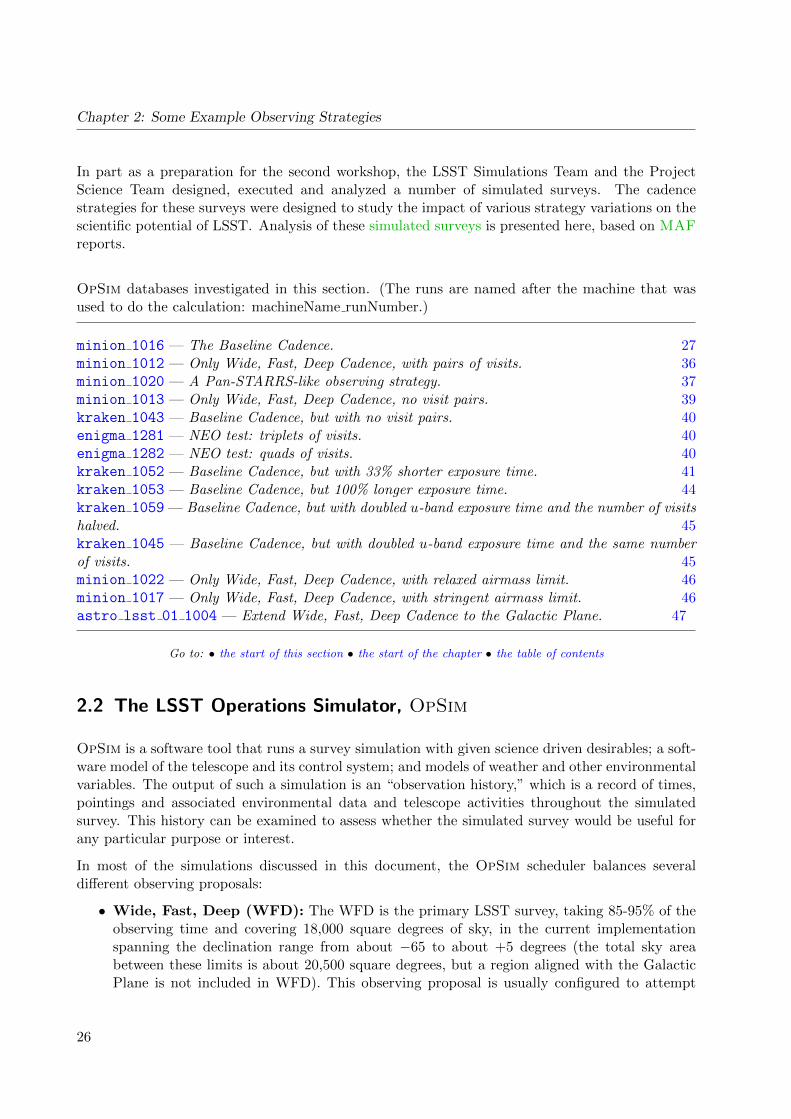
Figure 2.1: The median airmass in the r band across the sky for simulated cadence minion 1016 is shown inAitoff projection of equatorial coordinates in the left panel. The red line shows the Ecliptic and the blue line showsthe Galactic equator. The blue curve splits to enclose the so-called “Galactic confusion zone”. The correspondingairmass histogram is shown in the right panel. For the main survey area, the maximum allowed airmass was set to1.5.

1. The total number of visits is 2,447,931, with 85.1% spent on the Universal proposal (themain Wide, Fast, Deep (WFD) survey and henceforth known as the WFD proposal), 6.5%on the North Ecliptic Spur proposal, 1.7% on the Galactic Plane proposal, 2.2% on the SouthCelestial Pole proposal, and 4.5% on the Deep Drilling Cosmology proposal (5 fields).3

2. The median number of visits per night is 816, the range is 88 to 1,104, with 3,026 observingnights. The mean slew time is 6.8 seconds (median: 4.8 sec) and the total exposure time(after 10 yeras) is 73.4 Msec. The surveying efficiency, or the median total open shutter time(per night) as a fraction of the observing time (the ratio of the open shutter time to the sumof the open shutter time, readout time and slew time) is 73%.

3. The 25%-75% quartiles for the number of filter changes per night are 2 and 6, with the meanof 4.3 The total number of filter changes through the survey is 14,194.

4. In the r band, the median effective seeing for all proposals is 0.93 arcsec (for the moretraditional geometric FWHM, the median is 0.81 arcsec). We define “geometric FWHM” asthe actual full-width-at-half-maximum. The “Effective FWHM” is the FWHM of a singleGaussian describing the PSF and is typically ∼ 15% larger than the geometric FWHM. Themedian airmass for all filters and all proposals is 1.23. The median single-visit 5σ depth forpoint sources in r band in the WFD area is 24.16 (using the best current estimate of thefiducial depth at airmass of one, m5(r) = 24.39, defined by the SRD Table 5). The variationof the median airmass for the r band observations with the position on the sky is shown inFigure 2.1.

5. The median single-visit depths for WFD fields are (23.14, 24.47, 24.16, 23.40, 22.23, 21.57)

3The community-contributed white papers leading to the Deep Drilling fields defined in the Baseline Cadence canbe found via https://community.lsst.org/t/deep-drilling-whitepapers/732.

28

2.3 The Baseline Observing Strategy

Figure 2.2: The coadded 5σ depth for point sources in the r band across the sky at the end of 10 years for simulatedcadence minion 1016 is shown in Aitoff projection of equatorial coordinates. The red line shows the Ecliptic andthe blue line shows the Galactic equator (it bifurcates around the so-called “Galactic confusion zone”). The medianvalue across the WFD Cadence area is 27.1, with RMS scatter of only 0.04 mag. The small dark dots are DeepDrilling fields, with a median 5σ depth of 28.6.

in the ugrizy bands4. These values are shallower than the zenith dark time values for threemain reasons: the sky is expected to be brighter for non-dark time and away from zenith, thesky brightness model currently implemented in OpSim has some shortcomings (a new modelhas been implemented for version 4), and the moon avoidance is not as aggressive as it couldbe (many observations are taken very close to the moon avoidance limit of 30 degrees, ratherthan farther away where the sky is darker). As a result, the median limiting depths aboveare brighter than typical zenith dark-time images by close to 1 mag in the z and y bands,and a few tenths of a magnitude in the u, g and i bands.

6. For the 2,293 (overlapping) fields from the WFD area, the median number of visits in theugrizy bands is (62, 88, 199, 201, 180, 180), respectively. Not only do these medians exceedthe requested number of visits (design specification from the SRD5) of (56, 80, 184, 184, 160,

4Note that these values depend on externally supplied values for fiducial zenith dark time single-epoch 5σ depths;the following values were used in analysis described here: (23.62, 24.85, 24.39, 23.94, 23.36, 22.45) in the ugrizybands, respectively. These values are similar, but not identical, to the values listed in Table 2 from the latestversion (v3.1) of the LSST overview paper: (23.68, 24.89, 24.43, 24.00, 23.45, 22.60). This discrepancy is due tocontinuing improvements in the system performance estimates.

5The LSST Science Requirements Document (SRD) is available as http://ls.st/lpm-17

29

Chapter 2: Some Example Observing Strategies

0.5 0.6 0.7 0.8 0.9 1.0Parallax Normed (ratio)

0.000

0.168

0.336

0.504

0.671

0.839

Are

a (

10

00

s of

square

degre

es)

minion_1016 All Visits (non-dithered): Parallax Normed

0.2 0.3 0.4 0.5 0.6 0.7Proper Motion Normed (ratio)

0.000

0.839

1.679

2.518

3.357

4.196

5.036

5.875

Are

a (

10

00

s of

square

degre

es)

minion_1016 All Visits (non-dithered): Proper Motion Normed

Figure 2.3: The trigonometric parallax errors (left) and proper motion errors (right), normalized by the values foridealized perfectly optimized cadences (parallax: all the observations are taken at maximum parallax factor, resultingin a peak at the South Ecliptic pole; proper motion: a half of all visits are obtained on the first day and the reston the last day of the survey), obtained for simulated cadence minion 1016 are shown in Aitoff projection ofequatorial coordinates.

160) in the ugrizy bands, but the minimum number of visits per field over this area does so,too. This result is quite encouraging given that only 85% of observing time was spent on theWFD Cadence proposal.

7. The median coadded 5σ depth for point sources in the ugrizy bands is (25.4, 27.0, 27.1, 26.4,25.2, 24.4), respectively, for the WFD area. The distribution of coadded depth across thesky is fairly uniform, as illustrated in Figure 2.2.

8. For the 2,293 fields from the WFD area, the median geometric FWHM for seeing is 0.78arcsec in the r band and 0.77 arcsec in the i band. The median airmass in the urz bands is1.25, 1.20 and 1.26 (the maximum allowed airmass for the WFD area was set to 1.5). Themedian sky brightness in the ury bands is 22.0 mag/arcsec2, 21.1 mag/arcsec2, and 17.3mag/arcsec2, respectively (for comparison, the assumed dark sky brightness at zenith in theury bands is 23.0, 21.2 and 18.6 mag/arcsec2). The current model sky brightness in the yband is biased very high because most y band (and many z band) observations are taken in

30

2.3 The Baseline Observing Strategy

10 5 0 5 10HA

0

2000

4000

6000

8000

10000

12000

14000

Hour

Angle

His

togra

m

minion_1016: Hour Angle Histogram

u

g

r

i

z

y

Figure 2.4: Histograms in the left panel show the distribution of hour angles (HA) in 6 bands for all proposals fromsimulated cadence minion 1016 (the distributions are similar for WFD fields considered alone). Note the biastowards observations west from the meridian. The right panel shows the distribution across the sky of the mean HAfor all observations in the r band.

twilight where OpSim currently uses a very simple (and bright) sky model.

9. Restricted to the WFD fields, a unique area of 18,000 square degrees received at least 888visits per field (summed over bands; the SRD design value is 825).

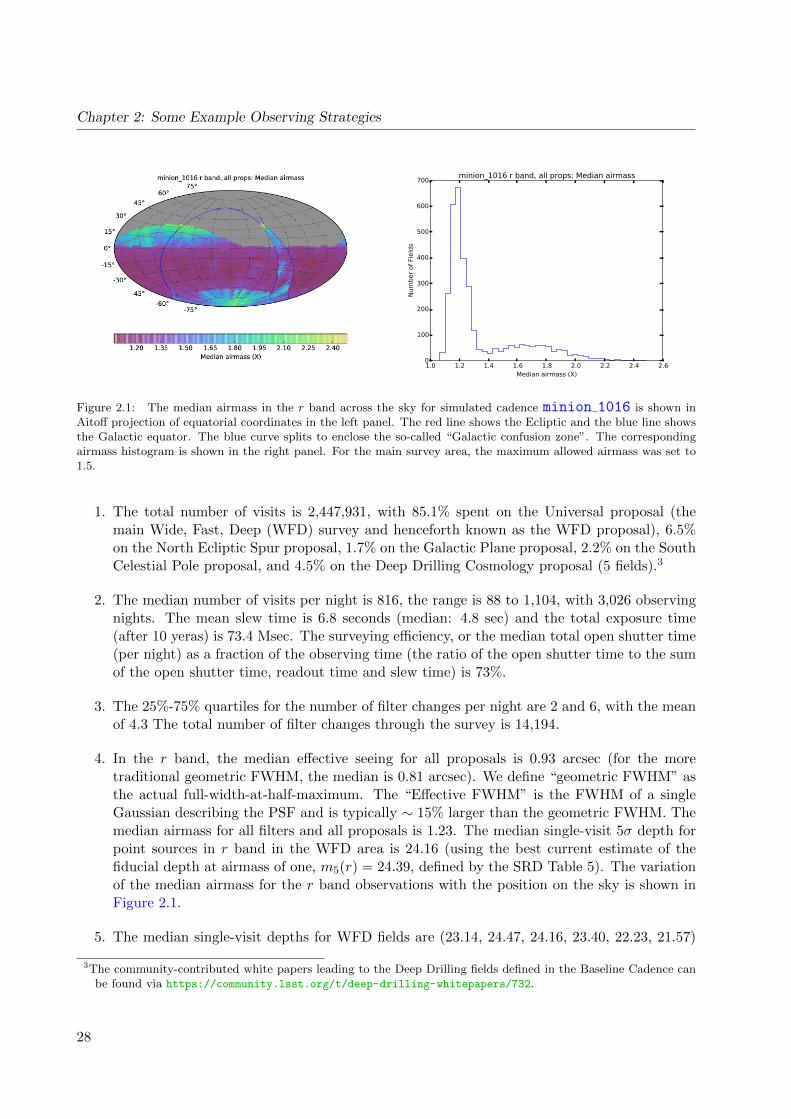
10. The median trigonometric parallax and proper motion errors are 0.62 mas and 0.17 mas/yr,respectively, for bright sources (limited by assumed systematic errors in relative astrometryof 10 mas), and 7.9 mas and 2.3 mas/yr for points sources with r = 24 (assuming flat spectralenergy distribution), over the WFD fields. The variation of parallax and proper motion errorsacross the sky is visualized in Figure 2.3.

For comparison, the old Baseline Cadence, opsim3.61 (obtained with an older version of the OpSimcode), delivered 2,651,588 visits, or 8.3% more than minion 1016 (this is due to known effectsand changes in the code, such as more pre-scheduled down time in the new version). Perhapsthe most important (and undesired!) difference between the two simulations is that the BaselineCadence spent 6.5% of the observing time on the North Ecliptic Spur proposal (vs. 4% spent onthe corresponding Universal North proposal in opsim3.61), and less than 90% of time on the WFDproposal.

Analysis of the hour angle distribution, shown in Figure 2.4 and Figure 2.5, reveals a strongbias towards observations west from the meridian for the main survey. This pattern is beinginvestigated: it may be caused by specific features of the cost function implemented in the OpSimcode. Removing the bias has the potential to increase the survey depth by around ∼ 10% (thesurvey would reach it’s current limiting depth in 9 years rather than 10).

Another potentially undesirable feature, seen in practically all simulations analyzed here, is that upto about a quarter of visits in the main survey area represents the third, the fourth and sometimeseven the fifth visit to a field in the same night. For a large number of time-domain programs,these visits could be used instead to decrease the field inter-night revisit time. For more details,see Section 3.2. The position angle distributions for this simulation are shown in Figure 2.6.

31

Chapter 2: Some Example Observing Strategies

Figure 2.5: The color-coded map in the left panel shows the visit count from the Baseline Cadence simulationminion 1016 in the equal-area Lambert projection of the horizontal coordinate system (altitude-azimuth), withnorth on top and west towards the right, for all six bands and proposals (Wide, Fast, Deep, Galactic Plane, DeepDrilling fields, North Ecliptic Spur, and South Celestial Pole region). The WFD Cadence was limited to airmassbelow 1.5, while other proposals sampled higher airmass, too (see the histogram in Figure 2.1). Note the strongpropensity of fields for westward observations (the median airmass is about 1.2). The right panel is analogous, butonly shows the r band visits for WFD fields.

0 1 2 3 4 5 6rotSkyPos

0

1000

2000

3000

4000

5000

6000

7000

8000

9000

Posi

tion A

ngle

His

togra

m

minion_1016: Position Angle Histogram

u

g

r

i

z

y

Figure 2.6: The left panel shows the position angle distribution (in radians) in each band for the main survey fieldsin minion 1016. The position angle is the angle between “up” in the image and North on the sky. The variationof the root-mean-square scatter of the r band distribution across the sky is shown in the right panel.

Time-domain Analysis

Figure 2.8 shows the median revisit time distribution when all bands are considered, and Figure 2.9shows the median revisit time distribution in the band. On average, fields in the main survey getrevisited about every 3 days using all filters, and every 15 days when using only r band visits (30days when using only u band visits is the longest median revisit time). Figure 2.10 shows themaximum inter-night gap, which on average is about 5-6 months.

The temporal sampling for this simulation is sufficient to enable a large recovery fraction forSNe. Figure 2.11 shows that a large fraction of LSST SNe will be detected before their maximum

32

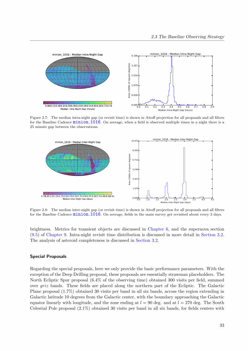
2.3 The Baseline Observing Strategy

0.0 0.1 0.2 0.3 0.4 0.5 0.6 0.7 0.8 0.9

Median Intra-Night Gap (hours)

0.000

0.839

1.679

2.518

3.357

4.196

Are

a (

10

00

s of

square

degre

es)

minion_1016 : Median Intra-Night Gap

Figure 2.7: The median intra-night gap (or revisit time) is shown in Aitoff projection for all proposals and all filtersfor the Baseline Cadence minion 1016. On average, when a field is observed multiple times in a night there is a25 minute gap between the observations.

0.5 1.0 1.5 2.0 2.5 3.0 3.5 4.0 4.5Median Inter-Night Gap (days)

0.000

1.679

3.357

5.036

6.714

8.393

10.072

Are

a (

10

00

s of

square

degre

es)

minion_1016 : Median Inter-Night Gap

Figure 2.8: The median inter-night gap (or revisit time) is shown in Aitoff projection for all proposals and all filtersfor the Baseline Cadence minion 1016. On average, fields in the main survey get revisited about every 3 days.

brightness. Metrics for transient objects are discussed in Chapter 6, and the supernova section(9.5) of Chapter 9. Intra-night revisit time distribution is discussed in more detail in Section 3.2.The analysis of asteroid completeness is discussed in Section 3.2.

Special Proposals

Regarding the special proposals, here we only provide the basic performance parameters. With theexception of the Deep Drilling proposal, these proposals are essentially strawman placeholders. TheNorth Ecliptic Spur proposal (6.4% of the observing time) obtained 300 visits per field, summedover griz bands. These fields are placed along the northern part of the Ecliptic. The GalacticPlane proposal (1.7%) obtained 30 visits per band in all six bands, across the region extending inGalactic latitude 10 degrees from the Galactic center, with the boundary approaching the Galacticequator linearly with longitude, and the zone ending at l = 90 deg. and at l = 270 deg. The SouthCelestial Pole proposal (2.1%) obtained 30 visits per band in all six bands, for fields centers with

33

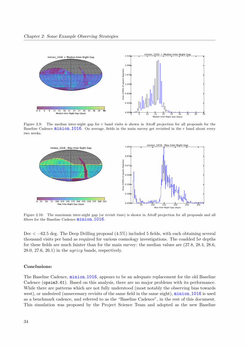
Chapter 2: Some Example Observing Strategies

0 5 10 15 20 25 30 35 40 45Median Inter-Night Gap (days)

0.000

0.420

0.839

1.259

1.679

2.098

2.518

Are

a (

10

00

s of

square

degre

es)

minion_1016 r: Median Inter-Night Gap

Figure 2.9: The median inter-night gap for r band visits is shown in Aitoff projection for all proposals for theBaseline Cadence minion 1016. On average, fields in the main survey get revisited in the r band about everytwo weeks.

50 100 150 200 250 300Max Inter-Night Gap (days)

0.000

0.168

0.336

0.504

0.671

0.839

1.007

Are

a (

10

00

s of

square

degre

es)

minion_1016 : Max Inter-Night Gap

Figure 2.10: The maximum inter-night gap (or revisit time) is shown in Aitoff projection for all proposals and allfilters for the Baseline Cadence minion 1016.

Dec < −62.5 deg. The Deep Drilling proposal (4.5%) included 5 fields, with each obtaining severalthousand visits per band as required for various cosmology investigations. The coadded 5σ depthsfor these fields are much fainter than for the main survey: the median values are (27.8, 28.4, 28.6,28.0, 27.6, 26.1) in the ugrizy bands, respectively.

Conclusions:

The Baseline Cadence, minion 1016, appears to be an adequate replacement for the old BaselineCadence (opsim3.61). Based on this analysis, there are no major problems with its performance.While there are patterns which are not fully understood (most notably the observing bias towardswest), or undesired (unnecessary revisits of the same field in the same night), minion 1016 is usedas a benchmark cadence, and referred to as the “Baseline Cadence”, in the rest of this document.This simulation was proposed by the Project Science Team and adopted as the new Baseline

34

2.3 The Baseline Observing Strategy

0.0 0.1 0.2 0.3 0.4 0.5 0.6SNAlert (Fraction Detected)

0.000

0.420

0.839

1.259

1.679

2.098

2.518

2.938

3.357

Are

a (

10

00

s of

square

degre

es)

minion_1016 : SNAlert

Figure 2.11: The fraction of simulated Type Ia SNe at a redshift of 0.5 detected pre-peak in any filter for theBaseline Cadence minion 1016. About 40% of all such SNe from the main survey will be detected before theirmaximum brightness.

Cadence by the LSST Change Control Board in August 2016.

An important feature of minion 1016 simulation is that the mean slew time of 6.8 sec (whichincludes filter change time) is very close to the minimum possible slew time of about 4.5 sec.The implication is that the surveying efficiency, assuming 30 sec exposure time per visit, can beincreased by at most about 6% (that is, the total open-shutter time is within about 6% fromits possible maximum, given everything else unchanged). Nevertheless, there are other surveyaspects, including sky coverage and temporal sampling functions, that can be further optimized,as discussed in Section 2.4 below.

The main remaining known problems with minion 1016 simulation include

• A strong bias towards observations west from the meridian for the main survey, see Figure 2.5.This bias significantly degrades the survey seeing and depth.

• Several proposals complete after only 3-4 years, resulting in regions of sky where the propermotions are poorly constrained due to the short observing baseline. See Figure 2.12.

• The sky brightness model has systematic errors, particularly in twilight time, resulting inestimates of limit depths (m5 for single visits and coadded depths) that are too shallow byabout 0.3 mag in the u band, and 0.5-1.0 mag in the z and y bands.

• The moon avoidance angle of 30 deg. allows too many z band observations with elevated skybrightness due to moonshine, resulting in about 0.2-0.3 mag shallower depth.

• There are too many unrequested and unnecessary revisits of the same field in the same night(that is, more than two visits to the same field in the same night).

Most of these issues are expected to be resolved by OpSim version 4.

Go to: • the start of this section • the start of the chapter • the table of contents

35

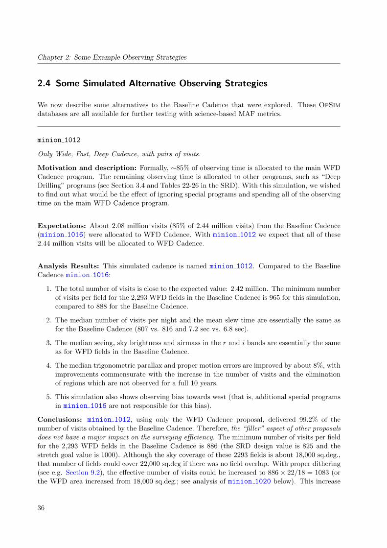
Chapter 2: Some Example Observing Strategies

2.4 Some Simulated Alternative Observing Strategies

We now describe some alternatives to the Baseline Cadence that were explored. These OpSimdatabases are all available for further testing with science-based MAF metrics.

minion 1012

Only Wide, Fast, Deep Cadence, with pairs of visits.

Motivation and description: Formally, ∼85% of observing time is allocated to the main WFDCadence program. The remaining observing time is allocated to other programs, such as “DeepDrilling” programs (see Section 3.4 and Tables 22-26 in the SRD). With this simulation, we wishedto find out what would be the effect of ignoring special programs and spending all of the observingtime on the main WFD Cadence program.

Expectations: About 2.08 million visits (85% of 2.44 million visits) from the Baseline Cadence(minion 1016) were allocated to WFD Cadence. With minion 1012 we expect that all of these2.44 million visits will be allocated to WFD Cadence.

Analysis Results: This simulated cadence is named minion 1012. Compared to the BaselineCadence minion 1016:

1. The total number of visits is close to the expected value: 2.42 million. The minimum numberof visits per field for the 2,293 WFD fields in the Baseline Cadence is 965 for this simulation,compared to 888 for the Baseline Cadence.

2. The median number of visits per night and the mean slew time are essentially the same asfor the Baseline Cadence (807 vs. 816 and 7.2 sec vs. 6.8 sec).

3. The median seeing, sky brightness and airmass in the r and i bands are essentially the sameas for WFD fields in the Baseline Cadence.

4. The median trigonometric parallax and proper motion errors are improved by about 8%, withimprovements commensurate with the increase in the number of visits and the eliminationof regions which are not observed for a full 10 years.

5. This simulation also shows observing bias towards west (that is, additional special programsin minion 1016 are not responsible for this bias).

Conclusions: minion 1012, using only the WFD Cadence proposal, delivered 99.2% of thenumber of visits obtained by the Baseline Cadence. Therefore, the “filler” aspect of other proposalsdoes not have a major impact on the surveying efficiency. The minimum number of visits per fieldfor the 2,293 WFD fields in the Baseline Cadence is 886 (the SRD design value is 825 and thestretch goal value is 1000). Although the sky coverage of these 2293 fields is about 18,000 sq.deg.,that number of fields could cover 22,000 sq.deg if there was no field overlap. With proper dithering(see e.g. Section 9.2), the effective number of visits could be increased to 886× 22/18 = 1083 (orthe WFD area increased from 18,000 sq.deg.; see analysis of minion 1020 below). This increase

36

2.4 Some Simulated Alternative Observing Strategies

is an improvement of 31% relative to the SRD design specification of 825 visits over 18,000 sq.deg.However, note again that there are no other programs in this simulation (i.e., if other programswere allocated 10% of the observing time, the implied overall “over-performance” in the numberof visits would be about 20%).

minion 1020

A Pan-STARRS-like observing strategy.

Motivation and description: “Pan-STARRS-like cadence” attempts to apply a uniform ca-dence strategy throughout the maximum size survey region, which is about 27,400 deg2. This issimilar to the Pan- STARRS’ 3PI survey which also tries to maximize sky area. The maximumacceptable airmass is kept at its default value of 1.5; this excludes fields with Dec < −78 degand Dec > +18 deg. The minion 1020 simulations utilizes a maximum Dec of +15 deg, uniformcadence and no other proposal, and requires pairs of visits as in the Baseline Cadence.

Expectations: The total number of visits should be roughly the same as in the Baseline Cadence,but spread over a 42% larger sky area (3,255 fields instead of 2,293), with fewer visits per field.

Analysis Results: This simulated cadence is named minion 1020. Compared to the BaselineCadence minion 1016:

1. The total number of visits is 2.42 million, and essentially identical to the number of visits inthe Baseline cadence.

2. The mean number of visits per field is 740, which is 81% of the number of visits for WFDfields obtained by the Baseline Cadence (but here the sky area is 42% larger). We note thatthis is below the number required by the SRD.

3. The median number of visits per night and the mean slew time are essentially the same asfor the Baseline Cadence.

4. The median seeing, sky brightness and airmass in the r and i bands for WFD fields areessentially the same as in the Baseline Cadence.

5. The median trigonometric parallax and proper motion errors show uniform behavior overthe entire enlarged area (see Figure 2.12), with the values similar to those obtained for theBaseline Cadence.

6. This simulation also shows observing bias towards west.

Due to increased sky area, which samples regions that can never achieve low airmass, the mediancoadded depth is about 0.15 mag shallower for this simulation than for the Baseline Cadence. As aresult, the counts of galaxies per unit area down to a fixed SNR would decrease by about 15-20%.At the same time, the area outside the Galactic plane is increased by about 30%, and thus the totalnumber of galaxies would be increased by about 10%, compared to WFD fields in the BaselineCadence. However, the increased median airmass also results in larger seeing, especially for theborderline regions, as illustrated in Figure 2.13. The increased median seeing would decrease the

37

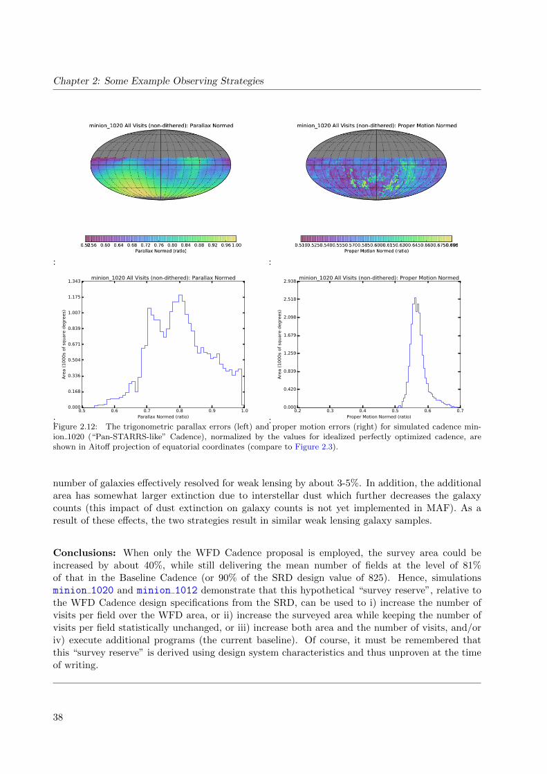
Chapter 2: Some Example Observing Strategies

: :

:0.5 0.6 0.7 0.8 0.9 1.0

Parallax Normed (ratio)

0.000

0.168

0.336

0.504

0.671

0.839

1.007

1.175

1.343

Are

a (

10

00

s of

square

degre

es)

minion_1020 All Visits (non-dithered): Parallax Normed

:0.2 0.3 0.4 0.5 0.6 0.7

Proper Motion Normed (ratio)

0.000

0.420

0.839

1.259

1.679

2.098

2.518

2.938A

rea (

10

00

s of

square

degre

es)

minion_1020 All Visits (non-dithered): Proper Motion Normed

Figure 2.12: The trigonometric parallax errors (left) and proper motion errors (right) for simulated cadence min-ion 1020 (“Pan-STARRS-like” Cadence), normalized by the values for idealized perfectly optimized cadence, areshown in Aitoff projection of equatorial coordinates (compare to Figure 2.3).

number of galaxies effectively resolved for weak lensing by about 3-5%. In addition, the additionalarea has somewhat larger extinction due to interstellar dust which further decreases the galaxycounts (this impact of dust extinction on galaxy counts is not yet implemented in MAF). As aresult of these effects, the two strategies result in similar weak lensing galaxy samples.

Conclusions: When only the WFD Cadence proposal is employed, the survey area could beincreased by about 40%, while still delivering the mean number of fields at the level of 81%of that in the Baseline Cadence (or 90% of the SRD design value of 825). Hence, simulationsminion 1020 and minion 1012 demonstrate that this hypothetical “survey reserve”, relative tothe WFD Cadence design specifications from the SRD, can be used to i) increase the number ofvisits per field over the WFD area, or ii) increase the surveyed area while keeping the number ofvisits per field statistically unchanged, or iii) increase both area and the number of visits, and/oriv) execute additional programs (the current baseline). Of course, it must be remembered thatthis “survey reserve” is derived using design system characteristics and thus unproven at the timeof writing.

38

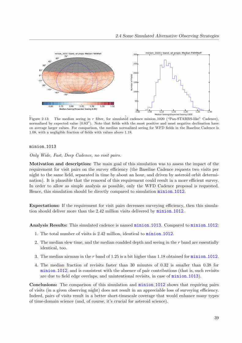
2.4 Some Simulated Alternative Observing Strategies

: :1.00 1.05 1.10 1.15 1.20 1.25 1.30

Median Seeing/(Expected Seeing 0.83)

0

50

100

150

200

250

300

Num

ber

of

Field

s

minion_1020 r band, all props: Median FWHMeff

Figure 2.13: The median seeing in r filter, for simulated cadence minion 1020 (“Pan-STARRS-like” Cadence),normalized by expected value (0.83′′). Note that fields with the most positive and most negative declination haveon average larger values. For comparison, the median normalized seeing for WFD fields in the Baseline Cadence is1.08, with a negligible fraction of fields with values above 1.18.

minion 1013

Only Wide, Fast, Deep Cadence, no visit pairs.

Motivation and description: The main goal of this simulation was to assess the impact of therequirement for visit pairs on the survey efficiency (the Baseline Cadence requests two visits pernight to the same field, separated in time by about an hour, and driven by asteroid orbit determi-nation). It is plausible that the removal of this requirement could result in a more efficient survey.In order to allow as simple analysis as possible, only the WFD Cadence proposal is requested.Hence, this simulation should be directly compared to simulation minion 1012.

Expectations: If the requirement for visit pairs decreases surveying efficiency, then this simula-tion should deliver more than the 2.42 million visits delivered by minion 1012.

Analysis Results: This simulated cadence is named minion 1013. Compared to minion 1012:

1. The total number of visits is 2.42 million, identical to minion 1012.

2. The median slew time, and the median coadded depth and seeing in the r band are essentiallyidentical, too.

3. The median airmass in the r band of 1.25 is a bit higher than 1.18 obtained for minion 1012.

4. The median fraction of revisits faster than 30 minutes of 0.32 is smaller than 0.38 forminion 1012, and is consistent with the absence of pair contributions (that is, such revisitsare due to field edge overlaps, and unintentional revisits, in case of minion 1013).

Conclusions: The comparison of this simulation and minion 1012 shows that requiring pairsof visits (in a given observing night) does not result in an appreciable loss of surveying efficiency.Indeed, pairs of visits result in a better short-timescale coverage that would enhance many typesof time-domain science (and, of course, it’s crucial for asteroid science).

39

Chapter 2: Some Example Observing Strategies

kraken 1043

Baseline Cadence, but with no visit pairs.

Motivation and description: The main goal of this simulation was to assess the impact ofthe requirement for visit pairs on the survey efficiency. Instead of the idealized case above whichcompared only the WFD Cadence proposal fields, in this more realistic case all proposals fromthe Baseline Cadence are executed. Hence, this simulation should be compared to the BaselineCadence (minion 1016).

Expectations: A slight, or no, increase in surveying efficiency and thus the total number of visitsis expected when compared to the Baseline Cadence.

Analysis Results: This simulated cadence is named kraken 1043. Compared to minion 1016,

1. The total number of visits is 2.51 million, or 2.4% more than in the Baseline Cadence.

2. The mean slew time is 5.8 sec, or 15% shorter than for the Baseline Cadence. This decreasein the mean slew time implies an efficiency increase of 2.8% and explains the actual 2.4%improvement implied by the total number of visits. Note that this simulation has the shortestmean slew time of all simulations investigated here (the nominal shortest slew and settle timeis about 4.5 sec).

3. The median airmass in the r band is slightly larger for this simulation than for the BaselineCadence: 1.29 vs. 1.22.

Conclusions: Unlike the comparison of minion 1013 and minion 1012, here the removal ofvisit pair requirement results in a 15% shorter mean slew time and consequently in 2.4% morevisits.

enigma 1281

NEO test: triplets of visits.

enigma 1282

NEO test: quads of visits.

Motivation and description: Many science programs can benefit from having more than a pairof visits in a night; in particular, Solar System science may critically depend on having more thanjust a pair, depending on the performance of the Moving Object Pipeline Software (MOPS). Thesetwo simulations were run to investigate the effects of requiring more than just a pair of visits ineach night. The first, enigma 1281, requests sets of three visits (triplets) in each night. Thesecond, enigma 1282, requests sets of four visits (quads) in each night. There is no constraint onthe filter chosen for these sets of visits – it may be changed or it may remain the same. Thesesimulations should be compared to the Baseline Cadence, minion 1016, and to the kraken 1043,

40

2.4 Some Simulated Alternative Observing Strategies

which all keep the special surveys, but simply vary the sequences requested in the WFD Cadence.

Expectations: The general expectations are that science cases which require many visits ontimescales of a few hours will benefit with these runs, while science cases which prefer visits to bespaced more widely over time will see negative impacts.

Analysis Results: First, we emphasize that “requested” is not the same as “delivered”: eventhe “no pairs” simulation kraken 1043 ends up having multiple visits in a given night to thesame fields, and when multiple visits per night are requested, not all fields get to have completedsequences. The statistics of how many fields are combined into sequences of a given number ofvisits is shown in Figure 2.14. As evident, the highest peak is at the requested number of visits ina sequence, but not all visits are incorporated into requested sequences: some are in both shorterand longer sequences. The “no pairs” simulation includes multiple visits to some fields, becausethe current version of the algorithm is not told not to do so. As illustrated in Figure 2.15, suchrevisits typically happen within 10 minutes from the first visit. This (unintended) behavior impliesthat the naive expectation above is probably incorrect, or at least softened.

The median inter-night revisit rate is affected by requesting more visits within single night, asexpected – there are only so many visits available, and if more occur in a particular night, it islikely (without some kind of rolling cadence) that the result is longer intervals between subsequentnights. This is demonstrated in Figure 2.16, where it can be seen that the inter-night revisit rateincreases by about 30% from 3 nights to 4 nights if we go from pairs to triplets (or quads).

Details of the impacts on Solar System science is left to Chapter 3, in particular the impact oncompleteness is evaluated in Section 3.2.

The impact of requesting sequences with 3 or 4 visits to the same field on other science programsis not yet analyzed in detail. The impact on static science should be minimal, except perhapsfor a bit worse behavior of various systematic errors (because fewer nights, with their observingconditions, are sampled).

Conclusions: The effect of requesting pairs, single visits, triplets or quads, is softened with thecurrent behavior of the scheduler, where it is not uncommon to receive more than the requestednumber of visits within a night. The inter-night revisit rates are affected, increasing the inter-nightrevisit rate by about a night for triplets and quads and reducing the inter-night revisit rate byabout a night when no visit pairs are requested (from a baseline value of about 3 nights).

kraken 1052

Baseline Cadence, but with 33% shorter exposure time.

Motivation and description: The optimal exposure time per visit for the main survey, in thelimit of a single value for all bands and at all times, is in the range of about 20–60 seconds (Ivezicet al. 2008, see Section 2.2.2 in the version 3.1 LSST overview paper). This simulation investigatesthe effect of decreasing the exposure time per visit to 20 seconds (from its nominal value of 30seconds). The shorter exposure time results in 0.22 mag shallower faint limit per visit (the effect

41

Chapter 2: Some Example Observing Strategies

0 2 4 6 8 10

N visits per field per night

0

200000

400000

600000

800000

1000000

1200000

Num

ber

of

vis

its

in

baseline (minion_1016)

no pairs (kraken_1043)

pairs (minion_1012)

triples (enigma_1281)

quads (enigma_1282)

Figure 2.14: The distribution of the number of visits used for nightly sequences of length given on the horizontalaxis. Only griz bands are used. Note that even “no pairs” simulation (kraken 1043) includes multiple visits.The highest peak is at the requested number of visits in a sequence.

: :

Figure 2.15: The comparison of the median intra-night gap (per field) distributions for the Baseline Cadence (left)and simulation kraken 1043, which did not request pairs of visits per night. Despite no need for pairs, simulationkraken 1043 produced them “spontaneously”, as well as longer sequences (see Figure 2.14). The mean field revisittime is much shorter (about 6 minutes, see the right panel) than for the Baseline Cadence (22 minutes).

is larger in the u band, see kraken 1059).

Expectations: The total number of visits is expected to increase by about 50%, compared tominion 1016, to 3.70 million, for the same survey efficiency. However, the shorter exposure timewill have a significant impact on the survey efficiency: assuming a slew time of 7 sec, the efficiency

42

2.4 Some Simulated Alternative Observing Strategies

:

0 1 2 3 4 5 6

Median Inter-Night Gap

0.000

1.679

3.357

5.036

6.714

8.393

10.072

Are

a (

1000s

of

square

degre

es)

: Median Inter-Night Gap

minion_1016

kraken_1043

enigma_1281

enigma_1282

Figure 2.16: Comparison of the median inter-night gap distribution for minion 1016, kraken 1043,enigma 1281, and enigma 1282. The peak median inter-night revisit rate (per field) is about 3 days forthe baseline cadence, minion 1016, about 2 days for kraken 1043, and closer to 4 for both enigma 1281and enigma 1282.

drops from 73% to 65% (comparing 30/(30+4+7) vs. 20/(20+4+7)). Therefore, the expectedincrease in the number of visits is about 32% and the expected number of visits is 3.2 million.

Analysis Results: This simulated cadence is named kraken 1052. Compared to the BaselineCadence:

1. The total number of visits is 3.23 million, representing an increase of 31% that is very closeto the expected value of 32%.

2. The median number of visits per night is 1079, or about 32% more than for the Baseline Ca-dence. The total open shutter time is 14% smaller for this simulation, and easily understoodas due to expected 11% decrease due to smaller surveying efficiency (the mean slew time isthe same as in the Baseline Cadence, 6.9 sec).

3. The main survey (WFD, 18,000 sq.deg.) fields received 33% more visits than in the BaselineCadence. The increase in the minimum number of visits over that area is 9% (from 886 to963). In addition, another 1,000 sq.deg. (6% of the nominal WFD) area has more than 961visits.

43

Chapter 2: Some Example Observing Strategies

4. Most other performance parameters are essentially unchanged: the fraction of visits spenton the main survey (88% vs. 85%), the median seeing in the r band (0.93 arcsec vs. 0.94arcsec), and the median airmass (1.23 vs. 1.22).

Conclusions: The comparison of kraken 1052 and minion 1016 simulations demonstrates thatthe effect of shorter exposures can be easily understood using simple efficiency estimates. With thevisit exposure time is decreased from 30 sec to 20 sec, the surveying efficiency and the total openshutter time drops by ∼10%, while the number of (shorter exposure time) visits (for all proposals)increases by 32%.

kraken 1053

Baseline Cadence, but 100% longer exposure time.

Motivation and description: This simulation investigates the effect of increasing the exposuretime per visit to 60 seconds (from its nominal value of 30 seconds). The longer exposure time re-sults in 0.38 mag deeper faint limit per visit (the effect is larger in the u band, see kraken 1059).The number of exposures per visit was kept at 2.

Expectations: The total number of visits is expected to decrease by about a factor of 2 in caseof no significant impact on the survey efficiency. However, the longer exposure time improvesefficiency by a factor of 2 × (34 + 7)/(64 + 7) − 1 = 15%, and thus the expected total number ofvisits is 0.5×1.15 = 58% of the number of visits in the Baseline Cadence (assuming the same meanslew time of 7 seconds).

Analysis Results: This simulated cadence is named kraken 1053. Compared to the BaselineCadence:

1. The total number of visits is 1.42 million or 58% of the visits obtained with the BaselineCadence, and the total open-shutter time is 16% higher than for the Baseline Cadence. Bothresults are in good agreement with above expectations.

2. The median number of visits per night is 467, or 57% of the value obtained with the BaselineCadence. The mean slew time is 0.5 sec longer than that obtained with the Baseline Cadence.

3. This simulation has significantly different time allocation per proposal, compared to theBaseline Cadence: 74% spent on the WFD proposal (vs. 85%) and 11% spent on the NorthEcliptic Spur proposal (vs. 6%) (with smaller and less important differences for other pro-posals). Because of these differences, the results of this test may not be very robust.

Conclusions: Simple estimates of the total number of visits and the improvement in efficiencyare in good agreement with delivered values. Of course, the increased efficiency comes at the costof fewer visits, which is disadvantageous for time-domain science. There are other consequence ofa longer exposure time, including saturation at fainter mags, worse bleed trails and scattered lightfrom bright stars, and more trailing of fast-moving asteroids.

44

2.4 Some Simulated Alternative Observing Strategies

kraken 1059

Baseline Cadence, but with doubled u-band exposure time and the number of visits halved.

Motivation and description: The read-out noise in the u band is not negligible compared tothe background noise as in other bands, due to darker u band sky. The current best estimatesfor survey performance (Ivezic et al. 2008, see Table 2 in the version 3.1 LSST overview paper)indicate that the coadded depth in the u band could be improved by 0.24 mag by increasing theexposure time per visit from 30 seconds to 60 seconds (assuming the same total exposure time,which implies a decrease in the number of visits by a factor of two). To keep the total exposuretime in the u band unchanged, the requested number of visits in this simulation is decreased by afactor of 2 relative to the Baseline Cadence specification.

Expectations: The total exposure time in the u band should remain unchanged. The single visitsdepth should be 0.62 mag deeper due to increased exposure time, and the coadded depth shouldbe 0.24 mag deeper (due to decreased impact of readout noise).

Analysis Results: This simulated cadence is named kraken 1059. Compared to the BaselineCadence (minion 1016):

1. The total number of visits is 2.32 million or 95% of the Baseline Cadence values. The fractionof time allocated to the main survey is 84% vs. 85% for the Baseline Cadence, and for theNES proposal 7% vs. 6%.

Conclusions: The u band exposure time can be increased from 30 seconds to 60 seconds withouta significant impact on the survey efficiency. This change would result in a gain of about 0.2 magin the coadded depth, with the same total exposure time allocated to the u band. However, thenumber of visits in the u band would be decreased by about a factor of two, with a negative impacton time-domain science.

kraken 1045

Baseline Cadence, but with doubled u-band exposure time and the same number of visits.

Motivation and description: This simulation is similar to kraken 1059, which increased theexposure time per visit in the u band from 30 seconds to 60 seconds, with the requested number ofvisits decreased by a factor of 2. That change resulted in a gain of about 0.2 mag in the coaddeddepth, just from reducing overheads. However, in order to keep the same total exposure timeallocated to the u band, the number of u band visits in kraken 1059 was decreased by about afactor of two relative to Baseline Cadence, and this had a negative impact on time-domain sci-ence. To further investigate this tradeoff, the kraken 1045 simulation was designed and carriedout. kraken 1045 retains the Baseline Cadence requested number of visits per field: hence, thecoadded depth in the u band in this simulation could be improved by up to 0.6 mag.

Expectations: Given that about 7% of all visits are allocated to the u band (56 out of 825), thetotal number of visits for other bands will decrease when the number of the u band is doubled,

45

Chapter 2: Some Example Observing Strategies

resulting in about 0.04 mag shallower data in bands other than the u band.

Analysis Results: This simulated cadence is named kraken 1045. Compared to the BaselineCadence (minion 1016):

1. The total number of visits is 2.36 million or 95.5% of the Baseline Cadence values. Thefraction of time allocated to the main survey is 85% vs. 85% for the Baseline Cadence, andfor the NES proposal 7% vs. 6%.

The median number of visits in the grizy filters in the main survey decreases by about 7%.The median single visit depth for main survey is 0.53 mags deeper, and the median coaddedu band image is 0.50 mags deeper. The other filters reach shallower coadded depth than inthe Baseline Cadence by about 0.05 mag.

Conclusions: When the u band exposure time is increased from 30 seconds to 60 seconds, andthe number of visits is kept unchanged, the single-visit and coadded depths would be improvedby about 0.5 mag. This improvement would come at the expense of about 7% fewer visits inother bands (with about 0.05 mag shallower coadded depths). These promising results should beconsidered when designing the next incarnation of baseline cadence.

minion 1022

Only Wide, Fast, Deep Cadence, with relaxed airmass limit.

Motivation and description: What is the effect of changing the airmass limit from 1.5 to2.0? To avoid complicated analysis, we use only the WFD cadence proposal and thus compare tominion 1012 (which has the same footprint on ths sky).

Analysis Results: This simulated cadence is named minion 1022. Compared to minion 1012,it collected 99.1% visits. This fraction is identical to the loss of efficiency due to slightly longer meanslew time: 7.2 sec vs. 6.8 sec. In addition, minion 1022 has much worse airmass distributionsthan minion 1012, extending to the allowed maximum of 2.0. For example, the median for the rband and WFD fields is 1.30, compared to 1.19 for minion 1012.

Conclusions: This simulation confirms that it’s a bad idea to relax the airmass limit: as a result,the airmass distribution always widens. In addition, relaxed airmass limit tends to result in alonger mean slew time. For a given proposal, the airmass limit has to be as tight as possible, whilestill allowing observations of all requested fields.

minion 1017

Only Wide, Fast, Deep Cadence, with stringent airmass limit.

Motivation and description: What is the effect of changing the airmass limit from 1.5 to1.3? To avoid complicated analysis, we use only the WFD Cadence proposal and thus compare tominion 1012 (i.e., we are not including the North Ecliptic Spur, South Celestial Pole, or DeepDrilling Fields in this simulation).

46

2.4 Some Simulated Alternative Observing Strategies

Analysis Results: This simulated cadence is named minion 1017. Compared to minion 1012,it collected essentially the same number of visits. The mean slew time is also essentially unchanged(7.4 sec vs. 7.2 sec). The airmass distributions is improved compared to minion 1012. Forexample, the median for the r band and WFD fields is 1.11, compared to 1.18 for minion 1012.The limiting coadded depth in u and g bands is about 0.1 mag deeper than for the BaselineCadence.

Conclusions: It is possible to achieve the same surveying efficiency with much more stringentairmass limit than 1.5, which was used in most simulations to date. Given this encouragingbehavior, an analogous experiment should be executed for the Baseline Cadence (i.e. a simulationlike minion 1016, with airmass limit for the main survey set to 1.3) – after the “Western bias”is fixed in OpSim version 4.

astro lsst 01 1004

Extend Wide, Fast, Deep Cadence to the Galactic Plane.

Motivation and description: What is the effect of extending the ‘normal’ WFD Cadence andnumber of exposures to the region of the Galactic Plane within the WFD declination limits? Fieldswhich were previously contained in the Galactic Plane proposal, but which fell within the range ofthe WFD declination limits, were reassigned to the standard WFD proposal instead of the muchmore limited Galactic Plane proposal. The remaining proposals were unchanged, and thus wecompare this to the Baseline Cadence, minion 1016.

Analysis Results: This simulated cadence is named astro lsst 01 1004. Compared withminion 1016, there are small to no changes in proposals other than the WFD and Galactic Planeproposals themselves. The fields which remained in the Galactic Plane proposal obtained thesame number of visits as expected (30 in each bandpass). There were differences observed in theoverall status of observations taken under the WFD Cadence, in the WFD proposal, however. Thenumber of fields included in the WFD proposal increased from 2293 to 2470 (∼ 8%), as 177 fieldswere moved from the Galactic Plane proposal into the WFD. The total number of observationsobtained by the WFD proposal increased from 2085270 to 2116203; an increase of only 1.5%. As aresult, the median number of visits per field was reduced in all bands, as well as the correspondingcoadded depth.

Conclusions: In both of these runs, the WFD proposal received about 85% of the total numberof visits in the survey. Extending the WFD Cadence to the Galactic Plane, without increasing theoverall priority of the WFD proposal, results in slightly fewer visits per field as a result, by about5%, and a slightly lower coadded depth, by about 0.04 magnitudes. It is worthwhile to note thatincreasing the priority of the WFD proposal could increase the total fraction of time devoted toWFD, returning the typical number of visits and coadded depth to baseline levels while decreasingtime spent in other proposals. Metrics targeted for specific science cases, explored in later chapters,will help determine whether this is a worthwhile trade.

Go to: • the start of this section • the start of the chapter • the table of contents

47

Chapter 2: Some Example Observing Strategies

2.5 Future Work: Rolling Cadence

Stephen Ridgway

With a total of ∼ 800 visits spaced approximately uniformly over 10 years, and distributed among6 filters, it is not clear that LSST can offer the sufficiently dense sampling in time for study oftransients with typical durations less than or ' 1week. This is particularly a concern for key sciencerequiring well-sampled SNIa light curves. “Rolling” cadences stand out as a general solution thatcan potentially enhance sampling rates by 2× or more, on some of the sky all of the time and allof the sky some of the time, while maintaining a sufficient uniformity for survey objectives thatrequire it. In this section we provide an introduction to the concept of rolling cadence, and givesome examples of ways in which it can be implemented.

2.5.1 The Uniform Cadence

Current schedule simulations allocate visits as pairs separated by 30-60 minutes, for the purposesof identifying asteroids. For most other science purposes, the 30-60 minute spacing is too small toreveal temporal information, and a pair will constitute effectively a single epoch of measurement.If the expected 824 (design value) LSST visits are realized as 412 pairs, and distributed uniformlyover 10 observing seasons of 6 months each, the typical separation between epochs will be 4 days(typically in different filters). The most numerous visits will be in the r and i filters, and the repeatvisit rate in either of these will be ' 20 days.

The possibility is still open that, for asteroid identification, visits might be required as triples orquadruples (which provide a more robust tracking), in which case the universal temporal samplingwill be further slowed by 1.5 or 2×.

Under a strict universal cadence it is not possible to satisfy a need for more frequent sampleepochs. This has led the LSST Project simulations group to investigate the options opened up byreinterpreting the concept of a universal cadence. Instead of aiming for a strategy which attemptsto observe all fields “equally” all the time, it would allow significant deviations from equal coverageduring the survey, returning to balance at the end of the survey.

Stronger divergence from a universal cadence, allowing significant inhomogeneities to remain atthe end of the survey, is of course possible, but is not under investigation or discussed here.

There is currently considerable interest in the community in strategies that provide enhancedsampling over a selected area of the sky, and rotating the selected area in order to exercise enhancedsampling over all of the survey area part of the time. The class of cadences that provides suchintervals of enhanced visits, with the focus region shifting from time to time, is termed here a“rolling cadence.” As a point of terminology, observing a single sky area with enhanced cadencefor a period of time will be described as a “roll”.

48

2.5 Future Work: Rolling Cadence

2.5.2 Rolling Cadence Basics

Assume a fixed number of observing epochs for each point on the sky, nominally distributeduniformly over the 10-year survey duration. A subset of these can be reallocated to provideimproved sampling of a given sky region in a given time interval. This will have the inevitableeffects of: (1) reducing the number of epochs available for that sky region during the rest of thesurvey (affecting, for example, proper motion studies), and (2) displace observations of other skyregions during the time of the improved temporal sampling (affecting, for example, early largescale structure studies needing high depth uniformity). In short, the cadence outside the enhancedinterval will be degraded.

The essential parameters of rolling cadence are: (1) the number of samples taken from the uniformcadence, and (2) the enhancement factor for the observing rate. LSST document 16370, “ARolling Cadence Strategy for the Operations Simulator”, by K. Cook and S. Ridgway, containsmore detailed discussion and analysis.

2.5.3 Supernovae and Rolling Cadence

Pending more quantitative guidance, the SN objective for rolling cadence is to obtain multi-bandtime series that are significantly longer than the typical SN duration, and that have a cadencesignificantly faster than uniform. As an example we discuss the option of a rolling cadence withthe regular distribution of filters.

As a simple example, consider improving the cadence by a factor of 2 or 3. If we accept thatsome regions of the sky will be enhanced every year, and that uniform sky coverage will only beachieved at the end of 10 years, then we could use, e.g., 10% of the total epochs in a single roll.If the enhancement is 2×, each roll would last for ' 6 months, with high efficiency for captureof complete SN events. If the enhancement is 4×, each roll would last for 2 months, with lowerefficiency.

If it is important to achieve survey uniformity after 3 years, the available visits for each roll wouldbe reduced also. With a 2× enhancement of epoch frequency, a roll would last 2 months.

Some leverage would be gained by using more than 10% of the available visits for a single roll.However, this begins to impact the sampling of slow variables reduce schedule flexibility androbustness, and should be approached with caution.

From these examples, it appears that a 2× enhancement with uniformity closure after 10 yearsis relatively feasible and promising. Much higher gains, or more rapid closure, require additionalcompromises.

2.5.4 Fast Transients and Rolling Cadence

Fast transients as a science topic are addressed in Chapter 6. In this section, the demands of fasttransients are used to directly constrain or orient the rolling cadence development.

49

Chapter 2: Some Example Observing Strategies

By “fast transients”, we are referring to events that are sufficiently fast that they are not addressedby the rolling cadence designed for SN observations, and slow enough that they are not covered inthe cosmological “deep drilling field” cadences (Section 1.1, Section 2.2). For higher tempo rolls,it is quite difficult to obtain full color data, because of the constraints on filter selection. For thisexample, we will examine a rolling cadence utilizing only the r and i filters, as they are used formost visits. They are close in wavelength, and we assume that sufficient color information will beobtained by the “background” uniform survey that continues during a roll.

Again using 10% of the available visits from the full 10 year survey for a single roll, we find thatthere would be enough epochs for each roll to acquire 1 visit per day for 21 consecutive days, givingan enhancement of 10×.

Alternatively, the same epochs could be used to observe a target every 20 minutes for 12 hoursduring a single night (here it is assumed that visit pairs are not required, doubling the availableepochs) for an enhancement of 300×.

Several different possible redeployments of portions of a uniform survey have been described, eachusing 10% of available time. Of course it is possible in principle to implement multiple options,sequentially or maybe in parallel in some cases. This may pose considerable challenges to thescheduling strategy design by introducing incompatible boundary conditions.

While rolling cadences are powerful, they have limitations. For example, sampling events that lastlonger than '1 day and less than ' 1 week have the obvious problem of diurnal availability. In thisexample, intermediate cadences could be implemented in the circumpolar region, where diurnalaccess is much extended. This is an example of a case in which a mini-survey of a limited numberof regions could be considered as an alternative to a rolling cadence applied to the entire mainsurvey.

2.5.5 Constraints, Trades and Compromises for Rolling Cadences

While rolling cadences offer some attractive benefits, it is important to realize that rolling cadencesare very highly constrained, and that they do bring disadvantages and compromises.

There are strong arguments against beginning a rolling cadence in the first, or even the second yearof the survey. Early in the survey, it is important to obtain for each field/filter combination, anadequate number of good quality photometric images, and at least one image in excellent seeing, tosupport closure of photometry reductions, generation of template images for differencing analysis,and to establish the baseline for proper motion studies.

Since many major science goals require a significant degree of survey homogeneity, it may beadvisable to implement a strategy that brings the survey to nominal uniform depth at severaltimes, e.g. after 3 or 5 years. This would strongly constrain rolling cadences. We note that such astrategy would also allow a lot of science to be done without waiting the whole 10-years.

Some science objectives favor certain distributions of visits. For astrometry, visits early and latein the survey and at large parallax factors, are beneficial. Slow variables may benefit from uniformspacing. Rolling cadences might impact these constraints either favorably or unfavorably.

50

2.6 Summary

Many objectives are served by randomization of observing conditions for each field. Some rollingcadences could tend to reduce this randomization, for example by acquiring a large number ofobservations during a meteorologically favorable or unfavorable season, or during a period of in-strument performance variance.

Dithering may prove challenging with a rolling cadence, since it reduces temporal coverage at theboundaries of the selected sky region. This is negligible for small dithers, but important for largedithers, which are under consideration; making the contiguous roll area as large as possible shouldmitigate this issue.

These cautions illustrate that evaluation of rolling cadences must be based on the full range ofschedule performance metrics, and not just those targeted by rolling cadence development.

2.5.6 Directions

While preliminary experiments with rolling cadences have been carried out with OpSim, theseexperiments have significant deficiencies, and are not suited for in-depth study as of this writing.Designing and simulating a family of rolling cadences is one of the main goals for the Project’s“SOCS and Scheduler” team for OpSim version 4.

Rolling cadences will need to satisfy the basic survey science requirements (including those onsky area, depth and visit count ), and then be evaluated using the same set of metrics as forother cadences. Of particular interest will be metrics that clearly distinguish the gains availablewith rolling cadences; that is, metrics that measure schedule performance for variable targets, andespecially those with strong sampling requirements, or more rapid variability.

Go to: • the start of this section • the start of the chapter • the table of contents

2.6 Summary

The most important conclusion of this chapter is that the upper limit on possible schedulingefficiency improvements for the Baseline Cadence is close to 6%. This conclusion is by and largebased on the fact that the mean slew time for the Baseline Cadence is 6.9 sec, and thus only slightlylarger than the design specifications for the system slew and settle time of 4.5 sec. Nevertheless,there are a number of features to understand, and some to fix, and there is substantial optimizationpotential in temporal sampling functions and further optimization of the sky area and observingstrategy details, that can result in enhanced science even with the same integrated open-shuttertime (e.g. by obtaining deeper data through an improved sampling of observing conditions).

The main other questions addressed here are:

1. By what factor could we exceed the SRD design specification for the number of visits if onlythe WFD Cadence proposal was implemented?

51

Chapter 2: Some Example Observing Strategies

A simulation that only implemented the WFD Cadence proposal exceeded the design speci-fication for the number of visits by about 40% (over the design specification for the sky areaof 18,000 sq.deg.)

2. By what factor could we exceed the SRD design specification for the sky coverage if onlythe WFD Cadence proposal was implemented with the design specification for the number ofvisits?

The Pan-STARRS-like strategy results in about 40% larger sky coverage (about 25,000sq.deg.), with the mean number of visits at 92% of the design specification. The total numberof visits is the same as for the Baseline Cadence, implying similar surveying efficiency.

Therefore, the available “margin” relative to the SRD design specifications for the mainsurvey is equivalent to about 30-40% larger sky coverage, or about 30-40% more visits perfield. The SRD assumes that 10% margin will be available for other programs. The implied“survey reserve”, relative to the WFD Cadence design specifications from the SRD, can beused to:

a) increase the number of visits per field over the WFD area, or

b) increase the surveyed area while keeping the number of visits per field statisticallyunchanged, or

c) increase both area and the number of visits, and/or

d) execute additional programs (the current baseline).

3. What is the effect of auxiliary proposals on surveying efficiency?

A comparison of simulations which only implemented the WFD Cadence proposal to thosethat included all other programs did not show a significant change of efficiency (older simu-lations, not analyzed here, showed increases in surveying efficiency of up to about 3% due toshorter slewing time).

4. What is the effect of visit pairs on surveying efficiency?

Relinquishing the visit pair requirement results in up to 2-3% improvement of the surveyingefficiency. The impact on some time-domain science would be positive, while for NEO andmain-belt asteroid science it would be strongly negative.

5. Can the effects of variations of the visit exposure time on surveying efficiency be predictedusing simple efficiency estimates?

Simple estimates based on comparing exposure (open shutter) and total visit times are ingood agreement with simulations. Decreasing the visit exposure time to 20 seconds decreasesthe total open shutter time by 10%, and increasing it to 60 seconds increases the total openshutter time by 16%, relative to the Baseline Cadence and standard exposure time of 30seconds. The number of visits changes by factors of 1.35 and 0.58.

52

2.6 Summary

6. What are the effects of doubling the exposure time only in the u band?

The effect of doubling the exposure time only in the u band, while simultaneously halvingthe number of requested visits, has no significant effect on the survey efficiency.

The effect of doubling the exposure time only in the u band, with the number of requestedvisits unchanged, is a decrease in the number of visits in other bands by about 6%.

7. What is the impact of the hard airmass limit, X < 1.5, on the surveying efficiency?

It is a very bad idea to relax the airmass limit! It is possible to achieve the same survey-ing efficiency with a much more stringent airmass limit than 1.5, which was used in mostsimulations to date.

Go to: • the start of this section • the start of the chapter • the table of contents

53

3 Discovering and Characterizing Small Bodiesin the Solar System

Chapter editors: Lynne Jones, David Trilling.

Contributing authors: Zeljko Ivezic, Miguel de Val-Borro.

3.1 Introduction

LSST has tremendous potential as a discovery and characterization tool for small bodies in theSolar System. With LSST, we have the opportunity to increase our sample sizes of PotentiallyHazardous Asteroids (PHAs), Near Earth Objects (NEOs), Main Belt Asteroids (MBAs), JupiterTrojans, Centaurs, Trans-Neptunian Objects (TNOs), Scattered Disk Objects (SDOs), comets andother small body populations such as Earth mini-moons, irregular satellites, and other planetaryTrojan populations, by at least an order of magnitude, often two orders of magnitude or more.In addition to hundreds of astrometric measurements for most objects, LSST will also provideprecisely calibrated multiband photometry. With this information, we can also characterize thesepopulations – deriving colors, light curves, rotation periods, spin states, and even shape modelswhere possible.

The motivation behind studying these small body populations is fundamentally to understandplanet formation and evolution. The orbital parameters of these populations record traces ofthe orbital evolution of the giant planets. The migration of Jupiter, Saturn and Neptune inparticular have left marks on the orbital distribution of MBAs, Jupiter Trojans, TNOs and SDOs.Rapid migration of Jupiter and Saturn may have emplaced a large number of planetesimals in theScattered Disk; later slow migration of Neptune will affect the number of TNOs in resonance andthe details of their orbital parameters within the resonance. Adding color information providesfurther insights; colors roughly track composition, indicating formation location and temperatureor space weathering history. For example, the color gradient of main belt asteroids, combined withtheir orbital distribution, suggests that perhaps Jupiter migrated inwards, mixing planetesimalsfrom the outer Solar System into the outer parts of the main belt, before eventually migratingoutwards. Studying the size distribution of each of the small body populations themselves providesmore constraints on planetesimal formation; this is complicated by the effects of dynamical stirringfrom the giant planets, which can increase the rate of erosion vs. growth during collisions, and bythe existence of the remnants of collisions such as collisional families in the main belt. The presenceof binaries and range of spin states and shapes provides further constraints on the history of eachpopulation. The location of the planets before migration, the amount of migration, and the sizedistribution of the small bodies themselves (after detangling the dynamical evolution) all tell a

55

Chapter 3: Solar System

deeper story about how the planets in the Solar System formed, and how our formation historyfits into the range of observed extrasolar planetary systems.

These Solar System populations are unique when compared to other objects which will be investi-gated by LSST, due to the simple fact that they move across the sky. Metrics to evaluate LSST’sperformance for moving objects need to be based on ‘per object’ measurements, rather than ata series of points on the sky or per field pointing. For all metrics discussed in this chapter, theorbit of each object is integrated over the time of the simulated opsim survey and the detectionsof each object are recorded (using the footprint of the focal plane and including trailing losses andadjusting for the colors of the objects in each filter to generate SNR and likelihood of detection);these series of observations per object are then the basis for metric evaluations.

Go to: • the start of this section • the start of the chapter • the table of contents

3.2 Discovery: Linking Solar System Objects

Lynne Jones, David Trilling, Zeljko Ivezic

Discovering, rather than simply detecting, small objects throughout the Solar System requiresunambiguously linking a series of detections together into an orbit. The orbit provides the infor-mation necessary to scientifically characterize the object itself and to understand the populationas a whole. Without orbits, the detections of Solar System Objects (SSOs) by LSST will be oflimited use; objects discovered with other facilities could be followed up by LSST, but almost theentire science benefit to planetary astronomy would be lost. Linking and orbit determination forSolar System objects is similar to source association for non-moving objects; it provides the meansto identify multiple detections as coming from a single object.

Therefore, the first concern regarding the Solar System is related to the question “Can we accuratelylink individual detections of moving objects into orbits?”. This requirement poses varying levels ofdifficulty as we move from Near Earth Objects (NEOs) through the Main Belt Asteroids (MBAs)and to Trans-Neptunian Objects (TNOs) and Scattered Disk Objects (SDOs), as well as for cometsand for other unusual but very interesting populations such as Earth minimoons (see e.g. Bolinet al. 2014; Fedorets et al. 2017). Due to their small heliocentric and geocentric distances, NEOsappear to move with relatively high velocities and are distributed over a large fraction of thesky, including regions far from the ecliptic plane. MBAs are densely distributed, primarily withinabout 30 degrees of the ecliptic. TNOs and SDOs move slowly, however short time intervals betweenrepeat visits in each night may make these difficult to link. Comets and Earth mini-moons mayrequire more complicated orbit fitting to allow for non-gravitational or geocentric orbits. Therequirements of accurately linking individual detections into orbits also implies that we do notcreate false objects by incorrectly linking detections and/or noise.

Much of the answer to this question comes down to the performance of various pieces of LSST DataManagement software. In particular, important questions are the rate of false positive detectionsresulting from difference imaging, possible limitations of the Moving Object Processing System(MOPS) to extend to high apparent velocities, and the capability to unambiguously determineif a linkage is ‘real’ or not via orbit determination (done as part of MOPS). Thus this question

56

3.2 Discovery: Linking Solar System Objects

includes concerns beyond the limits of the OpSim simulated surveys, although it still bears onthe observing strategy requirements for discovering Solar System Objects. An in-depth study ofthe performance of difference imaging and MOPS is currently ongoing. However, we can make arange of assumptions on how MOPS will perform and evaluate how many and which objects canbe linked under observational cadence, given those assumptions.

It is important to emphasize that for the vast majority of LSST-observed moving objects, LSSTwill be both the discovery and the recovery facility. Most LSST-observed objects will be too faintto be observed by assets that are currently carrying out Solar System small bodies observations,and the number of detections will be so large that the existing infrastructure could not observemore than a tiny fraction, even if they were bright enough. Therefore, as described in this section,LSST’s performance for detecting and re-detecting minor bodies is critical to the success of theproject; no outside contributions will be significant.

3.2.1 Target measurements and discoveries

The criteria for ‘discovery’ with MOPS depends on the number of observations of an object acquiredper night within some time window (creating ‘tracklets’), repeated over a number of nights withinwindow of some days (creating ‘tracks’), which are then linked into an orbit with a threshold onastrometric residuals. The current assumptions are that we can link detections into orbits with 2detections per night within 90 minutes, repeated for 3 nights within a window of 15 days. Theadditional assumptions are that with these 6 observations, we will be able to create low-accuracyorbits that will suffice to link additional observations obtained at later (or earlier, in the LSSTarchive) times, and that the orbit fitting will enable rejection of mislinkages.

We can also use other requirements for discovery. Requiring 4 detections in each night is a fairlycommon discovery criteria for NEO surveys, as it reduces the number of mislinked tracklets toalmost zero. We could also require 4 nights of pairs within a window of 20 days, in order toimprove the initial orbit fitting and mislinkage rejection. We can also assume MOPS will performbetter than the current assumptions, and evaluate discovery criteria of 3 pairs within a 30 daywindow.

With these discovery criteria, we can then evaluate the completeness of an LSST simulated survey,for a given population. We can look at this as a function of H magnitude and as a function oforbital parameters.

For PHAs and NEOs there are special considerations in terms of completion that arise from plan-etary defense concerns. For most other populations, the general desire is simply to have a highlevel of completeness, with no gaps in completeness that depend strongly on orbital parameters. Inparticular, the desire is to be able to calibrate any selection effects in discovery so that the surveycompleteness can be used to debias the underlying population models.

Discovery opportunity, and thus the completeness of the underlying population, is very sensitive tothe time interval between observations. Waiting longer between observations within a night meansthat objects may move beyond a single LSST field of view. Longer times between revisits meansthat observing in large contiguous blocks (rather than narrow, disconnected strips) within a nightbecomes more important to make sure that objects are followed between pointings, especially if

57

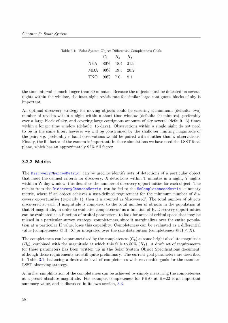
Chapter 3: Solar System

Table 3.1: Solar System Object Differential Completeness Goals

Cb Hb Hf

NEA 80% 18.4 21.9

MBA 90% 19.5 20.2

TNO 90% 7.0 8.1

the time interval is much longer than 30 minutes. Because the objects must be detected on severalnights within the window, the inter-night revisit rate for similar large contiguous blocks of sky isimportant.

An optimal discovery strategy for moving objects could be ensuring a minimum (default: two)number of revisits within a night within a short time window (default: 90 minutes), preferablyover a large block of sky, and covering large contiguous amounts of sky several (default: 3) timeswithin a longer time window (default: 15 days). Observations within a single night do not needto be in the same filter, however we will be constrained by the shallower limiting magnitude ofthe pair; e.g. preferably r band observations would be paired with i rather than u observations.Finally, the fill factor of the camera is important; in these simulations we have used the LSST focalplane, which has an approximately 92% fill factor.

3.2.2 Metrics

The DiscoveryChancesMetric can be used to identify sets of detections of a particular objectthat meet the defined criteria for discovery: X detections within T minutes in a night, Y nightswithin a W day window; this describes the number of discovery opportunities for each object. Theresults from the DiscoveryChancesMetric can be fed to the MoCompletenessMetric summarymetric, where if an object achieves a user-defined requirement for the minimum number of dis-covery opportunities (typically 1), then it is counted as ‘discovered’. The total number of objectsdiscovered at each H magnitude is compared to the total number of objects in the population atthat H magnitude, in order to evaluate ‘completeness’ as a function of H. Discovery opportunitiescan be evaluated as a function of orbital parameters, to look for areas of orbital space that may bemissed in a particular survey strategy; completeness, since it marginalizes over the entire popula-tion at a particular H value, loses this capability. Completeness can be evaluated as a differentialvalue (completeness @ H=X) or integrated over the size distribution (completeness @ H ≤ X).

The completeness can be parametrized by the completeness (Cb) at some bright absolute magnitude(Hb), combined with the magnitude at which this falls to 50% (Hf ). A draft set of requirementsfor these parameters has been written up in the Solar System Object Specifications document,although these requirements are still quite preliminary. The current goal parameters are describedin Table 3.1, balancing a desireable level of completeness with reasonable goals for the standardLSST observing strategy.

A further simplification of the completeness can be achieved by simply measuring the completenessat a preset absolute magnitude. For example, completeness for PHAs at H=22 is an importantsummary value, and is discussed in its own section, 3.3.

58

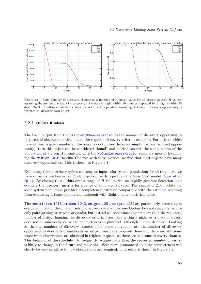
3.2 Discovery: Linking Solar System Objects

0 5 10 15 20 25 30

H (mag)

0

20

40

60

80

100

120

140

Mean n

um

ber

of

dis

covery

chance

s

minion_1016: Number of discovery chances

NEOMBATNO

0 5 10 15 20 25 30

H (mag)

0.0

0.2

0.4

0.6

0.8

1.0

Com

ple

teness

<=

H

minion_1016: Cumulative Completeness - 3 pairs in 15 nights

NEOMBATNO

Figure 3.1: Left: Number of discovery chances as a function of H (mean value for all objects at each H value),assuming the minimum criteria for discovery - 2 visits per night within 90 minutes, repeated for 3 nights within 15days. Right: Resulting cumulative completeness for each population, assuming that only 1 discovery opportunity isrequired to ‘discover’ each object.

3.2.3 OpSim Analysis

The basic output from the DiscoveryChancesMetric is the number of discovery opportunities(e.g. sets of observations that match the required discovery criteria) available. For objects whichhave at least a given number of discovery opportunities (here, we simply use one required oppor-tunity), then this object can be considered “found” and marked towards the completeness of thepopulation at a given H magnitude with the MoCompletenessMetric summary metric. Examin-ing the minion 1016 Baseline Cadence with these metrics, we find that most objects have manydiscovery opportunities. This is shown in Figure 3.1.

Evaluating these metrics requires choosing an input solar system population; for all tests here, wehave chosen a random set of 2,000 objects of each type from the Grav S3M model (Grav et al.2011). By cloning these orbits over a range of H values, we can rapidly generate detections andevaluate the discovery metrics for a range of simulated surveys. The sample of 2,000 orbits persolar system population provides a completeness estimate comparable with the estimate resultingfrom evaluating a larger population, although with slightly more statistical noise.

The runs minion 1016, kraken 1043, enigma 1281, enigma 1282 are particularly interesting toevaluate in light of the different sets of discovery criteria. Because OpSim does not currently requireonly pairs (or singles, triplets or quads), but instead will sometimes acquire more than the requestednumber of visits, changing the discovery criteria from pairs within a night to triplets or quads,does not automatically cause the completeness to plummet, although it does decrease. Lookingat the raw numbers of discovery chances offers some enlightenment: the number of discoveryopportunities does falls dramatically as we go from pairs to quads, however, there are still sometimes when observations are obtained in triplets or quads, so there are still some discovery chances.This behavior of the scheduler (to frequently acquire more than the requested number of visits)is likely to change in the future and make this effect more pronounced, but the completeness willclearly be very sensitive to how observations are acquired. This effect is shown in Figure 3.2.

59

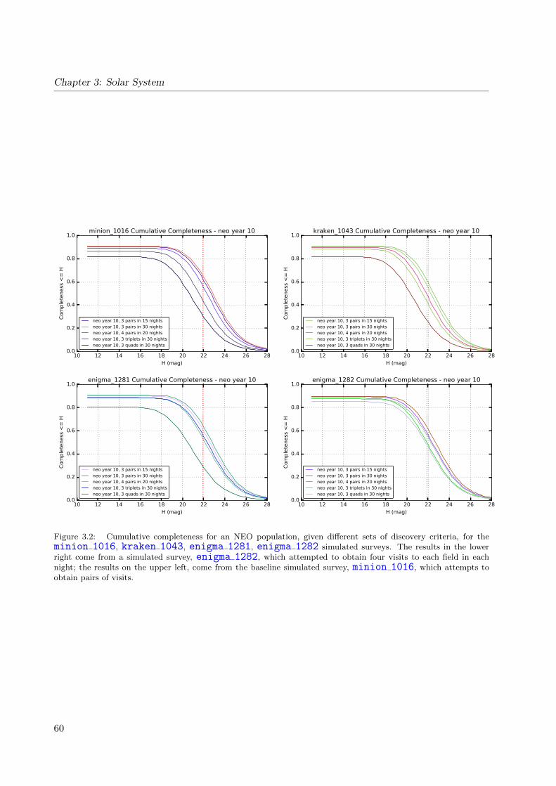
Chapter 3: Solar System

10 12 14 16 18 20 22 24 26 28

H (mag)

0.0

0.2

0.4

0.6

0.8

1.0

Com

ple

teness

<=

H

minion_1016 Cumulative Completeness - neo year 10

neo year 10, 3 pairs in 15 nightsneo year 10, 3 pairs in 30 nightsneo year 10, 4 pairs in 20 nightsneo year 10, 3 triplets in 30 nightsneo year 10, 3 quads in 30 nights

10 12 14 16 18 20 22 24 26 28

H (mag)

0.0

0.2

0.4

0.6

0.8

1.0

Com

ple

teness

<=

H

kraken_1043 Cumulative Completeness - neo year 10

neo year 10, 3 pairs in 15 nightsneo year 10, 3 pairs in 30 nightsneo year 10, 4 pairs in 20 nightsneo year 10, 3 triplets in 30 nightsneo year 10, 3 quads in 30 nights

10 12 14 16 18 20 22 24 26 28

H (mag)

0.0

0.2

0.4

0.6

0.8

1.0

Com

ple

teness

<=

H

enigma_1281 Cumulative Completeness - neo year 10

neo year 10, 3 pairs in 15 nightsneo year 10, 3 pairs in 30 nightsneo year 10, 4 pairs in 20 nightsneo year 10, 3 triplets in 30 nightsneo year 10, 3 quads in 30 nights

10 12 14 16 18 20 22 24 26 28

H (mag)

0.0

0.2

0.4

0.6

0.8

1.0

Com

ple

teness

<=

H

enigma_1282 Cumulative Completeness - neo year 10

neo year 10, 3 pairs in 15 nightsneo year 10, 3 pairs in 30 nightsneo year 10, 4 pairs in 20 nightsneo year 10, 3 triplets in 30 nightsneo year 10, 3 quads in 30 nights

Figure 3.2: Cumulative completeness for an NEO population, given different sets of discovery criteria, for theminion 1016, kraken 1043, enigma 1281, enigma 1282 simulated surveys. The results in the lowerright come from a simulated survey, enigma 1282, which attempted to obtain four visits to each field in eachnight; the results on the upper left, come from the baseline simulated survey, minion 1016, which attempts toobtain pairs of visits.

60

3.2 Discovery: Linking Solar System Objects

0 2 4 6 8 10

Years into survey

0.0

0.1

0.2

0.3

0.4

0.5

0.6

0.7

Com

ple

teness

@ H

<=

22.0

0

Cumulative completeness as a function of time

neo H<=22.00

0 2 4 6 8 10

Years into survey

0.0

0.1

0.2

0.3

0.4

0.5

0.6

0.7

0.8

0.9

Com

ple

teness

@ H

<=

20.2

5

Cumulative completeness as a function of time

mba H<=20.25

0 2 4 6 8 10

Years into survey

0.0

0.2

0.4

0.6

0.8

1.0

Com

ple

teness

@ H

<=

8.0

0

Cumulative completeness as a function of time

tno H<=8.00

Figure 3.3: Completeness as a function of time, for NEO, MBA and TNO populations. The completeness increasesrapidly for the first few years, then increases more slowly. The NEO completeness rises more slowly than otherpopulations, as more NEOs become available to discover due to changing their orbital positioning relative to Earth(becoming closer and brighter, or moving away from sightlines behind the Sun). The TNO completeness rises mostrapidly with time, as these objects move slowly; we find most of these objects within the first two years and thenimprove their characterization over the rest of the survey (measuring better orbits and obtaining lightcurves andcolors).

Table 3.2: Solar System Object Differential Completeness in minion 1016

Cb Hb Hf

NEA 87.5% 18.5 21.5

MBA 89% 19.5 20.2

TNO 96% 7.0 8.3

Another aspect to consider is to look at how the completeness increases over time. The com-pleteness as a function of time is plotted for particular H values, depending on the population, inFigure 3.3.

3.2.4 Discussion

A large portion of the risk in being able to discover moving objects lies in the currently uncertainperformance of the MOPS software. Figure 3.2 clearly shows that with the baseline cadence, if wemust have triplets or pairs, or even just require 4 pairs of observations over 20 nights, that thecompleteness falls. The performance will likely fall even further if the scheduler stops obtainingmore than the minimum requested number of observations.

With the expected MOPS discovery requirements, minion 1016 performs adequately for mostsolar system objects, as seen in Table 3.2, although completeness falls off more rapidly for faintobjects than desired for NEOs. To investigate this effect, more metrics will have to be developedto discover why these fainter NEOs are not being discovered (are they simply missing appropriatesequences of observations due to the cadence or is something more subtle occurring?).

Go to: • the start of this section • the start of the chapter • the table of contents

61

Chapter 3: Solar System

3.3 Discovery of Potentially Hazardous Asteroids

Zeljko Ivezic, Lynne Jones.

The U.S. Congress has given a mandate to NASA to implement a Near-Earth Object (NEO) Surveyprogram to detect, track, catalog, and characterize the physical characteristics of near-Earth objectsequal to or greater than 140 meters in diameter1. The goal is to achieve a completeness of 90%. Inrecent practice, adopted here, the completeness is evaluated for a subset of NEOs called PotentiallyHazardous Asteroids2 (PHA), with H≤22, where H is the absolute magnitude3 in the Johnson’s Vband.

The discovery criteria for PHAs follows the same guidelines and metrics found in the previoussection, 3.2, but is worth discussing separately to focus on its main figure of merit - completenessfor PHAs with H≤22 magnitudes.

3.3.1 Target measurements and discoveries

Using the same range of discovery criteria as in the previous section, 3.2, we can look at thedifferential and cumulative completeness for a population of PHAs. For this sample of PHAs,we pulled the orbits of 2,000 objects with MOID <= 0.05 AU from the Grav S3M model (Gravet al. 2011). These orbits were then cloned over a range of H values to evaluate the chances ofdiscovery for that orbit at each of those H values. The differential completeness as a function ofH is then simply the fraction of objects which receive at least one set of observations which meetthe discovery criteria during the course of the survey. The cumulative completeness is similar,but integrated over H by assuming an H distribution with a power-law index of α = 0.3. Bothdifferential and cumulative completeness are relevant metrics: the former provides more insight inthe behavior of a particular simulation, while the latter is a metric given to NASA by the U.S.Congress.

To match the NEO mandate, the cumulative completeness at H=22 can be used as a figure ofmerit.

3.3.2 Metrics

The metrics used here are the same as in 3.2, although run with different input populations.

1See http://www.gpo.gov/fdsys/pkg/PLAW-109publ155/pdf/PLAW-109publ155.pdf2Potentially Hazardous Asteroids (PHAs) are defined as asteroids with a minimum orbit intersection distance

(MOID) of 0.05 AU or less.3Absolute magnitude is the magnitude that an asteroid would have at a distance of 1 AU from the Sun and from the

Earth, viewed at zero phase angle. This is an impossible configuration, of course, but the definition is motivatedby desire to separate asteroid physical characteristics from the observing configuration.

62

3.3 Discovery of Potentially Hazardous Asteroids

3.3.3 OpSim Analysis

The differential and cumulative completeness for the baseline survey, minion 1016, at a range ofyears is shown in Figure 3.4. The baseline cadence achieves a cumulative completeness of 66% forH≤22 PHAs when requiring pairs of visits on 3 separate nights within 15 days. The differentialcompleteness at H=22 for the same survey is 49%, 17% lower due to increasing completenesstoward smaller H (larger objects).

:10 12 14 16 18 20 22 24 26 28

H (mag)

0.0

0.2

0.4

0.6

0.8

1.0

Com

ple

teness

@ H

minion_1016 PHA Differential Completeness

PHA 3 pairs in 15 nights yr 1 : @ H(=22.0) = 6.6%

PHA 3 pairs in 15 nights yr 2 : @ H(=22.0) = 13.9%

PHA 3 pairs in 15 nights yr 4 : @ H(=22.0) = 25.9%

PHA 3 pairs in 15 nights yr 6 : @ H(=22.0) = 35.1%

PHA 3 pairs in 15 nights yr 8 : @ H(=22.0) = 42.2%

PHA 3 pairs in 15 nights yr 10 : @ H(=22.0) = 48.8%

101102103104 D (m)

:10 12 14 16 18 20 22 24 26 28

H (mag)

0.0

0.2

0.4

0.6

0.8

1.0

Com

ple

teness

<=

H

minion_1016 PHA Cumulative Completeness

PHA 3 pairs in 15 nights yr 1 : @ H(<=22.0) = 14.6%

PHA 3 pairs in 15 nights yr 2 : @ H(<=22.0) = 28.5%

PHA 3 pairs in 15 nights yr 4 : @ H(<=22.0) = 44.8%

PHA 3 pairs in 15 nights yr 6 : @ H(<=22.0) = 53.8%

PHA 3 pairs in 15 nights yr 8 : @ H(<=22.0) = 60.5%

PHA 3 pairs in 15 nights yr 10 : @ H(<=22.0) = 65.6%

101102103104 D (m)

Figure 3.4: The PHA completeness for minion 1016, as a function of the object’s absolute visual magnitude Hon the horizontal axes (left: differential completeness at a given H; right: cumulative completeness for all objectsbrighter than a given H), as it increases year over year. The cumulative completeness for H≤22 NEOs (those withdiameters larger than 140m) for this simulation is 66% after 10 years.

We find that the PHA and NEO completeness are very similar for a given simulated survey and setof discovery criteria, as shown in Figure 3.5, a reasonable result given that the input populationsare very similar. The analysis of the various observing run strategies (singles, pairs, triples orquads of visits) described in the previous section thus applies to PHAs as well.

:

Figure 3.5: Comparison of the cumulative NEO and PHA completeness for the baseline cadence minion 1016.

Go to: • the start of this section • the start of the chapter • the table of contents

63

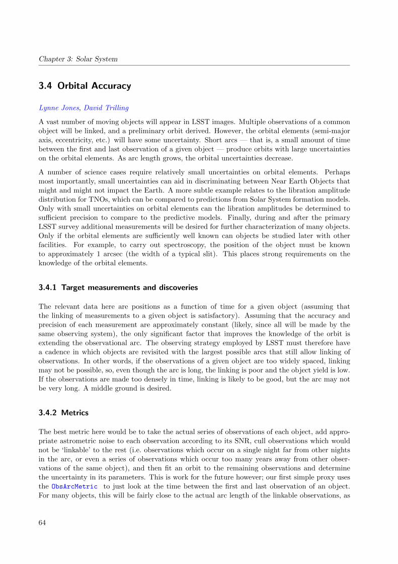
Chapter 3: Solar System

3.4 Orbital Accuracy

Lynne Jones, David Trilling

A vast number of moving objects will appear in LSST images. Multiple observations of a commonobject will be linked, and a preliminary orbit derived. However, the orbital elements (semi-majoraxis, eccentricity, etc.) will have some uncertainty. Short arcs — that is, a small amount of timebetween the first and last observation of a given object — produce orbits with large uncertaintieson the orbital elements. As arc length grows, the orbital uncertainties decrease.

A number of science cases require relatively small uncertainties on orbital elements. Perhapsmost importantly, small uncertainties can aid in discriminating between Near Earth Objects thatmight and might not impact the Earth. A more subtle example relates to the libration amplitudedistribution for TNOs, which can be compared to predictions from Solar System formation models.Only with small uncertainties on orbital elements can the libration amplitudes be determined tosufficient precision to compare to the predictive models. Finally, during and after the primaryLSST survey additional measurements will be desired for further characterization of many objects.Only if the orbital elements are sufficiently well known can objects be studied later with otherfacilities. For example, to carry out spectroscopy, the position of the object must be knownto approximately 1 arcsec (the width of a typical slit). This places strong requirements on theknowledge of the orbital elements.

3.4.1 Target measurements and discoveries

The relevant data here are positions as a function of time for a given object (assuming thatthe linking of measurements to a given object is satisfactory). Assuming that the accuracy andprecision of each measurement are approximately constant (likely, since all will be made by thesame observing system), the only significant factor that improves the knowledge of the orbit isextending the observational arc. The observing strategy employed by LSST must therefore havea cadence in which objects are revisited with the largest possible arcs that still allow linking ofobservations. In other words, if the observations of a given object are too widely spaced, linkingmay not be possible, so, even though the arc is long, the linking is poor and the object yield is low.If the observations are made too densely in time, linking is likely to be good, but the arc may notbe very long. A middle ground is desired.

3.4.2 Metrics

The best metric here would be to take the actual series of observations of each object, add appro-priate astrometric noise to each observation according to its SNR, cull observations which wouldnot be ‘linkable’ to the rest (i.e. observations which occur on a single night far from other nightsin the arc, or even a series of observations which occur too many years away from other obser-vations of the same object), and then fit an orbit to the remaining observations and determinethe uncertainty in its parameters. This is work for the future however; our first simple proxy usesthe ObsArcMetric to just look at the time between the first and last observation of an object.For many objects, this will be fairly close to the actual arc length of the linkable observations, as

64

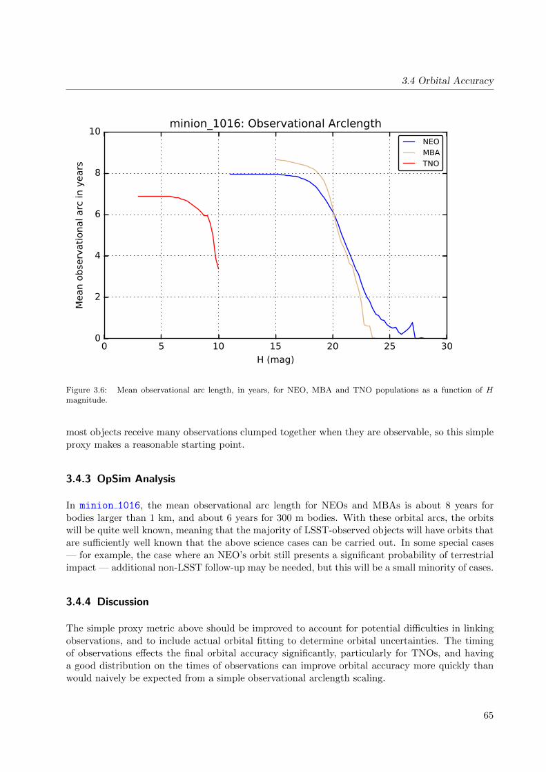
3.4 Orbital Accuracy

0 5 10 15 20 25 30

H (mag)

0

2

4

6

8

10

Mean o

bse

rvati

onal arc

in y

ears

minion_1016: Observational Arclength

NEOMBATNO

Figure 3.6: Mean observational arc length, in years, for NEO, MBA and TNO populations as a function of Hmagnitude.

most objects receive many observations clumped together when they are observable, so this simpleproxy makes a reasonable starting point.

3.4.3 OpSim Analysis

In minion 1016, the mean observational arc length for NEOs and MBAs is about 8 years forbodies larger than 1 km, and about 6 years for 300 m bodies. With these orbital arcs, the orbitswill be quite well known, meaning that the majority of LSST-observed objects will have orbits thatare sufficiently well known that the above science cases can be carried out. In some special cases— for example, the case where an NEO’s orbit still presents a significant probability of terrestrialimpact — additional non-LSST follow-up may be needed, but this will be a small minority of cases.

3.4.4 Discussion

The simple proxy metric above should be improved to account for potential difficulties in linkingobservations, and to include actual orbital fitting to determine orbital uncertainties. The timingof observations effects the final orbital accuracy significantly, particularly for TNOs, and havinga good distribution on the times of observations can improve orbital accuracy more quickly thanwould naively be expected from a simple observational arclength scaling.

65

Chapter 3: Solar System

A figure of merit, including requirements on the orbital accuracy for various classes of objects,should also be developed.

As an intermediate step, we have carried out two anecdotal studies of orbital accuracy. In the first,we took an arbitrary (real) NEO — object 2016 DL — with a six year arc. This is representativeand typical of NEOs that will be observed by LSST. The maximum positional uncertainty for thisobject over the next ten years is 25 arcsec (3σ). This is small enough that essentially any kind offollow-up observation would be possible (presuming that pre-imaging is possible for spectroscopy,for example, to locate the moving object). The uncertainties on the orbital parameters of thisobject are on the order of 1 part in 104 or even smaller. This level of precision should allow all theinvestigations described above.

In the second experiment, we took an arbitrary (real) TNO — object 2015 SO20 — that has a fiveyear arc. For this object, the maximum positional uncertainty over the next ten years is ∼20”,and its orbital elements are known to around 1 part in 105. Again, this level of precision shouldenable all of the science investigations described above.

Go to: • the start of this section • the start of the chapter • the table of contents

3.5 Detecting Comet Activity

Lynne Jones, David Trilling, Miguel de Val-Borro

Comets are the remnant building blocks of the Solar System that have been stored at cold tem-peratures beyond the ice line, either in the Kuiper belt or the Oort cloud, since their formation.Measuring the evolution of cometary activity over a range of heliocentric distances with LSST willallow us to understand the overall comet activity and to link these observations with the physicaland chemical conditions in the early solar nebula during planet formation. Comets are classified intwo main dynamical families, Jupiter Family comets (JFCs) that have low-inclination orbits withperiods less than 20 years, and Long-period comets (LPCs) that originate in the Oort Cloud at adistance of more than 10000 AU and have large orbital eccentricities and nearly isotropic distribu-tion of inclinations. Currently there are over 400 Jupiter-family comets known, most of which arefaint compared with the LPCs. LSST will observe about 104 individual comets repeatedly includ-ing measurements of known objects over its 10-year survey (Solontoi 2010). The determination oftheir activity levels at various heliocentric distances will be used to study the time evolution ofeach object individually and to find the connection between comet families and their formationregion in the Solar System.

Several cometary volatiles result in strong emission bands excited by solar radiation that emit byresonant fluorescence at optical and near-ultraviolet wavelengths. The LSST u filter peaks nearthe CN (0–0) emission band at 3880 A. Although CN is not the most abundant daughter speciesfrom cometary volatiles and the OH (0–0) emission band at 3080 A is generally stronger, CNproduction rates provide an excellent proxy of the level of overall gas activity in comets. LSST willoffer a unique opportunity to produce a large database of CN production rates, vastly increasingour current knowledge (see e.g. A’Hearn et al. 1995, 2012). Other bands such as r, i, and z willdetect continuum brightness that is produced by reflected radiation from dust particles in the coma.

66

3.5 Detecting Comet Activity

Thus, it will be possible to obtain the evolution of the gas-to-dust production ratio at high cadenceas a function of heliocentric distance in different comet families. The greatly increased sample sizecompared with previous catalogs (A’Hearn et al. 1995) will allow for statistical comparison of thecomet families and to link them to other small body populations in the Solar System.

A recently discovered population of main-belt asteroids eject dust and produce coma and tailsgiving them the appearance of comets (Jewitt 2012). This so-called main-belt comets or activeasteroids have the orbital characteristics of asteroids with TJ > 3 and lose mass during part oftheir orbits. The cometary activity observed in these objects may be driven by primordial waterice that is trapped near the surface and sublimates when it is exposed to sunlight. Main-beltcomets are important because they may have been able to preserve water ice despite the effect ofsolar radiation and heating from the decay of short-lived radioactive nuclei. The asteroids in theouter regions of the main belt can therefore have a substantial fraction of water and other volatilesthat may have supplied the volatile content of terrestrial planets. Most of the main-belt-cometsare faint with very weak comae that are active during part of their orbits. Given the expectedflux sensitivity of LSST, the transient cometary activity of main-belt asteroids will be observableincluding many objects that could be below the detection limits of current photometric surveys.The LSST observations will thus help to understand the overlap between different populations inthe Solar System such as the relationship between comets and asteroids.

3.5.1 Target measurements and discoveries

LSST will make an exceptionally large number of comet observations. About 104 comets willbe observed on average of 50 times by LSST during its main survey, while a few objects will beobserved more than 1000 times (Solontoi 2010). Simulations of characteristic comet orbits haveshown that LSST will observe some Jupiter Family comets (JFCs) hundreds of times over theirfull orbits (Solontoi 2010). Individual LPCs are predicted to be observed by LSST with dozensof observations as they approach or recede from the center of the Solar System or during theirperihelion passage. Thus, these observations will trace the onset of outgassing from quiescence atlarge heliocentric distances and the decline of activity after perihelion.

Ensuring that any activity or outgassing of a comet or active asteroid is clearly identifiable withLSST DM or contributed Level 3 software is not a solved problem, though there is ongoing worktoward this goal both within and outside the project. In the meantime, it does not seem unreason-able to assume that the main requirement, in terms of cadence, is to actually have an observationat a time when activity is visible, as well as at surrounding times to determine the start and endpoints of that activity.

Cometary activity and outgassing can last for various periods of time, usually on the order ofdays to weeks. It can be transient, perhaps due to a collision or other resurfacing event, or itcan be periodic, such as repeated activity when an object approaches perihelion. Thus, in orderto characterize the fraction of active asteroids, or to understand the causes of their activity, or tounderstand cometary activity as a function of source population (and thus presumably composition)and heliocentric distance, the goal would be to have repeated observations spread throughout theperiod when the object is visible.

67

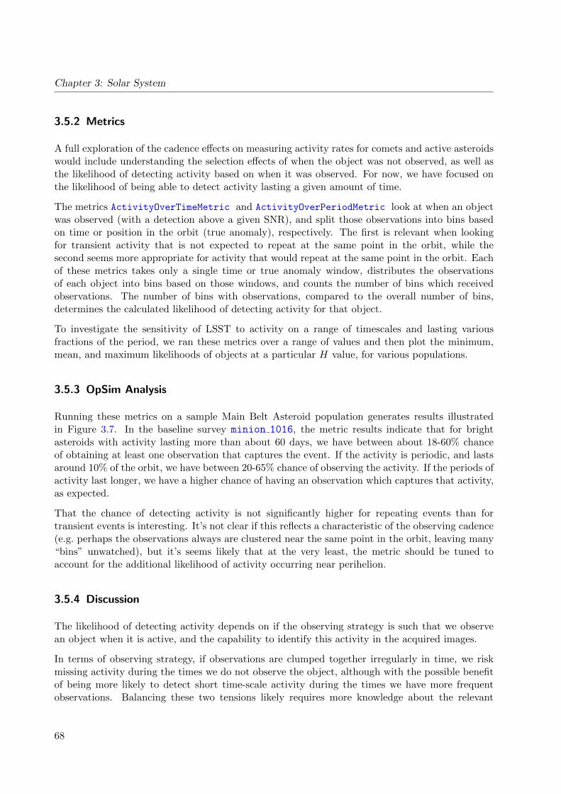
Chapter 3: Solar System

3.5.2 Metrics

A full exploration of the cadence effects on measuring activity rates for comets and active asteroidswould include understanding the selection effects of when the object was not observed, as well asthe likelihood of detecting activity based on when it was observed. For now, we have focused onthe likelihood of being able to detect activity lasting a given amount of time.

The metrics ActivityOverTimeMetric and ActivityOverPeriodMetric look at when an objectwas observed (with a detection above a given SNR), and split those observations into bins basedon time or position in the orbit (true anomaly), respectively. The first is relevant when lookingfor transient activity that is not expected to repeat at the same point in the orbit, while thesecond seems more appropriate for activity that would repeat at the same point in the orbit. Eachof these metrics takes only a single time or true anomaly window, distributes the observationsof each object into bins based on those windows, and counts the number of bins which receivedobservations. The number of bins with observations, compared to the overall number of bins,determines the calculated likelihood of detecting activity for that object.

To investigate the sensitivity of LSST to activity on a range of timescales and lasting variousfractions of the period, we ran these metrics over a range of values and then plot the minimum,mean, and maximum likelihoods of objects at a particular H value, for various populations.

3.5.3 OpSim Analysis

Running these metrics on a sample Main Belt Asteroid population generates results illustratedin Figure 3.7. In the baseline survey minion 1016, the metric results indicate that for brightasteroids with activity lasting more than about 60 days, we have between about 18-60% chanceof obtaining at least one observation that captures the event. If the activity is periodic, and lastsaround 10% of the orbit, we have between 20-65% chance of observing the activity. If the periods ofactivity last longer, we have a higher chance of having an observation which captures that activity,as expected.

That the chance of detecting activity is not significantly higher for repeating events than fortransient events is interesting. It’s not clear if this reflects a characteristic of the observing cadence(e.g. perhaps the observations always are clustered near the same point in the orbit, leaving many“bins” unwatched), but it’s seems likely that at the very least, the metric should be tuned toaccount for the additional likelihood of activity occurring near perihelion.

3.5.4 Discussion

The likelihood of detecting activity depends on if the observing strategy is such that we observean object when it is active, and the capability to identify this activity in the acquired images.

In terms of observing strategy, if observations are clumped together irregularly in time, we riskmissing activity during the times we do not observe the object, although with the possible benefitof being more likely to detect short time-scale activity during the times we have more frequentobservations. Balancing these two tensions likely requires more knowledge about the relevant

68

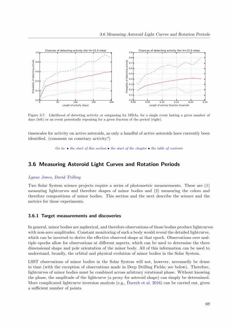
3.6 Measuring Asteroid Light Curves and Rotation Periods

0 50 100 150 200

Length of activity (days)

0.0

0.2

0.4

0.6

0.8

1.0

Pro

babili

ty o

f dete

ctin

g a

ctiv

ity

Chances of detecting activity (for H=15.0 mba)

0.00 0.05 0.10 0.15 0.20 0.25

Length of activity (fraction of period)

0.0

0.1

0.2

0.3

0.4

0.5

0.6

0.7

0.8

0.9

Pro

babilt

y o

f dete

ctin

g a

ctiv

ity

Chances of detecting activity (for H=15.0 mba)

Figure 3.7: Likelihood of detecting activity or outgassing for MBAs, for a single event lasting a given number ofdays (left) or an event potentially repeating for a given fraction of the period (right).

timescales for activity on active asteroids, as only a handful of active asteroids have currently beenidentified. (comment on cometary activity?)

Go to: • the start of this section • the start of the chapter • the table of contents

3.6 Measuring Asteroid Light Curves and Rotation Periods

Lynne Jones, David Trilling

Two Solar System science projects require a series of photometric measurements. These are (1)measuring lightcurves and therefore shapes of minor bodies and (2) measuring the colors andtherefore compositions of minor bodies. This section and the next describe the science and themetrics for these experiments.

3.6.1 Target measurements and discoveries

In general, minor bodies are aspherical, and therefore observations of those bodies produce lightcurveswith non-zero amplitudes. Constant monitoring of such a body would reveal the detailed lightcurve,which can be inverted to derive the effective observed shape at that epoch. Observations over mul-tiple epochs allow for observations at different aspects, which can be used to determine the threedimensional shape and pole orientation of the minor body. All of this information can be used tounderstand, broadly, the orbital and physical evolution of minor bodies in the Solar System.

LSST observations of minor bodies in the Solar System will not, however, necessarily be densein time (with the exception of observations made in Deep Drilling Fields; see below). Therefore,lightcurves of minor bodies must be combined across arbitrary rotational phase. Without knowingthe phase, the amplitude of the lightcurve (a proxy for asteroid shape) can simply be determined.More complicated lightcurve inversion analysis (e.g., Durech et al. 2016) can be carried out, givena sufficient number of points.

69

Chapter 3: Solar System

0 5 10 15 20 25 30

H (mag)

0.0

0.2

0.4

0.6

0.8

1.0

Fract

ion o

f obje

cts

minion_1016: Potential for lightcurve inversion

neombatno

0 5 10 15 20 25 30

H (mag)

0.0

0.2

0.4

0.6

0.8

1.0

Fract

ion o

f obje

cts

enigma_1282: Potential for lightcurve inversion

neombatno

Figure 3.8: Fraction of the sample population with the potential for lightcurve inversion, as a function of Hmagnitude for NEOs, MBAs and TNOs, for simulated surveys minion 1016 and enigma 1282.

3.6.2 Metrics

The general requirement for successful lightcurve inversion is to have a large number of observations,at high SNR, over a wide range of time. A guideline is that ∼100 measurements of an asteroidover ∼years, calibrated with a photometric accuracy of ∼5% (SNR=20) or better, is sufficientto generate a coarse shape model. This sparse data inversion gives correct results for both fast(0.2–2 h) and slow (>24 h) rotators (Durech et al. 2007).

The metric LightcurveInversionMetric simply checks to see if the observations of a particularobject meet these requirements, and if so, identifies that object as having the potential for lightcurveinversion.

3.6.3 OpSim Analysis

Most solar system objects receive many observations, and bright objects will have high SNR in mostof those observations, so it is not surprising that the baseline cadence, minion 1016, performsreasonably well with this metric. Running the same metric on other simulated surveys tends toshow similar results, although enigma 1282 demonstrates that a higher fraction of TNOs getsuitable observations for lightcurve inversion, according to this metric illustrated in Figure 3.8. Ofcourse, TNOs are unlikely to be good candidates for full lightcurve inversion due to the limitedrange of phase angles the observations cover (due to the large distance to the TNOs), and thisindicates one limitation of this simple metric. This does indicate however, that it is likely we cansignificantly increase the numbers of TNOs for which we can determine rotation periods (even ifnot full shape and spin measurements).

3.6.4 Discussion

A risk which is not captured by this simple metric is that the observations included for the lightcurveinversion estimate here could potentially occur far apart in time such that linking between the

70

3.7 Measuring Asteroid Colors

observations (to determine that they belong to the same object) is not possible.

Further work needs to be done to understand the necessary final figure of merit, in particular, howmany light curve inversion targets are necessary, and how should they be spread among differentsizes of objects? Small objects have different shape and rotation distributions than larger objects,so it is interesting scientifically to understand objects at a range of H magnitude. In addition, thismetric currently uses observations in any filter; further work should be done to determine if this issufficient, or if observations must occur in a single filter.

A final point is that asteroid lightcurves can sometimes be used to discover and characterize binaryasteroid systems. In general, sparse lightcurves, such as those that LSST will produce, are notsufficient for binary studies, but some sophisticated analysis and fortuitous observation timingcould reveal asteroid binarity.

Go to: • the start of this section • the start of the chapter • the table of contents

3.7 Measuring Asteroid Colors

Lynne Jones, David Trilling

The varying compositions of asteroids result in a range of optical colors. Sloan filters in generalare sufficiently diagnostic to discriminate among different compositional class (e.g., Parker et al.2008). Therefore, when a Solar System minor body is observed in griz (Solar System objects aregenerally quite faint in u band and many fewer will be detected), the color can be used to determinethe composition and, downstream, composition as a function of asteroid size, family membership,orbital elements, or many other parameters.

One obstacle to determining asteroid colors is that asteroid rotation periods are on the order of2–20 hours, so that after an initial measurement all further measurements (in the same filter, orother filters) are obtained at an arbitrary rotational phase. Unless the lightcurve is also known(perhaps determined from a large series of measurements in the same bandpass, such as describedin the section above), multi-band measurements must occur at closely spaced times in order tominimize the effects of the lightcurve on the measured color.

3.7.1 Target measurements and discoveries

Analysis of existing databases of TNO multi-band measurements indicate that pairs of high SNRmeasurements (SNR> 10), acquired within a short time period (< 2 hrs) can provide an accuratecolor measurement (Peixinho et al. 2015). This is roughly consistent with expectations based onthe rotation periods.

71

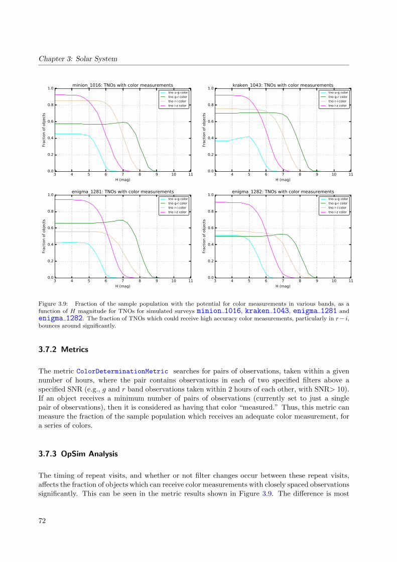
Chapter 3: Solar System

3 4 5 6 7 8 9 10 11

H (mag)

0.0

0.2

0.4

0.6

0.8

1.0

Fract

ion o

f obje

cts

minion_1016: TNOs with color measurements

tno u-g colortno g-r colortno r-i colortno i-z color

3 4 5 6 7 8 9 10 11

H (mag)

0.0

0.2

0.4

0.6

0.8

1.0

Fract

ion o

f obje

cts

kraken_1043: TNOs with color measurements

tno u-g colortno g-r colortno r-i colortno i-z color

3 4 5 6 7 8 9 10 11

H (mag)

0.0

0.2

0.4

0.6

0.8

1.0

Fract

ion o

f obje

cts

enigma_1281: TNOs with color measurements

tno u-g colortno g-r colortno r-i colortno i-z color

3 4 5 6 7 8 9 10 11

H (mag)

0.0

0.2

0.4

0.6

0.8

1.0

Fract

ion o

f obje

cts

enigma_1282: TNOs with color measurements

tno u-g colortno g-r colortno r-i colortno i-z color

Figure 3.9: Fraction of the sample population with the potential for color measurements in various bands, as afunction of H magnitude for TNOs for simulated surveys minion 1016, kraken 1043, enigma 1281 andenigma 1282. The fraction of TNOs which could receive high accuracy color measurements, particularly in r− i,bounces around significantly.

3.7.2 Metrics

The metric ColorDeterminationMetric searches for pairs of observations, taken within a givennumber of hours, where the pair contains observations in each of two specified filters above aspecified SNR (e.g., g and r band observations taken within 2 hours of each other, with SNR> 10).If an object receives a minimum number of pairs of observations (currently set to just a singlepair of observations), then it is considered as having that color “measured.” Thus, this metric canmeasure the fraction of the sample population which receives an adequate color measurement, fora series of colors.

3.7.3 OpSim Analysis

The timing of repeat visits, and whether or not filter changes occur between these repeat visits,affects the fraction of objects which can receive color measurements with closely spaced observationssignificantly. This can be seen in the metric results shown in Figure 3.9. The difference is most

72

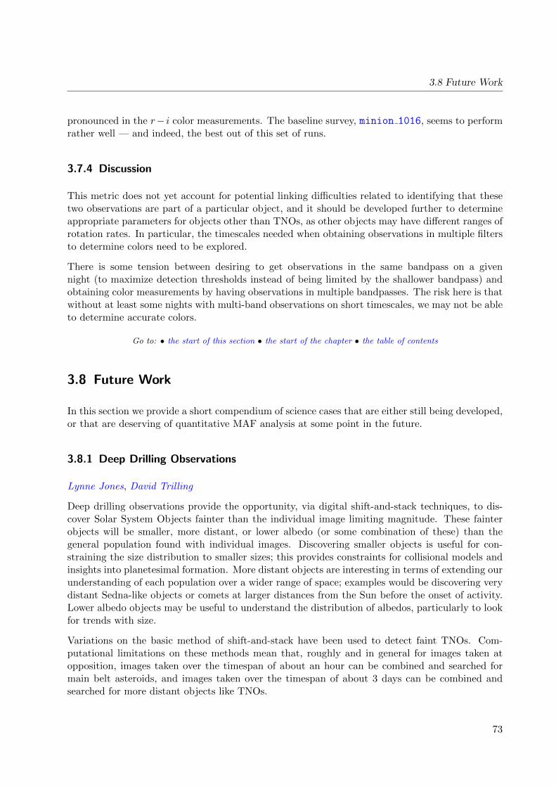
3.8 Future Work

pronounced in the r− i color measurements. The baseline survey, minion 1016, seems to performrather well — and indeed, the best out of this set of runs.

3.7.4 Discussion

This metric does not yet account for potential linking difficulties related to identifying that thesetwo observations are part of a particular object, and it should be developed further to determineappropriate parameters for objects other than TNOs, as other objects may have different ranges ofrotation rates. In particular, the timescales needed when obtaining observations in multiple filtersto determine colors need to be explored.

There is some tension between desiring to get observations in the same bandpass on a givennight (to maximize detection thresholds instead of being limited by the shallower bandpass) andobtaining color measurements by having observations in multiple bandpasses. The risk here is thatwithout at least some nights with multi-band observations on short timescales, we may not be ableto determine accurate colors.

Go to: • the start of this section • the start of the chapter • the table of contents

3.8 Future Work

In this section we provide a short compendium of science cases that are either still being developed,or that are deserving of quantitative MAF analysis at some point in the future.

3.8.1 Deep Drilling Observations

Lynne Jones, David Trilling

Deep drilling observations provide the opportunity, via digital shift-and-stack techniques, to dis-cover Solar System Objects fainter than the individual image limiting magnitude. These fainterobjects will be smaller, more distant, or lower albedo (or some combination of these) than thegeneral population found with individual images. Discovering smaller objects is useful for con-straining the size distribution to smaller sizes; this provides constraints for collisional models andinsights into planetesimal formation. More distant objects are interesting in terms of extending ourunderstanding of each population over a wider range of space; examples would be discovering verydistant Sedna-like objects or comets at larger distances from the Sun before the onset of activity.Lower albedo objects may be useful to understand the distribution of albedos, particularly to lookfor trends with size.

Variations on the basic method of shift-and-stack have been used to detect faint TNOs. Com-putational limitations on these methods mean that, roughly and in general for images taken atopposition, images taken over the timespan of about an hour can be combined and searched formain belt asteroids, and images taken over the timespan of about 3 days can be combined andsearched for more distant objects like TNOs.

73

Chapter 3: Solar System

With extragalactic deep drilling fields as in the baseline cadence, where observations are taken ina series of filters (g, r, and i would be useful for this purpose) each night, every three or four days,we could use shift-and-stack to coadd the 50 images obtained in gri bandpasses in a single night.This would allow detection of objects about 2 magnitudes fainter than in the regular survey, orapproximately r = 26.5.

The Solar System Science Collaboration developed a deep drilling proposal specifically targeted tosearch for very faint Main Belt Asteroids (MBAs), Jupiter Trojans, and TNOs. This proposal canbe summarized as follows:

• 9 fields, in a 3x3 contiguous grid block centered on a spot where Jupiter Trojans and NeptuneTrojans coincide (if possible, based on timing)

• 8 sequences of ∼ 1.5 hour r-band exposures per field, in continuous observing blocks. Eachof these blocks would have a coadded limiting magnitude of about r = 27, letting us push tosmaller sizes than possible with the general extragalactic deep drilling fields.

• These 1.5 hour blocks would be spaced apart in time

1. Two blocks acquired on two nights, 1.5 months before the fields come to opposition

2. Two blocks acquired on two nights when the fields are at opposition

3. Two blocks acquired on two nights, 1.5 months after the fields come to opposition

4. Two blocks acquired on two nights when the fields are at opposition again, one yearlater.

• The location of the fields would be adjusted slightly to account for the bulk motion of TNOsin the field, thus letting us follow the majority of these very small objects over the courseof a year, providing fairly accurate orbits. Most of the Jupiter Trojans and MBAs woulddiffuse out of the fields, however we would still have approximate sizes from the magnitudeand distance estimates provided by two nights of observations.

This proposal differs from the general extragalactic deep drilling fields in that the field selection,observing cadence, and filter choice is better suited for exploring faint Solar System Objects.More details are available in the Solar System Collaboration Deep Drilling whitepaper, https://lsstcorp.org/sites/default/files/WP/Becker-solarsystem-01.pdf.

Go to: • the start of this section • the start of the chapter • the table of contents

74

4 The Milky Way Galaxy

Chapter editors: Will Clarkson, Kathy Vivas

Contributing authors:

Chris Britt, Dana I. Casetti-Dinescu, Laura Chomiuk, Victor Debattista, John E. Gizis, Zeljko Ivezic,Michael C. Liu, Peregrine McGehee, Dave Monet, David Nidever, Colin Slater, Jay Strader, Pe-ter Yoachim

Summary

LSST should produce significant contributions to most areas of Galactic astronomy, with appropri-ate choices of observing strategy enabling a huge diversity of investigations. Galactic science casesfall roughly into two observational categories based on stellar density and/or Galactic latitude. (i)Strategy assessment for the high-density or low-latitude cases is dominated by large variation intotal time allocation for the inner Plane (where most of the Galaxy’s stars are found), since the cur-rent strategy options tend to complete their inner-Plane observations within the first ∼ 7 monthsof the survey (see Chapter 2). Any science case requiring coverage longer than a year in theseregions will not be well-served by most of the currently-run strategy simulations. Quantitatively,Figures of Merit (FoMs)1 for these science cases therefore suggest the baseline cadence to be factors∼ 6 − 60 worse than the two comparison strategies chosen that allocate more time to the innerPlane (Tables 4.6 & 4.7). While figures of merit for a number of science cases in this categoryhave been specified and are in the implementation phase (Section 4.2.2), at present it is at least asimportant that a wider range of strategies be specified and run with inner-Plane coverage spreadover the full ten-year survey time baseline. We encourage the reader to supply suggestions forsimulations meeting this need.

(ii). For science cases not restricted in latitude (including Solar Neighborhood studies), basicfigures of merit have been run for three choices of strategy (e.g. Sub-section 4.3.2). For example:while some degree of calibration is ongoing, at present roughly 12% of fields show problematicdegeneracy against differential chromatic refraction for all three strategies, impacting precisionastrometry. Effort is now needed to implement the science figures of merit in Sub-section 4.3.2that are based on these astrometry indications. Assessment of the science strategy impact on theHalo (Section 4.4) largely rests on the implementation of a robust star/galaxy separation metricinto MAF. This development is ongoing, led by one of the authors of this Chapter (CTS).

1See Section 1.2 for definition of terms, and Chapter 2 for more on the simulated observing strategies.

75

Chapter 4: The Milky Way Galaxy

4.1 Introduction

LSST Milky Way science cases cover lengthscales ranging from a few pc (such as sensitive surveys oflow-mass objects in the Solar Neighborhood), up to many tens of kpc (such as surveys for low-masssatellite galaxies of the Milky Way and their post-disruption remnant streams, and beyond this,investigations of resolved stellar populations in the Local Volume). In this chapter, we investigatea limited set of representative Galactic science cases, with the aims of demonstrating the scientifictrade-offs of different observing strategies and of motivating readers to contribute to consderationsof LSST’s observing strategy. The LSST Science Book (particularly chapters 6 and 7) and Ivezicet al. (2008, in particular Sections 2.1.4 and 4.4) present a broader treatment of both sciencequestions and science cases relevant to Galactic science.2

Concern about observations towards the inner Galactic Plane has for several years been a commontheme in feedback on LSST’s observing strategy, as the Baseline survey currently expends relativelylittle observing time per field at low Galactic latitudes (30 visits per filter, closely spaced intime). With few visits per filter and a condensed time sampling, populations found in scientificallyinteresting numbers only at low Galactic latitudes might be detected with low efficiency by LSSTunder this Baseline strategy. (An example is the probing of the mass function of moderate-separation extrasolar planets via intra-disk planetary microlensing, as argued forcefully in Gould2013).

We explore the scientific impact of shallow Plane observations by comparing Metrics and Figuresof Merit evaluated for the Baseline cadence (minion 1016), for the PanSTARRS-like strategy(minion 1020) which has essentially uniform depth at all Galactic latitudes observed, and forthe astro lsst 01 1004 strategy in which the plane is part of the Wide-Fast-Deep survey. Theevaluation of Figures of Merit generated by these three observing strategies will quantify how arange of Milky Way science cases could be substantially improved by selecting a strategy withincrease Plane coverage, without significant cost to the rest of LSST’s scientific investigations.

4.1.1 Chapter terminology and structure

To tame the diversity of science cases, we have picked representative cases and grouped themwithin broad scientific areas, devoting one Section of this chapter to each grouping of cases. Asmall number of Figures of Merit (FoMs) have been described for each case. At present, sciencecases are grouped in the following way: Section 4.2 assesses the impact of observing strategy onLSST’s ability to map some representative astrophysically important populations that are foundmostly or exclusively in the Plane. Several observational challenges for LSST find their sharpestexpression in Milky Way science, including (but not limited to) measurements of stellar parallax,absolute astrometry, and proper motions (including the tie-in to the reference frame which will beprovided by the gaia mission). For this reason, specific issues relating to precision astrometry aredeveloped in Section 4.3. Section 4.4 assesses the degree to which structures in the Milky Way’shalo can be discriminated and mapped, using tracer populations distinguished by variability and/orderived stellar parameters. Finally, Section 4.5 presents descriptions of investigations that are

2We do however provide motivating details for certain science cases in this Chapter, particularly in Section 4.2, asthose cases are not emphasized in the LSST Science Book or the relevant sections of Ivezic et al. (2008).

76

4.2 Populations in the Milky Way Disk

needed to properly determine LSST’s utility for Milky Way science, but which are as yet relativelyincompletely developed.

Summary Tables are provided that present the figure of merit for each science case within a givensection (one row per figure of merit) evaluated for each tested observing strategy (one column perstrategy). This summary information appears in Table 4.6 (the Disk), Table 4.7 (Astrometry).

Go to: • the start of this section • the start of the chapter • the table of contents

4.2 Populations in the Milky Way Disk

Will Clarkson, Jay Strader, Chris Britt, Laura Chomiuk

Many populations of great importance to Astronomy exist predominantly in or near the GalacticPlane, and yet are sufficiently sparsely-distributed (and/or faint enough) that LSST is likely tobe the only facility in the forseeable future that will be able to identify a statistically meaning-ful sample. Some (such as the novae that allow detailed study of the route to Type Ia Super-novae) offer unique laboratories to study processes of fundamental importance to astrophysics atall scales. Others (like slow-microlensing events heralding an unseen compact object population;e.g. Wyrzykowski et al. 2016) offer the only probe of important populations.

We remind the reader that variability studies can be performed in regions where stars are sub-stantially more spatially crowded than could be tolerated for aperture photometry. Microlensingstudies provide a good example, routinely using difference imaging (e.g. Alard & Lupton 1998;Kerins et al. 2010) to detect variability in highly crowded regions, with observations by facilitieswith higher spatial resolution used for follow-up characterization.

At present, minion 1016 allocates 30 exposures in all six filters to fields in the Galactic “zone ofavoidance,” typically completing these fields within the first 200 days of the survey (see Figure 4.1).This rapid completion of inner-plane observations imprints a strong signal on metrics and FoMs(see for example the right panel of Figure 2.3). In this section, we consider the scientific merit ofminion 1016 and other observing strategies to study the relative impacts of the distribution andnumber of visits on Galactic plane science.

Before proceeding further, we point out that static science should not be sacrificed completelyto variability studies. LSST’s adopted observing strategy must retain at least a minimum totaldepth in each of the u, g, r, i, z, y filters, along all sight-lines (and evaluated appropriately foreach field), in order to constrain and disentangle populations photometrically (e.g. Berry et al.2012; Ivezic et al. 2008). If there are any filters deemed unimportant to variability studies in anyfields, it will likely be the photometric confusion limit (for static science) that sets the minimumtotal integration times in those cases.

4.2.1 Target measurements and discoveries

Four Milky Way disk science cases that have complementary dependencies on observing strategy(e.g. slow intrinsic variability vs fast intrinsic variability vs no variability) are:

77

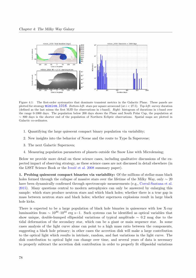
Chapter 4: The Milky Way Galaxy

Figure 4.1: The first-order systematics that dominate transient metrics in the Galactic Plane. These panels areplotted for strategy minion 1016. Bottom-left: stars per square arcsecond (at i < 27.5). Top-left: survey duration(defined as the last minus the first MJD for observations in i-band). Right: histogram of durations in i-band overthe range 0-1000 days. The population below 200 days shows the Plane and South Polar Cap, the population at∼ 800 days is the shorter end of the population of Northern Ecliptic observations. Spatial maps are plotted inGalactic co-ordinates.

1. Quantifying the large quiescent compact binary population via variability;

2. New insights into the behavior of Novae and the route to Type Ia Superovae;

3. The next Galactic Supernova;

4. Measuring population parameters of planets outside the Snow Line with Microlensing;

Below we provide more detail on these science cases, including qualitative discussions of the ex-pected impact of observing strategy, as these science cases are not discussed in detail elsewhere (inthe LSST Science Book or the Ivezic et al. 2008 summary paper).

1. Probing quiescent compact binaries via variability: Of the millions of stellar-mass blackholes formed through the collapse of massive stars over the lifetime of the Milky Way, only ∼ 20have been dynamically confirmed through spectroscopic measurements (e.g., Corral-Santana et al.2015). Many questions central to modern astrophysics can only be answered by enlarging thissample: which stars produce neutron stars and which black holes; whether there is a true gap inmass between neutron stars and black holes; whether supernova explosions result in large blackhole kicks.

There is expected to be a large population of black hole binaries in quiescence with low X-rayluminosities from ∼ 1030–1033 erg s−1. Such systems can be identified as optical variables thatshow unique, double-humped ellipsoidal variations of typical amplitude ∼ 0.2 mag due to thetidal deformation of the secondary star, which can be a giant or main sequence star. In somecases analysis of the light curve alone can point to a high mass ratio between the components,suggesting a black hole primary; in other cases the accretion disk will make a large contributionto the optical light which results in intrinsic, random, and fast variations in the light curve. Thedisk contribution to optical light can change over time, and several years of data is necessaryto properly subtract the accretion disk contribution in order to properly fit ellipsoidal variations

78

4.2 Populations in the Milky Way Disk

(Cantrell et al. 2010). The brighter sources will be amenable to spectroscopy with the currentgeneration of 4-m to 10-m telescopes to dynamically confirm new black holes; spectroscopy of allcandidates should be possible with the forthcoming generation of large telescopes. Thus, LSSTwould trigger a rich variety of observational investigations of the accretion/outflow process throughstudies of this large, dark population.

While we have focused above on black hole binaries, we note that LSST will, with suitable cadence,allow crucial measurements of the populations of neutron star and white dwarf binaries. Forexample, the total number of compact binaries is presently poorly understood—Population modelsof neutron star X-ray binaries diverge by orders of magnitude, largely due to uncertainties inthe common envelope phase of binary evolution (e.g., Pfahl et al. 2003; Kiel & Hurley 2006; vanHaaften et al. 2015). This is poorly constrained but has a large impact on, for example, LIGOevent rates. A simple test case of common envelope evolution is available in the number of dwarfnovae (DNe; accretion disk instability outbursts around white dwarfs), a population that does notsuffer from some of the complicating factors that neutron star and black hole binaries do (e.g.supernova kicks). Theoretical estimates routinely yield a significantly higher number of DNe thanare observed in the solar neighborhood. Understanding the true specific frequency of these systemsprovides a key check on common envelope evolution. LSST will detect dwarf novae, which last atleast several days with typical amplitudes of 4–6 mag, out to kpc scales. This will allow a test ofnot only the number of cataclysmic variables, but also of the 3D distribution within the Galaxyand dependence on metallicity gradients (Britt et al. 2015).

Response to observing strategy: Since most black hole candidates have been identified near the planein the inner Milky Way (68% and 92% identified within 5 and 10 of the Plane, respectively), thisscience case requires that LSST observe the plane with sufficient cadence to detect the ∼hundredsof quiescent black-hole binaries by virtue of their variability. The natural choice for a surveyfor low-luminosity black hole binaries would be to extend the Wide-Fast-Deep survey throughoutthe Plane in the direction of the inner Milky Way. The orbital period of these systems is short(typically < 1 day), so that a rolling cadence for at least parts of the Plane should be considered.For DNe, the cadence of observations is critical in obtaining an accurate measure of the populationof cataclysmic variables, as a long baseline is necessary to recover systems with a low duty cycle,while widely-spaced observations would miss short outbursts.

2. Novae and the route to Type Ia Supernovae: Only ∼ 15 novae (explosions on thesurfaces of white dwarfs) are discovered in the Milky Way each year, while observations of externalgalaxies show that the rate should be a factor of ∼ 3 higher (Shafter et al. 2014). Evidently, we aremissing 50–75% of novae due to their location in crowded, extinguished regions, where they are notbright enough to be discovered at the magnitude limits of existing transient surveys. Fundamentalfacts about novae are unknown: how much mass is ejected in typical explosions; whether whitedwarfs undergoing novae typically gain or lose mass; whether the binary companion is importantin shaping the observed properties of nova explosions. Novae can serve as scaled-down models ofsupernova explosions that can be tested in detail, e.g., in the interaction of the explosion withcircumstellar material (e.g., Chomiuk et al. 2015). Further, since accreting white dwarfs are primecandidates as progenitors of Type Ia supernovae, only detailed study of novae can reveal whetherparticular systems are increasing toward the Chandrasekhar mass as necessary in this scenario.

Response to observing strategy: Most novae occur in the Galactic Plane and Bulge, and therefore theinclusion of the Plane in a survey of sufficient cadence to find these events promptly is of paramount

79

Chapter 4: The Milky Way Galaxy

importance for this science. These events will trigger multi-wavelength follow-up ranging from theradio to X-ray and γ-rays; these data are necessary for accurate measurements of the ejected mass.

3. The First Galactic Supernova: A supernova in the Milky Way would be among the mostimportant astronomical events of our lifetime, with enormous impacts on stellar astrophysics,compact objects, nucleosynthesis, and neutrino and gravitational wave astronomy. The estimatedrate of supernovae (both core-collapse and Type Ia) in the Milky Way is about 1 per 20–25 years(Adams et al. 2013); hence there is a 40–50% chance that this would occur during the 10-yearLSST survey. If fortunate, such an event will be located relatively close to the Sun and will be aneasily observed (perhaps even naked-eye) event. However, we must be cognizant of the likelihoodthat the supernova could go off in the mid-Plane close to the Galactic Center or on the other sideof the Milky Way—both regions covered by LSST. While any core-collapse event will produce asubstantial neutrino flux, alerting us to its existence, such observations will not offer precise spatiallocalization. The models of Adams et al. (2013) indicate that LSST is the only planned facilitythat can offer an optical transient alert of nearly all Galactic supernovae.

Response to observing strategy: Even if the supernova is not too faint, LSST will likely be thesole facility with synoptic observations preceding the explosion, providing essential photometricdata leading up to the event—but only if LSST covers the Plane at a frequent cadence. Just howfrequent is open to exploration at present, but the prospect of high-sensitivity observations of thelocation of such a supernova before it takes place are clearly of enormous scientific value.

4. Population parameters of planets beyond the Snow Line with Microlensing: Gould(2013) shows that, LSST could contribute a highly valuable survey for intra-disk microlensing (inwhich disk stars are lensed by other objects in the disk, such as exoplanets, brown dwarfs, orcompact objects). The lower stellar density compared to past bulge-focused microlensing surveyswould be offset by the larger area covered by LSST. The predicted rate of high magnificationmicrolensing events that are very sensitive to planets would be ∼ 25 per year. This survey wouldbe able to detect planets at moderate distances from their host stars, a regime poorly probedby standard Doppler and transit techniques. The LSST data alone would not be sufficient: thedetection of a slow (∼ days) timescale increase in brightness of a disk star would need to triggerintensive photometric observations from small (1-m to 2-m class) telescopes that would observeat high cadence for the 1–2 months of the microlensing event. This would represent an excellentsynergy between LSST and the wider observing community, and would directly take advantage ofthe capabilities unique to LSST.

Response to observing strategy: To catch lensing events as they start to brighten, with sufficientfidelity to trigger the intensive follow-up required, the models of Gould (2013) suggest each fieldshould be observed once every few nights. With sparser coverage, the survey would lose sensitivityto microlensing events in progress. Comparison with a similar sample towards the inner MilkyWay would be highly useful, which would argue for observations of the entire visible Plane withsimilar cadence.

Microlensing is also discussed elsewhere in this document, in the context of exoplanets Sub-section 5.5.3, of the Magellanic Clouds (Chapter 7), of AGN (Section 8.4), and of WFIRST fieldstowards the Bulge (Section 11.4). Although the WFIRST discussion in Section 11.4 assumes thatBulge fields will be observed at least at low cadence (∼ 1 observation per day) for the first eight

80

4.2 Populations in the Milky Way Disk

years of the survey, this is inconsistent with the Baseline strategy that puts all the Galactic Planeobservations into the first few years of the survey.

4.2.2 Figures of Merit

Here we describe the Figures of Merit (FoMs) we currently intend to implement and evaluate forthe candidate observing strategies of interest. Where these FoM have already been evaluated, weprovide the numerical results in Table 4.6. At present, only FoM 3.1 has been implemented andrun for three surveys, with the others in development. The FoMs are:

• FoM 1.1 - Fraction of quiescent black hole binaries detectable through ellipsoidal variability;

• FoM 1.2 - Uncertainty on the duty cycle distribution of Dwarf Novae;

• FoM 2.1 - Fraction of Novae detected by LSST (specific and total);

• FoM 2.2 - Fraction of Novae caught early enough by LSST to schedule followup observations;

• FoM 3.1 - Fraction of Galactic supernovae for which LSST would detect variability before themain Supernova event;

• FoM 4.1 - Fraction of accurately-triggered Microlens candidates;

• FoM 4.2 - Uncertainty in the mass function of intra-disk microlensed planets.

With the exception of FoM 3.1 above, all these Figures of Merit are likely to be impacted by spatialconfusion, as the populations of interest tend to lie at low Galactic latitudes. Metrics for assessingthe impact of crowding have been developed (e.g. CrowdingMetrics.ipynb in sims maf contrib),and these should be incorporated into all the FoMs described here. For the present, however,we note that intrinsic source confusion is not a function of observing strategy (assuming theconfusion limit is well above the formal limiting magnitude without it). Running the FoMs withoutaccounting for source confusion isolates the impact of strategy alone on the science that can beperformed, as FoMs can be compared in a relative sense. Inclusion of crowding will later set theabsolute scale for each FoM.

In these FoMs, “uncertainty” can be taken to mean both random and systematic uncertainty,likely recorded as separate numbers for each FoM. We anticipate determining the FoMs that recordpopulation parameter-uncertainty in a Monte Carlo sense. This is particularly relevant for FoMsin which the event rate per pointing may be low (. 1 event per pointing per decade) but not solow that only 1-few events are expected over the whole sky over the lifetime of the survey (as isthe case for FoM 3.1, the First Galactic Supernova). In very rare-event cases, the FoM can scalewith the stellar density and the recovery fraction of that particular transient, and need only beevaluated once for the entire survey.

Since (at the time of writing) evaluating a Metric with relaxed SQL constraints typically takesabout 0.5-1.5 hours (on a reasonably modern laptop), we do not expect to perform Monte Carlopopulation simulations initially. In the medium-term, when Monte Carlo experiments in the targetpopulations are desired, the best strategy may be to evaluate the run of a particular metric againsta parameter of interest (apparent magnitude, say, which is also expected to lead to a turnover inthe importance of confusion error), and the investigator’s preferred Monte Carlo framework for

81

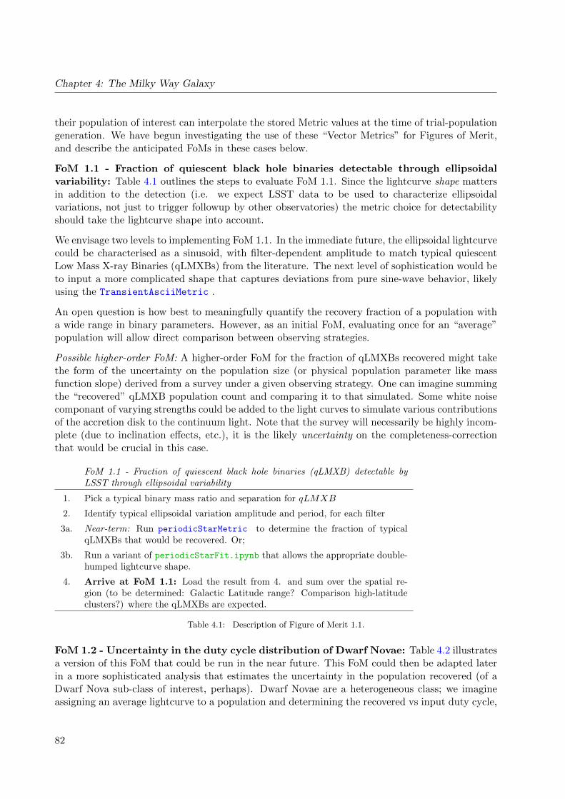
Chapter 4: The Milky Way Galaxy

their population of interest can interpolate the stored Metric values at the time of trial-populationgeneration. We have begun investigating the use of these “Vector Metrics” for Figures of Merit,and describe the anticipated FoMs in these cases below.

FoM 1.1 - Fraction of quiescent black hole binaries detectable through ellipsoidalvariability: Table 4.1 outlines the steps to evaluate FoM 1.1. Since the lightcurve shape mattersin addition to the detection (i.e. we expect LSST data to be used to characterize ellipsoidalvariations, not just to trigger followup by other observatories) the metric choice for detectabilityshould take the lightcurve shape into account.

We envisage two levels to implementing FoM 1.1. In the immediate future, the ellipsoidal lightcurvecould be characterised as a sinusoid, with filter-dependent amplitude to match typical quiescentLow Mass X-ray Binaries (qLMXBs) from the literature. The next level of sophistication would beto input a more complicated shape that captures deviations from pure sine-wave behavior, likelyusing the TransientAsciiMetric .

An open question is how best to meaningfully quantify the recovery fraction of a population witha wide range in binary parameters. However, as an initial FoM, evaluating once for an “average”population will allow direct comparison between observing strategies.

Possible higher-order FoM: A higher-order FoM for the fraction of qLMXBs recovered might takethe form of the uncertainty on the population size (or physical population parameter like massfunction slope) derived from a survey under a given observing strategy. One can imagine summingthe “recovered” qLMXB population count and comparing it to that simulated. Some white noisecomponant of varying strengths could be added to the light curves to simulate various contributionsof the accretion disk to the continuum light. Note that the survey will necessarily be highly incom-plete (due to inclination effects, etc.), it is the likely uncertainty on the completeness-correctionthat would be crucial in this case.

FoM 1.1 - Fraction of quiescent black hole binaries (qLMXB) detectable byLSST through ellipsoidal variability

1. Pick a typical binary mass ratio and separation for qLMXB

2. Identify typical ellipsoidal variation amplitude and period, for each filter

3a. Near-term: Run periodicStarMetric to determine the fraction of typicalqLMXBs that would be recovered. Or;

3b. Run a variant of periodicStarFit.ipynb that allows the appropriate double-humped lightcurve shape.

4. Arrive at FoM 1.1: Load the result from 4. and sum over the spatial re-gion (to be determined: Galactic Latitude range? Comparison high-latitudeclusters?) where the qLMXBs are expected.

Table 4.1: Description of Figure of Merit 1.1.

FoM 1.2 - Uncertainty in the duty cycle distribution of Dwarf Novae: Table 4.2 illustratesa version of this FoM that could be run in the near future. This FoM could then be adapted laterin a more sophisticated analysis that estimates the uncertainty in the population recovered (of aDwarf Nova sub-class of interest, perhaps). Dwarf Novae are a heterogeneous class; we imagineassigning an average lightcurve to a population and determining the recovered vs input duty cycle,

82

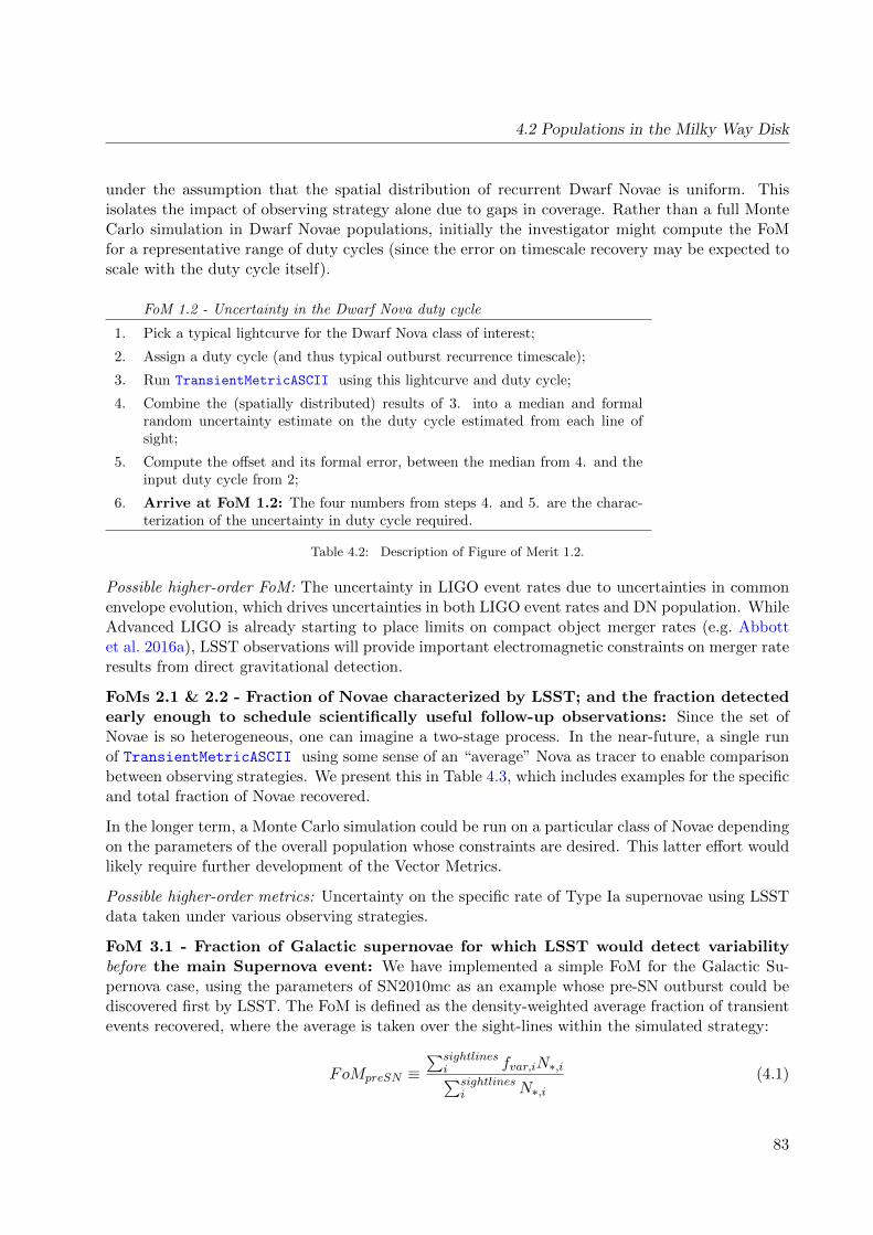
4.2 Populations in the Milky Way Disk

under the assumption that the spatial distribution of recurrent Dwarf Novae is uniform. Thisisolates the impact of observing strategy alone due to gaps in coverage. Rather than a full MonteCarlo simulation in Dwarf Novae populations, initially the investigator might compute the FoMfor a representative range of duty cycles (since the error on timescale recovery may be expected toscale with the duty cycle itself).

FoM 1.2 - Uncertainty in the Dwarf Nova duty cycle

1. Pick a typical lightcurve for the Dwarf Nova class of interest;

2. Assign a duty cycle (and thus typical outburst recurrence timescale);

3. Run TransientMetricASCII using this lightcurve and duty cycle;

4. Combine the (spatially distributed) results of 3. into a median and formalrandom uncertainty estimate on the duty cycle estimated from each line ofsight;

5. Compute the offset and its formal error, between the median from 4. and theinput duty cycle from 2;

6. Arrive at FoM 1.2: The four numbers from steps 4. and 5. are the charac-terization of the uncertainty in duty cycle required.

Table 4.2: Description of Figure of Merit 1.2.

Possible higher-order FoM: The uncertainty in LIGO event rates due to uncertainties in commonenvelope evolution, which drives uncertainties in both LIGO event rates and DN population. WhileAdvanced LIGO is already starting to place limits on compact object merger rates (e.g. Abbottet al. 2016a), LSST observations will provide important electromagnetic constraints on merger rateresults from direct gravitational detection.

FoMs 2.1 & 2.2 - Fraction of Novae characterized by LSST; and the fraction detectedearly enough to schedule scientifically useful follow-up observations: Since the set ofNovae is so heterogeneous, one can imagine a two-stage process. In the near-future, a single runof TransientMetricASCII using some sense of an “average” Nova as tracer to enable comparisonbetween observing strategies. We present this in Table 4.3, which includes examples for the specificand total fraction of Novae recovered.

In the longer term, a Monte Carlo simulation could be run on a particular class of Novae dependingon the parameters of the overall population whose constraints are desired. This latter effort wouldlikely require further development of the Vector Metrics.

Possible higher-order metrics: Uncertainty on the specific rate of Type Ia supernovae using LSSTdata taken under various observing strategies.

FoM 3.1 - Fraction of Galactic supernovae for which LSST would detect variabilitybefore the main Supernova event: We have implemented a simple FoM for the Galactic Su-pernova case, using the parameters of SN2010mc as an example whose pre-SN outburst could bediscovered first by LSST. The FoM is defined as the density-weighted average fraction of transientevents recovered, where the average is taken over the sight-lines within the simulated strategy:

FoMpreSN ≡∑sightlines

i fvar,iN∗,i∑sightlinesi N∗,i

(4.1)

83

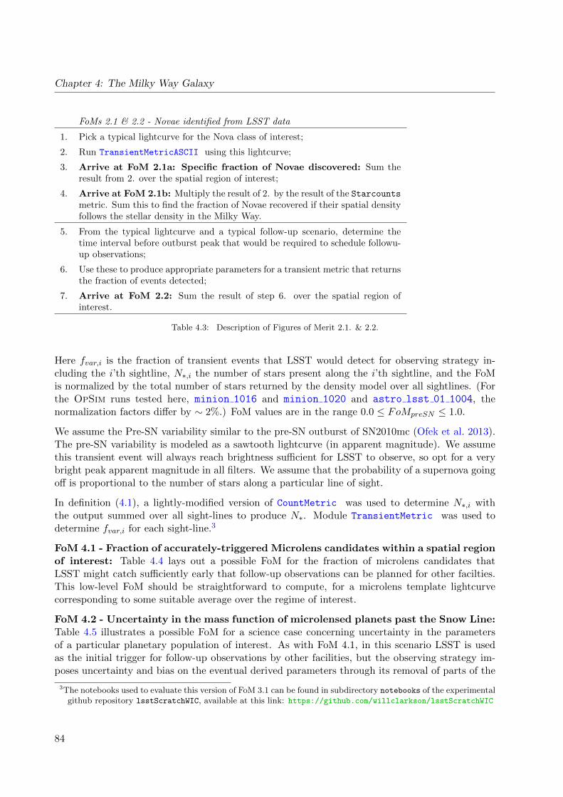
Chapter 4: The Milky Way Galaxy

FoMs 2.1 & 2.2 - Novae identified from LSST data

1. Pick a typical lightcurve for the Nova class of interest;

2. Run TransientMetricASCII using this lightcurve;

3. Arrive at FoM 2.1a: Specific fraction of Novae discovered: Sum theresult from 2. over the spatial region of interest;

4. Arrive at FoM 2.1b: Multiply the result of 2. by the result of the Starcountsmetric. Sum this to find the fraction of Novae recovered if their spatial densityfollows the stellar density in the Milky Way.

5. From the typical lightcurve and a typical follow-up scenario, determine thetime interval before outburst peak that would be required to schedule followu-up observations;

6. Use these to produce appropriate parameters for a transient metric that returnsthe fraction of events detected;

7. Arrive at FoM 2.2: Sum the result of step 6. over the spatial region ofinterest.

Table 4.3: Description of Figures of Merit 2.1. & 2.2.

Here fvar,i is the fraction of transient events that LSST would detect for observing strategy in-cluding the i’th sightline, N∗,i the number of stars present along the i’th sightline, and the FoMis normalized by the total number of stars returned by the density model over all sightlines. (Forthe OpSim runs tested here, minion 1016 and minion 1020 and astro lsst 01 1004, thenormalization factors differ by ∼ 2%.) FoM values are in the range 0.0 ≤ FoMpreSN ≤ 1.0.

We assume the Pre-SN variability similar to the pre-SN outburst of SN2010mc (Ofek et al. 2013).The pre-SN variability is modeled as a sawtooth lightcurve (in apparent magnitude). We assumethis transient event will always reach brightness sufficient for LSST to observe, so opt for a verybright peak apparent magnitude in all filters. We assume that the probability of a supernova goingoff is proportional to the number of stars along a particular line of sight.

In definition (4.1), a lightly-modified version of CountMetric was used to determine N∗,i withthe output summed over all sight-lines to produce N∗. Module TransientMetric was used todetermine fvar,i for each sight-line.3

FoM 4.1 - Fraction of accurately-triggered Microlens candidates within a spatial regionof interest: Table 4.4 lays out a possible FoM for the fraction of microlens candidates thatLSST might catch sufficiently early that follow-up observations can be planned for other facilties.This low-level FoM should be straightforward to compute, for a microlens template lightcurvecorresponding to some suitable average over the regime of interest.

FoM 4.2 - Uncertainty in the mass function of microlensed planets past the Snow Line:Table 4.5 illustrates a possible FoM for a science case concerning uncertainty in the parametersof a particular planetary population of interest. As with FoM 4.1, in this scenario LSST is usedas the initial trigger for follow-up observations by other facilities, but the observing strategy im-poses uncertainty and bias on the eventual derived parameters through its removal of parts of the

3The notebooks used to evaluate this version of FoM 3.1 can be found in subdirectory notebooks of the experimentalgithub repository lsstScratchWIC, available at this link: https://github.com/willclarkson/lsstScratchWIC

84

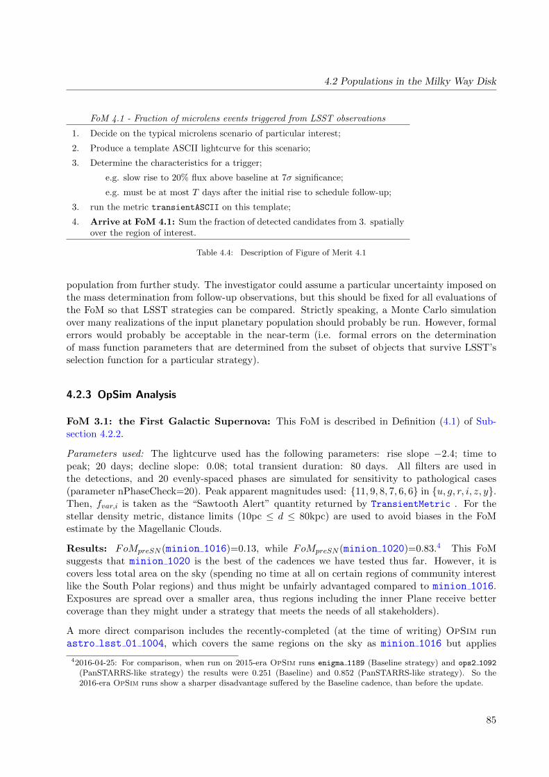
4.2 Populations in the Milky Way Disk

FoM 4.1 - Fraction of microlens events triggered from LSST observations

1. Decide on the typical microlens scenario of particular interest;

2. Produce a template ASCII lightcurve for this scenario;

3. Determine the characteristics for a trigger;

e.g. slow rise to 20% flux above baseline at 7σ significance;

e.g. must be at most T days after the initial rise to schedule follow-up;

3. run the metric transientASCII on this template;

4. Arrive at FoM 4.1: Sum the fraction of detected candidates from 3. spatiallyover the region of interest.

Table 4.4: Description of Figure of Merit 4.1

population from further study. The investigator could assume a particular uncertainty imposed onthe mass determination from follow-up observations, but this should be fixed for all evaluations ofthe FoM so that LSST strategies can be compared. Strictly speaking, a Monte Carlo simulationover many realizations of the input planetary population should probably be run. However, formalerrors would probably be acceptable in the near-term (i.e. formal errors on the determinationof mass function parameters that are determined from the subset of objects that survive LSST’sselection function for a particular strategy).

4.2.3 OpSim Analysis

FoM 3.1: the First Galactic Supernova: This FoM is described in Definition (4.1) of Sub-section 4.2.2.

Parameters used: The lightcurve used has the following parameters: rise slope −2.4; time topeak; 20 days; decline slope: 0.08; total transient duration: 80 days. All filters are used inthe detections, and 20 evenly-spaced phases are simulated for sensitivity to pathological cases(parameter nPhaseCheck=20). Peak apparent magnitudes used: 11, 9, 8, 7, 6, 6 in u, g, r, i, z, y.Then, fvar,i is taken as the “Sawtooth Alert” quantity returned by TransientMetric . For thestellar density metric, distance limits (10pc ≤ d ≤ 80kpc) are used to avoid biases in the FoMestimate by the Magellanic Clouds.

Results: FoMpreSN (minion 1016)=0.13, while FoMpreSN (minion 1020)=0.83.4 This FoMsuggests that minion 1020 is the best of the cadences we have tested thus far. However, it iscovers less total area on the sky (spending no time at all on certain regions of community interestlike the South Polar regions) and thus might be unfairly advantaged compared to minion 1016.Exposures are spread over a smaller area, thus regions including the inner Plane receive bettercoverage than they might under a strategy that meets the needs of all stakeholders).

A more direct comparison includes the recently-completed (at the time of writing) OpSim runastro lsst 01 1004, which covers the same regions on the sky as minion 1016 but applies

42016-04-25: For comparison, when run on 2015-era OpSim runs enigma 1189 (Baseline strategy) and ops2 1092

(PanSTARRS-like strategy) the results were 0.251 (Baseline) and 0.852 (PanSTARRS-like strategy). So the2016-era OpSim runs show a sharper disadvantage suffered by the Baseline cadence, than before the update.

85

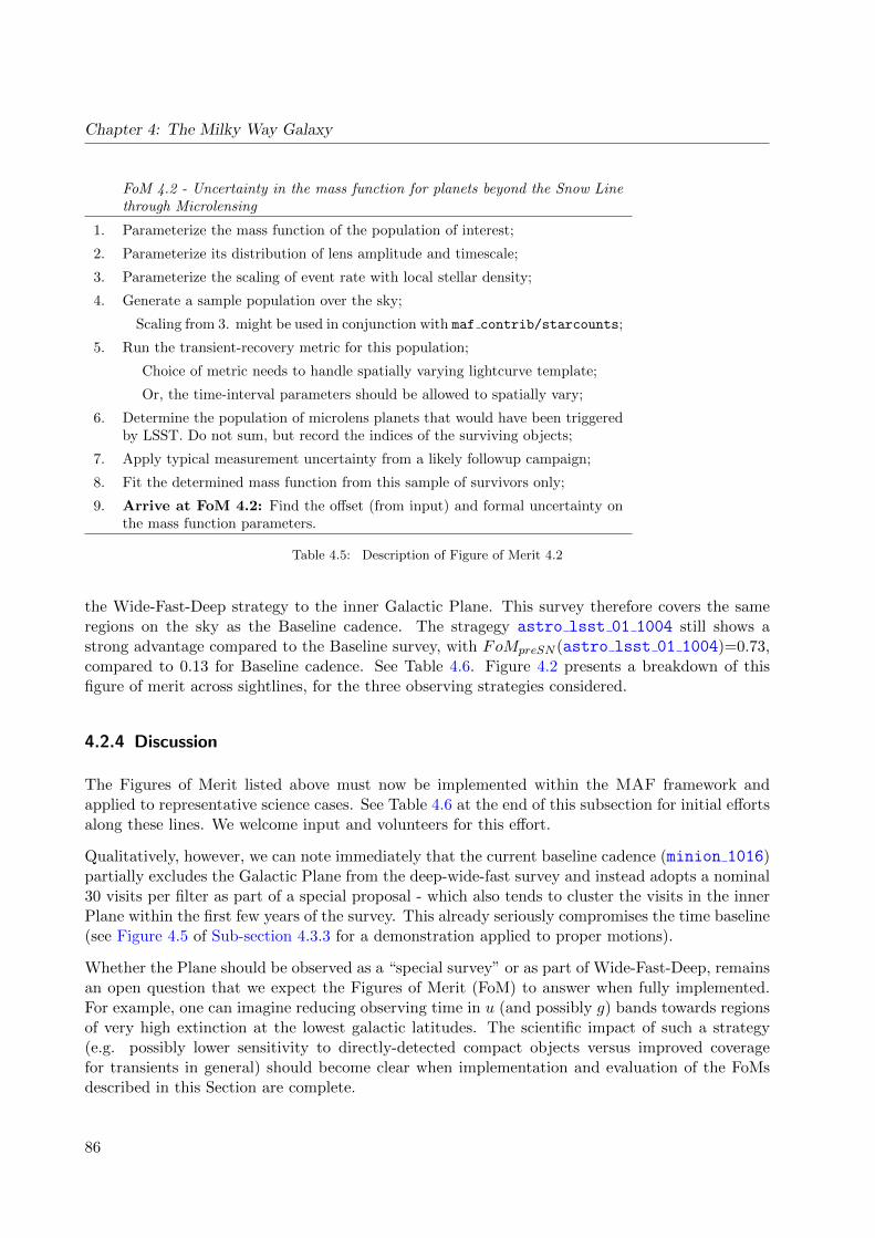
Chapter 4: The Milky Way Galaxy

FoM 4.2 - Uncertainty in the mass function for planets beyond the Snow Linethrough Microlensing

1. Parameterize the mass function of the population of interest;

2. Parameterize its distribution of lens amplitude and timescale;

3. Parameterize the scaling of event rate with local stellar density;

4. Generate a sample population over the sky;

Scaling from 3. might be used in conjunction with maf contrib/starcounts;

5. Run the transient-recovery metric for this population;

Choice of metric needs to handle spatially varying lightcurve template;

Or, the time-interval parameters should be allowed to spatially vary;

6. Determine the population of microlens planets that would have been triggeredby LSST. Do not sum, but record the indices of the surviving objects;

7. Apply typical measurement uncertainty from a likely followup campaign;

8. Fit the determined mass function from this sample of survivors only;

9. Arrive at FoM 4.2: Find the offset (from input) and formal uncertainty onthe mass function parameters.

Table 4.5: Description of Figure of Merit 4.2

the Wide-Fast-Deep strategy to the inner Galactic Plane. This survey therefore covers the sameregions on the sky as the Baseline cadence. The stragegy astro lsst 01 1004 still shows astrong advantage compared to the Baseline survey, with FoMpreSN (astro lsst 01 1004)=0.73,compared to 0.13 for Baseline cadence. See Table 4.6. Figure 4.2 presents a breakdown of thisfigure of merit across sightlines, for the three observing strategies considered.

4.2.4 Discussion

The Figures of Merit listed above must now be implemented within the MAF framework andapplied to representative science cases. See Table 4.6 at the end of this subsection for initial effortsalong these lines. We welcome input and volunteers for this effort.

Qualitatively, however, we can note immediately that the current baseline cadence (minion 1016)partially excludes the Galactic Plane from the deep-wide-fast survey and instead adopts a nominal30 visits per filter as part of a special proposal - which also tends to cluster the visits in the innerPlane within the first few years of the survey. This already seriously compromises the time baseline(see Figure 4.5 of Sub-section 4.3.3 for a demonstration applied to proper motions).

Whether the Plane should be observed as a “special survey” or as part of Wide-Fast-Deep, remainsan open question that we expect the Figures of Merit (FoM) to answer when fully implemented.For example, one can imagine reducing observing time in u (and possibly g) bands towards regionsof very high extinction at the lowest galactic latitudes. The scientific impact of such a strategy(e.g. possibly lower sensitivity to directly-detected compact objects versus improved coveragefor transients in general) should become clear when implementation and evaluation of the FoMsdescribed in this Section are complete.

86

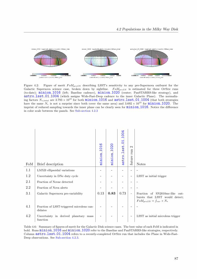
4.2 Populations in the Milky Way Disk

Figure 4.2: Figure of merit FoMpreSN describing LSST’s sensitivity to any pre-Supernova outburst for theGalactic Supernova science case, broken down by sightline. FoMpreSN is estimated for three OpSim runs(to-date); minion 1016 (left; Baseline cadence), minion 1020 (center; PanSTARRS-like strategy), andastro lsst 01 1004 (which assigns Wide-Fast-Deep cadence to the inner Galactic Plane). The normaliz-ing factors N∗,total are 3.793 × 1010 for both minion 1016 and astro lsst 01 1004 (that both strategieshave the same N∗ is not a surprise since both cover the same area) and 3.692 × 1010 for minion 1020. Theimprint of reduced sampling towards the inner plane can be clearly seen for minion 1016. Notice the differencein color scale between the panels. See Sub-section 4.2.3

FoM Brief description minion1016

minion1020

astrolsst011004

futu

reru

n2

Notes

1.1 LMXB ellipsoidal variations - - - - -

1.2 Uncertainty in DNe duty cycle - - - - LSST as initial trigger

2.1 Fraction of Novae detected - - - - -

2.2 Fraction of Nova alerts - - - - -

3.1 Galactic Supernova pre-variability 0.13 0.83 0.73 - Fraction of SN2010mc-like out-bursts that LSST would detect;FoMpreSN = fvar ×N∗

4.1 Fraction of LSST-triggered microlens can-didates

- - - - -

4.2 Uncertainty in derived planetary massfunction

- - - - LSST as initial microlens trigger

Table 4.6: Summary of figures-of-merit for the Galactic Disk science cases. The best value of each FoM is indicated inbold. Runs minion 1016 and minion 1020 refer to the Baseline and PanSTARRS-like strategies, respectively.Column astro lsst 01 1004 refers to a recently-completed OpSim run that includes the Plane in Wide-Fast-Deep observations. See Sub-section 4.2.3.

87

Chapter 4: The Milky Way Galaxy

4.2.5 Conclusions

We answer below the ten questions posed in Sub-section 1.3.2.

While the science cases developed thus far all rest on variability sensitivity in one way or another,we should point out that static science should not be sacrificed completely to variability studies.This suggests that any strategy covering the inner Milky Way must retain at least a minimumtotal depth in each of the u, g, r, i, z, y filters, along all sight-lines, in order to constrain stellareffective temperatures, metallicities, and interstellar extinction directly from LSST photometry(see for example the presentation in Ivezic et al. 2008, and associated papers). The implied figureof merit for static science is straightforward in principle - simply evaluate the photometric depthin each filter at which the confusion limit is reached at the required photometric precision - but inpractice depends on the actual set stellar populations along each line of sight. This figure of meritis likely to set the minimum acceptable exposure time in each filter in each field, and will requirea combination of modeling work and experience with existing photometric datasets.

Q1: Does the science case place any constraints on the tradeoff between the sky coverage andcoadded depth? For example, should the sky coverage be maximized (to ∼30,000 deg2, as e.g.,in Pan-STARRS) or the number of detected galaxies (the current baseline of 18,000 deg2)?

A1: Figures of Merit addressing this question have been specified in this chapter, but implementa-tion and execution are still in progress. Co-added depth is less important to this science thantemporal coverage sufficient to measure the variability (at a range of timescales) central tothe science cases in this chapter section. Qualitatively, we expect the FoMs will indicate thatthe sky coverage within the inner Disk should be maximized subject to the constraint thatall fields experience LSST coverage throughout the full ten-year survey (a condition currentlynot satisfied by the current baseline cadence, minion 1016). This is because some of theimportant transients are relatively rare, and/or the spatial distribution of the populationwithin the Milky Way disk is of scientific importance. To our knowledge, only two OpSimruns currently exist (minion 1020 and astro lsst 01 1004) which subject the popula-tions of interest in this section to coverage approaching that of Wide-Fast-Deep. A greatervariety of strategies of inner-plane coverage is needed to explore any tradeoffs between timecoverage and spatial coverage within the inner Disk. One example might be an OpSim runwith (say) 50% spatial coverage at Wide-Fast-Deep-like levels, the other 50% at coveragesimilar to the Plane mini-survey in minion 1016.

Q2: Does the science case place any constraints on the tradeoff between uniformity of sampling andfrequency of sampling? For example, a rolling cadence can provide enhanced sample ratesover a part of the survey or the entire survey for a designated time at the cost of reducedsample rate the rest of the time (while maintaining the nominal total visit counts).

A2: The frequency of sampling is critical for the science cases in this section. Requirement on theuniformity of the sampling depends on the timescale of variability and is difficult to projectwithout the FoMs being evaluated. A FoM to quantify the relative importance of each hasbeen outlined in the chapter, but its implementation and execution are still in progress. Agreater variety of observing strategy simulations that offer full-time-baseline coverage of theinner Plane are also needed on which to run the FoMs. We require suggestions for OpSim

88

4.2 Populations in the Milky Way Disk

runs with a variety of temporal distributions of exposures within the ten-year survey lifetime,towards the inner Plane.

Q3: Does the science case place any constraints on the tradeoff between the single-visit depth andthe number of visits (especially in the u-band where longer exposures would minimize theimpact of the readout noise)?

A3: This depends strongly on the line of sight, especially in u-band where reddening reduces sen-sitivity in any individual visit (thus impacting variability-searches for very blue objects). Inthose lines of sight, however, large co-added depth in u would still be useful for static pop-ulation studies. For some science cases, single-visit photometric depth provides diminishingreturns even in the redder filters (for example, once depth i & 24 were reached, going deeperwould likely not result in finding more dwarf novae, since this depth would already be suffi-cient to find such sources beyond the far side of the Bulge). However, OpSim coverage is stillrelatively sparse in the spatial regions discussed. We suggest augmenting the OpSim coveragetowards the inner Milky Way with runs with a variety of u-band depths (see for example thediscussion of strategies kraken 1059 and kraken 1045 in Chapter 2). To-date, sufficientOpSim coverage to answer questions about preferred coverage vs. filter for the inner planesimply does not exist.

Q4: Does the science case place any constraints on the Galactic plane coverage (spatial coverage,temporal sampling, visits per band)?

A4: Yes. Galactic plane coverage (in most cases, the inner Plane) is crucial to all the sciencecases in this Section, because the populations of interest are not found outside the plane insufficient numbers. In most cases, this coverage must be sufficiently spread out in time fordiscovery through variability to be possible over the entire ten-year survey.

Q5: Does the science case place any constraints on the fraction of observing time allocated to eachband?

A5: We do not have quantitative answers to this question yet since the FoMs are mostly stillunder development and await a sufficient range of OpSim runs to answer them. Qualitatively,however: LSST will likely be crucial in providing prompt color information for the rare-but-important events in the inner plane (including unusual or scientifically critical microlensingevents alerted by LSST or other facilities), so we urge nonzero coverage in all six filters.Taking the specific case of outbursts from compact objects: having two red filters (e.g. r− i)would help tremendously in breaking degeneracies between distance and luminosity since thespectrum of the outbursts discussed here is typically vega-like (so any unusual r − i colorshould be the result largely of interstellar reddening). The minimum observing time allocatedto each band is likely to be set by the requirement to retain static science goals such aspopulation dissection (see, e.g. Ivezic et al. 2008); at the present date, however, figures ofmerit for static science in the inner plane have not yet been evaluated.

Q6: Does the science case place any constraints on the cadence for deep drilling fields?

A6: The science cases in this chapter do not place any constraints on the deep-drilling fieldsalready identified. Were deep-drilling-like cadence to be possible for a few fields within theinner plane, however, it would be hugely useful. For example, to recover ellipsoidal variablesat short periods, the shortest gap in observations should be ∼20 minutes. Not all observations

89

Chapter 4: The Milky Way Galaxy

need to be so close together, but it is important to have at least a few baselines that short inorder to reliably recover periods between 80 minutes and 2 hours, where the majority of CVs(and potentially a new population of X-ray faint short period XRB outbursts) should be.These considerations also apply to any LSST observational campaign that will complementWFIRST observations of the Bulge (Section 11.4).

Q7: Assuming two visits per night, would the science case benefit if they are obtained in the sameband or not?

A7: Qualitatively, visits in two different filters are weakly preferred. Science cases requiring dis-crimination of the class of object would benefit from color information afforded by observingin different filters during the same night, and for most of the science cases in this sectionthe variation plays out in days rather than hours. However, for a subset of the science cases(e.g. ellipsoidal variations of counterparts to eRosita sources), observations at the same filterwould be preferred. If the color variation with phase is smaller than the orbital variations,then having the colors could give the best of both worlds.

Q8: Will the case science benefit from a special cadence prescription during commissioning or earlyin the survey, such as: acquiring a full 10-year count of visits for a small area (either in allthe bands or in a selected set); a greatly enhanced cadence for a small area?

A8: No, as long as all fields obtain at least some coverage in all filters throughout the full 10-yearsurvey lifetime. Our expectation is that a given field will experience nonuniform cadence overthe ten-year survey, with some intervals of high cadence followed by some intervals of lowcadence. It would be useful for some fields to experience their high-cadence intervals duringthe first year in order to better understand detectability and systematics, and to update anypopulation simulations as LSST’s performance is better constrained.

Q9: Does the science case place any constraints on the sampling of observing conditions (e.g.,seeing, dark sky, airmass), possibly as a function of band, etc.?

A9: At this stage we do not believe that any special conditions are required. The inner plane issomewhat unusual in that it will likely be confusion-limited rather than sky-limited. Thusbetter seeing would obviously be better for the science, however we do not at this stage haveany quantitative constraints.

Q10: Does the case have science drivers that would require real-time exposure time optimizationto obtain nearly constant single-visit limiting depth?

A10: Not as long as the achieved limiting depth is accurately understood once observations havebeen taken. In these confusion-limited regions, this question is probably constrained moreby the performance of the photometry software than by real-time observing considerations.

Go to: • the start of this section • the start of the chapter • the table of contents

90

4.3 Astrometry with LSST: Positions, Proper Motions, and Parallax

4.3 Astrometry with LSST: Positions, Proper Motions, and Parallax

Will Clarkson, Jay Strader, Dave Monet, Dana I. Casetti-Dinescu, John E. Gizis, Michael C. Liu,Peter Yoachim

A number of Milky Way science cases of interest to the Astronomical community will dependcritically on the astrometric accuracy LSST will deliver. While “astrometry” is not a sciencecase in the framework of this white paper, LSST’s astrometric performance will be sensitive to theparticular choice of observing strategy. Hence, the LSST Observing Strategy needs to be examinedfor systematic trends that might limit or even preclude precise measures of stellar positions, propermotions, parallaxes, and perturbations that arise from unseen companions.

Tying together the LSST and Gaia optical reference frames will be critical to many of the sciencecases discussed here (and in the LSST Science book), but the final as-delivered performance of Gaiais of course not yet known. For example, the apparent magnitude range needed for reference frametie-in is not yet constrained for crowded fields (where bright stars will likely form the essentialLSST-Gaia reference frame tracer population), but this will impact the useful LSST exposure timefor these regions, with corresponding observing strategy implications.

It will be vital for the interaction between LSST and Gaia to be studied in detail, in terms ofastrometry, photometry, spatial crowding, and instrumental issues, which will be greatly facilitatedby the second Gaia data-release (e.g. Gaia Collaboration et al. 2016). With Gaia-DR2 still in thefuture at the time of writing, here we outline some candidate astrometry science cases, and performthe relative comparison between candidate observing strategies. As we show, stark differences dueto time-sampling are already apparent, particularly for inner-Plane regions of the Milky Way.

Sub-section 4.3.1 highlights two science cases at opposite scales of distance from the Sun that re-quire accurate and precise astrometry and/or proper motion measurements. Sub-section 4.3.2presents Metrics for LSST’s astrometric performance, and discusses Figures of Merit for thetwo highlighted science cases. These metrics are applied to two example OpSim runs in Sub-section 4.3.3. Finally in Section 4.3.4, the work that is still needed is discussed, both in terms ofthe Metrics and the Figures of Merit that depend on them.

4.3.1 Target Measurements and Discoveries

1. Identification of Streams in the Galactic Halo Using Proper Motions

Much of the Milky Way’s stellar halo was built by the accretion of smaller galaxies. Given thatthese galaxies were generally of low mass, their tidal debris should still form coherent structuresin phase space, especially in the outer Galaxy where dynamical times are long. The identificationof these streams would allow a reconstruction of the accretion history of the Milky Way. Tidesalso lead to the dissolution of globular clusters, leaving notably thin streams that serve as sensitivetracers both of the Galactic potential and of the presence of dark subhalos.

A relatively small number of streams, originating from both dwarfs and globular clusters, havebeen identified via photometry of individual stars in large surveys such as SDSS. However, onlythe highest surface brightness structures can be found in this manner, and it is often difficultto trace the streams over their full extent. LSST will enable streams to be identified by stellar

91

Chapter 4: The Milky Way Galaxy

proper motions, and combined with targeted follow-up spectroscopy, will yield full 6-D positionand velocity measurements suitable for dynamical modeling. Further, it will allow the discoveryof tidal debris that is no longer spatially coherent but which can be unambiguously identified inphase space.

Finally, streams and other kinematically-distinct halo substructure can be identified and charac-terized by combining proper motions and photometry in reduced proper-motion diagrams (e.g.,Carlin et al. 2012), and by analyzing proper-motions of tracers such as RR Lyrae and giants overlarge portions of the sky (e.g., Casetti-Dinescu et al. 2015).

Response to observing strategy: Most stars in streams will be main-sequence stars, and the old mainsequence turnoff is located at r ∼ 24 at a distance of 100 kpc. The nominal LSST proper motionprecision at this magnitude is 1 mas yr−1, corresponding to about 475 km s−1 at this distance. Theproper motion measurements will be better for brighter stars, but in general ensembles of starswill be necessary for accurate measurements. To make accurate proper motion measurements forfaint stars, several key components are required. First, a zero point must be established, possiblyvia background galaxies located in each field. Next, the observations must cover a sufficient rangeof epochs to reliably detect linear proper motions.

In principle, streams can be detected using proper motions alone, as kinematically colder popula-tions than the Galactic field through which they are observed. On the assumption that intrinsicproper motion dispersion in a stream is negligible compared to the field dispersion, the faintnesslimit for proper motion-only detection of streams is set approximately by the apparent magnitudeat which LSST’s proper motion error becomes comparable to or larger than the field proper mo-tion dispersion. Based on LSST’s nominal astrometric performance (as communicated in the LSSTScience Book), this limit will be reached at r ∼ 22.5 (Casetti-Dinescu et al. 2017, forthcoming).

However, characterization of these streams requires their identification over their full lengths ofmany degrees of the sky, for which relative astrometry over small fields will not be sufficient. Overmost of the main-survey area, asbolute proper motion calibration may be achieved using the largenumber of background galaxies expected (e.g. Ivezic et al. 2008) to set the proper motion zeropoint. By using Gaia stars at the bright end as absolute proper-motion calibrators we can quantifythe precision and accuracy of background galaxies as a link to an inertial reference system, andthus improve the calibration at the faint end of the survey.

Matching LSST’s astrometry to the radio International Celestial Reference System (ICRS) - andthus calibrating LSST’s absolute astrometry - is highly likely to proceed via the Gaia opticalreference frame. Therefore, tying LSST’s position to Gaia’s final delivered reference frame will beessential. The accuracy with which this tie-in can be achieved, will likely vary spatially and needsfurther exploration.

Secondary links to the radio ICRS might proceed by matching LSST positions directly to theradio frame traced by background QSOs. These considerations should be developed by the usercommunity, and will include issues including detectable optical or radio structures that degradethe positions or suggest a displacement between the location of the sources of the radio and opticalradiation.

2. The Most Complete Sample of Stars in the Solar Neighborhood

92

4.3 Astrometry with LSST: Positions, Proper Motions, and Parallax

The direct solar neighborhood offers our only chance to get make a complete sample of stars, browndwarfs, and stellar remnants that encompass the entire formation and dynamical history of theMilky Way. While Gaia will offer parallax measurements for perhaps billions of stars, its faintmagnitude limit of G ∼ 20 will limit its measurements of the lowest-mass objects and remnantsto nearby objects, much less than the thin disk scale height of ∼ 300 pc. For example, Gaia canonly measure parallaxes for 0.2M M dwarfs to about 100 pc and 0.1M M dwarfs to only 10 pc,showing that Gaia is ill-suited for studies of the coolest dwarfs. By contrast, LSST can measureparallaxes for > 105 M dwarfs and thousands of L/T brown dwarfs (the coolest Y dwarfs are toofaint even for LSST; little contribution is likely here beyond the sample provided by WISE). Gaiawill likewise be limited to cool white dwarfs within ∼ 100 pc with which to estimate the age ofthe disk, and the thick disk and halo will be out of reach. LSST can directly compare white dwarfluminosity functions to determine precise differential ages for the thin disk, thick disk, and halo.

Response to observing strategy: Successfully completing this project will require parallax measure-ments much fainter than possible with Gaia as well as a verification that the LSST and Gaiaparallax measurements are consistent in the overlapping magnitude range.

The measurement of stellar parallax puts the substantial constraints on the observing cadence.There are two major issues: the need to sample a wide range of parallax factor (related to time ofyear), and breaking the correlation between differential color refraction and parallax factor.

“Parallax factors” characterize the ellipse of the star’s apparent motion as seen over the course ofa year. The shape of the ellipse is given by the Earth’s orbit and is not a free parameter in theastrometric solution. The amplitude of the right ascension parallax factor is close to unity whilethe amplitude of the declination parallax factor is dominated by the sine of ecliptic latitude. Theright ascension parallax factor has maximum amplitude when the star is approximately six hoursfrom the Sun, so the optimum time for parallax observing is when the star is on the meridiannear evening or morning twilight. Atmospheric refraction displaces the star’s apparent position inthe direction of the zenith by an amount dependent on both the wavelength of the light and thedistance to the zenith. Whereas the measured position of star is a function of the total refraction,the measurement of parallax and proper motion depends on the differences in the refraction asa function of the color of each star and the circumstances of the observations. This dependenceis called differential color refraction. The combination of parallax factor and differential colorrefraction leads to two rules: (i) Observations need to cover the widest possible range in parallaxfactor, and (ii) The correlation between parallax factor and hour angle in the observations needsto be minimized.

4.3.2 Metrics and Figures of Merit for LSST’s delivered astrometric accuracy

First we discuss metrics for the observing strategy that affect all of LSST’s astrometric measure-ments, then discuss figures of merit for the two science cases. (The three general metrics wereidentified years ago and are already in the suite of MAF utilities, and they should be reviewedprior to making final decisions. For this reason, in addition to the Figures of Merit later in thechapter, we present spatial maps and histograms for the metrics themselves in Section 4.3.3, forrepresentative OpSim strategies.)

93

Chapter 4: The Milky Way Galaxy

A) For each LSST field, the parallax factors at each epoch of observation need to be computed.The ensemble of these must be checked for sufficient coverage of the parallactic ellipse. Inparticular, the number of measures with RA parallax factor less than –0.5 and greater than+0.5 needs to be tallied because these carry the most weight in the solution for the amplitude(parallax).

B) For each LSST field, the correlation between hour angle and parallax factor needs to beexamined for significance. The observing strategy must minimize the number of fields withthis correlation.

C) The epochs of observation for each field must be checked for a reasonable coverage over theduration of the survey and to avoid collections of too many visits during a few short intervals.

Within MAF, metrics A (parallax factor distribution) and B (hour angle and parallax correlation)are implemented in a slightly different manner from the prescription above. We describe theimplemented metrics here.

Parallax factor coverage: This is ParallaxCoverageMetric in MAF. For each pointing, theparallax factor coverage is parameterized as the weighted mean radius of arc 〈l〉 from the center ofmotion due to parallax, scaled to the range 0 ≤ 〈l〉 ≤ 1. Inverse-variance weighting is used bothfor 〈l〉 and for the center of motion due to parallax. For each measurement, the variance usedin the weighting is the estimate of the (uncrowded) astrometric uncertainty returned by OpSimfor a star of specified fiducial magnitude r at the center of the HEALPIX of interest. Whatconstitutes a “good” value for 〈l〉 depends on the location of the star in ecliptic co-ordinates.Near either ecliptic pole a star with uniform parallax coverage would have 〈l〉 ≈ 1.0 while on theecliptic uniform coverage would produce 〈l〉 ≈ 0.5. For any location, 〈l〉 ≈ 0 would mean all theobservations were taken with identical parallax factor and therefore any attempt to fit the parallaxamplitude would be completely degenerate with the object’s position.

Parallax-Hour angle correlation: This is MAF metric ParallaxDcrDegenMetric . At the levelof tens of milliarcsec, Differential Chromatic Refraction (DCR) shifts the apparent location ofthe star in a color-dependent manner. Depending on the hour-angle distribution of observationsthroughout the year, motion due to parallax can become degenerate with motion due to the patternof DCR values sampled. This metric returns the Pearson correlation coefficient ρ between the best-fit parallax amplitude and DCR amplitude, returning values in the range −1.0 ≤ ρ ≤ +1.0. Therange of acceptable values for this metric is still under investigation; Monte Carlo simulation byone of us (DGM) suggests the parallax error becomes independent of ρ (i.e. other effects dominate)for values |ρ| . 0.7.

For the stream project discussed above, a simple to state (but perhaps complex to implement)figure of merit is the number of streams that can be discovered in LSST via their proper motions.As a first attempt, it would be reasonable to assume about 100 halo streams from old, metal-poor dwarf galaxies with stellar masses 105 − 107M distributed as r−3.5. The stream widthsand internal velocity dispersions can be set from galaxy scaling relations, and their 3-D velocitiesconsistent with a simple Galactic mass model at their radii. Setting the stream lengths is morecomplicated, but should cover a large range from a few to many kpc. Over a given area, the stream“S/N” can roughly be taken as the number of stream stars (identified via proper motion, color,and magnitude) divided by the square root of the number of field stars. For globular clusters, asimilar number of streams could be included, but these should have much smaller widths (10s of

94

4.3 Astrometry with LSST: Positions, Proper Motions, and Parallax

pc) and typical masses 104 − 105M. Eventually it would be desirable to use actual simulatedstream parameters taken from cosmological models of the Milky Way (e.g., from the Aquariussimulation).

Solar neighborhood projects will be sensitive to the general parallax and proper motion metricsdiscussed above. More specific science figures of merit are required at this stage. For example, theprecision of the differential age measurement between the thin disk and halo, which would dependon the number of white dwarfs that can be isolated from each population.

4.3.3 OpSim Analysis

Here we present initial analysis of LSST’s astrometric performance. Two example strategies areassessed: the current baseline strategy, minion 1016, and the more recently-evaluated cadenceastro lsst 01 1004, which extends the Wide-Fast-Deep survey to the Galactic Plane (see Sec-tion Section 2.4 for more detail on this run).

Metrics: Parallax and proper motion precision

Here we present the expected astrometric performance of LSST as a function of location on-sky,for two main cuts on the survey strategies:

• By time: objects detected in g, r, i, z, after years 1, 2 and 10 of the survey (Figures 4.3 -4.6);

• By filter: objects detected in g, r, i, z, or in u only, or y only, over the full 10 years of thesurvey (Figures 4.7 - 4.10).

Astrometric performance for parallax is quantified using the following metrics:

1. Parallax factor coverage (following metric A of Sub-section 4.3.2); values farther from 0 arebetter). See Figures 4.3 & 4.7;

2. Parallax-Hour angle correlation (metric B of Sub-section 4.3.2; values closer to 0 are better).See Figures 4.4 & 4.8;

3. Proper motion error, for a star at apparent magnitude 21.0 in the filter specified (thisaddresses the distribution of measurement epochs, as recommended in Metric C in Sub-section 4.3.2; smaller values are better). See Figures 4.5 & 4.9;

4. Parallax error, for a star at apparent magnitude 21.0 in the filter specified (smaller valuesare better). See Figures 4.6 & 4.10.

Limitations of the results presented in Figures 4.3 to 4.10.:

i. The spatial maps are clipped at 95% in order to keep the color-scale at a sensible range;in some cases this has had the side effect of removing parts of the spatial coverage in theminion 1016 maps.

95

Chapter 4: The Milky Way Galaxy

ii. This analysis neglected spatial confusion in high-density regions. While this confusion wouldbe the same whatever observing strategy was chosen, the measurement uncertainties forproper motion and parallax uncertainty should be regarded as lower limits.

iii. The choice of fiducial apparent magnitude r = u = y = 21.0 is arbitrary. It would beinformative to repeat the analysis for a range of target apparent magnitudes that are better-matched to the specific science cases.

iv. The comparison between single-filter and griz detections likely overestimates the measure-ment precision for the u-only and y-only detections, as an object only detected in a singlefilter may well not be detected in all images taken in that filter. While the comparison be-tween filter subsets for a given strategy may therefore be highly approximate, the comparisonbetween strategies for the same filter should be more reliable.

Indications at this date: Despite these limitations, we note the following:

I1. To first order, proper motion and parallax error are dominated by the total time coverage,as might be expected. For some of the mini-survey regions, particularly (but not limitedto) the inner-Plane, the baseline strategy minion 1016 is dramatically worse for astrometrythan the two alternative candidate strategies tested here. When the tendency of OpSim tocluster mini-surveys within the first year is corrected, detailed comparison of strategies canproceed given the full spread of observing epochs.

I2. Taking snapshots of the survey at various stages of completion (Figures 4.3 - 4.6), strategyastro lsst 01 1004 is not significantly worse than the current baseline strategy minion 1016;

I3. For the extremes of object color (objects detected only in the bluest or only in the reddestfilter), most of the astrometry metrics suggest worse performance with additional structure inthe spatial variation of astrometric performance (see Figures 4.7 - 4.10), compared to objectsdetected in all filters. Further exploration is strongly suggested.

I4. The two strategies offering enhanced inner-Plane coverage, astro lsst 01 1004 and minion 1020,do not meaningfully differ from each other purely in terms of delivered astrometric precision.5

Figures of Merit depending on the Metrics

Building on the first-order metrics above, this subsection communicates scientific figures of meritfor the cases identified in Sub-section 4.3.1 above.

Table 4.7 summarizes the Figures of Merit (FoMs) for Astrometry science cases. At the time ofwriting, FoMs have been implemented to summarize the random uncertainty in proper motionand parallax, for two regions experiencing extreme values of these quantities: the inner Plane(conservatively defined in this section as |b| . 7o and |l| . 80o), and the main survey (excludingthe inner plane and the Southern Polar region, taken here as δ2000.0 < −60.0o). Figure 4.11illustrates these selection-regions on the sky. These form FoM 1.1-1.4, and have to-date been runfor the OpSim runs minion 1016 (Baseline cadence), minion 1020 (similar to PanSTARRS-1),

5However, the absence of the Northern Ecliptic Spur from minion 1020 makes it unlikely that this candidatestrategy will score highly for Solar System studies.

96

4.3 Astrometry with LSST: Positions, Proper Motions, and Parallax

and the recently-completed astro lsst 01 1004 (which applies Wide-Fast-Deep cadence to muchof the inner Galactic Plane).

From the point of view of parallax and proper motion, the latter two strategies do not negativelyimpact the non-plane regions, but they substantially improve the sampling for proper motions andparallax (again, neglecting the effects of spatial crowding).

FoM 1.5 in Table 4.7 reports the total number of fields with Parallax/Hour-angle correlation|ρ| < 0.7.

At the time of writing, FoMs 2-5 in Table 4.7 are still at the specification stage, and are describedin Section 4.3.4.

4.3.4 Topics that will need to be addressed

Here we present suggestions for further work, first on figures of merit for the science cases, andthen on additional Metrics for LSST’s astrometric performance.

Further work on science Figures of Merit

At the time of writing, the Figures of Merit for both the highlighted Science cases need to beimplemented and applied to OpSim output, preferably in a format that can be summarized in asingle Table in this section. These figures of merit are discussed above in Section 4.3.2 (particularlyfor the Halo Streams science project). Figures of merit for the two science cases might be:

1. Number of streams that LSST can discover via their proper motions;

2. Uncertainty and bias in the thin and thick disk differential age measurement when usingwhite dwarfs from each population as tracers.

Given the diversity of science cases that use local Solar Neighborhood populations as tracers, itmay be advantageous to subdivide the Solar Neighborhood projects into further figures of merit.Two further example figures of merit might then be:

3. Uncertainty and bias in the Brown Dwarf mass function using Solar Neighborhood tracers;

4. Uncertainty and bias in the thickness in the main sequence of M-dwarfs within 25pc fromthe Sun, once variability has been characterized and removed.

Further work on Astrometry Metrics

The MAF metrics presented in Sections 4.3.3 and 4.3.2 are only part of the study of LSST’spredicted astrometric performance. Detailed simulations and studies need to be done in manyother areas as part of the prediction and verification of LSST’s astrometric performance. Amongthe most important are the following.

97

Chapter 4: The Milky Way Galaxy

FoM Brief description minion1016

minion1020

astrolsst011004

futu

reru

n2

Notes

1.1 Median parallax error at r = 21(main survey)

0.69 0.72 0.69 - See region definitions inFigure 4.11.

1.2. Median parallax error at r = 21(plane)

2.68 0.91 0.89 - Smaller values are bet-ter.

1.3. Median proper motion error atr = 21 (main survey)

0.19 0.19 0.19 -

1.4. Median proper motion error atr = 21 (plane)

16.7 0.26 0.25 -

1.5. Fields with Parallax-DCR corre-lation coefficient ρ ≥ 0.7 / totalfields

3486 /31116

3586 /30107

3690 /31116

- Smaller is better. Valuereported after full 10years of survey forgriz detections.

2.1. Number of streams LSST can dis-cover via proper motions

- - - - -

3.1. Uncertainty and bias in thin- andthick-disk differential age mea-surement via white dwarfs

- - - - -

4.1. Uncertainty and bias in browndwarf mass function from the So-lar Neighborhood

- - - - Using astrometry met-rics for objects detectedonly in the reddest fil-ter(s)

4.2. Uncertainty and bias in whitedwarf mass function from the So-lar Neighborhood

- - - - Using astrometry met-rics for objects detectedonly in the bluest fil-ter(s)

5.1. Uncertainty and bias in SolarNeighborhood M-dwarf thicknesson the MS

- - - - -

Table 4.7: Summary of Figures of Merit for the Milky Way Astrometry science cases. The best value of each FoM isindicated in bold. Runs minion 1016 and minion 1020 refer to the Baseline and PanSTARRS-like strategies,respectively. Column astro lsst 01 1004 refers to a recently-completed OpSim run that includes the Planein Wide-Fast-Deep observations. See Section 4.3.

98

4.3 Astrometry with LSST: Positions, Proper Motions, and Parallax

• How well do galaxies perform as astrometric reference objects? Are certain shapes or colorsbetter than others? What is the surface density of “good” astrometric reference galaxies asa function of filter?

• How does the astrometric performance depend on stellar density? If there are fields in whichphotometry is only possible via difference imaging, what are the limitations on astrometryin these fields?

• Does the “brighter-wider” effect in the deep-depletion CCDs introduce a magnitude terminto the centroid positions?

• Deep-driling fields will likely be essential to fully understand LSST’s astrometric behaviorover the entire survey. How should Deep-Drilling fields be specified to fully characterizeLSST’s delivered astrometric performance?

4.3.5 Conclusions

Here we answer the ten questions posed in Sub-section 1.3.2:

Q1: Does the science case place any constraints on the tradeoff between the sky coverage andcoadded depth? For example, should the sky coverage be maximized (to ∼30,000 deg2, as e.g.,in Pan-STARRS) or the number of detected galaxies (the current baseline of 18,000 deg2)?

A1: We do expect tradeoffs between depth and sky coverage, but we do not yet have the FoMevaluations to set quantitative constraints. For example, we expect some combination ofdepth and survey volume would optimize the completeness to objects among the populationsin the Solar Neighborhood. More generally, perhaps, in fields away from the galactic mid-plane, the lengthscales over which the proper motion zeropoints can be accurately constrainedwill depend on the spatial density of well-measured background galaxies (finer lengthscalecorresponding to greater co-added depth). The depth must therefore be sufficient to sampleenough of these galaxies to constrain variations of astrometric zeropoint on lengthscales atleast as fine as those imposed by the LSST system itself (or the atmosphere, whicheveris finer). We anticipate that this tradeoff can be informed by simulation under a set ofassumptions for these variations.

Q2: Does the science case place any constraints on the tradeoff between uniformity of sampling andfrequency of sampling? For example, a rolling cadence can provide enhanced sample ratesover a part of the survey or the entire survey for a designated time at the cost of reducedsample rate the rest of the time (while maintaining the nominal total visit counts).

A2: Yes, although for astrometry the language of these constraints is slightly different. The par-allactic ellipse must be sufficiently covered, the correlation between hour angle and parallaxfactor must be minimized, and the visits must be sufficiently distributed (both within a yearand over the ten-year time baseline) to produce the best precision in both proper motion andparallax. See Section 4.3.2.

Q3: Does the science case place any constraints on the tradeoff between the single-visit depth andthe number of visits (especially in the u-band where longer exposures would minimize theimpact of the readout noise)?

99

Chapter 4: The Milky Way Galaxy

A3: More visits at the standard exposure time are generally preferred to a few visits with longerexposures, in order to achieve as broad a temporal coverage as possible (see Section 4.3.2).The u-band itself is likely to be of limited use for astrometry (except possibly for extremelyblue objects with little signal in any of the other filters) due to differential chromatic refraction(DCR), however of course u-band will still be useful for photometric constraints.

Q4: Does the science case place any constraints on the Galactic plane coverage (spatial coverage,temporal sampling, visits per band)?

A4: Not for the example of detecting Galactic Halo streams via proper motions (Section 4.3.1). Forthe Solar Neighborhood populations, avoiding the inner Galactic mid-plane would obviouslyreduce the completeness of the census of nearby objects with parallax determinations dueto the reduction in total area surveyed. However, this reduction may be incremental ratherthan serious. The impact of an inner-plane zone of avoidance on the recovery of the param-eters describing these constituent populations has not yet been evaluated. Of course, thisall changes for astrometry of objects of interest that lie in the inner plane (see also Section4.2), where (for example) the reduced proper motion will be a useful diagnostic. At present,however, the performance of the LSST software stack towards crowded fields is as-yet un-known - as is the performance of Gaia in these regions. As this performance becomes betterunderstood, it will be possible to quantitatively compare strategies for astrometry towardsthe inner plane.

Q5: Does the science case place any constraints on the fraction of observing time allocated to eachband?

A5: Yes, but indirectly through the requirement to measure all the populations of interest inthe Solar Neighborhood. Making the assumption that this science case requires parallaxmeasurements for extremely blue objects as well as extremely red objects, which might eachbe measurable only in a single very red or blue filter, would suggest at a minimum thatthe coverage considerations of Section 4.3.2 be applied to observations in u and Y filtersseparately, as well as at least one mid-range filter. However the quantitative impact onpopulation recovery from various filter-distributions has yet to be assessed at this date.Further work is needed to determine if the increased sensitivity of u-band astrometry toDCR relative to g-band would prevent its use for astrometry.

Q6: Does the science case place any constraints on the cadence for deep drilling fields?

A6: The deep-drilling fields will provide essential characterization of LSST’s delivered astrometricperformance, providing at least a sanity check on the characterization of astrometric accuracyfor all observed fields. The observational design of the deep-drilling fields needs to be carefullyconsidered in terms of their utility for calibrating the non-deep-drilling fields, as well as interms of maximizing the astrometric precision of the deep-drilling fields in their own right(for which the considerations of Section 4.3.2 will apply).

Q7: Assuming two visits per night, would the science case benefit if they are obtained in the sameband or not?

A7: While detailed investigation is still pending, we expect that using different filters within thesame night would be preferred to allow better constraint of DCR effects. Doing different

100

4.4 Mapping the Milky Way Halo

filters on the same night might reduce the number of free parameters (like seeing and parallaxfactor) and give more pairs for direct filter-A vs. filter-B astrometry.

Q8: Will the case science benefit from a special cadence prescription during commissioning or earlyin the survey, such as: acquiring a full 10-year count of visits for a small area (either in allthe bands or in a selected set); a greatly enhanced cadence for a small area?

A8: It is vital for astrometry that at least a few fields be observed with both sufficient parallaxfactor coverage and sufficient number of visits, early in the survey, to demonstrate parallaxprecision specified in the Science Requirements Document. In these fields, sufficient exposuresmust be reserved for the entire 10-year survey baseline so that proper motion precision is nottoo badly compromised in these fields. This combination of factors may require dedicatedcommissioning observations of these fields in addition to the 10-year survey operations. Inaddition, however, at least a few fields must be observed at a variety of values of single-visitachieved depth, and FWHM, in order to constrain the degree to which FWHM will actuallypredict the achieved astrometric precision (see also the answer to Q10 below). This secondset of requirements may also be best served by dedicated commissioning observations.

Q9: Does the science case place any constraints on the sampling of observing conditions (e.g.,seeing, dark sky, airmass), possibly as a function of band, etc.?

A9: The observations need to be planned in such a way that the correlation between parallaxand hour-angle is minimized, to avoid deneracies between the motion due to atmosphericrefraction and the motion that is sought due to parallax. See Section 4.3.2.

Q10: Does the case have science drivers that would require real-time exposure time optimizationto obtain nearly constant single-visit limiting depth?

A10: While optimization on an exposure-to-exposure basis is perhaps unlikely, selection betweenobservations in response to conditions (on a timescale of perhaps 10 minutes) will be crucialto maximize achieved astrometric precision. The rules by which this selection would proceed,still need to be charted. For example, while maintaining limiting depth might suggest shorterexposure times when the FWHM is narrow, this may not translate to improved astrometricerror across an LSST chip, because the lengthscales of the turbulence driving the FWHM isnot the same as that of the turbulence driving astrometric error across an LSST chip.

Go to: • the start of this section • the start of the chapter • the table of contents

4.4 Mapping the Milky Way Halo

Kathy Vivas, Colin Slater, David Nidever

The study of the halo of the Milky Way is of the highest importance, not only to understand theformation and early evolution of our own galaxy, but also to test current models of hierarchicalgalaxy formation. LSST will provide an unprecedented combination of area, depth, wavelengthrange and long time-baseline for imaging data, allowing detailed studies of the present-day structureof this old Galactic component. Here we focus our attention on halo investigations using three tracerpopulations. While we anticipate more cases will be developed and compared between strategy

101

Chapter 4: The Milky Way Galaxy

choices, we have selected populations here that illustrate many of the most important challenges.We describe the figures of merit (and the diagnostic metrics on which they depend) that will allowquantitative assessment of the impact of the choice of observing strategy on the constraints LSSTwill afford. We first briefly discuss the use of three main population tracers to chart the halopopulation. More detail on each of these tracer populations, and the general scientific motivationsfor studies of the Milky Way halo with LSST, can be found in LSST Science Collaboration et al.(2009).

1. RR Lyrae stars have been known for several decades as excellent tracers of the halo population.They are not only old stars (> 10 Gyrs) but they are also excellent standard candles that allowconstruction of three-dimensional maps. RR Lyrae stars have been used to survey Milky Way halopopulations extending out to ∼ 60 − 80 kpc from the Galactic center (Drake et al. 2013b,a; Zinnet al. 2014; Torrealba et al. 2015, among others). Beyond ∼ 80 kpc, the halo is mostly unchartedterritory.

The RR Lyrae surveys suggest the halo is filled with substructures (clumps of elevated stellardensity) which are usually interpreted as debris from destroyed satellite galaxies. This substructureoverlies a smooth component in the distribution of RR Lyrae stars, whose number density is well-described by a power law in galactocentric distance, steepening at radii & 30 kpc (Zinn et al. 2014).Thus, beyond ∼ 60 kpc, few field RR Lyrae stars are expected. However, we presume that any RRLyrae star beyond this distance may be part of either debris material or distant low-luminositysatellite galaxies that have been escaped detection until now (Sesar et al. 2014; Baker & Willman2015). LCDM models predict debris as far as 0.5 Mpc from the galactic center. This is the territorythat will be explored by LSST.

2. Red giant stars can similarly be used to trace the structure of the halo up to large distances.They have the advantage of being bright and are numerous compared to the RR Lyrae stars butnot as good distance indicators.

3. Main sequence stars, although less luminous than RR Lyraes or Red Giants, are so much morenumerous that statistical studies can be pursued in a manner not generally possible for thosepopulations. Using the technique of photometric metallicities (Ivezic et al. 2008), the Sloan DigitalSky Survey (SDSS) provided unprecedented maps of the metallicity distribution up to ∼ 10 kpcfrom the Galactic center, unveiling not only the mean metallicity distribution of the halo but also,sub-structures within the halo. LSST will extend these studies all the way to the outermost partsof the Galaxy.

4.4.1 Target measurements and discoveries

Accurate measurement of these three tracer populations implies the following requirements:

1. RR Lyrae stars: These are bright horizontal-branch variable stars with periods between0.2 to 1.0 days and large amplitudes, particularly in the bluer bandpasses (g amplitudes0.5−1.5 mag). Oluseyi et al. (2012) made an intensive search for RR Lyrae stars in simulatedLSST data and reached to the conclusion that this type of stars can be recovered to distances∼ 600 kpc. A similar procedure can now be performed using MAF to directly compare LSSTcadence scenarios to each other. Chapter 5 discusses the discovery metrics for variable stars

102

4.4 Mapping the Milky Way Halo

including RR Lyrae stars. However, optimal recovery may involve more complex metricsinvolving the simultaneous use of multi-band time series (VanderPlas & Ivezic 2015; Vivaset al. 2016). Besides recovery of variable stars, red-wavelength mean magnitudes z and y areparticularly valuable since they provide the most accurate distance indicators. (Caceres &Catelan 2008).

2. Main sequence stars: lacking any distinguishable variability, the challenge in selecting a largeand clean sample of main sequence stars comes from tremendous number of small and nearly-unresolved galaxies present at faint magnitudes. Precise star/galaxy separation is thus thelimiting factor on the useful depth of the main sequence sample. In addition to identifyingdwarfs, using dwarfs to map the metallicity distribution of the halo requires precise u-banddata, since it exhibits the strongest metallicity dependence of the LSST filters.

3. Red Giants: due to their intrinsic luminosity, the Red Giants will sample a far larger volumethan main sequence stars at similar apparent magnitudes. However, they must first be identi-fied and separated from the very numerous main sequence stars present in the foreground. Agravity-sensitive photometric index can be used for separating efficiently giants from dwarfs.The u-band magnitude is essential for such an index, so the behavior of the u-band limit-ing magnitude must therefore be charted under the various observational strategies underconsideration. Figure 4.12 shows the distance that can be reached by M-giants of differentmetallicities assuming limiting magnitude u = 26.0.

4.4.2 Metrics

Star-Galaxy Separation: For main sequence stars, the useful depth of the survey will likelynot be the photometric detection limit, but will instead be set by the ability to differentiate starsfrom unresolved background galaxies. Towards faint magnitudes the contamination by galaxiesworsens significantly for several reasons: the number of galaxies is rising substantially, the angularsize of galaxies is shrinking, and our ability to distinguish stars from marginally resolved galaxiesdiminishes for faint sources simply due to photon statistics. While the fundamental properties ofthe contaminant sources are beyond our control, our ability to reject these sources depends onsurvey parameters which do vary with the choice of observing strategy, such as the distribution ofseeing across visits and the depth of these visits.

We are currently in the process of developing a metric that will estimate our ability to separate starsand galaxies for any observation depth and seeing conditions. This requires both an understandingof how images of a source are measured and classified as either a star or galaxy, and how thepopulation of stars and galaxies vary in number and size (for galaxies) with depth. Our modeluses the distribution of galaxies in size and number, derived from HST COSMOS observations,along with a fully Bayesian model decision formalism to compute the expected completeness andcontamination in star-galaxy separation. Computationally, for each position in the survey footprintwe interpolate the results from that work on a grid in seeing, galaxy size, and coadd depth, thenintegrate over the distribution of galaxy sizes. This modeling process is currently being verifiedagainst existing surveys, and will be incorporated into the observing strategy study at a later date.

Some of the higher-level figures of merit described below will depend on this star/galaxy separationdiagnostic metric.

103

Chapter 4: The Milky Way Galaxy

Distance to the farthest RR Lyrae stars: This metric charts our ability to recover an RRLyrae star from LSST data as a function of its distance. An RR Lyrae star may be consideredas recovered if its period and amplitude are within 10% of the intrinsic values. The procedurefollowed by Oluseyi et al. (2012) is a good example on how this can be achieved. They built a largenumber of synthetic light curves spanning the properties of known RR Lyrae stars and “observed”them with the cadence given by the OpSim runs available at that time. Anticipated improvementsover this previous work include the use of simultaneous multi-band information to recover periods(e.g., VanderPlas & Ivezic 2015; Vivas et al. 2016).

However, a first look into this problem using MAF can be achieved by simplifying the procedureand only test if a star with period 0.55 days (the mean period for RR Lyrae stars) can be recoveredby metrics already available in MAF. Then, distance can be calculated using the mean magnitudeof the recovered RR Lyrae stars (in the reddest bands available to LSST) and the interstellarextinction at that point of the sky (maps are available now in MAF). This metric should computethe largest distance that can be measured with a 10% precision at which certain percentage of RRLyrae stars (eg. 80%) can be recovered by LSST. It is expected that the results of this metricat low galactic latitudes will be largely dependent on the chosen observational strategy (throughvariations in cadence towards the Plane).

A reasonable Figure of Merit for this sub-project is the volume of the halo within RR Lyrae starscan be recovered. Similarly, another Figure of Merit would be the fraction of the Galactic thickdisk’s volume that can be traced by RR Lyrae stars.

Distance to the farthest main sequence stars and giant stars: Since variability is not thesignal property for these tracer populations, metrics are somewhat simpler than for the RR Lyrae.Here the distance metric requires the determination of the limiting u-band magnitude for whichgalaxy/star separation is reliable to a certain level. In these cases, distances depend on metallicity.Then, a figure of merit is the volume of the halo mapped with stars within a specified metallicityrange.

WFIRST Synergy: The extended optical-IR baseline that will be provided by WFIRST (Spergelet al. 2015) in ∼ 2, 000 sq degrees of the sky at high galactic latitudes will provide additional waysto improve both the star-galaxy separation (e.g. Banerji et al. 2015) and the disentangling of stellartracers in the halo of the Milky Way (e.g. Dalcanton et al. 2012). Chapter 11 discusses some areasof interaction between both surveys. Metrics related to stellar populations in the halo using theoverlap between both surveys are still to be developed.

4.4.3 Conclusions

Here we answer the ten questions posed in Sub-section 1.3.2:

Q1: Does the science case place any constraints on the tradeoff between the sky coverage andcoadded depth? For example, should the sky coverage be maximized (to ∼30,000 deg2, as e.g.,in Pan-STARRS) or the number of detected galaxies (the current baseline of 18,000 deg2)?

A1: Yes - depth is generally preferred over increased sky-coverage. Fields with insufficient depthfor star-galaxy separation to the required level of reliability will not be useful for the science

104

4.4 Mapping the Milky Way Halo

in this section. While we expect this will lead to preference of achieving minimum depth vsexpanding the sky-coverage, at this date we do not yet have quantitative limits.

Q2: Does the science case place any constraints on the tradeoff between uniformity of sampling andfrequency of sampling? For example, a rolling cadence can provide enhanced sample ratesover a part of the survey or the entire survey for a designated time at the cost of reducedsample rate the rest of the time (while maintaining the nominal total visit counts).

A2: Uniformity is generally preferred over sampling frequency. Coverage over the full ten-yearsurvey must be maintained at sufficient cadence to be sensitive to RR Lyrae and δ Scutipopulations, which are identified by variability. For the other tracers (where co-added depthis the key requirement), sampling considerations are less important.

Q3: Does the science case place any constraints on the tradeoff between the single-visit depth andthe number of visits (especially in the u-band where longer exposures would minimize theimpact of the readout noise)?

A3: Single-visit depth is not a strong requirement for Halo science. Depth in u-band is dependenton the choice of tracer. For example, selection of red giants depends on accurate u-bandphotometry, which is not the case for turnoff stars (Section 4.4.1).

Q4: Does the science case place any constraints on the Galactic plane coverage (spatial coverage,temporal sampling, visits per band)?

A4: No.

Q5: Does the science case place any constraints on the fraction of observing time allocated to eachband?

A5: Yes, depending on the tracer population (Section 4.4.1).

Q6: Does the science case place any constraints on the cadence for deep drilling fields?

A6: Not strongly. However, achieving huge co-added depth in fields containing Halo structurewould greatly aid the understanding of observations of Halo structure throughout the mainsurvey region.

Q7: Assuming two visits per night, would the science case benefit if they are obtained in the sameband or not?

A7: Halo science does not constrain the intra-night filter choice for a given field.

Q8: Will the case science benefit from a special cadence prescription during commissioning or earlyin the survey, such as: acquiring a full 10-year count of visits for a small area (either in allthe bands or in a selected set); a greatly enhanced cadence for a small area?

A8: It would be good to observe at least a few fields towards known Halo structure, with a highfraction of observations in the first year or so, to best characterize LSST’s performance forHalo science and make predictions for the rest of the survey.

Q9: Does the science case place any constraints on the sampling of observing conditions (e.g.,seeing, dark sky, airmass), possibly as a function of band, etc.?

105

Chapter 4: The Milky Way Galaxy

A9: Generally best-seeing is preferred to enable star/galaxy separation. We do not at this datehave quantitiative evaluations of a Figure of Merit for this, however.

Q10: Does the case have science drivers that would require real-time exposure time optimizationto obtain nearly constant single-visit limiting depth?

A10: No.

Go to: • the start of this section • the start of the chapter • the table of contents

4.5 Future Work

Will Clarkson, Kathy Vivas, Victor Debattista

In this final section we provide an extremely brief list of important science cases that are still inan early stage of development, but that are deserving of quantitative MAF analysis in the future.

4.5.1 Further considerations for Milky Way static science

One important area of Milky Way science on which further community input is still sorely needed,is static science (a category that includes population disentanglement through deep, multicolorphotometry), particularly in regions outside the main “Wide-Fast-Deep” (WFD) survey (Sections4.3 & 4.4 include discussion of static science in WFD regions). Since static science depends on depth(for, e.g., precise colors near the main sequence turn-off of some population) and uniformity overthe survey (to aid characterization of strong selection functions), static science observing require-ments may be in tension with (or at least not explicitly addressed by) requirements communicatedelsewhere in this chapter.

For example, probing deep within spatially crowded populations may lead to a sharper requirementon the selection of observations in good seeing conditions towards crowded regions, than has beenapparent to-date. This needs quantification.

To pick another example, while we have indicated that co-added depth is a lower priority thantemporal coverage for variability-driven studies in the Galactic Disk (conclusion A.1 in Section4.2), co-added depth will likely be crucial for population disentanglement through photometry.While a judiciously-chosen observing strategy should be able to support both static and variablescience, at this date quantitative trade-offs have not yet been specified.

In many cases the implementation of figures of merit for static science in the Milky Way is com-plicated by the requirement to interface custom population simulations with the observationalcharacterizations produced by the MAF framework. For many investigators, the preferred methodmay be to use MAF to produce parameterizations of the observational quantities of interest - forexample, the run of photometric uncertainty against apparent magnitude, for each location on thesky, and including spatial confusion (all of which MAF can currently produce6) - and then use

6See the tutorials at https://github.com/LSST-nonproject/sims_maf_contrib for more information.

106

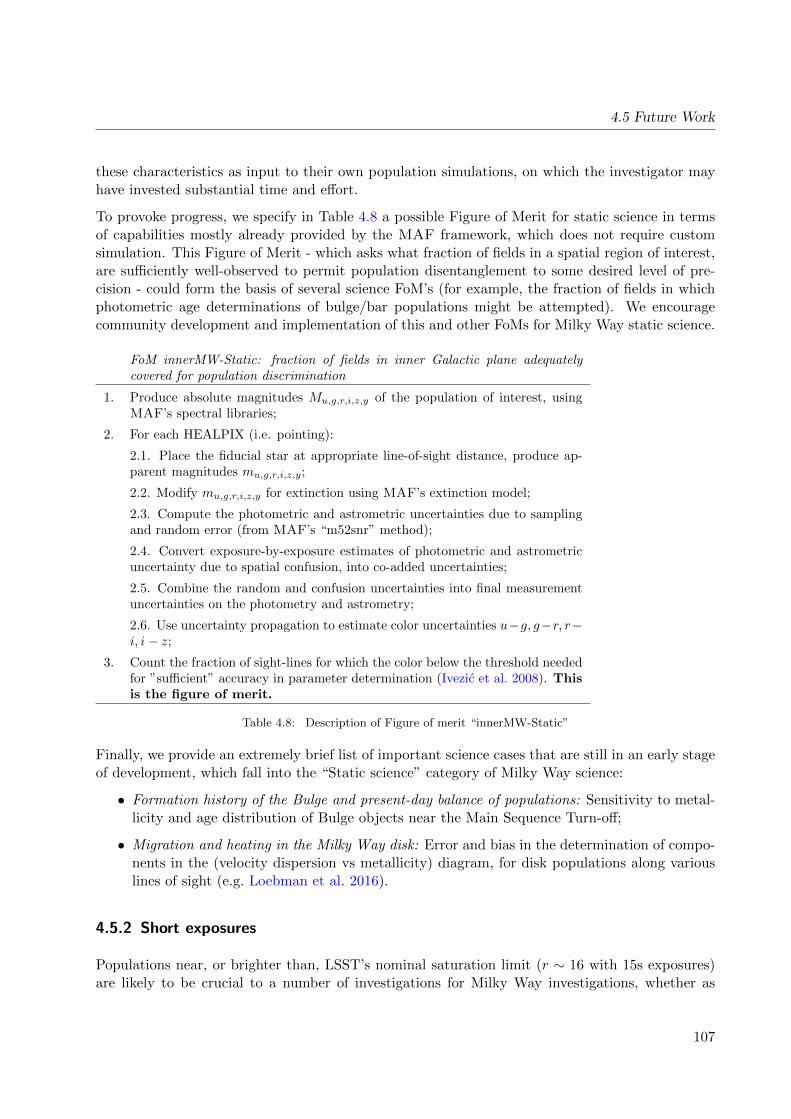
4.5 Future Work

these characteristics as input to their own population simulations, on which the investigator mayhave invested substantial time and effort.

To provoke progress, we specify in Table 4.8 a possible Figure of Merit for static science in termsof capabilities mostly already provided by the MAF framework, which does not require customsimulation. This Figure of Merit - which asks what fraction of fields in a spatial region of interest,are sufficiently well-observed to permit population disentanglement to some desired level of pre-cision - could form the basis of several science FoM’s (for example, the fraction of fields in whichphotometric age determinations of bulge/bar populations might be attempted). We encouragecommunity development and implementation of this and other FoMs for Milky Way static science.

FoM innerMW-Static: fraction of fields in inner Galactic plane adequatelycovered for population discrimination

1. Produce absolute magnitudes Mu,g,r,i,z,y of the population of interest, usingMAF’s spectral libraries;

2. For each HEALPIX (i.e. pointing):

2.1. Place the fiducial star at appropriate line-of-sight distance, produce ap-parent magnitudes mu,g,r,i,z,y;

2.2. Modify mu,g,r,i,z,y for extinction using MAF’s extinction model;

2.3. Compute the photometric and astrometric uncertainties due to samplingand random error (from MAF’s “m52snr” method);

2.4. Convert exposure-by-exposure estimates of photometric and astrometricuncertainty due to spatial confusion, into co-added uncertainties;

2.5. Combine the random and confusion uncertainties into final measurementuncertainties on the photometry and astrometry;

2.6. Use uncertainty propagation to estimate color uncertainties u−g, g−r, r−i, i− z;

3. Count the fraction of sight-lines for which the color below the threshold neededfor ”sufficient” accuracy in parameter determination (Ivezic et al. 2008). Thisis the figure of merit.

Table 4.8: Description of Figure of merit “innerMW-Static”

Finally, we provide an extremely brief list of important science cases that are still in an early stageof development, which fall into the “Static science” category of Milky Way science:

• Formation history of the Bulge and present-day balance of populations: Sensitivity to metal-licity and age distribution of Bulge objects near the Main Sequence Turn-off;

• Migration and heating in the Milky Way disk: Error and bias in the determination of compo-nents in the (velocity dispersion vs metallicity) diagram, for disk populations along variouslines of sight (e.g. Loebman et al. 2016).

4.5.2 Short exposures

Populations near, or brighter than, LSST’s nominal saturation limit (r ∼ 16 with 15s exposures)are likely to be crucial to a number of investigations for Milky Way investigations, whether as

107

Chapter 4: The Milky Way Galaxy

science tracers in their own right, or as contaminants that might interfere with measurements offainter program objects (due, for example, to charge bleeds of bright, foreground disk objects).

Quantitative exploration of these issues now requires involvement from the community (e.g. todetermine LSST’s discovery space for bright tracers in context with other facilities and surveys likeZTF, Gaia and VVV), and the project (e.g. to determine the parameters of short exposures thatmight be supported by the facility). To provoke development, here we list a few example questionsregarding short exposures that still need resolution:

• What level of bright-object charge-bleeding can be tolerated? For example, is some minimumdistribution of position-angles required in order to spread the bleeds azimuthally over theset of observations of a particular line of sight (so that different pixels fall under bleeds indifferent exposures)?7 What is this minimum?

• What is the science impact of restricting targets to r & 16?

• Will the proposed twilight survey of short exposures be adequate for science cases requiringshort exposures? Are there enough observations from other surveys (e.g. DES or other DE-Cam surveys) to cover the bright end of the entire LSST footprint, and are new observationsof very bright objects required scientifically in any case?

• What is the bright limit required for adequate astrometric cross-calibration against Gaia?

• To what extent would a given bright cutoff hamper the combination of LSST photometry orastrometry with that from other surveys (like VVV)?

• How short an exposure time can the facility support? Does the OpSim framework alreadyinclude all the operational limitations on scheduling short exposures?

4.5.3 The Local Volume

Finally, we remind the reader that substantial opportunity remains to develop science figures ofmerit for Local Volume science cases. Figures of Merit for Local Volume science likely share muchcommon ground with those for the Halo (discussed in Section 4.4), and substantial prior expertiseexists (e.g. Hargis et al. 2014). One straightforward Figure of Merit (FoM) might be the fractionof dwarf galaxies in the Local Volume that are correctly identified as a function of survey strategy.

Go to: • the start of this section • the start of the chapter • the table of contents

7Note that with ∼ 30 exposures per filter per field over ten years towards some regions, charge bleeds on the detectorfor a given object might not be spread over a large range of orientations. The spread of charge bleed angles onthe detector - as a spatially-varying metric - should be implemented and included in figures of merit.

108

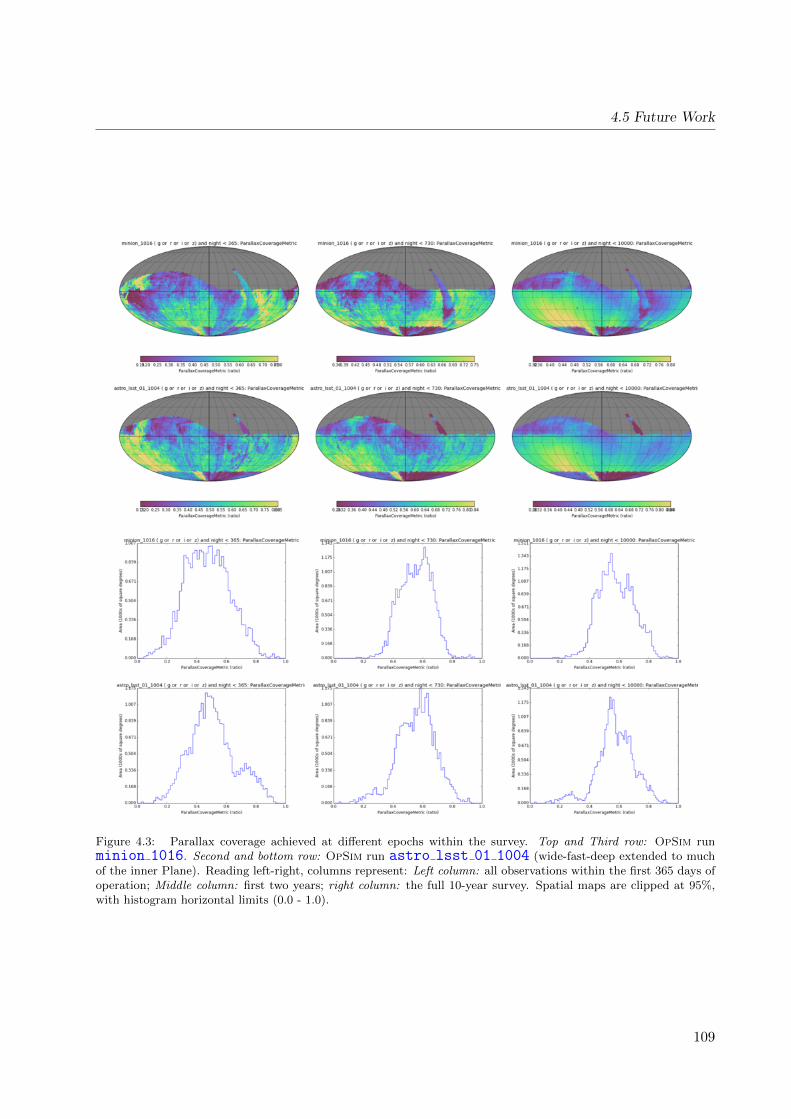
4.5 Future Work

Figure 4.3: Parallax coverage achieved at different epochs within the survey. Top and Third row: OpSim runminion 1016. Second and bottom row: OpSim run astro lsst 01 1004 (wide-fast-deep extended to muchof the inner Plane). Reading left-right, columns represent: Left column: all observations within the first 365 days ofoperation; Middle column: first two years; right column: the full 10-year survey. Spatial maps are clipped at 95%,with histogram horizontal limits (0.0 - 1.0).

109

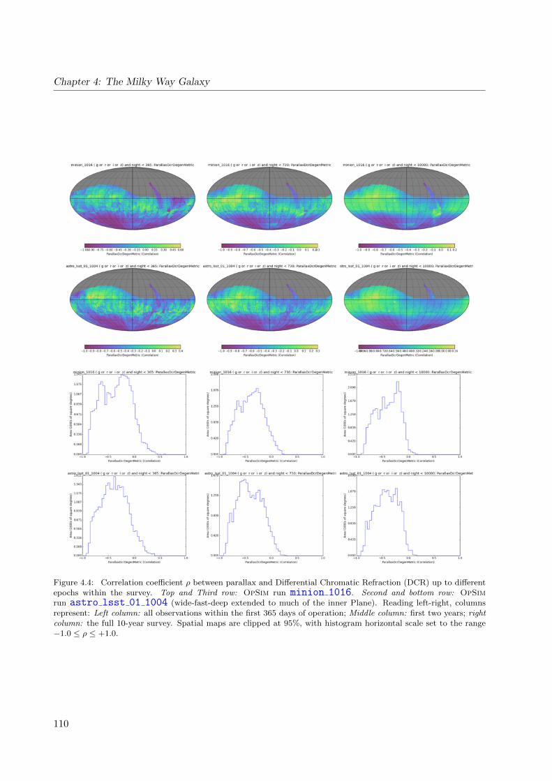
Chapter 4: The Milky Way Galaxy

Figure 4.4: Correlation coefficient ρ between parallax and Differential Chromatic Refraction (DCR) up to differentepochs within the survey. Top and Third row: OpSim run minion 1016. Second and bottom row: OpSimrun astro lsst 01 1004 (wide-fast-deep extended to much of the inner Plane). Reading left-right, columnsrepresent: Left column: all observations within the first 365 days of operation; Middle column: first two years; rightcolumn: the full 10-year survey. Spatial maps are clipped at 95%, with histogram horizontal scale set to the range−1.0 ≤ ρ ≤ +1.0.

110

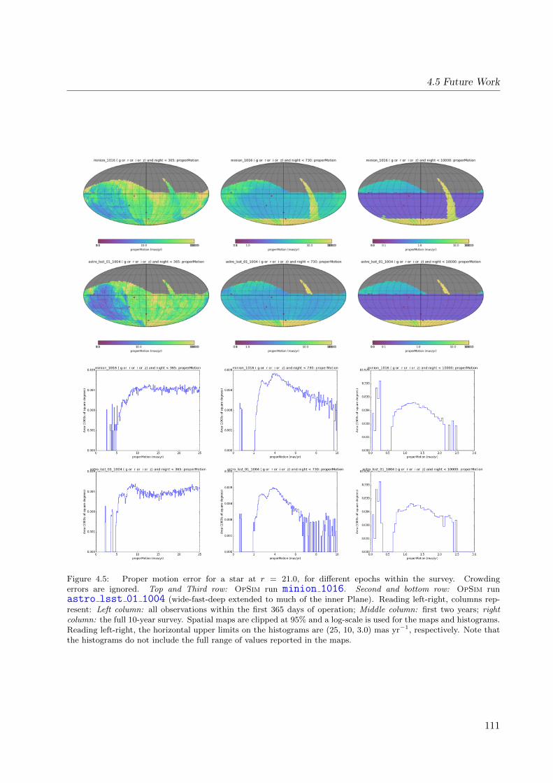
4.5 Future Work

Figure 4.5: Proper motion error for a star at r = 21.0, for different epochs within the survey. Crowdingerrors are ignored. Top and Third row: OpSim run minion 1016. Second and bottom row: OpSim runastro lsst 01 1004 (wide-fast-deep extended to much of the inner Plane). Reading left-right, columns rep-resent: Left column: all observations within the first 365 days of operation; Middle column: first two years; rightcolumn: the full 10-year survey. Spatial maps are clipped at 95% and a log-scale is used for the maps and histograms.Reading left-right, the horizontal upper limits on the histograms are (25, 10, 3.0) mas yr−1, respectively. Note thatthe histograms do not include the full range of values reported in the maps.

111

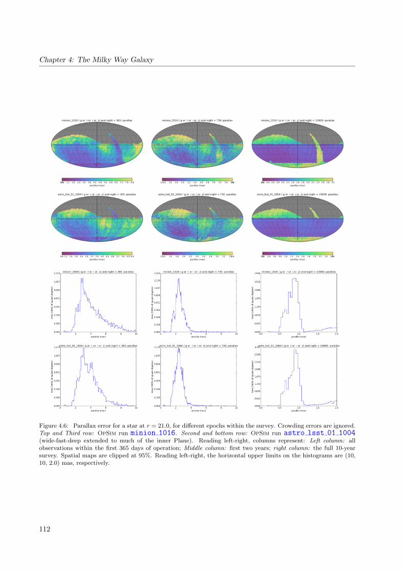
Chapter 4: The Milky Way Galaxy

Figure 4.6: Parallax error for a star at r = 21.0, for different epochs within the survey. Crowding errors are ignored.Top and Third row: OpSim run minion 1016. Second and bottom row: OpSim run astro lsst 01 1004(wide-fast-deep extended to much of the inner Plane). Reading left-right, columns represent: Left column: allobservations within the first 365 days of operation; Middle column: first two years; right column: the full 10-yearsurvey. Spatial maps are clipped at 95%. Reading left-right, the horizontal upper limits on the histograms are (10,10, 2.0) mas, respectively.

112

4.5 Future Work

Figure 4.7: Parallax coverage achieved for three extremes of object color, over the full 10-year survey. Top and Thirdrow: OpSim run minion 1016. Second and bottom row: OpSim run astro lsst 01 1004 (wide-fast-deepextended to much of the inner Plane). Reading left-right, columns represent: Left column: Objects detected onlyin the bluest filter; Middle column: objects detected only in the reddest filter; Right column: objects detected in allfilters. Spatial maps are clipped at 95%, with histogram horizontal limits (0.0 - 1.0).

113

Chapter 4: The Milky Way Galaxy

Figure 4.8: Correlation coefficient ρ between parallax and Differential Chromatic Refraction (DCR), selecting filtersfor three extremes of object color, over the full 10-year survey. Top and Third row: OpSim run minion 1016.Second and bottom row: OpSim run astro lsst 01 1004 (wide-fast-deep extended to much of the inner Plane).Reading left-right, columns represent: Left column: Objects detected only in the bluest filter; Middle column: objectsdetected only in the reddest filter; Right column: objects detected in all filters. Spatial maps are clipped at 95%,with histogram horizontal scale set to the range −1.0 ≤ ρ ≤ +1.0.

114

4.5 Future Work

Figure 4.9: Proper motion error for a star at apparent magnitude m = 21.0, for three extremes of object colorand assessed over the full survey. Crowding errors are ignored. Top and Third row: OpSim run minion 1016.Second and bottom row: OpSim run astro lsst 01 1004 (wide-fast-deep extended to much of the inner Plane).Reading left-right, columns represent: Left column: Objects detected only in the bluest filter; the fiducial objecthas apparent magnitude u = 21.0; Middle column: objects detected only in the reddest filter (so y = 21.0); Rightcolumn: objects detected in all filters (using r = 21.0 and a “flat” spectrum within MAF). Spatial maps are clippedat 95% and a log-scale is used for both the spatial maps and histograms. Reading left-right, the horizontal upperlimits on the histograms are (4.0, 4.0, 3.0) mas yr−1, respectively. Note that the histograms do not include the fullrange of values reported in the maps.

115

Chapter 4: The Milky Way Galaxy

Figure 4.10: Parallax error for a star at apparent magnitude m = 21.0, for three extremes of object color and assessedover the full survey. Crowding errors are ignored. Top and Third row: OpSim run minion 1016. Second andbottom row: OpSim run astro lsst 01 1004 (wide-fast-deep extended to much of the inner Plane). Readingleft-right, columns represent: Left column: Objects detected only in the bluest filter; the fiducial object has apparentmagnitude u = 21.0; Middle column: objects detected only in the reddest filter (so y = 21.0); Right column: objectsdetected in all filters (using r = 21.0 and a “flat” spectrum within MAF). Spatial maps are clipped at 95%. Readingleft-right, the horizontal upper limits on the histograms are (10, 10, 2.0) mas, respectively. Note that the histogramsdo not include the full range of values reported in the maps.

116

4.5 Future Work

Figure 4.11: Selection regions for the Astrometry Figures of Merit (FoMs) 1.1-1.4. Figures of Merit 1.1 and 1.3refer to the “main survey” region shown in the middle panel (which for the FoM also avoids the region of the SouthGalactic Pole). The right panel shows the inner Plane region to which FoMs 1.2 & 1.4 refer. The left-hand panelshows the entire survey region for reference. This example shows run minion 1016. See Table 4.7 and Section4.3.2.

Figure 4.12: Distance to which red giant stars can be identified in the galactic halo assuming a limiting magnitudeof u=26.0. The color code scales with the metallicity of the stars. More metal-poor stars can be detected to fartherdistances.

117

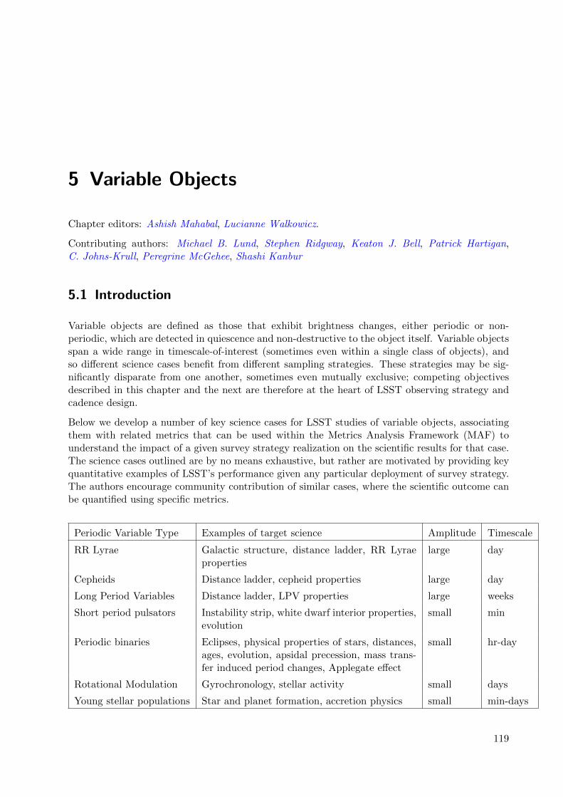
5 Variable Objects

Chapter editors: Ashish Mahabal, Lucianne Walkowicz.

Contributing authors: Michael B. Lund, Stephen Ridgway, Keaton J. Bell, Patrick Hartigan,C. Johns-Krull, Peregrine McGehee, Shashi Kanbur

5.1 Introduction

Variable objects are defined as those that exhibit brightness changes, either periodic or non-periodic, which are detected in quiescence and non-destructive to the object itself. Variable objectsspan a wide range in timescale-of-interest (sometimes even within a single class of objects), andso different science cases benefit from different sampling strategies. These strategies may be sig-nificantly disparate from one another, sometimes even mutually exclusive; competing objectivesdescribed in this chapter and the next are therefore at the heart of LSST observing strategy andcadence design.

Below we develop a number of key science cases for LSST studies of variable objects, associatingthem with related metrics that can be used within the Metrics Analysis Framework (MAF) tounderstand the impact of a given survey strategy realization on the scientific results for that case.The science cases outlined are by no means exhaustive, but rather are motivated by providing keyquantitative examples of LSST’s performance given any particular deployment of survey strategy.The authors encourage community contribution of similar cases, where the scientific outcome canbe quantified using specific metrics.

Periodic Variable Type Examples of target science Amplitude Timescale

RR Lyrae Galactic structure, distance ladder, RR Lyraeproperties

large day

Cepheids Distance ladder, cepheid properties large day

Long Period Variables Distance ladder, LPV properties large weeks

Short period pulsators Instability strip, white dwarf interior properties,evolution

small min

Periodic binaries Eclipses, physical properties of stars, distances,ages, evolution, apsidal precession, mass trans-fer induced period changes, Applegate effect

small hr-day

Rotational Modulation Gyrochronology, stellar activity small days

Young stellar populations Star and planet formation, accretion physics small min-days

119

Chapter 5: Variable Objects

Go to: • the start of this section • the start of the chapter • the table of contents

5.2 The Cepheid Mass-Luminosity Relation

Classical Cepheids begin to pulsate once they evolve up the giant branch and execute bluewardloops on the HR diagram that take them into the Instability Strip. Cepheid masses and luminositiesin the instability strip are connected through the Mass-Luminosity (ML) relation. This ML relationis strongly dependent on stellar evolution physics. Canonical/Non-canonical ML relations arisefrom varying treatments of convective core overshoot and mass loss (Brocato & Castellani 1992;Bono et al. 2000; Marconi et al. 2013).

Stellar pulsation models adopt a given ML relation and then compute a theoretical light curvefor a range of different temperatures and metallicities. This theoretical light curve can then betransformed into LSST wavebands using stellar atmospheres ((Bono et al. 2000) and referencestherein) and quantitatively compared to observed LSST light curves through Fourier decompositionof the form

V = A0 +

k=N∑k=1

Akcos(kωt+ φk),

where ω = 2π/P, with P the period, N is the order of the fit. The coefficients Rk1 = Ak/A1

and φk1 = φk − kφ1 can be computed for both theoretical and LSST observed light curves. Thesecoefficients are sensitive to the adopted ML relation and other global parameters such as metallicityand effective temperature. By utilizing such a decomposition, the multiwavelength light curves thatthe LSST will produce for both Cepheids and RR Lyraes can rigorously constrain Cepheid andRR Lyrae global stellar parameters such as the ML relation. Of course, knowledge of the MLrelation through this approach can then lead to another “theoretical” distance scale using bothCepheids and RR Lyraes. However, in the case of Cepheids, given good enough cadence in LSSTbands and thus an accurate Fourier decomposition with precisely known Fourier parameters, it willbe possible to discriminate between canonical and non-canonical ML relations and thus provideconstraints for stellar evolution physics. A good Figure of Merit for this science case would be onebased on the precision with which we can infer the parameters of these relations.

Bhardwaj et al. (2014) describes in detail the way the quantitative structure of Cepheid and RRLyrae light curves vary with period and optical band. Given appropriate cadence, LSST lightcurves will provide accurate Fourier decompositions at multiple wavelengths that can significantlyaugment these results and provide an important database with which to connect quantitativeaspects of Cepheid and RR Lyrae light curve structure to pulsation envelope physics. Two examplesare the following.

• 1) RRab stars found in stripe 82 of the SDSS exhibit a flat Period-Color (PC) relation atminimum light at certain SDSS colors but not at others. LSST observations of RRab starswill be able to augment this result and investigate if there are any links to the structuralproperties of observed light curves.

• 2) Short period (logP ≤ 0.4) FU Cepheids in the SMC exhibit a noticeable break in their(V − I) PC relation at certain phases of pulsation phases. At the same period, the Fourier

120

5.2 The Cepheid Mass-Luminosity Relation

parameter R21 displays a strong turnover. LSST data will be important in seeing if thisresult extends to LSST colors.

Bhardwaj et al. (2014, 2015, and references therein) have demonstrated how Cepheid and RR LyraePeriod-Color(PC)/Period-Luminosity (PL)/ Period-Wesenheit(PW)/Period-Luminosity-Color(PLC)relations vary significantly both as a function pulsation phase and period and observation band.The LSST database on Cepheids and RR Lyraes will provide an excellent database to furtherinvestigate the variation of these relations with pulsation phase with a view to understanding pul-sation physics and constraining theoeretical models. Currently, the literature only discusses theserelations at mean light, that is the average over pulsation phase. Yet this averaging process maskssome dependencies: there are pulsation phases with very high/low PL/PC dispersion and thereare some phases where the relation is highly nonlinear. In the era of precision cosmology, it is im-portant to understand the tools that we use to construct a distance scale. The LSST database onCepheids and RR Lyraes will be an important database with which to investigate the multiphaseproperties of PL/PC/PW/PLC relations.

What cadence is required for “accurate multiwavelength Fourier decomposition”? Cepheids andRR Lyraes are strictly periodic. Then for known variables, whose periods are already known,such Fourier decompositions can be carried out on folded light curves. In such situations given acadence, one possible measure of the success of this Fourier decomposition could be the maximumphase gap in the folded light curve. Another measure could be the error on the Fourier parameters(Petersen 1986). One way forward is to carry out a detailed Fourier analysis of any one simulatedschedule.

5.2.1 Description of Relevant Metrics

Despite the range in scientific motivation for the cases presented in this chapter, there are somecommon metrics that are widely applicable (or may be combined in a variety of ways with othermetrics to suit a variety of applications). The present science case provides as good a venue as anyin which to introduce these common metrics.

Metric Description

Eclipsing/transiting systemdiscovery

Fraction of discoveries vs fractional duration of eclipse

Lightcurve shape recovery ...

Phase gap Histogram vs period of the median and maximum phase gapsachieved in all fields

Period determination (perioddependent)

Fraction of targets vs survey duration, for which the periodcan be determined to 5-sigma confidence

Period variability (period de-pendent)

Fraction of targets vs survey duration, for which a periodchange of 1% can be determined with 5-sigma confidence

The ability to identify that an object is periodic, and to correctly determine that object’s period,are widely applicable measures of discovery. In the case of regular variables (as outlined below),these two measures together can uniquely identify a population. Other kinds of periodic systems

121

Chapter 5: Variable Objects

(transiting planets for example) also require a measurement of periodicity, but have a much widerrange of relevant periods, and looser requirements on the strictness of that periodicity.

Lund et al. (2016) discuss three diagnostic metrics that have been incorporated into the MAF.Two of these metrics deal explicitly with time variable behavior: a) observational triplets, and b)detection of periodic variability.

Figure 5.1: The value for the Periodogram Purity Function for candidate Baseline Cadence minion 1016. ThePeriodogram Purity Function provides a measure of the power lost due to aliasing.

Periodogram purity function (PeriodicMetric)

This metric calculates the Fourier power spectral window function of each field (Roberts et al.1987) as a means of quantifying the completeness of phase coverage for a given periodic variable.The periodogram purity is defined as 1 minus the Fourier power spectral window function. in theperfect case, all power in the window function is concentrated in a delta function at zero, and iszero at all other frequencies. As power “leaks” away from the correct frequency as a consequenceof discrete, non-ideal data sampling, the periodogram becomes more structured. For the purposesof MAF metrics, which are designed to quantify performance as a single number, the periodogram

122

5.2 The Cepheid Mass-Luminosity Relation

Figure 5.2: The median phase gap for candidate Baseline Cadence minion 1016. The MAF PhaseGapMetric

looks at periods between 3 and 35 days by default.

purity is quantified as the minimum value of the periodogram purity function at non-zero frequencyshifts; the ideal case would be a periodogram purity metric value of 1.

Phase Gap Metric PhaseGapMetric

The Phase Gap Metric is designed to examine the largest phase gaps in the observing schedule.For a given point in the sky, a series of periods are randomly selected (by default, 5 periods), witha default minimum of 3 days and maximum of 35 days. The largest phase gap for each period iscalculated, and the metric plots the median (Figure 5.2) and maximum (Figure 5.3) of this subsetof values that contains the maximum phase gap per period. The Phase Gap Metric is part ofvarMetrics.

Period Deviation Metric PeriodDeviationMetric

The Period Deviation Metric calculates the error in recovering the correct period of a sinusoidusing a given observing schedule and a Lomb-Scargle periodogram. For a given point in the sky,

123

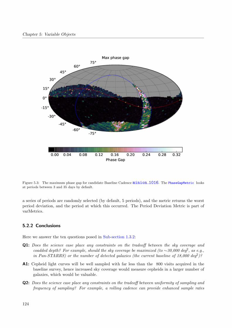
Chapter 5: Variable Objects

Figure 5.3: The maximum phase gap for candidate Baseline Cadence minion 1016. The PhaseGapMetric looksat periods between 3 and 35 days by default.

a series of periods are randomly selected (by default, 5 periods), and the metric returns the worstperiod deviation, and the period at which this occurred. The Period Deviation Metric is part ofvarMetrics.

5.2.2 Conclusions

Here we answer the ten questions posed in Sub-section 1.3.2:

Q1: Does the science case place any constraints on the tradeoff between the sky coverage andcoadded depth? For example, should the sky coverage be maximized (to ∼30,000 deg2, as e.g.,in Pan-STARRS) or the number of detected galaxies (the current baseline of 18,000 deg2)?

A1: Cepheid light curves will be well sampled with far less than the 800 visits acquired in thebaseline survey, hence increased sky coverage would measure cepheids in a larger number ofgalaxies, which would be valuable.

Q2: Does the science case place any constraints on the tradeoff between uniformity of sampling andfrequency of sampling? For example, a rolling cadence can provide enhanced sample rates

124

5.2 The Cepheid Mass-Luminosity Relation

over a part of the survey or the entire survey for a designated time at the cost of reducedsample rate the rest of the time (while maintaining the nominal total visit counts).

A2: An enhanced cadence could provide earlier discovery and period confirmation for a subset oftargets, but this is not a high priority.

Q3: Does the science case place any constraints on the tradeoff between the single-visit depth andthe number of visits (especially in the u-band where longer exposures would minimize theimpact of the readout noise)?

A3: No strong constraint.

Q4: Does the science case place any constraints on the Galactic plane coverage (spatial coverage,temporal sampling, visits per band)?

A4: LSST observations of galactic cepheids are not high priority, since they are bright for LSST.

Q5: Does the science case place any constraints on the fraction of observing time allocated to eachband?

A5: No strong constraint as long as good representation of all.

Q6: Does the science case place any constraints on the cadence for deep drilling fields?

A6: This would only apply in deep drilling fields that were chosen to study relatively near-bygalaxies, for which cepheid optimization would no doubt be considered explicitly.

Q7: Assuming two visits per night, would the science case benefit if they are obtained in the sameband or not?

A7: Different bands would provide more rapid characterization of targets, but this is not a strongbenefit.

Q8: Will the case science benefit from a special cadence prescription during commissioning or earlyin the survey, such as: acquiring a full 10-year count of visits for a small area (either in allthe bands or in a selected set); a greatly enhanced cadence for a small area?

A8: Enhanced cadences could provide earlier science, but cepheids are not a strong driver for this.

Q9: Does the science case place any constraints on the sampling of observing conditions (e.g.,seeing, dark sky, airmass), possibly as a function of band, etc.?

A9: No constraints that are particular to cepheids, but good seeing will aid the study of stars inthe crowded fields of external galaxies.

Q10: Does the case have science drivers that would require real-time exposure time optimizationto obtain nearly constant single-visit limiting depth?

A10: No.

Go to: • the start of this section • the start of the chapter • the table of contents

125

Chapter 5: Variable Objects

5.3 Characterizing Multiperiodic, Short-Period Pulsating Variables

Keaton J. Bell

Most pulsating variable stars exhibit a superposition of multiple simultaneous pulsation modes.While these multiperiodic pulsators are observationally more complex than classical pulsators, theycommunicate a greater wealth of information about the stars. Global nonradial pulsations passthrough and are affected by the interiors of stars, and the measured frequencies of photometricvariability are eigenfrequencies of stars as physical systems. Therefore, the observation and studyof photometric variability in multiperiodic pulsating stars is the most powerful method by whichwe can probe stellar interiors.

The current state and modern tools of the field of asteroseismology are thoroughly discussed byAerts et al. (2010). The locations of the known classes of pulsating variable in the H-R Diagramare indicated in their Figure 1.12, and a summary of their general properties—including pulsationamplitudes and timescales—is provided in their Appendix A.

Sections 8.6 and 8.7 of the Science Book express the anticipated contributions that LSST willmake to the study of pulsating variables. While the sparseness of observations (low duty cycle)over the LSST survey lifetime will make exact period solutions difficult, if not impossible for mostmultiperiodic, short-period pulsating variables, the Science Book correctly emphasizes that thephotometric precision and multi-color information will yield detections of variability that can betreated statistically to determine the ensemble properties of different classes of pulsating star.The dependence of pulsational power on a star’s position in 5-color parameter space, as well asthe relative pulsation amplitudes in different passbands, informs the least understood aspects ofpulsation theory: mode selection and amplitude limiting mechanisms. A thorough statistical viewof pulsating stars requires on the order of thousands of objects per type at a minimum, with robustdetections of variability in multiple passbands.

5.3.1 The Case for ZZ Cetis

Of the known classes of pulsating variable star, the ZZ Cetis (pulsating hydrogen-atmospherewhite dwarfs) are the faintest, and among those with the lowest pulsation amplitudes. These willbe the most difficult for LSST to detect and characterize, and they therefore provide an importantbenchmark for assessing the effectiveness of different proposed observing strategies for the studyof pulsating stars. If LSST is well suited for ZZ Ceti science, it will be a useful tool for all classesof pulsator.

Most details of ZZ Ceti stars are not strictly relevant to this analysis, so we direct the interestedreader to recent reviews by Winget & Kepler (2008), Fontaine & Brassard (2008), and Althauset al. (2010).

As white dwarfs with atmospheres spectroscopically dominated by hydrogen cool to betweenroughly 12,500 and 10,600 K, they are observed as the photometrically variable ZZ Cetis. Thesquare root of the total observed pulsational power (intrinsic root-mean-squared signal) in theseobjects is on the order of 1% and the mean pulsation periods are ∼10 min (e.g., Mukadam et al.

126

5.3 Characterizing Multiperiodic, Short-Period Pulsating Variables

2006). Because the pulsation periods are the typical LSST revisit time, the survey will essentiallysample the pulsations randomly in phase.

The ability to detect pulsations relies on the recognition that scatter in the flux measurementssignificantly exceeds what can be attributed to noise. LSST’s sensitivity to these pulsations dependsprimarily on two things: the photometric precision and the total number of measurements. Byaffecting these survey characteristics, the choice of observing strategy impacts LSST’s success inits goal of exploring the variable universe. Strategies that maximize photometric precision and thetotal number of visits in all filters optimize the survey toward this goal, but there are tradeoffsbetween these dual requirements related primarily to exposure time that are complicated and mustbe explored in MAF to be understood.

While consideration of observations across all filters together provides the greatest sensitivity todetecting overall variability, the measurement of pulsational power in individual filters serves thescience needs for pulsating stars best. Since sparse temporal sampling will make measuring theindividual periods of complex, multi-modal pulsating stars challenging, LSST’s greatest contribu-tions to this field may lie in its ability to measure relative pulsational power across many passbands.For ZZ Cetis in particular, there is a dependence of the relative amplitudes measured in differentfilters on the geometry of the pulsations—specifically the spherical degrees, `, of the sphericalharmonic wave patterns associated with the pulsation modes. Determining the ` values associatedwith individual modes is essential for comparing measured pulsation frequencies with those cal-culated for asteroseismic stellar models. The difficulty in determining ` is currently the greatestlimitation on white dwarf asteroseismology. LSST has the potential to statistically constrain therelative contributions of modes of different ` to the overall photometric variations. The calculationsby Brassard et al. (1995) of relative pulsation amplitudes in different filters show that measuringthe amplitude in the u band is crucial for gaining leverage on this problem.

5.3.2 Metrics

We have developed a custom MAF metric that calculates a “variability depth” for every point onthe sky equal to the magnitude limit for detecting a population of photometric variables with agiven disk-integrated root-mean-squared (r.m.s.) underlying signal to a desired level of completenessand a tolerable level of contamination. The metric makes the simplifying assumptions that thetypical revisit time for a field is longer than the pulsation periods (appropriate for many pulsators,including ZZ Cetis) and that the intrinsic variability takes the form of a Gaussian (which, formulti-periodic pulsators, is supported by the central limit theorem). The metric relies on thetotal number of visits and signal-to-noise per visit (scaled from the 5σ-depth, with Gaussian errorsassumed) for the calculation, and is included in sims maf contrib as VarDepth. Example outputof this metric is displayed in Figure 5.4.

We specialize this metric for the case of ZZ Ceti pulsators by including maps of the expecteddistribution of ZZ Cetis in the Galaxy. These maps were precomputed for the u and r filtersby querying the CatSim database for white dwarfs with an SQL constraint to include only thosewith hydrogen atmospheres and with effective temperatures between 10,600 and 12,500 K (i.e.,inside the ZZ Ceti instability strip). While the boundaries of the instability strip depend slightlyon surface gravity, the width of the strip does not change much, so these temperature cuts yield

127

Chapter 5: Variable Objects

Figure 5.4: Example output of the VarDepth MAF metric run on the current baseline cadence, minion 1016,after 10 years of survey operations. Input parameters and SQL queries were set to calculate the magnitude limit fordetecting 90% of pulsators with 1% r.m.s. variability from a cut on the measured variance in the r band (allowingcontamination from 10% of nonvariable sources).

representative counts. The white dwarf spectral energy distributions were calculated for CatSimby Pierre Bergeron et al.1 The ZZCetiCounts metric calculates the number of ZZ Cetis that weexpect to detect in each part of the sky, and the sum of the results gives the total number of ZZCetis with variability detected by LSST.

The measured r.m.s. scatter from pulsations in ZZ Cetis is typically of order ∼1%, with a meanvalue around 3% (Mukadam et al. 2006). Since we aim to statistically determine the ensembleamplitude properties in multiple filters for a large population of ZZ Cetis (particularly in the ufilter), we adopt the following figure of merit for LSST’s ability to study pulsating stars: thatsignificant variability should be detected in the u band for at least 1000 ZZ Cetis by the end ofthe 10 yr survey operations. A sample of this size can be binned to track changes in pulsationalpower as white dwarfs cool across the ZZ Ceti instability strip, without the results being undulyinfluenced by random sampling of inclination angle or the white dwarf mass distribution. It alsoensures that LSST contributes an order-of-magnitude improvement to the number of ZZ Cetisknown.

5.3.3 OpSim Analysis

For comparison purposes, we calculate the number of ZZ Cetis detected in both the u and r fil-ters, assuming intrinsic r.m.s. variability of 1% for two of the currently available OpSim runs:minion 1016, the current baseline cadence, and kraken 1045, with doubled u-band exposure

1http://www.astro.umontreal.ca/~bergeron/CoolingModels/

128

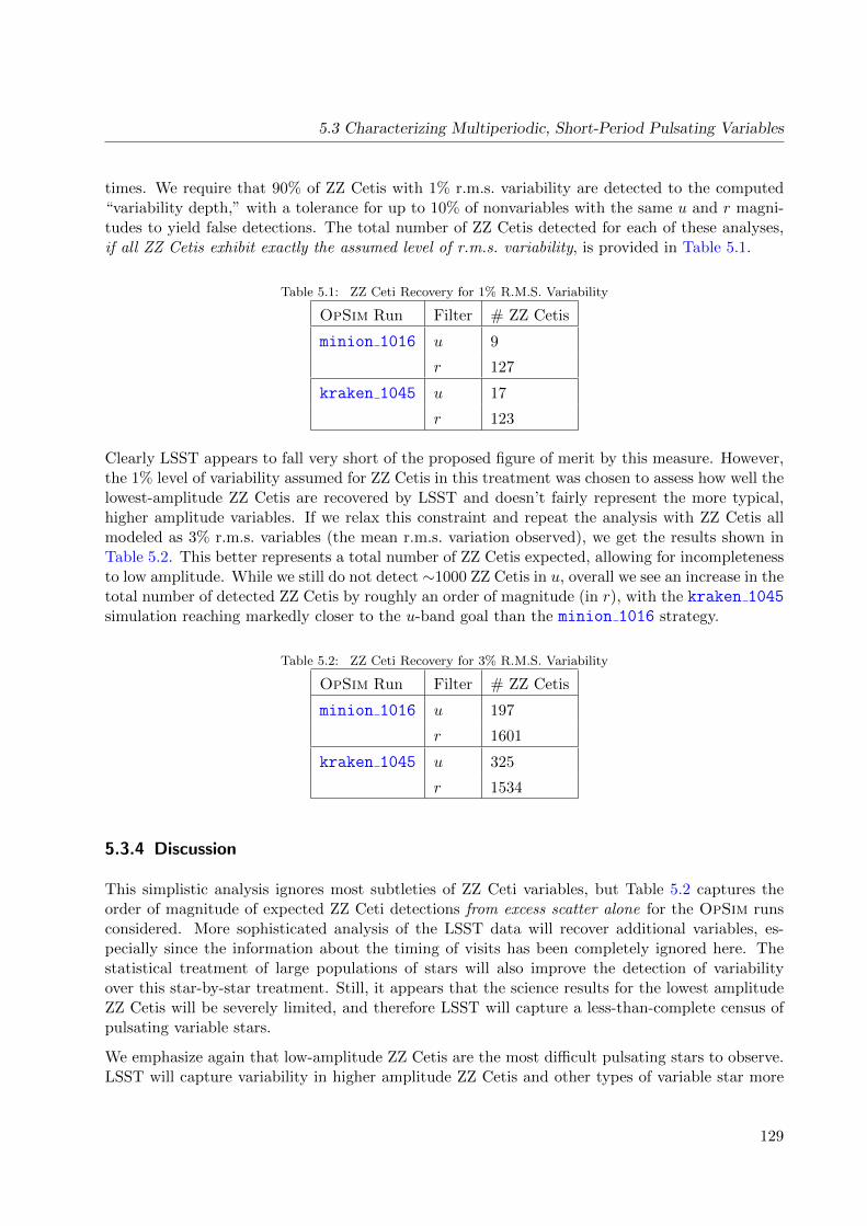
5.3 Characterizing Multiperiodic, Short-Period Pulsating Variables

times. We require that 90% of ZZ Cetis with 1% r.m.s. variability are detected to the computed“variability depth,” with a tolerance for up to 10% of nonvariables with the same u and r magni-tudes to yield false detections. The total number of ZZ Cetis detected for each of these analyses,if all ZZ Cetis exhibit exactly the assumed level of r.m.s. variability, is provided in Table 5.1.

Table 5.1: ZZ Ceti Recovery for 1% R.M.S. Variability

OpSim Run Filter # ZZ Cetis

minion 1016 u 9

r 127

kraken 1045 u 17

r 123

Clearly LSST appears to fall very short of the proposed figure of merit by this measure. However,the 1% level of variability assumed for ZZ Cetis in this treatment was chosen to assess how well thelowest-amplitude ZZ Cetis are recovered by LSST and doesn’t fairly represent the more typical,higher amplitude variables. If we relax this constraint and repeat the analysis with ZZ Cetis allmodeled as 3% r.m.s. variables (the mean r.m.s. variation observed), we get the results shown inTable 5.2. This better represents a total number of ZZ Cetis expected, allowing for incompletenessto low amplitude. While we still do not detect ∼1000 ZZ Cetis in u, overall we see an increase in thetotal number of detected ZZ Cetis by roughly an order of magnitude (in r), with the kraken 1045simulation reaching markedly closer to the u-band goal than the minion 1016 strategy.

Table 5.2: ZZ Ceti Recovery for 3% R.M.S. Variability

OpSim Run Filter # ZZ Cetis

minion 1016 u 197

r 1601

kraken 1045 u 325

r 1534

5.3.4 Discussion

This simplistic analysis ignores most subtleties of ZZ Ceti variables, but Table 5.2 captures theorder of magnitude of expected ZZ Ceti detections from excess scatter alone for the OpSim runsconsidered. More sophisticated analysis of the LSST data will recover additional variables, es-pecially since the information about the timing of visits has been completely ignored here. Thestatistical treatment of large populations of stars will also improve the detection of variabilityover this star-by-star treatment. Still, it appears that the science results for the lowest amplitudeZZ Cetis will be severely limited, and therefore LSST will capture a less-than-complete census ofpulsating variable stars.

We emphasize again that low-amplitude ZZ Cetis are the most difficult pulsating stars to observe.LSST will capture variability in higher amplitude ZZ Cetis and other types of variable star more

129

Chapter 5: Variable Objects

completely, and LSST observations of all candidate pulsating white dwarfs will certainly still beworthy of careful analysis. We note that the kraken 1045 strategy with 60 s exposures in u doesa much better job of measuring stellar variability overall, at the expense of a practically negligibledecrease in r-band detections. We argue that any observing strategy that increases the typicalVarDepth limit in the u band will improve LSST’s scientific yield for all stellar pulsation studies.

5.3.5 Conclusions

Here we answer the ten questions posed in Sub-section 1.3.2:

Q1: Does the science case place any constraints on the tradeoff between the sky coverage andcoadded depth? For example, should the sky coverage be maximized (to ∼30,000 deg2, as e.g.,in Pan-STARRS) or the number of detected galaxies (the current baseline of 18,000 deg2)?

A1: Coadded depth is not directly a limitation on detecting variability, but both improve with thenumber of revisits to the same field, N , as roughly

√N . A larger field of view also increases

the potential population of variable stars discovered, but pushing to higher airmass wheredata quality is poorer does not make for a good trade unless the survey area is extended tostrategically target more variable stars, e.g., over more of the Galactic plane.

Q2: Does the science case place any constraints on the tradeoff between uniformity of sampling andfrequency of sampling? For example, a rolling cadence can provide enhanced sample ratesover a part of the survey or the entire survey for a designated time at the cost of reducedsample rate the rest of the time (while maintaining the nominal total visit counts).

A2: While the time distribution of observations has not been considered here, this will significantlyimpact variable star science with LSST. Future development of MAF metrics should addressspecifically how the distribution of visits (rather than only number, area, and signal-to-noiseas addressed above) ease the challenges of amplitude and period recovery in sparely sampledobservations. Revisit times much shorter than pulsation timescales (<∼5 min) can help toconstrain the periods. Perhaps more importantly, cadences that produce the least compli-cated spectral windows and the highest “effective Nyquist frequencies” will best facilitateperiod recovery (e.g., Eyer & Bartholdi 1999).

Q3: Does the science case place any constraints on the tradeoff between the single-visit depth andthe number of visits (especially in the u-band where longer exposures would minimize theimpact of the readout noise)?

A3: We specifically support increased time spent in the u-band, with the goal of measuring the rel-ative pulsation amplitudes in multiple filters. Increased signal-to-noise per u-band exposureenables more measurements of pulsational power in u, though pulsating star science wouldbe hurt by a corresponding decrease in the total number of u-band visits per field .

Q4: Does the science case place any constraints on the Galactic plane coverage (spatial coverage,temporal sampling, visits per band)?

A4: The Galactic plane contains a higher concentration of multi-periodic pulsating stars that LSSTwill be able to characterize in the time domain. Pulsating star science benefits from moresurvey time spent in the Galactic plane.

130

5.3 Characterizing Multiperiodic, Short-Period Pulsating Variables

Q5: Does the science case place any constraints on the fraction of observing time allocated to eachband?

A5: For the ZZ Ceti case study, u-band observations are particularly important for potentiallyconstraining pulsation geometries. The metric developed in this section measures the ex-pected number of ZZ Cetis detected in the u-band, and we advocate for observing strategiesthat increase this number.

For classical pulsators, such as δ Scuti stars (P∼hrs) and γ Dor stars (P∼days), multi-bandphotometry is important for mode identification. Enough data in each band is required todetermine the pulsation’s amplitude and phase. For these pulsators, the u-band is the leastinformative (e.g., Garrido et al. 1990).

Q6: Does the science case place any constraints on the cadence for deep drilling fields?

A6: The results of the VarDepth MAF metric run on the current baseline cadence, minion 1016,shows that after 10 years, deep drilling fields are sensitive to pulsation amplitude measure-ments in the r-band ≈1.5 mag fainter than for identical objects in the main survey. Theimprovement to period recoverability could be far greater in deep drilling fields, but newMAF metrics must be developed to demonstrate this and to help select between specificproposed cadences.

The possibility to obtain data at a high cadence for extended periods of time in the deepdrilling fields will also facilitate the asteroseismology of solar-like oscillators (∼minutes formain-sequence stars and ∼hours for red giants). However, a MAF metric is required todetermine the specific requirements.

Q7: Assuming two visits per night, would the science case benefit if they are obtained in the sameband or not?

A7: Analyses that will successfully extract the maximum pulsation science from LSST will haveto address data across all passbands together, and there is no current indication of how or ifthe nightly revisit filter selection will affect this.

Q8: Will the case science benefit from a special cadence prescription during commissioning or earlyin the survey, such as: acquiring a full 10-year count of visits for a small area (either in allthe bands or in a selected set); a greatly enhanced cadence for a small area?

A8: A few hours of continuous sampling of a few fields during commissioning would produceimmediate science results for many multi-modal pulsating stars, as well as help accelerateLSST’s ultimate characterization of variable stars in these fields.

Furthermore, by mimicking the 10-yr survey for a small area, the scientific community canobtain evidence-based estimates of the yield of different variable classes and example powerspectra. This will also provide proof-of-concept data that will facilitate the recruitment ofscientists to work on LSST.

Q9: Does the science case place any constraints on the sampling of observing conditions (e.g.,seeing, dark sky, airmass), possibly as a function of band, etc.?

A9: The VarDepth MAF metric can help assess how the adjustments made by the observingstrategy to observing conditions affect the variable star science output.

131

Chapter 5: Variable Objects

Q10: Does the case have science drivers that would require real-time exposure time optimizationto obtain nearly constant single-visit limiting depth?

A10: No. Consistent exposure times are simpler to interpret as they smooth over any underlyingvariability by a consistent amount.

Go to: • the start of this section • the start of the chapter • the table of contents

5.4 Discovery and Characterization of Young Stellar Populations

Patrick Hartigan, C. Johns-Krull, Peregrine McGehee

5.4.1 Introduction

All young stars exhibit some form of photometric variability, and these variations hold the key tounderstanding the diverse physical processes present at starbirth such as mass accretion events fromcircumstellar disks, presence of warps in envelopes, creation of new knots in stellar jets, evolutionof stellar angular momenta, starspot longevity and cycles, and the frequency and strength offlares. With the proper cadences and filter choices, LSST will make a significant impact in ourunderstanding of all these phenomena simply by providing large enough samples to allow us torelate these aspects of the young stars and their environments to stellar properties such as mass, age,binarity, and their location within their nascent dark clouds in a statistically significant manner.

Low-mass (. 1.5M) pre-main-sequence stars separate into two main categories, depending uponwhether or not an optically thick dusty circumstellar disk exists in the system: young stars withoutdusty inner disks are known as ‘weak-lined T Tauri stars’ (wTTs), while those that have innerdusty disks are called ‘classical T Tauri stars’. The nature of the variability in young stars changeswith evolutionary status. In cTTs, variability is primarily caused by unsteady mass infall fromcircumstellar disks onto their stars, and from periodic extinction events that unfold as denseclumps or disk warps circle the star in Keplerian orbits. Once the disks become optically thin,variability in the wTTs phase is dominated by small-amplitude (typically ∼ 0.1 mag) quasi-periodicvariations that arise from cool star spots, though active regions that generate X-rays in these objectsundoubtedly produce optical flares as well.

At the extreme end of cTTs phenomena, rare massive outbursts of up to 6 magnitudes withdecay times between several months to over a hundred years in pre-main-sequence stars (EX Ori’s(Herbig et al. 2001) and FU Ori’s (Hartmann & Kenyon 1996)) are of great interest to studies ofdisk accretion because they indicate the onset of a major disk instability. Only a handful of suchsystems have been found, and LSST will easily detect any new ones. In addition to triggeringfollow-up observations, LSST will define the first population constraints on the duration of highstates, particularly for the shorter-lived versions of these eruptive variables.

Obtaining rotation periods for large numbers of pre-main-sequence stars is the only way to quantifyhow angular momenta of young stars vary with age. For both wTTs and cTTs, phase-coherencein the rotation periods defines the longevity of star spots, while the amplitude of the periodiccomponent of the lightcurve constrains the spot coverage (and temperature if multiple filters are

132

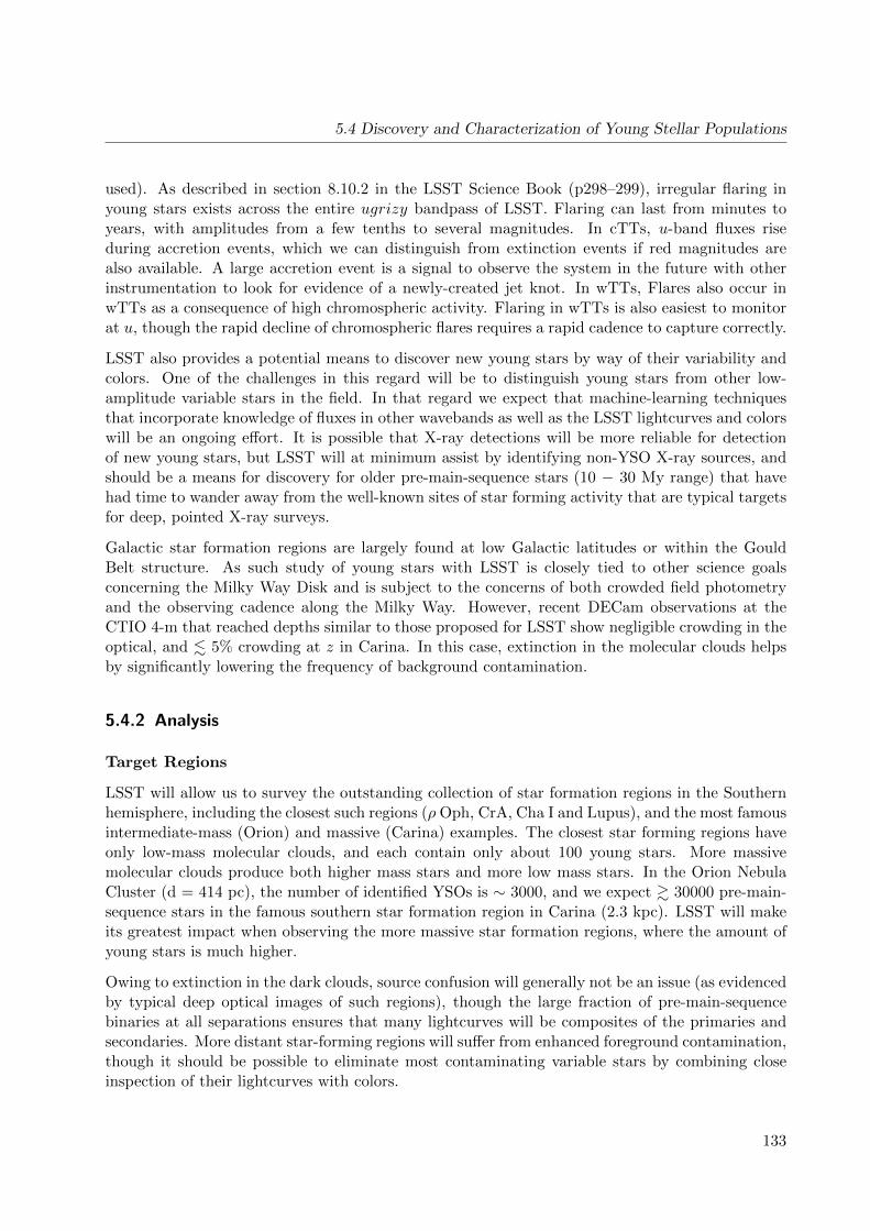
5.4 Discovery and Characterization of Young Stellar Populations

used). As described in section 8.10.2 in the LSST Science Book (p298–299), irregular flaring inyoung stars exists across the entire ugrizy bandpass of LSST. Flaring can last from minutes toyears, with amplitudes from a few tenths to several magnitudes. In cTTs, u-band fluxes riseduring accretion events, which we can distinguish from extinction events if red magnitudes arealso available. A large accretion event is a signal to observe the system in the future with otherinstrumentation to look for evidence of a newly-created jet knot. In wTTs, Flares also occur inwTTs as a consequence of high chromospheric activity. Flaring in wTTs is also easiest to monitorat u, though the rapid decline of chromospheric flares requires a rapid cadence to capture correctly.

LSST also provides a potential means to discover new young stars by way of their variability andcolors. One of the challenges in this regard will be to distinguish young stars from other low-amplitude variable stars in the field. In that regard we expect that machine-learning techniquesthat incorporate knowledge of fluxes in other wavebands as well as the LSST lightcurves and colorswill be an ongoing effort. It is possible that X-ray detections will be more reliable for detectionof new young stars, but LSST will at minimum assist by identifying non-YSO X-ray sources, andshould be a means for discovery for older pre-main-sequence stars (10 − 30 My range) that havehad time to wander away from the well-known sites of star forming activity that are typical targetsfor deep, pointed X-ray surveys.

Galactic star formation regions are largely found at low Galactic latitudes or within the GouldBelt structure. As such study of young stars with LSST is closely tied to other science goalsconcerning the Milky Way Disk and is subject to the concerns of both crowded field photometryand the observing cadence along the Milky Way. However, recent DECam observations at theCTIO 4-m that reached depths similar to those proposed for LSST show negligible crowding in theoptical, and . 5% crowding at z in Carina. In this case, extinction in the molecular clouds helpsby significantly lowering the frequency of background contamination.

5.4.2 Analysis

Target Regions

LSST will allow us to survey the outstanding collection of star formation regions in the Southernhemisphere, including the closest such regions (ρOph, CrA, Cha I and Lupus), and the most famousintermediate-mass (Orion) and massive (Carina) examples. The closest star forming regions haveonly low-mass molecular clouds, and each contain only about 100 young stars. More massivemolecular clouds produce both higher mass stars and more low mass stars. In the Orion NebulaCluster (d = 414 pc), the number of identified YSOs is ∼ 3000, and we expect & 30000 pre-main-sequence stars in the famous southern star formation region in Carina (2.3 kpc). LSST will makeits greatest impact when observing the more massive star formation regions, where the amount ofyoung stars is much higher.

Owing to extinction in the dark clouds, source confusion will generally not be an issue (as evidencedby typical deep optical images of such regions), though the large fraction of pre-main-sequencebinaries at all separations ensures that many lightcurves will be composites of the primaries andsecondaries. More distant star-forming regions will suffer from enhanced foreground contamination,though it should be possible to eliminate most contaminating variable stars by combining closeinspection of their lightcurves with colors.

133

Chapter 5: Variable Objects

Metrics:

A. Magnitude Limits, Filter Choices

To quantify YSO studies with LSST, we consider V 927 Tau, a rather faint, moderately-reddened0.2 M young star in the Taurus cloud as a target goal. Extrapolating this star to the distance ofCarina we have u=24.0, g=23.0, r=20.8, i=19.4, and z=18.0. For reference, a typical young starin the Carina X-ray catalog has an i-magnitude of 18. Objects that suffer larger extinctions alongthe line of sight will be easiest to observe in the red. The universal cadence option of 2×15 secexposures will yield σ = 0.02 mag for r=21.8, a magnitude fainter than V 927 Tau would be inCarina. We show below that this photometric uncertainty suffices to recover a typical period fromsuch an object. The mass function of young stars peaks around 0.3 M, so LSST will determineperiods to near the hydrogen burning limit with nominal r-band measurements for a region likeCarina. Of course, several additional magnitudes of extinction will exist towards many embeddedsources. For example, if we assume an additional five magnitudes of extinction at V for the V 927Tau-like example above, then r=25.2 and σ = 0.41 mag per visit with universal cadence, so nousable lightcurve will be possible at r. However, z=20.5 in this case, where σ < 0.01 mag andprecision lightcurves are again possible.

B. Period Recovery for wTTs

In order to assess how well LSST will recover periods, we created the following model for wTTsvariability. Based on current surveys of wTTs, the periods are distributed approximately as aPoisson distribution with a mean of 3.5 days (Affer et al. 2013). Amplitudes are typically 0.1magnitude (Grankin et al. 2008), so we adopt a Poisson distribution that has a mean amplitude of0.05 mag, and then add 0.05 mag to ensure that the mean variability is 0.1 mag. Shapes of T-Taurilightcurves can be sinusoidal, but many are ‘bowl-shaped’, influenced by the distribution of largedark starspots (Alencar et al. 2010). For the bowl lightcurves we assumed a Gaussian shape witha FWHM in a uniform distribution of extent between 0 and 0.75 in phase. Our simulations coverboth of these shapes. Errors for each point were taken to be 0.02 magnitude, corresponding toabout r ∼ 21.8 for a universal cadence.

One set of simulations assumed a cadence of one observation every three days over the course ofa year. If we define a successful period recovery to be better than a 1% error, then using thestandard Scargle method (Horne & Baliunas 1986) we are able to find the correct period in 98% ofthe the sinusoidal, and 86% of the bowl lightcurves, with the most difficult challenges being at theshort end of the period distribution. If we change the cadence to once every 7 days, the ability torecover periods drops to 82% and 59% , respectively, for the two shapes. Interestingly, restrictingthe sample to the highest-amplitude sources (& 0.1 magnitude) does little to aid period recovery.The main issue remains the short-period systems where P . 2 days.

Overall, standard cadences of once every few days should suffice to find most periodic T-Tauri starsthat have periods & 3 days. A dedicated campaign to observe star-forming regions at time intervalsof an hour or less is required to capture the shorter-period systems. The r-filter should suffice formost objects, though some benefit will be had by going to z to allow the more heavily-extinctedsources to be observed.

C. Period Recovery for cTTs

134

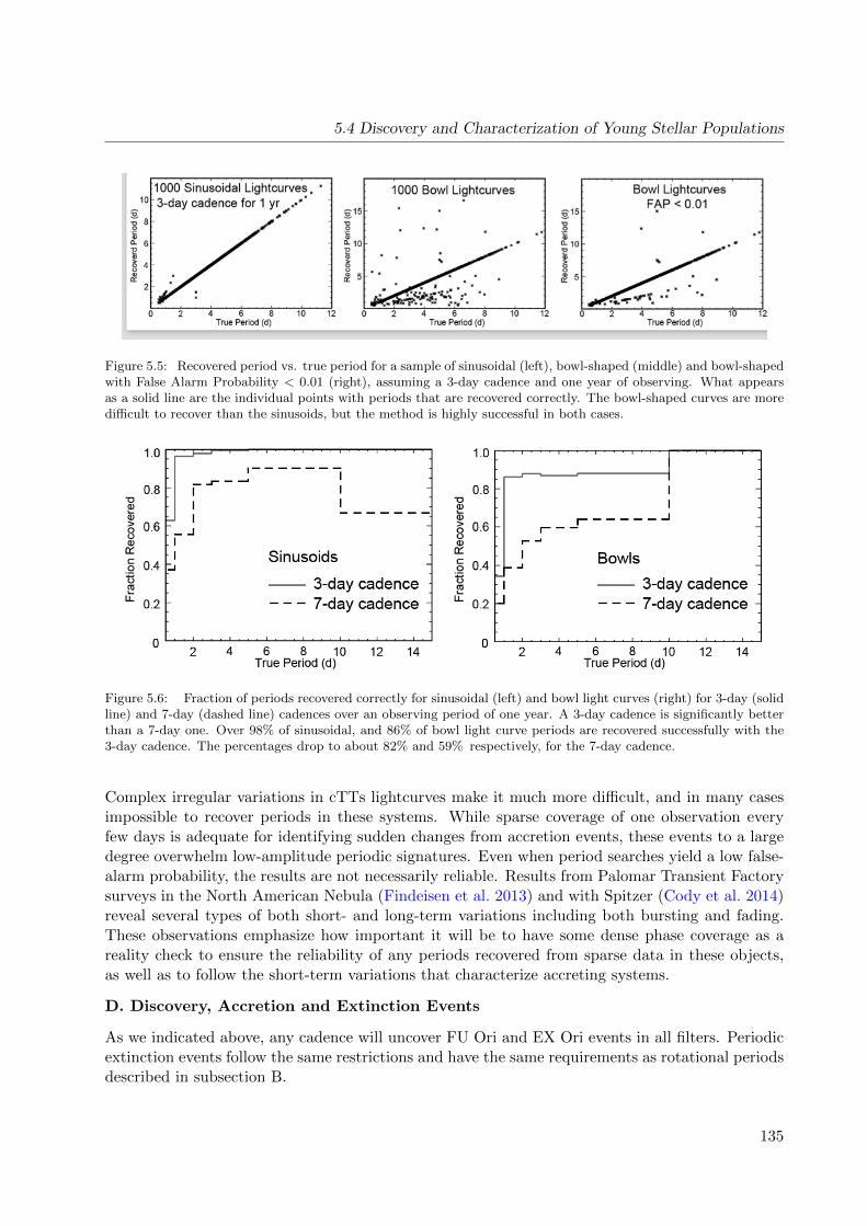
5.4 Discovery and Characterization of Young Stellar Populations

Figure 5.5: Recovered period vs. true period for a sample of sinusoidal (left), bowl-shaped (middle) and bowl-shapedwith False Alarm Probability < 0.01 (right), assuming a 3-day cadence and one year of observing. What appearsas a solid line are the individual points with periods that are recovered correctly. The bowl-shaped curves are moredifficult to recover than the sinusoids, but the method is highly successful in both cases.

Figure 5.6: Fraction of periods recovered correctly for sinusoidal (left) and bowl light curves (right) for 3-day (solidline) and 7-day (dashed line) cadences over an observing period of one year. A 3-day cadence is significantly betterthan a 7-day one. Over 98% of sinusoidal, and 86% of bowl light curve periods are recovered successfully with the3-day cadence. The percentages drop to about 82% and 59% respectively, for the 7-day cadence.

Complex irregular variations in cTTs lightcurves make it much more difficult, and in many casesimpossible to recover periods in these systems. While sparse coverage of one observation everyfew days is adequate for identifying sudden changes from accretion events, these events to a largedegree overwhelm low-amplitude periodic signatures. Even when period searches yield a low false-alarm probability, the results are not necessarily reliable. Results from Palomar Transient Factorysurveys in the North American Nebula (Findeisen et al. 2013) and with Spitzer (Cody et al. 2014)reveal several types of both short- and long-term variations including both bursting and fading.These observations emphasize how important it will be to have some dense phase coverage as areality check to ensure the reliability of any periods recovered from sparse data in these objects,as well as to follow the short-term variations that characterize accreting systems.

D. Discovery, Accretion and Extinction Events

As we indicated above, any cadence will uncover FU Ori and EX Ori events in all filters. Periodicextinction events follow the same restrictions and have the same requirements as rotational periodsdescribed in subsection B.

135

Chapter 5: Variable Objects

Figure 5.7: Left and center: Same as Fig 2 but restricting the sample to amplitudes greater than 0.1 mag. Themethod is only marginally more successful with the larger amplitude objects than it is with the entire sample. Right:The narrowest 278 bowls have a significantly higher error rate than the entire sample does.

In order to assess the ability of LSST to identify and classify eruptive variables (FUor/EXor),we construct Table 5.3, which shows a possible Figure of Merit for the recovery by LSST of thedistribution of EXor high-state duration in outburst.

5.4.3 Summary and Recommendations

Performance for Nominal Cadences

Nominal cadences that return to a star-forming region every 3-4 days will suffice to determinerotation periods for ∼ 90% of the young stars within the magnitude limits of LSST. These cadencesare also adequate to detect major episodic accretion events like FU Ori’s and EX Ori’s. However,a more focused annual campaign of about a week duration is necessary to optimize period recoveryand angular momentum studies of young stars.

The Need for Annual Dense Coverage of a Few Selected Regions

Occasional dense coverage of targeted regions is the only way to get quantitative information onshort-term accretion and flare activity. Dense coverage also removes degeneracies for periodicvariables that have periods less than a day, and is the only way to provide a sanity check on anyperiods recovered for cTTs, which have complex irregular light variations. Comparing longevitiesof starspots across the mass ranges of young stars requires two well-sampled lightcurves separatedby large time intervals. The embedded and Classical T Tauri stars also undergo significant andrapid color changes due to both accretion processes and extinction variations, so it is important toinclude multiple filters in any dense coverage campaign.

These goals can be accomplished by having a week every year where one or more selected fieldsare observed once every 30 minutes in u, r and z. A young star with a 2-day period sampled every30 minutes provides a data point every 0.01 in phase. For the best-case scenario, observing for 7nights and 10 hours per night would yield 140 photometric points in each filter. Depending on theperiod aliasing, this coverage should populate the phases well enough to identify most of the largestarspots on the stellar photospheres.

At the beginning of LSST operations we argue that a targeted test field be observed in this mannerto illustrate what can be done with LSST in this mode. Combining a densely-packed short-interval

136

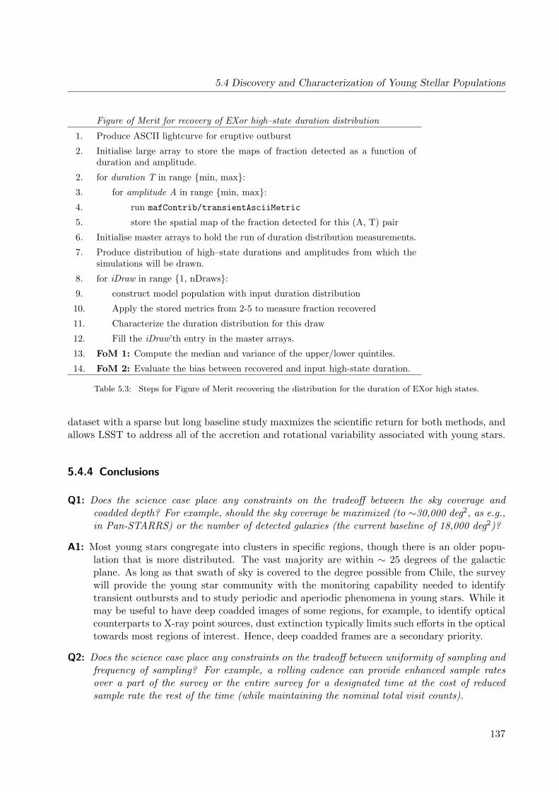
5.4 Discovery and Characterization of Young Stellar Populations

Figure of Merit for recovery of EXor high–state duration distribution

1. Produce ASCII lightcurve for eruptive outburst

2. Initialise large array to store the maps of fraction detected as a function ofduration and amplitude.

2. for duration T in range min, max:3. for amplitude A in range min, max:4. run mafContrib/transientAsciiMetric

5. store the spatial map of the fraction detected for this (A, T) pair

6. Initialise master arrays to hold the run of duration distribution measurements.

7. Produce distribution of high–state durations and amplitudes from which thesimulations will be drawn.

8. for iDraw in range 1, nDraws:9. construct model population with input duration distribution

10. Apply the stored metrics from 2-5 to measure fraction recovered

11. Characterize the duration distribution for this draw

12. Fill the iDraw’th entry in the master arrays.

13. FoM 1: Compute the median and variance of the upper/lower quintiles.

14. FoM 2: Evaluate the bias between recovered and input high-state duration.

Table 5.3: Steps for Figure of Merit recovering the distribution for the duration of EXor high states.

dataset with a sparse but long baseline study maxmizes the scientific return for both methods, andallows LSST to address all of the accretion and rotational variability associated with young stars.

5.4.4 Conclusions

Q1: Does the science case place any constraints on the tradeoff between the sky coverage andcoadded depth? For example, should the sky coverage be maximized (to ∼30,000 deg2, as e.g.,in Pan-STARRS) or the number of detected galaxies (the current baseline of 18,000 deg2)?

A1: Most young stars congregate into clusters in specific regions, though there is an older popu-lation that is more distributed. The vast majority are within ∼ 25 degrees of the galacticplane. As long as that swath of sky is covered to the degree possible from Chile, the surveywill provide the young star community with the monitoring capability needed to identifytransient outbursts and to study periodic and aperiodic phenomena in young stars. While itmay be useful to have deep coadded images of some regions, for example, to identify opticalcounterparts to X-ray point sources, dust extinction typically limits such efforts in the opticaltowards most regions of interest. Hence, deep coadded frames are a secondary priority.

Q2: Does the science case place any constraints on the tradeoff between uniformity of sampling andfrequency of sampling? For example, a rolling cadence can provide enhanced sample ratesover a part of the survey or the entire survey for a designated time at the cost of reducedsample rate the rest of the time (while maintaining the nominal total visit counts).

137

Chapter 5: Variable Objects

A2: We discussed cadences in some detail above. To obtain the best constraints on periods, atime-intensive (∼ one week/year) campaign on a few selected regions is warranted. Nominalcoverage over the galactic plane will suffice to identify eruptive variables.

Q3: Does the science case place any constraints on the tradeoff between the single-visit depth andthe number of visits (especially in the u-band where longer exposures would minimize theimpact of the readout noise)?

A3: This item is discussed in section A above. In young stars, the u-band is particularly usefulas a measure of accretion. At the same time, for period determinations, denser cadencesproduce fewer problems with aliasing for the typical young star variable with a rotationperiod between a day and two weeks.

Q4: Does the science case place any constraints on the Galactic plane coverage (spatial coverage,temporal sampling, visits per band)?

A4: A nominal sampling of once every few days will suffice to identify interesting eruptive variablesas long as the galactic plane coverage is good (item A1). However, a sparse temporal samplingsuch as this will make it difficult to interpret the lightcurves of the tens of thousands of TTauri stars observed by LSST. A single week’s campaign of dense sampling, e.g., 2-3 timesper night, of targeted regions will greatly improve our ability to separate periodic variablesfrom aperiodic ones. Knowing the rotation periods of thousands of young stars within a givenstar forming region will be a major contribution that LSST makes to this field of research.Such data will allow us to learn how angular momentum is distributed among newborn stars,whether it changes with mass and location in the cloud, and how it varies as the stars age.

Q5: Does the science case place any constraints on the fraction of observing time allocated to eachband?

A5: In the case we made above for dense sampling, we argued for z, r, and u. The u-band allowsus to follow mass accretion variability, while r and z (for most objects) will be dominated byphotospheric flux. The r-z color is an important constraint for models of star spots. Morecolors are always useful, but having a photospheric color index plus one accretion measureare the science drivers for filter choices. Once u, r, and z are observed, having higher cadencesis preferable to having more bands. The exposure times and magnitudes for typical objectsare described in section A above.

Q6: Does the science case place any constraints on the cadence for deep drilling fields?

A6: Absolutely. We argue in the ‘Summary and Recommendations’ section above for the advan-tages of a single week of denser monitoring for specific regions, with the goal of having severalobservations per night, separated in time by at least an hour from one another. The goalhere is to provide some basis in reality for interpreting the irregular lightcurves of youngstars, which also typically have a periodic component. Depending on the longevity of thestar spots, a period might be obvious in high-cadence data taken over a week, but disappearover a year if some spots vanish and others form.

Q7: Assuming two visits per night, would the science case benefit if they are obtained in the sameband or not?

138

5.5 Future Work

A7: If the data are taken in the same band it means better sampling for periods. With differentbands it means a lightcurve in two bands, which is also useful. It’s probably a wash, and wecan follow whatever the drivers are for the other science cases of LSST.

Q8: Will the case science benefit from a special cadence prescription during commissioning or earlyin the survey, such as: acquiring a full 10-year count of visits for a small area (either in allthe bands or in a selected set); a greatly enhanced cadence for a small area?

A8: Yes, definitely. We ought to see what we can get out of a dedicated week-long LSST cadenceon specific regions. If the results are impressive we follow up on different regions every year(or even return to the same regions).

Q9: Does the science case place any constraints on the sampling of observing conditions (e.g.,seeing, dark sky, airmass), possibly as a function of band, etc.?

A9: Better seeing helps with unresolved binaries and for regions where contamination comes intoplay, for example, in the plane but away from dark clouds. Some of the fainter objects willbe affected if the Moon is very bright and close. However generally these constraints areprobably in a “typical” category and will not affect the design of the survey.

Q10: Does the case have science drivers that would require real-time exposure time optimizationto obtain nearly constant single-visit limiting depth?

A10: No.

Go to: • the start of this section • the start of the chapter • the table of contents

5.5 Future Work

In this section we provide a short compendium of science cases that are either still being developed,or that are deserving of quantitative MAF analysis at some point in the future.

5.5.1 Discovery of Periodic Pulsating Variables

Lucianne Walkowicz, Stephen Ridgway

Regular variables, such as Cepheids and RR Lyraes, are valuable tracers of Galactic structure andcosmic distance. In this case of these and other strictly (or nearly-strictly) periodic variables, datafrom different cycles of observation can be phase-folded to create a more fully sampled lightcurveas LSST visits will occur effectively at random phases. In a 10-year survey, most periodic stars ofalmost any period will benefit from excellent phase coverage in all filters (only a very small periodrange close to the sidereal day will be poorly observed). Therefore, most implementations of theLSST observing strategy will provide good sampling of periodic variables.

However, different implementations of the survey may result in different resulting sample sizes ofthese periodic variables, and may also affect the environments in which these stars are discovered.In this section, we create a framework for understanding how current implementations of the

139

Chapter 5: Variable Objects

observing strategy influence (or even bias) the resultant sample size and environments where theseimportant tracers may be identified.

Tracing Galactic Structure with RR Lyrae

RR Lyrae variables are crucial tracers of structure in the Galaxy and beyond into the Local Group.The incredible sample of RR Lyrae anticipated from LSST observations will enable discovery ofGalactic tidal stream and neighboring dwarf galaxies throughout much of the Local Group (Ivezicet al. 2008). LSST also creates the possibility of detecting and studying RRL variables in theMagellenic Clouds; see Chapter [CHAPTER] for discussion.

Oluseyi et al. (2012) carried out an extensive simulation of period and lightcurve shape recoveryof RR Lyrae variables using an early OpSim run opsim1 29. Correctly identifying the periodaids in building the sample of interest, whereas fitting the lightcurve shape makes it possible tomeasure the metallicity of the star. In their simulation, they employed both a Fourier analysisand template matching to recover the lightcurve shape, finding that template matching yielded amore accurate lightcurve shape measurement in the presence of sparse data. The results of thissimulation showed that the vast majority of RR Lyrae will be discovered by the baseline observingstrategy (as deployed in opsim1 29) within 5 years of survey operations. Half of both RRLaband RRLc stars will be found out to ∼600 kpc and ∼250 kpc (respectively) by the end of the10-year main survey, and template matching techniques for lightcurve shape recovery will providemetallicities to ∼0.15dex.

The Cepheid Cosmic Distance Ladder

Classical cepheids remain an essential step in the cosmic distance ladder. Their calibration is basedlargely on LMC cepheids and known (assumed) distance of the LMC. The associated errors, whileuncertain, are believed to be of ∼7%. (Madore, Barry F.; Freedman, Wendy L. (2009). ”Con-cerning the Slope of the Cepheid Period?Luminosity Relation”. The Astrophysical Journal 696(2): 1498. arXiv:0902.3747. Bibcode:2009ApJ...696.1498M. doi:10.1088/0004-637X/696/2/1498.)New developments in galactic studies are poised to support substantially improved descriptive in-formation concerning nearby galactic cepheids, with possible substantial reductions in this error,by accurately securing the PL slope and zero point.

Cepheid calibration errors are associated in part with uncertainties in extinction, both interstel-lar and in some cases circumstellar, and in metalicity. At present, the direct, local calibrationof cepheids is limited by the availability of a few direct distance measurements, obtained withHST, with errors ∼10%. The GAIA mission is expected to return ∼9000 Galactic cepheids, ofall periods, colors and metallicities, with distance errors less than 10% (many of them much less)- Windmark, F.; Lindegren, L.; Hobbs, D., 2011A&A...530A..76W. It is expected to deliver atleast 1000 cepheids in the LMC with expected mean distance error ∼7-8% (Clementini (2010) -011EAS....45..267C). GAIA, as well as other methods, will also support determination of the 3-dmap of galactic interstellar extinction - including possible variations in the extinction law. Theserich data sets will be supported with direct measurements of cepheid diameters (A. Merand et al,

140

5.5 Future Work

A&A in press) and advances in stellar hydrodynamics (Mundprecht et al. 2013) which will pro-vide theoretical and empirical basis for calibrations to reconcile known physics with observationalcorrection factors.

Galactic cepheids will generally be too bright for LSST, but cepheids in the local group are suffi-ciently bright that LSST photometry will be limited by calibration errors rather than by brightness.This dataset will provide superb support for integration of GAIA-based galactic cepheid studieswith extra-galactic cepheid studies.

GAIA will provide similar precision data with the potential to identify or support distance determi-nations from many other galactic star types. LSST photometric catalogs will represent a uniquelyextensive and complete database for such investigations.

Metric Analysis

Several metrics currently exist in the MAF for evaluating how LSST survey strategy affect therecovery of periodic sources. For example, the PeriodicMetric makes use of the periodogrampurity function, which effectively quantifies aliasing introduced into periodogram analysis fromthe sampling of the lightcurve. Similarly, the phase gap metric (PhaseGapMetric), evaluates theperiodicity of the source lightcurve and its coverage in phase space (the latter being relevant forshape recovery).

Recreating the template matching results of the Oluseyi et al. (2012) simulation requires samplingspecific input lightcurves and comparing with the library of available shapes; this necessarilyrequires a step outside of the MAF, but can easily be enabled using the lightcurve simulation toolsunder development.

Current simulations of the main survey show a broad uniformity of visits, with thorough random-ization of visit phase per period, giving very good phase coverage with minimum phase gaps.

For periodic variable science, two cadence characteristics should be avoided:

• an exactly uniform spacing of visits (which is anyway virtually impossible);

• a very non-uniform distribution, such as most visits concentrated in a few survey years.

A metric for maximum phase gap will guard against the possibility that a very unusual cadencemight compromise the random sampling of periodic variables.

In each case, it would help to jump-start science programs if some fraction of targets had morecomplete measurements early in the survey.

5.5.2 Conclusions

Here we answer the ten questions posed in Sub-section 1.3.2:

Q1: Does the science case place any constraints on the tradeoff between the sky coverage andcoadded depth? For example, should the sky coverage be maximized (to ∼30,000 deg2, as e.g.,in Pan-STARRS) or the number of detected galaxies (the current baseline of 18,000 deg2)?

141

Chapter 5: Variable Objects

A1: No strong constraint - but see Q4.

Q2: Does the science case place any constraints on the tradeoff between uniformity of sampling andfrequency of sampling? For example, a rolling cadence can provide enhanced sample ratesover a part of the survey or the entire survey for a designated time at the cost of reducedsample rate the rest of the time (while maintaining the nominal total visit counts).

A2: An enhanced cadence could provide earlier discovery and period confirmation for a subset oftargets, but this is not a high priority.

Q3: Does the science case place any constraints on the tradeoff between the single-visit depth andthe number of visits (especially in the u-band where longer exposures would minimize theimpact of the readout noise)?

A3: No strong constraint.

Q4: Does the science case place any constraints on the Galactic plane coverage (spatial coverage,temporal sampling, visits per band)?

A4: Most stars are in the galactic plane. For periodic pulsators, it is desirable to obtain multiplevisits in all filters, with at least 20-50 epochs in several filters. Obtaining this coverage ismore important to periodic pulsator science than greater sky coverage.

Q5: Does the science case place any constraints on the fraction of observing time allocated to eachband?

A5: No strong constraint, as long as there is a good representation of each, including u.

Q6: Does the science case place any constraints on the cadence for deep drilling fields?

A6: For deep drilling on the galaxy or nearby galaxies, the best cadences would cover a range ofperiods from minutes to days - longer periods would be satisfactorily sampled by the mainsurvey.

Q7: Assuming two visits per night, would the science case benefit if they are obtained in the sameband or not?

A7: Different bands would provide more rapid characterization of targets, but this is not a strongbenefit.

Q8: Will the case science benefit from a special cadence prescription during commissioning or earlyin the survey, such as: acquiring a full 10-year count of visits for a small area (either in allthe bands or in a selected set); a greatly enhanced cadence for a small area?

A8: Enhanced cadences could provide earlier science, or somewhat deeper science, depending ondetails, but periodic variables are not a strong driver for this.

Q9: Does the science case place any constraints on the sampling of observing conditions (e.g.,seeing, dark sky, airmass), possibly as a function of band, etc.?

A9: No constraints that are particular to variable stars.

Q10: Does the case have science drivers that would require real-time exposure time optimizationto obtain nearly constant single-visit limiting depth?

142

5.5 Future Work

A10: No.

Go to: • the start of this section • the start of the chapter • the table of contents

5.5.3 Probing Planet Populations with LSST

Michael B. Lund, Avi Shporer, Keivan Stassun

This section describes the unique discovery space for extrasolar planets with LSST, namely, planetsin relatively unexplored environments.

A large number of exoplanets have been discovered over the past few decades, with over 1500exoplanets now confirmed. These discoveries are primarily the result of two detection methods:The radial velocity (RV) method where the planet’s minimum mass is measured, and the transitmethod where the planet radius is measured and RV follow-up allows the measurement of theplanet’s mass and hence mean density. Other methods are currently being developed and use todiscover an increasing number of planets, including the microlensing method and direct imaging.In addition, the Gaia mission is expected to discover a large number of planets using astrometry(Perryman 2014).

The Kepler mission has an additional almost 4000 planet candidates. While these planet candi-dates have not been confirmed, the sample is significant enough that planet characteristics can bestudied statistically, including radius and period distributions and planet occurrence rates. LSSTwill extend previous transiting planet searches by observing stellar populations that have generallynot been well-studied by previous transiting planet searches, including star clusters, the galacticbulge, red dwarfs, white dwarfs (see below), and the Magellanic Clouds (see Sub-section 7.2.2).Most known exoplanets have been found relatively nearby, as exoplanet systems with measureddistances have a median distance of around 80 pc, and 80% of these systems are within 320 pc (ex-oplanets.org). LSST is able to recover transiting exoplanets at much larger distances, including inthe galactic bulge and the Large Magellanic Cloud, allowing for measurements of planet occurrencerates in these other stellar environments (Lund et al. 2015; Jacklin et al. 2015). Red dwarfs haveoften been underrepresented in searches that have focused on solar-mass stars, however red dwarfsare plentiful, and better than 1 in 7 are expected to host earth-sized planets in the habitable zone(Dressing & Charbonneau 2015).

Another currently unexplored environment where LSST will be able to probe the exoplanet pop-ulation is planets orbiting white dwarfs (WDs). Such systems teach us about the future evolutionof planetary systems with main-sequence primaries, including that of the Solar System. Whena WD is eclipsed by a planet (or any other faint low-mass object, including a brown dwarf ora small star) the radius and temperature ratios lead to a very deep eclipse, possibly a completeoccultation, where during eclipse the target can drop below the detection threshold. The existenceof planets orbiting WDs has been suggested observationally (e.g., Farihi et al. 2009; Jura et al.2009; Zuckerman et al. 2010; Debes et al. 2012). and theoretically (e.g., Nordhaus et al. 2010).A few brown dwarf companions were already discovered (e.g., Maxted et al. 2006; Casewell et al.2012; Littlefair et al. 2006, 2014), and Vanderburg et al. (2015) recently discovered a disintegratingplanetary body orbiting a WD (see also Croll et al. 2015; Gansicke et al. 2016; Rappaport et al.2016).

143

Chapter 5: Variable Objects

While most of the sky that LSST will survey will be at much lower cadences than transitingplanet searches employ, a sufficient understanding of the LSST efficiency for detecting planetscombined with the large number of targets may still provide significant results. Additionally, themultiband nature of LSST provides an extra benefit, as exoplanet transits are achromatic whilemany potential astrophysical false positives, such as binary stars, are not. Indeed, as demonstratedby Lund et al. (2015), the multi-band LSST light curves can likely be combined to create mergedlight curves with denser sampling and effectively higher cadence, enabling detection of transitingexoplanets. The deep-drilling fields in particular should prove to be a rich trove of transitingexoplanet detections, with transit-period recoverability rates as high as ∼50% or more among HotJupiters around solar-type stars out to distances of many kpc and even the Magellanic Clouds insome cases (Lund et al. 2015; Jacklin et al. 2015). Yields may be expected perhaps as early asthe third year of LSST operations (Jacklin et al., in prep). The ability to detect transiting planetsoutside of the deep-drilling fields is less certain; here the details of the cadence among the variouspassbands will likely be particularly important to assess carefully.

5.5.4 Metrics

The detection of transiting planets will be dependent on having observations that will providesufficient phase coverage for transiting planets, with periods that can range from less than one dayup to tens of days. In order to address this range of periods, an initial metric that can be usedto address the detection of transiting planets is the Periodogram Purity Function, discussed morethoroughly in Section 5.2.1.

5.5.5 Discussion

In general, the detection of transiting exoplanets with LSST will rely on a small subset of potentiallydetectable planets that can be sufficiently separated from statistical noise, rather than a clearthreshold in a planet’s properties that would distinguish detectable planets vs. nondetectableplanets. This will mean that the best calculation of planet yields will have to come from simulationsof light curves for large numbers of stellar systems in order to characterize LSST. The computationtime involved in this process is sufficiently prohibitive to prevent a metric being developed baseddirectly on these simulated light curves, however future work may be able to map relationshipsbetween metric values for individual fields and the corresponding numbers of planets that can bedetected.

5.5.6 Conclusions

Q1: Does the science case place any constraints on the tradeoff between the sky coverage andcoadded depth? For example, should the sky coverage be maximized (to ∼30,000 deg2, as e.g.,in Pan-STARRS) or the number of detected galaxies (the current baseline of 18,000 deg2)?

A1: Longer time series and more data points per star are more valuable than greater sky coverage.

144

5.5 Future Work

Q2: Does the science case place any constraints on the tradeoff between uniformity of sampling andfrequency of sampling? For example, a rolling cadence can provide enhanced sample ratesover a part of the survey or the entire survey for a designated time at the cost of reducedsample rate the rest of the time (while maintaining the nominal total visit counts).

A2: Cadences suitable for transit timescales (hours-days) are very useful, and complementary tostandard longer timescale cadence.

Q3: Does the science case place any constraints on the tradeoff between the single-visit depth andthe number of visits (especially in the u-band where longer exposures would minimize theimpact of the readout noise)?

A3: Number of visits is most valuable.

Q4: Does the science case place any constraints on the Galactic plane coverage (spatial coverage,temporal sampling, visits per band)?

A4: Most planets will be identified in galactic plane fields. Long visit sequences to rich stellarfields may be productive, if crowding and flux contamination can be managed.

Q5: Does the science case place any constraints on the fraction of observing time allocated to eachband?

A5: No strong constraint, but multiple bands care needed to test for achromatism.

Q6: Does the science case place any constraints on the cadence for deep drilling fields?

A6: Only applicable for deep drilling in the galaxy or local group - cadences that sample transittimescales (hours-days) are complementary to long, sparse time series from the main survey.

Q7: Assuming two visits per night, would the science case benefit if they are obtained in the sameband or not?

A7: No strong preference.

Q8: Will the case science benefit from a special cadence prescription during commissioning or earlyin the survey, such as: acquiring a full 10-year count of visits for a small area (either in allthe bands or in a selected set); a greatly enhanced cadence for a small area?

A8: A mix of cadence types, including a greatly enhance cadence, in a rich stellar field, would serveto evaluate different cadences and to test the photometric performance in crowded fields.

Q9: Does the science case place any constraints on the sampling of observing conditions (e.g.,seeing, dark sky, airmass), possibly as a function of band, etc.?

A9: None unique to planets.

Q10: Does the case have science drivers that would require real-time exposure time optimizationto obtain nearly constant single-visit limiting depth?

A10: No.

Go to: • the start of this section • the start of the chapter • the table of contents

145

6 Eruptive and Explosive Transients

Chapter editors: Eric C. Bellm, Federica B. Bianco

Contributing Authors:

Iair Arcavi, Laura Chomiuk, Zoheyr Doctor, Wen-fai Fong, Zoltan Haiman, Vassiliki Kalogera,Ashish Mahabal, Raffaella Margutti, Tom Matheson, Stephen Ridgway, Ohad Shemmer, Nathan Smith,Paula Szkody, Virginia Trimble, Stefano Valenti, Bevin Ashley Zauderer

6.1 Introduction

Explosive and eruptive transients are physically and phenomenologically diverse. What theseevents share are rare, large-amplitude deviations from a quiescent state. These outbursts aretypically unpredictable and of limited duration, and so their discovery and characterization aresensitive to the detailed observing strategy. Often, followup observations with other facilities canprovide significant additional scientific value, but this creates a challenge to identify candidateevents while they are still visible.

Transients such as novae, supernovae (SNe), and long gamma-ray bursts (GRBs) probe the finalstages of stellar evolution. Tidal Disruption Events (TDEs), short GRBs, and Cataclysmic Vari-ables (CVs) give us the opportunity to study compact and binary objects. Massive star eruptionsallow us to understand mass loss mechanisms and chemical enrichment. The brightest transients(GRBs, TDEs, SNe) are light beams that can be seen over cosmic distances, and some transients—most notably Type Ia SNe—are cosmological tracers. In this chapter we focus on LSST’s potentialto advance the astrophysics of eruptive and explosive transients; the use of SNe for cosmology isdiscussed in Chapter 9. Transients in the Milky Way Disk are discussed in more detail in Chapter 4.

Cadence choices will determine LSST’s ability to discover, classify, and characterize these events.However, due to their different time scales, different phenomena will benefit from different sam-pling strategies—sometimes significantly different, and at times orthogonal. Competing objectivesdescribed in this chapter are at the heart of LSST’s observing strategy and cadence design.

When evaluating a particular observation or series of observations in light of how they perform fora specific science case, it may be helpful to think of metrics as lying along a continuum betweendiscovery and characterization. Discovery requires a minimum amount of information to recognizean event or object as a candidate of interest. It is particulary relevant for science cases that requiretriggering followup resources in real time from the live event stream.

147

Chapter 6: Transients

Characterization, on the other hand, implies that basic properties of the event may be determinedfrom the LSST observations, including but not limited to the classification of the event. It isparticular relevant for science cases requiring analysis of large samples of completed lightcurves.

Characterization and classification of transient events benefits from substantial temporal samplingover the finite duration of the event along with color information (perhaps contemporaneous).Transient events slower than ∼ weeks may be adequately sampled by a uniform LSST cadence.Obtaining adequate sampling for faster-evolving events may require special scheduling strategies.For some event types, LSST can only be expected to provide a discovery service, and followupwill necessarily be performed elsewhere—so long as the cadence is sufficient to identify the eventtype. For some events, such as detecting electromagnetic counterparts to gravitational wave events(GWs), serendipitous discoveries are unlikely, but enabling a ToO program would provide theopportunity for LSST to contribute significantly to this science.

We consider a non-exhaustive set of “astronomical transients” in the paragraphs that follow. Fora few of these transients, we quantify the ability of LSST cadences to produce data useful forvarious science goals. These case studies include SNe, GRBs, and GWs. For other transientfamilies (Novae, LBVs, TDEs) we provide more general information in Section 6.6, and we invitethe community to further develop the ideas proposed here, as well as further other related goals,into quantified science cases.

6.1.1 Targets and Measurements

Table 6.1 is a non-exhaustive list of phenomena to which we are referring as eruptive and explosivetransients in this document.

10−2 10−1 100 101 102

−30

−25

−20

−15

−10

−5

Characteristic Timescale [day]

Peak

Lum

inos

ity [M

V]

PTF11agg

iPTF13dsw

iPTF13bxl

iPTF14ybiPTF13ekl

iPTF14aue

iPTF14bfu

iPTF14cvaiPTF14cyb

Thermonuclear Supernovae

Classical Novae

Luminous Red Novae

Intermediate Luminosity Red Transients

Core−Collapse Supernovae

Luminous Supernovae Relativistic Explosions

.Ia Explosions

Calcium−rich Gap Transients

1038

1040

1042

1044

1046

Peak

Lum

inos

ity [e

rg s−1

]

Figure 6.1: Peak luminosity-characteristic decay timescale plot for explosive transients (adapted from Kasliwal2011).

148

6.1 Introduction

Transient Type Science drivers Amplitude Time Scale EventRate

Flare stars Flare frequency, en-ergy, stellar age, spaceweather

large min verycommon

X-ray Novae Interacting binaries,stellar evolution, SNprogenitors, nuclearphysics

large weeks rare

Cataclysmic variables(6.6.3)

Interacting binaries,stellar evolution, com-pact objects

large min - days common

LBV variability (6.6.5) Late stages stellar evo-lution, Mass loss, SNprogenitors

large weeks-years rare

Massive star eruptions(6.6.5)

Late stages stellar evo-lution, Mass loss, SNprogenitors

extreme weeks-years rare

Supernovae (6.3) stellar evolution, feed-back, chemical enrich-ment, cosmology

extreme days - months verycommon

GRBs (6.4) jet physics, SN connec-tion, stellar evolution

extreme min - days rare (op-tical dis-covery)

TDEs (6.6.1) Massive BH demo-graphics, accretionphysics

large weeks-months very rare

LIGO detections (GW,6.5)

EM characterization unknown unknown very rare

Unknown Discovery unknown unknown rare

Table 6.1: Overiew of major types of optical transients. Common events have hundreds or thousands of exemplars,while rare event classes have only a few or tens.

149

Chapter 6: Transients

6.1.2 Transient time scales

Optical transients display a wide range of intrinsic timescales (Figure 6.1), and even some long-livedevents have short-duration features of interest.

For very short-lived phenomena (stellar flares, GRBs), the main function of LSST will be to providediscoveries and/or simple characterization. Followup to discovery/identification, if required, musttake place elsewhere. This implies that the LSST observations must be sufficient to recognize in realtime that an event is fast-evolving in order to to trigger followup. However, assessing the rise slopeis best done with a single filter, because when observing with different filters it is very difficultto separate lightcurve evolution from color variations. Colors are informative when consideringstatistical samples (Section 6.3) as long as the epoch of peak can be reliably determined.

SNe fall in an intermediate time range. LSST will provide multiple visits in multiple filters duringthe typical SN duration (months). This sampling may still be insufficient for many science ob-jectives, such as photometric classification of SN subtypes. However, moderate changes to LSSTobserving strategy may enhance the sampling for part of the sky part of the time, greatly improv-ing the usefulness of SN observations. Metrics that assess the discovery rate of SN are included inChapter 9. Here we are interested in assessing the ability of LSST to discriminate SN from othertransients, SN subtypes from one another, and to identify particularly interesting SNe: for exam-ple those that show signature of shock break-out, companion interaction in the early light curve,or would be candidates for flash spectroscopy follow-up (e.g., Gal-Yam et al. 2014). In addition,metrics that quantify LSST’s ability to constrain SN physics in a statistically large sample of SNare needed.

TDEs have only recently started to be characterized in the optical bands. The current sample ofevents show relatively long time-scales (rise and decline of the light curve is over months). Wewould like to assess through metrics how well TDEs can be distinguished from supernovae basedon their light curve shape and color (in real-time so that followup observations can be triggered)and how well the LSST light curves themselves can be used to model the TDE emission and deducethe black hole properties.

Large amplitude flares from AGN may mimic explosive transients; they are discussed in Chapter 8.

In addition we hope that LSST will provide a wealth of serendipitous discoveries of yet-to-be-observed transients. An ideal transient discovery survey would include balanced coverage of alltime scales. LSST will cover longer time periods well, but will have to make some choices ofemphasis in coverage of shorter time-scales.

In the sections that follow we will use several case studies to assess LSST’s performance for a rangeof time-domain science:

• The ability of a given LSST cadence to discriminate truly young transients from those onlyfirst detected well after their explosion date (Section 6.2). This ability is a crucial input tofollow-up strategy design. We identify a region of lightcurve slope that is characteristic of avariety of transients in their early phases and assess the ability of LSST’s cadences to placetransients within this phase-space. More sophisticated classification algorithms will likely benecessary, but are beyond the scope of this whitepaper.

150

6.1 Introduction

• The statistical constraints to a transient class that can be obtained over the course of theLSST survey, from the LSST survey data alone (assuming a successful classification). Wediscuss SN Ia early interaction signatures and IIb shock break-out (Section 6.3).

• The ability to identify in real-time a rapidly-evolving object of interest and trigger promptfollow-up observations. For this topic GRBs are used as a case study (Section 6.4).

• The value of triggered Target-of-Opportunity observations for following up very rare, fast-evolving events. Here the kilonova counterparts expected from Advanced LIGO triggers areused as a case study (Section 6.5).

• The insight that a cadence gives into single transient classes. We discuss CVs, massive stareruptions, and TDEs (Section 6.6).

6.1.3 Metrics

Two metrics were developed and are used in this chapter specifically for transient phenomena:

• transientAsciiMetric : accepts an ASCII file in input, so that realistic transient shapescan be used, with different shapes for different filters. The output can be the series of LSSTobservations (magnitude and error), or the fraction of transients detected (with user-specifiedconstraints). This metric is used in Section 6.3.

• GRBTransientMetric : calculates the fraction of GRB-like transients detected (with user-specified constraints) using an F (t) ∝ t−α lightcurve. This metric is used in Section 6.4.

Additionally, the standard MAF metrics that quantify the gaps between consecutive visits to a fieldwithin a night and over multiple nights (IntraNightGapsMetric and InterNightGapsMetric )are of great value and are heavily used throughout this chapter, in Section 6.2, Section 6.3,and Section 6.5 for example. These quantify the median times between consecutive visits to a fieldwithin one night and over multiple nights, respectively.

Further metrics relevant to transient science are discused in Chapter 4, Chapter 9, and Chapter 5.

Many science cases can be developed and tested with these metrics, and we encourage users todo so. In addition, we are collecting a library of representative transient lightcurves in a separateGitHub repository1 and we encourage readers to contribute their transient models or observations.

6.1.4 OpSim Analysis

The current set of simulated cadences provide poor coverage in any one filter for transient eventslonger than a visit pair (∼30 minutes) and shorter than ∼ weeks (Figure 6.2 and Figure 6.3;Table 6.2).

As discussed in the subsequent sections, this gap in the sampling hinders characterization of fast-evolving transients. A cadence with two visits separated by an hour or two rather than 20 minuteswould provide better discrimination. A third visit in the same night in a different filter would

1https://github.com/LSSTTVS/LSST_TVS_RoadMap

151

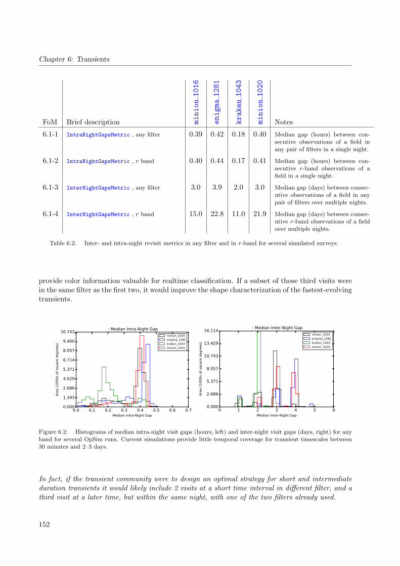
Chapter 6: Transients

FoM Brief description minion1016

enigma1281

kraken1043

minion1020

Notes

6.1-1 IntraNightGapsMetric , any filter 0.39 0.42 0.18 0.40 Median gap (hours) between con-secutive observations of a field inany pair of filters in a single night.

6.1-2 IntraNightGapsMetric , r band 0.40 0.44 0.17 0.41 Median gap (hours) between con-secutive r-band observations of afield in a single night.

6.1-3 InterNightGapsMetric , any filter 3.0 3.9 2.0 3.0 Median gap (days) between consec-utive observations of a field in anypair of filters over multiple nights.

6.1-4 InterNightGapsMetric , r band 15.0 22.8 11.0 21.9 Median gap (days) between consec-utive r-band observations of a fieldover multiple nights.

Table 6.2: Inter- and intra-night revisit metrics in any filter and in r-band for several simulated surveys.

provide color information valuable for realtime classification. If a subset of those third visits werein the same filter as the first two, it would improve the shape characterization of the fastest-evolvingtransients.

Figure 6.2: Histograms of median intra-night visit gaps (hours, left) and inter-night visit gaps (days, right) for anyband for several OpSim runs. Current simulations provide little temporal coverage for transient timescales between30 minutes and 2–3 days.

In fact, if the transient community were to design an optimal strategy for short and intermediateduration transients it would likely include 2 visits at a short time interval in different filter, and athird visit at a later time, but within the same night, with one of the two filters already used.

152

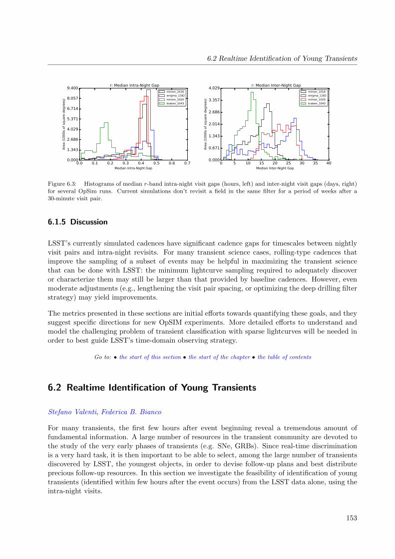
6.2 Realtime Identification of Young Transients

Figure 6.3: Histograms of median r-band intra-night visit gaps (hours, left) and inter-night visit gaps (days, right)for several OpSim runs. Current simulations don’t revisit a field in the same filter for a period of weeks after a30-minute visit pair.

6.1.5 Discussion

LSST’s currently simulated cadences have significant cadence gaps for timescales between nightlyvisit pairs and intra-night revisits. For many transient science cases, rolling-type cadences thatimprove the sampling of a subset of events may be helpful in maximizing the transient sciencethat can be done with LSST: the minimum lightcurve sampling required to adequately discoveror characterize them may still be larger than that provided by baseline cadences. However, evenmoderate adjustments (e.g., lengthening the visit pair spacing, or optimizing the deep drilling filterstrategy) may yield improvements.

The metrics presented in these sections are initial efforts towards quantifying these goals, and theysuggest specific directions for new OpSIM experiments. More detailed efforts to understand andmodel the challenging problem of transient classification with sparse lightcurves will be needed inorder to best guide LSST’s time-domain observing strategy.

Go to: • the start of this section • the start of the chapter • the table of contents

6.2 Realtime Identification of Young Transients

Stefano Valenti, Federica B. Bianco

For many transients, the first few hours after event beginning reveal a tremendous amount offundamental information. A large number of resources in the transient community are devoted tothe study of the very early phases of transients (e.g. SNe, GRBs). Since real-time discriminationis a very hard task, it is then important to be able to select, among the large number of transientsdiscovered by LSST, the youngest objects, in order to devise follow-up plans and best distributeprecious follow-up resources. In this section we investigate the feasibility of identification of youngtransients (identified within few hours after the event occurs) from the LSST data alone, using theintra-night visits.

153

Chapter 6: Transients

The Baseline Cadence minion 1016 predicts that, on average, fields in the main survey are revis-ited every ∼ 3 days in any filter (Figure 2.8), and every ∼ 15 days when using only r band visits(Figure 2.9). Hence, we are most likely to discover faint transients that are within 3 days of peakbrightness. However, for the small subset of nearby events, we can hope to discover them withina few days of explosion. The challenge is to discriminate these truly young events from newly-discovered SN that are near peak brightness. Within the minion 1016 cadence, and most cadencesrealized thus far, the second intra-night visit occurs around 30 minutes (left panel of Figure 6.3).after the first visit (to maximize the Solar System moving objects recovery, Chapter 3). We want tounderstand how the intra-night gap enables, affects, and can be used to maximize the identificationof new transients as young , where, by young, we mean within a day of outburst/explosion.

To begin to answer this question, we limit our investigation to light curve shape in just the r band,and specifically to what can be done in r band. We have selected a representative set of transientswith good photometric coverage in the first week after the the outburst/explosion (left panel ofFigure 6.4) and computed the light curve slope as a function of time in magnitudes per day (rightpanel of Figure 6.4). In Figure 6.5 we report the change in r brightness between the first andthe second visit for the same set of transients as function of phase. The similarity matrices inFigure 6.6 represent the distance in this quantity for each transient pair for time gaps betweenobservations ranging between 30 minutes and 24 hours.

Despite the heterogeneity in light curve shapes, most of the transients show a similar change inbrightness on short time scales. This confirms that early classification of the transient sub-type isa major challenge. However, since in general young transients show a fast increase in brightness,it is much easier to assess whether a transient is young. Simply put, young transients will showa much larger brightness change between visits than old events. This discrimination is aided bya larger time gap between visits (e.g. 2 hours). Within 30 minutes the change in brightness is ofthe order of 1%, or even less, for most transients even within the first ∼ 3 days from the startof the outburst/explosion (Figure 6.4, left). Thus a measurement of the change would requirea SNR & 500 on each measurement. Longer gaps give us more leverage: with a time gap of∼ 2 hours after the first visit, the change of brightness will increase to ∼ 5%. However the breadthof the gap is not unlimited: a gap of 24 hours imposes a significant delay in triggering follow upfor these fast-evolving events.

A natural metric to compare cadences for this purpose is the median time difference between thefirst and last observations of a field each night. This differs from the IntraNightGapsMetric , asthe latter only compares consecutive observations of a field and hence underestimates the nightlytime baseline when there are three or more observations of a field in a night.

The classification of interesting transients, at an early stage, can be aided by using supplementaryinformation, such as historical information from previous visits, and by color information about thetransient. But to properly assess the color of an evolving transient, the gap between observationsin different filters should not exceed a few hours (Section 6.3).

Finally, we stress that the quality and completeness of early multiwavelengh data available atthis time is limited. The sample of astronomical transients used here is not comprehensive, and auniform set of homogeneous data of different transients is still needed in order to further investigatethe ideal separation between observations, the need for color information, and the tension betweenthe two.

154

6.2 Realtime Identification of Young Transients

In the light of these considerations, we recommend the simulation of a cadence with three visitsper field, per night, two in the same band, but spaced by two hours or more, and a third in adifferent band. This criteria could be limited to the extragalactic sky, away from both the eclipticplane and the galactic plane, where recovery of Solar System objects puts less strain on the cadencerequirements. The current 3-visit OpSim run (enigma 1281) is inadequate since it does notinclude the constraint of one visit being in a different filter.

Furthermore, we note that the currently envisioned deep drilling cadence prioritizes depth per visitat the expense of a higher cadence. One hour per night on a deep drilling field reaches a depth thatnot required for almost all transient science cases, and by cycling to a different field each night, thetime between visits for a particular field (4-5 days) is too long for many important science cases.Even with higher overhead, a more useful approach for nearly all transient science, that the deepdrilling fields are designed to facilitate, would be to observe three or four of the available fields eachnight for 15 or 20 minutes.

Figure 6.4: Left : r′-band light curve for representative transients as function of the phase from the beginning of thetransient outburst/explosion for the first few days of the transient life. Right : slope of the transient evolution. Datafrom: SN Ia, Olling et al. (2015); SNII, Rubin et al. (2016); SN .Ia, Shen et al. (2010); SN Ib, Valenti et al. (2011), Caoet al. (2013); SN Ic, Mazzali et al. (2002); CV, Sokoloski et al. (2013), Finzell et al. (in prep), SN Ia+interaction(see Section 6.3).

6.2.1 Conclusions

Here we answer the ten questions posed in Sub-section 1.3.2:

Q1: Does the science case place any constraints on the tradeoff between the sky coverage andcoadded depth? For example, should the sky coverage be maximized (to ∼30,000 deg2, as e.g.,in Pan-STARRS) or the number of detected galaxies (the current baseline of 18,000 deg2)?

A1: No strong constraint, as long as larger sky coverage does not compete with dense cadencesrequired for fast transients.

155

Chapter 6: Transients

0 2 4 6 8 10Days after explosion

0.15

0.10

0.05

0.00

0.05

∆m

ag

30 minutes

SN Ia

SN Ic

SN Ib

SN Ib

SN II

SN II

SN II

CV

CV

CV

.Ia

.Ia

Ia+shock

0 2 4 6 8 10Days after explosion

0.15

0.10

0.05

0.00

0.05

∆m

ag

2 hours

0 2 4 6 8 10Days after explosion

1.0

0.8

0.6

0.4

0.2

0.0

0.2

∆m

ag

24 hours

Figure 6.5: Observed magnitude change between two consecutive observations for a representative set of astronomicaltransients, as a function of the phase. We consider observation gaps of 30 minutes (left panel), 2 hours (central panel)and 24 hours (right panel).

Q2: Does the science case place any constraints on the tradeoff between uniformity of sampling andfrequency of sampling? For example, a rolling cadence can provide enhanced sample ratesover a part of the survey or the entire survey for a designated time at the cost of reducedsample rate the rest of the time (while maintaining the nominal total visit counts).

A2: Frequency of sampling is far more important than uniformity of sampling for early classifi-cation of interesting cadence. The rolling cadence is definitely the first step to take, but itis still not enough to identify young transients. A longer than .4 hours intra-night gap or,even better a one day cadence would allow young transients to vary enough to be identified.If the second visit occurs on 0.4-hour time scale, a different filter would be preferred (colorinformation can be alternatively used to identify young transients)

Q3: Does the science case place any constraints on the tradeoff between the single-visit depth andthe number of visits (especially in the u-band where longer exposures would minimize theimpact of the readout noise)?

A3: Anything that reduces the number of visits per field potentially compromises the objectives.

Q4: Does the science case place any constraints on the Galactic plane coverage (spatial coverage,temporal sampling, visits per band)?

A4: The requirement for multiple visits/filters per night applies to all fields.

Q5: Does the science case place any constraints on the fraction of observing time allocated to eachband?

A5: No.

Q6: Does the science case place any constraints on the cadence for deep drilling fields?

A6: As discussed in detail above, short bursts of visits separated by several days is not satisfactory- deep drilling cadences can be devised to provide excellent sampling.

156

6.2 Realtime Identification of Young Transients

Figure 6.6: Similarity matrix of the transients in Figure 6.4 and Figure 6.5 in r filter for time gaps (starting withthe top left panel) of 0.5, 2, 5, and 24 hours. The similarity is measured as the Euclidean distance between themagnitude change of each transient’s pair and it is represented in log scale, with darker colors indicating a largerdistance (to a maximum difference |∆Mag1 −∆Mag2| ∼ 8). For each transient’s pair the similarity is calculatedfor 8 phases within the life of the transients, with the first observation starting at explosion, and as late as 3.5 daysafter explosion, in 12 hour increments, thus 8 values are associated to each transient pair (as indicated by the tickmarkers).

Q7: Assuming two visits per night, would the science case benefit if they are obtained in the sameband or not?

A7: If two visits only, different filters may be the most effective. If more than two visits, the mostclosely spaced pair should be in the same filter, and the other visits should include at leastone other filter.

Q8: Will the case science benefit from a special cadence prescription during commissioning or earlyin the survey, such as: acquiring a full 10-year count of visits for a small area (either in allthe bands or in a selected set); a greatly enhanced cadence for a small area?

A8: A greatly enhanced cadence would provide a strong test of the methodology and would jump-start the science.

157

Chapter 6: Transients

Q9: Does the science case place any constraints on the sampling of observing conditions (e.g.,seeing, dark sky, airmass), possibly as a function of band, etc.?

A9: None unique to transients.

Q10: Does the case have science drivers that would require real-time exposure time optimizationto obtain nearly constant single-visit limiting depth?

A10: No.

Go to: • the start of this section • the start of the chapter • the table of contents

6.3 Supernovae as Transients

Federica B. Bianco

Supernovae (SNe) represent the final dramatic stages of the life of many stars. The term SN coversa diverse set of phenomena: explosion of low mass stars in binary systems, thermonuclear SNor SN Ia (also discussed in Section 9.5), explosions of high mass stars, core collapse (CC) SNe,and even terminal explosions of more exotic systems, yet to be understood, like Super LuminousSNe (SLSNe). Phenomenologically, the observables of the explosion are also diverse. The transientduration ranges from weeks to months and even years. The electromagnetic energy radiated rangesbetween ∼ 0.1 (faintest CC SNe), to ∼ 1 (SN Ia) and ∼ 100 (SLSNe) ×1049 erg, corresponding toabsolute magnitudes at peak ranging between ∼ −19 and ∼ −22.

LSST’s contribution to SNe studies can be substantial. Synoptic surveys such as SDSS, SNLS,PTF, PanSTARRS have revolutionized our understanding of SN time and again, exposing theirdiversity, and revealing different progenitor channels. LSST’s first crucial input will be discovery:the normal type Ia SN rate out to redshift z = 1 is estimated to be ∼ 200 (sq.deg.)−1 per year2,and SN Ia represent only about 1/4 of all SN events (Li et al. 2011b): tens of millions of starswill explode within the LSST footprint every year. The main factors affecting LSST SN scienceconcern:

1. LSST’s SN discovery power,

2. LSST’s discrimination power,

3. the quality of the statistical sample over time.

Items 1 and 2 are time sensitive, while the latter is not, although it is interesting to understandthe pace at which a science question can be advanced in the lifetime of LSST.

Discovery: the SN Ia discovery is rate is a standard LSST time-domain metric: a fraction of∼ 40% SN Ia z . 0.5 are expected to be discovered pre-peak luminosity within the standard LSSTsurvey (e.g. minion 1016 Figure 2.11). The topic of SNe discovery is discussed in further detailin Section 9.5.

2http://www.lsst.org/sites/default/files/docs/Wood-Vasey_086.11.pdf

158

6.3 Supernovae as Transients

The next step is then discrimination, and the question we need to answer, for SNe as well as for mostother transients, is: will LSST photometry allow us to distinguish SN from other transients, and todistinguish the different types of SN? And further: will this be achievable in time to appropriatelydirect follow-up efforts? This is particularly difficult considering that photometric classificationschemes have only achieved modest performances in distinguishing, for example, SN Ic from SN Ia.

When a large statistical sample of SNe is generated, LSST’s photometry may allow setting con-straints on the diversity of the sample, even as a standalone survey, without the aid of follow-upefforts. Thus LSST alone can shed light on the diversity within the population of SN,which in turn may constrain the genesis of the explosion.3 For SN Ia, where the exploding star isa carbon-oxygen White Dwarf (WD), a major outstanding question that can be answered by anLSST photometric sample is what is the percentage of SN Ia that arise from a double-degenerate(DD) progenitor system (a carbon-oxygen WD-WD binary), from a single-degenerate (SD) system(a WD-Main Sequence or WD-Red Giant (RG) binary), or from a merger (a WD-WD binary witha He and a carbon-oxygen WD). Answering this question would reduce the scatter in the Hubblediagram if SNe from different progenitors are shown to require different standardization (Scolnicet al. 2014). On the CC SN side: the diversity of SN sub-classes, and the relationship betweenthem (is there a phenomenological continuum or are they actually distinct classes, e.g. betweenIIp and IIL, or Ib and IIb?) is yet to be understood. Exceptionally well-studied objects mayanswer these questions: individual SN Ia with tight constraints on the progenitor system show, forexample, that both single and double degenerate progenitors exist (e.g. SN 2011fe, Li et al. 2011a,Olling et al. 2015 and PTF 11kx, Dilday et al. 2012). However, a statistical sample is needed toset constraints on populations (Hayden et al. 2010; Bianco et al. 2011).

Thus the technical question to be answered is: how much detail can be sacrificed in favor ofsample size without compromising diagnostic power? And the diagnostic power relies on color andsampling: thus what is the trade-off between cadence in the same filter, and observations in differentfilters. Specifically, transients can be distinguished early from two photometric characteristics:rise time and color. There is a tension between these observables, as discussed in Section 6.2.Obtaining colors relies of course on obtaining photometry in different bands as close as possibleto simultaneously. However, assessing the rise slope is best done with a single filter, so promptcharacterization also needs multiple epochs within a night, although separated by at least a fewhours, in the same filter, as observing with different filters it is impossible (or very hard) to separateshape from color. Colors are an important diagnostic for the statistical sample: as long as theepoch of peak is reliably assessed coadded light curves can be studied, which is the goal of theanalysis that follows.

6.3.1 Distinguishing progenitor scenarios

In this chapter we envision and design a SN related metric that works on a large sample (months-to-years of LSST data) and assesses the ability to characterize the contribution of SNe with specificfeatures to the global population: as a test case we will use the identification of an early blueexcess for SN type Ia, a signature of interaction with a companion, and thus of a SD progenitor.Equivalently, the presence of an early blue excess in CC SNe could be the signature of shock

3Reliable typing of a SN and redshift determination would still require auxiliary data.

159

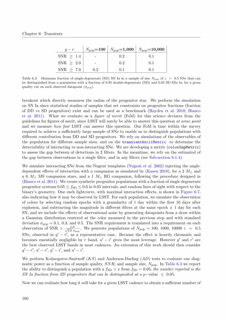
Chapter 6: Transients

g − r Npop=100 Npop=1,000 Npop=10,000

SNR ≥ 1.4 - 0.2 0.1

SNR ≥ 2.0 - 0.2 0.1

SNR ≥ 7.0 0.2 0.1 0.1

Table 6.3: Minimum fraction of single-degenerate (SD) SN Ia in a sample of size Npop of z = 0.5 SNe that canbe distinguished from a population with a fraction of 0.95 double-degenerate (DD) and 0.05 SD SNe Ia, for a givenquality cut on each observed datapoint (σpop).

breakout which directly measures the radius of the progenitor star. We perform the simulationon SN Ia since statistical studies of samples that set constraints on progenitor fractions (fractionof DD vs SD progenitors) exist and can be used as a benchmark (Hayden et al. 2010; Biancoet al. 2011). What we evaluate as a figure of merit (FoM) for this science deviates from theguidelines for figures of merit, since LSST will surely be able to answer this question at some pointand we measure how fast LSST can answer this question. Our FoM is time within the surveyrequired to achieve a sufficiently large sample of SNe to enable us to distinguish populations withdifferent contribution from DD and SD progenitors. We rely on simulations of the observables ofthe population for different sample sizes, and on the transientAsciiMetric to determine thedetectability of interacting vs non-interacting SNe. We are developing a metric (colorGapMetric)to assess the gap between of detections in 2 filters. In the meantime, we rely on the estimated ofthe gap between observations in a single filter, and in any filters (see Sub-section 6.1.4).

We simulate interacting SNe from the Nugent templates (Nugent et al. 2002) injecting the angle-dependent effects of interaction with a companion as simulated by (Kasen 2010), for a 2 M anda 6 M MS companion stars, and a 1 M RG companion, following the procedure designed in(Bianco et al. 2011). We create synthetic progenitor populations with a fraction of single degenerateprogenitor systems 0.05 ≤ fSD ≤ 0.6 in 0.05 intervals, and random lines of sight with respect to thebinary’s geometry. One such lightcurve, with maximal interaction effects, is shown in Figure 6.7,also indicating how it may be observed by LSST. For each population, we simulate the observationof colors by selecting random epochs with a granularity of 1 day within the first 10 days afterexplosion, and subtracting the magnitude in different filters at the same epoch ± 1 day for eachSN, and we include the effects of observational noise by generating datapoints from a draw withina Gaussian distribution centered at the color measured in the previous step and with standarddeviation σpop = 0.1, 0.3, and 0.5. The SNR requirement is translated into a requirement on eachobservation of SNR > 1.0√

2.0 σpop. We generate populations of Npop = 100, 1000, 10000 z = 0.5

SNe, observed in g′ − r′, as a representative case. Because the effect is heavily chromatic andbecomes essentially negligible by r band, u′ − i′ gives the most leverage. However g′ and r′ arethe best observed LSST bands in most cadences. An extension of this work should then considerg′ − r′, u′ − r′, g′ − i′, and u′ − i′.

We perform Kolmogorov-Smirnoff (KS) and Anderson-Darling (AD) tests to evaluate our diag-nostic power as a function of sample quality, SNR, and sample size, Npop. In Table 6.3 we reportthe ability to distinguish a population with a fSD > x from fSD = 0.05; the number reported is theSN Ia fraction from SD progenitors that can be distinguished at a p−value ≤ 0.05.

Now we can evaluate how long it will take for a given LSST cadence to obtain a sufficient number of

160

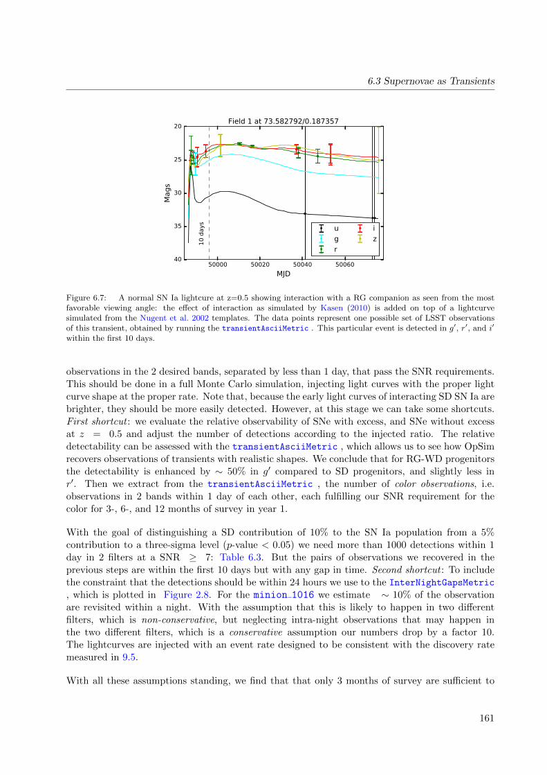
6.3 Supernovae as Transients

50000 50020 50040 50060

MJD

20

25

30

35

40

Mags

10 d

ays

Field 1 at 73.582792/0.187357

u

g

r

i

z

Figure 6.7: A normal SN Ia lightcure at z=0.5 showing interaction with a RG companion as seen from the mostfavorable viewing angle: the effect of interaction as simulated by Kasen (2010) is added on top of a lightcurvesimulated from the Nugent et al. 2002 templates. The data points represent one possible set of LSST observationsof this transient, obtained by running the transientAsciiMetric . This particular event is detected in g′, r′, and i′

within the first 10 days.

observations in the 2 desired bands, separated by less than 1 day, that pass the SNR requirements.This should be done in a full Monte Carlo simulation, injecting light curves with the proper lightcurve shape at the proper rate. Note that, because the early light curves of interacting SD SN Ia arebrighter, they should be more easily detected. However, at this stage we can take some shortcuts.First shortcut : we evaluate the relative observability of SNe with excess, and SNe without excessat z = 0.5 and adjust the number of detections according to the injected ratio. The relativedetectability can be assessed with the transientAsciiMetric , which allows us to see how OpSimrecovers observations of transients with realistic shapes. We conclude that for RG-WD progenitorsthe detectability is enhanced by ∼ 50% in g′ compared to SD progenitors, and slightly less inr′. Then we extract from the transientAsciiMetric , the number of color observations, i.e.observations in 2 bands within 1 day of each other, each fulfilling our SNR requirement for thecolor for 3-, 6-, and 12 months of survey in year 1.

With the goal of distinguishing a SD contribution of 10% to the SN Ia population from a 5%contribution to a three-sigma level (p-value < 0.05) we need more than 1000 detections within 1day in 2 filters at a SNR ≥ 7: Table 6.3. But the pairs of observations we recovered in theprevious steps are within the first 10 days but with any gap in time. Second shortcut : To includethe constraint that the detections should be within 24 hours we use to the InterNightGapsMetric

, which is plotted in Figure 2.8. For the minion 1016 we estimate ∼ 10% of the observationare revisited within a night. With the assumption that this is likely to happen in two differentfilters, which is non-conservative, but neglecting intra-night observations that may happen inthe two different filters, which is a conservative assumption our numbers drop by a factor 10.The lightcurves are injected with an event rate designed to be consistent with the discovery ratemeasured in 9.5.

With all these assumptions standing, we find that that only 3 months of survey are sufficient to

161

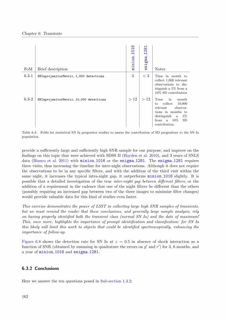
Chapter 6: Transients

FoM Brief description minion1016

enigma1281

Notes

6.3-1 SNIaprojenitorMetric, 1,000 detections 3 < 3 Time in month tocollect 1,000 relevantobservations to dis-tinguish a 5% from a10% SD contribution

6.3-2 SNIaprojenitorMetric, 10,000 detections > 12 > 12 Time in monthto collect 10,000relevant observa-tions in months todistinguish a 5%from a 10% SDcontribution.

Table 6.4: FoMs for statistical SN Ia progenitor studies to assess the contribution of SD progenitors to the SN Iapopulation.

provide a sufficiently large and sufficiently high SNR sample for our purpose, and improve on thefindings on this topic that were achieved with SDSS II (Hayden et al. 2010), and 3 years of SNLSdata (Bianco et al. 2011) with minion 1016 or the enigma 1281. The enigma 1281 requiresthree visits, thus increasing the timeline for inter-night observations. Although it does not requirethe observations to be in any specific filters, and with the addition of the third visit within thesame night, it increases the typical intra-night gap, it outperforms minion 1016 slightly. It ispossible that a detailed investigation of the true inter-night gap between different filters, or theaddition of a requirement in the cadence that one of the night filters be different than the others(possibly requiring an increased gap between two of the three images to minimize filter changes)would provide valuable data for this kind of studies even faster.

This exercise demonstrates the power of LSST in collecting large high SNR samples of transients,but we must remind the reader that these conclusions, and generally large sample analysis, relyon having properly identified both the transient class (normal SN Ia) and the date of maximum!This, once more, highlights the importance of prompt identification and classification: for SN Iathis likely will limit this work to objects that could be identified spectroscopically, enhancing theimportance of follow-up.

Figure 6.8 shows the detection rate for SN Ia at z = 0.5 in absence of shock interaction as afunction of SNR (obtained by summing in quadrature the errors on g′ and r′) for 3, 6 months, anda year of minion 1016 and enigma 1281.

6.3.2 Conclusions

Here we answer the ten questions posed in Sub-section 1.3.2:

162

6.3 Supernovae as Transients

2 4 6 8 10 12

g ′− r ′ SNR

103

104

N d

ete

ctio

ns

(no inte

ratc

tion)

1 year - minion_1016

6 months - minion_1016

3 months - minion_1016

1 year - enigma_1281

6 months - enigma_1281

3 months - enigma_1281

minion_1016

enigma_1281

Figure 6.8: Normal SN Ia light cure at z=0.5 detected by the minion 1016 (solid lines) and enigma 1281cadence (dashed line) in 3 months, 6 months, and 1 year, that provide color information useful to constrain theprogenitor distribution. Line are third-degree polynomial fits.

Q1: Does the science case place any constraints on the tradeoff between the sky coverage andcoadded depth? For example, should the sky coverage be maximized (to ∼30,000 deg2, as e.g.,in Pan-STARRS) or the number of detected galaxies (the current baseline but with 18,000deg2)?

A1: Yes, although this question can be answered with a full simulation that includes a coordinatedependent event rate while the current simulation assumes uniform probability of a transientin the field-of-view and cannot evaluate this trade-off

Q2: Does the science case place any constraints on the tradeoff between uniformity of sampling andfrequency of sampling? For example, a rolling cadence can provide enhanced sample ratesover a part of the survey or the entire survey for a designated time at the cost of reducedsample rate the rest of the time (while maintaining the nominal total visit counts).

A2: Yes: this science case is sensitive to both. A more sophisticated simulation which also measuresthe ability to correctly identify the epoch of maximum would be more powerful to answerthe question.

Q3: Does the science case place any constraints on the tradeoff between the single-visit depth andthe number of visits (especially in the u-band where longer exposures would minimize theimpact of the readout noise)?

A3: Yes, because the diagnostic power depends on both the SNR of each observation and the gapbetween observations.

Q4: Does the science case place any constraints on the Galactic plane coverage (spatial coverage,temporal sampling, visits per band)?

A4: No.

163

Chapter 6: Transients

Q5: Does the science case place any constraints on the fraction of observing time allocated to eachband?

A5: Yes, since it relies on obtaining observations in at least 2 filters.

Q6: Does the science case place any constraints on the cadence for deep drilling fields?

A6: Yes, although the results have not been analyzed separately for WFD and DD fields.

Q7: Assuming two visits per night, would the science case benefit if they are obtained in the sameband or not?

A7: No. Although we would benefit greatly from 2 visits in the same filters, and one visit in adifferent filter to constrain simultaneously shape and color.”

Q8: Will the case science benefit from a special cadence prescription during commissioning or earlyin the survey, such as: acquiring a full 10-year count of visits for a small area (either in allthe bands or in a selected set); a greatly enhanced cadence for a small area?

A8: A full event rate needs to be included in the simulation to answer this question.

Q9: Does the science case place any constraints on the sampling of observing conditions (e.g.,seeing, dark sky, airmass), possibly as a function of band, etc.?

A9: Indirectly, since detection efficiency depends on SNR.

Q10: Does the case have science drivers that would require real-time exposure time optimizationto obtain nearly constant single-visit limiting depth?

A10: No.

Go to: • the start of this section • the start of the chapter • the table of contents

6.4 Gamma-Ray Burst Afterglows

Eric C. Bellm

Gamma-ray bursts (GRBs) are relativistic explosions typically classified by the temporal durationof their initial gamma-ray emission: Long GRBs, that mark the endpoint of the lives of somemassive stars, and short GRBs, believed to originate from the merger of binary neutron stars.GRB emission is known to be beamed: the initial prompt gamma-ray emission is seen only forobservers looking at the jet axis. The longer-wavelength X-ray, optical, and radio afterglow maybe seen both by on- and off-axis observers. The latter case is known as an orphan afterglow, dueto the absence of gamma-ray emission. On- and off-axis afterglows are predicted to have differenttemporal signatures in the optical: On-axis events decay as a power-law until a jet break, whileoff-axis events should be fainter and show an initial rise (Figure 6.9). Despite systematic searches,no convincing orphan afterglow candidates have yet been discovered, limiting our knowledge of thebeaming fraction of GRBs and hence their true rates. Well-sampled orphan afterglow lightcurveswould also permit study of the GRB jet structure.

164

6.4 Gamma-Ray Burst Afterglows

10-1 100 101 102 103

t−t0 (day)

15

20

25

r (m

ag)

GRB afterglows θj =4

θobs=0

θobs=5

θobs=10

θobs=15

θobs=20

θobs=25

Figure 6.9: Predicted light curves of GRB afterglows by off-axis angle with respect to the jet axis θobs (Figure8.8, LSST Science Collaboration et al. 2009). The forward shock model is derived from Totani & Panaitescu (2002)and assumes a jet half opening angle θj = 4, the isotropic equivalent energy of Eiso = 5× 1053erg, ambient mediumdensity n = 1 g cm−3, and the slope of the electron energy distribution p = 2.1. The apparent AB r-band magnitudesassume a source redshift z = 1.

Because of their rarity, in all but one case (Cenko et al. 2015) to date GRBs have been discoveredusing their prompt emission by hard X-ray or gamma-ray all-sky monitors. This selection imposesbiases on the population of relativistic explosions we observe. Baryon-loading in the GRB jet—a“dirty fireball” (Rhoads 2003)—can lead to on-axis events without gamma-ray emission. Onlyone plausible candidate has been identified to date (Cenko et al. 2013). Discovery of new dirtyfireballs—if distinguished from off-axis events–would clarify the rates of these events and enhanceour understanding of the diversity of stellar death.

LSST is the survey most capable of resolving these decades-old questions. Due to its large apertureand etendue, LSST can detect faint, fast-fading, and rare cosmological events, potentially enablingpopulation studies of the high-redshift universe. Ghirlanda et al. (2015) estimated LSST coulddetect 50 orphan afterglows each year, more than any other planned survey.

The challenge of detecting and recognizing GRB afterglows in the LSST data in real time makesthis science case a useful proxy for other fast transient science cases that benefit from N > 2visits per night. In particular, this includes discovering supernovae soon after explosion for flashspectroscopy or shock breakout searches.

6.4.1 Target measurements and discoveries

GRB afterglow discovery is among the science cases that places the greatest stress on the LSSTcadence. Because afterglows fade rapidly—dropping several magnitudes in the first few hours—high cadence observations are required to detect the fast fading. If an afterglow candidate canbe recognized in real time, it will be possible to trigger TOO spectroscopy (to measure a redshift

165

Chapter 6: Transients

and confirm the event is cosmological), X-ray and radio observations (to detect a high-energycounterpart and the presence of a jet), and additional photometry (to characterize the lightcurveevolution). If there is no source at the location of the transient in the coadded reference image,two consecutive observations in the same filter separated by an hour or two are the minimumrequired to potentially trigger followup of a fast-fading event. However, a third observation withina night or two—ideally in the same filter—would improve the purity of the sample and reduce thereliance on triggered followup. Observations in other bands at high cadence are less useful becausethey require assumptions about the event’s SED and its evolution to determine if a source is trulyfading.

Distinguishing orphan afterglows from on-axis events (whether conventional GRBs or dirty fire-balls) will also require more than two detections. Orphan events may prove harder to recognize inreal time, because they are intrinsically fainter than on-axis events and show an initial rise ratherthan a rapid decay (Figure 6.9). Additionally, because of relativistic time dilation, high redshiftevents are easier to detect, but these events will be fainter and more difficult to follow up. Ac-cordingly, population studies of orphan afterglow candidates may by necessity be conducted withLSST photometry alone. Such studies may only be productive if LSST has sufficiently frequentrevisits to a field in a single filter.

6.4.2 Metrics

The core figure of merit for GRB afterglows is simply the raw number of on- and off-axis eventsdetectable in two, three, or more observations, preferably in a single filter.

The appropriate way to derive these detections is to conduct a Monte Carlo simulation of a cosmo-logical population of GRBs and fold it through the LSST observing cadence (cf. Japelj & Gomboc2011). We are developing this infrastructure for the MAF framework.

In the meantime, simplified metrics can give us a general idea of how well a given cadence can char-acterize fast-evolving transients such as GRBs. We have created a new metric, GRBTransientMetric, that replaces the linearly rising and decaying lightcurve in TransientMetric with the F ∼ t−αdecay characteristic of on-axis afterglows. (For the time being, we neglect the jet break thatsteepens the rate of decay; this implies that our detectability estimates are optimistic.)

We simulate on-axis afterglows at random sky positions using the parameters of Japelj & Gomboc(2011). The R-band apparent magnitude at 1 minute after explosion is randomly drawn from aGaussian with µ = 15.35, σ = 1.59 and decays with α = 1.0. For these estimates we simply assumezero color difference between in all LSST bands. There are roughly 300 on-axis GRBs per yearwith these parameters; we calculate the average fraction of these events which have at least one,two, or three detections in any single filter.

6.4.3 OpSim Analysis

We ran GRBTransientMetric on several OpSim v3.3.5 runs with a range of characteristics:minion 1016, the baseline cadence; enigma 1281, with three visits per WFD field; kraken 1043,with no visit pairs; and minion 1020, a PanSTARRS-like cadence.

166

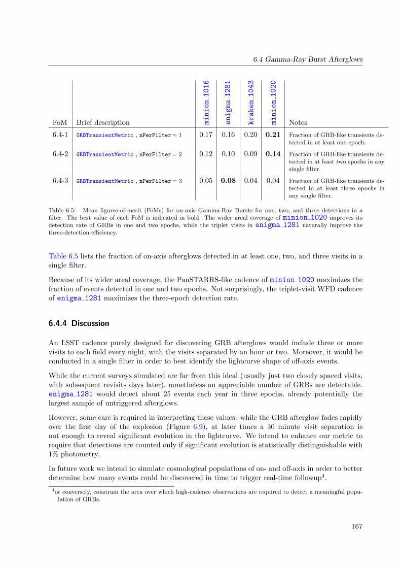
6.4 Gamma-Ray Burst Afterglows

FoM Brief description minion1016

enigma1281

kraken1043

minion1020

Notes

6.4-1 GRBTransientMetric , nPerFilter= 1 0.17 0.16 0.20 0.21 Fraction of GRB-like transients de-tected in at least one epoch.

6.4-2 GRBTransientMetric , nPerFilter= 2 0.12 0.10 0.09 0.14 Fraction of GRB-like transients de-tected in at least two epochs in anysingle filter.

6.4-3 GRBTransientMetric , nPerFilter= 3 0.05 0.08 0.04 0.04 Fraction of GRB-like transients de-tected in at least three epochs inany single filter.

Table 6.5: Mean figures-of-merit (FoMs) for on-axis Gamma-Ray Bursts for one, two, and three detections in afilter. The best value of each FoM is indicated in bold. The wider areal coverage of minion 1020 improves itsdetection rate of GRBs in one and two epochs, while the triplet visits in enigma 1281 naturally improve thethree-detection efficiency.

Table 6.5 lists the fraction of on-axis afterglows detected in at least one, two, and three visits in asingle filter.

Because of its wider areal coverage, the PanSTARRS-like cadence of minion 1020 maximizes thefraction of events detected in one and two epochs. Not surprisingly, the triplet-visit WFD cadenceof enigma 1281 maximizes the three-epoch detection rate.

6.4.4 Discussion

An LSST cadence purely designed for discovering GRB afterglows would include three or morevisits to each field every night, with the visits separated by an hour or two. Moreover, it would beconducted in a single filter in order to best identify the lightcurve shape of off-axis events.

While the current surveys simulated are far from this ideal (usually just two closely spaced visits,with subsequent revisits days later), nonetheless an appreciable number of GRBs are detectable.enigma 1281 would detect about 25 events each year in three epochs, already potentially thelargest sample of untriggered afterglows.

However, some care is required in interpreting these values: while the GRB afterglow fades rapidlyover the first day of the explosion (Figure 6.9), at later times a 30 minute visit separation isnot enough to reveal significant evolution in the lightcurve. We intend to enhance our metric torequire that detections are counted only if significant evolution is statistically distinguishable with1% photometry.

In future work we intend to simulate cosmological populations of on- and off-axis in order to betterdetermine how many events could be discovered in time to trigger real-time followup4.

4or conversely, constrain the area over which high-cadence observations are required to detect a meaningful popu-lation of GRBs.

167

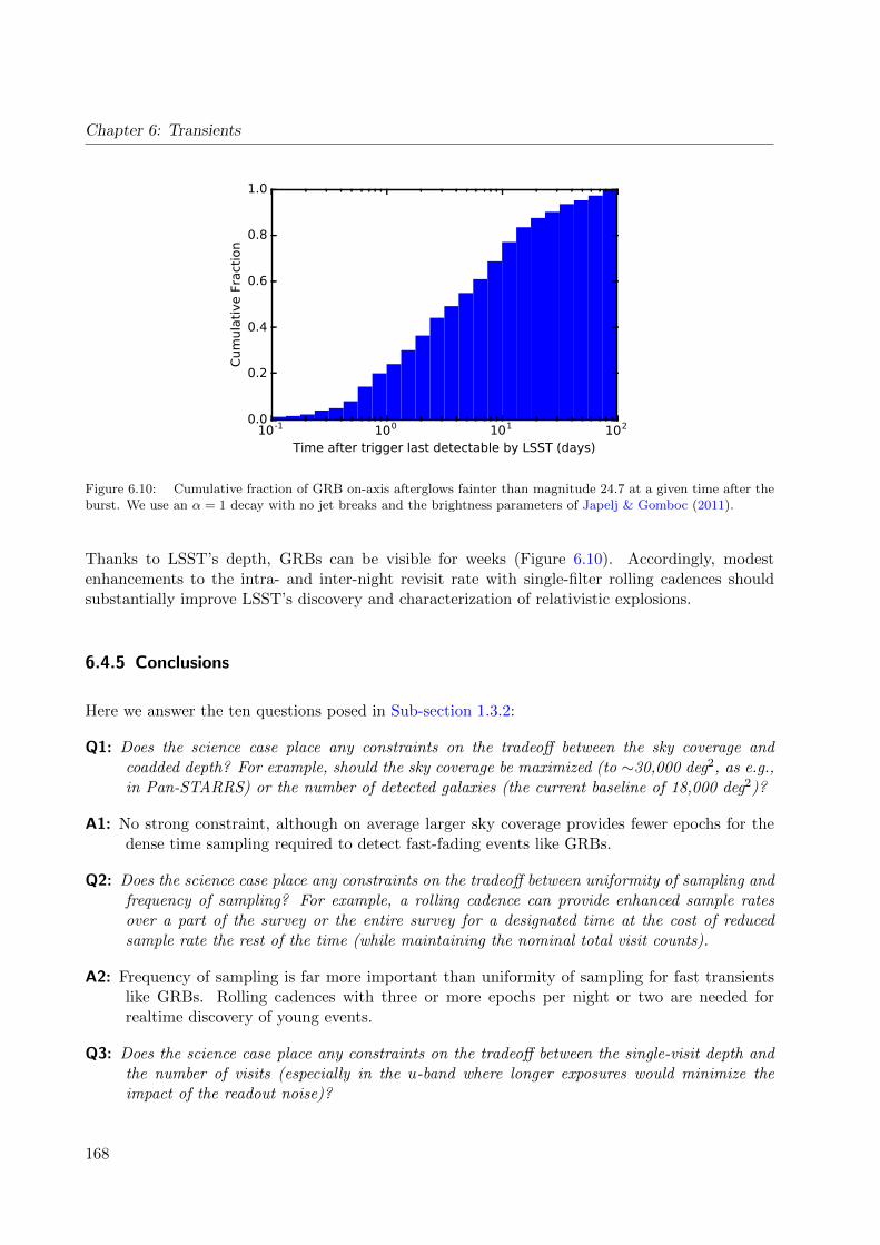
Chapter 6: Transients

10-1 100 101 102

Time after trigger last detectable by LSST (days)

0.0

0.2

0.4

0.6

0.8

1.0

Cum

ula

tive F

ract

ion

Figure 6.10: Cumulative fraction of GRB on-axis afterglows fainter than magnitude 24.7 at a given time after theburst. We use an α = 1 decay with no jet breaks and the brightness parameters of Japelj & Gomboc (2011).

Thanks to LSST’s depth, GRBs can be visible for weeks (Figure 6.10). Accordingly, modestenhancements to the intra- and inter-night revisit rate with single-filter rolling cadences shouldsubstantially improve LSST’s discovery and characterization of relativistic explosions.

6.4.5 Conclusions

Here we answer the ten questions posed in Sub-section 1.3.2:

Q1: Does the science case place any constraints on the tradeoff between the sky coverage andcoadded depth? For example, should the sky coverage be maximized (to ∼30,000 deg2, as e.g.,in Pan-STARRS) or the number of detected galaxies (the current baseline of 18,000 deg2)?

A1: No strong constraint, although on average larger sky coverage provides fewer epochs for thedense time sampling required to detect fast-fading events like GRBs.

Q2: Does the science case place any constraints on the tradeoff between uniformity of sampling andfrequency of sampling? For example, a rolling cadence can provide enhanced sample ratesover a part of the survey or the entire survey for a designated time at the cost of reducedsample rate the rest of the time (while maintaining the nominal total visit counts).

A2: Frequency of sampling is far more important than uniformity of sampling for fast transientslike GRBs. Rolling cadences with three or more epochs per night or two are needed forrealtime discovery of young events.

Q3: Does the science case place any constraints on the tradeoff between the single-visit depth andthe number of visits (especially in the u-band where longer exposures would minimize theimpact of the readout noise)?

168

6.4 Gamma-Ray Burst Afterglows

A3: While greater single visit depth probes a greater cosmological volume within which to detectGRBs and other fast transients, our efficiency at discovering GRBs with LSST is drivenentirely by the time sampling. Accordingly we prefer a larger number of visits per field togreater single-exposure depth, independent of band..

Q4: Does the science case place any constraints on the Galactic plane coverage (spatial coverage,temporal sampling, visits per band)?

A4: As GRBs are cosmological events, we expect to detect very few at low Galactic latitudes dueto extinction. Accordingly this science case is insensitive to observing plans in the Planeexcept insofar as they limit the number and cadence of exposures at higher latitudes.

Q5: Does the science case place any constraints on the fraction of observing time allocated to eachband?

A5: No strong constraints, although detection of faint afterglows will benefit from exposures takenin the bands with deepest single-exposure depth.

Q6: Does the science case place any constraints on the cadence for deep drilling fields?

A6: Deep drilling fields provide an excellent opportunity to achieve the high time sampling requiredto discover GRBs while they are young. As discussed above, a good fast transient cadencemight have a minimum of three visits in a night separated by an hour or two, preferably ina single filter, with revisits every night.

Q7: Assuming two visits per night, would the science case benefit if they are obtained in the sameband or not?

A7: Due to the need to constrain the lightcurve shape, it is best if the observations are in the samefilter–especially with only two visits per night. Otherwise there is a degeneracy between the(evolving) color of the event and its lightcurve shape.

Q8: Will the case science benefit from a special cadence prescription during commissioning or earlyin the survey, such as: acquiring a full 10-year count of visits for a small area (either in allthe bands or in a selected set); a greatly enhanced cadence for a small area?

A8: A dedicated experiment providing enhanced cadences over a small area (as described above)would provide an ideal experiment to determine the rate of fast transients. Such an observingstrategy would also facilitate organizing necessary followup resources (spectroscopy, X-rayfollowup) because the observing period would be known in advance.

Q9: Does the science case place any constraints on the sampling of observing conditions (e.g.,seeing, dark sky, airmass), possibly as a function of band, etc.?

A9: None unique to the science.

Q10: Does the case have science drivers that would require real-time exposure time optimizationto obtain nearly constant single-visit limiting depth?

A10: No.

Go to: • the start of this section • the start of the chapter • the table of contents

169

Chapter 6: Transients

6.5 Gravitational Wave Sources

Raffaella Margutti, Zoheyr Doctor, Wen-fai Fong, Zoltan Haiman, Vassiliki Kalogera, Virginia Trim-ble, Bevin Ashley Zauderer

The first detection of Gravitational Waves (GW) by the advanced LIGO/Virgo collaboration (Ab-bott et al. 2016b, 2009; Acernese 2008) has recently opened a new window of exploration into ourUniverse. The amount of information that can be revealed by the properties of the GW emissionis immense and holds promises for revolutionary insights, including accurate masses and spins ofneutron stars and black holes, tests of General Relativity and an accurate census of the neutronstar (NS) and black hole (BH) populations that might challenge our current understanding of mas-sive stellar evolution. However, GW events are poorly localized (10-100 deg2 at the time of LSSToperations). The identification of EM counterparts would provide precise localization and distancemeasurements, in addition to the necessary astrophysical context (e.g. host galaxy properties,connection to specific stellar populations) to fully exploit the revolutionary power of this new GWera.

6.5.1 Target measurements and discoveries

The first GW event was found to be associated with the merger of two black holes (Abbott et al.2016b,c). Although no EM counterpart was expected to accompany a black-hole black-hole (BBH)merger, it seems now possible that even BBH mergers might produce short GRB-like EM emission(Connaughton et al. 2016; Loeb 2016; Zhang 2016; Perna et al. 2016; Stone et al. 2016). Indeed,in analogy with supermassive BH mergers, shocks might develop in the just-formed circumbinaryaccretion disk (if a disk forms), which can produce a bright afterglow following the BBH merger(e.g. Lippai et al. 2008; Corrales et al. 2010; Schnittman 2013). Albeit speculative in nature, it isadvisable to keep an open mind about the possibility of EM counterparts to BBH mergers.

The most promising and better understood EM counterparts to GW events are “kilonovae” (Li &Paczynski 1998; Metzger et al. 2010; Metzger & Berger 2012; Kasen et al. 2013; Barnes & Kasen2013). Kilonovae are short-lived (typical time scale of one week), apparently faint (z ∼ 21 mag atpeak at 120 Mpc), red (i − z ≈ 1 mag), isotropic transients (Figure 6.11) due to the radioactivedecay of r-process elements synthesized in the merger ejecta of a NS-NS or NS-BH system. Thesemerging systems are the favored progenitors of short GRBs. Indeed, a signature consistent withkilonova emission has been recently found following the short GRB 130603B (Berger et al. 2013;Tanvir et al. 2013). The key piece of information that enabled the discovery of kilonova-like emissionassociated with this short GRB was its sub-arcsecond localization enabled by the detection of theoptical afterglow, which allowed for an effective kilonova search with the Hubble Space Telescope(Figure 6.11). In contrast, the typical localization region of GW events in the LSST era is expectedto be of the order of a few tens of square degrees (LIGO Scientific Collaboration et al. 2013). It isthus clear that the major challenges faced by the optical follow-up of GW events is represented bythe combination of poor localizations with faint and fast evolving red electromagnetic counterparts.

The detection of an optical counterpart in conjunction with a GW event will significantly leveragethe GW signal. LSST, with its the wide FOV, wavelength coverage and exquisite sensitivity isuniquely poised to identify and characterize counterparts to GW events.

170

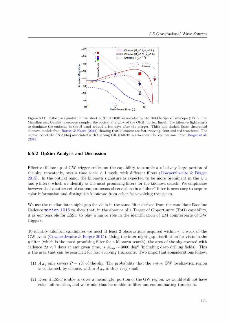
6.5 Gravitational Wave Sources

Figure 6.11: Kilonova signature in the short GRB 130603B as revealed by the Hubble Space Telescope (HST). TheMagellan and Gemini telescopes sampled the optical afterglow of the GRB (dotted lines). The kilonova light startsto dominate the emission in the H band around a few days after the merger. Thick and dashed lines: theoreticalkilonova models from Barnes & Kasen (2013) showing that kilonovae are fast-evolving, faint and red transients. Thelight-curve of the SN 2006aj associated with the long GRB 060218 is also shown for comparison. From Berger et al.(2013).

6.5.2 OpSim Analysis and Discussion

Effective follow up of GW triggers relies on the capability to sample a relatively large portion ofthe sky, repeatedly, over a time scale < 1 week, with different filters (Cowperthwaite & Berger2015). In the optical band, the kilonova signature is expected to be more prominent in the i, zand y filters, which we identify as the most promising filters for the kilonova search. We emphasizehowever that another set of contemporaneous observations in a “bluer” filter is necessary to acquirecolor information and distinguish kilonovae from other fast-evolving transients.

We use the median inter-night gap for visits in the same filter derived from the candidate BaselineCadence minion 1016 to show that, in the absence of a Target of Opportunity (ToO) capability,it is not possible for LSST to play a major role in the identification of EM counterparts of GWtriggers.

To identify kilonova candidates we need at least 2 observations acquired within ∼ 1 week of theGW event (Cowperthwaite & Berger 2015). Using the inter-night gap distribution for visits in they filter (which is the most promising filter for a kilonova search), the area of the sky covered withcadence ∆t < 7 days at any given time, is Asky ∼ 3000 deg2 (including deep drilling fields). Thisis the area that can be searched for fast evolving transients. Two important considerations follow:

(1) Asky only covers P ∼ 7% of the sky. The probability that the entire GW localization regionis contained, by chance, within Asky is thus very small.

(2) Even if LSST is able to cover a meaningful portion of the GW region, we would still not havecolor information, and we would thus be unable to filter out contaminating transients.

171

Chapter 6: Transients

We conclude that relying on the serendipitous alignment of the LSST fields with the GW localizationmap is not an effective strategy to follow up GW triggers and identify their EM counterparts. Wethus strongly recommend a ToO capability as part of the baseline LSST operations strategy.

Ideally, the ToO capability will allow for imaging of the GW localization map at least twice over∆t .1 week with a “red” filter (i, z or y), and will include the possibility to designate a desired setof filters to obtain color information. By the time of LSST operation the typical size of the GWlocalization region is expected to be 10-100 deg2, which would require a small number of LSSTre-pointings. We thus do not anticipate a significantly disruptive impact on other LSST campaigns(especially if only the GW triggers with the best localizations in the southern sky are selected forLSST ToOs).

At the price of re-shuffling a reasonably small number of fields, if equipped with ToO capabilities,LSST can be the premier player in the era of EM follow up to GW sources.

Go to: • the start of this section • the start of the chapter • the table of contents

6.6 Future Work

In this section we provide a short compendium of science cases that are either still being developed,or that are deserving of quantitative MAF analysis at some point in the future.

6.6.1 Tidal Disruption Events

Iair Arcavi

A star passing close to a supermassive black hole (SMBH; M & 106M) will be torn apart bytidal forces. For certain (. 108M) black hole masses, the disruption will occur outside the eventhorizon and will be accompanied by an observable flare (Hills 1975; Rees 1988). Such flares can beused to study inactive SMBHs, which are otherwise inaccessible beyond the nearby (. 100 Mpc)universe.

We are now building our understanding of how observational properties of TDEs are affected by theSMBH. Theory claims to provide such a connection (e.g. Lodato et al. 2009; Guillochon et al. 2014),but uncertainties in the physics of the disruption, subsequent accretion and emission mechanismsare currently topics of debate (e.g. Strubbe & Murray 2015; Guillochon et al. 2014; Roth et al.2015), and new models are vigorously being developed (e.g. Piran et al. 2015; Hayasaki et al. 2015;Svirski et al. 2015; Bonnerot et al. 2015).

TDEs are rare (∼ 10−5−10−4 events per galaxy per year; Wang & Merritt 2004; Stone & Metzger2015), and until recently, TDE candidates were discovered mostly in archival data (e.g. Donleyet al. 2002; Gezari et al. 2006; Esquej et al. 2007). Now, however, wide-field transient surveys havestarted discovering TDEs in real time.

Generally, two types of TDE candidates have been identified:

172

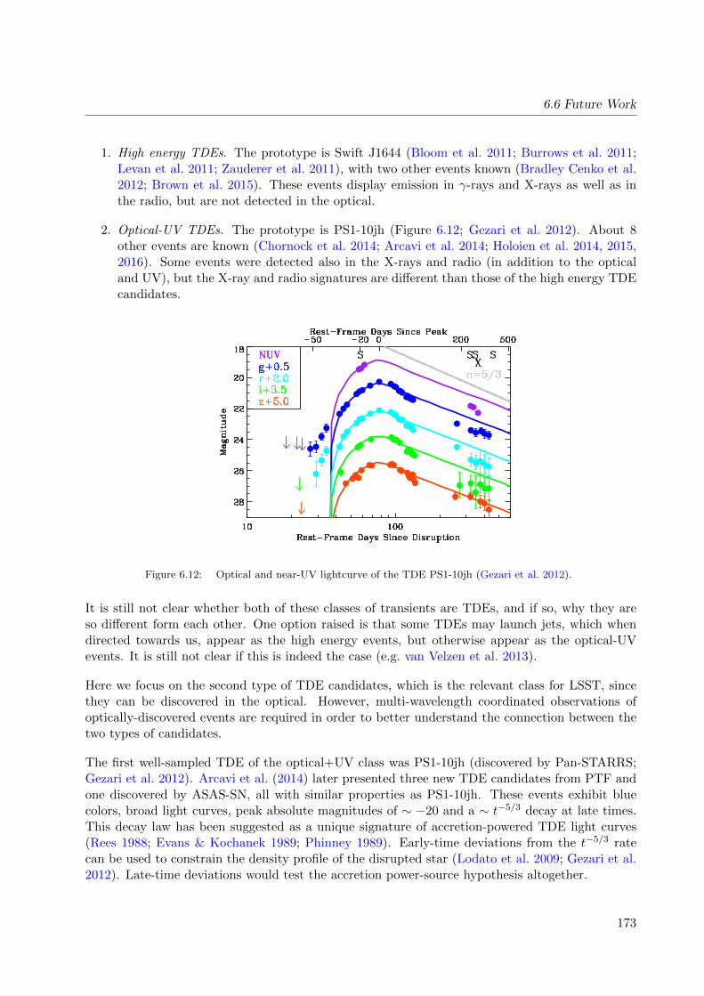
6.6 Future Work

1. High energy TDEs. The prototype is Swift J1644 (Bloom et al. 2011; Burrows et al. 2011;Levan et al. 2011; Zauderer et al. 2011), with two other events known (Bradley Cenko et al.2012; Brown et al. 2015). These events display emission in γ-rays and X-rays as well as inthe radio, but are not detected in the optical.

2. Optical-UV TDEs. The prototype is PS1-10jh (Figure 6.12; Gezari et al. 2012). About 8other events are known (Chornock et al. 2014; Arcavi et al. 2014; Holoien et al. 2014, 2015,2016). Some events were detected also in the X-rays and radio (in addition to the opticaland UV), but the X-ray and radio signatures are different than those of the high energy TDEcandidates.

Figure 6.12: Optical and near-UV lightcurve of the TDE PS1-10jh (Gezari et al. 2012).

It is still not clear whether both of these classes of transients are TDEs, and if so, why they areso different form each other. One option raised is that some TDEs may launch jets, which whendirected towards us, appear as the high energy events, but otherwise appear as the optical-UVevents. It is still not clear if this is indeed the case (e.g. van Velzen et al. 2013).

Here we focus on the second type of TDE candidates, which is the relevant class for LSST, sincethey can be discovered in the optical. However, multi-wavelength coordinated observations ofoptically-discovered events are required in order to better understand the connection between thetwo types of candidates.

The first well-sampled TDE of the optical+UV class was PS1-10jh (discovered by Pan-STARRS;Gezari et al. 2012). Arcavi et al. (2014) later presented three new TDE candidates from PTF andone discovered by ASAS-SN, all with similar properties as PS1-10jh. These events exhibit bluecolors, broad light curves, peak absolute magnitudes of ∼ −20 and a ∼ t−5/3 decay at late times.This decay law has been suggested as a unique signature of accretion-powered TDE light curves(Rees 1988; Evans & Kochanek 1989; Phinney 1989). Early-time deviations from the t−5/3 ratecan be used to constrain the density profile of the disrupted star (Lodato et al. 2009; Gezari et al.2012). Late-time deviations would test the accretion power-source hypothesis altogether.

173

Chapter 6: Transients

The spectral signatures of these TDEs are still a puzzle. PS1-10jh displayed only He II emissionlines, lacking any signs of H. Some of the Arcavi et al. (2014) sample, however, do display Hemission. In fact, a continuum of H / He emission ratios for this class of transients is beingrevealed, and is now a focus of theoretical modelling (Strubbe & Murray 2015; Roth et al. 2015).

The second recent discovery relating to this new sample concerns their host galaxies (Arcavi et al.2014; French et al. 2016), most of which are post-starburst galaxies. These galaxies show little orno signs of on-going star formation, but their significant A stellar populations indicate that starformation ceased abruptly a few hundred Myr to a Gyr ago (Dressler & Gunn 1983). Galaxies withthese characteristics often show signs of recent galaxy-galaxy mergers (Zabludoff et al. 1996), whichproduced the starburst and evolved the bulge. Optical-UV TDEs are intrinsically over abundantin post-starburst galaxies by a factor of ∼ 30−200 (depending on the characteristics of the galaxy;French et al. 2016). The reason for the strong preference of TDEs for post-starburst galaxies hasstill not been determined.

LSST’s contribution to TDE studies will be substantial. van Velzen et al. (2011) estimate thatLSST could discover approximately 4000 TDEs per year. The main drivers for studying TDEswith LSST are:

• Measuring black hole masses: This involves fitting models to TDE light curves. It is alsorelevant to correlate these measurements with host galaxy properties (mass, bulge/disk de-composition).

• Constraining galactic dynamics by measuring the TDE rates as functions of black hole massand galaxy types.

• Characterizing TDE emission signatures.

A metric is required for measuring how well TDEs can be identified and distinguished from super-novae and active galactic nuclei. In general, we expect TDEs to:

• Be located in the center of their host.

• Display approximately constant blue (few 104K) colors.

• Evolve slowly (weeks-months).

• Not show past AGN-like variability.

• Preferentially peak around mag -20.

• Preferentially be hosted in a post-starburst galaxy.

These criteria are based on our current knowledge of optical TDEs, which is still in its early stages.The field is rapidly evolving, and it is possible that new observations will change the current pictureof TDE emission. This metric is probably best combined with those discussed in Section 6.3 foridentifying supernovae, though the luminosity function of TDEs (or what constitutes a “typical”TDE light curve) is not yet known.

A second metric is required to asses the accuracy with which the black hole mass can be constrainedfrom the TDE light curves. This metric can be based on existing theoretical models to fit simulatedTDE light curves (such as TDEFit; Guillochon et al. 2014).

174

6.6 Future Work

6.6.2 Conclusions

Here we answer the ten questions posed in Sub-section 1.3.2:

Q1: Does the science case place any constraints on the tradeoff between the sky coverage andcoadded depth? For example, should the sky coverage be maximized (to ∼30,000 deg2, as e.g.,in Pan-STARRS) or the number of detected galaxies (the current baseline of 18,000 deg2)?

A1: The number of events discovered will be approximately proportional to the sky area surveyed,multiplied by the average length of coverage, so added sky area is beneficial, as long as theobserving season per field is not shortened.

Q2: Does the science case place any constraints on the tradeoff between uniformity of sampling andfrequency of sampling? For example, a rolling cadence can provide enhanced sample ratesover a part of the survey or the entire survey for a designated time at the cost of reducedsample rate the rest of the time (while maintaining the nominal total visit counts).

A2: Uniform sampling is optimum.

Q3: Does the science case place any constraints on the tradeoff between the single-visit depth andthe number of visits (especially in the u-band where longer exposures would minimize theimpact of the readout noise)?

A3: No, as long as all filters are well represented.

Q4: Does the science case place any constraints on the Galactic plane coverage (spatial coverage,temporal sampling, visits per band)?

A4: This science will be accomplished away from the galactic plane.

Q5: Does the science case place any constraints on the fraction of observing time allocated to eachband?

A5: Increased u-filter cadence valuable for TDE.

Q6: Does the science case place any constraints on the cadence for deep drilling fields?

A6: Only cadences that sample timescales of weeks and greater will be useful.

Q7: Assuming two visits per night, would the science case benefit if they are obtained in the sameband or not?

A7: Different bands would be strongly preferred.

Q8: Will the case science benefit from a special cadence prescription during commissioning or earlyin the survey, such as: acquiring a full 10-year count of visits for a small area (either in allthe bands or in a selected set); a greatly enhanced cadence for a small area?

A8: A sparse cadence applied to a large sky area would be scientifically productive, but this is nota strong constraint.

Q9: Does the science case place any constraints on the sampling of observing conditions (e.g.,seeing, dark sky, airmass), possibly as a function of band, etc.?

175

Chapter 6: Transients

A9: No.

Q10: Does the case have science drivers that would require real-time exposure time optimizationto obtain nearly constant single-visit limiting depth?

A10: No.

Go to: • the start of this section • the start of the chapter • the table of contents

6.6.3 Cataclismic Variables

Paula Szkody, Federica B. Bianco

Cataclysmic Variables (CVs) encompass a broad group of objects including novae, dwarf novae,novalikes, and AM CVn systems, all with different amplitudes and rate of variability. The onething they all have in common is active mass transfer from a late type companion to a whitedwarf. These create variability on a wide range of timescales:

• minutes flickering in dwarf novae and novalikes, pulsations in accreting white dwarfs in theinstability strip, orbital periods of AM CVn systems

• hours orbital periods of novae, dwarf novae and novalikes

• days normal outburst lengths of dwarf novae

• weeks outburst length of superoutbursts in short orbital period dwarf novae, outburst recur-rence time of normal outbursts in short orbital period dwarf novae

• months outburst recurrence time of longer period dwarf novae, various state changes innovalikes, declines in novae

• years for the outburst recurrence timescales of the shortest period dwarf novae and therecurrence times in recurrent novae

The amplitudes range from tenths of mags for flickering and pulsations to 4 mags for normal dwarfnovae and changes in novalike states up to 9-15 mags for the largest amplitude dwarf novae andclassical novae.

These large differences make correct classification with LSST difficult but necessary in order toreach goals of assessing the correct number of types of objects for population studies of the endpoints of binary evolution. Multiple filters (especially the blue u and g) along with amplitudeand recurrence of variation provide the best discrimination, as all CVs are bluer during outburstand high states of accretion. Long term, evenly sampled observations can provide indications ofthe low amplitude random variability and catch some of the more frequent outbursts, but highersampling is needed to determine whether an object has a normal or superoutburst, to catch a riseto outburst or to a different accretion state or to follow a nova. Novae typically have rise timesof a few days, while the decline time and shape provide information as to the mass, distance andcomposition. The time to decline by 2-3 magnitudes is correlated with composition, WD massand location in the galaxy, thus enabling a study of Galactic chemical evolution. As with SN, thediagnostic power for all these systems rests on color and sampling.

176

6.6 Future Work

Metrics to be developed would assess the abilities of a given observing strategy to distinguishbetween new novae and dwarf novae outbursts and identify high and low states. This discriminia-tion is provided by measurement of the shapes and recurrence times of large variations as well asblue colors to distinguish low amplitude variability that would indicate new pulsators or novalikes.Population studies rely on the numbers of long orbital period (low amplitude, wide outbursts)vs. short orbital period (patterns of short outbursts followed by larger, longer superoutbursts)dwarf novae at different places in the galaxy, as well as the numbers of recurrent (1-10 yrs) vs.normal novae (10,000 yrs, about 35/galaxy/yr). Objects particulary worthy of later followup arecontaining highly magnetic white dwarfs. These objects can be identified in a large sample whenthe magnitude for a majority of the years is a faint (low) state and a small percentage of timeis a bright (high) state, combined with a red color (due to cyclotron emission from the magneticaccretion column).

6.6.4 Conclusions

Q1: Does the science case place any constraints on the tradeoff between the sky coverage andcoadded depth? For example, should the sky coverage be maximized (to ∼30,000 deg2, as e.g.,in Pan-STARRS) or the number of detected galaxies (the current baseline of 18,000 deg2)?

A1: Extending the sky area is not a priority for this science.

Q2: Does the science case place any constraints on the tradeoff between uniformity of sampling andfrequency of sampling? For example, a rolling cadence can provide enhanced sample ratesover a part of the survey or the entire survey for a designated time at the cost of reducedsample rate the rest of the time (while maintaining the nominal total visit counts).

A2: Intervals of higher cadence are extremely valuable and a rolling cadence is a satisfactoryapproach, subject to cadence details.

Q3: Does the science case place any constraints on the tradeoff between the single-visit depth andthe number of visits (especially in the u-band where longer exposures would minimize theimpact of the readout noise)?

A3: Increasing the number of u-band visits will improve the characterization of CV phenomena.

Q4: Does the science case place any constraints on the Galactic plane coverage (spatial coverage,temporal sampling, visits per band)?

A4: Most CVs will be detected in the galactic plane, and a long, rich series of visits is needed.

Q5: Does the science case place any constraints on the fraction of observing time allocated to eachband?

A5: u-band is diagnostic, especially u-g.

Q6: Does the science case place any constraints on the cadence for deep drilling fields?

A6: For deep drilling in the galactic plane or for local group galaxies, the best cadences wouldobtain several epochs per night in each filter, rather than concentrating all acquisition witha filter in a single rapid burst.

177

Chapter 6: Transients

Q7: Assuming two visits per night, would the science case benefit if they are obtained in the sameband or not?

A7: Same filter and different filter each offer valuable information, and a mix of these two optionswould be preferred pending test of both cadences.

Q8: Will the case science benefit from a special cadence prescription during commissioning or earlyin the survey, such as: acquiring a full 10-year count of visits for a small area (either in allthe bands or in a selected set); a greatly enhanced cadence for a small area?

A8: It would be very helpful to CV studies - and many other areas of transient science - tounderstand variability across all timescales. Especially valuable would be a cadence thatwould cover one (cluster, rich star field) with all the timescales that will not be stronglyrepresented in the main survey, starting at 15 seconds.

Q9: Does the science case place any constraints on the sampling of observing conditions (e.g.,seeing, dark sky, airmass), possibly as a function of band, etc.?

A9: No.

Q10: Does the case have science drivers that would require real-time exposure time optimizationto obtain nearly constant single-visit limiting depth?

A10: No.

Go to: • the start of this section • the start of the chapter • the table of contents

6.6.5 LBVs and related non-supernova transients

Nathan Smith

There is a large and diverse class of visible-wavelength transient sources recognized in nearby galax-ies that appear to be distinct from traditional novae and from SNe, and have often been associatedwith the giant eruptions of luminous blue varibles (LBV), such as the 19th century outburst ofη Carinae. Broadly speaking, members of this class of transients share the common propertiesthat they have peak luminosities below those of most core-collapse SNe and more luminous thannovae and CVs (absolute magnitudes of roughly −9 to −15 mag). They also have H-rich spectra(usually) with relatively narrow lines that indicate modest bulk outflow velocities of 102 to 103

km s−1 (although some have exhibited small amounts of material at faster speeds). They tend toevolve on fairly long timescales of weeks to years (although sometimes they exhibit a quick riseto peak similar to SNe II-P). This group of transients has gone by many names, such as LBVeruptions, SN impostors, Type V supernovae, intermediate-luminosity optical (or red) transients,as well as others that often include a physical interpretation.

Observationally, these eruptions are understood to represent important and dramatic mass-lossepisodes in the lives of massive stars, based on empirical estimates of the amount of ejected matter.These eruptions are expected to instigate mass loss that is comparable to or more important thanmetallicity-dependent winds of massive stars. This mode of mass loss, regardless of the mechanism,may be a very important ingredient in the evolution of massive stars that is currently not included

178

6.6 Future Work

in stellar evolution models. Correcting this is one of the key science drivers in trying to understandthe physics these eruptions.

Theoretically, these eruptions are not understood. Some theoretical ideas involve (1) winds drivenby super-Eddington instabilities (although the root cause for suddenly exceeding the Eddingtonlimit remains unexplained), (2) hydrodynamic explosions caused by deep-seated energy deposition,such as unsteady nuclear burning, (3) accretion onto companion stars in binary systems (degenerateor not), (4) mergers in binary and triple systems, (5) electron-capture SNe, and (6) “failed SNe”associated with a weak explosion and envelope ejection that results from black hole formationduring core collapse. Because of the relatively low total energy indicated by radiative luminositiesand outflow speeds, these are usually discussed as non-terminal eruptions, however, the last twoare terminal events that are less luminous and lower energy than normal SNe, and the last 3 shouldonly occur once for a given source. All these theoretical mechanisms may lead to similar observedphenomena: weak explosions, moderate luminosities, slow expansion, dusty aftermath, but thisclass of objects may represent a mixed-bag of different mechanisms that get lumped together bydefault as “other” because they are not traditional SNe.

Rates for these LBV-like eruptions are still very poorly constrained; numbers are very roughlyconsistent with a volumetric rate comparable to that of core-collapse SNe or larger. Limitedinformation often makes classification into various subgroups difficult or highly subjective, thussubclass rates are even less well constrained. Evidence suggests that the brightest events occurrless frequently and that numbers increase as one moves to lower luminosity. At the faint end,it becomes difficult to distinguish between eruptions and regular variability of LBVs, or betweenmassive star eruptions and CVs. With deep LSST stacks identifying faint CV in quiescent statesthis will change dramatically in the LSST age, with the unvailing of detailed progenitor information.Having deep, pre-eruption characterization of sources at the positions of these eruptive transients(as well as SN precursors) will likely be a major contribution of LSST. An important empiricaldiscriminant of subgroups in this class comes from their progenitor stars. Some are indeed seento be very luminous, blue supergiant stars consistent with traditional LBVs. Some, however, havesomewhat less luminous, heavily dust-obscured progenitor stars that have been associated witheither dust-enshrouded blue or red supergiants, or alternatively, with super-AGB stars of 8-10 M

An area of recent interest is that eruptive non-terminal transients have been observed, in somecases, to precede much more powerful explosions that are seen as Type IIn supernovae. Detectabilityof SN precursors eruptions is discussed in Chapter 4. LSST can provide a large enough sample ofthese events to enable the study or rates. SN precursors have observed or inferred properties thatare very similar to LBVs and related transients, but then again, most of the LBVs and other SNimpostors have been observed for decades and have not gone SN (yet). Being able to distinguishwhich of these optical transients are SN precursors and which are not is a major science driver.The amount of mass lost in a precursor eruption may dramatically alter the type of SN that isobserved. Even if the pre-SN transients are not observed directly, pre-SN eruptive mass loss can beinferred and constrained with persistent observations of the detected eruptions’ lightcurves (andspectra) through circumstellar interaction diagnostocs of the bright eruptions and explosions.

In terms of timescales, many of the eruptive transients exhibit rise and decline timescales similarto normal SNe II-P or II-L, but with fainter peak luminosity. For these, observational cadencerequirements will be the same as SNe. For some eruptive transients, however, the rise timescalescan be very long (rising a few magnitudes in years). While LSST’s cadence will certainly be fast

179

Chapter 6: Transients

enough, being able to discover slowly rising transients that do not change much from night tonight will be an important metric, and the edge effects should be investigated. For the faster-risingtransients, just like for SNe, spectroscopic follow-up is needed to discriminate these from normalSNe, and also contextual information about the host galaxy (and hence, the absolute magnitude)is needed to differentiate these non-terminal eruptions from Type IIn supernovae (their spectralook similar, although LBVs do tend to have narrower lines). Multiwavelength follow-up is oftenextremely valuable or even essential; i.e. mid-IR tells us if an optically invisible source is cloakedin a dust shell but still quite luminous; Xrays and radio tell us if an expanding shock wave is thelikely source of persistent luminosity. For these reasons, nearby cases will continue to be the mostvaluable in deciphering the physics of subclasses, whereas the increased volume in which LSSTdiscovers these fainter transients will drastically improve our understanding of their rates. Armedwith both a better understanding of their underlying physics and characterization, as well as theirrates and duty cycles, these eruptive events can then be incorporated into stellar evolution modelsand population synthesis/feedback models.

Go to: • the start of this section • the start of the chapter • the table of contents

Go to: • the start of this section • the start of the chapter • the table of contents

180

7 The Magellanic Clouds

Chapter Editors: David Nidever, Knut Olsen

7.1 Introduction

The Magellanic Clouds have always had outsized importance for astrophysics. They are criticalsteps in the cosmological distance ladder, they are a binary galaxy system with a unique interactionhistory, and they are laboratories for studying all manner of astrophysical phenomena. They areoften used as jumping-off points for investigations of much larger scope and scale; examples are thesearches for extragalactic supernova prompted by the explosion of SN1987A and the dark mattersearches through the technique of gravitational microlensing. More than 17,000 papers in theNASA ADS include the words “Magellanic Clouds” in their abstracts or as part of their keywords,highlighting their importance for a wide variety of astronomical studies.

An LSST survey that did not include coverage of the Magellanic Clouds and their peripherywould be tragically incomplete. LSST has a unique role to play in surveys of the Clouds. First,its large AΩ will allow us to probe the thousands of square degrees that comprise the extendedperiphery of the Magellanic Clouds with unprecedented completeness and depth, allowing us todetect and map their extended disks, stellar halos, and debris from interactions that we alreadyhave strong evidence must exist. Second, the ability of LSST to map the entire main bodies in onlya few pointings will allow us to identify and classify their extensive variable source populationswith unprecedented time and areal coverage, discovering, for example, extragalactic planets, rarevariables and transients, and light echoes from explosive events that occurred thousands of yearsago. Finally, the large number of observing opportunities that the LSST 10-year survey willprovide will enable us to produce a static imaging mosaic of the main bodies of the Clouds withextraordinary image quality, an invaluable legacy product of LSST.

We have several important scientific questions that can be grouped into two themes, as follows.

Galaxy Formation and Evolution

The study of the formation and evolution of the Large and Small Magellanic Clouds (LMC andSMC, respectively), especially their interaction with each other and the Milky Way. The MagellanicClouds (MCs) are a unique local laboratory for studying the formation and evolution of dwarfgalaxies in exquisite detail. LSST’s large FOV will be able to map out the three-dimensionalstructure, metallicity and kinematics in great detail. Within this theme we have three mainscience questions:

181

Chapter 7: The Magellanic Clouds

1. What are the stellar and dark matter mass profiles of the Magellanic Clouds? To answer thiswe need to map their extended disks, halos, debris, and streams. We can use streams andRR Lyrae stars as probes of the 3D mass profile.

2. What is the satellite population of the Magellanic Clouds? The discovery of dwarf satellitesby the Dark Energy Survey and other surveys hint at LSST’s potential here.

3. What are the internal dynamics of the Magellanic Clouds? Proper motions from HST andfrom the ground have measured the bulk motions of the Clouds and have, in combinationwith spectroscopy, begun to unravel the three dimensional internal dynamics of the Clouds.

Stellar Astrophysics and Exoplanets

The MCs have been used for decades to study stellar astrophysics, microlensing and other processes.The fact that the objects are effectively all at a single known distance makes it much easier tostudy them than in, for example, the Milky Way, while the MCs’ especial proximity allows us toexplore deeper into the luminosity function of the stellar populations. LSST will extend these MCstudies to fainter magnitudes, higher cadence, and larger area. Within this theme we have threemain science questions:

1. How do exoplanet statistics in the Magellanic Clouds compare to those in the Milky Way?The calculations in the next section show that LSST can measure transits of Jupiter-likeplanets, an intriguing prospect given the Clouds’ lower metallicity environment.

2. What are the variable star and transient population of the Clouds? LSST will enable popu-lation studies, linking star formation and chemical enrichment histories.

3. What can we learn about supernovae and other explosive events from their light echoes?Echoes can give view of such events unavailable by any other means.

Many different types of objects and measurements with their own cadence “requirements” willfall into these two broad categories (with some overlap). A very important aspect of the “galaxyevolution” science theme is not just the cadence but also the sky coverage of the Magellanic Clouds“mini-survey.” A common misunderstanding is that the MCs only cover a few degrees on the sky.That is, however, just the central regions of the MCs akin to the thinking of the Milky Way as thejust the bulge. The full galaxies are actually much larger with LMC stars detected at ∼21 (∼18kpc) and SMC stars at ∼10 (∼11 kpc) from their respective centers. The extended stellar debrisfrom their interaction likely extends to even larger distances. Therefore, to get a complete pictureof the complex structure of the MCs will require a mini-survey that covers ∼2000 deg2. Note, thatfor the second science case this is not as much of an issue since the large majority of the relevantobjects will be located in the high-density, central regions of the MCs.

Our investigation of how the LSST observing strategy will affect the science outline here is still inits infancy. Some of the disgnostic and figure of merit metrics developed elsewhere in this papermay be useful for assessing the Magellanic Cloud science cases as well. In the meantime we presentbelow two science cases in the early stages of development that show some of the promise LSSTshows in this area.

Go to: • the start of this section • the start of the chapter • the table of contents

182

7.2 Future Work

7.2 Future Work

In this section we provide a short compendium of science cases that are either still being developed,or that are deserving of quantitative MAF analysis at some point in the future.

7.2.1 The Proper Motion of the LMC and SMC

David Nidever, Knut Olsen

In the last decade work with HST has been able to measure the bulk tangential (in the planeof the sky) velocities (∼300 km/s) of the Magellanic Clouds (Kallivayalil et al. 2016a,b,2013) andeven the rotation of the LMC disk (van der Marel & Kallivayalil 2014). Gaia will measure preciseproper motions of stars to ∼20th magnitude which will include the Magellanic red giant branchstars. LSST will be complementary to Gaia and measure proper motions of stars in the ∼20–24mag range that includes Magellanic main-sequence stars which are far more numerous than giants,and, therefore, more useful for mapping extended stellar structures. The LSST 10-year surveyproper motion precision will be ∼0.3–0.4 mas/yr at LMC main-sequence turnoff at r≈22.5–23.This will allow for accurate measurement of proper motions of individual stars at the ∼5σ level.

Besides measuring kinematics, the LSST proper motions can be used to produce clean samples ofMagellanic stars. In addition, LSST proper motions can be used to improve star/galaxy separationwhich is quite significant for faint, blue Magellanic main-sequence stars.

Metrics

The natural Figure of Merit for this science case is the precision with which the proper motionof the Magellanic Clouds can be measured. This is likely to depend on the following diagnosticmetrics:

• Single star proper motion precision, possibly quantified as. the significance level (σ-level)of the proper motion measurement of one Magellanic MSTO star (r=23 mag). We wouldexpect this to take values of ∼2.0 mas yr−1 / σpm.

• Another useful diagnostic metric would be the surface brightness limit of the Magellanicstructures, using MSTO stars.

• A metric quantifying how much of the expected Magellanic debris/structure Besla et al. (from2012) model) we can detect would allow the proper motion science case to be extended toperipheral structures. This would depend mostly on the area covered, but we could also usethe surface brightness limit (calculated above) directly.

183

Chapter 7: The Magellanic Clouds

7.2.2 Exoplanets in the LMC and SMC

Michael B. Lund, Miguel de Val-Borro

While exoplanets are discussed in greater depth in Sub-section 5.5.3, it is also worth noting herethe unique circumstance of exoplanets in the Magellanic Clouds. To date, all detected exoplanetshave been found around host stars within the Milky Way. Any constraints that could be applied toplanet occurrence rates in such a different stellar population as is found in the Magellanic Cloudswould provide a fresh insight into the limits that are to be placed on planet formation rates.

The transit method of exoplanet detection is constrained by sufficient period coverage in theobservations taken, and in the dimming caused by the star’s transit being large enough withrespect to the noise in observations that the periodic signal of the transit can be recovered. Therelatively small chance of a planet being present and properly aligned is offset by observing a largenumber of stars simultaneously. Simulations have already shown that LSST has the capability torecover the correct periods for large exoplanets around stars at the distance of the LMC Lundet al. (2015). We note that it would be unlikely to be able to conduct follow-up observations of thediscovered candidates to confirm their planetary nature at a distance of ∼ 50 kpc. Further workis needed to characterize the ability to detect these planets with sufficiently significant power todetermine the planet yield that could be expected from the LMC (Lund et al. in prep).

Metrics

The case of transiting exoplanets in the Magellanic Clouds will benefit from the same metrics thatare used by transiting exoplanets within the Milky Way, and are addressed in Sub-section 5.2.1and Sub-section 5.5.3. The key properties of the OpSim to be measured will be those that relateto the number of observations that will be made during planetary transits, and the overall phasecoverage of observations. Unlike the general case of transiting planets in LSST, transiting planetsin the Magellanic Clouds specifically will likely only have any meaning in deep-drilling fields, orsome other comparable cadence.

Go to: • the start of this section • the start of the chapter • the table of contents

184

8 Active Galactic Nuclei

Chapter editors: Ohad Shemmer, Timo Anguita.

Contributing authors: Vishal Kasliwal, Christina Peters, Niel Brandt, Gordon Richards, Scott An-derson, Matt O’Dowd, Robert Wagoner

Summary

To zeroth order, AGN science with LSST will benefit from the longest temporal baseline (to aidboth selection and variability studies), the most uniform cadence in terms of even sampling foreach band, and uniform sky coverage while maximizing the area, but excluding the Galactic plane.It is also expected that any reasonable perturbation to the nominal LSST observing strategywill not have a major effect on AGN science. While denser sampling at shorter wavelengths willaid investigations of the size and structure of the AGN central engine via intrinsic continuumvariability and microlensing, care must be taken not to compromise the coadded Y -band depthwhich is crucial for detecting the distant-most quasars. Assuming two visits per night, two differentbands are preferred. Science cases related to intrinsic continuum and broad-emission line variabilitywill benefit from the denser sampling offered in the DDFs. These fields will provide powerful “truthtables” that are crucial for AGN selection algorithms, enable construction of high-quality powerspectral density functions, and enable measurements of continuum-continuum and line-continuumtime lags. The benefits and tradeoffs with respect to the main survey involve high-quality lightcurves but for only a small fraction (∼ 1%) of all sources, preferentially those at lower luminosities.Certain science cases will benefit greatly from even denser sampling, i.e., ∼ 1−1000 d−1, of a smallerarea, perhaps during the commissioning phase, as long as the temporal baseline will extend overthe ten years of the project. Another justification to this strategy is the fact that very few AGNs,or transient AGNs, have been monitored at these frequencies on such a long baseline, leaving roomfor discovery.

8.1 Introduction

The purpose of this chapter is to identify AGN science cases that may be affected by the LSSTobserving strategy and to specify the metrics that can be used to quantify any potential effects.Since the total number of metrics that can be quantified is quite large, and the potential effectsare not likely to be significant in most cases, the goal of this chapter is to identify potential “showstoppers” that may undermine key AGN research areas. For example, certain perturbations mayreduce significantly the number of “interesting” AGNs, such as z > 6 quasars, lensed quasars, ortransient AGNs. Another example is photometric reverberation mapping which is one of LSST’s

185

Chapter 8: AGN

greatest potential advantages for AGN research but is also very sensitive to the cadence; care mustbe taken to ensure that the observing strategy does not undermine the ability to make the bestuse of this method.

This chapter is organized as follows. Section 8.2 describes potential effects the LSST ObservingStrategy may have on the selection of LSST AGNs in the entire survey, hereafter, the AGN census.Subsamples of this census are then used throughout this chapter for discussing particular sciencecases. Section 8.3 discusses potential effects of the Observing Strategy on studying AGN continuum(or disk) variability. Section 8.4 describes how the LSST cadence may affect estimates or constraintson the size and structure of the AGN central engine from observations of microlensing events.Section 8.5 presents science cases that are still being developed quantitatively, including samplingeffects on measurements related to the broad emission line region in AGNs. Finally, section 8.6discusses additional AGN science aspects that may be affected significantly by the LSST cadence.

Note: Transient AGN and tidal disruption events are discussed in detail in the transients chapter(Chapter 6), while gravitationally-lensed AGN are covered in the cosmology chapter (Section 9.6).

8.2 AGN Selection and Census

Ohad Shemmer, Niel Brandt, Gordon Richards, Vishal Kasliwal, Scott Anderson

One basic figure of merit for AGN science is the total number of AGNs discovered in the entireLSST survey, as a function of luminosity and redshift. The main goal is therefore to adjust theObserving Strategy in order to maximize this number. Doing so will provide tighter constraintswithin the context of various cosmological science cases, such as quasar clustering, z > 6 quasarsand reionization, and strong gravitational lensing.

8.2.1 Target measurements and discoveries

It is expected that ≈ 107−108 AGNs will be selected in the main LSST survey using a combinationof criteria, split broadly into four categories: colors, astrometry, variability, and multiwavelengthmatching with other surveys (LSST Science Collaboration et al. 2009; Shemmer et al. 2013). TheLSST Observing strategy will mostly affect the first three of these categories as described furtherbelow.

Colors: The LSST observing strategy will determine the depth in each band, as a function ofposition on the sky, and will thus affect the color selection of AGNs. Additionally, it will affect thereliability of the actual determination of the color, due to the non-negligible time gaps betweenobservations using two different filters for a particular LSST field. This will eventually determinethe AGN L− z distribution and, in particular, may affect the identification of quasars at z & 6 if,for example, Y -band exposures are not sufficiently deep.

Variability: some AGNs can be effectively distinguished from (variable) stars, and from quiescentgalaxies, by exhibiting certain characteristic variability patterns (e.g., Butler & Bloom 2011).Picking the right cadence can increase the effectiveness of AGN selection. Ultimately, hybridcolor and variability algorithms will be employed to enhance the selection process (e.g., Peters

186

8.2 AGN Selection and Census

et al. 2015); this may be particularly important for selecting obscured sources which comprise asignificant fraction of the entire AGN population.

Astrometry: In cases where selection by color and variability is insufficient for a reliable iden-tification, AGNs can be further selected among sources having zero proper motion, within theuncertainties. The LSST cadence may affect the level of this uncertainty in each band, and cer-tainly the temporal baseline for proper motion measurement, and may therefore affect the abilityto identify (mostly fainter) AGN. Differential chromatic refraction (DCR), making use of the astro-metric offset a source with emission lines has with respect to a source with a featureless power-lawspectrum, can help in the selection of AGNs and in confirming their photometric redshifts (Kacz-marczik et al. 2009). The DCR effect is more pronounced at higher airmasses. Therefore, it couldbe advantageous to have at least one visit, per source, at airmass greater than about 1.4 (thoughof course there is a trade-off with the additional extinction, for faint sources). AGN selection andphotometric redshift confirmation may be affected since the LSST cadence will affect the airmassdistribution, in each band, for each AGN candidate. The deep drilling fields (DDFs) will provide atruth table for determining the predictive power of the DCR method as a function of the airmassdistribution of the observations.

The most critical measurement for the AGN census is having a reliable and precise redshift foreach source, obtained both from a photometric and an ‘astrometric’ redshift from DCR.

8.2.2 Metrics

The following are most important for the AGN census:

1) Determine the mean (averaged across the sky) uncertainty on astrometric redshifts de-rived from DCR as a function of airmass, image quality, and limiting magnitude. These uncer-tainties should be compared to the corresponding uncertainties on the photomteric redshift.

2) Estimate the number of quasars at z > 6 that LSST can discover during a single visit,as well as in the entire survey, and verify that these numbers do not fall short of the originalpredictions. To first order this simply requires computing the maximum depth in the Y -band(for both single visits and the coadd), averaged across the sky for the nominal OpSim, as well asassessing the ability to reject L and T dwarfs via astrometry.

3) Assess the effect of non-simultaneous colors on AGN selection. First, the term colorshould be clearly defined. Potential definitions include the difference between the co-adds in twobands for the entire survey (or at a certain point in time during the survey), the difference betweenthe mdian magnitude in each band during the survey, or the difference between observations intwo bands that are closely spaced in time. Next, each source would be represented as an ellipsein color-color space. The aim is to assess the sizes of the ellipses and how these sizes could beminimized by perturbing the current cadence.

4) Assess how the sampling affects the selection of AGN by variability (e.g., interactions withred-noise power spectrum).

5) Check how overall survey length affects proper motion measurements and consequently AGNselection.

187

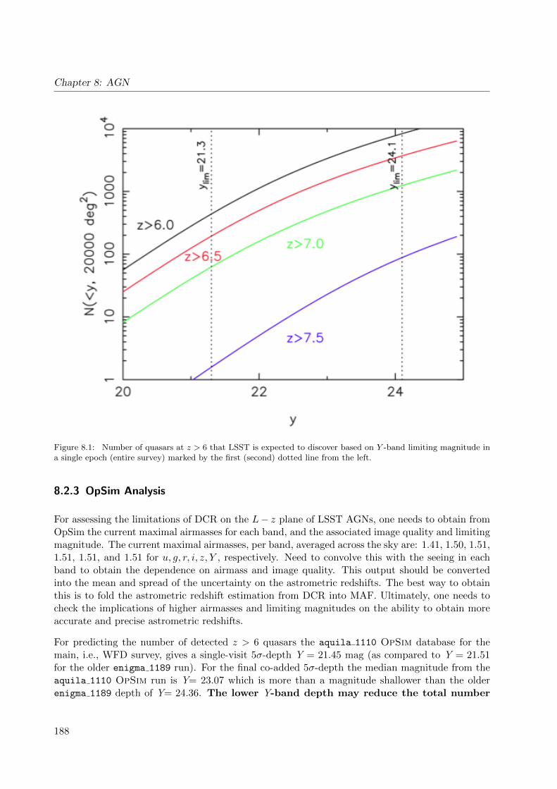
Chapter 8: AGN

Figure 8.1: Number of quasars at z > 6 that LSST is expected to discover based on Y -band limiting magnitude ina single epoch (entire survey) marked by the first (second) dotted line from the left.

8.2.3 OpSim Analysis

For assessing the limitations of DCR on the L− z plane of LSST AGNs, one needs to obtain fromOpSim the current maximal airmasses for each band, and the associated image quality and limitingmagnitude. The current maximal airmasses, per band, averaged across the sky are: 1.41, 1.50, 1.51,1.51, 1.51, and 1.51 for u, g, r, i, z, Y , respectively. Need to convolve this with the seeing in eachband to obtain the dependence on airmass and image quality. This output should be convertedinto the mean and spread of the uncertainty on the astrometric redshifts. The best way to obtainthis is to fold the astrometric redshift estimation from DCR into MAF. Ultimately, one needs tocheck the implications of higher airmasses and limiting magnitudes on the ability to obtain moreaccurate and precise astrometric redshifts.

For predicting the number of detected z > 6 quasars the aquila 1110 OpSim database for themain, i.e., WFD survey, gives a single-visit 5σ-depth Y = 21.45 mag (as compared to Y = 21.51for the older enigma 1189 run). For the final co-added 5σ-depth the median magnitude from theaquila 1110 OpSim run is Y= 23.07 which is more than a magnitude shallower than the olderenigma 1189 depth of Y= 24.36. The lower Y-band depth may reduce the total number

188

8.2 AGN Selection and Census

of quasars at z > 6 discovered by LSST by a factor of ∼ 2 (see Fig. 8.1).

As for general AGN selection, the effects of the sampling on variability selection should be assessed,and the amplitudes of the uncertainties in color-color space and how these depend on the cadenceshould be simulated. The combination of LSST photometry with that from WFIRST and/orEuclid data should also be considered, both for extending the upper limit in detectable redshift to∼ 10, but also improving the completeness and purity of the sample at lower redshifts.

8.2.4 Conclusions

Here we answer the ten questions posed in Sub-section 1.3.2:

Q1: Does the science case place any constraints on the tradeoff between the sky coverage andcoadded depth? For example, should the sky coverage be maximized (to ∼30,000 deg2, as e.g.,in Pan-STARRS) or the number of detected galaxies (the current baseline of 18,000 deg2)?

A1: The main FoM for AGN science is maximizing the number of AGNs detected. Since the co-added depth is already pushing well into the regime of low-luminosity AGNs, that suggeststhat area is preferred over depth.

Q2,3,5: Does the science case place any constraints on the tradeoff between uniformity of samplingand frequency of sampling? Does the science case place any constraints on the tradeoff betweenthe single-visit depth and the number of visits (especially in the u-band where longer exposureswould minimize the impact of the readout noise)? Does the science case place any constraintson the fraction of observing time allocated to each band?

A2,3,5: It should be possible to do a MAF analysis to determine the relative selection completenessand efficiency for OpSim outputs with different uniformity/frequency of sampling. The samecan be said for constraining the fraction of observing time in each band (where u is themost important for z . 3 and Y is most important for z & 6) and for determining whethernightly visits should be in the same band or not, and for the trade-off of single-visit depthand number of visits. However, the AGN census is unlikely to be the driver in these decisions.

Q4: Does the science case place any constraints on the Galactic plane coverage (spatial coverage,temporal sampling, visits per band)?

A4: Given the desire for maximal extragalactic area, added Galactic plane coverage would bedetrimental to AGN science.

Q6: Does the science case place any constraints on the cadence for deep drilling fields?

A6: Nearly any cadence discussed for the deep drilling fields will be more than adequate for AGNselection (as opposed to AGN physics, which will provide constraints); however added depthduring commissioning would enable more robust truth tables.

Q7: Assuming two visits per night, would the science case benefit if they are obtained in the sameband or not?

A7: No preference.

189

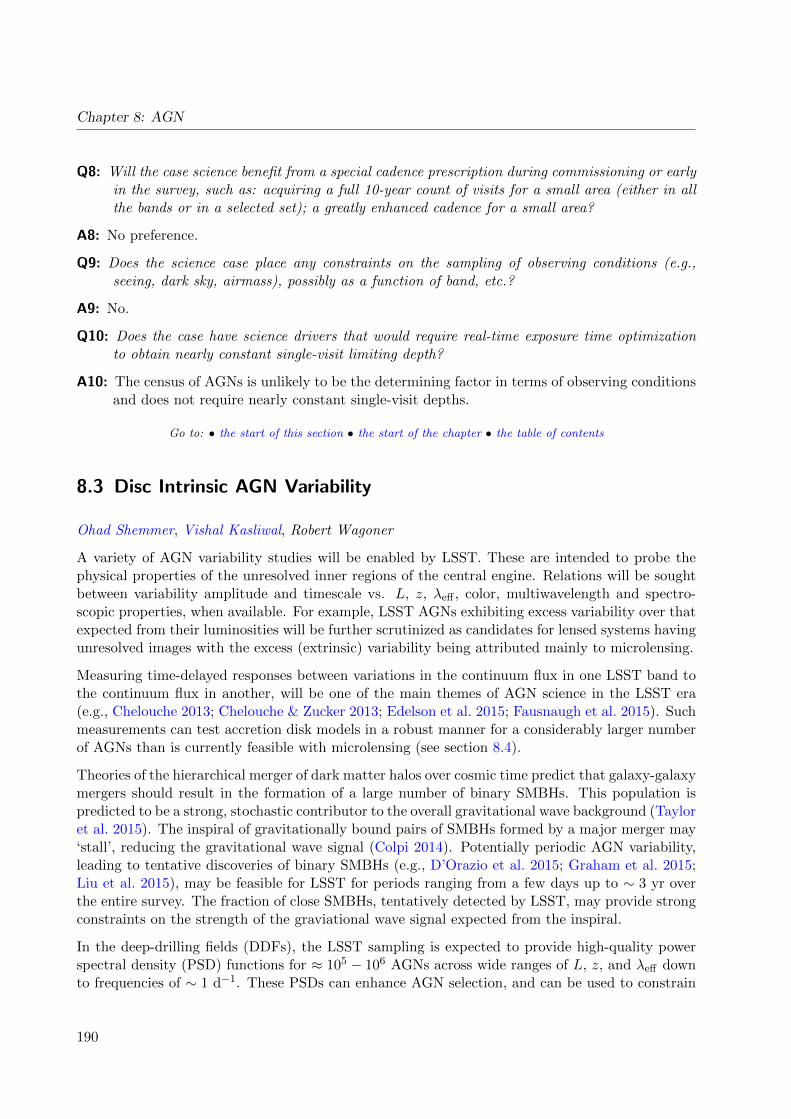
Chapter 8: AGN

Q8: Will the case science benefit from a special cadence prescription during commissioning or earlyin the survey, such as: acquiring a full 10-year count of visits for a small area (either in allthe bands or in a selected set); a greatly enhanced cadence for a small area?

A8: No preference.

Q9: Does the science case place any constraints on the sampling of observing conditions (e.g.,seeing, dark sky, airmass), possibly as a function of band, etc.?

A9: No.

Q10: Does the case have science drivers that would require real-time exposure time optimizationto obtain nearly constant single-visit limiting depth?

A10: The census of AGNs is unlikely to be the determining factor in terms of observing conditionsand does not require nearly constant single-visit depths.

Go to: • the start of this section • the start of the chapter • the table of contents

8.3 Disc Intrinsic AGN Variability

Ohad Shemmer, Vishal Kasliwal, Robert Wagoner

A variety of AGN variability studies will be enabled by LSST. These are intended to probe thephysical properties of the unresolved inner regions of the central engine. Relations will be soughtbetween variability amplitude and timescale vs. L, z, λeff , color, multiwavelength and spectro-scopic properties, when available. For example, LSST AGNs exhibiting excess variability over thatexpected from their luminosities will be further scrutinized as candidates for lensed systems havingunresolved images with the excess (extrinsic) variability being attributed mainly to microlensing.

Measuring time-delayed responses between variations in the continuum flux in one LSST band tothe continuum flux in another, will be one of the main themes of AGN science in the LSST era(e.g., Chelouche 2013; Chelouche & Zucker 2013; Edelson et al. 2015; Fausnaugh et al. 2015). Suchmeasurements can test accretion disk models in a robust manner for a considerably larger numberof AGNs than is currently feasible with microlensing (see section 8.4).

Theories of the hierarchical merger of dark matter halos over cosmic time predict that galaxy-galaxymergers should result in the formation of a large number of binary SMBHs. This population ispredicted to be a strong, stochastic contributor to the overall gravitational wave background (Tayloret al. 2015). The inspiral of gravitationally bound pairs of SMBHs formed by a major merger may‘stall’, reducing the gravitational wave signal (Colpi 2014). Potentially periodic AGN variability,leading to tentative discoveries of binary SMBHs (e.g., D’Orazio et al. 2015; Graham et al. 2015;Liu et al. 2015), may be feasible for LSST for periods ranging from a few days up to ∼ 3 yr overthe entire survey. The fraction of close SMBHs, tentatively detected by LSST, may provide strongconstraints on the strength of the graviational wave signal expected from the inspiral.

In the deep-drilling fields (DDFs), the LSST sampling is expected to provide high-quality powerspectral density (PSD) functions for ≈ 105 − 106 AGNs across wide ranges of L, z, and λeff downto frequencies of ∼ 1 d−1. These PSDs can enhance AGN selection, and can be used to constrain

190

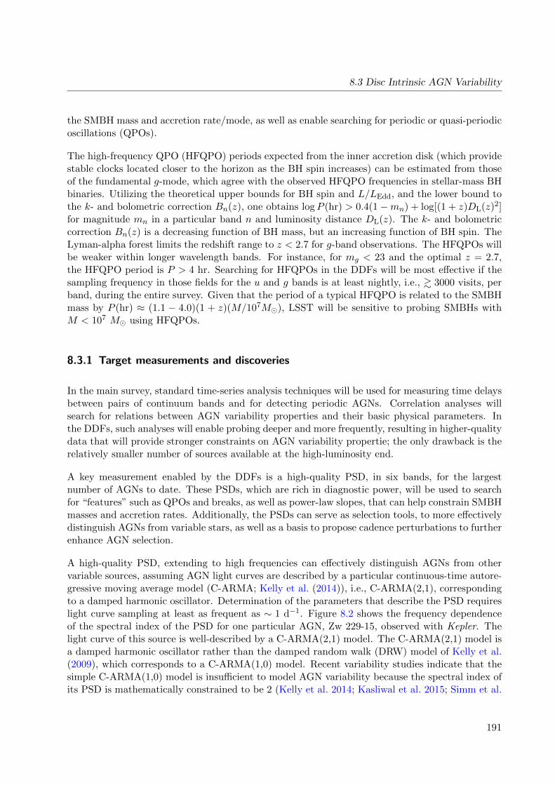
8.3 Disc Intrinsic AGN Variability

the SMBH mass and accretion rate/mode, as well as enable searching for periodic or quasi-periodicoscillations (QPOs).

The high-frequency QPO (HFQPO) periods expected from the inner accretion disk (which providestable clocks located closer to the horizon as the BH spin increases) can be estimated from thoseof the fundamental g-mode, which agree with the observed HFQPO frequencies in stellar-mass BHbinaries. Utilizing the theoretical upper bounds for BH spin and L/LEdd, and the lower bound tothe k- and bolometric correction Bn(z), one obtains logP (hr) > 0.4(1−mn) + log[(1 + z)DL(z)2]for magnitude mn in a particular band n and luminosity distance DL(z). The k- and bolometriccorrection Bn(z) is a decreasing function of BH mass, but an increasing function of BH spin. TheLyman-alpha forest limits the redshift range to z < 2.7 for g-band observations. The HFQPOs willbe weaker within longer wavelength bands. For instance, for mg < 23 and the optimal z = 2.7,the HFQPO period is P > 4 hr. Searching for HFQPOs in the DDFs will be most effective if thesampling frequency in those fields for the u and g bands is at least nightly, i.e., & 3000 visits, perband, during the entire survey. Given that the period of a typical HFQPO is related to the SMBHmass by P (hr) ≈ (1.1 − 4.0)(1 + z)(M/107M), LSST will be sensitive to probing SMBHs withM < 107 M using HFQPOs.

8.3.1 Target measurements and discoveries

In the main survey, standard time-series analysis techniques will be used for measuring time delaysbetween pairs of continuum bands and for detecting periodic AGNs. Correlation analyses willsearch for relations between AGN variability properties and their basic physical parameters. Inthe DDFs, such analyses will enable probing deeper and more frequently, resulting in higher-qualitydata that will provide stronger constraints on AGN variability propertie; the only drawback is therelatively smaller number of sources available at the high-luminosity end.

A key measurement enabled by the DDFs is a high-quality PSD, in six bands, for the largestnumber of AGNs to date. These PSDs, which are rich in diagnostic power, will be used to searchfor “features” such as QPOs and breaks, as well as power-law slopes, that can help constrain SMBHmasses and accretion rates. Additionally, the PSDs can serve as selection tools, to more effectivelydistinguish AGNs from variable stars, as well as a basis to propose cadence perturbations to furtherenhance AGN selection.

A high-quality PSD, extending to high frequencies can effectively distinguish AGNs from othervariable sources, assuming AGN light curves are described by a particular continuous-time autore-gressive moving average model (C-ARMA; Kelly et al. (2014)), i.e., C-ARMA(2,1), correspondingto a damped harmonic oscillator. Determination of the parameters that describe the PSD requireslight curve sampling at least as frequent as ∼ 1 d−1. Figure 8.2 shows the frequency dependenceof the spectral index of the PSD for one particular AGN, Zw 229-15, observed with Kepler. Thelight curve of this source is well-described by a C-ARMA(2,1) model. The C-ARMA(2,1) model isa damped harmonic oscillator rather than the damped random walk (DRW) model of Kelly et al.(2009), which corresponds to a C-ARMA(1,0) model. Recent variability studies indicate that thesimple C-ARMA(1,0) model is insufficient to model AGN variability because the spectral index ofits PSD is mathematically constrained to be 2 (Kelly et al. 2014; Kasliwal et al. 2015; Simm et al.

191

Chapter 8: AGN

−3 −2 −1 0 1ν (d−1)

−25

−20

−15

−10

−5

0

5

10

Pow

er(a

rb.u

nits

)

log10 Numerator(ν)

ν4

ν2

ν0

log10 PSD(ν)= log10 Numerator(ν)− log10 Denominator(ν)PSD∼ const

PSD∼ ν−2

PSD∼ ν−2 + ν−4

PSD∼ ν−4

PSD∼ ν−2

log10 Denominator(ν)

(a) (b)

Figure 8.2: (a) shows the PSD of Zw 229-15 as a function of frequency, obtained from Kepler photometry. ThePSD (purple) is the ratio of an even polynomial numerator (orange) to an even polynomial denominator (brown).This AGN is well-described by a C-ARMA(2,1) model; different powers of frequency dominate its PSD at differentfrequencies depending on the hyperparameters of this model. The wide frequency range enables detection of PSDspectral index variations ranging between 0 and 4. Clearly, the light curve of this AGN must be sampled ontimescales shorter than 1 − 5 days in order to observe the ν−4 behavior characteristic of a higher order randomwalk. This is illustrated in (b) where we see the frequencies and time intervals probed by SDSS, Kepler and a lightcurve constructed by combining the two datasets (SDSS+K2). Each vertical dashed line corresponds to a pair ofobservations seperated by the indicated δt (top axis). We plot (for illustration), two C-ARMA models with thesame overall power - a damped random walk, i.e. a C-ARMA(1.0) process, and a damped harmonic oscillator, i.e aC-ARMA(2,1) process. It is clear that SDSS (Kepler) cannot probe the highest (lowest) frequencies. However thecombination of the two can cover the full frequency range. The LSST cadence should be chosen to provide similartemporal coverage in the DDFs.

2015). Insufficient sampling of an AGN light curve (e.g., a few times a month), can therefore resultin the erroneous conclusion that a DRW model adequately characterizes the variability.

Accurate recovery of the PSD parameters can be greatly enhanced by increasing the samplingfrequency. To illustrate the effects of the cadence, Figure 8.3 shows how the inferred joint distribu-tion of two hyperparameters of the C-ARMA(2,1) model, the oscillator timescale and the dampingratio, depend on the sampling frequency. Degrading the sampling frequency from 1/(30 min), cor-responding to Kepler light curves, to 1/(3 d), corresponding to the nominal DDF cadence, changesboth the size and the shape of the joint distribution, degrading both the accuracy and correlationof the inferred hyperparameters. Furthermore, the C-ARMA formalism may enable adjusting thecadence of the DDFs once the LSST survey begins to determine the sampling pattern in real time.

8.3.2 Metrics

While additional quantitative work is required for determining the optimal cadence for fully cap-turing AGN accretion physics and to enhance AGN selection, it is clear that even the nominalDDF sampling (e.g. in db:baseCadence) is barely sufficient, and more frequent sampling wouldbe ideal. The ability to detect HFQPOs should also improve by increasing the sampling frequency,the amplitudes of such features are quite uncertain, as are the (short) duty cycles. Observations,theory and numerical simulations have only suggested that the fractional modulation should besmall (less than a few percent). Thus it is not obvious how to choose a metric and observing

192

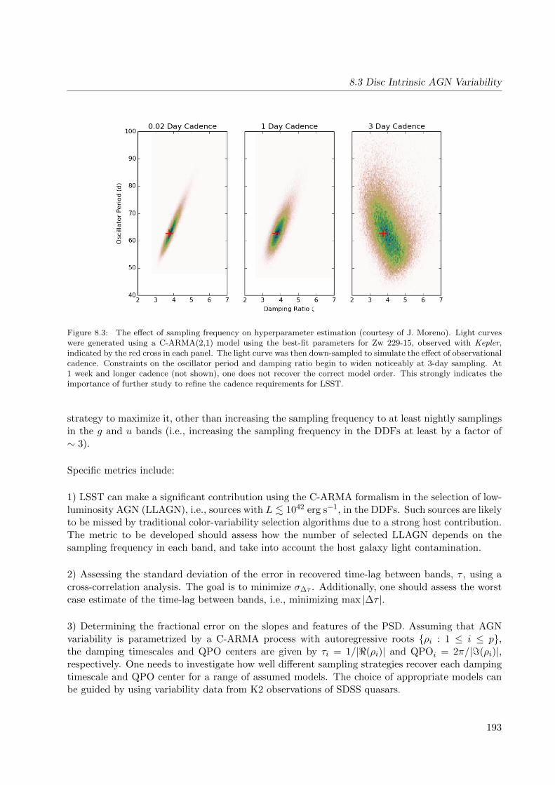
8.3 Disc Intrinsic AGN Variability

Figure 8.3: The effect of sampling frequency on hyperparameter estimation (courtesy of J. Moreno). Light curveswere generated using a C-ARMA(2,1) model using the best-fit parameters for Zw 229-15, observed with Kepler,indicated by the red cross in each panel. The light curve was then down-sampled to simulate the effect of observationalcadence. Constraints on the oscillator period and damping ratio begin to widen noticeably at 3-day sampling. At1 week and longer cadence (not shown), one does not recover the correct model order. This strongly indicates theimportance of further study to refine the cadence requirements for LSST.

strategy to maximize it, other than increasing the sampling frequency to at least nightly samplingsin the g and u bands (i.e., increasing the sampling frequency in the DDFs at least by a factor of∼ 3).

Specific metrics include:

1) LSST can make a significant contribution using the C-ARMA formalism in the selection of low-luminosity AGN (LLAGN), i.e., sources with L . 1042 erg s−1, in the DDFs. Such sources are likelyto be missed by traditional color-variability selection algorithms due to a strong host contribution.The metric to be developed should assess how the number of selected LLAGN depends on thesampling frequency in each band, and take into account the host galaxy light contamination.

2) Assessing the standard deviation of the error in recovered time-lag between bands, τ , using across-correlation analysis. The goal is to minimize σ∆τ . Additionally, one should assess the worstcase estimate of the time-lag between bands, i.e., minimizing max |∆τ |.

3) Determining the fractional error on the slopes and features of the PSD. Assuming that AGNvariability is parametrized by a C-ARMA process with autoregressive roots ρi : 1 ≤ i ≤ p,the damping timescales and QPO centers are given by τi = 1/|<(ρi)| and QPOi = 2π/|=(ρi)|,respectively. One needs to investigate how well different sampling strategies recover each dampingtimescale and QPO center for a range of assumed models. The choice of appropriate models canbe guided by using variability data from K2 observations of SDSS quasars.

193

Chapter 8: AGN

8.3.3 Discussion

While science-driven metric analysis is still to be performed, we expect the key requirement emerg-ing from such an analysis to be to increase the nominal sampling frequency in the DDFs by at leasta factor of 3, i.e., having at least 3000 visits, per band, during the entire survey. Alternatively,if this sampling is not feasible for all the DDFs, it would be beneficial to identify a subset of“special” DDFs which would be sampled by this frequency. Such DDFs would also benefit frombeing circumpolar, enabling a more uniform sampling to produce the highest quality PSDs.

8.3.4 Conclusions

Here we answer the ten questions posed in Sub-section 1.3.2:

Q1: Does the science case place any constraints on the tradeoff between the sky coverage andcoadded depth? For example, should the sky coverage be maximized (to ∼30,000 deg2, as e.g.,in Pan-STARRS) or the number of detected galaxies (the current baseline of 18,000 deg2)?

A1: The disc-intrinsic variability science case places no direct constraints on the tradeoff betweenthe sky coverage and the coadded depth.

Q2: Does the science case place any constraints on the tradeoff between uniformity of sampling andfrequency of sampling? For example, a rolling cadence can provide enhanced sample ratesover a part of the survey or the entire survey for a designated time at the cost of reducedsample rate the rest of the time (while maintaining the nominal total visit counts).

A2: Preliminary studies of the impact of the survey strategy on the disc-intrinsic variability sciencecase indicate that having the longest-possible temporal baseline, i.e., the interval between thefirst and last observation, is mandatory. The temporal baseline must be at least 2-3 × thelongest timescale (τ) built into the light curve (Koz lowski 2017). MacLeod et al. (2010) findthat max τ ∼ 1000 d suggesting that survey strategies that do not visit every field at boththe beginning and end of the survey will be sub-optimal for this science case. Furthermore,Fig. 8.2a demonstrates that in order to accurately distinguish between various stochasticmodels of AGN variability, the high frequency behavior of the light curve must be sufficientlyexplored by utilizing the DDFs.

Q3: Does the science case place any constraints on the tradeoff between the single-visit depth andthe number of visits (especially in the u-band where longer exposures would minimize theimpact of the readout noise)?

A3: The science cases would benefit from maximizing the number of visits.

Q4: Does the science case place any constraints on the Galactic plane coverage (spatial coverage,temporal sampling, visits per band)?

A4: AGN science cases would benefit from minimizing coverage of the Galactic plane.

Q5: Does the science case place any constraints on the fraction of observing time allocated to eachband?

194

8.4 AGN Size and Structure with Microlensing

A5: In general, the science cases place no constraints on the fraction of observing time allocatedto each band. For QPOs, however, shorter wavelengths are preferred.

Q6: Does the science case place any constraints on the cadence for deep drilling fields?

A6: The science cases would benefit from maximizing the sampling rate in the DDFs to at leastone visit per day in each band.

Q7: Assuming two visits per night, would the science case benefit if they are obtained in the sameband or not?

A7: Both continuum-continuum lag studies as well as color-variability studies of AGN would bestrongly benefited by having the two (or more) visits per night be in different bands.

Q8: Will the case science benefit from a special cadence prescription during commissioning or earlyin the survey, such as: acquiring a full 10-year count of visits for a small area (either in allthe bands or in a selected set); a greatly enhanced cadence for a small area?

A8: The disc-intrinsic variability science case would be benefited by having a greatly enhancedcadence for a small commissioning area of the sky as long as this area is followed up with thenormal revisit schedule later during the survey in order to ensure that the temporal baselinefor this region is as long as possible.

Q9: Does the science case place any constraints on the sampling of observing conditions (e.g.,seeing, dark sky, airmass), possibly as a function of band, etc.?

A9: The disc-intrinsic variability science case places no constraints on the sampling of observingconditions.

Q10: Does the case have science drivers that would require real-time exposure time optimizationto obtain nearly constant single-visit limiting depth?

A10: No

Go to: • the start of this section • the start of the chapter • the table of contents

8.4 AGN Size and Structure with Microlensing

Timo Anguita, Matt O’Dowd

Microlensing due to stars projected on top of individual gravitationally-lensed quasar images pro-duces additional magnification which can be used to probe the structure of the background high-redshift AGN.

The microlensing method is based on the fact that the variability amplitude depends on the quasarsize relative to the Einstein radius of a star (projected into the source plane). By comparing thevariability amplitudes at different wavelengths, we can determine the relative source sizes and testthe predicted wavelength scaling: Assuming a thermal profile for accretion disks, sizes in differentemission wavelengths can be probed and as such, constraints on the slope of this thermal profilecan be obtained. Given the sheer number of lensed systems that LSST is expected to discover

195

Chapter 8: AGN

(∼ 8000), this will allow us to stack systems for better constraints and hopefully determine theluminosity and redshift evolution of the disk size and profile. Due to the typical relative velocitiesof lenses, microlenses, observers (Earth) and source AGN, the microlensing variation timescalesare between months to a few decades.

8.4.1 Target measurements and discoveries

Analysis of microlensing induced variability will allow the measurement of accretion disk sizes Rλand their thermal profile slope α, which together strongly contrain the physics of accretion. Thisneeds to be done per system discovered. Assuming ∼1000 lensed quasars with high-quality lightcurves (i.e. that allow time-delay measurements, see Section 9.6), a relationship between the size,thermal profile slope, and luminosity of the accretion disk and the mass of the black hole will likelybe derived.

How precisely are we going to be able to measure these parameters for a given survey strategy?This is not a simple question to answer due to the significant degeneracies that plague the phe-nomenon. This is what our MAF metric will quantify. Before we design this, we need to predictand statistically quantify the degeneracies and sensitivities.

The quasar microlensing optical depth is ∼ 1, so every lensed quasar should be affected by mi-crolensing at any given point in time to a different extent. This continuous, low-level microlens-ing can provide useful statistical constraints on size and geometry for both accretion disks (e.g.,Kochanek 2004; Bate et al. 2008; Floyd et al. 2009; Blackburne et al. 2011, 2014; Jimenez-Vicenteet al. 2014) and broad emission line regions (e.g. Kochanek 2004; Richards et al. 2004; Waythet al. 2005; Sluse et al. 2011; O’Dowd et al. 2011; Guerras et al. 2013). Over LSST’s 10-year life,the resulting library of light curves will enable a statistical analysis of this low-level microlensingthat will far exceed previous efforts.

Note, however, that the larger the apparent magnification, the more stringent are the constraintson the geometric properties of the source. Mosquera & Kochanek (2011) studied the expectedmicrolensing timescales for all known lensed quasars at the time. They found that the medianEinstein crossing time scales, which can statistically be interpreted as the time between high-magnification events, in the observed I-band, is of the order of ∼ 20 yr (with a distributionbetween 10 and 40 yr). Additionally, the source crossing time (duration of a high-magnificationevent) is ∼ 7.3 months (with a distribution tail up to 3 yr). This basically means that out of allthe lensed quasar images (microlensing between images is completely uncorrelated) about half ofthem will undergo strong microlensing events during the 10 yr baseline of LSST. However, sincethe typical number of lensed images is either two or four, this means that, statistically, in everysystem, one (for doubles) or two (for quads) high magnification events should be observed in 10 yrof LSST monitoring.

Strong lensing events also provide our best chance of investigating anomalies in accretion diskgeometries. For example, warps due to multiple accretion events or magnetic fields, fragmentationdue to gravitational instability, and hot spots due to embedded star formation can all result indeviations from smooth temperature profiles. Such anomalies are expected to have an effect onthe light curves of strong microlensing events.

196

8.4 AGN Size and Structure with Microlensing

Note that, the important cadence parameter is the source crossing time. Ideally, high-magnificationevents would need to be as uniformly sampled as possible. The ∼ 7.3 months crossing time is themedian for the observed i-band, but this time would be significantly shorter for bluer bands: for athermal profile with slope α : Rλ ∝ λα implies source crossing time ts ∝ λ1/α → tu = ti×(λu/λi)

1/α.For a Shakura-Sunyaev slope of α = 0.75 this would correspond to ∼ 7.3× (3600/8140)4/3 monthswhich is ≈ 2.5 months in the u-band.

In terms of the cadence, at least three evenly sampled data points per band within two to threemonths would be preferred to be able to map the constraining high-magnification event, and thesewould hopefully be uniformly spaced. Additionally, LSST can trigger imaging of high-magnificationevents with dedicated facilities to enhance these constraints. More frequent sampling (e.g., in theDDFs) would increase such constraints significantly. However, since lensed quasars are not thatcommon, this smaller area would mean that only a modest number (< 100) of suitable systemswill be monitored in the DDFs.

Regarding the season length, the “months” timescale of high magnification events very likely meansthat we can/will miss high magnification events in the season gaps, at least in the bluer bands.

“Show stopper”: observations spread on timescales larger than 3 months. This would likely miss thehigh-magnification events. In those cases we could perhaps consider close consecutive photometricbands as equivalent accretion disk regions, however this would mean weaker constraints on thethermal profile.

Note that the discussion above is centered on high-magnification events. Even though these producethe most valuable information on short timescales (e.g., Anguita et al. 2008; Eigenbrod et al. 2008),low magnification events or no magnification events can set constraints on the structure of highredshift AGN as well as the lensing galaxies (e.g. Gil-Merino et al. 2005). In particular, sinceisolated high-magnification events are rare, accretion disk size studies with microlensing are doneby a Bayesian analysis of long (several years) light curves of microlensing in every lensed imagesimultaneously compared to source plane microlensing magnification patterns (e.g., Kochanek 2004;Blackburne et al. 2014). Constraints using this method rely on the fact that even when not strong,several uncorrelated microlensing induced variations in all lensed images as well as anomalous(single epoch) flux ratios (e.g., Bate et al. 2008; Rojas et al. 2014) in all available bands needto be consistent with the underlying geometrical structure of the background accretion disk. It isimportant to take into consideration that the timescales directly depend on the projected velocitiesof the three-plane system: the redshifts of the lens and source as well as their respective peculiarvelocites along the CMB dipole velocity in the direction towards the lensing galaxies (observer’speculiar velocity).

Long-timescale high-accuracy multi-band data as will be delivered by LSST have never been ob-tained to date for any lensed system. Coupling this fact to a factor ∼10 increase in the number oflensed quasars known, LSST will enable totally new and unprecedented perspectives for microlens-ing studies.

Microlensing Aided Reverberation Mapping: Quasar broad emission lines exhibit a verywide range of ionization energies. This implies differences in the incident ionizing flux, and suggeststhat we may expect a radial stratification of ionization species This is indeed observed in bothreverberation mapping (see review by Gaskell 2009) and gravitational microlensing (Guerras et al.2013). However proximity to the ionizing source alone isn’t enough to explain the wide range of

197

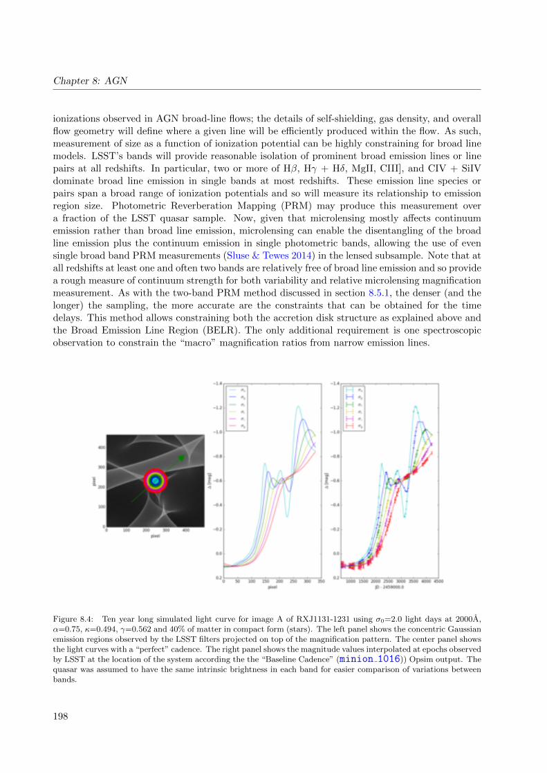
Chapter 8: AGN

ionizations observed in AGN broad-line flows; the details of self-shielding, gas density, and overallflow geometry will define where a given line will be efficiently produced within the flow. As such,measurement of size as a function of ionization potential can be highly constraining for broad linemodels. LSST’s bands will provide reasonable isolation of prominent broad emission lines or linepairs at all redshifts. In particular, two or more of Hβ, Hγ + Hδ, MgII, CIII], and CIV + SiIVdominate broad line emission in single bands at most redshifts. These emission line species orpairs span a broad range of ionization potentials and so will measure its relationship to emissionregion size. Photometric Reverberation Mapping (PRM) may produce this measurement overa fraction of the LSST quasar sample. Now, given that microlensing mostly affects continuumemission rather than broad line emission, microlensing can enable the disentangling of the broadline emission plus the continuum emission in single photometric bands, allowing the use of evensingle broad band PRM measurements (Sluse & Tewes 2014) in the lensed subsample. Note that atall redshifts at least one and often two bands are relatively free of broad line emission and so providea rough measure of continuum strength for both variability and relative microlensing magnificationmeasurement. As with the two-band PRM method discussed in section 8.5.1, the denser (and thelonger) the sampling, the more accurate are the constraints that can be obtained for the timedelays. This method allows constraining both the accretion disk structure as explained above andthe Broad Emission Line Region (BELR). The only additional requirement is one spectroscopicobservation to constrain the “macro” magnification ratios from narrow emission lines.

Figure 8.4: Ten year long simulated light curve for image A of RXJ1131-1231 using σ0=2.0 light days at 2000A,α=0.75, κ=0.494, γ=0.562 and 40% of matter in compact form (stars). The left panel shows the concentric Gaussianemission regions observed by the LSST filters projected on top of the magnification pattern. The center panel showsthe light curves with a “perfect” cadence. The right panel shows the magnitude values interpolated at epochs observedby LSST at the location of the system according the the “Baseline Cadence” (minion 1016)) Opsim output. Thequasar was assumed to have the same intrinsic brightness in each band for easier comparison of variations betweenbands.

198

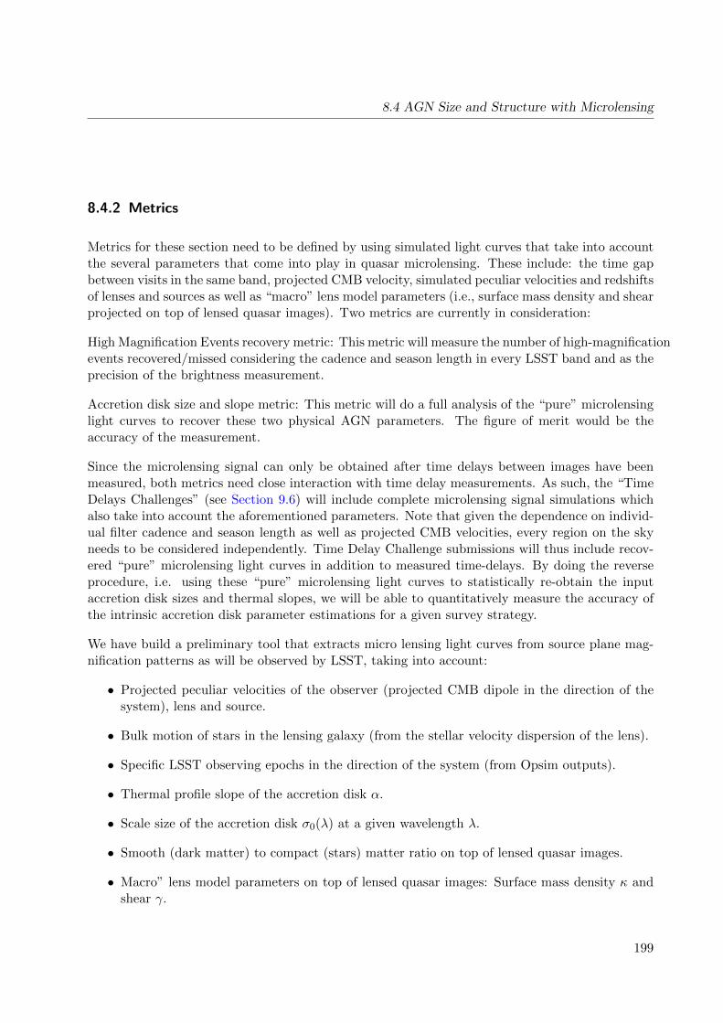
8.4 AGN Size and Structure with Microlensing

8.4.2 Metrics

Metrics for these section need to be defined by using simulated light curves that take into accountthe several parameters that come into play in quasar microlensing. These include: the time gapbetween visits in the same band, projected CMB velocity, simulated peculiar velocities and redshiftsof lenses and sources as well as “macro” lens model parameters (i.e., surface mass density and shearprojected on top of lensed quasar images). Two metrics are currently in consideration:

High Magnification Events recovery metric: This metric will measure the number of high-magnificationevents recovered/missed considering the cadence and season length in every LSST band and as theprecision of the brightness measurement.

Accretion disk size and slope metric: This metric will do a full analysis of the “pure” microlensinglight curves to recover these two physical AGN parameters. The figure of merit would be theaccuracy of the measurement.

Since the microlensing signal can only be obtained after time delays between images have beenmeasured, both metrics need close interaction with time delay measurements. As such, the “TimeDelays Challenges” (see Section 9.6) will include complete microlensing signal simulations whichalso take into account the aforementioned parameters. Note that given the dependence on individ-ual filter cadence and season length as well as projected CMB velocities, every region on the skyneeds to be considered independently. Time Delay Challenge submissions will thus include recov-ered “pure” microlensing light curves in addition to measured time-delays. By doing the reverseprocedure, i.e. using these “pure” microlensing light curves to statistically re-obtain the inputaccretion disk sizes and thermal slopes, we will be able to quantitatively measure the accuracy ofthe intrinsic accretion disk parameter estimations for a given survey strategy.

We have build a preliminary tool that extracts micro lensing light curves from source plane mag-nification patterns as will be observed by LSST, taking into account:

• Projected peculiar velocities of the observer (projected CMB dipole in the direction of thesystem), lens and source.

• Bulk motion of stars in the lensing galaxy (from the stellar velocity dispersion of the lens).

• Specific LSST observing epochs in the direction of the system (from Opsim outputs).

• Thermal profile slope of the accretion disk α.

• Scale size of the accretion disk σ0(λ) at a given wavelength λ.

• Smooth (dark matter) to compact (stars) matter ratio on top of lensed quasar images.

• Macro” lens model parameters on top of lensed quasar images: Surface mass density κ andshear γ.

199

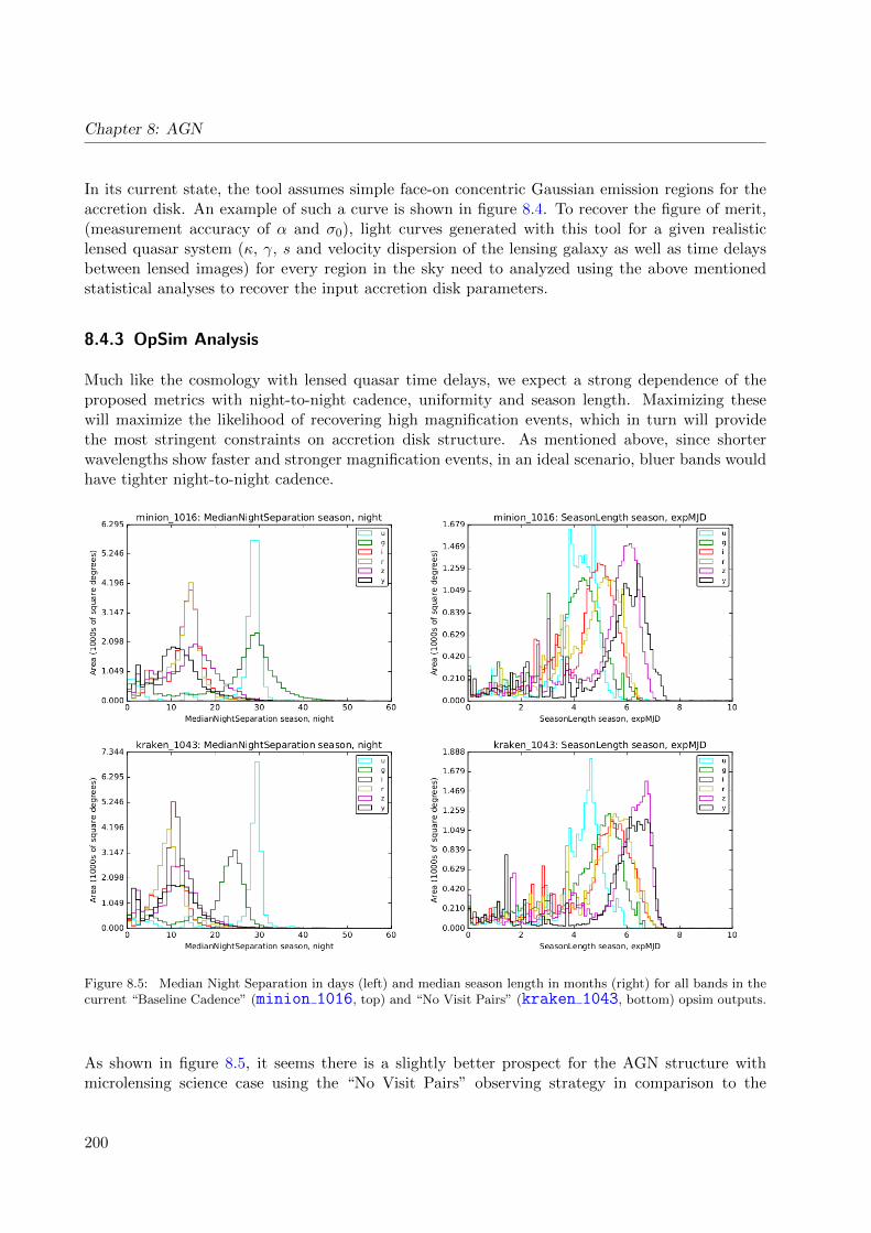
Chapter 8: AGN

In its current state, the tool assumes simple face-on concentric Gaussian emission regions for theaccretion disk. An example of such a curve is shown in figure 8.4. To recover the figure of merit,(measurement accuracy of α and σ0), light curves generated with this tool for a given realisticlensed quasar system (κ, γ, s and velocity dispersion of the lensing galaxy as well as time delaysbetween lensed images) for every region in the sky need to analyzed using the above mentionedstatistical analyses to recover the input accretion disk parameters.

8.4.3 OpSim Analysis

Much like the cosmology with lensed quasar time delays, we expect a strong dependence of theproposed metrics with night-to-night cadence, uniformity and season length. Maximizing thesewill maximize the likelihood of recovering high magnification events, which in turn will providethe most stringent constraints on accretion disk structure. As mentioned above, since shorterwavelengths show faster and stronger magnification events, in an ideal scenario, bluer bands wouldhave tighter night-to-night cadence.

Figure 8.5: Median Night Separation in days (left) and median season length in months (right) for all bands in thecurrent “Baseline Cadence” (minion 1016, top) and “No Visit Pairs” (kraken 1043, bottom) opsim outputs.

As shown in figure 8.5, it seems there is a slightly better prospect for the AGN structure withmicrolensing science case using the “No Visit Pairs” observing strategy in comparison to the

200

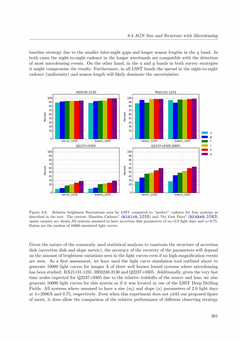
8.4 AGN Size and Structure with Microlensing

baseline strategy due to the smaller inter-night gaps and longer season lengths in the g band. Inboth cases the night-to-night cadence in the longer wavebands are compatible with the detectionof most microlensing events. On the other hand, in the u and g bands in both survey strategiesit might compromise the results. Furthermore, in all LSST bands the spread in the night-to-nightcadence (uniformity) and season length will likely dominate the uncertainties.

Figure 8.6: Relative brightness fluctuations seen by LSST compared to “perfect” cadence for four systems asdescribed in the text. The current “Baseline Cadence” (minion 1016) and “No Visit Pairs” (kraken 1043)opsim outputs are shown.All systems assumed to have accretion disk parameters of σ0=2.0 light days and α=0.75.Ratios are the median of 10000 simulated light curves.

Given the nature of the commonly used statistical analyses to constrain the structure of accretiondisk (accretion disk and slope metric), the accuracy of the recovery of the parameters will dependon the amount of brightness variations seen in the light curves even if no high-magnification eventsare seen. As a first assessment, we have used the light curve simulation tool outlined above togenerate 10000 light curves for images A of three well known lensed systems where microlensinghas been studied: RXJ1131-1231, HE0230-2130 and Q2237+0305. Additionally, given the very fasttime scales expected for Q2237+0305 due to the relative redshifts of the source and lens, we alsogenerate 10000 light curves for this system as if it was located in one of the LSST Deep DrillingFields. All systems where assumed to have a size (σ0) and slope (α) parameters of 2.0 light daysat λ=2000A and 0.75, respectively. Even when this experiment does not yield our proposed figureof merit, it does allow the comparison of the relative performance of different observing strategy

201

Chapter 8: AGN

regarding microlensing signal recovery.

The results of this experiment are shown in Figure 8.6. For this analysis, at least for the foursystems studied, we can see that even when the “No Visit Pairs” observing strategy shows aslightly better prospect compared to the “Baseline Cadence” for our science case, the difference isnegligible. Note also that with the exception of Q2227+0305 (due to its very short time scales), bothobserving strategies will be able to map the expected microlensing induced brightness variationsat a very high rate. It is important to consider that this is an optimistic analysis because thephotometric uncertainties (including the dominating ones that come from the intrinsic variabilitycorrection from time delay measurements) have not been taken into account.

8.4.4 Conclusions

Here we answer the ten questions posed in Sub-section 1.3.2:

Q1: Does the science case place any constraints on the tradeoff between the sky coverage andcoadded depth? For example, should the sky coverage be maximized (to ∼30,000 deg2, as e.g.,in Pan-STARRS) or the number of detected galaxies (the current baseline of 18,000 deg2)?

A1: Given that lensed quasars are rare, maximizing the area coverage would increase the numberof systems to study. Even if this comes at a cadence cost given that in most cases the studiedOpSim experiments provide sufficient temporal constraints.

Q2: Does the science case place any constraints on the tradeoff between uniformity of sampling andfrequency of sampling? For example, a rolling cadence can provide enhanced sample ratesover a part of the survey or the entire survey for a designated time at the cost of reducedsample rate the rest of the time (while maintaining the nominal total visit counts).

A2: Given the long timescales of microlensing events and the inability of predicting high-magnificationevents, uniform sampling would be better.

Q3: Does the science case place any constraints on the tradeoff between the single-visit depth andthe number of visits (especially in the u-band where longer exposures would minimize theimpact of the readout noise)?

A3: No.

Q4: Does the science case place any constraints on the Galactic plane coverage (spatial coverage,temporal sampling, visits per band)?

A4: Not really, however, minimizing the coverage of the Galactic would benefit all AGN sciencecases.

Q5: Does the science case place any constraints on the fraction of observing time allocated to eachband?

A5: Ideally, shorter wavelengths should get denser (uniform) sampling.

Q6: Does the science case place any constraints on the cadence for deep drilling fields?

202

8.5 Future Work

A6: As in the main survey, AGN microlensing would benefit if the deep drilling fields observationswould span long timescales with uniform coverage.

Q7: Assuming two visits per night, would the science case benefit if they are obtained in the sameband or not?

A7: Not very important for our since case. Given a choice, different bands would be better.

Q8: Will the case science benefit from a special cadence prescription during commissioning or earlyin the survey, such as: acquiring a full 10-year count of visits for a small area (either in allthe bands or in a selected set); a greatly enhanced cadence for a small area?

A8: No.

Q9: Does the science case place any constraints on the sampling of observing conditions (e.g.,seeing, dark sky, airmass), possibly as a function of band, etc.?

A9: Seeing and Airmass are directly related to the ability to accurately separate the flux frompossibly blended lensed images. As with most transient science cases, excellent seeing imagesare required as templates for image substraction.

Q10: Does the case have science drivers that would require real-time exposure time optimizationto obtain nearly constant single-visit limiting depth?

A10: No.

Go to: • the start of this section • the start of the chapter • the table of contents

8.5 Future Work

In this section we provide a short compendium of science cases that are either still being developed,or that are deserving of quantitative MAF analysis at some point in the future.

8.5.1 The Size and Structure of the Broad Emission Line Region

Ohad Shemmer

LSST may provide estimates of the size and structure of the broad emission line region (BELR)using the photometric reverberation mapping (PRM) method. This method enables one to measurethe time-delayed response of the flux in one band to the flux in another by using cross-correlationtechniques on AGN light curves (e.g., Chelouche et al. 2014).

The main challenge of PRM is to detect, with high confidence, the time lag between the variationsof a BELR line-rich band with respect to variations in a line-poor band, given the relatively smallflux contributions (∼ 10%) of BELR lines to each LSST band. Nevertheless, LSST is expected todeliver BELR line-continuum time delays in ∼ 105 − 106 sources, which is unprecedented whencompared to ∼ 60− 80 such measurements conducted, to date, via the traditional, yet much moreexpensive (per source) spectroscopic method. Sources in the DDFs will benefit from the highest

203

Chapter 8: AGN

quality PRM time-delay measurements given the factor of ∼ 10 denser sampling (Chelouche et al.2014).

Target measurements and discoveries

The PRM measurements will probe the size and structure of the BELR, in a statistical sense, andmay provide improved SMBH mass estimates for sources that have at least single-epoch spectra.PRM will also be used to trigger follow-up spectrophotometric monitoring of “promising” casesdepending on their variability properties. The goal is to obtain RBELR measures for different BELRlines in certain luminosity and redshift bins; for example, PRM may provide mean RBELR for Lyαin quasars at 2.1 . z . 2.2 with 45 . logL(erg s−1) . 46, or mean RBELR for C iv λ1549 inquasars at 1.6 . z . 1.7 with 44 . logL(erg s−1) . 45.

The PRM method is very sensitive to the sampling in each band, therefore the ability to derivereliable time delays can be affected significantly by the LSST cadence. The best results will beobtained by having the most uniform sampling equally for each band. Since the observed line-continuum lags scale with luminosity and redshift, PRM with the LSST will be limited by theaverage time gaps between successive observations in a particular band. Additionally, there isa trade-off between the number of DDFs and the number of time delays that PRM can obtain(Chelouche et al. 2014). For example, an increase in the number of DDFs, with similarly densesampling in each field, can yield a proportionately larger number of high-quality time delays, downto somewhat lower luminosities (to the extent that host-galaxy contamination can be neglected),but at the expense of far fewer time delays (for relatively high luminosity sources) in the mainsurvey.

Metrics

The average and the dispersion in the number of visits, per band, across the sky for the nominalOpSim (during the entire survey) should be computed. Since PRM works best for uniform sam-pling, one should compare the distributions of the number of visits in each band, averaged acrossthe sky, and identify ways to minimize any potential differences between these distributions. Byrunning PRM simulations, one should identify the 1) minimum number of visits (in any band)that can yield any meaningful BELR-continuum lag estimates, and 2) the largest difference inthe number of visits between two different bands that can yield any meaningful BELR-continuumlag estimates. These simulations should be repeated by doubling the nominal number of DDFs.Finally, the uncertainties on RBELR values achieved with the nominal OpSim should be assessed,and potential perturbations to the cadence should be pointed out to reduce these uncertainties.

Another metric is the accuracy of the slope α, ∆α, in the RBELR ∝ Lα relation. Spectrophotometricmonitoring typically yields α ' 0.50± 0.05.

Go to: • the start of this section • the start of the chapter • the table of contents

204

8.6 Discussion

8.6 Discussion

The goals of this Chapter were 1) to define and quantify key metrics for AGN science that canbe measured and tested using the current LSST observing strategy, and 2) to identify reasonableperturbations that may be beneficial for AGN science. Undoubtedly, additional work is requiredto refine many of these metrics and perform more rigorous tests and simulations. The following listidentifies additional cadence-related aspects for further consideration. Together with the metricsdiscussed in this Chapter, this may be regarded as a road map for further investigations that shouldbe performed during the planning stage.

1) Assuming a total of ten DDFs, it would be beneficial if one of those fields could be sampledmore heavily than the others and would be visited nightly (or even more frequently, e.g., from ∼ 1to ∼ 1000 min) per band. This can be justified by the fact that a) very few AGNs or transientAGNs have been monitored at these frequencies on such a long baseline, leaving room for discovery,and b) this may probe intermediate-mass black holes (∼ 104 − 105 M) via PRM or PSDs. Goodcandidate fields are the Magellanic Clouds and the Chandra Deep Field-South. An observationalstrategy should be developed and implemented either in a new OpSim, or during commissioning.

2) In order to have more informative metrics, accurate model light curves are needed that canreproduce fiducial light curves in different bands, at different inherent luminosities, and at differentredshifts. This may be developed together with the Strong Lensing Science Collaboration.

3) There is a need to compare the science content in this Chapter with the AGN chapter in the LSSTScience Book as well as with the Ivezic et al. overview paper (http://arxiv.org/pdf/0805.2366v4.pdf)to ensure that no key science aspect is overlooked or compromised by the nominal cadence.

4) It is worth checking whether any aspect of blazar science might be compromised by the nominalcadence, or would benefit from a specific cadence requirement.

5) The effects of the cadence on the overall LSST astrometry accuracy and precision should beassessed in terms of potential effects on AGN selection. For example, AGN selection may benefitfrom very good depth at least in the 1st and 10th year of the survey.

Beyond this, we anticipate more AGN science cases emerging, and needing to be evaluated viascience-driven MAF analysis. For example, regular (non-quasi) periodicity, possibly to probe thepopulation of binary SMBHs, is an observing mode we have not yet focused much attention on.What would be a good cadence to do that science? We encourage more questions like this as webuild up the metric analysis outlined in the chapter to date.

Go to: • the start of this section • the start of the chapter • the table of contents

205

9 Accurate Cosmological Measurements on theLargest Scales

Chapter editors: Eric Gawiser, Michelle Lochner.

Contributing authors: Humna Awan, Eric Gawiser, Peter Kurczynski, Lynne Jones, Josh Meyers,Tony Tyson, Melissa L. Graham, Samuel Schmidt, Andy Connolly, Zeljko Ivezic, Jeonghee Rho,Rahul Biswas, Seth Digel, Ryan Foley, Lluıs Galbany, Phillipe Gris, Renee Hlozek, Saurabh W. Jha,Richard Kessler, Alex Kim, Alex Malz, Jason D. McEwen, Jeffrey Newman, Hiranya V. Peiris,Kara Ponder, Robert L. Schuhmann, Christopher Stubbs, W. Michael Wood-Vasey, Phil Marshall,Timo Anguita

9.1 Introduction

Cosmology is one of the key science themes for which LSST was designed. Our goal is to measurecosmological parameters, such as the equation of state of dark energy or departures from Gen-eral Relativity, with sufficient accuracy to distinguish one model from another and hence driveour theoretical understanding of how the universe works as a whole. To do this will necessarilyinvolve a variety of different measurements that can act as cross-checks and break any parameterdegeneracies.

The Dark Energy Science Collaboration (DESC) has identified five different cosmological probesenabled by the LSST: weak lensing (WL), large-scale structure (LSS), Type Ia supernovae (SN),strong lensing (SL), and clusters of galaxies (CL). In all these cases, the primary concern is theresidual systematic error: the shapes and photometric redshifts of galaxies and the properties ofsupernova and lensed quasar light curves will all need to be measured with extraordinary accuracyin order to properly harness the statistical power available through LSST. This accuracy willcome from the abundance and heterogeneity of the individual measurements and the degree towhich they can be modeled and understood. This latter point implies a need for uniformity inthe survey, which enables powerful simplifying assumptions to be made when calibrating on thelargest, cosmologically most important scales. The need for heterogeneity in the measurementsalso requires uniformity in the sense that the nuisance parameters that describe the systematiceffects need to be sampled over as wide a range as possible (e.g., the need to sample a wide rangeof roll angles to minimize shape error; observing conditions to understand photometric errors dueto the changing atmosphere).

In this chapter we look at some of the key measurements planned by DESC and how they dependon the Observing Strategy.

207

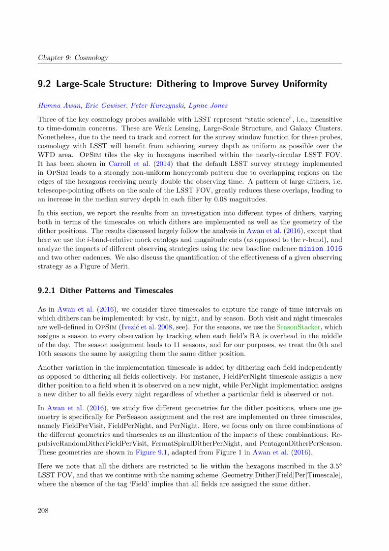
Chapter 9: Cosmology

9.2 Large-Scale Structure: Dithering to Improve Survey Uniformity

Humna Awan, Eric Gawiser, Peter Kurczynski, Lynne Jones

Three of the key cosmology probes available with LSST represent “static science”, i.e., insensitiveto time-domain concerns. These are Weak Lensing, Large-Scale Structure, and Galaxy Clusters.Nonetheless, due to the need to track and correct for the survey window function for these probes,cosmology with LSST will benefit from achieving survey depth as uniform as possible over theWFD area. OpSim tiles the sky in hexagons inscribed within the nearly-circular LSST FOV.It has been shown in Carroll et al. (2014) that the default LSST survey strategy implementedin OpSim leads to a strongly non-uniform honeycomb pattern due to overlapping regions on theedges of the hexagons receiving nearly double the observing time. A pattern of large dithers, i.e.telescope-pointing offsets on the scale of the LSST FOV, greatly reduces these overlaps, leading toan increase in the median survey depth in each filter by 0.08 magnitudes.

In this section, we report the results from an investigation into different types of dithers, varyingboth in terms of the timescales on which dithers are implemented as well as the geometry of thedither positions. The results discussed largely follow the analysis in Awan et al. (2016), except thathere we use the i-band-relative mock catalogs and magnitude cuts (as opposed to the r-band), andanalyze the impacts of different observing strategies using the new baseline cadence minion 1016and two other cadences. We also discuss the quantification of the effectiveness of a given observingstrategy as a Figure of Merit.

9.2.1 Dither Patterns and Timescales

As in Awan et al. (2016), we consider three timescales to capture the range of time intervals onwhich dithers can be implemented: by visit, by night, and by season. Both visit and night timescalesare well-defined in OpSim (Ivezic et al. 2008, see). For the seasons, we use the SeasonStacker, whichassigns a season to every observation by tracking when each field’s RA is overhead in the middleof the day. The season assignment leads to 11 seasons, and for our purposes, we treat the 0th and10th seasons the same by assigning them the same dither position.

Another variation in the implementation timescale is added by dithering each field independentlyas opposed to dithering all fields collectively. For instance, FieldPerNight timescale assigns a newdither position to a field when it is observed on a new night, while PerNight implementation assignsa new dither to all fields every night regardless of whether a particular field is observed or not.

In Awan et al. (2016), we study five different geometries for the dither positions, where one ge-ometry is specifically for PerSeason assignment and the rest are implemented on three timescales,namely FieldPerVisit, FieldPerNight, and PerNight. Here, we focus only on three combinations ofthe different geometries and timescales as an illustration of the impacts of these combinations: Re-pulsiveRandomDitherFieldPerVisit, FermatSpiralDitherPerNight, and PentagonDitherPerSeason.These geometries are shown in Figure 9.1, adapted from Figure 1 in Awan et al. (2016).

Here we note that all the dithers are restricted to lie within the hexagons inscribed in the 3.5

LSST FOV, and that we continue with the naming scheme [Geometry]Dither[Field]Per[Timescale],where the absence of the tag ‘Field’ implies that all fields are assigned the same dither.

208

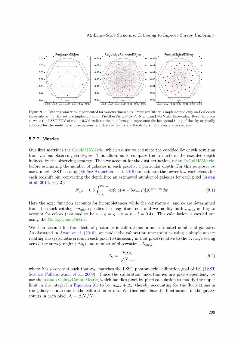
9.2 Large-Scale Structure: Dithering to Improve Survey Uniformity

0.03 0.02 0.01 0.00 0.01 0.02 0.03

0.03

0.02

0.01

0.00

0.01

0.02

0.03

PentagonDither

0.03 0.02 0.01 0.00 0.01 0.02 0.03

0.03

0.02

0.01

0.00

0.01

0.02

0.03

RepulsiveRandomDither

0.03 0.02 0.01 0.00 0.01 0.02 0.03

0.03

0.02

0.01

0.00

0.01

0.02

0.03

FermatSpiralDither

Figure 9.1: Dither geometries implemented for various timescales. PentagonDither is implemented only on PerSeasontimescale, while the rest are implemented on FieldPerVisit, FieldPerNight, and PerNight timescales. Here the greencurve is the LSST FOV of radius 0.305 radians; the blue hexagon represents the hexagonal tiling of the sky originallyadopted for the undithered observations; and the red points are the dithers. The axes are in radians.

9.2.2 Metrics

Our first metric is the CoaddM5Metric, which we use to calculate the coadded 5σ depth resultingfrom various observing strategies. This allows us to compare the artifacts in the coadded depthinduced by the observing strategy. Then we account for the dust extinction, using ExGalM5Metric,before estimating the number of galaxies in each pixel at a particular depth. For this purpose, weuse a mock LSST catalog (Munoz Arancibia et al. 2015) to estimate the power law coefficients foreach redshift bin, converting the depth into an estimated number of galaxies for each pixel (Awanet al. 2016, Eq. 2):

Ngal = 0.5

∫ mmax

−∞erfc[a(m− 5σstack)]10c1m+c2dm (9.1)

Here the erfc function accounts for incompleteness while the constants c1 and c2 are determinedfrom the mock catalog. mmax specifies the magnitude cut, and we modify both mmax and c2 toaccount for colors (assumed to be u − g = g − r = r − i = 0.4). This calculation is carried outusing the GalaxyCountMetric.

We then account for the effects of photometric calibrations in our estimated number of galaxies.As discussed in Awan et al. (2016), we model the calibration uncertainties using a simple ansatzrelating the systematic errors in each pixel to the seeing in that pixel (relative to the average seeingacross the survey region; ∆si) and number of observations Nobs,i:

∆i =k∆si√Nobs,i

(9.2)

where k is a constant such that σ∆i matches the LSST photometric calibration goal of 1% (LSSTScience Collaboration et al. 2009). Since the calibration uncertainties are pixel-dependent, weuse the pseudo-GalaxyCountsMetric, which handles pixel-by-pixel calculation to modify the upperlimit in the integral in Equation 9.1 to be mmax + ∆i, thereby accounting for the fluctuations inthe galaxy counts due to the calibration errors. We then calculate the fluctuations in the galaxycounts in each pixel, δi = ∆Ni/N .

209

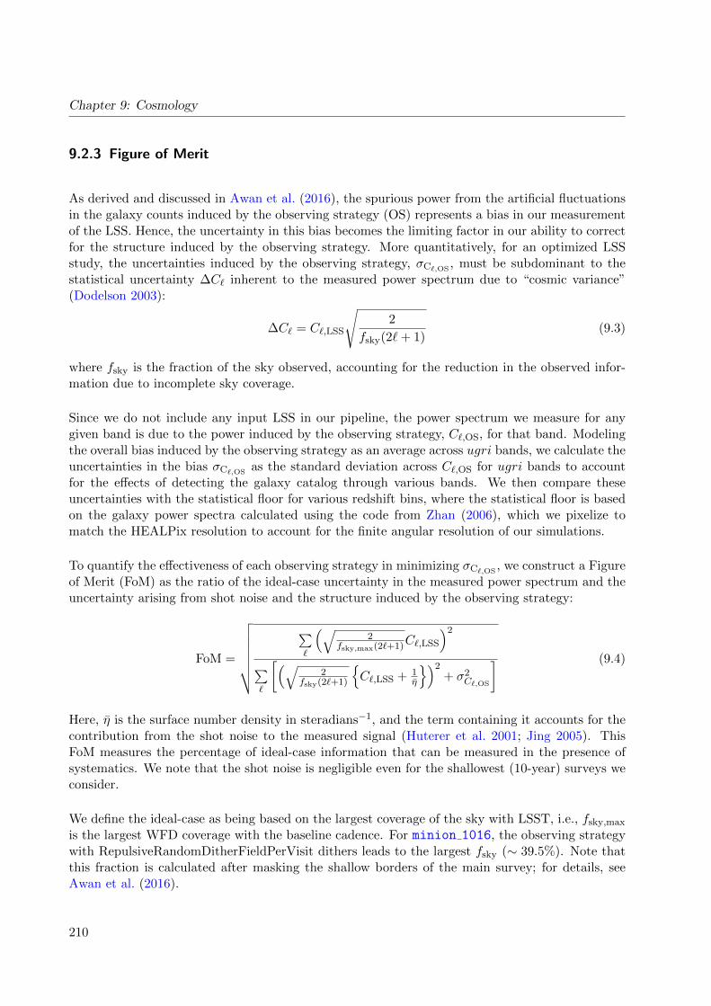
Chapter 9: Cosmology

9.2.3 Figure of Merit

As derived and discussed in Awan et al. (2016), the spurious power from the artificial fluctuationsin the galaxy counts induced by the observing strategy (OS) represents a bias in our measurementof the LSS. Hence, the uncertainty in this bias becomes the limiting factor in our ability to correctfor the structure induced by the observing strategy. More quantitatively, for an optimized LSSstudy, the uncertainties induced by the observing strategy, σC`,OS

, must be subdominant to thestatistical uncertainty ∆C` inherent to the measured power spectrum due to “cosmic variance”(Dodelson 2003):

∆C` = C`,LSS

√2

fsky(2`+ 1)(9.3)

where fsky is the fraction of the sky observed, accounting for the reduction in the observed infor-mation due to incomplete sky coverage.

Since we do not include any input LSS in our pipeline, the power spectrum we measure for anygiven band is due to the power induced by the observing strategy, C`,OS, for that band. Modelingthe overall bias induced by the observing strategy as an average across ugri bands, we calculate theuncertainties in the bias σC`,OS

as the standard deviation across C`,OS for ugri bands to accountfor the effects of detecting the galaxy catalog through various bands. We then compare theseuncertainties with the statistical floor for various redshift bins, where the statistical floor is basedon the galaxy power spectra calculated using the code from Zhan (2006), which we pixelize tomatch the HEALPix resolution to account for the finite angular resolution of our simulations.

To quantify the effectiveness of each observing strategy in minimizing σC`,OS, we construct a Figure

of Merit (FoM) as the ratio of the ideal-case uncertainty in the measured power spectrum and theuncertainty arising from shot noise and the structure induced by the observing strategy:

FoM =

√√√√√√√∑(√

2fsky,max(2`+1)C`,LSS

)2

∑ [(√2

fsky(2`+1)

C`,LSS + 1

η

)2+ σ2

C`,OS

] (9.4)

Here, η is the surface number density in steradians−1, and the term containing it accounts for thecontribution from the shot noise to the measured signal (Huterer et al. 2001; Jing 2005). ThisFoM measures the percentage of ideal-case information that can be measured in the presence ofsystematics. We note that the shot noise is negligible even for the shallowest (10-year) surveys weconsider.

We define the ideal-case as being based on the largest coverage of the sky with LSST, i.e., fsky,max

is the largest WFD coverage with the baseline cadence. For minion 1016, the observing strategywith RepulsiveRandomDitherFieldPerVisit dithers leads to the largest fsky (∼ 39.5%). Note thatthis fraction is calculated after masking the shallow borders of the main survey; for details, seeAwan et al. (2016).

210

9.2 Large-Scale Structure: Dithering to Improve Survey Uniformity

9.2.4 A Comment on Terminology

For clarity, we make a note on the terminology we have introduced. Strictly speaking, the biascaused by the observing strategy is a window function bias, as the survey window function (Wi)accounts for the effective survey geometry which scales the fluctuations in the galaxy counts ineach pixel: 1 + δobs,i = Wi(1 + δLSS,i). Comparing this with Equation 4 in Awan et al. (2016),1 + δobs,i = (1 + δOS,i)(1 + δLSS,i), we see that the bias induced by the observing strategy is directlyrelated to the window function: 1 + δOS,i = Wi

Then, for the total power, we have⟨δ2

obs,i

⟩=⟨δ2

LSS,i

⟩ ⟨(1 + δOS,i)

2⟩

+⟨δ2

OS,i

⟩=⟨δ2

LSS,i

⟩ ⟨W 2i

⟩+⟨(Wi − 1)2

⟩(9.5)

where the first equality is based on Equation 6 in Awan et al. (2016) and the second one holdsgiven the relation between δOS,i and Wi. Since the bias induced by the observing strategy δ2

OS,i =

(Wi − 1)2, the uncertainties in the bias are the window function uncertainties.

Generally the window function is assumed to be known perfectly and its uncertainties are notexplicitly identified as such. To avoid confusion and focus on the window function uncertaintiesarising from the observing strategy, we continue using the terms bias induced by the observingstrategy and its uncertainties in favor of window function and its uncertainties.

9.2.5 OpSim Analysis and Results

For the purposes of our analysis, we use HEALPix resolution of Nside

= 256, effectively tilingeach 3.5 FOV with about 190 HEALPix pixels. Using the metrics discussed in Sub-section 9.2.2,we analyze σC`,OS

from various observing strategies. First we present the results for the baselinecadence, minion 1016.

25.6 25.8 26.0 26.2 26.4 26.6 26.8 27.0i-band Coadded Depth

0

200

400

600

800

1000

1200

1400

Are

a (

deg

2)

NoDitherPentagonDitherPerSeasonFermatSpiralDitherPerNightRepulsiveRandomDitherFieldPerVisit

Figure 9.2: Histogram for the i-band coadded 5σ depth after the full, 10-year survey.

211

Chapter 9: Cosmology

Figure 9.2 shows the histogram for the i-band coadded 5σ depth from minion 1016 for the fourobserving strategies. We observe a bimodal distribution for the undithered survey – the deeperdepth mode corresponds to the overlapping regions between the hexagons, while the rest of thesurvey contributes to the shallower mode. In contrast, all dithered surveys lead to unimodaldistributions as the overlapping regions between the fields change frequently, leading to moreuniformity. We also note that frequent dithering leads to deeper regions as we observe morepeaked histograms for FieldPerVisit and PerNight strategies.

Figure 9.3 shows the plots for the i-band coadded 5σ depth for the observing strategies. As inAwan et al. (2016), we find that the undithered survey leads to a strong honeycomb pattern whichis much weaker in all of the dithered surveys. We again observe that the dithered surveys aredeeper than the undithered survey in terms of the median depth across the survey region.

Figure 9.3: Plots for the i-band coadded 5σ depth based on minion 1016 for various observing strategies. Thetop left plot shows the Mollweide projection for NoDither while the bottom left shows the corresponding Cartesianprojection, restricted to 180 >RA> −180 (left-right), −70 <Dec< 10 (bottom-top). Only the latter is shownfor the rest of the strategies.

In order to quantify the angular characteristics observed in the skymaps, we calculate the angularpower spectra corresponding to the skymaps for the i-band coadded 5σ depth. Figure 9.4 showsthese spectra for the four observing strategies. We observe a sharp reduction in the artificial powerin the dithered surveys when compared to the undithered one: the strong honeycomb pattern in theundithered survey leads to a large peak around ` ∼ 150, while the peak is about 10 times weakerin the dithered surveys. We do, however, observe variations amongst the various dither strategies:while RepulsiveRandom dithers lead to small power for all timescales, PerSeason dithers lead tolarge power on larger angular scales, and both PerSeason and FermatSpiral lead to large poweraround ` ∼ 150 (which still is < 10× the corresponding peak from the undithered survey).

We then proceed to calculate the bias induced by the observing strategy and its uncertainty fromthe different observing strategies. First, we examine simulated results after only one year of

212

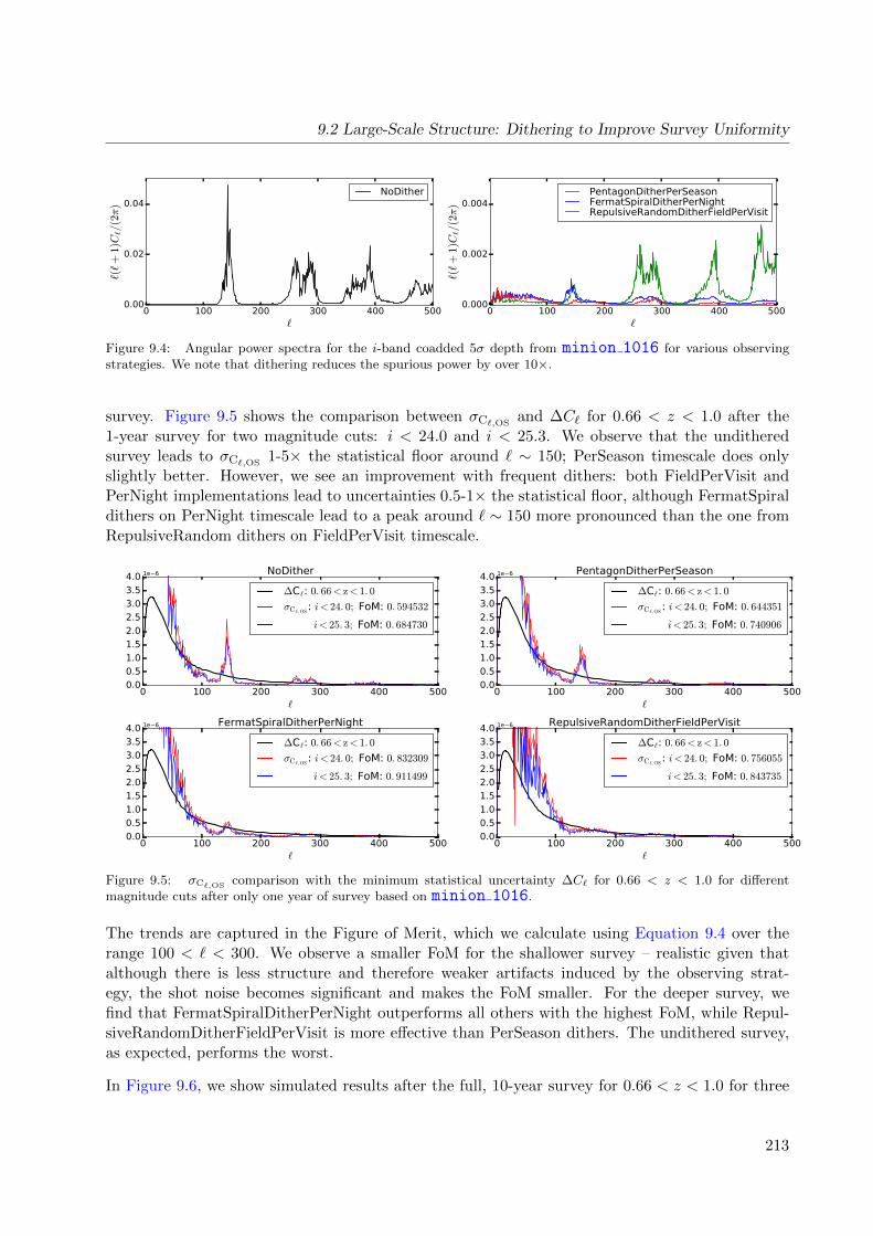
9.2 Large-Scale Structure: Dithering to Improve Survey Uniformity

0 100 200 300 400 500`

0.00

0.02

0.04

`(`+

1)C

`/(2π)

NoDither

0 100 200 300 400 500`

0.000

0.002

0.004

`(`+

1)C

`/(2π)

PentagonDitherPerSeasonFermatSpiralDitherPerNightRepulsiveRandomDitherFieldPerVisit

Figure 9.4: Angular power spectra for the i-band coadded 5σ depth from minion 1016 for various observingstrategies. We note that dithering reduces the spurious power by over 10×.

survey. Figure 9.5 shows the comparison between σC`,OSand ∆C` for 0.66 < z < 1.0 after the

1-year survey for two magnitude cuts: i < 24.0 and i < 25.3. We observe that the unditheredsurvey leads to σC`,OS

1-5× the statistical floor around ` ∼ 150; PerSeason timescale does onlyslightly better. However, we see an improvement with frequent dithers: both FieldPerVisit andPerNight implementations lead to uncertainties 0.5-1× the statistical floor, although FermatSpiraldithers on PerNight timescale lead to a peak around ` ∼ 150 more pronounced than the one fromRepulsiveRandom dithers on FieldPerVisit timescale.

0 100 200 300 400 500`

0.00.51.01.52.02.53.03.54.0 1e 6 NoDither

∆C`: 0. 66< z< 1. 0

σC`,OS: i < 24. 0; FoM: 0. 594532

i < 25. 3; FoM: 0. 684730

0 100 200 300 400 500`

0.00.51.01.52.02.53.03.54.0 1e 6 PentagonDitherPerSeason

∆C`: 0. 66< z< 1. 0

σC`,OS: i < 24. 0; FoM: 0. 644351

i < 25. 3; FoM: 0. 740906

0 100 200 300 400 500`

0.00.51.01.52.02.53.03.54.0 1e 6 FermatSpiralDitherPerNight

∆C`: 0. 66< z< 1. 0

σC`,OS: i < 24. 0; FoM: 0. 832309

i < 25. 3; FoM: 0. 911499

0 100 200 300 400 500`

0.00.51.01.52.02.53.03.54.0 1e 6 RepulsiveRandomDitherFieldPerVisit

∆C`: 0. 66< z< 1. 0

σC`,OS: i < 24. 0; FoM: 0. 756055

i < 25. 3; FoM: 0. 843735

Figure 9.5: σC`,OS comparison with the minimum statistical uncertainty ∆C` for 0.66 < z < 1.0 for differentmagnitude cuts after only one year of survey based on minion 1016.

The trends are captured in the Figure of Merit, which we calculate using Equation 9.4 over therange 100 < ` < 300. We observe a smaller FoM for the shallower survey – realistic given thatalthough there is less structure and therefore weaker artifacts induced by the observing strat-egy, the shot noise becomes significant and makes the FoM smaller. For the deeper survey, wefind that FermatSpiralDitherPerNight outperforms all others with the highest FoM, while Repul-siveRandomDitherFieldPerVisit is more effective than PerSeason dithers. The undithered survey,as expected, performs the worst.

In Figure 9.6, we show simulated results after the full, 10-year survey for 0.66 < z < 1.0 for three

213

Chapter 9: Cosmology

different magnitude cuts: i < 24.0, i < 25.3 and i < 27.5. We observe stark differences betweenthe undithered and dithered surveys: the former leads to large uncertainties in the bias inducedby the observing strategy while the latter is effective in bringing σC`,OS

well below the statisticalfloor. The effectiveness of all three dithered surveys in minimizing the uncertainties implies moreflexibility in choosing the dither strategy for years 2-10.

Analyzing the FoM more closely, we observe that the gold sample leads to smaller FoM than boththe shallower and deeper catalogs. The larger FoM for shallower catalog is realistic, given lessstructure with shallow depth leads to weaker artifacts and the shot noise is negligible over the fullten-year survey, but the out-of-trend behavior of gold sample hints at a peculiarity of the varianceacross the ugri bands at that depth for the baseline cadence. We investigate this behavior brieflyand find that the u-band-induced artifacts add the most to the uncertainties in the bias inducedby the observing strategy, as the gold sample u-band cadence in the minion 1016 is different fromgri cadences. This issue still needs to be further investigated, with potentially incorporating theimportance of each band to calculate an overall bias induced by the observing strategy. We note,however, that this peculiarity is particularly enhanced for the undithered survey.

0 100 200 300 400 500`

0.00.51.01.52.02.53.03.54.0 1e 6 NoDither

∆C`: 0. 66< z< 1. 0

σC`,OS: i < 24. 0; FoM: 0. 918973

i < 25. 3; FoM: 0. 651813

i < 27. 5; FoM: 0. 846697

0 100 200 300 400 500`

0.00.51.01.52.02.53.03.54.0 1e 6 PentagonDitherPerSeason

∆C`: 0. 66< z< 1. 0

σC`,OS: i < 24. 0; FoM: 0. 966752

i < 25. 3; FoM: 0. 960194

i < 27. 5; FoM: 0. 969101

0 100 200 300 400 500`

0.00.51.01.52.02.53.03.54.0 1e 6 FermatSpiralDitherPerNight

∆C`: 0. 66< z< 1. 0

σC`,OS: i < 24. 0; FoM: 0. 971228

i < 25. 3; FoM: 0. 963028

i < 27. 5; FoM: 0. 970290

0 100 200 300 400 500`

0.00.51.01.52.02.53.03.54.0 1e 6 RepulsiveRandomDitherFieldPerVisit

∆C`: 0. 66< z< 1. 0

σC`,OS: i < 24. 0; FoM: 0. 977822

i < 25. 3; FoM: 0. 971457

i < 27. 5; FoM: 0. 978681

Figure 9.6: σC`,OS comparison with the minimum statistical uncertainty ∆C` for 0.66 < z < 1.0 for differentmagnitude cuts after the full, 10-year survey based on minion 1016.

The trends observed here remain consistent for all five redshift bins. We note that our choice ofdithers is particularly important for the one-year survey as only one of the three dither strategiesleads to a large FoM. Therefore, in the absence of effective dithers, systematics correction methodswill become necessary after the one-year survey. However, these methods may not lead to significantimprovements for a dithered 10-year survey as dithers of most kinds are effective in reducing theuncertainties well below the minimum statistical limit.

To further probe the effects of dithers, we run the 1-year and 10-year analyses for two cadences be-sides the baseline cadence: kraken 1043 which does not require visit pairs, and minion 1020which implements a Pan-STARRS-like observing strategy offering a larger area coverage. InFigure 9.7, we compare the results from these two cadences with those from minion 1016 for0.66 < z < 1.0 for the i < 25.3 galaxy sample after only one year of survey. We see that the

214

9.2 Large-Scale Structure: Dithering to Improve Survey Uniformity

undithered survey leads to large uncertainties in the bias induced by the observing strategy withall three cadences, with the peak uncertainty 5-15× the statistical floor. As expected, the un-dithered survey with the wider coverage minion 1020 cadence leads to stronger artifacts and amuch smaller FoM (by ∼ 33% in comparison with minion 1016), while not requiring visit-pairs isslightly more effective than the baseline (FoM increases by about 6%). We see very similar trendsfor the three cadences for PerSeason dithers although the peak σC`,OS

ranges between 3-9× thestatistical floor; FoM based on minion 1020 is worse than that from minion 1016 by about 25%and kraken 1043 improves on the baseline FoM by ∼ 5%.

As before, σC`,OSimproves with more frequent dithering. It is only about 1-3× the statistical floor

for FermatSpiral dithers on PerNight timescale. In contrast to NoDither and PerSeason dithers,both minion 1020 and kraken 1043 perform better than baselineminion 1016 with PerNightdithers: FoM from the wider coverage cadence is about 4.5% better than for the baseline cadence,while we see a 4% better FoM with kraken 1043.

For RepulsiveRandom dithers on FieldPerVisit timescale, we find that the uncertainties in thebias induced by the observing strategy are on the same scale as the statistical floor. The widercoverage cadence outperforms the baseline cadence significantly as the wider survey FoM is about18% better than the baseline FoM while the improvement is about 3% when not requiring visit-pairs. We emphasize that the differences between results with different cadences is highly dependenton the observing strategy: the wider coverage with no or infrequent dithers performs quite poorlywhile it significantly improves the FoM when large, frequent dithers are implemented. On the otherhand, not requiring visit-pairs leads to comparatively larger improvement for infrequent dithersthan frequent ones (compared to the baseline).

0 100 200 300 400 500`

0.00.51.01.52.02.53.03.54.0 1e 6 NoDither

∆C`: 0. 66< z< 1. 0

σC`,OS: minion1016; FoM: 0. 684730

minion1020; FoM: 0. 458889

kraken1043; FoM: 0. 728393

0 100 200 300 400 500`

0.00.51.01.52.02.53.03.54.0 1e 6 PentagonDitherPerSeason

∆C`: 0. 66< z< 1. 0

σC`,OS: minion1016; FoM: 0. 740906

minion1020; FoM: 0. 556250

kraken1043; FoM: 0. 781261

0 100 200 300 400 500`

0.00.51.01.52.02.53.03.54.0 1e 6 FermatSpiralDitherPerNight

∆C`: 0. 66< z< 1. 0

σC`,OS: minion1016; FoM: 0. 911499

minion1020; FoM: 0. 952231

kraken1043; FoM: 0. 948173

0 100 200 300 400 500`

0.00.51.01.52.02.53.03.54.0 1e 6 RepulsiveRandomDitherFieldPerVisit

∆C`: 0. 66< z< 1. 0

σC`,OS: minion1016; FoM: 0. 843735

minion1020; FoM: 0. 998372

kraken1043; FoM: 0. 864074

Figure 9.7: σC`,OS comparison with the minimum statistical uncertainty ∆C` for 0.66 < z < 1.0 for three differentcadences for i < 25.3 after only one year of survey.

Finally, we show the simulated results for different cadences after the 10-year survey in Figure 9.8.As in Figure 9.6, we see that all the dithered surveys effectively minimize the uncertainties, re-gardless of the cadence. We do observe, however, that the wider coverage minion 1020 stillunderperforms significantly for the undithered survey (FoM about 30% less than baseline FoM)

215

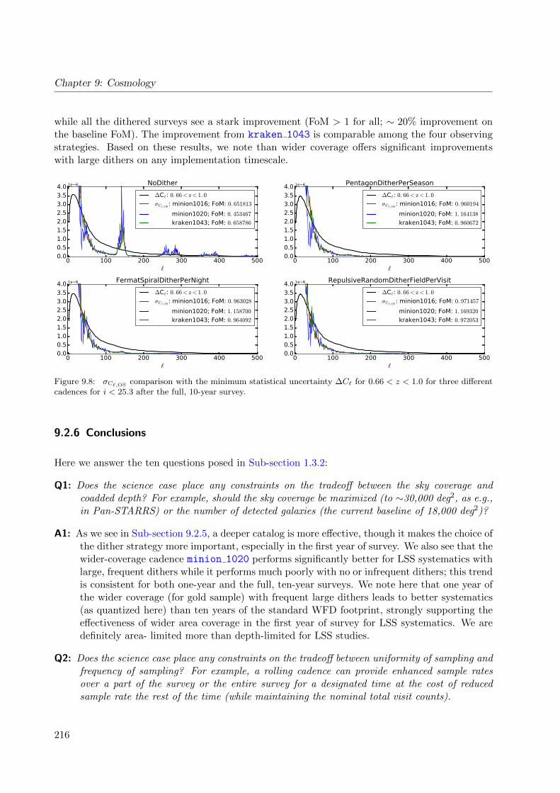
Chapter 9: Cosmology

while all the dithered surveys see a stark improvement (FoM > 1 for all; ∼ 20% improvement onthe baseline FoM). The improvement from kraken 1043 is comparable among the four observingstrategies. Based on these results, we note than wider coverage offers significant improvementswith large dithers on any implementation timescale.

0 100 200 300 400 500`

0.00.51.01.52.02.53.03.54.0 1e 6 NoDither

∆C`: 0. 66< z< 1. 0

σC`,OS: minion1016; FoM: 0. 651813

minion1020; FoM: 0. 453467

kraken1043; FoM: 0. 658786

0 100 200 300 400 500`

0.00.51.01.52.02.53.03.54.0 1e 6 PentagonDitherPerSeason

∆C`: 0. 66< z< 1. 0

σC`,OS: minion1016; FoM: 0. 960194

minion1020; FoM: 1. 164138

kraken1043; FoM: 0. 960672

0 100 200 300 400 500`

0.00.51.01.52.02.53.03.54.0 1e 6 FermatSpiralDitherPerNight

∆C`: 0. 66< z< 1. 0

σC`,OS: minion1016; FoM: 0. 963028

minion1020; FoM: 1. 158700

kraken1043; FoM: 0. 964092

0 100 200 300 400 500`

0.00.51.01.52.02.53.03.54.0 1e 6 RepulsiveRandomDitherFieldPerVisit

∆C`: 0. 66< z< 1. 0

σC`,OS: minion1016; FoM: 0. 971457

minion1020; FoM: 1. 169320

kraken1043; FoM: 0. 972053

Figure 9.8: σC`,OS comparison with the minimum statistical uncertainty ∆C` for 0.66 < z < 1.0 for three differentcadences for i < 25.3 after the full, 10-year survey.

9.2.6 Conclusions

Here we answer the ten questions posed in Sub-section 1.3.2:

Q1: Does the science case place any constraints on the tradeoff between the sky coverage andcoadded depth? For example, should the sky coverage be maximized (to ∼30,000 deg2, as e.g.,in Pan-STARRS) or the number of detected galaxies (the current baseline of 18,000 deg2)?

A1: As we see in Sub-section 9.2.5, a deeper catalog is more effective, though it makes the choice ofthe dither strategy more important, especially in the first year of survey. We also see that thewider-coverage cadence minion 1020 performs significantly better for LSS systematics withlarge, frequent dithers while it performs much poorly with no or infrequent dithers; this trendis consistent for both one-year and the full, ten-year surveys. We note here that one year ofthe wider coverage (for gold sample) with frequent large dithers leads to better systematics(as quantized here) than ten years of the standard WFD footprint, strongly supporting theeffectiveness of wider area coverage in the first year of survey for LSS systematics. We aredefinitely area- limited more than depth-limited for LSS studies.

Q2: Does the science case place any constraints on the tradeoff between uniformity of sampling andfrequency of sampling? For example, a rolling cadence can provide enhanced sample ratesover a part of the survey or the entire survey for a designated time at the cost of reducedsample rate the rest of the time (while maintaining the nominal total visit counts).

216

9.2 Large-Scale Structure: Dithering to Improve Survey Uniformity

A2: Depth uniformity is critical for LSS systematics. As we demonstrated in Sub-section 9.2.5,LSS studies will benefit strongly from large dithers and wide area coverage. We do not haveconstraints on the cadence.

Q3: Does the science case place any constraints on the tradeoff between the single-visit depth andthe number of visits (especially in the u-band where longer exposures would minimize theimpact of the readout noise)?

A3: From our investigation into the large uncertainties in the bias induced by the observing strat-egy observed in the gold sample in the baseline cadence, in comparison with the shallowerand deeper catalogs, we find that u-band-induced artifacts add the most to the uncertaintiesin the bias. Hence there could be a significant penalty from reducing the number of u-bandvisit. At minimum, doing so would make the choice of dither pattern more important. Thisissue still needs to be further investigated.

Q4: Does the science case place any constraints on the Galactic plane coverage (spatial coverage,temporal sampling, visits per band)?

A4: LSS systematics do not place any constraints on the Galactic plane coverage.

Q5: Does the science case place any constraints on the fraction of observing time allocated to eachband?

A5: Increasing the number of visits leads to greater survey uniformity. At present, this is worst(among ugri) in the u-band, so increasing the fraction of u-band observing time would likelyhelp.

Q6: Does the science case place any constraints on the cadence for deep drilling fields?

A6: LSS systematics do not constrain the cadence for deep drilling fields as long as the main surveydithers are not affected.

Q7: Assuming two visits per night, would the science case benefit if they are obtained in the sameband or not?

A7: We do not see significant difference between obtaining two visits per night in the same bandor not, although we do see a mild benefit in not obtaining the visits in the same band as itallows greater variation in atmospheric conditions in each band.

Q8: Will the case science benefit from a special cadence prescription during commissioning or earlyin the survey, such as: acquiring a full 10-year count of visits for a small area (either in allthe bands or in a selected set); a greatly enhanced cadence for a small area?

A8: We will request full, 10-year depth during commissioning to validate our choice of ditherpattern.

Q9: Does the science case place any constraints on the sampling of observing conditions (e.g.,seeing, dark sky, airmass), possibly as a function of band, etc.?

A9: Seeing will play a role in the photometric calibration errors. However, these errors appear tobe subdominant to the artifacts induced by the observing strategy.

217

Chapter 9: Cosmology

Q10: Does the case have science drivers that would require real-time exposure time optimizationto obtain nearly constant single-visit limiting depth?

A10: We do not require any real-time exposure time optimization.

9.2.7 Discussion

In this section, we presented results for the impacts of LSST observing strategy on LSS studies.Using the OpSim cadence baseline minion 1016, we demonstrate that dithers are necessary forboth 1-year and 10-year surveys. We find that of the three dither strategies discussed here, Fer-matSpiral dithers on PerNight timescale are the most effective for the gold sample after one-yearof survey while dithers of all kinds are effective after the ten-year survey. These results imply theneed for a very careful choice of the observing strategy in the first year while there is quite a rangeof choice for years 2-10.

We also analyze two other cadences and find that frequent dithering with maximum sky coveragecould allow a significant fraction LSST-enabled LSS science after one-year. Assuming that thequality of photometric redshifts is fixed (when it actually improves with depth) and that ouransatz for window function uncertainties is representative, our results can go as far as implyingthat the wider coverage for a few years is far more important than more years of the baseline WFDcoverage.

Future work will entail improving our analysis to better constrain the artifacts induced by theobserving strategy by, e.g., including uncertainties in the dust extinction, using improved modelsfor the photometric calibration uncertainties, more realistic galaxy colors, incorporating improvedmock catalogs to better estimate the galaxy counts as well as its uncertainties, and a better estimateof the uncertainties in the bias induced by the observing strategy by a more thorough accountingof the effects of each band. Also, the development and the analysis of the effectiveness of varioussystematics correction methods needs to be carried out, especially for the 1-year survey, as only afew observing strategies reduce the artifacts. Finally, the effectiveness of various dithers still needsto be assessed for other science probes.

A baseline dithering pattern “Hexdither” is generated for all OpSim runs with the dithered fieldpointings output as part of the Sqlite database (using the “ditheredRA” and “ditheredDec” pa-rameters). The dithering strategies discussed in this section are incorporated within the MAFanalysis framework and can be applied as a post-processing step to each simulated OpSim survey.Integration of dithering within the scheduling of the telescope, as opposed to a post-processingstep, is expected to be delivered with the v1.5 release of OpSim v4 (currently scheduled for June2019).

Go to: • the start of this section • the start of the chapter • the table of contents

218

9.3 Weak Lensing

9.3 Weak Lensing

Josh Meyers, Tony Tyson.

Much of LSST cosmology may be limited by systematic rather than statistical errors. This isespecially true of weak gravitational lensing, which relies on very accurate (i.e. low bias), estimatesof the shear of large ensembles of galaxies. Measurements of the noisy shapes of many galaxies,and high signal-to-noise measurements of PSF calibration stars are made. Even though the shotnoise of the shape of an individual galaxy is very large, any small shear bias could accumulateover many such galaxies. As outlined in the SRD, uniformity of seeing in the bands used for weaklensing and special observing strategies are required in order to reduce additive and multiplicativeshear systematics.

Achieving the ultimate sensitivity of the LSST to weak lensing science places stringent requirementson our ability to accurately estimate galaxy shapes and redshifts, which in turn demands precise andaccurate knowledge of the point spread function, astrometry, and photometry. These measurementsare influenced by the interaction of light with the Earth’s atmosphere, the telescope optics, andthe CCD sensors. Systematics in the shear are introduced in each case. Observing strategies havebeen developed for suppressing these systematics in current lensing surveys, such as the Deep LensSurvey1. These and new methods will be applied to the LSST survey.

To leading order, we can express the effect of shear systematics in the observed shear γobsi as a

small linear perturbation of the true shear γi,

γobsi = (1 +mi)γi + ci,

where mi is the multiplicative and ci is the additive systematic in the ith shear component. Thesesystematics have contributions from the atmosphere and the detector+optics. Systematic errorsin modeling the PSF from images of stars and in interpolating the PSF from the positions of starsto the positions of galaxies propagate to systematic errors in the galaxy shear. To leading order,the PSF contributions to the additive systematic are a linear function of the PSF ellipticity. Thebest observing strategies cause the average PSF ellipticity at a given point (over all exposures) toaverage towards zero.

From the LSST SRD requirements on residual systematics in the galaxy shear-shear correlationfunction one can specify the level of residual shear systematics at which statistical uncertaintiesbecome subdominant. Over the sample of 3-4 billion galaxies, the shear systematics must be below3 parts in 10,000 for additive shear |c|, and 3 parts in 1000 for multiplicative shear |m|. Each visit toa sky patch encounters these systematics. In particular, each re-visit to a given field generates thesame CCD-based additive shear systematic. Some observing strategies can effectively randomizethese over all visits to a field. It is important to note that the full survey shear-shear correlationerror due to these systematics is expected to be no better than the corresponding systematic in anygiven field after all re-visits to that field. This is because the useful angular scales in cosmic shearare less than a field radius of several degrees, and the systematics floor in shear-shear correlationis set therefore by the floor in any one typical field. Below we discuss the observing strategies forsuppressing shear systematics and metrics for their success.

1dls.physics.ucdavis.edu

219

Chapter 9: Cosmology

9.3.1 Target Selection

Image quality must be uniformly good in the bands used for weak lensing shear. These willbe mainly the r and i bands, though it is possible that the z band will also be used for shearmeasurement. The decision on which field to observe next must be based mainly on its weaklensing priority (LSST Science Collaboration et al. 2009, Sec 3.1 and Figure 14.4). Depending onthe current weather and seeing, the scheduler will have a list of priorities for next-field, based onprior history of coverage. The relevant parameters are seeing, depth, and camera rotation anglewith respect to North and to zenith. Nearby fields in need of coverage in these bands should begiven high priority if the seeing is better than some specified value, likely 0.7 arcsec FWHM (LSSTScience Collaboration et al. 2009, Sec 14.5.2).

9.3.2 Target Measurements

It is expected that even after optimization of camera optics and electronics, systematic image shapeerrors will be associated with the orientation of the camera focal plane. Using data from vendorCCDs, simulations of LSST observing have shown that a combination of x-y dithering on the skyand pipeline processing with pixel re-map (to cancel much of the CCD frame fixed distortions)can get well within a factor of ten of the goal for shear systematics residuals. Simulations whichadd camera angle dithering show that the residual shear systematics goal can be achieved in fieldswith relatively uniform seeing history (Jee & Tyson 2011). To average down the PSF systematicsover many re-visits we benefit from uniformly distributed image quality over the ensemble. Anon-uniform history in some field can be addressed by the scheduler taking that into account forthe offending rotation angle(s) in the history of prior visits.

Thus shear systematics will be reduced by randomization of the orientation of the camera with re-spect to the sky. This is represented by the parameter RotSkyPos, defined as the angle between the+y camera direction and North. We can construct diagnostic metrics that quantify the uniformityof its distribution at each sky position. Given the spin 2 symmetry of shear, the optimal strategyfor shear systematics will be to aim for uniformity of RotSkyPos mod π, since angles separated byπ radians are degenerate.

Similarly, the telescope optics may harbor systematic aberrations, and these also could be mitigatedby recording images with a uniform distribution of parallactic angle, which is the angle betweenNorth and zenith for a given field observation. Differential chromatic refraction (DCR) effectswill also be mitigated by varying the parallactic angle, though the exact relationship is complexsince the parallactic angle sets both the DCR magnitude and direction for a given observation.Re-visits to a given field should be distributed over parallactic angles (or equivalently, hour angles),consistent with airmass and seeing limits. Note that wide hour angle coverage for a given field willalso be helpful in order to efficiently achieve full 180 deg coverage in CCD sky angle.

As argued below, survey depth is more important than survey area early in the survey. Uniformityof depth is important, but less so than uniformity in camera rotator shear suppression. Simulationshave shown that for the Gold sample of galaxies, uniformity at the 0.2 mag level in limiting mag-nitude produces little shear bias. The largest effect comes from bias in weak lensing magnificationtomography Morrison et al. (2012). This is important in the joint analysis of LSST multi probes

220

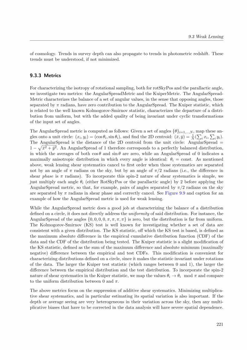
9.3 Weak Lensing

of cosmology. Trends in survey depth can also propagate to trends in photometric redshift. Thesetrends must be understood, if not minimized.

9.3.3 Metrics

For characterizing the isotropy of rotational sampling, both for rotSkyPos and the parallactic angle,we investigate two metrics: the AngularSpreadMetric and the KuiperMetric. The AngularSpread-Metric characterizes the balance of a set of angular values, in the sense that opposing angles, thoseseparated by π radians, have zero contribution to the AngularSpread. The Kuiper statistic, whichis related to the well known Kolmogorov-Smirnov statistic, characterizes the departure of a distri-bution from uniform, but with the added quality of being invariant under cyclic transformationsof the input set of angles.

The AngularSpread metric is computed as follows: Given a set of angles θi=1,...,N , map these an-gles onto a unit circle: (xi, yi) = (cos θi, sin θi), and find the 2D centroid: (x, y) = 1

N (∑

i xi,∑

i yi).The AngularSpread is the distance of the 2D centroid from the unit circle: AngularSpread =1−

√x2 + y2. An AngularSpread of 1 therefore corresponds to a perfectly balanced distribution,

in which the averages of both cos θ and sin θ are zero, while an AngularSpread of 0 indicates amaximally anisotropic distribution in which every angle is identical: θi = const. As mentionedabove, weak lensing shear systematics cancel to first order when those systematics are separatednot by an angle of π radians on the sky, but by an angle of π/2 radians (i.e., the difference inshear phase is π radians). To incorporate this spin-2 nature of shear systematics is simple, wejust multiply each angle θi (either RotSkyPos or the parallactic angle) by 2 before applying theAngularSpread metric, so that, for example, pairs of angles separated by π/2 radians on the skyare separated by π radians in shear phase and correctly cancel. See Figure 9.9 and caption for anexample of how the AngularSpread metric is used for weak lensing.

While the AngularSpread metric does a good job at characterizing the balance of a distributiondefined on a circle, it does not directly address the uniformity of said distribution. For instance, theAngularSpread of the angles 0, 0, 0, 0, π, π, π, π is zero, but the distribution is far from uniform.The Kolmogorov-Smirnov (KS) test is well known for investigating whether a set of data areconsistent with a given distribution. The KS statistic, off which the KS test is based, is defined asthe maximum absolute difference in the empirical cumulative distribution function (CDF) of thedata and the CDF of the distribution being tested. The Kuiper statistic is a slight modification ofthe KS statistic, defined as the sum of the maximum difference and absolute minimum (maximallynegative) difference between the empirical and test CDFs. This modification is convenient forcharacterizing distributions defined on a circle, since it makes the statistic invariant under rotationsof the data. The larger the Kuiper test statistic (which ranges between 0 and 1), the larger thedifference between the empirical distribution and the test distribution. To incorporate the spin-2nature of shear systematics in the Kuiper statistic, we map the values θi → θi mod π and compareto the uniform distribution between 0 and π.

The above metrics focus on the suppression of additive shear systematics. Minimizing multiplica-tive shear systematics, and in particular estimating its spatial variation is also important. If thedepth or average seeing are very heterogeneous in their variation across the sky, then any multi-plicative biases that have to be corrected in the data analysis will have severe spatial dependence.

221

Chapter 9: Cosmology

Headless position angles Shear phases

Figure 9.9: Demonstration of AngularSpread metric. Left: Three position angles are indicated on a unit circle,using headless vectors since shear systematics are invariant to 180-degree rotations. Right: The corresponding shearphases, which are twice the position angles, on a unit circle. The black arrow indicates the 2D centroid of the 2Dshear phases. The AngularSpread metric is the distance from the tip of this black arrow to the unit circle. Notethat the blue and green position angle symbols, which are separated by nearly 90-degrees and hence produce nearlyopposing shear systematics, correspond to blue and green shear phase vectors separated by nearly 180-degrees andhence nearly cancel geometrically in the computation of the AngularSpread.

222

9.3 Weak Lensing

Homogeneity of depth and seeing certainly helps, and that is an observing strategy question asdiscussed above. A specific metric for multiplicative systematics would be useful in our next Op-Sim runs. A useful metric to be applied to full observing simulations is the mean ratio (and spatialvariance) of observed vs simulated shear amplitudes over a large sample vs z-bins. Since Multi-Fitjoint star-galaxy fits to individual visits will be used for data analysis, these PSF effects will beinherited for each exposure and over that full field in a properly weighted fashion. Other sciencecases value uniformity of image quality as well, and this type of metric may be applied duringobserving.

9.3.4 OpSim Analysis

The distribution of AngularSpread for 2× rotSkyPos is shown in Figure 9.10 for the latest baselineOpSim run, minion 1016. The left panel shows a sky map for the i-band (in this and the followingfigures, the sky maps vary only minimally between the two principal lensing filters, r and i), whilethe right panel shows a histogram of values for each LSST filter. The distribution of the Kuiperstatistic for rotSkyPos mod π is similarly shown in Figure 9.11.

While we do not currently have a method to quantitatively connect the distribution of rotSkyPosto cosmological systematics, these figures appear to indicate that rotSkyPos is already being wellsampled in current simulations due to the rotator tracking the sky during exposures, being subjectto cable wrap limits, and occasionally resetting to 0-degrees for filter changes.

Jee & Tyson (2011) did a study of the shear residual systematics due to known LSST CCDbrighter-fatter anisotropy in 100 revisits to a single field with random angular orientations andseeing sampled from the expected distribution. The Data Management (DM) pipeline will usea model of the charge transport in the CCD to re-map pixel shapes, sizes, and areas in pixellevel data processing. The needed factor of 10 suppression of the CCD-based shear systematicresiduals (post pixel remap pipeline correction) was obtained, reaching the SRD floor on cosmicshear systematics (presented at weak lensing systematics workshop, Dec 2015)2. Of course, therequirements for spatial dithering for shear systematics residuals depend on the precision of thepixel processing for removal of the CCD based additive shear systematic. We assume that thispixel level remap in the DM pipeline cannot correct to better than 3 times the rms errors in thelab tests for dynamic and static CCD systematics.

The distribution of parallactic angles is similarly shown in Figure 9.12 and Figure 9.13. Thesefigures show significantly less isotropy and significantly more structure across the survey footprintthan those for rotSkyPos, likely due to the fact that, unlike rotSkyPos, the parallactic angle isindependent of the camera rotator position. Hence, the parallactic angle is more tightly constrainedby geometry than rotSkyPos. In fact, the only mechanism by which the parallactic angle variesfor a given field is through variations in the hour angle at which that field is observed.

2https://indico.bnl.gov/conferenceDisplay.py?confId=1604

223

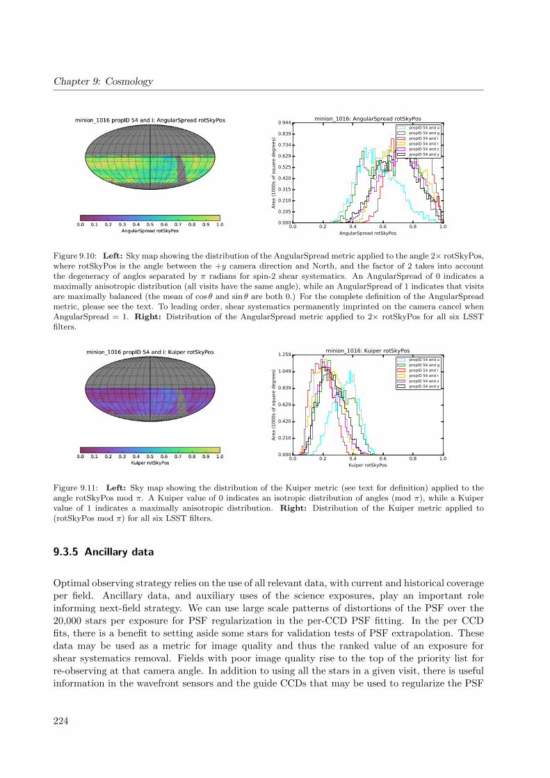
Chapter 9: Cosmology

0.0 0.2 0.4 0.6 0.8 1.0

AngularSpread rotSkyPos

0.000

0.105

0.210

0.315

0.420

0.525

0.629

0.734

0.839

0.944

Are

a (

10

00

s of

square

degre

es)

minion_1016: AngularSpread rotSkyPos

propID 54 and u propID 54 and g propID 54 and i propID 54 and r propID 54 and z propID 54 and y

Figure 9.10: Left: Sky map showing the distribution of the AngularSpread metric applied to the angle 2× rotSkyPos,where rotSkyPos is the angle between the +y camera direction and North, and the factor of 2 takes into accountthe degeneracy of angles separated by π radians for spin-2 shear systematics. An AngularSpread of 0 indicates amaximally anisotropic distribution (all visits have the same angle), while an AngularSpread of 1 indicates that visitsare maximally balanced (the mean of cos θ and sin θ are both 0.) For the complete definition of the AngularSpreadmetric, please see the text. To leading order, shear systematics permanently imprinted on the camera cancel whenAngularSpread = 1. Right: Distribution of the AngularSpread metric applied to 2× rotSkyPos for all six LSSTfilters.

0.0 0.2 0.4 0.6 0.8 1.0

Kuiper rotSkyPos

0.000

0.210

0.420

0.629

0.839

1.049

1.259

Are

a (

10

00

s of

square

degre

es)

minion_1016: Kuiper rotSkyPos

propID 54 and u propID 54 and g propID 54 and i propID 54 and r propID 54 and z propID 54 and y

Figure 9.11: Left: Sky map showing the distribution of the Kuiper metric (see text for definition) applied to theangle rotSkyPos mod π. A Kuiper value of 0 indicates an isotropic distribution of angles (mod π), while a Kuipervalue of 1 indicates a maximally anisotropic distribution. Right: Distribution of the Kuiper metric applied to(rotSkyPos mod π) for all six LSST filters.

9.3.5 Ancillary data

Optimal observing strategy relies on the use of all relevant data, with current and historical coverageper field. Ancillary data, and auxiliary uses of the science exposures, play an important roleinforming next-field strategy. We can use large scale patterns of distortions of the PSF over the20,000 stars per exposure for PSF regularization in the per-CCD PSF fitting. In the per CCDfits, there is a benefit to setting aside some stars for validation tests of PSF extrapolation. Thesedata may be used as a metric for image quality and thus the ranked value of an exposure forshear systematics removal. Fields with poor image quality rise to the top of the priority list forre-observing at that camera angle. In addition to using all the stars in a given visit, there is usefulinformation in the wavefront sensors and the guide CCDs that may be used to regularize the PSF

224

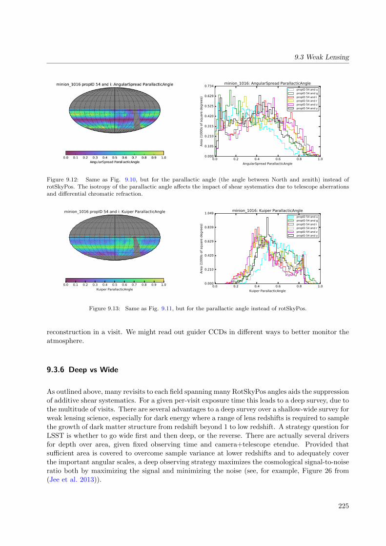
9.3 Weak Lensing

0.0 0.2 0.4 0.6 0.8 1.0

AngularSpread ParallacticAngle

0.000

0.105

0.210

0.315

0.420

0.525

0.629

0.734

Are

a (

10

00

s of

square

degre

es)

minion_1016: AngularSpread ParallacticAngle

propID 54 and u propID 54 and g propID 54 and i propID 54 and r propID 54 and z propID 54 and y

Figure 9.12: Same as Fig. 9.10, but for the parallactic angle (the angle between North and zenith) instead ofrotSkyPos. The isotropy of the parallactic angle affects the impact of shear systematics due to telescope aberrationsand differential chromatic refraction.

minion_1016 propID 54 and i: Kuiper ParallacticAngle

0.0 0.1 0.2 0.3 0.4 0.5 0.6 0.7 0.8 0.9 1.0

Kuiper ParallacticAngle0.0 0.2 0.4 0.6 0.8 1.0

Kuiper ParallacticAngle

0.000

0.210

0.420

0.629

0.839

1.049

Are

a (

10

00

s of

square

degre

es)

minion_1016: Kuiper ParallacticAngle

propID 54 and u propID 54 and g propID 54 and i propID 54 and r propID 54 and z propID 54 and y

Figure 9.13: Same as Fig. 9.11, but for the parallactic angle instead of rotSkyPos.

reconstruction in a visit. We might read out guider CCDs in different ways to better monitor theatmosphere.

9.3.6 Deep vs Wide

As outlined above, many revisits to each field spanning many RotSkyPos angles aids the suppressionof additive shear systematics. For a given per-visit exposure time this leads to a deep survey, due tothe multitude of visits. There are several advantages to a deep survey over a shallow-wide survey forweak lensing science, especially for dark energy where a range of lens redshifts is required to samplethe growth of dark matter structure from redshift beyond 1 to low redshift. A strategy question forLSST is whether to go wide first and then deep, or the reverse. There are actually several driversfor depth over area, given fixed observing time and camera+telescope etendue. Provided thatsufficient area is covered to overcome sample variance at lower redshifts and to adequately coverthe important angular scales, a deep observing strategy maximizes the cosmological signal-to-noiseratio both by maximizing the signal and minimizing the noise (see, for example, Figure 26 from(Jee et al. 2013)).

225

Chapter 9: Cosmology

First, a deep survey strategy boosts the amplitude of the cosmic shear signals due to the increasedamplitude of the lensing kernel. Given the same lens mass, the amplitude of lensing signals is asimple function of the two distances: observer-to-lens versus lens-to-source. For example, when alens is at z = 0.5, the shear for a source at z = 1.1 is nearly twice that at z = 0.7, leading to afactor of 4 ratio in correlation function amplitudes. Thus, a deep survey can take advantage of thegeometric effect of gravitational lensing more efficiently.

Second, a deep survey strategy enables a longer redshift baseline to break parameter degeneracies.For example, shallower surveys with wider area are not efficient in shrinking the length of the“banana” in the ΩM -σ8 plane because of the σ8Ωα

M = const degeneracy. The deep strategycompensates for the loss of volume due to a reduced area by extending the volume along the lineof sight.

Third, deep surveys provide more useful galaxies per area. This merit does not entirely overlapwith the second point. In addition to new sources at higher redshift, the fainter limiting magnitudeenables detection of fainter galaxies at a given redshift and better signal-to-noise ratio. Thisargument requires that photometric redshifts of this population of galaxies is as well-calibratedas those at lower redshift. This may be done via angular cross-correlation with the brighterphotometric sample galaxies with known spectra, in test patches. Needless to say, the increasedsource density reduces the impact of shape noise caused by intrinsic ellipticity dispersion.

Fourth, it mitigates the effects of intrinsic alignments (IA), an important theoretical systematicin precision cosmic shear. Current studies (Heymans et al. 2013) indicate that IA effects aredominated by luminous red galaxies (LRGs). Because a deep survey can access fainter galaxies,the net IA systematic decreases because the fraction of the LRGs decreases at fainter limitingmagnitude. Using the approach of Joachimi et al. (2011), at z = 0.5 the amplitude of the IA powerspectrum is reduced by a factor of two for an increase in the limiting r magnitude from 24 to 27mag.

For cosmic shear the volume at ∼ 5 arcminute to several degree scales and over a wide rangeof redshift is most important. Once a fair sampling of cosmic variance is achieved the depthmatters most, because of the z-width of the lensing kernel. With fixed survey duration on acamera+telescope of fixed etendue, it is better to prioritize depth in order to maximize the weaklensing cosmological signal-to-noise ratio. In particular, for the LSST survey it would be helpful tohave several widely spaced deep drilling fields done early and deeper than the main survey, in orderto explore detailed observing strategies – particularly the angle dither scheme. Deep drilling data isuseful to a variety of LSST science drivers, including Bayesian analyses. By the same reasoning, itwould be important to cover a significant area [perhaps 2000 sq. deg] to full depth during the firstyear of the survey. This would allow full assessment of systematics, and could be chosen to overlapthe WFIRST footprint. Such an overlap may enable additional systematics checks of photometricredshift accuracy (exploiting WFIRST infrared photometry) and the impact of blends (exploitingthe smaller WFIRST PSF).

Metrics for reaching the SRD goals for WL related science are needed. Long before LSST is onthe sky such metrics can be applied to realistic simulations of LSST observing, in order to informthe scheduler proposal ranking algorithm. One metric is the sample variance in cosmic shear in10 sq. deg DD fields versus that, for say, 1000 sq. deg. A related systematics metric would be thesuppression of additive PSF systematic residuals in 1000 sq. deg worth of pointings over the sky,

226

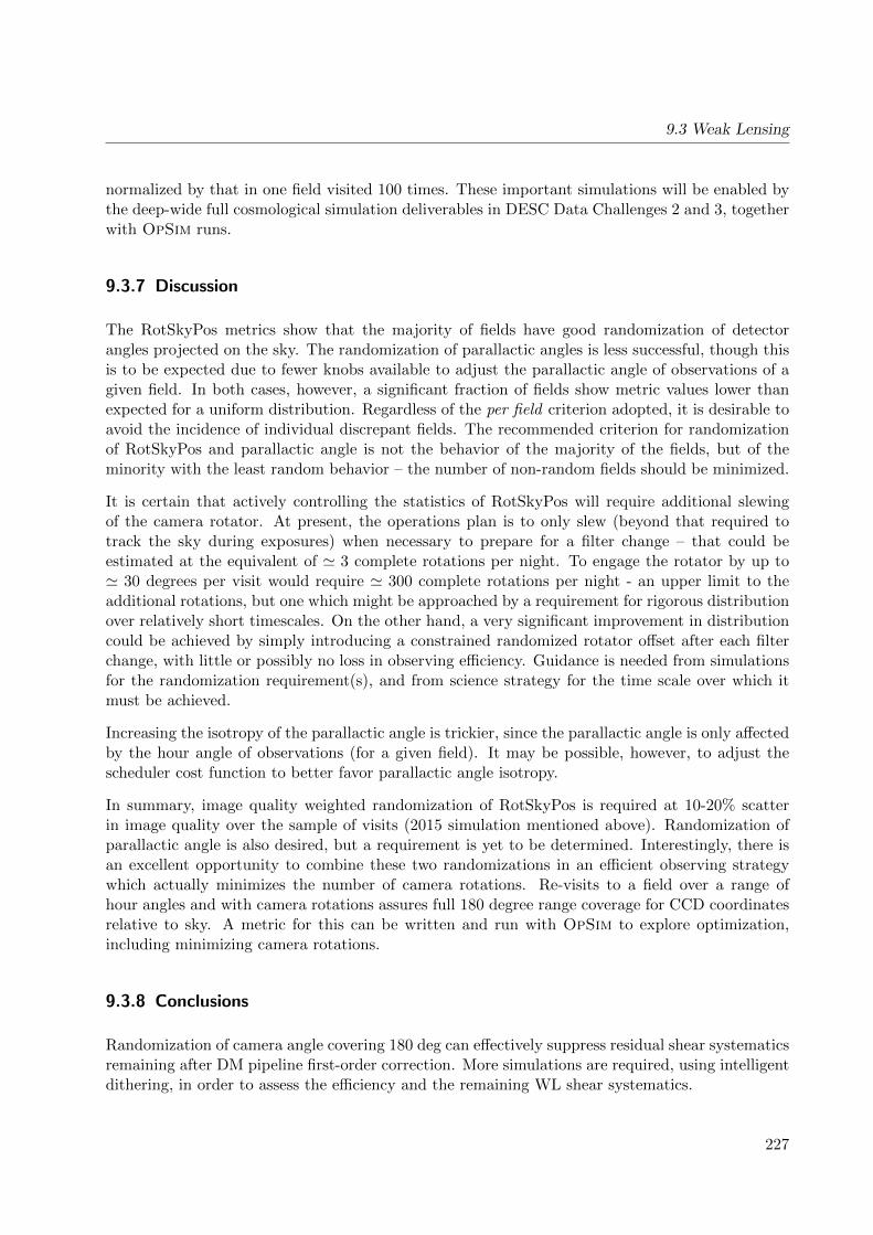
9.3 Weak Lensing

normalized by that in one field visited 100 times. These important simulations will be enabled bythe deep-wide full cosmological simulation deliverables in DESC Data Challenges 2 and 3, togetherwith OpSim runs.

9.3.7 Discussion

The RotSkyPos metrics show that the majority of fields have good randomization of detectorangles projected on the sky. The randomization of parallactic angles is less successful, though thisis to be expected due to fewer knobs available to adjust the parallactic angle of observations of agiven field. In both cases, however, a significant fraction of fields show metric values lower thanexpected for a uniform distribution. Regardless of the per field criterion adopted, it is desirable toavoid the incidence of individual discrepant fields. The recommended criterion for randomizationof RotSkyPos and parallactic angle is not the behavior of the majority of the fields, but of theminority with the least random behavior – the number of non-random fields should be minimized.

It is certain that actively controlling the statistics of RotSkyPos will require additional slewingof the camera rotator. At present, the operations plan is to only slew (beyond that required totrack the sky during exposures) when necessary to prepare for a filter change – that could beestimated at the equivalent of ' 3 complete rotations per night. To engage the rotator by up to' 30 degrees per visit would require ' 300 complete rotations per night - an upper limit to theadditional rotations, but one which might be approached by a requirement for rigorous distributionover relatively short timescales. On the other hand, a very significant improvement in distributioncould be achieved by simply introducing a constrained randomized rotator offset after each filterchange, with little or possibly no loss in observing efficiency. Guidance is needed from simulationsfor the randomization requirement(s), and from science strategy for the time scale over which itmust be achieved.

Increasing the isotropy of the parallactic angle is trickier, since the parallactic angle is only affectedby the hour angle of observations (for a given field). It may be possible, however, to adjust thescheduler cost function to better favor parallactic angle isotropy.

In summary, image quality weighted randomization of RotSkyPos is required at 10-20% scatterin image quality over the sample of visits (2015 simulation mentioned above). Randomization ofparallactic angle is also desired, but a requirement is yet to be determined. Interestingly, there isan excellent opportunity to combine these two randomizations in an efficient observing strategywhich actually minimizes the number of camera rotations. Re-visits to a field over a range ofhour angles and with camera rotations assures full 180 degree range coverage for CCD coordinatesrelative to sky. A metric for this can be written and run with OpSim to explore optimization,including minimizing camera rotations.

9.3.8 Conclusions

Randomization of camera angle covering 180 deg can effectively suppress residual shear systematicsremaining after DM pipeline first-order correction. More simulations are required, using intelligentdithering, in order to assess the efficiency and the remaining WL shear systematics.

227

Chapter 9: Cosmology

We can now provide answers to the ten questions posed in Sub-section 1.3.2:

Q1: Does the science case place any constraints on the tradeoff between the sky coverage andcoadded depth? For example, should the sky coverage be maximized (to ∼30,000 deg2, as e.g.,in Pan-STARRS) or the number of detected galaxies (the current baseline of 18,000 deg2)?

A1: On the scale of thousands of sq.deg, the WL signal and control of systematics is enhanced bydeeper (larger cosmological volume) rather than wider surveying. These considerations ledto the 18,000 sq.deg per ten years baseline.

Q2: Does the science case place any constraints on the tradeoff between uniformity of sampling andfrequency of sampling? For example, a rolling cadence can provide enhanced sample ratesover a part of the survey or the entire survey for a designated time at the cost of reducedsample rate the rest of the time (while maintaining the nominal total visit counts).

A2: WL is generally agnostic on this issue. Total good IQ x depth is most important, and thismight benefit from rolling cadences if the mean airmass is lower, resulting in a higher IQ.

Q3: Does the science case place any constraints on the tradeoff between the single-visit depth andthe number of visits (especially in the u-band where longer exposures would minimize theimpact of the readout noise)?

A3: 30-sec or longer u band exposures will help S/N.

Q4: Does the science case place any constraints on the Galactic plane coverage (spatial coverage,temporal sampling, visits per band)?

A4: WL ugrizy imaging must avoid low Galactic latitudes due to stellar crowding, bright stars,and dust. Data at low latitudes will not be used for WL.

Q5: Does the science case place any constraints on the fraction of observing time allocated to eachband?

A5: This depends on the relative system throughput vs wavelength. For the case of high u bandQE CCDs, approximately u10%, g10%, r22%, i22%, z18%, y18%. The comes from 80, 80,184, 184, 160, 160 ugrizy 30-sec visits per 9.6 sq.deg fields over 18,000 sq.deg per ten years –from the SRD, driven by required low surface brightness shear measurement and the neededS/N for photo-z for the gold sample of galaxies. The longer integrations at longer wavelengthsis due to the red color of the sky background.

Q6: Does the science case place any constraints on the cadence for deep drilling fields?

A6: It will be helpful if the individual exposure times in all bands are similar to the main survey.A long series of exposures in each filter would be good. Dithering in x-y-theta betweenexposures using intelligent dithering is needed in order to detect low level systematics and tohelp calibrate the main survey galaxy blending. Emphasis on excellent seeing is important.Spreading the DD observing over many half nights, maximizing the HA coverage, will beneeded.

Q7: Assuming two visits per night, would the science case benefit if they are obtained in the sameband or not?

228

9.3 Weak Lensing

A7: Not necessarily. In fact, occasional back-to back gr exposures help calibrate systematics fromchromatic refraction.

Q8: Will the case science benefit from a special cadence prescription during commissioning or earlyin the survey, such as: acquiring a full 10-year count of visits for a small area (either in allthe bands or in a selected set); a greatly enhanced cadence for a small area?

A8: Yes, ugrizy full depth over at least 1000 sq.deg. Suppression of WL systematics will depend onearly detection of issues. This, and the development and validation of MultiFit pipline, shearmeasurement algorithms, cosmological analysis algorithms, and associated covariances willrely on early deep surveying of a few thousand square degrees. This also benefits co-analysiswith WFIRST or Euclid data.

Q9: Does the science case place any constraints on the sampling of observing conditions (e.g.,seeing, dark sky, airmass), possibly as a function of band, etc.?

A9: WL benefits significantly from good uniform seeing, IQ, and depth in the r and I bands. Forexample, imaging in the r and i bands in seeing worse than 1 arcsec is not productive, andrevisits to that field should await better seeing. The associated photo-z relies on uniformdepth spatially. This means low airmass.

Q10: Does the case have science drivers that would require real-time exposure time optimizationto obtain nearly constant single-visit limiting depth?

A10: Yes. Uniform residual shear is even more important than depth. Dithering in x-y-thetabetween exposures using intelligent dithering is needed in order to detect low level systematicsand to help calibrate the main survey galaxy blending. In intelligent dithering the scheduleris aware of the past history of the IQ in that field in the two bands used for WL shear(nominally r and i). The algorithm tries to uniformly sample camera angles relative to northwith uniformly good IQ. Rotation angles of previous poor IQ visits need to be repeated.

Go to: • the start of this section • the start of the chapter • the table of contents

229

Chapter 9: Cosmology

9.4 Photometric Redshifts

Melissa L. Graham, Samuel Schmidt, Andy Connolly, Zeljko Ivezic

9.4.1 Introduction

Photometric redshifts are an essential part of every cosmology probe within LSST. The prin-cipal concern for LSST photo-z performance is to meet the stringent requirements on redshiftuncertainty, bias, and catastrophic outlier rate as laid out in the Science Requirements document.Photo-z’s are dependent on precise measurements of galaxy colors, thus cadence and depth vari-ations must be examined as a function of all six LSST filter bandpasses. Overall image depthand signal-to-noise is our primary concern. For studies of Large Scale Structure, Weak Lensing,Clusters, and Supernova host galaxies, survey uniformity is desired for the full depth survey, whilethe temporal details of how we reach full depth are not as important as uniformity both as a func-tion of sky position and observing conditions. However, as we desire science-grade photometricredshifts after one year of operations, two years, and so forth, the cadence must meet some basicrequirements for the six-band system at least on the timescales of the yearly data releases.

Specifications. The Science Requirements Document (SRD; Ivezic et al. 2011) defines the mini-mum statistical specifications for photometric redshifts for an i < 25, magnitude-limited sample of4 × 109 galaxies from 0.3 < z < 3.0 as: (1) the root-mean-square of the error in photo-z must beσ < 0.02; (2) the fraction of outliers must be < 10%; and (3) the average bias must be < 0.003. Thedetails for how these statistics are calculated are discussed in the Metrics section below. With thisin mind, we are developing software to show that our photo-z algorithms can meet specificationsfor LSST baseline parameters and to simulate the impact of deviations from the 10-year baselineplan on photo-z statistics.

Planned Experiments. This software is designed to allow the user to modify LSST baselineparameters, simulate a set of test galaxy observations (i.e., magnitudes with errors appropriate forthe given LSST parameters) from a training catalog with “true” magnitudes and redshifts and arealistic intrinsic dispersion in color, magnitude, and redshift, run a photometric redshift algorithmon the test galaxies (i.e., matching in color-space to the training catalog), and output statisticsfor analysis. Modifiable LSST input parameters will include: the limiting magnitude applied tothe galaxy catalogs (e.g., i < 25); the number of visits per filter; the number of years of LSSTobservations that have passed (this can be a fraction of a year); systematic offsets to the magnitudesin each filter (default = 0); and coefficients for the magnitude uncertainties in each filter (default= 1). Output for user analysis will include catalogs of zphot and the metrics for photo-z in anydesired redshift range. For example, we will be able to vary the total number of u-band visits andexamine how this affects the fraction of outliers at 1, 5, and 10-years of the survey. In this software,parameters of the photo-z algorithm itself will also be modifiable, allowing us to test options inthe algorithms against various LSST observing strategies.

Currently implemented photo-z algorithm. We draw Ntest “test” and Ntrain “training”galaxies from a catalog of simulated galaxies, ensuring no overlap. We determine their magnitudeuncertainties as appropriate for the LSST parameters, randomly scatter their magnitudes to in-duce an observational error, and calculate the associated colors and color errors. We calculate the

230

9.4 Photometric Redshifts

Mahalanobis distance (Mahalanobis 1936) in color space between each test galaxy and the 10% oftraining set galaxies closest matched in apparent i-band magnitude (i.e., thereby applying a crudeprior on magnitude), and then use it to identify a color-matched subset of training galaxies using athreshold defined by the χ2 percentage point function at 68%. We draw a random training galaxyfrom this subset and use its redshift as the photo-z for that test galaxy. We then calculate ourstatistical metrics on the photometric redshifts for the test sample, using each test galaxy’s originalcatalog redshift as the “true” redshift. Our adopted method is not necessarily the “best” way tocalculate photometric redshifts, but due to its relatively direct relation between the photometricerrors and the uncertainty in the estimated photo-z, it is especially appropriate analyzing the im-pact of changes to the LSST observing strategy. Also, this process is open to substituting alternatephotometric redshift algorithms, a variety of galaxy catalogs, and/or adding different priors. Notethat for this experiment, we always assume that the training set galaxies have photometric errorsequivalent to that of the full-depth (i.e., 10-year) LSST catalog.

9.4.2 Metrics

The primary metrics we will use to evaluate LSST observing strategies with respect to the SRDphoto-z specifications are the robust standard deviation, the robus bias, and the fraction of outliers.For all test galaxies we calculate ∆z = (ztrue − zphot)/(1 + zphot), and identify galaxies in theinterquartile range (IQR) of ∆z. The robust standard deviation is calculated by dividing the full-width of the IQR by 1.349 (i.e., assuming a Gaussian distribution, which we find to be appropriate).The robust bias is the mean value of ∆z for IQR galaxies. Outlier galaxies are identified as thosewith ∆z exceeding the larger of 0.06 or 3σ, where σ is the robust standard deviation for all galaxieswith 0.3 ≤ zphot ≤ 3.0. The IQR is used to exclude outliers from influencing these statistics; inother words, the robust standard deviation and bias are for a subset of “good” photo-z’s.

9.4.3 Initial Results

To demonstrate this software with a preliminary analysis, we apply the currently implementedphoto-z algorithm to a galaxy catalog based on the Millennium simulation (Springel et al. 2005),which uses the galaxy formation models of (Gonzalez-Perez et al. 2014) and was constructedusing the lightcone techniques described by Merson et al. (2013). We use Ntrain = 1000000 andNtest = 50000 galaxies, and apply the condition of i < 25 after scattering based on their magnitudeerrors in order to generate a sample for which the LSST SRD specifications apply. For thisdemonstration we show how the photo-z metrics evolve with respect to two of the basic LSSTparameters: the year of the survey, and the number of u-band visits. When we simulate resultsin a given year of LSST, we assume uniform progression in all filters (i.e., the total number ofvisits per filter, [56, 80, 184, 184, 160, 160] in [u,g,r,i,z,y], is distributed evenly over allyears). When we simulate the LSST 10-year results for a given number of u-band visits, the visitsremoved/added to u-band are added/subtracted evenly to/from the other five filters. The resultsof these tests are presented in Figure 9.14 and 9.15. For example, in this demonstration we cansee how the photo-z results will improve over time, and how the fraction of outliers at low zphot

actually increases for the first half of the survey as the standard deviation improves. We can alsosee that a lack of u-band data induces more scatter in the photo-z results at z < 0.5 and z > 2.0,

231

Chapter 9: Cosmology

but that allotting more than 56 visits to u-band does not necessarily improve the results, since thiscomes at the expense of visits in the other filters.

Figure 9.14: Photometric vs. true (i.e., catalog) redshifts. Across the top row we show results from 0.5, 2.0 and10.0 years of the LSST survey, and across the bottom row we show results for 0, 56 (baseline), and 96 u-band visits.

9.4.4 Discussion

Additional considerations for observing strategy. As mentioned above, overall image depthand signal-to-noise is our primary concern, so we are not testing changes in e.g., the inter-night gaptime or the exposure time of individual visits. Our software is instead focused on modifying otherLSST parameters such as systematic offsets to the magnitudes in each filter and/or coefficientsfor the magnitude uncertainties in each filter in order to simulate improvements or degradationsthe system throughput, sky background brightness, and other such factors. We also aim to testairmass distributions (i.e., changes to the effective filter functions), different progression rates forfilters (e.g., a scenario in which we complete all u-band by year 2), scenarios in which some areasof sky have better/worse coverage at any given time, and so forth. In all respects we are open tosuggestions from the community, and direct interested readers towards Graham et al. (2017; inprep.).

Considerations for building the real training catalog. All photometric redshift algorithmsrequire training set data consisting of objects with secure spectroscopic redshifts. For LSST, manyof these will be contained in a small number of training/calibration fields (e.g. COSMOS, VVDS).

232

9.4 Photometric Redshifts

Figure 9.15: Three photo-z metrics as a function of LSST parameters. From left to right, the y-axis is the robuststandard deviation, the fraction of outliers, and the robus bias. The top row shows these statistics as a function ofthe number of years of LSST survey, and the bottom row shows them as a function of the number of u-band visits.Colors show these relations for four bins in redshift: 0.3–3.0 (black), 0.3–0.5 (blue), 0.9–1.1 (green), and 2.0–3.0(red). Grey lines mark the SRD specification for each statistical measure.

Imaging these fields to full depth in all six bands early in the survey (but under the range ofobserving conditions expected for the ten year survey) will be key to characterizing performance.Inclusion of these patches of full-depth imaging must be included in any cadence design. Futuresimulations of photo-z results can include varying the quality of the training catalog obtained byLSST.

Integration with MAF. One way to extend our program to be able to evaluate observingstrategies simulated with OpSim could be to use the MAF to enable us to simulate representativesamples of galaxies across the mock LSST sky, and compute the metrics we have defined. It may bepossible to avoid such a large computation by first defining some intermediate diagnostic metrics,such as the u-band coverage, and working out how our higher level metrics depend on them, usingsome approximate interpolation formulae.

Connecting to the Dark Energy Figure of Merit. The metrics we have defined here shouldbe able to be related to the DETF Figure of Merit, but because photo-zs affect all of the LSS, WLand CL cosmological probes, this step may need to wait until a joint Figure of Merit MAF metricis developed.

233

Chapter 9: Cosmology

9.4.5 Conclusions

Here we answer the ten questions posed in Sub-section 1.3.2:

Q1: Does the science case place any constraints on the tradeoff between the sky coverage andcoadded depth? For example, should the sky coverage be maximized (to ∼30,000 deg2, as e.g.,in Pan-STARRS) or the number of detected galaxies (the current baseline of 18,000 deg2)?

A1: Since increasing the areal coverage comes at the expense of depth per pointing, this willadversely affect the photometric redshift quality. We estimate that only 80% of the galaxieswould then meet the signal-to-noise threshold for photo-z analysis, but that this would bemore than offset by the extra area and the final catalog would be 108% the size. Althoughthis appears to be a net gain, it would change the redshift range for analysis.

Q2: Does the science case place any constraints on the tradeoff between uniformity of sampling andfrequency of sampling? For example, a rolling cadence can provide enhanced sample ratesover a part of the survey or the entire survey for a designated time at the cost of reducedsample rate the rest of the time (while maintaining the nominal total visit counts).

A2: The sampling frequency is not important to photo-z, but building a uniform depth as afunction of time would enable early science that relies on photo-z, so long as this depth isdistributed across all filters. This distribution probably does not need to be exactly even,but tolerances have yet to be studied (e.g. rolling cadence may lead to seasonal variationsthat induce large-scale patchiness in the depth). However, sampling to full depth in all ofthe bands except g would have a negative impact, for example.

Q3: Does the science case place any constraints on the tradeoff between the single-visit depth andthe number of visits (especially in the u-band where longer exposures would minimize theimpact of the readout noise)?

A3: Photo-z would be improved if the u-band magnitude uncertainties could be further minimized,so long as this does not take away visits from other filters. If this could be done by longeru-band exposures during single-visits but less overall u-band visits, that would be good forphoto-z.

Q4: Does the science case place any constraints on the Galactic plane coverage (spatial coverage,temporal sampling, visits per band)?

A4: Galactic plane coverage is not applicable to photo-z.

Q5: Does the science case place any constraints on the fraction of observing time allocated to eachband?

A5: We find that at least 20 u-band visits are necessary for the photo-z statistics to meet speci-fications.

Q6: Does the science case place any constraints on the cadence for deep drilling fields?

A6: Cadence of the DDF is not applicable to photo-z.

Q7: Assuming two visits per night, would the science case benefit if they are obtained in the sameband or not?

234

9.4 Photometric Redshifts

A7: Intra-night filter changes do not affect photo-z.

Q8: Will the case science benefit from a special cadence prescription during commissioning or earlyin the survey, such as: acquiring a full 10-year count of visits for a small area (either in allthe bands or in a selected set); a greatly enhanced cadence for a small area?

A8: Photometric redshift analysis would be greatly assisted by acquiring a full 10-yr count of visitsin all six bands for a small area during commissioning or early in the survey, especially ifthese assets are in regions covered by existing spectroscopic surveys.

Q9: Does the science case place any constraints on the sampling of observing conditions (e.g.,seeing, dark sky, airmass), possibly as a function of band, etc.?

A9: Preliminary analysis shows that photometric redshifts may benefit by sampling in airmass,especially in the u-band, but a full assessment of the tradeoffs is pending. In general, a moreuniform distribution of conditions is a guard against systematics.

Q10: Does the case have science drivers that would require real-time exposure time optimizationto obtain nearly constant single-visit limiting depth?

A10: No

Go to: • the start of this section • the start of the chapter • the table of contents

235

Chapter 9: Cosmology

9.5 Supernova Cosmology and Physics

Lead authors: Jeonghee Rho, Rahul Biswas, Michelle Lochner

Contributing authors: Seth Digel, R. E. Firth, Ryan Foley, Lluıs Galbany, Phillipe Gris, Renee Hlozek,Zeljko Ivezic, Saurabh W. Jha, Richard Kessler, Alex Kim, Alex Malz, Jason D. McEwen, Jef-frey Newman, Hiranya V. Peiris, Kara Ponder, Robert L. Schuhmann, Christopher Stubbs, Mark Sul-livan, W. Michael Wood-Vasey

9.5.1 Introduction

The acceleration of the rate of expansion of the Universe at late times is one of the most exciting andfundamental discoveries(Riess et al. 1998; Perlmutter et al. 1999) in recent times. This discoverywas made using Type Ia supernovae (SNIa) as standardizable candles, and implies that 76% ofthe energy density of the Universe is composed of dark energy (Frieman et al. 2008). Type Iasupernovae are believed to be explosions of white dwarfs that have approached the Chandrasekharmass and are disrupted by thermonuclear fusion of carbon and oxygen.

This section is concerned with the detection and characterization of supernovae (SNe) over timewith LSST and their various scientific applications. A crucial application is the use of SNIA (liketype IIP) to trace to trace the recent expansion history of the universe, and confront models of thephysics driving the late time accelerated expansion of the universe.

LSST will improve on past surveys by observing a substantial number of well-characterized super-novae, at high redshift. This large sample is not necessarily tied to the large area of LSST and canrather be obtained from a relatively small spatial region, such as the Deep Drilling Fields (DDF)with larger numbers of well-measured light curves due to the long time interval and high volumeat high redshifts.

On the other hand, the Wide-Fast-Deep (WFD) aspect will make the LSST survey the first to scana very large area of the sky for SNe. SNe that are detected and well characterized by the WFDwill provide

• a large, well-calibrated low redshift sample (z . 0.1) to replace/supplement the current setof low redshift supernovae from a mixture of surveys. Such a large, clean low redshift sampleis crucial in providing a longer lever arm for the determination of cosmological parametersfrom supernovae.

• a low and medium redshift (z . 0.8 and peaking at z ∼ 0.4 ) sample spanning large areasof the sky and therefore with the ability of tracing large scale structure in a novel way,particularly due to the inclusion of estimates radial distances. This will be possible bycombining redshift estimates from supernova light curves in conjunction with photometricredshifts from host galaxies. Such a sample could also be used to probe the isotropy of thelate time universe.

• This large sample of SNe will also enable further sharpening of our understanding of theproperties of the SN population of both Type Ia and core-collapse SNe (see Section 6.3).Aside from the science described in Section 6.3, this understanding will also be extremely

236

9.5 Supernova Cosmology and Physics

important to the goal of SN cosmology from LSST. When selecting supernovae satisfyingspecific criteria from observations in magnitude limited surveys, a lack of understanding ofthe population properties leads to selection biases in SNIa cosmology as well as the steps inphotometric classification Kessler & Scolnic (2017); Scolnic & Kessler (2016). The WFD SNIa sample will dramatically increase the size of the sample available to train such an empiricalmodel, as well as understand the probability of deviations and scatter from this model. Asidefrom issues like calibration which need to be addressed separately, a larger sample of suchwell measured SNe is probably the only way to address ‘systematics’ due to deviations fromthe empirical model.

9.5.2 Target measurements and discoveries

SNe of different types are visible over observer time scales of about a few weeks (e.g., type Ia) tonearly a year (type IIP). During the full ten-year survey, LSST will scan the entire southern skyrepeatedly with a WFD cadence, and certain specific locations of the sky called the Deep DrillingFields (DDF) with special enhanced cadence.

This spatio-temporal window should contain millions of SNe. However, the actual sequence ofobservations by LSST, defined by the series of field pointing as a function of time in filter bands(along with weather conditions), and conditions used for detection will determine the extent towhich each SN can be detected and characterized well. Characterization of the SNe is at thecore of a number of science programs that use them as bright, abundant objects with empiricallydetermined intrinsic brightnesses. While type IIP supernovae may prove to be useful standardcandles (Sanders et al. 2015), we will focus this work on the more well-established type Ia SNe.

Ultimately, the study of dark energy using LSST supernovae will be performed by an analysisinferring the parameters of a cosmological model using a sample of supernovae constructed fromthe LSST observations, and astrophysical models of supernovae that allow one to relate the peakintrinsic brightness to observed properties of the supernova. We should emphasize that while suchanalyses have been performed on previous SN surveys, the analyses that would be performed on areally large dataset would be different and is currently under study. Estimates of the potential ofsuch surveys have often been measured using figures of merit such as the Dark Energy Task Forcefigure of merit (Albrecht et al. 2006). The main goal of such a metric is to estimate the potentialof a survey in elucidating the understanding of dark energy. However, our primary aim here isto study the relative impact that different LSST Observing strategies would have on such darkenergy analysis, rather than absolute impact, and to communicate the characteristics of the surveythat make a strategy better than others. This necessitates studying the quality of observationscorresponding to typical individual supernovae or groups of supernovae rather than producing asingle output for a survey. Therefore we identify some of the key steps in the supernova analysiswhich are directly related to observational characteristics of survey, and define metrics in terms ofsuch quantities. In fact, these metrics should be thought of as a total of scores, where these scorescharacterize the sequences of observation on small patches of the sky in small time windows. Thekey steps we have chosen are

a. The detection of SNe

b. Estimating the intrinsic peak brightness of a supernovae and its redshift

237

Chapter 9: Cosmology

c. Photometric classification

The efficacy of photometric typing, redshifts and estimation of intrinsic brightnesses are all de-pendent on the amount of information available in the observed light curves of SNe. While thesesteps are not necessarily independent, it is useful to think of the requirements on some of thesesteps separately; it is not unlikely that combinations of some of the steps would still be affectedby similar requirements. Further, in the absence of a complete analysis, we opt for certain ad-hoccriteria in determining the threshold for such observations. This would be necessary even if wewere to perform an analysis similar to past surveys.

Supernova detectionSupernova light curves consisting of flux measurements at different times are built through pho-tometry at specific locations on each of the observed images. A finite list of such specific locationsis constructed through a transient detection pipeline studying difference images. In brief, thisprocess consists of studying subtractions between a ‘template’ image (coadded over time so that asupernova flux averages to a small value) and single visit images called ‘science images’ at differenttimes, after correcting for differences in resolution, observing conditions and pixel registration.In such difference images, one expects to obtain non zero pixel values at locations of transientsincluding supernovae, and pixel values at other locations (including locations of static astrophys-ical sources) to be consistent with zero aside from noise. The efficiency of detecting a supernovain a single exposure depends on a number of factors, the most significant of which is the signal(brightness of the supernova in the science image compared to the template) to noise (SNR) in therelevant image.

Supernova classificationBecause LSST will discover significantly more SNe than can be spectroscopically confirmed, pho-tometric classification of supernova type from multi-band light curves is crucial. While cosmologywith a photometric SNe sample with contamination from core collapse SNe is possible (see for ex-ample Kunz et al. (2007); Newling et al. (2011); Hlozek et al. (2012); Knights et al. (2013); Bernsteinet al. (2012); Gjergo et al. (2013); Campbell et al. (2013); Rubin et al. (2015); Jones et al. (2016)), these methods still benefit from accurate class probabilities from classification algorithms. Toinvestigate the effect of observing strategy on SNe classification, we use the multi-faceted machinelearning pipeline developed in Lochner et al. (2016).

Estimating intrinsic supernova brightness at peakThe ultimate goal of using SNe (type SN Ia or SN IIP) for cosmology requires estimating theintrinsic brightness of each SN at peak. The first (and sometimes only, depending on the lightcurve model) step is fitting the calibrated fluxes to a light curve model with a set of parameters.According to the ansatz used in SN cosmology, the intrinsic brightness of SNe is largely determinedby the parameters of the light curve model; hence the uncertainties on the inferred parameterslargely determine the uncertainties on the inferred peak intrinsic brightness or distance moduli ofthe SNe. This means the error on the fitted distance modulus parameter is a useful proxy for thequality of the light curve and the accuracy of the resulting cosmological inference.

238

9.5 Supernova Cosmology and Physics

9.5.3 Metrics

Since the steps described above are all necessary for the determination of SN intrinsic brightnesses,a metric for supernova cosmology must quantify the ability to perform these steps on each supernovaof the sample. To connect this to the output of OpSim, we propose the following strategy:

• Study the sequences of observations in small spatial regions of the sky so that the sequencesof observations relate to positions of astrophysical objects like supernovae. This capability isalready built into MAF with multiple slicers like the OpSimFieldSlicer or the Healpixslicer.For example, in Figure 9.16, we show such a sequence for a WFD and DDF field for a singleyear.

• On each such spatial region, we look at sliding time windows, each time window of size about70 days (corresponding roughly to a supernova Type Ia lifetime starting 20 days before peakand extending to about 50 days after peak). As an example, we choose a time window aroundthe night=570, which has an MJD value of 49923 for both the fields (fieldID: 744 and 309)shown in Figure 9.16 and show the time window in Figure 9.17.

• We assign a metric value that we call perSNMetric PM to each of these time windows toestimate the quality of observations for a supernova whose rough lifetime matches that timewindow. The prescription for assigning these values to each time window defines our metricand should quantify the success of the steps mentioned above. We would expect this valueto be a function of the properties of the sequence of observations and the properties of thetransients (SN) being studied.

PM = PM(observationSequence,SNproperties)

• We add up the perSNMetric for the time windows to estimate the metric values M for thespatial region of the sky surveyed.

M =∑i

PMi.

This gives us our final metric M .

To define the metric M, we need to define the perSNMetric. Two different approaches to definingthe perSNMetric for a given OpSim run are possible: a) Use a simulated supernovae Type Ia withspecific parameters, observed with the sequence of observations in the above time window, andevaluate the success of each step. b) Study heuristics of the observation sequences by using largesimulations with randomized parameter values. Here we will discuss the simpler approach (a).

Steps in the PerSNMetric

As described before, the measurement of the distance modulus is the result of several steps. There-fore, we expect the perSNMetric to be a product of metrics in each of the steps:

PMi =∏steps

PM stepsi (9.6)

239

Chapter 9: Cosmology

400 450 500 550 600 650 700

Yzirgu

fieldID: 309 (ra: +240.06 dec: -62.02), visits: 72, nights: 365, nights in bands: 40

0.0 0.6 1.2 1.8 2.4 3.0 3.6 4.2 4.8 5.4 6.0

400 450 500 550 600 650 700

Yzirgu

fieldID: 744 (ra: +0.00 dec: -45.52), visits: 2691, nights: 365, nights in bands: 138

0 3 6 9 12 15 18 21 24 27

-150°-120° -90° -60° -30° 0° 30° 60° 90° 120° 150°

-75°-60°

-45°

-30°

-15°

0°

15°

30°

45°

60°75°

Figure 9.16: Example of the cadence in the 2nd season in a WFD Field (fieldID 309) (top-panel) and a DeepDrilling Field (fieldID 744) (middle panel) and the spatial location of these two fields shown on a map. The cadenceplots show a heatmap of the number of observations per night during the second season in each filter u, g, r, i, z,y. The header shows the fieldID and location of the field, the total number of visits during that period, the numberof distinct nights on which observations are taken, and the number of distinct observations (where observations areconsidered indistinct if they are on the same night and use the same band).

49910 49920 49930 49940 49950 49960 49970

Yzirgu

fieldID: 309 (ra: +240.06 dec: -62.02), visits: 14, nights: 70, nights in bands: 9

0.0 0.2 0.4 0.6 0.8 1.0 1.2 1.4 1.6 1.8 2.0

49810 49820 49830 49840 49850 49860 49870

Yzirgu

fieldID: 309 (ra: +240.06 dec: -62.02), visits: 38, nights: 70, nights in bands: 20

0.0 0.6 1.2 1.8 2.4 3.0 3.6 4.2 4.8 5.4 6.0

49910 49920 49930 49940 49950 49960 49970

Yzirgu

fieldID: 744 (ra: +0.00 dec: -45.52), visits: 1060, nights: 70, nights in bands: 54

0 3 6 9 12 15 18 21 24 27

Figure 9.17: Example of a time window in a WFD Field (fieldID 309) (top-panel) and a second time window (middlepanel) on the same field, and a Deep Drilling Field (fieldID 744) (bottom panel) all extending -20 days before and50 days after a chosen night or MJD. For the Deep Drilling Field in the bottom panel, and the WFD field in the toppanel, the chosen date around which the time window is constructed is the MJD of 49923, which is also 570 nightsinto the survey and marked by a red vertical line (which can be used to compare the location to Figure 9.16. Themiddle panel shows a window in Field 309 centered around an MJD of 49823 or a night of 470 which may also becompared to Figure 9.16. The plots again show the heatmap of observations in each filter in each night as in thecadence plots of Figure 9.16.

240

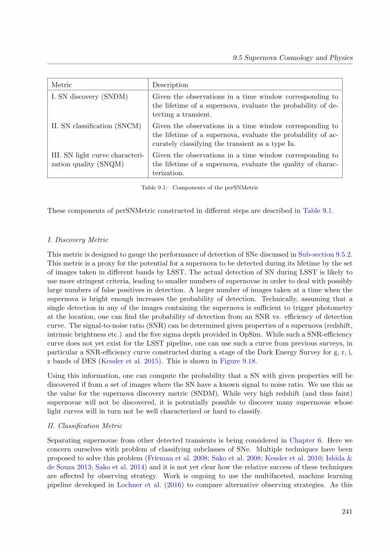
9.5 Supernova Cosmology and Physics

Metric Description

I. SN discovery (SNDM) Given the observations in a time window corresponding tothe lifetime of a supernova, evaluate the probability of de-tecting a transient.

II. SN classification (SNCM) Given the observations in a time window corresponding tothe lifetime of a supernova, evaluate the probability of ac-curately classifying the transient as a type Ia.

III. SN light curve characteri-zation quality (SNQM)

Given the observations in a time window corresponding tothe lifetime of a supernova, evaluate the quality of charac-terization.

Table 9.1: Components of the perSNMetric

These components of perSNMetric constructed in different steps are described in Table 9.1.

I. Discovery Metric

This metric is designed to gauge the performance of detection of SNe discussed in Sub-section 9.5.2.This metric is a proxy for the potential for a supernova to be detected during its lifetime by the setof images taken in different bands by LSST. The actual detection of SN during LSST is likely touse more stringent criteria, leading to smaller numbers of supernovae in order to deal with possiblylarge numbers of false positives in detection. A larger number of images taken at a time when thesupernova is bright enough increases the probability of detection. Technically, assuming that asingle detection in any of the images containing the supernova is sufficient to trigger photometryat the location, one can find the probability of detection from an SNR vs. efficiency of detectioncurve. The signal-to-noise ratio (SNR) can be determined given properties of a supernova (redshift,intrinsic brightness etc.) and the five sigma depth provided in OpSim. While such a SNR-efficiencycurve does not yet exist for the LSST pipeline, one can use such a curve from previous surveys, inparticular a SNR-efficiency curve constructed during a stage of the Dark Energy Survey for g, r, i,z bands of DES (Kessler et al. 2015). This is shown in Figure 9.18.

Using this information, one can compute the probability that a SN with given properties will bediscovered if from a set of images where the SN have a known signal to noise ratio. We use this asthe value for the supernova discovery metric (SNDM). While very high redshift (and thus faint)supernovae will not be discovered, it is potentially possible to discover many supernovae whoselight curves will in turn not be well characterized or hard to classify.

II. Classification Metric

Separating supernovae from other detected transients is being considered in Chapter 6. Here weconcern ourselves with problem of classifying subclasses of SNe. Multiple techniques have beenproposed to solve this problem (Frieman et al. 2008; Sako et al. 2008; Kessler et al. 2010; Ishida &de Souza 2013; Sako et al. 2014) and it is not yet clear how the relative success of these techniquesare affected by observing strategy. Work is ongoing to use the multifaceted, machine learningpipeline developed in Lochner et al. (2016) to compare alternative observing strategies. As this

241

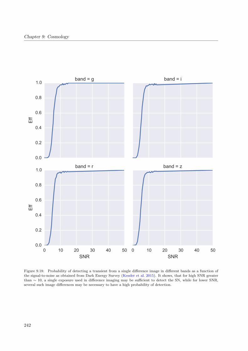
Chapter 9: Cosmology

0.0

0.2

0.4

0.6

0.8

1.0

Eff

band = g band = i

0 10 20 30 40 50SNR

0.0

0.2

0.4

0.6

0.8

1.0

Eff

band = r

0 10 20 30 40 50SNR

band = z

Figure 9.18: Probability of detecting a transient from a single difference image in different bands as a function ofthe signal-to-noise as obtained from Dark Energy Survey (Kessler et al. 2015). It shows, that for high SNR greaterthan ∼ 10, a single exposure used in difference imaging may be sufficient to detect the SN, while for lower SNR,several such image differences may be necessary to have a high probability of detection.

242

9.5 Supernova Cosmology and Physics

pipeline employs a variety of different feature extraction and machine learning techniques, it is idealto investigate the effect of observing strategy on the supernova classification. The exact metricused to determine the efficacy of the classification depends on the exact problem at hand. Forproducing a general purpose, well-classified set of all types of supernovae (for example, to studysupernova population statistics), one could use the AUC metric used in Lochner et al. (2016),which is a good balance between purity and completeness. Ideally, one would like a metric tobe evaluated per object and included in the PerSNMetric. This is, however, challenging as thesuccess of classification will depend strongly on the nature of the available training set, which willin turn depend on the spectroscopic follow-up program of LSST and the availability of additionaltraining data. Once a training set is determined and the classification algorithm trained, a usefulper-object metric is the classification probability of an object being a Ia, which will be higher ifthe light curve is well-measured. This probability is confounded by other factors (for example,other types appearing similar to Ia’s), making classification a very difficult metric to include onthe per-object level. This is therefore left for future work.

III. Quality Metric

We construct the quality metric for the perSNMetric by obtaining the light curve of the SN in thetime window described above. We fit the light curve, using the SALT2 model (Guy et al. 2007;Betoule et al. 2014), and approximately estimate the uncertainty in distance from the light curvefit alone. Of course, as is well known, luminosity distance estimates of supernova Type Ia alsoshow an intrinsic scatter of around 0.1 in previous surveys, which may be expected to decreasewith better training samples and understanding of underlying correlations of SN Ia properties andtheir environments. We compute a quality metric for each SN Ia as the ratio of the square of theintrinsic dispersion to variance of the distance indicator from the supernova.

QM = 0.052/σ2µ.

If our sample had a perfect discovery rate, and good classification (for example if we had spec-troscopic classification), the uncertainty on cosmological parameters would be entirely due to thisquality metric and would be expected to scale with the quality metric as

1

σ∼√∑ 1.0

1.0 + 1.0/QM

where the sum is over the SNe in the sample.

9.5.4 OpSim Analysis

The scientific goal of characterizing SNe is, to a large extent, dependent on how well the lightcurves of individual SNe are sampled in time and filters. To study this, we re-index the OpSimoutput on spatial locations rather than use the temporal index. Here, we first illustrate in termsthe cadence in two example LSST fields.

We analyzed the OpSim output of the Baseline Observing Strategy, enigma 1189 sqlite.db3 whichincludes Deep Drilling Fields (DDF) and the main survey (WFD). While this is no longer the

3http://ops2.tuc.noao.edu/runs/

243

Chapter 9: Cosmology

current baseline observing strategy, we do not anticipate our conclusions would change with theuse of minion 1016. Future work will include repeating our analyses with new OpSim runs, suchas kraken 1043, which does not enforce visit pairs, and the new experimental rolling cadences.

Using the OpSim output enigma 1189, we generated light curves for a type Ia supernova with aredshift of z=0.5 at a few different locations. A date in MJD is chosen where the LSST simulateddata are reasonably well populated. We used the SALT2-extended model with x0, x1 and c set sothat the SN Ia would have a specific magnitude of −19.3 in the rest frame BessellB band. This wasperformed using a version of SNCosmo to interpolate the SALT2 surfaces, and the LSST catalogsimulation package to calculate the flux for LSST bandpasses.

Figure 9.19 shows the light curve in different filters in a deep drilling field. The number of visitsfor 50 days (which is the period of the simulated SN Ia light curve in rest-frame, which translatesto 75 days at z=0.5) is 53 per filter. For this light curve, the supernova quality metric (SNQM)and the discovery metric (SNDM), are both equal to 1. SNDM=1 indicates that this object is atransient that will be definitely discovered, and SNQM=1 indicates that the light curves will be ofhigh quality enough to contribute extremely well to the inference of cosmological parameters. Thelight curves and quantified metric demonstrate that data from Deep Drilling Fields would generatehigh quality light curves, allowing a high rate of supernova discovery.

In contrast, Figure 9.20 shows a light curve from the WFD survey. This light curve is generatedin Field 290 and has an average number of data points in the light curve of 2 per filter. Usingthese light curves, the probability (SNDM) of detecting this supernova is less than 0.1. Figure 9.21directly compares the light curves and cadences of the two fields considered, from the DDF andWFD.

Analysis Results: To further study the quality of light curves across the survey, we simulatethe same type Ia supernova in 16 different fields, including DDF 290 already studied, from theenigma 1189 OpSim run and record the average number of visits per 50 day time window (Ta-ble 9.2). A well-known rule of thumb (R. Foley, priv. communication) for good quality SN lightcurves is to demand 7-10 epochs per light curve spread over 50 days or so for more than one filter.Table 9.2 list characteristics of light curves towards 15 fields in the OpSim output.

We summarize results of light curve analysis using OpSim output as follows:

• A high portion of the light curves, in both the WFD and DDF, can be identified as transientsusing the SN discovery metric (SNDM>0.5 in Table 9.2). This metric is currently using SNRof detections.

• Light curves from WFD show poor qualities (SNQM<0.3) whereas the light curves from DDFshow high quality (≥1). Note that we examined only a few cases of SNe at redshift of 0.5and the metric will be applied to a much larger range of SNe in future simulations.

• We have explored ways to improve SN classification (Lochner et al. 2016) and the classificationmetric is described in Section 9.5.3. In this analysis, we have not yet considered classificationbased on individual light curves. This is because, unlike the discovery and quality metric, itis difficult to discuss classification of a single object without having a well-defined trainingset, which is yet to be determined for LSST.

244

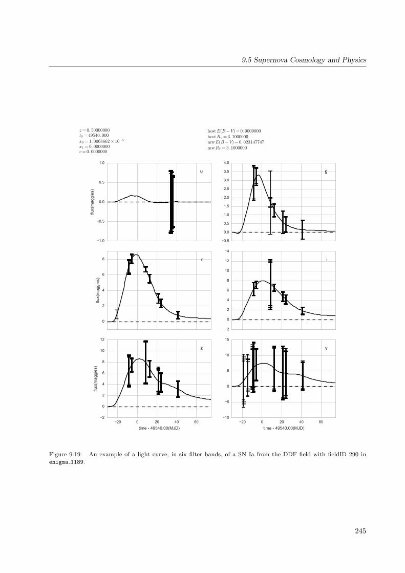
9.5 Supernova Cosmology and Physics

1.0

0.5

0.0

0.5

1.0

flux(

mag

gies

)

u

0.5

0.0

0.5

1.0

1.5

2.0

2.5

3.0

3.5

4.0

g

0

2

4

6

8

flux(

mag

gies

)

r

2

0

2

4

6

8

10

12

14

i

20 0 20 40 60time - 49540.00(MJD)

2

0

2

4

6

8

10

12

flux(

mag

gies

)

z

20 0 20 40 60time - 49540.00(MJD)

10

5

0

5

10

15

y

z= 0. 50000000t0 = 49540. 000

x0 = 1. 0068662× 10−5

x1 = 0. 0000000c= 0. 0000000

hostE(B−V) = 0. 0000000

hostRV = 3. 1000000mwE(B−V) = 0. 023147747mwRV = 3. 1000000

Figure 9.19: An example of a light curve, in six filter bands, of a SN Ia from the DDF field with fieldID 290 inenigma 1189.

245

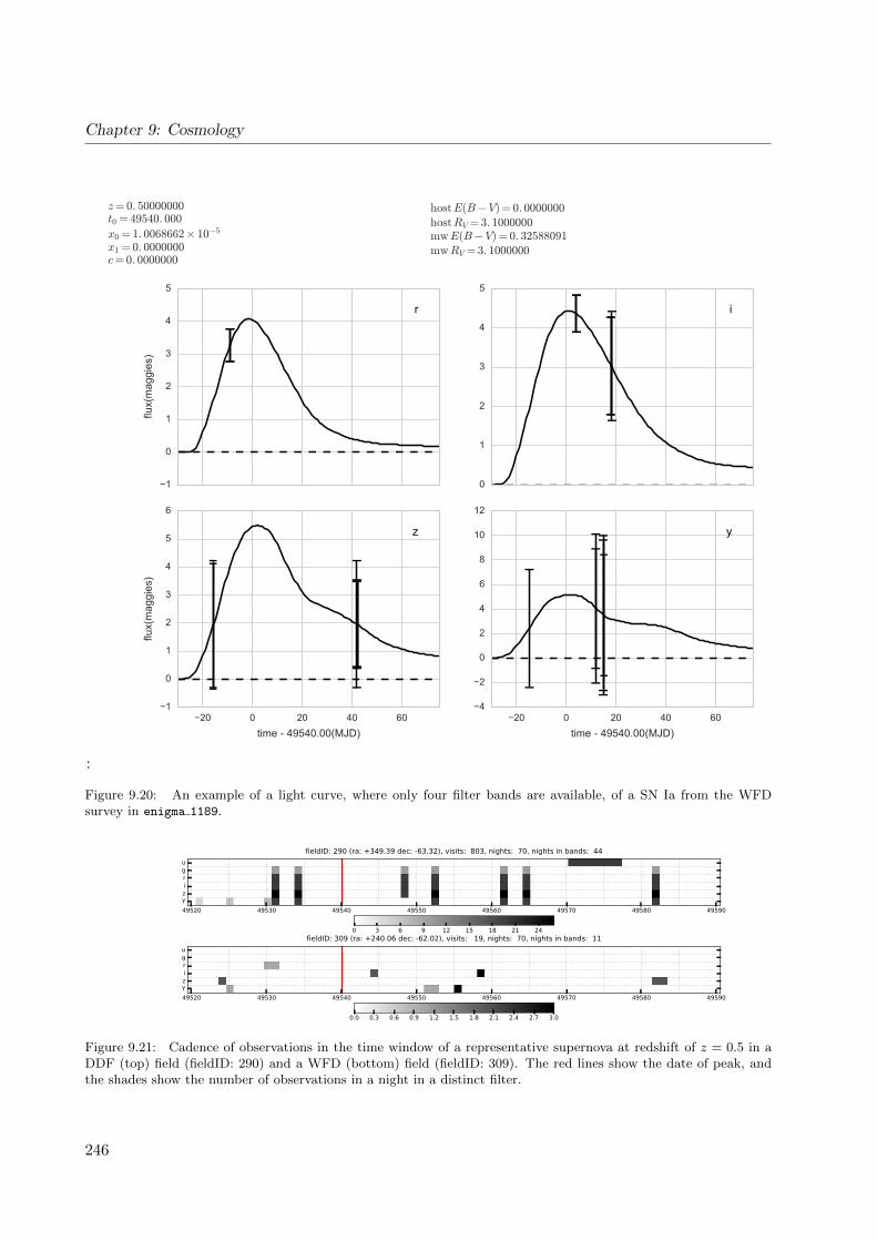
Chapter 9: Cosmology

:

1

0

1

2

3

4

5

flux(

mag

gies

)

r

0

1

2

3

4

5

i

20 0 20 40 60time - 49540.00(MJD)

1

0

1

2

3

4

5

6

flux(

mag

gies

)

z

20 0 20 40 60time - 49540.00(MJD)

4

2

0

2

4

6

8

10

12

y

z= 0. 50000000t0 = 49540. 000

x0 = 1. 0068662× 10−5

x1 = 0. 0000000c= 0. 0000000

hostE(B−V) = 0. 0000000

hostRV = 3. 1000000mwE(B−V) = 0. 32588091mwRV = 3. 1000000

Figure 9.20: An example of a light curve, where only four filter bands are available, of a SN Ia from the WFDsurvey in enigma 1189.

49520 49530 49540 49550 49560 49570 49580 49590

Yzirgu

fieldID: 290 (ra: +349.39 dec: -63.32), visits: 803, nights: 70, nights in bands: 44

0 3 6 9 12 15 18 21 24

49520 49530 49540 49550 49560 49570 49580 49590

Yzirgu

fieldID: 309 (ra: +240.06 dec: -62.02), visits: 19, nights: 70, nights in bands: 11

0.0 0.3 0.6 0.9 1.2 1.5 1.8 2.1 2.4 2.7 3.0

Figure 9.21: Cadence of observations in the time window of a representative supernova at redshift of z = 0.5 in aDDF (top) field (fieldID: 290) and a WFD (bottom) field (fieldID: 309). The red lines show the date of peak, andthe shades show the number of observations in a night in a distinct filter.

246

9.5 Supernova Cosmology and Physics

• In conclusion, based on the SNQM, we have showed that WFD data alone using the BaselineObserving Strategy are not useful for SN studies.

Need for LSST observing strategy optimization for SN science:

The results from our OpSim analysis motivate our proposal of a rolling cadence in order to improvethe sampling of SNe over a much larger area than the DDFs. The DDF are useful for SNe atredshifts between 0.6 and 1.2, and the WFD will help us to increase the number of SNe at lowredshift as shown in Figure 11.1 of LSST science book (LSST Science Collaboration et al. 2009).For example, a higher number of SNe at z = 0.4 is expected from WFD than DDF. Consequently,DDF will have only a few SNe at low redshift, since the DDF sample is limited to small patchesof sky. A significant scatter in distance modulus of low redshift SNe is found (e.g. Suzuki et al.2012) which hinders deriving accurate cosmological parameters. Since the cosmology measurementrequires low as well as high redshift distance moduli, a large sample of low redshift SNe will improvethe cosmological parameter inference. The WFD would also provide a useful sample of nearbysupernovae to better constrain variations in SNe populations (for both type Ia and core-collapseSNe). Light curves from WFD with reasonable quality can be achieved using our new proposedobserving strategy.

A larger sample of well-characterized light curves from the WFD can address two key science goals:

• Tightly constraining cosmological parameters (ΩM and ΩΛ) by improving the measurementof distance modulus of low redshifted SNe. Without implementing the new observing strategythat we recommend below, LSST will not be able to make a significant contribution to SNcosmology below z<0.5.

• The WFD offers a unique opportunity for isotropy studies (complementary to large-scalegalaxy surveys) and dynamical dark energy studies. Apparent luminosities and numbercounts can be estimated for a large range of angular scales and redshifts with WFD. However,this science case will only be possible with a large sample of well-characterized SN Ia in alarge field of view, providing further support for our recommendation of a rolling cadenceobserving strategy.

9.5.5 Discussion

For enigma 1189 (and also, most likely, for the current baseline strategy), the DDF fields willproduce an exquisite sample of well-characterized SNe for cosmology and astrophysics studies.Further analysis is required to determine exactly how many (useful) supernovae will be detectedand what the resulting cosmological constraints will be, but in this section we have discussed andmotivated several important intermediate metrics.

247

Chapter 9: Cosmology

FieldID (R.A., Decl.) Number of LSST visitsper year (u,g,r,i,z,y)

Number ofAvg. dataper SN pe-riod per fil-ter

SNDM SNQM

290DDF

(349.386,-63.321) 2363 (398,229,402,414,522,396)

53 1.0 1.6

17 (190,-83) 239 (38,41,41,44,33,42) 5.3 .. ..

22 (20,-83) 252 (52,56,40,21,37,44) 5.7 .. ..

217 (116,-66) 220 (36,38,37,32,44,33) 5.0 .. ..

309 (240.05,-62.02) 101 (2,5,11,19,19,45) 2.2 1.00 0.10

645 (120,-50) 80 (4,7,9,18,24,18) 1.8 0.54 0.01

949 (80,-40) 96 (5,8,15,17,27,24) 2.2 0.99 0.09

948 (280,-40) 86 (4,2,6,4,24,18) 2.0 0.99 <0.002

1401 (58,-27) 98 (3,3,9,26,31,26) 2.2 0.77 0.002

1754 (30,-20) 86 (3,4,10,21,27,21) 2.0 1.00 0.05

1720 (100,-20) 58 (4,2,6,4,24,18) 1.3 0.99 0.03

2556 (6.097, -1.105) 80 (4,7,9,18,24,18) 1.8 1.00 0.05

2718 (50,+1.5) 72 (3,6,10,12,22,19) 1.6 1.00 0.09

2751 (320, +5) 7 (0,0,2,0,4,0) 0.2 0.09 0.02

3606 (60,+20) 72 (0,8,13,22,29,0) 1.6 .. ..

Table 9.2: Table of 15 fields in the OpSim run enigma 1189. The first column is simply an index, with the specialexample fields of the DDF field 290 indicated. The position of the fields is shown in column 2. The third columncontains the total and per filter band number of visits per year and this is averaged per filter per 50 day time windowin column 4. It can be seen that with this observing strategy, only the deep drilling fields are suitable for supernovacosmology, where 7-9 data points per filter band is considered adequate quality. SNDM and SNQM are SN discoveryand quality metric, respectively, in the last two columns. Note that the metric measurements are missing for someentries due to a spatial mismatch in fields that will be rectified in future.

248

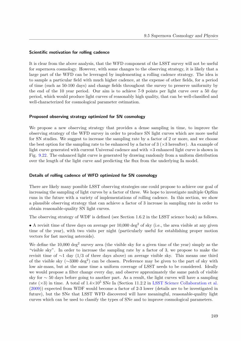
9.5 Supernova Cosmology and Physics

Scientific motivation for rolling cadence

It is clear from the above analysis, that the WFD component of the LSST survey will not be usefulfor supernova cosmology. However, with some changes to the observing strategy, it is likely that alarge part of the WFD can be leveraged by implementing a rolling cadence strategy. The idea isto sample a particular field with much higher cadence, at the expense of other fields, for a periodof time (such as 50-100 days) and change fields throughout the survey to preserve uniformity bythe end of the 10 year period. Our aim is to achieve 7-9 points per light curve over a 50 dayperiod, which would produce light curves of reasonably high quality, that can be well-classified andwell-characterized for cosmological parameter estimation.

Proposed observing strategy optimized for SN cosmology

We propose a new observing strategy that provides a dense sampling in time, to improve theobserving strategy of the WFD survey in order to produce SN light curves which are more usefulfor SN studies. We suggest to increase the sampling rate by a factor of 2 or more, and we choosethe best option for the sampling rate to be enhanced by a factor of 3 (×3 hereafter). An example oflight curve generated with current Universal cadence and with ×3 enhanced light curve is shown inFig. 9.22. The enhanced light curve is generated by drawing randomly from a uniform distributionover the length of the light curve and predicting the flux from the underlying Ia model.

Details of rolling cadence of WFD optimized for SN cosmology

There are likely many possible LSST observing strategies one could propose to achieve our goal ofincreasing the sampling of light curves by a factor of three. We hope to investigate multiple OpSimruns in the future with a variety of implementations of rolling cadence. In this section, we showa plausible observing strategy that can achieve a factor of 3 increase in sampling rate in order toobtain reasonable-quality SN light curves.

The observing strategy of WDF is defined (see Section 1.6.2 in the LSST science book) as follows.

• A revisit time of three days on average per 10,000 deg2 of sky (i.e., the area visible at any giventime of the year), with two visits per night (particularly useful for establishing proper motionvectors for fast moving asteroids).

We define the 10,000 deg2 survey area (the visible sky for a given time of the year) simply as the“visible sky”. In order to increase the sampling rate by a factor of 3, we propose to make therevisit time of ∼1 day (1/3 of three days above) on average visible sky. This means one thirdof the visible sky (∼3300 deg2) can be chosen. Preference may be given to the part of sky withlow air-mass, but at the same time a uniform coverage of LSST needs to be considered. Ideallywe would propose a filter change every day, and observe approximately the same patch of visiblesky for ∼ 50 days before going to another part. As a result, the light curves will have a samplingrate (×3) in time. A total of 1.4×105 SNe Ia (Section 11.2.2 in LSST Science Collaboration et al.(2009)) expected from WDF would become a factor of 2-3 lower (details are to be investigated infuture), but the SNe that LSST WFD discovered will have meaningful, reasonable-quality lightcurves which can be used to classify the types of SNe and to improve cosmological parameters.

249

Chapter 9: Cosmology

Figure 9.22: An example of light curve of SN Type Ia generated using OpSim output at RA. of 58 and Decl. of-27 (left) and the same light curve after the sampling rate is enhanced by a factor of 3 (right).

250

9.5 Supernova Cosmology and Physics

9.5.6 Conclusion

Here we answer the ten questions posed in Sub-section 1.2.1:

Q1: Does the science case place any constraints on the tradeoff between the sky coverage andcoadded depth? For example, should the sky coverage be maximized (to ∼30,000 deg2, as e.g.,in Pan-STARRS) or the number of detected galaxies (the current baseline of 18,000 deg2)?

A1: For supernova observations, the most important aspect is cadence: we need a good samplingof well-measured light curves of supernovae. If the sky coverage can be increased withoutsacrificing the number of observations per supernova (i.e., over one season), such as using arolling cadence strategy, this will greatly improve supernova science. Inasmuch as requiringincreased sky coverage could negatively affect cadence over one season, our preference is notto increase to a larger sky coverage.

Q2: Does the science case place any constraints on the tradeoff between uniformity of sampling andfrequency of sampling? For example, a rolling cadence can provide enhanced sample ratesover a part of the survey or the entire survey for a designated time at the cost of reducedsample rate the rest of the time (while maintaining the nominal total visit counts).

A2: Frequency of sampling is much more important than uniformity over long time scales for allforms of supernova science. For SN Ia cosmology, light-curve sampling should be about threetimes as frequent as for the current baseline WFD cadence. While further investigation isneeded, a reasonable length of a season with enhanced rates is around 120-150 days. A rollingcadence will allow this improved sampling while still keeping the sky coverage and co-addeddepth, by concentrating on different fields in different seasons (see Section 9.5 for details).

Q3: Does the science case place any constraints on the tradeoff between the single-visit depth andthe number of visits (especially in the u-band where longer exposures would minimize theimpact of the readout noise)?

A3: In general for supernova science, the number of visits is more important to the single-visitdepth, though we would not advocate any decrease in single-visit exposure time (below 2x15sec). The U band is useful for the low-z (wide-area) sample and and their calibration of theHubble diagram. It is not obvious if longer exposures are helpful at this time for supernovascience.

Q4: Does the science case place any constraints on the Galactic plane coverage (spatial coverage,temporal sampling, visits per band)?

A4: Our supernova science is extragalactic and will use high Galactic-latitude fields almost exclu-sively (to minimize Milky Way extinction systematic uncertainties). Survey time spent onGalactic fields takes away from survey time for our science; we would optimize for less timein the Galactic plane.

Q5: Does the science case place any constraints on the fraction of observing time allocated to eachband?

251

Chapter 9: Cosmology

A5: For supernova science, we have no strong preference for any band and would benefit fromroughly uniform depth per band. While redder bands are more useful for higher redshiftsupernovae, the bluer bands are helpful especially for lower redshift objects. Visits in eachband should be uniformly spread in time. A higher number of visits to redder bands ispreferred for DDF.

Q6: Does the science case place any constraints on the cadence for deep drilling fields?

A6: Our optimal cadence would for the DDFs would be nightly or every other night; every threenights would be acceptable. Beyond this we run the risk of large gaps more than ∼7 days,which would be detrimental to supernova science. Ideally, the DDFs would be observed inall available filters, though not all filters are needed every night (so for instance some filterscould be observed on night 1, the others on night 2, and repeat). The single-night depthshould be 1-2 mag deeper than a WFD field, but not much more; any extra time is betterspent on a different night.

We would like a suitable number of extragalactic DDFs in total so that at least a few (∼3 to5) are being observed at any time in the survey: we would limit an increase in the number ofDDFs if it came at the expense of our preferred high cadence. Each field should be observedfor a “season” of length at least ∼120-150 days, staggering the fields so new fields cycle in asold ones cycle out. In addition, for DDFs, the u-band exposure time could be increased tominimize readout noise.

Q7: Assuming two visits per night, would the science case benefit if they are obtained in the sameband or not?

A7: Supernova science benefits enormously from having color information, particularly in discoveryand early epochs to help classification. Two visits in the same band will be less useful thanvisits in different bands.

Q8: Will the case science benefit from a special cadence prescription during commissioning or earlyin the survey, such as: acquiring a full 10-year count of visits for a small area (either in allthe bands or in a selected set); a greatly enhanced cadence for a small area?

A8: During commissioning, we would like as many DDFs as possible observed in all filters (withfew times the per-night exposure time) so that templates can be created for each of the DDfields we consider. This will allow us to find useful supernovae in these DDFs as soon as thesurvey starts, and provide us with useful time to deal with any issues in the image subtractionetc. before the survey begins.

Early in the survey, we must build templates for all fields (more broadly than just the DDFs).Our favored method for doing this is to devote the bulk of year 1 to covering the full skyarea, with a rolling cadence survey commencing thereafter. As above, the templates shouldbe at least a few times the exposure time of a single visit (so that the template noise doesnot dominate the subtraction). This is particularly important in the first 3-5 weeks of thesurvey, to ensure that we get useful data from the rest of the critical first year.

Q9: Does the science case place any constraints on the sampling of observing conditions (e.g.,seeing, dark sky, airmass), possibly as a function of band, etc.?

252

9.6 Strong Gravitational Lens Time Delays

A9: While supernova observations benefit from good seeing, it is not as strong a requirement asit is for other science cases. Moreover we would like to limit any image coaddition issuesfor very good seeing (under the assumption that these remain): we can make good use ofobserving conditions with slightly poorer seeing.

Q10: Does the case have science drivers that would require real-time exposure time optimizationto obtain nearly constant single-visit limiting depth?

A10: A sufficiently long (or nominal), fixed exposure time should be adequate for supernova sci-ence. No real-time optimization is necessary, and single-visit science is not the limiting factorfor SNe science.

Go to: • the start of this section • the start of the chapter • the table of contents

9.6 Strong Gravitational Lens Time Delays

Phil Marshall, Lynne Jones, Timo Anguita

The multiple images of strongly lensed quasars and supernovae have delayed arrival times: vari-ability in the first image will be observed in the second image some time later, as the photons takedifferent paths around the deflector galaxy, and through different depths of gravitational potential.If the lens mass distribution can be modeled independently, using a combination of high resolu-tion imaging of the distorted quasar/SN host galaxy and stellar dynamics in the lens galaxy, themeasured time delays can be used to infer the “time delay distance” in the system. This distanceenables a direct physical measurement of the Hubble constant, independent of the distance lad-der. Treu & Marshall (2016) provide a recent review of this cosmological probe, including its themain systematic errors and observational follow-up demands. High resolution follow-up imagingand spectroscopy is needed to constrain the lens galaxy mass distribution, and this is expected todominate the systematic error budget in systems with good measured time delays. In tis sectionwe investigate the cadence needed for LSST to provide these good time delays, in lensed quasarsystems. We leave the assessment of lensed supernova time delays to future work.

9.6.1 Target measurements and discoveries

For this cosmological probe to be competitive with LSST’s others, the time delays of severalhundred systems (which will be distributed uniformly over the extragalactic sky) will need tobe measured with bias below the sub-percent level, while the precision required is a few percentper lens. In galaxy-scale lenses, the kind that are most accurately modeled, these time delaysare typically between several days and several weeks long, and so are measurable in monitoringcampaigns having night-to-night cadence of between one and a few days, and seasons lasting severalmonths or more.

This size of sample seems plausible: Oguri & Marshall (2010) predicted that several thousandlensed quasar systems should be detectable at LSST single visit depth and resolution, and Liaoet al. (2015) found that around 400 of these should yield time delay measurements of high enoughquality for cosmography. To obtain accurate as well as precise lensed quasar time delays, several

253

Chapter 9: Cosmology

monitoring seasons are required. Lensed supernova time delays have not yet been measured, buttheir transient nature means that their time delay measurements may be more sensitive to cadencethan season or campaign length.

9.6.2 Metrics

Anticipating that the time delay accuracy would depend on night-to-night cadence, season length,and campaign length, we carried out a large scale simulation and measurement program thatcoarsely sampled these schedule properties. In Liao et al. (2015), we simulated 5 different lightcurve datasets, each containing 1000 lenses, and presented them to the strong lensing communityin a “Time Delay Challenge.” These 5 challenge “rungs” differed by their schedule properties, inthe ways shown in Table 9.3. Entries to the challenge consisted of samples of measured time delays,the quality of which the challenge team then measured via three primary diagnostic metrics: timedelay accuracy, time delay precision, and useable sample fraction (i.e. the number of lenses thatcould be measured well, divided by the number of simulated lenses in the dataset). The accuracy ofa sample was defined to be the mean fractional offset between the estimated and true time delayswithin the sample. The precision of a sample was defined to be the mean reported fractionaluncertainty within the sample.

Focusing on the best challenge submissions made by the community, we derived a simple powerlaw model for the variation of each of the time delay accuracy, time delay precision, and useablesample fraction, with the schedule properties cadence, season length and campaign length. Thesemodels are shown in Figure 9.23, reproduced from Liao et al. (2015), and are given by the followingequations:

|A|model ≈ 0.06%

(cad

3days

)0.0 ( sea

4months

)−1.0(

camp

5years

)−1.1

Pmodel ≈ 4.0%

(cad

3days

)0.7 ( sea

4months

)−0.3(

camp

5years

)−0.6

fmodel ≈ 30%

(cad

3days

)−0.4 ( sea

4months

)0.8(

camp

5years

)−0.2

All three of these diagnostic metrics would, in an ideal world, be optimized: this could be achievedby decreasing the night-to-night cadence (to better sample the light curves), extending the ob-serving season length (to maximize the chances of capturing a strong variation and its echo), andextending the campaign length (to increase the number of effective time delay measurements).

The quantity of greatest scientific interest is the accuracy in cosmological parameters: this couldbe computed as follows. Setting a required accuracy threshold defines the available number oflenses, which in turns gives us the mean precision per lens there. Combining the whole sample,we would get the error on the weighted mean time delay, as used by Coe & Moustakas (2009).This uncertainty, which scales as one over the square root of the number of available lenses, canbe roughly equated to the statistical uncertainty on the Hubble constant (Coe & Moustakas 2009;Treu & Marshall 2016). The Figure of Merit would be the final percentage precision on H0, as away to sum up the sample size and time delay measurability (at fixed accuracy requirement).

254

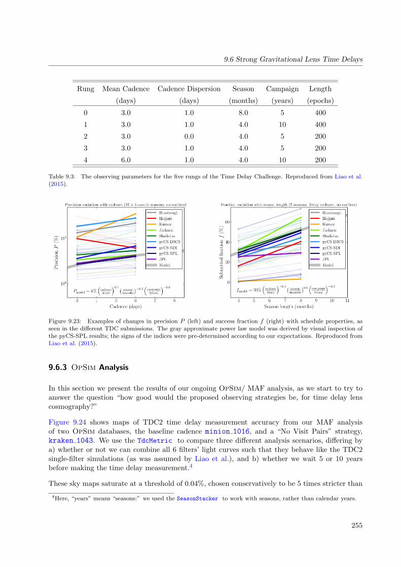
9.6 Strong Gravitational Lens Time Delays

Rung Mean Cadence Cadence Dispersion Season Campaign Length

(days) (days) (months) (years) (epochs)

0 3.0 1.0 8.0 5 400

1 3.0 1.0 4.0 10 400

2 3.0 0.0 4.0 5 200

3 3.0 1.0 4.0 5 200

4 6.0 1.0 4.0 10 200

Table 9.3: The observing parameters for the five rungs of the Time Delay Challenge. Reproduced from Liao et al.(2015).

Figure 9.23: Examples of changes in precision P (left) and success fraction f (right) with schedule properties, asseen in the different TDC submissions. The gray approximate power law model was derived by visual inspection ofthe pyCS-SPL results; the signs of the indices were pre-determined according to our expectations. Reproduced fromLiao et al. (2015).

9.6.3 OpSim Analysis

In this section we present the results of our ongoing OpSim/ MAF analysis, as we start to try toanswer the question “how good would the proposed observing strategies be, for time delay lenscosmography?”

Figure 9.24 shows maps of TDC2 time delay measurement accuracy from our MAF analysisof two OpSim databases, the baseline cadence minion 1016, and a “No Visit Pairs” strategy,kraken 1043. We use the TdcMetric to compare three different analysis scenarios, differing bya) whether or not we can combine all 6 filters’ light curves such that they behave like the TDC2single-filter simulations (as was assumed by Liao et al.), and b) whether we wait 5 or 10 yearsbefore making the time delay measurement.4

These sky maps saturate at a threshold of 0.04%, chosen conservatively to be 5 times stricter than

4Here, “years” means “seasons:” we used the SeasonStacker to work with seasons, rather than calendar years.

255

Chapter 9: Cosmology

that used by Hojjati & Linder. We can see that the area of sky providing lenses measurable atthis accuracy or better increases markedly as we move from ri to ugrizy. These maps predict thatwhile the accuracy should increase between DR5 and DR10, the sky area yielding accuracy betterthan 0.04% should already be close to the full WFD area (18000 square degrees) by DR5: thisbodes well for our ability to make use of shorter campaign sky areas observed at higher frequency,as would emerge from a rolling cadence strategy.

To summarize the diagnostic metric results, we first compute the area of this “high accuracy”(A < 0.04%) sky. We can then compute the cadence, season, and campaign length just in theseareas; these values are reported in Table 9.4. The high accuracy area can be used to define a “GoldSample” of lenses, whose mean precision per lens we can compute. The TDC2 useable fractionaveraged over this area gives us the approximate size of this sample: we simply re-scale the 400lenses predicted by Liao et al. (2015) by this fraction over the 30% found in TDC2. While thesenumbers are approximate, the ratios between different observing and analysis strategies provide auseful indication of relative merit. In this table, the impacts of higher night-to-night sampling rateand survey length can be seen.5

As described above, we follow Coe & Moustakas (2009) and compute a very simple time delaydistance Figure of Merit “DPrecision” as follows. We first combine the fractional time delayprecision in quadrature with an assumed 4% “modeling uncertainty,” and then divide this by thesquare root of the number of Gold Sample lenses. This estimated ensemble distance precision canbe straightforwardly related to cosmological parameter precision, as Coe & Moustakas (2009) show(it’s very roughly the precision on the Hubble constant). This distance precision Figure of Merit isgiven in the final column of Table 9.4. We see that in DR5, being able to combine all filters insteadof just ri should give a FoM of 0.29% instead of 1.25%; between DR5 and DR10 this then shouldimprove to 0.24. This suggests that time delay measurement is primarily analysis-limited. In the“No Visit Pairs” strategy, we seet that the DR5 all-band FoM is 0.26%, just a 10% improvement.This might be because the “No Visit Pairs” does not insist that the visits in the visit pairs are splitover different nights, only that they don’t have to be taken on the same night. We might expect amore aggressive approach to splitting visit pairs to make a bigger difference – but it seems unlikelythat it would be a factor of two improvement.

9.6.4 Discussion

The main risk involved with this science case is that the “multi-filter” light curve analysis presentedhere, which extrapolates from the results of the single-filter TDC1, does not represent accuratelythe real-life combination of all 6 filters together. The second time delay challenge (TDC2) will helpanswer this question. For now, just using 2 filters gives an upper limit on the overall precision weshould expect.

Naively, we would expect the relaxation of the visit pairs requirement to increase the night-to-night cadence by a factor of two, if the visits are redistributed randomly in time. However, itseems OpSim is not as liberal as this, such that we do not see much improvement over the baseline

5The small decrease in the number of useable lenses with ugrizy going from 5 years to 10 years is due to theslightly lower precision in 5 years, and is an artifact of how the metrics are calculated (as global means ratherthan running totals).

256

9.6 Strong Gravitational Lens Time Delays

Figure 9.24: Sky maps of the TDC2 time delay measurement accuracy metric A for the baseline cadenceminion 1016 (left) and the “No Visit Pairs” strategy, kraken 1043 (right). The rows show the build upof data quality with time and analysis capability, from 5 years of r and i-band light curve data only (top row), to5 years of hypothetically-combined ugrizy light curve data (middle row), to 10 years of hypothetically-combinedugrizy light curve data (bottom row). The maps saturate at the threshold accuracy of 0.04, such that any regionsthat are not yellow should yield high accuracy lens time delays, while the yellow regions show where high accuracytime delay measurement is not possible.

cadence. Efficiency maximization could be preventing visits being fully split. We are interestedin any changes to the WFD survey time sampling that reduce the inter-night gaps: these wouldinclude rolling cadence schemes.

9.6.5 Conclusions

Based on the above results, we now answer the ten questions posed in Sub-section 1.3.2:

Q1: Does the science case place any constraints on the tradeoff between the sky coverage andcoadded depth? For example, should the sky coverage be maximized (to ∼30,000 deg2, as e.g.,in Pan-STARRS) or the number of detected galaxies (the current baseline of 18,000 deg2)?

A1: Yes: it’s probably better to have smaller area and better data, especially if the multi-filterlight curve analysis turns out to be difficult. This conclusion is partly informed by theapparently small difference between 5 years and 10 years campaign length, although we needto be careful: COSMOGRAIL studies show that the longer monitoring campaigns yieldsignificantly higher accuracy results.

257

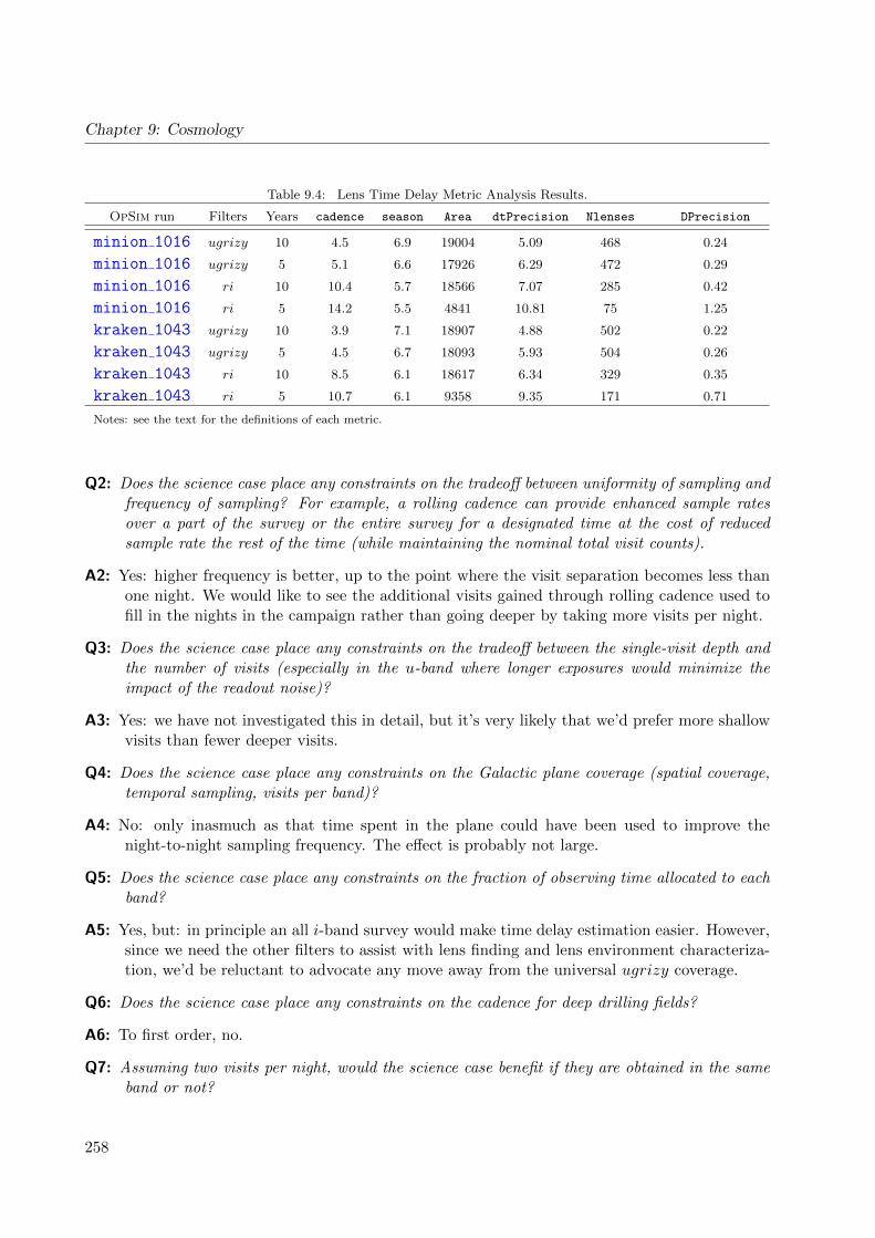
Chapter 9: Cosmology

Table 9.4: Lens Time Delay Metric Analysis Results.

OpSim run Filters Years cadence season Area dtPrecision Nlenses DPrecision

minion 1016 ugrizy 10 4.5 6.9 19004 5.09 468 0.24

minion 1016 ugrizy 5 5.1 6.6 17926 6.29 472 0.29

minion 1016 ri 10 10.4 5.7 18566 7.07 285 0.42

minion 1016 ri 5 14.2 5.5 4841 10.81 75 1.25

kraken 1043 ugrizy 10 3.9 7.1 18907 4.88 502 0.22

kraken 1043 ugrizy 5 4.5 6.7 18093 5.93 504 0.26

kraken 1043 ri 10 8.5 6.1 18617 6.34 329 0.35

kraken 1043 ri 5 10.7 6.1 9358 9.35 171 0.71

Notes: see the text for the definitions of each metric.

Q2: Does the science case place any constraints on the tradeoff between uniformity of sampling andfrequency of sampling? For example, a rolling cadence can provide enhanced sample ratesover a part of the survey or the entire survey for a designated time at the cost of reducedsample rate the rest of the time (while maintaining the nominal total visit counts).

A2: Yes: higher frequency is better, up to the point where the visit separation becomes less thanone night. We would like to see the additional visits gained through rolling cadence used tofill in the nights in the campaign rather than going deeper by taking more visits per night.

Q3: Does the science case place any constraints on the tradeoff between the single-visit depth andthe number of visits (especially in the u-band where longer exposures would minimize theimpact of the readout noise)?

A3: Yes: we have not investigated this in detail, but it’s very likely that we’d prefer more shallowvisits than fewer deeper visits.

Q4: Does the science case place any constraints on the Galactic plane coverage (spatial coverage,temporal sampling, visits per band)?

A4: No: only inasmuch as that time spent in the plane could have been used to improve thenight-to-night sampling frequency. The effect is probably not large.

Q5: Does the science case place any constraints on the fraction of observing time allocated to eachband?

A5: Yes, but: in principle an all i-band survey would make time delay estimation easier. However,since we need the other filters to assist with lens finding and lens environment characteriza-tion, we’d be reluctant to advocate any move away from the universal ugrizy coverage.

Q6: Does the science case place any constraints on the cadence for deep drilling fields?

A6: To first order, no.

Q7: Assuming two visits per night, would the science case benefit if they are obtained in the sameband or not?

258

9.6 Strong Gravitational Lens Time Delays

A7: Unclear: different bands are probably going to be better, but this has not been tested. Itwould clearly provide good information on the AGN color variability model.

Q8: Will the case science benefit from a special cadence prescription during commissioning or earlyin the survey, such as: acquiring a full 10-year count of visits for a small area (either in allthe bands or in a selected set); a greatly enhanced cadence for a small area?

A8: Not really. We rely on the difference imaging working well, so making a good template acrossas much sky as possible would be good. Including a known lens system (from DES, perhaps)in any deep field would be useful too: we would be happy if the cadence to be similar toWDF to be able to test our software.

Q9: Does the science case place any constraints on the sampling of observing conditions (e.g.,seeing, dark sky, airmass), possibly as a function of band, etc.?

A9: No.

Q10: Does the case have science drivers that would require real-time exposure time optimizationto obtain nearly constant single-visit limiting depth?

A10: No.

Go to: • the start of this section • the start of the chapter • the table of contents

259

10 Special Surveys

Chapter editors: David Nidever, Knut Olsen.

10.1 Introduction

The four main LSST science themes, as defined by the Science Book, drive the design of LSST’smain Wide-Fast-Deep survey. However, it has always been recognized that many important sci-entific projects, including some that are highly relevant to LSST’s main science themes, are notwell served by the areal coverage and/or cadence constraints placed on the WFD survey. To thisend, the LSST Project set aside a nominal 10% of the observing time to serve what are collectivelycalled “special surveys.”

Projects that will certainly make use of this ≈ 10% time (that is not dedicated to the WFDsurvey) include the Deep Drilling fields and the Galactic Plane surveys, as well as any surveywishing to observe at declinations below −60, such as the Magellanic Clouds. These specialprograms have the potential to heavily oversubscribe the nominal 10% of time assigned to them. Itis of thus critical importance for these programs to define compelling science cases, clearly justifytheir observing requirements, and derive metrics to quantify the performance of a given schedulefor the program. This chapter provides a venue for such investigations.

A minimal set of 4 “extragalactic” Deep Drilling Fields have been included in many of the OpSimruns to date, including the baseline cadence simulation, minion 1016 (Chapter 2), and have beenevaluated in various science sections throughout this paper. As described in Sub-section 1.3.3, therewill be a further call for Deep Drilling Field proposals, and so we defer discussion of such observingprograms to that activity. In this chapter we collect together various ideas for additional specialsurveys or otherwise unusual observing programs, and the discussion of their metric evaluation.

In Section 10.2 a number of different concepts for special surveys that would support solar systemscience is described. This is followed by an extensive discussion of short exposure observing attwighlight (Section 10.3). If short exposure times will indeed be a possibility, it won’t just be solarsystem science that benefits: an example of a small program that could make good use of such acapability is the open star cluster special survey proposed in Section 10.4. We expect the ideasin this chapter to be developed (or discarded) over the time before the survey starts: this whitepaper aims to provide a (potentially temporary) home for them during that period.

261

Chapter 10: Special Surveys

10.2 Solar System Special Surveys

David Trilling, Lynne Jones.

There are several populations of Near Earth Objects (Solar System bodies whose orbits bringthem close to the Earth’s orbit) that, because of their orbital properties, would not be easilydetected in the wide-fast-deep survey. These populations are very interesting for both scientificand sociological purposes, though, due to their close proximity to the Earth, and in fact theirpotential for impacting the Earth. LSST will have the capability to carry out surveys for thesepopulations by using a small amount of special survey time. Two of these special surveys havepointings that fall within the nominal wide-fast-deep plan, and simply require a modification ofthe cadence. The third program is a twilight program, with a special cadence (though all twilightprograms are likely to have special cadences). These three programs are listed here and describedbelow. The three special surveys are the following:

• A special survey to look for mini-moons, which are temporarily captured satellites of theEarth;

• A special survey to find meter-sized impactors up to two weeks prior to impact. This wouldallow telescopic characterization of these impactors, which could be compared to laboratorymeasurements of the meteorites derived from the impactor. Advanced warning of an impactoralso allows detailed study of impact physics by being on location when the impact occurs;

• A special survey to observe the “sweetspot” in twilight fields to look for NEOs in very Earth-like orbits that would otherwise not be found in opposition fields.

These surveys will support three important scientific investigations:

1. What are the properties of the population of objects that is nearest to the Earth?

2. What is the impact risk from NEOs in populations that have not yet been well characterized(mini-moons, sweetspot objects)?

3. How do the telescopic properties of an impactor relate to the laboratory-measured propertiesof the ensuing meteorites?

Some details of the special cadence requirements for these science investigations are described inthe following section.

10.2.1 Target measurements and discoveries

Special cadences

Each of the three Solar System special surveys requires a special cadence. These cadences aredescribed here.

262

10.2 Solar System Special Surveys

• Mini-moons Mini-moons are objects that are temporary satellites of the Earth (Bolin et al.2014; Fedorets et al. 2017) Therefore, they have orbital motions similar to the Earth’s moon,and much faster than other Solar System populations. Therefore, a special cadence is requiredto detect these objects enough times to link objects, create tracklets, and determine orbits.A suggested cadence for a mini-moon survey is a series of 3 second exposures, with eachpointing visited at least twice per night. Such a survey would cover essentially all of theopposition sky each night. The opposition sky should be re-observed several nights in a rowin order to link objects from night to night and determine their orbits. While the detailsof this special cadence are not yet fully refined, this special survey would likely have littleimpact on the overall LSST program since this small-scale program, which extends over asmall number of nights, is effectively a compressed rolling cadence in which the aggregatefield coverage is unchanged.

• Impactors The Earth is struck by meter-sized impactors about once a month (e.g. Bosloughet al. 2015; Tricarico 2017, Trilling et al.2017 submitted). On two occasions, impactingasteroids have been discovered some hours before impact, but there are no existing surveysthat are dedicated to finding impactors. Impactors generally have small apparent motionson the sky (because their orbits are not too different than the Earth’s). The single exposuredepth of LSST images suggests that a meter-sized NEO could be discovered perhaps a weekbefore impact, given the typical Earth-relative velocity of such a body (e.g. Chesley & Veres2017). A suggested cadence for an impactor survey would be to survey the opposition patchfour times per night. This is more visits than in the nominal cadence, and would allow highfidelity linking of observations to find orbits. The nominal wide-fast-deep cadence (twice pernight, three times during a lunation) has a latency of orbit determination of up to two weeks,which is not acceptable for the impactor survey, as an impact would occur on a timescale ofjust a few days from discovery. The cadence of four observations/night should be repeatedroughly every three days, so that an object on an inbound trajectory could be observed atleast once, and possibly twice, before impact. Note that this cadence is compatible with thewide-fast-deep survey, in that the fields and exposure times are nominal; the only difference isthat each field is visited four times in a night, and that the fields are revisited every few nights.The overall impact of this special survey on the wide-fast-deep survey is likely to be small,and possibly negligible. Given the importance of this small but significant investigation, it iscritical that the survey simulators be capable of including such a special survey in planningfor LSST operations.

• Twilight/sweetspot survey

NEOs on very Earth-like orbits are relatively unlikely to come to opposition, and thereforeare relatively unlikely to appear in data obtained in the wide-fast-deep survey. These ob-jects are particularly interesting since, having very Earth-like orbits, they are the most likelyobjects to be Earth impactors. These objects are most likely to be detected in a twilightsurvey that looks at the “sweetspot” — a location at around 60 degrees Solar elongation thatis only visible at twilight. Because these sweetspot fields are only visible for 30–60 twilightminutes each night, a special cadence is required to find and link these objects to determinetheir orbits. These observations would be best carried out in the z filter (because the ob-servations are made in twilight, when the sky is still relatively bright). Fields should berevisited at 15 minute intervals, and each field should be revisited every other night during

263

Chapter 10: Special Surveys

this experiment, so that observations can be linked. (A long interval between observationsprohibits linking.) The total experiment should last roughly one week, so that each objectwould have a tracklet on four nights (nights 1,3,5,7). During twilight, some 25 pointingscould be visited after the sky is sufficiently dark but before the fields have set. Because theseobservations are made during twilight, there may be no significant impact on the nominalwide-fast-deep survey. See Section 10.3 for a more extensive discussion of short exposure andtwilight observing in special survey mode.

Measurements

For each of these three programs, the most important measurement to be made is the positionof any object as a function of time. In other words, the usual measurements of moving objectsfrom LSST images is also the requirement for the source detections for these special surveys. Asusual for Solar System surveys, there is a trade-off of sensitivity (Solar System objects are mosteasily detected in r band) against characterization (observing a given object in multiple filtersyields an estimate of composition). For these three cases, discovery and good orbit determinationis probably more important than immediate characterization from LSST measurements, so thenominal expectation is that the nighttime special surveys would be carried out in r band and thetwilight program in z band.

10.2.2 Metrics

The metrics to be used to determine the efficacy of LSST at scientific success of these specialsurveys are identical to those employed in Chapter 3. The most important of these metrics includethe completeness as a function of size; the number of detections over a given length of time (forinstance, the one week approach timescale of impactors); and the quality of the derived orbit.These metrics are defined in more detail in Chapter 3. The important question is: how much valuedo the special surveys add?

The current default observing strategy does not include any of these special surveys. Therefore, thescientific yield, at this default, is zero. Both the mini-moons and impactor surveys are relativelysmall experiments, on the scale of the LSST project, at something like 10–20 hours total perinstance of the experiment. (The impactor experiment, for example, might be carried out oneor several times a year, both to build up statistics and to identify further potential impactors.)Furthermore, the impactors survey cadence is different from the nominal wide-fast-deep survey,but could be a simple modification of the nominal wide-fast-deep survey cadence.

The twilight/sweetspot survey is also not included in the current baseline OpSim strategy, andnor are any twilight observations (Section 10.3). It is critical to ensure that OpSim can handle thekind of dedicated cadences described above in order to assess the global impact of these small-scalebut highly important Solar System special surveys.

Go to: • the start of this section • the start of the chapter • the table of contents

264

10.3 Short Exposure Surveying

10.3 Short Exposure Surveying

Christopher Stubbs

The current LSST requirements stipulate a minimum exposure time of 5 seconds, with an expecteddefault exposure time of 15 seconds. This document advocates for decreasing the minimum expo-sure time requirement from 5 to 0.1 seconds. This would increase the dynamic range for brightsources (compared to the default 15 sec time) by about 5 magnitudes, to a total of 13 astronomicalmagnitudes (where dynamic range is the difference between the brightest unsaturated source andthe faintest point source detectable at 5 sigma). This is a large factor, and would enable a widerange of science goals, outlined below. One interesting aspect of this is that it would allow usto operate the LSST system during twilight times that would otherwise saturate the array dueto background sky brightness. This would allow a number of the goals described below to becarried out without impacting the primary survey by conducting observations during twilight skyconditions that would saturate the array at longer exposure times.

10.3.1 Introduction

Since the twilight sky brightness is an important factor discussed below, we provide here a verybrief outline of the temporal evolution of the background sky brightness.

Tyson & Gal (1993) provide a simple framework that serves our purposes well. They provideobservational data as well as a simple model for the evolution of twilight sky brightness. Figure 1from that paper is included below, as Figure 10.1. They show that a good model for the skybrightness evolution is given by an exponential with log10(S) = (k/τ)t + C, where S is the skybrightness in electrons per pixel per second, C is the dark sky background, k = (10.6 minutes)−1

is a universal (band-independent) timescale during which the sky’s surface brightness changes bya factor of ten (at latitude −30 degrees), and τ is a season-dependent factor that ranges from 1.0at the equinox to 1.07 in austral winter and 1.20 in austral summer. So the rule of thumb is thatwe should expect it to take 4.25 minutes for the sky background to change by one magnitude persquare arc sec. (In what follows we’ll ignore the increased twilight time in summer and winter.)

For current generation typical astronomical camera systems that take over a minute to read out,this 4.2 minute time scale means that only a handful of images can be obtained during twilighttime. But for the LSST camera with a 2 second readout time, we can obtain hundreds of shortexposures during twilight. Even if we are limited to a 15 second cadence due to thermal stabilityor data transfer limitations there is a large amount of time opened up that we can use.

What do we stand to gain in operational time with shorter exposures? If the standard surveyterminates taking 15 second exposures due to some sky brightness criterion, by shifting to 0.1 secimages at that point we will have changed the sky flux per pixel by 2.5 log10(150) = 5.4 magnitudes.This brings us back into a high dynamic range regime, as described below.

Figure 10.2 illustrates the principles that underpin this proposal. LSST is a unique combinationof hardware and software, that will deliver reliable catalogs of both the static and the dynamicsky. By pushing towards shorter integration times we can greatly expand the scientific reach ofthe system.

265

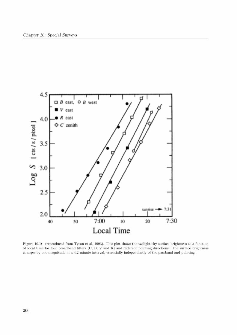
Chapter 10: Special Surveys

Figure 10.1: (reproduced from Tyson et al, 1993). This plot shows the twilight sky surface brightness as a functionof local time for four broadband filters (C, B, V and R) and different pointing directions. The surface brightnesschanges by one magnitude in a 4.2 minute interval, essentially independently of the passband and pointing.

266

10.3 Short Exposure Surveying

The dynamic range in magnitudes that we can achieve for a given integration time depends on thesky background, the read noise, and the full well depth per pixel. We will adopt a typical valueof 100Ke for the full well depth, but the arguments presented below are essentially independentof this value. The dynamic range in magnitudes is limited on the bright end by the point sourcewhose PSF peak exceeds full well, and on the faint end by the 5σ point source sensitivity, whichdepends on sky brightness per pixel. So we are squeezed between the two parameters of full welldepth and sky background.

Figure 10.2: Twilight dynamic range. As we enter morning twilight time, the increasing sky brightness requiresbrighter sources for 5 sigma detection, and also limits unsaturated objects to increasingly fainter sources. Eventuallythe gap between these goes to zero. But operating at shorter exposure times allows us to push useful survey operationsinto brighter twilight time, and also to increase the dynamic range of the LSST survey products. The black linescorrespond to 15 second integrations (nominally in the r band), the red lines to 5 second exposures, and the bluecurves to 0.1 second exposures. The upper lines in each case represent the 5 sigma point source detection thresholdwhile the lower line corresponds to the source brightness that produces saturation in the peak pixel of the PSF.Adding shorter exposure times increases our dynamic range in flux, and adds valuable observing time.

The 5-sigma limiting flux scales as the square root of the sky brightness, while the saturation fluxdecreases linearly as sky brightness increases. So the two curves in Figure 10.2 have slopes thatdiffer by a factor of two. Operating during bright-sky time with short exposures adds about 20minutes of observing per twilight, or 40 minutes per night. This is a non-trivial resource!

Figure 10.2 shows one reason why it is not advantageous to go below 0.1 second exposures- wewould lose the overlap between a twilight survey and the standard LSST object catalog.

267

Chapter 10: Special Surveys

10.3.2 Science Drivers for Shorter Exposures

Having set the stage for the opportunity to operate at shorter exposure times either during darksky time, or during twilight, or both, we now describe some of the scientific motivations for doingso.

Discovery space at short time scales.

LSST is a time domain discovery machine. It is hard to anticipate the importance of being ableto detect astronomical variability on short time scales. By extending the time domain sensitivityto phenomena with a characteristic time of less than 5 seconds, we will have added 1.5 orders ofmagnitude in time domain sensitivity.

Taking short exposures does not necessarily imply a requirement on fast image cadence. Periodicvariability can be readily detected and characterized with a succession of short images that donot satisfy the Nyquist criterion, as long as we know the time associated with each data point toadequate accuracy. But it does seem appropriate to investigate the maximum possible rapid-fireimaging rate for LSST, presumably limited by either data transfer bottlenecks or by thermal issueswithin the camera.

Distances to Nearby SN Ia- an essential ingredient in using supernovae to probe dark energy.

The determination of the equation of state parameter of the Dark Energy using type Ia supernovaeentails measuring the redshift dependence of the luminosity distances to objects over a rangeof redshifts. The low end of this redshift range is limited by peculiar velocities to consideringsupernovae at redshifts z>0.01. At this distance (distance modulus of µ =33) the peak brightnessof a type Ia supernova is r=15 and exceeds the expected LSST point source saturation limit.

Moreover, the rate on the sky of these bright nearby supernovae is so low that in the standardcadence we don’t expect to obtain well-sampled multiband light curves for them. But we willdiscover many of them on the rise. Using twilight time with short exposures to obtain appropriatetemporal and passband coverage will allow us to extend the LSST SN Hubble diagram across theentire redshift range of 0.01 to 1.

It is vitally important that we obtain these nearby-SN light curves on the same photometric system,reduced with the same data reduction pipeline, as the distant sample. This means we really mustuse the LSST instrument and software in order to avoid systematic errors arising from differencesin photometric systems or algorithmic issues.

We stress that this twilight SN followup campaign can be accomplished without impacting themain survey, during the roughly 20 minutes per night of twilight that would otherwise unusable atthe default exposure time. We would use the brighter twilight time to obtain pointed observationson nearby supernovae, motivated by the importance of photometric uniformity described above.

268

10.3 Short Exposure Surveying

A Bright Star Survey for Galactic Science.

We could also use the added twilight time to conduct a bright star survey, and the precise as-trometry and photometry from LSST can then be used in conjunction with archived data rangingfrom 11th to 27th AB magnitudes. This short-exposure domain would extend the LSST dynamicrange in fluxes by two orders of magnitude, towards the bright end. Moreover, obtaining precisepositions, fluxes and variability at these brighter magnitudes would greatly increase the overlapwith the historical archive of astronomical information, including from digitized plate data. Wewould be able to obtain astrometric and color information to high precision, as well time series forvariability studies.

An example of an application to Milky Way structure studies comes from RR Lyrae variable stars.With a saturation magnitude of around 16th in the standard LSST survey, RR Lyrae closer than20 kpc will be saturated in the standard LSST images. So we will lose nearly all Galactic RRLyrae. Extending the survey’s bright limit to 11th magnitude will allow us to collect light curvesfor RR Lyrae beyond ∼ 100 parsecs, collecting essentially all Southern hemisphere Galactic RRLyrae.

Another application for stellar population studies is measuring the fraction of binary stars as afunction of stellar type, metallicity, age and environment. By conducting a variability survey inthe 11-18 magnitude range we can capitalize on temperature and metallicity data already in handfor many of these objects.

Another application of a bright star survey would be to search for planetary transits in the mag-nitude range appropriate for radial velocity followup observations using 30 meter class telescopes.For high dispersion spectrographs at the 4m aperture class, most targets are currently around8th magnitude, so we should expect 30m telescopes to attain similar radial velocity precisions forsources of magnitude 8 + 5log(30/4) = 12. By going to shorter exposures we obtain almost anhour’s additional observing time per night when these sources don’t saturate, whereas they are farbeyond saturation in the default 15 second LSST survey images.

A typical (r−K) color between SDSS and 2MASS is r−K=3. The 2MASS catalog is completedown to K∼14 which corresponds to r∼17. So most 2MASS stars will be saturated in the standardLSST 15 second observations. A bright star survey will allow a multiband match to the 2MASSdata, as well as an astrometric comparison between the two catalogs.

Finally, as pointed out in Section 10.2, the apparent magnitude of solar system objects dependson their distance from us and from the sun, as well as illumination and observation geometry.Extending the bright limit will allow us to track asteroid positions as they approach opposition –see Section 10.2 for more details.

10.3.3 Counterarguments

What About Scintillation Effects?

Short exposure times suffer from scintillation effects. An estimate for uncertainty due to scintil-lation is provided by http://astro.corlan.net/gcx/scint.txt. For a 0.1 second integration

269

Chapter 10: Special Surveys

we expect a fractional flux uncertainty of 0.15 at 2 airmasses and 0.043 at 1 airmass, for a 10 cmaperture. Scaling this up to the 8.5m aperture of LSST by a factor D2/3 predicts fractional fluxvariations of below one percent, even at two airmasses, for a 0.1 second exposure. So scintillationshould not impact our ability to make precision measurements of flux and position.

What about just doing this with smaller telescopes?

A possible counter-argument to the proposal of allowing for shorter exposure times is that muchof this can be done with smaller telescopes. But it’s important to bear in mind that LSST is asystem, and the data reduction and dissemination tools are as important as the hardware. Weintend to deliver accessible, high-quality, well-calibrated photometry on a common photometricsystem and correspondingly good positions. If we do so from a co-added point source depth of27th to the short-exposure bright limit of 11th magnitude we will span over six decades in flux on awell-calibrated flux scale. We would also have the ability to study astrophysical variability on timescales from 0.1 second to 10 years, which is nine decades in the time domain. This combinationof temporal and flux dynamic range would be a truly remarkable achievement, and would yieldscience benefits far beyond the illustrative examples provided above. Much of this discovery spaceis enabled by going to shorter exposures.

10.3.4 Proposed Implementation and Impacts

The implementation of this would simply entail taking short-exposure images during twilight timethat would otherwise go unused. The data rate would go up, and the number of shutter cycles pernight would also increase, and so both the telescope and data management teams would need toadvise on the cost of the program.

Go to: • the start of this section • the start of the chapter • the table of contents

10.4 A Mini-Survey of the Old Open Cluster M67

Suzanne Hawley, Ruth Angus, Derek Buzasi, James Davenport, Mark Giampapa, Vinay Kashyap,Søren Meibom.

10.4.1 Introduction

As coeval, equidistant, and chemically homogeneous collections of stars, open star clusters areideal for studying the dependence of astrophysical phenomena on the most fundamental stellarparameters - age and mass. Indeed, there are few fields in astronomy that do not rely on results fromcluster studies, and clusters play a central role in establishing how stellar rotation and magneticactivity can be used to constrain the ages of stars and stellar populations. From an observationalperspective, because of their angular extent they are accessible to efficient surveys in both imagingand multi-object spectroscopy. A selection of clusters representing a sequence in age can be used

270

10.4 A Mini-Survey of the Old Open Cluster M67

to establish critical empirical relationships such as the dependence of activity on rotation, therelationships between activity, rotation and stellar age, the evolution of activity cycles, and thenature and evolution of flare activity—an urgent area of investigation in view of the potentialimpacts on the structure and evolution of exoplanet atmospheres in systems with late-type hoststars.

Unfortunately for observers, open clusters dissipate on timescales which are generally comparableto stellar evolution timescales on the lower main sequence, so older clusters are relatively rare. Inaddition, most clusters lie close to the galactic plane, where determining membership is significantlycomplicated by the large numbers of foreground and background stars.

In this section, we suggest an LSST survey of M67, an open cluster whose relative compactness,age, and location above the galactic plane combine to make it the ideal cluster for a closer look.This proposed program could be adapted to include more clusters; we leave that more ambitiousinvestigation to future work.

10.4.2 Science Case

The evolution of the rotation rate and magnetic activity in solar-type stars are intimately con-nected. Stellar rotation drives a magnetic dynamo, producing a surface magnetic field and mag-netic activity which manifests as starspots, chromospheric (Ca II HK, Hα) and coronal (X-ray)emission, and flares. The magnetic field also drives a stellar wind causing angular momentumloss (“magnetic braking”) which in turn slows the rotation rate over time, leading to decreasedmagnetic activity. More magnetically active stars (larger spots, stronger Ca II HK, Hα and X-rayemission, more flares) therefore tend to be younger and to rotate faster. The rotation-age relation-ship is known as gyrochronology, and the correlation between rotation, age and magnetic activityfor solar-type stars was first codified by Skumanich (1972). However, the decrease in rotationrate and magnetic field strength over long time-scales is poorly understood and, in some cases,hotly contested (Angus et al. 2015, Van Saders et al. 2016). Recent asteroseismic data from theKepler spacecraft have revealed that magnetic braking may cease at around solar Rossby number,implying that gyrochronology is not applicable to older stars (Van Saders 2016).

In addition, the rotational behavior of lower mass stars is largely unknown due to the faintnessof mid-late type M dwarfs. There is reason to believe that M dwarfs cooler than spectral typeM4 may behave differently from the G, K and early M stars, since that spectral type marks theboundary where the star becomes fully convective, and a solar-type shell dynamo (which requiresan interface region between the convective envelope and radiative core of the star) can no longeroperate. Using chromospheric Hα emission as a proxy, West et al. (2008) studied a large sampleof M dwarfs from SDSS and showed that magnetic activity in mid-late M dwarfs lasts much longerthan in the earlier type stars.

The difficulties inherent in understanding the evolution of stellar rotation and activity on thelower main sequence are further increased by our inability to obtain accurate ages for field starswith ages comparable to that of the Sun, which appears to be just the range of ages for whichour understanding of the phenomena are most suspect. While asteroseismology can address thissituation with exquisite precision, it can only do so for the brighter stars accessible to space missionssuch as Kepler. Making use of older open clusters is a way to fill this gap.

271

Chapter 10: Special Surveys

The solar-age and solar-metallicity open cluster, M67, is a benchmark cluster for understandingstellar evolution and the nature of late-type stars at solar age. M67 is unique due to its solarchemical composition, the fact that it is relatively nearby (∼ 900 pc), and its relatively low ex-tinction due to its location above the galactic plane. Extensive proper motion, radial velocityand photometric surveys have been carried out (e.g., Girard et al. 1989, Montgomery et al. 1993,Yadav et al. 2008, Geller et al. 2015), while Giampapa et al. (2006) conducted a survey of chromo-spheric activity in the solar-type members of M67 which yielded interesting insights on the rangeof magnetic activity on sun-like stars in comparison with the range exhibited by the Sun duringthe sunspot cycle. Nehag et al. (2011) find that solar twins in M67 have photospheric spectra thatare virtually indistinguishable from the Sun’s at echelle resolutions.

Located in the sky at approximately RA = 9h and Dec = +12, M67 is an exceptionally meritoriousand accessible candidate for an LSST special survey, which would also enable productive follow-upobservations by an array of OIR facilities. (While we would like to study multiple clusters withLSST, we focus here on M67 in the special survey section because it is very slightly outside ofthe nominal footprint of the survey. Extending this science case to multiple clusters is a topic forfuture work.) LSST observations of M67 would yield data on the rotation periods and variabilityof its members at high precisions, particularly for dwarfs later than about K0 (V > 16). Little isknown about the nature of variability on short and long time scales for low-mass dwarfs at solarage. For example, the frequency of ‘superflaring’ at solar age could be investigated for the firsttime. Furthermore, the combination of LSST observations and OIR synoptic datasets for M67would enable the characterization of the conditions of the habitable zones in late- type stars atsolar age.

In addition to sun-like stars, M67 includes an array of interesting objects such as blue stragglers(Shetrone & Sandquist 2000), an AM Her star (Gilliland et al. 1991, Pasquini et al. 1994), a redstraggler, two subgiants (Mathieu et al. 2003), and detected X-ray sources due to stellar coronalemission (e.g., Pasquini & Belloni 1998). Davenport & Sandquist (2010) found a minimum binaryfraction of 45% in the cluster. Other investigations include studies of the white dwarf coolingsequence (Richer et al. 1998), angular momentum evolution near the turnoff (Melo et al. 2001),and the behavior of key light elements such as lithium and beryllium (e.g., Randich et al. 2007).

10.4.3 Observing Plans

Performing the special survey of M67 which we advocate would require two modifications to thebaseline LSST operations mode. LSST does not plan to observe as far north as Dec = +12 inits main survey, but the M67 field should certainly be accessible for a special survey as a singlepointing. Since imaging the entire cluster would require less than a single LSST field, we viewthis additional pointing as being of minimal inconvenience relative to the expected scientific gain.As we anticipate rotation periods ranging from ∼ days up to several months, we would requiresampling over all of these timescales, though it need not be continuous.

A second potential complication is that the cluster is relatively bright. While dwarfs below aboutspectral K0 in M67 are fainter than the LSST bright limit of ∼ 16, the cluster G dwarfs willsaturate the LSST detectors in a 15-second integration. We suggest two alternative approaches toaddress this issue. First, if the short exposure surveying mode suggested in Section 10.3 is adopted,

272

10.4 A Mini-Survey of the Old Open Cluster M67

then the new LSST minimum exposure time of 0.1 seconds would easily accommodate the entireM67 main sequence. Alternatively, or if the short exposure mode is not adopted, we note thatwork with the Kepler mission (e.g., Haas et al. 2011) has shown success using custom pixel masksto accurately perform photometry on stars as much as 6 magnitudes brighter than the saturationlevel. Similar techniques applied to the LSST fields should enable photometry for the G dwarfs,particularly those in less-crowded portions of the field.

Go to: • the start of this section • the start of the chapter • the table of contents

273

11 Synergy with WFIRST

Chapter editor: Jason Rhodes.

Contributing authors: David Rubin, David Bennett, Matthew T. Penny, Rachel Street.

Summary

WFIRST will launch in ∼ 2025 for a 5 year mission to explore dark energy, find and characterizeexoplanets, and take wide, deep infrared surveys of the galactic and extragalactic sky. WFIRSTwas recognized by the Astro2010 Decadal Survey as an excellent NIR complement to LSST’s opti-cal capabilities. More recent work has recognized the strong synergy these two projects will havein helping to address cosmological questions in the 2020s (Jain et al. 2015). Together, the twoobservatories can accomplish significantly more (and better) science than either can alone in theareas of weak lensing, large-scale structure studies, strong lensing, supernova studies, exoplanetinvestigations, and photometric redshift determination. Accomplishing this will require coordi-nated observations. We have identified three areas of proposed coordination: 1. Early coverage ofthe > 2000 square degree WFIRST High Latitude Survey to the full optical depth for enhancedphotometric redshifts for both LSST and WFIRST; 2. Coordinated LSST optical observations inthe WFIRST supernova discovery fields; 3. Precursor, simultaneous, and follow-up observationsof the WFIRST microlensing fields near the galactic bulge.

We note here that the focus of the WFIRST input to this paper is on suggesting changes orenhancements to the LSST observing strategy (cadence or survey overlap) that will provide mutualbenefit for WFIRST and LSST. The observing strategy suggestions here are not exhaustive of thepossibilities for synergy between WFIRST and LSST; rather the suggestions here are based on theplanned primary WFIRST surveys that are driving the WFIRST mission requirements. As theplans and possibilities for WFIRST Guest Observer surveys evolve, and the ideas for additionalscience investigations that will make use of planned WFIRST survey data mature, the communityshould continue to look for areas of survey synergy. Both WFIRST and LSST should considersurvey modifications that would increase the global combined science output of the two surveys.

11.1 Introduction

The Wide Field Infrared Survey Telescope (WFIRST) is a NASA mission that entered PhaseA in February 2016. WFIRST was the highest recommendation for large space missions in the2010 New Worlds New Horizons Decadal Survey. That recommendation envisioned a wide-fieldobservatory with near infrared (NIR) capabilities to complement LSST’s optical capabilities; the

275

Chapter 11: Synergy with WFIRST

Decadal Survey recognized the obvious synergy between WFIRST and LSST. WFIRST’s designhas evolved since 2010 and the design being pursued for a mid-2020s launch uses an existing 2.4mtelescope donated to NASA, giving WFIRST capabilities not envisioned by the Decadal Survey.WFIRST has 3 primary science objectives:

• Determine the nature of the dark energy that is driving the current accelerating expansionof the universe using a combination of weak lensing, galaxy clustering (including BaryonAcoustic Oscillations and Redshift Space Distortions), and supernovae type Ia (SN).

• Study exoplanets through a statistical microlensing survey and via direct imaging and spec-troscopy with a coronagraph.

• Perform NIR surveys of the galactic and extragalactic sky via a Guest Observer program.

WFIRST will be at L2 to enable the thermal stability needed for the precise astrometric, photo-metric, and morphological measurements required for these science goals. The baseline WFIRSTmission architecture is described in detail in the final report of the WFIRST Science DefinitionTeam (Spergel et al. 2015) The WFIRST Wide Field Instrument(WFI) has a NIR focal plane witha ∼ 0.28 square degree field of view made up 18 4k×4k Teledyne H4RG NIR detectors and willhave imaging capabilities from 0.5− 2 microns and grism spectroscopy capabilities from 1− 2 mi-crons with R ∼ 461λ. The WFI also contains an Integral Field Channel (IFC) spectrometer withR ∼ 100 resoluton over the range 0.6 − 2 microns for SN follow up. The exoplanet coronagraphwill have imaging (0.43− 0.97 microns) and spectroscopic (0.6− 0.97 microns) capabilities with acontrast ratio of 1 part in a billion.

WFIRST’s 5 year primary mission is envisioned to have ∼ 2years dedicated to a ∼ 2200 squaredegree High Latitude Survey (HLS) for weak lensing and galaxy clustering, ∼ 1 year of microlensingobservations divided into 6 seasons, ∼ 0.5 years of SN search and follow-up, ∼ 0.8 years dedicatedto the coronagraph and the remaining time dedicated to competitively selected Guest Observerobservations. WFIRST has no expendables that would prevent an extended mission of 10 years orlonger, and an extended mission will likely be given over entirely to Guest Observer observations.

The synergy with LSST is very promising indeed. In this chapter we aim to lay out three specificprojects in the three main WFIRST science areas, and test the simulated LSST Observing Strate-gies for their performance in each case. Then, we use these results to design a suite of modifiedLSST Observing Strategies, which we propose as new OpSim simulation runs.

Go to: • the start of this section • the start of the chapter • the table of contents

11.2 Cosmology with the WFIRST HLS and LSST

Jason Rhodes

WFIRST’s High Latitude Survey (HLS) will cover 2200 square degrees in 4 NIR photometricfilters (3 of which will be sufficiently sampled for weak lensing shape measurements) and NIRgrism spectroscopy. The benefits of overlapping spectroscopic and photometric surveys for darkenergy constraints and systematics mitigation are strong. The primary scientific driver of thephotometric portion of the WFIRST HLS is weak gravitational lensing, but there is a wide range

276

11.2 Cosmology with the WFIRST HLS and LSST

of ancillary science that will be possible with the publicly available WFIRST HLS data (see forinstance, the SDT report mentioned above). However, the requirements on the HLS are largely setby constraints from weak lensing measurements. Each galaxy in the WFIRST weak lensing surveyneeds to have an accurate photometric redshift. This requires optical photometry that reaches thedepth of the NIR photometry WFIRST will acquire (J 27AB). Thus, the WFIRST weak lensingsurvey will require the full 10-year LSST depth in 4 optical bands for optimal photometric redsfhiftdetermination.

There is strong benefit not just to WFIRST, but to LSST, in coordinating observations of theWFIRST HLS survey field. The combination of full-depth LSST data and WFIRST HLS NIRdata will provide the gold standard in photo-zs. Furthermore, WFIRST grism observations overthe same area will provide many millions of high quality slitless spectra and WFIRST’s IFC can berun in parallel with WFI observations to provide many more very accurate spectroscopic redshiftsin the survey area. Thus, the WFIRST photometric data will help to provide better LSST photo-zsand WFIRST will also provide many of the spectra needed as a training set to calibrate the photo-zs for both missions. A further benefit to LSST might be the reduced need for LSST observationsat the reddest end of the LSST wavelength range (the z and y filters), where both the atmosphereand the physics of CCDs make ground-based observations less efficient than what WFIRST canachieve. Further work is needed to quantify this benefit, especially as the WFIRST proposedfilter set is evolving.Finally, the joint processing of LSST and WFIRST data will provide betterobject deblending parameters than LSST can achieve alone; WFIRST will be able to provide amorphological prior for the deblending of LSST images.

11.2.1 Measuring Dark Energy Parameters

The goal in this science project would be to measure Dark Energy parameters from various weaklensing probes, capitalizing on the improved photometric redshifts that a joint analysis of LSSTand WFIRST photometry would provide. A useful Figure of Merit is the usual Dark Energy TaskForce figure of merit, quantifying the available precision on the equation of state parameters w0

and wa. For example, we are interested in improvements in the weak lensing DE FoM as the LSSTphotometric redshifts and galaxy shapes are improved over the whole LSST survey area via jointanalysis with WFIRST. We are also interested in increasing the WFIRST DE FoM as quickly aspossible. Indeed, the basic problem we face is one of timing: being able to combine the WFIRSTdata with the LSST sooner will accelerate the production of cosmological results.

Therefore, we propose an acceleration of the LSST survey over about 10% of the LSST surveyarea (the ∼ 2200 WFIRST HLS) such that the full LSST ten years survey depth is reached on atimescale that maximizes the joint usefulness of LSST and WFIRST data on that area. Assumingthe two year WFIRST HLS is taken in the first four years of a WFIRST mission that launches in2024, this would require reaching full LSST depth over that area in ∼ 2028 rather than ∼ 2032.Since the HLS area is roughly 1/8 as large as the LSST “Main Survey”” region, this could beachieved by devoting 1.25 years of LSST observations to the HLS area, assuming that it covers awide enough range of Right Ascension. More practically, it could be achieved by devoting 25% ofLSST observing time to this area during each of the first 5 years of the LSST survey, which doublesthe time it would naturally be observed during those years at a modest reduction in coverage ofthe rest of the Main Survey area during that time period. Given existing plans to speed up the

277

Chapter 11: Synergy with WFIRST

LSST cadence over small sub-areas of the LSST survey, this may only require coordination of thelocations of the accelerated LSST area and the WFIRST HLS. As LSST and WFIRST progress,there is a mutual benefit in continuing discussions about the optimal joint observation schedule.

A simple, first order diagnostic metric would be the amount of LSST/WFIRST overlapping surveyarea that reaches the full LSST depth when the WFIRST HLS is completed. Such a metricis straightforward, but not able to be meanigfully encoded until the 2020s, when the WFIRSTlaunch date and survey plan is more definite. Strawman survey plans could, however, be evaluatedto help with LSST schedule planning. A slightly more complicated metric could include the pace atwhich the overlapping LSST/WFIRST survey areas are both taken to full depth, since this wouldmake each data set maximally useful to the US community (or anyone with immediate access toboth WFIRST and LSST data). WFIRST data is unlikely to have any proprietary period. Currentplans call for the WFIRST HLS to be conducted in multiple passes, but the exact survey patternis still undecided, so this metric is also not quantifiable yet.

There may be some reduced need for the the LSST reddest bands in the WFIRST HLS overlaparea, which should also be folded into the metric. We note that the default survey strategy wouldonly achieve the full LSST photometric depth over the WFIRST HLS after 10 years of survey(∼ 2032).

11.2.2 Discussion

Increasing the cadence of the LSST survey over ∼ 10% of the LSST survey has science benefits thatgo far beyond the LSST/WFIRST synergy described here: an observing strategy that met the jointWFIRST/LSST cosmology goals could also provide the kind of “rolling cadence” favored by otherscience teams. There are benefits to certain aspects of time-domain science. Every effort should bemade to coordinate all discussions of increased survey cadence (resulting in full LSST depth wellbefore 10 years) over sub-areas of the LSST survey footprint. Specific attention should be paid towhether the accelerated portions of the LSST survey can completely overlap the WFIRST HLS,and whether the position of the WFIRST HLS can be determined, in part, by other science driverswithin LSST. This will require close LSST and WFIRST coordination at the Project levels.

11.2.3 Conclusions

Even before implementing the metrics decsribed above, we can offer tentative answers to the tenquestions posed in Sub-section 1.3.2:

Q1: Does the science case place any constraints on the tradeoff between the sky coverage andcoadded depth?

A1: WFIRST requires the full 10 year LSST depth over the ∼ 2000 square degree WFIRST HighLatitude Survey.

Q2: Does the science case place any constraints on the tradeoff between uniformity of sampling andfrequency of sampling? For example, a rolling cadence can provide enhanced sample ratesover a part of the survey or the entire survey for a designated time at the cost of reducedsample rate the rest of the time (while maintaining the nominal total visit counts).

278

11.2 Cosmology with the WFIRST HLS and LSST

A2: The WFIRST HLS synergy does not place constraints on the uniformity of time sampling.

Q3: Does the science case place any constraints on the tradeoff between the single-visit depth andthe number of visits?

A3: The WFIRST HLS only places requirements on the total depth in the 5 LSST photometricfilters.

Q4: Does the science case place any constraints on the Galactic plane coverage (spatial coverage,temporal sampling, visits per band)?

A4: No: the WFIRST HLS will not be in the Galactic plane.

Q5: Does the science case place any constraints on the fraction of observing time allocated to eachband?

A5: There are multiple solutions to the allocation of depth to each of the 5 LSST and 3 WFIRSTbands that will be used for optimzed photometric redshifts. This is a area of ongoing study.

Q6: Does the science case place any constraints on the cadence for deep drilling fields?

A6: No.

Q7: Assuming two visits per night, would the science case benefit if they are obtained in the sameband or not?

A7: The WFIRST HLS is largely agnostic about the timing of the different filters.

Q8: Will the case science benefit from a special cadence prescription during commissioning or earlyin the survey, such as: acquiring a full 10-year count of visits for a small area (either in allthe bands or in a selected set); a greatly enhanced cadence for a small area?

A8: The WFIRST HLS synergy would be globally maximized (for both LSST and WFIRST) ifthe full LSST depth in all 5 bands is reached in the first 5 years of LSST operations.

Q9: Does the science case place any constraints on the sampling of observing conditions (e.g.,seeing, dark sky, airmass), possibly as a function of band, etc.?

A9: The benefit to LSST of having high precision space based galaxy shape measurements wouldbe maximized if the observing conditions allowed for the best possible LSST shapes forcross-calibration of shear measurements.

Q10: Does the case have science drivers that would require real-time exposure time optimizationto obtain nearly constant single-visit limiting depth?

A10: No.

Go to: • the start of this section • the start of the chapter • the table of contents

279

Chapter 11: Synergy with WFIRST

11.3 Supernova Cosmology with WFIRST and LSST

David Rubin

The WFIRST SN survey seeks to measure thousands of SNe Ia with excellent systematics con-trol over a two-year period. The Science Definition Team (SDT) outlined a three-tiered cadencedimaging survey: wide to z = 0.4 (27.44 square degrees), medium to z = 0.8 (8.96 square degrees),deep to z = 1.7 (5.04 square degrees). SNe discovered in the imaging would be followed withIFU spectrophotometry, helping to monitor changes in SN physical parameters and the extinctiondistribution with redshift. However, the LSST DDFs offer a path to high signal-to-noise, wellcalibrated, multi-band optical imaging over an even larger area than WFIRST can survey. If thewide and medium tiers are replaced with LSST DDF discoveries, then WFIRST can offer spec-trophotometry (with good host-galaxy subtraction) for ∼ 2,000 LSST SNe, with screening spectrafor ∼ 1-2,000 more. As the WFI and IFU operate in parallel, this survey could provide sparselysampled NIR imaging for ∼ 5,000 SNe up to z = 1 at the same time as the spectroscopy. The jointsurvey would thus provide systematics control (almost certainly better than either survey alone),as well as a cross-check of LSST photometric typing and host-galaxy-only redshift assignment.

11.3.1 Target measurements and discoveries

The targets of the measurements are related to those enumerated in Sub-section 9.5.2. The SNemust be detected ∼ 10 observer-frame days before maximum light, so that there is time for ashallow screening spectrum before deeper spectrophotmetry around maximum. There should beenough visits per filter so that some photometric screening can be done before WFIRST triggersany spectroscopy. There should be an identification of the host galaxy (if seen), so that jointWFIRST/LSST photometric redshifts can be used to provide a distance-limited sample (mini-mizing selection effects). Finally, the light curve should continue after the SN has been sent toWFIRST, so that important light-curve parameters (date of maximum, rise time and decline time,etc.) can be measured.

11.3.2 Metrics

The primary metrics are based on constraining cosmological parameters; the DETF FoM is stan-dard. For the joint observations proposed here, this FoM increases about 20%, from ∼ 300 forWFIRST alone (with a Stage IV CMB constraint) to ∼ 370. However, the number of SNe atz ∼ 0.5 increases by ∼ 50% over a WFIRST-only survey, improving some w(z)-derived FoM valuesby 40%.

The cosmological metric will essentially depend on the number of SNe meeting the above targets.It will degrade if core-collapse SNe are mistakenly sent to WFIRST for followup, if SNe Ia are sentto WFIRST but the LSST light curve is lost due to weather gaps, or if the cadence and depthsimply do not allow the measurement of light curve parameters. These metrics will be stronglyrelated to those in Sub-section 9.5.3, but with more emphasis on the rising portion of the lightcurve.

280

11.3 Supernova Cosmology with WFIRST and LSST

11.3.3 Conclusions

Here we answer the ten questions posed in Sub-section 1.3.2. As WFIRST will only cadence a few10’s of square degrees, we assume that the overlap region will be contained in the DDFs, not inthe main survey. We thus place no constraints on the main survey.

Q1: Does the science case place any constraints on the tradeoff between the sky coverage andcoadded depth?

A1: In terms of direct overlap with WFIRST, there is no constraint. There are secondary consid-erations (such as constraining Milky Way extinction and probing isotropy) that may prefera larger number of square degrees, but this has not been investigated.

Q2: Does the science case place any constraints on the tradeoff between uniformity of samplingand frequency of sampling?

A2: No constraints.

Q3: Does the science case place any constraints on the tradeoff between the single-visit depth andthe number of visits (especially in the u-band where longer exposures would minimize theimpact of the readout noise)?

A3: In the DDFs, the SN Ia science would not be harmed by having longer exposures and less-frequent visits, at least if there was one observation every few days in each filter. No constrainton the main survey.

Q4: Does the science case place any constraints on the Galactic plane coverage (spatial coverage,temporal sampling, visits per band)?

A4: No constraints.

Q5: Does the science case place any constraints on the fraction of observing time allocated to eachband?

A5: This has not been quantitatively investigated. Based on experience with other programs, thereddest filters (z and Y) should receive the most time.

Q6: Does the science case place any constraints on the cadence for deep drilling fields?

A6: To obtain good light curves, we would want at least one observation every few days per filter.This is also a requirement for photometric typing to obtain reasonable purity if WFIRSTspectroscopy is to be triggered. Note: of all the questions, this one is the most important tothe program.

Q7: Assuming two visits per night, would the science case benefit if they are obtained in the sameband or not?

A7: No benefit.

Q8: Will the case science benefit from a special cadence prescription during commissioning or earlyin the survey, such as: acquiring a full 10-year count of visits for a small area (either in allthe bands or in a selected set); a greatly enhanced cadence for a small area?

281

Chapter 11: Synergy with WFIRST

A8: For the DDFs, such observations might help provide deep SN-free (template) images or host-galaxy photometric redshifts. This has not been quantitatively investigated. No constraintson the main survey.

Q9: Does the science case place any constraints on the sampling of observing conditions (e.g.,seeing, dark sky, airmass), possibly as a function of band, etc.?

A9: As long as the DDF observations reach the targeted depths, there is no benefit to the SN Iascience from having specific observing conditions.

Q10: Does the case have science drivers that would require real-time exposure time optimizationto obtain nearly constant single-visit limiting depth?

A10: We do not currently know of any benefit to the SN Ia science from doing this.

Go to: • the start of this section • the start of the chapter • the table of contents

11.4 Exoplanetary Microlensing with WFIRST and LSST

David Bennett, Matthew T. Penny, Rados law Poleski, Rachel Street.

One of the most exciting prospects of future micolensing surveys is the characterization of thepopulation of “rogue” or free-floating planets. While recent estimates of the rogue planet abun-dance (Mroz et al. 2017 in prep) have cast doubt on the large population of rogue planets inferredby Sumi et al. (2011), they have clearly demonstrated that microlensing surveys have the sensi-tivity necessary to detect them. Firm detections of the rogue planet population that might bepredicted by planet formation simulations awaits the accumulation of sufficient survey durationfor giant rogue planets, and the WFIRST microlensing survey for smaller planets (Spergel et al.2015; Barclay et al. 2017).

Microlensing’s rogue planets are isolated in the sense that no host star can be detected by mi-crolensing. Depending on the peak magnification and light curve coverage, this can imply that ahost must be > 10 AU or > 100 AU away, and Bennett et al. (2012) have argued that the medianseparation of possible host stars is likely to be > 30 AU. The presence and properties of a hoststar can be constrained either with WFIRST’s diffraction limited survey images separated by themission duration, or adaptive optics observations on large telescopes (≥ 8 m) taken 4–8 years afterthe rogue planet event (Gould 2016; Henderson & Shvartzvald 2016).

A major weakness with the microlensing survey data sets that can be used to detect rogue planetsis that, thus far, the properties of the population can only been inferred by their Einstein radiuscrossing time, tE, distribution. But, the Einstein radius crossing time depends not only on the lensmass, but also on its distance and transverse velocity. As a result, we cannot directly infer themass or distance distribution of the rogue planet sample.

Our understanding of the rogue planet distribution can be greatly improved by measuring themicrolensing parallax effect (Gould 1992; Alcock et al. 1995). Combining tE with the microlensparallax πE yields a mass-distance relationship, a narrower range of possible lens masses and aprojection of the lens-source relative velocity, which can in certain cases be used to identify the

282

11.4 Exoplanetary Microlensing with WFIRST and LSST

Magnification

Time since UT 00:00 April 19 2025 (days)

10-M⊕ FFP πE = 16.1 is = 20.9

WFIRST-W149WFIRST-Z087

LSST-zLSST-iLSST-rLSST-g

0

2

4

6

8

10

12

0.2 0.4 0.6

Figure 11.1: A simulated light curve of a 10M⊕ planet with a microlensing parallax mass measurement fromsimultaneous WFIRST and LSST observations. The short duration of WFIRST planetary microlensing events andthe high extinction in WFIRST’s fields requires high-cadence (ideally every 15-30 min) observations in the redderbands (i or z, preferably). During WFIRST observations around the equinoxes, the LSST-WFIRST microlensingfield will only be visible for a few hours per night.

lens as belonging to the Galactic disk or bulge (Yee et al. 2015). The mass and distance of the lenscan be uniquely solved for if, in addition to parallax, the angular diameter of the Einstein ring canbe measured via finite source effects (Nemiroff & Wickramasinghe 1994). Finite source effects willbe measured in a substantial fraction of events involving bound and free-floating planets.

Typically, microlensing parallax is measured using the orbital motion of the Earth, but it canalso be measured using light curve observations from telescopes at different locations in the SolarSystem (Dong et al. 2007; Calchi Novati et al. 2015) or even different locations on Earth (Gouldet al. 2009). In the case of microlensing by planetary mass objects, the event durations are too shortto allow a significant light curve change due to the Earth’s orbital motion, but near simultaneousobservations from Earth and a satellite orbiting at the Earth-Sun L2 point (where WFIRST willorbit) allows the measurement of microlensing parallax signals for planetary mass lenses (Gouldet al. 2003). The principles of the technique are identical to those employed by the K2 Campaign 9microlensing parallax survey (Henderson et al. 2016; Henderson & Shvartzvald 2016; Penny et al.2017). Figure 11.1 shows an example of the light curves for one of the rogue planets with a massdetermined by simultaneous WFIRST and LSST observations.

WFIRST planetary microlensing events will greatly improve our understanding of not only rogueplanets population but also of planets in wide orbits similar to those of Uranus or Neptune andwith a wide range of masses (Spergel et al. 2015). Such cold planets cannot be studied usingtechniques other than microlensing (e.g., Gaudi 2012) and WFIRST gives us a unique opportunityto detect a statistically significant number of wide orbit planets. A wide-orbit planet adds anadditional peak to the otherwise standard microlensing light curve produced by the host star thatoccurs a few Einstein crossing timescales before or after the host event’s peak (e.g., Poleski et al.2014). Typical host event timescales are ∼25 days, so it will be common for the host peak of awide-orbit planet discovered by WFIRST to lie outside of WFIRST’s 72 day observing window,

283

Chapter 11: Synergy with WFIRST

but inside the time when LSST can observe it. Without ground-based observations outside theWFIRST window, the properties of many wide-orbit planet detections by WFIRST will be poorlyconstrained, particularly the mass ratio of the planet to its host, and its projected separation fromthe host. However, deep, low-cadence LSST monitoring of the WFIRST microlensing field overwhole bulge observing season will reveal the peaks of planet host microlensing events that areunobservable to the WFIRST and will enable measurement of the projected separation and massratio.

11.4.1 A Proposed Observing Strategy

Based on the desiderata above, we propose simultaneous high cadence observations of the WFIRSTmicrolensing fields by LSST during each of the six 72-day WFIRST exoplanet microlensing surveysessions. These will allow microlensing parallax measurements to determine the distances andmasses of a representative sub-sample of the rogue planets found by the WFIRST microlensingsurvey. These measurements will be crucial for the interpretation of WFIRST’s rogue planetdiscoveries, and they cannot be obtained by another method.

We also propose continuous monitoring of the WFIRST microlensing fields at a cadence of oneobservation per day starting a year before and ending a year after the WFIRST microlensingsurvey. This will allow us to constrain the presence of a host star for rogue planet candidates and,if the host is detected, measure the planet-host mass ratio and projected separation.

A single LSST pointing, centered on the WFIRST microlensing fields, would cover all 10 WFIRSTmicrolensing fields.

For our preliminary estimates of the high-cadence observing, we assume that the bulge is observedevery 30 minutes when the bulge is at an airmass of < 2.5 for 76-day observing runs (each 72-dayWFIRST observing season plus 2 days on either side). Each visit consists of 3 exposures, one 2sec exposure followed by two 15 sec exposures. With a 2 sec readout and 1 sec for the shutterto open and close, this comes to 39 sec on target per visit (since the final readout can be donewhile slewing). If we assume a 30 deg slew in Azimuth before and after each microlensing pointing,the slews to and from the target should take 22 sec, which is 12 sec above the average. So, eachvisit will take 61 sec out of the regular observing sequence. The number of observations per night,assuming a 30 minute cadence, for a Spring 2025 observing session are given in Table 11.1. We willrequire that these observations be taken in the riz or y filters with at least 3 (or 0) observationsin each filter per night. The total number of observations with this observing plan is 649 or 11.0hour per 76-day observing session or 3894 observations and 66.0 hours for all the high cadenceobservations that we propose.

These observing plans can be altered by changing the cadence of the high cadence observationsfrom once every 30 minutes to once every 15, 60, or 120 minutes, or we could change the numberof WFIRST microlensing observing seasons that were covered. We have not yet simulated thedifferent observing cadences, however.

The low-cadence (1 observation per day) observations taken when WFIRST is not observing, wouldconsist of 1270 visits if we assume that the observations are not taken during the time when theu filter is on the telescope (this is assumed to be 1/6 of the time). The low-cadence off-season

284

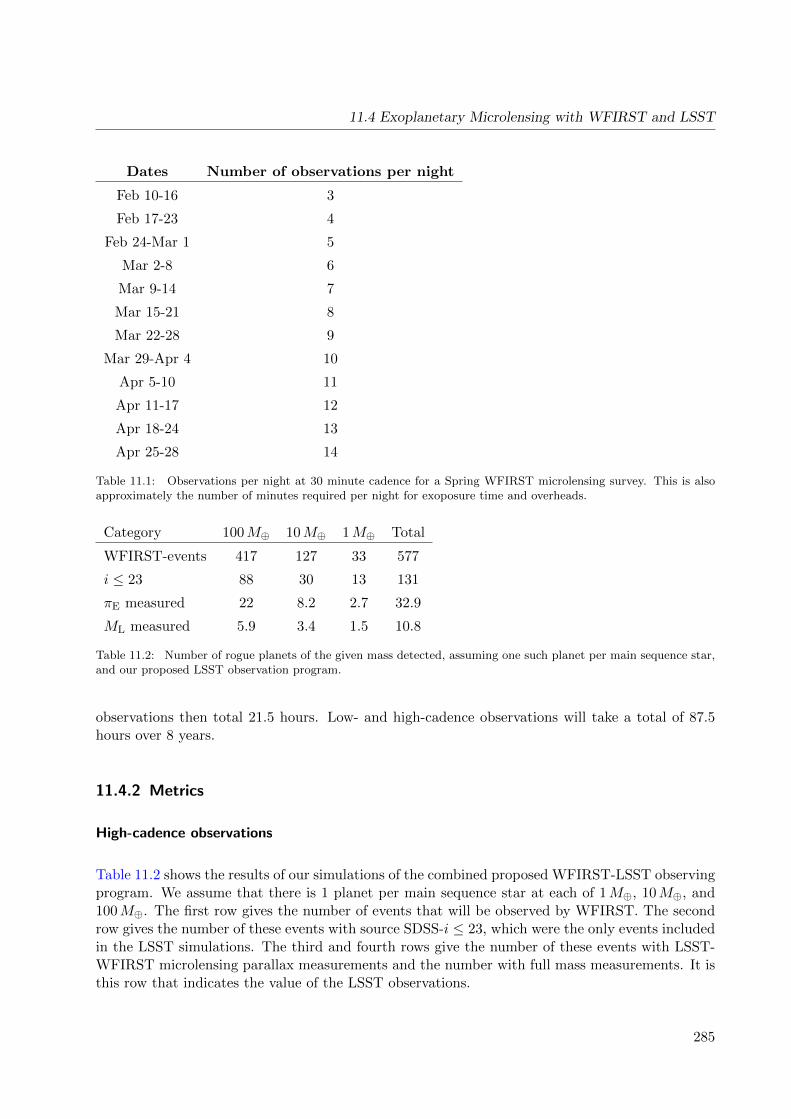
11.4 Exoplanetary Microlensing with WFIRST and LSST

Dates Number of observations per night

Feb 10-16 3

Feb 17-23 4

Feb 24-Mar 1 5

Mar 2-8 6

Mar 9-14 7

Mar 15-21 8

Mar 22-28 9

Mar 29-Apr 4 10

Apr 5-10 11

Apr 11-17 12

Apr 18-24 13

Apr 25-28 14

Table 11.1: Observations per night at 30 minute cadence for a Spring WFIRST microlensing survey. This is alsoapproximately the number of minutes required per night for exoposure time and overheads.

Category 100M⊕ 10M⊕ 1M⊕ Total

WFIRST-events 417 127 33 577

i ≤ 23 88 30 13 131

πE measured 22 8.2 2.7 32.9

ML measured 5.9 3.4 1.5 10.8

Table 11.2: Number of rogue planets of the given mass detected, assuming one such planet per main sequence star,and our proposed LSST observation program.

observations then total 21.5 hours. Low- and high-cadence observations will take a total of 87.5hours over 8 years.

11.4.2 Metrics

High-cadence observations

Table 11.2 shows the results of our simulations of the combined proposed WFIRST-LSST observingprogram. We assume that there is 1 planet per main sequence star at each of 1M⊕, 10M⊕, and100M⊕. The first row gives the number of events that will be observed by WFIRST. The secondrow gives the number of these events with source SDSS-i ≤ 23, which were the only events includedin the LSST simulations. The third and fourth rows give the number of these events with LSST-WFIRST microlensing parallax measurements and the number with full mass measurements. It isthis row that indicates the value of the LSST observations.

285

Chapter 11: Synergy with WFIRST

One can see from the final column that the LSST observations should yield more than 30 rogueplanet microlensing parallax measurements and more than 10 rogue planet mass measurements.These are measurements that cannot be made by other methods, as there is currently no otherknown way to measure the mass distribution and abundance of dark, isolated objects. In addition,this program would also yield masses for a somewhat larger number of bound planets (Gould et al.2003), although many of these will have their masses determined by other means as well.

For a proxy for a Figure of Merit, we select the product of the numbers of rogue planet microlensingparallax measurements πE and rogue planet mass measurements ML. We expect this quantity tobe simply related to the ultimate precision on any rogue planet population hyperparameter wemay try to infer from the LSST-WFIRST sample. Some additional work is still needed to test anddevelop this metric so that it can be easily incorporated into the MAF based on OpSim runs. Thevalue of this product is 355 for our straw man program.

Low-cadence observations

LSST observations will improve models for WFIRST planetary events in a number of ways buthere we focus on detection of the planet host peak if it was missed and poorly constrained byWFIRST. We simulate a population of planets with masses of 0.1M⊕, 1M⊕, and 10M⊕ thatfollow logarithmic mass function with normalization extrapolated from (Cassan et al. 2012). Wenarrow the sample of planets detected by WFIRST in a number of steps. First, we reject the eventswith host peak during the LSST high-cadence observations, i.e., during one of six 76-day longcampaigns. Second, we exclude the events for which flux increase during the WFIRST observingseason is at least 0.75 of the event maximum flux increase, because in these cases WFIRST datawill strongly constrain the host peak even though it is not fully observed. Third, we require atleast a single LSST observation within ±0.05tE of the host peak and the magnified source flux tobe brighter than SDSS-z of 23 mag. The expected number of 0.1M⊕, 1M⊕, and 10M⊕ planets forwhich host peak is detected are 2.1, 8.7, and 36.9, respectively. We chose a sum of those as a proxyfor a Figure of Merit. For the observing strategy presented above the value of this Figure of Meritis 47.7. If a maximum airmass is chosen to be 2.0 instead of 2.5, then the requested time decreasesby 6% and Figure of Merit decreases by 12%. The metric is based solely on the distribution ofpeak times and source magnitudes for a given WFIRST simulation, so once this is set, the metriccan be easily computed for any OpSim run.

11.4.3 Discussion

The rough estimates of our metrics and Figure of Merit given above were carried out using a verysimple model for the LSST observations we have proposed. We would hope to refine this analysisusing the output of an OpSim run where the WFIRST+LSST microlensing program was includedas an additional special survey, and our Figure of Merit coded in the MAF. We do not expect theimpact of this special survey on other science cases to be high, as it would only need 12–24 hoursper year in total. The risk seems similar, but smaller than that of a Deep Drilling Field.

WFIRST microlesning field will have the highest cadence among LSST bulge fields, hence, shouldbe significantly affect Figures of Merit for Milky Way, galactic transients, and stellar variability.

286

11.4 Exoplanetary Microlensing with WFIRST and LSST

11.4.4 Conclusions

Here we answer the ten questions posed in Sub-section 1.3.2:

Q1: Does the science case place any constraints on the tradeoff between the sky coverage andcoadded depth?

A1: No: this is irrelevant to the microlensing survey. We have specific cadence requirements andmuch less interest in coadded depth.

Q2: Does the science case place any constraints on the tradeoff between uniformity of samplingand frequency of sampling?

A2: During the microlensing survey, we must maintain the requested 30 or 15 minute cadence towithin 3 minutes. Outside of the microlensing survey, we must maintain our daily cadenceto within 4 hours.

Q3: Does the science case place any constraints on the tradeoff between the single-visit depth andthe number of visits (especially in the u-band where longer exposures would minimize theimpact of the readout noise)?

A3: There is no trade-off: we cannot reduce our cadence.

Q4: Does the science case place any constraints on the Galactic plane coverage (spatial coverage,temporal sampling, visits per band)?

A4: All of the observations must take place in a field that we will specify near the Galactic Center,at Galactic coordinates of roughly l = 1 deg, b = −1.5 deg.

Q5: Does the science case place any constraints on the fraction of observing time allocated to eachband?

A5: We require observations to be in a passband at least as red as the r-band, i.e. that 0% of theobserving time be in the u or g-bands.

Q6: Does the science case place any constraints on the cadence for deep drilling fields?

A6: Our proposal may amount to a new deep drilling field in the central Galactic bulge. In thiscase, the constraints would be 15 or 30 min cadence during 6 WFIRST microlensing seasons,and 1 day cadence otherwise.

Q7: Assuming two visits per night, would the science case benefit if they are obtained in the sameband or not?

A7: We propose between 3 and 14 visits per night during the WFIRST microlensing survey, and1 visit per night otherwise. We have no restrictions other than the restriction to no visits inthe u and g-bands.

Q8: Will the case science benefit from a special cadence prescription during commissioning or earlyin the survey, such as: acquiring a full 10-year count of visits for a small area (either in allthe bands or in a selected set); a greatly enhanced cadence for a small area?

287

Chapter 11: Synergy with WFIRST

A8: We require many visits during the WFIRST exoplanet microlensing seasons, starting in 2025.Before that, we require only one observation per night.

Q9: Does the science case place any constraints on the sampling of observing conditions (e.g.,seeing, dark sky, airmass), possibly as a function of band, etc.?

A9: There is value in relaxing a default airmass constraint, where it would mean no observationswere taken. We only have strict cadence requirements.

Q10: Does the case have science drivers that would require real-time exposure time optimizationto obtain nearly constant single-visit limiting depth?

A10: No.

Go to: • the start of this section • the start of the chapter • the table of contents

288

12 Conclusions, Tensions and Trade-offs

Chapter editors: Zeljko Ivezic, Stephen Ridgway, Phil Marshall

In this chapter we summarize the findings of the science cases in this white paper, and proposesome actionable conclusions for the LSST Project. We then discuss the tensions and tradeoffsapparent in these findings.

12.1 Summary of Cadence Constraints

Zeljko Ivezic

The authors of the preceding chapters’ science cases provided guidelines for improving the baselineLSST cadence, via their 10-question conclusions sections (see Sub-section 1.3.2). We summarizethis input below, extracting a number of recommendations for the Project to consider. The mostimportant suggested action items for the Project Team include i) implementation, analysis andoptimization of the “rolling cadence” idea, and ii) execution of a systematic effort to furtheroptimize the ultimate LSST cadence strategy.

Q1: Increased sky coverage is possible, at the price of fewer visits per field and shallower coaddeddepth. Does the science case place any constraints on the tradeoff between the sky coverageand depth? For example, should the sky coverage be maximized (to ∼30,000 deg2, as e.g., inPan-STARRS) or the number of detected galaxies (the current baseline of 18,000 deg2)?

A general conclusion from many science cases is that the sky coverage can be increased onlyif the baseline single-visit and coadded depths are not significantly degraded. For example,the number of galaxies above some threshold photo-z quality would increase by about 8%with the larger sky area, but the redshift range would be diminished a bit. Milky Waymapping and large-scale structure studies (e.g. galaxy clustering, BAO) are area-limitedmore than depth-limited and thus a larger sky coverage is preferred for them. In time-domain cases where the LSST baseline performance is already more than adequate, a largersky coverage is preferred, too (AGNs, extra-galactic cepheids); when cadence performance isbarely sufficient or insufficient, smaller sky area with better temporal sampling is suggested(supernovae, strong lensing).

The Project would enable finer optimization by providing several more simulations with thesky coverage in between the baseline cadence sky area of 18,000 deg2) and the so-called“Pan-STARRS cadence” with ∼30,000 deg2. MAF analysis should be extended to computethe effective number of galaxies good for weak lensing, as well as to track the performanceof star-galaxy separation.

289

Chapter 12: Conclusions, Tensions and Trade-offs

Q2: Does the science case place any constraints on the tradeoff between uniformity of sampling andfrequency of sampling? For example, a rolling cadence can provide enhanced sample ratesover a part of the survey or the entire survey for a designated time at the cost of reducedsample rate the rest of the time (while maintaining the nominal total visit counts).

Supernovae provide one of the strongest drivers for the implementation of rolling cadence.A sampling rate about three times higher than the uniform sampling implemented in thebaseline cadence (revisit time scale of about one day), and lasting 3-4 months, is suggested.It is likely that such a rolling cadence would also be beneficial for constraining asteroid orbitsand for studying short time scale variables (e.g. cataclysmic variables). Extreme cases of arolling cadence, with roughly week-long campaigns, for special sky regions would be beneficialfor studies of Young Stellar Objects, for example.

Other types of transients also require a rolling cadence, with necessary compromises. A fastercadence in bluer filters in a shorter rolling window, and slower cadence in redder filters, mayhelp address the trade-offs.

The production and analysis of several families of rolling cadence simulations should be a highpriority, because this baseline cadence modification might provide more significant sciencebenefits than any other proposed modification.

Q3: Does the science case place any constraints on the tradeoff between the single-visit depth andthe number of visits (especially in the u-band where longer exposures would minimize theimpact of the readout noise)?

A large number of science cases would benefit from deeper u band data (both single-visit andco-added depth), as long as the total number of visits is not decreased (of course, increasingthe number of u band visits would be beneficial for u band survey science, too).

Simulated cadence kraken 1045, which doubled the u band exposures from 30 sec to 60 secwhile retaining the Baseline number of visits, demonstrated that an improvement of u bandsingle-visit depth of 0.5 mag can be achieved with only a minor loss of coadded depth andthe number of visits in other bands. We advocate taking u band exposures that are longenough to be sky noise dominated. The Project should investigate this option further andpotentially modify the baseline per-band exposure time allocation.

Q4: Does the science case place any constraints on the Galactic plane coverage (spatial coverage,temporal sampling, visits per band)?

A general comment made by science cases that depend on the Galactic plane coverage isthat Figures of Merit (FoM) exist, but that “many OpSim runs with a variety of temporaldistributions of exposures within the ten-year survey lifetime [are needed] to make theseFOMs useful.”

The Project could consider producing a family of simulations that explore different cadencestrategies for the Galactic disk coverage.

Q5: Does the science case place any constraints on the fraction of observing time allocated to eachband?

290

12.1 Summary of Cadence Constraints

Generally, the baseline time allocation is satisfactory. Potential improvements depend onstudied population (e.g. young stellar objects) and the required imaging depth. The casefor deeper u band data (both single-visit and coadded depth) has the strongest drivers. Thefraction of visits in red bands should be higher for deep drilling fields than for the mainsurvey.

When producing a new generation of deep drilling simulations, the Project should revisit theper-band exposure time allocation for deep drilling fields.

Q6: Does the science case place any constraints on the cadence for deep drilling fields?

The strongest constraints for the deep drilling field (DDF) cadence come from supernovae.DDFs should be preferrably visited nightly, 1-2 mag deeper than for the main survey visits.At least a few extragalactic fields should be observed at any month, with each field observedfor a “season” of length at least 120-150 days, staggering the fields so new fields cycle in asold ones cycle out, and avoiding the moon. For potential deep drilling fields within the innerGalactic plane, short temporal baselines would be very useful. In the case of Young StellarPopulations, for example, a single week of denser monitoring for specific regions is suggested,with the goal of having several observations per night, separated in time by at least an hourfrom one another. A more extensive study of the value of a Galactic deep drilling field isrequired.

Q7: Assuming two visits per night, would the science case benefit if they are obtained in the sameband or not?

Most science cases prefer the visits in a pair to be taken in two different bands. Exceptionsare GRBs and asteroids; in the case of GRBs the second visit is needed to promptly establishvariability and in the case of asteroids different bands result in decreased sample completeness.

The Project could investigate whether it is possible to increase the fraction of visit pairs withdifferent bandpasses.

Q8: Will the case science benefit from a special cadence prescription during commissioning or earlyin the survey, such as: acquiring a full 10-year count of visits for a small area (either in allthe bands or in a selected set); a greatly enhanced cadence for a small area?

A lot of excellent suggestions were made by multiple science cases. For example, photo-zanalysis would be greatly assisted by acquiring a full 10-yr count of visits for a small areaduring commissioning or early in the survey, especially if these regions would be also coveredby existing spectroscopic surveys. The Comissioning Science Verification Team should incor-porate these suggestions, when possible, into the Commissioning plan, as well as to socializethe existing plan for “mini surveys” with Science Collaborations.

Q9: Does the science case place any constraints on the sampling of observing conditions (e.g.,seeing, dark sky, airmass), possibly as a function of band, etc.?

The strongest drivers are formulated for obtaining good seeing data (the weak lensing case forgood seeing in the r and i bands is already implemented in the simulator) and for minimizingvarious correlations (e.g. parallax factor vs. hour angle).

291

Chapter 12: Conclusions, Tensions and Trade-offs

The Project could analyze the impact of secular effects on randomizing various correlationsvs. an explicit algorithmic driver to do so implemented in the Scheduler.

Q10: Does the case have science drivers that would require real-time exposure time optimizationto obtain nearly constant single-visit limiting depth?

No strong driver for real-time exposure time optimization was identified.

The Project could monitor the fate of a similar proposal considered by the upcoming ZwickyTransient Facility.

Go to: • the start of this section • the start of the chapter • the table of contents

12.2 Tensions and Tradeoffs

Stephen Ridgway

The LSST survey will be carried out with physical and operational constraints that will impactall science objectives. These include design limitations, such as the aperture of the telescope, thedetector noise and readout time, and the limited number of filter changes that can be supportedduring the lifetime of the survey. They include natural constraints, such as the quantity of usefulobserving time in 10 years, and system optimization constraints, such as exposure time and skycoverage.

The LSST observing schedule can be designed, to some extent, to minimize the impact that theselimitations have on any one or few science objectives. As the science objectives become morenumerous and more complex, the optimization becomes more difficult and the chances increasethat significant compromises may be required.

In the science chapters of this report, science objectives are described, and for each, diagnosticmetrics, and in some cases figures of merit, are designed to represent quantitatively the interests ofthat topic in a schedule optimization. Not all of these metric sets are fully worked out, and in mostcases they are provisional pending further analysis and community review and input. However,they do already suffice to bring attention to many special requirements.

The design of the LSST scheduler, and of the algorithms that will select the visit sequences, hasa considerable distance to go before hard cadence questions must be confronted and resolved.However, it is already possible to survey the reach of science needs, and to identify areas ofcompetition which may become candidates for careful trades and decisions in the years before thesurvey begins.

In the rest of this chapter, we review the possible tensions that are now evident, and where tradeoffsmay become necessary. Most potential tensions within the main survey concern temporal samplingfor variable targets. Tensions among static science objectives, and between static science andvariable science, may be less likely and mild. The strongest points of tension may turn out to bebetween mini-surveys and the main survey; similarly, rolling cadences (Section 2.5) are also likelyto introduce new tensions.

292

12.2 Tensions and Tradeoffs

12.2.1 Discussion: Variable Targets – Where’s The Tension?

Strictly periodic targets are relatively neutral to cadence speed, since successive periods can becombined to improve phase coverage steadily through the survey. The only odd cases are ultra-short (< 1 minute) and ultra long (>10 years) periods, and periods very, very close to one siderealday. However, with precision measurements over a long term, some of the very interesting resultsfor periodic variables will be in period drifts or slight deviations from periodicity. Furthermore,even periodic targets benefit from an early interval of higher frequency sampling, at least in somesky regions, as this can accelerate the ramp up of the science.

However, by far the majority of variables and transients, stellar and galactic, are not periodic.The analysis of their aperiodic light curves will be greatly simplified (or may absolutely require)sufficient sampling within a characteristic interval that depends on the target type. One wouldlike to satisfy the sampling theorem, with visits at twice the frequency of the highest frequencycontent, but this is only a conceptual guide: knowledge of, and experience with, the targets andthe science objectives can provide practical criteria.

A truly uniform cadence provides a revisit rate of one visit pair every 16 days (in the r or ibands), or every 3.7 days (in any filter) – assuming a 5 month observing season. This is a sparsesample rate for many variable types. Achieving higher sample rates requires (possibly very strong)deviations from complete uniformity. Thus the obvious conclusion: rapid cadences cannot applyeverywhere all the time. Rapid cadences must be designed, executed selectively, bounded by thenumber of visits available, and coordinated with all other such cadences, as well as more generalsurvey requirements.

Examples

Several examples will illustrate the diversity of cadences that are represented in the science pro-grams described in this white paper.

QSO variability tends to be stronger in low temporal frequencies A uniform distribution of theLSST visits, with minimal seasonal gaps, provides fairly good support for identifying QSOs fromtheir variability pattern.

For a SN, sufficient sampling must be acquired during the life of the event. A good cadence inat least one filter is required to support classification, and multiple colors to support photometricredshift determination. A uniform LSST cadence, even with large seasonal gaps, does not providea sufficient sampling rate for SN science - an enhancement of a factor of 2 or greater is stronglyrequested.

To determine the rotational period of stars with spots, sampling must resolve light variationssufficiently to constrain periodicity within the spot lifetime, which is typically several weeks. Thiscadence is much more rapid than provided by a uniformly distributed WFD visit pattern.

Flaring stars and interacting binaries, and new fast transients in general, may show dramatic fluxchanges in minutes to hours, and correct identification of such events may require several datapoints, and possibly more than one filter, on a similar time scale.

293

Chapter 12: Conclusions, Tensions and Trade-offs

The solar system small body case is particularly complex. The science is one of the main LSSTdrivers. Detection of PHAs has a non-scientific and even political component. Asteroid confusioncan interfere with transient discovery. The density of targets is a strong function of positionon the sky. Characterization of solar system objects, by determination of orbits, requires visitpatterns on short timescale (≈ hour return) and intermediate time scale (≈2 weeks) - long timescaleconfirmation occurs naturally later in the survey. The number and pattern of rapid revisits requiredfor positive identification depends strongly on the false positive rate.

How to provide a range of cadence speeds

The problem of sampling diverse events was of course recognized very early in survey planning.Previous cadence development has explored the following special cadence options:

Rapid revisits – this feature was introduced for study of solar system bodies and most sched-ule simulations give high priority to acquiring visits in pairs with 30 minute separation.Experiments have been done with triples, in case that should prove necessary for asteroidcharacterization. The possibility of using a different revisit pattern in different parts of thesky (e.g. less frequent away from the ecliptic) has been mentioned but has not yet beenimplemented in OpSim. Different patterns for different filters (e.g. not using pairs for visitsin the u and y bands) have been suggested and investigated. The use of visit pairs is clearlya very high impact decision, for practical purposes reducing by a factor of 2 the effectiverevisit rate for other targets. However, rapid pairs are very effective for measuring brightnessgradients for rapidly varying objects, and thus particularly valuable for the difficult problemof characterizing blank sky, short timescale, transients.

Mini-surveys – these can include special cadences. The deep drilling concept utilizes rapid visitsequences to achieve greater depth without saturation of detector wells, giving sky-limitedtrue time series with ≈30 second sampling steps. The possibilities for mini-surveys arelimitless, but of course they are bounded by the amount of time available outside the mainsurvey. The trade between mini-surveys and the main survey is discussed below.

Rolling cadence – this would allow for the possibility of re-deploying visits within the main surveyso as to respond to special cadence demands without compromising main survey goals (or,perhaps in principle, trading against main survey goals in a measured and optimum way).Rolling cadences were introduced in Section 2.5. As an example, the average 9 visit pairs peryear in the r filter, which would be distributed over a season in a uniform survey, could bedistributed over 2 months, 1 month, 1 week, or 1 day, in a rolling cadence (leaving no visitsin r for the rest of the season). Or, more conservatively for the main survey, half (4-5 visitpairs) could be spent in an enhanced visit rate, reserving the other half to maintain visitpairs in the rest of the season. Also, a rolling cadence can concern any number of filters; forexample, one filter could be used to provide short bursts of rapid sampling, while other filterscould maintain a uniform distribution. In particular, for discovering transients a simulationwith faster cadence in bluer filters in a shorter rolling window and slower cadence in redderfilters in a longer rolling window may help address many of the trade-offs involved. Differentrolling cadences can be used in different parts of the sky, or at different times during the

294

12.2 Tensions and Tradeoffs

survey. There is an immense range of possibilities for rolling cadence, and the surface hasbarely been scratched: OpSim 4 should allow this approach to be explored in detail.

Commissioning survey – the highest priority of the commissioning schedule is, of course, commis-sioning the hardware and software of the LSST system. However, a secondary objective isto demonstrate system operation in the planned survey mode - presumably including mainsurvey, deep drilling, rolling cadences, etc. There have been other suggestions, going beyondthese basics, such as integrating some fields to the full survey depth, or acquiring some specialcadences. However, there is no assurance that all of these will be possible, and they will beprioritized following formal commissioning objectives.

Other options for special cadences

Pre-survey options – there are a number of survey instruments (e.g. CTIO, CFHT, Subaru) thatcan easily reach the single visit depth of LSST. These resources could be used to explorelimited sky regions (≈1% of the LSST sky) with cadences that are planned for LSST (orcadences that are not planned for LSST), providing touchstone datasets especially for themore common target types that will dominate the survey.

Twilight survey – Section 10.3 describes a concept for twilight data acquisition, using shortexposures to tolerate bright sky and extend the dynamic range of the survey overall. Thistime is not required for current LSST science, and in principle could be allocated to z, y filtersin short bursts (20 minutes) of fast cadence (< 15 seconds) imaging, within the sensitivitylimits of the twilight sky.

Follow-up – LSST is, in large part, a discovery machine. It is not realistic to expect LSST toprovide its own follow-up for all possible target types and characteristics. Fortunately, manyof the most useful discoveries will be bright enough to follow-up with smaller, more accessibleapertures. Follow-up can be far more customized to the science needs than a general purposeLSST cadence. Faint targets of sufficient value may likewise merit followup with exceptionalground and space-based resources (see Najita et al. 2016, for analysis and discussion).

Frequency of filter changes

Multi-color visits are a very special case for LSST. Changing the huge optical filters will be asubstantial mechanical task. While filter change time is not fully characterized, it will be slowenough (about 2 minutes) that filter change frequency will compete directly with efficiency. Also,the mechanisms have a finite lifetime: “rapid” multi-color sequences will be the exception ratherthan the rule.

Many science objectives for variable targets would be best served by simultaneous (or nearlyso) color information. It is important to identify when and if rapid filter changes are of value oressential, and to trade this against the efficiency and limited lifetime of the filter change mechanism.

295

Chapter 12: Conclusions, Tensions and Trade-offs

Tension between rapid and slow cadences

In summary, we can readily identify competing demands for very different cadences, including fastcadences in multiple ranges. For characteristic times ranging from .1 minute to ∼1 month, auniform visit distribution cannot be fully satisfactory, and in some cases it may turn out to betotally unsatisfactory. A number of concepts for alternate cadences are available. None can providerapid cadence all the time over all the sky. It may be possible to provide cadences matched to mostrequirements over part of the sky all of the time, and over all of the sky at some time. For transienttargets, a complex survey cadence may obtain limited duration but “appropriate” sampling of afraction of the actual events, with the exact fraction still to be decided but inevitably significantlyless than one.

The tension in scheduling is between science objectives and limited scheduling flexibility. Theconfrontation between science requirements and schedule performance leans on the metrics andmerit functions that are the major goal of this white paper. It should be clear from the foregoingchapters that the difficult goal of metrics analysis is not in describing sampling for the science,which is “easy.” The more difficult part is in determining the number of science targets forwhich adequate sampling can be provided by a simulation, and perhaps the greatest challenge isdetermining how many such targets with the specified sampling are required for a science objective.It is only when this step has been accomplished for a large part of the science that competitionbetween the science objectives can become a quantitative process.

Discussion: Static Target Science – Is There Any Tension?

The needs of static target science appear to have fewer points of potential tension among themthan variable targets. The major cadence-related concerns are:

Photometry – the best photometric performance will be achieved after the calibration has beenclosed around the sky, with superior image quality and superior photometric quality visits toevery field. The sooner that it is achieved during the survey, the sooner high quality photom-etry will be available. This could be a target of active schedule control, with correspondingdecreasing flexibility in some other schedule variables.

Astrometry – both proper motions and parallaxes are served by any schedule that spreads visitswell over the duration of the survey. Parallaxes benefit from observing at a range of hourangles (for control of HA-dependent biases), which is slightly in competition with the prefer-ence to observe at small airmass for best image quality, but typical simulated schedules showgood astrometric performance. A rolling cadence that moved a significant fraction of visitsfrom one time period of the survey to another could impact the astrometric performance(either for better or for worse), though as long as the fraction of visits concerned was small,the effect would correspondingly be small.

Homogeneity – an example of required homogeneity is image quality. Just as the atmosphere offersa range of image quality during a night and from night to night, each point on the sky willbe observed with a range of image quality. To enable understanding of selection effects, andto compare sky regions on an even playing field, it is desirable that for each filter, all partsof the sky should be observed with a similar distribution of image quality, and in particular

296

12.2 Tensions and Tradeoffs

with similar best image quality. Achieving homogeneity of conditions actively could be quitechallenging, but simulations show that with a large number of independent visits, it occursnaturally to good approximation. (In Chapter 2 we saw that some higher order declinationand seasonal effects persist in the current Baseline Cadence: these are expected to be reducedfurther with OpSim 4.) Any cadence that relied on concentrated bursts of visits in a shortinterval would tend to reduce the spread of conditions observed. However, such an extremehas not been proposed or studied.

Randomization – closely related to homogeneity, randomization is means of achieving homogene-ity in some observing parameters. Examples are the projected angles of camera and telescopeoptics on the sky. These are less random than sky conditions, as they depend on instrumentsetup and schedule history. Simulations show that optics angles are well randomized passively(i.e. without scheduler optimization) for most points on the sky, but not for all. Randomiza-tion could be improved, for example by actively running the camera rotator when advancingfrom one sky position to the next, in order to populate under represented camera angles. Therotation takes time, and could reduce the overall efficiency of the survey. Only simulationscan explore the impact of these additional mechanical motions.

Dithering – dithering of visits is a powerful method of improving homogeneity of sky coveragepassively. Few compromises have been identified with dithering thus far. Dithering for smallregions has a price. Imagine the loss in depth due to large dithers with a single FOV, e.g. adeep drilling field (this has not been proposed). Due to this effect, certain rolling cadencescan have a potential small loss of efficiency or efficacity when implemented with dithering.

The foregoing shows that within the static science domain, there are few and mild points of tensionand potential competition.

12.2.2 Discussion: Tension Between Static And Variable Science

For the most part, the tensions between static science and variable science are modest and easilyunderstood. A variable-driven cadence that requires special timing of visits may result in lossof efficiency due to increased slew times, or observing under less optimum conditions (larger air-mass). Special cadences are likely to reduce randomization and homogenization to a small degree.However, except for very aggressive cadence implementations, these are second-order effects. Fur-thermore, they are readily measurable with simple metrics: the impact of variable science scheduleconsiderations on static science should be small, although this situation may well change under arolling cadence.

12.2.3 Discussion: Mini-surveys and the Main Survey – Tension for Sure

The LSST proposal and current plan allow a fraction of the total survey time for mini-surveys.These may cover either special sky regions, special cadences, or both. The fraction 10% hasbeen carried for mini-surveys, but this is not a sacred number. In Chapter 2, current schedulingexperience has shown that the main survey program, to design depth, can be accomplished in ≈85% of the available time. However, improvements in simulations could move this estimate up or

297

Chapter 12: Conclusions, Tensions and Trade-offs

down. Adequacy of the design depths could be reconsidered. And of course the execution of thesurvey could encounter unprecedented circumstances.

Proposals for mini-surveys include deep drilling fields, the northern ecliptic, and the Magellanicclouds. Notional suggestions for deep drilling fields alone would exceed 10%. Most schedulesimulations have allocated a limited number of visits to the Galactic plane (based on the expectationthat crowding would limit the useful stacked depth). However, as detailed in Chapter 4, manyareas of Galactic science could benefit from a more aggressive visit plan (as they are not driven bystacked image depth), perhaps similar to the main survey.

At present there is no evidence that the trade between main and mini-surveys will require difficultcompromises. But it is a natural area of tension, and since is likely to be exacerbated by weatherdisruptions (not to mention the evolution of the science), it is likely to be with us through the lifeof the survey.

12.2.4 Final Thoughts

The likely points of technical and scientific tension in scheduling are apparent from the schedulesimulation experience (Chapter 2) and the science objectives and metrics (Chapter 3–Chapter 10).Static science has relatively few and mild points of concern. Variable science has little and moderatetension with static science, although this situation may change with rolling cadences. Variablescience has many points of tension between different variable science objectives, owing to the widerange of time scales. These lead to contrasting technical demands, and may or may not prove tobe areas of scientific competition.

The science teams are urged to continue to define and refine metrics, and in particular their all-important Figures of Merit, and the MAF developers to provide tools for the large-scale comparisonof simulated schedules by whole suites of metrics. OpSim 4 will allow exploration of the kinds ofrolling cadences preferred by various science teams, and it will be important to be able to evaluatethese more flexible simulations of the LSST observing strategy across the whole range of scienceprojects, so that the prioritization decisions that need to be made are as well-informed as possible.

Go to: • the start of this section • the start of the chapter • the table of contents

298

12.2 Tensions and Tradeoffs

Acknowledgements

The authors of this paper are a subset of the membership of the LSST Science Collaborations: wethank our colleagues for many useful discussions on the topic of LSST observing strategy, and theLSST Corporation for providing financial support for our various collaboration meetings duringwhich so many of these conversations take place. We are very grateful to Tim Jenness (LSSTPublication Board Chair), Michael Reuter, Chris Stubbs, and Sandrine Thomas for arranging andcarrying out the Project review of the introductory, OpSim, and conclusions chapters of this paper,and to the members of the Science Advisory Council for reviewing the science case sections: TimoAnguita, Niel Brandt, Jason Kalirai, Mansi Kasliwal, David Kirkby, Charles Liu, Renu Malhotra,Nelson Padilla, Anze Slosar, and Michael Strauss. We acknowledge the support of the LSST Projectin the form of three “cadence workshops” (in Phoenix in August 2015, Bremerton in August 2016,and Tucson in November 2016), and for the creation and maintenance of the OpSim and MAFtools. This paper was, and is still being, researched and written collaboratively using the GitHubsoftware development platform.

299

Appendix: MAF Metrics

This appendix contains two tables, listing the titles and one-line summaries of each metric providedwith the MAF package (Table A.1) and contributed by the community (Table A.2). The Pythoncode for both the MAF metrics amd the contributed metrics can be found on GitHub.1

Table A.1: Metrics provided by the MAF package.

Metric Name Description

AccumulateCountMetric Calculate the number of visits over time.

AccumulateM5Metric The 5-sigma depth accumulated over time.

AccumulateMetric Calculate the accumulated stat.

AccumulateUniformityMetric Make a 2D version of UniformityMetric.

ActivityOverPeriodMetric Count the fraction of the orbit that receive observations, such that activity is

detectable.

ActivityOverTimeMetric Count the time periods where we would have a chance to detect activity on a

moving object.

AveGapMetric Calculate the gap between consecutive observations, in hours.

AveSlewFracMetric Average time for slew activity, multiplied by percent of total slews.

BaseMetric Base class for the metrics.

BaseMoMetric Base class for the moving object metrics.

BinaryMetric Return 1 if there is data.

ChipVendorMetric Examine coverage with a mixed chip vendor focal plane.

Coaddm5Metric Calculate the coadded m5 value at this gridpoint.

ColorDeterminationMetric Identify SS objects which could have observations suitable to determine colors.

CompletenessMetric Compute the completeness and joint completeness of requested observations.

CountMetric Count the length of a simData column slice.

CountRatioMetric Count the length of a simData column slice, then divide by a normalization

value.

CountSubsetMetric Count the length of a simData column slice which matches “subset”.

CountUniqueMetric Return the number of unique values

CrowdingMagUncertMetric Given a stellar magnitude, calculate the mean uncertainty on the magnitude from

crowding.

CrowdingMetric Calculate whether the coadded depth in r has exceeded the confusion limit.

1MAF: https://github.com/lsst/sims_maf/tree/master/python/lsst/sims/mafsims maf contrib: https://github.com/LSST-nonproject/sims_maf_contrib/tree/master/mafContrib

Documentation at https://sims-maf.lsst.io/

301

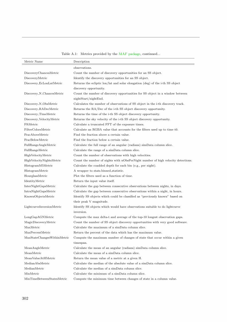
Table A.1: Metrics provided by the MAF package, continued...

Metric Name Description

observations.

DiscoveryChancesMetric Count the number of discovery opportunities for an SS object.

DiscoveryMetric Identify the discovery opportunities for an SS object.

Discovery EcLonLatMetric Returns the ecliptic lon/lat and solar elongation (deg) of the i-th SS object

discovery opportunity.

Discovery N ChancesMetric Count the number of discovery opportunities for SS object in a window between

nightStart/nightEnd.

Discovery N ObsMetric Calculates the number of observations of SS object in the i-th discovery track.

Discovery RADecMetric Returns the RA/Dec of the i-th SS object discovery opportunity.

Discovery TimeMetric Returns the time of the i-th SS object discovery opportunity.

Discovery VelocityMetric Returns the sky velocity of the i-th SS object discovery opportunity.

FftMetric Calculate a truncated FFT of the exposure times.

FilterColorsMetric Calculate an RGBA value that accounts for the filters used up to time t0.

FracAboveMetric Find the fraction above a certain value.

FracBelowMetric Find the fraction below a certain value.

FullRangeAngleMetric Calculate the full range of an angular (radians) simData column slice.

FullRangeMetric Calculate the range of a simData column slice.

HighVelocityMetric Count the number of observations with high velocities.

HighVelocityNightsMetric Count the number of nights with nObsPerNight number of high velocity detections.

HistogramM5Metric Calculate the coadded depth for each bin (e.g., per night).

HistogramMetric A wrapper to stats.binned statistic.

HourglassMetric Plot the filters used as a function of time.

IdentityMetric Return the input value itself.

InterNightGapsMetric Calculate the gap between consecutive observations between nights, in days.

IntraNightGapsMetric Calculate the gap between consecutive observations within a night, in hours.

KnownObjectsMetric Identify SS objects which could be classified as “previously known” based on

their peak V magnitude.

LightcurveInversionMetric Identify SS objects which would have observations suitable to do lightcurve

inversion.

LongGapAGNMetric Compute the max delta-t and average of the top-10 longest observation gaps.

MagicDiscoveryMetric Count the number of SS object discovery opportunities with very good software.

MaxMetric Calculate the maximum of a simData column slice.

MaxPercentMetric Return the percent of the data which has the maximum value.

MaxStateChangesWithinMetric Compute the maximum number of changes of state that occur within a given

timespan.

MeanAngleMetric Calculate the mean of an angular (radians) simData column slice.

MeanMetric Calculate the mean of a simData column slice.

MeanValueAtHMetric Return the mean value of a metric at a given H.

MedianAbsMetric Calculate the median of the absolute value of a simData column slice.

MedianMetric Calculate the median of a simData column slice.

MinMetric Calculate the minimum of a simData column slice.

MinTimeBetweenStatesMetric Compute the minimum time between changes of state in a column value.

302

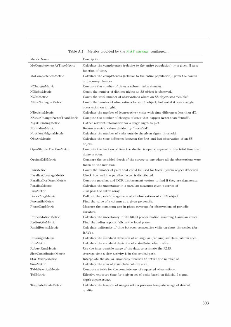
Table A.1: Metrics provided by the MAF package, continued...

Metric Name Description

MoCompletenessAtTimeMetric Calculate the completeness (relative to the entire population) ¡= a given H as a

function of time,

MoCompletenessMetric Calculate the completeness (relative to the entire population), given the counts

of discovery chances.

NChangesMetric Compute the number of times a column value changes.

NNightsMetric Count the number of distinct nights an SS object is observed.

NObsMetric Count the total number of observations where an SS object was “visible”.

NObsNoSinglesMetric Count the number of observations for an SS object, but not if it was a single

observation on a night.

NRevisitsMetric Calculate the number of (consecutive) visits with time differences less than dT.

NStateChangesFasterThanMetric Compute the number of changes of state that happen faster than “cutoff”.

NightPointingMetric Gather relevant information for a single night to plot.

NormalizeMetric Return a metric values divided by “normVal”.

NoutliersNsigmaMetric Calculate the number of visits outside the given sigma threshold.

ObsArcMetric Calculate the time difference between the first and last observation of an SS

object.

OpenShutterFractionMetric Compute the fraction of time the shutter is open compared to the total time the

dome is open.

OptimalM5Metric Compare the co-added depth of the survey to one where all the observations were

taken on the meridian.

PairMetric Count the number of pairs that could be used for Solar System object detection.

ParallaxCoverageMetric Check how well the parallax factor is distributed.

ParallaxDcrDegenMetric Compute parallax and DCR displacement vectors to find if they are degenerate.

ParallaxMetric Calculate the uncertainty in a parallax measures given a serries of

PassMetric Just pass the entire array.

PeakVMagMetric Pull out the peak V magnitude of all observations of an SS object.

PercentileMetric Find the value of a column at a given percentile.

PhaseGapMetric Measure the maximum gap in phase coverage for observations of periodic

variables.

ProperMotionMetric Calculate the uncertainty in the fitted proper motion assuming Gaussian errors.

RadiusObsMetric Find the radius a point falls in the focal plane.

RapidRevisitMetric Calculate uniformity of time between consecutive visits on short timescales (for

RAV1).

RmsAngleMetric Calculate the standard deviation of an angular (radians) simData column slice.

RmsMetric Calculate the standard deviation of a simData column slice.

RobustRmsMetric Use the inter-quartile range of the data to estimate the RMS.

SlewContributionMetric Average time a slew activity is in the critical path.

StarDensityMetric Interpolate the stellar luminosity function to return the number of

SumMetric Calculate the sum of a simData column slice.

TableFractionMetric Compute a table for the completeness of requested observations.

TeffMetric Effective exposure time for a given set of visits based on fiducial 5-sigma

depth expectations.

TemplateExistsMetric Calculate the fraction of images with a previous template image of desired

quality.

303

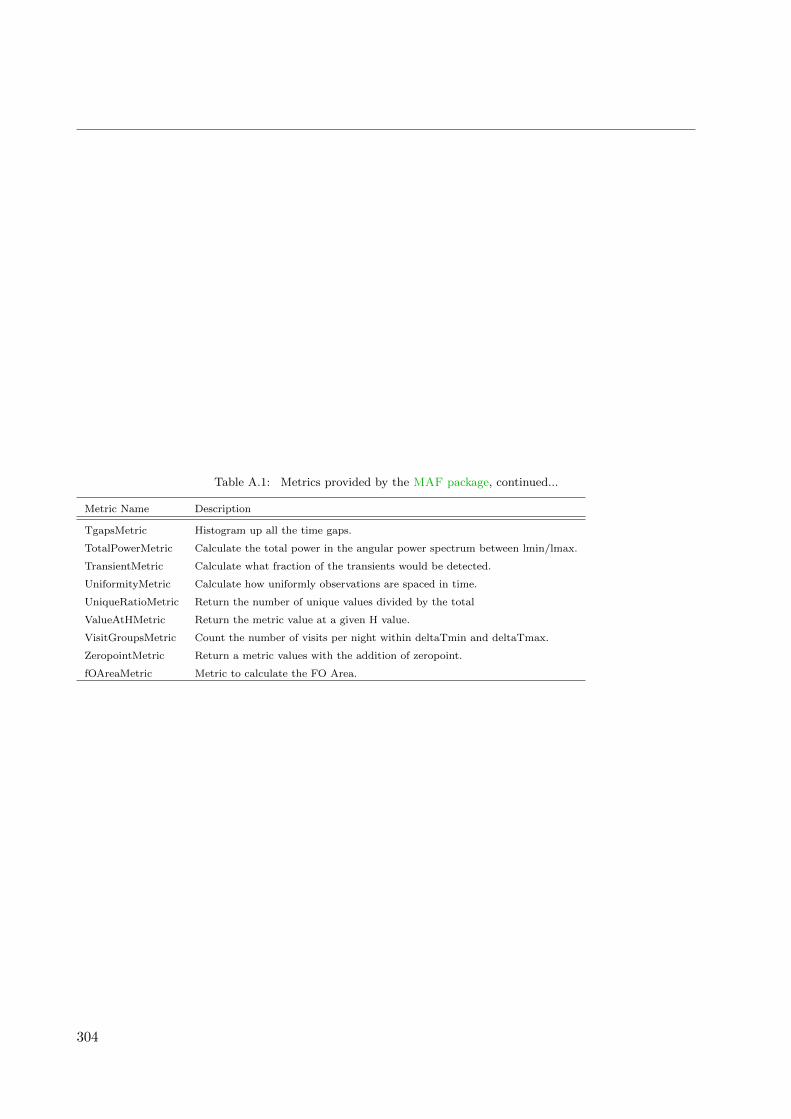
Table A.1: Metrics provided by the MAF package, continued...

Metric Name Description

TgapsMetric Histogram up all the time gaps.

TotalPowerMetric Calculate the total power in the angular power spectrum between lmin/lmax.

TransientMetric Calculate what fraction of the transients would be detected.

UniformityMetric Calculate how uniformly observations are spaced in time.

UniqueRatioMetric Return the number of unique values divided by the total

ValueAtHMetric Return the metric value at a given H value.

VisitGroupsMetric Count the number of visits per night within deltaTmin and deltaTmax.

ZeropointMetric Return a metric values with the addition of zeropoint.

fOAreaMetric Metric to calculate the FO Area.

304

Table A.2: Community-contributed MAF metrics in the sims maf contrib package.

Metric Name Description

AngularSpreadMetric Compute the angular spread statistic which measures uniformity of a distribution

angles accounting for 2pi periodicity.

CampaignLengthMetric The campaign length, in seasons.

GRBTransientMetric Detections for on-axis GRB afterglows decaying as

GalaxyCountsMetric Estimate the number of galaxies expected at a particular coadded depth.

GalaxyCountsMetric extended Estimate galaxy counts per HEALpix pixel. Accomodates for dust extinction,

magnitude cuts,

MeanNightSeparationMetric The mean separation between nights within a season, and then the mean over the

campaign.

NumObsMetric Calculate the number of observations per data slice.

PeriodDeviationMetric Measure the percentage deviation of recovered periods for pure sine wave

variability (in magnitude).

PeriodicMetric From a set of observation times, uses code provided by Robert Siverd (LCOGT) to

calculate the spectral window function.

PeriodicStarMetric At each slicePoint, run a Monte Carlo simulation to see how well a periodic

source can be fit.

RelRmsMetric Relative scatter metric (RMS over median).

SEDSNMetric Computes the S/Ns for a given SED.

SNMetric Calculate the signal to noise metric in a given filter for an object of a given

magnitude.

SeasonLengthMetric The mean season length, in months.

StarCountMassMetric Find the number of stars in a given field in the mass range fainter than

magnitude 16 and bright enough to have noise less than 0.03 in a given band. M1

and M2 are the upper and lower limits of the mass range. “band” is the band to

be observed.

StarCountMetric Find the number of stars in a given field between D1 and D2 in parsecs.

TdcMetric Combine campaign length, season length, and mean night speartion into a single

metric.

ThreshSEDSNMetric Computes the metric whether the S/N is bigger than the threshold in all the

bands for a given SED

TransientAsciiMetric Based on the transientMetric, but uses an ascii input file and provides option

to write out lightcurve.

TripletBandMetric Find the number of “triplets” of three images taken in the same band, based on

user-selected minimum and maximum intervals (in hours),

TripletMetric Find the number of “triplets” of three images taken in any band, based on user-

selected minimum and maximum intervals (in hours),

305

References

Abbott, B. P., Abbott, R., Adhikari, R., et al. 2009, Phys. Rev. D , 80, 102001Abbott, B. P., Abbott, R., Abbott, T. D., et al. 2016a, Physical Review X, 6, 041015—. 2016b, Physical Review Letters, 116, 131102—. 2016c, ArXiv e-prints, arXiv:1602.08492 [astro-ph.HE]Acernese, F. e. a. 2008, Phys. Rev. D , 26Adams, S. M., Kochanek, C. S., Beacom, J. F., Vagins, M. R., & Stanek, K. Z. 2013, ApJ , 778, 164Aerts, C., Christensen-Dalsgaard, J., & Kurtz, D. W. 2010, AsteroseismologyAffer, L., Micela, G., Favata, F., Flaccomio, E., & Bouvier, J. 2013, MNRAS , 430, 1433A’Hearn, M. F., Millis, R. L., Schleicher, D. G., Osip, D. J., & Birch, P. V. 1995, Icarus, 118, 223A’Hearn, M. F., Feaga, L. M., Keller, H. U., et al. 2012, ApJ , 758, 29Alard, C., & Lupton, R. H. 1998, ApJ , 503, 325Albrecht, A., Bernstein, G., Cahn, R., et al. 2006, ArXiv Astrophysics e-prints, astro-ph/0609591Alcock, C., Allsman, R. A., Alves, D., et al. 1995, ApJL, 454, L125Alencar, S. H. P., Teixeira, P. S., Guimaraes, M. M., et al. 2010, A&A, 519, A88Althaus, L. G., Corsico, A. H., Isern, J., & Garcıa-Berro, E. 2010, A&ARv, 18, 471Anguita, T., Schmidt, R. W., Turner, E. L., et al. 2008, A&A, 480, 327Arcavi, I., Gal-Yam, A., Sullivan, M., et al. 2014, ApJ , 793, 38Awan, H., Gawiser, E., Kurczynski, P., et al. 2016, ApJ , 829, 50Baker, M., & Willman, B. 2015, AJ , 150, 160Banerji, M., Jouvel, S., Lin, H., et al. 2015, MNRAS , 446, 2523Barclay, T., Quintana, E. V., Raymond, S. N., & Penny, M. T. 2017, ArXiv e-prints, arXiv:1704.08749 [astro-ph.EP]Barnes, J., & Kasen, D. 2013, ApJ , 775, 18Bate, N. F., Floyd, D. J. E., Webster, R. L., & Wyithe, J. S. B. 2008, MNRAS , 391, 1955Bennett, D. P., Sumi, T., Bond, I. A., et al. 2012, ApJ , 757, 119Berger, E., Fong, W., & Chornock, R. 2013, ApJL, 774, L23Bernstein, J. P., Kessler, R., Kuhlmann, S., et al. 2012, ApJ , 753, 152Berry, M., Ivezic, Z., Sesar, B., et al. 2012, ApJ , 757, 166Besla, G., Kallivayalil, N., Hernquist, L., et al. 2012, MNRAS , 421, 2109Betoule, M., Kessler, R., Guy, J., et al. 2014, A&A, 568, A22Bhardwaj, A., Kanbur, S. M., Singh, H. P., Macri, L. M., & Ngeow, C.-C. 2015, MNRAS , 447, 3342Bhardwaj, A., Kanbur, S. M., Singh, H. P., & Ngeow, C.-C. 2014, MNRAS , 445, 2655Bianco, F. B., Howell, D. A., Sullivan, M., et al. 2011, ApJ , 741, 20Blackburne, J. A., Kochanek, C. S., Chen, B., Dai, X., & Chartas, G. 2014, ApJ , 789, 125Blackburne, J. A., Pooley, D., Rappaport, S., & Schechter, P. L. 2011, ApJ , 729, 34Bloom, J. S., Giannios, D., Metzger, B. D., et al. 2011, Science (New York, N.Y.), 333, 203Bolin, B., Jedicke, R., Granvik, M., et al. 2014, Icarus, 241, 280Bonnerot, C., Rossi, E. M., Lodato, G., & Price, D. J. 2015, MNRAS , 455, 2253Bono, G., Caputo, F., Cassisi, S., Marconi, M., & Piersanti, L.and Tornambe, N. 2000, ApJ , 543, 955Bono, G., Castellani, V., & Marconi, M. 2000, ApJ , 529, 293Boslough, M., Brown, P., & Harris, A. 2015, 2015 IEEE Aerospace ConferenceBradley Cenko, S., Krimm, H. A., Horesh, A., et al. 2012, ApJ , 753, 77Brassard, P., Fontaine, G., & Wesemael, F. 1995, ApJS , 96, 545Britt, C. T., Maccarone, T., Pretorius, M. L., et al. 2015, MNRAS , 448, 3455Brocato, E., & Castellani, V. 1992, A&A, 258, 397Brown, G. C., Levan, A. J., Stanway, E. R., et al. 2015, MNRAS , 452, 4297Burrows, D. N., Kennea, J. A., Ghisellini, G., et al. 2011, Nature, 476, 421Butler, N. R., & Bloom, J. S. 2011, AJ , 141, 93

307

Chapter : References

Caceres, C., & Catelan, M. 2008, ApJS , 179, 242Calchi Novati, S., Gould, A., Udalski, A., et al. 2015, ApJ , 804, 20Campbell, H., D’Andrea, C. B., Nichol, R. C., et al. 2013, ApJ , 763, 88Cantrell, A. G., Bailyn, C. D., Orosz, J. A., et al. 2010, ApJ , 710, 1127Cao, Y., Kasliwal, M. M., Arcavi, I., et al. 2013, ApJL, 775, L7Carlin, J. L., Majewski, S. R., Casetti-Dinescu, D. I., et al. 2012, ApJ , 744, 25Carroll, C. M., Gawiser, E., Kurczynski, P. L., et al. 2014, in Society of Photo-Optical Instrumentation Engineers

(SPIE) Conference Series, Vol. 9149, Society of Photo-Optical Instrumentation Engineers (SPIE) ConferenceSeries, 0

Casetti-Dinescu, D. I., Nusdeo, D. A., Girard, T. M., Korchagin, V. I., & van Altena, W. F. 2015, ApJL, 810, L4Casewell, S. L., Burleigh, M. R., Wynn, G. A., et al. 2012, ApJL, 759, L34Cassan, A., Kubas, D., Beaulieu, J.-P., et al. 2012, Nature, 481, 167Cenko, S. B., Kulkarni, S. R., Horesh, A., et al. 2013, ApJ , 769, 130Cenko, S. B., Urban, A. L., Perley, D. A., et al. 2015, ApJL, 803, L24Chelouche, D. 2013, ApJ , 772, 9Chelouche, D., Shemmer, O., Cotlier, G. I., Barth, A. J., & Rafter, S. E. 2014, ApJ , 785, 140Chelouche, D., & Zucker, S. 2013, ApJ , 769, 124Chesley, S. R., & Veres, P. 2017, ArXiv e-prints, arXiv:1705.06209 [astro-ph.EP]Chomiuk, L., Soderberg, A. M., Chevalier, R. A., et al. 2015, ArXiv e-prints, arXiv:1510.07662 [astro-ph.HE]Chornock, R., Berger, E., Gezari, S., et al. 2014, ApJ , 780, 44Cody, A. M., Stauffer, J., Baglin, A., et al. 2014, AJ , 147, 82Coe, D., & Moustakas, L. A. 2009, ApJ , 706, 45Colpi, M. 2014, Space Science Reviews, 183, 189Connaughton, V., Burns, E., Goldstein, A., et al. 2016, ArXiv e-prints, arXiv:1602.03920 [astro-ph.HE]Corral-Santana, J. M., Casares, J., Munoz-Darias, T., et al. 2015, ArXiv e-prints, arXiv:1510.08869 [astro-ph.HE]Corrales, L. R., Haiman, Z., & MacFadyen, A. 2010, MNRAS , 404, 947Cowperthwaite, P. S., & Berger, E. 2015, ApJ , 814, 25Croll, B., Dalba, P. A., Vanderburg, A., et al. 2015, ArXiv e-prints, arXiv:1510.06434 [astro-ph.EP]Dalcanton, J. J., Williams, B. F., Melbourne, J. L., et al. 2012, ApJS , 198, 6Debes, J. H., Walsh, K. J., & Stark, C. 2012, ApJ , 747, 148Dilday, B., Howell, D. A., Cenko, S. B., et al. 2012, Science, 337, 942Dodelson, S. 2003, Modern Cosmology, Academic Press (Academic Press)Dong, S., Udalski, A., Gould, A., et al. 2007, ApJ , 664, 862Donley, J. L., Brandt, W. N., Eracleous, M., & Boller, T. 2002, AJ , 124, 1308D’Orazio, D. J., Haiman, Z., & Schiminovich, D. 2015, Nature, 525, 351Drake, A. J., Catelan, M., Djorgovski, S. G., et al. 2013a, ApJ , 765, 154—. 2013b, ApJ , 763, 32Dressing, C. D., & Charbonneau, D. 2015, ApJ , 807, 45Dressler, A., & Gunn, J. E. 1983, ApJ , 270, 7Durech, J., Scheirich, P., Kaasalainen, M., et al. 2007, in IAU Symposium, Vol. 236, Near Earth Objects, our Celestial

Neighbors: Opportunity and Risk, ed. G. B. Valsecchi, D. Vokrouhlicky, & A. Milani, 191Edelson, R., Gelbord, J. M., Horne, K., et al. 2015, ApJ , 806, 129Eigenbrod, A., Courbin, F., Meylan, G., et al. 2008, A&A, 490, 933Esquej, P., Saxton, R. D., Freyberg, M. J., et al. 2007, Astronomy and Astrophysics, 462, L49Evans, C. R., & Kochanek, C. S. 1989, ApJ , 346, L13Eyer, L., & Bartholdi, P. 1999, A&AS , 135, 1Farihi, J., Jura, M., & Zuckerman, B. 2009, ApJ , 694, 805Fausnaugh, M. M., Denney, K. D., Barth, A. J., et al. 2015, ArXiv e-prints, arXiv:1510.05648Fedorets, G., Granvik, M., & Jedicke, R. 2017, Icarus, 285, 83Findeisen, K., Hillenbrand, L., Ofek, E., et al. 2013, ApJ , 768, 93Floyd, D. J. E., Bate, N. F., & Webster, R. L. 2009, MNRAS , 398, 233Fontaine, G., & Brassard, P. 2008, PASP , 120, 1043French, K. D., Arcavi, I., & Zabludoff, A. 2016, ApJ , 818, L21Frieman, J. A., Turner, M. S., & Huterer, D. 2008, ARAA, 46, 385Gaia Collaboration, Prusti, T., de Bruijne, J. H. J., et al. 2016, A&A, 595, A1Gal-Yam, A., Arcavi, I., Ofek, E. O., et al. 2014, Nature, 509, 471

308

Chapter : References

Gansicke, B. T., Aungwerojwit, A., Marsh, T. R., et al. 2016, ApJL, 818, L7Garrido, R., Garcia-Lobo, E., & Rodriguez, E. 1990, A&A, 234, 262Gaskell, C. M. 2009, New Astronomy Reviews, 53, 140Gaudi, B. S. 2012, ARAA, 50, 411Gezari, S., Martin, D. C., Milliard, B., et al. 2006, ApJ , 653, L25Gezari, S., Chornock, R., Rest, A., et al. 2012, Nature, 485, 217Ghirlanda, G., Salvaterra, R., Campana, S., et al. 2015, A&A, 578, A71Gil-Merino, R., Wambsganss, J., Goicoechea, L. J., & Lewis, G. F. 2005, A&A, 432, 83Gjergo, E., Duggan, J., Cunningham, J. D., et al. 2013, Astroparticle Physics, 42, 52Gonzalez-Perez, V., Lacey, C. G., Baugh, C. M., et al. 2014, MNRAS , 439, 264Gould, A. 1992, ApJ , 392, 442—. 2013, ArXiv e-prints, arXiv:1304.3455 [astro-ph.GA]—. 2016, Journal of Korean Astronomical Society, 49, 123Gould, A., Gaudi, B. S., & Han, C. 2003, ApJL, 591, L53Gould, A., Udalski, A., Monard, B., et al. 2009, ApJL, 698, L147Graham, M. J., Djorgovski, S. G., Stern, D., et al. 2015, Nature, 518, 74Grankin, K. N., Bouvier, J., Herbst, W., & Melnikov, S. Y. 2008, A&A, 479, 827Grav, T., Jedicke, R., Denneau, L., et al. 2011, PASP , 123, 423Guerras, E., Mediavilla, E., Jimenez-Vicente, J., et al. 2013, ApJ , 764, 160Guillochon, J., Manukian, H., & Ramirez-Ruiz, E. 2014, ApJ , 783, 23Guy, J., Astier, P., Baumont, S., et al. 2007, A&A, 466, 11Hargis, J. R., Willman, B., & Peter, A. H. G. 2014, ApJL, 795, L13Hartmann, L., & Kenyon, S. J. 1996, ARAA, 34, 207Hayasaki, K., Stone, N. C., & Loeb, A. 2015, eprint arXiv:1501.05207Hayden, B. T., Garnavich, P. M., Kasen, D., et al. 2010, ApJ , 722, 1691Henderson, C. B., & Shvartzvald, Y. 2016, AJ , 152, 96Henderson, C. B., Poleski, R., Penny, M., et al. 2016, PASP , 128, 124401Herbig, G. H., Aspin, C., Gilmore, A. C., Imhoff, C. L., & Jones, A. F. 2001, PASP , 113, 1547Heymans, C., Grocutt, E., Heavens, A., et al. 2013, MNRAS , 432, 2433Hills, J. G. 1975, Nature, 254, 295Hlozek, R., Kunz, M., Bassett, B., et al. 2012, ApJ , 752, 79Hojjati, A., & Linder, E. V. 2014, Phys. Rev. D , 90, 123501Holoien, T. W.-S., Prieto, J. L., Bersier, D., et al. 2014, MNRAS , 445, 3263Holoien, T. W.-S., Kochanek, C. S., Prieto, J. L., et al. 2015, MNRAS , 455, 2918—. 2016, eprint arXiv:1602.01088Horne, J. H., & Baliunas, S. L. 1986, ApJ , 302, 757Huterer, D., Knox, L., & Nichol, R. C. 2001, ApJ , 555, 547Ishida, E. E. O., & de Souza, R. S. 2013, MNRAS , 430, 509Ivezic, v., Tyson, J. A., Allsman, R., et al. 2008, ArXiv e-prints, arXiv:0805.2366Ivezic, Z., Sesar, B., Juric, M., et al. 2008, ApJ , 684, 287Ivezic, Z., et al. 2011, LSST Science Requirements Document, LSST Project Management LPM-17, http://ls.st/

srd

Jacklin, S., Lund, M. B., Pepper, J., & Stassun, K. G. 2015, AJ , 150, 34Jain, B., Spergel, D., Bean, R., et al. 2015, ArXiv e-prints, arXiv:1501.07897 [astro-ph.IM]Japelj, J., & Gomboc, A. 2011, PASP , 123, 1034Jee, M. J., & Tyson, J. A. 2011, PASP , 123, 596Jee, M. J., Tyson, J. A., Schneider, M. D., et al. 2013, ApJ , 765, 74Jewitt, D. 2012, AJ , 143, 66Jimenez-Vicente, J., Mediavilla, E., Kochanek, C. S., et al. 2014, ApJ , 783, 47Jing, Y. P. 2005, ApJ , 620, 559Joachimi, B., Mandelbaum, R., Abdalla, F. B., & Bridle, S. L. 2011, A&A, 527, A26Jones, D. O., Scolnic, D. M., Riess, A. G., et al. 2016, ArXiv e-prints, arXiv:1611.07042Jura, M., Farihi, J., & Zuckerman, B. 2009, AJ , 137, 3191Kaczmarczik, M. C., Richards, G. T., Mehta, S. S., & Schlegel, D. J. 2009, AJ , 138, 19Kasen, D. 2010, ApJ , 708, 1025Kasen, D., Badnell, N. R., & Barnes, J. 2013, ApJ , 774, 25

309

Chapter : References

Kasliwal, M. M. 2011, PhD thesis, California Institute of TechnologyKasliwal, V. P., Vogeley, M. S., & Richards, G. T. 2015, MNRAS , 451, 4328Kelly, B. C., Bechtold, J., & Siemiginowska, A. 2009, ApJ , 698, 895Kelly, B. C., Becker, A. C., Sobolewska, M., Siemiginowska, A., & Uttley, P. 2014, ApJ , 788, 33Kerins, E., Darnley, M. J., Duke, J. P., et al. 2010, MNRAS , 409, 247Kessler, R., & Scolnic, D. 2017, ApJ , 836, 56Kessler, R., Bassett, B., Belov, P., et al. 2010, PASP , 122, 1415Kessler, R., Marriner, J., Childress, M., et al. 2015, AJ , 150, 172Kiel, P. D., & Hurley, J. R. 2006, MNRAS , 369, 1152Knights, M., Bassett, B. A., Varughese, M., et al. 2013, JCAP, 1, 39Kochanek, C. S. 2004, ApJ , 605, 58Koz lowski, S. 2017, A&A, 597, A128Kunz, M., Bassett, B. A., & Hlozek, R. A. 2007, Phys. Rev. D , 75, 103508Levan, A. J., Tanvir, N. R., Cenko, S. B., et al. 2011, Science (New York, N.Y.), 333, 199Li, L.-X., & Paczynski, B. 1998, ApJL, 507, L59Li, W., Bloom, J. S., Podsiadlowski, P., et al. 2011a, Nature, 480, 348Li, W., Leaman, J., Chornock, R., et al. 2011b, MNRAS , 412, 1441Liao, K., Treu, T., Marshall, P., et al. 2015, ApJ , 800, 11LIGO Scientific Collaboration, Virgo Collaboration, Aasi, J., et al. 2013, ArXiv e-prints, arXiv:1304.0670 [gr-qc]Lippai, Z., Frei, Z., & Haiman, Z. 2008, ApJL, 676, L5Littlefair, S. P., Dhillon, V. S., Marsh, T. R., et al. 2006, Science, 314, 1578Littlefair, S. P., Casewell, S. L., Parsons, S. G., et al. 2014, MNRAS , 445, 2106Liu, T., Gezari, S., Heinis, S., et al. 2015, ApJL, 803, L16Lochner, M., McEwen, J. D., Peiris, H. V., Lahav, O., & Winter, M. K. 2016, ApJS , 225, 31Lodato, G., King, A. R., & Pringle, J. E. 2009, MNRAS , 392, 332Loeb, A. 2016, ApJL, 819, L21Loebman, S. R., Debattista, V. P., Nidever, D. L., et al. 2016, ApJL, 818, L6LSST Science Collaboration, Abell, P. A., Allison, J., et al. 2009, ArXiv e-prints, arXiv:0912.0201 [astro-ph.IM]Lund, M. B., Pepper, J., & Stassun, K. G. 2015, AJ , 149, 16Lund, M. B., Siverd, R. J., Pepper, J. A., & Stassun, K. G. 2016, PASP , 128, 025002MacLeod, C. L., Ivezic, Z., Kochanek, C. S., et al. 2010, ApJ , 721, 1014Mahalanobis, P. C. 1936, Proceedings of the National Institute of Sciences of India, 2, 49Marconi, M., Molinaro, R., Bono, G., et al. 2013, ApJL, 768, L6Maxted, P. F. L., Napiwotzki, R., Dobbie, P. D., & Burleigh, M. R. 2006, Nature, 442, 543Mazzali, P. A., Deng, J., Maeda, K., et al. 2002, ApJL, 572, L61Merson, A. I., Baugh, C. M., Helly, J. C., et al. 2013, MNRAS , 429, 556Metzger, B. D., & Berger, E. 2012, ApJ , 746, 48Metzger, B. D., Martınez-Pinedo, G., Darbha, S., et al. 2010, MNRAS , 406, 2650Morrison, C. B., Scranton, R., Menard, B., et al. 2012, MNRAS , 426, 2489Mosquera, A. M., & Kochanek, C. S. 2011, ApJ , 738, 96Munoz Arancibia, A. M., Navarrete, F. P., Padilla, N. D., et al. 2015, MNRAS , 446, 2291Mukadam, A. S., Montgomery, M. H., Winget, D. E., Kepler, S. O., & Clemens, J. C. 2006, ApJ , 640, 956Mundprecht, E., Muthsam, H. J., & Kupka, F. 2013, MNRAS , 435, 3191Najita, J., Willman, B., Finkbeiner, D. P., et al. 2016, ArXiv e-prints, arXiv:1610.01661 [astro-ph.IM]Nemiroff, R. J., & Wickramasinghe, W. A. D. T. 1994, ApJL, 424, L21Newling, J., Bassett, B. A., Hlozek, R., et al. 2011, ArXiv e-prints, arXiv:1110.6178 [astro-ph.IM]Nordhaus, J., Spiegel, D. S., Ibgui, L., Goodman, J., & Burrows, A. 2010, MNRAS , 408, 631Nugent, P., Kim, A., & Perlmutter, S. 2002, PASP , 114, 803O’Dowd, M., Bate, N. F., Webster, R. L., Wayth, R., & Labrie, K. 2011, MNRAS , 415, 1985Ofek, E. O., Sullivan, M., Cenko, S. B., et al. 2013, Nature, 494, 65Oguri, M., & Marshall, P. J. 2010, MNRAS , 405, 2579Olling, R. P., Mushotzky, R., Shaya, E. J., et al. 2015, Nature, 521, 332Oluseyi, H. M., Becker, A. C., Culliton, C., et al. 2012, AJ , 144, 9Parker, A., Ivezic, Z., Juric, M., et al. 2008, Icarus, 198, 138Peixinho, N., Delsanti, A., & Doressoundiram, A. 2015, A&A, 577, A35Penny, M. T., Rattenbury, N. J., Gaudi, B. S., & Kerins, E. 2017, AJ , 153, 161

310

Chapter : References

Perlmutter, S., Aldering, G., Goldhaber, G., et al. 1999, ApJ , 517, 565Perna, R., Lazzati, D., & Giacomazzo, B. 2016, ApJL, 821, L18Perryman, M. 2014, The Exoplanet HandbookPeters, C. M., Richards, G. T., Myers, A. D., et al. 2015, ApJ , 811, 95Petersen, J. O. 1986, A&A, 170, 59Pfahl, E., Rappaport, S., & Podsiadlowski, P. 2003, ApJ , 597, 1036Phinney, E. S. 1989, The Center of the Galaxy: Proceedings of the 136th Symposium of the International Astro-

nomical UnionPiran, T., Svirski, G., Krolik, J., Cheng, R. M., & Shiokawa, H. 2015, ApJ , 806, 164Poleski, R., Skowron, J., Udalski, A., et al. 2014, ApJ , 795, 42Rappaport, S., Gary, B. L., Kaye, T., et al. 2016, MNRAS , 458, 3904Rees, M. J. 1988, Nature, 333, 523Rhoads, J. E. 2003, ApJ , 591, 1097Richards, G. T., Keeton, C. R., Pindor, B., et al. 2004, ApJ , 610, 679Riess, A. G., Filippenko, A. V., Challis, P., et al. 1998, AJ , 116, 1009Roberts, D. H., Lehar, J., & Dreher, J. W. 1987, AJ , 93, 968Rojas, K., Motta, V., Mediavilla, E., et al. 2014, ApJ , 797, 61Roth, N., Kasen, D., Guillochon, J., & Ramirez-Ruiz, E. 2015, eprint arXiv:1510.08454Rubin, A., Gal-Yam, A., De Cia, A., et al. 2016, ApJ , 820, 33Rubin, D., Aldering, G., Barbary, K., et al. 2015, ApJ , 813, 137Sako, M., Bassett, B., Becker, A., et al. 2008, AJ , 135, 348Sako, M., Bassett, B., Becker, A. C., et al. 2014, ArXiv e-prints, arXiv:1401.3317 [astro-ph.CO]Sanders, N. E., Soderberg, A. M., Gezari, S., et al. 2015, ApJ , 799, 208Schnittman, J. D. 2013, Classical and Quantum Gravity, 30, 244007Scolnic, D., & Kessler, R. 2016, ApJL, 822, L35Scolnic, D., Rest, A., Riess, A., et al. 2014, ApJ , 795, 45Sesar, B., Banholzer, S. R., Cohen, J. G., et al. 2014, ApJ , 793, 135Shafter, A. W., Curtin, C., Pritchet, C. J., Bode, M. F., & Darnley, M. J. 2014, in Astronomical Society of the

Pacific Conference Series, Vol. 490, Stell Novae: Past and Future Decades, ed. P. A. Woudt & V. A. R. M. Ribeiro,77

Shemmer, O., Anderson, S. F., Ballantyne, D. R., et al. 2013, in American Astronomical Society Meeting Abstracts,Vol. 221, American Astronomical Society Meeting Abstracts #221, 247.10

Shen, K. J., Kasen, D., Weinberg, N. N., Bildsten, L., & Scannapieco, E. 2010, ApJ , 715, 767Simm, T., Salvato, M., Saglia, R., et al. 2015, ArXiv e-prints, arXiv:1510.06737Sluse, D., & Tewes, M. 2014, A&A, 571, A60Sluse, D., Schmidt, R., Courbin, F., et al. 2011, A&A, 528, A100Sokoloski, J. L., Crotts, A. P. S., Lawrence, S., & Uthas, H. 2013, ApJL, 770, L33Solontoi, M. 2010, PhD thesis, University of WashingtonSpergel, D., Gehrels, N., Baltay, C., et al. 2015, ArXiv e-prints, arXiv:1503.03757 [astro-ph.IM]Springel, V., White, S. D. M., Jenkins, A., et al. 2005, Nature, 435, 629Stone, N. C., & Metzger, B. D. 2015, MNRAS , 455, 859Stone, N. C., Metzger, B. D., & Haiman, Z. 2016, ArXiv e-prints, arXiv:1602.04226Strubbe, L. E., & Murray, N. 2015, MNRAS , 454, 2321Sumi, T., Kamiya, K., Bennett, D. P., et al. 2011, Nature, 473, 349Suzuki, N., Rubin, D., Lidman, C., et al. 2012, ApJ , 746, 85Svirski, G., Piran, T., & Krolik, J. 2015, eprint arXiv:1508.02389Tanvir, N. R., Levan, A. J., Fruchter, A. S., et al. 2013, Nature, 500, 547Taylor, S. R., Vallisneri, M., Ellis, J. A., et al. 2015, ArXiv e-prints, arXiv:1511.05564 [astro-ph.IM]Torrealba, G., Catelan, M., Drake, A. J., et al. 2015, MNRAS , 446, 2251Totani, T., & Panaitescu, A. 2002, ApJ , 576, 120Treu, T., & Marshall, P. J. 2016, Astronomy and Astrophysics Reviews, 24, 11Tricarico, P. 2017, Icarus, 284, 416Tyson, N. D., & Gal, R. R. 1993, AJ , 105, 1206Durech, J., Hanus, J., Oszkiewicz, D., & Vanco, R. 2016, A&A, 587, A48Valenti, S., Fraser, M., Benetti, S., et al. 2011, MNRAS , 416, 3138van der Marel, R. P., & Kallivayalil, N. 2014, ApJ , 781, 121

311

Chapter : References

van Haaften, L. M., Nelemans, G., Voss, R., van der Sluys, M. V., & Toonen, S. 2015, A&A, 579, A33van Velzen, S., Frail, D. A., Kording, E., & Falcke, H. 2013, Astronomy & Astrophysics, 552, A5van Velzen, S., Farrar, G. R., Gezari, S., et al. 2011, ApJ , 741, 73Vanderburg, A., Johnson, J. A., Rappaport, S., et al. 2015, Nature, 526, 546VanderPlas, J. T., & Ivezic, Z. 2015, ApJ , 812, 18Vivas, A. K., Olsen, K., Blum, R., et al. 2016, AJ , 151, 118Wang, J., & Merritt, D. 2004, ApJ , 600, 149Wayth, R. B., O’Dowd, M., & Webster, R. L. 2005, MNRAS , 359, 561Winget, D. E., & Kepler, S. O. 2008, ARAA, 46, 157Wyrzykowski, L., Kostrzewa-Rutkowska, Z., Skowron, J., et al. 2016, MNRAS , 458, 3012Yee, J. C., Udalski, A., Calchi Novati, S., et al. 2015, ApJ , 802, 76Zabludoff, A. I., Zaritsky, D., Lin, H., et al. 1996, ApJ , 466, 104Zauderer, B. A., Berger, E., Soderberg, A. M., et al. 2011, Nature, 476, 425Zhan, H. 2006, Journal of Cosmology and Astroparticle Physics, 8, 008Zhang, B. 2016, ArXiv e-prints, arXiv:1602.04542 [astro-ph.HE]Zinn, R., Horowitz, B., Vivas, A. K., et al. 2014, ApJ , 781, 22Zuckerman, B., Melis, C., Klein, B., Koester, D., & Jura, M. 2010, ApJ , 722, 725

312