IT Licentiate theses2013-005

Numerical Quantum Dynamics

EMIL KIERI

UPPSALA UNIVERSITYDepartment of Information Technology

Numerical Quantum Dynamics

Emil Kieriemil.kieri@it.uu.se

October 2013

Division of Scientific ComputingDepartment of Information Technology

Uppsala UniversityBox 337

SE-751 05 UppsalaSweden

http://www.it.uu.se/

Dissertation for the degree of Licentiate of Philosophy in Scientific Computing

c© Emil Kieri 2013ISSN 1404-5117

Printed by the Department of Information Technology, Uppsala University, Sweden

Abstract

We consider computational methods for simulating the dynamics of molec-ular systems governed by the time-dependent Schrodinger equation. Solv-ing the Schrodinger equation numerically poses a challenge due to its oftenhighly oscillatory solutions, and to the exponential growth of work and mem-ory with the number of particles in the system.

Two different classes of problems are studied: the dynamics of the nuclei in amolecule and the dynamics of an electron in orbit around a nucleus. For thefirst class of problems we present new computational methods which exploitthe relation between quantum and classical dynamics in order to make thecomputations more efficient. For the second class of problems, the lack ofregularity in the solution poses a computational challenge. Using knowledgeof the non-smooth features of the solution we construct a new method withtwo orders higher accuracy than what is achieved by direct application of adifference stencil.

Sammandrag

Vi betraktar Schrodingers ekvation for molekylrorelser. Att losa Schrodinger-ekvationen numeriskt ar utmanande pa grund av att svangningar i losningenmed mycket kort vaglangd ofta forekommer, och att berakningsarbetet vaxerexponentiellt nar antalet partiklar i systemet okar.

Vi studerar tva typer av problem: atomkarnors rorelser i en molekyl och enelektrons rorelser kring en atomkarna. Vi presenterar nya berakningsmetodersom utnyttjar relationen mellan kvantmekanik och klassisk mekanik, lampligafor problem av den forsta typen. For problem av den andra typen utgor detbegransade antalet kontinuerliga derivator i losningen en utmaning. Genomatt anvanda vad vi vet om derivatornas diskontinuiteter kan vi konstrueraen ny metod med tva ordningar hogre noggranhet an traditionella differens-metoder.

List of papers

This thesis is based on the following papers, which are referred to in thetext by their Roman numerals.

I E. Kieri, S. Holmgren, and H. O. Karlsson. An adaptive pseudospec-tral method for wave packet dynamics. J. Chem. Phys., 137:044111,2012.

II E. Kieri, G. Kreiss, and O. Runborg. Coupling of Gaussian beamand finite difference solvers for semiclassical Schrodinger equations.Technical Report 2013-019, Department of Information Technology,Uppsala University, 2013.

III E. Kieri. Accelerated convergence for Schrodinger equations with non-smooth potentials. Technical Report 2013-007, Department of Infor-mation Technology, Uppsala University, 2013. Submitted.

Reprints were made with permission from the publishers.

5

6

Contents

1 Quantum dynamics and the Schrodinger equation 9

1.1 Classical and quantum dynamics . . . . . . . . . . . . . . . . 9

1.2 Reduction of dimensionality . . . . . . . . . . . . . . . . . . . 12

1.3 A note on units . . . . . . . . . . . . . . . . . . . . . . . . . . 13

2 Computational challenges 15

2.1 High frequency waves and dispersion errors . . . . . . . . . . 15

2.2 Unbound problems and absorbing boundary conditions . . . . 17

2.3 Time integration . . . . . . . . . . . . . . . . . . . . . . . . . 18

3 Semiclassical modelling 19

3.1 Gaussian wave packets . . . . . . . . . . . . . . . . . . . . . . 20

3.1.1 A hybrid method . . . . . . . . . . . . . . . . . . . . . 21

3.2 Hagedorn wave packets . . . . . . . . . . . . . . . . . . . . . . 23

3.2.1 Beyond the Ehrenfest time scale . . . . . . . . . . . . 26

4 Electron dynamics 31

5 Author’s contributions 33

7

8

Chapter 1

Quantum dynamics and theSchrodinger equation

1.1 Classical and quantum dynamics

The most well-known model for the laws of nature which govern the dy-namics of physical objects is known as classical, or Newtonian, mechanics.It is adequate for most situations which we encounter in our daily lives. Itdoes however neglect certain effects which are important when the masses ofthe objects under consideration are very small. These effects are accountedfor by quantum mechanics, a different model for the same laws which wasdeveloped in the early 20th century. This section gives a brief introductionto the relation between the two models.

The classical dynamics of a system of N particles, each with mass m andwith positions and momenta q and p, respectively, can be formulated usingHamilton’s equations of motion [23],

dq

dt= ∇pH, q, p ∈ R3N , (1.1)

dp

dt= −∇qH. (1.2)

The Hamiltonian function

H =|p|2

2m+ V (q) (1.3)

9

gives the total energy of the system, and its two terms correspond to thekinetic and potential energies, respectively. The quantum dynamics forthe same system is determined by the time-dependent Schrodinger equa-tion (TDSE) [48],

i~ψt = Hψ, x ∈ R3N , t > 0, (1.4)

where ~ is the reduced Planck constant, with the Hamiltonian operator

H = − ~2

2m∆x + V (x). (1.5)

Note the similarity with the terms in the Hamiltonian function (1.3), alsothe terms of H correspond to the kinetic and potential energies. The Hamil-tonian operator is self-adjoint in L2. Therefore, the L2-norm of the wavefunction ψ is preserved during propagation. If not explicitly stated other-wise we will assume that ψ is normalised. We denote the inner product andnorm in L2 by

〈φ | ψ〉 =

∫φ∗ψ dx, ‖ψ‖ =

√〈ψ | ψ〉. (1.6)

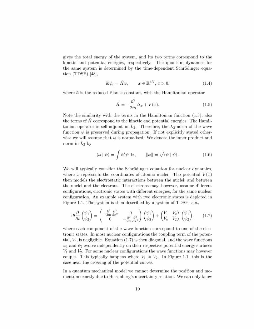
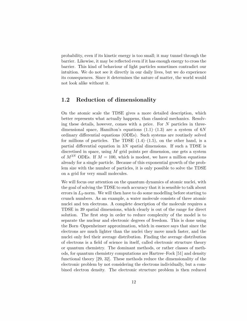
We will typically consider the Schrodinger equation for nuclear dynamics,where x represents the coordinates of atomic nuclei. The potential V (x)then models the electrostatic interactions between the nuclei, and betweenthe nuclei and the electrons. The electrons may, however, assume differentconfigurations, electronic states with different energies, for the same nuclearconfiguration. An example system with two electronic states is depicted inFigure 1.1. The system is then described by a system of TDSE, e.g.,

i~∂

∂t

(ψ1

ψ2

)=

(− ~2

2m∂2

∂x20

0 − ~22m

∂2

∂x2

)(ψ1

ψ2

)+

(V1 VcVc V2

)(ψ1

ψ2

), (1.7)

where each component of the wave function correspond to one of the elec-tronic states. In most nuclear configurations the coupling term of the poten-tial, Vc, is negligible. Equation (1.7) is then diagonal, and the wave functionsψ1 and ψ2 evolve independently on their respective potential energy surfacesV1 and V2. For some nuclear configurations the wave functions may howevercouple. This typically happens where V1 ≈ V2. In Figure 1.1, this is thecase near the crossing of the potential curves.

In a quantum mechanical model we cannot determine the position and mo-mentum exactly due to Heisenberg’s uncertainty relation. We can only know

10

x

V

V1

V2

Figure 1.1: An example of a two-state potential. The wave functions on thetwo potential energy surfaces V1 and V2 propagate independently for mostx, cf. (1.7), but interact near where V1 and V2 cross.

their probability densities, given by |ψ(x)|2 and |(Fψ)(ξ)|2, respectively,where

(Fψ)(ξ) = (2π~)−3N/2∫ψe−iξ

T x/~ dx (1.8)

is the Fourier transform of the wave function. As an example, consider aone-dimensional Gaussian wave function with equal uncertainty in positionand momentum,

ψ0(x) = (π~)−1/4 exp(− (x− q)2

2~+

i

~p(x− q)

). (1.9)

The standard deviations for position and momentum are√~/2 ∼ 10−17

m and 10−17 kgm/s, respectively. Heisenberg’s uncertainty relation indeedsays that the product of the standard deviations in position and momentumalways is at least ~/2. This clearly has negligible influence for macroscopicobjects, but leads to new phenomena for very light particles such as atomicnuclei or electrons. One such phenomenon is tunnelling. Consider a particlemoving towards a barrier. Classically, if its kinetic energy is larger thanthe potential energy of the barrier it will cross the barrier, otherwise itwill not. Quantum mechanics however allows it to cross, with a certain

11

probability, even if its kinetic energy is too small; it may tunnel through thebarrier. Likewise, it may be reflected even if it has enough energy to cross thebarrier. This kind of behaviour of light particles sometimes contradict ourintuition. We do not see it directly in our daily lives, but we do experienceits consequences. Since it determines the nature of matter, the world wouldnot look alike without it.

1.2 Reduction of dimensionality

On the atomic scale the TDSE gives a more detailed description, whichbetter represents what actually happens, than classical mechanics. Resolv-ing these details, however, comes with a price. For N particles in three-dimensional space, Hamilton’s equations (1.1)–(1.3) are a system of 6Nordinary differential equations (ODEs). Such systems are routinely solvedfor millions of particles. The TDSE (1.4)–(1.5), on the other hand, is apartial differential equation in 3N spatial dimensions. If such a TDSE isdiscretised in space, using M grid points per dimension, one gets a systemof M3N ODEs. If M = 100, which is modest, we have a million equationsalready for a single particle. Because of this exponential growth of the prob-lem size with the number of particles, it is only possible to solve the TDSEon a grid for very small molecules.

We will focus our attention on the quantum dynamics of atomic nuclei, withthe goal of solving the TDSE to such accuracy that it is sensible to talk abouterrors in L2-norm. We will then have to do some modelling before starting tocrunch numbers. As an example, a water molecule consists of three atomicnuclei and ten electrons. A complete description of the molecule requires aTDSE in 39 spatial dimensions, which clearly is out of the range for directsolution. The first step in order to reduce complexity of the model is toseparate the nuclear and electronic degrees of freedom. This is done usingthe Born–Oppenheimer approximation, which in essence says that since theelectrons are much lighter than the nuclei they move much faster, and thenuclei only feel their average distribution. Finding the average distributionof electrons is a field of science in itself, called electronic structure theoryor quantum chemistry. The dominant methods, or rather classes of meth-ods, for quantum chemistry computations are Hartree–Fock [51] and densityfunctional theory [29, 32]. These methods reduce the dimensionality of theelectronic problem by not considering the electrons individually, but a com-bined electron density. The electronic structure problem is then reduced

12

to a non-linear eigenvalue problem in three dimensions. In this thesis wewill assume that the electronic structure problem has already been solved,and a potential energy surface V (x) for the nuclear TDSE is available. Ifthe nuclei have the coordinates x, V (x) is their potential energy. However,even with the potential energy surface at hand the water molecule has threenuclei, which yields a TDSE in nine spatial dimensions. It is possible toreduce this further—we are typically not interested in the absolute locationor orientation of the molecule, but only in how the nuclei are positionedrelative to each other. By only considering the internal degrees of freedomwe get a TDSE in three spatial dimensions, a problem within range forcomputational solution.

Another approach, which is not further considered in this thesis, for mak-ing numerical simulation of big systems tractable starts from the other end.Sticking to the classical trajectories, one tries to model quantum mechan-ical phenomena into the method. A first step, common to most of thesemethods, is to consider an ensemble of trajectories rather than a single one.The initial positions and momenta of the classical trajectories are sampledfrom an initial quantum state. Functionals of the ensemble are then takenas approximations of quantum observables. By adding to this modelling,additional quantum features can be captured. One class of such methodsis surface hopping [37, 57], which models the coupling of different potentialenergy surfaces, cf. Figure 1.1. When a particle passes a region of strongcoupling between two electronic states it may ‘hop’ to the other state witha certain probability. Another method, aiming at taking effects such as tun-nelling into account, is ring-polymer molecular dynamics [18]. Each particleis there exchanged for a group of particles forming a ring, each particle inthe ring coupled to its two neighbours. These kinds of methods are feasiblefor much bigger systems than fully quantum mechanical methods, since thenumber of ODEs increase only linearly with the number of particles.

1.3 A note on units

In this thesis we will often use atomic units. Atomic units are defined byletting the mass of an electron, the elementary charge, the reduced Planckconstant ~, and Coulomb’s constant 1/(4πε0) all adopt the value 1. For thisreason, ~ does often not appear when the TDSE is stated.

We will also often use so-called semiclassical scaling. Starting in atomic

13

units we define the semiclassical parameter ε = 1/√m, where m is some

characteristic mass of the system. We then rescale time as t → t/ε, suchthat non-trivial dynamics happen on the time scale t ∼ 1, regardless of thesystem mass. We may also rescale the spatial coordinates such that theyall correspond to the same mass. The semiclassically scaled TDSE thenappears as

iεut = −ε2

2∆u+ V u. (1.10)

A typical solution to this equation is a wave packet with the width O(√ε)

and wave length O(ε). The limit ε → 0, in which classical dynamics isretained, is known as the classical limit.

14

Chapter 2

Computational challenges

When solving the TDSE numerically one faces a rich variety of challenges.The exponential growth with dimensionality of the computational work andmemory requirements is one of them. In this chapter we will discuss a fewmore, and some different approaches to their solution.

2.1 High frequency waves and dispersion errors

In the numerical simulation of wave equations the dominant source of erroris often dispersion error, i.e., that the phase velocity of a frequency compo-nent differs between the continuous and discretised problems. Consider forillustration the advection equation,

vt(x, t) + vx(x, t) = 0, x ∈ R, t > 0. (2.1)

This problem can be solved analytically using a Fourier transform in x.Given any plane wave initial condition, v(x, 0) = eiωx, ω ∈ R, the solutionat time t is v(x, t) = eiω(x−t). This means that waves of all frequencies aretransported with phase velocity 1. If we solve (2.1) using a finite differencemethod the high frequencies will be transported too slowly, and the highestfrequency that can be represented on the grid, with only two grid pointsper wave length, will not move at all. The phase velocity is approximatedbetter by higher order methods. If we use a pth order central finite differencestencil and require that the error should not exceed ε at time t, we need at

15

least

Mp = Cp

(ωtε

)1/p(2.2)

grid points per wave length [17, Ch. 3]. The constant Cp does not dependon ω or ε. This means that the advantage of higher order methods increasesthe higher the involved frequencies. Higher order methods are also morebeneficial if the problem is solved over a long time interval.

Consider now the free TDSE, i.e., the TDSE without potential,

ut(x, t) = iuxx(x, t), x ∈ R, t > 0. (2.3)

Also this problem can be solved using the Fourier transform. Given the sameplane wave initial condition, the solution at time t is u(x, t) = eiω(x−ωt). Thephase velocity is here proportional to the frequency. Using a pth order finitedifference method for this problem requires

M ′p = C ′p

(ω2t

ε

)1/p(2.4)

grid points per wave length in order to keep the error below ε at time t.Since the frequency appears with a larger exponent in (2.4) than in (2.2),higher order methods have a stronger advantage for the TDSE than forfirst order hyperbolic problems. For this reason, the Fourier pseudospectralmethod [14, 34, 35] has become very popular within the chemical physicscommunity.

In the Fourier pseudospectral method derivatives are calculated by expand-ing the discrete solution in plane waves, assuming periodic boundary condi-tions. This can be done efficiently using the fast Fourier transform (FFT).The derivatives can then be calculated analytically in the plane wave basis,whereafter an inverse FFT gives the pointwise derivatives. With the Fourierpseudospectral method, all frequencies that are representable on the grid getthe correct phase velocity—it behaves like an infinite order finite differencemethod. Fornberg showed in [12, 13] that if you construct an infinite ordercentral finite difference stencil, wrapping it around the periodic boundary aninfinite number of times, what you get is indeed the Fourier pseudospectralmethod.

In the semiclassical regime, i.e., for heavy particles, solutions to the Schro-dinger equation contain very high frequencies. Resolving the oscillationsmay then require an unaffordable amount of grid points already in one di-mension and solving on a grid will be unfeasible, also if a pseudospectral

16

method is used. Fortunately, there are approximate, asymptotic methodswhich perform well for high frequencies. In the context of the Schrodingerequation, such methods are called semiclassical. Methods of this kind willbe discussed further in Chapter 3.

2.2 Unbound problems and absorbing boundaryconditions

The Schrodinger equation is posed on an infinite domain. In order to makecomputations we must truncate the domain to finite size. In most cases thistruncation introduces artificial boundaries without physical meaning. It istherefore desirable that they have no or little influence on the results of thecomputations.

One can divide quantum molecular dynamics problems into two categories:bound and unbound problems. In bound problems the wave function stayslocalised for all time. Such problems may describe, e.g., the internal vibra-tions of molecules. Boundary treatment is usually not critical for boundproblems. If the domain is chosen big enough, such that wave functionhas negligible amplitude near the boundary, we can use any stable bound-ary condition without introducing significant error. Unbound problems, onthe other hand, model situations where the wave function moves or spreadsover an extended region. Examples of unbound problems include scatteringand dissociative chemical reactions. For unbound problems we might haveto truncate the domain where the solution is not small in order to havea domain of reasonable size. This introduces a need for absorbing bound-ary conditions (ABCs). If the wave function propagates out through theboundary we do not want it to be reflected. We want it to exit, never toreturn. In order to formulate ABCs for the Schrodinger equation we mustassume that the potential is constant in the normal direction at and outsidethe boundary. Otherwise it is possible that the solution outside where wewould truncate the domain affects the solution inside. The simulation resultwith truncated domain and ABCs will then differ from the solution withoutdomain truncation.

Exact ABCs can be formulated for the Schrodinger equation, but they areglobal in both time and space and therefore of limited use for computations.Practical, approximate ABCs fall into two main categories, local ABCs andabsorbing layers. Local ABCs attempt to approximate the exact, non-local

17

ABC, and was pioneered by Engquist and Majda [9]. Absorbing layers,which are more widely used for the TDSE, are layers surrounding the do-main in which the wave function is damped out. In the chemical physicscommunity this is most often done by adding an imaginary term to the po-tential [40, 42]. This term is called a complex absorbing potential. A moresophisticated technique is perfectly matched layers (PMLs), first proposedby Berenger for Maxwell’s equations [3]. In this thesis we will most oftenuse this technique, in particular the modal PML of Nissen and Kreiss [43].

2.3 Time integration

Despite being a wave equation, the TDSE incurs a parabolic-type time steprestriction for explicit Runge–Kutta or multistep methods, i.e., ∆t ≤ C∆x2

is required for stability. For this reason very small time steps are required,and such methods are normally not efficient for the Schrodinger equation.Instead splitting methods [11, 49] or methods for approximating the ma-trix exponential exp(−iH/∆t), where H is a discretisation matrix for theHamiltonian operator H, are more successful.

Multiplying the matrix exponential to the solution vector propagates thesemidiscretised TDSE exactly. Matrix function-vector products can be ap-proximated by Krylov subspace methods [27, 41]. This is the approachwe most often will use in this thesis. The approximate solution at timetn+1, ψn+1, is then calculated by computing the Galerkin approximationof the matrix exponential on the mth order Krylov subspace Km(H,ψn) =span(ψn, Hψn, . . . ,H

m−1ψn). An orthonormal basis for the Krylov subspacecan be computed using the Lanczos or Arnoldi process [2, 6, 36]. Anotherapproach, popular within the chemical physics community, is to expand thematrix exponential in Chebyshev polynomials [53].

In the case of an explicitly time-dependent Hamiltonian the matrix expo-nential no longer solves the semidiscretised system exactly. See, e.g., [28, 33]for methods applicable in that case.

18

Chapter 3

Semiclassical modelling

Since classical and quantum dynamics model the same kind of physics, onewould expect that they yield similar results in certain parameter regimes.They indeed do, for heavy particles. This has motivated the construc-tion of semiclassical methods, which take this property into account, andthereby perform better the heavier the particles. The validity of semiclas-sical approximations can, e.g., be understood through Ehrenfest’s theorem[54, Ch. 4], which relates the evolution of an expectation value 〈a〉 = 〈u | au〉of an operator a to its commutator with the Hamiltonian, [a, H] = aH−Ha.If a does not depend explicitly on time, the theorem reads

d

dt〈a〉 =

1

iε〈[a, H]〉. (3.1)

Applying Ehrenfest’s theorem to the position and momentum operators q =x and p = −iε∇ yields

d

dt〈q〉 = 〈p〉, (3.2)

d

dt〈p〉 = −〈∇V 〉. (3.3)

These relations have apparent similarities with their classical counterparts,Hamilton’s equations of motion,

d

dtq = p, (3.4)

d

dtp = −∇V (q). (3.5)

19

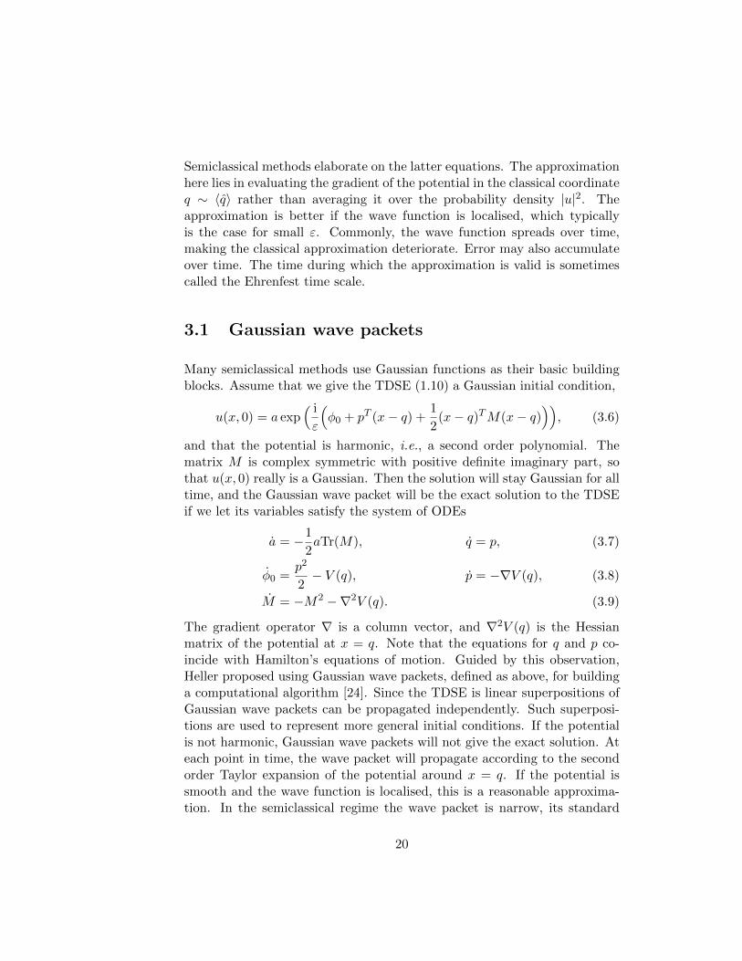
Semiclassical methods elaborate on the latter equations. The approximationhere lies in evaluating the gradient of the potential in the classical coordinateq ∼ 〈q〉 rather than averaging it over the probability density |u|2. Theapproximation is better if the wave function is localised, which typicallyis the case for small ε. Commonly, the wave function spreads over time,making the classical approximation deteriorate. Error may also accumulateover time. The time during which the approximation is valid is sometimescalled the Ehrenfest time scale.

3.1 Gaussian wave packets

Many semiclassical methods use Gaussian functions as their basic buildingblocks. Assume that we give the TDSE (1.10) a Gaussian initial condition,

u(x, 0) = a exp( i

ε

(φ0 + pT (x− q) +

1

2(x− q)TM(x− q)

)), (3.6)

and that the potential is harmonic, i.e., a second order polynomial. Thematrix M is complex symmetric with positive definite imaginary part, sothat u(x, 0) really is a Gaussian. Then the solution will stay Gaussian for alltime, and the Gaussian wave packet will be the exact solution to the TDSEif we let its variables satisfy the system of ODEs

a = −1

2aTr(M), q = p, (3.7)

φ0 =p2

2− V (q), p = −∇V (q), (3.8)

M = −M2 −∇2V (q). (3.9)

The gradient operator ∇ is a column vector, and ∇2V (q) is the Hessianmatrix of the potential at x = q. Note that the equations for q and p co-incide with Hamilton’s equations of motion. Guided by this observation,Heller proposed using Gaussian wave packets, defined as above, for buildinga computational algorithm [24]. Since the TDSE is linear superpositions ofGaussian wave packets can be propagated independently. Such superposi-tions are used to represent more general initial conditions. If the potentialis not harmonic, Gaussian wave packets will not give the exact solution. Ateach point in time, the wave packet will propagate according to the secondorder Taylor expansion of the potential around x = q. If the potential issmooth and the wave function is localised, this is a reasonable approxima-tion. In the semiclassical regime the wave packet is narrow, its standard

20

deviation is O(ε1/2). It has been shown, e.g. by Hagedorn [19], that the er-ror of Gaussian wave packets for Schrodinger equations with non-harmonicpotential is bounded by Ctε

1/2, where Ct is independent of ε.

Heller later proposed the frozen Gaussian approximation [25], where thespread variable M is kept constant. The method was further developed byHerman and Kluk [26], and is popular within the chemical physics com-munity. Error estimates in terms of ε were given by Swart and Rousse in[50].

The theory for Gaussian wave packets has been developed further by thenumerical analysis community in the context of high-frequency wave propa-gation. There, the Gaussian wave packets carry the name Gaussian beams.The focus has been on the wave equation and the Helmholtz equation. Byincluding more terms in the phase and amplitude expansions, higher orderGaussian beams can be constructed [55]. The superposition and propagationerror estimates will then depend on higher powers of ε than for the Gaus-sian wave packet described above, which is a first order Gaussian beam.Error estimates for arbitrary order Gaussian beams for the TDSE were de-rived in [38]. An overview of semiclassical methods for the TDSE, includingGaussian beams, is given in [30].

3.1.1 A hybrid method

Gaussian wave packets are asymptotic in nature, they converge to the exactsolution as ε → 0. Since ε is a property of the problem it always adopts afixed, finite value in a practical application. For a given ε, Gaussian wavepackets however work better in some situations than in others, the erroris smaller where the potential varies on a longer length scale. This can beunderstood through the locality assumption, the slower the variations ofthe potential, the less we lose when we truncate its Taylor expansion. InPaper II we propose a hybrid method, where we use finite differences onsummation-by-parts form [44, 47] in the vicinity of sharp variation in thepotential, and first order Gaussian beams elsewhere. A similar method waspreviously constructed by Jin and Qi [31], and Tanushev et al. used a relatedapproach for the scalar wave equation [56].

Our approach differs from the method in [31] by the way the interfaces be-tween the finite difference and Gaussian beam subdomains are handled. Theinterface treatment of [31] is robust, but expensive. It relies on extensive

21

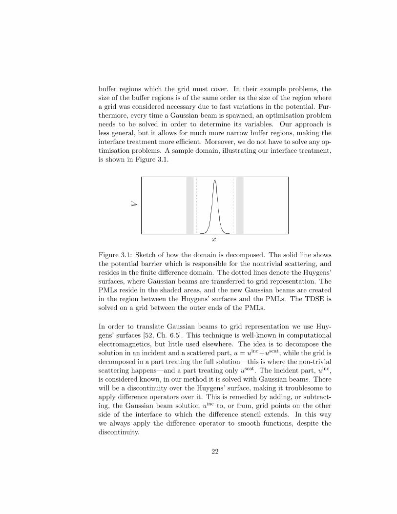
buffer regions which the grid must cover. In their example problems, thesize of the buffer regions is of the same order as the size of the region wherea grid was considered necessary due to fast variations in the potential. Fur-thermore, every time a Gaussian beam is spawned, an optimisation problemneeds to be solved in order to determine its variables. Our approach isless general, but it allows for much more narrow buffer regions, making theinterface treatment more efficient. Moreover, we do not have to solve any op-timisation problems. A sample domain, illustrating our interface treatment,is shown in Figure 3.1.

x

V

Figure 3.1: Sketch of how the domain is decomposed. The solid line showsthe potential barrier which is responsible for the nontrivial scattering, andresides in the finite difference domain. The dotted lines denote the Huygens’surfaces, where Gaussian beams are transferred to grid representation. ThePMLs reside in the shaded areas, and the new Gaussian beams are createdin the region between the Huygens’ surfaces and the PMLs. The TDSE issolved on a grid between the outer ends of the PMLs.

In order to translate Gaussian beams to grid representation we use Huy-gens’ surfaces [52, Ch. 6.5]. This technique is well-known in computationalelectromagnetics, but little used elsewhere. The idea is to decompose thesolution in an incident and a scattered part, u = uinc+uscat, while the grid isdecomposed in a part treating the full solution—this is where the non-trivialscattering happens—and a part treating only uscat. The incident part, uinc,is considered known, in our method it is solved with Gaussian beams. Therewill be a discontinuity over the Huygens’ surface, making it troublesome toapply difference operators over it. This is remedied by adding, or subtract-ing, the Gaussian beam solution uinc to, or from, grid points on the otherside of the interface to which the difference stencil extends. In this waywe always apply the difference operator to smooth functions, despite thediscontinuity.

22

Eventually, the scattered wave function will come out again through a Huy-gens’ surface. We prove a superposition result, a variant of [55, Thm. 2.1],which allows us to translate the grid representation of uscat to a superposi-tion of Gaussian beams using a buffer region no wider than the differenceoperator. This is done right outside the Huygens’ surface. After havingbeen translated to Gaussian beams, the grid solution is consumed by anabsorbing boundary condition, which we implement using a PML.

Our interface treatment allows us to reduce the buffer regions compared to[31], a buffer wide as a difference stencil and a PML, typically less than30 grid points, is sufficient. This gives a considerable increase in efficiency,but we have to sacrifice some generality. When the wave function exits thefinite difference domain through the Huygens’ surface the potential must notincrease—the wave function must be allowed to continue to the absorbingboundary condition, and the spawned Gaussian beams must be able to exitthe finite difference grid properly before entering again.

3.2 Hagedorn wave packets

In a series of papers [19, 20, 21, 22], Hagedorn elaborated further on theGaussian wave packets. He constructed more general functions, Gaussianswith certain polynomial prefactors, with shape variables evolved by ODEssimilar to those of Gaussian beams. He showed that the constructed func-tions, which we will call Hagedorn functions, then give the exact solutionfor harmonic potentials—they are indeed eigenfunctions of the harmonic os-cillator. In one dimension, the polynomial prefactors are scaled and shiftedHermite polynomials. In this section we review the construction of theHagedorn functions and their use in a numerical method for the TDSE.More details can be found in [10], and in the monograph [39]. A relatedmethod is the time-dependent discrete variable representation [1, 4], whichuses collocation with a tensor product basis of Hermite functions.

The Hagedorn functions can be defined recursively using the raising andlowering operators

R = (Rj)nj=1 =i√2ε

(P ∗(q − q)−Q∗(p− p)

), (3.10)

L = (Lj)nj=1 = − i√2ε

(P T (q − q)−QT (p− p)

). (3.11)

23

The matrices Q and P originate from a factorisation of the matrix M fora Gaussian beam, M = PQ−1. Application of Rj or Lj raises or lowersthe polynomial degree in the jth dimension. The definition of the Hagedornfunctions reads

ϕ0(x) = (πε)−n/4(detQ)−1/2×

× exp( i

ε

(φ0 + pT (x− q) +

1

2(x− q)TPQ−1(x− q)

)), (3.12)

ϕk+ej =1√kj + 1

Rjϕk, ϕk−ej =1√kjLjϕk. (3.13)

Here, k is a multi-index, and ej is the standard basis vector in Rn. Q andP are required to satisfy the compatibility relations

QTP − P TQ = 0, (3.14)

Q∗P − P ∗Q = 2iI. (3.15)

This implies Im (PQ−1) = (QQ∗)−1, which is a symmetric positive definitematrix. This in turn guarantees exponential decay at infinity of the Hage-dorn functions. The shape variables for ϕk are propagated according to thesystem of ODEs

q = p, Q = P, (3.16)

p = −∇V (q), P = −∇2V (q)Q, (3.17)

φ0 =p2

2− V (q). (3.18)

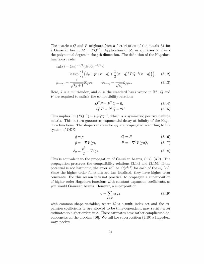
This is equivalent to the propagation of Gaussian beams, (3.7)–(3.9). Thepropagation preserves the compatibility relations (3.14) and (3.15). If thepotential is not harmonic, the error will be O(ε1/2) for each of the ϕk [22].Since the higher order functions are less localised, they have higher errorconstants. For this reason it is not practical to propagate a superpositionof higher order Hagedorn functions with constant expansion coefficients, asyou would Gaussian beams. However, a superposition

u =∑k∈K

ckϕk (3.19)

with common shape variables, where K is a multi-index set and the ex-pansion coefficients ck are allowed to be time-dependent, may satisfy errorestimates to higher orders in ε. These estimates have rather complicated de-pendencies on the problem [16]. We call the superposition (3.19) a Hagedornwave packet.

24

Given any set of variables {φ0, q, p,Q, P} satisfying (3.14)–(3.15), the Hage-dorn functions ϕk, k ∈ K, form a closed subspace of L2, and are orthonormalwith respect to the L2 inner product (1.6). Faou et al. constructed a com-putational algorithm [10] using a Galerkin ansatz over the time-dependentapproximation space spanned by a set of Hagedorn functions. This is coupledto a symplectic integration scheme for the shape variables which preservesthe relations (3.14)–(3.15). The method is time-reversible and conserves theL2-norm of the wave packet. The Galerkin condition, that ck should bepropagated such that the error is orthogonal to span{ϕk}, reads∑

k∈K〈ϕj |

(iε∂

∂t− H

)ckϕk〉 = 0, ∀j ∈ K. (3.20)

We decompose the potential in its second order Taylor polynomial aroundx = q and a remainder,

V (x) = V (q) + (x− q)T∇V (q) +1

2(x− q)T∇2V (q)(x− q) +W (x). (3.21)

Since the functions ϕk evolve such that each of them solve the TDSE with theharmonic potential V −W exactly, the evolution of the expansion coefficientsck is determined by the remainder term,

iεcj =∑k∈K

ck〈ϕj |Wϕk〉. (3.22)

The error estimates in terms of ε depend on the multi-index set K and onthe regularity of the potential. The exact assumptions and a proof can befound in [16], or in a different formulation in [22].

The propagation error of Hagedorn wave packets can be bounded from twodirections. On the one hand the method is semiclassical, with error boundedin terms of ε. On the other hand it is a spectral method, with error decayingexponentially with the number of basis functions. The reason for this doublenature is that the spectral method is formulated not for the full Schrodingerequation, but for the deviation from the semiclassical trajectory. We there-fore do not need to resolve the O(ε) oscillations as long as the wave packetstays close to its semiclassical trajectory, i.e., on the Ehrenfest time scale.

A potential issue of Hagedorn wave packets is the computational complexity.With |K| basis functions we need to evaluate ∼ |K|2 integrals 〈ϕj | Wϕk〉,cf. (3.22), in every time step. The cost is O(|K|3) if a full, tensor productbasis of Hagedorn functions is used. In Paper I we propose to propagate

25

the coefficients ck using a collocation ansatz, or a pseudospectral method,rather than a Galerkin method. With collocation we only need to evaluate|K| integrals, reducing the computational complexity to O(|K|2). We insteadpropagate ck by applying the action of W in coordinate space, and projectthe result back to the space spanned by the Hagedorn functions. We showthat this is equivalent to the Galerkin formulation in the limit ∆t→ 0, i.e.,this is a consistent discretisation of (3.22). The Galerkin formulation forHagedorn wave packets feature several attractive conservation properties,by using collocation we sacrifice time-reversibility and norm conservation.Moreover, we solve the system of ODEs (3.22) to first order of accuracy,compared to second order for the Galerkin formulation. This loss of accuracyis due to the projection to the space spanned by the Hagedorn functions—it is therefore only significant when the true solution extends outside theapproximation space. We argue that time integration error is not a majorconcern in that situation.

In related work, Russo and Smereka [45, 46] construct a semiclassical coor-dinate transform for the Schrodinger equation, which they call the Gaussianwave packet transform. They then get a Schrodinger type partial differen-tial equation for the deviations from the first order Gaussian beam solution.The situation is much like the case of Hagedorn wave packets, but we are nolonger forced to discretise in space with the Hagedorn functions. In [45, 46]the Fourier pseudospectral method is used instead.

3.2.1 Beyond the Ehrenfest time scale

The Hagedorn functions are highly oscillatory, the wave length is typicallymuch shorter than the spacing of the underlying pseudospectral grid. Theapplicability of the method relies on the semiclassical nature of the under-lying physical problem. As long as the classical path is a good approxima-tion, Hagedorn wave packets are both accurate and efficient. Beyond theEhrenfest time scale, however, when the semiclassical approximation doesnot hold, a lot of basis functions are needed in order to resolve the wavefunction. Moreover, since the approximation space is guided by the clas-sical path, which is then losing relevance, much of our effort may be putin less important parts of phase-space. In Paper I we propose an adaptivepseudospectral method based on Hagedorn wave packets. The aim is tofollow the actual path of the wave packet, whether or not it stays close toits classical path. We achieve this by estimating the support of the wave

26

function and steering the shape parameters q and QQ∗ such that the basismatches the support of the wave function. We still rely on the wave func-tion staying localised, but this is the only respect in which the method stillis semiclassical. The semiclassical error estimates in terms of ε no longerhold—we aim at situations where they would not be of much use anyway.We therefore rely on resolving the oscillations in the solution. The method ispseudospectral with a time-dependent basis set, where the evolution of thebasis is determined by the evolution of the solution. This kind of movingbasis adaptivity is sometimes called r-adaptivity. A review of r-adaptivemethods is given in [5].

The position and spread of a Hagedorn basis is determined by q and QQ∗,respectively. Their time-evolution depends on how we treat the potential—we are not forced to use the Taylor polynomial. We split the potential in asecond order polynomial and a remainder,

V (x) = V (q) + (x− q)T V1 +1

2(x− q)T V2(x− q) + W (x), (3.23)

where we may choose V1 and V2 as we please. If we exchange ∇V (q) and∇2V (q) in (3.17) for V1 and V2, and propagate the coefficients ck according toW instead of W , we still get a method which converges in the pseudospectralsense, i.e., as the number of basis functions is increased. We constrain thematricesQ and P to be diagonal. The shape parameters are then determinedby the second order ODEs

d2

dt2q = −V1 (3.24)

d2

dt2QQ∗ = 2PP ∗ − 2V2QQ

∗. (3.25)

By choosing V1 and V2 appropriately, using standard tools from automaticcontrol [15], we can control the values of q and QQ∗. We use a proportional-derivative controller to keep the values of q and QQ∗ close to time-dependentreference values, which are given by estimates of the support of the wavefunction.

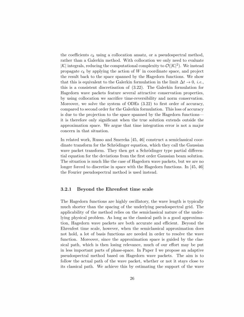
In Paper I we apply the new method to the photodissociation of IBr. Themolecular system has three coupled potential energy surfaces, which aresketched in Figure 3.2. The IBr molecule, initially in its ground state, isexposed to a laser pulse. Part of the wave packet is then excited by theelectric field to the first excited state, where it has enough energy to disso-ciate. Near the point where the two excited potential energy surfaces cross,

27

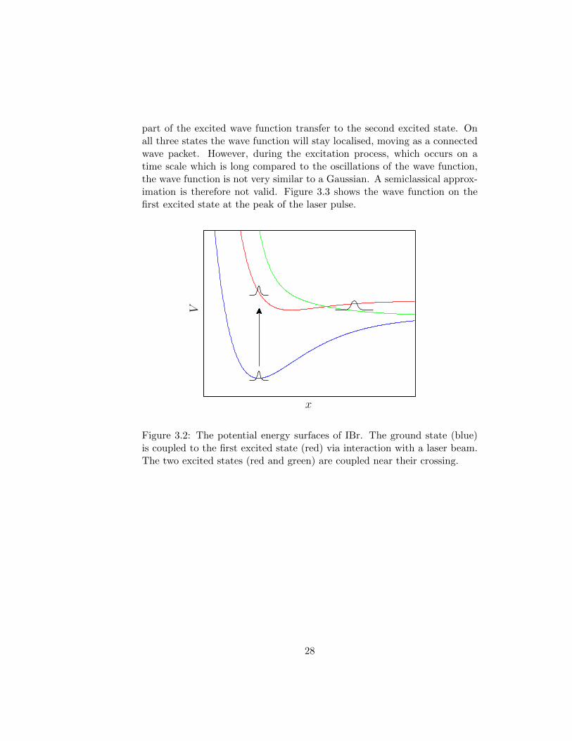
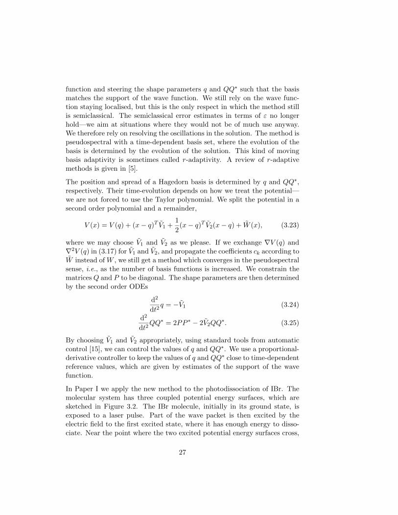
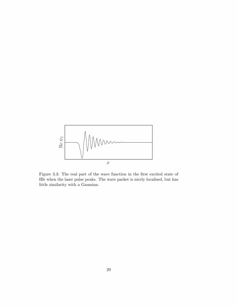
part of the excited wave function transfer to the second excited state. Onall three states the wave function will stay localised, moving as a connectedwave packet. However, during the excitation process, which occurs on atime scale which is long compared to the oscillations of the wave function,the wave function is not very similar to a Gaussian. A semiclassical approx-imation is therefore not valid. Figure 3.3 shows the wave function on thefirst excited state at the peak of the laser pulse.

x

V

Figure 3.2: The potential energy surfaces of IBr. The ground state (blue)is coupled to the first excited state (red) via interaction with a laser beam.The two excited states (red and green) are coupled near their crossing.

28

x

Reψ2

Figure 3.3: The real part of the wave function in the first excited state ofIBr when the laser pulse peaks. The wave packet is nicely localised, but haslittle similarity with a Gaussian.

29

30

Chapter 4

Electron dynamics

In Paper III we consider the dynamics of the electron in a hydrogen atomsubject to a laser beam. Though very similar in structure to the TDSE fornuclear dynamics, the resulting Schrodinger equation poses challenges of adifferent kind. The reason for this is that we now see the Born–Oppenheimerapproximation from the other end. For nuclear dynamics, the electrons moveso fast that the nuclei only feel their average effect, which can be modelledby a potential energy surface. For the electron the nucleus appears to standstill. The potential energy surface is then given by the Coulomb potentialof a point charge. In cylindrical coordinates, the resulting TDSE reads

iut = −1

2∆u− 1√

r2 + z2u− ze(t)u, (4.1)

where e(t) is the electric field strength of the laser beam. Previously in thisthesis the potential energy surfaces have been smooth, and assuming highregularity of the wave function has not been a problem. Now, the potentialis singular at the origin, and the lack of regularity of the solution limits therate of convergence which can be achieved by standard numerical methods.Higher order methods are therefore less beneficial.

The situation can be improved by a suitable choice of radial discretisation,a spectral method over a space spanned by Bessel functions [58, Ch. 18].We truncate the domain to the cylinder r ∈ [0, Lr] and define the functions

vk(r) =

√2

LrJ1(xk)J0

(xkrLr

), (4.2)

31

where Jn is the nth order Bessel function of the first kind, and xk is the kthzero of J0. These functions are orthonormal,

∫v∗j (r)vk(r)r dr = δjk, and

eigenfunctions to the radial part of the Laplacian. A Galerkin ansatz overthese functions results in system of Schrodinger equations in z and t witha potential which is continuous and bounded, but not smooth. If the axialcoordinate is discretised with the Fourier pseudospectral method, secondorder accuracy is achieved.

In Paper III we improve the regularity further. We note that the reductionin regularity of the solution is due to a single jump in the third derivativeof the solution, and derive the magnitude of that jump. By subtractingthe jump prior to applying the spatial differential operator we get increasedconvergence rate. One would expect that the order of accuracy would in-crease by one, to third order, but through a quite technical proof we showthat one actually gets a fourth order accurate method. This is confirmed bynumerical experiments.

This method has applications in the computation of high harmonic genera-tion [59], a technique for the generation of short pulses of light, consistingof odd order overtones of the laser frequency. The pulses reside in the spec-tral range between extreme ultra violet and soft x-ray. Such pulses havemany uses in experimental physics, e.g., for the time-resolved spectroscopyof electron dynamics [7, 8].

32

Chapter 5

Author’s contributions

Paper I

The author of this thesis had the main responsibility for preparing themanuscript and performed all computations. The ideas were developed bythe author in consultation with the co-authors.

Paper II

The author of this thesis had the main responsibility for preparing themanuscript and performed all computations. The ideas were developed inclose collaboration between the authors.

Paper III

The author of this thesis is the sole author of the manuscript.

33

34

Acknowledgements

I owe much gratitude to my adviser Sverker Holmgren for sharing his experi-ence and good judgement, for guiding me through the research topics as wellas the scientific community. I also want to thank my coadvisers Vasile Grad-inaru and Hans Karlsson for adding additional perspectives to my research.Thanks also to all friends and colleagues at TDB, who create the friendlyand cooperative environment. In particular Katharina Kormann, MarkusKowalewski and Gunilla Kreiss deserve acknowledgement for sharing theirexpertise with endless patience. Finally, I would like to thank Andreas Hel-lander and Per Lotstedt, who introduced me to the world of science duringmy MSc thesis work.

Funding for travel has gratefully been received from Stiftelsen SkandinaviskaMalm och Metalls forsknings- och utvecklingsfond, AngpanneforeningensForskningsstiftelse, and Knut och Alice Wallenbergs stiftelses resefond.

35

36

Bibliography

[1] S. Adhikari and G. D. Billing. A time-dependent discrete variable rep-resentation method. J. Chem. Phys., 113:1409–1414, 2000.

[2] W. E. Arnoldi. The principle of minimized iteration in the solution ofthe matrix eigenvalue problem. Q. Appl. Math., 9:17–29, 1951.

[3] J.-P. Berenger. A perfectly matched layer for the absorption of electro-magnetic waves. J. Comput. Phys., 114:185–200, 1994.

[4] G. D. Billing and S. Adhikari. The time-dependent discrete variable rep-resentation method in molecular dynamics. Chem. Phys. Lett., 321:197–204, 2000.

[5] C. J. Budd, W. Huang, and R. D. Russell. Adaptivity with movinggrids. Acta Numer., 18:111–241, 2009.

[6] J. W. Demmel. Applied Numerical Linear Algebra. SIAM, Philadelphia,PA, 1997.

[7] G. Doumy and L. F. DiMauro. Interrogating molecules. Science,322:1194–1195, 2008.

[8] M. Drescher, M. Hentschel, R. Kienberger, M. Uiberacker, V. Yakovlev,A. Scrinzi, T. Westerwalbesloh, U. Kleineberg, U. Heinzmann, andF. Krausz. Time-resolved atomic inner-shell spectroscopy. Nature,419:803–807, 2002.

[9] B. Engquist and A. Majda. Absorbing boundary conditions for thenumerical simulation of waves. Math. Comp., 31:629–651, 1977.

[10] E. Faou, V. Gradinaru, and C. Lubich. Computing semiclassical quan-tum dynamics with Hagedorn wavepackets. SIAM J. Sci. Comput.,31:3027–3041, 2009.

37

[11] M. D. Feit, J. A. Fleck, and A. Steiger. Solution of the Schrodingerequation by a spectral method. J. Comput. Phys., 47:412–433, 1982.

[12] B. Fornberg. On a Fourier method for the integration of hyperbolicequations. SIAM J. Numer. Anal., 12:509–528, 1975.

[13] B. Fornberg. The pseudospectral method: Comparisons with finitedifferences for the elastic wave equation. Geophysics, 52:483–501, 1987.

[14] B. Fornberg. A Practical Guide to Pseudospectral Methods. CambridgeUniversity Press, Cambridge, 1996.

[15] G. Franklin, J. D. Powell, and A. Emami-Naeini. Feedback Control ofDynamic Systems. Prentice Hall, Upper Saddle River, NJ, 5th edition,2006.

[16] V. Gradinaru and G. A. Hagedorn. Convergence of a semiclassicalwavepacket based time-splitting for the Schrodinger equation. Numer.Math., 2013. To appear.

[17] B. Gustafsson, H.-O. Kreiss, and J. Oliger. Time Dependent Problemsand Difference Methods. Wiley, New York, NY, 1995.

[18] S. Habershon, D. E. Manolopoulos, T. E. Markland, and T. F.Miller III. Ring-polymer molecular dynamics: Quantum effects in chem-ical dynamics from classical trajectories in an extended phase space.Annu. Rev. Phys. Chem., 64:387–413, 2013.

[19] G. A. Hagedorn. Semiclassical quantum mechanics I. The ~→ 0 limitfor coherent states. Commun. Math. Phys., 71:77–93, 1980.

[20] G. A. Hagedorn. Semiclassical quantum mechanics. III. The large orderasymptotics and more general states. Ann. Physics, 135:58–70, 1981.

[21] G. A. Hagedorn. Semiclassical quantum mechanics, IV: large orderasymptotics and more general states in more than one dimension. Ann.Inst. H. Poincare Phys. Theor., 42:363–374, 1985.

[22] G. A. Hagedorn. Raising and lowering operators for semiclassical wavepackets. Ann. Physics, 269:77–104, 1998.

[23] W. R. Hamilton. Second essay on a general method in dynamics. Philos.Trans. R. Soc. Lond., 125:95–144, 1835.

38

[24] E. J. Heller. Time-dependent approach to semiclassical dynamics. J.Chem. Phys., 62:1544–1555, 1975.

[25] E. J. Heller. Frozen Gaussians: A very simple semiclassical approxima-tion. J. Chem. Phys., 75:2923–2931, 1981.

[26] M. F. Herman and E. Kluk. A semiclasical justification for the useof non-spreading wavepackets in dynamics calculations. Chem. Phys.,91:27–34, 1984.

[27] M. Hochbruck and C. Lubich. On Krylov subspace approximations tothe matrix exponential operator. SIAM J. Numer. Anal., 34:1911–1925,1997.

[28] M. Hochbruck and C. Lubich. On Magnus integrators for time-dependent Schrodinger equations. SIAM J. Numer. Anal., 41:945–963,2003.

[29] P. Hohenberg and W. Kohn. Inhomogeneous electron gas. Phys. Rev.,136:B864–B871, 1964.

[30] S. Jin, P. Markowich, and C. Sparber. Mathematical and computationalmethods for semiclassical Schrodinger equations. Acta Numer., 20:121–209, 2011.

[31] S. Jin and P. Qi. A hybrid Schrodinger/Gaussian beam solver for quan-tum barriers and surface hopping. Kinet. Relat. Models, 4:1097–1120,2011.

[32] W. Kohn and L. J. Sham. Self-consistent equations including exchangeand correlation effects. Phys. Rev., 140:A1133–A1138, 1965.

[33] K. Kormann, S. Holmgren, and H. O. Karlsson. Accurate time propa-gation for the Schrodinger equation with an explicitly time-dependentHamiltonian. J. Chem. Phys., 128:184101, 2008.

[34] D. Kosloff and R. Kosloff. A Fourier method solution for the timedependent Schrodinger equation as a tool in molecular dynamics. J.Comput. Phys., 52:35–53, 1983.

[35] H.-O. Kreiss and J. Oliger. Comparison of accurate methods for theintegration of hyperbolic equations. Tellus, 24:199–215, 1972.

39

[36] C. Lanczos. An iteration method for the solution of the eigenvalueproblem of linear differential and integral operators. J. Res. Nat. Bur.Stand., 45:255–282, 1950.

[37] C. Lasser and T. Swart. Single switch surface hopping for a model ofpyrazine. J. Chem. Phys., 129:034302, 2008.

[38] H. Liu, O. Runborg, and N. M. Tanushev. Error estimates for Gaussianbeam superpositions. Math. Comp., 82:919–952, 2013.

[39] C. Lubich. From quantum to classical molecular dynamics: Reducedmodels and numerical analysis. European Math. Soc., Zurich, 2008.

[40] D. E. Manolopoulos. Derivation and reflection properties of atransmission-free absorbing potential. J. Chem. Phys., 117:9552–9559,2002.

[41] A. Nauts and R. E. Wyatt. New approach to many-state quantumdynamics: The recursive-residue-generation method. Phys. Rev. Lett.,51:2238–2241, 1983.

[42] D. Neuhasuer and M. Baer. The time-dependent Schrodinger equa-tion: Application of absorbing boundary conditions. J. Chem. Phys.,90:4351–4355, 1989.

[43] A. Nissen and G. Kreiss. An optimized perfectly matched layer for theSchrodinger equation. Commun. Comput. Phys., 9:147–179, 2011.

[44] A. Nissen, G. Kreiss, and M. Gerritsen. High order stable finite differ-ence methods for the Schrodinger equation. J. Sci. Comput., 55:173–199, 2013.

[45] G. Russo and P. Smereka. The Gaussian wave packet transform: Effi-cient computation of the semi-classical limit of the Schrodinger equa-tion. Part 1 – formulation and the one dimensional case. J. Comput.Phys., 233:192–209, 2013.

[46] G. Russo and P. Smereka. The Gaussian wave packet transform: Effi-cient computation of the semi-classical limit of the Schrodinger equa-tion. Part 2 – multidimensional case. Preprint, 2013.

[47] G. Scherer. On energy estimates for difference approximations to hy-perbolic partial differential equations. PhD thesis, Department of Com-puter Sciences, Uppsala University, 1977.

40

[48] E. Schrodinger. Quantisierung als Eigenwertproblem (Vierte Mit-teilung). Ann. Phys., 386:109–139, 1926.

[49] G. Strang. On the construction and comparison of difference schemes.SIAM J. Numer. Anal., 5:506–517, 1968.

[50] T. Swart and V. Rousse. A mathematical justification for the Herman-Kluk propagator. Commun. Math. Phys., 286:725–750, 2009.

[51] A. Szabo and N. S. Ostlund. Modern Quantum Chemistry: Introductionto Advanced Electronic Structure Theory. Dover, Mineola, NY, 1996.

[52] A. Taflove. Computational electrodynamics: The finite-difference time-domain method. Artech House, Boston, MA, 1995.

[53] H. Tal-Ezer and R. Kosloff. An accurate and efficient scheme for prop-agating the time dependent Schrodinger equation. J. Chem. Phys.,81:3967–3971, 1984.

[54] D. J. Tannor. Introduction to Quantum Mechanics: A Time-DependentPerspective. University Science Books, Sausalito, CA, 2007.

[55] N. M. Tanushev. Superpositions and higher order Gaussian beams.Commun. Math. Sci., 6:449–475, 2008.

[56] N. M. Tanushev, Y.-H. R. Tsai, and B. Engquist. A coupled finitedifference – Gaussian beam method for high frequency wave propaga-tion. In B. Engquist, O. Runborg, and Y.-H. R. Tsai, editors, Numer-ical Analysis of Multiscale Computations, volume 82 of Lecture Notesin Computational Science and Engineering, pages 401–420. Springer-Verlag, Berlin, 2012.

[57] J. C. Tully. Molecular dynamics with electronic transitions. J. Chem.Phys., 93:1061–1071, 1990.

[58] G. N. Watson. A Treatise on the Theory of Bessel Functions. Cam-bridge University Press, Cambridge, 2nd edition, 1966.

[59] C. Winterfeldt, C. Spielmann, and G. Gerber. Colloquium: Optimalcontrol of high-harmonic generation. Rev. Mod. Phys., 80:117–140,2008.

41

Recent licentiate theses from the Department of Information Technology

2013-004 Johannes Aman Pohjola: Bells and Whistles: Advanced Language Features inPsi-Calculi

2013-003 Daniel Elfverson: On Discontinuous Galerkin Multiscale Methods

2013-002 Marcus Holm: Scientific Computing on Hybrid Architectures

2013-001 Olov Rosen: Parallelization of Stochastic Estimation Algorithms on MulticoreComputational Platforms

2012-009 Andreas Sembrant: Efficient Techniques for Detecting and Exploiting RuntimePhases

2012-008 Palle Raabjerg: Extending Psi-calculi and their Formal Proofs

2012-007 Margarida Martins da Silva: System Identification and Control for GeneralAnesthesia based on Parsimonious Wiener Models

2012-006 Martin Tillenius: Leveraging Multicore Processors for Scientific Computing

2012-005 Egi Hidayat: On Identification of Endocrine Systems

2012-004 Soma Tayamon: Nonlinear System Identification with Applications to SelectiveCatalytic Reduction Systems

2012-003 Magnus Gustafsson: Towards an Adaptive Solver for High-Dimensional PDEProblems on Clusters of Multicore Processors

2012-002 Fredrik Bjurefors: Measurements in Opportunistic Networks

Department of Information Technology, Uppsala University, Sweden