null spaces of radon transforms

arX

iv:1

504.

0376

6v1

[m

ath.

FA]

15

Apr

201

5

NULL SPACES OF RADON TRANSFORMS

RICARDO ESTRADA AND BORIS RUBIN

Abstract. We obtain new descriptions of the null spaces of sev-eral projectively equivalent transforms in integral geometry. Thepaper deals with the hyperplane Radon transform, the totally ge-odesic transforms on the sphere and the hyperbolic space, thespherical slice transform, and the Cormack-Quinto spherical meantransform for spheres through the origin. The consideration ex-tends to the corresponding dual transforms and the relevant exte-rior/interior modifications. The method relies on new results forthe Gegenbauer-Chebyshev integrals, which generalize Abel typefractional integrals on the positive half-line.

1. Introduction

In the present article we solve open problems stated in [22] andrelated to the structure of the kernels (null spaces) of several Radon-like transforms. These transforms are projectively equivalent to thehyperplane Radon transform of functions on Rn and include the Funktransform on the sphere, its modification for spherical slices throughthe pole, the totally geodesic transform on the hyperbolic space, andthe Cormack-Quinto transform, which integrates functions on R

n overspheres passing through the origin.All these transforms have unilateral structure. This important fact

allows us to neglect some singularities, which restrict the correspondingclasses of admissible functions. For example, in the case of the hyper-plane Radon transform Rf on Rn, we can exclude hyperplanes throughthe origin and consider only almost all hyperplanes in Rn instead of allsuch planes. In such a setting, the behavior of f at the origin becomesirrelevant, and therefore, our consideration covers not only the classicalRadon transform, but also its exterior version, when both f and Rfare supported away from a fixed ball.

2010 Mathematics Subject Classification. Primary 44A12; Secondary 26A33,44A15.

Key words and phrases. Gegenbauer-Chebyshev fractional integrals, Radontransforms, null spaces.

1

http://arxiv.org/abs/1504.03766v1

2 RICARDO ESTRADA AND BORIS RUBIN

For square integrable functions, the kernels of the exterior Radontransform and the interior spherical mean transform were studied byQuinto [18, 19] who used the results of Ludwig [14]; see also Cormackand Quinto [7]. Our approach is different. It covers more general classesof functions and many other Radon-like transforms. For example, weshow that for any fixed a ≥ 0, the kernel of the Radon transform

(Rf)(θ, t) =

∫

θ⊥

f(tθ + u) dθu, θ ∈ Sn−1, |t| > a,

in the class of functions satisfying∫

|x|>a1

|f(x)||x| dx <∞ ∀ a1 > a, (1.1)

is essentially the set of functions ωj,m(x) of the form

ωj,m(x)= |x|2j−m−nYm(x/|x|); m=2, 3, . . . ; j=1, 2, . . . , [m/2],

where [m/2] is the integer part of m/2, and Ym is a spherical harmonicof degree m. The fact that these functions are annihilated by theoperator R is not new; cf. [5, 6, 18, 19, 22]. The crucial point and oneof the main results of the paper is that ωj,m(x) exhaust the kernel of Runder the assumption (1.1); see Theorem 3.7 for the precise statement.Note that the assumption (1.1) is pretty weak in the sense that it isnecessary for the existence of the Radon transforms of radial functions;see Theorem 3.1 below. Similar exact kernel descriptions are obtainedfor all Radon-like transforms mentioned above.The paper is organized as follows. Section 2 is devoted to Gegenbauer-

Chebyshev fractional integrals that form a background of our approach.In Section 3 we describe the kernels of the hyperplane Radon trans-form and its dual. The main results are stated in Theorems 3.7 and 3.6,which include the corresponding exterior and interior versions. Section4 contains the description of the kernel of the Cormack-Quinto trans-form, which integrates functions on Rn over spheres through the origin.Sections 5,6, and 7 contain similar results for the Funk transform on thesphere, the spherical slice transform, and the totally geodesic transformon the hyperbolic space, respectively. Our assumptions for functionsare inherited from (1.1) and provide the existence the correspondingRadon-like transforms in the Lebesgue sense.Notation. As usual, Z,N,R,C denote the sets of all integers, posi-

tive integers, real numbers, and complex numbers, respectively; Z+ ={j ∈ Z : j ≥ 0}; R+ = {a ∈ R : a > 0}. We will be dealing with thefollowing function spaces:

NULL SPACES OF RADON TRANSFORMS 3

C(R+) is the space of continuous complex-valued functions on R+;C∗(R+) = {ϕ ∈ C(R+) : lim

t→0+ϕ(t) < ∞; sup

t>0tk|ϕ(t)| < ∞ ∀k ∈ Z+};

S(R+) = {ϕ ∈ C∞(R+) : ϕ(ℓ) = (d/dt)ℓϕ ∈ C∗(R+) ∀ℓ ∈ Z+};C∞

c (R+) = {ϕ ∈ C∞(R+) : suppϕ is compact and 0 /∈ suppϕ}.In the following, Sn−1 = {x ∈ Rn : |x| = 1} is the unit sphere

in Rn = Re1 ⊕ · · · ⊕ Ren, where e1, . . . , en are the coordinate unit

vectors. For θ ∈ Sn−1, dθ denotes the surface element on Sn−1; σn−1 =2πn/2

/

Γ(n/2) is the surface area of Sn−1. We set d∗θ = dθ/σn−1 forthe normalized surface element on Sn−1.The letter c denotes an inessential positive constant that may vary

at each occurrence.

2. Some Properties of the Gegenbauer-Chebyshev

Integrals

The Gegenbauer polynomials Cλm(t), λ > −1/2, have the form

Cλm(t)=

M∑

j=0

cm,j tm−2j , cm,j=(−1)j

2m−2j Γ(m−j+λ)Γ(λ) j! (m−2j)!

, (2.1)

where M=[m/2] is the integer part of m/2; see [8]. In the case λ = 0,they are usually substituted by the Chebyshev polynomials Tm(t). If|t| ≤ 1, then

|Cλm(t)| ≤ c

{

1, if m is even,|t|, if m is odd, c ≡ c(λ,m) = const.

(2.2)

The same inequality holds for Tm(t); cf. 10.9(18) and 10.11(22) in [8].

2.1. The right-sided integrals. The right-sided Gegenbauer-Chebyshevintegrals of a function f on R+ are defined by

(Gλ,m− f)(t) =

1

cλ,m

∞∫

t

(r2 − t2)λ−1/2Cλm

(

t

r

)

f(r) r dr, (2.3)

(∗

Gλ,m− f)(t) =

t

cλ,m

∞∫

t

(r2 − t2)λ−1/2 Cλm

(r

t

)

f(r)dr

r2λ+1, (2.4)

cλ,m =Γ(2λ+m) Γ(λ+ 1/2)

2m! Γ(2λ), λ > −1/2, λ 6= 0. (2.5)


In the case λ = 0, when the Gegenbauer polynomials are substitutedby the Chebyshev ones, we set

(T m− f)(t) =

2√π

∞∫

t

(r2 − t2)−1/2 Tm

(

t

r

)

f(r) r dr, (2.6)

(∗

T m− f)(t) =

2t√π

∞∫

t

(r2 − t2)−1/2 Tm

(r

t

)

f(r)dr

r. (2.7)

In the following, all statements are presented for the case of Gegen-bauer polynomials Cλ

m(t). The corresponding statements for the Cheby-shev polynomials can be formally obtained by setting λ = 0 and provedsimilarly.

Proposition 2.1. [22, Proposition 3.1] Let a > 0, λ > −1/2. The

integrals (Gλ,m− f)(t) and (

∗

Gλ,m− f)(t) are finite for almost all t > a under

the following conditions.(i) For (Gλ,m

− f)(t):∞∫

a

|f(t)| t2λ−η dt <∞, η =

{

0 if m is even,1 if m is odd.

(2.8)

(ii) For (∗

Gλ,m− f)(t):

∞∫

a

|f(t)| tm−2 dt <∞. (2.9)

Proposition 2.2. If f ∈ S(R+), then Gλ,m− f is an infinitely differen-

tiable function on R+ such that tγ−1Gλ,m− f ∈ L1(R+) for all γ > 0.

Proof. The infinite differentiability of (Gλ,m− f)(t) is easily seen if we

write

(Gλ,m− f)(t) =

t2λ+1

cλ,m

∞∫

1

(s2 − 1)λ−1/2Cλm

(

1

s

)

f(ts) s ds.

The second statement can be checked straightforward by making useof (2.2). �

Proposition 2.3. The operator∗

Gλ,m− is injective on the class of con-

tinuous functions f on R+ satisfying

tγ−1f(t) ∈ L1(R+) for some γ > m− 1. (2.10)


Proof. We write∗

Gλ,m− f as a Mellin convolution

(∗

Gλ,m− f)(t)=

∞∫

0

g(s) f

(

t

s

)

ds

s, g(s)=

s

cλ,m(1−s2)λ−1/2

+ Cλm

(

1

s

)

.

By the formula 2.21.2(25) from [17],

g(z) =

∞∫

0

g(s) sz−1 ds

=

Γ

(

z+1−m2

)

Γ

(

λ+z+1+m

2

)

Γ

(

λ+z + 1

2

)

Γ

(

λ+z+2

2

) , Re z > m− 1.

Hence, f is uniquely reconstructed by the Mellin inversion formula (see,e.g., [15])

f(t) =1

2πi

γ+i∞∫

γ−i∞

f(z) g(z) dz, γ > m− 1,

which gives the desired injectivity result. �

We will also need the Riemann-Liouville fractional integrals

(Iα−f)(t) =1

Γ(α)

∞∫

t

f(s) ds

(s− t)1−α, t > 0, α > 0. (2.11)

The corresponding operators of fractional differentiation, which aredefined as the left inverses of Iα−, will be denoted by Dα

−.

Proposition 2.4. The operator Iα− is a bijection of S(R+) onto itself.

Proof. This fact is not new, and the proof is given for the sake ofcompleteness. Let f ∈ S(R+),

ϕ(t) = (Iα−f)(t) =1

Γ(α)

∞∫

0

sα−1 f(s+ t) ds.

This function is infinitely differentiable for t > 0 and all derivativesϕ(ℓ)(t) = (Iα−f

(ℓ))(t) have finite limit as t → 0+. Thus, Iα−f ∈ S(R+).The injectivity of Iα− is a standard fact from Fractional Calculus; see,e.g., [20, 24], so that Dα

−Iα−f = f . Here Dα

− has different forms, forinstance, (Dα

−ϕ)(t) = (−d/dt)m(Im−α− ϕ)(t) for any integer m > α.


Conversely, given any ϕ ∈ S(R+) and α > 0, for any integer m > α wehave

ϕ(t) = −∞∫

t

ϕ′(s) ds = · · · = (−1)m(Im− f(m))(t) = (Iα−ψ)(t),

where ψ = (−1)mIm−α− f (m) ∈ S(R+) by the first part of the proof.

Hence, Iα− : S(R+) → S(R+) is surjective. �

Proposition 2.5. [22, Lemma 3.4] Let λ > −1/2, m ≥ 2. Supposethat

∞∫

a

|f(t)| t2λ+m−1 dt <∞ ∀ a > 0. (2.12)

Then for almost all t > 0,

(∗

Gλ,m− Gλ,m

− f)(t) = 22λ+1(I2λ+1− f)(t). (2.13)

Definition 2.6. We denote by Dm(R+) the set of all functions ϕ ∈C∞

c (R+) satisfying the moment conditions

∞∫

0

rm−2k ϕ(r) dr = 0 ∀ 1 ≤ k ≤M, M = [m/2]. (2.14)

Proposition 2.7. If ϕ ∈ Dm(R+), then∗

Gλ,m− ϕ ∈ S(R+). Moreover, if

suppϕ ⊂ [a, b], 0 < a < b <∞, then (∗

Gλ,m− ϕ)(t) = 0 for all t > b.

Proof. The second statement is an immediate consequence of the right-

sided structure of∗

Gλ,m− ϕ. To prove the first statement, let f =

∗

Gλ,m− ϕ.

Then

f(t) =1

cλ,m

1∫

0

(1− s2)λ−1/2 Cλm

(

1

s

)

ϕ

(

t

s

)

ds.

Since ϕ is compactly supported, this function is infinitely differentiablefor t > 0 and we can write

f (ℓ)(t) =1

2 cλ,m

1∫

0

(1− x)λ−1/2 Cλm

(

1√x

)

ϕ(ℓ)

(

t√x

)

dx

(√x)ℓ+1

.


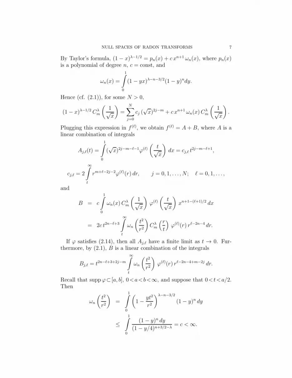
By Taylor’s formula, (1 − x)λ−1/2 = pn(x) + c xn+1 ωn(x), where pn(x)is a polynomial of degree n, c = const, and

ωn(x) =

1∫

0

(1− yx)λ−n−3/2(1− y)ndy.

Hence (cf. (2.1)), for some N > 0,

(1− x)λ−1/2 Cλm

(

1√x

)

=

N∑

j=0

cj (√x)2j−m + c xn+1 ωn(x)C

λm

(

1√x

)

.

Plugging this expression in f (ℓ), we obtain f (ℓ) = A+ B, where A is alinear combination of integrals

Aj,ℓ(t) =

1∫

0

(√x)2j−m−ℓ−1ϕ(ℓ)

(

t√x

)

dx = cj,ℓ t2j−m−ℓ+1,

cj,ℓ = 2

∞∫

t

rm+ℓ−2j−2ϕ(ℓ)(r) dr, j = 0, 1, . . . , N ; ℓ = 0, 1, . . . ,

and

B = c

1∫

0

ωn(x)Cλm

(

1√x

)

ϕ(ℓ)

(

t√x

)

xn+1−(ℓ+1)/2 dx

= 2c t2n−ℓ+3

∞∫

t

ωn

(

t2

r2

)

Cλm

(r

t

)

ϕ(ℓ)(r) rℓ−2n−4 dr.

If ϕ satisfies (2.14), then all Aj,ℓ have a finite limit as t → 0. Fur-thermore, by (2.1), B is a linear combination of the integrals

Bj,ℓ = t2n−ℓ+3+2j−m

∞∫

t

ωn

(

t2

r2

)

ϕ(ℓ)(r) rℓ−2n−4+m−2j dr.

Recall that suppϕ⊂ [a, b], 0<a<b<∞, and suppose that 0<t<a/2.Then

ωn

(

t2

r2

)

=

1∫

0

(

1− yt2

r2

)λ−n−3/2

(1− y)n dy

≤1

∫

0

(1− y)n dy

(1− y/4)n+3/2−λ= c <∞.


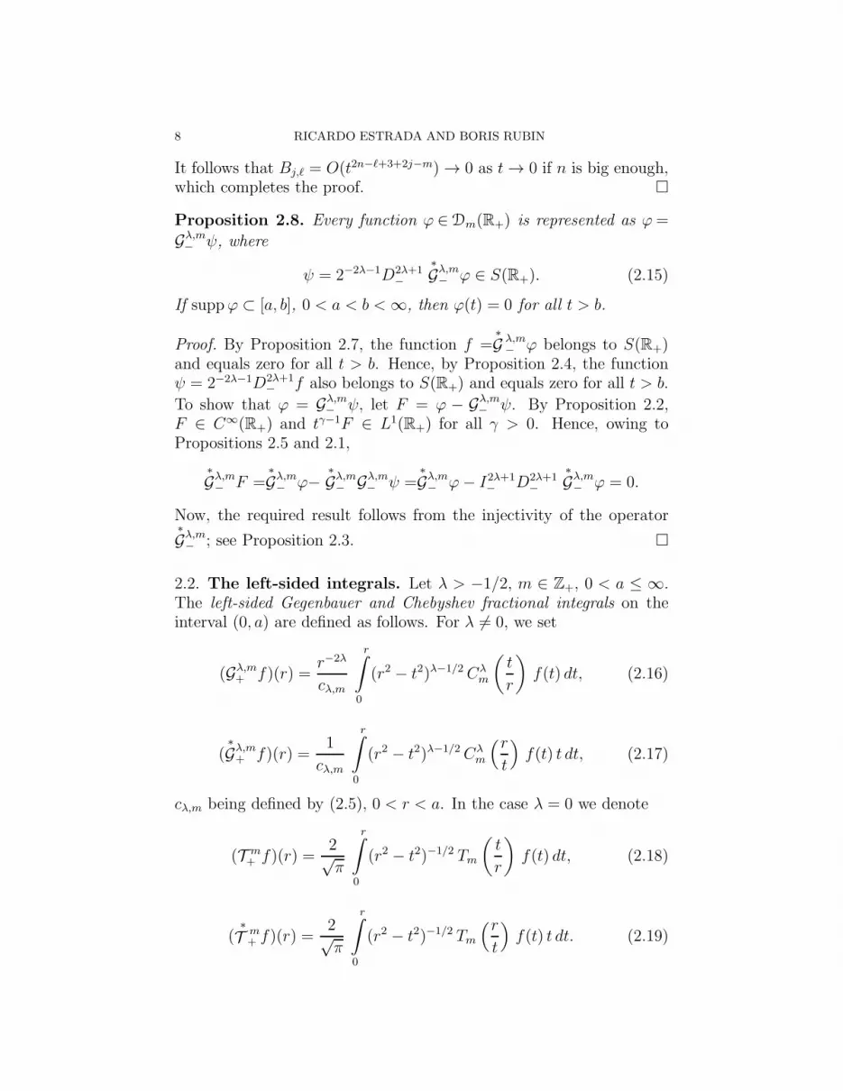
It follows that Bj,ℓ = O(t2n−ℓ+3+2j−m) → 0 as t→ 0 if n is big enough,which completes the proof. �

Proposition 2.8. Every function ϕ ∈Dm(R+) is represented as ϕ=

Gλ,m− ψ, where

ψ = 2−2λ−1D2λ+1−

∗

Gλ,m− ϕ ∈ S(R+). (2.15)

If suppϕ ⊂ [a, b], 0 < a < b <∞, then ϕ(t) = 0 for all t > b.

Proof. By Proposition 2.7, the function f =∗

G λ,m− ϕ belongs to S(R+)

and equals zero for all t > b. Hence, by Proposition 2.4, the functionψ = 2−2λ−1D2λ+1

− f also belongs to S(R+) and equals zero for all t > b.

To show that ϕ = Gλ,m− ψ, let F = ϕ − Gλ,m

− ψ. By Proposition 2.2,F ∈ C∞(R+) and tγ−1F ∈ L1(R+) for all γ > 0. Hence, owing toPropositions 2.5 and 2.1,

∗

Gλ,m− F =

∗

Gλ,m− ϕ−

∗

Gλ,m− Gλ,m

− ψ =∗

Gλ,m− ϕ− I2λ+1

− D2λ+1−

∗

Gλ,m− ϕ = 0.

Now, the required result follows from the injectivity of the operator∗

Gλ,m− ; see Proposition 2.3. �

2.2. The left-sided integrals. Let λ > −1/2, m ∈ Z+, 0 < a ≤ ∞.The left-sided Gegenbauer and Chebyshev fractional integrals on theinterval (0, a) are defined as follows. For λ 6= 0, we set

(Gλ,m+ f)(r) =

r−2λ

cλ,m

r∫

0

(r2 − t2)λ−1/2Cλm

(

t

r

)

f(t) dt, (2.16)

(∗

Gλ,m+ f)(r) =

1

cλ,m

r∫

0

(r2 − t2)λ−1/2Cλm

(r

t

)

f(t) t dt, (2.17)

cλ,m being defined by (2.5), 0 < r < a. In the case λ = 0 we denote

(T m+ f)(r) =

2√π

r∫

0

(r2 − t2)−1/2 Tm

(

t

r

)

f(t) dt, (2.18)

(∗

T m+ f)(r) =

2√π

r∫

0

(r2 − t2)−1/2 Tm

(r

t

)

f(t) t dt. (2.19)


The left-sided integrals are expressed through the right-sided ones bythe formulas

(Gλ,m+ f)(r) =

1

r(Gλ,m

− f1)

(

1

r

)

, f1(t) =1

t2λ+2f

(

1

t

)

; (2.20)

(∗

Gλ,m+ f)(r) = r2λ(

∗

Gλ,m− f2)

(

1

r

)

, f2(t) =1

tf

(

1

t

)

. (2.21)

These formulas combined with Proposition 2.1 give the followingstatement.

Proposition 2.9. Let a > 0, λ > −1/2. The integrals (2.16)-(2.19)are absolutely convergent for almost all r < a under the following con-ditions.(i) For (2.16), (2.18):

a∫

0

tη|f(t)| dt <∞, η =

{

0 if m is even,1 if m is odd.

(2.22)

(ii) For (2.17), (2.19):a

∫

0

t1−m|f(t)| dt <∞. (2.23)

Lemma 2.10. [22, Proposition 3.7] If m = 0, 1, then Gλ,m+ is injective

on R+ in the class of functions satisfying (2.22) for all a > 0. If m ≥ 2,

then Gλ,m+ is non-injective in this class of functions. Specifically, let

fk(t) = tk, where k is a nonnegative integer such that m−k = 2, 4, . . ..

Then (Gλ,m+ fk)(t) = 0 for all t > 0.

An important question is: Are there any other functions in the kernelof the operator Gλ,m

+ rather than fk in Lemma 2.10? Below we give anegative answer to this question under certain conditions, which arevery close to (2.22). Let

κλ,m(t) =

1 if m is even,t1+2λ if m is odd, −1/2 < λ < 0,t (1 + | log t|) if m is odd, λ = 0,t if m is odd, λ > 0.

(2.24)

Given 0 < a ≤ ∞, we denote by L1κ(0, a) the set of all function f on

(0, a) such thata1∫

0

|f(t)|κλ,m(t) dt ≤ ∞ ∀ a1 < a. (2.25)


Clearly, L1loc(0, a) ⊂ L1

κ(0, a).

Lemma 2.11. Suppose that m ≥ 2, M = [m/2], 0 < a ≤ ∞. If

f ∈ L1κ(0, a) and (Gλ,m

+ f)(r) = 0 for almost all 0 < r < a, then

f(t) =M∑

j=1

cj tm−2j a.e. on (0, a) (2.26)

with some coefficients cj.

Proof. We introduce auxiliary functions

ϕm−2k ∈ C∞c (0, a), k ∈ {1, 2, . . . ,M},

satisfyinga

∫

0

tm−2jϕm−2k(t) dt = δj,k =

{

1 if j = k,0 otherwise.

(2.27)

The existence of such functions is a consequence of the general factfrom functional analysis for bi-orthogonal systems; see, e.g., [12, p.160]. We set

cj =

a∫

0

f(t)ϕm−2j(t) dt. (2.28)

Let ω ∈ C∞c (0, a) be an arbitrary test function, and let

ϕ(t) = ω(t)−M∑

j=1

ϕm−2j(t)

a∫

0

sm−2jω(s) ds (∈ C∞c (0, a)). (2.29)

Then for any k ∈ {1, 2, . . . ,M},a

∫

0

tm−2kϕ(t) dt =

a∫

0

tm−2kω(t) dt

−M∑

j=1

[ a∫

0

tm−2kϕm−2j(t) dt

][ a∫

0

sm−2jω(s) ds

]

.

By (2.27), this givesa

∫

0

tm−2kϕ(t) dt = 0 ∀ k ∈ {1, 2, . . . ,M}.

Suppose that ϕ(t) ≡ 0 on some interval (a1, a) with a1 < a, and defineϕ ∈ C∞

c (R+) so that ϕ(t) = ϕ(t) if t ≤ a1 and ϕ(t) = 0 if t > a1.


By Proposition 2.8, ϕ is represented as ϕ=Gλ,m− ψ, where ψ belongs to

S(R+) and equals zero on (a1,∞). Then∞∫

0

f(t)ϕ(t) dt =

∞∫

0

f(t) (Gλ,m− ψ)(t) dt

=

a1∫

0

ψ(r)(Gλ,m+ f)(r) r2λ+1 dr = 0. (2.30)

Hence, by (2.29), (2.30), and (2.28),

a∫

0

f(t)ω(t) dt =

∞∫

0

f(t)

ϕ(t) +M∑

j=1

ϕm−2j(t)

a∫

0

sm−2jω(s) ds

dt

=M∑

j=1

cj

a∫

0

sm−2jω(s) ds =

a∫

0

[

M∑

j=1

cjsm−2j

]

ω(s) ds.

This gives (2.26).To complete the proof, we must justify application of Fubini’s the-

orem in (2.30). Replacing (Gλ,m+ f)(r) according to (2.16), and taking

absolute values, we have

I ≡a1∫

0

|ψ(r)| r drr

∫

0

(r2 − t2)λ−1/2

∣

∣

∣

∣

Cλm

(

t

r

)∣

∣

∣

∣

|f(t)| dt

≤ c

a1∫

0

r dr

r∫

0

(r2 − t2)λ−1/2

(

t

r

)η

|f(t)| dt,

where η = 0 if m is even and η = 1 if m is odd. If η = 0, then

I ≤ c

a1∫

0

|f(t)| dta1∫

t

(r2 − t2)λ−1/2 r dr ≤ c1

a1∫

0

|f(t)| dt <∞.

If η = 1, then

I ≤ c

a1∫

0

|f(t)| t g(t) dt,

where

g(t) =

a1∫

t

(r2 − t2)λ−1/2 dr = t2λa1/t∫

1

(s2 − 1)λ−1/2 ds.


The behavior of g(t) as t → 0 can be easily examined by consideringthe cases indicated in (2.24). This gives

I ≤ c

a1∫

0

|f(t)|κλ,m(t) dt <∞.

�

Lemma 2.11 combined with (2.20) gives the following result for theright-sided Gegenbauer-Chebyshev integrals.Let

κλ,m(t) =

t2λ if m is even,t−1 if m is odd, −1/2 < λ < 0,t2λ−1 (1 + | log t|) if m is odd, λ = 0,t2λ−1 if m is odd, λ > 0.

(2.31)

Given a ≥ ∞, we denote by L1κ(a,∞) the set of all function f on

(a,∞) such that

∞∫

a1

|f(t)| κλ,m(t) dt ≤ ∞ ∀ a1 > a. (2.32)

Lemma 2.12. Suppose that m ≥ 2, M = [m/2], a ≥ 0. If f ∈L1κ(a,∞) and (Gλ,m

− f)(r) = 0 for almost all r > a, then

f(t) =

M−1∑

k=0

ckt2k−m−2λ a.e. on (a,∞) (2.33)

with some coefficients ck.

Lemma 2.12 is an important complement of the following statement,which was proved in [22, Lemma 3.3].

Lemma 2.13. Let λ > −1/2. If m = 0, 1, then Gλ,m− is injective on R+

in the class of functions satisfying (2.8) for all a > 0. If m ≥ 2, then

Gλ,m− is non-injective in this class of functions. Specifically, let fk(t) =t−2λ−k−2, where k is a nonnegative integer such that m− k = 2, 4, . . ..Then (Gλ,m

− fk)(t) = 0 for all t > 0.

According to Lemma 2.12, the functions fk exhaust the kernel of theoperator Gλ,m

− in the space L1κ(a,∞), a ≥ 0.


3. Radon Transforms on Rn

We recall some known facts; see, e.g., [9, 11, 21, 23]. Let Πn be theset of all unoriented hyperplanes in Rn. The Radon transform of afunction f on Rn is defined by the formula

(Rf)(ξ) =

∫

ξ

f(x) dξx, ξ ∈ Πn, (3.1)

provided that this integral exists. Here dξx denotes the Euclideanvolume element in ξ. Every hyperplane ξ ∈ Πn has the form ξ = {x :x · θ = t}, where θ ∈ Sn−1, t ∈ R. Thus, we can write (3.1) as

(Rf)(θ, t) =

∫

θ⊥

f(tθ + u) dθu, (3.2)

where θ⊥ = {x : x · θ = 0} is the hyperplane orthogonal to θ andpassing through the origin, dθu is the Euclidean volume element in θ⊥.We set Zn = Sn−1 × R and equip Zn with the product measure d∗θdt,where d∗θ = σ−1

n−1dθ is the normalized surface measure on Sn−1.Clearly, (Rf)(θ, t) = (Rf)(−θ,−t) for every (θ, t) ∈ Zn.

Theorem 3.1. (cf. [21, Theorem 3.2]) If∫

|x|>a

|f(x)||x| dx <∞ ∀ a > 0, (3.3)

then (Rf)(ξ) is finite for almost all ξ ∈ Πn. If f is nonnegative, radial,and (3.3) fails, then (Rf)(ξ) ≡ ∞.

The dual Radon transform is an averaging operator that takes afunction ϕ(θ, t) on Zn to a function (R∗ϕ)(x) on Rn by the formula

(R∗ϕ)(x) =

∫

Sn−1

ϕ(θ, x · θ) d∗θ. (3.4)

The operators R and R∗ can be expressed one through another.

Lemma 3.2. [22, Lemma 2.6] Let x 6= 0, t 6= 0,

(Aϕ)(x)=1

|x|n ϕ(

x

|x| ,1

|x|

)

, (Bf)(θ, t)=1

|t|n f(

θ

t

)

. (3.5)

The following equalities hold provided that the expressions on eitherside exist in the Lebesgue sense:

(R∗ϕ)(x)=2

|x| σn−1(RAϕ)

(

x

|x| ,1

|x|

)

, (3.6)


(Rf)(θ, t)=σn−1

2|t| (R∗Bf)

(

θ

t

)

. (3.7)

Theorem 3.1 combined with (3.6) gives the following

Corollary 3.3. If ϕ(θ, t) is locally integrable on Zn, then the dualRadon transform (R∗ϕ)(x) is finite for almost all x ∈ R

n. If ϕ(θ, t) isnonnegative, independent of θ, i.e., ϕ(θ, t) ≡ ϕ0(t), and such that

a∫

0

ϕ0(t) dt = ∞,

for some a > 0, then (R∗ϕ)(x) ≡ ∞.

We fix a real-valued orthonormal basis {Ym,µ} of spherical harmonicsin L2(Sn−1); see, e.g., [16]. Here m ∈ Z+ and µ = 1, 2, . . . dn(m), where

dn(m) = (n+ 2m− 2)(n+m− 3)!

m! (n− 2)!(3.8)

is the dimension of the subspace of spherical harmonics of degree m.

Lemma 3.4. [22, Lemma 4.3] Let λ = (n− 2)/2, ϕ(θ, t) = v(t) Ym(θ),where Ym is a spherical harmonic of degree m and v(t) is a locally inte-grable function on R satisfying v(−t) = (−1)mv(t). Then (R∗ϕ)(x) ≡(R∗ϕ)(rθ) is finite for all θ ∈ Sn−1 and almost all r > 0. Furthermore,

(R∗ϕ)(rθ) = u(r) Ym(θ). (3.9)

The function u(r) is represented by the Gegenbauer integral (2.16) (orthe Chebyshev integral (2.18)) as follows.For n ≥ 3 :

u(r) =r−2λ

cλ,m

r∫

0

(r2 − t2)λ−1/2 Cλm

(

t

r

)

v(t) dt = πλ+1/2(Gλ,m+ v)(t),

(3.10)

cλ,m =π1/2Γ(2λ+m) Γ(λ+ 1/2)

2m! Γ(2λ) Γ(λ+ 1).

For n = 2 :

u(r) =2

π

r∫

0

(r2 − t2)−1/2 Tm

(

t

r

)

v(t) dt = π1/2(T m+ v)(t). (3.11)

In parallel with the Radon transforms Rf and R∗ϕ defined above,we shall also consider their exterior and interior versions, respectively.For a > 0, we denote

B+a = {x ∈ R

n : |x| < a}, B−a = {x ∈ R

n : |x| > a},


C+a = {(θ, t) ∈ Zn : |t| < a}, C−

a = {(θ, t) ∈ Zn : |t| > a}.When dealing with the exterior Radon transform, we assume that f isdefined on B−

a and (Rf)(θ, t) is considered for (θ, t) ∈ C−a . Similarly,

in the study of the interior dual Radon transform, it is supposed thatϕ is defined on C+

a and the values of (R∗ϕ)(x) lie in B+a .

Lemma 3.4 implies the following statement; cf. [22, Lemma 4.7].

Lemma 3.5. Let 0 < a ≤ ∞. If ϕ ∈ L1loc(C

+a ) is even, then for almost

all r ∈ (0, a),

(R∗ϕ)m,µ(r)≡∫

Sn−1

(R∗ϕ)(rθ) Ym,µ(θ) dθ=πλ+1/2 (Gλ,m

+ ϕm,µ)(r), (3.12)

where λ = (n − 2)/2 and Gλ,m+ ϕm,µ is the Gegenbauer integral (2.16)

(or the Chebyshev integral (2.18)).

The next theorem gives the description of the kernel of R∗ in termsof the Fourier-Laplace coefficients

ϕm,µ(t)=

∫

Sn−1

ϕ(θ, t) Ym,µ(θ) dθ. (3.13)

Theorem 3.6. Let ϕ(θ, t) be an even locally integrable function on C+a ,

0 < a ≤ ∞.(i) Suppose that ϕm,µ(t) = 0 for almost all t ∈ (0, a) if m = 0, 1, and

ϕm,µ is a linear combination of the form

ϕm,µ(t) =

M∑

j=1

cj tm−2j , cj = const, M = [m/2], (3.14)

if m ≥ 2. Then (R∗ϕ)(x) = 0 for almost all x ∈ B+a .

(ii) Conversely, if (R∗ϕ)(x) = 0 for almost all x ∈ B+a , then, for all

µ = 1, 2, . . . , dn(m) and almost all t < a, the following statements hold.(a) If m = 0, 1, then ϕm,µ(t) = 0.(b) If m ≥ 2, then ϕm,µ(t) has the form (3.14) with some constants cj.

Proof. The statement (i) was proved in [22, Theorem 4.5]. To prove(ii), we observe that if (R∗ϕ)(x) = 0 for almost all x ∈ B+

a , then, by

(3.12), (Gλ,m+ ϕm,µ)(r) = 0 for almost all r ∈ (0, a) and all m,µ. Be-

cause ϕ ∈ L1loc(C

+a ), then ϕm,µ ∈ L1

loc(0, a), and (3.14) is an immediateconsequence of Lemmas 2.10 and 2.11. �

Theorem 3.6 together with Lemma 3.2 imply the following result forthe Radon transform Rf .


Theorem 3.7. Given 0 ≤ a <∞, suppose that∫

|x|>a1

|f(x)||x| dx <∞ for all a1 > a, (3.15)

and let (Rf)(θ, t)= 0 almost everywhere on C−a . Then, for almost all

r > a, all the Fourier-Laplace coefficients

fm,µ(r) =

∫

Sn−1

f(rθ) Ym,µ(θ) dθ

have the form

fm,µ(r) =

0 if m=0, 1,[m/2]∑

j=1

cj r2j−m−n if m≥2,

(3.16)

with some constants cj. Conversely, for any constants cj and any fsatisfying (3.15) and (3.16), we have (Rf)(θ, t) = 0 almost everywhereon C−

a .

Proof. Suppose a > 0 (if a = 0 the changes are obvious). Note that(3.15) implies (Bf)(θ, t) ≡ |t|−nf(θ/t) ∈ L1

loc(C+1/a). If Rf = 0 a.e.

on C−a , then R∗Bf = 0 a.e. on B+

1/a. Hence, by Theorem 3.6, for

t ∈ (0, 1/a) we have

(Bf)m,µ(t)= t−n

∫

Sn−1

f

(

θ

t

)

Ym,µ(θ) dθ=

0 if m = 0, 1,M∑

j=1

cj tm−2j if m ≥ 2.

Changing variable t = 1/r, we obtain (3.16). Conversely, if fm,µ(r) = 0for m = 0, 1, and (3.16) holds for m ≥ 2, then (Bf)m,µ(t) = 0 if

m = 0, 1, and (Bf)m,µ(t) =M∑

j=1

cj tm−2j if m ≥ 2. The last equality is

obvious for t > 0. If t < 0, then

(Bf)m,µ(t) =

∫

Sn−1

(Bf)(θ, t) Ym,µ(θ) dθ

= (−1)m∫

Sn−1

(Bf)(θ, |t|) Ym,µ(θ) dθ

= (−1)mM∑

j=1

cj |t|m−2j =

M∑

j=1

cj tm−2j .


Hence, by Theorem 3.6, R∗Bf = 0 a.e. on B+1/a and therefore, by (3.7),

Rf = 0 a.e. on C−a . �

Remark 3.8. An interesting open problem is the following: What wouldbe the structure of the kernel of the Radon transform R if the action ofR is considered on functions, which may not satisfy (3.15) ?

This question is intimately connected with the remarkable result ofArmitage and Goldstein [2] who proved that there is a nonconstantharmonic function h on Rn, n ≥ 2, such that

∫

ξ|h| < ∞ and

∫

ξh = 0

for every hyperplane ξ; see also Zalcman [25] (n = 2) and Armitage [1].One can easily show that h does not satisfy (3.15). Indeed, suppose thecontrary, and let {hm,µ(r)} be the set of all Fourier-Laplace coefficientsof h(x) ≡ h(rθ). Then for any a > 0 and m ≥ 2,

a∫

0

|hm,µ(r)| dr ≤a

∫

0

dr

∫

Sn−1

|h(rθ)Ym,µ(θ)| dθ

=

∫

|x|<a

|h(x)Ym,µ(x/|x|)|dx

|x|n−1≤ c

∫

|x|<a

dx

|x|n−1<∞.

On the other hand, the inequality

a∫

0

∣

∣

∣

∣

∣

M∑

j=1

cj r2j−m−n

∣

∣

∣

∣

∣

dr <∞

is possible only if all cj are zeros. The latter means that h consists onlyof harmonics of degree 0 and 1. However, by Theorem 3.7, these har-monics must be zero. Hence, h(x) ≡ 0, which contradicts the Armitage-Goldstein’s result.

4. The Cormack-Quinto Transform

The Cormack-Quinto transform

(Qf)(x) =∫

Sn−1

f(x+ |x| θ) d∗θ (4.1)

assigns to a function f on Rn the mean values of f over spheres passing

to the origin. In (4.1), f is integrated over the sphere of radius |x| withcenter at x.There is a remarkable connection between (4.1) and the dual Radon

transform (3.4).


Lemma 4.1. [7, 22] Let n ≥ 2. Then

(Qf)(x) = |x|2−n(R∗ϕ)(x), ϕ(θ, t) = (2|t|)n−2 f(2tθ), (4.2)

provided that either side of this equality exists in the Lebesgue sense.

A consequence of Lemma 4.1 is the following description of the kernelof Q inherited from Theorem 3.6. We recall that the Fourier-Laplacecoefficients of f are defined by

fm,µ(r) =

∫

Sn−1

f(rθ) Ym,µ(θ) dθ, r > 0. (4.3)

Theorem 4.2. Given 0 < a ≤ ∞, suppose that∫

|x|<a1

|f(x)||x| dx <∞ ∀ a1 < 2a, (4.4)

and let (Qf)(x) = 0 for almost all x ∈ B+a . Then all the Fourier-

Laplace coefficients (4.3) have the form

fm,µ(r) =

0 if m=0, 1,[m/2]∑

j=1

cj rm−2j if m≥2,

(4.5)

for almost all r ∈ (0, 2a) with some constants cj. Conversely, for anyconstants cj and any f satisfying (4.4) and (4.5), we have (Qf)(x) = 0a.e. on B+

a .

5. The Funk Transform

The Funk transform F assigns to a function f on a sphere the inte-grals of f over “equators”. Specifically, for the unit sphere Sn in Rn+1

we have

(Ff)(θ) =

∫

{σ∈Sn: θ·σ=0}

f(σ) dθσ, (5.1)

where dθσ stands for the O(n+1)-invariant probability measure on the(n− 1)-dimensional section {σ ∈ Sn : θ · σ = 0}; see, e.g., [9, 11, 23].Let e1, . . . , en+1 be the coordinate unit vectors, R

n=Re1⊕· · ·⊕Ren,

Sn+ = {θ = (θ1, . . . , θn+1) ∈ Sn : 0 < θn+1 ≤ 1}. (5.2)

It is known that kerF = {0} if the action of F is considered on evenintegrable functions. Below we prove that the structure of the kernel ofF is different if the functions under consideration allow non-integrablesingularities at the poles ±en+1, so that the Funk transform still existsin the a.e. sense.


Consider the projection map

Rn ∋ x

µ−→ θ ∈ Sn+, θ = µ(x) =

x+ en+1

|x+ en+1|. (5.3)

This map extends to the bijection µ from the set Πn of all unorientedhyperplanes in Rn onto the set

Sn+ = {θ = (θ1, . . . , θn+1) ∈ Sn : 0 ≤ θn+1 < 1}. (5.4)

cf. (5.2). Specifically, if τ = {x ∈ Rn : x · η = t} ∈ Πn, η ∈ Sn−1 ⊂ Rn,t ≥ 0, and τ is the n-dimensional subspace containing the lifted planeτ + en+1, then θ ∈ Sn

+ is defined to be a normal vector to τ .The above notation is used in the following theorem.

Theorem 5.1. [22, Theorem 6.1] Let g(x) = (1 + |x|2)−n/2f(µ(x)),x ∈ Rn, where f is an even function on Sn. The Funk transform Fand the Radon transform R are related by the formula

(Ff)(θ) =2

σn−1 sin d(θ, en+1)(Rg)(µ−1θ), θ ∈ Sn

+, (5.5)

where d(θ, en+1) is the geodesic distance between θ and en+1.

Theorems 3.7 and 5.1 yield the corresponding result for the kernel ofthe operator F . For f even, it suffices to consider the points θ ∈ Sn,which are represented in the spherical polar coordinates as

θ = η sinψ + en+1 cosψ, η ∈ Sn−1, 0 < ψ < π/2.

The corresponding Fourier-Laplace coefficients (in the η-variable) havethe form

fm,µ(ψ) =

∫

Sn−1

f(η sinψ + en+1 cosψ) Ym,µ(η) dη. (5.6)

Theorem 5.2. Suppose that∫

|θn+1|<α

|f(θ)| dθ <∞ for all α ∈ (0, 1) (5.7)

and (Ff)(θ) = 0 a.e. on Sn. Then all the Fourier-Laplace coefficients(5.6) have the form

fm,µ(ψ)a.e.=

0 if m = 0, 1,

sin−n ψ[m/2]∑

j=1

cj cotm−2j ψ if m ≥ 2,

(5.8)

with some constants cj. Conversely, for any constants cj and any fsatisfying (5.7) and (5.8), we have (Ff)(θ) = 0 a.e. on Sn.


6. The Spherical Slice Transform

The spherical slice transform

(Sf)(γ) =

∫

γ

f(η) dγη, (6.1)

assigns to a function f on Sn the integrals of f over (n−1)-dimensionalgeodesic spheres γ ⊂ Sn passing through the north pole en+1. Everygeodesic sphere γ can be indexed by its center ξ = (ξ1, . . . , ξn+1) in thethe closed hemisphere

Sn+ = {ξ = (ξ1, . . . ξn+1) ∈ Sn : 0 ≤ ξn+1 ≤ 1},

so that

γ ≡ γ(ξ) = {η ∈ Sn : η · ξ = en+1 · ξ}, ξ ∈ Sn+.

Using spherical polar coordinates, for ξ ∈ Sn+ we write

ξ = θ sinψ + en+1 cosψ, θ ∈ Sn−1 ⊂ Rn, 0 ≤ ψ ≤ π/2,

γ ≡ γ(ξ) ≡ γ(θ, ψ), (Sf)(γ) ≡ (Sf)(ξ) ≡ (Sf)(θ, ψ).

Then

γ(ξ) = {η ∈ Sn : η · ξ = cosψ}.Consider the bijective mapping

Rn ∋ x

ν−→ η ∈ Sn \ {en+1}, ν(x) =2x+ (|x|2 − 1) en+1

|x|2 + 1. (6.2)

The inverse mapping ν−1 : Sn \ {en+1} → Rn is the stereographicprojection from the north pole en+1 onto Rn = Re1 ⊕ · · · ⊕ Ren. If

η = ω sinϕ+ en+1cosϕ, ω ∈ Sn−1, 0 < ϕ ≤ π,

then x = ν−1(η) = sω, s = cot(ϕ/2).

Lemma 6.1. [22, Lemma 7.2] The spherical slice transform on Sn andthe hyperplane Radon transform on Rn are linked by the formula

(Sf)(θ, ψ) = (Rg)(θ, t), t = cotψ, (6.3)

g(x) =

(

2

|x|2 + 1

)n−1

(f ◦ ν)(x), (6.4)

provided that either side of (6.3) is finite when f is replaced by |f |.


To describe the kernel of the operator S, we use the spherical har-monic decomposition of f(η) = f(ω sinϕ+en+1 cosϕ) in the ω-variable.Let

fm,µ(ϕ) =

∫

Sn−1

f(ω sinϕ+ en+1 cosϕ) Ym,µ(ω) dω. (6.5)

Then Theorems 3.7 and Lemma 6.1 imply the following statement.

Theorem 6.2. Suppose that∫

ηn+1>1−ε

|f(η)|(1− ηn+1)1/2

dη <∞ ∀ ε ∈ (0, 2], (6.6)

and (Sf)(ξ) = 0 for almost all ξ ∈ Sn+. Then all the Fourier-Laplace

coefficients (6.5) have the form

fm,µ(ϕ)a.e.=

0 if m=0, 1,

(1−cosϕ)1−n

[m/2]∑

j=1

cj

(

tanϕ

2

)n+m−2j

if m≥2,(6.7)

with some constants cj. Conversely, for any constants cj and any fsatisfying (6.6) and (6.7), we have (Sf)(ξ) = 0 a.e. on Sn

+.

7. The Totally Geodesic Radon Transform on the

Hyperbolic Space

Let En,1 ∼ Rn+1, n ≥ 2, be the (n+1)-dimensional pseudo-Euclideanreal vector space with the inner product

[x, y] = −x1y1 − . . .− xnyn + xn+1yn+1. (7.1)

The real hyperbolic space Hn is realized as the upper sheet of the two-sheeted hyperboloid in En,1, that is,

Hn = {x ∈ E

n,1 : [x, x] = 1, xn+1 > 0};see [10]. The corresponding one-sheeted hyperboloid is defined by

∗

Hn = {x ∈ En,1 : [x, x] = −1}.

The totally geodesic Radon transform of a function f on Hn is anintegral operator of the form

(Rf)(ξ) =

∫

{x∈Hn: [x,ξ]=0}

f(x) dξx, ξ ∈∗

Hn, (7.2)

and represents an even function on∗

Hn; see [4, 10, 11].


Using the projective equivalence of the operator (7.2) and the hy-perplane Radon transform R, as in [22, Lemma 8.3] (see also [13, 3]),we obtain the following kernel description, which is implied by The-orem 3.7. We write x ∈ Hn in the hyperbolic polar coordinates asx = θ sinhr + en+1 coshr, θ ∈ Sn−1, r > 0, and consider the Fourier-Laplace coefficients

fm,µ(r) =

∫

Sn−1

f(θ sinhr + en+1coshr) Ym,µ(θ) dθ. (7.3)

Theorem 7.1. Let∫

xn+1>1+δ

|f(x)| dx

xn+1<∞ ∀ δ > 0, (7.4)

and let (Rf)(ξ) = 0 a.e. on∗

Hn. Then all the Fourier-Laplace coeffi-cients (7.3) have the form

fm,µ(r)a.e.=

0 if m=0, 1,

sinh−n[m/2]∑

j=1

cj cothm−2j ψ if m≥2,

(7.5)

with some constants cj. Conversely, for any constants cj and any f

satisfying (7.4) and (7.5), we have (Rf)(ξ) = 0 a.e. on∗

Hn.

8. Conclusion

The list of projectively equivalent Radon-like transforms, the kernelsof which admit effective characterization using the results of the presentpaper, can be essentially extended. For example, one can obtain kerneldescriptions of the exterior/interior analogues of the Radon-like trans-forms (and their duals) from Sections 4-7. We leave this useful exerciseto the interested reader.

References

[1] D. H. Armitage, A non-constant continuous function on the plane whoseintegral on every line is zero, Amer. Math. Monthly 101 (1994), no. 9,892–894.

[2] D. H. Armitage and M. Goldstein, Nonuniqueness for the Radon trans-form, Proc. Amer. Math. Soc. 117 (1993), no. 1, 175–178.

[3] C. A. Berenstein, E. Casadio Tarabusi, and A. Kurusa, Radon transformon spaces of constant curvature, Proc. Amer. Math. Soc. 125 (1997),455–461.


[4] C. A. Berenstein and B. Rubin, Radon transform of Lp-functions on theLobachevsky space and hyperbolic wavelet transforms, Forum Math. 11(1999), 567–590.

[5] J. Boman, Holmgren’s uniqueness theorem and support theorems for realanalytic Radon transforms, Geometric analysis (Philadelphia, PA, 1991),23–30, Contemp. Math. 140, Amer. Math. Soc., Providence, RI, 1992.

[6] J. Boman and F. Lindskog, Support theorems for the Radon transformand Cramer-Wold theorems, J. of Theor. Probability 22, (2009), 683–710.

[7] A. M. Cormack and E. T. Quinto, A Radon transform on spheres throughthe origin in Rn and applications to the Darboux equation, Trans. Amer.Math. Soc. 260 (1980), no. 2, 575–581.

[8] A. Erdelyi (Editor), Higher transcendental functions, Vol. I and II,McGraw-Hill, New York, 1953.

[9] I. M. Gel’fand, S. G. Gindikin, andM. I. Graev, Selected topics in integralgeometry, Translations of Mathematical Monographs, AMS, Providence,Rhode Island, 2003.

[10] I. M. Gel’fand, M. I. Graev, and N. Ja. Vilenkin, Generalized functions,Vol 5, Integral geometry and representation theory, Academic Press,1966.

[11] S. Helgason, Integral geometry and Radon transform, Springer, NewYork-Dordrecht-Heidelberg-London, 2011.

[12] L. V. Kantorovich and G. P. Akilov, Functional analysis in normedspaces, (International Series of Monographs in Pure and Applied Math-ematics, Volume 46). New York, Macmillan, 1964.

[13] A. Kurusa, Support theorems for totally geodesic Radon transforms onconstant curvature spaces, Proc. Amer. Math. Soc. 122 (1994), 429–435.

[14] D. Ludwig, The Radon transform on Euclidean space, Comm. Pure Appl.Math. 19 (1966), 49–81.

[15] O. I. Marichev, Method of evaluation of integrals of special functions,Nauka i Technika, Minsk, 1978 (In Russian); Engl. translation: Handbookof integral transforms of higher transcendental functions: Theory and

Algorithmic Tables, Ellis Horwood Ltd., N. York etc.; Halsted Press,1983.

[16] C. Muller, Spherical harmonics, Springer, Berlin, 1966.[17] A. P. Prudnikov, Y. A. Brychkov, and O. I. Marichev, Integrals and se-

ries: special functions. Gordon and Breach Sci. Publ., New York-London,1986.

[18] E. T. Quinto, Null spaces and ranges for the classical and spherical Radontransforms, J. Math. Anal. Appl. 90 (1982) 408–420.

[19] , Singular value decompositions and inversion methods for theexterior Radon transform and a spherical transform, Journal of Math,Anal. and Appl. 95 (1983), 437–448.

[20] B. Rubin, Fractional Integrals and Potentials. Pitman Monographs andSurveys in Pure and Applied Mathematics 82. Longman, Harlow, 1996.

[21] , On the Funk-Radon-Helgason inversion method in integral ge-ometry, Cont. Math. 599 (2013), 175–198.


[22] , Gegenbauer-Chebyshev integrals and Radon transforms,Preprint 2015, arXiv:1410.4112v2.

[23] , Introduction to Radon transforms (with elements of fractionalcalculus and harmonic analysis), Encyclopedia of Mathematics and ItsApplications, 160, Cambridge University Press, 2015 (to appear).

[24] S. G. Samko, A. A. Kilbas, and O. I. Marichev, Fractional integrals andderivatives. Theory and applications, Gordon and Breach Sc. Publ., NewYork, 1993.

[25] L. Zalcman, Uniqueness and nonuniqueness for the Radon transform,Bull. London Math. Soc. 14 (1982), no. 3, 241–245.

Department of Mathematics, Louisiana State University, Baton Rouge,

LA, 70803 USA

E-mail address : [email protected]

Department of Mathematics, Louisiana State University, Baton Rouge,

Louisiana 70803, USA

E-mail address : [email protected]

null spaces of radon transforms

Documents