Normal offsets for digital image compression

Ward Van Aerschot? ∗, Maarten Jansen

Adhemar Bultheel

? Dept. of Comp. Science, K.U.Leuven, Celestijnenlaan 200A,B 3001 Leuven (Belgium) Dept. of Maths & Comp. Science,TU/e, 5600 MB Eindhoven (The Netherlands)

Dept. of Comp. Science, K.U.Leuven, Celestijnenlaan 200A,B 3001 Leuven (Belgium)

ABSTRACT

The wavelet transform is well suited for approximation of two dimensional functions with certain smoothness character-istics. Also point singularities, e.g. texture-like structures, can be compactly represented by wavelet methods. However,when representing line singularities following a smooth curve in the domain – and should therefore be characterizes bya few parameters – the number of needed wavelet coefficients rises dramatically since fine scale tensor product wavelets,catching these steep transitions, have small local support. Nonetheless, for images consisting of smoothly colored regionsseparated by smooth contours most of the information is comprised in line singularities (e.g. sketches). For this classofimages, wavelet methods have a suboptimal approximation rate due to their inability to take advantage of the way thosepoint singularities are placed to form up the smooth line singularity. To compensate for the shortcomings of tensor productwavelets there have already been developed several schemeslike curvelets,2 ridgelets,4 bandelets10 and so on. This paperproposes a nonlinearnormal offsetdecomposition method which partitions the domain such thatline singularities are ap-proximated by piecewise curves made up of borders of the subdomains resulting from the domain partitioning. Althoughmore general domain partitions are possible, we chose for a triangulation of the domain which approximates the contoursby polylines formed by triangle edges. The nonlinearity lies in the fact that the normal offset method searches from themidpoint of the edges of a coarse mesh along the normal direction until it pierces the image. These piercing points havethe property of being attracted towards steep color value transitions. As a consequence triangular edges are attractedto lineup against the contours.

Keywords: normal offsets , multiresolution, nonlinear approximation, piecewise smooth

1. INTRODUCTION

The goal of this paper is to compactly represent the class of images consisting of smoothly gray colored areas separatedby smooth contours. These images can also be seen as a piecewise smooth surface lying in the three dimensional space.This surface will be approximated by a meshM†. Mostly the locations of the verticesV- which define the geometry ofthe mesh- are represented by a list of indexed triples(xi, yi, zi). Everyzi coordinate has to be accompanied by its domainlocation(xi, yi) . However, one can also start from a coarse meshMj and construct a new meshMj+1 by adding newverticesVj+1 expressed in terms of old vertices. Normal meshes accomplish this by expressing a vertex as lying on distancefrom the midpoint of two old mesh pointsVj in a normal direction. So, only one scalar value is needed to fix a vertex’sposition. The meshes that can be built with such a method are called normal meshes. Normal meshes can be representedby a sequence of scalar values and as a consequence need threetimes less input data than the vector representation. Normalapproximations of curves have already extensively been studied in [Daubechies et al.]8 . In [Guskov et al.]7 normal meshesare constructed for compact representation of three dimensional surfaces and in [Jansen et al.]9 normal offsets are used forpiecewise smooth surface approximation in the functional setting. This paper investigates the suitability of normal offsets

∗Ward Van Aerschot is a doctoral student of the Flemish Fund for Scientific Research (FWO - Vlaanderen). This work was supported by the FWOproject G.0431.05.

†In what follows we assume that a meshM is defined by the triple(V, E ,F)

as a tool for image compression. Some specific adjustments will be made to meet this objective. The paper is organized asfollows. Section 2 briefly describes the concept of normal offsets. Section 3 puts forward some problems that arise whenextending the concept as described in Section 2 towards digital images. Section 4 discusses the approximation propertiesconsidering the class of images at interest, while Section 5examines compression properties.

2. NORMAL OFFSETS

2.1. Concept

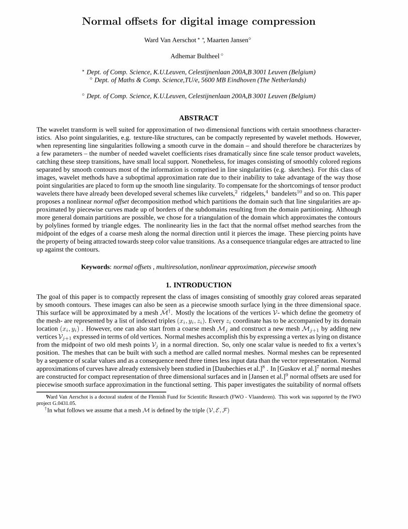
In the one dimensional setting the normal offset method can best be explained when compared to a linear prediction stepof the lifting scheme,12 a tool used for wavelet decompositions. Both construct a polyline interpolating several samplepoints. Between each two subsequent sample points, both methods will predict a new point as lying at the midpoint of aline connecting the two sample points. In most cases the realfunction value will differ from this prediction.

f(x)

Verticaldisplacement

Prediction

x

(a) Wavelets

Normaldisplacement

Piercing point

Prediction

f(x)

x

(b) Normal offsets

Figure 1. Conceptual comparison between wavelets and normal offsets

As for wavelets, the prediction stepstores a detail coefficient being the dif-ference between the predicted function valueand the real function value on the samelocation. This detail coefficient can beseen as a vertical offset with respect tothe ordinate-axis (Figure 1(a)). In con-trast, the normal offset method will searchfor a piercing point along a ray normal tothe line segment until it pierces the func-tion (Figure 1(b)). The signed distancebetween the prediction point and the pierc-ing point is kept. The old sample pointsare connected with the new points, form-ing an interpolating polyline approximation of the function. Note that the lifting step acts on functionsy = f(x) whilethe normal offset method considers every point as lying on a curvec(x, y) = 0 in the plane. Working with a geometricconstruction like normal offsets on a discrete function introduces its own peculiarities. A one dimensional discrete functionis defined by a sequence of couples(xi, yi), i = 0 . . .M on the basis of which we can construct a piecewise constant func-tion on [x0, xM ] asf =

∑Mi=0

yiΠ(x − xi), with Π the rectangle function. This function has a staircase-likeshape withdiscontinuities at almost every knot. Therefore, the use ofvertical offsets is favored since one easily finds a piercingpointas the corresponding function value. When using a normal search direction one cannot expect to always pierce throughthe ceiling of at least one of the rectangle functions. To provide a solution, the graph of the function will be completed byvertical lines at the discontinuities similar to the dashedline in Figure 1(b). The normal line will now be searched untilit pierces this connected curvec, the piercing point will beplacedon this line above the previously visitedxl. An extravertical offset will be introduced to encode the distance between the piercing point and(xl, f(xl)).

3. FROM CONTINUOUS SURFACES TO DISCRETE IMAGES

For applications such as image compression, the previous scheme has to be extended to work on two dimensional functions.These functions defined on domainΩ can also be seen as surfaces lying in a three dimensional space. The surface is nowbeing approximated by an interpolating triangular mesh. When extending normal polylines to normal meshes extra degreesof freedom have to be filled in. A normal direction can be defined in several ways, with respect to different hyperplanes.Another problem arises from the use of adiscreteset of domain points making up the regular grid, where special careshould be taken in edge-refinement methods (rasterization). The next paragraphs are devoted to matters concerning thedefinition of the normal direction in the two dimensional setting and aspects related to discrete edge refinement.

3.1. Normal direction

First of all we assume a base meshM0 already at our disposal. From this mesh we want to build a meshcontaining moredetail about the image surface. The projection of the straight line graph induced by the edges and vertices(E ,V) of M,defines a partition∆ = T onΩ. Jansen et al. defined the normal direction as going through the midpoint of an edge andstanding normal to a surface fitting its four neighbor vertices. Another approach could be shooting a ray normal to meshtriangular faceF while going through its center. The main drawback of such methods is that the projection on the domainof the piercing points is not constrained to be local, herebydestroying previous existing topologies. By local we mean thatthe piercing points lie in the same subdomainT as the vertices they depend on.

−2

−1

0

1

2

3

−2

−1

0

1

2

30

1

2

3

4

5

6

(a) Search direction normal toF and starting from its center

−2

−1

0

1

2

3

−2

−1

0

1

2

30

1

2

3

4

5

6

(b) Search direction normal toE , starting from its midpoint andlying in a vertical plane

Figure 2. (Left) Piercing points are found outside the triangles domain. (Right)Piercing points are found with their location on the domain boundary

Instead of global topological refinementswe opt for a local refinement strategy. Assuch, the different subdomains keep their in-dependence during further decomposition. Hav-ing a local refinement scheme subsequent par-titions will be nested, i.e.∆j ⊂ ∆j+1 . . ..This assures that, when shrinking (or thresh-olding) some normal offsets – thereby chang-ing the location of the mesh pointsV andtheir projection– the topology will be unaf-fected. This makes the method topologicallymore stable. The locality of such methodcould be forced by letting the search for apiercing point not exceed the boundary of itsoriginating domain triangleT . Or, it couldbe developed such that piercing points are al-ways found within the subdomain the normalray was shooted by restricting the ray to lie ina plane perpendicular to thexy-plane. Thisresults in an edge refinement procedure anda quad-tree structured subdivision scheme. It is this definition of a normal direction that we will use from now on.

3.2. Discrete edge refinement

The restriction of the normal direction to lie in a vertical plane results in an edge refinement method. The edges of eachT ∈ Ω are recursively subdivided. All works fine when applied to a continuous domainΩ = [0, 1]2 on whichf(x, y) isdefined. The prediction point lies exactly above the midpoint of the edge. In the digital setting, the point lying exactlyinbetween two end points of a triangle edge will almost never coincide with some pixel center. A roundoff to the nearestpixel center and a connection with both end points will result in a penetration of other triangles or in pixel locations beingmissed out. To overcome these problems domain edges are being defined as a set of pixel locations. And its subdividedparts are forced to use a subset of this set. The midpoint (i.e. the location of the prediction point) is simply expressed as anindex halfway between begin and end point of the edge. These pixel locations are the result of a rasterization process. Inthis paper we used the Bresenham algorithm1 which efficiently implements such a rasterization.

4. APPROXIMATION WITH NORMAL OFFSETS

4.1. Comparison with wavelets

The strength of the compression characteristics of a methodis mostly measured by itsn-term approximation rate withrespect to a certain space of functions. In approximation theory, it is well known that certain function norms (like Besovnorms) are equivalent to a sequence norm applied to the wavelet coefficients. It is also known that functions, which can beapproximated by a nonlinearwaveletapproximation method with a certain rate, are characterized as lying in an interpola-tion space between anLp space and a Besov space (we refer to Devore3 for a deeper study of nonlinear approximation).

In what follows we call the Horizon classH the class of images consisting of uniformly colored region separated by asmooth contour. Since the Horizon classH consists of imagesf(x, y) that also belong toB1/2

2,∞, normal offsetapproxima-tion outperforms the bestn-termwaveletapproximation rate which isO(n−1/2).6 The reason for this is that only a smallsubset of images belonging to certain smoothness spaces represent realistic images. Furthermore only a small subset ofthe images belonging to certain smoothness spaces also belong toH. From the connection between wavelet coefficientsand Besov norms it can be seen that the order in which the coefficients in each resolution level appear does not matter. Ineach resolution level, swapping the position of the waveletcoefficients –and thus destroying artifacts like edges– does notchange the smoothness characteristics of the image after reconstruction. Also sign reversal of wavelet coefficients–becausewavelets form unconditional bases for Besov spaces– does not affect the Besov norm. However, the reconstructed imageis unlikely to resemble a realistic image. Although smooth edges could be represented (or at least approximated) by fewparameters, wavelets do not take advantage of this redundancy in the domain. Where wavelets are well suited to catchpoint singularities they fail when it comes to line singularities. It should be clear that most likely there exist methods thatexploit the inherent properties of images∈ H to achieve a better approximation rate.

Y

Z

X

00

01 10 11

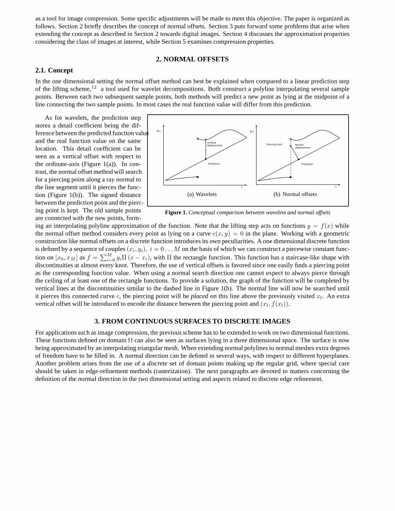
(a) (Top left) Three piercing points together with the old meshpoint Vj are shown. No edges are yet be defined. (Bottomright) Four possible interconnections between the set of pierc-ing points and verticesVj .

DRAWNCHECKEDENG APPRMGR APPR

UNLESS OTHERWISE SPECIFIEDDIMENSIONS ARE IN MILLIMETERS

ANGLES ±X.X°2 PL ±X.XX 3 PL ±X.XXX

NAMEAdministrator

DATE07/28/05 SOLID EDGE

EDS-PLM SOLUTIONSTITLE

SIZEA2

DWG NO REV

FILE NAME: 3mogelijkheden.dftSCALE: WEIGHT: SHEET 1 OF 1

REVISION HISTORYREV DESCRIPTION DATE APPROVED

a)

d)

b)

c)

(b) Piercing points are always situated between the dis-continuity and the midpoint of the edge. The gray arearepresentsΩ wheref(x, y)Ω ≡ 1. The dotted line mustbe part of the chosen interconnection since they subdi-vide with the maximum number of perfect approximatedsubtriangles.

Figure 3.

Normal offsetstry to approximate the line singularities by approximatingthe contourc (x, y) = 0 by a polyline,consisting of triangle edges. When constructing a higher detailed mesh the new piercing points have to be connected byedges and a new partition∆j+1 ⊂ ∆j is defined. If one refines all triangles as the first one shown atthe bottom of Figure3(a) no additional information about the mesh topology has to be stored. The compressed data only consists of geometricalinformation of which the topology is fixed in advance. Unfortunately, with this scheme we cannot expect that triangleedges, making up the polyline, take on a smooth path along thecontour, but rather a tooth-shaped one with many segmentscrossing the contour. We therefore introduce some extra topological parameters – with an increase of the storage cost forthe reconstruction of intermediate normal meshes – as long as it pays off at the level of compression when those meshesare truncated. The four possible interconnections of piercing points and previous vertices are depicted in Figure 3(a).

For images ofH we propose to take the interconnection that has at least one edge parallel to thexy−plane (and thereshould be at least one such interconnection). If there are several possibilities left, choose the one which minimizes theLp error. In case of more minima, we choose the one which partitions its parent triangle such that the smallest angle ismaximal (regularization). Algorithm 1 gives an overview ofthe full normal offset method for images∈ H. Since testingif there exist some edges that have equal function values is less computational demanding than calculating anLp-error,

line 13 is tailor made for images of the Horizon class, which causes a speedup in execution time.

Algorithm 1 Normal Offset algorithm for Images∈ H

Require: a base meshM0 consisting of verticesV and edgesE .1: Express eachE ∈ M0 by the sequenceli , i = 0, 1,−1, 2, ,−2, 3,−3, . . . |E|

2li ∈ N × N, as the output of the

Bresenhaml−

|E|2

, l |E|2

algorithm.

2: for j=1 . . . J do3: for each triangleFk in Mj do4: for eachEm,k ∈ ∂Fk: do5: calculate the normal linen(x, y) = z.6: d0 := n(li(0)) − f(li(0)).7: repeat8: k := k + 19: dk := n(li(k)) − f(li(k))

10: until di changes sign11: pm,k :=

lik−1

, n(lik−1)

12: end for13: G := g, the set of interconnections as depicted in Figure 3(a).14: Deleteg of which the number of edges parallel to thexy−plane is not maximal15: if #G 6= 1 then16: Deleteg of which εLp is not minimal17: if #G 6= 1 then18: Deleteg of which the minimal angle is not maximal19: end if20: end if21: g∗ := g22: for all edgesE∗ ∈ g∗ do23: if both end points are newly found piercing pointsthen24: Assign to edge the set of pixels by running the Bresenham algorithm.25: else26: Assign locations in accordance with there parents set oflocations. (this can be done by an index).27: end if28: end for29: end for30: end for

After this decomposition we have a tree structured hierarchical triangulation at our disposal. From this tree we selectthose normal offsets which produce a triangular meshM with the smallest difference with respect tof(x, y). This isdone by a pruning algorithm which prunes all descendants of aleaf’s parent such that the introduced error is as small aspossible. It can be proven that the normal offset method as described in Algorithm 1 has ann-term approximation rateof εL1

= O(n−1). Figure 4 shows the output of Algorithm 1 followed by ann-terms a pruning algorithm applied to thedigital image of Figure 4(a).

5. COMPRESSION

5.1. Lossless CompressionTo reduce the amount of data, all coefficients should be stored with the smallest possible number of bits. This can be reachedwhen we know something about the probability of coefficient values in terms of a PDF (probability density function) inadvance. Entropy encoders , like Huffman encoders, map eachvalue of a finite alphabetA to a string of bits (codeword),(C : A → 0, 1

r) , such that the expected number of bits is minimized.

Because digital images are represented as2 1

2D surfaces (surfaces lying in a 3 dimensional space represented by a 2

dimensional function) one can use thexy−plane as projection plane. The trick is not to store the signed length of the

(a)

0.5 1 1.5 2 2.5 35

5.5

6

6.5

7

7.5

8

log10

n

log 10

||ε|

| l 1

log10

||ε||l1

(n)

Clog10

n−1

(b)

Figure 4. Subfigure (a) depicts the original image∈ H with c(x, y) = x2 + y2 − R2 ≡ 0. Subfigure (b) shows the approximation rateof the normal offset method applied to Figure 4(a).

normal offsetnj,k but rather the signed lengthi(nj,k) of its projection on thexy-plane. The absolute value of the lattercan be seen as the number of cubes to be traversed along the rasterized line starting from the midpoint of the edge till thepiercing point is reached. The sign denotes in which direction to travel.

DRAWNCHECKEDENG APPRMGR APPR

UNLESS OTHERWISE SPECIFIEDDIMENSIONS ARE IN MILLIMETERS

ANGLES ±X.X°2 PL ±X.XX 3 PL ±X.XXX

NAMEAdministrator

DATE05/30/05 SOLID EDGE

EDS-PLM SOLUTIONSTITLE

SIZEA2

DWG NO REV

FILE NAME: distrubutie.dftSCALE: WEIGHT: SHEET 1 OF 1

REVISION HISTORYREV DESCRIPTION DATE APPROVED

L

α

Ηα

α

d i

v

Η/2

Figure 5. Crosscut of an image∈ H containing a contour.

It can easily be seen thati(nj,k) is bounded byhalf the rasterized edge length, and that these boundswill monotonically decrease as the resolution levelj

rises. However the magnitude of the normal indicesthemselves need not to decrease. These normal in-dices can be seen asrandomvariablesX with valuescoming from an alphabetA of sizeN .

A = 0, . . . , N − 1, with N =

⌈

|EXYj−1,k|2

⌉

. As-

sume we can model this source of information bymeans of a Markov process. Then, every symbolXi has a probabilitypi. The amount of informationcontained in a symbol sequence is measured by theentropyS:

S = −

N∑

i=1

pi log2(pi)

For a comprehensive reading about information theory we refer to the paper of C.E. Shannon.11 This entropy representsthe minimal number of bits per symbol, under the assumption that the sequence of symbols is very large. If we would notreckon with the statistical properties of the information source and represent allN possibilities withlog2 N bits and anequal probability,S will reach its maximum valueSmax = log2 N .

We will now give an a priori PDF of these normal indices when given two edge points, consideringfΩ(x, y) ∈ H,whereΩ = [0, 1] × [0, 1] ⊂ R × R . If the distanced as depicted in Figure 5 is uniformly distributed on the interval [0, L]

andH < L then the distribution ofinj,k– the orthogonal projection of the normal offsets on thexy-plane – will be:

p(inj,k) =

1

L −H tan α2

< inj,k< H tan α

2

1

2

(

1 −(

HL

)2)

inj,k= ±H tan α

2

0∣

∣inj,k

∣

∣ > H tan α2

tan

2

H α− tan

2

H αi

( )p i

1

l

21

12

H

l

− 2

11

2

H

l

−

Figure 6.The above picture represents the PDF if the distanced has a uniform distribution on[0, L]. The smaller the heightH comparedto L, the larger the probability ati = ±H tan α

2(large probability to pierce through the one of the horizontal regions) and the lower the

uniform distributed probability between−H tan α

2, H tan α

2

0 0.1 0.2 0.3 0.4 0.5 0.6 0.7 0.8 0.9 10.1

0.2

0.3

0.4

0.5

0.6

0.7

0.8

0.9

1

1.1

l=8

l=16

l=32 l=64 l=128 l=256

H/l

Ent

ropy

/log 2 l

Figure 7. S ∈ [0, 1]. For some values ofL the entropyS reaches valueslarger thanlog2 L. This is because we used a continuous set of values in-stead of finite setA. For larger L, this continuous expression approximatesthe discrete one. WhenH/L = 1 the PDF is a uniform distribution over[−L, L] andS takes on its maximal value.

In Figure 7 the value ofS is plotted for differentvalues ofL. The Figure also illustrates that whenL

rises the profit due to the a priori known distributiongets larger for a larger part ofH-values.

The entropy encoder generates a reduction of datawithout loss of information. In view of rate distor-tion theory, this agrees with a reduction of the dis-tortion even at the very beginning of the R/D-curve.This lossless compression is a full gain to the bitrate. Table 8(a) shows results for several test im-ages. Figure 8(b) schematically represents on whichdata the decoder and encoder can lay their hands onto produce a table which contains a codeword foreach possible value (and visa versa).

As a last step, all symbols can then be processedby an arithmetic encoder. This encoder maps all thedata –considering the frequency of the codewords– into one string of bits (representing a fractionalvalue between0 and 1) uniquely representing theoriginal data.5

Figuref(x, y) f(x, y) ∈ H? compression ratio

circle (Figure 4(a)) yes 1:2block (Figure 9(a)) yes 1:2

Lena no 5:7(a) This table shows some compression ratios on the normal indicesfor several test images.

Entropy coder (decoder)

Lenght & Height of Edge

Codeword

Normal index

PDF Model

(b) Schematic illustration of the entropy encoder and decoder.On the basis of the data of the edge , the normal indices can bemapped to codewords and visa versa.

Figure 8.

6. RESULTS AND CONCLUSIONS

We have tested our normal offset algorithm (Algorithm 1) on different kinds of test images, i.e. an Horizon class image,an image with smoothly colored regions separated by smooth contours and a realistic picture better known as ‘Lena’. Notethat the Horizon class is a subset of the class of images with smoothly colored regions and smooth contours which in itsturn is a subset of the more general class of realistic pictures. For all images, the algorithm started with a base meshM0

consisting of two triangles built from the four corners of the domain. In Figure 9 the normal offset decomposition of thetop image∈ H is subjected to an n-terms selection algorithm. We see that the triangulation needs few coefficients to alignalong the straight line discontinuity. In Figure 10 an Horizon class image with a curved contour is shown together withseveraln-terms approximations. If we compare this result with Figure 11 where the same image is approximated by abiorthogonal(2, 2) wavelet method with the same number of terms, we see that the contours are far more blocky. At last,the output for the ‘Lena’ picture is shown in Figure 13. In Figure 13(a) a pruned domain triangulation is shown. Evenwithout color information we can distinguish Lena’s shoulder, face contours, border of the mirror and parts of her hat.These are typically areas which own the properties suited for out normal offset algorithm. Figures 13(b)-13(d) representan intermediate mesh at resolution levelj = 6. From Figure 13(d) we notice that particular areas are well approximatedwhile sharp curved areas, like Lena’s nose and eyes, show deviations from the original image.

Instead of using such a simple base meshM0 as used in our experiments, further research will involve base mesheswhich already represent the basic geometry of the image. This will demand more data to store the initial mesh –as it willbe represented by a vector representation rather than a scalar one – but will lead to better quality approximations afterward.In the hope artifacts as seen in Figure 10 will disappear.

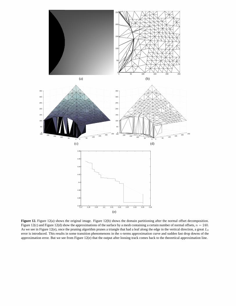
As we see in Figure 12, once the pruning algorithm prunes a triangle that had a leaf along the contour in the verticaldirection, a greatL2 error is introduced. The overall rate is the same as for the Horizon class images.

For images with smoothly colored areas and images like ‘Lena’, algorithm 1 will be expanded to use other norms forinterconnection rather than solely anL2 distance norm. Curvature norms will be combined with distance norms – like theL2 norm– which construct interconnections that resemble a similar shape as the above surface. If the shapes matches thesurface for some parts of an intermediate mesh, next refinements will have it easier to adapt towards the image surface. Asa consequence we could expect a better approximation rate towards these images similar to that of images of the Horizonclass.

0

50

100

150

200

2500 50 100 150 200 250

(a) original image

0

50

100

150

200

2500 50 100 150 200 250

(b) base mesh and 2 offsets

0

50

100

150

200

2500 50 100 150 200 250

(c) base mesh and 5 offsets

0

50

100

150

200

2500 50 100 150 200 250

(d) base mesh and 8 offsets

Figure 9. Picture (b)-(d) consist of onlyn (normal + vertical offsets). They are produced by an implementation of Algorithm1 followedby a pruning scheme on Picture(a).

0

50

100

150

200

250

300

350

400

450

500

0 50 100 150 200 250 300 350 400 450 500

(a) n=144

0

50

100

150

200

250

300

350

400

450

500

0 50 100 150 200 250 300 350 400 450 500

(b) n=200

0

50

100

150

200

250

300

350

400

450

500

0 50 100 150 200 250 300 350 400 450 500

(c) n=400

Figure 10.Compressed images of the original image in Figure 4(a) consisting of onlyn (normal + vertical offsets). They are producedby an implementation of Algorithm1 followed by a pruning scheme.

(a) n=144 (b) n=200 (c) n=400

Figure 11. Compressed images of Figure 4(a) where only then most significant wavelet coefficients are kept. We used a biorthogonal(2,2) wavelet decomposition scheme, which uses a linear prediction step corresponding to the prediction used in the normal offsetalgorithm.

(a)

0 50 100 150 200 2500

50

100

150

200

250

(b)

050

100150

200250

050

100150

200250

0

50

100

150

200

250

300

350

(c)

050

100150

200250

050

100150

200250

0

50

100

150

200

250

300

350

(d)

2.17 2.18 2.19 2.2 2.21 2.22 2.23 2.24 2.25 2.264.34

4.36

4.38

4.4

4.42

4.44

4.46

4.48

(e)

Figure 12. Figure 12(a) shows the original image. Figure 12(b) shows the domain partitioning after the normal offset decomposition.Figure 12(c) and Figure 12(d) show the approximations of thesurface by a mesh containing a certain number of normal offsets,n = 240.As we see in Figure 12(e), once the pruning algorithm prunes atriangle that had a leaf along the edge in the vertical direction, a greatL2

error is introduced. This results in some transition phenomenons in then-terms approximation curve and sudden fast drop downs of theapproximation error. But we see from Figure 12(e) that the output after loosing track comes back to the theoretical approximation line.

0

50

100

150

200

250

300

350

400

450

500

0 50 100 150 200 250 300 350 400 450 500

M:=1470

(a) A pruned domain triangulation ofLena. (b) Mesh representation ofM6 from which one can see thedense triangulation near contours.

(c) The image surface is well approximated when it behaves smoothand has discontinuities along smooth curves, which is clearly the casefor Lena’s shoulder and the border of the mirror.

(d) A colored version of Figure 13(b), where the areaaround shoulder, hat, mirror border and face have asharp representation.

Figure 13.Lena

REFERENCES

1. J. E. Bresenham. Algorithm for computer control of a digital plotter. pages 1–6, 1998.2. E. J. Candes and D. L. Donoho. Curvelets - a surprisingly effective nonadaptive representation for objects with edges.

Technical report, Department of Statistics, Stanford University, 2000.3. R. A. DeVore. Nonlinear approximation.Acta Numerica, 7:51–150, 1998.4. D. L. Donoho. Orthonormal ridgelets and linear singularities. SIAM J. Math. Anal., 31:1062–1099, 2000.5. Jr. G. G. Langdon. An introduction to arithmetic coding.IBM Journal of Research and Development, 28(2):135,

1985.6. C. Sinan Gunturk. How much should we rely on besov spacesas a framework for the mathematical study of images?

In Wavelet and Applications Workshop (WAW’98), 1998.7. I. Guskov, K. Vidimee, W. Sweldens, and P. Schroder. Normal meshes. InSIGGRAPH 2000 Conference Proceedings,

2000.8. O. Runborg I. Daubechies and W. Sweldens. Normal multiresolution approximation of curves.Constructive Approx-

imation :20, pages pp.399–463, 2004.9. M. Jansen, R. Baraniuk, and S. Lavu. Multiscale approximation of piecewise smooth two-dimensional functions

using normal triangulated meshes.Appl. Comp. Harm. Anal., 2005.10. E. Le Pennec and S. Mallat. Sparse geometrical image representations with bandelets.submitted, 2003.11. C. E. Shannon. A mathematical theory of communication.Bell System Technical Journal, 27:pp. 379–423 and

623–656, July and October, 1948.12. W. Sweldens. The lifting scheme: A custom-design construction of biorthogonal wavelets.Appl. Comput. Harmon.

Anal., 3(2):186–200, 1996.