non-conformal hydrodynamics in einstein-dilaton theory
TRANSCRIPT
arX
iv:1
205.
3883
v2 [
hep-
th]
26
Sep
2012 Non-conformal Hydrodynamics in Einstein-dilaton Theory
Shailesh Kulkarnia∗, Bum-Hoon Leeab†, Chanyong Parka‡, and Raju Roychowdhurya§
a Center for Quantum Spacetime (CQUeST), Sogang University, Seoul 121-742, KoreabDepartment of Physics,, Sogang University, Seoul 121-742, Korea
ABSTRACT
In the Einestein-dilaton theory with a Liouville potential parameterized by η, we find a Schwarzschild-
type black hole solution. This black hole solution, whose asymptotic geometry is described by the warped
metric, is thermodynamically stable only for 0 ≤ η < 2. Applying the gauge/gravity duality, we find that
the dual gauge theory represents a non-conformal thermal system with the equation of state depending
on η. After turning on the bulk vector fluctuations with and without a dilaton coupling, we calculate the
charge diffusion constant, which indicates that the life time of the quasi normal mode decreases with η.
Interestingly, the vector fluctuation with the dilaton coupling shows that the DC conductivity increases
with temperature, a feature commonly found in electrolytes.
∗e-mail : [email protected]†e-mail : [email protected]‡e-mail : [email protected]§e-mail : [email protected]
Contents
1 Introduction 1
2 Einstein-dilaton theory 3
3 Properties of the non-conformal dual gauge theory 7
3.1 Vector fluctuation without the dilaton coupling . . . . . . . . . . . . . . . . . . . . . . . . 7
3.2 Charge diffusion constant and Conductivity . . . . . . . . . . . . . . . . . . . . . . . . . . 9
4 Gauge Fluctuations coupled to dilaton field 11
4.1 Charge diffusion constant and Conductivity . . . . . . . . . . . . . . . . . . . . . . . . . . 13
5 Discussion 15
A Vector fluctuation without the dilaton coupling 17
A.1 Longitudinal modes: At(z) and Ay(z) . . . . . . . . . . . . . . . . . . . . . . . . . . . . . 17
A.2 Transverse mode: Ax(z) . . . . . . . . . . . . . . . . . . . . . . . . . . . . . . . . . . . . . 20
B Vector fluctuation coupled to the dilaton 21
B.1 Longitudinal modes: At(u) and Ay(u) . . . . . . . . . . . . . . . . . . . . . . . . . . . . . 21
B.2 Solution for transverse mode Ax(u) . . . . . . . . . . . . . . . . . . . . . . . . . . . . . . . 23
1 Introduction
In recent years, the applications of AdS/CFT correspondence [1, 2, 3] to strongly interacting gauge theo-
ries is one of the active frontiers in string theory. The more general concept, the so called gauge/gravity
duality, has been widely adopted to get a better understanding of QCD and condensed matter systems in
the strong coupling regime, on a non-AdS space like Lifshitz, Schrodinger and anisotropic space as dual
geometries [4]-[30]. This correspondence ushered in a fresh hope to test general lore about the quantum
field theory in a non-perturbative setting and thus learn general lessons regarding the strongly coupled
dynamics.
In [31, 32, 33], a very general black brane geometry, which also includes an asymptotically non-AdS
space, was examined to study the linear response transport coefficients of a strongly interacting theory
at finite temperature in the hydrodynamic limit. Authors showed that, there exists the universality of
the shear viscosity in terms of the universality of the gravitational coupling. In addition, they have
also clarified the relation between the transport coefficients at the horizon and boundary by using the
holographic renormalization flow [31, 34].
1
In the AdS black brane geometry the asymptotic limit is usually identified with an UV fixed point of
the gauge theory. The warped geometry, one of the non-AdS examples, lacks this feature. What is the
meaning of the asymptotic non-AdS space from the point of view of the gauge/gravity duality? If we add
a relevant or marginal operator to the conformal field theory at the UV fixed point, the conformality is
still preserved at least at that point [20, 24]. However, an irrelevant operator can break the conformality
of the theory away from the fixed point. This gives rise to the non-AdS geometry in the bulk. Thus, the
warped geometry might describe such a deformed conformal field theory with an inclusion of an irrelevant
operator.
Another interesting application of gauge/gravity duality can be found in the arena of AdS/CMT [35]-
[39] and the fluid/gravity correspondence [40]-[43]. Recently, AdS/CFT correspondence has been widely
used to investigate the critical behaviour of the condensed matter systems. However, if we are interested
in energy scales away from the critical point, we should modify the dual geometry by incorporating the
dilaton field to describe the running of the gauge coupling in the dual theory. A natural question that
might crop up is whether there exists an UV fixed point for the condensed matter system. Indeed, the
existence of a scale associated with the lattice spacing causes the underlying theory to be non-conformal.
This give us a hunch that the warped geometry might be a good candidate to investigate the general lore
of non-conformal relativistic field theory. Although the warped geometry is not yet treated on the same
footing as that of the AdS spacetimes, it is worthwhile to explore up to what extent the usual AdS/CFT
techniques can be stretched.
Motivated by this, we shall study in some detail the Einstein-dilaton theory with a Liouville potential.
Generally a Liouville potential is used to give mass to the dilaton, as can be derived from higher dimen-
sional string theory with a deficit central charge (see for example [44, 45]). The physical implications
for considering a Liouville potential in the action was studied in great depth in the context of Einstein-
Maxwell-dilaton theory in [46]. With a Liouville term the asymptotic structure gets modified and no more
do we get an asymptotically AdS solution, rather we have an warped geometry. The isometry group of a
warped geometry is usually smaller than that of the AdS space, however, it still preserves the Poincare
symmetry at the asymptotic region. This fact implies that if there exists a dual gauge theory in the sense
of the gauge/gravity duality, the corresponding gauge theory should be relativistic and non-conformal.
The non-conformality is closely related to the non-trivial profile of the bulk dilaton field.
In this paper, we consider Einstein-dilaton theory with a Liouville potential parametrized by η. By
solving the Einstein as well as the dilaton equations simultaneously, we are able to find a black hole
solution with an warped asymptotic geometry. This black hole satisfies the laws of thermodynamics
[47, 48] and represents a thermally equilibrated system whose equation of state parameter w crucially
depends on the parameter of the theory η. For η = 0, our black hole geometry reduces to the usual AdS
Schwarzschild black hole and represents an equilibrium system with conformal matter (energy-momentum
2
tensor being traceless). Next, employing the gauge/gravity duality to our warped geometry, we obtain
a dual gauge theory with non-conformal matter. We will follow a similar technique as prescribed in
[49, 50, 51]. In order to get a better handle over the non-conformal theory, we further investigate the
charge dissipation in the hydrodynamic limit. We achieve this by turning on the bulk vector fluctuations
with and without a dilaton coupling. Through these investigations, we find that the non-conformality
increases the charge diffusion constant and thus shortens the life time of the corresponding quasi normal
mode. In absence of the dilaton coupling, the real conductivity does not depend on the non-conformality.
If we consider the vector fluctuations coupled to the dilaton field, the conductivity of the dual non-
conformal theory depends on temperature. More precisely, the conductivity increases with temperature.
This type of behaviour is commonly found in electrolytes. Therefore, it is worthwhile to investigate the
physical properties of such thermodynamic systems at length and compare it with available data from
the condensed matter physics.
The plan of this paper is as follows: In Sec.2, we discuss the black brane solution of the Einstein-dilaton
theory and the corresponding thermodynamics. Taking into account the gauge/gravity duality in this
setting, we find that the dual field theory should be described in terms of a non-conformal gauge theory.
Sec.3 is devoted to the computation of gauge fluctuations without the dilaton coupling. From this, we
investigate the hydrodynamic transport coefficients viz. the charge diffusion constant and conductivity
of the non-conformal dual gauge theory. In Sec. 4, we redo similar sort of calculation for the gauge field
fluctuation with a dilaton coupling. Here we will find conductivity having a nontrivial dependence on
the temperature. Finally, we conclude our work with some remarks in Sec.5. The Appendices A and
B contain the details of the the computation for the longitudinal and transverse modes of the vector
fluctuation without and with a dilaton coupling.
2 Einstein-dilaton theory
We first consider the Einstein dilaton gravity theory
S =1
16πG
∫
d4x√−g
[
R− 2(∂φ)2 − V (φ)]
, (1)
with a Liouville-type scalar potential
V (φ) = 2Λeηφ, (2)
where Λ and η are the cosmological constant and an arbitrary constant, respectively. Since we are
interested in the AdS-like space, we concentrate on the case having negative cosmological constant,
Λ < 0 and set G = 1 for simplicity. Before finding a geometric solution of the above Einstein-dilaton
theory, we first consider the simplest case. If the scalar field is set to zero, the above action describes the
geometry with a negative cosmological constant, which is the Anti de-Sitter (AdS) space or Schwarzschild
3
AdS (SAdS) black hole (or brane). So, the pure AdS and SAdS black hole are the special solutions of
the more general ones.
For φ 6= 0 or η = 0, the Einstein equation and equation of motion for the scalar field are respectively
given by
Rµν −1
2Rgµν +
1
2gµνV (φ) = 2∂µφ∂νφ− gµν(∂φ)
2, (3)
1√−g ∂µ(√−ggµν∂νφ) =
1
4
∂V (φ)
∂φ. (4)
To solve these equations, we take the following metric ansatz
ds2 = −a(r)2dt2 + dr2
a(r)2+ b(r)2(dx2 + dy2), (5)
with
φ(r) = −k0 log ra(r) = a0r
a1 , b(r) = b0rb1 , (6)
which were also used for finding the generically hyperscaling violating solutions [20, 21, 23, 24, 26, 27,
28, 29]. By rescaling the x and y coordinates, we can choose b0 = 1 without any loss of generality. In
general, since the scalar field should satisfy the second order differential equation, the solution of the
scalar field should involve two integration constants. The most general ansatz for the scalar field is
φ = φ0 − k0 log r, (7)
where φ0 and k0 are two integration constants. However, φ0 can be set to zero by a suitable rescaling of
the cosmological constant, so we can choose φ0 = 0 without any loss of generality.
The non-black hole solution satisfying (3) and (4) is given by
a0 =(4 + η2)
√−Λ
2√
12− η2, k0 =
2η
4 + η2, a1 = b1 =
4
4 + η2, (8)
where all constants in the ansatz are exactly determined in terms of the original parameters, η and Λ in
the action.
According to the first relation in (8), the solution is well defined only for η2 < 12, which corresponds
to the Gubser bound [27, 52, 53]. After introducing new coordinates (except for η = 0)
r =1
a0(1− a1)r1−a1 ,
t = a1/(1−a1)0 (1− a1)
a1/(1−a1) t ,
x = aa1/(1−a1)0 (1− a1)
a1/(1−a1) x ,
y = aa1/(1−a1)0 (1− a1)
a1/(1−a1) y , (9)
4
the metric solution can be rewritten in the form of an warped geometry
ds2 = r2a1/(1−a1)[
−dt2 + dx2 + dy2]
+ dr2. (10)
Notice that the asymptotic warped geometry does not reduce to the AdS space for η 6= 0 but preserves
the ISO(1,2) isometry. Especially, for η = 0 together with Λ = −3, the above metric in (5) reduces
to the usual AdS metric without a dilaton field, in which the isometry group is enhanced to SO(2,3)
corresponding to the conformal group of the dual gauge theory. For η 6= 0, if we assume that the
gauge/gravity duality is still working, the dual gauge theory is not conformal but still contains the 2+1-
dimensional Poincare symmetry ISO(1,2), which corresponds to the relativistic non-conformal matter
theory. Although the dual theory of this background is non-conformal, if we consider the uplifting of it
to a higher dimension, the conformal symmetry can be restored [26, 27, 28, 29]. 1
The warped geometry can be easily generalized to the black hole geometry. Since the black hole
solution is exactly the same as the black brane solution in the Poincare patch, we will concentrate on
the Poincare patch without distinguishing them from now on. For the black hole, we consider a slightly
different metric ansatz [19, 20, 21, 22]
ds2 = −a(r)2f(r)dt2 + dr2
a(r)2f(r)+ b(r)2(dx2 + dy2), (11)
with the following black hole factor
f(r) = 1− δ m r−c, (12)
where m is the black hole mass and a constant δ is introduced for later convenience
δ =8π
V2(−Λ)
12− η2
4 + η2. (13)
Here, V2 =∫ L0 dxdy is a regularized area in (x, y) plane with an appropriate infrared cutoff L. Then, the
solution of the Einstein-dilaton theory is described by the same constants in (8) along with
c =12− η2
4 + η2. (14)
Notice that since η2 < 12, c is always positive. In the asymptotic region r → ∞, the metric reduces to
the previous one. This metric contains the effect of the scalar field. Strictly speaking, this corresponds
to a black brane due to the translational symmetry in x- and y-directions.
From the metric of the uncharged black hole, we can easily find the horizon rh satisfying f(rh) = 0
m =r(12−η2)/(4+η2)h
δ. (15)
1We would like to thank E. Kiritsis for pointing this to us.
5
The Hawking temperature TH defined by the surface gravity at the horizon, is given by
TH ≡ 1
4π
∂
∂r
{
a(r)2f(r)}
|r=rh
=(−Λ)(4 + η2)
16πr(4−η2)/(4+η2)h . (16)
The Bekenstein-Hawking entropy SBH is
SBH ≡ A(rh)
4
=V24r8/(4+η2)h , (17)
where A(rh) implies the area at the black hole horizon.
Usually, the black hole system provides a well-defined analogous thermodynamic system, so the black
hole should satisfy the first thermodynamic relation
0 = dE − THdSBH . (18)
From this relation we can determine the energy of the black hole by rewriting the Hawking temperature
in terms of the Bekenstein-Hawking entropy and then integrating it. In terms of the black hole horizon,
the energy is given by
E =(−Λ)V2
8π
4 + η2
12− η2r(12−η2)/(4+η2)h , (19)
and the free energy of this black hole is given by
F ≡ E − TS = −(−Λ)V264π
16− η4
12− η2r(12−η2)/(4+η2)h . (20)
Following the thermodynamic relation, the pressure of the system is given by P = −∂F/∂V2, so we can
easily read off the equation of state parameter from the following relation P = wE/V2
w =1
8(4− η2). (21)
Following the gauge/gravity duality, we can interpret the thermodynamic quantities of the black hole
system as ones of the dual gauge theory defined on the boundary. For η = 0, the solution of gravity
theory is given by the AdS black hole and corresponds to the gauge theory with the conformal matter
whose energy-momentum tensor is traceless. Since 0 < η2 < 12, the equation of state parameter ω can
have the following values
− 1 < w <1
2, (22)
which corresponds to the gauge theory with the non-conformal matter.
6
To check the thermodynamic stability of the dual gauge theory including non-conformal matter, we
calculate the specific heat of the black hole
Cuh ≡ dE
dTH
=(−Λ)V2
8π
4 + η2
4− η2
(
16π
(−Λ)(4 + η2)
)(12−η2)/(4−η2)
T8/(4−η2)H . (23)
The specific heat of the SAdS black hole can be obtained by setting η = 0 and it is always positive,
which implies that the SAdS black hole is thermodynamically stable. There exists another critical point
called the crossover point η2 = 4 [27, 53]. For the Einstein-Maxwell-dilaton theory, the critical points,
the Gubser bound and the crossover value for finite density geometries were studied in depth in [21]. For
η2 < 4, the black hole has positive specific heat. For η2 = 4, the specific heat of the black hole is singular,
while, in the other parameter region 4 < η2 < 12, it is negative. As a result, the black hole is stable only
for 0 ≤ η2 < 4, which implies, from the dual gauge theory point of view, that the non-conformal matter
having the equation of state parameter in the following region 0 < w < 12 provides the thermodynamically
stable system. In other cases −1 < w < 0, the dual gauge theory is thermodynamically unstable.
3 Properties of the non-conformal dual gauge theory
In the previous section, we have shown that if we use the gauge/gravity duality in the non-AdS back-
ground, then the warped geometry, which is the solution of the Einstein-dilaton theory, can describe the
non-conformal dual gauge theory. To understand the physical properties of this non-conformal dual gauge
theory, we need to investigate the linear response of the vector fluctuation in the hydrodynamic limit
with small frequency and momentum. Furthermore, the 4-dimensional warped geometry obtained here
may originate from the 10 - dimensional string theory and depending on the compactification mechanism
we can treat various vector fluctuations either with or without the dilaton coupling. In the gauge/gravity
duality, the nontrivial dilaton profile can be identified with the running coupling constant of the dual
gauge theory. It was also shown that the nontrivial dilaton coupling of the gauge fluctuation plays an
important role to determine the properties of the dual gauge theory leading to the strange metallic be-
havior [20, 21, 23, 30, 54, 55, 56]. Therefore it is, indeed interesting to study hydrodynamic properties of
the vector fluctuations with or without a nontrivial dialton profile. In this and the next section, we will
investigate such hydrodynamic properties without and with a nontrivial dilaton coupling, respectively.
3.1 Vector fluctuation without the dilaton coupling
We consider Maxwell field action as a fluctuation over the background geometry (11),
SM = − 1
4g24
∫
d4x√−gFµνFµν , (24)
7
where
Fµν = ∂µAν − ∂νAµ, (25)
and g24 is a constant coupling of the bulk gauge field. In the Ar = 0 gauge, we take Ai (i = t, x, y) in the
Fourier space as
Ai(t,x, r) =
∫
dωd2q
(2π)3e−i(ωt−q·x)Ai(ω,q, r), (26)
where q = (qx, qy) and x = (x, y). Due to the rotation symmetry along the (x, y) plane, we can consider,
without any loss of generality, the momentum only along y direction like q = (0, q). Then, the equations
of motion for the gauge fluctuations
∂ν[√−ggνρgµσFσρ
]
= 0, (27)
can be reduced to two parts, longitudinal and transverse. The longitudinal part is given by the following
set of coupled equations for At and Ay
0 = b2ωA′t + gqA′
y (28)
0 = b2A′′t + 2bb′A′
t −1
g(qωAy + q2At) (29)
0 = gA′′y + g′A′
y +1
g(ωqAt + ω2Ay), (30)
where the prime denotes the derivative with respect to the radial coordinate r and new function g(r) is
introduced for later convenience
g(r) = a(r)2f(r). (31)
The transverse mode governed by Ax satisfies the following equation
0 = A′′x +
g′
gA′
x +1
g2
[
ω2 − q2g
b2
]
Ax. (32)
To solve the coupled equations we introduce new coordinate z
z =TH
Λ
r1−2a1
2a1 − 1, (33)
with
Λ =
(−Λ
16π
)
(4 + η2)2
4− η2, (34)
where it must be noted that Λ is independent of temperature. Then, the metric components can be
rewritten in term of z as
g(z) = a20
[
z(2a1 − 1)
(
Λ
TH
)]e[
1− zd]
, (35)
b2(z) =
[
z(2a1 − 1)
(
Λ
TH
)]e
, (36)
8
where two constants d and e are defined as
d =c
2a1 − 1and e = − 2a1
2a1 − 1. (37)
Since 0 ≤ η2 < 4, we find that d ≥ 3 and e ≤ −2.
Notice that in the z coordinate the horizon is located at z = 1 and the asymptotic boundary is at z = 0.
Using the rescaled frequency and momenta
ω =ω
THand q =
q
TH, (38)
the coupled equations for the longitudinal modes become
0 = ωA′t + F (z)qA′
y (39)
0 = A′′t −
Λ2
F (z)
[
qωAy + q2At
]
, (40)
0 = A′′y +
F ′(z)
F (z)A′
y +Λ2
F 2(z)
[
ωqAt + ω2Ay
]
, (41)
while the transverse mode is governed by the following,
0 = A′′x +
F ′(z)
F (z)A′
x +Λ2
F 2(z)
[
ω2 − F (z)q2]
, (42)
where the prime means the derivative with respect to z and we define
F (z) =g(z)
b2(z)= a20(1− zd). (43)
At this point we refer our readers to the appendix A for a detailed computation for the longitudinal and
transverse modes of vector fluctuation.
3.2 Charge diffusion constant and Conductivity
The exposition in Appendix A put us in a position to calculate the retarded Green’s functions on the
boundary. The general strategy to get the Green’s function is discussed in [49, 50]. According to the
gauge/gravity duality, the on-shell gravity action corresponding to the boundary term can be regarded
as a generating functional of the dual gauge theory. Thus, the generating functional of the dual gauge
theory can be described by the boundary action of the bulk gauge fluctuation
SB =1
2g24
∫
dtdxdy√−ggzz(z)gij(z) Ai(z)∂zAj
∣
∣
∣
∣
z=0
, (44)
9
where i, j = t, x, y. Since, the boundary value of the gauge fluctuation plays the role of the source A0i for
an operator in the dual gauge theory, the retarded Green function of the dual operator can be derived
by the following relation
Gij = limz→0
δ2SB(z)
δA0i δA
0j
. (45)
The factor√−ggzz(z)gij(z) attain a constant value in z → 0 limit. Hence, only the leading terms in the
combination Ai(z)A′j(z) contribute to the finite part of the boundary action. Near the boundary, with
the aid of (A.22), (A.23), (A.24) and (A.26), we get
At(z)A′t(z) ≈ A0
t
(
ωqA0y + q2A0
t
)
(
i ωΛ− q2
) + · · · ,
Ay(z)A′y(z) ≈ A0
y
(
ω2A0y + qωA0
t
)
a20
(
i ωΛ− q2
) + · · · ,
Ax(z)A′x(z) ≈
(
Λ
a0
)2
(A0x)
2
(
iω
Λ− q2
)
+ · · · , (46)
where the ellipsis implies higher order terms which vanish at the boundary. Note that in our case, unlike
the 5-dimensional one [50], we do not find any divergent terms in the product of Ai(z) and A′j(z).
Using (46), the boundary action reduces to
SB = − TH2g24
{
A0t (q
2A0t + ωqA0
y) +A0y(ω
2A0y + ωq)A0
t
iω − Λq2− (A0
x)2(iω − Λq2)
}
+ · · · . (47)
Thus, the retarded Green’s functions of the longitudinal modes are given by
Gtt = − 1
g24
q2
iω −(
ΛTH
)
q2
, (48)
Gyy = − 1
g24
ω2
iω −(
ΛTH
)
q2
, (49)
Gty = Gyt = − 1
g24
ωq
iω −(
ΛTH
)
q2
, (50)
where we have re-expressed ω and q in terms of ω and q. From the above expression, the longitudinal
modes have a quasi normal pole as we expected and the charge diffusion constant D of this quasi normal
mode is
D =Λ
TH=
(−Λ)
16πTH
(4 + η2)2
4− η2. (51)
10
For the AdS black brane (η = 0 and Λ = −3), the charge diffusion constant is given by
D =3
4πTH, (52)
which shows the pole structure of the quasi normal mode in the dual conformal gauge theory. At this
point we would like to emphasize certain points. It is evident from (26) and the dispersion relation
ω = −iDq2 that the quasi normal mode decays with a half-life time t1/2 = 1D q2
. In case of conformal
gauge theory, once we fix the temperature the diffusion constant is determined uniquely. Thus, in the
hydrodynamic limit it is obvious that a quasi normal mode with a comparatively larger momentum will
decay rapidly. Alternatively, in a high temperature system the quasi normal mode can sustain for longer
time. On the other hand, in the non-conformal dual gauge theory, the diffusion constant depends on the
temperature as well as on the parameter η and (51) clearly shows that the diffusion constant increases
with η. Thus, we infer that when the system deviates from the conformality, the quasi normal mode
decays more rapidly.
The Green function of the transverse mode is
Gxx =1
g24
[
iω −(
Λ
TH
)
q2
]
, (53)
which has no pole as we expected. Interestingly, the Green function of the transverse mode (53) turned
out to be the inverse of the longitudinal one up to a multiplication factor. The real DC conductivity of
this system can be easily read off from (53)
σ = limω→0
Re
( Gxx
iω
)
=1
g24. (54)
Note that the non-conformality does not influence the DC conductivity.
4 Gauge Fluctuations coupled to dilaton field
From now on, we will investigate the charge diffusion constant and DC conductivity with a nontrivial
dilaton coupling. As shown in [23], the dilaton coupling can affect the dual hydrodynamics significantly.
The nontrivial dilaton profile, as we shall see, gives rise to the DC conductivity that depends on tem-
perature and η. To see this, we consider Maxwell field fluctuations coupled to a dlaton on the fixed
background geometry (11)
SMD = − 1
4g24
∫
d4x√−geαφFµνFµν , (55)
where eαφ is the bulk gauge coupling depending on the radial coordinate. Notice that we can apply the
same methodology used in the previous section. Instead of giving the details of the computation, here we
11
only state the necessary steps. The equations of motion for gauge fluctuations with the dilaton coupling
are
0 = ∂ν
[√−ggνρgµσeαφFσρ
]
. (56)
We introduce a new parameter such that,
δ = −αk0 =η2
4 + η2. (57)
Although α can have any arbitrary value, here we choose a special value, α = −η/2, for more concrete
calculation. Now since 0 ≤ η2 < 4, it automatically puts a bound on δ as 0 ≤ δ < 1/2. From (56), we
get the following set of coupled equations for At and Ay
0 = b2ωA′t + gqA′
y, (58)
0 = b2A′′t + 2bb′A′
t + b2A′t
(
δ
r
)
− T 2H
g(ωqAy + q2At) (59)
0 = gA′′y + g′A′
y + gA′y
(
δ
r
)
+T 2H
g(ωqAt + ω2Ay) (60)
where the prime denotes derivative with respect to the radial coordinate r. For the transverse mode Ax,
we have the following equation
0 = A′′x +
g′
gA′
x +A′x
(
δ
r
)
+T 2H
g2
[
ω2 − q2g
b2
]
Ax. (61)
For simplicity, we introduce new coordinate u
u =
(
TH
Λeff (TH)
)
r1−(2a1+δ)
(2a1 + δ − 1)(62)
with
Λeff = Λ2a1 − 1
2a1 + δ − 1
[
Λ
TH
(
4− η2
4 + η2
)
]δ
(
4+η2
4−η2
)
, (63)
where Λ was defined in (34) and Λeff has a nontrivial dependence on temperature. The metric coefficients
in u coordinate become
g(u) = a20
[
u(2a1 + δ − 1)
(
Λeff
TH
)]e[
1− ud]
(64)
b2(u) =
[
u(2a1 + δ − 1)
(
Λeff
TH
)]e
(65)
with
d =c
2a1 + δ − 1, e = − 2a1
2a1 + δ − 1. (66)
12
Since 0 ≤ η2 < 4, there exists a bound on d which is 2 < d ≤ 3 and e is found to be −2.
Then the coupled equations for the longitudinal modes are rewritten as
0 = ωA′t + F (u)qA′
y, (67)
0 = A′′t −
Λ2eff
H(u)
[
qωAy + q2At
]
, (68)
0 = A′′y +
F ′(u)
F (u)A′
y +Λ2eff
F (u)H(u)
[
ωqAt + ω2Ay
]
, (69)
while the differential equation of the decoupled transverse mode Ax is given by
0 = A′′x +
F ′(u)
F (u)A′
x +Λ2eff
F (u)H(u)
[
ω2 − F (u)q2]
, (70)
where the prime implies the derivative with respect to u. Here, we define several new functions
F (u) =g(u)
b2(u)= a20(1− ud), (71)
H(u) =g(u)
B2(u), (72)
where
B2(u) =
[
u(2a1 + δ − 1)
(
Λeff
TH
)]−γ
b2(u), (73)
γ =2δ
2a1 + δ − 1=η2
2. (74)
Therefore γ is bounded: 0 ≤ γ < 2.
Again the details of the vector fluctuation including the dilaton field can be found in Appendix B.
4.1 Charge diffusion constant and Conductivity
Near the asymptotic boundary u = 0, the solutions we found for the longitudinal modes (B.10) imply
the following relationship between the radial derivatives of the fields and their boundary values,
A′t =
Λ2eff
a20
(
ωqA0y + q2A0
y
)
[
(2a1 + δ − 1)(
Λeff
TH
)]γ
u1−γ
1− γ+
ωqA0y + q2A0
t(
iωΛeff
[
(2a1 + δ − 1)(
Λeff
TH
)]γ/2
− q2) , (75)
A′y = −
Λ2eff
a20
(
ωqA0t + ω2A0
t
)
[
(2a1 + δ − 1)(
Λeff
TH
)]γ
u1−γ
1− γ−
ωqA0t + ω2A0
y(
iωΛeff
[
(2a1 + δ − 1)(
Λeff
TH
)]γ/2
− q2) . (76)
13
From equations (75) and (76) we see that for 0 ≤ γ < 1 the first terms will give vanishing contribution
near the boundary however, for 1 < γ < 2 those are divergent terms.
Similarly, near the asymptotic boundary u = 0, the solution for the transverse mode A′x in (B.11)
and (B.15) is related to the boundary value of Ax in the following way,
A′x
=A0
xΛ2eff
a20
[
(2a1 + δ − 1)(
Λeff
TH
)]γ
iω
Λeff
{
(2a1 + δ − 1)
(
Λeff
TH
)}γ/2
− q2
1− γ
(
1− u1−γ)
. (77)
Here, we see that for 0 ≤ γ < 1 the first term in (77) will give vanishing contribution near the boundary
u = 0 however, 1 < γ < 2 that is a divergent piece, which may be cancelled by adding appropriate
counter term following the holographic renormalization scheme.
Finally applying the prescription formulated in Section 3.2 one finds the non-vanishing components
of the Green’s function to be
Gtt = − 1
g24
q2(
iω[
(2a1 + δ − 1)(
Λeff
TH
)]γ/2
−(
Λeff
TH
)
q2) , (78)
Gyy = − 1
g24
ω2
(
iω[
(2a1 + δ − 1)(
Λeff
TH
)]γ/2
−(
Λeff
TH
)
q2) , (79)
Gty = Gyt = − 1
g24
ωq(
iω[
(2a1 + δ − 1)(
Λeff
TH
)]γ/2
−(
Λeff
TH
)
q2) , (80)
Gxx =1
g24
iω[
(2a1 + δ − 1)(
Λeff
TH
)]γ/2− q2
(1− γ)[
(2a1 + δ − 1)(
Λeff
TH
)]γ
(
Λeff
TH
)
. (81)
In this case, due to the dilaton coupling, the Green function of the transverse mode is not exactly the
inverse of that of the longitudinal one. From the above expression, we can easily read off the diffusion
constant D, to be
D =(−Λ)
16πTH
(4 + η2)2
4. (82)
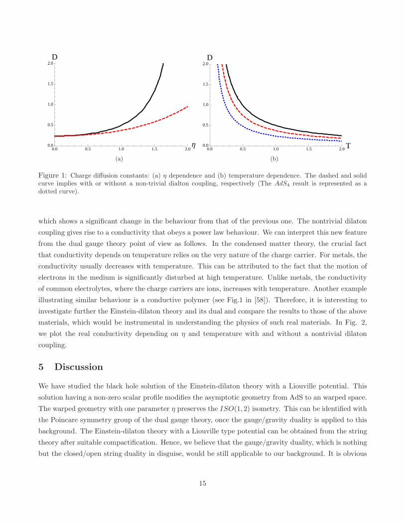
Since the charge diffusion constant in (82) is almost similar to that in (51), the quasi normal modes
possess similar qualitative features. In Fig. 1, we compare the charge diffusion constants of the quasi
normal modes with and without a nontrivial dilaton coupling.
From the retarded Green function of the transverse mode, the real DC conductivity is given by
σ =1
g24
[
16π
(−Λ)(4 + η2)
]η2
4−η2
Tη2
4−η2
H , (83)
14
0.0 0.5 1.0 1.5 2.0Η0.0
0.5
1.0
1.5
2.0D
(a)
0.0 0.5 1.0 1.5 2.0 T0.0
0.5
1.0
1.5
2.0D
(b)
Figure 1: Charge diffusion constants: (a) η dependence and (b) temperature dependence. The dashed and solidcurve implies with or without a non-trivial dialton coupling, respectively (The AdS4 result is represented as adotted curve).
which shows a significant change in the behaviour from that of the previous one. The nontrivial dilaton
coupling gives rise to a conductivity that obeys a power law behaviour. We can interpret this new feature
from the dual gauge theory point of view as follows. In the condensed matter theory, the crucial fact
that conductivity depends on temperature relies on the very nature of the charge carrier. For metals, the
conductivity usually decreases with temperature. This can be attributed to the fact that the motion of
electrons in the medium is significantly disturbed at high temperature. Unlike metals, the conductivity
of common electrolytes, where the charge carriers are ions, increases with temperature. Another example
illustrating similar behaviour is a conductive polymer (see Fig.1 in [58]). Therefore, it is interesting to
investigate further the Einstein-dilaton theory and its dual and compare the results to those of the above
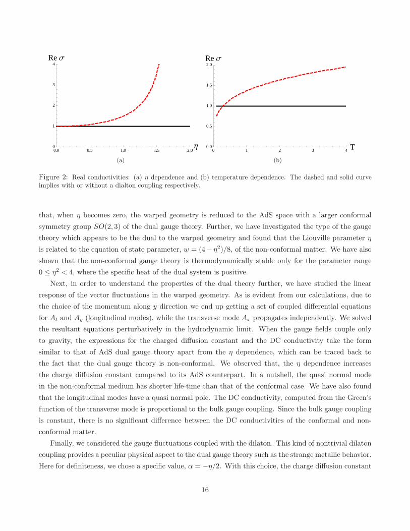
materials, which would be instrumental in understanding the physics of such real materials. In Fig. 2,
we plot the real conductivity depending on η and temperature with and without a nontrivial dilaton
coupling.
5 Discussion
We have studied the black hole solution of the Einstein-dilaton theory with a Liouville potential. This
solution having a non-zero scalar profile modifies the asymptotic geometry from AdS to an warped space.
The warped geometry with one parameter η preserves the ISO(1, 2) isometry. This can be identified with
the Poincare symmetry group of the dual gauge theory, once the gauge/gravity duality is applied to this
background. The Einstein-dilaton theory with a Liouville type potential can be obtained from the string
theory after suitable compactification. Hence, we believe that the gauge/gravity duality, which is nothing
but the closed/open string duality in disguise, would be still applicable to our background. It is obvious
15
0.0 0.5 1.0 1.5 2.0Η0
1
2
3
4Re Σ
(a)
0 1 2 3 4 T0.0
0.5
1.0
1.5
2.0Re Σ
(b)
Figure 2: Real conductivities: (a) η dependence and (b) temperature dependence. The dashed and solid curveimplies with or without a dialton coupling respectively.
that, when η becomes zero, the warped geometry is reduced to the AdS space with a larger conformal
symmetry group SO(2, 3) of the dual gauge theory. Further, we have investigated the type of the gauge
theory which appears to be the dual to the warped geometry and found that the Liouville parameter η
is related to the equation of state parameter, w = (4− η2)/8, of the non-conformal matter. We have also
shown that the non-conformal gauge theory is thermodynamically stable only for the parameter range
0 ≤ η2 < 4, where the specific heat of the dual system is positive.
Next, in order to understand the properties of the dual theory further, we have studied the linear
response of the vector fluctuations in the warped geometry. As is evident from our calculations, due to
the choice of the momentum along y direction we end up getting a set of coupled differential equations
for At and Ay (longitudinal modes), while the transverse mode Ax propagates independently. We solved
the resultant equations perturbatively in the hydrodynamic limit. When the gauge fields couple only
to gravity, the expressions for the charged diffusion constant and the DC conductivity take the form
similar to that of AdS dual gauge theory apart from the η dependence, which can be traced back to
the fact that the dual gauge theory is non-conformal. We observed that, the η dependence increases
the charge diffusion constant compared to its AdS counterpart. In a nutshell, the quasi normal mode
in the non-conformal medium has shorter life-time than that of the conformal case. We have also found
that the longitudinal modes have a quasi normal pole. The DC conductivity, computed from the Green’s
function of the transverse mode is proportional to the bulk gauge coupling. Since the bulk gauge coupling
is constant, there is no significant difference between the DC conductivities of the conformal and non-
conformal matter.
Finally, we considered the gauge fluctuations coupled with the dilaton. This kind of nontrivial dilaton
coupling provides a peculiar physical aspect to the dual gauge theory such as the strange metallic behavior.
Here for definiteness, we chose a specific value, α = −η/2. With this choice, the charge diffusion constant
16
has a similar form to that of the previous one with some modifications. For a fixed non-conformality,
the diffusion constant is smaller than the one, obtained from the dilaton free gauge fluctuation. This
also leads to the fact that the quasi normal mode with the dilaton coupling survives longer than that of
the free one. We have shown that the effective bulk gauge coupling depending nontrivially on the radial
coordinate can change the behaviour of the DC conductivity, dramatically. The DC conductivity of the
system increases with temperature, which is a typical aspect commonly found in electrolytes. Another
example with such a temperature dependence can be found in conductive polymers such as polypyrrole
films [58]. Thus, it would be interesting to investigate at length, the interplay between the dual gauge
theory of the warped geometry and the condensed matter system. We also would like to explore the
paradigm by including the metric fluctuation and thus determine other hydrodynamical quantities like
shear viscosity etc. We hope to report on these issues in near future.
Acknowledgement
C. Park would like to thank E. Kiritsis, R. Meyer and S. J. Sin for the valuable discussions. This
work was supported by the National Research Foundation of Korea(NRF) grant funded by the Korea
government(MEST) through the Center for Quantum Spacetime(CQUeST) of Sogang University with
grant number 2005-0049409. C. Park was also supported by Basic Science Research Program through
the National Research Foundation of Korea(NRF) funded by the Ministry of Education, Science and
Technology(2010-0022369).
A Vector fluctuation without the dilaton coupling
A.1 Longitudinal modes: At(z) and Ay(z)
The three equations of motion for the longitudinal modes, (39), (40) and (41), are not independent
because combining two of them yields the rest. By using (39) and (40) we get the following third order
differential equation
0 = A′′′t +
F ′(z)
F (z)A′′
t +Λ2
F 2(z)
[
ω2 − F (z)q2]
A′t. (A.1)
Since F (z) vanishes at z = 1, the solution of A′t should have a singular part at the horizon. If we take
the following ansatz
A′t(z) = (1− zd)νG(z), (A.2)
17
then the unknown function G(z) should be regular and at the same time independent of ω and q2 at the
horizon, the power ν can be exactly determined by the singular structure at the horizon to be,
ν = ± iωΛda20
. (A.3)
Since the black hole absorbs all kinds of field, there is no outgoing modes at the horizon. Therefore, it is
natural to impose the incoming boundary condition to A′t at the horizon, which breaks the unitarity of the
solution. In (A.3), the plus and minus signs correspond to the outgoing or incoming mode, respectively
and hence we have to choose the minus sign.
Then, the equation governing the unknown function G(z) becomes
0 = G′′(z)− 1
1− zdd(1 + 2ν)zd−1 G′(z)− 1
1− zd
[
d(d− 1)νzd−2 +Λ2
a20q2
]
G(z)
+1
(1− zd)2
[
d2ν2z2(d−1) +Λ2
a40ω2
]
G(z). (A.4)
Solving the above equation analytically is almost impossible, so we have to resort either to the numerical
method or take an appropriate approximation. Here, we will consider the hydrodynamic limit wherein,
ω << 1 and q2 << 1, and expand G(z) in the powers of ω and q2 as:
G(z) = G0(z) + ωG1(z) + q2G2(z) + ωq2G3(z) + · · · (A.5)
After substituting (A.5) into (A.4), we will determine G(z) up to leading orders in ω and q2.
At the zeroth order, (A.4) reads
0 = G′′0(z)−
dzd−1
1− zdG′
0(z), (A.6)
whose solution is given by
G0(z) = C0 z 2F1
[
1,1
d, 1 +
1
d, zd]
+ C, (A.7)
where C0 and C are two integration constants. Notice that the hypergeometric function diverges at the
horizon z = 1. Since G0(z) at horizon should be regular as mentioned earlier, the divergence of the
hypergeometric function should be removed by setting C0 = 0. Hence, we have
G0(z) = C, (A.8)
where C is an undetermined constant and will be fixed later by imposing another boundary condition at
the boundary.
18
At ω order, we arrive at the following differential eqn.
[
(1− zd)G′1(z)
]′
= −iC (d− 1)Λ
a20zd−2, (A.9)
where the result in (A.8) was used. The solution of the above equation is given by
G1(z) = C4 +C3z
1+d
(d+ 1)2F1
[
1, 1 +1
d, 2 +
1
d, zd]
+
[
C3z + iC
(
Λ
da20
)
ln(1− zd)
]
. (A.10)
Notice that the higher order solutions like G1(z), G2(z), ..., must vanish at the horizon in order to give
a constant number. The hypergeometric function and the last term in (A.10) contain divergent terms at
the horizon. Thus, the integration constant C3 should be related to C in order to remove the divergence.
The remaining constant C4 can be also determined in terms of C due to the vanishing of G1(z) at the
horizon [50, 57]
C4 = iC
(
Λ
da20
)
[d− EG− PG(0, 1 + 1/d)] , (A.11)
where EG is Eulergamma number and PG(a,b) denotes the ath derivative of digamma function ψ(b). As
a result, G1(z) is exactly determined in terms of C
G1(z) =iCΛ
a20G1(z), (A.12)
where
G1(z) =1
d(d+ 1)
[
z1+dd 2F1
[
1, 1 +1
d, 2 +
1
d, zd]
+ (1 + d)
{
(d z + ln(1− zd))−(
d− EG− PG(0, 1 +1
d)
)}]
. (A.13)
Following the same procedure, we can also fix G2(z) in terms of C at q2 order. The solution G2(z) is
given by
G2(z) = C
(
Λ2
2a20
)
z2
22F1
[
1,2
d, 1 +
2
d, zd]
+ C5 z 2F1
[
1,1
d, 1 +
1
d, zd]
+ C6. (A.14)
The regularity and vanishing conditions of G2 at the horizon fix two integration constants C5 and C6 in
terms of C
C5 = −C Λ2
a20(A.15)
C6 = −C Λ2
a20d[PG(0, 1/d) − PG(0, 2/d)] . (A.16)
19
Finally, we get the expression for G2(z) as
G2(z) = CΛ2
a20G2(z) (A.17)
with
G2(z) =z2
22F1
[
1,2
d, 1 +
2
d, zd]
− z 2F1
[
1,1
d, 1 +
1
d, zd]
−1
d(PG(0, 1/d) − PG(0, 2/d)) . (A.18)
After evaluating A′′t (z) from the above and substituting it into (40), we obtain
Ay(z) +q
ωAt(z) =
C(1− zd)νa20ωqΛ2
[
−dνzd−1
(
1 +iΛω
a20G1(z) +
Λ2q2
a20G2(z)
)
+(1− zd)
(
iΛω
a20G′
1(z) +Λ2q2
a20G′
2(z)
)]
. (A.19)
where ν is given in (A.3). To fix the overall integration constant C we impose the Dirichlet boundary
condition for At and Az at the boundary [50]
limz→0
At(z) = A0t and lim
z→0Ay(z) = A0
y. (A.20)
Rewriting C in terms of the boundary values of At(z) and Ay(z), we obtain
C =ωqA0
y + q2A0t
(
i ωΛ− q2
) . (A.21)
Thus, the solutions up to the ω and q2 order are given by
A′t(z) =
ωqA0y + q2A0
t(
i ωΛ− q2
) (1− zd)ν
[
1 +iωΛ
a20G1(z) +
q2Λ2
a20G2(z)
]
, (A.22)
A′y(z) = − ω
a20q
A′t(z)
(1− zd), (A.23)
where (39) was used in the last equation.
A.2 Transverse mode: Ax(z)
We solve the equation for the transverse mode (42), which is completely decoupled form longitudinal
modes. A comparison between (42) and (A.1) immediately shows that the differential equation for the
20
transverse mode is exactly the same as that of A′t(z). Therefore, without any calculation, we can find
the solution of (42).
Ax(z) = Cx(1− zd)ν
[
1 +iωΛ
a20G1(z) +
q2Λ2
a20G2(z)
]
+ · · · , (A.24)
where G1(z) and G2(z) are given by (A.13) and (A.18), respectively.
The ellipsis means higher order terms. However, the integration constant Cx is now different from
the previous one. To determine it, we again impose the Dirichlet boundary condition
limz→0
Ax(z) = A0x. (A.25)
Then, Cx can be determined in terms of the boundary value of Ax(z) as
Cx = A0x
[
1− iωΛ
a20d[d− EG− PG(0, 1 + 1/d)] − q2Λ2
da20[PG(0, 1/d) − PG(0, 2/d))]
]−1
. (A.26)
Thus, Ax(z) is determined upto leading orders in ω and q2.
B Vector fluctuation coupled to the dilaton
B.1 Longitudinal modes: At(u) and Ay(u)
Since the equations, (67), (68) and (69), are not independent we differentiate (68) with respect to u and
then substitute it into (67) to obtain a third order differential equation for At
0 = A′′′t +
H ′(u)
H(u)A′′
t +Λ2eff
H(u)F (u)
[
ω2 − F (u)q2]
A′t. (B.1)
Note that since H(u) vanishes at u = 1, the above differential equation has a singular point at u = 1.
We therefore consider the following ansatz
A′t(u) = (1− ud)νχ(u). (B.2)
where the unknown function χ(u) is regular and at the same time independent of ω and q2 at the horizon
(u = 1). Plugging the above ansatz, (B.1) becomes
0 =[
1− ud]νχ′′(u) +
γ
z
[
1− ud]νχ′(u)− d
[
1− ud]ν−1
ud−1χ′(u)(1 + 2ν)
−[
1− ud]ν−1
χ(u)
d(d − 1 + γ)νud−2 +
Λ2eff q
2
a20
1
uγ[
(2a1 + δ − 1)(
Λeff
TH
)]γ
+[
1− ud]ν−2
χ(u)
d2ν2u2(d−1) +
Λ2eff ω
2
a40
1
u2γ[
(2a1 + δ − 1)(
Λeff
TH
)]γ
. (B.3)
21
As computed in the previous section, the index ν can be determined from the singular structure at the
horizon by solving the indicial equation and keeping in mind the fact that there are no outgoing modes
at the horizon. Thus we get
ν = − iωΛeff
da20
1[
(2a1 + δ − 1)(
Λeff
TH
)]γ/2. (B.4)
We can solve (B.3) perturbatively by considering the hydrodynamic limit and expanding χ(u) in powers
of ω and q2, as
χ(u) = χ0(u) + ωχ1(u) + q2χ2(u) + ωq2χ3(u) + · · · . (B.5)
Following similar steps described in the previous section, we can find
χ0(u) = C (B.6)
where C remains to be determined. The next order solutions, χ1 and χ2, can also be determined by
imposing the regularity and vanishing conditions at the horizon in the following form:
χ1(u) = iC
Λeff
a20
1[
(2a1 + δ − 1)(
Λeff
TH
)]γ/2
χ1(u),
χ2(u) = C
Λ2eff
a20
1[
(2a1 + δ − 1)(
Λeff
TH
)]γ
χ2(u), (B.7)
where
χ1(u) =u1−γ
1− γ2F1
[
1,1− γ
d, 1 +
1− γ
d, ud]
+1
d
[
ln(1− ud) + EG+ PG(0,1− γ
d)
]
,
χ2(u) =u2−γ
2− γ2F1
[
1,2− γ
d, 1 +
2− γ
d, ud]
− u1−γ
1− γ2F1
[
1,1− γ
d, 1 +
1− γ
d, ud]
−1
d
[
PG
(
0,1− γ
d
)
− PG
(
0,2− γ
d
)]
. (B.8)
Here, notice that there exists a singular point at γ = 1 but as will be shown, the interesting physical
quantities like the charge diffusion constant and the real DC conductivity, are well behaved, despite this
singularity.
After imposing the Dirichlet boundary condition, the overall integration constant C can be fixed (up
to orders of ω and q2) in terms of the boundary values A0t and A0
y,
C =ωqA0
y + q2A0t
(
iωΛeff
[
(2a1 + δ − 1)(
Λeff
TH
)]γ/2
− q2) . (B.9)
22
After all the dusts get settled, one can write the final expressions for A′t(u) and A
′y(u) as
A′t(u) = (1− ud)ν
ωqA0y + q2A0
t(
iωΛeff
[
(2a1 + δ − 1)(
Λeff
TH
)]γ/2
− q2)
×
1 + iω
Λeff
a20
1[
(2a1 + δ − 1)(
Λeff
TH
)]γ/2
χ1 + q2
Λ2eff
a20
1[
(2a1 + δ − 1)(
Λeff
TH
)]γ
χ2
,
A′y(u) = − ω
q
1
a20(1− ud)A′
t(u). (B.10)
B.2 Solution for transverse mode Ax(u)
Unlike what happened for the dilaton free fluctuations, the equation for the transverse mode Ax(u), here
is not the same as the one for the longitudinal mode A′t(u) in (B.1). Hence, we need to solve (70) by
using the perturbative expansion in the hydrodynamic limit. The solution of the transverse mode Ax(u)
is given by
Ax(u) = Cx(1− ud)ν
1 + iω
Λeff
a20
1[
(2a1 + δ − 1)(
Λeff
TH
)]γ/2
ζ1(u)
+q2
Λ2eff
a20
1[
(2a1 + δ − 1)(
Λeff
TH
)]γ
ζ2(u)
, (B.11)
where ζ1(u) and ζ2(u) are given by
ζ1(u) =1
d(d+ 1)
[
u1+dd 2F1[1, 1 +1
d, 2 +
1
d, ud]
+ (1 + d)
(
(ud+ ln(1− ud))− (d− EG− PG(0, 1 +1
d))
)]
, (B.12)
ζ2(u) =
[
u2−γ
(1− γ)(2 − γ)2F1[1,
2− γ
d, 1 +
2− γ
d, ud]− u
(1− γ)2F1[1,
1
d, 1 +
1
d, ud]
− 1
d(1− γ)
(
PG(0,1
d)− PG(0, 2 − γ
d)
)]
. (B.13)
To determine the overall constant Cx we impose the Dirichlet boundary condition,
limz→0
Ax(u) = A0x. (B.14)
23
Finally, we can rewrite the constant Cx in terms of the boundary value A0x, as
Cx = A0x
1− iωΛeff
a20d
[
d− EG− PG(0, 1 + 1d )]
[
(2a1 + δ − 1)(
Λeff
TH
)]γ/2−q2Λ2
eff
da20
[
PG(0, 1d )− PG(0, 2−γd ))
]
(1− γ)[
(2a1 + δ − 1)(
Λeff
TH
)]γ
−1
. (B.15)
References
[1] J. M. Maldacena, Adv. Theor. Math. Phys. 2 (1998) 231 [hep-th/9711200].
[2] S. S. Gubser, I. R. Klebanov and A. M. Polyakov, Phys. Lett. B 428 (1998) 105 [hep-th/9802109].
[3] E. Witten, Adv. Theor. Math. Phys. 2 (1998) 253 [hep-th/9802150].
[4] S. Kachru, X. Liu and M. Mulligan, Phys. Rev. D 78, 106005 (2008) [arXiv:0808.1725 [hep-th]].
[5] S. F. Ross and O. Saremi, JHEP 0909, 009 (2009) [arXiv:0907.1846 [hep-th]].
[6] K. Balasubramanian and J. McGreevy, Phys. Rev. D 80, 104039 (2009) [arXiv:0909.0263 [hep-th]].
[7] D. -W. Pang, JHEP 1001, 120 (2010) [arXiv:0912.2403 [hep-th]].
[8] E. Megias, H. J. Pirner and K. Veschgini, Phys. Rev. D 83, 056003 (2011) [arXiv:1009.2953 [hep-ph]];
K. Veschgini, E. Megias and H. J. Pirner, Phys. Lett. B 696, 495 (2011) [arXiv:1009.4639 [hep-th]].
[9] Y. Nishida and D. T. Son, Phys. Rev. D 76, 086004 (2007) [arXiv:0706.3746 [hep-th]].
[10] D. T. Son, Phys. Rev. D 78 (2008) 046003 [arXiv:0804.3972 [hep-th]].
[11] C. P. Herzog, M. Rangamani and S. F. Ross, JHEP 0811, 080 (2008) [arXiv:0807.1099 [hep-th]].
[12] A. Adams, K. Balasubramanian and J. McGreevy, JHEP 0811, 059 (2008) [arXiv:0807.1111 [hep-
th]].
[13] M. Rangamani, S. F. Ross, D. T. Son and E. G. Thompson, JHEP 0901, 075 (2009) [arXiv:0811.2049
[hep-th]].
[14] C. P. Herzog, J. Phys. A A 42, 343001 (2009) [arXiv:0904.1975 [hep-th]].
[15] M. Rangamani, Class. Quant. Grav. 26 (2009) 224003 [arXiv:0905.4352 [hep-th]].
24
[16] G. T. Horowitz and J. Polchinski, gr-qc/0602037.
[17] S. A. Hartnoll, Class. Quant. Grav. 26, 224002 (2009) [arXiv:0903.3246 [hep-th]].
[18] M. Taylor, arXiv:0812.0530 [hep-th].
[19] H. A. Chamblin and H. S. Reall, Nucl. Phys. B 562, 133 (1999) [hep-th/9903225].
[20] K. Goldstein, S. Kachru, S. Prakash and S. P. Trivedi, JHEP 1008, 078 (2010) [arXiv:0911.3586
[hep-th]].
[21] C. Charmousis, B. Gouteraux, B. S.Kim, E. Kiritsis and R. Meyer, JHEP 11,151(2010)
[arXiv:1005.4690](hep-th).
[22] M. Cadoni, S. Mignemi and M. Serra, Phys. Rev. D 84, 084046 (2011) [arXiv:1107.5979 [gr-qc]].
[23] B. -H. Lee, S. Nam, D. -W. Pang and C. Park, Phys. Rev. D 83, 066005 (2011) [arXiv:1006.0779
[hep-th]].
[24] K. Goldstein, N. Iizuka, S. Kachru, S. Prakash, S. P. Trivedi and A. Westphal, JHEP 10, 027 (2010)
[arXiv:1007.2490] (hep-th).
[25] X. Dong, S. Harrison, S. Kachru, G. Torroba and H. Wang, arXiv:1201.1905 [hep-th].
[26] L. Huijse, S. Sachdev and B. Swingle, Phys. Rev. B 85, 035121 (2012) [arXiv:1112.0573 [cond-
mat.str-el]]; B. S. Kim, arXiv:1202.6062 [hep-th]; E. Perlmutter, arXiv:1205.0242 [hep-th].
[27] B. Gouteraux and E. Kiritsis, JHEP 1112, 036 (2011) [arXiv:1107.2116 [hep-th]].
[28] I. Kanitscheider and K. Skenderis, JHEP 0904, 062 (2009) [arXiv:0901.1487 [hep-th]].
[29] B. Gouteraux, J. Smolic, M. Smolic, K. Skenderis and M. Taylor, JHEP 1201, 089 (2012)
[arXiv:1110.2320 [hep-th]].
[30] B. -H. Lee, D. -W. Pang and C. Park, Int. J. Mod. Phys. A 26, 2279 (2011) [arXiv:1107.5822
[hep-th]].
[31] N. Iqbal and H. Liu, Phys. Rev. D 79, 025023 (2009) [arXiv:0809.3808 [hep-th]].
[32] I. Kanitscheider, K. Skenderis and M. Taylor, JHEP 0809, 094 (2008) [arXiv:0807.3324 [hep-th]].
[33] E. Perlmutter, JHEP 1102, 013 (2011) [arXiv:1006.2124 [hep-th]].
25
[34] K. Skenderis, Class. Quant. Grav. 19 (2002) 5849 [hep-th/0209067]; M. Henningson and K. Skenderis,
JHEP 9807, 023 (1998) [hep-th/9806087]; V. Balasubramanian and P. Kraus, Commun. Math. Phys.
208, 413 (1999) [hep-th/9902121]; S. de Haro, S. N. Solodukhin and K. Skenderis, Commun. Math.
Phys. 217, 595 (2001) [hep-th/0002230]; Y. Matsuo, S. -J. Sin and Y. Zhou, JHEP 1201, 130 (2012)
[arXiv:1109.2698 [hep-th]].
[35] S. Sachdev, arXiv:1002.2947 [hep-th].
[36] S. A. Hartnoll, Class. Quant. Grav 26, 224002 (2009) [arXiv:0903.3246 [hep-th]].
[37] J. McGreevy , Adv.High Energy Phys. 2010, 723105 (2010) [arXiv:0909.0518 [hep-th]].
[38] C. P. Herzog, J.Phys. A42, 343001 (2009) [arXiv:0904.1975 [hep-th]].
[39] N. Iqbal, H. Liu and M. Mezei, arXiv:1110.3814
[40] R. A. Janik and R. B. Peschanski, Phys. Rev. D 73, 045013 (2006) [hep-th/0512162].
[41] S. Bhattacharyya, S. Lahiri, R. Loganayagam and S. Minwalla, JHEP 0809, 054 (2008)
[arXiv:0708.1770 [hep-th]].
[42] S. Bhattacharyya, V. E. Hubeny, S. Minwalla and M. Rangamani, JHEP 0802, 045 (2008)
[arXiv:0712.2456 [hep-th]].
[43] V. E. Hubeny, S. Minwalla and M. Rangamani, arXiv:1107.5780 [hep-th].
[44] R. Gregory and J.A. Harvey, Phys. Rev. D 47, 2411 (1993)
[45] J.H. Horne and Gary T. Horowitz, Nucl. Phys. B399, 169 (1993)
[46] C. Charmousis, B. Gouteraux and J. Soda, Phys. Rev. D 80, 024028 (2009) [arXiv:0905.3337 [gr-qc]].
[47] J. D. Bekenstein, Phys. Rev. D7, 2333 (1973).
[48] S. W. Hawking, Comm. Math. Phys. 43, 199 (1975).
[49] D. T. Son and A. O. Starinets, JHEP 0209 (2002) 042 [hep-th/0205051].
[50] G. Policastro, D. T. Son and A. O. Starinets, JHEP 0209, 043 (2002) [hep-th/0205052];
[51] G. Policastro, D. T. Son and A. O. Starinets, JHEP 0212, 054 (2002) [hep-th/0210220].
[52] S. S. Gubser, Adv. Theor. Math. Phys. 4, 679 (2000) [hep-th/0002160].
26
[53] U. Gursoy and E. Kiritsis, JHEP 0802, 032 (2008) [arXiv:0707.1324 [hep-th]]; U. Gursoy, E. Kiritsis
and F. Nitti, JHEP 0802, 019 (2008) [arXiv:0707.1349 [hep-th]].
[54] A. Karch and A. O’Bannon, JHEP 0709, 024 (2007) [arXiv:0705.3870 [hep-th]].
[55] S. A. Hartnoll, J. Polchinski, E. Silverstein and D. Tong, JHEP 1004, 120 (2010) [arXiv:0912.1061
[hep-th]]; B. -H. Lee, D. -W. Pang and C. Park, JHEP 1007, 057 (2010) [arXiv:1006.1719 [hep-th]];
B. -H. Lee, D. -W. Pang and C. Park, JHEP 1011 (2010) 120 [arXiv:1009.3966 [hep-th]].
[56] G. Koutsoumbas, E. Papantonopoulos and G. Siopsis, JHEP 0907, 026 (2009) [arXiv:0902.0733 [hep-
th]]; C. Martinez, J. P. Staforelli and R. Troncoso, Phys. Rev. D 74, 044028 (2006) [hep-th/0512022];
Y. S. Myung and C. Park, Phys. Lett. B 704, 242 (2011) [arXiv:1007.0816 [hep-th]]; G. Tallarita
and S. Thomas, JHEP 1012, 090 (2010) [arXiv:1007.4163 [hep-th]]; C. Martinez and A. Montecinos,
Phys. Rev. D 82, 127501 (2010) [arXiv:1009.5681 [hep-th]].
[57] G. Policastro and A. Starinets, Nucl. Phys. B 610, 117 (2001) [hep-th/0104065].
[58] A. Kaynak, Materials Research Bulletin 33, 81 (1998).
27