nloptcontrol documentation - read the docs
TRANSCRIPT
NLOptControl DocumentationRelease 0.0.1-rc1
Huckleberry Febbo
January 16, 2017

Contents
1 Table of Contents 11.1 Background Information . . . . . . . . . . . . . . . . . . . . . . . . . . . . . . . . . . . . . . . . . 11.2 Package Functionality . . . . . . . . . . . . . . . . . . . . . . . . . . . . . . . . . . . . . . . . . . 81.3 Bibliography . . . . . . . . . . . . . . . . . . . . . . . . . . . . . . . . . . . . . . . . . . . . . . . 41
Bibliography 43
i

ii
CHAPTER 1
Table of Contents
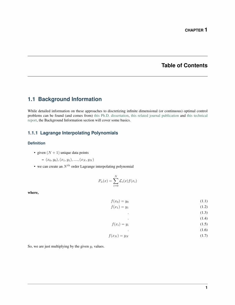
1.1 Background Information
While detailed information on these approaches to discretizing infinite dimensional (or continuous) optimal controlproblems can be found (and comes from) this Ph.D. dissertation, this related journal publication and this technicalreport, the Background Information section will cover some basics.
1.1.1 Lagrange Interpolating Polynomials
Definition
• given (𝑁 + 1) unique data points
– (𝑥0, 𝑦0), (𝑥1, 𝑦1), ...., (𝑥𝑁 , 𝑦𝑁 )
• we can create an 𝑁 𝑡ℎ order Lagrange interpolating polynomial
𝑃𝑛(𝑥) =
𝑁∑︁𝑖=0
ℒ𝑖(𝑥)𝑓(𝑥𝑖)
where,
𝑓(𝑥0) = 𝑦0 (1.1)𝑓(𝑥1) = 𝑦1 (1.2)
. (1.3)
. (1.4)𝑓(𝑥𝑖) = 𝑦𝑖 (1.5)
. (1.6)𝑓(𝑥𝑁 ) = 𝑦𝑁 (1.7)
So, we are just multiplying by the given 𝑦𝑖 values.
1
NLOptControl Documentation, Release 0.0.1-rc1
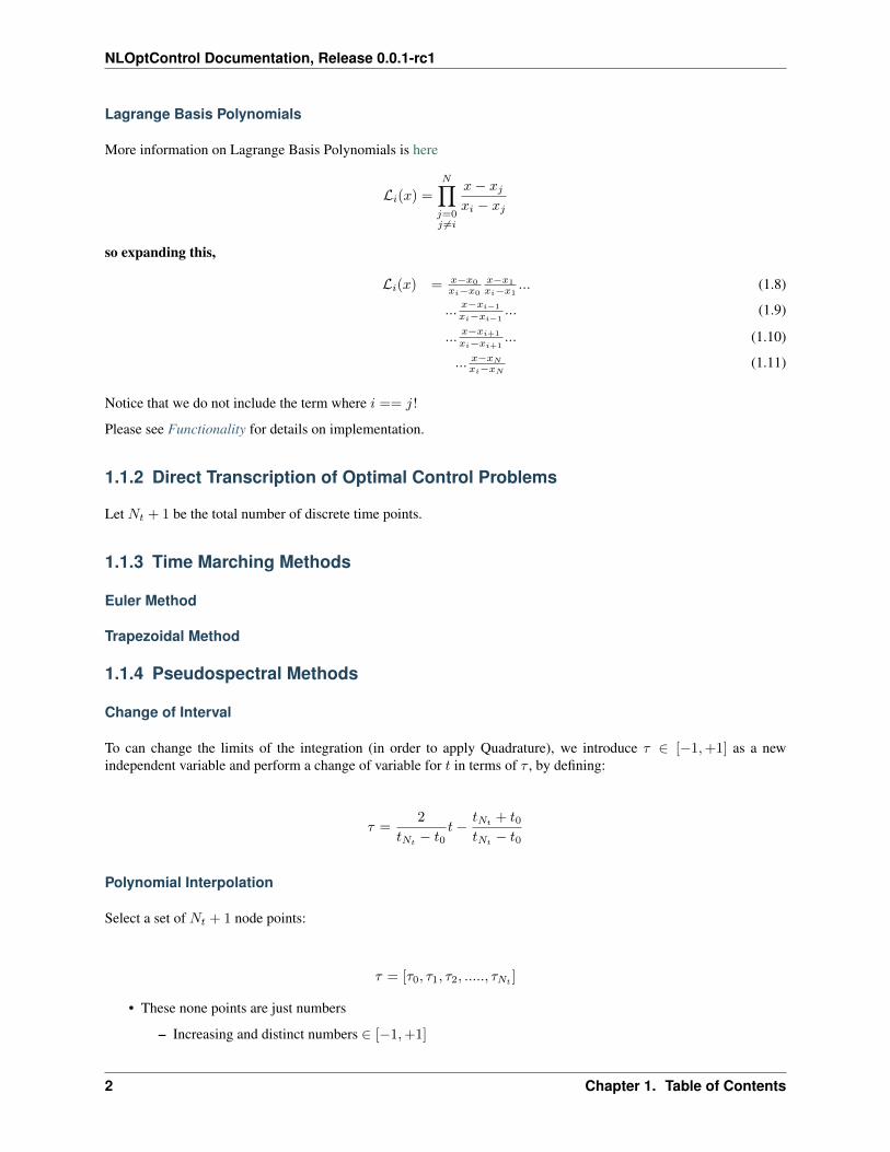
Lagrange Basis Polynomials
More information on Lagrange Basis Polynomials is here
ℒ𝑖(𝑥) =
𝑁∏︁𝑗=0𝑗 ̸=𝑖
𝑥− 𝑥𝑗𝑥𝑖 − 𝑥𝑗
so expanding this,
ℒ𝑖(𝑥) = 𝑥−𝑥0
𝑥𝑖−𝑥0
𝑥−𝑥1
𝑥𝑖−𝑥1... (1.8)
... 𝑥−𝑥𝑖−1
𝑥𝑖−𝑥𝑖−1... (1.9)
... 𝑥−𝑥𝑖+1
𝑥𝑖−𝑥𝑖+1... (1.10)
... 𝑥−𝑥𝑁
𝑥𝑖−𝑥𝑁(1.11)
Notice that we do not include the term where 𝑖 == 𝑗!
Please see Functionality for details on implementation.
1.1.2 Direct Transcription of Optimal Control Problems
Let 𝑁𝑡 + 1 be the total number of discrete time points.
1.1.3 Time Marching Methods
Euler Method
Trapezoidal Method
1.1.4 Pseudospectral Methods
Change of Interval
To can change the limits of the integration (in order to apply Quadrature), we introduce 𝜏 ∈ [−1,+1] as a newindependent variable and perform a change of variable for 𝑡 in terms of 𝜏 , by defining:
𝜏 =2
𝑡𝑁𝑡− 𝑡0
𝑡− 𝑡𝑁𝑡 + 𝑡0𝑡𝑁𝑡
− 𝑡0
Polynomial Interpolation
Select a set of 𝑁𝑡 + 1 node points:
𝜏 = [𝜏0, 𝜏1, 𝜏2, ....., 𝜏𝑁𝑡]
• These none points are just numbers
– Increasing and distinct numbers ∈ [−1,+1]
2 Chapter 1. Table of Contents
NLOptControl Documentation, Release 0.0.1-rc1
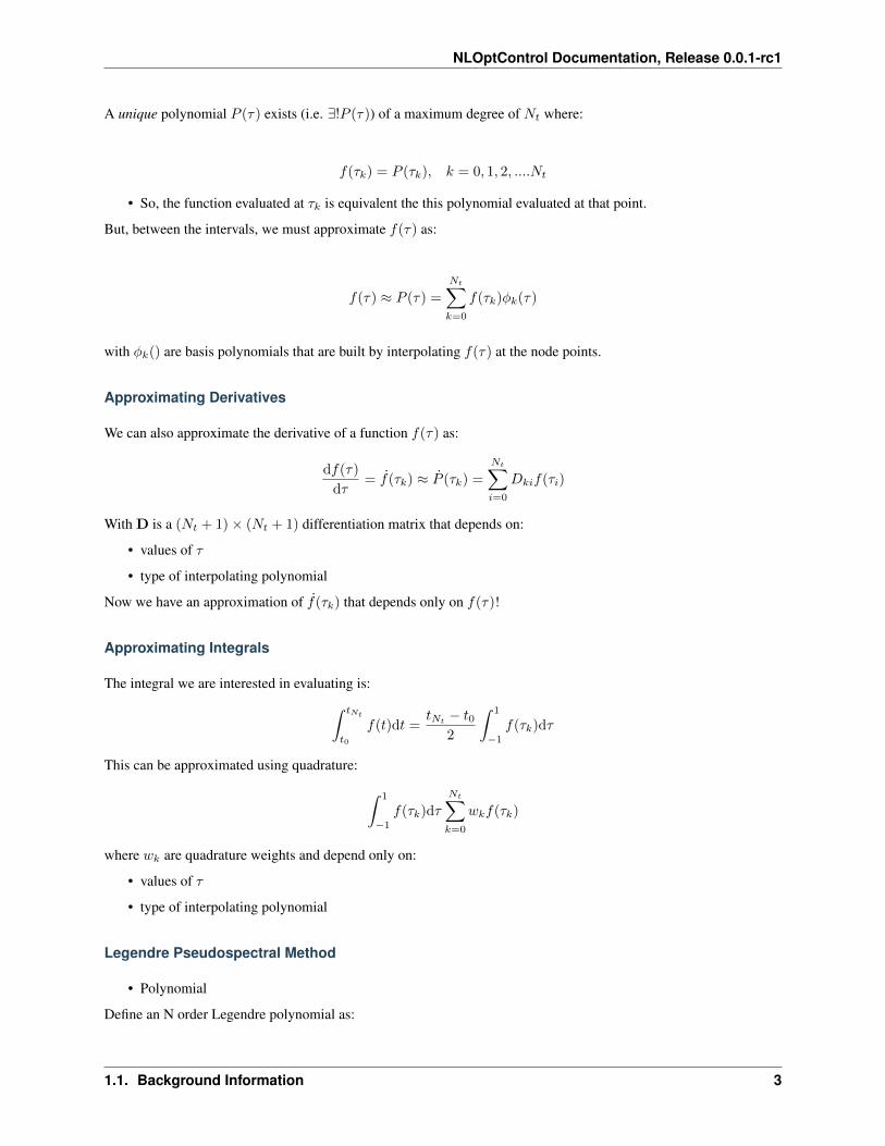
A unique polynomial 𝑃 (𝜏) exists (i.e. ∃!𝑃 (𝜏)) of a maximum degree of 𝑁𝑡 where:
𝑓(𝜏𝑘) = 𝑃 (𝜏𝑘), 𝑘 = 0, 1, 2, ....𝑁𝑡
• So, the function evaluated at 𝜏𝑘 is equivalent the this polynomial evaluated at that point.
But, between the intervals, we must approximate 𝑓(𝜏) as:
𝑓(𝜏) ≈ 𝑃 (𝜏) =
𝑁𝑡∑︁𝑘=0
𝑓(𝜏𝑘)𝜑𝑘(𝜏)
with 𝜑𝑘() are basis polynomials that are built by interpolating 𝑓(𝜏) at the node points.
Approximating Derivatives
We can also approximate the derivative of a function 𝑓(𝜏) as:
d𝑓(𝜏)
d𝜏= 𝑓(𝜏𝑘) ≈ �̇� (𝜏𝑘) =
𝑁𝑡∑︁𝑖=0
𝐷𝑘𝑖𝑓(𝜏𝑖)
With D is a (𝑁𝑡 + 1) × (𝑁𝑡 + 1) differentiation matrix that depends on:
• values of 𝜏
• type of interpolating polynomial
Now we have an approximation of 𝑓(𝜏𝑘) that depends only on 𝑓(𝜏)!
Approximating Integrals
The integral we are interested in evaluating is:∫︁ 𝑡𝑁𝑡
𝑡0
𝑓(𝑡)d𝑡 =𝑡𝑁𝑡 − 𝑡0
2
∫︁ 1
−1
𝑓(𝜏𝑘)d𝜏
This can be approximated using quadrature: ∫︁ 1
−1
𝑓(𝜏𝑘)d𝜏
𝑁𝑡∑︁𝑘=0
𝑤𝑘𝑓(𝜏𝑘)
where 𝑤𝑘 are quadrature weights and depend only on:
• values of 𝜏
• type of interpolating polynomial
Legendre Pseudospectral Method
• Polynomial
Define an N order Legendre polynomial as:
1.1. Background Information 3
NLOptControl Documentation, Release 0.0.1-rc1
𝐿𝑁 (𝜏) =1
2𝑁𝑁 !
d𝑛
d𝜏𝑁(𝜏2 − 1)𝑁
• Nodes
𝜏𝑘 =
⎧⎪⎨⎪⎩− 1, if 𝑘 = 0
kth root 𝑜𝑓�̇�𝑁𝑡(𝜏), if 𝑘 = 1, 2, 3, ..𝑁𝑡 − 1
+ 1 if 𝑘 = 𝑁𝑡
(1.12)
• Differentiation Matrix
• Interpolating Polynomial Function
1.1.5 hp-psuedospectral method
To solve the integral constraints within the optimal control problem we employs the hp-pseudospectral method. Thehp-psuedospectral method is an form of Gaussian Quadrature, which uses multi-interval collocation points.
Single Phase Optimal Control
Find:
• The state: x(𝑡)
• The control: u(𝑡)
• The integrals: q
• The initial time: 𝑡0
• The final time: 𝑡𝑓
To Minimize:
𝐽 = Φ(x(𝑡0),x(𝑡𝑓 ),q, 𝑡0, 𝑡𝑓 )
That Satisfy the Following Constraints:
• Dynamic Constraints:
dx
d𝑡= 𝜓(x(𝑡),u(𝑡), 𝑡)
• Inequality Path Constraints:
c𝑚𝑖𝑛 <= c(x(𝑡),u(𝑡), 𝑡) <= c𝑚𝑎𝑥
• Integral Constraints:
𝑞𝑖 =
∫︁ 𝑡𝑓
𝑡0
Υ𝑖(x(𝑡),u(𝑡), 𝑡) d𝑡, (𝑖 = 1, ...., 𝑛𝑞)
• Event Constraints:
b𝑚𝑖𝑛 <= b(x(𝑡0),x(𝑡𝑓 ), 𝑡𝑓 ,q) <= b𝑚𝑎𝑥
4 Chapter 1. Table of Contents
NLOptControl Documentation, Release 0.0.1-rc1
Change of Interval
To can change the limits of the integration (in order to apply Quadrature), we introduce 𝜏 ∈ [−1,+1] as a newindependent variable and perform a change of variable for 𝑡 in terms of 𝜏 , by defining:
𝑡 =𝑡𝑓 − 𝑡0
2𝜏 +
𝑡𝑓 + 𝑡02
The optimal control problem defined above (TODO: figure out equation references), is now redefined in terms of 𝜏 as:
Find:
• The state: x(𝜏)
• The control: u(𝜏)
• The integrals: q
• The initial time: 𝑡0
• The final time: 𝑡𝑓
To Minimize:
𝐽 = Φ(x(−1),x(+1),q, 𝑡0, 𝑡𝑓 )
That Satisfy the Following Constraints:
• Dynamic Constraints:
dx
d𝜏=𝑡𝑓 − 𝑡0
2𝜓(x(𝜏),u(𝜏), 𝜏, 𝑡0, 𝑡𝑓 )
• Inequality Path Constraints:
c𝑚𝑖𝑛 <= c(x(𝜏),u(𝜏), 𝜏, 𝑡0, 𝑡𝑓 ) <= c𝑚𝑎𝑥
• Integral Constraints:
𝑞𝑖 =𝑡𝑓 − 𝑡0
2
∫︁ +1
−1
Υ𝑖(x(𝜏),u(𝜏), 𝜏, 𝑡0, 𝑡𝑓 ) d𝜏, (𝑖 = 1, ...., 𝑛𝑞)
• Event Constraints:
b𝑚𝑖𝑛 <= b(x(−1),x(+1), 𝑡𝑓 ,q) <= b𝑚𝑎𝑥
Divide The Interval 𝜏 ∈ [−1,+1]
The interval 𝜏 ∈ [−1,+1] is now divided into a mesh of K mesh intervals as:
[𝑇𝑘−1, 𝑇𝑘], 𝑘 = 1, ..., 𝑇𝐾
with (𝑇0, ..., 𝑇𝐾) being the mesh points; which satisfy:
−1 = 𝑇0 < 𝑇1 < 𝑇2 < 𝑇3 < ........... < 𝑇𝐾−1 < 𝑇𝐾 = 𝑇𝑓 = +1
1.1. Background Information 5
NLOptControl Documentation, Release 0.0.1-rc1
Rewrite the Optimal Control Problem using the Mesh
Find:
• The state : x(𝑘)(𝜏) in mesh interval k
• The control: u(𝑘)(𝜏) in mesh interval k
• The integrals: q
• The initial time: 𝑡0
• The final time: 𝑡𝑓
To Minimize:
𝐽 = Φ(x(1)(−1),x(𝐾)(+1),q, 𝑡0, 𝑡𝑓 )
That Satisfy the Following Constraints:
• Dynamic Constraints:
dx(𝑘)(𝜏 (𝑘))
d𝜏 (𝑘)=𝑡𝑓 − 𝑡0
2𝜓(x(𝑘)(𝜏 (𝑘)),u(𝑘)(𝜏 (𝑘)), 𝜏 (𝑘), 𝑡0, 𝑡𝑓 ), (𝑘 = 1, ...,𝐾)
• Inequality Path Constraints:
c𝑚𝑖𝑛 <= c(x(𝑘)(𝜏 (𝑘)),u(𝑘)(𝜏 (𝑘)), 𝜏 (𝑘), 𝑡0, 𝑡𝑓 ) <= c𝑚𝑎𝑥, (𝑘 = 1, ...,𝐾)
• Integral Constraints:
𝑞𝑖 =𝑡𝑓 − 𝑡0
2
𝐾∑︁𝑘=1
∫︁ 𝑇𝑘
𝑇𝑘−1
Υ𝑖(x(𝑘)(𝜏 (𝑘)),u(𝑘)(𝜏 (𝑘)), 𝜏, 𝑡0, 𝑡𝑓 ) d𝜏, (𝑖 = 1, ...., 𝑛𝑞, 𝑘 = 1, ...,𝐾)
• Event Constraints:
b𝑚𝑖𝑛 <= b(x(1)(−1),x(𝐾)(+1), 𝑡𝑓 ,q) <= b𝑚𝑎𝑥
• State Continuity
– Also, we must now constrain the state to be continuous at each interior mesh point (𝑇1, ...𝑇𝑘−1) by en-forcing:
y𝑘(𝑇𝑘) = y𝑘+1(𝑇𝑘)
Optimal Control Problem Approximation
The optimal control problem will now be approximated using the Radau Collocation Method as which follows thedescription provided by [BGar11]. In collocation methods, the state and control are discretized at particular pointswithin the selected time interval. Once this is done the problem can be transcribed into a nonlinear programmingproblem (NLP) and solved using standard solvers for these types of problems, such as IPOPT or KNITRO.
6 Chapter 1. Table of Contents
NLOptControl Documentation, Release 0.0.1-rc1
For each mesh interval 𝑘 ∈ [1, ..,𝐾]:
x(𝑘)(𝜏) ≈ X(𝑘)(𝜏) =
𝑁𝑘+1∑︁𝑗=1
X(𝑘)𝑗
dℒ𝑘𝑗 (𝜏)
d𝜏(1.13)
𝑤ℎ𝑒𝑟𝑒, (1.14)
ℒ𝑘𝑗 (𝜏) =
∏︀𝑁𝑘+1𝑙=1𝑙 ̸=𝑗
𝜏−𝜏(𝑘)𝑙
𝜏(𝑘)𝑗 −𝜏
(𝑘)𝑙
(1.15)
𝑎𝑛𝑑, (1.16)
𝐷𝑘𝑖 = ℒ̇𝑖(𝜏𝑘) =dℒ𝑘
𝑗 (𝜏)
d𝜏 (1.17)
also,
• ℒ(𝑘)𝑗 (𝜏), (𝑗 = 1, ..., 𝑁𝑘 + 1) is a basis of Lagrange polynomials
• (𝜏𝑘1 , ....., 𝜏(𝑘)𝑁𝑘
) are the Legendre-Gauss-Radau collocation points in mesh interval k
– defined on the subinterval 𝜏 (𝑘) ∈ [𝑇𝑘−1, 𝑇𝑘]
– 𝜏(𝑘)𝑁𝑘+1 = 𝑇𝑘 is a noncollocated point
A basic description of Lagrange Polynomials is presented in Lagrange Interpolating Polynomials
The D matrix:
• Has a size = [𝑁𝑐] × [𝑁𝑐 + 1]
– with (1 <= 𝑘 <= 𝑁𝑐), (1 <= 𝑖 <= 𝑁𝑐 + 1)
– this non-square shape because the state approximation uses the 𝑁𝑐 + 1 points:(𝜏1, ...𝜏𝑁𝑐+1)
– but collocation is only done at the 𝑁𝑐 LGR points: (𝜏1, ...𝜏𝑁𝑐)
If we define the state matrix as:
X𝐿𝐺𝑅 =
⎡⎢⎢⎢⎢⎢⎢⎣X1
.
.
.
X𝑁𝑐+1
] (1.18)
The dynamics are collocated at the 𝑁𝑐 LGR points using:
D𝑘X𝐿𝐺𝑅 =
(𝑡𝑓−𝑡0)2 f(X𝑘,U𝑘, 𝜏, 𝑡0, 𝑡𝑓 ) 𝑓𝑜𝑟 𝑘 = 1, ..., 𝑁𝑐
with,
• D𝑘 being the 𝑘𝑡ℎ row of the D matrix.
1.1. Background Information 7
NLOptControl Documentation, Release 0.0.1-rc1
References
1.2 Package Functionality
1.2.1 Code Development
Approximation of Optimal Control Problem
Completed Functionality
Lagrange Basis Polynomials
Functionality The basic description of this functionality is detailed here Lagrange Interpolating Polynomials
lagrange_basis_poly() The Lagrange basis polynomial equations where turned into a function.
interpolate_lagrange() The interpolation functionality was pushed to a lower level. This allows the user to easilyuse code to interpolate a polynomial.
The development of these function can be:
• Viewed remotely on using the jupyter nbviewer.
• Viewed locally and interacted using IJulia
To do this in julia type:
using IJulianotebook(dir=Pkg.dir("NLOptControl/examples/LIP/lagrange_basis_poly_dev"))
Examples
Simple Interpolation -> ex#1 In this first example, we demonstrate the functionality using the interpolating func-tionality.
where:
𝑦(𝑥) = 𝑥2
and the interval from x=1 to x=3
with:
N = 2; # number of collocation points
8 Chapter 1. Table of Contents
NLOptControl Documentation, Release 0.0.1-rc1
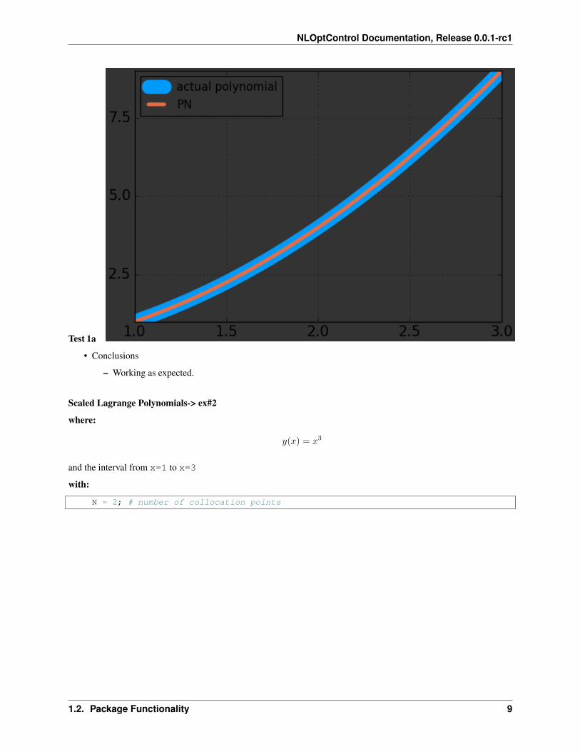
Test 1a
• Conclusions
– Working as expected.
Scaled Lagrange Polynomials-> ex#2
where:
𝑦(𝑥) = 𝑥3
and the interval from x=1 to x=3
with:
N = 2; # number of collocation points
1.2. Package Functionality 9
NLOptControl Documentation, Release 0.0.1-rc1
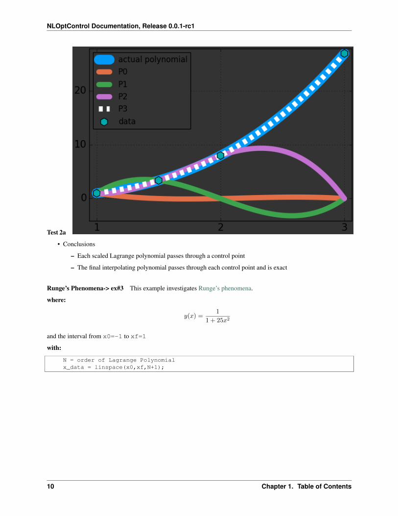
Test 2a
• Conclusions
– Each scaled Lagrange polynomial passes through a control point
– The final interpolating polynomial passes through each control point and is exact
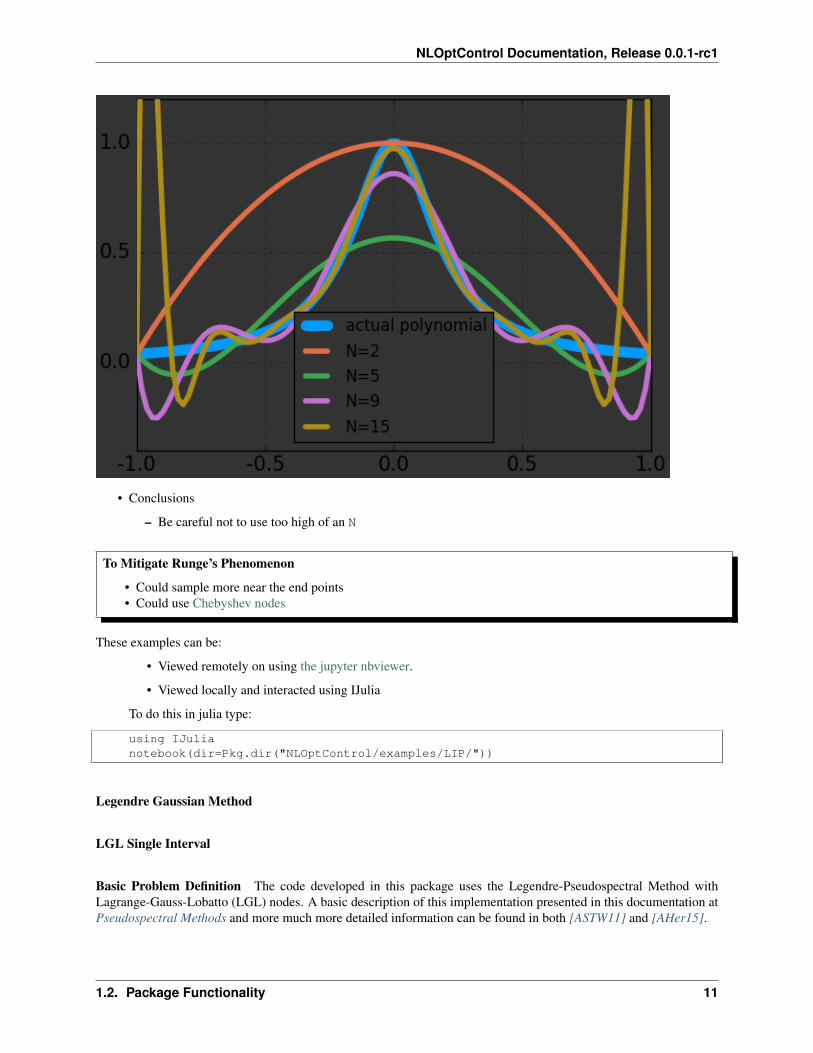
Runge’s Phenomena-> ex#3 This example investigates Runge’s phenomena.
where:
𝑦(𝑥) =1
1 + 25𝑥2
and the interval from x0=-1 to xf=1
with:
N = order of Lagrange Polynomialx_data = linspace(x0,xf,N+1);
10 Chapter 1. Table of Contents
NLOptControl Documentation, Release 0.0.1-rc1
• Conclusions
– Be careful not to use too high of an N
To Mitigate Runge’s Phenomenon
• Could sample more near the end points• Could use Chebyshev nodes
These examples can be:
• Viewed remotely on using the jupyter nbviewer.
• Viewed locally and interacted using IJulia
To do this in julia type:
using IJulianotebook(dir=Pkg.dir("NLOptControl/examples/LIP/"))
Legendre Gaussian Method
LGL Single Interval
Basic Problem Definition The code developed in this package uses the Legendre-Pseudospectral Method withLagrange-Gauss-Lobatto (LGL) nodes. A basic description of this implementation presented in this documentation atPseudospectral Methods and more much more detailed information can be found in both [ASTW11] and [AHer15].
1.2. Package Functionality 11
NLOptControl Documentation, Release 0.0.1-rc1
Examples
In these examples we use:
• Legendre-Gauss-Lobatto (LGL) nodes
• Single interval approximations
• Approximate integrals in the range of [-1,1]
• Approximate derivatives in the range of [-1,1]
These examples can be:
• Viewed remotely on using the jupyter nbviewer.
• Viewed locally and interacted using IJulia
To do this in julia type:
using IJulianotebook(dir=Pkg.dir("NLOptControl/examples/LGL_SI/"))
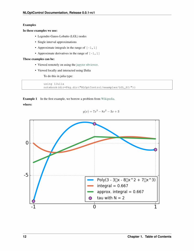
Example 1 In the first example, we borrow a problem from Wikipedia.
where:
𝑦(𝑥) = 7𝑥3 − 8𝑥2 − 3𝑥+ 3
12 Chapter 1. Table of Contents
NLOptControl Documentation, Release 0.0.1-rc1
Difference between the Wikipedia Example and this Example
The difference between Wikipedia example and this one is that the Wikipedia example uses Gauss-LegendreQuadrature while the code developed in this package uses Legendre-Pseudospectral Method with Lagrange-Gauss-Lobatto (LGL) nodes. Information on the difference between these methods and many more can befound in both [BSTW11] and [BHer15].
• Conclusions
– We are able to exactly determine the integral
References
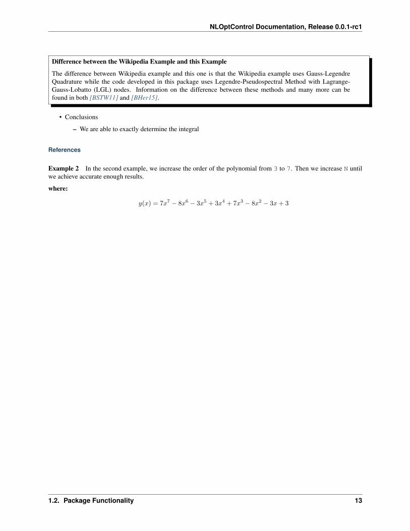
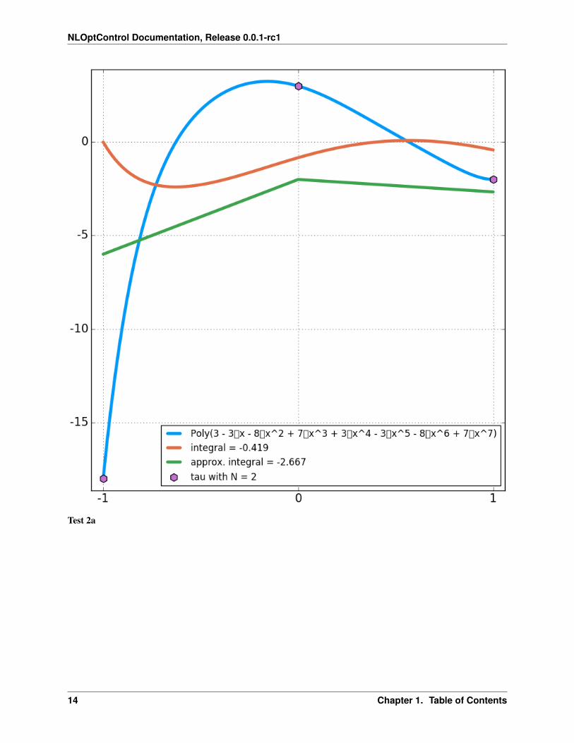
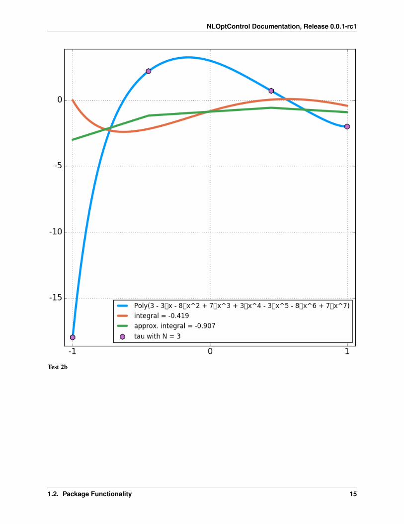
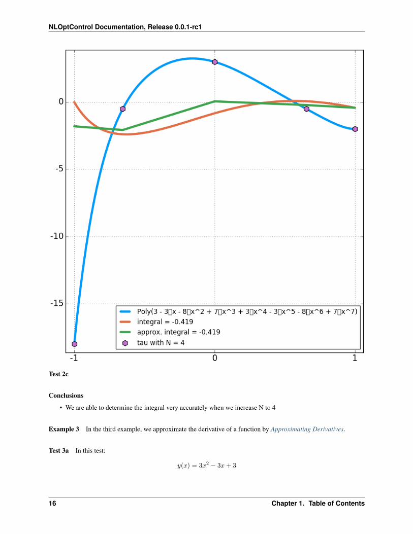
Example 2 In the second example, we increase the order of the polynomial from 3 to 7. Then we increase N untilwe achieve accurate enough results.
where:
𝑦(𝑥) = 7𝑥7 − 8𝑥6 − 3𝑥5 + 3𝑥4 + 7𝑥3 − 8𝑥2 − 3𝑥+ 3
1.2. Package Functionality 13
NLOptControl Documentation, Release 0.0.1-rc1
Test 2a
14 Chapter 1. Table of Contents
NLOptControl Documentation, Release 0.0.1-rc1
Test 2b
1.2. Package Functionality 15
NLOptControl Documentation, Release 0.0.1-rc1
Test 2c
Conclusions
• We are able to determine the integral very accurately when we increase N to 4
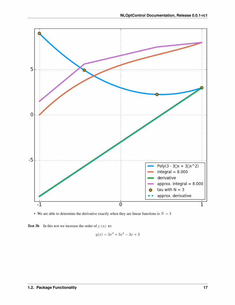
Example 3 In the third example, we approximate the derivative of a function by Approximating Derivatives.
Test 3a In this test:
𝑦(𝑥) = 3𝑥2 − 3𝑥+ 3
16 Chapter 1. Table of Contents
NLOptControl Documentation, Release 0.0.1-rc1
• We are able to determine the derivative exactly when they are linear functions is 𝑁 = 3
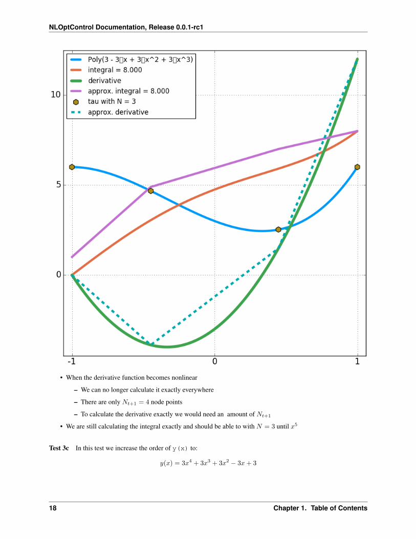
Test 3b In this test we increase the order of y(x) to:
𝑦(𝑥) = 3𝑥3 + 3𝑥2 − 3𝑥+ 3
1.2. Package Functionality 17
NLOptControl Documentation, Release 0.0.1-rc1
• When the derivative function becomes nonlinear
– We can no longer calculate it exactly everywhere
– There are only 𝑁𝑡+1 = 4 node points
– To calculate the derivative exactly we would need an amount of 𝑁𝑡+1
• We are still calculating the integral exactly and should be able to with 𝑁 = 3 until 𝑥5
Test 3c In this test we increase the order of y(x) to:
𝑦(𝑥) = 3𝑥4 + 3𝑥3 + 3𝑥2 − 3𝑥+ 3
18 Chapter 1. Table of Contents
NLOptControl Documentation, Release 0.0.1-rc1
• We are still calculating the integral exactly and should be able to with 𝑁 = 3 until 𝑥5
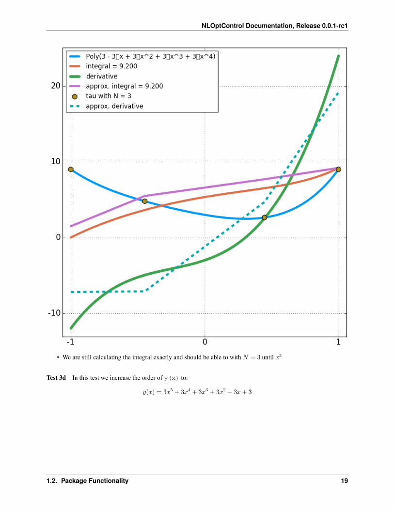
Test 3d In this test we increase the order of y(x) to:
𝑦(𝑥) = 3𝑥5 + 3𝑥4 + 3𝑥3 + 3𝑥2 − 3𝑥+ 3
1.2. Package Functionality 19
NLOptControl Documentation, Release 0.0.1-rc1
• We are still calculating the integral exactly with 𝑁 = 3!!
• The percent error is = 0.000000000000000000 %
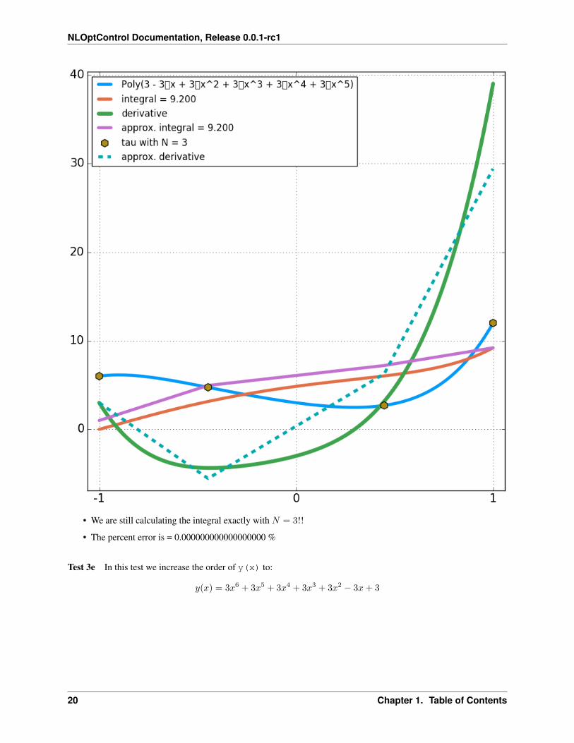
Test 3e In this test we increase the order of y(x) to:
𝑦(𝑥) = 3𝑥6 + 3𝑥5 + 3𝑥4 + 3𝑥3 + 3𝑥2 − 3𝑥+ 3
20 Chapter 1. Table of Contents
NLOptControl Documentation, Release 0.0.1-rc1
• As expected, we are not still calculating the integral exactly with 𝑁 = 3!!
• The percent error is = -1.818181818181822340 %
References
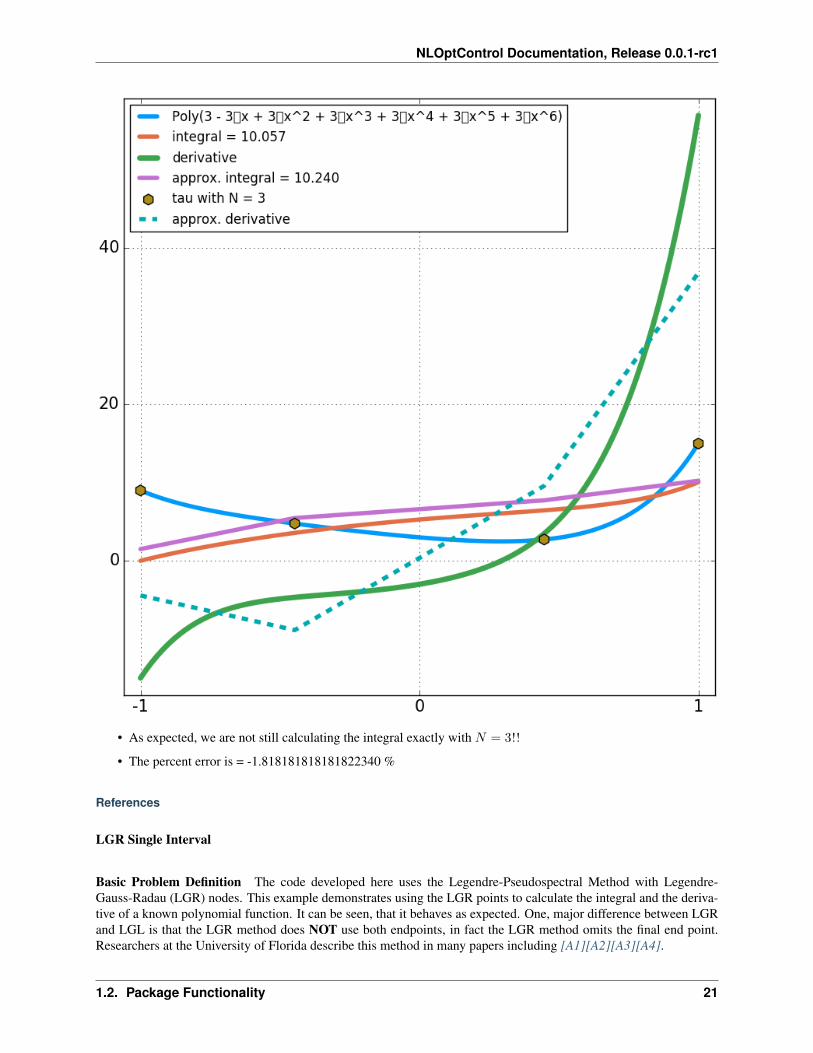
LGR Single Interval
Basic Problem Definition The code developed here uses the Legendre-Pseudospectral Method with Legendre-Gauss-Radau (LGR) nodes. This example demonstrates using the LGR points to calculate the integral and the deriva-tive of a known polynomial function. It can be seen, that it behaves as expected. One, major difference between LGRand LGL is that the LGR method does NOT use both endpoints, in fact the LGR method omits the final end point.Researchers at the University of Florida describe this method in many papers including [A1][A2][A3][A4].
1.2. Package Functionality 21
NLOptControl Documentation, Release 0.0.1-rc1
Examples
In these examples we use:
• Legendre-Gauss-Lobatto (LGR) nodes
• Single interval approximations
• Approximate integrals in the range of [x0,xf]
• Approximate derivatives in the range of [x0,xf]
These examples can be:
• Viewed remotely on using the jupyter nbviewer.
• Viewed locally and interacted using IJulia
To do this in julia type:
using IJulianotebook(dir=Pkg.dir("NLOptControl/examples/LGR_SI/"))
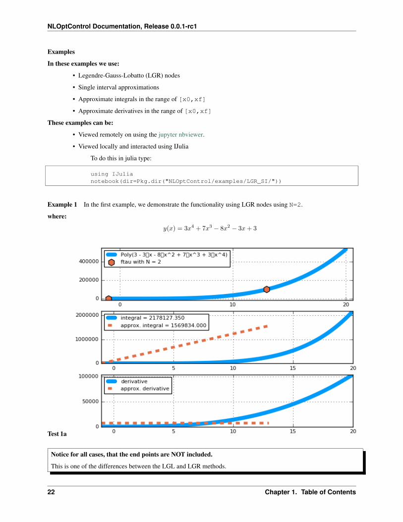
Example 1 In the first example, we demonstrate the functionality using LGR nodes using N=2.
where:
𝑦(𝑥) = 3𝑥4 + 7𝑥3 − 8𝑥2 − 3𝑥+ 3
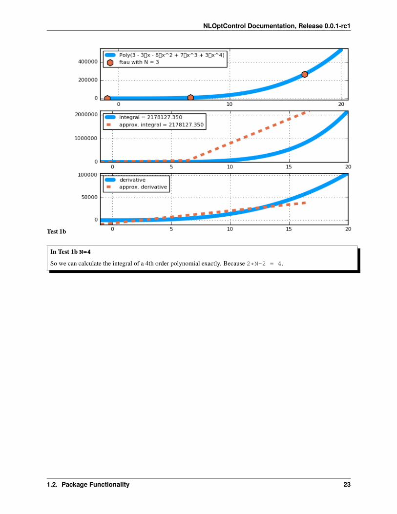
Test 1a
Notice for all cases, that the end points are NOT included.
This is one of the differences between the LGL and LGR methods.
22 Chapter 1. Table of Contents
NLOptControl Documentation, Release 0.0.1-rc1
Test 1b
In Test 1b N=4
So we can calculate the integral of a 4th order polynomial exactly. Because 2*N-2 = 4.
1.2. Package Functionality 23
NLOptControl Documentation, Release 0.0.1-rc1
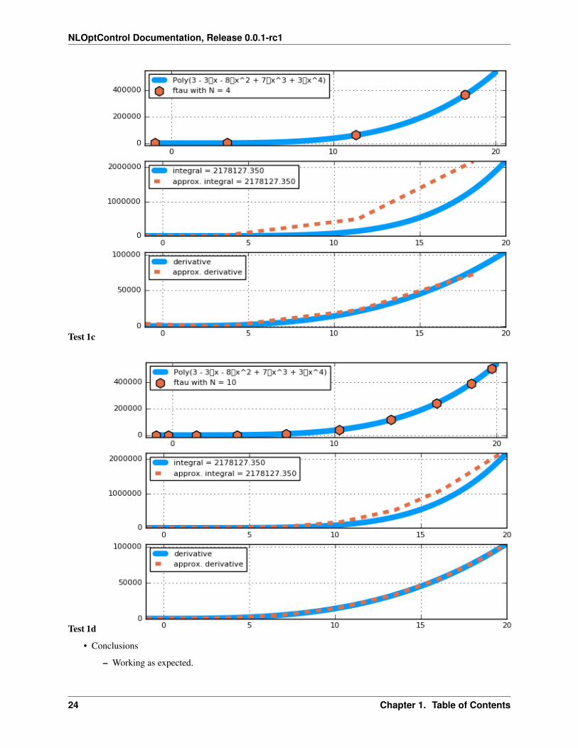
Test 1c
Test 1d
• Conclusions
– Working as expected.
24 Chapter 1. Table of Contents
NLOptControl Documentation, Release 0.0.1-rc1
References
LGR Multiple Interval Now, using Legendre-Gauss-Radau (LGR) points with multiple intervals to calculate theintegral and the derivative of a known polynomial function. This example demonstrates using the Legendre-Gauss-Radau (LGR) points to calculate the integral and the derivative of a known polynomial function using a multipleinterval approach.
Researchers at the University of Florida
describe this method in many papers including [CDar11][CGar11][CGPH+10][CGPH+09].
Functionality NOTE: this is not an exhaustive list and there are help notes for most functions, that can be easilyseen by typing:
julia>? # then press enter and type# the name of the function of interest
LGR_matrices(ps,nlp)
• Calculate LGR matrices
– IMatrix
– DMatrix
Notes:
• Make sure that you calculate these matrices before you try and use them in either integrate_states() or differen-tiate_state().
Examples
In these examples we use:
• Legendre-Gauss-Radau (LGR) nodes
• Multiple interval approximations
• Approximate integrals in the range of [x0,xf]
• Approximate derivatives in the range of [x0,xf]
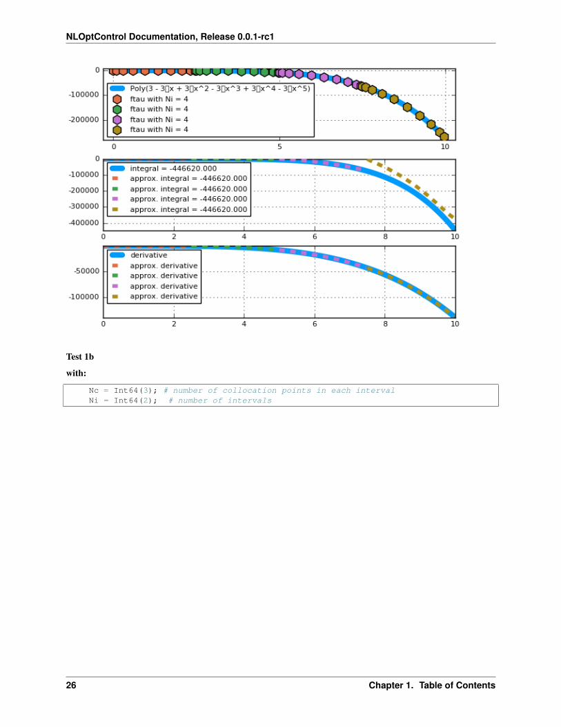
Neglecting Non-Collocated Point 𝑌 (𝑘)() -> ex#1 In this first example, we demonstrate the functionality using LGRnodes
where:
𝑦(𝑥) = −3𝑥5 + 3𝑥4 + 7𝑥3 − 8𝑥2 − 3𝑥+ 3
Test 1a
with:
Nc = Int64(10); # number of collocation points in each intervalNi = Int64(4); # number of intervals
1.2. Package Functionality 25
NLOptControl Documentation, Release 0.0.1-rc1
Test 1b
with:
Nc = Int64(3); # number of collocation points in each intervalNi = Int64(2); # number of intervals
26 Chapter 1. Table of Contents
NLOptControl Documentation, Release 0.0.1-rc1
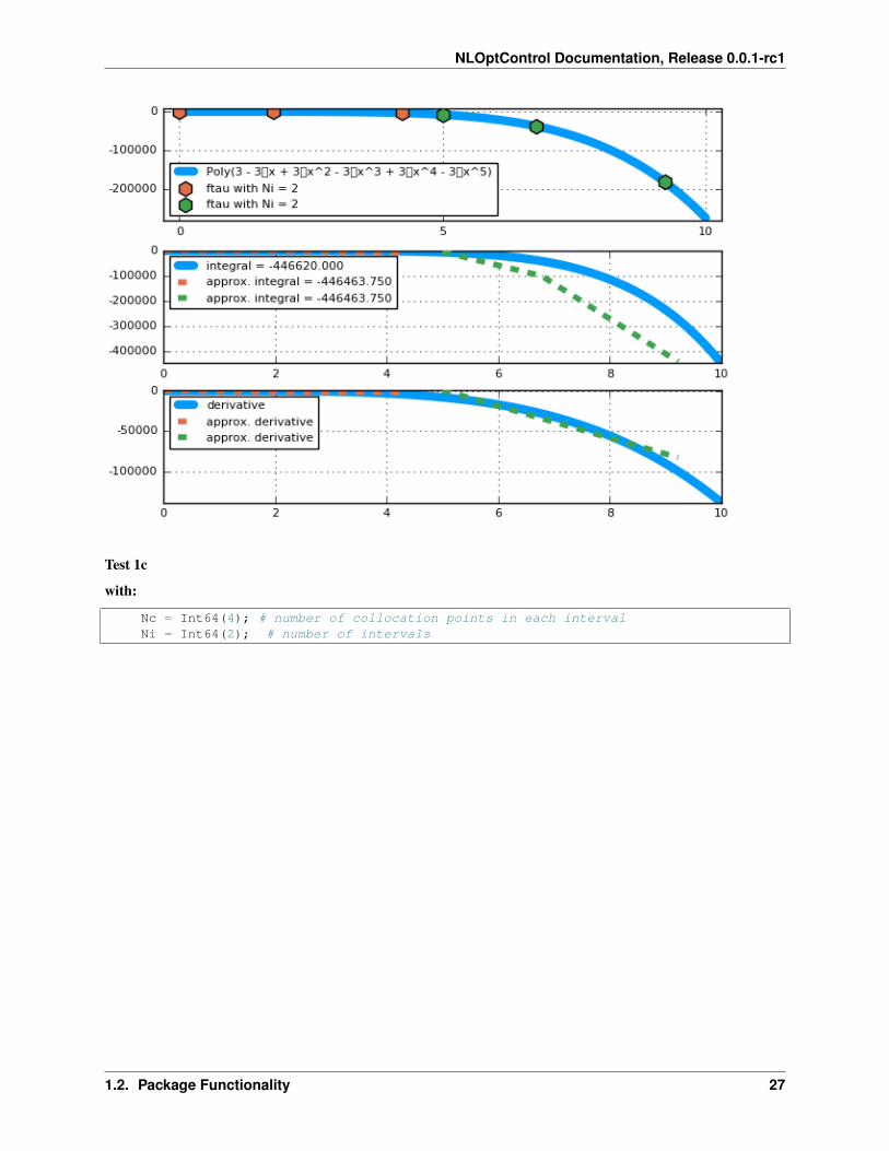
Test 1c
with:
Nc = Int64(4); # number of collocation points in each intervalNi = Int64(2); # number of intervals
1.2. Package Functionality 27
NLOptControl Documentation, Release 0.0.1-rc1
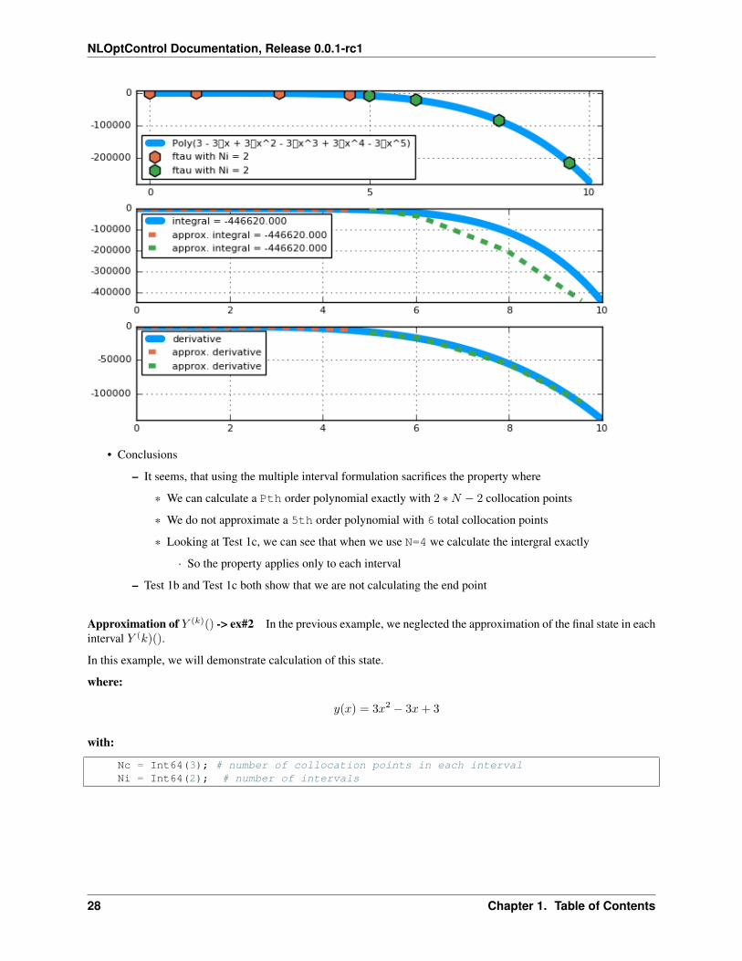
• Conclusions
– It seems, that using the multiple interval formulation sacrifices the property where
* We can calculate a Pth order polynomial exactly with 2 *𝑁 − 2 collocation points
* We do not approximate a 5th order polynomial with 6 total collocation points
* Looking at Test 1c, we can see that when we use N=4 we calculate the intergral exactly
· So the property applies only to each interval
– Test 1b and Test 1c both show that we are not calculating the end point
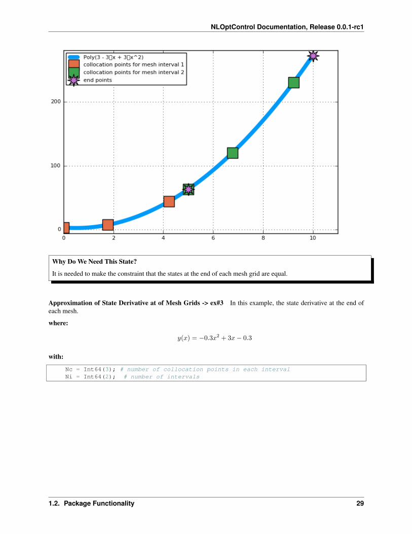
Approximation of 𝑌 (𝑘)() -> ex#2 In the previous example, we neglected the approximation of the final state in eachinterval 𝑌 (𝑘)().
In this example, we will demonstrate calculation of this state.
where:
𝑦(𝑥) = 3𝑥2 − 3𝑥+ 3
with:
Nc = Int64(3); # number of collocation points in each intervalNi = Int64(2); # number of intervals
28 Chapter 1. Table of Contents
NLOptControl Documentation, Release 0.0.1-rc1
Why Do We Need This State?
It is needed to make the constraint that the states at the end of each mesh grid are equal.
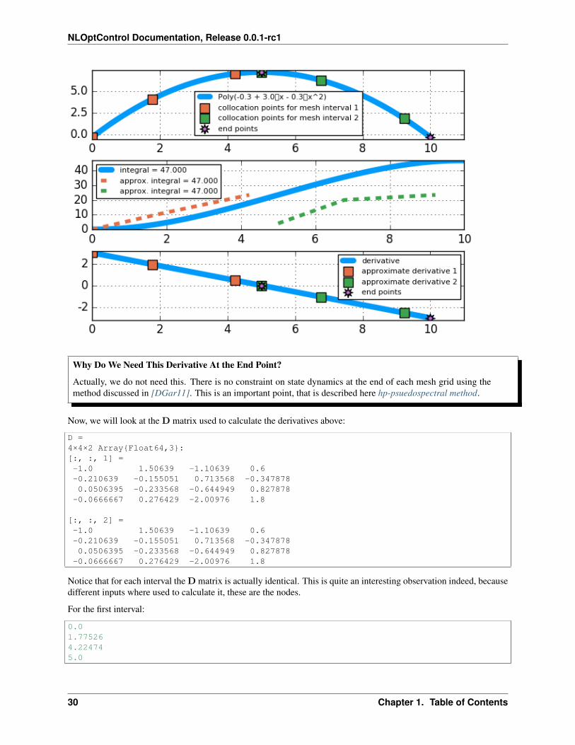
Approximation of State Derivative at of Mesh Grids -> ex#3 In this example, the state derivative at the end ofeach mesh.
where:
𝑦(𝑥) = −0.3𝑥2 + 3𝑥− 0.3
with:
Nc = Int64(3); # number of collocation points in each intervalNi = Int64(2); # number of intervals
1.2. Package Functionality 29
NLOptControl Documentation, Release 0.0.1-rc1
Why Do We Need This Derivative At the End Point?
Actually, we do not need this. There is no constraint on state dynamics at the end of each mesh grid using themethod discussed in [DGar11]. This is an important point, that is described here hp-psuedospectral method.
Now, we will look at the D matrix used to calculate the derivatives above:
D =4×4×2 Array{Float64,3}:[:, :, 1] =-1.0 1.50639 -1.10639 0.6-0.210639 -0.155051 0.713568 -0.3478780.0506395 -0.233568 -0.644949 0.827878
-0.0666667 0.276429 -2.00976 1.8
[:, :, 2] =-1.0 1.50639 -1.10639 0.6-0.210639 -0.155051 0.713568 -0.3478780.0506395 -0.233568 -0.644949 0.827878
-0.0666667 0.276429 -2.00976 1.8
Notice that for each interval the D matrix is actually identical. This is quite an interesting observation indeed, becausedifferent inputs where used to calculate it, these are the nodes.
For the first interval:
0.01.775264.224745.0
30 Chapter 1. Table of Contents
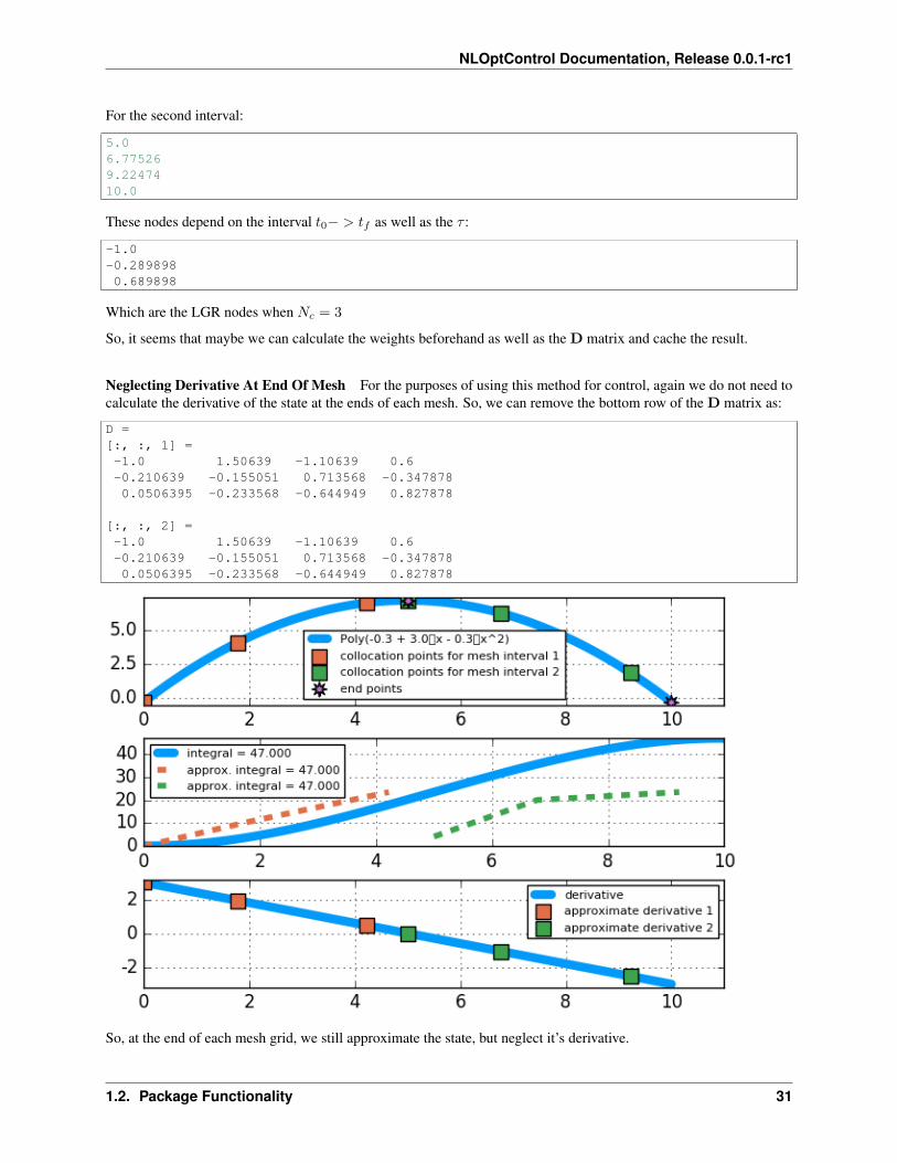
NLOptControl Documentation, Release 0.0.1-rc1
For the second interval:
5.06.775269.2247410.0
These nodes depend on the interval 𝑡0− > 𝑡𝑓 as well as the 𝜏 :
-1.0-0.2898980.689898
Which are the LGR nodes when 𝑁𝑐 = 3
So, it seems that maybe we can calculate the weights beforehand as well as the D matrix and cache the result.
Neglecting Derivative At End Of Mesh For the purposes of using this method for control, again we do not need tocalculate the derivative of the state at the ends of each mesh. So, we can remove the bottom row of the D matrix as:
D =[:, :, 1] =-1.0 1.50639 -1.10639 0.6-0.210639 -0.155051 0.713568 -0.3478780.0506395 -0.233568 -0.644949 0.827878
[:, :, 2] =-1.0 1.50639 -1.10639 0.6-0.210639 -0.155051 0.713568 -0.3478780.0506395 -0.233568 -0.644949 0.827878
So, at the end of each mesh grid, we still approximate the state, but neglect it’s derivative.
1.2. Package Functionality 31
NLOptControl Documentation, Release 0.0.1-rc1
References
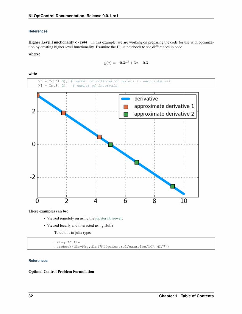
Higher Level Functionality -> ex#4 In this example, we are working on preparing the code for use with optimiza-tion by creating higher level functionality. Examine the IJulia notebook to see differences in code.
where:
𝑦(𝑥) = −0.3𝑥2 + 3𝑥− 0.3
with:
Nc = Int64(3); # number of collocation points in each intervalNi = Int64(2); # number of intervals
These examples can be:
• Viewed remotely on using the jupyter nbviewer.
• Viewed locally and interacted using IJulia
To do this in julia type:
using IJulianotebook(dir=Pkg.dir("NLOptControl/examples/LGR_MI/"))
References
Optimal Control Problem Formulation
32 Chapter 1. Table of Contents
NLOptControl Documentation, Release 0.0.1-rc1
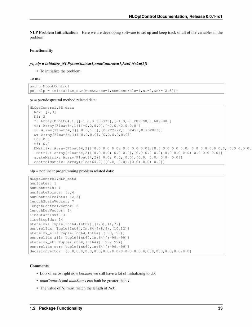
NLP Problem Initialization Here we are developing software to set up and keep track of all of the variables in theproblem.
Functionality
ps, nlp = initialize_NLP(numStates=1,numControls=1,Ni=1,Nck=[2])
• To initialize the problem
To use:
using NLOptControlps, nlp = initialize_NLP(numStates=1,numControls=1,Ni=2,Nck=[2,3]);
ps = pseudospectral method related data:
NLOptControl.PS_dataNck: [2,3]Ni: 2𝜏: Array{Float64,1}[[-1.0,0.333333],[-1.0,-0.289898,0.689898]]ts: Array{Float64,1}[[-0.0,0.0],[-0.0,-0.0,0.0]]𝜔: Array{Float64,1}[[0.5,1.5],[0.222222,1.02497,0.752806]]𝜔: Array{Float64,1}[[0.0,0.0],[0.0,0.0,0.0]]t0: 0.0tf: 0.0DMatrix: Array{Float64,2}[[0.0 0.0 0.0; 0.0 0.0 0.0],[0.0 0.0 0.0 0.0; 0.0 0.0 0.0 0.0; 0.0 0.0 0.0 0.0]]IMatrix: Array{Float64,2}[[0.0 0.0; 0.0 0.0],[0.0 0.0 0.0; 0.0 0.0 0.0; 0.0 0.0 0.0]]stateMatrix: Array{Float64,2}[[0.0; 0.0; 0.0],[0.0; 0.0; 0.0; 0.0]]controlMatrix: Array{Float64,2}[[0.0; 0.0],[0.0; 0.0; 0.0]]
nlp = nonlinear programming problem related data:
NLOptControl.NLP_datanumStates: 1numControls: 1numStatePoints: [3,4]numControlPoints: [2,3]lengthStateVector: 7lengthControlVector: 5lengthDecVector: 14timeStartIdx: 13timeStopIdx: 14stateIdx: Tuple{Int64,Int64}[(1,3),(4,7)]controlIdx: Tuple{Int64,Int64}[(8,9),(10,12)]stateIdx_all: Tuple{Int64,Int64}[(-99,-99)]controlIdx_all: Tuple{Int64,Int64}[(-99,-99)]stateIdx_st: Tuple{Int64,Int64}[(-99,-99)]controlIdx_ctr: Tuple{Int64,Int64}[(-99,-99)]decisionVector: [0.0,0.0,0.0,0.0,0.0,0.0,0.0,0.0,0.0,0.0,0.0,0.0,0.0,0.0]
Comments
• Lots of zeros right now because we still have a lot of initializing to do.
• numControls and numStates can both be greater than 1.
• The value of Ni must match the length of Nck
1.2. Package Functionality 33
NLOptControl Documentation, Release 0.0.1-rc1
generate_Fake_data(nlp,ps,𝛾)
• Generating some data to play with is useful:
nlp2ocp(nlp,ps)
• Turning the nonlinear-programming problem into an optimal control problem
– This function basically takes a large design variable an sorts it back into the original variables
𝜁, approx_int_st = integrate_state(ps,nlp) Approximates integral.
To use this function with Gaussian Quadrature (the default method):
𝜁, approx_int_st = integrate_state(ps,nlp)
To use this function with the LGRIM:
integrate_state(ps,nlp;(:mode=>:LGRIM))
d𝜁 = differentiate_state(ps,nlp) Approximate derivatives.
• Currently only using LGRDM as a method.
Examples
In these examples we use:
• Demonstrate functionality to setup optimal control problem
• Also include the development scripts of these functions
• There is not a webpage for all examples, but the interested user can check out them out using IJulia
NLP and OCP Functionality -> ex#2 In this example, we are continuing to work on preparing the code for usewith optimization by creating higher level functionality. Examine the IJulia notebook to see code.
Aside from using the new data structures we demonstrate:
• Using the integration matrix for the first time
• Using the higher level functionality
where:
𝑦(𝑥) = −0.3𝑥2 + 3𝑥− 0.3
Single Interval Problem with:
ps, nlp = initialize_NLP(numStates=1,numControls=1,Ni=1,Nck=[2]);
34 Chapter 1. Table of Contents
NLOptControl Documentation, Release 0.0.1-rc1
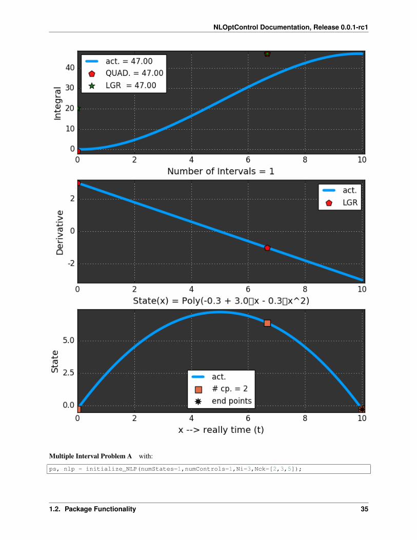
Multiple Interval Problem A with:
ps, nlp = initialize_NLP(numStates=1,numControls=1,Ni=3,Nck=[2,3,5]);
1.2. Package Functionality 35
NLOptControl Documentation, Release 0.0.1-rc1
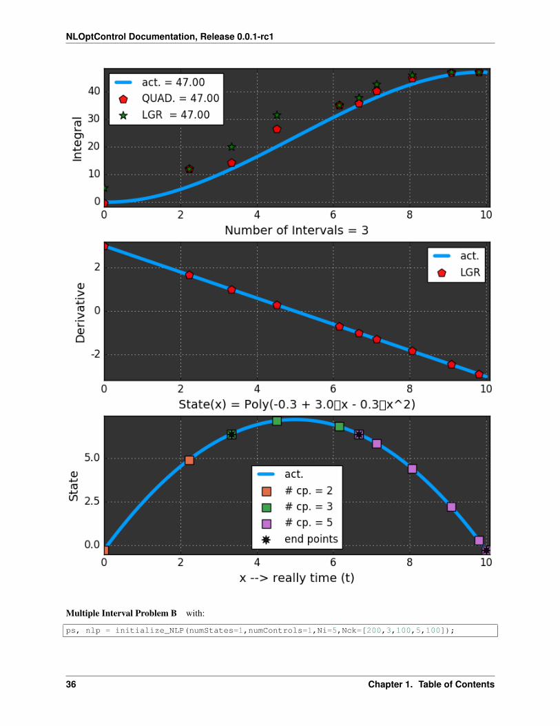
Multiple Interval Problem B with:
ps, nlp = initialize_NLP(numStates=1,numControls=1,Ni=5,Nck=[200,3,100,5,100]);
36 Chapter 1. Table of Contents
NLOptControl Documentation, Release 0.0.1-rc1
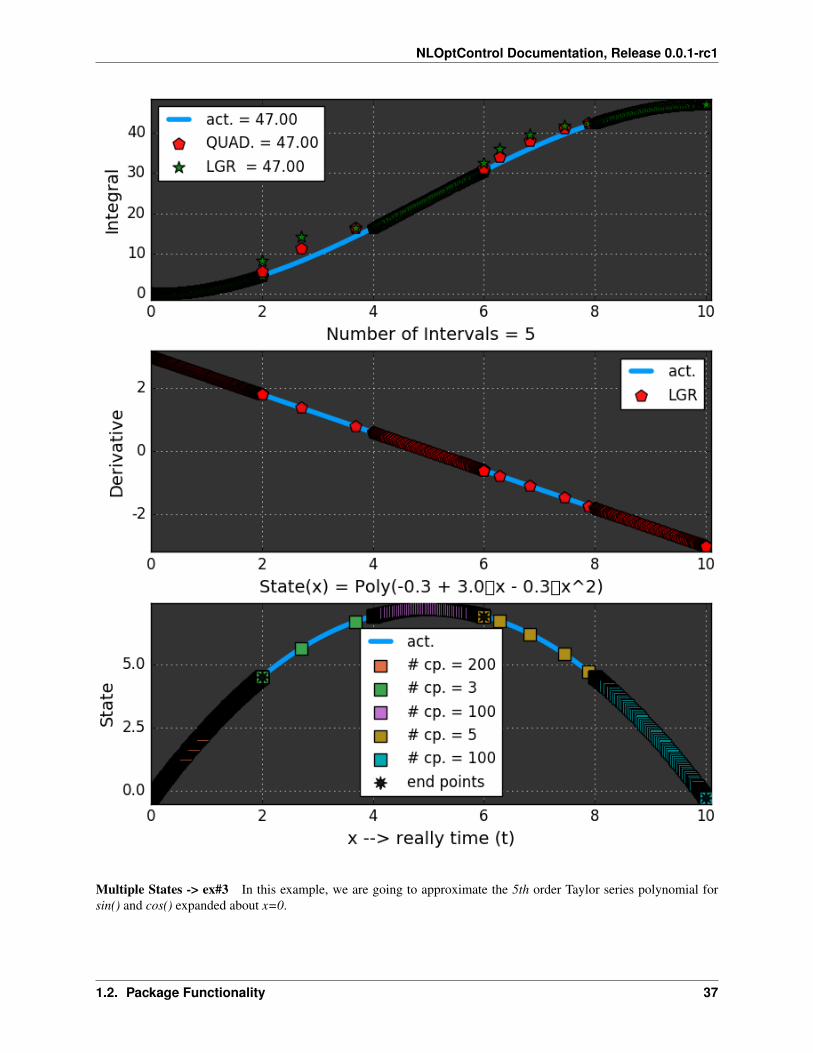
Multiple States -> ex#3 In this example, we are going to approximate the 5th order Taylor series polynomial forsin() and cos() expanded about x=0.
1.2. Package Functionality 37
NLOptControl Documentation, Release 0.0.1-rc1
where:
𝑠𝑖𝑛(𝑥)𝑃5(𝑥) = 𝑥− 𝑥3
3!+𝑥5
5!
𝑐𝑜𝑠(𝑥)𝑃5(𝑥) = 1 − 𝑥2
2!+𝑥4
4!
and:
t0 = Float64(0); tf = Float64(2);
Problem A with:
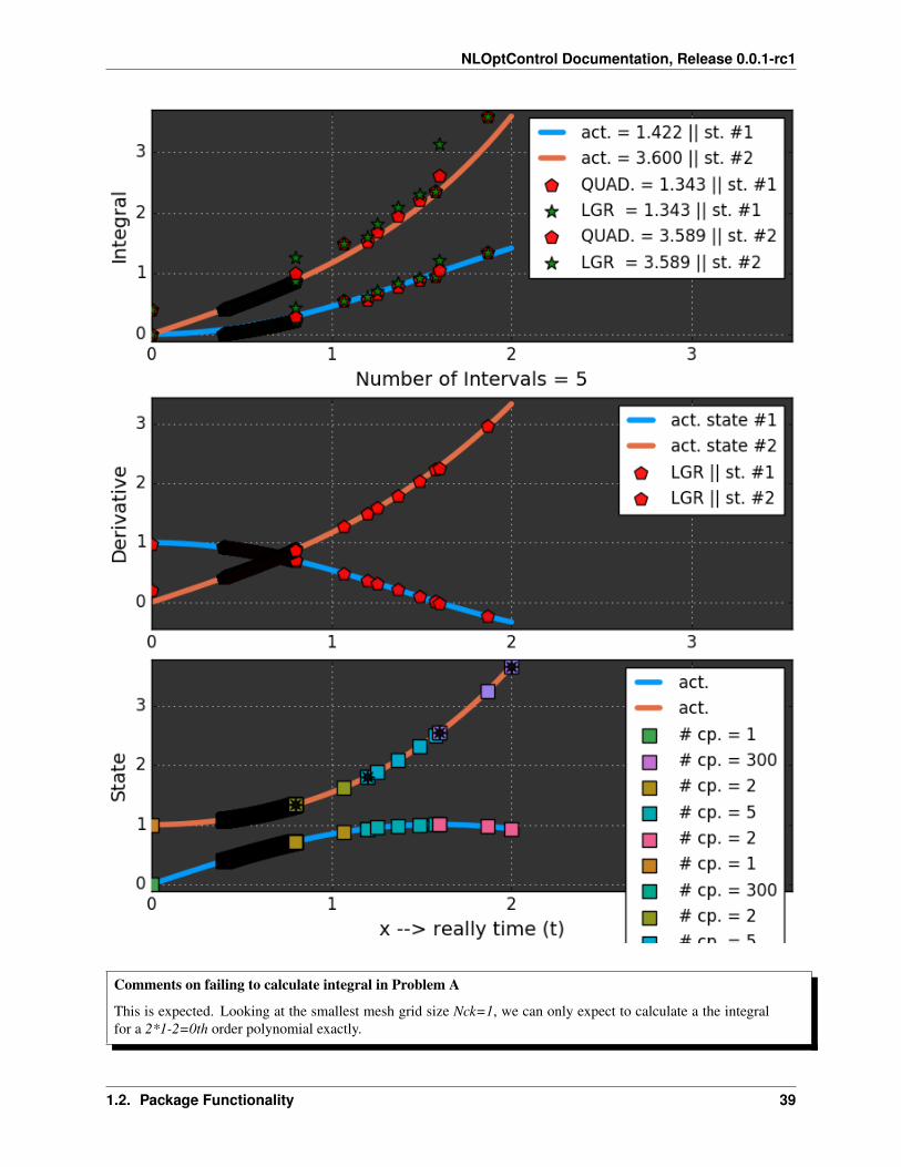
ps, nlp = initialize_NLP(numStates=1,numControls=1,Ni=5,Nck=[200,3,100,5,100]);
38 Chapter 1. Table of Contents
NLOptControl Documentation, Release 0.0.1-rc1
Comments on failing to calculate integral in Problem A
This is expected. Looking at the smallest mesh grid size Nck=1, we can only expect to calculate a the integralfor a 2*1-2=0th order polynomial exactly.
1.2. Package Functionality 39
NLOptControl Documentation, Release 0.0.1-rc1
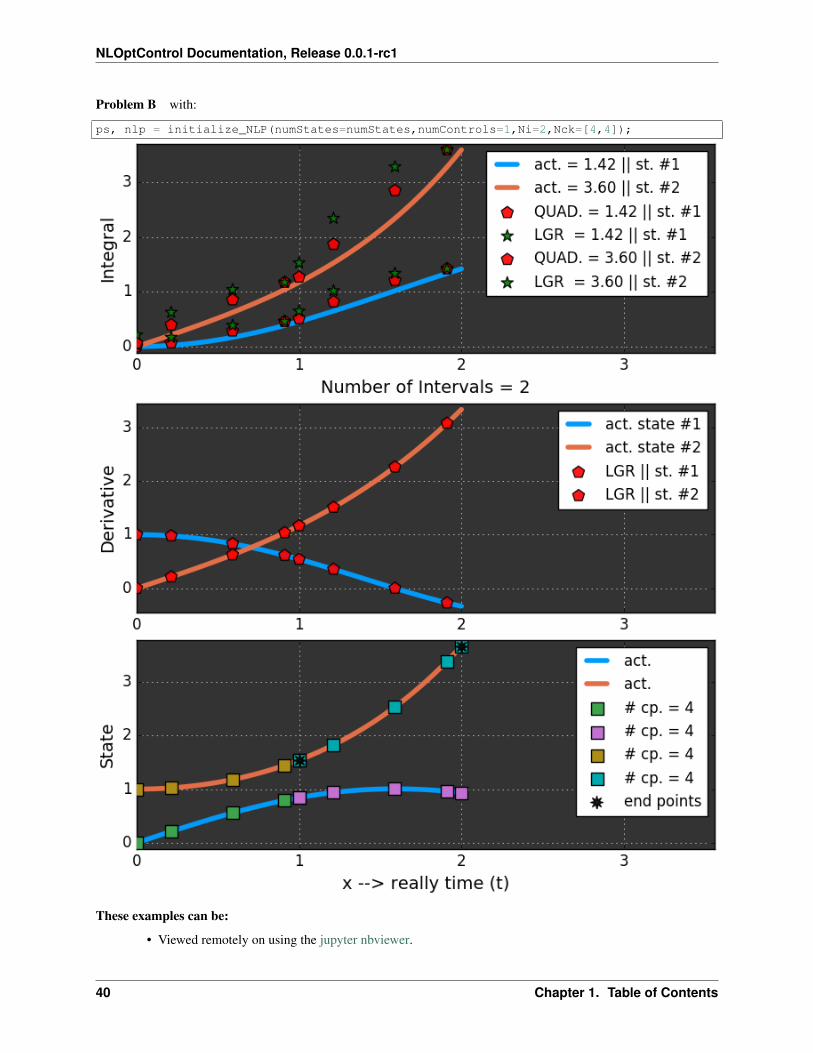
Problem B with:
ps, nlp = initialize_NLP(numStates=numStates,numControls=1,Ni=2,Nck=[4,4]);
These examples can be:
• Viewed remotely on using the jupyter nbviewer.
40 Chapter 1. Table of Contents
NLOptControl Documentation, Release 0.0.1-rc1
• Viewed locally and interacted using IJulia
To do this in julia type:
using IJulianotebook(dir=Pkg.dir("NLOptControl/examples/NLP2OCP/"))
Researchers at the University of Florida
Describe this method in many papers including [EDar11][EGar11][EGPH+10][EGPH+09].
References
Developing Code
This site documents current progress and functionality that is being developed.
Current Focus
Old Records This is for documentation that was created where something was still being worked on where:
1. Everything was not working as expected, but has now been fixed or is obsolete.
2. Removed Functionality
1.3 Bibliography
http://docs.juliadiffeq.org/latest/tutorials/ode_example.html#In-Place-Updates-1
https://github.com/JuliaDiffEq/ParameterizedFunctions.jl#ode-macros
http://docs.juliadiffeq.org/latest/tutorials/ode_example.html#Defining-Systems-of-Equations-Using-ParameterizedFunctions.jl-1 @ChrisRackauckas after looking at ParameterizedFunctions.jl, I realized that Ihave many many parameters and I it would be too much to write them all after the ‘’end” is there a way that Ican include a “parameters.jl” file to execute this? Also, I am currently automatic differentiation, and I noticed thatcurrently ParameterizedFunctions.jl uses symbolic differentiation. I remember you mentioning that you use automaticdifferentiation, can this also
1.3. Bibliography 41
NLOptControl Documentation, Release 0.0.1-rc1
42 Chapter 1. Table of Contents
Bibliography
[BGar11] Divya Garg. Advances in global pseudospectral methods for optimal control. PhD thesis, University ofFlorida, 2011.
[BHer15] Daniel Ronald Herber. Basic implementation of multiple-interval pseudospectral methods to solve optimalcontrol problems. UIUC-ESDL-2015-01, 2015.
[BSTW11] Jie Shen, Tao Tang, and Li-Lian Wang. Spectral methods: algorithms, analysis and applications. volume41. Springer Science & Business Media, 2011.
[AHer15] Daniel Ronald Herber. Basic implementation of multiple-interval pseudospectral methods to solve optimalcontrol problems. UIUC-ESDL-2015-01, 2015.
[ASTW11] Jie Shen, Tao Tang, and Li-Lian Wang. Spectral methods: algorithms, analysis and applications. volume41. Springer Science & Business Media, 2011.
[A1] Christopher L Darby. hp–Pseudospectral Method for Solving Continuous-Time Nonlinear Optimal Control Prob-lems. PhD thesis, University of Florida, 2011.
[A2] Divya Garg. Advances in global pseudospectral methods for optimal control. PhD thesis, University of Florida,2011.
[A3] Divya Garg, Michael Patterson, William W Hager, Anil V Rao, David A Benson, and Geoffrey T Hunting-ton. A unified framework for the numerical solution of optimal control problems using pseudospectral methods.Automatica, 46(11):1843–1851, 2010.
[A4] Divya Garg, Michael A Patterson, William W Hager, Anil V Rao, David A Benson, and Geoffrey T Huntington.An overview of three pseudospectral methods for the numerical solution of optimal control problems. Advancesin the Astronautical Sciences, 135(1):475–487, 2009.
[DGar11] Divya Garg. Advances in global pseudospectral methods for optimal control. PhD thesis, University ofFlorida, 2011.
[CDar11] Christopher L Darby. hp–Pseudospectral Method for Solving Continuous-Time Nonlinear Optimal ControlProblems. PhD thesis, University of Florida, 2011.
[CGar11] Divya Garg. Advances in global pseudospectral methods for optimal control. PhD thesis, University ofFlorida, 2011.
[CGPH+10] Divya Garg, Michael Patterson, William W Hager, Anil V Rao, David A Benson, and Geoffrey T Hunt-ington. A unified framework for the numerical solution of optimal control problems using pseudospectral methods.Automatica, 46(11):1843–1851, 2010.
43
NLOptControl Documentation, Release 0.0.1-rc1
[CGPH+09] Divya Garg, Michael A Patterson, William W Hager, Anil V Rao, David A Benson, and Geoffrey THuntington. An overview of three pseudospectral methods for the numerical solution of optimal control problems.Advances in the Astronautical Sciences, 135(1):475–487, 2009.
[EDar11] Christopher L Darby. hp–Pseudospectral Method for Solving Continuous-Time Nonlinear Optimal ControlProblems. PhD thesis, University of Florida, 2011.
[EGar11] Divya Garg. Advances in global pseudospectral methods for optimal control. PhD thesis, University ofFlorida, 2011.
[EGPH+10] Divya Garg, Michael Patterson, William W Hager, Anil V Rao, David A Benson, and Geoffrey T Hunt-ington. A unified framework for the numerical solution of optimal control problems using pseudospectral methods.Automatica, 46(11):1843–1851, 2010.
[EGPH+09] Divya Garg, Michael A Patterson, William W Hager, Anil V Rao, David A Benson, and Geoffrey THuntington. An overview of three pseudospectral methods for the numerical solution of optimal control problems.Advances in the Astronautical Sciences, 135(1):475–487, 2009.
44 Bibliography