New Filter method for categorical variables’ selection

Heni Bouhamed1,2, Thierry Lecroq1 and Ahmed Rebaï2

1 Department of Computer Science, Rouen University, LITIS EA 4108

Rouen, 76821, France

2 Bioinformatics Unit, Sfax University, Center of biotechnology of Sfax

Sfax, 3018, Tunisia

Abstract It is worth noting that the variable-selection process has become

an increasingly exciting challenge, given the dramatic increase in

the size of databases and the number of variables to be explored

and modelized. Therefore, several strategies and methods have

been developed with the aim of selecting the minimum number

of variables while preserving as much information for the interest

variable of the system to be modelized (variable to predict). In

this work, we will present a novel Filter method useful for

selecting variables, distinct for its joint application of both simple

as well as multivariate analyses to select variables. In the first

place, we will deal with the major prevailing strategies and

methods already underway. Secondly, we will expose our new

method and establish a comparison of its achieved results with

those of the existing methods. The experiments have been

implemented on two different databases, namely, a cardiac

diagnosis disease labeled "Spect Heart", and a car diagnosis,

called "Car Diagnosis 2". As for the ultimate section, it will bear

the conclusion as well some highlights for future research

perspectives and potential horizons.

Keywords: Variables selection; Filter method; Wrapper

strategy; Clustering.

1. Introduction

In the early 1990s, most publications pertaining to

variables selection covered areas often described by only a

few dozens of variables. Most recently, however, owing to

the increase in the capacity for collecting, storing and

handling data, the situation has greatly changed. It is not

uncommon, however, to meet in some areas, particularly

in bioinformatics or text mining, hundreds or even

thousands of variables. Consequently, new variable-

selection techniques have emerged in a bid to address this

change of scale, and above all, to consider the abundance

of redundant as well as irrelevant variables in the data

processing [5].

This problem appears to be even more serious with respect

to several learning applications, especially in the case of a

supervised process. Most often, we have a fixed-size

learning set available at our disposal whether regarding

variables or regarding individuals. Based on this set, we

have to construct a classification model for individuals.

This model is then used to predict the class of new

individuals. Intuitively, one might well consider that an

algorithm’s discriminating power increases with the

number of variables. The situation is not that simple, since

an increase in the number of variables might engender a

dramatic increase in the algorithm’s execution time. In

addition to this computational complexity, there is a

problem of the difficulties inherent in the content of

processed information to be posed: certain variables are

redundant while some others are irrelevant for the

prediction of classes. In this respect, three major categories

or families of approaches have been highlighted in the

literature. First, the Filter approaches [1, 2, 3, 4, 5, 10]

involve introducing the selection procedures prior to, and

independently of, the learning algorithm to be

implemented thereafter. Second, the Embedded

approaches [6, 9], according to which the selection process

is part of learning. This approach is perfectly illustrated by

the decision-tree inducing algorithms, whereby

consistency is the major advantage. Yet, consistency does

not necessarily mean performance, since one of the

selection’s primary objective is to produce a classifier

having the most effective generalization capabilities. As

for the idea of the Wrapper approach [8, 7, 10], it consists

in explicitly applying a performance criterion for the

purpose of retrieving the subset of relevant predictors.

It is as well-known fact that a single variable’s impact on

an information system’s interest variable or class may be

limited as compared to a subset’s impact, in which the

variables jointly react in a complementary manner

(Provided that these variables are not redundant) [11]. This

can be made clear, for instance, in the case study of the

variables responsible for a complex genetic disease in

which variables’ subsets complementarily react to develop

the disease. We can also refer to the example of marketing

variables, where separated subsets of variables influence

consumer behavior, although a single variable’s role might

seem insignificant. The major Filter methods sort out and

sift the variables by individual importance and select the

most important ones. This might lead to the possibility of

eliminating a variable whose individual impact is

relatively weak on the variable to predict, while on

combining it with a variables’ group, it turns out to be very

important and selectable. This problem is partially

resolved by means of the Wrapper strategy, as it

undertakes to select the subset that optimizes best a

classifier’s performance criterion, although the calculation

is the result of the addition or removal of a single variable

rather than a subset of variables. It is also a well-known

fact that the Wrapper strategy is greedy in algorithmic

complexity, as it is classified as an NP-Hard rated problem

[12]. Therefore, several heuristics have been adopted to

help optimize this problem, the most simple and best

known among which are: the Backward method (starting

from the whole set of variables, then eliminating variable

by variable) as well as the Forward method (addition

variable by variable). It is worth noting, however, that in

our present work, we undertake to jointly apply the single

variable analysis along with the multivariate analysis to

select variables associated with a variable to predict (or

class). Our conceived method is going to be tested on two

databases (well-known among data mining practitioners)

and compared to the two major approaches: Filter and

Wrapper. To note, the Embedded methods have been

excluded from the comparison owing to the fact that they,

predominantly, constitute specific learning methods and

their application cannot be generalized.

The remaining parts of this article are organized as follows:

in the next section, we will present some methods

pertaining to the Filter and Wrapper strategy. Then, a new

approach will be exposed which can be classified as a

Filter method, based primarily on the selection of variables

following ranking scores. Our method’s results will be

compared to those of the different methods presented in

“section 2.” with regard to a “car diagnosis” and a “cardiac

disease diagnosis” databases. Finally, we will close this

research work with a conclusion and some prospects for

future research.

2. State of art

2.1 The Wrapper strategy

The idea of the Wrapper approach [8] is to explicitly use

the performance criterion for finding and the subset of

relevant predictors. Most often, this lies in the error rate.

Actually, however, any criterion might fit well and can be

agreed upon. This may, for instance, be the cost if we

introduce a cost matrix of maladjusted classifications; it

can also be the under-curve area when evaluating the

classifier using a ROC curve; etc. In such cases, the

learning method should act as a black box, to which we

exhibit different groups of predictor variables, and

ultimately select the most appropriate one that best

optimizes the criterion. The solutions’ search strategy

plays a crucially-important role in the Wrapper strategy. It

can be very simple, with greedy approaches, adding

(Forward) or removing (Backward) a variable to the

current solution. It can also be very elaborate and intricate,

with approaches based on meta heuristics (genetic

algorithms, ants’ colonies, etc.). In this area, we consider

that the best is the enemy of good. Actually, an excessive

exploration of the solutions’ space leads us to over-

learning. In most cases, the greedy simplistic approaches

turn out to be the most suitable and appropriate. Indeed,

they permit to naturally smooth the path of the solutions’

space.

2.2 The Filter approach

The Filter approach consists in undertaking some

independent selection procedures of learning algorithms to

be implemented thereafter. The major advantage of such

methods is their high speed and flexibility. The “Ranking”

methods are certainly the most representative of this

family. The process consists in calculating an indicator,

individually, featuring the connection between the class

and each predictor. Variables’ are, then, arranged

according to the criterion’s decreasing value. We choose

the primary X variables’ using a statistical hypotheses test

to select the variables having a significant relationship

with the variable to predict. In the upcoming part, we will

present some Filter methods, most frequently mentioned or

cited in the literature [10, 1, 2, 3, 4, 5], and that will be

compared experimentally with our new method in “section

4.”.

The Correlation Feature Selection (CFS) method: The

CFS method [1] is based on an overall measure of measure

of "merit" of a subset M of m variables, considering both

their relevance and redundancy. It is written as:

The CFS method [1] is based on an overall Where is

the mean of correlations between predictor variables and

the target variable; , the mean of cross-correlations

among predictor variables.

Thus, the selection problem becomes an optimization

problem. We need to maximize the amount of "merit"

starting from all the candidate variables’ set. In this respect,

we can apply either some simple greedy strategies (such

methods as step by step, Forward or Backward) or

sophisticated ones (e.g. genetic algorithms, simulated

annealing, etc.). In practice, a simple technique, smoothing

the solutions’ space exploration, is largely sufficient. It

avoids the over-learning pitfall.

The algorithm (greedy selection "Forward") is linear in

respect of the observations’ number. All correlations can

be pre-calculated through a single pass on the data. Yet, it

is quadratic in respect of the number of descriptors.

Therefore, it is more advantageous especially for the huge

databases with a large number of observations but,

relatively, few descriptors.

Inversely, however, when the descriptors are very

numerous, calculation and memory storage of all cross-

correlations become a problem. It becomes more practical

and advantageous to calculate (and recalculate)

correlations on the fly. Experiments have shown that the

number of ultimately-selected variables is often very low.

The Mutual Information Feature Selection (MIFS)

method: The MIFS method [2] rests on a step-by-step

"Forward" algorithm. The evaluation criterion of adding a

supplementary variable X to the set M (of cardinal m) of

the already-selected variables can be written as:

I(Y, X / M) = I(Y,X)-

At each step, we choose the quantity-maximizing variable

I (Y, X / M), which is a partial mutual information. A

variable is considered to be interesting if its connection to

the target Y exceeds its average connection with the

already-selected predictors, taking into account relevance

and redundancy. The search ends when the best variable

X* is such that I (Y, X

* /M) ≤ 0. The selection algorithm is

also quadratic with respect to the number of variables in

the database.

The Fast Correlation-Based Filter (FCBF) method: The

FCBF [4, 5] method is based on the criterion “symmetrical

uncertainty - ρ”. However, it differs for the implemented

search strategy, based on the notion of "predominance".

Actually, the correlation between a variable X* and the

target Y is said to be predominant if and only if:

Concretely, a variable is considered interesting if:

- its correlation with the target variable is

sufficiently high, δ is the parameter that serves to modulate

this;

- there does not exist in the database any variable

which is more strongly correlated to it.

In terms of computing time, the approach is particularly

interesting, especially when we have to process databases

involving thousands of candidate predictors. Regarding the

capacity to detect "good" variables, the experiments have

shown that this method highly outperforms the other

approaches mentioned in this section.

The MODTREE method: Similarly, the MODTREE [3]

method is based on the notions of relevance and

redundancy, through it does not use the same correlation

measure, as it rests on the principle of pair-wise

comparison. The calculation is linear in number of

observations n, even if the criterion is based on the

principle of pair-wise comparisons. This makes it

operational for processing databases involving a large

number of lines. The partial correlation is applied to

achieve the step-by-step “Forward” selection. It measures

the correlation degree between two variables X and Y by

subtracting the effect of a third variable Z.

Similar to the CFS and the MIFS, the algorithm is

quadratic in terms of the number of predictor candidates. It

is especially worth noting that it obliges us to calculate the

cross-partial correlations’ table (initially, a simply raw

cross-correlations’ table), which has to be updated

whenever a new variable is added to the set M. The

memory footprint and computation time constraints

become stronger when we have to process databases

encompassing a large number of descriptors. Compared to

the CFS and FCBF methods, the experiments have shown

that MODTREE is also useful and able to detect the most

interesting predictors [3].

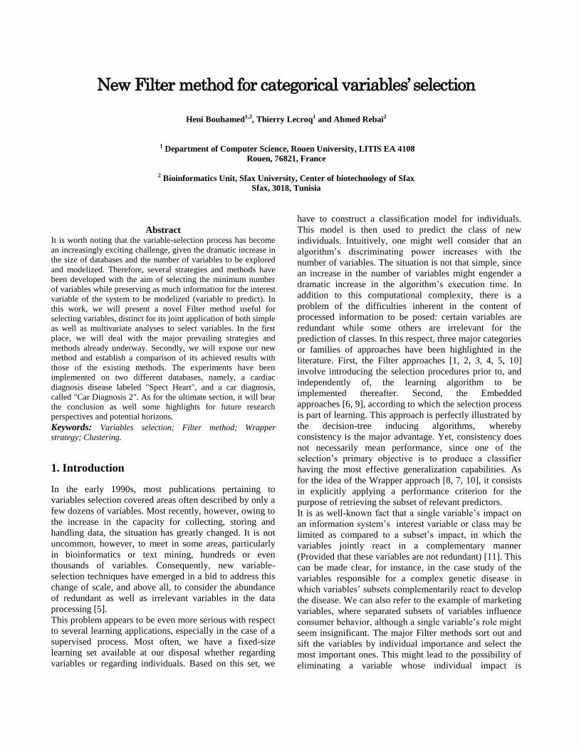
3. New Filter method of categorical variables

With our new Filter method, we propose, on a first stage,

to process the selection via a simple variable analysis with

an initial selection. On a second stage, we undertake to use

a multivariate analysis for a second and final selection.

3.1 Stages pursued by our new approach

• The first stage is consecrated to eliminating redundant

variables as well as the variables providing no information

(variables with a single categorical value with respect to a

database entire examples).

• The second step is devoted, in the first place, to the

simple-variable statistical analysis, then, in a second place,

to eliminating variables with very low statistical

significance.

• The third step consists in the variables’ clustering (a non-

supervised classification).

• The fourth step consists in merging the individual scores

of each cluster’s variables into a single representative

score and ranking all the clusters according to their new

scores.

• The fifth step is the selection of the r first clusters (see

Fig. 1).

3.2 Applied Methodologies and algorithms

Elimination of redundant variables: Throughout this

stage, a special course will be undertaken for the purpose

of eliminating redundant variables (for two or more

identical variables, only a single one will be selected) as

well as the variables having a single categorical value

according to all the data samples (as they provide no

information).

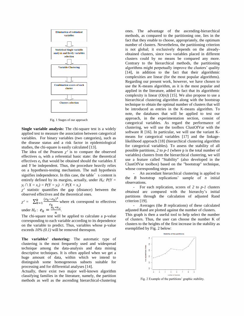
Fig. 1 Stages of our approach

Single variable analysis: The chi-square test is a widely

applied test to measure the association between categorical

variables. For binary variables (two categories), such as

the disease status and a risk factor in epidemiological

studies, the chi-square is easily calculated [13].

The idea of the Pearson χ² is to compare the observed

effectives ok with a referential basic state: the theoretical

effectives ek that would be obtained should the variables X

and Y be independent. Thus, the procedure heavily relies

on a hypothesis-testing mechanism. The null hypothesis

signifies independence. In this case, the table’s content is

entirely defined by its margins, actually, under H0: P(Y =

yl ∩ X = xc) = P(Y = yl) × P(X = xc)

χ² statistic quantifies the gap (distance) between the

observed effectives and the theoretical ones.

χ² = where ek correspond to effectives

under H0 : .

The chi-square test will be applied to calculate a p-value

corresponding to each variable according to its dependence

on the variable to predict. Thus, variables whose p-value

exceeds 10% (0.1) will be removed thereupon.

The variables’ clustering: The automatic type of

clustering is the most frequently used and widespread

technique among the data-analysis and data mining

descriptive techniques. It is often applied when we get a

huge amount of data, within which we intend to

distinguish some homogeneous subsets suitable for

processing and for differential analyses [14].

Actually, there exist two major well-known algorithm

classifying families in the literature, namely, the partition

methods as well as the ascending hierarchical-clustering

ones. The advantage of the ascending-hierarchical

methods, as compared to the partitioning one, lies in the

fact that they enable to choose, appropriately, the optimum

number of clusters. Nevertheless, the partitioning criterion

is not global; it exclusively depends on the already-

obtained clusters, since two variables placed in different

clusters could by no means be compared any more.

Contrary to the hierarchical methods, the partitioning

algorithms might perpetually improve the clusters’ quality

[14], in addition to the fact that their algorithmic

complexities are linear (for the most popular algorithms).

Regarding our present work, however, we have chosen to

use the K-means algorithm, as it is the most popular and

applied in the literature, added to fact that its algorithmic

complexity is linear (O(n)) [15]. We also propose to use a

hierarchical clustering algorithm along with the bootstrap

technique to obtain the optimal number of clusters that will

be introduced as entries in the K-means algorithm. To

note, the databases that will be applied to test our

approach, in the experimentation section, consist of

categorical variables. As regard the performance of

clustering, we will use the toolbox ClustOfVar with the

software R [16]. In particular, we will use the variant K-

means for categorical variables [17] and the linkage-

likelihood approach [18] (hierarchical clustering algorithm

for categorical variables). To assess the stability of all

possible partitions, 2 to p-1 (where p is the total number of

variables) clusters from the hierarchical clustering, we will

use a feature called "Stability" (also developed in the

ClustOfVar toolbox) based on the "bootstrap" technique,

whose corresponding steps are:

- An ascendant hierarchical clustering is applied to

the B bootstrap replications’ sample of n initial

observations.

- For each replication, scores of 2 to p-1 clusters

obtained are compared with the hierarchy’s initial

partitions through the calculation of adjusted Rand

criterion [19].

- Averages (the B replications) of these calculated

adjusted Rand are plotted against the number of clusters.

This graph is then a useful tool to help select the number

of clusters. Thus, the user can choose the number K of

clusters to the heights of the first increase in the stability as

exemplified by Fig. 2 below:

Fig. 2 Example of the partitions’ graphic stability.

According to “Fig. 2”, once stability is increased up to the

level of five clusters, the user can then select the partition

in five clusters.

Calculations of each cluster’s score and ranking: The

question raised in this step is how to derive a score for

each class based on the scores of variables within clusters.

Most of the methods used to combine scores in computer

science literature, and specifically in knowledge discovery

through database, are those that consist in merging scores

of independent variables such as: Average and Maximum

scores [20, 21], Sum, Minimum and product scores [22].

However, the statistical literature provides numerous

score-combining methods by taking into account the

correlations between variables. One of these is the

Truncated Product Method (TPM) (case of dependant

variable) [23] that combines p-values of correlated tests.

This method has already been compared with other

conventional methods and has proven its strength [24]. So,

we propose to use it in this step.

After applying the TPM algorithms, scores are

transformed as the logarithmic transformation –Log10(p-

value) in such a way that a high score value implies a high

degree of significance (association).

Selection of first r clusters: The purpose of this step is to

select clusters of variables that are the most associated to

the phenomenon (predicted variable). There are numerous

methods for selecting most influential variables depicted in

the statistical and computer-science literature. However, to

our knowledge, there are only a few methods that deal

with selecting clusters of variables. In this respect, we

reckon to propose a new method inspired from [25]. It

consists in calculating the empirical value of each cluster

score with the contribution of the scores obtained by

repeating steps 1, 2 and 4 B times on simulated data (the

initial clustering is to be kept). Selection is stopped once a

cluster’s empirical value increases for the first time reports

by the other(s) first cluster’s empirical value. On

simulating data, each variable’s states will be simulated

with the same initial composition categorical values.

We set:

score of cluster ranked i.

: the score of a cluster ranked i obtained after

applying steps 1, 2, and 4 to simulated data.

B: the number of simulations.

PTi: Empirical value of each cluster ranked i calculated as

PTi = .

The number of would be selected clusters is the first r

clusters before the first increase in PTi.

4. Experiments

The clustering was performed via the R language, more

specifically, the package ClustOfVar. The remainder of

our method has been developed in C language.

Noteworthy, the FCBF, CFS, MIFS and MODTREE

methods have been executed with the Tnagra 1.4 software,

available and free downloadable on the site:

http://eric.univ-lyon2.fr/~ricco/tanagra/. As for the

Wrapper strategy methods, they have been executed with

the Spina Research software, available and free

downloadable on the site: http://eric.univ-

lyon2.fr/~ricco/sipina.html .

4.1 Databases

Firstly, we undertake to test our approach on a heart-

diagnosis database (Spect Heart). It is made up of 23

variables (see Table 1.), among which is a status variable

called “overall_Diagnosis”, the global interest variable of

the information system. This Spect Heart domain is

available on the site

http://archive.ics.uci.edu/ml/datasets/SPECT+Heart.

Among the 267 data instances, 32 have been left aside for

the references’ testing phase. In addition, we have applied

our approach to a car diagnosis database (Car Diagnosis 2).

It involves 18 variables (see “Table 2.”), among which is a

status variable called “Car starts”, the information

system’s global interest variable. The parameters’

generating file of this database is available on the site

http://www.norsys.com/downloads/netlib/. Relying on

these parameters, we have been able to generate 10000

examples, among which 32 have been left aside for the

references’ testing phase.

Table 1. “Spect Heart” variables.

Variables’ names Possible states

F1 to F22 (0, 1)

Overall_Diagnosis (0, 1)

Table 2. “Car diagnosis 2” variables.

Variables’ names possible states

AL : Alternator (Okay, Faulty)

CS : Charging System (Okay, Faulty)

BA : Battery age (new, old, very_old)

BV: Battery voltage (strong, weak, dead)

MF: Main fuse (okay, blown)

DS: Distributor (Okay, Faulty)

PV: Voltage at plug (strong, weak, none)

SM: Starter Motor (Okay, Faulty)

SS: Starter system (Okay, Faulty)

HL: Head lights (bright, dim, off)

SP: Spark plugs (okay, too_wide, fouled)

SQ: Spark Quality (good, bad, very_bad)

CC: Car cranks (True, False)

TM: Spark timing (good, bad, very_bad)

FS: Fuel system (Okay, Faulty)

AF: Air filter (clean, dirty)

AS: Air system (Okay, Faulty)

ST: Car starts (True, False)

4.2 Results

The Spect Heart database: After an automated

exploration of this database, there will be neither

redundant variables nor any variables with a single

categorical value. The chi-square test results are presented

in “Table 3” below. The F7 variable, whose chi-square test

value equals 0.17, is automatically removed at this stage.

Regarding the clustering, the optimal number of clusters

chosen is equal to 4 (see Fig. 3). The results of applying

the K-means algorithm are presented in “Table 4”.

Fig. 3 Partitions’ Stability of “Spect Heart” database.

Table 3. Variables chi-square tests results of « Spect Heart » database.

Variables names Chi-square results

F1

F2

F3

F4

F5

F6

F7

F8

F9

F10

F11

F12

F13

F14

F15

F16

F17

F18

F19

F20

F21

F22

0.10

0.03

0.02

0.01

0.32

0.17

0.5×10-2

0.4×10-3

0.04

0.08

0.5×10-2

0.9×10-2

0.2×10-4

0.02

0.08

0.4×10-3

0.2×10-2

0.01

0.15

0.03

0.3×10-2

0.4×10-2

Table 4. Clustering results of the “Spect Heart” database.

Cluster 1 Cluster 2 Cluster 3 Cluster 4

F1, F5,

F10, F19

F2, F6, F7,

F11, F12, F17

F3, F8, F13,

F18, F21,

F22

F4, F9,

F14, F15,

F16, F20

After merging each cluster’s scores with the TPM

algorithm, and following the logarithmic transfomation of

these scores and the sorting of clusters, we obtain the

results presented in “Table 5”. As for the selection of

clusters to be retained, we have obtained the empirical

results PTi, presented in “Table 5”. As PTi increases at the

level of cluster 1, it is, then, a breakpoint. As for clusters 2

(irrespective of the variable F7), 3 and 4, they have been

retained. The final number of selected variables has been

equal to 17 (F2, F6, F11, F12, F17, F3, F8, F13, F18, F21,

F22, F4, F9, F14, F15, F16, F20).

The variable-selection results of the methods: FCBF, CFS,

MIFS, MODTREE, Forward Wrapper, Backward Wrapper

as well as those of our designed approach are shown in

“Table 6”. Eventually, the achieved results’ evaluation and

comparison will be presented in “subsection 4.3" of this

work.

Table 5. Clusters’ ranking by scores.

Cluster number Variables names Score PTi

3 F3 F8 F13 F18 F21 F22 2.1549 0.0000

4 F4 F9 F14 F15 F16 F20 0.6675 0.0000

2 F2 F6 F11 F12 F17 0.6326 0.0000

1 F1 F5 F10 F19 0.0814 0.0200

Table 6. Variables selected according to different methods. FCBF CFS MODTREE MIFS Wrapper

Forward

Wrapper

Backward

Our

Method

F10

F13

F16

F17

F8

F11

F13

F16

F17

F22

F13 F8

F13

F16

F17

F18

F20

F22

F13 F1

F2 F3

F4 F11

F2 F3 F5

F7 F8 F9

F10 F11

F12 F13

F14 F15

F16 F17

F18 F19

F21 F22

F2 F6

F11

F12

F17 F3

F8 F13

F18

F21

F22 F4

F9 F14

F15

F16

F20

The Car Diagnosis 2 database: Following this database’s

automated exploration, no redundant variable has been

detected. However, the variable "AL", whose value has

been equal to a single categorical value with respect to the

entirety of the studied examples, has been rejected. As

regard the variables CS, BA, HP, HL, DC and AF, whose

chi-square test values has been higher than 0.1, they are

automatically removed at this stage. Regarding the

clustering, the optimal number of selected clusters has

been equal to 3 (see Fig. 4); the results of applying the K-

means algorithm are presented in “Table 8”.

Fig. 4 The partitions’ stability of “Car Diagnosis 2” database.

Table 7. Results of the chi-square test application on « Car Diagnosis 2 »

database.

Variables names Chi-square results

CS

BA

BV

MF

PV

SM

SS

HL

SP

SQ

CC

DS

TM

FS

AF

AS

0.35

0.25

0.7×10-2

0.1×10-10

0.19

0.1×10-10

0.18×10-3

0.18

0.2×10-2

0.02

0.17

0.1×10-10

0.12×10-6

0.6×10-10

0.10

0.2×10-14

Table 8. Clustering results of the “Car diagnosis 2” database.

Cluster 1 Cluster 2 Cluster 3

CS : Charging

System

BA : Battery age

BV: Battery voltage

MF: Main fuse

PV: Voltage at plug

SM: Starter Motor

SS: Starter system

HL: Head lights

SP: Spark plugs

SQ: Spark Quality

CC: Car cranks

DS: Distributor

TM: Spark timing

FS: Fuel system

AF: Air filter

AS: Air system

After merging each cluster’s scores with the TPM

algorithm, and following the logarithmic transformation of

these scores as well as the sorting of clusters, we obtain

the results shown in “Table 9”.

Concerning the selection of clusters to be retained, we

have obtained the empirical results PTi depicted in

“Table 9”. Actually, as PTi has always been equal to 0, no

cluster will have to be eliminated. Hence, Clusters 1, 2 and

3 have been retained. The ultimate number of selected

variables is equal to 10 (BV, MF, SM, SS, SP, SQ, DS,

TM, FS, AS).

The variable-selection results of the methods: FCBF, CFS,

MIFS, MODTREE, Forward Wrapper, Backward Wrapper

as well as those of our designed approach are shown in

“Table 10.”. These results’ evaluation and comparison will

be presented in “subsection 4.3.”.

Table 9. Clusters’ ranking by scores.

Cluster number Variables names Score PTi

3 FS AS 3.7300 0.0000

1 BV MF SM SS SP SQ 2.9067 0.0000

2 DS TM 1.7443 0.0000

Table 10. Variables selected according to the different applied methods. FCBF CFS MODTREE MIFS Forward

Wrapper

Backward

Wrapper

Our

Method

SS

TM

FS

AS

AS AS FS

AF

AS

AS FS

CS AL

MF BV

BA SQ

AL CS

MF DS

SM SS

SP SQ

TM FS

AS

BV

MF

SM SS

SP SQ

DS

TM FS

AS

4.3 Inference and comparison of results

For the sake of evaluating the different methods’ results,

we will learn the Bayesian networks’ structures and

parameters of the variables selected via the methods:

FCBF, CFS, MIFS, MODTREE, Forward Wrapper,

Backward Wrapper as well as ours (variables selected with

the variable to be predicted or class). For this purpose, we

will use the Maximum Weight Spanning Tree (MWST)

[27] algorithm to attain the variables’ starting orders, with

the introduction of the variable to be predicted as an initial

variable repeatedly at each time [28]. Then, we will use

the K2 algorithm [26] so as to learn the different

structures. After the parameters’ learning, we will use 32

database samples (evidently not used during the learning

process) to infer each structure and calculate the states’

probabilities of the variable to predict, with respect to both

databases under study. Then, we will compare them with

those obtained by inferring the resulting learning structure

of all variables (without selection) with the variable to be

predicted. The purpose of this evaluation is to recognize

the methods that mostly preserve the information for the

variables to predict while eliminating the maximum of

variables. The results are presented graphically, comparing

the probabilities of the variable to be predicted with those

obtained by inferring all the variables’ structure (we will

test exclusively the probability for the predictable variable

to be at the state 1, as the variables to predict of both

studied databases are binary). Eventually, the "Spect

Heart" database attained results are presented in Appendix

A, while those pertaining to the "Car Diagnosis 2" one are

presented in Appendix B.

5. Discussion

On examining the achieved results, the Filter methods

(FCBF, MIFS, MODTREE and CFS) turn out to be very

selective, eliminating a great deal of variables. Actually,

this is very beneficial in terms of computational

complexity when exploiting the results; yet, there is still a

considerable loss of information especially with respect to

the CFS and MODTREE methods. Regarding the Wrapper

strategy, results differ significantly between the Forward

and Backward types of exploration. With the Backward

one, fewer variables have been removed; still, the

inference results remain identical to those of the entire

variables’ structure inference. The inference results via the

Forward Wrapper have been very close to the inference

results of all the variables’ structure, but not identical. Our

conceived approach along with the Backward Wrapper

strategy appear to be the only methods to safeguard and

maintain the complete information after eliminating

variables (inference results identical to those of all the

variables’ learning regarding both databases examined).

Nevertheless, our approach turns out to be more effective

since it has helped eliminate a higher number of variables

(elimination of 5 variables with respect to the "Spect

Heart" database, versus 4 variables eliminated with the

Backward Wrapper strategy and the elimination of 7

variables via our method, regarding the "Car Diagnosis2"

database, against 6 variables, too through the Backward

Wrapper strategy). We can, therefore, conclude that our

method appears to be more efficient than the Wrapper

(Forward and Backward explorations) as well as the other

Filter methods tested in this work. Regarding the

algorithmic computational complexity, it appears clear that

our envisaged framework along with the Wrapper strategy

methods can be classified as NP-Hard problems.

Noteworthy, in this respect, that our envisaged objective to

be targeted in future works will lie in devising certain

tools, or solutions, whereby to reduce the computational

complexity even further, above all with respect to the

clusters’ selection section.

It is also worth noting that the positively good results

achieved via our novel method may be due to its thorough

focus on the impact of several subsets of variables on the

variable to be predicted, in addition to the study of

variables’ separate association with that variable. To our

knowledge, our Filter method appears to be the exclusive

framework to jointly apply both the simple variable and

multivariate analyses for variables’ selection purposes.

Hence, the originality of such a novel framework, whose

contribution has led to a noticeable improvement in the

study area.

6. Conclusion

Throughout the present study, we have earnestly tried to

define a new Filter method useful for selecting categorical

variables. In a first place, we have presented the key

strategies and existing methods, while highlighting their

advantages and drawbacks. In a second place, we have

presented a novel Filter method that has been tested and

compared with the main existing methods through a two-

database experiment. On an ultimate stage, the different

models’ results have been evaluated, which has led to

prove that our designed approach turns out to be the most

efficient and accurate. Actually, it is the scheme that has

enabled to fully preserve the whole information while

eliminating the greatest number of variables. In future

research, we shall try to find new techniques for the

selection of clusters to reduce our method’s computational

complexity even more, and attempt to devise new

evaluation methods using new learning strategies.

References [1] M. Hall, S. Lloyd, Feature subset selection: a correlation

based filter approach, in International Conference On Neural

Information Processing and Intelligent Information Systems,

(1997) 855‐858.

[2] R. Battiti, Using mutual information for selecting features in

supervised neural net learning, IEEE Transactions on Neural

Networks, 5(4) (1994) 537‐550.

[3] R. Rakotomalala, S. Lallich, Construction d'arbres de

décision par optimisation, Revue Extraction des

Connaissances et Apprentissage, vol. 16, (2002) 685‐703.

[4] L. Yu, H. Liu, Feature Selection for High-Dimensional Data:

A Fast Correlation-Based Filter Solution. In Proceedings of

the twentieth international Conference on Machine Leaning

(ICML-03) Washington, D.C., (2003) 856-863.

[5] L. Yu, H. Liu, Efficient feature selection via analysis of

Relevance and Redundancy, Journal of machine learning

research (2004) 1205-1224.

[6] I. Guyon, A. Elisseeff, An introduction to variable and feature

selection, Journal of Machine Learning Research (2003)

1157-1182.

[7] A. L. Blum, P. Langley Selection of relevant features and

examples in machine learning. Artificial Intelligence (1997)

245-271.

[8] R. Kohavi, G. H. John, Wrappers for feature subset selection,

Artificial Intelligence 97 (1997) 273-324.

[9] T. N. Lal, O. Chapelle, J. Weston, A. Elisseeff, Embedded

methods. In I. Guyon, S. Gunn, M. Nikravesh, L. A. Zadeh,

editors, Feature Extraction: Foundations and Applications,

Studies in Fuzziness and Soft Computing 207, (2006) 137–

165.

[10] I. Inza, P. Larrañaga, R. Blanco, A. J. Cerrolaza, Filter

versus wrapper gene selection approaches in DNA

microarray domains. Artificial Intelligence in Medicine,

special issue in Data mining in genomics and proteomics,

31(2), (2004) 91-103.

[11] M. Geudj, D. Robelin, M. Hoebeke, M. Lamarine, J.

Wojcik, G. Nuel, Detecting Local High-Scoring Segments: a

First-Stage Approach for Genome-Wide Association Studies.

Statistical Applications in Genetics and Molecular Biology,

22. (2006) 1-16.

[12] E. Amaldi, V. Kann, On the approximation of minimizing

non zero variables or unsatisfied relations in linear systems.

Theoretical Computer Science, 209 (1998) 237–260.

[13] C. Herman, E. L. Lehman, “The use of Maximum

Likelihood Estimates in chi-square tests for goodness of fit,”

The annals of Mathematical Statistics volume 25, Number 3,

(1954) 579-586.

[14] S. Tufféry, Data mining et statistique décisionnelle:

l’intelligence des données, Editions TECHNIP. (2010).

[15] A.K. Jain, Data clustering: 50 years beyond K-means,

Pattern Recognition Letters. 31 (2010) 651-666.

[16] M. Chavent, V. Kuentz, B. Liquet, J. Saracco, ClustOfVar:

an R package for the clustering of variables. The R user

conference, University of Warwick Coventry UK. (2011) 63-

72.

[17] M. Chavent, V. Kuentz, J. Saracco, A partitioning method

for the clustering of categorical variables. In classification as

a tool for Research, Herman locarek-Junge, claus Weihs

(Eds), Springer, in Proceedings of the IFCS (2009) 181-205.

[18] I.C.Lerman,. Likelihood linkage analysis (LLA)

classification method: An example treated by hand,

Biochimie, 75 (5) (1993) 379-397.

[19] P. Green, A. Kreiger, A Generalized Rand-Index Method for

Consensus Clustering of Separate Partitions of the Same Data

Base, Journal of classification. (1999) 63-89.

[20] D. M. Lyons, D. F. Hsu, Combining multiple scoring

systems for target tracking using rank-score characteristics,

Information Fusion. 10 (2009) 124-136.

[21] H. N. Parkash, D. S. Guru, Offline signature verification: An

approach based on score level fusion, International journal of

computer applications (2010) 52-58.

[22] A. Jain, K. Nandakumar, A. Ross, Score normalization in

multimodal biometric systems, Pattern Recognition volume

38 Issue 12 (2005) 2270-2285.

[23] D. Zaykin, L. Zhivotovsky, P. Westfall, B. Weir, Truncated

product method for combining P-values, Wiley Inter Science

(2002) 217-226.

[24] H. Bouhamed, A. Rebai, T. Lecroq, M. Jaoua, Data-

organization before learning Multi-Entity Bayesian Networks

structure, Proceeding of World Academy of Science,

Engineering and Technology 78 (2011) 305-308.

[25] S. Karlin, S. Altshul, Applications and statistics for multiple

high-scoring segments in molecular sequences, Proceedings

of the National Academy of Science USA 90, (1993) 5873-

5877.

[26] G. Cooper, E. Hersovits, A Bayesian method for the

induction of probabilistic networks from data, Machine

learning. 9 (1992) 309-347.

[27] C. Chow, C. Liu, Approximating discrete probability

distributions with dependence trees. IEEE Transactions on

Information Theory. 14 (3) (1968) 462-467.

[28] O. Francois, P. Leray, Evaluation d'algorithmes

d'apprentissage de structure pour les réseaux bayésiens, In

Proceedings of 14ème Congrès Francophone Reconnaissance

des Formes et Intelligence Artificielle. (2004) 1453-1460.

Appendix A

Inference results’ comparisons under all variables’

learning and selected variables’ learning through each

method studied for the "Spect Heart" database.

Appendix B

Inference results’ comparisons under all variables’

learning and selected variables’ learning through each

method studied for the “Car Diagnosis 2” database.

Heni Bouhamed is preparing his PhD thesis on optimization in machine learning at the University Of Rouen, supervised by Thierry Lecroq and Ahmed Rebaï. His thesis is co-directed in partnership between the Center of Biotechnology of Sfax under the administrative supervision of the Tunisian Ministry of higher education and the LITIS laboratory in France.

Thierry Lecroq got his PhD thesis degree in computer science from Orleans University in 1992. He obtained his certificate of ability to supervise research from University of Rouen in 2000. Ahmed Rebaï got his PhD thesis degree in Biometry and Quantitative Genetics from the INA-PG France in 1995. He obtained his certificate of ability to supervise research from University of Paris 11 in 2002.