arX

iv:m

ath/

9801

119v

1 [

mat

h.A

G]

26

Jan

1998 Categorical Mirror Symmetry:

The Elliptic Curve

Alexander Polishchuk† and Eric Zaslow††

Department of Mathematics, Harvard University, Cambridge, MA 02138, USA

Abstract

We describe an isomorphism of categories conjectured by Kontsevich. If M and M are

mirror pairs then the conjectural equivalence is between the derived category of coherent

sheaves on M and a suitable version of Fukaya’s category of Lagrangian submanifolds

on M. We prove this equivalence when M is an elliptic curve and M is its dual curve,

exhibiting the dictionary in detail.

1/98

† email: apolish@math.harvard.edu†† email: zaslow@math.harvard.edu

1. Introduction and Summary

Mirror symmetry – equivalence between superconformal sigma models on certain pairs

of Calabi-Yau spaces – has grown into an industry since its discovery in 1989 [1] and the

subsequent translation into enumerative geometry in [2]. Nevertheless, its origins remain

mysterious. In 1994, Kontsevich conjectured that mirror symmetry could be interpreted

as an equivalence of categories over mirror pairs of spaces [3]. While this would not explain

mirror symmetry, it may be a way of putting it on more algebraic grounds. As it currently

stands – relating periods of Picard-Fuchs solutions in an appropriate basis to Gromov-

Witten invariants [4] – mirror symmetry is rather difficult to define rigorously. Further, it

has been pointed out in [5] that the appropriate moduli space for string theory should be

more than just the Kahler and complex moduli of the Calabi-Yau manifold. Kontsevich

introduced the constructions considered here in part as a way of naturally extending this

moduli space (see also [6]).

All of the above work had been done without the knowledge of D-branes. On a Calabi-

Yau three-fold (in Type IIB), D-branes correspond to minimal Lagrangian submanifolds

with unitary local systems (by which we mean flat U(n) gauge bundles). The conjecture

of [7] states that these objects are responsible for mirror symmetry. For tori, K3, and

certain orbifolds of tori, there is evidence for such a description [8], [9], [10], [11]. We find

it appealing, then, that Kontsevich’s conjecture nicely incorporates these objects on the

mirror side. Indeed, the conjecture of [7] may now be reinterpreted as a consequence of

the correspondence between distinguished objects in two equivalent categories.

Kontsevich’s conjecture is that if M and M are mirror pairs then Db(M), the bounded

derived category of coherent sheaves on M, is equivalent to the derived category of a

suitable enlargement of the category F(M) of minimal Lagrangian submanifolds on M

with unitary local systems: Db(M) ∼= Db(F(M)). F(M) was introduced by Fukaya in [12]

and refined by Kontsevich [3] for the conjecture. Db(F(M)) denotes the derived category

of the A∞-category F(M), constructed in [3] using twisted complexes. However, in the

case of elliptic curves one doesn’t need such a construction. Instead, we form a category

F0(M) from F(M) and prove1

Db(M) ∼= F0(M)

for the elliptic curve. In general, it seems that the category Db(F(M)) has to be further

localized to have a chance at equivalence with Db(M).

1 In the notation of [3], F0(M) would be called H(F(M)).

1

The torus is the first non-trivial check of this conjecture [3]. Here M = Eτ is an

elliptic curve with modular parameter τ and M = Eρ is a torus (the complex structure is

irrelevant here) with complexified Kahler parameter ρ = iA + b, where A is the area and

b defines a class in H2(M ;R)/H2(M ;Z). The mirror map is

ρ ↔ τ

(due to the positivity of A and the periodicity of b, the more natural parameter is perhaps

q = exp(2πiρ)). The equivalence that we detail in this simple case is non-trivial and involves

relations among theta functions and sections of higher rank bundles, as well. Note that

our equivalence provides some A∞-extension of the derived category of coherent sheaves

on an elliptic curve which we are unable to describe in a natural way.

In the next section, we describe the derived category of coherent sheaves on a manifold,

and then specifically on an elliptic curve. Unfortunately, the elliptic curve is the only

Calabi-Yau for which Db is so well understood (the case of K3 is discussed in [13]). In

section three, we discuss F , Kontsevich’s generalization of Fukaya’s category; the category

F0; and its definition for elliptic curves. In section four we address the equivalence

Db(Eτ ) ∼= F0(Eτ ) (1.1)

informally, in the simplest case, giving explicit examples along the way. The general proof

of (1.1) is our Main Theorem, and comprises section five. Concluding remarks and

speculations may be found in section six. A table of contents is listed below. A physicist

interested in getting a gist for the equivalence may wish to begin with the simple example

of section four.

2

1. Introduction

2. The Derived Category of Coherent Sheaves

2.1 Coherent Sheaves

2.2 The Derived Category

2.3 Vector Bundles on an Elliptic Curve

3. Fukaya’s Category, F(M)

3.1 Definition

3.2 A∞ Structure

3.3 F0(M)

4. The Simplest Example

5. Proof of Categorical Equivalence

5.1 The Functor Φ

5.2 Φ m2 = m2 Φ

5.3 Isogeny

5.4 The General Case

5.5 Extension to Torsion Sheaves

6. Conclusions

2. The Derived Category of Coherent Sheaves

2.1. Coherent Sheaves

Holomorphic vector bundles are locally free sheaves, by which we mean that the space

of sections over a neighborhood U ∋ z is O ⊕ ... ⊕ O = O⊕r, where r is the rank of the

vector bundle. Here O is the sheaf of holomorphic functions on U. A coherent sheaf S

admits a local presentation as an exact sequence O⊕p → O⊕q → S, and as a result a

syzygy (the local version of projective resolution), i.e. an exact sequence of sheaves

En → En−1 → ... → E0 → S → 0,

where the Ei are locally free. The complex (E .) has homology H0(E .) = S, all others

zero by exactness. Therefore, we can think of S as roughly equivalent to a complex of

3

locally free sheaves, if we only take homology. An example of a non-locally free sheaf is the

skyscraper sheaf Oz0over a point on a one-dimensional manifold, given by the exactness

of the following (local) sequence:

Oz−z0

−→ O −→ Oz0−→ 0. (2.1)

The map (z − z0) means multiplication by z − z0. Expanding functions in a power series

around z0, only the constants are not in the image of this map. Around every other point

we can find a neighborhood such that the map is surjective, and so we say that the stalk

over z0 is non-trivial, but trivial over every other point. The rank of the sheaf Oz0is thus

zero, but its degree is one, since there is a global section given by a choice of constant over

z0. The kernel of the map z − z0 is the sheaf of holomorphic functions vanishing at z0.

More generally, replacing multiplication by (z − z0) above by multiplication by (z − z0)n,

we get the definition of the sheaf Onz0supported at the point z0. Every coherent sheaf

on a complex curve is a direct sum of vector bundles and these “thickened” skyscraper

sheaves. The reason for this is that for any coherent sheaf, we can form the torsion part

Ftor, which is a direct sum of thickened skyscrapers. Ftor fits into the exact sequence

0 −→ Ftor −→ F −→ G −→ 0,

where G = F/Ftor is locally free (a vector bundle). However, one finds no nontrivial

extensions by Ftor, and so F = V ⊕ Ftor as claimed.

2.2. The Derived Category

The (bounded) derived category Db(M) of coherent sheaves on M is obtained from

the category of (bounded) complexes of coherent sheaves by inverting quasi-isomorphisms

– i.e., morphisms inducing isomorphisms on all cohomology sheaves of the complex. In the

case when M is a complex projective curve every object of Db(M) is isomorphic to the

direct sum of objects of the form F [n] where F is a coherent sheaf on M , F [n] denotes

the complex with the only non-zero term (equal to F ) in degree −n. Thus, every object

of Db(M) is a direct sum of objects of the form F [n] where F is either a vector bundle or

has support at a point.

4

2.3. Vector Bundles on an Elliptic Curve

We collect here some facts about theta functions, concentrating on the elliptic curve

[14]. Line bundles on an elliptic curve E = C/Λ have a simple description. The lattice

Λ has 2 generators, one of which (by a rescaling) can be chosen to be z → z + 1. Then

X = C∗/Z, where the coordinate on C∗ is u = exp(2πiz), and the action of the lattice is

u → qu, where q = exp(2πiτ). Call π′ the projection map π′ : C∗ → E. Now using the

fact that H1(C∗,O) = H2(C∗,O) = 0, the long exact sequence associated to the exact

sheaf sequence 0 → Z → O → O∗ → 0 tells us that H1(C∗,O∗) ∼= H2(C∗,Z). This map

is by definition the first Chern class, and therefore line bundles on C∗ are determined by

the first Chern class. But since there are no non-trivial two-forms on C∗, we learn that

the pull-back of any line bundle L over E is trivial over C∗.

More generally, the pull-back of every vector bundle on Eq to C∗ is trivial since all

vector bundles on E are obtained from line bundles by successive extensions. Thus, all

vector bundles on E are obtained by the following construction. Let V be an r-dimensional

vector space and A : C∗ → GL(V ) a holomorphic, vector-valued function. We define the

rank r holomorphic vector bundle Fq(V, A) on E by taking the quotient

Fq(V, A) = C∗ × V/(u, v) ∼ (uq, A(u) · v).

The theory of vector bundles on elliptic curves can be rephrased as a classification of such

holomorphic functions up to equivalence of A(u) and B(qu)A(u)B(u)−1 where B : C∗ →

GL(V ).

When V = C and A = ϕ a holomorphic function, we call Lq(ϕ) the line bundle

constructed in this way (or simply L(ϕ) if there is no ambiguity). We define L ≡ Lq(ϕ0),

where ϕ0(u) = exp(−πiτ − 2πiz) = q−1/2u−1. The line bundle L := L(φ0) will play a

distinguished role in our considerations since the classical theta-function is a section of L.

Every holomorphic line bundle on Eq has form t∗xL ⊗ Ln−1 for some n ∈ Z and x ∈ Eq,

where tx is the map of translation by x on Eq. For a torus, the theta function has as indices

τ, the modular parameter, and (c′, c′′) ∈ R2/Z2, a translation parametrizing different line

bundles of the same degree. The theta function is defined to be

θ[c′, c′′](τ, z) =∑

m∈Z

exp2πi[τ(m + c′)2/2 + (m + c′)(z + c′′)].

If (c′, c′′) = (0, 0), we will simply use the notation θ(τ, z). Then the n functions

θ[a/n, 0](nτ, nz), a ∈ Z/nZ, are the global sections of Ln.

5

Now consider the natural r-fold covering πr : Eqr → Eq which sends u to u.

Clearly, π−1r (u) = u, uq, uq2, ..., uqr−1. We have the natural functors of pull-back

and push-forward associated with πr. More concretely, π∗rFq(V, A) = Fqr(V, Ar), while

πr∗Fq(V, A) = Fq(V ⊗ Cr, πr∗A), where πr∗A(v ⊗ ei) = v ⊗ ei+1 for i = 1, . . . , r − 1,

πr∗A(v ⊗ er) = Av ⊗ e1. It is easy to see that the functor of pull-back commutes with

tensor product and duality. Also one has natural isomorphisms

πr∗(F1 ⊗ π∗rF2) ∼= πr∗(F1) ⊗ F2,

(πr∗(F ))∗ ∼= πr∗(F∗),

and

H0(Eq, πr∗(F )) ∼= H0(Eqr , F ).

It follows thatHom(F1, πr∗F2) ∼= Hom(π∗

rF1, F2),

Hom(πr∗F1, F2) ∼= Hom(F1, π∗rF2).

(2.2)

The following results will be useful in the sequel.

Proposition 1

Every indecomposable bundle of rank on Eq is isomorphic to the bundle of the form

πr∗(Lqr(φ) ⊗ Fqr(Ck, expN)) N is a constant indecomposable nilpotent matrix, where

φ = t∗xϕ0 · ϕn−10 for some n ∈ Z and x ∈ C∗, tx represents translation by x.

This proposition can be deduced easily from the classification of holomorphic bundles

on elliptic curves due to M. Atiyah [15].

Proposition 2

Let ϕ = t∗xϕ0 ·ϕn−10 , with n > 0. Then for any nilpotent endomorphism N ∈ End(V ),

there is a canonical isomorphism

Vϕ,N : H0(L(ϕ)

)⊗ V → H0

(L(ϕ) ⊗ F (V, expN)

).

Proof: Vϕ,N (f ⊗ v) = exp(DN/n)f · v, where D = −u ddu = − 1

2πiddz . Now since f

is a section of L we have f(qu) = ϕf(u). Now a section w of L ⊗ F (V, N) is equivalent

to a holomorphic vector-valued function of u obeying w(qu) = ϕ(u) exp(N) · w(u). First

6

note that D commutes with the operation u → uq, so [Df ](uq) = D(f(uq)). We also have

D(ϕf) = ϕ(D + n)f, which is easily checked. As a result, we find

exp(DN/n)f(qu)v = exp(DN/n)[ϕf(u)v]

=

n−1∑

k=0

1

k!nkDk(ϕf)Nkv

=

n−1∑

k=0

1

k!nkϕ(D + n)kfNkv

= exp[(D + n)N/n]fv

= exp(N)[exp(DN) · fv],

and the proposition is shown.

Proposition 3

Let ϕ1 = t∗x1ϕ0 ·ϕ

n1−10 , ϕ2 = t∗x2

ϕ0 ·ϕn2−10 , and let Ni ∈ End(Vi), i = 1, 2, be nilpotent

endomorphisms. Then

Vϕ1,N1(f1 ⊗ v1) Vϕ2,N2

(f2 ⊗ v2) =

Vϕ1ϕ2,N1+N2

[exp

(n2N1 − n1N2

n1 + n2

D

n1

)(f1) exp

(n1N2 − n2N1

n1 + n2

D

n2

)(f2)(v1 ⊗ v2)

],

where N1, N2 denote N1 ⊗1 and 1⊗N2 respectively, on the right hand side, and denotes

the natural composition of sections

H0(L(ϕ1) ⊗ F (V1, exp N1)

)⊗ H0

(L(ϕ2) ⊗ F (V2, expN2)

)→

H0(L(ϕ1ϕ2) ⊗ F (V1 ⊗ V2, exp(N1 ⊗ 1 + 1 ⊗ N2))

).

Recalling that exp ddz

is the generator of translations, we may write formally exp(N ·

ddz )f(z) = f(z + N). In this notation, the above formula looks like

V(f1 ⊗ v1) V(f2 ⊗ v2) = V

(f1

(z +

n1N2 − n2N1

2πin1(n1 + n2)

)f2

(z +

n2N1 − n1N2

2πin2(n1 + n2)

)(v1 ⊗ v2)

)

= V(f1

(ue

n1N2−n2N1n1(n1+n2)

)f2

(ue

n2N1−n1N2n2(n1+n2)

)(v1 ⊗ v2)

).

The proof is straightforward.

7

3. Fukaya’s Category, F(M)

3.1. Definition

Let M be a Calabi-Yau manifold with its unique, Ricci-flat Kahler metric and Kahler

form k (not just the cohomology class, but the differential form). Our main example will

be when M is a torus, E, with flat metric ds2 = A(dx2+dy2), so that its volume is equal to

A. We also specify an element b in H2(E;R)/H2(E;Z). We define a complexified Kahler

form ω ≡ b + ik.

A category is given by a set of objects and composable morphisms between objects.

A∞ categories have additional structures on the morphisms, which we will discuss later in

this section.

Objects: The objects of F(M) are special Lagrangian submanifolds of M – i.e.

minimal Lagrangian submanifolds – endowed with flat bundles with monodromies having

eigenvalues of unit modulus2, and one additional structure we will discuss momentarily. We

recall that a Lagrangian submanifold is one on which k restricts to zero. Though Fukaya

and Kontsevich have taken the submanifolds to simply be Lagrangian, we will need the

minimality condition as well.3 This, plus Kontsevich’s addition of the local system, is also

what one expects based on relations with D-branes [17]. Thus, an object Ui is a pair:

Ui = (Li, Ei).

In our example of a torus, the minimal submanifolds are just minimal lines, or

geodesics (the Lagrangian property is trivially true for one-dimensional submanifolds).

To define a closed submanifold in R2/(Z ⊕ Z) the slope of the line must be rational, so

can be given by a pair of integers (p, q). There is another real datum needed, which is the

point of interception with the line x = 0 (or y = 0 if p = 0). In the easiest case, the rank of

the unitary system is one, so that we can specify a flat line bundle on the circle by simply

specifying the monodromy around the circle, i.e. a complex phase exp(2πiβ), β ∈ R/Z.

2 Kontsevich only considered unitary local systems, or flat U(n) bundles. We prove an equiv-

alence of categories involving a larger class of objects. The Jordan blocks will be related to

non-stable vector bundles over the torus. See section five for details.3 A Lagrangian minimal (or “special Lagrangian”) submanifold L is a kind of calibrated sub-

manifold [16] associated to the Calabi-Yau form, Ω. This means that for a suitable complex phase

of Ω, we have Re(Ω)|L = VolL, where the volume form is determined by the induced metric.

Equivalently, one has k|L = 0 and Im(Ω)|L = 0.

8

For a general local system of rank r we can take (p, q) to have greatest common divisor

equal to r.

The additional structure we need is the following. A Lagrangian submanifold L of

real dimension n in a complex n-fold, M, defines not only a map from L to M but also

the Gauss map from L to V, where V fibers over M with fiber at x equal to the space of

Lagrangian planes at TxM. The space of Lagrangian planes has fundamental group equal

to Z, and we take as objects special Lagrangian submanifolds together with lfts of the

Gauss map into the fiber bundle over M with fiber equal to the universal cover of the

space of Lagrangian planes.

For our objects, we thus require more than the slope, which can be thought of as a

complex phase with rational tangency, and therefore as

exp iπα.

We need a choice of α itself. Clearly, the Z-degeneracy represents the deck transformations

of the universal cover of the space of slopes. Shifts by integers correspond to shifts by

grading of the bounded complexes in the derived category. There is no natural choice of

zero in Z.

Morphisms: The morphisms Hom(Ui,Uj) are defined as

Hom(Ui,Uj) = C#Li∩Lj ⊗ Hom(Ei, Ej),

where the second “Hom” in the above represents homomorphisms of vector spaces underly-

ing the local systems at the points of intersection. There is a Z-grading on the morphisms.

If p is a point in Li ∩ Lj then it has a Maslov index µ(p) ∈ Z.4

For our example, let us consider Hom(Ui,Uj), where the unitary systems have rank one,

and where the lines Li and Lj go through the origin. Then tanαi = q/p and tanαj = s/r,

with (p, q) and (r, s) both relatively prime pairs. For simplicity, one can think of the lines

as the infinite set of parallel lines on the universal cover of the torus, R ⊕ R. It is then

easy to see that there are

|ps − qr|

non-equivalent points of intersection. Since Hom(C,C) is one dimensional, the monodromy

is specified by a single complex phase Ti at each point of intersection. For rank n local

systems, Ti would be represented by an n × n matrix.

4 A discussion of the Maslov index may be found in chapter four of the first reference in [12].

9

The Z-grading on Hom(Ui,Uj) is constant for all points of intersection in our example

(they are all related by translation). If αi, αj are the real numbers representing the

logarithms of the slopes, as above, then for p ∈ Li ∩ Lj the grading is given by

µ(p) = −[αj − αi],

where the brackets represent the greatest integer. Note that −[x] − [−x] = 1, which

the Maslov index must obey for a one-fold. The Maslov index is non-symmetric. For

p ∈ Li ∩ Lj in an n-fold, µ(p)ij + µ(p)ji = n. The asymmetry is reassuring, as we know

that Hom(Ei, Ej) is not symmetric in the case of bundles. It is the extra data of the lift

of the Lagrangian plane which allowed us to define the Maslov index in this way.

Generally speaking, a category has composable morphisms which satisfy associativity

conditions. This is not generally true for the category F(M). However, we have instead on

F(M) an additional interesting structure making F(M) an A∞ category. Associativity

will hold cohomologically, in a way. The equivalence of categories that we will prove will

involve a true category F0(M), which we will construct from F(M) in section 3.3.

3.2. A∞ Structure

The category F(M) has an A∞ structure, by which we mean the composable mor-

phisms satisfy conditions analogous to those of an A∞ algebra [18]. An A∞ algebra is

a generalization of a differential, graded algebra. Namely, it is a Z-graded vector space,

with a degree one map, m1, which squares to zero ((m1)2 = 0). There are higher maps,

mk : A⊗k → A, as well.

Definition: An A∞ category, F consists of

• A class of objects Ob(F);

• For any two objects, X, Y, a Z-graded abelian group of morphisms Hom(X, Y );

• Composition maps

mk : Hom(X1, X2) ⊗ Hom(X2, X3) ⊗ ...Hom(Xk, Xk+1) → Hom(X1, Xk+1),

k ≥ 1, of degree 2 − k, satisfying the condition

n∑

r=1

n+1−r∑

s=1

(−1)εmn−r+1

(a1 ⊗ ... ⊗ as−1 ⊗ mr(as ⊗ ... ⊗ as+r−1) ⊗ as+r ⊗ ... ⊗ an

)= 0

for all n ≥ 1, where ε = (r + 1)s + r(n +∑s−1

j=1 deg(aj)).

10

An A∞ category with one object is called an A∞ algebra. The first condition (n = 1)

says that m1 is a degree one operator satisfying (m1)2 = 0, so it is a co-boundary operator

which we can denote d. The second condition says that m2 is a degree zero map satisfying

d(m2(a1⊗a2)) = m2(da1⊗a2)+(−1)deg(a1)m2(a1⊗da2), so m2 is a morphism of complexes

and induces a product on cohomologies. The third condition says that m2 is associative

at the level of cohomologies.

The A∞ structure on Fukaya’s category is given by summing over holomorphic maps

(up to projective equivalence) from the disc D2, which take the components of the bound-

ary S1 = ∂D2 to the special Lagrangian objects. An element uj of Hom(Uj ,Uj+1) is

represented by a pair

uj = tj · aj,

where aj ∈ Lj ∩ Lj+1, and tj is a matrix in Hom(Ej |aj, Ej+1|aj

).

mk(u1 ⊗ ... ⊗ uk) =∑

ak+1∈L1∩Lk+1

C(u1, ..., uk, ak+1) · ak+1,

where (notation explained below)

C(u1, ..., uk, ak+1) =∑

φ

± e2πi∫

φ∗ω · P e2πi∮

φ∗β , (3.1)

is a matrix in Hom(E1|a1, Ek+1|k=1). Here we sum over (anti-)holomorphic maps φ : D2 →

M, up to projective equivalence, with the following conditions along the boundary: there

are k + 1 points pj = e2πiαj such that φ(pj) = aj and φ(e2πiα) ∈ Lj for α ∈ (αj−1, αj).

In the above, ω = b + ik is the complexified Kahler form, the sign is positive (negative)

for (anti-)holomorphic maps, and P represents a path-ordered integration, where β is the

connection of the flat bundle along the local system on the boundary. Note that in the case

of all trivial local systems (β ≡ 0), the weighting is just the exponentiated complexified

area of the map. The path-ordered integral is defined by

P e2πi∮

φ∗β = P e2πi

∫αk+1

αk

βkdα· tk · P e

2πi∫

αk

αk−1βk−1dα

· tk−1 · ... · t1 · P e2πi

∫α1

αk+1β1dα

(this formula is easily understood by reading right to left). Following the integration along

the boundary, we get a homomorphism from E1 to Ek+1. The path ordering symbol is a

bit superfluous above, since the integral is one-dimensional, but we have retained it for

exposition.

Fukaya has shown the A∞ structure of his category in [12]. Our modifications should

not affect the proof.

11

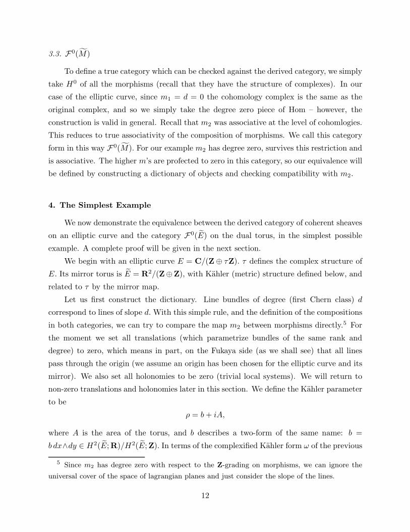
3.3. F0(M)

To define a true category which can be checked against the derived category, we simply

take H0 of all the morphisms (recall that they have the structure of complexes). In our

case of the elliptic curve, since m1 = d = 0 the cohomology complex is the same as the

original complex, and so we simply take the degree zero piece of Hom – however, the

construction is valid in general. Recall that m2 was associative at the level of cohomlogies.

This reduces to true associativity of the composition of morphisms. We call this category

form in this way F0(M). For our example m2 has degree zero, survives this restriction and

is associative. The higher m’s are profected to zero in this category, so our equivalence will

be defined by constructing a dictionary of objects and checking compatibility with m2.

4. The Simplest Example

We now demonstrate the equivalence between the derived category of coherent sheaves

on an elliptic curve and the category F0(E) on the dual torus, in the simplest possible

example. A complete proof will be given in the next section.

We begin with an elliptic curve E = C/(Z⊕ τZ). τ defines the complex structure of

E. Its mirror torus is E = R2/(Z⊕Z), with Kahler (metric) structure defined below, and

related to τ by the mirror map.

Let us first construct the dictionary. Line bundles of degree (first Chern class) d

correspond to lines of slope d. With this simple rule, and the definition of the compositions

in both categories, we can try to compare the map m2 between morphisms directly.5 For

the moment we set all translations (which parametrize bundles of the same rank and

degree) to zero, which means in part, on the Fukaya side (as we shall see) that all lines

pass through the origin (we assume an origin has been chosen for the elliptic curve and its

mirror). We also set all holonomies to be zero (trivial local systems). We will return to

non-zero translations and holonomies later in this section. We define the Kahler parameter

to be

ρ = b + iA,

where A is the area of the torus, and b describes a two-form of the same name: b =

b dx∧dy ∈ H2(E;R)/H2(E;Z). In terms of the complexified Kahler form ω of the previous

5 Since m2 has degree zero with respect to the Z-grading on morphisms, we can ignore the

universal cover of the space of lagrangian planes and just consider the slope of the lines.

12

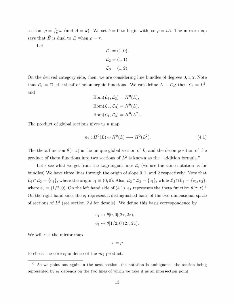
section, ρ =∫

Eω (and A = k). We set b = 0 to begin with, so ρ = iA. The mirror map

says that E is dual to E when ρ = τ.

LetL1 = (1, 0),

L2 = (1, 1),

L3 = (1, 2).

On the derived category side, then, we are considering line bundles of degrees 0, 1, 2. Note

that L1 = O, the sheaf of holomorphic functions. We can define L ≡ L2; then L3 = L2,

andHom(L1,L2) = H0(L),

Hom(L2,L3) = H0(L),

Hom(L1,L3) = H0(L2).

The product of global sections gives us a map

m2 : H0(L) ⊗ H0(L) −→ H0(L2). (4.1)

The theta function θ(τ, z) is the unique global section of L, and the decomposition of the

product of theta functions into two sections of L2 is known as the “addition formula.”

Let’s see what we get from the Lagrangian lines Li (we use the same notation as for

bundles) We have three lines through the origin of slope 0, 1, and 2 respectively. Note that

L1∩L2 = e1, where the origin e1 ≡ (0, 0). Also, L2∩L3 = e1, while L2∩L3 = e1, e2,

where e2 ≡ (1/2, 0). On the left hand side of (4.1), e1 represents the theta function θ(τ, z).6

On the right hand side, the ei represent a distinguished basis of the two-dimensional space

of sections of L2 (see section 2.3 for details). We define this basis correspondence by

e1 ↔ θ[0, 0](2τ, 2z),

e2 ↔ θ[1/2, 0](2τ, 2z).

We will use the mirror map

τ = ρ

to check the correspondence of the m2 product.

6 As we point out again in the next section, the notation is ambiguous: the section being

represented by e1 depends on the two lines of which we take it as an intersection point.

13

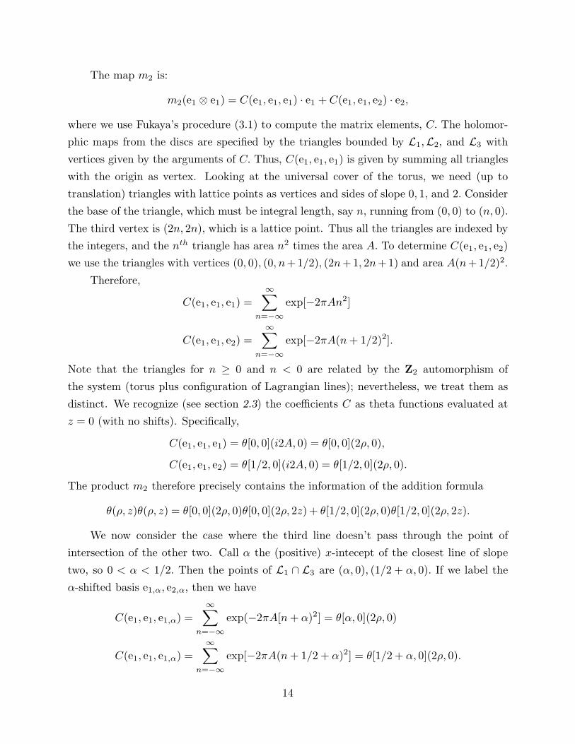
The map m2 is:

m2(e1 ⊗ e1) = C(e1, e1, e1) · e1 + C(e1, e1, e2) · e2,

where we use Fukaya’s procedure (3.1) to compute the matrix elements, C. The holomor-

phic maps from the discs are specified by the triangles bounded by L1,L2, and L3 with

vertices given by the arguments of C. Thus, C(e1, e1, e1) is given by summing all triangles

with the origin as vertex. Looking at the universal cover of the torus, we need (up to

translation) triangles with lattice points as vertices and sides of slope 0, 1, and 2. Consider

the base of the triangle, which must be integral length, say n, running from (0, 0) to (n, 0).

The third vertex is (2n, 2n), which is a lattice point. Thus all the triangles are indexed by

the integers, and the nth triangle has area n2 times the area A. To determine C(e1, e1, e2)

we use the triangles with vertices (0, 0), (0, n+1/2), (2n+1, 2n+1) and area A(n+1/2)2.

Therefore,

C(e1, e1, e1) =

∞∑

n=−∞

exp[−2πAn2]

C(e1, e1, e2) =

∞∑

n=−∞

exp[−2πA(n + 1/2)2].

Note that the triangles for n ≥ 0 and n < 0 are related by the Z2 automorphism of

the system (torus plus configuration of Lagrangian lines); nevertheless, we treat them as

distinct. We recognize (see section 2.3) the coefficients C as theta functions evaluated at

z = 0 (with no shifts). Specifically,

C(e1, e1, e1) = θ[0, 0](i2A, 0) = θ[0, 0](2ρ, 0),

C(e1, e1, e2) = θ[1/2, 0](i2A, 0) = θ[1/2, 0](2ρ, 0).

The product m2 therefore precisely contains the information of the addition formula

θ(ρ, z)θ(ρ, z) = θ[0, 0](2ρ, 0)θ[0, 0](2ρ, 2z) + θ[1/2, 0](2ρ, 0)θ[1/2, 0](2ρ, 2z).

We now consider the case where the third line doesn’t pass through the point of

intersection of the other two. Call α the (positive) x-intecept of the closest line of slope

two, so 0 < α < 1/2. Then the points of L1 ∩ L3 are (α, 0), (1/2 + α, 0). If we label the

α-shifted basis e1,α, e2,α, then we have

C(e1, e1, e1,α) =

∞∑

n=−∞

exp(−2πA[n + α)2] = θ[α, 0](2ρ, 0)

C(e1, e1, e1,α) =

∞∑

n=−∞

exp[−2πA(n + 1/2 + α)2] = θ[1/2 + α, 0](2ρ, 0).

14

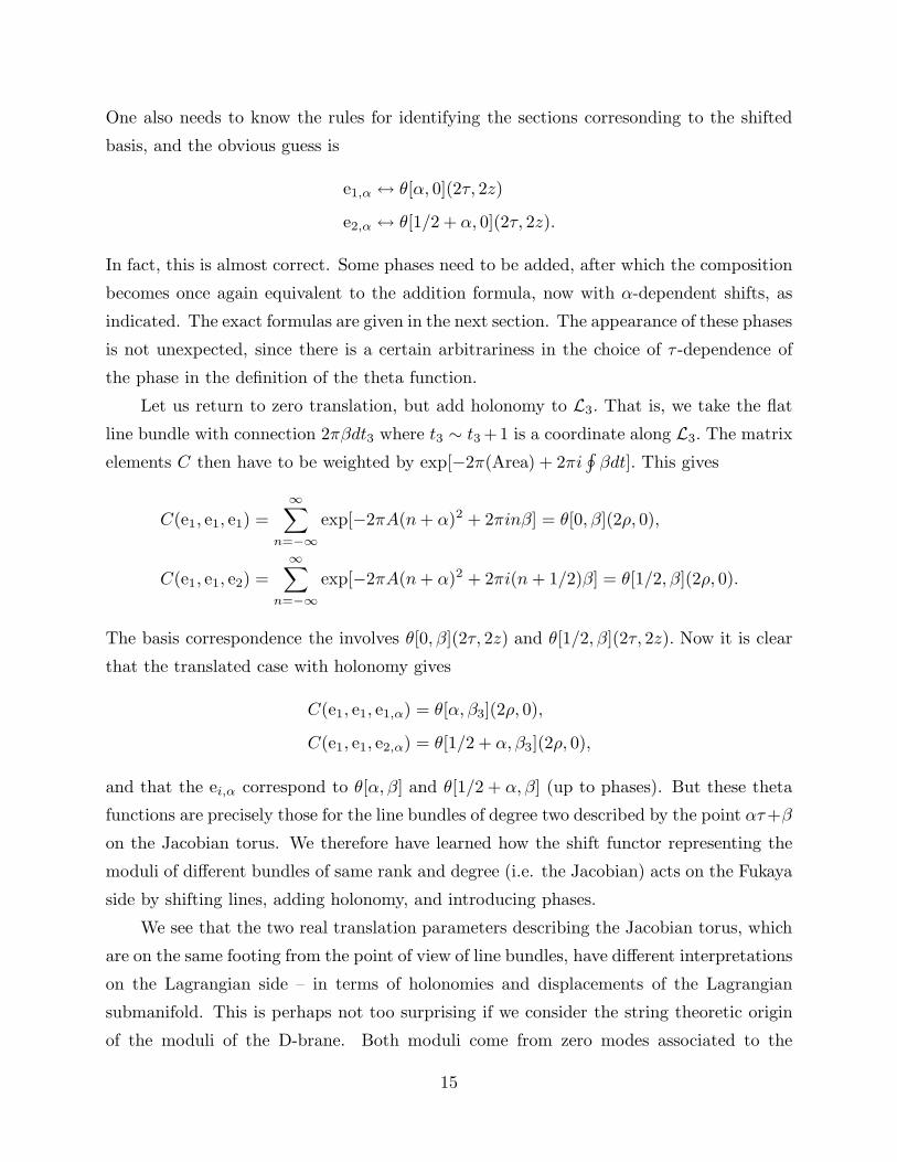
One also needs to know the rules for identifying the sections corresonding to the shifted

basis, and the obvious guess is

e1,α ↔ θ[α, 0](2τ, 2z)

e2,α ↔ θ[1/2 + α, 0](2τ, 2z).

In fact, this is almost correct. Some phases need to be added, after which the composition

becomes once again equivalent to the addition formula, now with α-dependent shifts, as

indicated. The exact formulas are given in the next section. The appearance of these phases

is not unexpected, since there is a certain arbitrariness in the choice of τ -dependence of

the phase in the definition of the theta function.

Let us return to zero translation, but add holonomy to L3. That is, we take the flat

line bundle with connection 2πβdt3 where t3 ∼ t3 +1 is a coordinate along L3. The matrix

elements C then have to be weighted by exp[−2π(Area) + 2πi∮

βdt]. This gives

C(e1, e1, e1) =∞∑

n=−∞

exp[−2πA(n + α)2 + 2πinβ] = θ[0, β](2ρ, 0),

C(e1, e1, e2) =∞∑

n=−∞

exp[−2πA(n + α)2 + 2πi(n + 1/2)β] = θ[1/2, β](2ρ, 0).

The basis correspondence the involves θ[0, β](2τ, 2z) and θ[1/2, β](2τ, 2z). Now it is clear

that the translated case with holonomy gives

C(e1, e1, e1,α) = θ[α, β3](2ρ, 0),

C(e1, e1, e2,α) = θ[1/2 + α, β3](2ρ, 0),

and that the ei,α correspond to θ[α, β] and θ[1/2 + α, β] (up to phases). But these theta

functions are precisely those for the line bundles of degree two described by the point ατ+β

on the Jacobian torus. We therefore have learned how the shift functor representing the

moduli of different bundles of same rank and degree (i.e. the Jacobian) acts on the Fukaya

side by shifting lines, adding holonomy, and introducing phases.

We see that the two real translation parameters describing the Jacobian torus, which

are on the same footing from the point of view of line bundles, have different interpretations

on the Lagrangian side – in terms of holonomies and displacements of the Lagrangian

submanifold. This is perhaps not too surprising if we consider the string theoretic origin

of the moduli of the D-brane. Both moduli come from zero modes associated to the

15

ten-dimensional gauge field. On the D-brane the transverse components become normal

vectors and the zero modes give the motions of the brane, while the parallel components

describe the flat bundle moduli (holonomy).

It is now a simple matter to check that these formulas are true for general ρ (recall ρ =∫

Eω), i.e. when b 6= 0, since we weight a holomorphic map from the disc by exp[2πi(

∫φ∗ω+

∮βdt)]. Complexifying the Kahler class in this way is familiar from mirror symmetry, and

the holonomy is expected for D-branes or open strings. We now have a clear description

of all the parameters involved in the mirror map τ ↔ ρ as well as the translational bundle

(or Lagrangian) moduli.

The composition is somewhat more involved for stable vector bundles of rank r and

degree d (which correspond to lines (r, d) with gcd(r, d) = 1), but as we will see in the next

section, these cases can be deduced from our knowledge of line bundles. The non-stable

bundles (which correspond to non-unitary local systems) are more subtle. Identifying a

proper basis for the global sections is the main difficulty. Fortunately, we will be able to

describe all sections in terms of simple theta functions. The Fukaya compositions are rather

easy to compute, as above, and the equivalence of these products to the decomposition of

sections of bundles will be shown to reduce to the classical addition formulas, as above.

5. Categorical Equivalence for the Elliptic Curve

We must construct the categorical equivalence in the general case, where the objects

in the derived category are more general than line bundles. We can immediately reduce to

indecomposable bundles, by linearity of m2. The idea, then, is to use the representation

of indecomposable vector bundles on elliptic curve as push-forwards under the isogenies of

line bundles tensored with bundles of type F (V, exp(N)) where N is a constant nilpotent

matrix (see section 2.3). Let us denote by L(E) the category of bundles on E of the form

L(φ) ⊗ F (V, exp(N)). We claim that it is sufficient to construct a natural equivalence of

L(E) with the appropriate subcategory in the Fukaya category. More precisely, we need

that these equivalences for elliptic curves Eqr and Eq commute with the corresponding

pull-back functors π∗r .

Main Theorem

The categories Db(Eq) and F0(Eq) are equivalent:

Db(Eq) ∼= F0(Eq)

16

(we use q = exp(2πiτ) instead of τ here).

We prove this by constructing a bijective functor Φ : Db(Eq) → F0(Eq) in five steps.

We first define it on a restricted class of objects: bundles of the form L(ϕ) ⊗ F (V, expN)

(step one). Then we show how this respects the composition law (step two). Step three

is showing that it commutes with isogenies. Then, in step four we treat general vector

bundles by constructing them from isogenies. Finally, in step five, we treat the only

remaining case: torsion sheaves, or thickened skyscrapers (recall that the derived category

is a sum of vector bundles and these sheaves which have support only at a point).

More specifically, we construct a fully faithful functor from the abelian category of

coherent sheaves to the Fukaya category. The choice of logarithms of slopes for the corre-

sponding objects is πiα, where α ∈ (−1/2, 1/2] (the right boundary is achieved by torsion

sheaves). On this subcategory Hom0 between lines with slopes exp(πiα1) and exp(πiα2)

is non-zero only if α1 < α2. This functor can be extended to the equivalence of the entire

derived category of coherent sheaves with the Fukaya category, using Serre duality and the

rule that the shift by one in the derived category corresponds to α 7→ α + 1.

5.1. The Functor Φ

Let L(Eq) denote the full subcategory of the category of vector bundles on Eq consist-

ing of bundles of the form L(ϕ)⊗F (V, expN), where ϕ = t∗xϕ0·ϕn−10 for some x ∈ Eq, n ∈ Z

(we use the conventions of section 2.3.)

We construct a functor

Φq : L(Eq) → F0(Eq),

where F0 denotes the Fukaya category and q denotes the exponential of the complexified

Kahler parameter on the right hand side (q = exp(2πiρ), and ρ = b + ik is equal to τ, as

per the mirror map). On the Fukaya side, an object is a pair of line Λ in R2/Z2 described

by a parametrization (x(t), y(t)) in R2 and a flat connection A on the line. We describe

the flat connection as a constant V valued one-form on R2 – the restriction to Λ is implied.

Specifically, the map Φ on objects is

Φ :(L(t∗ατ+βϕ0 · ϕ

n−10 ) ⊗ F (V, expN)

)7→ (Λ, A), Λ = (α + t, (n − 1)α + nt),

A = (−2πiβ · 1V + N)dx

(we subsequently drop the notation 1V for the identity map on V ). In other words,

the line has slope n (degree of the line bundle) and x-intercept α/n. The monodromy

17

matrix between points (x1, y1) and (x2, y2) is exp[−2πiβ(x2 − x1)] exp[N(x2 − x1)]. This

is precislely what we saw last section: the shifts are represented as translations of the line

and as monodromies.

It remains to describe the map on morphisms:

Φ : Hom(L(ϕ1)⊗F (V1, expN1), L(ϕ2) ⊗ F (V2, expN2)

)→

Hom0(Φ(L(ϕ1) ⊗ F (V1, expN1)), Φ(L(ϕ2) ⊗ F (V2, expN2))

),

where ϕi = t∗αiτ+βiϕ0 · ϕni−1, i = 1, 2, and Hom0 is the image in F0, i.e. the degree

zero part of Hom. Now recall Prop. 2. If n1 > n2, both of the above spaces are zero. If

n1 = n2, then either the above spaces are zero, or L(ϕ1) ∼= L(ϕ2) and the problem reduces

to homomorphisms of vector spaces. If n1 < n2, then

LHS = H0(L(ϕ2ϕ

−11 ) ⊗ F (V ∗

1 ⊗ exp(N2 − N∗1 ))

)

= H0(L(ϕ2ϕ−11 )) ⊗ (V ∗

1 ⊗ V2) by V,

while

RHS =⊕

ek∈Λ1∩Λ2

V ∗1 ⊗ V2 · ek.

The points of Λ1 ∩ Λ2 are easily found from Φ to be

ek =

(k + α2 − α1

n2 − n1,n1k + n1α2 − n2α1

n2 − n1

), k ∈ Z/(n2 − n1)Z.

We note that

ϕ2ϕ−11 = t∗α2τ+β2

ϕ0 · ϕn2−10 · t∗α1τ+β1

ϕ−10 ϕ−n1+1

0 = t∗α12τ+β12ϕn2−n1

0 ,

where

α12 =α2 − α1

n2 − n1, β12 =

β2 − β1

n2 − n1.

Now we have the standard basis of theta functions on H0(L(ϕ2ϕ−11 )) :

t∗α12τ+β12θ

[k

n2 − n1, 0

]((n2 − n1)τ, (n2 − n1)z

)=

θ

[k

n2 − n1, 0

] ((n2 − n1)τ, (n2 − n1)(z + α12τ + β12)

),

k ∈ Z/(n2−n1)Z. Let us call this function fk. The standard basis on the Fukaya side is also

indexed by k. We recall that α12 and β12 effect shifts and monodromies on the right hand

18

side, and this determines the identification of bases up to a constant. Let T ∈ V ∗1 ⊗ V2.

We define

Φ (V(fk ⊗ T )) = exp(−πiτα212(n2 − n1)) exp[α12(N2 − N∗

1 − 2πi(n2 − n1)β12)] · T ek.

5.2. Φ m2 = m2 Φ

We must check that the definition of Φ respects the composition maps in the two

categories. We have L(ϕi) ⊗ F (Vi, expNi), i = 1...3.

a) We have to compare compositions of sections

V

(t∗α12τ+β12

θ

[a

n2 − n1, 0

] ((n2 − n1)τ , (n2 − n1)z

)⊗ A

)

and

V

(t∗α23τ+β23

θ

[a

n3 − n2, 0

] ((n3 − n2)τ , (n3 − n2)z

)⊗ B

),

where A ∈ V ∗1 ⊗V2 and B ∈ V ∗

2 ⊗V3. Using Prop. 3, this composition is equal to V applied

to the following expression:

TrV2θ[ a

n2 − n1, 0

]((n2 − n1)τ , (n2 − n1)(z + α12τ + β12 −

N

n2 − n1)

)×

× θ[ b

n3 − n2, 0

]((n3 − n2)τ , (n3 − n2)(z + α23τ + β23 −

N

n3 − n2))· A ⊗ B,

where

N =1

2πi

−(n2 − n1)(N3 − N2) + (n3 − n2)(N2 − N∗1 )

n3 − n1

=1

2πi

(N2 −

(n2 − n1)N3 + (n3 − n2)N∗1

n3 − n1

)

(we have replaced N∗2 by N2 under the trace sign using 〈v, N∗

2 ξ〉 = 〈N2v, ξ〉 for v ∈ V2, ξ ∈

V ∗2 ). Now the addition formula (II.6.4 of [19]) implies the following θ-identity:

θ

[a

n2 − n1, 0

]((n2 − n1)τ , (n2 − n1)z1)

)· θ

[b

n3 − n2, 0

]((n3 − n2)τ , (n3 − n2)z2) =

=∑

m∈Z

exp

[πiτ

k2m

(n2 − n1)(n3 − n2)(n3 − n1)+ 2πi

km

n3 − n1(z2 − z1)

]×

θ

[a + b + (n3 − n2)m

n3 − n1, 0

] ((n3 − n1)τ , (n2 − n1)z1 + (n3 − n2)z2

),

where

km = (n2 − n1)b − (n3 − n2)a + (n2 − n1)(n3 − n2)m.

19

Plugging in z1 = z + α12τ + β12 −N

n2−n1and z2 = z + α12τ + β12 −

Nn2−n1

, we obtain

TrV2

∑

m∈Z

exp[ (πiτ)k2

m

(n2 − n1)(n3 − n2)(n3 − n1)

+(2πi)km

n3 − n1

((α23 − α12)τ + β23 − β12 +

n3 − n1

(n2 − n1)(n3 − n2)N

)]· A ⊗ B×

× θ

[a + b + (n3 − n2)m

n3 − n1, 0

] ((n3 − n1)(z + α13τ + β13)

).

b) In the Fukaya category, we need to compose A · ea and B · eb, where A ∈ V ∗1 ⊗ V2

and B ∈ V ∗2 ⊗ V3 and a ∈ Z/(n2 − n1)Z and b ∈ Z/(n3 −n2)Z label points in Λ1 ∩Λ2 and

Λ2 ∩ Λ3, respectively.7

The points of intersection are easily computed. For two lines Λi and Λj , the nj − ni

points of intersection in R2/Z2 are

ek =

(αij +

k

nj − ni,niαj − njαi + nik

nj − ni

).

We must sum over triangles in the plane formed by the Z-translates of Λ3 which pass

through points lattice-equivalent to eb. Note that such a triangle is uniquely determined

by the first coordinate of the intersection point of Λ3 with Λ2 which should be of the form

α23 + bn3−n2

+ m, m ∈ Z. The point of intersection ec in Λ1 ∩ Λ3 depends on m, and is

calculated to be given by the above formula with c = a + b + m(n3 − n2) mod (n3 − n1).

If we call l1 the horizontal distance (difference of x coordinates) between ea and ec, l2

the horizontal distance between ea and eb, and l3 the horizontal distance between eb and

ec (may be negative), then by adding up x and y differences we have

l1 = l2 + l3

n1l1 = n2l2 + n3l3.

Therefore, l1 = n3−n2

n3−n1l2, and l3 = n1−n2

n3−n1l2. Now we know l2 explicitly from above. The

area ∆ of the triangle (rather, the number of fundamental domains) formed by the vertices

is half that of the parallelogram determined by vectors (l1, n1l1) and (l2, n2l2). Hence,

∆ =1

2Det

(l1 l2

n1l1 n2l2

)= l1l2(n2 − n1)/2 =

(n3 − n1)(n2 − n1)

2(n3 − n2)(l2)

2.

7 There is some notational ambiguity: “What is e3?” The context should make it clear which

intersections are being indexed, and therefore what the range of the index should be.

20

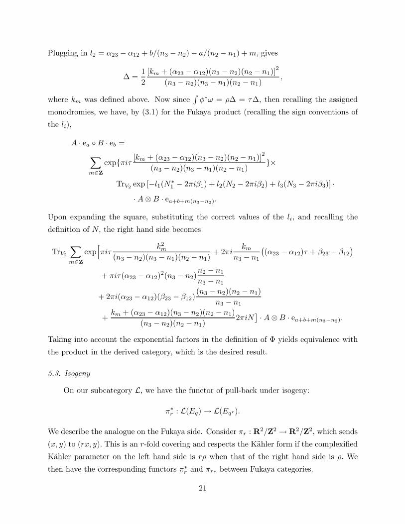
Plugging in l2 = α23 − α12 + b/(n3 − n2) − a/(n2 − n1) + m, gives

∆ =1

2

[km + (α23 − α12)(n3 − n2)(n2 − n1)]2

(n3 − n2)(n3 − n1)(n2 − n1),

where km was defined above. Now since∫

φ∗ω = ρ∆ = τ∆, then recalling the assigned

monodromies, we have, by (3.1) for the Fukaya product (recalling the sign conventions of

the li),

A · ea B · eb =

∑

m∈Z

expπiτ[km + (α23 − α12)(n3 − n2)(n2 − n1)]

2

(n3 − n2)(n3 − n1)(n2 − n1)×

TrV2exp [−l1(N

∗1 − 2πiβ1) + l2(N2 − 2πiβ2) + l3(N3 − 2πiβ3)] ·

· A ⊗ B · ea+b+m(n3−n2).

Upon expanding the square, substituting the correct values of the li, and recalling the

definition of N, the right hand side becomes

TrV2

∑

m∈Z

exp[πiτ

k2m

(n3 − n2)(n3 − n1)(n2 − n1)+ 2πi

km

n3 − n1

((α23 − α12)τ + β23 − β12

)

+ πiτ(α23 − α12)2(n3 − n2)

n2 − n1

n3 − n1

+ 2πi(α23 − α12)(β23 − β12)(n3 − n2)(n2 − n1)

n3 − n1

+km + (α23 − α12)(n3 − n2)(n2 − n1)

(n3 − n2)(n2 − n1)2πiN

]· A ⊗ B · ea+b+m(n3−n2).

Taking into account the exponential factors in the definition of Φ yields equivalence with

the product in the derived category, which is the desired result.

5.3. Isogeny

On our subcategory L, we have the functor of pull-back under isogeny:

π∗r : L(Eq) → L(Eqr).

We describe the analogue on the Fukaya side. Consider πr : R2/Z2 → R2/Z2, which sends

(x, y) to (rx, y). This is an r-fold covering and respects the Kahler form if the complexified

Kahler parameter on the left hand side is rρ when that of the right hand side is ρ. We

then have the corresponding functors π∗r and πr∗ between Fukaya categories.

21

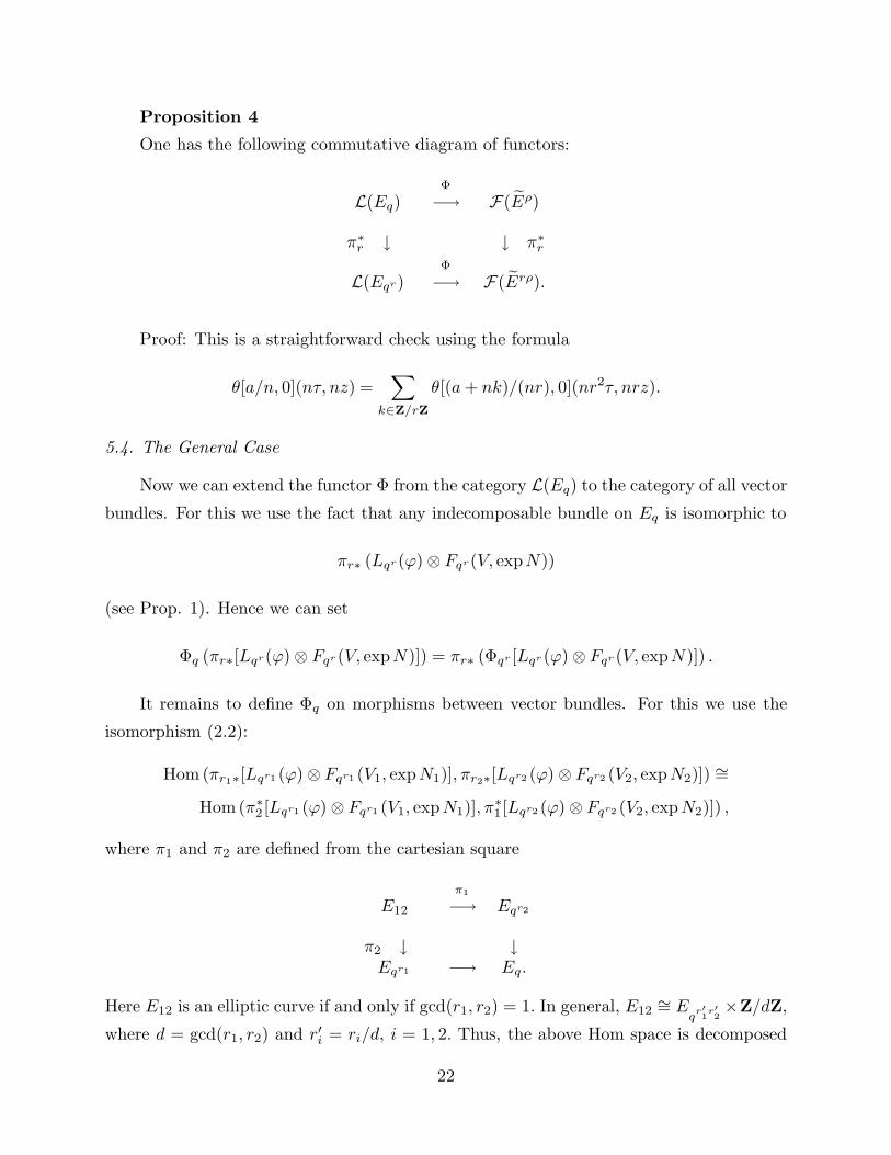
Proposition 4

One has the following commutative diagram of functors:

L(Eq)Φ

−→ F(Eρ)

π∗r ↓ ↓ π∗

r

L(Eqr)Φ

−→ F(Erρ).

Proof: This is a straightforward check using the formula

θ[a/n, 0](nτ, nz) =∑

k∈Z/rZ

θ[(a + nk)/(nr), 0](nr2τ, nrz).

5.4. The General Case

Now we can extend the functor Φ from the category L(Eq) to the category of all vector

bundles. For this we use the fact that any indecomposable bundle on Eq is isomorphic to

πr∗ (Lqr(ϕ) ⊗ Fqr(V, expN))

(see Prop. 1). Hence we can set

Φq (πr∗[Lqr(ϕ) ⊗ Fqr(V, expN)]) = πr∗ (Φqr [Lqr(ϕ) ⊗ Fqr(V, expN)]) .

It remains to define Φq on morphisms between vector bundles. For this we use the

isomorphism (2.2):

Hom (πr1∗[Lqr1 (ϕ) ⊗ Fqr1 (V1, expN1)], πr2∗[Lqr2 (ϕ) ⊗ Fqr2 (V2, expN2)]) ∼=

Hom(π∗2 [Lqr1 (ϕ) ⊗ Fqr1 (V1, expN1)], π

∗1 [Lqr2 (ϕ) ⊗ Fqr2 (V2, expN2)]) ,

where π1 and π2 are defined from the cartesian square

E12

π1

−→ Eqr2

π2 ↓ ↓Eqr1 −→ Eq.

Here E12 is an elliptic curve if and only if gcd(r1, r2) = 1. In general, E12∼= E

qr′1

r′2×Z/dZ,

where d = gcd(r1, r2) and r′i = ri/d, i = 1, 2. Thus, the above Hom space is decomposed

22

into a direct sum of d Hom spaces between objects of the category L(Eq

r′1

r′2). There is

a similar decomposition of the corresponding Hom spaces on the Fukaya side, so we just

take the direct sum of isomorphisms between Hom’s given by Φ on L(Eq

r′1

r′2). To check

that this extended map Φ is still compatible with compositions we note that given a

triple of vector bundles of the form πri∗ (Lqri (ϕi) ⊗ Fqri (Vi, expNi)) , i = 1...3, we can

embed the pairwise Hom’s into the corresponding Hom spaces between the pull-backs of

Lqri (ϕi) ⊗ Fqri (Vi, expNi) to the triple fibered product of Eqr1 , Eqr2 , and Eqr3 over Eq,

which is still a disjoint union of elliptic curves. Now the required compatibility follows

from the fact that the functor Φ on the L(Eq) commutes with the pull-back functor π∗r .

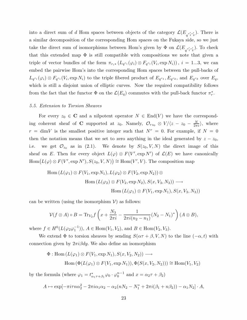
5.5. Extension to Torsion Sheaves

For every z0 ∈ C and a nilpotent operator N ∈ End(V ) we have the correspond-

ing coherent sheaf of C supported at z0. Namely, Orz0⊗ V/〈z − z0 − N

2πi〉, where

r = dimV is the smallest positive integer such that Nr = 0. For example, if N = 0

then the notation means that we set to zero anything in the ideal generated by z − z0,

i.e. we get Oz0as in (2.1). We denote by S(z0, V, N) the direct image of this

sheaf on E. Then for every object L(ϕ) ⊗ F (V ′, expN ′) of L(E) we have canonically

Hom(L(ϕ) ⊗ F (V ′, expN ′), S(z0, V, N)

)∼= Hom(V ′, V ). The composition map

Hom(L(ϕ1) ⊗ F (V1, expN1), L(ϕ2) ⊗ F (V2, expN2))⊗

Hom (L(ϕ2) ⊗ F (V2, expN2), S(x, V3, N3)) −→

Hom(L(ϕ1) ⊗ F (V1, expN1), S(x, V3, N3))

can be written (using the isomorphism V) as follows:

V(f ⊗ A) B = TrV2f

(x +

N3

2πi−

1

2πi(n2 − n1)(N2 − N1)

∗

)(A ⊗ B),

where f ∈ H0(L(ϕ2ϕ−11 )), A ∈ Hom(V1, V2), and B ∈ Hom(V2, V3).

We extend Φ to torsion sheaves by sending S(ατ + β, V, N) to the line (−α, t) with

connection given by 2πiβdy. We also define an isomorphism

Φ : Hom(L(ϕ1) ⊗ F (V1, expN1), S(x, V2, N2)) −→

Hom(Φ(L(ϕ1) ⊗ F (V1, expN1)), Φ(S(x, V2, N2))) ∼= Hom(V1, V2)

by the formula (where ϕ1 = t∗α1τ+β1ϕ0 · ϕ

n−10 and x = α2τ + β2)

A 7→ exp[−πiτnα22 − 2πiα1α2 − α2(nN2 − N∗

1 + 2πi(β1 + nβ2)) − α1N2] · A,

23

where A ∈ Hom(V1, V2).

It remains to check that Φ respects compositions. We only have to check this for

the composition of Hom’s between L(ϕ1) ⊗ F (V1, expN1), L(ϕ2) ⊗ F (V2, expN2), and

S(x, V3, N3). The proof of this is similar to the cases considered previously, but even

simpler. One needs only the definition of the theta function; no theta identities are used.

We leave the case of Hom’s from higher rank vector bundles as an exercise for the reader

(use πr∗).

Remark

Any automorphism ϕ of M preserving the Kahler structure and Ω induces an autoe-

quivalence ϕ∗ of the Fukaya category F(M) defined up to a shift by an integer. In the case

of the flat torus T = R2/Z2, this leads to an action of the central extension of SL(2;Z)

by Z in the Fukaya category F(T ). The corresponding projective action of SL(2;Z) on

Db(E) is given as follows. The matrix

(1 01 1

)acts by tensoring with L, while the matrix

(0 1−1 0

)acts as the Fourier-Mukai transform

S 7→ p2∗(p∗1S ⊗ P),

where P is the normalized Poincare line bundle on E × E given by

P = m∗O(−x0) ⊗ p∗1O(x0) ⊗ p∗2O(x0),

where m : E × E → E is the group law, x0 is the point corresponding to 1/2 + τ/2, and

p1, p2 are the projections.

6. Conclusions

We have shown that for the elliptic curve, as Kontsevich conjectured, mirror symmetry

has an interpretation in terms of the equivalence of two very different looking categories.

The nature of the equivalence certainly seems to equate odd D-branes (the Fukaya side)

with even D-branes, though the interpretation of D-branes as coherent sheaves (much less

a elements of the derived category) has as yet only been speculative [20], [21].

We have offered a detailed proof of categorical mirror symmetry in the case of the

elliptic curve. The composition law contains a wealth of information about holomorphic

discs in the mirror manifold, though it is not yet clear exactly how the many results of

24

ordinary mirror symmetry would follow from categorical mirror symmetry for a general

Calabi-Yau manifold.

We have given the dictionary for the categories, but it has not been through a con-

struction. The lack of a constructive approach not only hinders attempts towards a general

proof but makes it difficult to even guess at the dictionary between objects for other Calabi-

Yau mirror pairs. One would like to know if it is at all possible to construct the sheaf on

M corresponding to a given special-Lagrangian submanifold (and local system) on M? For

E and E we can answer in the affirmative with the following construction.8

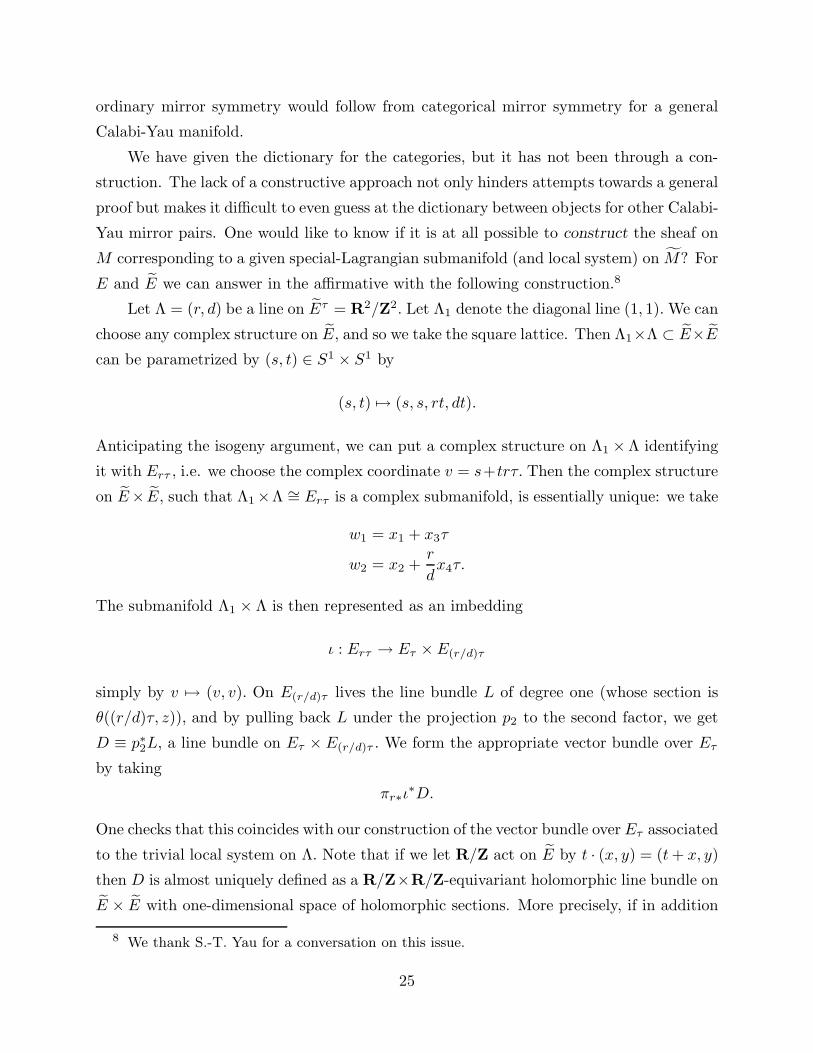
Let Λ = (r, d) be a line on Eτ = R2/Z2. Let Λ1 denote the diagonal line (1, 1). We can

choose any complex structure on E, and so we take the square lattice. Then Λ1×Λ ⊂ E×E

can be parametrized by (s, t) ∈ S1 × S1 by

(s, t) 7→ (s, s, rt, dt).

Anticipating the isogeny argument, we can put a complex structure on Λ1 ×Λ identifying

it with Erτ , i.e. we choose the complex coordinate v = s+trτ. Then the complex structure

on E× E, such that Λ1 ×Λ ∼= Erτ is a complex submanifold, is essentially unique: we take

w1 = x1 + x3τ

w2 = x2 +r

dx4τ.

The submanifold Λ1 × Λ is then represented as an imbedding

ι : Erτ → Eτ × E(r/d)τ

simply by v 7→ (v, v). On E(r/d)τ lives the line bundle L of degree one (whose section is

θ((r/d)τ, z)), and by pulling back L under the projection p2 to the second factor, we get

D ≡ p∗2L, a line bundle on Eτ × E(r/d)τ . We form the appropriate vector bundle over Eτ

by taking

πr∗ι∗D.

One checks that this coincides with our construction of the vector bundle over Eτ associated

to the trivial local system on Λ. Note that if we let R/Z act on E by t · (x, y) = (t + x, y)

then D is almost uniquely defined as a R/Z×R/Z-equivariant holomorphic line bundle on

E × E with one-dimensional space of holomorphic sections. More precisely, if in addition

8 We thank S.-T. Yau for a conversation on this issue.

25

we require that D is invariant under the inversion map z 7→ −z, and all its holomorphic

sections are even, then there are three such line bundles, one of them is p∗2L. Thus, the

construction is almost canonical once we fix the above R/Z-action on E and the R/Z-

equivariant projection E → R/Z : (x, y) 7→ x.

One cannot at present be too optimistic about generalizing this result to higher-

dimensional Calabi-Yau manifolds. The problem is that the Fukaya category composition

depends on the Kahler form, i.e. on the unique Calabi-Yau metric. The exact form of this

metric is of course not known. Abelian surfaces offer the only possible simple extensions of

this work – this is work in progress. Some hope may lie in the fact that areas of calibrated

submanifolds are topoligical, in a way, as the volume is the restriction of a closed form.

Another obstacle is that the derived category of coherent sheaves on a general Calabi-

Yau manifold is not easily studied. For K3 some facts are known [13], and through the

work of [22] we can expect some simplification for elliptically fibered manifolds, but a

precise statement of the composition eludes us. One may hope to construct a map between

objects, however. This may be a possible starting point. For example, the conjecture of

[7] can be interpreted as simply positing an object on the Fukaya side equivalent to the

skyscraper sheaf over a point on the mirror (derived category) side – the identification

of the moduli space of this object is immediately seen to be the mirror manifold itself.

Though Lagrangian submanifolds with flat U(1) bundles (the conjectured mirror objects

to the skyscrapers) may not seem too natural, we recall that the prequantum line bundle,

whose first Chern class equals the Kahler class, restricts to a flat line bundle on Lagrangian

submanifolds in the Calabi-Yau.

Even less is known about the Fukaya category. Special-Lagrangian submanifolds are

not a well-studied class of objects. Recent work of Hitchin [23] has only begun the inves-

tigation of these spaces as dually equivalent to complex submanifolds.

Finally, we anticipate a return to the connection of [24], in which the derived category

of coherent sheaves on a Fano variety was used to count the number of solitions of a

supersymmetric sigma model on that manifold. In that context, the moduli space was the

space of topological field theories, or in other words the “enlarged” moduli space. Armed

with the interpretation of D-branes as solitonic boundary states in a superconformal field

theory, we learn through Kontsevich’s work that the appearance of the derived category,

while still somewhat mysterious, is not likely to be accidental.

We look forward to further research on these matters.

26

Acknowledgements

The research of A.P. is supported by NSF grant DMS-9700458. E.Z. is supported by

grant DE-F602-88ER-25065.

27

References

[1] B. R. Greene and M. R. Plesser, “Duality in Calabi-Yau Moduli Space,” Nucl. Phys.

B338 (1990) 15-37.

[2] P. Candelas, X. C. De La Ossa, P. Green, and L Parkes, “A Pair of Calabi-Yau

Manifolds as an Exactly Soluble Superconformal Theory,” Nucl. Phys. B359 (1991)

21.

[3] M. Kontsevich, “Homological Algebra of Mirror Symmetry,” Proceedings of the 1994

International Congress of Mathematicians I, Birkauser, Zurich, 1995, p. 120; alg-

geom/9411018.

[4] Y. Ruan and G. Tian, A Mathematical Theory of Quantum Cohomology,” J. Diff.

Geom. 42 (1995) 259-367.

[5] E. Witten, “Mirror Manifolds and Topological Field Theory,” in Essays on Mirror

Symmetry, S.-T. Yau, ed., International Press, Hong Kong, 1992, pp. 120-159.

[6] M. Kontsevich, “Deformation Quantization of Poisson Manifolds, I,” q-alg/9709040; S.

Barannikov and M. Kontsevich, “Frobeinus Manifolds and Formality of Lie Algebras

of Polyvector Fields,” alg-geom/9710032.

[7] A. Strominger, S.-T. Yau, and E. Zaslow, “Mirror Symmetry is T -Duality,” Nucl.

Phys. B479 (1996) 243-259.

[8] C. Vafa and E. Witten, “On Orbifolds with Discrete Torsion,” J. Geom. Phys. 15

(1995) 189.

[9] B.Acharya, “A Mirror Pair of Calabi-Yau Fourfolds in Type II String Theory,” hep-

th/9703029.

[10] M. Gross and P. M. H. Wilson, “Mirror Symmetry via 3-Tori for a Class of Calabi-Yau

Threefolds,” alg-geom/9608004.

[11] N. C. Leung and C. Vafa, “Branes and Toric Geometry,” hep-th/9711013.

[12] K. Fukaya, Morse Homotopy, A∞-Category, and Floer Homologies,” in The Proceed-

ings of the 1993 GARC Workshop on Geometry and Topology, H. J. Kim, ed., Seoul

National University; “Floer Homology, A∞-Categories and Topological Field Theory”

(notes by P. Seidel), Kyoto University preprint Kyoto-Math 96-2.

[13] D. Orlov, “Equivalences of Derived Categories and K3 Surfaces,” alg-geom/9606006.

[14] P. Griffiths and J. Harris, Principles of Algebraic Geometry, Wiley & Sons, New York,

1978.

[15] M. F. Atiyah, “Vector Bundles over an Elliptic Curve,” Proc. Lond. Math. Soc. VII

(1957) 414-452.

[16] R. Harvey and H. B. Lawson, Jr., “Calibrated Geomtries,” Acta Math. 148 (1982)

47-157.

[17] K. Becker, M. Becker, and A. Strominger, “Fivebranes, Membranes, and Non-

Perturbative String Theory,” hep-th/9507158.

28

[18] J. Stasheff, “Homotopy Associativity of H-Spaces. I and II,” Trans. Amer. Math. Soc

108 (1963) 275-292 and 293-312.

[19] D. Mumford, Tata Lectures on Theta I, Birkhauser, Boston, 1983.

[20] J. A. Harvey and G. Moore, “On the Algebras of BPS States,” hep-th/9609017.

[21] D. R. Morrison, “The Geometry Underlying Mirror Symmetry,” alg-geom/9608006.

[22] R. Friedman, J. Morgan, and E. Witten, “Vector Bundles and F Theory,” hep-

th/9701162.

[23] N. Hitchin, “The Moduli Space of Special Lagrangian Submanifolds,” dg-ga/9711002.

[24] E. Zaslow, “Solitons and Helices: The Search for a Math-Physics Bridge,” Commun.

Math. Phys. 175 (1996) 337-375.

29