IEEE TRANSACTIONS ON MICROWAVE THEORY AND TECHNIQUES, VOL. 56, NO. 4, APRIL 2008 867

Neural Network Inverse Modeling andApplications to Microwave Filter Design

Humayun Kabir, Student Member, IEEE, Ying Wang, Member, IEEE,Ming Yu, Senior Member, IEEE, and Qi-Jun Zhang, Fellow, IEEE

Abstract—In this paper, systematic neural network modelingtechniques are presented for microwave modeling and designusing the concept of inverse modeling where the inputs to theinverse model are electrical parameters and outputs are geo-metrical parameters. Training the neural network inverse modeldirectly may become difficult due to the nonuniqueness of theinput–output relationship in the inverse model. We propose a newmethod to solve such a problem by detecting multivalued solutionsin training data. The data containing multivalued solutions aredivided into groups according to derivative information using aneural network forward model such that individual groups donot have the problem of multivalued solutions. Multiple inversemodels are built based on divided data groups, and are thencombined to form a complete model. A comprehensive modelingmethodology is proposed, which includes direct inverse modeling,segmentation, derivative division, and model combining tech-niques. The methodology is applied to waveguide filter modelingand more accurate results are achieved compared to the directneural network inverse modeling method. Full electromagneticsimulation and measurement results of -band circular wave-guide dual-mode pseudoelliptic bandpass filters are presented todemonstrate the efficiency of the proposed neural network inversemodeling methodology.

Index Terms—Computer-aided design, inverse modeling, mi-crowave filter modeling, neural networks.

I. INTRODUCTION

I N RECENT years, neural network techniques have been rec-ognized as a powerful tool for microwave design and mod-

eling problems. It has been applied to various microwave de-sign applications [1], [2] such as vias and interconnects [3], em-bedded passives [4], coplanar waveguide components [5], tran-sistor modeling [6]–[8], noise modeling [9], power-amplifiermodeling [10], analysis of multilayer shielded microwave cir-cuits [11], nonlinear microwave circuit optimization [12], etc.Neural networks have the ability to model multidimensional

Manuscript received July 21, 2007; revised November 13, 2007. This workwas supported in part by the Natural Sciences and Engineering ResearchCouncil of Canada (NSERC) and by COM DEV Ltd.

H. Kabir and Q.-J. Zhang are with the Department of Electronics, CarletonUniversity, Ottawa, ON, Canada K1S 5B6 (e-mail: hkabir@doe.carleton.ca;qjz@doe.carleton.ca).

Y. Wang is with the Faculty of Engineering and Applied Sciences, Universityof Ontario Institute of Technology, Oshawa, ON, Canada L1H 7K4 (e-mail:Ying.Wang@uoit.ca).

M. Yu is with COM DEV Ltd., Cambridge, ON, Canada N1R 7H6 (e-mail:Ming.Yu@comdev.ca).

Color versions of one or more of the figures in this paper are available onlineat http://ieeexplore.ieee.org.

Digital Object Identifier 10.1109/TMTT.2008.919078

nonlinear relationships. The evaluation from input to output ofa trained neural network model is also very fast. These featuresmake neural networks a useful alternative for device modelingwhere a mathematical model is not available or repetitive elec-tromagnetic (EM) simulation is required. Once a model is devel-oped, it can be used over and over again. This avoids repetitiveEM simulation where a simple change in the physical dimen-sion requires a complete re-simulation of the EM structure.

A neural network trained to model original EM problems canbe called the forward model where the model inputs are physicalor geometrical parameters and outputs are electrical parameters.For design purposes, the information is often processed in the re-verse direction in order to find the geometrical/physical param-eters for given values of electrical parameters, which is calledthe inverse problem. There are two methods to solve the inverseproblem, i.e., the optimization method and direct inverse mod-eling method. In the optimization method, the EM simulator orthe forward model is evaluated repetitively in order to find theoptimal solutions of the geometrical parameters that can lead toa good match between modeled and specified electrical param-eters. An example of such an approach is [13]. This method ofinverse modeling is also known as the synthesis method.

The formula for the inverse problem, i.e., compute the ge-ometrical parameters from given electrical parameters, is dif-ficult to find analytically. Therefore, the neural network be-comes a logical choice since it can be trained to learn from thedata of the inverse problem. We define the input neurons of aneural network to be the electrical parameters of the modelingproblem and the output neurons as the geometrical parameters.Training data for the neural network inverse model can be ob-tained simply by swapping the input and output data used totrain the forward model. This method is called the direct inversemodeling and an example of this approach is [14]. Once trainingis completed, the direct inverse model can provide inverse solu-tions immediately unlike the optimization method where repet-itive forward model evaluations are required. Therefore, the di-rect inverse model is faster than the optimization method usingeither the EM or the neural network forward model. A sim-ilar concept has been utilized in the neural inverse space map-ping (NISM) technique where the inverse of the mapping fromthe fine to the coarse model parameter spaces is exploited in aspace-mapping algorithm [15].

Though the neural network inverse model can provide the so-lution faster than the optimization method, it often encountersthe problem of nonuniqueness in the input–output (IO) relation-ship. It also causes difficulties during training because the sameinput values to the inverse model will have different values at

0018-9480/$25.00 © 2008 IEEE

Authorized licensed use limited to: University of Waterloo. Downloaded on April 18, 2009 at 12:12 from IEEE Xplore. Restrictions apply.

868 IEEE TRANSACTIONS ON MICROWAVE THEORY AND TECHNIQUES, VOL. 56, NO. 4, APRIL 2008

the output (multivalued solutions). Consequently, the neural net-work inverse model cannot be trained accurately. This is whytraining an inverse model may become more challenging thantraining a forward model.

This paper considers the application of neural networkinverse modeling techniques for microwave filter design. Someresults have been reported using neural network techniques tomodel microwave filters including the rectangular waveguideiris bandpass filter [16]–[18], low-pass microstrip step filter[19], -plane metal-insert filter [20], coupled microstrip linebandpass filter [21], etc. Waveguide dual-mode pseudoellipticfilters are often used in satellite applications due to its high

, compact size, and sharp selectivity [22]. This particularfilter holds complex characteristics whose conventional designprocedure follows an iterative approach, which is time con-suming. Moreover, the whole process has to be repeated evenwith a slight change in any of the design specifications. Themodeling time increases as the filter order increases. Recentlythe neural network modeling technique has been applied todesign a waveguide dual-mode pseudoelliptic filter [23]. Byapplying the neural network technique, filter design parameterswere generated hundreds of times faster than EM-based modelswhile retaining comparable accuracy.

The work in [23] primarily focused on how to apply the neuralnetwork to the waveguide dual mode pseudoelliptic filter de-sign. However, it did not address the issues of inverse mod-eling, including nonuniqueness problems. The neural networkinverse models in [23] were developed primarily using the di-rect method, although manual preprocessing of training datato take out observable contradictions partially dealt with themultivalued problem. The issues and problems in neural net-work inverse modeling still remain open and unsolved. Thispaper is a significant extension of the work presented in [23]. Anew and systematic neural network inverse modeling method-ology, completely beyond [23], is developed, and the problem ofnonuniqueness in inverse modeling is formally addressed. Theproposed methodology uses a set of novel criteria to detect mul-tivalued solutions in training data, and uses adjoint neural net-work [8] derivative information to separate training data intogroups, overcoming nonuniqueness problems in inverse modelsin a systematic way. Each group of data is used to train a sepa-rate inverse sub-model. Such inverse sub-models become moreaccurate since the individual groups of data do not have theproblem of multivalued solutions. A complete methodology tosolve the inverse modeling problem efficiently is proposed bycombining various techniques including the direct inverse mod-eling, segmenting the inverse model, identifying multivalued so-lutions, dividing training data that have multivalued solutions,and combining separately trained inverse sub-models. A signif-icant step is achieved beyond that of [23], where two actual fil-ters are made following the neural network solutions, and realmeasurements from the filters are used to compare and validatethe proposed neural network solutions.

Section II describes the formulation of the inverse models.The problem of nonuniqueness in the IO relationship is dis-cussed. A method to check the existence of multivalued so-lutions in training data and a method to divide the data intogroups are proposed. A method is proposed to combine the

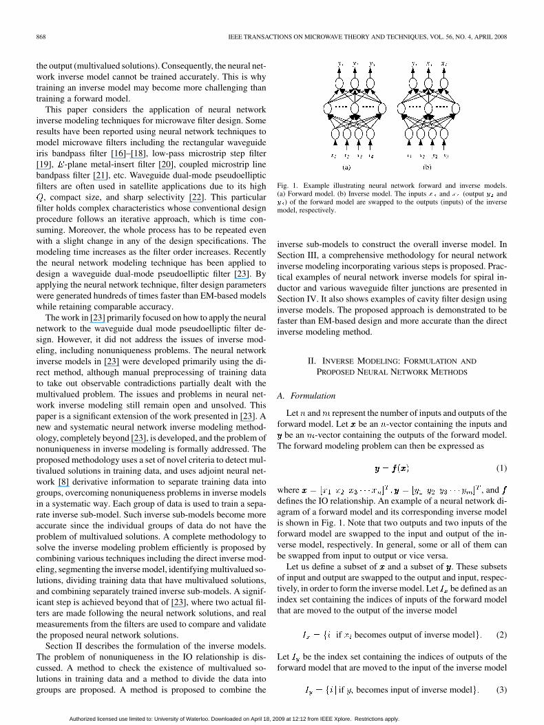
Fig. 1. Example illustrating neural network forward and inverse models.(a) Forward model. (b) Inverse model. The inputs x and x (output y andy ) of the forward model are swapped to the outputs (inputs) of the inversemodel, respectively.

inverse sub-models to construct the overall inverse model. InSection III, a comprehensive methodology for neural networkinverse modeling incorporating various steps is proposed. Prac-tical examples of neural network inverse models for spiral in-ductor and various waveguide filter junctions are presented inSection IV. It also shows examples of cavity filter design usinginverse models. The proposed approach is demonstrated to befaster than EM-based design and more accurate than the directinverse modeling method.

II. INVERSE MODELING: FORMULATION AND

PROPOSED NEURAL NETWORK METHODS

A. Formulation

Let and represent the number of inputs and outputs of theforward model. Let be an -vector containing the inputs and

be an -vector containing the outputs of the forward model.The forward modeling problem can then be expressed as

(1)

where , anddefines the IO relationship. An example of a neural network di-agram of a forward model and its corresponding inverse modelis shown in Fig. 1. Note that two outputs and two inputs of theforward model are swapped to the input and output of the in-verse model, respectively. In general, some or all of them canbe swapped from input to output or vice versa.

Let us define a subset of and a subset of . These subsetsof input and output are swapped to the output and input, respec-tively, in order to form the inverse model. Let be defined as anindex set containing the indices of inputs of the forward modelthat are moved to the output of the inverse model

if becomes output of inverse model (2)

Let be the index set containing the indices of outputs of theforward model that are moved to the input of the inverse model

if becomes input of inverse model (3)

Authorized licensed use limited to: University of Waterloo. Downloaded on April 18, 2009 at 12:12 from IEEE Xplore. Restrictions apply.

KABIR et al.: NEURAL NETWORK INVERSE MODELING AND APPLICATIONS TO MICROWAVE FILTER DESIGN 869

Let and be vectors of inputs and outputs of the inverse model.The inverse model can be defined as

(4)

where includes if and if includes ifand if ; and defines the IO relationship of the

inverse model. For example, the inputs and of Fig. 1(a)may represent the iris length and width of a filter, and outputsand may represent the electrical parameter such as the cou-pling parameter and insertion phase. To formulate the inversefilter model, we swap the iris length and width with couplingparameter and insertion phase. For the example, in Fig. 1, theinverse model is formulated as

(5)

(6)

(7)

(8)

After formulation is finished, the model can be trained withthe data. Usually data are generated by EM solvers originally ina forward way, i.e., given the iris length and compute couplingparameter. To train a neural network as an inverse model, weswap the generated data so that coupling parameter becomestraining data for neural network inputs and iris length becomestraining data for neural network outputs. The neural networktrained this way is the direct inverse model.

The direct inverse modeling method is simple, and is suitablewhen the problem is relatively easy, e.g., when the original IOrelationship is smooth and monotonic, and/or if the numbers ofinputs/outputs are small. On the other hand, if the problem iscomplicated and the models using the direct method are not ac-curate enough, then segmentation of training data can be utilizedto improve the model accuracy. Segmentation of microwavestructures has been reported in existing literature such as [17]where a large device is segmented into smaller units. We applythe segmentation concepts over the range of model inputs tosplit the training data into multiple sections, each covering asmaller range of input parameter space. Neural network modelsare trained for each section of data. A small amount of overlap-ping data can be reserved between adjacent sections so that theconnections between neighboring segmented models becomesmooth.

B. Nonuniqueness of IO Relationship inInverse Model and Proposed Solutions

When the original forward IO relationship is not monotonic,the nonuniqueness becomes an inherent problem in the inversemodel. In order to solve this problem, we start by addressingmultivalued solutions in training data as follows. If two differentinput values in the forward model lead to the same value ofoutput, then a contradiction arises in the training data of the in-verse model because the single input value in the inverse modelhas two different output values. Since we cannot train the neural

network inverse model to match two different output values si-multaneously, the training error cannot be reduced to a smallvalue. As a result, the trained inverse model will not be accu-rate. For this reason, it is important to detect the existence ofmultivalued solutions, which creates contradictions in trainingdata.

Detection of multivalued solutions would have been straight-forward if the training data were generated by deliberatelychoosing different geometrical dimensions such that they leadto the same electrical value. However, in practice, the trainingdata are not sampled at exactly those locations. Therefore, weneed to develop numerical criteria to detect the existence ofmultivalued solutions.

We assume and contain same amount of indices, andthat the indices in (or ) are in ascending order. Let us de-fine the distance between two samples of training data, samplenumber and , as

(9)

where and are the maximum and minimum valueof , respectively, as determined from training data. We use asuperscript to denote the sample index in training data. For ex-ample, and represent values of and in the thtraining data, respectively. Sample is in the neighborhoodof if , where is a user-defined threshold whosevalue depends on the step size of data sampling. The maximumand minimum “slope” between samples within the neighbor-hood of is defined as

(10)

and

Input sample will have multivalued solutions if, withinits neighborhood, the slope is larger than maximum allowed orthe ratio of maximum and minimum slope is larger than themaximum allowed slope change. Mathematically, if

(12)

and

(13)

then has multivalued solutions in its neighborhood whereis the maximum allowed slope and is the maximum

allowed slope change.We employ the simple criteria of (12) and (13) to detect pos-

sible multivalued solutions. A suggestion for can be at leasttwice the average step size of in training data. A referencevalue for can be approximately the inverse of a similarly

Authorized licensed use limited to: University of Waterloo. Downloaded on April 18, 2009 at 12:12 from IEEE Xplore. Restrictions apply.

870 IEEE TRANSACTIONS ON MICROWAVE THEORY AND TECHNIQUES, VOL. 56, NO. 4, APRIL 2008

defined “slope” between adjacent samples in the training dataof the forward model. The value of should be greaterthan 1. In the overall modeling method, conservative choicesof and (larger and smaller and ) lead tomore use of the derivative division procedure to be describedin Section II-C, while aggressive choices of and leadto early termination of the overall algorithm (or more use ofthe segmentation procedure) when model accuracy is achieved(or not achieved). In this way, the choices of andmainly affect the training time of the inverse models ratherthan model accuracy. The modeling accuracy is determinedfrom segmentation or from the derivative division step to bedescribed in Section II-C. Sample values of and aregiven through an example in Section IV-C.

C. Proposed Method to Divide Training DataContaining Multivalued Solutions

If existence of multivalued solutions is detected in trainingdata, we perform data preprocessing to divide the data into dif-ferent groups such that the data in each group do not have theproblem of multivalued solutions. To do this, we need to de-velop a method to decide which data samples should be movedinto which group. We propose to divide the overall training datainto groups based on derivatives of outputs versus inputs of theforward model. Let us define the derivatives of inputs and out-puts that have been exchanged to formulate the inverse model,evaluated at each sample, as

and (14)

where and is the total number oftraining samples. The entire training data should be dividedbased on the derivative criteria such that training samplessatisfying

(15)

belong to one group and training samples satisfying

(16)

belong to a different group. The value for is zero by default.However, to produce an overlapping connection at the breakpoint between the two groups, we can choose a small positivevalue for it. In that case, a small amount of data samples whoseabsolute values of derivative are less than will belong to bothgroups. The value for other than the default suggestion of zerocan be chosen as a value slightly larger than the smallest abso-lute value of derivatives of (14) for all training samples. Choiceof only affects the accuracy of the sub-models at the connec-tion region. The model accuracy for the rest of the region willremain unaffected.

This method exploits derivative information to divide thetraining data into groups. Therefore, accurate derivative is animportant requirement for this method. Computation of deriva-tives of (14) is not a straightforward task since no analyticalequation is available. We propose to compute the derivativesby exploiting the adjoint neural network technique [8]. We

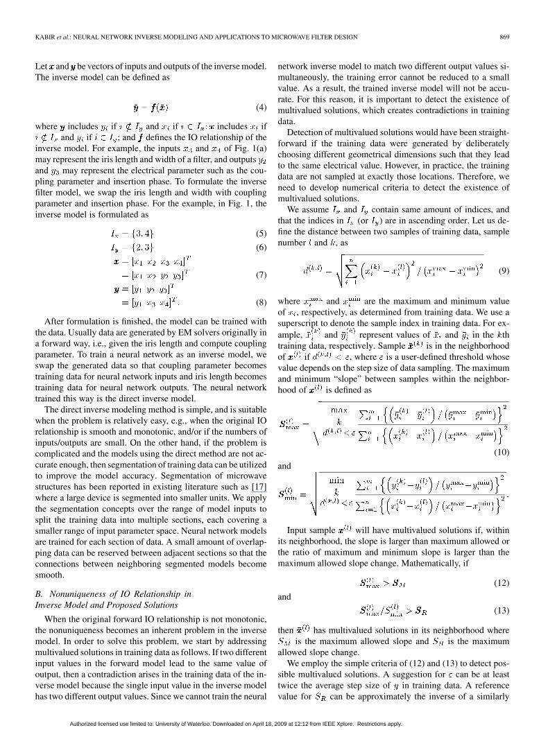
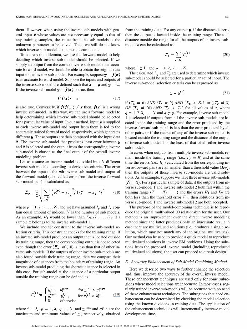
Fig. 2. Diagram of inverse sub-model combining technique after derivative di-vision for a two sub-model system. Inverse sub-model 1 and inverse sub-model 2in set (A) are competitively trained version of the inverse sub-models. Inversesub-model 1 and inverse sub-model 2 in set (B) are trained with the divided databased on derivative criteria (15) and (16). The input and output of the overallcombined model is �xxx and �yyy, respectively.

first train an accurate neural network forward model. Aftertraining is finished, its adjoint neural network can be used toproduce the derivative information used in (15) and (16). Thecomputed derivatives are employed to divide the training datainto multiple smaller groups according to (15) and (16) usingdifferent combinations of and . Multiple neural networksare then trained with the divided data. Each neural networkrepresents a sub-model of the overall inverse model.

Equations (12) and (13) play different roles versus (15) and(16) in our overall algorithm to be described in Section III.Equations (12) and (13) are used as simple and quick ways to de-tect the existence of contradictions in training data, but they donot give enough information on how the data should be divided.Equations (15) and (16), which require more computation (i.e.,require training forward neural model) and produce more infor-mation, are used to perform detailed task of dividing trainingdata into different groups to solve the multivalued problem.

D. Proposed Method to Combine the Inverse Sub-Models

We need to combine the multiple inverse sub-models toreproduce the overall inverse model completely. For this pur-pose, a mechanism is needed to select the right one amongmultiple inverse sub-models for a given input . Fig. 2 showsthe proposed inverse sub-model combining method for a twosub-model system. For convenience of explanation, suppose

is a randomly selected sample of training data. Ideally ifbelongs to a particular inverse sub-model, then the output

from it should be the most accurate one among various inversesub-models. Conversely, the outputs from the other inversesub-models should be less accurate if does not belong to

Authorized licensed use limited to: University of Waterloo. Downloaded on April 18, 2009 at 12:12 from IEEE Xplore. Restrictions apply.

KABIR et al.: NEURAL NETWORK INVERSE MODELING AND APPLICATIONS TO MICROWAVE FILTER DESIGN 871

them. However, when using the inverse sub-models with gen-eral input whose values are not necessarily equal to that ofany training samples, the value from the sub-models is theunknown parameter to be solved. Thus, we still do not knowwhich inverse sub-model is the most accurate one.

To address this dilemma, we use the forward model to helpdeciding which inverse sub-model should be selected. If wesupply an output from the correct inverse sub-model to an accu-rate forward model, we should be able to obtain the original datainput to the inverse sub-model. For example, supposeis an accurate forward model. Suppose the inputs and outputs ofthe inverse sub-model are defined such that and .If the inverse sub-model is true, then

(17)

is also true. Conversely, if then, is a wronginverse sub-model. In this way, we can use a forward model tohelp determining which inverse sub-model should be selectedfor a particular value of input. In our method, input is suppliedto each inverse sub-model and output from them is fed to theaccurately trained forward model, respectively, which generatesdifferent . These outputs are then compared with the input data

. The inverse sub-model that produces least error betweenand is selected and the output from the corresponding inversesub-model is chosen as the final output of the overall inversemodeling problem.

Let us assume an inverse model is divided into differentinverse sub-models according to derivative criteria. The errorbetween the input of the th inverse sub-model and output ofthe forward model (also called error from the inverse-forwardsub-model pair) is calculated as

(18)

where , and we have assumed and con-tain equal amount of indices. is the number of sub models.As an example, would be lower than if asample belongs to the inverse sub-model 1.

We include another constraint to the inverse sub-model se-lection criteria. This constraint checks for the training range. Ifan inverse sub-model produces an output that is located outsideits training range, then the corresponding output is not selectedeven though the error of (18) is less than that of other in-verse sub-models. If the outputs of other inverse sub-models arealso found outside their training range, then we compare theirmagnitude of distances from the boundary of training range. Aninverse sub-model producing the shortest distance is selected inthis case. For sub-model , the distance of a particular outputoutside the training range can be defined as

for

forotherwise

(19)

where and and are themaximum and minimum values of , respectively, obtained

from the training data. For any output , if the distance is zero,then the output is located inside the training range. The totaldistance outside the range for all the outputs of an inverse sub-model can be calculated as

(20)

where and .The calculated and are used to determine which inverse

sub-model should be selected for a particular set of input. Theinverse sub-model selection criteria can be expressed as

(21)

if AND AND , or (OR ) AND for all values of , where

and . For example, inverse sub-model1 is selected if outputs from all the inverse sub-models are lo-cated inside the training range and the error produced by theinverse-forward sub-pair 1 is less than the error produced by allother pairs, or if the output of any of the inverse sub-model islocated outside the training range and the distance of the outputof inverse sub-model 1 is the least of that of all other inversesub-models.

In cases when outputs from multiple inverse sub-models re-main inside the training range (i.e., ) and at the sametime the errors (i.e., ) calculated from the corresponding in-verse-forward pairs are all smaller than a threshold value ( ,then the outputs of those inverse sub-models are valid solu-tions. As an example, suppose we have three inverse sub-models

. For a particular sample of data, if the outputs from in-verse sub-model 1 and inverse sub-model 2 both fall within thetraining range and the errors and areboth less than the threshold error , then solutions from in-verse sub-model 1 and inverse sub-model 2 are both accepted.

The purpose of the model-combining technique is to repro-duce the original multivalued IO relationship for the user. Ourmethod is an improvement over the direct inverse modelingmethod since the latter produces only an inaccurate result incase there are multivalued solutions (i.e., produces a single so-lution, which may not match any of the original multivalues).Our method can be used to provide a quick model to reproducemultivalued solutions in inverse EM problems. Using the solu-tions from the proposed inverse model (including reproducedmultivalued solutions), the user can proceed to circuit design.

E. Accuracy Enhancement of Sub-Model Combining Method

Here we describe two ways to further enhance the selectionand, thus, improve the accuracy of the overall inverse model.These enhancement techniques are used only for some subre-gions where model selections are inaccurate. In most cases, reg-ularly trained inverse sub-models will be accurate with no needof these enhancement techniques. The subregions that need en-hancement can be determined by checking the model selectionusing the known divisions in training data. The application ofthe enhancement techniques will incrementally increase modeldevelopment time.

Authorized licensed use limited to: University of Waterloo. Downloaded on April 18, 2009 at 12:12 from IEEE Xplore. Restrictions apply.

872 IEEE TRANSACTIONS ON MICROWAVE THEORY AND TECHNIQUES, VOL. 56, NO. 4, APRIL 2008

1) Competitively Trained Inverse Sub-Model: To further im-prove the inverse sub-model selection accuracy, an additional setof competitively trained inverse sub-models can be used. Theseinverse sub-models are trained to learn not only what is correct,but also what is wrong. Correct data are the data that belong onlyto a particular inverse sub-model. Conversely, incorrect data arethe data in which belongs to other inverse sub-models and isdeliberately set to zero so that the inverse sub-model is forced tolearn wrong values of for that do not belong to this inversesub-model. The output values of these inverse sub-models arenot very accurate, but they are reliable to identify if an input ei-ther belongs or does not belong to the inverse sub-model. There-fore, they are used for the inverse sub-model selection purposeonly. Once the selection has been made, the final output is takenfrom the regularly trained (i.e., not competitively trained) in-verse sub-model. In Fig. 2, the inverse sub-models in set (A)represent the competitively trained inverse sub-models and set(B) represents regularly trained inverse sub-models.

2) Forward Sub-Model: The default forward model used inthe model combining method is trained with the entire set oftraining data. The decision of choosing the right inverse sub-model depends on the accuracy of both inverse sub-models andforward models. We can further tighten the accuracy of the for-ward model by training multiple forward sub-models using thesame groups of data used to train inverse sub-models. Theseforward sub-models capture the same data range as its inversecounterpart and, therefore, the inverse and forward sub-modelpairs are capable of producing more accurate decision. In Fig. 2,the forward models are replaced with the forward sub-models.

III. OVERALL INVERSE MODELING METHODOLOGY

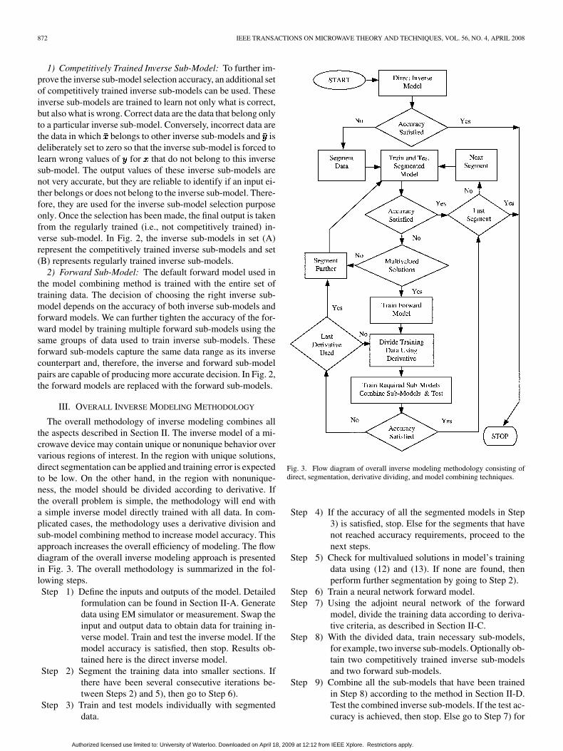
The overall methodology of inverse modeling combines allthe aspects described in Section II. The inverse model of a mi-crowave device may contain unique or nonunique behavior overvarious regions of interest. In the region with unique solutions,direct segmentation can be applied and training error is expectedto be low. On the other hand, in the region with nonunique-ness, the model should be divided according to derivative. Ifthe overall problem is simple, the methodology will end witha simple inverse model directly trained with all data. In com-plicated cases, the methodology uses a derivative division andsub-model combining method to increase model accuracy. Thisapproach increases the overall efficiency of modeling. The flowdiagram of the overall inverse modeling approach is presentedin Fig. 3. The overall methodology is summarized in the fol-lowing steps.Step 1) Define the inputs and outputs of the model. Detailed

formulation can be found in Section II-A. Generatedata using EM simulator or measurement. Swap theinput and output data to obtain data for training in-verse model. Train and test the inverse model. If themodel accuracy is satisfied, then stop. Results ob-tained here is the direct inverse model.

Step 2) Segment the training data into smaller sections. Ifthere have been several consecutive iterations be-tween Steps 2) and 5), then go to Step 6).

Step 3) Train and test models individually with segmenteddata.

Fig. 3. Flow diagram of overall inverse modeling methodology consisting ofdirect, segmentation, derivative dividing, and model combining techniques.

Step 4) If the accuracy of all the segmented models in Step3) is satisfied, stop. Else for the segments that havenot reached accuracy requirements, proceed to thenext steps.

Step 5) Check for multivalued solutions in model’s trainingdata using (12) and (13). If none are found, thenperform further segmentation by going to Step 2).

Step 6) Train a neural network forward model.Step 7) Using the adjoint neural network of the forward

model, divide the training data according to deriva-tive criteria, as described in Section II-C.

Step 8) With the divided data, train necessary sub-models,for example, two inverse sub-models. Optionally ob-tain two competitively trained inverse sub-modelsand two forward sub-models.

Step 9) Combine all the sub-models that have been trainedin Step 8) according to the method in Section II-D.Test the combined inverse sub-models. If the test ac-curacy is achieved, then stop. Else go to Step 7) for

Authorized licensed use limited to: University of Waterloo. Downloaded on April 18, 2009 at 12:12 from IEEE Xplore. Restrictions apply.

KABIR et al.: NEURAL NETWORK INVERSE MODELING AND APPLICATIONS TO MICROWAVE FILTER DESIGN 873

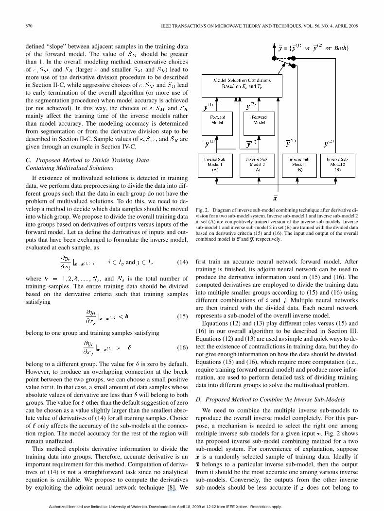
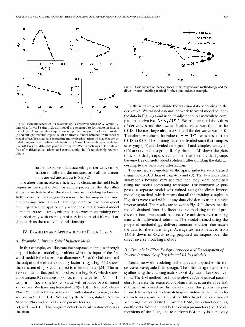
Fig. 4. Nonuniqueness of IO relationship is observed when Q versus Ddata of a forward spiral inductor model is exchanged to formulate an inversemodel. (a) Unique relationship between input and output of a forward model.(b) Nonunique relationship of IO of an inverse model obtained from forwardmodel of (a). Training data containing multivalued solutions of Fig. 4(b) are di-vided into groups according to derivative. (c) Group I data with negative deriva-tive. (d) Group II data with positive derivative. Within each group, the data arefree of multivalued solutions, and consequently, the IO relationship becomesunique.

further division of data according to derivative infor-mation in different dimensions, or if all the dimen-sions are exhausted, go to Step 2).

The algorithm increases efficiency by choosing the right tech-niques in the right order. For simple problems, the algorithmstops immediately after the direct inverse modeling technique.In this case, no data segmentation or other techniques are used,and training time is short. The segmentation and subsequenttechniques will be applied only when the directly trained modelcannot meet the accuracy criteria. In this way, more training timeis needed only with more complexity in the model IO relation-ship, such as the multivalued relationship.

IV. EXAMPLES AND APPLICATIONS TO FILTER DESIGN

A. Example 1: Inverse Spiral Inductor Model

In this example, we illustrate the proposed technique througha spiral inductor modeling problem where the input of the for-ward model is the inner mean diameter of the inductor, andthe output is the effective quality factor . Fig. 4(a) showsthe variation of with respect to inner diameter [24]. The in-verse model of this problem is shown in Fig. 4(b), which showsa nonunique IO relationship since, in the range fromto , a single value will produce two different

values. We have implemented (10)–(13) in NeuroModeler-Plus [25] to detect the existence of multivalued solutions, as de-scribed in Section II-B. We supply the training data to Neuro-ModelerPlus and set values of parameters as

and . The program detects several contradictions inthe data.

Fig. 5. Comparison of inverse model using the proposed methodology and thedirect inverse modeling method for the spiral inductor example.

In the next step, we divide the training data according to thederivative. We trained a neural network forward model to learnthe data in Fig. 4(a) and used its adjoint neural network to com-pute the derivatives . We compared all the valuesof derivatives and the lowest absolute value was found to be0.018. The next large absolute value of the derivative was 0.07.Therefore, we chose the value of , which is in from0.018 to 0.07. The training data are divided such that samplessatisfying (15) are divided into group I and samples satisfying(16) are divided into group II. Fig. 4(c) and (d) shows the plotsof two divided groups, which confirm that the individual groupsbecome free of multivalued solutions after dividing the data ac-cording to the derivative information.

Two inverse sub-models of the spiral inductor were trainedusing the divided data of Fig. 4(c) and (d). The two individualsub-models became very accurate and they were combinedusing the model combining technique. For comparative pur-poses, a separate model was trained using the direct inversemodeling method, which means that all the training samples inFig. 4(b) were used without any data division to train a singleinverse model. The results are shown in Fig. 5. It shows that themodel obtained from the direct inverse modeling method pro-duce an inaccurate result because of confusions over trainingdata with multivalued solutions. The model trained using theproposed methodology delivers accurate solutions that matchthe data for the entire range. Average test error reduced from13.6% down to 0.05% using proposed techniques over thedirect inverse modeling method.

B. Example 2: Filter Design Approach and Development ofInverse Internal Coupling Iris and IO Iris Models

Neural network modeling techniques are applied to the mi-crowave waveguide filter design. The filter design starts fromsynthesizing the coupling matrix to satisfy ideal filter specifica-tions. The EM method for finding physical/geometrical param-eters to realize the required coupling matrix is an iterative EMoptimization procedure. In our examples, this procedure per-forms EM analysis (mode-matching or finite-element methods)on each waveguide junction of the filter to get the generalizedscattering matrix (GSM). From the GSM, we extract couplingcoefficients. We then modify the design parameters (i.e., the di-mensions of the filter) and re-perform EM analysis iteratively

Authorized licensed use limited to: University of Waterloo. Downloaded on April 18, 2009 at 12:12 from IEEE Xplore. Restrictions apply.

874 IEEE TRANSACTIONS ON MICROWAVE THEORY AND TECHNIQUES, VOL. 56, NO. 4, APRIL 2008

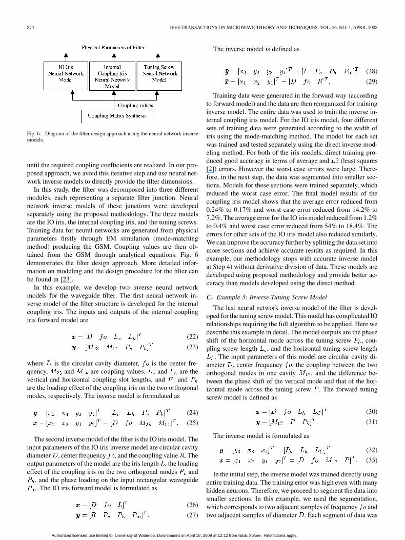
Fig. 6. Diagram of the filter design approach using the neural network inversemodels.

until the required coupling coefficients are realized. In our pro-posed approach, we avoid this iterative step and use neural net-work inverse models to directly provide the filter dimensions.

In this study, the filter was decomposed into three differentmodules, each representing a separate filter junction. Neuralnetwork inverse models of these junctions were developedseparately using the proposed methodology. The three modelsare the IO iris, the internal coupling iris, and the tuning screws.Training data for neural networks are generated from physicalparameters firstly through EM simulation (mode-matchingmethod) producing the GSM. Coupling values are then ob-tained from the GSM through analytical equations. Fig. 6demonstrates the filter design approach. More detailed infor-mation on modeling and the design procedure for the filter canbe found in [23].

In this example, we develop two inverse neural networkmodels for the waveguide filter. The first neural network in-verse model of the filter structure is developed for the internalcoupling iris. The inputs and outputs of the internal couplingiris forward model are

(22)

(23)

where is the circular cavity diameter, is the center fre-quency, and are coupling values, and are thevertical and horizontal coupling slot lengths, and andare the loading effect of the coupling iris on the two orthogonalmodes, respectively. The inverse model is formulated as

(24)

(25)

The second inverse model of the filter is the IO iris model. Theinput parameters of the IO iris inverse model are circular cavitydiameter , center frequency , and the coupling value . Theoutput parameters of the model are the iris length , the loadingeffect of the coupling iris on the two orthogonal modes and

, and the phase loading on the input rectangular waveguide. The IO iris forward model is formulated as

(26)

(27)

The inverse model is defined as

(28)

(29)

Training data were generated in the forward way (accordingto forward model) and the data are then reorganized for traininginverse model. The entire data was used to train the inverse in-ternal coupling iris model. For the IO iris model, four differentsets of training data were generated according to the width ofiris using the mode-matching method. The model for each setwas trained and tested separately using the direct inverse mod-eling method. For both of the iris models, direct training pro-duced good accuracy in terms of average and (least squares[2]) errors. However the worst case errors were large. There-fore, in the next step, the data was segmented into smaller sec-tions. Models for these sections were trained separately, whichreduced the worst case error. The final model results of thecoupling iris model shows that the average error reduced from0.24% to 0.17% and worst case error reduced from 14.2% to7.2%. The average error for the IO iris model reduced from 1.2%to 0.4% and worst case error reduced from 54% to 18.4%. Theerrors for other sets of the IO iris model also reduced similarly.We can improve the accuracy further by splitting the data set intomore sections and achieve accurate results as required. In thisexample, our methodology stops with accurate inverse modelat Step 4) without derivative division of data. These models aredeveloped using proposed methodology and provide better ac-curacy than models developed using the direct method.

C. Example 3: Inverse Tuning Screw Model

The last neural network inverse model of the filter is devel-oped for the tuning screw model. This model has complicated IOrelationships requiring the full algorithm to be applied. Here wedescribe this example in detail. The model outputs are the phaseshift of the horizontal mode across the tuning screw , cou-pling screw length , and the horizontal tuning screw length

. The input parameters of this model are circular cavity di-ameter , center frequency , the coupling between the twoorthogonal modes in one cavity , and the difference be-tween the phase shift of the vertical mode and that of the hor-izontal mode across the tuning screw . The forward tuningscrew model is defined as

(30)

(31)

The inverse model is formulated as

(32)

(33)

In the initial step, the inverse model was trained directly usingentire training data. The training error was high even with manyhidden neurons. Therefore, we proceed to segment the data intosmaller sections. In this example, we used the segmentation,which corresponds to two adjacent samples of frequency andtwo adjacent samples of diameter . Each segment of data was

Authorized licensed use limited to: University of Waterloo. Downloaded on April 18, 2009 at 12:12 from IEEE Xplore. Restrictions apply.

KABIR et al.: NEURAL NETWORK INVERSE MODELING AND APPLICATIONS TO MICROWAVE FILTER DESIGN 875

TABLE ICOMPARISON OF MODEL TEST ERRORS BETWEEN DIRECT

AND PROPOSED METHODS FOR TUNING SCREW MODEL

used to train a separate inverse model. Some of the segmentsproduced accurate models with error less than 1%, while otherswere still inaccurate.

The segments that could not reach the desired accuracywere checked for the existence of multivalued solutions indi-vidually. The method to check the existence of multivaluedsolutions using (10)–(13), as described in Section II-B, hasbeen implemented in NeuroModelerPlus [25] software. Weuse this program to detect the existence of multivalued solu-tions in the training data. For this example, neighborhood size

, maximum slope , and maximum slopechange were chosen. NeuroModelerPlus suggeststhat the data contain multivalued solutions. Therefore, we needto proceed to train a neural network forward model and applythe derivative division technique to divide the data.

To compute the derivative, we trained a neural network as aforward tuning screw model. Then derivatives were computedusing an adjoint neural network model through NeuroModeler-Plus. Considering and applying the derivativeto (15) and (16), we divided the data into groups I and II, re-spectively. Two inverse sub-models were trained using groupsI and II data. As in Step 8) of the methodology, we trained twoforward sub-models using data of groups I and II. The equa-tions for error criteria and , distance criteria and ,and model selection can be obtained using (18), (20), and (21),respectively.

The entire process was done using NeuroModelerPlus. Thesegments that failed to reach good accuracy before became morethan 99% accurate after a derivative division and model com-bining technique were applied. The process was continued untilall data were captured. A few of the sub-models needed the ac-curacy enhancement techniques to select the right models and,thus, reach the desired accuracy. The result of the inverse modelusing the proposed methodology is compared with the direct in-verse method in Table I, showing the average, , and worstcase errors between the model and test data. Table I demon-strates that the proposed methodology produces significantlybetter results than the direct method.

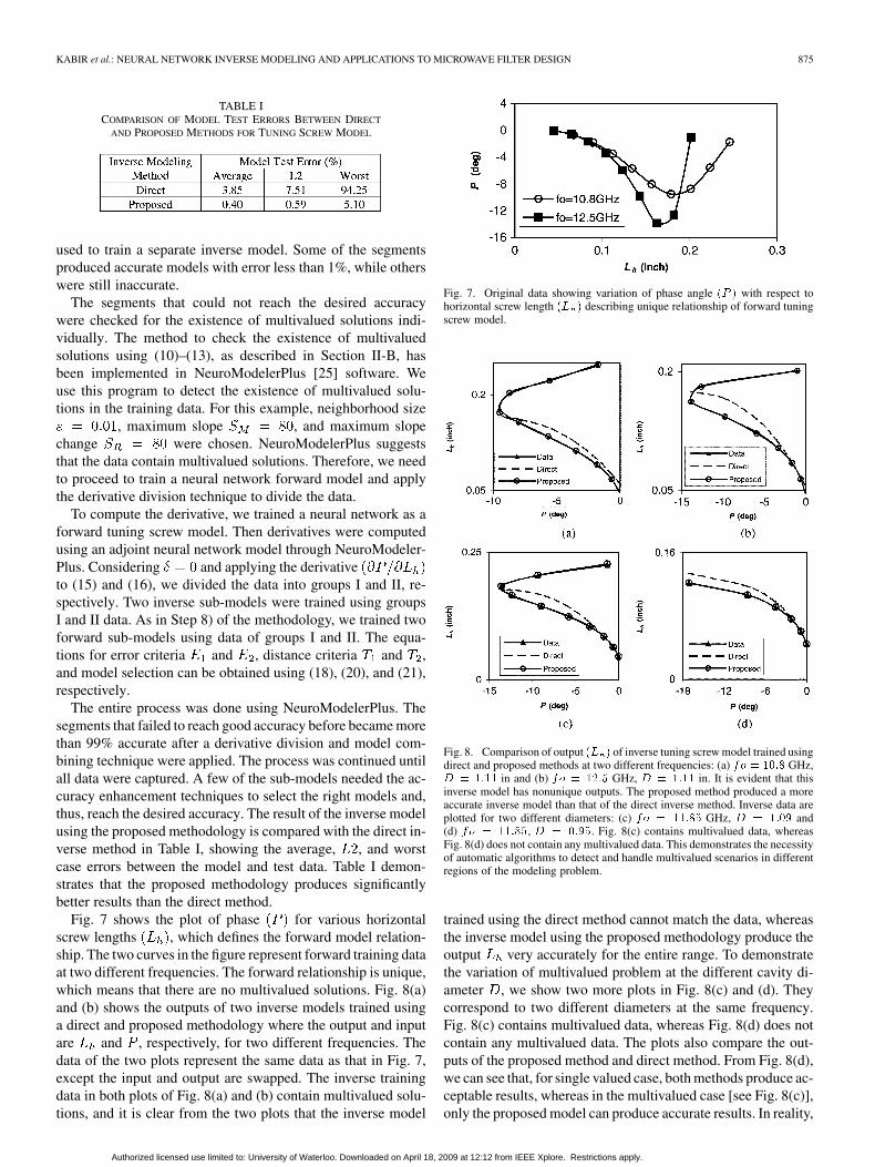
Fig. 7 shows the plot of phase for various horizontalscrew lengths , which defines the forward model relation-ship. The two curves in the figure represent forward training dataat two different frequencies. The forward relationship is unique,which means that there are no multivalued solutions. Fig. 8(a)and (b) shows the outputs of two inverse models trained usinga direct and proposed methodology where the output and inputare and , respectively, for two different frequencies. Thedata of the two plots represent the same data as that in Fig. 7,except the input and output are swapped. The inverse trainingdata in both plots of Fig. 8(a) and (b) contain multivalued solu-tions, and it is clear from the two plots that the inverse model

Fig. 7. Original data showing variation of phase angle (P ) with respect tohorizontal screw length (L ) describing unique relationship of forward tuningscrew model.

Fig. 8. Comparison of output (L ) of inverse tuning screw model trained usingdirect and proposed methods at two different frequencies: (a) fo = 10:8 GHz,D = 1:11 in and (b) fo = 12:5 GHz, D = 1:11 in. It is evident that thisinverse model has nonunique outputs. The proposed method produced a moreaccurate inverse model than that of the direct inverse method. Inverse data areplotted for two different diameters: (c) fo = 11:85 GHz, D = 1:09 and(d) fo = 11:85, D = 0:95. Fig. 8(c) contains multivalued data, whereasFig. 8(d) does not contain any multivalued data. This demonstrates the necessityof automatic algorithms to detect and handle multivalued scenarios in differentregions of the modeling problem.

trained using the direct method cannot match the data, whereasthe inverse model using the proposed methodology produce theoutput very accurately for the entire range. To demonstratethe variation of multivalued problem at the different cavity di-ameter , we show two more plots in Fig. 8(c) and (d). Theycorrespond to two different diameters at the same frequency.Fig. 8(c) contains multivalued data, whereas Fig. 8(d) does notcontain any multivalued data. The plots also compare the out-puts of the proposed method and direct method. From Fig. 8(d),we can see that, for single valued case, both methods produce ac-ceptable results, whereas in the multivalued case [see Fig. 8(c)],only the proposed model can produce accurate results. In reality,

Authorized licensed use limited to: University of Waterloo. Downloaded on April 18, 2009 at 12:12 from IEEE Xplore. Restrictions apply.

876 IEEE TRANSACTIONS ON MICROWAVE THEORY AND TECHNIQUES, VOL. 56, NO. 4, APRIL 2008

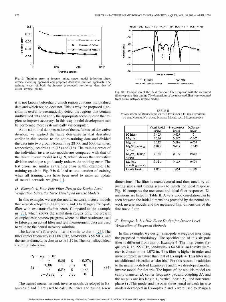
Fig. 9. Training error of inverse tuning screw model following directinverse modeling approach and proposed derivative division approach. Thetraining errors of both the inverse sub-models are lower than that ofdirect inverse model.

it is not known beforehand which region contains multivalueddata and which region does not. This is why the proposed algo-rithm is useful to automatically detect the regions that containmultivalued data and apply the appropriate techniques in that re-gion to improve accuracy. In this way, model development canbe performed more systematically via computer.

As an additional demonstration of the usefulness of derivativedivision, we applied the same derivative as that describedearlier in this section to the entire training data and dividedthe data into two groups (containing 28 000 and 6000 samples,respectively) according to (15) and (16). The training errors ofthe individual inverse sub-models are compared with that ofthe direct inverse model in Fig. 9, which shows that derivativedivision technique significantly reduces the training error. Thetest errors are similar as training error in this example. Thetraining epoch in Fig. 9 is defined as one iteration of trainingwhen all training data have been used to make an updateof neural network weights [1].

D. Example 4: Four-Pole Filter Design for Device LevelVerification Using the Three Developed Inverse Models

In this example, we use the neural network inverse modelsthat were developed in Examples 2 and 3 to design a four-polefilter with two transmission zeros. Compared to the examplein [23], which shows the simulation results only, the presentexample describes new progress, where the filter results are usedto fabricate an actual filter and real measurement data are usedto validate the neural network solutions.

The layout of a four-pole filter is similar to that in [23]. Thefilter center frequency is 11.06 GHz, bandwidth is 58 MHz, andthe cavity diameter is chosen to be 1.17 in. The normalized idealcoupling values are

(34)

The trained neural network inverse models developed in Ex-amples 2 and 3 are used to calculate irises and tuning screw

Fig. 10. Comparison of the ideal four-pole filter response with the measuredfilter response after tuning. The dimensions of the measured filter were obtainedfrom neural network inverse models.

TABLE IICOMPARISON OF DIMENSIONS OF THE FOUR-POLE FILTER OBTAINED

BY THE NEURAL NETWORK INVERSE MODEL AND MEASUREMENT

dimensions. The filter is manufactured and then tuned by ad-justing irises and tuning screws to match the ideal response.Fig. 10 compares the measured and ideal filter responses. Di-mensions are listed in Table II. A very good correlation can beseen between the initial dimensions provided by the neural net-work inverse models and the measured final dimensions of thefine tuned filter.

E. Example 5: Six-Pole Filter Design for Device LevelVerification of Proposed Methods

In this example, we design a six-pole waveguide filer usingthe proposed methodology. The specification of this six-polefilter is different from that of Example 4. The filter center fre-quency is 12.155 GHz, bandwidth is 64 MHz, and cavity diam-eter is chosen to be 1.072 in. This filter is higher in order andmore complex in nature than that of Example 4. This filter usesan additional iris called a “slot iris.” For this reason, in additionto the neural models of Examples 2 and 3, we developed anotherinverse model for slot iris. The inputs of the slot iris model arecavity diameter , center frequency , and coupling , andthe outputs are iris length , vertical phase , and horizontalphase . This model and the other three neural network inversemodels developed in Examples 2 and 3 were used to design a

Authorized licensed use limited to: University of Waterloo. Downloaded on April 18, 2009 at 12:12 from IEEE Xplore. Restrictions apply.

KABIR et al.: NEURAL NETWORK INVERSE MODELING AND APPLICATIONS TO MICROWAVE FILTER DESIGN 877

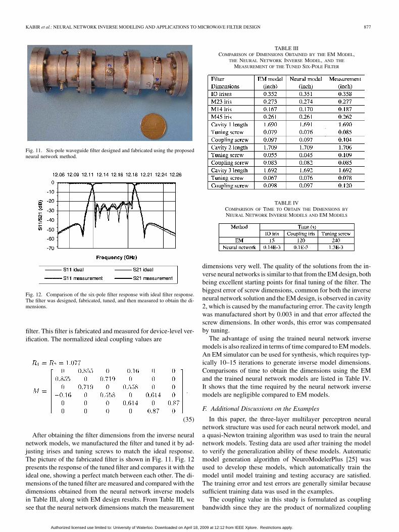
Fig. 11. Six-pole waveguide filter designed and fabricated using the proposedneural network method.

Fig. 12. Comparison of the six-pole filter response with ideal filter response.The filter was designed, fabricated, tuned, and then measured to obtain the di-mensions.

filter. This filter is fabricated and measured for device-level ver-ification. The normalized ideal coupling values are

(35)

After obtaining the filter dimensions from the inverse neuralnetwork models, we manufactured the filter and tuned it by ad-justing irises and tuning screws to match the ideal response.The picture of the fabricated filter is shown in Fig. 11. Fig. 12presents the response of the tuned filter and compares it with theideal one, showing a perfect match between each other. The di-mensions of the tuned filter are measured and compared with thedimensions obtained from the neural network inverse modelsin Table III, along with EM design results. From Table III, wesee that the neural network dimensions match the measurement

TABLE IIICOMPARISON OF DIMENSIONS OBTAINED BY THE EM MODEL,

THE NEURAL NETWORK INVERSE MODEL, AND THE

MEASUREMENT OF THE TUNED SIX-POLE FILTER

TABLE IVCOMPARISON OF TIME TO OBTAIN THE DIMENSIONS BY

NEURAL NETWORK INVERSE MODELS AND EM MODELS

dimensions very well. The quality of the solutions from the in-verse neural networks is similar to that from the EM design, bothbeing excellent starting points for final tuning of the filter. Thebiggest error of screw dimensions, common for both the inverseneural network solution and the EM design, is observed in cavity2, which is caused by the manufacturing error. The cavity lengthwas manufactured short by 0.003 in and that error affected thescrew dimensions. In other words, this error was compensatedby tuning.

The advantage of using the trained neural network inversemodels is also realized in terms of time compared to EM models.An EM simulator can be used for synthesis, which requires typ-ically 10–15 iterations to generate inverse model dimensions.Comparisons of time to obtain the dimensions using the EMand the trained neural network models are listed in Table IV.It shows that the time required by the neural network inversemodels are negligible compared to EM models.

F. Additional Discussions on the Examples

In this paper, the three-layer multilayer perceptron neuralnetwork structure was used for each neural network model, anda quasi-Newton training algorithm was used to train the neuralnetwork models. Testing data are used after training the modelto verify the generalization ability of these models. Automaticmodel generation algorithm of NeuroModelerPlus [25] wasused to develop these models, which automatically train themodel until model training and testing accuracy are satisfied.The training error and test errors are generally similar becausesufficient training data was used in the examples.

The coupling value in this study is formulated as couplingbandwidth since they are the product of normalized coupling

Authorized licensed use limited to: University of Waterloo. Downloaded on April 18, 2009 at 12:12 from IEEE Xplore. Restrictions apply.

878 IEEE TRANSACTIONS ON MICROWAVE THEORY AND TECHNIQUES, VOL. 56, NO. 4, APRIL 2008

values and bandwidth. In this way, bandwidth is no longerneeded as a model input, which helps in reducing training dataand increasing model accuracy.

The tuning time is approximately the same for both the EMand neural network design. Even though the EM method givesthe best solution of a filter, the physical machining processcannot guarantee 100% accurate dimension. Therefore, aftermanufacturing, the filter tuning is required. The amount of timespent on tuning also depends on how accurate the dimensionsare. If the dimensions are far different from their perfect values,then tuning time will increase. The neural network methodprovides approximately the same dimension as the EM method.They both provide excellent starting points for tuning. As aresult, the tuning time is relatively short and is the same forboth the EM and neural network methods. Consequently, thetuning time does not alter the comparison between the EM andneural network method.

The training time for the direct inverse tuning screw modelis approximately 6 min. In the proposed algorithm, if we per-form segmentation, it will add 28.5 s, and if multivalued solu-tions are detected in a segment, it adds another 7.5 s for a for-ward model for a small segment containing 200 samples. Thetraining time for the complete inverse tuning screw model usingthe proposed methodology is approximately 5.5 h. For the cou-pling iris, the direct inverse model containing 37000 samplestakes 26 min to train. The proposed method divides the modelinto four smaller segments, each containing approximately 9000samples, and takes ten additional minutes per segment. The timeto train a direct IO iris inverse model containing 125 000 datarequires 2.5 h. The training time using the proposed method-ology is 6 h, including the time for training segmented models.The training time for these models were obtained using the Neu-roModelerPlus parallel-automated model generation algorithm[25] on an Intel Quad core processor at 2.4 GHz. The trainingtime for the proposed inverse models is longer than that of thedirect inverse models. However, once the models are trained, theproposed model is very fast for the designer, providing solutionsnearly instantly.

The technique is useful for highly repeated design tasks suchas designing filters of different orders and different specifica-tions. The technique is not suitable if the inverse model is forthe purpose of only one or a few particular designs becausethe model training time will make the technique cost ineffec-tive. Therefore, the technique should be applied to inverse tasks,which will be reused frequently. In such a case, the benefit ofusing the models far outweigh the cost of training because ofthe following four reasons.

1) Training is a one-time investment, and the benefit of themodel increases when the model is used over and overagain. For example, the two different filters in this paperuse the same set of iris and tuning screw models.

2) Conventional EM design is part of the design cycle, whileneural network training is outside the design cycle.

3) Circuit design requires much human involvement, whileneural network training is a machine-based computationaltask.

4) Neural network training can be done by a model developerand the trained model can be used by multiple designers.

The neural network approach cuts expensive design time byshifting much burden to offline computer-based neural networktraining [2]. An even more significant benefit of the proposedtechnique is the new feasibility of interactive design and what–ifanalysis using the instant solutions of inverse neural networks,substantially enhancing design flexibility and efficiency.

V. CONCLUSION

Efficient neural network modeling techniques have beenpresented and applied to microwave filter modeling and design.The inverse modeling technique has been formulated and thenonuniqueness of the IO relationship has been addressed.Methods to identify multivalued solutions and divide trainingdata have been proposed for training inverse models. Data ofthe inverse model have been divided based on derivatives of theforward model and then used separately to train more accurateinverse sub-models. A method to correctly combine the inversesub-models has been presented. The inverse models developedusing the proposed techniques are more accurate than thatusing the direct method. The proposed methodology has beenapplied to waveguide filter modeling. Very good correlationwas found between neural network predicted dimensions andthat of perfectly tuned filters. This modeling approach is usefulfor a fast solution to inverse problems in microwave design.

REFERENCES

[1] Q. J. Zhang, K. C. Gupta, and V. K. Devabhaktuni, “Artificial neuralnetworks for RF and microwave design—From theory to practice,”IEEE Trans. Microw. Theory Tech., vol. 51, no. 4, pp. 1339–1350, Apr.2003.

[2] Q. J. Zhang and K. C. Gupta, Neural Networks for RF and MicrowaveDesign. Boston, MA: Artech House, 2000.

[3] P. M. Watson and K. C. Gupta, “EM-ANN models for microstrip viasand interconnects in dataset circuits,” IEEE Trans. Microw. TheoryTech., vol. 44, no. 12, pp. 2495–2503, Dec. 1996.

[4] V. K. Devabhaktuni, M. C. E. Yagoub, and Q. J. Zhang, “A robust al-gorithm for automatic development of neural-network models for mi-crowave applications,” IEEE Trans. Microw. Theory Tech., vol. 49, no.12, pp. 2282–2291, Dec. 2001.

[5] P. M. Watson and K. C. Gupta, “Design and optimization of CPW cir-cuits using EM-ANN models for CPW components,” IEEE Trans. Mi-crow. Theory Tech., vol. 45, no. 12, pp. 2515–2523, Dec. 1997.

[6] A. H. Zaabab, Q. J. Zhang, and M. S. Nakhla, “A neural network mod-eling approach to circuit optimization and statistical design,” IEEETrans. Microw. Theory Tech., vol. 43, no. 6, pp. 1349–1358, Jun. 1995.

[7] B. Davis, C. White, M. A. Reece, M. E. Bayne, Jr., W. L. Thompson,II, N. L. Richardson, and L. Walker, Jr., “Dynamically configurablepHEMT model using neural networks for CAD,” in IEEE MTT-S Int.Microw. Symp. Dig., Philadelphia, PA, Jun. 2003, vol. 1, pp. 177–180.

[8] J. Xu, M. C. E. Yagoub, R. Ding, and Q. J. Zhang, “Exact adjoint sensi-tivity analysis for neural-based microwave modeling and design,” IEEETrans. Microw. Theory Tech., vol. 51, no. 1, pp. 226–237, Jan. 2003.

[9] V. Markovic, Z. Marinkovic, and N. Males-llic, “Application of neuralnetworks in microwave FET transistor noise modeling,” in Proc.Neural Network Applicat. Elect. Eng., Belgrade, Yugoslavia, Sep.2000, pp. 146–151.

[10] M. Isaksson, D. Wisell, and D. Ronnow, “Wide-band dynamic mod-eling of power amplifiers using radial-basis function neural networks,”IEEE Trans. Microw. Theory Tech., vol. 53, no. 11, pp. 3422–3428,Nov. 2005.

[11] J. P. Garcia, F. Q. Pereira, D. C. Rebenaque, J. L. G. Tornero, and A.A. Melcon, “A neural-network method for the analysis of multilayeredshielded microwave circuits,” IEEE Trans. Microw. Theory Tech., vol.54, no. 1, pp. 309–320, Jan. 2006.

[12] V. Rizzoli, A. Costanzo, D. Masotti, A. Lipparini, and F. Mastri, “Com-puter-aided optimization of nonlinear microwave circuits with the aidof electromagnetic simulation,” IEEE Trans. Microw. Theory Tech.,vol. 52, no. 1, pp. 362–377, Jan. 2004.

Authorized licensed use limited to: University of Waterloo. Downloaded on April 18, 2009 at 12:12 from IEEE Xplore. Restrictions apply.

KABIR et al.: NEURAL NETWORK INVERSE MODELING AND APPLICATIONS TO MICROWAVE FILTER DESIGN 879

[13] M. M. Vai, S. Wu, B. Li, and S. Prasad, “Reverse modeling of mi-crowave circuits with bidirectional neural network models,” IEEETrans. Microw. Theory Tech., vol. 46, no. 10, pp. 1492–1494, Oct.1998.

[14] S. Selleri, S. Manetti, and G. Pelosi, “Neural network applications inmicrowave device design,” Int. J. RF Microw. Comput.-Aided Eng., vol.12, pp. 90–97, Jan. 2002.

[15] J. W. Bandler, M. A. Ismail, J. E. Rayas-Sanchez, and Q. J. Zhang,“Neural inverse space mapping (NISM) optimization for EM-base mi-crowave design,” Int. J. RF Microw. Comput.-Aided Eng., vol. 13, pp.136–147, Mar. 2003.

[16] G. Fedi, A. Gaggelli, S. Manetti, and G. Pelosi, “Direct-coupled cavityfilters design using a hybrid feedforward neural network—Finite ele-ments procedure,” Int. J. RF Microw. Comput.-Aided Eng., vol. 9, pp.287–296, May 1999.

[17] J. M. Cid and J. Zapata, “CAD of rectangular-waveguideH-plane cir-cuits by segmentation, finite elements and artificial neural networks,”Electron. Lett., vol. 37, pp. 98–99, Jan. 2001.

[18] A. Mediavilla, A. Tazon, J. A. Pereda, M. Lazaro, I. Santamaria, and C.Pantaleon, “Neuronal architecture for waveguide inductive iris band-pass filter optimization,” in Proc. IEEE INNS–ENNS Int. Neural Net-works Joint Conf., Como, Italy, Jul. 2000, vol. 4, pp. 395–399.

[19] F. Nunez and A. K. Skrivervik, “Filter approximation by RBF-NN andsegmentation method,” in IEEE MTT-S Int. Microw. Symp. Dig., FortWorth, TX, Jun. 2004, vol. 3, pp. 1561–1564.

[20] P. Burrascano, M. Dionigi, C. Fancelli, and M. Mongiardo, “A neuralnetwork model for CAD and optimization of microwave filters,” inIEEE MTT-S Int. Microw. Symp. Dig., Baltimore, MD, Jun. 1998, vol.1, pp. 13–16.

[21] A. S. Ciminski, “Artificial neural networks modeling for com-puter-aided design of microwave filter,” in Int. Microw., Radar,Wireless Commun. Conf., Gdansk, Poland, May 2002, vol. 1, pp.96–99.

[22] C. Kudsia, R. Cameron, and W.-C. Tang, “Innovations in microwavefilters and multiplexing networks for communications satellitesystems,” IEEE Trans. Microw. Theory Tech., vol. 40, no. 6, pp.1133–1149, Jun. 1992.

[23] Y. Wang, M. Yu, H. Kabir, and Q. J. Zhang, “Effective design of cross-coupled filter using neural networks and coupling matrix,” in IEEEMTT-S Int. Microw. Symp. Dig., San Francisco, CA, Jun. 2006, pp.1431–1434.

[24] I. Bahl, Lumped Elements for RF and Microwave Circuits. Boston,MA: Artech House, 2003.

[25] Q. J. Zhang, NeuroModelerPlus. Dept. Electron., Carleton Univ., Ot-tawa, ON, Canada.

Humayun Kabir (S’06) received the B.Sc. degreein electrical and electronic engineering from theBangladesh University of Engineering and Tech-nology, Dhaka, Bangladesh, in 1999, the M.S.E.E.degree in electrical engineering from the Universityof Arkansas, Fayetteville, in 2003, and is currentlyworking toward the Ph.D. degree in electronicsengineering at Carleton University, Ottawa, ON,Canada.

He was a Research Assistant with the High DensityElectronics Center (HiDEC), University of Arkansas,

Fayetteville, and COM DEV, Cambridge, ON, Canada, as a co-op student. Heis currently a Teaching and Research Assistant with Carleton University. Hisresearch interests include RF/microwave design and optimization.

Ying Wang (M’05) received the B.Eng. and Mas-ters degrees in electronic engineering from the Nan-jing University of Science and Technology, Nanjing,China, in 1993 and 1996, respectively, and the Ph.D.degree in electrical engineering from the Universityof Waterloo, Waterloo, ON, Canada, in 2000.

From 2000 to 2007, she was with COM DEV,Cambridge, ON, Canada, where she was involved inthe development of computer-aided design (CAD)software for design, simulation, and optimization ofmicrowave circuits for space application. In 2007,

she joined the Faculty of Engineering and Applied Sciences, University ofOntario Institute of Technology, Oshawa, ON, Canada, where she is currentlyan Assistant Professor. Her research interests include RF/microwave CAD,microwave circuits design, and radio wave propagation modeling.

Ming Yu (S’90–M’93–SM’01) received the Ph.D.degree in electrical engineering from the Universityof Victoria, Victoria, BC, Canada, in 1995.

In 1993, while working on his doctoral disserta-tion part time, he joined COM DEV, Cambridge, ON,Canada, as a Member of Technical Staff, where hewas involved in the design of passive microwave/RFhardware from 300 MHz to 60 GHz. He was also aprincipal developer of a variety of COM DEV’s de-sign and tuning software for microwave filters andmultiplexers. His varied experience with COM DEV

also includes being the Manager of filter/multiplexer technology (Space Group)and Staff Scientist of corporate research and development (R&D). He is cur-rently the Chief Scientist and Director of R&D. He is responsible for overseeingthe development of RF microelectromechanical system (MEMS) technology,computer-aided tuning and EM modeling, and optimization of microwave fil-ters/multiplexers for wireless applications. He is also an Adjunct Professor withthe University of Waterloo, Waterloo, ON, Canada. He has authored or coau-thored over 70 publications and numerous proprietary reports. He is frequentlya reviewer for IEE publications. He holds eight patents with four pending.

Dr. Yu is vice chair of the IEEE Technical Coordinating Committee 8 (TCC,MTT-8) and is a frequent reviewer of numerous IEEE publications. Since 2006,he has been the chair of the IEEE Technical Program Committee 11 (TPC-11).He was the recipient of the 1995 and 2006 COM DEV Ltd. Achievement Awardfor the development of computer-aided tuning algorithms and systems for mi-crowave filters and multiplexers.

Qi-Jun Zhang (S’84–M’87–SM’95–F’06) receivedthe B.Eng. degree from the East China EngineeringInstitute, Nanjing, China, in 1982, and the Ph.D. de-gree in electrical engineering from McMaster Uni-versity, Hamilton, ON, Canada, in 1987.

From 1982 to 1983, he was with the System Engi-neering Institute, Tianjin University, Tianjin, China.From 1988 to 1990, he was with Optimization Sys-tems Associates (OSA) Inc., Dundas, ON, Canada,where he developed advanced microwave optimiza-tion software. In 1990, he joined the Department of

Electronics, Carleton University, Ottawa, ON, Canada, where he is currently aProfessor. He has authored over 180 publications. He authored Neural Networksfor RF and Microwave Design (Artech House, 2000) and coedited Modeling andSimulation of High-Speed VLSI Interconnects (Kluwer, 1994). He contributedto Encyclopedia of RF and Microwave Engineering, (Wiley, 2005), Fundamen-tals of Nonlinear Behavioral Modeling for RF and Microwave Design (ArtechHouse, 2005), and Analog Methods for Computer-Aided Analysis and Diag-nosis (Marcel Dekker, 1988). He was a Guest Co-Editor for the “Special Issueon High-Speed VLSI Interconnects” of the International Journal of Analog Inte-grated Circuits and Signal Processing (Kluwer, 1994) and was a two-time GuestEditor for the “Special Issue on Applications of ANN to RF and MicrowaveDesign” of the International Journal of RF and Microwave CAE (Wiley, 1999,2002). He is an Editorial Board member of the International Journal of RF andMicrowave Computer-Aided Engineering and the International Journal of Nu-merical Modeling. His research interests are neural network and optimizationmethods for high-speed/high-frequency circuit design.

Dr. Zhang is a member on the Editorial Board of the IEEE TRANSACTIONS ON

MICROWAVE THEORY AND TECHNIQUES. He is a member of the Technical Com-mittee on Computer-Aided Design (MTT-1) of the IEEE Microwave Theoryand Techniques Society (IEEE MTT-S).

Authorized licensed use limited to: University of Waterloo. Downloaded on April 18, 2009 at 12:12 from IEEE Xplore. Restrictions apply.