(nas colloquium) earthquake prediction: the scientific challenge
TRANSCRIPT

Visit the National Academies Press online, the authoritative source for all books from the National Academy of Sciences, the National Academy of Engineering, the Institute of Medicine, and the National Research Council: • Download hundreds of free books in PDF • Read thousands of books online for free • Explore our innovative research tools – try the “Research Dashboard” now! • Sign up to be notified when new books are published • Purchase printed books and selected PDF files
Thank you for downloading this PDF. If you have comments, questions or just want more information about the books published by the National Academies Press, you may contact our customer service department toll-free at 888-624-8373, visit us online, or send an email to [email protected]. This book plus thousands more are available at http://www.nap.edu. Copyright © National Academy of Sciences. All rights reserved. Unless otherwise indicated, all materials in this PDF File are copyrighted by the National Academy of Sciences. Distribution, posting, or copying is strictly prohibited without written permission of the National Academies Press. Request reprint permission for this book.
ISBN: 0-309-58856-1, 128 pages, 8.5 x 11, (1996)
This PDF is available from the National Academies Press at:http://www.nap.edu/catalog/5709.html
http://www.nap.edu/catalog/5709.html
We ship printed books within 1 business day; personal PDFs are available immediately.
(NAS Colloquium) Earthquake Prediction: The Scientific Challenge
Proceedings of the National Academy of Sciences
PROCEEDINGS OF THE NATIONALACADEMY OF SCIENCES OF THE
UNITED STATES OF AMERICA
Table of Contents
Papers from a National Academy of Sciences Colloquium on Earthquake Prediction: The Scientific Challenge
Earthquake prediction: The scientific challengeL.Knopoff
3719–3720
Earthquake prediction: The interaction of public policy and scienceLucile M.Jones
3721–3725
Initiation process of earthquakes and its implications for seismic hazard reduction strategyHiroo Kanamori
3726–3731
Intermediate- and long-term earthquake predictionLynn R.Sykes
3732–3739
Scale dependence in earthquake phenomena and its relevance to earthquake predictionKeiiti Aki
3740–3747
Intermediate-term earthquake predictionV.I. Keilis-Borok
3748–3755
A selective phenomenology of the seismicity of Southern CaliforniaL.Knopoff
3756–3763
The repetition of large-earthquake rupturesKerry Sieh
3764–3771
Hypothesis testing and earthquake predictionDavid D.Jackson
3772–3775
What electrical measurements can say about changes in fault systemsTheodore R.Madden and Randall L.Mackie
3776–3780
Geochemical challenge to earthquake predictionHiroshi Wakita
3781–3786
Implications of fault constitutive properties for earthquake predictionJames H.Dieterich and Brian Kilgore
3787–3794
Nonuniformity of the constitutive law parameters for shear rupture and quasistatic nucleationto dynamic rupture: A physical model of earthquake generation processesMitiyasu Ohnaka
3795–3802
Rock friction and its implications for earthquake prediction examined via models of ParkfieldearthquakesTerry E.Tullis
3803–3810
Slip complexity in earthquake fault modelsJames R.Rice and Yehuda Ben-Zion
3811–3818
TABLE OF CONTENTS i
Abou
t thi
s PD
F fil
e: T
his
new
dig
ital r
epre
sent
atio
n of
the
orig
inal
wor
k ha
s be
en re
com
pose
d fro
m X
ML
files
cre
ated
from
the
orig
inal
pap
er b
ook,
not
from
the
orig
inal
type
setti
ng fi
les.
Pag
e br
eaks
are
true
to th
e or
igin
al; l
ine
leng
ths,
wor
d br
eaks
, hea
ding
sty
les,
and
oth
er ty
pese
tting
-spe
cific
form
attin
g, h
owev
er, c
anno
t be
reta
ined
, and
som
e ty
pogr
aphi
c er
rors
may
hav
e be
en a
ccid
enta
lly in
serte
d. P
leas
e us
e th
e pr
int v
ersi
on o
f thi
s pu
blic
atio
n as
the
auth
orita
tive
vers
ion
for a
ttrib
utio
n.
Copyright © National Academy of Sciences. All rights reserved.
(NAS Colloquium) Earthquake Prediction: The Scientific Challengehttp://www.nap.edu/catalog/5709.html

Dynamic friction and the origin of the complexity of earthquake sourcesRaúl Madariaga and Alain Cochard
3819–3824
Slip complexity in dynamic models of earthquake faultsJ.S.Langer, J.M.Carlson, Christopher R.Myers, and Bruce E.Shaw
3825–3829
The organization of seismicity on fault networksL.Knopoff
3830–3837
GEOPHYSICS Geometric incompatibility in a fault system
Andrei Gabrielov, Vladimir Keilis-Borok, and David D.Jackson 3838–3842
TABLE OF CONTENTS ii
Abou
t thi
s PD
F fil
e: T
his
new
dig
ital r
epre
sent
atio
n of
the
orig
inal
wor
k ha
s be
en re
com
pose
d fro
m X
ML
files
cre
ated
from
the
orig
inal
pap
er b
ook,
not
from
the
orig
inal
type
setti
ng fi
les.
Pag
e br
eaks
are
true
to th
e or
igin
al; l
ine
leng
ths,
wor
d br
eaks
, hea
ding
sty
les,
and
oth
er ty
pese
tting
-spe
cific
form
attin
g, h
owev
er, c
anno
t be
reta
ined
, and
som
e ty
pogr
aphi
c er
rors
may
hav
e be
en a
ccid
enta
lly in
serte
d. P
leas
e us
e th
e pr
int v
ersi
on o
f thi
s pu
blic
atio
n as
the
auth
orita
tive
vers
ion
for a
ttrib
utio
n.
Copyright © National Academy of Sciences. All rights reserved.
(NAS Colloquium) Earthquake Prediction: The Scientific Challengehttp://www.nap.edu/catalog/5709.html
This paper serves as an introduction to the following papers, which were presented at a colloquium entitled “Earthquake Prediction: TheScientific Challenge,” organized by Leon Knopoff (Chair), Keiiti Aki, Clarence R.Allen, James R.Rice, and Lynn R.Sykes, held February 10and 11, 1995, at the National Academy of Sciences in Irvine, CA.
Earthquake prediction: The scientific challenge
L.KNOPOFF
Department of Physics and Institute of Geophysics and Planetary Physics, University of California, Los Angeles, CA 90024–1567As recently as 20 years ago the problems of earthquake prediction research were approached through a compilation of a succession of isolated
case histories of presumed precursors to subsequent large and small earthquakes. The hope was that these precursory phenomena would appearbefore many, if not all, subsequent events. Alas, some of these hopes have either evaporated or have proved extremely difficult to document.Topics such as anomalies in the ratio of P- to S-wave velocities, magnetic fields, resistivity, tilt, emission of noble gases, and so on are no longer atthe leading edge of contemporary interest. Although interest in these areas is occasionally rekindled, the spark is difficult to fan into flame, andinvestment of support and effort in these areas has not been heavy in recent times.
Today our approach is much the same as before: we continue to study a succession of case histories of events leading to strong earthquakes.Even today, there are occasional reports of new precursory anomalies, such as a change in the magnetic field before the Loma Prieta earthquakeand, as will be discussed later in this collection of papers, observation of an increase of the concentration of chlorine and other ions in well watersbefore the Kobe earthquake. Whether these new areas will prove to be universals or disappear as others have remains for the future. But someavenues of phenomenology have continued to be pursued: clustering and anticlustering of earthquakes, creep measurements, changes in theattenuation factor, paleoseismicity methods, etc.
A second thread of earlier prediction research was the presumption that small earthquakes were scaled-down versions of large ones, and hencethe supposition was made that the study of small earthquakes would reveal important truths about large ones, a model if not driven by the scalingimplicit in the Gutenberg-Richter distribution, then at least with the notion of scaling lurking in the background. These ideas suggest that simpleisolated fractures in an elastic solid have a distribution of stresses and slips that are scaled only by the sizes of the cracks and hence whateverprecursors, and postcursors for that matter, that might be observed will also be similarly scaled. This direction of research has also undergonemodification over the years: on present-day models, earthquake fractures take place in a prestressed solid in which fluctuations are significantperturbations of the uniformity of the stress field. But small fractures take place in the shadows cast by the stress field of the larger and the largestfractures. The chain of self-similarity is broken for the largest earthquakes, since the largest fractures do not have stress fluctuations with evenlarger scales to contend with. Furthermore, the details of the fracture and of the properties of nearby rocks are not resolved observationally insmaller earthquakes, certainly not as clearly as in the case of large earthquakes. Today, the paradigms have shifted to the study of strongearthquakes and away from the more numerous small earthquakes, except insofar as the small ones give information about future large ones.
The issue of prediction has always been one of the establishment of the probability that an earthquake will occur within a specified timeinterval, a specified space interval, and a specified magnitude range. Contraction of these intervals remains an elusive goal. Because the techniquesthat are used differ, earthquake prediction research has been divided into three time intervals: those of short-term predictions which cover the timeinterval from a day to a few hundred days before a strong earthquake, of intermediate-term predictions covering the interval from about one year toone decade, and of long-term predictions that cover intervals longer than a decade before great earthquakes. “Earthquake prediction” in the popularlanguage is consonant with short-term prediction. At the present time, optimism is rather low about the prospects for short-term prediction, becauseof its local nature: one would have to be fortunate to have instruments within short range of the future focus of a strong earthquake. Even the mostpromising approach, through a study of accelerated precursory creep, does not seem to be a very productive lead, since the precursor is localized ina focal zone that is at least 15 km (straight down) from the nearest instrument.
Intermediate-term prediction has significant value in the United States and other industrialized nations, because it gives a useful lead-time forthe marshaling and focusing of resources for the strengthening of construction. Most efforts at intermediate-term prediction research have centeredon identification of patterns of earthquake occurrence by magnitude, time, and/or location prior to strong earthquakes. In this area too, we havebeen obliged to rely on well-instrumented case histories of precursory clustering and anticlustering presumed to be associated with future largeearthquakes. Systematization has been difficult because of the paucity of large earthquakes.
On the long time scale, the questions that are asked are whether given faults, and especially those that support the largest earthquakes, ruptureperiodically or not. Here the evidence is not to be gleaned from the study of seismic recordings or catalogs of earthquakes determined from theseismic recordings of the instrumental era, which starts in the case of Southern California after the Long Beach earthquake of 1933. The evidencein the long-term regime is derived from analysis of ancient faulting episodes and the interaction between the geometry of faults and the seismicityof the largest events; these are data that are difficult to obtain, because they rely largely on results of difficult geochronological measurements inexcavations across faults.
Over the past one or two decades remarkable progress has been made in detailing the case histories of the precursory state before largeearthquakes, including many cases in which these precursory intervals appear to be uneventful. The progress has been especially noteworthy inCalifornia where dense networks of seismographs, creep-measuring instruments, and other devices have succeeded in delineating the eventsprecursory to the Loma Prieta (1989), Landers (1992),
The publication costs of this article were defrayed in part by page charge payment. This article must therefore be hereby marked“advertisement” in accordance with 18 U.S.C. §1734 solely to indicate this fact.
EARTHQUAKE PREDICTION: THE SCIENTIFIC CHALLENGE 3719
Abou
t thi
s PD
F fil
e: T
his
new
dig
ital r
epre
sent
atio
n of
the
orig
inal
wor
k ha
s be
en re
com
pose
d fro
m X
ML
files
cre
ated
from
the
orig
inal
pap
er b
ook,
not
from
the
orig
inal
type
setti
ng fi
les.
Pag
e br
eaks
are
true
to th
e or
igin
al; l
ine
leng
ths,
wor
d br
eaks
, hea
ding
sty
les,
and
oth
er ty
pese
tting
-spe
cific
form
attin
g, h
owev
er, c
anno
t be
reta
ined
, and
som
e ty
pogr
aphi
c er
rors
may
hav
e be
en a
ccid
enta
lly in
serte
d. P
leas
e us
e th
e pr
int v
ersi
on o
f thi
s pu
blic
atio
n as
the
auth
orita
tive
vers
ion
for a
ttrib
utio
n.
Copyright © National Academy of Sciences. All rights reserved.
(NAS Colloquium) Earthquake Prediction: The Scientific Challengehttp://www.nap.edu/catalog/5709.html
and Northridge (1994) earthquakes. Progress in this field has been due to the development of a dense network of seismographs, a program that tooka number of years to install. Similarly, better tools are available for the study of precursory creep and changes in the earth's magnetic and electricfields. With the new generation of instruments, and with increased resolution in devising solutions to the inverse problem, some of the olderpresumptions about precursors have disappeared from the repertoire as noted above, others survive with increased intensity of attack, and a fewnew methods appear.
We remain in the case-history stage of the study of precursory clustering of earthquakes prior to strong earthquakes; these accounts ofclustering remain without statistical substantiation because of the paucity of strong earthquakes for study: These comments should not beinterpreted to be a plea that more strong earthquakes should take place.
Great progress has been made on the modeling front, partly through the extraordinary development of large-scale computing resources. Therehas been a remarkable increase in our understanding of the behavior of the deformation of rocks through laboratory measurements, and especiallyin the behavior of prefractured rocks, in the times before large-scale rupture. There has been unusual activity in the modeling, usually numerical, ofprocesses of self-organization of the stress field due to the occurrence of extended fractures in faulted systems. In particular, we have acquiredinsights into the physics of fracture, on preexisting, nonuniform faults.
Despite the optimistic tone of the above remarks, an ability to predict earthquakes either on an individual basis or on a statistical basis remainsremote. It is clear that the scientific issues must be understood before routine predictions can be announced, which in a generalized sense is anengineering problem.
There are other issues connected with earthquake prediction that were not discussed at the colloquium presented here: neither the organizationof national programs in earthquake prediction, nor the engineering problems, nor the problems of societal response to possible future predictions inthe three different time scales. With regard to the scientific issues, the colloquium committee developed a program that focused in roughly equalamounts on the laboratory and modeling research that is currently being performed on the one hand and on the observations relevant to the threetime scales on the other. The papers that follow are an excellent representation of the thoughts that were aired and cover the full range from thepessimistic to the optimistic.
It is a certainty that the problems of societal response and engineering response to earthquake predictions are not going to be solved until thescientific problems can be brought under control. These are no more difficult than they were several decades ago; they are only more clearlydefined today. We recognize today that the scientific problems are not simple.
A significant number of graduate students and young postdoctoral scholars were able to attend the Colloquium through generous support bythe National Science Foundation and the Southern California Earthquake Center.
EARTHQUAKE PREDICTION: THE SCIENTIFIC CHALLENGE 3720
Abou
t thi
s PD
F fil
e: T
his
new
dig
ital r
epre
sent
atio
n of
the
orig
inal
wor
k ha
s be
en re
com
pose
d fro
m X
ML
files
cre
ated
from
the
orig
inal
pap
er b
ook,
not
from
the
orig
inal
type
setti
ng fi
les.
Pag
e br
eaks
are
true
to th
e or
igin
al; l
ine
leng
ths,
wor
d br
eaks
, hea
ding
sty
les,
and
oth
er ty
pese
tting
-spe
cific
form
attin
g, h
owev
er, c
anno
t be
reta
ined
, and
som
e ty
pogr
aphi
c er
rors
may
hav
e be
en a
ccid
enta
lly in
serte
d. P
leas
e us
e th
e pr
int v
ersi
on o
f thi
s pu
blic
atio
n as
the
auth
orita
tive
vers
ion
for a
ttrib
utio
n.
Copyright © National Academy of Sciences. All rights reserved.
(NAS Colloquium) Earthquake Prediction: The Scientific Challengehttp://www.nap.edu/catalog/5709.html
This paper was presented at a colloquium entitled “Earthquake Prediction: The Scientific Challenge,” organized by Leon Knopoff(Chair), Keiiti Aki, Clarence R.Allen, James R.Rice, and Lynn R.Sykes, held February 10 and 11, 1995, at the National Academy of Sciences inIrvine, CA.
Earthquake prediction: The interaction of public policy and science
LUCILE M.JONES
U.S. Geological Survey, Pasadena, CA 91106ABSTRACT Earthquake prediction research has searched for both informational phenomena, those that provide information about
earthquake hazards useful to the public, and causal phenomena, causally related to the physical processes governing failure on a fault, toimprove our understanding of those processes. Neither informational nor causal phenomena are a subset of the other. I propose aclassification of potential earthquake predictors of informational, causal, and predictive phenomena, where predictors are causalphenomena that provide more accurate assessments of the earthquake hazard than can be gotten from assuming a random distribution.Achieving higher, more accurate probabilities than a random distribution requires much more information about the precursor than justthat it is causally related to the earthquake.
Research in earthquake prediction has two potentially compatible but distinctly different objectives: (i) phenomena that provide usinformation about the future earthquake hazard useful to those who live in earthquake-prone regions and (ii) phenomena causally related to thephysical processes governing failure on a fault that will improve our understanding of those processes. Both are important and laudable goals ofany research project, but they are distinct. We can call these informational phenomena and causal precursors.
It is obvious that not all causal precursors are informational. We investigate phenomena related to the earthquake process long before we haveenough information to tell the public about a significant change in the earthquake hazard. In addition, however, not all informational phenomenaare causal. We use the geologically and seismologically determined rates of past earthquake occurrence to assess the earthquake hazard in asocially useful way without knowing anything about the failure processes active on a fault. What, if anything, lies at the intersection of these twogroups is perhaps the greatest goal of earthquake prediction (Fig. 1).
Much of the early research in earthquake prediction in the 1970s was directed toward causal earthquake precursors. The laboratory researchshowing dilatancy and strain softening preceding rock failure encouraged many to believe that precursors arising from these processes could bemeasured in the field (e.g., refs. 1 and 2). When field measurements did not live up to this expectation, research in the 1980s began to shift towardnonprecursory processes, earthquake rates, and earthquake forecasting (e.g., ref. 7). In the last few years, as the informational capacity of rateanalyses has been more fully explored, interest is beginning to return to possibly causal precursors. However, our approach to the research and ourcommunication with the public now rests on a different foundation. The public has become accustomed to earthquake probabilities and processesfurther information within this context.
In this new environment, I believe we must clarify the difference between informational phenomena and causal precursors and where, ifanywhere, they overlap. To do so, I propose a grouping similar to the meteorological categories of climate and weather. If climate is what oneexpects and weather is what one gets, then earthquake climate is the hazard we expect from the known aggregate rates of earthquake occurrence,and earthquake weather would be the prediction of earthquakes from phenomena related to the failure of one particular patch of a fault.Nonprecursory informational phenomena are a type of climate, causal precursors are weather phenomena, and predictive precursors are weatherphenomena that predict earthquakes with a probability greater than expected from the climate. In this paper, I will classify proposed earthquakeprecursors into these three categories. Causal precursors, informational phenomena, and predictive precursors should all continue to be the focus ofscientific study, but only the latter two should be the basis for public policy.
CLASSIFICATIONS
Nonprecursory information predicts the earthquakes expected from the previously recorded rates of earthquakes. Because these estimates arebased on rates, they include no implied time to the mainshock. We use an arbitrary time to express the probabilities, but the probability is flat withtime, except when the rate itself varies with time, as in an aftershock sequence. Nonprecursory information does not require assumptions about theearthquake failure process such as stress state (i.e., earthquakes happen when the stress goes up) or in any way relate to the failure process of anyparticular event.
Causal precursors, in contrast, are deterministic and in some way causally related to the occurrence of one particular earthquake. Just as inweather where a hurricane must travel to shore before the rain and winds begin, the search for precursors assumes that something must happenbefore the earthquake can begin. Even if the temporal relationship to the mainshock is not understood, precursors assume that a temporalrelationship exists.
Predictive precursors assume a causal relationship with the mainshock and provide information about the earthquake hazard better thanachievable by assuming a random distribution of earthquakes. Because these are precursors, these imply a defined time for the mainshock. Toachieve predictive precursors, we must know much more about the phenomenon than simply that it exists.
We can classify phenomena related to the earthquake process into these three categories by considering the temporal distribution and theassumptions behind the analysis of that
The publication costs of this article were defrayed in part by page charge payment. This article must therefore be hereby marked“advertisement” in accordance with 18 U.S.C. §1734 solely to indicate this fact.
EARTHQUAKE PREDICTION: THE INTERACTION OF PUBLIC POLICY AND SCIENCE 3721
Abou
t thi
s PD
F fil
e: T
his
new
dig
ital r
epre
sent
atio
n of
the
orig
inal
wor
k ha
s be
en re
com
pose
d fro
m X
ML
files
cre
ated
from
the
orig
inal
pap
er b
ook,
not
from
the
orig
inal
type
setti
ng fi
les.
Pag
e br
eaks
are
true
to th
e or
igin
al; l
ine
leng
ths,
wor
d br
eaks
, hea
ding
sty
les,
and
oth
er ty
pese
tting
-spe
cific
form
attin
g, h
owev
er, c
anno
t be
reta
ined
, and
som
e ty
pogr
aphi
c er
rors
may
hav
e be
en a
ccid
enta
lly in
serte
d. P
leas
e us
e th
e pr
int v
ersi
on o
f thi
s pu
blic
atio
n as
the
auth
orita
tive
vers
ion
for a
ttrib
utio
n.
Copyright © National Academy of Sciences. All rights reserved.
(NAS Colloquium) Earthquake Prediction: The Scientific Challengehttp://www.nap.edu/catalog/5709.html
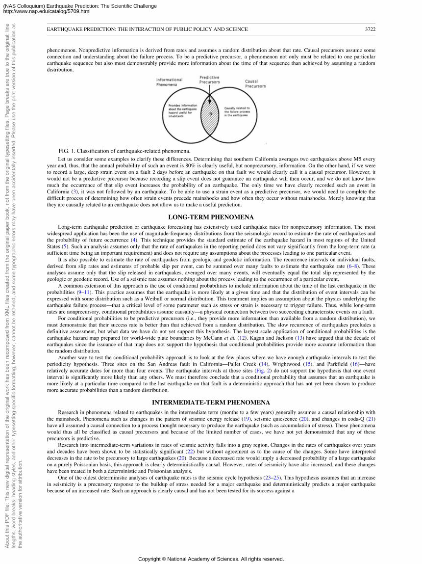
phenomenon. Nonpredictive information is derived from rates and assumes a random distribution about that rate. Causal precursors assume someconnection and understanding about the failure process. To be a predictive precursor, a phenomenon not only must be related to one particularearthquake sequence but also must demonstrably provide more information about the time of that sequence than achieved by assuming a randomdistribution.
FIG. 1. Classification of earthquake-related phenomena.Let us consider some examples to clarify these differences. Determining that southern California averages two earthquakes above M5 every
year and, thus, that the annual probability of such an event is 80% is clearly useful, but nonprecursory, information. On the other hand, if we wereto record a large, deep strain event on a fault 2 days before an earthquake on that fault we would clearly call it a causal precursor. However, itwould not be a predictive precursor because recording a slip event does not guarantee an earthquake will then occur, and we do not know howmuch the occurrence of that slip event increases the probability of an earthquake. The only time we have clearly recorded such an event inCalifornia (3), it was not followed by an earthquake. To be able to use a strain event as a predictive precursor, we would need to complete thedifficult process of determining how often strain events precede mainshocks and how often they occur without mainshocks. Merely knowing thatthey are causally related to an earthquake does not allow us to make a useful prediction.
LONG-TERM PHENOMENA
Long-term earthquake prediction or earthquake forecasting has extensively used earthquake rates for nonprecursory information. The mostwidespread application has been the use of magnitude-frequency distributions from the seismologic record to estimate the rate of earthquakes andthe probability of future occurrence (4). This technique provides the standard estimate of the earthquake hazard in most regions of the UnitedStates (5). Such an analysis assumes only that the rate of earthquakes in the reporting period does not vary significantly from the long-term rate (asufficient time being an important requirement) and does not require any assumptions about the processes leading to one particular event.
It is also possible to estimate the rate of earthquakes from geologic and geodetic information. The recurrence intervals on individual faults,derived from slip rates and estimates of probable slip per event, can be summed over many faults to estimate the earthquake rate (6–8). Theseanalyses assume only that the slip released in earthquakes, averaged over many events, will eventually equal the total slip represented by thegeologic or geodetic record. Use of a seismic rate assumes nothing about the process leading to the occurrence of a particular event.
A common extension of this approach is the use of conditional probabilities to include information about the time of the last earthquake in theprobabilities (9–11). This practice assumes that the earthquake is more likely at a given time and that the distribution of event intervals can beexpressed with some distribution such as a Weibull or normal distribution. This treatment implies an assumption about the physics underlying theearthquake failure process—that a critical level of some parameter such as stress or strain is necessary to trigger failure. Thus, while long-termrates are nonprecursory, conditional probabilities assume causality—a physical connection between two succeeding characteristic events on a fault.
For conditional probabilities to be predictive precursors (i.e., they provide more information than available from a random distribution), wemust demonstrate that their success rate is better than that achieved from a random distribution. The slow recurrence of earthquakes precludes adefinitive assessment, but what data we have do not yet support this hypothesis. The largest scale application of conditional probabilities is theearthquake hazard map prepared for world-wide plate boundaries by McCann et al. (12). Kagan and Jackson (13) have argued that the decade ofearthquakes since the issuance of that map does not support the hypothesis that conditional probabilities provide more accurate information thanthe random distribution.
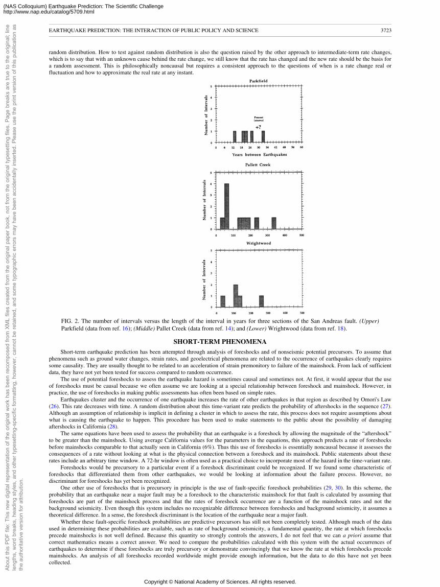
Another way to test the conditional probability approach is to look at the few places where we have enough earthquake intervals to test theperiodicity hypothesis. Three sites on the San Andreas fault in California—Pallet Creek (14), Wrightwood (15), and Parkfield (16)—haverelatively accurate dates for more than four events. The earthquake intervals at those sites (Fig. 2) do not support the hypothesis that one eventinterval is significantly more likely than any others. We must therefore conclude that a conditional probability that assumes that an earthquake ismore likely at a particular time compared to the last earthquake on that fault is a deterministic approach that has not yet been shown to producemore accurate probabilities than a random distribution.
INTERMEDIATE-TERM PHENOMENA
Research in phenomena related to earthquakes in the intermediate term (months to a few years) generally assumes a causal relationship withthe mainshock. Phenomena such as changes in the pattern of seismic energy release (19), seismic quiescence (20), and changes in coda-Q (21)have all assumed a causal connection to a process thought necessary to produce the earthquake (such as accumulation of stress). These phenomenawould thus all be classified as causal precursors and because of the limited number of cases, we have not yet demonstrated that any of theseprecursors is predictive.
Research into intermediate-term variations in rates of seismic activity falls into a gray region. Changes in the rates of earthquakes over yearsand decades have been shown to be statistically significant (22) but without agreement as to the cause of the changes. Some have interpreteddecreases in the rate to be precursory to large earthquakes (20). Because a decreased rate would imply a decreased probability of a large earthquakeon a purely Poissonian basis, this approach is clearly deterministically causal. However, rates of seismicity have also increased, and these changeshave been treated in both a deterministic and Poissonian analysis.
One of the oldest deterministic analyses of earthquake rates is the seismic cycle hypothesis (23–25). This hypothesis assumes that an increasein seismicity is a precursory response to the buildup of stress needed for a major earthquake and deterministically predicts a major earthquakebecause of an increased rate. Such an approach is clearly causal and has not been tested for its success against a
EARTHQUAKE PREDICTION: THE INTERACTION OF PUBLIC POLICY AND SCIENCE 3722
Abou
t thi
s PD
F fil
e: T
his
new
dig
ital r
epre
sent
atio
n of
the
orig
inal
wor
k ha
s be
en re
com
pose
d fro
m X
ML
files
cre
ated
from
the
orig
inal
pap
er b
ook,
not
from
the
orig
inal
type
setti
ng fi
les.
Pag
e br
eaks
are
true
to th
e or
igin
al; l
ine
leng
ths,
wor
d br
eaks
, hea
ding
sty
les,
and
oth
er ty
pese
tting
-spe
cific
form
attin
g, h
owev
er, c
anno
t be
reta
ined
, and
som
e ty
pogr
aphi
c er
rors
may
hav
e be
en a
ccid
enta
lly in
serte
d. P
leas
e us
e th
e pr
int v
ersi
on o
f thi
s pu
blic
atio
n as
the
auth
orita
tive
vers
ion
for a
ttrib
utio
n.
Copyright © National Academy of Sciences. All rights reserved.
(NAS Colloquium) Earthquake Prediction: The Scientific Challengehttp://www.nap.edu/catalog/5709.html
random distribution. How to test against random distribution is also the question raised by the other approach to intermediate-term rate changes,which is to say that with an unknown cause behind the rate change, we still know that the rate has changed and the new rate should be the basis fora random assessment. This is philosophically noncausal but requires a consistent approach to the questions of when is a rate change real orfluctuation and how to approximate the real rate at any instant.
FIG. 2. The number of intervals versus the length of the interval in years for three sections of the San Andreas fault. (Upper)Parkfield (data from ref. 16); (Middle) Pallet Creek (data from ref. 14); and (Lower) Wrightwood (data from ref. 18).
SHORT-TERM PHENOMENA
Short-term earthquake prediction has been attempted through analysis of foreshocks and of nonseismic potential precursors. To assume thatphenomena such as ground water changes, strain rates, and geoelectrical phenomena are related to the occurrence of earthquakes clearly requiressome causality. They are usually thought to be related to an acceleration of strain premonitory to failure of the mainshock. From lack of sufficientdata, they have not yet been tested for success compared to random occurrence.
The use of potential foreshocks to assess the earthquake hazard is sometimes causal and sometimes not. At first, it would appear that the useof foreshocks must be causal because we often assume we are looking at a special relationship between foreshock and mainshock. However, inpractice, the use of foreshocks in making public assessments has often been based on simple rates.
Earthquakes cluster and the occurrence of one earthquake increases the rate of other earthquakes in that region as described by Omori's Law(26). This rate decreases with time. A random distribution about this time-variant rate predicts the probability of aftershocks in the sequence (27).Although an assumption of relationship is implicit in defining a cluster in which to assess the rate, this process does not require assumptions aboutwhat is causing the earthquake to happen. This procedure has been used to make statements to the public about the possibility of damagingaftershocks in California (28).
The same equations have been used to assess the probability that an earthquake is a foreshock by allowing the magnitude of the “aftershock”to be greater than the mainshock. Using average California values for the parameters in the equations, this approach predicts a rate of foreshocksbefore mainshocks comparable to that actually seen in California (6%). Thus this use of foreshocks is essentially noncausal because it assesses theconsequences of a rate without looking at what is the physical connection between a foreshock and its mainshock. Public statements about theserates include an arbitrary time window. A 72-hr window is often used as a practical choice to incorporate most of the hazard in the time-variant rate.
Foreshocks would be precursory to a particular event if a foreshock discriminant could be recognized. If we found some characteristic offoreshocks that differentiated them from other earthquakes, we would be looking at information about the failure process. However, nodiscriminant for foreshocks has yet been recognized.
One other use of foreshocks that is precursory in principle is the use of fault-specific foreshock probabilities (29, 30). In this scheme, theprobability that an earthquake near a major fault may be a foreshock to the characteristic mainshock for that fault is calculated by assuming thatforeshocks are part of the mainshock process and that the rates of foreshock occurrence are a function of the mainshock rates and not thebackground seismicity. Even though this system includes no recognizable difference between foreshocks and background seismicity, it assumes atheoretical difference. In a sense, the foreshock discriminant is the location of the earthquake near a major fault.
Whether these fault-specific foreshock probabilities are predictive precursors has still not been completely tested. Although much of the dataused in determining these probabilities are available, such as rate of background seismicity, a fundamental quantity, the rate at which foreshocksprecede mainshocks is not well defined. Because this quantity so strongly controls the answers, I do not feel that we can a priori assume thatcorrect mathematics means a correct answer. We need to compare the probabilities calculated with this system with the actual occurrences ofearthquakes to determine if these foreshocks are truly precursory or demonstrate convincingly that we know the rate at which foreshocks precedemainshocks. An analysis of all foreshocks recorded worldwide might provide enough information, but the data to do this have not yet beencollected.
EARTHQUAKE PREDICTION: THE INTERACTION OF PUBLIC POLICY AND SCIENCE 3723
Abou
t thi
s PD
F fil
e: T
his
new
dig
ital r
epre
sent
atio
n of
the
orig
inal
wor
k ha
s be
en re
com
pose
d fro
m X
ML
files
cre
ated
from
the
orig
inal
pap
er b
ook,
not
from
the
orig
inal
type
setti
ng fi
les.
Pag
e br
eaks
are
true
to th
e or
igin
al; l
ine
leng
ths,
wor
d br
eaks
, hea
ding
sty
les,
and
oth
er ty
pese
tting
-spe
cific
form
attin
g, h
owev
er, c
anno
t be
reta
ined
, and
som
e ty
pogr
aphi
c er
rors
may
hav
e be
en a
ccid
enta
lly in
serte
d. P
leas
e us
e th
e pr
int v
ersi
on o
f thi
s pu
blic
atio
n as
the
auth
orita
tive
vers
ion
for a
ttrib
utio
n.
Copyright © National Academy of Sciences. All rights reserved.
(NAS Colloquium) Earthquake Prediction: The Scientific Challengehttp://www.nap.edu/catalog/5709.html
DISCUSSION
The last few decades of research in earthquake prediction have increased our understanding of the earthquake process and led to severalmethods for producing useful estimates of the seismic hazard (Table 1). However, as yet we have found no phenomena that can provide usinformation about the timing of a particular earthquake any better than we could achieve through assuming a random distribution of events (Fig. 3).
Because the public is driven by an emotional need for earthquake prediction only partially connected to practical need, scientists have an evengreater responsibility to communicate carefully their findings in earthquake prediction. By this, I do not mean keeping quiet about results. Afterevery major earthquake, a rumor spreads that scientists know the time of another earthquake but are keeping quiet to avoid panic. Our only defenseagainst this rumor is to make sure that it is never true. Our obligation is to communicate our results in the clearest possible way, including whenpossible a statistical assessment of their validity. When such is not possible, we should clearly acknowledge this and not expect these results to bethe basis of public policy.
Research should be separate from public policy, and the criteria for public use of earthquake information should be independent of the criteriafor scientific study. I propose that public policy should be based only on informational phenomena and, when they become available, predictiveprecursors. By this I mean that probabilities for public use, both short-term warnings and long-term forecasts for land-use planning, should bederived only from historical, geodetic, or geologic rates of activity and precursors that have been demonstrated to provide more accurateinformation than the rates alone. We cannot justify expenditures if we have not demonstrated that our assessment is better than random. Thisapproach to public policy is independent of scientific research where we must continue the research into causal precursors both for ourunderstanding of the physics of earthquakes and for any future hope of obtaining a predictive precursor.
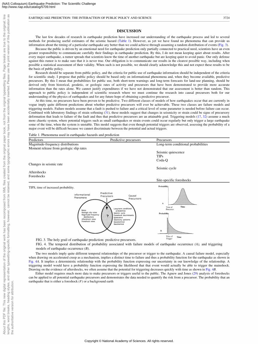
At this time, no precursors have been proven to be predictive. Two different classes of models of how earthquakes occur that are currently invogue imply quite different predictions about whether predictive precursors will ever be achievable. These two classes are failure models andtriggering models. Failure models assume that a fault is pushed to failure and a critical level of some parameter is needed before failure can occur.Combined with laboratory findings of strain softening (31), these models suggest that changes in seismicity or strain could be signs of precursorydeformation that leads to failure of the fault and thus that predictive precursors are an attainable goal. Triggering models (17, 32) assume a muchmore chaotic system, where potential triggers such as small earthquakes or strain events could occur regularly but only trigger a large earthquakesome of the time, when the system is unstable. This model suggests that even though potential triggers are observed, assessing the probability of amajor event will be difficult because we cannot discriminate between the potential and actual triggers.
Table 1. Phenomena used in earthquake hazards and prediction
Predictors Predictive precursors PrecursorsMagnitude-frequency distributions Long-term conditional probabilitiesMoment release from geologic slip rates
Seismic quiescenceTIPsCoda-Q
Changes in seismic rateSeismic cycle
AftershocksForeshocks
Site-specific foreshocks
TIPS, time of increased probability.
FIG. 3. The holy grail of earthquake prediction: predictive precursors.FIG. 4. The temporal distribution of probability associated with failure models of earthquake occurrence (A), and triggeringmodels of earthquake occurrence (B).The two models imply quite different temporal relationships of the precursor or trigger to the earthquake. A causal failure model, especially
when drawing on accelerated creep as a mechanism, implies a distinct time to failure and thus a probability function for the earthquake as shown inFig. 4A. It implies a deterministic relationship with the probability function expressing our uncertainty in our knowledge of the relationship. Atriggering model would have a probability function expressing the likelihood that that event would actually be able to trigger the mainshock.Drawing on the evidence of aftershocks, we often assume that the potential for triggering decreases quickly with time as shown in Fig. 4B.
Either model requires much more data to make precursors or triggers useful to the public. The Agnew and Jones (29) analysis of foreshockscan be applied to all potential earthquake precursors and demonstrates the data needed to quantify the risk from a precursor. The probability that anearthquake that is either a foreshock (F) or a background earth
EARTHQUAKE PREDICTION: THE INTERACTION OF PUBLIC POLICY AND SCIENCE 3724
Abou
t thi
s PD
F fil
e: T
his
new
dig
ital r
epre
sent
atio
n of
the
orig
inal
wor
k ha
s be
en re
com
pose
d fro
m X
ML
files
cre
ated
from
the
orig
inal
pap
er b
ook,
not
from
the
orig
inal
type
setti
ng fi
les.
Pag
e br
eaks
are
true
to th
e or
igin
al; l
ine
leng
ths,
wor
d br
eaks
, hea
ding
sty
les,
and
oth
er ty
pese
tting
-spe
cific
form
attin
g, h
owev
er, c
anno
t be
reta
ined
, and
som
e ty
pogr
aphi
c er
rors
may
hav
e be
en a
ccid
enta
lly in
serte
d. P
leas
e us
e th
e pr
int v
ersi
on o
f thi
s pu
blic
atio
n as
the
auth
orita
tive
vers
ion
for a
ttrib
utio
n.
Copyright © National Academy of Sciences. All rights reserved.
(NAS Colloquium) Earthquake Prediction: The Scientific Challengehttp://www.nap.edu/catalog/5709.html
quake (B) and we cannot tell which will be followed by a characteristic earthquake (C) is then the ratio of the number of foreshocks to the totalnumber of events or
[1]
Assuming the rate of foreshocks is the rate at which foreshocks precede mainshocks [P(F|C)] times the mainshock rate, P(F) =P(F|C)*P(C),then
[2]
Thus, the probability of a characteristic earthquake on the fault after a potential foreshock is a function of the rate of background earthquakes[P(B)], the rate of mainshocks [P(C)], and the rate at which foreshoeks preceded mainshocks [P(F|C)]. For other precursors, the probability of anearthquake after the phenomenon has occurred depends on the long-term probability of the mainshock, the false alarm rate of the phenomenon, andthe rate at which that phenomenon precedes the mainshock. Collecting the data to determine the last two quantities will require much effort beyonddemonstrating a correlation with the mainshock.
CONCLUSIONS
Phenomena related to earthquake prediction can be broken into three classes: (i) phenomena that provide information about the earthquakehazard useful to the public, (ii) precursors that are causally related to the failure process of a particular earthquake, and (iii) the intersection of thesetwo classes, predictive precursors that are causally related to a particular earthquake and provide probabilities of earthquake occurrence greaterthan achievable from a random distribution. In the long term, probabilities derived from geologic rates and historic catalogs are predictors, whileconditional probabilities are precursors. Aftershock and foreshock probabilities derived from time-decaying rates are predictors, whereas all otherinvestigated phenomena are precursors. At this time, no phenomenon has been shown to do better than random, and we have no predictiveprecursors so far. The data necessary to prove a better than random success are much greater than that needed to show a causal relationship to anearthquake.1. Aggerwal, Y.P., Sykes, L.R., Simpson, D.W. & Richards, P.G. (1973) J. Geophys. Res. 80, 718–732.2. Anderson, D.L. & Whitcomb, J. (1975) J. Geophys. Res. 80, 1497–1503.3. Linde, A.T. & Johnston, M.J.S. (1994) Trans. Am. Geophys. Union 75, 446 (abstr.).4. Allen, C.R., Amand, P.S., Richter, C.F. & Nordquist, J.M. (1965) Bull. Seismol. Soc. Am. 55, 753–797.5. Algermissen, S.T., Perkins, D.M., Thenhaus, P.C., Hanson, S.L. & Bender, B.L. (1982) U.S. Geol. Surv. Open-File Rep. 82–1033.6. Wesnousky, S.G., Seholz, C.H., Shimazaki, K. & Matsuda, T. (1984) Bull. Seismol. Soc. Am. 74, 687–708.7. Wesnousky, S.G. (1986) J. Geophys. Res. 91, 12587–12632.8. Ward, S.N. (1994) Bull. Seismol. Soc. Am. 84, 1293–1309.9. Sykes, L.R. & Nishenko, S.P. (1984) J. Geophys. Res. 89, 5905–5928.10. Working Group on California Earthquake Probabilities (1988) U.S. Geol. Surv. Open-File Rep. 88–398.11. Working Group on California Earthquake Probabilities (1990) U.S. Geol. Surv. Circ. 1053.12. McCann, W.R., Nishenko, S.P., Sykes, L.R. & Krause, J. (1979) Pure Appl. Geophys. 117, 1082–1147.13. Kagan, Y.Y. & Jackson, D.D. (1991) J. Geophys. Res. 96, 21419–21431.14. Sieh, K.E., Stuiver, M. & Brillinger, D. (1989) J. Geophys. Res. 94, 603–624.15. Fumal, T.E., Pezzopane, S.K., Weldon, R.J. II & Schwartz, D.P. (1993) Science 259, 199–203.16. Bakun, W.H. & McEvilly, T.V. (1984) J. Geophys. Res. 89, 3051–3058.17. Heaton, T.H. (1990) Phys. Earth Planet. Inter. 64, 1–20.18. Biasi, G. & Weldon, R., II (1996) J. Geophys. Res. 100, in press.19. Keilis-Borok, V. I., Knopoff, L., Rotwain, I.M. & Allen, C.R. (1988) Nature (London) 335, 690–694.20. Wyss, M. & Habermann, R.E. (1988) Pure Appl. Geophys. 126, 333–356.21. Aki, K. (1985) Earthquake Predict. Res. 3, 219–230.22. Reasenberg, P.A. & Matthews, M.V. (1988) Pure Appl. Geophys. 126, 373–406.23. Fedotov, S.A. (1965) Trans. Inst. Fiz. Zemli Akad. Nauk SSSR 36, 66–93.24. Ellsworth, W.L., Lindh, A.G., Prescott, W.H. & Herd, D.G. (1981) in Earthquake Prediction: An International Review: Maurice Ewing Series, eds.
Simpson, D.W. & Richards, P.G. (Am. Geophys. Union, Washington, DC), Vol. 4, 126–140.25. Mogi, K. (1985) Earthquake Prediction (Academic, Tokyo).26. Utsu, T. (1961) Geophys. Mag. 30, 521–605.27. Reasenberg, P.A. & Jones, L.M. (1989) Science 243, 1173–1176.28. Reasenberg, P.A. & Jones, L.M. (1994) Science 265, 1251–1252.29. Agnew, D.C. & Jones, L.M. (1991) J. Geophys. Res. 96, 11959– 11971.30. Jones, L.M., Sieh, K.E., Agnew, D.C., Allen, C.R., Bilham, R., Ghilarducci, M., Hager, B., Hauksson, E., Hudnut, K., Jackson, D. & Sylvester, A.
(1991) U.S. Geol. Surv. Open-File Rep. 91–32.31. Dieterich, J.H. (1979) J. Geophys. Res. 84, 2169–2175.32. Brune, J., Brown, S. & Johnson, P. (1993) Tectonophysics 218, 1–3, 59–67.
EARTHQUAKE PREDICTION: THE INTERACTION OF PUBLIC POLICY AND SCIENCE 3725
Abou
t thi
s PD
F fil
e: T
his
new
dig
ital r
epre
sent
atio
n of
the
orig
inal
wor
k ha
s be
en re
com
pose
d fro
m X
ML
files
cre
ated
from
the
orig
inal
pap
er b
ook,
not
from
the
orig
inal
type
setti
ng fi
les.
Pag
e br
eaks
are
true
to th
e or
igin
al; l
ine
leng
ths,
wor
d br
eaks
, hea
ding
sty
les,
and
oth
er ty
pese
tting
-spe
cific
form
attin
g, h
owev
er, c
anno
t be
reta
ined
, and
som
e ty
pogr
aphi
c er
rors
may
hav
e be
en a
ccid
enta
lly in
serte
d. P
leas
e us
e th
e pr
int v
ersi
on o
f thi
s pu
blic
atio
n as
the
auth
orita
tive
vers
ion
for a
ttrib
utio
n.
Copyright © National Academy of Sciences. All rights reserved.
(NAS Colloquium) Earthquake Prediction: The Scientific Challengehttp://www.nap.edu/catalog/5709.html
This paper was presented at a colloquium entitled “Earthquake Prediction: The Scientific Challenge,” organized by Leon Knopoff(Chair), Keiiti Aki, Clarence R.Allen, James R.Rice, and Lynn R.Sykes, held February 10 and 11, 1995, at the National Academy of Sciences inIrvine, CA.
Initiation process of earthquakes and its implications for seismichazard reduction strategy
HIROO KANAMORI
Seismological Laboratory, California Institute of Technology, Pasadena, CA 91125ABSTRACT For the average citizen and the public, “earthquake prediction” means “short-term prediction,” a prediction of a
specific earthquake on a relatively short time scale. Such prediction must specify the time, place, and magnitude of the earthquake inquestion with sufficiently high reliability. For this type of prediction, one must rely on some short-term precursors. Examinations of strainchanges just before large earthquakes suggest that consistent detection of such precursory strain changes cannot be expected. Otherprecursory phenomena such as foreshocks and nonseismological anomalies do not occur consistently either. Thus, reliable short-termprediction would be very difficult. Although short-term predictions with large uncertainties could be useful for some areas if their socialand economic environments can tolerate false alarms, such predictions would be impractical for most modern industrialized cities. Astrategy for effective seismic hazard reduction is to take full advantage of the recent technical advancements in seismology, computers,and communication. In highly industrialized communities, rapid earthquake information is critically important for emergency servicesagencies, utilities, communications, financial companies, and media to make quick reports and damage estimates and to determine whereemergency response is most needed. Long-term forecast, or prognosis, of earthquakes is important for development of realistic buildingcodes, retrofitting existing structures, and land-use planning, but the distinction between short-term and long-term predictions needs to beclearly communicated to the public to avoid misunderstanding.
In a narrow sense, an earthquake is a sudden failure process, but, in a broad sense, it is a long-term complex stress accumulation and releaseprocess occurring in the highly heterogeneous Earth's crust and mantle. The Earth's crust exhibits anelastic and nonlinear behavior for long-termprocesses. In this broad sense, “earthquake prediction research” often refers to the study of this entire long-term process, with the implication thatthe behavior of the crust in the future should be predictable to some extent from various measurements taken in the past and at present. Pursuit ofsuch physical processes is a respectable scientific endeavor, and significant advancements have been made on rupture dynamics, friction andconstitutive relations, interaction between faults, seismicity patterns, fault-zone structures, and nonlinear dynamics.
Many recent studies, however, have demonstrated that even a very simple nonlinear system exhibits very complex behavior, suggesting thatearthquake is either deterministic chaos, stochastic chaos, or both and is predictable only in a statistical sense (1). Even if the physics ofearthquakes is understood well enough, the obvious difficulty in making detailed measurements of various field variables (structure, strain, etc.) inthree dimensions in the Earth would make accurate deterministic predictions even more difficult. Nevertheless, a better understanding of thephysics of earthquakes and an increase in the knowledge about the space-time variation of the crustal process (i.e., seismicity and strainaccumulation) would allow seismologists to make useful statements on long-term behavior of the crust (2). This is often called “intermediate andlong-term earthquake prediction” and is important for long-term seismic hazard reduction measures such as development of realistic buildingcodes, retrofitting existing structures, and land-use planning. However, as urged by Allen (3), it would be better to use terms other than predictionsuch as “forecast” or “prognosis” for these types of statements. This distinction is especially important when issues on prediction arecommunicated to the general public.
For the average citizen and the public, “earthquake prediction” means prediction of a specific earthquake on a relatively short time scale—e.g., a few days (3). Such prediction must specify the time, place, and magnitude of the earthquake in question with sufficiently high reliability. Forthis type of prediction, one must rely on observations and identification of some short-term preparatory processes. Here we examine someobservations of strain changes immediately before an earthquake.
SHORT-TERM STRAIN PRECURSORS
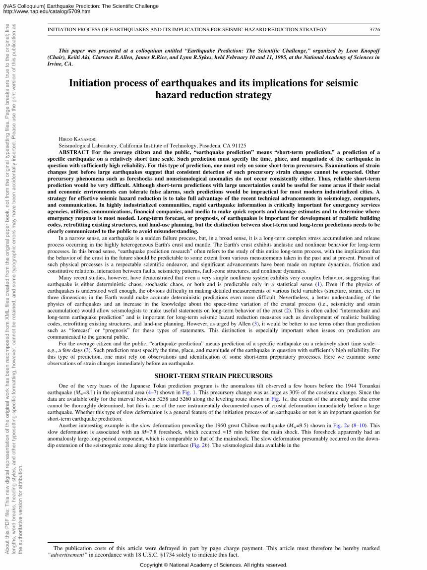
One of the very bases of the Japanese Tokai prediction program is the anomalous tilt observed a few hours before the 1944 Tonankaiearthquake (Mw=8.1) in the epicentral area (4–7) shown in Fig. 1. This precursory change was as large as 30% of the coseismic change. Since thedata are available only for the interval between 5258 and 5260 along the leveling route shown in Fig. 1c, the extent of the anomaly and the errorcannot be thoroughly determined, but this is one of the rare instrumentally documented cases of crustal deformation immediately before a largeearthquake. Whether this type of slow deformation is a general feature of the initiation process of an earthquake or not is an important question forshort-term earthquake prediction.
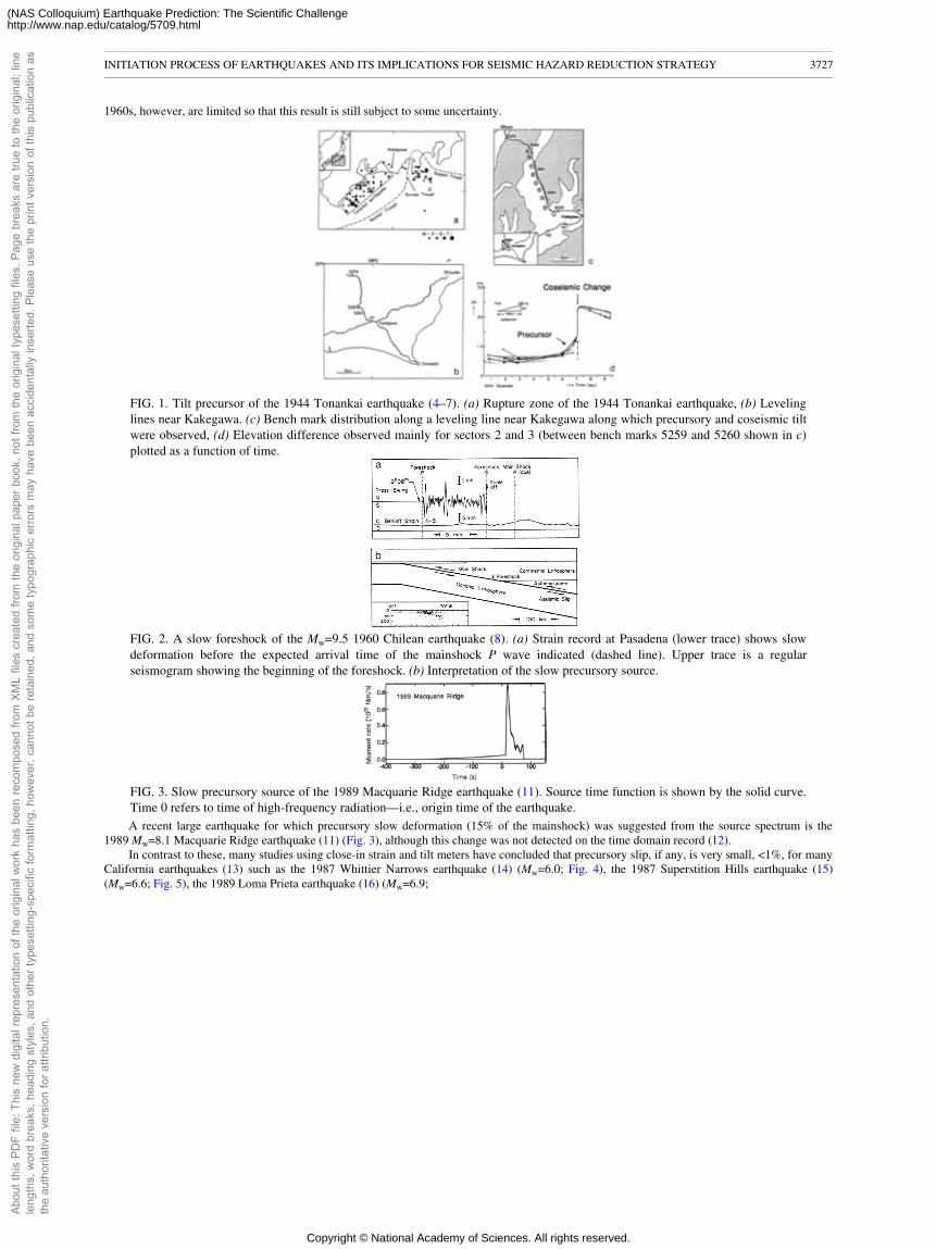
Another interesting example is the slow deformation preceding the 1960 great Chilean earthquake (Mw=9.5) shown in Fig. 2a (8–10). Thisslow deformation is associated with an M=7.8 foreshock, which occurred �15 min before the main shock. This foreshock apparently had ananomalously large long-period component, which is comparable to that of the mainshock. The slow deformation presumably occurred on the down-dip extension of the seismogenic zone along the plate interface (Fig. 2b). The seismological data available in the
The publication costs of this article were defrayed in part by page charge payment. This article must therefore be hereby marked“advertisement” in accordance with 18 U.S.C. §1734 solely to indicate this fact.
INITIATION PROCESS OF EARTHQUAKES AND ITS IMPLICATIONS FOR SEISMIC HAZARD REDUCTION STRATEGY 3726
Abou
t thi
s PD
F fil
e: T
his
new
dig
ital r
epre
sent
atio
n of
the
orig
inal
wor
k ha
s be
en re
com
pose
d fro
m X
ML
files
cre
ated
from
the
orig
inal
pap
er b
ook,
not
from
the
orig
inal
type
setti
ng fi
les.
Pag
e br
eaks
are
true
to th
e or
igin
al; l
ine
leng
ths,
wor
d br
eaks
, hea
ding
sty
les,
and
oth
er ty
pese
tting
-spe
cific
form
attin
g, h
owev
er, c
anno
t be
reta
ined
, and
som
e ty
pogr
aphi
c er
rors
may
hav
e be
en a
ccid
enta
lly in
serte
d. P
leas
e us
e th
e pr
int v
ersi
on o
f thi
s pu
blic
atio
n as
the
auth
orita
tive
vers
ion
for a
ttrib
utio
n.
Copyright © National Academy of Sciences. All rights reserved.
(NAS Colloquium) Earthquake Prediction: The Scientific Challengehttp://www.nap.edu/catalog/5709.html
1960s, however, are limited so that this result is still subject to some uncertainty.
FIG. 1. Tilt precursor of the 1944 Tonankai earthquake (4–7). (a) Rupture zone of the 1944 Tonankai earthquake, (b) Levelinglines near Kakegawa. (c) Bench mark distribution along a leveling line near Kakegawa along which precursory and coseismic tiltwere observed, (d) Elevation difference observed mainly for sectors 2 and 3 (between bench marks 5259 and 5260 shown in c)plotted as a function of time.
FIG. 2. A slow foreshock of the Mw=9.5 1960 Chilean earthquake (8). (a) Strain record at Pasadena (lower trace) shows slowdeformation before the expected arrival time of the mainshock P wave indicated (dashed line). Upper trace is a regularseismogram showing the beginning of the foreshock. (b) Interpretation of the slow precursory source.
FIG. 3. Slow precursory source of the 1989 Macquarie Ridge earthquake (11). Source time function is shown by the solid curve.Time 0 refers to time of high-frequency radiation—i.e., origin time of the earthquake.A recent large earthquake for which precursory slow deformation (15% of the mainshock) was suggested from the source spectrum is the
1989 Mw=8.1 Macquarie Ridge earthquake (11) (Fig. 3), although this change was not detected on the time domain record (12).In contrast to these, many studies using close-in strain and tilt meters have concluded that precursory slip, if any, is very small, <1%, for many
California earthquakes (13) such as the 1987 Whittier Narrows earthquake (14) (Mw=6.0; Fig. 4), the 1987 Superstition Hills earthquake (15)(Mw=6.6; Fig. 5), the 1989 Loma Prieta earthquake (16) (Mw=6.9;
INITIATION PROCESS OF EARTHQUAKES AND ITS IMPLICATIONS FOR SEISMIC HAZARD REDUCTION STRATEGY 3727
Abou
t thi
s PD
F fil
e: T
his
new
dig
ital r
epre
sent
atio
n of
the
orig
inal
wor
k ha
s be
en re
com
pose
d fro
m X
ML
files
cre
ated
from
the
orig
inal
pap
er b
ook,
not
from
the
orig
inal
type
setti
ng fi
les.
Pag
e br
eaks
are
true
to th
e or
igin
al; l
ine
leng
ths,
wor
d br
eaks
, hea
ding
sty
les,
and
oth
er ty
pese
tting
-spe
cific
form
attin
g, h
owev
er, c
anno
t be
reta
ined
, and
som
e ty
pogr
aphi
c er
rors
may
hav
e be
en a
ccid
enta
lly in
serte
d. P
leas
e us
e th
e pr
int v
ersi
on o
f thi
s pu
blic
atio
n as
the
auth
orita
tive
vers
ion
for a
ttrib
utio
n.
Copyright © National Academy of Sciences. All rights reserved.
(NAS Colloquium) Earthquake Prediction: The Scientific Challengehttp://www.nap.edu/catalog/5709.html
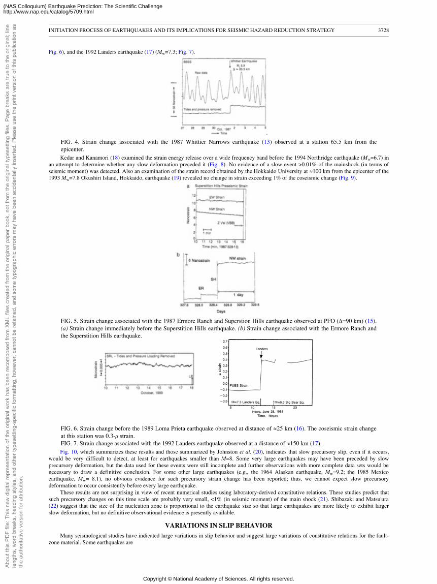
Fig. 6), and the 1992 Landers earthquake (17) (Mw=7.3; Fig. 7).
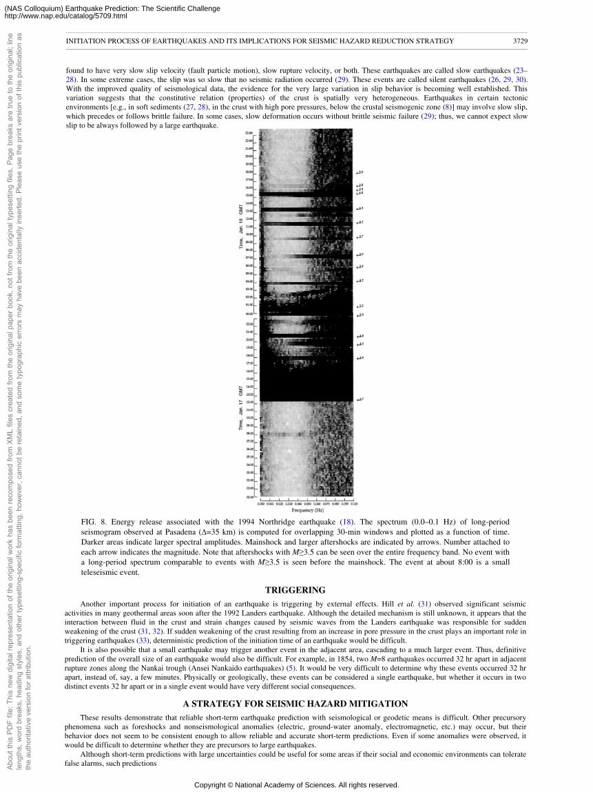
FIG. 4. Strain change associated with the 1987 Whittier Narrows earthquake (13) observed at a station 65.5 km from theepicenter.Kedar and Kanamori (18) examined the strain energy release over a wide frequency band before the 1994 Northridge earthquake (Mw=6.7) in
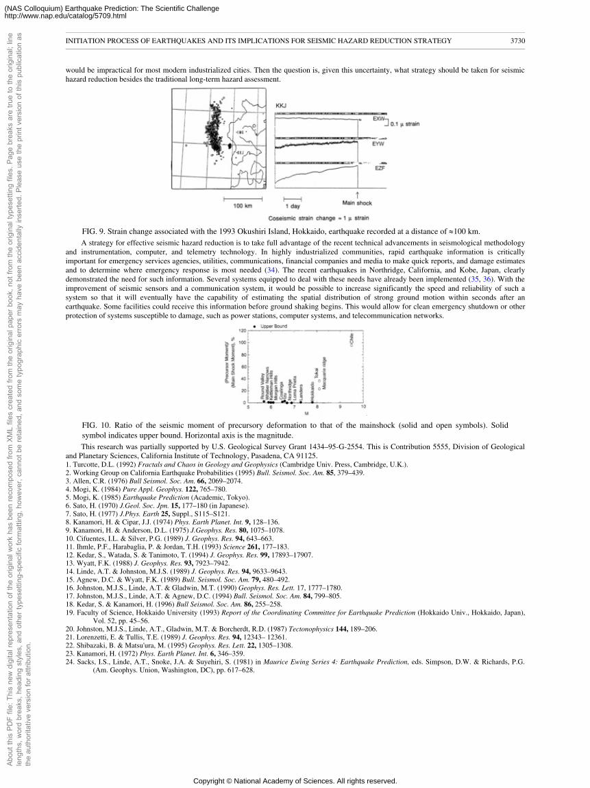
an attempt to determine whether any slow deformation preceded it (Fig. 8). No evidence of a slow event >0.01% of the mainshock (in terms ofseismic moment) was detected. Also an examination of the strain record obtained by the Hokkaido University at �100 km from the epicenter of the1993 Mw=7.8 Okushiri Island, Hokkaido, earthquake (19) revealed no change in strain exceeding 1% of the coseismic change (Fig. 9).
FIG. 5. Strain change associated with the 1987 Ermore Ranch and Superstion Hills earthquake observed at PFO (∆=90 km) (15).(a) Strain change immediately before the Superstition Hills earthquake. (b) Strain change associated with the Ermore Ranch andthe Superstition Hills earthquake.
FIG. 6. Strain change before the 1989 Loma Prieta earthquake observed at distance of �25 km (16). The coseismic strain changeat this station was 0.3-µ strain.FIG. 7. Strain change associated with the 1992 Landers earthquake observed at a distance of �150 km (17).Fig. 10, which summarizes these results and those summarized by Johnston et al. (20), indicates that slow precursory slip, even if it occurs,
would be very difficult to detect, at least for earthquakes smaller than M=8. Some very large earthquakes may have been preceded by slowprecursory deformation, but the data used for these events were still incomplete and further observations with more complete data sets would benecessary to draw a definitive conclusion. For some other large earthquakes (e.g., the 1964 Alaskan earthquake, Mw=9.2; the 1985 Mexicoearthquake, Mw= 8.1), no obvious evidence for such precursory strain change has been reported; thus, we cannot expect slow precursorydeformation to occur consistently before every large earthquake.
These results are not surprising in view of recent numerical studies using laboratory-derived constitutive relations. These studies predict thatsuch precursory changes on this time scale are probably very small, <1% (in seismic moment) of the main shock (21). Shibazaki and Matsu'ura(22) suggest that the size of the nucleation zone is proportional to the earthquake size so that large earthquakes are more likely to exhibit largerslow deformation, but no definitive observational evidence is presently available.
VARIATIONS IN SLIP BEHAVIOR
Many seismological studies have indicated large variations in slip behavior and suggest large variations of constitutive relations for the fault-zone material. Some earthquakes are
INITIATION PROCESS OF EARTHQUAKES AND ITS IMPLICATIONS FOR SEISMIC HAZARD REDUCTION STRATEGY 3728
Abou
t thi
s PD
F fil
e: T
his
new
dig
ital r
epre
sent
atio
n of
the
orig
inal
wor
k ha
s be
en re
com
pose
d fro
m X
ML
files
cre
ated
from
the
orig
inal
pap
er b
ook,
not
from
the
orig
inal
type
setti
ng fi
les.
Pag
e br
eaks
are
true
to th
e or
igin
al; l
ine
leng
ths,
wor
d br
eaks
, hea
ding
sty
les,
and
oth
er ty
pese
tting
-spe
cific
form
attin
g, h
owev
er, c
anno
t be
reta
ined
, and
som
e ty
pogr
aphi
c er
rors
may
hav
e be
en a
ccid
enta
lly in
serte
d. P
leas
e us
e th
e pr
int v
ersi
on o
f thi
s pu
blic
atio
n as
the
auth
orita
tive
vers
ion
for a
ttrib
utio
n.
Copyright © National Academy of Sciences. All rights reserved.
(NAS Colloquium) Earthquake Prediction: The Scientific Challengehttp://www.nap.edu/catalog/5709.html
found to have very slow slip velocity (fault particle motion), slow rupture velocity, or both. These earthquakes are called slow earthquakes (23–28). In some extreme cases, the slip was so slow that no seismic radiation occurred (29). These events are called silent earthquakes (26, 29, 30).With the improved quality of seismological data, the evidence for the very large variation in slip behavior is becoming well established. Thisvariation suggests that the constitutive relation (properties) of the crust is spatially very heterogeneous. Earthquakes in certain tectonicenvironments [e.g., in soft sediments (27, 28), in the crust with high pore pressures, below the crustal seismogenic zone (8)] may involve slow slip,which precedes or follows brittle failure. In some cases, slow deformation occurs without brittle seismic failure (29); thus, we cannot expect slowslip to be always followed by a large earthquake.
FIG. 8. Energy release associated with the 1994 Northridge earthquake (18). The spectrum (0.0–0.1 Hz) of long-periodseismogram observed at Pasadena (∆=35 km) is computed for overlapping 30-min windows and plotted as a function of time.Darker areas indicate larger spectral amplitudes. Mainshock and larger aftershocks are indicated by arrows. Number attached toeach arrow indicates the magnitude. Note that aftershocks with M≥3.5 can be seen over the entire frequency band. No event witha long-period spectrum comparable to events with M≥3.5 is seen before the mainshock. The event at about 8:00 is a smallteleseismic event.
TRIGGERING
Another important process for initiation of an earthquake is triggering by external effects. Hill et al. (31) observed significant seismicactivities in many geothermal areas soon after the 1992 Landers earthquake. Although the detailed mechanism is still unknown, it appears that theinteraction between fluid in the crust and strain changes caused by seismic waves from the Landers earthquake was responsible for suddenweakening of the crust (31, 32). If sudden weakening of the crust resulting from an increase in pore pressure in the crust plays an important role intriggering earthquakes (33), deterministic prediction of the initiation time of an earthquake would be difficult.
It is also possible that a small earthquake may trigger another event in the adjacent area, cascading to a much larger event. Thus, definitiveprediction of the overall size of an earthquake would also be difficult. For example, in 1854, two M=8 earthquakes occurred 32 hr apart in adjacentrupture zones along the Nankai trough (Ansei Nankaido earthquakes) (5). It would be very difficult to determine why these events occurred 32 hrapart, instead of, say, a few minutes. Physically or geologically, these events can be considered a single earthquake, but whether it occurs in twodistinct events 32 hr apart or in a single event would have very different social consequences.
A STRATEGY FOR SEISMIC HAZARD MITIGATION
These results demonstrate that reliable short-term earthquake prediction with seismological or geodetic means is difficult. Other precursoryphenomena such as foreshocks and nonseismological anomalies (electric, ground-water anomaly, electromagnetic, etc.) may occur, but theirbehavior does not seem to be consistent enough to allow reliable and accurate short-term predictions. Even if some anomalies were observed, itwould be difficult to determine whether they are precursors to large earthquakes.
Although short-term predictions with large uncertainties could be useful for some areas if their social and economic environments can toleratefalse alarms, such predictions
INITIATION PROCESS OF EARTHQUAKES AND ITS IMPLICATIONS FOR SEISMIC HAZARD REDUCTION STRATEGY 3729
Abou
t thi
s PD
F fil
e: T
his
new
dig
ital r
epre
sent
atio
n of
the
orig
inal
wor
k ha
s be
en re
com
pose
d fro
m X
ML
files
cre
ated
from
the
orig
inal
pap
er b
ook,
not
from
the
orig
inal
type
setti
ng fi
les.
Pag
e br
eaks
are
true
to th
e or
igin
al; l
ine
leng
ths,
wor
d br
eaks
, hea
ding
sty
les,
and
oth
er ty
pese
tting
-spe
cific
form
attin
g, h
owev
er, c
anno
t be
reta
ined
, and
som
e ty
pogr
aphi
c er
rors
may
hav
e be
en a
ccid
enta
lly in
serte
d. P
leas
e us
e th
e pr
int v
ersi
on o
f thi
s pu
blic
atio
n as
the
auth
orita
tive
vers
ion
for a
ttrib
utio
n.
Copyright © National Academy of Sciences. All rights reserved.
(NAS Colloquium) Earthquake Prediction: The Scientific Challengehttp://www.nap.edu/catalog/5709.html
would be impractical for most modern industrialized cities. Then the question is, given this uncertainty, what strategy should be taken for seismichazard reduction besides the traditional long-term hazard assessment.
FIG. 9. Strain change associated with the 1993 Okushiri Island, Hokkaido, earthquake recorded at a distance of �100 km.A strategy for effective seismic hazard reduction is to take full advantage of the recent technical advancements in seismological methodology
and instrumentation, computer, and telemetry technology. In highly industrialized communities, rapid earthquake information is criticallyimportant for emergency services agencies, utilities, communications, financial companies and media to make quick reports, and damage estimatesand to determine where emergency response is most needed (34). The recent earthquakes in Northridge, California, and Kobe, Japan, clearlydemonstrated the need for such information. Several systems equipped to deal with these needs have already been implemented (35, 36). With theimprovement of seismic sensors and a communication system, it would be possible to increase significantly the speed and reliability of such asystem so that it will eventually have the capability of estimating the spatial distribution of strong ground motion within seconds after anearthquake. Some facilities could receive this information before ground shaking begins. This would allow for clean emergency shutdown or otherprotection of systems susceptible to damage, such as power stations, computer systems, and telecommunication networks.
FIG. 10. Ratio of the seismic moment of precursory deformation to that of the mainshock (solid and open symbols). Solidsymbol indicates upper bound. Horizontal axis is the magnitude.This research was partially supported by U.S. Geological Survey Grant 1434–95-G-2554. This is Contribution 5555, Division of Geological
and Planetary Sciences, California Institute of Technology, Pasadena, CA 91125.1. Turcotte, D.L. (1992) Fractals and Chaos in Geology and Geophysics (Cambridge Univ. Press, Cambridge, U.K.).2. Working Group on California Earthquake Probabilities (1995) Bull. Seismol. Soc. Am. 85, 379–439.3. Allen, C.R. (1976) Bull Seismol. Soc. Am. 66, 2069–2074.4. Mogi, K. (1984) Pure Appl. Geophys. 122, 765–780.5. Mogi, K. (1985) Earthquake Prediction (Academic, Tokyo).6. Sato, H. (1970) J.Geol. Soc. Jpn. 15, 177–180 (in Japanese).7. Sato, H. (1977) J.Phys. Earth 25, Suppl., S115–S121.8. Kanamori, H. & Cipar, J.J. (1974) Phys. Earth Planet. Int. 9, 128–136.9. Kanamori, H. & Anderson, D.L. (1975) J.Geophys. Res. 80, 1075–1078.10. Cifuentes, I.L. & Silver, P.G. (1989) J. Geophys. Res. 94, 643–663.11. Ihmle, P.F., Harabaglia, P. & Jordan, T.H. (1993) Science 261, 177–183.12. Kedar, S., Watada, S. & Tanimoto, T. (1994) J. Geophys. Res. 99, 17893–17907.13. Wyatt, F.K. (1988) J. Geophys. Res. 93, 7923–7942.14. Linde, A.T. & Johnston, M.J.S. (1989) J. Geophys. Res. 94, 9633–9643.15. Agnew, D.C. & Wyatt, F.K. (1989) Bull. Seismol. Soc. Am. 79, 480–492.16. Johnston, M.J.S., Linde, A.T. & Gladwin, M.T. (1990) Geophys. Res. Lett. 17, 1777–1780.17. Johnston, M.J.S., Linde, A.T. & Agnew, D.C. (1994) Bull. Seismol. Soc. Am. 84, 799–805.18. Kedar, S. & Kanamori, H. (1996) Bull Seismol. Soc. Am. 86, 255–258.19. Faculty of Science, Hokkaido University (1993) Report of the Coordinating Committee for Earthquake Prediction (Hokkaido Univ., Hokkaido, Japan),
Vol. 52, pp. 45–56.20. Johnston, M.J.S., Linde, A.T., Gladwin, M.T. & Borcherdt, R.D. (1987) Tectonophysics 144, 189–206.21. Lorenzetti, E. & Tullis, T.E. (1989) J. Geophys. Res. 94, 12343– 12361.22. Shibazaki, B. & Matsu'ura, M. (1995) Geophys. Res. Lett. 22, 1305–1308.23. Kanamori, H. (1972) Phys. Earth Planet. Int. 6, 346–359.24. Sacks, I.S., Linde, A.T., Snoke, J.A. & Suyehiri, S. (1981) in Maurice Ewing Series 4: Earthquake Prediction, eds. Simpson, D.W. & Richards, P.G.
(Am. Geophys. Union, Washington, DC), pp. 617–628.
INITIATION PROCESS OF EARTHQUAKES AND ITS IMPLICATIONS FOR SEISMIC HAZARD REDUCTION STRATEGY 3730
Abou
t thi
s PD
F fil
e: T
his
new
dig
ital r
epre
sent
atio
n of
the
orig
inal
wor
k ha
s be
en re
com
pose
d fro
m X
ML
files
cre
ated
from
the
orig
inal
pap
er b
ook,
not
from
the
orig
inal
type
setti
ng fi
les.
Pag
e br
eaks
are
true
to th
e or
igin
al; l
ine
leng
ths,
wor
d br
eaks
, hea
ding
sty
les,
and
oth
er ty
pese
tting
-spe
cific
form
attin
g, h
owev
er, c
anno
t be
reta
ined
, and
som
e ty
pogr
aphi
c er
rors
may
hav
e be
en a
ccid
enta
lly in
serte
d. P
leas
e us
e th
e pr
int v
ersi
on o
f thi
s pu
blic
atio
n as
the
auth
orita
tive
vers
ion
for a
ttrib
utio
n.
Copyright © National Academy of Sciences. All rights reserved.
(NAS Colloquium) Earthquake Prediction: The Scientific Challengehttp://www.nap.edu/catalog/5709.html

25. Kanamori, H. & Kikuchi, M. (1993) Nature (London) 361, 714–716.26. Beroza, G.C. & Jordan, T.H. (1990) J. Geophys. Res. 95, 2485–2510.27. Linde, A.T., Suyehiro, K., Miura, S., Sacks, S.I. & Takagi, A. (1988) Nature (London) 334, 513–515.28. Kanamori, H. & Hauksson, E. (1992) Seismol Soc. Am. 82, 2087–2096.29. Linde, A.T. & Johnston, M.J.S. (1994) Eos, Transactions American Geophysical Union (Am. Geophys. Union, Washington, DC), Vol. 75, Suppl., p. 446.30 Jordan, T.H. (1991) Geophys. Res. Lett. 18, 2019–2022.31 Hill, D.P., Reasenberg, P.A., Michael, A., Arabaz, W.J., Beroza, G. (1993) Science 260, 1617–1623.32 Linde, A.T., Sacks, S.I., Johnston, M.J.S., Hill, D.P. & Billam, R.G. (1994) Nature (London) 371, 408–410.33 Sibson, R.H. (1992) Tectonophysics 211, 283–293.34 Panel on Real-Time Earthquake Warning (1991) Real-Time Earthquake Monitoring-Early Warning and Rapid Response (Natl. Acad. Press, Washington,
DC), pp. 1–52.35 Kanamori, H., Hauksson, E. & Heaton, T. (1991) Eos 72, 564.36 Nakamura, Y. (1988) in Proceedings of the Ninth World Conference on Earthquake Engineering (Kyoto), pp. 673–678.
INITIATION PROCESS OF EARTHQUAKES AND ITS IMPLICATIONS FOR SEISMIC HAZARD REDUCTION STRATEGY 3731
Abou
t thi
s PD
F fil
e: T
his
new
dig
ital r
epre
sent
atio
n of
the
orig
inal
wor
k ha
s be
en re
com
pose
d fro
m X
ML
files
cre
ated
from
the
orig
inal
pap
er b
ook,
not
from
the
orig
inal
type
setti
ng fi
les.
Pag
e br
eaks
are
true
to th
e or
igin
al; l
ine
leng
ths,
wor
d br
eaks
, hea
ding
sty
les,
and
oth
er ty
pese
tting
-spe
cific
form
attin
g, h
owev
er, c
anno
t be
reta
ined
, and
som
e ty
pogr
aphi
c er
rors
may
hav
e be
en a
ccid
enta
lly in
serte
d. P
leas
e us
e th
e pr
int v
ersi
on o
f thi
s pu
blic
atio
n as
the
auth
orita
tive
vers
ion
for a
ttrib
utio
n.
Copyright © National Academy of Sciences. All rights reserved.
(NAS Colloquium) Earthquake Prediction: The Scientific Challengehttp://www.nap.edu/catalog/5709.html
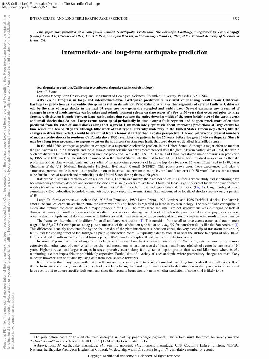
This paper was presented at a colloquium entitled “Earthquake Prediction: The Scientific Challenge,” organized by Leon Knopoff(Chair), Keiiti Aki, Clarence R.Allen, James R.Rice, and Lynn R.Sykes, held February 10 and 11, 1995, at the National Academy of Sciences inIrvine, CA.
Intermediate- and long-term earthquake prediction
(earthquake precursors/California tectonics/earthquake statistics/seismology)LYNN R.SYKES
Lamont-Doherty Earth Observatory and Department of Geological Sciences, Columbia University, Palisades, NY 10964ABSTRACT Progress in long- and intermediate-term earthquake prediction is reviewed emphasizing results from California.
Earthquake prediction as a scientific discipline is still in its infancy. Probabilistic estimates that segments of several faults in Californiawill be the sites of large shocks in the next 30 years are now generally accepted and widely used. Several examples are presented ofchanges in rates of moderate-size earthquakes and seismic moment release on time scales of a few to 30 years that occurred prior to largeshocks. A distinction is made between large earthquakes that rupture the entire downdip width of the outer brittle part of the earth's crustand small shocks that do not. Large events occur quasi-periodically in time along a fault segment and happen much more often thanpredicted from the rates of small shocks along that segment. I am moderately optimistic about improving predictions of large events fortime scales of a few to 30 years although little work of that type is currently underway in the United States. Precursory effects, like thechanges in stress they reflect, should be examined from a tensorial rather than a scalar perspective. A broad pattern of increased numbersof moderate-size shocks in southern California since 1986 resembles the pattern in the 25 years before the great 1906 earthquake. Since itmay be a long-term precursor to a great event on the southern San Andreas fault, that area deserves detailed intensified study.
In the mid 1960s, earthquake prediction emerged as a respectable scientific problem in the United States. Although a major effort to monitorthe San Andreas fault in California and the Alaska-Aleutian seismic zone was recommended after the great Alaskan earthquake of 1964, the war inVietnam diverted funds that might have been used for prediction. While the U.S.S.R., Japan, and China had started major programs in predictionby 1966, very little work on the subject commenced in the United States until the mid to late 1970s. I have been involved in work on earthquakeprediction and its plate tectonic basis and on studies of the space-time properties of large earthquakes for about 25 years. From 1984 to 1988, I wasChairman of the U.S. National Earthquake Prediction Evaluation Council (NEPEC). This paper draws upon those experiences and tries tosummarize progress made in earthquake prediction on an intermediate term (months to 10 years) and long term (10–30 years). I assess what appearto be fruitful lines of research and monitoring in the United States during the next 20 years.
Rather than discussing earthquakes on a global basis, I emphasize mainly the plate boundary in California where study and monitoring havebeen underway for many decades and accurate locations of seismic events are available. I focus on those large shocks that break the entire downdipwidth (W) of the seismogenic zone, i.e., the shallow part of the lithosphere that undergoes brittle deformation (Fig. 1). Large earthquakes aresometimes called delocalize, bounded, characteristic, or plate-rupturing events. Small (i.e., unbounded or localized shocks) rupture only a portionof W.
Large California earthquakes include the 1906 San Francisco, 1989 Loma Prieta, 1992 Landers, and 1966 Parkfield shocks. The latter isamong the smallest earthquakes that rupture the entire width W and, hence, is regarded as large in my terminology. The recent Kobe earthquake inJapan also ruptured the entire width of a major strike-slip fault (2). The terms large and small are not synonymous with damaging or lack ofdamage. A number of small earthquakes have resulted in considerable damage and loss of life when they are located close to population centers,occur at shallow depth, and shake structures with little or no earthquake resistance. Large earthquakes in remote regions often result in little damage.
The frequency-size relationship differs for small and large earthquakes (1). The transition from small to large events occurs at about momentmagnitude (Mw) 7.5 for earthquakes along plate boundaries of the subduction type but at only Mw 5.9 for transform faults like the San Andreas (1).This difference is mainly accounted for by the shallow dip of the plate interface at subduction zones, the very steep dip of transform (strike-slip)faults, and the cooling effect of the downgoing plate at subduction zones. W typically extends from at or near the surface to depths of only 10–20km for strike-slip faults in California and from depths of 10–50 km for interplate thrust events at subduction zones.
In terms of phenomena that change prior to large earthquakes, I emphasize seismic precursors. In California, seismic monitoring is moreextensive than other types of geophysical or geochemical measurements, and the record of instrumentally recorded shocks extends back nearly 100years. Higher stresses and larger changes in stress probably occur along fault zones at depths greater than several kilometers where in situmonitoring is either impossible or prohibitively expensive. Earthquakes of a variety of sizes at depths where premonitory changes are most likelyto occur, however, can be studied by using data from local seismic networks.
It is my view that many large earthquakes will turn out to be more predictable on intermediate and long time scales than small events. If so,this is fortunate since many very damaging shocks are large by my terminology. I devote considerable attention to the quasi-periodic nature oflarge events that rerupture specific fault segments since that property bears strongly upon whether prediction of some kind is likely to be
The publication costs of this article were defrayed in part by page charge payment. This article must therefore be hereby marked“advertisement” in accordance with 18 U.S.C. §1734 solely to indicate this fact.
Abbreviations: M, earthquake magnitude; Mo, seismic moment; Mw, moment magnitude; CFF, Coulomb failure function; NEPEC,National Earthquake Prediction Evaluation Council; W, downdip width; L, rupture length; N, cumulative number of events.
INTERMEDIATE- AND LONG-TERM EARTHQUAKE PREDICTION 3732
Abou
t thi
s PD
F fil
e: T
his
new
dig
ital r
epre
sent
atio
n of
the
orig
inal
wor
k ha
s be
en re
com
pose
d fro
m X
ML
files
cre
ated
from
the
orig
inal
pap
er b
ook,
not
from
the
orig
inal
type
setti
ng fi
les.
Pag
e br
eaks
are
true
to th
e or
igin
al; l
ine
leng
ths,
wor
d br
eaks
, hea
ding
sty
les,
and
oth
er ty
pese
tting
-spe
cific
form
attin
g, h
owev
er, c
anno
t be
reta
ined
, and
som
e ty
pogr
aphi
c er
rors
may
hav
e be
en a
ccid
enta
lly in
serte
d. P
leas
e us
e th
e pr
int v
ersi
on o
f thi
s pu
blic
atio
n as
the
auth
orita
tive
vers
ion
for a
ttrib
utio
n.
Copyright © National Academy of Sciences. All rights reserved.
(NAS Colloquium) Earthquake Prediction: The Scientific Challengehttp://www.nap.edu/catalog/5709.html
feasible. I criticize the view (3–5) that large shocks, like small, are strongly clustered, not quasi-periodic. Clearly, large shocks are not strictlyperiodic. I think the important questions are how predictable and how chaotic are large shocks and on what time-space scales? In this review Iexclude short-term prediction (time scales of hours to months) since very little progress has been made in that area. For lack of space I also excludethe Parkfield prediction experiment and failure of predictions made for that area.
FIG. 1. Two types of earthquakes—small and large. L is rupture length along strike of fault; W is its downdip width (1).
EARTHQUAKES IN THE SAN FRANCISCO BAY AREA
Several large earthquakes according to the terminology used herein have occurred in the San Francisco Bay area (Fig. 2) since 1836. Of thoseevents, the greatest amount of information is available (6–10) for the great (Mw 7.7) 1906 earthquake that ruptured a 430-km portion of the SanAndreas fault (Fig. 2A), the 1989 Loma Prieta shock of Mw 6.9 that broke a 40-km segment of that fault (Figs. 2C and 3), and the 1868 event(Fig 2D). on the Hayward fault of Mw 6.8. Not as much is known about the shock of Mw ≥7.2 of 1838 that ruptured the San Andreas fault from justsouth of San Francisco to opposite San Jose but also is inferred to have ruptured the adjacent Loma Prieta segment to the southeast based on acomparison of shaking at Monterey in 1838 and 1906 (7, 8). Intensity reports (i.e., qualitative descriptions of seismic shaking) become morereliable after 1850.
FIG. 2. Distribution of earthquakes of magnitude (M) 5 or larger in San Francisco Bay area for four time intervals (6). Majoractive faults are shown. Solid circles, epicenters of 1906, 1989, and 1868 earthquakes; heavy solid lines, rupture zones of thosethree large shocks; dashed lines enclose events taken to be within their precursory areas. Arrows in A denote sense of strike-slipmotion along San Andreas fault. Note very low activity near most of 1906 rupture zone from 1920 to 1954 and higher activity inperiods before large three events.Changes in Rates of Moderate-Size Earthquakes. The frequency of moderate-size shocks, herein taken to be events of 5 ≤ M < 7, where M
is earthquake magnitude, has varied by as much as a factor of 20 in the Bay area during the past 150 years (6, 12, 13). From 1882 until the great1906 shock, activity was very high along faults in the area out to about 75 km from those segments of the San Andreas fault that rupturedsubsequently in 1906 (Fig. 2A). Those moderate-size events are well enough located based on intensity reports that most, and perhaps all, occurredon faults other than the San Andreas. The northernmost event in Fig. 2A, however, is not well enough located to ascertain on which fault itoccurred. Moderate activity dropped off dramatically after 1906 and remained low until about 1955 (Fig. 2B).
Sykes and Nishenko (8) remarked in 1984 that moderate activity increased to the southeast of San Francisco from 1955 to 1982 but in asmaller region than in the 25 years preceding the 1906 earthquake. They concluded that that pattern might represent a long-term precursor to afuture event of M=7.0 along the southern 75 km of the San Andreas fault of Fig. 3. That pattern became better developed from 1982 to 1989(Fig. 2C). The 1989 earthquake, the first large event to occur on the San Andreas fault in the San Francisco Bay area since 1906, was centeredalong that fault segment (Figs. 2C and 3). A similar pattern of moderate activity occurred from 1855 to 1868 in the area surrounding the coming1868 shock on the Hayward fault (Fig. 2D). Moderate-sized events shut off in the region after 1868 and did not resume for 13 years.
The patterns of activity that stand out strongly in Fig. 2 are increased rates of moderate-size shocks in the 20–30 years preceding the threelarge events. The size of the region of increased activity appears to scale with the length of the rupture zone of the coming large event (Fig. 2),being much longer for the 1906 earthquake. Moderate activity decreased greatly after the 1868 and 1906 shocks. It is reasonable to ask if thesechanges are an artifact of either differing methods of determining M or the completeness of catalogs. The record is complete for M≥5 since 1910and, except in the far northern part of Fig. 2, for M≥5.5 since 1850 (6, 14, 15). The values of M prior to 1906, which are based mainly on the sizesof the felt areas of shocks, are probably underestimated with respect to more recent instrumental values (13). Thus, the large number of events inFig. 2A prior to the 1906 shock is not an artifact of overestimating M. Most of the changes in frequency of occurrence of earthquakes in the Bayarea are confined to moderate-size events. The rate of smaller earthquakes in the entire area has remained nearly constant (13).
Changes in Rate of Release of Seismic Moment. Looking for changes in the cumulative number (N) of events ≥M, as in the previoussection, suffers from the fact that small changes in the determination of M near the lower cutoff used can affect N at about a factor of 1.5. Since thenumber of small earthquakes in a large region follows the relationship
log N=A−bM [1]and b is close to 1.0, about half of the cumulative numbers of events are found between M and M+0.3. Most of the seismic moment (Mo)
released in a region, however, is contained in the few largest earthquakes. The cumulative moment release as a function of time, ΣMo, is not verysensitive to the lower cutoff
INTERMEDIATE- AND LONG-TERM EARTHQUAKE PREDICTION 3733
Abou
t thi
s PD
F fil
e: T
his
new
dig
ital r
epre
sent
atio
n of
the
orig
inal
wor
k ha
s be
en re
com
pose
d fro
m X
ML
files
cre
ated
from
the
orig
inal
pap
er b
ook,
not
from
the
orig
inal
type
setti
ng fi
les.
Pag
e br
eaks
are
true
to th
e or
igin
al; l
ine
leng
ths,
wor
d br
eaks
, hea
ding
sty
les,
and
oth
er ty
pese
tting
-spe
cific
form
attin
g, h
owev
er, c
anno
t be
reta
ined
, and
som
e ty
pogr
aphi
c er
rors
may
hav
e be
en a
ccid
enta
lly in
serte
d. P
leas
e us
e th
e pr
int v
ersi
on o
f thi
s pu
blic
atio
n as
the
auth
orita
tive
vers
ion
for a
ttrib
utio
n.
Copyright © National Academy of Sciences. All rights reserved.
(NAS Colloquium) Earthquake Prediction: The Scientific Challengehttp://www.nap.edu/catalog/5709.html
in M but is to the values of Mo for the largest few events sampled.
FIG. 3. Seismicity along the San Andreas fault, 1969–1989, from north of San Francisco at left to San Juan Bautista at right (10).The size of symbols increases with magnitude. (A) Brackets indicate fault segments forecast by various authors as discussed intext. SSCM is Southern Santa Cruz Mountains segment of fault. (B) Rectangles give location of 1989 rupture zone as inferredfrom geodetic data (11). Distance is measured to northwest along fault from San Juan Bautista.ΣMo was computed for shocks of M≥5 prior to the three large events in Fig. 2 and before the Mw 6.0 earthquake of 1948 in southern California
(6). ΣMo was calculated only for shocks within the precursory areas outlined in Fig. 2. Those areas were chosen qualitatively to include most of theregion in which major changes in activity occur with time. They extend out to about the same distance in Fig. 2C where the rate of small shockswas found to differ significantly before and after the 1989 earthquake (16, 17). ΣMo increases nearly exponentially with time prior to each of thosefour large earthquakes with a time constant τ of 4–11 years.
Thus, the release of Mo, like the frequency of moderate-size events, is concentrated in the latter part of the time interval between large shocksalong a given fault segment. Several other examples of high rates of moderate activity preceding large earthquakes are given in ref. 6. Thus,changes in N and Mo qualify as intermediate- to long-term seismic precursors.
Probabilities of Large Shocks Along Segments of San Andreas Fault. During the last 15 years, a consensus has developed among workersstudying the San Andreas fault that stresses are built up as a result of the relative motion of the Pacific and North American plates and that faultsegments that ruptured a relatively small amount in their last large earthquake are more likely to rerupture sooner than segments that experiencedrelatively large displacement (8–10, 15, 18). For example, the Parkfield segment of the San Andreas fault has ruptured historically about every 22years in shocks of about Mw 6 with an average displacement of 0.5–1.0 m. Some other segments of the San Andreas rupture in shocks of Mw�7.5with displacements of several meters and repeat times of 100–400 years. Changes in fault strike, presence of a major compressive (transpressive)fault step, relatively low fluid pressures at depth, and unusually large W probably contribute to a fault segment being a so-called asperity (i.e., adifficult place to rupture) and hence to its being a segment with a long repeat time and particularly large M. Nevertheless, a quantitativeunderstanding of why a segment ruptures with a certain Mw is lacking. This is an area in which considerable progress could be made inunderstanding fault mechanics during the next 20 years.
The term “characteristic earthquake” has been used in various ways in the literature to describe the slip behavior of large shocks. One viewbased on detection of prehistoric earthquakes in trenches was that large events are nearly exact duplicates of previous prehistoric events in terms ofdisplacement as a function of distance (L) along a fault (19). Such models suffer, however, from cumulative displacement over many cycles oflarge shocks being nonuniform along a major fault, a violation of the idea that long-term plate motion is nearly uniform along strike. One of thecommon features of large earthquakes along plate boundaries is that a fault segment may break by itself one time but in conjunction with one ormore adjacent segments another time. The Loma Prieta segment of the San Andreas fault ruptured by itself in 1989, with the adjacent Peninsularsegment in 1838, and with yet several additional segments to the north in 1906 (7, 8). This type of behavior is also common for large thrustearthquakes at subduction zones. This undoubtedly contributes to variations in individual repeat times of large events. Thus, the idea that largeshocks are like preceding ones in rupturing the same fault segment and in having the same displacement as a function of L is clearly not correct.
Another hypothesis is that a given fault segment ruptures in a large event with a certain “characteristic displacement” that differs from onefault segment to another but remains the same for that segment regardless of whether it breaks alone or in conjunction with another segment (20).This model permits repeat times to differ among segments but for the cumulative
INTERMEDIATE- AND LONG-TERM EARTHQUAKE PREDICTION 3734
Abou
t thi
s PD
F fil
e: T
his
new
dig
ital r
epre
sent
atio
n of
the
orig
inal
wor
k ha
s be
en re
com
pose
d fro
m X
ML
files
cre
ated
from
the
orig
inal
pap
er b
ook,
not
from
the
orig
inal
type
setti
ng fi
les.
Pag
e br
eaks
are
true
to th
e or
igin
al; l
ine
leng
ths,
wor
d br
eaks
, hea
ding
sty
les,
and
oth
er ty
pese
tting
-spe
cific
form
attin
g, h
owev
er, c
anno
t be
reta
ined
, and
som
e ty
pogr
aphi
c er
rors
may
hav
e be
en a
ccid
enta
lly in
serte
d. P
leas
e us
e th
e pr
int v
ersi
on o
f thi
s pu
blic
atio
n as
the
auth
orita
tive
vers
ion
for a
ttrib
utio
n.
Copyright © National Academy of Sciences. All rights reserved.
(NAS Colloquium) Earthquake Prediction: The Scientific Challengehttp://www.nap.edu/catalog/5709.html
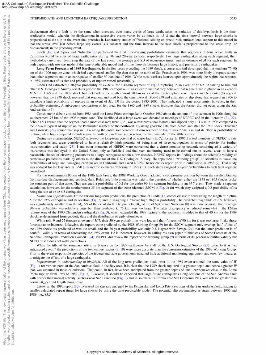
displacement along a fault to be the same when averaged over many cycles of large earthquakes. A variation of this hypothesis is the time-predictable model, wherein the displacement in successive events varies by as much as 1.5–2 and the time interval between large shocks isproportional to the slip in the event that precedes it. Laboratory studies of frictional sliding on precut rock surfaces lend support to this model inthat the stress level just before large slip events is a constant and the time interval to the next shock is proportional to the stress drop (ordisplacement) in the preceding event.
Lindh (18) and Sykes and Nishenko (8) performed the first time-varying probabilistic estimates that segments of four active faults inCalifornia would be sites of large earthquakes during 30- and 20-year periods, respectively. For large earthquakes along each segment, theirmethodology involved identifying the date of the last event, the average and SD of recurrence times, and an estimate of M for each segment. Inboth papers, wide use was made of the time-predictable model and of time intervals between large historic and prehistoric earthquakes.
Long-Term Forecasts of 1989 Earthquake. In the few years preceding the 1989 shock, a consensus had developed that the southern 75–90km of the 1906 rupture zone, which had experienced smaller slip than that to the north of San Francisco in 1906, was more likely to rupture soonerthan other segments and in an earthquake of smaller M than that of 1906. While most workers focused upon approximately the region that rupturedin 1989, estimates of its size and probability of rupture varied substantially.
Lindh (18) estimated a 30-year probability of 47–83% for a 45-km segment of Fig. 3 rupturing in an event of M 6.5. In talking to him andother U.S. Geological Survey scientists prior to the 1989 earthquake, it was clear to me that they believed that segment had ruptured in an event ofM 6.5 in 1865 and the 1838 shock had not broken the southernmost 50 km or so of the 1906 rupture zone. Sykes and Nishenko (8) argued,however, that the 1838 shock ruptured that segment and used both the time interval 1906–1838 and estimates of slip along that segment in 1906 tocalculate a high probability of rupture in an event of Mw 7.0 for the period 1983–2003. They indicated a large uncertainty, however, in theirprobability estimates. A subsequent comparison of felt areas for the 1865 and 1989 shocks indicates that the former did not occur along the SanAndreas fault (7).
Considerable debate ensued from 1984 until the Loma Prieta earthquake in October 1989 about the amount of displacement in 1906 along thesouthernmost 75 km of the 1906 rupture zone. The likelihood of a large event was debated at meetings of NEPEC and in the literature (21, 22).Scholz (21) argued that the segment had a more east-west trend (i.e., was a transpressional feature) and slipped only 1–1.4 m in 1906 compared tothe 2.5–4 m typical of rupture on the Peninsular segment to the northwest. By using geodetic data from before and after the 1906 shock, Thatcherand Lisowski (22) argued that slip in 1906 along the entire southernmost 90-km segment of Fig. 3 was 2.6±0.3 m and its 30-year probability ofrupture, while high compared to fault segments north of San Francisco, was low for the remainder of the 20th century.
During my chairmanship, NEPEC reviewed the long-term potential of major faults in California. In 1987 I asked members of NEPEC to ratefault segments and areas considered to have a relatively high potential of being sites of large earthquakes in terms of priority for furtherinstrumentation and study (23). I and other members of NEPEC were concerned that a dense monitoring network consisting of a variety ofinstruments was deployed in the United States only at Parkfield and that such monitoring need to be carried out in several areas to have areasonable chance of observing precursors to a large earthquake within a few decades. NEPEC reports its findings about the scientific validity ofearthquake predictions made by others to the director of the U.S. Geological Survey. He appointed a “working group” of scientists to assess theprobabilities of large and damaging earthquakes in California and asked NEPEC to review its report prior to publication in 1988 (9). That studywas updated for the Bay area in 1990 (10) and for southern California in 1995 (17). Each study assigned 30-year probabilities to each fault segmentconsidered.
For the southernmost 90 km of the 1906 fault break, the 1988 Working Group adopted a compromise position between the results obtainedfrom surface displacements and geodetic data. Relatively little attention was paid to the question of whether either the 1838 or 1865 shocks brokethe southern part of that zone. They assigned a probability of 0.2 for the entire 90-km segment breaking in an M 7 event. They made a separatecalculation, however, for the southernmost 35-km segment of that zone (denoted SSCM in Fig. 3) for which they assigned a 0.3 probability of itsbeing the site of an M 6.5 earthquake.
Evaluation of predictions. Of the various long-term predictions, the prediction of Lindh (18) comes closest to forecasting the length of ruptureL for the 1989 earthquake and its location (Fig. 3) and in assigning a relative high 30-year probability. His predicted magnitude of 6.5, however,was significantly smaller than the Mw 6.9 of the event itself. The predicted Mw of 7.0 of Sykes and Nishenko (8) was more accurate; their average20-year probability was relatively large but their predicted L, 75 km, was too large. The latter discrepancy is reduced somewhat if the 12-kmrupture zone of the 1990 Chittenden earthquake (Fig. 3), which extended the 1989 rupture to the southeast, is added to that of 40 km for the 1989shock, as determined from geodetic data and the distribution of early aftershocks.
While refs. 9 and 22 forecast an event of M 7, their 30-year probabilities were low and their forecast of 90 km for L was too large. I take thoseforecasts to be incorrect. Likewise, the rupture zone predicted by the 1988 Working Group (9) for the SSCM segment only overlaps half of that ofthe 1989 shock; its predicted M was too small, and the 30-year probability was only 0.3. I agree with Savage (24) that the latter prediction is ofdoubtful validity in terms of forecasting the 1989 event. He is incorrect, however, in calling his own paper “Criticisms of Some Forecasts of theNational Earthquake Prediction Council” (24). NEPEC did review the report of the working group (9) in terms of its general scientific validity butNEPEC itself does not make predictions.
While the title of the summary article in Science on the 1989 earthquake by staff of the U.S. Geological Survey (25) refers to it as “ananticipated event,” the predictions of the two earliest papers (8, 18) were more accurate than the consensus estimates of the 1988 Working Group.Prior to the event responsible agencies of the federal and state governments installed little additional monitoring equipment and took few measuresto mitigate the effects of a large earthquake.
Improvements in understanding in hindsight. All of the long-term predictions made prior to the 1989 event assumed the same value of W(Fig. 1) for various parts of the San Andreas fault in the Bay area. It is clear that the 1989 shock ruptured to a greater depth and hence a greater Wthan was assumed in those calculations. That could, in fact, have been anticipated from the greater depths of small earthquakes close to the LomaPrieta rupture from 1969 to 1989 (Fig. 3). Likewise, it should be expected that large future earthquakes along sections of the San Andreas faultwith deeper than normal activity, such as near San Francisco (Fig. 3) and in southern California near San Gorgonio Pass, will release greater thannormal Mo per unit length along strike.
Likewise, the 1990 report (10) increased the slip rate assigned to the Peninsular and Loma Prieta sections of the San Andreas fault, leading tosmaller calculated repeat times for large shocks by using the time-predictable model. The potential slip accumulated as strain between 1906 and1989 [i.e., 83.5
INTERMEDIATE- AND LONG-TERM EARTHQUAKE PREDICTION 3735
Abou
t thi
s PD
F fil
e: T
his
new
dig
ital r
epre
sent
atio
n of
the
orig
inal
wor
k ha
s be
en re
com
pose
d fro
m X
ML
files
cre
ated
from
the
orig
inal
pap
er b
ook,
not
from
the
orig
inal
type
setti
ng fi
les.
Pag
e br
eaks
are
true
to th
e or
igin
al; l
ine
leng
ths,
wor
d br
eaks
, hea
ding
sty
les,
and
oth
er ty
pese
tting
-spe
cific
form
attin
g, h
owev
er, c
anno
t be
reta
ined
, and
som
e ty
pogr
aphi
c er
rors
may
hav
e be
en a
ccid
enta
lly in
serte
d. P
leas
e us
e th
e pr
int v
ersi
on o
f thi
s pu
blic
atio
n as
the
auth
orita
tive
vers
ion
for a
ttrib
utio
n.
Copyright © National Academy of Sciences. All rights reserved.
(NAS Colloquium) Earthquake Prediction: The Scientific Challengehttp://www.nap.edu/catalog/5709.html
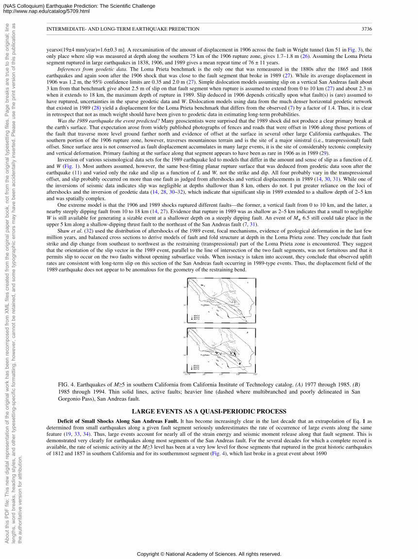
years×(19±4 mm/year)=1.6±0.3 m]. A reexamination of the amount of displacement in 1906 across the fault in Wright tunnel (km 51 in Fig. 3), theonly place where slip was measured at depth along the southern 75 km of the 1906 rupture zone, gives 1.7–1.8 m (26). Assuming the Loma Prietasegment ruptured in large earthquakes in 1838, 1906, and 1989 gives a mean repeat time of 76 ± 11 years.
Inferences from geodetic data. The Loma Prieta benchmark is the only one that was remeasured in the 1880s after the 1865 and 1868earthquakes and again soon after the 1906 shock that was close to the fault segment that broke in 1989 (27). While its average displacement in1906 was 1.2 m, the 95% confidence limits are 0.35 and 2.0 m (27). Simple dislocation models assuming slip on a vertical San Andreas fault about3 km from that benchmark give about 2.5 m of slip on that fault segment when rupture is assumed to extend from 0 to 10 km (27) and about 2.3 mwhen it extends to 18 km, the maximum depth of rupture in 1989. Slip deduced in 1906 depends critically upon what fault(s) is (are) assumed tohave ruptured, uncertainties in the sparse geodetic data and W. Dislocation models using data from the much denser horizontal geodetic networkthat existed in 1989 (28) yield a displacement for the Loma Prieta benchmark that differs from the observed (7) by a factor of 1.4. Thus, it is clearin retrospect that not as much weight should have been given to geodetic data in estimating long-term probabilities.
Was the 1989 earthquake the event predicted? Many geoscientists were surprised that the 1989 shock did not produce a clear primary break atthe earth's surface. That expectation arose from widely published photographs of fences and roads that were offset in 1906 along those portions ofthe fault that traverse more level ground farther north and evidence of offset at the surface in several other large California earthquakes. Thesouthern portion of the 1906 rupture zone, however, traverses mountainous terrain and is the site of a major sinistral (i.e., transpressional) faultoffset. Since surface area is not conserved as fault displacement accumulates in many large events, it is the site of considerably tectonic complexityand vertical deformation. Primary faulting at the surface along that segment appears to have been as rare in 1906 as in 1989 (29).
Inversion of various seismological data sets for the 1989 earthquake led to models that differ in the amount and sense of slip as a function of Land W (Fig. 1). Most authors assumed, however, the same best-fitting planar rupture surface that was deduced from geodetic data soon after theearthquake (11) and varied only the rake and slip as a function of L and W, not the strike and dip. All four probably vary in the transpressionaloffset, and slip probably occurred on more than one fault as judged from aftershocks and vertical displacements in 1989 (14, 30, 31). While one ofthe inversions of seismic data indicates slip was negligible at depths shallower than 8 km, others do not. I put greater reliance on the loci ofaftershocks and the inversion of geodetic data (14, 28, 30–32), which indicate that significant slip in 1989 extended to a shallow depth of 2–5 kmand was spatially complex.
One extreme model is that the 1906 and 1989 shocks ruptured different faults—the former, a vertical fault from 0 to 10 km, and the latter, anearby steeply dipping fault from 10 to 18 km (14, 27). Evidence that rupture in 1989 was as shallow as 2–5 km indicates that a small to negligibleW is still available for generating a sizable event at a shallower depth on a steeply dipping fault. An event of Mw 6.5 still could take place in theupper 5 km along a shallow-dipping thrust fault to the northeast of the San Andreas fault (7, 31).
Shaw et al. (32) used the distribution of aftershocks of the 1989 event, focal mechanisms, evidence of geological deformation in the last fewmillion years, and balanced cross sections to derive models of fault and fold structure at depth in the Loma Prieta zone. They conclude that faultstrike and dip change from southeast to northwest as the restraining (transpressional) part of the Loma Prieta zone is encountered. They suggestthat the orientation of the slip vector in the 1989 event, parallel to the line of intersection of the two fault segments, was not fortuitous and that itpermits slip to occur on the two faults without opening subsurface voids. When isostacy is taken into account, they conclude that observed upliftrates are consistent with long-term slip on this section of the San Andreas fault occurring in 1989-type events. Thus, the displacement field of the1989 earthquake does not appear to be anomalous for the geometry of the restraining bend.
FIG. 4. Earthquakes of M≥5 in southern California from California Institute of Technology catalog. (A) 1977 through 1985. (B)1985 through 1994. Thin solid lines, active faults; heavier line (dashed where multibranched and poorly delineated in SanGorgonio Pass), San Andreas fault.
LARGE EVENTS AS A QUASI-PERIODIC PROCESS
Deficit of Small Shocks Along San Andreas Fault. It has become increasingly clear in the last decade that an extrapolation of Eq. 1 asdetermined from small earthquakes along a given fault segment seriously underestimates the rate of occurrence of large events along the samefeature (19, 33, 34). Thus, large events account for nearly all of the strain energy and seismic moment release along that fault segment. This isdemonstrated very clearly for earthquakes along most segments of the San Andreas fault. For the several decades for which a complete record isavailable, the rate of seismic activity at the M≥3 level has been at a very low level for those segments that ruptured in the great historic earthquakesof 1812 and 1857 in southern California and for its southernmost segment (Fig. 4), which last broke in a great event about 1690
INTERMEDIATE- AND LONG-TERM EARTHQUAKE PREDICTION 3736
Abou
t thi
s PD
F fil
e: T
his
new
dig
ital r
epre
sent
atio
n of
the
orig
inal
wor
k ha
s be
en re
com
pose
d fro
m X
ML
files
cre
ated
from
the
orig
inal
pap
er b
ook,
not
from
the
orig
inal
type
setti
ng fi
les.
Pag
e br
eaks
are
true
to th
e or
igin
al; l
ine
leng
ths,
wor
d br
eaks
, hea
ding
sty
les,
and
oth
er ty
pese
tting
-spe
cific
form
attin
g, h
owev
er, c
anno
t be
reta
ined
, and
som
e ty
pogr
aphi
c er
rors
may
hav
e be
en a
ccid
enta
lly in
serte
d. P
leas
e us
e th
e pr
int v
ersi
on o
f thi
s pu
blic
atio
n as
the
auth
orita
tive
vers
ion
for a
ttrib
utio
n.
Copyright © National Academy of Sciences. All rights reserved.
(NAS Colloquium) Earthquake Prediction: The Scientific Challengehttp://www.nap.edu/catalog/5709.html
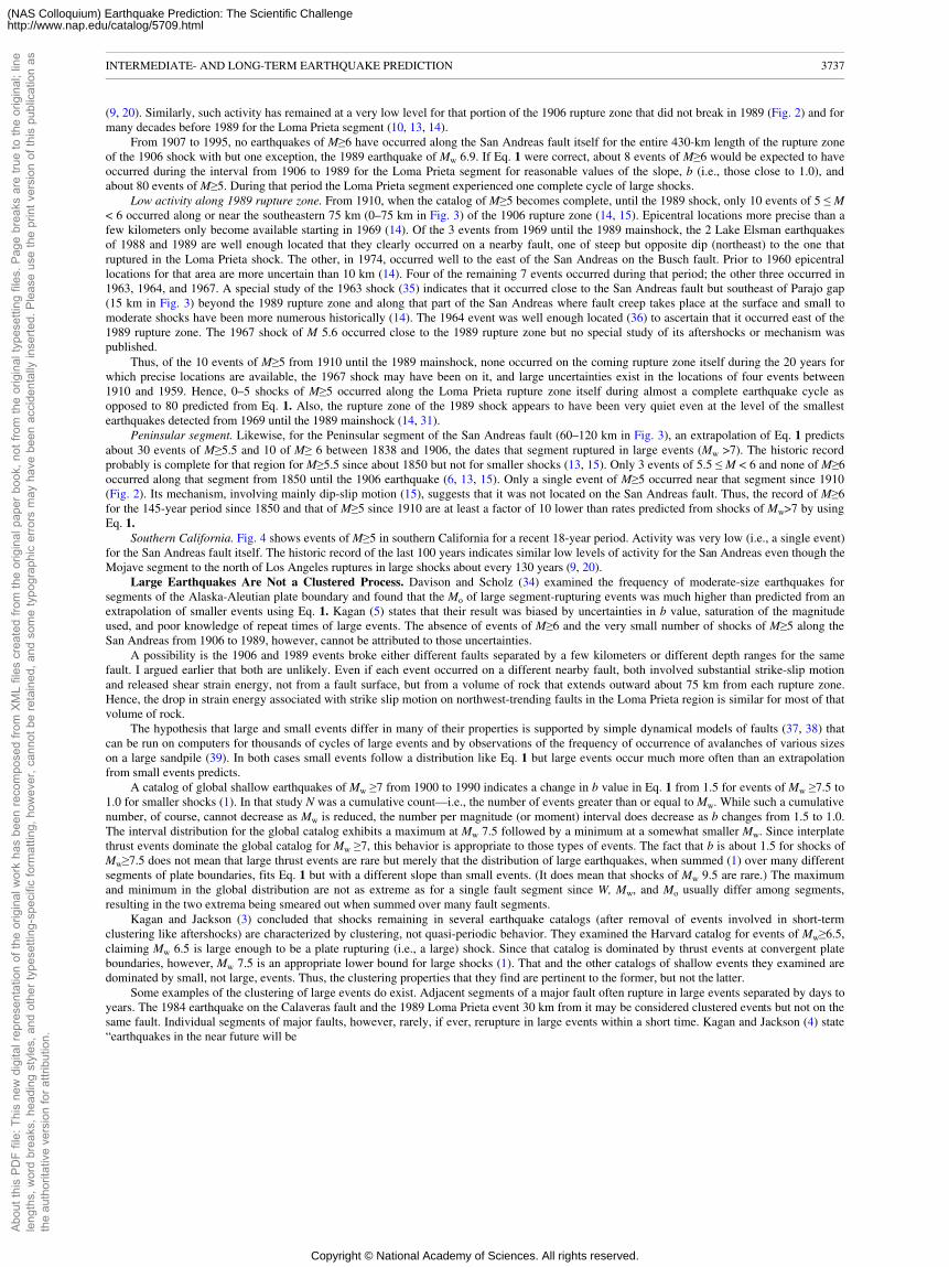
(9, 20). Similarly, such activity has remained at a very low level for that portion of the 1906 rupture zone that did not break in 1989 (Fig. 2) and formany decades before 1989 for the Loma Prieta segment (10, 13, 14).
From 1907 to 1995, no earthquakes of M≥6 have occurred along the San Andreas fault itself for the entire 430-km length of the rupture zoneof the 1906 shock with but one exception, the 1989 earthquake of Mw 6.9. If Eq. 1 were correct, about 8 events of M≥6 would be expected to haveoccurred during the interval from 1906 to 1989 for the Loma Prieta segment for reasonable values of the slope, b (i.e., those close to 1.0), andabout 80 events of M≥5. During that period the Loma Prieta segment experienced one complete cycle of large shocks.
Low activity along 1989 rupture zone. From 1910, when the catalog of M≥5 becomes complete, until the 1989 shock, only 10 events of 5 ≤ M< 6 occurred along or near the southeastern 75 km (0–75 km in Fig. 3) of the 1906 rupture zone (14, 15). Epicentral locations more precise than afew kilometers only become available starting in 1969 (14). Of the 3 events from 1969 until the 1989 mainshock, the 2 Lake Elsman earthquakesof 1988 and 1989 are well enough located that they clearly occurred on a nearby fault, one of steep but opposite dip (northeast) to the one thatruptured in the Loma Prieta shock. The other, in 1974, occurred well to the east of the San Andreas on the Busch fault. Prior to 1960 epicentrallocations for that area are more uncertain than 10 km (14). Four of the remaining 7 events occurred during that period; the other three occurred in1963, 1964, and 1967. A special study of the 1963 shock (35) indicates that it occurred close to the San Andreas fault but southeast of Parajo gap(15 km in Fig. 3) beyond the 1989 rupture zone and along that part of the San Andreas where fault creep takes place at the surface and small tomoderate shocks have been more numerous historically (14). The 1964 event was well enough located (36) to ascertain that it occurred east of the1989 rupture zone. The 1967 shock of M 5.6 occurred close to the 1989 rupture zone but no special study of its aftershocks or mechanism waspublished.
Thus, of the 10 events of M≥5 from 1910 until the 1989 mainshock, none occurred on the coming rupture zone itself during the 20 years forwhich precise locations are available, the 1967 shock may have been on it, and large uncertainties exist in the locations of four events between1910 and 1959. Hence, 0–5 shocks of M≥5 occurred along the Loma Prieta rupture zone itself during almost a complete earthquake cycle asopposed to 80 predicted from Eq. 1. Also, the rupture zone of the 1989 shock appears to have been very quiet even at the level of the smallestearthquakes detected from 1969 until the 1989 mainshock (14, 31).
Peninsular segment. Likewise, for the Peninsular segment of the San Andreas fault (60–120 km in Fig. 3), an extrapolation of Eq. 1 predictsabout 30 events of M≥5.5 and 10 of M≥ 6 between 1838 and 1906, the dates that segment ruptured in large events (Mw >7). The historic recordprobably is complete for that region for M≥5.5 since about 1850 but not for smaller shocks (13, 15). Only 3 events of 5.5 ≤ M < 6 and none of M≥6occurred along that segment from 1850 until the 1906 earthquake (6, 13, 15). Only a single event of M≥5 occurred near that segment since 1910(Fig. 2). Its mechanism, involving mainly dip-slip motion (15), suggests that it was not located on the San Andreas fault. Thus, the record of M≥6for the 145-year period since 1850 and that of M≥5 since 1910 are at least a factor of 10 lower than rates predicted from shocks of Mw>7 by usingEq. 1.
Southern California. Fig. 4 shows events of M≥5 in southern California for a recent 18-year period. Activity was very low (i.e., a single event)for the San Andreas fault itself. The historic record of the last 100 years indicates similar low levels of activity for the San Andreas even though theMojave segment to the north of Los Angeles ruptures in large shocks about every 130 years (9, 20).
Large Earthquakes Are Not a Clustered Process. Davison and Scholz (34) examined the frequency of moderate-size earthquakes forsegments of the Alaska-Aleutian plate boundary and found that the Mo of large segment-rupturing events was much higher than predicted from anextrapolation of smaller events using Eq. 1. Kagan (5) states that their result was biased by uncertainties in b value, saturation of the magnitudeused, and poor knowledge of repeat times of large events. The absence of events of M≥6 and the very small number of shocks of M≥5 along theSan Andreas from 1906 to 1989, however, cannot be attributed to those uncertainties.
A possibility is the 1906 and 1989 events broke either different faults separated by a few kilometers or different depth ranges for the samefault. I argued earlier that both are unlikely. Even if each event occurred on a different nearby fault, both involved substantial strike-slip motionand released shear strain energy, not from a fault surface, but from a volume of rock that extends outward about 75 km from each rupture zone.Hence, the drop in strain energy associated with strike slip motion on northwest-trending faults in the Loma Prieta region is similar for most of thatvolume of rock.
The hypothesis that large and small events differ in many of their properties is supported by simple dynamical models of faults (37, 38) thatcan be run on computers for thousands of cycles of large events and by observations of the frequency of occurrence of avalanches of various sizeson a large sandpile (39). In both cases small events follow a distribution like Eq. 1 but large events occur much more often than an extrapolationfrom small events predicts.
A catalog of global shallow earthquakes of Mw ≥7 from 1900 to 1990 indicates a change in b value in Eq. 1 from 1.5 for events of Mw ≥7.5 to1.0 for smaller shocks (1). In that study N was a cumulative count—i.e., the number of events greater than or equal to Mw. While such a cumulativenumber, of course, cannot decrease as Mw is reduced, the number per magnitude (or moment) interval does decrease as b changes from 1.5 to 1.0.The interval distribution for the global catalog exhibits a maximum at Mw 7.5 followed by a minimum at a somewhat smaller Mw. Since interplatethrust events dominate the global catalog for Mw ≥7, this behavior is appropriate to those types of events. The fact that b is about 1.5 for shocks ofMw≥7.5 does not mean that large thrust events are rare but merely that the distribution of large earthquakes, when summed (1) over many differentsegments of plate boundaries, fits Eq. 1 but with a different slope than small events. (It does mean that shocks of Mw 9.5 are rare.) The maximumand minimum in the global distribution are not as extreme as for a single fault segment since W, Mw, and Mo usually differ among segments,resulting in the two extrema being smeared out when summed over many fault segments.
Kagan and Jackson (3) concluded that shocks remaining in several earthquake catalogs (after removal of events involved in short-termclustering like aftershocks) are characterized by clustering, not quasi-periodic behavior. They examined the Harvard catalog for events of Mw≥6.5,claiming Mw 6.5 is large enough to be a plate rupturing (i.e., a large) shock. Since that catalog is dominated by thrust events at convergent plateboundaries, however, Mw 7.5 is an appropriate lower bound for large shocks (1). That and the other catalogs of shallow events they examined aredominated by small, not large, events. Thus, the clustering properties that they find are pertinent to the former, but not the latter.
Some examples of the clustering of large events do exist. Adjacent segments of a major fault often rupture in large events separated by days toyears. The 1984 earthquake on the Calaveras fault and the 1989 Loma Prieta event 30 km from it may be considered clustered events but not on thesame fault. Individual segments of major faults, however, rarely, if ever, rerupture in large events within a short time. Kagan and Jackson (4) state“earthquakes in the near future will be
INTERMEDIATE- AND LONG-TERM EARTHQUAKE PREDICTION 3737
Abou
t thi
s PD
F fil
e: T
his
new
dig
ital r
epre
sent
atio
n of
the
orig
inal
wor
k ha
s be
en re
com
pose
d fro
m X
ML
files
cre
ated
from
the
orig
inal
pap
er b
ook,
not
from
the
orig
inal
type
setti
ng fi
les.
Pag
e br
eaks
are
true
to th
e or
igin
al; l
ine
leng
ths,
wor
d br
eaks
, hea
ding
sty
les,
and
oth
er ty
pese
tting
-spe
cific
form
attin
g, h
owev
er, c
anno
t be
reta
ined
, and
som
e ty
pogr
aphi
c er
rors
may
hav
e be
en a
ccid
enta
lly in
serte
d. P
leas
e us
e th
e pr
int v
ersi
on o
f thi
s pu
blic
atio
n as
the
auth
orita
tive
vers
ion
for a
ttrib
utio
n.
Copyright © National Academy of Sciences. All rights reserved.
(NAS Colloquium) Earthquake Prediction: The Scientific Challengehttp://www.nap.edu/catalog/5709.html
similar in location and mechanism to those of the recent past.” That proposition, however, is pertinent to small earthquakes. Most, and perhaps all,large events along a given fault segment occur quasi-periodically in time. The fault segments that rupture in large events that I examined are partsof very active faults, the main loci of plate motion. Whether large shocks in areas of complex multibranched faulting, as in Asia, occur quasi-periodically is yet to be ascertained.
RECENT BUILDUP OF ACTIVITY IN SOUTHERN CALIFORNIA
Fig. 4 shows earthquakes of M≥5 in southern California for the periods 1977–1985 and 1986–1994. In the first 9-year period, no shocks ofthat size occurred on or close to the San Andreas fault, while in the second interval, activity occurred on both sides of the San Andreas fault along a200-km-long zone in the transverse ranges and the northern Los Angeles basin. That pattern of activity, especially the occurrence of severalearthquakes of M>6, resembles that in the 25 years before the 1906 earthquake (Fig. 2A). It was not centered near the Landers earthquake.
The possibility that the recent pattern of activity is a long-term precursor to a great earthquake along the southern San Andreas fault deservesserious study and debate. Segments of the fault in that region have not ruptured in great earthquakes since either 1812 or about 1690 (9, 20). Also,changes in stress generated by the Landers sequence of shocks resulted in portions of the fault in San Gorgonio Pass moving closer to failure byabout 10 years (40). The San Andreas fault undergoes a complex compressional left step in San Gorgonio Pass that is much larger than that in theLoma Prieta region. Much remains to be learned about the distribution of faults at depth, possible changes in seismic activity, the loci of volumesof weak- and strong-rock, fluid pressures, and the state of stress. An intensified effort is needed to understand that area in detail, which did nothappen before the 1989 earthquake. Damage and loss of life may not be greatest in large events such as one on the southern San Andreas.Moderate-size shocks that are part of the buildup to a great earthquake but located closer to centers of population may cause the largestcatastrophes. The Northridge event of 1994 may turn out to be such an example.
DISCUSSION AND SUMMARY
Time-varying probabilistic estimates of large earthquakes for segments of several active faults in California are now in their secondgeneration (10, 20) and are generally accepted and widely used. Debate continues about the width of the probability function to use either ingeneral or for specific segments. Since those predictions are for 30-year periods, however, the probability gain with respect to a randomdistribution in time is only about a factor of 1.5–3. Those long-term forecasts, which have replaced the earlier seismic gap concepts of the 1970s,help to focus scarce scientific resources on specific areas and conversely to indicate segments unlikely to rupture in the next few decades. Whileprogress can be expected over the next 20 years in improving those types of forecasts, probability gains likely will remain less than 5–10.
Major changes in the space-time distribution of moderate-size earthquakes have occurred in the San Francisco Bay area during the timeintervals between large shocks. Computer modeling of earthquakes (37, 38) and studies of avalanches on a large sandpile (39) show manysimilarities to those found for shocks in the Bay area. All indicate that large events occur much more frequently than predicted by extrapolatingrates of small events. In each case the rate of moderate-size events increases before large events and the dimension of the region of increasedactivity increases with the size of the coming large event. Much, if not all, of the activity that builds up prior to a large earthquake in the Bay area,however, occurs off its rupture zone on nearby faults. This is an important lesson for prediction and a factor that needs to be incorporated in futurecomputer modeling.
These and three other findings make me moderately optimistic for intermediate- and long-term prediction.(i) Rates of relative plate motion are virtually constant from a few to a few million years. Plate motion is the driving engine that leads to the
buildup of elastic stresses that are released in earthquakes along plate boundaries. Accurate estimates of long-term rates of deformation havebecome available for many active faults by using space geodesy.
(ii) The key nonlinearity in the earthquake process appears to be associated with the stick-slip frictional force at fault interfaces (37). Most ofthat effect is concentrated during or close to the rupture time of large shocks. Fortunately, socially useful prediction needs to be attempted only forthe next large event, not several such shocks into the future where nonlinear effects become cumulative. A better understanding of the nature ofrupture in the last large event seems crucial to long-term prediction. Better modeling of fault interactions should permit a choice of which faultsegments will rupture either separately or together in the next large earthquake along the San Andreas fault in southern California.
(iii) I foresee progress being made by recognizing that precursory processes are tensorial in character, not scalar. Stress (and its evolution withtime), which is basic to an understanding of the earthquake process, is a second-order tensor. This would explain why increases as well asdecreases in seismicity have been reported as precursors. While activity in most of the San Francisco Bay area decreased greatly soon after thegreat 1906 earthquake, the moderate activity that did take place in the next few decades was largely concentrated south and west of the end of therupture zone (Fig. 2B) in areas that are predicted from dislocation models to have, in fact, moved closer to failure (15).
Moderate-size shocks are modulated in their occurrence by changes in the Coulomb failure function (∆CFF) at the time of large events (6, 15–17, 31, 40). The ratio of the numbers of small events before to that after the 1989 earthquake for individual nearby fault segments changed inaccord with predictions of ∆CFF by using dislocation models (16, 17, 31). These changes occurred for fault segments extending out to 75–100 kmfrom the 1989 rupture zone. This corresponds to ∆CFF > 0.01 to 0.03 MPa, where 1 MPa=10 bars. Those changes are about a factor of 10 timeslarger than those generated by earth tides. Thus, changes in rates of small earthquakes may become more useful for prediction when individualfault segments are analyzed separately.
Changes in the distribution of moderate-size events in the Bay area of the past 150 years can be explained in terms of a drop in stress at thetime of large earthquakes and the slow buildup of stress with time. The 1906 shock created a broad area of reduced shear stress (or CFF) andsuppressed moderate activity for many decades until stresses were gradually restored by plate motion. The southern Calaveras fault was one of thefirst to return to the pre-1906 stress level and was the site of some of the earliest moderate activity prior to 1989 (6, 15, 17).
The pair of Lake Elsman earthquakes of M 5.3 and 5.4 that occurred 16 and 2.5 months before the 1989 mainshock may be interpreted as anintermediate-term precursor. Both occurred on a fault dipping steeply to the northeast �2 km from the 1989 rupture zone. Like the 1989 event, theyinvolved strike slip and reverse slip (14, 31). No other moderate-size events occurred on or near the 1989 rupture zone since the shocks of 1964and 1967. As shear stress was restored in the region, some of the last places to be returned to the pre-1906 level of CFF were faults very close tothe San Andreas, like the Lake Elsman fault. Those events resulted in the release of short-term (5 day)
INTERMEDIATE- AND LONG-TERM EARTHQUAKE PREDICTION 3738
Abou
t thi
s PD
F fil
e: T
his
new
dig
ital r
epre
sent
atio
n of
the
orig
inal
wor
k ha
s be
en re
com
pose
d fro
m X
ML
files
cre
ated
from
the
orig
inal
pap
er b
ook,
not
from
the
orig
inal
type
setti
ng fi
les.
Pag
e br
eaks
are
true
to th
e or
igin
al; l
ine
leng
ths,
wor
d br
eaks
, hea
ding
sty
les,
and
oth
er ty
pese
tting
-spe
cific
form
attin
g, h
owev
er, c
anno
t be
reta
ined
, and
som
e ty
pogr
aphi
c er
rors
may
hav
e be
en a
ccid
enta
lly in
serte
d. P
leas
e us
e th
e pr
int v
ersi
on o
f thi
s pu
blic
atio
n as
the
auth
orita
tive
vers
ion
for a
ttrib
utio
n.
Copyright © National Academy of Sciences. All rights reserved.
(NAS Colloquium) Earthquake Prediction: The Scientific Challengehttp://www.nap.edu/catalog/5709.html
warnings. While they may have had some value in terms of public preparedness, they were, in fact, false alarms.If it had been realized that the Lake Elsman events were on a nearby but different fault, an intermediate-term warning would have been more
appropriate. They probably indicated the return of stresses in that area to pre-1906 levels rather than the initiation of accelerated precursory slip onthe San Andreas fault itself. Another example of an intermediate-term seismic precursor is the northward growth in aftershock activity in theJoshua Tree earthquake sequence in southern California between its mainshock on April 23 and the Landers shock of June 28, 1992 (41). Whilethese precursors are subtle in character, they, and other examples, indicate that precursory phenomena likely exist on time scales of months to adecade.
How earthquake prediction is and has been viewed in the United States has a number of parallels to skepticism about continental drift andpaleomagnetism prior to the late 1960s. Like them, prediction invokes strong views about what problems are “worth working on.” Earthquakeprediction has suffered in this regard; only 10–20 scientists in the U.S. are currently working on intermediate-term prediction. Work in predictionalso has suffered from a general belief that only short-term predictions would have social value. While not possible now, a well-founded 5-yearprediction could be of greater value since serious mitigation measures could be undertaken.
Several observations of precursors have turned out upon reexamination to be artifacts of either environmental changes affecting instrumentsor changes in earthquake catalogs that are of human, not natural, origin. A superficial application of the ideas of chaos has led some to concludethat earthquakes are not predictable. Several workers active in studying earthquakes as an example of deterministic chaos, however, are moderatelyoptimistic about prediction. Long- and intermediate-term prediction are areas where I think progress is possible in the next 20 years. Much remainsto be done in understanding the physics of earthquakes and the role of fluid pressures at depth in fault zone and in deploying dense networks of avariety of observing instruments.
I thank J.Deng, S.Jaumé, C.Scholz, and B.Shaw for critical comments and discussions. This work was supported by grants from the U.S.Geological Survey, the National Science Foundation, and the Southern California Earthquake Center (SCEC). This is Lamont-Doherty EarthObservatory Contribution 5486 and SCEC contribution 319.1. Pacheco, J.F., Scholz, C.H. & Sykes, L.R. (1992) Nature (London) 355, 71–73.2. Summeriville, P. (1995) Eos Trans. Am. Geophys. Union 76, 49–51.3. Kagan, Y.Y. & Jackson, D.D. (1991) Geophys. J. Int. 104, 117–133.4. Kagan, Y.Y. & Jackson, D.D. (1994) J. Geophys. Res. 99, 13685–13700.5. Kagan, Y.Y. (1993) Bull. Seismol. Soc. Am. 83, 7–24.6. Sykes, L.R. & Jaumé, S.C. (1990) Nature (London) 348, 595– 599.7. Tuttle, M.P. & Sykes, L.R. (1992) Bull. Seismol Soc. Am. 82, 1802–1820.8. Sykes, L.R. & Nishenko, S.P. (1984) J. Geophys. Res. 89, 5905–5927.9. Working Group on California Earthquake Probabilities (1988) U.S. Geol. Surv. Open-File Rep. 88–398, 1–62.10. Working Group on California Earthquake Probabilities (1990) U.S. Geol. Surv. Circ. 1053, 1–51.11. Lisowski, M., Preseott, W.H., Savage, J.C. & Johnson, M.J.S. (1990) Geophys. Res. Lett. 17, 1437–1440.12. Tocher, D. (1959) Calif. Div. Mines Spec. Rep. 57, 39–48 and 125–127.13. Ellsworth, W.L. (1990) U.S. Geol. Surv. Prof. Paper 1515, 153– 187.14. Olson, J.A. & Hill, D.P. (1993) U.S. Geol. Surv. Prof. Paper 1550-C, C3-C16.15. Jaumé, S.C. & Sykes, L.R. (1996) J. Geophys. Res. 101, 765–789.16. Reasenberg, P.A. & Simpson, R.W. (1992) Science 255, 1687– 1690.17. Simpson, R.W. & Reasenberg, P.A. (1994) U.S. Geol. Surv. Prof. Paper 1550-F, F55-F89.18. Lindh, A.G. (1983) U.S. Geol. Surv. Open-File Rep. 83–63, 1–5.19. Sehwartz, D.P. & Coppersmith, K.J. (1984) J. Geophys. Res. 89, 5681–5698.20. 1994 Working Group on the Probabilities of Future Large Earthquakes in Southern California (1995) Bull. Seismol. Soc. Am. 85, 379–439.21. Scholz, C.H. (1985) Geophys. Res. Lett. 12, 717–719.22. Thatcher, W. & Lisowski, M. (1987) J. Geophys. Res. 92, 4771– 4784.23. Schearer, C.F. (1988) U.S. Geol. Surv. Open-File Rep. 88–37, 296–300.24. Savage, J. (1991) Bull. Seismol. Soc. Am. 81, 862–881.25. U.S. Geological Survey Staff (1990) Science 247, 286–293.26. Prentice, C.S. & Ponti, D.J. (1994) Eos Trans. Am. Geophys. Union 75, 343 (abstr.).27. Segall, P. & Lisowski, M. (1990) Science 250, 1241–1244.28. Snay, R.A., Neugebauer, H.C. & Preseott, W.H. (1991) Bull. Seismol. Soc. Am. 81, 1647–1659.29. Prentice, C.S. & Sehwartz, D.P. (1991) Bull. Seismol. Soc. Am. 81, 1424–1479.30. Marshall, G.A., Stein, R.S. & Thatcher, W. (1991) Bull. Seismol. Soc. Am. 81, 1660–1693.31. Seeber, L. & Armbruster, J.G. (1990) Geophys. Res. Lett. 17, 1425–1428.32. Shaw, J.H., Bischke, R. & Suppe, J. (1994) U.S. Geol. Surv. Prof. Paper 1550-F, F3-F21.33. Wesnousky, S.G., Scholz, C.H., Shimazaki, K. & Matsuda, T. (1984) Bull. Seismol. Soc. Am. 74, 687–708.34. Davison, F.C., Jr., & Scholz, C.H. (1985) Bull. Seismol. Soc. Am. 75, 1349–1361.35. Udias, A. (1965) Bull. Seismol. Soc. Am. 55, 85–106.36. McEvilly, T.V. (1966) Bull. Seismol. Soc. Am. 56, 755–773.37. Carlson, J.M. (1991) J. Geophys. Res. 96, 4255–4267.38. Pepke, S.L., Carlson, J.M. & Shaw, B.E. (1994) J. Geophys. Res. 99, 6769–6788.39. Rosendahl, J.M., Vekic, M. & Rutledge, J.E. (1994) Phys. Rev. Lett. 73, 537–540.40. Jaumé, S.C. & Sykes, L.R. (1992) Science 258, 1325–1328.41. Hauksson, E., Jones, L.M., Hutton, K. & Eberhart-Phillips, D. (1993) J. Geophys. Res. 98, 19835–19858.
INTERMEDIATE- AND LONG-TERM EARTHQUAKE PREDICTION 3739
Abou
t thi
s PD
F fil
e: T
his
new
dig
ital r
epre
sent
atio
n of
the
orig
inal
wor
k ha
s be
en re
com
pose
d fro
m X
ML
files
cre
ated
from
the
orig
inal
pap
er b
ook,
not
from
the
orig
inal
type
setti
ng fi
les.
Pag
e br
eaks
are
true
to th
e or
igin
al; l
ine
leng
ths,
wor
d br
eaks
, hea
ding
sty
les,
and
oth
er ty
pese
tting
-spe
cific
form
attin
g, h
owev
er, c
anno
t be
reta
ined
, and
som
e ty
pogr
aphi
c er
rors
may
hav
e be
en a
ccid
enta
lly in
serte
d. P
leas
e us
e th
e pr
int v
ersi
on o
f thi
s pu
blic
atio
n as
the
auth
orita
tive
vers
ion
for a
ttrib
utio
n.
Copyright © National Academy of Sciences. All rights reserved.
(NAS Colloquium) Earthquake Prediction: The Scientific Challengehttp://www.nap.edu/catalog/5709.html
This paper was presented at a colloquium entitled “Earthquake Prediction: The Scientific Challenge,” organized by Leon Knopoff(Chair), Keiiti Aki, Clarence R.Allen, James R.Rice, and Lynn R.Sykes, held February 10 and 11, 1995, at the National Academy of Sciences inIrvine, CA.
Scale dependence in earthquake phenomena and its relevance toearthquake prediction
KEIITI AKI
Department of Earth Sciences, University of Southern California, Los Angeles, CA 90089–0740ABSTRACT The recent discovery of a low-velocity, low-Q zone with a width of 50–200 m reaching to the top of the ductile part of the
crust, by observations on seismic guided waves trapped in the fault zone of the Landers earthquake of 1992, and its identification with theshear zone inferred from the distribution of tension cracks observed on the surface support the existence of a characteristic scale length ofthe order of 100 m affecting various earthquake phenomena in southern California, as evidenced earlier by the kink in the magnitude-frequency relation at about M3, the constant corner frequency for earthquakes with M below about 3, and the source-controlled fmax of 5–10 Hz for major earthquakes. The temporal correlation between coda Q−1 and the fractional rate of occurrence of earthquakes in themagnitude range 3–3.5, the geographical similarity of coda Q−1 and seismic velocity at a depth of 20 km, and the simultaneous change ofcoda Q−1 and conductivity at the lower crust support the hypotheses that coda Q−1 may represent the activity of creep fracture in theductile part of the lithosphere occurring over cracks with a characteristic size of the order of 100 m. The existence of such a characteristicscale length cannot be consistent with the overall self-similarity of earthquakes unless we postulate a discrete hierarchy of suchcharacteristic scale lengths. The discrete hierarchy of characteristic scale lengths is consistent with recently observed logarithmicperiodicity in precursory seismicity.
A starting point for the science of earthquake prediction may be to find what seismogenic structures control the earthquake processes. Wehave invented jargon to describe structures such as asperities, barriers, breakdown zones, locking depth, and the brittle-ductile transition zone. Ifthere is any distinct structure controlling earthquake processes, it should show up as scale-dependent phenomena—namely, departure from self-similarity. However, if all earthquakes are put together as shown, for example, in the seismic moment-source dimension relation summarized byAbercrombie and Leary (1) the self-similarity roughly holds over the range of source dimension from 10 cm to 100 km, telling us that there may beno universal structure controlling earthquake processes.
There is still a hope that we may find such a controlling structure if we focus our attention on a specific fault zone or a specific seismic regionand use techniques with higher resolution and accuracy. To explain why I have such a hope, I shall first describe my encounters with scale-dependent earthquake phenomena in the past two decades.
After I found (2) that the ω-squared scaling law with a constant stress drop independent of magnitude explains the observed source spectralratios (3) and resolves inconsistencies between surface wave magnitude and body wave magnitude, a natural follow-up was to determine thescaling law in various parts of the earth and map the stress drop globally. During the course of this work, we (4) found that very often the shape ofthe seismic spectrum does not obey the ω-squared scaling law but stays the same over a considerable range (2–3 orders) of seismic moment. Thismeans that the corner frequency stays at a constant value and stress drop decreases with decreasing magnitude. Rautian et al. (5) have studied thesame problem independently in the former Soviet Union and discovered the same phenomena. The existence of a constant corner frequency mustmean that there is a unique scale length governing the earthquake phenomena. The value of the constant corner frequency varied from place toplace in the range from a few to >10 Hz.
My next encounter with the unique scale length was when Papageorgiou and I (6) were trying to predict the strong motion acceleration powerspectra by using the specific barrier model. We found that the shape of the acceleration power spectrum is flat for frequencies higher than thesubevent corner frequency, but the flat part is limited to the fmax [term coined by Hanks (7)] beyond which the spectrum sharply decays withincreasing frequency (6). We found that fmax is in the range of a few to 10 Hz and shows a slight dependence on magnitude. It was very natural forme to suspect a tie between the constant corner frequency for small earthquakes and the fmax for large earthquakes. Papageorgiou and Aki (6)attributed the origin of fmax to the cohesive zone of an earthquake fault.
My third encounter with a unique scale length associated with earthquakes occurred when Okubo and I (8) were measuring the fractaldimension of the San Andreas fault with the map of fault traces published by the U.S. Geological Survey. We found that there is an upper boundlength beyond which the fault ceases to be fractal, and it ranges from a few hundred meters to a kilometer, in agreement with the size of thecohesive zone inferred from fmax.
My fourth encounter with the unique scale length is the finding of a kink in the frequency magnitude relation at about M=3 from therecordings made at a borehole station within the Newport-Inglewood fault zone in southern California (9). The size of an M=3 earthquake is a fewhundred meters, which roughly corresponds to the size of the cohesive zone estimated from fmax.
My most intriguing encounter with a characteristic scale length, however, was the very strong temporal correlation between coda Q−1 and thefractional rate of earthquakes with magnitudes in a certain range (10, 11). On the other hand, the most direct confirmation of the fault zonestructure with a characteristic width came from the observation of the seismic guided waves trapped in the fault zone of the Landers earthquake(12). In the present paper, I focus on these latter two subjects—namely, the coda Q and fault zone trapped
The publication costs of this article were defrayed in part by page charge payment. This article must therefore be hereby marked“advertisement” in accordance with 18 U.S.C. §1734 solely to indicate this fact.
SCALE DEPENDENCE IN EARTHQUAKE PHENOMENA AND ITS RELEVANCE TO EARTHQUAKE PREDICTION 3740
Abou
t thi
s PD
F fil
e: T
his
new
dig
ital r
epre
sent
atio
n of
the
orig
inal
wor
k ha
s be
en re
com
pose
d fro
m X
ML
files
cre
ated
from
the
orig
inal
pap
er b
ook,
not
from
the
orig
inal
type
setti
ng fi
les.
Pag
e br
eaks
are
true
to th
e or
igin
al; l
ine
leng
ths,
wor
d br
eaks
, hea
ding
sty
les,
and
oth
er ty
pese
tting
-spe
cific
form
attin
g, h
owev
er, c
anno
t be
reta
ined
, and
som
e ty
pogr
aphi
c er
rors
may
hav
e be
en a
ccid
enta
lly in
serte
d. P
leas
e us
e th
e pr
int v
ersi
on o
f thi
s pu
blic
atio
n as
the
auth
orita
tive
vers
ion
for a
ttrib
utio
n.
Copyright © National Academy of Sciences. All rights reserved.
(NAS Colloquium) Earthquake Prediction: The Scientific Challengehttp://www.nap.edu/catalog/5709.html
modes—in order to infer the interrelations between fault zone structures and earthquake processes.
THREE-DIMENSIONAL STRUCTURE OF THE 1992 LANDERS EARTHQUAKE FAULT ZONE
As far as I know, seismic guided waves trapped in a fault zone were first discovered in a three-dimensional vertical seismic profilingexperiment conducted in the area surrounding a borehole drilled into the fault zone of the Oroville, California, earthquake of 1975 (13, 14).Records of borehole seismographs placed near the fault zone showed an unusually long-period wave train when the seismic source (a thumper)crossed the fault zone at the surface. The characteristic waveform was attributed to a Love wave-type mode trapped in a low-velocity, low-Q zone.Similar trapped modes were also identified in some of the borehole seismograms obtained at the San Andreas fault near Parkfield, California (15).
The Landers, California, earthquake of 1992 offered a wealth of data for studying various aspects of fault zone trapped modes. By comparingthe observed waveform with the synthetic waveform for a low-velocity, low-Q zone, Li et al. (12) estimated a fault zone width around 180 m, withshear velocity of 2.0–2.2 km/sec and a Q value of �50.
Interestingly, a similar estimate of fault zone width was made in an entirely different study. From a detailed study of tension cracks on thesurface, Johnson et al. (16) concluded that the Landers fault rupture is not a distinct slip across a fault plane but rather a belt of localized shearingspread over a width of 50–200 m. They suggested that this might be a common structure of an earthquake fault, which might have beenunrecognized previously because the shearing is small, and surficial material is usually not as brittle as in the Landers area. We identify this shearzone with the low-velocity, low-Q zone found from the trapped modes because their widths are virtually the same. Since the trapped modes wereobserved from aftershocks with focal depths of >10 km, we conclude that the shear zone found by Johnson et al. (16) extends to the same depth.
More recently, Li et al. (17) conducted an active experiment by shooting explosives in the Landers fault zone. They successfully recorded notonly the direct trapped modes but also the reflection from the bottom of the fault zone at a depth of �10 km.
A CALCRUST (California Consortium for Crustal Studies) seismic reflection line was shot in the area of a similar geological setting as theLanders epicentral area. The resultant CDP time section (18) clearly presents the transition from nonreflective upper crust to strongly reflectivelower crust, which has been identified with the ductile part of the crust globally (19). The transition occurs at a depth of 10 km, in agreement withthe bottom depth of the low-velocity, low-Q zone found from the trapped modes. Thus, combining all these observations, we have strong evidencesupporting the hypothesis that the shear zone found near the surface extends to the top of the ductile part of the crust.
Furthermore, if we identify the low-velocity, low-Q zone with the breakdown zone of the specific barrier model (6), the source of controlledfmax will be of the order of rupture velocity divided by the zone width (�10 Hz), in agreement with our observations.
In any case, the shear zone with a width of 200 m can serve only as the micromechanism of earthquakes with a fault length much longer than,say, 1 km. Thus, earthquakes associated with this fault zone must be scale dependent, and we should observe a departure from self-similarity.
Let us now turn to recent results from coda Q−1 studies relevant to the subject of the present paper. Since coda waves are not explained in anyexisting seismology textbook, I shall first briefly describe what they are.
SEISMIC CODA WAVES
When an earthquake occurs in the earth, seismic waves are propagated away from the source. After P waves, S waves, and various surfacewaves are gone, the area around the seismic source is still vibrating. The amplitude of vibration is uniform in space, except for the local site effect,which tends to amplify the motion at soft soil sites compared to hard rock sites. These residual vibrations are called seismic coda waves and theydecay very slowly with time. The rate of decay is roughly the same independent of the locations of seismic source and recording station, as long asthey are located in a given region.
The closest phenomenon to this coda wave is the residual sound in a room, first studied by Sabine (20). If someone shoots a gun in a room,the sound energy remains for a long time because of incoherent multiple reflections. This residual sound has a very stable, robust nature similar toseismic coda waves, independent of the locations where the gun was shot or where the sound in the room was recorded. The residual soundremains in the room because of multiple reflections at the rigid wall, ceiling, and floor of the room. Since we cannot hypothesize any room-likestructure in the earth, we attribute seismic coda waves to backscattering from numerous heterogeneities in the earth. We may consider seismic codaas waves trapped in a random medium.
The seismic coda waves from a local earthquake can be best described by the time-dependent power spectrum P(ω|t), where ω is the angularfrequency and t is the time measured from the origin time of the earthquake. P(ω|t) can be measured from the squared output of a bandpass filtercentered at frequency ω or from the squared Fourier amplitude obtained from a time window centered at t. The most extraordinary property of P(ω|t) is the simple separability of the effects of seismic source, propagation path, and recording site response expressed by the following equation. Thecoda power spectrum Pij(ω|t) observed at the ith station due to the jth earthquake can be written as
Pij(ω|t)=Sj(ω) Ri(ω) C(ω|t), [1]for t greater than about twice the travel time of S waves from they jth earthquake to the ith station. Eq. 1 means that Pij(ω|t) can be written as a
product of a term that depends only on the earthquake source, a term that depends only on the recording site, and a term common to all theearthquakes and recording sites in a given region.
The above property of coda waves expressed by Eq. 1 was first recognized by Aki (21) for aftershocks of the Parkfield, California, earthquakeof 1966. The condition that Eq. 1 holds for t greater than about twice the travel time of S waves was found by the extensive study of coda waves incentral Asia by Rautian and Khalturin (22). Numerous investigators demonstrated the validity of Eq. 1 for earthquakes around the world, assummarized in a review article by Herraiz and Espinosa (23). In general, Eq. 1 holds more accurately for a greater lapse time t and for higherfrequencies (e.g., see ref. 24). Coda waves are a powerful tool for seismologists because Eq. 1 offers a simple means to separate the effects ofsource, path, and recording site. The equation has been used for a variety of practical applications, including mapping of the frequency-dependentsite amplification factor (e.g., see ref. 25), discrimination of quarry blasts from earthquakes (24), the single station method for determiningfrequency-dependent attenuation coefficients (26), and normalizing the regional seismic network data to a common source and recording sitecondition (27).
In the following, I focus on the common decay function C(ω|t) on the right side of Eq. 1. I first introduce coda Q to characterize C(ω|t) in theframework of single-scattering theory and then summarize the current results on what the
SCALE DEPENDENCE IN EARTHQUAKE PHENOMENA AND ITS RELEVANCE TO EARTHQUAKE PREDICTION 3741
Abou
t thi
s PD
F fil
e: T
his
new
dig
ital r
epre
sent
atio
n of
the
orig
inal
wor
k ha
s be
en re
com
pose
d fro
m X
ML
files
cre
ated
from
the
orig
inal
pap
er b
ook,
not
from
the
orig
inal
type
setti
ng fi
les.
Pag
e br
eaks
are
true
to th
e or
igin
al; l
ine
leng
ths,
wor
d br
eaks
, hea
ding
sty
les,
and
oth
er ty
pese
tting
-spe
cific
form
attin
g, h
owev
er, c
anno
t be
reta
ined
, and
som
e ty
pogr
aphi
c er
rors
may
hav
e be
en a
ccid
enta
lly in
serte
d. P
leas
e us
e th
e pr
int v
ersi
on o
f thi
s pu
blic
atio
n as
the
auth
orita
tive
vers
ion
for a
ttrib
utio
n.
Copyright © National Academy of Sciences. All rights reserved.
(NAS Colloquium) Earthquake Prediction: The Scientific Challengehttp://www.nap.edu/catalog/5709.html
coda Q is in terms of scattering attenuation and intrinsic absorption. Then, I will survey the spatial and temporal variation in coda Q−1 and describehow they are related to earthquake processes in the lithosphere.
INTRODUCING CODA Q (OR CODA Q 1)
The first attempt to predict the explicit form of P(ω|t) for a mathematical model of earthquake source and earth medium was made by Aki andChouet (28). Their models were based on the following assumptions.
(i) Both primary and scattered waves are S waves.(ii) Multiple scatterings are neglected.
(iii) Scatterers are distributed randomly with a uniform density.(iv) Background elastic medium is uniform and unbounded.
Assumption i has been supported by various observations, such as the common site amplification (29) and the common attenuation (26)between S waves and coda waves. It is also supported theoretically because the S to P conversion scattering due to a localized heterogeneity is anorder of magnitude smaller than the P to S scattering as shown by Aki (30) with the reciprocal theorem. Zeng (31) showed that the abovedifference in conversion scattering between P to S and S to P leads to the dominance of S waves in the coda.
Since the observed P(ω|t) is independent of the distance between the source and receiver, we can simplify the problem further by colocatingthe source and receiver. Then, we find (ref. 28; see also ref. 32 for more detailed derivation) that
P(ω|t)=β/2·g(π)|�o(ω|βt/2)|2, [2]where β is the shear wave velocity, g(θ) is the directional scattering coefficient, and �o (ω|r) is the Fourier transform of the primary waves at
distance r from the source. g(θ) is defined as 4π times the fractional loss of energy by scattering per unit travel distance of primary waves and perunit solid angle at the radiation direction θ measured from the direction of primary wave propagation.
Aki and Chouet (28) adopted the following form for |�o(ω|r)|.
|����o(ω|r)|=|S(ω)|r−1exp(−ωr/(2βQc)), [3]where |S(ω)| is the source spectrum, r−1 represents the geometrical spreading, and Qc is introduced to express the attenuation. Combining Eqs.
2 and 3, and including the attenuation of scattered waves, we have
[4]
Qc is called coda Q, and Qc−1 is called coda Q−1.
The measurement of coda Q according to Eq. 4 is very simple. Coda Q−1 is the slope of straight line fitting the measured ln(t2P(ω|t)) vs. ωt.Since there is a weak but sometimes significant dependence of the slope on the time window for which the fit is made, it has become a necessaryroutine to specify the time window for each measured coda Q−1.
Because of the simplicity of measurement of coda Q−1, its geographical variation over a large area as well as its temporal variation over a longtime can be studied relatively easily. Before presenting those results, however, we need to clarify the physical meaning of coda Q−1.
PHYSICAL MEANING OF CODA Q
The physical meaning of coda Q−1 has been debated for almost 20 years. Within the context of the single scattering theory, coda Q−1 appearsto represent an effective attenuation including both absorption and scattering loss. This idea prevailed for some time after Aki (26) found a closeagreement between coda Q−1 and Q−1 of S waves measured in the Kanto region, Japan. On the other hand, numerical experiments by Frankel andClayton (33), laboratory experiments by Matsunami (34), and theoretical studies including multiple scattering effects (e.g., ref. 35) concluded thatthe coda Q−1 measured from the time window later than the mean free time (mean free path divided by wave velocity) should correspond only tothe intrinsic absorption and should not include the effect of scattering loss. The debates concerning this issue were summarized by Aki (36).
To resolve the above issue, attempts have been made to separately determine the scattering loss and the intrinsic loss in regions where coda Q−1 has been measured. For this purpose, it is necessary to include multiple scattering in the theoretical model, either by the radiative energy transferapproach (37) or by the inclusion of several multiple-path contributions to the single-scattering model (38). Recently, Zeng et al. (39) demonstratedthat all these approaches can be derived as approximate solutions of the following integral equation for the seismic energy density E(x, t) per unitvolume at location r and at time t due to an impulsive point source applied at χo at t=0.
[5]
where the symbols are defined as follows: E(x, t), seismic energy per unit volume at x and t; β, velocity of wave propagation; η, totalattenuation coefficient: η=ηs+ηi (energy decays with distance |x| as exp[−η|x|]); ηi, intrinsic absorption coefficient; ηs, scattering attenuationcoefficient; Qs
−1=ηsβ/ω, scattering Q−1; Qi−1=ηiβ/ω, absorption Q−1; B=ηs/η, albedo; Lc=1/η, extinction distance; L=1/ηs, mean free path; βEo(t), rate
of energy radiated from a point source at xo at t.The assumptions underlying Eq. 5 are less restrictive and more explicit than the assumptions used in deriving Eqs. 2 and 4. The background
medium is still uniform and unbounded, but scattering coefficients and absorption coefficients are explicitly specified, and all the multiplescatterings are included, although scattering is assumed to be isotropic. Eq. 5 gives the seismic energy density as a function of distance and time incontrast to Eqs. 2 and 4, which depend on time only. By comparing the predicted with the observed energy density in space and time, we canuniquely determine the scattering loss and the intrinsic absorption separately.
An effective method using the Monte Carlo solution of Eq. 5 was developed by Hoshiba et al. (40), who calculated seismic energy integratedover three consecutive time windows (e.g., 0–15, 15–30, and 30–45 sec from the S wave arrival time) and plotted them against their distance fromthe source. The method has been applied to various parts of Japan (41), Hawaii, Long Valley, California, central California (27), and southernCalifornia (42).
Although for a more complete understanding of coda Q we need models with nonuniform scattering and absorption coefficients, the resultsobtained so far assure us empirically that coda Q−1 are bounded rather narrowly between intrinsic Q−1 and total Q−1. With this understanding ofcoda Q−1, we shall now proceed to the spatial and temporal correlation observed between coda Q−1 and seismicity.
SCALE DEPENDENCE IN EARTHQUAKE PHENOMENA AND ITS RELEVANCE TO EARTHQUAKE PREDICTION 3742
Abou
t thi
s PD
F fil
e: T
his
new
dig
ital r
epre
sent
atio
n of
the
orig
inal
wor
k ha
s be
en re
com
pose
d fro
m X
ML
files
cre
ated
from
the
orig
inal
pap
er b
ook,
not
from
the
orig
inal
type
setti
ng fi
les.
Pag
e br
eaks
are
true
to th
e or
igin
al; l
ine
leng
ths,
wor
d br
eaks
, hea
ding
sty
les,
and
oth
er ty
pese
tting
-spe
cific
form
attin
g, h
owev
er, c
anno
t be
reta
ined
, and
som
e ty
pogr
aphi
c er
rors
may
hav
e be
en a
ccid
enta
lly in
serte
d. P
leas
e us
e th
e pr
int v
ersi
on o
f thi
s pu
blic
atio
n as
the
auth
orita
tive
vers
ion
for a
ttrib
utio
n.
−
1−
Copyright © National Academy of Sciences. All rights reserved.
(NAS Colloquium) Earthquake Prediction: The Scientific Challengehttp://www.nap.edu/catalog/5709.html
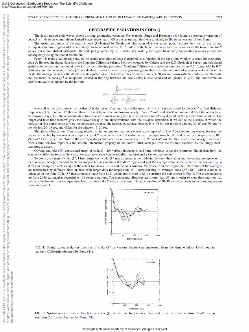
GEOGRAPHIC VARIATION IN CODA Q
The decay rate of coda waves shows a strong geographic variation. For example, Singh and Herrmann (43) found a systematic variation ofcoda Q at 1 Hz in the conterminous United States, more than 1000 in the central part decaying gradually to 200 in the western United States.
The spatial resolution of the map of coda Q obtained by Singh and Herrmann (43) was rather poor, because they had to use distantearthquakes to cover regions of low seismicity. As mentioned earlier, Eq. 1 holds for the lapse time to greater than about twice the travel time for Swaves. For a more distant earthquake, the coda part governed by Eq. 1 starts later, making the region traveled by backscattered waves greater andconsequently losing the spatial resolution.
Peng (44) made a systematic study of the spatial resolution of coda Q mapping as a function of the lapse time window selected for measuringcoda Q. He used the digital data from the Southern California Seismic Network operated by Caltech and the U.S. Geological Survey and calculatedspatial auto correlation function of coda Q−1 by the following procedure. Southern California is divided into meshes of size 0.2° (longitude) by 0.2°(latitude), and the average of coda Q−1 is calculated for each mesh by using seismograms that share the midpoint of epicenter and station in themesh. The average value for the ith mesh is designated as χi. Then two circles of radius r and r + 20 km are drawn with the center at the ith mesh,and the mean of coda Q−1 at midpoints located in the ring between the two circles is calculated and designated as yi(r). The autocorrelationcoefficient ρ(r) is computed by the formula
where M is the total number of meshes, χ� is the mean of χi, and ` (r) is the mean of yi(r). ρ(r) is calculated for coda Q−1 at four differentfrequencies (1.5, 3, 6, and 12 Hz) and three different lapse time windows—namely, 15–30, 20–45, and 30–60 sec measured from the origin time.As shown in Figs. 1–3, the autocorrelation functions are similar among different frequencies but clearly depend on the selected time window. Thelonger and later time window gives the slower decay in the autocorrelation with the distance separation. If we define the distance at which thecorrelation first comes close to 0 as the coherence distance, the average coherence distance is �135 km for the time window 30–60 sec, 90 km forthe window 20–45 sec, and 45 km for the window 15–30 sec.
The above observation offers strong support to the assumption that coda waves are composed of S to S back-scattering waves, because thedistances traveled by S waves with a typical crustal S wave velocity of 3.5 km/sec in half the lapse time 60, 45, and 30 sec are, respectively, 105,79, and 53 km, which are close to the corresponding coherence distance—namely, 135, 90, and 45 km. In other words, the coda Q−1 measuredfrom a time window represents the seismic attenuation property of the earth's crust averaged over the volume traversed by the singly back-scattering S waves.
Ouyang and Aki (45) constructed maps of coda Q−1 for various frequencies and time windows using the enormous digital data from theSouthern California Seismic Network, now available at the Southern California Earthquake Center data center.
To construct a map of coda Q−1, I first assign each coda Q−1 measurement at the midpoint between the station and the earthquake epicenter. Ithen average coda Q−1 measurements for midpoints lying within a 0.2°×0.2° region and plot the average value at the center of this region. Fig. 4shows an example of such a map for the center frequency 12 Hz and the coda window 20–30 sec from the origin time. The values of the averagesare represented by different sizes of dots, with larger dots for larger coda Q−1, corresponding to averaged coda Q−1 (10−3) within a range asindicated on the right. Coda Q−1 measurements made from 8931 seismograms were used to construct the map shown in Fig. 4. These seismogramsare from 2446 earthquakes recorded at 161 seismic stations. The hypocentral distances are shorter than 35 km in order to meet the condition thatthe coda window starts at the lapse time later than twice the S wave arrival time. The time window of 20–30 sec corresponds to the sampling regionof radius 30–45 km.
FIG. 1. Spatial autocorrelation function of coda Q−1 at various frequencies measured from the time window 15–30 sec insouthern California obtained by Peng (44).
FIG. 2. Spatial autocorrelation function of coda Q−1 at various frequencies measured from the time window 20–45 sec insouthern California obtained by Peng (44).
SCALE DEPENDENCE IN EARTHQUAKE PHENOMENA AND ITS RELEVANCE TO EARTHQUAKE PREDICTION 3743
Abou
t thi
s PD
F fil
e: T
his
new
dig
ital r
epre
sent
atio
n of
the
orig
inal
wor
k ha
s be
en re
com
pose
d fro
m X
ML
files
cre
ated
from
the
orig
inal
pap
er b
ook,
not
from
the
orig
inal
type
setti
ng fi
les.
Pag
e br
eaks
are
true
to th
e or
igin
al; l
ine
leng
ths,
wor
d br
eaks
, hea
ding
sty
les,
and
oth
er ty
pese
tting
-spe
cific
form
attin
g, h
owev
er, c
anno
t be
reta
ined
, and
som
e ty
pogr
aphi
c er
rors
may
hav
e be
en a
ccid
enta
lly in
serte
d. P
leas
e us
e th
e pr
int v
ersi
on o
f thi
s pu
blic
atio
n as
the
auth
orita
tive
vers
ion
for a
ttrib
utio
n.
Copyright © National Academy of Sciences. All rights reserved.
(NAS Colloquium) Earthquake Prediction: The Scientific Challengehttp://www.nap.edu/catalog/5709.html
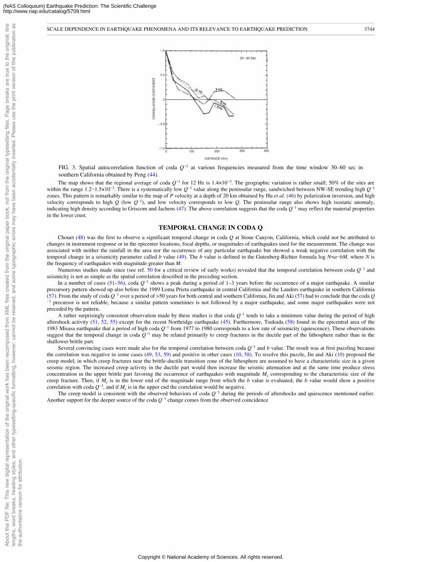
FIG. 3. Spatial autocorrelation function of coda Q−1 at various frequencies measured from the time window 30–60 sec insouthern California obtained by Peng (44).The map shows that the regional average of coda Q−1 for 12 Hz is 1.4×10⁻³. The geographic variation is rather small; 50% of the sites are
within the range 1.2−1.5×10⁻³. There is a systematically low Q−1 value along the peninsular range, sandwiched between NW-SE trending high Q−1
zones. This pattern is remarkably similar to the map of P velocity at a depth of 20 km obtained by Hu et al. (46) by polarization inversion, and highvelocity corresponds to high Q (low Q−1), and low velocity corresponds to low Q. The peninsular range also shows high isostatic anomaly,indicating high density according to Griscom and Jachens (47). The above correlation suggests that the coda Q−1 may reflect the material propertiesin the lower crust.
TEMPORAL CHANGE IN CODA Q
Chouet (48) was the first to observe a significant temporal change in coda Q at Stone Canyon, California, which could not be attributed tochanges in instrument response or in the epicenter locations, focal depths, or magnitudes of earthquakes used for the measurement. The change wasassociated with neither the rainfall in the area nor the occurrence of any particular earthquake but showed a weak negative correlation with thetemporal change in a seismicity parameter called b value (49). The b value is defined in the Gutenberg-Richter formula log N=a−bM, where N isthe frequency of earthquakes with magnitude greater than M.
Numerous studies made since (see ref. 50 for a critical review of early works) revealed that the temporal correlation between coda Q−1 andseismicity is not as simple as the spatial correlation described in the preceding section.
In a number of cases (51–56), coda Q−1 shows a peak during a period of 1–3 years before the occurrence of a major earthquake. A similarprecursory pattern showed up also before the 1989 Loma Prieta earthquake in central California and the Landers earthquake in southern California(57). From the study of coda Q−1 over a period of >50 years for both central and southern California, Jin and Aki (57) had to conclude that the coda Q−1 precursor is not reliable, because a similar pattern sometimes is not followed by a major earthquake, and some major earthquakes were notpreceded by the pattern.
A rather surprisingly consistent observation made by these studies is that coda Q−1 tends to take a minimum value during the period of highaftershock activity (51, 52, 55) except for the recent Northridge earthquake (45). Furthermore, Tsukuda (58) found in the epicentral area of the1983 Misasa earthquake that a period of high coda Q−1 from 1977 to 1980 corresponds to a low rate of seismicity (quiescence). These observationssuggest that the temporal change in coda Q−1 may be related primarily to creep fractures in the ductile part of the lithosphere rather than in theshallower brittle part.
Several convincing cases were made also for the temporal correlation between coda Q−1 and b value. The result was at first puzzling becausethe correlation was negative in some cases (49, 53, 59) and positive in other cases (10, 58). To resolve this puzzle, Jin and Aki (10) proposed thecreep model, in which creep fractures near the brittle-ductile transition zone of the lithosphere are assumed to have a characteristic size in a givenseismic region. The increased creep activity in the ductile part would then increase the seismic attenuation and at the same time produce stressconcentration in the upper brittle part favoring the occurrence of earthquakes with magnitude Mc corresponding to the characteristic size of thecreep fracture. Then, if Mc is in the lower end of the magnitude range from which the b value is evaluated, the b value would show a positivecorrelation with coda Q−1, and if Mc is in the upper end the correlation would be negative.
The creep model is consistent with the observed behaviors of coda Q−1 during the periods of aftershocks and quiescence mentioned earlier.Another support for the deeper source of the coda Q−1 change comes from the observed coincidence
SCALE DEPENDENCE IN EARTHQUAKE PHENOMENA AND ITS RELEVANCE TO EARTHQUAKE PREDICTION 3744
Abou
t thi
s PD
F fil
e: T
his
new
dig
ital r
epre
sent
atio
n of
the
orig
inal
wor
k ha
s be
en re
com
pose
d fro
m X
ML
files
cre
ated
from
the
orig
inal
pap
er b
ook,
not
from
the
orig
inal
type
setti
ng fi
les.
Pag
e br
eaks
are
true
to th
e or
igin
al; l
ine
leng
ths,
wor
d br
eaks
, hea
ding
sty
les,
and
oth
er ty
pese
tting
-spe
cific
form
attin
g, h
owev
er, c
anno
t be
reta
ined
, and
som
e ty
pogr
aphi
c er
rors
may
hav
e be
en a
ccid
enta
lly in
serte
d. P
leas
e us
e th
e pr
int v
ersi
on o
f thi
s pu
blic
atio
n as
the
auth
orita
tive
vers
ion
for a
ttrib
utio
n.
Copyright © National Academy of Sciences. All rights reserved.
(NAS Colloquium) Earthquake Prediction: The Scientific Challengehttp://www.nap.edu/catalog/5709.html
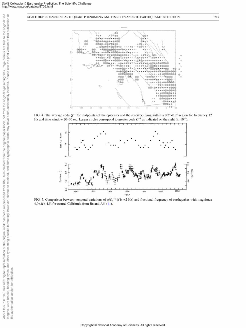
FIG. 4. The average coda Q−1 for midpoints (of the epicenter and the receiver) lying within a 0.2°×0.2° region for frequency 12Hz and time window 20–30 sec. Larger circles correspond to greater coda Q−1 as indicated on the right (in 10−3).
FIG. 5. Comparison between temporal variations of πfQc−1 (f is �2 Hz) and fractional frequency of earthquakes with magnitude
4.0<M< 4.5, for central California from Jin and Aki (11).
SCALE DEPENDENCE IN EARTHQUAKE PHENOMENA AND ITS RELEVANCE TO EARTHQUAKE PREDICTION 3745
Abou
t thi
s PD
F fil
e: T
his
new
dig
ital r
epre
sent
atio
n of
the
orig
inal
wor
k ha
s be
en re
com
pose
d fro
m X
ML
files
cre
ated
from
the
orig
inal
pap
er b
ook,
not
from
the
orig
inal
type
setti
ng fi
les.
Pag
e br
eaks
are
true
to th
e or
igin
al; l
ine
leng
ths,
wor
d br
eaks
, hea
ding
sty
les,
and
oth
er ty
pese
tting
-spe
cific
form
attin
g, h
owev
er, c
anno
t be
reta
ined
, and
som
e ty
pogr
aphi
c er
rors
may
hav
e be
en a
ccid
enta
lly in
serte
d. P
leas
e us
e th
e pr
int v
ersi
on o
f thi
s pu
blic
atio
n as
the
auth
orita
tive
vers
ion
for a
ttrib
utio
n.
Copyright © National Academy of Sciences. All rights reserved.
(NAS Colloquium) Earthquake Prediction: The Scientific Challengehttp://www.nap.edu/catalog/5709.html
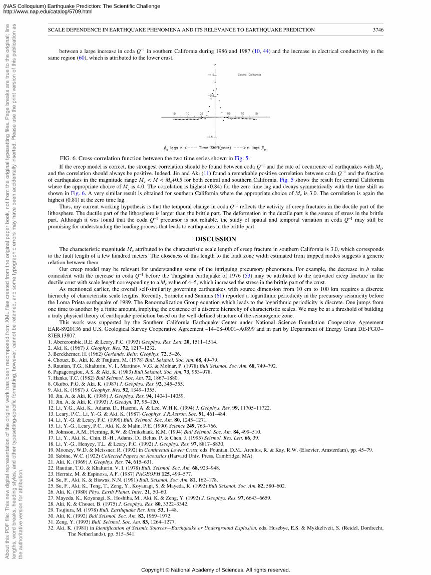
between a large increase in coda Q−1 in southern California during 1986 and 1987 (10, 44) and the increase in electrical conductivity in thesame region (60), which is attributed to the lower crust.
FIG. 6. Cross-correlation function between the two time series shown in Fig. 5.If the creep model is correct, the strongest correlation should be found between coda Q−1 and the rate of occurrence of earthquakes with Mc,
and the correlation should always be positive. Indeed, Jin and Aki (11) found a remarkable positive correlation between coda Q−1 and the fractionof earthquakes in the magnitude range Mc < M < Mc+0.5 for both central and southern California. Fig. 5 shows the result for central Californiawhere the appropriate choice of Mc is 4.0. The correlation is highest (0.84) for the zero time lag and decays symmetrically with the time shift asshown in Fig. 6. A very similar result is obtained for southern California where the appropriate choice of Mc is 3.0. The correlation is again thehighest (0.81) at the zero time lag.
Thus, my current working hypothesis is that the temporal change in coda Q−1 reflects the activity of creep fractures in the ductile part of thelithosphere. The ductile part of the lithosphere is larger than the brittle part. The deformation in the ductile part is the source of stress in the brittlepart. Although it was found that the coda Q−1 precursor is not reliable, the study of spatial and temporal variation in coda Q−1 may still bepromising for understanding the loading process that leads to earthquakes in the brittle part.
DISCUSSION
The characteristic magnitude Mc attributed to the characteristic scale length of creep fracture in southern California is 3.0, which correspondsto the fault length of a few hundred meters. The closeness of this length to the fault zone width estimated from trapped modes suggests a genericrelation between them.
Our creep model may be relevant for understanding some of the intriguing precursory phenomena. For example, the decrease in b valuecoincident with the increase in coda Q−1 before the Tangshan earthquake of 1976 (53) may be attributed to the activated creep fracture in theductile crust with scale length corresponding to a Mc value of 4–5, which increased the stress in the brittle part of the crust.
As mentioned earlier, the overall self-similarity governing earthquakes with source dimension from 10 cm to 100 km requires a discretehierarchy of characteristic scale lengths. Recently, Sornette and Sammis (61) reported a logarithmic periodicity in the precursory seismicity beforethe Loma Prieta earthquake of 1989. The Renormalization Group equation which leads to the logarithmic periodicity is discrete. One jumps fromone time to another by a finite amount, implying the existence of a discrete hierarchy of characteristic scales. We may be at a threshold of buildinga truly physical theory of earthquake prediction based on the well-defined structure of the seismogenic zone.
This work was supported by the Southern California Earthquake Center under National Science Foundation Cooperative AgreementEAR-8920136 and U.S. Geological Survey Cooperative Agreement –14–08–0001–A0899 and in part by Department of Energy Grant DE-FG03–87ER13807.1. Abercrombie, R.E. & Leary, P.C. (1993) Geophys. Res. Lett. 20, 1511–1514.2. Aki, K. (1967) J. Geophys. Res. 72, 1217–1232.3. Berckhemer, H. (1962) Gerlands. Beitr. Geophys. 72, 5–26.4. Chouet, B., Aki, K. & Tsujiura, M. (1978) Bull. Seismol. Soc. Am. 68, 49–79.5. Rautian, T.G., Khalturin, V. I., Martinov, V.G. & Molnar, P. (1978) Bull Seismol. Soc. Am. 68, 749–792.6. Papageorgiou, A.S. & Aki, K. (1983) Bull Seismol. Soc. Am. 73, 953–978.7. Hanks, T.C. (1982) Bull Seismol. Soc. Am. 72, 1867–1880.8. Okubo, P.G. & Aki, K. (1987) J. Geophys. Res. 92, 345–355.9. Aki, K. (1987) J. Geophys. Res. 92, 1349–1355.10. Jin, A. & Aki, K. (1989) J. Geophys. Res. 94, 14041–14059.11. Jin, A. & Aki, K. (1993) J. Geodyn. 17, 95–120.12. Li, Y.G., Aki, K., Adams, D., Hasemi, A. & Lee, W.H.K. (1994) J. Geophys. Res. 99, 11705–11722.13. Leary, P.C., Li, Y.-G. & Aki, K. (1987) Geophys. J.R.Astron. Soc. 91, 461–484.14. Li, Y.-G. & Leary, P.C. (1990) Bull. Seismol. Soc. Am. 80, 1245–1271.15. Li, Y.-G., Leary, P.C., Aki, K. & Malin, P.E. (1990) Science 249, 763–766.16. Johnson, A.M., Fleming, R.W. & Cruikshank, K.M. (1994) Bull Seismol. Soc. Am. 84, 499–510.17. Li, Y., Aki, K., Chin, B.-H., Adams, D., Beltas, P. & Chen, J. (1995) Seismol. Res. Lett. 66, 39.18. Li, Y.-G., Henyey, T.L. & Leary, P.C. (1992) J. Geophys. Res. 97, 8817–8830.19. Mooney, W.D. & Meissner, R. (1992) in Continental Lower Crust, eds. Fountan, D.M., Arculus, R. & Kay, R.W. (Elsevier, Amsterdam), pp. 45–79.20. Sabine, W.C. (1922) Collected Papers on Acoustics (Harvard Univ. Press, Cambridge, MA).21. Aki, K. (1969) J. Geophys. Res. 74, 615–631.22. Rautian, T.G. & Khalturin, V. I. (1978) Bull. Seismol. Soc. Am. 68, 923–948.23. Herraiz, M. & Espinosa, A.F. (1987) PAGEOPH 125, 499–577.24. Su, F., Aki, K. & Biswas, N.N. (1991) Bull. Seismol. Soc. Am. 81, 162–178.25. Su, F., Aki, K., Teng, T., Zeng, Y., Koyanagi, S. & Mayeda, K. (1992) Bull Seismol. Soc. Am. 82, 580–602.26. Aki, K. (1980) Phys. Earth Planet. Inter. 21, 50–60.27. Mayeda, K., Koyanagi, S., Hoshiba, M., Aki, K. & Zeng, Y. (1992) J. Geophys. Res. 97, 6643–6659.28. Aki, K. & Chouet, B. (1975) J. Geophys. Res. 80, 3322–3342.29. Tsujiura, M. (1978) Bull. Earthquake Res. Inst. 53, 1–48.30. Aki, K. (1992) Bull Seismol. Soc. Am. 82, 1969–1972.31. Zeng, Y. (1993) Bull. Seismol. Soc. Am. 83, 1264–1277.32. Aki, K. (1981) in Identification of Seismic Sources—Earthquake or Underground Explosion, eds. Husebye, E.S. & Mykkeltveit, S. (Reidel, Dordrecht,
The Netherlands), pp. 515–541.
SCALE DEPENDENCE IN EARTHQUAKE PHENOMENA AND ITS RELEVANCE TO EARTHQUAKE PREDICTION 3746
Abou
t thi
s PD
F fil
e: T
his
new
dig
ital r
epre
sent
atio
n of
the
orig
inal
wor
k ha
s be
en re
com
pose
d fro
m X
ML
files
cre
ated
from
the
orig
inal
pap
er b
ook,
not
from
the
orig
inal
type
setti
ng fi
les.
Pag
e br
eaks
are
true
to th
e or
igin
al; l
ine
leng
ths,
wor
d br
eaks
, hea
ding
sty
les,
and
oth
er ty
pese
tting
-spe
cific
form
attin
g, h
owev
er, c
anno
t be
reta
ined
, and
som
e ty
pogr
aphi
c er
rors
may
hav
e be
en a
ccid
enta
lly in
serte
d. P
leas
e us
e th
e pr
int v
ersi
on o
f thi
s pu
blic
atio
n as
the
auth
orita
tive
vers
ion
for a
ttrib
utio
n.
Copyright © National Academy of Sciences. All rights reserved.
(NAS Colloquium) Earthquake Prediction: The Scientific Challengehttp://www.nap.edu/catalog/5709.html

33. Frankel, A. & Clayton, R.W. (1986) J. Geophys. Res. 91, 6465– 6489.34. Matsunami, K. (1991) Phys. Earth Planet. Inter. 67, 104–114.35. Shang, T. & Gao, L.S. (1988) Sci. Sin. Ser. V 31, 1503–1514.36. Aki, K. (1991) Phys. Earth Planet. Inter. 67, 1–3.37. Wu, R. (1985) Geophys. J.R.Astron. Soc. 82, 57–80.38. Gao, L.S., Lee, L.C., Biswas, N.N. & Aki, K. (1983) Bull. Seismol. Soc. Am. 73, 377–390.39. Zeng, Y., Su, F. & Aki, K. (1991) J. Geophys. Res. 96, 607–619.40. Hoshiba, M, Sato, H. & Fehler, M. (1991) Paper Meteorol. Geophys. 42, 65–91.41. Hoshiba, M. (1993) J. Geophys. Res. 98, 15809–15824.42. Jin, A., Mayeda, K., Adams, D. & Aki, K. (1994) J. Geophys. Res. 99, 17835–17848.43. Singh, S.K. & Herrmann, R.B. (1983) J. Geophys. Res. 88, 527–538.44. Peng, J.Y. (1989) Thesis (Univ. Southern California, Los Angeles).45. Ouyang, H. & Aki, K. (1994) Eos 75, 168 (abstr.).46. Hu, G., Menke, W. & Powell, C. (1994) J. Geophys. Res. 99, 15245–15256.47. Griscom, A. & Jachens, R.C. (1990) San Andreas Fault System, California (U.S. Geological Survey, Reston, Va), Professional Paper 1515, pp. 239–260.48. Chouet, B. (1979) Geophys. Res. Lett. 6, 143–146.49. Aki, K. (1985) Earthquake Prediction Res. 3, 219–230.50. Sato, H. (1988) PAGEOPH 126, 465–498.51. Gusev, A.A. & Lemzikov, V.K. (1984) Vulk. Seismol. 4, 76–90.52. Novelo-Casanova, D. A, Berg, E., Hsu, H. & Helsley, C.E. (1985) Geophys. Res. Lett. 12, 789–792.53. Jin, A. & Aki, K. (1986) J. Geophys. Res. 91, 665–673.54. Sato, H. (1986) J. Geophys. Res. 91, 2049–2061.55. Faulkner, J. (1988) Thesis (Univ. of Southern California, Los Angeles).56. Su, F. & Aki, K. (1990) PAGEOPH 133, 23–52.57. Jin, A. & Aki, K. (1993) J. Geodyn. 17, 95–120.58. Tsukuda, T. (1988) PAGEOPH 128, 261–280.59. Robinson, R. (1987) PAGEOPH 125, 579–596.60. Madden, T.R., LaTorraca, G.A. & Park, S.K. (1993) J. Geophys. Res. 98, 795–808.61. Sornette, D. & Sammis, C.G. (1995) J. Phys. (Paris), in press.
SCALE DEPENDENCE IN EARTHQUAKE PHENOMENA AND ITS RELEVANCE TO EARTHQUAKE PREDICTION 3747
Abou
t thi
s PD
F fil
e: T
his
new
dig
ital r
epre
sent
atio
n of
the
orig
inal
wor
k ha
s be
en re
com
pose
d fro
m X
ML
files
cre
ated
from
the
orig
inal
pap
er b
ook,
not
from
the
orig
inal
type
setti
ng fi
les.
Pag
e br
eaks
are
true
to th
e or
igin
al; l
ine
leng
ths,
wor
d br
eaks
, hea
ding
sty
les,
and
oth
er ty
pese
tting
-spe
cific
form
attin
g, h
owev
er, c
anno
t be
reta
ined
, and
som
e ty
pogr
aphi
c er
rors
may
hav
e be
en a
ccid
enta
lly in
serte
d. P
leas
e us
e th
e pr
int v
ersi
on o
f thi
s pu
blic
atio
n as
the
auth
orita
tive
vers
ion
for a
ttrib
utio
n.
Copyright © National Academy of Sciences. All rights reserved.
(NAS Colloquium) Earthquake Prediction: The Scientific Challengehttp://www.nap.edu/catalog/5709.html
This paper was presented at a colloquium entitled “Earthquake Prediction: The Scientific Challenge,” organized by Lean Knopoff(Chair), Keiiti Aki, Clarence R.Allen, James R.Rice, and Lynn R.Sykes, held February 10 and 11, 1995, at the National Academy of Sciences inIrvine, CA.
Intermediate-term earthquake prediction
(premonitory seismicity patterns/dynamics of seismicity/chaotic systems/instability)V.I.KEILIS-BOROK
International Institute of Earthquake Prediction Theory and Mathematical Geophysics, Russian Academy of Sciences, Warshavskoye shosse79, kor 2, Moscow 113556, Russia
ABSTRACT An earthquake of magnitude M and linear source dimension L(M) is preceded within a few years by certain patterns ofseismicity in the magnitude range down to about (M−3) in an area of linear dimension about 5L−10L. Prediction algorithms based on suchpatterns may allow one to predict ����80% of strong earthquakes with alarms occupying altogether 20–30% of the time-space considered.An area of alarm can be narrowed down to 2L-3L when observations include lower magnitudes, down to about (M−4). In spite of theirlimited accuracy, such predictions open a possibility to prevent considerable damage. The following findings may provide for furtherdevelopment of prediction methods: (i) long-range correlations in fault system dynamics and accordingly large size of the areas over whichdifferent observed fields could be averaged and analyzed jointly, (ii) specific symptoms of an approaching strong earthquake, (iii) thepartial similarity of these symptoms worldwide, (iv) the fact that some of them are not Earth specific: we probably encountered inseismicity the symptoms of instability common for a wide class of nonlinear systems.
Commonly known are five major stages of earthquake prediction, which are usually distinguished. They differ in characteristic time intervalsfor which an alarm is declared. The background stage provides a map of maximal possible magnitudes and a map of average recurrence time forstrong earthquakes of different magnitudes. The other four stages are as follows: long-term (tens of years), intermediate-term (years), short-term(months to weeks), and immediate (days and less). A smaller time interval in present predictions does not necessarily mean a smaller area of alarmwhere a strong earthquake has to be expected. Possibility of prediction has been explored separately for different stages and, with rare exceptions,their connection is not yet achieved. Here we review the intermediate-term stage.
A new understanding of the earthquake prediction problem and the whole dynamics of seismicity has crystallized over the past decade: theseismically active lithosphere has become regarded as a hierarchical nonlinear (chaotic) dissipative system (e.g., see refs. 1–3). The simplest sourceof nonlinearity of this system is abrupt triggering of an earthquake when the stress exceeds the strength of a fault. Other powerful sources ofnonlinearity are provided by a multitude of the processes controlling the distribution of strength within the lithosphere. Among such processes arenonlinear filtration of fluids (4), stress corrosion, caused by surface-active fluids (5, 6), dissolution of rocks (6), buckling, microfracturing, phasetransformation of the minerals, etc. Except for rather special cases, none of these mechanisms predominates to such an extent that the others can beneglected. In the time scale relevant to intermediate-term earthquake prediction, these mechanisms seem to make the lithosphere a chaotic system;this is an inevitable conjecture, but it is not yet proven in a mathematical sense.
Predictability of a chaotic process may be achieved in two ways. First, such process often follows a certain scenario; recognizing its beginningone would know the subsequent development. Second, a chaotic process may become predictable, up to a limit, after an averaging. Most of theresults described below are obtained in the second way. It was found that the approach of a “strong” earthquake may be indicated by certainpatterns in an earthquake sequence; they are called premonitory seismicity patterns and are used in prediction algorithms reviewed here.
A test of prediction algorithms is crucially important, since they are inevitably adjusted retrospectively. The algorithms discussed here weretested first by applying them to the regions or time periods not involved either in the design of the algorithm or in the fitting of adjustableparameters. The ultimate test is the advance prediction. We review here only such prediction methods that are formally defined so that theirperformance can be tested and statistical significance can be evaluated. A methodology for such evaluation is suggested (7).
FOUR PARADIGMS
The search of premonitory seismicity patterns in observed and in computer-simulated seismicity revealed four of their basic features, whichare important for understanding the earthquake prediction problem. In hindsight, they are obvious, being common for many nonlinear systems. Forseismology, they are hardly news either, as they correspond to many well-known traits of the dynamics of seismicity, such as the Gutenberg-Richter relation, the Omori law, and migration of seismicity (8). Nevertheless, these features are the new paradigms in earthquake predictionresearch where they are often overlooked. We outline them here as a background for the discussion of prediction algorithms in the next section.
(i) Long-Range Correlations. The generation of an earthquake is not localized around its source. A flow of earthquakes is generated by asystem of blocks and faults rather than each earthquake by a single fault. Accordingly, the signal of an approaching earthquake may inconvenientlycome not from a narrow vicinity of the incipient source but from a much wider area; its linear dimension at intermediate-term stage is at least 5L(M)−10L(M), with M being the magnitude of the incipient earthquake and L(M) the characteristic length of its source. Moreover, according to ref. 9,this dimension can reach
The publication costs of this article were defrayed in part by page charge payment. This article must therefore be hereby marked“advertisement” in accordance with 18 U.S.C. §1734 solely to indicate this fact.
Abbreviation: TIP, time of increased probability of a strong earthquake (an alarm).
INTERMEDIATE-TERM EARTHQUAKE PREDICTION 3748
Abou
t thi
s PD
F fil
e: T
his
new
dig
ital r
epre
sent
atio
n of
the
orig
inal
wor
k ha
s be
en re
com
pose
d fro
m X
ML
files
cre
ated
from
the
orig
inal
pap
er b
ook,
not
from
the
orig
inal
type
setti
ng fi
les.
Pag
e br
eaks
are
true
to th
e or
igin
al; l
ine
leng
ths,
wor
d br
eaks
, hea
ding
sty
les,
and
oth
er ty
pese
tting
-spe
cific
form
attin
g, h
owev
er, c
anno
t be
reta
ined
, and
som
e ty
pogr
aphi
c er
rors
may
hav
e be
en a
ccid
enta
lly in
serte
d. P
leas
e us
e th
e pr
int v
ersi
on o
f thi
s pu
blic
atio
n as
the
auth
orita
tive
vers
ion
for a
ttrib
utio
n.
Copyright © National Academy of Sciences. All rights reserved.
(NAS Colloquium) Earthquake Prediction: The Scientific Challengehttp://www.nap.edu/catalog/5709.html
�100L: the Parkfield earthquakes with a magnitude of �6 are preceded by a rise of activity in as far as the Great Basin or the Gulf of California.Such an area may include different types of faults. Many examples for different regions worldwide can be found (10–13). Other evidence andpossible mechanisms of long-range correlations are discussed in the last section.
(ii) Premonitory Phenomena. Before a strong earthquake, the earthquake flow in a medium magnitude range becomes more intense andirregular; earthquakes become more clustered in space and time and the range of their correlation probably increases (12, 13). These symptomsmay be interpreted as an increased response of the lithosphere to excitation (possibly provided by consecutive earthquakes themselves); such aresponse is symptomatic of a critical state in many other nonlinear systems. Some of these symptoms are formally defined in the next section.
(iii) Similarity. In robust definition, the normalized premonitory phenomena are identical in the magnitude range of at least M≥4.5 and for awide variety of neotectonic environments (12–14), which include subduction zones, transform faults, intraplate faults in the platforms, inducedseismicity near artificial lakes, and rock bursts in mines. This similarity is limited and on its background the regional variations of premonitoryphenomena begin to emerge.
(iv) The Non-Earth-Specific Nature of Some Premonitory Phenomena. Many premonitory seismicity patterns are found in the models ofexceedingly simple design. Some of such models, consisting of lattices of interacting point elements, are totally free of Earth-specific (or evensolid-body-specific) mechanisms (15–17); other models retain only the simplest mechanism-friction (18–21). A stochastic model suggested in ref.22 goes a long way toward explaining swarms, quiescence, foreshocks, and mainshocks as a coordinated sequence.
PREDICTION ALGORITHMS
The algorithms reviewed here are based on a common general scheme of data analysis and on premonitory seismicity patterns with similarscaling and normalization. We outline these common features first.
Scheme of Data Analysis. The scheme of data analysis (Fig. 1) can be summarized as follows:(i) Strong earthquakes are identified by the condition M≥ M0. M0 is the given threshold chosen in such a way that the average time interval
between strong earthquakes is sufficiently large in the area considered. The intervals (M0, M0+ 0.5) may be analyzed separately.(ii) Prediction is aimed at determination of a time of increased probability (TIP) that is the time interval within which a strong earthquake
has to be expected.(iii) A seismic region under investigation is overlaid by areas whose size depends on M0. In each area, the sequence of earthquakes is
analyzed. We determine its robust averaged traits, which are useful for prediction (the most commonly considered traits are indicated inFig. 1). These traits are depicted by functions of time t defined in the sliding time windows with a common end t. We search for thefunctions whose values have different distributions inside and outside the TIPs. One or several of such functions could be used forprediction; a combination of precursors may be useful for prediction even if some of them show unsatisfactory performance when usedseparately. A variety of premonitory seismicity patterns was found in such a way.
FIG. 1. General scheme of prediction. Vertical lines show earthquake sequence in an area. Several traits of this sequence aredefined in sliding time windows shown by horizontal bars. TIPs (alarms) are recognized by one or several such traits.Obviously this scheme is open for inclusion of other traits and other data, not necessarily seismological ones.Major Common Characteristics. Major common characteristics of premonitory patterns considered here include the following:
(i) Robustness. We have to look for the patterns common in a wide variety of regions and magnitude ranges as well as within sufficientlylong time periods; otherwise the test of prediction algorithms would be practically impossible. Accordingly, premonitory patterns aregiven robust definitions in which the diversity of circumstances is averaged away while some predictive power is retained.
(ii) Time scale. The earthquake flow is averaged over time intervals a few years long and duration of alarms is about the same. Theseintervals do not depend on M0, while according to the Gutenberg-Richter relation the earthquakes with smaller magnitudes occur morefrequently; the average time between the earthquakes of magnitude M is proportional to 10BM.* This is not a contradiction, since theGutenberg-Richter law refers to a given region, the same for all magnitudes, while premonitory patterns are defined for an area with alinear dimension proportional to 10aM0. The average time between the earthquakes in such an area would be proportional to 10(B−av)M0 where v is the fractal dimension of the cloud of the epicenters. The existing estimations of parameters B (�1), a (0.5−1), and v (1.2−2) do not contradict the hypothesis that the expression in brackets is close to 0 as if the earthquakes with different magnitudes haveabout the same recurrence time in their own cells. Still, for some premonitory patterns the time scale may depend on M0 (23).
(iii) Normalization. Normalization of an earthquake flow is necessary to ensure that a prediction algorithm can be applied with the same setof adjustable parameters in the regions with different seismicity. In the studies reviewed here, an earthquake flow is normalized by theminimal magnitude cutoff Mmin? defined by one of the two conditions: Mmin=(M0−a) or Ñ(Mmin)=b, Ñ being the average annual numberof earthquakes with magnitude M≥Mmin; parameters a and b are common for all areas. If the second condition is applied, the intensityof the earthquake flow considered is the same in different areas, while Mmin may be different.
I now describe the prediction algorithms; the first one is defined in greater detail, for illustration.
ALGORITHM M8
*Here and below the letters A, B, C�, a, b, c�, etc., signify numerical parameters; a letter may have a different meaning in differentdefinitions.
INTERMEDIATE-TERM EARTHQUAKE PREDICTION 3749
Abou
t thi
s PD
F fil
e: T
his
new
dig
ital r
epre
sent
atio
n of
the
orig
inal
wor
k ha
s be
en re
com
pose
d fro
m X
ML
files
cre
ated
from
the
orig
inal
pap
er b
ook,
not
from
the
orig
inal
type
setti
ng fi
les.
Pag
e br
eaks
are
true
to th
e or
igin
al; l
ine
leng
ths,
wor
d br
eaks
, hea
ding
sty
les,
and
oth
er ty
pese
tting
-spe
cific
form
attin
g, h
owev
er, c
anno
t be
reta
ined
, and
som
e ty
pogr
aphi
c er
rors
may
hav
e be
en a
ccid
enta
lly in
serte
d. P
leas
e us
e th
e pr
int v
ersi
on o
f thi
s pu
blic
atio
n as
the
auth
orita
tive
vers
ion
for a
ttrib
utio
n.
Algorithm M8 (13) was designed by retrospective analysis of seismicity preceding the greatest (M≥8) earthquakes world- wide, hence its
Copyright © National Academy of Sciences. All rights reserved.
(NAS Colloquium) Earthquake Prediction: The Scientific Challengehttp://www.nap.edu/catalog/5709.html
name. The scheme of prediction described above (Fig. 1) is implemented by this algorithm in the following way:(i) The territory considered is scanned by overlapping circles with the diameter D(M0). A set of such circles, considered for prediction of
Californian earthquakes with M≥7, is shown in Fig. 2A.(ii) Within each circle, the sequence of earthquakes is considered with aftershocks eliminated {ti, mi, hi, bi(e)}, i=1, 2� Here ti is the origin
time, ti≤ti+1; m is the magnitude, hi is focal depth, and b(ei) is the number of aftershocks during the first e days. The sequence isnormalized by lower magnitude cutoff Mmin(Ñ), with a standard value of Ñ.
(iii) Several functions of time t characterizing this sequence are computed in the sliding time windows (t−s, t) and magnitude rangeM0>Mi≥Mmin(Ñ). These functions include
(a) N(t), the number of the main shocks.(b) L(t), the deviation of N(t) from the long-term trend.
Ncum(t) is the total number of the main shocks with M≥Mmin from the beginning of the sequence t0 to t.(c) Z(t), concentration of the main shocks estimated as the ratio of the average diameter of the source l to the average distance between
them r. The following coarse estimations of r and l are assumed: r~N−1/3, l~N−1·Σ(t), where Σ(t)= Σi 10d(Mi−f), and Mmin≤Mi≤M0−g; thevalue of d is chosen in such a way that each summand is proportional to the linear dimension of the source (in practice, to the cubicroot of energy, E1/3). A more refined estimation of Z has been considered in ref. 24.
FIG. 2. Advance prediction by algorithm M8 of the Loma Prieta, California, earthquake, 1989, M=7.1. (A) Areas of alarms. Theterritory was scanned by eight overlapping circles. TIPs were diagnosed in the darkened circles. Star shows the epicenter of theLoma Prieta earthquake. Solid polygon shows the reduced area of alarm; it is determined in retrospection by applying algorithmMendocino Scenario described below. (B) Diagnosis of the TIP in the third from she bottom circle. Very large values offunctions (dots) are concentrated in a 3-year interval, 1985–1987 (light rectangle). TIP was declared for the next 5 years (darkerrectangle). Other explanations are given in the text.(d) B(t)=max{i} {bi}, the maximal number of aftershocks (a measure of earthquake clustering); the earthquake sequence {i} is considered in
the time window (t−s�, t) and in the magnitude range (M0−p, M0−q).(iv) Each of the functions N, L, Z is calculated for Ñ=20 and Ñ=10. As a result, the earthquake sequence is given a robust averaged
description by seven functions: N, L, Z (twice each) and B.(v) Very large values are identified for each function using the condition that they exceed Q percentiles (i.e., they are higher than Q% of
the encountered values).(vi) An alarm or TIP is declared for 5 years, when at least 6 of 7 functions, including B, become very large within a narrow time window (t
−u, t). To make a prediction more stable, this condition is required for two consecutive moments, t and t+0.5 years.
Standard Parameters. The following standard values of parameters indicated above are fixed in the algorithm M8‡: D(M0)={exp(M0−5.6)+1}° in degrees of meridian (this is 276, 560, and 1333 km for M0=6, 7, and 8, respectively), s=6 years, s�=1 year, g=0.5, p=2, q=0.2, u=3 years,Q=75% for B and 90% for the other 6 functions.
Obviously, the magnitude scale used in this and other algorithms described here should not saturate within the magnitude range considered;otherwise computation of the function becomes meaningless. Accordingly, maximal magnitudes indicated in the catalog are used; MS usually istaken for larger magnitudes and mb for smaller ones. The use of only the mb scale, which saturates at about mb=6, renders invalid the “test ofalgorithm M8” in ref. 25.
An example of prediction by algorithm M8 is given in Fig. 2 . Shown at the top of Fig. 2B is the sequence of the main shocks in the third fromthe bottom circle in Fig. 2A. Seven functions describing the earthquake flow are plotted below; indexes 1 and 2 correspond to Ñ=10 and 20,respectively. Very large values are indicated by the solid circles. The start of the TIP (July 1987) is indicated by a vertical line. Loma Prietaearthquake, California, 1989, M=7.1, occurred 28 months later. Note that in the adjacent circle the TIP started in 1985. A more detailed casehistory of this prediction (made in advance) is described in ref. 26.
‡In this and other algorithms described here, all adjustable parameters are defined in a robust way, so that their reasonable variation doesnot affect the predictions.
INTERMEDIATE-TERM EARTHQUAKE PREDICTION 3750
Abou
t thi
s PD
F fil
e: T
his
new
dig
ital r
epre
sent
atio
n of
the
orig
inal
wor
k ha
s be
en re
com
pose
d fro
m X
ML
files
cre
ated
from
the
orig
inal
pap
er b
ook,
not
from
the
orig
inal
type
setti
ng fi
les.
Pag
e br
eaks
are
true
to th
e or
igin
al; l
ine
leng
ths,
wor
d br
eaks
, hea
ding
sty
les,
and
oth
er ty
pese
tting
-spe
cific
form
attin
g, h
owev
er, c
anno
t be
reta
ined
, and
som
e ty
pogr
aphi
c er
rors
may
hav
e be
en a
ccid
enta
lly in
serte
d. P
leas
e us
e th
e pr
int v
ersi
on o
f thi
s pu
blic
atio
n as
the
auth
orita
tive
vers
ion
for a
ttrib
utio
n.
Copyright © National Academy of Sciences. All rights reserved.
(NAS Colloquium) Earthquake Prediction: The Scientific Challengehttp://www.nap.edu/catalog/5709.html
Performance. Algorithm M8 was first applied retrospectively (13) with prefixed parameters to the following 12 regions not considered in itsdevelopment (the values of M0, defining a strong earthquake, are indicated in brackets).
Circum Pacific belt. Central America [8], Kamchatka-Kuril Island [7.5], Japan-Taiwan [7.5], South America [7.5], and Western US [7.5 and7].
Alpine-Himalayan belt. The Lake Baikal and the Stanovoy range [6.7], the Caucasus [6.5], the Pamir and Tien Shan [6.5], Eastern Tien Shan[6.5], Western Turkmenia [6.5], the Apennines [6.5], and the area of induced seismicity near Koyna reservoir [4.9].
The time intervals from 9 to 40 years long, all ending around 1985, were considered in different regions, depending on availability of data.An experiment in advance prediction (27, 28) started in about 1985 for the Circum Pacific belt [8 and 7.5], western United States [7.0], the
seven above-mentioned regions of the Alpine-Himalayan belt, and Lesser Antilles [6]. The breakdown of predictions may be summarized in Table 1.
ALGORITHM CN
Algorithm CN (12, 29) was designed by retrospective analysis of seismicity patterns preceding the earthquakes with M≥6.5 in California andthe adjacent part of Nevada, hence its name. The essence of this algorithm can be summarized as follows.
(i) Areas of investigation are selected taking into account the spatial distribution of seismicity.(ii) Within each area we consider the earthquakes with the average annual number Ñ=3 (after elimination of aftershocks). As compared
with Ñ=20 in algorithm M8 this gives a higher magnitude cutoff Mmin.(iii) The sequence of earthquakes is described by 9 functions. Three of them—N, Z, and B—are similar to the ones defined above, although
with different values of the numerical parameters. Other functions depict the share of relatively higher magnitudes in the sequenceconsidered, the different variations of this sequence in time, and the average value of source areas, where the slip (or rupture) took place.
(iv) Following the pattern recognition routine (30), these functions are coarsely discretized so that we distinguish only large, medium, andsmall values divided by 2/3 and 1/3 percentiles or large and small values divided by 1/2 percentile.
(v) The alarms (TIPs) are determined by certain combinations—pairs or triplets—of these discretized functions; these combinations werefound by applying the pattern recognition algorithm called subclasses (30). Qualitatively, a TIP is diagnosed when earthquakeclustering is high, seismicity is irregular, high and growing, and the increase of seismicity was preceded by a quiescence. Examples ofprediction by algorithm CN are given in Fig. 3.
Table 1. Breakdown of predictions
Prediction Strong earthquakes, total/predicted Time-space occupied by TIPsIn retrospect 25/22 (88%) 16%In advance 33/26 (78%) 19%Total 58/48 (83%)
Performance. Algorithm CN was first tested retrospectively with prefixed parameters for the following 21 regions (12).Circum Pacific belt. Northern and Southern California [6.4], the Gulf of California [6.6], Cocos plate margins [6.5], and adjacent to the belt
Lesser Antillean arc [5.5].Alpine-Himalayan belt. The area of intermediate-depth earthquakes in Vrancea, East Carpatheans [6.4], the Pamir [6.5], the Tien Shan [6.5],
the Baikal [6.4], Central Italy [5.6], the Caucasus [6.4], Kangra, Nepal and Assam regions in the Himalayas [6.4], Krasnovodsk, Elburz and KopetDag areas [6.4], and the Dead Sea rift [5.0].
Low seismicity regions. Northern and Southern Appalachians [5.0], Brabant-Ardennes [4.5].The earthquake catalogs available allowed one to consider time intervals from 12 to 22 years in each region, except 32 years in Italy and 45
years in California. Sixty strong earthquakes occurred in all the regions during these intervals. Of them 50 (83%) occurred during the TIPs and 10were missed. TIPs in a region occupy on an average 27% of the time, from 2 to 4 years per earthquake (except 6–8 years in the southern part ofDead Sea rift, Kopet Dag, and Vrancea).
An experiment in advance prediction for all these regions was subsequently carried out for 3–12 more years in a region (31). The breakdownof predictions is as follows:
strong earthquakes M0≤M≤M0+0.5 M>M0+0.5total/predicted 11/8(73%) 11/4(36%)The duration of a TIP was from 1 to 2 years per earthquake but 6 years in Nepal. We see that prediction by algorithm CN is more reliable for
strong earthquakes, which occur on an average once in 7–10 years (Ñ=0.15−0.1); prediction of stronger earthquakes should probably be madeseparately, in larger areas. This breakdown is not made for the retrospective test, since the magnitudes were often rounded up to 0.5 during thecorresponding time intervals.
On the whole, algorithm CN gets 2/3 of strong earthquakes within the TIPs, occupying 1/3 of the time. In subduction zones, performance ofthis algorithm is poor, although the 9 functions, mentioned above, do have different distributions within and outside of the TIPs. It seems that othercombinations of functions have to be used for subduction zones.
FIG. 3. Strong earthquakes and TIPs diagnosed by algorithm CN (12). Vertical lines show moments of strong earthquakes,dashed lines indicate failures to predict. Solid, hatched, and open bars show correct, false, and current TIPs.
ALGORITHM MENDOCINO SCENARIO
Algorithm Mendocino scenario (32) is designed to solve the following problem: given a TIP diagnosed for certain territory U at the momentT, we have to find within U a smaller area V where the predicted strong earthquake has to be expected. To apply this algorithm, we need areasonably complete catalog of
INTERMEDIATE-TERM EARTHQUAKE PREDICTION 3751
Abou
t thi
s PD
F fil
e: T
his
new
dig
ital r
epre
sent
atio
n of
the
orig
inal
wor
k ha
s be
en re
com
pose
d fro
m X
ML
files
cre
ated
from
the
orig
inal
pap
er b
ook,
not
from
the
orig
inal
type
setti
ng fi
les.
Pag
e br
eaks
are
true
to th
e or
igin
al; l
ine
leng
ths,
wor
d br
eaks
, hea
ding
sty
les,
and
oth
er ty
pese
tting
-spe
cific
form
attin
g, h
owev
er, c
anno
t be
reta
ined
, and
som
e ty
pogr
aphi
c er
rors
may
hav
e be
en a
ccid
enta
lly in
serte
d. P
leas
e us
e th
e pr
int v
ersi
on o
f thi
s pu
blic
atio
n as
the
auth
orita
tive
vers
ion
for a
ttrib
utio
n.
Copyright © National Academy of Sciences. All rights reserved.
(NAS Colloquium) Earthquake Prediction: The Scientific Challengehttp://www.nap.edu/catalog/5709.html

earthquakes with magnitudes M ≥ (M0–4), which is a much lower threshold than in algorithms M8 and CN. This algorithm was designed byretrospective analysis of seismicity prior to the Eureka earthquake (1980; M=7.2) near Cape Mendocino in California, hence its name. Its essencecan be summarized as follows (Fig. 4).
FIG. 4. Reduction of alarm area by applying the Mendocino scenario algorithm (32). Explanations are given in the text.FIG. 5. Applications of Mendocino scenario algorithm (28). Circles and dark polygons show alarm areas obtained respectivelyby M8 and Mendocino scenario algorithms. Small open circles show actual epicenters of strong earthquakes. In each caseM0=7.5 and the diameter D(M0) of the circle is 853 km. Strong earthquakes: (a) Santa Cruz Island, 11/28/1985 and 12/21/1985,M=7.6. (b) New Guinea, 02/08/1987, M=7.6 and 10/16/1987, M=7.7. (c) Costa Rica, 04/22/1991, M=7.6. (d) Landers,California, 06/28/1992, M=7.6. (e) Guam Island, 08/08/1993, M=8.2. (f) Fiji, 03/09/1994, M=7.6. (g) Shikotan Island,10/04/1994, M=8.3. (h) Tonga, 04/07/1995, M=8.0.(i) Territory U is scanned by small squares of s×s size. Let (i, j) be the discretized coordinates of the centers of the squares.(ii) Within each square (i, j) the number of earthquakes n(i,j,k), aftershocks included, is calculated for consecutive short time windows u
months long starting from the time t0= (T—6 years) onward, to allow for the earthquakes that contributed to the TIP's diagnosis; k is the sequencenumber of a time window. In this way the time-space considered is divided into small boxes (i, j, k) of the size (s×s×u).
(iii) Quiet boxes are singled out for each square; they are defined by the condition that n(i, j, k) is below Q percentile.(iv) The clusters of q or more quiet boxes connected in space or in time are identified. Area V is the territorial projection of these clusters, as
illustrated in Fig. 4. The standard values of parameters adjusted for the case of the Eureka earthquake are as follows: u=2 months, Q=10%, q=4,and s=3D/16, D being the diameter of the circle used in algorithm M8.
Table 2. Breakdown of predictionsEpicenters of strong earthquakes are
Predictions Within V Outside V Area V is not foundIn retrospect 16 1 –In advance 9 3 4Total 25 4 4
A detailed description of the Mendocino Scenario has been given in ref. 32.Performance. The Mendocino Scenario with prefixed parameters was first applied in retrospect (32) to 17 areas of the TIPs U: 12 areas in the
Circum Pacific belt, 4 in the Tien Shan, and 1 in Armenia. Later on 16 more areas U with values of M0 from 6 to 8 were analyzed (28); the resultsare illustrated in Fig. 5. The breakdown of predictions is given in Table 2.
The reduced areas of alarm V were 4–14 times smaller than the original areas U, 7 times on an average, but four epicenters were missed. Incase when the area V is not found, the alarm continues for the whole area U. Sometimes an area V closely outlines the source of the subsequentstrong earthquake (33), which may be the limit of accuracy for intermediate-term prediction.
PREDICTION OF THE NEXT STRONG EARTHQUAKE (34–37)
Consider a strong earthquake with magnitude M1 and occurrence time t1. The problem is to predict whether the next strong earthquake withmagnitude M2≥(M1−a) will occur before the time (t1+T) within distance R(M1) from the epicenter of the first earthquake; this may be a strongaftershock or the next strong main shock. To solve this problem, analyze the catalog of the aftershocks of the first earthquake during the first s daysand the catalog of earthquakes during S years before it, both for magnitudes above M1−m. The aftershocks are counted within the same distance R(M1); the preceding earthquakes are counted within a larger distance CR.
The Algorithm. The algorithm for such predictions was found by a retrospective analysis of 21 Californian earthquakes with M≥6.4 (34). Itcan be briefly described as follows:
(i) Seven characteristics of the sequence of the aftershocks are calculated, reflecting the number of the aftershocks, the total area of theirsources, their maximal distance from the main shock, and the irregularity of this sequence. One more characteristic is the number ofearthquakes in the time interval (t1−S, t1−S�) preceding the first strong earthquake. As in the algorithm CN, we distinguish only coarsevalues of each characteristic, large and small or large, medium and small.
(ii) Prediction is made in two steps.
Table 3. Breakdown of predictions (37)Number of predictions total/errors
Prediction: will the next strong earthquake occur? In retrospect In advanceStep i No 52/1 1/0Step ii No 34/1 6/0Step ii Yes 12/4 4/2Total 98/6 11/2
INTERMEDIATE-TERM EARTHQUAKE PREDICTION 3752
Abou
t thi
s PD
F fil
e: T
his
new
dig
ital r
epre
sent
atio
n of
the
orig
inal
wor
k ha
s be
en re
com
pose
d fro
m X
ML
files
cre
ated
from
the
orig
inal
pap
er b
ook,
not
from
the
orig
inal
type
setti
ng fi
les.
Pag
e br
eaks
are
true
to th
e or
igin
al; l
ine
leng
ths,
wor
d br
eaks
, hea
ding
sty
les,
and
oth
er ty
pese
tting
-spe
cific
form
attin
g, h
owev
er, c
anno
t be
reta
ined
, and
som
e ty
pogr
aphi
c er
rors
may
hav
e be
en a
ccid
enta
lly in
serte
d. P
leas
e us
e th
e pr
int v
ersi
on o
f thi
s pu
blic
atio
n as
the
auth
orita
tive
vers
ion
for a
ttrib
utio
n.
Copyright © National Academy of Sciences. All rights reserved.
(NAS Colloquium) Earthquake Prediction: The Scientific Challengehttp://www.nap.edu/catalog/5709.html
(a) If the number of the aftershocks is below a threshold D), the next strong earthquake is not expected within the above time and distancewhatever other characteristics.
(b) If this number is D or more, 8 characteristics listed above are considered. The algorithm of prediction was determined by using thepattern recognition algorithm called Hamming distance (38). Qualitatively, the occurrence of the next strong earthquake is predicted inthe case when the number of the aftershocks is large, their sequence is highly irregular in time, they are concentrated closely to theepicenter of the main shock, and the activity preceding the first strong earthquake is low. A detailed description of this algorithm isgiven in ref. 34. The following standard values of numerical parameters were chosen: a=1, R(M1)=0.03×100.5M1 km, C=1.5, T=1.5years, m= 3, s=40 days, S=5 years, S�=90 days, and D=10.
Performance. This algorithm was tested with prefixed parameters in the following 9 regions (the minimal considered values of M1 areindicated in brackets): California [6.4], the Balkans [7.0], the Pamir and Tien Shan [6.4], the Caucasus [6.4], Iberia and Maghrib [6.0], Italy [6.0],the Baikal and the Stanovoy range [5.5], Turkmenia [5.5], and the Dead Sea rift [5.0]. The breakdown of predictions is given in Table 3.
The rate of failures to predict (wrong No) is particularly low. Two current alarms have not expired yet.One may note the case history of the prediction made after the Landers earthquake in California, 6/28/1992, M1=7.6. It was predicted (36) that
an earthquake with M ≥ 6.6 will occur at the distance up to R [7.6]=199 km within 1.5 years, so that the alarm expired on 12/28/93. The subsequentNorthridge earthquake, M=6.6, occurred within this radius, but 19 days after the expiration of the alarm, so that the prediction was counted aboveas a false alarm. The applications of this algorithm in subduction zones are so far unsuccessful.
SINGLE PREMONITORY SEISMICITY PATTERNS
It is not clear yet whether some single premonitory pattern may compete in prediction with the algorithms described above. We shallenumerate here the patterns which are formally defined and therefore can be tested.
(i) Pattern Σ. Pattern Σ (23) is defined as the sum of the source areas in the earthquakes of medium magnitudes. This sum is coarselyestimated by the function Σ(t) with parameter d chosen in such a way that each summand is roughly proportional to E2/3. An alarm is declaredwhen this sum rises closely to the source area of a single earthquake of magnitude M0. This is the first reported premonitory pattern featuringworldwide similarity and long-range correlations.
(ii) Burst of Aftershocks. Burst of aftershocks or pattern B (7, 39, 40) is defined as a main shock in a medium magnitude range with a largenumber of aftershocks, bi≥C. So far this is the only premonitory seismicity pattern for which statistical significance in a strict sense is established(7).
(iii) Seismic Flux. Seismic flux is defined as a spatiotemporal distribution of seismicity smoothed by the magnitude-dependent Gaussiankernels (41). This smoothing is introduced to eliminate the coarse discretization of prediction algorithms in which an earthquake may be eithercounted in or not depending on a slight change of the hypocenter, or the magnitude, or the occurrence time. According to ref. 41, strongearthquakes are often preceded by a sharp extremum of seismic flux.
(iv) Other Formally Defined Premonitory Patterns. Other patterns include the swarms of the main shocks (42–44), the reversal ofterritorial distribution of seismicity that is activation of relatively quiet faults and quiescence on relatively active faults (45), the rise of seismicactivity (10, 15, 23, 46), and the seismic quiescence (17, 47, 48). The last two patterns are not mutually exclusive, since they take place in differentareas and time intervals. Less substantiated so far but sufficiently well defined are the following premonitory phenomena: increase of the range ofspatial correlation in the earthquake flow (49), and log-periodic variations of the earthquake flow on the background of its exponential rise (16, 46,50).
(v) Events Time Scale. Of particular promise is an analysis of precursors with time measured in the number of the earthquakes within acertain magnitude range (51). This time scale allows one to make a uniform analysis of foreshocks, main shocks, and aftershocks.
With exception of pattern B the rate of successes and errors for single patterns is yet little explored.
DISCUSSION
Performance of Prediction Algorithms. On average, the algorithms discussed above provide for the prediction of �80% of strongearthquakes in a given region with alarms occupying from 20% to 30% of space-time. This can be done on the basis of earthquake catalogs,routinely available in most of the regions. With more complete catalogs, the areas of alarm may be substantially reduced in the secondapproximation at the cost of additional failures to predict. So far, this performance was mainly evaluated in retrospective studies, althoughadjustable parameters were chosen a priori; preliminary results of decisive tests—by advance predictions—are encouraging.
There are serious limitations in this performance. The areas covered by alarms are large (in the first approximation) and the rate of falsealarms is substantial. In the prediction of the next strong earthquake to come, its magnitude is estimated with low accuracy (≥M1−1) and the first10 or 40 days are not considered. Nevertheless, considerable damage may be prevented by such predictions, if their formulation is specific (thoughnot necessarily precise) and if it includes the probability of a false alarm (e.g., see refs. 52 and 53).
Analysis of Model-Generated Seismicity. Analysis of model-generated seismicity confirms that the algorithms described above tap rathergeneral symptoms of subcritical state. Algorithms CN and M8 were successfully applied to the earthquake sequences generated by a numerical two-dimensional block model (19) consisting of a brick wall of 20 blocks. All the functions characterizing an earthquake sequence in algorithm CNwere successfully tested on a model consisting of interacting elastic discs.
At least two premonitory patterns depicting the raise of seismic activity have been found first in lattice-type models and after that in theobserved seismicity. These patterns are the active zone size (21) and the upward bend of the Gutenberg-Richter relation for higher magnitudes(15). A similar premonitory change of this relation was found first in microfracturing of steel, with fracture size from 0.01 to 3 mm, and after thatin seismicity, in the magnitude range from 3 to 6.5 (54).
Why Is a Stalemate in Earthquake Prediction Efforts Often Reported in Contradiction to the Studies Reviewed Here? In the author'sopinion, such a stalemate is due to the too biased search of possible precursors and it may be overcome if only there is an awareness that:
(i) Non-local precursors are possible.(ii) An averaging of observations is necessary: it is well known that a sure way not to predict a chaotic process is to consider it in a too fine
detail.(iii) Other stages of earthquake prediction besides background and immediate ones are important to prevent damage.
On Nonlocal Precursors. They are not the only manifestations of long-range correlations in the dynamics of seismicity. Other manifestationscovering even larger distances include migration of seismicity along active faults up to the distances of 103 km (8), correlation of the strongestearthquakes worldwide with perturbations of the Chandler wobble and Earth's rotation (55), and alternate rises of seismicity in distant areas [suchareas may be separated by hundreds of kilometers for
INTERMEDIATE-TERM EARTHQUAKE PREDICTION 3753
Abou
t thi
s PD
F fil
e: T
his
new
dig
ital r
epre
sent
atio
n of
the
orig
inal
wor
k ha
s be
en re
com
pose
d fro
m X
ML
files
cre
ated
from
the
orig
inal
pap
er b
ook,
not
from
the
orig
inal
type
setti
ng fi
les.
Pag
e br
eaks
are
true
to th
e or
igin
al; l
ine
leng
ths,
wor
d br
eaks
, hea
ding
sty
les,
and
oth
er ty
pese
tting
-spe
cific
form
attin
g, h
owev
er, c
anno
t be
reta
ined
, and
som
e ty
pogr
aphi
c er
rors
may
hav
e be
en a
ccid
enta
lly in
serte
d. P
leas
e us
e th
e pr
int v
ersi
on o
f thi
s pu
blic
atio
n as
the
auth
orita
tive
vers
ion
for a
ttrib
utio
n.
Copyright © National Academy of Sciences. All rights reserved.
(NAS Colloquium) Earthquake Prediction: The Scientific Challengehttp://www.nap.edu/catalog/5709.html
seismicity in magnitudes 5 range (9) and are even spread worldwide (56) for higher magnitudes].Nevertheless, in earthquake prediction research long-range correlations are often regarded as counterintuitive, probably on the ground that in a
wide class of simple elastic models redistribution of stress and strain after an earthquake would be confined to the vicinity of its source (SaintVenant principle). This argument is not applicable to a media with microinhomogenuities, including the lithosphere, where the loss of strength(damage) and the change of stress propagate not by entirely elastic mechanisms (e.g., see ref. 57). Moreover, redistribution of stress may be notrelevant to this argument, since the earthquakes involved in long-range correlations may not trigger each other but reflect an underlying large-scaleprocess such as microfluctuations in the movement of tectonic plates (9) or of crustal blocks within fault zones (18), migration of fluids (4), andperturbation of the ductile layer beneath the seismically active zone (58). Accordingly, there is no reason to look for premonitory phenomena onlynear an incipient fault break.
Unexplored Possibilities. Unexplored possibilities to develop the next generation of prediction algorithms seem to emerge, supported by themodels reproducing the dynamics of seismicity (e.g., see refs. 2, 3, and 15–22), by abundance of relevant observations still not explored withadequate scaling and apart from that by a large collection of failures to predict, false alarms and successful predictions (e.g., see refs. 12, 13, 27,28, 31, and 37). The algorithms described here may not use the most optimal sets of premonitory patterns and of the values of adjustableparameters, so that both sets can be possibly optimized. More fundamental possibilities can be enumerated as follows.
(i) To consider premonitory phenomena separately inside and outside the potential nucleation zones of strong earthquakes. Such zones areformed around some fault junctions (30). Thus, as suggested in (59), some false alarms can be identified by high activity near thesejunctions.
(ii) To use for prediction the kinematic and geometric incompatibilities of the movements in a fault system (60, 61), reflecting its instabilityas a whole. In this way one may integrate the data on seismicity, creep, strain, GPS, and possibly on the migration of fluids.
(iii) To integrate different stages of prediction, following the singular experience of prediction of the Haicheng earthquake in China, 1976(62).
While the performance of the algorithms described here is modest, only a small fraction of the wealth of unexplored possibilities has beenmade use of.
This paper was written when I was a visiting professor in the Department of the Earth, Atmospheric, and Planetary Sciences, MassachusettsInstitute of Technology. I am very grateful to V. Kossobokov, I.Rotwain, M.Simons, F.Press, T.Jordan, A.Gabrielov, P.Molnar, Ch.Marone, andL.Knopoff for discussions, important suggestions, and highly relevant preprints. Ms. Z.Oparina provided patient and competent help in preparationof the manuscript. The studies reviewed in this paper were partly supported by the following grants: International Sciences Foundation (MB3000;MB3300), U.S. National Science Foundation (EAR 94 23818), International Association for the Promotion of Cooperation with Scientists from theIndependent States of the Former Soviet Union (INTAS-93–809), Russian Foundation for Basic Research (944–05–16444a), and United StatesGeological Survey (under the Cooperation in Environment Protection, area IX).1. Keilis-Borok, V.I. (1990) Rev. Geophys. 28, 19–34.2. Turcotte, D.L. (1992) Fractals and Chaos in Geophysics (Cambridge Univ. Press, Cambridge, U.K.).3. Newman, W.I., Gabrielov, A. & Turcotte, D.L., eds. (1994) Nonlinear Dynamics and Predictability of Geophysical Phenomena (Geophysical Monograph
Series, IUGG-Am. Geophys. Union, Washington, DC).4. Barenblatt, G.M., Keilis-Borok, V.I. & Monin, A.S. (1983) Dokl Akad. Nauk. SSSR 269, 831–834.5. Gabrielov, A.M. & Keilis-Borok, V.I. (1983) PAGEOPH 121, 477–494.6. Traskin, V.Yu. (1985) in Physical and Chemical Mechanics of Natural Dispersed Systems (Moscow Univ., Moscow), pp. 140– 196.7. Molchan, G.M., Dmitrieva, O.E., Rotwain, I.M. & Dewey, J. (1990) Phys. Earth Planet. Inter. 61, 128–139.8. Vilkovich, E.V. & Shnirman, M.G. (1982) Comput. Seismol 14, 27–37.9. Press, F. & Allen, C. (1995) J. Geophys. Res. 100, 6421–6430.10. Knopoff, L., Levshina, T., Keilis-Borok, V.I. & Mattoni, C. (1996) J. Geophys. Res. 101, 5779–5796.11. Keilis-Borok, V. L (1982) Tectonophysics 85, 47–60.12. Keilis-Borok, V.I. & Rotwain, I.M. (1990) Phys. Earth Planet. Inter. 61, 57–72.13. Keilis-Borok, V.I. & Kossobokov, V.G. (1990) Phys. Earth Planet. Inter. 61, 73–83.14. Kossobokov, V.G., Rastogi, B.K. & Gaur, V.K. (1989) Proc. Indian Acad. Set. Earth Planet. Sci. 98, No. 4, 309–318.15. Narkunskaya, G.S. & Shnirman, M.G. (1994) Computational Seismology and Geodynamics (Am. Geophys. Union, Washington, DC), Vol. 1, pp. 20–24.16. Newman, W.I., Turcotte, D.L. & Gabrielov, A. (1995) Phys. Rev. E 52, 4827–4835.17. Ogata, Y. (1992) J. Geophys. Res. 97, 19845–19871.18. Primakov, I.M., Rotwain, I.M. & Shnirman, M.G. (1993) Mathematical Modelling of Seismotectonic Processes in the Lithosphere for Earthquake
Prediction Research (Nauka, Moscow), pp. 32–41.19. Gabrielov, A.M., Levsina, T.A. & Rotwain, I.M. (1990) Phys. Earth Planet. Inter. 61, 18–28.20. Shaw, B.E., Carlson, J.M. & Lander, J.S. (1992) J. Geophys. Res. 97, 479.21. Kossobokov, V.G. & Carlson, J.M. (1995) J. Geophys. Res. 100, 6431–6441.22. Yamashita, T. & Knopoff, L. (1992) J. Geophys. Res. 97, 19873– 19879.23. Keilis-Borok, V.I. & Malinovskaya, L.N. (1964) J. Geophys. Res. 69, 3019–3024.24. Romashkova, L.L. & Kossobokov, V.G. (1996) Computat. Seismol. 28, in press.25. Habermann, R.E. & Creamer, F. (1994) Bull. Seismol. Soc. Am. 84, 1551–1559.26. Keilis-Borok, V.I., Knopoff, L., Kossobokov, V.G. & Rotwain, I.M. (1990) Geophys. Res. Lett. 17, 1461–1464.27. Healy, J.H., Kossobokov, V.G. & Dewey, J.W. (1992) A Test to Evaluate the Earthquake Prediction Algorithm M8 (USGS Open-File Report 92–401).28. Kossobokov, V.G. & Romashkova, L.L. (1995) IUGG XXI General Assembly (July 2–14, 1995, Boulder, Colorado), Abstracts Week A, SA31F-7, A378
(abstr.).29. Keilis-Borok, V.I., Knopoff, L., Rotwain, I.M. & Allen, C. (1988) Nature (London) 335, 690–694.30. Gelfand, I.M., Guberman, Sh. A., Keilis-Borok, V.I., Knopoff, L., Press, F., Ranzman, E.Ya., Rotwain, I.M. & Sadovsky, A.M. (1976) Phys. Earth
Planet. Inter. 11, 227–283.31. Novikova, O.V. & Rotwain, I.M. (1996) Doklady RAN, in press.32. Kossobokov, V.G., Keilis-Borok, V.I. & Smith, S.W. (1990) J. Geophys. Res. 95, 19763–19772.33. Kossobokov, V.G., Healy, J.H., Dewey, J.W. & Tikhonov, I.N. (1994) EOS Transactions 75 (AGU Fall Meeting addendum) S51F-11.34. Vorobieva, I.A. & Levshina, T.A. (1994) Computational Seismology and Geodynamics (Am. Geophys. Union, Washington, DC), Vol. 2, pp. 27–36.35. Vorobieva, I.A. & Panza, G.F. (1993) PAGEOPH 141, 25–41.36. Levshina, T. & Vorobieva, I. (1992) EOS, Trans. Amer. Geophys. Un. 73, 382.37. Vorobieva, I.A. (1995) Computational Seismology 28.38. Gvishiani, A.D., Zelevinsky, A.V., Keilis-Borok, V.I. & Kosobokov, V.G. (1980) Comput. Seismol. 13, 30–43.39. Keilis-Borok, V.I., Knopoff, L. & Rotwain, I.M. (1980) Nature (London) 283, 259–263.40. Molchan, G.M. & Rotwain, I.M. (1983) Comput. Seismol. 15, 56–70.
INTERMEDIATE-TERM EARTHQUAKE PREDICTION 3754
Abou
t thi
s PD
F fil
e: T
his
new
dig
ital r
epre
sent
atio
n of
the
orig
inal
wor
k ha
s be
en re
com
pose
d fro
m X
ML
files
cre
ated
from
the
orig
inal
pap
er b
ook,
not
from
the
orig
inal
type
setti
ng fi
les.
Pag
e br
eaks
are
true
to th
e or
igin
al; l
ine
leng
ths,
wor
d br
eaks
, hea
ding
sty
les,
and
oth
er ty
pese
tting
-spe
cific
form
attin
g, h
owev
er, c
anno
t be
reta
ined
, and
som
e ty
pogr
aphi
c er
rors
may
hav
e be
en a
ccid
enta
lly in
serte
d. P
leas
e us
e th
e pr
int v
ersi
on o
f thi
s pu
blic
atio
n as
the
auth
orita
tive
vers
ion
for a
ttrib
utio
n.
Copyright © National Academy of Sciences. All rights reserved.
(NAS Colloquium) Earthquake Prediction: The Scientific Challengehttp://www.nap.edu/catalog/5709.html
41. Khohlov, A.V. & Kossobokov, V.G. (1993) Mathematical Modelling of Seismotectonic Processes in the Lithosphere for Earthquake PredictionResearch (Nauka, Moscow), pp. 42–45.
42. Caputo, M., Gasperini, P., Keilis-Borok, V.I., Marcelli, L. & Rotwain, I.M. (1977) Annali di Geofisica (Roma), Vol. 30, No. 3, 4, pp. 269–283.43. Caputo, M., Console, R., Gabrielov, A.M., Keilis-Borok, V.I. & Sidorenko, T.V. (1983) Geophys. J.R.Astr. Soc. 75, 71–75.44. Keilis-Borok, V.I., Lamoreaux, R., Johnson, C. & Minster, B. (1982) in Earthquake Prediction Research, ed. Rikitake, T. (Elsevier, Amsterdam).45. Shebalin, P., Girarden, N., Rotwain, I.M., Keilis-Borok, V.I. & Dubois, J. (1996) Phys. Earth Planet. Inter., in press.46. Bufe, C.G., Nishenko, S.P. & Varnes, D.J. (1994) PAGEOPH 142, 83–99.47. Wyss, M. & Habermann, R.E. (1988) PAGEOPH 126, 319–332.48. Wiemer, S. & Wyss, M. (1994) Bull. Seismol. Soc. Am. 84, 900–916.49. Prozorov, A.G. & Schreider, S.Yu. (1990) PAGEOPH 133, 329–347.50. Sornette, D. & Sammis, C.G. (1995) J. Phys. I France.51. Schreider, S.Yu. (1990) Phys. Earth Planet. Inter. 61, 113–127.52. Keilis-Borok, V.I. & Primakov, I. (1994) Proc. of the Intl. Scientific Conf. EUROPROTECH (UDINE, May 6–8, 1993), pp. 17–46.53. Molchan, G.M. (1994) Computational Seismology and Geodynamics (Am. Geophys. Union, Washington, DC), Vol. 2, pp. 1–10.54. Botvina, L.R., Rotwain, I.M., Keilis-Borok, V.I. & Oparina, I.B. (1995) Doklady RAN 345, 809–812.55. Press, F. & Briggs, P. (1975) Nature (London) 256, 270–273.56. Romanowicz, B. (1993) Science 260, 1923–1926.57. Barenblatt, G.I. (1993) in Theoretical and Applied Mechanics, eds. Bodner, E.R., Singer, J., Solan, A. & Hashin, Z. (Elsevier, Amsterdam), pp. 25–52.58. Aki, K. (1996) Proc. Natl. Acad. Sci. USA 93, 3740–3747.59. Rundkvist, D.V. & Rotwain, I.M. (1994) in Theoretical Problems of Geodynamics and Seismology (Nauka, Moscow), pp. 201–245.60. Gabrielov, A.M., Keilis-Borok, V.I. & Jackson, D. (1996) Proc. Natl. Acad. Sci. USA 93, 3838–3842.61. Minster, J.B. & Jordan, T.H. (1984) in Tectonics and Sedimentation Along the California Margin: Pacific Section, eds. Crouch, J.K. & Bachman, S.B.
(Academic, San Diego), Vol. 38, pp. 1–16.62. Ma, Z., Fu, Z., Zhang, Y., Wang, C., Zhang, G. & Liu, D. (1990) Earthquake Prediction: Nine Major Earthquakes in China (Springer, New York).
INTERMEDIATE-TERM EARTHQUAKE PREDICTION 3755
Abou
t thi
s PD
F fil
e: T
his
new
dig
ital r
epre
sent
atio
n of
the
orig
inal
wor
k ha
s be
en re
com
pose
d fro
m X
ML
files
cre
ated
from
the
orig
inal
pap
er b
ook,
not
from
the
orig
inal
type
setti
ng fi
les.
Pag
e br
eaks
are
true
to th
e or
igin
al; l
ine
leng
ths,
wor
d br
eaks
, hea
ding
sty
les,
and
oth
er ty
pese
tting
-spe
cific
form
attin
g, h
owev
er, c
anno
t be
reta
ined
, and
som
e ty
pogr
aphi
c er
rors
may
hav
e be
en a
ccid
enta
lly in
serte
d. P
leas
e us
e th
e pr
int v
ersi
on o
f thi
s pu
blic
atio
n as
the
auth
orita
tive
vers
ion
for a
ttrib
utio
n.
Copyright © National Academy of Sciences. All rights reserved.
(NAS Colloquium) Earthquake Prediction: The Scientific Challengehttp://www.nap.edu/catalog/5709.html
This paper was presented at a colloquium entitled “Earthquake Prediction: The Scientific Challenge,” organized by Leon Knopoff(Chair), Keiiti Aki, Clarence R.Allen, James R.Rice, and Lynn R.Sykes, held February 10 and 11, 1995, at the National Academy of Sciences inIrvine, CA.
A selective phenomenology of the seismicity of Southern California
L.KNOPOFF
Institute of Geophysics and Planetary Physics and Department of Physics, University of California, Los Angeles, CA 90024–1567ABSTRACT Predictions of earthquakes that are based on observations of precursory seismicity cannot depend on the average
properties of the seismicity, such as the Gutenberg-Richter (G-R) distribution. Instead it must depend on the fluctuations in seismicity. Wesummarize the observational data of the fluctuations of seismicity in space, in time, and in a coupled space-time regime over the past 60 yrin Southern California, to provide a basis for determining whether these fluctuations are correlated with the times and locations of futurestrong earthquakes in an appropriate time- and space-scale. The simple extrapolation of the G-R distribution must lead to an overestimateof the risk due to large earthquakes. There may be two classes of earthquakes: the small earthquakes that satisfy the G-R law and thelarger and large ones. Most observations of fluctuations of seismicity are of the rate of occurrence of smaller earthquakes. Largeearthquakes are observed to be preceded by significant quiescence on the faults on which they occur and by an intensification of activity atdistance. It is likely that the fluctuations are due to the nature of fractures on individual faults of the network of faults. There aresignificant inhomogeneities on these faults, which we assume will have an important influence on the nature of self-organization ofseismicity. The principal source of the inhomogeneity on the large scale is the influence of geometry—i.e., of the nonplanarity of faults andthe system of faults.
THE MAGNITUDE-FREQUENCY LAW
Assume that our goal is the prediction of large earthquakes in a region as well studied as Southern California. Large earthquakes in SouthernCalifornia occur so rarely that statistically based predictions of large earthquakes are not possible. We therefore try to limit the broad range ofpossible extrapolation scenarios that can be constructed from meager geological or geophysical observations with physics-based models. Beforeone can discuss efforts to model the physics of earthquakes, and especially of large earthquakes, one must appreciate the relevant phenomenologywhich must perforce form the targets of modeling efforts.
The extraordinary simplicity and universality of the familiar Gutenberg-Richter (G-R) power-law relation for the frequency of occurrence ofearthquakes with a given energy has been a magnet for the statistical physics community, especially since power law relations also characterize theproperties of magnetism, melting, etc., near critical points. The scale-independence of an empirical power law implies that the underlying physicsis also to be found in scale-independent processes, and this course has been followed with much visibility and success in the model of self-organized criticality (1–8) and its application to the development of power-law relations for earthquakes.
The G-R power-law relation for earthquakes—the distribution of the number of earthquakes with seismic energy radiated greater than E,
Ncum~E−b/β [1]where b is the usual coefficient in the magnitude-frequency relation and is a number close to 1 for any region world wide (9, 10), and β is the
coefficient in the radiated energy vs. magnitude relation, which has been measured to be 1.5 (11, 12), and has been calculated to be 3/2 for all butthe largest earthquakes (13).
While the arguments for self-similarity are persuasive, there are even more persuasive arguments that the power-law relation cannot beextended to the largest energies and that large earthquakes obey different statistics and, hence, are subject to a different set of physicalinterrelationships than are small ones. Expression 1 cannot be extended indefinitely to infinite energies; otherwise the exponent b/β�2/3 wouldimply that an infinite amount of energy be available from the motion of tectonic plates for the generation of earthquakes (14). Thus, there must be acutoff or rolloff to the distribution at its large energy end. It follows that the occurrence of large earthquakes must take place under a different setof rules than the small ones. Thus, while the system is undoubtedly self-organizing, it is not self-organizing to a critical state.
There is also a power-law seismic moment-frequency relation with a similar exponent (15, 16). In the moment-frequency form, Eq. 1describes the distribution of the product of the integrated final slip in the earthquake over the area of the rupture surface. Although the moment iswritten in energy units, it should not be considered to be anything other than a measure of slip, and thus this distribution is a constraint on the slip.By an argument similar to the above, we can show that the integrated slip rate on all earthquakes in the region cannot exceed the slip rate betweenthe tectonic plates. Thus the moment distribution, too, must have a rolloff or cutoff.
It has been expressed frequently that the G-R law provides a basis for estimating seismic risk by extrapolating the statistics of smallearthquakes to estimate the probability of occurrence of large ones (see ref. 17, for example). From the argument above, an extrapolation of thistype can seriously overestimate the frequency of occurrence of large earthquakes. If the real distribution has a cutoff, its extrapolation may providea finite estimate of the probability of occurrence of very large earthquakes that may never occur.
Because the G-R power-law distribution cannot be appropriate for large earthquakes, the properties of models of
The publication costs of this article were defrayed in part by page charge payment. This article must therefore be hereby marked“advertisement” in accordance with 18 U.S.C. §1734 solely to indicate this fact.
Abbreviations: G-R, Gutenberg-Richter; SAF, San Andreas fault.
A SELECTIVE PHENOMENOLOGY OF THE SEISMICITY OF SOUTHERN CALIFORNIA 3756
Abou
t thi
s PD
F fil
e: T
his
new
dig
ital r
epre
sent
atio
n of
the
orig
inal
wor
k ha
s be
en re
com
pose
d fro
m X
ML
files
cre
ated
from
the
orig
inal
pap
er b
ook,
not
from
the
orig
inal
type
setti
ng fi
les.
Pag
e br
eaks
are
true
to th
e or
igin
al; l
ine
leng
ths,
wor
d br
eaks
, hea
ding
sty
les,
and
oth
er ty
pese
tting
-spe
cific
form
attin
g, h
owev
er, c
anno
t be
reta
ined
, and
som
e ty
pogr
aphi
c er
rors
may
hav
e be
en a
ccid
enta
lly in
serte
d. P
leas
e us
e th
e pr
int v
ersi
on o
f thi
s pu
blic
atio
n as
the
auth
orita
tive
vers
ion
for a
ttrib
utio
n.
Copyright © National Academy of Sciences. All rights reserved.
(NAS Colloquium) Earthquake Prediction: The Scientific Challengehttp://www.nap.edu/catalog/5709.html
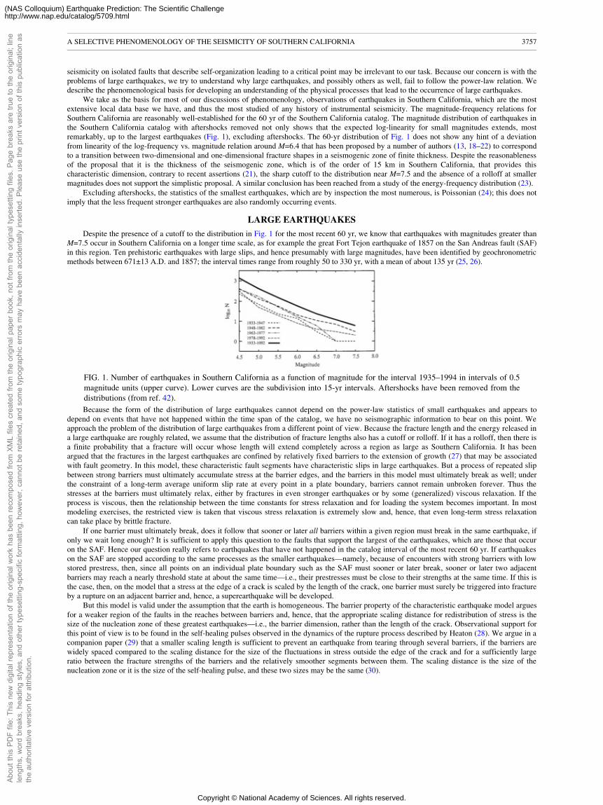
seismicity on isolated faults that describe self-organization leading to a critical point may be irrelevant to our task. Because our concern is with theproblems of large earthquakes, we try to understand why large earthquakes, and possibly others as well, fail to follow the power-law relation. Wedescribe the phenomenological basis for developing an understanding of the physical processes that lead to the occurrence of large earthquakes.
We take as the basis for most of our discussions of phenomenology, observations of earthquakes in Southern California, which are the mostextensive local data base we have, and thus the most studied of any history of instrumental seismicity. The magnitude-frequency relations forSouthern California are reasonably well-established for the 60 yr of the Southern California catalog. The magnitude distribution of earthquakes inthe Southern California catalog with aftershocks removed not only shows that the expected log-linearity for small magnitudes extends, mostremarkably, up to the largest earthquakes (Fig. 1), excluding aftershocks. The 60-yr distribution of Fig. 1 does not show any hint of a deviationfrom linearity of the log-frequency vs. magnitude relation around M=6.4 that has been proposed by a number of authors (13, 18–22) to correspondto a transition between two-dimensional and one-dimensional fracture shapes in a seismogenic zone of finite thickness. Despite the reasonablenessof the proposal that it is the thickness of the seismogenic zone, which is of the order of 15 km in Southern California, that provides thischaracteristic dimension, contrary to recent assertions (21), the sharp cutoff to the distribution near M=7.5 and the absence of a rolloff at smallermagnitudes does not support the simplistic proposal. A similar conclusion has been reached from a study of the energy-frequency distribution (23).
Excluding aftershocks, the statistics of the smallest earthquakes, which are by inspection the most numerous, is Poissonian (24); this does notimply that the less frequent stronger earthquakes are also randomly occurring events.
LARGE EARTHQUAKES
Despite the presence of a cutoff to the distribution in Fig. 1 for the most recent 60 yr, we know that earthquakes with magnitudes greater thanM=7.5 occur in Southern California on a longer time scale, as for example the great Fort Tejon earthquake of 1857 on the San Andreas fault (SAF)in this region. Ten prehistoric earthquakes with large slips, and hence presumably with large magnitudes, have been identified by geochronometricmethods between 671±13 A.D. and 1857; the interval times range from roughly 50 to 330 yr, with a mean of about 135 yr (25, 26).
FIG. 1. Number of earthquakes in Southern California as a function of magnitude for the interval 1935–1994 in intervals of 0.5magnitude units (upper curve). Lower curves are the subdivision into 15-yr intervals. Aftershocks have been removed from thedistributions (from ref. 42).Because the form of the distribution of large earthquakes cannot depend on the power-law statistics of small earthquakes and appears to
depend on events that have not happened within the time span of the catalog, we have no seismographic information to bear on this point. Weapproach the problem of the distribution of large earthquakes from a different point of view. Because the fracture length and the energy released ina large earthquake are roughly related, we assume that the distribution of fracture lengths also has a cutoff or rolloff. If it has a rolloff, then there isa finite probability that a fracture will occur whose length will extend completely across a region as large as Southern California. It has beenargued that the fractures in the largest earthquakes are confined by relatively fixed barriers to the extension of growth (27) that may be associatedwith fault geometry. In this model, these characteristic fault segments have characteristic slips in large earthquakes. But a process of repeated slipbetween strong barriers must ultimately accumulate stress at the barrier edges, and the barriers in this model must ultimately break as well; underthe constraint of a long-term average uniform slip rate at every point in a plate boundary, barriers cannot remain unbroken forever. Thus thestresses at the barriers must ultimately relax, either by fractures in even stronger earthquakes or by some (generalized) viscous relaxation. If theprocess is viscous, then the relationship between the time constants for stress relaxation and for loading the system becomes important. In mostmodeling exercises, the restricted view is taken that viscous stress relaxation is extremely slow and, hence, that even long-term stress relaxationcan take place by brittle fracture.
If one barrier must ultimately break, does it follow that sooner or later all barriers within a given region must break in the same earthquake, ifonly we wait long enough? It is sufficient to apply this question to the faults that support the largest of the earthquakes, which are those that occuron the SAF. Hence our question really refers to earthquakes that have not happened in the catalog interval of the most recent 60 yr. If earthquakeson the SAF are stopped according to the same processes as the smaller earthquakes—namely, because of encounters with strong barriers with lowstored prestress, then, since all points on an individual plate boundary such as the SAF must sooner or later break, sooner or later two adjacentbarriers may reach a nearly threshold state at about the same time—i.e., their prestresses must be close to their strengths at the same time. If this isthe case, then, on the model that a stress at the edge of a crack is scaled by the length of the crack, one barrier must surely be triggered into fractureby a rupture on an adjacent barrier and, hence, a superearthquake will be developed.
But this model is valid under the assumption that the earth is homogeneous. The barrier property of the characteristic earthquake model arguesfor a weaker region of the faults in the reaches between barriers and, hence, that the appropriate scaling distance for redistribution of stress is thesize of the nucleation zone of these greatest earthquakes—i.e., the barrier dimension, rather than the length of the crack. Observational support forthis point of view is to be found in the self-healing pulses observed in the dynamics of the rupture process described by Heaton (28). We argue in acompanion paper (29) that a smaller scaling length is sufficient to prevent an earthquake from tearing through several barriers, if the barriers arewidely spaced compared to the scaling distance for the size of the fluctuations in stress outside the edge of the crack and for a sufficiently largeratio between the fracture strengths of the barriers and the relatively smoother segments between them. The scaling distance is the size of thenucleation zone or it is the size of the self-healing pulse, and these two sizes may be the same (30).
A SELECTIVE PHENOMENOLOGY OF THE SEISMICITY OF SOUTHERN CALIFORNIA 3757
Abou
t thi
s PD
F fil
e: T
his
new
dig
ital r
epre
sent
atio
n of
the
orig
inal
wor
k ha
s be
en re
com
pose
d fro
m X
ML
files
cre
ated
from
the
orig
inal
pap
er b
ook,
not
from
the
orig
inal
type
setti
ng fi
les.
Pag
e br
eaks
are
true
to th
e or
igin
al; l
ine
leng
ths,
wor
d br
eaks
, hea
ding
sty
les,
and
oth
er ty
pese
tting
-spe
cific
form
attin
g, h
owev
er, c
anno
t be
reta
ined
, and
som
e ty
pogr
aphi
c er
rors
may
hav
e be
en a
ccid
enta
lly in
serte
d. P
leas
e us
e th
e pr
int v
ersi
on o
f thi
s pu
blic
atio
n as
the
auth
orita
tive
vers
ion
for a
ttrib
utio
n.
Copyright © National Academy of Sciences. All rights reserved.
(NAS Colloquium) Earthquake Prediction: The Scientific Challengehttp://www.nap.edu/catalog/5709.html
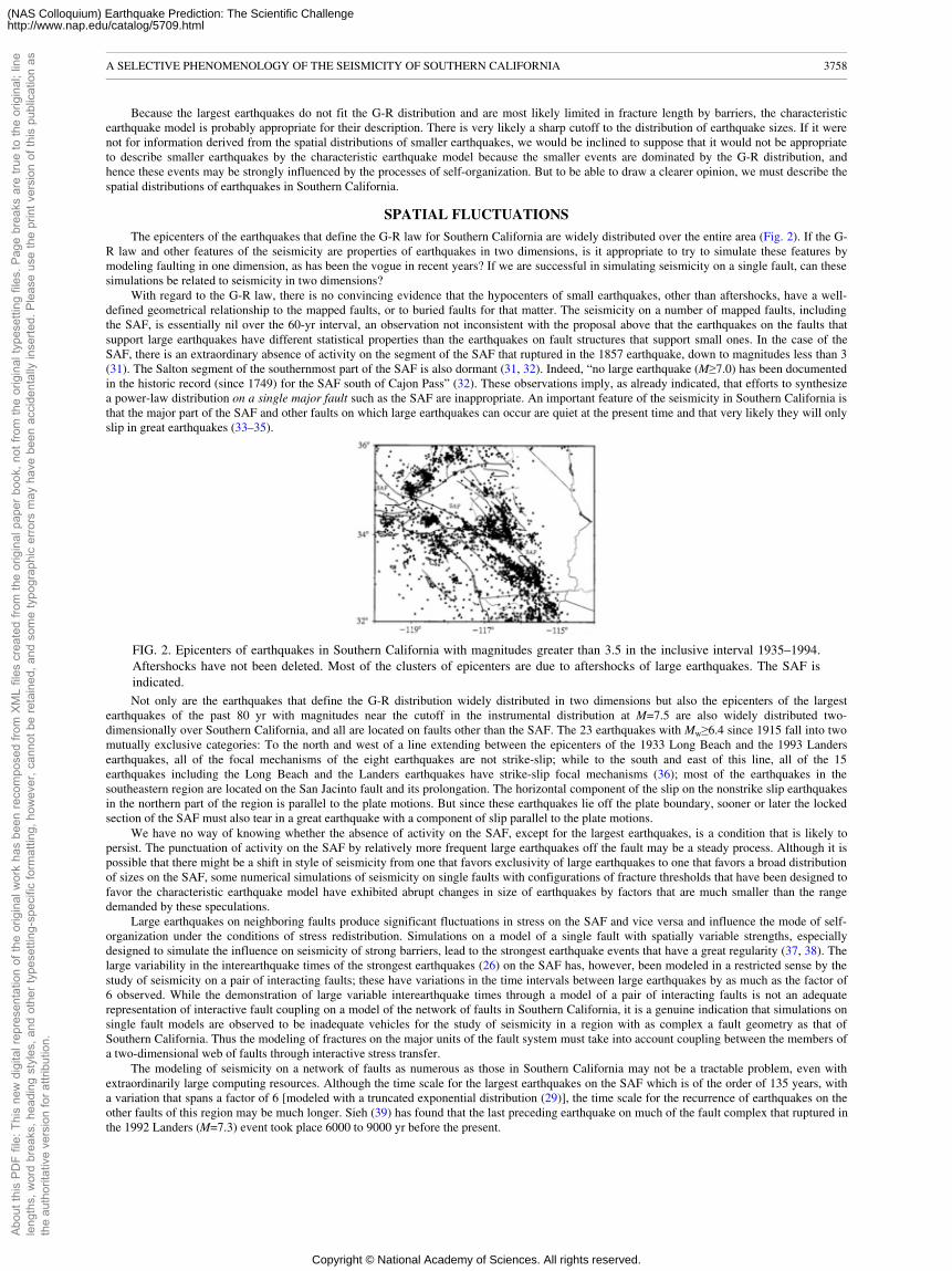
Because the largest earthquakes do not fit the G-R distribution and are most likely limited in fracture length by barriers, the characteristicearthquake model is probably appropriate for their description. There is very likely a sharp cutoff to the distribution of earthquake sizes. If it werenot for information derived from the spatial distributions of smaller earthquakes, we would be inclined to suppose that it would not be appropriateto describe smaller earthquakes by the characteristic earthquake model because the smaller events are dominated by the G-R distribution, andhence these events may be strongly influenced by the processes of self-organization. But to be able to draw a clearer opinion, we must describe thespatial distributions of earthquakes in Southern California.
SPATIAL FLUCTUATIONS
The epicenters of the earthquakes that define the G-R law for Southern California are widely distributed over the entire area (Fig. 2). If the G-R law and other features of the seismicity are properties of earthquakes in two dimensions, is it appropriate to try to simulate these features bymodeling faulting in one dimension, as has been the vogue in recent years? If we are successful in simulating seismicity on a single fault, can thesesimulations be related to seismicity in two dimensions?
With regard to the G-R law, there is no convincing evidence that the hypocenters of small earthquakes, other than aftershocks, have a well-defined geometrical relationship to the mapped faults, or to buried faults for that matter. The seismicity on a number of mapped faults, includingthe SAF, is essentially nil over the 60-yr interval, an observation not inconsistent with the proposal above that the earthquakes on the faults thatsupport large earthquakes have different statistical properties than the earthquakes on fault structures that support small ones. In the case of theSAF, there is an extraordinary absence of activity on the segment of the SAF that ruptured in the 1857 earthquake, down to magnitudes less than 3(31). The Salton segment of the southernmost part of the SAF is also dormant (31, 32). Indeed, “no large earthquake (M≥7.0) has been documentedin the historic record (since 1749) for the SAF south of Cajon Pass” (32). These observations imply, as already indicated, that efforts to synthesizea power-law distribution on a single major fault such as the SAF are inappropriate. An important feature of the seismicity in Southern California isthat the major part of the SAF and other faults on which large earthquakes can occur are quiet at the present time and that very likely they will onlyslip in great earthquakes (33–35).
FIG. 2. Epicenters of earthquakes in Southern California with magnitudes greater than 3.5 in the inclusive interval 1935–1994.Aftershocks have not been deleted. Most of the clusters of epicenters are due to aftershocks of large earthquakes. The SAF isindicated.Not only are the earthquakes that define the G-R distribution widely distributed in two dimensions but also the epicenters of the largest
earthquakes of the past 80 yr with magnitudes near the cutoff in the instrumental distribution at M=7.5 are also widely distributed two-dimensionally over Southern California, and all are located on faults other than the SAF. The 23 earthquakes with Mw≥6.4 since 1915 fall into twomutually exclusive categories: To the north and west of a line extending between the epicenters of the 1933 Long Beach and the 1993 Landersearthquakes, all of the focal mechanisms of the eight earthquakes are not strike-slip; while to the south and east of this line, all of the 15earthquakes including the Long Beach and the Landers earthquakes have strike-slip focal mechanisms (36); most of the earthquakes in thesoutheastern region are located on the San Jacinto fault and its prolongation. The horizontal component of the slip on the nonstrike slip earthquakesin the northern part of the region is parallel to the plate motions. But since these earthquakes lie off the plate boundary, sooner or later the lockedsection of the SAF must also tear in a great earthquake with a component of slip parallel to the plate motions.
We have no way of knowing whether the absence of activity on the SAF, except for the largest earthquakes, is a condition that is likely topersist. The punctuation of activity on the SAF by relatively more frequent large earthquakes off the fault may be a steady process. Although it ispossible that there might be a shift in style of seismicity from one that favors exclusivity of large earthquakes to one that favors a broad distributionof sizes on the SAF, some numerical simulations of seismicity on single faults with configurations of fracture thresholds that have been designed tofavor the characteristic earthquake model have exhibited abrupt changes in size of earthquakes by factors that are much smaller than the rangedemanded by these speculations.
Large earthquakes on neighboring faults produce significant fluctuations in stress on the SAF and vice versa and influence the mode of self-organization under the conditions of stress redistribution. Simulations on a model of a single fault with spatially variable strengths, especiallydesigned to simulate the influence on seismicity of strong barriers, lead to the strongest earthquake events that have a great regularity (37, 38). Thelarge variability in the interearthquake times of the strongest earthquakes (26) on the SAF has, however, been modeled in a restricted sense by thestudy of seismicity on a pair of interacting faults; these have variations in the time intervals between large earthquakes by as much as the factor of6 observed. While the demonstration of large variable interearthquake times through a model of a pair of interacting faults is not an adequaterepresentation of interactive fault coupling on a model of the network of faults in Southern California, it is a genuine indication that simulations onsingle fault models are observed to be inadequate vehicles for the study of seismicity in a region with as complex a fault geometry as that ofSouthern California. Thus the modeling of fractures on the major units of the fault system must take into account coupling between the members ofa two-dimensional web of faults through interactive stress transfer.
The modeling of seismicity on a network of faults as numerous as those in Southern California may not be a tractable problem, even withextraordinarily large computing resources. Although the time scale for the largest earthquakes on the SAF which is of the order of 135 years, witha variation that spans a factor of 6 [modeled with a truncated exponential distribution (29)], the time scale for the recurrence of earthquakes on theother faults of this region may be much longer. Sieh (39) has found that the last preceding earthquake on much of the fault complex that ruptured inthe 1992 Landers (M=7.3) event took place 6000 to 9000 yr before the present.
A SELECTIVE PHENOMENOLOGY OF THE SEISMICITY OF SOUTHERN CALIFORNIA 3758
Abou
t thi
s PD
F fil
e: T
his
new
dig
ital r
epre
sent
atio
n of
the
orig
inal
wor
k ha
s be
en re
com
pose
d fro
m X
ML
files
cre
ated
from
the
orig
inal
pap
er b
ook,
not
from
the
orig
inal
type
setti
ng fi
les.
Pag
e br
eaks
are
true
to th
e or
igin
al; l
ine
leng
ths,
wor
d br
eaks
, hea
ding
sty
les,
and
oth
er ty
pese
tting
-spe
cific
form
attin
g, h
owev
er, c
anno
t be
reta
ined
, and
som
e ty
pogr
aphi
c er
rors
may
hav
e be
en a
ccid
enta
lly in
serte
d. P
leas
e us
e th
e pr
int v
ersi
on o
f thi
s pu
blic
atio
n as
the
auth
orita
tive
vers
ion
for a
ttrib
utio
n.
Copyright © National Academy of Sciences. All rights reserved.
(NAS Colloquium) Earthquake Prediction: The Scientific Challengehttp://www.nap.edu/catalog/5709.html
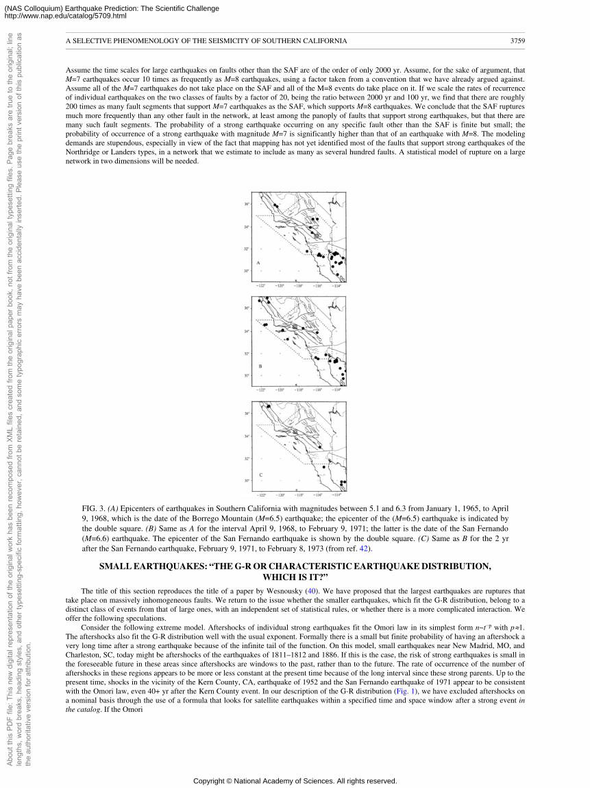
Assume the time scales for large earthquakes on faults other than the SAF are of the order of only 2000 yr. Assume, for the sake of argument, thatM=7 earthquakes occur 10 times as frequently as M=8 earthquakes, using a factor taken from a convention that we have already argued against.Assume all of the M=7 earthquakes do not take place on the SAF and all of the M=8 events do take place on it. If we scale the rates of recurrenceof individual earthquakes on the two classes of faults by a factor of 20, being the ratio between 2000 yr and 100 yr, we find that there are roughly200 times as many fault segments that support M=7 earthquakes as the SAF, which supports M=8 earthquakes. We conclude that the SAF rupturesmuch more frequently than any other fault in the network, at least among the panoply of faults that support strong earthquakes, but that there aremany such fault segments. The probability of a strong earthquake occurring on any specific fault other than the SAF is finite but small; theprobability of occurrence of a strong earthquake with magnitude M=7 is significantly higher than that of an earthquake with M=8. The modelingdemands are stupendous, especially in view of the fact that mapping has not yet identified most of the faults that support strong earthquakes of theNorthridge or Landers types, in a network that we estimate to include as many as several hundred faults. A statistical model of rupture on a largenetwork in two dimensions will be needed.
FIG. 3. (A) Epicenters of earthquakes in Southern California with magnitudes between 5.1 and 6.3 from January 1, 1965, to April9, 1968, which is the date of the Borrego Mountain (M=6.5) earthquake; the epicenter of the (M=6.5) earthquake is indicated bythe double square. (B) Same as A for the interval April 9, 1968, to February 9, 1971; the latter is the date of the San Fernando(M=6.6) earthquake. The epicenter of the San Fernando earthquake is shown by the double square. (C) Same as B for the 2 yrafter the San Fernando earthquake, February 9, 1971, to February 8, 1973 (from ref. 42).
SMALL EARTHQUAKES: “THE G-R OR CHARACTERISTIC EARTHQUAKE DISTRIBUTION,WHICH IS IT?”
The title of this section reproduces the title of a paper by Wesnousky (40). We have proposed that the largest earthquakes are ruptures thattake place on massively inhomogeneous faults. We return to the issue whether the smaller earthquakes, which fit the G-R distribution, belong to adistinct class of events from that of large ones, with an independent set of statistical rules, or whether there is a more complicated interaction. Weoffer the following speculations.
Consider the following extreme model. Aftershocks of individual strong earthquakes fit the Omori law in its simplest form n~t−p with p�1.The aftershocks also fit the G-R distribution well with the usual exponent. Formally there is a small but finite probability of having an aftershock avery long time after a strong earthquake because of the infinite tail of the function. On this model, small earthquakes near New Madrid, MO, andCharleston, SC, today might be aftershocks of the earthquakes of 1811–1812 and 1886. If this is the case, the risk of strong earthquakes is small inthe foreseeable future in these areas since aftershocks are windows to the past, rather than to the future. The rate of occurrence of the number ofaftershocks in these regions appears to be more or less constant at the present time because of the long interval since these strong parents. Up to thepresent time, shocks in the vicinity of the Kern County, CA, earthquake of 1952 and the San Fernando earthquake of 1971 appear to be consistentwith the Omori law, even 40+ yr after the Kern County event. In our description of the G-R distribution (Fig. 1), we have excluded aftershocks ona nominal basis through the use of a formula that looks for satellite earthquakes within a specified time and space window after a strong event inthe catalog. If the Omori
A SELECTIVE PHENOMENOLOGY OF THE SEISMICITY OF SOUTHERN CALIFORNIA 3759
Abou
t thi
s PD
F fil
e: T
his
new
dig
ital r
epre
sent
atio
n of
the
orig
inal
wor
k ha
s be
en re
com
pose
d fro
m X
ML
files
cre
ated
from
the
orig
inal
pap
er b
ook,
not
from
the
orig
inal
type
setti
ng fi
les.
Pag
e br
eaks
are
true
to th
e or
igin
al; l
ine
leng
ths,
wor
d br
eaks
, hea
ding
sty
les,
and
oth
er ty
pese
tting
-spe
cific
form
attin
g, h
owev
er, c
anno
t be
reta
ined
, and
som
e ty
pogr
aphi
c er
rors
may
hav
e be
en a
ccid
enta
lly in
serte
d. P
leas
e us
e th
e pr
int v
ersi
on o
f thi
s pu
blic
atio
n as
the
auth
orita
tive
vers
ion
for a
ttrib
utio
n.
Copyright © National Academy of Sciences. All rights reserved.
(NAS Colloquium) Earthquake Prediction: The Scientific Challengehttp://www.nap.edu/catalog/5709.html
and G-R laws hold for a long time after the parent, then how many earthquakes in the Southern California catalog are in reality aftershocks ofstrong events that took place before the start of the catalog? If the Omori law is taken literally, then are all of the earthquakes that constitute theobservations of the G-R distribution today aftershocks of past strong events(?). Since aftershocks depend on the existence of a mechanism forproviding for a time delay between the main, strong shock and the aftershock, any model that purports to describe seismicity in a region such asSouthern California and uses the G-R law as a paradigm must include a mechanism for time delays—i.e., some nonelastic stress transfer. Underthis assumption, the G-R law does not tell us anything about future seismicity since aftershocks only refer to the past history of strong shocks.
However, today there are no significant aftershocks of the 1857 earthquake on the SAF. Thus at least for SAF earthquakes, the Omori lawdoes not have an infinite tail, and there is a temporal cutoff for aftershocks. We speculate that the map of Southern California seismicity, which isdominated by the smallest earthquakes (Fig. 2), shows that some faults can produce long-term and others only short-term aftershocks. It is likelythat we should not assume that all earthquakes in Southern California can be modeled under the same set of physical rules. Thus, we conclude thatthe relationship between the present-day small earthquakes that define the G-R law and future large earthquakes on the major faults is ill-defined;there exists the possibility that there is no relationship between present small and future large earthquakes.
Assume that the smaller earthquakes do not take place on the same fault structures as the larger ones. Then, except in unusual circumstances,the two populations of small and large earthquakes have independent distributions; we can assume that the smaller events fit the G-R law, and thelarger ones have their own distribution, whatever that may be. If large mapped faults, or faults that are large enough to be mapped, are reserved forbig earthquakes, then where do the small ones take place? The process zones at the tips of cracks are regions of highly deformed and/or brokenmaterial. As a fault grows, it must certainly grow through its own process zone. Thus we expect that the entire length of all faults must besurrounded by a zone of weakened material. Under an increasing tectonic stress, this zone will slip in small earthquakes. Irregular slip in largeearthquakes on the nearby fault surface could cause fluctuations in stress that could trigger aftershocks in the adjoining process zone; aftershockscan thus occur along the entire length of a large earthquake, both in the process zone nearby and in the process zone beyond the ends of the crackby the more conventional mechanism of stress intensification. Thus small earthquakes with rupture lengths that are most frequently, but notnecessarily, less than the thickness of the process zone occur in an elongated three-dimensional zone astride the fault. Hence, the distribution ofsmall earthquakes on this model is characterized by the distribution of sizes of contacts where slips might take place in a three-dimensional spaceand might have different focal mechanisms, as well as different spatial locations, than the larger earthquakes, consistent with our conjecture.
If small and large earthquakes have different temporal distributions, why does the projection of the distribution for small earthquakes inSouthern California extend almost perfectly into the magnitude range of the largest earthquakes in the past 60 yr, only to be truncated by an abruptcutoff (Fig. 1)? Suppose that we divide Southern California into smaller seismic zones that each includes at least one fault that supports largeearthquakes. Assume each zone will have its own G-R law for small earthquakes and that the exponent is the same for each. But the cutoff (orrolloff) will depend on the properties of the dominant fault in the zone, and especially its length, and we can expect that it will be different for eachregion. The sum of the seismicity distributions over all zones will give the seismicity for all of Southern California; the spatially cumulativedistribution will have the usual power-law relation for small earthquakes with the usual exponent; but the rolloff for the spatial sum distributionwill reflect the distribution of cutoffs (or rolloffs) for the zones. Because the summation seismicity has a sharp cutoff (Fig. 1), then either thedistributions for each of the zones must have the same cutoff, which seems very unlikely, or the distributions at the large magnitude ends must varywidely, with some of the zones having a rate for large earthquakes that is greater than the extrapolation of the seismicity from the simple power-law relation, and some less than it. Thus the properties of the large earthquakes differ significantly from the G-R law for small earthquakes in eachzone, and hence the small and large earthquakes interact differently. On the last model, the sharp cutoff in Fig. 1 is a coincidence.
Of course, there is always the argument that the distribution in Fig. 1 is based only on two earthquakes in the magnitude range 7.25−7.75 and,hence, the uncertainties are so large that the apparent sharp cutoff is a statistical fluctuation itself. In either case, one cannot say much about thevalidity of extending the G-R curve out to the largest magnitudes.
SPACE-TIME FLUCTUATIONS
We have argued that the G-R law, which describes small earthquakes, excluding aftershocks, over a 60-yr period in Southern California,cannot be used directly to predict large earthquakes. However if the distribution is temporally variable or it is not Poissonian, fluctuations in themagnitude-frequency law might give possible indications of forthcoming large earthquakes. Fluctuations are indeed found on a time scale of 15 yr,in the magnitude range of 4.8–6.2 approximately, that are significant at the 2σ level (Fig. 1). Jones has also identified that there was a significantincrease in the rate of occurrence of earthquakes with M≥5 in Southern California by a factor of two over the interval 1986–1992 in comparisonwith the rate over the 40 yr preceding 1986 (41). On the time scale of the order of 1–10 yr, there is an increase in the rate of occurrence ofearthquakes with magnitudes greater than 5.1 before all of the strongest earthquakes in California with magnitudes M≥ 6.8 (42). It is doubtfulwhether these fluctuations in seismicity might be useful for earthquake prediction on the above time scale, because their space scale is so large,being of the order of the size of Southern California. No detailed exploration has been made as yet to see if similar fluctuations are to be found forsmaller magnitudes, at shorter distances, and over shorter time intervals before strong earthquakes with magnitudes less than 6.8.
We have listed above nonuniform properties of earthquake occurrence that includes observations that (i) the rate of occurrence of thestrongest earthquakes differs from the extrapolations of the G-R law for small earthquakes, (ii) there is long-term spatial quiescence at allmagnitudes on the faults that support the largest earthquakes, (iii) there are fluctuations in the interval times between the strongest earthquakes onthe SAF, and (iv) there are temporal fluctuations of intermediate-magnitude seismicity. We mention briefly the phenomenology of fluctuations thatare coupled in space and in time. Kanamori (43) has given an excellent review of space-time-coupled fluctuations: quiescence or reduced activityhas been identified prior to 41 very strong earthquakes worldwide out of a list of 52 earthquakes, over a time scale of a few months to as much as30 yr, and over distance scales that are usually of the order of the dimensions of the fracture of the strong earthquake. Wyss and Habermann (44)have identified 17 cases of earthquakes that preceded by seismic quiescence on time scales of the order of 1 to 6 yr and distance scales of the orderof the size of the fracture length in the strong earthquake. These examples include several earthquakes in Southern California.
A SELECTIVE PHENOMENOLOGY OF THE SEISMICITY OF SOUTHERN CALIFORNIA 3760
Abou
t thi
s PD
F fil
e: T
his
new
dig
ital r
epre
sent
atio
n of
the
orig
inal
wor
k ha
s be
en re
com
pose
d fro
m X
ML
files
cre
ated
from
the
orig
inal
pap
er b
ook,
not
from
the
orig
inal
type
setti
ng fi
les.
Pag
e br
eaks
are
true
to th
e or
igin
al; l
ine
leng
ths,
wor
d br
eaks
, hea
ding
sty
les,
and
oth
er ty
pese
tting
-spe
cific
form
attin
g, h
owev
er, c
anno
t be
reta
ined
, and
som
e ty
pogr
aphi
c er
rors
may
hav
e be
en a
ccid
enta
lly in
serte
d. P
leas
e us
e th
e pr
int v
ersi
on o
f thi
s pu
blic
atio
n as
the
auth
orita
tive
vers
ion
for a
ttrib
utio
n.
Copyright © National Academy of Sciences. All rights reserved.
(NAS Colloquium) Earthquake Prediction: The Scientific Challengehttp://www.nap.edu/catalog/5709.html
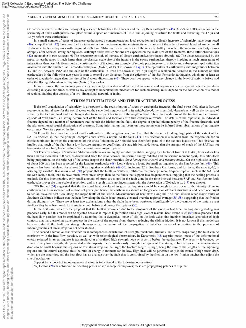
Of particular interest is the case history of quiescence before both the Landers and the Big Bear earthquakes (45). A 75% to 100% reduction in theseismicity of small earthquakes took place within a space of dimensions of 10–20 km adjoining or astride the faults and extending for 4.5 yr and1.6 yr before these earthquakes.
In a small number of cases of Japanese earthquakes, a contemporaneous local reduction and a distant increase of seismicity have been noted(46). Knopoff et al. (42) have described an increase in intermediate-magnitude seismicity to distances of the order of several hundred km before all11 documentable earthquakes with magnitudes ≥6.8 in California over a time scale of the order of 1–10 yr as noted; the increase in activity ceasesabruptly after selected strong earthquakes. Although stress redistributions are expected on the scale size of the fractures, these latter observations(42) are notable in two respects: (i) The precursory episode of increase of distant earthquakes terminates abruptly, (ii) The distances spanned by theprecursor earthquakes is much larger than the classical scale size of the fracture in the strong earthquakes, thereby implying a much larger range ofinteractions than possible from standard elastic models of fracture. An example of remote prior increase in activity and subsequent rapid extinctionassociated with the smaller San Fernando earthquake (M=6.6) of 1971 is shown in Fig. 3. The epicenters of earthquakes with magnitudes between4.7 and 6.3 between 1965 and the date of the earthquake in 1972 are shown in two 3-yr stages; a remarkable decrease in the number of suchearthquakes in the following two years is seen to extend over distances from the epicenter of the San Fernando earthquake, which are at least anorder of magnitude larger than the size of its fracture dimensions (42). There does not appear to be any change in the level of activity before andafter the Borrego Mountain earthquake (M=6.5) 3 yr earlier.
In most cases, the anomalous precursory seismicity is widespread in two dimensions, and arguments for or against intermediate-termclustering in space and time, as well as any attempt to understand the mechanism for such clustering, must depend on the construction of a modelof regional faulting that consists of a two-dimensional network of faults.
STRESS FLUCTUATIONS AND THE FRACTURE PROCESS
If the self-organization of seismicity is a response to the redistribution of stress by earthquake fractures, the final stress field after a fracturerepresents an initial state for the next fracture on the same fault segment and in its neighborhood; the stress field depends as well on the increase ofstress by the tectonic load and the changes due to subsequent fractures in the neighborhood. Thus, the conditions of the fracture in the dynamicepisode of “fast time” is a strong determinant of the times and locations of future earthquake events. The details of the rupture in an individualfracture depend on a number of parameters that include the friction on the fault, the degree of spatial inhomogeneity of the fracture threshold, andthe aforementioned spatial distribution of prestress. Some information that bears on these points can be inferred from observations of earthquakeoccurrence. We cite a part of the list.
(i) From the focal mechanisms of small earthquakes in the neighborhood, we learn that the stress field along large parts of the extent of theSAF is oriented so that the principal compressional stress is normal to the fault (47). This orientation is a rotation from the expectation for anelastic continuum in which the component of the stress field on the SAF should be a shear field parallel to the tectonic load stress. This observationimplies that much of the fault has a low fracture strength or coefficient of static friction, and, hence, that the strength of much of the SAF has notbeen restored to a fully healed value after the most recent major rupture.
(ii) The stress drops in Southern California earthquakes are highly variable quantities, ranging by a factor of from 300 to 400, from values lessthan 1 bar to more than 300 bars, as determined from the ratio between the seismic energy radiated and the seismic moment Es/Mo, this ratio itselfbeing proportional to the ratio σ/µ of the stress drop to the shear modulus, for a homogeneous earth and fracture model. On the high side, a valueof about 300 bars has been reported for the Landers earthquake (48). Low values are found for small earthquakes on the San Jacinto fault (49). Thisquantity has been tabulated for almost 500 earthquakes worldwide (49–53), including 22 in Southern California, and for these, the ratio Es/Mo isalso highly variable. Kanamori et al. (50) propose that the faults in Southern California that undergo more frequent rupture, such as the SAF andthe San Jacinto fault, tend to have much lower stress drops than do the faults that support less frequent events, implying that the healing process isgradual. On this interpretation, only small amounts of stress are stored in the fault zone in the time interval between SAF and San Jacinto faultearthquakes, over the time scale of repetition, and is a result that is not inconsistent with the observation of Zoback et al. (47) (see above).
(iii) Bullard (54) suggested that the frictional heat developed in great earthquakes should be enough to melt rocks in the vicinity of majorearthquake faults in some tens of millions of years (and hence that earthquakes should no longer occur on old fault structures), and hence one oughtto see an elevated heat flow along the major faults of the world. Measurements of heat flow along the SAF and several other major faults ofSouthern California indicate that the heat flow along the faults is not greatly elevated over the regional average (55–58), suggesting that the frictionduring sliding is low. There are at least two explanations: either the faults have been weakened significantly by the dynamics of the rupture eventitself, or they have been weak for some time both before and during the ruptures (56).
In the first case, which is the proposal that the fault is weakened due to the dynamics of the event in fast time, melting during sliding wasproposed early, but this model can be rejected because it implies high friction and a high level of residual heat. Brune et al. (59) have proposed thatthe heat flow paradox can be explained by assuming that a dynamical mode of slip on the fault exists that involves interface separation of faultcontacts that has a traveling wave property in the wake of the rupture front, thereby reducing the sliding friction. It is not known if this model canbe successful if the fault has strong inhomogeneity; the nature of the propagation of interface waves of separation in the presence ofinhomogeneities of stress drop has not been studied.
The second alternative asks whether an inhomogeneous distribution of strength thresholds, frictions, and stress drops along the fault can beconsistent with the heat flow paradox, as well as with seismological observations. In Kanamori's (43) asperity model, most of the deformationalenergy released in an earthquake is accumulated at a localized high strength node or asperity before the earthquake. The asperity is bounded byzones of very low strength; slip generated at the asperity then spreads easily through the region of low strength. In this model the average stressdrop can be small because the regions of low stress drop can be large; the fracture length is large, being the sum of the lengths of the adjoiningregions and the central asperity; thus the ratio of energy to moment can be low. High heat will be generated only in the zones of high stress drop,which are the asperities, and the heat flow has an average over the fault that is constrained by the friction on the low-friction patches that adjoin thesite of nucleation.
Support for a model of inhomogeneous fracture is to be found in the following observations:(iv) Heaton (28) has observed self-healing pulses of slip in large earthquakes; these are propagating patches of slip that
A SELECTIVE PHENOMENOLOGY OF THE SEISMICITY OF SOUTHERN CALIFORNIA 3761
Abou
t thi
s PD
F fil
e: T
his
new
dig
ital r
epre
sent
atio
n of
the
orig
inal
wor
k ha
s be
en re
com
pose
d fro
m X
ML
files
cre
ated
from
the
orig
inal
pap
er b
ook,
not
from
the
orig
inal
type
setti
ng fi
les.
Pag
e br
eaks
are
true
to th
e or
igin
al; l
ine
leng
ths,
wor
d br
eaks
, hea
ding
sty
les,
and
oth
er ty
pese
tting
-spe
cific
form
attin
g, h
owev
er, c
anno
t be
reta
ined
, and
som
e ty
pogr
aphi
c er
rors
may
hav
e be
en a
ccid
enta
lly in
serte
d. P
leas
e us
e th
e pr
int v
ersi
on o
f thi
s pu
blic
atio
n as
the
auth
orita
tive
vers
ion
for a
ttrib
utio
n.
Copyright © National Academy of Sciences. All rights reserved.
(NAS Colloquium) Earthquake Prediction: The Scientific Challengehttp://www.nap.edu/catalog/5709.html
imply a reduction in the scale length of fracture, as indicated above; the best-documented example of self-healing patches of slip is the inversionfor the slip in the Landers earthquake (60). It can be shown that self-healing slip pulses of constant duration require a critical scaling dimension fortheir generation. Cochard and Madariaga (30) have argued persuasively that the critical scale size is given by the dimensions of a nucleation zone,which we equate with an asperity. In this model, the pulse generated at the asperity breaks into a region of lower stress drop, wherein its velocity ofgrowth attenuates, slip begins to diminish, and ultimately a velocity-dependent friction that is intrinsic to the healing process causes ultimatecessation of motion.
(v) The earthquakes studied by Heaton (28, 60) show significant irregularities of the slip distributions in the rupture plane, which indicate thepresence of significant inhomogeneity of stress drop and/or fracture threshold in the plane. The slip at the surface in the Landers earthquake of1992 has been studied in detail in the field (60–62) and over the entire plane by inversion of the seismic signal (60, 63, 64). Of particular interest isthe presence of time delays of about 1–3 sec between termination of rupture on one strand of the fault and initiation of rupture on a neighboringstrand (60, 63, 64). These time delays between rupture of successive strands of the large fracture can be accounted for by inhomogeneity of thefracture threshold or the stress drop, or both, as well as by a slip-weakening in slow time, over the time interval of the time delay, of the strength inthe high-stress drop barriers.
SUMMARY
We summarize these observations on the seismicity of Southern California as follows. Not all faults in Southern California behave in the sameway statistically. For example, the SAF today supports large earthquakes only and does not support small ones. Hence an effort to apply auniversal model that yields the G-R statistical law is doomed to failure.
The G-R law is valid for small earthquakes but not for large ones. The G-R law is a manifestation of seismicity over the entire area ofSouthern California. Thus efforts to model the power-law character through a process of self-organization on a single fault is misdirected. Thepower law is probably a manifestation of the distribution of little faults and/or aftershocks in two dimensions—i.e., it is a manifestation of thegeometry of faulting in Southern California.
Although we do not know what the distribution for large earthquakes is, the distribution for large earthquakes on faults other than the SAF islikely to show large spatial fluctuations. Large earthquakes on the SAF occur more frequently than large earthquakes on any other major fault inSouthern California; the SAF is the most rapidly slipping element of the fault network but may be slipping under conditions of low average stressdrop—i.e., a small energy-to-moment ratio.
The temporal distribution of earthquakes must be dependent on the limitations of fracture size. What stops the growth of a fracture is theencounter of a growing crack with a barrier region, which is a zone of large stress drop. If the large stress drops are localized, the earthquakeruptures are confined, and the characteristic earthquake model is appropriate. Localization is possible where significant changes in the geometry offaulting are encountered, such as at sites of step-overs (echeloning) or bifurcations (fault junctions). Under the constraint of uniform average rate ofmoment release, strong barrier sites must themselves break or the stresses at these sites must relax. Not only is geometry on a network of faultslikely to be important for the modeling enterprise, but also the geometry of individual faults is going to lead to fluctuations in strength, in rapidityof restoration of strength (suturing) after a big earthquake. These geometrical fluctuations are likely to lead to nonuniformity of slip. Temporalfluctuations in seismicity imply the importance of time-dependent stress transmission processes, such as those associated with creep. Probably themost alluring proposal for intermediate-term earthquake prediction is the idea that local quiescence of small earthquakes develops near the site of afuture strong earthquake and that intermediate magnitude activity increases at distance from the future earthquake. The most likely candidate formodeling the fluctuations in stress drops and fracture thresholds is an asperity model for individual earthquakes and a barrier model that accountsfor the complexity of the fault network.
This research was supported by a grant from the Southern California Earthquake Center. This paper is publication number 4621 of theInstitute of Geophysics and Planetary Physics, University of California, Los Angeles, and is publication number 322 of the Southern CaliforniaEarthquake Center.1. Bak, P. & Tang, C. (1989) J. Geophys. Res. 94, 15635–15637.2. Nakanishi, H. (1990) Phys. Rev. A 41, 7086–7089.3. Nakanishi, H. (1991) Phys. Rev. A 43, 6613–6621.4. Christensen, K. & Olami, Z. (1992) J. Geophys. Res. 97, 8729– 8735.5. Christensen, K. & Olami, Z. (1992) Phys. Rev. A 46, 1829–1838.6. Christensen, K., Olami, Z. & Bak, P. (1992) Phys. Rev. Lett. 68, 2417–2420.7. Olami, Z., Feder, H.J.S. & Christensen, K. (1992) Phys. Rev. Lett. 68, 1244–1247.8. Olami, Z. & Christensen, K. (1992) Phys. Rev. A 46, 1720–1723.9. Gutenberg, B. & Richter, C.F. (1944) Bull. Seismol Soc. Am. 34, 185–188.10. Gutenberg, B. & Richter, C.F. (1954) Seismicity of the Earth (Princeton Univ. Press, Princeton, NJ).11. Gutenberg, B. & Richter, C.F. (1956) Ann. Geofis. 9, 1–15.12. Gutenberg, B. (1956) Q.J.Geol. Soc. London 112, 1–14.13. Kanamori, H. & Anderson, D.L. (1975) Bull. Seismol. Soc. Am. 65, 1073–1095.14. Knopoff, L. & Kagan, Y. (1977) J. Geophys. Res. 82, 5647–5657.15. Kanamori, H. (1977) J. Geophys. Res. 82, 2981–2987.16. Hanks, T.C. & Kanamori, H. (1979) J. Geophys. Res. 84, 2348– 2350.17. Turcotte, D.L. (1990) Global Planet. Change 3, 301–308.18. Rundle, J.B. (1989) J. Geophys. Res. 94, 12337–12342.19. Romanowicz, B. (1992) Geophys. Res. Lett. 19, 481–484.20. Romanowicz, B. & Rundle, J.B. (1993) Bull. Seismol. Soc. Am. 83, 1294–1297.21. Pacheco, J.F., Scholz, C.H. & Sykes, L.R. (1992) Nature (London) 355, 71–73.22. Okal, R. & Romanowicz, B.A. (1994) Phys. Earth Planet. Inter. 87, 55–76.23. Sornette, D., Knopoff, L., Kagan, Y. & Vanneste, C. (1996) J. Geophys. Res., in press.24. Gardner, J.K. & Knopoff, L. (1974) Bull. Seismol. Soc. Am. 64, 1363–1367.25. Sieh, K.E. (1978) J. Geophys. Res. 83, 3907–3939.26. Sieh, K., Stuiver, M. & Brillinger, D. (1989) J. Geophys. Res. 94, 603–623.27. Schwartz, D.P. & Coppersmith, K.J. (1984) J. Geophys. Res. 89, 5681–5698.28. Heaton, T.H. (1990) Phys. Earth Planet. Inter. 64, 1–20.29. Knopoff, L. (1996) Proc. Natl. Acad. Sci. USA 93, 3830–3837.30. Cochard, A. & Madariaga, R. (1994) Pure Appl Geophys. 142, 419–445.31. Sieh, K.E. & Williams, P.L. (1990) J. Geophys. Res. 95, 6629– 6645.32. Jones, L.M. (1988) J. Geophys. Res. 93, 8869–8891.33. Raleigh, C.B., Sieh, K.E., Sykes, L.R. & Anderson, D.L. (1982) Science 217, 1097–1104.34. Lindh, A.G. (1983) U.S. Geol. Survey Open File Rep. 83–63.35. Sykes, L.R. & Nishenko, S.P. (1984) J. Geophys. Res. 89, 5905–5927.36. Press, F. & Allen, C.R. (1995) J. Geophys. Res. 100, 6421–6430.37. Knopoff, L. (1993) Proc. Am. Philos. Soc. 137, 339–349.
A SELECTIVE PHENOMENOLOGY OF THE SEISMICITY OF SOUTHERN CALIFORNIA 3762
Abou
t thi
s PD
F fil
e: T
his
new
dig
ital r
epre
sent
atio
n of
the
orig
inal
wor
k ha
s be
en re
com
pose
d fro
m X
ML
files
cre
ated
from
the
orig
inal
pap
er b
ook,
not
from
the
orig
inal
type
setti
ng fi
les.
Pag
e br
eaks
are
true
to th
e or
igin
al; l
ine
leng
ths,
wor
d br
eaks
, hea
ding
sty
les,
and
oth
er ty
pese
tting
-spe
cific
form
attin
g, h
owev
er, c
anno
t be
reta
ined
, and
som
e ty
pogr
aphi
c er
rors
may
hav
e be
en a
ccid
enta
lly in
serte
d. P
leas
e us
e th
e pr
int v
ersi
on o
f thi
s pu
blic
atio
n as
the
auth
orita
tive
vers
ion
for a
ttrib
utio
n.
Copyright © National Academy of Sciences. All rights reserved.
(NAS Colloquium) Earthquake Prediction: The Scientific Challengehttp://www.nap.edu/catalog/5709.html
38. Knopoff, L. & Ni, X.X. (1995) in Impact, Waves and Fracture, eds. Batra, R.C., Mal, A.K. & MacSiphigh, G.P. (Am. Soc. Mech. Eng., New York), pp.175–187.
39. Sieh, K. (1996) Proc. Natl. Acad. Sci. USA 93, 3764–3776.40. Wesnousky, S.G. (1994) Bull. Seismol. Soc. Am. 84, 1960–1970.41. Jones, L.M. (1994) Bull. Seismol. Soc. Am. 84, 892–899.42. Knopoff, L., Levshina, T., Keilis-Borok, V.I. & Mattoni, C. (1995) J. Geophys. Res. 101, 5779–5796.43. Kanamori, H. (1981) Earthquake Prediction: An International Review, eds. Simpson, D.W. & Richards, P.G. (Am. Geophys. Union, Washington, DC),
pp. 1–19.44. Wyss, M. & Habermann, R. (1988) Pure Appl. Geophys. 126, 319–332.45. Wiemer, S. & Wyss, M. (1994) Bull. Seismol. Soc. Am. 84, 900–916.46. Mogi, K. (1969) Bull. Earthquake Res. Inst., Tokyo Univ. 47, 395–417.47. Zoback, M.D., Zoback, M.L., Mount, V., Eaton, J., Healy, J., et al. (1987) Science 238, 1105–1111.48. Kanamori, H., Thio, H.-K., Dreger, D., Hauksson, E. & Heaton, T. (1992) Geophys. Res. Lett. 19, 2267–2270.49. Kanamori, H., Mori, J., Hauksson, E., Heaton, T.H. & Hutton, L.K. (1993) Bull. Seismol. Soc. Am. 83, 330–346.50. Vassiliou, M.S. & Kanamori, H. (1982) Bull. Seismol. Soc. Am. 72, 371–388.51. Kikuchi, M. & Fukao, Y. (1988) Bull. Seismol. Soc. Am. 78, 1707–1724.52. Houston, H. (1992) Geophys. Res. Lett. 17, 1413–1417.53. Choy, G.L. & Boatwright, J.L. (1995) J. Geophys. Res. 100, 18205–18228.54. Bullard, E.C. (1954) in The Earth as a Planet, ed. Kuiper, G.P. (Univ. of Chicago Press, Chicago, IL), pp. 57–137.55. Henyey, T.L. & Wasserburg, G.J. (1971) J. Geophys. Res. 76, 7924–7946.56. Lachenbruch, A.H. & Sass, J.H. (1980) J. Geophys. Res. 97, 6185–6222.57. Lachenbruch, A.H. & Sass, J.H. (1988) Geophys. Res. Lett. 15, 981–984.58. Lachenbruch, A.H. & Sass, J.H. (1992) J. Geophys. Res. 97, 4995–5015.59. Brune, J.N., Brown, S. & Johnson, P.A. (1993) Tectonophysics 218, 59–67.60. Wald, D.J. & Heaton, T.H. (1994) Bull. Seismol. Soc. Am. 84, 668–691.61. Sieh, K., Jones, L., Hauksson, E., Hudnut, K., Eberhart-Phillips, D., Heaton, T., Hough, S., Hutton, K., Kanamori, H., Lilje, A., Lindval, S., McGill,
S.F., Mori, J., Rubin, C., Spotila, J.A., Stock, J., Thio, H., Treiman, J., Wernicke, B. & Zachariasen, J. (1993) Science 260, 171–176.62. Spotila, J.A. & Sieh, K. (1995) J. Geophys. Res. 100, 543–559.63. Campillo, M. & Archuleta, R.J. (1993) Geophys. Res. Lett. 20, 647–650.64. Cohee, B.P. & Beroza, G.C. (1994) Bull Seismol. Soc. Am. 84, 692–712.
A SELECTIVE PHENOMENOLOGY OF THE SEISMICITY OF SOUTHERN CALIFORNIA 3763
Abou
t thi
s PD
F fil
e: T
his
new
dig
ital r
epre
sent
atio
n of
the
orig
inal
wor
k ha
s be
en re
com
pose
d fro
m X
ML
files
cre
ated
from
the
orig
inal
pap
er b
ook,
not
from
the
orig
inal
type
setti
ng fi
les.
Pag
e br
eaks
are
true
to th
e or
igin
al; l
ine
leng
ths,
wor
d br
eaks
, hea
ding
sty
les,
and
oth
er ty
pese
tting
-spe
cific
form
attin
g, h
owev
er, c
anno
t be
reta
ined
, and
som
e ty
pogr
aphi
c er
rors
may
hav
e be
en a
ccid
enta
lly in
serte
d. P
leas
e us
e th
e pr
int v
ersi
on o
f thi
s pu
blic
atio
n as
the
auth
orita
tive
vers
ion
for a
ttrib
utio
n.
Copyright © National Academy of Sciences. All rights reserved.
(NAS Colloquium) Earthquake Prediction: The Scientific Challengehttp://www.nap.edu/catalog/5709.html
This paper was presented at a colloquium entitled “Earthquake Prediction: The Scientific Challenge,” organized by Leon Knopoff(Chair), Keiiti Aki, Clarence R.Allen, James R.Rice, and Lynn R.Sykes, held February 10 and 11, 1995, at the National Academy of Sciences inIrvine, CA.
The repetition of large-earthquake ruptures
KERRY SIEH
Seismological Laboratory, Division of Geological and Planetary Sciences, California Institute of Technology, Pasadena, CA 91125ABSTRACT This survey of well-documented repeated fault rupture confirms that some faults have exhibited a “characteristic”
behavior during repeated large earthquakes—that is, the magnitude, distribution, and style of slip on the fault has repeated during two ormore consecutive events. In two cases faults exhibit slip functions that vary little from earthquake to earthquake. In one other well-documented case, however, fault lengths contrast markedly for two consecutive ruptures, but the amount of offset at individual sites wassimilar. Adjacent individual patches, 10 km or more in length, failed singly during one event and in tandem during the other. Morecomplex cases of repetition may also represent the failure of several distinct patches. The faults of the 1992 Landers earthquake providean instructive example of such complexity. Together, these examples suggest that large earthquakes commonly result from the failure ofone or more patches, each characterized by a slip function that is roughly invariant through consecutive earthquake cycles. Thepersistence of these slip-patches through two or more large earthquakes indicates that some quasi-invariant physical property controls thepattern and magnitude of slip. These data seem incompatible with theoretical models that produce slip distributions that are highlyvariable in consecutive large events.
Few faults have ruptured more than once during the instrumental or historical period. And only in a few of these rare cases have the rupturesbeen documented well enough to enable unambiguous comparisons of sequential ruptures. Clearly then, attempts to understand the nature ofrecurrent faulting have not relied heavily upon on observation. Nonetheless, knowledge of the spatial and temporal complexity of earthquakerecurrence is essential to an eventual understanding of the behavior of active faults and to reliable earthquake hazard evaluations and forecasts.
Long intervals between ruptures of the same fault usually preclude the exclusive use of seismographic data to investigate recurrent behavior—the instrumental record is usually too short to have captured two or more ruptures of the same fault plane. One noteworthy exception is thediscovery (1) of nearly identical repetitions of magnitude M4 to M5 earthquakes on each of 10 small patches of the San Andreas fault along itscreeping reach in central California.
The fact that most seismically active regions exhibit populations of small-to-moderate earthquakes that obey the Gutenberg-Richter (G-R)relationship, where
log n=a−bM
suggests that individual faults also obey a G-R relationship (n =number of earthquakes of a given M, a and b are constants). But, if this weretrue, failure of a fault would occur as a series of events ranging over several magnitudes of average slip and failure area.
This is not the case along several major faults in southern California. Wesnousky found that the b value of the G-R relationship for smallearthquakes in 40-km-wide fault-straddling belts grossly underpredicts the moment release in the largest events on most of these faults (2). Thisdiscrepancy would be even greater were these belts narrowed to just a few km surrounding the principal fault zone. Thus, the G-R relationshipreflects the regional population of fault sizes rather than the population of rupture sizes on a given seismogenic structure. Wesnousky, therefore,finds “characteristic” fault behavior is more attractive than a G-R model. By this he means that a given fault plane is devoid of events other thanones of a characteristic size.
Theoretical models of recurring fault slip suggest a wide variety of long-term behaviors for faults, ranging from production of earthquakepopulations that obey the G-R relationship to production of similar, “characteristic” events through many cycles. Rice and Ben-Zion (3) argue thatmodels of smooth faults produce highly regular (“characteristic”) slip events in both space and time, if the cell size is smaller than the nucleationsize of the earthquake. Like Wesnousky (2), they conclude that geometrical irregularities along faults and the spectrum of fault sizes in a region arewhat produce G-R distributions, but that simple, individual faults ought to produce highly regular repetition of similar events.
The concept of a “characteristic earthquake,” in which the failure of one fault or one portion of a fault occurs repeatedly in events with nearlyidentical rupture lengths, locations, and slip magnitudes, arose more than a decade ago, from paleoseismic studies along the San Andreas andWasatch faults (4, 5). The hypothesis was inspired by the observation that at many paleoseismic sites, displacements and sense of slip were similarover two or more consecutive slip events. Furthermore, geometric irregularities and patterns of historical behavior along these faults suggested theexistence of quasi-permanent boundaries between segments characterized by independent seismic histories.
Data that enable direct assessment of the variability of source parameters on the same fault are surprisingly sparse. What I offer in this shortpaper is an examination of a few well-documented fault ruptures. I review evidence only from historical earthquakes with well documentedsurficial ruptures, because surficial rupture is directly observable. From among these I have further limited my survey to faults that have relativelywell-documented evidence of previous ruptures. I proceed from the most simple cases to complex ones.
EXAMPLES OF CHARACTERISTIC SLIP
Superstition Hills Fault. Among the most complete data sets pertinent to earthquake repetition are two that provide
The publication costs of this article were defrayed in part by page charge payment. This article must therefore be hereby marked“advertisement” in accordance with 18 U.S.C. §1734 solely to indicate this fact.
Abbreviations: G-R, Gutenberg-Richter; MX, magnitude X.
THE REPETITION OF LARGE-EARTHQUAKE RUPTURES 3764
Abou
t thi
s PD
F fil
e: T
his
new
dig
ital r
epre
sent
atio
n of
the
orig
inal
wor
k ha
s be
en re
com
pose
d fro
m X
ML
files
cre
ated
from
the
orig
inal
pap
er b
ook,
not
from
the
orig
inal
type
setti
ng fi
les.
Pag
e br
eaks
are
true
to th
e or
igin
al; l
ine
leng
ths,
wor
d br
eaks
, hea
ding
sty
les,
and
oth
er ty
pese
tting
-spe
cific
form
attin
g, h
owev
er, c
anno
t be
reta
ined
, and
som
e ty
pogr
aphi
c er
rors
may
hav
e be
en a
ccid
enta
lly in
serte
d. P
leas
e us
e th
e pr
int v
ersi
on o
f thi
s pu
blic
atio
n as
the
auth
orita
tive
vers
ion
for a
ttrib
utio
n.
Copyright © National Academy of Sciences. All rights reserved.
(NAS Colloquium) Earthquake Prediction: The Scientific Challengehttp://www.nap.edu/catalog/5709.html
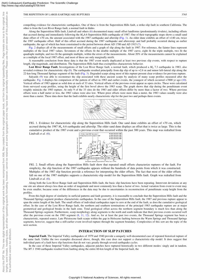
compelling evidence for characteristic earthquakes. One of these is from the Superstition Hills fault, a strike-slip fault in southern California. Theother is from the Lost River Range fault, a normal fault in Idaho.
Along the Superstition Hills fault, Lindvall and others (6) documented many small offset landforms (predominantly rivulets), including offsetsthat accrued during and immediately following the Mw6.6 Superstition Hills earthquake of 1987. One of their topographic maps shows a small sanddune offset of �70 cm, the amount associated with the 1987 earthquake and afterslip (Fig. 1). An older dune exhibits an offset of �140 cm, twicethe 1987 earthquake offset. Half of this offset accrued during the 1987 earthquake and aftercreep; and half probably occurred during an earlierearthquake, the age of which has been constrained to the period between about AD 1700 and AD 1915 (7).
Fig. 2 displays all of the measurements of small offsets and a graph of slip along the fault in 1987. For reference, the fainter lines representmultiples of the local 1987 values. Seventeen of the offsets fit the double multiple of the 1987 curve, eight fit the triple multiple, two fit thequadruple multiple, and two fit the quintuple multiple, within the errors of the measurements. About 20% of the measurements cannot be explainedas a multiple of the local 1987 offset, and most of these are only marginally misfit.
A reasonable conclusion from these data is that the 1987 event nearly duplicated at least two previous slip events, with respect to rupturelength, slip magnitude, and distribution. The Superstition Hills fault thus exemplifies characteristic behavior.
Lost River Range Fault. Investigations of the Lost River Range fault, a normal fault, which produced a MS 7.3 earthquake in 1983, alsorevealed evidence for characteristic slip (8). The earthquake resulted principally from dip slip of up to �2.6 m and minor left-lateral slip along the22-km-long Thousand Springs segment of the fault (Fig. 3). Degraded scarps along most of this rupture present clear evidence for previous rupture.
Salyards (9) was able to reconstruct the slip associated with these ancient scarps by analysis of many scarp profiles measured after theearthquake. Fig. 4 displays his comparison of the pattern of offset in 1983 and earlier events, the youngest of which occurred �7000 yr ago (10).Vertical offsets of 1983 appear as solid dots at each of 33 sites. Vertical offsets of the previous event appear as open circles. These were calculatedfrom surveyed scarp profiles, using the height of the first bevel above the 1983 scarp. The graph shows that slip during the penultimate eventroughly mimicks the 1983 rupture. At only 9 of the 33 sites do the 1983 and older offsets differ by more than a factor of two. Where previousoffsets were a half meter or less, the 1983 values were also low. Where prior offsets were more than a meter, the 1983 values usually were alsomore than a meter. These data show that the fault exhibits nearly characteristic slip for the past two and perhaps three events.
FIG. 1. Evidence for characteristic slip along the Superstition Hills fault. One sand dune exhibits an offset of �70 cm, whichaccrued during the 1987 Mw 6.6 earthquake and afterslip. The older sand dune displays an offset that is twice as large. This is thecumulative product of the 1987 event and a previous event that occurred within the past 300 years. This map was redrafted fromLindvall et al. (6).
FIG. 2. Small offsets along the Superstition Hills fault show that repeated small offsets characterize ruptures of the fault. Forsimplicity, the slip function of the 1987 earthquake appears without the hundreds of data points from which it was constructed.Multiples of the 1987 slip function provide a reference for interpreting the older offsets. The fact that most of the older offsetsfall on one of the 1987 multiples supports a characteristic-slip model for the Superstition Hills fault. Graph was redrafted fromLindvall et al. (6).Along both the Lost River Range fault and Superstition Hills fault, the basic slip functions have been repeating. Interevent deviations at any
one site are almost always less than an order of magnitude and most commonly less than a factor of two. Actual variation from event to event maybe even smaller, because some of the differences in the data may be due to uncertainties in reconstruction of penultimate scarp height from theprofiles.
From this high degree of similarity in surficial patterns and fault geometry, it is reasonable to conclude that the Superstition Hills fault and theThousand Springs segment produce characteristic earthquakes. In the case of the Superstition Hills fault, the 1987 and previous rupture appear tospan the entire length of the fault. The small offsets of individual earthquakes taper to zero at the end of the fault, as does the cumulative geologicaloffset. In the case of the Lost River Range fault, the northern and southern terminations of the principal 1983 earthquake rupture are at majorgeometrical and geological breaks in the fault zone. Total geological offset across the northern segment boundary is much less than along theThousand Springs segment. Furthermore, scarp morphology along segments to the north and south indicate that their previous events occurred wellafter the previous event on the 1983 segment (8, 11, 12). And so, for at least the past two events, the Thousand Springs segment has been acharacteristic, repeated source. Late Pleistocene fault scarps within the gap in Holocene faulting between the Warm Springs and Thousand Springssegments, however, suggest that a still-earlier event involved rupture through the segment boundary. Complexities of this sort are the topic of thenext section.
INTERACTION OF SLIP PATCHES
Imperial Fault. The Imperial Valley earthquakes of 1979 and 1940 provide a uniquely well-documented case of repeated historical rupture ofthe same fault. Unlike the two examples discussed above, though, this case does not support a characteristic-slip model. It does suggest thatindividual parts of a fault have slip functions that do not vary greatly through several earthquake cycles.
In the case of these Imperial Valley earthquakes, adjacent patches have ruptured historically in two different modes: singly and in tandem.The M7.1 1940 earthquake resulted from faulting along the entire 60-km length of the Imperial fault, the
THE REPETITION OF LARGE-EARTHQUAKE RUPTURES 3765
Abou
t thi
s PD
F fil
e: T
his
new
dig
ital r
epre
sent
atio
n of
the
orig
inal
wor
k ha
s be
en re
com
pose
d fro
m X
ML
files
cre
ated
from
the
orig
inal
pap
er b
ook,
not
from
the
orig
inal
type
setti
ng fi
les.
Pag
e br
eaks
are
true
to th
e or
igin
al; l
ine
leng
ths,
wor
d br
eaks
, hea
ding
sty
les,
and
oth
er ty
pese
tting
-spe
cific
form
attin
g, h
owev
er, c
anno
t be
reta
ined
, and
som
e ty
pogr
aphi
c er
rors
may
hav
e be
en a
ccid
enta
lly in
serte
d. P
leas
e us
e th
e pr
int v
ersi
on o
f thi
s pu
blic
atio
n as
the
auth
orita
tive
vers
ion
for a
ttrib
utio
n.
Copyright © National Academy of Sciences. All rights reserved.
(NAS Colloquium) Earthquake Prediction: The Scientific Challengehttp://www.nap.edu/catalog/5709.html
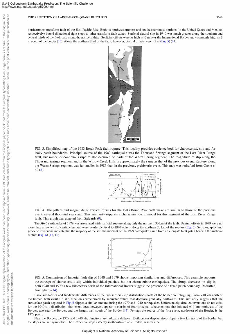
northernmost transform fault of the East Pacific Rise. Both its northwesternmost and southeasternmost portions (in the United States and Mexico,respectively) bound dilatational right-steps to other transform fault zones. Surficial dextral slip in 1940 was much greater along the southern andcentral thirds of the fault than along the northern third. Surficial offsets were as high as 6 m near the International Border and commonly high as 3m south of the border (13). Along the northern third of the fault, however, dextral offsets were <1 m (Fig. 5) (14).
FIG. 3. Simplified map of the 1983 Borah Peak fault rupture. This locality provides evidence both for characteristic slip and forleaky patch boundaries. Principal source of the 1983 earthquake was the Thousand Springs segment of the Lost River Rangefault, but minor, discontinuous rupture also occurred on parts of the Warm Spring segment. The magnitude of slip along theThousand Springs segment and in the Willow Creek Hills is approximately the same as that of the previous event. Rupture alongthe Warm Springs segment was far smaller in 1983 than in the previous, prehistoric event. This map was redrafted from Crone etal. (8).
FIG. 4. The pattern and magnitude of vertical offsets for the 1983 Borah Peak earthquake are similar to those of the previousevent, several thousand years ago. This similarity supports a characteristic-slip model for this segment of the Lost River Rangefault. This graph was adapted from Salyards (9).The M6.6 earthquake of 1979 was associated with surficial rupture along only the northern 30 km of the fault. Dextral offsets in 1979 were no
more than a few tens of centimeters and were nearly identical to 1940 offsets along the northern 20 km of the rupture (Fig. 5). Seismographic andgeodetic inversions indicate that the majority of the seismic moment of the 1979 earthquake came from an elongate fault patch beneath the surficialrupture (Fig. 6) (15, 16).
FIG. 5. Comparison of Imperial fault slip of 1940 and 1979 shows important similarities and differences. This example supportsthe concept of characteristic slip within individual patches, but not characteristic earthquakes. The abrupt decreases in slip inboth 1940 and 1979 a few kilometers north of the International Border suggest the presence of a fixed patch boundary. Redraftedfrom Sharp (14).Basic similarities and fundamental differences of the two surficial-slip distributions north of the border are intriguing. From �10 km north of
the border, both exhibit a slip function characterized by submeter values that decrease gradually northward. This similarity suggests that thesubsurface patch depicted in Fig. 6 slipped a similar amount during the 1979 and 1940 earthquakes. Unfortunately, detailed inversions do not existfor the 1940 slip distribution; that event does, however, appear to consist of four principal subevents: one that initiated �10 km northwest of theBorder, two near the Border, and the largest well south of the Border (13). Perhaps the source of the first event, northwest of the Border, is the1979 patch.
Near the Border, the 1979 and 1940 slip functions are radically different. Both curves display steep slopes a few km north of the border, butthe slopes are antisymmetric: The 1979 curve slopes steeply southeastward at �1 m/km, whereas the
THE REPETITION OF LARGE-EARTHQUAKE RUPTURES 3766
Abou
t thi
s PD
F fil
e: T
his
new
dig
ital r
epre
sent
atio
n of
the
orig
inal
wor
k ha
s be
en re
com
pose
d fro
m X
ML
files
cre
ated
from
the
orig
inal
pap
er b
ook,
not
from
the
orig
inal
type
setti
ng fi
les.
Pag
e br
eaks
are
true
to th
e or
igin
al; l
ine
leng
ths,
wor
d br
eaks
, hea
ding
sty
les,
and
oth
er ty
pese
tting
-spe
cific
form
attin
g, h
owev
er, c
anno
t be
reta
ined
, and
som
e ty
pogr
aphi
c er
rors
may
hav
e be
en a
ccid
enta
lly in
serte
d. P
leas
e us
e th
e pr
int v
ersi
on o
f thi
s pu
blic
atio
n as
the
auth
orita
tive
vers
ion
for a
ttrib
utio
n.
Copyright © National Academy of Sciences. All rights reserved.
(NAS Colloquium) Earthquake Prediction: The Scientific Challengehttp://www.nap.edu/catalog/5709.html
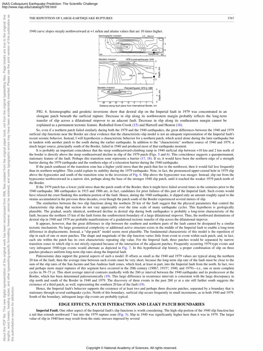
1940 curve slopes steeply northwestward at �1 m/km and attains values that are 10 times higher.
FIG. 6. Seismographic and geodetic inversions show that dextral slip on the Imperial fault in 1979 was concentrated in anelongate patch beneath the surficial rupture. Decrease in slip along its northwestern margin probably reflects the long-termtransfer of slip across a dilatational stepover to an adacent fault. Decrease in slip along its southeastern margin cannot beexplained as a permanent tectonic feature. Redrafted from Crook (15) and Hartzell and Heaton (16).So, even if a northern patch failed similarly during both the 1979 and the 1940 earthquakes, the great differences between the 1940 and 1979
surficial slip functions near the Border are clear evidence that the characteristic-slip model is not an adequate representation of the Imperial fault'srecent seismic behavior. Instead, I will hypothesize a characteristic behavior for a northern patch, which acted alone during the later earthquake butin tandem with another patch to the south during the earlier earthquake. In addition to the “characteristic” northern source of 1940 and 1979, amuch larger source, principally south of the Border, failed in 1940 and produced most of that earthquake moment.
It is probably an important coincidence that the steep southeastward-climbing ramp in 1940 surficial slip between �10 km and 2 km north ofthe border is directly above the steep southeastward decline in slip of the 1979 patch (Figs. 5 and 6). This coincidence suggests a quasipermanent,stationary feature of the fault. Perhaps this transition zone represents a barrier (17, 18). If so, it would have been the northern edge of a strengthbarrier during the 1979 earthquake and the southern edge of a relaxation barrier during the 1940 earthquake.
If the patch southeast of the transition zone has a higher yield stress than the patch that lies to the northwest, then it would fail less frequentlythan its northern neighbor. This could explain its stability during the 1979 earthquake. Note, in fact, the pronounced upper-crustal hole in 1979 slipabove the hypocenter and south of the transition zone in the inversions of Fig. 6. Slip above the hypocenter was meager. Instead, slip ran from thehypocenter northwestward in a narrow slot, perhaps along the base of the stronger 1940 slip patch, until it reached the weaker 1979 patch north ofthe Border.
If the 1979 patch has a lower yield stress than the patch south of the Border, then it might have failed several times in the centuries prior to the1940 earthquake. M6 earthquakes in 1915 and 1906 are, in fact, candidates for prior failures of this part of the Imperial fault. Such events wouldhave relaxed the crust flanking this northern portion of the fault. Hence, during the 1940 earthquake, it slipped only an amount roughly equal to thestrains accumulated in the previous three decades, even though the patch south of the Border experienced several meters of slip.
The similarities between the two slip functions along the northern 20 km of the fault suggest that the physical parameters that control thecharacteristic slip along that section do not vary appreciably over the time scale of many earthquake cycles. This hypothesis is geologicallyplausible. The gradual, nearly identical, northward decline in dextral slip during both earthquakes is probably a long-term characteristic of thefault, because the northern 15 km of the fault forms the southwestern boundary of a large dilatational stepover. Thus, the northward diminutions ofdextral slip in 1940 and 1979 are probable manifestations of a gradational tectonic transfer of slip across the dilatational stepover.
It appears, however, that the great difference in slip between the southern and northern parts of the fault cannot be dissipated by a similartectonic mechanism. No large geometrical complexity or additional active structure exists in the middle of the Imperial fault to enable a long-termdifference in displacements. Instead, a “slip-patch” model seems most plausible. The fundamental characteristic of this model is the repetition ofslip in each of one or more patches. The shape and magnitude of the slip function varies little from event to event within each patch, and, in fact,each site within the patch has its own characteristic repeating slip value. For the Imperial fault, three patches would be separated by narrowtransition zones in which slip is not strictly repeated because of the interaction of the adjacent patches. Frequently occurring 1979-type events andvery infrequent 1940-type events would alternate as depicted in Fig. 7. In this hypothetical slip history, a proper combination of slip on threepatches produces uniform long-term slip rates along the Imperial fault.
Paleoseismic data support the general aspects of such a model. If offsets as small as the 1940 and 1979 values are typical along the northern20 km of the fault, then the average time between such events must be very short, because the long-term slip rate of the fault must be close to thesum of the slip rates of the San Jacinto and San Andreas fault zones, which feed, at least in part, into the Imperial fault from the north. In fact, twoand perhaps more major ruptures of this segment have occurred in the 20th century (1906?, 1915?, 1940, and 1979)—i.e., one or more completecycles in 39–73 yr. This short average interval contrasts markedly with the 260-yr interval between the 1940 earthquake and its predecessor at theBorder, which has been determined paleoseismically (19). This large difference in recurrence intervals is consistent with the large discrepancy inslip north and south of the Border in 1940 and 1979. The discovery of three events in the past 260 yr at a site still farther south suggests theexistence of a third patch, as well, representing the southern 20 km of the fault (19).
Hence, the Imperial fault's behavior supports the existence of at least two and perhaps three discrete patches, separated by a boundary that isstationary through several earthquake cycles. North of this boundary, surficial slip occurs frequently in small increments, as in both 1940 and 1979.South of the boundary, infrequent large slip events are probably typical.
EDGE EFFECTS, PATCH INTERACTION AND LEAKY PATCH BOUNDARIES
Imperial Fault. One other aspect of the Imperial fault's slip functions is worth considering. The high-slip portion of the 1940 slip function hasa tail that extends northward 7 km into the 1979 rupture zone (Fig. 5). Slip in 1940 was significantly higher here than it was in 1979. The largervalue of slip in 1940 here may result from the static stresses imposed by several
THE REPETITION OF LARGE-EARTHQUAKE RUPTURES 3767
Abou
t thi
s PD
F fil
e: T
his
new
dig
ital r
epre
sent
atio
n of
the
orig
inal
wor
k ha
s be
en re
com
pose
d fro
m X
ML
files
cre
ated
from
the
orig
inal
pap
er b
ook,
not
from
the
orig
inal
type
setti
ng fi
les.
Pag
e br
eaks
are
true
to th
e or
igin
al; l
ine
leng
ths,
wor
d br
eaks
, hea
ding
sty
les,
and
oth
er ty
pese
tting
-spe
cific
form
attin
g, h
owev
er, c
anno
t be
reta
ined
, and
som
e ty
pogr
aphi
c er
rors
may
hav
e be
en a
ccid
enta
lly in
serte
d. P
leas
e us
e th
e pr
int v
ersi
on o
f thi
s pu
blic
atio
n as
the
auth
orita
tive
vers
ion
for a
ttrib
utio
n.
Copyright © National Academy of Sciences. All rights reserved.
(NAS Colloquium) Earthquake Prediction: The Scientific Challengehttp://www.nap.edu/catalog/5709.html
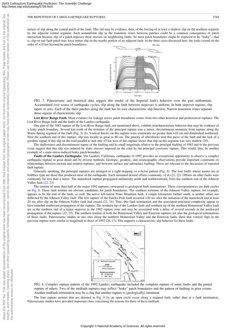
meters of slip along the central patch of the fault. This tail may be evidence, then, of the forcing of at least a shallow slip on the northern segmentby the adjacent central segment. Such nonuniform slip in the transition zones between patches could be a common consequence of patchinteraction because slip of a patch imposes shear stresses on neighboring faults. So most patch boundaries might be expected to be “leaky”—thatis, slip on one fault patch may force minor slip on the nearby portion of an adjacent fault. In the three cases discussed here, the leaks extend on theorder of �10 km beyond the patch boundaries.
FIG. 7. Paleoseismic and historical data suggest this model of the Imperial fault's behavior over the past millennium.Accumulated over scores of earthquake cycles, slip along the fault between stepovers is uniform. In both stepover regions, sliptapers to zero. Each of the three patches along the fault has its own characteristic slip function. Narrow transition zones separatethese regions of characteristic slip.Lost River Range Fault. More evidence for leakage across patch boundaries comes from two other historical and prehistorical ruptures: The
Lost River Range fault and the faults of the Landers earthquake.One part of the 1983 rupture of the Lost River Range fault, not mentioned above, exhibits noncharacteristic behavior that may be evidence of
a leaky patch boundary. Several km north of the terminus of the principal rupture was a minor, discontinuous mountain front rupture along theWarm Spring segment of the fault (Fig. 3) (8). Vertical throws on this rupture were commonly no greater than �10 cm and diminished northward.Near the southern end of this rupture, slip was locally as great as 80 cm. The paucity of aftershocks near this piece of the fault and the lack of ageodetic signal of this slip on the road parallel to and only �5 km west of this rupture shows that slip on this segment was very shallow (20).
The shallowness and discontinuous nature of the faulting and its small magnitude relative to the principal faulting of 1983 and to the previousevent suggest that this slip was induced by static stresses imposed on the crust by the principal coseismic rupture. This would, thus, be anotherexample of a static-stress-induced leaky patch boundary.
Faults of the Landers Earthquake. The Landers, California, earthquake of 1992 provides an exceptional opportunity to observe a complexearthquake rupture in great detail and by diverse methods. Geologic, geodetic, and seismographic observations provide important constraints onrelationships between ancient and modern ruptures, and between surface and subsurface faulting. These are relevant to the discussion of repeatedfault rupture.
Generally speaking, the principal ruptures are arranged in a right-stepping en echelon pattern (Fig. 8). The four faults whose names are inboldface type are those that produced most of the earthquake. Each sustained dextral offsets commonly >2 m (21, 22). Offsets on other faults werecommonly far less than a meter. The mainshock rupture propagated unilaterally north and northwestward, from the southern end of the JohnsonValley fault (22, 23).
The termini of more than half of the major 1992 ruptures correspond to geological fault terminations. These correspondences are dark circleson Fig. 8. These fault termini are obvious candidates for patch boundaries. The southern terminus of the Johnson Valley rupture, for example,appears to be the end of the fault, as well: the active left-lateral Pinto Mountain fault, a couple kilometers farther south, is neither offset nordeflected by the Johnson Valley fault. The first rupture of the Eureka Peak fault occurred �30 sec after the initiation of the mainshock and at least20 sec after slip on the Johnson Valley fault had ceased (22, 24). Thus, this fault termination and the associated structural complexity appear tohave retarded southward propagation of the rupture. The northern tip of the Landers fault and southern tip of the northern Homestead Valley faultare at the northern end of a major stepover in the 1992 rupture zone and may be associated with a delay of several seconds in the northwardpropagation of the rupture (22, 25). The northern termini of both the Homestead Valley and Emerson ruptures are also the geological terminationsof those faults. Paleoseismic studies at two sites along the northern Homestead Valley and the Emerson faults show that vertical slips in theprevious rupture were similar in magnitude to those of 1992 (26, 27). This supports a characteristic-slip behavior for these faults.
FIG. 8. Complex rupture pattern of the 1992 Landers earthquake included the complete rupture of some faults and the partialrupture of others. Two of the midfault ruptures may reflect “leaky” patch boundaries and the pattern of faulting in prior events.Another midfault termination may be a clue that another rupture is (geologically) imminent.The four rupture termini that are denoted in Fig. 8 by an open circle occur along a mapped fault, rather than at a fault termination.
Paleoseismic studies have provided important clues concerning the reasons for three of these midfault
THE REPETITION OF LARGE-EARTHQUAKE RUPTURES 3768
Abou
t thi
s PD
F fil
e: T
his
new
dig
ital r
epre
sent
atio
n of
the
orig
inal
wor
k ha
s be
en re
com
pose
d fro
m X
ML
files
cre
ated
from
the
orig
inal
pap
er b
ook,
not
from
the
orig
inal
type
setti
ng fi
les.
Pag
e br
eaks
are
true
to th
e or
igin
al; l
ine
leng
ths,
wor
d br
eaks
, hea
ding
sty
les,
and
oth
er ty
pese
tting
-spe
cific
form
attin
g, h
owev
er, c
anno
t be
reta
ined
, and
som
e ty
pogr
aphi
c er
rors
may
hav
e be
en a
ccid
enta
lly in
serte
d. P
leas
e us
e th
e pr
int v
ersi
on o
f thi
s pu
blic
atio
n as
the
auth
orita
tive
vers
ion
for a
ttrib
utio
n.
Copyright © National Academy of Sciences. All rights reserved.
(NAS Colloquium) Earthquake Prediction: The Scientific Challengehttp://www.nap.edu/catalog/5709.html
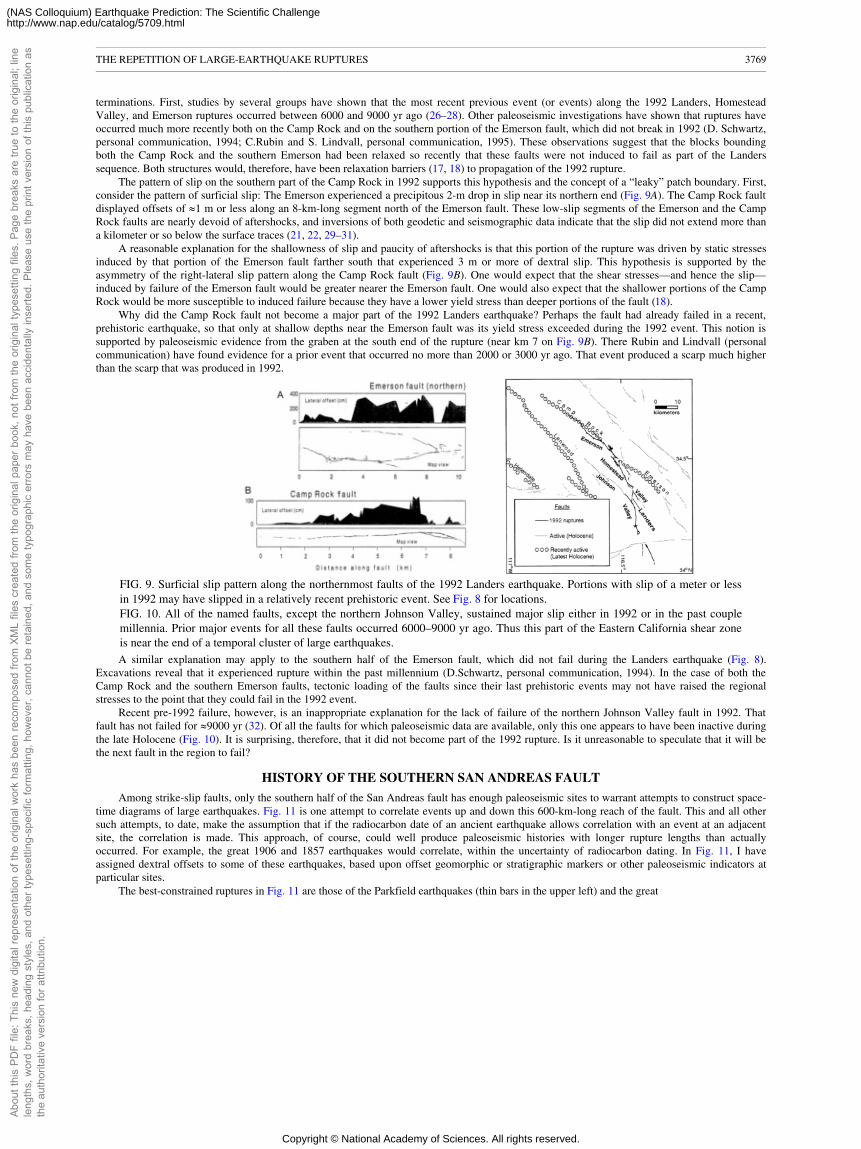
terminations. First, studies by several groups have shown that the most recent previous event (or events) along the 1992 Landers, HomesteadValley, and Emerson ruptures occurred between 6000 and 9000 yr ago (26–28). Other paleoseismic investigations have shown that ruptures haveoccurred much more recently both on the Camp Rock and on the southern portion of the Emerson fault, which did not break in 1992 (D. Schwartz,personal communication, 1994; C.Rubin and S. Lindvall, personal communication, 1995). These observations suggest that the blocks boundingboth the Camp Rock and the southern Emerson had been relaxed so recently that these faults were not induced to fail as part of the Landerssequence. Both structures would, therefore, have been relaxation barriers (17, 18) to propagation of the 1992 rupture.
The pattern of slip on the southern part of the Camp Rock in 1992 supports this hypothesis and the concept of a “leaky” patch boundary. First,consider the pattern of surficial slip: The Emerson experienced a precipitous 2-m drop in slip near its northern end (Fig. 9A). The Camp Rock faultdisplayed offsets of �1 m or less along an 8-km-long segment north of the Emerson fault. These low-slip segments of the Emerson and the CampRock faults are nearly devoid of aftershocks, and inversions of both geodetic and seismographic data indicate that the slip did not extend more thana kilometer or so below the surface traces (21, 22, 29–31).
A reasonable explanation for the shallowness of slip and paucity of aftershocks is that this portion of the rupture was driven by static stressesinduced by that portion of the Emerson fault farther south that experienced 3 m or more of dextral slip. This hypothesis is supported by theasymmetry of the right-lateral slip pattern along the Camp Rock fault (Fig. 9B). One would expect that the shear stresses—and hence the slip—induced by failure of the Emerson fault would be greater nearer the Emerson fault. One would also expect that the shallower portions of the CampRock would be more susceptible to induced failure because they have a lower yield stress than deeper portions of the fault (18).
Why did the Camp Rock fault not become a major part of the 1992 Landers earthquake? Perhaps the fault had already failed in a recent,prehistoric earthquake, so that only at shallow depths near the Emerson fault was its yield stress exceeded during the 1992 event. This notion issupported by paleoseismic evidence from the graben at the south end of the rupture (near km 7 on Fig. 9B). There Rubin and Lindvall (personalcommunication) have found evidence for a prior event that occurred no more than 2000 or 3000 yr ago. That event produced a scarp much higherthan the scarp that was produced in 1992.
FIG. 9. Surficial slip pattern along the northernmost faults of the 1992 Landers earthquake. Portions with slip of a meter or lessin 1992 may have slipped in a relatively recent prehistoric event. See Fig. 8 for locations.FIG. 10. All of the named faults, except the northern Johnson Valley, sustained major slip either in 1992 or in the past couplemillennia. Prior major events for all these faults occurred 6000–9000 yr ago. Thus this part of the Eastern California shear zoneis near the end of a temporal cluster of large earthquakes.A similar explanation may apply to the southern half of the Emerson fault, which did not fail during the Landers earthquake (Fig. 8).
Excavations reveal that it experienced rupture within the past millennium (D.Schwartz, personal communication, 1994). In the case of both theCamp Rock and the southern Emerson faults, tectonic loading of the faults since their last prehistoric events may not have raised the regionalstresses to the point that they could fail in the 1992 event.
Recent pre-1992 failure, however, is an inappropriate explanation for the lack of failure of the northern Johnson Valley fault in 1992. Thatfault has not failed for �9000 yr (32). Of all the faults for which paleoseismic data are available, only this one appears to have been inactive duringthe late Holocene (Fig. 10). It is surprising, therefore, that it did not become part of the 1992 rupture. Is it unreasonable to speculate that it will bethe next fault in the region to fail?
HISTORY OF THE SOUTHERN SAN ANDREAS FAULT
Among strike-slip faults, only the southern half of the San Andreas fault has enough paleoseismic sites to warrant attempts to construct space-time diagrams of large earthquakes. Fig. 11 is one attempt to correlate events up and down this 600-km-long reach of the fault. This and all othersuch attempts, to date, make the assumption that if the radiocarbon date of an ancient earthquake allows correlation with an event at an adjacentsite, the correlation is made. This approach, of course, could well produce paleoseismic histories with longer rupture lengths than actuallyoccurred. For example, the great 1906 and 1857 earthquakes would correlate, within the uncertainty of radiocarbon dating. In Fig. 11, I haveassigned dextral offsets to some of these earthquakes, based upon offset geomorphic or stratigraphic markers or other paleoseismic indicators atparticular sites.
The best-constrained ruptures in Fig. 11 are those of the Parkfield earthquakes (thin bars in the upper left) and the great
THE REPETITION OF LARGE-EARTHQUAKE RUPTURES 3769
Abou
t thi
s PD
F fil
e: T
his
new
dig
ital r
epre
sent
atio
n of
the
orig
inal
wor
k ha
s be
en re
com
pose
d fro
m X
ML
files
cre
ated
from
the
orig
inal
pap
er b
ook,
not
from
the
orig
inal
type
setti
ng fi
les.
Pag
e br
eaks
are
true
to th
e or
igin
al; l
ine
leng
ths,
wor
d br
eaks
, hea
ding
sty
les,
and
oth
er ty
pese
tting
-spe
cific
form
attin
g, h
owev
er, c
anno
t be
reta
ined
, and
som
e ty
pogr
aphi
c er
rors
may
hav
e be
en a
ccid
enta
lly in
serte
d. P
leas
e us
e th
e pr
int v
ersi
on o
f thi
s pu
blic
atio
n as
the
auth
orita
tive
vers
ion
for a
ttrib
utio
n.
Copyright © National Academy of Sciences. All rights reserved.
(NAS Colloquium) Earthquake Prediction: The Scientific Challengehttp://www.nap.edu/catalog/5709.html
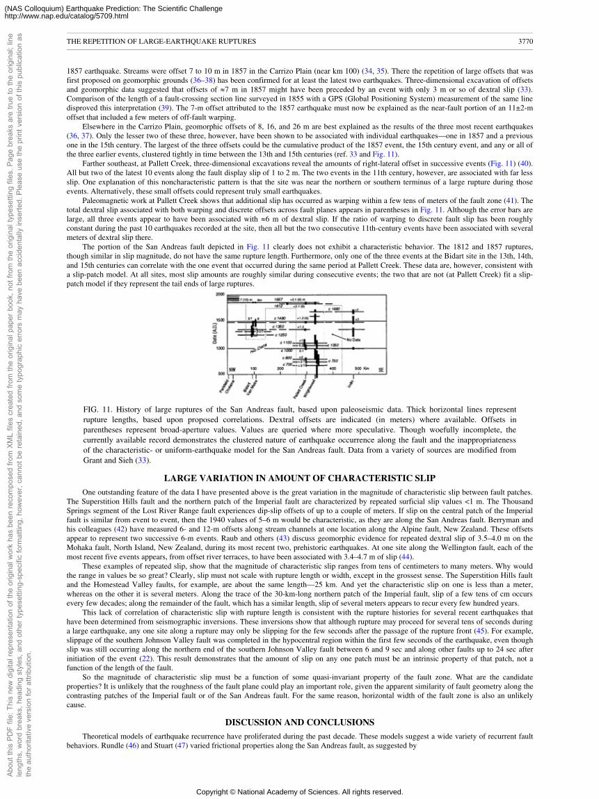
1857 earthquake. Streams were offset 7 to 10 m in 1857 in the Carrizo Plain (near km 100) (34, 35). There the repetition of large offsets that wasfirst proposed on geomorphic grounds (36–38) has been confirmed for at least the latest two earthquakes. Three-dimensional excavation of offsetsand geomorphic data suggested that offsets of �7 m in 1857 might have been preceded by an event with only 3 m or so of dextral slip (33).Comparison of the length of a fault-crossing section line surveyed in 1855 with a GPS (Global Positioning System) measurement of the same linedisproved this interpretation (39). The 7-m offset attributed to the 1857 earthquake must now be explained as the near-fault portion of an 11±2-moffset that included a few meters of off-fault warping.
Elsewhere in the Carrizo Plain, geomorphic offsets of 8, 16, and 26 m are best explained as the results of the three most recent earthquakes(36, 37). Only the lesser two of these three, however, have been shown to be associated with individual earthquakes—one in 1857 and a previousone in the 15th century. The largest of the three offsets could be the cumulative product of the 1857 event, the 15th century event, and any or all ofthe three earlier events, clustered tightly in time between the 13th and 15th centuries (ref. 33 and Fig. 11).
Farther southeast, at Pallett Creek, three-dimensional excavations reveal the amounts of right-lateral offset in successive events (Fig. 11) (40).All but two of the latest 10 events along the fault display slip of 1 to 2 m. The two events in the 11th century, however, are associated with far lessslip. One explanation of this noncharacteristic pattern is that the site was near the northern or southern terminus of a large rupture during thoseevents. Alternatively, these small offsets could represent truly small earthquakes.
Paleomagnetic work at Pallett Creek shows that additional slip has occurred as warping within a few tens of meters of the fault zone (41). Thetotal dextral slip associated with both warping and discrete offsets across fault planes appears in parentheses in Fig. 11. Although the error bars arelarge, all three events appear to have been associated with �6 m of dextral slip. If the ratio of warping to discrete fault slip has been roughlyconstant during the past 10 earthquakes recorded at the site, then all but the two consecutive 11th-century events have been associated with severalmeters of dextral slip there.
The portion of the San Andreas fault depicted in Fig. 11 clearly does not exhibit a characteristic behavior. The 1812 and 1857 ruptures,though similar in slip magnitude, do not have the same rupture length. Furthermore, only one of the three events at the Bidart site in the 13th, 14th,and 15th centuries can correlate with the one event that occurred during the same period at Pallett Creek. These data are, however, consistent witha slip-patch model. At all sites, most slip amounts are roughly similar during consecutive events; the two that are not (at Pallett Creek) fit a slip-patch model if they represent the tail ends of large ruptures.
FIG. 11. History of large ruptures of the San Andreas fault, based upon paleoseismic data. Thick horizontal lines representrupture lengths, based upon proposed correlations. Dextral offsets are indicated (in meters) where available. Offsets inparentheses represent broad-aperture values. Values are queried where more speculative. Though woefully incomplete, thecurrently available record demonstrates the clustered nature of earthquake occurrence along the fault and the inappropriatenessof the characteristic- or uniform-earthquake model for the San Andreas fault. Data from a variety of sources are modified fromGrant and Sieh (33).
LARGE VARIATION IN AMOUNT OF CHARACTERISTIC SLIP
One outstanding feature of the data I have presented above is the great variation in the magnitude of characteristic slip between fault patches.The Superstition Hills fault and the northern patch of the Imperial fault are characterized by repeated surficial slip values <1 m. The ThousandSprings segment of the Lost River Range fault experiences dip-slip offsets of up to a couple of meters. If slip on the central patch of the Imperialfault is similar from event to event, then the 1940 values of 5–6 m would be characteristic, as they are along the San Andreas fault. Berryman andhis colleagues (42) have measured 6- and 12-m offsets along stream channels at one location along the Alpine fault, New Zealand. These offsetsappear to represent two successive 6-m events. Raub and others (43) discuss geomorphic evidence for repeated dextral slip of 3.5–4.0 m on theMohaka fault, North Island, New Zealand, during its most recent two, prehistoric earthquakes. At one site along the Wellington fault, each of themost recent five events appears, from offset river terraces, to have been associated with 3.4–4.7 m of slip (44).
These examples of repeated slip, show that the magnitude of characteristic slip ranges from tens of centimeters to many meters. Why wouldthe range in values be so great? Clearly, slip must not scale with rupture length or width, except in the grossest sense. The Superstition Hills faultand the Homestead Valley faults, for example, are about the same length—25 km. And yet the characteristic slip on one is less than a meter,whereas on the other it is several meters. Along the trace of the 30-km-long northern patch of the Imperial fault, slip of a few tens of cm occursevery few decades; along the remainder of the fault, which has a similar length, slip of several meters appears to recur every few hundred years.
This lack of correlation of characteristic slip with rupture length is consistent with the rupture histories for several recent earthquakes thathave been determined from seismographic inversions. These inversions show that although rupture may proceed for several tens of seconds duringa large earthquake, any one site along a rupture may only be slipping for the few seconds after the passage of the rupture front (45). For example,slippage of the southern Johnson Valley fault was completed in the hypocentral region within the first few seconds of the earthquake, even thoughslip was still occurring along the northern end of the southern Johnson Valley fault between 6 and 9 sec and along other faults up to 24 sec afterinitiation of the event (22). This result demonstrates that the amount of slip on any one patch must be an intrinsic property of that patch, not afunction of the length of the fault.
So the magnitude of characteristic slip must be a function of some quasi-invariant property of the fault zone. What are the candidateproperties? It is unlikely that the roughness of the fault plane could play an important role, given the apparent similarity of fault geometry along thecontrasting patches of the Imperial fault or of the San Andreas fault. For the same reason, horizontal width of the fault zone is also an unlikelycause.
DISCUSSION AND CONCLUSIONS
Theoretical models of earthquake recurrence have proliferated during the past decade. These models suggest a wide variety of recurrent faultbehaviors. Rundle (46) and Stuart (47) varied frictional properties along the San Andreas fault, as suggested by
THE REPETITION OF LARGE-EARTHQUAKE RUPTURES 3770
Abou
t thi
s PD
F fil
e: T
his
new
dig
ital r
epre
sent
atio
n of
the
orig
inal
wor
k ha
s be
en re
com
pose
d fro
m X
ML
files
cre
ated
from
the
orig
inal
pap
er b
ook,
not
from
the
orig
inal
type
setti
ng fi
les.
Pag
e br
eaks
are
true
to th
e or
igin
al; l
ine
leng
ths,
wor
d br
eaks
, hea
ding
sty
les,
and
oth
er ty
pese
tting
-spe
cific
form
attin
g, h
owev
er, c
anno
t be
reta
ined
, and
som
e ty
pogr
aphi
c er
rors
may
hav
e be
en a
ccid
enta
lly in
serte
d. P
leas
e us
e th
e pr
int v
ersi
on o
f thi
s pu
blic
atio
n as
the
auth
orita
tive
vers
ion
for a
ttrib
utio
n.
Copyright © National Academy of Sciences. All rights reserved.
(NAS Colloquium) Earthquake Prediction: The Scientific Challengehttp://www.nap.edu/catalog/5709.html
variable offsets during the 1857 earthquake and along-strike variations in recurrence intervals, to create synthetic histories many earthquake cycleslong. Some of their histories mimick the actual historical and paleoseismic record of the fault, in that certain portions of the fault experienceinfrequent repeated offsets of several meters, whereas others experience frequent small offsets. Ward (48) has developed synthetic histories oflarge earthquakes along the Middle American subduction zone, using static dislocation theory and fault segments based upon the fault's historicalbehavior. His models produce a variety of behaviors, including fault patches that are highly “characteristic” and patches that produce a variety ofevent sizes and rupture lengths. In all three of these attempts to model fault histories, the locations of rupture terminations and transitions fromhigh- to low-slip patches are roughly stationary.
Rice and his colleagues (3, 49) have argued that theoretical models of smooth faults produce slip events that are highly regular in both spaceand time, if the numerical cell size one uses is small compared to the dimensions of the earthquake's nucleation patch. An individual fault can bemade to deviate from highly regular repetition of events only if it is allowed to change state between earthquakes, while it is not slipping (49). Inthese “aging” models, slip at a site varies by more than an order of magnitude, and slip-patch boundaries vary wildly with time. Even in thisversion of their smooth-fault models, however, power-law frequency-size earthquake populations of the G-R type fail to occur. From this, theyconclude that observed G-R earthquake populations reflect geometrical irregularities along faults and the spectrum of fault sizes in a region.Wesnousky's study (2) of paleoseismic and instrumental data for major faults in southern California supports this view that structures fail in largeearthquakes that are grossly underpredicted by the G-R statistics of smaller earthquakes in the surrounding region.
Well-documented examples of repeated fault rupture are rare. But sparse available data support the view that smooth, individual fault patchesfail during characteristic slip events. At sites where recent slip was small, previous events usually exhibit slip of the same magnitude. Likewise,where recent slip was meters, previous events usually exhibit slip of the same magnitude. Synthetic earthquake histories characterized by highlyirregular slip during consecutive events do not appear to reflect reality.
Contrary to the “characteristic earthquake” model, patches commonly fail either singly or in tandem with one or more adjacent patches. Onlyalong transition zones between slip patches does slip at a site appear to deviate much from event to event. Large seismic rupture in a transitionregion during one event may alternate with aseismic slip induced there by static stresses from coseismic slip on a neighboring patch.
The small differences in a patch's slip function over two or more earthquake cycles indicate that slip is controlled principally by a physicalproperty of the patch, not the length of the rupture or dynamic properties of the rupture, such as directivity.
Carrie Sieh assisted in drafting the figures. I deeply appreciate support during the past two decades by the National Earthquake HazardsReduction Program, through the U.S. Geological Survey's external grants program. My studies of the Landers earthquake were supported byCalifornia Institute of Technology's Earthquake Research Affiliates and by the National Science Foundation/U.S. Geological Survey SouthernCalifornia Earthquake Center. This paper is California Institute of Technology Division of Geological and Planetary Sciences contribution number5588 and Southern California Earthquake Center contribution number 218.1. Ellsworth, W.L. (1991) Clocks in the Earth: Repeatability and Variability in Earthquake Recurrence (Natl. Acad. Sci., Washington, DC).2. Wesnousky, S. (1995) Bull. Seismol Soc. Am. 84, 1940–1959.3. Rice, J. & Ben-Zion, Y. (1996) Proc. Natl. Acad. Sci. USA 92, 3811–3818.4. Schwartz, D. & Coppersmith, K. (1984) J. Geophys. Res. 89, 581–598.5. Sieh, K. (1984) J. Geophys. Res. 83, 3907–3939.6. Lindvall, S., Rockwell, T. & Hudnut, K. (1989) Bull. Seismol. Soc. Am. 79, 342–361.7. Hudnut, K. & Sieh, K. (1989) Bull Seismol. Soc. Am. 79, 304–329.8. Crone, A.J., et al. (1987) Bull Seismol. Soc. Am. 77, 739–770.9. Salyards, S. (1985) Proceedings of Workship Twenty Eight on the Borah Peak, Idaho, Earthquake (U.S. Geological Survey), Vol. A, pp. 59–75.10. Hanks, T.C. & Schwartz, D.P. (1987) Bull Seismol. Soc. Am. 77, 837–846.11. Wallace, R.E. (1987) Bull. Seismol. Soc. Am. 77, 868–877.12. Crone, A.J. & Haller, K.M. (1991) J. Struct. Geol. 13, 151–164.13. Trifunac, M.D. & Brune, J.N. (1970) Bull Seismol. Soc. Am. 60, 137–160.14. Sharp, R.V. (1982) U.S. Geol. Surv. Prof. Pap. 1254, 213–221.15. Crook, C. (1984) Thesis (Univ. of London, London).16. Hartzell, S. & Heaton, T. (1984) Bull Seismol. Soc. Am. 72, 1553– 1583.17. Aki, K. (1979) J. Geophys. Res. 84, 6140–6148.18. Scholz, C.H. (1990) The Mechanics of Earthquake Faulting (Cambridge Univ. Press, New York).19. Thomas, A. & Rockwell, T. (1995) J. Geophys. Res., in press.20. Barrientos, S., Stein, R.S. & Ward, S.N. (1987) Bull. Seismol. Soc. Am. 77, 784–808.21. Sieh, K., et al. (1993) Science 260, 171–176.22. Wald, D.J. & Heaton, T.H. (1994) Bull. Seismol. Soc. Am. 84, 668–691.23. Hough, S. (1994) Bull Seismol. Soc. Am. 84, 817–825.24. Cohee, B. & Beroza, G. (1994) Bull Seismol. Soc. Am. (Special issue on 1992 Landers Earthquake Sequence).25. Spotila, J. & Sieh, K. (1995) J. Geophys. Res. 100, 543–559.26. Rubin, C. & Sieh, K. (1993) Eos Trans. Am. Geophys. Union. 74, 612.27. Rockwell, T.K., Schwartz, D., Sieh, K., Rubin, C., Lindvall, S., Herzberg, M., Padgett, D. & Fumal, T. (1993) Eos Trans. Am. Geophys. Union. 74, 67.28. Hecker, S., Fumal, T., Powers, T., Hamilton, J., Garvin, C., Schwartz, D. & Cints, F. (1993) Eos Trans. Am. Geophys. Union 74, 612.29. Bock, Y., Agnew, D., Fang, P., Genrich, J., Hager, B., Herring, T., Hudnut, K., King, R., Larsen, S., Minster, J., Stark, K., Udowindski, S. & Wyatt, F.
(1993) Nature (London) 361, 337–340.30. Hudnut, K. W., Bock, Y., Cline, M., Fang, P., Feng, Y., Freymueller, J., Ge, X., Gross, W., Jackson, D., Kim, M., King, N., Langbein, J., Larsen, S.,
Lisowski, M., Shen, Z., Svarc, J. & Zhang, J. (1994) Bull. Seismol Soc. Am. 84, 625–645.31. Hauksson, E., Jones, L.M., Hutton, K. & Phillips, D.E. (1993) J. Geophys. Res. 98, 19835–19858.32. Herzberg, M. & Rockwell, T. (1993) Eos Trans. Am. Geophys. Union 74, 612.33. Grant, L. & Sieh, K. (1994) J. Geophys. Res. 99, 6819–6841.34. Sieh, K. (1978) Bull. Seismol. Soc. Am. 68, 1421–1448.35. Grant, L. & Sieh, K. (1993) Bull Seismol. Soc. Am. 83, 619–635.36. Sieh, K. (1981) in International Research Conference on Intraplate Earthquakes, September 17–19, 1979, ed. Petrovski, J. (Ohrid, Yugoslavia), pp. 209–
218.37. Sieh, K. (1980) Proceedings of the Earthquake Prediction Research Symposium (Seismol. Soc. Japan), pp. 175–185.38. Sieh, K.E. & Jahns, R.H. (1984) Geol. Soc. Am. Bull. 95, 883–896.39. Grant, L. & Donnellan, A. (1993) Bull Seismol. Soc. Am. 84, 241–246.40. Sieh, K. (1984) J. Geophys. Res. 89, 7641–7670.41. Salyards, S., Sieh, K. & Kirschvink, J. (1992) J. Geophys. Res. 97, 12457–12470.42. Berryman, K., Beanland, S., Copper, A., Cutten, H., Norris R. & Wood, P. (1992) Ann. Tecton. 6, 126–163.43. Raub, M.L., Cutten, H.N.C. & Hull, A.G. (1987) Seismotectonic Hazard Analysis of the Mohaka Fault North Island, New Zealand, Proceedings of the
Pacific Conference on Earthquake Engineering (New Zealand Natl. Soc. for Earthquake Eng., Wellington, New Zealand), Vol. 3, pp. 219–230.44. Berryman, K. & Beanland, S. (1991) J. Struct. Geol. 13, 177–189.45. Heaton, T.H. (1990) Phys. Earth Planetary Interiors 64, 1–20.46. Rundle, J. (1988) J. Geophys. Res. 93, 6255–6274.47. Stuart, W.D. (1986) J. Geophys. Res. 91, 13771–13786.48. Ward, S.N. (1991) J. Geophys. Res. 96, 21433–21442.49. Rice, J.R. (1988) J. Geophys. Res. 98, 9885–9907.
THE REPETITION OF LARGE-EARTHQUAKE RUPTURES 3771
Abou
t thi
s PD
F fil
e: T
his
new
dig
ital r
epre
sent
atio
n of
the
orig
inal
wor
k ha
s be
en re
com
pose
d fro
m X
ML
files
cre
ated
from
the
orig
inal
pap
er b
ook,
not
from
the
orig
inal
type
setti
ng fi
les.
Pag
e br
eaks
are
true
to th
e or
igin
al; l
ine
leng
ths,
wor
d br
eaks
, hea
ding
sty
les,
and
oth
er ty
pese
tting
-spe
cific
form
attin
g, h
owev
er, c
anno
t be
reta
ined
, and
som
e ty
pogr
aphi
c er
rors
may
hav
e be
en a
ccid
enta
lly in
serte
d. P
leas
e us
e th
e pr
int v
ersi
on o
f thi
s pu
blic
atio
n as
the
auth
orita
tive
vers
ion
for a
ttrib
utio
n.
Copyright © National Academy of Sciences. All rights reserved.
(NAS Colloquium) Earthquake Prediction: The Scientific Challengehttp://www.nap.edu/catalog/5709.html
This paper was presented at a colloquium entitled “Earthquake Prediction: The Scientific Challenge,” organized by Leon Knopoff(Chair), Keiiti Aki, Clarence R.Allen, James R.Rice, and Lynn R.Sykes, held February 10 and 11, 1995, at the National Academy of Sciences inIrvine, CA.
Hypothesis testing and earthquake prediction
(probability/significance/likelihood/simulation/Poisson)DAVID D.JACKSON
Southern California Earthquake Center, University of California, Los Angeles, CA 90095–1567ABSTRACT Requirements for testing include advance specification of the conditional rate density (probability per unit time, area,
and magnitude) or, alternatively, probabilities for specified intervals of time, space, and magnitude. Here I consider testing fully specifiedhypotheses, with no parameter adjustments or arbitrary decisions allowed during the test period. Because it may take decades to validateprediction methods, it is worthwhile to formulate testable hypotheses carefully in advance. Earthquake prediction generally implies thatthe probability will be temporarily higher than normal. Such a statement requires knowledge of “normal behavior”— that is, it requires anull hypothesis. Hypotheses can be tested in three ways: (i) by comparing the number of actual earthquakes to the number predicted, (ii)by comparing the likelihood score of actual earthquakes to the predicted distribution, and (iii) by comparing the likelihood ratio to that ofa null hypothesis. The first two tests are purely self-consistency tests, while the third is a direct comparison of two hypotheses. Predictionsmade without a statement of probability are very difficult to test, and any test must be based on the ratio of earthquakes in and out of theforecast regions.
Hypothesis testing is an essential part of the scientific method, and it is especially important in earthquake prediction because public safely,public funds, and public trust are involved. However, earthquakes occur apparently at random, and the larger, more interesting earthquakes areinfrequent enough that a long time may be required to test a hypothesis. For this reason, it is important to formulate hypotheses carefully so thatthey may be reasonably evaluated at some future time.
SINGLE PREDICTION
The simplest definition of earthquake prediction involves specification in advance of the time interval, region, and magnitude range in whicha future earthquake is predicted to occur. To be meaningful, all of these ranges should be defined in such a way that any future earthquake could beobjectively judged to be either inside or outside the range. In addition, some definition should be given for the “location” of an earthquake, since anearthquake does not occur at a point, and the region should be specified in three dimensions, because deep earthquakes may be different incharacter from shallow earthquakes. An example of a testable earthquake prediction is as follows:
“An earthquake with moment magnitude equal to or greater than 6.0 will occur between 00:00 January 1, 1996, and 00:00 January 1, 1997,with hypocenter shallower than 20 km, within the latitude range 32.5 degrees N and 40.0 degrees north, and within the longitude range 114 W to125 W. The moment magnitude shall be determined from the most recent version of the Harvard Central Moment tensor catalog as of July 1, 1997,and the hypocenter shall be determined by the most recent version of the Preliminary Determination of Epicenters (PDE) catalog as of July 1,1997. All times are Greenwich Mean Times.”
This definition illustrates the difficulty of giving even a simple definition of a predicted event: there are different magnitude scales, differentlistings of hypocenters, and different time zones. If these are not specified in advance, one cannot objectively state that some future earthquakedoes or does not satisfy the prediction. An earthquake that meets the definition of a predicted event may be called a qualifying earthquake. In thediscussion to follow, I will usually drop the adjective; the term earthquake should be interpreted as a qualifying earthquake. The example illustratesanother problem: the prediction may not be very meaningful, because the area is fairly large (it includes all of California) and fairly active. Theoccurrence of an earthquake matching the prediction would not be very conclusive, because earthquakes satisfying the size and location conditionsoccur at the rate of about 1.5 per year. Thus, a single success of this type would not convincingly validate the theory used to make the prediction,and knowing the background rate is important in evaluating the prediction. One can then compare the observed earthquake record (in this case, theoccurrence or not of a qualifying earthquake) with the probabilities for either case according to a “null hypothesis,” that earthquakes occur atrandom, at a rate determined by past behavior. In this example, we could consider the null hypothesis to be that earthquakes result from a Poissonprocess with a rate of r=1.5/yr; the probability that at least one qualifying earthquake would occur at random is
p0=1−exp(−r*t).For r=1.5/yr and t=1 yr, p0=0.78. [1]What can be said if a prediction is not satisfied? In principle, one could reject the prediction and the theory behind it. In practice, few
scientists would completely reject a theory for one failure, no matter how embarrassing. In some cases, a probability is attached to a simpleprediction; for the Parkfield, California, long-term prediction (1), this probability was taken to be 0.95. In such a case the conclusions that can bedrawn from success depend very much on the background probability, and only weak conclusions can be drawn from failure. In the Parkfield case,the predicted event was never rigorously defined, but clearly no qualifying earthquake occurred during the predicted time interval (1983–1993).The background rate of Parkfield earthquakes is usually taken to be 1/22 yr; for t= 10 yr, p0=0.37. Thus, a qualifying earthquake, had it occurred,would not have been sufficient evidence to reject the Poissonian null hypothesis. Most scientists involved in the
The publication costs of this article were defrayed in part by page charge payment. This article must therefore be hereby marked“advertisement” in accordance with 18 U.S.C. §1734 solely to indicate this fact.
HYPOTHESIS TESTING AND EARTHQUAKE PREDICTION 3772
Abou
t thi
s PD
F fil
e: T
his
new
dig
ital r
epre
sent
atio
n of
the
orig
inal
wor
k ha
s be
en re
com
pose
d fro
m X
ML
files
cre
ated
from
the
orig
inal
pap
er b
ook,
not
from
the
orig
inal
type
setti
ng fi
les.
Pag
e br
eaks
are
true
to th
e or
igin
al; l
ine
leng
ths,
wor
d br
eaks
, hea
ding
sty
les,
and
oth
er ty
pese
tting
-spe
cific
form
attin
g, h
owev
er, c
anno
t be
reta
ined
, and
som
e ty
pogr
aphi
c er
rors
may
hav
e be
en a
ccid
enta
lly in
serte
d. P
leas
e us
e th
e pr
int v
ersi
on o
f thi
s pu
blic
atio
n as
the
auth
orita
tive
vers
ion
for a
ttrib
utio
n.
Copyright © National Academy of Sciences. All rights reserved.
(NAS Colloquium) Earthquake Prediction: The Scientific Challengehttp://www.nap.edu/catalog/5709.html
Parkfield prediction have responded to the failed prediction by modifying the parameters, rather than by abandoning the entire theory on which itwas founded.
Some predictions (like Parkfield) are intended to be terminated as soon as they are satisfied by a qualifying earthquake, while others, such asthose based on earthquake clustering, might be “renewed” to predict another earthquake if a qualifying earthquake occurs. Thus, when beginningan earthquake prediction test, it is helpful to describe in advance any conditions that would lead to a termination of the test.
MULTIPLE PREDICTIONS
Suppose there are P predictions, either for separate regions, separate times, separate magnitude ranges, or some combination thereof. Tosimplify the following discussion, we refer to the magnitude-space-time interval for each prediction as a “region.” Let p0j, for (i=1,�, P), be therandom probabilities of satisfying the predictions in each region, according to the null hypothesis, and let ci for (i=1,�, P), be 1 for each regionthat is “filled” by a qualifying earthquake, and 0 for those not filled. Thus, ci is 1 for each successful prediction and zero for each failure.According to this scheme only the first qualifying earthquake counts in each region, so that implicitly the prediction for each region is terminatedas soon as it succeeds. A reasonable measure of the success of the predictions is the total number of regions filled by qualifying earthquakes. Theprobability of having as many or more successes at random is approximately that given by the Poisson distribution
[2]
where λ is the expected number of successes according to the null hypothesis. The choice of the rate parameter λ requires some care. Ifmultiple events in each region are to be counted separately, then λ is simply the sum of the rates in the individual regions, multiplied by the timeinterval. If, instead, only the first earthquake within each region counts, then λ is the sum of the probabilities, over all regions, of success during thetime interval t. The difference between the two approaches is small when all rates are small, so that there is very little chance of having more thanone event in a region. The difference becomes important when some of the rates are high; in the first approach, the sum of the rates may exceed P/t, whereas this is prohibited in the second approach because each region may have only one success. The first approach is appropriate if thephysical hypothesis predicts an enhanced rate of activity that is expected to continue after the first qualifying event in each region. The secondapproach is more appropriate when the hypothesis deals only with the first event, which changes the physical conditions and the earthquake rates.An advantage of the second approach is that it is less sensitive to treatment of aftershocks. Under the first approach, aftershocks must bespecifically included in the prediction model or else excluded from the catalog used to make the test. Whether aftershocks are explicitly predictedor excluded from the catalog, the results of the test may be very sensitive to the specific algorithm used to predict or recognize aftershocks.
Eq. 2 is approximate, depending on λ being large compared to one. There are also a few other, more subtle, assumptions. A more robust, butalso approximate, estimate of the probabilities may be obtained by simulation. Assume the second approach above, that the prediction for eachregion is either no earthquake, or at least one. Draw at random a large number of simulated catalogs, also represented by ci for (i=1,�, P). For eachcatalog, for each region, draw a random number from a uniform distribution between 0 and 1; if that random number is less than p0j, then ci=1;otherwise, ci=0. For each synthetic catalog, we count the number of successes and compile a cumulative distribution of that number for allsynthetic catalogs. Then the proportion of simulated catalogs having N or more events is a good estimate of the corresponding probability.Simulation has several advantages: it can be tailored to specific probability models for each zone, it can be used to estimate other statistics asdiscussed below, and its accuracy depends on the number of simulations rather than the number and type of regions. Disadvantages are that itrequires more computation, and it is harder to document and verify than an analytic formula like Eq. 2.
The “M8” prediction algorithm of Keilis-Borok and Kossobokov (2) illustrates some of the problems of testing prediction hypotheses. Themethod identifies five-year “times of increased probabilities,” or TIPs, for regions based largely on the past seismic record. Regions are spatiallydefined as the areas within circles about given sites, and a lower magnitude threshold is specified. TIPs occur at any time in response to earthquakeoccurrence; thus, the probabilities are strongly time dependent. The method apparently predicted 39 of 44 strong earthquakes over several regionsof the world, while the declared TIPs occupied only 20% of the available space-time. However, this apparently high success rate must be viewed inthe context of the normal seismicity patterns. Most strong earthquakes occur within a fairly small fraction of the map, so that some success couldbe achieved simply by declaring TIPs at random times in the more active parts of the earth. A true test of the M8 algorithm requires a good nullhypothesis that accounts for the spatial variability of earthquake occurrence. Constructing a reasonable null hypothesis is difficult because itrequires the background or unconditional rate of large earthquakes within the TIP regions. However, this rate is low, and the catalog available fordetermining the rate is short. Furthermore, the meaning of a TIP is not explicit: is it a region with higher rate than other regions, or higher than forother times within that region? How much higher than normal is the rate supposed to be?
PROBABILISTIC PREDICTION
An earthquake prediction hypothesis is much more useful, and much more testable, if probabilities are attached to each region. Let theprobabilities for each region be labeled pj, for j=1 through P. For simplicity, I will henceforth consider the case in which a prediction for any regionis terminated if it succeeds, so that the only possibility for each region is a failure (no qualifying earthquake) or a success (one or more qualifyingearthquakes). In this case, several different statistical tests are available. Kagan and Jackson (3) discuss three of them, applying them to the seismicgap theory of Nishenko (4). Papadimitriou and Papazachos (5) give another example of a long-term prediction with regional probabilities attached.
(i) The “N test,” based on the total number of successes. This number is compared with the distributions predicted by the null hypothesis (justas described above) and by the experimental hypothesis to be tested. Usually, the null hypothesis is based on the assumption that earthquakeoccurrence is a Poisson process, with rates determined by past behavior, and the test hypothesis is that the rates are significantly higher in someplaces. Two critical values of N can be established. Let N1 be the smallest value of N, such that the probability of N or more successes according tothe null hypothesis is less than 0.05. Then the null hypothesis can be rejected if the number of successes in the experiment exceeds N1. Let N2 bethe largest value of N, such that the probability of N or fewer successes according to the test hypothesis is less than 0.05. Then the test hypothesiscan be rejected if N is less than or equal to N2. If N1 is less than N2, then there is a range of possible success counts for which neither hypothesiscan be rejected. According to classical hypothesis testing methodology, one does not
HYPOTHESIS TESTING AND EARTHQUAKE PREDICTION 3773
Abou
t thi
s PD
F fil
e: T
his
new
dig
ital r
epre
sent
atio
n of
the
orig
inal
wor
k ha
s be
en re
com
pose
d fro
m X
ML
files
cre
ated
from
the
orig
inal
pap
er b
ook,
not
from
the
orig
inal
type
setti
ng fi
les.
Pag
e br
eaks
are
true
to th
e or
igin
al; l
ine
leng
ths,
wor
d br
eaks
, hea
ding
sty
les,
and
oth
er ty
pese
tting
-spe
cific
form
attin
g, h
owev
er, c
anno
t be
reta
ined
, and
som
e ty
pogr
aphi
c er
rors
may
hav
e be
en a
ccid
enta
lly in
serte
d. P
leas
e us
e th
e pr
int v
ersi
on o
f thi
s pu
blic
atio
n as
the
auth
orita
tive
vers
ion
for a
ttrib
utio
n.
Copyright © National Academy of Sciences. All rights reserved.
(NAS Colloquium) Earthquake Prediction: The Scientific Challengehttp://www.nap.edu/catalog/5709.html
accept the test hypothesis unless the null hypothesis is rejected. This practice is based on the notion that the null hypothesis is inherently morebelievable because of its simplicity. However, there is not always uniform agreement on which hypothesis is simpler or inherently more believable.The method presented here gives no special preference to the null hypothesis, although such preference can always be applied at the end to breakties. If N1 exceeds N2, there will be a range of possible outcomes for which both hypotheses may be rejected.
(ii) The “L test,” based on the likelihood values according to each distribution. Suppose as above that we have P regions of time-space-magnitude, a test hypothesis with probabilities pj, and a null hypothesis with probabilities p0j. Assuming the test hypothesis, the joint probabilityfor a given outcome is , where is the probability of a particular outcome in a given region. This is more conveniently represented in itslogarithmic form . Here there are only two possibilities for each region, and the outcome probability is pj for a success and 1−pj fora failure. The log-likelihood function can then be represented by
[3]
Under a few simple assumptions, L will be normally distributed with a mean and variance readily calculable from Eq. 3. Alternatively,simulated catalogs cj may be constructed as described above, and the distribution of L may be estimated by the simulated sample distribution. Thehypothesis test is made by comparing the value of L, using the actual earthquake record, with the distribution of simulated catalogs. If L for theactual catalog is less than 95% of the simulated values, then the hypothesis should be rejected. The L test may be applied to both the test hypothesisand the null hypothesis separately. Either, neither, or both might be rejected.
(iii) The “R test,” based on the ratio of the likelihood value of the test hypothesis to that of the null hypothesis. The log of this ratio is
[4]
R is the difference between two log-likelihood functions, with the test hypothesis having the positive sign and the null hypothesis the negativesign. Thus, positive values favor the test hypothesis, and negative values favor the null hypothesis. The hypothesis test involves calculating thedistributions of R for the test hypothesis (that is, assuming that cj is a sample of the process with probabilities pj), and for the null hypothesis(assuming the cj correspond to pj). The log-likelihood ratio will be normally distributed if the log-likelihood functions for both the test and nullhypotheses, calculated using Eq. 3, are normally distributed. Alternatively, the distributions may be calculated as follows: First, generate simulatedcatalogs using the probabilities pj. Then compute the log-likelihood ratio for each catalog using Eq. 4 and compute the sample distribution of log-likelihood values. Now generate a suite of simulated catalogs using p0j, the probabilities for the null hypothesis. For each of these, calculate R fromEq. 4 and compute their distribution. Again, two critical values may be calculated. Let R1 be the least value of R, such that less than 5% of thecatalogs simulated using the null hypothesis have a larger value of R. Then the null hypothesis can be rejected with 95% confidence if the actualvalue of R exceeds R1. Let R2 be the largest value of R, such that 5% or less of the catalogs simulated using the test hypothesis have a smaller valueof R. Then the test hypothesis can be rejected with 95% confidence if the actual value of R is less than R2. As in the other tests, either, neither, orboth of the two hypotheses may fail the test.
Let us now revisit the topic of predictions in which no probability is given for the test hypothesis. These might be interpreted as identifyingregions for which the probability of an earthquake is larger than that for other regions or in which the ratio of probability according to the testhypothesis to that of the null hypothesis is especially high. These predictions are often discussed in terms of a trade-off curve, in which the fractionof earthquakes predicted is compared to the fraction of space-time for which “alarms” are active. As more of time-space is covered by predictions,more earthquakes will be successfully predicted. Success of a prediction scheme is measured by comparing it with a hypothetical scheme whichoccupies the same proportion of space-time. An optimum threshold can be calculated if costs can be assigned to maintaining a state of alert and tounpredicted earthquakes. However, if probabilities are given for each region, then a prediction scheme can be tested using all of the probabilities,and there is no need to establish a threshold for declaring alerts. This separates the problem of testing scientific hypotheses from the policyproblem of how to respond to predictions.
PREDICTIONS BASED ON RATE-DENSITY MAPS
Predictions based on subdividing magnitude-time-space into regions have the disadvantage that probabilities may differ strongly from oneregion to another, so the success or failure of a hypothesis may depend strongly on small errors in location or magnitude estimates. Furthermore,earthquakes that occur just outside the boundaries of a high probability region pose a strong temptation to bend the boundaries or adjust theearthquake data. Statistical procedures should account for uncertainty in measurement and for imperfect specificity in stating hypotheses. One wayto achieve these goals is to formulate hypotheses in terms of smaller regions, allowing for some smoothing of probability from one region toanother. In fact, many prediction hypotheses lend themselves to description in terms of continuous variables, such as functions of distance fromprevious earthquakes or locations of geophysical anomalies. Let us consider a refinement of the “region” concept to include infinitesimal regionsof time-space, in which pj=� (xj, yj, tj, mj) dx dy dt dm. Here dx, dy, dt, and dm are small increments of longitude, latitude, time, and magnitude,respectively. The function � is often referred to in the statistical literature as the “conditional intensity,” but I will use the notation “conditional ratedensity” to avoid confusion with the seismic intensity. The term “conditional” is used because earthquake prediction usually refers to a temporalincrease in earthquake likelihood inferred from the existence of some special geophysical circumstance. If dx dy dt dm is made arbitrarily small,then 1−pj approaches 1, and log(1−pj) approaches −pj. After some algebra, we then obtain
[5]
where N is the number of earthquakes that actually occurred, N' is the total number of earthquakes predicted by the test hypothesis, and N�0 isthe total number of earthquakes predicted by the null hypothesis. The sum is over those earthquakes that actually occurred.
A consequence of shrinking the regions to an infinitesimal size is that there is no longer any reason to distinguish between the first and laterearthquakes in a region; all of the regions are so small that the probability of a second event in a given box is also infinitesimal. Anotherconsequence is that aftershocks must be dealt with carefully. No longer is it possible to assume that they will be unimportant if we consider onlythe first
HYPOTHESIS TESTING AND EARTHQUAKE PREDICTION 3774
Abou
t thi
s PD
F fil
e: T
his
new
dig
ital r
epre
sent
atio
n of
the
orig
inal
wor
k ha
s be
en re
com
pose
d fro
m X
ML
files
cre
ated
from
the
orig
inal
pap
er b
ook,
not
from
the
orig
inal
type
setti
ng fi
les.
Pag
e br
eaks
are
true
to th
e or
igin
al; l
ine
leng
ths,
wor
d br
eaks
, hea
ding
sty
les,
and
oth
er ty
pese
tting
-spe
cific
form
attin
g, h
owev
er, c
anno
t be
reta
ined
, and
som
e ty
pogr
aphi
c er
rors
may
hav
e be
en a
ccid
enta
lly in
serte
d. P
leas
e us
e th
e pr
int v
ersi
on o
f thi
s pu
blic
atio
n as
the
auth
orita
tive
vers
ion
for a
ttrib
utio
n.
Copyright © National Academy of Sciences. All rights reserved.
(NAS Colloquium) Earthquake Prediction: The Scientific Challengehttp://www.nap.edu/catalog/5709.html
qualifying earthquake in a region. Now it is virtually certain that the aftershocks from an earthquake in one region will occur in another. One wayto deal with aftershocks is to use a declustered catalog in making the test. Another is to build aftershock prediction into both the test and nullhypotheses. Kagan and Knopoff (6) offer an algorithm for modeling the probability of earthquakes following an earlier quake. Testing a hypothesison “new data”—that is, using a hypothesis formulated before the occurrence of the earthquakes on which it is tested—now requires that thehypothesis be updated very quickly following a significant earthquake. Rapid updating presents a practical problem, because accurate data on theoccurrence of important earthquakes may not be available before significant aftershocks occur. One solution is to specify in advance the rules bywhich the hypothesis will be updated and let the updating be done automatically on the basis of preliminary information. A more careful evaluationof the hypothesis may be carried out later with revised data, as long as no adjustments are made except as specified by rules established in advance.
Introducing aftershocks into the model makes it more difficult to compute confidence limits for the log-likelihood ratio than would otherwisebe the case. Because the rate density may change dramatically at some time unknown at the beginning of a test period, it is very difficult tocompute even the expected numbers of events analytically unless the aftershock models are very simple.
Rhoades and Evison (7) give an example of a method, based on the occurrence of earthquake swarms, in which the prediction is formulated interms of a conditional rate density. They are currently testing the method against a Poissonian null hypothesis in New Zealand and Japan. Theyupdate the conditional rate calculations to account for earthquakes as they happen. As discussed above, it is particularly difficult to establishconfidence limits for this type of prediction experiment.
DISCUSSION
A fair test of an earthquake prediction hypothesis must involve an adequate null hypothesis that incorporates well-known features ofearthquake occurrence. Most seismologists agree that earthquakes are clustered both in space and in time. Even along a major plate boundary,some regions are considerably more active than others. Foreshocks and aftershocks are manifestations of temporal clustering. Accounting for thesephenomena quantitatively is easier said than done. Even a Poissonian null hypothesis requires that the-rate density be specified as a function ofspatial variables, generally by smoothing past seismicity. Choices for the smoothing kernel, the time interval, and the magnitude distribution maydetermine how well the null hypothesis represents future seismicity, just as similar decisions will affect the performance of the test hypothesis. Inmany areas of the world, available earthquake catalogs are insufficiently complete to allow an accurate estimate of the background rate. Kagan andJackson (8) constricted a global average seismicity model based on earthquakes since 1977 reported in the Harvard catalog of central momenttensors. They determined the optimum smoothing for each of several geographic regions and incorporated anisotropic smoothing to account for thetendency of earthquakes to occur along faults and plate boundaries. They did not incorporate aftershock occurrence into their model, and theavailable catalog covers a relatively short time span. In many areas, it may be advantageous to use older catalogs that include important largeearthquakes, even though the data may be less accurate than that in more recent catalogs. To date, there is no comprehensive treatment of spatiallyand temporally varying seismicity that can be readily adapted as a null hypothesis.
Binary (on/off) predictions can be derived from statements of conditional probability within regions of magnitude-time-space, which can inturn be derived from a specification of the conditional rate density. Thus, the conditional rate density contains the most information. Predictionsspecified in this form are no more difficult to test than other predictions, so earthquake predictions should be expressed as conditional rate densitieswhenever possible.
I thank Yan Kagan, David Vere-Jones, Frank Evison, and David Rhoades for useful discussions on these ideas. This work was supported byU.S. Geological Survey Grant 1434–94-G-2425 and by the Southern California Earthquake Center through P.O. 566259 from the University ofSouthern California. This is Southern California Earthquake Center contribution no. 321.1. Bakun, W.H. & Lindh, A.G. (1985) Science 229, 619–624.2. Keilis-borok, V.I. & Kossobokov, V.G. (1990) Phys. Earth Planet. Inter. 61, 73–83.3. Kagan, Y.Y. & Jackson, D.D. (1995) J. Geophys. Res. 100, 3943–3959.4. Nishenko, S.P. (1991) Pure Applied Geophys. 135, 169–259.5. Papadimitriou, E.E. & Papazaehos, B.C. (1994) J. Geophys. Res. 99, 15387–15398.6. Kagan, Y.Y. & Knopoff, L. (1987) Science 263, 1563–1567.7. Rhoades, D.A. & Evison, F.F. (1993) Geophys. J. Int. 113, 371–381.8. Kagan, Y.Y. & Jackson, D.D. (1994) J. Geophys. Res. 99, 13685–13700.
HYPOTHESIS TESTING AND EARTHQUAKE PREDICTION 3775
Abou
t thi
s PD
F fil
e: T
his
new
dig
ital r
epre
sent
atio
n of
the
orig
inal
wor
k ha
s be
en re
com
pose
d fro
m X
ML
files
cre
ated
from
the
orig
inal
pap
er b
ook,
not
from
the
orig
inal
type
setti
ng fi
les.
Pag
e br
eaks
are
true
to th
e or
igin
al; l
ine
leng
ths,
wor
d br
eaks
, hea
ding
sty
les,
and
oth
er ty
pese
tting
-spe
cific
form
attin
g, h
owev
er, c
anno
t be
reta
ined
, and
som
e ty
pogr
aphi
c er
rors
may
hav
e be
en a
ccid
enta
lly in
serte
d. P
leas
e us
e th
e pr
int v
ersi
on o
f thi
s pu
blic
atio
n as
the
auth
orita
tive
vers
ion
for a
ttrib
utio
n.
Copyright © National Academy of Sciences. All rights reserved.
(NAS Colloquium) Earthquake Prediction: The Scientific Challengehttp://www.nap.edu/catalog/5709.html
This paper was presented at a colloquium entitled “Earthquake Prediction: The Scientific Challenge,” organized by Leon Knopoff(Chair), Keiiti Aki, Clarence R.Allen, James R.Rice, and Lynn R.Sykes, held February 10 and 11, 1995, at the National Academy of Sciences inIrvine, CA.
What electrical measurements can say about changes in fault systems
THEODORE R.MADDEN AND RANDALL L.MACKIE
Department of Earth, Atmospheric, and Planetary Sciences, Massachusetts Institute of Technology, Cambridge, MA 02139ABSTRACT Earthquake zones in the upper crust are usually more conductive than the surrounding rocks, and electrical geophysical
measurements can be used to map these zones. Magnetotelluric (MT) measurements across fault zones that are parallel to the coast andnot too far away can also give some important information about the lower crustal zone. This is because the long-period electric currentscoming from the ocean gradually leak into the mantle, but the lower crust is usually very resistive and very little leakage takes place. If alower crustal zone is less resistive it will be a leakage zone, and this can be seen because the MT phase will change as the ocean currentsleave the upper crust. The San Andreas Fault is parallel to the ocean boundary and close enough to have a lot of extra ocean currentscrossing the zone. The Loma Prieta zone, after the earthquake, showed a lot of ocean electric current leakage, suggesting that the lowercrust under the fault zone was much more conductive than normal. It is hard to believe that water, which is responsible for theconductivity, had time to get into the lower crustal zone, so it was probably always there, but not well connected. If this is true, then thepoorly connected water would be at a pressure close to the rock pressure, and it may play a role in modifying the fluid pressure in theupper crust fault zone. We also have telluric measurements across the San Andreas Fault near Palmdale from 1979 to 1990, and beginningin 1985 we saw changes in the telluric signals on the fault zone and east of the fault zone compared with the signals west of the fault zone.These measurements were probably seeing a better connection of the lower crust fluids taking place, and this may result in a fluid flowfrom the lower crust to the upper crust. This could be a factor in changing the strength of the upper crust fault zone.
The San Andreas Fault (SAF) is weak in an absolute sense, as evidenced by the lack of a pronounced heat flow peak near the fault. This mayimply that the SAF moves under shear stresses much smaller than laboratory friction values would seem to indicate (1). The SAF is also weak in arelative sense. That is, the adjacent crust is mechanically stronger than the fault zone, as evidenced by the large angles the principal stressdirections make relative to the trace of the SAF (2). This means that the adjacent crust supports much more shear stress than does the SAF (themaximum shear stress in the adjacent crust is not oriented parallel to the fault).
One possible explanation for the observed fault weakness is that the fault zone is made up of inherently weak materials. Another possibleexplanation (3, 4) is the existence of elevated pore pressures in a permeable slip zone having the usual laboratory frictional values (Byerlee's lawwith frictional coefficient 0.6−0.9). Here, we define the slip zone to be the very narrow region that actually moves during an earthquake, whereasthe fault zone is wider and is due to the slip zone changing position over geologic time. Rice (4) showed that pore pressure distributions that arehigh within the slip zone and low within the rest of the fault zone and the adjacent crust would be consistent with both the relative and absoluteweakness of the SAF. His argument was based on the fact that the stress state within the slip zone would not have to be the same as that within therest of the fault zone and the adjacent crust, although the stresses on surfaces parallel to the fault must be continuous. In the Rice (4) model, highpore pressures are maintained by continuous injection of fluids into the fault zone from deeper in the lower crust or the mantle. Such a scenariowould give the lower crust a special role in the earthquake cycle, since pore pressures there are probably already close to the overburden pressure.In the Byerlee (3) model, it was assumed that water comes from the surrounding country rock and is maintained at high fluid pressures due tocompaction within the fault.
There is considerable evidence from petrologic and geochemical studies that fault zones typically see large infiltrations of fluids (5, 6). Theexistence of high fluid pressures within the SAF has been suggested as the cause for creep and frequent seismicity (7, 8). Whether the fluids thatinfiltrate the SAF fault zone come from deeper within the crust is not definitively known, although the carbon isotopes present in spring out-flowsalong the SAF in the coastal ranges are compatible with mantle origin (8). Indeed, there is considerable debate concerning the existence of freewater within the lower crust (9, 10). The presence of free water in the lower crust would explain many of the seismic (11) and electrical (12)anomalies associated with the lower crust, but there are attendant rheologic and petrologic problems with maintaining water in the lower crust (13,14). However, it is possible that a small amount of water may be present in the lower crust in equilibrium with a hydrated mineralogy that is notpresent at the earth's surface (15). Even in the ductile lower crust, water may exist in connected pathways if the wetting angles are low enough (16)or if fluid pressures can be maintained at close to the lithostatic pressure (17).
Magnetotelluric (MT) and telluric measurements on the SAF have given us some interesting information about the lower crustal section ofthis fault zone. The active slip zones are usually very thin, and their electrical conductivity is hard to measure from the surface unless the surfacerocks are very resistive. Unfortunately, fault zones are usually conductive and much wider than the active slip zone, so it is hard to measure theelectrical conductivity of the active slip zone. However, the lower crust is usually very resistive, and there is a possibility of
The publication costs of this article were defrayed in part by page charge payment. This article must therefore be hereby marked“advertisement” in accordance with 18 U.S.C. §1734 solely to indicate this fact.
Abbreviations: SAF, San Andreas Fault; MT, magnetotelluric; TM, transverse magnetic.
WHAT ELECTRICAL MEASUREMENTS CAN SAY ABOUT CHANGES IN FAULT SYSTEMS 3776
Abou
t thi
s PD
F fil
e: T
his
new
dig
ital r
epre
sent
atio
n of
the
orig
inal
wor
k ha
s be
en re
com
pose
d fro
m X
ML
files
cre
ated
from
the
orig
inal
pap
er b
ook,
not
from
the
orig
inal
type
setti
ng fi
les.
Pag
e br
eaks
are
true
to th
e or
igin
al; l
ine
leng
ths,
wor
d br
eaks
, hea
ding
sty
les,
and
oth
er ty
pese
tting
-spe
cific
form
attin
g, h
owev
er, c
anno
t be
reta
ined
, and
som
e ty
pogr
aphi
c er
rors
may
hav
e be
en a
ccid
enta
lly in
serte
d. P
leas
e us
e th
e pr
int v
ersi
on o
f thi
s pu
blic
atio
n as
the
auth
orita
tive
vers
ion
for a
ttrib
utio
n.
Copyright © National Academy of Sciences. All rights reserved.
(NAS Colloquium) Earthquake Prediction: The Scientific Challengehttp://www.nap.edu/catalog/5709.html
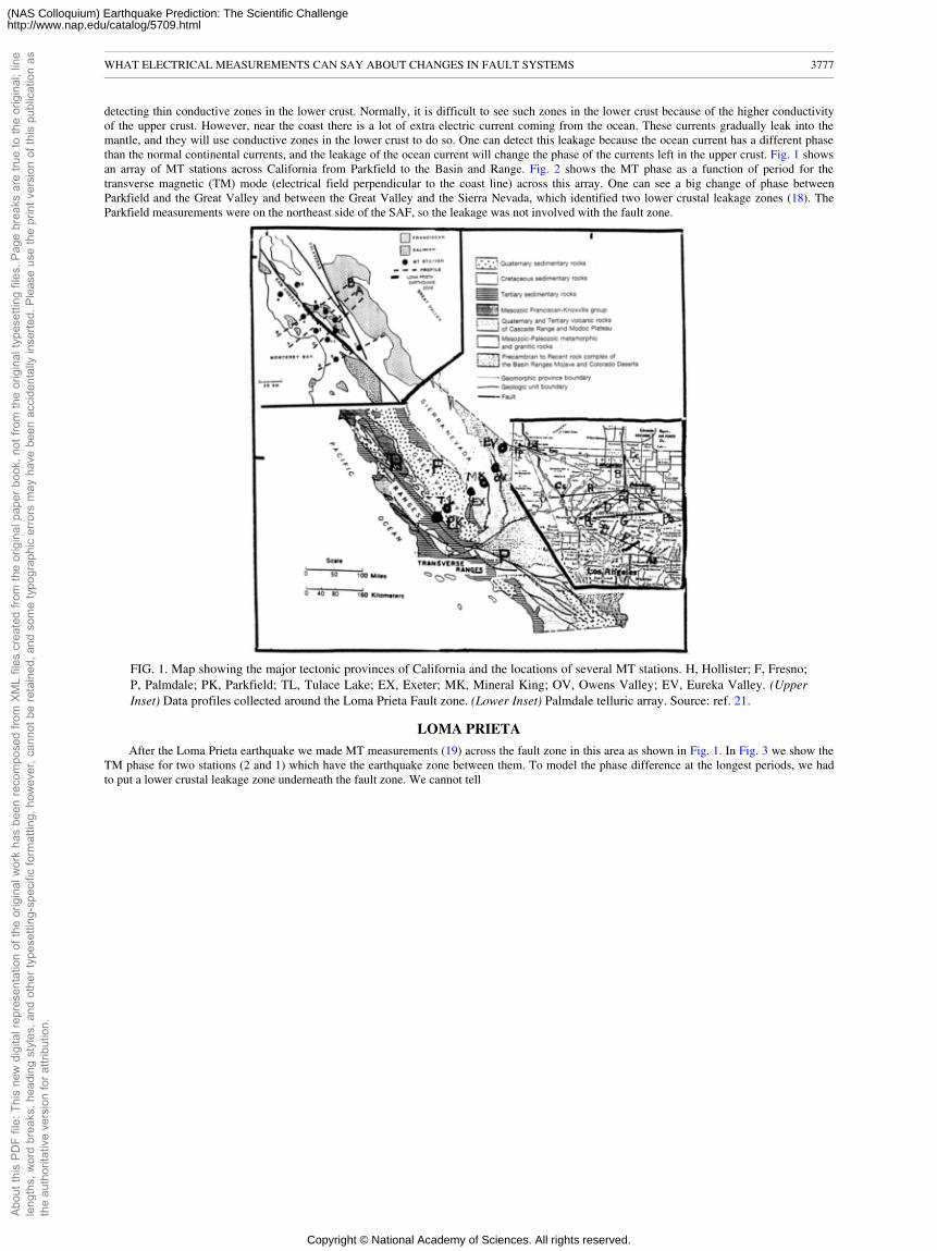
detecting thin conductive zones in the lower crust. Normally, it is difficult to see such zones in the lower crust because of the higher conductivityof the upper crust. However, near the coast there is a lot of extra electric current coming from the ocean. These currents gradually leak into themantle, and they will use conductive zones in the lower crust to do so. One can detect this leakage because the ocean current has a different phasethan the normal continental currents, and the leakage of the ocean current will change the phase of the currents left in the upper crust. Fig. 1 showsan array of MT stations across California from Parkfield to the Basin and Range. Fig. 2 shows the MT phase as a function of period for thetransverse magnetic (TM) mode (electrical field perpendicular to the coast line) across this array. One can see a big change of phase betweenParkfield and the Great Valley and between the Great Valley and the Sierra Nevada, which identified two lower crustal leakage zones (18). TheParkfield measurements were on the northeast side of the SAF, so the leakage was not involved with the fault zone.
FIG. 1. Map showing the major tectonic provinces of California and the locations of several MT stations. H, Hollister; F, Fresno;P, Palmdale; PK, Parkfield; TL, Tulace Lake; EX, Exeter; MK, Mineral King; OV, Owens Valley; EV, Eureka Valley. (UpperInset) Data profiles collected around the Loma Prieta Fault zone. (Lower Inset) Palmdale telluric array. Source: ref. 21.
LOMA PRIETA
After the Loma Prieta earthquake we made MT measurements (19) across the fault zone in this area as shown in Fig. 1. In Fig. 3 we show theTM phase for two stations (2 and 1) which have the earthquake zone between them. To model the phase difference at the longest periods, we hadto put a lower crustal leakage zone underneath the fault zone. We cannot tell
WHAT ELECTRICAL MEASUREMENTS CAN SAY ABOUT CHANGES IN FAULT SYSTEMS 3777
Abou
t thi
s PD
F fil
e: T
his
new
dig
ital r
epre
sent
atio
n of
the
orig
inal
wor
k ha
s be
en re
com
pose
d fro
m X
ML
files
cre
ated
from
the
orig
inal
pap
er b
ook,
not
from
the
orig
inal
type
setti
ng fi
les.
Pag
e br
eaks
are
true
to th
e or
igin
al; l
ine
leng
ths,
wor
d br
eaks
, hea
ding
sty
les,
and
oth
er ty
pese
tting
-spe
cific
form
attin
g, h
owev
er, c
anno
t be
reta
ined
, and
som
e ty
pogr
aphi
c er
rors
may
hav
e be
en a
ccid
enta
lly in
serte
d. P
leas
e us
e th
e pr
int v
ersi
on o
f thi
s pu
blic
atio
n as
the
auth
orita
tive
vers
ion
for a
ttrib
utio
n.
Copyright © National Academy of Sciences. All rights reserved.
(NAS Colloquium) Earthquake Prediction: The Scientific Challengehttp://www.nap.edu/catalog/5709.html
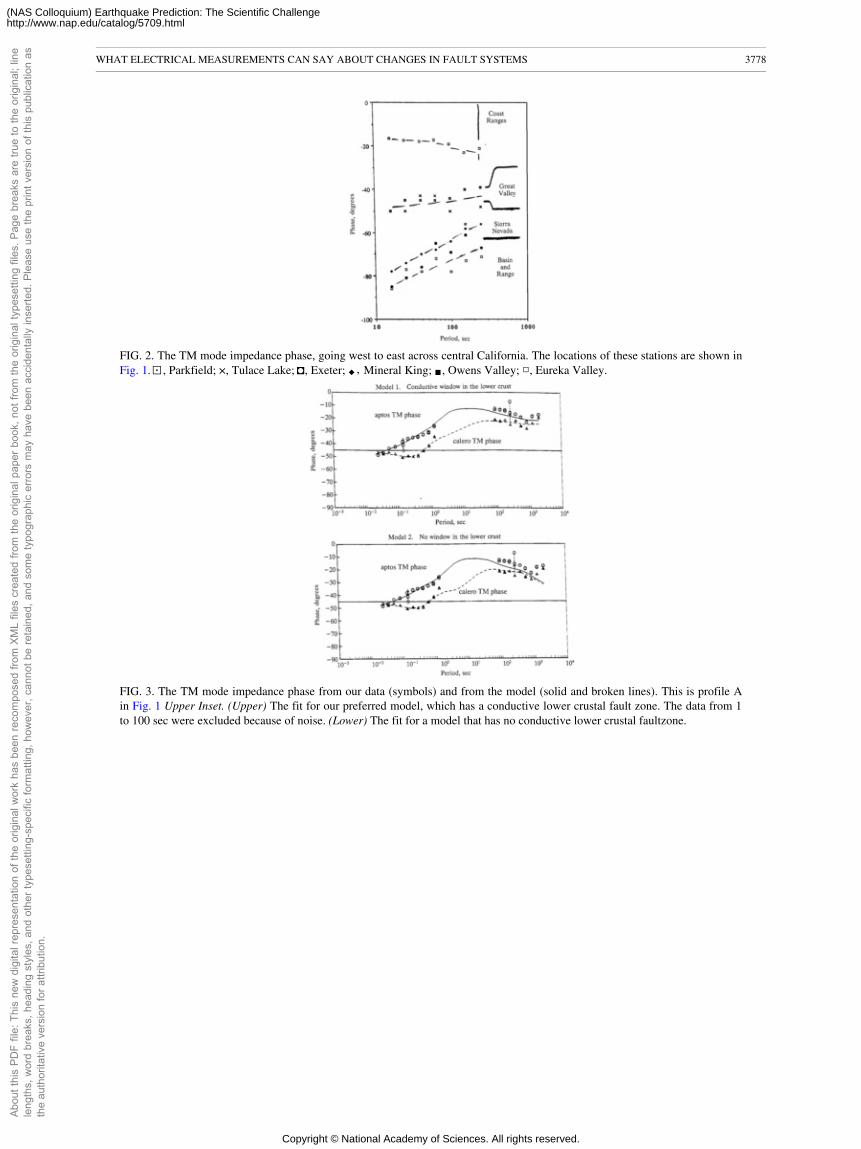
FIG. 2. The TM mode impedance phase, going west to east across central California. The locations of these stations are shown inFig. 1. , Parkfield; ×, Tulace Lake; , Exeter; , Mineral King; , Owens Valley; �, Eureka Valley.
FIG. 3. The TM mode impedance phase from our data (symbols) and from the model (solid and broken lines). This is profile Ain Fig. 1 Upper Inset. (Upper) The fit for our preferred model, which has a conductive lower crustal fault zone. The data from 1to 100 sec were excluded because of noise. (Lower) The fit for a model that has no conductive lower crustal faultzone.
WHAT ELECTRICAL MEASUREMENTS CAN SAY ABOUT CHANGES IN FAULT SYSTEMS 3778
Abou
t thi
s PD
F fil
e: T
his
new
dig
ital r
epre
sent
atio
n of
the
orig
inal
wor
k ha
s be
en re
com
pose
d fro
m X
ML
files
cre
ated
from
the
orig
inal
pap
er b
ook,
not
from
the
orig
inal
type
setti
ng fi
les.
Pag
e br
eaks
are
true
to th
e or
igin
al; l
ine
leng
ths,
wor
d br
eaks
, hea
ding
sty
les,
and
oth
er ty
pese
tting
-spe
cific
form
attin
g, h
owev
er, c
anno
t be
reta
ined
, and
som
e ty
pogr
aphi
c er
rors
may
hav
e be
en a
ccid
enta
lly in
serte
d. P
leas
e us
e th
e pr
int v
ersi
on o
f thi
s pu
blic
atio
n as
the
auth
orita
tive
vers
ion
for a
ttrib
utio
n.
� � � �
Copyright © National Academy of Sciences. All rights reserved.
(NAS Colloquium) Earthquake Prediction: The Scientific Challengehttp://www.nap.edu/catalog/5709.html
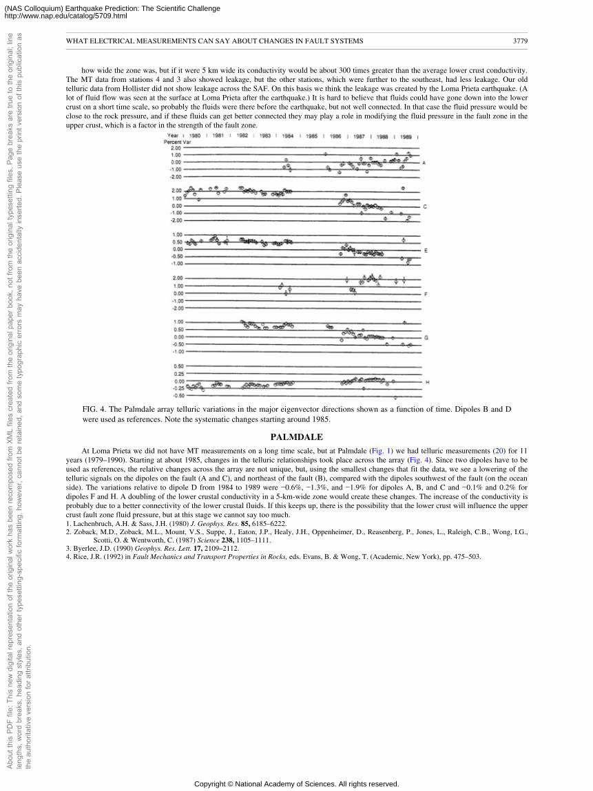
how wide the zone was, but if it were 5 km wide its conductivity would be about 300 times greater than the average lower crust conductivity.The MT data from stations 4 and 3 also showed leakage, but the other stations, which were further to the southeast, had less leakage. Our oldtelluric data from Hollister did not show leakage across the SAF. On this basis we think the leakage was created by the Loma Prieta earthquake. (Alot of fluid flow was seen at the surface at Loma Prieta after the earthquake.) It is hard to believe that fluids could have gone down into the lowercrust on a short time scale, so probably the fluids were there before the earthquake, but not well connected. In that case the fluid pressure would beclose to the rock pressure, and if these fluids can get better connected they may play a role in modifying the fluid pressure in the fault zone in theupper crust, which is a factor in the strength of the fault zone.
FIG. 4. The Palmdale array telluric variations in the major eigenvector directions shown as a function of time. Dipoles B and Dwere used as references. Note the systematic changes starting around 1985.
PALMDALE
At Loma Prieta we did not have MT measurements on a long time scale, but at Palmdale (Fig. 1) we had telluric measurements (20) for 11years (1979–1990). Starting at about 1985, changes in the telluric relationships took place across the array (Fig. 4). Since two dipoles have to beused as references, the relative changes across the array are not unique, but, using the smallest changes that fit the data, we see a lowering of thetelluric signals on the dipoles on the fault (A and C), and northeast of the fault (B), compared with the dipoles southwest of the fault (on the oceanside). The variations relative to dipole D from 1984 to 1989 were −0.6%, −1.3%, and −1.9% for dipoles A, B, and C and −0.1% and 0.2% fordipoles F and H. A doubling of the lower crustal conductivity in a 5-km-wide zone would create these changes. The increase of the conductivity isprobably due to a better connectivity of the lower crustal fluids. If this keeps up, there is the possibility that the lower crust will influence the uppercrust fault zone fluid pressure, but at this stage we cannot say too much.1. Lachenbruch, A.H. & Sass, J.H. (1980) J. Geophys. Res. 85, 6185–6222.2. Zoback, M.D., Zoback, M.L., Mount, V.S., Suppe, J., Eaton, J.P., Healy, J.H., Oppenheimer, D., Reasenberg, P., Jones, L., Raleigh, C.B., Wong, I.G.,
Scotti, O. & Wentworth, C. (1987) Science 238, 1105–1111.3. Byerlee, J.D. (1990) Geophys. Res. Lett. 17, 2109–2112.4. Rice, J.R. (1992) in Fault Mechanics and Transport Properties in Rocks, eds. Evans, B. & Wong, T. (Academic, New York), pp. 475–503.
WHAT ELECTRICAL MEASUREMENTS CAN SAY ABOUT CHANGES IN FAULT SYSTEMS 3779
Abou
t thi
s PD
F fil
e: T
his
new
dig
ital r
epre
sent
atio
n of
the
orig
inal
wor
k ha
s be
en re
com
pose
d fro
m X
ML
files
cre
ated
from
the
orig
inal
pap
er b
ook,
not
from
the
orig
inal
type
setti
ng fi
les.
Pag
e br
eaks
are
true
to th
e or
igin
al; l
ine
leng
ths,
wor
d br
eaks
, hea
ding
sty
les,
and
oth
er ty
pese
tting
-spe
cific
form
attin
g, h
owev
er, c
anno
t be
reta
ined
, and
som
e ty
pogr
aphi
c er
rors
may
hav
e be
en a
ccid
enta
lly in
serte
d. P
leas
e us
e th
e pr
int v
ersi
on o
f thi
s pu
blic
atio
n as
the
auth
orita
tive
vers
ion
for a
ttrib
utio
n.
Copyright © National Academy of Sciences. All rights reserved.
(NAS Colloquium) Earthquake Prediction: The Scientific Challengehttp://www.nap.edu/catalog/5709.html

5. Etheridge, M.A., Wall, V.J., Cox, S.F. & Vernon, R.H. (1984) J. Geophys. Res. 89, 4344–4358.6. Kerrich, R., LaTour, T.E. & Willmore, L. (1984) J. Geophys. Res. 89, 4331–4343.7. Berry, F.A.F. (1973) Am. Assoc. Pet. Geoi. Bull. 57, 1219–1249.8. Irwin, W.P. & Barnes, I. (1975) Geology 3, 713–716.9. Hyndman, R.D. & Shearer, P.M. (1989) Geophys. J. Int. 98, 343–365.10. Bailey, R.C. (1990) Geophys. Res. Lett. 17, 1129–1132.11. Jones, T.D. & Nur, A. (1982) Geology 10, 260–263.12. Shankland, T.J. & Ander, M.E. (1983) J. Geophys. Res. 88, 9475–9484.13. Yardley, B.W.D. (1986) Nature (London) 323, 111.14. Newton, R.C. (1990) Tectonophysics 182, 2137.15. Gough, D.I. (1986) Nature (London) 323, 143–144.16. Watson, E.B. & Brenan, J.M. (1987) Earth Planet. Sci. Lett. 85, 497–515.17 Walder, J. & Nur, A. (1984) J. Geophys. Res. 89, 11539–11548.18. Park, S.K., Biasi, G.P., Mackie, R.L. & Madden, T.R. (1991) J. Geophys. Res. 96, 353–376.19. Mackie, R.L., Madden, T.R. & Nichols, E.A. (1996) U.S. Geological Survey Professional Paper, Special Issue, Loma Prieta, in press.20. Madden, T.R., LaTorraca, G.A. & Park, S.K. (1993) J. Geophys. Res. 98, 795–808.21. Norris, R.M. & Webb, R.W. (1976) Geology of California (Wiley, New York).
WHAT ELECTRICAL MEASUREMENTS CAN SAY ABOUT CHANGES IN FAULT SYSTEMS 3780
Abou
t thi
s PD
F fil
e: T
his
new
dig
ital r
epre
sent
atio
n of
the
orig
inal
wor
k ha
s be
en re
com
pose
d fro
m X
ML
files
cre
ated
from
the
orig
inal
pap
er b
ook,
not
from
the
orig
inal
type
setti
ng fi
les.
Pag
e br
eaks
are
true
to th
e or
igin
al; l
ine
leng
ths,
wor
d br
eaks
, hea
ding
sty
les,
and
oth
er ty
pese
tting
-spe
cific
form
attin
g, h
owev
er, c
anno
t be
reta
ined
, and
som
e ty
pogr
aphi
c er
rors
may
hav
e be
en a
ccid
enta
lly in
serte
d. P
leas
e us
e th
e pr
int v
ersi
on o
f thi
s pu
blic
atio
n as
the
auth
orita
tive
vers
ion
for a
ttrib
utio
n.
Copyright © National Academy of Sciences. All rights reserved.
(NAS Colloquium) Earthquake Prediction: The Scientific Challengehttp://www.nap.edu/catalog/5709.html
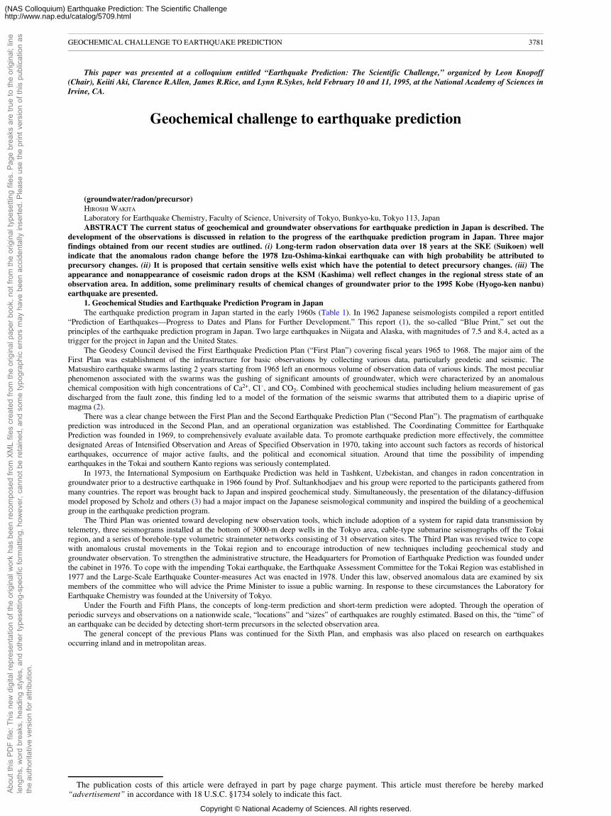
This paper was presented at a colloquium entitled “Earthquake Prediction: The Scientific Challenge,” organized by Leon Knopoff(Chair), Keiiti Aki, Clarence R.Allen, James R.Rice, and Lynn R.Sykes, held February 10 and 11, 1995, at the National Academy of Sciences inIrvine, CA.
Geochemical challenge to earthquake prediction
(groundwater/radon/precursor)HIROSHI WAKITA
Laboratory for Earthquake Chemistry, Faculty of Science, University of Tokyo, Bunkyo-ku, Tokyo 113, JapanABSTRACT The current status of geochemical and groundwater observations for earthquake prediction in Japan is described. The
development of the observations is discussed in relation to the progress of the earthquake prediction program in Japan. Three majorfindings obtained from our recent studies are outlined. (i) Long-term radon observation data over 18 years at the SKE (Suikoen) wellindicate that the anomalous radon change before the 1978 Izu-Oshima-kinkai earthquake can with high probability be attributed toprecursory changes. (ii) It is proposed that certain sensitive wells exist which have the potential to detect precursory changes. (iii) Theappearance and nonappearance of coseismic radon drops at the KSM (Kashima) well reflect changes in the regional stress state of anobservation area. In addition, some preliminary results of chemical changes of groundwater prior to the 1995 Kobe (Hyogo-ken nanbu)earthquake are presented.
1. Geochemical Studies and Earthquake Prediction Program in JapanThe earthquake prediction program in Japan started in the early 1960s (Table 1). In 1962 Japanese seismologists compiled a report entitled
“Prediction of Earthquakes—Progress to Dates and Plans for Further Development.” This report (1), the so-called “Blue Print,” set out theprinciples of the earthquake prediction program in Japan. Two large earthquakes in Niigata and Alaska, with magnitudes of 7.5 and 8.4, acted as atrigger for the project in Japan and the United States.
The Geodesy Council devised the First Earthquake Prediction Plan (“First Plan”) covering fiscal years 1965 to 1968. The major aim of theFirst Plan was establishment of the infrastructure for basic observations by collecting various data, particularly geodetic and seismic. TheMatsushiro earthquake swarms lasting 2 years starting from 1965 left an enormous volume of observation data of various kinds. The most peculiarphenomenon associated with the swarms was the gushing of significant amounts of groundwater, which were characterized by an anomalouschemical composition with high concentrations of Ca2+, Cl−, and CO2. Combined with geochemical studies including helium measurement of gasdischarged from the fault zone, this finding led to a model of the formation of the seismic swarms that attributed them to a diapiric uprise ofmagma (2).
There was a clear change between the First Plan and the Second Earthquake Prediction Plan (“Second Plan”). The pragmatism of earthquakeprediction was introduced in the Second Plan, and an operational organization was established. The Coordinating Committee for EarthquakePrediction was founded in 1969, to comprehensively evaluate available data. To promote earthquake prediction more effectively, the committeedesignated Areas of Intensified Observation and Areas of Specified Observation in 1970, taking into account such factors as records of historicalearthquakes, occurrence of major active faults, and the political and economical situation. Around that time the possibility of impendingearthquakes in the Tokai and southern Kanto regions was seriously contemplated.
In 1973, the International Symposium on Earthquake Prediction was held in Tashkent, Uzbekistan, and changes in radon concentration ingroundwater prior to a destructive earthquake in 1966 found by Prof. Sultankhodjaev and his group were reported to the participants gathered frommany countries. The report was brought back to Japan and inspired geochemical study. Simultaneously, the presentation of the dilatancy-diffusionmodel proposed by Scholz and others (3) had a major impact on the Japanese seismological community and inspired the building of a geochemicalgroup in the earthquake prediction program.
The Third Plan was oriented toward developing new observation tools, which include adoption of a system for rapid data transmission bytelemetry, three seismograms installed at the bottom of 3000-m deep wells in the Tokyo area, cable-type submarine seismographs off the Tokairegion, and a series of borehole-type volumetric strainmeter networks consisting of 31 observation sites. The Third Plan was revised twice to copewith anomalous crustal movements in the Tokai region and to encourage introduction of new techniques including geochemical study andgroundwater observation. To strengthen the administrative structure, the Headquarters for Promotion of Earthquake Prediction was founded underthe cabinet in 1976. To cope with the impending Tokai earthquake, the Earthquake Assessment Committee for the Tokai Region was established in1977 and the Large-Scale Earthquake Counter-measures Act was enacted in 1978. Under this law, observed anomalous data are examined by sixmembers of the committee who will advice the Prime Minister to issue a public warning. In response to these circumstances the Laboratory forEarthquake Chemistry was founded at the University of Tokyo.
Under the Fourth and Fifth Plans, the concepts of long-term prediction and short-term prediction were adopted. Through the operation ofperiodic surveys and observations on a nationwide scale, “locations” and “sizes” of earthquakes are roughly estimated. Based on this, the “time” ofan earthquake can be decided by detecting short-term precursors in the selected observation area.
The general concept of the previous Plans was continued for the Sixth Plan, and emphasis was also placed on research on earthquakesoccurring inland and in metropolitan areas.
The publication costs of this article were defrayed in part by page charge payment. This article must therefore be hereby marked“advertisement” in accordance with 18 U.S.C. §1734 solely to indicate this fact.
GEOCHEMICAL CHALLENGE TO EARTHQUAKE PREDICTION 3781
Abou
t thi
s PD
F fil
e: T
his
new
dig
ital r
epre
sent
atio
n of
the
orig
inal
wor
k ha
s be
en re
com
pose
d fro
m X
ML
files
cre
ated
from
the
orig
inal
pap
er b
ook,
not
from
the
orig
inal
type
setti
ng fi
les.
Pag
e br
eaks
are
true
to th
e or
igin
al; l
ine
leng
ths,
wor
d br
eaks
, hea
ding
sty
les,
and
oth
er ty
pese
tting
-spe
cific
form
attin
g, h
owev
er, c
anno
t be
reta
ined
, and
som
e ty
pogr
aphi
c er
rors
may
hav
e be
en a
ccid
enta
lly in
serte
d. P
leas
e us
e th
e pr
int v
ersi
on o
f thi
s pu
blic
atio
n as
the
auth
orita
tive
vers
ion
for a
ttrib
utio
n.
Copyright © National Academy of Sciences. All rights reserved.
(NAS Colloquium) Earthquake Prediction: The Scientific Challengehttp://www.nap.edu/catalog/5709.html
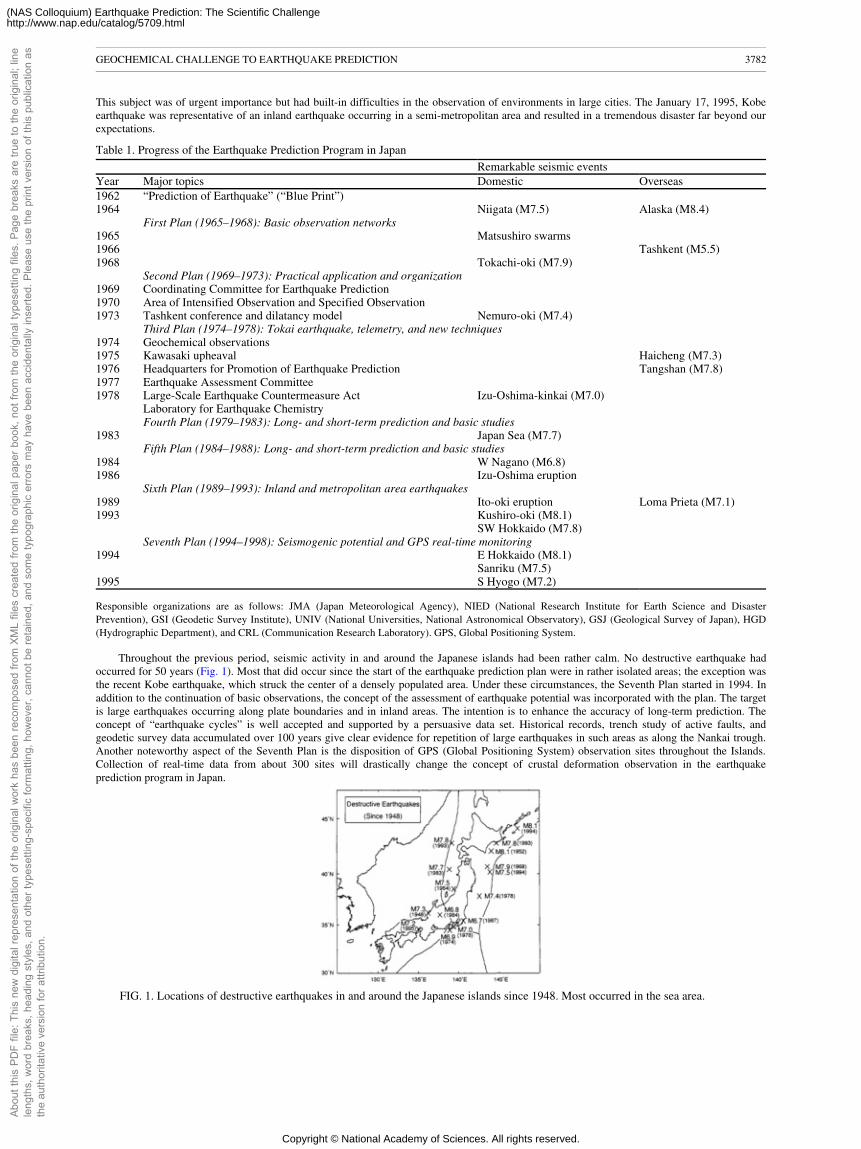
This subject was of urgent importance but had built-in difficulties in the observation of environments in large cities. The January 17, 1995, Kobeearthquake was representative of an inland earthquake occurring in a semi-metropolitan area and resulted in a tremendous disaster far beyond ourexpectations.
Table 1. Progress of the Earthquake Prediction Program in Japan
Remarkable seismic eventsYear Major topics Domestic Overseas1962 “Prediction of Earthquake” (“Blue Print”)1964 Niigata (M7.5) Alaska (M8.4)
First Plan (1965–1968): Basic observation networks1965 Matsushiro swarms1966 Tashkent (M5.5)1968 Tokachi-oki (M7.9)
Second Plan (1969–1973): Practical application and organization1969 Coordinating Committee for Earthquake Prediction1970 Area of Intensified Observation and Specified Observation1973 Tashkent conference and dilatancy model Nemuro-oki (M7.4)
Third Plan (1974–1978): Tokai earthquake, telemetry, and new techniques1974 Geochemical observations1975 Kawasaki upheaval Haicheng (M7.3)1976 Headquarters for Promotion of Earthquake Prediction Tangshan (M7.8)1977 Earthquake Assessment Committee1978 Large-Scale Earthquake Countermeasure Act
Laboratory for Earthquake ChemistryIzu-Oshima-kinkai (M7.0)
Fourth Plan (1979–1983): Long- and short-term prediction and basic studies1983 Japan Sea (M7.7)
Fifth Plan (1984–1988): Long- and short-term prediction and basic studies1984 W Nagano (M6.8)1986 Izu-Oshima eruption
Sixth Plan (1989–1993): Inland and metropolitan area earthquakes1989 Ito-oki eruption Loma Prieta (M7.1)1993 Kushiro-oki (M8.1)
SW Hokkaido (M7.8)Seventh Plan (1994–1998): Seismogenic potential and GPS real-time monitoring
1994 E Hokkaido (M8.1)Sanriku (M7.5)
1995 S Hyogo (M7.2)
Responsible organizations are as follows: JMA (Japan Meteorological Agency), NIED (National Research Institute for Earth Science and DisasterPrevention), GSI (Geodetic Survey Institute), UNIV (National Universities, National Astronomical Observatory), GSJ (Geological Survey of Japan), HGD(Hydrographic Department), and CRL (Communication Research Laboratory). GPS, Global Positioning System.
Throughout the previous period, seismic activity in and around the Japanese islands had been rather calm. No destructive earthquake hadoccurred for 50 years (Fig. 1). Most that did occur since the start of the earthquake prediction plan were in rather isolated areas; the exception wasthe recent Kobe earthquake, which struck the center of a densely populated area. Under these circumstances, the Seventh Plan started in 1994. Inaddition to the continuation of basic observations, the concept of the assessment of earthquake potential was incorporated with the plan. The targetis large earthquakes occurring along plate boundaries and in inland areas. The intention is to enhance the accuracy of long-term prediction. Theconcept of “earthquake cycles” is well accepted and supported by a persuasive data set. Historical records, trench study of active faults, andgeodetic survey data accumulated over 100 years give clear evidence for repetition of large earthquakes in such areas as along the Nankai trough.Another noteworthy aspect of the Seventh Plan is the disposition of GPS (Global Positioning System) observation sites throughout the Islands.Collection of real-time data from about 300 sites will drastically change the concept of crustal deformation observation in the earthquakeprediction program in Japan.
FIG. 1. Locations of destructive earthquakes in and around the Japanese islands since 1948. Most occurred in the sea area.
GEOCHEMICAL CHALLENGE TO EARTHQUAKE PREDICTION 3782
Abou
t thi
s PD
F fil
e: T
his
new
dig
ital r
epre
sent
atio
n of
the
orig
inal
wor
k ha
s be
en re
com
pose
d fro
m X
ML
files
cre
ated
from
the
orig
inal
pap
er b
ook,
not
from
the
orig
inal
type
setti
ng fi
les.
Pag
e br
eaks
are
true
to th
e or
igin
al; l
ine
leng
ths,
wor
d br
eaks
, hea
ding
sty
les,
and
oth
er ty
pese
tting
-spe
cific
form
attin
g, h
owev
er, c
anno
t be
reta
ined
, and
som
e ty
pogr
aphi
c er
rors
may
hav
e be
en a
ccid
enta
lly in
serte
d. P
leas
e us
e th
e pr
int v
ersi
on o
f thi
s pu
blic
atio
n as
the
auth
orita
tive
vers
ion
for a
ttrib
utio
n.
Copyright © National Academy of Sciences. All rights reserved.
(NAS Colloquium) Earthquake Prediction: The Scientific Challengehttp://www.nap.edu/catalog/5709.html
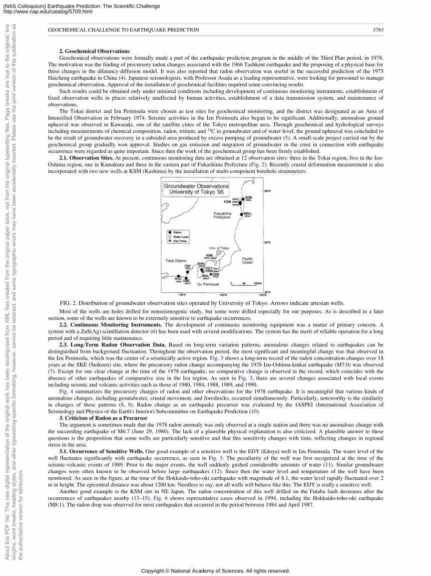
2. Geochemical ObservationsGeochemical observations were formally made a part of the earthquake prediction program in the middle of the Third Plan period, in 1978.
The motivation was the finding of precursory radon changes associated with the 1966 Tashkent earthquake and the proposing of a physical base forthese changes in the dilatancy-diffusion model. It was also reported that radon observation was useful in the successful prediction of the 1975Haicheng earthquake in China (4). Japanese seismologists, with Professor Asada as a leading representative, were looking for personnel to managegeochemical observation. Approval of the installation of geochemical facilities required some convincing results.
Such results could be obtained only under minimal conditions including development of continuous monitoring instruments, establishment offixed observation wells in places relatively unaffected by human activities, establishment of a data transmission system, and maintenance ofobservations.
The Tokai district and Izu Peninsula were chosen as test sites for geochemical monitoring, and the district was designated as an Area ofIntensified Observation in February 1974. Seismic activities in the Izu Peninsula also began to be significant. Additionally, anomalous groundupheaval was observed in Kawasaki, one of the satellite cities of the Tokyo metropolitan area. Through geochemical and hydrological surveysincluding measurements of chemical composition, radon, tritium, and 14C in groundwater and of water level, the ground upheaval was concluded tobe the result of groundwater recovery in a subsided area produced by excess pumping of groundwater (5). A small-scale project carried out by thegeochemical group gradually won approval. Studies on gas emission and migration of groundwater in the crust in connection with earthquakeoccurrence were regarded as quite important. Since then the work of the geochemical group has been firmly established.
2.1. Observation Sites. At present, continuous monitoring data are obtained at 12 observation sites: three in the Tokai region, five in the Izu-Oshima region, one in Kamakura and three in the eastern part of Fukushima Prefecture (Fig. 2). Recently crustal deformation measurement is alsoincorporated with two new wells at KSM (Kashima) by the installation of multi-component borehole strainmeters.
FIG. 2. Distribution of groundwater observation sites operated by University of Tokyo. Arrows indicate artesian wells.Most of the wells are holes drilled for nonseismogenic study, but some were drilled especially for our purposes. As is described in a later
section, some of the wells are known to be extremely sensitive to earthquake occurrences.2.2. Continuous Monitoring Instruments. The development of continuous monitoring equipment was a matter of primary concern. A
system with a ZnS(Ag) scintillation detector (6) has been used with several modifications. The system has the merit of reliable operation for a longperiod and of requiring little maintenance.
2.3. Long-Term Radon Observation Data. Based on long-term variation patterns, anomalous changes related to earthquakes can bedistinguished from background fluctuation. Throughout the observation period, the most significant and meaningful change was that observed inthe Izu Peninsula, which was the center of a seismically active region. Fig. 3 shows a long-term record of the radon concentration changes over 18years at the SKE (Suikoen) site, where the precursory radon change accompanying the 1978 Izu-Oshima-kinkai earthquake (M7.0) was observed(7). Except for one clear change at the time of the 1978 earthquake, no comparative change is observed in the record, which coincides with theabsence of other earthquakes of comparative size in the Izu region. As seen in Fig. 3, there are several changes associated with local eventsincluding seismic and volcanic activities such as those of 1980, 1984, 1988, 1989, and 1990.
Fig. 4 summarizes the precursory changes of radon and other observations for the 1978 earthquake. It is meaningful that various kinds ofanomalous changes, including groundwater, crustal movement, and foreshocks, occurred simultaneously. Particularly, noteworthy is the similarityin changes of these patterns (8, 9). Radon change as an earthquake precursor was evaluated by the IASPEI (International Association ofSeismology and Physics of the Earth's Interior) Subcommittee on Earthquake Prediction (10).
3. Criticism of Radon as a PrecursorThe argument is sometimes made that the 1978 radon anomaly was only observed at a single station and there was no anomalous change with
the succeeding earthquake of M6.7 (June 29, 1980). The lack of a plausible physical explanation is also criticized. A plausible answer to thesequestions is the proposition that some wells are particularly sensitive and that this sensitivity changes with time, reflecting changes in regionalstress in the area.
3.1. Occurrence of Sensitive Wells. One good example of a sensitive well is the EDY (Edoya) well in Izu Peninsula. The water level of thewell fluctuates significantly with earthquake occurrence, as seen in Fig. 5. The peculiarity of the well was first recognized at the time of theseismic-volcanic events of 1989. Prior to the major events, the well suddenly gushed considerable amounts of water (11). Similar groundwaterchanges were often known to be observed before large earthquakes (12). Since then the water level and temperature of the well have beenmonitored. As seen in the figure, at the time of the Hokkaido-toho-oki earthquake with magnitude of 8.1, the water level rapidly fluctuated over 2m in height. The epicentral distance was about 1200 km. Needless to say, not all wells will behave like this. The EDY is really a sensitive well.
Another good example is the KSM site in NE Japan. The radon concentration of this well drilled on the Futaba fault decreases after theoccurrences of earthquakes nearby (13–15). Fig. 6 shows representative cases observed in 1994, including the Hokkaido-toho-oki earthquake(M8.1). The radon drop was observed for most earthquakes that occurred in the period between 1984 and April 1987.
GEOCHEMICAL CHALLENGE TO EARTHQUAKE PREDICTION 3783
Abou
t thi
s PD
F fil
e: T
his
new
dig
ital r
epre
sent
atio
n of
the
orig
inal
wor
k ha
s be
en re
com
pose
d fro
m X
ML
files
cre
ated
from
the
orig
inal
pap
er b
ook,
not
from
the
orig
inal
type
setti
ng fi
les.
Pag
e br
eaks
are
true
to th
e or
igin
al; l
ine
leng
ths,
wor
d br
eaks
, hea
ding
sty
les,
and
oth
er ty
pese
tting
-spe
cific
form
attin
g, h
owev
er, c
anno
t be
reta
ined
, and
som
e ty
pogr
aphi
c er
rors
may
hav
e be
en a
ccid
enta
lly in
serte
d. P
leas
e us
e th
e pr
int v
ersi
on o
f thi
s pu
blic
atio
n as
the
auth
orita
tive
vers
ion
for a
ttrib
utio
n.
Copyright © National Academy of Sciences. All rights reserved.
(NAS Colloquium) Earthquake Prediction: The Scientific Challengehttp://www.nap.edu/catalog/5709.html
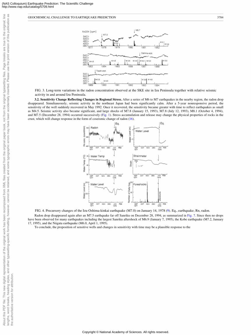
FIG. 3. Long-term variations in the radon concentration observed at the SKE site in Izu Peninsula together with relative seismicactivity in and around Izu Peninsula.3.2. Sensitivity Change Reflecting Changes in Regional Stress. After a series of M6 to M7 earthquakes in the nearby region, the radon drop
disappeared. Simultaneously, seismic activity in the northeast Japan had been significantly calm. After a 5-year nonresponsive period, thesensitivity of the well suddenly recovered in May 1992. Once it recovered, the sensitivity became greater with time to reflect earthquakes as smallas M4.5. Seismic activity also became significant, and large shocks of M7.8 (January 15, 1993), M7.8 (July 12, 1993), M8.1 (October 4, 1994),and M7.5 (December 28, 1994) occurred successively (Fig. 1). Stress accumulation and release may change the physical properties of rocks in thecrust, which will change response in the form of coseismic change of radon (16).
FIG. 4. Precursory changes of the Izu-Oshima-kinkai earthquake (M7.0) on January 14, 1978 (9). Eq., earthquake; Rn, radon.Radon drop disappeared again after an M7.5 earthquake far off Sanriku on December 28, 1994, as summarized in Fig. 7. Since then no drops
have been observed for many earthquakes including the largest Sanriku aftershock of M6.9 (January 7, 1995), the Kobe earthquake (M7.2, January17, 1995), and the Niigata earthquake (M6.0, April 1, 1995).
To conclude, the proposition of sensitive wells and changes in sensitivity with time may be a plausible response to the
GEOCHEMICAL CHALLENGE TO EARTHQUAKE PREDICTION 3784
Abou
t thi
s PD
F fil
e: T
his
new
dig
ital r
epre
sent
atio
n of
the
orig
inal
wor
k ha
s be
en re
com
pose
d fro
m X
ML
files
cre
ated
from
the
orig
inal
pap
er b
ook,
not
from
the
orig
inal
type
setti
ng fi
les.
Pag
e br
eaks
are
true
to th
e or
igin
al; l
ine
leng
ths,
wor
d br
eaks
, hea
ding
sty
les,
and
oth
er ty
pese
tting
-spe
cific
form
attin
g, h
owev
er, c
anno
t be
reta
ined
, and
som
e ty
pogr
aphi
c er
rors
may
hav
e be
en a
ccid
enta
lly in
serte
d. P
leas
e us
e th
e pr
int v
ersi
on o
f thi
s pu
blic
atio
n as
the
auth
orita
tive
vers
ion
for a
ttrib
utio
n.
Copyright © National Academy of Sciences. All rights reserved.
(NAS Colloquium) Earthquake Prediction: The Scientific Challengehttp://www.nap.edu/catalog/5709.html
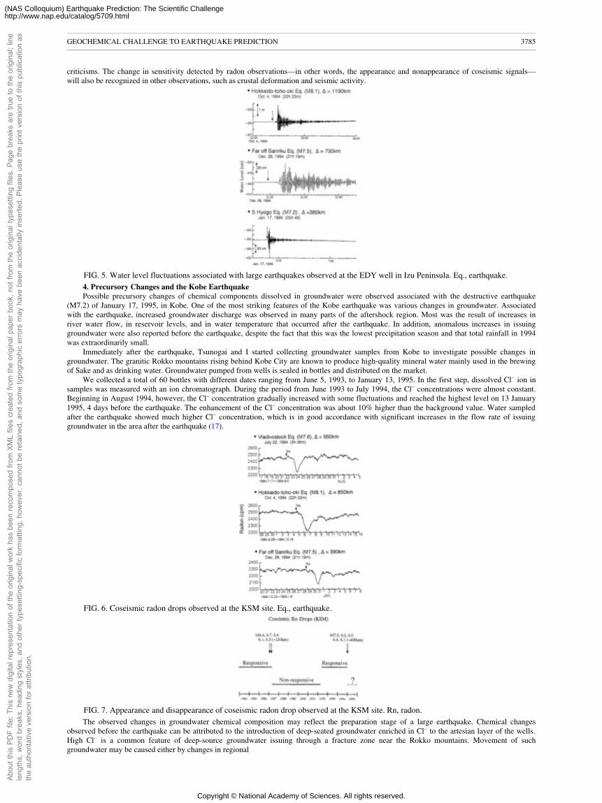
criticisms. The change in sensitivity detected by radon observations—in other words, the appearance and nonappearance of coseismic signals—will also be recognized in other observations, such as crustal deformation and seismic activity.
FIG. 5. Water level fluctuations associated with large earthquakes observed at the EDY well in Izu Peninsula. Eq., earthquake.4. Precursory Changes and the Kobe EarthquakePossible precursory changes of chemical components dissolved in groundwater were observed associated with the destructive earthquake
(M7.2) of January 17, 1995, in Kobe. One of the most striking features of the Kobe earthquake was various changes in groundwater. Associatedwith the earthquake, increased groundwater discharge was observed in many parts of the aftershock region. Most was the result of increases inriver water flow, in reservoir levels, and in water temperature that occurred after the earthquake. In addition, anomalous increases in issuinggroundwater were also reported before the earthquake, despite the fact that this was the lowest precipitation season and that total rainfall in 1994was extraordinarily small.
Immediately after the earthquake, Tsunogai and I started collecting groundwater samples from Kobe to investigate possible changes ingroundwater. The granitic Rokko mountains rising behind Kobe City are known to produce high-quality mineral water mainly used in the brewingof Sake and as drinking water. Groundwater pumped from wells is sealed in bottles and distributed on the market.
We collected a total of 60 bottles with different dates ranging from June 5, 1993, to January 13, 1995. In the first step, dissolved Cl− ion insamples was measured with an ion chromatograph. During the period from June 1993 to July 1994, the Cl− concentrations were almost constant.Beginning in August 1994, however, the Cl− concentration gradually increased with some fluctuations and reached the highest level on 13 January1995, 4 days before the earthquake. The enhancement of the Cl− concentration was about 10% higher than the background value. Water sampledafter the earthquake showed much higher Cl− concentration, which is in good accordance with significant increases in the flow rate of issuinggroundwater in the area after the earthquake (17).
FIG. 6. Coseismic radon drops observed at the KSM site. Eq., earthquake.
FIG. 7. Appearance and disappearance of coseismic radon drop observed at the KSM site. Rn, radon.The observed changes in groundwater chemical composition may reflect the preparation stage of a large earthquake. Chemical changes
observed before the earthquake can be attributed to the introduction of deep-seated groundwater enriched in Cl− to the artesian layer of the wells.High Cl− is a common feature of deep-source groundwater issuing through a fracture zone near the Rokko mountains. Movement of suchgroundwater may be caused either by changes in regional
GEOCHEMICAL CHALLENGE TO EARTHQUAKE PREDICTION 3785
Abou
t thi
s PD
F fil
e: T
his
new
dig
ital r
epre
sent
atio
n of
the
orig
inal
wor
k ha
s be
en re
com
pose
d fro
m X
ML
files
cre
ated
from
the
orig
inal
pap
er b
ook,
not
from
the
orig
inal
type
setti
ng fi
les.
Pag
e br
eaks
are
true
to th
e or
igin
al; l
ine
leng
ths,
wor
d br
eaks
, hea
ding
sty
les,
and
oth
er ty
pese
tting
-spe
cific
form
attin
g, h
owev
er, c
anno
t be
reta
ined
, and
som
e ty
pogr
aphi
c er
rors
may
hav
e be
en a
ccid
enta
lly in
serte
d. P
leas
e us
e th
e pr
int v
ersi
on o
f thi
s pu
blic
atio
n as
the
auth
orita
tive
vers
ion
for a
ttrib
utio
n.
Copyright © National Academy of Sciences. All rights reserved.
(NAS Colloquium) Earthquake Prediction: The Scientific Challengehttp://www.nap.edu/catalog/5709.html
tectonic stress or by permeability change due to micro-crack formation in rocks prior to the destructive earthquake.The result indicates that groundwater observations can provide useful information on the earthquake formation process and clues to
understanding the mechanism of inland earthquakes. The use of commercial bottled water will be a source of information to obtain preseismic data.Detailed descriptions of the study will be published elsewhere. Further study including stable isotope measurements will be helpful instrengthening the findings.
5. ConclusionsDetection of precursory phenomena is of primary importance for earthquake prediction purposes. Coseismic signals, similarly, are useful for
clarifying the mechanisms of precursory phenomena. Appearance and nonappearance of coseismic drops in radon content are indicative of stressstates in the region.
Our experience enables us to arrive at several conclusions. (i) It is clear that movements of fluids in the crust are associated with earthquakes,(ii) Earthquake-related changes are not observed at all observation wells but only at a limited number of wells. At sensitive sites, marked changesin groundwater movement that are significantly large and effective even at large distances are observed. (iii) Even at sensitive wells, theappearance of signals likely depends on the state of stress accumulation in the region. The sensitivity change is thought to be caused by changes inphysical properties of rocks including opening and closure of microcracks.
A possible precursory change in groundwater chemistry at the time of the 1995 Kobe earthquake will substantiate the importance ofgeochemical and hydrological study.
Fluid movements in the crust play a vital role in earthquake occurrence. Besides its original purpose of predicting earthquakes, monitoring ofgroundwater movements will also be essential to supplement all kinds of observations on the ground surface and particularly to increase theaccuracy of crustal deformation measurement including GPS measurement.
The author thanks his colleagues, M.Ohno, T.Mori, S. Xu, and U. Tsunogai, for help in drawing illustrations and chemical analysis.1. Tsuboi, C., Wadati, K. & Hagiwara, T. (1962) Report of the Earthquake Prediction Research Group in Japan (Earthquake Research Inst., Univ. of
Tokyo, Tokyo), p. 21.2. Wakita, H., Fujii, N., Matsuo, S., Notsu, K., Nagao, K. & Takaoka, N. (1978) Science 200, 430–432.3. Scholz, H., Sykes, L.R. & Aggarwal, Y.P. (1973) Science 181, 803–810.4. Heicheng Earthquake Study Delegation (1977) Eos Trans., AGU, 58, 236–272.5. Wakita, H. (1975) Technocrat 8, 6–17.6. Noguchi, M. & Wakita, H. (1977) J. Geophys. Res. 42, 1353–1357.7. Wakita, H., Nakamura, Y., Notsu, K., Noguchi, M. & Asada, T. (1980) Science 207, 882–883.8. Wakita, H., Nakamura, Y. & Sano, Y. (1988) PureAppl. Geophys. 126, 267–278.9. Wakita, H. (1981) in Earthquake Prediction: An International Review, Maurice Ewing Series eds. Simpson, W. & Richards, P.G. (Am. Geophys. Union,
Washington, DC, Vol. 4), pp. 527–532.10. Wyss, M. (1991) Evaluation of Proposed Earthquake Precursors (Am. Geophys. Union, Washington, DC), p. 94.11. Sato, T., Wakita, H., Notsu, K. & Igarashi, G. (1992) Geochem. J. 26, 73–83.12. Wakita, H. (1982) in Earthquake Prediction Techniques, ed. Asada, T. (Univ. of Tokyo Press, Tokyo), pp. 175–216.13. Wakita, H., Igarashi, G., Nakamura, Y. & Notsu, K. (1989) Geophys. Res. Lett. 16, 417–420.14. Igarashi, G., Wakita, H. & Notsu, K. (1990) Tohoku Geophys. J. (Sci. Rept. Tohoku Univ., Ser. 5) 33, 163–175.15. Igarashi, G. & Wakita, H. (1990) Tectonophysics 180, 237–254.16. Igarashi, G., Tohjima, Y. & Wakita, H. (1993) Geophys. Res. Lett. 20, 1807–1810.17. Tsunogai, U. & Wakita, H. (1996) Science 269, 61–63.
GEOCHEMICAL CHALLENGE TO EARTHQUAKE PREDICTION 3786
Abou
t thi
s PD
F fil
e: T
his
new
dig
ital r
epre
sent
atio
n of
the
orig
inal
wor
k ha
s be
en re
com
pose
d fro
m X
ML
files
cre
ated
from
the
orig
inal
pap
er b
ook,
not
from
the
orig
inal
type
setti
ng fi
les.
Pag
e br
eaks
are
true
to th
e or
igin
al; l
ine
leng
ths,
wor
d br
eaks
, hea
ding
sty
les,
and
oth
er ty
pese
tting
-spe
cific
form
attin
g, h
owev
er, c
anno
t be
reta
ined
, and
som
e ty
pogr
aphi
c er
rors
may
hav
e be
en a
ccid
enta
lly in
serte
d. P
leas
e us
e th
e pr
int v
ersi
on o
f thi
s pu
blic
atio
n as
the
auth
orita
tive
vers
ion
for a
ttrib
utio
n.
Copyright © National Academy of Sciences. All rights reserved.
(NAS Colloquium) Earthquake Prediction: The Scientific Challengehttp://www.nap.edu/catalog/5709.html
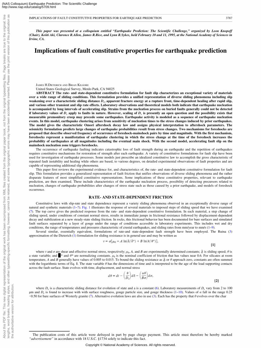
This paper was presented at a colloquium entitled “Earthquake Prediction: The Scientific Challenge,” organized by Leon Knopoff(Chair), Keiiti Aki, Clarence R.Allen, James R.Rice, and Lynn R.Sykes, held February 10 and 11, 1995, at the National Academy of Sciences inIrvine, CA.
Implications of fault constitutive properties for earthquake prediction
JAMES H.DIETERICH AND BRIAN KILGORE
United States Geological Survey, Menlo Park, CA 94025ABSTRACT The rate- and state-dependent constitutive formulation for fault slip characterizes an exceptional variety of materials
over a wide range of sliding conditions. This formulation provides a unified representation of diverse sliding phenomena including slipweakening over a characteristic sliding distance Dc, apparent fracture energy at a rupture front, time-dependent healing after rapid slip,and various other transient and slip rate effects. Laboratory observations and theoretical models both indicate that earthquake nucleationis accompanied by long intervals of accelerating slip. Strains from the nucleation process on buried faults generally could not be detectedif laboratory values of Dc apply to faults in nature. However, scaling of Dc is presently an open question and the possibility exists thatmeasurable premonitory creep may precede some earthquakes. Earthquake activity is modeled as a sequence of earthquake nucleationevents. In this model, earthquake clustering arises from sensitivity of nucleation times to the stress changes induced by prior earthquakes.The model gives the characteristic Omori aftershock decay law and assigns physical interpretation to aftershock parameters. Theseismicity formulation predicts large changes of earthquake probabilities result from stress changes. Two mechanisms for foreshocks areproposed that describe observed frequency of occurrence of foreshock-mainshock pairs by time and magnitude. With the first mechanism,foreshocks represent a manifestation of earthquake clustering in which the stress change at the time of the foreshock increases theprobability of earthquakes at all magnitudes including the eventual main shock. With the second model, accelerating fault slip on themainshock nucleation zone triggers foreshocks.
The occurrence of earthquake faulting indicates catastrophic loss of fault strength during an earthquake and the repetition of earthquakesrequires constitutive mechanisms for restoration of strength after each earthquake. A variety of constitutive formulations for fault slip have beenused for investigation of earthquake processes. Some models just prescribe an idealized constitutive law to accomplish the gross characteristic ofrepeated fault instability and healing while others are based, to various degrees, on detailed experimental observations of fault properties and arecapable of representing additional slip phenomena.
This paper first reviews the experimental evidence for, and characteristics of, the rate- and state-dependent constitutive formulation for faultslip. This formulation provides a generalized representation of fault friction that unifies observations of diverse sliding phenomena and the ratherdisparate features of most simplified constitutive representations. Some implications of these constitutive properties, relevant to earthquakeprediction, are then examined. These include characteristics of the earthquake nucleation process, possibility of detecting precursors related tonucleation, changes of earthquake probabilities after changes of stress state such as those caused by a prior earthquake, and models of foreshockoccurrence.
RATE- AND STATE-DEPENDENT FRICTION
Constitutive laws with slip-rate and state dependence represent a variety sliding phenomena observed in an exceptionally diverse range ofnatural and synthetic materials (1–7). Fig. 1 illustrates the response of several materials to imposed steps of sliding speed that we have examined(7). The top curve gives the predicted response from the rate- and state-dependent constitutive formulation. In each material, a step change ofsliding speed, under conditions of constant normal stress, results in immediate jumps in frictional resistance followed by displacement-dependentdecay and stabilization at a new steady-state sliding friction. In rocks, this frictional behavior has been documented for bare surfaces and simulatedfault surfaces separated by a layer of gouge under the range of conditions accessible in laboratory experiments. This includes wet and dryconditions, the range of temperatures and pressures characteristic of crustal earthquakes, and sliding rates from mm/year to mm/s (1–9).
Several similar, essentially equivalent, formulations of rate-and state-dependent fault strength have been employed. The Ruina (3)approximation of the Dieterich (1) formulation for sliding resistance is in general use and may be written as
[1]
where τ and σ are shear and effective normal stress, respectively; µ0, A, and B are experimentally determined constants; is sliding speed; θ isa state variable; and * and θ* are normalizing constants. µ0 is the nominal coefficient of friction that has values near 0.6. For silicates at roomtemperature, A and B generally have values of 0.005 to 0.015. To bound the sliding resistance as or θ approach zero, constants are often summedwith the logarithmic terms of Eq. 1. The state variable θ has the dimensions of time and is interpreted to be the age of the load supporting contactsacross the fault surface. State evolves with time, displacement, and normal stress
[2]
where Dc is a characteristic sliding distance for evolution of state and a is a constant (6). Laboratory measurements of Dc vary from 2 to 100µm and Dc is found to increase with with surface roughness, gouge particle size, and gouge thickness (1–10). Values of α fall in the range 0.25−0.50 for bare surfaces of Westerly granite (7). Alternative evolution laws are also in use (3). Each has the property that θ evolves over the char
The publication costs of this article were defrayed in part by page charge payment. This article must therefore be hereby marked“advertisement” in accordance with 18 U.S.C. §1734 solely to indicate this fact.
IMPLICATIONS OF FAULT CONSTITUTIVE PROPERTIES FOR EARTHQUAKE PREDICTION 3787
Abou
t thi
s PD
F fil
e: T
his
new
dig
ital r
epre
sent
atio
n of
the
orig
inal
wor
k ha
s be
en re
com
pose
d fro
m X
ML
files
cre
ated
from
the
orig
inal
pap
er b
ook,
not
from
the
orig
inal
type
setti
ng fi
les.
Pag
e br
eaks
are
true
to th
e or
igin
al; l
ine
leng
ths,
wor
d br
eaks
, hea
ding
sty
les,
and
oth
er ty
pese
tting
-spe
cific
form
attin
g, h
owev
er, c
anno
t be
reta
ined
, and
som
e ty
pogr
aphi
c er
rors
may
hav
e be
en a
ccid
enta
lly in
serte
d. P
leas
e us
e th
e pr
int v
ersi
on o
f thi
s pu
blic
atio
n as
the
auth
orita
tive
vers
ion
for a
ttrib
utio
n.
Copyright © National Academy of Sciences. All rights reserved.
(NAS Colloquium) Earthquake Prediction: The Scientific Challengehttp://www.nap.edu/catalog/5709.html
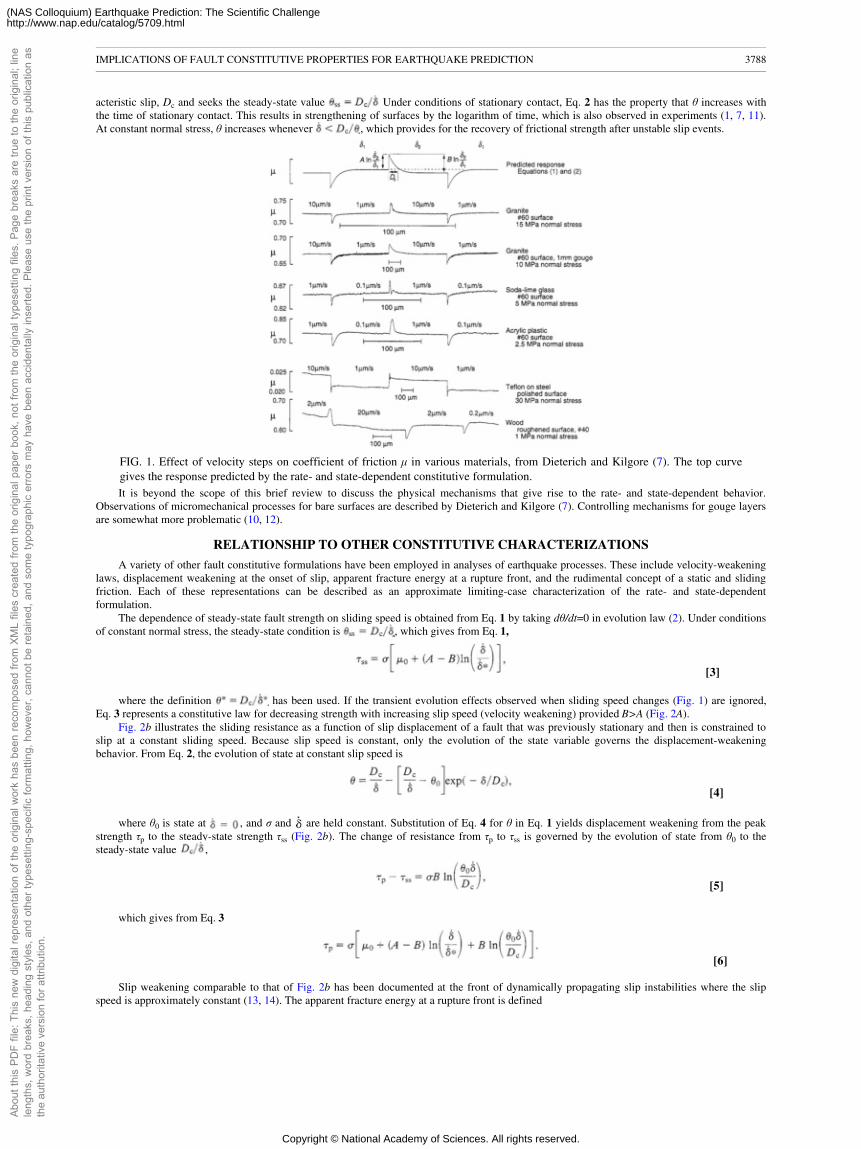
acteristic slip, Dc and seeks the steady-state value Under conditions of stationary contact, Eq. 2 has the property that θ increases withthe time of stationary contact. This results in strengthening of surfaces by the logarithm of time, which is also observed in experiments (1, 7, 11).At constant normal stress, θ increases whenever , which provides for the recovery of frictional strength after unstable slip events.
FIG. 1. Effect of velocity steps on coefficient of friction µ in various materials, from Dieterich and Kilgore (7). The top curvegives the response predicted by the rate- and state-dependent constitutive formulation.It is beyond the scope of this brief review to discuss the physical mechanisms that give rise to the rate- and state-dependent behavior.
Observations of micromechanical processes for bare surfaces are described by Dieterich and Kilgore (7). Controlling mechanisms for gouge layersare somewhat more problematic (10, 12).
RELATIONSHIP TO OTHER CONSTITUTIVE CHARACTERIZATIONS
A variety of other fault constitutive formulations have been employed in analyses of earthquake processes. These include velocity-weakeninglaws, displacement weakening at the onset of slip, apparent fracture energy at a rupture front, and the rudimental concept of a static and slidingfriction. Each of these representations can be described as an approximate limiting-case characterization of the rate- and state-dependentformulation.
The dependence of steady-state fault strength on sliding speed is obtained from Eq. 1 by taking dθ/dt=0 in evolution law (2). Under conditionsof constant normal stress, the steady-state condition is , which gives from Eq. 1,
[3]
where the definition has been used. If the transient evolution effects observed when sliding speed changes (Fig. 1) are ignored,Eq. 3 represents a constitutive law for decreasing strength with increasing slip speed (velocity weakening) provided B>A (Fig. 2A).
Fig. 2b illustrates the sliding resistance as a function of slip displacement of a fault that was previously stationary and then is constrained toslip at a constant sliding speed. Because slip speed is constant, only the evolution of the state variable governs the displacement-weakeningbehavior. From Eq. 2, the evolution of state at constant slip speed is
[4]
where θ0 is state at , and σ and are held constant. Substitution of Eq. 4 for θ in Eq. 1 yields displacement weakening from the peakstrength τp to the steady-state strength τss (Fig. 2b). The change of resistance from τp to τss is governed by the evolution of state from θ0 to thesteady-state value ,
[5]
which gives from Eq. 3
[6]
Slip weakening comparable to that of Fig. 2b has been documented at the front of dynamically propagating slip instabilities where the slipspeed is approximately constant (13, 14). The apparent fracture energy at a rupture front is defined
IMPLICATIONS OF FAULT CONSTITUTIVE PROPERTIES FOR EARTHQUAKE PREDICTION 3788
Abou
t thi
s PD
F fil
e: T
his
new
dig
ital r
epre
sent
atio
n of
the
orig
inal
wor
k ha
s be
en re
com
pose
d fro
m X
ML
files
cre
ated
from
the
orig
inal
pap
er b
ook,
not
from
the
orig
inal
type
setti
ng fi
les.
Pag
e br
eaks
are
true
to th
e or
igin
al; l
ine
leng
ths,
wor
d br
eaks
, hea
ding
sty
les,
and
oth
er ty
pese
tting
-spe
cific
form
attin
g, h
owev
er, c
anno
t be
reta
ined
, and
som
e ty
pogr
aphi
c er
rors
may
hav
e be
en a
ccid
enta
lly in
serte
d. P
leas
e us
e th
e pr
int v
ersi
on o
f thi
s pu
blic
atio
n as
the
auth
orita
tive
vers
ion
for a
ttrib
utio
n.
Copyright © National Academy of Sciences. All rights reserved.
(NAS Colloquium) Earthquake Prediction: The Scientific Challengehttp://www.nap.edu/catalog/5709.html
by the shaded area in Fig. 2b. Finally, if all rate and evolution effects are ignored, τp and τss define simple static and sliding friction parameterssometimes used in modeling of earthquake processes.
FIG. 2. Limiting case responses of the rate- and state-dependent constitutive formulation, (a) Effect of sliding speed on steady-state friction. The minimum slip speed is 0.001. (b) Displacement weakening from peak friction at the onset of slip to steady-state friction at constant slip speed. The shaded area gives the apparent fracture energy for the onset of slip.Each of these alternate characterizations has some appeal because their use often permits simplified analytical methods to be employed and
experimental evidence can be cited in support of their use. However, none of the simpler forms is able to represent the full range of phenomenarepresented by the rate- and state-dependent formulation and observed in laboratory experiments. We emphasize that unconstrained slidinghistories will violate the particular conditions required for the experimental observation of the isolated properties illustrated in Fig. 2. Therefore,use of these more idealized constitutive formulations can yield theoretical solutions for sliding behaviors that are fundamentally different from theactual phenomena.
UNSTABLE FAULT SLIP
The rate- and state-dependent constitutive formulation has been employed in modeling of various fault slip phenomena including stable creep,earthquake slip, and earthquake afterslip (15–18). Characteristics of sliding instabilities in systems consisting of a single slider connected to aloading point through a spring of stiffness K have been extensively analyzed and applied to analysis of laboratory fault experiments (1–6, 19–21).For an instability to occur, those studies establish that the system stiffness must be less than the critical value
[7]
where ξ depends on loading conditions and constitutive parameters. For stiffnesses K<Kc, unstable slip (stick-slip) will ensue, K>Kc results instable slip, and at K=Kc the system is neutrally stable. If shear and normal stresses are coupled through a spring inclined at an angle to the slidingsurface
[8]
where µss=τss/σ and � is the angle between the spring and the sliding surface [taken as positive if an increase of shear stress results in andecrease of normal stress (21)]. Eq. 8 applies to instabilities that arise from perturbations of steady-state slip. When �=0, normal stress remainsconstant during slip. If �<−cot−1µss, slider lock-up or instability will occur independent of specific constitutive properties.
Conditions for sliding instabilities on a fault patch embedded in an elastic medium are obtained by combining the spring and slider resultswith elasticity solutions for displacement along a crack (22). This yields
[9]
where Lc is the minimum patch half-length for unstable fault slip, G is the shear modulus (Poisson's ratio taken to be 0.25), and η is a factorwith values near 1 that depends upon the geometry of the slip patch and assumptions relating to slip or stress conditions on the patch. Lc defines alower bound for the dimensions of the earthquake source.
The relationship for Lc has been verified by laboratory experiments that employ a biaxial apparatus that accommodates samples withsimulated faults 2 m long. See Okubo and Dieterich (13), for description of the apparatus. Fig. 3 illustrates an example of a confined slip event inwhich the region of slip is approximately equal to Lc. For the conditions of the experiments (σ=5 MPa), measured constitutive parameters(ξ=0.4B=0.004, Dc=2 µm), and assumed model parameters (G=15,000 MPa, η=0.67), Lc is estimated to be 75 cm. The observed region of slip forthe event shown in Fig. 3 is 60–90 cm long. We have observed numerous confined slip events by using this apparatus. In all cases, the length of thezone of unstable slip is never less than the predicted Lc, within the uncertainty of the observations and model parameters. The unstable slip eventshown in Fig. 3 also illustrates an interval of stable slip prior to the instability, which is characteristic of unstable fault slip in the laboratory. Thistopic is taken up in the following section.
EARTHQUAKE NUCLEATION
The process leading to the localized initiation of unstable earthquake fault slip is sometimes referred to as earthquake nucleation (22–24). Thissubject is relevant to earthquake prediction because the nucleation process may be accompanied by detectable precursors and because nucleationdetermines the time and place of origin of earthquakes. Also, it is shown below that the sensitivity of the nucleation times to stress changes mayresult in significant changes of earthquake probabilities after relatively small stress perturbations, such as occur in the vicinity of prior earthquakes.
Numerical models of nucleation on faults with rate- and state-dependent properties indicate that the initiation of unstable slip is preceded by along interval of accelerating slip that spontaneously localizes to a subsection of the fault where stresses, relative to τss, are highest (24). Fig. 4illustrates
IMPLICATIONS OF FAULT CONSTITUTIVE PROPERTIES FOR EARTHQUAKE PREDICTION 3789
Abou
t thi
s PD
F fil
e: T
his
new
dig
ital r
epre
sent
atio
n of
the
orig
inal
wor
k ha
s be
en re
com
pose
d fro
m X
ML
files
cre
ated
from
the
orig
inal
pap
er b
ook,
not
from
the
orig
inal
type
setti
ng fi
les.
Pag
e br
eaks
are
true
to th
e or
igin
al; l
ine
leng
ths,
wor
d br
eaks
, hea
ding
sty
les,
and
oth
er ty
pese
tting
-spe
cific
form
attin
g, h
owev
er, c
anno
t be
reta
ined
, and
som
e ty
pogr
aphi
c er
rors
may
hav
e be
en a
ccid
enta
lly in
serte
d. P
leas
e us
e th
e pr
int v
ersi
on o
f thi
s pu
blic
atio
n as
the
auth
orita
tive
vers
ion
for a
ttrib
utio
n.
Copyright © National Academy of Sciences. All rights reserved.
(NAS Colloquium) Earthquake Prediction: The Scientific Challengehttp://www.nap.edu/catalog/5709.html
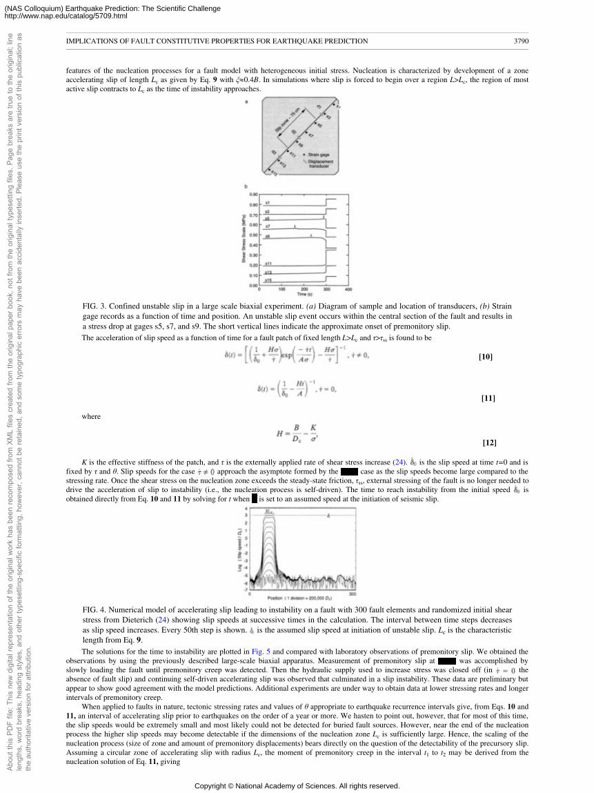
features of the nucleation processes for a fault model with heterogeneous initial stress. Nucleation is characterized by development of a zoneaccelerating slip of length Lc as given by Eq. 9 with ξ�0.4B. In simulations where slip is forced to begin over a region L>Lc, the region of mostactive slip contracts to Lc as the time of instability approaches.
FIG. 3. Confined unstable slip in a large scale biaxial experiment. (a) Diagram of sample and location of transducers, (b) Straingage records as a function of time and position. An unstable slip event occurs within the central section of the fault and results ina stress drop at gages s5, s7, and s9. The short vertical lines indicate the approximate onset of premonitory slip.The acceleration of slip speed as a function of time for a fault patch of fixed length L>Lc and τ>τss is found to be
[10]
[11]
where
[12]
K is the effective stiffness of the patch, and τ is the externally applied rate of shear stress increase (24). is the slip speed at time t=0 and isfixed by τ and θ. Slip speeds for the case approach the asymptote formed by the case as the slip speeds become large compared to thestressing rate. Once the shear stress on the nucleation zone exceeds the steady-state friction, τss, external stressing of the fault is no longer needed todrive the acceleration of slip to instability (i.e., the nucleation process is self-driven). The time to reach instability from the initial speed isobtained directly from Eq. 10 and 11 by solving for t when is set to an assumed speed at the initiation of seismic slip.
FIG. 4. Numerical model of accelerating slip leading to instability on a fault with 300 fault elements and randomized initial shearstress from Dieterich (24) showing slip speeds at successive times in the calculation. The interval between time steps decreasesas slip speed increases. Every 50th step is shown. is the assumed slip speed at initiation of unstable slip. Lc is the characteristiclength from Eq. 9.The solutions for the time to instability are plotted in Fig. 5 and compared with laboratory observations of premonitory slip. We obtained the
observations by using the previously described large-scale biaxial apparatus. Measurement of premonitory slip at was accomplished byslowly loading the fault until premonitory creep was detected. Then the hydraulic supply used to increase stress was closed off (in theabsence of fault slip) and continuing self-driven accelerating slip was observed that culminated in a slip instability. These data are preliminary butappear to show good agreement with the model predictions. Additional experiments are under way to obtain data at lower stressing rates and longerintervals of premonitory creep.
When applied to faults in nature, tectonic stressing rates and values of θ appropriate to earthquake recurrence intervals give, from Eqs. 10 and11, an interval of accelerating slip prior to earthquakes on the order of a year or more. We hasten to point out, however, that for most of this time,the slip speeds would be extremely small and most likely could not be detected for buried fault sources. However, near the end of the nucleationprocess the higher slip speeds may become detectable if the dimensions of the nucleation zone Lc is sufficiently large. Hence, the scaling of thenucleation process (size of zone and amount of premonitory displacements) bears directly on the question of the detectability of the precursory slip.Assuming a circular zone of accelerating slip with radius Lc, the moment of premonitory creep in the interval t1 to t2 may be derived from thenucleation solution of Eq. 11, giving
IMPLICATIONS OF FAULT CONSTITUTIVE PROPERTIES FOR EARTHQUAKE PREDICTION 3790
Abou
t thi
s PD
F fil
e: T
his
new
dig
ital r
epre
sent
atio
n of
the
orig
inal
wor
k ha
s be
en re
com
pose
d fro
m X
ML
files
cre
ated
from
the
orig
inal
pap
er b
ook,
not
from
the
orig
inal
type
setti
ng fi
les.
Pag
e br
eaks
are
true
to th
e or
igin
al; l
ine
leng
ths,
wor
d br
eaks
, hea
ding
sty
les,
and
oth
er ty
pese
tting
-spe
cific
form
attin
g, h
owev
er, c
anno
t be
reta
ined
, and
som
e ty
pogr
aphi
c er
rors
may
hav
e be
en a
ccid
enta
lly in
serte
d. P
leas
e us
e th
e pr
int v
ersi
on o
f thi
s pu
blic
atio
n as
the
auth
orita
tive
vers
ion
for a
ttrib
utio
n.
Copyright © National Academy of Sciences. All rights reserved.
(NAS Colloquium) Earthquake Prediction: The Scientific Challengehttp://www.nap.edu/catalog/5709.html
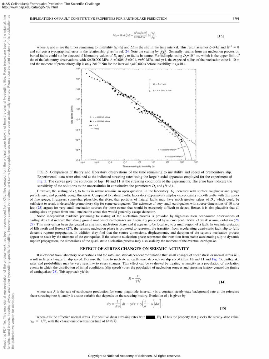
[13]
where t1 and t2 are the times remaining to instability (t1>t2) and ∆δ is the slip in the time interval. This result assumes ξ=0.4B and and corrects a typographical error in the relationship given in ref. 24. Note the scaling by . Generally, strains from the nucleation process onburied faults could not be detected if laboratory values of Dc apply to faults in nature. For example, using Dc=10−4 m, which is the upper limit ofthe of the laboratory observations, with G=20,000 MPa, A =0.006, B=0.01, σ=50 MPa, and η=1, the expected radius of the nucleation zone is 10 mand the moment of premonitory slip is only 2×10³ Nm for the interval t1=10,000 s before instability to t2=10 s.
FIG. 5. Comparison of theory and laboratory observations of the time remaining to instability and speed of premonitory slip.Experimental data were obtained at the indicated stressing rates using the large biaxial apparatus employed for the experiment ofFig. 3. The curves give the solutions of Eqs. 10 and 11 at the stressing conditions of the experiments. The error bars indicate thesensitivity of the solutions to the uncertainties in constitutive the parameters Dc and (B−A).However, the scaling of Dc to faults in nature remains an open question. In the laboratory, Dc increases with surface roughness and gouge
particle size, and possibly gouge thickness. Compared to natural faults, laboratory experiments employ exceptionally smooth faults with thin zonesof fine gouge. It appears somewhat plausible, therefore, that portions of natural faults may have much greater values of Dc, which could besufficient to result in detectable premonitory slip for some earthquakes. The existence of very small earthquakes with source dimensions of 10 m orless (25) argues for very small nucleation sources for those events that would be extremely difficult to detect. Hence, it is also plausible that allearthquakes originate from small nucleation zones that would generally escape detection.
Some independent evidence pertaining to scaling of the nucleation process is provided by high-resolution near-source observations ofearthquakes that indicate that strong ground motions of earthquakes are frequently preceded by an emergent interval of weak seismic radiation (26,27). This interval has been designated as a seismic nucleation phase and it appears to be localized to a small region of a fault. In one interpretationof Ellsworth and Beroza (27), the seismic nucleation phase is proposed to represent the transition from accelerating quasi-static fault slip to fullydynamic rupture propagation. In addition they find that the source dimensions, displacements, and duration of the seismic nucleation processappear to scale by the moment of the earthquake. If the seismic nucleation phase represents the transition from stable accelerating slip to dynamicrupture propagation, the dimensions of the quasi-static nucleation process may also scale by the moment of the eventual earthquake.
EFFECT OF STRESS CHANGES ON SEISMIC ACTIVITY
It is evident from laboratory observations and the rate- and state-dependent formulation that small changes of shear stress or normal stress willresult in large changes in slip speed. Because the time to nucleate an earthquake depends on slip speed (Eqs. 10 and 11 and Fig. 5), earthquakerates and probabilities may be very sensitive to stress changes. This effect can be evaluated by treating seismicity as a population of nucleationevents in which the distribution of initial conditions (slip speeds) over the population of nucleation sources and stressing history control the timingof earthquakes (28). This approach yields
[14]
where rate R is the rate of earthquake production for some magnitude interval, r is a constant steady-state background rate at the referenceshear stressing rate , and γ is a state variable that depends on the stressing history. Evolution of γ is given by
[15]
where σ is the effective normal stress. For positive shear stressing rates with , Eq. 15 has the property that γ seeks the steady-state value,, with the characteristic relaxation time of .
IMPLICATIONS OF FAULT CONSTITUTIVE PROPERTIES FOR EARTHQUAKE PREDICTION 3791
Abou
t thi
s PD
F fil
e: T
his
new
dig
ital r
epre
sent
atio
n of
the
orig
inal
wor
k ha
s be
en re
com
pose
d fro
m X
ML
files
cre
ated
from
the
orig
inal
pap
er b
ook,
not
from
the
orig
inal
type
setti
ng fi
les.
Pag
e br
eaks
are
true
to th
e or
igin
al; l
ine
leng
ths,
wor
d br
eaks
, hea
ding
sty
les,
and
oth
er ty
pese
tting
-spe
cific
form
attin
g, h
owev
er, c
anno
t be
reta
ined
, and
som
e ty
pogr
aphi
c er
rors
may
hav
e be
en a
ccid
enta
lly in
serte
d. P
leas
e us
e th
e pr
int v
ersi
on o
f thi
s pu
blic
atio
n as
the
auth
orita
tive
vers
ion
for a
ttrib
utio
n.
Copyright © National Academy of Sciences. All rights reserved.
(NAS Colloquium) Earthquake Prediction: The Scientific Challengehttp://www.nap.edu/catalog/5709.html
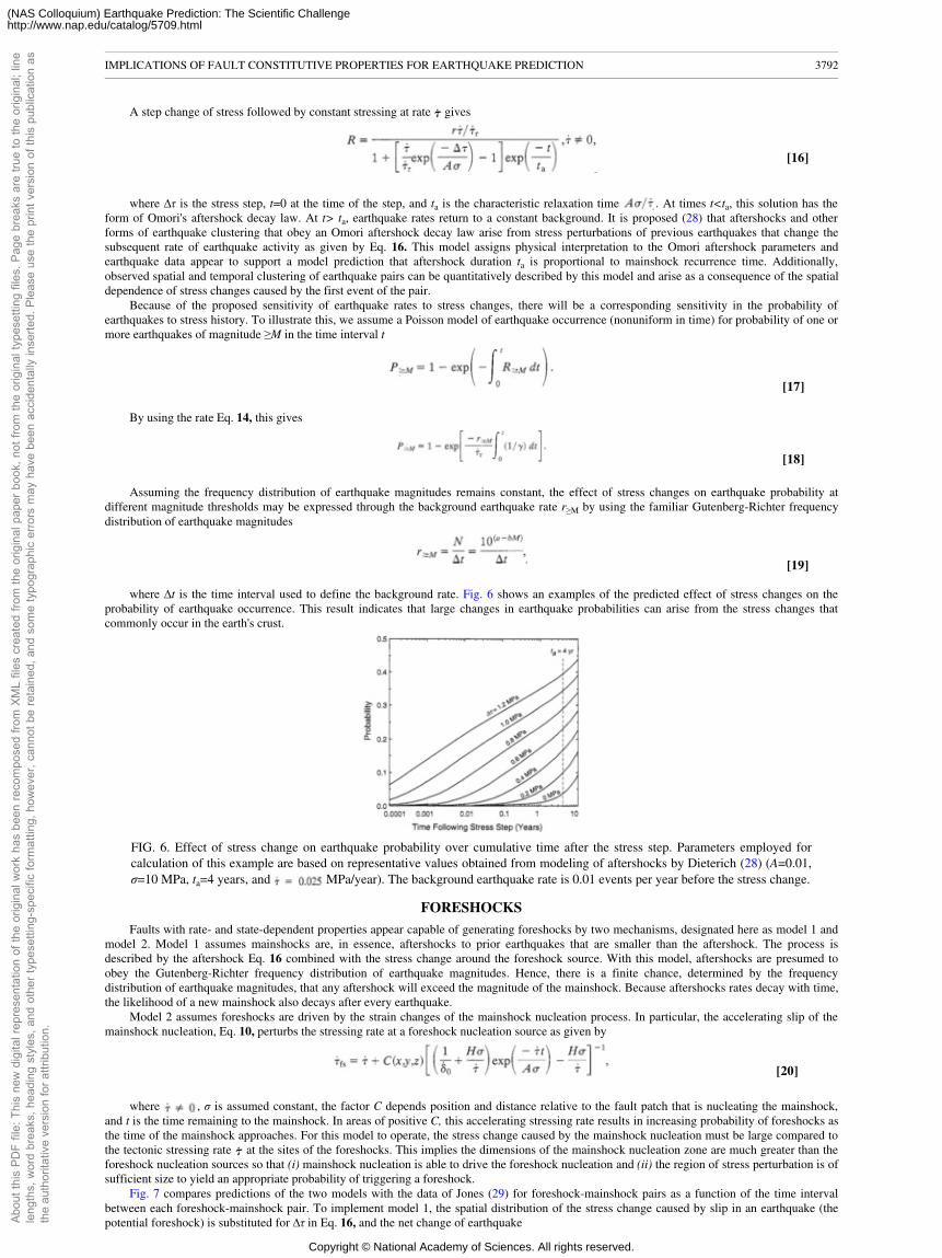
A step change of stress followed by constant stressing at rate gives
[16]
where ∆τ is the stress step, t=0 at the time of the step, and ta is the characteristic relaxation time . At times t<ta, this solution has theform of Omori's aftershock decay law. At t> ta, earthquake rates return to a constant background. It is proposed (28) that aftershocks and otherforms of earthquake clustering that obey an Omori aftershock decay law arise from stress perturbations of previous earthquakes that change thesubsequent rate of earthquake activity as given by Eq. 16. This model assigns physical interpretation to the Omori aftershock parameters andearthquake data appear to support a model prediction that aftershock duration ta is proportional to mainshock recurrence time. Additionally,observed spatial and temporal clustering of earthquake pairs can be quantitatively described by this model and arise as a consequence of the spatialdependence of stress changes caused by the first event of the pair.
Because of the proposed sensitivity of earthquake rates to stress changes, there will be a corresponding sensitivity in the probability ofearthquakes to stress history. To illustrate this, we assume a Poisson model of earthquake occurrence (nonuniform in time) for probability of one ormore earthquakes of magnitude ≥M in the time interval t
[17]
By using the rate Eq. 14, this gives
[18]
Assuming the frequency distribution of earthquake magnitudes remains constant, the effect of stress changes on earthquake probability atdifferent magnitude thresholds may be expressed through the background earthquake rate r≥M by using the familiar Gutenberg-Richter frequencydistribution of earthquake magnitudes
[19]
where ∆t is the time interval used to define the background rate. Fig. 6 shows an examples of the predicted effect of stress changes on theprobability of earthquake occurrence. This result indicates that large changes in earthquake probabilities can arise from the stress changes thatcommonly occur in the earth's crust.
FIG. 6. Effect of stress change on earthquake probability over cumulative time after the stress step. Parameters employed forcalculation of this example are based on representative values obtained from modeling of aftershocks by Dieterich (28) (A=0.01,σ=10 MPa, ta=4 years, and MPa/year). The background earthquake rate is 0.01 events per year before the stress change.
FORESHOCKS
Faults with rate- and state-dependent properties appear capable of generating foreshocks by two mechanisms, designated here as model 1 andmodel 2. Model 1 assumes mainshocks are, in essence, aftershocks to prior earthquakes that are smaller than the aftershock. The process isdescribed by the aftershock Eq. 16 combined with the stress change around the foreshock source. With this model, aftershocks are presumed toobey the Gutenberg-Richter frequency distribution of earthquake magnitudes. Hence, there is a finite chance, determined by the frequencydistribution of earthquake magnitudes, that any aftershock will exceed the magnitude of the mainshock. Because aftershocks rates decay with time,the likelihood of a new mainshock also decays after every earthquake.
Model 2 assumes foreshocks are driven by the strain changes of the mainshock nucleation process. In particular, the accelerating slip of themainshock nucleation, Eq. 10, perturbs the stressing rate at a foreshock nucleation source as given by
[20]
where , σ is assumed constant, the factor C depends position and distance relative to the fault patch that is nucleating the mainshock,and t is the time remaining to the mainshock. In areas of positive C, this accelerating stressing rate results in increasing probability of foreshocks asthe time of the mainshock approaches. For this model to operate, the stress change caused by the mainshock nucleation must be large compared tothe tectonic stressing rate at the sites of the foreshocks. This implies the dimensions of the mainshock nucleation zone are much greater than theforeshock nucleation sources so that (i) mainshock nucleation is able to drive the foreshock nucleation and (ii) the region of stress perturbation is ofsufficient size to yield an appropriate probability of triggering a foreshock.
Fig. 7 compares predictions of the two models with the data of Jones (29) for foreshock-mainshock pairs as a function of the time intervalbetween each foreshock-mainshock pair. To implement model 1, the spatial distribution of the stress change caused by slip in an earthquake (thepotential foreshock) is substituted for ∆τ in Eq. 16, and the net change of earthquake
IMPLICATIONS OF FAULT CONSTITUTIVE PROPERTIES FOR EARTHQUAKE PREDICTION 3792
Abou
t thi
s PD
F fil
e: T
his
new
dig
ital r
epre
sent
atio
n of
the
orig
inal
wor
k ha
s be
en re
com
pose
d fro
m X
ML
files
cre
ated
from
the
orig
inal
pap
er b
ook,
not
from
the
orig
inal
type
setti
ng fi
les.
Pag
e br
eaks
are
true
to th
e or
igin
al; l
ine
leng
ths,
wor
d br
eaks
, hea
ding
sty
les,
and
oth
er ty
pese
tting
-spe
cific
form
attin
g, h
owev
er, c
anno
t be
reta
ined
, and
som
e ty
pogr
aphi
c er
rors
may
hav
e be
en a
ccid
enta
lly in
serte
d. P
leas
e us
e th
e pr
int v
ersi
on o
f thi
s pu
blic
atio
n as
the
auth
orita
tive
vers
ion
for a
ttrib
utio
n.
Copyright © National Academy of Sciences. All rights reserved.
(NAS Colloquium) Earthquake Prediction: The Scientific Challengehttp://www.nap.edu/catalog/5709.html
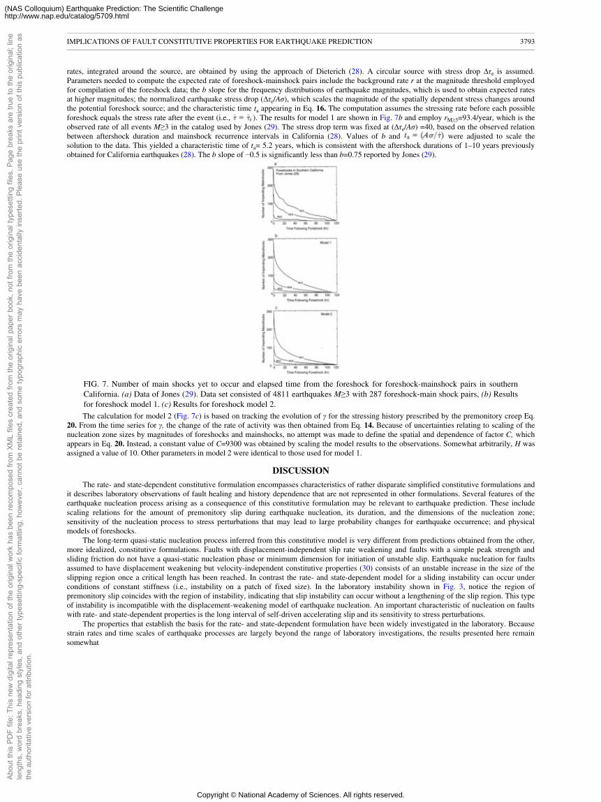
rates, integrated around the source, are obtained by using the approach of Dieterich (28). A circular source with stress drop ∆τe is assumed.Parameters needed to compute the expected rate of foreshock-mainshock pairs include the background rate r at the magnitude threshold employedfor compilation of the foreshock data; the b slope for the frequency distributions of earthquake magnitudes, which is used to obtain expected ratesat higher magnitudes; the normalized earthquake stress drop (∆τe/Aσ), which scales the magnitude of the spatially dependent stress changes aroundthe potential foreshock source; and the characteristic time ta appearing in Eq. 16. The computation assumes the stressing rate before each possibleforeshock equals the stress rate after the event (i.e., ). The results for model 1 are shown in Fig. 7b and employ rM≥3=93.4/year, which is theobserved rate of all events M≥3 in the catalog used by Jones (29). The stress drop term was fixed at (∆τe/Aσ) =40, based on the observed relationbetween aftershock duration and mainshock recurrence intervals in California (28). Values of b and were adjusted to scale thesolution to the data. This yielded a characteristic time of ta= 5.2 years, which is consistent with the aftershock durations of 1–10 years previouslyobtained for California earthquakes (28). The b slope of −0.5 is significantly less than b=0.75 reported by Jones (29).
FIG. 7. Number of main shocks yet to occur and elapsed time from the foreshock for foreshock-mainshock pairs in southernCalifornia. (a) Data of Jones (29). Data set consisted of 4811 earthquakes M≥3 with 287 foreshock-main shock pairs, (b) Resultsfor foreshock model 1. (c) Results for foreshock model 2.The calculation for model 2 (Fig. 7c) is based on tracking the evolution of γ for the stressing history prescribed by the premonitory creep Eq.
20. From the time series for γ, the change of the rate of activity was then obtained from Eq. 14. Because of uncertainties relating to scaling of thenucleation zone sizes by magnitudes of foreshocks and mainshocks, no attempt was made to define the spatial and dependence of factor C, whichappears in Eq. 20. Instead, a constant value of C=9300 was obtained by scaling the model results to the observations. Somewhat arbitrarily, H wasassigned a value of 10. Other parameters in model 2 were identical to those used for model 1.
DISCUSSION
The rate- and state-dependent constitutive formulation encompasses characteristics of rather disparate simplified constitutive formulations andit describes laboratory observations of fault healing and history dependence that are not represented in other formulations. Several features of theearthquake nucleation process arising as a consequence of this constitutive formulation may be relevant to earthquake prediction. These includescaling relations for the amount of premonitory slip during earthquake nucleation, its duration, and the dimensions of the nucleation zone;sensitivity of the nucleation process to stress perturbations that may lead to large probability changes for earthquake occurrence; and physicalmodels of foreshocks.
The long-term quasi-static nucleation process inferred from this constitutive model is very different from predictions obtained from the other,more idealized, constitutive formulations. Faults with displacement-independent slip rate weakening and faults with a simple peak strength andsliding friction do not have a quasi-static nucleation phase or minimum dimension for initiation of unstable slip. Earthquake nucleation for faultsassumed to have displacement weakening but velocity-independent constitutive properties (30) consists of an unstable increase in the size of theslipping region once a critical length has been reached. In contrast the rate- and state-dependent model for a sliding instability can occur underconditions of constant stiffness (i.e., instability on a patch of fixed size). In the laboratory instability shown in Fig. 3, notice the region ofpremonitory slip coincides with the region of instability, indicating that slip instability can occur without a lengthening of the slip region. This typeof instability is incompatible with the displacement-weakening model of earthquake nucleation. An important characteristic of nucleation on faultswith rate- and state-dependent properties is the long interval of self-driven accelerating slip and its sensitivity to stress perturbations.
The properties that establish the basis for the rate- and state-dependent formulation have been widely investigated in the laboratory. Becausestrain rates and time scales of earthquake processes are largely beyond the range of laboratory investigations, the results presented here remainsomewhat
IMPLICATIONS OF FAULT CONSTITUTIVE PROPERTIES FOR EARTHQUAKE PREDICTION 3793
Abou
t thi
s PD
F fil
e: T
his
new
dig
ital r
epre
sent
atio
n of
the
orig
inal
wor
k ha
s be
en re
com
pose
d fro
m X
ML
files
cre
ated
from
the
orig
inal
pap
er b
ook,
not
from
the
orig
inal
type
setti
ng fi
les.
Pag
e br
eaks
are
true
to th
e or
igin
al; l
ine
leng
ths,
wor
d br
eaks
, hea
ding
sty
les,
and
oth
er ty
pese
tting
-spe
cific
form
attin
g, h
owev
er, c
anno
t be
reta
ined
, and
som
e ty
pogr
aphi
c er
rors
may
hav
e be
en a
ccid
enta
lly in
serte
d. P
leas
e us
e th
e pr
int v
ersi
on o
f thi
s pu
blic
atio
n as
the
auth
orita
tive
vers
ion
for a
ttrib
utio
n.
Copyright © National Academy of Sciences. All rights reserved.
(NAS Colloquium) Earthquake Prediction: The Scientific Challengehttp://www.nap.edu/catalog/5709.html
speculative. However, agreement of the rate- and state-dependent model for seismic activity with observations of aftershocks and earthquakeclustering (28) lends support to the use of the formulation over the time-scale aftershock phenomena (months to years). This includes apparentconfirmation of a predicted independence of aftershock duration ta on earthquake magnitude and an inverse dependence of ta on stressing rate.Alternative mechanisms for aftershocks and clustering, based on viscoelastic stress transfer or diffusion processes that alter fault stress, lead tocharacteristic aftershock times that are insensitive to stressing rates but depend on a characteristic length of the mainshock disturbance.
Both foreshock models provide comparable fits to the data. Model 1 is more specific than model 2, and the parameters used for the model 1computation appear consistent with other results. The value (∆τe/Aσ)=40 is based on the aftershock analysis of Dieterich (28). Assuming a typicallaboratory value of A=0.001 and earthquake stress drop ∆τe=4 MPa, this gives σ=10 MPa. In turn, these values and years give astressing rate MPa/year. Model 2 is nonspecific and demonstrates only that the shape of the predicted temporal decay of foreshock-mainshock pairs is consistent with the data. The large value of the stress coupling parameter, C=9300, indicates strong coupling between slipduring mainshock nucleation and stresses at regions of foreshock nucleation. This suggests the model 2 mechanism can work only if foreshocksnucleate at the edges of the mainshock nucleation zone or perhaps as small patches embedded within the slipping region for mainshock nucleation.1. Dieterich, J.H. (1979) J. Geophys. Res. 84, 2161–2168.2. Dieterich, J.H. (1981) Mechanical Behavior of Crustal Rocks, Geophysical Monograph 24, eds. Carter, N.L., Friedman, M., Logan, J.M. & Stearns, D.W.
(Am. Geophys. Union, Washington, DC), pp. 103–120.3. Ruina, A.L. (1983) J. Geophys. Res. 88, 10359–10370.4. Weeks, J.D. & Tullis, T.E. (1985) J. Geophys. Res. 90, 7821–7826.5. Tullis, T.E. & Weeks, J.D. (1986) Pure Appl. Geophys. 124, 383–414.6. Linker, M.F. & Dieterich, J.H. (1992) J. Geophys. Res. 97, 4923–4940.7. Dieterich, J.H. & Kilgore, B.D. (1994) PureAppl. Geophys. 143, 283–302.8. Blanpied, M.L., Lockner, D.A. & Byerlee, J.D. (1991) Geophys. Res. Lett. 18, 609–612.9. Kilgore, B.D., Blanpied, M.L. & Dieterich, J.H. (1993) Geophys. Res. Lett. 20, 903–906.10. Marone, C. & Kilgore, B. (1993) Nature (London) 362, 618–621.11. Beeler, N.M., Tullis, T.E. & Weeks, J.D. (1994) Geophys. Res. Lett. 21, 1987–1990.12. Sammis, C.G. & Biegel, R.L. (1989) Pure & Appl. Geophys. 131, 253–271.13. Okubo, P.G. & Dieterich, J.H. (1984) J. Geophys. Res. 89, 5817–5827.14. Ohnaka, M., Kuwahara, Y., Yamamoto, K. & Hirasawa, T. (1986) Earthquake Source Mechanics, Vol. 6, Geophysical Monograph 37, eds. Das, S.,
Boatwright, J. & Scholz, C.H. (Am. Geophys. Union, Washington, DC), pp. 13–24.15. Tse, S.T. & Rice, J.R. (1986) J. Geophys. Res. 91, 9452–9472.16. Stuart, W.D. (1988) Pure Appl. Geophys. 126, 619–641.17. Marone, C.C., Scholz, C.H. & Bilham, R. (1991) J. Geophys. Res. 91, 8441–8452.18. Rice, J.R. (1993) J. Geophys. Res. 98, 9885–9907.19. Rice, J.R. & Ruina, A.L. (1983) J. Appl Mech. 50, 343–349.20. Gu, Y. & Wong, T.-F. (1991) J. Geophys. Res. 96, 21677–21691.21. Dieterich, J.H. & Linker, M.F. (1992) Geophys. Res. Lett. 19, 1691–1694.22. Dieterich, J.H. (1986) Earthquake Source Mechanics, Vol. 6, Geophysical Monograph 37, eds. Das, S., Boatwright, J. & Scholz, C.H. (Am. Geophys.
Union, Washington, DC), pp. 37–47.23. Ohnaka, Y. (1992) Tectonophysics 211, 149–178.24. Dieterich, J.H. (1992) Tectonophysics 211, 115–134.25. Abercrombie, R. & Leary, P. (1993) Geophys. Res. Lett. 20, 1511–1514.26. Iio, Y. (1992) Geophys. Res. Lett. 19, 477–480.27. Ellsworth, W.L. & Beroza, G.C. (1995) Nature (London) 268, 851–855.28. Dieterich, J.H. (1994) J. Geophys. Res. 99, 2601–2618.29. Jones, L.M. (1985) Bull. Seismol. Soc. Am. 75, 1669–1679.30. Shibazaki, B. & Matsu'ura, M. (1992) Geophys. Res. Lett. 19, 1189–1192.
IMPLICATIONS OF FAULT CONSTITUTIVE PROPERTIES FOR EARTHQUAKE PREDICTION 3794
Abou
t thi
s PD
F fil
e: T
his
new
dig
ital r
epre
sent
atio
n of
the
orig
inal
wor
k ha
s be
en re
com
pose
d fro
m X
ML
files
cre
ated
from
the
orig
inal
pap
er b
ook,
not
from
the
orig
inal
type
setti
ng fi
les.
Pag
e br
eaks
are
true
to th
e or
igin
al; l
ine
leng
ths,
wor
d br
eaks
, hea
ding
sty
les,
and
oth
er ty
pese
tting
-spe
cific
form
attin
g, h
owev
er, c
anno
t be
reta
ined
, and
som
e ty
pogr
aphi
c er
rors
may
hav
e be
en a
ccid
enta
lly in
serte
d. P
leas
e us
e th
e pr
int v
ersi
on o
f thi
s pu
blic
atio
n as
the
auth
orita
tive
vers
ion
for a
ttrib
utio
n.
Copyright © National Academy of Sciences. All rights reserved.
(NAS Colloquium) Earthquake Prediction: The Scientific Challengehttp://www.nap.edu/catalog/5709.html
This paper was presented at a colloquium entitled “Earthquake Prediction: The Scientific Challenge,” organized by Leon Knopoff(Chair), Keiiti Aki, Clarence R.Allen, James R.Rice, and Lynn R.Sykes, held February 10 and 11, 1995, at the National Academy of Sciences inIrvine, CA.
Nonuniformity of the constitutive law parameters for shear ruptureand quasistatic nucleation to dynamic rupture: A physical model of
earthquake generation processes
MITIYASU OHNAKA
Earthquake Research Institute, University of Tokyo, Bunkyo-ku, Tokyo 113, JapanABSTRACT Based on the recent high-resolution laboratory experiments on propagating shear rupture, the constitutive law that
governs shear rupture processes is discussed in view of the physical principles and constraints, and a specific constitutive law is proposedfor shear rupture. It is demonstrated that nonuniform distributions of the constitutive law parameters on the fault are necessary forcreating the nucleation process, which consists of two phases: (i) a stable, quasistatic phase, and (ii) the subsequent accelerating phase.Physical models of the breakdown zone and the nucleation zone are presented for shear rupture in the brittle regime. The constitutive lawfor shear rupture explicitly includes a scaling parameter Dc that enables one to give a common interpretation to both small scale rupturein the laboratory and large scale rupture as earthquake source in the Earth. Both the breakdown zone size Xc and the nucleation zone sizeL are prescribed and scaled by Dc, which in turn is prescribed by a characteristic length λc representing geometrical irregularities of thefault. The models presented here make it possible to understand the earthquake generation process from nucleation to unstable, dynamicrupture propagation in terms of physics. Since the nucleation process itself is an immediate earthquake precursor, deep understanding ofthe nucleation process in terms of physics is crucial for the short-term (or immediate) earthquake prediction.
The mechanical instability that gives rise to a dynamically propagating shear rupture is caused by frictional slip failure on a preexisting faultor shear fracture of intact materials. As will be discussed later, frictional slip instability and shear fracture instability of intact rock are the twoextreme cases of shear rupture. Therefore, if there is a constitutive law that governs the shear rupture, both frictional slip failure and shear fractureof intact materials should be treated unifyingly and quantitatively in terms of the single constitutive law. The shear rupture can proceed stably andquasistatically at a slow speed even in the brittle regime or, alternatively, propagate unstably and dynamically at a fast speed close to sonicvelocities. These two extreme phases are part of the rupture process, so that both phases should also be treated unifyingly and quantitatively by thesingle constitutive law. These must be kept in mind when we discuss what type and form are the most appropriate and physically reasonable for theconstitutive law of earthquake shear rupture.
The stability or instability of the rupture process once the rupture has occurred is governed by how progressively the local strength in thebreakdown zone behind the rupture front degrades with ongoing local slip displacement. The transient response of the shear traction to the localslip displacement in the breakdown zone is a key to the quantitative analysis of the stability or instability of the rupture. The breakdown zone isdefined as the zone behind the tip of a propagating rupture over which the shear strength degrades with ongoing slip to a residual friction stresslevel. Careful and well prepared, high-resolution laboratory experiments (1–3) have made it possible to reveal the transient response of the shearstress to the local slip displacement in the breakdown zone, and a specific form of the constitutive law for shear rupture can be determined fromthese experimental observations so as to meet the physical principles and constraints established.
We first wish to discuss what type and form are the most appropriate and physically reasonable as the constitutive law for shear rupture and topresent a specific constitutive law for shear rupture and a model of the breakdown zone based on a series of our high-resolution laboratoryexperiments on local breakdown near the propagating front during shear rupture along a fault of weak junction in a large rock sample (1–3). Wethen present a model of earthquake rupture nucleation, which is also based on intrinsic properties of the local breakdown during shear rupturenucleation revealed in the recent high-resolution laboratory experiments. The shear rupture nucleation is defined here as the transition process (orzone) where shear rupture grows with a slow speed from the point where the shear rupture nucleus is formed to the critical point beyond which therupture front propagates at a speed close to sonic velocities. Data obtained from the high-resolution laboratory experiments enable one to discusshow unstable, dynamic shear rupture is nucleated in the brittle regime and its mechanical conditions in terms of the constitutive law for shearrupture in the framework of fracture mechanics. The breakdown zone and the nucleation zone will be modeled physically in terms of theconstitutive law parameters, and it will be shown how well and physically reasonably the breakdown zone and the nucleation zone are scaled interms of one of the constitutive law parameters, which in turn strongly depends on a characteristic length representing geometrical irregularities ofthe rupturing fault. Finally, we discuss the earthquake nucleation and immediate precursors associated with the nucleation.
CONSTITUTIVE LAW FOR SHEAR RUPTURE
Basic Principles. The surface of a solid, even when best-prepared, is made up of asperities. When two surfaces of solid materials are pressedin contact, they do not touch over the entire area Aa (apparent area of contact), but they get in contact only at a number of asperities. The sum of theareas of all the asperity contacts constitutes the real area of contact Ar(<Aa). The atomic interaction between the surfaces takes place at these reallycontacting portions (atom-to-atom contact); however, the powerful interatomic forces are of very short range, of the order of a
The publication costs of this article were defrayed in part by page charge payment. This article must therefore be hereby marked“advertisement” in accordance with 18 U.S.C. §1734 solely to indicate this fact.
NONUNIFORMITY OF THE CONSTITUTIVE LAW PARAMETERS FOR SHEAR RUPTURE AND QUASISTATIC NUCLEATION TODYNAMIC RUPTURE: A PHYSICAL MODEL OF EARTHQUAKE GENERATION PROCESSES
3795
Abou
t thi
s PD
F fil
e: T
his
new
dig
ital r
epre
sent
atio
n of
the
orig
inal
wor
k ha
s be
en re
com
pose
d fro
m X
ML
files
cre
ated
from
the
orig
inal
pap
er b
ook,
not
from
the
orig
inal
type
setti
ng fi
les.
Pag
e br
eaks
are
true
to th
e or
igin
al; l
ine
leng
ths,
wor
d br
eaks
, hea
ding
sty
les,
and
oth
er ty
pese
tting
-spe
cific
form
attin
g, h
owev
er, c
anno
t be
reta
ined
, and
som
e ty
pogr
aphi
c er
rors
may
hav
e be
en a
ccid
enta
lly in
serte
d. P
leas
e us
e th
e pr
int v
ersi
on o
f thi
s pu
blic
atio
n as
the
auth
orita
tive
vers
ion
for a
ttrib
utio
n.
Copyright © National Academy of Sciences. All rights reserved.
(NAS Colloquium) Earthquake Prediction: The Scientific Challengehttp://www.nap.edu/catalog/5709.html
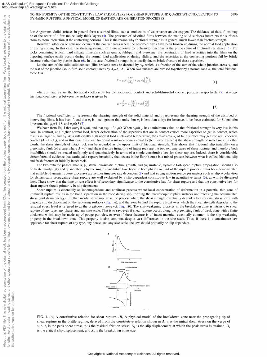
few Angstroms. Solid surfaces in general form adsorbed films, such as molecules of water vapor and/or oxygen. The thickness of these films maybe of the order of a few molecularly thick layers (4). The presence of adsorbed films between the mating solid surfaces interrupts the surface'satom-to-atom interaction at the contacting portions. This is the reason why frictional strength is in general much lower than fracture strength.
However, adhesion or cohesion occurs at the contact areas where the adsorbed films have been broken up during the normal load applicationor during sliding. In this case, the shearing strength of these adhesive (or cohesive) junctions is the prime cause of frictional resistance (5). Forrocks containing typical, hard silicate minerals such as quartz, feldspar, and pyroxene, the penetration of hard asperities into the films on theopposing surface easily occurs during the normal load application or during sliding, and the asperities at the contacting portions fail by brittlefracture, rather than by plastic shear (6). In this case, frictional strength is primarily due to brittle fracture of these asperities.
Let the sum of the solid-solid contact (film-broken) areas be denoted by A1, which is a fraction of the sum of the whole junction areas Ar, andthe rest of the junction (solid-film-solid contact) areas by A2=Ar−A1. When two surfaces are pressed together by a normal load N, the total frictionalforce F is
[1]
where µ1 and µ2 are the frictional coefficients for the solid-solid contact and solid-film-solid contact portions, respectively (7). Averagefrictional coefficient µ between the surfaces is given by
[2]
The frictional coefficient µ1 represents the shearing strength of the solid material and µ2 represents the shearing strength of the adsorbed orintervening films. It has been found that µ1 is much greater than unity, but µ2 is less than unity; for instance, it has been estimated for Solenhofenlimestone that µ1=4–18, and µ2=0.3 (7).
We have from Eq. 2 that µ=µ2 if A1=0, and that µ=µ1 if A2=0. When A1=0, µ has a minimum value, so that frictional strength is very low in thiscase. In contrast, at a higher normal load, larger deformation of the asperities that are in contact causes more asperities to get in contact, whichresults in larger Ar and A1. At a sufficiently high normal load at elevated temperature, the entire area Aa of fault surface may get into real, cohesivecontact (A1=Ar=Aa), and in this case the shear frictional resistance comes equal to (but never exceeds) the shear strength of intact rock. In otherwords, the shear strength of intact rock can be regarded as the upper limit of frictional strength. This shows that frictional slip instability on apreexisting fault (of a case where A1=0) and shear fracture instability of intact rock are the two extreme cases of shear rupture, and therefore bothinstabilities should be treated unifyingly and quantitatively in terms of a single constitutive law for shear rupture. Indeed, there is considerablecircumferential evidence that earthquake rupture instability that occurs in the Earth's crust is a mixed process between what is called frictional slipand fresh fracture of initially intact rock.
The two extreme phases, that is, (i) stable, quasistatic rupture growth, and (ii) unstable, dynamic fast-speed rupture propagation, should alsobe treated unifyingly and quantitatively by the single constitutive law, because both phases are part of the rupture process. It has been demonstratedthat unstable, dynamic rupture processes are neither time nor rate dependent (8) and that strong motion source parameters such as slip accelerationfor dynamically propagating shear rupture are well explained by a slip-dependent constitutive law in quantitative terms (3), as will be discussedlater. These show that the time or rate effect is of secondary significance to the constitutive law for shear rupture and that the constitutive law forshear rupture should primarily be slip dependent.
Shear rupture is essentially an inhomogeneous and nonlinear process where local concentration of deformation in a potential thin zone ofimminent rupture results in the bond separation in the zone during slip, forming the macroscopic rupture surfaces and releasing the accumulatedstress (and strain energy). In other words, shear rupture is the process where the shear strength eventually degrades to a residual stress level withongoing slip displacement on the rupturing surfaces (Fig. 1A), and the zone behind the rupture front over which the shear strength degrades to theresidual stress level is referred to as the breakdown zone (cf. Fig. 1B). The slip-weakening property in the breakdown zone is intrinsic to shearrupture of any type, any phase, and any size scale. That is to say, even if shear rupture occurs along the preexisting fault of weak zone with a finitethickness, which may be made up of gouge particles, or even if shear fracture is of intact material, essentially common is the slip-weakeningproperty in the breakdown zone. This property is also common, despite vast differences in the size scale. Thus, if there is a constitutive lawapplicable for shear rupture of any type, any phase, and any size scale, the law should primarily be slip dependent.
FIG. 1. (A) A constitutive relation for shear rupture. (B) A physical model of the breakdown zone near the propagating tip ofshear rupture in the brittle regime, derived from the constitutive relation shown in A. τi is the initial shear stress on the verge ofslip, τp is the peak shear stress, τr is the residual friction stress, Da is the slip displacement at which the peak stress is attained, Dc
is the critical slip displacement, and Xc is the breakdown zone size.
NONUNIFORMITY OF THE CONSTITUTIVE LAW PARAMETERS FOR SHEAR RUPTURE AND QUASISTATIC NUCLEATION TODYNAMIC RUPTURE: A PHYSICAL MODEL OF EARTHQUAKE GENERATION PROCESSES
3796
Abou
t thi
s PD
F fil
e: T
his
new
dig
ital r
epre
sent
atio
n of
the
orig
inal
wor
k ha
s be
en re
com
pose
d fro
m X
ML
files
cre
ated
from
the
orig
inal
pap
er b
ook,
not
from
the
orig
inal
type
setti
ng fi
les.
Pag
e br
eaks
are
true
to th
e or
igin
al; l
ine
leng
ths,
wor
d br
eaks
, hea
ding
sty
les,
and
oth
er ty
pese
tting
-spe
cific
form
attin
g, h
owev
er, c
anno
t be
reta
ined
, and
som
e ty
pogr
aphi
c er
rors
may
hav
e be
en a
ccid
enta
lly in
serte
d. P
leas
e us
e th
e pr
int v
ersi
on o
f thi
s pu
blic
atio
n as
the
auth
orita
tive
vers
ion
for a
ttrib
utio
n.
Copyright © National Academy of Sciences. All rights reserved.
(NAS Colloquium) Earthquake Prediction: The Scientific Challengehttp://www.nap.edu/catalog/5709.html
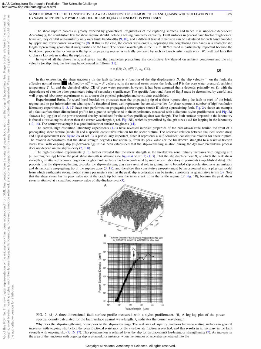
The shear rupture process is greatly affected by geometrical irregularities of the rupturing surfaces, and hence it is size-scale dependent.Accordingly, the constitutive law for shear rupture should include a scaling parameter explicitly. Fault surfaces in general have fractal roughnesses;however, they exhibit self-similarity only over finite bandwidths (9, 10), and a different fractal dimension can be calculated for each band boundedby upper and lower corner wavelengths (9). If this is the case, the corner wavelength λc separating the neighboring two bands is a characteristiclength representing geometrical irregularities of the fault. The corner wavelength in the 10- to 10−6-m band is particularly important because thebreakdown process that occurs near the tip of propagating rupture is virtually governed by such a characteristic length scale. We will find later thatλc plays a key role in scaling the rupture size.
In view of all the above facts, and given that the parameters prescribing the constitutive law depend on ambient conditions and the slipvelocity (or slip rate), the law may be expressed as follows (11):
[3]
In this expression, the shear traction τ on the fault surfaces is a function of the slip displacement D, the slip velocity ` on the fault, theeffective normal stress (defined by , where σn is the normal stress across the fault, and P is the pore water pressure), ambienttemperature T, λc, and the chemical effect CE of pore water pressure; however, it has been assumed that τ depends primarily on D, with thedependence of τ on the other parameters being of secondary significance. The specific functional form of Eq. 3 must be determined by careful andwell prepared laboratory experiments so as to meet the physical principles and constraints established.
Experimental Basis. To reveal local breakdown processes near the propagating tip of a shear rupture along the fault in rock of the brittleregime, and to get information on what specific functional form well represents the constitutive law for shear rupture, a number of high-resolutionlaboratory experiments (1–3, 12) have been performed on propagating shear rupture (mode II) along a preexisting fault. Fig. 2A shows an exampleof a fault surface three-dimensional profile for a granite sample used in the experiments, measured with a diamond stylus profilometer, and Fig. 2Bshows a log-log plot of the power spectral density calculated for the surface profile against wavelength. The fault surface prepared in the laboratoryis fractal at wavelengths shorter than the corner wavelength λc (cf. Fig. 2B), which is prescribed by the grit sizes used for lapping in the laboratory(13, 14). The corner wavelength is a good indicator of surface roughness (14).
The careful, high-resolution laboratory experiments (1–3) have revealed intrinsic properties of the breakdown zone behind the front of apropagating shear rupture (mode II) and a specific constitutive relation for the shear rupture. The observed relation between the local shear stressand slip displacement (see figure 2A of ref. 3) is particularly important, since it represents a self-consistent constitutive relation for shear rupture.The relation demonstrates that the shear strength degrades transitionally, from its peak value (or the breakdown strength) to a residual frictionstress level with ongoing slip (slip-weakening). It has been established that the slip-weakening relation during the dynamic breakdown processdoes not depend on the slip velocity (2, 3, 8).
The high-resolution experiments (1, 3) further revealed that the shear strength in the breakdown zone initially increases with ongoing slip(slip-strengthening) before the peak shear strength is attained (see figure 4 of ref. 3) (1, 3). That the slip displacement Da at which the peak shearstrength τp is attained becomes larger on rougher fault surfaces has been confirmed by more recent laboratory experiments (unpublished data). Theproperty that the slip-strengthening precedes the slip-weakening plays an essential role in giving rise to bounded slip acceleration near an unstablyand dynamically propagating tip of the rupture zone (3, 15), and therefore this constitutive property must be incorporated into a physical modelfrom which earthquake strong motion source parameters such as the peak slip acceleration can be treated rigorously in quantitative terms (3). Notethat the shear stress has its peak value not at the crack tip but near the inner crack tip in the brittle regime (cf. Fig. 1B), because the peak shearstress is attained at a small but nonzero value of slip displacement (3).
FIG. 2. (A) A three-dimensional fault surface profile measured with a stylus profilometer. (B) A log-log plot of the powerspectral density calculated for the fault surface against wavelength. λc indicates the corner wavelength.Why does the slip-strengthening occur prior to the slip-weakening? The real area of asperity junctions between mating surfaces in general
increases with ongoing slip before the peak frictional resistance or the steady-state friction is reached, and this results in an increase in the faultstrength with ongoing slip (7, 16, 17). This phenomenon is referred to as the slip (or displacement) hardening or strengthening (7). An increase inthe area of the junctions with ongoing slip is attained, for instance, when the number of asperities penetrated into the
NONUNIFORMITY OF THE CONSTITUTIVE LAW PARAMETERS FOR SHEAR RUPTURE AND QUASISTATIC NUCLEATION TODYNAMIC RUPTURE: A PHYSICAL MODEL OF EARTHQUAKE GENERATION PROCESSES
3797
Abou
t thi
s PD
F fil
e: T
his
new
dig
ital r
epre
sent
atio
n of
the
orig
inal
wor
k ha
s be
en re
com
pose
d fro
m X
ML
files
cre
ated
from
the
orig
inal
pap
er b
ook,
not
from
the
orig
inal
type
setti
ng fi
les.
Pag
e br
eaks
are
true
to th
e or
igin
al; l
ine
leng
ths,
wor
d br
eaks
, hea
ding
sty
les,
and
oth
er ty
pese
tting
-spe
cific
form
attin
g, h
owev
er, c
anno
t be
reta
ined
, and
som
e ty
pogr
aphi
c er
rors
may
hav
e be
en a
ccid
enta
lly in
serte
d. P
leas
e us
e th
e pr
int v
ersi
on o
f thi
s pu
blic
atio
n as
the
auth
orita
tive
vers
ion
for a
ttrib
utio
n.
Copyright © National Academy of Sciences. All rights reserved.
(NAS Colloquium) Earthquake Prediction: The Scientific Challengehttp://www.nap.edu/catalog/5709.html
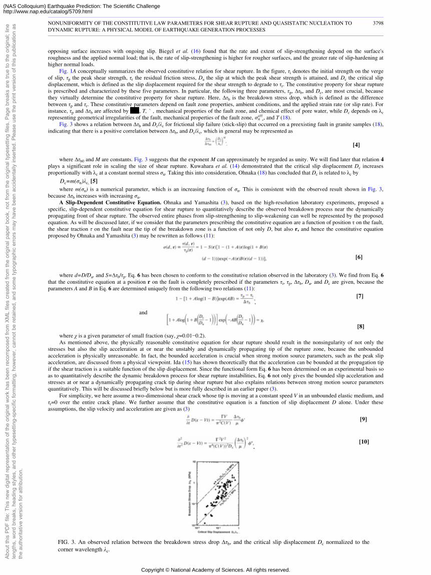
opposing surface increases with ongoing slip. Biegel et al. (16) found that the rate and extent of slip-strengthening depend on the surface'sroughness and the applied normal load; that is, the rate of slip-strengthening is higher for rougher surfaces, and the greater rate of slip-hardening athigher normal loads.
Fig. 1A conceptually summarizes the observed constitutive relation for shear rupture. In the figure, τi denotes the initial strength on the vergeof slip, τp the peak shear strength, τr the residual friction stress, Da the slip at which the peak shear strength is attained, and Dc the critical slipdisplacement, which is defined as the slip displacement required for the shear strength to degrade to τr. The constitutive property for shear ruptureis prescribed and characterized by these five parameters. In particular, the following three parameters, τp, ∆τb, and Dc, are most crucial, becausethey virtually determine the constitutive property for shear rupture. Here, ∆τb is the breakdown stress drop, which is defined as the differencebetween τp and τr. These constitutive parameters depend on fault zone properties, ambient conditions, and the applied strain rate (or slip rate). Forinstance, τp and ∆τb are affected by , T, ` , mechanical properties of the fault zone, and chemical effect of pore water, while Dc depends on λcrepresenting geometrical irregularities of the fault, mechanical properties of the fault zone, , and T (18).
Fig. 3 shows a relation between ∆τb and Dc/λc for frictional slip failure (stick-slip) that occurred on a preexisting fault in granite samples (18),indicating that there is a positive correlation between ∆τb, and Dc/λc, which in general may be represented as
[4]
where ∆τb0 and M are constants. Fig. 3 suggests that the exponent M can approximately be regarded as unity. We will find later that relation 4plays a significant role in scaling the size of shear rupture. Kuwahara et al. (14) demonstrated that the critical slip displacement Dc increasesproportionally with λc at a constant normal stress σn. Taking this into consideration, Ohnaka (18) has concluded that Dc is related to λc by
Dc=m(σn)λc, [5]where m(σn) is a numerical parameter, which is an increasing function of σn. This is consistent with the observed result shown in Fig. 3,
because ∆τb increases with increasing σn.A Slip-Dependent Constitutive Equation. Ohnaka and Yamashita (3), based on the high-resolution laboratory experiments, proposed a
specific, slip-dependent constitutive equation for shear rupture to quantitatively describe the observed breakdown process near the dynamicallypropagating front of shear rupture. The observed entire phases from slip-strengthening to slip-weakening can well be represented by the proposedequation. As will be discussed later, if we consider that the parameters prescribing the constitutive equation are a function of position τ on the fault,the shear traction τ on the fault near the tip of the breakdown zone is a function of not only D, but also r, and hence the constitutive equationproposed by Ohnaka and Yamashita (3) may be rewritten as follows (11):
[6]
where d=D/Da, and S=∆τb/τp. Eq. 6 has been chosen to conform to the constitutive relation observed in the laboratory (3). We find from Eq. 6that the constitutive equation at a position r on the fault is completely prescribed if the parameters τi, τp, ∆τb, Da, and Dc are given, because theparameters A and B in Eq. 6 are determined uniquely from the following two relations (11):
[7]
and
[8]
where χ is a given parameter of small fraction (say, χ=0.01−0.2).As mentioned above, the physically reasonable constitutive equation for shear rupture should result in the nonsingularity of not only the
stresses but also the slip acceleration at or near the unstably and dynamically propagating tip of the rupture zone, because the unboundedacceleration is physically unreasonable. In fact, the bounded acceleration is crucial when strong motion source parameters, such as the peak slipacceleration, are discussed from a physical viewpoint. Ida (15) has shown theoretically that the acceleration can be bounded at the propagation tipif the shear traction is a suitable function of the slip displacement. Since the functional form Eq. 6 has been determined on an experimental basis soas to quantitatively describe the dynamic breakdown process for shear rupture instabilities, Eq. 6 not only gives the bounded slip acceleration andstresses at or near a dynamically propagating crack tip during shear rupture but also explains relations between strong motion source parametersquantitatively. This will be discussed briefly below but is more fully described in an earlier paper (3).
For simplicity, we here assume a two-dimensional shear crack whose tip is moving at a constant speed V in an unbounded elastic medium, andτr=0 over the entire crack plane. We further assume that the constitutive equation is a function of slip displacement D alone. Under theseassumptions, the slip velocity and acceleration are given as (3)
[9]
[10]
NONUNIFORMITY OF THE CONSTITUTIVE LAW PARAMETERS FOR SHEAR RUPTURE AND QUASISTATIC NUCLEATION TODYNAMIC RUPTURE: A PHYSICAL MODEL OF EARTHQUAKE GENERATION PROCESSES
3798
Abou
t thi
s PD
F fil
e: T
his
new
dig
ital r
epre
sent
atio
n of
the
orig
inal
wor
k ha
s be
en re
com
pose
d fro
m X
ML
files
cre
ated
from
the
orig
inal
pap
er b
ook,
not
from
the
orig
inal
type
setti
ng fi
les.
Pag
e br
eaks
are
true
to th
e or
igin
al; l
ine
leng
ths,
wor
d br
eaks
, hea
ding
sty
les,
and
oth
er ty
pese
tting
-spe
cific
form
attin
g, h
owev
er, c
anno
t be
reta
ined
, and
som
e ty
pogr
aphi
c er
rors
may
hav
e be
en a
ccid
enta
lly in
serte
d. P
leas
e us
e th
e pr
int v
ersi
on o
f thi
s pu
blic
atio
n as
the
auth
orita
tive
vers
ion
for a
ttrib
utio
n.
FIG. 3. An observed relation between the breakdown stress drop ∆τb, and the critical slip displacement Dc normalized to thecorner wavelength λc.
Copyright © National Academy of Sciences. All rights reserved.
(NAS Colloquium) Earthquake Prediction: The Scientific Challengehttp://www.nap.edu/catalog/5709.html
where the rupture has been assumed to propagate in the positive x direction. In the above equations, C(V) is a known function of V, µ is therigidity, and �� and �� are the dimensionless slip velocity and slip acceleration, respectively. is a dimensionless quantity defined by (3)
is related to the shear fracture energy Gc by (3)
which shows that Gc is prescribed by ∆τb and Dc alone, since can virtually be regarded as constant for the present model (3).The dimensionless slip velocity �� and slip acceleration �� have been calculated numerically, and it has been found that the calculated results
agree well with experimental results in the laboratory (3). One specific example derived theoretically from the present model is
where is the maximum slip acceleration, the maximum slip velocity, and the cutoff frequency of the power spectral densityof the slip acceleration versus time record observed at a position near the fault. The cutoff frequency is equal to the reciprocal of thebreakdown time Tc, defined as the time required for the crack tip to break down. The theoretical relation 13 agrees quantitatively with theexperimental results (3).
It is thus concluded that the slip-dependent constitutive Eq. 6 not only does not give rise to unrealistic singularities of slip acceleration andstresses at or near the rupture front but also can quantitatively explain experimental data on an unstably, dynamically propagating shear rupture.This provides a physical constraint to be imposed on the constitutive law for shear rupture.
BREAKDOWN ZONE AND A SCALING PARAMETER
When we assume that the shear traction τ on the fault in the breakdown zone is a function of the slip displacement D, and that its specificrelation is given as shown in Fig. 1A, spatial distributions of the shear stress and slip displacement near the tip of the breakdown zone can becalculated theoretically, as illustrated in Fig. 1B (3). This breakdown zone model (Fig. 1) is scale independent, so that it is applicable to shearrupture of any scale. However, some of the model parameters are scale dependent; this will be discussed below.
In tensile fracture, the relative displacement to open a crack is perpendicular to the macroscopic fracture plane, and hence the size of thecohesive zone is not affected by geometric irregularities of the fracturing surfaces. By contrast, in shear rupture, the relative displacement is on therupturing plane, and hence the rupturing surfaces are in mutual contact and interactive throughout the breakdown process. This shows that the sizeof the breakdown zone is affected by geometrical irregularities of rupturing surfaces and that the critical slip displacement is necessarily size-scaledependent, as demonstrated by the laboratory experiments. For instance, the large amount of slip displacement is required for an asperity of largesize to break down. Accordingly, Dc is a fundamental parameter for scaling the shear rupture size, and at the same time it is a crucial parameter forprescribing the slip-dependent constitutive law. It is essentially important that the constitutive law for shear rupture includes a scaling parameter Dcexplicitly. In fact, the vast difference in size and time scales between the laboratory and field rupture events is successfully scaled in terms of Dc, aswill be discussed below, and the breakdown zone model (Fig. 1) based on the slip-dependent constitutive law in the framework of fracturemechanics enables one to give a common interpretation to both small scale rupture in the laboratory and large scale rupture as earthquake source inthe Earth (1, 3, 12, 19).
The breakdown zone size Xc is directly related to Dc by (3)
for the present slip-weakening model. Here, ξ is a numerical parameter, and k has a value ranging from 1.4 to 2.7, assuming that τi/∆τb=0.5−0.8, and that V/Vs=0.1−0.5 (Vs, shear wave velocity). This indicates that Dc/Xc has the same order of magnitude of ∆τb/µ. Since the stressparameters τp, τr, and, consequently, ∆τb(=τp−τr) in the vicinity of the tip of propagating rupture are independent of the size scale (1, 12), Xc and Gcare necessarily size-scale dependent (1) (for Gc see Eq. 12), because Dc is size-scale dependent. As will be discussed later, if the breakdown oflarger λc results in the fault rupture of larger size, both Dc and Xc necessarily increase with an increase in the geometric scale. It is obvious from Eq.14, however, that the ratio of Dc to Xc is independent of the size scale, because ∆τb is size-scale independent.
Laboratory data on stick-slip show that ∆τb/µ has a value ranging from 10−5 to 10−3 according to different normal stresses; however, ∆τb/µdoes not exceed the order of magnitude of 10−3 even if the applied normal stress is high enough (1). This is because frictional strength on theprecut fault can never exceed the shear strength of intact rock even at sufficiently high normal stresses, and because ∆τb/µ for intact rock takes aconstant value of the order of 10−3 despite the variation of normal stress over wide ranges (1). It thus follows from Eq. 14 that Dc/Xc is of the orderof 10−3 or less. This agrees with values of Dc/Xc estimated by Papageorgiou and Aki (20) for earthquakes of moderate-to-large sizes with differentfault lengths ranging from 20 to 300 km.
The earthquake source strong motion can be represented by such parameters as , , and . From Eqs. 9 and 10, we have
The cutoff frequency at the source is similarly expressed for the present model as (3)
[18]
These relations show that and are proportional to the reciprocal of Dc, while is independent of Dc. Since Dc is size-scaledependent (but V and ∆τb are size-scale independent), both and are size-scale dependent, while is size-scale independent (1, 12).We can thus conclude that Dc, which is one of the constitutive law parameters, plays a fundamental role in scaling the physical quantitiesdependent on the size scale.
NUCLEATION PROCESS OF UNSTABLE, DYNAMIC RUPTURE
The high-resolution laboratory experiments on rock in the brittle regime (2, 12) have shown that an intrinsic part of dynamic rupture is thenucleation process, which consists of two phases; (i) an initial quasistatic phase, and (ii) the subsequent accelerating phase. Fig. 4 shows a plot ofthe rupture
NONUNIFORMITY OF THE CONSTITUTIVE LAW PARAMETERS FOR SHEAR RUPTURE AND QUASISTATIC NUCLEATION TODYNAMIC RUPTURE: A PHYSICAL MODEL OF EARTHQUAKE GENERATION PROCESSES
3799
Abou
t thi
s PD
F fil
e: T
his
new
dig
ital r
epre
sent
atio
n of
the
orig
inal
wor
k ha
s be
en re
com
pose
d fro
m X
ML
files
cre
ated
from
the
orig
inal
pap
er b
ook,
not
from
the
orig
inal
type
setti
ng fi
les.
Pag
e br
eaks
are
true
to th
e or
igin
al; l
ine
leng
ths,
wor
d br
eaks
, hea
ding
sty
les,
and
oth
er ty
pese
tting
-spe
cific
form
attin
g, h
owev
er, c
anno
t be
reta
ined
, and
som
e ty
pogr
aphi
c er
rors
may
hav
e be
en a
ccid
enta
lly in
serte
d. P
leas
e us
e th
e pr
int v
ersi
on o
f thi
s pu
blic
atio
n as
the
auth
orita
tive
vers
ion
for a
ttrib
utio
n.
τ
τ
τ
Copyright © National Academy of Sciences. All rights reserved.
(NAS Colloquium) Earthquake Prediction: The Scientific Challengehttp://www.nap.edu/catalog/5709.html
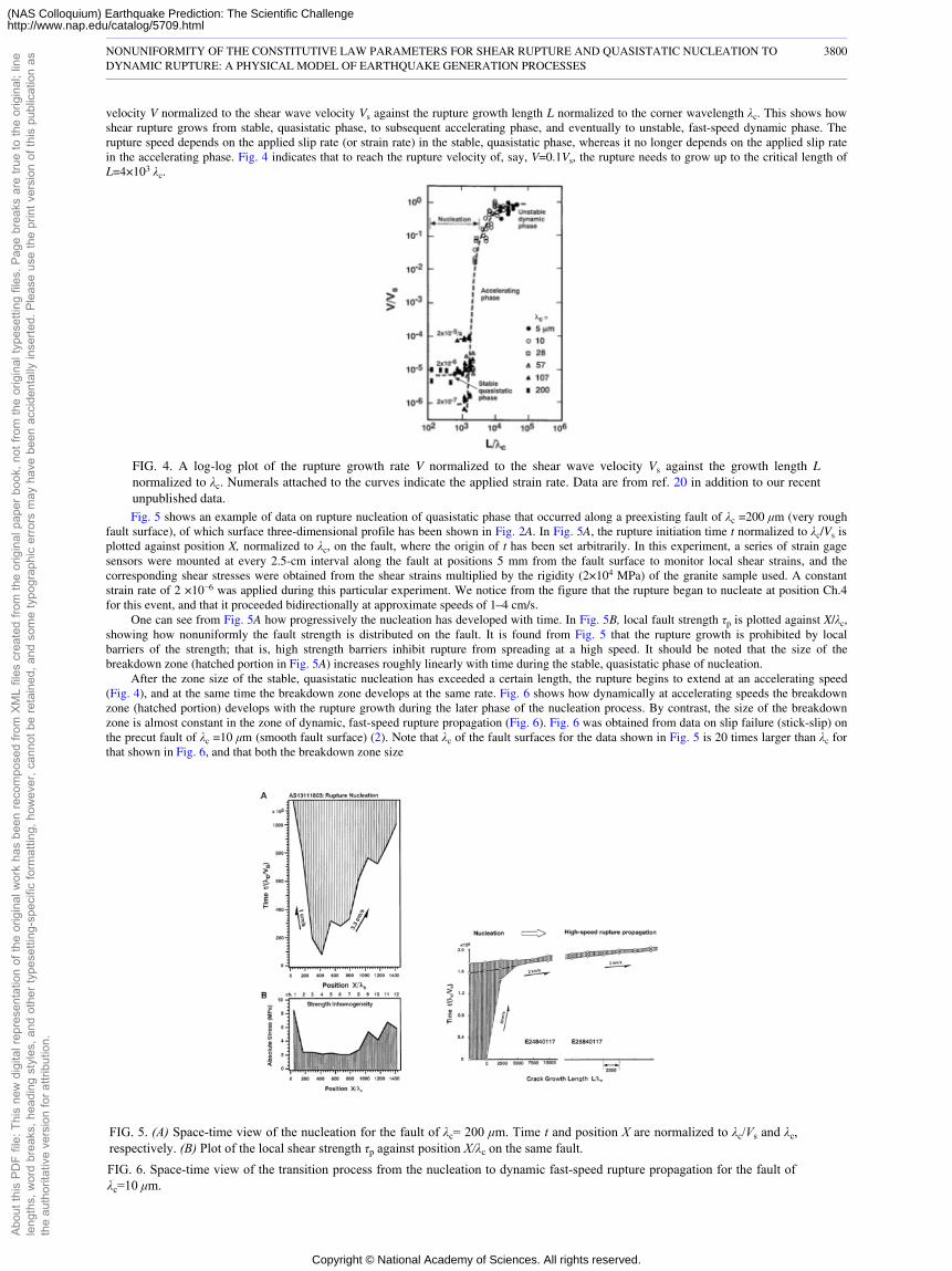
velocity V normalized to the shear wave velocity Vs against the rupture growth length L normalized to the corner wavelength λc. This shows howshear rupture grows from stable, quasistatic phase, to subsequent accelerating phase, and eventually to unstable, fast-speed dynamic phase. Therupture speed depends on the applied slip rate (or strain rate) in the stable, quasistatic phase, whereas it no longer depends on the applied slip ratein the accelerating phase. Fig. 4 indicates that to reach the rupture velocity of, say, V=0.1Vs, the rupture needs to grow up to the critical length ofL=4×10³ λc.
FIG. 4. A log-log plot of the rupture growth rate V normalized to the shear wave velocity Vs against the growth length Lnormalized to λc. Numerals attached to the curves indicate the applied strain rate. Data are from ref. 20 in addition to our recentunpublished data.Fig. 5 shows an example of data on rupture nucleation of quasistatic phase that occurred along a preexisting fault of λc =200 µm (very rough
fault surface), of which surface three-dimensional profile has been shown in Fig. 2A. In Fig. 5A, the rupture initiation time t normalized to λc/Vs isplotted against position X, normalized to λc, on the fault, where the origin of t has been set arbitrarily. In this experiment, a series of strain gagesensors were mounted at every 2.5-cm interval along the fault at positions 5 mm from the fault surface to monitor local shear strains, and thecorresponding shear stresses were obtained from the shear strains multiplied by the rigidity (2×10⁴ MPa) of the granite sample used. A constantstrain rate of 2 ×10⁻⁶ was applied during this particular experiment. We notice from the figure that the rupture began to nucleate at position Ch.4for this event, and that it proceeded bidirectionally at approximate speeds of 1–4 cm/s.
One can see from Fig. 5A how progressively the nucleation has developed with time. In Fig. 5B, local fault strength τp is plotted against X/λc,showing how nonuniformly the fault strength is distributed on the fault. It is found from Fig. 5 that the rupture growth is prohibited by localbarriers of the strength; that is, high strength barriers inhibit rupture from spreading at a high speed. It should be noted that the size of thebreakdown zone (hatched portion in Fig. 5A) increases roughly linearly with time during the stable, quasistatic phase of nucleation.
After the zone size of the stable, quasistatic nucleation has exceeded a certain length, the rupture begins to extend at an accelerating speed(Fig. 4), and at the same time the breakdown zone develops at the same rate. Fig. 6 shows how dynamically at accelerating speeds the breakdownzone (hatched portion) develops with the rupture growth during the later phase of the nucleation process. By contrast, the size of the breakdownzone is almost constant in the zone of dynamic, fast-speed rupture propagation (Fig. 6). Fig. 6 was obtained from data on slip failure (stick-slip) onthe precut fault of λc =10 µm (smooth fault surface) (2). Note that λc of the fault surfaces for the data shown in Fig. 5 is 20 times larger than λc forthat shown in Fig. 6, and that both the breakdown zone size
NONUNIFORMITY OF THE CONSTITUTIVE LAW PARAMETERS FOR SHEAR RUPTURE AND QUASISTATIC NUCLEATION TODYNAMIC RUPTURE: A PHYSICAL MODEL OF EARTHQUAKE GENERATION PROCESSES
3800
Abou
t thi
s PD
F fil
e: T
his
new
dig
ital r
epre
sent
atio
n of
the
orig
inal
wor
k ha
s be
en re
com
pose
d fro
m X
ML
files
cre
ated
from
the
orig
inal
pap
er b
ook,
not
from
the
orig
inal
type
setti
ng fi
les.
Pag
e br
eaks
are
true
to th
e or
igin
al; l
ine
leng
ths,
wor
d br
eaks
, hea
ding
sty
les,
and
oth
er ty
pese
tting
-spe
cific
form
attin
g, h
owev
er, c
anno
t be
reta
ined
, and
som
e ty
pogr
aphi
c er
rors
may
hav
e be
en a
ccid
enta
lly in
serte
d. P
leas
e us
e th
e pr
int v
ersi
on o
f thi
s pu
blic
atio
n as
the
auth
orita
tive
vers
ion
for a
ttrib
utio
n.
FIG. 5. (A) Space-time view of the nucleation for the fault of λc= 200 µm. Time t and position X are normalized to λc/Vs and λc,respectively. (B) Plot of the local shear strength τp against position X/λc on the same fault.FIG. 6. Space-time view of the transition process from the nucleation to dynamic fast-speed rupture propagation for the fault ofλc=10 µm.
Copyright © National Academy of Sciences. All rights reserved.
(NAS Colloquium) Earthquake Prediction: The Scientific Challengehttp://www.nap.edu/catalog/5709.html
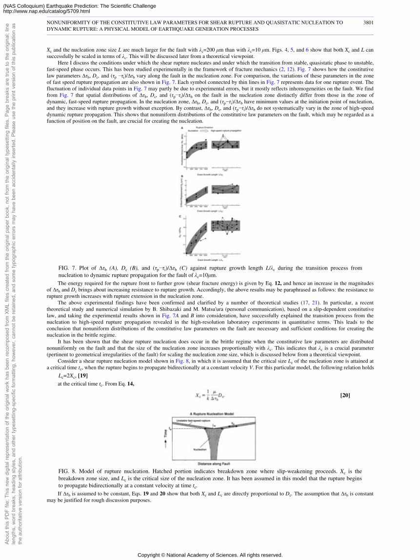
Xc and the nucleation zone size L are much larger for the fault with λc=200 µm than with λc=10 µm. Figs. 4, 5, and 6 show that both Xc and L cansuccessfully be scaled in terms of λc. This will be discussed later from a theoretical viewpoint.
Here I discuss the conditions under which the shear rupture nucleates and under which the transition from stable, quasistatic phase to unstable,fast-speed phase occurs. This has been studied experimentally in the framework of fracture mechanics (2, 12). Fig. 7 shows how the constitutivelaw parameters ∆τb, Dc, and (τp −τi)/∆τb vary along the fault in the nucleation zone. For comparison, the variations of these parameters in the zoneof fast speed rupture propagation are also shown in Fig. 7. Each symbol connected by thin lines in Fig. 7 represents data for one rupture event. Thefluctuation of individual data points in Fig. 7 may partly be due to experimental errors, but it mostly reflects inhomogeneities on the fault. We findfrom Fig. 7 that spatial distributions of ∆τb, Dc, and (τp−τi)/∆τb on the fault in the nucleation zone distinctly differ from those in the zone ofdynamic, fast-speed rupture propagation. In the nucleation zone, ∆τb, Dc, and (τp−τi)/∆τb have minimum values at the initiation point of nucleation,and they increase with rupture growth without exception. By contrast, ∆τb, Dc, and (τp−τi)/∆τb do not systematically vary in the zone of high-speeddynamic rupture propagation. This shows that nonuniform distributions of the constitutive law parameters on the fault, which may be regarded as afunction of position on the fault, are crucial for creating the nucleation.
FIG. 7. Plot of ∆τb (A), Dc (B), and (τp−τi)/∆τb (C) against rupture growth length L/λc during the transition process fromnucleation to dynamic rupture propagation for the fault of λc=10µm.The energy required for the rupture front to further grow (shear fracture energy) is given by Eq. 12, and hence an increase in the magnitudes
of ∆τb and Dc brings about increasing resistance to rupture growth. Accordingly, the above results may be paraphrased as follows: the resistance torupture growth increases with rupture extension in the nucleation zone.
The above experimental findings have been confirmed and clarified by a number of theoretical studies (17, 21). In particular, a recenttheoretical study and numerical simulation by B. Shibazaki and M. Matsu'ura (personal communication), based on a slip-dependent constitutivelaw, and taking the experimental results shown in Fig. 7A and B into consideration, have successfully explained the transition process from thenucleation to high-speed rupture propagation revealed in the high-resolution laboratory experiments in quantitative terms. This leads to theconclusion that nonuniform distributions of the constitutive law parameters on the fault are necessary and sufficient conditions for creating thenucleation in the brittle regime.
It has been shown that the shear rupture nucleation does occur in the brittle regime when the constitutive law parameters are distributednonuniformly on the fault and that the size of the nucleation zone increases proportionally with λc. This indicates that λc is a crucial parameter(pertinent to geometrical irregularities of the fault) for scaling the nucleation zone size, which is discussed below from a theoretical viewpoint.
Consider a shear rupture nucleation model shown in Fig. 8, in which it is assumed that the critical size Lc of the nucleation zone is attained ata critical time tc, when the rupture begins to propagate bidirectionally at a constant velocity V. For this particular model, the following relation holds
Lc=2Xc, [19]at the critical time tc. From Eq. 14,
[20]
FIG. 8. Model of rupture nucleation. Hatched portion indicates breakdown zone where slip-weakening proceeds. Xc is thebreakdown zone size, and Lc is the critical size of the nucleation zone. It has been assumed in this model that the rupture beginsto propagate bidirectionally at a constant velocity at time tc.If ∆τb is assumed to be constant, Eqs. 19 and 20 show that both Xc and Lc are directly proportional to Dc. The assumption that ∆τb is constant
may be justified for rough discussion purposes.
NONUNIFORMITY OF THE CONSTITUTIVE LAW PARAMETERS FOR SHEAR RUPTURE AND QUASISTATIC NUCLEATION TODYNAMIC RUPTURE: A PHYSICAL MODEL OF EARTHQUAKE GENERATION PROCESSES
3801
Abou
t thi
s PD
F fil
e: T
his
new
dig
ital r
epre
sent
atio
n of
the
orig
inal
wor
k ha
s be
en re
com
pose
d fro
m X
ML
files
cre
ated
from
the
orig
inal
pap
er b
ook,
not
from
the
orig
inal
type
setti
ng fi
les.
Pag
e br
eaks
are
true
to th
e or
igin
al; l
ine
leng
ths,
wor
d br
eaks
, hea
ding
sty
les,
and
oth
er ty
pese
tting
-spe
cific
form
attin
g, h
owev
er, c
anno
t be
reta
ined
, and
som
e ty
pogr
aphi
c er
rors
may
hav
e be
en a
ccid
enta
lly in
serte
d. P
leas
e us
e th
e pr
int v
ersi
on o
f thi
s pu
blic
atio
n as
the
auth
orita
tive
vers
ion
for a
ttrib
utio
n.
Copyright © National Academy of Sciences. All rights reserved.
(NAS Colloquium) Earthquake Prediction: The Scientific Challengehttp://www.nap.edu/catalog/5709.html
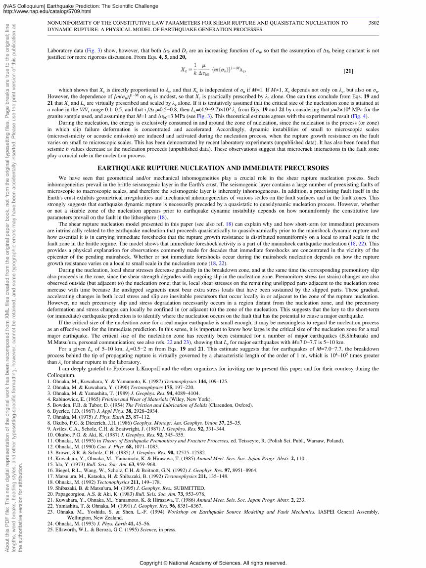
Laboratory data (Fig. 3) show, however, that both ∆τb and Dc are an increasing function of σn, so that the assumption of ∆τb being constant is notjustified for more rigorous discussion. From Eqs. 4, 5, and 20,
[21]
which shows that Xc is directly proportional to λc, and that Xc is independent of σn if M=1. If M�1, Xc depends not only on λc, but also on σn.However, the dependence of {m(σn)}1−M on σn is modest, so that Xc is practically prescribed by λc alone. One can thus conclude from Eqs. 19 and21 that Xc and Lc are virtually prescribed and scaled by λc alone. If it is tentatively assumed that the critical size of the nucleation zone is attained ata value in the V/Vs range 0.1–0.5, and that τi/∆τb=0.5−0.8, then Lc=(4.9−9.7)×103 λc from Eqs. 19 and 21 by considering that µ=2×10⁴ MPa for thegranite sample used, and assuming that M=1 and ∆τb0=3 MPa (see Fig. 3). This theoretical estimate agrees with the experimental result (Fig. 4).
During the nucleation, the energy is exclusively consumed in and around the zone of nucleation, since the nucleation is the process (or zone)in which slip failure deformation is concentrated and accelerated. Accordingly, dynamic instabilities of small to microscopic scales(microseismicity or acoustic emission) are induced and activated during the nucleation process, when the rupture growth resistance on the faultvaries on small to microscopic scales. This has been demonstrated by recent laboratory experiments (unpublished data). It has also been found thatseismic b values decrease as the nucleation proceeds (unpublished data). These observations suggest that microcrack interactions in the fault zoneplay a crucial role in the nucleation process.
EARTHQUAKE RUPTURE NUCLEATION AND IMMEDIATE PRECURSORS
We have seen that geometrical and/or mechanical inhomogeneities play a crucial role in the shear rupture nucleation process. Suchinhomogeneities prevail in the brittle seismogenic layer in the Earth's crust. The seismogenic layer contains a large number of preexisting faults ofmicroscopic to macroscopic scales, and therefore the seismogenic layer is inherently inhomogeneous. In addition, a preexisting fault itself in theEarth's crust exhibits geometrical irregularities and mechanical inhomogeneities of various scales on the fault surfaces and in the fault zones. Thisstrongly suggests that earthquake dynamic rupture is necessarily preceded by a quasistatic to quasidynamic nucleation process. However, whetheror not a sizable zone of the nucleation appears prior to earthquake dynamic instability depends on how nonuniformly the constitutive lawparameters prevail on the fault in the lithosphere (18).
The shear rupture nucleation model presented in this paper (see also ref. 18) can explain why and how short-term (or immediate) precursorsare intrinsically related to the earthquake nucleation that proceeds quasistatically to quasidynamically prior to the mainshock dynamic rupture andhow essential it is in carrying immediate foreshocks that the rupture growth resistance is distributed nonuniformly on a local to small scale in thefault zone in the brittle regime. The model shows that immediate foreshock activity is a part of the mainshock earthquake nucleation (18, 22). Thisprovides a physical explanation for observations commonly made for decades that immediate foreshocks are concentrated in the vicinity of theepicenter of the pending mainshock. Whether or not immediate foreshocks occur during the mainshock nucleation depends on how the rupturegrowth resistance varies on a local to small scale in the nucleation zone (18, 22).
During the nucleation, local shear stresses decrease gradually in the breakdown zone, and at the same time the corresponding premonitory slipalso proceeds in the zone, since the shear strength degrades with ongoing slip in the nucleation zone. Premonitory stress (or strain) changes are alsoobserved outside (but adjacent to) the nucleation zone; that is, local shear stresses on the remaining unslipped parts adjacent to the nucleation zoneincrease with time because the unslipped segments must bear extra stress loads that have been sustained by the slipped parts. These gradual,accelerating changes in both local stress and slip are inevitable precursors that occur locally in or adjacent to the zone of the rupture nucleation.However, no such precursory slip and stress degradation necessarily occurs in a region distant from the nucleation zone, and the precursorydeformation and stress changes can locally be confined in (or adjacent to) the zone of the nucleation. This suggests that the key to the short-term(or immediate) earthquake prediction is to identify where the nucleation occurs on the fault that has the potential to cause a major earthquake.
If the critical size of the nucleation zone for a real major earthquake is small enough, it may be meaningless to regard the nucleation processas an effective tool for the immediate prediction. In this sense, it is important to know how large is the critical size of the nucleation zone for a realmajor earthquake. The critical size of the nucleation zone has recently been estimated for a number of major earthquakes (B.Shibazaki andM.Matsu'ura, personal communication; see also refs. 22 and 23), showing that Lc for major earthquakes with M=7.0−7.7 is 5−10 km.
For a given Lc of 5–10 km, λc=0.5−2 m from Eqs. 19 and 21. This estimate suggests that for earthquakes of M=7.0−7.7, the breakdownprocess behind the tip of propagating rupture is virtually governed by a characteristic length of the order of 1 m, which is 104–105 times greaterthan λc for shear rupture in the laboratory.
I am deeply grateful to Professor L.Knopoff and the other organizers for inviting me to present this paper and for their courtesy during theColloquium.1. Ohnaka, M., Kuwahara, Y. & Yamamoto, K. (1987) Tectonophysics 144, 109–125.2. Ohnaka, M. & Kuwahara, Y. (1990) Tectonophysics 175, 197–220.3. Ohnaka, M. & Yamashita, T. (1989) J. Geophys. Res. 94, 4089–4104.4. Rabinowicz, E. (1965) Friction and Wear of Materials (Wiley, New York).5. Bowden, F.B. & Tabor, D. (1954) The Friction and Lubrication of Solids (Clarendon, Oxford).6. Byerlee, J.D. (1967) J. Appl Phys. 38, 2928–2934.7. Ohnaka, M. (1975) J. Phys. Earth 23, 87–112.8. Okubo, P.G. & Dieterich, J.H. (1986) Geophys. Monogr. Am. Geophys. Union 37, 25–35.9. Aviles, C.A., Scholz, C.H. & Boatwright, J. (1987) J. Geophys. Res. 92, 331–344.10. Okubo, P.G. & Aki, K. (1987) J. Geophys. Res. 92, 345–355.11. Ohnaka, M. (1995) in Theory of Earthquake Premonitory and Fracture Processes, ed. Teisseyre, R. (Polish Sci. Publ., Warsaw, Poland).12. Ohnaka, M. (1990) Can. J. Phys. 68, 1071–1083.13. Brown, S.R. & Scholz, C.H. (1985) J. Geophys. Res. 90, 12575–12582.14. Kuwahara, Y., Ohnaka, M., Yamamoto, K. & Hirasawa, T. (1985) Annual Meet. Seis. Soc. Japan Progr. Abstr. 2, 110.15. Ida, Y. (1973) Bull. Seis. Soc. Am. 63, 959–968.16. Biegel, R.L., Wang, W., Scholz, C.H. & Boitnott, G.N. (1992) J. Geophys. Res. 97, 8951–8964.17. Matsu'ura, M., Kataoka, H. & Shibazaki, B. (1992) Tectonophysics 211, 135–148.18. Ohnaka, M. (1992) Tectonophysics 211, 149–178.19. Shibazaki, B. & Matsu'ura, M. (1995) J. Geophys. Res., SUBMITTED.20. Papageorgiou, A.S. & Aki, K. (1983) Bull. Seis. Soc. Am. 73, 953–978.21. Kuwahara, Y., Ohnaka, M., Yamamoto, K. & Hirasawa, T. (1986) Annual Meet. Seis. Soc. Japan Progr. Abstr. 2, 233.22. Yamashita, T. & Ohnaka, M. (1991) J. Geophys. Res. 96, 8351–8367.23. Ohnaka, M., Yoshida, S. & Shen, L.-F. (1994) Workshop on Earthquake Source Modeling and Fault Mechanics, IASPEI General Assembly,
Wellington, New Zealand.24. Ohnaka, M. (1993) J. Phys. Earth 41, 45–56.25. Ellsworth, W.L. & Beroza, G.C. (1995) Science, in press.
NONUNIFORMITY OF THE CONSTITUTIVE LAW PARAMETERS FOR SHEAR RUPTURE AND QUASISTATIC NUCLEATION TODYNAMIC RUPTURE: A PHYSICAL MODEL OF EARTHQUAKE GENERATION PROCESSES
3802
Abou
t thi
s PD
F fil
e: T
his
new
dig
ital r
epre
sent
atio
n of
the
orig
inal
wor
k ha
s be
en re
com
pose
d fro
m X
ML
files
cre
ated
from
the
orig
inal
pap
er b
ook,
not
from
the
orig
inal
type
setti
ng fi
les.
Pag
e br
eaks
are
true
to th
e or
igin
al; l
ine
leng
ths,
wor
d br
eaks
, hea
ding
sty
les,
and
oth
er ty
pese
tting
-spe
cific
form
attin
g, h
owev
er, c
anno
t be
reta
ined
, and
som
e ty
pogr
aphi
c er
rors
may
hav
e be
en a
ccid
enta
lly in
serte
d. P
leas
e us
e th
e pr
int v
ersi
on o
f thi
s pu
blic
atio
n as
the
auth
orita
tive
vers
ion
for a
ttrib
utio
n.
Copyright © National Academy of Sciences. All rights reserved.
(NAS Colloquium) Earthquake Prediction: The Scientific Challengehttp://www.nap.edu/catalog/5709.html
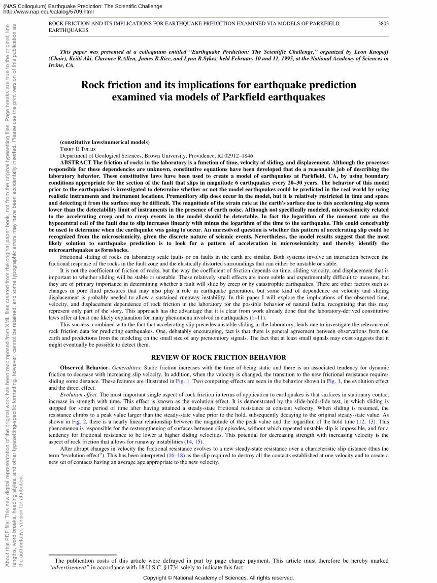
This paper was presented at a colloquium entitled “Earthquake Prediction: The Scientific Challenge,” organized by Leon Knopoff(Chair), Keiiti Aki, Clarence R.Allen, James R.Rice, and Lynn R.Sykes, held February 10 and 11, 1995, at the National Academy of Sciences inIrvine, CA.
Rock friction and its implications for earthquake predictionexamined via models of Parkfield earthquakes
(constitutive laws/numerical models)TERRY E.TULLIS
Department of Geological Sciences, Brown University, Providence, RI 02912–1846ABSTRACT The friction of rocks in the laboratory is a function of time, velocity of sliding, and displacement. Although the processes
responsible for these dependencies are unknown, constitutive equations have been developed that do a reasonable job of describing thelaboratory behavior. These constitutive laws have been used to create a model of earthquakes at Parkfield, CA, by using boundaryconditions appropriate for the section of the fault that slips in magnitude 6 earthquakes every 20–30 years. The behavior of this modelprior to the earthquakes is investigated to determine whether or not the model earthquakes could be predicted in the real world by usingrealistic instruments and instrument locations. Premonitory slip does occur in the model, but it is relatively restricted in time and spaceand detecting it from the surface may be difficult. The magnitude of the strain rate at the earth's surface due to this accelerating slip seemslower than the detectability limit of instruments in the presence of earth noise. Although not specifically modeled, microseismicity relatedto the accelerating creep and to creep events in the model should be detectable. In fact the logarithm of the moment rate on thehypocentral cell of the fault due to slip increases linearly with minus the logarithm of the time to the earthquake. This could conceivablybe used to determine when the earthquake was going to occur. An unresolved question is whether this pattern of accelerating slip could berecognized from the microseismicity, given the discrete nature of seismic events. Nevertheless, the model results suggest that the mostlikely solution to earthquake prediction is to look for a pattern of acceleration in microseismicity and thereby identify themicroearthquakes as foreshocks.
Frictional sliding of rocks on laboratory scale faults or on faults in the earth are similar. Both systems involve an interaction between thefrictional response of the rocks in the fault zone and the elastically distorted surroundings that can either be unstable or stable.
It is not the coefficient of friction of rocks, but the way the coefficient of friction depends on time, sliding velocity, and displacement that isimportant to whether sliding will be stable or unstable. These relatively small effects are more subtle and experimentally difficult to measure, butthey are of primary importance in determining whether a fault will slide by creep or by catastrophic earthquakes. There are other factors such aschanges in pore fluid pressures that may also play a role in earthquake generation, but some kind of dependence on velocity and slidingdisplacement is probably needed to allow a sustained runaway instability. In this paper I will explore the implications of the observed time,velocity, and displacement dependence of rock friction in the laboratory for the possible behavior of natural faults, recognizing that this mayrepresent only part of the story. This approach has the advantage that it is clear from work already done that the laboratory-derived constitutivelaws offer at least one likely explanation for many phenomena involved in earthquakes (1–11).
This success, combined with the fact that accelerating slip precedes unstable sliding in the laboratory, leads one to investigate the relevance ofrock friction data for predicting earthquakes. One, debatably encouraging, fact is that there is general agreement between observations from theearth and predictions from the modeling on the small size of any premonitory signals. The fact that at least small signals may exist suggests that itmight eventually be possible to detect them.
REVIEW OF ROCK FRICTION BEHAVIOR
Observed Behavior. Generalities. Static friction increases with the time of being static and there is an associated tendency for dynamicfriction to decrease with increasing slip velocity. In addition, when the velocity is changed, the transition to the new frictional resistance requiressliding some distance. These features are illustrated in Fig. 1. Two competing effects are seen in the behavior shown in Fig. 1, the evolution effectand the direct effect.
Evolution effect. The most important single aspect of rock friction in terms of application to earthquakes is that surfaces in stationary contactincrease in strength with time. This effect is known as the evolution effect. It is demonstrated by the slide-hold-slide test, in which sliding isstopped for some period of time after having attained a steady-state frictional resistance at constant velocity. When sliding is resumed, theresistance climbs to a peak value larger than the steady-state value prior to the hold, subsequently decaying to the original steady-state value. Asshown in Fig. 2, there is a nearly linear relationship between the magnitude of the peak value and the logarithm of the hold time (12, 13). Thisphenomenon is responsible for the restrengthening of surfaces between slip episodes, without which repeated unstable slip is impossible, and for atendency for frictional resistance to be lower at higher sliding velocities. This potential for decreasing strength with increasing velocity is theaspect of rock friction that allows for runaway instabilities (14, 15).
After abrupt changes in velocity the frictional resistance evolves to a new steady-state resistance over a characteristic slip distance (thus theterm “evolution effect”). This has been interpreted (16–18) as the slip required to destroy all the contacts established at one velocity and to create anew set of contacts having an average age appropriate to the new velocity.
The publication costs of this article were defrayed in part by page charge payment. This article must therefore be hereby marked“advertisement” in accordance with 18 U.S.C. §1734 solely to indicate this fact.
ROCK FRICTION AND ITS IMPLICATIONS FOR EARTHQUAKE PREDICTION EXAMINED VIA MODELS OF PARKFIELDEARTHQUAKES
3803
Abou
t thi
s PD
F fil
e: T
his
new
dig
ital r
epre
sent
atio
n of
the
orig
inal
wor
k ha
s be
en re
com
pose
d fro
m X
ML
files
cre
ated
from
the
orig
inal
pap
er b
ook,
not
from
the
orig
inal
type
setti
ng fi
les.
Pag
e br
eaks
are
true
to th
e or
igin
al; l
ine
leng
ths,
wor
d br
eaks
, hea
ding
sty
les,
and
oth
er ty
pese
tting
-spe
cific
form
attin
g, h
owev
er, c
anno
t be
reta
ined
, and
som
e ty
pogr
aphi
c er
rors
may
hav
e be
en a
ccid
enta
lly in
serte
d. P
leas
e us
e th
e pr
int v
ersi
on o
f thi
s pu
blic
atio
n as
the
auth
orita
tive
vers
ion
for a
ttrib
utio
n.
Copyright © National Academy of Sciences. All rights reserved.
(NAS Colloquium) Earthquake Prediction: The Scientific Challengehttp://www.nap.edu/catalog/5709.html
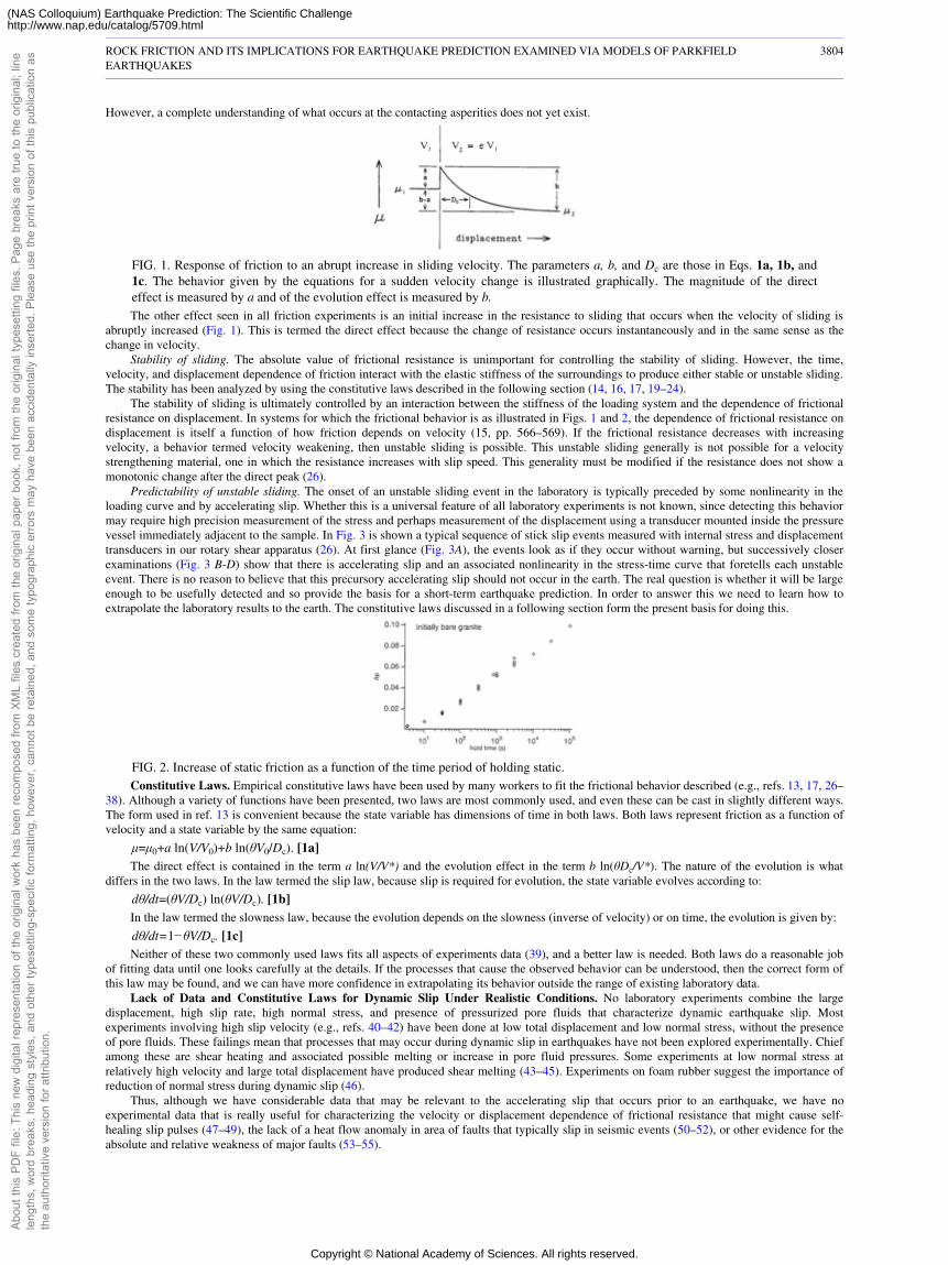
However, a complete understanding of what occurs at the contacting asperities does not yet exist.
FIG. 1. Response of friction to an abrupt increase in sliding velocity. The parameters a, b, and Dc are those in Eqs. 1a, 1b, and1c. The behavior given by the equations for a sudden velocity change is illustrated graphically. The magnitude of the directeffect is measured by a and of the evolution effect is measured by b.
The other effect seen in all friction experiments is an initial increase in the resistance to sliding that occurs when the velocity of sliding isabruptly increased (Fig. 1). This is termed the direct effect because the change of resistance occurs instantaneously and in the same sense as thechange in velocity.
Stability of sliding. The absolute value of frictional resistance is unimportant for controlling the stability of sliding. However, the time,velocity, and displacement dependence of friction interact with the elastic stiffness of the surroundings to produce either stable or unstable sliding.The stability has been analyzed by using the constitutive laws described in the following section (14, 16, 17, 19–24).
The stability of sliding is ultimately controlled by an interaction between the stiffness of the loading system and the dependence of frictionalresistance on displacement. In systems for which the frictional behavior is as illustrated in Figs. 1 and 2, the dependence of frictional resistance ondisplacement is itself a function of how friction depends on velocity (15, pp. 566–569). If the frictional resistance decreases with increasingvelocity, a behavior termed velocity weakening, then unstable sliding is possible. This unstable sliding generally is not possible for a velocitystrengthening material, one in which the resistance increases with slip speed. This generality must be modified if the resistance does not show amonotonic change after the direct peak (26).
Predictability of unstable sliding. The onset of an unstable sliding event in the laboratory is typically preceded by some nonlinearity in theloading curve and by accelerating slip. Whether this is a universal feature of all laboratory experiments is not known, since detecting this behaviormay require high precision measurement of the stress and perhaps measurement of the displacement using a transducer mounted inside the pressurevessel immediately adjacent to the sample. In Fig. 3 is shown a typical sequence of stick slip events measured with internal stress and displacementtransducers in our rotary shear apparatus (26). At first glance (Fig. 3A), the events look as if they occur without warning, but successively closerexaminations (Fig. 3 B-D) show that there is accelerating slip and an associated nonlinearity in the stress-time curve that foretells each unstableevent. There is no reason to believe that this precursory accelerating slip should not occur in the earth. The real question is whether it will be largeenough to be usefully detected and so provide the basis for a short-term earthquake prediction. In order to answer this we need to learn how toextrapolate the laboratory results to the earth. The constitutive laws discussed in a following section form the present basis for doing this.
FIG. 2. Increase of static friction as a function of the time period of holding static.Constitutive Laws. Empirical constitutive laws have been used by many workers to fit the frictional behavior described (e.g., refs. 13, 17, 26–
38). Although a variety of functions have been presented, two laws are most commonly used, and even these can be cast in slightly different ways.The form used in ref. 13 is convenient because the state variable has dimensions of time in both laws. Both laws represent friction as a function ofvelocity and a state variable by the same equation:
µ=µ0+a ln(V/V0)+b ln(θV0/Dc). [1a]The direct effect is contained in the term a ln(V/V*) and the evolution effect in the term b ln(θDc/V*). The nature of the evolution is what
differs in the two laws. In the law termed the slip law, because slip is required for evolution, the state variable evolves according to:
dθ/dt=(θV/Dc) ln(θV/Dc). [1b]In the law termed the slowness law, because the evolution depends on the slowness (inverse of velocity) or on time, the evolution is given by:
dθ/dt=1−θV/Dc. [1c]Neither of these two commonly used laws fits all aspects of experiments data (39), and a better law is needed. Both laws do a reasonable job
of fitting data until one looks carefully at the details. If the processes that cause the observed behavior can be understood, then the correct form ofthis law may be found, and we can have more confidence in extrapolating its behavior outside the range of existing laboratory data.
Lack of Data and Constitutive Laws for Dynamic Slip Under Realistic Conditions. No laboratory experiments combine the largedisplacement, high slip rate, high normal stress, and presence of pressurized pore fluids that characterize dynamic earthquake slip. Mostexperiments involving high slip velocity (e.g., refs. 40–42) have been done at low total displacement and low normal stress, without the presenceof pore fluids. These failings mean that processes that may occur during dynamic slip in earthquakes have not been explored experimentally. Chiefamong these are shear heating and associated possible melting or increase in pore fluid pressures. Some experiments at low normal stress atrelatively high velocity and large total displacement have produced shear melting (43–45). Experiments on foam rubber suggest the importance ofreduction of normal stress during dynamic slip (46).
Thus, although we have considerable data that may be relevant to the accelerating slip that occurs prior to an earthquake, we have noexperimental data that is really useful for characterizing the velocity or displacement dependence of frictional resistance that might cause self-healing slip pulses (47–49), the lack of a heat flow anomaly in area of faults that typically slip in seismic events (50–52), or other evidence for theabsolute and relative weakness of major faults (53–55).
ROCK FRICTION AND ITS IMPLICATIONS FOR EARTHQUAKE PREDICTION EXAMINED VIA MODELS OF PARKFIELDEARTHQUAKES
3804
Abou
t thi
s PD
F fil
e: T
his
new
dig
ital r
epre
sent
atio
n of
the
orig
inal
wor
k ha
s be
en re
com
pose
d fro
m X
ML
files
cre
ated
from
the
orig
inal
pap
er b
ook,
not
from
the
orig
inal
type
setti
ng fi
les.
Pag
e br
eaks
are
true
to th
e or
igin
al; l
ine
leng
ths,
wor
d br
eaks
, hea
ding
sty
les,
and
oth
er ty
pese
tting
-spe
cific
form
attin
g, h
owev
er, c
anno
t be
reta
ined
, and
som
e ty
pogr
aphi
c er
rors
may
hav
e be
en a
ccid
enta
lly in
serte
d. P
leas
e us
e th
e pr
int v
ersi
on o
f thi
s pu
blic
atio
n as
the
auth
orita
tive
vers
ion
for a
ttrib
utio
n.
Copyright © National Academy of Sciences. All rights reserved.
(NAS Colloquium) Earthquake Prediction: The Scientific Challengehttp://www.nap.edu/catalog/5709.html
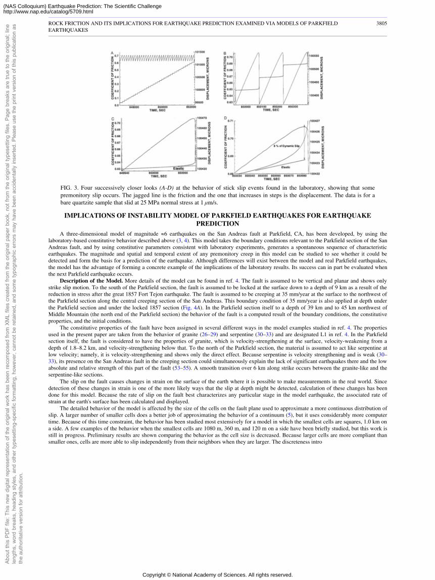
FIG. 3. Four successively closer looks (A-D) at the behavior of stick slip events found in the laboratory, showing that somepremonitory slip occurs. The jagged line is the friction and the one that increases in steps is the displacement. The data is for abare quartzite sample that slid at 25 MPa normal stress at 1 µm/s.
IMPLICATIONS OF INSTABILITY MODEL OF PARKFIELD EARTHQUAKES FOR EARTHQUAKEPREDICTION
A three-dimensional model of magnitude �6 earthquakes on the San Andreas fault at Parkfield, CA, has been developed, by using thelaboratory-based constitutive behavior described above (3, 4). This model takes the boundary conditions relevant to the Parkfield section of the SanAndreas fault, and by using constitutive parameters consistent with laboratory experiments, generates a spontaneous sequence of characteristicearthquakes. The magnitude and spatial and temporal extent of any premonitory creep in this model can be studied to see whether it could bedetected and form the basis for a prediction of the earthquake. Although differences will exist between the model and real Parkfield earthquakes,the model has the advantage of forming a concrete example of the implications of the laboratory results. Its success can in part be evaluated whenthe next Parkfield earthquake occurs.
Description of the Model. More details of the model can be found in ref. 4. The fault is assumed to be vertical and planar and shows onlystrike slip motion. To the south of the Parkfield section, the fault is assumed to be locked at the surface down to a depth of 9 km as a result of thereduction in stress after the great 1857 Fort Tejon earthquake. The fault is assumed to be creeping at 35 mm/year at the surface to the northwest ofthe Parkfield section along the central creeping section of the San Andreas. This boundary condition of 35 mm/year is also applied at depth underthe Parkfield section and under the locked 1857 section (Fig. 4A). In the Parkfield section itself to a depth of 39 km and to 45 km northwest ofMiddle Mountain (the north end of the Parkfield section) the behavior of the fault is a computed result of the boundary conditions, the constitutiveproperties, and the initial conditions.
The constitutive properties of the fault have been assigned in several different ways in the model examples studied in ref. 4. The propertiesused in the present paper are taken from the behavior of granite (26–29) and serpentine (30–33) and are designated L1 in ref. 4. In the Parkfieldsection itself, the fault is considered to have the properties of granite, which is velocity-strengthening at the surface, velocity-weakening from adepth of 1.8–8.2 km, and velocity-strengthening below that. To the north of the Parkfield section, the material is assumed to act like serpentine atlow velocity; namely, it is velocity-strengthening and shows only the direct effect. Because serpentine is velocity strengthening and is weak (30–33), its presence on the San Andreas fault in the creeping section could simultaneously explain the lack of significant earthquakes there and the lowabsolute and relative strength of this part of the fault (53–55). A smooth transition over 6 km along strike occurs between the granite-like and theserpentine-like sections.
The slip on the fault causes changes in strain on the surface of the earth where it is possible to make measurements in the real world. Sincedetection of these changes in strain is one of the more likely ways that the slip at depth might be detected, calculation of these changes has beendone for this model. Because the rate of slip on the fault best characterizes any particular stage in the model earthquake, the associated rate ofstrain at the earth's surface has been calculated and displayed.
The detailed behavior of the model is affected by the size of the cells on the fault plane used to approximate a more continuous distribution ofslip. A larger number of smaller cells does a better job of approximating the behavior of a continuum (5), but it uses considerably more computertime. Because of this time constraint, the behavior has been studied most extensively for a model in which the smallest cells are squares, 1.0 km ona side. A few examples of the behavior when the smallest cells are 1080 m, 360 m, and 120 m on a side have been briefly studied, but this work isstill in progress. Preliminary results are shown comparing the behavior as the cell size is decreased. Because larger cells are more compliant thansmaller ones, cells are more able to slip independently from their neighbors when they are larger. The discreteness intro
ROCK FRICTION AND ITS IMPLICATIONS FOR EARTHQUAKE PREDICTION EXAMINED VIA MODELS OF PARKFIELDEARTHQUAKES
3805
Abou
t thi
s PD
F fil
e: T
his
new
dig
ital r
epre
sent
atio
n of
the
orig
inal
wor
k ha
s be
en re
com
pose
d fro
m X
ML
files
cre
ated
from
the
orig
inal
pap
er b
ook,
not
from
the
orig
inal
type
setti
ng fi
les.
Pag
e br
eaks
are
true
to th
e or
igin
al; l
ine
leng
ths,
wor
d br
eaks
, hea
ding
sty
les,
and
oth
er ty
pese
tting
-spe
cific
form
attin
g, h
owev
er, c
anno
t be
reta
ined
, and
som
e ty
pogr
aphi
c er
rors
may
hav
e be
en a
ccid
enta
lly in
serte
d. P
leas
e us
e th
e pr
int v
ersi
on o
f thi
s pu
blic
atio
n as
the
auth
orita
tive
vers
ion
for a
ttrib
utio
n.
Copyright © National Academy of Sciences. All rights reserved.
(NAS Colloquium) Earthquake Prediction: The Scientific Challengehttp://www.nap.edu/catalog/5709.html
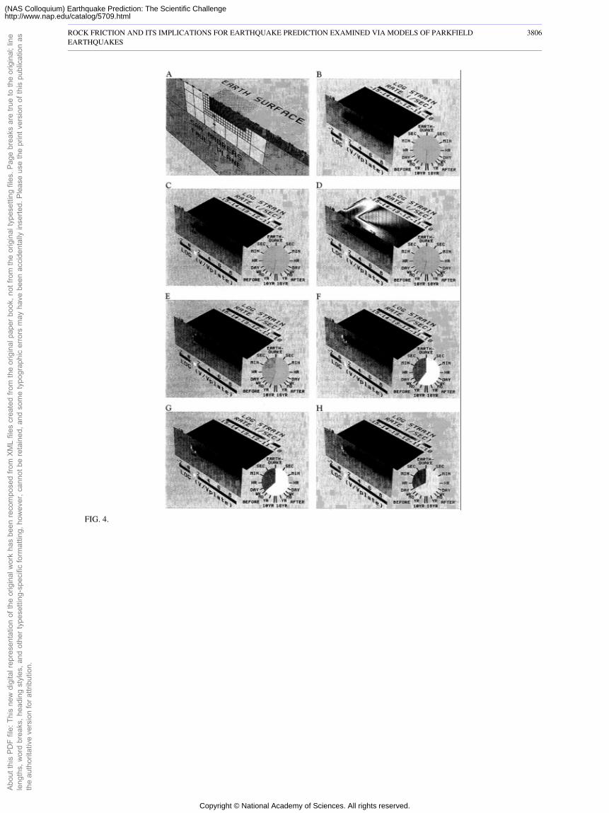
FIG. 4.
ROCK FRICTION AND ITS IMPLICATIONS FOR EARTHQUAKE PREDICTION EXAMINED VIA MODELS OF PARKFIELDEARTHQUAKES
3806
Abou
t thi
s PD
F fil
e: T
his
new
dig
ital r
epre
sent
atio
n of
the
orig
inal
wor
k ha
s be
en re
com
pose
d fro
m X
ML
files
cre
ated
from
the
orig
inal
pap
er b
ook,
not
from
the
orig
inal
type
setti
ng fi
les.
Pag
e br
eaks
are
true
to th
e or
igin
al; l
ine
leng
ths,
wor
d br
eaks
, hea
ding
sty
les,
and
oth
er ty
pese
tting
-spe
cific
form
attin
g, h
owev
er, c
anno
t be
reta
ined
, and
som
e ty
pogr
aphi
c er
rors
may
hav
e be
en a
ccid
enta
lly in
serte
d. P
leas
e us
e th
e pr
int v
ersi
on o
f thi
s pu
blic
atio
n as
the
auth
orita
tive
vers
ion
for a
ttrib
utio
n.
Copyright © National Academy of Sciences. All rights reserved.
(NAS Colloquium) Earthquake Prediction: The Scientific Challengehttp://www.nap.edu/catalog/5709.html
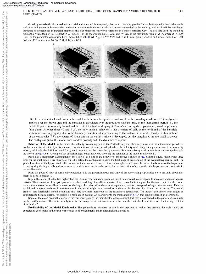
duced by oversized cells introduces a spatial and temporal heterogeneity that in a crude way proxies for the heterogeneity that variations inrock type and geometric irregularities on the fault may cause in the real world. As models are studied with smaller grid sizes, it will be possible tointroduce heterogeneities in material properties that can represent real world variations in a more controlled way. The cell size used (5) should besubstantially less than h*=2GDc/[π(B−A)m], where G is the shear modulus (30 GPa) and (B−A)m is the maximum value of B−A, where B−A=σn(b−a). For the parameter values used here [model L1 of ref. 4], (B−A)m is 0.575 MPa and Dc is 13 mm, giving h*=431 m. Our cell sizes h of 1080,360, and 120 m represent h/h* of 2.51, 0.84, and 0.28.
FIG. 4. Behavior at selected times in the model with the smallest grid size h=1 km. In A the boundary condition of 35 mm/year isapplied over the brown area and the behavior is calculated over the grey area with the grid. In the interseismic period (B), theParkfield patch is essentially locked and the rest of the fault is slipping at 35 mm/year. A rapid creep event (D) would represent afalse alarm. At other times (C and E-H), the only unusual behavior is that a variety of cells at the north end of the Parkfieldsection are creeping rapidly, due to the boundary condition of slip extending to the surface in the north. Finally, within an hourof the earthquake (I-K), the pattern of strain rate on the earth's surface is developed, but the magnitudes are too small to detect.The earthquake (L) in this model does not deal properly with the dynamics of rupture.Behavior of the Model. In the model the velocity weakening part of the Parkfield segment slips very slowly in the interseismic period. Its
northwest end is eaten into by episodic creep events until one of them, at a depth where the velocity weakening is the greatest, accelerates to a slipvelocity of 1 m/s, the definition used for dynamic rupture, and becomes the hypocenter. Representative typical images from an earthquake cycleare shown in Fig. 4 B-L. A complete set of such images exists in a video showing the behavior of the model in more detail.
Results of a preliminary examination of the effect of cell size on the behavior of the model is shown in Fig. 5. In this figure, models with threesizes for the smallest cells are shown, all for 0.1 s before the earthquake to show the final stage of acceleration of the eventual hypocentral cell. Thegeneral location of the hypocentral cell is similar in these models. However, this is a complex issue, since the model tends to move the hypocenterto nearby slightly larger cells and so successive models were run in each case to find a distribution of cells so that the hypocenter occurred withinthe smallest cells.
From the point of view of earthquake prediction, it is the pattern in space and time of the accelerating slip leading up to the main shock thatmight be used to predict it.
Slip in the model at velocities higher than the 35 mm/year boundary condition might be expected to correspond to increased microearthquakeactivity. The coarseness of the grid precludes explicit modeling of small earthquakes. It is reasonable to imagine that the more rapid the slip event,the more numerous the small earthquakes or the larger their size, since these more rapid creep events correspond to larger moment rates. Thus thespatial and temporal variation in moment rate in the model might be expected to be detected in the earth by changes in seismicity. The modelpredicts that foreshocks should occur and that they are more numerous as the mainshock approaches. The model also shows what might beconsidered to be false alarms, for example, a rapid creep event at 2.8 years prior to the mainshock (Fig. 4D) that can be regarded as a foreshock.
Some of the creep events that occur in the few years prior to the mainshock are large enough that they are reflected in the pattern of strain rateon the earth's surface. This is invariably true for the creep event that accelerates to become the mainshock, and it is true for the larger of the“foreshocks.”
Predictability of the Model Earthquake. The premonitory increases in slip in the hypocentral region that precede the main shock areexpected to correspond in the earth to increases in microseismicity and in foreshocks that could be
ROCK FRICTION AND ITS IMPLICATIONS FOR EARTHQUAKE PREDICTION EXAMINED VIA MODELS OF PARKFIELDEARTHQUAKES
3807
Abou
t thi
s PD
F fil
e: T
his
new
dig
ital r
epre
sent
atio
n of
the
orig
inal
wor
k ha
s be
en re
com
pose
d fro
m X
ML
files
cre
ated
from
the
orig
inal
pap
er b
ook,
not
from
the
orig
inal
type
setti
ng fi
les.
Pag
e br
eaks
are
true
to th
e or
igin
al; l
ine
leng
ths,
wor
d br
eaks
, hea
ding
sty
les,
and
oth
er ty
pese
tting
-spe
cific
form
attin
g, h
owev
er, c
anno
t be
reta
ined
, and
som
e ty
pogr
aphi
c er
rors
may
hav
e be
en a
ccid
enta
lly in
serte
d. P
leas
e us
e th
e pr
int v
ersi
on o
f thi
s pu
blic
atio
n as
the
auth
orita
tive
vers
ion
for a
ttrib
utio
n.
Copyright © National Academy of Sciences. All rights reserved.
(NAS Colloquium) Earthquake Prediction: The Scientific Challengehttp://www.nap.edu/catalog/5709.html
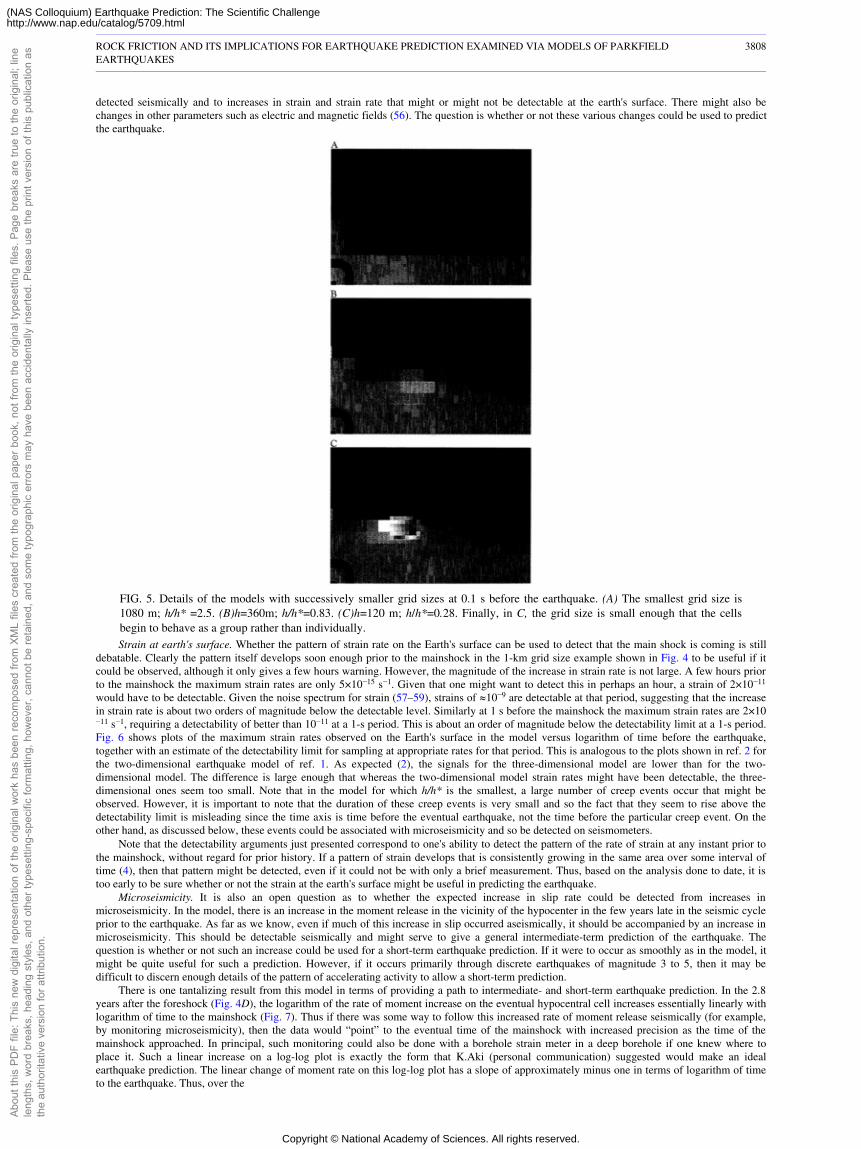
detected seismically and to increases in strain and strain rate that might or might not be detectable at the earth's surface. There might also bechanges in other parameters such as electric and magnetic fields (56). The question is whether or not these various changes could be used to predictthe earthquake.
FIG. 5. Details of the models with successively smaller grid sizes at 0.1 s before the earthquake. (A) The smallest grid size is1080 m; h/h* =2.5. (B)h=360m; h/h*=0.83. (C)h=120 m; h/h*=0.28. Finally, in C, the grid size is small enough that the cellsbegin to behave as a group rather than individually.Strain at earth's surface. Whether the pattern of strain rate on the Earth's surface can be used to detect that the main shock is coming is still
debatable. Clearly the pattern itself develops soon enough prior to the mainshock in the 1-km grid size example shown in Fig. 4 to be useful if itcould be observed, although it only gives a few hours warning. However, the magnitude of the increase in strain rate is not large. A few hours priorto the mainshock the maximum strain rates are only 5×10⁻¹⁵ s−1. Given that one might want to detect this in perhaps an hour, a strain of 2×10⁻¹¹
would have to be detectable. Given the noise spectrum for strain (57–59), strains of �10−9 are detectable at that period, suggesting that the increasein strain rate is about two orders of magnitude below the detectable level. Similarly at 1 s before the mainshock the maximum strain rates are 2×10⁻¹¹ s−1, requiring a detectability of better than 10−11 at a 1-s period. This is about an order of magnitude below the detectability limit at a 1-s period.Fig. 6 shows plots of the maximum strain rates observed on the Earth's surface in the model versus logarithm of time before the earthquake,together with an estimate of the detectability limit for sampling at appropriate rates for that period. This is analogous to the plots shown in ref. 2 forthe two-dimensional earthquake model of ref. 1. As expected (2), the signals for the three-dimensional model are lower than for the two-dimensional model. The difference is large enough that whereas the two-dimensional model strain rates might have been detectable, the three-dimensional ones seem too small. Note that in the model for which h/h* is the smallest, a large number of creep events occur that might beobserved. However, it is important to note that the duration of these creep events is very small and so the fact that they seem to rise above thedetectability limit is misleading since the time axis is time before the eventual earthquake, not the time before the particular creep event. On theother hand, as discussed below, these events could be associated with microseismicity and so be detected on seismometers.
Note that the detectability arguments just presented correspond to one's ability to detect the pattern of the rate of strain at any instant prior tothe mainshock, without regard for prior history. If a pattern of strain develops that is consistently growing in the same area over some interval oftime (4), then that pattern might be detected, even if it could not be with only a brief measurement. Thus, based on the analysis done to date, it istoo early to be sure whether or not the strain at the earth's surface might be useful in predicting the earthquake.
Microseismicity. It is also an open question as to whether the expected increase in slip rate could be detected from increases inmicroseismicity. In the model, there is an increase in the moment release in the vicinity of the hypocenter in the few years late in the seismic cycleprior to the earthquake. As far as we know, even if much of this increase in slip occurred aseismically, it should be accompanied by an increase inmicroseismicity. This should be detectable seismically and might serve to give a general intermediate-term prediction of the earthquake. Thequestion is whether or not such an increase could be used for a short-term earthquake prediction. If it were to occur as smoothly as in the model, itmight be quite useful for such a prediction. However, if it occurs primarily through discrete earthquakes of magnitude 3 to 5, then it may bedifficult to discern enough details of the pattern of accelerating activity to allow a short-term prediction.
There is one tantalizing result from this model in terms of providing a path to intermediate- and short-term earthquake prediction. In the 2.8years after the foreshock (Fig. 4D), the logarithm of the rate of moment increase on the eventual hypocentral cell increases essentially linearly withlogarithm of time to the mainshock (Fig. 7). Thus if there was some way to follow this increased rate of moment release seismically (for example,by monitoring microseismicity), then the data would “point” to the eventual time of the mainshock with increased precision as the time of themainshock approached. In principal, such monitoring could also be done with a borehole strain meter in a deep borehole if one knew where toplace it. Such a linear increase on a log-log plot is exactly the form that K.Aki (personal communication) suggested would make an idealearthquake prediction. The linear change of moment rate on this log-log plot has a slope of approximately minus one in terms of logarithm of timeto the earthquake. Thus, over the
ROCK FRICTION AND ITS IMPLICATIONS FOR EARTHQUAKE PREDICTION EXAMINED VIA MODELS OF PARKFIELDEARTHQUAKES
3808
Abou
t thi
s PD
F fil
e: T
his
new
dig
ital r
epre
sent
atio
n of
the
orig
inal
wor
k ha
s be
en re
com
pose
d fro
m X
ML
files
cre
ated
from
the
orig
inal
pap
er b
ook,
not
from
the
orig
inal
type
setti
ng fi
les.
Pag
e br
eaks
are
true
to th
e or
igin
al; l
ine
leng
ths,
wor
d br
eaks
, hea
ding
sty
les,
and
oth
er ty
pese
tting
-spe
cific
form
attin
g, h
owev
er, c
anno
t be
reta
ined
, and
som
e ty
pogr
aphi
c er
rors
may
hav
e be
en a
ccid
enta
lly in
serte
d. P
leas
e us
e th
e pr
int v
ersi
on o
f thi
s pu
blic
atio
n as
the
auth
orita
tive
vers
ion
for a
ttrib
utio
n.
Copyright © National Academy of Sciences. All rights reserved.
(NAS Colloquium) Earthquake Prediction: The Scientific Challengehttp://www.nap.edu/catalog/5709.html
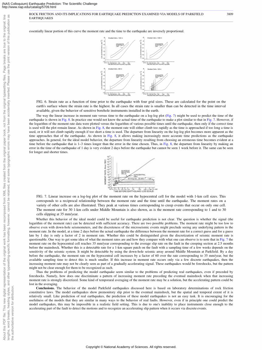
essentially linear portion of this curve the moment rate and the time to the earthquake are inversely proportional.
FIG. 6. Strain rate as a function of time prior to the earthquake with four grid sizes. These are calculated for the point on theearth's surface where the strain rate is the highest. In all cases the strain rate is smaller than can be detected in the time intervalavailable, given the behavior of sensitive borehole instruments installed in the earth.The way the linear increase in moment rate versus time to the earthquake on a log-log plot (Fig. 7) might be used to predict the time of the
earthquake is shown in Fig. 8. In practice one would not know the actual time of the earthquake to make a plot similar to that in Fig. 7. However, ifthe logarithm of the moment rate data were plotted versus the logarithm of various possible times until the earthquake, then only if the correct timeis used will the plot remain linear. As shown in Fig. 8, the moment rate will either climb too rapidly as the time is approached if too long a time isused, or it will not climb rapidly enough if too short a time is used. The departure from linearity on the log-log plot becomes more apparent as thetime approaches that of the earthquake. As shown in Fig. 8, it allows making increasingly more accurate time predictions as the earthquakeapproaches. In general, for the ideal model behavior, the departure from linearity resulting from choosing an erroneous time becomes evident at atime before the earthquake that is 1–3 times longer than the error in the time chosen. Thus, in Fig. 8, the departure from linearity by making anerror in the time of the earthquake of 1 day is very evident 2 days before the earthquake but cannot be seen 1 week before it. The same can be seenfor longer and shorter times.
FIG. 7. Linear increase on a log-log plot of the moment rate on the hypocentral cell for the model with 1-km cell sizes. Thiscorresponds to a reciprocal relationship between the moment rate and the time until the earthquake. The moment rates on avariety of other cells are also illustrated. They peak at various times corresponding to creep events that occur on only one cell.The moment rate for 30 1-km cells under Middle Mountain is also shown, as is the moment rate corresponding to 1 and to 30cells slipping at 35 mm/year.Whether this behavior of the ideal model could be useful for earthquake prediction is not clear. The question is whether the signal (the
logarithm of the moment rate) can be detected with sufficient accuracy. There are two possible problems. The moment rate might be too low toobserve even with down-hole seismometers, and the discreteness of the microseismic events might preclude seeing any underlying pattern in themoment rate. In the model, at a time 2 days before the actual earthquake the difference between the moment rate for a correct guess and for a guesslate by 1 day is only a factor of 2 in moment rate. Whether this could be distinguished given the discretization of seismic moment rate isquestionable. One way to get some idea of what the moment rates are and how they compare with what one can observe is to note that in Fig. 7 themoment rate on the hypocentral cell reaches 35 mm/year corresponding to the average slip rate on the fault in the creeping section at 2.5 monthsbefore the mainshock. Whether this is a detectable rate for a 1-km square patch on the fault with a sampling time of a few weeks depends on thesensitivity of the seismic system. It might be detectable by using the down-hole seismic array around Middle Mountain at Parkfield. By a daybefore the earthquake, the moment rate on the hypocentral cell increases by a factor of 60 over the rate corresponding to 35 mm/year, but theavailable sampling time to detect this is much smaller. If this increase in moment rate occurs only via a few discrete earthquakes, then theincreasing moment rate may not be clearly seen as part of a gradually accelerating signal. These earthquakes would be foreshocks, but the patternmight not be clear enough for them to be recognized as such.
Thus the problems of predicting the model earthquake seem similar to the problems of predicting real earthquakes, even if preceded byforeshocks. Namely, how does one discriminate a pattern of increasing moment rate preceding the eventual mainshock when that increasingmoment rate is strongly discretized. Some kind of temporaral averaging of the moment rate may be a solution, but the accelerating pattern could belost in the averaging.
Conclusions. The behavior of the model Parkfield earthquakes discussed here is based on laboratory determinations of rock frictionconstitutive laws. The model earthquakes show premonitory slip prior to the eventual mainshock, but the spatial and temporal extent of it isrelatively small. Like prediction of real earthquakes, the prediction of these model earthquakes is not an easy task. It is encouraging for theusefulness of the models that they are similar in many ways to the behavior of real faults. However, even if in principle one could predict themodel earthquakes, this may be impossible in a realistic field setting. This is due to one's inability to place instruments close enough to theaccelerating part of the fault to detect the motions and to recognize an accelerating slip pattern when it occurs via discrete events.
ROCK FRICTION AND ITS IMPLICATIONS FOR EARTHQUAKE PREDICTION EXAMINED VIA MODELS OF PARKFIELDEARTHQUAKES
3809
Abou
t thi
s PD
F fil
e: T
his
new
dig
ital r
epre
sent
atio
n of
the
orig
inal
wor
k ha
s be
en re
com
pose
d fro
m X
ML
files
cre
ated
from
the
orig
inal
pap
er b
ook,
not
from
the
orig
inal
type
setti
ng fi
les.
Pag
e br
eaks
are
true
to th
e or
igin
al; l
ine
leng
ths,
wor
d br
eaks
, hea
ding
sty
les,
and
oth
er ty
pese
tting
-spe
cific
form
attin
g, h
owev
er, c
anno
t be
reta
ined
, and
som
e ty
pogr
aphi
c er
rors
may
hav
e be
en a
ccid
enta
lly in
serte
d. P
leas
e us
e th
e pr
int v
ersi
on o
f thi
s pu
blic
atio
n as
the
auth
orita
tive
vers
ion
for a
ttrib
utio
n.
Copyright © National Academy of Sciences. All rights reserved.
(NAS Colloquium) Earthquake Prediction: The Scientific Challengehttp://www.nap.edu/catalog/5709.html
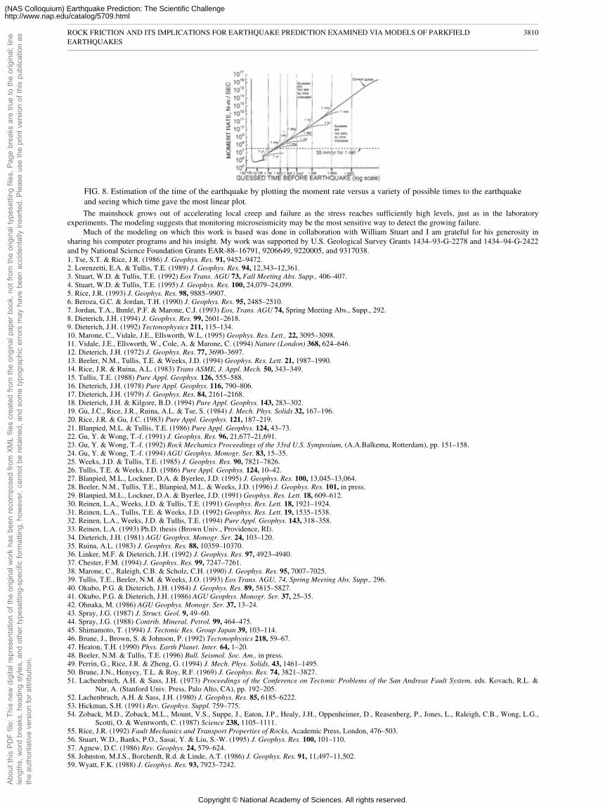
FIG. 8. Estimation of the time of the earthquake by plotting the moment rate versus a variety of possible times to the earthquakeand seeing which time gave the most linear plot.The mainshock grows out of accelerating local creep and failure as the stress reaches sufficiently high levels, just as in the laboratory
experiments. The modeling suggests that monitoring microseismicity may be the most sensitive way to detect the growing failure.Much of the modeling on which this work is based was done in collaboration with William Stuart and I am grateful for his generosity in
sharing his computer programs and his insight. My work was supported by U.S. Geological Survey Grants 1434–93-G-2278 and 1434–94-G-2422and by National Science Foundation Grants EAR-88–16791, 9206649, 9220005, and 9317038.1. Tse, S.T. & Rice, J.R. (1986) J. Geophys. Res. 91, 9452–9472.2. Lorenzetti, E.A. & Tullis, T.E. (1989) J. Geophys. Res. 94, 12,343–12,361.3. Stuart, W.D. & Tullis, T.E. (1992) Eos Trans. AGU 73, Fall Meeting Abs. Supp., 406–407.4. Stuart, W.D. & Tullis, T.E. (1995) J. Geophys. Res. 100, 24,079–24,099.5. Rice, J.R. (1993) J. Geophys. Res. 98, 9885–9907.6. Beroza, G.C. & Jordan, T.H. (1990) J. Geophys. Res. 95, 2485–2510.7. Jordan, T.A., Ihmlé, P.F. & Marone, C.J. (1993) Eos, Trans. AGU 74, Spring Meeting Abs., Supp., 292.8. Dieterich, J.H. (1994) J. Geophys. Res. 99, 2601–2618.9. Dieterich, J.H. (1992) Tectonophysics 211, 115–134.10. Marone, C., Vidale, J.E., Ellsworth, W.L. (1995) Geophys. Res. Lett., 22, 3095–3098.11. Vidale, J.E., Ellsworth, W., Cole, A. & Marone, C. (1994) Nature (London) 368, 624–646.12. Dieterich, J.H. (1972) J. Geophys. Res. 77, 3690–3697.13. Beeler, N.M., Tullis, T.E. & Weeks, J.D. (1994) Geophys. Res. Lett. 21, 1987–1990.14. Rice, J.R. & Ruina, A.L. (1983) Trans ASME, J. Appl. Mech. 50, 343–349.15. Tullis, T.E. (1988) Pure Appl. Geophys. 126, 555–588.16. Dieterich, J.H. (1978) Pure Appl. Geophys. 116, 790–806.17. Dieterich, J.H. (1979) J. Geophys. Res. 84, 2161–2168.18. Dieterich, J.H. & Kilgore, B.D. (1994) Pure Appl. Geophys. 143, 283–302.19. Gu, J.C., Rice, J.R., Ruina, A.L. & Tse, S. (1984) J. Mech. Phys. Solids 32, 167–196.20. Rice, J.R. & Gu, J.C. (1983) Pure Appl. Geophys. 121, 187–219.21. Blanpied, M.L. & Tullis, T.E. (1986) Pure Appl. Geophys. 124, 43–73.22. Gu, Y. & Wong, T.-f. (1991) J. Geophys. Res. 96, 21,677–21,691.23. Gu, Y. & Wong, T.-f. (1992) Rock Mechanics Proceedings of the 33rd U.S. Symposium, (A.A.Balkema, Rotterdam), pp. 151–158.24. Gu, Y. & Wong, T.-f. (1994) AGU Geophys. Monogr. Ser. 83, 15–35.25. Weeks, J.D. & Tullis, T.E. (1985) J. Geophys. Res. 90, 7821–7826.26. Tullis, T.E. & Weeks, J.D. (1986) Pure Appl. Geophys. 124, 10–42.27. Blanpied, M.L., Lockner, D.A. & Byerlee, J.D. (1995) J. Geophys. Res. 100, 13,045–13,064.28. Beeler, N.M., Tullis, T.E., Blanpied, M.L. & Weeks, J.D. (1996) J. Geophys. Res. 101, in press.29. Blanpied, M.L., Lockner, D.A. & Byerlee, J.D. (1991) Geophys. Res. Lett. 18, 609–612.30. Reinen, L.A., Weeks, J.D. & Tullis, T.E. (1991) Geophys. Res. Lett. 18, 1921–1924.31. Reinen, L.A., Tullis, T.E. & Weeks, J.D. (1992) Geophys. Res. Lett. 19, 1535–1538.32. Reinen, L.A., Weeks, J.D. & Tullis, T.E. (1994) Pure Appl. Geophys. 143, 318–358.33. Reinen, L.A. (1993) Ph.D. thesis (Brown Univ., Providence, RI).34. Dieterich, J.H. (1981) AGU Geophys. Monogr. Ser. 24, 103–120.35. Ruina, A.L. (1983) J. Geophys. Res. 88, 10359–10370.36. Linker, M.F. & Dieterich, J.H. (1992) J. Geophys. Res. 97, 4923–4940.37. Chester, F.M. (1994) J. Geophys. Res. 99, 7247–7261.38. Marone, C., Raleigh, C.B. & Scholz, C.H. (1990) J. Geophys. Res. 95, 7007–7025.39. Tullis, T.E., Beeler, N.M. & Weeks, J.O. (1993) Eos Trans. AGU, 74, Spring Meeting Abs. Supp., 296.40. Okubo, P.G. & Dieterich, J.H. (1984) J. Geophys. Res. 89, 5815–5827.41. Okubo, P.G. & Dieterich, J.H. (1986) AGU Geophys. Monogr. Ser. 37, 25–35.42. Ohnaka, M. (1986) AGU Geophys. Monogr. Ser. 37, 13–24.43. Spray, J.G. (1987) J. Struct. Geol. 9, 49–60.44. Spray, J.G. (1988) Contrib. Mineral. Petrol. 99, 464–475.45. Shimamoto, T. (1994) J. Tectonic Res. Group Japan 39, 103–114.46. Brune, J., Brown, S. & Johnson, P. (1992) Tectonophysics 218, 59–67.47. Heaton, T.H. (1990) Phys. Earth Planet. Inter. 64, 1–20.48. Beeler, N.M. & Tullis, T.E. (1996) Bull. Seismol. Soc. Am., in press.49. Perrin, G., Rice, J.R. & Zheng, G. (1994) J. Mech. Phys. Solids, 43, 1461–1495.50. Brune, J.N., Henyey, T.L. & Roy, R.F. (1969) J. Geophys. Res. 74, 3821–3827.51. Lachenbruch, A.H. & Sass, J.H. (1973) Proceedings of the Conference on Tectonic Problems of the San Andreas Fault System, eds. Kovach, R.L. &
Nur, A. (Stanford Univ. Press, Palo Alto, CA), pp. 192–205.52. Lachenbruch, A.H. & Sass, J.H. (1980) J. Geophys. Res. 85, 6185–6222.53. Hickman, S.H. (1991) Rev. Geophys. Suppl. 759–775.54. Zoback, M.D., Zoback, M.L., Mount, V.S., Suppe, J., Eaton, J.P., Healy, J.H., Oppenheimer, D., Reasenberg, P., Jones, L., Raleigh, C.B., Wong, L.G.,
Scotti, O. & Wentworth, C. (1987) Science 238, 1105–1111.55. Rice, J.R. (1992) Fault Mechanics and Transport Properties of Rocks, Academic Press, London, 476–503.56. Stuart, W.D., Banks, P.O., Sasai, Y. & Liu, S.-W. (1995) J. Geophys. Res. 100, 101–110.57. Agnew, D.C. (1986) Rev. Geophys. 24, 579–624.58. Johnston, M.J.S., Borcherdt, R.d. & Linde, A.T. (1986) J. Geophys. Res. 91, 11,497–11,502.59. Wyatt, F.K. (1988) J. Geophys. Res. 93, 7923–7242.
ROCK FRICTION AND ITS IMPLICATIONS FOR EARTHQUAKE PREDICTION EXAMINED VIA MODELS OF PARKFIELDEARTHQUAKES
3810
Abou
t thi
s PD
F fil
e: T
his
new
dig
ital r
epre
sent
atio
n of
the
orig
inal
wor
k ha
s be
en re
com
pose
d fro
m X
ML
files
cre
ated
from
the
orig
inal
pap
er b
ook,
not
from
the
orig
inal
type
setti
ng fi
les.
Pag
e br
eaks
are
true
to th
e or
igin
al; l
ine
leng
ths,
wor
d br
eaks
, hea
ding
sty
les,
and
oth
er ty
pese
tting
-spe
cific
form
attin
g, h
owev
er, c
anno
t be
reta
ined
, and
som
e ty
pogr
aphi
c er
rors
may
hav
e be
en a
ccid
enta
lly in
serte
d. P
leas
e us
e th
e pr
int v
ersi
on o
f thi
s pu
blic
atio
n as
the
auth
orita
tive
vers
ion
for a
ttrib
utio
n.
Copyright © National Academy of Sciences. All rights reserved.
(NAS Colloquium) Earthquake Prediction: The Scientific Challengehttp://www.nap.edu/catalog/5709.html
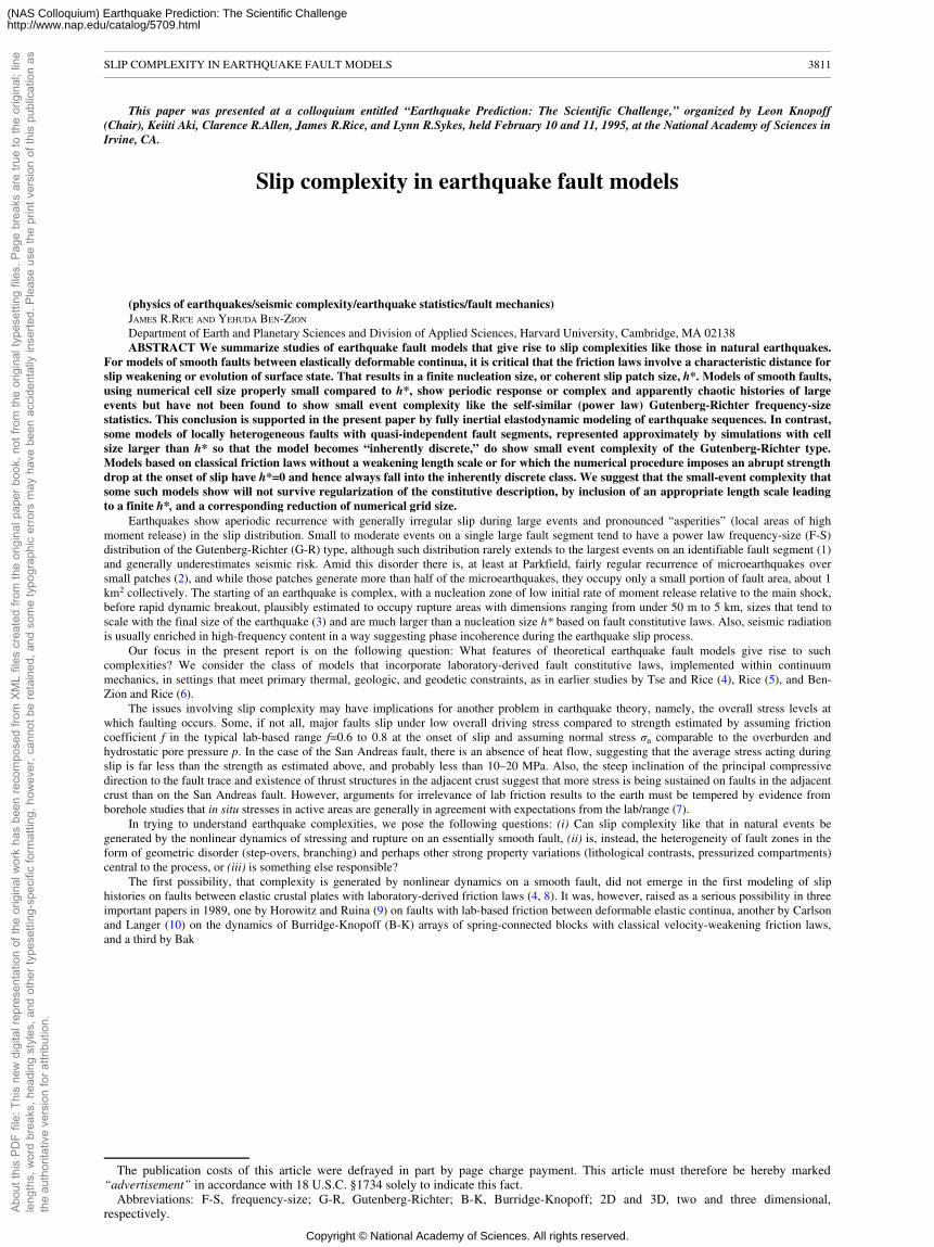
This paper was presented at a colloquium entitled “Earthquake Prediction: The Scientific Challenge,” organized by Leon Knopoff(Chair), Keiiti Aki, Clarence R.Allen, James R.Rice, and Lynn R.Sykes, held February 10 and 11, 1995, at the National Academy of Sciences inIrvine, CA.
Slip complexity in earthquake fault models
(physics of earthquakes/seismic complexity/earthquake statistics/fault mechanics)JAMES R.RICE AND YEHUDA BEN-ZION
Department of Earth and Planetary Sciences and Division of Applied Sciences, Harvard University, Cambridge, MA 02138ABSTRACT We summarize studies of earthquake fault models that give rise to slip complexities like those in natural earthquakes.
For models of smooth faults between elastically deformable continua, it is critical that the friction laws involve a characteristic distance forslip weakening or evolution of surface state. That results in a finite nucleation size, or coherent slip patch size, h*. Models of smooth faults,using numerical cell size properly small compared to h*, show periodic response or complex and apparently chaotic histories of largeevents but have not been found to show small event complexity like the self-similar (power law) Gutenberg-Richter frequency-sizestatistics. This conclusion is supported in the present paper by fully inertial elastodynamic modeling of earthquake sequences. In contrast,some models of locally heterogeneous faults with quasi-independent fault segments, represented approximately by simulations with cellsize larger than h* so that the model becomes “inherently discrete,” do show small event complexity of the Gutenberg-Richter type.Models based on classical friction laws without a weakening length scale or for which the numerical procedure imposes an abrupt strengthdrop at the onset of slip have h*=0 and hence always fall into the inherently discrete class. We suggest that the small-event complexity thatsome such models show will not survive regularization of the constitutive description, by inclusion of an appropriate length scale leadingto a finite h*, and a corresponding reduction of numerical grid size.
Earthquakes show aperiodic recurrence with generally irregular slip during large events and pronounced “asperities” (local areas of highmoment release) in the slip distribution. Small to moderate events on a single large fault segment tend to have a power law frequency-size (F-S)distribution of the Gutenberg-Richter (G-R) type, although such distribution rarely extends to the largest events on an identifiable fault segment (1)and generally underestimates seismic risk. Amid this disorder there is, at least at Parkfield, fairly regular recurrence of microearthquakes oversmall patches (2), and while those patches generate more than half of the microearthquakes, they occupy only a small portion of fault area, about 1km2 collectively. The starting of an earthquake is complex, with a nucleation zone of low initial rate of moment release relative to the main shock,before rapid dynamic breakout, plausibly estimated to occupy rupture areas with dimensions ranging from under 50 m to 5 km, sizes that tend toscale with the final size of the earthquake (3) and are much larger than a nucleation size h* based on fault constitutive laws. Also, seismic radiationis usually enriched in high-frequency content in a way suggesting phase incoherence during the earthquake slip process.
Our focus in the present report is on the following question: What features of theoretical earthquake fault models give rise to suchcomplexities? We consider the class of models that incorporate laboratory-derived fault constitutive laws, implemented within continuummechanics, in settings that meet primary thermal, geologic, and geodetic constraints, as in earlier studies by Tse and Rice (4), Rice (5), and Ben-Zion and Rice (6).
The issues involving slip complexity may have implications for another problem in earthquake theory, namely, the overall stress levels atwhich faulting occurs. Some, if not all, major faults slip under low overall driving stress compared to strength estimated by assuming frictioncoefficient f in the typical lab-based range f=0.6 to 0.8 at the onset of slip and assuming normal stress σn comparable to the overburden andhydrostatic pore pressure p. In the case of the San Andreas fault, there is an absence of heat flow, suggesting that the average stress acting duringslip is far less than the strength as estimated above, and probably less than 10–20 MPa. Also, the steep inclination of the principal compressivedirection to the fault trace and existence of thrust structures in the adjacent crust suggest that more stress is being sustained on faults in the adjacentcrust than on the San Andreas fault. However, arguments for irrelevance of lab friction results to the earth must be tempered by evidence fromborehole studies that in situ stresses in active areas are generally in agreement with expectations from the lab/range (7).
In trying to understand earthquake complexities, we pose the following questions: (i) Can slip complexity like that in natural events begenerated by the nonlinear dynamics of stressing and rupture on an essentially smooth fault, (ii) is, instead, the heterogeneity of fault zones in theform of geometric disorder (step-overs, branching) and perhaps other strong property variations (lithological contrasts, pressurized compartments)central to the process, or (iii) is something else responsible?
The first possibility, that complexity is generated by nonlinear dynamics on a smooth fault, did not emerge in the first modeling of sliphistories on faults between elastic crustal plates with laboratory-derived friction laws (4, 8). It was, however, raised as a serious possibility in threeimportant papers in 1989, one by Horowitz and Ruina (9) on faults with lab-based friction between deformable elastic continua, another by Carlsonand Langer (10) on the dynamics of Burridge-Knopoff (B-K) arrays of spring-connected blocks with classical velocity-weakening friction laws,and a third by Bak
The publication costs of this article were defrayed in part by page charge payment. This article must therefore be hereby marked“advertisement” in accordance with 18 U.S.C. §1734 solely to indicate this fact.
Abbreviations: F-S, frequency-size; G-R, Gutenberg-Richter; B-K, Burridge-Knopoff; 2D and 3D, two and three dimensional,respectively.
SLIP COMPLEXITY IN EARTHQUAKE FAULT MODELS 3811
Abou
t thi
s PD
F fil
e: T
his
new
dig
ital r
epre
sent
atio
n of
the
orig
inal
wor
k ha
s be
en re
com
pose
d fro
m X
ML
files
cre
ated
from
the
orig
inal
pap
er b
ook,
not
from
the
orig
inal
type
setti
ng fi
les.
Pag
e br
eaks
are
true
to th
e or
igin
al; l
ine
leng
ths,
wor
d br
eaks
, hea
ding
sty
les,
and
oth
er ty
pese
tting
-spe
cific
form
attin
g, h
owev
er, c
anno
t be
reta
ined
, and
som
e ty
pogr
aphi
c er
rors
may
hav
e be
en a
ccid
enta
lly in
serte
d. P
leas
e us
e th
e pr
int v
ersi
on o
f thi
s pu
blic
atio
n as
the
auth
orita
tive
vers
ion
for a
ttrib
utio
n.
Copyright © National Academy of Sciences. All rights reserved.
(NAS Colloquium) Earthquake Prediction: The Scientific Challengehttp://www.nap.edu/catalog/5709.html
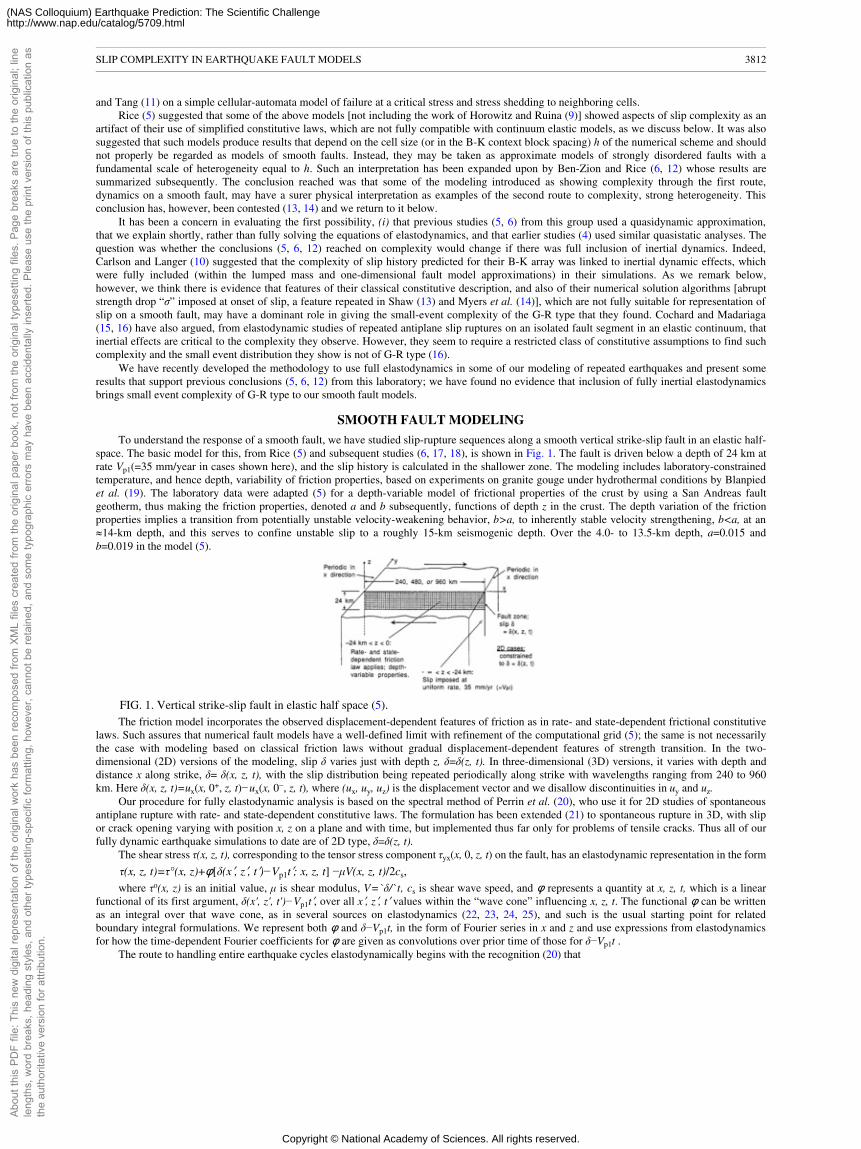
and Tang (11) on a simple cellular-automata model of failure at a critical stress and stress shedding to neighboring cells.Rice (5) suggested that some of the above models [not including the work of Horowitz and Ruina (9)] showed aspects of slip complexity as an
artifact of their use of simplified constitutive laws, which are not fully compatible with continuum elastic models, as we discuss below. It was alsosuggested that such models produce results that depend on the cell size (or in the B-K context block spacing) h of the numerical scheme and shouldnot properly be regarded as models of smooth faults. Instead, they may be taken as approximate models of strongly disordered faults with afundamental scale of heterogeneity equal to h. Such an interpretation has been expanded upon by Ben-Zion and Rice (6, 12) whose results aresummarized subsequently. The conclusion reached was that some of the modeling introduced as showing complexity through the first route,dynamics on a smooth fault, may have a surer physical interpretation as examples of the second route to complexity, strong heterogeneity. Thisconclusion has, however, been contested (13, 14) and we return to it below.
It has been a concern in evaluating the first possibility, (i) that previous studies (5, 6) from this group used a quasidynamic approximation,that we explain shortly, rather than fully solving the equations of elastodynamics, and that earlier studies (4) used similar quasistatic analyses. Thequestion was whether the conclusions (5, 6, 12) reached on complexity would change if there was full inclusion of inertial dynamics. Indeed,Carlson and Langer (10) suggested that the complexity of slip history predicted for their B-K array was linked to inertial dynamic effects, whichwere fully included (within the lumped mass and one-dimensional fault model approximations) in their simulations. As we remark below,however, we think there is evidence that features of their classical constitutive description, and also of their numerical solution algorithms [abruptstrength drop “σ” imposed at onset of slip, a feature repeated in Shaw (13) and Myers et al. (14)], which are not fully suitable for representation ofslip on a smooth fault, may have a dominant role in giving the small-event complexity of the G-R type that they found. Cochard and Madariaga(15, 16) have also argued, from elastodynamic studies of repeated antiplane slip ruptures on an isolated fault segment in an elastic continuum, thatinertial effects are critical to the complexity they observe. However, they seem to require a restricted class of constitutive assumptions to find suchcomplexity and the small event distribution they show is not of G-R type (16).
We have recently developed the methodology to use full elastodynamics in some of our modeling of repeated earthquakes and present someresults that support previous conclusions (5, 6, 12) from this laboratory; we have found no evidence that inclusion of fully inertial elastodynamicsbrings small event complexity of G-R type to our smooth fault models.
SMOOTH FAULT MODELING
To understand the response of a smooth fault, we have studied slip-rupture sequences along a smooth vertical strike-slip fault in an elastic half-space. The basic model for this, from Rice (5) and subsequent studies (6, 17, 18), is shown in Fig. 1. The fault is driven below a depth of 24 km atrate Vp1(=35 mm/year in cases shown here), and the slip history is calculated in the shallower zone. The modeling includes laboratory-constrainedtemperature, and hence depth, variability of friction properties, based on experiments on granite gouge under hydrothermal conditions by Blanpiedet al. (19). The laboratory data were adapted (5) for a depth-variable model of frictional properties of the crust by using a San Andreas faultgeotherm, thus making the friction properties, denoted a and b subsequently, functions of depth z in the crust. The depth variation of the frictionproperties implies a transition from potentially unstable velocity-weakening behavior, b>a, to inherently stable velocity strengthening, b<a, at an�14-km depth, and this serves to confine unstable slip to a roughly 15-km seismogenic depth. Over the 4.0- to 13.5-km depth, a=0.015 andb=0.019 in the model (5).
FIG. 1. Vertical strike-slip fault in elastic half space (5).The friction model incorporates the observed displacement-dependent features of friction as in rate- and state-dependent frictional constitutive
laws. Such assures that numerical fault models have a well-defined limit with refinement of the computational grid (5); the same is not necessarilythe case with modeling based on classical friction laws without gradual displacement-dependent features of strength transition. In the two-dimensional (2D) versions of the modeling, slip δ varies just with depth z, δ=δ(z, t). In three-dimensional (3D) versions, it varies with depth anddistance x along strike, δ= δ(x, z, t), with the slip distribution being repeated periodically along strike with wavelengths ranging from 240 to 960km. Here δ(x, z, t)=ux(x, 0+, z, t)−ux(x, 0−, z, t), where (ux, uy, uz) is the displacement vector and we disallow discontinuities in uy and uz.
Our procedure for fully elastodynamic analysis is based on the spectral method of Perrin et al. (20), who use it for 2D studies of spontaneousantiplane rupture with rate- and state-dependent constitutive laws. The formulation has been extended (21) to spontaneous rupture in 3D, with slipor crack opening varying with position x, z on a plane and with time, but implemented thus far only for problems of tensile cracks. Thus all of ourfully dynamic earthquake simulations to date are of 2D type, δ=δ(z, t).
The shear stress τ(x, z, t), corresponding to the tensor stress component τyx(x, 0, z, t) on the fault, has an elastodynamic representation in the form
τ(x, z, t)=τ°(x, z)+�[δ(x�, z�, t�)−Vp1t�; x, z, t] −µV(x, z, t)/2cs,where τo(x, z) is an initial value, µ is shear modulus, V=`δ/`t, cs is shear wave speed, and � represents a quantity at x, z, t, which is a linear
functional of its first argument, δ(x', z', t')−Vp1t�, over all x�, z�, t� values within the “wave cone” influencing x, z, t. The functional � can be writtenas an integral over that wave cone, as in several sources on elastodynamics (22, 23, 24, 25), and such is the usual starting point for relatedboundary integral formulations. We represent both � and δ−Vp1t, in the form of Fourier series in x and z and use expressions from elastodynamicsfor how the time-dependent Fourier coefficients for � are given as convolutions over prior time of those for δ−Vp1t .
The route to handling entire earthquake cycles elastodynamically begins with the recognition (20) that
SLIP COMPLEXITY IN EARTHQUAKE FAULT MODELS 3812
Abou
t thi
s PD
F fil
e: T
his
new
dig
ital r
epre
sent
atio
n of
the
orig
inal
wor
k ha
s be
en re
com
pose
d fro
m X
ML
files
cre
ated
from
the
orig
inal
pap
er b
ook,
not
from
the
orig
inal
type
setti
ng fi
les.
Pag
e br
eaks
are
true
to th
e or
igin
al; l
ine
leng
ths,
wor
d br
eaks
, hea
ding
sty
les,
and
oth
er ty
pese
tting
-spe
cific
form
attin
g, h
owev
er, c
anno
t be
reta
ined
, and
som
e ty
pogr
aphi
c er
rors
may
hav
e be
en a
ccid
enta
lly in
serte
d. P
leas
e us
e th
e pr
int v
ersi
on o
f thi
s pu
blic
atio
n as
the
auth
orita
tive
vers
ion
for a
ttrib
utio
n.
Copyright © National Academy of Sciences. All rights reserved.
(NAS Colloquium) Earthquake Prediction: The Scientific Challengehttp://www.nap.edu/catalog/5709.html
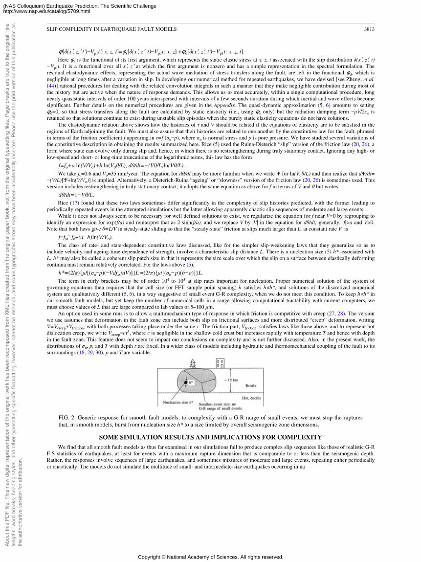
�[δ(x�, z,� t�)−Vp1t�; x, z, t]=�s[δ(x�, z�, t)−Vp1t; x, z] +�d[δ(x�, z�, t�)−Vp1t; x, z, t].Here �s is the functional of its first argument, which represents the static elastic stress at x, z, t associated with the slip distribution δ(x�, z�, t)
−Vp1t. It is a functional over all x�, z� at which the first argument is nonzero and has a simple representation in the spectral formulation. Theresidual elastodynamic effects, representing the actual wave mediation of stress transfers along the fault, are left in the functional �d, which isnegligible at long times after a variation in slip. In developing our numerical method for repeated earthquakes, we have devised [see Zheng, et al.(44)] rational procedures for dealing with the related convolution integrals in such a manner that they make negligible contribution during most ofthe history but are active when the nature of response demands. This allows us to treat accurately, within a single computational procedure, longnearly quasistatic intervals of order 100 years interspersed with intervals of a few seconds duration during which inertial and wave effects becomesignificant. Further details on the numerical procedures are given in the Appendix. The quasi-dynamic approximation (5, 6) amounts to setting�d=0, so that stress transfers along the fault are calculated by static elasticity (i.e., using �s only) but the radiation damping term −µV/2cs isretained so that solutions continue to exist during unstable slip episodes when the purely static elasticity equations do not have solutions.
The elastodynamic relation above shows how the histories of τ and V should be related if the equations of elasticity are to be satisfied in theregions of Earth adjoining the fault. We must also assure that their histories are related to one another by the constitutive law for the fault, phrasedin terms of the friction coefficient f appearing in τ=f (σn−p), where σn is normal stress and p is pore pressure. We have studied several variations ofthe constitutive description in obtaining the results summarized here. Rice (5) used the Ruina-Dieterich “slip” version of the friction law (20, 26), aform where state can evolve only during slip and, hence, in which there is no restrengthening during truly stationary contact. Ignoring any high- orlow-speed and short- or long-time truncations of the logarithmic terms, this law has the form
f=fo+a ln(V/Vo)+b ln(V0θ/L), dθ/dt=−(Vθ/L)ln(Vθ/L).
We take fo=0.6 and Vo=35 mm/year. The equation for dθ/dt may be more familiar when we write Ψ for ln(Voθ/L) and then realize that dΨ/dt=−(V/L)[Ψ+ln(V/Vo)] is implied. Alternatively, a Dieterich-Ruina “ageing” or “slowness” version of the friction law (20, 26) is sometimes used. Thisversion includes restrengthening in truly stationary contact; it adopts the same equation as above for f in terms of V and θ but writes
dθ/dt=1−Vθ/L.Rice (17) found that these two laws sometimes differ significantly in the complexity of slip histories predicted, with the former leading to
periodically repeated events in the attempted simulations but the latter allowing apparently chaotic slip sequences of moderate and large events.While it does not always seem to be necessary for well defined solutions to exist, we regularize the equation for f near V=0 by regrouping to
identify an expression for exp(f/a) and reinterpret that as 2 sinh(f/a), and we replace V by |V| in the equation for dθ/dt; generally, |f|�a and V>0.Note that both laws give θ=L/V in steady-state sliding so that the “steady-state” friction at slips much larger than L, at constant rate V, is
f=fss` fo+(a−b)ln(V/Vo).
The class of rate- and state-dependent constitutive laws discussed, like for the simpler slip-weakening laws that they generalize so as toinclude velocity and ageing-time dependence of strength, involve a characteristic slip distance L. There is a nucleation size (5) h* associated withL; h* may also be called a coherent slip patch size in that it represents the size scale over which the slip on a surface between elastically deformingcontinua must remain relatively correlated. For the laws above (5),
h*=(2/π){µ/[(σn−p)(−Vdfss/dV)]}L =(2/π){µ/[(σn−p)(b−a)]}L.
The term in curly brackets may be of order 104 to 105 at slip rates important for nucleation. Proper numerical solution of the system ofgoverning equations then requires that the cell size (or FFT sample point spacing) h satisfies h�h*, and solutions of the discretized numericalsystem are qualitatively different (5, 6), in a way suggestive of small event G-R complexity, when we do not meet this condition. To keep h�h* inour smooth fault models, but yet keep the number of numerical cells in a range allowing computational tractability with current computers, wemust choose values of L that are large compared to lab values of 5–100 µm.
An option used in some runs is to allow a multimechanism type of response in which friction is competitive with creep (27, 28). The versionwe use assumes that deformation in the fault zone can include both slip on frictional surfaces and more distributed “creep” deformation, writingV=Vcreep+Vfriction, with both processes taking place under the same τ. The friction part, Vfriction, satisfies laws like those above, and to represent hotdislocation creep, we write Vcreep=cτ3, where c is negligible in the shallow cold crust but increases rapidly with temperature T and hence with depthin the fault zone. This feature does not seem to impact our conclusions on complexity and is not further discussed. Also, in the present work, thedistributions of σn, p, and T with depth z are fixed. In a wider class of models including hydraulic and thermomechanical coupling of the fault to itssurroundings (18, 29, 30), p and T are variable.
FIG. 2. Generic response for smooth fault models; to complexify with a G-R range of small events, we must stop the rupturesthat, in smooth models, burst from nucleation size h* to a size limited by overall seismogenic zone dimensions.
SOME SIMULATION RESULTS AND IMPLICATIONS FOR COMPLEXITY
We find that all smooth fault models as thus far examined in our simulations fail to produce complex slip sequences like those of realistic G-RF-S statistics of earthquakes, at least for events with a maximum rupture dimension that is comparable to or less than the seismogenic depth.Rather, the responses involve sequences of large earthquakes, and sometimes mixtures of moderate and large events, repeating either periodicallyor chaotically. The models do not simulate the multitude of small- and intermediate-size earthquakes occurring in na
SLIP COMPLEXITY IN EARTHQUAKE FAULT MODELS 3813
Abou
t thi
s PD
F fil
e: T
his
new
dig
ital r
epre
sent
atio
n of
the
orig
inal
wor
k ha
s be
en re
com
pose
d fro
m X
ML
files
cre
ated
from
the
orig
inal
pap
er b
ook,
not
from
the
orig
inal
type
setti
ng fi
les.
Pag
e br
eaks
are
true
to th
e or
igin
al; l
ine
leng
ths,
wor
d br
eaks
, hea
ding
sty
les,
and
oth
er ty
pese
tting
-spe
cific
form
attin
g, h
owev
er, c
anno
t be
reta
ined
, and
som
e ty
pogr
aphi
c er
rors
may
hav
e be
en a
ccid
enta
lly in
serte
d. P
leas
e us
e th
e pr
int v
ersi
on o
f thi
s pu
blic
atio
n as
the
auth
orita
tive
vers
ion
for a
ttrib
utio
n.
Copyright © National Academy of Sciences. All rights reserved.
(NAS Colloquium) Earthquake Prediction: The Scientific Challengehttp://www.nap.edu/catalog/5709.html
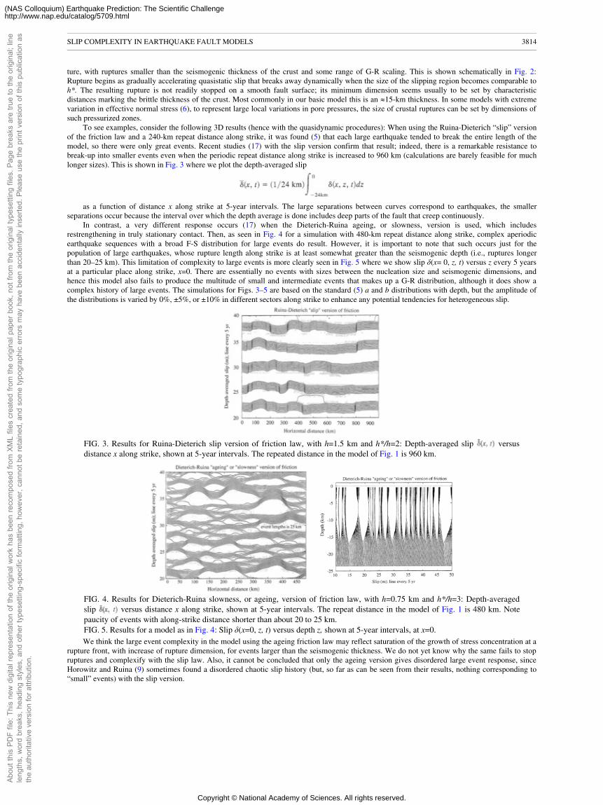
ture, with ruptures smaller than the seismogenic thickness of the crust and some range of G-R scaling. This is shown schematically in Fig. 2:Rupture begins as gradually accelerating quasistatic slip that breaks away dynamically when the size of the slipping region becomes comparable toh*. The resulting rupture is not readily stopped on a smooth fault surface; its minimum dimension seems usually to be set by characteristicdistances marking the brittle thickness of the crust. Most commonly in our basic model this is an �15-km thickness. In some models with extremevariation in effective normal stress (6), to represent large local variations in pore pressures, the size of crustal ruptures can be set by dimensions ofsuch pressurized zones.
To see examples, consider the following 3D results (hence with the quasidynamic procedures): When using the Ruina-Dieterich “slip” versionof the friction law and a 240-km repeat distance along strike, it was found (5) that each large earthquake tended to break the entire length of themodel, so there were only great events. Recent studies (17) with the slip version confirm that result; indeed, there is a remarkable resistance tobreak-up into smaller events even when the periodic repeat distance along strike is increased to 960 km (calculations are barely feasible for muchlonger sizes). This is shown in Fig. 3 where we plot the depth-averaged slip
as a function of distance x along strike at 5-year intervals. The large separations between curves correspond to earthquakes, the smallerseparations occur because the interval over which the depth average is done includes deep parts of the fault that creep continuously.
In contrast, a very different response occurs (17) when the Dieterich-Ruina ageing, or slowness, version is used, which includesrestrengthening in truly stationary contact. Then, as seen in Fig. 4 for a simulation with 480-km repeat distance along strike, complex aperiodicearthquake sequences with a broad F-S distribution for large events do result. However, it is important to note that such occurs just for thepopulation of large earthquakes, whose rupture length along strike is at least somewhat greater than the seismogenic depth (i.e., ruptures longerthan 20–25 km). This limitation of complexity to large events is more clearly seen in Fig. 5 where we show slip δ(x= 0, z, t) versus z every 5 yearsat a particular place along strike, x=0. There are essentially no events with sizes between the nucleation size and seismogenic dimensions, andhence this model also fails to produce the multitude of small and intermediate events that makes up a G-R distribution, although it does show acomplex history of large events. The simulations for Figs. 3–5 are based on the standard (5) a and b distributions with depth, but the amplitude ofthe distributions is varied by 0%, ±5%, or ±10% in different sectors along strike to enhance any potential tendencies for heterogeneous slip.
FIG. 3. Results for Ruina-Dieterich slip version of friction law, with h=1.5 km and h*/h=2: Depth-averaged slip versusdistance x along strike, shown at 5-year intervals. The repeated distance in the model of Fig. 1 is 960 km.
FIG. 4. Results for Dieterich-Ruina slowness, or ageing, version of friction law, with h=0.75 km and h*/h=3: Depth-averagedslip versus distance x along strike, shown at 5-year intervals. The repeat distance in the model of Fig. 1 is 480 km. Notepaucity of events with along-strike distance shorter than about 20 to 25 km.FIG. 5. Results for a model as in Fig. 4: Slip δ(x=0, z, t) versus depth z, shown at 5-year intervals, at x=0.We think the large event complexity in the model using the ageing friction law may reflect saturation of the growth of stress concentration at a
rupture front, with increase of rupture dimension, for events larger than the seismogenic thickness. We do not yet know why the same fails to stopruptures and complexify with the slip law. Also, it cannot be concluded that only the ageing version gives disordered large event response, sinceHorowitz and Ruina (9) sometimes found a disordered chaotic slip history (but, so far as can be seen from their results, nothing corresponding to“small” events) with the slip version.
SLIP COMPLEXITY IN EARTHQUAKE FAULT MODELS 3814
Abou
t thi
s PD
F fil
e: T
his
new
dig
ital r
epre
sent
atio
n of
the
orig
inal
wor
k ha
s be
en re
com
pose
d fro
m X
ML
files
cre
ated
from
the
orig
inal
pap
er b
ook,
not
from
the
orig
inal
type
setti
ng fi
les.
Pag
e br
eaks
are
true
to th
e or
igin
al; l
ine
leng
ths,
wor
d br
eaks
, hea
ding
sty
les,
and
oth
er ty
pese
tting
-spe
cific
form
attin
g, h
owev
er, c
anno
t be
reta
ined
, and
som
e ty
pogr
aphi
c er
rors
may
hav
e be
en a
ccid
enta
lly in
serte
d. P
leas
e us
e th
e pr
int v
ersi
on o
f thi
s pu
blic
atio
n as
the
auth
orita
tive
vers
ion
for a
ttrib
utio
n.
Copyright © National Academy of Sciences. All rights reserved.
(NAS Colloquium) Earthquake Prediction: The Scientific Challengehttp://www.nap.edu/catalog/5709.html
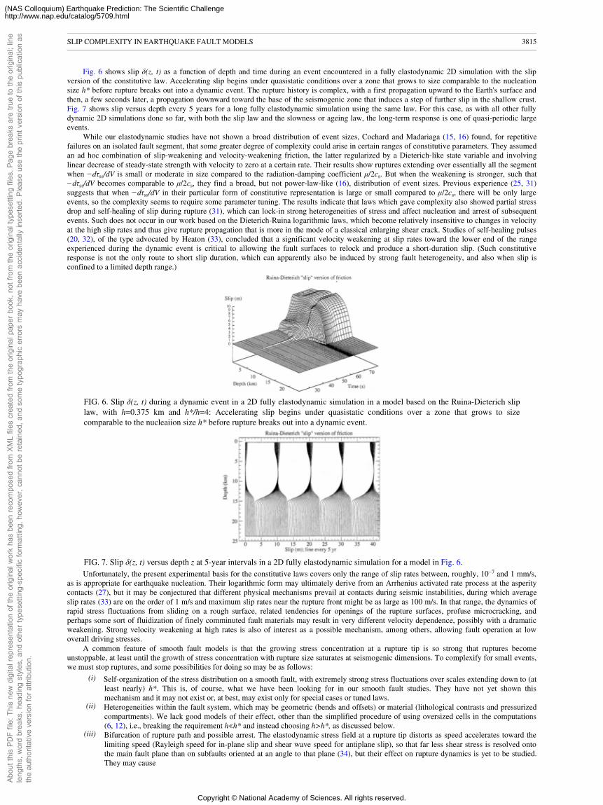
Fig. 6 shows slip δ(z, t) as a function of depth and time during an event encountered in a fully elastodynamic 2D simulation with the slipversion of the constitutive law. Accelerating slip begins under quasistatic conditions over a zone that grows to size comparable to the nucleationsize h* before rupture breaks out into a dynamic event. The rupture history is complex, with a first propagation upward to the Earth's surface andthen, a few seconds later, a propagation downward toward the base of the seismogenic zone that induces a step of further slip in the shallow crust.Fig. 7 shows slip versus depth every 5 years for a long fully elastodynamic simulation using the same law. For this case, as with all other fullydynamic 2D simulations done so far, with both the slip law and the slowness or ageing law, the long-term response is one of quasi-periodic largeevents.
While our elastodynamic studies have not shown a broad distribution of event sizes, Cochard and Madariaga (15, 16) found, for repetitivefailures on an isolated fault segment, that some greater degree of complexity could arise in certain ranges of constitutive parameters. They assumedan ad hoc combination of slip-weakening and velocity-weakening friction, the latter regularized by a Dieterich-like state variable and involvinglinear decrease of steady-state strength with velocity to zero at a certain rate. Their results show ruptures extending over essentially all the segmentwhen −dτss/dV is small or moderate in size compared to the radiation-damping coefficient µ/2cs. But when the weakening is stronger, such that−dτss/dV becomes comparable to µ/2cs, they find a broad, but not power-law-like (16), distribution of event sizes. Previous experience (25, 31)suggests that when −dτss/dV in their particular form of constitutive representation is large or small compared to µ/2cs, there will be only largeevents, so the complexity seems to require some parameter tuning. The results indicate that laws which gave complexity also showed partial stressdrop and self-healing of slip during rupture (31), which can lock-in strong heterogeneities of stress and affect nucleation and arrest of subsequentevents. Such does not occur in our work based on the Dieterich-Ruina logarithmic laws, which become relatively insensitive to changes in velocityat the high slip rates and thus give rupture propagation that is more in the mode of a classical enlarging shear crack. Studies of self-healing pulses(20, 32), of the type advocated by Heaton (33), concluded that a significant velocity weakening at slip rates toward the lower end of the rangeexperienced during the dynamic event is critical to allowing the fault surfaces to relock and produce a short-duration slip. (Such constitutiveresponse is not the only route to short slip duration, which can apparently also be induced by strong fault heterogeneity, and also when slip isconfined to a limited depth range.)
FIG. 6. Slip δ(z, t) during a dynamic event in a 2D fully elastodynamic simulation in a model based on the Ruina-Dieterich sliplaw, with h=0.375 km and h*/h=4: Accelerating slip begins under quasistatic conditions over a zone that grows to sizecomparable to the nucleaiion size h* before rupture breaks out into a dynamic event.
FIG. 7. Slip δ(z, t) versus depth z at 5-year intervals in a 2D fully elastodynamic simulation for a model in Fig. 6.Unfortunately, the present experimental basis for the constitutive laws covers only the range of slip rates between, roughly, 10−7 and 1 mm/s,
as is appropriate for earthquake nucleation. Their logarithmic form may ultimately derive from an Arrhenius activated rate process at the asperitycontacts (27), but it may be conjectured that different physical mechanisms prevail at contacts during seismic instabilities, during which averageslip rates (33) are on the order of 1 m/s and maximum slip rates near the rupture front might be as large as 100 m/s. In that range, the dynamics ofrapid stress fluctuations from sliding on a rough surface, related tendencies for openings of the rupture surfaces, profuse microcracking, andperhaps some sort of fluidization of finely comminuted fault materials may result in very different velocity dependence, possibly with a dramaticweakening. Strong velocity weakening at high rates is also of interest as a possible mechanism, among others, allowing fault operation at lowoverall driving stresses.
A common feature of smooth fault models is that the growing stress concentration at a rupture tip is so strong that ruptures becomeunstoppable, at least until the growth of stress concentration with rupture size saturates at seismogenic dimensions. To complexify for small events,we must stop ruptures, and some possibilities for doing so may be as follows:
(i) Self-organization of the stress distribution on a smooth fault, with extremely strong stress fluctuations over scales extending down to (atleast nearly) h*. This is, of course, what we have been looking for in our smooth fault studies. They have not yet shown thismechanism and it may not exist or, at best, may exist only for special cases or tuned laws.
(ii) Heterogeneities within the fault system, which may be geometric (bends and offsets) or material (lithological contrasts and pressurizedcompartments). We lack good models of their effect, other than the simplified procedure of using oversized cells in the computations(6, 12), i.e., breaking the requirement hh* and instead choosing h>h*, as discussed below.
(iii) Bifurcation of rupture path and possible arrest. The elastodynamic stress field at a rupture tip distorts as speed accelerates toward thelimiting speed (Rayleigh speed for in-plane slip and shear wave speed for antiplane slip), so that far less shear stress is resolved ontothe main fault plane than on subfaults oriented at an angle to that plane (34), but their effect on rupture dynamics is yet to be studied.They may cause
SLIP COMPLEXITY IN EARTHQUAKE FAULT MODELS 3815
Abou
t thi
s PD
F fil
e: T
his
new
dig
ital r
epre
sent
atio
n of
the
orig
inal
wor
k ha
s be
en re
com
pose
d fro
m X
ML
files
cre
ated
from
the
orig
inal
pap
er b
ook,
not
from
the
orig
inal
type
setti
ng fi
les.
Pag
e br
eaks
are
true
to th
e or
igin
al; l
ine
leng
ths,
wor
d br
eaks
, hea
ding
sty
les,
and
oth
er ty
pese
tting
-spe
cific
form
attin
g, h
owev
er, c
anno
t be
reta
ined
, and
som
e ty
pogr
aphi
c er
rors
may
hav
e be
en a
ccid
enta
lly in
serte
d. P
leas
e us
e th
e pr
int v
ersi
on o
f thi
s pu
blic
atio
n as
the
auth
orita
tive
vers
ion
for a
ttrib
utio
n.
Copyright © National Academy of Sciences. All rights reserved.
(NAS Colloquium) Earthquake Prediction: The Scientific Challengehttp://www.nap.edu/catalog/5709.html
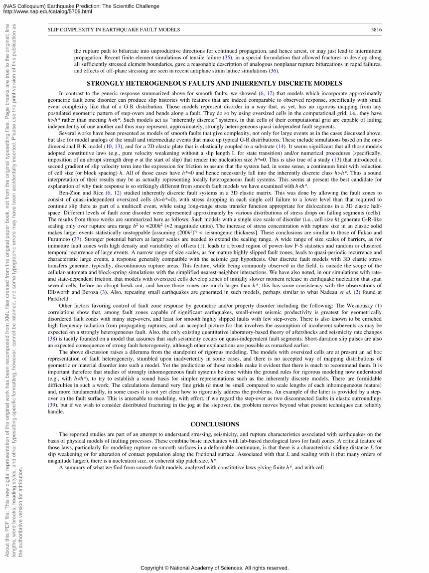
the rupture path to bifurcate into unproductive directions for continued propagation, and hence arrest, or may just lead to intermittentpropagation. Recent finite-element simulations of tensile failure (35), in a special formulation that allowed fractures to develop alongall sufficiently stressed element boundaries, gave a reasonable description of analogous nonplanar rupture bifurcations in rapid failures,and effects of off-plane stressing are seen in recent antiplane strain lattice simulations (36).
STRONGLY HETEROGENEOUS FAULTS AND INHERENTLY DISCRETE MODELS
In contrast to the generic response summarized above for smooth faults, we showed (6, 12) that models which incorporate approximatelygeometric fault zone disorder can produce slip histories with features that are indeed comparable to observed response, specifically with smallevent complexity like that of a G-R distribution. Those models represent disorder in a way that, as yet, has no rigorous mapping from anypostulated geometric pattern of step-overs and bends along a fault. They do so by using oversized cells in the computational grid, i.e., they haveh>h* rather than meeting h�h*. Such models act as “inherently discrete” systems, in that cells of their computational grid are capable of failingindependently of one another and thus may represent, approximately, strongly heterogeneous quasi-independent fault segments.
Several works have been presented as models of smooth faults that give complexity, not only for large events as in the cases discussed above,but also for model analogs of the small and intermediate events that make up typical G-R distributions. These include simulations based on the one-dimensional B-K model (10, 13), and for a 2D elastic plate that is elastically coupled to a substrate (14). It seems significant that all those modelsadopted constitutive laws (e.g., pure velocity weakening without a slip length L for state transition) and/or numerical procedures (specifically,imposition of an abrupt strength drop σ at the start of slip) that render the nucleation size h*=0. This is also true of a study (13) that introduced asecond gradient of slip velocity term into the expression for friction to assure that the system had, in some sense, a continuum limit with reductionof cell size (or block spacing) h. All of those cases have h*=0 and hence necessarily fall into the inherently discrete class h>h*. Thus a soundinterpretation of their results may be as actually representing locally heterogeneous fault systems. This seems at present the best candidate forexplanation of why their response is so strikingly different from smooth fault models we have examined with h�h*.
Ben-Zion and Rice (6, 12) studied inherently discrete fault systems in a 3D elastic matrix. This was done by allowing the fault zones toconsist of quasi-independent oversized cells (h>h*=0), with stress dropping in each single cell failure to a lower level than that required tocontinue slip there as part of a multicell event, while using long-range stress transfer function appropriate for dislocations in a 3D elastic half-space. Different levels of fault zone disorder were represented approximately by various distributions of stress drops on failing segments (cells).The results from those works are summarized here as follows: Such models with a single size scale of disorder (i.e., cell size h) generate G-R-likescaling only over rupture area range h2 to �200h2 (�2 magnitude units). The increase of stress concentration with rupture size in an elastic solidmakes larger events statistically unstoppable [assuming (200h2)½ < seismogenic thickness]. These conclusions are similar to those of Fukao andFurumoto (37). Stronger potential bariers at larger scales are needed to extend the scaling range. A wide range of size scales of barriers, as forimmature fault zones with high density and variability of offsets (1), leads to a broad region of power-law F-S statistics and random or clusteredtemporal recurrence of large events. A narrow range of size scales, as for mature highly slipped fault zones, leads to quasi-periodic recurrence andcharacteristic large events, a response generally compatible with the seismic gap hypothesis. Our discrete fault models with 3D elastic stresstransfers generate, typically, discontinuous rupture areas. This feature, while being commonly observed in the field, is outside the scope of thecellular-automata and block-spring simulations with the simplified nearest-neighbor interactions. We have also noted, in our simulations with rate-and state-dependent friction, that models with oversized cells develop zones of initially slower moment release in earthquake nucleation that spanseveral cells, before an abrupt break out, and hence those zones are much larger than h*; this has some consistency with the observations ofEllsworth and Beroza (3). Also, repeating small earthquakes are generated in such models, perhaps similar to what Nadeau et al. (2) found atParkfield.
Other factors favoring control of fault zone response by geometric and/or property disorder including the following: The Wesnousky (1)correlations show that, among fault zones capable of significant earthquakes, small-event seismic productivity is greatest for geometricallydisordered fault zones with many step-overs, and least for smooth highly slipped faults with few step-overs. There is also known to be enrichedhigh frequency radiation from propagating ruptures, and an accepted picture for that involves the assumption of incoherent subevents as may beexpected on a strongly heterogeneous fault. Also, the only existing quantitative laboratory-based theory of aftershocks and seismicity rate changes(38) is tacitly founded on a model that assumes that such seismicity occurs on quasi-independent fault segments. Short-duration slip pulses are alsoan expected consequence of strong fault heterogeneity, although other explanations are possible as remarked earlier.
The above discussion raises a dilemma from the standpoint of rigorous modeling. The models with oversized cells are at present an ad hocrepresentation of fault heterogeneity, stumbled upon inadvertently in some cases, and there is no accepted way of mapping distributions ofgeometric or material disorder into such a model. Yet the predictions of those models make it evident that there is much to recommend them. It isimportant therefore that studies of strongly inhomogeneous fault systems be done within the ground rules for rigorous modeling now understood(e.g., with h�h*), to try to establish a sound basis for simpler representations such as the inherently discrete models. There are formidabledifficulties in such a work: The calculations demand very fine grids (h must be small compared to scale lengths of each inhomogeneous feature)and, more fundamentally, in some cases it is not yet clear how to rigorously address the problems. An example of the latter is provided by a step-over on the fault surface. This is amenable to modeling, with effort, if we regard the step-over as two disconnected faults in elastic surroundings(39), but if we wish to consider distributed fracturing in the jog at the stepover, the problem moves beyond what present techniques can reliablyhandle.
CONCLUSIONS
The reported studies are part of an attempt to understand stressing, seismicity, and rupture characteristics associated with earthquakes on thebasis of physical models of faulting processes. These combine basic mechanics with lab-based rheological laws for fault zones. A critical feature ofthose laws, particularly for modeling rupture on smooth surfaces in a deformable continuum, is that there is a characteristic sliding distance L forslip weakening or for alteration of contact population along the frictional surface. Associated with that L and scaling with it (but many orders ofmagnitude larger), there is a nucleation size, or coherent slip patch size, h*.
A summary of what we find from smooth fault models, analyzed with constitutive laws giving finite h*, and with cell
SLIP COMPLEXITY IN EARTHQUAKE FAULT MODELS 3816
Abou
t thi
s PD
F fil
e: T
his
new
dig
ital r
epre
sent
atio
n of
the
orig
inal
wor
k ha
s be
en re
com
pose
d fro
m X
ML
files
cre
ated
from
the
orig
inal
pap
er b
ook,
not
from
the
orig
inal
type
setti
ng fi
les.
Pag
e br
eaks
are
true
to th
e or
igin
al; l
ine
leng
ths,
wor
d br
eaks
, hea
ding
sty
les,
and
oth
er ty
pese
tting
-spe
cific
form
attin
g, h
owev
er, c
anno
t be
reta
ined
, and
som
e ty
pogr
aphi
c er
rors
may
hav
e be
en a
ccid
enta
lly in
serte
d. P
leas
e us
e th
e pr
int v
ersi
on o
f thi
s pu
blic
atio
n as
the
auth
orita
tive
vers
ion
for a
ttrib
utio
n.
Copyright © National Academy of Sciences. All rights reserved.
(NAS Colloquium) Earthquake Prediction: The Scientific Challengehttp://www.nap.edu/catalog/5709.html
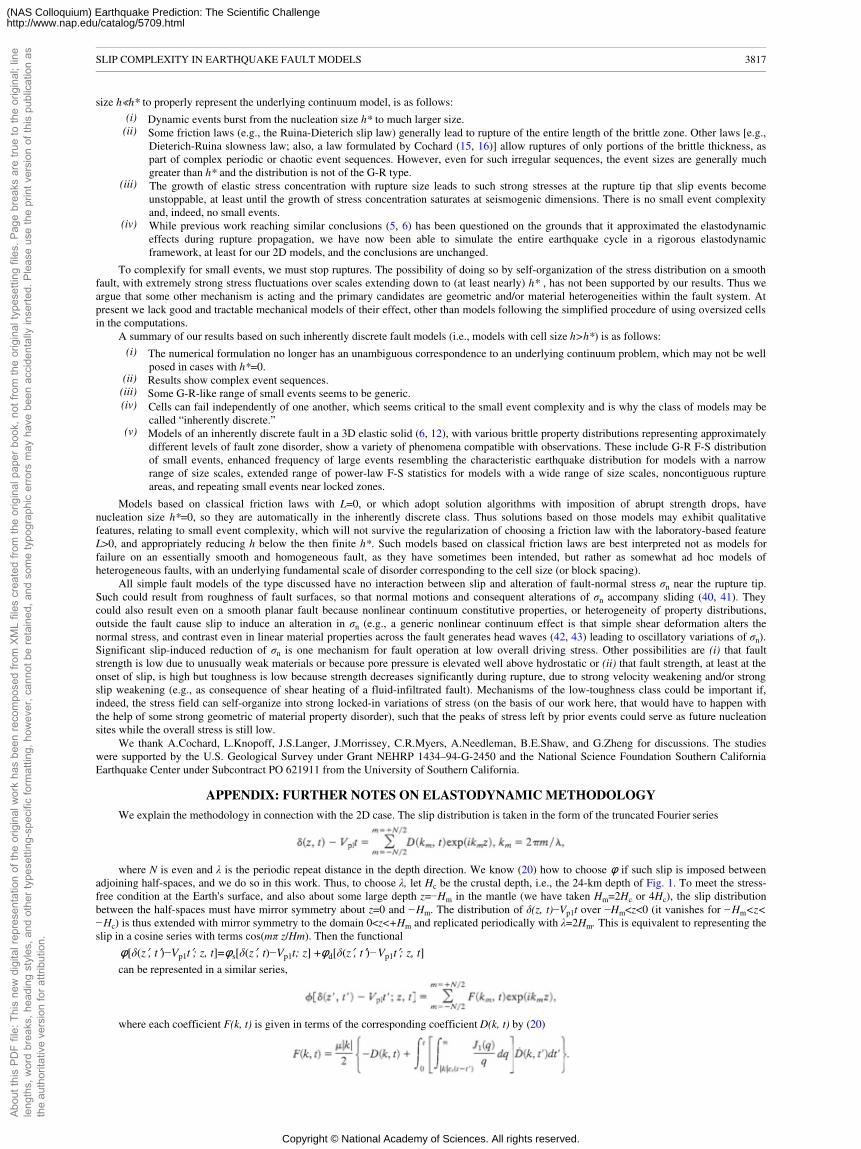
size h�h* to properly represent the underlying continuum model, is as follows:(i) Dynamic events burst from the nucleation size h* to much larger size.
(ii) Some friction laws (e.g., the Ruina-Dieterich slip law) generally lead to rupture of the entire length of the brittle zone. Other laws [e.g.,Dieterich-Ruina slowness law; also, a law formulated by Cochard (15, 16)] allow ruptures of only portions of the brittle thickness, aspart of complex periodic or chaotic event sequences. However, even for such irregular sequences, the event sizes are generally muchgreater than h* and the distribution is not of the G-R type.
(iii) The growth of elastic stress concentration with rupture size leads to such strong stresses at the rupture tip that slip events becomeunstoppable, at least until the growth of stress concentration saturates at seismogenic dimensions. There is no small event complexityand, indeed, no small events.
(iv) While previous work reaching similar conclusions (5, 6) has been questioned on the grounds that it approximated the elastodynamiceffects during rupture propagation, we have now been able to simulate the entire earthquake cycle in a rigorous elastodynamicframework, at least for our 2D models, and the conclusions are unchanged.
To complexify for small events, we must stop ruptures. The possibility of doing so by self-organization of the stress distribution on a smoothfault, with extremely strong stress fluctuations over scales extending down to (at least nearly) h* , has not been supported by our results. Thus weargue that some other mechanism is acting and the primary candidates are geometric and/or material heterogeneities within the fault system. Atpresent we lack good and tractable mechanical models of their effect, other than models following the simplified procedure of using oversized cellsin the computations.
A summary of our results based on such inherently discrete fault models (i.e., models with cell size h>h*) is as follows:(i) The numerical formulation no longer has an unambiguous correspondence to an underlying continuum problem, which may not be well
posed in cases with h*=0.(ii) Results show complex event sequences.
(iii) Some G-R-like range of small events seems to be generic.(iv) Cells can fail independently of one another, which seems critical to the small event complexity and is why the class of models may be
called “inherently discrete.”(v) Models of an inherently discrete fault in a 3D elastic solid (6, 12), with various brittle property distributions representing approximately
different levels of fault zone disorder, show a variety of phenomena compatible with observations. These include G-R F-S distributionof small events, enhanced frequency of large events resembling the characteristic earthquake distribution for models with a narrowrange of size scales, extended range of power-law F-S statistics for models with a wide range of size scales, noncontiguous ruptureareas, and repeating small events near locked zones.
Models based on classical friction laws with L=0, or which adopt solution algorithms with imposition of abrupt strength drops, havenucleation size h*=0, so they are automatically in the inherently discrete class. Thus solutions based on those models may exhibit qualitativefeatures, relating to small event complexity, which will not survive the regularization of choosing a friction law with the laboratory-based featureL>0, and appropriately reducing h below the then finite h*. Such models based on classical friction laws are best interpreted not as models forfailure on an essentially smooth and homogeneous fault, as they have sometimes been intended, but rather as somewhat ad hoc models ofheterogeneous faults, with an underlying fundamental scale of disorder corresponding to the cell size (or block spacing).
All simple fault models of the type discussed have no interaction between slip and alteration of fault-normal stress σn near the rupture tip.Such could result from roughness of fault surfaces, so that normal motions and consequent alterations of σn accompany sliding (40, 41). Theycould also result even on a smooth planar fault because nonlinear continuum constitutive properties, or heterogeneity of property distributions,outside the fault cause slip to induce an alteration in σn (e.g., a generic nonlinear continuum effect is that simple shear deformation alters thenormal stress, and contrast even in linear material properties across the fault generates head waves (42, 43) leading to oscillatory variations of σn).Significant slip-induced reduction of σn is one mechanism for fault operation at low overall driving stress. Other possibilities are (i) that faultstrength is low due to unusually weak materials or because pore pressure is elevated well above hydrostatic or (ii) that fault strength, at least at theonset of slip, is high but toughness is low because strength decreases significantly during rupture, due to strong velocity weakening and/or strongslip weakening (e.g., as consequence of shear heating of a fluid-infiltrated fault). Mechanisms of the low-toughness class could be important if,indeed, the stress field can self-organize into strong locked-in variations of stress (on the basis of our work here, that would have to happen withthe help of some strong geometric of material property disorder), such that the peaks of stress left by prior events could serve as future nucleationsites while the overall stress is still low.
We thank A.Cochard, L.Knopoff, J.S.Langer, J.Morrissey, C.R.Myers, A.Needleman, B.E.Shaw, and G.Zheng for discussions. The studieswere supported by the U.S. Geological Survey under Grant NEHRP 1434–94-G-2450 and the National Science Foundation Southern CaliforniaEarthquake Center under Subcontract PO 621911 from the University of Southern California.
APPENDIX: FURTHER NOTES ON ELASTODYNAMIC METHODOLOGY
We explain the methodology in connection with the 2D case. The slip distribution is taken in the form of the truncated Fourier series
where N is even and λ is the periodic repeat distance in the depth direction. We know (20) how to choose � if such slip is imposed betweenadjoining half-spaces, and we do so in this work. Thus, to choose λ, let Hc be the crustal depth, i.e., the 24-km depth of Fig. 1. To meet the stress-free condition at the Earth's surface, and also about some large depth z=−Hm in the mantle (we have taken Hm=2Hc or 4Hc), the slip distributionbetween the half-spaces must have mirror symmetry about z=0 and −Hm. The distribution of δ(z, t)−Vp1t over −Hm<z<0 (it vanishes for −Hm<z<−Hc) is thus extended with mirror symmetry to the domain 0<z<+Hm and replicated periodically with λ=2Hm. This is equivalent to representing theslip in a cosine series with terms cos(mπ z/Hm). Then the functional
�[δ(z�, t�)−Vp1t�; z, t]=�s[δ(z�, t)−Vp1t; z] +�d[δ(z�, t�)−Vp1t�; z, t]can be represented in a similar series,
where each coefficient F(k, t) is given in terms of the corresponding coefficient D(k, t) by (20)
SLIP COMPLEXITY IN EARTHQUAKE FAULT MODELS 3817
Abou
t thi
s PD
F fil
e: T
his
new
dig
ital r
epre
sent
atio
n of
the
orig
inal
wor
k ha
s be
en re
com
pose
d fro
m X
ML
files
cre
ated
from
the
orig
inal
pap
er b
ook,
not
from
the
orig
inal
type
setti
ng fi
les.
Pag
e br
eaks
are
true
to th
e or
igin
al; l
ine
leng
ths,
wor
d br
eaks
, hea
ding
sty
les,
and
oth
er ty
pese
tting
-spe
cific
form
attin
g, h
owev
er, c
anno
t be
reta
ined
, and
som
e ty
pogr
aphi
c er
rors
may
hav
e be
en a
ccid
enta
lly in
serte
d. P
leas
e us
e th
e pr
int v
ersi
on o
f thi
s pu
blic
atio
n as
the
auth
orita
tive
vers
ion
for a
ttrib
utio
n.
Copyright © National Academy of Sciences. All rights reserved.
(NAS Colloquium) Earthquake Prediction: The Scientific Challengehttp://www.nap.edu/catalog/5709.html
The first term within the curly brackets corresponds to �s and the second, with the convolution integral, corresponds to �d.We deal with stress and displacement at values of x, z corresponding to FFT sample points, and these values are constrained to be related to
one another to meet the constitutive law. In the 3D spectral implementation, δ(x, z, t) is expanded as a Fourier series in z and x, with vertical period2Hm and mirror symmetries as above, and with horizontal period along strike as noted in Fig. 1. Other formulations (4–6, 8, 12, 25) have beenbased on a cellular basis set for the slip distribution, making it spatially uniform within rectangular cells and enforcing the constitutive law in termsof the stresses at cell centers.
The mirror symmetry condition of the spectral formulation causes the shear-free conditions τzx(x, y, 0, t)=τzy(x, y, 0, t) =0 to be met exactly atthe Earth's surface, and also at z= −Hm. However, the symmetry condition replaces the condition of vanishing normal stress, τzz(x, y, 0, t)=0, at thesurface with vanishing displacement, uz(x, y, 0, t)=0. One condition implies the other in the 2D cases but not in 3D. A number of 3D trial runs withthe quasidynamic procedures, comparing spectral results with uz=0 to those for the cellular slip basis in a formulation meeting τzz=0, have shownno qualitative differences for results with the different boundary conditions. That may be less so with full elastodynamics since the former casedisallows Rayleigh waves on z=0.
The fully elastodynamic results so far available on modeling repeated sequences of earthquakes have used coarse meshes of 64 or 128 FFTsample points through the 24-km thickness. These are zero-padded below 24 km and repeated as images above the earth's surface such that thetotal number of FFT points is 4 or 8 times greater than the basic 64 or 128 points for Hm=2Hc or Hm=4Hc, respectively. The studies of repeatedearthquakes have been done on SPARC10 workstations, whereas the basic spectral elastodynamic methodology (20, 21) was also implemented onthe massively parallel Connection Machine 5 (CM5, available with up to 512 processors). We anticipate that the version of the fully elastodynamicprogram with �s extracted and �d truncated, to deal with long earthquake histories, can be similarly implemented on the CM5 and extended to 3Dfault modeling.1. Wesnousky, S.G. (1994) Bull. Seismol. Soc. Am. 84, 1940–1959.2. Nadeau, R.M., Foxall, W. & McEvilly, T.V. (1995) Science 267, 503–507.3. Ellsworth, W.L. & Beroza, G.C. (1995) Science 268, 851–855.4. Tse, S.T. & Rice, J.R. (1986) J. Geophys. Res. 91, 9452–9472.5. Rice, J.R. (1993) J. Geophys. Res. 98, 9885–9907.6. Ben-Zion, Y. & Rice, J.R. (1995) J. Geophys. Res. 100, 12959– 12983.7. Zoback, M.D., Apel, R., Baumgartner, J., Brudy, M., Emmermann, R., Engeser. B., Fuchs, K., Kessels, W., Rischmuller, H., Rummel, F. & Vernik, L.
(1993) Nature (London) 365, 633–635.8. Stuart, W.D. (1988) Pure Appl Geophys. 126, 619–641.9. Horowitz, F.G. & Ruina, A. (1989) J. Geophys. Res. 94, 10279– 10298.10. Carlson, J.M. & Langer, J.S. (1989) Phys. Rev. A 40, 6470–6484.11. Bak, P. & Tang, C. (1989) J. Geophys. Res. 94, 15635–15637.12. Ben-Zion, Y. & Rice, J.R. (1993) J. Geophys. Res. 98, 14109– 14131.13. Shaw, B.E. (1994) Geophys. Res. Lett. 21, 1983–1986.14. Myers, C.R., Shaw, B.E. & Langer, J.S. (1994) “Slip complexity in a crustal plane model of an earthquake fault”, preprint, Report 94–98, NSF Institute
for Theoretical Physics (Santa Barbara, CA).15. Cochard, A. & Madariaga, R. (1994) EOS Trans. Am. Geophys. Union 75, Suppl. 44, 461 (abstr.).16. Cochard, A., (1995) Ph.D. thesis (University of Paris).17. Rice, J.R. (1994) EOS Trans. Am. Geophys. Union 75, Suppl. 44, 441 (abstr.).18. Rice, J.R. (1994) EOS Trans. Am. Geophys. Union 75, Suppl. 44, 426 (abstr.).19. Blanpied, M.L., Lockner, D.A. & Byerlee, J.D. (1991) Geophys. Res. Lett. 18, 609–612.20. Perrin, G., Rice, J.R. & Zheng, G. (1995) J. Mech. Phys. Solids 43, 1461–1495.21. Geubelle, P. & Rice, J.R. (1995) J. Mech. Phys. Solids 43, 1791–1824.22. Das, S. (1980) Geophys. J.R.Astron. Soc. 62, 591–604.23. Andrews, D.J. (1985) Bull. Seismol. Soc. Am. 75, 1–21.24. Das, S. & Kostrov, B.V. (1987) J. Appl. Mech. 54, 99–104.25. Cochard, A. & Madariaga, R. (1994) Pure Appl. Geophys. 142, 419–445.26. Beeler, N., Tullis, T.E. & Weeks, J.D. (1994) Geophys. Res. Lett. 21, 1987–1990.27. Chester, F.M. & Higgs, N. (1992) J. Geophys. Res. 97, 1859–1870.28. Reinen, L.A., Tullis, T.E. & Weeks, J.D. (1992) Geophys. Res. Lett. 19, 1535–1538.29. Sleep, N.H. & Blanpied, M.L. (1992) Nature (London) 359, 687–692.30. Segall, P. & Rice, J.R. (1995) J. Geophys. Res. 100, 22155–22171.31. Madariaga, R. & Cochard, A. (1994) Ann. Geofis. 37, 1349–1375.32. Beeler, N.M. & Tullis, T.E. (1995) Bull Seismol. Soc. Am., in press.33. Heaton, T.H. (1990) Phys. Earth Planet. Inter. 64, 1–20.34. Rice, J.R. (1980) in Physics of the Earth's Interior, eds, Dziewonski, A.M. & Boschi, E. (North-Holland, Amsterdam), pp. 555– 649.35. Xu, X.P. & Needleman, A. (1994) J. Mech. Phys. Solids 42, 1397–1434.36. Marder, M. & Gross, S. (1995) J. Mech. Phys. Solids 43, 1–48.37. Fukao, Y. & Furumoto, M. (1985) Phys. Earth Planet. Inter. 37, 149–168.38. Dieterich, J. (1994) J. Geophys. Res. 99, 2601–2618.39. Harris, R. & Day, S.M. (1993) J. Geophys. Res. 98, 4461–4472.40. Lomnitz-Adler, J. (1991) J. Geophys. Res. 96, 6121–6131.41. Brune, J.N., Brown, S. & Johnson, P.A. (1993) Tectonophysics 218, 59–67.42. Ben-Zion, Y. (1990) Geophys. J. Int. 101, 507–528.43. Ben-Zion, Y. & Malin, P. (1991) Science 251, 1592–1594.44. Zheng, G., Ben-Zion, Y., Rice, J.R. & Morrissey, J. (1995) EOS Trans. Am. Geophys. Union 76, Suppl. 46, 405 (abstr.).
SLIP COMPLEXITY IN EARTHQUAKE FAULT MODELS 3818
Abou
t thi
s PD
F fil
e: T
his
new
dig
ital r
epre
sent
atio
n of
the
orig
inal
wor
k ha
s be
en re
com
pose
d fro
m X
ML
files
cre
ated
from
the
orig
inal
pap
er b
ook,
not
from
the
orig
inal
type
setti
ng fi
les.
Pag
e br
eaks
are
true
to th
e or
igin
al; l
ine
leng
ths,
wor
d br
eaks
, hea
ding
sty
les,
and
oth
er ty
pese
tting
-spe
cific
form
attin
g, h
owev
er, c
anno
t be
reta
ined
, and
som
e ty
pogr
aphi
c er
rors
may
hav
e be
en a
ccid
enta
lly in
serte
d. P
leas
e us
e th
e pr
int v
ersi
on o
f thi
s pu
blic
atio
n as
the
auth
orita
tive
vers
ion
for a
ttrib
utio
n.
Copyright © National Academy of Sciences. All rights reserved.
(NAS Colloquium) Earthquake Prediction: The Scientific Challengehttp://www.nap.edu/catalog/5709.html
This paper was presented at a colloquium entitled “Earthquake Prediction: The Scientific Challenge,” organized by Leon Knopoff(Chair), Keiiti Aki, Clarence R.Allen, James R.Rice, and Lynn R.Sykes, held February 10 and 11, 1995, at the National Academy of Sciences inIrvine, CA
Dynamic friction and the origin of the complexity of earthquakesources
RAÚL MADARIAGA* AND ALAIN COCHARD
Département de Sismologie, Centre National de la Recherche Scientifique Unite Associée 195, Institut de Physique du Globe de Paris etUniversité Paris 7, case 89, 4 Place Jussieu, 75252 Paris Cedex 05, France
ABSTRACT We study a simple antiplane fault of finite length embedded in a homogeneous isotropic elastic solid to understand theorigin of seismic source heterogeneity in the presence of nonlinear rate- and state-dependent friction. All the mechanical properties of themedium and friction are assumed homogeneous. Friction includes a characteristic length that is longer than the grid size so that ourmodels have a well-defined continuum limit. Starting from a heterogeneous initial stress distribution, we apply a slowly increasinguniform stress load far from the fault and we simulate the seismicity for a few 1000 events. The style of seismicity produced by this modelis determined by a control parameter associated with the degree of rate dependence of friction. For classical friction models with rate-independent friction, no complexity appears and seismicity is perfectly periodic. For weakly rate-dependent friction, large ruptures arestill periodic, but small seismicity becomes increasingly nonstationary. When friction is highly rate-dependent, seismicity becomesnonperiodic and ruptures of all sizes occur inside the fault. Highly rate-dependent friction destabilizes the healing process producingpremature healing of slip and partial stress drop. Partial stress drop produces large variations in the state of stress that in turn produceearthquakes of different sizes. Similar results have been found by other authors using the Burridge and Knopoff model. We conjecturethat all models in which static stress drop is only a fraction of the dynamic stress drop produce stress heterogeneity.
A fundamental problem for understanding seismicity and the nature of large earthquakes is the origin of stress and slip complexity on seismicfaults. Although seismicity has been carefully studied, the dynamics of the observed complexity of seismic sources is poorly understood although itis generally considered to be mainly due to fault segmentation. Initial work on seismic source dynamics (1–3) was derived from models of mode Ifracture. In mode I, residual stress after opening a crack is obviously zero. This assumption had the virtue of simplifying the solution of the crackproblems and allowed us to calculate radiation (4) and compare it with empirical models of radiation (5). At the end of the 1970s, the first modelsof complexity (asperities and barriers) were proposed but their relation to seismicity was not explored (6–8). A fundamental question that was leftunanswered in these models was how do asperities arise on a fault loaded by very slow tectonic forces? According to current models, asperities aredue to preseismic slip and foreshocks that concentrate stresses on locked areas of the fault; so that it is not enough to consider individual events,but the complete seismicity of the fault before a large event has to be studied in detail. To do this we have to specify the state of stress before andafter an earthquake. In most of the previous work on earthquake dynamics as reviewed by Kostrov and Das (9), it was invariably assumed thatresidual stress after any event was uniform and equal to zero. This is very unlikely as we have attempted to show in our recent work (10, 11).
The question of the origin of complexity was posed from a completely different point of view by research on self-organized criticality (12),and on the artificial seismicity of the box and spring model of Burridge and Knopoff (13–18). These studies suggested that stress and slip wouldbecome spontaneously heterogeneous because of nonlinear instabilities in the mechanical model of a frictional fault. These results led to aninteresting controversy because quasi-static models studied by Rice using the experimentally derived friction laws by Dieterich (19, 20) and Ruina(21) did not give rise to any significant heterogeneity. Rice and coworkers (22, 23) suggested that heterogeneity may be due to the lack of acontinuum limit of some of these models.
Without waiting for the clarification of nature of heterogeneity of problems for the Burridge and Knopoff models, we started a study of asimple antiplane fault model (10, 11) where the only change with respect to Kostrov's original formulation (3) was that the friction law wasassumed to be rate dependent, as suggested by Carlson and Langer (14). In the present paper, we present results for a simple fault with rate-dependent friction that has been regularized at small scales by using a slip-weakening zone (24). We will demonstrate that depending on the valueof a single parameter that measures the rate dependence of friction, we either produce complexity or suppress it. We are of course quite aware thatour fault models are very crude and lack many complexities of actual faults; yet some of them have a large number of the features observed inactual seismicity including slip and stress complexity, events of many different sizes, variable recurrence times, etc.
DEFINITION OF THE MODEL
Let us consider, as in Fig. 1, a two-dimensional antiplane crack of length 2L embedded in a linear elastic medium of elastic constant µ andmass density ρ. The elastic medium is subject to a slowly increasing uniform shear stress σyz(x, y, t)=Te(t), due to slow plate motion or intraplatedeformation. As the external stress, Te(t), increases with time, the frictional resistance to slip between the walls of the fault is eventually overcome,and slip occurs. The amount of slip and the history of slip on the fault depends on the nonlinear friction law that relates shear stress transmittedacross the fault T(x, 0, t), to slip D(x, 0, t), slip velocity V(x, 0, t)=` (x, 0, t), and possibly to certain state variables θi(x, 0, t). The exact nature of this
The publication costs of this article were defrayed in part by page charge payment. This article must therefore be hereby marked“advertisement” in accordance with 18 U.S.C. §1734 solely t indicate this fact.
*To whom reprints requests should be addressed.
DYNAMIC FRICTION AND THE ORIGIN OF THE COMPLEXITY OF EARTHQUAKE SOURCES 3819
Abou
t thi
s PD
F fil
e: T
his
new
dig
ital r
epre
sent
atio
n of
the
orig
inal
wor
k ha
s be
en re
com
pose
d fro
m X
ML
files
cre
ated
from
the
orig
inal
pap
er b
ook,
not
from
the
orig
inal
type
setti
ng fi
les.
Pag
e br
eaks
are
true
to th
e or
igin
al; l
ine
leng
ths,
wor
d br
eaks
, hea
ding
sty
les,
and
oth
er ty
pese
tting
-spe
cific
form
attin
g, h
owev
er, c
anno
t be
reta
ined
, and
som
e ty
pogr
aphi
c er
rors
may
hav
e be
en a
ccid
enta
lly in
serte
d. P
leas
e us
e th
e pr
int v
ersi
on o
f thi
s pu
blic
atio
n as
the
auth
orita
tive
vers
ion
for a
ttrib
utio
n.
Copyright © National Academy of Sciences. All rights reserved.
(NAS Colloquium) Earthquake Prediction: The Scientific Challengehttp://www.nap.edu/catalog/5709.html
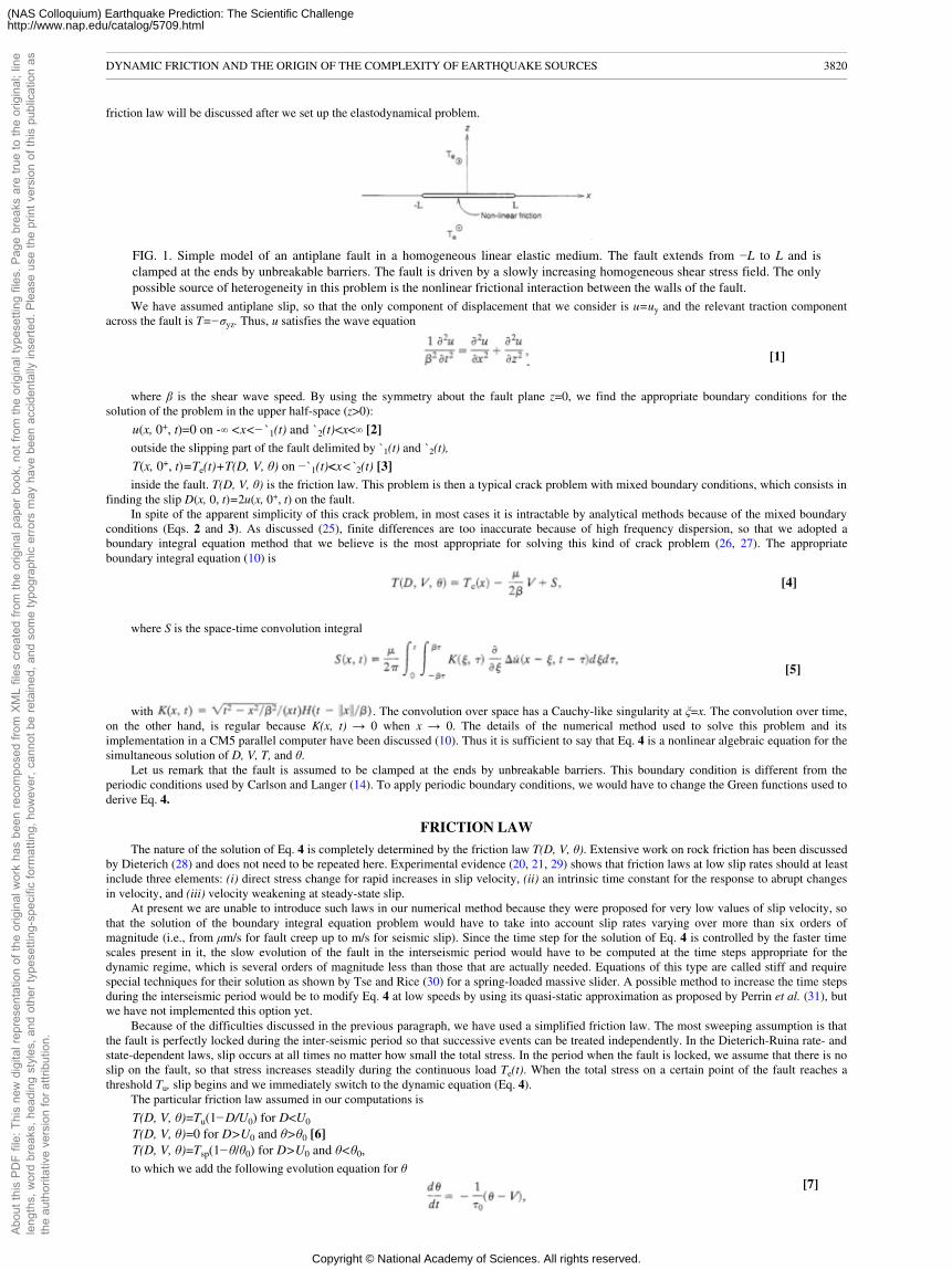
friction law will be discussed after we set up the elastodynamical problem.
FIG. 1. Simple model of an antiplane fault in a homogeneous linear elastic medium. The fault extends from −L to L and isclamped at the ends by unbreakable barriers. The fault is driven by a slowly increasing homogeneous shear stress field. The onlypossible source of heterogeneity in this problem is the nonlinear frictional interaction between the walls of the fault.We have assumed antiplane slip, so that the only component of displacement that we consider is u=uy and the relevant traction component
across the fault is T=−σyz. Thus, u satisfies the wave equation
[1]
where β is the shear wave speed. By using the symmetry about the fault plane z=0, we find the appropriate boundary conditions for thesolution of the problem in the upper half-space (z>0):
u(x, 0+, t)=0 on -� <x<−`1(t) and `2(t)<x<� [2]outside the slipping part of the fault delimited by `1(t) and `2(t),
T(x, 0+, t)=Te(t)+T(D, V, θ) on −`1(t)<x<`2(t) [3]inside the fault. T(D, V, θ) is the friction law. This problem is then a typical crack problem with mixed boundary conditions, which consists in
finding the slip D(x, 0, t)=2u(x, 0+, t) on the fault.In spite of the apparent simplicity of this crack problem, in most cases it is intractable by analytical methods because of the mixed boundary
conditions (Eqs. 2 and 3). As discussed (25), finite differences are too inaccurate because of high frequency dispersion, so that we adopted aboundary integral equation method that we believe is the most appropriate for solving this kind of crack problem (26, 27). The appropriateboundary integral equation (10) is
[4]
where S is the space-time convolution integral
[5]
with . The convolution over space has a Cauchy-like singularity at ξ=x. The convolution over time,on the other hand, is regular because K(x, t) → 0 when x → 0. The details of the numerical method used to solve this problem and itsimplementation in a CM5 parallel computer have been discussed (10). Thus it is sufficient to say that Eq. 4 is a nonlinear algebraic equation for thesimultaneous solution of D, V, T, and θ.
Let us remark that the fault is assumed to be clamped at the ends by unbreakable barriers. This boundary condition is different from theperiodic conditions used by Carlson and Langer (14). To apply periodic boundary conditions, we would have to change the Green functions used toderive Eq. 4.
FRICTION LAW
The nature of the solution of Eq. 4 is completely determined by the friction law T(D, V, θ). Extensive work on rock friction has been discussedby Dieterich (28) and does not need to be repeated here. Experimental evidence (20, 21, 29) shows that friction laws at low slip rates should at leastinclude three elements: (i) direct stress change for rapid increases in slip velocity, (ii) an intrinsic time constant for the response to abrupt changesin velocity, and (iii) velocity weakening at steady-state slip.
At present we are unable to introduce such laws in our numerical method because they were proposed for very low values of slip velocity, sothat the solution of the boundary integral equation problem would have to take into account slip rates varying over more than six orders ofmagnitude (i.e., from µm/s for fault creep up to m/s for seismic slip). Since the time step for the solution of Eq. 4 is controlled by the faster timescales present in it, the slow evolution of the fault in the interseismic period would have to be computed at the time steps appropriate for thedynamic regime, which is several orders of magnitude less than those that are actually needed. Equations of this type are called stiff and requirespecial techniques for their solution as shown by Tse and Rice (30) for a spring-loaded massive slider. A possible method to increase the time stepsduring the interseismic period would be to modify Eq. 4 at low speeds by using its quasi-static approximation as proposed by Perrin et al. (31), butwe have not implemented this option yet.
Because of the difficulties discussed in the previous paragraph, we have used a simplified friction law. The most sweeping assumption is thatthe fault is perfectly locked during the inter-seismic period so that successive events can be treated independently. In the Dieterich-Ruina rate- andstate-dependent laws, slip occurs at all times no matter how small the total stress. In the period when the fault is locked, we assume that there is noslip on the fault, so that stress increases steadily during the continuous load Te(t). When the total stress on a certain point of the fault reaches athreshold Tu, slip begins and we immediately switch to the dynamic equation (Eq. 4).
The particular friction law assumed in our computations is
T(D, V, θ)=Tu(1−D/U0) for D<U0
T(D, V, θ)=0 for D>U0 and θ>θ0 [6]T(D, V, θ)=Tsp(1−θ/θ0) for D>U0 and θ<θ0,to which we add the following evolution equation for θ
[7]
DYNAMIC FRICTION AND THE ORIGIN OF THE COMPLEXITY OF EARTHQUAKE SOURCES 3820
Abou
t thi
s PD
F fil
e: T
his
new
dig
ital r
epre
sent
atio
n of
the
orig
inal
wor
k ha
s be
en re
com
pose
d fro
m X
ML
files
cre
ated
from
the
orig
inal
pap
er b
ook,
not
from
the
orig
inal
type
setti
ng fi
les.
Pag
e br
eaks
are
true
to th
e or
igin
al; l
ine
leng
ths,
wor
d br
eaks
, hea
ding
sty
les,
and
oth
er ty
pese
tting
-spe
cific
form
attin
g, h
owev
er, c
anno
t be
reta
ined
, and
som
e ty
pogr
aphi
c er
rors
may
hav
e be
en a
ccid
enta
lly in
serte
d. P
leas
e us
e th
e pr
int v
ersi
on o
f thi
s pu
blic
atio
n as
the
auth
orita
tive
vers
ion
for a
ttrib
utio
n.
Copyright © National Academy of Sciences. All rights reserved.
(NAS Colloquium) Earthquake Prediction: The Scientific Challengehttp://www.nap.edu/catalog/5709.html
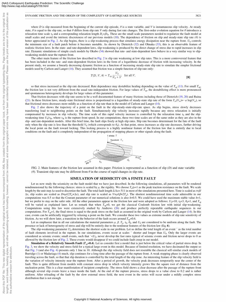
where D is slip measured from the beginning of the current slip episode, θ is a state variable, and V is instantaneous slip velocity. At steadystate, θ is equal to the slip rate, so that θ differs from slip rate V only during fast rate changes. The first-order evolution equation for θ introduces arelaxation time scale τ0 and a corresponding relaxation length Dc=βτ0. These are the small scale parameters needed to regularize the fault model atsmall scales and avoid the intrinsic discreteness of our previous models (10). The dependence of friction on slip and steady-state slip rate (θ) isbetter appreciated in Fig. 2. As slip begins, there is a slip-weakening process that simulates energy dissipation near the rupture front. U0 controlsthe minimum size of a fault patch before it becomes unstable. As shown by Dieterich (32) and Ohnaka (33), this is an observable feature ofrealistic friction laws. In the state- and rate-dependent laws, slip-weakening is produced by the direct change of stress due to rapid increases in sliprate. Dynamic simulations of simple crack models by Okubo (34) showed that rate- and state-dependent laws behave in a very similar way to slip-weakening models near the rupture front.
The other main feature of the friction law described in Fig. 2 is slip rate weakening at low slip rates. This is a more controversial feature thathas been included in the rate- and state-dependent friction laws in the form of a logarithmic decrease of friction with increasing velocity. In thepresent study, we assume a linearly decreasing dynamic friction as a function of increasing steady-state slip rate to simulate the simpler frictionalmodels used by Carlson and Langer (14). They assumed that friction was a simple function of slip rate only:
[8]
so that stress increased as the slip rate decreased. Rate dependence may destabilize healing depending on the value of Tsp (11). For small Tsp,the friction law is not very different from the usual rate-independent friction. For large values of Tsp, the destabilizing effect is more pronouncedand spontaneous heterogeneity develops for large values of this parameter.
That friction decreases with slip rate seems to be a well documented feature of many frictions including those of Dieterich (19, 20) and Ruina(21). In these friction laws, steady-state frictional stress is proportional to a logarithm of steady-state slip rate of the form Tss(Vss)=−a log(Vss), sothat frictional stress decreases more mildly as a function of slip rate than in the model of Carlson and Langer (14).
Fig. 2 also shows the trajectory of a point on the fault in the slip-steady-state-slip-rate space. As slip begins, stress slowly decreasestransferring load to neighboring points on the fault. Simultaneously slip velocity increases rapidly because any stress relaxation is initiallycompensated by increases in slip velocity. The time scale of this rapid velocity increase is controlled by the relaxation time τ0 and the slip-weakening time U0/vR, where vR is the rupture front speed. In our computations, these two time scales are of the same order as they are also in theslip- and rate-dependent models. After this brief time, the fault slips freely at high slip rates. Slip rate becomes determinant for the fate of the faultonly when the slip rate is less than the threshold V0 (which corresponds to θ0). At that point, stress increases as slip rate decreases, further drivingthe local point on the fault toward locking. This locking process is a highly nonlinear feature of the friction law that is entirely due to localconditions on the fault and is completely independent of the propagation of stopping phases or other signals along the fault.
FIG. 2. Main features of the friction law assumed in this paper. Friction is represented as a function of slip (D) and state variable(θ). Transient slip rate may be different from θ in the course of rapid changes in slip rate.
SIMULATION OF SEISMICITY ON A FINITE FAULT
Let us now study the seismicity on the fault model that we have just described. In the following simulations, all parameters will be renderednondimensional by the following choices: stress is scaled by µ, the rigidity. We choose Tu/µ=1 as the peak traction resistance on the fault. We scalelength by the unit step ∆x used to discretize the fault. The total fault length L/∆x= 511 in most of the simulations presented here. Time is scaled as t×β/∆x, slip scales are scaled as D×µ/(2Tu×∆x), and slip rate is scaled as V×µ/(β×2Tu). The shortest nondimensional time scale admissible in ourcomputations was 0.5 so that the Courant parameter of our numerical solutions is also h=0.5. We could have used the maximum stable value h=1,but we prefer to stay on the safer side. All the other parameters appear in the friction law and were adopted as follows: U0=10, τ0=3, θ0=1, and Tspwill be varied as explained later. Let us remark that when Tsp=0, we get the classical Coulomb friction law with initial slip-weakening.Computations using this law were extensively studied by Andrews (26) and produce perfectly repeatable earthquake sequences in ourcomputations. For Tsp=1, the final stress is equal to the peak stress on the fault as assumed in the original work by Carlson and Langer (14). In thiscase, events can be artificially triggered by relaxing a point on the fault. We consider these two values as extreme models of slip rate sensitivity offriction. As we will show later, a transition in the behavior of the fault occurs around Tsp=0.6.
Let us emphasize that in all our calculations the material parameters µ, β, Tu, τ0, θ0, and U0 are considered to be uniform along the fault. Thepresence or lack of heterogeneity of stress and slip will be entirely due to the nonlinear features of the friction law (Eq. 6).
The slip-weakening parameter U0 determines the shortest scale in our problem. Let us define the total length of an event ` as the total numberof fault elements involved in the rupture. In our simulations, events occur at scales ` shorter and longer than U0. Only the larger events areconsidered as seismic events; small events, such that `<U0, never develop the fast rates typical of seismic events and friction never drops to 0 asallowed by the friction law of Fig. 2. These events would disappear if we could include fault creep in our model.
Simulation of a Relatively Smooth Fault (Tsp=0.4). Let us consider first a model that is just below the critical value of partial stress drop. InFig. 3, we show the velocity and stress field for a typical large event in this model. Because of limited resolution, we have decimated the output sothat Fig. 3 (and also Fig. 4) presents only 1 line in 10. Although the slip velocity field does not resemble the classical self-similar crack models ofBurridge (1) or Madariaga (4) much, slip continues for a long time after the passage of the rupture front. A weak stopping phase is clearly observedtraveling across the fault, so that that slip duration is controlled by the total length of the slip zone. An interesting feature of the slip velocity field isthe variation of velocity intensity near the rupture front. After a period of growth, the velocity peak decreases temporarily near the center of thefault. This is quite different from models with constant stress drop in which velocity intensity grows like the square root of distance from thenucleation point. This is a clear manifestation of incipient complexity. The stress field shows a clear decrease after the passage of the rupture frontalthough several slip events leave a trace inside the fault. At the end of the rupture process, stress drops to a value close to 0.2 and is ratheruniform. After reloading of the fault by the slow external stress field, the next event in the series will occur under a mildly complex stressdistribution that is not enough
DYNAMIC FRICTION AND THE ORIGIN OF THE COMPLEXITY OF EARTHQUAKE SOURCES 3821
Abou
t thi
s PD
F fil
e: T
his
new
dig
ital r
epre
sent
atio
n of
the
orig
inal
wor
k ha
s be
en re
com
pose
d fro
m X
ML
files
cre
ated
from
the
orig
inal
pap
er b
ook,
not
from
the
orig
inal
type
setti
ng fi
les.
Pag
e br
eaks
are
true
to th
e or
igin
al; l
ine
leng
ths,
wor
d br
eaks
, hea
ding
sty
les,
and
oth
er ty
pese
tting
-spe
cific
form
attin
g, h
owev
er, c
anno
t be
reta
ined
, and
som
e ty
pogr
aphi
c er
rors
may
hav
e be
en a
ccid
enta
lly in
serte
d. P
leas
e us
e th
e pr
int v
ersi
on o
f thi
s pu
blic
atio
n as
the
auth
orita
tive
vers
ion
for a
ttrib
utio
n.
Copyright © National Academy of Sciences. All rights reserved.
(NAS Colloquium) Earthquake Prediction: The Scientific Challengehttp://www.nap.edu/catalog/5709.html
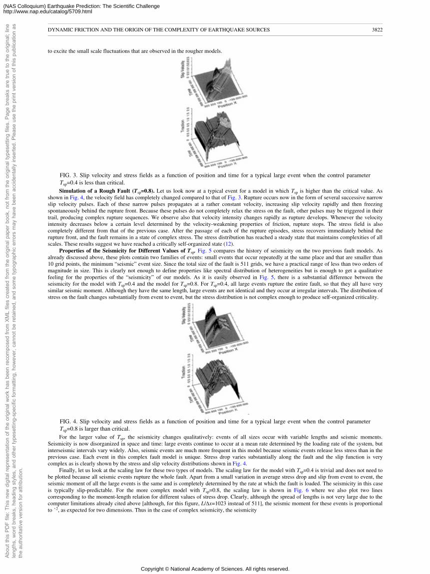
to excite the small scale fluctuations that are observed in the rougher models.
FIG. 3. Slip velocity and stress fields as a function of position and time for a typical large event when the control parameterTsp=0.4 is less than critical.Simulation of a Rough Fault (Tsp=0.8). Let us look now at a typical event for a model in which Tsp is higher than the critical value. As
shown in Fig. 4, the velocity field has completely changed compared to that of Fig. 3. Rupture occurs now in the form of several successive narrowslip velocity pulses. Each of these narrow pulses propagates at a rather constant velocity, increasing slip velocity rapidly and then freezingspontaneously behind the rupture front. Because these pulses do not completely relax the stress on the fault, other pulses may be triggered in theirtrail, producing complex rupture sequences. We observe also that velocity intensity changes rapidly as rupture develops. Whenever the velocityintensity decreases below a certain level determined by the velocity-weakening properties of friction, rupture stops. The stress field is alsocompletely different from that of the previous case. After the passage of each of the rupture episodes, stress recovers immediately behind therupture front, and the fault remains in a state of complex stress. The stress distribution has reached a steady state that maintains complexities of allscales. These results suggest we have reached a critically self-organized state (12).
Properties of the Seismicity for Different Values of Tsp. Fig. 5 compares the history of seismicity on the two previous fault models. Asalready discussed above, these plots contain two families of events: small events that occur repeatedly at the same place and that are smaller than10 grid points, the minimum “seismic” event size. Since the total size of the fault is 511 grids, we have a practical range of less than two orders ofmagnitude in size. This is clearly not enough to define properties like spectral distribution of heterogeneities but is enough to get a qualitativefeeling for the properties of the “seismicity” of our models. As it is easily observed in Fig. 5, there is a substantial difference between theseismicity for the model with Tsp=0.4 and the model for Tsp=0.8. For Tsp=0.4, all large events rupture the entire fault, so that they all have verysimilar seismic moment. Although they have the same length, large events are not identical and they occur at irregular intervals. The distribution ofstress on the fault changes substantially from event to event, but the stress distribution is not complex enough to produce self-organized criticality.
FIG. 4. Slip velocity and stress fields as a function of position and time for a typical large event when the control parameterTsp=0.8 is larger than critical.For the larger value of Tsp, the seismicity changes qualitatively: events of all sizes occur with variable lengths and seismic moments.
Seismicity is now disorganized in space and time: large events continue to occur at a mean rate determined by the loading rate of the system, butinterseismic intervals vary widely. Also, seismic events are much more frequent in this model because seismic events release less stress than in theprevious case. Each event in this complex fault model is unique. Stress drop varies substantially along the fault and the slip function is verycomplex as is clearly shown by the stress and slip velocity distributions shown in Fig. 4.
Finally, let us look at the scaling law for these two types of models. The scaling law for the model with Tsp=0.4 is trivial and does not need tobe plotted because all seismic events rupture the whole fault. Apart from a small variation in average stress drop and slip from event to event, theseismic moment of all the large events is the same and is completely determined by the rate at which the fault is loaded. The seismicity in this caseis typically slip-predictable. For the more complex model with Tsp=0.8, the scaling law is shown in Fig. 6 where we also plot two linescorresponding to the moment-length relation for different values of stress drop. Clearly, although the spread of lengths is not very large due to thecomputer limitations already cited above [although, for this figure, L/∆x=1023 instead of 511], the seismic moment for these events is proportionalto `2, as expected for two dimensions. Thus in the case of complex seismicity, the seismicity
DYNAMIC FRICTION AND THE ORIGIN OF THE COMPLEXITY OF EARTHQUAKE SOURCES 3822
Abou
t thi
s PD
F fil
e: T
his
new
dig
ital r
epre
sent
atio
n of
the
orig
inal
wor
k ha
s be
en re
com
pose
d fro
m X
ML
files
cre
ated
from
the
orig
inal
pap
er b
ook,
not
from
the
orig
inal
type
setti
ng fi
les.
Pag
e br
eaks
are
true
to th
e or
igin
al; l
ine
leng
ths,
wor
d br
eaks
, hea
ding
sty
les,
and
oth
er ty
pese
tting
-spe
cific
form
attin
g, h
owev
er, c
anno
t be
reta
ined
, and
som
e ty
pogr
aphi
c er
rors
may
hav
e be
en a
ccid
enta
lly in
serte
d. P
leas
e us
e th
e pr
int v
ersi
on o
f thi
s pu
blic
atio
n as
the
auth
orita
tive
vers
ion
for a
ttrib
utio
n.
Copyright © National Academy of Sciences. All rights reserved.
(NAS Colloquium) Earthquake Prediction: The Scientific Challengehttp://www.nap.edu/catalog/5709.html
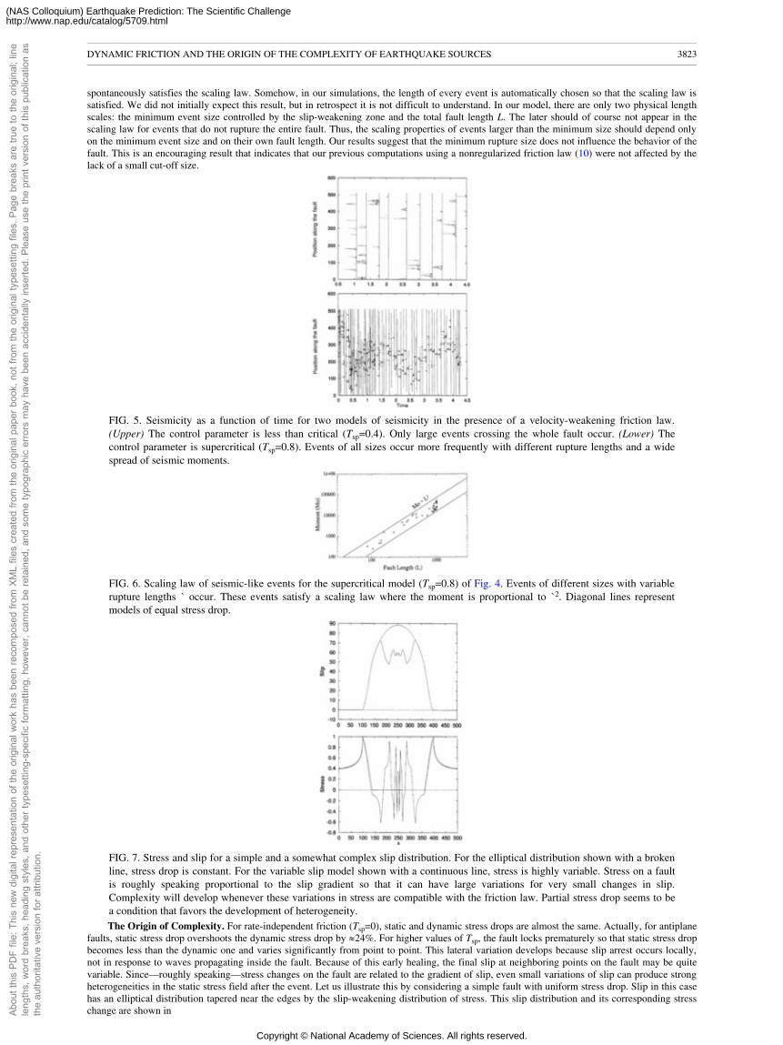
spontaneously satisfies the scaling law. Somehow, in our simulations, the length of every event is automatically chosen so that the scaling law issatisfied. We did not initially expect this result, but in retrospect it is not difficult to understand. In our model, there are only two physical lengthscales: the minimum event size controlled by the slip-weakening zone and the total fault length L. The later should of course not appear in thescaling law for events that do not rupture the entire fault. Thus, the scaling properties of events larger than the minimum size should depend onlyon the minimum event size and on their own fault length. Our results suggest that the minimum rupture size does not influence the behavior of thefault. This is an encouraging result that indicates that our previous computations using a nonregularized friction law (10) were not affected by thelack of a small cut-off size.
FIG. 5. Seismicity as a function of time for two models of seismicity in the presence of a velocity-weakening friction law.(Upper) The control parameter is less than critical (Tsp=0.4). Only large events crossing the whole fault occur. (Lower) Thecontrol parameter is supercritical (Tsp=0.8). Events of all sizes occur more frequently with different rupture lengths and a widespread of seismic moments.
FIG. 6. Scaling law of seismic-like events for the supercritical model (Tsp=0.8) of Fig. 4. Events of different sizes with variablerupture lengths ` occur. These events satisfy a scaling law where the moment is proportional to `2. Diagonal lines representmodels of equal stress drop.
FIG. 7. Stress and slip for a simple and a somewhat complex slip distribution. For the elliptical distribution shown with a brokenline, stress drop is constant. For the variable slip model shown with a continuous line, stress is highly variable. Stress on a faultis roughly speaking proportional to the slip gradient so that it can have large variations for very small changes in slip.Complexity will develop whenever these variations in stress are compatible with the friction law. Partial stress drop seems to bea condition that favors the development of heterogeneity.The Origin of Complexity. For rate-independent friction (Tsp=0), static and dynamic stress drops are almost the same. Actually, for antiplane
faults, static stress drop overshoots the dynamic stress drop by �24%. For higher values of Tsp, the fault locks prematurely so that static stress dropbecomes less than the dynamic one and varies significantly from point to point. This lateral variation develops because slip arrest occurs locally,not in response to waves propagating inside the fault. Because of this early healing, the final slip at neighboring points on the fault may be quitevariable. Since—roughly speaking—stress changes on the fault are related to the gradient of slip, even small variations of slip can produce strongheterogeneities in the static stress field after the event. Let us illustrate this by considering a simple fault with uniform stress drop. Slip in this casehas an elliptical distribution tapered near the edges by the slip-weakening distribution of stress. This slip distribution and its corresponding stresschange are shown in
DYNAMIC FRICTION AND THE ORIGIN OF THE COMPLEXITY OF EARTHQUAKE SOURCES 3823
Abou
t thi
s PD
F fil
e: T
his
new
dig
ital r
epre
sent
atio
n of
the
orig
inal
wor
k ha
s be
en re
com
pose
d fro
m X
ML
files
cre
ated
from
the
orig
inal
pap
er b
ook,
not
from
the
orig
inal
type
setti
ng fi
les.
Pag
e br
eaks
are
true
to th
e or
igin
al; l
ine
leng
ths,
wor
d br
eaks
, hea
ding
sty
les,
and
oth
er ty
pese
tting
-spe
cific
form
attin
g, h
owev
er, c
anno
t be
reta
ined
, and
som
e ty
pogr
aphi
c er
rors
may
hav
e be
en a
ccid
enta
lly in
serte
d. P
leas
e us
e th
e pr
int v
ersi
on o
f thi
s pu
blic
atio
n as
the
auth
orita
tive
vers
ion
for a
ttrib
utio
n.
Copyright © National Academy of Sciences. All rights reserved.
(NAS Colloquium) Earthquake Prediction: The Scientific Challengehttp://www.nap.edu/catalog/5709.html
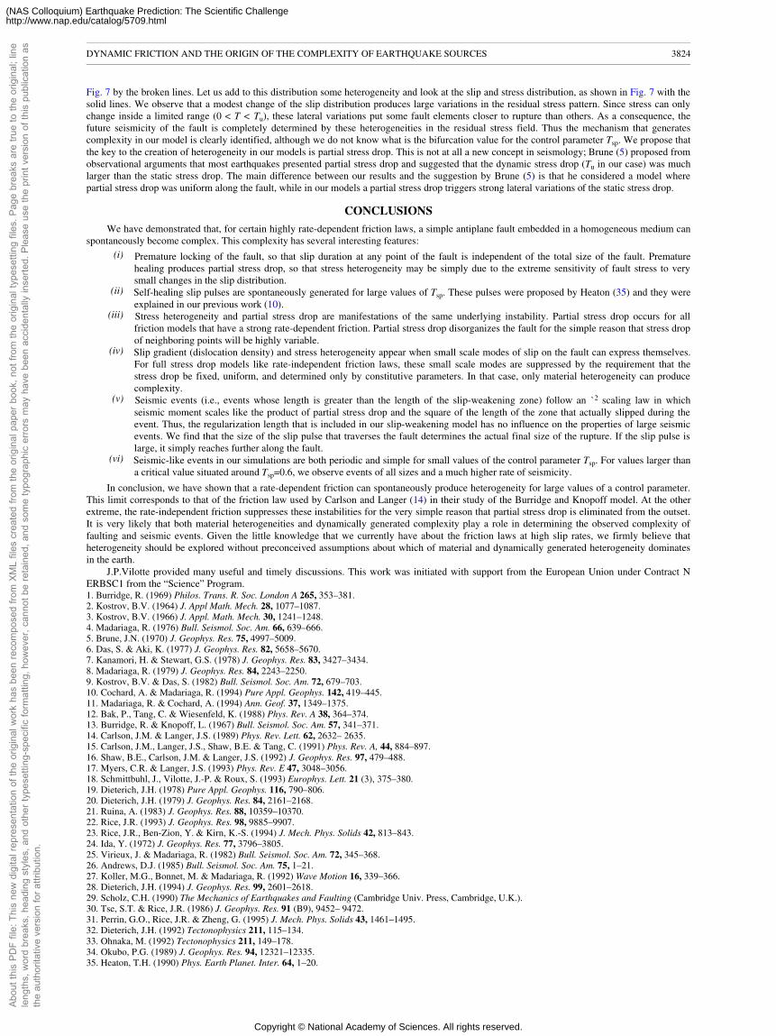
Fig. 7 by the broken lines. Let us add to this distribution some heterogeneity and look at the slip and stress distribution, as shown in Fig. 7 with thesolid lines. We observe that a modest change of the slip distribution produces large variations in the residual stress pattern. Since stress can onlychange inside a limited range (0 < T < Tu), these lateral variations put some fault elements closer to rupture than others. As a consequence, thefuture seismicity of the fault is completely determined by these heterogeneities in the residual stress field. Thus the mechanism that generatescomplexity in our model is clearly identified, although we do not know what is the bifurcation value for the control parameter Tsp. We propose thatthe key to the creation of heterogeneity in our models is partial stress drop. This is not at all a new concept in seismology; Brune (5) proposed fromobservational arguments that most earthquakes presented partial stress drop and suggested that the dynamic stress drop (Tu in our case) was muchlarger than the static stress drop. The main difference between our results and the suggestion by Brune (5) is that he considered a model wherepartial stress drop was uniform along the fault, while in our models a partial stress drop triggers strong lateral variations of the static stress drop.
CONCLUSIONS
We have demonstrated that, for certain highly rate-dependent friction laws, a simple antiplane fault embedded in a homogeneous medium canspontaneously become complex. This complexity has several interesting features:
(i) Premature locking of the fault, so that slip duration at any point of the fault is independent of the total size of the fault. Prematurehealing produces partial stress drop, so that stress heterogeneity may be simply due to the extreme sensitivity of fault stress to verysmall changes in the slip distribution.
(ii) Self-healing slip pulses are spontaneously generated for large values of Tsp. These pulses were proposed by Heaton (35) and they wereexplained in our previous work (10).
(iii) Stress heterogeneity and partial stress drop are manifestations of the same underlying instability. Partial stress drop occurs for allfriction models that have a strong rate-dependent friction. Partial stress drop disorganizes the fault for the simple reason that stress dropof neighboring points will be highly variable.
(iv) Slip gradient (dislocation density) and stress heterogeneity appear when small scale modes of slip on the fault can express themselves.For full stress drop models like rate-independent friction laws, these small scale modes are suppressed by the requirement that thestress drop be fixed, uniform, and determined only by constitutive parameters. In that case, only material heterogeneity can producecomplexity.
(v) Seismic events (i.e., events whose length is greater than the length of the slip-weakening zone) follow an `2 scaling law in whichseismic moment scales like the product of partial stress drop and the square of the length of the zone that actually slipped during theevent. Thus, the regularization length that is included in our slip-weakening model has no influence on the properties of large seismicevents. We find that the size of the slip pulse that traverses the fault determines the actual final size of the rupture. If the slip pulse islarge, it simply reaches further along the fault.
(vi) Seismic-like events in our simulations are both periodic and simple for small values of the control parameter Tsp. For values larger thana critical value situated around Tsp=0.6, we observe events of all sizes and a much higher rate of seismicity.
In conclusion, we have shown that a rate-dependent friction can spontaneously produce heterogeneity for large values of a control parameter.This limit corresponds to that of the friction law used by Carlson and Langer (14) in their study of the Burridge and Knopoff model. At the otherextreme, the rate-independent friction suppresses these instabilities for the very simple reason that partial stress drop is eliminated from the outset.It is very likely that both material heterogeneities and dynamically generated complexity play a role in determining the observed complexity offaulting and seismic events. Given the little knowledge that we currently have about the friction laws at high slip rates, we firmly believe thatheterogeneity should be explored without preconceived assumptions about which of material and dynamically generated heterogeneity dominatesin the earth.
J.P.Vilotte provided many useful and timely discussions. This work was initiated with support from the European Union under Contract NERBSC1 from the “Science” Program.1. Burridge, R. (1969) Philos. Trans. R. Soc. London A 265, 353–381.2. Kostrov, B.V. (1964) J. Appl Math. Mech. 28, 1077–1087.3. Kostrov, B.V. (1966) J. Appl. Math. Mech. 30, 1241–1248.4. Madariaga, R. (1976) Bull. Seismol. Soc. Am. 66, 639–666.5. Brune, J.N. (1970) J. Geophys. Res. 75, 4997–5009.6. Das, S. & Aki, K. (1977) J. Geophys. Res. 82, 5658–5670.7. Kanamori, H. & Stewart, G.S. (1978) J. Geophys. Res. 83, 3427–3434.8. Madariaga, R. (1979) J. Geophys. Res. 84, 2243–2250.9. Kostrov, B.V. & Das, S. (1982) Bull. Seismol. Soc. Am. 72, 679–703.10. Cochard, A. & Madariaga, R. (1994) Pure Appl. Geophys. 142, 419–445.11. Madariaga, R. & Cochard, A. (1994) Ann. Geof. 37, 1349–1375.12. Bak, P., Tang, C. & Wiesenfeld, K. (1988) Phys. Rev. A 38, 364–374.13. Burridge, R. & Knopoff, L. (1967) Bull. Seismol. Soc. Am. 57, 341–371.14. Carlson, J.M. & Langer, J.S. (1989) Phys. Rev. Lett. 62, 2632– 2635.15. Carlson, J.M., Langer, J.S., Shaw, B.E. & Tang, C. (1991) Phys. Rev. A, 44, 884–897.16. Shaw, B.E., Carlson, J.M. & Langer, J.S. (1992) J. Geophys. Res. 97, 479–488.17. Myers, C.R. & Langer, J.S. (1993) Phys. Rev. E 47, 3048–3056.18. Schmittbuhl, J., Vilotte, J.-P. & Roux, S. (1993) Europhys. Lett. 21 (3), 375–380.19. Dieterich, J.H. (1978) Pure Appl. Geophys. 116, 790–806.20. Dieterich, J.H. (1979) J. Geophys. Res. 84, 2161–2168.21. Ruina, A. (1983) J. Geophys. Res. 88, 10359–10370.22. Rice, J.R. (1993) J. Geophys. Res. 98, 9885–9907.23. Rice, J.R., Ben-Zion, Y. & Kirn, K.-S. (1994) J. Mech. Phys. Solids 42, 813–843.24. Ida, Y. (1972) J. Geophys. Res. 77, 3796–3805.25. Virieux, J. & Madariaga, R. (1982) Bull. Seismol. Soc. Am. 72, 345–368.26. Andrews, D.J. (1985) Bull. Seismol. Soc. Am. 75, 1–21.27. Koller, M.G., Bonnet, M. & Madariaga, R. (1992) Wave Motion 16, 339–366.28. Dieterich, J.H. (1994) J. Geophys. Res. 99, 2601–2618.29. Scholz, C.H. (1990) The Mechanics of Earthquakes and Faulting (Cambridge Univ. Press, Cambridge, U.K.).30. Tse, S.T. & Rice, J.R. (1986) J. Geophys. Res. 91 (B9), 9452– 9472.31. Perrin, G.O., Rice, J.R. & Zheng, G. (1995) J. Mech. Phys. Solids 43, 1461–1495.32. Dieterich, J.H. (1992) Tectonophysics 211, 115–134.33. Ohnaka, M. (1992) Tectonophysics 211, 149–178.34. Okubo, P.G. (1989) J. Geophys. Res. 94, 12321–12335.35. Heaton, T.H. (1990) Phys. Earth Planet. Inter. 64, 1–20.
DYNAMIC FRICTION AND THE ORIGIN OF THE COMPLEXITY OF EARTHQUAKE SOURCES 3824
Abou
t thi
s PD
F fil
e: T
his
new
dig
ital r
epre
sent
atio
n of
the
orig
inal
wor
k ha
s be
en re
com
pose
d fro
m X
ML
files
cre
ated
from
the
orig
inal
pap
er b
ook,
not
from
the
orig
inal
type
setti
ng fi
les.
Pag
e br
eaks
are
true
to th
e or
igin
al; l
ine
leng
ths,
wor
d br
eaks
, hea
ding
sty
les,
and
oth
er ty
pese
tting
-spe
cific
form
attin
g, h
owev
er, c
anno
t be
reta
ined
, and
som
e ty
pogr
aphi
c er
rors
may
hav
e be
en a
ccid
enta
lly in
serte
d. P
leas
e us
e th
e pr
int v
ersi
on o
f thi
s pu
blic
atio
n as
the
auth
orita
tive
vers
ion
for a
ttrib
utio
n.
Copyright © National Academy of Sciences. All rights reserved.
(NAS Colloquium) Earthquake Prediction: The Scientific Challengehttp://www.nap.edu/catalog/5709.html
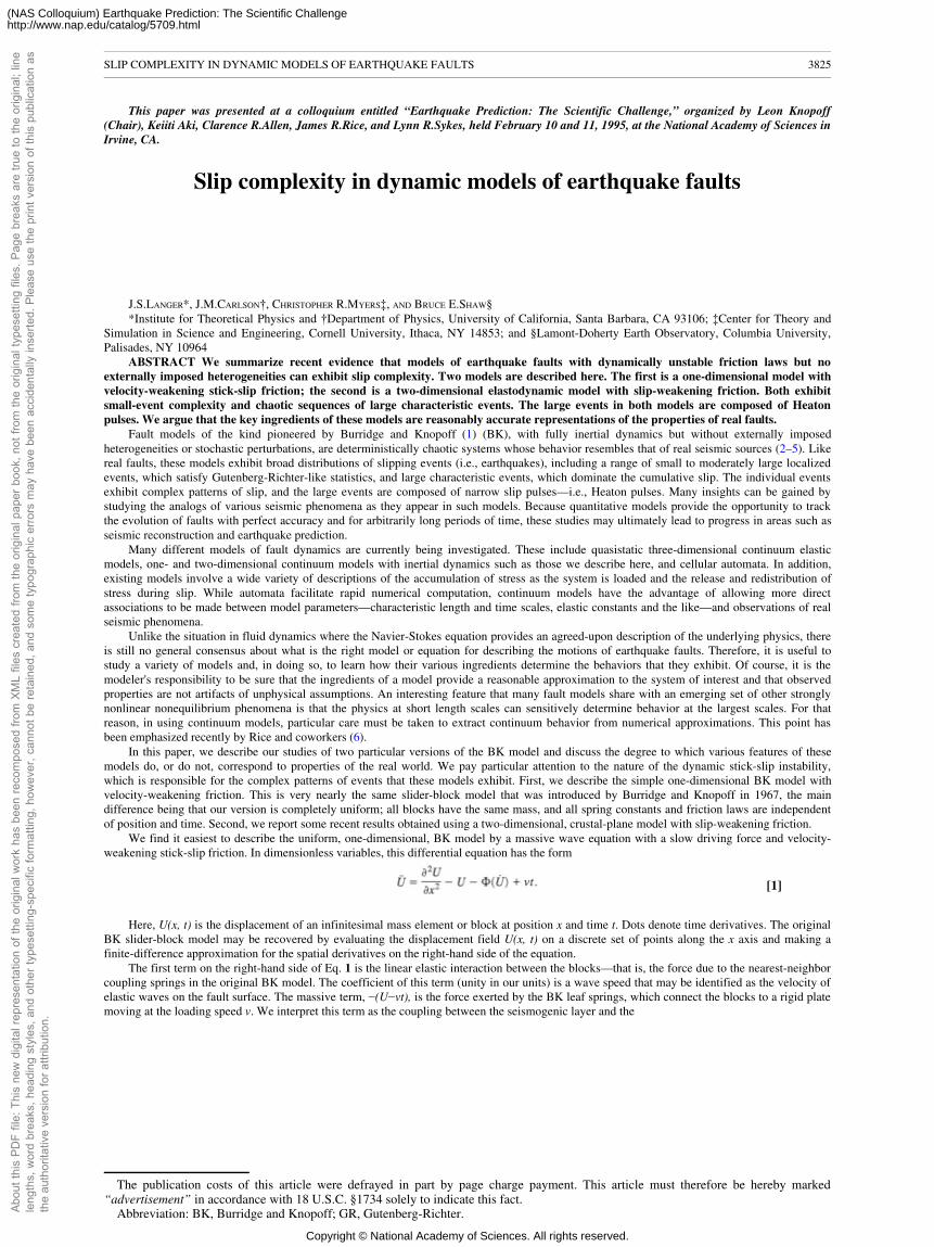
This paper was presented at a colloquium entitled “Earthquake Prediction: The Scientific Challenge,” organized by Leon Knopoff(Chair), Keiiti Aki, Clarence R.Allen, James R.Rice, and Lynn R.Sykes, held February 10 and 11, 1995, at the National Academy of Sciences inIrvine, CA.
Slip complexity in dynamic models of earthquake faults
J.S.LANGER*, J.M.CARLSON†, CHRISTOPHER R.MYERS‡, AND BRUCE E.SHAW§*Institute for Theoretical Physics and †Department of Physics, University of California, Santa Barbara, CA 93106; ‡Center for Theory and
Simulation in Science and Engineering, Cornell University, Ithaca, NY 14853; and §Lamont-Doherty Earth Observatory, Columbia University,Palisades, NY 10964
ABSTRACT We summarize recent evidence that models of earthquake faults with dynamically unstable friction laws but noexternally imposed heterogeneities can exhibit slip complexity. Two models are described here. The first is a one-dimensional model withvelocity-weakening stick-slip friction; the second is a two-dimensional elastodynamic model with slip-weakening friction. Both exhibitsmall-event complexity and chaotic sequences of large characteristic events. The large events in both models are composed of Heatonpulses. We argue that the key ingredients of these models are reasonably accurate representations of the properties of real faults.
Fault models of the kind pioneered by Burridge and Knopoff (1) (BK), with fully inertial dynamics but without externally imposedheterogeneities or stochastic perturbations, are deterministically chaotic systems whose behavior resembles that of real seismic sources (2–5). Likereal faults, these models exhibit broad distributions of slipping events (i.e., earthquakes), including a range of small to moderately large localizedevents, which satisfy Gutenberg-Richter-like statistics, and large characteristic events, which dominate the cumulative slip. The individual eventsexhibit complex patterns of slip, and the large events are composed of narrow slip pulses—i.e., Heaton pulses. Many insights can be gained bystudying the analogs of various seismic phenomena as they appear in such models. Because quantitative models provide the opportunity to trackthe evolution of faults with perfect accuracy and for arbitrarily long periods of time, these studies may ultimately lead to progress in areas such asseismic reconstruction and earthquake prediction.
Many different models of fault dynamics are currently being investigated. These include quasistatic three-dimensional continuum elasticmodels, one- and two-dimensional continuum models with inertial dynamics such as those we describe here, and cellular automata. In addition,existing models involve a wide variety of descriptions of the accumulation of stress as the system is loaded and the release and redistribution ofstress during slip. While automata facilitate rapid numerical computation, continuum models have the advantage of allowing more directassociations to be made between model parameters—characteristic length and time scales, elastic constants and the like—and observations of realseismic phenomena.
Unlike the situation in fluid dynamics where the Navier-Stokes equation provides an agreed-upon description of the underlying physics, thereis still no general consensus about what is the right model or equation for describing the motions of earthquake faults. Therefore, it is useful tostudy a variety of models and, in doing so, to learn how their various ingredients determine the behaviors that they exhibit. Of course, it is themodeler's responsibility to be sure that the ingredients of a model provide a reasonable approximation to the system of interest and that observedproperties are not artifacts of unphysical assumptions. An interesting feature that many fault models share with an emerging set of other stronglynonlinear nonequilibrium phenomena is that the physics at short length scales can sensitively determine behavior at the largest scales. For thatreason, in using continuum models, particular care must be taken to extract continuum behavior from numerical approximations. This point hasbeen emphasized recently by Rice and coworkers (6).
In this paper, we describe our studies of two particular versions of the BK model and discuss the degree to which various features of thesemodels do, or do not, correspond to properties of the real world. We pay particular attention to the nature of the dynamic stick-slip instability,which is responsible for the complex patterns of events that these models exhibit. First, we describe the simple one-dimensional BK model withvelocity-weakening friction. This is very nearly the same slider-block model that was introduced by Burridge and Knopoff in 1967, the maindifference being that our version is completely uniform; all blocks have the same mass, and all spring constants and friction laws are independentof position and time. Second, we report some recent results obtained using a two-dimensional, crustal-plane model with slip-weakening friction.
We find it easiest to describe the uniform, one-dimensional, BK model by a massive wave equation with a slow driving force and velocity-weakening stick-slip friction. In dimensionless variables, this differential equation has the form
[1]
Here, U(x, t) is the displacement of an infinitesimal mass element or block at position x and time t. Dots denote time derivatives. The originalBK slider-block model may be recovered by evaluating the displacement field U(x, t) on a discrete set of points along the x axis and making afinite-difference approximation for the spatial derivatives on the right-hand side of the equation.
The first term on the right-hand side of Eq. 1 is the linear elastic interaction between the blocks—that is, the force due to the nearest-neighborcoupling springs in the original BK model. The coefficient of this term (unity in our units) is a wave speed that may be identified as the velocity ofelastic waves on the fault surface. The massive term, −(U−vt), is the force exerted by the BK leaf springs, which connect the blocks to a rigid platemoving at the loading speed v. We interpret this term as the coupling between the seismogenic layer and the
The publication costs of this article were defrayed in part by page charge payment. This article must therefore be hereby marked“advertisement” in accordance with 18 U.S.C. §1734 solely to indicate this fact.
Abbreviation: BK, Burridge and Knopoff; GR, Gutenberg-Richter.
SLIP COMPLEXITY IN DYNAMIC MODELS OF EARTHQUAKE FAULTS 3825
Abou
t thi
s PD
F fil
e: T
his
new
dig
ital r
epre
sent
atio
n of
the
orig
inal
wor
k ha
s be
en re
com
pose
d fro
m X
ML
files
cre
ated
from
the
orig
inal
pap
er b
ook,
not
from
the
orig
inal
type
setti
ng fi
les.
Pag
e br
eaks
are
true
to th
e or
igin
al; l
ine
leng
ths,
wor
d br
eaks
, hea
ding
sty
les,
and
oth
er ty
pese
tting
-spe
cific
form
attin
g, h
owev
er, c
anno
t be
reta
ined
, and
som
e ty
pogr
aphi
c er
rors
may
hav
e be
en a
ccid
enta
lly in
serte
d. P
leas
e us
e th
e pr
int v
ersi
on o
f thi
s pu
blic
atio
n as
the
auth
orita
tive
vers
ion
for a
ttrib
utio
n.
Copyright © National Academy of Sciences. All rights reserved.
(NAS Colloquium) Earthquake Prediction: The Scientific Challengehttp://www.nap.edu/catalog/5709.html
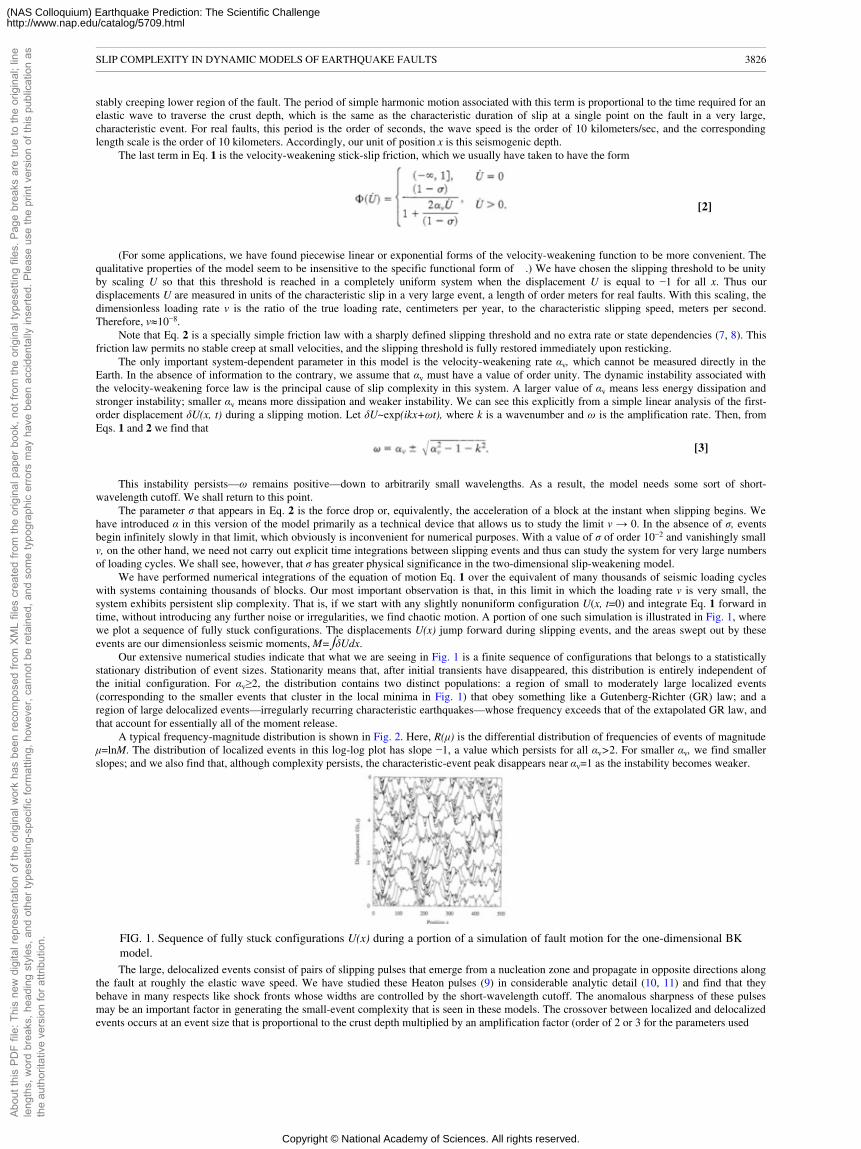
stably creeping lower region of the fault. The period of simple harmonic motion associated with this term is proportional to the time required for anelastic wave to traverse the crust depth, which is the same as the characteristic duration of slip at a single point on the fault in a very large,characteristic event. For real faults, this period is the order of seconds, the wave speed is the order of 10 kilometers/sec, and the correspondinglength scale is the order of 10 kilometers. Accordingly, our unit of position x is this seismogenic depth.
The last term in Eq. 1 is the velocity-weakening stick-slip friction, which we usually have taken to have the form
[2]
(For some applications, we have found piecewise linear or exponential forms of the velocity-weakening function to be more convenient. Thequalitative properties of the model seem to be insensitive to the specific functional form of .) We have chosen the slipping threshold to be unityby scaling U so that this threshold is reached in a completely uniform system when the displacement U is equal to −1 for all x. Thus ourdisplacements U are measured in units of the characteristic slip in a very large event, a length of order meters for real faults. With this scaling, thedimensionless loading rate v is the ratio of the true loading rate, centimeters per year, to the characteristic slipping speed, meters per second.Therefore, v�10−8.
Note that Eq. 2 is a specially simple friction law with a sharply defined slipping threshold and no extra rate or state dependencies (7, 8). Thisfriction law permits no stable creep at small velocities, and the slipping threshold is fully restored immediately upon resticking.
The only important system-dependent parameter in this model is the velocity-weakening rate αv, which cannot be measured directly in theEarth. In the absence of information to the contrary, we assume that αv must have a value of order unity. The dynamic instability associated withthe velocity-weakening force law is the principal cause of slip complexity in this system. A larger value of αv means less energy dissipation andstronger instability; smaller αv means more dissipation and weaker instability. We can see this explicitly from a simple linear analysis of the first-order displacement δU(x, t) during a slipping motion. Let δU~exp(ikx+ωt), where k is a wavenumber and ω is the amplification rate. Then, fromEqs. 1 and 2 we find that
[3]
This instability persists—ω remains positive—down to arbitrarily small wavelengths. As a result, the model needs some sort of short-wavelength cutoff. We shall return to this point.
The parameter σ that appears in Eq. 2 is the force drop or, equivalently, the acceleration of a block at the instant when slipping begins. Wehave introduced α in this version of the model primarily as a technical device that allows us to study the limit v → 0. In the absence of σ, eventsbegin infinitely slowly in that limit, which obviously is inconvenient for numerical purposes. With a value of σ of order 10−2 and vanishingly smallv, on the other hand, we need not carry out explicit time integrations between slipping events and thus can study the system for very large numbersof loading cycles. We shall see, however, that σ has greater physical significance in the two-dimensional slip-weakening model.
We have performed numerical integrations of the equation of motion Eq. 1 over the equivalent of many thousands of seismic loading cycleswith systems containing thousands of blocks. Our most important observation is that, in this limit in which the loading rate v is very small, thesystem exhibits persistent slip complexity. That is, if we start with any slightly nonuniform configuration U(x, t=0) and integrate Eq. 1 forward intime, without introducing any further noise or irregularities, we find chaotic motion. A portion of one such simulation is illustrated in Fig. 1, wherewe plot a sequence of fully stuck configurations. The displacements U(x) jump forward during slipping events, and the areas swept out by theseevents are our dimensionless seismic moments, M=�δUdx.
Our extensive numerical studies indicate that what we are seeing in Fig. 1 is a finite sequence of configurations that belongs to a statisticallystationary distribution of event sizes. Stationarity means that, after initial transients have disappeared, this distribution is entirely independent ofthe initial configuration. For αv≥2, the distribution contains two distinct populations: a region of small to moderately large localized events(corresponding to the smaller events that cluster in the local minima in Fig. 1) that obey something like a Gutenberg-Richter (GR) law; and aregion of large delocalized events—irregularly recurring characteristic earthquakes—whose frequency exceeds that of the extapolated GR law, andthat account for essentially all of the moment release.
A typical frequency-magnitude distribution is shown in Fig. 2. Here, R(µ) is the differential distribution of frequencies of events of magnitudeµ=lnM. The distribution of localized events in this log-log plot has slope −1, a value which persists for all αv>2. For smaller αv, we find smallerslopes; and we also find that, although complexity persists, the characteristic-event peak disappears near αv=1 as the instability becomes weaker.
FIG. 1. Sequence of fully stuck configurations U(x) during a portion of a simulation of fault motion for the one-dimensional BKmodel.The large, delocalized events consist of pairs of slipping pulses that emerge from a nucleation zone and propagate in opposite directions along
the fault at roughly the elastic wave speed. We have studied these Heaton pulses (9) in considerable analytic detail (10, 11) and find that theybehave in many respects like shock fronts whose widths are controlled by the short-wavelength cutoff. The anomalous sharpness of these pulsesmay be an important factor in generating the small-event complexity that is seen in these models. The crossover between localized and delocalizedevents occurs at an event size that is proportional to the crust depth multiplied by an amplification factor (order of 2 or 3 for the parameters used
SLIP COMPLEXITY IN DYNAMIC MODELS OF EARTHQUAKE FAULTS 3826
Abou
t thi
s PD
F fil
e: T
his
new
dig
ital r
epre
sent
atio
n of
the
orig
inal
wor
k ha
s be
en re
com
pose
d fro
m X
ML
files
cre
ated
from
the
orig
inal
pap
er b
ook,
not
from
the
orig
inal
type
setti
ng fi
les.
Pag
e br
eaks
are
true
to th
e or
igin
al; l
ine
leng
ths,
wor
d br
eaks
, hea
ding
sty
les,
and
oth
er ty
pese
tting
-spe
cific
form
attin
g, h
owev
er, c
anno
t be
reta
ined
, and
som
e ty
pogr
aphi
c er
rors
may
hav
e be
en a
ccid
enta
lly in
serte
d. P
leas
e us
e th
e pr
int v
ersi
on o
f thi
s pu
blic
atio
n as
the
auth
orita
tive
vers
ion
for a
ttrib
utio
n.
Copyright © National Academy of Sciences. All rights reserved.
(NAS Colloquium) Earthquake Prediction: The Scientific Challengehttp://www.nap.edu/catalog/5709.html
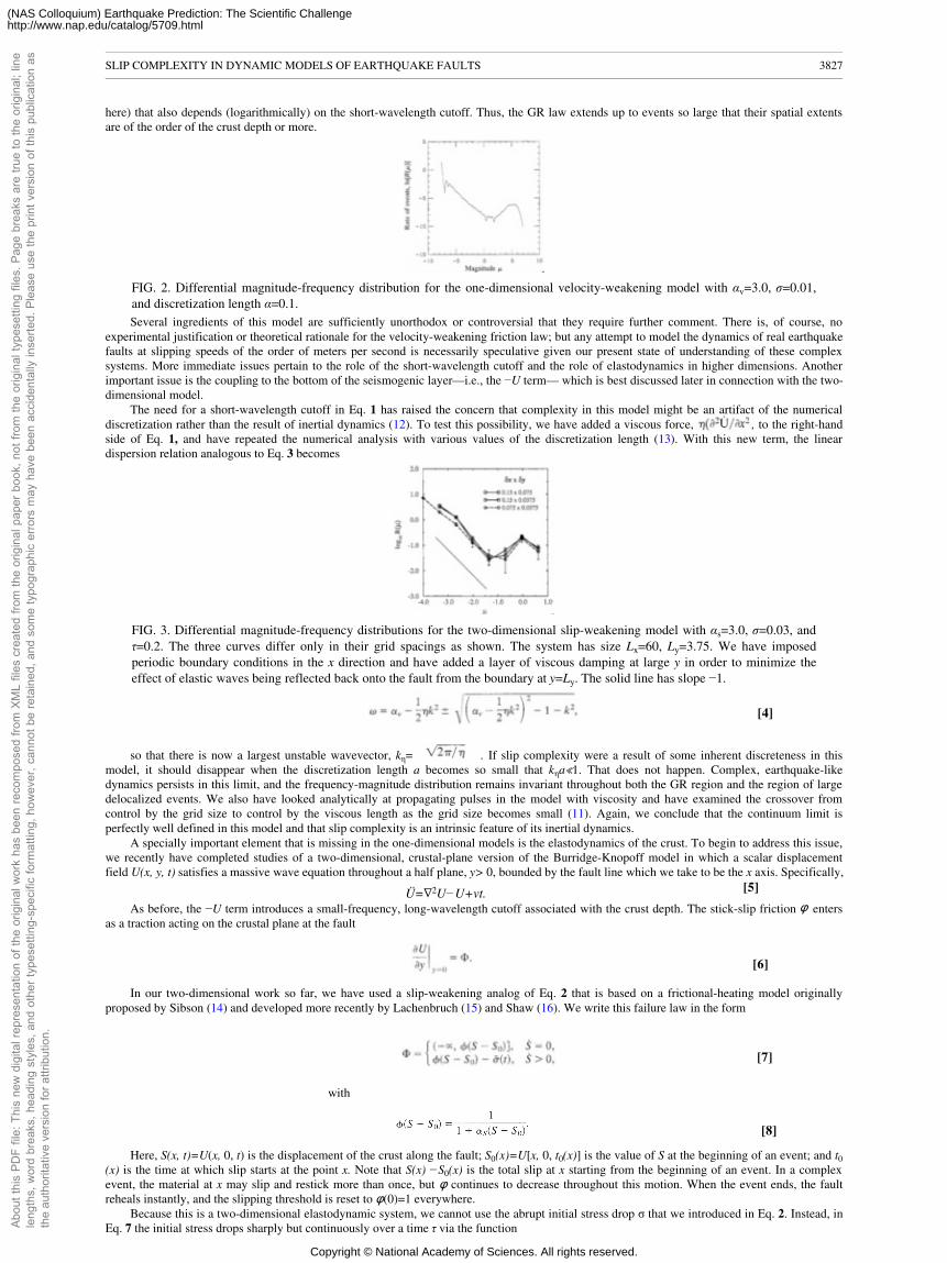
here) that also depends (logarithmically) on the short-wavelength cutoff. Thus, the GR law extends up to events so large that their spatial extentsare of the order of the crust depth or more.
FIG. 2. Differential magnitude-frequency distribution for the one-dimensional velocity-weakening model with αv=3.0, σ=0.01,and discretization length α=0.1.Several ingredients of this model are sufficiently unorthodox or controversial that they require further comment. There is, of course, no
experimental justification or theoretical rationale for the velocity-weakening friction law; but any attempt to model the dynamics of real earthquakefaults at slipping speeds of the order of meters per second is necessarily speculative given our present state of understanding of these complexsystems. More immediate issues pertain to the role of the short-wavelength cutoff and the role of elastodynamics in higher dimensions. Anotherimportant issue is the coupling to the bottom of the seismogenic layer—i.e., the −U term— which is best discussed later in connection with the two-dimensional model.
The need for a short-wavelength cutoff in Eq. 1 has raised the concern that complexity in this model might be an artifact of the numericaldiscretization rather than the result of inertial dynamics (12). To test this possibility, we have added a viscous force, , to the right-handside of Eq. 1, and have repeated the numerical analysis with various values of the discretization length (13). With this new term, the lineardispersion relation analogous to Eq. 3 becomes
FIG. 3. Differential magnitude-frequency distributions for the two-dimensional slip-weakening model with αs=3.0, σ=0.03, andτ=0.2. The three curves differ only in their grid spacings as shown. The system has size Lx=60, Ly=3.75. We have imposedperiodic boundary conditions in the x direction and have added a layer of viscous damping at large y in order to minimize theeffect of elastic waves being reflected back onto the fault from the boundary at y=Ly. The solid line has slope −1.
[4]
so that there is now a largest unstable wavevector, kη= . If slip complexity were a result of some inherent discreteness in thismodel, it should disappear when the discretization length a becomes so small that kηa�1. That does not happen. Complex, earthquake-likedynamics persists in this limit, and the frequency-magnitude distribution remains invariant throughout both the GR region and the region of largedelocalized events. We also have looked analytically at propagating pulses in the model with viscosity and have examined the crossover fromcontrol by the grid size to control by the viscous length as the grid size becomes small (11). Again, we conclude that the continuum limit isperfectly well defined in this model and that slip complexity is an intrinsic feature of its inertial dynamics.
A specially important element that is missing in the one-dimensional models is the elastodynamics of the crust. To begin to address this issue,we recently have completed studies of a two-dimensional, crustal-plane version of the Burridge-Knopoff model in which a scalar displacementfield U(x, y, t) satisfies a massive wave equation throughout a half plane, y> 0, bounded by the fault line which we take to be the x axis. Specifically,
Ü=�2U−U+vt. [5]
As before, the −U term introduces a small-frequency, long-wavelength cutoff associated with the crust depth. The stick-slip friction entersas a traction acting on the crustal plane at the fault
[6]
In our two-dimensional work so far, we have used a slip-weakening analog of Eq. 2 that is based on a frictional-heating model originallyproposed by Sibson (14) and developed more recently by Lachenbruch (15) and Shaw (16). We write this failure law in the form
[7]
with
[8]
Here, S(x, t)=U(x, 0, t) is the displacement of the crust along the fault; S0(x)=U[x, 0, t0(x)] is the value of S at the beginning of an event; and t0(x) is the time at which slip starts at the point x. Note that S(x) −S0(x) is the total slip at x starting from the beginning of an event. In a complexevent, the material at x may slip and restick more than once, but � continues to decrease throughout this motion. When the event ends, the faultreheals instantly, and the slipping threshold is reset to �(0)=1 everywhere.
Because this is a two-dimensional elastodynamic system, we cannot use the abrupt initial stress drop σ that we introduced in Eq. 2. Instead, inEq. 7 the initial stress drops sharply but continuously over a time τ via the function
SLIP COMPLEXITY IN DYNAMIC MODELS OF EARTHQUAKE FAULTS 3827
Abou
t thi
s PD
F fil
e: T
his
new
dig
ital r
epre
sent
atio
n of
the
orig
inal
wor
k ha
s be
en re
com
pose
d fro
m X
ML
files
cre
ated
from
the
orig
inal
pap
er b
ook,
not
from
the
orig
inal
type
setti
ng fi
les.
Pag
e br
eaks
are
true
to th
e or
igin
al; l
ine
leng
ths,
wor
d br
eaks
, hea
ding
sty
les,
and
oth
er ty
pese
tting
-spe
cific
form
attin
g, h
owev
er, c
anno
t be
reta
ined
, and
som
e ty
pogr
aphi
c er
rors
may
hav
e be
en a
ccid
enta
lly in
serte
d. P
leas
e us
e th
e pr
int v
ersi
on o
f thi
s pu
blic
atio
n as
the
auth
orita
tive
vers
ion
for a
ttrib
utio
n.
�
Copyright © National Academy of Sciences. All rights reserved.
(NAS Colloquium) Earthquake Prediction: The Scientific Challengehttp://www.nap.edu/catalog/5709.html
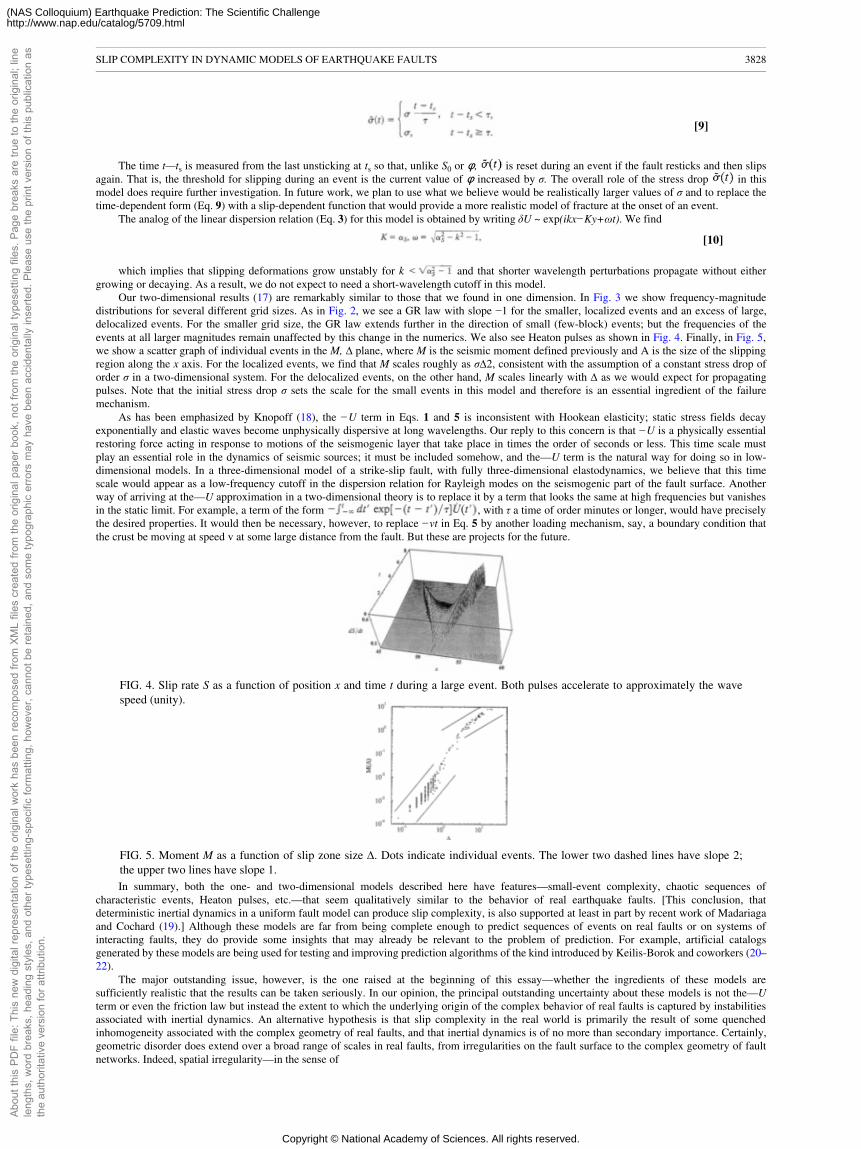
[9]
The time t—ts is measured from the last unsticking at ts so that, unlike S0 or �, is reset during an event if the fault resticks and then slipsagain. That is, the threshold for slipping during an event is the current value of � increased by σ. The overall role of the stress drop in thismodel does require further investigation. In future work, we plan to use what we believe would be realistically larger values of σ and to replace thetime-dependent form (Eq. 9) with a slip-dependent function that would provide a more realistic model of fracture at the onset of an event.
The analog of the linear dispersion relation (Eq. 3) for this model is obtained by writing δU ~ exp(ikx−Ky+ωt). We find
[10]
which implies that slipping deformations grow unstably for k and that shorter wavelength perturbations propagate without eithergrowing or decaying. As a result, we do not expect to need a short-wavelength cutoff in this model.
Our two-dimensional results (17) are remarkably similar to those that we found in one dimension. In Fig. 3 we show frequency-magnitudedistributions for several different grid sizes. As in Fig. 2, we see a GR law with slope −1 for the smaller, localized events and an excess of large,delocalized events. For the smaller grid size, the GR law extends further in the direction of small (few-block) events; but the frequencies of theevents at all larger magnitudes remain unaffected by this change in the numerics. We also see Heaton pulses as shown in Fig. 4. Finally, in Fig. 5,we show a scatter graph of individual events in the M, ∆ plane, where M is the seismic moment defined previously and A is the size of the slippingregion along the x axis. For the localized events, we find that M scales roughly as σ∆2, consistent with the assumption of a constant stress drop oforder σ in a two-dimensional system. For the delocalized events, on the other hand, M scales linearly with ∆ as we would expect for propagatingpulses. Note that the initial stress drop σ sets the scale for the small events in this model and therefore is an essential ingredient of the failuremechanism.
As has been emphasized by Knopoff (18), the −U term in Eqs. 1 and 5 is inconsistent with Hookean elasticity; static stress fields decayexponentially and elastic waves become unphysically dispersive at long wavelengths. Our reply to this concern is that −U is a physically essentialrestoring force acting in response to motions of the seismogenic layer that take place in times the order of seconds or less. This time scale mustplay an essential role in the dynamics of seismic sources; it must be included somehow, and the—U term is the natural way for doing so in low-dimensional models. In a three-dimensional model of a strike-slip fault, with fully three-dimensional elastodynamics, we believe that this timescale would appear as a low-frequency cutoff in the dispersion relation for Rayleigh modes on the seismogenic part of the fault surface. Anotherway of arriving at the—U approximation in a two-dimensional theory is to replace it by a term that looks the same at high frequencies but vanishesin the static limit. For example, a term of the form , with τ a time of order minutes or longer, would have preciselythe desired properties. It would then be necessary, however, to replace −vt in Eq. 5 by another loading mechanism, say, a boundary condition thatthe crust be moving at speed v at some large distance from the fault. But these are projects for the future.
FIG. 4. Slip rate S as a function of position x and time t during a large event. Both pulses accelerate to approximately the wavespeed (unity).
FIG. 5. Moment M as a function of slip zone size ∆. Dots indicate individual events. The lower two dashed lines have slope 2;the upper two lines have slope 1.In summary, both the one- and two-dimensional models described here have features—small-event complexity, chaotic sequences of
characteristic events, Heaton pulses, etc.—that seem qualitatively similar to the behavior of real earthquake faults. [This conclusion, thatdeterministic inertial dynamics in a uniform fault model can produce slip complexity, is also supported at least in part by recent work of Madariagaand Cochard (19).] Although these models are far from being complete enough to predict sequences of events on real faults or on systems ofinteracting faults, they do provide some insights that may already be relevant to the problem of prediction. For example, artificial catalogsgenerated by these models are being used for testing and improving prediction algorithms of the kind introduced by Keilis-Borok and coworkers (20–22).
The major outstanding issue, however, is the one raised at the beginning of this essay—whether the ingredients of these models aresufficiently realistic that the results can be taken seriously. In our opinion, the principal outstanding uncertainty about these models is not the—Uterm or even the friction law but instead the extent to which the underlying origin of the complex behavior of real faults is captured by instabilitiesassociated with inertial dynamics. An alternative hypothesis is that slip complexity in the real world is primarily the result of some quenchedinhomogeneity associated with the complex geometry of real faults, and that inertial dynamics is of no more than secondary importance. Certainly,geometric disorder does extend over a broad range of scales in real faults, from irregularities on the fault surface to the complex geometry of faultnetworks. Indeed, spatial irregularity—in the sense of
SLIP COMPLEXITY IN DYNAMIC MODELS OF EARTHQUAKE FAULTS 3828
Abou
t thi
s PD
F fil
e: T
his
new
dig
ital r
epre
sent
atio
n of
the
orig
inal
wor
k ha
s be
en re
com
pose
d fro
m X
ML
files
cre
ated
from
the
orig
inal
pap
er b
ook,
not
from
the
orig
inal
type
setti
ng fi
les.
Pag
e br
eaks
are
true
to th
e or
igin
al; l
ine
leng
ths,
wor
d br
eaks
, hea
ding
sty
les,
and
oth
er ty
pese
tting
-spe
cific
form
attin
g, h
owev
er, c
anno
t be
reta
ined
, and
som
e ty
pogr
aphi
c er
rors
may
hav
e be
en a
ccid
enta
lly in
serte
d. P
leas
e us
e th
e pr
int v
ersi
on o
f thi
s pu
blic
atio
n as
the
auth
orita
tive
vers
ion
for a
ttrib
utio
n.
Copyright © National Academy of Sciences. All rights reserved.
(NAS Colloquium) Earthquake Prediction: The Scientific Challengehttp://www.nap.edu/catalog/5709.html
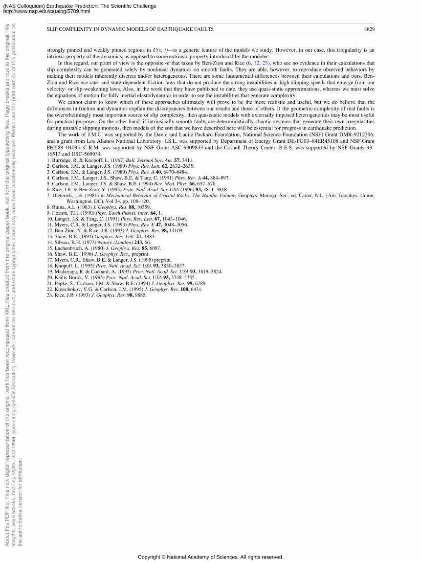
strongly pinned and weakly pinned regions in U(x, t)—is a generic feature of the models we study. However, in our case, this irregularity is anintrinsic property of the dynamics, as opposed to some extrinsic property introduced by the modeler.
In this regard, our point of view is the opposite of that taken by Ben-Zion and Rice (6, 12, 23), who see no evidence in their calculations thatslip complexity can be generated solely by nonlinear dynamics on smooth faults. They are able, however, to reproduce observed behaviors bymaking their models inherently discrete and/or heterogeneous. There are some fundamental differences between their calculations and ours. Ben-Zion and Rice use rate- and state-dependent friction laws that do not produce the strong instabilities at high slipping speeds that emerge from ourvelocity- or slip-weakening laws. Also, in the work that they have published to date, they use quasi-static approximations, whereas we must solvethe equations of motion for fully inertial elastodynamics in order to see the instabilities that generate complexity.
We cannot claim to know which of these approaches ultimately will prove to be the more realistic and useful, but we do believe that thedifferences in friction and dynamics explain the discrepancies between our results and those of others. If the geometric complexity of real faults isthe overwhelmingly most important source of slip complexity, then quasistatic models with externally imposed heterogeneities may be most usefulfor practical purposes. On the other hand, if intrinsically smooth faults are deterministically chaotic systems that generate their own irregularitiesduring unstable slipping motions, then models of the sort that we have described here will be essential for progress in earthquake prediction.
The work of J.M.C. was supported by the David and Lucile Packard Foundation, National Science Foundation (NSF) Grant DMR-9212396,and a grant from Los Alamos National Laboratory. J.S.L. was supported by Department of Energy Grant DE-FG03–84ER45108 and NSF GrantPHY89–04035. C.R.M. was supported by NSF Grant ASC-9309833 and the Cornell Theory Center. B.E.S. was supported by NSF Grants 93–16513 and USC-569934.1. Burridge, R. & Knopoff, L. (1967) Bull. Seismol Soc. Am. 57, 3411.2. Carlson, J.M. & Langer, J.S. (1989) Phys. Rev. Lett. 62, 2632–2635.3. Carlson, J.M. & Langer, J.S. (1989) Phys. Rev. A 40, 6470–6484.4. Carlson, J.M., Langer, J.S., Shaw, B.E. & Tang, C. (1991) Phys. Rev. A 44, 884–897.5. Carlson, J.M., Langer, J.S. & Shaw, B.E. (1994) Rev. Mod. Phys. 66, 657–670.6. Rice, J.R. & Ben-Zion, Y. (1995) Proc. Natl. Acad. Sci. USA (1996) 93, 3811–3818.7. Dieterich, J.H. (1981) in Mechanical Behavior of Crustal Rocks: The Handin Volume, Geophys. Monogr. Ser., ed. Carter, N.L. (Am. Geophys. Union,
Washington, DC), Vol 24, pp. 108–120.8. Ruina, A.L. (1983) J. Geophys. Res. 88, 10359.9. Heaton, T.H. (1990) Phys. Earth Planet. Inter. 64, 1.10. Langer, J.S. & Tang, C. (1991) Phys. Rev. Lett. 67, 1043–1046.11. Myers, C.R. & Langer, J.S. (1993) Phys. Rev. E 47, 3048–3056.12. Ben-Zion, Y. & Rice, J.R. (1993) J. Geophys. Res. 98, 14109.13. Shaw, B.E. (1994) Geophys. Res. Lett. 21, 1983.14. Sibson, R.H. (1973) Nature (London) 243, 66.15. Lachenbruch, A. (1980) J. Geophys. Res. 85, 6097.16. Shaw, B.E. (1996) J. Geophys. Res., preprint.17. Myers, C.R., Shaw, B.E. & Langer, J.S. (1995) preprint.18. Knopoff, L. (1995) Proc. Natl. Acad. Sci. USA 93, 3830–3837.19. Madariaga, R. & Cochard, A. (1995) Proc. Natl. Acad. Sci. USA 93, 3819–3824.20. Keilis-Borok, V. (1995) Proc. Natl. Acad. Sci. USA 93, 3748–3755.21. Pepke, S., Carlson, J.M. & Shaw, B.E. (1994) J. Geophys. Res. 99, 6789.22. Kossobokov, V.G. & Carlson, J.M. (1995) J. Geophys. Res. 100, 6431.23. Rice, J.R. (1993) J. Geophys. Res. 98, 9885.
SLIP COMPLEXITY IN DYNAMIC MODELS OF EARTHQUAKE FAULTS 3829
Abou
t thi
s PD
F fil
e: T
his
new
dig
ital r
epre
sent
atio
n of
the
orig
inal
wor
k ha
s be
en re
com
pose
d fro
m X
ML
files
cre
ated
from
the
orig
inal
pap
er b
ook,
not
from
the
orig
inal
type
setti
ng fi
les.
Pag
e br
eaks
are
true
to th
e or
igin
al; l
ine
leng
ths,
wor
d br
eaks
, hea
ding
sty
les,
and
oth
er ty
pese
tting
-spe
cific
form
attin
g, h
owev
er, c
anno
t be
reta
ined
, and
som
e ty
pogr
aphi
c er
rors
may
hav
e be
en a
ccid
enta
lly in
serte
d. P
leas
e us
e th
e pr
int v
ersi
on o
f thi
s pu
blic
atio
n as
the
auth
orita
tive
vers
ion
for a
ttrib
utio
n.
Copyright © National Academy of Sciences. All rights reserved.
(NAS Colloquium) Earthquake Prediction: The Scientific Challengehttp://www.nap.edu/catalog/5709.html
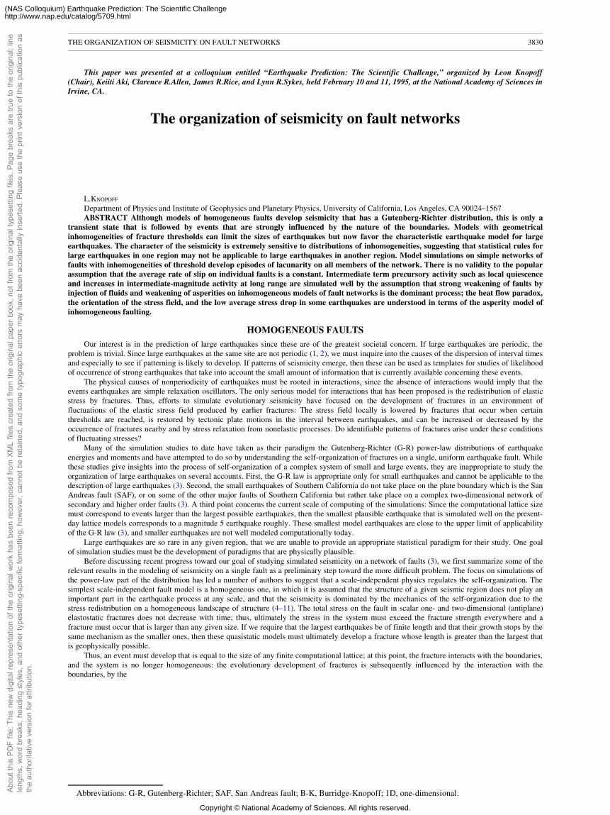
This paper was presented at a colloquium entitled “Earthquake Prediction: The Scientific Challenge,” organized by Leon Knopoff(Chair), Keiiti Aki, Clarence R.Allen, James R.Rice, and Lynn R.Sykes, held February 10 and 11, 1995, at the National Academy of Sciences inIrvine, CA.
The organization of seismicity on fault networks
L.KNOPOFF
Department of Physics and Institute of Geophysics and Planetary Physics, University of California, Los Angeles, CA 90024–1567ABSTRACT Although models of homogeneous faults develop seismicity that has a Gutenberg-Richter distribution, this is only a
transient state that is followed by events that are strongly influenced by the nature of the boundaries. Models with geometricalinhomogeneities of fracture thresholds can limit the sizes of earthquakes but now favor the characteristic earthquake model for largeearthquakes. The character of the seismicity is extremely sensitive to distributions of inhomogeneities, suggesting that statistical rules forlarge earthquakes in one region may not be applicable to large earthquakes in another region. Model simulations on simple networks offaults with inhomogeneities of threshold develop episodes of lacunarity on all members of the network. There is no validity to the popularassumption that the average rate of slip on individual faults is a constant. Intermediate term precursory activity such as local quiescenceand increases in intermediate-magnitude activity at long range are simulated well by the assumption that strong weakening of faults byinjection of fluids and weakening of asperities on inhomogeneous models of fault networks is the dominant process; the heat flow paradox,the orientation of the stress field, and the low average stress drop in some earthquakes are understood in terms of the asperity model ofinhomogeneous faulting.
HOMOGENEOUS FAULTS
Our interest is in the prediction of large earthquakes since these are of the greatest societal concern. If large earthquakes are periodic, theproblem is trivial. Since large earthquakes at the same site are not periodic (1, 2), we must inquire into the causes of the dispersion of interval timesand especially to see if patterning is likely to develop. If patterns of seismicity emerge, then these can be used as templates for studies of likelihoodof occurrence of strong earthquakes that take into account the small amount of information that is currently available concerning these events.
The physical causes of nonperiodicity of earthquakes must be rooted in interactions, since the absence of interactions would imply that theevents earthquakes are simple relaxation oscillators. The only serious model for interactions that has been proposed is the redistribution of elasticstress by fractures. Thus, efforts to simulate evolutionary seismicity have focused on the development of fractures in an environment offluctuations of the elastic stress field produced by earlier fractures: The stress field locally is lowered by fractures that occur when certainthresholds are reached, is restored by tectonic plate motions in the interval between earthquakes, and can be increased or decreased by theoccurrence of fractures nearby and by stress relaxation from nonelastic processes. Do identifiable patterns of fractures arise under these conditionsof fluctuating stresses?
Many of the simulation studies to date have taken as their paradigm the Gutenberg-Richter (G-R) power-law distributions of earthquakeenergies and moments and have attempted to do so by understanding the self-organization of fractures on a single, uniform earthquake fault. Whilethese studies give insights into the process of self-organization of a complex system of small and large events, they are inappropriate to study theorganization of large earthquakes on several accounts. First, the G-R law is appropriate only for small earthquakes and cannot be applicable to thedescription of large earthquakes (3). Second, the small earthquakes of Southern California do not take place on the plate boundary which is the SanAndreas fault (SAF), or on some of the other major faults of Southern California but rather take place on a complex two-dimensional network ofsecondary and higher order faults (3). A third point concerns the current scale of computing of the simulations: Since the computational lattice sizemust correspond to events larger than the largest possible earthquakes, then the smallest plausible earthquake that is simulated well on the present-day lattice models corresponds to a magnitude 5 earthquake roughly. These smallest model earthquakes are close to the upper limit of applicabilityof the G-R law (3), and smaller earthquakes are not well modeled computationally today.
Large earthquakes are so rare in any given region, that we are unable to provide an appropriate statistical paradigm for their study. One goalof simulation studies must be the development of paradigms that are physically plausible.
Before discussing recent progress toward our goal of studying simulated seismicity on a network of faults (3), we first summarize some of therelevant results in the modeling of seismicity on a single fault as a preliminary step toward the more difficult problem. The focus on simulations ofthe power-law part of the distribution has led a number of authors to suggest that a scale-independent physics regulates the self-organization. Thesimplest scale-independent fault model is a homogeneous one, in which it is assumed that the structure of a given seismic region does not play animportant part in the earthquake process at any scale, and that the seismicity is dominated by the mechanics of the self-organization due to thestress redistribution on a homogeneous landscape of structure (4–11). The total stress on the fault in scalar one- and two-dimensional (antiplane)elastostatic fractures does not decrease with time; thus, ultimately the stress in the system must exceed the fracture strength everywhere and afracture must occur that is larger than any given size. If we require that the largest earthquakes be of finite length and that their growth stops by thesame mechanism as the smaller ones, then these quasistatic models must ultimately develop a fracture whose length is greater than the largest thatis geophysically possible.
Thus, an event must develop that is equal to the size of any finite computational lattice; at this point, the fracture interacts with the boundaries,and the system is no longer homogeneous: the evolutionary development of fractures is subsequently influenced by the interaction with theboundaries, by the
Abbreviations: G-R, Gutenberg-Richter; SAF, San Andreas fault; B-K, Burridge-Knopoff; 1D, one-dimensional.
THE ORGANIZATION OF SEISMICITY ON FAULT NETWORKS 3830
Abou
t thi
s PD
F fil
e: T
his
new
dig
ital r
epre
sent
atio
n of
the
orig
inal
wor
k ha
s be
en re
com
pose
d fro
m X
ML
files
cre
ated
from
the
orig
inal
pap
er b
ook,
not
from
the
orig
inal
type
setti
ng fi
les.
Pag
e br
eaks
are
true
to th
e or
igin
al; l
ine
leng
ths,
wor
d br
eaks
, hea
ding
sty
les,
and
oth
er ty
pese
tting
-spe
cific
form
attin
g, h
owev
er, c
anno
t be
reta
ined
, and
som
e ty
pogr
aphi
c er
rors
may
hav
e be
en a
ccid
enta
lly in
serte
d. P
leas
e us
e th
e pr
int v
ersi
on o
f thi
s pu
blic
atio
n as
the
auth
orita
tive
vers
ion
for a
ttrib
utio
n.
Copyright © National Academy of Sciences. All rights reserved.
(NAS Colloquium) Earthquake Prediction: The Scientific Challengehttp://www.nap.edu/catalog/5709.html
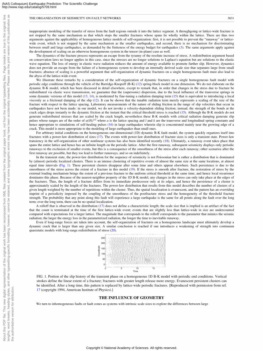
inappropriate modeling of the transfer of stress from the fault regions outside it into the lattice segment. A throughgoing or lattice-wide fracture isnot stopped by the same mechanism as that which stops the smaller fractures whose spans lie wholly within the lattice. There are thus twoarguments against the applicability of homogeneous lattice models of self-organization: first, it is not possible to prevent the “runaway” or lattice-wide event, which is not stopped by the same mechanism as the smaller earthquakes, and second, there is no mechanism for discriminatingbetween small and large earthquakes, as demanded by the finiteness of the energy budget for earthquakes (3). The same arguments apply againstthe development of scaling on an otherwise homogeneous system in the tensor (in-plane) case as well.
The dynamics of the fracture process represents an escape from the tyranny of the resolute increase of stress. A redistribution argument basedon conservation laws no longer applies in this case, since the stresses are no longer solutions to Laplace's equation but are solutions to the elasticwave equation. The loss of energy in elastic wave radiation reduces the amount of energy available to promote further slip. However, dynamicsdoes not provide an escape from the failure of a homogeneous system to develop an internally derived scale size that separates large from smallfractures; absence of scaling is a powerful argument that self-organization of dynamic fractures on a single homogeneous fault must also lead tothe abyss of the lattice-wide event.
We illustrate these remarks by a consideration of the self-organization of dynamic fractures on a single homogeneous fault model withperiodic edge conditions through the vehicle of the Burridge-Knopoff (B-K) (12) spring-block model in one dimension. We do not elaborate on thedynamic B-K model, which has been discussed in detail elsewhere, except to remark that, in order that changes in the stress due to fracture beredistributed via elastic wave transmission, we guarantee that the (supersonic) dispersion, due to the local influence of the transverse springs insome dynamic versions of this model (13, 14), is moderated by fine-tuning a radiation damping term (15) that is equivalent to introducing a localviscosity as a frictional damping of the slip (12). It can be shown that the tunable radiation term merely represents a scaling of the size of thefracture with respect to the lattice spacing. Laboratory measurements of the nature of sliding friction in the range of slip velocities that occur inearthquakes have not been made: in our model, we do not invoke a velocity-dependent sliding friction; instead, the strength of the bonds at thecrack edges drops instantly to the dynamic friction at the instant that the critical threshold stress is reached (15). Although the B-K models do notgenerate redistributed stresses that are scaled by the crack length, nevertheless these B-K models with critical radiation damping generate slippulses whose ranges are of the order of a(l/k)1/2 where a is the lattice spacing and l and k are the transverse and longitudinal spring constants andhence appropriate to simulations of self-healing pulses (16) in large earthquakes wherein slip is concentrated mainly near the growing edge of acrack. This model is more appropriate to the modeling of large earthquakes than small ones.
For arbitrary initial conditions on the homogeneous one-dimensional (1D) dynamic B-K fault model, the system quickly organizes itself intofractures with a power-law distribution of sizes (17). The events with power-law distribution of fracture sizes is only a transient state. Power-lawtransiency in the self-organization of other nonlinear systems has also been identified recently (18). Ultimately, a runaway event takes place thatspans the entire lattice and hence has an infinite length on the periodic lattice. After the first runaway, subsequent seismicity displays only periodicrunaways to the exclusion of smaller events, but this is a consequence of the smoothness of the stress after each runaway; other scenarios after thefirst runaway are possible, but they too lead to further runaways, and so on indefinitely.
In the transient state, the power-law distribution for the sequence of seismicity is not Poissonian but is rather a distribution that is dominatedby (almost) periodic localized clusters. There is an intense clustering of repetitive events of almost the same size at the same locations, at almostequal time intervals (Fig. 1). These persistent clusters disappear after some time and others appear elsewhere. Such persistence is due to thesmoothness of the stress across the extent of a fracture in this model (19). If the stress is smooth after fracture, the restoration of stress by theexternal loading mechanism brings the extent of a previous fracture to the uniform critical threshold at the same time, and hence local recurrencedominates this phase. Because of the nearest-neighbor property of the 1D B-K model, any changes in the stress can only take place at the edges ofthe fractures. Thus, the length of a fracture differs from its immediate predecessor only at its edges, and hence the persistence of a cluster isapproximately scaled by the length of the fractures. The power-law distribution that results from this model describes the number of clusters of agiven length weighted by the number of repetitions within the cluster. Thus, the spatial localization is evanescent, and the pattern has an overridingimprint of a periodicity imposed by the coupling of the smoothness of the postfracture stress and the homogeneity of the threshold fracturestrength. The probability that any point along this fault will experience a large earthquake is the same for all points along the fault over the longterm; over the long term, there can be no spatial localization.
A rolloff that is observed in the distribution (17) does not define a characteristic length; the scale size that is implied is an artifact of the factthat the count is terminated at the time of the first lattice-wide event; events that are slightly less than lattice-wide in size are undercountedcompared with expectations for a larger lattice. The magnitude that corresponds to the rolloff corresponds to the parameter that mimics the seismicradiation; the larger the energy loss in the parameterized radiation, the longer the time to inevitable runaway.
Even if long-range forces are taken into account, the self-organization of fractures on a homogeneous landscape must ultimately develop adynamic crack that is larger than any given size. A similar conclusion is reached if one introduces a weakening of strength into continuumquasistatic models with long-range redistribution of stress (20).
FIG. 1. Portion of the slip history of the transient phase on a homogeneous 1D B-K model with periodic end conditions. Verticalstrokes define the linear extent of a fracture; fractures with greater length release more energy. Evanescent persistent clusters canbe identified. After a long time, this pattern is replaced by lattice-wide periodic fractures. [Reproduced with permission from ref.17 (copyright 1994, American Institute of Physics).]
THE INFLUENCE OF GEOMETRY
We turn to inhomogeneous faults or fault zones as systems with intrinsic scale sizes to explore the differences between large
THE ORGANIZATION OF SEISMICITY ON FAULT NETWORKS 3831
Abou
t thi
s PD
F fil
e: T
his
new
dig
ital r
epre
sent
atio
n of
the
orig
inal
wor
k ha
s be
en re
com
pose
d fro
m X
ML
files
cre
ated
from
the
orig
inal
pap
er b
ook,
not
from
the
orig
inal
type
setti
ng fi
les.
Pag
e br
eaks
are
true
to th
e or
igin
al; l
ine
leng
ths,
wor
d br
eaks
, hea
ding
sty
les,
and
oth
er ty
pese
tting
-spe
cific
form
attin
g, h
owev
er, c
anno
t be
reta
ined
, and
som
e ty
pogr
aphi
c er
rors
may
hav
e be
en a
ccid
enta
lly in
serte
d. P
leas
e us
e th
e pr
int v
ersi
on o
f thi
s pu
blic
atio
n as
the
auth
orita
tive
vers
ion
for a
ttrib
utio
n.
Copyright © National Academy of Sciences. All rights reserved.
(NAS Colloquium) Earthquake Prediction: The Scientific Challengehttp://www.nap.edu/catalog/5709.html
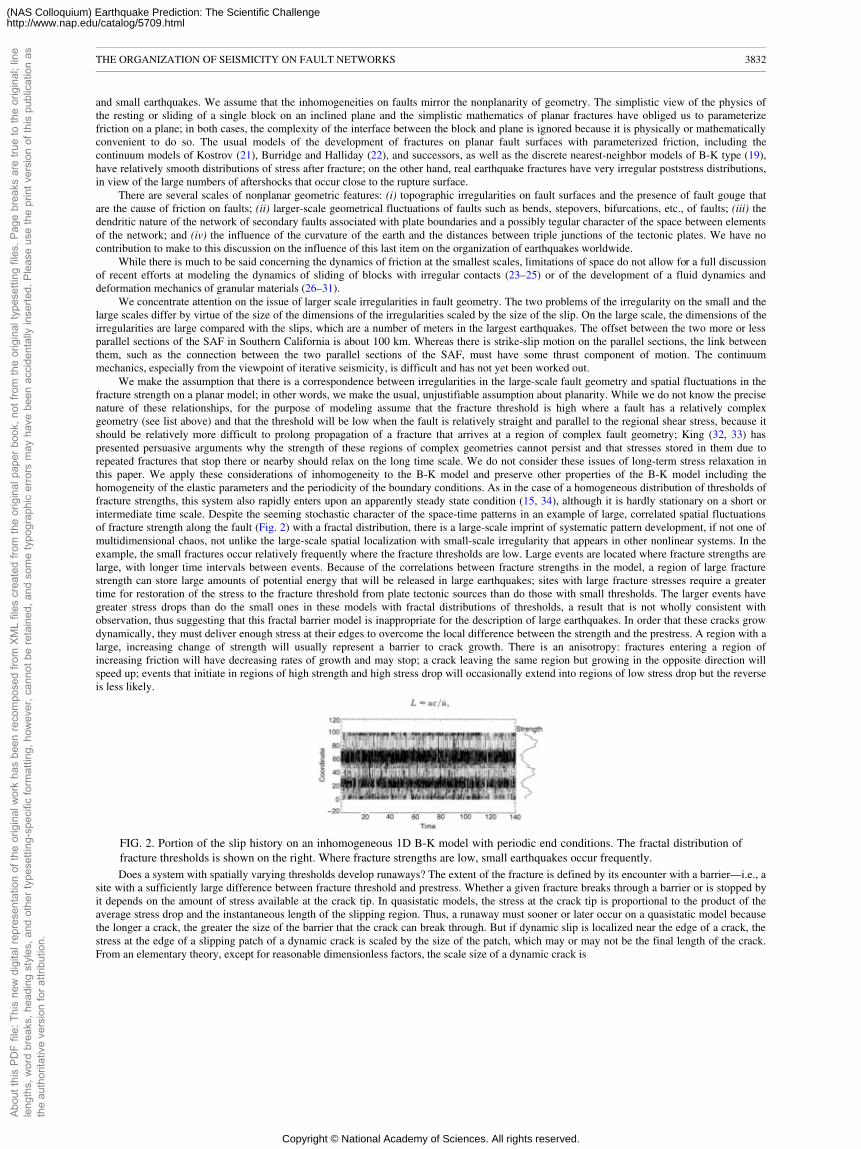
and small earthquakes. We assume that the inhomogeneities on faults mirror the nonplanarity of geometry. The simplistic view of the physics ofthe resting or sliding of a single block on an inclined plane and the simplistic mathematics of planar fractures have obliged us to parameterizefriction on a plane; in both cases, the complexity of the interface between the block and plane is ignored because it is physically or mathematicallyconvenient to do so. The usual models of the development of fractures on planar fault surfaces with parameterized friction, including thecontinuum models of Kostrov (21), Burridge and Halliday (22), and successors, as well as the discrete nearest-neighbor models of B-K type (19),have relatively smooth distributions of stress after fracture; on the other hand, real earthquake fractures have very irregular poststress distributions,in view of the large numbers of aftershocks that occur close to the rupture surface.
There are several scales of nonplanar geometric features: (i) topographic irregularities on fault surfaces and the presence of fault gouge thatare the cause of friction on faults; (ii) larger-scale geometrical fluctuations of faults such as bends, stepovers, bifurcations, etc., of faults; (iii) thedendritic nature of the network of secondary faults associated with plate boundaries and a possibly tegular character of the space between elementsof the network; and (iv) the influence of the curvature of the earth and the distances between triple junctions of the tectonic plates. We have nocontribution to make to this discussion on the influence of this last item on the organization of earthquakes worldwide.
While there is much to be said concerning the dynamics of friction at the smallest scales, limitations of space do not allow for a full discussionof recent efforts at modeling the dynamics of sliding of blocks with irregular contacts (23–25) or of the development of a fluid dynamics anddeformation mechanics of granular materials (26–31).
We concentrate attention on the issue of larger scale irregularities in fault geometry. The two problems of the irregularity on the small and thelarge scales differ by virtue of the size of the dimensions of the irregularities scaled by the size of the slip. On the large scale, the dimensions of theirregularities are large compared with the slips, which are a number of meters in the largest earthquakes. The offset between the two more or lessparallel sections of the SAF in Southern California is about 100 km. Whereas there is strike-slip motion on the parallel sections, the link betweenthem, such as the connection between the two parallel sections of the SAF, must have some thrust component of motion. The continuummechanics, especially from the viewpoint of iterative seismicity, is difficult and has not yet been worked out.
We make the assumption that there is a correspondence between irregularities in the large-scale fault geometry and spatial fluctuations in thefracture strength on a planar model; in other words, we make the usual, unjustifiable assumption about planarity. While we do not know the precisenature of these relationships, for the purpose of modeling assume that the fracture threshold is high where a fault has a relatively complexgeometry (see list above) and that the threshold will be low when the fault is relatively straight and parallel to the regional shear stress, because itshould be relatively more difficult to prolong propagation of a fracture that arrives at a region of complex fault geometry; King (32, 33) haspresented persuasive arguments why the strength of these regions of complex geometries cannot persist and that stresses stored in them due torepeated fractures that stop there or nearby should relax on the long time scale. We do not consider these issues of long-term stress relaxation inthis paper. We apply these considerations of inhomogeneity to the B-K model and preserve other properties of the B-K model including thehomogeneity of the elastic parameters and the periodicity of the boundary conditions. As in the case of a homogeneous distribution of thresholds offracture strengths, this system also rapidly enters upon an apparently steady state condition (15, 34), although it is hardly stationary on a short orintermediate time scale. Despite the seeming stochastic character of the space-time patterns in an example of large, correlated spatial fluctuationsof fracture strength along the fault (Fig. 2) with a fractal distribution, there is a large-scale imprint of systematic pattern development, if not one ofmultidimensional chaos, not unlike the large-scale spatial localization with small-scale irregularity that appears in other nonlinear systems. In theexample, the small fractures occur relatively frequently where the fracture thresholds are low. Large events are located where fracture strengths arelarge, with longer time intervals between events. Because of the correlations between fracture strengths in the model, a region of large fracturestrength can store large amounts of potential energy that will be released in large earthquakes; sites with large fracture stresses require a greatertime for restoration of the stress to the fracture threshold from plate tectonic sources than do those with small thresholds. The larger events havegreater stress drops than do the small ones in these models with fractal distributions of thresholds, a result that is not wholly consistent withobservation, thus suggesting that this fractal barrier model is inappropriate for the description of large earthquakes. In order that these cracks growdynamically, they must deliver enough stress at their edges to overcome the local difference between the strength and the prestress. A region with alarge, increasing change of strength will usually represent a barrier to crack growth. There is an anisotropy: fractures entering a region ofincreasing friction will have decreasing rates of growth and may stop; a crack leaving the same region but growing in the opposite direction willspeed up; events that initiate in regions of high strength and high stress drop will occasionally extend into regions of low stress drop but the reverseis less likely.
FIG. 2. Portion of the slip history on an inhomogeneous 1D B-K model with periodic end conditions. The fractal distribution offracture thresholds is shown on the right. Where fracture strengths are low, small earthquakes occur frequently.Does a system with spatially varying thresholds develop runaways? The extent of the fracture is defined by its encounter with a barrier—i.e., a
site with a sufficiently large difference between fracture threshold and prestress. Whether a given fracture breaks through a barrier or is stopped byit depends on the amount of stress available at the crack tip. In quasistatic models, the stress at the crack tip is proportional to the product of theaverage stress drop and the instantaneous length of the slipping region. Thus, a runaway must sooner or later occur on a quasistatic model becausethe longer a crack, the greater the size of the barrier that the crack can break through. But if dynamic slip is localized near the edge of a crack, thestress at the edge of a slipping patch of a dynamic crack is scaled by the size of the patch, which may or may not be the final length of the crack.From an elementary theory, except for reasonable dimensionless factors, the scale size of a dynamic crack is
THE ORGANIZATION OF SEISMICITY ON FAULT NETWORKS 3832
Abou
t thi
s PD
F fil
e: T
his
new
dig
ital r
epre
sent
atio
n of
the
orig
inal
wor
k ha
s be
en re
com
pose
d fro
m X
ML
files
cre
ated
from
the
orig
inal
pap
er b
ook,
not
from
the
orig
inal
type
setti
ng fi
les.
Pag
e br
eaks
are
true
to th
e or
igin
al; l
ine
leng
ths,
wor
d br
eaks
, hea
ding
sty
les,
and
oth
er ty
pese
tting
-spe
cific
form
attin
g, h
owev
er, c
anno
t be
reta
ined
, and
som
e ty
pogr
aphi
c er
rors
may
hav
e be
en a
ccid
enta
lly in
serte
d. P
leas
e us
e th
e pr
int v
ersi
on o
f thi
s pu
blic
atio
n as
the
auth
orita
tive
vers
ion
for a
ttrib
utio
n.
Copyright © National Academy of Sciences. All rights reserved.
(NAS Colloquium) Earthquake Prediction: The Scientific Challengehttp://www.nap.edu/catalog/5709.html
where u is the mean slip, ú is the mean slip velocity, and c is the speed of the edge of the crack, which we take to be the shear wave velocity. Forthe largest earthquakes such as Landers or San Francisco, the scale size is of the order of 15 km, a distance that is more appropriate to the thicknessof the seismogenic zone than is the length of the crack, by factors of 5 and 30 in the two cases. Thus, the stress at one edge of the largestearthquakes does not depend on the conditions at the remote, opposite edge but depends instead on some local property. We remark in passing thatthe range of aftershocks beyond the edge of an earthquake fracture can be expected to be scaled by L (35), which is more appropriately 15 km thanthe total length of the fracture. Conversely, the relatively short range of aftershocks in great earthquakes implies the presence of a moving patch ofslip as the mode of rupture and is a condition observed for a number of earthquakes (16). If the scale size of rupture is independent of the length ofthe rupture in the largest earthquakes, then the stress at the edge does not increase with increasing length of rupture, and hence a sufficiently strongbarrier will stop crack growth. If there are several such barriers in a region, then the breaking of one of these will not cause the others to fail.Hence, there will be no runaway in this case. Because of the nearest-neighbor coupling of stresses in the B-K model and the short range of stressinteractions on the ruptured segment, this model is not likely to develop runaways in the presence of a nonuniform distribution of fracturestrengths. Since large fluctuations in fracture thresholds serve to prevent runaways, and vanishingly small ones do not, we expect that there shouldbe a transition between the cases of small fluctuations in barrier strengths, which allow for runaways, and those of large fluctuations, which allowfor localization.
The distribution of earthquakes that is found on these inhomogeneous models is very sensitive to the distribution of fracture thresholds. Aspiky distribution of fracture strengths, intended to simulate a sparse distribution of barriers on a single fault, leads to a very different display ofspace-time seismicity, from the preceding case (Fig. 3). In the example, the ratio of threshold fracture strengths in the spikes to that of the broadand almost flat valleys between them is very large. The space-time patterns show much greater regularity than in the preceding example. However,the notable interruptions from one seemingly stable pattern to another equally seemingly stable pattern, occur at times that are episodic and notapparently predictable, even on a deterministic model such as this one. These instabilities are triggered by the breaking of the strong barriers thatform the borders to the deep, broad valleys of low strength, in contrast to models with infinite barriers at the edge of the lattice. Even the site withthe greatest strength must break because of the constraint that the long-term average slip velocity be uniform at all lattice sites. The barrierearthquakes are usually strong, since these are the sites of large storage of deformational potential energy. The opening of the barrier gatestransfers a large stress from one low strength valley to another and changes the stress distribution in the adjoining valley, thereby triggering a newmode of repetitive fractures in the valley. We suppose that in models with inhomogeneous thresholds the relaxation of the stresses in the barriersare important events, whether the thresholds are spiky or not. To assume that barriers are unbreakable with infinite thresholds leads to evolutionaryhistories that are not reliable.
In some cases, the valley with low fluctuations appears to be smooth and fractures are throughgoing from one barrier spike to the next barrierspike. But if the valley is sufficiently long, seismicity in the valleys breaks up into shorter fracture segments; these cases would appear to beconsistent with a long model with homogeneous fracture strengths as described above (17). The factors that determine whether the seismicity in thevalleys will be of one type or the other are the ratio between the fracture strengths of the peaks and valleys, which determines the strength of thestress impulse that is sent into a valley from a rupture at a peak, and the ratio between the length of the valley and the scale size for the B-K Green'sfunction a(l/k)1/2, which determines how far into the valley the stress impulse can travel.
In the models of this section, we have found it possible to generate a series of large or barrier events that belong to a different class than smallor valley events. Some of the valleys break only in long fractures, while others break in a broad distribution of events having the G-R distribution,which is schematically a pattern not unlike seismicity in Southern California, although there are significant differences. The models are sensitive tothe choice of geometry, but generally these models favor the characteristic earthquake model for large events on some of the faults of the systemand the statistical model for smaller events on other faults of the system. The large events are stopped by significant barriers associated with majorgeometrical features of long faults. In these models, the smaller events are dominated by processes of self-organization on relatively smooth faults,since we have not allowed for their occurrence on individual faultlets that are not directly linked to major faults nearby.
FIG. 3. Same as Fig. 2, but with a spiky distribution of fracture thresholds as shown on the right. Episodic shifts in periodicityare associated with fractures that breach the barriers. [Reproduced with permission from ref. 25 (copyright 1995, AmericanSociety of Mechanical Engineers).]By the arguments above, I have tried to suggest that the G-R law is not a characteristic of faults that support large earthquakes. If this is the
case, what is the structure that supports the G-R law? Although the scale independence implied by the G-R law may arise due to self-organizationon the scale independent, homogeneous system, this system has the defects already enumerated, that it does not develop localization, it does notprovide for a discrimination between small and large earthquakes, and it does not prevent runaways. An orthogonal point of view is that the G-Rdistribution is a consequence of the geometry of the fault network, as are the properties of the largest earthquakes. On the geometrical model, wesuppose that the power law distribution of earthquake sizes is due to seismicity on a myriad of isolated and noninteractive faults having a power-law distribution of sizes and strewn over the entire space. The failure of the SAF and several of the other faults to observe the regularity of the G-Rlaw suggests therefore that the faults that support large earthquakes have different physical properties and geometry than do the smaller ones, aconclusion already suggested by the phenomenology. If the G-R law is an image of a power-law distribution of sizes of small faults or fracturesurfaces, why is the G-R distribution universal? One possible answer is to propose that the formation of the fault surfaces of small dimension thatsupport small earthquakes is linked to the process of slip on the larger, irregular faults, which may induce the formation of these secondaryfractures. Under this model, the universality of the G-R law is a consequence of the universality of the fracture process of a three-dimensionalstructure under the influence
THE ORGANIZATION OF SEISMICITY ON FAULT NETWORKS 3833
Abou
t thi
s PD
F fil
e: T
his
new
dig
ital r
epre
sent
atio
n of
the
orig
inal
wor
k ha
s be
en re
com
pose
d fro
m X
ML
files
cre
ated
from
the
orig
inal
pap
er b
ook,
not
from
the
orig
inal
type
setti
ng fi
les.
Pag
e br
eaks
are
true
to th
e or
igin
al; l
ine
leng
ths,
wor
d br
eaks
, hea
ding
sty
les,
and
oth
er ty
pese
tting
-spe
cific
form
attin
g, h
owev
er, c
anno
t be
reta
ined
, and
som
e ty
pogr
aphi
c er
rors
may
hav
e be
en a
ccid
enta
lly in
serte
d. P
leas
e us
e th
e pr
int v
ersi
on o
f thi
s pu
blic
atio
n as
the
auth
orita
tive
vers
ion
for a
ttrib
utio
n.
Copyright © National Academy of Sciences. All rights reserved.
(NAS Colloquium) Earthquake Prediction: The Scientific Challengehttp://www.nap.edu/catalog/5709.html
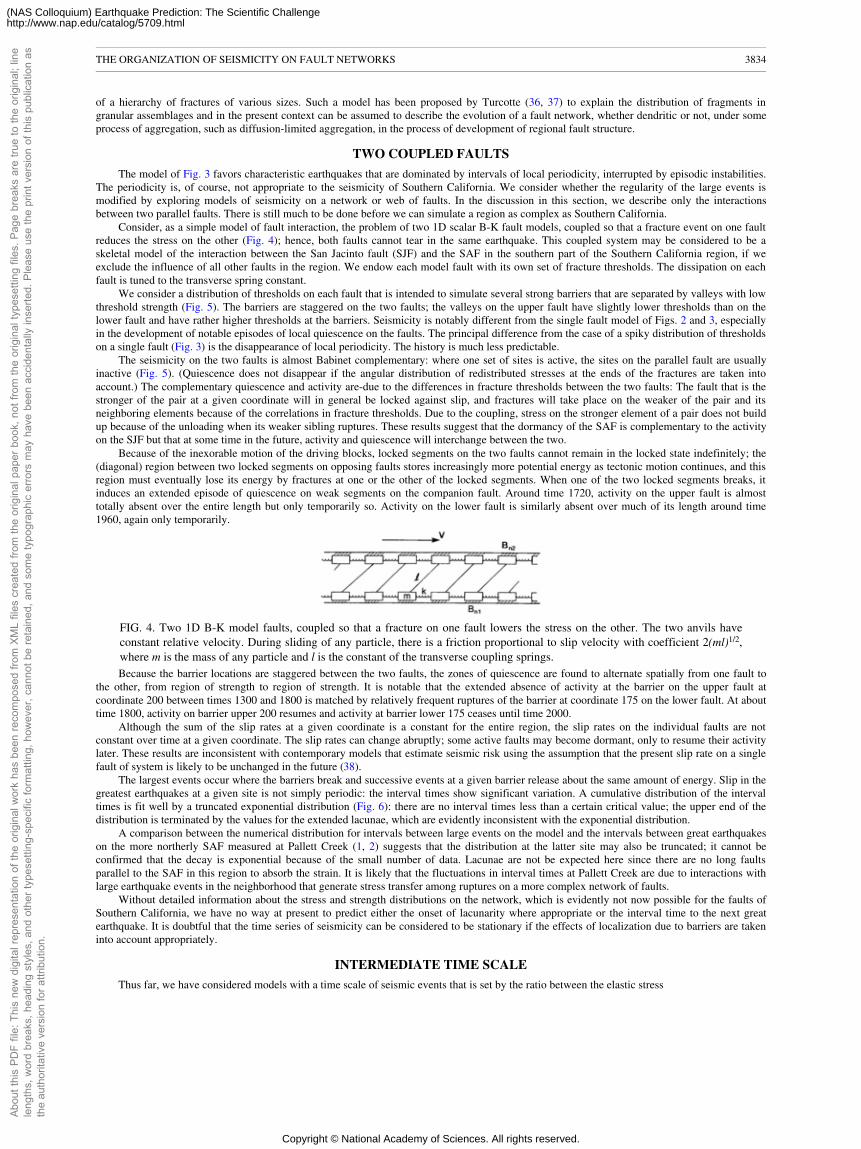
of a hierarchy of fractures of various sizes. Such a model has been proposed by Turcotte (36, 37) to explain the distribution of fragments ingranular assemblages and in the present context can be assumed to describe the evolution of a fault network, whether dendritic or not, under someprocess of aggregation, such as diffusion-limited aggregation, in the process of development of regional fault structure.
TWO COUPLED FAULTS
The model of Fig. 3 favors characteristic earthquakes that are dominated by intervals of local periodicity, interrupted by episodic instabilities.The periodicity is, of course, not appropriate to the seismicity of Southern California. We consider whether the regularity of the large events ismodified by exploring models of seismicity on a network or web of faults. In the discussion in this section, we describe only the interactionsbetween two parallel faults. There is still much to be done before we can simulate a region as complex as Southern California.
Consider, as a simple model of fault interaction, the problem of two 1D scalar B-K fault models, coupled so that a fracture event on one faultreduces the stress on the other (Fig. 4); hence, both faults cannot tear in the same earthquake. This coupled system may be considered to be askeletal model of the interaction between the San Jacinto fault (SJF) and the SAF in the southern part of the Southern California region, if weexclude the influence of all other faults in the region. We endow each model fault with its own set of fracture thresholds. The dissipation on eachfault is tuned to the transverse spring constant.
We consider a distribution of thresholds on each fault that is intended to simulate several strong barriers that are separated by valleys with lowthreshold strength (Fig. 5). The barriers are staggered on the two faults; the valleys on the upper fault have slightly lower thresholds than on thelower fault and have rather higher thresholds at the barriers. Seismicity is notably different from the single fault model of Figs. 2 and 3, especiallyin the development of notable episodes of local quiescence on the faults. The principal difference from the case of a spiky distribution of thresholdson a single fault (Fig. 3) is the disappearance of local periodicity. The history is much less predictable.
The seismicity on the two faults is almost Babinet complementary: where one set of sites is active, the sites on the parallel fault are usuallyinactive (Fig. 5). (Quiescence does not disappear if the angular distribution of redistributed stresses at the ends of the fractures are taken intoaccount.) The complementary quiescence and activity are-due to the differences in fracture thresholds between the two faults: The fault that is thestronger of the pair at a given coordinate will in general be locked against slip, and fractures will take place on the weaker of the pair and itsneighboring elements because of the correlations in fracture thresholds. Due to the coupling, stress on the stronger element of a pair does not buildup because of the unloading when its weaker sibling ruptures. These results suggest that the dormancy of the SAF is complementary to the activityon the SJF but that at some time in the future, activity and quiescence will interchange between the two.
Because of the inexorable motion of the driving blocks, locked segments on the two faults cannot remain in the locked state indefinitely; the(diagonal) region between two locked segments on opposing faults stores increasingly more potential energy as tectonic motion continues, and thisregion must eventually lose its energy by fractures at one or the other of the locked segments. When one of the two locked segments breaks, itinduces an extended episode of quiescence on weak segments on the companion fault. Around time 1720, activity on the upper fault is almosttotally absent over the entire length but only temporarily so. Activity on the lower fault is similarly absent over much of its length around time1960, again only temporarily.
FIG. 4. Two 1D B-K model faults, coupled so that a fracture on one fault lowers the stress on the other. The two anvils haveconstant relative velocity. During sliding of any particle, there is a friction proportional to slip velocity with coefficient 2(ml)1/2,where m is the mass of any particle and l is the constant of the transverse coupling springs.Because the barrier locations are staggered between the two faults, the zones of quiescence are found to alternate spatially from one fault to
the other, from region of strength to region of strength. It is notable that the extended absence of activity at the barrier on the upper fault atcoordinate 200 between times 1300 and 1800 is matched by relatively frequent ruptures of the barrier at coordinate 175 on the lower fault. At abouttime 1800, activity on barrier upper 200 resumes and activity at barrier lower 175 ceases until time 2000.
Although the sum of the slip rates at a given coordinate is a constant for the entire region, the slip rates on the individual faults are notconstant over time at a given coordinate. The slip rates can change abruptly; some active faults may become dormant, only to resume their activitylater. These results are inconsistent with contemporary models that estimate seismic risk using the assumption that the present slip rate on a singlefault of system is likely to be unchanged in the future (38).
The largest events occur where the barriers break and successive events at a given barrier release about the same amount of energy. Slip in thegreatest earthquakes at a given site is not simply periodic: the interval times show significant variation. A cumulative distribution of the intervaltimes is fit well by a truncated exponential distribution (Fig. 6): there are no interval times less than a certain critical value; the upper end of thedistribution is terminated by the values for the extended lacunae, which are evidently inconsistent with the exponential distribution.
A comparison between the numerical distribution for intervals between large events on the model and the intervals between great earthquakeson the more northerly SAF measured at Pallett Creek (1, 2) suggests that the distribution at the latter site may also be truncated; it cannot beconfirmed that the decay is exponential because of the small number of data. Lacunae are not be expected here since there are no long faultsparallel to the SAF in this region to absorb the strain. It is likely that the fluctuations in interval times at Pallett Creek are due to interactions withlarge earthquake events in the neighborhood that generate stress transfer among ruptures on a more complex network of faults.
Without detailed information about the stress and strength distributions on the network, which is evidently not now possible for the faults ofSouthern California, we have no way at present to predict either the onset of lacunarity where appropriate or the interval time to the next greatearthquake. It is doubtful that the time series of seismicity can be considered to be stationary if the effects of localization due to barriers are takeninto account appropriately.
INTERMEDIATE TIME SCALE
Thus far, we have considered models with a time scale of seismic events that is set by the ratio between the elastic stress
THE ORGANIZATION OF SEISMICITY ON FAULT NETWORKS 3834
Abou
t thi
s PD
F fil
e: T
his
new
dig
ital r
epre
sent
atio
n of
the
orig
inal
wor
k ha
s be
en re
com
pose
d fro
m X
ML
files
cre
ated
from
the
orig
inal
pap
er b
ook,
not
from
the
orig
inal
type
setti
ng fi
les.
Pag
e br
eaks
are
true
to th
e or
igin
al; l
ine
leng
ths,
wor
d br
eaks
, hea
ding
sty
les,
and
oth
er ty
pese
tting
-spe
cific
form
attin
g, h
owev
er, c
anno
t be
reta
ined
, and
som
e ty
pogr
aphi
c er
rors
may
hav
e be
en a
ccid
enta
lly in
serte
d. P
leas
e us
e th
e pr
int v
ersi
on o
f thi
s pu
blic
atio
n as
the
auth
orita
tive
vers
ion
for a
ttrib
utio
n.
Copyright © National Academy of Sciences. All rights reserved.
(NAS Colloquium) Earthquake Prediction: The Scientific Challengehttp://www.nap.edu/catalog/5709.html
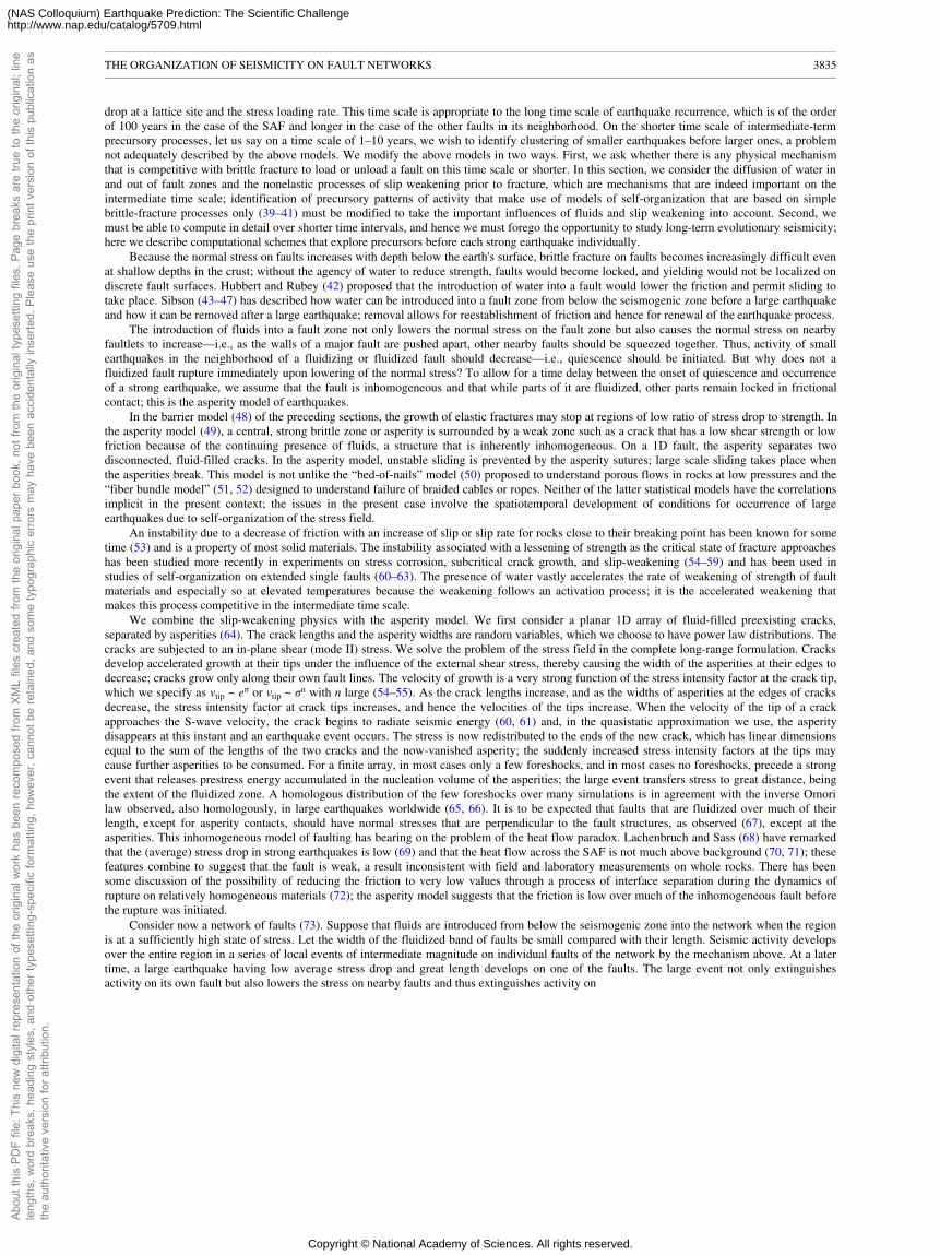
drop at a lattice site and the stress loading rate. This time scale is appropriate to the long time scale of earthquake recurrence, which is of the orderof 100 years in the case of the SAF and longer in the case of the other faults in its neighborhood. On the shorter time scale of intermediate-termprecursory processes, let us say on a time scale of 1–10 years, we wish to identify clustering of smaller earthquakes before larger ones, a problemnot adequately described by the above models. We modify the above models in two ways. First, we ask whether there is any physical mechanismthat is competitive with brittle fracture to load or unload a fault on this time scale or shorter. In this section, we consider the diffusion of water inand out of fault zones and the nonelastic processes of slip weakening prior to fracture, which are mechanisms that are indeed important on theintermediate time scale; identification of precursory patterns of activity that make use of models of self-organization that are based on simplebrittle-fracture processes only (39–41) must be modified to take the important influences of fluids and slip weakening into account. Second, wemust be able to compute in detail over shorter time intervals, and hence we must forego the opportunity to study long-term evolutionary seismicity;here we describe computational schemes that explore precursors before each strong earthquake individually.
Because the normal stress on faults increases with depth below the earth's surface, brittle fracture on faults becomes increasingly difficult evenat shallow depths in the crust; without the agency of water to reduce strength, faults would become locked, and yielding would not be localized ondiscrete fault surfaces. Hubbert and Rubey (42) proposed that the introduction of water into a fault would lower the friction and permit sliding totake place. Sibson (43–47) has described how water can be introduced into a fault zone from below the seismogenic zone before a large earthquakeand how it can be removed after a large earthquake; removal allows for reestablishment of friction and hence for renewal of the earthquake process.
The introduction of fluids into a fault zone not only lowers the normal stress on the fault zone but also causes the normal stress on nearbyfaultlets to increase—i.e., as the walls of a major fault are pushed apart, other nearby faults should be squeezed together. Thus, activity of smallearthquakes in the neighborhood of a fluidizing or fluidized fault should decrease—i.e., quiescence should be initiated. But why does not afluidized fault rupture immediately upon lowering of the normal stress? To allow for a time delay between the onset of quiescence and occurrenceof a strong earthquake, we assume that the fault is inhomogeneous and that while parts of it are fluidized, other parts remain locked in frictionalcontact; this is the asperity model of earthquakes.
In the barrier model (48) of the preceding sections, the growth of elastic fractures may stop at regions of low ratio of stress drop to strength. Inthe asperity model (49), a central, strong brittle zone or asperity is surrounded by a weak zone such as a crack that has a low shear strength or lowfriction because of the continuing presence of fluids, a structure that is inherently inhomogeneous. On a 1D fault, the asperity separates twodisconnected, fluid-filled cracks. In the asperity model, unstable sliding is prevented by the asperity sutures; large scale sliding takes place whenthe asperities break. This model is not unlike the “bed-of-nails” model (50) proposed to understand porous flows in rocks at low pressures and the“fiber bundle model” (51, 52) designed to understand failure of braided cables or ropes. Neither of the latter statistical models have the correlationsimplicit in the present context; the issues in the present case involve the spatiotemporal development of conditions for occurrence of largeearthquakes due to self-organization of the stress field.
An instability due to a decrease of friction with an increase of slip or slip rate for rocks close to their breaking point has been known for sometime (53) and is a property of most solid materials. The instability associated with a lessening of strength as the critical state of fracture approacheshas been studied more recently in experiments on stress corrosion, subcritical crack growth, and slip-weakening (54–59) and has been used instudies of self-organization on extended single faults (60–63). The presence of water vastly accelerates the rate of weakening of strength of faultmaterials and especially so at elevated temperatures because the weakening follows an activation process; it is the accelerated weakening thatmakes this process competitive in the intermediate time scale.
We combine the slip-weakening physics with the asperity model. We first consider a planar 1D array of fluid-filled preexisting cracks,separated by asperities (64). The crack lengths and the asperity widths are random variables, which we choose to have power law distributions. Thecracks are subjected to an in-plane shear (mode II) stress. We solve the problem of the stress field in the complete long-range formulation. Cracksdevelop accelerated growth at their tips under the influence of the external shear stress, thereby causing the width of the asperities at their edges todecrease; cracks grow only along their own fault lines. The velocity of growth is a very strong function of the stress intensity factor at the crack tip,which we specify as vtip ~ eσ or vtip ~ σn with n large (54–55). As the crack lengths increase, and as the widths of asperities at the edges of cracksdecrease, the stress intensity factor at crack tips increases, and hence the velocities of the tips increase. When the velocity of the tip of a crackapproaches the S-wave velocity, the crack begins to radiate seismic energy (60, 61) and, in the quasistatic approximation we use, the asperitydisappears at this instant and an earthquake event occurs. The stress is now redistributed to the ends of the new crack, which has linear dimensionsequal to the sum of the lengths of the two cracks and the now-vanished asperity; the suddenly increased stress intensity factors at the tips maycause further asperities to be consumed. For a finite array, in most cases only a few foreshocks, and in most cases no foreshocks, precede a strongevent that releases prestress energy accumulated in the nucleation volume of the asperities; the large event transfers stress to great distance, beingthe extent of the fluidized zone. A homologous distribution of the few foreshocks over many simulations is in agreement with the inverse Omorilaw observed, also homologously, in large earthquakes worldwide (65, 66). It is to be expected that faults that are fluidized over much of theirlength, except for asperity contacts, should have normal stresses that are perpendicular to the fault structures, as observed (67), except at theasperities. This inhomogeneous model of faulting has bearing on the problem of the heat flow paradox. Lachenbruch and Sass (68) have remarkedthat the (average) stress drop in strong earthquakes is low (69) and that the heat flow across the SAF is not much above background (70, 71); thesefeatures combine to suggest that the fault is weak, a result inconsistent with field and laboratory measurements on whole rocks. There has beensome discussion of the possibility of reducing the friction to very low values through a process of interface separation during the dynamics ofrupture on relatively homogeneous materials (72); the asperity model suggests that the friction is low over much of the inhomogeneous fault beforethe rupture was initiated.
Consider now a network of faults (73). Suppose that fluids are introduced from below the seismogenic zone into the network when the regionis at a sufficiently high state of stress. Let the width of the fluidized band of faults be small compared with their length. Seismic activity developsover the entire region in a series of local events of intermediate magnitude on individual faults of the network by the mechanism above. At a latertime, a large earthquake having low average stress drop and great length develops on one of the faults. The large event not only extinguishesactivity on its own fault but also lowers the stress on nearby faults and thus extinguishes activity on
THE ORGANIZATION OF SEISMICITY ON FAULT NETWORKS 3835
Abou
t thi
s PD
F fil
e: T
his
new
dig
ital r
epre
sent
atio
n of
the
orig
inal
wor
k ha
s be
en re
com
pose
d fro
m X
ML
files
cre
ated
from
the
orig
inal
pap
er b
ook,
not
from
the
orig
inal
type
setti
ng fi
les.
Pag
e br
eaks
are
true
to th
e or
igin
al; l
ine
leng
ths,
wor
d br
eaks
, hea
ding
sty
les,
and
oth
er ty
pese
tting
-spe
cific
form
attin
g, h
owev
er, c
anno
t be
reta
ined
, and
som
e ty
pogr
aphi
c er
rors
may
hav
e be
en a
ccid
enta
lly in
serte
d. P
leas
e us
e th
e pr
int v
ersi
on o
f thi
s pu
blic
atio
n as
the
auth
orita
tive
vers
ion
for a
ttrib
utio
n.
Copyright © National Academy of Sciences. All rights reserved.
(NAS Colloquium) Earthquake Prediction: The Scientific Challengehttp://www.nap.edu/catalog/5709.html
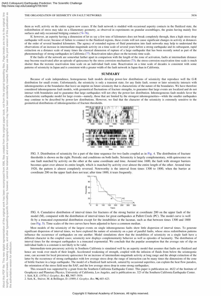
them as well; activity on the entire region now ceases. If the fault network is studded with occasional asperity contacts in the fluidized state, theredistribution of stress may take on a filamentary geometry, as observed in experiments on granular assemblages, the grains having mainly freesurfaces and only occasional bridging contacts (74–76).
If, however, an asperity having a dimension of let us say a few tens of kilometers does not break completely through, then a high stress dropearthquake will occur; because of failure to connect to the fluidized regions, these events will not cause significant changes in activity at distancesof the order of several hundred kilometers. The agency of extended regions of fluid penetration into fault networks may help to understand theobservations of an increase in intermediate-magnitude activity on a time scale of several years before a strong earthquake and its subsequent, rapidextinction on a distance scale of many times the classical dimension of rupture of a large earthquake that has been recently noted as part of thephenomenology of strong earthquakes in California (77). Reactivation takes place on the tectonic time scale.
If the faults of the network are somewhat farther apart in comparison with the length of the zone of activation, faults at intermediate distancemay become reactivated after an episode of quiescence by the stress corrosion mechanism (73); the stress-corrosion reactivation time scale is muchshorter than the tectonic reactivation time scale on an individual fault zone. Reactivation on a time scale of decades is consistent with somepatterns of seismicity in Japan and is consistent with a greater width of the fault network in Japan than in California.
SUMMARY
Because of scale independence, homogeneous fault models develop power-law distributions of seismicity that reproduce well the G-Rdistribution for small events. Unfortunately, the seismicity is only a transient state; for any finite fault, sooner or later seismicity interacts withinhomogeneities at the boundaries that leave an imprint on future seismicity that is characteristic of the nature of the boundaries. We have thereforeconsidered inhomogeneous fault models, with geometrical fluctuations of fracture strengths, to guarantee that large events are localized and do notinteract with boundaries and to guarantee that large earthquakes will not obey the power-law distribution. Inhomogeneous fault models favor thecharacteristic earthquake model for large events—namely, those that are limited by the strongest inhomogeneities—while the smaller earthquakesmay continue to be described by power-law distributions. However, we find that the character of the seismicity is extremely sensitive to thegeometrical distributions of inhomogeneities of fracture thresholds.
FIG. 5. Distribution of seismicity for a part of the time sequence for two faults coupled as in Fig. 4. The distribution of fracturethresholds is shown on the right. Periodic end conditions on both faults. Seismicity is largely complementary, with quiescence onone fault matched by activity on the other at the same coordinate and time. Around time 1600, the fault with stronger barriersbecomes quiet over almost its entire length, which is matched by activity over almost the entire length of the other. Around time1920, the pattern is almost completely reversed. Noteworthy is the interval from times 1300 to 1800, when the barrier atcoordinate 200 on the upper fault does not tear; after time 1800, it tears frequently.
FIG. 6. Cumulative distribution of interval times for fractures of the strong barrier at coordinate 200 on the upper fault of themodel (M), compared with the distribution of interval times for great earthquakes at Pallett Creek (PC). The model curve is wellfit by a truncated exponential distribution except for the instabilities at the lacunae, such as that between times 1300 and 1800(see Fig. 5). Time scales of the two curves have been adjusted to have a common median.Most models of the seismicity of the largest events on single inhomogeneous faults show little dispersion of interval times. To generate
significant dispersion of interval times, we have explored the nature of seismicity on a pair of parallel faults, whose stress redistribution patternsinfluence the occurrence of earthquakes on one another. Model simulations show that the instabilities of seismicity on a single fault have adifferent character in the coupled cases; seismicity now displays complementarity behavior as well as episodes of lacunarity. The distribution ofinterval times for the strongest earthquakes is a truncated exponential. We conclude that the popular assumption that the average rate of slip onindividual faults is a constant is not likely to be valid.
Intermediate-term precursory activity in Southern California is simulated well by an asperity model that assumes that faults are fluidized andhence are weak over much of their length. Accelerated weakening of strength, coupled with the infusion of fluids from below the seismogeniczone, can account for local precursory quiescence for an increase of intermediate-magnitude activity at long range and the abrupt extinction of thelatter by the occurrence of strong earthquakes with low average stress drop; the range of interaction can be many times the dimensions of the zoneof brittle fracture in a large earthquake. The model of a fluidized fault network, sutured by occasional asperities, can explain the heat flow paradox,the orientation of the stress field near the SAF, and the low average stress drop in some strong earthquakes.
This research was supported by a grant from the Southern California Earthquake Center. This paper is publication no. 4622 of the Institute ofGeophysics and Planetary Physics, University of California, Los Angeles, and is publication no. 323 of the Southern California Earthquake Center.1. Sieh, K.E. (1978) J. Geophys. Res. 83, 3907–3939.2. Sieh, K., Stuiver, M. & Brillinger, D. (1989) J. Geophys. Res. 94, 603–623.
THE ORGANIZATION OF SEISMICITY ON FAULT NETWORKS 3836
Abou
t thi
s PD
F fil
e: T
his
new
dig
ital r
epre
sent
atio
n of
the
orig
inal
wor
k ha
s be
en re
com
pose
d fro
m X
ML
files
cre
ated
from
the
orig
inal
pap
er b
ook,
not
from
the
orig
inal
type
setti
ng fi
les.
Pag
e br
eaks
are
true
to th
e or
igin
al; l
ine
leng
ths,
wor
d br
eaks
, hea
ding
sty
les,
and
oth
er ty
pese
tting
-spe
cific
form
attin
g, h
owev
er, c
anno
t be
reta
ined
, and
som
e ty
pogr
aphi
c er
rors
may
hav
e be
en a
ccid
enta
lly in
serte
d. P
leas
e us
e th
e pr
int v
ersi
on o
f thi
s pu
blic
atio
n as
the
auth
orita
tive
vers
ion
for a
ttrib
utio
n.
Copyright © National Academy of Sciences. All rights reserved.
(NAS Colloquium) Earthquake Prediction: The Scientific Challengehttp://www.nap.edu/catalog/5709.html
3. Knopoff, L. (1996) Proc. Natl. Acad. Sci. USA, 3756–3763.4. Bak, P. & Tang, C. (1989) J. Geophys. Res. 94, 15635–15637.5. Nakanishi, H. (1990) Phys. Rev. A 41, 7086–7089.6. Nakanishi, H. (1991) Phys. Rev. A 43, 6613–6621.7. Christensen, K. & Olami, Z. (1992) J. Geophys. Res. 97, 8729–8735.8. Christensen, K. & Olami, Z. (1992) Phys. Rev. A 46, 1829–1838.9. Christensen, K., Olami, Z. & Bak, P. (1992) Phys. Rev. Lett. 68, 2417–2420.10. Olami, Z., Feder, H.J.S. & Christensen, K. (1992) Phys. Rev. Lett. 68, 1244–1247.11. Olami, Z. & Christensen, K. (1992) Phys. Rev. A 46, 1720–1723.12. Burridge, R. & Knopoff, L. (1967) Bull. Seismol. Soc. Am. 57, 341–371.13. Carlson, J. & Langer, J.S. (1989) Phys. Rev. Lett. 62, 2632–2635.14. Carlson, J.M. & Langer, J.S. (1989) Phys. Rev. A 40, 6470–6484.15. Knopoff, L., Landoni, J.A. & Abinante, M.S. (1992) Phys. Rev. A 46, 7445–7449.16. Heaton, T.H. (1990) Phys. Earth Planet. Inter. 64, 1–20.17. Xu, H.J. & Knopoff, L. (1994) Phys. Rev. E 50, 3577–3581.18. Wacker, A., Bose, S. & Sehöll, E. (1995) Europhys. Lett. 31, 257–262.19. Abinante, M.S. & Knopoff, L. (1995) Phys. Rev. E 52, 5675–5678.20. Rice, J.R. (1993) J. Geophys. Res. 98, 9885–9907.21. Kostrov, B.V. (1996) J. Appl. Math. Mech. 30, 1241–1248.22. Burridge, R. & Halliday, G.S. (1971) Geophys. J.R.Astron. Soc. 25, 261–283.23. Lomnitz-Adler, J. (1991) J. Geophys. Res. 96, 6121–6131.24. Pisarenko, D. & Mora, P. (1994) Pure Appl. Geophys. 142, 447–466.25. Knopoff, L. & Ni, X.X. (1995) in Impact, Waves and Fracture, eds. Batra, R.C., Mal, A.K. & MacSiphigh, G.P. (Am. Soc. Mech. Engrs., New York),
pp. 175–187.26. Scott, D.R., Marone, C.J. & Sammis, C.G. (1994) J. Geophys. Res. 99, 7231–7246.27. Chester, F.M. (1994) J. Geophys. Res. 99, 7247–7261.28. Herrmann, H.J. (1992) Physica A 191, 263–276.29. Knight, J.B., Jaeger, H.M. & Nagel, S.R. (1993) Phys. Rev. Lett. 70, 3728–3731.30. Ehrichs, E.E., Jaeger, H.M., Karczmar, G.S., Knight, J.B., Kuperman, V.Y. & Nagel, S.R. (1995) Science 267, 1632–1634.31. Tillemans, H.-J. & Herrmann, H.J. (1995) Physica A 217, 261–288.32. King, G. (1986) Pure Appl. Geophys. 124, 567–585.33. King, G. & Nabelek, J. (1985) Science 228, 984–987.34. Knopoff, L. (1993) Proc. Am. Philos. Soc. 137, 339–349.35. Chen, Y.-T. & Knopoff, L. (1986) Geophys. J.R. Astron. Soc. 87, 1005–1024.36. Turcotte, D.L. (1986) J. Geophys. Res. 91, 1921–1926.37. Turcotte, D.L. (1992) Fractals and Chaos in Geology and Geophysics (Cambridge Univ. Press, Cambridge, U.K.).38. Working Group on California Earthquake Probabilities (1995) Bull. Seismol. Soc. Am. 85, 379–439.39. Kossobokov, V.G. & Carlson, J.M. (1995) J. Geophys. Res. 100, 6431–6441.40. Pepke, S.L., Carlson, J.M. & Shaw, B.E. (1994) J. Geophys. Res. 99, 6769–6788.41. Shaw, B.E., Carlson, J.M. & Langer, J.S. (1992) J. Geophys. Res. 97, 479–488.42. Hubbert, M.K. & Rubey, W.W. (1959) Bull. Geol Soc. Am. 70, 115–205.43. Sibson, R.H. (1981) in Earthquake Prediction: An International Review, eds. Simpson, D.W. & Richards, P.G. (Am. Geophys. Union, Washington,
DC), pp. 593–603.44. Sibson, R.H., Moore, J. McM. & Rankin, A.H. (1975) J. Geol Soc. London 131, 652–659.45. Sibson, R.H. (1992) Earth-Science Rev. 32, 141–144.46. Sibson, R.H. (1992) Tectonophysics 211, 283–293.47. Sibson, R.H. (1994) Geol. Soc. Spec. Publ. 78, 69–84.48. Aki, K. (1979) J. Geophys. Res. 84, 6140–6148.49. Kanamori, H. (1981) in Earthquake Prediction: An International Review, eds. Simpson, D.W. & Richards, P.G. (Am. Geophys. Union, Washington,
DC), pp. 1–19.50. Gangi, A.F. (1978) Int. J.Rock Mech. Min. Sciences Geomech. Abstr. 15, 249–257.51. Newman, W.I. & Gabrielov, A.M. (1991) Int. J.Fract. 50, 1–14.52. Newman, W.I., Gabrielov, A.M., Durand, T.A., Phoenix, S.L. & Turcotte, D.L. (1994) Physica D 77, 200–216.53. Griggs, D.T. (1940) Bull. Geol. Soc. Am. 51, 1001–1022.54. Atkinson, B.K. (1982) J. Struct. Geol. 4, 41–56.55. Atkinson, B.K. (1984) J. Geophys. Res. 89, 4077–4114.56. Dieterich, J.H. (1978) Pure Appl. Geophys. 116, 790–806.57. Dieterich, J.H. (1979) J. Geophys. Res. 84, 2161–2168.58. Dieterich, J.H. (1981) Geophys. Monogr. Am. Geophys. Union 24, 103–120.59. Ruina, A. (1983) J. Geophys. Res. 88, 19359–10370.60. Cao, T. & Aki, K. (1984) Pure Appl. Geophys. 122, 10–24.61. Cao, T. & Aki, K. (1986) Pure Appl. Geophys. 124, 487–513.62. Dieterich, J.H. (1986) Geophys. Monogr. Am. Geophys. Union 37, 37–47.63. Dieterich, J.H. (1988) Pure Appl. Geophys. 126, 589–617.64. Yamashita, T. & Knopoff, L. (1989) Geophys. J.R.Astron. Soc. 96, 389–399.65. Kagan, Y.Y. & Knopoff, L. (1978) Geophys. J.R.Astron. Soc. 55, 67–86.66. Jones, L.M. & Molnar, P. (1979) J. Geophys. Res. 84, 3596–3608.67. Zoback, M.D., Zoback, M.L., Mount, V., Eaton, J., Healy, J. et al. (1987) Science 238, 1105–1111.68. Lachenbruch, A.H. & Sass, J.H. (1992) J. Geophys. Res. 97, 4995–5015.69. Kanamori, H. & Anderson, D.L. (1975) Bull. Seismol. Soc. Am. 65, 1073–1095.70. Brune, J.N., Henyey, T.L. & Roy, R.F. (1969) J. Geophys. Res. 74, 3821–3827.71. Lachenbruch, A.H. & Sass, J.H. (1980) J. Geophys. Res. 85, 6185–6222.72. Brune, J.N., Brown, S. & Johnson, P.A. (1993) Tectonophysics 218, 59–67.73. Yamashita, T. & Knopoff, L. (1992) J. Geophys. Res. 97, 19873–19879.74. Dantu, P. (1967) Ann. Ponts Chausées 4, 144.75. Travers, T., Ammi, M., Bideau, D., Gervois, A., Messager, J.C. & Troadec, J.P. (1987) Europhys. Lett. 4, 329–332.76. Liu, C.-h., Nagel, S.R., Schecter, D.A., Coppersmith, S.N., Majumdar, S., Narayan, O. & Witten, T.A. (1995) Science 269, 513–515.77. Knopoff, L., Levshina, T., Keilis-Borok, V.I. & Mattoni, C. (1996) J. Geophys. Res. 101, 5779–5796.78. Yamashita, T. (1995) J. Geophys. Res. 100, 8339–8350.
THE ORGANIZATION OF SEISMICITY ON FAULT NETWORKS 3837
Abou
t thi
s PD
F fil
e: T
his
new
dig
ital r
epre
sent
atio
n of
the
orig
inal
wor
k ha
s be
en re
com
pose
d fro
m X
ML
files
cre
ated
from
the
orig
inal
pap
er b
ook,
not
from
the
orig
inal
type
setti
ng fi
les.
Pag
e br
eaks
are
true
to th
e or
igin
al; l
ine
leng
ths,
wor
d br
eaks
, hea
ding
sty
les,
and
oth
er ty
pese
tting
-spe
cific
form
attin
g, h
owev
er, c
anno
t be
reta
ined
, and
som
e ty
pogr
aphi
c er
rors
may
hav
e be
en a
ccid
enta
lly in
serte
d. P
leas
e us
e th
e pr
int v
ersi
on o
f thi
s pu
blic
atio
n as
the
auth
orita
tive
vers
ion
for a
ttrib
utio
n.
Copyright © National Academy of Sciences. All rights reserved.
(NAS Colloquium) Earthquake Prediction: The Scientific Challengehttp://www.nap.edu/catalog/5709.html
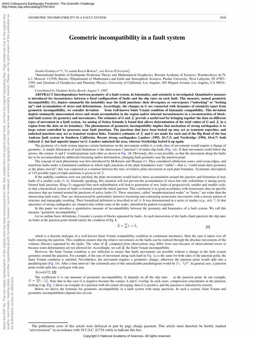
Geometric incompatibility in a fault system
ANDREI GABRIELOV*†, VLADIMIR KEILIS-BOROK*, AND DAVID D.JACKSON‡*International Institute of Earthquake Prediction Theory and Mathematical Geophysics, Russian Academy of Sciences, Warshavskoye sh.79,
k.2. Moscow 113556, Russia; †Departments of Mathematics and Earth and Atmospheric Sciences, Purdue University, West Lafayette, IN 47907–1395; and ‡Institute of Geophysics and Planetary Physics, University of California, Los Angeles, 405 Hilgard Avenue, Los Angeles, CA 90024–1567
Contributed by Vladimir Keilis-Borok, August 7, 1995ABSTRACT Interdependence between geometry of a fault system, its kinematics, and seismicity is investigated. Quantitative measure
is introduced for inconsistency between a fixed configuration of faults and the slip rates on each fault. This measure, named geometricincompatibility (G), depicts summarily the instability near the fault junctions: their divergence or convergence (“unlocking” or “lockingup”) and accumulation of stress and deformations. Accordingly, the changes in G are connected with dynamics of seismicityApart fromgeometric incompatibility, we consider deviation from well-known Saint Venant condition of kinematic compatibility. This deviationdepicts summarily unaccounted stress and strain accumulation in the region and/or internal inconsistencies in a reconstruction of block-and fault system (its geometry and movements). The estimates of G and provide a useful tool for bringing together the data on differenttypes of movement in a fault system. An analog of Stokes formula is found that allows determination of the total values of G and in aregion from the data on its boundary. The phenomenon of geometric incompatibility implies that nucleation of strong earthquakes is tolarge extent controlled by processes near fault junctions. The junctions that have been locked up may act as transient asperities, andunlocked junctions may act as transient weakest links. Tentative estimates of and G are made for each end of the Big Bend of the SanAndreas fault system in Southern California. Recent strong earthquakes Landers (1992, M=7.3) and Northridge (1994, M=6.7) bothreduced but had opposite impact on G: Landers unlocked the area, whereas Northridge locked it up again.
The geometry of a fault system imposes certain limitations on the movements within it; a wide class of movements would require a change ofgeometry. A simple illustration of such limitations is the intersection (“junction”) of strike-slip faults (Fig. 1A). If their movement could follow thearrows, the corners A and C would penetrate each other as shown in Fig. 1B. Obviously, this is not possible, so that the movement along the faultshas to be accommodated by additional fracturing and/or deformation, changing fault geometry near the junction point.
The concept of such phenomena was first introduced by McKenzie and Morgan (1). They considered subduction zones, mid-ocean ridges, andtransform faults under a formulated condition in which triple junctions of the plate boundaries were “stable”—that is, “could retain their geometryas the plates moved”; this was expressed as a relation between the rates of relative plate movement at each plate boundary. Systematic descriptionof 125 possible types of triple junctions is given in ref. 2.
If the stability condition were not satisfied, the plate movements would lead to stress accumulation around the junction and formation of newfaults of a smaller scale (3, 4). Generally speaking, this situation will not prevent the accumulation of stress but only redistribute it among newlyformed fault junctions. King (3) suggested that such redistribution will lead to generation of new faults of progressively smaller and smaller scale,so that a hierarchical system of faults is formed around the initial junction. This conclusion is in good accordance with neotectonic data on specificstructures that are formed around the junctions of active faults (5). These structures, called “morphostructural nodes” or “knots,” are wider than theintersecting fault zones. They are characterized by particularly intensive fracturing and contrasting neotectonic movements with a mosaic pattern ofstructure and topography resulting. Their formalized definition is described in ref. 6. It was demonstrated in a series of studies (e.g., refs. 7, 8) thatepicenters of strong earthquakes are situated only within some of the nodes, identified by pattern recognition.
In this paper we introduce a quantitative measure of incompatibility between the geometry and kinematics of a fault system. We call thismeasure “geometric incompatibility.”
Let us outline basic definitions. Consider a system of blocks separated by faults. At each intersection of the faults (fault junction) the slip rateson faults at the junction point should satisfy the condition of Eq. 1
[1]
which is a discrete analogue of a well-known Saint Venant compatibility condition in continuum mechanics. Here the sum is taken over allfaults entering the junction. This condition ensures that the relative movements on the faults can be realized through the absolute movements of thevolumes (blocks) separated by the faults. The value of computed from observations may differ from zero because of observational errors orbecause some deformations are not allowed for. Accordingly, we call the Saint Venant incompatibility.
However, the Saint Venant condition is not sufficient to ensure that faults movements are possible without a change in the fault systemgeometry around the junction. For example, if the rate of movement along each fault in Fig. 1a is the same for both sides of the junction point, theSaint Venant condition is satisfied. Nevertheless, the movement requires a geometric change; otherwise the junction point would split into aparallelogram (Fig. 1b). After a time interval t the (oriented) area of this unrealizable parallelogram would be . In general case, a junctionpoint would split into a polygon with area
S(t)=Gt2/2. [2]The coefficient G is our measure of geometric incompatibility. It depends on all the slip rates at the junction point. In our example,
. Note that in this case G is negative because the corners A and C overlap. In such cases, compression concentrates at the junction,locking it up. Fig. 2 shows an example of a junction with all corners diverging; then G is positive, and the junction is unlocked by tension.
Below we derive the formulas for geometric incompatibility in a fault system with many junctions. In such a system, Saint Venant andgeometric incompatibilities depend also on rota
The publication costs of this article were defrayed in part by page charge payment. This article must therefore be hereby marked“advertisement” in accordance with 18 U.S.C. §1734 solely to indicate this fact.
GEOMETRIC INCOMPATIBILITY IN A FAULT SYSTEM 3838
Abou
t thi
s PD
F fil
e: T
his
new
dig
ital r
epre
sent
atio
n of
the
orig
inal
wor
k ha
s be
en re
com
pose
d fro
m X
ML
files
cre
ated
from
the
orig
inal
pap
er b
ook,
not
from
the
orig
inal
type
setti
ng fi
les.
Pag
e br
eaks
are
true
to th
e or
igin
al; l
ine
leng
ths,
wor
d br
eaks
, hea
ding
sty
les,
and
oth
er ty
pese
tting
-spe
cific
form
attin
g, h
owev
er, c
anno
t be
reta
ined
, and
som
e ty
pogr
aphi
c er
rors
may
hav
e be
en a
ccid
enta
lly in
serte
d. P
leas
e us
e th
e pr
int v
ersi
on o
f thi
s pu
blic
atio
n as
the
auth
orita
tive
vers
ion
for a
ttrib
utio
n.
Copyright © National Academy of Sciences. All rights reserved.
(NAS Colloquium) Earthquake Prediction: The Scientific Challengehttp://www.nap.edu/catalog/5709.html
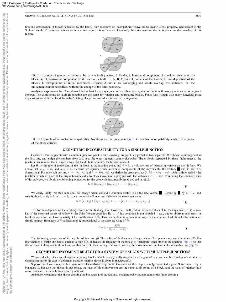
tion and deformation of blocks separated by the faults. Both measures of incompatibility have the following useful property, reminiscent of theStokes formula: To estimate their values in a whole region, it is sufficient to know only the movements on the faults that cross the boundary of thisregion.
FIG. 1. Example of geometric incompatibility near fault junction. 1, Faults; 2, horizontal component of absolute movement of ablock, ; 3, horizontal component of slip rate on a fault, ; A, B, C, and D, corners of the blocks; a, initial position of theblocks; b, extrapolation of initial movement. Corners A and C are converging and would overlap; this indicates that themovement cannot be realized without the change of the fault geometry.Analytical expressions for G are derived below first for a single junction and then for a system of faults with many junctions within a given
contour. The expressions for a single junction are the same for rotating and nonrotating blocks. For a fault system with many junctions theseexpressions are different for deformable/rotating blocks; we consider this case in the Appendix.
FIG. 2. Example of geometric incompatibility. Notations are the same as in Fig. 1. Geometric incompatibility leads to divergenceof the block corners.
GEOMETRIC INCOMPATIBILITY FOR A SINGLE JUNCTION
Consider n fault segments with a common junction point; a fault crossing this point is regarded as two segments. We choose some segment asthe first one, and assign the numbers from 2 to n to the other segments counterclockwise. The n blocks separated by these faults meet at thejunction. We number them in such a way that the ith fault separates the blocks i and i+1.
Let be the rate of movement of the ith block at the junction point, and the rate of relative movement on the ith fault. Wealways set and Because we consider only horizontal components of the movements, the vectors and are two-dimensional. For two such vectors, and , we define the cross-product . After a time period t thejunction, which we place at the origin, becomes, due to block movement, a polygon with the vertices . Computing the (oriented) areaof this polygon, we obtain the following expression for the geometric incompatibility G defined in ref. 2:
[3]
We easily verify that this sum does not change when we add a common vector to all the rate vectors . Replacing by andsubstituting , we can rewrite G in terms of the relative movement rates :
[4]
This formula depends on the arbitrary choice of the first segment. However, it will lead to the same values of G, for any choice, if —i.e., if the observed values of satisfy the Saint Venant condition Eq. 1. If this condition is not satisfied— e.g., due to observational errors orblock deformation, we have to satisfy it by modification of . This can be done in a nonunique way. In the absence of additional information wesimply subtract from each of a fraction of proportional to the absolute value of :
[5]
The following properties of G may be of interest: (i) The value of G does not change when all slip rates reverse directions, (ii) Forintersections of strike-slip faults, a negative sign of G indicates the tendency of the blocks to “penetrate” each other at the junction (Fig. 1), so thatthe movement along one fault locks up another fault. On the contrary, if G were positive, the movement on one fault unlocks another one (Fig. 2).
GEOMETRIC INCOMPATIBILITY FOR A SYSTEM OF FAULTS WITH MULTIPLE JUNCTIONS
We consider here the case of rigid nonrotating blocks, which is analytically simpler than the general case and can be of independent interest.Generalization for the case of deformable and/or rotating blocks is given in the Appendix.
Suppose we have a map with a system of blocks divided by faults. Consider on this map a simply connected region D surrounded by aboundary L. Because the blocks do not rotate, the rates of block movement are the same at all points of a block, and the rates of relative faultmovements are the same between fault junctions.
As before, we number the blocks crossing the boundary L of the region D counterclockwise, and number the faults crossing
GEOMETRIC INCOMPATIBILITY IN A FAULT SYSTEM 3839
Abou
t thi
s PD
F fil
e: T
his
new
dig
ital r
epre
sent
atio
n of
the
orig
inal
wor
k ha
s be
en re
com
pose
d fro
m X
ML
files
cre
ated
from
the
orig
inal
pap
er b
ook,
not
from
the
orig
inal
type
setti
ng fi
les.
Pag
e br
eaks
are
true
to th
e or
igin
al; l
ine
leng
ths,
wor
d br
eaks
, hea
ding
sty
les,
and
oth
er ty
pese
tting
-spe
cific
form
attin
g, h
owev
er, c
anno
t be
reta
ined
, and
som
e ty
pogr
aphi
c er
rors
may
hav
e be
en a
ccid
enta
lly in
serte
d. P
leas
e us
e th
e pr
int v
ersi
on o
f thi
s pu
blic
atio
n as
the
auth
orita
tive
vers
ion
for a
ttrib
utio
n.
Copyright © National Academy of Sciences. All rights reserved.
(NAS Colloquium) Earthquake Prediction: The Scientific Challengehttp://www.nap.edu/catalog/5709.html
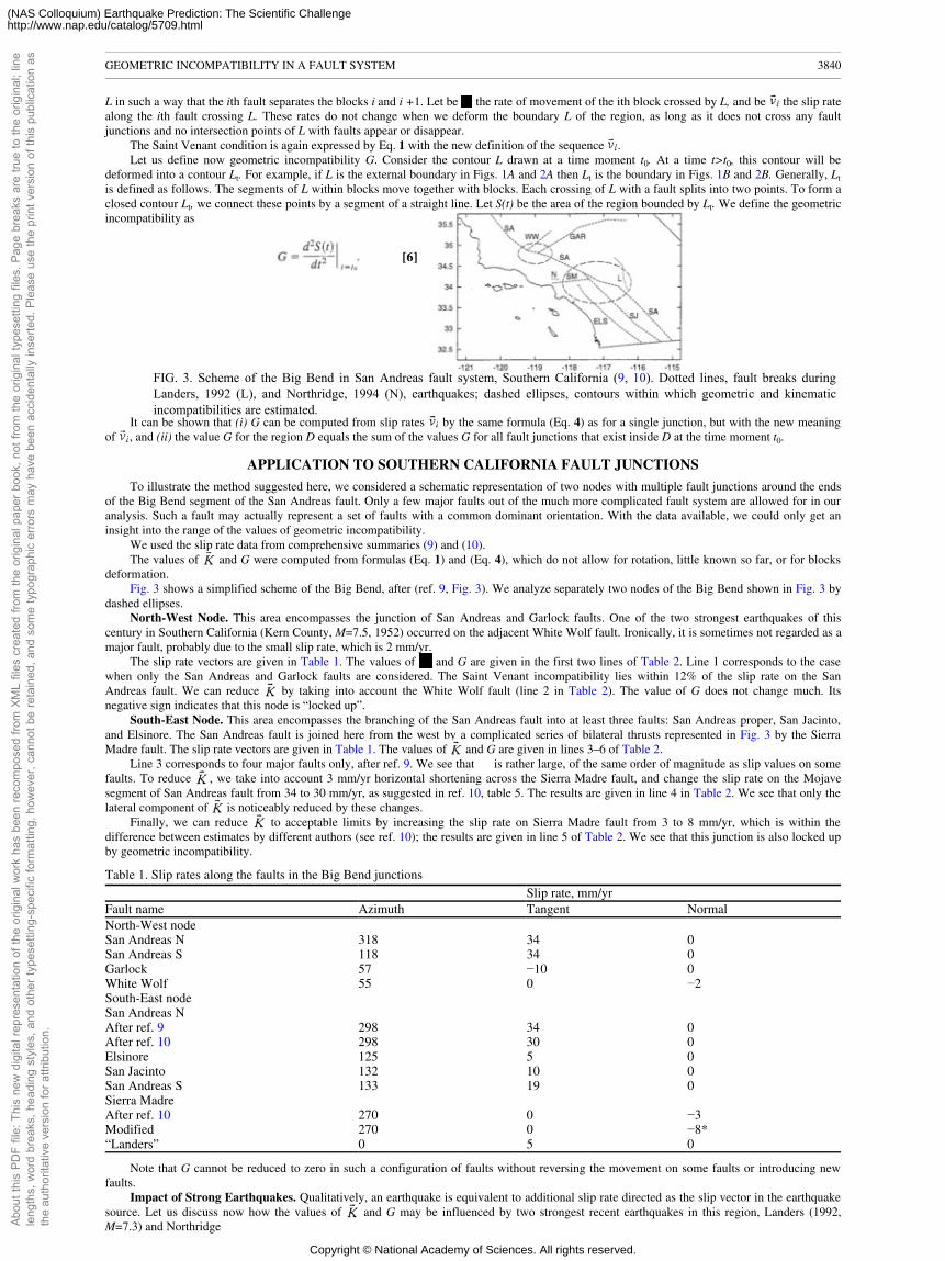
L in such a way that the ith fault separates the blocks i and i +1. Let be the rate of movement of the ith block crossed by L, and be the slip ratealong the ith fault crossing L. These rates do not change when we deform the boundary L of the region, as long as it does not cross any faultjunctions and no intersection points of L with faults appear or disappear.
The Saint Venant condition is again expressed by Eq. 1 with the new definition of the sequence .Let us define now geometric incompatibility G. Consider the contour L drawn at a time moment t0. At a time t>t0, this contour will be
deformed into a contour Lt. For example, if L is the external boundary in Figs. 1A and 2A then Lt is the boundary in Figs. 1B and 2B. Generally, Ltis defined as follows. The segments of L within blocks move together with blocks. Each crossing of L with a fault splits into two points. To form aclosed contour Lt, we connect these points by a segment of a straight line. Let S(t) be the area of the region bounded by Lt. We define the geometricincompatibility as
[6]
It can be shown that (i) G can be computed from slip rates by the same formula (Eq. 4) as for a single junction, but with the new meaningof , and (ii) the value G for the region D equals the sum of the values G for all fault junctions that exist inside D at the time moment t0.
APPLICATION TO SOUTHERN CALIFORNIA FAULT JUNCTIONS
To illustrate the method suggested here, we considered a schematic representation of two nodes with multiple fault junctions around the endsof the Big Bend segment of the San Andreas fault. Only a few major faults out of the much more complicated fault system are allowed for in ouranalysis. Such a fault may actually represent a set of faults with a common dominant orientation. With the data available, we could only get aninsight into the range of the values of geometric incompatibility.
We used the slip rate data from comprehensive summaries (9) and (10).The values of and G were computed from formulas (Eq. 1) and (Eq. 4), which do not allow for rotation, little known so far, or for blocks
deformation.Fig. 3 shows a simplified scheme of the Big Bend, after (ref. 9, Fig. 3). We analyze separately two nodes of the Big Bend shown in Fig. 3 by
dashed ellipses.North-West Node. This area encompasses the junction of San Andreas and Garlock faults. One of the two strongest earthquakes of this
century in Southern California (Kern County, M=7.5, 1952) occurred on the adjacent White Wolf fault. Ironically, it is sometimes not regarded as amajor fault, probably due to the small slip rate, which is 2 mm/yr.
The slip rate vectors are given in Table 1. The values of and G are given in the first two lines of Table 2. Line 1 corresponds to the casewhen only the San Andreas and Garlock faults are considered. The Saint Venant incompatibility lies within 12% of the slip rate on the SanAndreas fault. We can reduce by taking into account the White Wolf fault (line 2 in Table 2). The value of G does not change much. Itsnegative sign indicates that this node is “locked up”.
South-East Node. This area encompasses the branching of the San Andreas fault into at least three faults: San Andreas proper, San Jacinto,and Elsinore. The San Andreas fault is joined here from the west by a complicated series of bilateral thrusts represented in Fig. 3 by the SierraMadre fault. The slip rate vectors are given in Table 1. The values of and G are given in lines 3–6 of Table 2.
Line 3 corresponds to four major faults only, after ref. 9. We see that is rather large, of the same order of magnitude as slip values on somefaults. To reduce , we take into account 3 mm/yr horizontal shortening across the Sierra Madre fault, and change the slip rate on the Mojavesegment of San Andreas fault from 34 to 30 mm/yr, as suggested in ref. 10, table 5. The results are given in line 4 in Table 2. We see that only thelateral component of is noticeably reduced by these changes.
Finally, we can reduce to acceptable limits by increasing the slip rate on Sierra Madre fault from 3 to 8 mm/yr, which is within thedifference between estimates by different authors (see ref. 10); the results are given in line 5 of Table 2. We see that this junction is also locked upby geometric incompatibility.
Table 1. Slip rates along the faults in the Big Bend junctionsSlip rate, mm/yr
Fault name Azimuth Tangent NormalNorth-West nodeSan Andreas N 318 34 0San Andreas S 118 34 0Garlock 57 −10 0White Wolf 55 0 −2South-East nodeSan Andreas NAfter ref. 9 298 34 0After ref. 10 298 30 0Elsinore 125 5 0San Jacinto 132 10 0San Andreas S 133 19 0Sierra MadreAfter ref. 10 270 0 −3Modified 270 0 −8*“Landers” 0 5 0
Note that G cannot be reduced to zero in such a configuration of faults without reversing the movement on some faults or introducing newfaults.
Impact of Strong Earthquakes. Qualitatively, an earthquake is equivalent to additional slip rate directed as the slip vector in the earthquakesource. Let us discuss now how the values of and G may be influenced by two strongest recent earthquakes in this region, Landers (1992,M=7.3) and Northridge
GEOMETRIC INCOMPATIBILITY IN A FAULT SYSTEM 3840
Abou
t thi
s PD
F fil
e: T
his
new
dig
ital r
epre
sent
atio
n of
the
orig
inal
wor
k ha
s be
en re
com
pose
d fro
m X
ML
files
cre
ated
from
the
orig
inal
pap
er b
ook,
not
from
the
orig
inal
type
setti
ng fi
les.
Pag
e br
eaks
are
true
to th
e or
igin
al; l
ine
leng
ths,
wor
d br
eaks
, hea
ding
sty
les,
and
oth
er ty
pese
tting
-spe
cific
form
attin
g, h
owev
er, c
anno
t be
reta
ined
, and
som
e ty
pogr
aphi
c er
rors
may
hav
e be
en a
ccid
enta
lly in
serte
d. P
leas
e us
e th
e pr
int v
ersi
on o
f thi
s pu
blic
atio
n as
the
auth
orita
tive
vers
ion
for a
ttrib
utio
n.
FIG. 3. Scheme of the Big Bend in San Andreas fault system, Southern California (9, 10). Dotted lines, fault breaks duringLanders, 1992 (L), and Northridge, 1994 (N), earthquakes; dashed ellipses, contours within which geometric and kinematicincompatibilities are estimated.
Copyright © National Academy of Sciences. All rights reserved.
(NAS Colloquium) Earthquake Prediction: The Scientific Challengehttp://www.nap.edu/catalog/5709.html
(1994, M=6.7). The corresponding fault breaks are indicated on Fig. 3 by dotted lines.
Data are taken from ref. 10 unless otherwise indicated. Tangent component is positive for right-lateral strike-slip; the normal component is positive forextension.*Closer to the upper estimate indicated in ref. 10.
Table 2. Saint Venant and geometric (G) incompatibilities in the Big Bend junctions
No. , East, mm/yr , North, mm/yr G, mm2/yr2
North-West end of Big Bend1 −1.1 3.9 −326.72 0.0 2.2 −324.3South-East end of Big Bend3 −4.6 −6.6 −22.44 −1.1 −5.4 −106.95 −1.1 −0.4 −234.16 −1.1 −0.4 30.0
To analyze the impact of the Landers earthquake, we included in our computation 5 mm/yr of right-lateral slip along the meridional part of itsfault break. The rest of the parameters were the same as for line 4 of Table 2. The results are shown in line 6. Comparing these lines, we see thatthe Landers earthquake leads to a reduction of both incompatibilities and, because G becomes positive, unlocks the junction.
At the same time, this earthquake created a new junction and therefore new incompatibility on the bend of its own fault break.The Northridge earthquake occurred on a bilateral thrust fault in the above-mentioned compression zone represented in our scheme (Fig. 3) by
the Sierra Madre fault. The Landers earthquake, although more complicated, started as a submeridional right-lateral strike-slip. Though different inmechanism and location, both earthquakes reduce similarly. However, their contribution to G is opposite.
The Northridge earthquake is equivalent to an increase of the thrust rate on Sierra Madre fault. Comparing lines 4 and 5 in Table 2, we seethat, due to such an increase, the meridional component of would be reduced. However, |G| becomes larger, so that this earthquake locks up theregion.
Coarse quantitative estimates can be done as suggested in ref. 11. Consider a fault with length L and width H. An earthquake on this faultcauses a fault break of length l and width h and an average slip vector . We spread this slip over the whole fault and over the recurrence time T.The additional slip rate on the fault is roughly estimated as
Because this relation is very coarse, we can use, at the best, only the orders of magnitude for all parameters involved, taking the valuesindicated in ref. 10.
Assuming l�102 km, h�101 km, d�103 mm, L�102 km, H�101 km, T�102−103 yr, we get for additional slip rate an estimate ve�100−101 mm/yr. Comparing these numbers with numerical experiments in Table 1, we see that the contribution of strong earthquakes to geometric andkinematic incompatibilities is indeed essential. For example, Landers earthquake alone could well unlock the region completely, reversing the signof G.
DISCUSSION
(i) This work is a continuation of the quest for integral parameters that control the dynamics of seismicity. Geometric G and kinematic incompatibilities in an active fault system seem to be highly relevant for this purpose, representing the tendency of a system to stress and strainaccumulation and fracturing. This interconnection may determine some of the features of seismicity, regardless of the physical processes involved.
Geometric incompatibility seems to be the only known parameter that gives a comprehensive description of fault junctions.The analogs of the Stokes formula established here allow one to estimate G and in a complicated area from observations on its boundary,
thus reducing the requirements for observations.(ii) Because geometric incompatibility depicts the locking up or unlocking of the fault junctions, it may be one of the major factors controlling
nucleation (triggering) of strong earthquakes. It is generally accepted that earthquakes occur when the stress exceeds the static friction (strength).Traditionally, such triggering is assigned to “strong” fault segments. Actually, this condition will be first reached rather near a fault junction whereboth factors are more favorable: The strength may be much smaller due to intense fracturing. And the stress itself may rise faster due to geometricincompatibility.
This conjecture is in accordance with the well-confirmed conclusion that epicenters of strong earthquakes—that is, their nucleation areas, are,as a rule, confined to the vicinity of fault junctions (7, 8).
(iii) Existing observations allow, at best, only coarse estimates of G and . Still, they provide important insight into how different faults andearthquakes may affect the general equilibrium of a region. In particular, the impact of a strong earthquake cannot be neglected: it is comparablewith the role of long-term (“geodetic”) movements and, moreover, it may reverse the geometric incompatibility, locking the junction up orunlocking it. A junction that is locked up may act as a transient asperity until it is broken by a strong earthquake or unlocked by subsequentimpacts. A junction that is unlocked may act as a “weakest link” in the earthquake triggering or, alternatively, as a relaxation barrier.
In this way, geometric incompatibility and, therefore, seismicity may migrate within a fault system.(iv) Simplifications in our analysis may be summarized as follows: we considered rigid blocks and horizontal movements; in computations
possible rotation, being unknown, was not allowed for. When more data are available, these simplifications may have to be removed.(v) Summing up, geometric incompatibility deserves attention as an important integral characteristic of the tectonic development of fault
systems. In particular, it may be one of the parameters that controls the dynamics of seismicity.
APPENDIX: INCOMPATIBILITIES FOR DEFORMABLE AND ROTATING BLOCKS
For a system of deformable blocks, the Saint Venant compatibility condition, in the integral form, can be written as follows (ref. 12, see alsoref. 13). Let be displacement rate vector. Its components ui(x) are smooth functions within each block, with discontinuities at the blockboundaries. Let L be a closed contour crossing the block boundaries at the points x1,�,xn counterclockwise, and let x0 be a fixed reference point.For v =1,�, n, let and be the rate of movement in the blocks that contain the contour L before and after it crosses the blockboundary at xv, and let be the rate of relative movement of the two blocks at xv. Then
[A1]
GEOMETRIC INCOMPATIBILITY IN A FAULT SYSTEM 3841
Abou
t thi
s PD
F fil
e: T
his
new
dig
ital r
epre
sent
atio
n of
the
orig
inal
wor
k ha
s be
en re
com
pose
d fro
m X
ML
files
cre
ated
from
the
orig
inal
pap
er b
ook,
not
from
the
orig
inal
type
setti
ng fi
les.
Pag
e br
eaks
are
true
to th
e or
igin
al; l
ine
leng
ths,
wor
d br
eaks
, hea
ding
sty
les,
and
oth
er ty
pese
tting
-spe
cific
form
attin
g, h
owev
er, c
anno
t be
reta
ined
, and
som
e ty
pogr
aphi
c er
rors
may
hav
e be
en a
ccid
enta
lly in
serte
d. P
leas
e us
e th
e pr
int v
ersi
on o
f thi
s pu
blic
atio
n as
the
auth
orita
tive
vers
ion
for a
ttrib
utio
n.
Copyright © National Academy of Sciences. All rights reserved.
(NAS Colloquium) Earthquake Prediction: The Scientific Challengehttp://www.nap.edu/catalog/5709.html
should be zero, for all i. Here is the strain tensor.Linearization of defines affine operators
[A2]
For x=xv, let be the operators corresponding to . The operator , linearization of the relative rate of movement of twoblocks at xv, does not depend on the rate of movement of the coordinate system. Expression in brackets in A1 can be rewritten as the ith componentof the vector Σv Vv(x0).
When the blocks are rigid, the integral in A1 vanishes, and the Saint Venant compatibility condition is satisfied if and only if the affine operator
[A3]
is zero. This is an element of the Lie algebra of the orthogonal affine group. This operator is a natural generalization of the Saint Venantincompatibility . Note that K satisfies an analog of the Stokes formula: its value on any contour is equal to the sum of its values over thejunctions within the contour. This can be easily deduced from A1.
Geometric incompatibility for a system of deformable blocks can be defined as
[A4]
It is easy to check that the value of G does not depend on the rate of movement of the coordinate system. Thus G is an invariant of the rate ofdeformation.
For rigid blocks, the integral in A4 vanishes, and the geometric incompatibility becomes
[A5]
similar to Eq. 3. This is an element of , the external square of the Lie algebra of the orthogonal affine group. If K=0, this can berewritten as
G=V1�V2+(V1+V2�V3)+�+(V1+�+Vn−2�Vn−1), [A6]
similar to (Eq. 4). Otherwise, Vv should be modified as in (Eq. 5) to make K=0.For a system of rigid blocks, an analog of the Stokes formula is valid for G: its value for a contour is equal to the sum of its values over the
junctions within the contour, when the Saint Venant incompatibility is zero for all these junctions.For a system of two-dimensional rigid blocks, let x=(x, y), and Vv(x, y)=(Xv−yωv, Yv+xωv). Here (Xv, Yv) is the relative displacement rate at
the origin, and ωv is the relative rotation rate of the two blocks adjacent at xv. In this case, is three-dimensional, and the Saint Venantincompatibility has three components:
[A7]
The space is also three-dimensional. Accordingly, the geometric incompatibility G has three components:
[A8]
Here , define the operators in Eq. A5. Expression A6 can be rewritten similarly in terms of Xv, Yv, and ωv.This work was supported by National Science Foundation Grant no. 931650, and P.O. no. 56659 from University of Southern California, on
behalf of the Southern California Earthquake Center. The first author (A.G.) was partly supported by the U.S. Army Research Office through theMathematical Sciences Institute of Cornell University, Contract DAAL03–91-C-0027, and Department of Geological Sciences at CornellUniversity, under National Science Foundation Grant no. EAR-94–23818.1. McKenzie, D.P. & Morgan, W.J. (1969) Nature (London) 224, 125–133.2. Cronin, V.S. (1992) Tectonophysics 207, 287–301.3. King, G.C.P. (1983) Pure Appl. Geophys. 121, 761–815.4. King, G.C.P. (1986) Pure Appl Geophys. 124, 567–583.5. Gerasimov, I. & Rantsman, E. (1973) Geomorphol. Res. 1, 1–13.6. Alekseevskaya, M., Gabrielov, A., Gel'fand, I., Gvishiani, A. & Rantsman, E. (1977) J. Geophys. 43, 227–233.7. Gelfand, I.M., Guberman, Sh. A, Keilis-Borok, V.I., Knopoff, L., Press, F., Ranzman, E.Y., Rotwain, I.M. & Sadovsky, A.M. (1976) Phys. Earth Planet.
Int. 11, 227–283.8. Guberman, Sh.I. & Rotwain, I.M. (1986) Izvestia Akad. Nauk SSSR 12, 72–74.9. Feigl, K.L., Agnew, D.C., Bock, Y., Dong, D., Donnellan, A., Hager, B.H., Herring, T.A., Jackson, D.D., Jordan, T.H., King, R.W., Larsen, S., Larson,
K.M., Murray, M.H., Shen, Z. & Webb, F.H. (1993) J. Geophys. Res. 98, 21677–21712.10. Working Group on California Earthquake Probabilities (1995) Bull. Seis. Soc. Am. 85, 379–439.11. Brune, J. (1968) J. Geophys. Res. 73, 777–784.12. Fung, Y.C. (1965) Foundation of Solid Mechanics (Prentice-Hall, Englewood Cliffs, NJ), Chap. 4.13. Minster, J.B. & Jordan, T.H. (1984) in Tectonics and Sedimentation Along the California Margin: Pacific Section, eds. Crouch, J.K. & Bachman, S.B.
(Soc. Econ. Paleontol. Mineral., Los Angeles), Vol. 38, pp. 1–6.
GEOMETRIC INCOMPATIBILITY IN A FAULT SYSTEM 3842
Abou
t thi
s PD
F fil
e: T
his
new
dig
ital r
epre
sent
atio
n of
the
orig
inal
wor
k ha
s be
en re
com
pose
d fro
m X
ML
files
cre
ated
from
the
orig
inal
pap
er b
ook,
not
from
the
orig
inal
type
setti
ng fi
les.
Pag
e br
eaks
are
true
to th
e or
igin
al; l
ine
leng
ths,
wor
d br
eaks
, hea
ding
sty
les,
and
oth
er ty
pese
tting
-spe
cific
form
attin
g, h
owev
er, c
anno
t be
reta
ined
, and
som
e ty
pogr
aphi
c er
rors
may
hav
e be
en a
ccid
enta
lly in
serte
d. P
leas
e us
e th
e pr
int v
ersi
on o
f thi
s pu
blic
atio
n as
the
auth
orita
tive
vers
ion
for a
ttrib
utio
n.
Copyright © National Academy of Sciences. All rights reserved.
(NAS Colloquium) Earthquake Prediction: The Scientific Challengehttp://www.nap.edu/catalog/5709.html