multivariate statistical methods for evaluating biodegradation of mineral oil

Journal of Chromatography A, 1090 (2005) 133–145

Multivariate statistical methods for evaluatingbiodegradation of mineral oil

Jan H. Christensena,∗, Asger B. Hansenb, Ulrich Karlsonb, John Mortensenc, Ole Andersenc

a Department of Natural Sciences, Royal Veterinary and Agricultural University, Thorvaldsensvej 40, 1871 Frederiksberg C, Denmarkb Department of Environmental Chemistry and Microbiology, National Environmental Research Institute, Frederiksborgvej 399, 4000 Roskilde, Denmark

c Department of Life Sciences and Chemistry, Roskilde University, Universitesvej 1, 4000 Roskilde, Denmark

Received 28 February 2005; received in revised form 24 June 2005; accepted 6 July 2005Available online 1 August 2005

Abstract

Two methods were developed for evaluating natural attenuation and bioremediation of mineral oil after environmental spills and during invitro experiments. Gas chromatography–mass spectrometry (GC–MS) in selected ion monitoring (SIM) mode was used to obtain compound-specific data. The chromatographic data were then preprocessed either by calculating the first derivative, retention time alignment andn aromaticc tic ratios tos il exposedt d U-strains)om n thec component1 s along PC2.F les from Ua ent bacteriala metabolicc©

K

1

etea(pp

inal

ada-

ever,icalher-,del’

pable

per-

0d

ormalization or by peak identification, quantification and calculation of diagnostic ratios within homologue series of polycyclicompounds (PACs). Finally, principal component analysis (PCA) was applied to the preprocessed chromatograms or diagnostudy the fate of the oil. The methods were applied to data from an in vitro biodegradation experiment with a North Sea crude oo three mixtures of bacterial strains: R (alkane degraders and surfactant producers), U (PAC degraders) and M (mixture of R- anver a 1-year-period with five sampling times. Assessment of variation in degradability within isomer groups of methylfluorenes (m/z180),ethylphenanthrenes (m/z 192) and methyldibenzothiophenes (m/z 198) was used to evaluate the effects of microbial degradation o

omposition of the oil. The two evaluation methods gave comparable results. In the objective pattern matching approach, principal(PC1) described the general changes in the isomer abundances, whereas M samples were separated from U and R sampleurthermore, in the diagnostic ratio approach, a third component (PC3) could be extracted; although minor, it separated R sampnd M samples. These results demonstrated that the two methods were able to differentiate between the effects due to the differctivities, and that bacterial strain mixtures affected the PAC isomer patterns in different ways in accordance with their differentapabilities.2005 Elsevier B.V. All rights reserved.

eywords:Biodegradation; Oil spills; PCA; COW; GC–MS; Chemical fingerprinting

. Introduction

Crude oil and refined petroleum products released into thenvironment are subject to a number of weathering processes

hat change the oil composition, including physical (e.g.vaporation, emulsification, natural dispersion, dissolutionnd sorption), chemical (photodegradation) and biologicalmainly microbial degradation) processes[1]. The physicalrocesses result in redistribution of oil components in com-artments of the environment, while photodegradation and

∗ Corresponding author. Tel.: +45 35282456; fax: +45 35282398.E-mail address:[email protected] (J.H. Christensen).

microbial degradation lead to transformation of the origcompounds.

Numerous authors have investigated microbial degrtion of mixtures of petroleum hydrocarbons, in situ[2–5]and under laboratory conditions[6–9]. Evaluation of the rolof biodegradation in environmental oil samples is, howeoften difficult due to the inherent complexity of the chemhydrocarbon mixtures, and due to the variety of weating processes affecting oil composition[10]. Consequentlymost bioremediation studies have been limited to few ‘mocompounds, and to a selection of bacterial strains caof utilizing petroleum hydrocarbons for growth[6,11–14].Although, hundreds of such investigations have been

021-9673/$ – see front matter © 2005 Elsevier B.V. All rights reserved.oi:10.1016/j.chroma.2005.07.025

134 J.H. Christensen et al. / J. Chromatogr. A 1090 (2005) 133–145

formed since the 1980s, the development of evaluation tech-niques has been limited. Gas chromatography-flame ion-ization detection (GC-FID) and Gas chromatography–massspectrometry (GC–MS) are the standard methods for the anal-ysis of petroleum hydrocarbons[7,9,15].

Bulk properties such as total petroleum hydrocarbon(TPH) concentration, measured by GC-FID, and gravimet-ric analysis of the aliphatic, aromatic and polar fractions ofweathered oil samples have been used frequently to evalu-ate the effects of oil weathering[2,16,17]. GC–MS analysiscan, on the other hand, resolve a broad range of petroleumhydrocarbons including individual PACs within homologueseries. Thus, evaluation of compound-specific data providedby GC–MS can lead to more comprehensive assessments ofweathering and biodegradation. The distribution of alkylatedPAC homologues of naphthalene, dibenzothiophene, phenan-threne, fluorene and chrysene are commonly employed inthis respect[9,18,19]. In general, increased molecular com-plexity leads to a decrease in the susceptibility to microbialattack. Specifically, the rate of PAC degradation in the envi-ronment decreases with increasing compound size (numberof rings) and degree of alkylation[9,20,21]. Thus, the rateof degradation of alkylated PACs is C0 > C1 > C2 > C3 > C4,where Cx denotes the total numberx of side chain car-bon atoms. Similar effects occur for physical weatheringsuch as evaporation and dissolution, since the physicochem-i ty)a tion[

kercn tlyi oun-t of oilo rvedi ical,c ringc ts ofm ss ins fielda ucha ,p ctedb

ationin ation[ ersw e the1d lky-l u-o ben-z andu lar,W ation

as a decrease in the ratios (3MP + 2MP)/(4 + 9MP + 1MP),(2 + 3MD)/1MD and

∑MF/1MF [5,9].

Changes in isomer patterns within alkylated PAC seriesand in the corresponding diagnostic ratios are highly specificfor biodegradation, as no such changes occur during phys-ical weathering[9]. In contrast, a few studies have shownthat chemical weathering can lead to changes in the isomerpatterns, although the sequences of alteration are differentfrom those observed during biodegradation[32]. Jacquot etal. observed increasing photodegradability of methylphenan-threnes for the sequence 2MP < 1MP < 3MP < 4 + 9MP[32]wherexMP denotes the positionx of the methyl substituentin the phenanthrene skeleton. These differences may be usedto distinguish between chemical and biological weatheringeffects.

Methods for evaluating the effects of weathering, andspecifically biodegradation, on the composition of spilledoil have mainly been limited to subjective pattern match-ing and univariate plots. Multivariate statistical methods suchas principal component analysis (PCA) provide useful toolsfor more extensive and objective chemical characterizationbased on chromatographic data. Multivariate methods havebeen used regularly for data analysis in organic geochem-istry [33,34], but they have only recently been adopted foroil spill identification [35–39] and for studying the fate ofpetroleum hydrocarbons in the environment[27,40]. Thea man-i siso cili-t bio-d

g ins hasb nt ofd eth-o d andn elec-t ues n inv rudeo a 1-y datafm ne( biald

2

am-p pre-p A orw valu-a ho-d

cal properties of PACs (i.e. boiling point and solubililso depend on number of rings and degree of alkyla

9].Normalization to a conservative internal mar

ompound such as 17�,21�-hopane [22–25], 17�,21�-orhopane[17] or vanadium[26] has been used frequen

n weathering studies to correct for heterogeneity encered in field samples and to calculate the percent lossr individual analytes[21]. Percent losses based on prese

nternal markers describe the combined effects of physhemical and biological weathering processes. Only duontrolled laboratory experiments can the isolated effecicrobial degradation be described by subtracting the lo

terile controls. Conversely, in samples collected in thefter oil spills, the low molecular weight hydrocarbons ss heptadecane (nC17), octadecane (nC18), pristane (Pr)hytane (Ph) and 2–3 ring PACs are often heavily affey physical weathering processes.

Several authors have observed that microbial degrads isomer specific[5,7,9,15,27,28]. Changes innC17/Pr andC18/Ph have long been used as indicators for biodegrad

4,29]. Likewise, preferential degradation of specific isomithin homologue PAC series have been described sinc980s [7,28,30]. Recently, Wang et al.[5,9,31] observedifferential susceptibility to degradation within series of a

ated PAC homologues of C1–C3-naphthalenes, methylflrenes (MF), methylphenanthrenes (MP) and methyldiothiophenes (MD) by subjective pattern matchingnivariate comparison of diagnostic ratios. In particuang et al. observed isomer specific microbial degrad

dvantages of multivariate over univariate methods arefold. In particular, they allow for simultaneous analyf a large number of correlated variables, and thus fa

ate a more comprehensive evaluation of the effects ofegradation.

Here, we present two novel methods for evaluatinitu and in vitro biodegradation of mineral oil. The aimeen to reduce time and cost, to increase the amouata considered and to increase the objectivity. The mds are based on chemometric data analysis of aligneormalized regions of GC–MS chromatograms and a s

ion of diagnostic ratios of PAC isomers within homologeries. These methods were applied to data from aitro biodegradation experiment where a North Sea cil was exposed to three mixed bacterial inocula overear-period with five sampling times. Chromatographicrom tiered GC–MS analysis of methylfluorene (m/z 180),ethylphenanthrene (m/z192) and methyldibenzothiophem/z198) groups were used for evaluating effects of microegradation.

. Methods

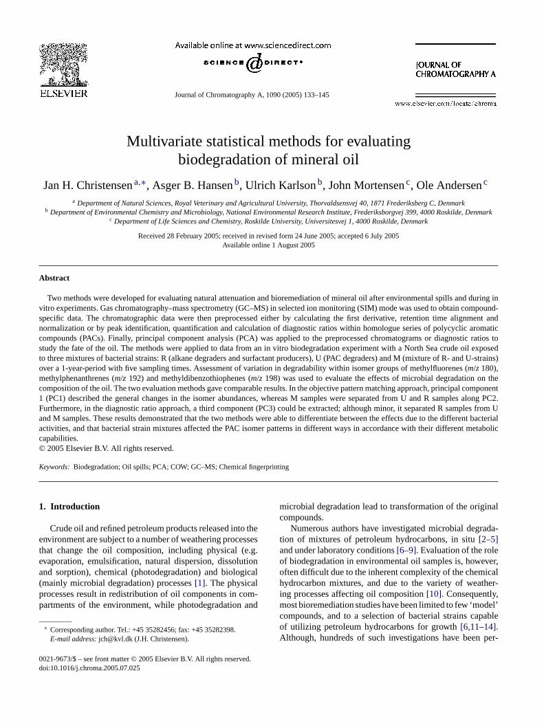
The methodology employed consists of four steps: sle preparation and GC–MS analysis, chromatographicrocessing, multivariate statistical data analysis by PCeighted-least-squares PCA (WLS-PCA) and data etion. Fig. 1 presents a flowchart of this general metology.

J.H. Christensen et al. / J. Chromatogr. A 1090 (2005) 133–145 135

Fig. 1. Flowchart of the general method based on multivariate statistical data analysis for evaluating biodegradation of mineral oil.

The techniques used in the method are automated andobjective extensions of standard evaluation techniques oftenused in the literature, based on previously published meth-ods for chemical fingerprinting using chemometrics[35,38].Until now, assessment of environmental oil degradation has toa large degree been based on subjective evaluation of changesin GC–MS chromatograms and univariate plots of concentra-tions and diagnostic ratios.

2.1. In vitro biodegradation experiment

2.1.1. Bacterial strain mixturesThree mixtures of bacterial strains were used, R, U and M

where M was a mixture of R- and U-strains:R was a mixture of bacterial long-chain alkane degraders

and biosurfactant producers, includingPseudomonas aerug-inosaRR1,Weeksellasp. RR7,Acinetobacter calcoaceticus


RR8,Burkholderia cepaciaRR10,Rhodococcusspp. RR12and RR14 andXylella fastidiosaRR15, which have beencharacterized elsewhere[41].

U was a mixture of bacterial PAC degraders includ-ing unclassified Gram-positive strains VM445, VM450 andVM504 andSphingomonassp. VM506[42],MycobacteriumfrederiksbergenseFan9[43] and a mixture of strains pre-viously described in detail[44]: Sphingobiumsp. EPA505,Pseudomonas aeruginosaCRE11, Mycobacterium van-baaleniiPYR-1,MycobacteriumgilvumGJ-3p,SphingobiumchungbukensisLB126,Mycobacteriumsp. VF1,Mycobac-terium frederiksbergenseLB501T andNocardia asteroidesVM451. Previously, each strain in the U-mixture was foundto degrade one or several of the following unsubstituted PACs:phenanthrene, anthracene, fluorene, fluoranthene, pyrene orbiphenyl by incubation with14C-labelled pure compounds(data not shown). In addition, their ability to grow in seawater-modified M9 medium was ensured in a pre-experiment usinga complex medium (data not shown).

2.1.2. IncubationA sample of Brent Crude oil was autoclaved (121◦C,

30 min) and incubated at 10◦C in trace element-supplemented[45] M9 medium[46] (modified by replacing9/10 of the M9 with autoclaved Baltic Sea water) on a rotarys ere1 iuma d as asksep ,1

thee esa ced.H ken ad ticalr day1 hee toa ls aree to

assess the biodegradation of oil exposed to any of the threemixtures of bacterial strains, while the sterile controls wereused to isolate the effects of physical weathering.

2.2. Sample preparation and GC–MS analysis

The experimental procedure used here is based on a semi-quantitative approach with limited sample preparation andcleanup. The sample units (oil and water) were extracted threetimes with∼10 mL dichloromethane by shaking the flasks.The water and dichloromethane phases were then separated ina 100 mL separatory funnel, and the dichloromethane phasecleaned through a funnel with glasswool and sodium sulphateto remove particles and water. Each sample was adjusted toa precise volume of 50 mL with dichloromethane resultingin a nominal oil concentration of 2000 mg/L at the begin-ning of the experiment. A selection of surrogate standardswas spiked to samples prior to extraction to enable com-pound quantification using the internal standard method,but the standards were not used for quantification in thisstudy.

The GC–MS analyses were performed in one GC-runcovering a large variety of petroleum hydrocarbon groupsincluding, alkanes, alkylbenzenes, petroleum biomarkers andthe C0-C4-alkylated PACs (e.g. naphthalenes, dibenzothio-p enes).OS ora-t HP-5m desa pro-g( 300,a erea itor-i nes( -z m-i andm

nes, m

haker (200 rpm) in the dark. The experimental units w00 mL Erlenmeyer flasks each containing 25.5 mL mednd 100 mg oil. The experimental treatments includeeries of sterile control flasks (SC), and three series of flxposed to either R mixture, initial density 3.1× 106 cellser mL, U mixture, 4.0× 106 cells per mL or M mixture.1× 106 cells per mL.

At 20, 54, 132, 224 and 364 days after the start ofxperiment, two complete experimental units (replicatandb) per treatment plus one sterile control were sacrifience, the complete data set comprised four samples taay 0, seven samples per incubation time plus four analyeplicates of one extract of a R-treatment sacrificed at32 (sample 3a-R), leading to a total of 43 samples. Txtraction of two samples (1a-R and 5-SC) failed, leadingtotal of 41 samples in the entire data set. Sample labexplained inFig. 6. The aim of the in vitro experiment was

Fig. 2. Chemical structures of methylfluore

t

henes, fluorenes, phenanthrenes, biphenyls and chrysil extracts were analyzed on a Finnigan TRACE DSQTM

ingle Quadrupole GC–MS (Thermo Electron Corpion) operating in EI mode and equipped with a 60 mMS capillary column (0.25 mm I.D.× 0.25�m film). Oneicrolitre of aliquots were injected in PTV splitless mo

tarting at 35◦C and increasing with 14.5◦C/s to 315◦Cnd hold for 1 min during transfer. Column temperatureram: 35◦C (2 min), 60◦C/min to 100◦C, 5◦C/min to 31520 min) and transfer line and ion source temperatures:nd 250◦C, respectively. Fortyfour mass fragments wcquired in eight groups of 12 ions using selected ion mon

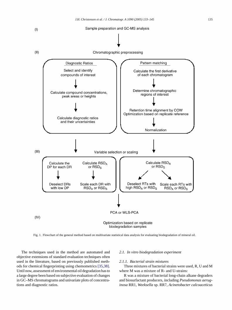
ng (SIM). GC–MS/SIM chromatograms of methylfluorem/z180), methylphenanthrenes (m/z192) and methyldibenothiophenes (m/z 198) were used in this study. The che

cal structures of methylfluorene, methylphenanthreneethyldibenzothiophene are shown inFig. 2.

ethylphenanthrenes and methyldibenzothiophenes.


A blank and a laboratory reference oil solution were ana-lyzed between every eight sample extracts (samples wereanalyzed as part of a larger sequence of samples, blanks,references and quantification standards). The reference oilsolution was a 1:1 mixture of Brent crude oil and a heavyfuel oil with a nominal oil concentration of 2500 mg/L. Thereferences were used for quality control, optimizing the datapreprocessing and calculating the relative analytical standarddeviation (RSDA).

Although the above sample preparation scheme andGC–MS analytical protocol are recommended as part of ahyphenated method, standard sample preparation and frac-tionation procedures, as those described by Wang et al.[47,48], can be used alternatively. This would increase theanalytical time and costs, but may further enhance the ana-lytical selectivity and robustness.

2.3. Data preprocessing

Multivariate data analyses of sections of GC–MS/SIMchromatograms and diagnostic ratios respectively, requiredifferent preprocessing to reduce variations in oil compo-sition unrelated to biodegradation. A selection of prepro-cessing procedures, including baseline removal, normaliza-tion and chromatographic alignment was performed usinga modification of the method to preprocess fingerprintingdv andi eakq

int tos ther r isd fectso ionsw tiond

2ly

at firstd eenc ardb

ticala hiftscH ctso posi-t andt /SIMc arp-i edi orre-

Fig. 3. GC–MS/SIM chromatograms of (a)m/z180, (b)m/z192 and (c)m/z198 in unweathered Brent crude oil.

ata recently described by Christensen et al.[38]. Con-ersely, the diagnostic ratio approach required selectiondentification of compounds of interest as well as puantification.

A proper variable selection or weighting of variableshe fitting of the PCA model is important to exclude orcale down noisy variables, leading to an increase inesolution power of the PCA model. Resolution poweefined as the ability of the PCA model to describe the eff biodegradation, which is the ratio between the variatithin replicate biodegradation samples to the total variaescribed by the model (c.f. Eqs.(5a)–(5c)).

.3.1. Preprocessing of sections of chromatogramsChromatographic baselines (seeFig. 3a–c) can negative

ffect both warping[49,50] and normalization[38] and arehus, removed by calculating the first derivative. Theerivative is calculated numerically as the difference betwonsecutive points, which makes integration straightforwy cumulative summation.

The most severe impediment to multivariate statisnalysis of sections of chromatograms is retention time saused mainly by deterioration of the capillary column[51].ence, PCA will model both such time shifts and effef biodegradation as genuine variations in sample com

ion. This hinders any sensible interpretation of the PCAhereby creates a need for alignment. Here, the GC–MShromatograms were aligned by correlation optimized wng (COW). In COW, a ‘target chromatogram’ is dividnto segments, and the optimal boundary positions for c


sponding segments are determined for each of the remainingchromatograms (‘sample chromatograms’). Segment lengthand slack are used as inputs in the COW algorithm, where theslack parameter is the number of data points each boundaryis allowed to move. Furthermore, a new parameter, padsize,defined as the number of segments comprised of noise thatare added to each end of the chromatograms is introduced.It allows for adequate corrections in the parts retained forthe PCA. The noise regions (i.e. pads), added to each chro-matogram prior to warping, are removed immediately afterwarping.

The method described by Christensen et al.[38] to opti-mize the warping parameters was used. Hence, the optimalchoice of warping parameters is the one that maximizes thefirst singular value in the PCA model without mean center-ing based on the replicate reference oils. The use of COW foraligning chromatograms has been described in detail else-where[38,49,50].

Normalization using Eq.(1) as described by Christensenet al.[38] was applied to compensate for concentration effectsand sensitivity changes,

xNnj = xnj√∑J

j=1x2nj

(1)

w tt nt emew tiontc ces.Ht tion.Ui cteda indi-v tas then ram,t

heM omh

2tita-

t tived con-c hosep ec erec

D

whereaSn is the peak area, peak height or concentration of

compoundn or the sum of several compounds in an oil sam-ple. The commercial GC–MS software Xcalibur v. 1.3 wasused for peak identification and integration. The diagnosticratios and the RSDA’s were calculated in Microsoft Excelfrom peak areas and exported to MATLAB 6.5.1 for chemo-metric data analysis.

2.4. Variable selection

Some diagnostic ratios or chromatographic abundancesare more informative than others, while still others may leadto incorrect conclusions, if kept in the data set. Hence, aproper variable selection is paramount in order to keep theuncertainties to a minimum and yield reliable results.

The approach used here to select diagnostic ratios andretention times for PCA corresponds to the method suggestedby Christensen et al. which are based on the diagnostic power(DP) (Eq.(3)) and RSDA, respectively[35,38].

DP = RSDV

RSDA(3)

where RSDA is calculated from the replicate reference oilsand RSDV is the relative standard deviation of the 41 labo-ratory biodegradation samples. The denominator in Eq.(3)c esw sam-p sses.S s canb witht tion,o dt

2

datam rcdl et rd q.(

X

I ast-s lgo-rw d inM mh

herexnj is the first derivative of then-th chromatogram ahe j-th retention time andJ is the total number of retentioimes. In this study, a more complex normalization schas also adopted by using only a limited set of reten

imes. The selection criterion was based on the RSDA’s cal-ulated from aligned and normalized replicate referenence, only chromatographic abundances with RSDA less

han a predefined threshold were used for normalizander such circumstances, the denominator in Eq.(1) is mod-

fied to the sum of the squared first derivatives of selebundances. In addition, the relative importance of theidualm/zchromatograms (m/z180, 192 and 198) in the daet, can be adjusted by multiplying each data point withumber of retention times in the respective chromatog

ermed relative scaling of chromatograms.Preprocessing was performed in MATLAB 6.5.1 (T

athWorks). The COW algorithm was downloaded frttp://www.models.kvl.dk.

.3.2. Data preprocessing of diagnostic ratiosDiagnostic ratios can be calculated either from quan

ive (i.e. compound concentrations) or from semi-quantitaata (i.e. peak areas or heights). Ratios of compoundentrations or double-normalized diagnostic ratios, as troposed by Christensen et al.[35], describe the relativhemical composition. In this study, diagnostic ratios walculated by using Eq.(2),

R = aSn

(aSn + aS

n∗)(2)

an be substituted by RSDS, which in biodegradation studiould be the relative standard deviation calculated fromles affected by physical or chemical weathering proceubsequently, either an increasing number of variablee excluded from the data analysis starting with the one

he smallest DP and removing one at a time until exhausr, alternatively, variables with RSDA below a predefine

hreshold are excluded from the PCA.

.5. Chemometric data analysis

The preprocessed data are collected in a two-wayatrix (X) of size I (oil samples)× J (diagnostic ratios o

hromatographic abundances). Subsequently,X is bilinearlyecomposed by PCA into products of scores,t (I× 1), and

oading vectors,pT (1× J) (i.e. T in superscript means thransposed matrix ofp), plus residuals,E (I× J). The bilineaecomposition withK principal components is defined in E4).

=(

K∑k=1

tk × pTk

)+ E (4)

n addition, PCA was fitted according to a weighted-lequares criterion (WLS-PCA). We applied the PCAW aithm [52] for this purpose using the inverse of RSDA aseights. All chemometric data analyses were performeATLAB 6.5.1 The PCAW algorithm was downloaded frottp://www-its.chem.uva.nl/research/pac.

http://www.models.kvl.dk/

http://www-its.chem.uva.nl/research/pac


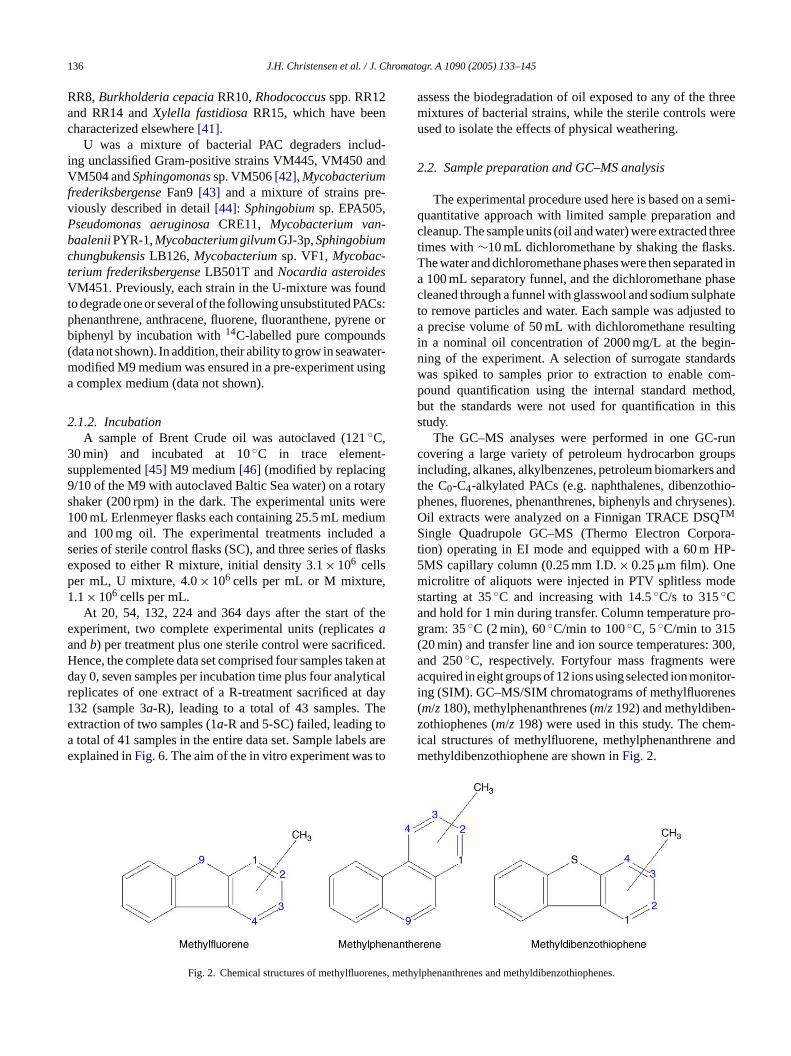
2.6. Optimal preprocessing and data analysis

The optimal combination of preprocessing and data analy-sis is determined by maximizing the resolution power. Specif-ically, the optimization was done by minimizing the varianceof replicate samplesswith respect to their average scorestS(Eq. (5a)) compared to the variance explained by the model(Eq.(5b)) using a predefined number of principal componentsK.

dRep =∑

s

(ns − 1)−1∑i ∈ Ss

(ti − ts)(ti − ts)T (5a)

dAll =I∑

i=1

titTi (5b)

r = dRep

dAll(5c)

whereSsare the row indexes for thens replicates of oil samples, t i is thei-th row ofT, andr is dimensionless. Thus, the PCAwith highest resolution power minimizesr (Eq.(5c)), wheredAll is the normalization factor that accounts for the increasein dRep due to a larger number of principal components.

3

tingb plesf leted efer-e sam-p fromm1i biald ancesT d int sd ass-

TD nes,m

N n

123456789111

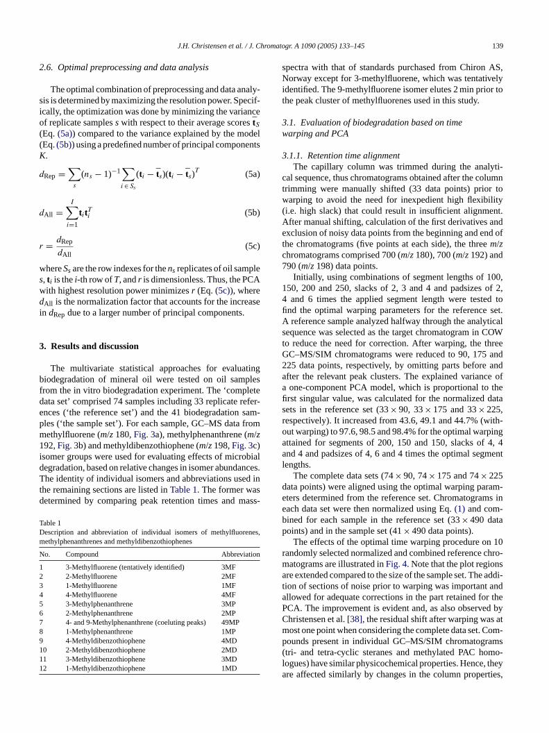
spectra with that of standards purchased from Chiron AS,Norway except for 3-methylfluorene, which was tentativelyidentified. The 9-methylfluorene isomer elutes 2 min prior tothe peak cluster of methylfluorenes used in this study.

3.1. Evaluation of biodegradation based on timewarping and PCA

3.1.1. Retention time alignmentThe capillary column was trimmed during the analyti-

cal sequence, thus chromatograms obtained after the columntrimming were manually shifted (33 data points) prior towarping to avoid the need for inexpedient high flexibility(i.e. high slack) that could result in insufficient alignment.After manual shifting, calculation of the first derivatives andexclusion of noisy data points from the beginning and end ofthe chromatograms (five points at each side), the threem/zchromatograms comprised 700 (m/z180), 700 (m/z192) and790 (m/z198) data points.

Initially, using combinations of segment lengths of 100,150, 200 and 250, slacks of 2, 3 and 4 and padsizes of 2,4 and 6 times the applied segment length were tested tofind the optimal warping parameters for the reference set.A reference sample analyzed halfway through the analyticalsequence was selected as the target chromatogram in COWto reduce the need for correction. After warping, the threeG and2 anda ce ofa thefi datasr ith-o inga 4, 4a mentl

d ram-e ms ine -bp

10r chro-m sa addi-t anda r theP d byC atm Com-p ms( mo-l , theya ties,

. Results and discussion

The multivariate statistical approaches for evaluaiodegradation of mineral oil were tested on oil sam

rom the in vitro biodegradation experiment. The ‘compata set’ comprised 74 samples including 33 replicate rnces (‘the reference set’) and the 41 biodegradationles (‘the sample set’). For each sample, GC–MS dataethylfluorene (m/z180,Fig. 3a), methylphenanthrene (m/z92,Fig. 3b) and methyldibenzothiophene (m/z198,Fig. 3c)

somer groups were used for evaluating effects of microegradation, based on relative changes in isomer abundhe identity of individual isomers and abbreviations use

he remaining sections are listed inTable 1. The former waetermined by comparing peak retention times and m

able 1escription and abbreviation of individual isomers of methylfluoreethylphenanthrenes and methyldibenzothiophenes

o. Compound Abbreviatio

3-Methylfluorene (tentatively identified) 3MF2-Methylfluorene 2MF1-Methylfluorene 1MF4-Methylfluorene 4MF3-Methylphenanthrene 3MP2-Methylphenanthrene 2MP4- and 9-Methylphenanthrene (coeluting peaks) 49MP1-Methylphenanthrene 1MP4-Methyldibenzothiophene 4MD

0 2-Methyldibenzothiophene 2MD1 3-Methyldibenzothiophene 3MD2 1-Methyldibenzothiophene 1MD

.

C–MS/SIM chromatograms were reduced to 90, 17525 data points, respectively, by omitting parts beforefter the relevant peak clusters. The explained varianone-component PCA model, which is proportional to

rst singular value, was calculated for the normalizedets in the reference set (33× 90, 33× 175 and 33× 225,espectively). It increased from 43.6, 49.1 and 44.7% (wut warping) to 97.6, 98.5 and 98.4% for the optimal warpttained for segments of 200, 150 and 150, slacks ofnd 4 and padsizes of 4, 6 and 4 times the optimal seg

engths.The complete data sets (74× 90, 74× 175 and 74× 225

ata points) were aligned using the optimal warping paters determined from the reference set. Chromatograach data set were then normalized using Eq.(1) and comined for each sample in the reference set (33× 490 dataoints) and in the sample set (41× 490 data points).

The effects of the optimal time warping procedure onandomly selected normalized and combined referenceatograms are illustrated inFig. 4. Note that the plot regionre extended compared to the size of the sample set. The

ion of sections of noise prior to warping was importantllowed for adequate corrections in the part retained foCA. The improvement is evident and, as also observehristensen et al.[38], the residual shift after warping wasost one point when considering the complete data set.ounds present in individual GC–MS/SIM chromatogratri- and tetra-cyclic steranes and methylated PAC hoogues) have similar physicochemical properties. Hencere affected similarly by changes in the column proper


Fig. 4. First derivative of the normalized and combined chromatograms ofm/z180, 192 and 198 for 10 references: (a) without time alignment and (b)with time alignment. The optimal COW parameters consisted of segmentlengths of 200, 150 and 150, slack of four for all threem/zvalues and padsizeof 4, 6 and 4 times the optimal segment lengths.

which is the most likely reason for the consistently high warp-ing quality of COW on GC–MS/SIM data.

Conversely, in chromatograms based on less selectivedetectors such as GC-FID, retention time shifts may appearmore irregular since the variation in physicochemical prop-erties of the compounds present generally are greater thanin a GC–MS/SIM chromatogram with more closely relatedcompounds. Thus, closely related isomers (as detected byGC–MS/SIM) are not expected to change their order of elu-tion even if significant changes in the column stationary phasetake place, while compounds with different physicochemicalproperties (as detected by GC-FID) often do, and COW can-not adequately correct for such changes. This may explainwhy some authors[49,50] have experienced that optimalchromatographic alignment is achieved if the segment lengthis of the same order of magnitude as the peaks, since a highflexibility is necessary to correct for irregular retention timeshifts.

Fig. 5. (a) Weights (RSDA−1) used for WLS-PCA and (b) the aligned andnormalized, mean combined chromatogram of unweathered Brent crude oil.The mean was calculated from four replicate samples.

3.1.2. Variable selectionThe RSDA’s were calculated from the aligned and nor-

malized reference set using the optimal warping parametersand the complete chromatographic sections (90, 175 and225 data points, respectively) for normalization. The RSDA’swere used for variable selection by excluding retention timeswith RSDA below a predefined threshold thereby retain-ing the peak regions.Fig. 5a shows the weights (RSDA

−1)used in WLS-PCA to scale the importance of retentiontimes with respect to their analytical uncertainty, andFig. 5bshows the first derivative of the aligned and normalizedmean combined chromatogram of the unweathered Brentcrude oil.

The peak and noise regions have, respectively, high andlow weights. Thus, the importance of peak regions is high,compared to those of noise regions, during fitting of the PCAmodel (Fig. 5).

3.1.3. Chemometric data analysisPCA was performed on the mean-centered sample set

using combinations of normalization, relative scaling of thethree GC–MS/SIM chromatograms, PCA methods and opti-mal number of principal components (PCs). The chromato-graphic sections (90, 175 and 225 data points, respectively)were applied for normalization using Eq.(1). Furthermore,t erei ointsi -s d byt d ther edt ).F tiono ro-c

hresholds from 0.1 to 1.0 with increments of 0.1 wmposed, thereby retaining between 13 and 78 data pn m/z180, 23–116 inm/z192 and 17–133 inm/z198. Subequently, data were either left unchanged or multipliehe sizes of the corresponding data sets. This increaseelative importance ofm/z 198 (225 data points) comparo m/z 192 (175 data points) andm/z 180 (90 data pointsinally, data were analyzed by PCA with variable selecr WLS-PCA using two or three PCs. The optimal prepessing and data analysis was obtained by minimizingr in


Eq. (5) (maximizing resolution power) using the duplicatebiodegradation samples to calculatedRep.

The resolution power of PCA models with three PCs wassignificantly lower (r = 0.0346–0.231) than for PCA mod-els with two PCs (r = 0.0188–0.0477). Furthermore, fromvisual inspection of loadings it was clear that PC3 and higherorder components described the residual shifts rather thansystematic changes in chemical composition. Residual shiftsshow up in the cumulative sum of loadings as first deriva-tive peaks. As an increasing number of PCs is extracted fromdata, the ratio between the systematic information and thevariations caused by insufficient alignment decreases untilthe latter becomes the most pronounced. Christensen et al.[38] extracted four reliable components from the calibrationset of 61 oil samples× 1231 data points. In this study onlytwo components could be extracted, since the number of inde-pendent variations was smaller.

Normalization and relative scaling of chromatogramsinfluenced the resolution power. Normalization consistentlyaffected ther-value for WLS-PCA from 0.206 (with a thresh-old at 0.1) to 0.230 (using all data for normalization). Relativescaling diminished the resolution power of the PCA model,because them/z 198 chromatogram became more influen-tial and thereby introducing more noise in data (e.g. ther-value of PCA with variable selection using a threshold of0.2 increased from 0.0188 without scaling to 0.0263 withs

so holdo atap er( dataa utionp singt lysisf ntv ancel

CAw ithR sd

0 to1 atedf , atl vei renesa nt int naf-f thatm itionh pre-p ionso o thec ple)o

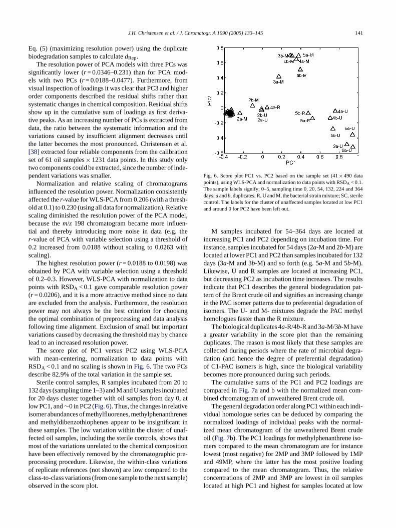
Fig. 6. Score plot PC1 vs. PC2 based on the sample set (41× 490 datapoints), using WLS-PCA and normalization to data points with RSDA < 0.1.The sample labels signify; 0–5, sampling time 0, 20, 54, 132, 224 and 364days;aandb, duplicates; R, U and M, the bacterial strain mixture; SC, sterilecontrol. The labels for the cluster of unaffected samples located at low PC1and around 0 for PC2 have been left out.

M samples incubated for 54–364 days are located atincreasing PC1 and PC2 depending on incubation time. Forinstance, samples incubated for 54 days (2a-M and 2b-M) arelocated at lower PC1 and PC2 than samples incubated for 132days (3a-M and 3b-M) and so forth (e.g. 5a-M and 5b-M).Likewise, U and R samples are located at increasing PC1,but decreasing PC2 as incubation time increases. The resultsindicate that PC1 describes the general biodegradation pat-tern of the Brent crude oil and signifies an increasing changein the PAC isomer patterns due to preferential degradation ofisomers. The U- and M- mixtures degrade the PAC methylhomologues faster than the R mixture.

The biological duplicates 4a-R/4b-R and 3a-M/3b-M havea greater variability in the score plot than the remainingduplicates. The reason is most likely that these samples arecollected during periods where the rate of microbial degra-dation (and hence the degree of preferential degradation)of C1-PAC isomers is high, since the biological variabilitybecomes more pronounced during such periods.

The cumulative sums of the PC1 and PC2 loadings arecompared inFig. 7a and b with the normalized mean com-bined chromatogram of unweathered Brent crude oil.

The general degradation order along PC1 within each indi-vidual homologue series can be deduced by comparing thenormalized loadings of individual peaks with the normal-ized mean chromatogram of the unweathered Brent crudeo iso-m tancel MPa dingc lativec plesl t low

caling).The highest resolution power (r = 0.0188 to 0.0198) wa

btained by PCA with variable selection using a thresf 0.2–0.3. However, WLS-PCA with normalization to doints with RSDA < 0.1 gave comparable resolution powr = 0.0206), and it is a more attractive method since nore excluded from the analysis. Furthermore, the resolower may not always be the best criterion for choo

he optimal combination of preprocessing and data anaollowing time alignment. Exclusion of small but importaariations caused by decreasing the threshold may by chead to an increased resolution power.

The score plot of PC1 versus PC2 using WLS-Pith mean-centering, normalization to data points wSDA < 0.1 and no scaling is shown inFig. 6. The two PCescribe 82.9% of the total variation in the sample set.

Sterile control samples, R samples incubated from 232 days (sampling time 1–3) and M and U samples incub

or 20 days cluster together with oil samples from day 0ow PC1, and∼0 in PC2 (Fig. 6). Thus, the changes in relatisomer abundances of methylfluorenes, methylphenanthnd methyldibenzothiophenes appear to be insignifica

hese samples. The low variation within the cluster of uected oil samples, including the sterile controls, showsost of the variations unrelated to the chemical composave been effectively removed by the chromatographicrocessing procedure. Likewise, the within-class variatf replicate references (not shown) are low compared tlass-to-class variations (from one sample to the next sambserved in the score plot.

il (Fig. 7b). The PC1 loadings for methylphenanthreneers compared to the mean chromatogram are for ins

owest (most negative) for 2MP and 3MP followed by 1nd 49MP, where the latter has the most positive loaompared to the mean chromatogram. Thus, the reoncentrations of 2MP and 3MP are lowest in oil samocated at high PC1 and highest for samples located a


Fig. 7. Loading plots based on the sample set (41× 490), using WLS-PCAand normalization to data points with RSDA < 0.1. (a) The cumulative sumof the PC1 loadings (red and broken line) compared with the cumulativesum of the aligned and normalized mean chromatogram of unweatheredBrent crude oil (blue line) and (b) The cumulative sum of the PC2 loadings(red and broken line) compared with the unweathered Brent crude oil (forinterpretation of the references to color in this figure legend, the reader isreferred to the web version of this article).

PC1 (the unaffected samples), whereas the opposite is thecase for 49MP. The general degradation orders observedare 2MP = 3MP > 1MP > 49MP for the methylphenanthrenehomologue series, 3MF > 1MF > 2MF > 4MF for methylfluo-renes and 2MD > 1MD > 4MD > 3MD for methyldibenzoth-iophenes. It is of special interest that the co-eluting peaks2- and 3-methyldibenzothiophenes (23MD), which usuallyare considered as one common peak cluster, show preferential degradation. Hence, 2MD is the isomer most susceptibleto microbial degradation by R, U and M mixtures, whereas3MD is the least degradable. In fact, due to the significantpeak overlap, the retention time of 3MD changes due to lossof 2MD, a trend which can be observed in the loading plot asa shift to higher retention time of the 3MD isomer peak.

Another interesting observation in the score plot is thatthe M versus the U and R samples are separated along PC2

Table 2Description of diagnostic ratios, RSDA, RSDV and DP for each diagnosticratio calculated from the reference set

Diagnostic ratios RSDV (%) RSDA (%) DP

2MP/(1MP + 2MP) 72.4 0.7 101.33MP/(3MP + 1MP) 66.2 0.7 100.83MP/(3MP + 49MP) 67.8 0.8 88.82MP/(2MP + 49MP) 74.0 0.9 79.11MF/(1MF + 4MF) 11.2 0.3 35.23MF/(3MF + 4MF) 72.1 2.2 33.12MD/(2MD + 1MD) 73.8 2.3 31.849MP/(49MP + 1MP) 15.0 0.5 28.72MF/(2MF + 4MF) 33.0 1.4 24.22MF/(2MF + 1MF) 50.8 2.2 22.63MF/(3MF + 1MF) 74.0 3.4 21.73MF/(3MF + 2MF) 66.3 3.2 20.53MP/(3MP + 2MP) 10.1 0.5 18.72MD/(2MD + 3MD) 74.7 4.8 15.64MD/(4MD + 1MD) 7.5 0.7 10.94MD/(4MD + 2MD) 12.2 1.6 7.73MD/(3MD + 1MD) 20.9 2.9 7.34MD/(4MD + 3MD) 5.1 2.0 2.6

Thus M, the combined mixture of bacterial strains in U and R,affected the PAC isomer pattern differently than did both theU and the R mixtures. The PC2 loadings are compared withthe aligned and normalized mean chromatogram of unweath-ered Brent crude oil inFig. 7b. The comparison indicatesa less preferential degradation of 1MF (most positive load-ing) over 2MF (most negative) and 1MD (most positive) over∑

23MD (most negative) in M samples than in U and R sam-ples. Furthermore, a more preferential degradation of 1MP(most negative) over 49MP (most positive) is observed.

3.2. Evaluation of biodegradation based on diagnosticratios and PCA

3.2.1. Data and variable selectionAll possible combinations of diagnostic ratios of single

compounds within each of the homologue series of C1-PACswere calculated. Hence, 18 diagnostic ratios (Table 2) withpotential sensitivity to biodegradation due to preferentialdegradation of specific isomers were included in this study.The reference set (33 samples× 18 diagnostic ratios) wasused to calculate the RSDA’s, whereas the sample set (41samples× 18 diagnostic ratios) was used to calculate RSDVand the PCA models. The RSDA, RSDV and DP for eachdiagnostic ratio are listed inTable 2.

3e set

u os-t 38i inedb cateb

tiont and

-

.

.2.2. Chemometric data analysisPCA was performed on the mean-centered sampl

sing PCA with variable selection (including 1–18 diagnic ratios) and WLS-PCA, with 2 and 3 PCs leading tondividual PCAs. The optimal data analysis was determy optimizing the resolution power based on the dupliiodegradation samples.

The number of PCs was determined by cross validao three, and further verified by evaluating the loadings


Fig. 8. WLS-PCA on mean-centered data using 3 PCs. (a) Score plot of PC1vs. PC2 based on the sample set (41× 18) and (b) loading plot of PC1 vs.PC2. The labels of diagnostic ratios are simplified.

scores. The optimal number of PCs varied depending on thenumber of diagnostic ratios retained for the analysis. Thehighest resolution power (r = 0.0207–0.0251) was obtainedby PCA with variable selection using between 5 and 13 diag-nostic ratios with highest DP. However, the resolution powerwas comparable for the WLS-PCA model (r = 0.0252).

The score and loading plots of PC1 versus PC2 for thethree-component WLS-PCA model with mean-centering areshown inFig. 8a and b, respectively. The three PCs describe98.9% of the total variation in the sample set.

PC1 describes the general biodegradation pattern ofthe Brent crude oil. The effects of microbial degrada-tion on the relative isomer abundances are shown as anincrease (ratios located at high PC1 in the loading plot)or decrease (ratios located at low PC1) in the diagnosticratios. The general biodegradation trends observed alongPC1 causes among others a decrease in 3MP/(3MP + 1MP),2MD/(2MD + 3MD) and 3MF/(3MF + 4MF) and an increasein 4MD/(4MD + 1MD). The M versus U and R samples areseparated along PC2. The cause of this separation can be

explained by a stronger increase in 49MP/(49MP + 1MP) anda weaker increase in 2MF/(2MF + 1MF) and 3MD/(3MD +1MD). Hence, 1MD is less degraded compared to

∑MD and

1MP more degraded than 49MP in M samples than in U and Rsamples. The within-class variations (e.g. the unaffected oilsamples) are, as for the evaluation based on time-warping andPCA, much less than the class-to-class variations. The con-clusions made fromFig. 8a and b correspond to those madefrom Figs. 6 and 7using time warping and PCA. In addition,although a minor component, data for U and R samples areseparated by PC3 due to less preferential degradation of e.g.1MF over 2MF and 3MP over 2MP in R samples comparedto U samples.

Co-elution of compounds at low concentrations that inter-fere with target compounds, such as C5-naphthalenes withC1-dibenzothiophenes inm/z198, may affect the results neg-atively. The risk of introducing undesirable variability fromsuch minor components is higher when using preprocessedchromatographic sections compared to the diagnostic ratioapproach based on peak identification and quantification.Furthermore, the biodegraded samples are more likely to beaffected since the relative abundances of these minor com-ponents may change due to selective weathering processes.However, since the concentrations of the C1-PAC isomers arehigh in Brent crude oil the results are, in the present study,most likely unaffected by co-elution of minor components.

hlyo Thec anda ter-v s ana spe-c erentv ffi-c waso h thet e oft plesf

ym-m ctt es ini eakr ctorss nt ofp

4

pillsa er-e deo eth-o alysiso p-

Time warping combined with PCA represents a higbjective alternative to standard evaluation methods.omplete data treatment, including data preprocessingnalysis, can be performed with only limited human inention. However, whether or not the method provideppropriate tool for assessing effects of weathering in aific case study depends on the ratio between the inhariability in the data set and the variability due to insuient alignment. Two components were extracted, whichne less than by the diagnostic ratio approach. Althoug

hird component (PC3) explained only a minor percentaghe total variance it was important for separating R samrom U (and M) samples.

Furthermore, variations in peak shape (e.g. from setrical to tailing) during column deterioration will affe

he multivariate data analysis negatively due to changntensity distribution of adjacent retention times within pegions. Peak quantification is less affected by these faince peak areas and heights are relatively independeeak shape.

. Conclusions and perspectives

Assessments of biodegradation in the field after oil snd during in vitro experiments are difficult due to the inhnt chemical complexity of mineral oil and to the multituf processes changing its composition. The two novel mds presented in this paper enabled a comprehensive anf the effects of biodegradation with limited time consum


tion and cost and high objectivity compared with standardassessment methods. In the first method based on analysesof sections of chromatograms, the large data set (41 sam-ples× 490 retention times) was evaluated in three plots (i.e.one score plot and two loading plots). In the diagnostic ratioapproach, a third component was extracted from the data set(41 samples× 18 diagnostic ratios) distinguishing R from Usamples. The results showed that the PAC degradation patternwas different for each of the three bacterial strain mixtures.Thus, preferential degradation patterns in the natural envi-ronment cannot be established from data obtained during invitro experiments using simple mixtures of bacterial strains.

A wide range of potential applications exists for the twoevaluation methods described in this paper such as assess-ment of other complex mixtures of contaminants (e.g. per-sistent organic pollutants) and other weathering processes.The relative changes in the homologue series ofn-alkanes(e.g.m/z 85) can for example be used to deduce the effectsof evaporation, whereas ratios ofn-alkanes and isoprenoidscan describe the initial phase of biodegradation.

Furthermore, by normalizing to one or several surrogatestandards (which corresponds to the internal quantificationmethod) or by using the normalization factor of the clos-est reference for normalization (which corresponds to theexternal quantification method), concentration effects can beretained in data. Such modifications would allow the moni-t n-m bjec-t s.

A

hni-c theP om-m nd“ ralS entalR

R

uar.

02)

.O.

, L.2.001)

las,

[8] G. Thouand, P. Bauda, J. Oudot, G. Kirsch, C. Sutton, J.F. Vidalie,Can. J. Microbiol. 45 (1999) 106.

[9] Z.D. Wang, M. Fingas, S. Blenkinsopp, G. Sergy, M. Landriault, L.Sigouin, J. Foght, K. Semple, D.W.S. Westlake, J. Chromatogr. A809 (1998) 89.

[10] R.C. Prince, R.M. Garrett, R.E. Bare, M.J. Grossman, T. Townsend,J.M. Suflita, K. Lee, E.H. Owens, G.A. Sergy, J.F. Braddock, J.E.Lindstrom, R.R. Lessard, Spill. Sci. Technol. B 8 (2003) 145.

[11] B.V. Chang, S.H. Wei, S.Y. Yuan, J. Environ. Sci. Heal. B 36 (2001)177.

[12] W.R. Cullen, X.F. Li, K.J. Reimer, Sci. Total. Environ. 156 (1994)27.

[13] A.T. Law, K.S. Teo, J. Mar. Biotechnol. 5 (1997) 162.[14] J.C. Roper, F.K. Pfaender, Environ. Toxicol. Chem. 20 (2001)

223.[15] H. Budzinski, N. Raymond, T. Nadalig, M. Gilewicz, P. Garrigues,

J.C. Bertrand, P. Caumette, Org. Geochem. 28 (1998) 337.[16] T.K. Dutta, S. Harayama, Environ. Sci. Technol. 34 (2000) 1500.[17] J. Oudot, F.X. Merlin, P. Pinvidic, Mar. Environ. Res. 45 (1998) 113.[18] P.D. Boehm, G.S. Douglas, W.A. Burns, P.J. Mankiewicz, D.S. Page,

A.E. Bence, Mar. Pollut. Bull. 34 (1997) 599.[19] D. Munoz, P. Doumenq, M. Guiliano, F. Jacquot, P. Scherrer, G.

Mille, Talanta 45 (1997) 1.[20] C.E. Cerniglia, Biodegradation 3 (1992) 351.[21] G.S. Douglas, A.E. Bence, R.C. Prince, S.J. McMillen, E.L. Butler,

Environ. Sci. Technol. 30 (1996) 2332.[22] J.R. Bragg, R.C. Prince, E.J. Harner, R.M. Atlas, Nature 368 (1994)

413.[23] E.L. Butler, G.S. Douglas, W.G. Steinhauer, On-Site Bioreclamation,

2001, p. 515.[24] R.C. Prince, D.L. Elmendorf, J.R. Lute, C.S. Hsu, C.E. Halth, J.D.

ech-

[ iol.

[ nol.

[[[ 993)

[[[ mo-

[[ 984)

[ nder-

[ rker,

[ 01)

[ hnol.

[ Anal.

[ nol.

[ F.

[[ tedt,

[ .[

oring of levels of complex mixtures of pollutants in enviroental samples with limited use of resources and high o

ivity compared to standard tiered analytical approache

cknowledgements

The authors acknowledge Lotte Frederiksen for tecal assistance, D. Springael for providing several ofAC-degrading bacterial strains, and the European Cission (contracts “BIOSTIMUL”, QLRT-1999-00326, a

ALARM”, GOCE-CT-2003-506675), the Danish Natuciences Research Council and the National Environmesearch Institute, Denmark, for funding.

eferences

[1] Z.D. Wang, M. Fingas, J. Chromatogr. A 712 (1995) 321.[2] G. Mille, D. Munoz, F. Jacquot, L. Rivet, J.C. Bertrand, Est

Coast. Shelf. S 47 (1998) 547.[3] R.C. Prince, E.H. Owens, G.A. Sergy, Mar. Pollut. Bull. 44 (20

1236.[4] T.C. Sauer, J.S. Brown, P.D. Boehm, D.V. Aurand, J. Michel, M

Hayes, Mar. Pollut. Bull. 27 (1993) 117.[5] Z. Wang, M. Fingas, H. Blenkinsopp, G. Sergy, M. Landriault

Sigouin, P. Lambert, Environmen. Sci. Technol. 32 (1998) 222[6] J.D. Leblond, T.W. Schultz, G.S. Sayler, Chemosphere 42 (2

333.[7] S.J. Rowland, R. Alexander, R.I. Kagi, D.M. Jones, A.G. Doug

Org. Geochem. 9 (1986) 153.

Senius, G.J. Dechert, G.S. Douglas, E.L. Butler, Environ. Sci. Tnol. 28 (1994) 142.

25] D. Venosa, M.T. Suidan, D. King, B.A. Wrenn, J. Ind. MicrobBiot. 18 (1997) 131.

26] T. Sasaki, H. Maki, M. Ishihara, S. Harayama, Environ. Sci. Tech32 (1998) 3618.

27] J.H. Christensen, Polycycl. Aromat. Comp. 22 (2002) 703.28] M.C. Kennicutt, Oil. Chem. Pollut. 4 (1988) 89.29] L.B. Christensen, T.H. Larsen, Ground. Water. Monit. R 13 (1

142.30] J.K. Volkman, Org. Geochem. 6 (1984) 619.31] Z. Wang, M. Fingas, Environ. Sci. Technol. 29 (1995) 2842.32] F. Jacquot, M. Guiliano, P. Doumenq, D. Munoz, G. Mille, Che

sphere 33 (1996) 671.33] N. Telnaes, B. Dahl, Org. Geochem. 10 (1986) 425.34] K. Øygard, O. Grahl-Nielsen, S. Ulvøen, Org. Geochem. 6 (1

561.35] J.H. Christensen, A.B. Hansen, G. Tomasi, J. Mortensen, O. A

sen, Environ. Sci. Technol. 38 (2004) 2912.36] W.A. Burns, P.J. Mankiewicz, A.E. Bence, D.S. Page, K.R. Pa

Environ. Toxicol. Chem 16 (1997) 1119.37] S.A. Stout, A.D. Uhler, K.J. McCarthy, Environ. Forens. 2 (20

87.38] J.H. Christensen, G. Tomasi, A.B. Hansen, Environ. Sci. Tec

39 (2005) 255.39] J.H. Christensen, A.B. Hansen, J. Mortensen, O. Andersen,

Chem. 77 (2005) 2210.40] C.D. Simpson, C.F. Harrington, W.R. Cullen, Environ. Sci. Tech

32 (1998) 3266.41] L. Yuste, M.E. Corbella, M.J. Turiegano, U. Karlson, A. Puyes,

Rojo, FEMS Microbiol. Ecol. 32 (2000) 69.42] D. Springael, Personal Communication, 2005.43] P.A. Willumsen, U. Karlson, E. Stackebrandt, R.M. Kroppens

Int. J. Syst. Evol. Micr. 51 (2001) 1715.44] A.R. Johnsen, U. Karlson, Appl. Microbiol. Biot 63 (2004) 45245] T. Bauchop, S.R. Elsden, J. Gen. Microbiol 23 (1960) 457.


[46] J. Sambrook, E.F. Fritsch, T. Maniatis, Molecular Cloning: A Labo-ratory Manual, Cold Spring Harbor Laboratory, Spring Harbor, NewYork, 1989.

[47] Z.D. Wang, M. Fingas, K. Li, J. Chromatogr. Sci. 32 (1994)367.

[48] Z.D. Wang, M. Fingas, K. Li, J. Chromatogr. Sci. 32 (1994) 361.

[49] N.P.V. Nielsen, J.M. Carstensen, J. Smedsgaard, J. Chromatogr. A805 (1998) 17.

[50] G. Tomasi, F. van den Berg, C. Andersson, J. Chemometr. 18 (2004)231.

[51] C.G. Fraga, B.J. Prazen, R.E. Synovec, Anal. Chem. 72 (2000) 4154.[52] H.A.L. Kiers, Psychometrika 62 (1997) 251.

multivariate statistical methods for evaluating biodegradation of mineral oil

Documents