Procedia Engineering 89 ( 2014 ) 901 – 908

Available online at www.sciencedirect.com

1877-7058 © 2014 Published by Elsevier Ltd. This is an open access article under the CC BY-NC-ND license (http://creativecommons.org/licenses/by-nc-nd/3.0/).Peer-review under responsibility of the Organizing Committee of WDSA 2014doi: 10.1016/j.proeng.2014.11.523

ScienceDirect

16th Conference on Water Distribution System Analysis, WDSA 2014

Multivariate Statistical Analysis for Water Demand Modeling C. M. Fontanazzaa*, V. Notaroa, V. Puleoa, G. Frenia

aFaculty of Engineering and Architecture, University of Enna “Kore”, Enna, Italy

Abstract

The actual level of water demand is the driving force behind the hydraulic dynamics in water distribution systems. Consequently, it is crucial to estimate it as accurately as possible in order to result in reliable simulation models. In this paper, a copula-based multivariate analysis has been proposed and used for demand prediction for given return period. The analysis is applied to water consumption data collected in the water distribution network of Palermo (Italy). The approach showed to produce consisted demand patterns and to be a powerful tool to be coupled with water distribution network models for design or analysis problems. © 2014 The Authors. Published by Elsevier Ltd. Peer-review under responsibility of the Organizing Committee of WDSA 2014.

Keywords: Multivariate analysis; vine copula; water demand modeling.

1. Introduction

Urban development is creating new problems for the management of water distribution systems, which are called upon to respond to a growing drinking water demand, which is also highly variable in space and time. The general goal for any water utility is to supply constantly water to all customers of good quality and under sufficient pressure [1,2]. The reliability of the water distribution system of that utility depends on the combination of different factors that play an important role in the design and management of the system: water demand variability, size and maintenance of pipes, volumes of urban reservoirs. The development of powerful computers made hydraulic engineers able to simulate the behavior of water supply systems for almost any scenario. However, the accurate prediction of pressures, flows and water quality parameters depends strongly on the quality of the input data. Data needed to simulate the behavior of water distribution network, such as pipes friction coefficients, nodal demands, and their temporal variation contain uncertainty, consequently affect our confidence in the outcome of the

* Corresponding author: Tel.: +39-320-6404501

E-mail address: chiara.fontanazza@unikore.it

© 2014 Published by Elsevier Ltd. This is an open access article under the CC BY-NC-ND license (http://creativecommons.org/licenses/by-nc-nd/3.0/).Peer-review under responsibility of the Organizing Committee of WDSA 2014

902 C.M. Fontanazza et al. / Procedia Engineering 89 ( 2014 ) 901 – 908

simulation. There has been agreement in the literature that uncertainties in nodal demands and their variation with time is one of the main source of error responsible for discrepancies between measured and model simulated flows and pressures.

Residential water demand is one of the most difficult parameters to determine when modeling drinking water distribution networks. The simulation of a water distribution system is often carried out by assuming averaged values, both in space and in time, of water demands: the spatial averaged values are obtained by clustering the water consumption of users afferent each node of the network, the time averaged values are obtained as the mean of the instantaneous values of the nodal demands. The simulation results obtained by considering these simplifications could be not much reliable for the hydraulically disadvantages zones of the network. Therefore, water demand modeling has been a very active field of study. Researchers have been above all interested in domestic water consumption by households that is the principal rate of the total volume supplied by the water distribution system in urban regions, often equal to 75% [3]. The prediction of water demand can be done on different time scales: short- and long-term forecasting of the municipal water demand is essential to water utilities for system planning, design, and asset management. Short-term forecasting is useful for operation and management of existing water supply systems within a specific time period, whereas long-term forecasting is important for system planning, design, and asset management. The detailed modeling of the hydraulic behavior of drinking water distribution systems could be get by implementing a domestic water demand modeling in one of the several software programs recently developed. Until today stochastic models for instantaneous residential water demand (for references see section 2.1) have been used to obtain realistic demand patterns for the hydraulic distribution network solvers. Several basic parameters related to the residential water usage are necessary to apply these models, such as the frequency, duration and intensity statistics of the demand pulses. This methodology shows a limit in authors’ opinion: it neglects the statistical dependence of the parameters characterizing the consumption process. Many approaches are used in hydrology to develop statistical multivariate analysis. Among methodologies present in literature, the method based on the copula, recently introduced in hydrology, is applied in this paper.

This study has two objectives: (1) to propose a procedure based on a multivariate statistical analysis of the main features of the water consumption process at domestic level; (2) to define a more realistic demand patterns with a given return period. The present paper is organized as in the following: in section 2, a brief review of the studies concerning with demand modeling and multivariate statistical analysis is introduced; in section 3, the case study to which the procedure is applied is presented; in section 4, the multivariate analysis of the consumption process and the resulting demand patterns is described; finally, in section 5, the conclusions of this paper are drawn.

2. Literature review

2.1. Urban water demand modeling

Qi and Chang [4] and House-Peters and Chang [5] present an overview of water demand prediction models on various time scales. The time scale for any prediction model is dictated by the purpose for which the prediction model is to be used [6]. Most of the researches on water consumptions carried out in the past started from the need to quantify the global demand, by means of long-term forecasting [7,8,9,10], and to fix a suitable rate structure [11]. New reasons to better characterize the domestic water consumption have lately come out: the need to assure water volumes demanded by costumers and to supply them with sufficient pressure and good quality, have stand out among these [12,13,14,15]. The many approaches proposed to forecast short- and long-term municipal water demands in the past few decades might be grouped into five categories: the regression analysis, the time series analysis, the computational intelligence approach, and the stochastic model.

Traditional regression analyses were normally carried out based on statistical estimation of the relationship between water demand and some explanatory variables (i.e., independent variables), such as socioeconomic factors, and assumed that the relationships will continue in the future. Such a regression analysis approach can then be applied for both short- and long-term analyses when a training dataset is available [8, 16, 17, 18, 19, 20, 21, among others]. Time series analysis in water demand forecasting is based on a statistical abstraction of the various trends that inherently contribute to the change of water demand over time. A time series model may inevitably include a long-term trend component, a cyclical component, and a short-term variance component. The time series analysis

903 C.M. Fontanazza et al. / Procedia Engineering 89 ( 2014 ) 901 – 908

has been extensively used for short-term water demand forecasting [1,9,10,22,23,24,25,26,27,28,29,30,31,32,33]. The computational intelligence models, including artificial neural networks (ANN), fuzzy logic, and agent-based models, are mathematically suited to simulate complex systems. For example, the ANN were developed for short-term water demand forecasting [34,35,36,37,38,39,40]. ANNs have been offered as effective alternatives to traditional linear modeling approaches because of their ability to explicitly analyze nonlinear time series events. ANNs have been proposed as an improved method for short-term forecasting of peak daily [36,41] and hourly [42] water demand.

The above-mentioned researches deal with water demand modeling at a big spatial scale (e.g. entire network level). At a domestic service level, water demand is sporadic, characterized by sudden demand pulses, and tends to have a stochastic character [13,14], especially when considering time scales on the order of seconds. Therefore, several stochastic models for domestic demand determination were developed. These models include the Poisson Rectangular Pulse model [13,14,15,43,44], the Neyman-Scott Rectangular Pulse model [45] and some more [46].

2.2. Multivariate statistical analysis

The copula function is a new analysis method well-known in the theory of probabilistic metric space before and recently introduced by De Michele and Salvadori [47] in hydrology. The copula function permits separate investigation of the marginal properties and interdependence structures of variables. Therefore, it synthesizes the dependence structure of the variables in the purest and most essential form [48] without assuming that variables are normal or have the same marginal distributions. The application of copulas in simulations of multivariate data, extreme value analysis and modeling dependence structure is becoming popular in hydrological analysis [47, 48, 49, 50, 51, 52]. A historical review and a discussion of major developments in the theory and application of copulas can be found in Schweizer [53] and Kotz [54]. While there is a multitude of bivariate copula, the class of multivariate copulas is still quite restricted. As matter of fact, building higher-dimensional copulas is generally recognized as a difficult problem. The idea of constructing a multivariate dependence model from bivariate copulas as building blocks called pair-copulas goes back to the paper of Joe [55]. He gave the construction of the first pair-copula in terms of distribution functions.

Bedford and Cooke [56,57] realized that there were a significant number of possible pair-copulas constructions (PCC), thus they organized them in graphical way by sequentially designing trees which identify the bivariate copula densities needed to make up a d-dimensional density. It involves only products of bivariate copulas. Since the trees are intrinsically related they called these distributions regular vines (R-vines). Their primary interest was to use vines in the modeling of large networks so they restricted themselves to the case of Gaussian pair-copulas. Aas et al. [58] were the first to recognize that this construction principle can be extended by using arbitrary pair-copulas, since the construction principle has no restriction on the choice of pair-copulas. Vine copulas are flexible models for multivariate dependencies which specify a factorization of the copula density into a product of conditional bivariate copulas. The class of regular vines is still very general and embraces a large number of possible pair-copula decompositions; it includes two simple tree structures, such as line trees and star trees, the first one corresponds to D-vines, while the second one corresponds to C-vines.

3. The case study

The multivariate statistical analysis described in the next section have been applied to water consumption data obtained monitoring eight dwellings located in Palermo (Italy) during the entire 2007. The customers that took part in the consumption monitoring program have been selected according to the following characteristics: family with at least two members; family members of 4-70 years old; one electric household appliance at least (dishwasher or washing-machine); negligible outdoor consumptions; cooperation. The selected eight families were the only that agreed to take part in the consumption monitoring program. Instrument packs to monitor domestic water use were installed on the service line of the secure indoor locations in each of the eight dwellings. The instrument package included a data logger, 4-20 mA impulse sensor. Data loggers were coupled with an input sensor inserted between the base and register head of a multi-jet water meter. The water meter had Q1 = 15 l/h, Q2 = 22.5 l/h, Q3 = 1500 l/h,

904 C.M. Fontanazza et al. / Procedia Engineering 89 ( 2014 ) 901 – 908

Q4 = 5000 l/h. The input sensor monitored revolutions of a magnet fixed to a positive displacement nutating disc in the measuring chamber of the meter. At each consumption of 0.5 liters, the sensor transmitted a signal to the data logger. Consumptions recorded at each user were reported in a text file where six fields were stored: day, month, year, hour, minute and second at which a use with a volume of 0.5 l occurs. Water demands were downloaded connecting the data logger to a portable pc.

A four steps process was used to transform the raw input signals into archived residential water consumptions: Step 1 involves data retrieval; Step 2 involves data correction (signal repeated removing, putting water demand reading in chronological order) and water uses separation; in step 3, leaks and ultra-low demands were censored; in step 4, the volume of each pulse was uniformly distributed over the duration of the pulse. A sparse matrix collected flow values (l/sec) having as number of columns the seconds in a day and as number of rows the days during which consumption data were recorded (changing for each user).

4. Consumption data analysis

In this paper the vine copula method has been used to build the 3-D copula for the main variables of domestic water consumption: the total daily volume, Vd; the daily peak coefficient, Kp, expressed as the ratio between the maximum consumption in a given time step, Vmax, and the total daily volume; and time to peak, Tp. As first step of the analysis, the related marginal distributions (FVd, FKp, FTp) and the transformed variables (V, K, R), approximately uniformly distributed in [0, 1], were identified for the triplets (Vd , Kp, Tp). The related marginal distribution of each variable was obtained by fitting several distribution functions to the empirical CDF and by carrying out a K-S test ad goodness-of-fit test in order to choose the best distribution. All the three variables (Vd, Kp, Tp) show a good fitting with the GEV distribution. The parameters of the GEV marginal distributions for user 1 are showed in Table 1.

Table 1. Parameters of the GEV marginal distributions of (Vd , Kp, Tp) for user 1

k

FVd GEV -0.23 0.17 0.37

FKp GEV 0.37 0.04 0.13

FTp GEV 0.45 0.08 0.37

As second step, the statistical dependence between the three variables (V, K, T) was evaluated by estimating the

Kendall’s k rank correlation of each couple of variables V-K, V-T and K-T. For user 1, V-K and V-T showed a negative correlation, with Kendall’s k values equal to -0.42 and -0.12, respectively; only the pairwise K-T had a positive correlation, with k equal to 0.07. Furthermore, the correlation was higher for V-K and V-R, and lower for K-T. Then, the vine copula method was used to build the 3-D copula for the variables (V, K, R). In the three-dimensional case there are no differences between a C- or a D-vine, only the ordering of variables can be changed. Fig. 1 shows the possible schemes for composing a 3-D vine copula. In the second tree, the two conditional CDF values are calculated for all triplets (V, K, R).

Fig. 1. Possible structures of a 3-D vine

VK RCKV CRV

RVKVCKR|V

KV RCVK CRK

KRVKCVR|K

RV KCVR CKR

RKVRCVK|R

a) b) c)

905 C.M. Fontanazza et al. / Procedia Engineering 89 ( 2014 ) 901 – 908

These “conditioned observations”, which are again approximately uniformly distributed in [0, 1], are then used to fit another bivariate copula, e.g. CKR |V, CVK |R or CVR |K. Considering the 3-D vine structure of Fig. 1a) the full density function cVKR of the three-dimensional copula is thus given by:

vr,cvk,cvr,F,vk,Fcrk,v,c RVKVV|RV|KV|KRVKR (1)

Combining the bivariate copulas, as in Eq. (1), and substituting the marginal distribution functions FVd, FKp and FTp yields the three-dimensional distribution function of (Vd, Kp, Tp). The full density function fVdKpTp of the distribution of each triplet (Vd, Kp, Tp) is then given by:

pTpKdVRVKVV|RV|KV|KRppdTKV tfkfvfvr,cvk,cvr,F,vk,Fct,k,vfppdppd

(2)

According to Eq. (1) and (2), three bivariate copulas need to be fitted to derive the building blocks of the 3-D vine copula (e.g. in Fig. 1a, the CKV, CRV and CKR|V bivariate copula). The maximum likelihood estimation method (MLE) was adopted to fit a copula from each family investigated for each pair of variables: the copula showing the highest log-likelihood value was selected as best fitting. The copula families investigated include Normal, Student, Gumbel, Frank, Clayton, BB1, BB6, BB7, BB8 and their rotated version. All the possible schemes of 3-D vine copula showed in Fig. 1 were built. The log-likelihood and the Akaike’s Information Criterion (AIC) values were evaluated for each of the three vine copula schemes built for identifying the best fitting vine copula model for the analyzed dataset. Table 2 shows copula families, parameters and the Kendall’s k rank correlation of the bivariate copula composing the three 3-D vine copula built for user 1 together with the related log-likelihood and AIC values. The best fitting 3-D vine, having the higher log-likelihood value and the lower AIC value, is that showed in Fig. 1a.

Table 2. Copula families, parameters and Kendall’s k of the building blocks of the 3-D vine copula constructed for user 1

3-D vine Fig. 1a 3-D vine Fig. 1b 3-D vine Fig. 1c

Log-likelihood 106.31 79.22 105.60

AIC -204.63 -148.44 -201.20

CVK CVR CKR|V CVK CKR CVR|K CVK CKR CVR|K

Family copula* 33 40 5 40 10 5 33 10 40

par 0.17 -3.24 2.83 -3.24 1.80 0.97 -0.17 1.80 -4.49

par2 0.00 0.96 0.00 0.96 0.90 0.00 0.00 0.90 -0.90

Kendall’s k bivariate copula -0.08 -0.51 0.29 -0.51 0.22 0.11 0.08 0.22 -0.58

*5 = Frank copula; 10 = BB8 copula; 33 = rotated Clayton copula (270 degrees); 40 = rotated BB8 copula (270 degrees) After the identification of the best fitting 3-D vine copula model, the analysis focused on the identification of the

triplets related to a given return period. The multivariate return period of the triplets (V, K, R) was assessed by means of the copula’s Kendall distribution function KC(t) approach proposed by Salvadori et al. [59]. According to this, the return period TKEN3 is given by:

KEN3

1CKEN3

CKEN3 T1

μ1KttK1

μT (3)

where is the mean inter-arrival time expressed in years (in the case of daily event, = 1/365). The copula’s Kendall distribution function KC(t): I→I is defined as:

trk,v,CPtKC (4)

906 C.M. Fontanazza et al. / Procedia Engineering 89 ( 2014 ) 901 – 908

where t I is the probability level. According to Eq. (4), after fixing the design return period TKEN3, the corresponding probability level tKEN3 can be

assessed by means of the inverse of the copula’s Kendall distribution function KC(t). In 3-D this corresponds to an iso-surface, i.e. all triplets (v, k, r) on this surface have the same copula value equal to tKEN3. Kc(t) allows at calculating the probability that a random point (v, k, r) in the unit cubic space has a smaller or larger copula value than a given critical probability level t = tKEN3. The Kendall distribution function is an univariate representation of multivariate information as it is the CDF of the copula’s iso-surface. Therefore, Kc(t) turns out to be an essential tool for calculating a copula based return period for multivariate events [60].

A numerical evaluation based on a sample of 1,000,000 points simulated from the 3-D vine copula was carried out to calculate the inverse of Kc(t), as no closed form exists for the cumulative distribution function of the 3-D vine copula adopted in this analysis (for more details see Salvadori et al. [59]). Two return period were set, TKEN3 = 2

years and TKEN3 = 5 years. According to Eq. (4) and the numerical evaluation of Kc(t), the related tKEN3 values were calculated and resulted equal to 0.522 and 0.695, respectively. Thus, from the iso-surface corresponding to C(V, K, R) = tKEN3, 1,000 triplets (V, K, R) were sampled and the corresponding 1,000 triplets (Vd, Kp, Tp) having iso probability were obtained by the inverse marginal distribution. As final step of the analysis, a pattern was statistically assigned to each triplet (Vd, Kp, Tp) taking into account the historical series of consumption. A mass curve (Huff curve) was obtained for each recorded daily consumption pattern as representation of the normalized time versus the normalized cumulative water consumption from the beginning of the day. Then, the Huff curve of the recorded daily consumption pattern that minimized the following objective function [61] was assigned to each statistical triplet (Vd, Kp, Tp):

2

h isto ricald

max

lstatisticad

max

VV

VVS (5).

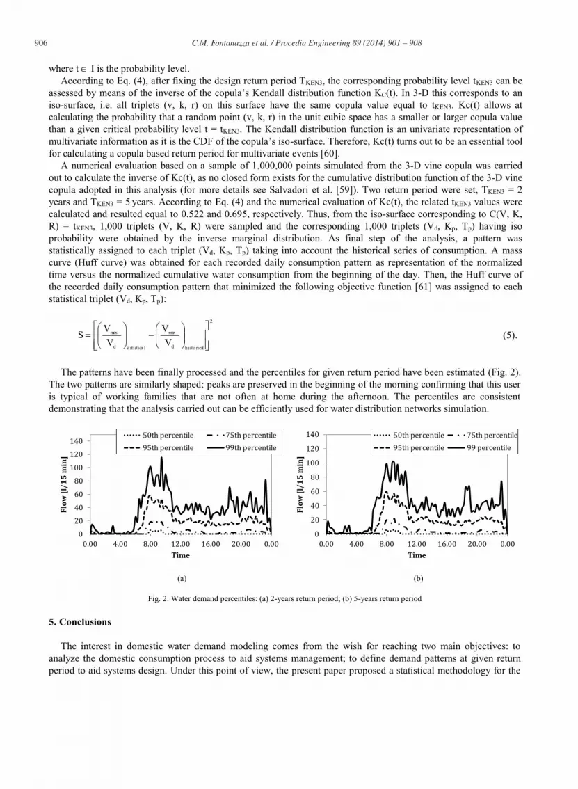
The patterns have been finally processed and the percentiles for given return period have been estimated (Fig. 2). The two patterns are similarly shaped: peaks are preserved in the beginning of the morning confirming that this user is typical of working families that are not often at home during the afternoon. The percentiles are consistent demonstrating that the analysis carried out can be efficiently used for water distribution networks simulation.

(a) (b)

Fig. 2. Water demand percentiles: (a) 2-years return period; (b) 5-years return period

5. Conclusions

The interest in domestic water demand modeling comes from the wish for reaching two main objectives: to analyze the domestic consumption process to aid systems management; to define demand patterns at given return period to aid systems design. Under this point of view, the present paper proposed a statistical methodology for the

020406080100120140

0.00 4.00 8.00 12.00 16.00 20.00 0.00

Flow

[l/1

5 m

in]

Time

50th percentile 75th percentile95th percentile 99th percentile

020406080100120140

0.00 4.00 8.00 12.00 16.00 20.00 0.00

Flow

[l/1

5 m

in]

Time

50th percentile 75th percentile95th percentile 99 percentile

907 C.M. Fontanazza et al. / Procedia Engineering 89 ( 2014 ) 901 – 908

definition of water consumption patterns based on return period and multivariate probabilistic approach. The method tried to avoid the usual assumption of a constant water demand pattern for network simulation. It is based on a multivariate statistical analysis: a 3-D vine copula was built for the main features of the consumption process at domestic level. The water demand was predicted for given return period by means of patterns that was statistically generated taking into account the historical series of consumption to which the methodology was applied. The analysis of the percentiles of the water demand for given return period showed that the proposed approach produced consisted demand patterns and will be a powerful tool to be coupled with water distribution network models for design or analysis problems.

References

[1] S.L. Zhou, T.A. McMahon, A. Walton, J. Lewis, Forecasting operational demand for an urban water supply zone, J. Hydrol. 259 (2002) 189-202.

[2] M. Herrera, L. Torgo, J. Izquierdo, R. Pérez-García, Predictive models for forecasting hourly urban water demand, J. Hydrol. 387 (2010) 141-150.

[3] J.E. Flack, Urban water conservation: increasing efficiency-in-use residential water demand, ASCE, New York, 1982. [4] C. Qi, N. Chang, System dynamics modeling for municipal water demand estimation in an urban region under uncertain economic impacts, J.

Environ. Manage. 92 (2011) 1628-1641. [5] L.A. House Peters, H. Chang, Urban water demand modeling: Review of concepts, methods, and organizing principles, Water Resour. Res.

47 W05401 (2011) doi:10.1029/2010WR009624. [6] M. Bakker, K. Van Schagen, J. Timmer, Flow control by prediction of water demand, J. Water Supply Res. T. 52 (2003) 417-424. [7] B. Dziegielewski, J.J. Boland, Forecasting urban water use: the IWR-main model, Water Resour. Bull. 25 (1989) 101-109. [8] D.R. Maidment, S.P. Miaou, M.M. Crawford, Daily water use in nine cities, Water Resour. Res. 22 (1986) 845-851. [9] S.P. Miaou, A class of time series urban water demand models with non-linear climatic effects, Water Resour. Res., 26 (1990) 169-178. [10] S.L. Zhou, T.A. McMahon, A. Walton, J. Lewis, Forecasting daily urban water demand: a case study of Melbourne, J. Hydrol., 236 (2000)

153-164. [11] E. Rothstein, Water demand monitoring in Austin, Texas, J. AWWA 84 (1992) 52-58. [12] R.M. Clark, W.M. Grayman, R.M. Males, A.F. Hess, Modeling contaminate propagation in drinking water distribution system, J. Environ.

Eng.-ASCE 119 (1993) 349-364. [13] S.G. Buchberger, L. Wu, A model for instantaneous residential water demands, J. Hydraul. Eng.-ASCE 121 (1995) 232-246. [14] S.G. Buchberger, G.J. Wells, Intensity, duration and frequency of residential water demands, J. Water Res. Pl.-ASCE 130 (1996) 386-394. [15] R. Guercio, R. Magini, I. Pallavicini, Instantaneous residential water demand as stochastic point process, in: C.A. Brebbia, P.

Anagnostopoulos, K. L. Katsifarakis (Eds.), Water Resources Management, WIT Press, Southampton, 2001, pp. 129-138. [16] C.W. Howe, F.P. Linaweaver, The impact of price on residential water demand and its relation to systems design, Water Resour. Res. 3

(1967) 13-22. [17] A.E. Cassuto, S. Ryan, Effect of price on the residential demand for water within an agency, J. AWWA 15 (1979) 345-353. [18] H.S. Foster, B.R. Beattie, Urban residential demand for water in the United States, Land Econ. 55 (1979) 43-58. [19] T.C. Hughes, Peak period design standards for small western U.S. water supply system, J. AWWA 16 (1980) 661-667. [20] R. Billings, D. Agthe, State-space versus multiple regression for forecasting urban water demand, J. Water Res. Pl.-ASCE 124 (1998) 113-

117. [21] M.S. Babel, A.D. Gupta, P. Pradhan, A multivariate econometric approach for domestic water demand modeling: an application to

Kathmandu, Nepal, Water Resour. Manag. 21 (2007) 573-589. [22] R.D. Hansen, R. Narayanan, Monthly time series model of municipal water demand, Water Resour. Bull. 17 (1981) 578-585. [23] D.R. Maidment, E. Parzen, Time patterns of water use in Six Texas cities, J. Water Res. Pl.-ASCE 110 (1984) 90-106. [24] D.R. Maidment, S.P. Miaou, M.M. Crawford, Transfer function models of daily urban water use, Water Resour. Res. 21 (1985) 425-432. [25] S.L. Franklin, D.R. Maidment, An evaluation of weekly and monthly time series forecasts of municipal water use, Water Resour. Bull. 22

(1986) 611-621. [26] J.A. Smith, A model of daily municipal water use for short-term forecasting Water Resour. Res. 24 (1988) 201-206. [27] T. Sastri, J.B. Valdes, Rainfall intervention analysis for on-line applications, J. Water Res. Pl.-ASCE 115 (1989) 397-415. [28] P.W. Jowitt, C. Xu, Demand forecasting for water distribution systems, Civil Eng. Syst. 9 (1992) 105-121. [29] C. Homwongs, T. Sastri, J.W. Foster III, Adaptive forecasting of hourly municipal water consumption, J. Water Res. Pl.-ASCE 120 (1994)

888-905. [30] B. Molino, G. Rasulo, L. Taglialatela, Forecast model of water consumption for Naples, Water Resour. Manag. 10 (1996), 321-332. [31] A. Aly, N. Wanakule, Short-term forecasting for urban water consumption, J. Water Res. Pl.-ASCE 130 (2004) 405-410. [32] S. Gato, N. Jayasuriya, P. Roberts, Temperature and rainfall thresholds for base use urban water demand modeling, J. Hydrol. 337 (2007)

364-376. [33] S. Alvisi, M. Franchini, A. Marinelli, A short-term, pattern-based model for water-demand forecasting, J. Hydroinform. 9 (2007) 39-50.

908 C.M. Fontanazza et al. / Procedia Engineering 89 ( 2014 ) 901 – 908

[34] A. Jain, A.K. Vershney, U.C. Joshi, Short-term water demand forecast modeling at IIT Kanpur using artificial neural networks, Water Resour. Manag. 15 (2001) 299-321.

[35] J. Liu, H.H.G. Savenije, J. Xu, Forecast of water demand in Weinan City in China using WDF-ANN model, Phys. Chem. Earth 28 (2003) 219-224.

[36] J. Bougadis, K. Adamowski, R. Diduch, Short-term municipal water demand forecasting, Hydrol. Process. 19 (2005) 137-148. [37] A. Jain, A.M. Kumar, Hybrid neural network models for hydrologic time series forecasting, Appl. Soft. Comput. 7 (2006) 585-592. [38] P. Cutore, A. Campisano, Z. Kapelan, C. Modica, D. Savic, Probabilistic prediction of urban water consumption using the SCEM-UA

algorithm, Urban Water J. 5 (2008) 125-132 [39] M. Ghiassi, D.K. Zimbra, H. Saidane, Urban water demand forecasting with a dynamic artificial neural network model, J. Water Res. Pl.-

ASCE 134 (2008) 138-146. [40] J. Caiado, Performance of combined double seasonal univariate time series models for forecasting water demand, J. Hydrol. Eng. 15 (2010)

215-222. [41] J.S. Adamowski, Peak daily water demand forecast modeling using artificial neural networks, J. Water Res. Pl.-ASCE 134 (2008) 119-128. [42] M. Herrera, L. Torgo, J. Izquierdo, R. Perez Garcia, Predictive models for forecasting hourly urban water demand, J. Hydrol. 387 (2010)

141-150. [43] S.G. Buchberger, J.T. Carter, Y. Lee, T.G. Schade, Random demands, travel times, and water quality in deadends, IWA Publishing, London,

2003. [44] V.J. García, R. García-Bartual, E. Cabrera, F. Arregui, J. García-Serra, Stochastic model to evaluate residential water demands, J. Water Res.

Pl.-ASCE 130 (2004) 386-394. [45] S. Alvisi, M. Franchini, A. Marinelli, A stochastic model for representing drinking water demand at residential level, Water Resour. Manag.

17 (2003) 197-222. [46] E.J.M. Blokker, J.H.G. Vreeburg, J.C.van Dijk, Simulating residential water demand with a stochastic end-use model, J. Water Res. Pl.-

ASCE 136 (2010) 19-26. [47] C. De Michele, G. Salvadori, A generalized Pareto intensity-duration model of storm rainfall exploiting 2-copulas, J. Geophys. Res. 108

(2003) doi:10.1029/2002JD002534. [48] A. Bárdossy, G.G.S. Pegram, Copula based multisite model for daily precipitation simulation, Hydrol. Earth Syst. Sci. 13 (2009) 2299-2314. [49] A.C. Favre, S. El Adlouni, L. Perreault, N. Thiémonge, B. Bobée, Multivariate hydrological frequency analysis using copulas, Water

Resour. Res. 40 (2004) doi:10.1029/2003WR002456. [50] G. Salvadori, C. De Michele, Analytical calculation of storm volume statistics involving Pareto-like intensityduration marginals, Geophys.

Res. Lett. 31 (2004) doi:10.1029/2003GL018767. [51] G. Salvadori, C. De Michele, Frequency analysis via copulas: Theoretical aspects and applications to hydrological events, Water Resour.

Res. 40 (2004) doi:10.1029/2004WR003133. [52] S. Grimaldi, F. Serinaldi, Design hyetograph analysis with 3-copula function, Hydrolog. Sci. J. 51 (2006) 223-238. [53] B. Schweizer B., Thirty years of copulas, in: G. Dall Aglio, S. Kotz, G. Salinetti (Eds.), Advance in probability distributions with given

marginals, Kluwer Academic Publishers, Dordrecht, 1991, pp. 13-50. [54] S. Kotz, Some remarks on copulas in relation to modern multivariate analysis, Proceedings of International Symposium on Contemporary

multivariate analysis and its applications, 19-24 May, Hong Kong, 1997. [55] H. Joe, Families of m-variate distributions with given margins and m(m-1)/2 bivariate dependence parameters, in: L. Rüschendorf, B.

Schweizer, M.D. Taylor (Eds.), Distributions with Fixed Marginals and Related Topics, Institute of Mathematical Statistics, Beachwood, 1996, pp. 120-141.

[56] T. Bedford, R.M. Cooke, Probability density decomposition for conditionally dependent random variables modeled by vines, Ann. Math. Artif. Intel. 32 (2001) 245-268.

[57] T. Bedford, R.M. Cooke, Vines - a new graphical model for dependent random variables, Ann. Stat. 30 (2002) 1031-1068. [58] K. Aas, C. Czado, A. Frigessi, H. Bakken, Pair-copula construction of multiple dependence, Insur. Math. Econ. 44 (2009) 182-198. [59] G. Salvadori, C. De Michele, F. Durante, On the return period and design in a multivariate framework, Hydrol. Earth Syst. Sci. 15 (2011)

3293-3305. [60] B. Graler, M.J. van de Berg, S. Vanderberghe, A. Petroselli, S. Grimaldi, B. De Baets, N.E.C. Verhoest, Multivariate return period in

hydrology: a critical and pratical review focusing on synthetic design hyetograph estimation, Hydrol. Earth Syst. Sci. 17 (2013) 1281-1296. [61] C.M. Fontanazza, G. Freni, G. La Loggia, V. Notaro, Uncertainty evaluation of design rainfall for urban flood risk analysis, Water Sci.

Technol. 63 (2011) 2641-2650.