UNIVERSITA’ DEGLI STUDI DI BERGAMO DIPARTIMENTO DI INGEGNERIA GESTIONALE E DELL’INFORMAZIONE°

QUADERNI DEL DIPARTIMENTO†

Department of Management and Information Technology

Working Paper

Series “Mathematics and Statistics”

n. 6/MS – 2006

Multivariate statistical sensitivity analysis of a computer model for pharmaceutical industry market and innovation dynamics

by

Alessandro Fassò, Franco Malerba, Luigi Orsenigo, Michele Pezzoni

° Viale Marconi. 5, I – 24044 Dalmine (BG), ITALY, Tel. +39-035-2052339; Fax. +39-035-562779 † Il Dipartimento ottempera agli obblighi previsti dall’art. 1 del D.L.L. 31.8.1945, n. 660 e successive modificazioni.

COMITATO DI REDAZIONE§

Series Economics and Management (EM): Stefano Paleari, Andrea Salanti Series Information Technology (IT): Stefano Paraboschi Series Mathematics and Statistics (MS): Luca Brandolini, Alessandro Fassò § L’accesso alle Series è approvato dal Comitato di Redazione. I Working Papers ed i Technical Reports della Collana dei Quaderni del Dipartimento di Ingegneria Gestionale e dell’Informazione costituiscono un servizio atto a fornire la tempestiva divulgazione dei risultati dell’attività di ricerca, siano essi in forma provvisoria o definitiva.

Multivariate statistical sensitivity analysisof a computer model

for pharmaceutical industry market andinnovation dynamics

Alessandro Fassò�, Franco Malerbay, Luigi Orsenigoz, Michele Pezzonix

September 22, 2006

Abstract

Statistical sensitivity analysis is a useful technique to analyze mul-tivariate stochastic computer model in order to better understand thecause and e¤ect relationships between input parameters and outputobservations. This paper is based on a pre-existent formal evolution-ary economic model that simulates the main aspects of the market andthe innovation processes that take place inside the pharmaceutical in-dustry. It belongs to the family of �History-Friendly�models. Our pur-pose is to reveal the critical input parameters concerning R&D costs,research opportunities, regulatory regime, demand and �rm�s featuresin the mechanisms of innovation and market dynamics through theuse of multivariate statistical sensitivity analysis. This preliminarywork represents a �rst step in the introduction of a complete analysiswith a mixed linear model.

Keywords: History-Friendly model, Pharmaceutical industry, Sto-chastic computer model, Mixed linear model.

�University of Bergamo, Dept. IGI, Via Marconi 5, 24044 Dalmine BG, Italy.Email: alessandro.fasso@unibg.it. Work partially supported by Italian MIUR-Co�n 2004grants.

yCESPRI, Bocconi University, Milan, Italy.Email: franco.malerba@unibocconi.it

zDepartment of Engineering, University of Brescia and CESPRI, Bocconi University,Milan, Italy.Email: luigi.orsenigo@unibocconi.it

xDepartment of Engineering, University of Brescia, Italy.Email: michele.pezzoni@tin.it

1

1 Introduction

In this paper we propose a concise method to analyze a stochastic com-puter model of the pharmaceutical industry through the use of the sensitiv-ity analysis technique. The model belongs to the family of �History-Friendly�evolutionary economic models. These models aim to capture the essence ofthe qualitative theory, pointed out by the technology and industry scholars.They also try to give a possible logical explanation. The modelling processphilosophy starts from empirical studies which describe the mechanisms in-side pharmaceutical industry. The motivations underlying this modellingstile has been discussed extensively in previous works, see e.g. Malerba etal.,(1999),(2001): Is worth to remember that one of the reason for interest inHistory-Friendly models is to understand what kind of factors and dynamicprocesses are important for the industry evolution. In this paper we try toexplain what are the factors that can indeed explain the observed patterns ofindustrial dynamics, in particular about innovation and imitation processes,prices and industry structure. The technique that appears more promising forassessing the impact of the main industry parameters, seems to be the sensi-tivity analysis (SA). The modern concept of sensitivity analysis for computermodels arises from the logical intersection of some variance decompositionand some sampling or computer experiment techniques, see e.g. Saltelli etal. (2000) and references therein: This technique has been recently appliedto various kinds of computer models both in Econometrics and Finance, seee.g. Saltelli et al (2004) and in environmental models, see e.g. Fassò (2006)and Fassò and Perri (2002) : Cheap computer models, which run fast, andexpensive computer models, which take CPU time and storage capability,usually requires di¤erent SA techniques. In this paper, we are concernedwith a cheap code based extensive simulations which allow to assess the roleand the interactions of the various input parameters in in�uencing the multi-output model. The paper is organized as follows. Section 2 introduces theprobabilistic structure of a Stochastic Computer Model (SCM) for assessingthe uncertainty arising from the so-called stochastic game and proposes a sta-tistical emulator to be estimated on available simulated data. Section 3, afterextending sensitivity analysis (SA) to cope with SCM; discusses appropri-ate sampling and preliminary estimation techniques for the proposed SCMemulator. Section 4, after a brief summary of the pharmaceutical industryhistory, introduces the key features of the Stochastic Computer Model. InSection 5 we assess the in�uence of input parameters which concern costs,environment and opportunity conditions, regulatory regime, �rm�s featuresand demand on multi-outputs in innovation and imitation processes, pricesand industry structure.

2

2 Stochastic Computer Models

A Stochastic Computer Model (SCM) may be described by a computablecode or multi-valued function z such that

z = z (x; �) ;

where x is a k-dimensional input parameter which is known at the time thecode is run, while � is an unobservable random vector, which is generated bythe code itself. In market behavior SCM�s, the random element � is called thestochastic game component of the SCM and the input model x = (x1; :::; xk)de�nes e.g. market dimensions, side conditions, initial values.In the setup of SA, x has a known probability distribution, P (x) say,

which may be a multivariate distribution with discrete and/or continuosmarginals and possible dependency structure among the x components. Gen-erally speaking, the stochastic game � has a known or unknown conditionaldistribution

P (�jx)

and, in some cases, it is independent on x, so that P (�jx) = P (�).It turns out that, for given x, the output z is a random vector with

distributionP (zjx)

with the �rst two conditional moments given by

� (x) = E (zjx)

and� 2 (x) = V ar (zjx) :

The output uncertainty is given, in general terms, by the unknown mar-ginal distribution

P (z)

and this may be decomposed into two components, one is related to thestochastic game � and the other one accounts for the input variability.When the output z is single-valued, using E () for the mathematical ex-

pectation and V ar () for the variance of a random variable, recalling the wellknown ANOVA decomposition, which is given by

V ar (z) = V ar (� (x)) + E�� 2 (x)

�, (1)

we note that the rateE (� 2 (x))

V ar (z)

is the residual uncertainty or the quota of the global output uncertaintywhich depends on the stochastic game � averaged over the input space.

3

On the other side, V ar (� (x)) is the accountable output uncertainty andmay be related to each single input xj using SA techniques discussed insection 3 below. Actually

�2 =V ar (� (x))

V ar (z)

is the well known Pearson�s correlation ratio and 1 � �2 represents the best�tting error among emulators which will be discussed below.

2.1 Heteroskedastic SCM�s

We say that the SCM is conditionally homoskedastic if the conditional out-put uncertainty does not depend on the particular input parameter valuex = x0, namely if

� 2 (x) = � 2

for every x. Otherwise the SCM is called conditionally heteroskedastic and� 2 (x) gives the conditional or local output uncertainty whose understandingand modelling gives further insight into SCM comprehension. For example,Fassò et al. (2003) considered a parabola model � 2 (x) = �0 + �1x

21 based

only on the �rst input x1:

2.2 Input feasibility set

LetDz be the (extended) output set and let Fz � Dz be the output feasibilityset where the model give pleasant outputs. For example we exclude from Fzthose points corresponding to a zero �rms market (all died).It is then of interest to de�ne the input feasibility set Fx, which is such

that the corresponding average output is feasible, in symbols:

x 2 Fx ) � (x) 2 Fz: (2)

In this case it may be important to compute the probability of an unfea-sible output, namely

u (x) = P (z 2 Dz � Fzjx)

for every feasible input x 2 Fx:Note that feasibility concept may introduces constraints on the input

parameter distribution which are not compatible with input independence.For example one may start from an unconstrained input distribution P0 (x)with independent components,

P0 (x) = P0 (x1) � ::: � P0 (xk)

but after imposing feasibility, that is using

P (x) = P0 (xjx 2 Fx)

such independence may be lost.

4

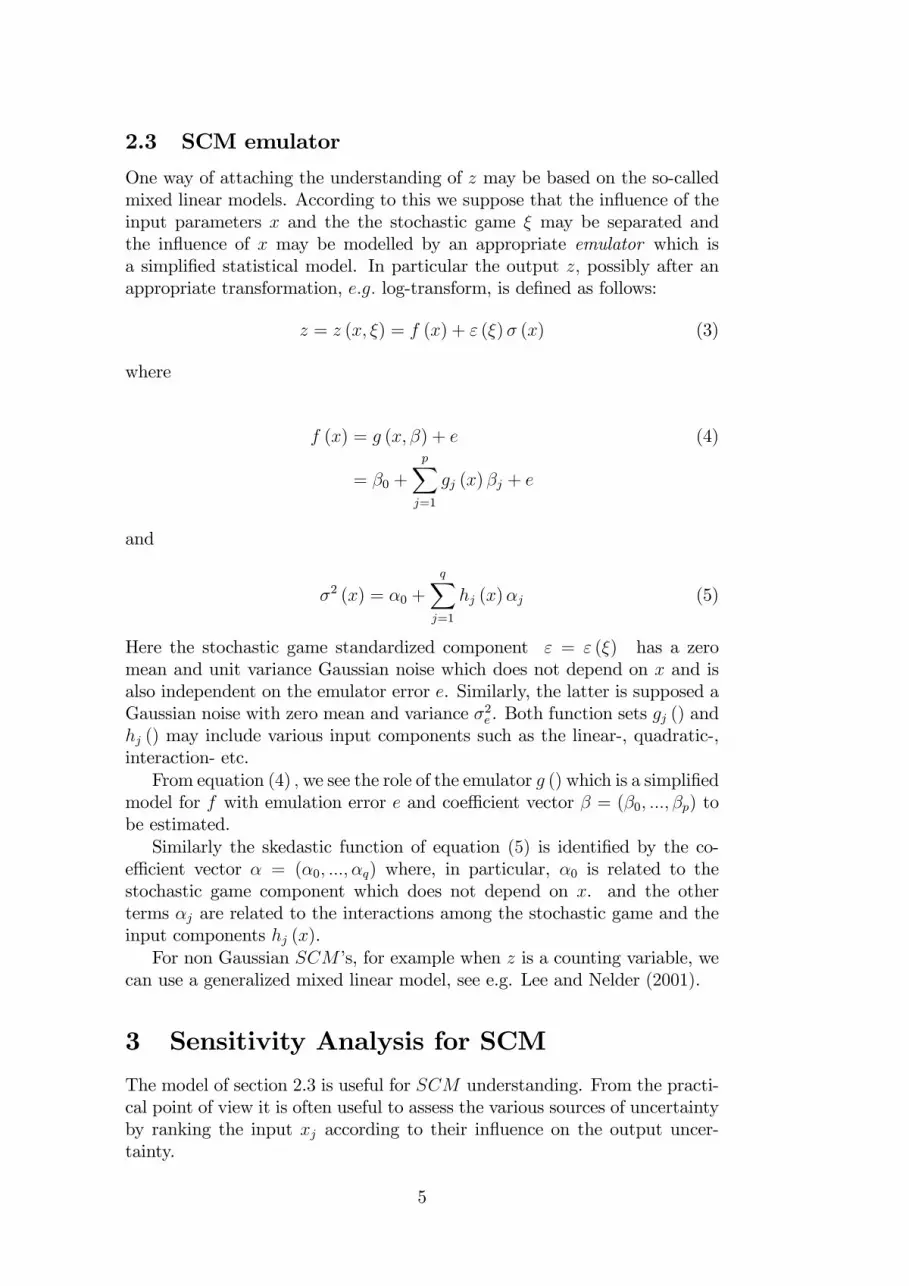
2.3 SCM emulator

One way of attaching the understanding of z may be based on the so-calledmixed linear models. According to this we suppose that the in�uence of theinput parameters x and the the stochastic game � may be separated andthe in�uence of x may be modelled by an appropriate emulator which isa simpli�ed statistical model. In particular the output z; possibly after anappropriate transformation, e:g: log-transform, is de�ned as follows:

z = z (x; �) = f (x) + " (�)� (x) (3)

where

f (x) = g (x; �) + e (4)

= �0 +

pXj=1

gj (x) �j + e

and

�2 (x) = �0 +

qXj=1

hj (x)�j (5)

Here the stochastic game standardized component " = " (�) has a zeromean and unit variance Gaussian noise which does not depend on x and isalso independent on the emulator error e. Similarly, the latter is supposed aGaussian noise with zero mean and variance �2e . Both function sets gj () andhj () may include various input components such as the linear-, quadratic-,interaction- etc.From equation (4) ; we see the role of the emulator g () which is a simpli�ed

model for f with emulation error e and coe¢ cient vector � = (�0; :::; �p) tobe estimated.Similarly the skedastic function of equation (5) is identi�ed by the co-

e¢ cient vector � = (�0; :::; �q) where, in particular, �0 is related to thestochastic game component which does not depend on x. and the otherterms �j are related to the interactions among the stochastic game and theinput components hj (x).For non Gaussian SCM�s, for example when z is a counting variable, we

can use a generalized mixed linear model, see e.g. Lee and Nelder (2001).

3 Sensitivity Analysis for SCM

The model of section 2.3 is useful for SCM understanding. From the practi-cal point of view it is often useful to assess the various sources of uncertaintyby ranking the input xj according to their in�uence on the output uncer-tainty.

5

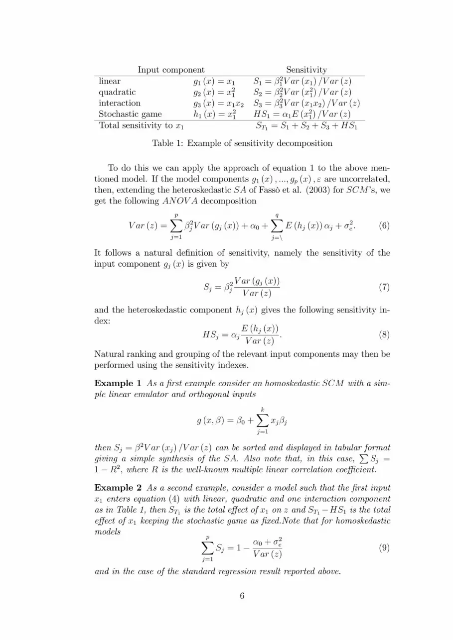
Input component Sensitivitylinear g1 (x) = x1 S1 = �21V ar (x1) =V ar (z)quadratic g2 (x) = x21 S2 = �22V ar (x

21) =V ar (z)

interaction g3 (x) = x1x2 S3 = �23V ar (x1x2) =V ar (z)Stochastic game h1 (x) = x21 HS1 = �1E (x

21) =V ar (z)

Total sensitivity to x1 ST1 = S1 + S2 + S3 +HS1

Table 1: Example of sensitivity decomposition

To do this we can apply the approach of equation 1 to the above men-tioned model. If the model components g1 (x) ; :::; gp (x) ; " are uncorrelated,then, extending the heteroskedastic SA of Fassò et al. (2003) for SCM�s, weget the following ANOV A decomposition

V ar (z) =

pXj=1

�2jV ar (gj (x)) + �0 +

qXj=n

E (hj (x))�j + �2e : (6)

It follows a natural de�nition of sensitivity, namely the sensitivity of theinput component gj (x) is given by

Sj = �2jV ar (gj (x))

V ar (z)(7)

and the heteroskedastic component hj (x) gives the following sensitivity in-dex:

HSj = �jE (hj (x))

V ar (z): (8)

Natural ranking and grouping of the relevant input components may then beperformed using the sensitivity indexes.

Example 1 As a �rst example consider an homoskedastic SCM with a sim-ple linear emulator and orthogonal inputs

g (x; �) = �0 +

kXj=1

xj�j

then Sj = �2V ar (xj) =V ar (z) can be sorted and displayed in tabular formatgiving a simple synthesis of the SA: Also note that, in this case,

PSj =

1�R2; where R is the well-known multiple linear correlation coe¢ cient.

Example 2 As a second example, consider a model such that the �rst inputx1 enters equation (4) with linear, quadratic and one interaction componentas in Table 1, then ST1 is the total e¤ect of x1 on z and ST1�HS1 is the totale¤ect of x1 keeping the stochastic game as �xed.Note that for homoskedasticmodels

pXj=1

Sj = 1��0 + �2eV ar (z)

(9)

and in the case of the standard regression result reported above.

6

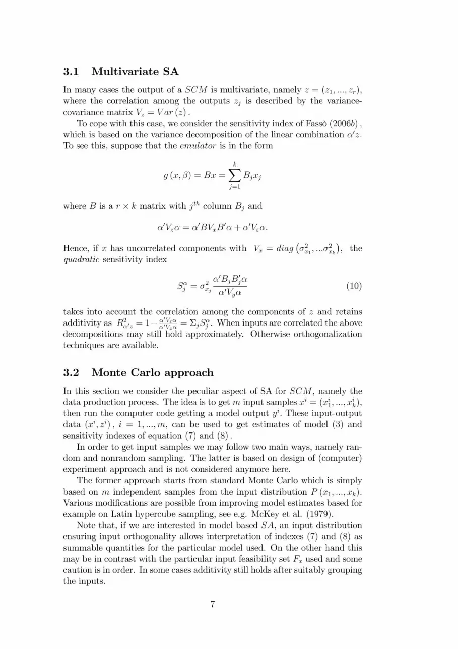
3.1 Multivariate SA

In many cases the output of a SCM is multivariate, namely z = (z1; :::; zr),where the correlation among the outputs zj is described by the variance-covariance matrix Vz = V ar (z) :To cope with this case, we consider the sensitivity index of Fassò (2006b) ;

which is based on the variance decomposition of the linear combination �0z:To see this, suppose that the emulator is in the form

g (x; �) = Bx =kXj=1

Bjxj

where B is a r � k matrix with jth column Bj and

�0Vz� = �0BVxB0�+ �0V"�:

Hence, if x has uncorrelated components with Vx = diag��2x1 ; :::�

2xk

�, the

quadratic sensitivity index

S�j = �2xj�0BjB

0j�

�0Vy�(10)

takes into account the correlation among the components of z and retainsadditivity as R2�0z = 1� �0V"�

�0Vz�= �jS

�j . When inputs are correlated the above

decompositions may still hold approximately. Otherwise orthogonalizationtechniques are available.

3.2 Monte Carlo approach

In this section we consider the peculiar aspect of SA for SCM , namely thedata production process. The idea is to getm input samples xi = (xi1; :::; x

ik),

then run the computer code getting a model output yi: These input-outputdata (xi; zi) ; i = 1; :::;m, can be used to get estimates of model (3) andsensitivity indexes of equation (7) and (8) :In order to get input samples we may follow two main ways, namely ran-

dom and nonrandom sampling. The latter is based on design of (computer)experiment approach and is not considered anymore here.The former approach starts from standard Monte Carlo which is simply

based on m independent samples from the input distribution P (x1; :::; xk).Various modi�cations are possible from improving model estimates based forexample on Latin hypercube sampling, see e.g. McKey et al. (1979).Note that, if we are interested in model based SA, an input distribution

ensuring input orthogonality allows interpretation of indexes (7) and (8) assummable quantities for the particular model used. On the other hand thismay be in contrast with the particular input feasibility set Fx used and somecaution is in order. In some cases additivity still holds after suitably groupingthe inputs.

7

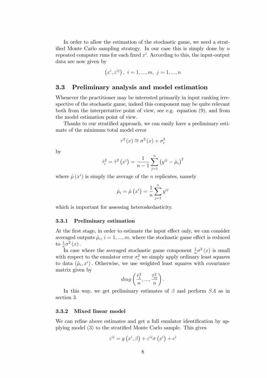
In order to allow the estimation of the stochastic game, we need a strat-i�ed Monte Carlo sampling strategy. In our case this is simply done by nrepeated computer runs for each �xed xi: According to this, the input-outputdata are now given by�

xi; zij�; i = 1; :::;m; j = 1; :::; n

3.3 Preliminary analysis and model estimation

Whenever the practitioner may be interested primarily in input ranking irre-spective of the stochastic game, indeed this component may be quite relevantboth from the interpretative point of view, see e.g. equation (9), and fromthe model estimation point of view.Thanks to our strati�ed approach, we can easily have a preliminary esti-

mate of the minimum total model error

� 2 (x) �= �2 (x) + �2e

by

�̂ 2i = �̂ 2�xi�=

1

n� 1

nXj=1

�yij � �̂i

�2where �̂ (xi) is simply the average of the n replicates, namely

�̂i = �̂�xi�=1

n

nXj=1

yij

which is important for assessing heteroskedasticity.

3.3.1 Preliminary estimation

At the �rst stage, in order to estimate the input e¤ect only, we can consideraveraged outputs �̂i, i = 1; :::;m, where the stochastic game e¤ect is reducedto 1

n�2 (x) :In case where the averaged stochastic game component 1

n�2 (x) is small

with respect to the emulator error �2e we simply apply ordinary least squaresto data (�̂i; xi) : Otherwise, we use weighted least squares with covariancematrix given by

diag

��̂ 21n; :::;

�̂ 2mn

�:

In this way, we get preliminary estimates of � and perform SA as insection 3.

3.3.2 Mixed linear model

We can re�ne above estimates and get a full emulator identi�cation by ap-plying model (3) to the strati�ed Monte Carlo sample. This gives

zij = g�xi; �

�+ "ij�

�xi�+ ei

8

which is a linear model with mixed e¤ects, where the input componentsgj (x

i) are the outer covariates, the emulator error ei is the random e¤ectand "ij� (xi) is the heteroskedastic error.

4 A model for pharmaceutical industry

4.1 Main features of the market

In this section we give an overall description of pharmaceutical industryevolution resuming only in general therms the main patterns of developmentanalyzed by several scholars.The history of pharmaceutical industry can be usefully divided into three

major epochs. The �rst, corresponding roughly to the period 1850-1945, inwhich little new drug development occurred, and in which there was very lit-tle research and was based on relatively primitive methods. The large scaleof development of penicillin during the World War II marked the emergenceof the second period of industry evolution. This period was characterized bythe institution and formalization of in-house R&D programs and relativelyrapid rates of drug introduction. During the early part of this period theindustry relied largely on so called �random�screening as method for �ndingnew drugs, but in the seventies the industry began a transition to �guided�drug discovery, a research methodology that allowed a great advance in mole-cular biochemistry, pharmacology and enzymology. The third epoch of theindustry has its roots in the seventies but did not come to full �ower untilquite recently as the use of the tools of genetic engineering in the productionand discovery of new drugs become more widely di¤used.An in-deep story and extensive analysis and discussion of the patterns of

pharmaceutical industry have been undertaken by several scholars and willnot be discussed here. In this paper we model the �random�screening periodbut we report some hints to the whole story of the industry. As a way of in-troduction we brie�y discuss the key aspects strictly linked to the model. Inthe history of the pharmaceutical industry, faced with such a �target-rich�en-vironment but with very little detailed knowledge of the biological underspin-nings of speci�c diseases, pharmaceutical companies developed an approachto research that is now referred as �random screening�. Under this approach,natural and chemically derived compounds are randomly screened in test-tube experiments and laboratory animals for potential therapeutic activity.Pharmaceutical companies maintained enormous �libraries�of chemical com-pounds, and increased their collections by searching for new compounds inplaces such as swamps, stream and soil samples. Thousand of compoundsmight be subjected to multiple screens before researchers can focus on promis-ing substance. Serendipity played a key role since in general the �mechanismof action�of most drug was not well understood. Researchers were generallyforced to rely on the use animal models as screens. Under this regime itwas not uncommon for companies to discover a drug to treat one diseasewhile searching for a treatment for another. The �design�of new compounds

9

was a slow, painstaking process that drew heavily on analytical and med-ical chemistry skills. Several important classes of drug were discovered thisway, including the most important diuretics, many of the most widely usedpsychoactive drugs and several powerful antibiotics. The chemists workingwithin this regime codi�ed little of the knowledge acquired, so new com-pounds design was driven by the skills of individual chemist. However, thesuccessful introduction of a new chemical entity has to be considered asquite rare event. From the mid 1970s substantial advantages in physiology,pharmacology, enzymology and cell biology led to enormous progress in theability to understand the mechanism of action of some existing drugs and thebiochemical and molecular roots of many diseases. This new knowledge hasa profound impact on the process of discovery of new drugs o¤ering to theresearches a signi�cantly more e¤ective way to screen compounds. Moreover,the availability of drugs whose mechanisms of action are well known madepossible signi�cant advances in the medical understanding of a number ofkey diseases. This understanding led to the development of the technique of�rational drug design�. Researches are now beginning to be able to �design�compounds that might have particular therapeutic e¤ects. The advent of�biotechnology�had a signi�cant impact both on organizational competen-cies required to be a successful player in the pharmaceutical industry andindustry structure in general.

After this brief introduction, it could be useful to �x some of the qualita-tive characteristic about mechanisms and factors a¤ecting industry evolution,stylized in the History-Friendly model. First of all innovative new drugs ar-rive quite rarely but after the arrival they experience extremely high rates ofmarket growth. This entails a highly skewed distribution of the returns oninnovation and of product market size as well as of the intra-�rm distributionof sales across products. So, few �blockbusters�dominate the product rangeof all mayor �rms (Matraves C,(1999)). The industry has been character-ized by a signi�cant heterogeneity in terms of �rms�strategic orientations,indeed other �rms not specialized in R&D and innovation, but in imitationand marketing are able to survive. In general terms the �oligopolistic core�ofthe industry as been composed by a stable group of �rms, which maintainedover time an innovation-oriented strategy. At the same time the industry wascharacterized by quite low level of concentration both at aggregate level andin the individual sub-markets like e.g. cardiovascular, diuretics, tranquilizers,etc. There is evidence that institutional factors seems to have played a de-cisive role in the development of pharmaceutical industry. The institutionalarrangements surrounding the public support of basic research, intellectualproperty protection, procedures of product testing and approval, pricing andreimbursement policies have all strongly in�uenced both the process of inno-vation and the economic returns (and thus incentives) for undertaking suchinnovation. Something more may be said about intellectual property pro-tection. Pharmaceutical has historically been one of the few industry werepatent provide a solid protection against imitations, for two main reasons.The �rst is that small variants in the molecule�s structure can drastically

10

alter its pharmacological properties. The second reason is that other �rmsmight undertake research in the same therapeutic class as an innovator, butthe probability of �nding another compound with the same therapeutic prop-erties that does not infrange on the original patent could be quite small. Theprocedures of product approval are also very important. Pharmaceuticalsare regulated products. Procedures for approval have a deep impact on boththe costs of innovating and on �rms ability to sustain market position oncetheir product has been approved. Since the early 1960s most countries havesteadily increased the stringency of their product approval precesses. How-ever it was the USA, with the Kefauver-Harris Amendament Act in 1962,and the UK, with Medicine Act in 1971, that look by far the most stringentstances among industrialized countries. Federal and Drug Administration(FDA) shifted from a role of essentially an evaluator of evidence and re-search �ndings at the end of research process, to an active participant ofthe process itself. The resources necessary to obtain approval of a new drugapplication have been largely increased. They probably caused a sharp in-crease in both R&D costs and gestation times for new chemical entities.Although the process of development and approval increased costs, it signi�-cantly increased the barrier to imitation, even when the patent expired. Theintroduction of tougher regulatory environment in the UK and in USA wasfollowed by a sharp fall of the number of new drug lanced and many smallor weak �rms exited the market.

4.2 Model setup

In this section we describe the basic features of the model implemented forthe analysis of the �random screening�era (Malerba, Orsenigo (2001) (2002)).This description considers the essence of the model and leaves to the para-graphs 4.2.1, 4.2.2, 4.2.3 and 4.2.4 the speci�c details. At the beginning, inthe age of random screening, a number of �rms enter the market and start tointeract in the simulation environment. The �rms start to invest in randomsearches for promising molecules that might be the basis for development of adrug in particular therapeutic category. Some molecules seem to be promis-ing for the drug development phase and are patented. After the selection ofthe molecule that seems more pro�table, �rms consume time and �nancialresources to turn it in a marketable drug. The investments in research anddevelopment are arranged in �xed share of budget and expose the �rms tothe risk of running out of money and failure. After the development phasesuccessfully ended, �rms engage in marketing activities and begin sellingtheir drugs. Sales are in�uenced by drug quality, price charged and �rms�marketing e¤orts. At the beginning successful drugs in a particular thera-peutic category face no competition. But after some times other �rms maydiscover and develop competing drug. Moreover, after patent expiration, im-itation occurs and the market share and revenue of original innovator startto be eroded. For �rms the imitation of drugs is less expensive and less timeconsuming but also less pro�table. After a �rm has successfully developed a

11

drug, it begins searching again for a new promising molecule and the processbegins all over again. The �rms engage sequentially in di¤erent projects untilthe end of simulation or the failure, they will progressively diversify into newtherapeutic categories. In the next section we will provide a more detaileddescription of the simulation model.

4.2.1 Topography

The environment where �rms act is composed by several therapeutic cate-gories (TC). Each therapeutic category has a di¤erent number of potentialcustomers (patients). The economic size of a TC depends on the number ofpatients buying and on the prices of the products, in other words is expressedby total sales. Patients of TCs are divided in a certain number of submar-kets (n:sub) where a minimum level of quality of the drugs is required to sell(QCsub). Thus, some groups of consumer do not buy a drug if its qualityis not satisfactory. The number of patients in the overall therapeutic cate-gory (NTC) is exogenously given and grows at a certain rate (GNTC) duringeach simulation period. This is known by the �rms. In the model there aren (n = 100) therapeutic categories each with a speci�c number of patientsdrawn from a normal distributionNTC~N(�NTC ; �NTC ). Within a therapeuticcategory there are a certain number of molecules M (M = 150), which �rmsaim to discover and which are the basis of pharmaceutical products. Eachmolecule is characterized by a certain value of quality Q. A large percentageof molecules have null value of quality (Qnull), thus are useless for the �rms.Others, from which the �rms will generate drugs, have a positive value ofquality drawn from a normal distribution Q~N(�Q; �Q). When a molecule isdiscovered by a �rm, the patent protection starts. This grants the protectionin two ways. First, the width (PW ), prevents competitors from develop-ing all the molecules located in the neighborhood of the patented. Second,speci�es the temporal duration of the patent (PD) up to that time in whichthe molecule become imitable by other �rms. Once the drug development issuccessful, it gets an economic value (PQ) equal to the value of the moleculequality Qi, where i = 1; 2; ::; 150 for each TC. The economic value of productin�uences the demand function for such product, described in section 4.2.3.

4.2.2 The �rms

Basic features of �rms. At the beginning of the simulation a number Fof �rms potentially could enter the market. They starts with a budget B(B = 3000) equal for all. In the model, �rms have a limited understandingof the environment and their behavior follows some simple rules-of-thumb androutines. In particular the �rms are engaged in three sequential activities re-peated until the exit of the market or the end of simulation: search, researchand marketing. The �rst process invests a given share of budget (BS) in theactivity of looking for the promising molecules in the environment. The sec-ond process invests another share of budget (BR) in the activity of developingthe molecule in a marketable drug, this is very time and resources consuming

12

and �rms risk to fail running out of money. The residual share of budget(BM) is invested in marketing activities to promote the selling of the newdrug to win the competition of other products in the same TC. Firms arecharacterized by di¤erent �strategies�and have di¤erent propensities of in-vestments in the three activities. At the beginning of the simulation only halfof the �rms try to enter the market. This group is labelled �innovators�. Afterpatent expiration, when the �rst patented molecule become available for all,another group of �rms try to enter the market developing products from un-patented molecules. This is the �free-riding�behavior of the �imitative��rms.In the model, the marketing propensity of the �rms, �,is �xed for the inno-vators (�inno) and imitators (�imi) and account the relation (�inno) > (�imi).The R&D investments propensity of the �rms is then de�ned by a share ofbudget (1 � �) that complements the share of the propensity to marketinginvestments. Thus, the �rms�budget is divided among search, research andmarketing activities as follows:

Resources for search (BS): (1� �)!B

Resources for research (BR): (1� �)(1� !)B

Resources for marketing (BM): �B

Where ! (randomly drawn from a uniform distribution) is invariant and�rm speci�c.Innovative activities. In the age of �random screening� the innovators

look for new molecules through the search process. The amount of moneyinvested in search activities, BS, determines a number (XTC) of TC exploredby a �rm during its current project, equation (11).

XTC =BSDC

(11)

The parameter DC represent the cost of draw of a molecule from a TC.Firm selects randomly some TCs and molecules making XTC extractions. Agreater expenditure in search process allows the �rms to have more chancesto make successful extractions. Moreover there is a �xed cost (FC) that �rmshave to pay for each period when they are involved in the search activity.Firms have few information about the molecules drawn, due to the limitedunderstanding of the environment, and know only whether Qi is greaterthan zero or not. In the case of non-zero quality molecule, and if it hasnot been patented by others, then patent protection for that molecule isobtained. If a �rm experiences successful extractions in more than one TCand thus �nds more than one molecule having a positive Q, it chooses tostart research activity on the TC which shows the best expected pro�ts.In the case of the absence of products in TC the �rm suppose to becomeleader in the therapeutic category, and calculates expected pro�ts. Thiscriterion addresses the �rms to the TC with the greatest number of patients

13

and less crowed. The patented molecules that are not selected become partof a portfolio of �sleeping molecules�that can be exploited in every furtherround of search. If search is successful, the �rms move to next activity: theresearch. Only after a product has been developed or in case the project hasfailed the �rm will start another search iteration.Imitative activities. For imitative �rms the phase of search explanation is

quite easy, they do not spent resources to draw a TC: The imitative �rms lookfor already discovered and developed molecules whose patent has expired.When the available molecules with expired patent are in more than one TC,they select the TC with the best pro�t expected using the same criterion ofinnovators. In the TC selected for imitation, �rms chose the molecule withhighest �perceived�quality, R. R is a function of Q as shown in equation(12).

Ri = (1 + e�)Qi (12)

Where i = 1; 2; ::; 150 for each therapeutic category and e� is drawn froma uniform distribution (e� 2 U [�0:1;+0:1]). Hence, high quality moleculeswill be more frequently picked up by imitators.Research activities. Research activity means the actuation of a product

development project that �transforms�a molecule into a drug that can besold with certain characteristic of quality. This process is very time andmoney expensive, in particular for innovative research, while is quite cheapfor imitative research. Both innovators and imitators do research. A �rm,starting with a research budget Br, progresses toward the full developmentof the drug. That is to say, �rm have to �climb�a �xed number of steps(stotal = 30) in order to develop a drug having a quality Q. Each stepsimplies unitary cost CS. Thus, the total cost of developing a drug is equalto CS �stotal. Firms di¤er in costs and research investment but have the samenumber of step to �climb�. It is clear that the research speed is proportionalto the value of Br and to the research costs. Firms move faster if they paymore in each period according to the following relationship:

st � st�1 = � � BrCS

Where st � st�1 are the number of steps �climbed�between t and t � 1periods, Br is the budget spent by the �rm in research, CS is the cost ofa single step of research, � is a �xed coe¢ cient that proportions budgetresources dedicated to research in a single period. The � coe¢ cient andcosts CS are di¤erent for innovators and imitators.The costs of a single step of research grows each period at a certain

rate CG; starting from a high value for innovation (Cinno) and low valuefor imitation (Cimi). The growth represent the increment of expenditurecaused by more stringent rules, growing complexity of clinical trials �xedby external agencies (e.g. the FDA) (Grabowsky, H.(2002)). Procedures ofproduct approval of an innovative product are many time more expensive

14

than the imitative one, hundred millions against few millions of dollars, inparticular after the Hatch-Waxman Act in 1984.Given its budget Br a �rm may be able to buy all the steps to develop

a drug. Before commercialization the last obstacle is to warrant a minimumlevel of quality, requirement to enter the market. There is an exogenousthreshold on quality of the product �xed to represent a kind of�quality check�(QC), imposed, for example in the USA, by the Federal and Drug Adminis-tration. Below this value the drug cannot be commercialized and the projectfails. Reached the minimum quality, the product is labelled as imitationif risen from a molecule with expired patent or otherwise it is labelled asinnovative.Marketing activities. When the develop process come to an end and

the quality of the drug is over the threshold for entering the market the�rm invests the budget BM ; sets for marketing. The launch of the producttime TL is the moment when the �rm creates the �product image�AjTL ,proportional to marketing spending. Moreover, the �rm will pro�t from amarketing expenditure � from its previous products k 6= j. The �image�iseroded in the course of time at a rate equal to eA in each period. The levelof the �image�, Ajt in period t is given by:

AjTL = BMTL+ � �

Xk 6=j

[Ak]

for t = TL

Ajt = Ajt�1 � (1� eA)

for t > TL:

4.2.3 Demand and market share

In this model, each �rm sells a speci�c quantity of drugs in every period andpays a very low cost for manufacturing every single unit k produced. Thecostumers are homogenous and we do not distinguish between patients andphysicians. Decision to buy a speci�c drug depends on several factors: qualityPQ, price P and image level Aj. The quality of the drug decides the numberof submarkets (n:sub) reached, thus the number of well-disposed patients tobuy. Therefore, low quality drugs, probably with many contraindication, willreach few patients even if there are few competitors in the TC. The numberof patients in each submarket (Nsub) is give by:

Nsub =NTCn:sub

The share of a drug in a submarket depends by a �merit�function (Ui;t).The factors listed previously, determine value of merit by:

Ui;t = PQai ��1

Pi;t

�b� Aci;t (13)

15

Where PQi is the economic value of the drug, equal to quality Qi, Pi;tis the price applied by the �rm (see below) Ai;t is the image of the product.a, b and c are speci�c to each TC and drawn from uniform distributions.The market share of product i in the submarket sub of TC is proportionalto its relative merit as compared to the other competing drugs in the samesubmarket and is given by:

Si;sub =UiUsub

Where Usub is the sum of the merit of all products in the submarket. Firmsmay have a product accessing di¤erent submarkets. Thus, their market sharein the TC is given by:

Si;TC =

PSi;sub

n:sub

When the share of patients for each product is given, it�s time for the�rms to adjust the selling prices for the next period (t + 1) if some marketconditions have changed. The price of product i at time t depends, indirectlythrough the mark-up (mupi), from its market shares at t� 1. The prices areset using the two following equations:

Pi = k � (1 +mupi)

mupi;t = (1� �) �mupi;t�1 + � ��

Si;TC� � Si;TC

�Where the cost of production is a constant k for all �rms, � is a constant

to weight the past mark-up in respect of present share state and � is anelasticity. Mark-up (mup) is the desire rate of return that each �rm wantsto obtain from selling its drug. Thus, higher the mup higher the price, butalso lower the demand (equation (13)). Moreover the erosion of the marketshare in a TC by the competition of other products produce an adjustment ofprices, on the contrary the monopolistic position of a drug in a TC producesa rise of prices.

4.2.4 Budget accounting and exit rules

Revenue of �rm f for product i is �f;i, and it is given by:

�i;f =

n:subX1

[Pi � (Si;sub �Nsub)� k � (Si;sub �Nsub)]

�i;f =

n:subX1

[K �mupi � (Si;sub �Nsub)]

because �rm f may have more than one product, total revenue (�TOTf ) isthe sum of revenues obtained from all the products of the �rm:

16

�TOTf =

productsfXi=1

[�i;f ]

The revenues, in each period, accumulate in an account that is used as abudget to �nance search, research and marketing investments. Thus, we areassuming that �rms reinvest their whole budget, without paying dividendsto shareholders. Before de�ning the exit rules it is important to calculate thetotal share of pharmaceutical market owned by a single �rm. It is given by:

Stot;f =�TOTfP[�TOTf ]

Firms with very low level of total market share and with a low level ofe¢ ciency in the search and research activities exit the market. The threeexit rules are given by:

Ef > (1� r) ��1

F

�+ r � Stot;;f

�TOTf < 1 �DC

�TOTf < 2 � CS

Where r, Ef , 1 and 2 are constants. When one of the rule is satis�edthe �rm exits the market.

4.3 Parameters of interest

In this section we explore which parameters, in the input and output lists,seem to be promising for the SA. We will test the sensitivity of the model to�ve main groups of features: research and development costs, environmentand opportunity conditions, regulatory regime, demand and �rm�s features.In table (2) we report the input parameters used in the SCM . The meaningof the input parameters is fully explained in section 4.2 but for clearness wereport in the table a brief explanation. For some output parameters, reportedin table (3), are useful some detailed notes. The �rst output of the SCMmodel analyzed is the Her�ndahl index, equation (14), which measures thelevel of concentration in the whole industry (TH).

TH =

FXi=1

[Stot;i]2 (14)

This index summarize in a single value the structural features of the market.Another index, calculated almost in the same way, is the mean Her�ndahlindex (HTC), the only di¤erence is that we consider each TC as a separatemarket, and in the end we calculate the mean of the indexes of the overallTCs. The mean e¤ective patent life (EPL) represent the average duration

17

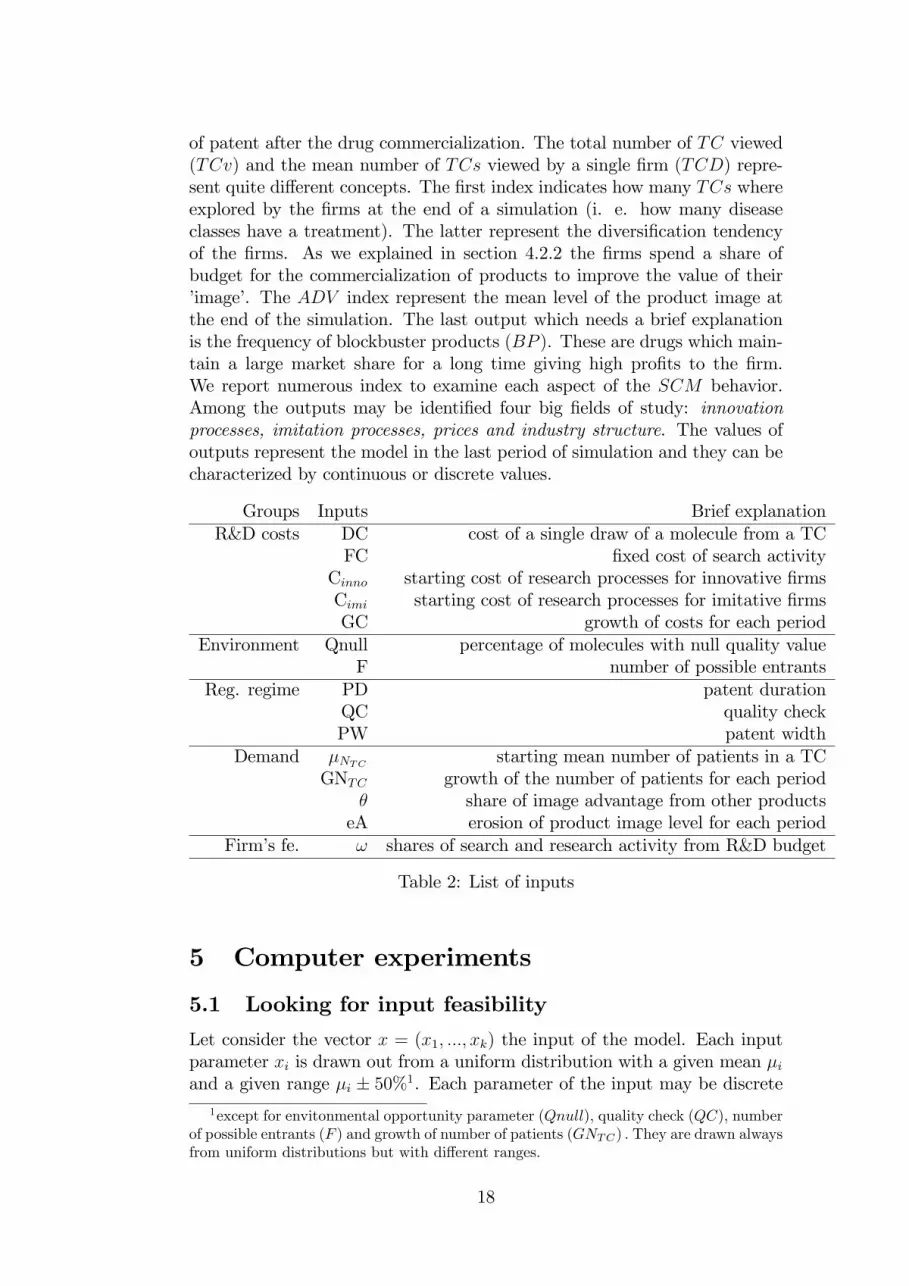
of patent after the drug commercialization. The total number of TC viewed(TCv) and the mean number of TCs viewed by a single �rm (TCD) repre-sent quite di¤erent concepts. The �rst index indicates how many TCs whereexplored by the �rms at the end of a simulation (i. e. how many diseaseclasses have a treatment). The latter represent the diversi�cation tendencyof the �rms. As we explained in section 4.2.2 the �rms spend a share ofbudget for the commercialization of products to improve the value of their�image�. The ADV index represent the mean level of the product image atthe end of the simulation. The last output which needs a brief explanationis the frequency of blockbuster products (BP ). These are drugs which main-tain a large market share for a long time giving high pro�ts to the �rm.We report numerous index to examine each aspect of the SCM behavior.Among the outputs may be identi�ed four big �elds of study: innovationprocesses, imitation processes, prices and industry structure. The values ofoutputs represent the model in the last period of simulation and they can becharacterized by continuous or discrete values.

Groups Inputs Brief explanationR&D costs DC cost of a single draw of a molecule from a TC

FC �xed cost of search activityCinno starting cost of research processes for innovative �rmsCimi starting cost of research processes for imitative �rmsGC growth of costs for each period

Environment Qnull percentage of molecules with null quality valueF number of possible entrants

Reg. regime PD patent durationQC quality checkPW patent width

Demand �NTC starting mean number of patients in a TCGNTC growth of the number of patients for each period

� share of image advantage from other productseA erosion of product image level for each period

Firm�s fe. ! shares of search and research activity from R&D budget

Table 2: List of inputs

5 Computer experiments

5.1 Looking for input feasibility

Let consider the vector x = (x1; :::; xk) the input of the model. Each inputparameter xi is drawn out from a uniform distribution with a given mean �iand a given range �i � 50%1. Each parameter of the input may be discrete

1except for envitonmental opportunity parameter (Qnull), quality check (QC), numberof possible entrants (F ) and growth of number of patients (GNTC) : They are drawn alwaysfrom uniform distributions but with di¤erent ranges.

18

Groups Outputs Brief explanationStructure TH total Her�ndahl index

HTC mean Her�ndahl index in the TCsAfin alive innovative �rmsAFim alive imitative �rmsSzin mean size of innovative �rmsSzim mean size of imitative �rms

Innovation pr. Nin number of innovative drugsImitation pr. Nim number of imitative drugsPrices Pin mean price of innovative drugs

Pim mean price of imitative drugsPtot mean total prices

Others TCv number of TC explored by the �rmsTCD mean number of TC explored by a �rmfSH innovative �rms shareBP blockbuster frequencyEPL mean e¤ective patent lifeADV mean image level of products

Table 3: List of outputs

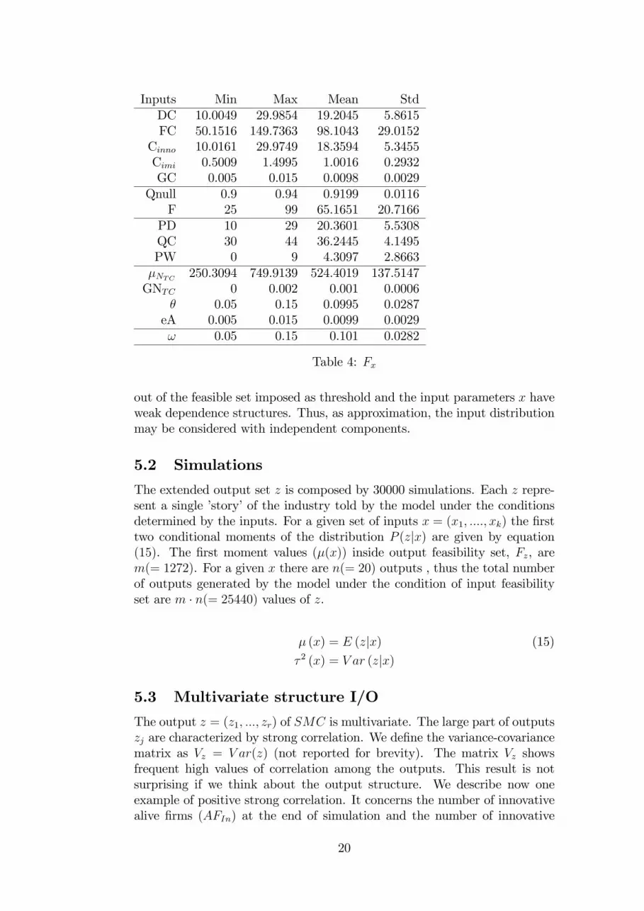
or continuos. The mean value �i; rises from the i-th component of bx =(bx1; :::; bxk) vector considered as the standard set. We de�ne the extendedoutput, originated with the input set x, asDz. Now we introduce the conceptof input feasibility set explained in section 2.2. We choose to exclude the lesspleasant outputs from Dz using the simple criterion of do not consider lesssigni�cant results. The �rst step is to de�ne an output feasibility set Fzthrough the use of simple conditions on Dz. Thus, we de�ne feasible outputall the model results that have the minimum features that allow to de�ne theexistence of the pharmaceutical market. Two necessary requirements appearclear. The �rst is the necessity of existence, at least, of one imitative �rm andone innovative �rm which compete in the market. The condition of an emptymarket is not very interesting simply because nothing happens. Moreover,an analysis of the parameters in the state of an empty market may be self-defeating because, under a minimum threshold of di¢ cult conditions, theresult is always an empty market. The feasible second state is the conditionof low value of concentration. It is widely recognized and is also an empiricalevidence that the structure of pharmaceutical industry is characterized by alow level of concentration and our attempt is to remain quite close to the�History-Friendly� results. Thus, we �x a maximum level of concentrationthat appears feasible. Once de�ned Fz the next step is to apply equation (2)to extended output set Dz and then deduce Fx. Imposing input feasibility,causes the loss of input independence as explained in section 2.2. In table(4) we report the input feasibility set Fx (outcome of the process).

From an analysis of the Fz andDz (not reported here for brevity) emergesthat the independence of the inputs is quite preserved, only few results are

19

Inputs Min Max Mean StdDC 10.0049 29.9854 19.2045 5.8615FC 50.1516 149.7363 98.1043 29.0152

Cinno 10.0161 29.9749 18.3594 5.3455Cimi 0.5009 1.4995 1.0016 0.2932GC 0.005 0.015 0.0098 0.0029

Qnull 0.9 0.94 0.9199 0.0116F 25 99 65.1651 20.7166

PD 10 29 20.3601 5.5308QC 30 44 36.2445 4.1495PW 0 9 4.3097 2.8663�NTC 250.3094 749.9139 524.4019 137.5147GNTC 0 0.002 0.001 0.0006

� 0.05 0.15 0.0995 0.0287eA 0.005 0.015 0.0099 0.0029! 0.05 0.15 0.101 0.0282

Table 4: Fx

out of the feasible set imposed as threshold and the input parameters x haveweak dependence structures. Thus, as approximation, the input distributionmay be considered with independent components.

5.2 Simulations

The extended output set z is composed by 30000 simulations. Each z repre-sent a single �story�of the industry told by the model under the conditionsdetermined by the inputs. For a given set of inputs x = (x1; ::::; xk) the �rsttwo conditional moments of the distribution P (zjx) are given by equation(15). The �rst moment values (�(x)) inside output feasibility set, Fz, arem(= 1272). For a given x there are n(= 20) outputs , thus the total numberof outputs generated by the model under the condition of input feasibilityset are m � n(= 25440) values of z.

� (x) = E (zjx) (15)

� 2 (x) = V ar (zjx)

5.3 Multivariate structure I/O

The output z = (z1; :::; zr) of SMC is multivariate. The large part of outputszj are characterized by strong correlation. We de�ne the variance-covariancematrix as Vz = V ar(z) (not reported for brevity). The matrix Vz showsfrequent high values of correlation among the outputs. This result is notsurprising if we think about the output structure. We describe now oneexample of positive strong correlation. It concerns the number of innovativealive �rms (AFIn) at the end of simulation and the number of innovative

20

drugs sold on the market (NIn). It is quite intuitive that the two outputs arestrongly correlated, considering that the only sources of wealth for the �rmsare the sold products.As we said in section 2 we are able to separate the quota of the global

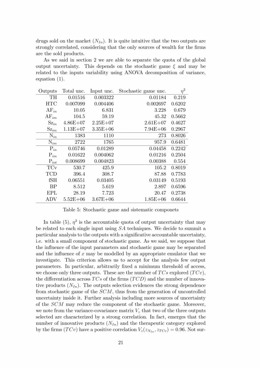
output uncertainty. This depends on the stochastic game � and may berelated to the inputs variability using ANOVA decomposition of variance,equation (1).

Outputs Total unc. Input unc. Stochastic game unc. �2

TH 0.01516 0.003322 0.01184 0.219HTC 0.007099 0.004406 0.002697 0.6202AFin 10.05 6.831 3.228 0.679AFim 104.5 59.19 45.32 0.5662Szin 4.86E+07 2.25E+07 2.61E+07 0.4627Szim 1.13E+07 3.35E+06 7.94E+06 0.2967Nin 1383 1110 273 0.8026Nim 2722 1765 957.9 0.6481Pin 0.05746 0.01289 0.04458 0.2242Pim 0.01622 0.004062 0.01216 0.2504Ptot 0.008699 0.004823 0.00388 0.554TCv 530.7 425.9 105.2 0.8019TCD 396.4 308.7 87.88 0.7783fSH 0.06551 0.03405 0.03149 0.5193BP 8.512 5.619 2.897 0.6596EPL 28.19 7.723 20.47 0.2738ADV 5.52E+06 3.67E+06 1.85E+06 0.6644

Table 5: Stochastic game and sistematic componets

In table (5), �2 is the accountable quota of output uncertainty that maybe related to each single input using SA techniques. We decide to summit aparticular analysis to the outputs with a signi�cative accountable uncertainty,i.e. with a small component of stochastic game. As we said, we suppose thatthe in�uence of the input parameters and stochastic game may be separatedand the in�uence of x may be modelled by an appropriate emulator that weinvestigate. This criterion allows us to accept for the analysis few outputparameters. In particular, arbitrarily �xed a minimum threshold of access,we choose only three outputs. These are the number of TCs explored (TCv),the di¤erentiation across TCs of the �rms (TCD) and the number of innova-tive products (NIn). The outputs selection evidences the strong dependencefrom stochastic game of the SCM , thus from the generation of uncontrolleduncertainty inside it. Further analysis including more sources of uncertaintyof the SCM may reduce the component of the stochastic game. Moreover,we note from the variance-covariance matrix Vz that two of the three outputsselected are characterized by a strong correlation. In fact, emerges that thenumber of innovative products (NIn) and the therapeutic category exploredby the �rms (TCv) have a positive correlation Vz(zNIn ; zTCv) = 0:96. Not sur-

21

prisingly the random draw mechanism on the environment (�random search�)produces a spread placement of innovative products in the TCs, thus manyproducts means more probability to explore di¤erent TCs. Follows that wedecided to investigate only the emulator components of the number of in-novative products (NIn) considering that the behavior of TCv is quite thesame.

5.4 Computer simulation results and data analysis

In this section we examine the input e¤ect only. As explained in section3.3.1, for a preliminary estimate of coe¢ cients � to perform the SA we canconsider the average values of outputs b�i, i = 1; :::;m and apply ordinaryleast squares to data (b�i; xi). After, we proceed eliminating the unimpor-tant parameters and make the graphical analysis of the residual. Followingthis lines we searched for a statistical model having residuals almost inde-pendent from the x and normally distributed or at last symmetric aroundzero, with small Mean Squared Error (MSE). Moreover we searched for alittle complexity as measurer by Akaike Information Criterion (AIC) andBayesian Information Criterion (BIC): Thus, the �rst step is to eliminateunimportant parameters with t tests. To identify a threshold, common to allthe model � coe¢ cients, for the p-values we exploit the optimization of themodel complexity in accordance with AIC and BIC. To do this we considerthe whole multivariate output and we calculate the variance of the residualsas explained in equation (16).

b�2" = V ar(V" � �0) (16)

Where V" matrix contains the residuals of the regressions and b�2" is thevariance of the linear combination V" ��0. Moreover, we consider k the wholenumber of parameters in the multivariate model and m as the number ofobservations b�i. AIC and BIC, functions of b�2" , k andm; are both optimizedfor a threshold p-value of 10�7.After the model simpli�cation we focus on a deep analysis of few outputs,

selected, as explained in section 5.3, for the low component of stochasticgame. At the end of this Section, in table (6) and table (7), where are listedthe importances of the input parameters, we decided to report all the SIs inorder to give an overall description of the model through the univariate andmultivariate SAs even if the stochastic game component largely determinatessome outputs. For example, we observe that the number of patients in theTCs in�uences for the 10.29% the total Her�ndahl index, being the maximumquota of accountable output uncertainty only the 21.9%.

5.4.1 Number of innovations (N In)

Now we explore the number of innovations in the market (NIn) because ithas a high value of �2 and so variance depends largely from inputs. First ofall we simplify the model omitting the unimportant parameters and we get a

22

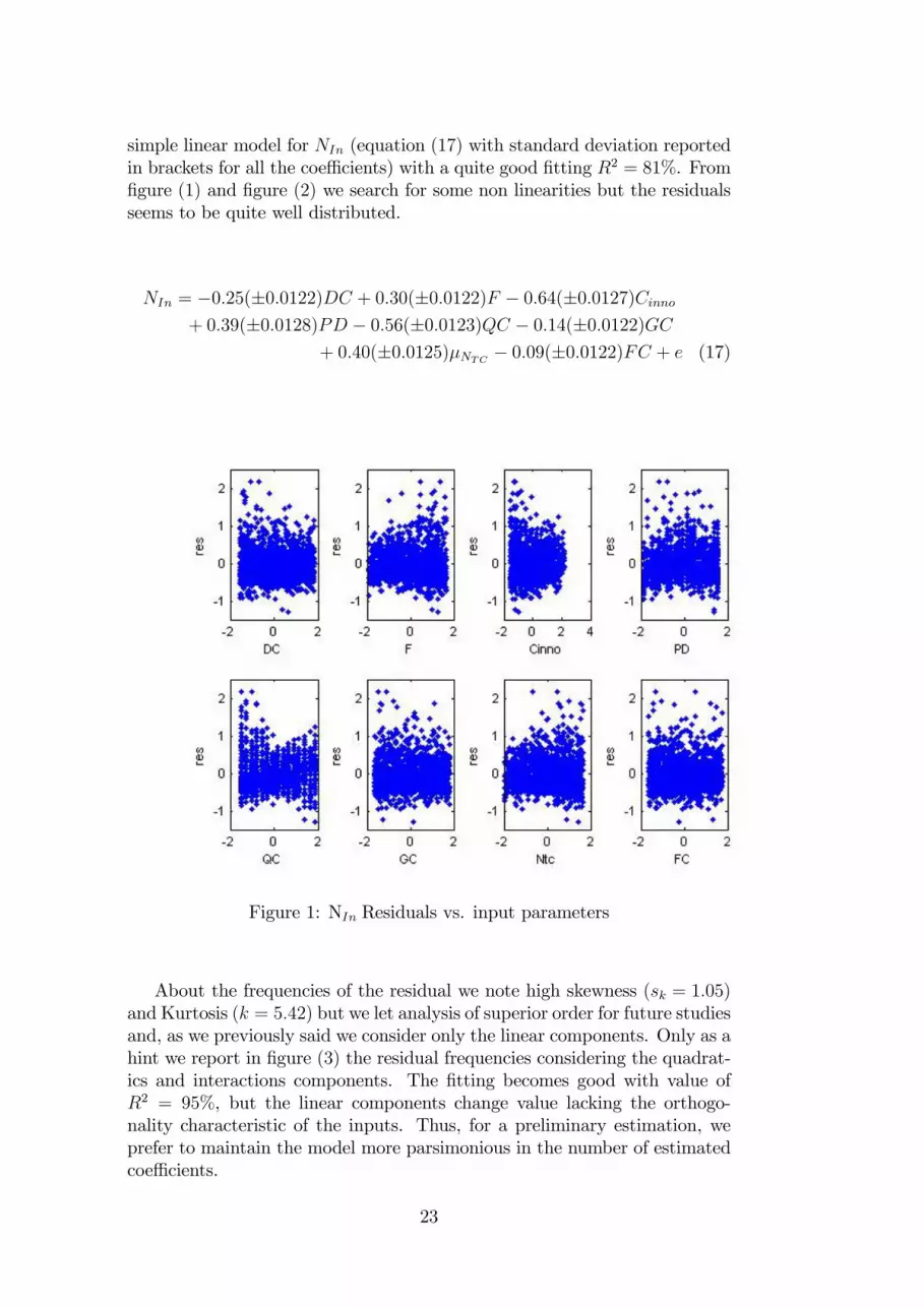
simple linear model for NIn (equation (17) with standard deviation reportedin brackets for all the coe¢ cients) with a quite good �tting R2 = 81%. From�gure (1) and �gure (2) we search for some non linearities but the residualsseems to be quite well distributed.

NIn = �0:25(�0:0122)DC + 0:30(�0:0122)F � 0:64(�0:0127)Cinno+ 0:39(�0:0128)PD � 0:56(�0:0123)QC � 0:14(�0:0122)GC

+ 0:40(�0:0125)�NTC � 0:09(�0:0122)FC + e (17)

Figure 1: NIn Residuals vs. input parameters

About the frequencies of the residual we note high skewness (sk = 1:05)and Kurtosis (k = 5:42) but we let analysis of superior order for future studiesand, as we previously said we consider only the linear components. Only as ahint we report in �gure (3) the residual frequencies considering the quadrat-ics and interactions components. The �tting becomes good with value ofR2 = 95%, but the linear components change value lacking the orthogo-nality characteristic of the inputs. Thus, for a preliminary estimation, weprefer to maintain the model more parsimonious in the number of estimatedcoe¢ cients.

23

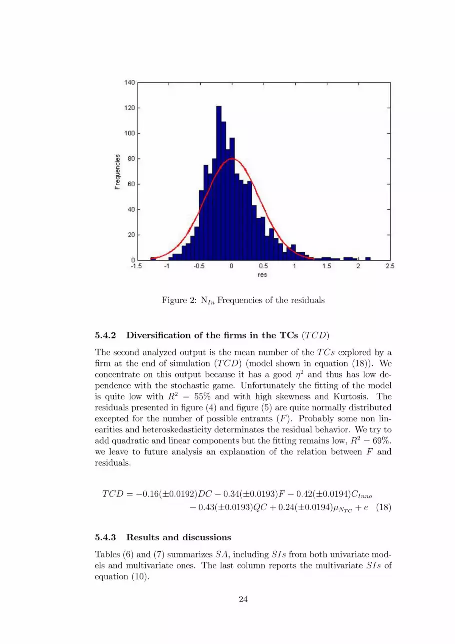
Figure 2: NIn Frequencies of the residuals

5.4.2 Diversi�cation of the �rms in the TCs (TCD)

The second analyzed output is the mean number of the TCs explored by a�rm at the end of simulation (TCD) (model shown in equation (18)). Weconcentrate on this output because it has a good �2 and thus has low de-pendence with the stochastic game. Unfortunately the �tting of the modelis quite low with R2 = 55% and with high skewness and Kurtosis. Theresiduals presented in �gure (4) and �gure (5) are quite normally distributedexcepted for the number of possible entrants (F ). Probably some non lin-earities and heteroskedasticity determinates the residual behavior. We try toadd quadratic and linear components but the �tting remains low, R2 = 69%.we leave to future analysis an explanation of the relation between F andresiduals.

TCD = �0:16(�0:0192)DC � 0:34(�0:0193)F � 0:42(�0:0194)CInno� 0:43(�0:0193)QC + 0:24(�0:0194)�NTC + e (18)

5.4.3 Results and discussions

Tables (6) and (7) summarizes SA, including SIs from both univariate mod-els and multivariate ones. The last column reports the multivariate SIs ofequation (10).

24

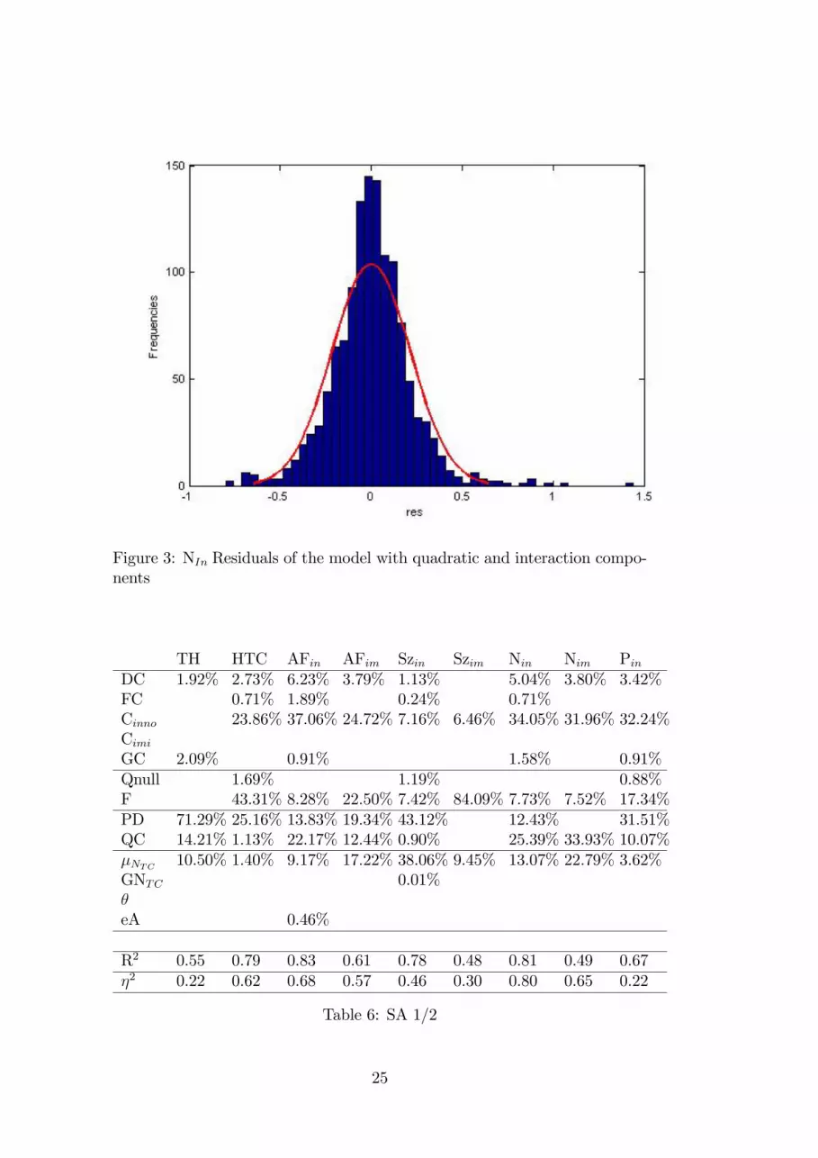
Figure 3: NIn Residuals of the model with quadratic and interaction compo-nents

TH HTC AFin AFim Szin Szim Nin Nim PinDC 1.92% 2.73% 6.23% 3.79% 1.13% 5.04% 3.80% 3.42%FC 0.71% 1.89% 0.24% 0.71%Cinno 23.86% 37.06% 24.72% 7.16% 6.46% 34.05% 31.96% 32.24%CimiGC 2.09% 0.91% 1.58% 0.91%Qnull 1.69% 1.19% 0.88%F 43.31% 8.28% 22.50% 7.42% 84.09% 7.73% 7.52% 17.34%PD 71.29% 25.16% 13.83% 19.34% 43.12% 12.43% 31.51%QC 14.21% 1.13% 22.17% 12.44% 0.90% 25.39% 33.93% 10.07%�NTC 10.50% 1.40% 9.17% 17.22% 38.06% 9.45% 13.07% 22.79% 3.62%GNTC 0.01%�eA 0.46%

R2 0.55 0.79 0.83 0.61 0.78 0.48 0.81 0.49 0.67�2 0.22 0.62 0.68 0.57 0.46 0.30 0.80 0.65 0.22

Table 6: SA 1/2

25

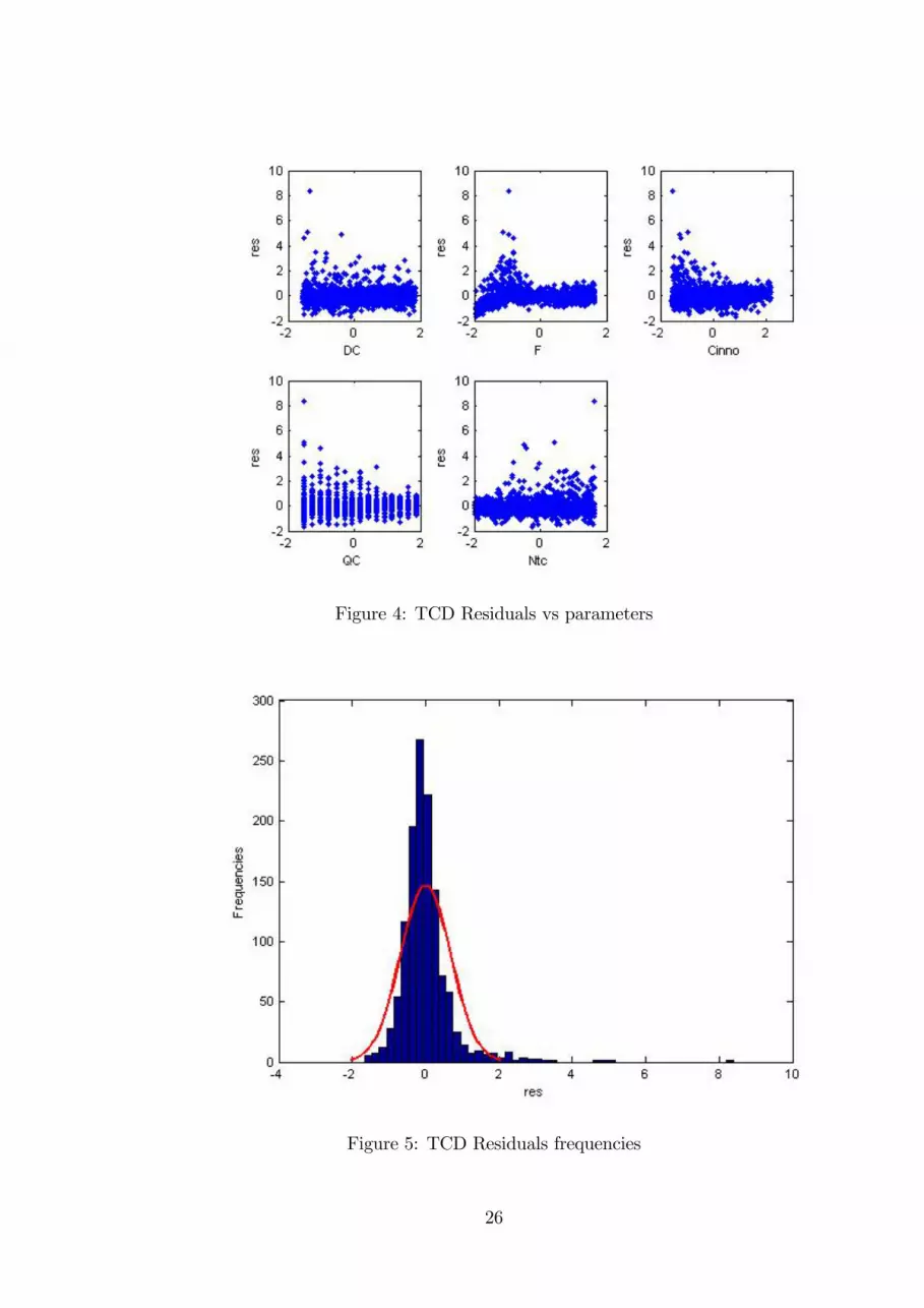
Figure 4: TCD Residuals vs parameters

Figure 5: TCD Residuals frequencies

26

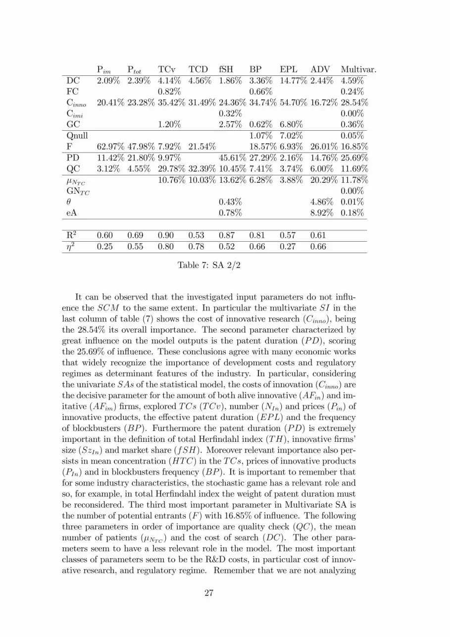
Pim Ptot TCv TCD fSH BP EPL ADV Multivar.DC 2.09% 2.39% 4.14% 4.56% 1.86% 3.36% 14.77% 2.44% 4.59%FC 0.82% 0.66% 0.24%Cinno 20.41% 23.28% 35.42% 31.49% 24.36% 34.74% 54.70% 16.72% 28.54%Cimi 0.32% 0.00%GC 1.20% 2.57% 0.62% 6.80% 0.36%Qnull 1.07% 7.02% 0.05%F 62.97% 47.98% 7.92% 21.54% 18.57% 6.93% 26.01% 16.85%PD 11.42% 21.80% 9.97% 45.61% 27.29% 2.16% 14.76% 25.69%QC 3.12% 4.55% 29.78% 32.39% 10.45% 7.41% 3.74% 6.00% 11.69%�NTC 10.76% 10.03% 13.62% 6.28% 3.88% 20.29% 11.78%GNTC 0.00%� 0.43% 4.86% 0.01%eA 0.78% 8.92% 0.18%

R2 0.60 0.69 0.90 0.53 0.87 0.81 0.57 0.61�2 0.25 0.55 0.80 0.78 0.52 0.66 0.27 0.66

Table 7: SA 2/2

It can be observed that the investigated input parameters do not in�u-ence the SCM to the same extent. In particular the multivariate SI in thelast column of table (7) shows the cost of innovative research (Cinno), beingthe 28.54% its overall importance. The second parameter characterized bygreat in�uence on the model outputs is the patent duration (PD), scoringthe 25.69% of in�uence. These conclusions agree with many economic worksthat widely recognize the importance of development costs and regulatoryregimes as determinant features of the industry. In particular, consideringthe univariate SAs of the statistical model, the costs of innovation (Cinno) arethe decisive parameter for the amount of both alive innovative (AFin) and im-itative (AFim) �rms, explored TCs (TCv), number (NIn) and prices (Pin) ofinnovative products, the e¤ective patent duration (EPL) and the frequencyof blockbusters (BP ). Furthermore the patent duration (PD) is extremelyimportant in the de�nition of total Her�ndahl index (TH), innovative �rms�size (SzIn) and market share (fSH). Moreover relevant importance also per-sists in mean concentration (HTC) in the TCs, prices of innovative products(PIn) and in blockbusters frequency (BP ). It is important to remember thatfor some industry characteristics, the stochastic game has a relevant role andso, for example, in total Her�ndahl index the weight of patent duration mustbe reconsidered. The third most important parameter in Multivariate SA isthe number of potential entrants (F ) with 16.85% of in�uence. The followingthree parameters in order of importance are quality check (QC), the meannumber of patients (�NTC ) and the cost of search (DC). The other para-meters seem to have a less relevant role in the model. The most importantclasses of parameters seem to be the R&D costs, in particular cost of innov-ative research, and regulatory regime. Remember that we are not analyzing

27

the stochastic game component, largely important for many characteristicsof the market, but we rank the inputs x according to the in�uence on outputuncertainty of emulator, that is a statistical simpli�ed model. The amountof innovative products (NIn) is an interesting case of univariate SA becausehas low stochastic game component and good �tting. The variance of thisoutput depends closely from input variance and thus the SA on emulatoris very meaningful. The most important parameters, considering as outputthe number of innovative products, are the cost of innovative development(Cinno) and the parameters of the regulatory regime ((QC) and (PD)) . Alsothe number of patients (�NTC ) plays a key role.

6 Conclusions

A statistical procedure has been proposed for preliminary analysis to evaluatethe in�uence of some parameters in a History-Friendly stochastic computermodel of the pharmaceutical industry. The parameters analyzed deal withdemand, regulatory regime, costs, environmental characteristics and �rm�sfeatures. At �rst we assumed that the in�uence of the input parameters andthe stochastic game on the output variance could be separated. Thus, wemodelled the in�uence of the inputs by an appropriate emulator which is asimpli�ed statistical model. After, using the emulator, we carried on rankingthe parameters through the univariate and multivariate SAs. In the lattermethod, the in�uence of the inputs on the stochastic computer model hasbeen assessed. Considering the entire aspects of the pharmaceutical industryinvestigated, the most important parameters result to be the innovation costsand the regulatory regime. Considering the number of innovations, as acase of particular univariate SA characterized by low value of the stochasticgame, emerges that costs of innovation and the regulatory regime play alsoa decisive role in determining the productiveness of the innovative process.This path of analysis allows a preliminary evaluation. In some cases insertingheteroskedasticity, quadratic components, interactions and detailed study ofthe stochastic game component of the mixed linear model could improve theaccuracy of the results. The next step (a proposal for future works) will beto extend the analysis of the model, introducing the omitted components.However we underline the importance of this analysis in order to summarizethe large and complex problem of understanding and ranking what featuresplay a relevant role in a market model for pharmaceutical industry. Justat this level of widening the procedure gives useful indications about theoutputs of the model and the subordinate economic theory.

28

References

Bottazzi G.,Dosi G, Lippi M., Pammolli F.,Riccaboni M. (2001), Innovationand corporate growth in the evolution of the drug industry, Interna-tional Journal of Industrial Organization, 19, 1161-1187

Fassò A. (2006a) Sensitivity Analysis and Water Quality. Working PaperGRASPA, 23, (www.graspa.org). In print on: Wymer L. Ed, Recre-ational Beaches: Statistical Framework for Water Quality Criteria andMonitoring. Wiley.

Fassò A. (2006b) Sensitivity Analysis for Environmental Models and Moni-toring Networks. In: Voinov, A., Jakeman, A., Rizzoli, A. (eds). Pro-ceedings of the iEMSs Third Biennial Meeting: "Summit on Environ-mental Modelling and Software". International Environmental Mod-elling and Software Society, Burlington, USA, July 2006. CD ROM.www.iemss.org/iemss2006/sessions/all.html

Fassò A., Esposito E., Porcu E., Reverberi A.P., Vegliò F. (2003) Statisti-cal Sensitivity Analysis of Packed Column Reactors for ContaminatedWastewater. Environmetrics. 14(8), 743 - 759.

Fassò A., Perri P.F. Sensitivity (2002) Analysis. In Abdel H. El-Shaarawiand Walter W. Piegorsch (eds) Encyclopedia of Environmetrics, 4,1968�1982, Wiley.

Grabowski, H. (2002) Patents and new products in the development ofpharmaceutical industry

Grabowski H., Vernon J, (1992), Brand loyalty, Entry, and price competi-tion in pharmaceuticals after the 1984 drug act, Journal of Low andEconomics, Vol.35,N.2,pp.311-350

Henderson R., Cockburn I., (1996), Scale, scope and spillovers: the determi-nants of research productivity in drug discovery Journal of Economics

Kennedy M.C. O�Hagan A. (2001) Bayesian calibration of computer models,J. Royal Stat. Soc. B, 63, 425-464.

Lee, Y., Nelder, J.A. (2001) Hierarchical generalized linear models: a syn-thesis of generalised linear models, random-e¤ect models and struc-tured dispersions. Biometrika, 88, 987-1006.

Malerba F., Nelson R., Orsenigo L., Winter S., (2001),Competition andindustrial policies in a History Friendly model of evolution of the com-puter industry;International Journal of Industrial Organization,19,635-664

Malerba F., Nelson R., Orsenigo L., Winter S., (1999);History Friendlymodels of industry evolution: the computer industry,Industrial andCorporate Change, 8, 1

29

Malerba F., Orsenigo L. (2002) Innovation and market structure in thedynamics of the pharmaceutical industry and biotechnology: towardsa history friendly model, Industrial and Corporte Change, 11, 667-703

Malerba F., Orsenigo L. (2001), Towards a History Friendly model of inno-vation, market structure and regulation in the dynamics of the phar-maceutical industry: the age of random screening. WP n.124

Matraves C., (1999) Market structure R&D and advertising in the pharma-ceutical industry. The Journal of Industrial Economics, XLVII

McKay M. D., Beckman R. J., Conover, W. J. (1979), A comparison ofthree methods for selecting values of input variables in the analysis ofoutput from a computer code, Technometrics, 21 , 239-245.

Saltelli A., Chan K., Scott M. (2000) Sensitivity Analysis, Wiley, New York.

Saltelli A., Tarantola S., Campolongo F., Ratto M. (2004) Sensitivity Analy-sis in Practice: A Guide to Assessing Scienti�c Models, Wiley.

30