multiobjective optimization of space structures under static and seismic loading conditions

12

Multiobjective Optimization of SpaceStructures under Static and Seismic LoadingConditions

Nikos D. Lagaros, Manolis Papadrakakis, and Vagelis Plevris

Summary. This chapter presents a evolution strategies approach for multiobjectivedesign optimization of structural problems such as space frames and multi-layeredspace trusses under static and seismic loading conditions. A rigorous approach anda simplified one with respect to the loading condition are implemented for findingoptimal design of a structure under multiple objectives.

12.1 Introduction

In single-objective optimization problems the optimal solution is usuallyclearly defined, this does not hold in real-world problems having multipleand conflicting objectives. Instead of a single optimal solution, there is rathera set of alternative solutions, generally denoted as the set of Pareto-optimalsolutions. These solutions are optimal in the wider sense that no other solutionin the search space is superior to them when all objectives are considered.In the absence of preference information, none of the corresponding trade-offs can be said to be better than the others. On the other hand, thesearch space can be too large and too complex, which, the usual caseof real-world problems, to be solved by the conventional deterministicoptimizers. Thus, efficient optimization strategies are required that are ableto deal with the multiple objectives and the complexity of the search space.Evolutionary Algorithms (EAs) have several characteristics that are desirablefor this kind of problems and most frequently outperform the deterministicoptimizers. The application of EA in multiobjective optimization problems hasreceived considerable attention in the last five years due to the difficulty ofconventional optimization techniques, such as the gradient-based optimizers,to be extended to multi-objective optimization problems. For dealing with themulti-objective optimization problems there are some typical methods, such aslinear weighting method, distance function method and constraint method. Intreating such a problem using gradient based optimizers, we have to combinethem with the typical methods. On the other hand, the structure of the EA

274 Lagaros et al.

optimizers have been recognized to be more appropriate to multiobjectiveoptimization problems since early in their development [1]. EA optimizersemploy multiple individuals that can search for multiple solutions in parallel.Using some modifications on the operators used by the EA optimizers thesearch process can be driven to a family of solutions representing the set ofPareto-optimal solutions.

Structural sizing optimization at its early stages of development wasmainly single-objective. The aim was to minimize the weight of the structureunder certain restrictions imposed by design codes. Although some workhas been published in the past dealing with multi-objective optimization [2-7] this was restricted to simple academic examples. Optimization of large-scale structures, such as sizing optimization of multi-storey 3D frames andtrusses is a computationally intensive task. The optimization problem becomesmore intensive when dynamic loading is involved [8]. The feasible designspace in structural optimization problems under dynamic constraints is oftendisconnected or disjoint [9, 10] which causes difficulties for many conventionaloptimizers. Due to the uncertain nature of the seismic loading, structuraldesigns are often based on design response spectra of the region and onsome simplified assumptions of the structural behavior under earthquakes.In the case of a direct consideration of the seismic loading the optimization ofstructural systems requires the solution of the dynamic equations of motionwhich can be orders of magnitude more computationally intensive than thecase of static loading.

In this work, both the rigorous approach and the simplified one withrespect to the loading condition are implemented and their efficiency iscompared in the framework of finding the optimum design of a structureunder multiple objectives. In the context of the rigorous approach a number ofartificial accelerograms are produced from the design response spectrum of theregion for elastic structural response, which constitutes the multiple loadingconditions under which the structures are optimally designed. The elasticdesign response spectrum can be seen as an envelope of response spectra,for a specific damping ratio, of different earthquakes most likely to occur inthe region. This approach is compared with the approximate one based onsimplifications adopted by the seismic codes. The Pareto sets obtained for acharacteristic problem indicate the difference of the two Pareto sets obtainedby the rigorous approach and the simplified one.

12.2 Single-objective Structural Optimization

In sizing optimization problems the aim is to minimize a single-objectivefunction, usually the weight of the structure, under certain behavioralconstraints on stress and displacements. The design variables are mostfrequently chosen to be dimensions of the cross-sectional areas of the membersof the structure. Due to fabrication limitations the design variables are not

12 Multi-Objective Structural Optimization under Seismic Loading 275

continuous but discrete since cross-sections belong to a certain set. A discretestructural optimization problem can be formulated in the following form:

min f(s)subject to gj(s) ≤ 0 j = 1, . . . , k

si ∈ Rd, i = 1, . . . , n(12.1)

where Rd is a given set of discrete values and the design variables si (i =1, . . . , n) can take values only from this set.

In the optimal design of 3D frames and trusses the constraints arethe member stresses and nodal displacements or inter-storey drifts. Forrigid frames with I-shapes, the stress constraints, under allowable stressdesign requirements specified by Eurocode 3 [11] are expressed by the non-dimensional ratio q of the following formulas

q =fa

σa+

fyb

σyb

+fz

b

σzb

≤ 1.0 iffa

σa≤ 0.15 (12.2)

and

q =fa

0.60 × σy+

fyb

σyb

+fz

b

σzb

≤ 1.0 iffa

σa> 0.15 (12.3)

where fa is the computed compressive axial stress, fyb , fz

b are the computedbending stresses for y and z axis, respectively. σa is the allowable compressiveaxial stress, σy

b , σzb are the allowable bending stresses for y and z axis,

respectively, and σy is the yield stress of the steel. The allowable inter-storeydrift is limited to 1.5% of the height of each storey.

Space truss structures usually have the topology of single or multi-layeredflat or curved grids that can be easily constructed in practice. Most frequentlythe constraints are the member stresses, nodal displacements, or frequencies.The stress constraints can be written as |σ| ≤ |σa|, where σ is the maximumaxial stress in each element group for all loading cases, σa = 0.60 × σy is theallowable axial stress and σy is the yield stress. Similarly, the displacementconstraints can be written as |d| ≤ da, where da is the limiting value of thedisplacement at a certain node, or the maximum nodal displacement.

Euler buckling occurs in truss structures when the magnitude of amember’s compressive stress is greater than a critical stress that, for the firstbuckling mode of a pin-connected member, is equal to

σb =Pb

A= − 1

A

(π2EI

L2

)(12.4)

where Pb is the computed compressive axial force, I is the moment of inertia, Lis the member length. Thus, the compressive stress should be less (in absolutevalues) than the critical Euler buckling stress |σ| ≤ |σb|. The values of theconstraint functions are normalized in order to improve the performance ofthe optimization procedure as: σ/σa ≤ 1 for tension member σa = 0.60 × σy,

σ/σb ≤ 1 for compression member σb = E(π/(l/r)

)2and d/da ≤ 1.

276 Lagaros et al.

The sizing optimization methodology with EA proceeds using the followingsteps: (1) At the outset of the optimization the geometry, the boundaries andthe loads of the structure under investigation have to be defined. (2) Thedesign variables, which may or may not be independent to each other, are alsoproperly selected. Furthermore, the constraints are also defined in this stage inorder to formulate the optimization problem as in (12.1). (3) A finite elementanalysis is then carried out and the displacements and stresses are evaluated.(4) The design variables are being optimized using the selection, crossover andmutation operators. If the convergence criteria for the optimization algorithmare satisfied, then the optimum solution has been found and the process isterminated, else the optimizer updates the design variable values and thewhole process is repeated from Step (3).

12.3 Multiobjective Structural Optimization

In practical applications of structural optimization of 3D frames and trussesthe weight rarely gives a representative measure of the performance of thestructure. In fact, several conflicting and incommensurable criteria usuallyexist in real-life design problems that have to be dealt simultaneously.This situation forces the engineer to look for a good compromisedesign between the conflicting requirements. These kinds of problems arecalled optimization problems with many objectives. The consideration ofmultiobjective optimization in its present sense originated towards the endof the last century when Pareto presented the optimality concept in economicproblems with several competing criteria [12]. The first applications in the fieldof structural optimization with multiple objectives appeared at the end of theseventies [2-7]. Since then, although many techniques have been developedin order to deal with multiobjective optimization problems and a numberof structural optimization problems have been dealt with multiobjectives,the corresponding applications were confined to mathematical functions orPareto-structural optimization problems under only static loading conditions[13-21].

12.3.1 Criteria and Conflict

Any engineer who looks for the optimum design of a structure is facedwith the question of which criteria are suitable for measuring the economy,the performance, the strength and the serviceability of a structure. Anyquantity that, when changed, has a direct influence on the economy and/orthe performance, the strength and the serviceability of the structure, can beconsidered as a criterion. On the other hand, those quantities that must onlysatisfy some imposed requirements are not criteria but they can be treatedas constraints. Most of the commonly used design quantities have a criterionnature rather than a constraint nature because in the engineer’s mind these


should take the minimum or maximum possible values. Most of the structuraloptimization problems are treated with a single objective, usually the weightof the structure, subjected to some strength constraints. These constraints areset as equality or inequality constraints using some upper and lower limits.Some times there is a difficulty in selecting these limits and these parametersare treated as criteria.

One important basic property in the multi-criterion formulation is theconflict that may or may not exist between the criteria. Only those quantitiesthat are competing should be treated as independent criteria whereas theothers can be combined into a single criterion to represent the whole group.The concept of the conflict has deserved only a little attention in the literaturewhile on the contrary the solution procedures have been studied to a greatextent. According to the latter presentation the local conflict between twocriteria can be defined as follows: The functions fi and fj are called locallycollinear with no conflict at point s if there is c > 0 such that ∇fi(s) =c∇fj(s). Otherwise, the functions are called locally conflicting at s.

According to the previous definition any two criteria are locally conflictingat a point of the design space if their maximum improvement is achieved indifferent directions. The global conflict between two criteria can be defined asfollows: The functions fi and fj are called globally conflicting in the feasibleregion � of the design space when the two optimization problems mins∈ fi(s)and mins∈ fj(s) have different optimal solutions.

12.3.2 Formulation of a Multiple Objective Optimization Problem

In formulating an optimization problem the choice of the design variables,criteria and constraints certainly represents the most important decision madeby the engineer. The designs, which will be considered here, are fixed at thisvery early stage. In general the mathematical formulation of a multiobjectiveproblem includes a set of n design variables, a set of m objective and a set ofk constraint functions and can be defined as follows:

mins∈ [f1(s), . . . , fm(s)]T

subject to gj(s) ≤ 0 j = 1, . . . , ksi ∈ Rd, i = 1, . . . , n

(12.5)

where the vector s = [s1, . . . , sn]T represents a design variable vector and � isthe feasible set in design space Rn. It is defined as the set of design variablesthat satisfy the constraint functions g(s) in the form:

� = {s ∈ Rn|gj(s) ≤ 0} . (12.6)

Usually there exists no unique point which would give an optimum for allm criteria simultaneously. Thus the common optimality concept used in scalaroptimization must be replaced by a new one, the so-called Pareto optimum:A design vector s∗ ∈ � is Pareto optimal for the problem of Equation 12.5 if

278 Lagaros et al.

and only if there exists no other design vector s ∈ � such that fi(s) ≤ fi(s∗)for i = 1, . . . , m with fj(s) < fj(s∗) for at least one objective j.

According to the above definition the design vector s∗ is considered as aPareto-optimal solution if there is no other feasible design vector that improvesat least one objective without worsening any other objective. The solution ofoptimization problems with multiple objectives is the set of the Pareto-optimalsolutions. The problem of Equation 12.5 can be regarded, as being solvedafter the set of Pareto-optimal solutions has been determined. In practicalapplications, however, it is necessary to classify this set because the engineerwants a unique final solution. Thus a compromise should be made among thePareto-optimal solutions.

12.3.3 Solving the Multiobjective Optimization Problem

Typical methods for generating the Pareto-optimal set combine the objectivesinto a single, parameterized objective function by analogy to the decisionmaking search step. However, the parameters of this function are not set bythe decision making but systematically varied by the optimizer. Basically, thisprocedure is independent of the underlying optimization algorithm. Threepreviously used methods [ 4-7] are briefly discussed and are compared inthis study in terms of computational time and efficiency with the proposedmodified ES for treating multiobjective optimization problems.

Linear Weighting Method

The first method, called the linear weighting method, combines all theobjectives into a single scalar parameterized objective function by usingweighting coefficients. If wi, i = 1, . . . , m are the weighting coefficients, theproblem of Equation 12.5 can be written as follows:

mins∈

m∑i=1

wifi(s) (12.7)

with no loss of generality the following normalization of the weightingcoefficients is employed:

m∑i=1

wi = 1 . (12.8)

By varying these weights it is now possible to generate the set of Pareto-optimal solutions for Equation 12.5. The weighting coefficients correspondto the preference of the engineer for each criteria. Every combination ofthose weighting coefficients correspond to a single Pareto-optimal solution,thus, performing a set of optimization processes using different weightingcoefficients it is possible to generate the full set of Pareto-optimal solutions.


In real-world problems there is not a common unit for the objectivesleading to differences of some orders of magnitude between the values of theobjectives. It is therefore suggested that the objectives should be normalizedaccording to the following expression:

fi(s) =fi(s) − fi,min

fi,max − fi,min(12.9)

where the normalized objectives fi(s) ∈ [0, 1], i = 1, . . . , m, use the samedesign space with the non-normalized ones, while fi,min and fi,max are theminimum and maximum values of the objective function i.

Distance Function Method

The distance methods are based on the minimization of the distance betweenthe set of the objective function values and some chosen reference pointsbelonging to the criterion space. Whereas criterion space is defined as theset of the objective function values that correspond to design vectors of thefeasible domain. The resulting scalar problem is:

mins∈

dp(s) (12.10)

where the distance function can be written as follows:

dp(s) ={ m∑

i=1

wi

[fi(s) − zi

]p}1/p

(12.11)

where p is an integer number.This technique has been widely used in structural optimization. The

reference point zid ∈ Rm that is selected by the engineer is also called idealor utopian point. A reference point that is frequently used is the following:

zid =[fi,min, . . . , fm,min

]T (12.12)

where fi,min is the optimum solution of the single-objective optimizationproblem where the ith objective function is treated as the unique objective.The normalization function Equation 12.8 for the weighting factors wi is alsoused. In the case that p = ∞ Equation 12.10 is transformed to the minimaxproblem:

mins∈

maxi

[wifi(s)

], i = 1, . . . , m . (12.13)

In the case of p = 1 the formulation of the distance method is equivalent tothe linear method when the reference point used is the zero z = 0, while thecase of p = 2 the method is called the weighted quadratic method.

280 Lagaros et al.

Constraint Method

According to this method the original multi-criterion problem is replaced bya scalar problem where one criterion fk is chosen as the objective functionand all the other criteria are removed into the constraints. By introducingparameters εi into these new constraints an additional feasible set is obtained:

�k(εi) = {s ∈ Rn|fi(s) ≤ εi, i = 1, . . . , m with i �= k} . (12.14)

If the resulting feasible set is denoted by �k = � ∩ �k the parameterizedscalar problem can be expressed as:

mins∈k

fk(s) . (12.15)

The constraint method gives the opportunity to obtain the full domain ofoptimum solutions, in the horizontal or vertical direction using one criterionas the objective function and the other as the constraint.

Modified Evolution Strategies for Multiobjective Optimization

The three above-mentioned methods are the typical ones. The typical methodshave been used in the past combined with mathematical programmingoptimization algorithms where one design point was examined at eachoptimization step as an optimum design candidate. In order to locate the setof pareto-optimal solutions a family of optimization runs have to be executed.On the other hand evolutionary algorithms instead of a single design point,they work simultaneously with a population of design points, which is apopulation of optimum design candidates, in the space of design variables.This characteristic has been proved very useful since it is easy to implementthese methods in a parallel computing environment. Due to this characteristic,evolutionary algorithms have a great potential in finding multiple optima, in asingle optimization run, which is very useful in Pareto optimization problems.Since the early 1990s many researchers have suggested the use of evolutionaryalgorithms in multiobjective optimization problems [22-26] an overview of allthese methods can be found in Fonseca and Fleming [1] and Zitzler [27].

In our study the method of Evolution Strategies (ES) is used, and somechanges have to been made in the random operators that are usually used inorder to implement ES in multiobjective optimization problems and guide theconvergence to a population that represent the set of Pareto-optimal solutions.The idea in those changes is (1) the selection of the parent population at eachgeneration has to be changed in order to guide the search procedure towardsthe set of pareto optimum solutions, and (2) to prevent convergence to a singledesign point, and preserve diversity in the population in every generation step.The first demand can be fulfilled if the selection of the individual is chosenfor reproduction potentially a different objective [22]. A random selection


of the objective is implemented in this study. While in order to preservediversity in the population and fulfill the second requirement, fitness sharingis implemented [28]. The idea behind sharing is to degrade those individualsthat are represented in the higher percentage of the population. The modifiedobjectives after sharing are the following:

f ′i(s) =

fi(s)∑h sh(d(s, h)

) (12.16)

where the sharing function used in the current study is as follows:

sh(d(s, h)

)={

1 − (d(s,h)σshare

)aif d(s, h) < σshare

0 otherwise(12.17)

The distance function used is in the objective space:

d(s, h) = ‖f(s) − f(h)‖ . (12.18)

12.4 Structural Design under Seismic Loading

The equations of equilibrium for a finite element system in motion for the ithdesign vector, can be written in the usual form:

M(si)ut + C(si)ut + K(si)ut = Rt (12.19)

where M(si), C(si) and K(si) are the mass, damping and stiffness matricesfor the ith design vector si; Rt is the external load vector, while ut, ut

and ut are the displacement, velocity, and acceleration vectors of the finiteelement assemblage, respectively. The solution methods of direct integrationof equations of motion and of response spectrum modal analysis, which isbased on the mode superposition approach, will be considered in the followingparagraphs.

The Newmark integration scheme is adopted in the present study toperform the direct time integration of the equations of motion where theequilibrium Equation 12.19 is considered at time t + ∆t

M(si)ut+∆t + C(si)ut+∆t + K(si)ut+∆t = Rt+∆t (12.20)

and the variation of velocity and displacement are given by

ut+∆t = ut + [(1 − δ)ut + δut+∆t]∆t (12.21)

ut+∆t = ut + ut∆t + [(12

− α)ut + αut+∆t]∆t2 (12.22)

where α and δ are parameters that can be determined to obtain integrationaccuracy and stability. Solving for ut+∆t in terms of ut+∆t from Equation

282 Lagaros et al.

12.22 and then substituting for ut+∆t in (12.21) we obtain equations for ut+∆t

and ut+∆t each in terms of the unknown displacements ut+∆t only. These tworelations for ut+∆t and ut+∆t are substituted into Equation 12.20 to solve forut+∆t. As a result of this substitution the following well-known equilibriumequation is obtained at each ∆t

Keff(si)ut+∆t = Refft+∆t . (12.23)

12.4.1 Creation of Artificial Accelerograms

The selection of the proper external loading Rt for design purposes is notan easy task due to the uncertainties involved in the seismic loading. Forthis reason a rigorous treatment of the seismic loading is to assume that thestructure is subjected to a set of artificial earthquakes that are more likely tooccur in the region where the structure is located. These seismic excitationsare produced as a series of artificial accelerograms compatible with the elasticdesign response spectrum of the region.

In this work the implementation published by Taylor [29] for the generationof statistically independent artificial acceleration time histories is adopted.This method is based on the fact that any periodic function can be expandedinto a series of sinusoidal waves:

x(t) =∑

k

Ak sin(ωkt + ϕk) (12.24)

where Ak is the amplitude, ωk is the cyclic frequency and φk is the phase angleof the kth contributing sinusoid. By fixing an array of amplitudes and thengenerating different arrays of phase angles, different motions can be generatedwhich are similar in general appearance but different in the ’details’. Thecomputer uses a random number generator subroutine to produce strings ofphase angles with a uniform distribution in the range between 0 and 2π. Theamplitudes Ak are related to the spectral density function in the followingway:

G(ωk)∆ω =A2

k

2(12.25)

where G(ωk)∆ω may be interpreted as the contribution to the total powerof the motion from the sinusoid with frequency ωk. The power of the motionproduced by Equation 12.24 does not vary with time. To simulate the transientcharacter of real earthquakes, the steady-state motion is multiplied by adeterministic envelope function I(t):

Z(t) = I(t)∑

k

Aksin(ωkt + ϕk) . (12.26)

The resulting motion is stationary in frequency content with peakacceleration close to the target peak acceleration. In this study a trapezoidal


intensity envelope function is adopted. The generated peak acceleration isartificially modified to match the target peak acceleration, which correspondsto the chosen elastic design response spectrum. An iterative procedure isimplemented to smooth the calculated spectrum and improve the matching[29].

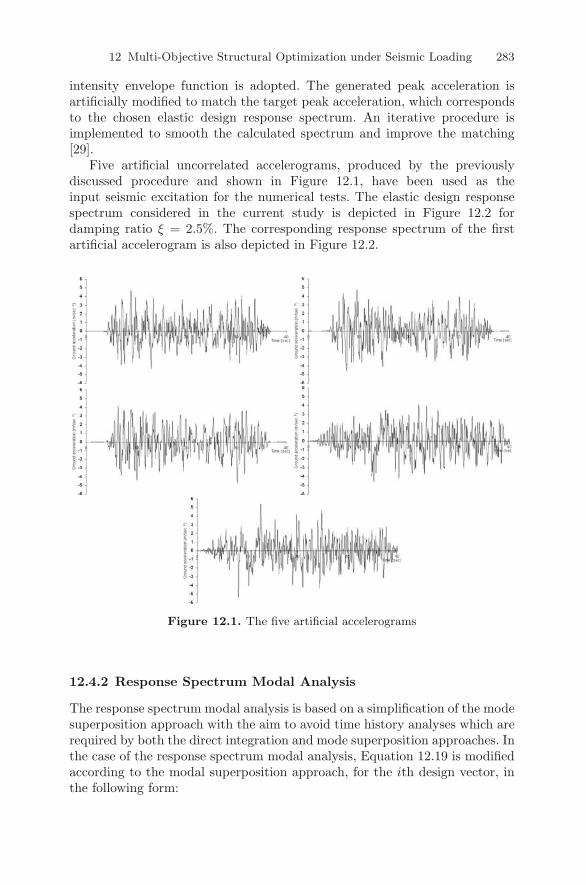
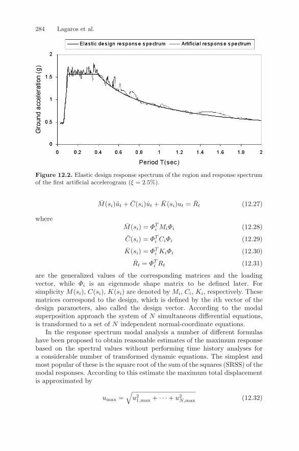
Five artificial uncorrelated accelerograms, produced by the previouslydiscussed procedure and shown in Figure 12.1, have been used as theinput seismic excitation for the numerical tests. The elastic design responsespectrum considered in the current study is depicted in Figure 12.2 fordamping ratio ξ = 2.5%. The corresponding response spectrum of the firstartificial accelerogram is also depicted in Figure 12.2.

Figure 12.1. The five artificial accelerograms

12.4.2 Response Spectrum Modal Analysis

The response spectrum modal analysis is based on a simplification of the modesuperposition approach with the aim to avoid time history analyses which arerequired by both the direct integration and mode superposition approaches. Inthe case of the response spectrum modal analysis, Equation 12.19 is modifiedaccording to the modal superposition approach, for the ith design vector, inthe following form:

284 Lagaros et al.

Figure 12.2. Elastic design response spectrum of the region and response spectrumof the first artificial accelerogram (ξ = 2.5%).

M(si)ut + C(si)ut + K(si)ut = Rt (12.27)

whereM(si) = ΦT

i MiΦi (12.28)

C(si) = ΦTi CiΦi (12.29)

K(si) = ΦTi KiΦi (12.30)

Rt = ΦTi Rt (12.31)

are the generalized values of the corresponding matrices and the loadingvector, while Φi is an eigenmode shape matrix to be defined later. Forsimplicity M(si), C(si), K(si) are denoted by Mi, Ci, Ki, respectively. Thesematrices correspond to the design, which is defined by the ith vector of thedesign parameters, also called the design vector. According to the modalsuperposition approach the system of N simultaneous differential equations,is transformed to a set of N independent normal-coordinate equations.

In the response spectrum modal analysis a number of different formulashave been proposed to obtain reasonable estimates of the maximum responsebased on the spectral values without performing time history analyses fora considerable number of transformed dynamic equations. The simplest andmost popular of these is the square root of the sum of the squares (SRSS) of themodal responses. According to this estimate the maximum total displacementis approximated by

umax =√

u21,max + · · · + u2

N,max (12.32)


where uj,max corresponds to the maximum displacement calculated from thejth transformed dynamic equations over the complete time period. The useof Equation 12.32 permits this type of “dynamic” analysis by knowing onlythe maximum modal coordinates uj,max.

The following steps summarize the response spectrum modal analysisadopted in this study and by a number of seismic codes around the world:

1. Calculate a number m′ < N of eigenfrequencies and the correspondingeigenmode shape matrices, which are classified in the following order(ω1

i , . . . , ωm′i ), Φi = [φ1

i , . . . , φm′i ], respectively, where ωj

i , φji are the jth

eigenfrequency-eigenmode corresponding to the ith design vector. m′ is auser specified number, based on experience or on previous test analyses,which has to satisfy the requirement of Step 6.

2. Calculate the generalized masses, according to the following equation:

mji = φj

i

TMiφ

ji . (12.33)

3. Calculate the coefficients Lji , according to the following equation:

Lji = φj

i

TMir (12.34)

where r is the influence vector, which represents the displacements of themasses resulting from static application of a unit, ground displacement.

4. Calculate the modal participation factor Γ ji , according to the following

equation:

Γ ji =

Lji

mji

. (12.35)

5. Calculate the effective modal mass for each design vector and for eacheigenmode, by the following equation:

mjeff,i =

Lji

2

mji

. (12.36)

6. Calculate a number m < m′ of the important eigenmodes. According toEurocode the minimum number of the eigenmodes that has to be takeninto consideration is defined by the following assumption: The sum of theeffective eigenmasses must not be less than 90% of the total vibrating massmtot of the system, so the first m eigenmodes that satisfy the equation

m∑j=1

mjeff,i ≥ 0.90mtot (12.37)

are taken into consideration.7. Calculate the values of the spectral acceleration Rd(Tj) that correspond

to each eigenperiod Tj of the important modes.

286 Lagaros et al.

8. Calculate the modal displacements according to equation

(SD)j =Rd(Tj)

ω2j

=Rd(Tj) × T 2

j

4π2 . (12.38)

9. Calculate the modal displacements:

uj,max = Γ ji × φj

i × (SD)j . (12.39)

10. The total maximum displacement is calculated by superimposing themaximum modal displacements according to Equation 12.32.

12.5 Solution of the Optimization Problem

The optimization problem is solved with evolution strategies. Evolutionstrategies were proposed for parameter optimization problems in the 1970s byRechenberg [30] and Schwefel [31]. Similar to genetic algorithms, ES imitatebiological evolution in nature and have three characteristics that make themdifferent from other conventional optimization algorithms: (1) in place ofthe usual deterministic operators, they use randomized operators: mutation,selection as well as recombination; (2) instead of a single design point, theywork simultaneously with a population of design points in the space ofvariables; (3) they can handle continuous, discrete, and mixed optimizationproblems. The second characteristic allows for a natural implementationof ES on parallel computing environments. The ES were initially appliedfor continuous optimization problems, but recently they have also beenimplemented in discrete and mixed optimization problems.

12.5.1 ES for Discrete Optimization Problems

The multi-membered ES adopted in the current study, based on the discreteformulation, use three operators: recombination, mutation, and selectionoperators that can be included in the algorithm as follows:

Step 1 (recombination and mutation)

The population of µ parents at gth generation produces λ offsprings. Thegenotype of any descendant differs only slightly from that of its parents. Forevery offspring vector a temporary parent vector s = [s1, . . . , sn]T is first builtby means of recombination. For discrete problems the following recombinationcases can be used:

si =

⎧⎪⎪⎪⎪⎨⎪⎪⎪⎪⎩

sα,i or sb,i randomlysm,i or sb,i randomlysbj,i

sα,i or sbj,i randomlysm,i or sbj,i randomly

(12.40)


where si is the ith component of the temporary parent vector s, sα,i and sb,i

are the ith components of the vectors sa and sb which are two parent vectorsrandomly chosen from the population. The vector sm is not randomly chosenbut is the best of the µ parent vectors in the current generation. In case Cof (12.40), si = sbj,i means that the ith component of s is chosen randomlyfrom the ith components of all µ parent vectors. From the temporary parents an offspring can be created following the mutation operator.

Let as consider the temporary parent s(g)p of the generation g that produces

an offspring s(g)o through the mutation operator as follows:

s(g)o = s(g)

p + z(g) (12.41)

where z(g) = [z(g)1 , . . . , z

(g)n ]T is a random vector. The mutation operator in

the continuous version of ES produces a normally distributed random changevector z(g). Each component of this vector has a small standard deviationvalue σi and zero mean value. As a result of this there is a possibility thatall components of a parent vector may be changed, but usually the changesare small. In the discrete version of ES the random vector z(g) is properlygenerated in order to force the offspring vector to move to another set ofdiscrete values. The fact that the difference between any two adjacent valuescan be relatively large is against the requirement that the variance σ2

i shouldbe small. For this reason it is suggested that not all the components of aparent vector, but only a few of them (e.g. k), should be randomly changed inevery generation. This means that n−k components of the randomly changedvector z(g) will have a zero value. In other words, the terms of vector z(g) arederived from

z(g)i =

{(κ + 1)δsi for k randomly chosen components

0 for n − k other components (12.42)

where δsi is the difference between two adjacent values in the discrete set andκ is a random integer number, which follows the Poisson distribution

p(κ) =(γ)κ

γ!e−γ (12.43)

where γ is the standard deviation as well as the mean value of the randomnumber κ. This shows how the random change z

(g)i is controlled by the

parameter γ. The choice of k depends on the size of the problem and it isusually taken as 1/5 of the total number of design variables. The k componentsare selected using uniform random distribution in every generation accordingto Equation 12.42.

Step 2 (selection)

There are two different types of the multi-membered ES:

288 Lagaros et al.

• (µ + λ)-ES: The best µ individuals are selected from a temporarypopulation of (µ+λ) individuals to form the parents of the next generation.

• (µ, λ)-ES: The µ individuals produce λ offsprings (µ ≤ λ) and the selectionprocess defines a new population of µ individuals from the set of λoffsprings only.

In order to implement ES in Pareto optimization problems the selectionoperator is based on randomly chosen objectives. For discrete optimizationthe procedure terminates when the following termination criteria is satisfied:when the ratio µb/µ has reached a given value εd (=0.5 to 0.8) where µb is thenumber of the parent vectors in the current generation with the best objectivefunction value.

12.5.2 ES in Multiobjective Structural Optimization Problems

The application of EAs in multiobjective optimization problems has received alot of attention in the last five years [21-28]due to the difficulty of conventionaloptimization techniques, such as gradient based methods, to be extended tomultiobjective optimization problems. EAs, however, have been recognized tobe more appropriate to multiobjective optimization problems since early intheir development [1]. Multiple individuals can search for multiple solutions inparallel, taking advantage of any similarities available in the family of possiblesolutions to the problem.

In the first implementation where the typical methods are used, theoptimization procedure, in order to generate a set of Pareto-optimal solutions,initiates with a set of parent design vectors needed by the ES optimizer and aset of weighting coefficients for the combination of all objectives into a singlescalar parameterized objective function. These weighting coefficients are notset by the engineer but are being systematically varied by the optimizer aftera Pareto-optimal solution has been achieved. There is an outer loop whichsystematically varies the parameters of the parameterized objective function,and is called the decision making loop. The inner loop is the classical ESprocess, starting with a set of parent vectors. If any of these parent vectorsgives an infeasible design then this parent vector is modified until it becomesfeasible. Subsequently, the offsprings are generated and checked if they are inthe feasible region. The number of parents and offsprings involved affects thecomputational efficiency of the multi-membered ES discussed in this work. Ithas been observed that values of µ and λ equal to the number of the designvariables produce better results.

The ES algorithm when combined with the typical methods for multi-objective structural optimization applications under seismic loading can bestated as follows:

Outer loop - Decision making loopSet the parameters wi of the parameterized objective functionInner loop - ES loop


1. Selection step: selection of si, (i = 1, 2 . . . , µ) parent vectors of the designvariables

2. Analysis step: solve M(si)u + C(si)u + K(si)u = Rt, (i = 1, . . . , µ)3. Evaluation of parameterized objective function4. Constraints check: all parent vectors become feasible5. Offspring generation: generate sj , (j = 1, . . . , λ) offspring vectors of the

design variables6. Analysis step: solve M(sj)u + C(sj)u + K(sj)u = Rt, (j = 1, . . . , λ)7. Evaluation of the parameterized objective function8. Constraints check: if satisfied continue, else change sj and go to step 59. Selection step: selection of the next generation parents according to (µ+λ)

or (µ, λ) selection schemes10. Convergence check: If satisfied stop, else go to step 5

End of Inner loopEnd of Outer loop

In the second implementation the special characteristic of the EA optimizersare used. The ESMO algorithm for multiobjective structural optimizationapplications under seismic loading can be stated as follows:

1. Selection step: selection of si, (i = 1, 2 . . . , µ) parent vectors of the designvariables

2. Analysis step: solve M(si)u + C(si)u + K(si)u = Rt, (i = 1, . . . , µ)3. Evaluation of parameterized objective function4. Constraints check: all parent vectors become feasible5. Offspring generation: generate sj , (j = 1, . . . , λ) offspring vectors of the

design variables6. Analysis step: solve M(sj)u + C(sj)u + K(sj)u = Rt, (j = 1, . . . , λ)7. Evaluation of the parameterized objective function8. Constraints check: if satisfied continue, else change sj and go to step 59. Selection step: random selection of the potential objective for each

individual and selection of the next generation parents according to (µ+λ)or (µ, λ) selection scheme

10. Fitness sharing11. Convergence check: If satisfied stop, else go to step 5

12.6 Numerical Results

Three benchmark test examples, one six-storey space frame and one multi-layered space truss, are investigated. The following abbreviations are usedin this section: DTI refers to the Newmark Direct time Integration Method;RSMA refers to the Response Spectrum Modal Analysis; LWM refers to theLinear Weighting Method; DFM refers to the Distance Function Method; CM

290 Lagaros et al.

refers to the Constraint Method and ESMO refers to the proposed EvolutionStrategies for treating Multiobjective Optimization problems.

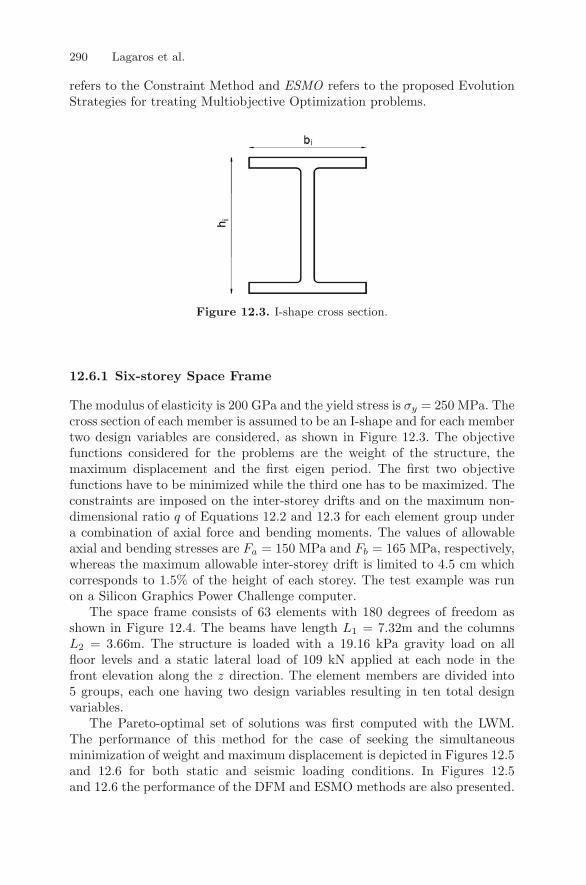
Figure 12.3. I-shape cross section.

12.6.1 Six-storey Space Frame

The modulus of elasticity is 200 GPa and the yield stress is σy = 250 MPa. Thecross section of each member is assumed to be an I-shape and for each membertwo design variables are considered, as shown in Figure 12.3. The objectivefunctions considered for the problems are the weight of the structure, themaximum displacement and the first eigen period. The first two objectivefunctions have to be minimized while the third one has to be maximized. Theconstraints are imposed on the inter-storey drifts and on the maximum non-dimensional ratio q of Equations 12.2 and 12.3 for each element group undera combination of axial force and bending moments. The values of allowableaxial and bending stresses are Fa = 150 MPa and Fb = 165 MPa, respectively,whereas the maximum allowable inter-storey drift is limited to 4.5 cm whichcorresponds to 1.5% of the height of each storey. The test example was runon a Silicon Graphics Power Challenge computer.

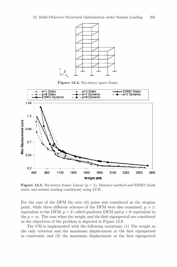
The space frame consists of 63 elements with 180 degrees of freedom asshown in Figure 12.4. The beams have length L1 = 7.32m and the columnsL2 = 3.66m. The structure is loaded with a 19.16 kPa gravity load on allfloor levels and a static lateral load of 109 kN applied at each node in thefront elevation along the z direction. The element members are divided into5 groups, each one having two design variables resulting in ten total designvariables.

The Pareto-optimal set of solutions was first computed with the LWM.The performance of this method for the case of seeking the simultaneousminimization of weight and maximum displacement is depicted in Figures 12.5and 12.6 for both static and seismic loading conditions. In Figures 12.5and 12.6 the performance of the DFM and ESMO methods are also presented.


Figure 12.4. Six-storey space frame.

Figure 12.5. Six-storey frame: Linear (p = 1), Distance method and ESMO (bothstatic and seismic loading conditions) using LVM.

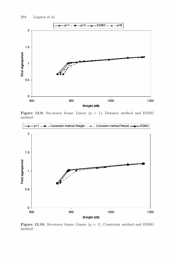
For the case of the DFM the zero (0) point was considered as the utopianpoint, while three different schemes of the DFM were also examined, p = 1:equivalent to the LWM, p = 2: called quadratic LWM and p = 8: equivalent tothe p = ∞. The case when the weight and the first eigenperiod are consideredas the objectives of the problem is depicted in Figure 12.9.

The CM is implemented with the following variations: (1) The weight asthe only criterion and the maximum displacement or the first eigenperiodas constraint; and (2) the maximum displacement or the first eigenperiod

292 Lagaros et al.

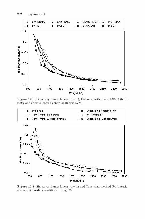
Figure 12.6. Six-storey frame: Linear (p = 1), Distance method and ESMO (bothstatic and seismic loading conditions)using LVM.

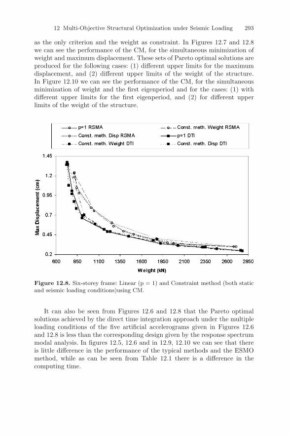
Figure 12.7. Six-storey frame: Linear (p = 1) and Constraint method (both staticand seismic loading conditions) using CM.


as the only criterion and the weight as constraint. In Figures 12.7 and 12.8we can see the performance of the CM, for the simultaneous minimization ofweight and maximum displacement. These sets of Pareto optimal solutions areproduced for the following cases: (1) different upper limits for the maximumdisplacement, and (2) different upper limits of the weight of the structure.In Figure 12.10 we can see the performance of the CM, for the simultaneousminimization of weight and the first eigenperiod and for the cases: (1) withdifferent upper limits for the first eigenperiod, and (2) for different upperlimits of the weight of the structure.

Figure 12.8. Six-storey frame: Linear (p = 1) and Constraint method (both staticand seismic loading conditions)using CM.

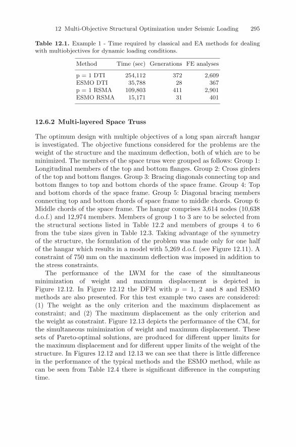
It can also be seen from Figures 12.6 and 12.8 that the Pareto optimalsolutions achieved by the direct time integration approach under the multipleloading conditions of the five artificial accelerograms given in Figures 12.6and 12.8 is less than the corresponding design given by the response spectrummodal analysis. In figures 12.5, 12.6 and in 12.9, 12.10 we can see that thereis little difference in the performance of the typical methods and the ESMOmethod, while as can be seen from Table 12.1 there is a difference in thecomputing time.

294 Lagaros et al.

Figure 12.9. Six-storey frame: Linear (p = 1), Distance method and ESMOmethod.

Figure 12.10. Six-storey frame: Linear (p = 1), Constraint method and ESMOmethod


Table 12.1. Example 1 - Time required by classical and EA methods for dealingwith multiobjectives for dynamic loading conditions.

Method Time (sec) Generations FE analyses

p = 1 DTI 254,112 372 2,609ESMO DTI 35,788 28 367p = 1 RSMA 109,803 411 2,901ESMO RSMA 15,171 31 401

12.6.2 Multi-layered Space Truss

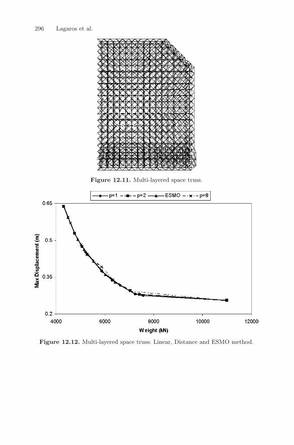
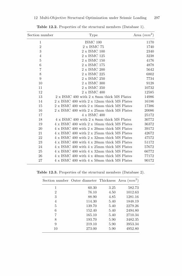
The optimum design with multiple objectives of a long span aircraft hangaris investigated. The objective functions considered for the problems are theweight of the structure and the maximum deflection, both of which are to beminimized. The members of the space truss were grouped as follows: Group 1:Longitudinal members of the top and bottom flanges. Group 2: Cross girdersof the top and bottom flanges. Group 3: Bracing diagonals connecting top andbottom flanges to top and bottom chords of the space frame. Group 4: Topand bottom chords of the space frame. Group 5: Diagonal bracing membersconnecting top and bottom chords of space frame to middle chords. Group 6:Middle chords of the space frame. The hangar comprises 3,614 nodes (10,638d.o.f.) and 12,974 members. Members of group 1 to 3 are to be selected fromthe structural sections listed in Table 12.2 and members of groups 4 to 6from the tube sizes given in Table 12.3. Taking advantage of the symmetryof the structure, the formulation of the problem was made only for one halfof the hangar which results in a model with 5,269 d.o.f. (see Figure 12.11). Aconstraint of 750 mm on the maximum deflection was imposed in addition tothe stress constraints.

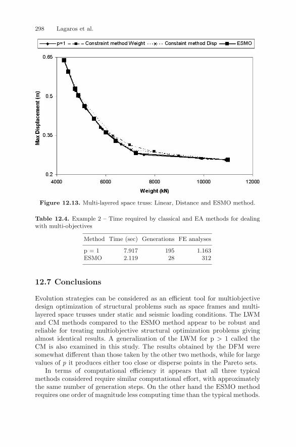
The performance of the LWM for the case of the simultaneousminimization of weight and maximum displacement is depicted inFigure 12.12. In Figure 12.12 the DFM with p = 1, 2 and 8 and ESMOmethods are also presented. For this test example two cases are considered:(1) The weight as the only criterion and the maximum displacement asconstraint; and (2) The maximum displacement as the only criterion andthe weight as constraint. Figure 12.13 depicts the performance of the CM, forthe simultaneous minimization of weight and maximum displacement. Thesesets of Pareto-optimal solutions, are produced for different upper limits forthe maximum displacement and for different upper limits of the weight of thestructure. In Figures 12.12 and 12.13 we can see that there is little differencein the performance of the typical methods and the ESMO method, while ascan be seen from Table 12.4 there is significant difference in the computingtime.

296 Lagaros et al.

Figure 12.11. Multi-layered space truss.

Figure 12.12. Multi-layered space truss: Linear, Distance and ESMO method.


Table 12.2. Properties of the structural members (Database 1).

Section number Type Area (mm2)

1 ISMC 100 11702 2 x ISMC 75 17403 2 x ISMC 100 23404 2 x ISMC 125 32385 2 x ISMC 150 41766 2 x ISMC 175 48787 2 x ISMC 200 56428 2 x ISMC 225 68029 2 x ISMC 250 773410 2 x ISMC 300 912811 2 x ISMC 350 1073212 2 x ISMC 400 1258513 2 x ISMC 400 with 2 x 8mm thick MS Plates 1498614 2 x ISMC 400 with 2 x 12mm thick MS Plates 1618615 2 x ISMC 400 with 2 x 16mm thick MS Plates 1738616 2 x ISMC 400 with 2 x 25mm thick MS Plates 2008617 4 x ISMC 400 2517218 4 x ISMC 400 with 2 x 8mm thick MS Plates 3077219 4 x ISMC 400 with 2 x 16mm thick MS Plates 3637220 4 x ISMC 400 with 2 x 20mm thick MS Plates 3917221 4 x ISMC 400 with 2 x 25mm thick MS Plates 4267222 4 x ISMC 400 with 2 x 32mm thick MS Plates 4757223 4 x ISMC 400 with 4 x 20mm thick MS Plates 5117224 4 x ISMC 400 with 4 x 25mm thick MS Plates 5767225 4 x ISMC 400 with 4 x 32mm thick MS Plates 6677226 4 x ISMC 400 with 4 x 40mm thick MS Plates 7717227 4 x ISMC 400 with 4 x 50mm thick MS Plates 90172

Table 12.3. Properties of the structural members (Database 2).

Section number Outer diameter Thickness Area (mm2)

1 60.30 3.25 582.732 76.10 4.50 1012.633 88.90 4.85 1281.164 114.30 5.40 1848.195 139.70 5.40 2279.266 152.40 5.40 2494.807 165.10 5.40 2710.348 193.70 5.90 3482.359 219.10 5.90 3953.3410 273.00 5.90 4952.80

298 Lagaros et al.

Figure 12.13. Multi-layered space truss: Linear, Distance and ESMO method.

Table 12.4. Example 2 – Time required by classical and EA methods for dealingwith multi-objectives

Method Time (sec) Generations FE analyses

p = 1 7.917 195 1.163ESMO 2.119 28 312

12.7 Conclusions

Evolution strategies can be considered as an efficient tool for multiobjectivedesign optimization of structural problems such as space frames and multi-layered space trusses under static and seismic loading conditions. The LWMand CM methods compared to the ESMO method appear to be robust andreliable for treating multiobjective structural optimization problems givingalmost identical results. A generalization of the LWM for p > 1 called theCM is also examined in this study. The results obtained by the DFM weresomewhat different than those taken by the other two methods, while for largevalues of p it produces either too close or disperse points in the Pareto sets.

In terms of computational efficiency it appears that all three typicalmethods considered require similar computational effort, with approximatelythe same number of generation steps. On the other hand the ESMO methodrequires one order of magnitude less computing time than the typical methods.


The presented results indicate that it is possible to achieve an optimal designunder seismic loading. Both design methodologies based on a number ofartificially generated earthquakes and the response spectrum modal analysisadopted by the seismic codes have been implemented and compared. Themore rigorous dynamic approach based on time history analyses gives moreeconomic designs than the approximate response spectrum modal analysis, atthe expense of requiring more computational effort.

References

1. Fonseca, CM, and Fleming, PJ, An Overview of Evolutionary Algorithms inMultiobjective Optimization, Evolutionary Computations, 1995; 3: 1-16.

2. Stadler, W, Natural Structural Shapes of Shallow Arches, Journal of AppliedMechanics, 1977; 44: 291-298.

3. Leitmann, G, Some Problems of Scalar and Vector-valued Optimization inLinear Viscoelasticity, Journal of Optimization Theory and Applications, 1977;23: 93-99.

4. Stadler, W, Natural Structural Shapes (The Static Case), Quarterly Journal ofMechanics and Applied Mathematics, 1978; 31: 169-217.

5. Gerasimov, EN, and Repko, VN, Multi-criteria Optimization, Soviet AppliedMechanics, 1978; 14: 1179-1184.

6. Koski, J, Truss Optimization with Vector Criterion, Publication No. 6, TampereUniversity of Technology, 1979.

7. Cohon, JL, Multi-objective Programming and Planning, New York, AcademicPress, 1978.

8. Papadrakakis, M, Lagaros, ND, and Plevris, V, Optimum Design of SpaceFrames Under Seismic Loading, International Journal of Structural Stabilityand Dynamics, 2001; 1: 105-124.

9. Cassis, JH, Optimum Design of Structures Subjected to Dynamic Loads, PhDThesis, University of California, Los Angeles, 1974.

10. Johnson, EH, Disjoint Design Spaces in Optimization of Harmonically ExcitedStructures, AIAA Journal, 1976; 14: 259-261.

11. Eurocode 3, Design of Steel Structures, Part1.1: General Rules for Buildings,CEN, ENV 1993-1-1/1992.

12. Pareto, V, Cours d’economique Politique, vol. 1&2, Lausanne, Rouge, 1897.13. Adali, S, Pareto Optimal Design of Beams Subjected to Support Motion,

Computers and Structures, 1983; 16: 297-303.14. Baier, H, Structural Optimization in Industrial Environment, In H Eschenauer

and N Olhoff (eds.) Optimization Methods in Structural Design, Proceedings ofthe Euromech-Colloquium 164, University of Siegen, Bibliographisches InstitutA6, Zurich, pp. 140-145, 1983.

15. Diaz, A, Sensitivity Information in Multiobjective Optimization, EngineeringOptimization, 1987; 12:281-297.

16. Hajela, P, and Shih, CJ, Multi-objective Optimum Design in Mixed Integer andDiscrete Design Variable Problems, AIAA Journal, 1990; 28: 670-675.

17. Rozvany, GIN Structural Design via Optimality Criteria, Dordecht, Kluwer,1989.

300 Lagaros et al.

18. Goicoechea, A, Hansen DR, and Duckstein L, Multi-objective Decision Analysiswith Engineering and Business Applications, New York, Wiley, 1982.

19. Koski, J, Bicriterion Optimum Design Method for Elastic Trusses, ActaPolytechnica Scandinavica, Mechanical engineering series No 86, Dissertation,Helsinki, 1984.

20. Sandgren, E, Multicriteria Design Optimization by Goal Programming, In HAdeli (ed.) Advances in Design Optimization, Chapman & Hall, pp. 225-265,1994.

21. Kamal, CS, and Adeli, H, Fuzzy Discrete Multicriteria Cost Optimization ofSteel Structures, Journal of Structural Engineering, 2000; 126: 1339-1347.

22. Schaffer, JD. Multiple Objective Optimization with Vector Evaluated GeneticAlgorithms, PhD thesis, Vanderbilt University, 1984.

23. Fonseca, CM, and Fleming, PJ, Genetic Algorithms for MultiobjectiveOptimization: Formulation, Discussion and Generalization, In S Forrest S (ed.)Proceedings of the 5th International Conference on Genetic Algorithms, SanMateo, California, Morgan Kaufmann, pp. 416-423, 1993.

24. Horn, J, Nafpliotis, N, and Goldberg, DE, A Niched Pareto Genetic Algorithmfor Multiobjective Optimization, In Proceedings of the 1st IEEE Conferenceon Evolutionary Computation, IEEE World Congress on EvolutionaryComputation, Volume 1, Piscataway, NJ, pp. 82-87, 1994.

25. Deb, K, and Goldberg, DE, An Investigation of Niche and Species Formationin Genetic Function Optimization, In JD Schaffer (ed.) Proceedings of the3rd International Conference on Genetic Algorithms, San Mateo, California,Morgan Kaufmann, pp. 42-50, 1989.

26. Hajela, P, and Lin, CY, Genetic Search Strategies in Multicriterion OptimalDesign, Structural Optimization, 1992; 4: 99-107.

27. Zitzler, E, Evolutionary Algorithms for Multiobjective Optimization: Methodsand Applications, PhD thesis, Swiss Federal Institute of Technology Zurich,Computer Engineering and Networks Laboratory, 1999.

28. Goldberg, DE, and Richardson, J, Genetic Algorithms with Sharing forMultimodal Function Optimization, In JJ Grefenstette (ed) Genetic Algorithmsand Their Applications, Proceedings of the 2nd International Conference onGenetic Algorithms, Hillsdale, NJ, Lawrence Erlbaum, pp. 41-49, 1987.

29. Taylor, CA, EQSIM, A Program for Generating Spectrum CompatibleEarthquake Ground Acceleration Time Histories, Reference Manual, BristolEarthquake Engineering Data Acquisition and Processing System, December,1989.

30. Rechenberg, I, Evolution Strategy: Optimization of Technical SystemsAccording to the Principles of Biological Evolution, Stuttgart, Frommann-Holzboog, 1973.

31. Schwefel, HP, Numerical Optimization for Computer Models, Chi Chester, UK,Wiley & Sons, 1981.

multiobjective optimization of space structures under static and seismic loading conditions

Documents