multimode collocated vibration control with multiple piezoelectric transducers
TRANSCRIPT

Multimode Collocated Vibration Control with Multiple
Piezoelectric Transducers
Ivan Giorgio
To cite this version:
Ivan Giorgio. Multimode Collocated Vibration Control with Multiple Piezoelectric Transducers.Mechanical engineering. Universita degli studi di Roma I, 2008. English. <tel-00798635>
HAL Id: tel-00798635
https://tel.archives-ouvertes.fr/tel-00798635
Submitted on 9 Mar 2013
HAL is a multi-disciplinary open accessarchive for the deposit and dissemination of sci-entific research documents, whether they are pub-lished or not. The documents may come fromteaching and research institutions in France orabroad, or from public or private research centers.
L’archive ouverte pluridisciplinaire HAL, estdestinee au depot et a la diffusion de documentsscientifiques de niveau recherche, publies ou non,emanant des etablissements d’enseignement et derecherche francais ou etrangers, des laboratoirespublics ou prives.

Ivan Giorgio
Multimode Collocated Vibration Control with Multiple
Piezoelectric Transducers
June 2008


PhD in
Theoretical and Applied Mechanics
XX Cycle
Multimode Collocated Vibration Control with
Multiple Piezoelectric Transducers
by
Ivan Giorgio
Thesis submitted in conformity with the requirements
for the Degree of
Doctor of Philosophy
Tutor:
prof. Dionisio Del Vescovo
Printed on August 18, 2008

Ivan Giorgio: Multimode Collocated Vibration Control with Multiple Piezoelectric
Transducers, © June 2008

Abstract
Multimode Collocated Vibration Control with Multiple
Piezoelectric Transducers
In this thesis a new approach is presented to control vibrations for one-
and two-dimensional mechanical structures, as beam or thin plates, by means
of several piezoelectric transducers shunted with a proper electric network
system. The governing equations for the whole system are coupled to each
other through the direct and converse piezoelectric effect. The mechanical
equations are expressed in accordance with the modal theory considering n
vibration modes, that in need of control, and the electrical equations reduce
to the one-dimensional charge equation of electrostatics for each of n consid-
ered piezoelectric transducers. In this electromechanical system, a shunting
electric device forms an electric subsystem working as multi-degree of free-
dom damped vibration absorber for the mechanical subsystem. Herein, it is
introduced a proper transformation of the electric coordinates in order to
approximate the governing equations for the whole shunted system with n
uncoupled, single mode piezoelectric shunting systems that can be readily
damped by the methods reported in literature. A further numerical optimisa-
tion problem on the spatial distribution of the piezoelectric elements allows
to achieve an effective multi-mode damping. Numerical case studies of two
relevant systems, a double clamped beam and a fully clamped plate, allow
to take into account issues relative to the proposed approach for vibration
control. Laboratory experiments carried out in real time on a beam clamped
at both ends consent to validate the proposed technique.


“The unexamined life is not worth living”
(Plato, The Apology of Socrates [38a])


Whœver limiting his worldly ambitions
finds satisfaction in the speculative life
has in the approval of an enlightened and competent judge
a powerful incentive to labours,
the benefits of whi are great but remote,
and therefore su as the vulgar altogether fail to recognise.
To su a judge and to his gracious attention
I now dedicate this work.


Preface
The immediate reason to draw up this thesis is the necessity to summarise
all the work done by me in three years of study, in accordance with my duty,
given that1:
“... non fa scïenza,
sanza lo ritenere avere inteso.”
Two are criteria that have driven me to write this thesis: comprehensibil-
ity and synthesis. I have chosen to provide both examples and explanations
in order to satisfy the first criterion, albeit these involve a larger length of
this work. It is true that Abbot Terrasson tells us that if the size of a book were
measured not by the number of its pages but by the time required to understand
it, then we could say about many books that they would be much shorter if they
were not so short. Examples and explanations certainly make easier to under-
stand the written but they also involve some inopportune effects. In fact, if
we are concerned with the distinctness and the comprehensibility of a volu-
minous whole of speculative cognition that yet coheres in one principle, then
we could just as legitimately say that many books would have turned out much
more distinct if they had not been intended to be quite so distinct that is, “clear”
in the popular sense —plenty of examples. For the aids to distinctness, while
helpful in parts of a book, are often distracting in the book as a whole. They
keep the reader from arriving quickly enough at an overview of the whole;
and with all their bright colours they do cover up and conceal the articula-
tion of the dissertation. However, if we are concerned with the synthesis, it
is worth saying that examples and explanations are necessary for a popular
publication but this report is written primarily for engineers, and they do not
1Dante Alighieri (1265–1321). La Divina Commedia, Par., V, 41–42.
VII

Preface
need of these facilities. Hence, as good as always, I have tried to achieve a
right balance taking into account all these points of view.
Acknowledgments
I would like to thank my supervisor Dionisio Del Vescovo, for his many
suggestions and constant support during this research. I am also thankful to
Antonio Culla and Corrado Maurini for their guidance and friendly encourage-
ment, which gave me a better perspective on my own results and provided
many useful references.
Of course, I am grateful to my parents for their patience and love. Without
them this work would never have come into existence. In particular I would
like to acknowledge the “Laboratoire de Modélisation en Mécanique” (CNRS-
UMR 7607, University of Paris 6).
Rome, Italy Ivan Giorgio
June 2008
VIII

Contents
Introduction 1
I Vibration Control Using Piezoelectric Transducers 11
I.1 Modal Approach to Modelling . . . . . . . . . . . . . . . . . . . 12
I.2 An Independent Modal-Space Shunt Damping Technique . . . 15
I.2.1 Linear Transformation for Independent Control . . . . . 21
I.2.2 Piezoelectric Placement for Independent Control . . . . 23
I.3 Two-Equation Systems Uncoupled . . . . . . . . . . . . . . . . . 24
I.4 Controllability and Observability . . . . . . . . . . . . . . . . . . 26
I.5 Vibration Control with a Single Piezoelectric Transducer . . . . 27
I.6 Generalised Passive Approach . . . . . . . . . . . . . . . . . . . 27
I.6.1 Parallel Configuration . . . . . . . . . . . . . . . . . . . . 28
I.6.2 Series Configuration . . . . . . . . . . . . . . . . . . . . . 34
I.6.3 Comparisons . . . . . . . . . . . . . . . . . . . . . . . . . 38
I.7 Generalised Hybrid Approach . . . . . . . . . . . . . . . . . . . 41
I.7.1 A Passive Shunt Circuit with Compensating Action . . . 44
I.8 Generalised Active Control . . . . . . . . . . . . . . . . . . . . . 45
I.8.1 Optimal Control in the Time Domain . . . . . . . . . . . 48
I.8.2 Pole Allocation with State Feedback Control . . . . . . . 49
I.8.3 State Estimation . . . . . . . . . . . . . . . . . . . . . . . . 50
I.9 Control and Observer Spillover . . . . . . . . . . . . . . . . . . . 52
II Physical System Models 54
II.1 First Order Theory of Thin Plates . . . . . . . . . . . . . . . . . . 54
II.1.1 Introduction . . . . . . . . . . . . . . . . . . . . . . . . . . 54
II.1.2 Hamiltonian Formulation . . . . . . . . . . . . . . . . . . 57
II.2 Piezoelectric Transducers . . . . . . . . . . . . . . . . . . . . . . 59
IX

Contents
II.2.1 General Notices . . . . . . . . . . . . . . . . . . . . . . . . 59
II.2.2 Equations of Plate with Transducers . . . . . . . . . . . . 64
II.3 Modal Analysis . . . . . . . . . . . . . . . . . . . . . . . . . . . . 68
II.4 Finite Element Model . . . . . . . . . . . . . . . . . . . . . . . . . 69
III Numerical Simulations 72
III.1 Clamped-Clamped Beam Case Study . . . . . . . . . . . . . . . 72
III.1.1 Numerical Results . . . . . . . . . . . . . . . . . . . . . . 77
III.2 Fully Clamped Plate Case Study . . . . . . . . . . . . . . . . . . 83
III.2.1 Piezoelectric Transducer Allocation . . . . . . . . . . . . 83
III.2.2 Numerical Results and Comparisons . . . . . . . . . . . 86
IV Laboratory Experiments 93
IV.1 Experimental Set Up . . . . . . . . . . . . . . . . . . . . . . . . . 93
IV.1.1 Mobility Estimations . . . . . . . . . . . . . . . . . . . . . 94
IV.2 System Identification . . . . . . . . . . . . . . . . . . . . . . . . . 97
IV.2.1 Mechanical Parameters . . . . . . . . . . . . . . . . . . . 97
IV.2.2 Piezoelectric Parameters . . . . . . . . . . . . . . . . . . . 102
IV.3 Control Validation . . . . . . . . . . . . . . . . . . . . . . . . . . 107
IV.3.1 The Control System . . . . . . . . . . . . . . . . . . . . . 107
IV.3.2 Results . . . . . . . . . . . . . . . . . . . . . . . . . . . . . 108
Conclusions 112
A Rectangular Plates 115
A.1 Newtonian Formulation . . . . . . . . . . . . . . . . . . . . . . . 115
A.2 Hamiltonian Formulation . . . . . . . . . . . . . . . . . . . . . . 119
A.3 Vibration of Fully Clamped Plates . . . . . . . . . . . . . . . . . 121
A.4 Modal Analysis with the Finite Element Model . . . . . . . . . 130
Bibliography 143
X

List of Figures
1 Crystals without a permanent polarisation . . . . . . . . . . . . 5
2 Ferroelectric crystals . . . . . . . . . . . . . . . . . . . . . . . . . 6
I.1 Block diagram of the electro-mechanical system . . . . . . . . . 24
I.2 Shunt circuit in parallel configuration . . . . . . . . . . . . . . . 28
I.3 Root locus for parallel shunt circuit . . . . . . . . . . . . . . . . 32
I.4 Mobilities for parallel shunt circuit . . . . . . . . . . . . . . . . . 34
I.5 Shunt circuit in series configuration . . . . . . . . . . . . . . . . 35
I.6 Mobilities for series shunt circuit . . . . . . . . . . . . . . . . . . 39
I.7 Sensitivity functions for fixed points method . . . . . . . . . . . 39
I.8 Sensitivity functions for pole allocation method . . . . . . . . . 40
I.9 Ratio between the mobility peaks for passive circuit . . . . . . . 41
I.10 Shunt circuit with compensating action . . . . . . . . . . . . . . 44
I.11 Mobilities with different compensating actions . . . . . . . . . . 46
I.12 Sensitivity functions with different compensating actions . . . . 46
I.13 Mobilities for active control . . . . . . . . . . . . . . . . . . . . . 50
I.14 Sensitivity functions for active control . . . . . . . . . . . . . . . 51
I.15 Block diagram of the observer estimate . . . . . . . . . . . . . . 52
II.1 Plate representation . . . . . . . . . . . . . . . . . . . . . . . . . . 55
II.2 Scheme of the piezoelectric transducers . . . . . . . . . . . . . . 60
II.3 A detail of the scheme for modelling the system with FEM . . . 70
III.1 Piezoelectric transducers placement on the beam . . . . . . . . 75
III.2 Simulink model . . . . . . . . . . . . . . . . . . . . . . . . . . . . 76
III.3 Beam mobility for passive approach in parallel configuration . 79
III.4 Beam mobility for passive approach in series configuration . . 80
III.5 Beam mobility for hybrid approach in parallel configuration . . 80
XI

List of Figures
III.6 Beam mobility for active approach . . . . . . . . . . . . . . . . . 81
III.7 Beam impulse response for passive approach in parallel con-
figuration . . . . . . . . . . . . . . . . . . . . . . . . . . . . . . . . 81
III.8 Beam impulse response for hybrid approach in parallel config-
uration . . . . . . . . . . . . . . . . . . . . . . . . . . . . . . . . . 82
III.9 Beam impulse response for active approach . . . . . . . . . . . . 82
III.10Smart Plate . . . . . . . . . . . . . . . . . . . . . . . . . . . . . . . 83
III.11Piezoelectric placement index . . . . . . . . . . . . . . . . . . . . 85
III.12Plate mobility for passive approach in parallel configuration . . 87
III.13Plate mobility for hybrid approach in parallel configuration . . 88
III.14Plate mobility for active approach . . . . . . . . . . . . . . . . . 88
III.15Plate impulse response for passive approach in parallel config-
uration . . . . . . . . . . . . . . . . . . . . . . . . . . . . . . . . . 89
III.16Plate impulse response for hybrid approach in parallel config-
uration . . . . . . . . . . . . . . . . . . . . . . . . . . . . . . . . . 89
III.17Plate impulse response for active approach . . . . . . . . . . . . 90
III.18Electrical scheme for current flowing control . . . . . . . . . . . 90
III.19Comparison of the proposed and the current flowing control . 92
IV.1 Beam representation . . . . . . . . . . . . . . . . . . . . . . . . . 94
IV.2 Mobility of the beam actuated by the first piezo-element . . . . 96
IV.3 Mobility of the beam actuated by the second piezo-element . . 96
IV.4 Mobility of the beam actuated by the third piezo-element . . . 97
IV.5 Regenerated mobility of the beam actuated by the first piezo-
element . . . . . . . . . . . . . . . . . . . . . . . . . . . . . . . . . 99
IV.6 Nyquist plot of mobility of the beam actuated by the first piezo-
element . . . . . . . . . . . . . . . . . . . . . . . . . . . . . . . . . 99
IV.7 Regenerated mobility of the beam actuated by the second piezo-
element . . . . . . . . . . . . . . . . . . . . . . . . . . . . . . . . . 100
IV.8 Nyquist plot of mobility of the beam actuated by the second
piezo-element . . . . . . . . . . . . . . . . . . . . . . . . . . . . . 100
IV.9 Regenerated mobility of the beam actuated by the third piezo-
element . . . . . . . . . . . . . . . . . . . . . . . . . . . . . . . . . 101
IV.10Nyquist plot of mobility of the beam actuated by the third
piezo-element . . . . . . . . . . . . . . . . . . . . . . . . . . . . . 101
XII

List of Figures
IV.11Regenerated impedance of the first piezo-transducer . . . . . . 104
IV.12Nyquist plot of impedance of the first piezo-transducer . . . . . 104
IV.13Regenerated impedance of the second piezo-transducer . . . . 105
IV.14Nyquist plot of impedance of the second piezo-transducer . . . 105
IV.15Regenerated impedance of the third piezo-transducer . . . . . . 106
IV.16Nyquist plot of impedance of the third piezo-transducer . . . . 106
IV.17 FRF function of the beam to measure coupling coefficients . . . 108
IV.18Simulink model for the real-time application . . . . . . . . . . . 109
IV.19 Inertance with control of the first and the second mode . . . . . 109
IV.20 Inertance with control of the first and the third mode . . . . . . 110
IV.21 Inertance with control of the second and the third mode . . . . 110
A.1 Convention for loads acting on the plate . . . . . . . . . . . . . 116
A.2 Plate characteristic functions . . . . . . . . . . . . . . . . . . . . 129
A.3 First mode shape of the plate . . . . . . . . . . . . . . . . . . . . 130
A.4 Second mode shape of the plate . . . . . . . . . . . . . . . . . . 131
A.5 Third mode shape of the plate . . . . . . . . . . . . . . . . . . . 131
A.6 Fourth mode shape of the plate . . . . . . . . . . . . . . . . . . . 132
A.7 Fifth mode shape of the plate . . . . . . . . . . . . . . . . . . . . 132
A.8 First mode rotation around the axis X of the plate . . . . . . . . 133
A.9 Second mode rotation around the axis X of the plate . . . . . . 133
A.10 Third mode rotation around the axis X of the plate . . . . . . . 134
A.11 Fourth mode rotation around the axis X of the plate . . . . . . 134
A.12 Fifth mode rotation around the axis X of the plate . . . . . . . . 135
A.13 First mode rotation around the axis Y of the plate . . . . . . . . 135
A.14 Second mode rotation around the axis Y of the plate . . . . . . 136
A.15 Third mode rotation around the axis Y of the plate . . . . . . . 136
A.16 Fourth mode rotation around the axis Y of the plate . . . . . . . 137
A.17 Fifth mode rotation around the axis Y of the plate . . . . . . . . 137
XIII

List of Tables
II.1 Voigt notation . . . . . . . . . . . . . . . . . . . . . . . . . . . . . 62
III.1 Piezoelectric properties . . . . . . . . . . . . . . . . . . . . . . . . 73
III.2 Specifications of the piezoelectric transducers . . . . . . . . . . 74
III.3 Plate specifications . . . . . . . . . . . . . . . . . . . . . . . . . . 84
III.4 Parameters of the current flowing circuits used for comparison 91
IV.1 Damping ratio of the bending modes . . . . . . . . . . . . . . . 98
IV.2 Resonance frequencies of the beam . . . . . . . . . . . . . . . . . 102
IV.3 Curve-fitting estimated piezoelectric coupling coefficients . . . 103
IV.4 Curve-fitting estimated piezoelectric capacitances . . . . . . . . 103
IV.5 Measured piezoelectric coupling coefficients . . . . . . . . . . . 107
IV.6 Predicted piezoelectric coupling coefficients . . . . . . . . . . . 107
A.1 SS mode parameters . . . . . . . . . . . . . . . . . . . . . . . . . 127
A.2 SA mode parameters . . . . . . . . . . . . . . . . . . . . . . . . . 127
A.3 AS mode parameters . . . . . . . . . . . . . . . . . . . . . . . . . 127
A.4 AA mode parameters . . . . . . . . . . . . . . . . . . . . . . . . . 128
XIV

Introduction
Piezoelectric materials have been a great expansion in the engineering
application of structural control. One reason for this is that it may be
possible to create certain types of systems capable of adapting to or correct-
ing for changing operating conditions. The advantage of incorporating these
special types of material into the structure is that the sensing and actuating
mechanism becomes part of the structure.
In the last years the employ of structures more and more thin had made
arise numerous issues regarding vibrations. The challenge of reliability and
durability of mechanical structures is an important task for engineers, the
design of systems leading to the efficient control of structural vibrations in
order to reduce fatigue load, crack propagation and damage appears to be an
attractive opportunity. Then the object of this dissertation is to investigate the
possibility to reduce vibrations. Thus, the topics presented in this research
work are chiefly concerned with application to mechanical vibrations, sys-
tem identification, automotive, railway and aerospace industries. To take into
account a possible effective control, piezoelectric transducers are employed.
This is primarily due to their abilities but also to the growing availability
of more efficient piezoelectric ceramics. Smart structures using piezoelec-
tric material are successfully employed in reducing vibration [Alessandroni
et al., 2005; Dosch et al., 1992; Anderson and Hagood, 1994; Hollkamp and
Starchville, 1994; Badel et al., 2006; Wu, 1998; Tang and Wang, 2001; dell’Isola
and Vidoli, 1998; Thorp et al., 2001]. Piezoelectric materials produce a voltage
when strained and conversely strain when undergone to a voltage. This prop-
erty is very interesting, because a piezoelectric element can be indifferently
used either as a sensor or an actuator. Moreover, these piezoelectric element
skills can be simultaneously employed to obtain a collocated sensor-actuator
1

Introduction
control and to achieve with ease a stable control. The piezoelectric transduc-
ers coupled to mechanical structures can convey the mechanical energy flow
toward electric network systems where it is dissipated: it is a piezoelectric
shunt-damping. The use of the piezoelectric shunt damping technique for vi-
bration reduction in one and two dimensional flexible structures is a very
common practice because of the strong electromechanical coupling associ-
ated with currently available piezoelectric transducers. In this technique the
piezoelectric transducers, bonded on the flexible structure, are shunted by
a passive electric network that acts as a damped vibration absorber for the
host mechanical structure. A classical application of this method is a single
resonant piezoelectric shunting system studied in [Hagood and Flotow, 1991;
Wu, 1996]. The damper is formed by a piezoelectric element shunted with an
inductor and a resistor. The external shunt circuit with the inherent piezo-
electric capacitance is a RLC circuit. Its natural frequency is imposed equal
to one natural frequency of the host mechanical structure by maximising the
energy exchange. The resistance role is to maximise the electric dissipation
of the energy coming from the mechanical structure. Its main drawback is
the requirement of high-value inductors, 10–1000 H, working at high-voltage.
For this reason, passive components are simulated by active circuits, synthetic
impedances or alternatively admittances, which require an external feeding.
Subsequent applications involve one piezoelectric transducer coupled with
a multi-resonant electric network to damp a set of mechanical modes. Hol-
lkamp’s circuit is one of this kind [Hollkamp, 1994]. The shunt circuit consists
of a set of branches whose main is an RL circuit. The other branches are RLC
shunts. The number of controlled mechanical modes is equal to the number
of the branches. An issue of this technique is the necessity of retuning the
circuit when a branch is added. Indeed, in [Hollkamp, 1994] is proposed no
closed-form tuning solution. Further approaches use multiple piezoelectric
transducers by shunting each of them to a proper multi-resonant electric net-
work [Moheimani et al., 2004]. In practice, to account for the undesired cross
influence of the shunt circuits on the mechanical modes to be controlled, a
fine-tuning is due.
In [dell’Isola and Vidoli, 1998; Andreaus et al., 2004; Maurini et al., 2004;
Alessandroni et al., 2005] systems with periodically distributed piezoelectric
2 of 143

Introduction
transducers and modular shunting networks are considered. This approach
adopts homogenised continuum modelling and looks for periodic lumped
electric systems having, in the continuum limit, the same dynamic behaviour
of the mechanical structure to be controlled. The drawback of this “contin-
uum mechanics” approach is the requirement of a high number of piezoelec-
tric elements and complicated shunting networks, in order to approach the
continuum limit. Moreover, different types of structures, e.g. beams or plates,
demand the solution of specific design problems. The theoretical and numeri-
cal results provided optimal electric networks for damping flexural vibrations
of beams [Andreaus et al., 2004; Maurini et al., 2004] and plates [Alessandroni
et al., 2005]; in reference [dell’Isola et al., 2004] a first experimental implemen-
tation is presented.
The interpretation of piezoelectric shunt damping systems as a feedback
control problem allows to employ this technique to realise collocated vibra-
tion active control in which piezoelectric transducers are used both as sensors
and actuators. In [Tang and Wang, 2001], it is proposed the use of “negative
capacitance” carrying out with an active devise op-amp based. Other appli-
cations perform active control systems no-collocated, as reported in [Rizet
et al., 2000], where the implementation of a modal filtering on a DSP board
is proposed to control the flexural vibrations of a beam.
Semi-active techniques [Badel et al., 2006; Niederberger and Morari, 2006]
develop non-linear switching shunting to avoid the use of high-value induc-
tors and to obtain a wide-band damping, with reduced power requirements.
As showed in [Niederberger and Morari, 2006], the switch shunt is less per-
forming but more robust than the standard RL shunt.
In conclusion, as underlined in [Chopra, 2002; Moheimani, 2003], the de-
velopment of efficient and reliable techniques for control with multiple pie-
zoelectric transducers remains an open problem.
The aim of this study is to extend the resonant shunting techniques to
control multiple modes with multiple piezoelectric transducers by an electric
network which connects the whole set of piezoelectric elements. The key idea
in this thesis is to make the whole shunted system equivalent to a set of
independent, single resonant piezoelectric shunting systems. Therefore, it is
possible to use the widely investigated methods presented in literature.
3 of 143

Introduction
A Brief Digression on Piezoelectricity
In 1880, the brothers Pierre and Jacques Curie predicted and demon-
strated piezoelectricity2. They showed that crystals of tourmaline, quartz and
Rochelle salt (sodium potassium tartrate tetrahydrate) generate electrical po-
larisation from mechanical stress. Quartz and Rochelle salt exhibited the most
piezoelectricity. Converse piezoelectricity was mathematically deduced from
fundamental thermodynamic principles by Lippmann in 1881. The Curies
immediately confirmed the existence of the “converse effect”, and went on
to obtain quantitative proof of the complete reversibility of electro-elasto-
mechanical deformations in piezoelectric crystals. More exactly the piezo-
electricity is the aptitude of a material to show polarisation charges on cer-
tain faces as a result of the application of mechanical stress. This effect is
called direct piezoelectric or piezo-generator. It is reversible, indeed, if one
imposes an external electric-field vector, the body will be strained in a way
that depends on the direction and magnitude of electric vector. This is in-
verse piezoelectric effect or piezo-motor. The deformation is of the order of
nanometres, nevertheless piezoelectric materials find useful applications such
as the production and detection of sound, generation of high voltages, elec-
tronic frequency generation, microbalance, and ultra-fine focusing of optical
assemblies.
Necessary condition for existence of the piezoelectric phenomenon is the
anisotropy of the material. Piezoelectric materials are crystals not having a
crystallographic symmetric centre. Punctual groups not-centre-symmetric are
21 of the 32 crystallographic classes and, more exactly, if one represents them
by an international standard, are
1, 2, 3, 4, 6,
m, mm2, 3m, 4, 4mm, 42m, 6, 6mm, 62m, 43m,
222, 32, 422, 622, 23, 432.
The piezoelectric phenomenon is possible only for 20 of these because the 432,
that belongs to the cubic system, even though not centre-symmetric, shows
characteristics of symmetry combining do not allow any piezoelectric effect.
2The word is derived from the Greek πιεζεω, which means I squeeze or press.
4 of 143

Introduction
P
f
f
3B
3A
1.1: Unloaded crystal.
P
f
f
3B
3A
1.2: Loaded crystal.
Figure 1: The subfigure 1.1 shows a crystal having a ternary symmetryaxis with lack of external loads. In this crystal are depicted electric dipolemoments on a proper crystallographic plane. The vector sum of elec-tric dipole moments is zero for each group of vectors. The subfigure 1.2shows a crystal undergone a compression by force,~f, that generates a po-larisation, ~P. The total vector sum of electric dipole moments is not morezero.
The piezoelectric phenomenon can be explained by two different exam-
ples. The former is characterised by the presence of some electric dipole mo-
ments for each elementary cell, whose vector sum is zero. If one applies a
mechanical or electric load in a given direction, a polar moment not-null
arises. Figure 1 sketches a simplified illustration of this case. A hydrostatics
pressure does not allow the piezoelectric phenomenon because the load is the
same in all directions. The quartz (SiO2) is a member of this class. The latter
is distinguished, in lack of external perturbations, by an electric dipole mo-
ment not-null, and so by only one permanent polar axis. Figure 2 depicts a
sketch of this second mechanism. They have a related property known as py-
roelectricity. This property, known as early as the 19th century and named by
David Brewster in 1824, is the aptitude of certain mineral crystals to generate
electrical charge on their surfaces in case they undergo an uniform heating.
This electric charge is proportional to the difference of temperature and it
is the result of electric dipole magnitude variation. It is worth to note that
even crystals not pyroelectric can show a superficial electric charge if it is
heated not uniformly, as consequence of internal stress due to thermal ex-
5 of 143

Introduction
P
P
P
f
f
A
B
2.1: Unloaded crystal.
P
P
P
f
f
A
B
2.2: Loaded crystal.
Figure 2: The subfigure 2.1 shows a crystal lattice having a permanentpolarisation, that is ferroelectric one in an undeformed state, where thepolarisation is due to the position not symmetric of the ion A+. Thesubfigure 2.2 shows a lattice in presence of a compression force,~f, thatproduced a variation of polarisation, ∆~P, the piezoelectric induced polar-isation.
pansion. Only 10 of the 20 not-symmetric-centre classes, written above, are
pyroelectric. These crystals, differently by those not having polar axis, shows
piezoelectric properties even in case of hydrostatics pressure. Examples of
pyroelectric crystals are the tourmaline3 and zinc oxide (ZnO).
Ferroelectric materials are particular pyroelectric crystals which have got
the ability to invert own electric dipole moment through the application of
electric field with appropriate strength. The presence of a dipole moment
not-null, however, is not sufficient to guarantee the ferroelectricity. Besides,
not all pyroelectric crystals can be ferroelectric; the electric field necessary to
obtain the inversion of dipole could be too strong and cause the breaking of
material. The graph of induced polarization4, ~P, or of stored charge, Q, ver-
sus to applied voltage, V, in ferroelectrics has a hysteretic cycle, in contrast
to other dielectrics that show a linear relationship. There is in this cycle a
residual polarisation ~Pr, whose verse is depend on history of V, that is the
3Tourmaline have general formulae: AX3Y6(BO3)3Si6O18(O, OH, F)4. In this A means cal-
cium or sodium; X means aluminium, iron, lithium or magnesium; Y means aluminium, and
less usually chrome or iron.4The polarisation is a vector quantity defined as the electric dipole moment per unit of
volume. Also called dielectric or electric polarisation.
6 of 143
Introduction
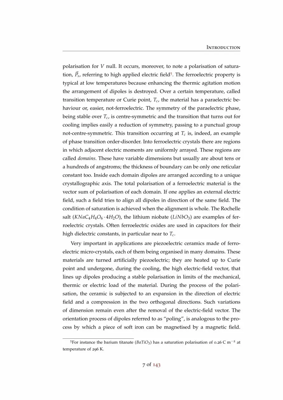
polarisation for V null. It occurs, moreover, to note a polarisation of satura-
tion, ~Ps, referring to high applied electric field5. The ferroelectric property is
typical at low temperatures because enhancing the thermic agitation motion
the arrangement of dipoles is destroyed. Over a certain temperature, called
transition temperature or Curie point, Tc, the material has a paraelectric be-
haviour or, easier, not-ferroelectric. The symmetry of the paraelectric phase,
being stable over Tc, is centre-symmetric and the transition that turns out for
cooling implies easily a reduction of symmetry, passing to a punctual group
not-centre-symmetric. This transition occurring at Tc is, indeed, an example
of phase transition order-disorder. Into ferroelectric crystals there are regions
in which adjacent electric moments are uniformly arrayed. These regions are
called domains. These have variable dimensions but usually are about tens or
a hundreds of angstroms; the thickness of boundary can be only one reticular
constant too. Inside each domain dipoles are arranged according to a unique
crystallographic axis. The total polarisation of a ferroelectric material is the
vector sum of polarisation of each domain. If one applies an external electric
field, such a field tries to align all dipoles in direction of the same field. The
condition of saturation is achieved when the alignment is whole. The Rochelle
salt (KNaC4H4O6 · 4H2O), the lithium niobate (LiNbO3) are examples of fer-
roelectric crystals. Often ferroelectric oxides are used in capacitors for their
high dielectric constants, in particular near to Tc.
Very important in applications are piezoelectric ceramics made of ferro-
electric micro-crystals, each of them being organised in many domains. These
materials are turned artificially piezoelectric; they are heated up to Curie
point and undergone, during the cooling, the high electric-field vector, that
lines up dipoles producing a stable polarisation in limits of the mechanical,
thermic or electric load of the material. During the process of the polari-
sation, the ceramic is subjected to an expansion in the direction of electric
field and a compression in the two orthogonal directions. Such variations
of dimension remain even after the removal of the electric-field vector. The
orientation process of dipoles referred to as “poling”, is analogous to the pro-
cess by which a piece of soft iron can be magnetised by a magnetic field.
5For instance the barium titanate (BaTiO3) has a saturation polarisation of 0.26 C m−2 at
temperature of 296 K.
7 of 143

Introduction
When the ceramic reaches the Curie point, it loses utterly and permanently
its piezoelectric properties. The Curie point provides the upper limit of the
temperature that can be achieved by a piezo-ceramic. The polarisation pro-
cess of the piezo-ceramics is explained by its ferroelectric properties. In the
ceramics, as it is comprehensible, a perfect alignment will never be obtained,
because of mechanical stresses and of defects in grains of the material that
does not allow the shift of the polar axis in the direction more favourable.
At first the piezo-ceramic was isotropic, owing to the random orientation of
micro-crystals; after the application of the electric field such isotropy is de-
stroyed in the direction of the polarisation axis, but it is maintained in the
plane orthogonal to it. Such a material is called orthotropic. It is undeni-
able that materials naturally piezoelectric have not grains with preferential
directions of polarisation, and so they have reduced capacity of macroscopic
deformation. The advantages of ceramic materials are summarised, without a
doubt, in high efficiency of transformation electro-mechanic, even above 50%,
in a good workable, in a lot of shapes obtainable, in a mass production. The
greater disadvantages are linked up to the possibility of depolarisation; cer-
tainly, significant electric fields in opposite directions to the polarisation, or
high alternating electric fields, or also important mechanical stresses, as well
as temperatures higher than Curie point involve the loss of the piezoelectric
property. It is important to note the phenomenon of the aging that is the
decrease of the piezoelectric properties with the pass of time from the polari-
sation. Solid solutions of lead titanate-zirconate Pb(Ti, Zr)O3, usually pointed
out with short form PZT, is the most popular piezoelectric material in use.
The success of these alloys stays on remarkable inducible polarisation and
in a high transition temperature, 493–623 K, that allows the variation of their
chemical composition by thermic treatments at high temperatures, changing
as a result also heavily any physic properties without a decay of piezoelectric
features. A PZT material shows strains of about 0.1% of the original dimen-
sion. They are divided into hard and soft PZT. The former has a narrow
hysteretic cycle, resists to high mechanical or electric loads, and besides ages
more slowly. It is suitable to be employed as generator and transducer with
high voltage or power. The latter has a large sensitivity and high dielectric
constants but the depolarisation and the heating turn out easy. It is used as
8 of 143

Introduction
sensor or transducer with high impedance.
Other materials with piezoelectric effect are piezo-polymers, as the poly-
vinyl difluoride, PVDF, and copolymers of vinylidene fluoride, VDF, trifluo-
roethylene, TrFE, e tetrafluoroethylene TeFE. Even they undergo a process of
poling completely analogous to that of piezo-ceramics. They are used at high
frequencies, in contrast with piezo-ceramics that cannot be used because too
fragile. These materials have a wide range of frequency of employment, a
low acoustic impedance, a high elastic deformation, as well as a high dielec-
tric strength6. They have, however, low acting temperatures and a modest
efficiency in the electro-mechanical conversion. In other words they are more
right as sensors rather than actuators. There are notable differences between
PVDF and PZT materials. For instance, on average, PZT is approximately
four times as dense, forty times stiffer, and has a permittivity one hundred
times as great as that of PVDF. Therefore, PVDF is much more compliant
and lightweight, making it more attractive for sensing applications, lessening
the insertion error. In contrast, PZT is often preferred as an actuator since it
exhibits a greater induced strain [Moheimani, 2003].
Finally there are piezo-composites too, or rather materials made of poly-
mers and piezo-ceramics.
Features of better consideration in a piezoelectric material are:
a) high efficiency of electro-mechanical transformation;
b) wide range of frequency of employment;
c) good stability at variation of environment conditions as the temperature
or the humidity;
d) easily workable;
e) several shapes obtainable.
Damages due to aging are typical of sensors and are negligible for ac-
tuators, because in actuators the material undergoes an electric-field vector
with the same direction of the polarisation. A further issue in piezoelectrics
6The maximum electrical field that a material can withstand without rupture; usually
specified in volts per millimetre of thickness. Also known as electric strength.
9 of 143
Introduction
is given by the creep. This last, however, is very small, at its maximum value
achieved in few hours it differs of 1% from last driven motion.
In the end, it is useful to note that electrostrictive materials are not pie-
zoelectric and possess no spontaneous polarisation. The electrostriction is a
form of elastic deformation of a dielectric induced by an applied electric field,
associated with those components of strain which are independent of reversal
of field direction, in contrast to the piezoelectric effect. It is found in all di-
electric materials although their deformations are usually too small, approxi-
mately between 10−7% and 10
−5% of the original dimension, to utilise practi-
cally. Electrostrictive ceramics, based on a class of materials known as relaxor
ferroelectrics, however, show strains comparable to piezoelectrics, 0.1% of the
original dimension, and have already found application in many commercial
systems. When correctly used they can be virtually loss free up to hundreds
of kilohertzs.
10 of 143

CHAPTER I
Vibration Control Using Piezoelectric Transducers
Knowledge is of no value unless you put it
into practice.
Anton Chekhov (1860–1904)
Russian playwright
Structural vibration control is to implement energy dissipation devices
or control systems into structures to reduce excessive vibration. Specif-
ically, this chapter deals with control of one- and two-dimensional structures
to reduce vibrations related to multiple mechanical modes by shunting sev-
eral piezoelectric transducers with a multi-port electric system. Since each
of the piezoelectric transducers integrate actuation and sensing capabilities
within a single transducer, a collocated control is obtained. The electric net-
work can be a passive electrical impedance system that acts to increase the
mechanical damping. In spite of the passive nature of this control, however,
this network is commonly made with an active electrical device that estab-
lishes a certain relationship between voltage and current at its terminals be-
cause of actualisation issues; in fact, it turns out that very large inductors,
even about hundreds henries, are required. This technique, called “virtual
passive approach”, implements in an active manner the behaviour of passive
damping systems. It is possible for the collocated nature of the piezoelectric
transducers, see [Juang and Phan, 1992]. Besides, it is argued in [Moheimani,
2003] that the shunt damping technique can be interpreted as a multi-variable
feedback control problem, in which the impedance, or alternatively the ad-
11

Chapter I. Vibration Control Using Piezoelectric Transducers
mittance of the electrical multi-port shunt, constitutes the feedback controller.
Herein, following this approach the control signal is assumed the current
flowing through each piezoelectric transducer and the measurement is as-
sumed the voltage on the same piezoelectric element. Thus, considering that
even for passive damping systems it is advantageous to mimic them with ac-
tive devices, the restriction of the passivity for the controller can be removed
by implementing also purely active control in which this arrangement is used
to obtain better performance.
I.1 Modal Approach to Modelling
Linearly elastic continua, such as beams or plates, can be modelled with
the same general formulation. Let w(x, t) be the displacement field, defined
for all point x over a domain A denoting the region occupied by system. The
partial differential equation describing the behaviour of these systems is
L [w(x, t)] +∂
∂tD [w(x, t)] + M(x)
∂2w∂t2 (x, t) = f (x, t) (I.1)
in which L and M are linear homogeneous differential operators respectively
of orders 2k and 2m with k > m with respect to the spatial coordinate xi.
They constitute a model of the stiffness and the mass density of system. D
is a linear homogeneous differential operator of order 2k similar to L, used
to model a viscous damping. The term f describes an external distributed or
point load; in case of a point force, f is of type Fj(t)δ(x− xj) acting at point
xj, with δ the Dirac delta. The equation (I.1) is completed with the following
boundary conditions
Br [w(x, t)] = 0 r = 1,2, . . . k (I.2)
which must be satisfied at every point of the boundary ∂A of the domain A .
In Eqs. (I.2) Br are linear differential operators of orders ranging from zero
to 2k−1.
As above mentioned, piezoelectric devices can be used to reduce the vi-
brations of one or two dimensional systems and with the target of obtaining
a collocated control by means of a set of np piezoelectric transducers, they
can be used simultaneously as sensors and actuators. The Eq. (I.1) can be
12 of 143

I.1. Modal Approach to Modelling
rewritten
Lp [w(x, t)] +∂
∂tDp [w(x, t)] + Mp(x)
∂2w∂t2 (x, t) =
= fd(x, t) +np
∑h=1
Ph [℘h(x)]dφh
dt(t) (I.3)
where fd(x, t) is the disturbance load to the structure; the second term on
the right hand side of Eq. (I.3) involves that each of np piezoelectric patches
applies a forcing input proportional to the time derivative of the flux linkage
φh, i.e. the terminal voltage of the h-th transducer. In particular Ph is a linear
homogeneous differential operator and ℘h(x) is a spatial function of piezo-
electric localisation that takes the value one where the piezoelectric element
is placed and zero everywhere else. As an example of Ph, for two dimen-
sional bending problems, it can be considered proportional to the Laplacian
operator [Koshigoe and Murdock, 1993]. Besides the subscript p in operators
Lp and Mp, and Dp, indicates the presence of the piezoelectric transducers
which cause a slight difference. As a first order of approximation, each piezo-
electric transducer is, according to Norton’s theorem, electrically equivalent
to a strain dependent charge generator in parallel with a capacitance Ch and
a resistance Rh [Yang and Jeng, 1996]. Dynamic equations for transducers,
implying the charge conservation, can thus be expressed as
Qh(t) = Chdφh
dt(t) +
1Rh
φh(t) +∫
Ah
Ph [w(x, t)] dAh h = 1,2, . . . np (I.4)
in which Qh is the induced charge and each Ph, that represents the piezo-
electric effect, is integrated on the region Ah occupied by the h-th transducer.
In ordinary applications, the internal resistance Rh is very large and can be
neglected.
To simplify the theoretical analysis, a normalised flux linkage is defined
ψh =√
Ch φh h = 1,2, . . . np (I.5)
Substituting (I.5) in equation (I.3) can then be obtained
Lp [w(x, t)] +∂
∂tDp [w(x, t)] + Mp(x)
∂2w∂t2 (x, t) =
= fd(x, t) +np
∑h=1Ph [℘h(x)]
dψh
dt(t) (I.6)
13 of 143

Chapter I. Vibration Control Using Piezoelectric Transducers
where Ph = (1/√
Ch)Ph. Besides, the Eq. (I.4) becomes
Qh(t) =dψh
dt(t) +
1Rh Ch
ψh(t) +∫
Ah
Ph [w(x, t)] dAh h = 1,2, . . . np (I.7)
being Qh(t) = (1/√
Ch)Qh(t).
The displacement, w, of the considered system may be expanded in the
series
w(x, t) = ∑i
Wi(x) ηi(t) with i = 1,2, . . . (I.8)
where Wi(x) are the mode shapes of the i-th normal mode of the undamped
system removing excitation fd and under short circuit condition, φh = 0 , h =
1, . . . np1, i.e. the eigenfunctions that are obtained by solving the eigenvalue
problem
Lp [W(x)] = λ Mp(x)W(x) (I.9)
with its associated boundary conditions deduced from the (I.2). In order to
make the decomposition unique, the eigenfunctions are normalised to one.
The coefficient ηi(t) is the generalised coordinate describing the response of
the i-th normal mode. In accord with the procedures based on the modal
analysis, functions ηi(t)’s satisfy, taking nm normal modes into account, nm
ordinary differential equations that in matrix form can be written as
η + D η + Ω2 η− Γ ψ = f (I.10)
where, denoting each natural frequency of undamped oscillation under short
circuit condition with ωi, the nm × nm matrix Ω is defined as Ωih = ωi δih
with δih the Kronecker delta, the nm × nm damping matrix D is given by
Dih =∫
AWi(x) Dp [Wh(x)] dA (I.11)
Note that the matrix D is symmetric if the operator Dp is self-adjoint. How-
ever a very typical case is light damping, in this situation, it is possible to
consider an approximate solution by neglecting the coupling of the normal
coordinates due to damping and, thus, ignore the off-diagonal elements in the
damping matrix D. The nm × np piezoelectric coupling matrix Γ whose entries
Γih represent the coupling coefficient between the i-th normal mode shape
1The superscript dot denotes the derivative with respect to t.
14 of 143

I.2. An Independent Modal-Space Shunt Damping Technique
and the h-th piezoelectric transducer, being the operator Ph self-adjoint, is
defined by
Γih =∫
AWi(x)Ph [℘h(x)] dA =
∫
A℘h(x)Ph [Wi(x)] dA (I.12)
whilst the nm-dimensional vector f , representing mode forces, is given by
fi(t) =∫
AWi(x) fd(x, t)dA (I.13)
In order to complete the description of considered electro-mechanic sys-
tem the Eqs. (I.7) may be rewritten in compact form, using the expression (I.8)
truncating higher frequency terms that lie out of the bandwidth of interest,
keeping in mind the definition (I.12) and differentiating with respect to t, as
follows
ψ + Ξ ψ + ΓT η = ı (I.14)
where the np × np matrix Ξ is defined as Ξih = [1/(Rh Ch)] δih. The super-
scripted T indicates the transpose of a matrix. The column ı represents the
np-dimensional vector of normalised currents flowing through the piezoelec-
tric elements.
For future reference, it is convenient to introduce the unit-frequency nor-
malised coupling matrix Γ = Ω−1 Γ, so that the governing equations for the
electro-mechanic system can be summarised in the form
η + D η + Ω2 η−Ω Γ ψ = f
ψ + Ξ ψ + (Ω Γ)T η = ı(I.15)
I.2 An Independent Modal-Space Shunt Damping Technique
It is indicated that the problem can be cast as a multi-variable feedback
control problem. The model of a flexible structure integrating multiple pie-
zoelectric transducers is made up considering as control signal the current
flowing through each piezoelectric transducer and the voltage on the same
piezoelectric element is the measurement. An alternative approach is to con-
sider as control signal the terminal voltages and as electric degree of freedom
to measure the charge. The chosen set up is primarily due to the following
15 of 143

Chapter I. Vibration Control Using Piezoelectric Transducers
aspects: the easiness to measure high voltage and to supply current with re-
quired accuracy on a piezoelectric element, as well as the minor influence of
the hysteretic phenomena of the piezoelectric transducers driven by current
source.
Introducing the problem, we made the assumption that the number of
piezoelectric transducers, np, is different from the number of the modes, nm,
in need of control. At this point we want to relax this assumption and so
consider nm = np = n, in order to use each electric degree of freedom, ψh, to
control one mechanical degree of freedom, ηi.
It is significant to examine an undamped system. To this end, Eqs. (I.15)
become
η + Ω2 η−Ω Γ ψ = f
ψ + (Ω Γ)T η = ı(I.16)
Note that a small amount of mechanical damping is not relevant to design
a proper shunt network system because it does not produce a significant
change in the natural mechanica frequencies and modes. In addition, this
damping has beneficial effect both on control performance and stability prob-
lem. It is strongly recommended that the piezoelectric coupling matrix Γ is
not a singular matrix in order to avoid lack of controllability and observabil-
ity. In general Eqs. (I.16) represent a set of 2n simultaneous linear second-
order ordinary differential equations with constant coefficients. The analysis
of such a set of equations is not a simple task, and we wish to explore means
of facilitating it. To this end, the system can be express in a different set of
generalised electric coordinates χk(t) , k = 1, . . . n, such that any coordinate
ψh(t) , h = 1, . . . n, is a linear combination of the new coordinates χk(t).
Hence, let us consider the linear transformation
ψ = Uχ (I.17)
in which U is a constant orthogonal square matrix, referred to as a trans-
formation matrix. The matrix U can be regarded as an operator transforming
the vector χ into the vector ψ. The key idea is to obtain a set of equations
equivalent to Eqs. (I.16), consisting of n single mode piezoelectric shunting
systems, that is to say n uncoupled systems of two coupled equations, each
pair constituted by a mechanical equation and an electrical one [Hagood and
16 of 143

I.2. An Independent Modal-Space Shunt Damping Technique
Flotow, 1991; Wu, 1996]. It means that each component of χ influences only
the corresponding component of η and vice versa. In this case the electric co-
ordinate transformation U is employed as a “mode-filter”, making possible
to control a single mechanical degree of freedom without any effect on the
others. This uncoupling, thus, allows to use a single-mode vibration control
very easy to realise by methods that have been widely investigated in the
literature [Hagood and Flotow, 1991; Tang and Wang, 2001].
Because U is constant it also connects the vector χ and the voltage vec-
tor ψ and in the same way the second derivatives. Inserting Eqs. (I.17) into
Eqs. (I.16), it can write
η + Ω2 η−Ω ΓU χ = f
Uχ + ΓTΩ η = ı(I.18)
Next, premultiplying both sides of the second equation by UT, the transpose
of U, and applying the orthogonal properties of U, it obtains2
η + Ω2 η−Ω G χ = f
χ + (Ω G )T η = z(I.20)
where the matrix G = ΓU is the electro-mechanical coupling matrix in the new
electric coordinates, and thus the notation for a matrix Gik has the row index
labelling the i-th mechanical degree of freedom ηi(t) and the column labelling
the k-th electrical degree of freedom χk(t). The n-dimensional vector
z = UTı (I.21)
has for elements the new electric forcing terms associated with the coordi-
nates χk(t). Comparing Eqs. (I.20) with (I.16), it is possible to note that the
form of the system does not change for the orthogonality assumption of the
transformation matrix U. Besides, it is clear from equations (I.20) that if G
were diagonal, recalling that Ω is diagonal, it would be possible to identify
2The matrix UTU that multiplies the term χ can be interpreted in a more natural manner
by considering the electric energy stored in the inherent piezoelectric capacitances. Indeed,
this energy can be expressed in the form
12
ψTψ =12
χTUTUχ (I.19)
where UTU is the capacitive matrix corresponding to the coordinates χk(t).
17 of 143

Chapter I. Vibration Control Using Piezoelectric Transducers
n single mode piezoelectric shunting systems. In view of this, the object of
the transformation (I.17) is to produce a matrix G as diagonal as possible. In
other words, the purpose is thus to allow a satisfactory coordination in con-
trol actions of all piezoelectric transducers so that they work together in an
efficient way to control at the same time all mechanical degrees of freedom of
interest, i.e. no control effort is used unnecessarily.
Remark I.1. Generally the piezoelectric coupling matrix Γ, whose properties
depend on the configuration of piezoelectric transducers bonded on the host
structure, is not diagonal therefore the Eqs. (I.16) are coupled through the
piezoelectric coupling actions. In spite of it, if Γ were diagonal it would be
possible to identify immediately n uncoupled systems of two coupled equa-
tions without recourse to transformation U. But there would be something
inefficient with this arrangement. The action of a piezoelectric transducer is
local and so, working each of them on only one mechanical degree of free-
dom, the global damping is very weak. In addition, it is difficult to find an
optimal pattern of the piezoelectric set that makes Γ diagonal.
LetMn denote the vector space of all square matrices of order n over real
field R. It is useful to endowMn with the habitual inner product
A · B = trace(ABT) (I.22)
where A and B are any two elements of Mn. Accordingly, let us define the
Euclidean or Frobenius norm of A by the equations
‖A‖ = (A · A)12 =
√√√√m
∑i=1
n
∑j=1|Aij|2 (I.23)
It gives also the distance of any matrix A from the null one.
We state here and prove later that given any square matrix Γ in Mn and
a matrix U belonging to the orthogonal group Orth(n), the problem of diag-
onalising G = ΓU admits solution if and only if the rows of Γ are mutually
perpendicular. If it does not occur, an exact diagonalisation of G is not feasi-
ble, so that a different approach is desirable. Herein it is proposed to find the
best transformation matrix U that makes G approximatively diagonal. Using
18 of 143

I.2. An Independent Modal-Space Shunt Damping Technique
the point of view of the set theory, let G be the set of all possible electro-
mechanical coupling matrix that is the set of the matrices ΓU as U varies over
the orthogonal group Orth(n) as well let Dn be the vector subspace of the
diagonal matrices of order n, the wanted U is the matrix which identifies the
Euclidean distance between these two sets. Such distance d(G,Dn) between
the sets G and Dn is defined as the infimum of all distances between any two
of their respective elements, ΓU and D, and can be expressed as
d(G,Dn) = infU∈Orth(n)
inf
D∈Dn‖ΓU − D‖
(I.24)
where the expression inside the curly brackets defines the orthogonal pro-
jection of ΓU onto Dn and indeed represents the closest diagonal matrix to
ΓU. Thus, for any matrix U, there exists a unique matrix DΓU that belongs
to Dn that attain the infimum as D varies in Dn. Therefore, this infimum is a
minimum that can be written as
ε = minD∈Dn
‖ΓU − D‖ = ‖ΓU − DΓU‖ (I.25)
The non-negative quantity ε identified by ‖ΓU − DΓU‖ represents the error
in the approximation of ΓU with a diagonal matrix.
To find the orthogonal projection DΓU for a given matrix Γ and any or-
thogonal matrix U, let B = Di : i = 1,2, . . . n be the standard basis of D
consisted of n diagonal matrices with one in the ii-th entry and zero else-
where. Then, since the matrix DΓU can be written in the form
DΓU = ∑nh=1 αhDh (I.26)
the coefficients αh can be obtained by using the orthogonality of the projec-
tion (ΓU − DΓU) · Dh = 0 and the orthonormality of the unit matrices of the
chosen basis Dh · Dk = δhk to get αh = ΓU · Dh. Thus, the orthogonal projec-
tion of ΓU over D is the operation of taking the diagonal part of the matrix
ΓU.
The theorem of Weierstrass assures the existence of a matrix U that attain
the infimum of the expression (I.24) as U varies in Orth(n), it states in fact that
the real valued continuous function of the matrix U, ε, assumes a minimum
and a maximum value on the compact subset Orth(n) ofMn. Thus, the above
19 of 143

Chapter I. Vibration Control Using Piezoelectric Transducers
optimisation problem equivalently expressed in terms of squared distance
becomes
d(G,Dn)2 = minU∈Orth(n)
‖ΓU − DΓU‖2 (I.27)
Taking the properties of the above inner product for granted, one can expand
the cost function for the optimisation problem (I.27) as follows
‖ΓU − DΓU‖2 = (ΓU − DΓU) · (ΓU − DΓU) =
= ΓU · ΓU − 2ΓU · DΓU + DΓU · DΓU
(I.28)
Next, being the matrix U orthogonal, it is easy to check that
ΓU · ΓU = Γ · Γ (I.29)
that is to say the norm of coupling matrix G = ΓU does not depend on
transformation matrix U. Once again taking into account the orthogonality of
the projection, it is possible to write
(ΓU − DΓU) · DΓU = 0 (I.30)
Therefore, introducing the Eqs. (I.29) and (I.30) into Eq. (I.28), it turns out that
‖ΓU − DΓU‖2 = Γ · Γ− DΓU · DΓU (I.31)
It is clear from the Eq. (I.31) that, for any fixed matrix Γ, the optimisation
problem (I.27) is equivalent to the problem
maxU∈Orth(n)
‖DΓU‖2 (I.32)
It is appropriate to pause at this point and reflect on the last results. It
turns out that any matrix G is associated with the transfer of power through
the piezoelectric elements between the mechanical degrees of freedom, ηi(t),
and the electric degrees of freedom, χk(t), employed to control vibrations.
The relation (I.29) shows that this power depend only on the matrix Γ and
therefore the piezoelectric placement. The role of the transformation matrix
U is thus not to increase the whole transferred power but to improve the way
of exchanging energy between the two linked systems. In fact, the two equiv-
alent optimisation problems (I.32) and (I.27) have the purpose to increase the
sum of squared on-diagonal entries of the coupling matrix G , i.e. to increase
20 of 143

I.2. An Independent Modal-Space Shunt Damping Technique
the exchanged power between one mechanical mode and the corresponding
electric degree of freedom that will be used to control the same mode, and
simultaneously to decrease the sum of squared off-diagonal entries of G , i.e.
to decrease the exchanged power between a mechanical mode and the not
corresponding electric degrees of freedom.
It remains to prove that if and only if Γ has the rows mutually perpen-
dicular, there exists a matrix U that makes G exactly diagonal. First, suppose
that Γ has the rows mutually perpendicular. Then taking the matrix U with
unit columns aligned with the rows of Γ, it is easy to see the diagonality of
G = ΓU. Now, suppose that G is diagonal. Thus, it follows that the rows of
G are mutually perpendicular. Finally, since the matrix U is orthogonal, also
the rows of Γ are mutually perpendicular, indeed ΓT = UG T.
Solving the optimisation problem (I.32), a matrix U that depends on a
given Γ is obtained. Therefore, a further optimisation step can be performed
varying Γ consistent with the constraints, to obtain an electro-mechanical
coupling matrix G as close as possible diagonal. These two proposed step of
optimisation, on U and Γ, are discussed in the following sections.
I.2.1 Linear Transformation for Independent Control
The optimisation problem (I.32) can be solved by using the method of
Lagrange multipliers. To this end, let ϑ(U) the objective function
ϑ(U) = DΓU · DΓU (I.33)
subject to the orthogonal constraint
UUT − I = O (I.34)
where I is the identity matrix and O the zero matrix both of size n. Now,
define the Lagrangian, Λ, as
Λ(U, S) = DΓU · DΓU − (UUT − I) · S (I.35)
where S is a symmetric matrix of undetermined multipliers. Setting the par-
tial derivatives of Λ with respect to U and S equal to zero, it is possible to
write the system of equations
SU = ΓTDΓU
UUT − I = O(I.36)
21 of 143

Chapter I. Vibration Control Using Piezoelectric Transducers
which solved yields the stationary values for the objective function (I.33). In
detail, the Lagrange multiplier matrix S can be expressed as
S = ΓTDΓUUT (I.37)
Since the matrix S must be symmetric
S = ΓTDΓUUT = UDΓU Γ = ST (I.38)
the first equation of the (I.36) becomes
(ΓU)TDΓU = DΓU ΓU (I.39)
Finally, taking only the significant equations of the (I.39) and (I.34), the equa-
tion set that solved the problem (I.32) consists of the following equations
∑r,h
(ΓirΓih − ΓjrΓjh
)UirUjh = 0 ∀ i < j
∑r
UirUjr = δij ∀ i ≥ j(I.40)
that is a system of n2 quadratic equations in n2 unknown variables, Uij. There
is a geometric interpretation of this system. Each equation is a quadric in
n2-dimensional space and hence, the solution set is the intersection of these
quadrics.
On the other hand, multiplying S by ST, or changing the order ST by S, it is
found a matrix symmetric and positive definite S2 and thus S can be inter-
preted as the square root of this matrix, that is in a more compact form
S =(
ΓTDΓU DΓU Γ) 1
2or S = U
(DΓU ΓΓTDΓU
) 12 UT (I.41)
in which the orthogonal properties of the matrix U are used. Substituting the
expressions (I.41) into the first equation of the (I.36) an implicit formula for
U in terms of Γ can be expressed as follows
U =(
ΓTDΓU DΓU Γ)− 1
2ΓTDΓU (I.42)
or equivalently
U = ΓTDΓU
(DΓU ΓΓTDΓU
)− 12
(I.43)
22 of 143

I.2. An Independent Modal-Space Shunt Damping Technique
These two matrix expressions are very interesting because can be interpreted
as the polar decomposition theorem but with a diagonal weighting matrix
DΓU which is not constant. Therefore, in view of a numerical solution the
starting guess can be advantageously initialised to the orthogonal factor of
ΓT in accordance with the polar decomposition theorem.
It is undeniable that this first step of optimisation allows to obtain a ma-
trix G that is the best approximation of a diagonal matrix for a given matrix
Γ. Based on the above considerations, to improve the performance it is ap-
propriate a further step of optimisation for the matrix Γ.
I.2.2 Piezoelectric Placement for Independent Control
An additional optimisation problem can be performed varying Γ through
a placement modification of the piezoelectric transducers. This general pur-
pose can be accomplished by acting in two different directions. On the one
hand, we can improve the performance by a proper placement of the piezo-
electric elements increasing the transfer of power through the piezoelectric
elements, and on the other hand achieving a reasonable approximation for
uncoupling of the Eqs. (I.20). In particular, the former target is to enhance the
norm of the matrix Γ. The latter target is to diminish the error in the approxi-
mation of G with a diagonal matrix, see Eq. (I.25). It should be noted that such
error vanishes as the rows of Γ tend to be mutually perpendicular, in this case
indeed the matrix G is absolutely diagonal. To this end, consider the matrix
ΓΓT can be uniquely decomposed into the sum of two matrices, its diagonal
part, DΓΓT and its non-diagonal part, NΓΓT3. In fact, the diagonal entries of
DΓΓT are the squared lengths of the rows of Γ and each of them represents
the whole power transferred related to the corresponding mechanical degree
of freedom. Recall that the row indexes of Γ are associated with mechanical
degrees of freedom and the column indexes with the piezoelectric transduc-
ers. Furthermore, the entries below or above the main diagonal of NΓΓT are
all the dot products between any two different rows of Γ and vanish only if
they are perpendicular. Hence, a natural objective function can be introduced
3The matrix NΓΓT is symmetric and belongs to the orthogonal complement D⊥ of D in
Mn, that is the set of all matrices that are orthogonal to every matrix in D.
23 of 143

Chapter I. Vibration Control Using Piezoelectric Transducers
as
µ(Γ) = ‖DΓΓT‖ − b‖NΓΓT‖ (I.44)
where b is a proper positive real weight. Now, in accordance with the above,
the additional optimisation problem is to find the matrix Γ that maximises
the objective function (I.44), that is
maxΓ∈S
µ(Γ) (I.45)
in which S is the set of all possible Γ. Thus, the goal here is to find a matrix Γ
whose rows approach to be of maximum length and mutually perpendicular.
On the whole, these two proposed step of optimisation on U and Γ reduce the
error ε decreasing the unnecessary control effort and simultaneously enhance
the transfer power. I.3. TWO-EQUATION SYSTEMS UNCOUPLED
Mechanical
Structure
Piezoelectric
Transducers
Controller
Disturbingforce f (t)
Electric tomechanicalcoupling
Γ ψ
Outputη(t),η(t)
Mechanicalto electriccoupling
ΓT η
Controlcurrentsı(t)
Actualvoltagesψ (t)
FIGURE I.1: Block diagram of the electro-mechanical system.
I.3 Two-Equation Systems Uncoupled
As indicated before, the idea of control is to impose certain currents on
the piezoelectric transducers bonded on the considered structure, with a law
that depends on the actual terminal voltages of the same transducers, so as
to cause the system to exhibit satisfactory reduction of vibrations. The collo-
cated feedback control system of Fig. I.1 can be regarded as representing such a
system. In particular, equations (I.15) can be used to draw this block diagram.
The reference input is absent because it represents the desired output, i.e. no vi-
bration. In Section I.2.1, a change of the electric variable has been introduced
to obtain a set of n equation systems uncoupled, each consisting in two cou-
pled equations, one for a mechanical degree of freedom and the other for an
electric degree of freedom. Hence, the equations (I.20) will be used in place of
the equations (I.15). Now, recalling that G is quasi-diagonal and therefore ne-
glecting its off-diagonal entries, it is possible to set Gjk = gj δjk and, thus, the
equations (I.20) can be written in the scalar form
ηj(t) + ω2j ηj(t)− ωj gj χ j(t) = f j(t)
χ j(t) + ωj gj ηj(t) = zj(t), j = 1, 2, . . . n (I.43)
26 of 107
Figure I.1: Block diagram of the electro-mechanical system.
I.3 Two-Equation Systems Uncoupled
As indicated before, the idea of control is to impose certain currents on
the piezoelectric transducers bonded on the considered structure, with a law
that depends on the actual terminal voltages of the same transducers, so as to
cause the system to exhibit satisfactory reduction of vibrations. The collocated
feedback control system of Fig. I.1 can be regarded as representing such a sys-
tem. In particular, equations (I.15) can be used to draw this block diagram.
24 of 143

I.3. Two-Equation Systems Uncoupled
The reference input is absent because it represents the desired output, i.e. no vi-
bration. In Section I.2.1, a change of the electric variable has been introduced
to obtain a set of n single mode piezoelectric shunting systems uncoupled.
Hence, the equations (I.20) can be used in place of the equations (I.15). Now,
recalling that G is quasi-diagonal and therefore neglecting its off-diagonal
entries, it is possible to set Gjk = gj δjk and, thus, the equations (I.20) can be
written in the scalar form
ηj(t) + ω2j ηj(t)−ωj gj χ j(t) = f j(t)
χ j(t) + ωj gj ηj(t) = zj(t), j = 1,2, . . . n (I.46)
In feedback control, it is suitable to assume the control action zj = uj · ı does
not depend explicitly on t but on the electric degrees of freedom given by χ
and its derivatives. It is of great significance the case in which zj depends on
χj and its first derivative alone, or in detail
zj = zj(χj, χj), j = 1,2, . . . n (I.47)
It should be noted that Eqs. (I.47) do not restrict the functions zj to being lin-
ear in the generalised coordinates χj and χj and indeed this dependence can
be linear or not. The reduced systems (I.46) with two degrees of freedom and
the control laws (I.47) represent closed-loop equations. In contrast, Eqs. (I.46), in
which the generalised action zj depends explicitly on the time t and not on
the generalised electric coordinates χj and/or χj, are referred to as open-loop
equations. The open-loop equations represent a set of n uncoupled systems
of two coupled equations. If the feedback control actions zj are defined as in
(I.47), then their effect is not to recouple the reduced systems. Hence, even the
closed-loop equations are a set of n uncoupled systems. As a consequence, the
design of the control laws (I.47) can be carried out with methods based on two
degrees of freedom electro-mechanical systems. Before addressing this sub-
ject, it will prove convenient to calculate also the state equations equivalent to
the (I.46). To this aim, the identities ηj(t) ≡ ηj(t) are adjoined to Eqs. (I.46), so
that, introducing the j-th state vector wj(t) = [ηj(t), ηj(t), χj(t)]T, Eqs. (I.46)
assume the following aspect
wj(t) = Λjwj(t) + aj f j(t) + bjzj(t), j = 1,2, . . . n (I.48)
25 of 143

Chapter I. Vibration Control Using Piezoelectric Transducers
where
Λj =
0 1 0
−ω2j 0 ωj gj
0 −ωj gj 0
, aj =
0
1
0
, bj =
0
0
1
, j = 1,2, . . . n (I.49)
are coefficient matrices. In feedback control, it is customary to consider even
the relationship between the state vector, wj(t), and the considered output,
vj(t), defined as
vj(t) = cTj wj(t), j = 1,2, . . . n (I.50)
in which assuming each variable χj as system output
cTj = [0 0 1], j = 1,2, . . . n (I.51)
At this point, it is worthy to recall the relation between the output vj and
the actual electric output ψ , or in detail
vj(t) = χj(t) = uj · ψ (t), j = 1,2, . . . n (I.52)
where uj is the j-th unit length column of the transformation matrix U.
I.4 Controllability and Observability
In order to consider the controllability of the n systems (I.48) in need to
control, let us examine the controllability matrices
Cj =[bj
... Λj bj... Λ2
j bj
]=
0 0 ωj gj
0 ωj gj 0
1 0 −(ωj gj)2
, j = 1,2, . . . n (I.53)
Equations (I.53) permit to state that the n reduced systems (I.48) are control-
lable if and only if each and every controllability matrix Cj is of full rank
3; this is clearly the case because the matrix Γ is invertible and, thus, each
element gj is different from zero.
Next, let us consider the concept of observability introducing for the gener-
alised voltage χj the observability matrices
Oj =
cTj
cTj Λj
cTj Λ2
j
=
0 0 1
0 −ωj gj 0
ω3j gj 0 −(ωj gj)2
, j = 1,2, . . . n (I.54)
26 of 143
I.5. Vibration Control with a Single Piezoelectric Transducer
The n reduced systems (I.48) are observable if and only if each and every
observability matrix Oj is of full rank 3. Thus, each system (I.48) is clearly
observable.
I.5 Vibration Control with a Single Piezoelectric Transducer
Let us return to the problem design of the control law (I.47). Each of the
systems (I.46) has the same form of the a single mechanical degree of free-
dom system with a single piezoelectric transducer having a unit inherent
capacitance. The problem of vibration control of these systems has been un-
der investigation for many years. The traditional approaches can be classify
in two way: one a passive approach in which the piezoelectric element are
integrated with an external shunt circuit, and the other an active approach
based on measured feedback signal and control actions. It is important to
note that shunting the piezoelectric in a passive way does not preclude the
use of shunted piezoelectric materials as active actuators allowing hybrid so-
lutions. This Section is dedicated to the available techniques for systems in
study adjusting classical results to the considered configuration.
I.6 Generalised Passive Approach
The key idea of passive control is to shunt a piezoelectric transducer with
an electrical impedance, or admittance. The last is more adequate for the
planned beforehand purpose because, recalling the spirit of virtual passive
approach, it is assumed to supply currents and to measure voltages. As the
base structure vibrates, a voltage appears across the electrodes of the pie-
zoelectric transducer, which causes the flow of electric current through the
admittance. For a strictly passive admittance, it involves a loss of vibration
energy. Hence, the electric admittance can be interpreted as a means of ex-
tracting mechanical energy from the host structure thanks to the piezoelectric
transducer. The passive shunt circuit realised with a resistor and an inductor
connected in series or in parallel were firstly proposed in [Hagood and Flo-
tow, 1991] and in [Wu, 1996], respectively. It has been shown that with proper
design of these components, one can obtain an electrical damper.
27 of 143

Chapter I. Vibration Control Using Piezoelectric Transducers
I.6.1 Parallel Configuration
In the case of a shunt circuit with a resistor, rj, and an inductor, `j, con-
nected in parallel, the control action (I.47) is given by
zj = − 1rj
χj(t)− 1`j
χj(t), j = 1,2, . . . n (I.55)
ýu/ωi gi ηi ↓ ÿ
ci
øzi ÿ ÿ
`i
ÿ ri
ÿ
ÿ ÿû χi
ÿ
Figure I.2: Equivalent circuit for a virtual passive shunt circuit in parallel
configuration.
Introducing the notation
1`j
= v2j ,
1rj
= 2 vjζ j and β j =vj
ωj(I.56)
the closed-loop equations are written as follows
ηj(t) + ω2j ηj(t)−ωj gj χ j(t) = f j(t)
χ j(t) + 2 vjζ jχj(t) + v2j χj(t) + ωj gj ηj(t) = 0
(I.57)
In the second equation of (I.57), it can be recognised the electric subsystem
constituted by the parallel of rj, `j and a unit capacitance, whose eigenfre-
quency is vj, and loss factor is ζ j.
Laplace transforming (I.57) and letting the initial condition be equal to
zero, it possible computing the mechanical mobility, defined as the ratio be-
tween the transformed mode velocity, L[ηj], and the transformed disturbing
modal force, L[ f j], where the symbol L denotes the Laplace transform. Hence,
the closed-loop transfer function from modal disturbing force f j to mode ve-
locity ηj is
Mj(s; β j, ζ j) =s (s2 + 2 β j ωj ζ j s + β2
j ω2j )
s4 + 2 β j ωj ζ j s3 + ω2j (1 + β2
j + g2j )s2 + 2 β j ω3
j ζ j s + β2j ω4
j(I.58)
28 of 143

I.6. Generalised Passive Approach
where the complex variable s defines the Laplace domain whilst β j and ζ j
are the tuning parameters. To deal with the problem of control efforts and
saturating actuators, it is opportune to introduce: the transfer function from
modal disturbing force f j to control action zj, defined as the ratio between
their Laplace transforms, that is
Szj(s) =ωj gjs (2 β j ωj ζ j s + β2
j ω2j )
s4 + 2 β j ωj ζ j s3 + ω2j (1 + β2
j + g2j )s2 + 2 β j ω3
j ζ j s + β2j ω4
j(I.59)
Herein two optimization way are showed. The former is based on the min-
imisation of the maximum value of the magnitude of the mobility. The latter
minimises the decay time of free oscillations by the proper assignment of the
closed-loop poles.
Optimal Control in the Frequency Domain: the Fixed Points Theory
The fixed points method was developed by Den Hartog in [Hartog, 1956]
for mechanical vibration absorbers. The theory can be used to determine the
optimal resonance circular frequency, vj, and damping ratio, ζ j, of the electric
subsystem, that reduces, without any increase, the modal velocity amplitudes
of the mechanical structure in the neighbourhood of its natural frequency,
ωj. The underlying principle of the theory is that for a certain fixed value
of vj in the mobility (I.58), of the composite system, primary structure and
shunt circuit, there exist two points that are common to all curves of the
mobility, regardless of the damping value in the shunt circuit. The locations
of the invariant points depend only on the inductance tuning, i.e. β j tuning.
Thus, it is possible to determine the optimum values of β j and ζ j one by
one. It is important to remark that, in general, such two fixed points exist for
continuous structures with well separated natural frequencies; here, this is
clearly the case thanks to the transformation U above specified. In order to
calculate the locations of the fixed points, setting s = ip, the magnitudes of
the mobility (I.58), are equated for two comfortable different values of ζ j
β2j ω2
j p− p3
p4 −ω2j (1 + β2
j + g2j ) p2 + β2
j ω4j
∣∣∣∣∣ζ j=0
= − pω2
j − p2
∣∣∣∣∣ζ j→∞
(I.60)
solving the (I.60) for the frequency p, the two fixed points are given by
pB,T j =12
ωj
√(2 + 2β2
j + g2j )±
√(2 + 2β2
j + g2j )2 − 16β2
j (I.61)
29 of 143

Chapter I. Vibration Control Using Piezoelectric Transducers
where the subscript B is related to the minus and T to the plus. To calcu-
late the optimal ratio β j, letting ζ j approach infinity, the magnitudes of the
mobility (I.58) at these two fixed points are equated
pBj
ω2j − pB
2j
= −pT j
ω2j − pT
2j
(I.62)
Hence, the optimal ratio β j is
βoptj = 1 (I.63)
Under the optimal ratio β j, the aforementioned two fixed points are situated
at
pB,T j =12
ωj
√(4 + g2
j )± gj
√(8 + g2
j ) (I.64)
Finally, the optimal damping can be computed by taking the derivative of the
magnitude of the mobility with respect to the frequency p and equating such
derivative at the fixed points to zero so that the magnitude of the mobility has
the minimum possible value for its peak amplitudes. The optimal damping is
ζoptj =
√6
4gj (I.65)
Obtained performances is characterised by small peak amplitudes; in partic-
ular, these peak amplitudes are the mobility magnitudes at fixed points, or
Moptj =
pBj
ω2j − pB
2j
= −pT j
ω2j − pT
2j
(I.66)
An important index to evaluate the performance of this method is linked to
the relative distance between the fixed points. Indeed, as this distance in-
creases, peak amplitudes decrease. In this case such index is
pT2j − pB
2j
ω2j
=12
gj
√(8 + g2
j ) (I.67)
Pole Allocation
The closed-loop pole locations have a direct impact on time response char-
acteristics such as transient oscillations. In pole allocation method, these poles
are selected in advance following the criterion of maximising all closed-loop
pole distances from the imaginary axis, remaining on the left part of the
30 of 143

I.6. Generalised Passive Approach
complex plane. This means to obtain on the one hand a large gain margin
which guarantees asymptotic stability, on the other hand the largest decaying
of free oscillations. Now, the optimal tuning parameters, β j and ζ j, allowing
to reach the design specifications for making the closed-loop poles equal in
pairs, as they are complex conjugates. A more extensive discussion is pre-
sented in [Hagood and Flotow, 1991]. Hence, denoting the closed-loop poles
associated with the j-th system by
sj1,2 = aj + i bj, sj3,4 = aj − i bj (I.68)
the related characteristic polynomial is
(s− sj1)2(s− sj3)
2 =
= s4 − 4 aj s3 + (6 a2j + 2 b2
j )s2 − 4 aj(a2j + b2
j ) s + (a2j + b2
j )2 (I.69)
Next, equating (I.69) to the denominator of the mobility (I.58) i.e. the char-
acteristic polynomial in s of the system (I.57), the optimal tuning parameters
can be found
βoptj = 1, ζ
optj = gj (I.70)
and the optimal real and imaginary part of the closed-loop poles are
aoptj = −1
2ωj gj, bopt
j = ±12
ωj
√(4− g2
j ) (I.71)
whilst the optimal damping factor, equal for the four poles, is
ςoptj =
∣∣∣∣∣∣aj√
a2j + b2
j
∣∣∣∣∣∣=
gj
2(I.72)
On the Stability
At this point, it is possible to assemble the generalised control vector z
z = −R χ−L χ (I.73)
defining the diagonal matrices Rhk = (1/rh)δhk and Lhk = (1/`h)δhk. Thus,
the actual control law, ı, assumes the form
ı = −NR ψ −NL ψ (I.74)
31 of 143

Chapter I. Vibration Control Using Piezoelectric Transducers
−2.5 −2 −1.5 −1 −0.5 0 0.5 1−1.5
−1
−0.5
0
0.5
1
1.5
2.5 2 1.5 1 0.5
0.97
0.880.707 0.45 0.125
0.97
0.880.707 0.45 0.125
Real Axis
Imag
inar
y A
xis
ζj = 0
ζj → ∞
−1.133
−0.883
0.883
1.133
Figure I.3: The root locus diagram shows the trajectories of the closed-loop poles of the feedback system, with gj equal to 0.25, as ζ j variesover a continuous range of values, unchanging the optimal value of β j.The frequency are normalised with respect to ωj
utilising definitions (I.17) and (I.21) and setting
NR = UR UT NL = UL UT (I.75)
whereNR andNL are control gain matrices. Because rh and `h are strictly pos-
itive and the matrix U is orthogonal, it follows that the gain matrices NR and
NL are symmetric and positive definite. These two n× n matrices can represent
the inductive and the resistive part of a resistive-inductive network shunts to
the piezoelectric terminals. The column vectors uh’s of the matrix U can be
interpreted as their common eigenvectors, and (1/rh)’s and (1/`h)’s are the
corresponding eigenvalues. Besides, to assure their realization with purely
passive components, the control gain matrices should fulfil other conditions
as well as being symmetric and positive definite. A sufficient further condi-
tion is the property to be diagonally dominant matrices, see e.g. [Weinberg,
1962]. In the preceding discussion, this additional condition has not been con-
sidered, therefore, obtained gain matrices can require active components for
their actualization.
Now, inserting the control law (I.74) in the governing equations (I.16), it
32 of 143

I.6. Generalised Passive Approach
can be written
η + Ω2 η− Γ ψ = f
ψ +NR ψ +NL ψ + ΓT η = 0(I.76)
Next, multiplying on the left the first equation of the (I.76) by ηT and the
second equation by ψT and rearranging, one obtains
ddt
(12
ηTη +12
ηTΩ2η
)= ηTΓ ψ
ddt
(12
ψT
ψ +12
ψTNLψ
)= −ψ
TNR ψ − ψT
ΓT η
(I.77)
On the left hand side of the first equation it is possible identify the kinetic
energy expressed in terms of modal velocities and the potential energy ex-
pressed in terms of modal displacements; on the left hand side of the second
equation it is possible to recognise the electric energy stored in the piezo-
electric inherent capacitances and the electric energy associated to the “in-
ductive” gain matrix, NL. Last terms on the right hand side represent the
power through the piezoelectric elements toward the mechanical subsystem
in the first equation, and toward the electric subsystem in the second equa-
tion. Hence, the balance of power through the piezoelectric elements yields
ηTΓ ψ − ψT
ΓT η = 0 (I.78)
Next, exploiting the (I.78), Eqs. (I.77) can be rearranged as follows
ddt
(12
ηTη +12
ηTΩ2η +12
ψT
ψ +12
ψTNLψ
)= −ψ
TNR ψ (I.79)
The expression inside the parentheses on the left hand side of Eqs. (I.79)
can be identified as the total energy of the system, including the effect of
the “inductive” matrix, NL. The objective of the feedback control is to drive
the total energy to zero. Being the “resistive” matrix NR positive definite, the
right hand side of Eqs. (I.79) is sure negative, except when ψ vanishes. Thus,
the energy is being dissipated at all times until the whole structure is driven
to rest. Hence, in this case the electro-mechanical structure is guaranteed to
be asymptotically stable. Moreover, anyway being the gain matrices NR and
NL positive definite even an unconditional stability is assured.
33 of 143

Chapter I. Vibration Control Using Piezoelectric Transducers
0.63 0.916 1 1.092 1.6−10
0
15.05
30
normalised frequency p/ωj
mag
nitu
de d
B
ζ
j = 0
ζj → ∞
Fixed pointsmethod Pole allocationmethod Fixed points
Figure I.4: Mobilities for a virtual passive shunt circuit realised with aresistor and an inductor connected in parallel and with a generalisedcoupling coefficient, gj, equal to 0.25.
I.6.2 Series Configuration
Another possible kind of shunt circuit is constituted by a resistor, rj, and
an inductor, `j, connected in series, as displayed in Fig. I.5. It can be shown
to have the governing equation
zj(t) +rj
`jzj(t) = − 1
`jχj(t), j = 1,2, . . . n (I.80)
consequently, the control action has the form
zj = −∫ t
0
1`j
e− rj
`j(t−h)
χj(h) dh, j = 1,2, . . . n (I.81)
Let us denote
1`j
= v2j ,
rj
`j= 2 vjζ j and β j =
vj
ωj(I.82)
Before continuing, it is convenient to introduce the natural frequency of the
primary, mechanical structure under open circuit condition as
ωj = ωj
√(1 + g2
j ) (I.83)
34 of 143

I.6. Generalised Passive Approach
ýu/ωi gi ηi ↓ ÿ
ci
øzi ÿ ÿ
`iÿ riÿ ÿ
û χi
ÿ
Figure I.5: Equivalent circuit for a virtual passive shunt circuit in series
configuration.
This expression is computed by imposing zj equal to zero in (I.46).
In this case, the closed-loop transfer functions of interest are given by
Mj(s; β j, ζ j) =s (s2 + 2 β j ωj ζ j s + β2
j ω2j )
s4 + 2 β j ωj ζ j s3 + ω2j (1 + β2
j + g2j )s2 + 2 β j ωjω
2j ζ j s + β2
j ω4j
(I.84)
Szj(s) =β2
j ω3j gj s
s4 + 2 β j ωj ζ j s3 + ω2j (1 + β2
j + g2j )s2 + 2 β j ωjω
2j ζ j s + β2
j ω4j
(I.85)
Optimal Control in the Frequency Domain: the Fixed Points Theory
Going along the same procedure for the parallel connection again, the
magnitudes of the mobility (I.84), are equated for two comfortable different
values of ζ j
β2j ω2
j p− p3
p4 −ω2j (1 + β2
j + g2j ) p2 + β2
j ω4j
∣∣∣∣∣ζ j=0
= − pω2
j − p2
∣∣∣∣∣ζ j→∞
(I.86)
to obtain the locations of the fixed points
pB,T j =12
ωj
√√√√√[2β2j + 2(1 + g2
j )]±
√√√√[2β2j + 2(1 + g2
j )]2 − 16β2j
(1 +
g2j
2
)
(I.87)
Next, letting ζ j approach infinity and equating the magnitudes of the mobil-
ity (I.84) at these two fixed points
pBj
ω2j − pB
2j
= −pT j
ω2j − pT
2j
(I.88)
35 of 143

Chapter I. Vibration Control Using Piezoelectric Transducers
the optimal ratio β j is found to be
βoptj =
√2
(1 + g2j )√
2 + g2j
(I.89)
and the two optimal fixed points are placed at
pB,T j =12
ωj
√√√√√(2 + 2 g2
j )[(4 + 3 g2
j )± gj
√8 + 5 g2
j
]
2 + g2j
(I.90)
On the contrary of the parallel connection, nevertheless, under the opti-
mal ratio β j, imposing that the magnitude of the mobility (I.84) has horizontal
tangents at two fixed points, leads one to obtain two different values of the
optimal damping factor ζ j. This means that only one peak amplitude equates
the value of mobility magnitude at one fixed point, whilst in the neighbour-
hood of the other fixed point the other peak amplitude is a little greater.
Recalling it, the peak amplitudes of mobility (I.84) are about the mobility
magnitudes at fixed points, or
Moptj∼=
pBj
ω2j − pB
2j
= −pT j
ω2j − pT
2j
(I.91)
and the before introduced performance index is
pT2j − pB
2j
ω2j
=
(1 + g2
j
2 + g2j
)gj
√(8 + 5 g2
j ) (I.92)
Pole Allocation
The optimisation criterion used in the case of parallel connection is still
valid for the present case as the mobility (I.84) has the same form of the (I.58).
Hence, equating the characteristic polynomial (I.69) with the denominator of
the new mobility (I.84), the optimal tuning parameters are
βoptj = 1 + g2
j , ζoptj =
gj√(1 + g2
j )(I.93)
and the optimal real and imaginary part of the closed-loop poles can be writ-
ten as
aoptj = −1
2ωj gj, bopt
j = ±12
ωj
√(4− g2
j ) (I.94)
36 of 143

I.6. Generalised Passive Approach
At the same time, the optimal damping factor, equal for the four poles, is
ςoptj =
∣∣∣∣∣∣aj√
a2j + b2
j
∣∣∣∣∣∣=
gj
2(I.95)
On the Stability
In this case, the generalised control vector z satisfies the differential equa-
tion
L z + R z = −χ (I.96)
defining the diagonal matrices Lhk = `hδhk and Rhk = rhδhk. The actual con-
trol law, ı, fulfils
NL ı +NR ı = −ψ (I.97)
utilising definitions (I.17) and (I.21) and setting
NL = UL UT NR = UR UT (I.98)
where NR and NL are control gain matrices. Because `h and rh are strictly
positive and the matrix U is orthogonal, the gain matrices NR and NL are
symmetric and positive definite. Similar considerations can be made even in
this case for the network interpretation.
To examine the stability of the system, it is not adequate to work with
the governing equations (I.16) that describe the system in terms of flux link-
age but the equivalent governing equations in terms of electric charge are
more easy. In these equations, each piezoelectric transducer is, according to
Thevenin’s theorem, electrically equivalent to a strain dependent voltage gen-
erator in series with a capacitance. Under these considerations, the governing
equations are
¨η + Ω2 η−Λ q = f
q−ΛT η = ψ(I.99)
where, denoting each natural frequency of undamped oscillation under open
circuit condition with ωj the matrix Ω is defined as Ωjh = ωj δjh and Λ is the
n× n piezoelectric coupling matrix, q(t) = [Q1, . . .Qh, . . .Qn]T is the charge
vector and η is the n-dimensional vector of generalised coordinates describing
37 of 143

Chapter I. Vibration Control Using Piezoelectric Transducers
the response of mechanical normal modes under open circuit condition, while
the n-dimensional vector f , represents the corresponding mode forces. Now,
considering the relation, q = ı, and inserting the control law (I.97) in the
governing equations (I.99), it can be written
¨η + Ω2 η−Λ q = f
NL q +NR q + q−ΛT η = 0(I.100)
Next, multiplying on the left the first equation of the (I.100) by ˙ηT and the
second equation by qT and rearranging, one obtains
ddt
(12
˙ηT ˙η +12
ηTΩ2η
)= ˙ηTΛ q
ddt
(12
qTNL q +12
qTq)
= −qTNR q + qTΛT η
(I.101)
Last terms on the right hand side represent the power through the piezo-
electric elements toward the mechanical subsystem in the first equation, and
toward the electric subsystem in the second equation. Hence, from the bal-
ance of power through the piezoelectric elements, one obtains
˙ηTΛ q + qTΛT η = 0 (I.102)
using the (I.102), Eqs. (I.101) can be rearranged as follows
ddt
(12
˙ηT ˙η +12
ηTΩ2η +12
qTNL q +12
qTq)
= −qTNR q (I.103)
Even in this case, the expression inside the parentheses on the left hand side
of Eqs. (I.103) can be identified as the total energy of the system, including
the effect of the positive definite “inductive” matrix, NL. Being the “resistive”
matrixNR positive definite, the right hand side of Eqs. (I.103) is sure negative,
except when q vanishes. Thus, the whole structure dissipates energy contin-
uously. In view of above discussion, it is clear that the electro-mechanical
structure is asymptotically stable.
I.6.3 Comparisons
The effect of introduced shunt circuits is compared using two different
judgement tools. On one hand the ratio between the maximum mobility mag-
nitudes of the series and parallel connection, for the fixed points method; on
38 of 143

I.6. Generalised Passive Approach
0.63 0.94 1.05 1.12 1.6−10
0
14.92
30
normalised frequency p/ωj
mag
nitu
de d
B
ζ
j = 0
ζj → ∞
Fixed pointsmethod Pole allocationmethod Fixed points
Figure I.6: Mobilities for a virtual passive shunt circuit realised with aresistor and an inductor connected in series and with a generalised cou-pling coefficient, gj, equal to 0.25.
0.5 1 2−25
0
15
normalised frequency p/ωj
mag
nitu
de d
B
ParallelSeries
Figure I.7: Comparison between Sensitivity functions, Szj , for the fixedpoints method with gj equal to 0.25.
39 of 143

Chapter I. Vibration Control Using Piezoelectric Transducers
0.5 1 2−25
0
15
normalised frequency p/ωj
mag
nitu
de d
B
ParallelSeries
Figure I.8: Comparison between Sensitivity functions, Szj , for the poleallocation method with gj equal to 0.25.
the other hand the real part of the closed-loop poles, for the pole allocation
method.
The ratio between the optimal mobility peak amplitudes of the series and
of the parallel connection depends only on the generalised electro-mechanical
coupling coefficient gj. The plot of such ratio versus gj is shown in Fig. I.9.
Clearly, the series connection provides a greater reduction in the mobility
peak amplitude than the parallel one. Therefore, the performance of the series
connection is better than the other connection, even though the difference is
little.
Similar conclusions can be found comparing the aforementioned index
associated to the relative distance between the fixed points, actuality(
1 + g2j
2 + g2j
)gj
√(8 + 5 g2
j )
∣∣∣∣∣Series
>12
gj
√(8 + g2
j )∣∣∣∣Parallel
(I.104)
The real part of the closed-loop poles promotes again the series connection
12
ωj gj
∣∣∣∣Series
>12
ωj gj
∣∣∣∣Parallel
(I.105)
But, even in this case, the difference has a slight evidence.
40 of 143

I.7. Generalised Hybrid Approach
0 0.1 0.2 0.3 0.4 0.5 0.6 0.7 0.8 0.9 10.85
0.9
0.95
1
1.05
generalised coupling coefficient gj
MSe
ries
opt
/ M
Para
llel
opt
Figure I.9: Ratio between the optimal mobility peak amplitudes of theseries and of the parallel connection, for the fixed points method.
In any case, it is impossible to change parameters so as to produce im-
provement in all performance indexes. Changes in parameters improving the
performance as measured by one criterion degrade the performance as mea-
sured by another criterion. The figures I.4 and I.6 show that the mobilities
obtained with the pole allocation method, in both cases, series and parallel
connection, have peak amplitudes larger than those obtained with the fixed
points method. Same result, but with roles reversed, occurs if the minimum
decay time is compared for two methods. On contrary, as regards the con-
trol effort, there are not differences of great significance, see Figs. I.7 and I.8.
Hence, there are limits to the performance improvement that can be achieved
by modifying parameters for the given configuration. In order to improve
further performances, it is advisable to redesign the control system.
I.7 Generalised Hybrid Approach
It is well known, in general, that the increase of the electro-mechanical
coupling coefficient improves performances of the passive damping. The rea-
son of it is clear, a larger electro-mechanical coupling allows a greater con-
version between vibration and electrical energy that is stored and dissipated
in the shunt circuit. Besides, a larger coupling coefficient implies a greater
41 of 143

Chapter I. Vibration Control Using Piezoelectric Transducers
distance between two fixed points, therefore, a larger vibration suppression
can be achieved on a broader range of frequencies. Hence, it would be desir-
able to examine the possibility of enhancing the electro-mechanical coupling
coefficient. As stated previously by several authors [Bondoux, 1996; Tang and
Wang, 2001; Behrens et al., 2003], a compensation of the piezoelectric capac-
itive reactance in a piezoelectric shunt can increase the electro-mechanical
coupling coefficient. The key idea, here, is to reduce as closely as possible the
electric response of the piezoelectric transducer by means of a compensating
current to obtain a greater weigh for the response related to the mechanical
dynamic. This compensation is clearly active, therefore, adding it to passive
shunt circuits before mentioned, a hybrid control is accomplished.
Let us return, now, to the reduced generalised systems (I.46) of second
order. Denoting the ratio of the compensating action by κj with j = 1,2, . . . nand adding the further feedback control generalised current, zj, it can be
written
ηj(t) + ω2j ηj(t)−ωj gj χ j(t) = f j(t)
χ j(t) + ωj gj ηj(t) = κjχ j(t) + zj(t)(I.106)
in which the unit coefficient of χ j on the left hand side of the second equa-
tion plays the role of a generalised piezoelectric capacitance. To evaluate the
effect of a total or partial compensation of generalised piezoelectric capaci-
tance, it is important to compute the change of the coupling coefficient as κj
varies. To this end, it is possible to express, in general, the generalised electro-
mechanical coupling gj as function of natural frequencies of the mechanical
structure under short and open circuit conditions. From Eq.(I.83), this func-
tion can be defined as
gj =
√√√√ ω2j −ω2
j
ω2j
(I.107)
Next, setting zj equal to zero in the second equation of the (I.106) to calculate
the natural frequency of the mechanical structure under open circuit condi-
tion with the compensation, integrating respect to t and solving for χ j, one
obtains
χ j(t) = − ωj gj
(1− κj)ηj(t) (I.108)
42 of 143

I.7. Generalised Hybrid Approach
Substituting in the first equation of the (I.106), it can write
ηj(t) + ω2j
[1 +
g2j
(1− κj)
]ηj(t) = f j(t) (I.109)
Thus, the natural frequency of the mechanical structure under open circuit
condition in presence of compensating action is
(ωκjj )2 = ω2
j
[1 +
g2j
(1− κj)
](I.110)
In the end, observing that the natural frequency of the mechanical structure
under short circuit condition remains the same, the apparent coupling coeffi-
cient is
gj =
√√√√ (ωκjj )2 −ω2
j
ω2j
=gj√
1− κj, (I.111)
Hence, with κj over the interval (0, 1), the apparent coupling coefficient is
more than when the compensation there is not. It should be remarked that
if κj is less than zero the coupling gj is still defined but smaller than before;
however, in this case instead to compensate the capacitive reactance, a further
generalised capacitance is added. On the other hand, κj must not be greater
than one because the compensation makes the system unstable. In addition,
it is worthy of consideration that the further control action zj does not need
to be a passive law.
Remark I.2. The capacitance compensation can be interpreted, roughly speak-
ing, as a “negative” capacitance that is added in parallel to the generalised
piezoelectric element. In [Tang and Wang, 2001] analogous considerations are
made with a “negative” capacitance connects in series, but with the differ-
ence that the “negative” capacitance increases the overall capacitance of the
shunt circuit. On contrary of the parallel connection, the compensation action
can not be totally because of a stability issue. Thus the apparent coupling
coefficient has an upper bound. In view of these considerations, then, it is
preferable to add “negative” capacitances in parallel, since the limitations for
the growth of the apparent coupling coefficient are less restrictive.
43 of 143

Chapter I. Vibration Control Using Piezoelectric Transducers
I.7.1 A Passive Shunt Circuit with Compensating Action
To test the effectiveness of the compensation of the generalised piezo-
electric capacitance, it is used together with a shunt circuit constituted by a
resistor, rj, and an inductor, `j, connected in parallel. Similar discussion can
be made for the series connection.
ýu/ωi gi ηi ↓ ÿ
ci
øzi ÿ ÿ
`i
ÿ ri
ÿ
ÿ ÿû χi
ÿ
/ ↑ κiχi
Figure I.10: Equivalent circuit for a virtual hybrid shunt circuit with com-pensating action.
The further control action, therefore, is given by
zj = − 1rj
χj(t)− 1`j
χj(t) (I.112)
Replacing the control law (I.112) and the definition (I.111) in (I.106), one ob-
tains the closed-loop equations
ηj + ω2j ηj −ωj gj
√1− κj χ j = f j
(1− κj)χ j +1rj
χj +1`j
χj + ωj gj
√1− κj ηj = 0
(I.113)
In this case, it is better to work with the auxiliary variable, υj, defined as
υj =√
1− κj χj (I.114)
and substituting in (I.113), it is possible to write
ηj(t) + ω2j ηj(t)−ωj gj υ j(t) = f j(t)
υ j(t) + 2 vjζ jυj(t) + v2j υj(t) + ωj gj ηj(t) = 0
(I.115)
where
v2j =
1`j (1− κj)
, 2 vjζ j =1
rj (1− κj)(I.116)
Comparing the equations (I.115) with the (I.57), it is clear that the application
of the fixed points theory or pole allocation method yields similar results
but with a coupling coefficient greater. The figure I.11 shows the mechanical
mobility with different values of κj.
44 of 143

I.8. Generalised Active Control
On the Stability
Following the approach of section I.6.1, the generalised control vector z
can be shown to have the form
z = K χ−R χ −L χ (I.117)
in which the matrices K , R and L are defined by Khk = κhδhk, Rhk =
(1/rh)δhk and Lhk = (1/`h)δhk. Thus, the actual control law, ı, can be specified
as
ı = NC ψ −NR ψ −NL ψ (I.118)
where the control gain matrices, using definitions (I.17) and (I.21), are
NC = UK UT NR = UR UT NL = UL UT (I.119)
Because κh, rh and `h are strictly positive and U is orthogonal, the gain matri-
ces are all symmetric and positive definite.
Next, the power balance of the whole system whit the capacitance compen-
sation can be written as followsddt
[12
ηTη +12
ηTΩ2η +12
ψT(I −NC) ψ +
12
ψTNLψ
]= −ψ
TNR ψ (I.120)
The expression inside the parentheses on the left hand side of Eqs. (I.120)
can be recognised as the total energy of the system, including the effect of
the compensating matrix, NC and of the “inductive” matrix, NL. Hence, in
the case of compensating action, considering I as the identity matrix of order
n, the matrix (I − NC) must be positive definite to assure the asymptotic
stability as well as matrices NL and NR. Recalling the definition of NC, it is
possible to write
(I −NC) = U(I −K ) UT (I.121)
From which, it is clear that all diagonal elements of K must be less than one
to have the matrix (I − NC) positive definite, i.e. all its eigenvalues strictly
positive and so to ensure the stability of the whole system.
I.8 Generalised Active Control
In Section I.3, the state equations (I.48) for generalised reduced systems
have been introduced as
wj(t) = Λjwj(t) + aj f j(t) + bjzj(t), j = 1,2, . . . n (I.122)
45 of 143

Chapter I. Vibration Control Using Piezoelectric Transducers
0.5 0.8 1 1.25 2
−4
−2
0
2
4
6
8
10
12
14
16
normalised frequency p/ωj
mag
nitu
de d
B
κ
j = 0
κj = 0.5
κj =0.7
κj = 0.9
Figure I.11: Mobilities for a virtual hybrid shunt circuit with differentcompensating actions and gj equal to 0.25 for κj null.
0.5 1 2−25
0
15
normalised frequency p/ωj
mag
nitu
de d
B
κ
j = 0
κj = 0.5
κj = 0.7
κj = 0.9
Figure I.12: Sensitivity functions, Szj with different compensating actionsand gj equal to 0.25 for κj null.
46 of 143

I.8. Generalised Active Control
where wj(t) = [ηj(t), ηj(t), χj(t)]T is the state vector. The system is subject
to the mechanical disturbance, f j(t), and is driven by the control generalised
current, zj(t). Now, let us consider the case in which the control action de-
pends on the state wj. Therefore, denoting the 3-dimensional feedback gain
vector with dj, the state-feedback law is of type
zj(t) = −dTj wj(t) (I.123)
Introducing Eq. (I.123) into (I.122), it is possible to write for state feedback
control
wj(t) =(
Λj − bjdTj
)wj(t) + aj f j(t) (I.124)
From these equations it follows that the closed-loop poles depend on the
control gain vector dTj whose entries are indicated by [dηj dηj dχj ]. The closed-
loop poles, in fact, are the eigenvalues of (Λj−bjdTj ). On the other hand, they
also are poles of the closed-loop mobility from modal disturbing force f j to
modal velocity ηj, or
Mj(s) =s (s + dχj)
s3 + dχj s2 + (ω2j + ωj gj dηj + ω2
j g2j )s + ω2
j dχj + ωj gj dηj
(I.125)
and of the closed-loop transfer function from modal disturbing force f j to
control action zj, or
Szj(s) = −s (dηj s + dηj −ωj gj dχj)
s3 + dχj s2 + (ω2j + ωj gj dηj + ω2
j g2j )s + ω2
j dχj + ωj gj dηj
(I.126)
One of the most important objects of the control is to ensure the asymp-
totic stability, i.e. that the closed-loop poles lie in the left half of the complex
plane. Applying the Routh-Hurwitz criterion on the characteristic equation of
the closed-loop system (I.124), the asymptotic stability is guaranteed by the
conditions
dχj > 0
dηj dχj + ωj gj dχj − dηj > 0
ω2j dχj + ωj gj dηj > 0
(I.127)
Two of the most widely used methods for calculating control gains are
optimal control and pole allocation. These methods are discussed in the fol-
lowing sections.
47 of 143

Chapter I. Vibration Control Using Piezoelectric Transducers
I.8.1 Optimal Control in the Time Domain
The optimal control problem can be defined as follows:
Determine an admissible control zj(t) causing the system to
go to rest, as close as possible, in accordance with an admissible
trajectory in the state space that minimises the cost function
J(zj) =∫ t f
t0
h[wj(t), zj(t), t
]dt (I.128)
in which h is a given function, t0 is the initial time and t f is the
final time. An optimal control can not exist, and if it exists there is
no guarantee that it is unique. However, it is possible to define a
variety of cost functions for a given system by choosing different
function h in order to obtain a suited result.
The Linear Regulator Problem
The linear regulator problem is an optimal control in which the control ac-
tion is a linear function of the state. So, the state-feedback law is of type (I.123)
and minimises the quadratic cost function
J(zj) =12
∫ t f
t0
[wT
j (t)Hj wj(t) + zj(t) εj zj(t)]
dt (I.129)
subject to the system dynamics (I.122). The weight matrix Hj is real sym-
metric positive semi-definite and εj is a strictly positive scalar. The optimal
control problem characterised by the (I.129) can be interpreted as the prob-
lem of driven the initial state as close as possible to zero and at the same time
inserting a penalty on the control effort. A suited choice for Hj is
Hj =
ω2j 0 0
0 1 0
0 0 1
(I.130)
It should be noted that the first term of the integrand in the quadratic cost
function (I.129) represents, with the assumption (I.130), the total generalised
energy of the reduced system, as a matter of fact
12
wTj (t)Hj wj(t) =
12
ω2j η2
j +12
η2j +
12
χ2j (I.131)
48 of 143

I.8. Generalised Active Control
The optimal feedback control gain vector has the form
dTj = ε−1
j bTj Kj (I.132)
where Kj is a 3×3 symmetric matrix that solves the Riccati equation. Being each
system (I.122) controllable and Λj, bj, Hj and ej constant, the Riccati equation
has a solution that approaches a constant value as the final time increases. In
this case the Riccati equation becomes
ΛTKj + KjΛ− Kjbjε−1j bT
j Kj + Hj = O (I.133)
which is an algebraic equation, also called steady-state matrix Riccati equation.
I.8.2 Pole Allocation with State Feedback Control
In pole allocation method, the closed-loop poles are chosen in advance
and the gains, [dηj dηj dχj ], are computed so as to produce these poles. In the
addressed case the characteristic polynomial is of third order, thus, it admits
of a real root and a pair of complex conjugate roots. Therefore, denoting the
closed-loop eigenvalues associated with the j-th system (I.124) by
sj1,2 = aj ± i bj, sj3 = cj (I.134)
the related characteristic polynomial is
(s− sj1)(s− sj2)(s− sj3) =
= s3 − (2 aj + cj) s2 + (a2j + b2
j + 2 aj cj) s− cj (a2j + b2
j ) (I.135)
Next, equating (I.135) to the denominator of the mobility (I.125), i.e. the char-
acteristic polynomial of the system (I.124), the control gains can be calculated.
To this end, it is worth assuming
aj = −β j ωj ς j (I.136)
a2j + b2
j = β2j ω2
j (I.137)
cj = −αj ωj (I.138)
where αj, β j and ς j are strictly positive. These assumptions emphasise the
natural frequency of conjugate complex poles, β j ωj, and their damping factor
49 of 143

Chapter I. Vibration Control Using Piezoelectric Transducers
ς j. The real part of all poles are imposed to be strictly negative to guarantee
asymptotic stability. Finally, the control gains are
dηj =ω2
j
gj
[αj (β2
j − 1)− 2 β j ς j
](I.139)
dηj =ωj
gj
[β2
j + 2 αj β j ς j − (1 + g2j )]
(I.140)
dχj = 2 β j ωj ς j + αj ωj (I.141)
In the way indicated, by tuning of the parameters β j, αj and ς j, it is pos-
sible, on the basis of several criteria, to obtain a different performance of the
control system. For instance, a good choice for β j is 1 because it is not neces-
sary to alter the open-loop frequency ωj.
0.1 1 10−30
−20
−10
0
10
20
normalised frequency p/ωj
mag
nitu
de d
B
Optimal ControlPole Allocation
Figure I.13: Mobilities for active control and with gj equal to 0.25. In poleallocation method, parameters β j, αj and ς j are fixed equal to one.
I.8.3 State Estimation
In this section, the feedback controls discussed until now are based on the
assumption that the full state vector, wj(t), is available for measurement. But
under normal conditions, it is not practical to measure the full state vector.
50 of 143

I.8. Generalised Active Control
1 10 20−25
0
15
normalised frequency p/ωj
mag
nitu
de d
B
Optimal ControlPole Allocation
Figure I.14: Sensitivity functions, Szj for active control and with gj equalto 0.25 and β j, αj and ς j equalt to one in pole allocation method.
In order to provide more flexibility and advantage, an estimated state is used
instead of the actual state. This estimate is obtained by means of a state esti-
mator, also known as observer. A state estimate, wj(t), can be provided by the
observer with equations
˙wj(t) = Λjwj(t) + bjzj(t) + kj
[χj − cT
j wj(t)]
(I.142)
where the 3-dimensional vector kj is the observer gain. The observer (I.142)
uses the known input, zj(t), and the measurement χj(t) = uj · ψ (t) to gener-
ate the state estimate wj(t). A block diagram of the observer is depicted in
Figure I.15. The use of an observer is possible thanks to the separation princi-
ple. It implies that the observer eigenvalues can be chosen independently of
the closed-loop poles of the system (I.124).
A deterministic approach allows to assign the observer poles. The ob-
server obtained in this way is usually known as a Luenberger observer. In order
to compute a Luenberger observer, the characteristic polynomial associated
51 of 143

Chapter I. Vibration Control Using Piezoelectric Transducers
CHAPTER I. ACTIVE CONTROL OF ONE AND TWO DIMENSIONAL STRUCTURES
Reduced
System
Observer
f j(t)
w j(t)
χj(t)zj(t)
FIGURE I.15: Block diagram of the observer estimate.
the matrix (Λj − kjcTj ) of the observer can be written in the form
det[sI −Λj + kjcTj ] =
= s3 + k3 j s2 + (ω2j + ω2
j g2j − ωj gj k2 j)s + ω3
j gj k1 j + ω2j k3 j (I.140)
where k1 j, k2 j and k3 j are the components of the observer gain vector kj. Because
the observer (I.139) is a 3-dimensional system, it is suited setting the observer
poles in this parametric way
sj1,2= −µj ωj σj ± i µj ωj
√1− σ2
j , sj3= −νj ωj (I.141)
in which µj, νj and σj are designing parameters real and positive. Hence, im-
posing that the (I.141) are roots of the polynomial (I.140) and solving for k1 j, k2 j
and k3 j, one obtains
k1 j =1
gj
[νj (µ2
j − 1)− 2 µj σj
](I.142)
k2 j =ωj
gj
[(1 + g2
j )− µ2j − 2 µj νj σj
](I.143)
k3 j = 2 µj ωj σj + νj ωj (I.144)
I.9 Control and Observer Spillover
It is well known that a combination of control and observation spillover
due to the uncontrolled modes in a distributed parameter systems controlled
55 of 107
Figure I.15: Block diagram of the observer estimate.
with the matrix (Λj − kjcTj ) of the observer can be written in the form
det[sI −Λj + kjcTj ] =
= s3 + k3 j s2 + (ω2j + ω2
j g2j −ωj gj k2 j)s + ω3
j gj k1 j + ω2j k3 j (I.143)
where k1 j, k2 j and k3 j are the components of the observer gain vector kj.
Because the observer (I.142) is a 3-dimensional system, it is suited setting the
observer poles in this parametric way
sj1,2 = −µj ωj σj ± i µj ωj
√1− σ2
j , sj3 = −νj ωj (I.144)
in which µj, νj and σj are designing parameters real and positive. Hence,
imposing that the (I.144) are roots of the polynomial (I.143) and solving for
k1 j, k2 j and k3 j, one obtains
k1 j =1gj
[νj (µ2
j − 1)− 2 µj σj
](I.145)
k2 j =ωj
gj
[(1 + g2
j )− µ2j − 2 µj νj σj
](I.146)
k3 j = 2 µj ωj σj + νj ωj (I.147)
I.9 Control and Observer Spillover
It is well known that a combination of control and observation spillover
due to the uncontrolled modes in a distributed parameter systems controlled
by a finite number of actuators and sensors can be cause of instability. In order
52 of 143

I.9. Control and Observer Spillover
to consider the effect of the control actions on the uncontrolled modes, refer-
ring to them as residual, they are denoted by the subscript R differently from
the controlled modes denoted by the subscript C. By separating the residual
modes from the controlled modes, the equations for the electro-mechanical
system has the matrix form
ηC + Ω2C ηC − ΓC ψ = f C
ηR + Ω2R ηR − ΓR ψ = f R
ψ + ΓTC ηC + ΓT
R ηR = ı
(I.148)
Next, it is possible to examine how the transformation U that solves the prob-
lem (I.32) affects the spillover. To this end, introducing U, the equations (I.148)
can be rearranged as
ηC + Ω2C ηC − ΓCU χ = f C (I.149a)
ηR + Ω2R ηR − ΓRU χ = f R (I.149b)
χ + UTΓTC ηC + UT ΓT
R ηR = z (I.149c)
It is clear from (I.149b) that there is control spillover in the residual modes
due to the matrix product ΓRU. The residual modes, usually at high frequen-
cies, are more difficult to excite and therefore they generally can be ignored.
In the (I.149c) the term UT ΓTR ηR is responsible for the observation spillover
which clearly causes same performance degradation. In any case, observation
spillover can be greatly reduced by a proper design of control laws. Indeed,
if the control law affects only the frequency range in the neighbourhood of
the natural frequencies of controlled modes, as in the generalised passive
approach thanks to the tuning procedure, the spillover due to the residual
modes can be neglected. In the case of active control with state observer, this
last can be used as a filter in order to exclude the contribution of the resid-
ual modes. It is for this reason that the Luenberger observer has been used
instead of the more usual Kalman filter. Moreover, distributed sensors, like
piezoelectric patches, have a natural cutoff wavelength due to their finite sur-
face, therefore, there is a finite and limited number of modes that are actually
measured. Besides, any structure has a small amount of mechanical damp-
ing that increases the stability margin to be often sufficient to overcome the
observation spillover.
53 of 143

CHAPTER II
Physical System Models
Everything should be made as simple as pos-
sible, but not simpler.
Albert Einstein (1879–1955)
German physicist
Areview is presented here of the physical systems that are pertinent to
material in later chapters. In this chapter it is explained and discussed
the model of a full clamped rectangular thin plate. In order to provide the
necessary elements to develop the proposed subject, first the model of thin
plate is introduced and soon afterward piezoelectric transducers employed
for control purposes are taken in consideration with the involving electro-
mechanical coupling with the plate.
II.1 First Order Theory of Thin Plates
II.1.1 Introduction
This section is dedicated to provide the governing equation of a thin plate
with small deflections [Timoshenko and Woinowsky-Krieger, 1959]. A very
satisfactory approximate theory of plate bending can be developed by ne-
glecting the shear energy with respect to the bending energy.
Let the no-strain configuration be the reference one for a rectangular plate
with boundary conditions completely clamped, see figure II.1. All introduced
vector valued functions or tensors, unless otherwise noted, are defined into
54

II.1. First Order Theory of Thin Plates
Figure II.1: Reference configuration and reference frame.
domain P = [0, L1]× [0, L2]× [−h/2, h/2] and into C2(P) that is the class
of continuous functions in P together with their derivatives up to order 2.
It is worth identifying between two sub-problems which are uncoupled each
other, when the deformation motion of a plate is examined: one the in-plane
problem and the other the out-of-plane problem. The former is regarded as a
stretching problem; the latter is regarded as a bending problem. Herein, the
bending problem will be dealt for its importance with regard to vibrations.
In order to write the plate equation, it is assumed all points constituting the
plate configuration have a perpendicular motion with respect to the plane
x1x2. This displacement is called w(x1, x2, t), considering it as the restriction
of the total displacement field to the middle surface. The dependence by the
variable x3, that is to say the coordinate representing the distance with sign
between a certain point of the plate and the middle surface, is neglected
because one can assume the deflection w reasonable constant along x3, in
the theory takes in account. Let the displacement w be much smaller than the
uniform thickness, h, and let us assume that points of the plate lying initially
on a normal-to-the-middle plane of the plate remain on the normal-to-the-
middle surface of the plate after bending. In addition, it is assumed negligible
55 of 143

Chapter II. Physical System Models
the rotational inertia. This is justifiable, as to neglect the shear energy, only
at opportune low frequencies. That is to say an upper limit exists for the
range of interesting frequencies beyond that it is necessary to introduce into
model corrective contributions for both phenomena here neglected. These
assumptions are characteristic of the Kirchhoff model. As for the external loads,
they are assumed uniformly distribute.
It is reasonable admit the following components of stress tensor, T, are
zero because of the plane-stress hypothesis for the external faces1
T33 = 0 ∀ x1, x2, x3 ∈P
T13 = T23 = 0 ∀ x1, x2 ∈ A and x3 = ± h/2(II.1)
where A = (0, L1)× (0, L2).
Taking in account these assumptions, by easy geometric argumentations,
one finds
u(x1, x2, x3, t) = −x3∂w∂x1
v(x1, x2, x3, t) = −x3∂w∂x2
(II.2)
where u and v are the displacement coordinates along x1 and x2 axes, respec-
tively. Made hypotheses for components of the small strain tensor, S, which
is symmetric, lead to
S11 ,∂u∂x1
= −x3∂2w∂x2
1
S22 ,∂v∂x2
= −x3∂2w∂x2
2
S12 ,12
( ∂v∂x1
+∂u∂x2
)= −x3
∂2w∂x1∂x2
S33 ,∂w∂x3
= x3ν
1− ν
(∂2w∂x2
1+
∂2w∂x2
2
)
S13 ,12
( ∂w∂x1
+∂u∂x3
)= 0
S23 ,12
( ∂w∂x2
+∂v∂x3
)= 0
(II.3)
where ν is the Poisson ratio. The component S33 has been calculated utilising
the Hook’s laws
Sij =1 + ν
YTij −
ν
YTkkδij (II.4)
1See the observation at page 117 of the appendix A.1.
56 of 143

II.1. First Order Theory of Thin Plates
where Y indicates the Young’s modulus and δij is the Kronecker symbol. The
repeated indexes, according to Einstein’s convention, imply the sum.
Remark II.1. It could seem contradictory to consider the dependence of S33 by
x3 differently from w, recalling that this strain component is defined as the
derivative of such displacement relative to x3. This apparent discrepancy can
be removed keeping in mind that the S33 series expansion has a zero constant
term and thus, it is not at all allowed to neglect the linear term, although it is
very small, with respect to zero. It is worth noting, on the other hand, that S33
is of the same order of magnitude as the S11 and S22. If one assumes it zero,
besides, a plane-strain hypothesis is made having yet considered a plane-
stress hypothesis. The two assumptions coexist if and only if the Poisson
ratio is zero.
II.1.2 Hamiltonian Formulation
Analytical Considerations
After removed all doubts on the hypotheses and on the restrictions of the
used model to describe the plate by means of the strong formulation2, the
governing equation of the plate will be derived by the Hamiltonian formula-
tion in view to add the piezoelectric transducers, that introduce discontinu-
ities in the stiffness and in the inertial term for which it is hard to consider a
law that describes appropriately the loads applied by them.
It is worth, however, before to go ahead recalling briefly some overture
elements. Assuming a motion M, known as true path, then, synchronous varied
paths, X, are all fictitious motions belong to the set of possible motions, F ,
having a small variation with respect to M and coinciding with it at the limits
of an arbitrary, but given, range of time I = [t0, t1]. In other words for any
generic instant t ∈ I the assuming configuration of the system during the
true path is extremely close to that one of varied paths having introduced in
F an adapted metric. This small variation can be arbitrarily chosen, provided
2See appendix A.1.
57 of 143

Chapter II. Physical System Models
it is compatible with the constraints. Defining on F the functional S
S(X) =∫ t1
t0
(K−Π +W) dt (II.5)
where K represents the kinetic energy, Π the elastic strain energy, andW the
work done by the not conservative external forces, one is able to state the
Hamilton’s principle in the following form
δS = 0 (II.6)
It is significant to remark that the integral S calculated between the initial
instant, t0, and the final one, t1, assumes a certain value for all the possible
motions, true or varied. The equation (II.6) expresses the circumstance that
the variation in path δS , passing from a generic true path to any synchronous
varied path between the same initial and final configurations, is zero, that is
to say X is a stationary point in F of the functional S if and only if coincide
with M.
Mechanical Energy of the Plate
In order to apply the Hamilton’s principle, it is necessary the computation
of the mechanical energy for the system taken in account. The kinetic energy
of the plate occupying the domain P is given by
K =12
∫∫
Aρ h(∂w
∂t
)2dA (II.7)
where ρ is the mass density and dA is the element of measure in A ⊂ R2.
The elastic strain potential is
Φ =12
Tij Sij (II.8)
Using the (II.4), it can be written in this fashion
Φ =Y
2(1− ν2)
[S 2
11 + 2ν S11 S22 + S 222 + 2 (1− ν) S 2
12
](II.9)
considering the (II.3) and integrating along x3 from −h/2 to h/2, one obtains
the two-dimensional elastic potential
ϕ =B2
[(∂2w∂x2
1
)2+(∂2w
∂x22
)2+ 2 ν
∂2w∂x2
1
∂2w∂x2
2+ 2 (1− ν)
( ∂2w∂x2∂x1
)2](II.10)
58 of 143

II.2. Piezoelectric Transducers
where B is the flexural modulus. Finally, the integration on the open set A of
ϕ yields the strain energy of the plate
Π =∫∫
Aϕ dA (II.11)
Remark II.2. Note that into (II.8) the components of stress tensor T13 and T23
are different from zero as said in the remark A.1 at page 117. In order to
obtain the (II.9), however, the terms corresponding to such components have
been neglected because, in spite of the fact that they are different from zero,
representing the effect of the shear energy, they are smaller than terms cor-
responding to the bending energy, provided that the frequency range taken
into account has not an upper limit too high.
The work of external forces, p, acting on A is given by
W =∫∫
Ap w dA (II.12)
Calculating variations of these terms and introducing them into (II.6), the
equation of the plate is obtained with the boundary conditions3. Summaris-
ing, the governing equation of the plate has the form
B ∇4w(x1, x2, t) + ρ h∂2w∂t2 (x1, x2, t) = p(x1, x2, t) ∀ x1, x2 ∈ A (II.13)
II.2 Piezoelectric Transducers
II.2.1 General Notices
The word transducer, in this circumstance, is used with the meaning of a
device that can transfer energy between one system and another. In case that
such a flow of energy is turned towards the system to control and the purpose
is to make work on this, the transducer behaves as actuator; on contrary, if the
energy moves in opposite direction and the purpose is to bring information,
then it has a behaviour of a sensor.3See the appendix A.2.
59 of 143

Chapter II. Physical System Models
Piezoelectric materials can be used both as actuators and as sensors be-
cause of reversibility of the piezoelectric effect. Thanks to the direct effect a
piezoelectric patch is a sensor of strain, in a similar manner of a strain gauge,
or of a strain rate; for the converse effect it is able to impose local deforma-
tion by the application of suitable voltage or charge, that is to say it is an
actuator. Moreover, the piezoelectric element can be utilised even at the same
time in both the way, making it particularly attractive for many applications.
Here, piezoelectric transducers placed on the host plate in an antisymmetric
arrangement are employed as showed in figure II.2, in order to measure and
to induce only bending deformation. This arrangement is to avoid measuring
and exciting the in-plane motion, in order to reduce the observer or control
spillover.
Figure II.2: Piezoelectric transducers in bending configuration.
Hypotheses made with regard to these transducers for the nature of pie-
zoelectric material involve two different points of view: the mechanical and
the electrical one. The mechanical assumptions are similar to these made for
the thin plate and they are summarised by the following hypotheses:
a) the piezoelectric patches are perfectly bonded on the upper and lower
surfaces of plate with an antisymmetric arrangement;
b) the “fibres” of the piezoelectric items that are orthogonal to the middle
60 of 143

II.2. Piezoelectric Transducers
surface of the plate in the no-strain reference configuration, keep remain-
ing orthogonal also in any other configuration, i.e. even for them are ne-
glected the shear deformations;
c) the thickness of piezoelectric transducers, hp, is assumed much less large
than the one of plate, h;
d) it is adopted a plane-stress hypothesis;
e) it is neglected rotational inertia.
As regards electrical assumptions, the full electromagnetic equations are
not needed under ordinary conditions. The quasi-electrostatic approximation
is adequate because the phase velocities of vibration waves are approximately
five orders of magnitude less than the velocities of electromagnetic waves.
Under these circumstances, magnetic effects can be shown to be negligible
compared to electrical effects. The electric field vector, ~E, is considered con-
stant along the x3 axis and only its Cartesian component on such axis, E3, is
supposed significant on basis of geometric considerations.
Constitutive relations of the piezoelectric continuous poled in the thick-
ness direction according to the linear theory of piezoelectricity [ANSI/IEEE
Std 176-1987] can be expressed, in agreement with summation convention, in
this way
Sij = sijklTkl + drijEr (II.14)
s and d are the compliance tensor with constant electric field and the piezo-
electric tensor, respectively. The (II.14) must be completed with the equation
concerning the electric displacement, ~D
Di = diklTkl + εijEj (II.15)
where ε is the dielectric tensor with constant stress.
In order to write the elastic and piezoelectric tensors in the compressed
matrix form, a different notation is introduced in place of the tensor one. This
matrix notation, referred to as Voigt, consists of replacing a couple of indexes
by one according to Table II.1. It should be remarked that when the Voigt
notation is used, the transformation properties of the tensors become unclear.
Hence, the tensor indexes must be employed when coordinate transforma-
tions have to be made.
61 of 143

Chapter II. Physical System Models
Table II.1: Index correspondences between tensor and Voigt notation.
tensor notation Voigt notation
11 1
22 2
33 3
23 or 32 4
31 or 13 5
12 or 21 6
Therefore, the constitutive relationships (II.14) and (II.15) in the new notation
can be simplified as
Sp = spqTq + drpEr (II.16a)
Di = dikTk + εijEj (II.16b)
Using this notation, thanks to the symmetry of tensors due to the transverse
isotropy of piezoelectric material4, the second order tensors of stress, T, and of
small strain, S, become 6-dimensional column arrays, the fourth order tensor
of compliance s a square matrix 6×6, and the three order piezoelectric tensor
a matrix 3×6. Besides, these matrices are not full, and can be typified in the
following way
s =
s11 s12 s13 0 0 0
s12 s22 s23 0 0 0
s13 s23 s33 0 0 0
0 0 0 s44 0 0
0 0 0 0 s55 0
0 0 0 0 0 (s11 − s12)
(II.17)
d =
0 0 0 0 d15 0
0 0 0 d24 0 0
d31 d32 d33 0 0 0
(II.18)
4The piezoelectric material undergone the poling process, as this usually used, indeed, is
orthotropic.
62 of 143

II.2. Piezoelectric Transducers
ε =
ε11 0 0
0 ε22 0
0 0 ε33
(II.19)
In order to derive a two dimensional theory from the three dimensional
one described above, the significant equations of the (II.16a), expressing the
components of s and recalling that T3 = 0 for the plane-stress hypothesis5, it
can be written
S1 =1
Yp(T1 − νpT2) + d31E3
S2 =1
Yp(T2 − νpT1) + d32E3
S6 =(1 + νp)
YpT6
(II.20)
where Yp is the in-plane Young’s modulus at constant electric field and νp
equal to −s12/s11 is the Poisson ratio of piezoelectric material; d31 supposed
identical to d32 is the piezoelectric strain constant with electric field along x3
axis and strain along x1 or x2 axes in the order given. Resolving the equa-
tions (II.20) for the variables Tj, one finds
T1 = Kmm(S1 + νpS2)− KmeE3
T2 = Kmm(S2 + νpS1)− KmeE3
T6 = Kmm(1− νp)S6
(II.21)
The material constants Kmm and Kme into (II.21) are given by
Kmm =Yp
1− ν2
p
Kme = d31Yp
1− νp
(II.22)
The only significant component of the electric displacement, ~D, it yields
D3 = d31T1 + d32T2 + ε33E3 (II.23)
using the (II.21) the equation (II.23) can be rewritten as
D3 = Kme(S1 + S2) + KeeE3 (II.24)5It should be noted that the same considerations made on T4 and T5 for the plate, are still
valid.
63 of 143

Chapter II. Physical System Models
where
Kee =(
ε33 − 2 d 231
Yp
1− νp
)(II.25)
For more details the reader is referred to [Mitchell and Reddy, 1995; Alessan-
droni et al., 2004; Gopinathan et al., 2000; Fernandes and Pouget, 2002].
II.2.2 Equations of Plate with Transducers
The Hamilton’s principle, used to obtain governing equations of plates
with the piezoelectric transducers in bending configuration, can be expressed
in the form
δ∫ t1
t0
(K−Π + Lp +W) dt = 0 (II.26)
The kinetic energy of the plate, K, and the strain energy, Π, have been com-
puted above in section II.1.2. The modified Lagrangian function, Lp, is de-
fined as the difference between the kinetic energy of piezoelectric patches,
Kp, and their electric enthalpy, H. The kinetic energy of a piezoelectric pair is
Kp =∫∫
Aρp hp
(∂w∂t
)2℘ dA (II.27)
where dA is the element of measure on open set, A = (0, L1)× (0, L2), the
constant ρp is the mass density of the piezoelectric material and w has the
same meaning of above, i.e. the transverse displacement of the middle surface
of the plate. The function ℘(x1, x2) defined by
℘ = [H1(x1 − x1,i)− H1(x1 − x1, f )][H2(x2 − x2,i)− H2(x2 − x2, f )]
being H1(x1) and H2(x2) the Heaviside or unitary step functions, selects the
area, Ap = (x1,i, x1, f )× (x2,i, x2, f ), occupied by the pair of the patches.
The density of electric enthalpy, returning to the tensor notation and tak-
ing the Einstein’s convention in account, was defined by Maugin in 1985 as
follows
H (Sij, Ei) =12
Tij Sij −12
DiEi (II.28)
Next, neglecting the shear energy compared to the bending energy and sub-
stituting into (II.28) constitutive relations (II.21) and (II.24), the density of
electric enthalpy becomes
H =12
Kmm
[S 2
11 + 2 νp S11 S22 + S 222 + 2 (1− νp) S 2
12
]+
− Kme(S11 + S22) E3 −12
Kee E 23
(II.29)
64 of 143

II.2. Piezoelectric Transducers
On the basis of a geometric analysis about transducers, the significant com-
ponents of the small strain tensor can be made explicit only inside of the area
delineated by the patches
S11 = −x3∂2w∂x2
1S22 = −x3
∂2w∂x2
2S12 = −x3
∂2w∂x2∂x1
(II.30)
recollecting that the electric field vector, ~E, is conservative, it is possible to
describe it in terms of its potential, V (x1, x2, x3), obtaining ~E = −∇V . Be-
sides, the voltage imposed at the electrodes of transducers is specified by
V = −(V |x3=hp+h/2 − V |x3=h/2) and, in agreement with made hypotheses,
the only significant component of the electric field is
E3 = ± Vhp
℘
where the plus sign corresponds to the upper patch and the minus sign to
the lower one. Carrying out the due substitutions in the (II.29), it has
H =12
Kmm
[(∂2w∂x2
1
)2+(∂2w
∂x22
)2+ 2νp
∂2w∂x2
1
∂2w∂x2
2+ 2(1−νp)
( ∂2w∂x2∂x1
)2]x2
3+
+
±Kme
(∂2w∂x2
1+
∂2w∂x2
2
) Vhp
x3 −12
KeeV2
h 2p
℘
(II.31)
Finally, integrating H on Ix3 = [−h/2 − hp,−h/2] ∪ [h/2, h/2 + hp] with
respect to the variable x3, the electric enthalpy can be written as
H(w, V) =∫∫
A
Kmm
[(∂2w∂x2
1
)2+(∂2w
∂x22
)2+ 2νp
∂2w∂x2
1
∂2w∂x2
2+
+ 2(1− νp)( ∂2w
∂x2∂x1
)2](
h2 hp
4+
h h2p
2+
h3p
3
)+
+Kme
(∂2w∂x2
1+
∂2w∂x2
2
)(h + hp) V − Kee
V2
hp
℘ dA
(II.32)
The last term of the (II.26), δW , represents the sum of the virtual external
mechanical work, δWm, and the virtual external electrical work, δWe. The
former is
δWm =∫∫
Ap δw dA (II.33)
whilst the latter is
δWe =∫∫
A2q+ δV ℘ dA (II.34)
65 of 143

Chapter II. Physical System Models
where q is the density of the free electrical charge per unit of surface on the
electrodes of each patch. It should be noted that q is not the polarisation
charge showing on the opposite faces in the thickness direction of the piezo-
electric material. The superscripts “+” indicates the external electrodes of the
piezoelectric elements connected in parallel.
Elaborating the (II.26), the two governing equations for the plate equipped
with a double wafer transducer in bending configuration is given by
B∇4w + m∂2w∂t2 = p + Kme (h + hp) V∇2℘
2 q+ = 2CeeV + Kme (h + hp)(∂2w
∂x21
+∂2w∂x2
2
) (II.35)
The first equation is defined in A , whilst the second is defined only on the
area covered by the pair of patches, in Ap, and both equations are valid for all
t in R+0 . The constants appearing in the (II.35) are the capacitance per unit of
surface at null strain, Cee = Kee/hp. The total bending stiffness B is the sum
of the plate bending stiffness B and the term due to the piezoelectric material
Kmm
(h2 hp
2 + h h2p + 2
3 h3p
)℘, similarly the total mass per unit of surface m is
the sum of ρ h and 2ρp hp℘. In addition to the boundary conditions already
seen for the fully clamped plate (A.13), the further conditions are to be taken
into account for the transducers
2Kmm∆H2
[∂3w∂x3
1+ (2− νp)
∂3w∂x1∂x2
2
]x1=x1, f
x1=x1,i
= 0 (II.36a)
2Kmm∆H1
[∂3w∂x3
2+ (2− νp)
∂3w∂x2∂x2
1
]x2=x2, f
x2=x2,i
= 0 (II.36b)
[[4Kmm(1− νp)
∂2w∂x1∂x2
]x1=x1, f
x1=x1,i
]x2=x2, f
x2=x2,i
= 0 (II.36c)
Herein the notation [ f (x1)]x1, fx1,i = f (x1, f )− f (x1,i) has been used. As for ∆H1
and ∆H2, they are [H1(x1− x1,i)−H1(x1− x1, f )] and [H2(x2− x2,i)−H2(x2−x2, f )], respectively. The first two boundary conditions indicate a generalised
force along the x3 axis that is zero on all the perimeter of each transducer;
whilst the last correspond to a twisting moment null on the corners.
The first equation of the (II.35) evidences the effect of piezoelectric trans-
ducers, i.e. an increase of the mass and of the bending stiffness placed on the
area covered by them, Ap, as well as a bending moment acting on the perime-
ter of the same area Ap and proportional to the voltage, V, imposed to the
66 of 143

II.2. Piezoelectric Transducers
pair of patches connected in parallel. The second equation of the (II.35) repre-
sents the Coulomb’s theorem at a dielectric-conductor interface, q f ree = ~D · n,
where n is the outward unit normal to the conductor surface. The free charge
per unit of surface on each external electrode is given by
q+ = −D3|x3=hp+h/2 = D3|x3=−hp−h/2 (II.37)
thus, summing the second and the third term of the (II.37) the result is exactly
the second equation of the (II.35), neglecting hp with respect to h/2.
Remark II.3. The electric displacement vector ~D satisfies the Maxwell’s equa-
tion for an insulator, assuming zero the components D1 and D2
∂D3
∂x3= 0 (II.38)
By the analysis of the constitutive relation (II.24), being the electric field con-
stant, it is clear that the Maxwell’s equation (II.38) can not be satisfied owing
to the linear dependence of the small strain tensor on x3. The equation (II.38)
is valid if the electric potential, V , has a quadratic dependence on x3. Hence,
it should be written
V = a0(x1, x2) + a1(x1, x2) x3 + a2(x1, x2) x23 (II.39)
where the relevant coefficients, a1 and a2, can be estimated by the satisfaction
of the (II.38) imposing the boundary condition given by the voltage, V. Thus,
it has
a2 =− 12
Kme
Kee
(∂2w∂x2
1+
∂2w∂x2
2
)
a1 =± Vhp∓ a2(h + hp)
(II.40)
The double sign in this last equation is correlated to the antisymmetric con-
figuration of the patches. That upper is referred to the transducer on top and
that lower to the transducer on bottom. Moreover, in the usually applications
the coefficient a2 is negligible and thus V is considered linear in x3, like above.
Finally, it is possible to represent the dynamic of the plate with several
67 of 143

Chapter II. Physical System Models
transducers attached with an appropriate pattern for the control of vibrations
B∇4w + m∂2w∂t2 = p +
np
∑r=1
Kme (h + hp)∇2℘rdφr
dt
Qr = Crdφr
dt+∫
Ar
Kme (h + hp)(∂2w
∂x21
+∂2w∂x2
2
)dAr, r = 1,2, . . . np
(II.41)
in which electric equations are integrated on the area occupied by each pie-
zoelectric pair, np is the number of piezoelectric transducers bonded on the
plate, Qr is the induced charge on the r-th pair of patches and φr is the asso-
ciated flux linkage. Besides, Cr = 2CeeAr is the overall inherent capacitance of
the r-th piezoelectric pair. The total bending stiffness and the total mass per
unit of surface are respectively
B = B +np
∑r=1
Kmm
(h2 hp
2+ h h2
p +23
h3p
)℘r (II.42)
m = ρ h + 2np
∑r=1
ρp hp℘r (II.43)
II.3 Modal Analysis
Making the substitution (I.5), equations (II.41) can be rewritten as follows
B∇4w + m∂2w∂t2 = p +
np
∑r=1
Kme (h + hp)√Cr
∇2℘rdψr
dt
Qr =dψr
dt+∫
Ar
Kme (h + hp)√Cr
(∂2w∂x2
1+
∂2w∂x2
2
)dAr, r = 1,2, . . . np
(II.44)
In order to consider the eigenvalue problem (I.9), assuming the boundary
conditions of fully clamped edges for the transverse displacement, w, and the
short circuit condition for normalised voltage, ψr, it is possible to write
w = 0 and∂w∂x1
= 0 along x1 = 0, L1
w = 0 and∂w∂x2
= 0 along x2 = 0, L2
ψr = 0 r = 1, . . . np
(II.45)
68 of 143

II.4. Finite Element Model
Let us assume that the eigenfunctions W(x1, x2) defined by the relation (I.8)
are orthogonal and normalised to unit modal mass, thus they satisfy the re-
lations
∫
Aρ h WiWj dA + 2
np
∑r=1
∫
Ar
ρp hpWiWj dAr = δij (II.46a)∫
AB∇4[Wi]Wj dA +
+np
∑r=1
∫
Ar
Kmm
(h2 hp
2+ h h2
p +23
h3p
)∇4[Wi]Wj dAr = ω2
i δij
(II.46b)
Substituting the expression (I.8) into the (II.44), the mode model of the smart
plate can be obtained
η + Ω2 η− Γ ψ = f
ψ + ΓT η = ı(II.47)
where
Γir =Kme (h + hp)√
Cr
∫ x(r)
2, f
x(r)2,i
[∂Wi
∂x1
]x(r)1, f
x(r)1,i
dx2 +∫ x(r)
1, f
x(r)1,i
[∂Wi
∂x2
]x(r)2, f
x(r)2,i
dx1
(II.48)
are entries of the electro-mechanical coupling matrix Γ and considering the
unit-frequency normalised coupling matrix Γ
Γir =1
ωiΓir (II.49)
whilst
fi =∫
Ap(x1, x2, t)Wi dA i = 1, . . . nm (II.50)
are generalised forces per unit of surface.
II.4 Finite Element Model
Once fixed the position of the piezoelectric elements, accurate estimate of
the natural frequencies and corresponding plate mode shapes, including ef-
fects of the piezoelectric transducers under short circuit condition, is obtained
by a finite element analysis. To this end, the commercial code ANSYSr is em-
ployed to perform this analysis. The finite element model, here elaborated, is
based on the choice of brick elements for the discretization of piezoelectric
patches and of quadrilateral shell elements for modelling the plate given that
69 of 143

Chapter II. Physical System Models
they are designed to model efficiently thin structures. Indeed, Ansys includes
3D solid elements with piezoelectric capabilities, but not piezoelectric plate or
shell elements. More in detail, the overall structure is modelled using elastic
shell elements, shell93, for the plate and 3D solid elements, solid226, with
piezoelectric capabilities for the transducers. The shell93 element is an eight
node structural shell element with six degrees of freedom at each node, three
for displacements and three for rotations. The solid226 element has twenty
nodes with four degrees of freedom per node, three for displacements and
one for the electric potential. It is clear that the connection between these
two kind of elements is a crucial problem for modelling overall structure.
The condition of bonding the piezoelectric material on the plate is realised
in Ansys by constraint equations, where node displacements of piezoelectric
element at the interface with the plate are imposed to make null the relative
displacement between the two types of element according to the hypothe-
ses of the Kirchhoff-Love model applied to the plate, as proposed in [Tliba
and Abou-Kandil, 2005]. In order to use the Kirchhoff-Love hypotheses, the
element mesh must ensure that each nodal point of the solid element for pie-
zoelectric transducers matches the nodal point of the related shell element at
the interface, see the figure II.3.
Figure II.3: A frame detail of a plate modelled as shell elements and apiezoelectric transducer modelled as solid elements.
The element mesh is sufficiently fine in order to have acceptable accuracy.
To assess accuracy, the mesh is refined until the results shows little change.
For higher accuracy, the aspect ratio of the elements is assigned as close to
unity as possible. For this reason and to avoid excessively increasing the num-
70 of 143

II.4. Finite Element Model
ber of elements and the time of computation, piezoelectric transducers are
modelled using solid elements with twenty nodes, specifically consisting of
one element along the direction of minimum thickness.
The short circuit condition for the piezoelectric elements is modelled by
imposing a null voltage on both electrodes of each patch.
71 of 143

CHAPTER III
Numerical Simulations
For everything you have missed, you have
gained something else, and for everything
you gain, you lose something else.
Ralph Waldo Emerson (1803–1882)
American Poet
Numerical case studies are considered in this chapter to determine features
of proposed vibration controls. At first a numerical analysis is performed
on a thin beam with both ends clamped. To further illustrate characteristics
of these controls a second case is considered involving a rectangular fully
clamped plate. Herein, a most important assumption is to consider for each
mechanical mode in need of control two identical thin slice of piezoelectric
material bonded symmetrically onto either faces of the thin structures and
connected in parallel. They are bonded with inverted polarization directions
in order to produce opposite deformations and to induce pure bending. In
this way each transducer pair is associated to one electric degree of freedom
because of the parallel connection.
III.1 Clamped-Clamped Beam Case Study
The clamped-clamped beam is made of aluminium with a rectangular
cross section of height h equal to 2.9 × 10⁻³ m and width 2 × 10
−2 m and
having length L equal to 0.45 m. Three pairs of piezoelectric elements are
bonded on the beam to implement the proposed technique on three mechan-
72

III.1. Clamped-Clamped Beam Case Study
ical modes. The modes of interest are the lowest because they are prominent
in the dynamics of interest. The piezoelectric transducers are assumed to be
of ceramic material with properties given in table III.1. The example results
given below are for piezoelectric patches of width bp equal to 1.8× 10⁻² m
and thickness hp equal to 2.67 × 10⁻⁴ m. Table III.2 displays lengths of the
piezoelectric transducers and their positions defined as the distance of each
piezoelectric pair from the left end of the beam.
Table III.1: Material characteristics of the piezoelectric transducers.
symbol value unit
Permittivity at constant Stress ε33 3800 ε0
Piezoelectric Strain Constant d33 650× 10−12 m V−1
d31 −320× 10−12 m V−1
Density Mass ρpe 7800 kg m−3
Young Modulus Y3 50× 109 Pa
Y1 62× 109 Pa
Poisson’s Ratio νpe 0.31
The derivation of governing equations for the beam with piezoelectric patches
involves more discussion than is worthwhile here [Maurini, 2005]. Indeed, a
mode model of the beam with piezoelectric transducers has the same form
presented in chapter I
η + Ω2 η−Ω Γ ψ = f
ψ + (Ω Γ)T η = ı(III.1)
In agreement with classical results [Park, 2003; Maurini et al., 2006], the ex-
pression for the entries of the normalised piezoelectric coupling matrix Γ are
Γjr =d31 Y1 (h + hp) bp
ωj√
Cr
[∂Wj
∂x1
]x(r)1, f
x(r)1,i
(III.2)
where the notation [ f (x1)]x1, fx1,i = f (x1, f ) − f (x1,i) has been used, x(r)
1,i and
x(r)1, f represent respectively the start and end of the r-th pair of transducers,
∂Wj/∂x1 is the mode rotation function of the beam for the j-th mechanical
73 of 143

Chapter III. Numerical Simulations
mode under short circuit condition and ωj is the natural frequency associated
with it. These entries are also proportional to the average mode curvature of
the region covered by the piezoelectric patches. The r-th capacitance of the
two-element piezoelectric transducer, according to assumption of section II.2,
is
Cr = 2(
ε33 − 2 d 231 Y1
) ar bp
hp(III.3)
Locations of piezoelectric transducers are important to ensure an accept-
able level of vibration reduction. This can be achieved by placing the two-
element piezoelectric transducers in order to enhance the coupling between
each transducer and the mechanical modes of interest. To this end, the expres-
sion (III.2) has been used to compute the piezoelectric coupling Γir with the
approximation to use the mode shapes of the Euler-beam without changes
due to the piezoelectric mass and stiffness.
Table III.2: Specifications of the piezoelectric transducers.
piezo length ar (m) location x(r)1,i (m)
1 0.036 0.003
2 0.07 0.155
3 0.036 0.411
Given any piezoelectric transducer, it is possible to calculate the piezoelectric
coupling with different modes and to display it as a function of the piezoelec-
tric length and the piezoelectric position on the beam. The obtained graphs
for each of the first three mechanical modes are showed in the left hand
side of the figure III.1. Also the mode rotations and curvatures of these three
modes, i.e. derivatives of mode shapes respectively of orders one and two, are
displayed at right hand side for their significance. The analysis performed on
these graphs justifies the chosen locations that are summarised in table III.2.
Indeed two piezoelectric pairs are placed near to the clamps of the beam and
one is located close to, but not exactly, the middle section to sense or excite
even the second mode. The lengths are chosen to obtain coupling coefficients
with comparable values of wavelengths of modes of interest.
In previous sections the assumption that the system possesses negligible
74 of 143

III.1. Clamped-Clamped Beam Case Study
Figure III.1: On the left hand side are depicted the plots of piezoelectriccoupling between one piezoelectric transducer and the first three me-chanical modes, as the length of piezoelectric element and its positionvary on the beam. On the right hand side are displayed rotations andcurvatures for the first three modes.
mechanical damping is made. At this point the damping effect is included.
Introducing this effect and recalling the relation (I.5) to make explicit the
electric flux linkage φ, the governing equations for the whole system assume
the form
η + D η + Ω2 η = P φ + f
C φ + ℵp φ = −PT η + ι(III.4)
in which Ω is the diagonal matrix of natural frequencies under the short-
circuit condition, φ = 0; the matrix P defined as
P = Ω Γ√
C (III.5)
is the piezoelectric coupling matrix; f is the modal mechanical forcing vector.
The vector η has as elements the modal coordinates. In this case the damping
is assumed of the proportional type. This implies that the matrix D is diagonal
and can be expressed as
Dij = 2ξ jωjδij (III.6)
where ξ j is the damping ratio of the j-th mode assumed equal to 4× 10⁻³
for all modes and δij is the Kronecker symbol. The second equation is the
75 of 143

Chapter III. Numerical Simulations
current balance at the electrodes of the piezoelectric elements. The matrix
C is a diagonal positive definite matrix of piezoelectric capacitances, whose
elements Chδhk represent inherent capacitances of piezoelectric patches at
blocked modal deflections, η = 0, the matrix ℵp is a diagonal positive def-
inite matrix , whose entries are (1/Rh)δhk being Rh the internal resistances
assumed all equal to 10 MΩ; the term ι =√
C ı represents the currents flow-
ing through the piezoelectric transducers. With the chosen electromechani-
cal state variables, the conservative piezoelectric coupling appears in a gyro-
scopic form. In the mechanical equation, the term P φ represents the mechan-
ical modal forces due to the piezoelectric voltages. In the electric equation, the
term PT η may be interpreted as a set of current generators in parallel con-
nection with the inherent piezoelectric capacitances whose current intensities
are proportional to the mechanical modal velocities.
ModalVelocities
mechanicaldisturbing forces
Piezoelectric Transducers Pairs
mode shapes at Measurement Point
-C-
modalpartecipation
K*u
Voltage Scope
VelocityScope
To Workspace
Simulation
State -Space Systemwith Piezoelectrics Short Circuited
x' = Ax +Bu y = Cx+Du
Short CircuitCondition
0
Pz 3
Rp (3)
Rp (3)*Cp (3).s+1
Pz 2
Rp (2)
Rp (2)*Cp (2).s+1
Pz 1
Rp (1)
Rp (1)*Cp (1).s+1
Piezo -Electo -Mechanical Coupling Matrix P* u
Open CircuitCondition
0
[Laser _Vel ]
[Vol ]
[Ic ]
[Laser _Vel ]
Excitationfrom Workspace
[Time , Ft ]
Electrical Admittance
Voltages Currents
Dot Product
7.996
Current Scope
ControlCurrents
[Ic]
Clock
ActualVoltages
[Vol ]
(Piezo -Electo -Mechanical Coupling Matrix ).'
P.'* u
75
5
105
33
3
33
3
33
3
33
5
5
55
5
5
3
33
3
33
3
Figure III.2: Simulink diagram of the studied system.
The system (III.4) can be modelled in Simulink and the diagram III.2
shows this model. A great care has been devoted to set up the model in or-
der to allow Simulink to execute it faster and more accurately. This numeric
scheme is based on two feedback loops that simulate the interaction between
the host mechanical system and the piezoelectric transducers and between
these and the control device, i.e. an electric admittance. The forcing input to
the mechanical system under short circuit condition is the sum of the me-
76 of 143

III.1. Clamped-Clamped Beam Case Study
chanical disturbing forces and the piezoelectric coupling actions. The electric
behaviour of each transducer is modelled by the inherent capacitance of the
piezoelectric patch in parallel with the internal resistance. To take account
of the spillover problem the system model is characterised by five mechan-
ical modes instead of three. The Simulink model permits both to calculate
all frequency response functions, FRF, of interest and to predict the output
time history due to a known input like an impulse. The main objective in this
analysis is to estimate input-output relationships. A dual channel FFT anal-
ysis of the input and output of a system is performed to calculate a function
FRF which describes its dynamic behaviour, assuming the system is linear.
Indeed, this function characterises the system independent of the input sig-
nal. The locations used to excite the beam and to compute its response have
been chosen to avoid the nodes appearing for low frequency bending modes.
In the simulation the beam is exited by an impulse with a frequency spec-
trum covering a frequency range from near zero to fmax that is 1200 Hz at
8× 10⁻² m from one end of the beam. To model the impulse, the disturbance
force is a half sine. This force is characterised by its peak value F0 and time
duration τ. The peak value is assumed equal to 1 N and the time duration
τ is equal to 2.78× 10⁻⁴ s so that 1/τ = 1.5 fmax. The time of simulation T
is equal to 10.49 s, thus the frequency analysis has a frequency resolution ∆ f
equal to 0.1 Hz. A fixed-step solver is considered because requires less mem-
ory to implement and is faster than the variable-step solver. The simulation
step size equal to the discrete sample time is 1/12500 s to avoid computation
errors. The output is the velocity at the point x1 equal to 0.333 m.
III.1.1 Numerical Results
The unit-frequency normalised coupling matrix Γ has been computed, ac-
cording to the formula (III.2), using the mode shapes and natural frequencies
of the double clamped beam provided by a finite element model realised with
Ansis. The same assumptions of the plate in section II.4 are used for the An-
sis model of the beam. The frame of the system is modelled with a uniform
mesh consisting in 153×7 shell elements for the beam, 12×7×1 solid elements
for each piezoelectric patch at the beam ends and 24×7×1 elements for the
77 of 143

Chapter III. Numerical Simulations
central piezoelectric patches. Therefore, the matrix Γ is
Γ =
−0.111 0.133 −0.111
0.096 −0.097 −0.099
−0.081 −0.102 −0.083
(III.7)
Solving the equation set (I.40) using the matrix (III.7), it obtains a transforma-
tion matrix
U =
−0.404 0.642 −0.652
0.656 −0.293 −0.696
−0.638 −0.709 −0.302
(III.8)
that yields the new coupling matrix
G =
0.202 −0.032 0.013
−0.040 0.160 0.035
0.018 0.037 0.149
(III.9)
Here, the second step of optimisation introduced in section I.2.2 has not been
performed and the rows of Γ are not mutually perpendicular. In fact, the
angles ϑij between the i-th row and the j-th row of Γ are
ϑ12 = 0.619 π
ϑ13 = 0.455 π
ϑ23 = 0.369 π
(III.10)
For this reason, the entries below and above the main diagonal of G are only
an order of magnitude less than the diagonal entries, so the undesired pie-
zoelectric cross actions decrease but do not vanish. In this case, the proposed
method exploits the fact that in vicinity of a natural frequency, the behaviour
of the beam is dominated by a single mode, as for most mechanical systems.
The piezoelectric shunting controller acts almost independently on the var-
ious modes in part by the effect of the transformation U and in part by a
proper designing that introduces damping in the near of the resonances of
interest without cross actions. Therefore, the controller is designed to affect
only those frequency ranges close to the resonances of mechanical modes in
need of control. Hence, even though it is impractical to make the rows of Γ
mutually perpendicular, a useful performance can be obtained for a most part
of mechanical systems whose poles are well spaced in frequency domain. On
78 of 143

III.1. Clamped-Clamped Beam Case Study
the contrary, this last feature is unnecessary if the rows of Γ can be made
mutually perpendicular.
Figures from III.3 to III.6 display the transfer mobilities of the uncontrolled
beam with short-circuited piezoelectric elements and the beam with the op-
timal shunts outlined in sections I.6, I.7 and I.8. It is shown that at the first,
second and third eigenfrequencies the controlled beam mobility decreases
of about 20 dB for the passive controllers and even 30 dB for active con-
trollers. Figures III.7-III.9 shows the comparison between impulse response
of the controlled and uncontrolled beam. The controlled response decreases
faster than the uncontrolled one. In fact, at 0.15 s the controlled response
reduces of about 99% for all cases, instead of the uncontrolled one that de-
creases of 98% at 1 s.
The active controllers reach better performance than the passive controllers
but with a greater control effort. In other respect, the passive controllers are
unconditionally stable.
74.6 206.2 402.6 660.1 954.2−4
−3
−2
−1
0
1
Frequency (hertz)
Pha
se (
rad/
π)
74.6 206.2 402.6 660.1 954.2
−80
−70
−60
−50
−40
−30
−20
−10
0
10
Mob
ility
Mod
ulus
(dB
re
1 m
s−
1 /N)
UncontrolledPole allocationFixed Points
Figure III.3: Mobility of the uncontrolled beam and the comparison withproposed control for the passive approach in parallel configurationimplemented on the first three modes.
79 of 143

Chapter III. Numerical Simulations
74.3 206.2 402.5 660.1 954.2
−80
−70
−60
−50
−40
−30
−20
−10
0
10
Mob
ility
Mod
ulus
(dB
re
1 m
s−
1 /N)
74.3 206.2 402.5 660.1 954.2−4
−3
−2
−1
0
1
Frequency (hertz)
Pha
se (
rad/
π)
UncontrolledSeries configuration
Figure III.4: Mobility of the uncontrolled beam and the comparison withproposed control for the passive approach in series configuration im-plemented on the first three modes.
74.3 206.2 402.5 660.1 954.2−4
−3
−2
−1
0
1
Frequency (hertz)
Pha
se (
rad/
π)
74.3 206.2 402.5 660.1 954.2
−80
−70
−60
−50
−40
−30
−20
−10
0
10
Mob
ility
Mod
ulus
(dB
re
1 m
s−
1 /N)
UncontrolledCC 60%CC 30%
Figure III.5: Mobility of the uncontrolled beam and the comparison withproposed control for the hybrid approach with capacitance compen-sation (CC) of 30% and 60% applied on the first three modes.
80 of 143

III.1. Clamped-Clamped Beam Case Study
74.6 206.2 402.6 660.1 954.2
−80
−70
−60
−50
−40
−30
−20
−10
0
10
Mob
ility
Mod
ulus
(dB
re
1 m
s−
1 /N)
74.6 206.2 402.6 660.1 954.2−4
−3
−2
−1
0
1
Frequency (hertz)
Pha
se (
rad/
π)
UncontrolledOptimal ControlPole allocation
Figure III.6: Mobility of the uncontrolled beam and the comparison withproposed control for the active approach implemented on the firstthree modes.
0 0.1 0.2 0.3 0.4 0.5 0.6 0.7 0.8 0.9 1-0.01
-0.005
0
0.005
0.01
0.015
time (s)
velo
city
(m/s
)
without ControlFixed PointsPole allocation
Figure III.7: Impulse response of the uncontrolled beam and the com-parison with proposed control for the passive approach in parallelconfiguration.
81 of 143

Chapter III. Numerical Simulations
0 0.1 0.2 0.3 0.4 0.5 0.6 0.7 0.8 0.9 1-0.01
-0.005
0
0.005
0.01
0.015
time (s)
velo
city
(m/s
)
without ControlCC 60%CC 30%
Figure III.8: Impulse response of the uncontrolled beam and the compar-ison with proposed control for the hybrid approach with capacitancecompensation (CC) of 30% and 60%.
0 0.1 0.2 0.3 0.4 0.5 0.6 0.7 0.8 0.9 1-0.01
-0.005
0
0.005
0.01
0.015
time (s)
velo
city
(m/s
)
without ControlOptimal ControlPole allocation
Figure III.9: Impulse response of the uncontrolled beam and the compar-ison with proposed control for the active approach.
82 of 143

III.2. Fully Clamped Plate Case Study
III.2 Fully Clamped Plate Case Study
The plate investigated in this case study is a rectangular fully clamped alu-
minium plate with multiple piezoelectric transducer pairs in bending config-
uration according to figure III.10. In order to control five mechanical modes,
the proposed control uses five piezoelectric transducer pairs. Let the five
transducer pairs be identical, consisting of thin rectangular laminae thickness
polarised, piezoelectric ceramic, covered by metal electrodes with negligible
mechanical properties. The model used below is based on that developed
in chapter II. The domain A = [0, L1]× [0, L2] denotes the region occupied
by the plate and Ak = [x(k)1,i , x(k)
1, f ] × [x(k)2,i , x(k)
2, f ] is the region occupied by the
k-th transducer pair. Tables III.3 and III.1 report the material and geometric
characteristics of the plate and of the piezoelectric elements.
Figure III.10: Plate with five piezoelectric transducer pairs in bendingconfiguration.
III.2.1 Piezoelectric Transducer Allocation
This section presents an example that illustrates the optimisation prob-
lem of the transducer allocation on the plate using the procedure outlined
in section I.2.2 based on the index (I.44), which reduces the error ε of a G
83 of 143

Chapter III. Numerical Simulations
Table III.3: Geometric and material characteristics of the plate.
symbol value unit
Length L1 0.297 m
Width L2 0.210 m
Thickness h 0.001 m
Density mass ρ 2700 kg m−3
Young modulus Y 69× 109 Pa
Poisson’s ratio ν 0.33
non-diagonal. To set up the problem, one piezoelectric pair out of five, A1,
is placed right in the middle of the plate a priori. The other four piezoelec-
tric pairs are located to form a symmetric pattern as shown in figure III.10.
Lengths, a, and widths, b, of the piezoelectric laminae are fixed equal and
comparable with wave lengths of the modes of interest. Thus, the edges of
the piezoelectric elements are 3.6× 10⁻² m, whilst the thickness hp is equal to
2.67× 10⁻⁴ m. These choices allow to make a parameterisation of the trans-
ducer arrangement by means of two scalar parameters [α1, α2] which repre-
sent the coordinates of left lower corner, [x(2)1,i , x(2)
2,i ], of the piezoelectric pair
A2. Holding their symmetry the positions of piezoelectric pairs from A2 to
A5 are dependent only on the position of A2. Thus, the goal in this example
is to find a set of values [α1, α2] that maximise the index (I.44), that is
µ(Γ) = ‖DΓΓT‖ − 12‖NΓΓT‖ (III.11)
as parameters [α1, α2], subject to the constraint to avoid overlap between
transducers, vary in a quarter of the plate. Remind that the matrix Γ is related
to the distribution of the piezoelectric transducer pairs, indeed, it can write
Γ = Γ(α1, α2).
To solve this two-dimensional problem, it is necessary to calculate the
coupling matrix, Γ, which requires the computation of the mode shapes and
the natural frequencies of the plate under short circuit condition. The con-
sidered case study has not an eigenvalue problem that leads to closed-form
solutions, owing to boundary conditions as well as mass and stiffness distri-
butions that are non-uniform and non-linear for piezoelectric pairs. Thus, it
84 of 143

III.2. Fully Clamped Plate Case Study
is opportune to seek approximate solutions as for mode shapes and natural
frequencies. For this reason, the entries of Γ have been computed, according
to the formula (II.49), using the mode shapes and natural frequencies of the
plate provided by finite element model realised with Ansis. The frame of the
system is modelled with a uniform mesh consisting in 75×53 shell elements
for the plate and 9×9×1 solid elements for each piezoelectric patch. The plate
is constrained at its border where displacements and rotations are zero, and
the piezoelectric electrodes are short-circuited that is their reference potential
is imposed equal to zero.
0 0.02 0.04 0.06 0.08 0.1 0.12 0.1306
0
0.01
0.02
0.03
0.04
0.05
0.06
0.07
0.080.0871
0.1
0.2
0.3
0.4
0.50.5568
x1,i (2)
x2,i (2)
µ(Γ)
Figure III.11: Piezoelectric placement objective function µ(Γ) for a quar-ter of plate.
This optimisation is iterative and requires the computation of the whole fi-
nite element model at each step, thus it is very expensive. For this reason,
a roughly analysis is previously performed using mode shapes and natural
frequencies of the plate without transducers. This analysis based on the pro-
cedure described in appendix A.3, permits to make faster the following finite
element analysis using as initial guess for the parameter vector [α1, α2] the
optimal parameter vector obtained in this preceding step, see figure III.11.
Thus, the starting guess is initialised to [6.22, 5.50] × 10−2 and the optimal
parameter vector obtained with the finite element model is
[α1, α2] = [6.76, 5.54]× 10−2 (III.12)
85 of 143

Chapter III. Numerical Simulations
which corresponds to the position of the piezoelectric elements represented in
figure III.10. Note that the finite element analysis yields little different result
from the preliminary one, so it could be safely ignored.
III.2.2 Numerical Results and Comparisons
The unit-frequency normalised coupling matrix Γ for the plate is given by
Γ =
0.196 0.0849 0.0849 0.0849 0.0849
0 0.151 −0.151 −0.151 0.151
0 0.149 0.149 −0.149 −0.149
0.212 −0.121 −0.121 −0.121 −0.121
0 0.198 −0.198 0.198 −0.198
(III.13)
the transformation matrix U is
U =
0.754 0 0 0.657 0
0.328 0.5 0.5 −0.377 0.5
0.328 −0.5 0.5 −0.377 −0.5
0.328 −0.5 −0.5 −0.377 0.5
0.328 0.5 −0.5 −0.377 −0.5
(III.14)
and the coupling matrix in the coordinates χk(t) becomes
G =
0.250 0 0 9.75× 10⁻⁴
0
0 0.302 0 0 0
0 0 0.297 0 0
7.84× 10⁻⁴
0 0 0.323 0
0 0 0 0 0.396
(III.15)
In this case the second step of optimisation introduced in section I.2.2 has
been performed and the rows of Γ are all mutually perpendicular, although
the angle ϑ14 between the first row and the fourth row of Γ is a slightly
different, it is in fact 0.498π.
To validate damping performances of the proposed control, a Simulink
model with the same layout used for the beam is employed. In detail, the
plate is excited by an impulse with a frequency spectrum over a frequency
range from near zero to fmax that is 1000 Hz. The mobility is considered be-
tween the transversal force applied at the point Pf shown in figure III.10, and
86 of 143

III.2. Fully Clamped Plate Case Study
the transversal velocity calculated at the same point. The position of the point
Pf is chosen to excite and observe all modes in the frequency range of interest
by avoiding nodal lines as more as possible. The impulse has a peak value F0
of 1 N and a time duration τ of 3.33× 10⁻⁴ s so that 1/τ = 1.5 fmax. The time
of simulation T is equal to 10.49 s, thus the frequency resolution ∆ f is 0.1 Hz.
The simulation step size is set equal to 1/12500 s to avoid computation er-
rors. To take into account the spillover problem the system model consists of
ten mechanical modes instead of five. Figures from III.12 to III.14 display the
point mobilities of the uncontrolled plate with short-circuited piezoelectric el-
ements and the controlled plate with the optimal shunting networks outlined
in sections I.6, I.7 and I.8. It is shown that at the first five eigenfrequencies the
controlled plate mobility decreases of about 25 dB for the passive controllers
and even 26 dB for active controllers. The proposed control is equally effec-
tive on all modes acting simultaneously on five picks. Similar considerations
to the ones presented for the beam can be made about the plate.
141 227 355 391 429 612 689 820
−70
−60
−50
−40
−30
−20
−10
0
10
Mob
ility
Mod
ulus
(dB
re
1 m
s−
1 /N)
141 227 355 391 429 587 689 760−1
−0.5
0
0.5
1
Frequency (hertz)
Pha
se (
rad/
π)
UncontrolledFixed pointsPole allocation
Figure III.12: Mobility of the uncontrolled plate and the comparison withproposed control for the passive approach in parallel configurationimplemented on the first five modes.
87 of 143

Chapter III. Numerical Simulations
141 227 355 391 429 612 689 820
−70
−60
−50
−40
−30
−20
−10
0
10
Mob
ility
Mod
ulus
(dB
re
1 m
s−
1 /N)
141 227 355 391 429 587 689 760−1
−0.5
0
0.5
1
Frequency (hertz)
Pha
se (
rad/
π)
UncontrolledCC 60%CC 30%
Figure III.13: Mobility of the uncontrolled plate and the comparison withproposed control for the hybrid approach with capacitance compen-sation (CC) of 30% and 60% applied on the first five modes.
141 227 355 391 429 612 689 820
−70
−60
−50
−40
−30
−20
−10
0
10
Mob
ility
Mod
ulus
(dB
re
1 m
s−
1 /N)
141 227 355 391 429 587 689 760−1
−0.5
0
0.5
1
Frequency (hertz)
Pha
se (
rad/
π)
UncontrolledOptimal ControlPole Allocation
Figure III.14: Mobility of the uncontrolled plate and the comparison withproposed control for the active approach implemented on the firstfive modes.
88 of 143

III.2. Fully Clamped Plate Case Study
0 0.05 0.1 0.15 0.2 0.25 0.3 0.35 0.4 0.45 0.5-0.015
-0.01
-0.005
0
0.005
0.01
0.015
0.02
time (s)
velo
city
(m/s
)
without ControlPole allocation
Figure III.15: Impulse response of the uncontrolled plate and the com-parison with proposed control for the passive approach in parallelconfiguration.
0 0.05 0.1 0.15 0.2 0.25 0.3 0.35 0.4 0.45 0.5-0.015
-0.01
-0.005
0
0.005
0.01
0.015
0.02
time (s)
velo
city
(m/s
)
without ControlCC 30%
Figure III.16: Impulse response of the uncontrolled plate and the compar-ison with proposed control for the hybrid approach with capacitancecompensation (CC) of 30% and 60%.
89 of 143

Chapter III. Numerical Simulations
0 0.05 0.1 0.15 0.2 0.25 0.3 0.35 0.4 0.45 0.5-0.015
-0.01
-0.005
0
0.005
0.01
0.015
0.02
time (s)
velo
city
(m/s
)
without ControlPole allocation
Figure III.17: Impulse response of the uncontrolled plate and the com-parison with proposed control for the active approach.
Several authors extended the technique of the single shunt to damp multi-
ple mechanical modes [Hollkamp, 1994; Wu, 1998; Behrens et al., 2003]. They
shunt a single piezoelectric element with a circuit including several resistors,
capacitors, and inductors, to obtain a multi-resonant behaviour.
Figure III.18: A single shunt for multi-modal current flowing control.
Among the different solutions, the current flowing shunt circuit proposed
in [Behrens et al., 2003] seems the most efficient thanks to the modular cir-
90 of 143

III.2. Fully Clamped Plate Case Study
cuital pattern and the reduced number of elements. The shunt has as many
parallel branches as the number of mechanical modes to be damped. Each
branch is a series composed of two inductors Li, Li, a capacitor Ki and a re-
sistor Ri. The series LiKi behaves as a passband filter centred at the eigenfre-
quency ωi of the i-th mechanical mode; in that frequency interval, the series
LiRi operates in a similar way as in a resistive-inductive single resonant cir-
cuit. Ideally, with this configuration each branch controls a single mechanical
mode, without affecting the others. With this assumption, the optimal induc-
tance for i-th mode would have the following expression
Li = Li + Li =1
ω 2i
(1Ki
+1
Ch
)(III.16)
where Ch is the capacitance of the piezoelectric transducer. To account for
the undesired cross influence of the branches on the mechanical modes to be
controlled, a further numerical fine-tuning is applied. Also, the additional ca-
pacitances Ki’s are set approximately to 10% of the piezoelectric capacitance
Ch, considering that additional capacitances worsen the electro-mechanical
coupling and smaller capacitances requires larger inductances. Finally, the
Table III.4: Parameters of the five current flowing circuits identical usedfor comparison.
I branch II branch III branch IV branch V branch
Li H 89.61 33.98 13.97 11.14 8.84
Ri kΩ 4.5 3.5 1.7 1.5 1.5
Ki nF 14.6 14.6 14.6 14.6 14.6
performance of the proposed shunting controls is compared with this multi-
modal shunting technique. To make this method comparable with the pro-
posed shunting technique, the single-shunt approach is generalised for the
use of multiple piezoelectric patches. Consequently, the five piezoelectric ele-
ments are shunted with five identical multi-resonant current flowing circuits.
Table III.4 reports the corresponding numerical values for the circuital com-
ponents in figure III.18. The inductances of each shunt are chosen according
to (III.16), with a further numerical fine-tuning. The resistances Ri’s are opti-
91 of 143

Chapter III. Numerical Simulations
mised numerically to minimise the maximum amplitude of the plate mobility
function around each natural frequency.
141 227 355 391 429 612 689 820
−70
−60
−50
−40
−30
−20
−10
0
10
Mob
ility
Mod
ulus
(dB
re
1 m
s−
1 /N)
141 227 355 391 429 587 689 760−1
−0.5
0
0.5
1
Frequency (hertz)
Pha
se (
rad/
π)
UncontrolledProposed ControlCurrent Flowing Control
Figure III.19: Mobility of the uncontrolled plate and the comparison be-tween the proposed control for passive approach in parallel configu-ration and the current flowing control on the first five modes.
Figure III.19 shows that with this approach the maximum reduction in the
magnitude of mobility is of about 15 dB instead of 25 dB. The main feature of
the proposed technique is to exploit the coupling of the different piezoelectric
transducers in an optimal way, by the maximisation of the transfer power and
improvement of the energy flux efficiency between the mechanical and electri-
cal system. Furthermore, the proposed approach does not employ additional
capacitances which reduce the efficiency of electromechanical coupling.
92 of 143

CHAPTER IV
Laboratory Experiments
If we were not ignorant there would be no
probability, there could only be certainty. But
our ignorance cannot be absolute, for then
there would be no longer any probability at
all. Thus the problems of probability may be
classed according to the greater or less depth
of our ignorance.
Henri Poincaré (1854–1912)
French physicist
Experimental results are presented in this chapter for a thin beam with
both ends clamped to illustrate the effectiveness of proposed controls.
First, a system parameter identification is accomplished for obtaining an ad-
equate understanding —both mechanical and electrical— of the laboratory
prototype through a multi-degree-of-freedom curve-fitting. Comparison be-
tween numerical simulations and experimental measurements is shown. Fi-
nally, the proposed control is tested and proved to be reliable.
IV.1 Experimental Set Up
The test system is a uniform aluminium beam with rectangular cross sec-
tion and experimentally clamped boundary conditions at both ends. Great
attention has been devoted to fix end points of the beam to ground, in order
to ensure that the whole assembly gives repeatable results. One of the tackled
93

Chapter IV. Laboratory Experiments
problems is the change in stiffness due to axial load caused by environment
temperature variations. To avoid this problem the axial displacement at one
end is allowed. Three pairs of piezoelectric ceramic rectangular patches are
bonded symmetrically to either side of the beam surface. Each pair is con-
nected in parallel. They are used as actuator to provide disturbing force, as
sensor and also as shunting layer. Experimental structure is displayed in fig-
ure IV.1 and is the same described in chapter III.
Figure IV.1: Experimental beam.
IV.1.1 Mobility Estimations
To estimate mobilities of interest, the beam is excited by one piezoelec-
tric actuator with a random band-limited signal so as to excite four bending
modes with a frequency spectrum covering a range from near zero to 700 Hz.
A power amplifier to drive the piezoelectric actuator with voltage is used.
The National Instruments PCI-6711 board is used as an arbitrary waveform
generator. The analog outputs of this board have a resolution of 12 bits with
an update rate of 1 megasample per second, a maximum voltage range of
±10 V and a range accuracy of 8.62 mV. It is well known that the piezoelec-
tric material presents a non-linear behaviour when the level of excitation is
very high. To check for non-linearity a particular mobility measurement has
94 of 143

IV.1. Experimental Set Up
been repeated a number of times using different levels and types of excita-
tion. Thus, a level of excitation equal to 1 V has been chosen to avoid non-
linearity. A Polytec scanning laser vibrometer PSV-400 provides the output at
the point with a distance 0.33 m from the left end of the beam. The National
Instruments PCI-4552 board is the data acquisition device that have a reso-
lution of 16 bits with a frequency accuracy of ±25 ppm and sampling rates
from 5 to 204.8 kilosample per second in increments of 190.735 microsample
per second. The analysis is performed with a frequency resolution of about
195 mHz and 64 averages. The sample frequency is 3.2 kHz to avoid alias-
ing. The nominal estimate of the mobility function magnitudes,∣∣H( f )
∣∣, and
phases, α( f ), are shown in figures IV.2-IV.4 using each of the three piezo-
electric transducers as actuator. The coherence data advise that the estimate
mobility magnitudes and phases involves random or bias errors. However,
it should be noted that the coherence is near unity at most frequencies and
there are significant notches also at frequencies that coincide with notches in
mobility magnitudes as it is expected.
In the figures, it is shown also the uncertainty regions at all frequencies.
Assuming 3 standard deviations of the normal distribution, there is a 99.6%
probability that the true response is within the uncertainty band. The random
error is directly related to the coherence function γ2xy( f ) and the number of
averages nd used in calculations of the spectral density estimates. The nor-
malised random error of the mobility magnitude∣∣H( f )
∣∣ and the standard
deviation of the mobility phase α( f ), in accordance with [Bendat and Piersol,
1980], are given by
ε[∣∣H( f )
∣∣] =
√1− γ2
xy( f )∣∣γxy( f )
∣∣√2ndσ[α( f )] = arcsinε
[∣∣H( f )∣∣] (IV.1)
Specifically, the magnitude |H( f )| and the phase α( f ) can be expressed with
the 99.6% confidence interval by
|H( f )| =∣∣H( f )
∣∣ (1± 3 ε[∣∣H( f )
∣∣])α( f ) = α( f )± 3 σ[α( f )]
(IV.2)
95 of 143

Chapter IV. Laboratory Experiments
75.2 210.3 405.9 661
0
0.5
1C
oher
ence
−80
−75
−70
−65
−60
−55
−50
−45
−40
−35
−30
Mag
nitu
de (
dB−
Ref
.: 0
dB =
1 m
/s /
V)
75.2 210.3 405.9 661
−2
0
2
Frequency, Hz
Pha
se, r
ad
Figure IV.2: Mobility function for beam experiment using as actuator thefirst piezoelectric double element.
75.2 210.3 405.9 661
0
0.5
1
Coh
eren
ce
−110
−100
−90
−80
−70
−60
−50
−40
−30
−20
Mag
nitu
de (
dB−
Ref
.: 0
dB =
1 m
/s /
V)
75.2 210.3 405.9 661
−2
0
2
Frequency, Hz
Pha
se, r
ad
Figure IV.3: Mobility function for beam experiment using as actuator thesecond piezoelectric double element.
96 of 143

IV.2. System Identification
75.2 210.3 405.9 661
0
0.5
1
Coh
eren
ce
−110
−100
−90
−80
−70
−60
−50
−40
−30M
agni
tude
(dB
−R
ef.:
0 dB
= 1
m/s
/ V
)
75.2 210.3 405.9 661
−2
0
2
Frequency, Hz
Pha
se, r
ad
Figure IV.4: Mobility function for beam experiment using as actuator thethird piezoelectric double element.
IV.2 System Identification
IV.2.1 Mechanical Parameters
The mobility functions estimated are collected as magnitude and phase
vectors depending on the frequency. Denoting the generic mobility measured
data with a complex vector H(Ωl) at each circular frequency Ωl of the mea-
sure, modal parameters, that is resonance frequencies, damping ratios and
modal constants, are extracted from the actual measured data by perform-
ing multi-degree of freedom curve fits. To this end, consider the following
mobility evaluated at the same frequencies
H(Ωl) =4
∑r=1
i Ωl PrhWr(x1,m)ω2
r −Ω2l + 2 ξrωri Ωl
+i Ωl
KRes(IV.3)
where the quantity KRes is the residual stiffness due to the high frequency
modes, see [Ewins, 1984]. The coefficients PrhWr(x1,m), ωr, ξr, KRes are all to
be determined as the index r varies over the modes of interest taking into
account the h-th piezoelectric actuator. The modal constant PrhWr(x1,m) is the
product of the coupling matrix entry Prh and the mode shape of the beam
97 of 143

Chapter IV. Laboratory Experiments
evaluated at the measure point x1,m. This non-linear curve-fitting problem is
solved in least-squares sense defining the cost function
E =N
∑l=1
wl(Ωl)∣∣∣(
H(Ωl)− H(Ωl))2∣∣∣ (IV.4)
in which wl(Ωl) is a weighting factor, and N is the number of the data points.
The curve fit process has to determine the values of the unknown modal
parameters such that the error E is minimised.
After performing the curve fits, to evaluate the goodness of fit the R2 indi-
cator has been examined separately for the magnitude and phase of mobility
functions. Indeed, R2 can take on any value less than or equal to one, with
a value closer to one indicating a better fit. In particular, the R2 is adjusted
based on the residual degrees of freedom, V, defined as the number of data
values N minus the number of fitted coefficients F. Therefore, the degrees of
freedom adjusted R2 is defined as
R2 = 1− SSE (N − 1)SST (V)
(IV.5)
in which SSE is the sum of squares due to error and represents the total
deviation from the fit to the response values whilst SST is also called the sum
of squares about the mean and represents the total deviation from the mean
to the response values.
During the estimation process, uncertainty information is taken into ac-
count. The coherence function, γ2xy(Ωl), is chosen as weighting function wl .
In figures IV.5-IV.10, it is shown the comparison between the measured mo-
bility functions and the regenerated curves obtained by the extracted modal
parameters. The obtained modal parameters of interest are summarised in
tables IV.2 and IV.1. In table IV.2 are presented also the resonance frequen-
cies obtained by the finite element analysis for comparing experimental and
numerical results.
Table IV.1: Damping ratio of the bending modes.
mode 1 mode 2 mode 3 mode 4
(3.48± 0.04)10−3 (2.97± 0.06)10
−3 (2.30± 0.06)10−3 (4.2± 0.1)10
−3
98 of 143

IV.2. System Identification
75.2 210.3 405.9 661
−90
−80
−70
−60
−50
−40
−30
Mag
nitu
de (
dB−
Ref
.: 0
dB =
1 m
/s /
V )
75.2 210.3 405.9 661−3
−2
−1
0
1
2
3
Frequency, Hz
Pha
se,
rad
Measured dataRegeneratedcurve
R2 = 0.99977
R2 = 0.99988
Figure IV.5: Comparison of measured mobility with the first piezoelectricactuator and curve fit.
−0.02 −0.015 −0.01 −0.005 0 0.005 0.01 0.015 0.02 0.025−0.015
−0.01
−0.005
0
0.005
0.01
0.015
Real axis
Imag
inar
y ax
is
mode 1
mode 2
mode 4mode 3
Figure IV.6: Nyquist plot of mobility with the first piezoelectric actuatorand curve fit.
99 of 143

Chapter IV. Laboratory Experiments
75.2 210.3 405.9 661
−110
−100
−90
−80
−70
−60
−50
−40
−30
−20
Mag
nitu
de (
dB−
Ref
.: 0
dB =
1 m
/s /
V )
75.2 210.3 405.9 661−3
−2
−1
0
1
2
3
Frequency, Hz
Pha
se,
rad
Measured dataRegenerated curve
R2 = 0.99785
R2 = 0.99969
Figure IV.7: Comparison of measured mobility with the second piezo-electric actuator and curve fit.
−0.04 −0.03 −0.02 −0.01 0 0.01 0.02
−0.02
−0.015
−0.01
−0.005
0
0.005
0.01
0.015
0.02
0.025
Real axis
Imag
inar
y ax
is
mode 3
mode 4
mode 2
mode 1
Figure IV.8: Nyquist plot of mobility with the second piezoelectric actu-ator and curve fit.
100 of 143

IV.2. System Identification
75.2 210.3 405.9 661
−140
−120
−100
−80
−60
−40
−20
Mag
nitu
de (
dB−
Ref
.: 0
dB =
1 m
/s /
V )
75.2 210.3 405.9 661−3
−2
−1
0
1
2
3
Frequency, Hz
Pha
se,
rad
Measured dataRegenerated curve
R2 = 0.99947
R2 = 0.99986
Figure IV.9: Comparison of measured mobility with the third piezoelec-tric actuator and curve fit.
−0.03 −0.025 −0.02 −0.015 −0.01 −0.005 0 0.005−0.015
−0.01
−0.005
0
0.005
0.01
0.015
Real axis
Imag
inar
y ax
is
mode 2
mode 1
mode 4
mode 3
Figure IV.10: Nyquist plot of mobility with the third piezoelectric actua-tor and curve fit.
101 of 143

Chapter IV. Laboratory Experiments
Table IV.2: Resonance frequencies of the beam.
experimental (Hz) numerical (Hz) discrepancy (%)
mode 1 75.2± 0.2 74.6 0.8
mode 2 210.3± 0.3 209.6 0.3
mode 3 405.9± 0.2 405.6 0.08
mode 4 661.0± 0.7 662.4 0.2
IV.2.2 Piezoelectric Parameters
Piezoelectric parameters can be extracted from electric impedances of
the piezoelectric transducers by performing multi-degree of freedom curve
fits. The piezoelectric impedances to be measured is obtained by applying a
broad-band random excitation current over a frequency range near zero to
700 Hz and then measuring the resulting voltage response on the same pi-
ezoelectric transducer. This type of test requires a current source which is
voltage driven. By using a Fourier analysis, the electric impedance, Zh(Ωl),
can be estimated as a complex vector for the h-th piezoelectric transducer at
each circular frequency Ωl of the measure. The analysis is performed with a
frequency resolution of 0.1 Hz and 15 averages. Piezoelectric parameters, that
is capacitances and coupling coefficients, can be obtained directly by fitting
the actual measured data with the following impedance
Zh(Ωl) =Gm
i Ωl
(Ch +
1i Ωl RN
+4
∑r=1
P2rh
ω2r −Ω2
l + 2 ξrωri Ωl
)−1
(IV.6)
where Gm, equal to 0.0065 S, is the transconductance1 of the voltage controlled
current source and RN is its Norton’s equivalent resistance. The coefficients
P 2rh and Ch are all to be determined. This non-linear curve-fitting problem
is solved in least-squares sense as made for the mobility functions. The nor-
malised piezoelectric coupling coefficients are computed by the following re-
lationship
Γjh =Pjh
ωj√
Ch(IV.7)
1Transconductance, also known as mutual conductance, is the ratio of the current at the
output port and the voltage at the input ports of certain electronic components.
102 of 143

IV.2. System Identification
The obtained piezoelectric parameters are summarised in tables IV.3 and
IV.4. In figures IV.11-IV.16, it is shown the comparison between the mea-
sured piezoelectric impedances and the regenerated curves obtained by the
extracted piezoelectric parameters.
Table IV.3: Curve-fitting estimated piezoelectric coupling coefficients.
piezo 1 piezo 2 piezo 3
mode 1 −0.093± 0.005 0.111± 0.005 −0.100± 0.003
mode 2 0.075± 0.002 −0.084± 0.003 −0.090± 0.002
mode 3 −0.063± 0.001 −0.084± 0.002 −0.073± 0.002
mode 4 −0.042± 0.001 −0.123± 0.002 0.046± 0.001
Table IV.4: Curve-fitting estimated piezoelectric capacitances (nF).
pair 1 pair 2 pair 3
100.4± 0.5 204± 2 96.6± 0.4
Alternatively it is possible to perform an identification procedure based
on one-mode approximation to measure the piezoelectric coupling param-
eters exploiting the classical results based on the inductive-resistive single
resonant piezoelectric shunt circuit and the fixed point theory. For further
details the reader is referred to the paper [Porfiri et al., 2007]. The beam is ex-
cited through one piezoelectric transducer by a voltage source using a chirp
signal of amplitude 1 V which rises linearly in frequency nearly to the me-
chanical eigenfrequency of interest for a time of 10 s. A second two-element
piezoelectric transducer is used as sensor, to obtain the frequency response
function of the system. The last piezoelectric transducer is shunted with a
series RL tuned circuit where the inductor is a variable device op-amp based.
According with the fixed point theory, the coupling parameters are calculated
103 of 143

Chapter IV. Laboratory Experiments
73.4 207.8 401.7 656.2
20
25
30
35
40
45
50
Mag
nitu
de (
dB−
ref.:
0 d
B =
1 V
/V)
73.4 207.8 401.7 656.2−1.5
−1
−0.5
0
frequency, Hz
Pha
se,
rad
Measured dataRegenerated curve
R2 = 0.999844
R2 = 0.996005
Figure IV.11: Comparison of measured electric impedance of the first pi-ezoelectric transducer and curve fit.
−50 0 50 100 150 200−220
−200
−180
−160
−140
−120
−100
−80
−60
−40
−20
Real axis
Imag
inar
y ax
is
mode 1
mode 3mode 4
mode 2
Figure IV.12: Nyquist plot of impedance of the first piezoelectric trans-ducer and curve fit.
104 of 143

IV.2. System Identification
73.5 207.5 401.7 655.8
5
10
15
20
25
30
35
40
45
Mag
nitu
de (
dB−
ref.:
0 d
B =
1 V
/V)
73.5 207.5 401.7 655.8−2
−1.5
−1
−0.5
0
0.5
1
frequency, Hz
Pha
se,
rad
Measured dataRegenerated curve
R2 =0.999920
R2 =0.994826
Figure IV.13: Comparison of measured electric impedance of the secondpiezoelectric transducer and curve fit.
−40 −20 0 20 40 60 80 100 120 140−120
−100
−80
−60
−40
−20
0
Real axis
Imag
inar
y ax
is
mode 1
mode 2mode 3
mode 4
Figure IV.14: Nyquist plot of impedance of the second piezoelectric trans-ducer and curve fit.
105 of 143

Chapter IV. Laboratory Experiments
73.3 207.3 400.7 656.1
20
25
30
35
40
45
50
Mag
nitu
de (
dB−
ref.:
0 d
B =
1 V
/V)
73.3 207.3 400.7 656.1−1.5
−1
−0.5
0
frequency, Hz
Pha
se,
rad
Measured dataRegenerated curve
R2 =0.999931
R2 =0.997888
Figure IV.15: Comparison of measured electric impedance of the thirdpiezoelectric transducer and curve fit.
−50 0 50 100 150 200 250
−220
−200
−180
−160
−140
−120
−100
−80
−60
−40
−20
Real axis
Imag
inar
y ax
is
mode 1
mode 2mode 4
mode 3
Figure IV.16: Nyquist plot of impedance of the third piezoelectric trans-ducer and curve fit.
106 of 143

IV.3. Control Validation
using the following relation
Γjr =
√√√√√−β2jr +
√√√√β4jr +
(ω2
T −ω2S
)2
ω4j
(IV.8)
where β jr is the ratio of the electric resonance of the RLC shunt circuit on
the r-th piezoelectric transducer and the mechanical eigenfrequency ωj. The
frequencies ωS and ωT are the fixed points as depicted in figure IV.17. The
inductance is tuned to have a ratio β jr equal to one. The obtained results are
shown in table IV.5. In table IV.6 are shown the coupling coefficients obtained
via a finite element model and the comparison between direct measurement
and prediction.
Table IV.5: Normalised piezoelectric coupling coefficients.
piezo 1 piezo 2 piezo 3
mode 1 −0.095± 0.007 0.12± 0.02 −0.105± 0.007
mode 2 0.083± 0.005 −0.09± 0.01 −0.090± 0.009
mode 3 −0.068± 0.007 −0.09± 0.01 −0.078± 0.008
mode 4 −0.05 ± 0.01 −0.14± 0.03 0.06 ± 0.01
Table IV.6: Predicted normalised piezoelectric coupling coefficients.
piezo 1 ∆1 (%) piezo 2 ∆2 (%) piezo 3 ∆3 (%)
mode 1 -0.1106 14 0.1327 9 -0.1105 5
mode 2 0.0965 14 -0.0973 7 -0.0987 9
mode 3 -0.0802 15 -0.1025 12 -0.0828 6
mode 4 -0.0637 21 -0.1417 1 0.0610 2
IV.3 Control Validation
IV.3.1 The Control System
To test the proposed control, laboratory experiments carried out in real
time. Specifically, the MathWorks xPC Target is used to create a real-time
107 of 143

Chapter IV. Laboratory Experiments
60 65 70 75 80 85 90
−1.4
−1.2
−1
−0.8
−0.6
−0.4
Frequency (hertz)
Pha
se (
rad/
π)
60 65 70 75 80 85 90
−15
−10
−5
0
5
10
15
20F
RF
Mod
ulus
(dB
ref
. to
1)
Open circuitShort cirtuitno ResistanceR = 0.47 kΩR = 1 kΩR = 2.2 kΩ
Figure IV.17: FRF of the beam with shunt circuit on the central piezoelec-tric pair close to the first beam mode to measure coupling coefficientsby fixed points, ωS and ωT .
controller using a standard PC. The xPC Target is an environment that uses
a target PC, separate from a host PC, for running real-time applications. In
this environment a desktop computer is used as a host PC with Matlab and
Simulink to create a model using Simulink blocks. After creating this model
with I/O blocks, it is possible to use the host PC with a C/C++ compiler to
create executable code. It is downloaded from the host to the target PC run-
ning the xPC Target real-time kernel. Target applications created with xPC
Target run in real time on target PC without using a Windows operating sys-
tem. It should be noted that model size, complexity, and target PC hardware
affect maximum speed or minimal sample time of execution. The model em-
ployed, see figure IV.18, can run with a sample time as fast as 33.3 µs, i.e.
30 kHz.
IV.3.2 Results
This section presents the results obtained applying the control technique
described in chapter I. To check the validity of control, a dual channel FFT
analysis is performed to calculate a transfer inertance function which de-
scribes the dynamic behaviour of the system. The disturbance actuator is the
108 of 143

IV.3. Control Validation
Virtual Admittance
actualvoltages
imposedcurrents
acceleration output
disturbing input
Outputs1
Resistance matrix
K*uPCI-6733 DA
PCI-6733National Instr .Analog Output
1
2
3
PCI-6052E AD
PCI-6052ENational Instr .Analog Input
1
2
3
Inductance martrix
K*u
Gain
GTr
CompensatedIntegrator2
1
s+ki
CompensatedIntegrator1
1
s+ki
Chirp Signal
Figure IV.18: Simulink diagram for the real-time application.
73 198 385 645−4
−2
0
Frequency (hertz)
Pha
se (
rad/
π)
73 198 385 645
−30
−20
−10
0
10
20
30
40
50
Mod
ulus
(dB
re
1 m
s−
2 /V)
UncontrolledControlled
Figure IV.19: Inertance function of the beam and comparison with pro-posed control for the first and the second modes.
109 of 143

Chapter IV. Laboratory Experiments
73 198 385 645−4
−2
0
Frequency (hertz)
Pha
se (
rad/
π)
73 198 385 645
−30
−20
−10
0
10
20
30
40
50
Mod
ulus
(dB
re
1 m
s−
2 /V)
UncontrolledControlled
Figure IV.20: Inertance function of the beam and comparison with pro-posed control for the first and the third modes.
73 198 385 645−4
−2
0
Frequency (hertz)
Pha
se (
rad/
π)
73 198 385 645
−30
−20
−10
0
10
20
30
40
50
Mod
ulus
(dB
re
1 m
s−
2 /V)
UncontrolledControlled
Figure IV.21: Inertance function of the beam and comparison with pro-posed control for the second and the third modes.
110 of 143

IV.3. Control Validation
first piezoelectric pairs driven by a linear chirp waveform with a frequency
range from 50 Hz to 800 Hz and an amplitude equal to 3 V. This kind of exci-
tation is chosen instead of a random signal, because the real time application
is not stable for long time acquisition. Therefore, a random analysis, that re-
quired a long time to be representative, is not suitable for this experiment. The
National Instruments PCI-6733 board is used to imposed the forcing inputs.
The analog outputs of this board have a resolution of 16 bits with an update
rate of 1 megasample per second, a maximum voltage range of ±10 V and a
range accuracy of 2.24 mV. A Brüel & Kjær accelerometer is used to measure
the response of the system and, therefore, to estimate inertances. The Na-
tional Instruments PCI-6052E board is the data acquisition device that have a
resolution of 16 bits with a memory on board of 512 samples, a range accu-
racy of 4.747 mV and a sampling rate of 333 kilosample per second. The other
two piezoelectric transducers are utilised to control the beam vibrations. To
implement the shunt control network, voltage-controlled current sources are
employed in conjunction with the PCI-6733 board as shown in figure IV.18.
The measurement time is 10 s, hence the frequency analysis has a frequency
resolution ∆ f = 0.1 Hz. The figures from IV.19 to IV.21 shows the transfer
inertance functions and the comparison between the system without control
and with the control applied on two modes. It is shown also as the virtual
passive network system used to control two modes acts over different pair of
modes attesting to be equally able to accomplish the purpose of reducing
vibrations.
111 of 143

Conclusions
This research work is concerned with modelling and analysis of devices
for control of mechanical structure vibrations using piezoelectric trans-
ducers. It casts into the framework of advanced technology and engineering
science and a special attention is devoted to the control of vibrations of one or
two dimensional elastic continua as beam or plate equipped with piezoelec-
tric transducers connected to electric network systems. The main result of this
thesis is an extension of the known piezoelectric shunt damping techniques.
A specific technique has been presented for controlling a certain num-
ber of structural modes by an identical amount of piezoelectric transducers
shunted with a multi-terminal electric network system. The design of the sys-
tem for control vibrations is based on the intent to make the whole consid-
ered system equivalent to a set of independent, single resonant piezoelectric
shunting systems, referred to as generalised piezoelectric shunting systems. A
particular attention is devoted to a passive approach using different kinds
of generalised piezoelectric shunting system with resistive-inductive circuits,
parallel and series configurations. Two methods are considered for optimis-
ing the generalised electrical circuit of control: (i) the fixed points theory and
(ii) pole allocation. Comparisons of the results are discussed in details. Dif-
fering from existing approaches which consider several shunts separately, the
proposed shunting technique consider a multi-terminal network which inter-
connects the piezoelectric transducers for a spatial, simultaneous control of
different mechanical modes. In the case of the passive approach, the shunting
network forms, with the inherent piezoelectric capacitances at blocked modal
deflections, a multi-degrees of freedom electric system having the following
modal properties: (i) the same natural frequencies of the set of mechanical
modes to be controlled, (ii) optimal damping ratios to absorb the mechanical
112

Conclusions
energy, (iii) eigenvectors that maximise the spatial coupling with the original
mechanical modes having the same eigenfrequency.
Two optimization problems were shown. By introducing a proper trans-
formation of electric coordinates, a one to one correspondence between the
modal mechanical and new electric degree of freedom is approximately at-
tained in order to regard the whole system as a set of the generalised piezo-
electric shunting systems. Further, the distribution of the piezoelectric trans-
ducers is improved to maximise the damping performance. Two numerical
cases, a double clamped beam and a fully clamped plate, was developed to
validate the technique. Specifically, mobility functions are computed for the
mechanical systems with piezoelectric transducers connected to optimal elec-
tric shunt networks and comparisons to uncontrolled systems place the effi-
ciency of the control in evidence. The numerical simulations, performed with
Simulink, show that the damping performance is considerably increased
with respect to existing techniques for reducing vibrations in a wide range of
frequencies. This is mainly due to two reasons: the effective optimal use of
all the transducers for all the modes, the avoidance of the usage of additional
external capacitors, which decrease the electromechanical couplings.
Besides, an experimental test case was accomplished in order to test the
effectiveness of the proposed control: an aluminium double clamped beam
with rectangular cross section and equipped with three pairs of piezoelectric
elements. In experimental implementations, the required shunting network
was obtained by an active feedback control, measuring the voltages at pie-
zoelectric electrodes and using multiple voltage-controlled current sources to
impose the forcing signal in order to mimic the behaviour of the designed
network. This control was carried out on real time with the help of a desktop
computer and Matlab and Simulink software. The present damping tech-
nique can be classified as a virtual passive damping in the sense of [Juang and
Phan, 1992]. The main advantage with respect to purely active approaches
is the unconditionally stability of the system. The formulation is model-
independent in the sense that a very accurate knowledge of the system dy-
namics, linear or non-linear, is not an essential requisite in the design process,
therefore this approach is robust with respect to parameter variations. An im-
portant feature of this formulation is that the controller gains have physical
113 of 143

Conclusions
interpretation. Therefore, one can visualise how the controller is removing
energy from the system and tune the controller gains accordingly. Since pi-
ezoelectric elements exhibit actuation and sensing abilities within a single
transducer, this approach is feasible considering it requires the collocation of
sensors and actuators.
Suggestions for Future Works
Herein most attention is devoted to a passive approach even for the pro-
vided advantages. On the other hand, the suggested technique can be applied
for active structural control which, in spite of a major control effort and stabil-
ity issues, allows to obtain better performance. In section III numerical sim-
ulations involving active controllers are performed and comparisons of the
results are commented but now, to check the validity of this active approach
experimental test cases are needed.
The proposed technique for designing control systems reducing vibra-
tions is based on a good understanding of the mechanical structure endowed
with piezoelectric transducers and its environment. However, in a number
of instances, the structure to be controlled is too complicated and the basic
physical processes in it are not fully understood. Control design techniques
then need to be augmented with an identification technique aimed at obtain-
ing a progressively better understanding of the structure to be controlled. It
is, thus, intuitive to aggregate system identification and control. In this dis-
sertation, the two steps are taken separately. Therefore, I suggest as line of
approach for further development the use of adaptive controllers that is cen-
tred around a fixed-structure controller of the same kind presented herein
but with adjustable parameters, i.e. controllers possess a mechanism for auto-
matically adjusting parameters based on system identification and posterior
information. The use of adaptive control is justified on complex systems ex-
hibiting non-linear and time-varying dynamics or when the use of a fixed
controller cannot achieve a satisfactory compromise between robust stability
and performance.
Finally, as a further application, it is possible to consider the problem of
acoustic radiation. Noise reduction of panels is increasingly required in air-
crafts, cars, ships, buildings, etc., to provide a comfortable living environment.
114 of 143

APPENDIX A
Rectangular Plates
A.1 Newtonian Formulation
In order to write the governing equation of the plate take a rectangular
element, ABCD, out of plate, whose sides are parallel to coordinate axes and
having lengths arbitrary small, respectively ∆x1 and ∆x2, and corner A with
coordinates (x1, x2). In this case the only significant loads are: the shear forces
V1 and V2; the bending moments M1 and M2; the twisting moment M12.
They are considered per unit of length. Single subscripts are representative
for the normal to side on which they act. See the figure A.1 for agreements
with signs. Let f3 be an arbitrary load per unit of surface acting orthogonally
to middle surface. The basic tool in applying Newton’s second law is the
free-body diagram. Free-body diagram allows to write the equilibrium of the
forces along the x3 axis for the element ABCD∫ x2+∆x2
x2
[V1(x1 + ∆x1, x2, t)−V1(x1, x2, t)] dx2 +
+∫ x1+∆x1
x1
[V2(x1, x2 + ∆x2, t)−V2(x1, x2, t)] dx1 +
+∫ x2+∆x2
x2
∫ x1+∆x1
x1
f3(x1, x2, t) dx1 dx2 = 0
(A.1)
taking in account the definition of partial derivative and grouping together
the terms, it can be shown that∫ x2+∆x2
x2
∫ x1+∆x1
x1
(∂V1(x1, x2, t)∂x1
+∂V2(x1, x2, t)
∂x2+ f3(x1, x2, t)
)dx1dx2 = 0
(A.2)
115

Appendix A. Rectangular Plates
Figure A.1: Free-body diagram. Agreements with positive signs of loadper unit of length acting on arbitrary plate element.
owing to the arbitrary chosen of ∆x1 and ∆x2 and because the integrand
function is continuous the (A.2) is equivalent to the equation at any point
into A
∂V1(x1, x2, t)∂x1
+∂V2(x1, x2, t)
∂x2+ f3(x1, x2, t) = 0 ∀ x1, x2 ∈ A (A.3)
Equilibrium of the moments with respect to the pole A projected on the
x1 axis can be developed in this way∫ x1+∆x1
x1
[M2(x1, x2 + ∆x2, t)−M2(x1, x2, t)] dx1 +
+∫ x2+∆x2
x2
[M12(x1 + ∆x1, x2, t)−M12(x1, x2, t)] dx2 +
−∫ x2+∆x2
x2
V1(x1 + ∆x1, x2, t)(x2 − x2) dx2 +
+∫ x2+∆x2
x2
V1(x1, x2, t)(x2 − x2) dx2 +
−[ ∫ x1+∆x1
x1
V2(x1, x2 + ∆x2, t) dx1
]∆x2 +
−∫ x2+∆x2
x2
∫ x1+∆x1
x1
f3(x1, x2, t)(x2 − x2) dx1dx2 = 0
(A.4)
using the (A.3) and integrating by parts the last addend of the (A.4) it obtains∫ x2+∆x2
x2
∫ x1+∆x1
x1
(∂M2(x1, x2, t)∂x2
+∂M12(x1, x2, t)
∂x1−V2(x1, x2, t)
)dx1dx2 = 0
(A.5)
116 of 143

A.1. Newtonian Formulation
and likewise said for the (A.3)
∂M12(x1, x2, t)∂x1
+∂M2(x1, x2, t)
∂x2−V2(x1, x2, t) = 0 ∀ x1, x2 ∈ A (A.6)
Proceeding in the same way for the equilibrium of the moments along the x2
axis with respect to the pole A, it can be written
∂M1(x1, x2, t)∂x1
+∂M12(x1, x2, t)
∂x2−V1(x1, x2, t) = 0 ∀ x1, x2 ∈ A (A.7)
At this point differentiating the (A.7) with respect to x1, the (A.6) with respect
to x2, summing term to term and using the (A.3), the governing equation of
plate in terms of moment is
∂2M1
∂x21
+ 2∂2M12
∂x1∂x2+
∂2M2
∂x22
+ f3 = 0 ∀ x1, x2 ∈ A (A.8)
The relationships between considered loads and the stress tensor compo-
nents are given by
M1 ,∫ h
2
− h2
T11 x3 dx3, M2 ,∫ h
2
− h2
T22 x3 dx3
M12 ,∫ h
2
− h2
T12 x3 dx3
(A.9)
V1 ,∫ h
2
− h2
T13 dx3, V2 ,∫ h
2
− h2
T23 dx3 (A.10)
Remark A.1. It is important to note from the (A.10) that if T13 and T23 are
identically null along the thickness, h, shear forces will be zero. It is absolutely
essential, however, to hold that they are different from zero for the above.
Actually, considering the (II.1), it is clear that the terms of order zero and
first, in which it is possible to expand such components of the stress tensor in
a Taylor series, are null. Hence, it is necessary to consider the terms of higher
order, that, albeit small, it is not allowed to neglect with respect to zero. It
can establish by some elementary considerations that the quadratic term is,
on the contrary, different from zero.
117 of 143

Appendix A. Rectangular Plates
Using the (II.4) and the (II.3), the relationships between displacements and
moments can be written as
M1 = −B(∂2w
∂x21
+ ν∂2w∂x2
2
)
M2 = −B(∂2w
∂x22
+ ν∂2w∂x2
1
)
M12 = −B (1− ν)( ∂2w
∂x1x2
)
(A.11)
where B is the flexural modulus and it is defined by
B =Yh3
12 (1− ν2)
In accord with the D’Alembert’s principle, to obtain the motion equation
is sufficient to relate f3 with the inertial force per unit of surface. It is given
by
f3 = −ρ h∂2w∂t2 + p(x1, x2, t)
where ρ is the mass density, constant for the homogeneity and p(x1, x2, t) is
any external pressure. Substituting the (A.11) into (A.8), finally the governing
equation of the plate assumes the form
B ∇4w(x1, x2, t) + ρ h∂2w∂t2 (x1, x2, t) = p(x1, x2, t) ∀ x1, x2 ∈ A (A.12)
The boundary conditions are given by
w(x1, x2, t) = 0 ∀ x1, x2 ∈ ∂A and ∀ t ≥ 0
∂w∂n
(x1, x2, t) = 0 ∀ x1, x2 ∈ ∂A and ∀ t ≥ 0(A.13)
and to complete the partial differential problem, the initial conditions take
the following form
w(x1, x2, 0) = w0(x1, x2) ∀ x1, x2 ∈ A
∂w∂t
(x1, x2, 0) = w0(x1, x2) ∀ x1, x2 ∈ A(A.14)
Into (A.13) and (A.14), the n indicates the normal to ∂A , w0 and w0 represent
the initial configuration and the initial velocity, respectively.
118 of 143

A.2. Hamiltonian Formulation
A.2 Hamiltonian Formulation
Hamilton’s principle, so as many other equivalent principles, called of
minimum action, on the contrary of Newtonian formulation reduces dynamic
problems to the investigation of a scalar integral. Such approach, also named
weak, not only are easier to employ, but are invariant with respect to the refer-
ence frame used. A variational principle, furthermore, provides the boundary
conditions compatible with made hypotheses. For instance, think with regard
to the generalised transverse shear force of the plate with the boundary con-
ditions completely free [Vasiliev, 2000]. In some cases the Newtonian formu-
lation, also called strong, is not applicable because it is not at all easy to find a
law that expresses correctly the acting force model. In the strong formulation,
if any term has discontinuities, it is not allowed to look for the solution that
satisfies the problem at all points, because does not exist. On contrary, it is
allowed to search solutions for the weak problem, in which weaker properties
are required.
At this point, Hamilton’s principle needs of greater investigation. In sec-
tion II.1.2, the expressions of the kinetic energy (II.7), the strain one (II.11) and
the virtual work of external forces (II.12) for a flexible thin plate are derived.
Maintaining the same meaning for symbols, if one introduces them into the
expression of the Hamilton’s principle (II.6) obtains
∫ t1
t0
∫∫
Aρ h
∂w∂t
δ
(∂w∂t
)dA +
−∫∫
AB[
∂2w∂x2
1δ
(∂2w∂x2
1
)+
∂2w∂x2
2δ
(∂2w∂x2
2
)]dA +
−∫∫
AB ν
[∂2w∂x2
2δ
(∂2w∂x2
1
)+
∂2w∂x2
1δ
(∂2w∂x2
2
) ]dA +
−∫∫
A2B (1− ν)
[∂2w
∂x1∂x2δ
(∂2w
∂x1∂x2
)]dA +
+∫∫
Ap δw dA
dt = 0
(A.15)
Assuming the operator δ and the derivatives, both spatial and temporal, are
commutative, that it is possible to interchange the integrations made with
respect to the time and these with respect to spatial variables, it can integrate
119 of 143

Appendix A. Rectangular Plates
by parts and obtain
IK = −∫∫
A
(∫ t1
t0
ρ h∂2w∂t2 δw dt
)dA (A.16)
where IK indicates the first addend of the (A.15) related to the kinetic en-
ergy. Here, δw is assumed equal to zero at t = t0 and t = t1 considering
synchronous varied paths. Indicating with IΠi the five terms of the (A.15)
related to the strain energy, it can be written
IΠ1 =∫ t1
t0
∫ L2
0
[−B
∂2w∂x2
1δ
(∂w∂x1
)+
∂
∂x1
(B
∂2w∂x2
1
)δw]x1=L1
x1=0dx2 dt +
−∫ t1
t0
[∫∫
A
∂2
∂x21
(B
∂2w∂x2
1
)δw dA
]dt
(A.17)
IΠ2 =∫ t1
t0
∫ L1
0
[−B
∂2w∂x2
2δ
(∂w∂x2
)+
∂
∂x2
(B
∂2w∂x2
2
)δw]x2=L2
x2=0dx1 dt +
−∫ t1
t0
[∫∫
A
∂2
∂x22
(B
∂2w∂x2
2
)δw dA
]dt
(A.18)
IΠ3 =∫ t1
t0
∫ L2
0
[−Bν
∂2w∂x2
2δ
(∂w∂x1
)+
∂
∂x1
(Bν
∂2w∂x2
2
)δw]x1=L1
x1=0dx2 dt +
−∫ t1
t0
[∫∫
A
∂2
∂x21
(B ν
∂2w∂x2
2
)δw dA
]dt
(A.19)
IΠ4 =∫ t1
t0
∫ L1
0
[−Bν
∂2w∂x2
1δ
(∂w∂x2
)+
∂
∂x2
(Bν
∂2w∂x2
1
)δw]x2=L2
x2=0dx1 dt +
−∫ t1
t0
[∫∫
A
∂2
∂x22
(B ν
∂2w∂x2
1
)δw dA
]dt
(A.20)
IΠ5 =∫ t1
t0
[[−2B(1− ν)
∂2w∂x1∂x2
δw]x1=L1
x1=0
]x2=L2
x2=0
dt +
+∫ t1
t0
∫ L2
0
[2B(1− ν)
∂3w∂x1∂x2
2δw]x1=L1
x1=0dx2 dt +
+∫ t1
t0
∫ L1
0
[2B(1− ν)
∂3w∂x2
1∂x2δw]x2=L2
x2=0dx1 dt +
−∫ t1
t0
[∫∫
A2B(1− ν)
∂4w∂x2
1∂x22
δw dA
]dt
(A.21)
120 of 143

A.3. Vibration of Fully Clamped Plates
where [ f (x1)]L10 = f (L1)− f (0). Substituting the (A.16)-(A.21) into (A.15) and
remembering that they are defined ∀w ∈ F , it leads to the equation
B(
∂4w∂x4
1+ 2
∂4w∂x2
1∂x22
+∂4w∂x4
2
)+ ρh
∂2w∂t2 = p (A.22)
this equation being defined into open set A ×R+0 . It also can be written
∫ L2
0B[(
∂3w∂x3
1+ (2− ν)
∂3w∂x1∂x2
2
)δw]x1=L1
x1=0dx2 = 0 (A.23a)
∫ L1
0B[(
∂3w∂x3
2+ (2− ν)
∂3w∂x2∂x2
1
)δw]x2=L2
x2=0dx1 = 0 (A.23b)
∫ L2
0−B
[(∂2w∂x2
1+ ν
∂2w∂x2
2
)δ
(∂w∂x1
)]x1=L1
x1=0dx2 = 0 (A.23c)
∫ L1
0−B
[(∂2w∂x2
2+ ν
∂2w∂x2
1
)δ
(∂w∂x2
)]x2=L2
x2=0dx1 = 0 (A.23d)
[[−2B(1− ν)
∂2w∂x1∂x2
δw]x1=L1
x1=0
]x2=L2
x2=0
= 0 (A.23e)
from which all possible boundary conditions can be derived. It is opportune
to note that the equation (A.23e), only defined on the corners of the plate,
takes in account the twisting moment that is not important all times that on
the ∂A is zero δw, as in the case completely clamped.
A.3 Vibration of Fully Clamped Plates
The transverse vibrations of a thin plate have a behaviour described by
the equation (II.13). This last, for free vibrations, assumes the form
B ∇4w(x1, x2, t) + ρ h∂2w∂t2 (x1, x2, t) = 0 ∀ x1, x2 ∈P (A.24)
being P the open set equal to (0, L1)× (0, L2). The boundary conditions on
all ∂P , that is the border of P , are given by a clamped edges for all t in R+0
and more precisely, they are
w(x1, x2, t) = 0
∂w∂n
= 0(A.25)
121 of 143

Appendix A. Rectangular Plates
where n represents the unit normal at the domain boundary ∂P . The initial
conditions are
w(x1, x2, 0) = w0(x1, x2) ∀ x1, x2 ∈P
∂w∂t
(x1, x2, 0) = w0(x1, x2) ∀ x1, x2 ∈P(A.26)
With the intention to use the Fourier’s method to solve the differential
problem (A.24), (A.25) and (A.26), let the generic stationary wave be ex-
pressed by
w = W(x1, x2)η(t) (A.27)
Substituting the particular solution (A.27) into the equation (A.24), assuming
that w 6= 0 there where w is defined, one finds
− η(t)η(t)
=B
ρ h∇4W(x1, x2)
W(x1, x2)= ω2 (A.28)
where ω2 represents an eigenvalue of the problem obtained from the last
relation of the (A.28)
Bρ h∇4W = ω2W ∀ x1, x2 ∈ P
W = 0 ∀ x1, x2 ∈ ∂P
∂W∂n
= 0 ∀ x1, x2 ∈ ∂P
(A.29)
The operator∇4 is self-adjoint1 and positive definite2 thus the problem (A.29)
has the same properties and its eigenvalues are a numerable infinite spectrum
of values all positive, i.e. ω2.
Exact solutions for the problem (A.29) are not representable with an ele-
mentary closed form; only when at least one pair of opposite sides is simply
1A linear operator, L, is self-adjoint in P if and only if ∀ u(x1, x2) and v(x1, x2) functions
opportunely smooth is valid∫∫
Pv L(u) dx1 dx2 =
∫∫
Pu L(v) dx1 dx2
2A linear operator, L, is positive definite in P if and only if ∀ u(x1, x2) opportunely smooth
is valid ∫∫
Pu L(u) dx1 dx2 ≥ 0
and the integral is equal to zero if and only if u is identically null.
122 of 143

A.3. Vibration of Fully Clamped Plates
supported, it is suitable to look for exact solutions in closed form. For other
edge constrains approximate methods are to be employed which at least con-
sent to satisfy the geometric boundary conditions. It is crucial to note that if
eigenfunctions are representable only with proper series of the some orthogo-
nal and complete system, it is very hard to handle them for whatever purpose
though they are suitably truncated. In order to find approximate solutions,
utilisable with ease, the Rayleigh’s principle can be employed. It asserts: “The
vibration frequency of a conservative system close to a configuration of stable equi-
librium has a stationary value in the neighbourhood of a natural mode”. In other
words, given a harmonic motion in the form (A.27), the first variation of E ,
computed as the difference between the maximum strain energy, ΠMax, and
the maximum kinetic energy, KMax, must be null ∀ eigenfunction W, that is a
natural mode. More precisely, E has this aspect
E (W) =12
∫∫
P
B[(∂2W
∂x21
)2+(∂2W
∂x22
)2+ 2 ν
∂2W∂x2
1
∂2W∂x2
2+
+ 2(1− ν)( ∂2W
∂x1∂x2
)2]−ω2ρhW2
dP (A.30)
The equation
δE = 0 (A.31)
is equivalent to the problem (A.29), indeed, if the variational calculation is
developed, then the same problem is obtained. In order to determine an ap-
proximate solution, it is reasonable to search for the optimum separable so-
lutions of the type W(x1, x2) = α(x1)β(x2). The factor functions are called
plate characteristic functions. This allows to write, from the equation (A.31),
two ordinary differential equations to solve simultaneously, with consider-
able simplifications because the linearity of the equations and the constancy
of their coefficients. For more details the reader is referred to [Rajalingham
et al., 1996, 1997]. In general, this factorisation is not at all allowed, here there
is the approximation. The variational formulation aids to understand what it
is doing. In truth, the solutions of these two ordinary equations are the best
approximations of the natural modes taking in account the constrain referred
to the factorisation. That is to say, defining an appropriate distance into the
space of the considered functions, this approximation minimises the errors.
123 of 143

Appendix A. Rectangular Plates
In order to put the problem in dimensionless form, it needs execute a
proper chance of variables. Let the new variables be
ξ1 = x1/L1 ξ2 = x2/L2 (A.32)
developing the (A.31) with the new variables, as above specified, two ordinary
differential equations are obtained
1λ2 B(00)αIV + 2B(02)αI I − (v2B(00) − λ2B(04))α = 0
λ2A(00)βIV + 2A(02)βI I − (v2A(00) − 1λ2 A(04))β = 0
(A.33)
where v = ωL1 L2(ρ h/B)1/2 is the dimensionless circular frequency, whilst
λ = L1/L2 is the aspect ratio and the coefficients are defined by
A(mn) =∫ 1
0
dmα
dξm1
dnα
dξn1
dξ1 B(mn) =∫ 1
0
dmβ
dξm2
dnβ
dξn2
dξ2 (A.34)
The boundary conditions become
α(0) = 0 α′(0) = 0 α(1) = 0 α′(1) = 0
β(0) = 0 β′(0) = 0 β(1) = 0 β′(1) = 0(A.35)
The general solution of the system (A.33) is representable in the following
way
α(ξ1) = C1 cos(p1ξ1) + C2 sin(p1ξ1) + C3 cosh(p2ξ1) + C4 sinh(p2ξ1)
β(ξ2) = D1 cos(q1ξ2) + D2 sin(q1ξ2) + D3 cosh(q2ξ2) + D4 sinh(q2ξ2)(A.36)
The characteristic parameters, p1, p2, q1 and q2, can be calculated by the impo-
sition of the boundary conditions (A.35) and by the congruence relations ob-
tained enforcing the (A.36) to be solutions of the (A.33) by means of the (A.34).
At this point, it is opportune to observe that for the symmetry of the plate and
of the boundary conditions, the two solutions (A.36) can be subdivided each
in two subset: symmetric, (S), or antisymmetric, (A), with respect to ξ1 = 1/2
and ξ2 = 1/2. In other words, the solutions assume this shape
α(ξ1) =
cosh[p2(ξ1 − 1/2)]cosh(p2/2)
− cos[p1(ξ1 − 1/2)]cos(p1/2)
(S)
sinh[p2(ξ1 − 1/2)]sinh(p2/2)
− sin[p1(ξ1 − 1/2)]sin(p1/2)
(A)(A.37)
124 of 143

A.3. Vibration of Fully Clamped Plates
along the ξ1 axis. Similar expressions can be found for the solutions in the
variable ξ2, substituting p1 and p2 with q1 and q2, respectively. The integra-
tion constants Cj and Dj are been computed imposing the condition of null
displacement on all the perimeter of the plate, separating the odd and the
even terms in order to obtain the solutions (S) and (A). Keep in mind that
eigenfunctions are defined unless of the multiplicative constant. Besides, im-
posing the conditions on the first derivatives on all the perimeter of the plate,
one finds
P(p1, p2) = 0 (A.38)
where
P(p1, p2) =
p2 tanh(p2/2) + p1 tan(p1/2) (S)
p1 tanh(p2/2)− p2 tan(p1/2) (A)(A.39)
The congruence relations, mentioned above, assume the appearance
p 22 − p 2
1 = 2 λ2 B(q1, q2) (A.40)
in particular, it has
B(q1, q2) =B∗ + 1
2 (q 22 − q 2
1 )[(q 2
2 −q 21 )
2q 22 q 2
1
]B∗ − 1
(A.41)
where
B∗ =
1− [1− p2 tanh(p2/2)]2 (S)
1−[
1− p2
tanh(p2/2)
]2
(A)(A.42)
Operating in the same manner for β(ξ2), from the conditions on the first
derivatives, it arrives to
Q(q1, q2) = 0 (A.43)
being, as it is easy to prove, Q(q1, q2) = P(q1, q2). Moreover, the congruence
relations allow to write
q 22 − q 2
1 =2
λ2 A (p1, p2) (A.44)
with A (p1, p2) = B(p1, p2). Again, from the congruence relations, it can be
written
v2 =1
λ2 p 22 p 2
1 + λ2q 22 q 2
1 −12(p 2
2 − p 21 )(q 2
2 − q 21 ) (A.45)
125 of 143

Appendix A. Rectangular Plates
From the equations (A.38) and (A.40) as well as from the (A.43) and (A.44), it
is possible calculate the characteristic parameters, and again, from these with
the (A.45), the approximate values for the natural circular frequencies can be
computed. It should be noted that if ( p1, p2) are characteristic parameters,
even ( p1,− p2), (− p1, p2) and (− p1,− p2) are possible parameters; however,
the sign of these is not crucial considering the (A.37). Thus, without loss of
generality, the characteristic parameters are assumed positive.
In order to computing the characteristic parameters it is possible to follow
the iterative scheme given below:
1) the equation (A.40) is solved with respect to p2;
2) the expression of p2 is introduced into the (A.38), thus p1 is calculated and
afterward p2;
3) knowing the couple (p1, p2), it can compute A ;
4) the equation (A.44) is solved for q2, that is substituted in the (A.43) to
calculate the couple (q1, q2);
5) with this last B is calculated and then, the points 1) and 2) as well as 3)
and 4) are repeated up to convergence;
6) setting B equal to zero as first step, the (A.38) becomes equivalent to the
frequency equation of the fully clamped beam.
Characteristic functions of a rectangular plate having aspect ratio, λ, a
sufficient difference from one denote a good approximation for the eigen-
functions of the problem (A.29). On contrary, in the case in which the aspect
ratio is close to one, it should be remarked some detail in addition. The reader
more careful has, of course, seen that characteristic functions have nodal lines
straight and parallel to Cartesian axes; but there can be vibrational modes
having nodal lines very bending. This occurs because the square plate has
eigenvalues with algebraic multiplicity greater than one, hence, the eigen-
functions referred to these eigenvalues constitute a space with dimension
greater than one. In other words, modal shapes correlated to these eigen-
values can be defined not in unique manner, as a set of functions linearly
126 of 143

A.3. Vibration of Fully Clamped Plates
dependent, but with whatever set of functions mutually orthogonal in num-
ber equal to the dimension of the eigenfunction space. Linear combinations
of functions with nodal lines straight can have got nodal lines bending. On
the other hand, in these cases so as to improve the approximation, it possible
to use the Rayleigh-Ritz method proper with the characteristic functions, that
assure a faster convergence.
Table A.1: SS mode parameters for aspect ratio λ =√
2.
mode p1 p2 q1 q2 v
(1, 1) 4.0774 8.0738 4.4914 5.652 39.305
(3, 1) 10.831 12.774 3.8334 10.638 103.15
(1, 3) 3.4834 20.184 10.952 11.435 178.07
(5, 1) 17.21 18.442 3.5638 16.629 227.14
Table A.2: SA mode parameters for aspect ratio λ =√
2.
mode p1 p2 q1 q2 v
(1, 2) 3.651 14.024 7.7688 8.4565 94.447
(3, 2) 10.533 17.016 7.3615 12.304 154.24
(5, 2) 17.046 21.551 7.0412 17.681 274.97
(1, 4) 3.3974 26.413 14.111 14.482 289.68
Table A.3: AS mode parameters for aspect ratio λ =√
2.
mode p1 p2 q1 q2 v
(2, 1) 7.5572 10.213 4.1022 7.8794 63.247
(4, 1) 14.035 15.548 3.6689 13.593 157.95
(2, 3) 6.9192 21.02 10.84 12.667 199.58
(4, 3) 13.599 23.959 10.55 16.736 287.37
127 of 143

Appendix A. Rectangular Plates
Table A.4: AA mode parameters for aspect ratio λ =√
2.
mode p1 p2 q1 q2 v
(2, 2) 7.1614 15.248 7.5733 10.065 116.62
(4, 2) 13.816 19.156 7.1817 14.895 207.17
(2, 4) 6.7741 27.04 14.04 15.472 310.93
(6, 2) 20.246 24.123 6.9331 20.579 357.33
A.2.1: SS plate characteristic function with v = 39.305.
A.2.2: AS plate characteristic function with v = 63.247.
128 of 143

A.3. Vibration of Fully Clamped Plates
A.2.3: SA plate characteristic function with v = 94.447.
A.2.4: SS plate characteristic function with v = 103.15.
A.2.5: AA plate characteristic function with v = 116.62.
Figure A.2: Plate characteristic functions with aspect ratio λ =√
2. On
the left hand side are exhibited the graph of the first five characteristic
functions. On the right hand side are displayed their isolines.
129 of 143

Appendix A. Rectangular Plates
A.4 Modal Analysis with the Finite Element Model
The following figures are the first five mode shapes of the plate intro-
duced in section III.2 computed with the finite element model of section II.4.
Soon afterward the mode rotations around axes X and Y are showed for
their importance. They, specifically, are used to determine the entries of the
coupling matrix Γ computing the integrals of the relation (II.48). Perform-
ing a modal analysis of an undamped plate with the finite element model
above mentioned, it is fairly straightforward to determine natural frequen-
cies and mode shapes. Besides, modal rotations around the axes x1 and x2,
respectively ROTXi and ROTYi, for each mode are available and given the
following relations
∂Wi
∂x1= −ROTYi
∂Wi
∂x2= ROTXi
(A.46)
it is possible, finally, to compute the above integrals numerically on the grid
of the nodal points.
Figure A.3: The first mode shape for a plate in study.
130 of 143

A.4. Modal Analysis with the Finite Element Model
Figure A.4: The second mode shape for a plate in study.
Figure A.5: The third mode shape for a plate in study.
131 of 143

Appendix A. Rectangular Plates
Figure A.6: The fourth mode shape for a plate in study.
Figure A.7: The fifth mode shape for a plate in study.
132 of 143

A.4. Modal Analysis with the Finite Element Model
Figure A.8: The first mode rotation around the axis X.
Figure A.9: The second mode rotation around the axis X.
133 of 143

Appendix A. Rectangular Plates
Figure A.10: The third mode rotation around the axis X.
Figure A.11: The fourth mode rotation around the axis X.
134 of 143

A.4. Modal Analysis with the Finite Element Model
Figure A.12: The fifth mode rotation around the axis X.
Figure A.13: The first mode rotation around the axis Y.
135 of 143

Appendix A. Rectangular Plates
Figure A.14: The second mode rotation around the axis Y.
Figure A.15: The third mode rotation around the axis Y.
136 of 143

A.4. Modal Analysis with the Finite Element Model
Figure A.16: The fourth mode rotation around the axis Y.
Figure A.17: The fifth mode rotation around the axis Y.
137 of 143

Bibliography
M. Al-Bassyiouni and B. Balachandran. Sound transmission through a flexible
panel into an enclosure: structural-acoustics model. Journal of Sound and
Vibration, 284:467–486, 2005.
S. Alessandroni, U. Andreaus, F. dell’Isola, and M. Porfiri. Piezo-Electro-
Mechanical (PEM) Kirchhoff-Love plates. European Journal of Mechanics -
A/Solids, 23:689–702, 2004. (Cited on page 64.)
S. Alessandroni, U. Andreaus, F. dell’Isola, and M. Porfiri. A passive electric
controller for multimodal vibrations of thin plates. Computers and Struc-
tures, 83:1236–1250, 2005. (Cited on pages 1, 2, and 3.)
E. H. Anderson and N. W. Hagood. Simultaneous piezoelectric sensing/
actuation: analysis and application to controlled structures. Journal of Sound
and Vibration, 174:617–639, 1994. (Cited on page 1.)
U. Andreaus, F. dell’Isola, and M. Porfiri. Piezoelectric passive distributed
controllers for beam flexural vibrations. Journal of Vibration and Control, 10
(5):625–659, 2004. (Cited on pages 2 and 3.)
ANSI/IEEE Std 176-1987. IEEE standard on piezoelectricity. The Institute of
Electrical and Electronics Engineers, Inc, 1987. (Cited on page 61.)
A. Badel, G. Sebald, D. Guyomar, M. Lallart, E. Lefeuvre, C. Richard, and
J. Qiu. Piezoelectric vibration control by syncronized switching on adap-
tive voltage sources: Towards wideband semi-active damping. Journal of
the Acoustical Society of America, 119(5):2815–2825, 2006. (Cited on pages 1
and 3.)
S. Behrens, S. O. R. Moheimani, and A. J. Fleming. Multiple mode current
138

Bibliography
flowing passive piezoelectric shunt controller. Journal of Sound and Vibration,
266:929–942, 2003. (Cited on pages 42 and 90.)
Julius S. Bendat and Allan G. Piersol. Engineering Applications of correlation
and spectral analysis. John Wiley & Sons, Inc., Los Angeles, California, 1980.
(Cited on page 95.)
D. Bondoux. Piezo-damping: a low power consumption technique for semi-
active damping of light structures. In Proc. SPIE, Smart Materials and Struc-
ture, volume 2779, pages 694–699, 1996. (Cited on page 42.)
I. Chopra. Review of state of art of smart materials structures and integrated
systems. AIAA Journal, 21:1087–1091, 2002. (Cited on page 3.)
M. Dalaei and A. D. Kerr. Natural vibration analysis of clamped rectangular
orthotropic plates. Journal of Sound and Vibration, 189(3):399–406, 1996.
F. dell’Isola and S. Vidoli. Continuum modelling of piezoelectromechanical
truss beams. Archive of Applied Mechanics, 68:1–19, 1998. (Cited on pages 1
and 2.)
F. dell’Isola, C. Maurini, and M. Porfiri. Passive damping of beam vibrations
through distributed electric networks and piezoelectric transducers: proto-
type design and experimental validation. Smart Materials and Structures, 13
(2):299–308, 2004. (Cited on page 3.)
J. Dosch, D. Inman, and E. Garcia. A self-sensing piezoelectric actuator for
collocated control. Journal of Intelligent Material Systems and Structures, 3:
166–185, 1992. (Cited on page 1.)
D. J. Ewins. Modal Testing: Theory and Practice. Research Studies Press, Ltd.,
London, England, 1984. (Cited on page 97.)
Amâncio Fernandes and Joël Pouget. An accurate modelling of piezoelectric
multi-layer plates. European Journal of Mechanics - A/Solids, 21:629–651, 2002.
(Cited on page 64.)
A. J. Fleming, S. Behrens, and S. O. R. Moheimani. Reducing the inductance
requirements of piezoelectric shunt damping systems. Smart Materials and
Structures, 12:57–65, 2003.
139 of 143

Bibliography
C. R. Fuller, S. J. Elliott, and P. A. Nelson. Active control of vibration. Academic
press Inc., 1996.
Senthil V. Gopinathan, Vasundara V. Varadan, and Vijay K. Varadan. A review
and critique of theories for piezoelectric laminates. Smart Materials and
Structures, 9:24–48, 2000. (Cited on page 64.)
N. W. Hagood and A. Von Flotow. Damping of structural vibrations with
piezoelectric materials and passive electrical networks. Journal of Sound and
Vibration, 146:243–268, 1991. (Cited on pages 2, 16, 17, 27, and 31.)
J. P. Den Hartog. Mechanical Vibrations. McGraw-Hill Book Company, Inc.,
New York, 1956. (Cited on page 29.)
J. J. Hollkamp. Multimodal passive vibration suppression with piezoelectric
materials and resonant shunts. Journal of Intelligent Material Systems and
Structures, 5:49–57, 1994. (Cited on pages 2 and 90.)
J. J. Hollkamp and T. F. Starchville. A self-tuning piezoelectric vibration ab-
sorber. Journal of Intelligent Material Systems and Structures, 5:559–566, 1994.
(Cited on page 1.)
T. Ikeda. Fundamentals of piezoelectricity. Oxford University Press, 1990.
J. N. Juang and M. Phan. Robust controller design for second-order dynamic
systems: a virtual passive approach. Journal of Guidance, Control and Dynam-
ics, 15:1192–1198, 1992. (Cited on pages 11 and 113.)
J. Kim and J. H. Kim. Multimode shunt damping of piezoelectric smart panel
for noise reduction. The Journal of the Acoustical Society of America, 116(2):
942–948, 2004.
S. Koshigoe and J. W. Murdock. A unified analysis of both active and pas-
sive damping for a plate with piezoelectric transducers. The Journal of the
Acoustical Society of America, 93(1):346–355, 1993. (Cited on page 13.)
W. P. Mason. Piezoelectric Crystals. Van Nostrand, Princeton, 1950.
C. Maurini. Piezoelectric composites for distributed passive electric control: beam
modelling, modal analysis, and experimental implementation. Phd thesis, Uni-
140 of 143

Bibliography
versité Pierre et Marie Curie and Università di Roma La Sapienza, 2005.
(Cited on page 73.)
C. Maurini, F. dell’Isola, and D. Del Vescovo. Comparison of piezoelectronic
networks acting as distributed vibration absorbers. Mechanical Systems and
Signal Processing, 18(5):1243–1271, 2004. (Cited on pages 2 and 3.)
C. Maurini, M. Porfiri, and J. Pouget. Numerical methods for modal analysis
of stepped piezoelectric beams. Journal of Sound and Vibration, 298:918–933,
2006. (Cited on page 73.)
Kenneth G. McConnell. Vibration Testing. John Wiley & Sons, Inc., Ames,
Iowa, 1995.
L. Meirovitch. Dynamics and control of Structures. A Wiley-Interscience publi-
cation, 1990.
V. V. Meleshko. Bending of an Elastic Rectangular Clamped Plate: Exact Ver-
sus ‘Engineering’ Solutions. Journal of Elasticity, 48:1–50, 1997.
J. A. Mitchell and J. N. Reddy. A refined hybrid plate theory for compos-
ite laminates with piezoelectric laminae. International Journal of Solids and
Structures, 32(16):2345–2367, 1995. (Cited on page 64.)
S. O. R. Moheimani, A. J. Fleming, and S. Behrens. Dynamics, stability, and
control of multivariable piezoelectric shunts. IEEE/ASME Transactions on
Mechatronics, 9(1):87–99, 2004. (Cited on page 2.)
S. O. Reza Moheimani. A survey of recent innovezions in vibration damping
and control using shuntend piezoelectric transducers. IEEE Transactions on
Control Systems Technology, 11(4):482–494, July 2003. (Cited on pages 3, 9,
and 11.)
D. Niederberger and M. Morari. An autonomous shunt circuit for vibration
damping. Smart Materials and Structures, 15(2):359–364, 2006. (Cited on
page 3.)
D. Niederberger, A. Fleming, S. O. R Moheimani, and M. Morari. Adap-
tive multi-mode resonant piezoelectric shunt damping. Smart Materials and
Structures, 13(5):1025–1035, 2004.
141 of 143

Bibliography
J. F. Nye. Physical Properties of Crystals: Their representation by Tensors and Ma-
trices. Oxford, New York, 1957.
C. H. Park. Dynamics modelling of beams with shunted piezoelectric ele-
ments. Journal of Sound and Vibration, 268:115–129, 2003. (Cited on page 73.)
G. Pavic. Numerical study of vibration damping, energy and energy flow in
a beam-plate system. Journal of Sound and Vibration, 291:902–931, 2006.
M. Porfiri, C. Maurini, and J. Pouget. Identification of electromechanical
modal parameters of linear piezoelectric structures. Smart Materials and
Structures, 16:323–331, 2007. (Cited on page 103.)
C. Rajalingham, R. B. Bhat, and G. D. Xistris. Vibration of rectangular plates
using plate characteristic functions as shape functions in the Rayleigh-Ritz
method. Journal of Sound and Vibration, 193(2):497–509, 1996. (Cited on
page 123.)
C. Rajalingham, R. B. Bhat, and G. D. Xistris. Vibration of rectangular plates
by reduction of the plate partial differential equation into simultaneous
ordinary differential equations. Journal of Sound and Vibration, 203(1):169–
180, 1997. (Cited on page 123.)
J. N. Reddy. On laminated composite plates with integrated sensors and
actuators. Engineering Structures, 21:568–593, 1999.
N. Rizet, M. Brissaud, and P. Gonnard. Modal control of beam flexural vi-
bration. Journal of the Acoustical Society of America, 107(4):2061–2067, 2000.
(Cited on page 3.)
A. M. Sadri, J. R. Wright, and R. J. Wynne. Modelling and optimal placement
of piezoelectric actuators in isotropic plates using genetic algorithms. Smart
Materials and Structures, 8:490–498, 1999.
C. C. Sung and J. T. Jan. The response of and sound power radiated by a
clamped rectangular plate. Journal of Sound and Vibration, 207(3):301–317,
1997.
142 of 143

Bibliography
J. Tang and K. W. Wang. Active-passive hybrid piezoelectric networks for vi-
bration control: comparisons and improvement. Smart Materials and Struc-
tures, 10:794–806, 2001. (Cited on pages 1, 3, 17, 42, and 43.)
O. Thorp, M. Ruzzene, and A. Baz. Attenuation and localization of wave
propagation in rods with periodic shunted piezoelectric patches. Smart
Materials and Structures, 10:979–989, 2001. (Cited on page 1.)
Stephen P. Timoshenko and S. Woinowsky-Krieger. Theory of Plates and Shells.
McGraw-Hill, New York, 2 edition, 1959. (Cited on page 54.)
S. Tliba and H. Abou-Kandil. Modélisation et contrôle actif des vibrations
d’une structure intelligente. In Actes du 7e Colloque National en Calcul des
Structures, 2005. (Cited on page 70.)
V. V. Vasiliev. Modern conceptions of plate theory. Composite Structures, 48:
39–48, 2000. (Cited on page 119.)
L. Weinberg. Network analysis and Synthesis. Mc-Graw-Hill, New York, 1962.
(Cited on page 32.)
S. Y. Wu. Piezoelectric shunts with a parallel R-L circuit for structural damp-
ing and vibration control. In Proc. SPIE, Smart Materials and Structure, vol-
ume 2720, pages 259–269, 1996. (Cited on pages 2, 17, and 27.)
S. Y. Wu. Method for multiple-mode shunt damping of structural vibration
using a single pzt transducer. Smart Structures and Materials 1998: Passive
Damping and Isolation, 3327:159–168, 1998. (Cited on pages 1 and 90.)
S. M. Yang and C. A. Jeng. Structural vibration suppression by concurrent
piezoelectric sensor and actuator. Journal of Smart Materials and Structures,
5:806–813, 1996. (Cited on page 13.)
K. Zhou, J. C. Doyle, and K. Glover. Robust and optimal control. Prentice Hall,
New Jersey, 1996.
143 of 143