monocular estimation of 3d shape and pose with data driven
TRANSCRIPT
Research Collection
Doctoral Thesis
Recovery of the 3D Virtual Human: Monocular Estimation of 3DShape and Pose with Data Driven Priors
Author(s): Dibra, Endri
Publication Date: 2018
Permanent Link: https://doi.org/10.3929/ethz-b-000266852
Rights / License: In Copyright - Non-Commercial Use Permitted
This page was generated automatically upon download from the ETH Zurich Research Collection. For moreinformation please consult the Terms of use.
ETH Library
Diss. ETH No. 25131
Recovery of the 3D Virtual Human:Monocular Estimation of 3D Shapeand Pose with Data Driven Priors
A dissertation submitted to
ETH Zurich
for the Degree of
Doctor of Sciences(Dr. sc. ETH Zurich)
presented by
Endri DibraMSc in Robotics, Systems and Control, ETH Zurich, Switzerlandborn April 19, 1988citizen of Albania
accepted on the recommendation of
Prof. Dr. Markus Gross, examinerProf. Dr. Michael Black, co-examinerProf. Dr. Otmar Hilliges, co-examiner
2018

ii
Abstract
The virtual world is increasingly merging with the real one. Consequently aproper human representation in the virtual world is becoming more importantas well. Despite recent technological advances in making the virtual human pres-ence more realistic, we are still far from having a fully immersive experience inthe virtual world, in part due to the lack of proper capturing and modeling ofa virtual double. Thus, new methods and techniques are needed to obtain andrecover a realistic virtual doppelganger. This thesis aims to make virtual humanrepresentation accessible for every person, by showcasing how it can be obtainedunder inexpensive minimalistic sensor requirements. Potential fields of applica-tion of the findings could be the estimation of body shape from selfies, healthmonitoring and garment fitting.
In this thesis we investigate the problem of reconstructing the 3D virtual humanfrom monocular imagery, mainly coming from an RGB sensor. Instead of focusingon the full avatar at once, we separately consider three constituting parts of it: thenaked body, clothing and the human hand. The preeminent focus is on the esti-mation of the 3D shape and pose from 2D images, e.g. taken from a smart-phone,making use of data-driven priors in order to alleviate this ill-posed problem. Weutilize discriminative methods, with a focus on CNNs, and leverage existing andnew realistically rendered synthetic datasets to learn important statistics. In thisway, our presented data-driven methods can generalize well and provide accu-rate reconstructions on unseen real input data. Our research is not only basedon single views and annotated groundtruth data for supervised learning, but alsoshows how to utilize multiple views simultaneously, or leverage from them dur-ing training time, in order to boost performance achieved from a single view atinference time. In addition, we demonstrate how to train and refine unsupervisedwith unlabeled real data, by integrating lightweight differentiable renderers intoCNNs.
In the first part of the thesis, we aim to estimate the intrinsic body shape, regard-less of the adopted pose. Under assumptions of uniform background colours andposes under minimal self-occlusion, we show three different approaches for esti-mating the body shape: Firstly, by basing our estimation on handcrafted featuresin combination with CCA and random forest regressors, secondly by basing it onsimple standard CNNs, and thirdly by basing it on more involved CNNs with
iii
generative and cross-modal components. We show robustness to pose changes,silhouette noise and state-of-the-art performance on existing datasets, outper-forming also optimization based approaches.
The second part of the thesis tackles the estimation of garment shape from oneor two images. Two possible estimations of the garment shape are provided: onethat gets deformed from a template garment (i.e. from a t-shirt or a dress) andsecond one that gets deformed from the underlying body. Our analysis includesempirical evidence which shows the advantages and disadvantages of utilizingeither of the estimation methods. We adopt lightweight CNNs in combinationwith a new realistically rendered garment dataset, synthesized under physicallycorrect dynamic assumptions, in order to tackle the very difficult problem of es-timating 3D shape from an image. Training purely on synthetic data, we are thefirst to show that garment shape estimation from real images is possible throughCNNs.
The last and concluding part of the thesis focuses on the problem of inferringa 3D hand pose from an RGB or depth image. To this end, our proposal is anend-to-end CNN system that leverages data from our newly proposed realisti-cally rendered hand dataset, consisting of 3 million samples of hands in variousposes, orientations, textures and illuminations. Utilizing this dataset in a super-vised training setting, helped us not only with pose inference tasks, but also withhand segmentation. We additionally introduce network components based ondifferentiable renderers that enabled us to train and refine our networks with un-labeled real images in an unsupervised fashion, showing clear improvements. Wedemonstrate on-par and improved performance over state-of-the-art methods fortwo input modalities, under various tasks varying from 3D pose estimation togesture recognition.
iv
Zusammenfassung
Die reale Welt, in der wir leben, verschmilzt immer starker mit der virtuellen Weltund erfordert eine angemessene menschliche Reprasentation in letzterer. Trotzder jungsten technologischen Fortschritten, die es uns ermoglichen, die mensch-liche virtuelle Prasenz realistischer zu gestalten, ohne unser virtuelles “Double”komplett zu vermessen und zu modellieren, sind wir noch weit von vollstandigimmersive Erlebnisse in der virtuellen Welt entfernt. Es werden neue Methodenund Techniken benotigt, um einen realistischen virtuellen Doppelganger zu er-stellen. Um diese Techniken fur jede Person zuganglich zu machen, mussen die-se unter kostengunstigen und minimalistischen Sensoranforderungen arbeitenkonnen.
Diese Arbeit untersucht das Problem der Rekonstruktion des virtuellen 3D-Menschen aus monokularen Bildern, die hauptsachlich von RGB-Sensoren stam-men. Anstatt sich auf den vollen Avatar auf einmal zu konzentrieren, betrach-ten wir die folgenden drei Teile getrennt: den nackten Korper, Kleidung und diemenschliche Hand. Unser Hauptaugenmerk liegt auf der Ermittlung der drei-dimensionalen Form und Haltung von Personen anhand von 2D-Bildern. Diesestammen z.B. von Smartphones und werden gemeinsam mit datengetriebenenPriors verwendet, um dieses unterbestimmte Problem zu losen. Wir verwendendiskriminierende Methoden mit Fokus auf CNNs und nutzen existierende undneue realistisch gerenderte synthetische Datensatze, um zugrundeliegende Sta-tistiken zu lernen. Auf diese Weise konnen unsere vorgestellten datengetriebe-nen Methoden gut verallgemeinern und genaue Rekonstruktionen fur ungesehe-ne reale Eingabedaten liefern. Unsere Forschung basiert nicht nur auf einzelnenAnsichten und annotierten Groundtruth-Daten fur Supervised Learning, sondernzeigt auch, wie mehrere Ansichten gleichzeitig oder wahrend der Trainingszeitgenutzt werden konnen, um die Resultate aus einer einzigen Ansicht zur Infe-renzzeit zu verbessern. Daruber hinaus demonstrieren wir, wie unsupervised mit-tels nicht annotierter realer Daten trainiert und verfeinert werden kann, indemleichtgewichtige differenzierbare Renderer in CNNs integriert werden.
Im ersten Teil der Arbeit haben wir uns zum Ziel gesetzt, die Korperform, un-abhangig von der Haltung des Korpers zu ermitteln. Reale Anwendungen hierfursind die Bestimmung der Korperform aus Selfies, Gesundheitsuberwachung oderdie personalisierte Anpassung von Kleidung. Unter der Annahme einheitlicher
v

Hintergrundfarben und Korperhaltungen unter minimaler Selbstokklusion wirddieses Problem mit drei verschiedenen Ansatzen angegangen: einer basiert aufhandgefertigten Features in Kombination mit CCA und Random Forest Regres-sors, ein zweiter basiert auf einfachen Standard-CNNs und der dritte basierendauf komplexeren CNNs mit generativen und cross-modalen Komponenten. Wirzeigen Robustheit gegenuber veranderter Korperhaltung, verrauschter Silhouet-ten und erreichen State of the Art Ergebnisse bei bestehenden Datensatzen undubertreffen dabei auch optimierungsbasierte Methoden.
Der zweite Teil der Arbeit beschaftigt sich mit der Abschatzung der Formvon Kleidungsstucken aus einem oder zwei Bildern. Zwei mogliche Vorgehenzur Bestimmung der Kleidungsstuckform sind vorgesehen, eine, die von einemTemplate-Kleidungsstuck (eines T-Shirts oder eines Kleides) deformiert wird, undeine, welche vom darunterliegenden Korper deformiert wird. Wir liefern empiri-sche Daten fur die Vor- und Nachteile der Verwendung der beiden Modelle. Wirverwenden einfache CNNs in Kombination mit einem neuen realistisch geren-derten Kleidungsstuck-Datensatz, der unter physikalisch korrekten dynamischenAnnahmen synthetisiert wurde, um dieses schwierige Problem anzugehen. Nacheinem Training auf rein synthetischen Daten sind wir, unseres Wissens nach, dieersten, die zeigen, dass die Bestimmung der Kleidungsstuckform auch von realenBildern durch CNNs moglich ist.
Der letzte und abschliende Teil der Arbeit beschaftigt sich mit dem Problem,eine 3D-Handhaltung aus einem RGB- oder Tiefenbild abzuleiten. Zu diesemZweck ist unser Vorschlag ein End-to-End-CNN-System, das aus unserem neuvorgeschlagenen realistisch gerenderten Hand-Datensatz besteht, der aus 3 Mil-lionen Handmustern in verschiedenen Haltungen, Orientierungen, Texturenund Beleuchtungen besteht. Durch die Verwendung dieses Datensatzes in ei-ner uberwachten Trainingsumgebung konnen nicht nur Inferenzaufgaben, son-dern auch Handsegmentierungen durchgefuhrt werden. Daruber hinaus stellenwir Netzwerkkomponenten auf Basis differenzierbarer Renderer vor, die es unsermoglichen, unsere Netzwerke unsupervised, ohne annotierte reale Bilder zutrainieren und zu verfeinern. Wir demonstrieren eine gleichwertige und verbes-serte Leistung gegenuber Methoden nach dem aktuellen Stand der Technik furzwei Eingabemodalitaten bei verschiedenen Aufgaben, die von der 3D-Haltungs-Schatzung bis zur Gestenerkennung reichen.
vi

Acknowledgments
Starting, pursuing and completing an academic path is due to a weighted mixturebetween opportunity, inspiration, possibility and support. All these factors wereimportant throughout my academic life and different people have played differ-ent roles in this equation. I would initially like to express my immense gratitudeto my parents, sister and grandparents, for contributing to all of the above factors.Thank you for making me who I am and giving me your unconditional supportin all the decisions I have taken so far.
I would like to sincerely thank my thesis advisor, Prof. Markus Gross, for givingme the opportunity to be part of the Computer Graphics Lab and explore this veryexciting field, allowing me to pursue my own research ideas. I would also like tothank him for convincing me to come back to academia, after having started mycareer in industry.
I am also thankful to Prof. Michael Black and Prof. Otmar Hilliges, not only forrefereeing and examining my dissertation, but also for their inspiration throughtheir work and thought provoking conversations I was delighted to be a part ofduring my PhD. It was due to some of their very best works that I was pushed tothink out of the box, and produce something hopefully relevant for the commu-nity.
I would like to thank Paul Beardsley for being my first academic mentor andpreparing me for a PhD during my time at Disney Research Zurich. Thank youfor the opportunity and support. My gratitude goes to Stelian Coros and Bern-hard Tomasewski for their friendship and putting me in contact with CGL duringthat game of pool.
My PhD was initially coupled with the Vizrt company, that gave me an opportu-nity to work on research strongly tied with industrial applications. I would liketo thank the whole Vizrt team (Richard, Urs, Christoph, Stephan, Lars, Danni,Yannick, Hadi etc.) for making me feel part of them. Special thanks go to RemoZiegler for his larger involvement on the research projects and to Jens Puwein forinitially guiding me through a PhD in collaboration with an industrial partner.
I would like to thank Cengiz Oztireli for supporting me from the beginning andbeing my long-lasting collaborator throughout my whole PhD work and Prof.
vii

Yoshihiro Kanamori for the insightful comments and inputs during his time inCGL.
Most of the work and publications would not have been possible without thehelp of my co-authors and students: Himanshu Jain, Radek Danecek, ThomasWolf, Silvan Melchior, Ali Balkis, Matej Hamas, collaborators: Prof. Ladislav Ka-van, Petr Kadlecek and very helpful discussions with Martin Oswald, JohannesSchonberger, Torsten Sattler, Nikolay Savinov, Lubor Ladicky, Tobias Gunther,Vinicius Azevedo, Brian McWilliams, Alex Wan-Chun, Andrea Tagliasacchi.
Special thanks go to Thorsten Steinbock for supporting me in my lab job as an ITCoordinator, but also for helping all of us with cluster support during these GPUintensive CNN times.
I would like to thank my sister Kejda and my friend Simone Meyer and SunnieGroeneveld for their comments on the thesis.
I consider myself very lucky to have spent these amazing years around brilliantresearchers, friends and colleagues from the Institute of Visual Computing andDisney Research Zurich. I would like to mention all of them but I hope in for-giveness if anyone is missing: Simone Meyer, Riccardo Roveri, Christian Schu-macher, Vinicius Azevedo, Tobias Gunther, Byungsoo Kim, Pelin Dogan, RafaelWampler, Yeara Kozlov, Virag Varga, Marco Ancona, Severin Klingler, Niko BenHuber, Irene Baeza, Pascal Berard, Christian Schuller, Oliver Glauser, Olga Dia-manti, Michael Rabinovic, Olga Sorkine-Hornung, Kaan Yucer, Vittorio Megaro,Federico Perazzi, Martina Hafeli, Leo Helminger, Alexandre Chapiro, Loic Cic-cone, Thomas Muller, Ivan Ovinnikov, Romain Prevost, Claudia Pluss, BarbaraSolenthaler, Markus Portmann, Danielle Luterbacher, Ian Cherabier, Yagiz Aksoy,Thabo Beeler, Roland Moerzinger, Marcel Lancelle, Derek Bradley, Amit Bermano,Bernd Bickel, Jan Novak, Maurizio Nitti, Alessia Marra, Robert Sumner, FabioZund and Antoine Milliez. Big up goes to the Secaf chat for the super funnyvideos and posts.
Lastly, I would like to thank all of my friends from Zurich, Bremen and Albaniawho made my time even more enjoyable during my PhD.
viii

Contents
Abstract iii
Zusammenfassung v
Acknowledgements vii
Contents ix
List of Figures xiii
List of Algorithms xxi
List of Tables xxii
Introduction 11.1 Stating the Technical Problem . . . . . . . . . . . . . . . . . . . . . . 31.2 Principal Contributions . . . . . . . . . . . . . . . . . . . . . . . . . . 61.3 Thesis outline . . . . . . . . . . . . . . . . . . . . . . . . . . . . . . . 91.4 Publications . . . . . . . . . . . . . . . . . . . . . . . . . . . . . . . . 10
Related Work 132.1 Body Shape Estimation Methods . . . . . . . . . . . . . . . . . . . . 142.2 Garment Shape Estimation Methods . . . . . . . . . . . . . . . . . . 202.3 Hand Pose Estimation Methods . . . . . . . . . . . . . . . . . . . . . 23
Human Body Shape Estimation 273.1 Shape as a Geometric Model . . . . . . . . . . . . . . . . . . . . . . . 283.2 Data Generation . . . . . . . . . . . . . . . . . . . . . . . . . . . . . . 303.3 Shape Estimation with Handcrafted Features and CCA . . . . . . . 32
3.3.1 Method Overview . . . . . . . . . . . . . . . . . . . . . . . . 323.3.2 Feature Extraction . . . . . . . . . . . . . . . . . . . . . . . . 333.3.3 View Direction Classification . . . . . . . . . . . . . . . . . . 353.3.4 Learning Shape Parameters . . . . . . . . . . . . . . . . . . . 363.3.5 Validation and Results . . . . . . . . . . . . . . . . . . . . . . 37
3.4 Shape Estimation with Neural Networks (HS-Net) . . . . . . . . . . 44
ix
Contents
3.4.1 Method Overview . . . . . . . . . . . . . . . . . . . . . . . . 463.4.2 Learning A Global Mapping . . . . . . . . . . . . . . . . . . 483.4.3 Validation and Results . . . . . . . . . . . . . . . . . . . . . . 50
3.5 The Generative and Cross-Modal Estimator of Body Shape . . . . . 603.5.1 Method Overview . . . . . . . . . . . . . . . . . . . . . . . . 623.5.2 Generating 3D Shapes from HKS (HKS-Net) . . . . . . . . . 623.5.3 Cross-Modal Neural Network (CMNN) . . . . . . . . . . . . 643.5.4 Joint Training . . . . . . . . . . . . . . . . . . . . . . . . . . . 653.5.5 Experiments and Results . . . . . . . . . . . . . . . . . . . . . 65
3.6 Discussion and Conclusion . . . . . . . . . . . . . . . . . . . . . . . 86
Garment Shape Estimation 914.1 Synthetic Garment Data Generation . . . . . . . . . . . . . . . . . . 924.2 3D Garment Shape Estimation Method . . . . . . . . . . . . . . . . . 95
4.2.1 Preprocessing . . . . . . . . . . . . . . . . . . . . . . . . . . . 954.2.2 Mesh Deformation Representation . . . . . . . . . . . . . . . 964.2.3 Single-View Architecture . . . . . . . . . . . . . . . . . . . . 974.2.4 Loss Layer . . . . . . . . . . . . . . . . . . . . . . . . . . . . . 984.2.5 Two-View Architecture . . . . . . . . . . . . . . . . . . . . . 994.2.6 Interpenetration Handling . . . . . . . . . . . . . . . . . . . . 100
4.3 Experiments and Results . . . . . . . . . . . . . . . . . . . . . . . . . 1014.3.1 Datasets . . . . . . . . . . . . . . . . . . . . . . . . . . . . . . 1014.3.2 Qualitative Evaluation . . . . . . . . . . . . . . . . . . . . . . 1024.3.3 Quantitative Evaluation . . . . . . . . . . . . . . . . . . . . . 1064.3.4 Full Specification of the Architecture and Performance . . . 1114.3.5 Additional Experiments . . . . . . . . . . . . . . . . . . . . . 1154.3.6 Pixel Overlap of the Reconstruction . . . . . . . . . . . . . . 1164.3.7 Further Discussion . . . . . . . . . . . . . . . . . . . . . . . . 117
4.4 Conclusion . . . . . . . . . . . . . . . . . . . . . . . . . . . . . . . . . 118
Hand Pose Estimation 1195.1 3D Hand Pose Estimation from Depth Data . . . . . . . . . . . . . . 119
5.1.1 DepthNet Overview . . . . . . . . . . . . . . . . . . . . . . . 1215.1.2 Base CNN Model . . . . . . . . . . . . . . . . . . . . . . . . . 1225.1.3 Depth Component . . . . . . . . . . . . . . . . . . . . . . . . 1235.1.4 Collision Component . . . . . . . . . . . . . . . . . . . . . . . 1255.1.5 Physical Component . . . . . . . . . . . . . . . . . . . . . . . 1255.1.6 Derivation and Implementation . . . . . . . . . . . . . . . . 126
5.2 Experiments and Results . . . . . . . . . . . . . . . . . . . . . . . . . 1295.2.1 Architecture and Training Details . . . . . . . . . . . . . . . 1295.2.2 Datasets . . . . . . . . . . . . . . . . . . . . . . . . . . . . . . 1305.2.3 Feasibility of Learning Hand Pose and Shape . . . . . . . . . 131
x

Contents
5.2.4 Self Comparison . . . . . . . . . . . . . . . . . . . . . . . . . 1325.2.5 Comparison to State-of-the-art . . . . . . . . . . . . . . . . . 134
5.3 3D Hand Pose Estimation from RGB Images . . . . . . . . . . . . . 1365.3.1 Synthetic Dataset Generation . . . . . . . . . . . . . . . . . . 1385.3.2 Method Overview . . . . . . . . . . . . . . . . . . . . . . . . 141
5.4 Experiments and Results . . . . . . . . . . . . . . . . . . . . . . . . . 1465.4.1 Training Details and Architectures . . . . . . . . . . . . . . . 1465.4.2 Training and Test Datasets . . . . . . . . . . . . . . . . . . . . 1485.4.3 Segmentation Accuracy Improvement . . . . . . . . . . . . . 1535.4.4 Refinement with Unlabeled Data . . . . . . . . . . . . . . . . 1545.4.5 Refinement and Intersection Handling . . . . . . . . . . . . . 1545.4.6 Comparison to State-of-the-art . . . . . . . . . . . . . . . . . 156
5.5 Discussion and Conclusion . . . . . . . . . . . . . . . . . . . . . . . 161
Conclusion 1656.1 Limitations and Outlook . . . . . . . . . . . . . . . . . . . . . . . . . 166
References 171
xi

List of Figures
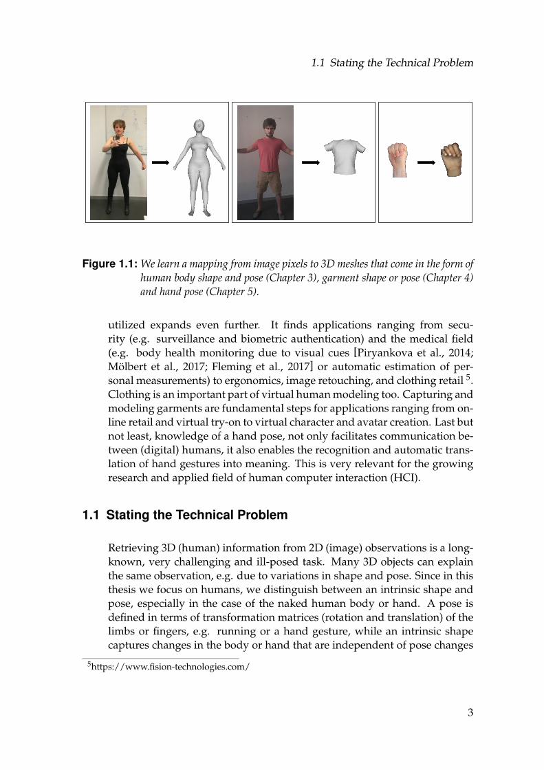
1.1 We learn a mapping from image pixels to 3D meshes that comein the form of human body shape and pose (Chapter 3), garmentshape or pose (Chapter 4) and hand pose (Chapter 5). . . . . . . . . 3
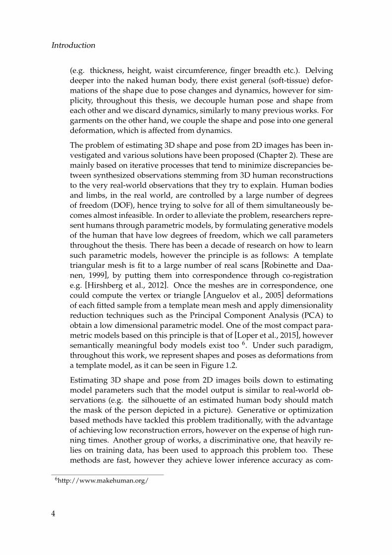
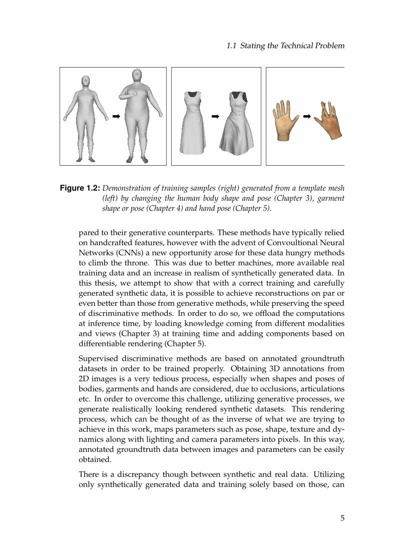
1.2 Demonstration of training samples (right) generated from a tem-plate mesh (left) by changing the human body shape and pose(Chapter 3), garment shape or pose (Chapter 4) and hand pose(Chapter 5). . . . . . . . . . . . . . . . . . . . . . . . . . . . . . . . . 5
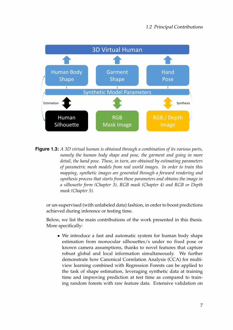
1.3 A 3D virtual human is obtained through a combination of its var-ious parts, namely the human body shape and pose, the garmentand going in more detail, the hand pose. These, in turn, are ob-tained by estimating parameters of parametric mesh models fromreal world images. In order to train this mapping, synthetic imagesare generated through a forward rendering and synthesis processthat starts from these parameters and obtains the image in a silhou-ette form (Chapter 3), RGB mask (Chapter 4) and RGB or Depthmask (Chapter 5). . . . . . . . . . . . . . . . . . . . . . . . . . . . . . 7
3.1 6 meshes from our database. The leftmost one is the mean mesh inthe rest pose. The others are from different people in various poses. 29
3.2 Overview of the first method. Training: Silhouettes from 36 viewsare extracted from meshes generated in various shapes and poses(Section 3.1). A View Classifier is learned (Section 3.3.3) from ex-tracted silhouette features (Section 3.3.2). View specific RegressionForests are then trained to estimate shape parameters by first pro-jecting features in CCA correlated spaces (Section 3.3.4). Testing:The extracted features from an input silhouette are used to first in-fer the camera view, and then the shape parameters by projectingthem into CCA spaces and feeding them into the correspondingRegression Forest. . . . . . . . . . . . . . . . . . . . . . . . . . . . . . 33
3.3 Normal depth computation in 2 different points. The arrows are thesilhouette normals. The normal depth is computed as the weightedmean of the lengths of the red lines. . . . . . . . . . . . . . . . . . . 35
3.4 3D measurements on the meshes used for validation. . . . . . . . . 37
xiii
List of Figures
3.5 Visual results for predictions on 4 test meshes. From left to right:predicted mesh, ground truth mesh, the two meshes frontally over-lapping, the two meshes from the side view, silhouette from thepredicted mesh, input silhouette. . . . . . . . . . . . . . . . . . . . . 39
3.6 Visual results for predictions on 3 females. From left to right: thetwo input images in a rest and selfie pose, the estimated mesh -same estimation is obtained for both poses, the two silhouettesfrom which features are extracted for each pose, the silhouette ofthe estimated mesh. . . . . . . . . . . . . . . . . . . . . . . . . . . . . 40
3.7 Noisy silhouette. . . . . . . . . . . . . . . . . . . . . . . . . . . . . . 423.8 (top) Meshes in running poses. (bottom) Meshes in walking poses. 433.9 Overview of the second method. Top: One of the four input types
(scaled frontal silhouette to a fixed height, shaded image, one ortwo unscaled silhouettes) are fed to the Human Shape Network(HS-Net), to learn a global mapping and estimate human shape pa-rameters (β), which can be used to reconstruct the human bodyshape. Bottom: The HS-Net architecture for the one view case. . . . 46
3.10 The three architectures considered for two input silhouettes. (a)both silhouettes are input as two channels (b) each silhouette is in-put into two separate convolutional layer (CL) blocks and outputsof the CL are concatenated through a Merge layer (c) same scenariohowever with a Max operation performed instead. . . . . . . . . . . 47
3.11 Mean error over all measurements for different input types. (top-left) 3 test meshes in slightly changing poses. (top-right) Illustra-tion of the body measurements (A - P) on the template mesh. . . . . 53
3.12 Meshes in various poses . . . . . . . . . . . . . . . . . . . . . . . . . 543.13 Examples of a half body silhouette (left) and a grayscale image with
Phong shading (right) . . . . . . . . . . . . . . . . . . . . . . . . . . . 553.14 Error plots for each of the body measurements (A - P) when noise
is applied, as compared to clean silhouettes. (top-left) 3 silhouetteswith noise parameters 1, 5 and 9. (Figure best seen in colors). . . . . 56
3.15 Mesh reconstruction for 4 real subjects in mildly varying poses.(left) Input image (middle) Extracted Silhouette (right) Reconstruc-tion of the estimated shape. . . . . . . . . . . . . . . . . . . . . . . . 57
3.16 Reconstructed meshes for various test inputs for two views net-work HS-2-Net-MM. (left to right) Original meshes (front and sideview); Silhouettes (front and side view); Reconstructed Meshes(front and side view) . . . . . . . . . . . . . . . . . . . . . . . . . . . 58
xiv
List of Figures
3.17 Visualization of randomly chosen 60 convolutional filters on a testinput for 3rd layer (left) and zoomed in view of four selected filters(right insets) for (a) one view case (HS-1-Net) and (b) two views case(HS-2-Net-CH). . . . . . . . . . . . . . . . . . . . . . . . . . . . . . . 59
3.18 Overview of the third method. (1) HKS-Net: HKS projected fea-tures as input, generates an embedding space which is mapped to3D meshes. (2),(3) and (4) Three modes of the Cross-Modal NeuralNetwork (CMNN) (only (2) is used at test time). (5) An architec-ture that requires both views at test time. The method uses eitherCMNN or (5), depending on the number of available input views. . 60
3.19 Plot of the mean error over all body measurements illustrated on amesh, for the methods from Table 3.7 and Table 3.8. . . . . . . . . . 67
3.20 Results for predictions on the test images from Method 1 of Sec-tion 3.3. From left to right: the two input images in a rest andselfie pose, the corresponding silhouettes, the estimated mesh byour method SF− 1− P, and by the first method. . . . . . . . . . . . 71
3.21 Predictions on four test subjects in different poses and with clothes.From left to right: input image, the corresponding silhouette, theestimated mesh by our method SF− 1− P. . . . . . . . . . . . . . . 71
3.22 Results for predictions on the test images from Method 1 of Sec-tion 3.3. From left to right: the input image in a rest pose, the corre-sponding silhouette, the estimated mesh by our method SF− 1− P,and by the method of [Bogo et al.,2016a]. . . . . . . . . . . . . . . . . 73
3.23 Estimated overlayed meshes utilizing our method overlayed on theinput images or scans (bottom-right). . . . . . . . . . . . . . . . . . . 74
3.24 Estimated overlayed meshes utilizing the method from [Bogo etal.,2016a] overlayed on the input images. . . . . . . . . . . . . . . . 75
3.25 Examples of two failure cases. . . . . . . . . . . . . . . . . . . . . . . 763.26 5 silhouettes representing the same person with noise applied to
them. Noise parameters (radii) considered 1,3,5,7 and 9 pixels. . . . 773.27 Error plots for the increase in the mean errors as compared to the
silhouettes without noise. The top line (SF − 1) demonstrates theerrors when training is performed on clean silhouettes and testingon noisy ones. On the other hand, the bottom line (SF− 1− Noise)demonstrates the errors when noise is inflicted into the trainingdata. The mean errors are computed over all body measurements.The noise parameter (radii) varies from 1 to 9 pixels. . . . . . . . . . 79
3.28 Visualization of the input silhouettes when a limb part is missing. . 803.29 Visualization of filter responses on the last convolutional layers of
SF− 1− P. The same person in three various poses is shown. . . . 82
xv
List of Figures
3.30 Network architecture for a single view case trained with SF− 1− Parchitecture. For other types of inputs, such as side view etc., thearchitecture is the same. . . . . . . . . . . . . . . . . . . . . . . . . . 83
3.31 Illustration of people in various poses considered throughout ourexperiments. . . . . . . . . . . . . . . . . . . . . . . . . . . . . . . . . 83
3.32 Mesh reconstruction (right) when a partial mesh (left) is input intothe HKS− Net. . . . . . . . . . . . . . . . . . . . . . . . . . . . . . . 84
3.33 Mesh reconstruction (right) when a posed mesh (left) is input intothe HKS− Net. . . . . . . . . . . . . . . . . . . . . . . . . . . . . . . 85
3.34 Mesh reconstruction (right) when a noisy mesh (left) is input intothe HKS− Net. . . . . . . . . . . . . . . . . . . . . . . . . . . . . . . 86
4.1 Garment 3D shape estimation using our CNN model and a single-view. From left to right: real-life images capturing a person wear-ing a T-shirt, segmented and cut-out garments and 3D estimationsof the shape. . . . . . . . . . . . . . . . . . . . . . . . . . . . . . . . . 92
4.2 Data generation pipeline. A human model is automatically rigged(a) and animated (b). Then a desired garment is designed (c), simu-lated under some motion (d), and realistically rendered (e). A maskof the rendered garment is used as a training input. . . . . . . . . . 93
4.3 Samples of masked and downscaled renderings of a garment for afront (top) and back (bottom) view. . . . . . . . . . . . . . . . . . . . 94
4.4 Video segmentation pipeline with our software. From left to right: First video frame, foreground and background scribbles, segmen-tation result on the frame, segmentation automatically propagatedto another frame. . . . . . . . . . . . . . . . . . . . . . . . . . . . . . 95
4.5 Our SqueezeNet incarnation for the two-view case. The single-view is similar, except that only one convolutional block is utilizedand there is no view-pooling layer. The input is one or two imagesof a masked garment, and the output is the garment mesh. For amore detailed description of the networks and a further discussionabout the architecture please see Section 4.3.4. . . . . . . . . . . . . 98
4.6 The garment meshes used for simulation . . . . . . . . . . . . . . . 1034.7 Recovered garment shapes with the ”Garment-from-Body” repre-
sentation. From left to right: initial rendering, segmented T-shirt,and rendering of the same scene using the estimated mesh. . . . . . 104
4.8 Recovered garment shapes with the ”Garment-from-Body” repre-sentation. From left to right: initial rendering, segmented dress andrendering of the same scene using the estimated mesh. . . . . . . . 104
4.9 Pose changes: input images (first row) and the estimations (secondrow). . . . . . . . . . . . . . . . . . . . . . . . . . . . . . . . . . . . . 105
xvi
List of Figures
4.10 Illumination changes: input images (first row) and the estimations(second row). . . . . . . . . . . . . . . . . . . . . . . . . . . . . . . . 105
4.11 View changes: input images (first row) and the estimations (secondrow). . . . . . . . . . . . . . . . . . . . . . . . . . . . . . . . . . . . . 106
4.12 Estimated T-shirt shapes from captured images. From left to right:original image, image after segmentation (input image), view of theestimated mesh from the front and back. . . . . . . . . . . . . . . . . 107
4.13 Estimated garment shapes from two views. From left to right: orig-inal image from the front and back, image after segmentation (in-put image) from the front and back, view of the estimated meshesfrom the front and back. . . . . . . . . . . . . . . . . . . . . . . . . . 108
4.14 Dress shapes estimated from real images. From left to right: orig-inal image, image after segmentation (input image), view of theestimated mesh from the front and back. Please note that none ofthe dresses match exactly our test dress in neither shape nor mate-rial stiffness or reflectance. Despite that, we are able to capture theoverall shape even for more challenging images (such as the firstimage, where the actress grabs the side of her dress). . . . . . . . . . 109
4.15 Demonstration of superiority of multi-view models over single-view models. (top) From left to right: initial rendering frontaland back view, the segmented and rescaled garment, frontal andback view. It can be observed that the mesh estimated by themulti-view model is much more accurate than that estimated bythe single-view model, especially on the back side. Front (middle)and back (bottom) views of (from left to right): ground truth ge-ometry, geometry estimated by the single-view SqueezeNet modeltrained on frontal views, and geometry estimated by the multi-view SqueezeNet model. . . . . . . . . . . . . . . . . . . . . . . . . . 112
xvii
List of Figures
4.16 Failure cases. From left to right: original image, image after seg-mentation (input image), view of the estimated mesh from thefront.First row: A very hard image. Similar silhouettes are not presentin the training set and the wrinkling patterns are also completelynew. Such cases can cause the estimation to fail.Second row: Here, the estimation is hindered by the imperfect seg-mentation at the top of the image as well as unseen wrinkling pat-terns.Third row: The specific dress captured slightly from the side isalso not part of the training set. However, please observe how ourtechnique tried to generate a very close shape (the wrinkles on thelower left part of the dress).Fourth row: The “intrinsic” shape of this dress is dramatically dif-ferent. Please observe how our model compensated for lack ofclothing on the right with a more plausible inwards deformation. . 113
4.17 Top: Single-view architecture. Bottom: Two-view architecture. . . . 1144.18 From left to right: simulation with a high resolution mesh, with the
corresponding low resolution mesh, and the estimated high reso-lution mesh with our method. For each case, we also show the rawmesh. The input to our method is the rendering of the simulationwith the low resolution mesh. . . . . . . . . . . . . . . . . . . . . . . 116
5.1 Overview of the training pipeline. Given a depth image as input, abase CNN model predicts the hand pose θ. Given θ, we calculate aloss consisting of a collision, physical and depth component. Dur-ing training, we update the weights of the base model, as well asP, a point cloud that represents the hand shape and gets iterativelyupdated to the real one. Since we can calculate the loss using onlythe input image, θ and P, our model can be trained without labeleddata. . . . . . . . . . . . . . . . . . . . . . . . . . . . . . . . . . . . . . 121
5.2 Overview of the different kinds of formats and hand images weprocess. From left to right (1) our rigged hand model with its 16joints (2) the uniformly sampled point cloud P of the rigged mesh(3) a rendering after transforming P using the render component(Section 5.1.3.1) (4) a typical noisy depth image input to the baseCNN model. (5) a rendering of points sampled from (4). (6) theabsolute difference between (3) and (5) . . . . . . . . . . . . . . . . . 122
5.3 Architecture of the base CNN model . . . . . . . . . . . . . . . . . . 1305.4 Firstly, we overfit our model on single depth images to give evi-
dence that learning the pose without any annotations is possible. . 132
xviii
List of Figures
5.5 In a second experiment, we optimize for the hand point cloud Ponly and demonstrate how the updates converge close to a globaloptimum. . . . . . . . . . . . . . . . . . . . . . . . . . . . . . . . . . . 133
5.6 ROC curves for the self comparison experiment on the NYU andICVL dataset. . . . . . . . . . . . . . . . . . . . . . . . . . . . . . . . 134
5.7 Two qualitative examples from our validation set are shown, aftertraining with 50k images from our training set without annotations.For each block, top row shows a 3D rendering of our hand model inthe predicted pose before (left) and after training (right). For visualcomparison, we demonstrate the RGB input image (center), whichis not utilized by this method. The bottom row shows the absolutedepth errors of the poses from above (left and right) (see Figure 5.2for details) and the input depth image (center). . . . . . . . . . . . . 135
5.8 Distribution of the MSE between the synthesized depth images (see(3) and (5) in Fig 5.2) over the frames of our validation set, beforeand after training on our training set. The vertical lines show themean values before (right) and after prediction (left). . . . . . . . . 136
5.9 Comparison to state-of-the-art methods on the NYU and ICVLdataset. For one of our curves (dashed), we remove the bias intro-duced from the mismatch between our hand model and the onesused as groundtruths for each dataset. . . . . . . . . . . . . . . . . . 137
5.10 Interpolation . . . . . . . . . . . . . . . . . . . . . . . . . . . . . . . . 1385.11 Overview of the extended training pipeline for the RGB input case.
Given a monocular RGB image as input, a SegNet based networkfirst segments out the background, the result of which is input intoSynthNet, a CNN model trained purely on synthetic data (Sec-tion 5.3.1) that predicts the hand pose in terms of angles θ. Inorder to fine-tune the network to real monocular data, providedthat a corresponding depth image is given, we augment the initialbase network with a depth loss component. We refer to this com-bination during training time as Re f Net. Given θ as well as P, apoint cloud that initially represents our hand model and gets iter-atively updated to the input one, the weights of SynthNet can beupdated without the need of labeled data. At test time, a forwardpass through SegNet and SynthNet estimates the desired pose. . . 140
5.12 Real predictions on the HGR dataset. . . . . . . . . . . . . . . . . . . 1415.13 (Left) Rigged hand model with max 51 DOF (Middle) 5 sam-
ples from our dataset in 5 different orientations (Right) Two semi-supervised refinement examples from our own dataset (top) andSenz3D (bottom) - from left to right: input, SynthNet unrefinedand refined prediction. . . . . . . . . . . . . . . . . . . . . . . . . . . 142
xix
List of Figures
5.14 Predictions with a CNN trained on silhouette (left) and RGB (con-verted to grayscale, right) input respectively. . . . . . . . . . . . . . 142
5.15 Realistically rendered hand model. . . . . . . . . . . . . . . . . . . . 1445.16 Qualitative results on various hand poses, shapes and color. . . . . 1475.17 Qualitative results on one individual in various hand poses. . . . . 1485.18 CNN architecture of the detection part. . . . . . . . . . . . . . . . . 1495.19 CNN architecture of OurSegNet. . . . . . . . . . . . . . . . . . . . . 1505.20 CNN architecture for pose inference SynthNet. . . . . . . . . . . . . 1515.21 Error Contribution Heatmap Full . . . . . . . . . . . . . . . . . . . . 1525.22 Three examples of segmentation improvement on StereoDS before
(left) and after (right) adding our synthetic training data. . . . . . . 1535.23 SynthNet predictions on (left) HGR dataset (middle) one individ-
ual hand (right) synthetic dataset from [Zimmermann and Brox,2017]. . . . . . . . . . . . . . . . . . . . . . . . . . . . . . . . . . . . . 153
5.24 Two examples from our validation set IntelDS. SynthNet predic-tions before (top) and after refinement (bottom). From left to right: RGB Input (I), Input Depth (D) , Synthesized Input Depth (DS),Prediction (DI) and Error in depth prediction. . . . . . . . . . . . . . 154
5.25 MSE histogram computed over pixel (depth) image difference forthe network before and after refining unsupervised. . . . . . . . . . 155
5.26 ROC curve corresponding to Figure 5.25. . . . . . . . . . . . . . . . 1565.27 From left to right : input image, SynthNet prediction, SynthNet re-
fined semi-supervised. SynthNet with interpenetration constrainthandling prediction. . . . . . . . . . . . . . . . . . . . . . . . . . . . 157
5.28 Kinematic Constraints Demonstration . . . . . . . . . . . . . . . . . 1575.29 Accuracy on the StereoDS dataset. (Left) Improvement in euler an-
gles due to refinement (Right) Comparison to state-of-the-art meth-ods trained to map onto 3D joints. We show our ROC curve trainedon angles along with a version trained on joints. . . . . . . . . . . . 159
5.30 MSE histogram of our (Color) and method from Section 5.1 (Depth)both before (Base) and after (Adapted) after unsupervised refine-ment. . . . . . . . . . . . . . . . . . . . . . . . . . . . . . . . . . . . . 160
5.31 ROC curve corresponding to Figure 5.30. . . . . . . . . . . . . . . . 1615.32 MSE variation per frame of our (Color) and the method from Sec-
tion 5.1 (Depth) both before (Base) and after (Adapted) after unsu-pervised refinement. . . . . . . . . . . . . . . . . . . . . . . . . . . . 162
6.1 First two columns: RGB hand images generated with GANs havinga synthetic RGB hand image as an input. Third column: Depthhand images generated with GANs having an RGB hand image asan input. . . . . . . . . . . . . . . . . . . . . . . . . . . . . . . . . . . 170
xx

List of Algorithms
1 Interpenetration removal algorithm . . . . . . . . . . . . . . . . . . . 102
xxi

List of Tables
3.1 Comparisons to variations of our method (RF, CCA-RF-1, CCA-RF-2) and ground truth, via various measurements. The measurementsare illustrated in Figure 3.4. Errors are represented as Mean±Std.Dev and are expressed in millimeters. . . . . . . . . . . . . . . . . . 38
3.2 Columns 1-3 show accuracy gain of applying CCA for the Frontal,Side and Frontal Side view altogether, over raw features. (VE)shows the error due to 10 degree view change and (VG), the gainof applying CCA. (N) is the error due to silhouette noise. (P12)shows the error of testing on 12 poses different from the trainingone, and the rest (Columns 8-11) demonstrate the errors while grad-ually adding more difficult poses from the training ones. Mean andStd. Deviation is computed over all the body measurements. . . . . 44
3.3 Comparisons of the complementary results via various measure-ments. The measurements are illustrated in Figure 3.4. Errors rep-resent Mean±Std. Dev and are expressed in millimeters. From leftto right: Our results without applying CCA, the new results underthe known scale assumption, the same with CCA applied to thefeatures, the ground truth error defined as the error between theoriginal model and its projection to the shape space spanned by the20 parameters we utilize. . . . . . . . . . . . . . . . . . . . . . . . . . 45
3.4 Error comparisons on body measurements for the various in-puts and presented training modalities. The measurements areillustrated in Figure 3.11 (top-right). Errors are represented asMean±Std. Dev and are expressed in millimeters. Our best achiev-ing method HS-2-Net-MM is highlighted. . . . . . . . . . . . . . . . 53
xxii
List of Tables
3.5 Results of the additional experiments with errors represented asMean±Std. Dev (in mm). All experiments are done with the in-put scaled to a fixed height. Experiments (from left to right): fullbody silhouettes; only half body silhouettes; trained on both halfand full body silhouettes but tested only on half; same as previousbut tested on full body silhouettes; grayscale images with shad-ing under Lambertian assumptions; grayscale images with Phongshading (we highlight the most significant decrease in error due toPhong shading as compared to the Lambertian case). . . . . . . . . 55
3.6 Nomenclature for the various experiments. For the architecturecomponents highlighted in colors and with numbers, please referto Figure 3.18. . . . . . . . . . . . . . . . . . . . . . . . . . . . . . . . 66
3.7 Body measurement errors comparison with shapes reconstructedfrom one scaled frontal silhouette. The nomenclature is presentedin Table 3.6. Last two columns show the results of the state-of-the-art methods. The measurements are illustrated in Figure 3.19 (top-right). Errors are expressed as Mean±Std. Dev in millimeters. Ourbest achieving method SFUS-HKS-1 is highlighted. . . . . . . . . . 68
3.8 Same as in Table 3.7, however with shapes reconstructed from twoviews at the same time. Last four columns show the results of theother state-of-the-art methods for the same task. Our best achievingmethod UF-US-HKS-2 is highlighted. . . . . . . . . . . . . . . . . . 69
3.9 Body measurement errors comparison over the various experi-ments considered here. Errors are expressed as Mean±Std. Devin millimeters. . . . . . . . . . . . . . . . . . . . . . . . . . . . . . . . 81
4.1 The performance of models trained on the “T-shirt” dataset. “GfG”stands for the ”Garment from Garment” representation. ”GfB”stands for the ”Garment from Body” representation. Each entryalso contains information on which architecture and loss functionwas used. MSE stands for vertex mean squared error and NCS formean cosine similarity of the face normals. . . . . . . . . . . . . . . 110
4.2 The performance of models trained on the ”Dress” dataset. ”GfG”stands for the ”Garment-from-Garment” representation, and ”GfB”for the ”Garment-from-Body” representation. Each entry also con-tains information on which architecture and loss function was used.MSE stands for vertex mean squared error and NCS stands formean cosine similarity of the face normals. . . . . . . . . . . . . . . 110
5.1 Allowed euler angle bounds for each joint or finger part. Values arein radians. . . . . . . . . . . . . . . . . . . . . . . . . . . . . . . . . . 126
xxiii

List of Tables
5.2 Segmentation accuracy in % for HandSegNet and OurSegNet (OSN)trained with and without our synthetic dataset. . . . . . . . . . . . . 153
5.3 Classification accuracy comparison, in % of correctly classifiedposes, on the RWTH and Senz3D. . . . . . . . . . . . . . . . . . . . . 157
5.4 Fingertip accuracy on the HGR Dataset computed as MSE overpixel errors, with image size 225× 225 pixels. . . . . . . . . . . . . . 158
5.5 Joint Angles vs Positions MSE on our synthetic dataset. . . . . . . . 158
xxiv

C H A P T E R 1Introduction
Humans are constantly trying to bring the virtual world as close as possibleto the real one. The most recent technological advances of the last decadeshave played an important role in bridging the gap between these two veryrelated and forked concepts about the world we live in. As a matter of factthis is true. Since the invention of the internet, a lot of advances and achieve-ments have been seen in the online world e.g. electronic retailing, ease of ac-quiring information, voice assistance, fast queries about questions and needsand most importantly an easy communication medium that virtually bringspeople together without the need to physically travel. Initial communicationattempts were achieved through e-mail or instant messaging, and more re-cently through video conferencing and virtual meeting rooms with cartoon-like avatars. The most natural way for humans to communicate with eachother though, are through close face-to-face physical interactions, and theabove-mentioned approaches lack such emotional presence or immersion,due to the current inability to properly represent the virtual human body.
Despite recent promising attempts and achievements to properly model,capture and place the human in the virtual world, in its current state, the lat-ter can be more described as a disembodied one, where humans are partedfrom their bodies. With bodies, we do not only mean the naked body as awhole, but also the clothes and garments that typically cover it and its parts.With respect to the body parts, we distinguish the hands, due to the high im-portance they play in mutual communication and manipulating the world.Thus, there is an imminent need for the presence of virtual humans or avatarcopies of one-self to make such an immersive experience richer.
1
Introduction
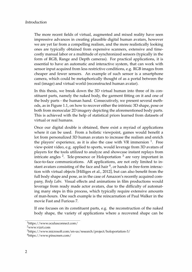
The more recent fields of virtual, augmented and mixed reality have seenimpressive advances in creating plausible digital human avatars, howeverwe are yet far from a compelling realism, and the more realistically lookingones are typically obtained from expensive scanners, extensive and time-costly manual labor or a multitude of synchronized sensors (typically in theform of RGB, Range and Depth cameras). For practical applications, it isessential to have an automatic and interactive system, that can work withsensor input acquired from less restrictive conditions, e.g. RGB images fromcheaper and fewer sensors. An example of such sensor is a smartphonecamera, which could be metaphorically thought of as a portal between thereal (image) and virtual world (reconstructed human avatar).
In this thesis, we break down the 3D virtual human into three of its con-stituent parts, namely the naked body, the garment fitting on it and one ofthe body parts - the human hand. Consecutively, we present several meth-ods, as in Figure 1.1, on how to recover either the intrinsic 3D shape, pose orboth from monocular 2D imagery depicting the aforementioned body parts.This is achieved with the help of statistical priors learned from datasets ofvirtual or real humans.
Once our digital double is obtained, there exist a myriad of applicationswhere it can be used. From a holistic viewpoint, games would benefit alot from personalized 3D human avatars to increase the realism and enrichthe players’ experience, as it is also the case with VR immersion 1. Freeview-point video, e.g. applied to sports, would leverage from 3D avatars ofplayers for the tools utilized to analyze and showcase instant replays fromintricate angles 2. Tele-presence or Holoportation 3 are very important inface-to-face communications. AR applications, are not only limited to in-stant avatars consisting of the face and hair 4, or hands in free-form interac-tion with virtual objects [Hilliges et al., 2012], but can also benefit from thefull body shape and pose, as in the case of Amazon’s recently acquired com-pany, Body Labs. Visual effects and animations in film productions wouldleverage from ready made actor avatars, due to the difficulty of automat-ing many steps in this process, which typically require extensive amountsof man-hours. One such example is the reincarnation of Paul Walker in themovie Fast and Furious 7.
If one focuses on its constituent parts, e.g. the reconstruction of the nakedbody shape, the variety of applications where a recovered shape can be
1https://www.oculusconnect.com/2www.vizrt.com3https://www.microsoft.com/en-us/research/project/holoportation-3/4https://www.pinscreen.com/
2
1.1 Stating the Technical Problem
Figure 1.1: We learn a mapping from image pixels to 3D meshes that come in the form ofhuman body shape and pose (Chapter 3), garment shape or pose (Chapter 4)and hand pose (Chapter 5).
utilized expands even further. It finds applications ranging from secu-rity (e.g. surveillance and biometric authentication) and the medical field(e.g. body health monitoring due to visual cues [Piryankova et al., 2014;Molbert et al., 2017; Fleming et al., 2017] or automatic estimation of per-sonal measurements) to ergonomics, image retouching, and clothing retail 5.Clothing is an important part of virtual human modeling too. Capturing andmodeling garments are fundamental steps for applications ranging from on-line retail and virtual try-on to virtual character and avatar creation. Last butnot least, knowledge of a hand pose, not only facilitates communication be-tween (digital) humans, it also enables the recognition and automatic trans-lation of hand gestures into meaning. This is very relevant for the growingresearch and applied field of human computer interaction (HCI).
1.1 Stating the Technical Problem
Retrieving 3D (human) information from 2D (image) observations is a long-known, very challenging and ill-posed task. Many 3D objects can explainthe same observation, e.g. due to variations in shape and pose. Since in thisthesis we focus on humans, we distinguish between an intrinsic shape andpose, especially in the case of the naked human body or hand. A pose isdefined in terms of transformation matrices (rotation and translation) of thelimbs or fingers, e.g. running or a hand gesture, while an intrinsic shapecaptures changes in the body or hand that are independent of pose changes
5https://www.fision-technologies.com/
3
Introduction
(e.g. thickness, height, waist circumference, finger breadth etc.). Delvingdeeper into the naked human body, there exist general (soft-tissue) defor-mations of the shape due to pose changes and dynamics, however for sim-plicity, throughout this thesis, we decouple human pose and shape fromeach other and we discard dynamics, similarly to many previous works. Forgarments on the other hand, we couple the shape and pose into one generaldeformation, which is affected from dynamics.
The problem of estimating 3D shape and pose from 2D images has been in-vestigated and various solutions have been proposed (Chapter 2). These aremainly based on iterative processes that tend to minimize discrepancies be-tween synthesized observations stemming from 3D human reconstructionsto the very real-world observations that they try to explain. Human bodiesand limbs, in the real world, are controlled by a large number of degreesof freedom (DOF), hence trying to solve for all of them simultaneously be-comes almost infeasible. In order to alleviate the problem, researchers repre-sent humans through parametric models, by formulating generative modelsof the human that have low degrees of freedom, which we call parametersthroughout the thesis. There has been a decade of research on how to learnsuch parametric models, however the principle is as follows: A templatetriangular mesh is fit to a large number of real scans [Robinette and Daa-nen, 1999], by putting them into correspondence through co-registratione.g. [Hirshberg et al., 2012]. Once the meshes are in correspondence, onecould compute the vertex or triangle [Anguelov et al., 2005] deformationsof each fitted sample from a template mean mesh and apply dimensionalityreduction techniques such as the Principal Component Analysis (PCA) toobtain a low dimensional parametric model. One of the most compact para-metric models based on this principle is that of [Loper et al., 2015], howeversemantically meaningful body models exist too 6. Under such paradigm,throughout this work, we represent shapes and poses as deformations froma template model, as it can be seen in Figure 1.2.
Estimating 3D shape and pose from 2D images boils down to estimatingmodel parameters such that the model output is similar to real-world ob-servations (e.g. the silhouette of an estimated human body should matchthe mask of the person depicted in a picture). Generative or optimizationbased methods have tackled this problem traditionally, with the advantageof achieving low reconstruction errors, however on the expense of high run-ning times. Another group of works, a discriminative one, that heavily re-lies on training data, has been used to approach this problem too. Thesemethods are fast, however they achieve lower inference accuracy as com-
6http://www.makehuman.org/
4
1.1 Stating the Technical Problem
Figure 1.2: Demonstration of training samples (right) generated from a template mesh(left) by changing the human body shape and pose (Chapter 3), garmentshape or pose (Chapter 4) and hand pose (Chapter 5).
pared to their generative counterparts. These methods have typically reliedon handcrafted features, however with the advent of Convoultional NeuralNetworks (CNNs) a new opportunity arose for these data hungry methodsto climb the throne. This was due to better machines, more available realtraining data and an increase in realism of synthetically generated data. Inthis thesis, we attempt to show that with a correct training and carefullygenerated synthetic data, it is possible to achieve reconstructions on par oreven better than those from generative methods, while preserving the speedof discriminative methods. In order to do so, we offload the computationsat inference time, by loading knowledge coming from different modalitiesand views (Chapter 3) at training time and adding components based ondifferentiable rendering (Chapter 5).
Supervised discriminative methods are based on annotated groundtruthdatasets in order to be trained properly. Obtaining 3D annotations from2D images is a very tedious process, especially when shapes and poses ofbodies, garments and hands are considered, due to occlusions, articulationsetc. In order to overcome this challenge, utilizing generative processes, wegenerate realistically looking rendered synthetic datasets. This renderingprocess, which can be thought of as the inverse of what we are trying toachieve in this work, maps parameters such as pose, shape, texture and dy-namics along with lighting and camera parameters into pixels. In this way,annotated groundtruth data between images and parameters can be easilyobtained.
There is a discrepancy though between synthetic and real data. Utilizingonly synthetically generated data and training solely based on those, can
5
Introduction
result in systems learning statistics from the data which are not represen-tative of the real ones. Despite the fact that our data is generated froma statistically-learned human body model, and our predictions always fallwithin the natural space of human bodies (or clothes, hands) the accuracycan be tremendously improved if real training data is infused into the sys-tem. Hence, we explore ways of incorporating real-world unlabeled data ina semi-supervised and unsupervised fashion, in order to improve our pre-dictions. Additionally, it is clear that having more than one view (image)representing the same object should improve predictions. We present meth-ods of leveraging from multiple views at training time, in order to boostinference from a single view at test time.
A schematic description of the general pipeline for obtaining the 3D virtualhuman, with respect to this thesis, is depicted in Figure 1.3. The humanavatar constitutes of its various parts: the naked human body, the garmentand going in more detail, the hand. In chronological order, we train for andaim to obtain intrinsic body shape, garment shape and hand pose parame-ters. Through a forward mapping between these parameters and images, wegenerate training data. With the help of our methods based on such trainingdata and presented in the following chapters, we obtain a mapping from realworld monocular images to these parameters, which in turn are utilized toreconstruct the 3D virtual human.
1.2 Principal Contributions
In terms of the bigger picture, this thesis aims to advance the field of recon-structing and tracking of the human avatar utilizing the least amount of sen-sors. Tackling this all at once is a very hard problem, hence, as previouslymentioned, we focus on and contribute to three crucial and representativeparts that constitute the virtual human, namely the naked body shape, thegarment shape and the hand pose. Our goal is to provide solutions for prac-tical applications that utilize RGB monocular cameras and run at interactiverates, in order to make them tangible and integrate them in today‘s smart-phones. In order to achieve this, we contribute to the community threefold:(a) by introducing several discriminative methods, largely based on CNN-s, that have lower run-times than but perform on par with and even betterthan acknowledged optimization based methods, (b) by providing realisti-cally looking synthetically generated datasets that are crucial for the trainingof fully supervised discriminative based methods, due to the scarcity of an-notated real datasets for the problems that we tackle and (c) by presentingways of utilizing multiple modes and views during training, in a supervised
6
1.2 Principal Contributions
3D Virtual Human
Human Body Shape
GarmentShape
HandPose
Human Silhouette
RGBMask Image
RGB / DepthImage
Synthetic Model Parameters
Estimation Synthesis
Figure 1.3: A 3D virtual human is obtained through a combination of its various parts,namely the human body shape and pose, the garment and going in moredetail, the hand pose. These, in turn, are obtained by estimating parametersof parametric mesh models from real world images. In order to train thismapping, synthetic images are generated through a forward rendering andsynthesis process that starts from these parameters and obtains the image ina silhouette form (Chapter 3), RGB mask (Chapter 4) and RGB or Depthmask (Chapter 5).
or un-supervised (with unlabeled data) fashion, in order to boost predictionsachieved during inference or testing time.
Below, we list the main contributions of the work presented in this thesis.More specifically:
• We introduce a fast and automatic system for human body shapeestimation from monocular silhouettes/s under no fixed pose orknown camera assumptions, thanks to novel features that capturerobust global and local information simultaneously. We furtherdemonstrate how Canonical Correlation Analysis (CCA) for multi-view learning combined with Regression Forests can be applied tothe task of shape estimation, leveraging synthetic data at trainingtime and improving prediction at test time as compared to train-ing random forests with raw feature data. Extensive validation on
7
Introduction
thousands of body shapes are provided via thorough comparisonsto state-of-the-art methods on synthetic meshes generated by fittingmeshes to real human scans.
• We present another system for human shape and body measure-ments estimation, from silhouettes (or shaded images) of people ingarment fitting like poses, by learning a global mapping to shape pa-rameters. To the best of our knowledge, this is the first system thatutilizes CNN-s to accurately reconstruct human body shapes fromimages. Thus, we show how to train from scratch an end-to-endfully supervised regression from CNNs with binary silhouette im-ages as input, and demonstrate how to incorporate more evidence(e.g. a second view) in order to improve prediction.
• Building up on the above, we introduce a novel neural network ar-chitecture for 3D body shape estimation from silhouettes consistingof three main components, (a) a generative component that can in-vert a pose-invariant 3D shape descriptor to reconstruct its neutralshape, (b) a predictive component that combines 2D and 3D cues tomap silhouettes to human body shapes, (c) a cross-modal compo-nent that leverages multi-view information to boost single view pre-dictions. This combination achieves state-of-the-art performance forhuman body shape estimation that significantly improves accuracyas compared to existing methods.
• We provide an end-to-end 3D garment shape estimation algorithm.The algorithm automatically extracts 3D shape from a single imagecaptured with an uncontrolled setup, that depicts a dynamic stateof a garment at interactive rates. To the best of our knowledge, weintroduce the first regressor system based on convolutional neuralnetworks (CNN-s) combined with statistical priors and a specializedloss function for garment shape estimation. In order to enable itstraining, we provide a new realistically rendered physically basedsynthetic garment dataset for a shirt and dress case. We further val-idate our approach by presenting experiments with several architec-tures, including those for single and multi-view setups.
• We demonstrate how to train or refine a CNN-based 3D hand poseestimation architecture, on unseen and unlabeled depth images,avoiding the need for annotated real data. This is achieved due toa new training pipeline that can accurately estimate 3D hand posewith the ability to refine itself on unlabeled depth images, using adepth loss component with a physical and collision regularizer. Theadvantage of utilizing such a method, to enhance estimations of sim-
8
1.3 Thesis outline
ple candidate CNN models, is demonstrated through extensive eval-uations and comparisons to state-of-the-art methods.
• Lastly, based on the approach from above that expects a depth im-age as an input, we introduce a complete system for 3D hand poseestimation and gesture recognition from monocular RGB data. Weshow how refining of an RGB-based network trained on syntheticdata is achieved with unlabeled RGB hand images and the corre-sponding depth maps. In order to achieve this, we initially dependon a new realistically rendered hand dataset with 3D annotationsthat we provide. This dataset helps both hand segmentation and 3Dpose inference. We validate our method on available datasets show-ing superior performance to related works for three different poseinference tasks.
1.3 Thesis outline
The remainder of this thesis is organized as follows:
• Chapter 2 gives a general overview of previous methods, focusingon estimating the virtual human and in more detail on body shape,garment shape and hand pose estimation from monocular imagery.
• Chapter 3 introduces three methods that can estimate the humanbody shape from monocular binary silhouette images. These meth-ods make use of Random Forest Regressors with specialized fea-tures and Convolutional Neural Networks along with supervisedand cross-modal learning to map images to meshes that representthe human body.
• Chapter 4 describes a CNN based method that can map garmentRGB images to garment shapes with the help of a proposed physi-cally simulated synthetic garment dataset.
• Chapter 5 introduces two discriminative methods for hand pose es-timation from either depth or monocular RGB images, that can betrained unsupervised from unseen and unlabeled real data, due to aspecialized differentiable renderer loss during training.
• Chapter 6 concludes this thesis with a discussion of the contribu-tions and a more elaborated outlook of potential methods that couldcomplement and improve the ones introduced here.
9
Introduction
1.4 Publications
In the context of this thesis, the technical contributions have led to top-tierpeer-reviewed conference publications:
• E. Dibra, C. Oztireli, R.Ziegler and M. Gross (2016). Shape from Self-ies: Human Body Shape Estimation Using CCA Regression Forests.Proceedings of the 14th European Conference of Computer Vision (ECCV),Amsterdam, The Netherlands, October 11-14, 2016 (Chapter 1).
• E. Dibra, H. Jain, C. Oztireli, R.Ziegler and M. Gross (2016). HS-Nets:Estimating Human Body Shape from Silhouettes with ConvolutionalNeural Networks. Fourth International Conference on 3D Vision (3DV),Stanford, CA, USA, October 25-28, 2016 (Chapter 1).
• E. Dibra, H. Jain, C. Oztireli, R.Ziegler and M. Gross (2017). Hu-man Shape from Silhouettes Using Generative HKS Descriptors andCross-Modal Neural Networks. IEEE Conference on Computer Visionand Pattern Recognition (CVPR), Honolulu, HI, USA, July 21-26, 2017(Spotlight) (Chapter 1).
• R. Danecek*, E. Dibra*, C. Oztireli, R.Ziegler and M. Gross (2017).DeepGarment : 3D Garment Shape Estimation from a Single Im-age. Computer Graphics Forum (Eurographics), Lyon, France, April 24-28, 2017 (Chapter 2).
• E. Dibra*, T. Wolf*, C. Oztireli and M. Gross (2017). How to Refine3D Hand Pose Estimation from Unlabelled Depth Data ? Fifth Inter-national Conference on 3D Vision (3DV), Qingdao, China, October 10-12,2017 (Chapter 3).
• E. Dibra, S. Melchior, A. Balkis, T. Wolf, C. Oztireli and M. Gross(2018). Monocular RGB Hand Pose Inference from Unsupervised Re-finable Nets. CVPR 1st International Workshop on Human Pose, Motion,Activities and Shape in 3D (3D Humans 2018), Salt Lake City, UT, USA,June 18-22, 2018 (Chapter 3).
Additional implementation and evaluation details not present in the abovepapers are included in this thesis, in addition to their contents. Althoughnot directly linked to the work presented here, the following peer-reviewedpublications were published during my PhD studies:
• E. Dibra, J. Maye, O. Diamanti, R. Siegwart and P.A. Beardsley(2015). Extending the Performance of Human Classifiers Using a
10

1.4 Publications
Viewpoint Specific Approach. Proceedings of the IEEE Winter Confer-ence on Applications of Computer Vision (WACV), Waikoloha, HI, USA,January 5-9, 2015.
11

Introduction
12
C H A P T E R 2Related Work
In the recent years, there has been a lot of progress from the Computer Vi-sion and Graphics community in producing a myriad of excellent meth-ods that attempt to estimate the virtual 3D human. The human body isvery complex, and capturing it in 3D, without the need of expensive cap-turing equipment, but through low-cost 2D sensors is a very relevant re-search task. Researchers, thus, have looked at this problem from variousperspectives and tackled it from various angles. Some have focused onthe static surface representation of the body as a whole [Balan et al., 2007;Balan and Black, 2008; Guan et al., 2009; Zhou et al., 2010; Jain et al., 2010;Hasler et al., 2010; Chen et al., 2013; Rhodin et al., 2016; Bogo et al., 2016a]utilizing simplified body models [Anguelov et al., 2005; Hasler et al., 2009;Neophytou and Hilton, 2013; Loper et al., 2015], others have attempted toexplore dynamics [Pons-Moll et al., 2015] and anatomically correct bodymodels [Kadlecek et al., 2016]. In parallel to works focusing on the hu-man body in its naked form, or under assumptions of tight clothing,several methods that tackle looser garment capturing [Hahn et al., 2014;Pons-Moll et al., 2017; Zhang et al., 2017; Yang et al., 2016; Jeong et al., 2015;Zhou et al., 2013; Guan et al., 2012; Bradley et al., 2008] under static ordynamic assumptions have been presented, as humans are typically seenin clothing apparel, for most everyday scenarios. Last but not least, dueto the need of covering details that are typically not captured when thehuman body is considered as a whole, there has been quite some workrecently that has focused on the capturing and estimation of smaller andmore targeted body parts, such as hands [Zimmermann and Brox, 2017;Spurr et al., 2018; Tagliasacchi et al., 2015; Oikonomidis et al., 2011; Tomp-
13
Related Work
son et al., 2014], faces [Cao et al., 2017; Beeler et al., 2010; Kim et al., 2017;Tewari et al., 2017], sometimes going even deeper into eyes [Berard et al.,2016; Berard et al., 2014; Sugano et al., 2014; Zhang et al., 2015] and hair [Huet al., 2015], with potential combinations of some of those components [Huet al., 2017].
With respect to the general attributes of a virtual human, previous meth-ods have focused on shape [Balan et al., 2007; Balan and Black, 2008;Guan et al., 2009; Zhou et al., 2010; Jain et al., 2010; Hasler et al., 2010;Chen et al., 2013], pose [Song et al., 2017; Mehta et al., 2016; Mehta et al.,2017], texture [de Aguiar et al., 2008; Eisemann et al., 2008] separately andin combination with each other [de Aguiar et al., 2008; Stoll et al., 2010;Gall et al., 2009; Carranza et al., 2003]. The majority of works focusing onpose have tackled the human body [Mehta et al., 2016; Mehta et al., 2017;Song et al., 2017], and more recently the human hand [Zimmermann andBrox, 2017; Spurr et al., 2018; Panteleris et al., 2017; Song et al., 2015;Mueller et al., 2017]. With respect to the shape, the human body as a wholehas had quite some attention, however less than its pose counterpart, mainlydue to data modeling, the limited availability of shape datasets and difficultyof capturing.
In this chapter, we focus on three sub-parts in more detail, namely the Hu-man Body Shape (Section 2.1), Garment Shape (Section 2.2) and Hand Pose(Section 2.3). For each part, we touch on the works adopted prior to and dur-ing the deep learning latest advent era, mainly focusing on 2D MonocularRGB Images as input, but also covering depth, multi-view and video basedworks.
2.1 Body Shape Estimation Methods
General Methods for Shape Estimation. It is an ill-posed problem to es-timate the 3D geometry of a human body from 2D imagery. Early meth-ods used simplifying assumptions such as the visual hull [Laurentini, 1994]by considering multiple views or simple body models with geometricprimitives [Delamarre and Faugeras, 1999; Kakadiaris and Metaxas, 1998;Mikic et al., 2003]. Although these work well for coarse pose and shapeapproximations, an accurate shape estimation cannot be obtained.
Human Body Shape Statistical Priors. As scanning of a multitude of peo-ple in various poses and shapes was made possible [Robinette and Daa-nen, 1999], more complete, parametric human body shape models werelearned [Anguelov et al., 2005; Hasler et al., 2009; Neophytou and Hilton,
14
2.1 Body Shape Estimation Methods
2013; Loper et al., 2015] that capture deformations due to shape and pose.Instead of assuming general geometry, human body shape model basedmethods started to rely on the limited degrees of freedom for the possiblebody shapes. Utilizing such a prior allows us to always stay within thespace of realistic body shapes, and reduces the problem of estimating theparameters of the model. Such models can also be combined with articula-tion models to simultaneously represent pose as joint angles or transforma-tions, and shape with parameters [Anguelov et al., 2005; Hasler et al., 2009;Neophytou and Hilton, 2013; Loper et al., 2015]. In our methods, we com-bine state-of-the-art 3D body shape databases [Yang et al., 2014; Pishchulinet al., 2015] containing thousands of meshes, and utilize a popular humanbody shape deformation model based on SCAPE [Anguelov et al., 2005].
Fitting Body Shapes by Silhouette Matching. The effectiveness of paramet-ric models with human priors, gave rise to methods that try to estimate thehuman body shape from single [Guan et al., 2009; Zhou et al., 2010; Jain etal., 2010; Hasler et al., 2010; Chen et al., 2013; Rhodin et al., 2016] or multipleinput images [Balan et al., 2007; Balan and Black, 2008; Hasler et al., 2010;Rhodin et al., 2016], by estimating the parameters of the model, throughmatching projected silhouettes of the 3D shapes to extracted image silhou-ettes by correspondence. Although this leads to accurate matching, despitepromising results on deformable 2D shape matching [Schmidt et al., 2007;Schmidt et al., 2009], establishing correspondences between the input andoutput silhouettes is a very challenging problem especially when the bodypose is not known or self occlusions are present. The simultaneous esti-mation of pose and shape is typically addressed by manual interaction toestablish and refine matching or pose estimation [Chen et al., 2013; Zhou etal., 2010; Jain et al., 2010], and under certain assumptions on the error met-ric, camera calibration and views [Guan et al., 2009; Balan and Black, 2008;Jain et al., 2010]. [Lahner et al., 2016] aim at automatically finding a corre-spondence between 2D and 3D deformable objects by casting it as an energyminimization problem, demonstrating good results however tackling onlythe problem of shape retrieval. A very recent work [Bogo et al., 2016a] at-tempts at estimating both the 3D pose and shape from a single 2D imagewith given 2D joints, making use of a 3D shape model based on skinningweights [Loper et al., 2015]. It utilizes a human body prior as a regularizer,for uncommon limb lengths or body inter-penetrations, achieving excellentresults on 3D pose estimations, however, lacking accuracy analysis on thegenerated body shapes.
In contrast to previous methods that directly match silhouettes, we formu-late shape estimation from silhouettes as a regression problem where globaland semantic information on the silhouettes are incorporated either through
15
Related Work
handcrafted features (Section 3.3.1) or by utilizing CNNs (Section 3.4 andSection 3.5). This leads to accurate, robust, and fast body shape estimationswithout manual interaction, resulting in a practical system.
Fitting Body Shapes by Mapping Statistical Models. While the abovemen-tioned works tackle the shape estimation problem by iteratively minimizingan energy function, another body of works estimate the 3D body shape byfirst constructing statistical models of 2D silhouette features and 3D bod-ies, and then defining a mapping between the parameters of each model [Xiet al., 2007; Sigal et al., 2007; Chen and Cipolla, 2009; Chen et al., 2010;Chen et al., 2011; Boisvert et al., 2013]. In terms of silhouette representationthey vary from PCA learned silhouette descriptors [Chen and Cipolla, 2009;Boisvert et al., 2013] to handcrafted features such as the Radial DistanceFunctions and Shape Contexts [Sigal et al., 2007]. In Section 3.3.1 we ad-ditionally introduce the Weighted Normal Depth and Curvature combinedfeatures. The statistical 3D body model is learned by applying PCA on tri-angle deformations from an average human body shape [Anguelov et al.,2005]. With respect to the body parameter estimations, [Xi et al., 2007] utilizea linear mapping, [Sigal et al., 2007] a mixture of kernel regressors and [Chenand Cipolla, 2009] a shared Gaussian process latent variable model. In ourmethod from Section 3.3.1 we utilize a combination of projections at Corre-lated Spaces and Random Forest Regressors, while [Boisvert et al., 2013] aninitial mapping with the method from [Chen and Cipolla, 2009] which is fur-ther refined by an optimization procedure with local fitting. The mentionedmethods target applications similar to ours, however they are lacking practi-cality for interactive applications due to their running times, and have beenevaluated under more restrictive assumptions with respect to the cameracalibration, poses, and amount of views required.
Under similar settings, our method from Section 3.4 attempts at finding amapping from one or two images directly, by training an end-to-end Convo-lutional Neural Network to regress to body shape parameters. On the otherhand, the method from Section 3.3.1 finds a fast mapping from specializedsilhouette features, projected at correlated spaces, to shape parameters uti-lizing random forest regressors.
In contrast to these methods, in our third method from Section 3.5, we firstlearn an embedding space from 3D shape descriptors, that are invariant toisometric deformations, by training a CNN to regress directly to 3D bodyshape vertices. Then, we learn a mapping from 2D silhouette images to thisnew embedding space. We demonstrate improved performance over theprevious methods working under restrictive assumptions (two views andknown camera calibration) with this set-up. Finally, by incorporating cross-
16
2.1 Body Shape Estimation Methods
modality learning from multiple views, we also outperform our first method(Section 3.3.1) under a more general setting (one view and unknown cameracalibration).
CNNs on Applications and 3D Shapes. With the rebirth of neural networks,classification and recognition tasks were revised [Krizhevsky et al., 2012a;Simonyan and Zisserman, 2014; He et al., 2015] and demonstrated more ac-curate results than previous works. Building on them, there have been recentworks using CNNs with 3D shapes for tasks like shape classification and re-trieval [Wu et al., 2015; Su et al., 2015; Fang et al., 2015], pose estimation [To-shev and Szegedy, 2014], image semantic segmentation [Long et al., 2015;Girshick et al., 2014] and human re-identification [Cheng et al., 2016]. Mostof the methods working on shapes though, tackled retrieval or classificationapplications and were geared towards rigid shapes (like chairs, tables etc.).To a smaller extent, works like [Toshev and Szegedy, 2014] and [Kendallet al., 2015] tackle regression with CNNs, however for human or camerapose estimation. It has also been a common theme for most of the previ-ous methods that accept a 2D input to use an RGB or grayscale image, oftenfine-tuning previous architectures trained on similar inputs.
Unlike the above, we newly introduce a method that tries to solve a regres-sion problem, for accurate human shape estimation, by training a CNN fromscratch, on binary input images (Section 3.4). We distinguish from otherCNN attempts like [Savva et al., ; Su et al., 2015], in that they utilize rigid3D shapes for matching and retrieval. We further illustrate that our archi-tectures work for different types of inputs such as multiple silhouettes, orimages with shading information.
While the improvement in accuracy and performance by utilizing Convo-lutional Neural Networks for 2D image related tasks is almost undisputedby now, there have been various efforts to adapt CNN-s also for 3D rep-resentations. One of the main paradigms is to represent the data as a lowresolution voxelized grid [Wu et al., 2015; Su et al., 2015; Rohit Girdhar,2016]. This representation has been mainly utilized for shape classificationand retrieval tasks [Wu et al., 2015; Su et al., 2015; Savva et al., ] or to finda mapping from 2D view representations of those shapes [Rohit Girdhar,2016], and has been geared towards rigid objects (like chairs, tables, carsetc.). Another possibility to represent the 3D shape, stemming more from theComputer Graphics community is that of 3D Shape Descriptors, which havebeen extensively studied for shape matching and retrieval [Iyer et al., 2005;Tangelder and Veltkamp, 2008; Vranic et al., 2001].
Various shape descriptors have been proposed, with most recent approachesbeing diffusion based methods [Sun et al., 2009; Bronstein et al., 2010; Rusta-
17

Related Work
mov, 2007]. Based on the Laplace-Beltrami operator that can robustly char-acterize the points on a meshed surface, some of the proposed descriptorsare the global point signature (GPS) [Rustamov, 2007], the heat kernel signa-ture (HKS) [Sun et al., 2009] and the Wave Kernel Signature (WKS) [Aubryet al., 2011]. Further works build on these and related descriptors andlearn better descriptors, mainly through CNN-s that are utilized in shaperetrieval, classification and especially shape matching [Pickup et al., 2014;Boscaini et al., 2016a; Boscaini et al., 2016b; Masci et al., 2015a; Masci etal., 2015b; Wei et al., 2016; Xie et al., 2016; Litman and Bronstein, 2014;Fang et al., 2015]. Their main objective is either to maximize the inter classvariance or to design features that find intra-class similarities.
In our third method (Section 3.5), on the other hand, we want to find suitabledescriptors that maximize intra-class variance (here human body shapes),and learn a mapping by regression to 3D body shapes, which to the best ofour knowledge has not been explored. Due to the properties of the HKS,such as invariance to isometric deformations and insensitivity to small per-turbations on the surface, which are very desirable in order to consistentlyexplain the same human body shape under varying non-rigid deformations,we start from the HKS and encode it into a new shape embedding space,from which we can decode the full body mesh or to which we can regresspossible views of the bodies. In this way, our method can be thought of asa generative technique that learns an inverse mapping, from the descriptorspace to the shape space.
Multi-View and Cross-Modality Learning. Throughout our methods weattempt to utilize information not necessarily present at inference time, suchas multiple views, and we look into techniques that leverage from this ad-ditional information during training time, to make predictions more robust.In the presence of multiple views or modalities representing the same data,unsupervised learning techniques have been proposed that leverage suchmodalities during training, to learn better representations that can be usefulwhen one of them is missing at test time. There exist a couple of applicationsthat rely on learning common representations, including 1) transfer learning,2) reconstruction of a missing view, 3) matching across views, and directlyrelated to our work 4) boosting single view performance utilizing data fromother views or otherwise called cross-modality learning.
Early works, like Canonical Correlation Analysis (CCA) [Hotelling, 1936]and it’s kernelized version [Hardoon et al., 2004] are statistical learning tech-niques that find maximally correlated linear and non-linear projections oftwo random vectors with the intention of maximizing mutual informationand minimizing individual noise. The projected spaces learn representa-
18
2.1 Body Shape Estimation Methods
tions of two data views such that each view‘s predictive ability is mutu-ally maximized. Hence, information present in either view that is uncorre-lated with the other view is automatically removed in the projected space.That is a helpful property in predictive tasks, that we utilize in Section 3.3.1.The aforementioned methods have been used for unsupervised data anal-ysis with multiple views [Hardoon et al., 2007], fusing learned features forbetter prediction [Sargin et al., 2007], reducing sample complexity using un-labeled data [Kakade and Foster, 2007], hallucinating multiple modalitiesfrom a single view [McWilliams et al., 2013] as well as a generalized versionof CCA [Sharma et al., 2012] for a classification and retrieval task. Despiteits power, CCA in combination with regression has found little usage sinceits proposal [Kakade and Foster, 2007]. It has only been empirically evalu-ated for linear regression [McWilliams et al., 2013], and utilized for an actionrecognition classification task [Kim et al., 2007]. More generally, except fora few works [McWilliams et al., 2013], utilizing cross-modality learning toimprove regression has had little attention. In our first method from Sec-tion 3.3.1 we demonstrate the application of CCA to cross-modality learningfor body shape estimation, showing that the prediction accuracy can be in-creased by fusing multi-view information at training time. To tackle someof the shortcomings of the CCA, such as the inability to scale well to largedatasets, a deep version of CCA [Andrew et al., 2013] that does not requirememorizing the whole training data has been developed, along with its GPUcounterpart implementation applied to the problem of matching images andtext [Yan and Mikolajczyk, 2015]. More recently Multimodal Autoencoders(MAEs) [Ngiam et al., 2011] have been proposed that also attempt to findcommon representations for two views/modalities by learning two kindsof reconstructions - self-reconstruction and cross-reconstruction (reconstruc-tion of the other view). Combining the advantages of both MAEs and CCA,the Correlational Neural Networks [Chandar et al., 2016] were presented,but these methods do not focus on boosting single view predictions.
Unlike these techniques, in our third method from Section 3.5, we presenta way to perform cross-modality learning by first learning representativefeatures through CNN-s, and then passing them through shared encodinglayers, with the objective of regressing to the embedding space. We demon-strate significant increase in performance over uni-modal predictions, andscalability to higher dimensional large scale data.
19
Related Work
2.2 Garment Shape Estimation Methods
Following the growing interest in online apparel shopping, virtual reality,and virtual cloth fitting for avatar creation, a wide variety of approacheshave been presented that tackle the problem of 3D cloth estimation andmodeling. With respect to the input expected, they could be divided intopose-based [Hahn et al., 2014], pose and shape based [Guan et al., 2012], sin-gle RGB image based [Zhou et al., 2013], [Yang et al., 2016], single silhouettebased [Jeong et al., 2015], multiple RGB images based [Popa et al., 2009] orRGB and Depth image based [Chen et al., 2015]. In terms of the estimationtechniques utilized, the methods can be classified as follows: Some of themare based on optimization routines that deform a cloth model to fit to image-space information (e.g. contour [Yang et al., 2016]), others find a mapping tocloth panels or measurements that in turn are used to reconstruct the mesheswith Physically Based Simulations (PBS) [Jeong et al., 2015], or directly finda mapping to 3D shape or shape deformations [Guan et al., 2012].
Our method, presented in Section 4.2, takes a single RGB image as the in-put, and estimates 3D vertex deformations. The current single image basedmethods come with various limitations such as the need for manual interac-tion and assumptions on the camera poses and lighting conditions [Yanget al., 2016; Jeong et al., 2015; Zhou et al., 2013], restriction on the com-plexity of human poses [Jeong et al., 2015; Zhou et al., 2013], symmetryassumptions for the back of the cloth [Zhou et al., 2013], inability to han-dle self occlusions [Zhou et al., 2013], high run-time [Bradley et al., 2008;Yang et al., 2016; Zhou et al., 2013], and the assumption of a statically stablephysical state on the cloth and underlying human body [Yang et al., 2016;Jeong et al., 2015] that prohibits the estimation of clothes under dynamicscenes. Our method aims at overcoming these limitations, making single-image 3D garment capture practical.
The cloth shape estimation techniques can be further split into several cate-gories based on the general approach utilized as follows:
Structure-from-Motion-based Techniques. These methods modify and ex-tend the standard SfM setup to estimate the shape of the garment. Someof the techniques rely on special markers depicted on the garment to makethe process easier, with early work focusing on reconstruction of just singlesheets of cloth or smaller pieces of garments from single images [Pritchardand Heidrich, 2003; Scholz and Magnor, 2004; Guskov et al., 2003]. The firstwork [Scholz et al., 2005] to solve the reconstruction problem for the entiregarment assumed special markers that are easily detectable and localizablein 3D via a standard multi-view camera setup. [White et al., 2007] optimized
20
2.2 Garment Shape Estimation Methods
the quality of the results further with a smarter marker selection and a newhole filling strategy producing high quality results with a speed of severalminutes per frame. [Bradley et al., 2008] utilized anchor points set to specialgarment locations that can be easily detected (e.g. sleeves or the neckline)in a controlled setup, eliminating the need of special markers. In a followup work [Popa et al., 2009], the final garment shape is further augmentedutilizing edge detection to deform areas using a handcrafted non-rigid lo-cal transformation that can reconstruct higher frequency plausible wrinkles.Unlike these works, we target a single image-based setting with a minimallycontrolled setup.
Shape-from-Shading-based Techniques. [Zhou et al., 2013] propose gar-ment modeling from a single image, utilizing statistical human body modelsand having the user outline the silhouette of the garment and set the bodypose. The initial shape is then estimated by constructing oriented facets foreach bone [Robson et al., 2011], and assuming symmetry in order to modelthe garment from the back as well. Then, shape-from-shading is used to re-cover higher frequency folds, achieving comparable results to the methodfrom [White et al., 2007], however with considerable user interaction, run-time in order of minutes, and the inability to handle self occlusions of thecharacter.
Data-driven Techniques. Most data-driven works have focused on estimat-ing the naked human body shape from images, mainly utilizing statisticalhuman body shape priors learned from 3D naked human body scans withtechniques similar to SCAPE [Anguelov et al., 2005]. [Balan and Black, 2008]utilized such a model to infer human body under clothing with a multi-camera setup. Other works estimate the human body from a single image bymapping silhouette features with random forests [Sigal et al., 2007], regres-sion forest with canonical correlation analysis (Section 3.3.1), or Gaussianprocess latent variables [Chen et al., 2010]. Other works focus on face shapeestimation [Cao et al., 2015], that enhance the quality by mapping clusteredwrinkle patterns to mesh height fields through local regressors.
Earlier data-driven techniques estimate 2D garment shapes based on com-puted 2D silhouette cloth descriptors and difference from naked body sil-houettes [Guan et al., 2010]. Applying this idea to 3D cloth modeling, agenerative model (DRAPE [Guan et al., 2012]) was proposed that allows todress any person in a given shape and pose, by learning a linear mappingfrom SCAPE [Anguelov et al., 2005] parameters to DRAPE cloth parameters.A similar approach was taken by [Alexandros Neophytou, 2014], utilizinganother technique for modeling human shapes, and a clothing model that istreated as a transformation factor from a reference body shape to the final
21
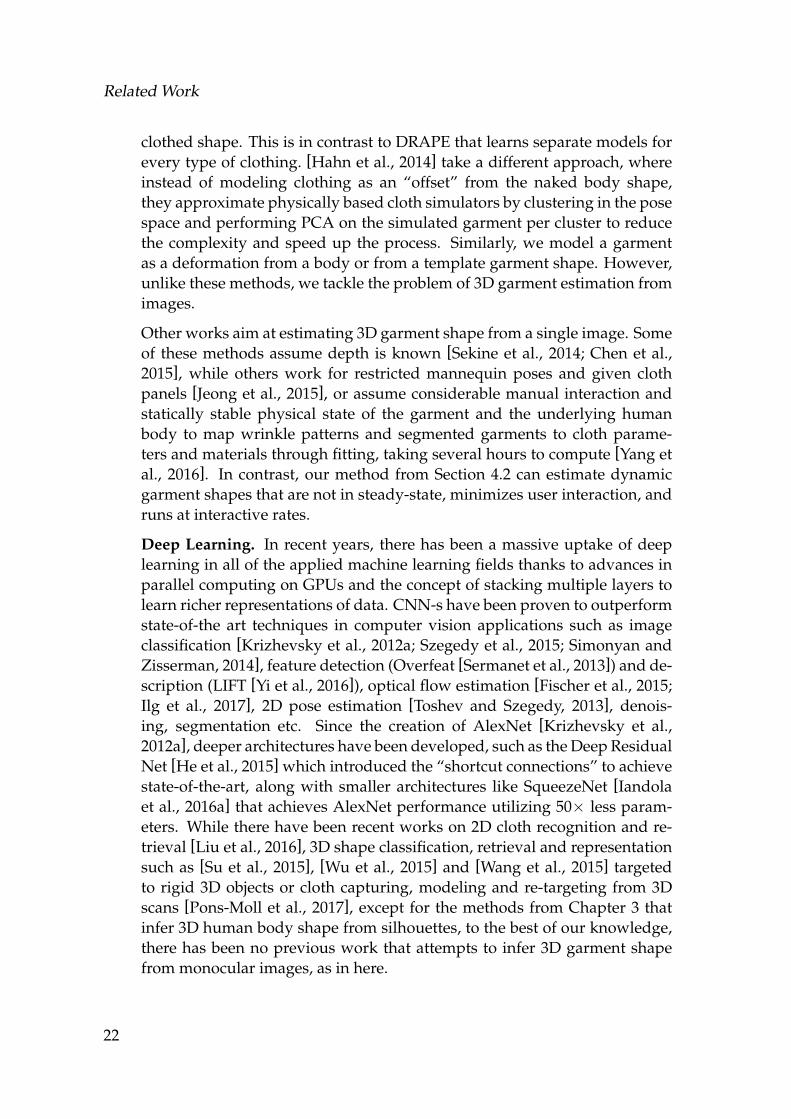
Related Work
clothed shape. This is in contrast to DRAPE that learns separate models forevery type of clothing. [Hahn et al., 2014] take a different approach, whereinstead of modeling clothing as an “offset” from the naked body shape,they approximate physically based cloth simulators by clustering in the posespace and performing PCA on the simulated garment per cluster to reducethe complexity and speed up the process. Similarly, we model a garmentas a deformation from a body or from a template garment shape. However,unlike these methods, we tackle the problem of 3D garment estimation fromimages.
Other works aim at estimating 3D garment shape from a single image. Someof these methods assume depth is known [Sekine et al., 2014; Chen et al.,2015], while others work for restricted mannequin poses and given clothpanels [Jeong et al., 2015], or assume considerable manual interaction andstatically stable physical state of the garment and the underlying humanbody to map wrinkle patterns and segmented garments to cloth parame-ters and materials through fitting, taking several hours to compute [Yang etal., 2016]. In contrast, our method from Section 4.2 can estimate dynamicgarment shapes that are not in steady-state, minimizes user interaction, andruns at interactive rates.
Deep Learning. In recent years, there has been a massive uptake of deeplearning in all of the applied machine learning fields thanks to advances inparallel computing on GPUs and the concept of stacking multiple layers tolearn richer representations of data. CNN-s have been proven to outperformstate-of-the art techniques in computer vision applications such as imageclassification [Krizhevsky et al., 2012a; Szegedy et al., 2015; Simonyan andZisserman, 2014], feature detection (Overfeat [Sermanet et al., 2013]) and de-scription (LIFT [Yi et al., 2016]), optical flow estimation [Fischer et al., 2015;Ilg et al., 2017], 2D pose estimation [Toshev and Szegedy, 2013], denois-ing, segmentation etc. Since the creation of AlexNet [Krizhevsky et al.,2012a], deeper architectures have been developed, such as the Deep ResidualNet [He et al., 2015] which introduced the “shortcut connections” to achievestate-of-the-art, along with smaller architectures like SqueezeNet [Iandolaet al., 2016a] that achieves AlexNet performance utilizing 50× less param-eters. While there have been recent works on 2D cloth recognition and re-trieval [Liu et al., 2016], 3D shape classification, retrieval and representationsuch as [Su et al., 2015], [Wu et al., 2015] and [Wang et al., 2015] targetedto rigid 3D objects or cloth capturing, modeling and re-targeting from 3Dscans [Pons-Moll et al., 2017], except for the methods from Chapter 3 thatinfer 3D human body shape from silhouettes, to the best of our knowledge,there has been no previous work that attempts to infer 3D garment shapefrom monocular images, as in here.
22
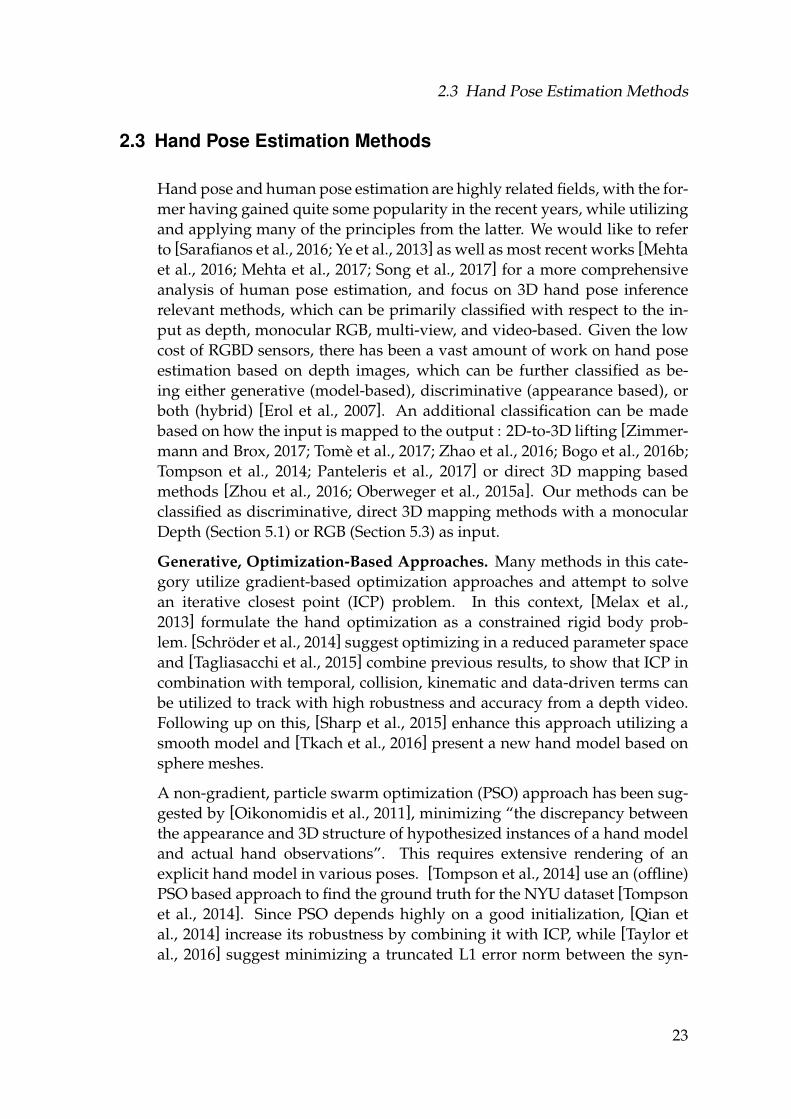
2.3 Hand Pose Estimation Methods
2.3 Hand Pose Estimation Methods
Hand pose and human pose estimation are highly related fields, with the for-mer having gained quite some popularity in the recent years, while utilizingand applying many of the principles from the latter. We would like to referto [Sarafianos et al., 2016; Ye et al., 2013] as well as most recent works [Mehtaet al., 2016; Mehta et al., 2017; Song et al., 2017] for a more comprehensiveanalysis of human pose estimation, and focus on 3D hand pose inferencerelevant methods, which can be primarily classified with respect to the in-put as depth, monocular RGB, multi-view, and video-based. Given the lowcost of RGBD sensors, there has been a vast amount of work on hand poseestimation based on depth images, which can be further classified as be-ing either generative (model-based), discriminative (appearance based), orboth (hybrid) [Erol et al., 2007]. An additional classification can be madebased on how the input is mapped to the output : 2D-to-3D lifting [Zimmer-mann and Brox, 2017; Tome et al., 2017; Zhao et al., 2016; Bogo et al., 2016b;Tompson et al., 2014; Panteleris et al., 2017] or direct 3D mapping basedmethods [Zhou et al., 2016; Oberweger et al., 2015a]. Our methods can beclassified as discriminative, direct 3D mapping methods with a monocularDepth (Section 5.1) or RGB (Section 5.3) as input.
Generative, Optimization-Based Approaches. Many methods in this cate-gory utilize gradient-based optimization approaches and attempt to solvean iterative closest point (ICP) problem. In this context, [Melax et al.,2013] formulate the hand optimization as a constrained rigid body prob-lem. [Schroder et al., 2014] suggest optimizing in a reduced parameter spaceand [Tagliasacchi et al., 2015] combine previous results, to show that ICP incombination with temporal, collision, kinematic and data-driven terms canbe utilized to track with high robustness and accuracy from a depth video.Following up on this, [Sharp et al., 2015] enhance this approach utilizing asmooth model and [Tkach et al., 2016] present a new hand model based onsphere meshes.
A non-gradient, particle swarm optimization (PSO) approach has been sug-gested by [Oikonomidis et al., 2011], minimizing “the discrepancy betweenthe appearance and 3D structure of hypothesized instances of a hand modeland actual hand observations”. This requires extensive rendering of anexplicit hand model in various poses. [Tompson et al., 2014] use an (offline)PSO based approach to find the ground truth for the NYU dataset [Tompsonet al., 2014]. Since PSO depends highly on a good initialization, [Qian etal., 2014] increase its robustness by combining it with ICP, while [Taylor etal., 2016] suggest minimizing a truncated L1 error norm between the syn-
23
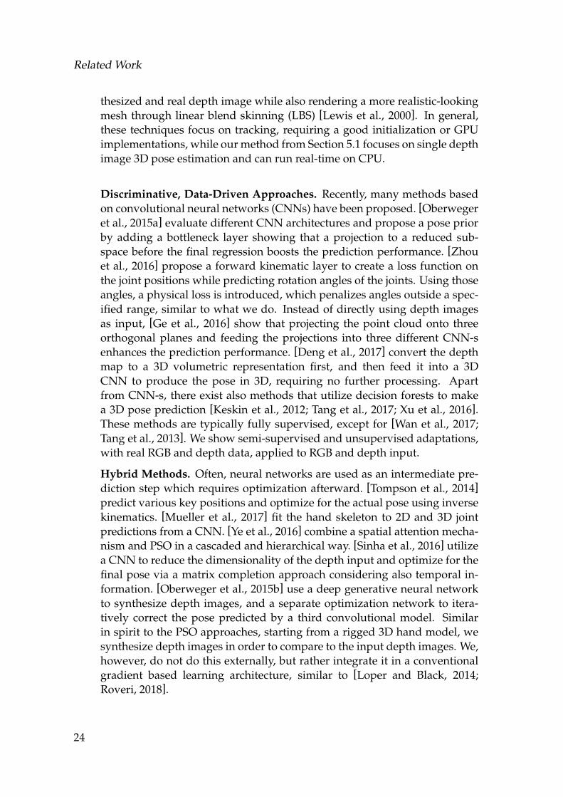
Related Work
thesized and real depth image while also rendering a more realistic-lookingmesh through linear blend skinning (LBS) [Lewis et al., 2000]. In general,these techniques focus on tracking, requiring a good initialization or GPUimplementations, while our method from Section 5.1 focuses on single depthimage 3D pose estimation and can run real-time on CPU.
Discriminative, Data-Driven Approaches. Recently, many methods basedon convolutional neural networks (CNNs) have been proposed. [Oberwegeret al., 2015a] evaluate different CNN architectures and propose a pose priorby adding a bottleneck layer showing that a projection to a reduced sub-space before the final regression boosts the prediction performance. [Zhouet al., 2016] propose a forward kinematic layer to create a loss function onthe joint positions while predicting rotation angles of the joints. Using thoseangles, a physical loss is introduced, which penalizes angles outside a spec-ified range, similar to what we do. Instead of directly using depth imagesas input, [Ge et al., 2016] show that projecting the point cloud onto threeorthogonal planes and feeding the projections into three different CNN-senhances the prediction performance. [Deng et al., 2017] convert the depthmap to a 3D volumetric representation first, and then feed it into a 3DCNN to produce the pose in 3D, requiring no further processing. Apartfrom CNN-s, there exist also methods that utilize decision forests to makea 3D pose prediction [Keskin et al., 2012; Tang et al., 2017; Xu et al., 2016].These methods are typically fully supervised, except for [Wan et al., 2017;Tang et al., 2013]. We show semi-supervised and unsupervised adaptations,with real RGB and depth data, applied to RGB and depth input.
Hybrid Methods. Often, neural networks are used as an intermediate pre-diction step which requires optimization afterward. [Tompson et al., 2014]predict various key positions and optimize for the actual pose using inversekinematics. [Mueller et al., 2017] fit the hand skeleton to 2D and 3D jointpredictions from a CNN. [Ye et al., 2016] combine a spatial attention mecha-nism and PSO in a cascaded and hierarchical way. [Sinha et al., 2016] utilizea CNN to reduce the dimensionality of the depth input and optimize for thefinal pose via a matrix completion approach considering also temporal in-formation. [Oberweger et al., 2015b] use a deep generative neural networkto synthesize depth images, and a separate optimization network to itera-tively correct the pose predicted by a third convolutional model. Similarin spirit to the PSO approaches, starting from a rigged 3D hand model, wesynthesize depth images in order to compare to the input depth images. We,however, do not do this externally, but rather integrate it in a conventionalgradient based learning architecture, similar to [Loper and Black, 2014;Roveri, 2018].
24
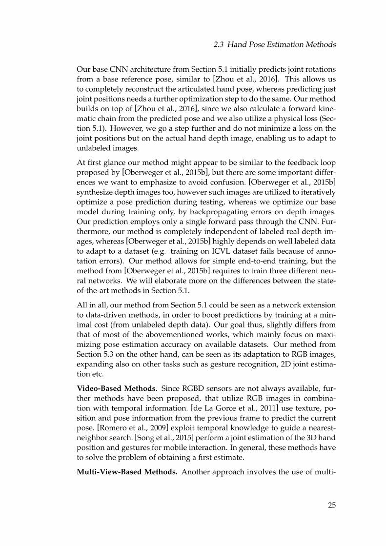
2.3 Hand Pose Estimation Methods
Our base CNN architecture from Section 5.1 initially predicts joint rotationsfrom a base reference pose, similar to [Zhou et al., 2016]. This allows usto completely reconstruct the articulated hand pose, whereas predicting justjoint positions needs a further optimization step to do the same. Our methodbuilds on top of [Zhou et al., 2016], since we also calculate a forward kine-matic chain from the predicted pose and we also utilize a physical loss (Sec-tion 5.1). However, we go a step further and do not minimize a loss on thejoint positions but on the actual hand depth image, enabling us to adapt tounlabeled images.
At first glance our method might appear to be similar to the feedback loopproposed by [Oberweger et al., 2015b], but there are some important differ-ences we want to emphasize to avoid confusion. [Oberweger et al., 2015b]synthesize depth images too, however such images are utilized to iterativelyoptimize a pose prediction during testing, whereas we optimize our basemodel during training only, by backpropagating errors on depth images.Our prediction employs only a single forward pass through the CNN. Fur-thermore, our method is completely independent of labeled real depth im-ages, whereas [Oberweger et al., 2015b] highly depends on well labeled datato adapt to a dataset (e.g. training on ICVL dataset fails because of anno-tation errors). Our method allows for simple end-to-end training, but themethod from [Oberweger et al., 2015b] requires to train three different neu-ral networks. We will elaborate more on the differences between the state-of-the-art methods in Section 5.1.
All in all, our method from Section 5.1 could be seen as a network extensionto data-driven methods, in order to boost predictions by training at a min-imal cost (from unlabeled depth data). Our goal thus, slightly differs fromthat of most of the abovementioned works, which mainly focus on maxi-mizing pose estimation accuracy on available datasets. Our method fromSection 5.3 on the other hand, can be seen as its adaptation to RGB images,expanding also on other tasks such as gesture recognition, 2D joint estima-tion etc.
Video-Based Methods. Since RGBD sensors are not always available, fur-ther methods have been proposed, that utilize RGB images in combina-tion with temporal information. [de La Gorce et al., 2011] use texture, po-sition and pose information from the previous frame to predict the currentpose. [Romero et al., 2009] exploit temporal knowledge to guide a nearest-neighbor search. [Song et al., 2015] perform a joint estimation of the 3D handposition and gestures for mobile interaction. In general, these methods haveto solve the problem of obtaining a first estimate.
Multi-View-Based Methods. Another approach involves the use of multi-
25
Related Work
ple cameras to compensate for the lack of depth data, alleviating the prob-lems with occluded parts. [Zhang et al., 2016] utilize stereo matching forhand tracking, [Simon et al., 2017] apply multi-view bootstrapping for key-point detection, and [Sridhar et al., 2014] estimate 3D hand pose from mul-tiple RGB cameras, with a hand shape representation based on a sum ofAnisotropic Gaussians, whereas [Sridhar et al., 2013] combine RGB andDepth data to obtain a richer input space.
Image-Based Methods. Due to the larger availability of regular color cam-eras, opposed to the abovementioned methods, in our method from Sec-tion 5.3, we make use of neither depth nor multi-camera or temporal in-formation. One of the first single frame based hand detection works,from [Athitsos and Sclaroff, 2003] utilize edge maps and Chamfer match-ing. With the exception of concurrent works [Spurr et al., 2018; Panteleriset al., 2017; Mueller et al., 2017], it was only recently that one of the firstmonocular RGB based methods [Zimmermann and Brox, 2017] for 3D handpose estimation was presented, utilizing CNN-s and synthetic datasets. Incontrast to our method, they split the prediction into a 2D joint localizationstep followed by a 3D up-lifting, and use their own synthetic dataset to com-plement the scarcity of existing datasets. We utilize our new, high quality,hand synthetic dataset to predict 3D joint angles directly from an RGB imageand strongly compare to [Zimmermann and Brox, 2017] on various tasks inSection 5.4.
26
C H A P T E R 3Human Body Shape Estimation
Estimating the human body shape from imagery is an important problemin computer vision with diverse applications. The estimated body shapeprovides an accurate proxy geometry for further tasks such as rendering freeviewpoint videos [Xu et al., 2011; Stoll et al., 2010; Casas et al., 2014; Starcket al., 2005], surveillance [Chen et al., 2013], tracking [Guan et al., 2008],biometric authentication, medical and personal measurements [Boisvert etal., 2013; Thaler et al., 2018], virtual cloth fitting [Guan et al., 2012; Wuhreret al., 2014; Rogge et al., 2014; Alexandros Neophytou, 2014], and artisticimage reshaping [Zhou et al., 2010]. Pose estimation is also tightly coupledwith shape estimation. Knowing the body shape significantly reduces thecomplexity and improves the robustness of pose estimation algorithms andthus expands the space of poses that can be reliably estimated [Ye and Yang,2014; de Aguiar et al., 2008].
However, as opposed to pose estimation, body shape estimation has re-ceived less attention from the community. The majority of existing al-gorithms are typically based on generative approaches that minimize anerror fitting term. They rely on either manual input [Zhou et al., 2010;Jain et al., 2010; Rogge et al., 2014], restrictive assumptions on the ac-quired images [Boisvert et al., 2013], or require information other thanjust 2D images (e.g. depth) [Weiss et al., 2011; Perbet et al., 2014; Hel-ten et al., 2013]. Furthermore, some of the methods have prohibitive com-plexity for real-time applications [Jain et al., 2010; Boisvert et al., 2013;Weiss et al., 2011]. A practical human body shape estimation algorithmshould be accurate, robust, efficient, automatic and fast. Additionally, it
27
Human Body Shape Estimation
should work with images acquired under less restrictive conditions andbody poses.
In contrast to optimization based approaches, it has been shown repeatedlythat utilizing neural networks can lead to superior results for many prob-lems such as classification [Krizhevsky et al., 2012a], segmentation [Longet al., 2015; Girshick et al., 2014], pose estimation [Toshev and Szegedy,2014] and shape classification or retrieval [Su et al., 2015; Wu et al., 2015;Fang et al., 2015]. Despite discriminative attempts to estimate the humanbody shape [Sigal et al., 2007; Chen et al., 2010], applying CNN techniquesto body shape estimation has had very little attention.
In this chapter, we present three discriminative methods that tackle the prob-lem of estimating the human body shape from monocular images. We focuson the silhouette as the most important visual cue, due to its relevance indescribing the human body, and the ease of extraction, as demonstrated inrecent works [Varol et al., 2017]. We initially introduce a method based onsilhouette features, that get mapped to the human body shape through ran-dom forest regressors, and for the remaining two main sections, we newlyexplore the utilization of CNN-s to tackle the very same task. We start withsimpler AlexNet [Krizhevsky et al., 2012b] like architectures and enhancethem with generative and cross-modal components, observing an improve-ment in accuracy as compared to both discriminative and generative works.All the three methods rely on a parametric body shape model, learned fromhuman body scans, hence, below we present it at first. Due to their dis-criminative nature and the variety of shapes that they need to capture, suchmethods leverage from training data abundance. Since the amount of realtraining data is very limited, we recur to synthetic ones, whose generationwe explain next and then introduce the three methods. In the end we con-clude the chapter with a discussion on the advantages and limitations ofeach method.
3.1 Shape as a Geometric Model
Deformable shape models are a common choice to tackle the problem ofhuman shape estimation from a few camera images [Balan et al., 2007;Sigal et al., 2007; Balan and Black, 2008; Guan et al., 2009; Zhou et al., 2010;Jain et al., 2010; Guan et al., 2012], in particular SCAPE [Anguelov et al.,2005]. While there exist other, more recent body models [Neophytou andHilton, 2013; Loper et al., 2015], we chose it mainly due to its simplicity andease of comparison with related methods that adopt it as well. It is a low-dimensional parametric model that captures correlated deformations due to
28
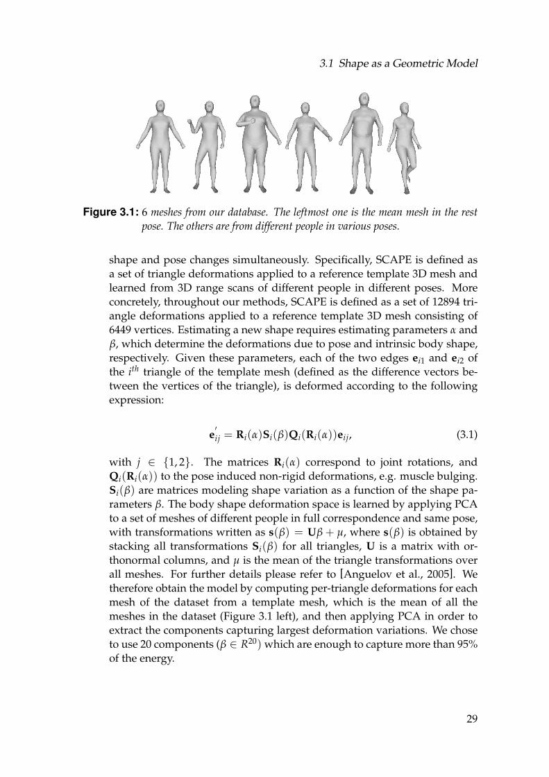
3.1 Shape as a Geometric Model
Figure 3.1: 6 meshes from our database. The leftmost one is the mean mesh in the restpose. The others are from different people in various poses.
shape and pose changes simultaneously. Specifically, SCAPE is defined asa set of triangle deformations applied to a reference template 3D mesh andlearned from 3D range scans of different people in different poses. Moreconcretely, throughout our methods, SCAPE is defined as a set of 12894 tri-angle deformations applied to a reference template 3D mesh consisting of6449 vertices. Estimating a new shape requires estimating parameters α andβ, which determine the deformations due to pose and intrinsic body shape,respectively. Given these parameters, each of the two edges ei1 and ei2 ofthe ith triangle of the template mesh (defined as the difference vectors be-tween the vertices of the triangle), is deformed according to the followingexpression:
e′ij = Ri(α)Si(β)Qi(Ri(α))eij, (3.1)
with j ∈ {1, 2}. The matrices Ri(α) correspond to joint rotations, andQi(Ri(α)) to the pose induced non-rigid deformations, e.g. muscle bulging.Si(β) are matrices modeling shape variation as a function of the shape pa-rameters β. The body shape deformation space is learned by applying PCAto a set of meshes of different people in full correspondence and same pose,with transformations written as s(β) = Uβ + µ, where s(β) is obtained bystacking all transformations Si(β) for all triangles, U is a matrix with or-thonormal columns, and µ is the mean of the triangle transformations overall meshes. For further details please refer to [Anguelov et al., 2005]. Wetherefore obtain the model by computing per-triangle deformations for eachmesh of the dataset from a template mesh, which is the mean of all themeshes in the dataset (Figure 3.1 left), and then applying PCA in order toextract the components capturing largest deformation variations. We choseto use 20 components (β ∈ R20) which are enough to capture more than 95%of the energy.
29
Human Body Shape Estimation
For all the methods, and more specifically the first two methods, we wouldlike to estimate the shape parameters β regardless of the pose (since thethird one attempts to directly estimate 3D mesh vertices). We take the com-mon assumption that the body shape does not significantly change due tothe range of poses we consider. Hence, we ignore pose dependent shapechanges given by Qi(R(α)). Decoupling pose and shape changes allows usto adopt a fast and efficient method from the graphics community for posechanges, known as Linear Blend Skinning (LBS) [Lewis et al., 2000], similarto previous works [Pishchulin et al., 2015; Jain et al., 2010; Feng et al., 2015;Yang et al., 2016]. Starting from a rest pose shape with vertices v1, ..., vn ∈ R4
in homogenous coordinates, LBS computes the new position of each vertexby a weighted combination of the bone transformation matrices T1, ..., Tm ina skeleton controlling the mesh, and skinning weights wi,1, ..., wi,m ∈ R foreach vertex vi, as given by the following formula:
v′i =
m
∑j=1
wi,jTjvi =
(m
∑j=1
wi,jTj
)vi (3.2)
In our model, the skinning weights are computed for a skeleton of 17 bodyparts (1 for the head, 2 for the torso, 2 for the hips and 3 for each of thelower and upper limbs) for the mean shape mesh using the heat diffusionmethod [Baran and Popovic, 2007a]. It has to be noted that wi,j ≥ 0 andwi,1 + · · · + wi,m = 1. Once the shape parameters β are estimated, recon-structing a new shape utilizing SCAPE involves solving a least-squares sys-tem over such parameters, which runs in milliseconds.
3.2 Data Generation
Our training based methods require numerous training and validation data.Gathering a big number of human shapes is a highly non-trivial task - dueto the need of specialized equipment for scanning people, the difficulty offinding a large number of them, and more importantly, due to the necessityof scanning them under minimalistic clothing, in order to better capture theintrinsic shapes. Unfortunately, there exists no freely available dataset of realhuman body shapes along with measurements. A feasible solution though,would be to learn a parametric shape model from a small subset of bodyshapes that capture body shape variances and generate synthetic data fromit, as explained in Section 3.1.
Taking advantage of the commercially available CAESAR dataset [Robinette
30
3.2 Data Generation
and Daanen, 1999] 1, containing people in an almost naked apparel, re-searchers have released two datasets [Yang et al., 2014; Pishchulin et al.,2015], consisting of meshes obtained by fitting a template mesh to subsetsof the CAESAR dataset. We merge these two datasets and construct a largerone, to enable learning a more general shape model. One of them [Yanget al., 2014], consists of around 1500 registered meshes in correspondence,however of higher resolution than the other dataset [Pishchulin et al., 2015].The resolutions respectively are 12500 vertices 25000 triangles and 6449 ver-tices 12894 triangles. Mesh resolution is not so important for our application,hence we map the higher resolution meshes to the lower resolution ones.This also improves the computation time. To achieve that, we first extract atemplate mesh, as the mean mesh of each dataset, and then apply non-rigidICP [Amberg et al., 2007] to the two template meshes. Afterwards, closestpoints in both meshes are computed, using barycentric coordinates in theclosest triangle. The retrieved mapping can be applied to all the remainingmeshes due to the same mesh connectivity.
We select 2900 meshes from the combined dataset for learning the shapemodel, leaving out around 1500 meshes for testing and experiments. In or-der to synthesize more training meshes, we sample from the 20 dimensionalmultivariate normal distribution spanned by the PCA space (Section 3.1),such that for a random sample β = [β1, β2, ..., β20], it holds that β ∼ N (µ, Σ)with µ being the 20-dimensional mean vector and Σ the 20× 20 covariancematrix of the parameters. To synthesize meshes in different poses, we gathera set of animations comprising of various poses (e.g. selfie, walking, run-ning, etc.). After transferring a generated pose to the template mesh usingLBS, we compute the resulting per-triangle deformations Ri. For a givenmesh with parameters β, the final pose is then given by e′ij = RiSi(β)eij,where eij are the edges of the template mesh (Section 3.1).
As the training set, we randomly generate around 100000 samples from themulti-variate distribution over the β parameters, and restrict them to fall intothe±3× Std.Dev range for each dimension of the PCA projected parametersto avoid getting unrealistic human shapes. After applying LBS on varioustemplate poses, in order to enrich the dataset, we can easily obtain silhou-ettes, shaded images and even mesh descriptors, which are inputs utilizedin the following methods. The silhouette is computed by projecting all themesh edges for which two coinciding triangles have normals pointing in op-posite directions, as seen by the camera viewpoint. For testing, we evaluateour method with images from the meshes left out from the training dataset,as well as on real ones.
1http://store.sae.org/caesar/
31
Human Body Shape Estimation
3.3 Shape Estimation with Handcrafted Features and CCA
In this first section, we propose a fast and automatic method for estimat-ing the 3D body shape of a person from images, utilizing multi-view semi-supervised learning. This method relies on extracting novel features froma given silhouette of a single person under minimal self-occlusion, like ina selfie, and a parametric human body shape model [Anguelov et al., 2005].The latter is utilized to generate meshes spanning a spectrum of human bodyshapes, from which silhouettes are computed over multiple views, as alsoexplained in Section 3.2, in poses compliant with the target applications fortraining. We firstly estimate viewing direction with high accuracy, by solv-ing a classification task. Utilizing the information simultaneously capturedin multiple synthetic views of the same body mesh, we apply Canonical Cor-relation Analysis (CCA) [Hotelling, 1936] to learn informative bases wherethe extracted features can be projected. A random forest regressor is thenadopted to learn a mapping from projected feature space to parameter space.This results in lower feature dimensionality, reducing the training and testtime drastically, and improves prediction as compared to plain regressionforests. We demonstrate our results on real people and comprehensivelyevaluate our method by validating it on thousands of body shapes.
3.3.1 Method Overview
The goal of our system is to infer the 3D body shape of a person from asingle or multiple monocular images fast and automatically. Specifically, wewould like to estimate the parameters of a 3D body shape model (Section 3.1)such that the corresponding body shape best approximates the 3D body ofthe subject depicted in the input images. Despite the ambiguity that the 2Dsilhouette withholds, the projection of the transformed mesh in the imageshould at least best explain it.
An overview of our system is depicted in Figure 3.2. The input to the shapeestimation algorithm is a 2D silhouette of the desired individual under min-imal self-occlusion (e.g. a selfie), which can be computed accurately for ourtarget scenarios, by learning a background model through Gaussian mixturemodels and using Graphcuts [Boykov and Jolly, 2001]. The word “selfie”here is used interchangingly to describe the activity of taking a selfie in frontof a mirror, and also as a label for poses representing mild self-occlusion(Figure 3.1). We then compute features extracted from the silhouettes (Sec-tion 3.3.2). These are first used to train a classifier on the camera viewingdirection (Section 3.3.3). The features from silhouettes of a particular view
32
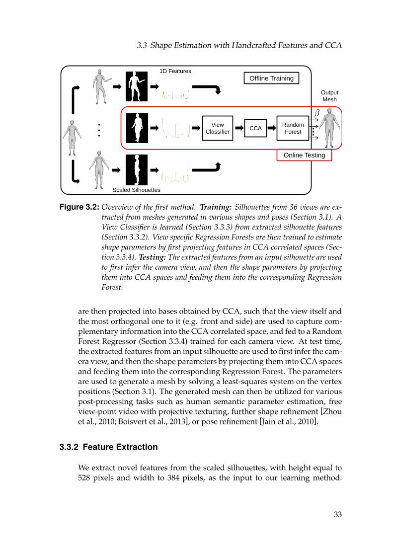
3.3 Shape Estimation with Handcrafted Features and CCA
Scaled Silhouettes
1D Features
Offline Training
Random
Forest
Output
Mesh
View
ClassifierCCA
Online Testing
Figure 3.2: Overview of the first method. Training: Silhouettes from 36 views are ex-tracted from meshes generated in various shapes and poses (Section 3.1). AView Classifier is learned (Section 3.3.3) from extracted silhouette features(Section 3.3.2). View specific Regression Forests are then trained to estimateshape parameters by first projecting features in CCA correlated spaces (Sec-tion 3.3.4). Testing: The extracted features from an input silhouette are usedto first infer the camera view, and then the shape parameters by projectingthem into CCA spaces and feeding them into the corresponding RegressionForest.
are then projected into bases obtained by CCA, such that the view itself andthe most orthogonal one to it (e.g. front and side) are used to capture com-plementary information into the CCA correlated space, and fed to a RandomForest Regressor (Section 3.3.4) trained for each camera view. At test time,the extracted features from an input silhouette are used to first infer the cam-era view, and then the shape parameters by projecting them into CCA spacesand feeding them into the corresponding Regression Forest. The parametersare used to generate a mesh by solving a least-squares system on the vertexpositions (Section 3.1). The generated mesh can then be utilized for variouspost-processing tasks such as human semantic parameter estimation, freeview-point video with projective texturing, further shape refinement [Zhouet al., 2010; Boisvert et al., 2013], or pose refinement [Jain et al., 2010].
3.3.2 Feature Extraction
We extract novel features from the scaled silhouettes, with height equal to528 pixels and width to 384 pixels, as the input to our learning method.
33
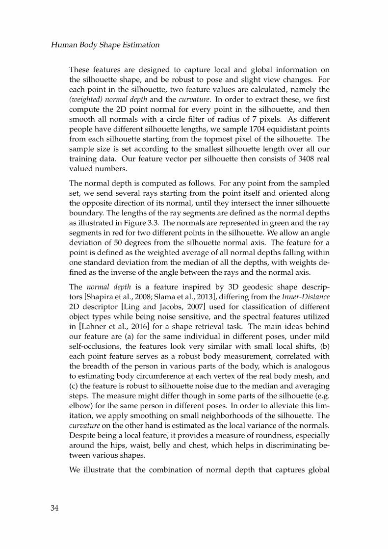
Human Body Shape Estimation
These features are designed to capture local and global information onthe silhouette shape, and be robust to pose and slight view changes. Foreach point in the silhouette, two feature values are calculated, namely the(weighted) normal depth and the curvature. In order to extract these, we firstcompute the 2D point normal for every point in the silhouette, and thensmooth all normals with a circle filter of radius of 7 pixels. As differentpeople have different silhouette lengths, we sample 1704 equidistant pointsfrom each silhouette starting from the topmost pixel of the silhouette. Thesample size is set according to the smallest silhouette length over all ourtraining data. Our feature vector per silhouette then consists of 3408 realvalued numbers.
The normal depth is computed as follows. For any point from the sampledset, we send several rays starting from the point itself and oriented alongthe opposite direction of its normal, until they intersect the inner silhouetteboundary. The lengths of the ray segments are defined as the normal depthsas illustrated in Figure 3.3. The normals are represented in green and the raysegments in red for two different points in the silhouette. We allow an angledeviation of 50 degrees from the silhouette normal axis. The feature for apoint is defined as the weighted average of all normal depths falling withinone standard deviation from the median of all the depths, with weights de-fined as the inverse of the angle between the rays and the normal axis.
The normal depth is a feature inspired by 3D geodesic shape descrip-tors [Shapira et al., 2008; Slama et al., 2013], differing from the Inner-Distance2D descriptor [Ling and Jacobs, 2007] used for classification of differentobject types while being noise sensitive, and the spectral features utilizedin [Lahner et al., 2016] for a shape retrieval task. The main ideas behindour feature are (a) for the same individual in different poses, under mildself-occlusions, the features look very similar with small local shifts, (b)each point feature serves as a robust body measurement, correlated withthe breadth of the person in various parts of the body, which is analogousto estimating body circumference at each vertex of the real body mesh, and(c) the feature is robust to silhouette noise due to the median and averagingsteps. The measure might differ though in some parts of the silhouette (e.g.elbow) for the same person in different poses. In order to alleviate this lim-itation, we apply smoothing on small neighborhoods of the silhouette. Thecurvature on the other hand is estimated as the local variance of the normals.Despite being a local feature, it provides a measure of roundness, especiallyaround the hips, waist, belly and chest, which helps in discriminating be-tween various shapes.
We illustrate that the combination of normal depth that captures global
34
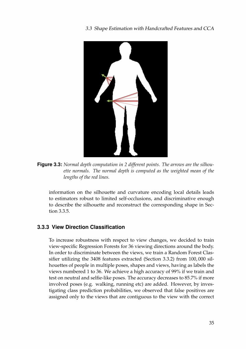
3.3 Shape Estimation with Handcrafted Features and CCA
Figure 3.3: Normal depth computation in 2 different points. The arrows are the silhou-ette normals. The normal depth is computed as the weighted mean of thelengths of the red lines.
information on the silhouette and curvature encoding local details leadsto estimators robust to limited self-occlusions, and discriminative enoughto describe the silhouette and reconstruct the corresponding shape in Sec-tion 3.3.5.
3.3.3 View Direction Classification
To increase robustness with respect to view changes, we decided to trainview-specific Regression Forests for 36 viewing directions around the body.In order to discriminate between the views, we train a Random Forest Clas-sifier utilizing the 3408 features extracted (Section 3.3.2) from 100, 000 sil-houettes of people in multiple poses, shapes and views, having as labels theviews numbered 1 to 36. We achieve a high accuracy of 99% if we train andtest on neutral and selfie-like poses. The accuracy decreases to 85.7% if moreinvolved poses (e.g. walking, running etc) are added. However, by inves-tigating class prediction probabilities, we observed that false positives areassigned only to the views that are contiguous to the view with the correct
35
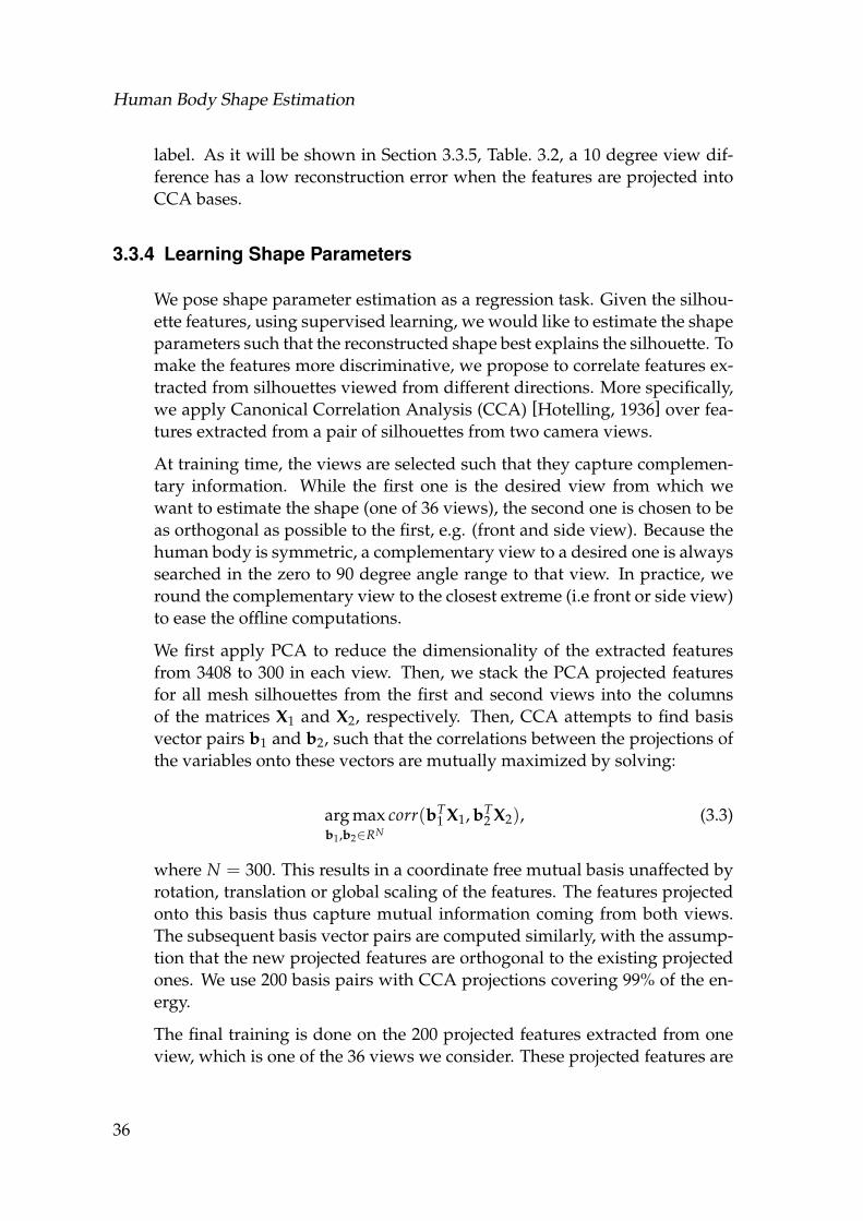
Human Body Shape Estimation
label. As it will be shown in Section 3.3.5, Table. 3.2, a 10 degree view dif-ference has a low reconstruction error when the features are projected intoCCA bases.
3.3.4 Learning Shape Parameters
We pose shape parameter estimation as a regression task. Given the silhou-ette features, using supervised learning, we would like to estimate the shapeparameters such that the reconstructed shape best explains the silhouette. Tomake the features more discriminative, we propose to correlate features ex-tracted from silhouettes viewed from different directions. More specifically,we apply Canonical Correlation Analysis (CCA) [Hotelling, 1936] over fea-tures extracted from a pair of silhouettes from two camera views.
At training time, the views are selected such that they capture complemen-tary information. While the first one is the desired view from which wewant to estimate the shape (one of 36 views), the second one is chosen to beas orthogonal as possible to the first, e.g. (front and side view). Because thehuman body is symmetric, a complementary view to a desired one is alwayssearched in the zero to 90 degree angle range to that view. In practice, weround the complementary view to the closest extreme (i.e front or side view)to ease the offline computations.
We first apply PCA to reduce the dimensionality of the extracted featuresfrom 3408 to 300 in each view. Then, we stack the PCA projected featuresfor all mesh silhouettes from the first and second views into the columnsof the matrices X1 and X2, respectively. Then, CCA attempts to find basisvector pairs b1 and b2, such that the correlations between the projections ofthe variables onto these vectors are mutually maximized by solving:
arg maxb1,b2∈RN
corr(bT1 X1, bT
2 X2), (3.3)
where N = 300. This results in a coordinate free mutual basis unaffected byrotation, translation or global scaling of the features. The features projectedonto this basis thus capture mutual information coming from both views.The subsequent basis vector pairs are computed similarly, with the assump-tion that the new projected features are orthogonal to the existing projectedones. We use 200 basis pairs with CCA projections covering 99% of the en-ergy.
The final training is done on the 200 projected features extracted from oneview, which is one of the 36 views we consider. These projected features are
36
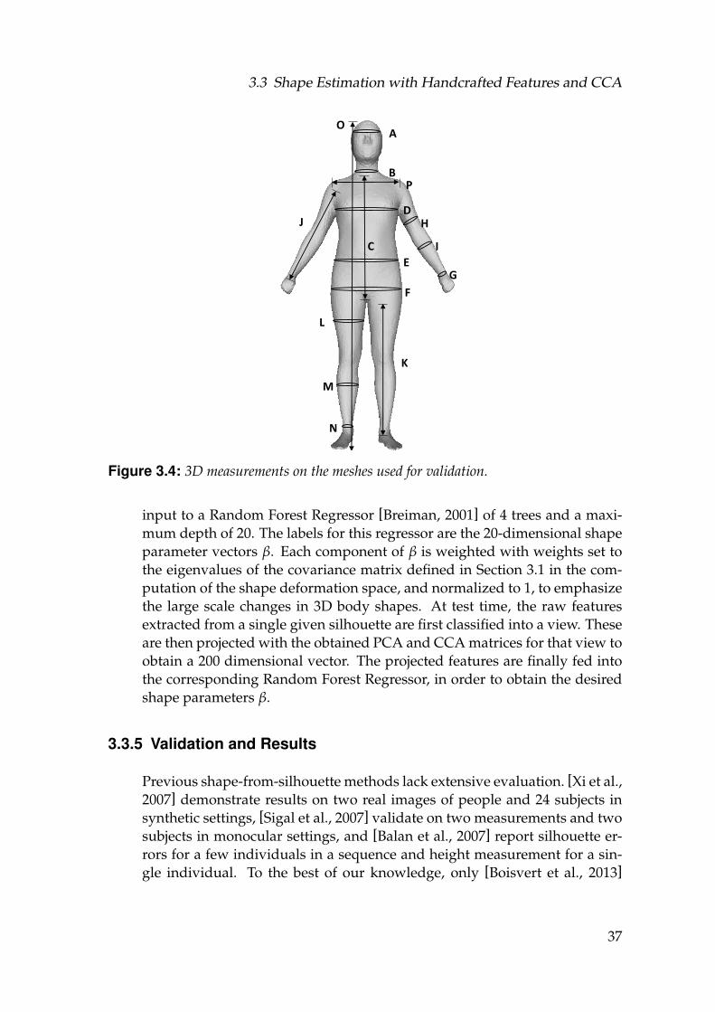
3.3 Shape Estimation with Handcrafted Features and CCA
A
B
C
DH
I
GE
F
P
O
K
L
M
N
J
Figure 3.4: 3D measurements on the meshes used for validation.
input to a Random Forest Regressor [Breiman, 2001] of 4 trees and a maxi-mum depth of 20. The labels for this regressor are the 20-dimensional shapeparameter vectors β. Each component of β is weighted with weights set tothe eigenvalues of the covariance matrix defined in Section 3.1 in the com-putation of the shape deformation space, and normalized to 1, to emphasizethe large scale changes in 3D body shapes. At test time, the raw featuresextracted from a single given silhouette are first classified into a view. Theseare then projected with the obtained PCA and CCA matrices for that view toobtain a 200 dimensional vector. The projected features are finally fed intothe corresponding Random Forest Regressor, in order to obtain the desiredshape parameters β.
3.3.5 Validation and Results
Previous shape-from-silhouette methods lack extensive evaluation. [Xi et al.,2007] demonstrate results on two real images of people and 24 subjects insynthetic settings, [Sigal et al., 2007] validate on two measurements and twosubjects in monocular settings, and [Balan et al., 2007] report silhouette er-rors for a few individuals in a sequence and height measurement for a sin-gle individual. To the best of our knowledge, only [Boisvert et al., 2013]
37
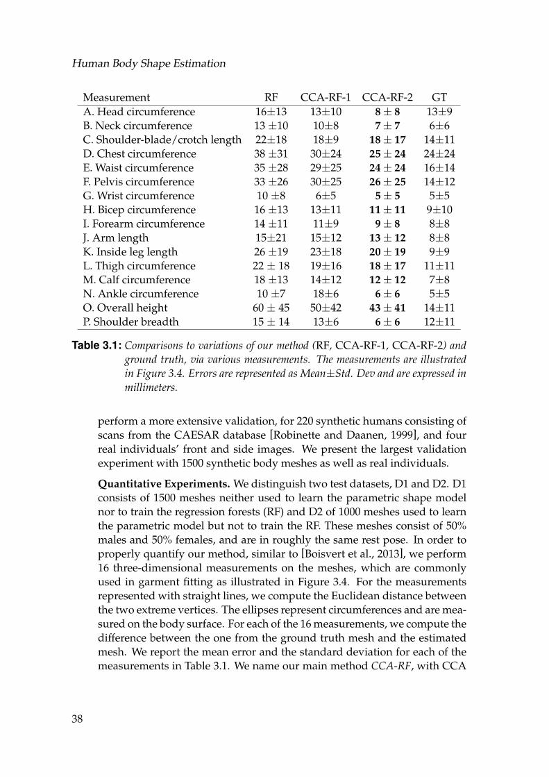
Human Body Shape Estimation
Measurement RF CCA-RF-1 CCA-RF-2 GTA. Head circumference 16±13 13±10 8± 8 13±9B. Neck circumference 13 ±10 10±8 7± 7 6±6C. Shoulder-blade/crotch length 22±18 18±9 18± 17 14±11D. Chest circumference 38 ±31 30±24 25± 24 24±24E. Waist circumference 35 ±28 29±25 24± 24 16±14F. Pelvis circumference 33 ±26 30±25 26± 25 14±12G. Wrist circumference 10 ±8 6±5 5± 5 5±5H. Bicep circumference 16 ±13 13±11 11± 11 9±10I. Forearm circumference 14 ±11 11±9 9± 8 8±8J. Arm length 15±21 15±12 13± 12 8±8K. Inside leg length 26 ±19 23±18 20± 19 9±9L. Thigh circumference 22 ± 18 19±16 18± 17 11±11M. Calf circumference 18 ±13 14±12 12± 12 7±8N. Ankle circumference 10 ±7 18±6 6± 6 5±5O. Overall height 60 ± 45 50±42 43± 41 14±11P. Shoulder breadth 15 ± 14 13±6 6± 6 12±11
Table 3.1: Comparisons to variations of our method (RF, CCA-RF-1, CCA-RF-2) andground truth, via various measurements. The measurements are illustratedin Figure 3.4. Errors are represented as Mean±Std. Dev and are expressed inmillimeters.
perform a more extensive validation, for 220 synthetic humans consisting ofscans from the CAESAR database [Robinette and Daanen, 1999], and fourreal individuals’ front and side images. We present the largest validationexperiment with 1500 synthetic body meshes as well as real individuals.
Quantitative Experiments. We distinguish two test datasets, D1 and D2. D1consists of 1500 meshes neither used to learn the parametric shape modelnor to train the regression forests (RF) and D2 of 1000 meshes used to learnthe parametric model but not to train the RF. These meshes consist of 50%males and 50% females, and are in roughly the same rest pose. In order toproperly quantify our method, similar to [Boisvert et al., 2013], we perform16 three-dimensional measurements on the meshes, which are commonlyused in garment fitting as illustrated in Figure 3.4. For the measurementsrepresented with straight lines, we compute the Euclidean distance betweenthe two extreme vertices. The ellipses represent circumferences and are mea-sured on the body surface. For each of the 16 measurements, we compute thedifference between the one from the ground truth mesh and the estimatedmesh. We report the mean error and the standard deviation for each of themeasurements in Table 3.1. We name our main method CCA-RF, with CCA
38
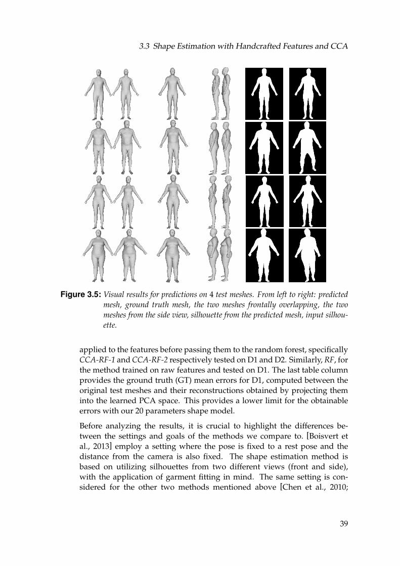
3.3 Shape Estimation with Handcrafted Features and CCA
Figure 3.5: Visual results for predictions on 4 test meshes. From left to right: predictedmesh, ground truth mesh, the two meshes frontally overlapping, the twomeshes from the side view, silhouette from the predicted mesh, input silhou-ette.
applied to the features before passing them to the random forest, specificallyCCA-RF-1 and CCA-RF-2 respectively tested on D1 and D2. Similarly, RF, forthe method trained on raw features and tested on D1. The last table columnprovides the ground truth (GT) mean errors for D1, computed between theoriginal test meshes and their reconstructions obtained by projecting theminto the learned PCA space. This provides a lower limit for the obtainableerrors with our 20 parameters shape model.
Before analyzing the results, it is crucial to highlight the differences be-tween the settings and goals of the methods we compare to. [Boisvert etal., 2013] employ a setting where the pose is fixed to a rest pose and thedistance from the camera is also fixed. The shape estimation method isbased on utilizing silhouettes from two different views (front and side),with the application of garment fitting in mind. The same setting is con-sidered for the other two methods mentioned above [Chen et al., 2010;
39
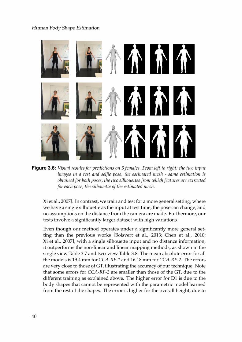
Human Body Shape Estimation
Figure 3.6: Visual results for predictions on 3 females. From left to right: the two inputimages in a rest and selfie pose, the estimated mesh - same estimation isobtained for both poses, the two silhouettes from which features are extractedfor each pose, the silhouette of the estimated mesh.
Xi et al., 2007]. In contrast, we train and test for a more general setting, wherewe have a single silhouette as the input at test time, the pose can change, andno assumptions on the distance from the camera are made. Furthermore, ourtests involve a significantly larger dataset with high variations.
Even though our method operates under a significantly more general set-ting than the previous works [Boisvert et al., 2013; Chen et al., 2010;Xi et al., 2007], with a single silhouette input and no distance information,it outperforms the non-linear and linear mapping methods, as shown in thesingle view Table 3.7 and two-view Table 3.8. The mean absolute error for allthe models is 19.4 mm for CCA-RF-1 and 16.18 mm for CCA-RF-2. The errorsare very close to those of GT, illustrating the accuracy of our technique. Notethat some errors for CCA-RF-2 are smaller than those of the GT, due to thedifferent training as explained above. The higher error for D1 is due to thebody shapes that cannot be represented with the parametric model learnedfrom the rest of the shapes. The error is higher for the overall height, due to
40
3.3 Shape Estimation with Handcrafted Features and CCA
the fixed scale in the training and testing silhouettes that we use. It is impor-tant to note the differences in errors between the RF and CCA-RF-1. There isan overall decrease of error when CCA is utilized, which shows that the pro-jection with the CCA bases significantly improves prediction. Additionally,we evaluate the performance of our method when the input comes from aless favorable view, the side view, achieving an error of 22.45 mm which isvery close to the one from only the frontal view. For completeness, we com-pare also to [Helten et al., 2013], who utilize an RGB-D camera for capturingthe body shapes, and a full RMSE map per vertex to measure the differences.Using two depth maps, fitting to the pose and testing only on 6 individualsthey report a mean error of 10.1 mm while we have a mean error of 19.19mm on 1500 meshes.
Qualitative Results. In Figure 3.5, we show example samples from our tests.In each row, first the predicted mesh is shown along with the ground truthtest mesh. Then, their overlap is illustrated. This is followed by the sideviews, and the silhouette of the estimated mesh and the input silhouette.Note that the input silhouettes are in different poses, but we show the esti-mated meshes in rest poses for easy comparisons. Our results are visuallyvery close to the ground truth shapes even under such pose changes.
Finally, we show an experiment where real pictures of three females aretaken in a rest and a selfie-like pose along with the estimated meshes inFigure 3.6. It is important to note that despite the pose change, the retrievedmesh for each person is the same. Another important observation is thateven though the input is scaled to the same size, the estimated parametersyield statistically plausible heights, which turned out to be sufficient in ob-taining an ordering based on relative height between the estimated meshes.We believe that this is due to the statistical shape model, where semantic pa-rameters like height and weight are correlated in the PCA parameter space.To the best of our knowledge, no previous work can resolve this task. Forexample, in the work by [Sigal et al., 2007], the mesh needs to be scaled if nocamera calibration is provided.
Poses, Views and Noise. We investigated accuracy in the presence of sil-houette noise, various poses, and different or multiple views. We run theexperiments with the data setup D1, explained above. For each experiment,we show the mean and standard deviation either of the accuracy gain or ofthe errors over all the body measurements in Table 3.2.
The first three columns show the accuracy gain of applying CCA-RF to thefront view (F), side view (S) or when concatenating both views together (FS),as compared to RF. A larger gain is obtained in the side view as compared tothe front view, due to additional information that is injected from the frontal
41
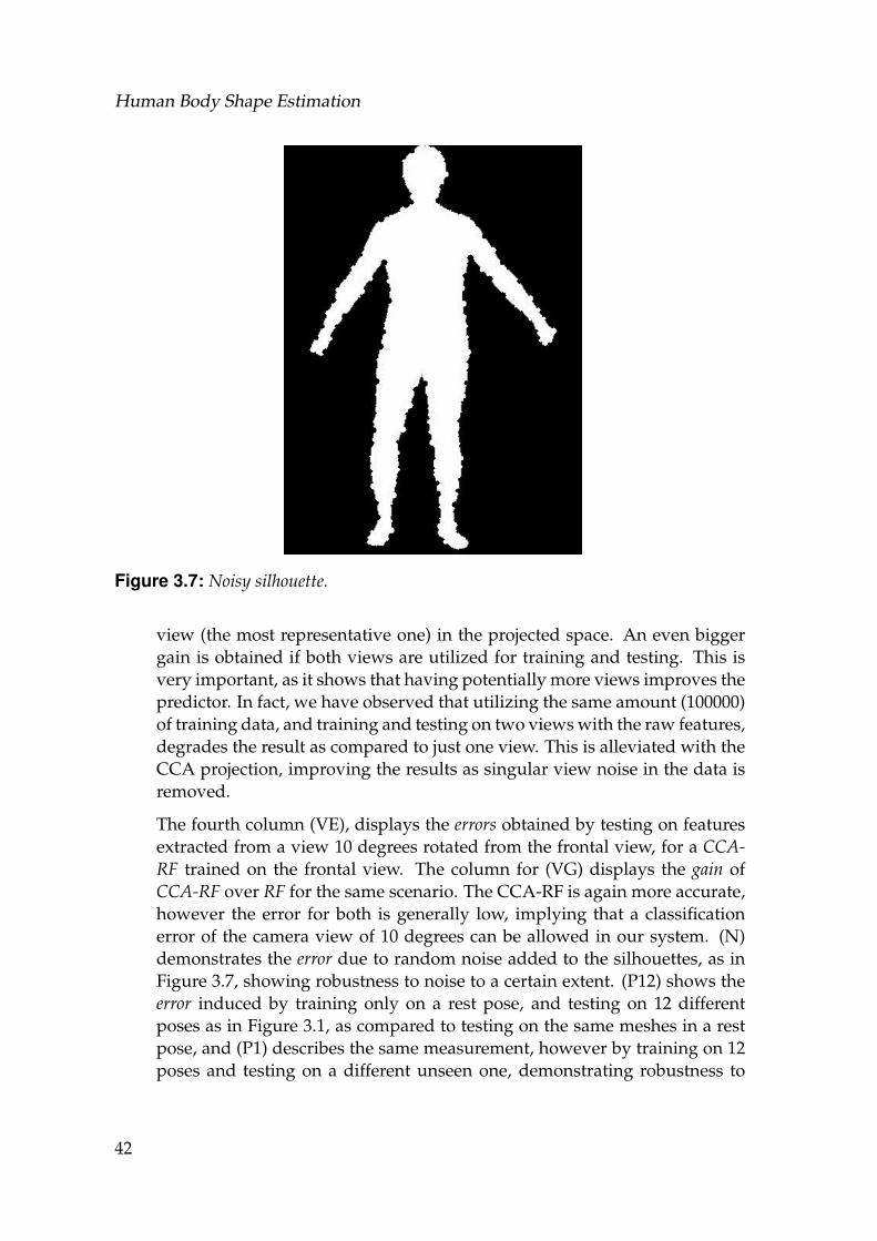
Human Body Shape Estimation
Figure 3.7: Noisy silhouette.
view (the most representative one) in the projected space. An even biggergain is obtained if both views are utilized for training and testing. This isvery important, as it shows that having potentially more views improves thepredictor. In fact, we have observed that utilizing the same amount (100000)of training data, and training and testing on two views with the raw features,degrades the result as compared to just one view. This is alleviated with theCCA projection, improving the results as singular view noise in the data isremoved.
The fourth column (VE), displays the errors obtained by testing on featuresextracted from a view 10 degrees rotated from the frontal view, for a CCA-RF trained on the frontal view. The column for (VG) displays the gain ofCCA-RF over RF for the same scenario. The CCA-RF is again more accurate,however the error for both is generally low, implying that a classificationerror of the camera view of 10 degrees can be allowed in our system. (N)demonstrates the error due to random noise added to the silhouettes, as inFigure 3.7, showing robustness to noise to a certain extent. (P12) shows theerror induced by training only on a rest pose, and testing on 12 differentposes as in Figure 3.1, as compared to testing on the same meshes in a restpose, and (P1) describes the same measurement, however by training on 12poses and testing on a different unseen one, demonstrating robustness to
42
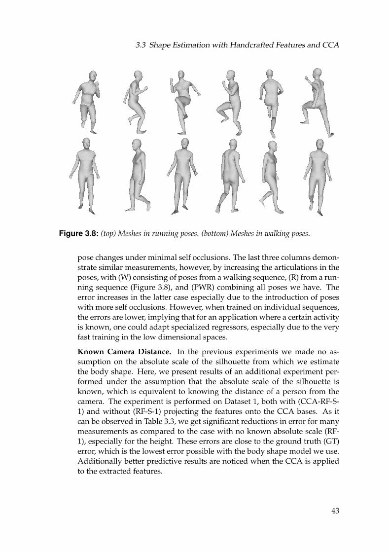
3.3 Shape Estimation with Handcrafted Features and CCA
Figure 3.8: (top) Meshes in running poses. (bottom) Meshes in walking poses.
pose changes under minimal self occlusions. The last three columns demon-strate similar measurements, however, by increasing the articulations in theposes, with (W) consisting of poses from a walking sequence, (R) from a run-ning sequence (Figure 3.8), and (PWR) combining all poses we have. Theerror increases in the latter case especially due to the introduction of poseswith more self occlusions. However, when trained on individual sequences,the errors are lower, implying that for an application where a certain activityis known, one could adapt specialized regressors, especially due to the veryfast training in the low dimensional spaces.
Known Camera Distance. In the previous experiments we made no as-sumption on the absolute scale of the silhouette from which we estimatethe body shape. Here, we present results of an additional experiment per-formed under the assumption that the absolute scale of the silhouette isknown, which is equivalent to knowing the distance of a person from thecamera. The experiment is performed on Dataset 1, both with (CCA-RF-S-1) and without (RF-S-1) projecting the features onto the CCA bases. As itcan be observed in Table 3.3, we get significant reductions in error for manymeasurements as compared to the case with no known absolute scale (RF-1), especially for the height. These errors are close to the ground truth (GT)error, which is the lowest error possible with the body shape model we use.Additionally better predictive results are noticed when the CCA is appliedto the extracted features.
43
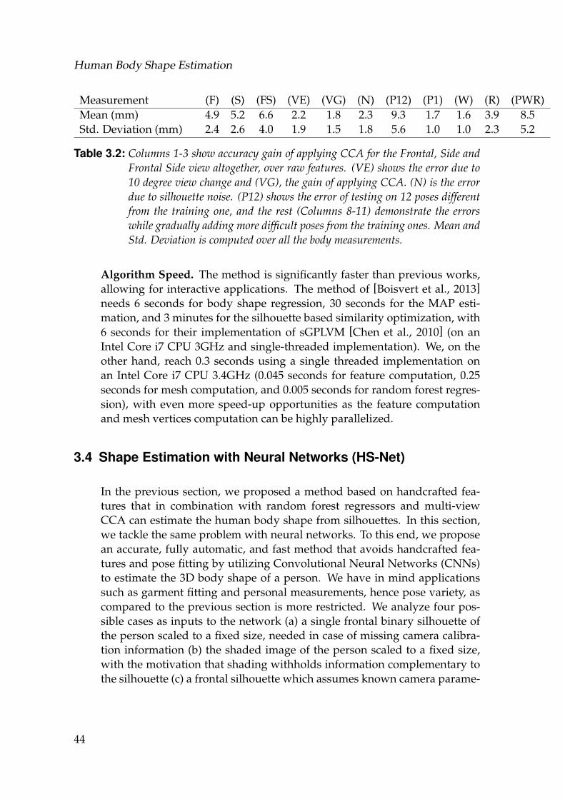
Human Body Shape Estimation
Measurement (F) (S) (FS) (VE) (VG) (N) (P12) (P1) (W) (R) (PWR)Mean (mm) 4.9 5.2 6.6 2.2 1.8 2.3 9.3 1.7 1.6 3.9 8.5Std. Deviation (mm) 2.4 2.6 4.0 1.9 1.5 1.8 5.6 1.0 1.0 2.3 5.2
Table 3.2: Columns 1-3 show accuracy gain of applying CCA for the Frontal, Side andFrontal Side view altogether, over raw features. (VE) shows the error due to10 degree view change and (VG), the gain of applying CCA. (N) is the errordue to silhouette noise. (P12) shows the error of testing on 12 poses differentfrom the training one, and the rest (Columns 8-11) demonstrate the errorswhile gradually adding more difficult poses from the training ones. Mean andStd. Deviation is computed over all the body measurements.
Algorithm Speed. The method is significantly faster than previous works,allowing for interactive applications. The method of [Boisvert et al., 2013]needs 6 seconds for body shape regression, 30 seconds for the MAP esti-mation, and 3 minutes for the silhouette based similarity optimization, with6 seconds for their implementation of sGPLVM [Chen et al., 2010] (on anIntel Core i7 CPU 3GHz and single-threaded implementation). We, on theother hand, reach 0.3 seconds using a single threaded implementation onan Intel Core i7 CPU 3.4GHz (0.045 seconds for feature computation, 0.25seconds for mesh computation, and 0.005 seconds for random forest regres-sion), with even more speed-up opportunities as the feature computationand mesh vertices computation can be highly parallelized.
3.4 Shape Estimation with Neural Networks (HS-Net)
In the previous section, we proposed a method based on handcrafted fea-tures that in combination with random forest regressors and multi-viewCCA can estimate the human body shape from silhouettes. In this section,we tackle the same problem with neural networks. To this end, we proposean accurate, fully automatic, and fast method that avoids handcrafted fea-tures and pose fitting by utilizing Convolutional Neural Networks (CNNs)to estimate the 3D body shape of a person. We have in mind applicationssuch as garment fitting and personal measurements, hence pose variety, ascompared to the previous section is more restricted. We analyze four pos-sible cases as inputs to the network (a) a single frontal binary silhouette ofthe person scaled to a fixed size, needed in case of missing camera calibra-tion information (b) the shaded image of the person scaled to a fixed size,with the motivation that shading withholds information complementary tothe silhouette (c) a frontal silhouette which assumes known camera parame-
44
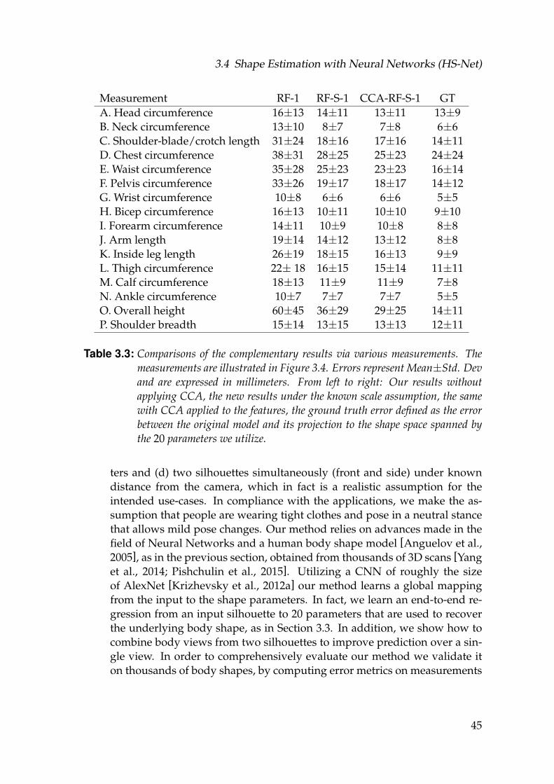
3.4 Shape Estimation with Neural Networks (HS-Net)
Measurement RF-1 RF-S-1 CCA-RF-S-1 GTA. Head circumference 16±13 14±11 13±11 13±9B. Neck circumference 13±10 8±7 7±8 6±6C. Shoulder-blade/crotch length 31±24 18±16 17±16 14±11D. Chest circumference 38±31 28±25 25±23 24±24E. Waist circumference 35±28 25±23 23±23 16±14F. Pelvis circumference 33±26 19±17 18±17 14±12G. Wrist circumference 10±8 6±6 6±6 5±5H. Bicep circumference 16±13 10±11 10±10 9±10I. Forearm circumference 14±11 10±9 10±8 8±8J. Arm length 19±14 14±12 13±12 8±8K. Inside leg length 26±19 18±15 16±13 9±9L. Thigh circumference 22± 18 16±15 15±14 11±11M. Calf circumference 18±13 11±9 11±9 7±8N. Ankle circumference 10±7 7±7 7±7 5±5O. Overall height 60±45 36±29 29±25 14±11P. Shoulder breadth 15±14 13±15 13±13 12±11
Table 3.3: Comparisons of the complementary results via various measurements. Themeasurements are illustrated in Figure 3.4. Errors represent Mean±Std. Devand are expressed in millimeters. From left to right: Our results withoutapplying CCA, the new results under the known scale assumption, the samewith CCA applied to the features, the ground truth error defined as the errorbetween the original model and its projection to the shape space spanned bythe 20 parameters we utilize.
ters and (d) two silhouettes simultaneously (front and side) under knowndistance from the camera, which in fact is a realistic assumption for theintended use-cases. In compliance with the applications, we make the as-sumption that people are wearing tight clothes and pose in a neutral stancethat allows mild pose changes. Our method relies on advances made in thefield of Neural Networks and a human body shape model [Anguelov et al.,2005], as in the previous section, obtained from thousands of 3D scans [Yanget al., 2014; Pishchulin et al., 2015]. Utilizing a CNN of roughly the sizeof AlexNet [Krizhevsky et al., 2012a] our method learns a global mappingfrom the input to the shape parameters. In fact, we learn an end-to-end re-gression from an input silhouette to 20 parameters that are used to recoverthe underlying body shape, as in Section 3.3. In addition, we show how tocombine body views from two silhouettes to improve prediction over a sin-gle view. In order to comprehensively evaluate our method we validate iton thousands of body shapes, by computing error metrics on measurements
45
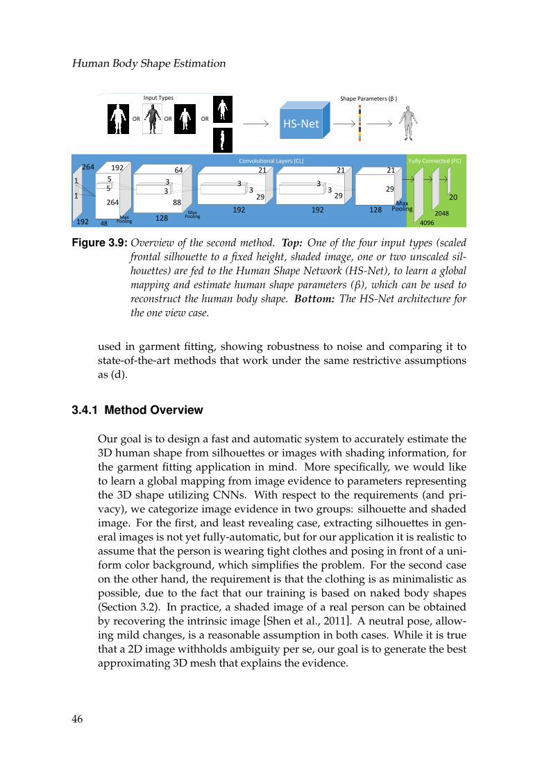
Human Body Shape Estimation
1
1
48128
192
55
33
33
128
192
264 192
264
64
88
21
29
21
29
MaxPooling
4096
2048
20
Fully Connected (FC)Convolutional Layers (CL)
MaxPooling
MaxPooling192
33
21
29
HS-NetOR OR OR
Input Types Shape Parameters (β )
Figure 3.9: Overview of the second method. Top: One of the four input types (scaledfrontal silhouette to a fixed height, shaded image, one or two unscaled sil-houettes) are fed to the Human Shape Network (HS-Net), to learn a globalmapping and estimate human shape parameters (β), which can be used toreconstruct the human body shape. Bottom: The HS-Net architecture forthe one view case.
used in garment fitting, showing robustness to noise and comparing it tostate-of-the-art methods that work under the same restrictive assumptionsas (d).
3.4.1 Method Overview
Our goal is to design a fast and automatic system to accurately estimate the3D human shape from silhouettes or images with shading information, forthe garment fitting application in mind. More specifically, we would liketo learn a global mapping from image evidence to parameters representingthe 3D shape utilizing CNNs. With respect to the requirements (and pri-vacy), we categorize image evidence in two groups: silhouette and shadedimage. For the first, and least revealing case, extracting silhouettes in gen-eral images is not yet fully-automatic, but for our application it is realistic toassume that the person is wearing tight clothes and posing in front of a uni-form color background, which simplifies the problem. For the second caseon the other hand, the requirement is that the clothing is as minimalistic aspossible, due to the fact that our training is based on naked body shapes(Section 3.2). In practice, a shaded image of a real person can be obtainedby recovering the intrinsic image [Shen et al., 2011]. A neutral pose, allow-ing mild changes, is a reasonable assumption in both cases. While it is truethat a 2D image withholds ambiguity per se, our goal is to generate the bestapproximating 3D mesh that explains the evidence.
46
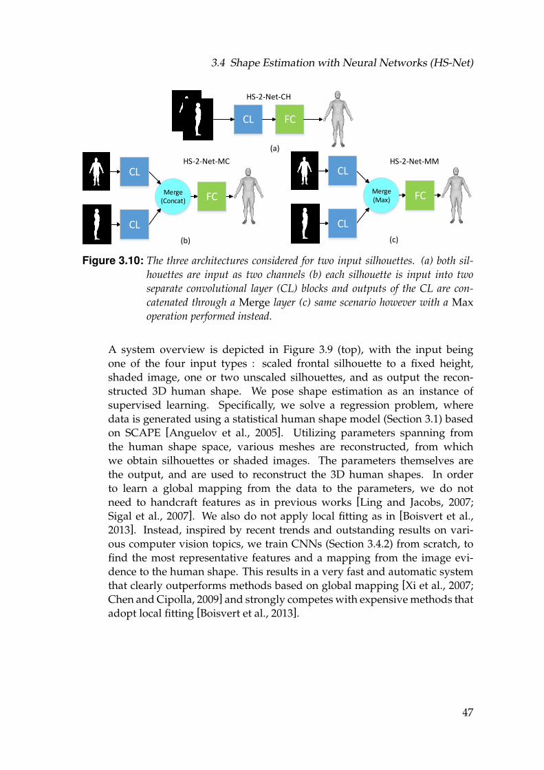
3.4 Shape Estimation with Neural Networks (HS-Net)
Merge (Concat)
CL FC
(a)
(b)
CL
CL
FCMerge (Max)
(c)
CL
CL
FC
HS-2-Net-CH
HS-2-Net-MMHS-2-Net-MC
Figure 3.10: The three architectures considered for two input silhouettes. (a) both sil-houettes are input as two channels (b) each silhouette is input into twoseparate convolutional layer (CL) blocks and outputs of the CL are con-catenated through a Merge layer (c) same scenario however with a Maxoperation performed instead.
A system overview is depicted in Figure 3.9 (top), with the input beingone of the four input types : scaled frontal silhouette to a fixed height,shaded image, one or two unscaled silhouettes, and as output the recon-structed 3D human shape. We pose shape estimation as an instance ofsupervised learning. Specifically, we solve a regression problem, wheredata is generated using a statistical human shape model (Section 3.1) basedon SCAPE [Anguelov et al., 2005]. Utilizing parameters spanning fromthe human shape space, various meshes are reconstructed, from whichwe obtain silhouettes or shaded images. The parameters themselves arethe output, and are used to reconstruct the 3D human shapes. In orderto learn a global mapping from the data to the parameters, we do notneed to handcraft features as in previous works [Ling and Jacobs, 2007;Sigal et al., 2007]. We also do not apply local fitting as in [Boisvert et al.,2013]. Instead, inspired by recent trends and outstanding results on vari-ous computer vision topics, we train CNNs (Section 3.4.2) from scratch, tofind the most representative features and a mapping from the image evi-dence to the human shape. This results in a very fast and automatic systemthat clearly outperforms methods based on global mapping [Xi et al., 2007;Chen and Cipolla, 2009] and strongly competes with expensive methods thatadopt local fitting [Boisvert et al., 2013].
47
Human Body Shape Estimation
3.4.2 Learning A Global Mapping
We pose the global mapping as an end-to-end regression problem, from 2Dinput image to shape parameters. We achieve this by training from scratcha CNN similar to that of AlexNet [Krizhevsky et al., 2012a] and adapting itto our inputs and regression task, as depicted in Figure 3.9 (bottom). Re-garding the number of input images we distinguish two cases : A frontalsingle view image, coming in different forms, and two images simultane-ously, from front and side.
3.4.2.1 Single View
The frontal view image can come in three forms. Firstly, a frontal binarysilhouette of the human in a neutral pose, scaled to a fixed height is con-sidered. This is the most general case, and assumes unknown camera cal-ibration, hence the need for a fixed scaling. Second, if the camera parame-ters are known, e.g. when the person stands a known distance away fromthe camera, the input is a fixed size image of varying silhouette size andheight. Estimating the real 3D shape from a 2D input silhouette is an ill-posed problem per se, due to the fact that a silhouette can represent vari-ous body shapes, even though we strive to reconstruct the shape that bestexplains it. Utilizing silhouettes only, has the advantage that no personalinformation is revealed, which is important for privacy protection. Allow-ing the problem to be a bit more relaxed, by adding further information, welastly consider the case of using additional image cues such as shading, com-plementary to the scaled silhouette, similar to [Guan et al., 2009]. In orderto synthetically generate training data, we render images with shading un-der Lambertian assumptions. In practice a similar result could be achievedby extracting the intrinsic image [Shen et al., 2011]. The input size for allthe mentioned methods is set to 264× 192 pixels. For each case, the singlechannel input images, along with the known shape parameters, are fed intoour Human Shape Network (HS-Net), which learns the mapping from inputto the shape parameters β. HS-Net is a modification of Alexnet [Krizhevskyet al., 2012a] customized to a regression problem, our various input types,intended application and the available hardware. The network consists offive convolutional blocks, followed by three fully connected layers as illus-trated in Figure 3.9 (bottom). Each layer is followed by an activation layer(ReLu). In addition, dropout layers are utilized between fully connected lay-ers to avoid overfitting and max pooling is used after the first, second andfifth convolutional blocks. The network is trained from scratch, since theavailable pre-trained models are geared towards classification and RGB or
48
3.4 Shape Estimation with Neural Networks (HS-Net)
grayscale images, while we tend to learn regression from binary images. Weexperimented with different optimization algorithms and observed that thebest results were obtained using RMSProp 2 and Adadelta [Zeiler, 2012]. Wedecided to utilize the Adadelta optimizer due to its capacity to automaticallyadjust the learning rate and prevent it from becoming too small.
3.4.2.2 Two Views
In compliance with the realistic scenario of estimating the body shape andthe body parts measurements as accurately as possible, we additionallyopted for the usage of two silhouettes simultaneously, where the person isseen from a full frontal and side view. This setting also assumes knowncamera parameters, same as the methods we compare to [Xi et al., 2007;Chen and Cipolla, 2009; Boisvert et al., 2013], which translates to knowingthe distance from the camera. One of the challenges of this case is how tocombine multiple view inputs in a way that the convolutional network canuse them coherently. We explore and evaluate three different approaches toachieve this. The first approach, utilizes a model architecture very similarto the one view case, however the input images from the different views arestacked along the channel dimension to form two channel images, see Fig-ure 3.10 (a). These two channel images are then fed into the network fortraining. By visualizing the output filters (Figure 3.17) for different layers onvarious test images, we observed that the network learns some filters morepronounced towards frontal views, while others favor the side views. Forthe second approach, the architecture differs from the previous case, in thatwe add a Merge layer similar to the view pooling layer of [Su et al., 2015],after two sets of convolutional layers with shared weights for each view,followed by fully connected layers. The input images from each view arefed into two separate five layer convolutional networks and merged usinga concatenation operation, see Figure 3.10 (b). The third approach distin-guishes from the second one in that the merge layer performs a Max oper-ation over each dimension, see Figure 3.10 (c). The motivation behind thelast two approaches, was to allow the network to separately learn featuresfrom individual images and then fuse them more discriminatively through amerging layer. The merge layer with max operation improves learning andsubsequently the estimation accuracy (see Table 3.4) over the two channelnetwork, as it combines evidence at a later stage of learning. All three meth-ods lead to improvements over the one view case, which we demonstrate inSection 3.4.3, where the merging with max operation performs the best.
2http://www.cs.toronto.edu/ tijmen/csc321/slides/lecture slides lec6.pdf
49
Human Body Shape Estimation
3.4.3 Validation and Results
Our method targets the application of human body shape and body partsestimation. In order to assess its reliability, one can not rely only on thevisual reconstruction of the mesh. Rigorous quantitative experiments arenecessary, especially of measurements over various important body parts. Ifthe latter can be estimated accurately, fitting clothes virtually or even buy-ing clothes online becomes more intuitive and appealing. Measuring dif-ferent body parts consistently in real datasets is difficult, as even the mosttrained individuals are reported to deviate up to 10 mm [Gordon et al., 1989].Hence, we evaluate on synthetic meshes, obtained by fitting a parametricmodel to real people scans from the CAESAR dataset, similar to the meth-ods we compare to [Boisvert et al., 2013]. Performing the evaluations on thisdataset, in addition to the shapes being very close to the real ones, has theadvantage that they are in full correspondence. Thus, it becomes easy toautomatically measure various body parts. Additionally, the poses adoptedfrom the real human scans, deviate from the neutral pose specified by exper-imenters while they are being scanned, Figure 3.11 (top-left). These meshesare quite realistic and in compliance with the variation of the poses that peo-ple adopt for our target applications. Different openings of the arms, legsand even shoulders can be noticed. In our experiments, we apply the samemeasurements as in [Boisvert et al., 2013] and the previous section, repeatedfor viewers courtesy in Figure 3.11 (top-right). For our evaluation we use1500 meshes and 4 real people on 16 body measurements, which to the bestof our knowledge is the most complete one so far, as compared to relatedwork. [Boisvert et al., 2013] evaluate on 220 meshes and 4 real people, [Xi etal., 2007] on 24 meshes and two real people, [Sigal et al., 2007] for two mea-surements only on two subjects and [Balan et al., 2007] for silhouette errorsand height measurement on a few individuals.
3.4.3.1 General Training and Set-Up Details
For each of the 100000 generated meshes, Section 3.2, we generate silhouettesfrom frontal and side views, as well as shaded images under lambertian as-sumptions with Maya3. As a preprocessing step, the images are centered,normalized to the [0,1] interval and fixed to the 264× 192 pixels resolutionfor all the cases. The resolution was chosen such that it neither impedeslearning of shape variations, nor is too big, due to the hardware and timeconstraints we had. We use 95000 images for training and 5000 for the net-
3http://www.autodesk.com/products/maya/
50
3.4 Shape Estimation with Neural Networks (HS-Net)
work validation. As explained above, the testing is performed on 1500 un-seen samples and real human ones. The network architecture is detailed inFigure 3.9 (bottom) for the one view input case. For the various experimentsthat we perform, we change the networks as explained in Section 3.4.2 andadopt the following nomenclature : HS-1-Net-S and HS-1-Net for the scaledand unscaled input silhouette and HS-1-Net-Im for the scaled shaded imageinput. Training usually converges between 15-25 epochs depending on theexperiment. The batch size was set to 32, to not be a proper divisor of thenumber of training samples per epoch, which is equal to half of total train-ing samples. This provides an easy way to simulate shuffling without hittingmemory constraints for such big datasets. We also experimented with batchnormalization [Ioffe and Szegedy, 2015] right after the convolutional layers,resulting in slight error increase. Applying batch normalization after thefully connected layers though, caused the network to converge to constantfunctions.
We experimented with the RMSprop, Adagrad [Duchi et al., 2011] andAdadelta [Zeiler, 2012] optimizers, in order to minimize the manual learn-ing rate adjustments. We observed that RMSprop (with an initial learningrate of 0.001) and Adadelta (with decay rate of 0.95) converged faster thanAdagrad, also with a smaller test error. Thus, all the reported experiment re-sults are for the models trained using Adadelta. We experimented with thesquared loss, with and without multiplying the last fully-connected layer bycustom weights. The weights are set to be the eigenvalues of the covariancematrix obtained from PCA, during the data generation step Section 3.1 andnormalized to 1, such that we emphasize large scale changes in 3D bodyshapes, as for the previous method. As expected, using squared loss withcustom weights performed better. For all the networks, we utilized Glorotuniform weight initialization [Glorot and Bengio, 2010].
For the two view case, we used the best performing network configurationsfrom the one view case, however the architectures were modified to fit theinput extension, as shown in Figure 3.10. The two selected views were thefrontal and the side one. We also distinguish between three cases here : HS-2-Net-CH for the input silhouettes passed as two channels of a single image,HS-2-Net-MM for separately training the two inputs as different single chan-nel images and applying a merge layer, that performs a max operation overeach dimension right after the output of the last convolutional layers (CL),and HS-2-Net-MC for the same architecture that concatenates the output ofCL, instead of max operation. All the CL have shared weights.
51
Human Body Shape Estimation
3.4.3.2 Quantitative Experiments
We perform 16 3D measurements on the test meshes which consist of malesand females in roughly equal numbers, similar to [Boisvert et al., 2013]. Themeasurements are illustrated in Figure 3.11 (top-right) and are widely usedin garment fitting. We compute the Euclidean distance between two extremevertices for the straight line measurements, while for the ellipsoidal ones,the perimeter is computed on the body surface. For each measurement wecalculate the difference between the value estimated and the ground truth,and report the mean error and standard deviation computed over the errorvalues for all the test meshes in Table 3.4. Additionally, we show how themean error over all measurements varies, for each different input type thatwe consider, in Figure 3.11. HS-2-Net-MM has the lowest error of 4.02 mm, ascompared to 11 mm of [Boisvert et al., 2013], which utilizes a more expensivelocal fitting algorithm. For completeness, we compare to the work of [Heltenet al., 2013], that utilizes an RGB-D camera for capturing the body shapes,and a full RMSE map per vertex to measure the differences. They report anerror of 10.1 mm, evaluating on 6 individuals from two depth maps, whilewe report an error of 7.4 mm on 1500 meshes.
We observed that using weights with squared loss function increases the ac-curacy of the model. The model trained on silhouettes with known cam-era parameters performs significantly better than the one with unknowncamera calibration. The shaded images network HS-1-Net-Im, performs alsoslightly better than the corresponding silhouette one HS-1-Net-S, implyingthat shading information possibly improves the shape estimation accuracy,but could also be related to added information due to grayscale input asopposed to a binary one. Lastly, HS-2-Net-CH demonstrates more accu-racy for the ellipsoidal errors while HS-2-Net-MC for the euclidean ones,despite their overall similar performance. In comparison to the other meth-ods, our network clearly outperforms the global methods [Xi et al., 2007;Chen and Cipolla, 2009] (Figure 3.8), and strongly compares to the methodfrom [Boisvert et al., 2013]. Adding a second view gives better results thana single view with noticeable improvements in the height and waist estima-tion.
We perform three additional experiments to show the extensibility of the ap-proach: (1) an experiment with more pronounced poses (2) partially visiblesilhouettes and (3) images rendered under specularity assumption. All thefollowing experiments were performed assuming unknown camera calibra-tion, hence scaled silhouettes similar to HS-1-Net-S.
Poses. We generated 95000 meshes in 10 different poses, Figure 3.12 and
52
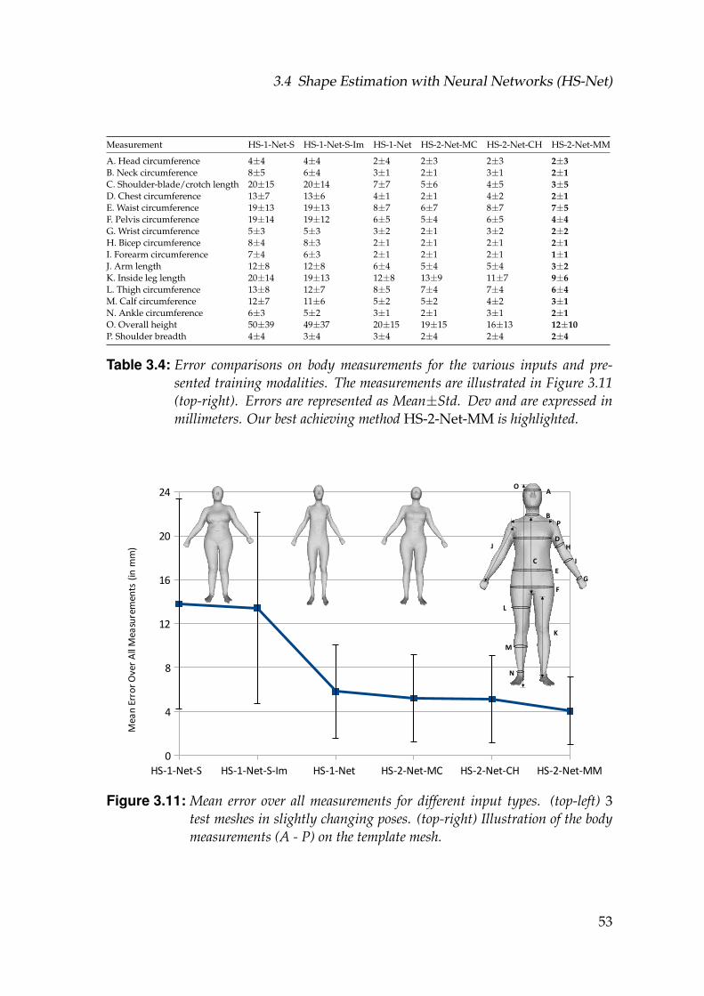
3.4 Shape Estimation with Neural Networks (HS-Net)
Measurement HS-1-Net-S HS-1-Net-S-Im HS-1-Net HS-2-Net-MC HS-2-Net-CH HS-2-Net-MM
A. Head circumference 4±4 4±4 2±4 2±3 2±3 2±3B. Neck circumference 8±5 6±4 3±1 2±1 3±1 2±1C. Shoulder-blade/crotch length 20±15 20±14 7±7 5±6 4±5 3±5D. Chest circumference 13±7 13±6 4±1 2±1 4±2 2±1E. Waist circumference 19±13 19±13 8±7 6±7 8±7 7±5F. Pelvis circumference 19±14 19±12 6±5 5±4 6±5 4±4G. Wrist circumference 5±3 5±3 3±2 2±1 3±2 2±2H. Bicep circumference 8±4 8±3 2±1 2±1 2±1 2±1I. Forearm circumference 7±4 6±3 2±1 2±1 2±1 1±1J. Arm length 12±8 12±8 6±4 5±4 5±4 3±2K. Inside leg length 20±14 19±13 12±8 13±9 11±7 9±6L. Thigh circumference 13±8 12±7 8±5 7±4 7±4 6±4M. Calf circumference 12±7 11±6 5±2 5±2 4±2 3±1N. Ankle circumference 6±3 5±2 3±1 2±1 3±1 2±1O. Overall height 50±39 49±37 20±15 19±15 16±13 12±10P. Shoulder breadth 4±4 3±4 3±4 2±4 2±4 2±4
Table 3.4: Error comparisons on body measurements for the various inputs and pre-sented training modalities. The measurements are illustrated in Figure 3.11(top-right). Errors are represented as Mean±Std. Dev and are expressed inmillimeters. Our best achieving method HS-2-Net-MM is highlighted.
HS-1-Net-S HS-1-Net-S-Im HS-1-Net HS-2-Net-MC HS-2-Net-CH HS-2-Net-MM0
4
8
12
16
20
24
Mea
n Er
ror
Ove
r A
ll M
easu
rem
ents
(in
mm
)
A
B
C
DH
I
GE
F
P
O
K
L
M
N
J
Figure 3.11: Mean error over all measurements for different input types. (top-left) 3test meshes in slightly changing poses. (top-right) Illustration of the bodymeasurements (A - P) on the template mesh.
53
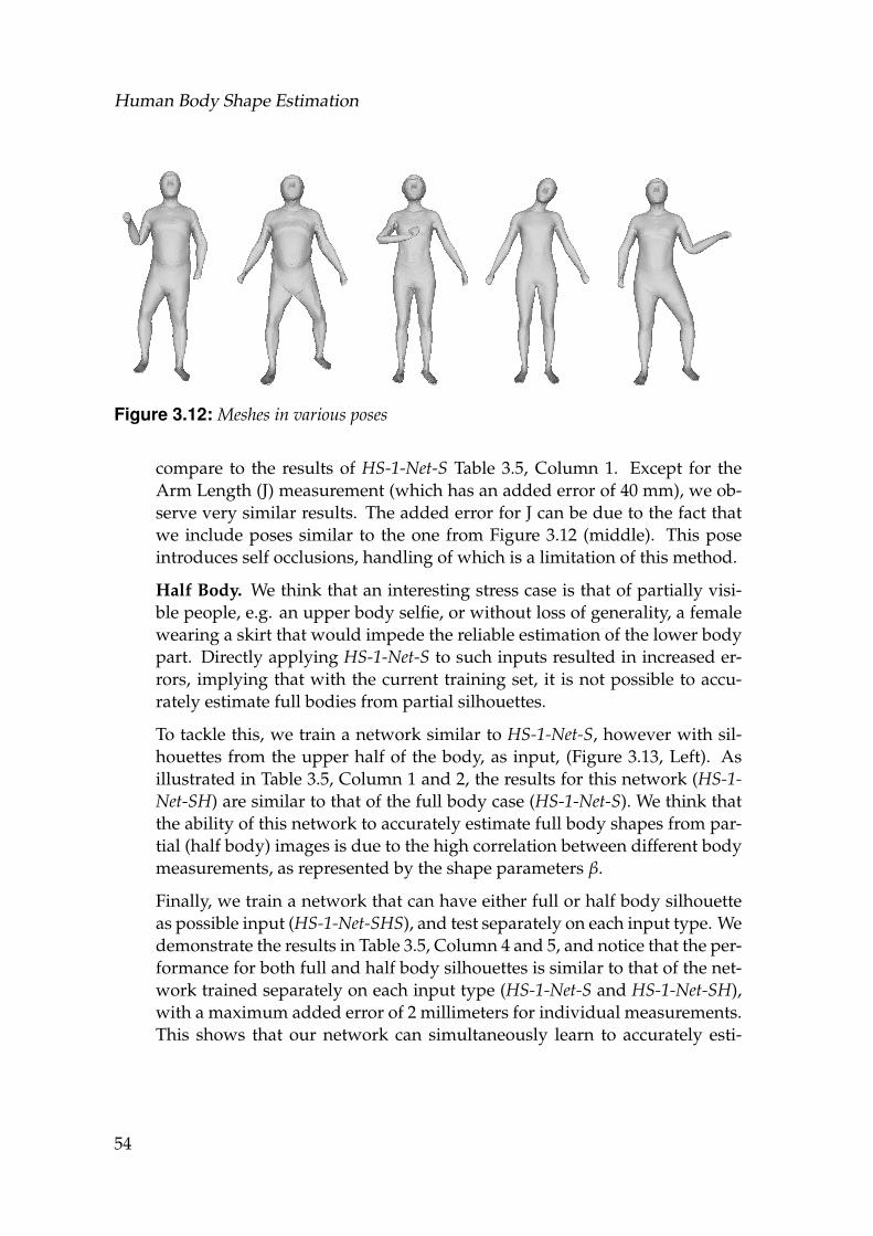
Human Body Shape Estimation
Figure 3.12: Meshes in various poses
compare to the results of HS-1-Net-S Table 3.5, Column 1. Except for theArm Length (J) measurement (which has an added error of 40 mm), we ob-serve very similar results. The added error for J can be due to the fact thatwe include poses similar to the one from Figure 3.12 (middle). This poseintroduces self occlusions, handling of which is a limitation of this method.
Half Body. We think that an interesting stress case is that of partially visi-ble people, e.g. an upper body selfie, or without loss of generality, a femalewearing a skirt that would impede the reliable estimation of the lower bodypart. Directly applying HS-1-Net-S to such inputs resulted in increased er-rors, implying that with the current training set, it is not possible to accu-rately estimate full bodies from partial silhouettes.
To tackle this, we train a network similar to HS-1-Net-S, however with sil-houettes from the upper half of the body, as input, (Figure 3.13, Left). Asillustrated in Table 3.5, Column 1 and 2, the results for this network (HS-1-Net-SH) are similar to that of the full body case (HS-1-Net-S). We think thatthe ability of this network to accurately estimate full body shapes from par-tial (half body) images is due to the high correlation between different bodymeasurements, as represented by the shape parameters β.
Finally, we train a network that can have either full or half body silhouetteas possible input (HS-1-Net-SHS), and test separately on each input type. Wedemonstrate the results in Table 3.5, Column 4 and 5, and notice that the per-formance for both full and half body silhouettes is similar to that of the net-work trained separately on each input type (HS-1-Net-S and HS-1-Net-SH),with a maximum added error of 2 millimeters for individual measurements.This shows that our network can simultaneously learn to accurately esti-
54
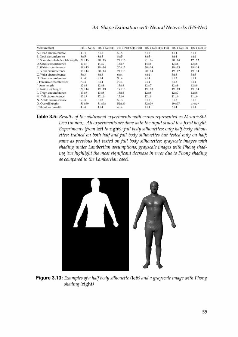
3.4 Shape Estimation with Neural Networks (HS-Net)
Measurement HS-1-Net-S HS-1-Net-SH HS-1-Net-SHS-Half HS-1-Net-SHS-Full HS-1-Net-Im HS-1-Net-IP
A. Head circumference 4±4 5±5 5±5 5±5 4±4 4±4B. Neck circumference 8±5 8±5 8±5 8±5 6±4 6±4C. Shoulder-blade/crotch length 20±15 20±15 21±16 21±16 20±14 17±12D. Chest circumference 13±7 14±7 15±7 14±6 13±6 13±8E. Waist circumference 19±13 19±14 20±15 20±14 19±13 19±14F. Pelvis circumference 19±14 20±14 21±15 20±14 19±12 19±14G. Wrist circumference 5±3 6±3 6±4 6±4 5±3 5±3H. Bicep circumference 8±4 8±4 9±4 9±4 8±3 8±4I. Forearm circumference 7±4 7±4 7±4 7±4 6±3 6±4J. Arm length 12±8 12±8 13±8 12±7 12±8 12±8K. Inside leg length 20±14 19±13 19±13 19±13 19±13 19±14L. Thigh circumference 13±8 13±8 13±8 12±8 12±7 12±8M. Calf circumference 12±7 12±6 12±6 12±6 11±6 11±6N. Ankle circumference 6±3 6±3 5±3 5±3 5±2 5±3O. Overall height 50±39 51±38 52±39 52±39 49±37 47±37P. Shoulder breadth 4±4 4±4 4±4 4±4 3±4 4±4
Table 3.5: Results of the additional experiments with errors represented as Mean±Std.Dev (in mm). All experiments are done with the input scaled to a fixed height.Experiments (from left to right): full body silhouettes; only half body silhou-ettes; trained on both half and full body silhouettes but tested only on half;same as previous but tested on full body silhouettes; grayscale images withshading under Lambertian assumptions; grayscale images with Phong shad-ing (we highlight the most significant decrease in error due to Phong shadingas compared to the Lambertian case).
Figure 3.13: Examples of a half body silhouette (left) and a grayscale image with Phongshading (right)
55
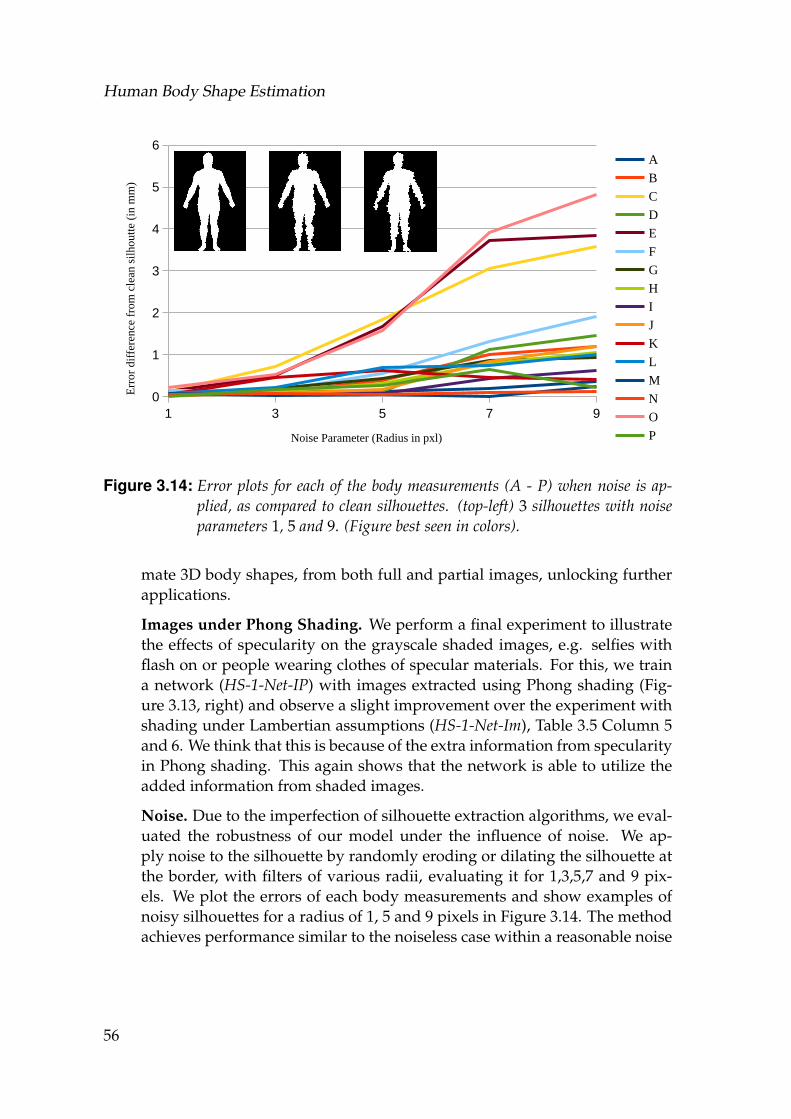
Human Body Shape Estimation
1 3 5 7 90
1
2
3
4
5
6A
B
C
D
E
F
G
H
I
J
K
L
M
N
O
PNoise Parameter (Radius in pxl)
Err
or d
iffe
renc
e fr
om c
lean
sil
hout
te (
in m
m)
Figure 3.14: Error plots for each of the body measurements (A - P) when noise is ap-plied, as compared to clean silhouettes. (top-left) 3 silhouettes with noiseparameters 1, 5 and 9. (Figure best seen in colors).
mate 3D body shapes, from both full and partial images, unlocking furtherapplications.
Images under Phong Shading. We perform a final experiment to illustratethe effects of specularity on the grayscale shaded images, e.g. selfies withflash on or people wearing clothes of specular materials. For this, we traina network (HS-1-Net-IP) with images extracted using Phong shading (Fig-ure 3.13, right) and observe a slight improvement over the experiment withshading under Lambertian assumptions (HS-1-Net-Im), Table 3.5 Column 5and 6. We think that this is because of the extra information from specularityin Phong shading. This again shows that the network is able to utilize theadded information from shaded images.
Noise. Due to the imperfection of silhouette extraction algorithms, we eval-uated the robustness of our model under the influence of noise. We ap-ply noise to the silhouette by randomly eroding or dilating the silhouette atthe border, with filters of various radii, evaluating it for 1,3,5,7 and 9 pix-els. We plot the errors of each body measurements and show examples ofnoisy silhouettes for a radius of 1, 5 and 9 pixels in Figure 3.14. The methodachieves performance similar to the noiseless case within a reasonable noise
56
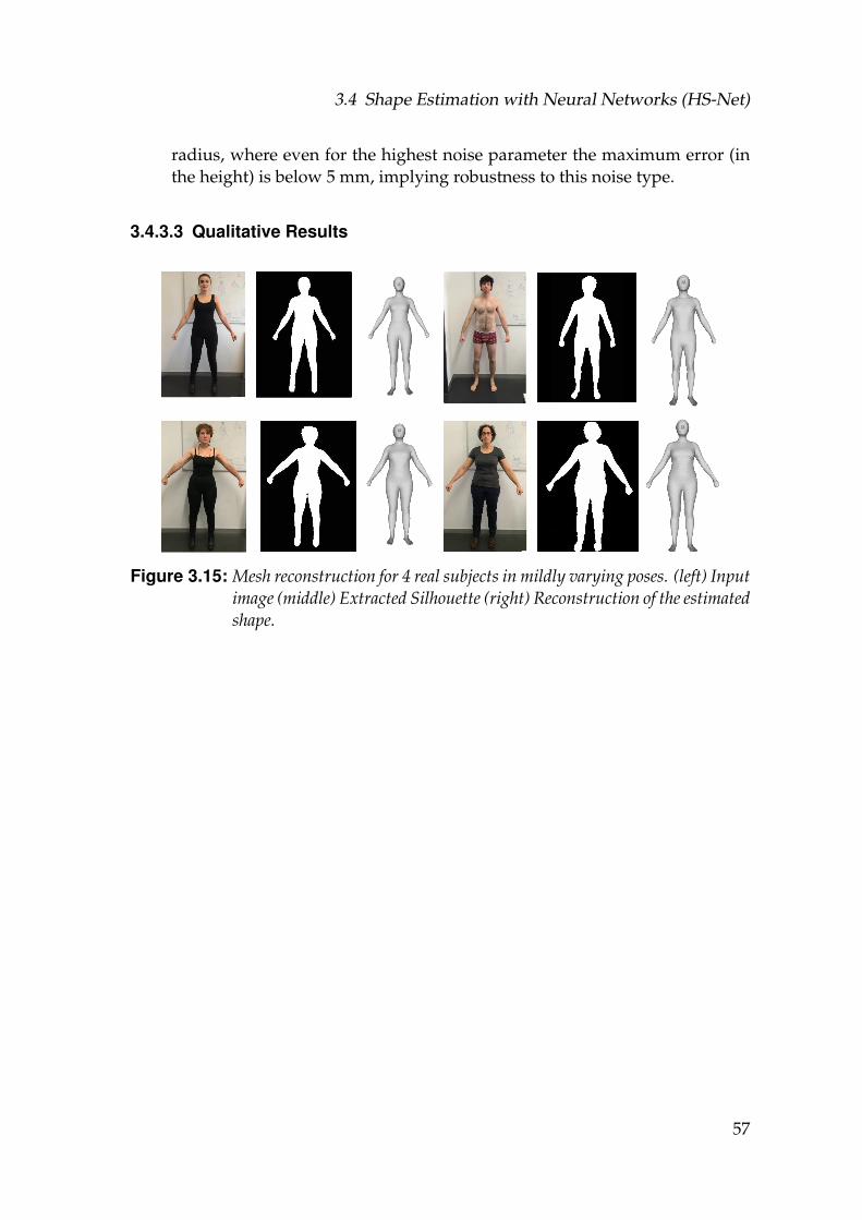
3.4 Shape Estimation with Neural Networks (HS-Net)
radius, where even for the highest noise parameter the maximum error (inthe height) is below 5 mm, implying robustness to this noise type.
3.4.3.3 Qualitative Results
Figure 3.15: Mesh reconstruction for 4 real subjects in mildly varying poses. (left) Inputimage (middle) Extracted Silhouette (right) Reconstruction of the estimatedshape.
57
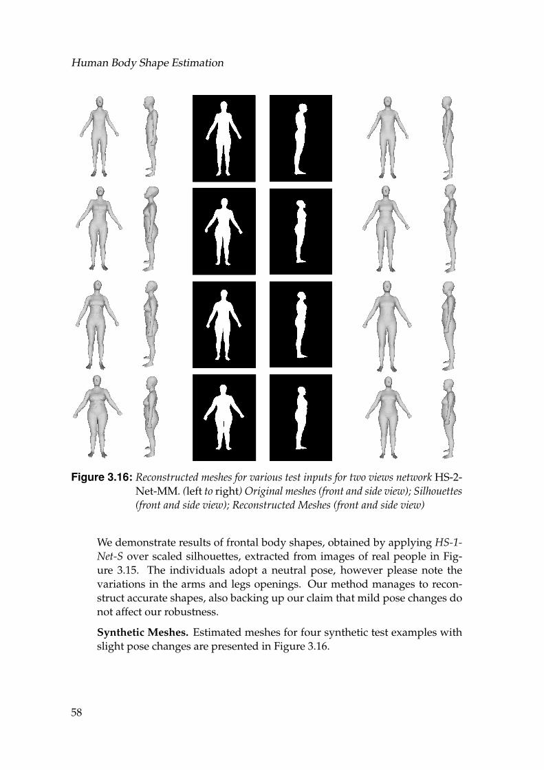
Human Body Shape Estimation
Figure 3.16: Reconstructed meshes for various test inputs for two views network HS-2-Net-MM. (left to right) Original meshes (front and side view); Silhouettes(front and side view); Reconstructed Meshes (front and side view)
We demonstrate results of frontal body shapes, obtained by applying HS-1-Net-S over scaled silhouettes, extracted from images of real people in Fig-ure 3.15. The individuals adopt a neutral pose, however please note thevariations in the arms and legs openings. Our method manages to recon-struct accurate shapes, also backing up our claim that mild pose changes donot affect our robustness.
Synthetic Meshes. Estimated meshes for four synthetic test examples withslight pose changes are presented in Figure 3.16.
58
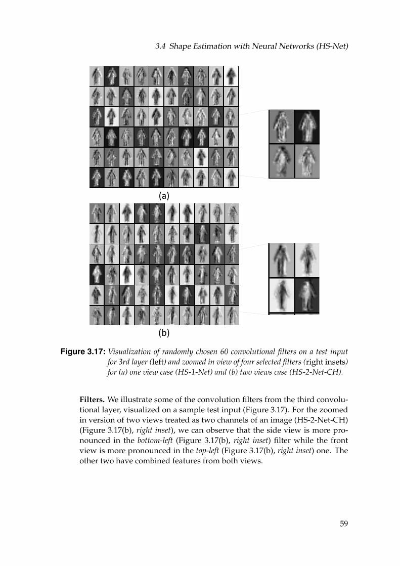
3.4 Shape Estimation with Neural Networks (HS-Net)
(a)
(b)
Figure 3.17: Visualization of randomly chosen 60 convolutional filters on a test inputfor 3rd layer (left) and zoomed in view of four selected filters (right insets)for (a) one view case (HS-1-Net) and (b) two views case (HS-2-Net-CH).
Filters. We illustrate some of the convolution filters from the third convolu-tional layer, visualized on a sample test input (Figure 3.17). For the zoomedin version of two views treated as two channels of an image (HS-2-Net-CH)(Figure 3.17(b), right inset), we can observe that the side view is more pro-nounced in the bottom-left (Figure 3.17(b), right inset) filter while the frontview is more pronounced in the top-left (Figure 3.17(b), right inset) one. Theother two have combined features from both views.
59
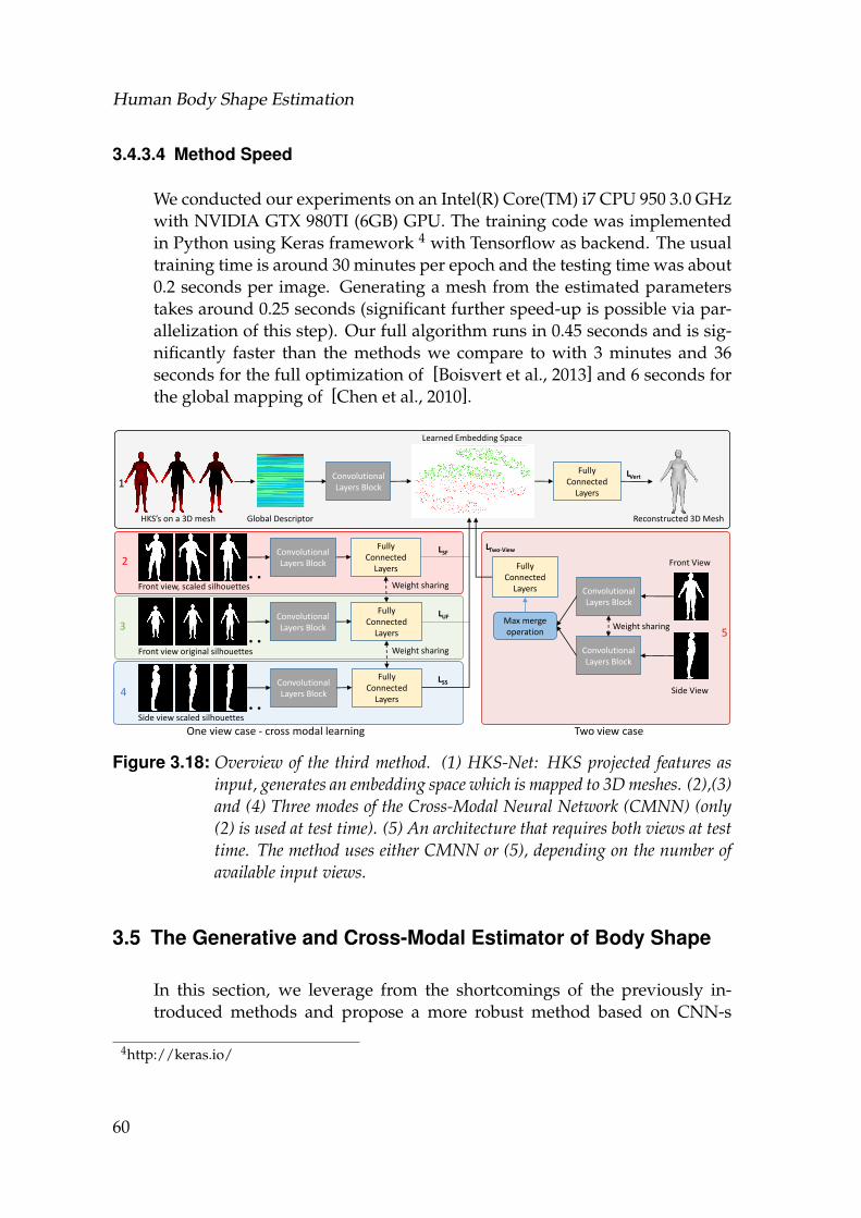
Human Body Shape Estimation
3.4.3.4 Method Speed
We conducted our experiments on an Intel(R) Core(TM) i7 CPU 950 3.0 GHzwith NVIDIA GTX 980TI (6GB) GPU. The training code was implementedin Python using Keras framework 4 with Tensorflow as backend. The usualtraining time is around 30 minutes per epoch and the testing time was about0.2 seconds per image. Generating a mesh from the estimated parameterstakes around 0.25 seconds (significant further speed-up is possible via par-allelization of this step). Our full algorithm runs in 0.45 seconds and is sig-nificantly faster than the methods we compare to with 3 minutes and 36seconds for the full optimization of [Boisvert et al., 2013] and 6 seconds forthe global mapping of [Chen et al., 2010].
Convolutional Layers Block
Fully Connected
Layers
HKS’s on a 3D mesh Reconstructed 3D Mesh
Learned Embedding Space
Global Descriptor
Two view caseOne view case - cross modal learning
1
Convolutional Layers Block
Convolutional Layers Block
Max merge operation
Fully Connected
Layers
Front View
Side View
Weight sharing5
LSF
LUF
LSS
LTwo-View
LVert
Convolutional Layers Block
Fully Connected
Layers
Front view, scaled silhouettes Weight sharing
2
Convolutional Layers Block
Fully Connected
Layers
Side view scaled silhouettes
4
Convolutional Layers Block
Fully Connected
Layers
Front view original silhouettes Weight sharing
3
Figure 3.18: Overview of the third method. (1) HKS-Net: HKS projected features asinput, generates an embedding space which is mapped to 3D meshes. (2),(3)and (4) Three modes of the Cross-Modal Neural Network (CMNN) (only(2) is used at test time). (5) An architecture that requires both views at testtime. The method uses either CMNN or (5), depending on the number ofavailable input views.
3.5 The Generative and Cross-Modal Estimator of Body Shape
In this section, we leverage from the shortcomings of the previously in-troduced methods and propose a more robust method based on CNN-s
4http://keras.io/
60
3.5 The Generative and Cross-Modal Estimator of Body Shape
to estimate the human body shape. We attempt to achieve it from a sin-gle or multiple silhouettes of a human body with poses compliant withthe two main applications explained in the previous sections: virtual gar-ment fitting assuming a neutral pose, as in [Chen and Cipolla, 2009;Boisvert et al., 2013] and Section 3.4, and shape from individually taken pic-tures or “Selfies” (e.g. through a mirror or a long selfie stick), assumingposes that exhibit mild self occlusion (Section 3.3). Compared to state-of-the-art in this domain, we achieve significantly higher accuracy on the re-constructed body shapes and simultaneously improve in speed if a GPU im-plementation is considered, or obtain similar run-times to the method fromSection 3.3 on the CPU. This is achieved thanks to a novel Neural Networkarchitecture (Figure 3.18) consisting of various components that (a) are ableto learn a body shape representation from 3D shape descriptors and mapthis representation to 3D shapes, (b) can successfully reconstruct a 3D bodymesh from one or two given body silhouettes, and (c) can leverage multi-view data at training time, to boost predictions for a single view at test timethrough cross-modality learning.
As referred and compared to in the previous sections, there exist methodsthat attempt to find a mapping from silhouettes to the parameters of a sta-tistical body shape model [Anguelov et al., 2005], utilizing handcrafted fea-tures as in Section 3.3, silhouette PCA representations [Chen and Cipolla,2009] possibly with local fine tuning [Boisvert et al., 2013], or CNN-s asin Section 3.4. Based on the obtained parameters, a least squares systemis solved to obtain the final mesh. We also use CNN-s to learn silhouettefeatures, but unlike in the previous section, we first map them to a shaperepresentation space that is generated from 3D shape descriptors (Heat Ker-nel Signature (HKS) [Sun et al., 2009]) invariant to isometric deformationsand maximizing intra-human-class variation, and then decode them to fullbody vertex positions. Regressing to this space improves the predictions andspeeds up the computation.
In Section 3.3, we demonstrated how to boost features coming from one view(scaled frontal) during test time, utilizing information from two views (frontand side) at training time, by projecting features with Canonical CorrelationAnalysis (CCA) [Hotelling, 1936]. CCA comes with shortcomings thoughas (1) it computes a linear projection, (2) it is hard in practice to extend it tomore than two views, and (3) suffers from lack of scalability to large datasetsas it has to “memorize” the whole training data set. As part of the methodpresented in this section, we propose an architecture (which we call Cross-Modal Neural Network (CMNN)) that is able to overcome the mentionedchallenges, by first generating features from various views separately, andthen combining them through shared layers. This leads to improvements
61
Human Body Shape Estimation
in predictive capabilities with respect to the uni-modal case. Abstractingaway from silhouettes, this network can be used as-is for other tasks wheremultiple views on the data are present, such as image and text retrieval, oraudio and image matching.
3.5.1 Method Overview
The main goal of our method is to accurately estimate a 3D body shape froma silhouette (or two) of a person adopting poses in compliance with twoapplications - virtual cloth fitting and self shape monitoring. On par withthe related work, we consider either a single frontal silhouette scaled to afixed size (no camera calibration information) with poses exhibiting mildself occlusions, or two views simultaneously (front and side, scaled or un-scaled) of a person in a neutral pose. We propose to tackle this problemwith a deep network architecture (Figure 3.18). Our network is composedof three core components: a generative component that can invert pose-invariant 3D shape descriptors, obtained from a multitude of 3D meshes(Section 3.1) to their corresponding 3D shape, by learning an embeddingspace (Section 3.5.2); a cross-modal component that leverages multi-viewinformation at training time to boost single view predictions at test time(Section 3.5.3); and a combination of losses to perform joint training overthe whole network (Section 3.5.4).
3.5.2 Generating 3D Shapes from HKS (HKS-Net)
The first part of our architecture aims at learning a mapping from 3D shapedescriptors to 3D meshes via a shape embedding space. We start by extract-ing Heat Kernel Signatures (HKS) and then projecting them to the eigenvec-tors of the Laplace-Beltrami operator to obtain a global descriptor. This isused to learn the embedding space, as well as an inverse mapping that cangenerate 3D shapes in a neutral pose given the corresponding descriptor.
Heat Kernel Signatures (HKS). Let a 3D shape be represented as a graphG = (V, E, W), where V, E and W represent the set of vertices, edges, andsome weights on the edges, respectively. The weights encode the underlyinggeometry of the shape, and can be computed via standard techniques fromthe mesh processing literature [Sun et al., 2009]. Given such a graph con-structed by connecting pairs of vertices on a surface with weighted edges,the heat kernel Ht(x, y) is defined as the amount of heat that is transferredfrom the vertex x to vertex y at time t, given a unit heat source at x [Sun et
62
3.5 The Generative and Cross-Modal Estimator of Body Shape
al., 2009]:Ht(x, y) = ∑
ie−λitφi(x)φi(y), (3.4)
where Ht denotes the heat kernel, t is the diffusion time, λi and φi representthe ith eigenvalue and the corresponding eigenvector of the Laplace-Beltramioperator, respectively, and x and y denote two vertices. Heat kernel has vari-ous nice properties that are desirable to represent human body shapes underdifferent poses. In particular, it is invariant under isometric deformationsof the shape, captures different levels of detail and global properties of theshape, and it is stable under perturbations [Sun et al., 2009].
The heat kernel at vertex x and time t can be used to define the heat kernelsignature HKSx(t) for this vertex:
HKSx(t) = Ht(x, x) = ∑i
e−λitφ2i (x). (3.5)
Hence, for each vertex x, we have a corresponding function HKSx(t) thatprovides a multi-scale descriptor for x. As the scale (i.e. t) increases, wecapture more and more global properties of the intrinsic shape. In practice,the times t are sampled to obtain a vector HKSx(tj), j ≤ J for each vertexx. In our technique, we use J = 100 time samples. Then for each tj, we canform the vectors hj := [HKSx1(tj), HKSx2(tj) · · · ]T.
Projected HKS Matrix. To learn the embedding space, the HKS for all ver-tices at a given time tj are projected onto the eigenvectors of the Laplace-Beltrami operator in order to obtain a 2D image capturing the global intrin-sic shape. Specifically, we compute a matrix M with Mij = φT
i hj, i.e. thedot product of the ith eigenvector of the Laplace-Beltrami operator and theheat kernel vector defined over the vertices for time tj. Since we use 300eigenvectors φi, we thus get a 300× 100 matrix M.
This is then used as input to the top part of our network (that we call HKS-Net, Figure 3.18 (1)) to learn an embedding space of about 4000 dimensions,by minimizing the per-vertex squared norm loss LVert. A simplistic represen-tation of this embedding, computed utilizing T-SNE [Maaten and Hinton,2008], is also presented in Figure 3.18, where female meshes are depicted ingreen dots and male meshes in red. An important property of HKS-Net isthat we can reconstruct a 3D mesh in a neutral pose when HKS-Net is pre-sented with a computed M. Hence, HKS-Net can invert the HKS descriptors.Although we do not utilize this property in the scope of this work, we be-lieve that this could be a valuable tool for geometry processing applications.But instead, we use the embedding space with 4000 dimensions as the targetspace for the cross-modal silhouette-based training of our network, whichwe explain next.
63
Human Body Shape Estimation
3.5.3 Cross-Modal Neural Network (CMNN)
The second component thus consists of finding a mapping from silhouettesto the newly learned embedding space. We generate five types of silhou-ettes that can be referred to as modes : frontal view scaled in various poseswith minor self occlusion, frontal view scaled in a neutral pose, side viewscaled in a neutral pose and front and side view unscaled in a neutral pose(Figure 3.18).5 Here, unscaled implies known camera calibration, and scaledmeans we resize the silhouettes such that they have the same height. Frontalmeans that the plane of the bones that form the torso is parallel to the cam-era plane, and side is a 90 degrees rotated version of the frontal view. Attest time, our results are not affected by slight deviations from these views.We thus center the silhouettes, and resize them to an image of resolution264× 192 before inputting them to the CMNN. We, of course, do not expectto use all the modes/views at once during testing, but our intention is toleverage the vast amount of data from various modes at training time forrobust predictions at test time.
We start by training a network similar in size to the one from the methodof Section 3.4 (5 convolutional and 3 dense layers), with AdaMax opti-mizer [Kingma and Ba, 2014], and learning rate of e−4, to map each mode in-dividually to the embedding space by minimizing squared losses on the 4000embedding space parameters (Figure 3.18 (2),(3) and (4) with the respectivelosses LSF, LUF and LSS). As shown in Table 3.7, we already achieve betterresults for the one-view case as compared to related works. This pre-trainingserves as an initialization for the convolutional weights of the Cross-ModalNeural Network (CMNN). The final cross-modal training is performed bystarting from the weights given by the pre-training, and optimizing for theshared weights for the fully connected layers with a combined loss, e.g. forscaled-front and scaled-side we minimize LSF + LSS, or for three modes, theloss is LSF + LUF + LSS.
The idea is to let each single convolutional network compute silhouette fea-tures separately first, and then correlate these high-level features at laterstages. We observed that we obtain significant improvements when cross-correlating various combinations of 2 modes and 3 modes during training(Table 3.7) as compared to the uni-modal results. CMNN offers several ad-vantages as compared to CCA. First, we obtain a non-linear correlation be-tween high-level features. Second, we can add as many modes as we want,
5Please note that throughout the text mode and view are used interchangeably to emphasize dif-ferent ways of representing the same 3D mesh.
64
3.5 The Generative and Cross-Modal Estimator of Body Shape
while it is not trivial to correlate more than two spaces with CCA. Finally,we do not need to store all training data in memory as in the case of CCA.
One of the main focuses of this section is estimating a 3D shape for thescaled-frontal case, with similar application scenarios as in the previous sec-tions. Hence, our desired test time mode, i.e. the desired input at test time,is a silhouette from a frontal view with unknown camera parameters. With-out loss of generality, we consider the unscaled-frontal and scaled-side asthe other additional modes. Note that this can be extended with more viewsand further variations.
3.5.4 Joint Training
Finally, we would like to jointly train HKS-Net and CMNN for obtaining thefinal generative network. This is done by using all losses at the same timeand backpropagating them to all parts of the architecture. We thus performa joint training with the HKS-Net by minimizing LSF + LUF + LSS + LVert.This training not only improves the mappings from 2D silhouettes to the3D meshes, but also improves the generative capabilities of the HKS-Net bylearning a better embedding space (Table 3.7 and Table 3.8).
Two-View Case. We also consider the case when two complementary inputsilhouette images (front and side) are given simultaneously, which furtherallows comparisons to some of the related works [Xi et al., 2007; Chen andCipolla, 2009; Boisvert et al., 2013] and the method from Section 3.4. For thiscase, we mainly consider neutral poses. As the architecture, we use the HKS-Net along with a network similar to the one used in Section 3.4 (Figure 3.18(5)) where, unlike in CMNN, the weight sharing is performed at early stagesduring convolutions, and the last convolutional layers are merged through amax-pooling operation. This is then trained with the sum of squared lossesLTwo−View + LVert, on the embedding space and the mesh vertex locations, asbefore. Similarly, the mapping to the embedding space is decoded to a 3Dmesh space through a forward pass in the dense layers of the HKS-Net. Thisachieves better results than that of the previous method, due to the newlylearned embedding (Table 3.8).
3.5.5 Experiments and Results
We have run an extensive set of experiments to ensure the reliability of ourtechnique. In this section, we report results of our qualitative and quan-titative tests, with thorough comparisons to the state-of-the-art. In order
65
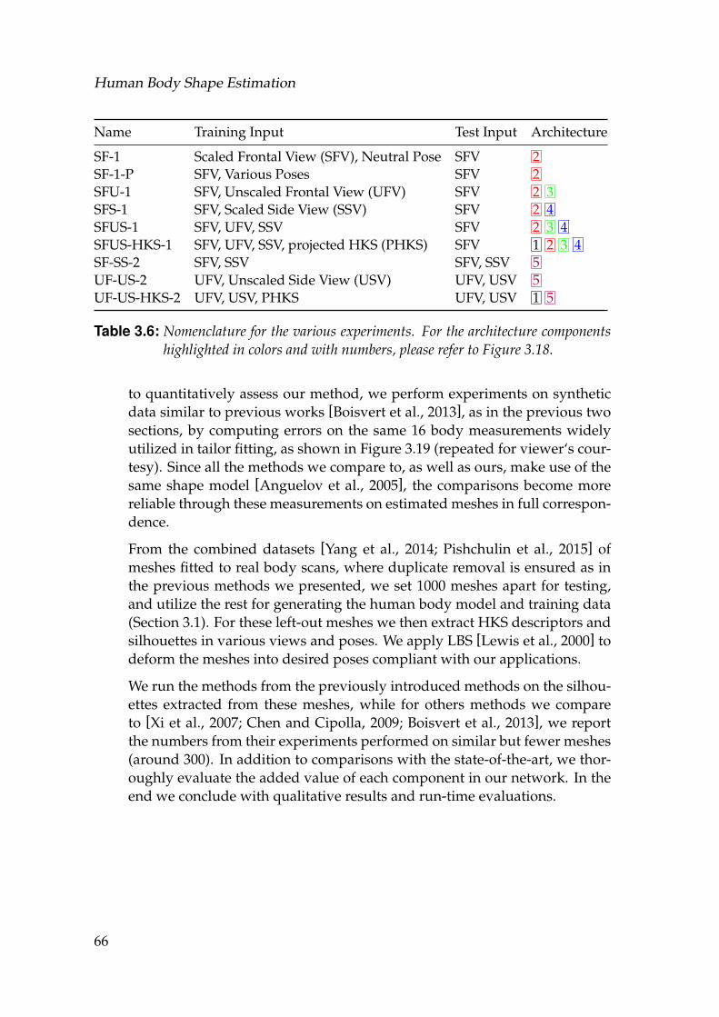
Human Body Shape Estimation
Name Training Input Test Input Architecture
SF-1 Scaled Frontal View (SFV), Neutral Pose SFV 2SF-1-P SFV, Various Poses SFV 2SFU-1 SFV, Unscaled Frontal View (UFV) SFV 2 3SFS-1 SFV, Scaled Side View (SSV) SFV 2 4SFUS-1 SFV, UFV, SSV SFV 2 3 4SFUS-HKS-1 SFV, UFV, SSV, projected HKS (PHKS) SFV 1 2 3 4SF-SS-2 SFV, SSV SFV, SSV 5UF-US-2 UFV, Unscaled Side View (USV) UFV, USV 5UF-US-HKS-2 UFV, USV, PHKS UFV, USV 1 5
Table 3.6: Nomenclature for the various experiments. For the architecture componentshighlighted in colors and with numbers, please refer to Figure 3.18.
to quantitatively assess our method, we perform experiments on syntheticdata similar to previous works [Boisvert et al., 2013], as in the previous twosections, by computing errors on the same 16 body measurements widelyutilized in tailor fitting, as shown in Figure 3.19 (repeated for viewer‘s cour-tesy). Since all the methods we compare to, as well as ours, make use of thesame shape model [Anguelov et al., 2005], the comparisons become morereliable through these measurements on estimated meshes in full correspon-dence.
From the combined datasets [Yang et al., 2014; Pishchulin et al., 2015] ofmeshes fitted to real body scans, where duplicate removal is ensured as inthe previous methods we presented, we set 1000 meshes apart for testing,and utilize the rest for generating the human body model and training data(Section 3.1). For these left-out meshes we then extract HKS descriptors andsilhouettes in various views and poses. We apply LBS [Lewis et al., 2000] todeform the meshes into desired poses compliant with our applications.
We run the methods from the previously introduced methods on the silhou-ettes extracted from these meshes, while for others methods we compareto [Xi et al., 2007; Chen and Cipolla, 2009; Boisvert et al., 2013], we reportthe numbers from their experiments performed on similar but fewer meshes(around 300). In addition to comparisons with the state-of-the-art, we thor-oughly evaluate the added value of each component in our network. In theend we conclude with qualitative results and run-time evaluations.
66
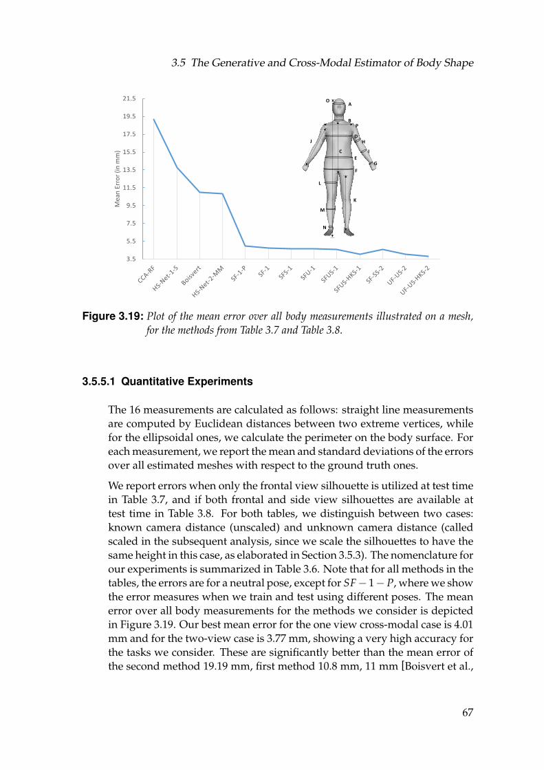
3.5 The Generative and Cross-Modal Estimator of Body Shape
3.5
5.5
7.5
9.5
11.5
13.5
15.5
17.5
19.5
21.5
Mea
n E
rro
r (i
n m
m)
A
B
C
DH
I
GE
F
P
O
K
L
M
N
J
Figure 3.19: Plot of the mean error over all body measurements illustrated on a mesh,for the methods from Table 3.7 and Table 3.8.
3.5.5.1 Quantitative Experiments
The 16 measurements are calculated as follows: straight line measurementsare computed by Euclidean distances between two extreme vertices, whilefor the ellipsoidal ones, we calculate the perimeter on the body surface. Foreach measurement, we report the mean and standard deviations of the errorsover all estimated meshes with respect to the ground truth ones.
We report errors when only the frontal view silhouette is utilized at test timein Table 3.7, and if both frontal and side view silhouettes are available attest time in Table 3.8. For both tables, we distinguish between two cases:known camera distance (unscaled) and unknown camera distance (calledscaled in the subsequent analysis, since we scale the silhouettes to have thesame height in this case, as elaborated in Section 3.5.3). The nomenclature forour experiments is summarized in Table 3.6. Note that for all methods in thetables, the errors are for a neutral pose, except for SF− 1− P, where we showthe error measures when we train and test using different poses. The meanerror over all body measurements for the methods we consider is depictedin Figure 3.19. Our best mean error for the one view cross-modal case is 4.01mm and for the two-view case is 3.77 mm, showing a very high accuracy forthe tasks we consider. These are significantly better than the mean error ofthe second method 19.19 mm, first method 10.8 mm, 11 mm [Boisvert et al.,
67
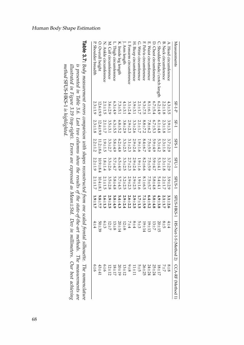
Human Body Shape Estimation
Measurem
entsSF-1-P
SF-1SFS-1
SFU-1
SFUS-1
SFUS-H
KS-1
HS-N
et-1-S(M
ethod2)
CC
A-R
F(M
ethod1)
A.H
eadcircum
ference4.3±
3.53.9±
3.13.7±
2.93.7±
2.93.9±
2.93.1±
2.64±
48±
8B.N
eckcircum
ference2.2±
1.82.3±
1.82.3±
1.82.3±
1.82.2±
1.72.1±
1.78±
57±
7C
.Shoulder-blade/crotchlength
6.2±4.9
6.1±4.8
5.3±4.2
5.3±4.1
5.4±4.1
4.9±3.8
20±15
18±17
D.C
hestcircumference
6.7±5.4
6.7±5.3
5.9±4.9
5.9±4.7
5.8±4.8
5.8±4.8
13±7
25±24
E.Waistcircum
ference8.1±
6.17.8±
6.27.5±
5.97.5±
5.97.5±
5.76.4±
5.219±
1324±
24F.Pelvis
circumference
9.3±7.5
8.8±7.2
8.4±6.7
8.2±6.6
8.1±6.5
7.1±5.9
19±14
26±25
G.W
ristcircumference
2.1±1.7
2.1±1.7
1.9±1.6
1.9±1.6
1.9±1.6
1.7±1.5
5±3
5±5
H.Bicep
circumference
3.9±3.1
3.3±2.6
2.9±2.4
2.9±2.4
2.9±2.5
2.9±2.5
8±4
11±11
I.Forearmcircum
ference3.1±
2.42.9±
2.33.1±
2.32.7±
2.32.9±
2.32.6±
2.27±
49±
8J.A
rmlength
4.1±3.1
3.8±2.9
3.3±2.5
3.3±2.5
3.2±2.5
2.9±2.4
12±8
13±12
K.Inside
leglength
7.3±5.1
6.8±5.2
6.2±4.8
6.5±4.9
5.7±4.5
5.4±4.3
20±14
20±19
L.Thigh
circumference
6.3±4.9
6.3±5.5
5.8±4.9
5.7±4.7
5.8±4.8
5.8±4.9
13±8
18±17
M.C
alfcircumference
3.6±2.9
3.5±3.1
3.3±2.7
3.3±2.6
3.5±2.8
2.9±2.5
12±7
12±12
N.A
nklecircum
ference2.1±
1.52.1±
1.71.9±
1.51.8±
1.42.1±
1.51.6±
1.36±
36±
6O
.Overallheight
12.6±9.9
12.4±9.9
11.2±8.6
10.9±8.4
10.4±8.1
9.8±7.7
50±39
43±41
P.Shoulderbreadth
2.3±1.9
2.3±1.8
2.2±1.2
2.2±1.9
2.1±1.7
1.9±1.7
4±4
6±6
Table3.7:Body
measurem
enterrors
comparison
with
shapesreconstructed
fromone
scaledfrontalsilhouette.
Thenom
enclatureis
presentedin
Table3.6.
Lasttw
ocolum
nsshow
theresults
ofthe
state-of-the-artm
ethods.The
measurem
entsare
illustratedin
Figure3.19
(top-right).Errors
areexpressed
asM
ean±Std.
Dev
inm
illimeters.
Our
bestachieving
method
SFUS-H
KS-1
ishighlighted.
68
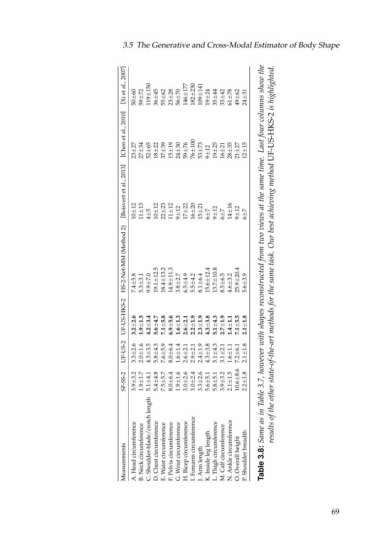
3.5 The Generative and Cross-Modal Estimator of Body Shape
Mea
sure
men
tsSF
-SS-
2U
F-U
S-2
UF-
US-
HK
S-2
HS-
2-N
et-M
M(M
etho
d2)
[ Boi
sver
teta
l.,20
13]
[ Che
net
al.,
2010
][ X
ieta
l.,20
07]
A.H
ead
circ
umfe
renc
e3.
9±3.
23.
3±2.
63.
2±2.
67.
4±5.
810±
1223±
2750±
60B.
Nec
kci
rcum
fere
nce
1.9±
1.7
2.0±
1.6
1.9±
1.5
5.3±
3.1
11±
1327±
3459±
72C
.Sho
ulde
r-bl
ade/
crot
chle
ngth
5.1±
4.1
4.3±
3.5
4.2±
3.4
9.9±
7.0
4±5
52±
6511
9±15
0D
.Che
stci
rcum
fere
nce
5.4±
4.8
5.8±
4.3
5.6±
4.7
19.1±
12.5
10±
1218±
2236±
45E.
Wai
stci
rcum
fere
nce
7.5±
5.7
7.6±
5.9
7.1±
5.8
18.4±
13.2
22±
2337±
3955±
62F.
Pelv
isci
rcum
fere
nce
8.0±
6.4
8.0±
6.4
6.9±
5.6
14.9±
11.3
11±
1215±
1923±
28G
.Wri
stci
rcum
fere
nce
1.9±
1.6
1.6±
1.4
1.6±
1.3
3.8±
2.7
9±12
24±
3056±
70H
.Bic
epci
rcum
fere
nce
3.0±
2.6
2.6±
2.1
2.6±
2.1
6.5±
4.9
17±
2259±
7614
6±17
7I.
Fore
arm
circ
umfe
renc
e3.
0±2.
42.
9±2.
12.
2±1.
95.
5±4.
216±
2076±
100
182±
230
J.A
rmle
ngth
3.3±
2.6
2.4±
1.9
2.3±
1.9
8.1±
6.4
15±
2153±
7310
9±14
1K
.Ins
ide
leg
leng
th5.
6±5.
14.
3±3.
84.
3±3.
815
.6±
12.4
6±7
9±12
19±
24L.
Thig
hci
rcum
fere
nce
5.8±
5.1
5.1±
4.3
5.1±
4.3
13.7±
10.8
9±12
19±
2535±
44M
.Cal
fcir
cum
fere
nce
3.9±
3.2
3.1±
2.1
2.7±
1.9
8.5±
6.5
6±7
16±
2133±
42N
.Ank
leci
rcum
fere
nce
2.1±
1.5
1.6±
1.1
1.4±
1.1
4.6±
3.2
14±
1628±
3561±
78O
.Ove
rall
heig
ht10
.6±
8.6
7.2±
6.1
7.1±
5.5
25.9±
20.4
9±12
21±
2749±
62P.
Shou
lder
brea
dth
2.2±
1.8
2.1±
1.8
2.1±
1.8
5.6±
3.9
6±7
12±
1524±
31
Tabl
e3.
8:Sa
me
asin
Tabl
e3.
7,ho
wev
erw
ithsh
apes
reco
nstr
ucte
dfr
omtw
ovi
ews
atth
esa
me
time.
Last
four
colu
mns
show
the
resu
ltsof
the
othe
rst
ate-
of-t
he-a
rtm
etho
dsfo
rth
esa
me
task
.Our
best
achi
evin
gm
etho
dU
F-U
S-H
KS-
2is
high
light
ed.
69
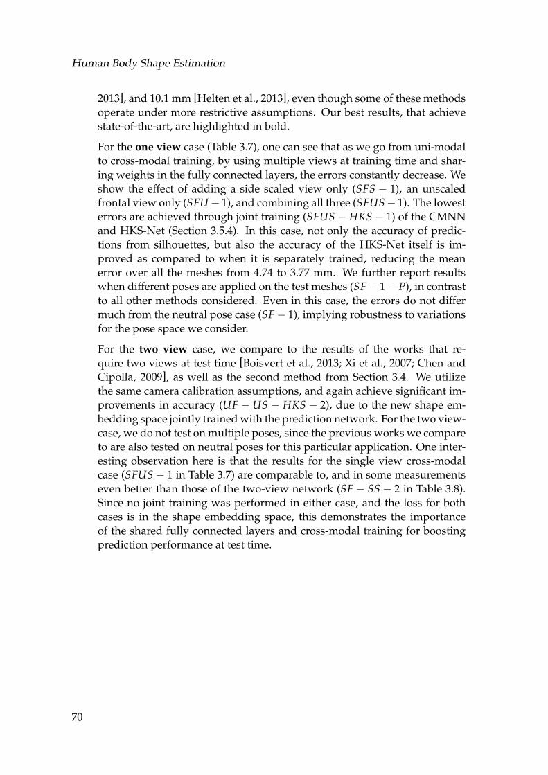
Human Body Shape Estimation
2013], and 10.1 mm [Helten et al., 2013], even though some of these methodsoperate under more restrictive assumptions. Our best results, that achievestate-of-the-art, are highlighted in bold.
For the one view case (Table 3.7), one can see that as we go from uni-modalto cross-modal training, by using multiple views at training time and shar-ing weights in the fully connected layers, the errors constantly decrease. Weshow the effect of adding a side scaled view only (SFS − 1), an unscaledfrontal view only (SFU− 1), and combining all three (SFUS− 1). The lowesterrors are achieved through joint training (SFUS− HKS− 1) of the CMNNand HKS-Net (Section 3.5.4). In this case, not only the accuracy of predic-tions from silhouettes, but also the accuracy of the HKS-Net itself is im-proved as compared to when it is separately trained, reducing the meanerror over all the meshes from 4.74 to 3.77 mm. We further report resultswhen different poses are applied on the test meshes (SF− 1− P), in contrastto all other methods considered. Even in this case, the errors do not differmuch from the neutral pose case (SF− 1), implying robustness to variationsfor the pose space we consider.
For the two view case, we compare to the results of the works that re-quire two views at test time [Boisvert et al., 2013; Xi et al., 2007; Chen andCipolla, 2009], as well as the second method from Section 3.4. We utilizethe same camera calibration assumptions, and again achieve significant im-provements in accuracy (UF −US − HKS − 2), due to the new shape em-bedding space jointly trained with the prediction network. For the two view-case, we do not test on multiple poses, since the previous works we compareto are also tested on neutral poses for this particular application. One inter-esting observation here is that the results for the single view cross-modalcase (SFUS− 1 in Table 3.7) are comparable to, and in some measurementseven better than those of the two-view network (SF − SS− 2 in Table 3.8).Since no joint training was performed in either case, and the loss for bothcases is in the shape embedding space, this demonstrates the importanceof the shared fully connected layers and cross-modal training for boostingprediction performance at test time.
70
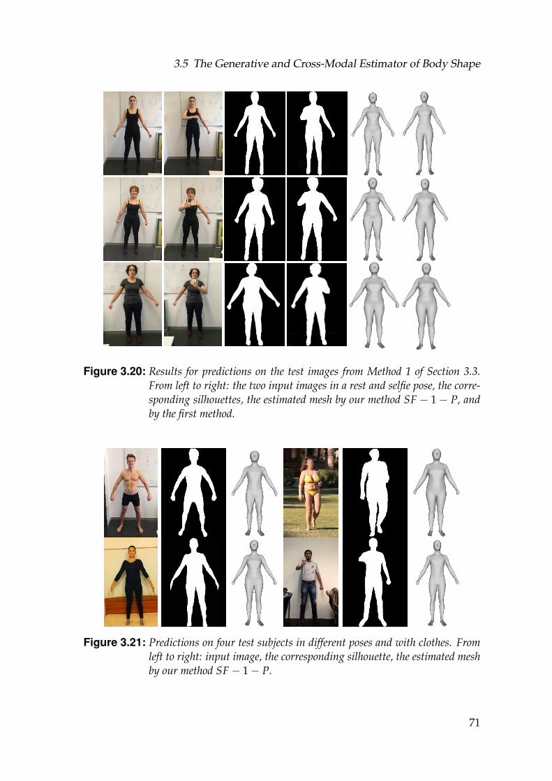
3.5 The Generative and Cross-Modal Estimator of Body Shape
Figure 3.20: Results for predictions on the test images from Method 1 of Section 3.3.From left to right: the two input images in a rest and selfie pose, the corre-sponding silhouettes, the estimated mesh by our method SF − 1− P, andby the first method.
Figure 3.21: Predictions on four test subjects in different poses and with clothes. Fromleft to right: input image, the corresponding silhouette, the estimated meshby our method SF− 1− P.
71
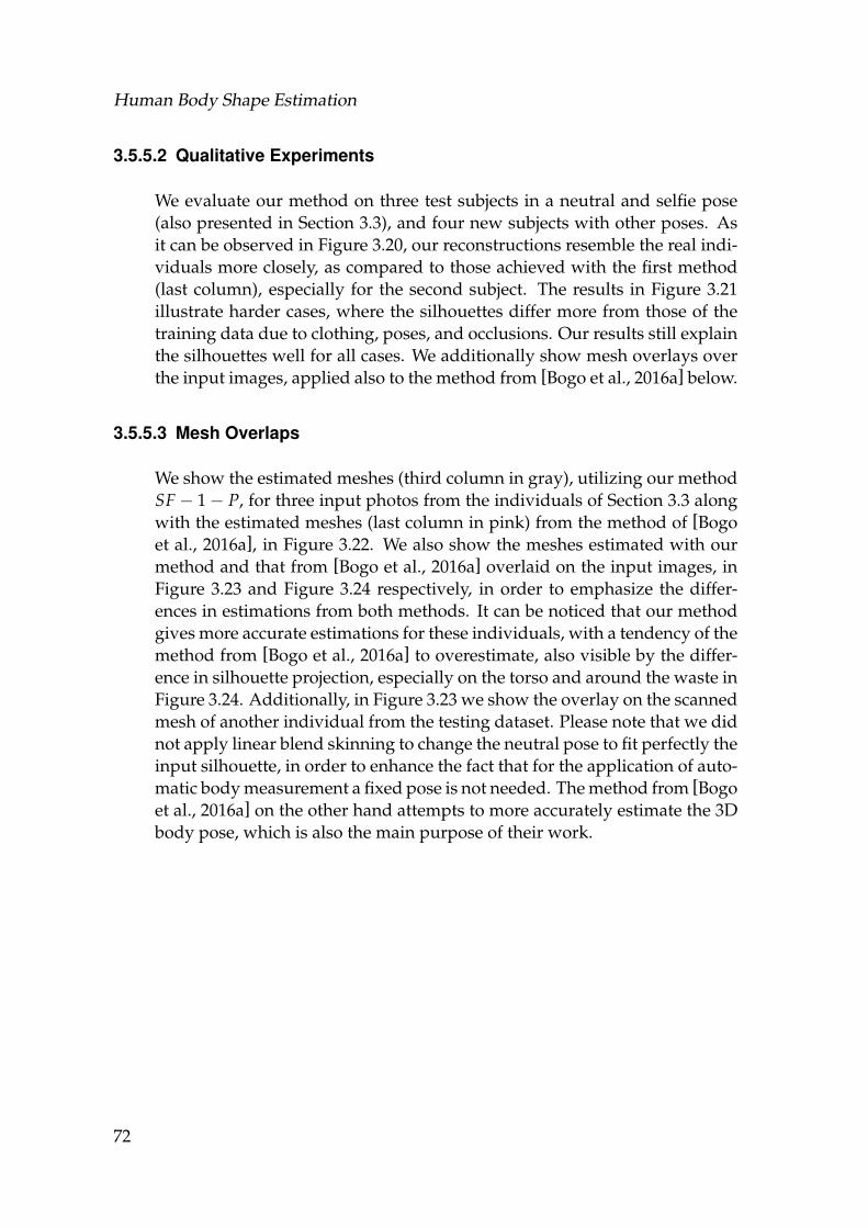
Human Body Shape Estimation
3.5.5.2 Qualitative Experiments
We evaluate our method on three test subjects in a neutral and selfie pose(also presented in Section 3.3), and four new subjects with other poses. Asit can be observed in Figure 3.20, our reconstructions resemble the real indi-viduals more closely, as compared to those achieved with the first method(last column), especially for the second subject. The results in Figure 3.21illustrate harder cases, where the silhouettes differ more from those of thetraining data due to clothing, poses, and occlusions. Our results still explainthe silhouettes well for all cases. We additionally show mesh overlays overthe input images, applied also to the method from [Bogo et al., 2016a] below.
3.5.5.3 Mesh Overlaps
We show the estimated meshes (third column in gray), utilizing our methodSF− 1− P, for three input photos from the individuals of Section 3.3 alongwith the estimated meshes (last column in pink) from the method of [Bogoet al., 2016a], in Figure 3.22. We also show the meshes estimated with ourmethod and that from [Bogo et al., 2016a] overlaid on the input images, inFigure 3.23 and Figure 3.24 respectively, in order to emphasize the differ-ences in estimations from both methods. It can be noticed that our methodgives more accurate estimations for these individuals, with a tendency of themethod from [Bogo et al., 2016a] to overestimate, also visible by the differ-ence in silhouette projection, especially on the torso and around the waste inFigure 3.24. Additionally, in Figure 3.23 we show the overlay on the scannedmesh of another individual from the testing dataset. Please note that we didnot apply linear blend skinning to change the neutral pose to fit perfectly theinput silhouette, in order to enhance the fact that for the application of auto-matic body measurement a fixed pose is not needed. The method from [Bogoet al., 2016a] on the other hand attempts to more accurately estimate the 3Dbody pose, which is also the main purpose of their work.
72
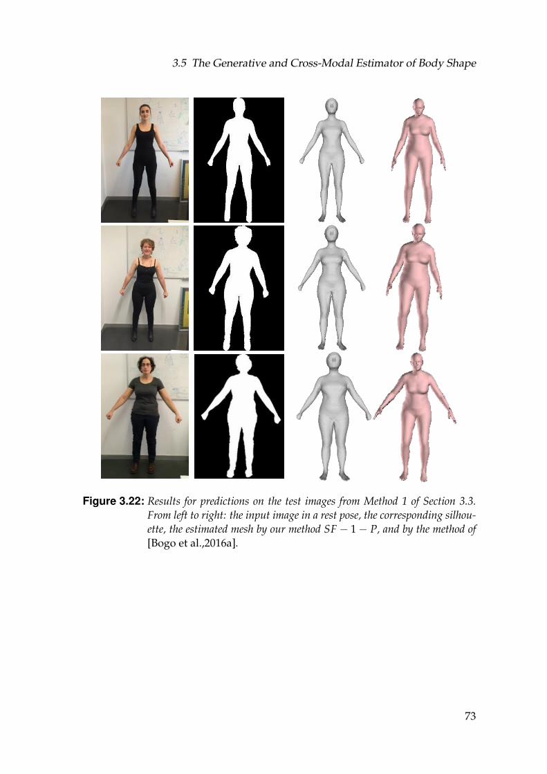
3.5 The Generative and Cross-Modal Estimator of Body Shape
Figure 3.22: Results for predictions on the test images from Method 1 of Section 3.3.From left to right: the input image in a rest pose, the corresponding silhou-ette, the estimated mesh by our method SF− 1− P, and by the method of[Bogo et al.,2016a].
73
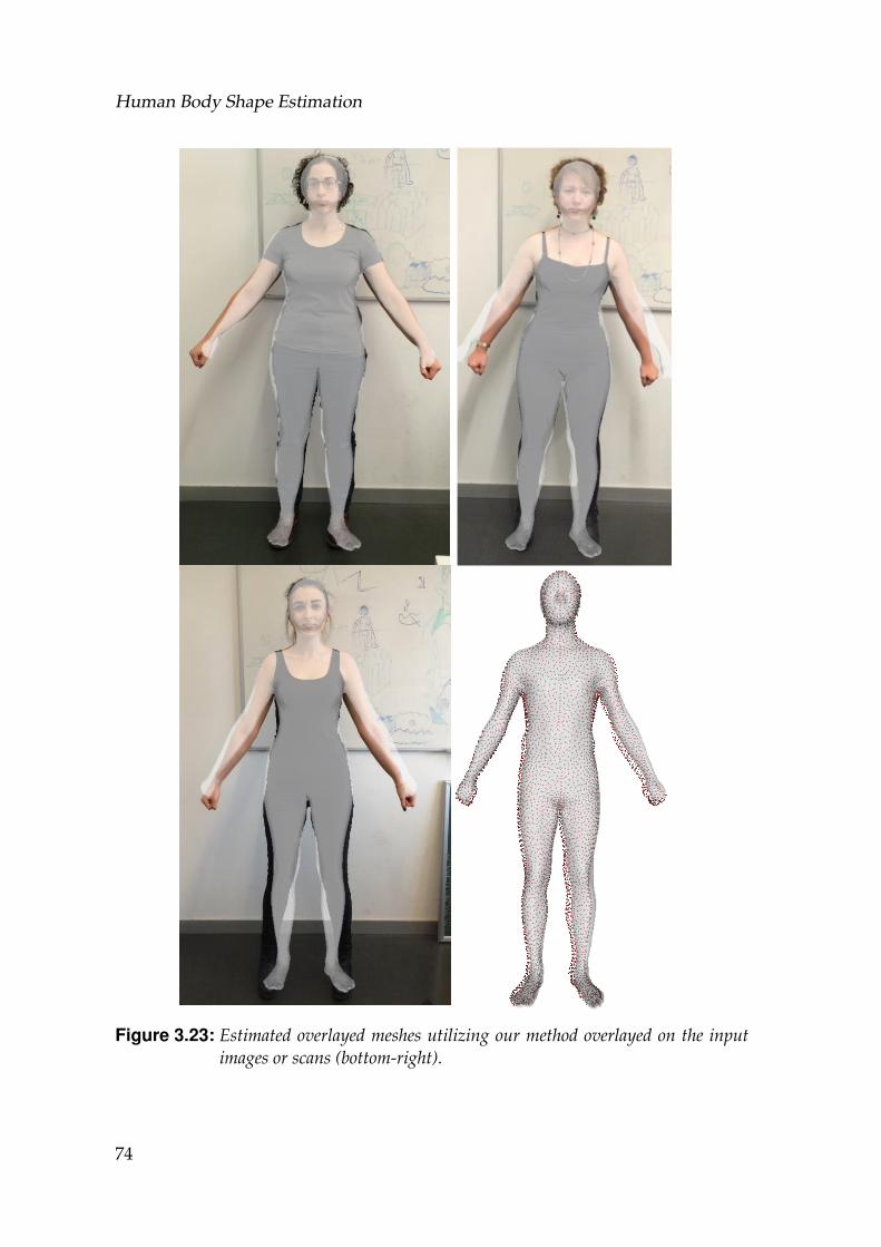
Human Body Shape Estimation
Figure 3.23: Estimated overlayed meshes utilizing our method overlayed on the inputimages or scans (bottom-right).
74
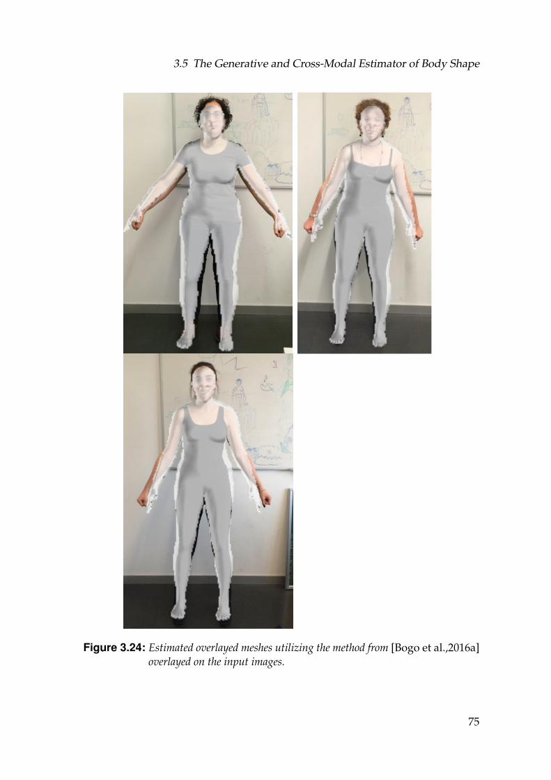
3.5 The Generative and Cross-Modal Estimator of Body Shape
Figure 3.24: Estimated overlayed meshes utilizing the method from [Bogo et al.,2016a]overlayed on the input images.
75
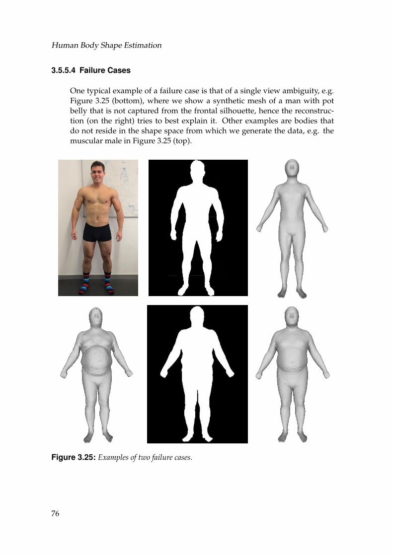
Human Body Shape Estimation
3.5.5.4 Failure Cases
One typical example of a failure case is that of a single view ambiguity, e.g.Figure 3.25 (bottom), where we show a synthetic mesh of a man with potbelly that is not captured from the frontal silhouette, hence the reconstruc-tion (on the right) tries to best explain it. Other examples are bodies thatdo not reside in the shape space from which we generate the data, e.g. themuscular male in Figure 3.25 (top).
Figure 3.25: Examples of two failure cases.
76
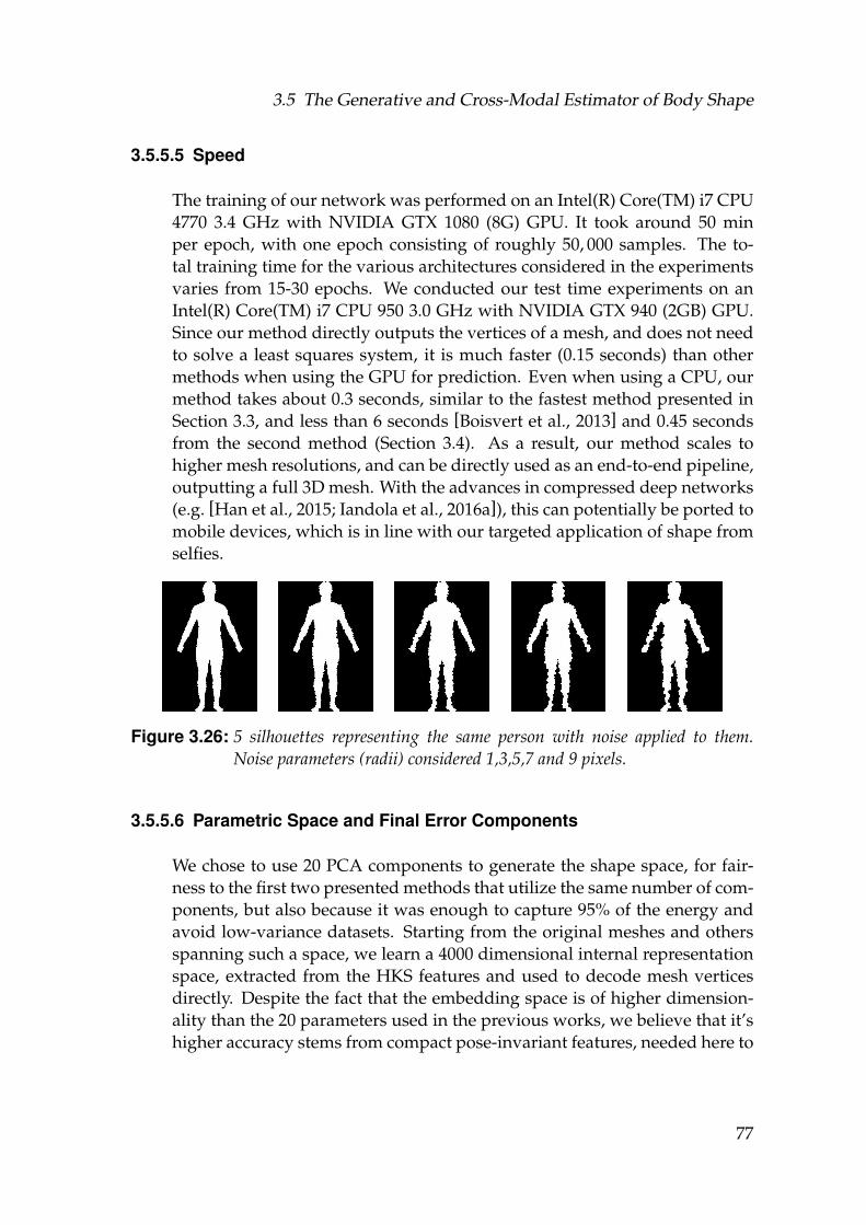
3.5 The Generative and Cross-Modal Estimator of Body Shape
3.5.5.5 Speed
The training of our network was performed on an Intel(R) Core(TM) i7 CPU4770 3.4 GHz with NVIDIA GTX 1080 (8G) GPU. It took around 50 minper epoch, with one epoch consisting of roughly 50, 000 samples. The to-tal training time for the various architectures considered in the experimentsvaries from 15-30 epochs. We conducted our test time experiments on anIntel(R) Core(TM) i7 CPU 950 3.0 GHz with NVIDIA GTX 940 (2GB) GPU.Since our method directly outputs the vertices of a mesh, and does not needto solve a least squares system, it is much faster (0.15 seconds) than othermethods when using the GPU for prediction. Even when using a CPU, ourmethod takes about 0.3 seconds, similar to the fastest method presented inSection 3.3, and less than 6 seconds [Boisvert et al., 2013] and 0.45 secondsfrom the second method (Section 3.4). As a result, our method scales tohigher mesh resolutions, and can be directly used as an end-to-end pipeline,outputting a full 3D mesh. With the advances in compressed deep networks(e.g. [Han et al., 2015; Iandola et al., 2016a]), this can potentially be ported tomobile devices, which is in line with our targeted application of shape fromselfies.
Figure 3.26: 5 silhouettes representing the same person with noise applied to them.Noise parameters (radii) considered 1,3,5,7 and 9 pixels.
3.5.5.6 Parametric Space and Final Error Components
We chose to use 20 PCA components to generate the shape space, for fair-ness to the first two presented methods that utilize the same number of com-ponents, but also because it was enough to capture 95% of the energy andavoid low-variance datasets. Starting from the original meshes and othersspanning such a space, we learn a 4000 dimensional internal representationspace, extracted from the HKS features and used to decode mesh verticesdirectly. Despite the fact that the embedding space is of higher dimension-ality than the 20 parameters used in the previous works, we believe that it’shigher accuracy stems from compact pose-invariant features, needed here to
77
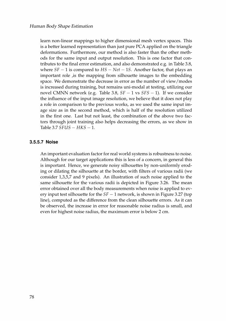
Human Body Shape Estimation
learn non-linear mappings to higher dimensional mesh vertex spaces. Thisis a better learned representation than just pure PCA applied on the triangledeformations. Furthermore, our method is also faster than the other meth-ods for the same input and output resolution. This is one factor that con-tributes to the final error estimation, and also demonstrated e.g. in Table 3.8,where SF − 1 is compared to HS− Net− 1S. Another factor, that plays animportant role ,is the mapping from silhouette images to the embeddingspace. We demonstrate the decrease in error as the number of view/modesis increased during training, but remains uni-modal at testing, utilizing ournovel CMNN network (e.g. Table 3.8, SF − 1 vs SFS − 1). If we considerthe influence of the input image resolution, we believe that it does not playa role in comparison to the previous works, as we used the same input im-age size as in the second method, which is half of the resolution utilizedin the first one. Last but not least, the combination of the above two fac-tors through joint training also helps decreasing the errors, as we show inTable 3.7 SFUS− HKS− 1.
3.5.5.7 Noise
An important evaluation factor for real world systems is robustness to noise.Although for our target applications this is less of a concern, in general thisis important. Hence, we generate noisy silhouettes by non-uniformly erod-ing or dilating the silhouette at the border, with filters of various radii (weconsider 1,3,5,7 and 9 pixels). An illustration of such noise applied to thesame silhouette for the various radii is depicted in Figure 3.26. The meanerror obtained over all the body measurements when noise is applied to ev-ery input test silhouette for the SF− 1 network, is shown in Figure 3.27 (topline), computed as the difference from the clean silhouette errors. As it canbe observed, the increase in error for reasonable noise radius is small, andeven for highest noise radius, the maximum error is below 2 cm.
78
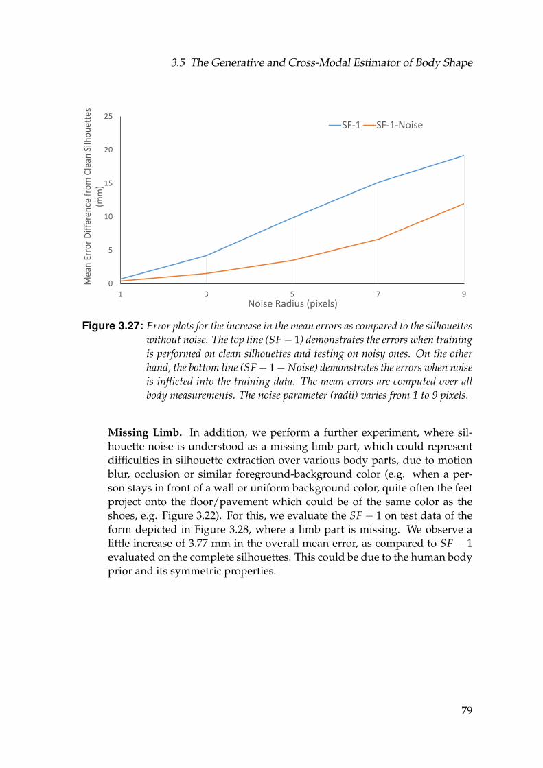
3.5 The Generative and Cross-Modal Estimator of Body Shape
0
5
10
15
20
25
1 3 5 7 9
Mea
n E
rro
r D
iffe
ren
ce f
rom
Cle
an S
ilho
uet
tes
(mm
)
Noise Radius (pixels)
SF-1 SF-1-Noise
Figure 3.27: Error plots for the increase in the mean errors as compared to the silhouetteswithout noise. The top line (SF− 1) demonstrates the errors when trainingis performed on clean silhouettes and testing on noisy ones. On the otherhand, the bottom line (SF− 1−Noise) demonstrates the errors when noiseis inflicted into the training data. The mean errors are computed over allbody measurements. The noise parameter (radii) varies from 1 to 9 pixels.
Missing Limb. In addition, we perform a further experiment, where sil-houette noise is understood as a missing limb part, which could representdifficulties in silhouette extraction over various body parts, due to motionblur, occlusion or similar foreground-background color (e.g. when a per-son stays in front of a wall or uniform background color, quite often the feetproject onto the floor/pavement which could be of the same color as theshoes, e.g. Figure 3.22). For this, we evaluate the SF − 1 on test data of theform depicted in Figure 3.28, where a limb part is missing. We observe alittle increase of 3.77 mm in the overall mean error, as compared to SF − 1evaluated on the complete silhouettes. This could be due to the human bodyprior and its symmetric properties.
79
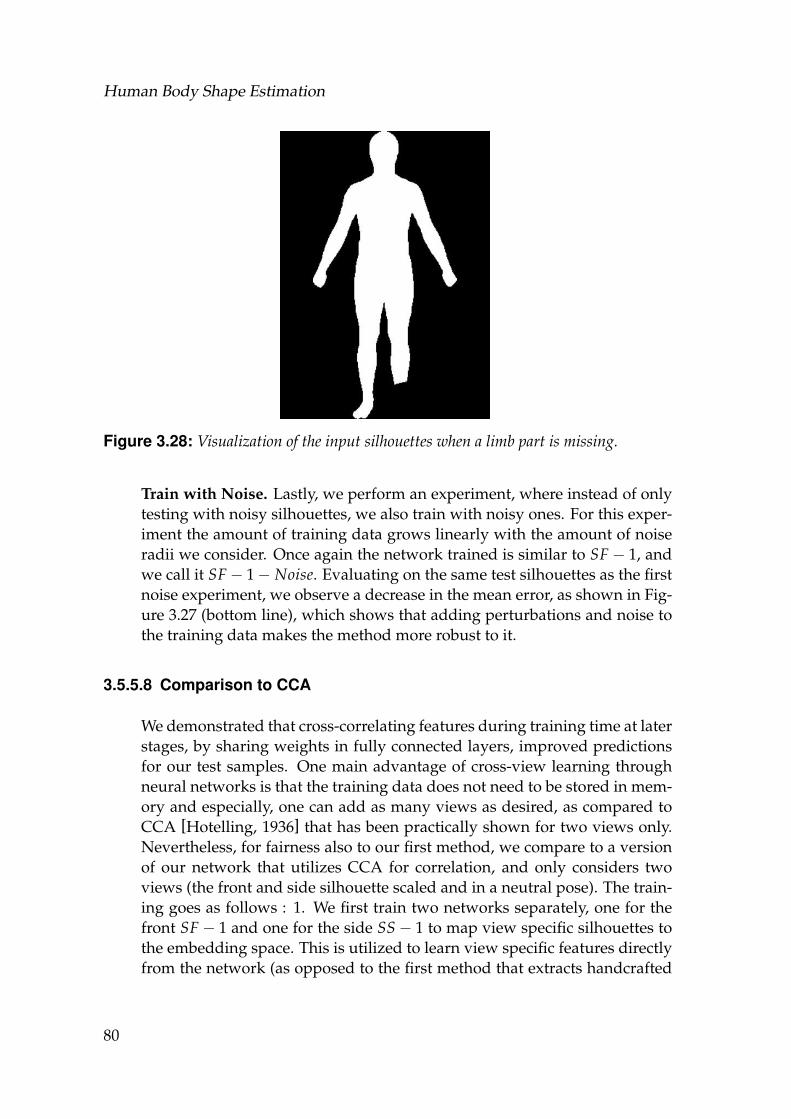
Human Body Shape Estimation
Figure 3.28: Visualization of the input silhouettes when a limb part is missing.
Train with Noise. Lastly, we perform an experiment, where instead of onlytesting with noisy silhouettes, we also train with noisy ones. For this exper-iment the amount of training data grows linearly with the amount of noiseradii we consider. Once again the network trained is similar to SF− 1, andwe call it SF− 1− Noise. Evaluating on the same test silhouettes as the firstnoise experiment, we observe a decrease in the mean error, as shown in Fig-ure 3.27 (bottom line), which shows that adding perturbations and noise tothe training data makes the method more robust to it.
3.5.5.8 Comparison to CCA
We demonstrated that cross-correlating features during training time at laterstages, by sharing weights in fully connected layers, improved predictionsfor our test samples. One main advantage of cross-view learning throughneural networks is that the training data does not need to be stored in mem-ory and especially, one can add as many views as desired, as compared toCCA [Hotelling, 1936] that has been practically shown for two views only.Nevertheless, for fairness also to our first method, we compare to a versionof our network that utilizes CCA for correlation, and only considers twoviews (the front and side silhouette scaled and in a neutral pose). The train-ing goes as follows : 1. We first train two networks separately, one for thefront SF− 1 and one for the side SS− 1 to map view specific silhouettes tothe embedding space. This is utilized to learn view specific features directlyfrom the network (as opposed to the first method that extracts handcrafted
80
3.5 The Generative and Cross-Modal Estimator of Body Shape
Measurements SFS-1 SF-1-CCA SFUS-1 SFUS-1-SH
A. Head circumference 3.7±2.9 4.3±3.5 3.9±2.9 4.2±3.4B. Neck circumference 2.3±1.8 2.8±2.1 2.2±1.7 2.2±1.9C. Shoulder-blade/crotch length 5.3±4.2 7.2±5.5 5.4±4.1 5.8±4.5D. Chest circumference 5.9±4.9 7.8±6.9 5.8±4.8 6.6±5.5E. Waist circumference 7.5±5.9 9.2±7.2 7.5±5.7 8.5±6.6F. Pelvis circumference 8.4±6.7 9.7±8.1 8.1±6.5 8.6±7.1G. Wrist circumference 1.9±1.6 3.1±2.1 1.9±1.6 2.1±1.7H. Bicep circumference 2.9±2.4 4.2±3.4 2.9±2.5 3.3±2.6I. Forearm circumference 3.1±2.3 3.3±2.6 2.9±2.3 3.2±2.5J. Arm length 3.3±2.5 4.5±3.6 3.2±2.5 3.5±2.9K. Inside leg length 6.2±4.8 7.4±6.0 5.7±4.5 6.2±5.1L. Thigh circumference 5.8±4.9 7.1±5.9 5.8±4.8 6.2±5.3M. Calf circumference 3.3±2.7 4.3±3.6 3.5±2.8 3.9±3.3N. Ankle circumference 1.9±1.5 2.1±1.6 2.1±1.5 2.3±1.7O. Overall height 11.2±8.6 14.1±11.1 10.4±8.1 11.9±9.5P. Shoulder breadth 2.2±1.2 2.6±2.1 2.1±1.7 2.2±1.9
Table 3.9: Body measurement errors comparison over the various experiments consid-ered here. Errors are expressed as Mean±Std. Dev in millimeters.
features); 2. Then, we extract 8064 features from the last convolutional layerover each view, for all of our training data, and since the dimensionalityis quite high, we apply dimensionality reduction through PCA up to 500dimensions that capture most of the energy. Starting from these 500 dimen-sional vectors we apply CCA, to find linear projection bases where the cor-relation of the projected features is maximized; 3. In the end, we train asmaller network of three fully connected layers SF− 1− CCA, to map fromthe 500 CCA projected features of the frontal view only (the desired one) tothe embedding space. At test time, a new frontal view silhouette is first in-put to SF − 1 that performs a forward pass to extract 8064 features, whichare then projected onto PCA and CCA. The projection is mapped throughSF− 1− CCA to the embedding space, which in turn reconstructs the meshwith the help of the HKS − Net. We demonstrate the results of this pro-cedure for the same synthetic meshes and we compare to our cross-modaltraining over two views SFS − 1 in Table 3.9. It can be noticed that ourmethod outperforms the CCA based one. The latter still performs well,however on the expense of added memory footprint and unscalability tomore than two views. Furthermore, it is not trivial to train the network end-to-end without splitting it into various components. And lastly, we think
81
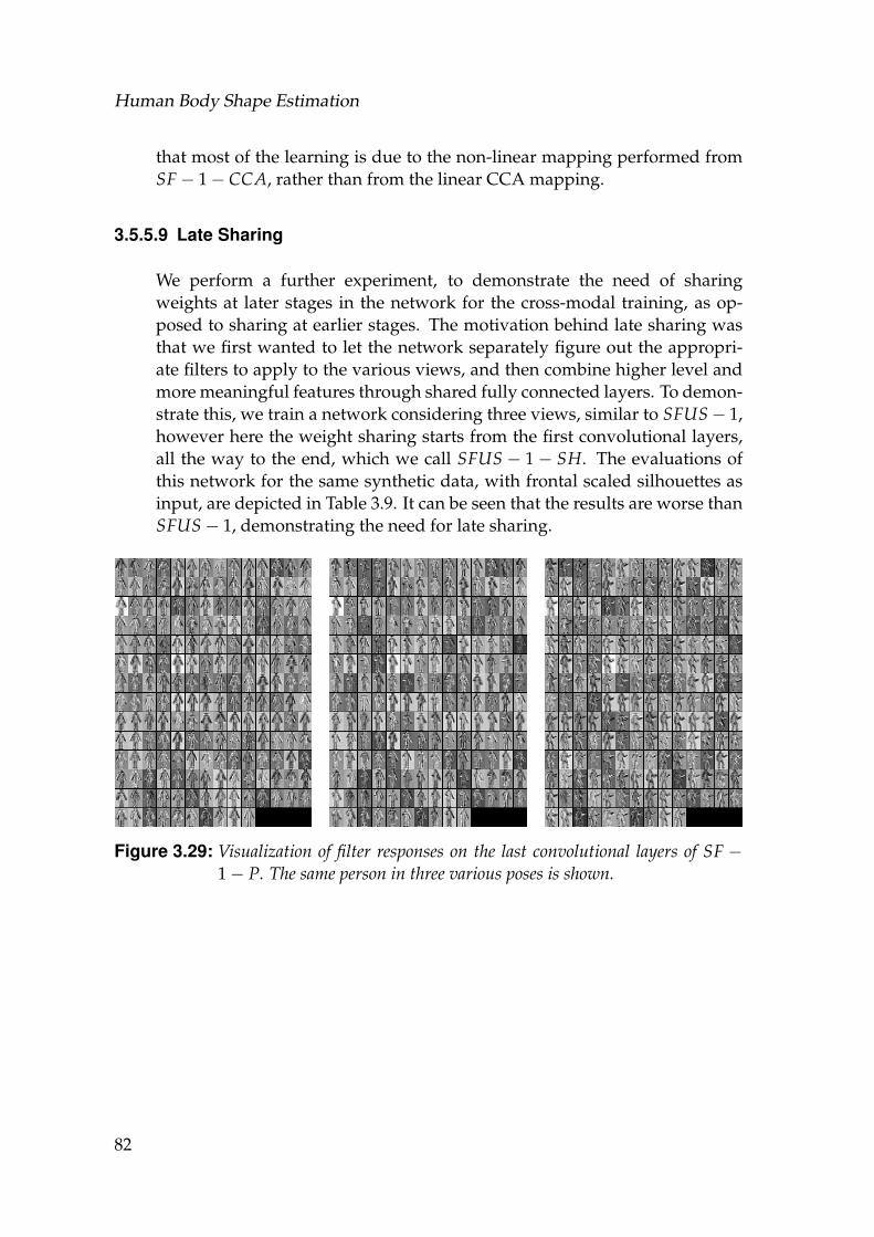
Human Body Shape Estimation
that most of the learning is due to the non-linear mapping performed fromSF− 1− CCA, rather than from the linear CCA mapping.
3.5.5.9 Late Sharing
We perform a further experiment, to demonstrate the need of sharingweights at later stages in the network for the cross-modal training, as op-posed to sharing at earlier stages. The motivation behind late sharing wasthat we first wanted to let the network separately figure out the appropri-ate filters to apply to the various views, and then combine higher level andmore meaningful features through shared fully connected layers. To demon-strate this, we train a network considering three views, similar to SFUS− 1,however here the weight sharing starts from the first convolutional layers,all the way to the end, which we call SFUS − 1− SH. The evaluations ofthis network for the same synthetic data, with frontal scaled silhouettes asinput, are depicted in Table 3.9. It can be seen that the results are worse thanSFUS− 1, demonstrating the need for late sharing.
Figure 3.29: Visualization of filter responses on the last convolutional layers of SF −1− P. The same person in three various poses is shown.
82

3.5 The Generative and Cross-Modal Estimator of Body Shape
Figure 3.30: Network architecture for a single view case trained with SF− 1− P archi-tecture. For other types of inputs, such as side view etc., the architecture isthe same.
Figure 3.31: Illustration of people in various poses considered throughout our experi-ments.
3.5.5.10 Convolutional Filters
For illustrative purposes, we also demonstrate the filter responses of one ofthe last convolutional layers for SF − 1− P when the input silhouette is ofa person in three various poses (Figure 3.29). A more detailed version ofthe single view architecture is depicted in Figure 3.30. The network inter-nally learns to distinguish between various body parts (e.g. limbs), as sim-ilar looking filters are applied to the same parts (e.g. hands), even thoughthe poses vary. An illustrative figure of the various poses we consider isdepicted in Figure 3.31.
83
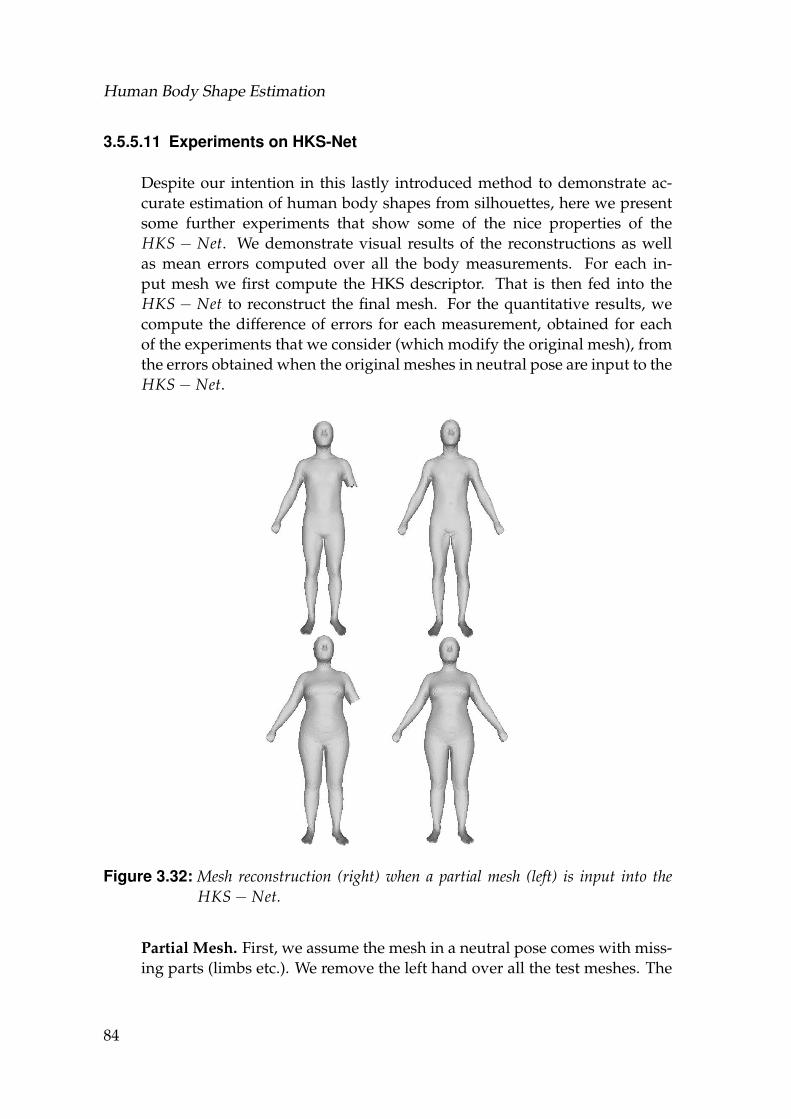
Human Body Shape Estimation
3.5.5.11 Experiments on HKS-Net
Despite our intention in this lastly introduced method to demonstrate ac-curate estimation of human body shapes from silhouettes, here we presentsome further experiments that show some of the nice properties of theHKS − Net. We demonstrate visual results of the reconstructions as wellas mean errors computed over all the body measurements. For each in-put mesh we first compute the HKS descriptor. That is then fed into theHKS − Net to reconstruct the final mesh. For the quantitative results, wecompute the difference of errors for each measurement, obtained for eachof the experiments that we consider (which modify the original mesh), fromthe errors obtained when the original meshes in neutral pose are input to theHKS− Net.
Figure 3.32: Mesh reconstruction (right) when a partial mesh (left) is input into theHKS− Net.
Partial Mesh. First, we assume the mesh in a neutral pose comes with miss-ing parts (limbs etc.). We remove the left hand over all the test meshes. The
84
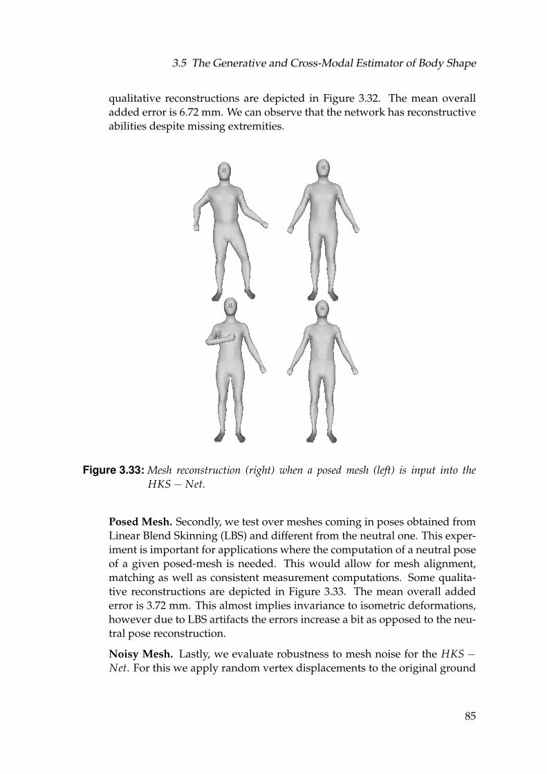
3.5 The Generative and Cross-Modal Estimator of Body Shape
qualitative reconstructions are depicted in Figure 3.32. The mean overalladded error is 6.72 mm. We can observe that the network has reconstructiveabilities despite missing extremities.
Figure 3.33: Mesh reconstruction (right) when a posed mesh (left) is input into theHKS− Net.
Posed Mesh. Secondly, we test over meshes coming in poses obtained fromLinear Blend Skinning (LBS) and different from the neutral one. This exper-iment is important for applications where the computation of a neutral poseof a given posed-mesh is needed. This would allow for mesh alignment,matching as well as consistent measurement computations. Some qualita-tive reconstructions are depicted in Figure 3.33. The mean overall addederror is 3.72 mm. This almost implies invariance to isometric deformations,however due to LBS artifacts the errors increase a bit as opposed to the neu-tral pose reconstruction.
Noisy Mesh. Lastly, we evaluate robustness to mesh noise for the HKS −Net. For this we apply random vertex displacements to the original ground
85
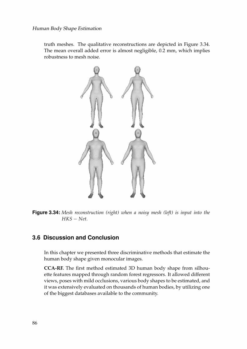
Human Body Shape Estimation
truth meshes. The qualitative reconstructions are depicted in Figure 3.34.The mean overall added error is almost negligible, 0.2 mm, which impliesrobustness to mesh noise.
Figure 3.34: Mesh reconstruction (right) when a noisy mesh (left) is input into theHKS− Net.
3.6 Discussion and Conclusion
In this chapter we presented three discriminative methods that estimate thehuman body shape given monocular images.
CCA-RF. The first method estimated 3D human body shape from silhou-ette features mapped through random forest regressors. It allowed differentviews, poses with mild occlusions, various body shapes to be estimated, andit was extensively evaluated on thousands of human bodies, by utilizing oneof the biggest databases available to the community.
86
3.6 Discussion and Conclusion
Withing the scope of this work, shape extraction from a single silhouette wasin focus, because of its various applications such as selfies or utilizing lim-ited video footage. However, this is an inherently ill-posed problem. Furtherviews can be incorporated to obtain more accurate reconstructions, similarto methods we compare to. This would lead to a better estimation especiallyin the areas around the belly and chest, hence decrease the elliptical bodymeasurement errors.
The accuracy of this method is tied to silhouette extraction. For the difficultcases of dynamic backgrounds or very loose clothes, the large scale silhou-ette deformations would skew our results. This could be tackled by fusingresults over multiple frames. Unlike [Chen et al., 2010] though, our resultsalways remain in the space of plausible human bodies. For small scale de-formations, as in Figure 3.7, we show in Table 3.2 (N) that our results stayrobust.
We assume that the silhouettes come in poses with limited partial occlusion.Under this assumption, we showed robustness, as the same mesh estimationis achieved from different poses (e.g. Figure 3.6). However, under morepronounced occlusions, our results start degrading (Table 3.2 (PWR)), whichcould be alleviated by increasing the number of training poses and utilizingdeeper learning.
Although we aimed at precise measurements for the evaluation, errors dueto discretization are inevitable, hence a standardized procedure on a stan-dard mesh dataset is needed as a benchmark. We believe that this workalong with that of [Boisvert et al., 2013] has set an important step towardsthis direction.
Since our system is designed for a general setting, we apply a fixed scale tothe silhouette, losing height information. We showed a fairly good perfor-mance on estimating the relative height and demonstrated better absoluteheight estimation, given that camera calibration is incorporated.
Our fast system, running in minutes for training and milliseconds for ex-ecution in single core CPU’s, while being memory lightweight due to thelow feature dimensionality, could be integrated into smart phones, allowingbody shapes to be reconstructed with one click of a button. Simultaneously,it can be used for 3D sport analysis, where estimation of a 3D shape of aplayer seen from a sparse set of cameras can improve projections of novel-views.
Finally, we showed how CCA, which captures relations in an unsupervisedlinear way, can be used to correlate different views in the data to improve
87
Human Body Shape Estimation
the prediction power and speed of the algorithm. We believe that captur-ing non-linear relations with Kernel CCA’s or deep architectures, such asauto-encoders, should lead to even better results. Our method illustratesthe utility of CCA for other vision applications where two or more viewsdescribing the same object or event exist, such as video-to-text matching orshape from various sources of information.
HKS-Net. With the second method, we abstracted away from handcraftedfeatures, and handled the accurate estimation of 3D human body shapefrom silhouettes (or shaded images ) utilizing CNNs. As with the previousmethod, the problem was posed as a regression that finds a global mappingfrom the various inputs that we presented to shape parameters. We exten-sively evaluated our technique on thousands of human bodies and real peo-ple.
In compliance with our main target applications, e.g. garment fitting andas opposed to the previous method, we mainly focused on shape estimationof people in neutral poses allowing mild pose changes, from one or twobinary silhouettes as well as shaded images as input. We showed that weoutperform methods based on global mapping and achieve similar resultsto more expensive methods that employ local fitting.
In the scope of the networks that we experimented with, we showed how tosimultaneously combine two binary silhouettes in order to improve predic-tion over a single one, and evaluated three different methods. This also set aground for the method presented last.
We also demonstrated in a synthetic experiment, that if shading informationis present, better results are achievable. Due to lack of real data though,it is difficult to assess its performance on real humans and believe that asintrinsic image extraction algorithms improve, it will lead to future works inthis domain.
Even though silhouette extraction is not a bottleneck for the target scenar-ios assumed by the method, e.g. due to potential uniform backgrounds, weevaluated the performance under the influence of noise of different levels,and showed that our method is robust to silhouette noise under reasonableassumptions. We further assumed humans in tight clothes. Applying ourmethod to a scenario where clothed people are present deteriorates the re-sults, however in contrast to previous works, the reconstructions remain inthe space of plausible human bodies, which is mainly due to the statisticalbody model which we utilize.
A limitation to our method is that with the current training, it can not han-dle poses that differ significantly from the neutral pose and contain self-
88
3.6 Discussion and Conclusion
occlusions. We could handle that by generating a larger training set includ-ing more pronounced poses, which is tackled in the last method.
Lastly, we showed that our system is orders of magnitude faster than themethods we compare to. Based on recent works [Chen et al., 2015] that tryto compress Neural Networks as well as the possible speed-up of our meshcomputation, our algorithm, which already runs at interactive rates, couldalso be integrated into smartphones in the foreseeable future.
HKS and Cross-Modal Net. Lastly, we built up on the previous twomethods and presented a novel method for capturing a 3D human bodyshape from a single silhouette with unknown camera parameters. Thiswas achieved by combining deep correlated features capturing different 2Dviews, and embedding spaces based on 3D shape descriptors in a novelCNN-based architecture. We extensively validated our results on syntheticand real data, demonstrating significant improvement in accuracy as com-pared to the state-of-the-art methods. We illustrated that each component ofthe architecture is important to achieve these improved results. Combinedwith the lowest running times over all the state-of-the-art, we thus provideda practical system for detailed human body measurements with millimetricaccuracy.
The proposed cross-modal neural network enhances features by incorpo-rating information coming from different modalities at training time. Theidea of such correlating networks can be extended for many other prob-lems where privileged data is available, or correlations among different datatypes (e.g image, text, audio) are to be exploited. HKS-Net like architecturescan be used for inverting shape descriptors, which can have various appli-cations for understanding and generating shapes.
Inferring 3D shapes from 2D projections is an ill-posed problem. As in theprevious methods, we also operate under mild occlusions and a certain levelof silhouette noise, which are realistic assumptions for many scenarios in-cluding ours. However, especially for severe occlusions, we would needstronger priors to infer correct 3D shapes. We believe that extending ourtechniques for images with shading cues can provide accurate estimationseven for such cases. A training, covering different environments and tex-tures, would be necessary for this case.
89

Human Body Shape Estimation
90
C H A P T E R 4Garment Shape Estimation
In the previous chapter, we tackled the capturing of human bodies, underno or tight clothing assumptions. Clothing, especially in a loose form, isan important part of virtual human modeling. Capturing and modelinggarments are fundamental steps for many applications ranging from on-line retail to virtual character and avatar creation. There exist many op-tions to model or capture garments with professional tools used by talentedartists, digitalized traditional garment sewing patterns, 3D meshes and ex-pensive physically based simulations, or 3D capture with advanced hard-ware in controlled setups. However, such tools and setups are not avail-able to most content generators and users. Instead, a practical approachis allowing the users to utilize commodity cameras and capture clothingfrom a single image or video. Such simple and practical capture systemshave recently been developed for human faces [Cao et al., 2015; Kim et al.,2017; Tewari et al., 2017], hair [Hu et al., 2015], eyes [Berard et al., 2016;Berard et al., 2014], body shapes [Balan et al., 2007; Balan and Black, 2008;Guan et al., 2009; Zhou et al., 2010; Jain et al., 2010; Hasler et al., 2010;Chen et al., 2013; Rhodin et al., 2016; Bogo et al., 2016a] and the tech-niques presented in the previous chapter, or hands [Tkach et al., 2016;Spurr et al., 2018; Zimmermann and Brox, 2017]. Cloth capturing from dy-namic scenes with monocular imagery remains a challenge due to the com-plex deformations.
A successful approach to solve such ill-posed capturing problems is utiliz-ing data-driven priors. With the recent advances in machine learning tech-niques, it has been demonstrated that accurate reconstructions of varioustypes and classes of objects can be obtained even from a single image, as in
91
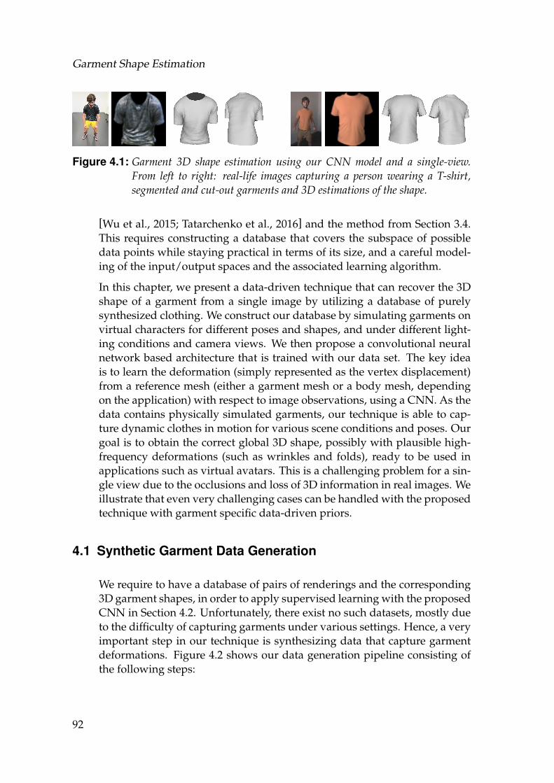
Garment Shape Estimation
Figure 4.1: Garment 3D shape estimation using our CNN model and a single-view.From left to right: real-life images capturing a person wearing a T-shirt,segmented and cut-out garments and 3D estimations of the shape.
[Wu et al., 2015; Tatarchenko et al., 2016] and the method from Section 3.4.This requires constructing a database that covers the subspace of possibledata points while staying practical in terms of its size, and a careful model-ing of the input/output spaces and the associated learning algorithm.
In this chapter, we present a data-driven technique that can recover the 3Dshape of a garment from a single image by utilizing a database of purelysynthesized clothing. We construct our database by simulating garments onvirtual characters for different poses and shapes, and under different light-ing conditions and camera views. We then propose a convolutional neuralnetwork based architecture that is trained with our data set. The key ideais to learn the deformation (simply represented as the vertex displacement)from a reference mesh (either a garment mesh or a body mesh, dependingon the application) with respect to image observations, using a CNN. As thedata contains physically simulated garments, our technique is able to cap-ture dynamic clothes in motion for various scene conditions and poses. Ourgoal is to obtain the correct global 3D shape, possibly with plausible high-frequency deformations (such as wrinkles and folds), ready to be used inapplications such as virtual avatars. This is a challenging problem for a sin-gle view due to the occlusions and loss of 3D information in real images. Weillustrate that even very challenging cases can be handled with the proposedtechnique with garment specific data-driven priors.
4.1 Synthetic Garment Data Generation
We require to have a database of pairs of renderings and the corresponding3D garment shapes, in order to apply supervised learning with the proposedCNN in Section 4.2. Unfortunately, there exist no such datasets, mostly dueto the difficulty of capturing garments under various settings. Hence, a veryimportant step in our technique is synthesizing data that capture garmentdeformations. Figure 4.2 shows our data generation pipeline consisting ofthe following steps:
92
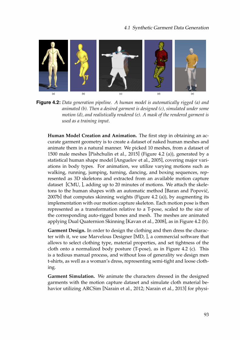
4.1 Synthetic Garment Data Generation
(a) (b) (c) (d) (e)
Figure 4.2: Data generation pipeline. A human model is automatically rigged (a) andanimated (b). Then a desired garment is designed (c), simulated under somemotion (d), and realistically rendered (e). A mask of the rendered garment isused as a training input.
Human Model Creation and Animation. The first step in obtaining an ac-curate garment geometry is to create a dataset of naked human meshes andanimate them in a natural manner. We picked 10 meshes, from a dataset of1500 male meshes [Pishchulin et al., 2015] (Figure 4.2 (a)), generated by astatistical human shape model [Anguelov et al., 2005], covering major vari-ations in body types. For animation, we utilize varying motions such aswalking, running, jumping, turning, dancing, and boxing sequences, rep-resented as 3D skeletons and extracted from an available motion capturedataset [CMU, ], adding up to 20 minutes of motions. We attach the skele-tons to the human shapes with an automatic method [Baran and Popovic,2007b] that computes skinning weights (Figure 4.2 (a)), by augmenting itsimplementation with our motion capture skeleton. Each motion pose is thenrepresented as a transformation relative to a T-pose, scaled to the size ofthe corresponding auto-rigged bones and mesh. The meshes are animatedapplying Dual Quaternion Skinning [Kavan et al., 2008], as in Figure 4.2 (b).
Garment Design. In order to design the clothing and then dress the charac-ter with it, we use Marvelous Designer [MD, ], a commercial software thatallows to select clothing type, material properties, and set tightness of thecloth onto a normalized body posture (T-pose), as in Figure 4.2 (c). Thisis a tedious manual process, and without loss of generality we design ment-shirts, as well as a woman’s dress, representing semi-tight and loose cloth-ing.
Garment Simulation. We animate the characters dressed in the designedgarments with the motion capture dataset and simulate cloth material be-havior utilizing ARCSim [Narain et al., 2012; Narain et al., 2013] for physi-
93
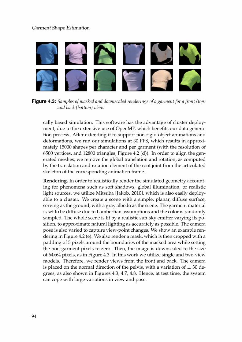
Garment Shape Estimation
Figure 4.3: Samples of masked and downscaled renderings of a garment for a front (top)and back (bottom) view.
cally based simulation. This software has the advantage of cluster deploy-ment, due to the extensive use of OpenMP, which benefits our data genera-tion process. After extending it to support non-rigid object animations anddeformations, we run our simulations at 30 FPS, which results in approxi-mately 15000 shapes per character and per garment (with the resolution of6500 vertices, and 12800 triangles, Figure 4.2 (d)). In order to align the gen-erated meshes, we remove the global translation and rotation, as computedby the translation and rotation element of the root joint from the articulatedskeleton of the corresponding animation frame.
Rendering. In order to realistically render the simulated geometry account-ing for phenomena such as soft shadows, global illumination, or realisticlight sources, we utilize Mitsuba [Jakob, 2010], which is also easily deploy-able to a cluster. We create a scene with a simple, planar, diffuse surface,serving as the ground, with a gray albedo as the scene. The garment materialis set to be diffuse due to Lambertian assumptions and the color is randomlysampled. The whole scene is lit by a realistic sun-sky emitter varying its po-sition, to approximate natural lighting as accurately as possible. The camerapose is also varied to capture view-point changes. We show an example ren-dering in Figure 4.2 (e). We also render a mask, which is then cropped with apadding of 5 pixels around the boundaries of the masked area while settingthe non-garment pixels to zero. Then, the image is downscaled to the sizeof 64x64 pixels, as in Figure 4.3. In this work we utilize single and two-viewmodels. Therefore, we render views from the front and back. The camerais placed on the normal direction of the pelvis, with a variation of ± 30 de-grees, as also shown in Figures 4.3, 4.7, 4.8. Hence, at test time, the systemcan cope with large variations in view and pose.
94
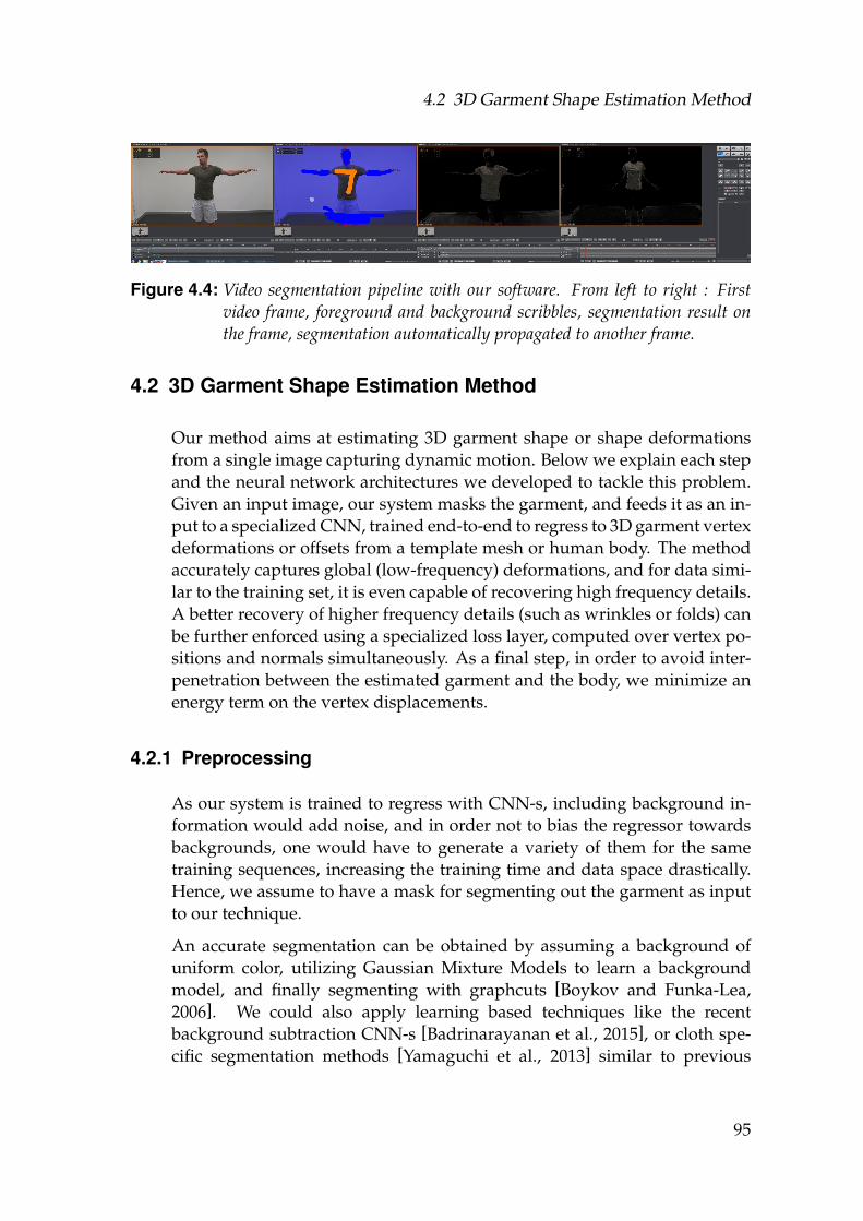
4.2 3D Garment Shape Estimation Method
Figure 4.4: Video segmentation pipeline with our software. From left to right : Firstvideo frame, foreground and background scribbles, segmentation result onthe frame, segmentation automatically propagated to another frame.
4.2 3D Garment Shape Estimation Method
Our method aims at estimating 3D garment shape or shape deformationsfrom a single image capturing dynamic motion. Below we explain each stepand the neural network architectures we developed to tackle this problem.Given an input image, our system masks the garment, and feeds it as an in-put to a specialized CNN, trained end-to-end to regress to 3D garment vertexdeformations or offsets from a template mesh or human body. The methodaccurately captures global (low-frequency) deformations, and for data simi-lar to the training set, it is even capable of recovering high frequency details.A better recovery of higher frequency details (such as wrinkles or folds) canbe further enforced using a specialized loss layer, computed over vertex po-sitions and normals simultaneously. As a final step, in order to avoid inter-penetration between the estimated garment and the body, we minimize anenergy term on the vertex displacements.
4.2.1 Preprocessing
As our system is trained to regress with CNN-s, including background in-formation would add noise, and in order not to bias the regressor towardsbackgrounds, one would have to generate a variety of them for the sametraining sequences, increasing the training time and data space drastically.Hence, we assume to have a mask for segmenting out the garment as inputto our technique.
An accurate segmentation can be obtained by assuming a background ofuniform color, utilizing Gaussian Mixture Models to learn a backgroundmodel, and finally segmenting with graphcuts [Boykov and Funka-Lea,2006]. We could also apply learning based techniques like the recentbackground subtraction CNN-s [Badrinarayanan et al., 2015], or cloth spe-cific segmentation methods [Yamaguchi et al., 2013] similar to previous
95
Garment Shape Estimation
works [Yang et al., 2016]. The masks used for segmentation can also be prop-agated if a video is used as the input. When assuming a background of uni-form color, we use an automatic method as elaborated above [Boykov andFunka-Lea, 2006]. Otherwise, we have an interactive segmentation pipelinebased on scribbles as illustrated in Figure 4.4.
4.2.2 Mesh Deformation Representation
We have two different representations for the garment deformation. Both arebased on the idea of vertex displacements, with different reference meshes.We will see in the next sections that each representation has its own advan-tages for different applications of our technique.
Garment-from-Garment Shape Representation. The output of our methodis a 3D mesh represented as follows : Let Sre f = (Vre f , Fre f ) be a referencegarment mesh which is dressed on a character in a T-pose, with V ∈ Rn×3
as the matrix storing the 3D coordinates of each vertex in each row, andFi,j ∈ {1, . . . , n} containing vertex indices, with each row defining one tri-angle of the mesh. We encode deformations of Sre f with difference vectorsfrom the reference vertices. We thus encode a mesh Sk that was createdby deforming Sre f with the matrix V′k = Vk − Vre f . In order to organizethe dataset more conveniently, V′k is flattened into v′k, where v′k ∈ R3n, andthese vectors for all meshes in the database are then stacked into a large ma-trix Y ∈ RM×3n, where M is the number of deformed shapes (or samples)in the database. Not all of the 3n degrees of freedom are necessary to rep-resent our shape deformation set. We compress the matrix Y by performinga principal component analysis (PCA) to get U ∈ R(N×l), l << 3n, whereU = PCAl(Y), and l = 1000, still achieving almost perfect reconstructionwhile reducing the dimensionality by a factor of 20. We thus set Y = U forthis case.
Garment-from-Body Shape Representation. Depending on the intendedapplication, an alternative representation can be opted. The above repre-sentation does not guarantee that any estimated garment shape will fit thebody mesh of our choice. Hence, if the intended application is to dress hu-man meshes, we can represent the garment mesh as an offset from a body.For a given pose, we thus first associate each vertex of the garment meshto its closest vertex on the body mesh, and compute the difference betweenthose to get V′k as above. The advantage of this alternative is that one canvary the body mesh and the garment dressed on that body will vary accord-ingly, avoiding major interpenetration artifacts. The downside is that with-out a specific body shape, the garment shape cannot be reconstructed. Hence
96
4.2 3D Garment Shape Estimation Method
the selection of the representation depends on the choice of the application,which is either garment shape estimation or body dressing estimation.
4.2.3 Single-View Architecture
We formulate the 3D garment shape estimation as an end-to-end regressionperformed by a Convolutional Neural Network (CNN), from an image de-picting a person wearing the garment to the 3D shape of the garment. Thenetwork learns a representation space of image features that are able to en-code the visual appearance of the possibly wrinkled clothing pattern.
Our dataset can be described with the input and output pairs D = (X ,Y).Let X be the set of our observations and xi ∈ X a sample from our observa-tion set, where i ∈ {1 . . . N}, and N is the number of samples in the dataset.The input xi may consist of one or more images corresponding to differentviews. In our experiments, we only use one or two camera views, specif-ically frontal view and/or back view. Our images are masked and resizedto 64× 64 pixels hence the full input becomes 64× 64× 3 dimensional. Theyi ∈ Y is the ground truth output data, which is obtained with either of the3D garment mesh representations as described above, corresponding to theobserved input xi. The Y can be either the PCA-reduced output denoted asYPCA, or the full-space dataset denoted as Y f ull (Section 4.2.2).
The regression can then be written as the map y = CNN(x), where CNNis the convolutional neural network model we consider. We have exper-imented with various CNN architectures including the ones presented inthe previous chapter and more recent and advanced ones, whose macro-architectural pattern is inspired by Alexnet [Krizhevsky et al., 2012b]. Theinput to the network is a 64x64-shaped RGB image. The convolutional partof the network can either contain a sequence of simple convolutional lay-ers or other more advanced convolutional architectural patterns. The con-volutional part is followed by a flattening layer, after which one or moredense layers are employed. The final dense layer yields the output of theregression. The activation function we use is always the rectified linear unit(ReLU). To avoid overfitting, dropout is added after the convolutional partof the net. We have considered the following architecture:
SqueezeNet, introduced by [Iandola et al., 2016b], achieves AlexNet perfor-mance but needs significantly less parameters and therefore is much fasterto train, thanks to its novel ”Fire” Layers. The benefit of this architectureis its short training time while maintaining a high degree of quality, whichmakes it a great candidate for heavy experimentation.
97
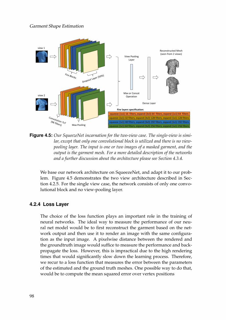
Garment Shape Estimation
view 1
view 2
Reconstructed Mesh (seen from 2 views)
Dense Layer
View PoolingLayer
Max or ConcatOperation
squeeze (1x1) 16 filters, expand (3x3) 64 filters, expand (1x1) 64 filters
squeeze (1x1) 32 filters, expand (3x3) 128 filters, expand (1x1) 128 filters
squeeze (1x1) 48 filters, expand (3x3) 192 filters, expand (1x1) 192 filters
squeeze (1x1) 64 filters, expand (3x3) 256 filters, expand (1x1) 256 filters
Fire layers specification:
Figure 4.5: Our SqueezeNet incarnation for the two-view case. The single-view is simi-lar, except that only one convolutional block is utilized and there is no view-pooling layer. The input is one or two images of a masked garment, and theoutput is the garment mesh. For a more detailed description of the networksand a further discussion about the architecture please see Section 4.3.4.
We base our network architecture on SqueezeNet, and adapt it to our prob-lem. Figure 4.5 demonstrates the two view architecture described in Sec-tion 4.2.5. For the single view case, the network consists of only one convo-lutional block and no view-pooling layer.
4.2.4 Loss Layer
The choice of the loss function plays an important role in the training ofneural networks. The ideal way to measure the performance of our neu-ral net model would be to first reconstruct the garment based on the net-work output and then use it to render an image with the same configura-tion as the input image. A pixelwise distance between the rendered andthe groundtruth image would suffice to measure the performance and back-propagate the loss. However, this is impractical due to the high renderingtimes that would significantly slow down the learning process. Therefore,we recur to a loss function that measures the error between the parametersof the estimated and the ground truth meshes. One possible way to do that,would be to compute the mean squared error over vertex positions
98
4.2 3D Garment Shape Estimation Method
L f ull(YP, YGT) =1n
n
∑i=1
∥∥∥YPi − YGT
i
∥∥∥2, (4.1)
where YP is the predicted output, and YGT is the corresponding groundtruth, and Yi denotes the i-th row of Y. If we regress to PCA component co-efficients instead of vertices, we use the following weighted mean squarederror function:
LPCA(YP, YGT) =1l
l
∑i=1
wi
∣∣∣YPi − YGT
i
∣∣∣ , (4.2)
Here, wi is the PCA variance ratio corresponding to the i-th principal compo-nent, and l is the number of components. In order to capture the curvaturebetter and in turn the folds and wrinkles, we extend Eq.4.1 by integratingnormal estimations through an additional term in the loss. At each train-ing iteration we compute the normals of the estimated vertices and comparethem to the ground truth normals computed on the ground truth garmentmeshes. The final loss becomes:
L∗(YP, YGT) =1n
n
∑i=1
∥∥∥YPi − YGT
i
∥∥∥2− λ
[k(
NPi
)TNGT
i
]3
, (4.3)
where the matrices N are the normals of the corresponding vertices, λ is aweighting term set by the user (throughout our experiments set to 1000) thatcontrols the influence of the normals as opposed to the vertex positions, andk a stretching term (set to 3) of the dot product, which when combined withthe cubic exponential, gives more weight to the penalization for estimatednormals that form a large angle with respect to the ground truth. This newloss function not only fixes some of the global deformation rotations, but alsostresses the high frequency wrinkle patters, as demonstrated in Section 4.3.
4.2.5 Two-View Architecture
We additionally tackle the problem of simultaneously predicting the gar-ment mesh when more evidence is included through a second view (e.g. afront and back view image of the garment). It turns out that simply con-catenating the images along the channel dimension and then passing themthrough an architecture similar to the single-view one described above per-forms worse than the networks trained on single-view input only. One rea-son for this would be that including a complementary view at the earlystages of the network, for the same amount of training data, might inflict
99
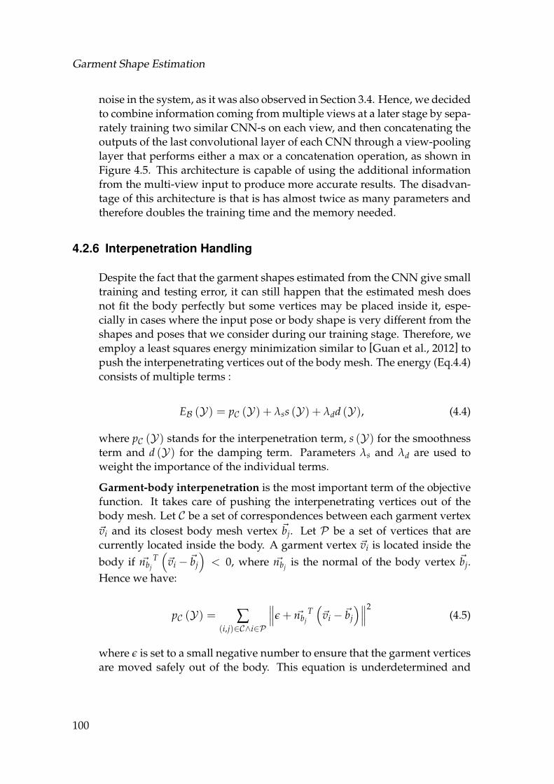
Garment Shape Estimation
noise in the system, as it was also observed in Section 3.4. Hence, we decidedto combine information coming from multiple views at a later stage by sepa-rately training two similar CNN-s on each view, and then concatenating theoutputs of the last convolutional layer of each CNN through a view-poolinglayer that performs either a max or a concatenation operation, as shown inFigure 4.5. This architecture is capable of using the additional informationfrom the multi-view input to produce more accurate results. The disadvan-tage of this architecture is that is has almost twice as many parameters andtherefore doubles the training time and the memory needed.
4.2.6 Interpenetration Handling
Despite the fact that the garment shapes estimated from the CNN give smalltraining and testing error, it can still happen that the estimated mesh doesnot fit the body perfectly but some vertices may be placed inside it, espe-cially in cases where the input pose or body shape is very different from theshapes and poses that we consider during our training stage. Therefore, weemploy a least squares energy minimization similar to [Guan et al., 2012] topush the interpenetrating vertices out of the body mesh. The energy (Eq.4.4)consists of multiple terms :
EB (Y) = pC (Y) + λss (Y) + λdd (Y), (4.4)
where pC (Y) stands for the interpenetration term, s (Y) for the smoothnessterm and d (Y) for the damping term. Parameters λs and λd are used toweight the importance of the individual terms.
Garment-body interpenetration is the most important term of the objectivefunction. It takes care of pushing the interpenetrating vertices out of thebody mesh. Let C be a set of correspondences between each garment vertex~vi and its closest body mesh vertex ~bj. Let P be a set of vertices that arecurrently located inside the body. A garment vertex ~vi is located inside thebody if ~nbj
T(~vi − ~bj
)< 0, where ~nbj is the normal of the body vertex ~bj.
Hence we have:
pC (Y) = ∑(i,j)∈C∧i∈P
∥∥∥ε + ~nbjT(~vi − ~bj
)∥∥∥2(4.5)
where ε is set to a small negative number to ensure that the garment verticesare moved safely out of the body. This equation is underdetermined and
100
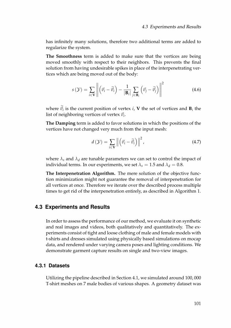
4.3 Experiments and Results
has infinitely many solutions, therefore two additional terms are added toregularize the system.
The Smoothness term is added to make sure that the vertices are beingmoved smoothly with respect to their neighbors. This prevents the finalsolution from having undesirable spikes in place of the interpenetrating ver-tices which are being moved out of the body:
s (Y) = ∑i∈V
∥∥∥∥∥(~vi − ~vi
)− 1|Bi| ∑
j∈Bi
(~vj − ~vj
)∥∥∥∥∥2
(4.6)
where ~vi is the current position of vertex i, V the set of vertices and Bi thelist of neighboring vertices of vertex ~vi.
The Damping term is added to favor solutions in which the positions of thevertices have not changed very much from the input mesh:
d (Y) = ∑i∈V
∥∥∥(~vi − ~vi
)∥∥∥2, (4.7)
where λs and λd are tunable parameters we can set to control the impact ofindividual terms. In our experiments, we set λs = 1.5 and λd = 0.8.
The Interpenetration Algorithm. The mere solution of the objective func-tion minimization might not guarantee the removal of interpenetration forall vertices at once. Therefore we iterate over the described process multipletimes to get rid of the interpenetration entirely, as described in Algorithm 1.
4.3 Experiments and Results
In order to assess the performance of our method, we evaluate it on syntheticand real images and videos, both qualitatively and quantitatively. The ex-periments consist of tight and loose clothing of male and female models witht-shirts and dresses simulated using physically based simulations on mocapdata, and rendered under varying camera poses and lighting conditions. Wedemonstrate garment capture results on single and two-view images.
4.3.1 Datasets
Utilizing the pipeline described in Section 4.1, we simulated around 100, 000T-shirt meshes on 7 male bodies of various shapes. A geometry dataset was
101
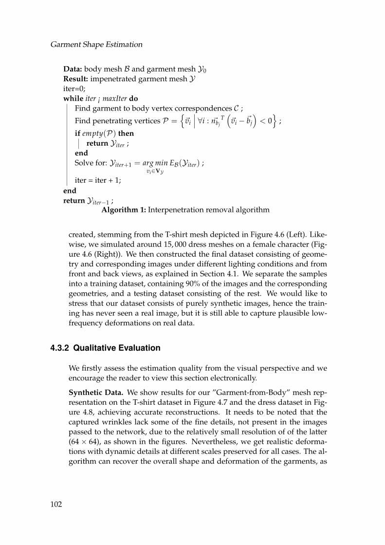
Garment Shape Estimation
Data: body mesh B and garment mesh Y0Result: impenetrated garment mesh Yiter=0;while iter ¡ maxIter do
Find garment to body vertex correspondences C ;
Find penetrating vertices P ={~vi
∣∣∣ ∀i : ~nbjT(~vi − ~bj
)< 0
};
if empty(P) thenreturn Yiter ;
endSolve for: Yiter+1 = arg min
vi∈VYEB(Yiter) ;
iter = iter + 1;endreturn Yiter−1 ;
Algorithm 1: Interpenetration removal algorithm
created, stemming from the T-shirt mesh depicted in Figure 4.6 (Left). Like-wise, we simulated around 15, 000 dress meshes on a female character (Fig-ure 4.6 (Right)). We then constructed the final dataset consisting of geome-try and corresponding images under different lighting conditions and fromfront and back views, as explained in Section 4.1. We separate the samplesinto a training dataset, containing 90% of the images and the correspondinggeometries, and a testing dataset consisting of the rest. We would like tostress that our dataset consists of purely synthetic images, hence the train-ing has never seen a real image, but it is still able to capture plausible low-frequency deformations on real data.
4.3.2 Qualitative Evaluation
We firstly assess the estimation quality from the visual perspective and weencourage the reader to view this section electronically.
Synthetic Data. We show results for our ”Garment-from-Body” mesh rep-resentation on the T-shirt dataset in Figure 4.7 and the dress dataset in Fig-ure 4.8, achieving accurate reconstructions. It needs to be noted that thecaptured wrinkles lack some of the fine details, not present in the imagespassed to the network, due to the relatively small resolution of of the latter(64× 64), as shown in the figures. Nevertheless, we get realistic deforma-tions with dynamic details at different scales preserved for all cases. The al-gorithm can recover the overall shape and deformation of the garments, as
102
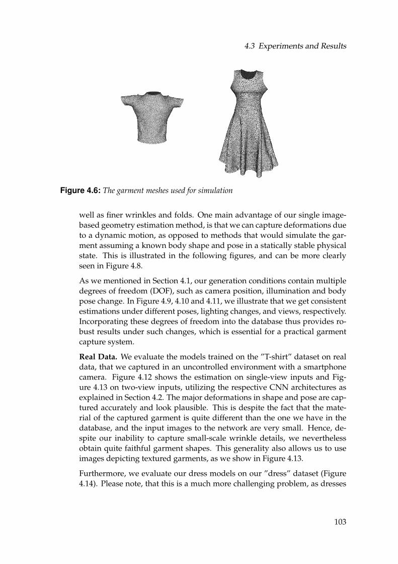
4.3 Experiments and Results
Figure 4.6: The garment meshes used for simulation
well as finer wrinkles and folds. One main advantage of our single image-based geometry estimation method, is that we can capture deformations dueto a dynamic motion, as opposed to methods that would simulate the gar-ment assuming a known body shape and pose in a statically stable physicalstate. This is illustrated in the following figures, and can be more clearlyseen in Figure 4.8.
As we mentioned in Section 4.1, our generation conditions contain multipledegrees of freedom (DOF), such as camera position, illumination and bodypose change. In Figure 4.9, 4.10 and 4.11, we illustrate that we get consistentestimations under different poses, lighting changes, and views, respectively.Incorporating these degrees of freedom into the database thus provides ro-bust results under such changes, which is essential for a practical garmentcapture system.
Real Data. We evaluate the models trained on the ”T-shirt” dataset on realdata, that we captured in an uncontrolled environment with a smartphonecamera. Figure 4.12 shows the estimation on single-view inputs and Fig-ure 4.13 on two-view inputs, utilizing the respective CNN architectures asexplained in Section 4.2. The major deformations in shape and pose are cap-tured accurately and look plausible. This is despite the fact that the mate-rial of the captured garment is quite different than the one we have in thedatabase, and the input images to the network are very small. Hence, de-spite our inability to capture small-scale wrinkle details, we neverthelessobtain quite faithful garment shapes. This generality also allows us to useimages depicting textured garments, as we show in Figure 4.13.
Furthermore, we evaluate our dress models on our ”dress” dataset (Figure4.14). Please note, that this is a much more challenging problem, as dresses
103
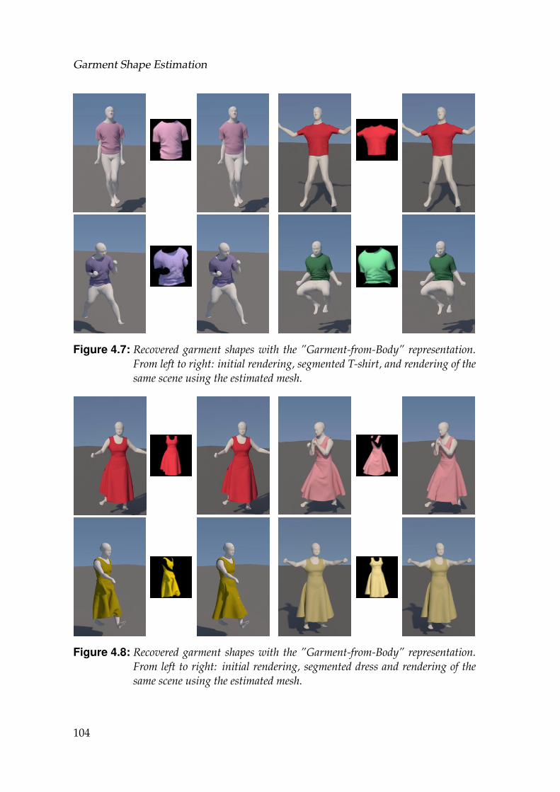
Garment Shape Estimation
Figure 4.7: Recovered garment shapes with the ”Garment-from-Body” representation.From left to right: initial rendering, segmented T-shirt, and rendering of thesame scene using the estimated mesh.
Figure 4.8: Recovered garment shapes with the ”Garment-from-Body” representation.From left to right: initial rendering, segmented dress and rendering of thesame scene using the estimated mesh.
104
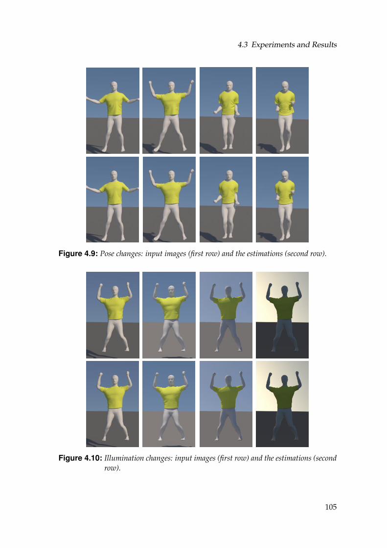
4.3 Experiments and Results
Figure 4.9: Pose changes: input images (first row) and the estimations (second row).
Figure 4.10: Illumination changes: input images (first row) and the estimations (secondrow).
105
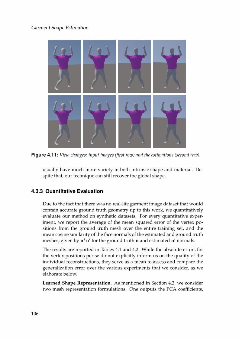
Garment Shape Estimation
Figure 4.11: View changes: input images (first row) and the estimations (second row).
usually have much more variety in both intrinsic shape and material. De-spite that, our technique can still recover the global shape.
4.3.3 Quantitative Evaluation
Due to the fact that there was no real-life garment image dataset that wouldcontain accurate ground truth geometry up to this work, we quantitativelyevaluate our method on synthetic datasets. For every quantitative exper-iment, we report the average of the mean squared error of the vertex po-sitions from the ground truth mesh over the entire training set, and themean cosine similarity of the face normals of the estimated and ground truthmeshes, given by nTn′ for the ground truth n and estimated n′ normals.
The results are reported in Tables 4.1 and 4.2. While the absolute errors forthe vertex positions per-se do not explicitly inform us on the quality of theindividual reconstructions, they serve as a mean to assess and compare thegeneralization error over the various experiments that we consider, as weelaborate below.
Learned Shape Representation. As mentioned in Section 4.2, we considertwo mesh representation formulations. One outputs the PCA coefficients,
106
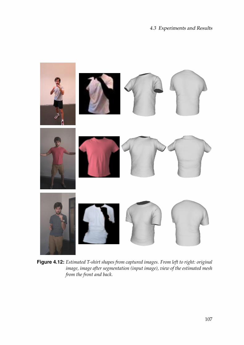
4.3 Experiments and Results
Figure 4.12: Estimated T-shirt shapes from captured images. From left to right: originalimage, image after segmentation (input image), view of the estimated meshfrom the front and back.
107
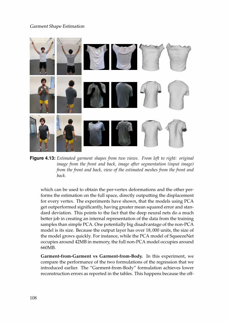
Garment Shape Estimation
Figure 4.13: Estimated garment shapes from two views. From left to right: originalimage from the front and back, image after segmentation (input image)from the front and back, view of the estimated meshes from the front andback.
which can be used to obtain the per-vertex deformations and the other per-forms the estimation on the full space, directly outputting the displacementfor every vertex. The experiments have shown, that the models using PCAget outperformed significantly, having greater mean squared error and stan-dard deviation. This points to the fact that the deep neural nets do a muchbetter job in creating an internal representation of the data from the trainingsamples than simple PCA. One potentially big disadvantage of the non-PCAmodel is its size. Because the output layer has over 18, 000 units, the size ofthe model grows quickly. For instance, while the PCA model of SqueezeNetoccupies around 42MB in memory, the full non-PCA model occupies around660MB.
Garment-from-Garment vs Garment-from-Body. In this experiment, wecompare the performance of the two formulations of the regression that weintroduced earlier. The ”Garment-from-Body” formulation achieves lowerreconstruction errors as reported in the tables. This happens because the off-
108
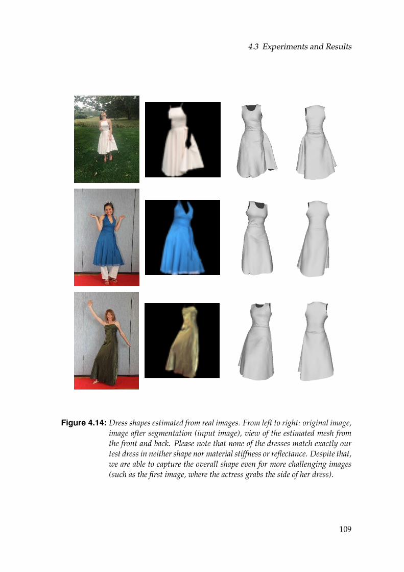
4.3 Experiments and Results
Figure 4.14: Dress shapes estimated from real images. From left to right: original image,image after segmentation (input image), view of the estimated mesh fromthe front and back. Please note that none of the dresses match exactly ourtest dress in neither shape nor material stiffness or reflectance. Despite that,we are able to capture the overall shape even for more challenging images(such as the first image, where the actress grabs the side of her dress).
109
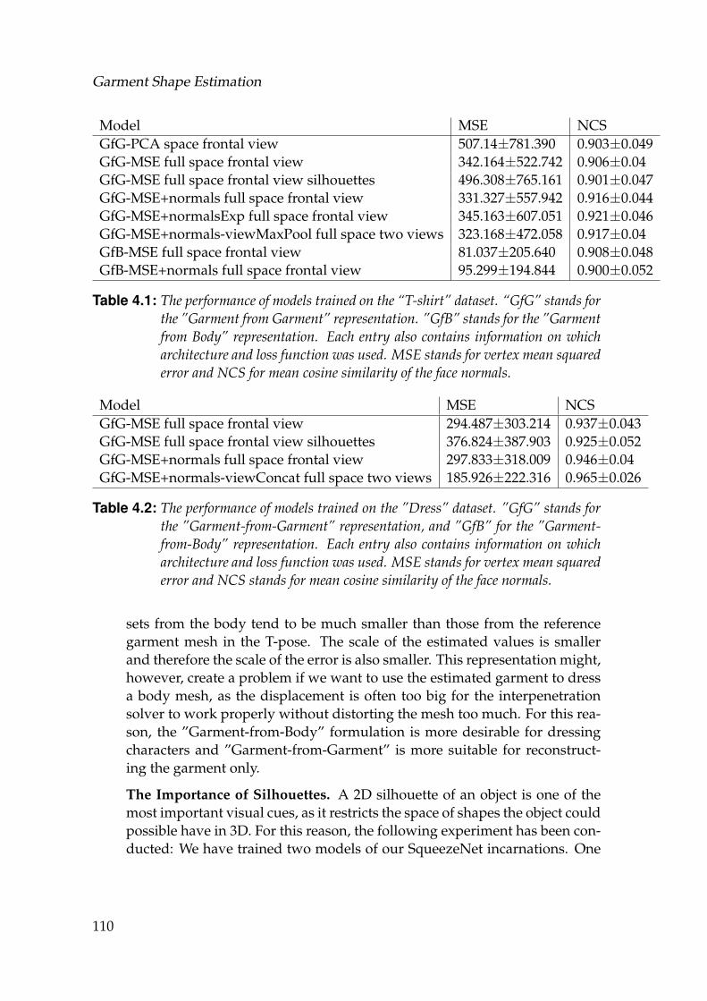
Garment Shape Estimation
Model MSE NCSGfG-PCA space frontal view 507.14±781.390 0.903±0.049GfG-MSE full space frontal view 342.164±522.742 0.906±0.04GfG-MSE full space frontal view silhouettes 496.308±765.161 0.901±0.047GfG-MSE+normals full space frontal view 331.327±557.942 0.916±0.044GfG-MSE+normalsExp full space frontal view 345.163±607.051 0.921±0.046GfG-MSE+normals-viewMaxPool full space two views 323.168±472.058 0.917±0.04GfB-MSE full space frontal view 81.037±205.640 0.908±0.048GfB-MSE+normals full space frontal view 95.299±194.844 0.900±0.052
Table 4.1: The performance of models trained on the “T-shirt” dataset. “GfG” stands forthe ”Garment from Garment” representation. ”GfB” stands for the ”Garmentfrom Body” representation. Each entry also contains information on whicharchitecture and loss function was used. MSE stands for vertex mean squarederror and NCS for mean cosine similarity of the face normals.
Model MSE NCSGfG-MSE full space frontal view 294.487±303.214 0.937±0.043GfG-MSE full space frontal view silhouettes 376.824±387.903 0.925±0.052GfG-MSE+normals full space frontal view 297.833±318.009 0.946±0.04GfG-MSE+normals-viewConcat full space two views 185.926±222.316 0.965±0.026
Table 4.2: The performance of models trained on the ”Dress” dataset. ”GfG” stands forthe ”Garment-from-Garment” representation, and ”GfB” for the ”Garment-from-Body” representation. Each entry also contains information on whicharchitecture and loss function was used. MSE stands for vertex mean squarederror and NCS stands for mean cosine similarity of the face normals.
sets from the body tend to be much smaller than those from the referencegarment mesh in the T-pose. The scale of the estimated values is smallerand therefore the scale of the error is also smaller. This representation might,however, create a problem if we want to use the estimated garment to dressa body mesh, as the displacement is often too big for the interpenetrationsolver to work properly without distorting the mesh too much. For this rea-son, the ”Garment-from-Body” formulation is more desirable for dressingcharacters and ”Garment-from-Garment” is more suitable for reconstruct-ing the garment only.
The Importance of Silhouettes. A 2D silhouette of an object is one of themost important visual cues, as it restricts the space of shapes the object couldpossible have in 3D. For this reason, the following experiment has been con-ducted: We have trained two models of our SqueezeNet incarnations. One
110
4.3 Experiments and Results
was trained on the image dataset we have, the other was trained only onthe silhouettes of the garments, loosing shading and color information. Asit can be observed in Table 4.1, the silhouette model performs well, but isoutperformed by the model trained on RGB images. This is an importantresult, as it proves that CNNs can in fact learn the shading cues, due to thewrinkling patterns and further enhance the quality of the estimation. Thisis also demonstrated in the next chapter. The silhouette though still remainsan important cue that the network automatically learns.
Comparison of Single-View and Multi-View Nets. In this experiment, wecompare the performance of single and multi-view CNN-s. The multi-viewarchitectures achieve superior performance in comparison to the single viewmodels on both datasets. Hence, our method can benefit from multi-viewinput to achieve a more accurate estimation. The difference is particularlyvisible on the dress dataset, as loose clothing has naturally more ambigui-ties of shape in the occluded parts. Please refer to Figure 4.15 for a visualcomparison.
Loss Function with Normals. We compare the performance of the modelsthat are optimized for MSE and those which try to account for the curvatureof the surface of the estimated mesh, by using the customized loss functionin Eq. 4.3, as described in Section 4.2. The results in Tables 4.1 and 4.2 showthat these models usually have slightly worse MSE, but their normals arealigned more accurately.
Failure Cases. In Figure 4.16, we present interesting failure cases for gar-ments with shapes or poses that were not present in the training set. Sim-ilarly, sometimes the input image is imperfect and contains noise (such assegmentation artifacts).
4.3.4 Full Specification of the Architecture and Performance
Here, we specify the full details for both single and two-view architec-tures, including the expansion on Fire layers (as proposed in [Iandola etal., 2016b]). The architectures are captured in Figure 4.17. Here we ex-pand on the choice of architecture. Initially, we experimented with muchbigger CNNs, such as Deep Residual Nets. However, due to the size ofsuch networks and the heavy experimentation needed, we decided to optfor SqueezeNet. It delivers comparable performance to the former, it is muchfaster to train and in our experience it converged more reliably. For this rea-son, we encourage the use of SqueezeNet for similar problems, as we alsodo for the Hand Pose estimation task in Section 5.3.2.2. Despite that, it isdefinitely possible to optimize the results further with deeper architectures.
111
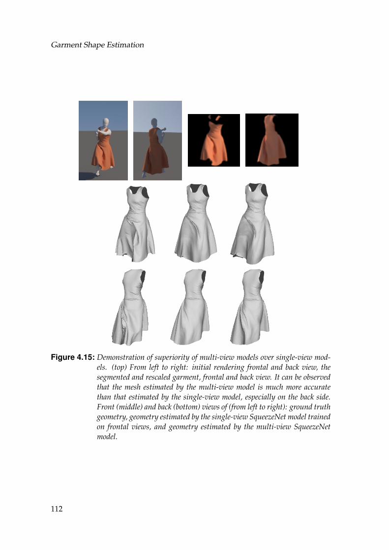
Garment Shape Estimation
Figure 4.15: Demonstration of superiority of multi-view models over single-view mod-els. (top) From left to right: initial rendering frontal and back view, thesegmented and rescaled garment, frontal and back view. It can be observedthat the mesh estimated by the multi-view model is much more accuratethan that estimated by the single-view model, especially on the back side.Front (middle) and back (bottom) views of (from left to right): ground truthgeometry, geometry estimated by the single-view SqueezeNet model trainedon frontal views, and geometry estimated by the multi-view SqueezeNetmodel.
112
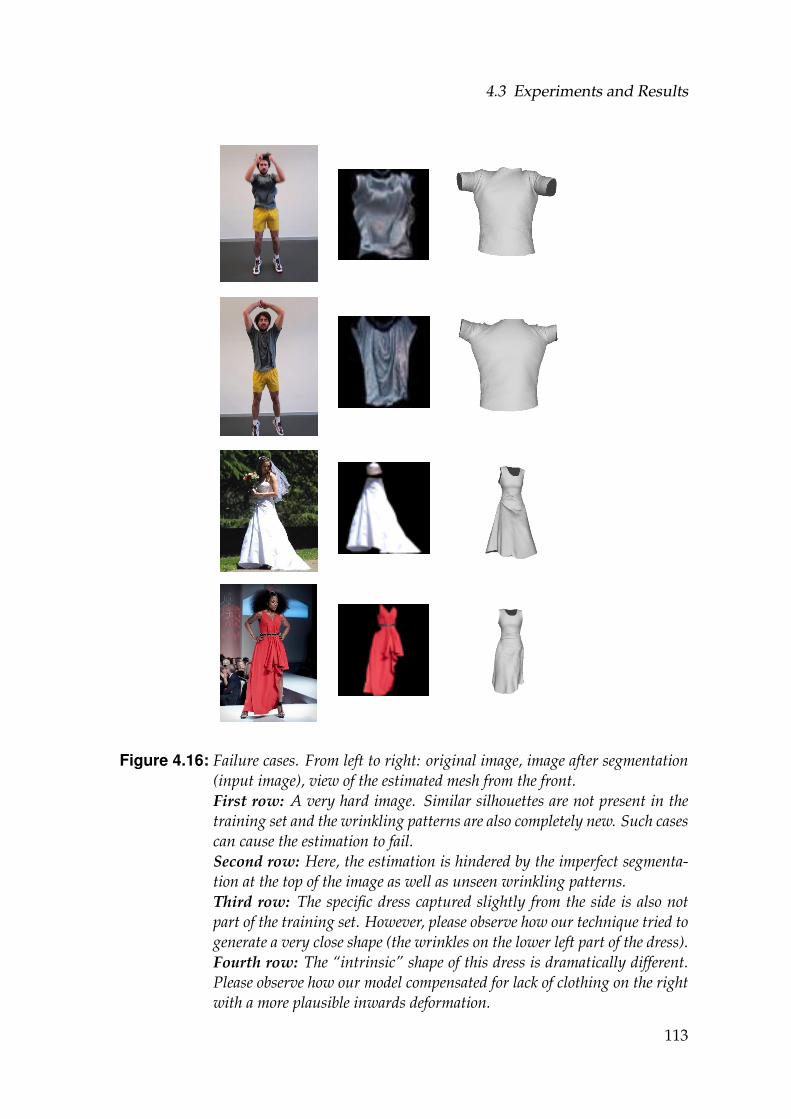
4.3 Experiments and Results
Figure 4.16: Failure cases. From left to right: original image, image after segmentation(input image), view of the estimated mesh from the front.First row: A very hard image. Similar silhouettes are not present in thetraining set and the wrinkling patterns are also completely new. Such casescan cause the estimation to fail.Second row: Here, the estimation is hindered by the imperfect segmenta-tion at the top of the image as well as unseen wrinkling patterns.Third row: The specific dress captured slightly from the side is also notpart of the training set. However, please observe how our technique tried togenerate a very close shape (the wrinkles on the lower left part of the dress).Fourth row: The “intrinsic” shape of this dress is dramatically different.Please observe how our model compensated for lack of clothing on the rightwith a more plausible inwards deformation.
113
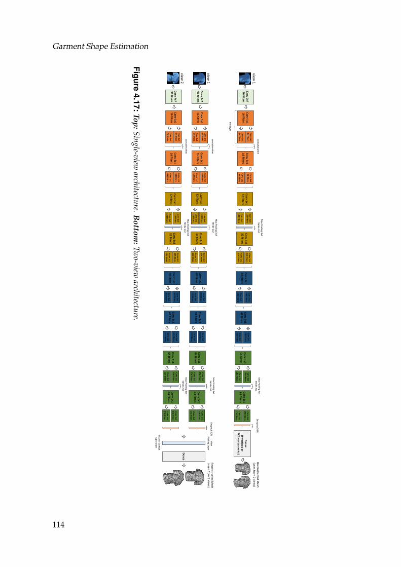
Garment Shape Estimation
Co
nv 7
x7
96
filtersC
on
v 1x1
16
filters
view 1
Co
nv 3
x36
4 filters
Co
nv 1
x16
4 filters
Co
nv 1
x11
6 filters
Co
nv 3
x36
4 filters
Co
nv 1
x16
4 filters
Co
nv 1
x13
2 filters
Co
nv 3
x31
28
filters
Co
nv 1
x11
28
filters
Co
nv 1
x13
2 filters
Co
nv 3
x31
28
filters
Co
nv 1
x11
28
filters
Co
nv 1
x14
8 filters
Co
nv 3
x31
92
filters
Co
nv 1
x11
92
filters
Co
nv 1
x14
8 filters
Co
nv 3
x31
92
filters
Co
nv 1
x11
92
filters
Co
nv 1
x16
4 filters
Co
nv 3
x32
56
filters
Co
nv 1
x12
56
filters
Co
nv 1
x16
4 filters
Co
nv 3
x32
56
filters
Co
nv 1
x12
56
filters
Den
se(# vertices o
r P
CA
com
po
nen
ts)
Reco
nstru
cted M
esh
(seen fro
m 2
views)
Co
nv 7
x7
96
filtersC
on
v 1x1
16
filters
view 1
Co
nv 3
x36
4 filters
Co
nv 1
x16
4 filters
Co
nv 1
x11
6 filters
Co
nv 3
x36
4 filters
Co
nv 1
x16
4 filters
Co
nv 1
x13
2 filters
Co
nv 3
x31
28
filters
Co
nv 1
x11
28
filters
Co
nv 1
x13
2 filters
Co
nv 3
x31
28
filters
Co
nv 1
x11
28
filters
Co
nv 1
x14
8 filters
Co
nv 3
x31
92
filters
Co
nv 1
x11
92
filters
Co
nv 1
x14
8 filters
Co
nv 3
x31
92
filters
Co
nv 1
x11
92
filters
Co
nv 1
x16
4 filters
Co
nv 3
x32
56
filters
Co
nv 1
x12
56
filters
Co
nv 1
x16
4 filters
Co
nv 3
x32
56
filters
Co
nv 1
x12
56
filters
Den
se
Reco
nstru
cted M
esh
(seen
from
2 view
s)
Co
nv 7
x7
96
filtersC
on
v 1x1
16
filters
view 2
Co
nv 3
x36
4 filters
Co
nv 1
x16
4 filters
Co
nv 1
x11
6 filters
Co
nv 3
x36
4 filters
Co
nv 1
x16
4 filters
Co
nv 1
x13
2 filters
Co
nv 3
x31
28
filters
Co
nv 1
x11
28
filters
Co
nv 1
x13
2 filters
Co
nv 3
x31
28
filters
Co
nv 1
x11
28
filters
Co
nv 1
x14
8 filters
Co
nv 3
x31
92
filters
Co
nv 1
x11
92
filters
Co
nv 1
x14
8 filters
Co
nv 3
x31
92
filters
Co
nv 1
x11
92
filters
Co
nv 1
x16
4 filters
Co
nv 3
x32
56
filters
Co
nv 1
x12
56
filters
Co
nv 1
x16
4 filters
Co
nv 3
x32
56
filters
Co
nv 1
x12
56
filters
View
P
oo
ling Layer
Max o
r Co
ncat
Op
eration
Figure4.17:Top:Single-view
architecture.Bottom
:Two-view
architecture.
114
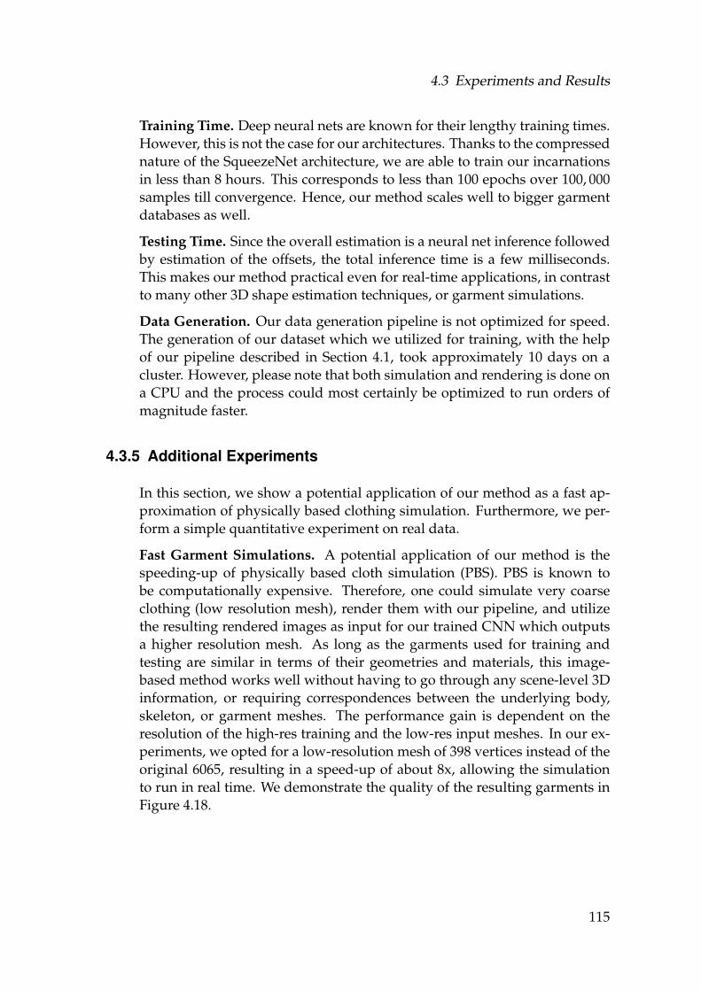
4.3 Experiments and Results
Training Time. Deep neural nets are known for their lengthy training times.However, this is not the case for our architectures. Thanks to the compressednature of the SqueezeNet architecture, we are able to train our incarnationsin less than 8 hours. This corresponds to less than 100 epochs over 100, 000samples till convergence. Hence, our method scales well to bigger garmentdatabases as well.
Testing Time. Since the overall estimation is a neural net inference followedby estimation of the offsets, the total inference time is a few milliseconds.This makes our method practical even for real-time applications, in contrastto many other 3D shape estimation techniques, or garment simulations.
Data Generation. Our data generation pipeline is not optimized for speed.The generation of our dataset which we utilized for training, with the helpof our pipeline described in Section 4.1, took approximately 10 days on acluster. However, please note that both simulation and rendering is done ona CPU and the process could most certainly be optimized to run orders ofmagnitude faster.
4.3.5 Additional Experiments
In this section, we show a potential application of our method as a fast ap-proximation of physically based clothing simulation. Furthermore, we per-form a simple quantitative experiment on real data.
Fast Garment Simulations. A potential application of our method is thespeeding-up of physically based cloth simulation (PBS). PBS is known tobe computationally expensive. Therefore, one could simulate very coarseclothing (low resolution mesh), render them with our pipeline, and utilizethe resulting rendered images as input for our trained CNN which outputsa higher resolution mesh. As long as the garments used for training andtesting are similar in terms of their geometries and materials, this image-based method works well without having to go through any scene-level 3Dinformation, or requiring correspondences between the underlying body,skeleton, or garment meshes. The performance gain is dependent on theresolution of the high-res training and the low-res input meshes. In our ex-periments, we opted for a low-resolution mesh of 398 vertices instead of theoriginal 6065, resulting in a speed-up of about 8x, allowing the simulationto run in real time. We demonstrate the quality of the resulting garments inFigure 4.18.
115
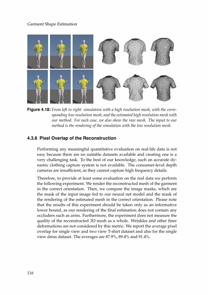
Garment Shape Estimation
Figure 4.18: From left to right: simulation with a high resolution mesh, with the corre-sponding low resolution mesh, and the estimated high resolution mesh withour method. For each case, we also show the raw mesh. The input to ourmethod is the rendering of the simulation with the low resolution mesh.
4.3.6 Pixel Overlap of the Reconstruction
Performing any meaningful quantitative evaluation on real-life data is noteasy because there are no suitable datasets available and creating one is avery challenging task. To the best of our knowledge, such an accurate dy-namic clothing capture system is not available. The consumer-level depthcameras are insufficient, as they cannot capture high frequency details.
Therefore, to provide at least some evaluation on the real data we performthe following experiment. We render the reconstructed mesh of the garmentin the correct orientation. Then, we compare the image masks, which arethe mask of the input image fed to our neural net model and the mask ofthe rendering of the estimated mesh in the correct orientation. Please notethat the results of this experiment should be taken only as an informativelower bound, as our rendering of the final estimation does not contain anyoccluders such as arms. Furthermore, the experiment does not measure thequality of the reconstructed 3D mesh as a whole. Wrinkles and other finerdeformations are not considered by this metric. We report the average pixeloverlap for single view and two view T-shirt dataset and also for the singleview dress dataset. The averages are 87.9%, 89.4% and 91.4%.
116
4.3 Experiments and Results
4.3.7 Further Discussion
A novel approach to clothing shape estimation was presented above, how-ever bringing along limitations too, which we will discuss next. We aim toprove our idea correct instead of deploying a ready-to-be-used, production-level solution for a specific purpose. However, we believe our study to be apioneering one, with the potential to spark a fruitful line of research in thisarea. The number of use cases and the simplicity of the method has a verybig potential for a vast amount of applications. Nevertheless, in order to bebroadly usable much more research has to be put into this direction. Thework explained in this chapter shall provide an initial setup, which can beexplored much further in the future.
Garment Generality. One of the limitations of our technique is that it has tobe trained for every type of clothing, as each reference garment mesh mayvary dramatically in resolution, depending on its shape complexity.
Impact of the Dataset Generation on Performance. Since our approach isdata driven, the performance is only as good as the training dataset. Thereare many factors that come into play when creating such a dataset, suchas the artistic quality of the reference garment design, the resolution of themesh, the versatility of the motion capture database and the characters ani-mated by it, the correct behavior of the physically based simulation and lastbut not least, the realism of the renderings (illumination, reflectance, tex-ture, occluders etc.). Please note, that our data generation pipeline is notperfect and as such does not create a perfect dataset. Despite that, we areable to estimate the rough shape of the garments quite accurately. The closerthe input image is to the training dataset, the better estimations we get andwith very similar images (the synthetic test set), we show that we are evencapable of recovering the high frequency detail. We believe that most ofthe flaws in the estimation could be lifted by creating an ultimate dataset.The creation of such a dataset, however, is another challenging engineeringtask. Another interesting line of research would be applying Generative Ad-versarial Nets [Goodfellow et al., 2014] which could help to create biggervariance in our training data. These relatively new approaches of generativeand discriminative nets have only recently been used for clothing in lowerresolution images [Lassner et al., 2017a].
Dependency on Segmentation. It is true that our technique requires qualitysegmentation of the garments on the input. Utilizing the recent deep learn-ing based works on image segmentation, such as [Long et al., 2014], couldeventually alleviate the need for supervised segmentation in an uncontrolledenvironment altogether.
117
Garment Shape Estimation
4.4 Conclusion
In this chapter, we proposed an end-to-end 3D garment shape estimation al-gorithm, that captures plausible garment deformations at interactive rates,from an uncontrolled single view setup depicting a dynamic garment state.Additionally, we showed how to achieve this by training a CNN based re-gressor with statistical priors and specialized loss functions, that utilizespurely synthetically generated data for training, demonstrating its scalabil-ity for such a supervised learning task. Finally, we showed how to lever-age information simultaneously present in multi-view setups in order to in-crease the predictive performance of the network and in turn the accuracyof the estimations.
We rely on a data generation pipeline, where the deformation of the humanbody shape and thus the garment is given by a standard skinning modelwith automatically computed weights and simple blending of bone trans-formations. We also use an off-the-shelf physical simulator for cloth defor-mation, and default parameters. These steps introduce certain artifacts. Bet-ter and tailored databases can be obtained by improving these steps, andconsidering accurate cloth parameters.
Our method relies on segmented garments from an image, although it tol-erates a certain amount of noise and inaccuracy, as illustrated in Figure 4.4,and moderately textured garments. By training on more data that cover alarger variety of cases, the method can be extended to handle complex tex-tures and unsegmented images, for non-garment deforming objects as well.
For practical purposes, such as hardware or time constraints, the networksare trained with relatively small input images of 64× 64 pixels. This pre-vents our method from capturing some of the wrinkles. With the currentprogress in the compactness of CNN representations, one could envisagehigher-frequency details to be captured as well.
118
C H A P T E R 5Hand Pose Estimation
In the previous chapters, we focused on the digital human body as a whole,with an extra layer of clothing added to it. In this chapter, we zoom-in andconcentrate on a very dexterous body part - the hand. On a higher level, weslowly shift from a semi pose-invariant, pure shape estimation of the humanbody and a slight coupling of shape and pose estimation of the garment, toa pure pose estimation of the free human hand and a nuance of internalhand shape estimation to help this process. Looking at it from a machinelearning point of view, as opposed to the previous chapters where a super-vised training with synthetic datasets was mostly a necessity, partly due tothe difficulty of data acquisition, here we explore unsupervised and semi-supervised learning with real unlabeled data. In order to explore the latter,we initially relax our RGB input requirement to a Depth one, and show howa pre-trained convolutional model, can be refined on unseen and unlabeleddepth images. Afterwards, we demonstrate it‘s adaptation to the RGB in-put case. The choice of initially exploring Depth was also influenced by theabundance of existing methods and to a smaller extent respective datasets,as opposed to the RGB case.
5.1 3D Hand Pose Estimation from Depth Data
Recent approaches in 3D hand pose estimation from a single depth im-age are predominantly based on convolutional neural network architec-tures [Tompson et al., 2014; Oberweger et al., 2015a; Zhou et al., 2016;Ge et al., 2016; Sinha et al., 2016; Ye et al., 2016], typically requiring labeled
119
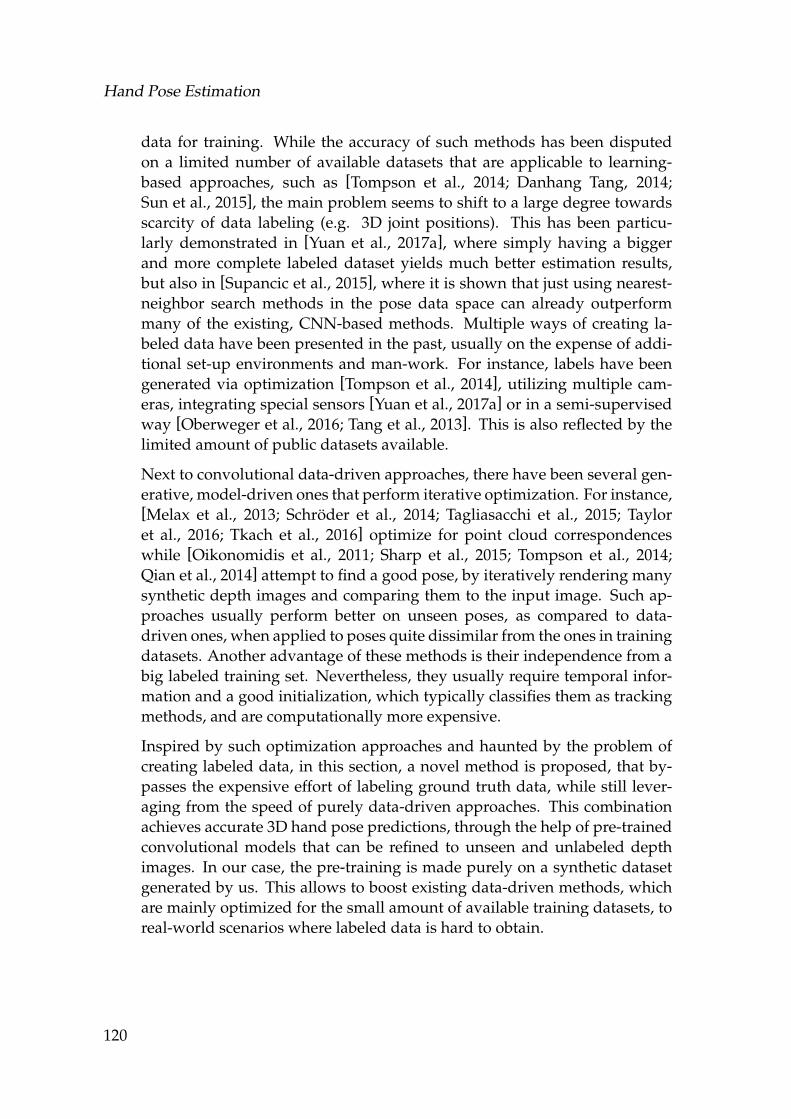
Hand Pose Estimation
data for training. While the accuracy of such methods has been disputedon a limited number of available datasets that are applicable to learning-based approaches, such as [Tompson et al., 2014; Danhang Tang, 2014;Sun et al., 2015], the main problem seems to shift to a large degree towardsscarcity of data labeling (e.g. 3D joint positions). This has been particu-larly demonstrated in [Yuan et al., 2017a], where simply having a biggerand more complete labeled dataset yields much better estimation results,but also in [Supancic et al., 2015], where it is shown that just using nearest-neighbor search methods in the pose data space can already outperformmany of the existing, CNN-based methods. Multiple ways of creating la-beled data have been presented in the past, usually on the expense of addi-tional set-up environments and man-work. For instance, labels have beengenerated via optimization [Tompson et al., 2014], utilizing multiple cam-eras, integrating special sensors [Yuan et al., 2017a] or in a semi-supervisedway [Oberweger et al., 2016; Tang et al., 2013]. This is also reflected by thelimited amount of public datasets available.
Next to convolutional data-driven approaches, there have been several gen-erative, model-driven ones that perform iterative optimization. For instance,[Melax et al., 2013; Schroder et al., 2014; Tagliasacchi et al., 2015; Tayloret al., 2016; Tkach et al., 2016] optimize for point cloud correspondenceswhile [Oikonomidis et al., 2011; Sharp et al., 2015; Tompson et al., 2014;Qian et al., 2014] attempt to find a good pose, by iteratively rendering manysynthetic depth images and comparing them to the input image. Such ap-proaches usually perform better on unseen poses, as compared to data-driven ones, when applied to poses quite dissimilar from the ones in trainingdatasets. Another advantage of these methods is their independence from abig labeled training set. Nevertheless, they usually require temporal infor-mation and a good initialization, which typically classifies them as trackingmethods, and are computationally more expensive.
Inspired by such optimization approaches and haunted by the problem ofcreating labeled data, in this section, a novel method is proposed, that by-passes the expensive effort of labeling ground truth data, while still lever-aging from the speed of purely data-driven approaches. This combinationachieves accurate 3D hand pose predictions, through the help of pre-trainedconvolutional models that can be refined to unseen and unlabeled depthimages. In our case, the pre-training is made purely on a synthetic datasetgenerated by us. This allows to boost existing data-driven methods, whichare mainly optimized for the small amount of available training datasets, toreal-world scenarios where labeled data is hard to obtain.
120
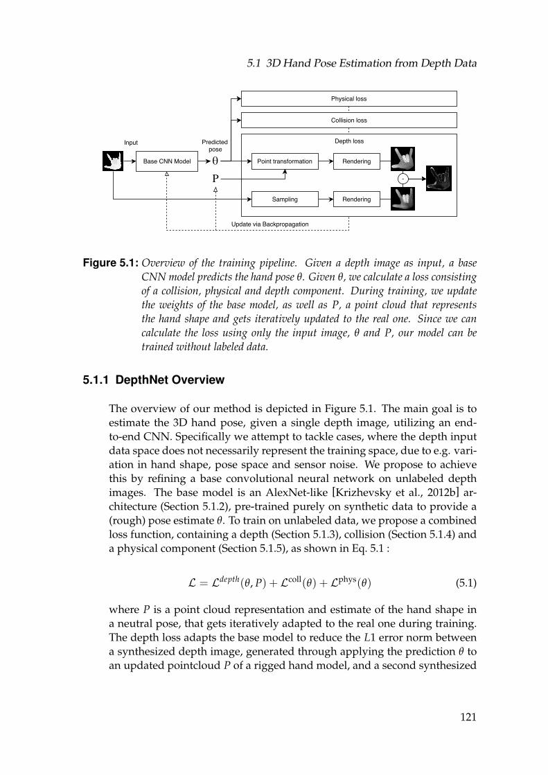
5.1 3D Hand Pose Estimation from Depth Data
Figure 5.1: Overview of the training pipeline. Given a depth image as input, a baseCNN model predicts the hand pose θ. Given θ, we calculate a loss consistingof a collision, physical and depth component. During training, we updatethe weights of the base model, as well as P, a point cloud that representsthe hand shape and gets iteratively updated to the real one. Since we cancalculate the loss using only the input image, θ and P, our model can betrained without labeled data.
5.1.1 DepthNet Overview
The overview of our method is depicted in Figure 5.1. The main goal is toestimate the 3D hand pose, given a single depth image, utilizing an end-to-end CNN. Specifically we attempt to tackle cases, where the depth inputdata space does not necessarily represent the training space, due to e.g. vari-ation in hand shape, pose space and sensor noise. We propose to achievethis by refining a base convolutional neural network on unlabeled depthimages. The base model is an AlexNet-like [Krizhevsky et al., 2012b] ar-chitecture (Section 5.1.2), pre-trained purely on synthetic data to provide a(rough) pose estimate θ. To train on unlabeled data, we propose a combinedloss function, containing a depth (Section 5.1.3), collision (Section 5.1.4) anda physical component (Section 5.1.5), as shown in Eq. 5.1 :
L = Ldepth(θ, P) + Lcoll(θ) + Lphys(θ) (5.1)
where P is a point cloud representation and estimate of the hand shape ina neutral pose, that gets iteratively adapted to the real one during training.The depth loss adapts the base model to reduce the L1 error norm betweena synthesized depth image, generated through applying the prediction θ toan updated pointcloud P of a rigged hand model, and a second synthesized
121
Hand Pose Estimation
Figure 5.2: Overview of the different kinds of formats and hand images we process. Fromleft to right (1) our rigged hand model with its 16 joints (2) the uniformlysampled point cloud P of the rigged mesh (3) a rendering after transformingP using the render component (Section 5.1.3.1) (4) a typical noisy depthimage input to the base CNN model. (5) a rendering of points sampled from(4). (6) the absolute difference between (3) and (5)
depth image based only on the input depth image. The collision and physi-cal loss can be thought as regularizers that penalize unnatural looking poses.
5.1.2 Base CNN Model
We start by training a CNN model which can predict a pose θ from a depthimage D. To represent θ, we adopt quaternions, however euler angles, ro-tation matrices or similar structures could possibly be utilized too. Withoutloss of generality, we chose our base network to be based on the AlexNetarchitecture [Krizhevsky et al., 2012b].
In order to initially train the network, we generate a lot of synthetic trainingdata, consisting of pairs of depth images and poses in our format of θ. Thedata is generated from a rigged 3D hand model, with 16 control joints, asdepicted in Figure 5.2 (1). Given the depth images of the synthetic trainingdata, we train the base model to minimize the mean squared error betweenthe pose from our dataset and the predicted pose.
Our trained CNN based model could be replaced by any other model thatcan predict a pose given a depth image. The only constraint in this case, isthat θ must be informative enough to calculate a forward kinematic chain,yielding the exact information on how each joint transforms to the predictedpose, as explained in Section 5.1.3.1. The base network is only supposed togive a rough initial prediction. The additional components, explained below,enable it to get refined by training with unlabeled data.
122
5.1 3D Hand Pose Estimation from Depth Data
5.1.3 Depth Component
In order to assess the prediction accuracy on unlabeled data, we opt at com-paring the input depth image D to a synthesized depth image from our pre-dicted pose θ and a pointcloud P sampled from the hand model. Hencerendering and synthesis of depth images given θ becomes a necessity, whichwe achieve by imitating the calculations of a common render applicationand utilizing linear blend skinning (LBS) [Lewis et al., 2000] to transformthe points according to θ.
5.1.3.1 Point Transformation
Forward Kinematics. The point transformation behaves similar to a ren-der application. This includes the forward kinematic chain, which yields foreach joint the transformation matrix, transforming from the model space ofa base pose into the model space of the skinned pose θ. This step is dif-ferentiable, as it only consists of matrix multiplications and trigonometricfunctions. We denote with M = [M1, . . . , Mm] those transformation matri-ces, where m is the number of joints used.
Linear Blend Skinning. In contrast to [Zhou et al., 2016] though, we donot just transform each joint position to its final position, but a bigger setof points P = [p1, . . . , pn] representing the whole hand, where each point isassociated with one or more joints. Let wi,j be the weight which defines howmuch the point pi is bound to the joint j. Linear blend skinning (LBS) [Lewiset al., 2000], f skin(P, M), transforms each point by a linear combination ofthe matrices Mj according to its weights:
pi := f skini (P, M) =
m
∑j=1
wi,jMj pi (5.2)
It can be noted that this method is not just differentiable with respect to M,which is a very important property that allows backpropagation to the basemodel, but also with respect to P. This allows us to relax the static handmodel to a dynamic one, that gets updated during training to automaticallyadapt to the hand shape. In order to give an intuitive advantage of this ap-proach, imagine a personalized adaption to a different real person‘s handshape, starting from a non-parametric 3D hand model. This becomes impor-tant, since in reality, not only the poses change but also the hand shapes.
123
Hand Pose Estimation
5.1.3.2 Depth Rendering
The 3D hand model shape and pose can be adapted to the real hand shapeand pose by iteratively minimizing a difference in depth projections (Ldepth),of points P and PD, sampled from the hand model and the input depth imageD, respectively. Instead of utilizing triangles as primitives, that involve adifficult rasterization step and produce an image which is not differentiable,we make use of a method based on [Roveri, 2018], to render a point cloud ina differentiable way. Instead of transforming the vertices of the model, weactually transform a point cloud P. P and its weights W are once uniformlysampled from the hand model, which acts therefore only as a hand shapeprior.
In order to render P in a differentiable way, we select only the points withthe lowest z-value, which are the ones closest to the camera, for each ofthe image coordinates (Di,j), and weight the z-value of each point with a2D basis function φ around its position. This weighting (smoothing) stepis important since otherwise, only picking a depth value at each widelyspaced sampled point would make the method non-differentiable. Letpi = [pi,x, pi,y, pi,z] ∈ PCL. The rendered depth image approximation isdefined as:
f depthi,j (P) = max
k(depthi,j(pk)) (5.3)
where we assume the points to be in the [0, 1] range and the z-values torepresent the depth with respect to the camera:
depthi,j(p) = (1− pz)φi,j(p) (5.4)
We choose φ ∈ C1 to have finite spatial support of a circle with radius r. Letdist2
i,j(p) = (j− px)2 + (i− py)2. We can define φ as:
φi,j(p) =
(1−
(disti,j(p)
r
)2)2
1dist2i,j(p)<r2 (5.5)
Even though the rendered images look like depth images, there is still avisible disparity between the synthesized and real images, as it can be seenin between Figure 5.2 (3) and (4). Therefore we also sample a point cloud PDfrom the real depth image D and render it using f depth, as in Figure 5.2 (5).The actual loss taken in the end is the L1 norm of the difference betweenboth synthesized images, Figure 5.2 (3) and (5):
Ldepth = ∑i,j| f depth
i,j ( f skin(P, M))− f depthi,j (PD)| (5.6)
124
5.1 3D Hand Pose Estimation from Depth Data
5.1.4 Collision Component
Inspired by [Tagliasacchi et al., 2015] and [Melax et al., 2013], we also attemptto avoid finger interpenetration by penalizing over a self-collision approx-imation of the hand mesh. We approximate the hand with cylinders andcheck for each cylinder if a joint position is inside. Let B = [b1, . . . bm] denotethe joint positions calculated using the joint transformation matrices M (see5.1.3.1). Let C ⊂ N×N be all joint indices paired with their parent. Hence,each pair (i, j) ∈ C describes a bone. We define the loss as:
Lcoll =1m ∑
(i,j)∈C
m
∑k=1
1i 6=k,j 6=k f coll(bi, bj, bk) (5.7)
where f coll(a, b, p) is the penetration depth of a point p into a cylinder withthe endpoints a and b and a fixed radius. The radius could be determined us-ing the point cloud P of our hand shape but we obtained reasonable resultsby choosing a fixed value.
5.1.5 Physical Component
The physical loss is defined similarly to [Zhou et al., 2016] and [Tagliasacchiet al., 2015]. We first transform our pose θ (which we represent in quater-nions) to euler angles using the function ϕ(θ). We can specify a valid range[ϕ, ϕ] for each angle, in euler angles. The bounds are determined manuallyby looking at the model while varying the pose. The loss penalizes posesoutside the specified range:
Lphys(θ) = max(ϕ− ϕ(θ), 0) + max(ϕ(θ)− ϕ, 0) (5.8)
In Table 5.1, we provide extra detail on the bounds for the valid range [ϕ, ϕ]of the euler angles for each finger part/joint of the rigged 3D hand model,depicted in Figure 5.2 and downloaded online from Turbosquid 1. An angleof zero represents the joint/finger in its neutral pose, which could be definedarbitrarily, but in our case is the open palm. There are three rotation axes.The first one has the same axis as the one from the finger. The second axisrotates the finger to the side (e.g. to account for the separation between thefingers). The third axis rotates the finger towards the palm. We first rotatearound the first axis, then around the third axis and lastly around the secondone.
1https://www.turbosquid.com/3d-models/rigged-male-hand-max/786338
125
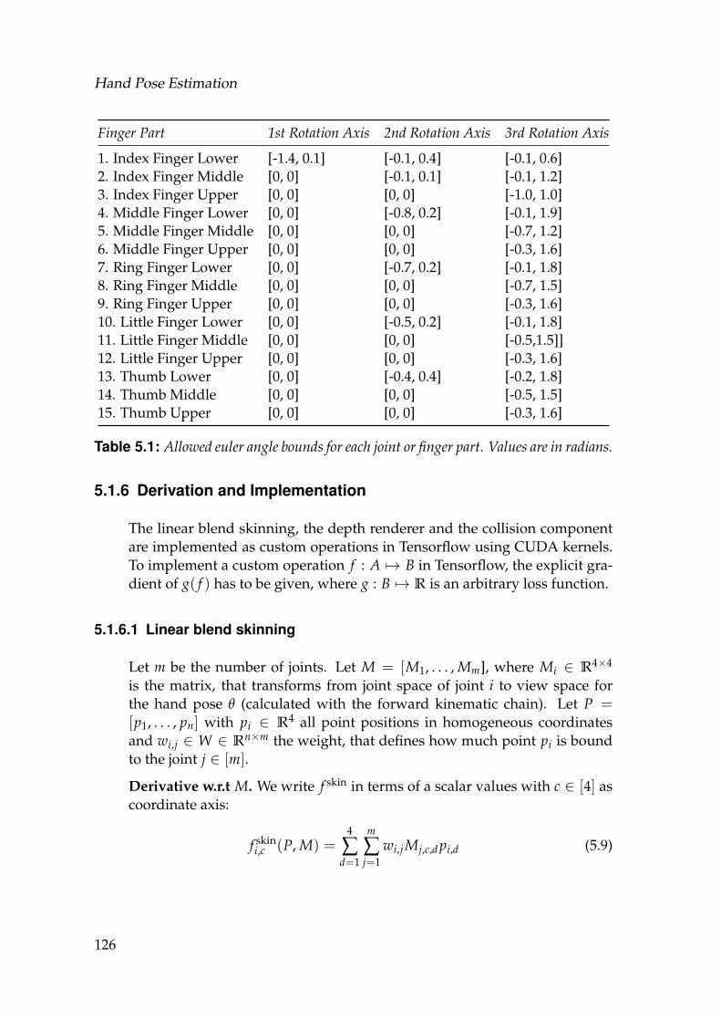
Hand Pose Estimation
Finger Part 1st Rotation Axis 2nd Rotation Axis 3rd Rotation Axis
1. Index Finger Lower [-1.4, 0.1] [-0.1, 0.4] [-0.1, 0.6]2. Index Finger Middle [0, 0] [-0.1, 0.1] [-0.1, 1.2]3. Index Finger Upper [0, 0] [0, 0] [-1.0, 1.0]4. Middle Finger Lower [0, 0] [-0.8, 0.2] [-0.1, 1.9]5. Middle Finger Middle [0, 0] [0, 0] [-0.7, 1.2]6. Middle Finger Upper [0, 0] [0, 0] [-0.3, 1.6]7. Ring Finger Lower [0, 0] [-0.7, 0.2] [-0.1, 1.8]8. Ring Finger Middle [0, 0] [0, 0] [-0.7, 1.5]9. Ring Finger Upper [0, 0] [0, 0] [-0.3, 1.6]10. Little Finger Lower [0, 0] [-0.5, 0.2] [-0.1, 1.8]11. Little Finger Middle [0, 0] [0, 0] [-0.5,1.5]]12. Little Finger Upper [0, 0] [0, 0] [-0.3, 1.6]13. Thumb Lower [0, 0] [-0.4, 0.4] [-0.2, 1.8]14. Thumb Middle [0, 0] [0, 0] [-0.5, 1.5]15. Thumb Upper [0, 0] [0, 0] [-0.3, 1.6]
Table 5.1: Allowed euler angle bounds for each joint or finger part. Values are in radians.
5.1.6 Derivation and Implementation
The linear blend skinning, the depth renderer and the collision componentare implemented as custom operations in Tensorflow using CUDA kernels.To implement a custom operation f : A 7→ B in Tensorflow, the explicit gra-dient of g( f ) has to be given, where g : B 7→ R is an arbitrary loss function.
5.1.6.1 Linear blend skinning
Let m be the number of joints. Let M = [M1, . . . , Mm], where Mi ∈ R4×4
is the matrix, that transforms from joint space of joint i to view space forthe hand pose θ (calculated with the forward kinematic chain). Let P =[p1, . . . , pn] with pi ∈ R4 all point positions in homogeneous coordinatesand wi,j ∈ W ∈ Rn×m the weight, that defines how much point pi is boundto the joint j ∈ [m].
Derivative w.r.t M. We write f skin in terms of a scalar values with c ∈ [4] ascoordinate axis:
f skini,c (P, M) =
4
∑d=1
m
∑j=1
wi,jMj,c,d pi,d (5.9)
126
5.1 3D Hand Pose Estimation from Depth Data
The derivative of f := f skin is:
∂ fi,c(P, M)
∂Mk,l,m= 1{l=c}wi,k pi,m (5.10)
The loss function g( f ) can be differentiated using the chain rule:
∂
∂Mk,l,mg( f (M, P)) =
n
∑i=1
4
∑c=1
∂g( f )∂ fi,c
∂ fi,c(P, M)
∂Mk,l,m(5.11)
=n
∑i=1
4
∑c=1
∂g( f )∂ fi,c
1{l=c}wi,k pi,m (5.12)
=n
∑i=1
∂g( f )∂ fi,l
wi,k pi,m (5.13)
Derivative w.r.t P. To update P, we also need to differentiate f skin w.r.t.P. In the equations above, we left out the batch dimension of f skin, sinceall the operations can be done in parallel and independently for each batchelement. However, our points P are the same for each batch element, hencemore precision is required here. Let f skin ∈ Rn×4 ×RN×n×4 7→ RN×n×4×4
where n is the number of points and N the size of the batch. Note that alsoM exists for each batch element and therefore has now four dimensions. Fora batch index b, point index i and coordinate index c we rewrite Eq. 5.9 as:
f skinb,i,c (P, M) =
4
∑d=1
m
∑j=1
wi,jMb,j,c,d pi,d (5.14)
Taking the derivative of f := f skin gives:
∂ fb,i,c(P, M)
∂pk,l= 1{k=i}
m
∑j=1
wi,jMb,j,c,l (5.15)
And the derivative of g( f ) is given by:
∂
∂pk,lg( f (M, P)) =
N
∑b=1
n
∑i=1
4
∑c=1
∂g( f )∂ fb,i,c
∂ fb,i,c(P, M)
∂pk,l
=N
∑b=1
n
∑i=1
4
∑c=1
∂g( f )∂ fb,i,c
1{k=i}m
∑j=1
wi,jMb,j,c,l
=N
∑b=1
4
∑c=1
∂g( f )∂ fb,k,c
m
∑j=1
wi,jMb,j,c,l (5.16)
127
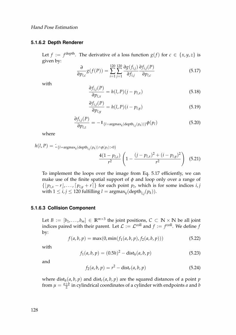
Hand Pose Estimation
5.1.6.2 Depth Renderer
Let f := f depth. The derivative of a loss function g( f ) for c ∈ {x, y, z} isgiven by:
∂
∂pl,cg( f (P)) =
120
∑i=1
120
∑j=1
∂g( fi,j)
∂ fi,j
∂ fi,j(P)∂pl,c
(5.17)
with∂ fi,j(P)
∂pl,x= h(l, P)(j− pl,x) (5.18)
∂ fi,j(P)∂pl,y
= h(l, P)(i− pl,y) (5.19)
∂ fi,j(P)∂pl,z
= −1{l=argmaxk(depthi,j(pk))}φ(pl) (5.20)
where
h(l, P) = 1{l=argmaxk(depthi,j(pk))∧φ(pl)>0}
4(1− pl,z)
r2
(1−
(j− pl,x)2 + (i− pl,y)
2
r2
)(5.21)
To implement the loops over the image from Eq. 5.17 efficiently, we canmake use of the finite spatial support of φ and loop only over a range of{bpl,x − rc, . . . , dpl,y + re} for each point pl, which is for some indices i, jwith 1 ≤ i, j ≤ 120 fulfilling l = argmaxk(depthi,j(pk)).
5.1.6.3 Collision Component
Let B := [b1, . . . , bm] ∈ Rm×3 the joint positions, C ⊂ N ×N be all jointindices paired with their parent. Let L := Lcoll and f := f coll. We define fby:
f (a, b, p) = max(0, min( f1(a, b, p), f2(a, b, p))) (5.22)
withf1(a, b, p) = (0.5h)2 − disth(a, b, p) (5.23)
andf2(a, b, p) = r2 − distr(a, b, p) (5.24)
where disth(a, b, p) and distr(a, b, p) are the squared distances of a point pfrom µ = a+b
2 in cylindrical coordinates of a cylinder with endpoints a and b
128
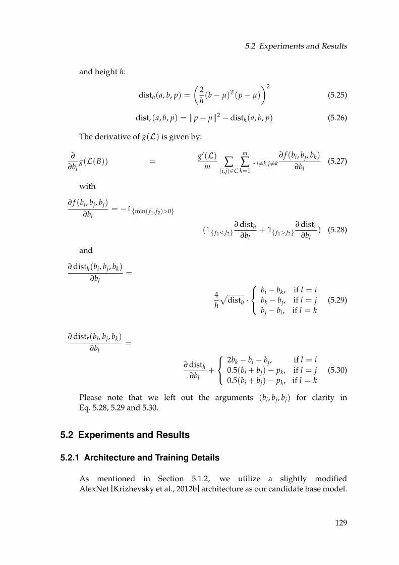
5.2 Experiments and Results
and height h:
disth(a, b, p) =(
2h(b− µ)T(p− µ)
)2
(5.25)
distr(a, b, p) = ‖p− µ‖2 − disth(a, b, p) (5.26)
The derivative of g(L) is given by:
∂
∂blg(L(B)) =
g′(L)m ∑
(i,j)∈C
m
∑k=1
1i 6=k,j 6=k∂ f (bi, bj, bk)
∂bl(5.27)
with
∂ f (bi, bj, bj)
∂bl= −1{min( f1, f2)>0}
(1{ f1< f2}∂ disth
∂bl+ 1{ f1> f2}
∂ distr
∂bl) (5.28)
and
∂ disth(bi, bj, bk)
∂bl=
4h
√disth ·
bi − bk, if l = ibk − bj, if l = jbj − bi, if l = k
(5.29)
∂ distr(bi, bj, bk)
∂bl=
∂ disth∂bl
+
2bk − bi − bj, if l = i0.5(bi + bj)− pk, if l = j0.5(bi + bj)− pk, if l = k
(5.30)
Please note that we left out the arguments (bi, bj, bj) for clarity inEq. 5.28, 5.29 and 5.30.
5.2 Experiments and Results
5.2.1 Architecture and Training Details
As mentioned in Section 5.1.2, we utilize a slightly modifiedAlexNet [Krizhevsky et al., 2012b] architecture as our candidate base model.
129
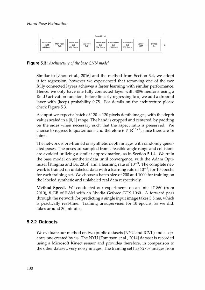
Hand Pose Estimation
Figure 5.3: Architecture of the base CNN model
Similar to [Zhou et al., 2016] and the method from Section 3.4, we adoptit for regression, however we experienced that removing one of the twofully connected layers achieves a faster learning with similar performance.Hence, we only have one fully connected layer with 4096 neurons using aReLU activation function. Before linearly regressing to θ, we add a dropoutlayer with (keep) probability 0.75. For details on the architecture pleasecheck Figure 5.3.
As input we expect a batch of 120× 120 pixels depth images, with the depthvalues scaled in a [0, 1] range. The hand is cropped and centered, by paddingon the sides when necessary such that the aspect ratio is preserved. Wechoose to regress to quaternions and therefore θ ∈ R16×4, since there are 16joints.
The network is pre-trained on synthetic depth images with randomly gener-ated poses. The poses are sampled from a feasible angle range and collisionsare avoided utilizing a similar approximation, as in Section 5.1.4. We trainthe base model on synthetic data until convergence, with the Adam Opti-mizer [Kingma and Ba, 2014] and a learning rate of 10−3. The complete net-work is trained on unlabeled data with a learning rate of 10−5, for 10 epochsfor each training set. We choose a batch size of 200 and 1000 for training onthe labeled synthetic and unlabeled real data respectively.
Method Speed. We conducted our experiments on an Intel i7 860 (from2010), 8 GB of RAM with an Nvidia Geforce GTX 1060. A forward passthrough the network for predicting a single input image takes 3.5 ms, whichis practically real-time. Training unsupervised for 10 epochs, as we did,takes around 30 minutes.
5.2.2 Datasets
We evaluate our method on two public datasets (NYU and ICVL) and a sep-arate one created by us. The NYU [Tompson et al., 2014] dataset is recordedusing a Microsoft Kinect sensor and provides therefore, in comparison tothe other dataset, very noisy images. The training set has 72757 images from
130
5.2 Experiments and Results
one person and three simultaneous views. The test set is a sequence of 8252images from two persons. The ground truth annotations are fitted with anoffline PSO approach and consist of 36 3D spatial hand features per frame.Similar to previous works [Zhou et al., 2016], we also use only a subset of 163D positions for evaluation.The ICVL dataset [Danhang Tang, 2014] is less noisy due to the usage ofthe Intel Creative Interactive Gesture Camera. Two test sequences from twodifferent persons with a total of 1596 frames are provided for testing andabout 180K frames for training from several persons. The ground truth of 163D bone center locations is obtained utilizing the tracking method proposedby [Melax et al., 2013]. We segment the images of NYU and ICVL by cuttingout a padded block around the 3D annotations. Furthermore, it is importantto mention that our 3D joint positions, that are dependent on our fixed 3Dmodel skeleton, deviate a lot from the ones used in both datasets, which isimportant for a fair comparison.Our own dataset is created using the Intel RealSense Camera and consists of2000 depth images for testing and 50000 depth images for training, from onlyone person wearing a black wristband. This allows for a simple brightnessbased segmentation to cut out the wrist, which makes it easy to separate theforeground from the background. We also capture a color image for eachframe for qualitative comparison. Note that we do not provide any anno-tations. We compare to different methods by computing ROC curves, thatdenote the fraction of frames below a maximum 3D join prediction error.
5.2.3 Feasibility of Learning Hand Pose and Shape
It has been shown by [Loper and Black, 2014] how to estimate the hu-man body shape from depth (and color) image differences using a gradi-ent based method, but except for the concurrent optimization based ap-proaches on differentiable offline [Remelli et al., 2017] and online [Tkachet al., 2017] calibration for hands, to the best of our knowledge, there existno CNN based works in the field of hand pose estimation. In methods uti-lizing PSO [Oikonomidis et al., 2011; Tompson et al., 2014; Qian et al., 2014;Sharp et al., 2015], we have seen that an error metric on depth images ismeaningful enough to intelligently sample, compare and prune candidateposes, however the gradient idea has not been exploited. Encouraged bysuch results, we show in two experiments that we can optimize for the handpose and shape.
Hand Pose Optimization. In our first experiment we attempt to overfit ourmodel on single images, in order to show that reasonable results are ob-
131
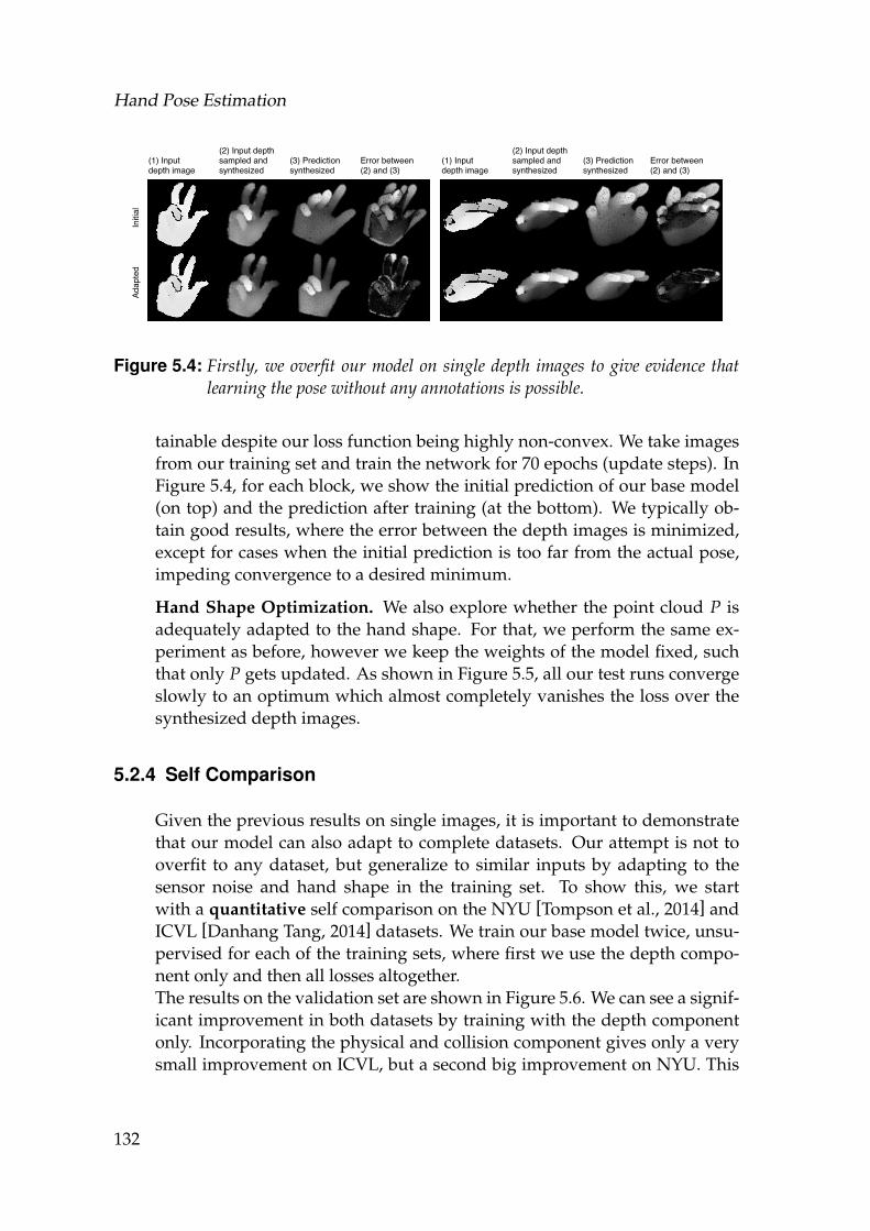
Hand Pose Estimation
Figure 5.4: Firstly, we overfit our model on single depth images to give evidence thatlearning the pose without any annotations is possible.
tainable despite our loss function being highly non-convex. We take imagesfrom our training set and train the network for 70 epochs (update steps). InFigure 5.4, for each block, we show the initial prediction of our base model(on top) and the prediction after training (at the bottom). We typically ob-tain good results, where the error between the depth images is minimized,except for cases when the initial prediction is too far from the actual pose,impeding convergence to a desired minimum.
Hand Shape Optimization. We also explore whether the point cloud P isadequately adapted to the hand shape. For that, we perform the same ex-periment as before, however we keep the weights of the model fixed, suchthat only P gets updated. As shown in Figure 5.5, all our test runs convergeslowly to an optimum which almost completely vanishes the loss over thesynthesized depth images.
5.2.4 Self Comparison
Given the previous results on single images, it is important to demonstratethat our model can also adapt to complete datasets. Our attempt is not tooverfit to any dataset, but generalize to similar inputs by adapting to thesensor noise and hand shape in the training set. To show this, we startwith a quantitative self comparison on the NYU [Tompson et al., 2014] andICVL [Danhang Tang, 2014] datasets. We train our base model twice, unsu-pervised for each of the training sets, where first we use the depth compo-nent only and then all losses altogether.The results on the validation set are shown in Figure 5.6. We can see a signif-icant improvement in both datasets by training with the depth componentonly. Incorporating the physical and collision component gives only a verysmall improvement on ICVL, but a second big improvement on NYU. This
132
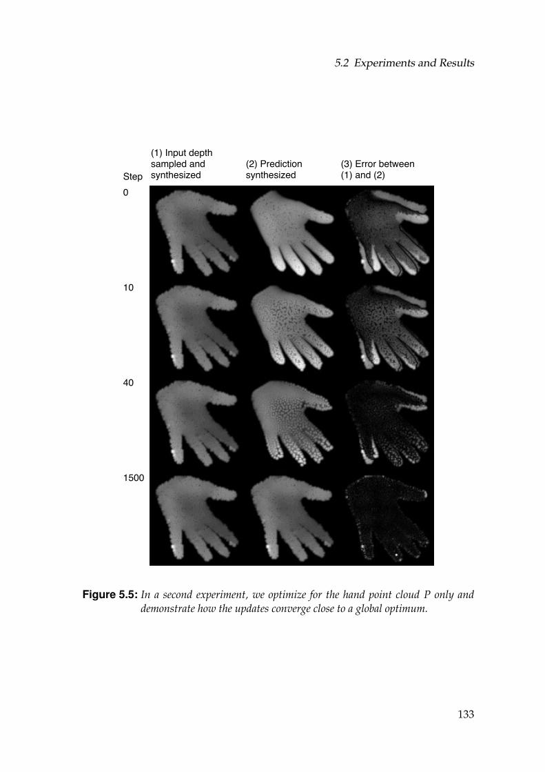
5.2 Experiments and Results
Figure 5.5: In a second experiment, we optimize for the hand point cloud P only anddemonstrate how the updates converge close to a global optimum.
133
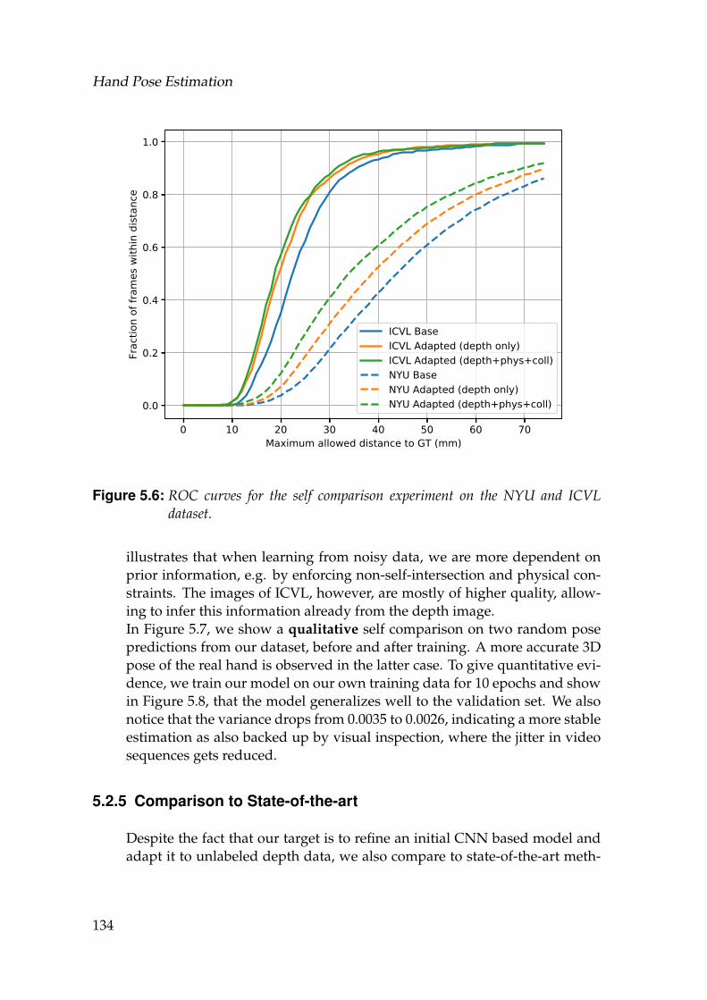
Hand Pose Estimation
0 10 20 30 40 50 60 70Maximum allowed distance to GT (mm)
0.0
0.2
0.4
0.6
0.8
1.0Fr
actio
n of
fram
es w
ithin
dist
ance
ICVL BaseICVL Adapted (depth only)ICVL Adapted (depth+phys+coll)NYU BaseNYU Adapted (depth only)NYU Adapted (depth+phys+coll)
Figure 5.6: ROC curves for the self comparison experiment on the NYU and ICVLdataset.
illustrates that when learning from noisy data, we are more dependent onprior information, e.g. by enforcing non-self-intersection and physical con-straints. The images of ICVL, however, are mostly of higher quality, allow-ing to infer this information already from the depth image.In Figure 5.7, we show a qualitative self comparison on two random posepredictions from our dataset, before and after training. A more accurate 3Dpose of the real hand is observed in the latter case. To give quantitative evi-dence, we train our model on our own training data for 10 epochs and showin Figure 5.8, that the model generalizes well to the validation set. We alsonotice that the variance drops from 0.0035 to 0.0026, indicating a more stableestimation as also backed up by visual inspection, where the jitter in videosequences gets reduced.
5.2.5 Comparison to State-of-the-art
Despite the fact that our target is to refine an initial CNN based model andadapt it to unlabeled depth data, we also compare to state-of-the-art meth-
134
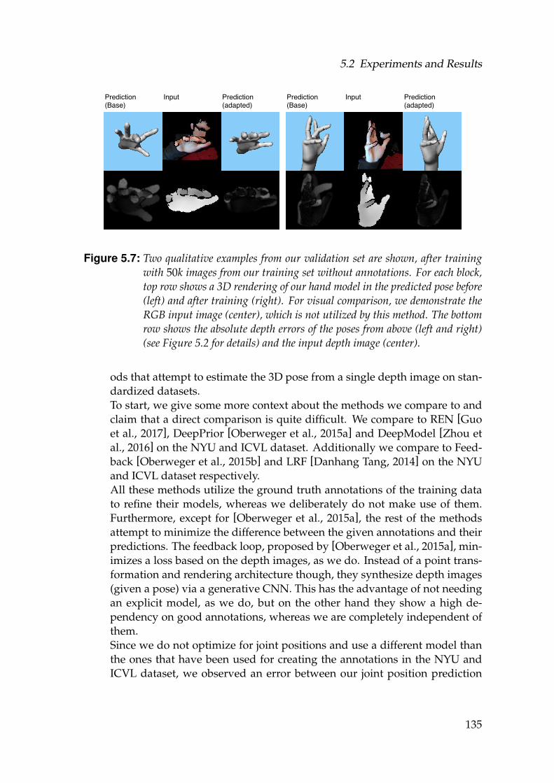
5.2 Experiments and Results
Figure 5.7: Two qualitative examples from our validation set are shown, after trainingwith 50k images from our training set without annotations. For each block,top row shows a 3D rendering of our hand model in the predicted pose before(left) and after training (right). For visual comparison, we demonstrate theRGB input image (center), which is not utilized by this method. The bottomrow shows the absolute depth errors of the poses from above (left and right)(see Figure 5.2 for details) and the input depth image (center).
ods that attempt to estimate the 3D pose from a single depth image on stan-dardized datasets.To start, we give some more context about the methods we compare to andclaim that a direct comparison is quite difficult. We compare to REN [Guoet al., 2017], DeepPrior [Oberweger et al., 2015a] and DeepModel [Zhou etal., 2016] on the NYU and ICVL dataset. Additionally we compare to Feed-back [Oberweger et al., 2015b] and LRF [Danhang Tang, 2014] on the NYUand ICVL dataset respectively.All these methods utilize the ground truth annotations of the training datato refine their models, whereas we deliberately do not make use of them.Furthermore, except for [Oberweger et al., 2015a], the rest of the methodsattempt to minimize the difference between the given annotations and theirpredictions. The feedback loop, proposed by [Oberweger et al., 2015a], min-imizes a loss based on the depth images, as we do. Instead of a point trans-formation and rendering architecture though, they synthesize depth images(given a pose) via a generative CNN. This has the advantage of not needingan explicit model, as we do, but on the other hand they show a high de-pendency on good annotations, whereas we are completely independent ofthem.Since we do not optimize for joint positions and use a different model thanthe ones that have been used for creating the annotations in the NYU andICVL dataset, we observed an error between our joint position prediction
135
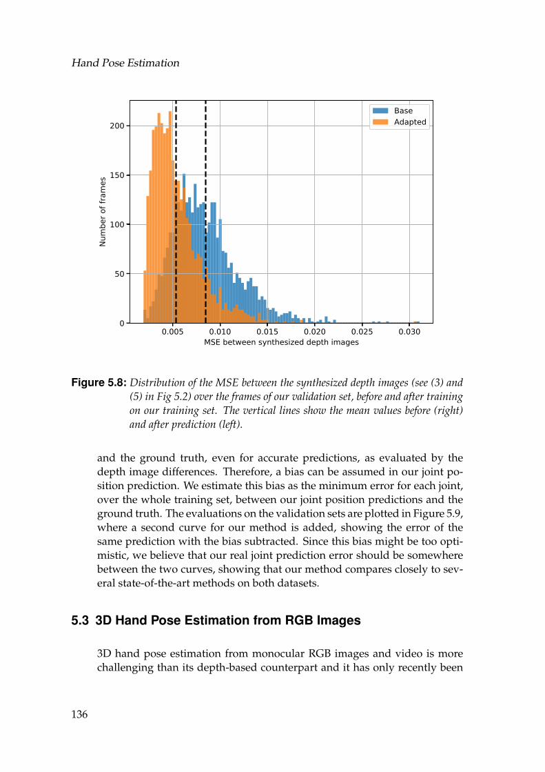
Hand Pose Estimation
0.005 0.010 0.015 0.020 0.025 0.030MSE between synthesized depth images
0
50
100
150
200
Num
ber o
f fra
mes
BaseAdapted
Figure 5.8: Distribution of the MSE between the synthesized depth images (see (3) and(5) in Fig 5.2) over the frames of our validation set, before and after trainingon our training set. The vertical lines show the mean values before (right)and after prediction (left).
and the ground truth, even for accurate predictions, as evaluated by thedepth image differences. Therefore, a bias can be assumed in our joint po-sition prediction. We estimate this bias as the minimum error for each joint,over the whole training set, between our joint position predictions and theground truth. The evaluations on the validation sets are plotted in Figure 5.9,where a second curve for our method is added, showing the error of thesame prediction with the bias subtracted. Since this bias might be too opti-mistic, we believe that our real joint prediction error should be somewherebetween the two curves, showing that our method compares closely to sev-eral state-of-the-art methods on both datasets.
5.3 3D Hand Pose Estimation from RGB Images
3D hand pose estimation from monocular RGB images and video is morechallenging than its depth-based counterpart and it has only recently been
136
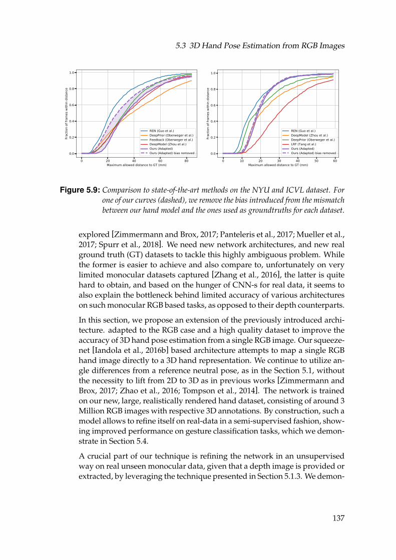
5.3 3D Hand Pose Estimation from RGB Images
0 20 40 60 80Maximum allowed distance to GT (mm)
0.0
0.2
0.4
0.6
0.8
1.0
Frac
tion
of fr
ames
with
in d
istan
ce
REN (Guo et al.)DeepPrior (Oberweger et al.)Feedback (Oberweger et al.)DeepModel (Zhou et al.)Ours (Adapted)Ours (Adapted) bias removed
0 10 20 30 40 50 60Maximum allowed distance to GT (mm)
0.0
0.2
0.4
0.6
0.8
1.0
Frac
tion
of fr
ames
with
in d
istan
ce
REN (Guo et al.)DeepModel (Zhou et al.)DeepPrior (Oberweger et al.)LRF (Tang et al.)Ours (Adapted)Ours (Adapted) bias removed
Figure 5.9: Comparison to state-of-the-art methods on the NYU and ICVL dataset. Forone of our curves (dashed), we remove the bias introduced from the mismatchbetween our hand model and the ones used as groundtruths for each dataset.
explored [Zimmermann and Brox, 2017; Panteleris et al., 2017; Mueller et al.,2017; Spurr et al., 2018]. We need new network architectures, and new realground truth (GT) datasets to tackle this highly ambiguous problem. Whilethe former is easier to achieve and also compare to, unfortunately on verylimited monocular datasets captured [Zhang et al., 2016], the latter is quitehard to obtain, and based on the hunger of CNN-s for real data, it seems toalso explain the bottleneck behind limited accuracy of various architectureson such monocular RGB based tasks, as opposed to their depth counterparts.
In this section, we propose an extension of the previously introduced archi-tecture. adapted to the RGB case and a high quality dataset to improve theaccuracy of 3D hand pose estimation from a single RGB image. Our squeeze-net [Iandola et al., 2016b] based architecture attempts to map a single RGBhand image directly to a 3D hand representation. We continue to utilize an-gle differences from a reference neutral pose, as in the Section 5.1, withoutthe necessity to lift from 2D to 3D as in previous works [Zimmermann andBrox, 2017; Zhao et al., 2016; Tompson et al., 2014]. The network is trainedon our new, large, realistically rendered hand dataset, consisting of around 3Million RGB images with respective 3D annotations. By construction, such amodel allows to refine itself on real-data in a semi-supervised fashion, show-ing improved performance on gesture classification tasks, which we demon-strate in Section 5.4.
A crucial part of our technique is refining the network in an unsupervisedway on real unseen monocular data, given that a depth image is provided orextracted, by leveraging the technique presented in Section 5.1.3. We demon-
137
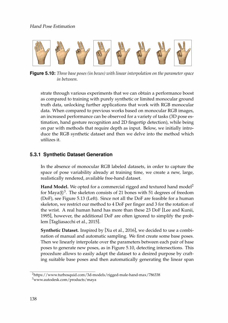
Hand Pose Estimation
Figure 5.10: Three base poses (in boxes) with linear interpolation on the parameter spacein between.
strate through various experiments that we can obtain a performance boostas compared to training with purely synthetic or limited monocular groundtruth data, unlocking further applications that work with RGB monoculardata. When compared to previous works based on monocular RGB images,an increased performance can be observed for a variety of tasks (3D pose es-timation, hand gesture recognition and 2D fingertip detection), while beingon par with methods that require depth as input. Below, we initially intro-duce the RGB synthetic dataset and then we delve into the method whichutilizes it.
5.3.1 Synthetic Dataset Generation
In the absence of monocular RGB labeled datasets, in order to capture thespace of pose variability already at training time, we create a new, large,realistically rendered, available free-hand dataset.
Hand Model. We opted for a commercial rigged and textured hand model2
for Maya R©3. The skeleton consists of 21 bones with 51 degrees of freedom(DoF), see Figure 5.13 (Left). Since not all the DoF are feasible for a humanskeleton, we restrict our method to 4 DoF per finger and 3 for the rotation ofthe wrist. A real human hand has more than these 23 DoF [Lee and Kunii,1995], however, the additional DoF are often ignored to simplify the prob-lem [Tagliasacchi et al., 2015].
Synthetic Dataset. Inspired by [Xu et al., 2016], we decided to use a combi-nation of manual and automatic sampling. We first create some base poses.Then we linearly interpolate over the parameters between each pair of baseposes to generate new poses, as in Figure 5.10, detecting intersections. Thisprocedure allows to easily adapt the dataset to a desired purpose by craft-ing suitable base poses and then automatically generating the linear span
2https://www.turbosquid.com/3d-models/rigged-male-hand-max/7863383www.autodesk.com/products/maya
138
5.3 3D Hand Pose Estimation from RGB Images
between them, as explained below. We end up with 399 such poses. In ad-dition to the varying poses, for each view (we consider 5 views - front, back,both sides and top, Figure 5.13 (Middle)) we apply 5 random rotations (45degrees for each DoF of the wrist joint) and illumination changes to eachimage. We also vary the texture and shape.
Base Poses. We enumerate the thumb poses separately and firstly focus onthe other four fingers. We fix three possible opening states of a finger: fullyopen, partially closed (metacarpophalangeal joint still stretched) and fullyclosed. Furthermore, we assume that if some fingers are not fully stretched,they are closed the same way (either all of them partially closed or fullyclosed). The side-movements are combined with the opening state of a fin-ger, e.g. they are ignored when the fingers are partially or fully closed, dueto the human hand limitations [Lee and Kunii, 1995]. A further simplifyingassumption we made was to enumerate side-movements by counting thegaps between the fingers as explained below:
• If all four fingers are fully open, there are three gaps in between.Each gap can be either open or closed, giving a total of 23 = 8 com-binations.
• If three fingers are fully open, the number of gaps depends on the(partially) closed finger, being either two or one. Since the closedfinger can be either fully or partially closed, we get a total of 2(22 +21 + 21 + 22) = 24 poses.
• If two fingers are fully open, we get a total of 2(21 + 20 + 21 + 20 +20 + 21) = 18 poses with the same considerations as in the previouscase.
• If only one finger is fully open, we do not have side-movements withour assumptions, giving a total of 2(20 + 20 + 20 + 20) = 8 poses.
• If all fingers are closed, they can be either partially of fully closed,giving a total of 2 poses.
Having in mind the interpolation to be performed, we fixed six differentposes of the thumb, giving a total of 6× 60 = 360 base poses. Additionally,we added four poses where the thumb touches one of the remaining fingerseach, since the above setting of separating the thumb from the remainingfingers does not handle this. We also added 6 poses with crossed fingers,because the focus on the gap between the fingers does not capture this. In theend, 29 base poses were created inspired by the HGR [Kawulok et al., 2014;Nalepa and Kawulok, 2014; Grzejszczak et al., 2016] dataset, giving a totalof 399 base poses.
139
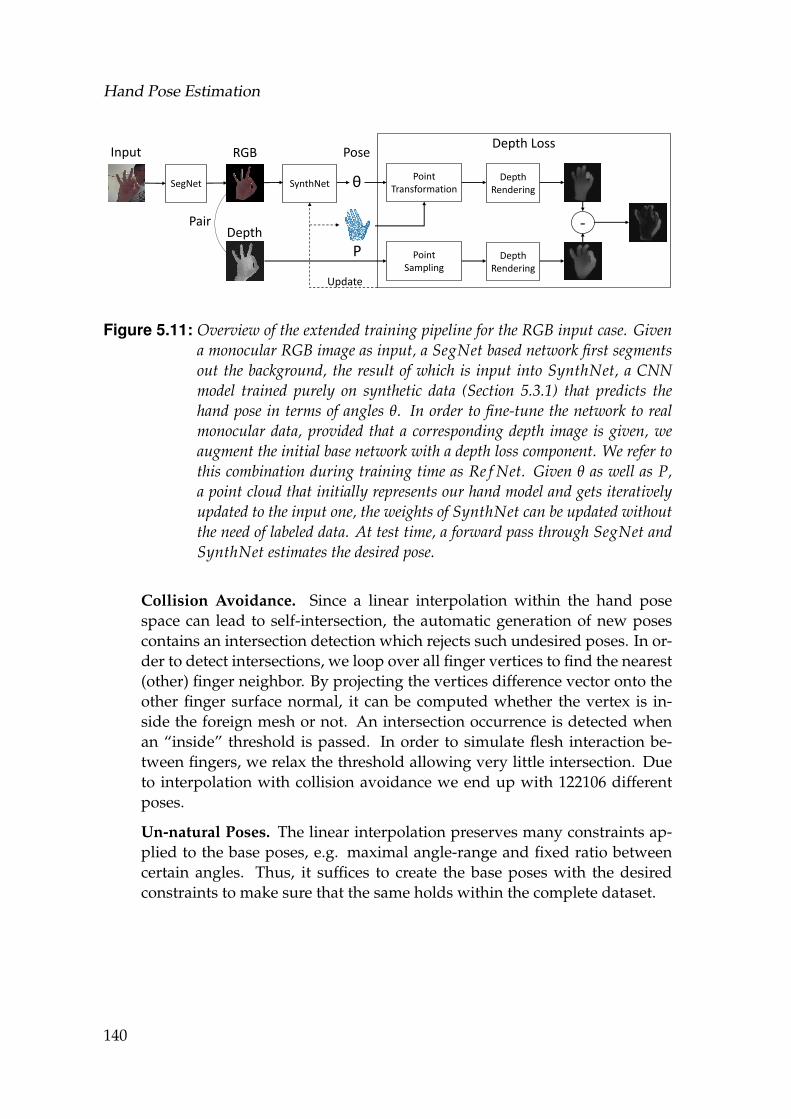
Hand Pose Estimation
SegNet SynthNet θ PointTransformation
DepthRendering
PointSampling
DepthRendering
Input PoseDepth Loss
-
PDepth
RGB
Pair
Update
Figure 5.11: Overview of the extended training pipeline for the RGB input case. Givena monocular RGB image as input, a SegNet based network first segmentsout the background, the result of which is input into SynthNet, a CNNmodel trained purely on synthetic data (Section 5.3.1) that predicts thehand pose in terms of angles θ. In order to fine-tune the network to realmonocular data, provided that a corresponding depth image is given, weaugment the initial base network with a depth loss component. We refer tothis combination during training time as Re f Net. Given θ as well as P,a point cloud that initially represents our hand model and gets iterativelyupdated to the input one, the weights of SynthNet can be updated withoutthe need of labeled data. At test time, a forward pass through SegNet andSynthNet estimates the desired pose.
Collision Avoidance. Since a linear interpolation within the hand posespace can lead to self-intersection, the automatic generation of new posescontains an intersection detection which rejects such undesired poses. In or-der to detect intersections, we loop over all finger vertices to find the nearest(other) finger neighbor. By projecting the vertices difference vector onto theother finger surface normal, it can be computed whether the vertex is in-side the foreign mesh or not. An intersection occurrence is detected whenan “inside” threshold is passed. In order to simulate flesh interaction be-tween fingers, we relax the threshold allowing very little intersection. Dueto interpolation with collision avoidance we end up with 122106 differentposes.
Un-natural Poses. The linear interpolation preserves many constraints ap-plied to the base poses, e.g. maximal angle-range and fixed ratio betweencertain angles. Thus, it suffices to create the base poses with the desiredconstraints to make sure that the same holds within the complete dataset.
140
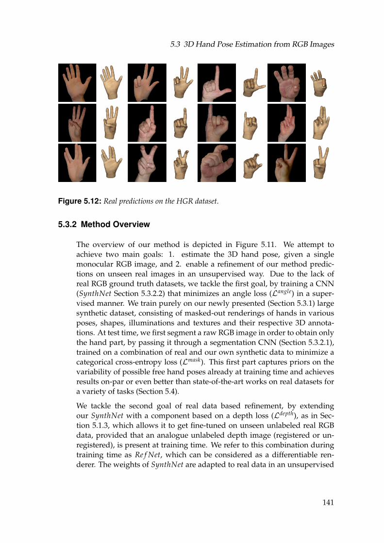
5.3 3D Hand Pose Estimation from RGB Images
Figure 5.12: Real predictions on the HGR dataset.
5.3.2 Method Overview
The overview of our method is depicted in Figure 5.11. We attempt toachieve two main goals: 1. estimate the 3D hand pose, given a singlemonocular RGB image, and 2. enable a refinement of our method predic-tions on unseen real images in an unsupervised way. Due to the lack ofreal RGB ground truth datasets, we tackle the first goal, by training a CNN(SynthNet Section 5.3.2.2) that minimizes an angle loss (Langle) in a super-vised manner. We train purely on our newly presented (Section 5.3.1) largesynthetic dataset, consisting of masked-out renderings of hands in variousposes, shapes, illuminations and textures and their respective 3D annota-tions. At test time, we first segment a raw RGB image in order to obtain onlythe hand part, by passing it through a segmentation CNN (Section 5.3.2.1),trained on a combination of real and our own synthetic data to minimize acategorical cross-entropy loss (Lmask). This first part captures priors on thevariability of possible free hand poses already at training time and achievesresults on-par or even better than state-of-the-art works on real datasets fora variety of tasks (Section 5.4).
We tackle the second goal of real data based refinement, by extendingour SynthNet with a component based on a depth loss (Ldepth), as in Sec-tion 5.1.3, which allows it to get fine-tuned on unseen unlabeled real RGBdata, provided that an analogue unlabeled depth image (registered or un-registered), is present at training time. We refer to this combination duringtraining time as Re f Net, which can be considered as a differentiable ren-derer. The weights of SynthNet are adapted to real data in an unsupervised
141
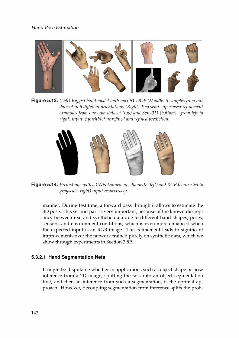
Hand Pose Estimation
Figure 5.13: (Left) Rigged hand model with max 51 DOF (Middle) 5 samples from ourdataset in 5 different orientations (Right) Two semi-supervised refinementexamples from our own dataset (top) and Senz3D (bottom) - from left toright: input, SynthNet unrefined and refined prediction.
Figure 5.14: Predictions with a CNN trained on silhouette (left) and RGB (converted tograyscale, right) input respectively.
manner. During test time, a forward pass through it allows to estimate the3D pose. This second part is very important, because of the known discrep-ancy between real and synthetic data due to different hand shapes, poses,sensors, and environment conditions, which is even more enhanced whenthe expected input is an RGB image. This refinement leads to significantimprovements over the network trained purely on synthetic data, which weshow through experiments in Section 3.5.5.
5.3.2.1 Hand Segmentation Nets
It might be disputable whether in applications such as object shape or poseinference from a 2D image, splitting the task into an object segmentationfirst, and then an inference from such a segmentation, is the optimal ap-proach. However, decoupling segmentation from inference splits the prob-
142
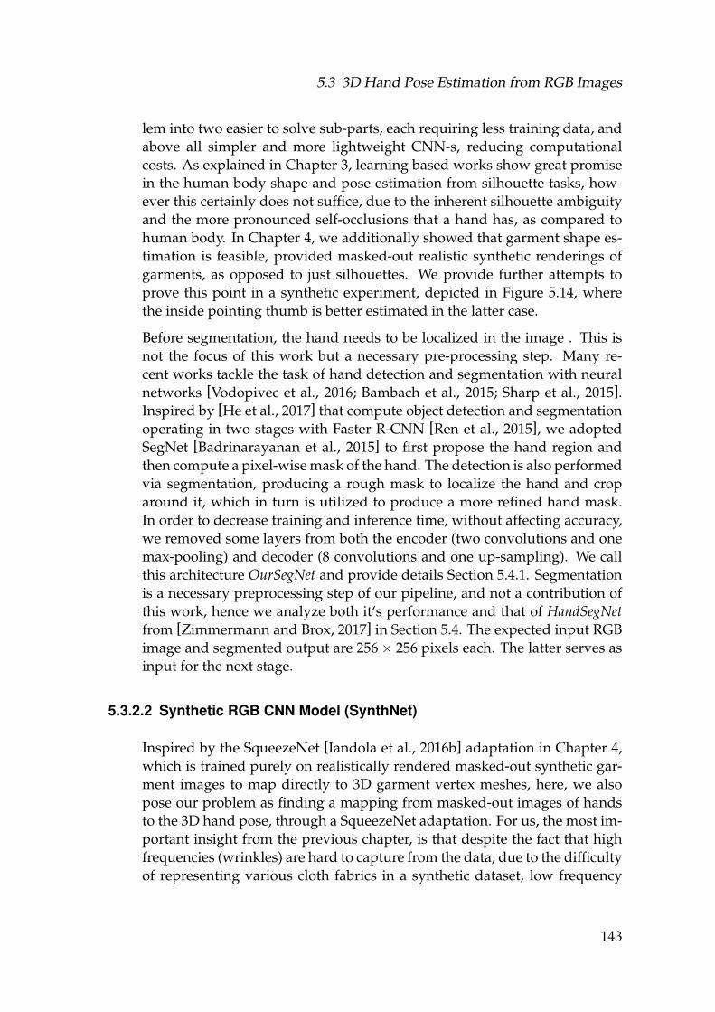
5.3 3D Hand Pose Estimation from RGB Images
lem into two easier to solve sub-parts, each requiring less training data, andabove all simpler and more lightweight CNN-s, reducing computationalcosts. As explained in Chapter 3, learning based works show great promisein the human body shape and pose estimation from silhouette tasks, how-ever this certainly does not suffice, due to the inherent silhouette ambiguityand the more pronounced self-occlusions that a hand has, as compared tohuman body. In Chapter 4, we additionally showed that garment shape es-timation is feasible, provided masked-out realistic synthetic renderings ofgarments, as opposed to just silhouettes. We provide further attempts toprove this point in a synthetic experiment, depicted in Figure 5.14, wherethe inside pointing thumb is better estimated in the latter case.
Before segmentation, the hand needs to be localized in the image . This isnot the focus of this work but a necessary pre-processing step. Many re-cent works tackle the task of hand detection and segmentation with neuralnetworks [Vodopivec et al., 2016; Bambach et al., 2015; Sharp et al., 2015].Inspired by [He et al., 2017] that compute object detection and segmentationoperating in two stages with Faster R-CNN [Ren et al., 2015], we adoptedSegNet [Badrinarayanan et al., 2015] to first propose the hand region andthen compute a pixel-wise mask of the hand. The detection is also performedvia segmentation, producing a rough mask to localize the hand and croparound it, which in turn is utilized to produce a more refined hand mask.In order to decrease training and inference time, without affecting accuracy,we removed some layers from both the encoder (two convolutions and onemax-pooling) and decoder (8 convolutions and one up-sampling). We callthis architecture OurSegNet and provide details Section 5.4.1. Segmentationis a necessary preprocessing step of our pipeline, and not a contribution ofthis work, hence we analyze both it‘s performance and that of HandSegNetfrom [Zimmermann and Brox, 2017] in Section 5.4. The expected input RGBimage and segmented output are 256× 256 pixels each. The latter serves asinput for the next stage.
5.3.2.2 Synthetic RGB CNN Model (SynthNet)
Inspired by the SqueezeNet [Iandola et al., 2016b] adaptation in Chapter 4,which is trained purely on realistically rendered masked-out synthetic gar-ment images to map directly to 3D garment vertex meshes, here, we alsopose our problem as finding a mapping from masked-out images of handsto the 3D hand pose, through a SqueezeNet adaptation. For us, the most im-portant insight from the previous chapter, is that despite the fact that highfrequencies (wrinkles) are hard to capture from the data, due to the difficultyof representing various cloth fabrics in a synthetic dataset, low frequency
143
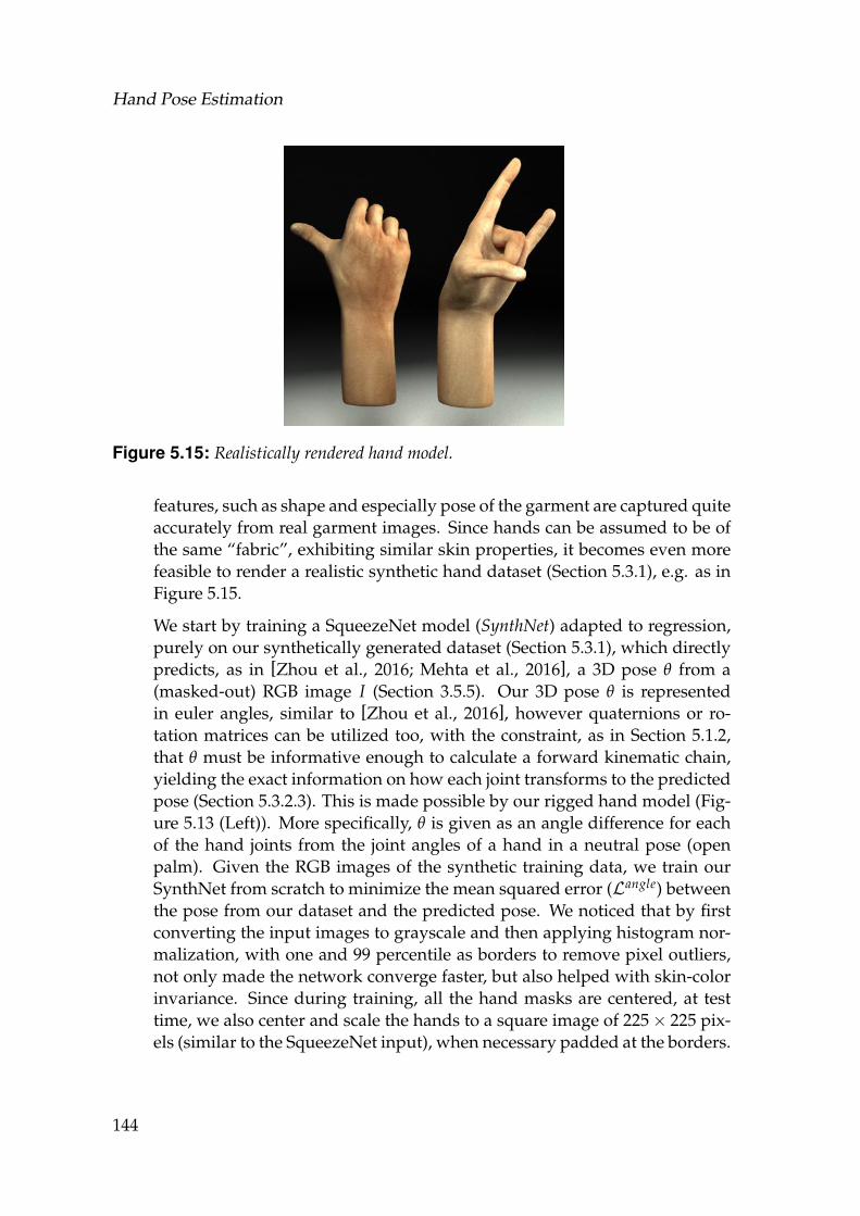
Hand Pose Estimation
Figure 5.15: Realistically rendered hand model.
features, such as shape and especially pose of the garment are captured quiteaccurately from real garment images. Since hands can be assumed to be ofthe same “fabric”, exhibiting similar skin properties, it becomes even morefeasible to render a realistic synthetic hand dataset (Section 5.3.1), e.g. as inFigure 5.15.
We start by training a SqueezeNet model (SynthNet) adapted to regression,purely on our synthetically generated dataset (Section 5.3.1), which directlypredicts, as in [Zhou et al., 2016; Mehta et al., 2016], a 3D pose θ from a(masked-out) RGB image I (Section 3.5.5). Our 3D pose θ is representedin euler angles, similar to [Zhou et al., 2016], however quaternions or ro-tation matrices can be utilized too, with the constraint, as in Section 5.1.2,that θ must be informative enough to calculate a forward kinematic chain,yielding the exact information on how each joint transforms to the predictedpose (Section 5.3.2.3). This is made possible by our rigged hand model (Fig-ure 5.13 (Left)). More specifically, θ is given as an angle difference for eachof the hand joints from the joint angles of a hand in a neutral pose (openpalm). Given the RGB images of the synthetic training data, we train ourSynthNet from scratch to minimize the mean squared error (Langle) betweenthe pose from our dataset and the predicted pose. We noticed that by firstconverting the input images to grayscale and then applying histogram nor-malization, with one and 99 percentile as borders to remove pixel outliers,not only made the network converge faster, but also helped with skin-colorinvariance. Since during training, all the hand masks are centered, at testtime, we also center and scale the hands to a square image of 225× 225 pix-els (similar to the SqueezeNet input), when necessary padded at the borders.
144
5.3 3D Hand Pose Estimation from RGB Images
5.3.2.3 Semi- and Unsupervised Refinement from RGB and Depth Images
Semi-Supervised Refinement on Real RGB Images. One advantage ofutilizing angles instead of joint positions, is that they can be easily be re-stricted to the allowed Degrees of Freedom, reducing the large space of in-feasible poses, and constraining the latent space [Choi et al., 2017]. Givena skeleton, angles can easily be converted to joints and hence fully de-termine a pose. This might penalize accuracy on exact 3D joint estima-tion tasks, under fixed hand skeleton model assumptions, however it canbe quite attractive for other tasks where the hand skeleton constellation ismore important than the exact joint position, e.g. hand gesture recogni-tion/classification. Another advantage of utilizing angles, is that it allowsany pre-trained fully supervised network (regardless whether real or syn-thetic data is used), to refine itself on easily obtainable real unlabeled RGBimages. Real images of hands in various shapes, skin colors, lighting condi-tions and rotations can be easily captured with cheap RGB sensors, under theconstraint that users perform pre-specified gestures, as in [Memo et al., 2015;Memo and Zanuttigh, 2017]. These gestures can be easily modeled, given asynthetic hand model, obtaining the ground truth (angles) without addi-tional manual effort. Angles are advantageous here, as various user poseswould map to the same ground-truth, regardless of the exact hand positionand rotation in the image. In this way, the input space is enriched with mul-tiple real images that map to the same angles, which in turn helps to fine-tune synthetic networks and improve the gesture recognition predictions.Details on this are provided in Figure 5.13 with the respective discussion inSection 5.4.4.
Unsupervised Refinement with Depth Images. SynthNet alone gives goodinitial predictions on various real data ((Section 5.4), Figure 5.12 and Fig-ure 5.23), however a discrepancy between synthetic and real datasets isknown in literature and practice. Following the method presented in Sec-tion 5.1.3, we extend our network with a component that enables SynthNetto get refined unsupervised, trained to minimize a depth loss (Ldepth) on un-labeled depth data, that have one-to-one correspondences to the input realRGB images. Unlike, the above we do not make use of the Physical and Col-lision component. Let‘s assume we have pairs of RGB and Depth images(I, D). Acquisition of such pairs is very cheap with today‘s RGBD sensors(Section 5.4.2). We compare the input depth image D to a synthesized depthimage DI , which is computed from SynthNet predicted pose θ, given I asinput, and a pointcloud P sampled from the hand mesh model, in order topredict the accuracy on unlabeled data. We transform the P points according
145
Hand Pose Estimation
to θ, applying Linear Blend Skinning (LBS) [Lewis et al., 2000], and subse-quently render them to obtain a synthetic depth image.
5.4 Experiments and Results
In Figure 5.16, we demonstrate qualitative results of poses inferred fromSynthNet, with input images from the HGR dataset [Kawulok et al., 2014;Nalepa and Kawulok, 2014; Grzejszczak et al., 2016] and one additional in-dividual performing various poses in Figure 5.17.
5.4.1 Training Details and Architectures
The architectures for the hand detection, segmentation and pose inferencemodel are illustrated in Figure 5.18, Figure 5.19 and Figure 5.20 respectivelyin more detail. We train HandSegNet with Adam optimizer [Kingma andBa, 2014] and an initial learning rate of 10−5 with decay 5× 10⁻⁴, changedto 10−6 and 10−7 over 10 epochs, and OurSegNet with Stochastic Gradi-ent Descent and the same initial learning rate for 30 epochs. SynthNet wastrained utilizing Adam optimizer, with an initial learning rate of 10−4 over10 epochs with a batch size of 100, while RefNet with Adam optimizer andlearning rate of 4× 10⁻³ for over 40 epochs with a batch size of 1000. Asinput we expect a batch of 120× 120 pixels depth images, with the depthvalues scaled in a [0, 1] range.
Heat Map Visualizations for SynthNet. In order to investigate further thenetwork’s learning capacity, we visualize features learned by our network,by relating image positions to error contributions. We adopt a techniqueintroduced by [Zeiler and Fergus, 2014] to regression. A black box is movedover different poses. For each position, the increase of error compared to theoriginal image is measured and finally visualized as a heatmap. We calculatethe mean squared error over different sets of parameters. Figure 5.21 showsheat-map examples for a variety of poses. As it can be noticed, most of thefingers demonstrate a high error throughout the whole finger when that partis missing, as we would expect.
Method Speed. We conducted our experiments on an Intel i7 860 (from2010), 8 GB of RAM with an Nvidia Geforce GTX 1060. A forward passthrough the network for predicting a single input image takes 3.5 ms, whichis practically real-time. Training unsupervised for 10 epochs, as we did,takes around 30 minutes.
146
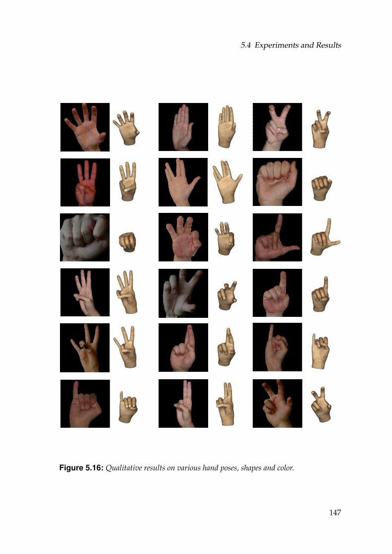
5.4 Experiments and Results
Figure 5.16: Qualitative results on various hand poses, shapes and color.
147
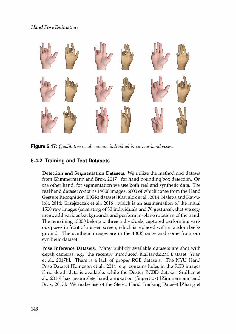
Hand Pose Estimation
Figure 5.17: Qualitative results on one individual in various hand poses.
5.4.2 Training and Test Datasets
Detection and Segmentation Datasets. We utilize the method and datasetfrom [Zimmermann and Brox, 2017], for hand bounding box detection. Onthe other hand, for segmentation we use both real and synthetic data. Thereal hand dataset contains 19000 images, 6000 of which come from the HandGesture Recognition (HGR) dataset [Kawulok et al., 2014; Nalepa and Kawu-lok, 2014; Grzejszczak et al., 2016], which is an augmentation of the initial1500 raw images (consisting of 33 individuals and 70 gestures), that we seg-ment, add various backgrounds and perform in-plane rotations of the hand.The remaining 13000 belong to three individuals, captured performing vari-ous poses in front of a green screen, which is replaced with a random back-ground. The synthetic images are in the 100K range and come from oursynthetic dataset.
Pose Inference Datasets. Many publicly available datasets are shot withdepth cameras, e.g. the recently introduced BigHand2.2M Dataset [Yuanet al., 2017b]. There is a lack of proper RGB datasets. The NYU HandPose Dataset [Tompson et al., 2014] e.g. contains holes in the RGB imagesif no depth data is available, while the Dexter RGBD dataset [Sridhar etal., 2016] has incomplete hand annotation (fingertips) [Zimmermann andBrox, 2017]. We make use of the Stereo Hand Tracking Dataset [Zhang et
148
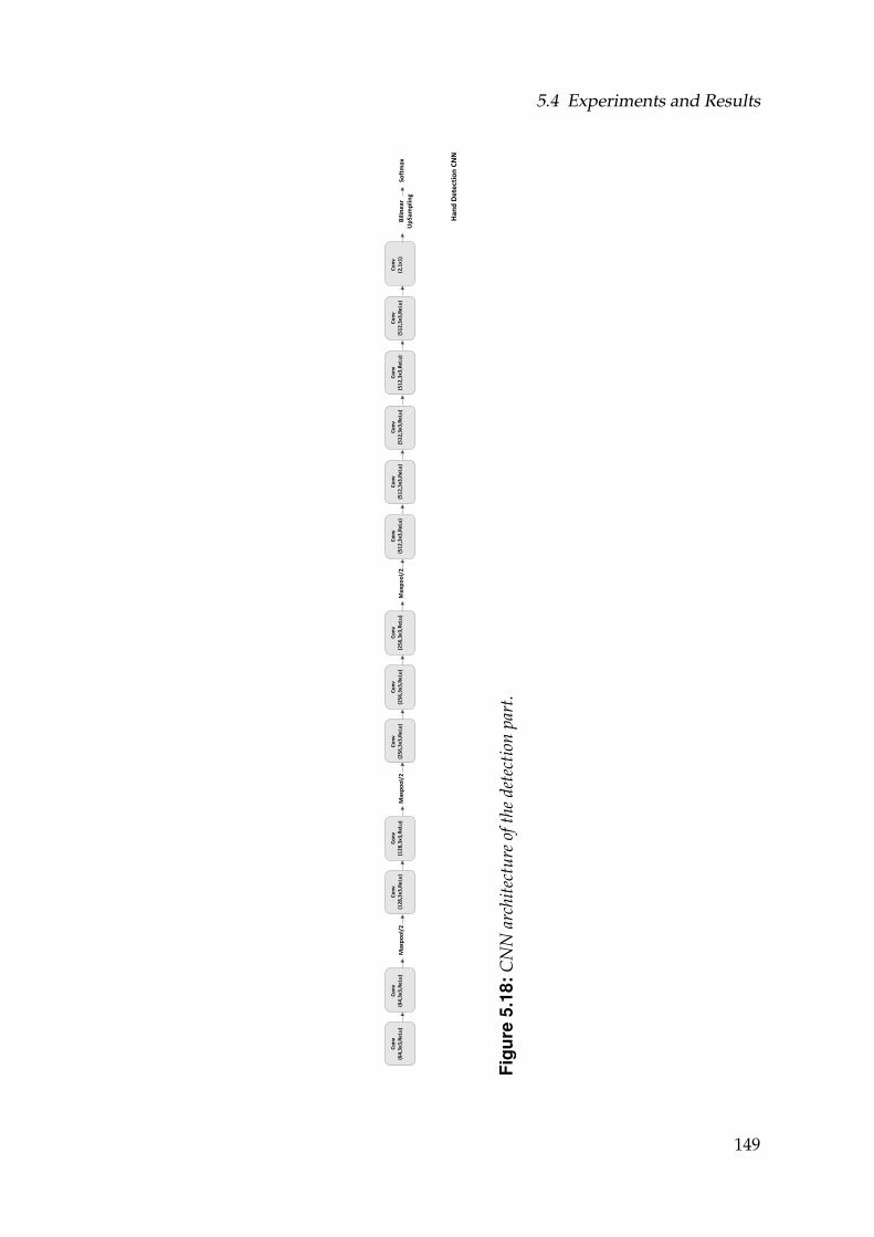
5.4 Experiments and Results
Max
po
ol/
2
Co
nv
(64
,3x3
,Re
Lu)
Co
nv
(64
,3x3
,Re
Lu)
Co
nv
(12
8,3
x3,R
eLu
)C
on
v(1
28
,3x3
,Re
Lu)
Co
nv
(25
6,3
x3,R
eLu
)C
on
v(2
56
,3x3
,Re
Lu)
Co
nv
(25
6,3
x3,R
eLu
)C
on
v(5
12
,3x3
,Re
Lu)
Co
nv
(51
2,3
x3,R
eLu
)C
on
v(5
12
,3x3
,Re
Lu)
Co
nv
(51
2,3
x3,R
eLu
)C
on
v(5
12
,3x3
,Re
Lu)
Co
nv
(2,1
x1)
Bili
ne
arU
pSa
mp
ling
Soft
max
Max
po
ol/
2M
axp
oo
l/2
Han
d D
ete
ctio
n C
NN
Figu
re5.
18:C
NN
arch
itect
ure
ofth
ede
tect
ion
part
.
149
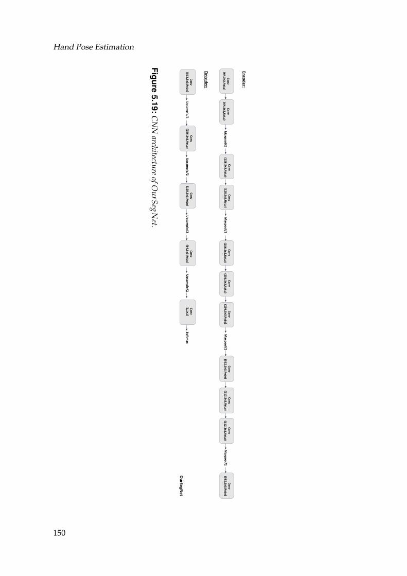
Hand Pose Estimation
Encoder:
OurSe
gNet
Conv
(512,3x3,ReLu)
Conv
(512,3x3,ReLu)
Maxp
ool/2
Conv
(64,3x3,ReLu)
Conv
(64,3x3,ReLu)
Conv
(128,3x3,ReLu)
Conv
(128,3x3,ReLu)
Maxp
ool/2
Conv
(256,3x3,ReLu)
Conv
(256,3x3,ReLu)
Conv
(256,3x3,ReLu)
Conv
(512,3x3,ReLu)
Conv
(512,3x3,ReLu)
Maxp
ool/2
Maxp
ool/2
Decoder:
Upsam
ple/2
Conv
(512,3x3,ReLu)
Conv
(256,3x3,ReLu)
Conv
(128,3x3,ReLu)
Conv
(64,3x3,ReLu)
Conv
(2,1x1)
Softm
axUpsam
ple/2
Upsam
ple/2
Upsam
ple/2
Figure5.19:C
NN
architectureofO
urSegNet.
150
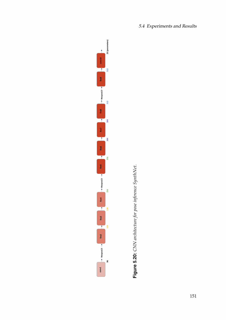
5.4 Experiments and Results
Max
po
ol/
2co
nv1
fire
2fi
re3
fire
4M
axp
oo
l/2
fire
5fi
re6
fire
7fi
re8
Max
po
ol/
2fi
re9
con
v10
96
12
81
28
25
62
56
38
43
84
51
25
12
23
(p
aram
ete
rs)
Figu
re5.
20:C
NN
arch
itect
ure
for
pose
infe
renc
eSy
nthN
et.
151
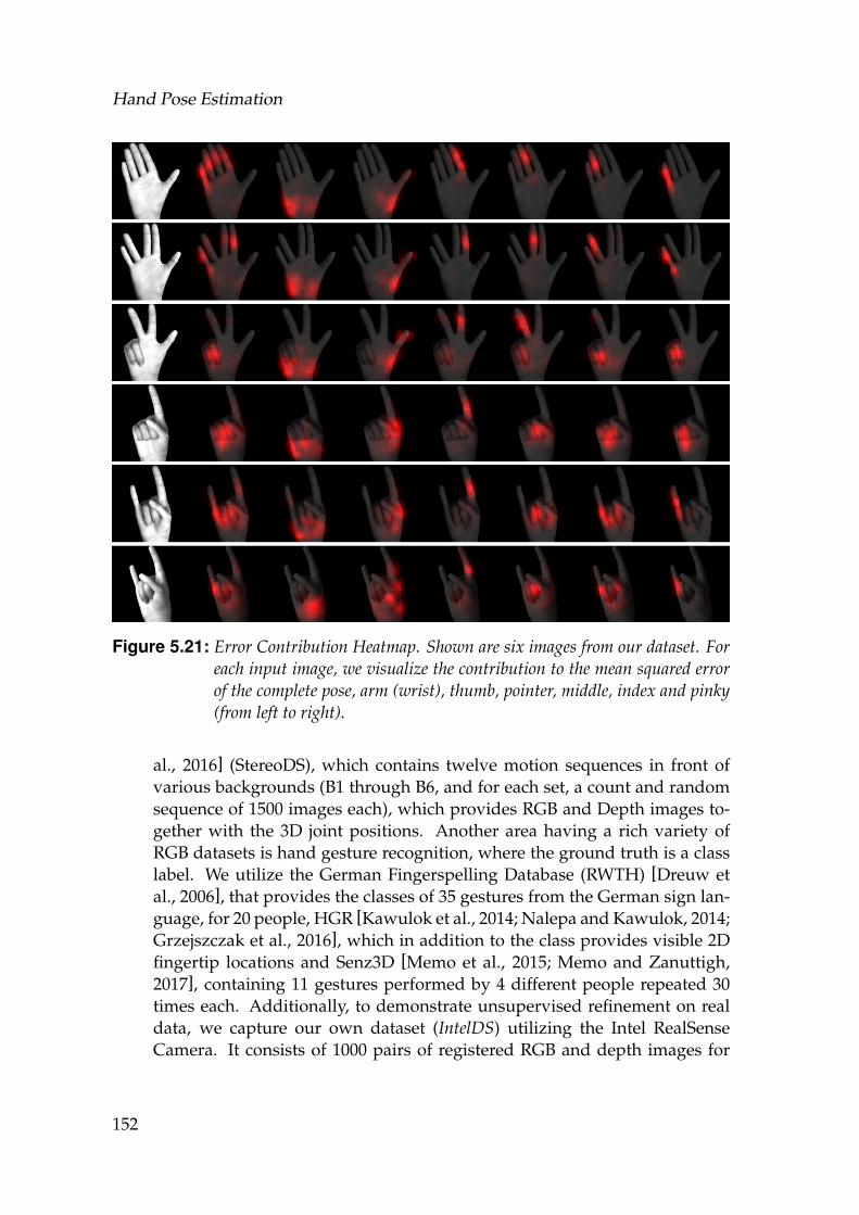
Hand Pose Estimation
Figure 5.21: Error Contribution Heatmap. Shown are six images from our dataset. Foreach input image, we visualize the contribution to the mean squared errorof the complete pose, arm (wrist), thumb, pointer, middle, index and pinky(from left to right).
al., 2016] (StereoDS), which contains twelve motion sequences in front ofvarious backgrounds (B1 through B6, and for each set, a count and randomsequence of 1500 images each), which provides RGB and Depth images to-gether with the 3D joint positions. Another area having a rich variety ofRGB datasets is hand gesture recognition, where the ground truth is a classlabel. We utilize the German Fingerspelling Database (RWTH) [Dreuw etal., 2006], that provides the classes of 35 gestures from the German sign lan-guage, for 20 people, HGR [Kawulok et al., 2014; Nalepa and Kawulok, 2014;Grzejszczak et al., 2016], which in addition to the class provides visible 2Dfingertip locations and Senz3D [Memo et al., 2015; Memo and Zanuttigh,2017], containing 11 gestures performed by 4 different people repeated 30times each. Additionally, to demonstrate unsupervised refinement on realdata, we capture our own dataset (IntelDS) utilizing the Intel RealSenseCamera. It consists of 1000 pairs of registered RGB and depth images for
152
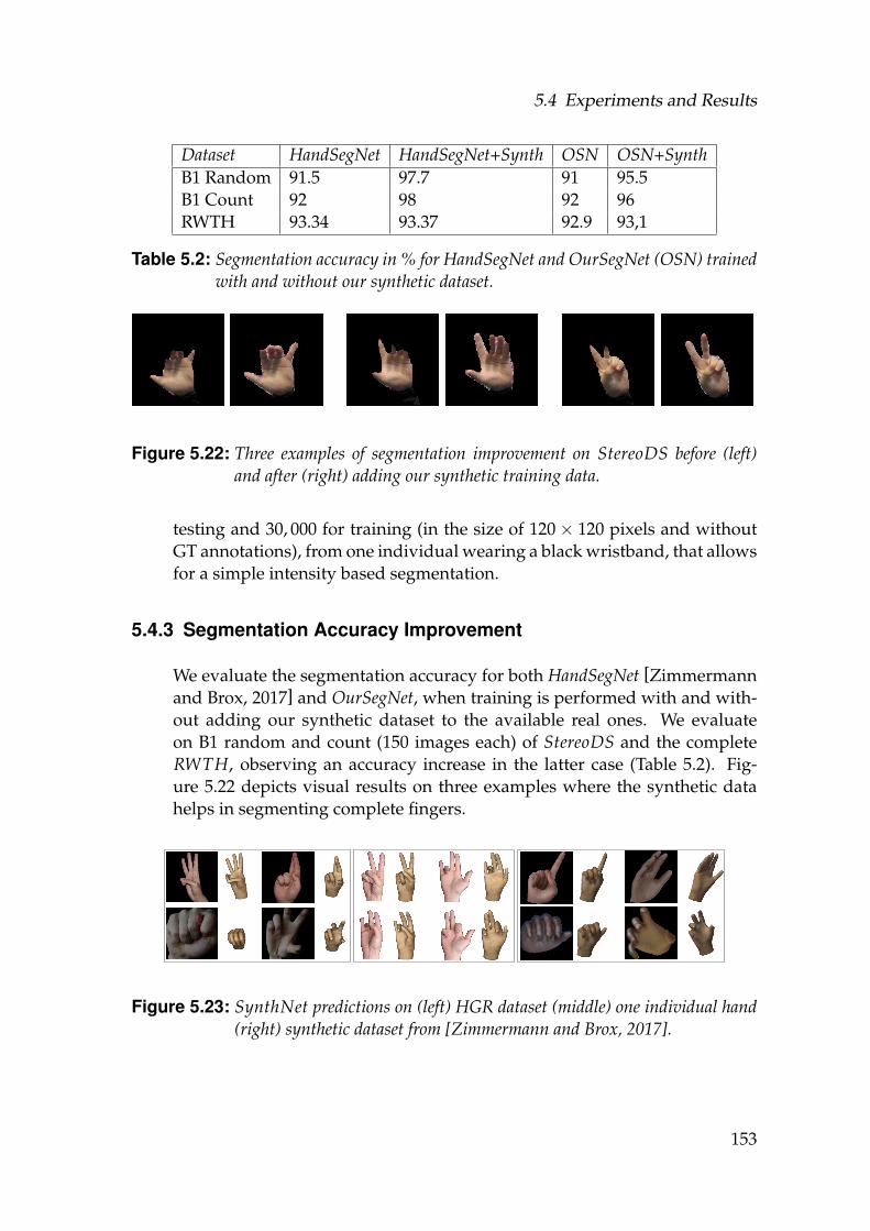
5.4 Experiments and Results
Dataset HandSegNet HandSegNet+Synth OSN OSN+SynthB1 Random 91.5 97.7 91 95.5B1 Count 92 98 92 96RWTH 93.34 93.37 92.9 93,1
Table 5.2: Segmentation accuracy in % for HandSegNet and OurSegNet (OSN) trainedwith and without our synthetic dataset.
Figure 5.22: Three examples of segmentation improvement on StereoDS before (left)and after (right) adding our synthetic training data.
testing and 30, 000 for training (in the size of 120× 120 pixels and withoutGT annotations), from one individual wearing a black wristband, that allowsfor a simple intensity based segmentation.
5.4.3 Segmentation Accuracy Improvement
We evaluate the segmentation accuracy for both HandSegNet [Zimmermannand Brox, 2017] and OurSegNet, when training is performed with and with-out adding our synthetic dataset to the available real ones. We evaluateon B1 random and count (150 images each) of StereoDS and the completeRWTH, observing an accuracy increase in the latter case (Table 5.2). Fig-ure 5.22 depicts visual results on three examples where the synthetic datahelps in segmenting complete fingers.
Figure 5.23: SynthNet predictions on (left) HGR dataset (middle) one individual hand(right) synthetic dataset from [Zimmermann and Brox, 2017].
153
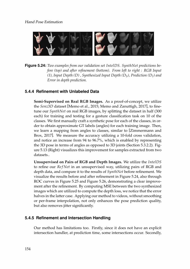
Hand Pose Estimation
Figure 5.24: Two examples from our validation set IntelDS. SynthNet predictions be-fore (top) and after refinement (bottom). From left to right : RGB Input(I), Input Depth (D) , Synthesized Input Depth (DS), Prediction (DI) andError in depth prediction.
5.4.4 Refinement with Unlabeled Data
Semi-Supervised on Real RGB Images. As a proof-of-concept, we utilizethe Senz3D dataset [Memo et al., 2015; Memo and Zanuttigh, 2017], to fine-tune our SynthNet on real RGB images, by splitting the dataset in half (300each) for training and testing for a gesture classification task on 10 of theclasses. We first manually craft a synthetic pose for each of the classes, in or-der to obtain approximate GT labels (angles) for each training image. Then,we learn a mapping from angles to classes, similar to [Zimmermann andBrox, 2017]. We measure the accuracy utilizing a 10-fold cross validation,and notice an increase from 94 to 96.7%, which is enabled by representingthe 3D pose in terms of angles as opposed to 3D joints (Section 5.3.2.2). Fig-ure 5.13 (Right) visualizes this improvement for samples extracted from twodatasets..
Unsupervised on Pairs of RGB and Depth Images. We utilize the IntelDSto refine our Re f Net in an unsupervised way, utilizing pairs of RGB anddepth data, and compare it to the results of SynthNet before refinement. Wevisualize the results before and after refinement in Figure 5.24, also throughROC curves in Figure 5.25 and Figure 5.26, demonstrating a clear improve-ment after the refinement. By computing MSE between the two synthesizedimages which are utilized to compute the depth loss, we notice that the errorhalves in the latter case. Applying our method to videos, without smoothingor per-frame interpolation, not only enhances the pose prediction quality,but also removes jitter significantly.
5.4.5 Refinement and Intersection Handling
Our method has limitations too. Firstly, since it does not have an explicitintersection handler, at prediction time, some intersections occur. Secondly,
154
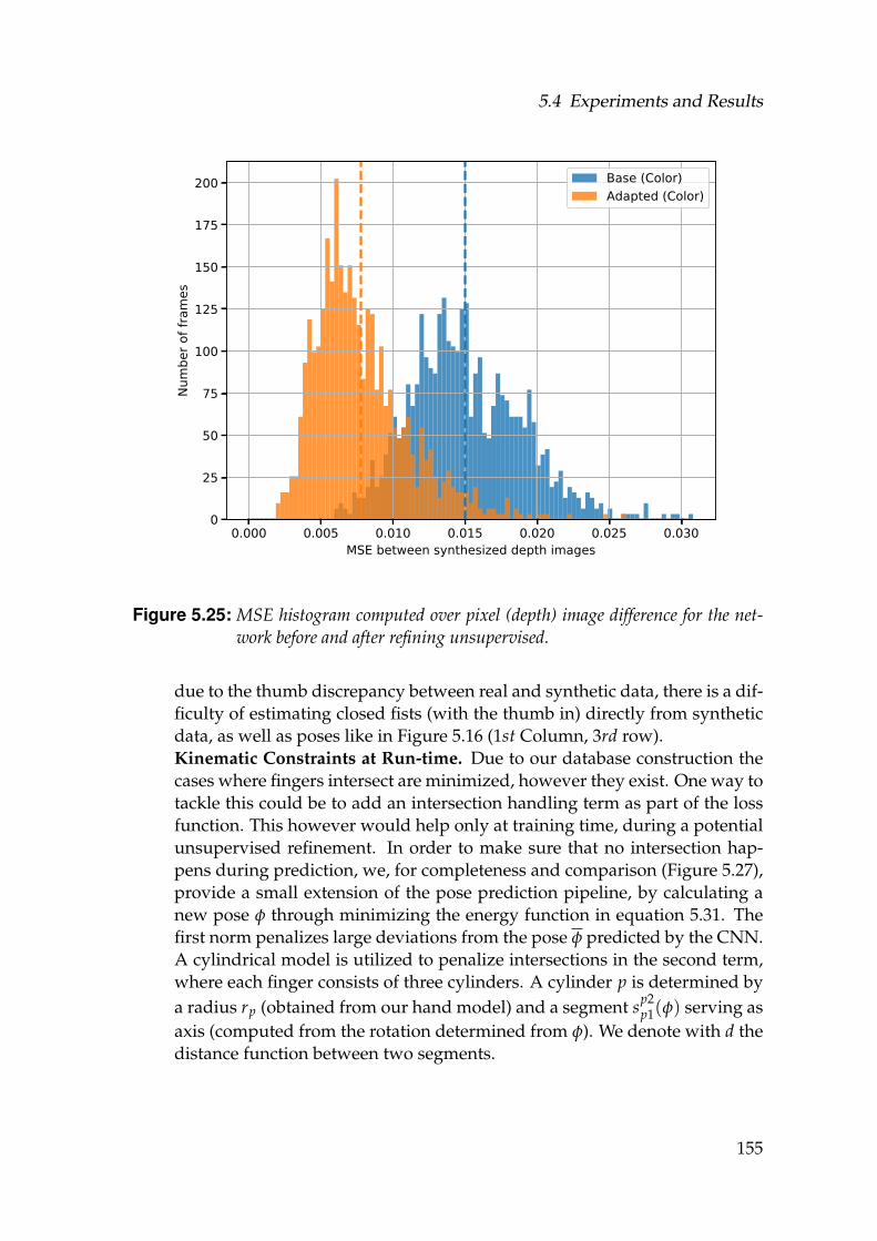
5.4 Experiments and Results
0.000 0.005 0.010 0.015 0.020 0.025 0.030MSE between synthesized depth images
0
25
50
75
100
125
150
175
200Nu
mbe
r of f
ram
esBase (Color)Adapted (Color)
Figure 5.25: MSE histogram computed over pixel (depth) image difference for the net-work before and after refining unsupervised.
due to the thumb discrepancy between real and synthetic data, there is a dif-ficulty of estimating closed fists (with the thumb in) directly from syntheticdata, as well as poses like in Figure 5.16 (1st Column, 3rd row).Kinematic Constraints at Run-time. Due to our database construction thecases where fingers intersect are minimized, however they exist. One way totackle this could be to add an intersection handling term as part of the lossfunction. This however would help only at training time, during a potentialunsupervised refinement. In order to make sure that no intersection hap-pens during prediction, we, for completeness and comparison (Figure 5.27),provide a small extension of the pose prediction pipeline, by calculating anew pose φ through minimizing the energy function in equation 5.31. Thefirst norm penalizes large deviations from the pose φ predicted by the CNN.A cylindrical model is utilized to penalize intersections in the second term,where each finger consists of three cylinders. A cylinder p is determined bya radius rp (obtained from our hand model) and a segment sp2
p1(φ) serving asaxis (computed from the rotation determined from φ). We denote with d thedistance function between two segments.
155
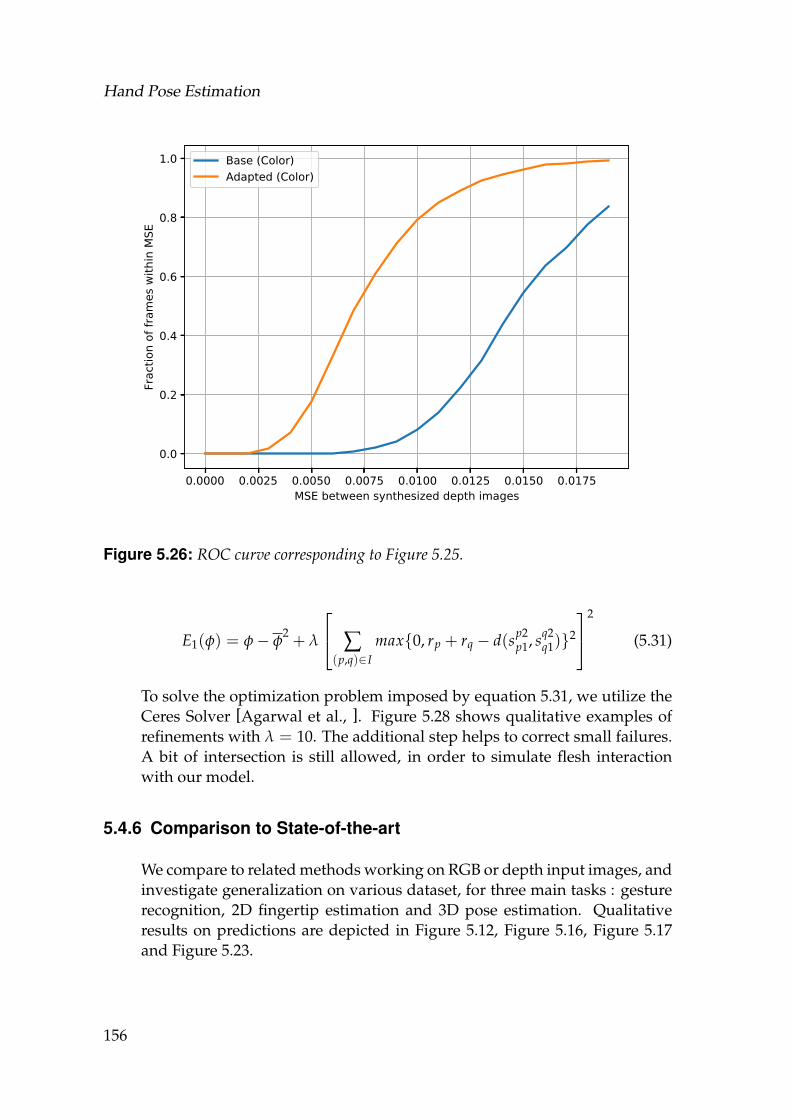
Hand Pose Estimation
0.0000 0.0025 0.0050 0.0075 0.0100 0.0125 0.0150 0.0175MSE between synthesized depth images
0.0
0.2
0.4
0.6
0.8
1.0Fr
actio
n of
fram
es w
ithin
MSE
Base (Color)Adapted (Color)
Figure 5.26: ROC curve corresponding to Figure 5.25.
E1(φ) = φ− φ2+ λ
∑(p,q)∈I
max{0, rp + rq − d(sp2p1, sq2
q1)}2
2
(5.31)
To solve the optimization problem imposed by equation 5.31, we utilize theCeres Solver [Agarwal et al., ]. Figure 5.28 shows qualitative examples ofrefinements with λ = 10. The additional step helps to correct small failures.A bit of intersection is still allowed, in order to simulate flesh interactionwith our model.
5.4.6 Comparison to State-of-the-art
We compare to related methods working on RGB or depth input images, andinvestigate generalization on various dataset, for three main tasks : gesturerecognition, 2D fingertip estimation and 3D pose estimation. Qualitativeresults on predictions are depicted in Figure 5.12, Figure 5.16, Figure 5.17and Figure 5.23.
156
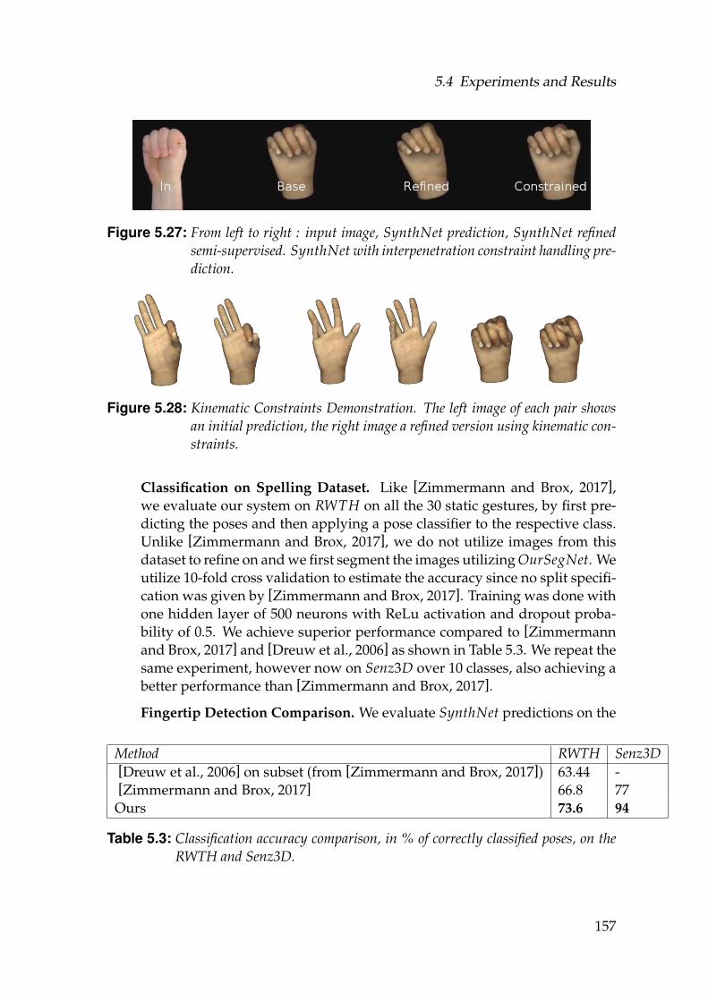
5.4 Experiments and Results
Figure 5.27: From left to right : input image, SynthNet prediction, SynthNet refinedsemi-supervised. SynthNet with interpenetration constraint handling pre-diction.
Figure 5.28: Kinematic Constraints Demonstration. The left image of each pair showsan initial prediction, the right image a refined version using kinematic con-straints.
Classification on Spelling Dataset. Like [Zimmermann and Brox, 2017],we evaluate our system on RWTH on all the 30 static gestures, by first pre-dicting the poses and then applying a pose classifier to the respective class.Unlike [Zimmermann and Brox, 2017], we do not utilize images from thisdataset to refine on and we first segment the images utilizing OurSegNet. Weutilize 10-fold cross validation to estimate the accuracy since no split specifi-cation was given by [Zimmermann and Brox, 2017]. Training was done withone hidden layer of 500 neurons with ReLu activation and dropout proba-bility of 0.5. We achieve superior performance compared to [Zimmermannand Brox, 2017] and [Dreuw et al., 2006] as shown in Table 5.3. We repeat thesame experiment, however now on Senz3D over 10 classes, also achieving abetter performance than [Zimmermann and Brox, 2017].
Fingertip Detection Comparison. We evaluate SynthNet predictions on the
Method RWTH Senz3D[Dreuw et al., 2006] on subset (from [Zimmermann and Brox, 2017]) 63.44 -[Zimmermann and Brox, 2017] 66.8 77
Ours 73.6 94
Table 5.3: Classification accuracy comparison, in % of correctly classified poses, on theRWTH and Senz3D.
157
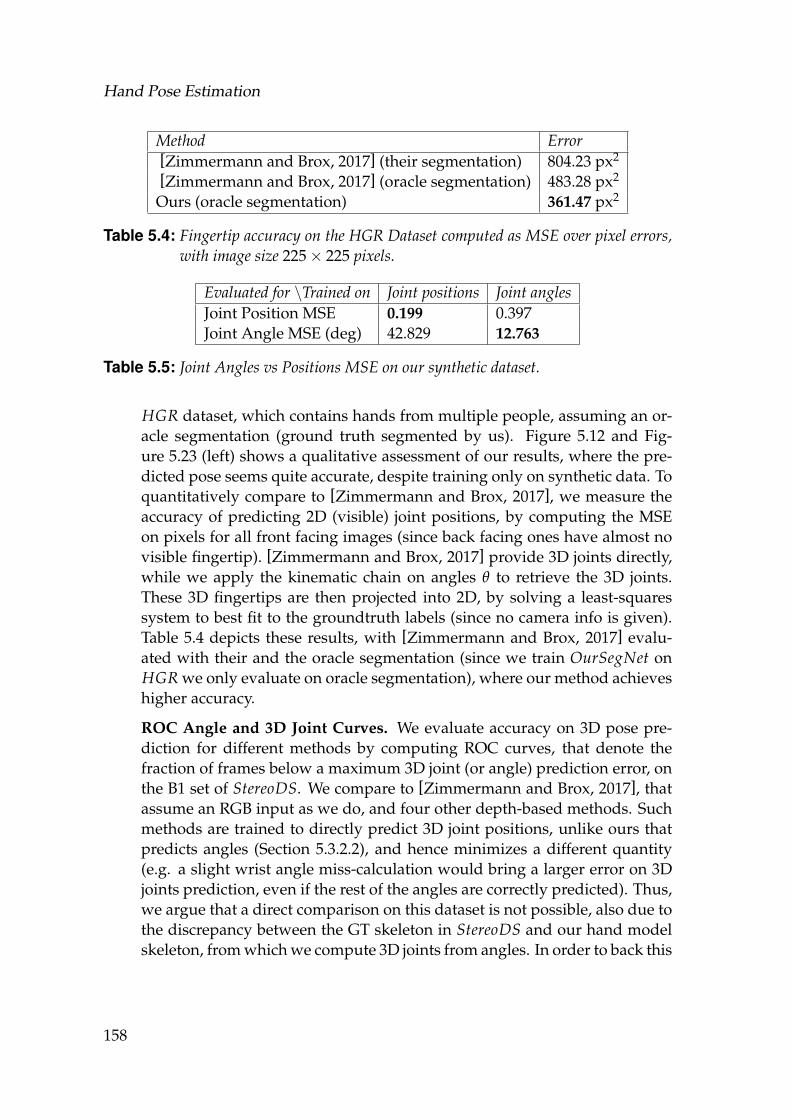
Hand Pose Estimation
Method Error[Zimmermann and Brox, 2017] (their segmentation) 804.23 px2
[Zimmermann and Brox, 2017] (oracle segmentation) 483.28 px2
Ours (oracle segmentation) 361.47 px2
Table 5.4: Fingertip accuracy on the HGR Dataset computed as MSE over pixel errors,with image size 225× 225 pixels.
Evaluated for \Trained on Joint positions Joint anglesJoint Position MSE 0.199 0.397Joint Angle MSE (deg) 42.829 12.763
Table 5.5: Joint Angles vs Positions MSE on our synthetic dataset.
HGR dataset, which contains hands from multiple people, assuming an or-acle segmentation (ground truth segmented by us). Figure 5.12 and Fig-ure 5.23 (left) shows a qualitative assessment of our results, where the pre-dicted pose seems quite accurate, despite training only on synthetic data. Toquantitatively compare to [Zimmermann and Brox, 2017], we measure theaccuracy of predicting 2D (visible) joint positions, by computing the MSEon pixels for all front facing images (since back facing ones have almost novisible fingertip). [Zimmermann and Brox, 2017] provide 3D joints directly,while we apply the kinematic chain on angles θ to retrieve the 3D joints.These 3D fingertips are then projected into 2D, by solving a least-squaressystem to best fit to the groundtruth labels (since no camera info is given).Table 5.4 depicts these results, with [Zimmermann and Brox, 2017] evalu-ated with their and the oracle segmentation (since we train OurSegNet onHGR we only evaluate on oracle segmentation), where our method achieveshigher accuracy.
ROC Angle and 3D Joint Curves. We evaluate accuracy on 3D pose pre-diction for different methods by computing ROC curves, that denote thefraction of frames below a maximum 3D joint (or angle) prediction error, onthe B1 set of StereoDS. We compare to [Zimmermann and Brox, 2017], thatassume an RGB input as we do, and four other depth-based methods. Suchmethods are trained to directly predict 3D joint positions, unlike ours thatpredicts angles (Section 5.3.2.2), and hence minimizes a different quantity(e.g. a slight wrist angle miss-calculation would bring a larger error on 3Djoints prediction, even if the rest of the angles are correctly predicted). Thus,we argue that a direct comparison on this dataset is not possible, also due tothe discrepancy between the GT skeleton in StereoDS and our hand modelskeleton, from which we compute 3D joints from angles. In order to back this
158
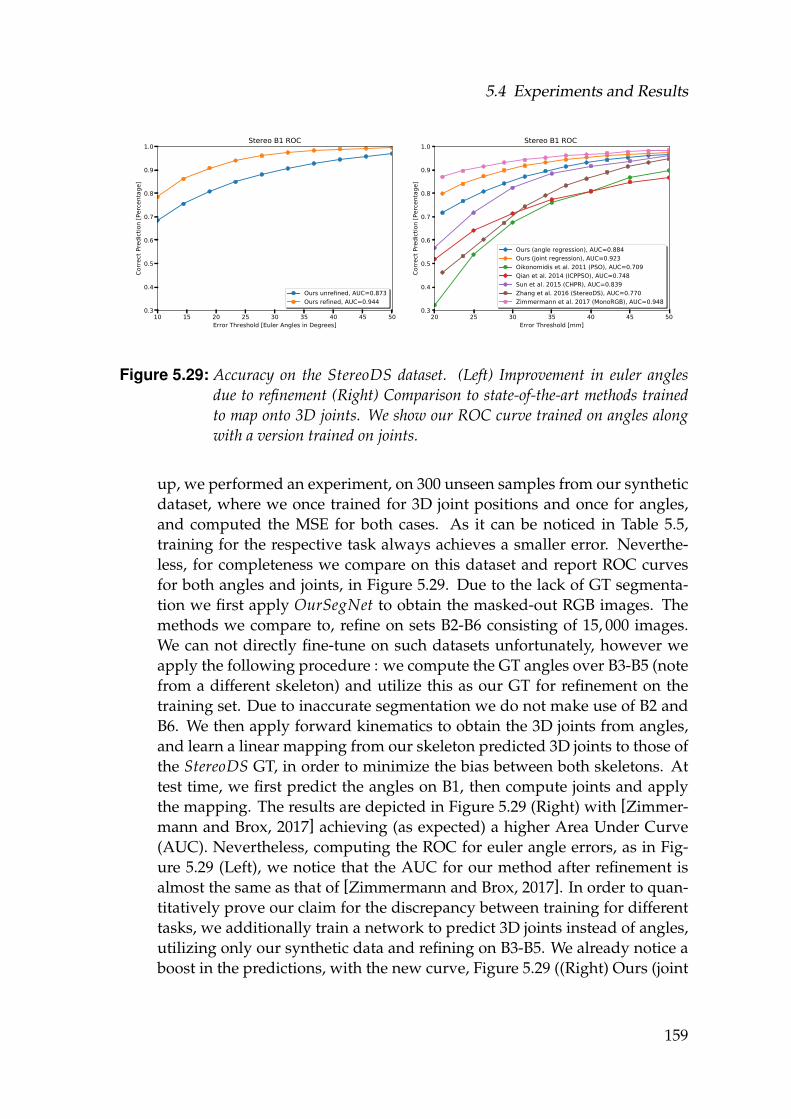
5.4 Experiments and Results
10 15 20 25 30 35 40 45 50Error Threshold [Euler Angles in Degrees]
0.3
0.4
0.5
0.6
0.7
0.8
0.9
1.0Co
rrect Prediction [Percentage]
Stereo B1 ROC
Ours unrefined, AUC=0.873Ours refined, AUC=0.944
20 25 30 35 40 45 50Error Threshold [mm]
0.3
0.4
0.5
0.6
0.7
0.8
0.9
1.0
Corre
ct Prediction [Percentage]
Stereo B1 ROC
Ours (angle regression), AUC=0.884Ours (joint regression), AUC=0.923Oikonomidis et al. 2011 (PSO), AUC=0.709Qian et al. 2014 (ICPPSO), AUC=0.748Sun et al. 2015 (CHPR), AUC=0.839Zhang et al. 2016 (StereoDS), AUC=0.770Zimmermann et al. 2017 (MonoRGB), AUC=0.948
Figure 5.29: Accuracy on the StereoDS dataset. (Left) Improvement in euler anglesdue to refinement (Right) Comparison to state-of-the-art methods trainedto map onto 3D joints. We show our ROC curve trained on angles alongwith a version trained on joints.
up, we performed an experiment, on 300 unseen samples from our syntheticdataset, where we once trained for 3D joint positions and once for angles,and computed the MSE for both cases. As it can be noticed in Table 5.5,training for the respective task always achieves a smaller error. Neverthe-less, for completeness we compare on this dataset and report ROC curvesfor both angles and joints, in Figure 5.29. Due to the lack of GT segmenta-tion we first apply OurSegNet to obtain the masked-out RGB images. Themethods we compare to, refine on sets B2-B6 consisting of 15, 000 images.We can not directly fine-tune on such datasets unfortunately, however weapply the following procedure : we compute the GT angles over B3-B5 (notefrom a different skeleton) and utilize this as our GT for refinement on thetraining set. Due to inaccurate segmentation we do not make use of B2 andB6. We then apply forward kinematics to obtain the 3D joints from angles,and learn a linear mapping from our skeleton predicted 3D joints to those ofthe StereoDS GT, in order to minimize the bias between both skeletons. Attest time, we first predict the angles on B1, then compute joints and applythe mapping. The results are depicted in Figure 5.29 (Right) with [Zimmer-mann and Brox, 2017] achieving (as expected) a higher Area Under Curve(AUC). Nevertheless, computing the ROC for euler angle errors, as in Fig-ure 5.29 (Left), we notice that the AUC for our method after refinement isalmost the same as that of [Zimmermann and Brox, 2017]. In order to quan-titatively prove our claim for the discrepancy between training for differenttasks, we additionally train a network to predict 3D joints instead of angles,utilizing only our synthetic data and refining on B3-B5. We already notice aboost in the predictions, with the new curve, Figure 5.29 ((Right) Ours (joint
159
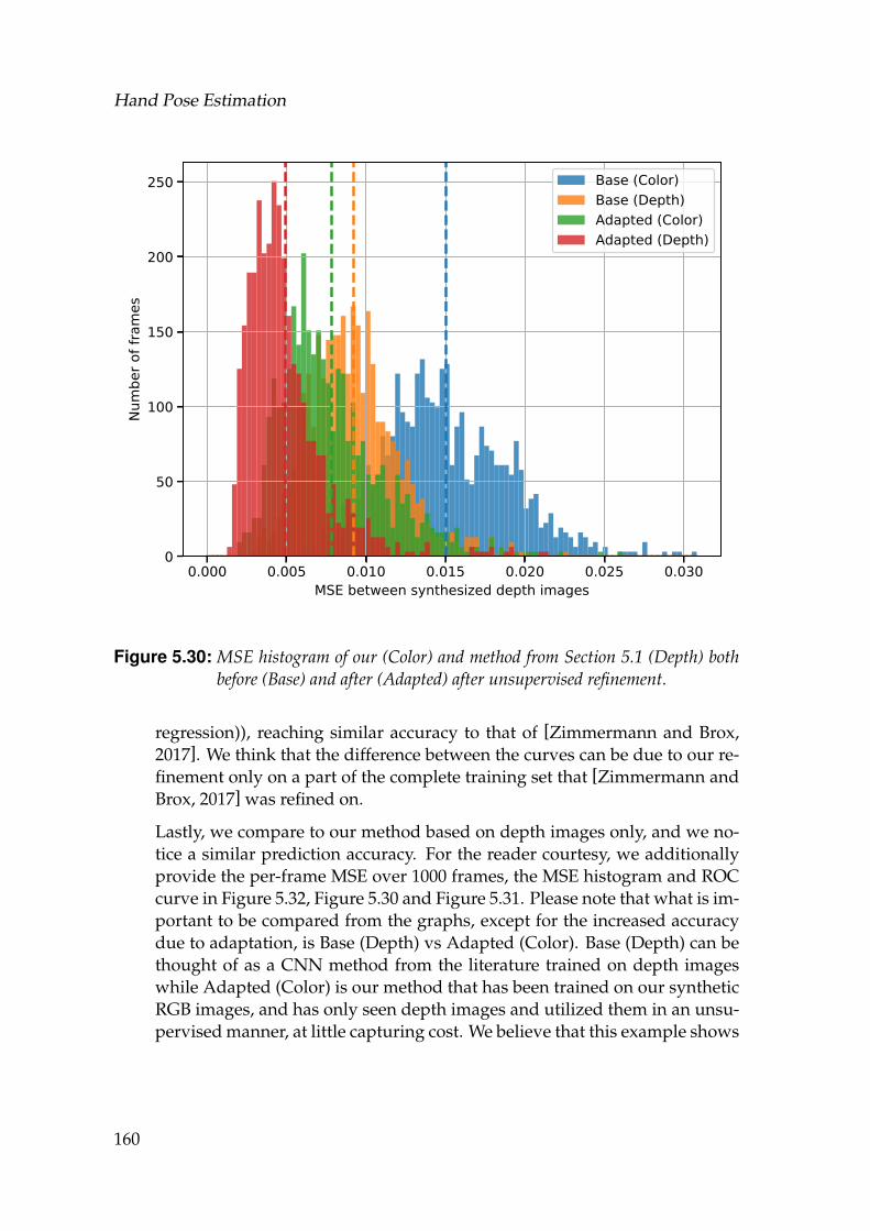
Hand Pose Estimation
0.000 0.005 0.010 0.015 0.020 0.025 0.030MSE between synthesized depth images
0
50
100
150
200
250
Num
ber o
f fra
mes
Base (Color)Base (Depth)Adapted (Color)Adapted (Depth)
Figure 5.30: MSE histogram of our (Color) and method from Section 5.1 (Depth) bothbefore (Base) and after (Adapted) after unsupervised refinement.
regression)), reaching similar accuracy to that of [Zimmermann and Brox,2017]. We think that the difference between the curves can be due to our re-finement only on a part of the complete training set that [Zimmermann andBrox, 2017] was refined on.
Lastly, we compare to our method based on depth images only, and we no-tice a similar prediction accuracy. For the reader courtesy, we additionallyprovide the per-frame MSE over 1000 frames, the MSE histogram and ROCcurve in Figure 5.32, Figure 5.30 and Figure 5.31. Please note that what is im-portant to be compared from the graphs, except for the increased accuracydue to adaptation, is Base (Depth) vs Adapted (Color). Base (Depth) can bethought of as a CNN method from the literature trained on depth imageswhile Adapted (Color) is our method that has been trained on our syntheticRGB images, and has only seen depth images and utilized them in an unsu-pervised manner, at little capturing cost. We believe that this example shows
160
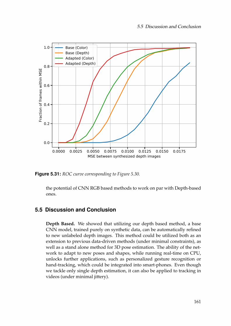
5.5 Discussion and Conclusion
0.0000 0.0025 0.0050 0.0075 0.0100 0.0125 0.0150 0.0175MSE between synthesized depth images
0.0
0.2
0.4
0.6
0.8
1.0
Frac
tion
of fr
ames
with
in M
SE
Base (Color)Base (Depth)Adapted (Color)Adapted (Depth)
Figure 5.31: ROC curve corresponding to Figure 5.30.
the potential of CNN RGB based methods to work on par with Depth-basedones.
5.5 Discussion and Conclusion
Depth Based. We showed that utilizing our depth based method, a baseCNN model, trained purely on synthetic data, can be automatically refinedto new unlabeled depth images. This method could be utilized both as anextension to previous data-driven methods (under minimal constraints), aswell as a stand alone method for 3D pose estimation. The ability of the net-work to adapt to new poses and shapes, while running real-time on CPU,unlocks further applications, such as personalized gesture recognition orhand-tracking, which could be integrated into smart-phones. Even thoughwe tackle only single depth estimation, it can also be applied to tracking invideos (under minimal jittery).
161
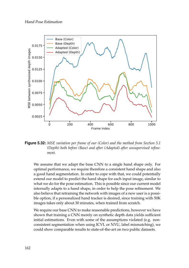
Hand Pose Estimation
0 200 400 600 800 1000Frame index
0.0025
0.0050
0.0075
0.0100
0.0125
0.0150
0.0175
MSE
bet
ween
synt
hesiz
ed d
epth
imag
es
Base (Color)Base (Depth)Adapted (Color)Adapted (Depth)
Figure 5.32: MSE variation per frame of our (Color) and the method from Section 5.1(Depth) both before (Base) and after (Adapted) after unsupervised refine-ment.
We assume that we adapt the base CNN to a single hand shape only. Foroptimal performance, we require therefore a consistent hand shape and alsoa good hand segmentation. In order to cope with that, we could potentiallyextend our model to predict the hand shape for each input image, similar towhat we do for the pose estimation. This is possible since our current modelinternally adapts to a hand shape, in order to help the pose refinement. Wealso believe that retraining the network with images of a new user is a possi-ble option, if a personalized hand tracker is desired, since training with 50Kimages takes only about 30 minutes, when trained from scratch.
We require our base CNN to make reasonable predictions, however we haveshown that training a CNN merely on synthetic depth data yields sufficientinitial estimations. Even with some of the assumptions violated (e.g. non-consistent segmentation when using ICVL or NYU, label mismatching), wecould show comparable results to state-of-the-art on two public datasets.
162
5.5 Discussion and Conclusion
RGB Based. When we switched from Depth to RGB input, we showed,through quantitative and qualitative evaluations, that lightweight CNN-s,trained purely on our newly proposed synthetic dataset, can achieve accu-rate pose inference for a variety of tasks, strongly competing with and evenoutperforming existing state-of-the-art. We additionally showed that by ex-tending its construction with a depth loss component, coupled with our poserepresentation, the accuracy is further improved via semi-supervised andunsupervised training with real unlabeled images. At the moment, we uti-lize training data generated from a single shape hand model. Despite thefact that we could show generalization on multiple real hands, and goodaccuracy especially on classification tasks, there is still room for improve-ment, e.g. experimenting with adding a second shape improved predictionon HGR by 10%. Our current optimization model allows an internal adap-tation to a hand shape, as in the Depth based case. Coupling our methodwith recent and more powerful hand shape models such as [Tkach et al.,2016] and [Romero et al., 2017]’s has the potential to improve and personal-ize hand pose estimation for a variety of human hand shapes.
Even though we showed improvements in segmentation, based on the syn-thetic dataset, most of it is due to the real GT training data we annotated. Asalso backed up by our refinement experiments, further real GT datasets withsegmentation and pose annotations are very important. Our technique canalso be seen as an economic and automatic way of creating a ground truthlabeled dataset and we believe will be instrumental in creating new datasetsas well.
Lastly, we envisage that both presented methods could be applied, withoutloss of generality, to human pose estimation tasks under minimal changes tothe underlying 3D model representation and architecture.
163

Hand Pose Estimation
164
C H A P T E R 6Conclusion
In this thesis, we investigated the problem of reconstructing the 3D virtualhuman from monocular imagery, mainly coming from an RGB sensor. In-stead of following a holistic approach, we separately considered three con-stituting parts of the human avatar: the naked body, clothing and the humanhand, considering that the human face has received more attention from thecommunity. We mainly focused on the estimation of the 3D shape and posefrom 2D images, potentially taken from a smart-phone, and throughout thethesis we utilized discriminative methods to find these mappings, focusingon CNNs, with the intention of preserving low run-times. We leveragedfrom existing and realistically synthesized datasets to learn important statis-tics and data-driven priors that can generalize well and provide accuratereconstructions on unseen real input data. Through this process, we did notonly base on single views and annotated groundtruth data for supervisedlearning. We also showed how to utilize multiple views simultaneously,and more importantly how to leverage from multiple views during trainingtime, in order to boost performance achieved from a single view at infer-ence time. On top of that, we demonstrated that learning and refining un-supervised with unlabeled real data is possible, by integrating lightweightdifferentiable renderers into CNNs.
With respect to the naked body, our aim was to estimate the intrinsic bodyshape, regardless of the adopted pose, with applications in mind such asshape from selfies, health monitoring and garment fitting. For this, we as-sumed that the human is depicted in a picture in uniform background, mak-ing it possible for a reliable silhouette extraction to be achievable with stan-dard methods, allowing poses under minimal self-occlusion. We tackled this
165
Conclusion
problem with three different approaches: one based on handcrafted featuresin combination with CCA and random forest regressors, a second one basedon simple standard CNNs, and a third one based on more involved CNNswith generative and cross-modal components. We showed robustness topose changes, silhouette noise and state-of-the-art performance on existingdatasets, outperforming also optimization based methods.
We then, tackled the estimation of garment shape from one or two images.Without loss of generalization, we assumed a t-shirt and a dress as our rep-resentative clothing whose shape is to be estimated. The images were seg-mented with standard techniques, under uniform background assumptions.We provided two possible estimations of the garment shape, one that getsdeformed from a template garment and another one that gets deformed fromthe underlying body, providing empirical evidence of the advantages in us-ing one versus the other. We utilized lightweight CNNs in combination witha new realistically rendered garment dataset synthesized under physicallycorrect assumptions, also due to dynamics, to tackle this very difficult prob-lem. Despite training only on synthetic data, to the best of our knowledge,we were the first to show that garment shape estimation also from real im-ages is possible through CNNs.
Lastly, we looked into the problem of inferring a 3D hand pose from an RGBor Depth image. To this end, we proposed an end-to-end CNN system thatleveraged from our newly proposed realistically rendered free hand dataset,consisting of 3 Million samples of hands in various poses, orientations, tex-tures and illuminations. This dataset proved to be helpful not only for poseinference tasks, but it also improved hand segmentation. We did not confineourselves to a fully supervised training with only synthetic data. Instead, weintroduced network components based on differentiable renderers that en-abled us to train and refine our networks with unlabeled real images in anunsupervised fashion, showing clear improvements. Maintaining simplic-ity, we could show on-par and improved performance over state-of-the-artmethods for two input modalities, under various tasks varying from 3D poseestimation to gesture recognition.
6.1 Limitations and Outlook
Some of the limitations and potential future directions of the methods pre-sented in this thesis were already mentioned in the ending sections of eachchapter. Here, we repeat and extend them by presenting some general andmore specific future directions that tackle the current limitations that ourmethods have.
166
6.1 Limitations and Outlook
Body Shape Estimation. Throughout this work we made use of one ofthe first human body parametric models based on SCAPE [Anguelov etal., 2005]. While this served our purpose, a trivial extension would be toincorporate, more efficient, compact and faster models [Loper et al., 2015]that have been developed since then and have been applied to similartasks [Bogo et al., 2016a]. Additionally, our template model was based onthe mean mesh stemming from both female and male population. Learningtwo separate models would definitely improve inference for the respectivetasks.
We decoupled intrinsic shape from shape deformations due to pose changes.While this suffices for the intended applications that we presented, peoplecome in a great variety of poses in everyday life, hence looking into thesetwo problems simultaneously is advantageous. Another point rooting forthis approach is that most of the works focusing on 3D human pose estima-tion, represent poses in terms of simple 3D joints and stick figures, whichcould in reality result in unrealistic human body shapes or even body inter-penetration, as also motivated by [Bogo et al., 2016a]. A combination of theseand our methods in a hybrid fashion or even completely through CNNs isan interesting area to explore.
We considered here a binary silhouette as our input from where the bodyshape is inferred. In order to simplify the problem, we deliberately didnot consider very important cues such as shading and texture. This de-cision was based on a couple of factors: a) a silhouette is the most rep-resentative cue or feature of the human body, b) there existed only nakedavailable scans of human bodies, despite the fact that humans are gener-ally depicted with clothing in images. Hence, no ground truth correspon-dences could be established between images and shapes. Under tight cloth-ing assumptions, a silhouette alleviated this problem. With current ad-vances in datasets, capturing and modeling, it is now possible to look atthe very same problem, however considering the full RGB image. Utiliz-ing the methods from the first chapter, coupled with unsupervised tech-niques from the third chapter, annotated datasets [Lassner et al., 2017b;Varol et al., 2017], differentiable rendering [Loper and Black, 2014] and gen-erative models [Lassner et al., 2017a], is a direction worth exploring. Basedon previous [Balan and Black, 2008] and current [Zhang et al., 2017] worksthat try to estimate the body shape under clothing from multiple camerasor scanners, we could exploit human body shape priors and trained net-works also for monocular imagery. Furthermore, similar to recent work onfaces [Tewari et al., 2017], one could think of applying autoencoders anddiscriminator components to estimate pose, shape, reflectance, lighting andcamera parameters simultaneously.
167
Conclusion
Despite the necessity of estimating shape from a single image, for more con-sistent shape estimations, we believe that multiple instances of the same per-son need to be taken into account at various time stamps, and potentiallyby considering more poses. This brings us towards videos, where not onlytemporal consistency could be exploited, but also dynamics [Pons-Moll etal., 2015], which we did not explore here. Lastly, in our attempt to utilizedata-driven techniques, which are typically based on sensor data (image in-puts or body scans), we discarded real-world priors. We could leverage froma well understood knowledge, gathered in the last century, about the innerworkings of the human body. Hence, as a continuation, instead of utilizingsurface or volumetric based meodels, we are exploring anatomically correctbody models, e.g. [Kadlecek et al., 2016], which are useful not only for thetask of anatomically correct human shape estimation from RGB images, butalso for extrapolation of secondary motion and interaction with external ob-jects and forces.
Garment Shape Estimation. For the task of garment shape estimation, werelied on a data generation pipeline where the deformation of the humanbody shape and thus the garment is given by a standard skinning modelwith automatically computed weights and simple blending of bone transfor-mations. These steps introduce certain artifacts. In order to avoid skinningproblems, a very reasonable choice would be to use a more compact humanbody model [Loper et al., 2015] that allows baking it with ready made mo-tion capture systems. We also used an off-the-shelf physical simulator forcloth deformation, with default parameters, few material properties and tar-geted to one clothing type. Better and tailored databases can be obtained byimproving these steps, and considering accurate cloth parameters. The per-formance of our data-driven approach can only be as good as the trainingdataset. The more realistic and general the dataset becomes the more detailscan be captured.
Our method relies on segmented garments from an image, although it toler-ates a certain amount of noise and moderately textured garments. By train-ing on more data covering a larger variety of cases and coupling it withtechniques based on GANs [Lassner et al., 2017a], the method can be ex-tended to handle complex textures and unsegmented images. Additionally,the networks were trained with relatively small input images, which pre-vented us from capturing high-frequency details, e.g. wrinkles. Our cur-rent method could be augmented with local wrinkle regressors similar tothe work by [Cao et al., 2015], under the assumption of a known cameracalibration. With the current progress in the compactness of CNN represen-tations and utilizing recently captured cloth datasets from scans [Pons-Mollet al., 2017], we believe that most of the above difficulties can be resolved.
168
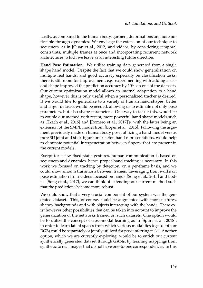
6.1 Limitations and Outlook
Lastly, as compared to the human body, garment deformations are more no-ticeable through dynamics. We envisage the extension of our technique tosequences, as in [Guan et al., 2012] and videos, by considering temporalconstraints, multiple frames at once and incorporating recurrent networkarchitectures, which we leave as an interesting future direction.
Hand Pose Estimation. We utilize training data generated from a singleshape hand model. Despite the fact that we could show generalization onmultiple real hands, and good accuracy especially on classification tasks,there is still room for improvement, e.g. experimenting with adding a sec-ond shape improved the prediction accuracy by 10% on one of the datasets.Our current optimization model allows an internal adaptation to a handshape, however this is only useful when a personalized tracker is desired.If we would like to generalize to a variety of human hand shapes, betterand larger datasets would be needed, allowing us to estimate not only poseparameters, but also shape parameters. One way to tackle this, would beto couple our method with recent, more powerful hand shape models suchas [Tkach et al., 2016] and [Romero et al., 2017]’s, with the latter being anextension of the SMPL model from [Loper et al., 2015]. Following the argu-ment previously made on human body pose, utilizing a hand model versuspure 3D joint and stick-figure or skeleton hand representations, would helpto eliminate potential interpenetration between fingers, that are present inthe current models.
Except for a few fixed static gestures, human communication is based onsequences and dynamics, hence proper hand tracking is necessary. In thiswork we focused on tracking by detection, on a per-frame basis, and wecould show smooth transitions between frames. Leveraging from works onpose estimation from videos focused on hands [Song et al., 2015] and bod-ies [Song et al., 2017], we can think of extending our current method suchthat the predictions become more robust.
We could show that a very crucial component of our system was the gen-erated dataset. This, of course, could be augmented with more textures,shapes, backgrounds and with objects interacting with the hands. There ex-ist however other possibilities that can be taken into account to improve thegeneralization of the networks trained on such datasets. One option wouldbe to utilize the concept of cross-modal learning as in [Spurr et al., 2018],in order to learn latent spaces from which various modalities (e.g. depth orRGB) could be separately or jointly utilized for pose inferring tasks. Anotheroption, which we are currently exploring, would be to enrich our currentsynthetically generated dataset through GANs, by learning mappings fromsynthetic to real images that do not have one-to-one correspondences. In this
169
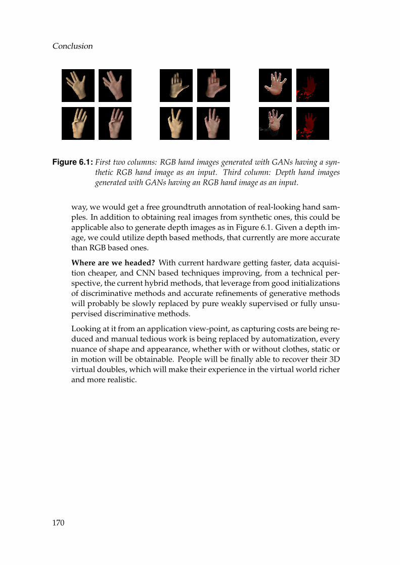
Conclusion
Figure 6.1: First two columns: RGB hand images generated with GANs having a syn-thetic RGB hand image as an input. Third column: Depth hand imagesgenerated with GANs having an RGB hand image as an input.
way, we would get a free groundtruth annotation of real-looking hand sam-ples. In addition to obtaining real images from synthetic ones, this could beapplicable also to generate depth images as in Figure 6.1. Given a depth im-age, we could utilize depth based methods, that currently are more accuratethan RGB based ones.
Where are we headed? With current hardware getting faster, data acquisi-tion cheaper, and CNN based techniques improving, from a technical per-spective, the current hybrid methods, that leverage from good initializationsof discriminative methods and accurate refinements of generative methodswill probably be slowly replaced by pure weakly supervised or fully unsu-pervised discriminative methods.
Looking at it from an application view-point, as capturing costs are being re-duced and manual tedious work is being replaced by automatization, everynuance of shape and appearance, whether with or without clothes, static orin motion will be obtainable. People will be finally able to recover their 3Dvirtual doubles, which will make their experience in the virtual world richerand more realistic.
170
References
[Agarwal et al., ] Sameer Agarwal, Keir Mierle, and Others. Ceres solver. http:
//ceres-solver.org.
[Alexandros Neophytou, 2014] Adrian Hilton Alexandros Neophytou. A layeredmodel of human body and garment deformation. 2014.
[Amberg et al., 2007] Brian Amberg, Sami Romdhani, and Thomas Vetter. Opti-mal step nonrigid ICP algorithms for surface registration. In 2007 IEEE Com-puter Society Conference on Computer Vision and Pattern Recognition (CVPR 2007),18-23 June 2007, Minneapolis, Minnesota, USA, 2007.
[Andrew et al., 2013] Galen Andrew, Raman Arora, Jeff A. Bilmes, and KarenLivescu. Deep canonical correlation analysis. In Proceedings of the 30th Inter-national Conference on Machine Learning, ICML 2013, Atlanta, GA, USA, 16-21June 2013, pages 1247–1255, 2013.
[Anguelov et al., 2005] Dragomir Anguelov, Praveen Srinivasan, Daphne Koller,Sebastian Thrun, Jim Rodgers, and James Davis. Scape: Shape completion andanimation of people. In SIGGRAPH, 2005.
[Athitsos and Sclaroff, 2003] Vassilis Athitsos and Stan Sclaroff. Estimating 3dhand pose from a cluttered image. In 2003 IEEE Computer Society Conference onComputer Vision and Pattern Recognition (CVPR 2003), 16-22 June 2003, Madison,WI, USA, pages 432–442, 2003.
[Aubry et al., 2011] Mathieu Aubry, Ulrich Schlickewei, and Daniel Cremers. Thewave kernel signature: A quantum mechanical approach to shape analysis. InComputer Vision Workshops (ICCV Workshops), 2011 IEEE International Conferenceon, pages 1626–1633. IEEE, 2011.
References
[Badrinarayanan et al., 2015] Vijay Badrinarayanan, Alex Kendall, and RobertoCipolla. Segnet: A deep convolutional encoder-decoder architecture for imagesegmentation. CoRR, abs/1511.00561, 2015.
[Balan et al., 2007] Alexandru O. Balan, Leonid Sigal, Michael J. Black, James E.Davis, and Horst W. Haussecker. Detailed human shape and pose from images.In CVPR, 2007.
[Bambach et al., 2015] Sven Bambach, Stefan Lee, David J. Crandall, and ChenYu. Lending a hand: Detecting hands and recognizing activities in complexegocentric interactions. In The IEEE International Conference on Computer Vision(ICCV), December 2015.
[Baran and Popovic, 2007a] Ilya Baran and Jovan Popovic. Automatic riggingand animation of 3d characters. ACM Trans. Graph., 2007.
[Baran and Popovic, 2007b] Ilya Baran and Jovan Popovic. Automatic riggingand animation of 3d characters. In ACM SIGGRAPH 2007 Papers, SIGGRAPH’07, New York, NY, USA, 2007. ACM.
[Beeler et al., 2010] Thabo Beeler, Bernd Bickel, Paul A. Beardsley, Bob Sumner,and Markus H. Gross. High-quality single-shot capture of facial geometry.ACM Trans. Graph., 29(4):40:1–40:9, 2010.
[Berard et al., 2014] Pascal Berard, Derek Bradley, Maurizio Nitti, Thabo Beeler,and Markus Gross. High-quality capture of eyes. ACM Trans. Graph., 33(6),2014.
[Berard et al., 2016] Pascal Berard, Derek Bradley, Markus Gross, and ThaboBeeler. Lightweight eye capture using a parametric model. ACM Trans. Graph.,35(4), 2016.
[Bogo et al., 2016a] Federica Bogo, Angjoo Kanazawa, Christoph Lassner, PeterGehler, Javier Romero, and Michael J Black. Keep it smpl: Automatic estima-tion of 3d human pose and shape from a single image. In European Conferenceon Computer Vision, pages 561–578. Springer, 2016.
[Bogo et al., 2016b] Federica Bogo, Angjoo Kanazawa, Christoph Lassner, Peter V.Gehler, Javier Romero, and Michael J. Black. Keep it SMPL: automatic estima-tion of 3d human pose and shape from a single image. In Computer Vision -ECCV 2016 - 14th European Conference, Amsterdam, The Netherlands, October 11-14, 2016, Proceedings, Part V, pages 561–578, 2016.
[Boisvert et al., 2013] Jonathan Boisvert, Chang Shu, Stefanie Wuhrer, andPengcheng Xi. Three-dimensional human shape inference from silhouettes: re-construction and validation. Mach. Vis. Appl., 24(1):145–157, 2013.
172
References
[Boscaini et al., 2016a] Davide Boscaini, Jonathan Masci, Emanuele Rodola, andMichael M. Bronstein. Learning shape correspondence with anisotropic convo-lutional neural networks. Technical Report arXiv:1605.06437, 2016.
[Boscaini et al., 2016b] Davide Boscaini, Jonathan Masci, Emanuele Rodola,Michael M. Bronstein, and Daniel Cremers. Anisotropic diffusion descriptors.volume 35, pages 431–441, 2016.
[Boykov and Funka-Lea, 2006] Yuri Boykov and Gareth Funka-Lea. Graph cutsand efficient n-d image segmentation. Int. J. Comput. Vision, 70(2):109–131,November 2006.
[Boykov and Jolly, 2001] Yuri Boykov and Marie-Pierre Jolly. Interactive graphcuts for optimal boundary and region segmentation of objects in N-D images.In ICCV, pages 105–112, 2001.
[Bradley et al., 2008] Derek Bradley, Tiberiu Popa, Alla Sheffer, Wolfgang Hei-drich, and Tamy Boubekeur. Markerless garment capture. ACM Trans. Graphics(Proc. SIGGRAPH), 27(3):99, 2008.
[Breiman, 2001] Leo Breiman. Random forests. Machine Learning, 2001.
[Bronstein et al., 2010] Alexander M Bronstein, Michael M Bronstein, Ron Kim-mel, Mona Mahmoudi, and Guillermo Sapiro. A gromov-hausdorff frameworkwith diffusion geometry for topologically-robust non-rigid shape matching. In-ternational Journal of Computer Vision, 89:266–286, 2010.
[Balan and Black, 2008] Alexandru O. Balan and Michael J. Black. The nakedtruth: Estimating body shape under clothing. In ECCV, 2008.
[Cao et al., 2015] Chen Cao, Derek Bradley, Kun Zhou, and Thabo Beeler. Real-time high-fidelity facial performance capture. ACM Trans. Graph., 34(4):46:1–46:9, July 2015.
[Cao et al., 2017] Zhe Cao, Tomas Simon, Shih-En Wei, and Yaser Sheikh. Real-time multi-person 2d pose estimation using part affinity fields. In CVPR, 2017.
[Carranza et al., 2003] Joel Carranza, Christian Theobalt, Marcus A. Magnor, andHans-Peter Seidel. Free-viewpoint video of human actors. In ACM SIGGRAPH2003 Papers, SIGGRAPH ’03, pages 569–577, New York, NY, USA, 2003. ACM.
[Casas et al., 2014] Dan Casas, Marco Volino, John Collomosse, and AdrianHilton. 4d video textures for interactive character appearance. Comp. Graph.Forum (Proc. Eurographics), 2014.
[Chandar et al., 2016] Sarath Chandar, Mitesh M. Khapra, Hugo Larochelle, andBalaraman Ravindran. Correlational neural networks. Neural Computation,28(2):257–285, 2016.
173
References
[Chen and Cipolla, 2009] Yu Chen and Roberto Cipolla. Learning shape priorsfor single view reconstruction. In ICCV Workshops, 2009.
[Chen et al., 2010] Yu Chen, Tae-Kyun Kim, and Roberto Cipolla. Inferring 3dshapes and deformations from single views. In ECCV, 2010.
[Chen et al., 2011] Yu Chen, Tae-Kyun Kim, and Roberto Cipolla. Silhouette-based object phenotype recognition using 3d shape priors. In ICCV, 2011.
[Chen et al., 2013] Xiaowu Chen, Yu Guo, Bin Zhou, and Qinping Zhao. De-formable model for estimating clothed and naked human shapes from a singleimage. The Visual Computer, 2013.
[Chen et al., 2015] Wenlin Chen, James T. Wilson, Stephen Tyree, Kilian Q. Wein-berger, and Yixin Chen. Compressing convolutional neural networks. CoRR,abs/1506.04449, 2015.
[Cheng et al., 2016] De Cheng, Yihong Gong, Sanping Zhou, Jinjun Wang, andNanning Zheng. Person re-identification by multi-channel parts-based cnnwith improved triplet loss function. In Proceedings of the IEEE Conference onComputer Vision and Pattern Recognition, pages 1335–1344, 2016.
[Choi et al., 2017] Chiho Choi, Sangpil Kim, and Karthik Ramani. Learning handarticulations by hallucinating heat distribution. In IEEE International Conferenceon Computer Vision, ICCV 2017, Venice, Italy, October 22-29, 2017, pages 3123–3132, 2017.
[CMU, ] CMU. Carnegie-Mellon Mocap Database.
[Danhang Tang, 2014] Alykhan Tejani T-K. Kim Danhang Tang, HyungJin Chang. Latent regression forest: Structured estimation of 3d articu-lated hand posture. CVPR, 2014.
[de Aguiar et al., 2008] Edilson de Aguiar, Carsten Stoll, Christian Theobalt,Naveed Ahmed, Hans-Peter Seidel, and Sebastian Thrun. Performance cap-ture from sparse multi-view video. In SIGGRAPH, 2008.
[de La Gorce et al., 2011] M. de La Gorce, D. J. Fleet, and N. Paragios. Model-based 3d hand pose estimation from monocular video. IEEE Transactions onPattern Analysis and Machine Intelligence, 33(9):1793–1805, Sept 2011.
[Delamarre and Faugeras, 1999] Q. Delamarre and O. Faugeras. 3d articulatedmodels and multi-view tracking with silhouettes. In ICCV, 1999.
[Deng et al., 2017] Xiaoming Deng, Shuo Yang, Yinda Zhang, Ping Tan, LiangChang, and Hongan Wang. Hand3d: Hand pose estimation using 3d neuralnetwork. CoRR, abs/1704.02224, 2017.
174
References
[Dreuw et al., 2006] Philippe Dreuw, Thomas Deselaers, Daniel Keysers, andHermann Ney. Modeling image variability in appearance-based gesture recog-nition. In ECCV Workshop on Statistical Methods in Multi-Image and Video Process-ing, pages 7–18, Graz, Austria, May 2006.
[Duchi et al., 2011] John Duchi, Elad Hazan, and Yoram Singer. Adaptive sub-gradient methods for online learning and stochastic optimization. Journal ofMachine Learning Research, 12(Jul):2121–2159, 2011.
[Eisemann et al., 2008] Martin Eisemann, Bert de Decker, Marcus A. Magnor,Philippe Bekaert, Edilson de Aguiar, Naveed Ahmed, Christian Theobalt, andAnita Sellent. Floating textures. Comput. Graph. Forum, 27(2):409–418, 2008.
[Erol et al., 2007] Ali Erol, George Bebis, Mircea Nicolescu, Richard D. Boyle, andXander Twombly. Vision-based hand pose estimation: A review. Comput. Vis.Image Underst., 108(1-2):52–73, October 2007.
[Fang et al., 2015] Yi Fang, Jin Xie, Guoxian Dai, Meng Wang, Fan Zhu, TiantianXu, and Edward Wong. 3d deep shape descriptor. In The IEEE Conference onComputer Vision and Pattern Recognition (CVPR), June 2015.
[Feng et al., 2015] Andrew Feng, Dan Casas, and Ari Shapiro. Avatar reshapingand automatic rigging using a deformable model. In Proceedings of the 8th ACMSIGGRAPH Conference on Motion in Games, pages 57–64, Paris, France, Novem-ber 2015. ACM Press.
[Fischer et al., 2015] Philipp Fischer, Alexey Dosovitskiy, Eddy Ilg, PhilipHausser, Caner Hazirbas, Vladimir Golkov, Patrick van der Smagt, Daniel Cre-mers, and Thomas Brox. Flownet: Learning optical flow with convolutionalnetworks. CoRR, abs/1504.06852, 2015.
[Fleming et al., 2017] Reuben Fleming, Betty J. Mohler, Javier Romero, Michael J.Black, and Martin Breidt. Appealing Avatars from 3D Body Scans: Perceptual Ef-fects of Stylization, pages 175–196. Springer International Publishing, 2017.
[Gall et al., 2009] Juergen Gall, Carsten Stoll, Edilson de Aguiar, ChristianTheobalt, Bodo Rosenhahn, and Hans-Peter Seidel. Motion capture using jointskeleton tracking and surface estimation. In CVPR, pages 1746–1753, 2009.
[Ge et al., 2016] Liuhao Ge, Hui Liang, Junsong Yuan, and Daniel Thalmann. Ro-bust 3d hand pose estimation in single depth images: from single-view cnn tomulti-view cnns. In Proc. CVPR, 2016.
[Girshick et al., 2014] Ross Girshick, Jeff Donahue, Trevor Darrell, and JitendraMalik. Rich feature hierarchies for accurate object detection and semantic seg-mentation. In Proceedings of the IEEE conference on computer vision and patternrecognition, pages 580–587, 2014.
175
References
[Glorot and Bengio, 2010] Xavier Glorot and Yoshua Bengio. Understanding thedifficulty of training deep feedforward neural networks. In In Proceedings ofthe International Conference on Artificial Intelligence and Statistics (AISTATS 10).Society for Artificial Intelligence and Statistics, 2010.
[Goodfellow et al., 2014] Ian Goodfellow, Jean Pouget-Abadie, Mehdi Mirza,Bing Xu, David Warde-Farley, Sherjil Ozair, Aaron Courville, and Yoshua Ben-gio. Generative adversarial nets. In Z. Ghahramani, M. Welling, C. Cortes,N. D. Lawrence, and K. Q. Weinberger, editors, Advances in Neural InformationProcessing Systems 27, pages 2672–2680. Curran Associates, Inc., 2014.
[Gordon et al., 1989] C. C. Gordon, T. Churchill, C. E. Clauser, B. Bradtmiller, andJ. T. McConville. Anthropometric survey of US Army personnel: Summarystatistics, interim report for 1988. Technical report, DTIC Document, 1989.
[Grzejszczak et al., 2016] Tomasz Grzejszczak, Michal Kawulok, and AdamGaluszka. Hand landmarks detection and localization in color images. Mul-timedia Tools and Applications, 75(23):16363–16387, 2016.
[Guan et al., 2008] Li Guan, Jean-Sebastien Franco, and Marc Pollefeys. Multi-object shape estimation and tracking from silhouette cues. In CVPR, 2008.
[Guan et al., 2009] Peng Guan, Alexander Weiss, Alexandru O. Balan, andMichael J. Black. Estimating human shape and pose from a single image. InICCV, 2009.
[Guan et al., 2010] Peng Guan, Oren Freifeld, and Michael J. Black. A 2d humanbody model dressed in eigen clothing. In Proceedings of the 11th European Con-ference on Computer Vision: Part I, ECCV’10, pages 285–298, Berlin, Heidelberg,2010. Springer-Verlag.
[Guan et al., 2012] Peng Guan, Loretta Reiss, David A. Hirshberg, AlexanderWeiss, and Michael J. Black. Drape: Dressing any person. ACM Trans. Graph.,2012.
[Guo et al., 2017] Hengkai Guo, Guijin Wang, Xinghao Chen, Cairong Zhang, FeiQiao, and Huazhong Yang. Region ensemble network: Improving convolu-tional network for hand pose estimation. CoRR, abs/1702.02447, 2017.
[Guskov et al., 2003] Igor Guskov, Sergey Klibanov, and Benjamin Bryant. Track-able surfaces. In SCA, 2003.
[Hahn et al., 2014] Fabian Hahn, Bernhard Thomaszewski, Stelian Coros,Robert W. Sumner, Forrester Cole, Mark Meyer, Tony DeRose, and MarkusGross. Subspace clothing simulation using adaptive bases. ACM Trans. Graph.,33(4):105:1–105:9, July 2014.
176
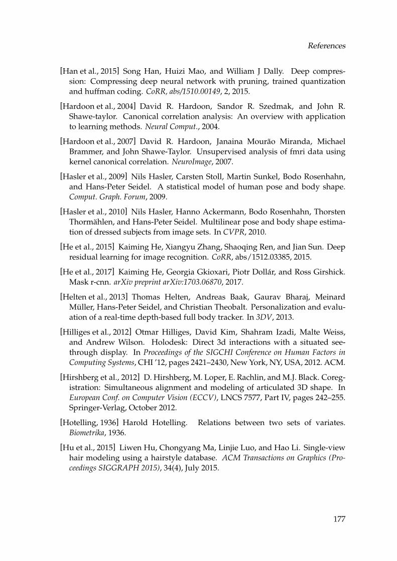
References
[Han et al., 2015] Song Han, Huizi Mao, and William J Dally. Deep compres-sion: Compressing deep neural network with pruning, trained quantizationand huffman coding. CoRR, abs/1510.00149, 2, 2015.
[Hardoon et al., 2004] David R. Hardoon, Sandor R. Szedmak, and John R.Shawe-taylor. Canonical correlation analysis: An overview with applicationto learning methods. Neural Comput., 2004.
[Hardoon et al., 2007] David R. Hardoon, Janaina Mourao Miranda, MichaelBrammer, and John Shawe-Taylor. Unsupervised analysis of fmri data usingkernel canonical correlation. NeuroImage, 2007.
[Hasler et al., 2009] Nils Hasler, Carsten Stoll, Martin Sunkel, Bodo Rosenhahn,and Hans-Peter Seidel. A statistical model of human pose and body shape.Comput. Graph. Forum, 2009.
[Hasler et al., 2010] Nils Hasler, Hanno Ackermann, Bodo Rosenhahn, ThorstenThormahlen, and Hans-Peter Seidel. Multilinear pose and body shape estima-tion of dressed subjects from image sets. In CVPR, 2010.
[He et al., 2015] Kaiming He, Xiangyu Zhang, Shaoqing Ren, and Jian Sun. Deepresidual learning for image recognition. CoRR, abs/1512.03385, 2015.
[He et al., 2017] Kaiming He, Georgia Gkioxari, Piotr Dollar, and Ross Girshick.Mask r-cnn. arXiv preprint arXiv:1703.06870, 2017.
[Helten et al., 2013] Thomas Helten, Andreas Baak, Gaurav Bharaj, MeinardMuller, Hans-Peter Seidel, and Christian Theobalt. Personalization and evalu-ation of a real-time depth-based full body tracker. In 3DV, 2013.
[Hilliges et al., 2012] Otmar Hilliges, David Kim, Shahram Izadi, Malte Weiss,and Andrew Wilson. Holodesk: Direct 3d interactions with a situated see-through display. In Proceedings of the SIGCHI Conference on Human Factors inComputing Systems, CHI ’12, pages 2421–2430, New York, NY, USA, 2012. ACM.
[Hirshberg et al., 2012] D. Hirshberg, M. Loper, E. Rachlin, and M.J. Black. Coreg-istration: Simultaneous alignment and modeling of articulated 3D shape. InEuropean Conf. on Computer Vision (ECCV), LNCS 7577, Part IV, pages 242–255.Springer-Verlag, October 2012.
[Hotelling, 1936] Harold Hotelling. Relations between two sets of variates.Biometrika, 1936.
[Hu et al., 2015] Liwen Hu, Chongyang Ma, Linjie Luo, and Hao Li. Single-viewhair modeling using a hairstyle database. ACM Transactions on Graphics (Pro-ceedings SIGGRAPH 2015), 34(4), July 2015.
177
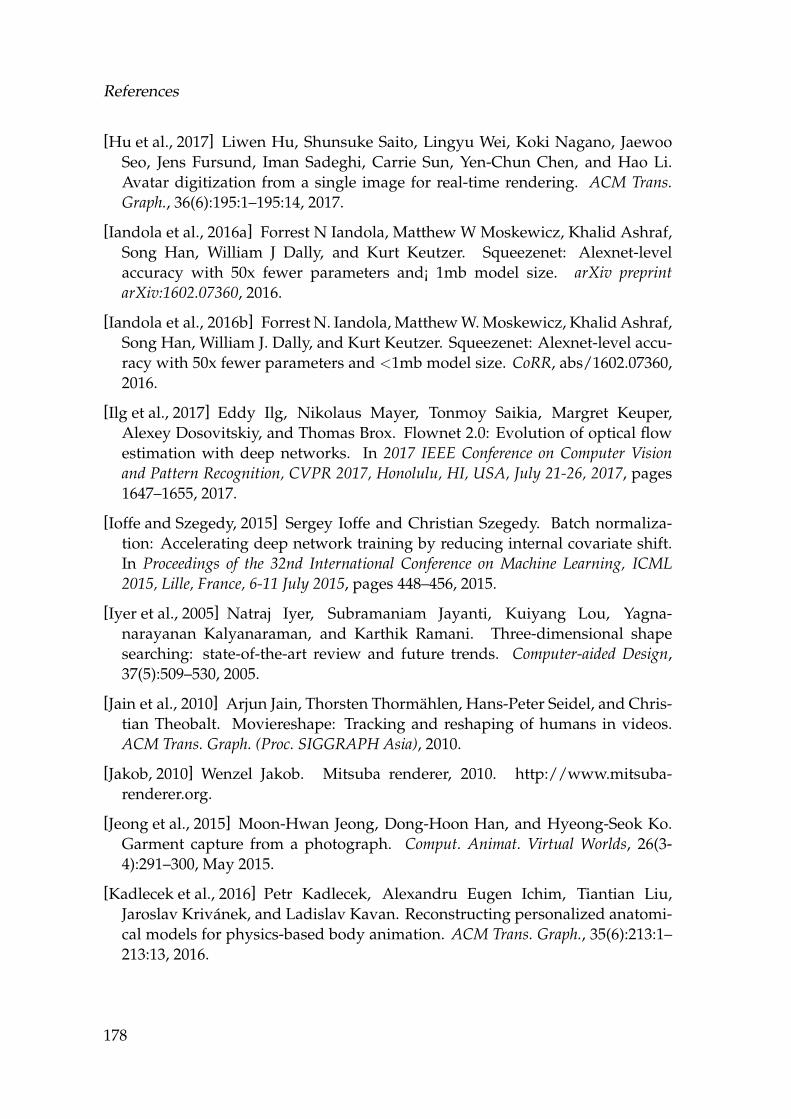
References
[Hu et al., 2017] Liwen Hu, Shunsuke Saito, Lingyu Wei, Koki Nagano, JaewooSeo, Jens Fursund, Iman Sadeghi, Carrie Sun, Yen-Chun Chen, and Hao Li.Avatar digitization from a single image for real-time rendering. ACM Trans.Graph., 36(6):195:1–195:14, 2017.
[Iandola et al., 2016a] Forrest N Iandola, Matthew W Moskewicz, Khalid Ashraf,Song Han, William J Dally, and Kurt Keutzer. Squeezenet: Alexnet-levelaccuracy with 50x fewer parameters and¡ 1mb model size. arXiv preprintarXiv:1602.07360, 2016.
[Iandola et al., 2016b] Forrest N. Iandola, Matthew W. Moskewicz, Khalid Ashraf,Song Han, William J. Dally, and Kurt Keutzer. Squeezenet: Alexnet-level accu-racy with 50x fewer parameters and <1mb model size. CoRR, abs/1602.07360,2016.
[Ilg et al., 2017] Eddy Ilg, Nikolaus Mayer, Tonmoy Saikia, Margret Keuper,Alexey Dosovitskiy, and Thomas Brox. Flownet 2.0: Evolution of optical flowestimation with deep networks. In 2017 IEEE Conference on Computer Visionand Pattern Recognition, CVPR 2017, Honolulu, HI, USA, July 21-26, 2017, pages1647–1655, 2017.
[Ioffe and Szegedy, 2015] Sergey Ioffe and Christian Szegedy. Batch normaliza-tion: Accelerating deep network training by reducing internal covariate shift.In Proceedings of the 32nd International Conference on Machine Learning, ICML2015, Lille, France, 6-11 July 2015, pages 448–456, 2015.
[Iyer et al., 2005] Natraj Iyer, Subramaniam Jayanti, Kuiyang Lou, Yagna-narayanan Kalyanaraman, and Karthik Ramani. Three-dimensional shapesearching: state-of-the-art review and future trends. Computer-aided Design,37(5):509–530, 2005.
[Jain et al., 2010] Arjun Jain, Thorsten Thormahlen, Hans-Peter Seidel, and Chris-tian Theobalt. Moviereshape: Tracking and reshaping of humans in videos.ACM Trans. Graph. (Proc. SIGGRAPH Asia), 2010.
[Jakob, 2010] Wenzel Jakob. Mitsuba renderer, 2010. http://www.mitsuba-renderer.org.
[Jeong et al., 2015] Moon-Hwan Jeong, Dong-Hoon Han, and Hyeong-Seok Ko.Garment capture from a photograph. Comput. Animat. Virtual Worlds, 26(3-4):291–300, May 2015.
[Kadlecek et al., 2016] Petr Kadlecek, Alexandru Eugen Ichim, Tiantian Liu,Jaroslav Krivanek, and Ladislav Kavan. Reconstructing personalized anatomi-cal models for physics-based body animation. ACM Trans. Graph., 35(6):213:1–213:13, 2016.
178
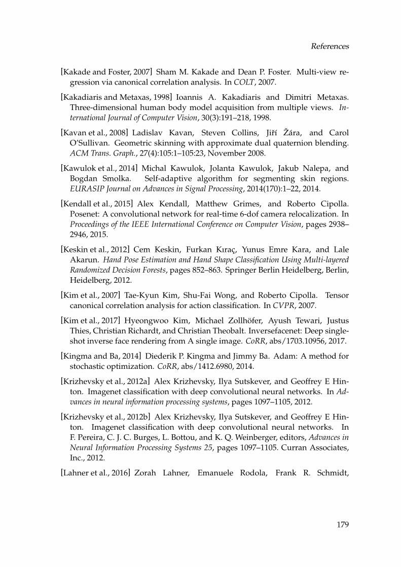
References
[Kakade and Foster, 2007] Sham M. Kakade and Dean P. Foster. Multi-view re-gression via canonical correlation analysis. In COLT, 2007.
[Kakadiaris and Metaxas, 1998] Ioannis A. Kakadiaris and Dimitri Metaxas.Three-dimensional human body model acquisition from multiple views. In-ternational Journal of Computer Vision, 30(3):191–218, 1998.
[Kavan et al., 2008] Ladislav Kavan, Steven Collins, Jirı Zara, and CarolO’Sullivan. Geometric skinning with approximate dual quaternion blending.ACM Trans. Graph., 27(4):105:1–105:23, November 2008.
[Kawulok et al., 2014] Michal Kawulok, Jolanta Kawulok, Jakub Nalepa, andBogdan Smolka. Self-adaptive algorithm for segmenting skin regions.EURASIP Journal on Advances in Signal Processing, 2014(170):1–22, 2014.
[Kendall et al., 2015] Alex Kendall, Matthew Grimes, and Roberto Cipolla.Posenet: A convolutional network for real-time 6-dof camera relocalization. InProceedings of the IEEE International Conference on Computer Vision, pages 2938–2946, 2015.
[Keskin et al., 2012] Cem Keskin, Furkan Kırac, Yunus Emre Kara, and LaleAkarun. Hand Pose Estimation and Hand Shape Classification Using Multi-layeredRandomized Decision Forests, pages 852–863. Springer Berlin Heidelberg, Berlin,Heidelberg, 2012.
[Kim et al., 2007] Tae-Kyun Kim, Shu-Fai Wong, and Roberto Cipolla. Tensorcanonical correlation analysis for action classification. In CVPR, 2007.
[Kim et al., 2017] Hyeongwoo Kim, Michael Zollhofer, Ayush Tewari, JustusThies, Christian Richardt, and Christian Theobalt. Inversefacenet: Deep single-shot inverse face rendering from A single image. CoRR, abs/1703.10956, 2017.
[Kingma and Ba, 2014] Diederik P. Kingma and Jimmy Ba. Adam: A method forstochastic optimization. CoRR, abs/1412.6980, 2014.
[Krizhevsky et al., 2012a] Alex Krizhevsky, Ilya Sutskever, and Geoffrey E Hin-ton. Imagenet classification with deep convolutional neural networks. In Ad-vances in neural information processing systems, pages 1097–1105, 2012.
[Krizhevsky et al., 2012b] Alex Krizhevsky, Ilya Sutskever, and Geoffrey E Hin-ton. Imagenet classification with deep convolutional neural networks. InF. Pereira, C. J. C. Burges, L. Bottou, and K. Q. Weinberger, editors, Advances inNeural Information Processing Systems 25, pages 1097–1105. Curran Associates,Inc., 2012.
[Lahner et al., 2016] Zorah Lahner, Emanuele Rodola, Frank R. Schmidt,
179
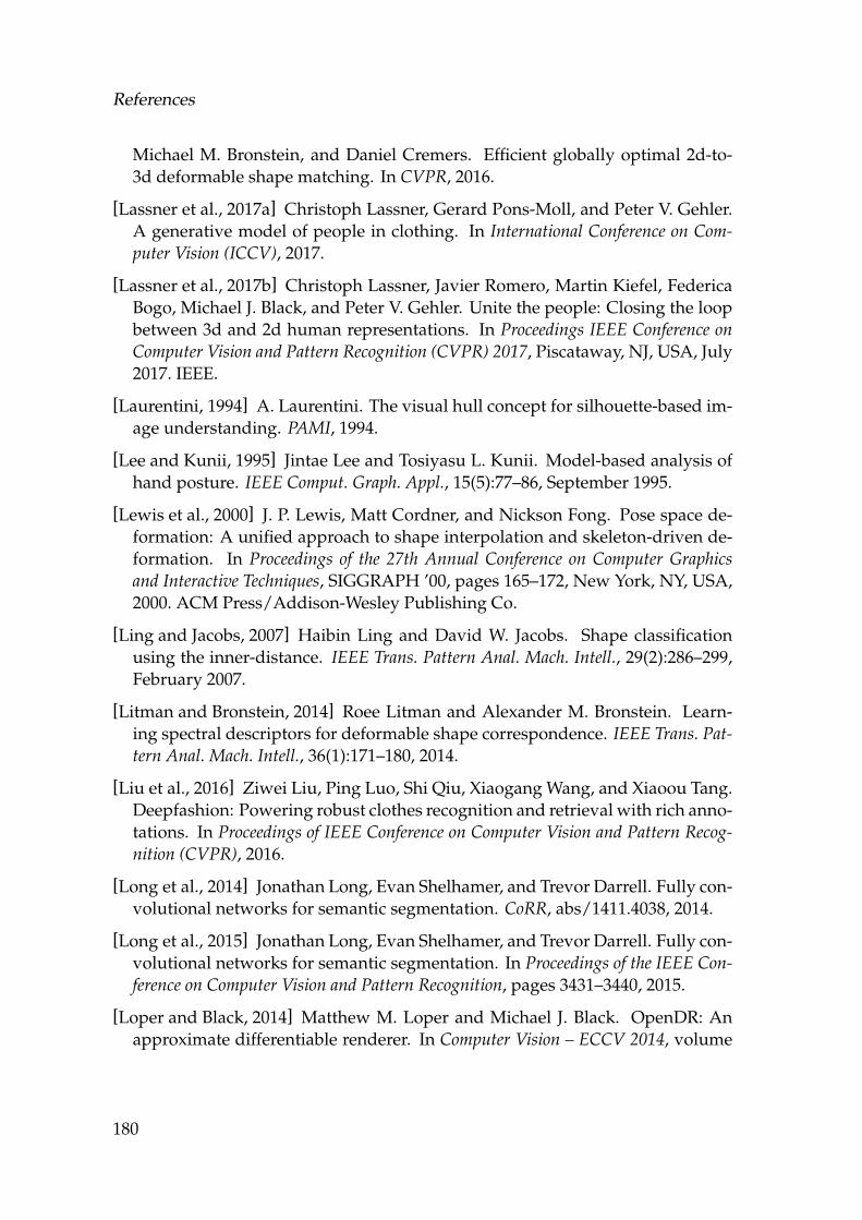
References
Michael M. Bronstein, and Daniel Cremers. Efficient globally optimal 2d-to-3d deformable shape matching. In CVPR, 2016.
[Lassner et al., 2017a] Christoph Lassner, Gerard Pons-Moll, and Peter V. Gehler.A generative model of people in clothing. In International Conference on Com-puter Vision (ICCV), 2017.
[Lassner et al., 2017b] Christoph Lassner, Javier Romero, Martin Kiefel, FedericaBogo, Michael J. Black, and Peter V. Gehler. Unite the people: Closing the loopbetween 3d and 2d human representations. In Proceedings IEEE Conference onComputer Vision and Pattern Recognition (CVPR) 2017, Piscataway, NJ, USA, July2017. IEEE.
[Laurentini, 1994] A. Laurentini. The visual hull concept for silhouette-based im-age understanding. PAMI, 1994.
[Lee and Kunii, 1995] Jintae Lee and Tosiyasu L. Kunii. Model-based analysis ofhand posture. IEEE Comput. Graph. Appl., 15(5):77–86, September 1995.
[Lewis et al., 2000] J. P. Lewis, Matt Cordner, and Nickson Fong. Pose space de-formation: A unified approach to shape interpolation and skeleton-driven de-formation. In Proceedings of the 27th Annual Conference on Computer Graphicsand Interactive Techniques, SIGGRAPH ’00, pages 165–172, New York, NY, USA,2000. ACM Press/Addison-Wesley Publishing Co.
[Ling and Jacobs, 2007] Haibin Ling and David W. Jacobs. Shape classificationusing the inner-distance. IEEE Trans. Pattern Anal. Mach. Intell., 29(2):286–299,February 2007.
[Litman and Bronstein, 2014] Roee Litman and Alexander M. Bronstein. Learn-ing spectral descriptors for deformable shape correspondence. IEEE Trans. Pat-tern Anal. Mach. Intell., 36(1):171–180, 2014.
[Liu et al., 2016] Ziwei Liu, Ping Luo, Shi Qiu, Xiaogang Wang, and Xiaoou Tang.Deepfashion: Powering robust clothes recognition and retrieval with rich anno-tations. In Proceedings of IEEE Conference on Computer Vision and Pattern Recog-nition (CVPR), 2016.
[Long et al., 2014] Jonathan Long, Evan Shelhamer, and Trevor Darrell. Fully con-volutional networks for semantic segmentation. CoRR, abs/1411.4038, 2014.
[Long et al., 2015] Jonathan Long, Evan Shelhamer, and Trevor Darrell. Fully con-volutional networks for semantic segmentation. In Proceedings of the IEEE Con-ference on Computer Vision and Pattern Recognition, pages 3431–3440, 2015.
[Loper and Black, 2014] Matthew M. Loper and Michael J. Black. OpenDR: Anapproximate differentiable renderer. In Computer Vision – ECCV 2014, volume
180
References
8695 of Lecture Notes in Computer Science, pages 154–169. Springer InternationalPublishing, September 2014.
[Loper et al., 2015] Matthew Loper, Naureen Mahmood, Javier Romero, GerardPons-Moll, and Michael J. Black. Smpl: a skinned multi-person linear model.ACM Trans. Graph., 34(6):248:1–248:16, 2015.
[Maaten and Hinton, 2008] Laurens van der Maaten and Geoffrey Hinton. Visu-alizing data using t-sne. Journal of Machine Learning Research, 9(Nov):2579–2605,2008.
[Masci et al., 2015a] Jonathan Masci, Davide Boscaini, Michael M. Bronstein, andPierre Vandergheynst. Geodesic convolutional neural networks on riemannianmanifolds. In Proc. of the IEEE International Conference on Computer Vision (ICCV)Workshops, pages 37–45, 2015.
[Masci et al., 2015b] Jonathan Masci, Davide Boscaini, Michael M. Bronstein, andPierre Vandergheynst. Shapenet: Convolutional neural networks on non-euclidean manifolds. CoRR, abs/1501.06297, 2015.
[McWilliams et al., 2013] Brian McWilliams, David Balduzzi, and Joachim MBuhmann. Correlated random features for fast semi-supervised learning. InC. J. C. Burges, L. Bottou, M. Welling, Z. Ghahramani, and K. Q. Weinberger,editors, Advances in Neural Information Processing Systems 26, pages 440–448.Curran Associates, Inc., 2013.
[MD, ] MD. Marvelous designer.
[Mehta et al., 2016] Dushyant Mehta, Helge Rhodin, Dan Casas, Oleksandr Sot-nychenko, Weipeng Xu, and Christian Theobalt. Monocular 3d human poseestimation using transfer learning and improved CNN supervision. CoRR,abs/1611.09813, 2016.
[Mehta et al., 2017] Dushyant Mehta, Srinath Sridhar, Oleksandr Sotnychenko,Helge Rhodin, Mohammad Shafiei, Hans-Peter Seidel, Weipeng Xu, Dan Casas,and Christian Theobalt. Vnect: real-time 3d human pose estimation with a sin-gle RGB camera. ACM Trans. Graph., 36(4):44:1–44:14, 2017.
[Melax et al., 2013] Stan Melax, Leonid Keselman, and Sterling Orsten. Dynamicsbased 3d skeletal hand tracking. In Proceedings of Graphics Interface 2013, GI’13, pages 63–70, Toronto, Ont., Canada, Canada, 2013. Canadian InformationProcessing Society.
[Memo and Zanuttigh, 2017] Alvise Memo and Pietro Zanuttigh. Head-mountedgesture controlled interface for human-computer interaction. In MultimediaTools and Applications, 2017.
181
References
[Memo et al., 2015] Alvise Memo, Ludovico Minto, and Pietro Zanuttigh. Ex-ploiting silhouette descriptors and synthetic data for hand gesture recognition.In Smart Tools and Apps for Graphics - Eurographics Italian Chapter Conference,Verona, Italy, October 15-16 2015., pages 15–23, 2015.
[Mikic et al., 2003] Ivana Mikic, Mohan Trivedi, Edward Hunter, and PamelaCosman. Human body model acquisition and tracking using voxel data. Inter-national Journal of Computer Vision, 53(3):199–223, 2003.
[Molbert et al., 2017] Simone Claire Molbert, Anne Thaler, Betty J. Mohler,Stephan Streuber, Javier Romero, Michael J. Black, Stephan Zipfel, Hans-OttoKarnath, and Katrin Elisabeth Giel. Assessing body image in anorexia nervosausing biometric self-avatars in virtual reality: Attitudinal components ratherthan visual body size estimation are distorted. Psychological Medicine, 26:1–12,July 2017.
[Mueller et al., 2017] Franziska Mueller, Florian Bernard, Oleksandr Sotny-chenko, Dushyant Mehta, Srinath Sridhar, Dan Casas, and Christian Theobalt.Ganerated hands for real-time 3d hand tracking from monocular RGB. CoRR,abs/1712.01057, 2017.
[Nalepa and Kawulok, 2014] Jakub Nalepa and Michal Kawulok. Fast and accu-rate hand shape classification. In Stanislaw Kozielski, Dariusz Mrozek, PawelKasprowski, Bozena Malysiak-Mrozek, and Daniel Kostrzewa, editors, BeyondDatabases, Architectures, and Structures, volume 424 of Communications in Com-puter and Information Science, pages 364–373. Springer, 2014.
[Narain et al., 2012] Rahul Narain, Armin Samii, and James F. O’Brien. Adap-tive anisotropic remeshing for cloth simulation. ACM Transactions on Graphics,31(6):147:1–10, November 2012. Proceedings of ACM SIGGRAPH Asia 2012,Singapore.
[Narain et al., 2013] Rahul Narain, Tobias Pfaff, and James F. O’Brien. Foldingand crumpling adaptive sheets. ACM Transactions on Graphics, 32(4):51:1–8, July2013. Proceedings of ACM SIGGRAPH 2013, Anaheim.
[Neophytou and Hilton, 2013] Alexandros Neophytou and Adrian Hilton. Shapeand pose space deformation for subject specific animation. In 3DV, 2013.
[Ngiam et al., 2011] Jiquan Ngiam, Aditya Khosla, Mingyu Kim, Juhan Nam,Honglak Lee, and Andrew Y. Ng. Multimodal deep learning. In Proceedings ofthe 28th International Conference on Machine Learning, ICML 2011, Bellevue, Wash-ington, USA, June 28 - July 2, 2011, pages 689–696, 2011.
[Oberweger et al., 2015a] Markus Oberweger, Paul Wohlhart, and Vincent Lep-
182
References
etit. Hands deep in deep learning for hand pose estimation. CoRR,abs/1502.06807, 2015.
[Oberweger et al., 2015b] Markus Oberweger, Paul Wohlhart, and Vincent Lep-etit. Training a feedback loop for hand pose estimation. In Proceedings of the2015 IEEE International Conference on Computer Vision (ICCV), ICCV ’15, pages3316–3324, Washington, DC, USA, 2015. IEEE Computer Society.
[Oberweger et al., 2016] Markus Oberweger, Gernot Riegler, Paul Wohlhart, andVincent Lepetit. Efficiently creating 3d training data for fine hand pose estima-tion. 2016 IEEE Conference on Computer Vision and Pattern Recognition (CVPR),pages 4957–4965, 2016.
[Oikonomidis et al., 2011] Iason Oikonomidis, Nikolaos Kyriazis, and AntonisArgyros. Efficient model-based 3d tracking of hand articulations using kinect.In Proceedings of the British Machine Vision Conference, pages 101.1–101.11, 2011.
[Panteleris et al., 2017] Paschalis Panteleris, Iason Oikonomidis, and Antonis A.Argyros. Using a single rgb frame for real time 3d hand pose estimation in thewild. CoRR, abs/1712.03866, 2017.
[Perbet et al., 2014] Frank Perbet, Sam Johnson, Minh-Tri Pham, and BjornStenger. Human body shape estimation using a multi-resolution manifold for-est. In CVPR, 2014.
[Pickup et al., 2014] D. Pickup, X. Sun, P. L. Rosin, R. R. Martin, Z. Cheng, Z. Lian,M. Aono, A. Ben Hamza, A. Bronstein, M. Bronstein, S. Bu, U. Castellani,S. Cheng, V. Garro, A. Giachetti, A. Godil, J. Han, H. Johan, L. Lai, B. Li, C. Li,H. Li, R. Litman, X. Liu, Z. Liu, Y. Lu, A. Tatsuma, and J. Ye. Shape retrievalof non-rigid 3d human models. In Proceedings of the 7th Eurographics Work-shop on 3D Object Retrieval, 3DOR ’15, pages 101–110, Aire-la-Ville, Switzerland,Switzerland, 2014. Eurographics Association.
[Piryankova et al., 2014] I. Piryankova, J. Stefanucci, J. Romero, S. de la Rosa,M. Black, and B. Mohler. Can i recognize my body’s weight? the influenceof shape and texture on the perception of self. ACM Transactions on AppliedPerception for the Symposium on Applied Perception, 11(3):13:1–13:18, September2014.
[Pishchulin et al., 2015] Leonid Pishchulin, Stefanie Wuhrer, Thomas Helten,Christian Theobalt, and Bernt Schiele. Building statistical shape spaces for 3dhuman modeling. CoRR, 2015.
[Pons-Moll et al., 2015] Gerard Pons-Moll, Javier Romero, Naureen Mahmood,and Michael J. Black. Dyna: A model of dynamic human shape in motion.
183
References
ACM Transactions on Graphics, (Proc. SIGGRAPH), 34(4):120:1–120:14, August2015.
[Pons-Moll et al., 2017] Gerard Pons-Moll, Sergi Pujades, Sonny Hu, and MichaelBlack. Clothcap: Seamless 4D clothing capture and retargeting. ACM Transac-tions on Graphics, (Proc. SIGGRAPH), 36(4), 2017. Two first authors contributedequally.
[Popa et al., 2009] Tiberiu Popa, Qingnan Zhou, Derek Bradley, VladislavKraevoy, Hongbo Fu, Alla Sheffer, and Wolfgang Heidrich. Wrinkling capturedgarments using space-time data-driven deformation. Computer Graphics Forum(Proc. Eurographics), 28(2):427–435, 2009.
[Pritchard and Heidrich, 2003] D. Pritchard and W. Heidrich. Cloth motion cap-ture, 2003.
[Qian et al., 2014] Chen Qian, Xiao Sun, Yichen Wei, Xiaoou Tang, and Jian Sun.Realtime and robust hand tracking from depth. In Proceedings of the IEEE Con-ference on Computer Vision and Pattern Recognition, pages 1106–1113, 2014.
[Remelli et al., 2017] Edoardo Remelli, Anastasia Tkach, Andrea Tagliasacchi,and Mark Pauly. Low-dimensionality calibration through local anisotropic scal-ing for robust hand model personalization. In Proceedings of the InternationalConference on Computer Vision, 2017.
[Ren et al., 2015] Shaoqing Ren, Kaiming He, Ross Girshick, and Jian Sun. Fasterr-cnn: Towards real-time object detection with region proposal networks. InAdvances in neural information processing systems, pages 91–99, 2015.
[Rhodin et al., 2016] Helge Rhodin, Nadia Robertini, Dan Casas, ChristianRichardt, Hans-Peter Seidel, and Christian Theobalt. General automatic hu-man shape and motion capture using volumetric contour cues. In ComputerVision - ECCV 2016 - 14th European Conference, Amsterdam, The Netherlands, Oc-tober 11-14, 2016, Proceedings, Part V, pages 509–526, 2016.
[Robinette and Daanen, 1999] Kathleen M. Robinette and Hein A. M. Daanen.The caesar project: A 3-d surface anthropometry survey. In 3DIM, 1999.
[Robson et al., 2011] C. Robson, R. Maharik, A. Sheffer, and N. Carr. Context-aware garment modeling from sketches. Computers and Graphics (Proc. SMI2011), pages 604–613, 2011.
[Rogge et al., 2014] Lorenz Rogge, Felix Klose, Michael Stengel, Martin Eise-mann, and Marcus Magnor. Garment replacement in monocular video se-quences. ACM Trans. Graph., 2014.
184
References
[Rohit Girdhar, 2016] Mikel Rodriguez A K Gupta Rohit Girdhar, DavidF Fouhey. Learning a predictable and generative vector representation for ob-jects. European Conference on Computer Vision, 2016.
[Romero et al., 2009] J. Romero, H. Kjellstrom, and D. Kragic. Monocular real-time 3d articulated hand pose estimation. In 2009 9th IEEE-RAS InternationalConference on Humanoid Robots, pages 87–92, Dec 2009.
[Romero et al., 2017] Javier Romero, Dimitrios Tzionas, and Michael J. Black. Em-bodied hands: Modeling and capturing hands and bodies together. ACM Trans-actions on Graphics, (Proc. SIGGRAPH Asia), 36(6), November 2017. (*) Two firstauthors contributed equally.
[Roveri, 2018] Riccardo Roveri. Tech report: Projection of unordered point setsand generation of distance field images with gaussian interpolation. Technicalreport, 2018.
[Rustamov, 2007] Raif M Rustamov. Laplace-beltrami eigenfunctions for defor-mation invariant shape representation. 2007.
[Sarafianos et al., 2016] Nikolaos Sarafianos, Bogdan Boteanu, Bogdan Ionescu,and Ioannis A. Kakadiaris. 3d human pose estimation: A review of the lit-erature and analysis of covariates. Computer Vision and Image Understanding,152:1–20, 2016.
[Sargin et al., 2007] Mehmet Emre Sargin, Yucel Yemez, Engin Erzin, and A. Mu-rat Tekalp. Audiovisual synchronization and fusion using canonical correlationanalysis. Trans. Multimedia, 2007.
[Savva et al., ] M Savva, F Yu, Hao Su, M Aono, B Chen, D Cohen-Or, W Deng,Hang Su, S Bai, X Bai, et al. Shrec16 track large-scale 3d shape retrieval fromshapenet core55.
[Schmidt et al., 2007] Frank R. Schmidt, Dirk Farin, and Daniel Cremers. Fastmatching of planar shapes in sub-cubic runtime. In ICCV, 2007.
[Schmidt et al., 2009] Frank R. Schmidt, Eno Toppe, and Daniel Cremers. Efficientplanar graph cuts with applications in computer vision. In CVPR, 2009.
[Scholz and Magnor, 2004] Volker Scholz and Marcus A. Magnor. Cloth motionfrom optical flow. In VMV, 2004.
[Scholz et al., 2005] Volker Scholz, Timo Stich, Michael Keckeisen, MarkusWacker, and Marcus Magnor. Garment motion capture using color-coded pat-terns. Computer Graphics forum, 24(3):439–448, September 2005. Conference Is-sue: 26th annual Conference Eurographics 2005, Dublin, Ireland, August 29th- September 2nd, 2005.
185
References
[Schroder et al., 2014] Matthias Schroder, Jonathan Maycock, Helge Ritter, andMario Botsch. Real-time hand tracking using synergistic inverse kinematics. InProceedings of IEEE International Conference on Robotics and Automation (ICRA),2014.
[Sekine et al., 2014] M. Sekine, K. Sugita, F. Perbet, B. Stenger, and M. Nishiyama.Virtual fitting by single-shot body shape estimation. In Int. Conf. on 3D BodyScanning Technologies, pages 406–413, October 2014.
[Sermanet et al., 2013] Pierre Sermanet, David Eigen, Xiang Zhang, MichaelMathieu, Rob Fergus, and Yann LeCun. Overfeat: Integrated recognition, lo-calization and detection using convolutional networks. CoRR, abs/1312.6229,2013.
[Shapira et al., 2008] Lior Shapira, Ariel Shamir, and Daniel Cohen-Or. Consis-tent mesh partitioning and skeletonisation using the shape diameter function.Visual Comput., 2008.
[Sharma et al., 2012] Abhishek Sharma, Abhishek Kumar, Hal Daume III, andDavid W. Jacobs. Generalized multiview analysis: A discriminative latentspace. In 2012 IEEE Conference on Computer Vision and Pattern Recognition, Prov-idence, RI, USA, June 16-21, 2012, pages 2160–2167, 2012.
[Sharp et al., 2015] Toby Sharp, Cem Keskin, Duncan Robertson, Jonathan Taylor,Jamie Shotton, David Kim, Christoph Rhemann, Ido Leichter, Alon Vinnikov,Yichen Wei, Daniel Freedman, Pushmeet Kohli, Eyal Krupka, Andrew Fitzgib-bon, and Shahram Izadi. Accurate, robust, and flexible real-time hand tracking.In Proceedings of the 33rd Annual ACM Conference on Human Factors in ComputingSystems, CHI ’15, pages 3633–3642, New York, NY, USA, 2015. ACM.
[Shen et al., 2011] Jianbing Shen, Xiaoshan Yang, Yunde Jia, and Xuelong Li. In-trinsic images using optimization. In CVPR, pages 3481–3487. IEEE ComputerSociety, 2011.
[Sigal et al., 2007] Leonid Sigal, Alexandru O. Balan, and Michael J. Black. Com-bined discriminative and generative articulated pose and non-rigid shape es-timation. In Advances in Neural Information Processing Systems 20, Proceedingsof the Twenty-First Annual Conference on Neural Information Processing Systems,Vancouver, British Columbia, Canada, December 3-6, 2007, pages 1337–1344, 2007.
[Simon et al., 2017] Tomas Simon, Hanbyul Joo, Iain Matthews, and Yaser Sheikh.Hand keypoint detection in single images using multiview bootstrapping. InCVPR, 2017.
[Simonyan and Zisserman, 2014] Karen Simonyan and Andrew Zisserman. Very
186
References
deep convolutional networks for large-scale image recognition. CoRR,abs/1409.1556, 2014.
[Sinha et al., 2016] Ayan Sinha, Chiho Choi, and Karthik Ramani. Deephand: Ro-bust hand pose estimation by completing a matrix imputed with deep features.In The IEEE Conference on Computer Vision and Pattern Recognition (CVPR), June2016.
[Slama et al., 2013] Rim Slama, Hazem Wannous, and Mohamed Daoudi. Ex-tremal human curves: A new human body shape and pose descriptor. In FG,2013.
[Song et al., 2015] Jie Song, Fabrizio Pece, Gabor Soros, Marion Koelle, and OtmarHilliges. Joint estimation of 3d hand position and gestures from monocularvideo for mobile interaction. In ACM Conference on Human Factors in ComputingSystems (CHI), CHI ’15, pages 3657–3660, New York, NY, USA, 2015. ACM.
[Song et al., 2017] Jie Song, Limin Wang, Luc Van Gool, and Otmar Hilliges. Thin-slicing network: A deep structured model for pose estimation in videos. InCVPR, 2017.
[Spurr et al., 2018] Adrian Spurr, Jie Song, Seonwook Park, and Otmar Hilliges.Cross-modal deep variational hand pose estimation. In CVPR, 2018.
[Sridhar et al., 2013] Srinath Sridhar, Antti Oulasvirta, and Christian Theobalt.Interactive markerless articulated hand motion tracking using rgb and depthdata. In Proceedings of the 2013 IEEE International Conference on Computer Vi-sion, ICCV ’13, pages 2456–2463, Washington, DC, USA, 2013. IEEE ComputerSociety.
[Sridhar et al., 2014] Srinath Sridhar, Helge Rhodin, Hans-Peter Seidel, AnttiOulasvirta, and Christian Theobalt. Real-time hand tracking using a sum ofanisotropic gaussians model. In Proceedings of the International Conference on 3DVision (3DV), December 2014.
[Sridhar et al., 2016] Srinath Sridhar, Franziska Mueller, Michael Zollhofer, DanCasas, Antti Oulasvirta, and Christian Theobalt. Real-time joint tracking ofa hand manipulating an object from RGB-D input. In Computer Vision - ECCV2016 - 14th European Conference, Amsterdam, The Netherlands, October 11-14, 2016,Proceedings, Part II, pages 294–310, 2016.
[Starck et al., 2005] J. Starck, G. Miller, and A. Hilton. Video-based character ani-mation. In ACM SIGGRAPH Eurographics SCA, 2005.
[Stoll et al., 2010] Carsten Stoll, Juergen Gall, Edilson de Aguiar, Sebastian Thrun,and Christian Theobalt. Video-based reconstruction of animatable human char-acters. In SIGGRAPH Asia, 2010.
187
References
[Su et al., 2015] Hang Su, Subhransu Maji, Evangelos Kalogerakis, and ErikLearned-Miller. Multi-view convolutional neural networks for 3d shape recog-nition. In Proceedings of the IEEE International Conference on Computer Vision,pages 945–953, 2015.
[Sugano et al., 2014] Yusuke Sugano, Yasuyuki Matsushita, and Yoichi Sato.Learning-by-synthesis for appearance-based 3d gaze estimation. In 2014 IEEEConference on Computer Vision and Pattern Recognition, CVPR 2014, Columbus,OH, USA, June 23-28, 2014, pages 1821–1828, 2014.
[Sun et al., 2009] Jian Sun, Maks Ovsjanikov, and Leonidas J Guibas. A con-cise and provably informative multi-scale signature based on heat diffusion.28(5):1383–1392, 2009.
[Sun et al., 2015] Xiao Sun, Yichen Wei, Shuang Liang, Xiaoou Tang, and Jian Sun.Cascaded hand pose regression. In The IEEE Conference on Computer Vision andPattern Recognition (CVPR), June 2015.
[Supancic et al., 2015] James Steven Supancic, Gregory Rogez, Yi Yang, JamieShotton, and Deva Ramanan. Depth-based hand pose estimation: methods,data, and challenges. In IEEE International Conference on Computer Vision, ICCV,2015.
[Szegedy et al., 2015] Christian Szegedy, Wei Liu, Yangqing Jia, Pierre Sermanet,Scott Reed, Dragomir Anguelov, Dumitru Erhan, Vincent Vanhoucke, and An-drew Rabinovich. Going deeper with convolutions. In Computer Vision andPattern Recognition (CVPR), 2015.
[Tagliasacchi et al., 2015] Andrea Tagliasacchi, Matthias Schroder, AnastasiaTkach, Sofien Bouaziz, Mario Botsch, and Mark Pauly. Robust articulated-icpfor real-time hand tracking. Computer Graphics Forum (Symposium on GeometryProcessing), 34(5), 2015.
[Tang et al., 2013] D. Tang, T. H. Yu, and T. K. Kim. Real-time articulated handpose estimation using semi-supervised transductive regression forests. In 2013IEEE International Conference on Computer Vision, pages 3224–3231, Dec 2013.
[Tang et al., 2017] Danhang Tang, Hyung Jin Chang, Alykhan Tejani, and Tae-Kyun Kim. Latent regression forest: Structured estimation of 3d hand poses.IEEE Trans. Pattern Anal. Mach. Intell., 39(7):1374–1387, 2017.
[Tangelder and Veltkamp, 2008] Johan W H Tangelder and Remco C Veltkamp.A survey of content based 3d shape retrieval methods. Multimedia Tools andApplications, 39(3):441, 2008.
[Tatarchenko et al., 2016] Maxim Tatarchenko, Alexey Dosovitskiy, and ThomasBrox. Multi-view 3d models from single images with a convolutional net-
188
References
work. In Computer Vision - ECCV 2016 - 14th European Conference, Amsterdam,The Netherlands, October 11-14, 2016, Proceedings, Part VII, pages 322–337, 2016.
[Taylor et al., 2016] Jonathan Taylor, Lucas Bordeaux, Thomas Cashman, BobCorish, Cem Keskin, Toby Sharp, Eduardo Soto, David Sweeney, JulienValentin, Benjamin Luff, Arran Topalian, Erroll Wood, Sameh Khamis, Push-meet Kohli, Shahram Izadi, Richard Banks, Andrew Fitzgibbon, and JamieShotton. Efficient and precise interactive hand tracking through joint, continu-ous optimization of pose and correspondences. ACM Trans. Graph., 35(4):143:1–143:12, July 2016.
[Tewari et al., 2017] Ayush Tewari, Michael Zollhofer, Hyeongwoo Kim, PabloGarrido, Florian Bernard, Patrick Perez, and Christian Theobalt. Mofa: Model-based deep convolutional face autoencoder for unsupervised monocular recon-struction. In IEEE International Conference on Computer Vision, ICCV 2017, Venice,Italy, October 22-29, 2017, pages 3735–3744, 2017.
[Thaler et al., 2018] Anne Thaler, Michael N. Geuss, Simone C. Molbert, Katrin E.Giel, Stephan Streuber, Javier Romero, Michael J. Black, and Betty J. Mohler.Body size estimation of self and others in females varying in BMI. PLoS ONE,13(2), February 2018.
[Tkach et al., 2016] Anastasia Tkach, Mark Pauly, and Andrea Tagliasacchi.Sphere-meshes for real-time hand modeling and tracking. ACM Transactionon Graphics (Proc. SIGGRAPH Asia), 2016.
[Tkach et al., 2017] Anastasia Tkach, Andrea Tagliasacchi, Edoardo Remelli,Mark Pauly, and Andrew Fitzgibbon. Online generative model personaliza-tion for hand tracking. ACM Transaction on Graphics (Proc. SIGGRAPH Asia),2017.
[Tome et al., 2017] Denis Tome, Chris Russell, and Lourdes Agapito. Lifting fromthe deep: Convolutional 3d pose estimation from a single image. CoRR,abs/1701.00295, 2017.
[Tompson et al., 2014] Jonathan Tompson, Murphy Stein, Yann Lecun, and KenPerlin. Real-time continuous pose recovery of human hands using convolu-tional networks. ACM Transactions on Graphics, 33, August 2014.
[Toshev and Szegedy, 2013] Alexander Toshev and Christian Szegedy. Deeppose:Human pose estimation via deep neural networks. CoRR, abs/1312.4659, 2013.
[Toshev and Szegedy, 2014] Alexander Toshev and Christian Szegedy. Deeppose:Human pose estimation via deep neural networks. In Proceedings of the IEEEConference on Computer Vision and Pattern Recognition, pages 1653–1660, 2014.
189
References
[Varol et al., 2017] Gul Varol, Javier Romero, Xavier Martin, Naureen Mahmood,Michael J. Black, Ivan Laptev, and Cordelia Schmid. Learning from synthetichumans. In Proceedings IEEE Conference on Computer Vision and Pattern Recogni-tion (CVPR) 2017, Piscataway, NJ, USA, July 2017. IEEE.
[Vodopivec et al., 2016] Tadej Vodopivec, Vincent Lepetit, and Peter Peer. Finehand segmentation using convolutional neural networks. arXiv preprintarXiv:1608.07454, 2016.
[Vranic et al., 2001] Dejan V Vranic, Dietmar Saupe, and J Richter. Tools for 3d-object retrieval: Karhunen-loeve transform and spherical harmonics. 2001.
[Wan et al., 2017] Chengde Wan, Thomas Probst, Luc J. Van Gool, and AngelaYao. Crossing nets: Dual generative models with a shared latent space forhand pose estimation. CoRR, abs/1702.03431, 2017.
[Wang et al., 2015] Fang Wang, Le Kang, and Yi Li. Sketch-based 3d shape re-trieval using convolutional neural networks. CoRR, abs/1504.03504, 2015.
[Wei et al., 2016] Shih-En Wei, Varun Ramakrishna, Takeo Kanade, and YaserSheikh. Convolutional pose machines. In 2016 IEEE Conference on ComputerVision and Pattern Recognition, CVPR 2016, Las Vegas, NV, USA, June 27-30, 2016,pages 4724–4732, 2016.
[Weiss et al., 2011] Alexander Weiss, David A. Hirshberg, and Michael J. Black.Home 3d body scans from noisy image and range data. In ICCV, 2011.
[White et al., 2007] Ryan White, Keenan Crane, and David Forsyth. Capturingand animating occluded cloth. In ACM Transactions on Graphics (SIGGRAPH),2007.
[Wu et al., 2015] Zhirong Wu, Shuran Song, Aditya Khosla, Fisher Yu, LinguangZhang, Xiaoou Tang, and Jianxiong Xiao. 3d shapenets: A deep representationfor volumetric shapes. In The IEEE Conference on Computer Vision and PatternRecognition (CVPR), June 2015.
[Wuhrer et al., 2014] Stefanie Wuhrer, Leonid Pishchulin, Alan Brunton, ChangShu, and Jochen Lang. Estimation of human body shape and posture underclothing. CVIU, 2014.
[Xi et al., 2007] Pengcheng Xi, Won-Sook Lee, and Chang Shu. A data-driven ap-proach to human-body cloning using a segmented body database. In PacificGraphics, 2007.
[Xie et al., 2016] Jin Xie, Meng Wang, and Yi Fang. Learned binary spectral shapedescriptor for 3d shape correspondence. In The IEEE Conference on ComputerVision and Pattern Recognition (CVPR), June 2016.
190
References
[Xu et al., 2011] Feng Xu, Yebin Liu, Carsten Stoll, James Tompkin, GauravBharaj, Qionghai Dai, Hans-Peter Seidel, Jan Kautz, and Christian Theobalt.Video-based characters: Creating new human performances from a multi-viewvideo database. In SIGGRAPH, 2011.
[Xu et al., 2016] Chi Xu, Ashwin Nanjappa, Xiaowei Zhang, and Li Cheng. Es-timate hand poses efficiently from single depth images. Int. J. Comput. Vision,116(1):21–45, January 2016.
[Yamaguchi et al., 2013] Kota Yamaguchi, M. Hadi Kiapour, and Tamara L. Berg.Paper doll parsing: Retrieving similar styles to parse clothing items. In TheIEEE International Conference on Computer Vision (ICCV), December 2013.
[Yan and Mikolajczyk, 2015] Fei Yan and Krystian Mikolajczyk. Deep correlationfor matching images and text. In The IEEE Conference on Computer Vision andPattern Recognition (CVPR), June 2015.
[Yang et al., 2014] Yipin Yang, Yao Yu, Yu Zhou, Sidan Du, James Davis, andRuigang Yang. Semantic parametric reshaping of human body models. In3DV, 2014.
[Yang et al., 2016] Shan Yang, Tanya Ambert, Zherong Pan, Ke Wang, Licheng Yu,Tamara L. Berg, and Ming C. Lin. Detailed garment recovery from a single-viewimage. CoRR, abs/1608.01250, 2016.
[Ye and Yang, 2014] Mao Ye and Ruigang Yang. Real-time simultaneous pose andshape estimation for articulated objects using a single depth camera. In CVPR,2014.
[Ye et al., 2013] Mao Ye, Qing Zhang, Liang Wang, Jiejie Zhu, Ruigang Yang, andJuergen Gall. A Survey on Human Motion Analysis from Depth Data, pages 149–187. Springer Berlin Heidelberg, Berlin, Heidelberg, 2013.
[Ye et al., 2016] Qi Ye, Shanxin Yuan, and Tae-Kyun Kim. Spatial attention deepnet with partial PSO for hierarchical hybrid hand pose estimation. CoRR,abs/1604.03334, 2016.
[Yi et al., 2016] Kwang Moo Yi, Eduard Trulls, Vincent Lepetit, and Pascal Fua.LIFT: learned invariant feature transform. CoRR, abs/1603.09114, 2016.
[Yuan et al., 2017a] Shanxin Yuan, Qi Ye, Bjorn Stenger, Siddhand Jain, and Tae-Kyun Kim. Bighand2.2m benchmark: Hand pose dataset and state of the artanalysis. CoRR, abs/1704.02612, 2017.
[Yuan et al., 2017b] Shanxin Yuan, Qi Ye, Bjorn Stenger, Siddhand Jain, and Tae-Kyun Kim. Bighand2.2m benchmark: Hand pose dataset and state of the artanalysis. CoRR, abs/1704.02612, 2017.
191
References
[Zeiler and Fergus, 2014] Matthew D. Zeiler and Rob Fergus. Visualizing and un-derstanding convolutional networks. In Computer Vision - ECCV 2014 - 13thEuropean Conference, Zurich, Switzerland, September 6-12, 2014, Proceedings, PartI, pages 818–833, 2014.
[Zeiler, 2012] Matthew D Zeiler. Adadelta: an adaptive learning rate method.arXiv preprint arXiv:1212.5701, 2012.
[Zhang et al., 2015] Xucong Zhang, Yusuke Sugano, Mario Fritz, and AndreasBulling. Appearance-based gaze estimation in the wild. In IEEE Conferenceon Computer Vision and Pattern Recognition, CVPR 2015, Boston, MA, USA, June7-12, 2015, pages 4511–4520, 2015.
[Zhang et al., 2016] Jiawei Zhang, Jianbo Jiao, Mingliang Chen, Liangqiong Qu,Xiaobin Xu, and Qingxiong Yang. 3d hand pose tracking and estimation usingstereo matching. CoRR, abs/1610.07214, 2016.
[Zhang et al., 2017] Chao Zhang, Sergi Pujades, Michael Black, and Gerard Pons-Moll. Detailed, accurate, human shape estimation from clothed 3D scan se-quences. In Proceedings IEEE Conference on Computer Vision and Pattern Recogni-tion (CVPR) 2017, Piscataway, NJ, USA, July 2017. IEEE. Spotlight.
[Zhao et al., 2016] Ruiqi Zhao, Yan Wang, and Aleix M. Martınez. A simple, fastand highly-accurate algorithm to recover 3d shape from 2d landmarks on asingle image. CoRR, abs/1609.09058, 2016.
[Zhou et al., 2010] Shizhe Zhou, Hongbo Fu, Ligang Liu, Daniel Cohen-Or, andXiaoguang Han. Parametric reshaping of human bodies in images. ACM Trans.Graph., 29(4), 2010.
[Zhou et al., 2013] Bin Zhou, Xiaowu Chen, Qiang Fu, Kan Guo, and Ping Tan.Garment modeling from a single image. Pacific Graphics, 2013.
[Zhou et al., 2016] Xingyi Zhou, Qingfu Wan, Wei Zhang, Xiangyang Xue, andYichen Wei. Model-based deep hand pose estimation. In IJCAI, 2016.
[Zimmermann and Brox, 2017] Christian Zimmermann and Thomas Brox. Learn-ing to estimate 3d hand pose from single RGB images. CoRR, abs/1705.01389,2017.
192