implementation of a 3d pose estimation algorithm
TRANSCRIPT
Universitat Politecnica de Catalunya
Masters Thesis
Implementation of a 3D pose estimationalgorithm
Author:
Edgar Riba Pi
Supervisors:
Dr. Francesc Moreno Noguer
Adrian Penate Sanchez
Master’s Degree in Automatic Control and Robotics
Insitut de Robotica i Informatica Industrial
(CSIC-UPC)
June 2015
Universitat Politecnica de Catalunya
Abstract
Escola Tecnica Superior d’Enginyeria Industrial de Barcelona (ETSEIB)
Systems Engineering, Automation and Industrial Informatics (ESAII)
Master’s Degree in Automatic Control and Robotics
Implementation of a 3D pose estimation algorithm
by Edgar Riba Pi
In this project, I present the implementation of a 3D pose estimation algorithm for rigid
objects considering a single monocular camera. The algorithm based on the matching
between natural feature points and a textured 3D model, recovers in an efficient way
the 3D pose of a given object using a PnP method. Furthermore, during this project
a C++ implementation of the UPnP [1] approach published by the supervisors of this
project has been done.
Both the algorithm and the UPnP source codes have been included in the OpenCV
library. The first as a tutorial explaining how developers could implement this kind of
algorithms, and the second as an extension of the Camera Calibration and 3D Recon-
struction module. In order to ensure the quality of the code, both passed the accuracy
and performance tests imposed by the organization before merging the code in the new
released version.

Acknowledgements
I would like to thank my supervisors, in special Adrian Penate for his patience and
support during the process of this project, and his magistral classes on 3D geometry.
To OpenCV and Google to give me the opportunity to participate in the Google Summer
of Code where most of the development of this project was done. In special Alexander
Shishkov from Itseez to help me and guide during the Summer of Code integrating the
source code into the library.
And finally, the guys from Aldebaran Robotics, to accept me as one of them during my
internship, in special to Vincent and Karsten for their support.
ii

Contents
Abstract i
Acknowledgements ii
Contents iii
1 Introduction 1
1.1 Poject Motivation . . . . . . . . . . . . . . . . . . . . . . . . . . . . . . . 1
1.2 Focus and Thesis Organization . . . . . . . . . . . . . . . . . . . . . . . . 2
2 Background 3
2.1 Calibrated Cameras . . . . . . . . . . . . . . . . . . . . . . . . . . . . . . 3
2.2 Uncalibrated Cameras . . . . . . . . . . . . . . . . . . . . . . . . . . . . . 4
2.3 Robust Estimation . . . . . . . . . . . . . . . . . . . . . . . . . . . . . . . 4
3 Problem Formulation 7
3.1 Camera Representation . . . . . . . . . . . . . . . . . . . . . . . . . . . . 7
3.1.1 The Perspective Projection Model . . . . . . . . . . . . . . . . . . 7
3.1.2 The Intrinsic Parameters . . . . . . . . . . . . . . . . . . . . . . . 9
3.1.3 The Extrinsic Parameters . . . . . . . . . . . . . . . . . . . . . . . 9
3.1.4 The Camera Calibration Estimation . . . . . . . . . . . . . . . . . 10
3.2 Camera Pose Parametrization . . . . . . . . . . . . . . . . . . . . . . . . . 11
3.2.1 Euler Angles . . . . . . . . . . . . . . . . . . . . . . . . . . . . . . 11
3.2.2 Exponential Map . . . . . . . . . . . . . . . . . . . . . . . . . . . . 11
3.3 External Parameters Matrix Estimation . . . . . . . . . . . . . . . . . . . 12
3.3.1 The Direct Linear Transformation . . . . . . . . . . . . . . . . . . 13
3.3.2 The Perspective-n-Point Problem . . . . . . . . . . . . . . . . . . . 13
3.3.2.1 EPnP . . . . . . . . . . . . . . . . . . . . . . . . . . . . . 14
3.3.2.2 UPnP . . . . . . . . . . . . . . . . . . . . . . . . . . . . . 17
3.4 Robust Estimation . . . . . . . . . . . . . . . . . . . . . . . . . . . . . . . 20
3.4.1 Non-Linear Reprojection Error . . . . . . . . . . . . . . . . . . . . 20
3.4.2 RANSAC . . . . . . . . . . . . . . . . . . . . . . . . . . . . . . . . 20
3.5 Bayesian Tracking . . . . . . . . . . . . . . . . . . . . . . . . . . . . . . . 21
3.5.1 Kalman Filter . . . . . . . . . . . . . . . . . . . . . . . . . . . . . . 22
4 Software Architecture 25
4.1 Use Cases Design . . . . . . . . . . . . . . . . . . . . . . . . . . . . . . . . 25
iii
Contents iv
4.1.1 Capture Image Data . . . . . . . . . . . . . . . . . . . . . . . . . . 27
4.1.2 Compute Features . . . . . . . . . . . . . . . . . . . . . . . . . . . 27
4.1.3 Model Registration . . . . . . . . . . . . . . . . . . . . . . . . . . . 28
4.1.4 Manual Registration . . . . . . . . . . . . . . . . . . . . . . . . . . 28
4.1.5 Extract Features Geometry . . . . . . . . . . . . . . . . . . . . . . 29
4.1.6 Robust Match . . . . . . . . . . . . . . . . . . . . . . . . . . . . . 30
4.1.7 Estimate Pose . . . . . . . . . . . . . . . . . . . . . . . . . . . . . 32
4.1.8 Update Tracker . . . . . . . . . . . . . . . . . . . . . . . . . . . . . 32
4.1.9 Reproject Mesh . . . . . . . . . . . . . . . . . . . . . . . . . . . . . 33
4.2 Activities Diagram . . . . . . . . . . . . . . . . . . . . . . . . . . . . . . . 33
4.3 Algorithm Implementation . . . . . . . . . . . . . . . . . . . . . . . . . . . 34
4.3.1 Classes Diagram . . . . . . . . . . . . . . . . . . . . . . . . . . . . 34
4.3.2 OpenCV . . . . . . . . . . . . . . . . . . . . . . . . . . . . . . . . . 34
4.3.3 The Input/Output module . . . . . . . . . . . . . . . . . . . . . . 35
4.3.4 The Visualization module . . . . . . . . . . . . . . . . . . . . . . . 37
4.3.5 The Core module . . . . . . . . . . . . . . . . . . . . . . . . . . . . 37
4.3.6 The Tracking module . . . . . . . . . . . . . . . . . . . . . . . . . 40
5 Results and Contributions 43
5.1 Pose Estimation Application . . . . . . . . . . . . . . . . . . . . . . . . . 43
5.2 OpenCV Tutorial . . . . . . . . . . . . . . . . . . . . . . . . . . . . . . . . 44
5.3 UPnP Implementation . . . . . . . . . . . . . . . . . . . . . . . . . . . . . 44
5.3.1 Method validation . . . . . . . . . . . . . . . . . . . . . . . . . . . 44
6 Future Work 47
A OpenCV tutorial 49
Bibliography 59
Chapter 1
Introduction
The current chapter presents the main motivations for the realisation of this project as
well as the objectives to achieve in its finalization. A brief description of the main topics
in 3D Computer Vision related to this work are provided in order to outline the applied
methodology.
1.1 Poject Motivation
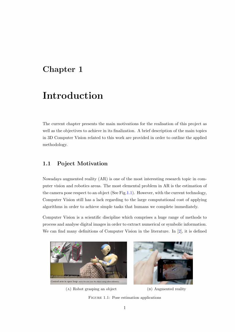
Nowadays augmented reality (AR) is one of the most interesting research topic in com-
puter vision and robotics areas. The most elemental problem in AR is the estimation of
the camera pose respect to an object (See Fig.1.1). However, with the current technology,
Computer Vision still has a lack regarding to the large computational cost of applying
algorithms in order to achieve simple tasks that humans we complete immediately.
Computer Vision is a scientific discipline which comprises a huge range of methods to
process and analyse digital images in order to extract numerical or symbolic information.
We can find many definitions of Computer Vision in the literature. In [2], it is defined
(a) Robot grasping an object (b) Augmented reality
Figure 1.1: Pose estimation applications
1

Chapter 1. Introduction 2
as a branch of artificial intelligence and image processing concerned with computer
processing of images from the real world.
Nonetheless, the real emergence of Computer Vision came with the necessity to auto-
matically analyse images in order to copy the human behaviour and still today is a
constant challenge to replicate generic methods such for depth estimation, relative pose
estimation or even classify perceived objects.
1.2 Focus and Thesis Organization
Objects can be textured, non textured, transparent, articulated, etc. In this project, we
will focus on giving a solution to objects recognition in addition to estimate its 3D pose
given an image sequence.
Until today there is no unique method to solve this essential task since many variables
will define the problem formulation. The most important actor to take into account is
the application goal, followed by the number of degrees of freedom of the object and the
camera, in addition to the camera sensor type. However, in this project we will focus
on the use of a monocular perspective camera to recover the six degrees of freedom that
define the relative position and orientation between the scene and the camera. The
proposed algorithm, based on a tracking by detection methodology [3], recovers the six
degrees of freedom of the camera considering natural feature points and a previously
registered 3D textured model.
We will first introduce in Chapter 2 the previous background and the premises about
the pose estimation problem in order to understand the applied methodology to solve
the problem. Chapter 3 will deal with the geometric and mathematics techniques used
to solve the pose estimation problem. Chapter 4 will introduce the designed software
architecture model. Finally, Chapter 5 and 6 will show the results and contributions
obtained during this project, and the proposed future work.

Chapter 2
Background
In this chapter, is presented the current state of the art related to pose estimation
algorithms, from the origin with the Direct Linear Transform (DLT) algorithm, to the
PnP problem for calibrated and uncalibrated cameras, in addition to robust estimation.
2.1 Calibrated Cameras
The camera pose estimation from n 3D-to-2D points correspondences is a fundamental
and already solved problem in geometric computer vision area. The main goal is to
estimate the six degrees of freedom of the camera pose and the camera calibration
parameters: the focal length, the principal point, the aspect ratio and the skew. A first
approach to solve the problem using a minimum of 6 pair of correspondences can be
done using the well-known Direct Linear Transform (DLT) algoritm [4].
Since the DLT algorithm requires the camera parameters, numerous simplifications to
the problem have been achieved in order to improve the solution accuracy and forming in
consequence a large set of new different algorithms. A variant of the previous algorithm
is the very called Perspective-n-Point problem, which assumes that the camera intrinsic
parameters are known. In its minimal version only three point correspondences are
needed to recover the camera pose [5]. There also exist many iterative solutions to
the over-constrained problem with n > 3 point correspondences [6–8] . However, the
non-iterative solutions are strongly differentiate for its computational complexity and
accuracy from O(n8) [9] to O(n2) [10] down to O(n) [11]. On the other hand, we can
differentiate between algebraic and geometric solutions considering as a representative
case Gao’s solution [5], also known as P3P, in which propose a triangular decomposition
of the equations system. Many other iterative methods for large values of n exist [6–8],
3

Chapter 2. Background 4
in this case, considering Lu’s method [8] as the most representative one since its good
performance in terms of speed and accuracy, produces slightly better results than the
non-iterative methods such as EPnP algorithm [11]. In some cases, in order to improve
the method accuracy, some non-linear optimizations such as Gauss-Newton are applied
with negligible cost.
In most of the cases, iterative methods get trapped in local minima, however, the aim
to find a global optimal solution encourage the researchers to reformulate the problem
as positive semidefinite quadratic optimization problem [12].
2.2 Uncalibrated Cameras
For the uncalibrated case, we can find many solutions assuming that the intrinsic pa-
rameters are unknown, the pixel size is squared, and the principal point is close to the
image center [4, 13], which then the problem is simplified to estimate only the focal
length. For this case, exist solutions to solve the minimal problem assuming unknown
focal lenght [14–17], as well as for the case with unknown focal length plus unknown
radial distortion [13, 17–19].
Groebner et al [16], bases the computation of the 5- and 6-point relative pose problem
with unknown focal length to solve large systems of polynomial equations [15], in both,
solving the problem computing the polynomial eigenvalues. Furthermore, Bujnak et
al [14] propose a general solution to the P4P Problem for cameras with unknown focal
length reducing the equation system to 5 with 4 unknowns and 20 monomials. More
recently, other solutions for the P4P Problem have been proposed for unknown focal
length and radial distortion [13, 18, 19] which always are followed by a robust estimation
method.
2.3 Robust Estimation
Since we are dealing with camera sensors, the presence of noise is unavoidable and the
methods to find the correspondences may give us some mismatches or outliers, then,
due to that fact, the solutions to the problem become unstable and not reliable.
In front of this problem, and the need to establish a robust pairing between features,
the most common solution is to include an extra iterative step using the RANSAC [20]
algorithm for outliers removal or even Least Median Squares [21]. Unfortunately, even
taking its minimal or non-minimal subsets [22], a supplementary high computational
Chapter 2. Background 5
load is always assured which brings the method to rely on a random sampling. Recent
attempts to reformulate the problem as a quasi-convex optimization problem have been
carried out in order to guarantee the estimation of global minima [23–25].
The original RANSAC algorithm has a lot of variations such as Guided-MLESAC [26]
and PROSAC [27] which are aimed to avoid sampling unlikely correspondences by using
appearance based scores. Additionally, GroupSAC [28] uses image segmentation in order
to sample the data more efficiently. Other techniques, such as Preemptive RANSAC [29]
or ARRSAC [30] are used in limited scenarios increasing then probability to obtain the
better estimation as possible. In [31], is presented MultiGS, which speeds up the search
strategy guided by the sampling information obtained from a residual sorting in addition
to be able to account for multiple structures in the scene.
May happen the absence of robust appearance information in graphs, which then the
problem can be solved as is proposed in [32]. Nonetheless, due to the high computational
cost, this graph methods are useless for large graphs.
During the next chapter, will be explained in detail all the mathematical methodol-
ogy and tools introduced in this chapter in order to deeply understand how the built
application works.

Chapter 3
Problem Formulation
The current chapter is aimed to explain from a geometric point of view the pose esti-
mation problem formulation using in this case a pinhole camera model.
3.1 Camera Representation
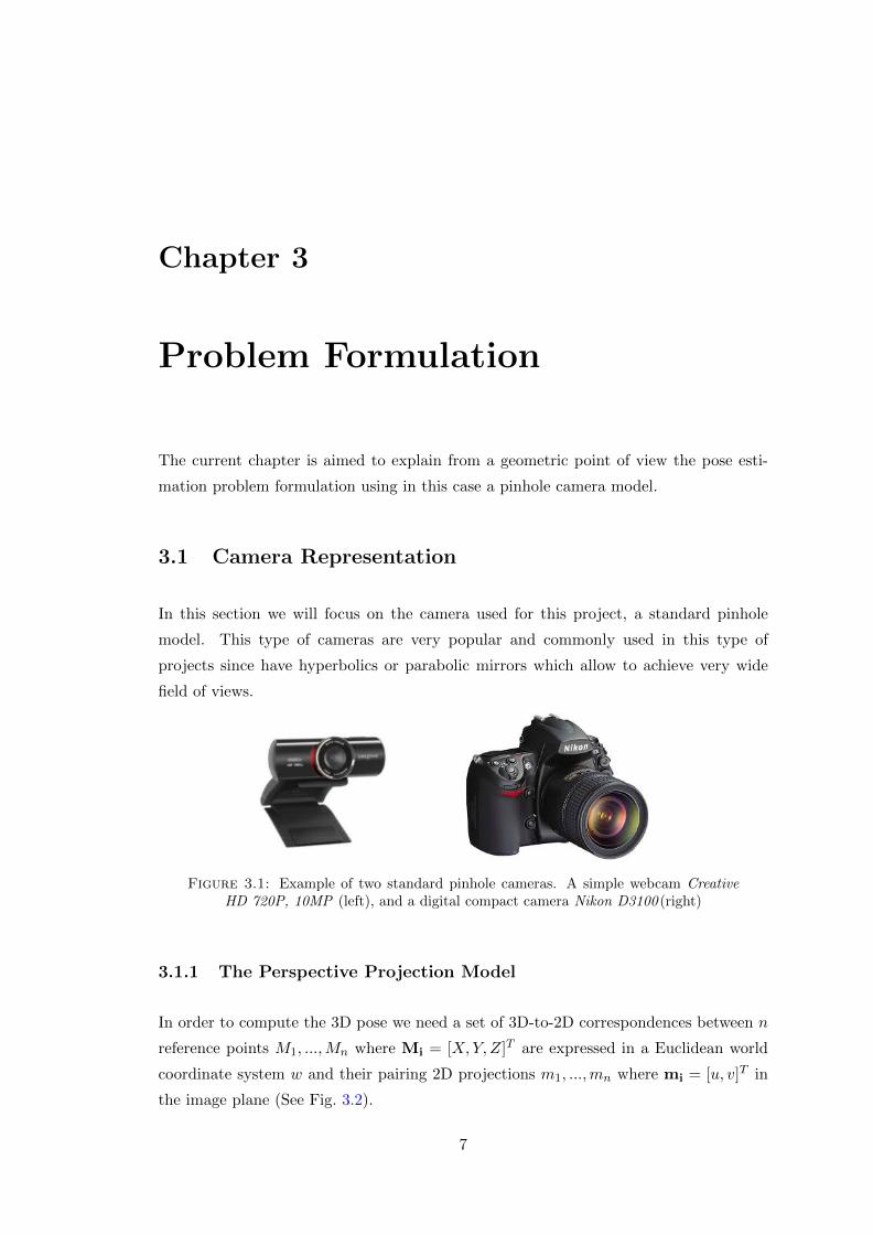
In this section we will focus on the camera used for this project, a standard pinhole
model. This type of cameras are very popular and commonly used in this type of
projects since have hyperbolics or parabolic mirrors which allow to achieve very wide
field of views.
Figure 3.1: Example of two standard pinhole cameras. A simple webcam CreativeHD 720P, 10MP (left), and a digital compact camera Nikon D3100 (right)
3.1.1 The Perspective Projection Model
In order to compute the 3D pose we need a set of 3D-to-2D correspondences between n
reference points M1, ...,Mn where Mi = [X,Y, Z]T are expressed in a Euclidean world
coordinate system w and their pairing 2D projections m1, ...,mn where mi = [u, v]T in
the image plane (See Fig. 3.2).
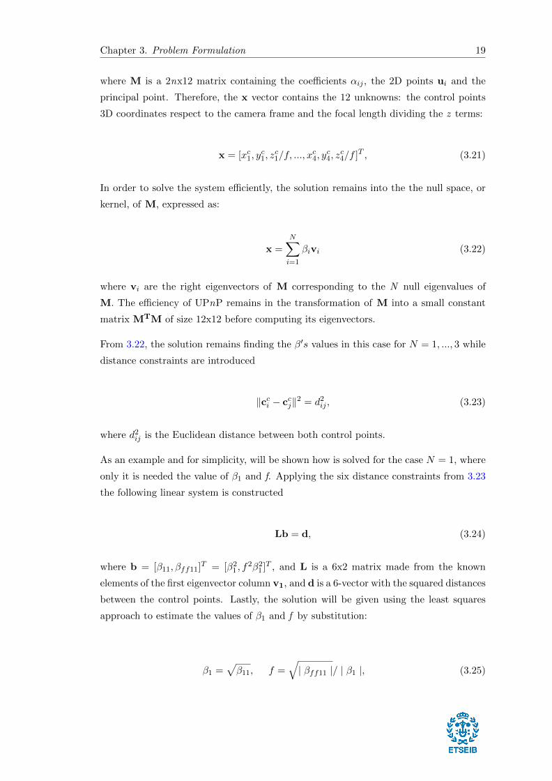
7
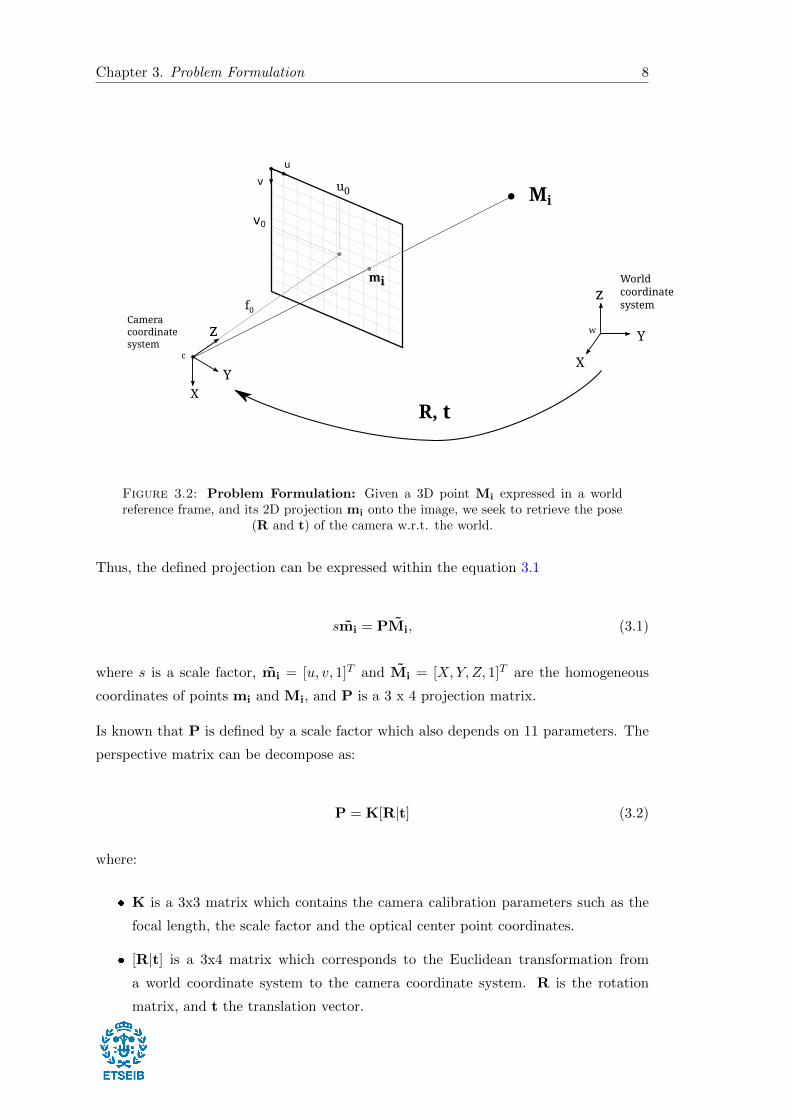
Chapter 3. Problem Formulation 8
R, t
Mi
World coordinate system
mi
z
YX
f0Cameracoordinate system
c
z
Y
X
u0
v0
v
u
w
Figure 3.2: Problem Formulation: Given a 3D point Mi expressed in a worldreference frame, and its 2D projection mi onto the image, we seek to retrieve the pose
(R and t) of the camera w.r.t. the world.
Thus, the defined projection can be expressed within the equation 3.1
smi = PMi, (3.1)
where s is a scale factor, mi = [u, v, 1]T and Mi = [X,Y, Z, 1]T are the homogeneous
coordinates of points mi and Mi, and P is a 3 x 4 projection matrix.
Is known that P is defined by a scale factor which also depends on 11 parameters. The
perspective matrix can be decompose as:
P = K[R|t] (3.2)
where:
K is a 3x3 matrix which contains the camera calibration parameters such as the
focal length, the scale factor and the optical center point coordinates.
[R|t] is a 3x4 matrix which corresponds to the Euclidean transformation from
a world coordinate system to the camera coordinate system. R is the rotation
matrix, and t the translation vector.
Chapter 3. Problem Formulation 9
3.1.2 The Intrinsic Parameters
In the previous section we defined K as a matrix with the internal camera calibration
parameters, usually referred as camera calibration matrix, can be expressed by the
following equation:
K =
αu s u0
0 αv v0
0 0 1
, (3.3)
where:
αu and αv are the scale factor defined in each coordinate direction u and v. This
scale factors are proportional to the camera focal length: α = kuf and α = kvf ,
where ku and kv are the total number of pixels per unit in the u and v directions.
c = [u0, v0]T represents the principal point coordinates, which it is the intersection
of the optical axis and the image plane.
s, referred as the skew angle, is the ratio which defines the perpendicularity of the
u and v directions. In modern cameras usually this value is zero.
In order to simplify the problem, often a common approximation is to set the principal
point c at the image center. Furthermore, in modern cameras we assume that the pixels
have a squared shape, which lead us then to take αu and αv with equal values. In
geometric computer vision it is said that when the camera calibration matrix or the
intrinsic parameters are known, the camera is calibrated.
3.1.3 The Extrinsic Parameters
Previously we defined [R|t] as a 3x4 matrix which corresponds to the Euclidean trans-
formation from a world coordinate system to the camera coordinate system. In fact this
matrix is the horizontal concatenation of the rotation matrix and the translation vector
which is often referred as the camera pose. (See eq. 3.4)
[R|t] =
R11 R12 R13 t1
R21 R22 R23 t2
R31 R32 R33 t3
, (3.4)
Chapter 3. Problem Formulation 10
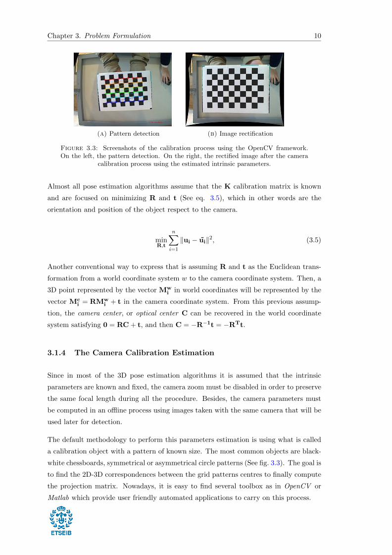
(a) Pattern detection (b) Image rectification
Figure 3.3: Screenshots of the calibration process using the OpenCV framework.On the left, the pattern detection. On the right, the rectified image after the camera
calibration process using the estimated intrinsic parameters.
Almost all pose estimation algorithms assume that the K calibration matrix is known
and are focused on minimizing R and t (See eq. 3.5), which in other words are the
orientation and position of the object respect to the camera.
minR,t
n∑i=1
‖ui − ui‖2, (3.5)
Another conventional way to express that is assuming R and t as the Euclidean trans-
formation from a world coordinate system w to the camera coordinate system. Then, a
3D point represented by the vector Mwi in world coordinates will be represented by the
vector Mci = RMw
i + t in the camera coordinate system. From this previous assump-
tion, the camera center, or optical center C can be recovered in the world coordinate
system satisfying 0 = RC + t, and then C = −R−1t = −RTt.
3.1.4 The Camera Calibration Estimation
Since in most of the 3D pose estimation algorithms it is assumed that the intrinsic
parameters are known and fixed, the camera zoom must be disabled in order to preserve
the same focal length during all the procedure. Besides, the camera parameters must
be computed in an offline process using images taken with the same camera that will be
used later for detection.
The default methodology to perform this parameters estimation is using what is called
a calibration object with a pattern of known size. The most common objects are black-
white chessboards, symmetrical or asymmetrical circle patterns (See fig. 3.3). The goal is
to find the 2D-3D correspondences between the grid patterns centres to finally compute
the projection matrix. Nowadays, it is easy to find several toolbox as in OpenCV or
Matlab which provide user friendly automated applications to carry on this process.
Chapter 3. Problem Formulation 11
3.2 Camera Pose Parametrization
In order to estimate the camera pose, first an appropriated parametrization of its trans-
lation vector and rotation matrix is needed.
A rotation matrix has only three degrees of freedom in R3, which means that it will
directly depend on the nine elements of the 3x3 rotation matrix. Since this matrix must
be orthonormal, are needed six additional non-linear constrains - three to force all three
columns to be of unit length, and three to ensure the orthogonality between them.
In the literature we can find some parametrizations which demonstrates that are effec-
tive for pose estimation: Euler angles, quaternions, and exponential maps [33]. In the
subsections below we will see in detail some properties about Euler angles and exponen-
tial maps. Quaterions will not be explained since have not been used for the completion
of this project.
3.2.1 Euler Angles
The rotation matrix R can be written as the product of three matrices representing
rotations around the X, Y, and Z axis, where we can find several conventions that
assures that. The most common one, takes α, β, γ respectively as a rotation angles
around the Z, Y, and X axis
R =
cosα − sinα 0
sinα cosα 0
0 0 1
cosβ 0 sinβ
0 1 0
− sinβ 0 cosβ
1 0 0
0 cos γ − sin γ
0 sin γ cos γ
, (3.6)
The extraction of the Euler angles for a given rotation matrix can be easily realized by
identifying the matrix coefficient as well as its analytical expression.
However, Euler angles have a well known drawback called gimbal lock, which it is caused
when two of the three rotations axis are aligned, producing no effect in one rotation axis.
For this reason, Eulers angles are not used anymore for pose estimation algorithms.
3.2.2 Exponential Map
The exponential map needs only three parameters to describe a rotation and does not
stumble in the gimbal lock problem.
Chapter 3. Problem Formulation 12
Given a 3D vector ~ω = [ωx, ωy, ωz]T and θ = ‖~ω‖ its norm, then an angular rotation θ
around an axis of direction ω can be represented as the infinite series
exp(Ω) = I + Ω +1
2!Ω2 +
1
3!Ω3 + · · · (3.7)
where Ω is the skew-symmetric matrix
Ω =
0 −ωz ωy
ωz 0 −ωx−ωy ωx 0
, (3.8)
In eq. 3.7 we can see that the exponential map representation can be rewritten as the
series expansion of an exponential. Then, it can be evaluated using Rodrigues formula
R(Ω) = exp(Ω) = I + sin θΩ + (1− cos θ)Ω2, (3.9)
To summarize, with the exponential map we can represent a rotation as a 3-vector which
each axis will have an associated magnitude. Moreover, using this representation the
gimbal lock problem of Euler angles is avoided.
3.3 External Parameters Matrix Estimation
In this section are presented the evolution over the time of some methods to estimate
the external camera parameters without any prior knowledge of camera position. It is
assumed that some correspondences between 3D points in the world coordinate system
and their projections in the image plane and the camera parameters are known.
The main objective of pose estimation is to find the perspective projection matrix P
which projects the 3D points Mi on mi given a set of n correspondences. We can rewrite
that in terms of PMi ≡ mi for all i, where ≡ represents the equality up to a scale factor.
The number of correspondences will depend on the used approach to recover the pose.
However, when the intrinsic parameters are known and n = 3, this known correspon-
dences Mi ↔mi produce 4 possible solutions. In the case of n = 4 or n = 5 pairings,in
[20] is shown that there are at least two solutions in general configurations. For n ≥ 4
and the points are coplanar and there is no triplets of collinear points, the solution is
unique. When n ≥ 6, the solution is unique.
Chapter 3. Problem Formulation 13
3.3.1 The Direct Linear Transformation
The Direct Linear Transform (DLT) was the starting point in pose recovering. First
used by photogrammetrists, and then introduced in the computer vision community,
this algorithm is able to estimate the projection matrix P by solving a linear equations
system with unknown camera parameters. For each pairing Mi ↔ mi, two linearly
independent equations can be written as follows:
P11Xi + P12Yi + P13Zi + P14
P31Xi + P32Yi + P33Zi + P34= ui,
P21Xi + P22Yi + P23Zi + P24
P31Xi + P32Yi + P33Zi + P34= vi,
This system can be written in the form of Ap = 0, where p is a vector composed by
the coefficients Pij . The solution to this system can be found from the Singular Value
Decomposition (SVD) of A taking the eigenvector with the minimal eigenvalue.
To recover the camera pose, then the camera calibration matrix K is needed in order
to be extracted from P up to a scale factor as follows: [R | t] ∼ K−1P. Finally, the
3x3 rotation matrix can be computed from the first three columns applying a correction
step [34].
Is known that pixel locations mi are often noisy, this method should be refined by an
iterative optimization step in order to minimize the non-linear reprojection error. We
will see this topic in subsection 3.3.3.
3.3.2 The Perspective-n-Point Problem
Since the DLT estimates 11 parameters of the projection matrix without knowing the
camera intrinsics and using only a single point, then the internal parameters must be
estimated in an offline process. However, this information can be used in addition to
introduce extra points in the system, which will make more robust the camera pose
estimation process.
When more than one point is introduced to solve the system, the problem becomes
to what it is called a Perspective n Point Problem, PnP in short, which determines
the position and orientation given a set of n pairings between 3D points and their 2D
projections (See fig. 3.4). As mentioned in Chapter 1, we can find in the literature many
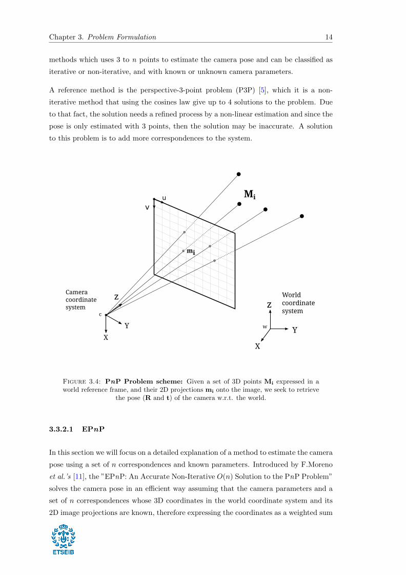
Chapter 3. Problem Formulation 14
methods which uses 3 to n points to estimate the camera pose and can be classified as
iterative or non-iterative, and with known or unknown camera parameters.
A reference method is the perspective-3-point problem (P3P) [5], which it is a non-
iterative method that using the cosines law give up to 4 solutions to the problem. Due
to that fact, the solution needs a refined process by a non-linear estimation and since the
pose is only estimated with 3 points, then the solution may be inaccurate. A solution
to this problem is to add more correspondences to the system.
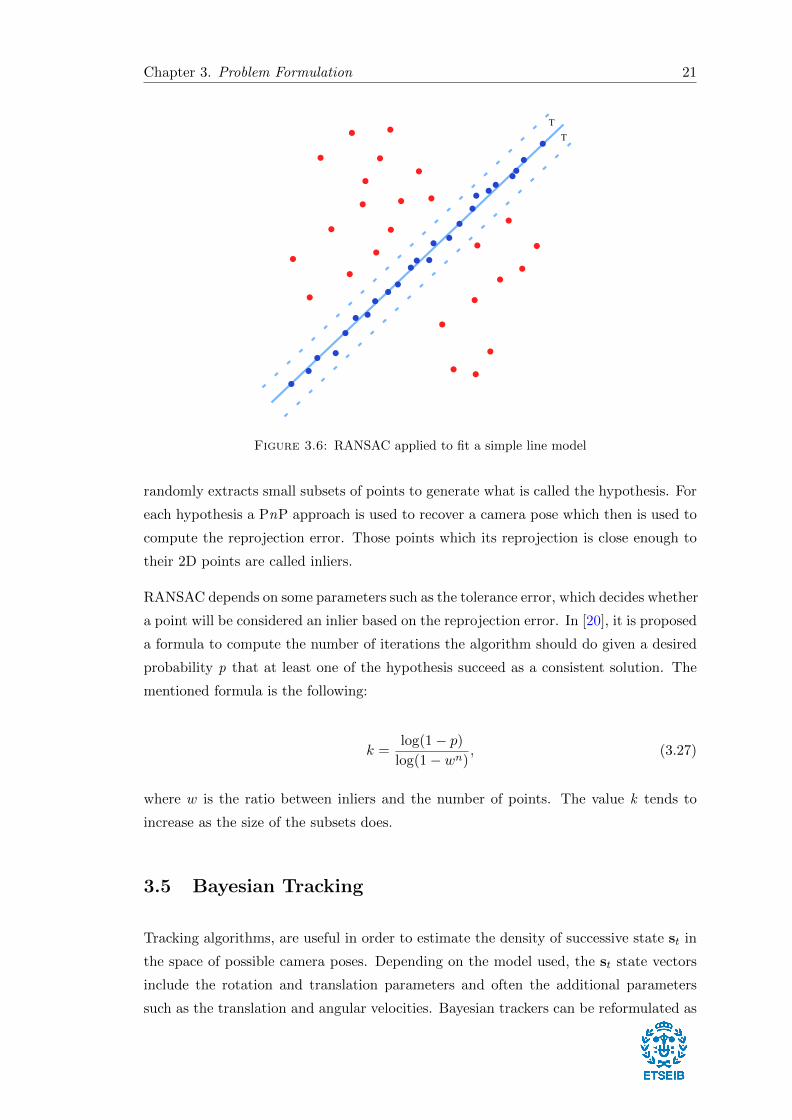
Mi
World coordinate system
mi
z
Y
X
Cameracoordinate system
c
z
Y
X
vu
w
Figure 3.4: PnP Problem scheme: Given a set of 3D points Mi expressed in aworld reference frame, and their 2D projections mi onto the image, we seek to retrieve
the pose (R and t) of the camera w.r.t. the world.
3.3.2.1 EPnP
In this section we will focus on a detailed explanation of a method to estimate the camera
pose using a set of n correspondences and known parameters. Introduced by F.Moreno
et al.’s [11], the ”EPnP: An Accurate Non-Iterative O(n) Solution to the PnP Problem”
solves the camera pose in an efficient way assuming that the camera parameters and a
set of n correspondences whose 3D coordinates in the world coordinate system and its
2D image projections are known, therefore expressing the coordinates as a weighted sum
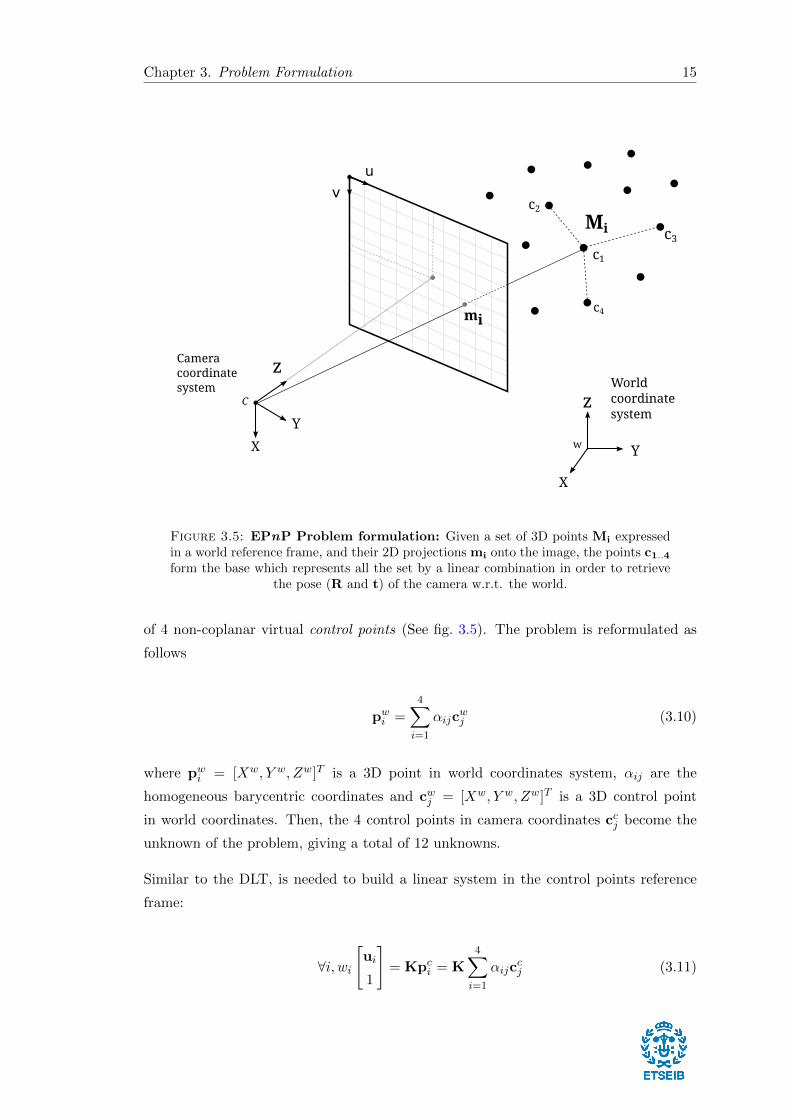
Chapter 3. Problem Formulation 15
Mi
World coordinate system
mi
z
Y
X
Cameracoordinate system
C z
Y
X
v
u
w
c2
c4
c3
c1
Figure 3.5: EPnP Problem formulation: Given a set of 3D points Mi expressedin a world reference frame, and their 2D projections mi onto the image, the points c1..4form the base which represents all the set by a linear combination in order to retrieve
the pose (R and t) of the camera w.r.t. the world.
of 4 non-coplanar virtual control points (See fig. 3.5). The problem is reformulated as
follows
pwi =
4∑i=1
αijcwj (3.10)
where pwi = [Xw, Y w, Zw]T is a 3D point in world coordinates system, αij are the
homogeneous barycentric coordinates and cwj = [Xw, Y w, Zw]T is a 3D control point
in world coordinates. Then, the 4 control points in camera coordinates ccj become the
unknown of the problem, giving a total of 12 unknowns.
Similar to the DLT, is needed to build a linear system in the control points reference
frame:
∀i, wi
[ui
1
]= Kpci = K
4∑i=1
αijccj (3.11)
Chapter 3. Problem Formulation 16
where wi are the scalar projective parameters, ui are the 2D coordinates [ui, vi]T , K is
the camera parameters matrix. This expression can be rewritten as follows:
∀i, wi
ui
vi
1
=
fu 0 uc
0 fv vc
0 0 1
4∑i=1
αijccj
xcj
ycj
zcj
(3.12)
From 3.12 we can obtain two linearly independent equations:
4∑i=1
αijfuxcj + αij(uc − ui)zcj = 0,
4∑i=1
αijfvycj + αij(vc − vi)zcj = 0,
Hence, a linear system is generated with the following form:
Mx = 0 (3.13)
where M is a 2nx12 matrix with known coefficients and x = [cc1, cc2, c
c3, c
c4]T is a 12-vector
made of the unknowns.
The solution to this system lies on the null space, or kernel, of M, expressed as:
x =N∑i=1
βivi (3.14)
where vi are the right eigenvectors of M, corresponding to the N null eigenvalues of
M. The efficiency of EPnP remains in the transformation of M into a small constant
matrix MTM of size 12x12 before computing the eigenvectors.
From 3.14, in theory the solution will be given by β′is for each N. Nonetheless, in practice
the solution will be obtained only for N = 1, ..., 4
Chapter 3. Problem Formulation 17
N = 1 : x = β1v1
N = 2 : x = β1v1 + β2v2
N = 3 : x = β1v1 + β2v2 + β3v3
N = 4 : x = β1v1 + β2v2 + β3v3 + β4v4
In order to find the correct betas, a geometric constraint must be added. The method
assumes that the distances between control points in the camera coordinate system
should be equal to the ones computed in the world coordinate system:
‖cci − ccj‖2 = ‖cwi − cwj ‖2, (3.15)
For simplicity, I will show only the case for N = 1, where:
‖βv[i] − βv[j]‖2 = ‖cwi − cwj ‖2, (3.16)
Then the beta can be computed as follows
β =
∑i,j∈[1;4] ‖v[i] − v[j]‖ · ‖cwi − cwj ‖∑
i,j∈[1;4] ‖v[i] − v[j]‖2, (3.17)
Once the betas are computed, in order to get the camera pose is needed to do the inverse
process. Firstly, compute the control points coordinates in the camera frame reference.
Secondly, compute the coordinates of all 3D points in camera frame reference and finally,
as shown in [35], extract the rotation matrix R and the translation vector t.
3.3.2.2 UPnP
The following method, ”Exhaustive Linearization for Robust Camera Pose and Focal
Length Estimation” or Uncalibrated PnP (UPnP), introduced by A. Penate et al.’s [1],
is an extension of the EPnP for the case of uncalibrated cameras. The method, allows
to estimate the camera pose in addition to the camera focal length in bounded time.
Although the solution is non-minimal, it becomes robust in front of several noise coming
from the input data.
Similar to the EPnP algorithm, the solution to the problem belongs to the kernel of a
matrix derived from the set of 2D-to-3D correspondences, which can be expressed as
Chapter 3. Problem Formulation 18
a linear combination of its eigenvectors. Again, the weights of this linear combination
become the unknown of the problem, solved by applying additional distance constraints.
It is assumed that a set of 2D-to-3D correspondences are given between n reference points
pw1 , ...,pwn respect to a world coordinate system w, and their 2D projections u1, ...,un
in the image plane. Furthermore, it is expected a squared pixel size camera with the
principal point (u0, v0) at the center of the image. Under these assumptions, the problem
is formulated to retrieve the focal length f, the rotation matrix R and the translation
vector t by minimizing an objective function based on the reprojection error:
minf,R,t
n∑i=1
‖ui − ui‖2, (3.18)
where ui is the projection of point pwi :
ki
[ui
1
]=
fu 0 uc
0 fv vc
0 0 1
[R | t]
[pwi
1
], (3.19)
with a ki scalar projective parameter.
Identically to the EPnP, each 3D point is rewritten in terms of barycentric coordinates
respect to 4 control points, turning then the problem in finding the solution of a 2n
equations with 12 unknowns linear system. The main difference of this method persists
on the perspective projection equations construction, which now the focal length is taken
into account:
4∑j=1
αijxcj + αij(u0 − ui)
zcjf
= 0,
4∑j=1
αijycj + αij(v0 − vi)
zcjf
= 0,
These equations can be expressed as the following linear system
Mx = 0, (3.20)
Chapter 3. Problem Formulation 19
where M is a 2nx12 matrix containing the coefficients αij , the 2D points ui and the
principal point. Therefore, the x vector contains the 12 unknowns: the control points
3D coordinates respect to the camera frame and the focal length dividing the z terms:
x = [xc1, yc1, z
c1/f, ..., x
c4, y
c4, z
c4/f ]T , (3.21)
In order to solve the system efficiently, the solution remains into the the null space, or
kernel, of M, expressed as:
x =N∑i=1
βivi (3.22)
where vi are the right eigenvectors of M corresponding to the N null eigenvalues of
M. The efficiency of UPnP remains in the transformation of M into a small constant
matrix MTM of size 12x12 before computing its eigenvectors.
From 3.22, the solution remains finding the β′s values in this case for N = 1, ..., 3 while
distance constraints are introduced
‖cci − ccj‖2 = d2ij , (3.23)
where d2ij is the Euclidean distance between both control points.
As an example and for simplicity, will be shown how is solved for the case N = 1, where
only it is needed the value of β1 and f. Applying the six distance constraints from 3.23
the following linear system is constructed
Lb = d, (3.24)
where b = [β11, βff11]T = [β21 , f
2β21 ]T , and L is a 6x2 matrix made from the known
elements of the first eigenvector column v1, and d is a 6-vector with the squared distances
between the control points. Lastly, the solution will be given using the least squares
approach to estimate the values of β1 and f by substitution:
β1 =√β11, f =
√| βff11 |/ | β1 |, (3.25)
Chapter 3. Problem Formulation 20
Once with the betas computed, the camera pose is estimated doing the inverse process.
Firstly, computing the control points coordinates in the camera frame reference. Sec-
ondly, computing the coordinates of all 3D points in camera frame reference. Finally, as
shown in [35], doing the extraction of the rotation matrix R and the translation vector
t.
3.4 Robust Estimation
Previously we mentioned the possibility to have noisy measurements and how this would
affect the pose estimation algorithms. Robust estimation is a methodology to compute
the camera pose removing as much as possible the noisy data introduced by gross errors.
There are two popular methods to solve that problem, the RANSAC algorithm and M-
estimators. Despite of the effectiveness of both algorithms, in this project we will only
focus on RANSAC that minimizes what is called the reprojection error.
3.4.1 Non-Linear Reprojection Error
In section 3.3.1 we talked about the sensitivity in front of the noise and the lack pre-
cision of measurements mi. A proposed methodology to improve results is refining the
estimated camera pose by doing a minimization of the sum of the reprojection errors,
which it is the accumulated squared distance between the projection of a 3D point Mi
and its measured 2D coordinates. It can therefore be written by
[R | t] = minR,t
n∑i=1
dist2(PMi,mi), (3.26)
which can be assumed as optimal due to the fact that each measurement is independent
and Gaussian. This minimization must be done into an iterative optimization scheme
which usually requires an initial estimation of the camera pose.
3.4.2 RANSAC
The Random Sample Consensus or RANSAC [20] is a non-deterministic iterative method
which estimates parameters of a mathematical model from observed data producing an
approximate result as the number of iterations increase. (See fig. 3.6)
In the context of camera pose estimation, it is very simple to implement since an initial
guess of the parameters is not needed. From the set of correspondences, the algorithm
Chapter 3. Problem Formulation 21
T
T
Figure 3.6: RANSAC applied to fit a simple line model
randomly extracts small subsets of points to generate what is called the hypothesis. For
each hypothesis a PnP approach is used to recover a camera pose which then is used to
compute the reprojection error. Those points which its reprojection is close enough to
their 2D points are called inliers.
RANSAC depends on some parameters such as the tolerance error, which decides whether
a point will be considered an inlier based on the reprojection error. In [20], it is proposed
a formula to compute the number of iterations the algorithm should do given a desired
probability p that at least one of the hypothesis succeed as a consistent solution. The
mentioned formula is the following:
k =log(1− p)
log(1− wn), (3.27)
where w is the ratio between inliers and the number of points. The value k tends to
increase as the size of the subsets does.
3.5 Bayesian Tracking
Tracking algorithms, are useful in order to estimate the density of successive state st in
the space of possible camera poses. Depending on the model used, the st state vectors
include the rotation and translation parameters and often the additional parameters
such as the translation and angular velocities. Bayesian trackers can be reformulated as
Chapter 3. Problem Formulation 22
what is called the propagation rule (Equation 3.28) which is a recursive equation that
relates over time t, the current with the previous density function of a process
p(st | zt−1 . . . z0) =
∫st−1
p(st | st−1)pt−1(st−1), (3.28)
where∫st−1
is the integration over the set of possible values for the previous state st−1.
The term p(st | zt−1 . . . z0) can be interpreted as a prediction on pt(st) made by applying
the motion model on the previous density state pt−1(st−1. The name of ”Bayesian
tracking” comes from the fact that Equation 3.28 is an equivalent reformulation of
Baye’s rule for the discrete time varying case.
Many tracking systems ignore the probability density function and retain only one single
hypothesis for the camera pose, usually the maximum-likelihood. Nevertheless, the
Bayesian formulation it is useful to make robust the tracking algorithms in front of bad
estimations. The most common Bayesian algorithms are Particle Filters and Kalman
Filters, even though in this project we will focus on the second one.
3.5.1 Kalman Filter
The Kalman Filter is a recursive method for estimate the state of a process that can be
applied in many areas, however, the purpose will be the application to 3D tracking. In
the literature we can find two main formulations of the problem, the Linear and non-
Linear cases, that using one or the other will depend on the complexity of the problem
and the expected accuracy. Nevertheless, in this project we will only focus on the simple
case, the Linear Kalman Filter.
The successive states st ∈ Rn of a discrete-time controlled process are assumed to envolve
according to a dynamics model written as follows
st = Ast−1 + wt, (3.29)
where A is called the state transition matrix, and wt represents the process noise which
is assumed to be normally distributed with zero mean. For tracking purposes, the state
vector will be comprised by the 6 parameters of the camera pose, plus the translational
and angular velocities.
The measurements zt such as the the camera pose at time t, are assumed to be related
to the state st by a linear measurement model
Chapter 3. Problem Formulation 23
zt = Cst + vt, (3.30)
where vt represents the measurement noise.
At each time step, the Kalman Filter makes a fist estimation of the current state called
the a priori state estimate s−t , which is refined by incorporating the measurements to
yield the a posteriori estimate st. s−t and its covariance matrix S−t , are computed during
the prediction stage and can be written as
s−t = Ast−1, (3.31)
S−t = ASt−1AT + Λw, (3.32)
where St−1 is the a posteriori estimate error covariance for the previous time step, and
Λw is the process covariance noise that measures quality of the motion model respect to
the reality. Next, the Kalman Filter does a ”measurement update” or correction. The
a posteriori state estimate st and its covariance matrix St are now generated by adding
the measurements zt
st = s−t + Gt(zt −Gs−t ), (3.33)
St = S−t −GtCS−t , (3.34)
where the Kalman gain Gt is computed as
Gt = S−t CT (CS−t CT + Λv)−1, (3.35)
with Λv being the measurements covariance matrix.
In the context of 3D tracking, the a priori state estimate s−t can be used to predict
the camera extrinsic parameters, therefore, the predicted measurement vector z−t is the
following
z−t = Cs−t , (3.36)

Chapter 3. Problem Formulation 24
The uncertainty on the prediction is represented by the covariance matrix Λz estimated
by propagating the uncertainty
Λz = CS−t CT + Λv, (3.37)

Chapter 4
Software Architecture
The aim of this chapter is to explain the algorithm implementation by using the well
known modelling language Unified Modeling Language (UML) [36]. To do that, an
activities diagram, an use of cases diagram and class diagrams are provided in order to
understand the application structure.
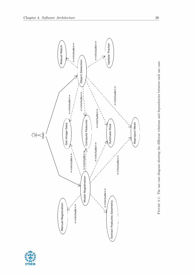
4.1 Use Cases Design
The current section pretends to illustrate the use cases model by an use cases diagram,
Figure 4.1, which represents all the application requirements including its internal and
external influences. The uses cases are considered as a high level requirements to achieve
the final task, in this case estimate an object pose. Each use case has its relationships
and dependencies represented with arrows. From Fig. 4.1 we can see that the application
will be composed by two main use cases: the model registration and the object detection,
which at the same time will share other use cases.
In the next sections, each use case is explained in detail attached to some visual illus-
trations with the expected results.
25
Chapter 4. Software Architecture 26
Mod
el R
eg
istr
ati
on
Ob
ject
Dete
cti
on
Get
Imag
e D
ata
Com
pute
Featu
res
Rob
ust
Matc
h
Esti
mate
Pose
Rep
roje
ct
Mesh
Up
date
Tra
cker
Extr
act
Featu
res G
eom
etr
y
Manu
al R
eg
istr
ati
on
User
<<
inclu
de>
>
<<
inclu
de>
>
<<
inclu
de>
>
<<
inclu
de>
>
<<
inclu
de>
>
<<
inclu
de>
>
<<
inclu
de>
>
<<
inclu
de>
>
<<
inclu
de>
>
<<
inclu
de>
><
<in
clu
de>
>
<<
inclu
de>
>
Fig
ure
4.1
:T
he
use
case
dia
gram
show
ing
the
diff
eren
tre
lati
on
san
dd
epen
den
cies
bet
wee
nea
chu
seca
se.
Chapter 4. Software Architecture 27
Figure 4.2: Screenshot of an image obtained from a standard camera and its matrixrepresentation. Image extracted from OpenCV official documentation.
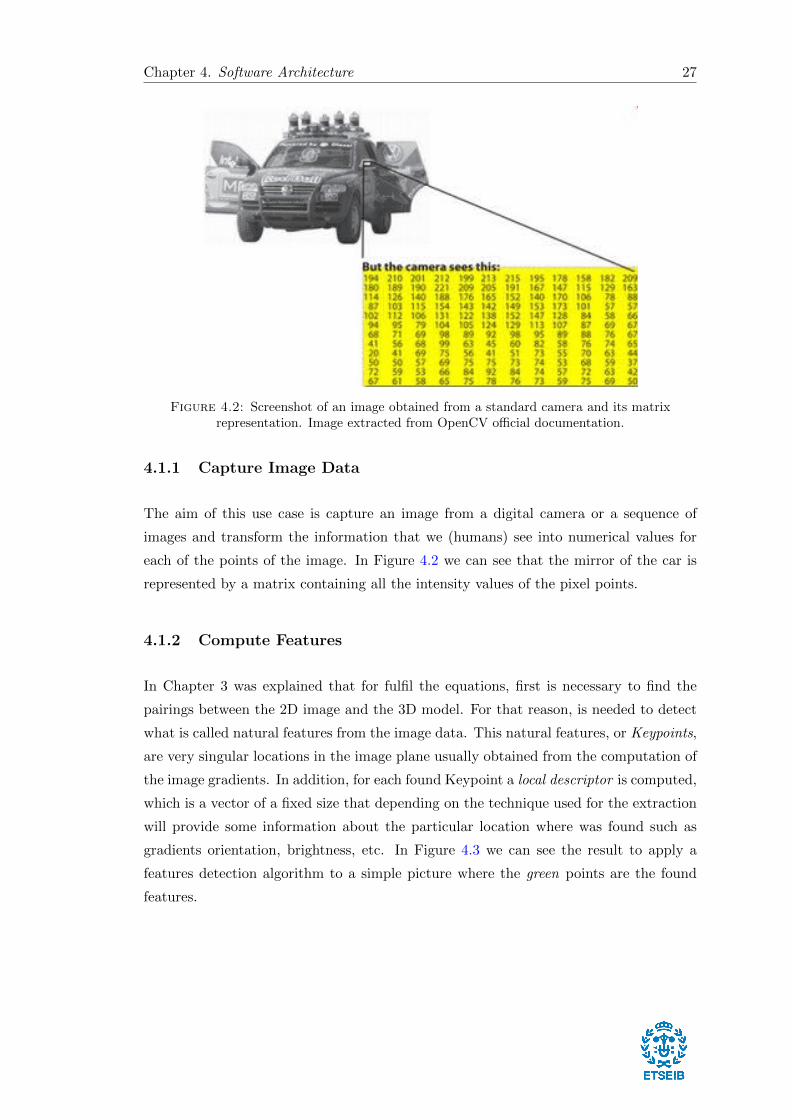
4.1.1 Capture Image Data
The aim of this use case is capture an image from a digital camera or a sequence of
images and transform the information that we (humans) see into numerical values for
each of the points of the image. In Figure 4.2 we can see that the mirror of the car is
represented by a matrix containing all the intensity values of the pixel points.
4.1.2 Compute Features
In Chapter 3 was explained that for fulfil the equations, first is necessary to find the
pairings between the 2D image and the 3D model. For that reason, is needed to detect
what is called natural features from the image data. This natural features, or Keypoints,
are very singular locations in the image plane usually obtained from the computation of
the image gradients. In addition, for each found Keypoint a local descriptor is computed,
which is a vector of a fixed size that depending on the technique used for the extraction
will provide some information about the particular location where was found such as
gradients orientation, brightness, etc. In Figure 4.3 we can see the result to apply a
features detection algorithm to a simple picture where the green points are the found
features.
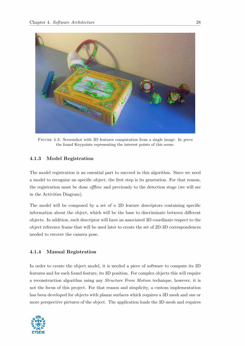
Chapter 4. Software Architecture 28
Figure 4.3: Screenshot with 2D features computation from a single image. In greenthe found Keypoints representing the interest points of this scene.
4.1.3 Model Registration
The model registration is an essential part to succeed in this algorithm. Since we need
a model to recognize an specific object, the first step is its generation. For that reason,
the registration must be done offline and previously to the detection stage (we will see
in the Activities Diagram).
The model will be composed by a set of n 2D feature descriptors containing specific
information about the object, which will be the base to discriminate between different
objects. In addition, each descriptor will have an associated 3D coordinate respect to the
object reference frame that will be used later to create the set of 2D-3D correspondences
needed to recover the camera pose.
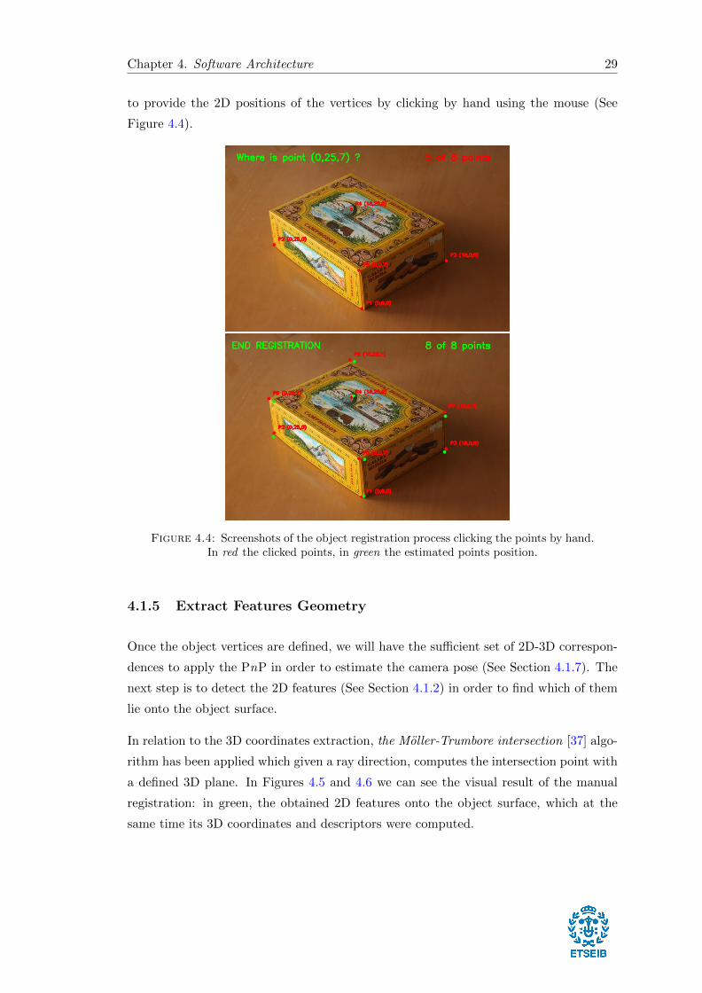
4.1.4 Manual Registration
In order to create the object model, it is needed a piece of software to compute its 2D
features and for each found feature, its 3D position. For complex objects this will require
a reconstruction algorithm using any Structure From Motion technique, however, it is
not the focus of this project. For that reason and simplicity, a custom implementation
has been developed for objects with planar surfaces which requires a 3D mesh and one or
more perspective pictures of the object. The application loads the 3D mesh and requires
Chapter 4. Software Architecture 29
to provide the 2D positions of the vertices by clicking by hand using the mouse (See
Figure 4.4).
Figure 4.4: Screenshots of the object registration process clicking the points by hand.In red the clicked points, in green the estimated points position.
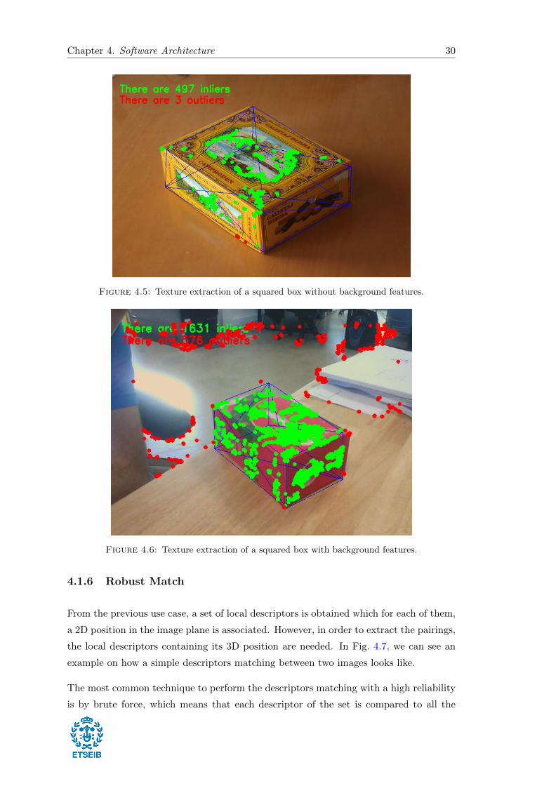
4.1.5 Extract Features Geometry
Once the object vertices are defined, we will have the sufficient set of 2D-3D correspon-
dences to apply the PnP in order to estimate the camera pose (See Section 4.1.7). The
next step is to detect the 2D features (See Section 4.1.2) in order to find which of them
lie onto the object surface.
In relation to the 3D coordinates extraction, the Moller-Trumbore intersection [37] algo-
rithm has been applied which given a ray direction, computes the intersection point with
a defined 3D plane. In Figures 4.5 and 4.6 we can see the visual result of the manual
registration: in green, the obtained 2D features onto the object surface, which at the
same time its 3D coordinates and descriptors were computed.
Chapter 4. Software Architecture 30
Figure 4.5: Texture extraction of a squared box without background features.
Figure 4.6: Texture extraction of a squared box with background features.
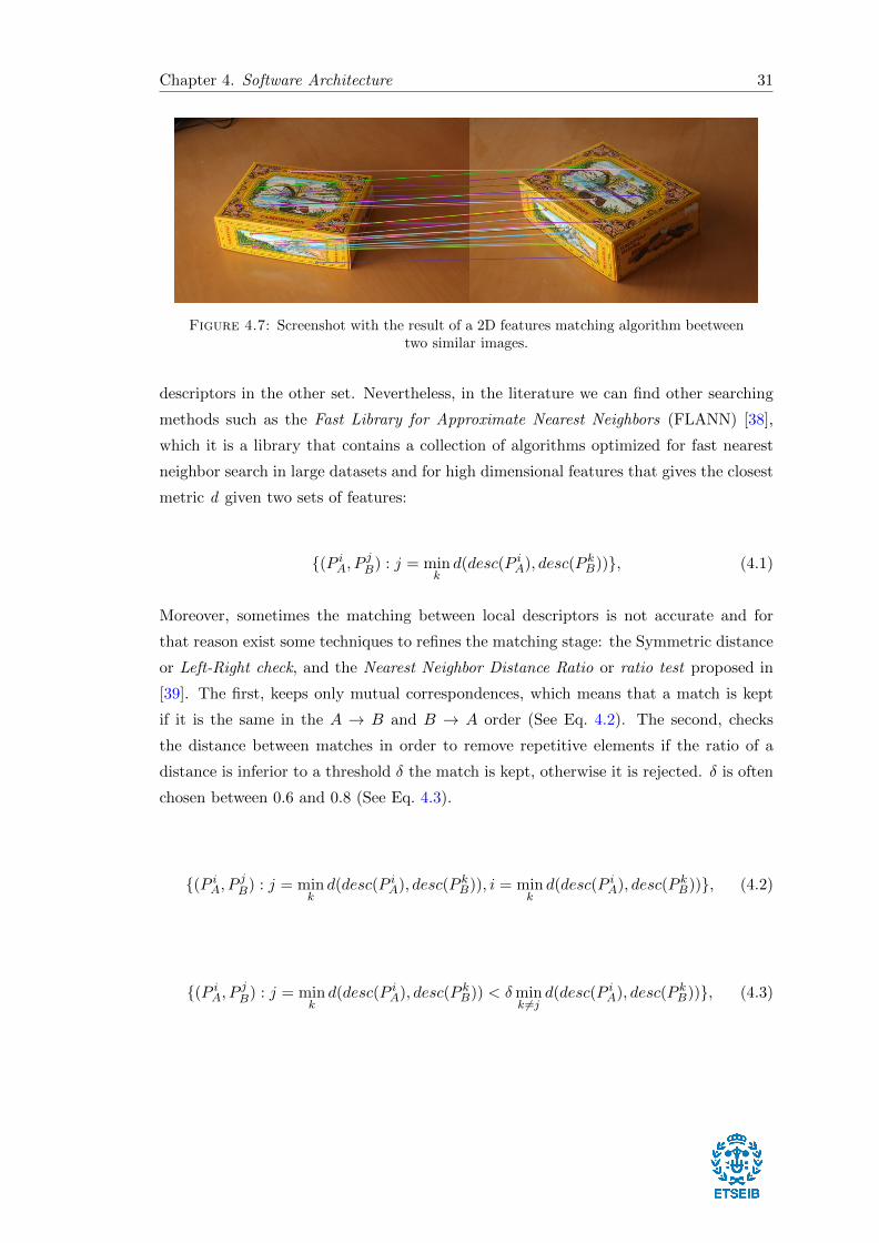
4.1.6 Robust Match
From the previous use case, a set of local descriptors is obtained which for each of them,
a 2D position in the image plane is associated. However, in order to extract the pairings,
the local descriptors containing its 3D position are needed. In Fig. 4.7, we can see an
example on how a simple descriptors matching between two images looks like.
The most common technique to perform the descriptors matching with a high reliability
is by brute force, which means that each descriptor of the set is compared to all the
Chapter 4. Software Architecture 31
Figure 4.7: Screenshot with the result of a 2D features matching algorithm beetweentwo similar images.
descriptors in the other set. Nevertheless, in the literature we can find other searching
methods such as the Fast Library for Approximate Nearest Neighbors (FLANN) [38],
which it is a library that contains a collection of algorithms optimized for fast nearest
neighbor search in large datasets and for high dimensional features that gives the closest
metric d given two sets of features:
(P iA, PjB) : j = min
kd(desc(P iA), desc(P kB)), (4.1)
Moreover, sometimes the matching between local descriptors is not accurate and for
that reason exist some techniques to refines the matching stage: the Symmetric distance
or Left-Right check, and the Nearest Neighbor Distance Ratio or ratio test proposed in
[39]. The first, keeps only mutual correspondences, which means that a match is kept
if it is the same in the A → B and B → A order (See Eq. 4.2). The second, checks
the distance between matches in order to remove repetitive elements if the ratio of a
distance is inferior to a threshold δ the match is kept, otherwise it is rejected. δ is often
chosen between 0.6 and 0.8 (See Eq. 4.3).
(P iA, PjB) : j = min
kd(desc(P iA), desc(P kB)), i = min
kd(desc(P iA), desc(P kB)), (4.2)
(P iA, PjB) : j = min
kd(desc(P iA), desc(P kB)) < δmin
k 6=jd(desc(P iA), desc(P kB)), (4.3)
Chapter 4. Software Architecture 32
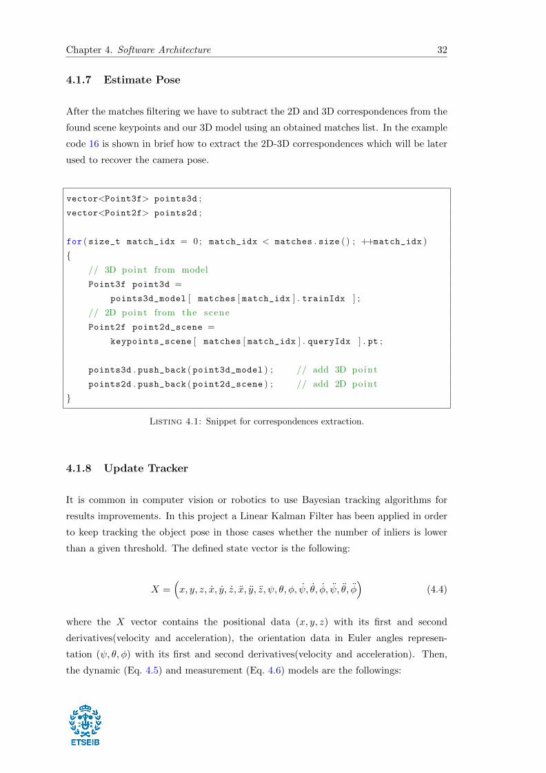
4.1.7 Estimate Pose
After the matches filtering we have to subtract the 2D and 3D correspondences from the
found scene keypoints and our 3D model using an obtained matches list. In the example
code 16 is shown in brief how to extract the 2D-3D correspondences which will be later
used to recover the camera pose.
vector<Point3f> points3d ;
vector<Point2f> points2d ;
for ( size_t match_idx = 0 ; match_idx < matches . size ( ) ; ++match_idx )
// 3D point from model
Point3f point3d =
points3d_model [ matches [ match_idx ] . trainIdx ] ;
// 2D point from the scene
Point2f point2d_scene =
keypoints_scene [ matches [ match_idx ] . queryIdx ] . pt ;
points3d . push_back ( point3d_model ) ; // add 3D point
points2d . push_back ( point2d_scene ) ; // add 2D point
Listing 4.1: Snippet for correspondences extraction.
4.1.8 Update Tracker
It is common in computer vision or robotics to use Bayesian tracking algorithms for
results improvements. In this project a Linear Kalman Filter has been applied in order
to keep tracking the object pose in those cases whether the number of inliers is lower
than a given threshold. The defined state vector is the following:
X =(x, y, z, x, y, z, x, y, z, ψ, θ, φ, ψ, θ, φ, ψ, θ, φ
)(4.4)
where the X vector contains the positional data (x, y, z) with its first and second
derivatives(velocity and acceleration), the orientation data in Euler angles represen-
tation (ψ, θ, φ) with its first and second derivatives(velocity and acceleration). Then,
the dynamic (Eq. 4.5) and measurement (Eq. 4.6) models are the followings:
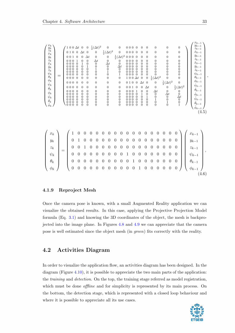
Chapter 4. Software Architecture 33
xkykzkxkykzkxkykzkψkθkφkψk
θkφkψk
θkφk
=
1 0 0 ∆t 0 0 12
(∆t)2 0 0 0 0 0 0 0 0 0 0 0
0 1 0 0 ∆t 0 0 12
(∆t)2 0 0 0 0 0 0 0 0 0 0
0 0 1 0 0 ∆t 0 0 12
(∆t)2 0 0 0 0 0 0 0 0 0
0 0 0 1 0 0 ∆t 0 0 0 0 0 0 0 0 0 0 00 0 0 0 1 0 0 ∆t 0 0 0 0 0 0 0 0 0 00 0 0 0 0 1 0 0 ∆t 0 0 0 0 0 0 0 0 00 0 0 0 0 0 1 0 0 0 0 0 0 0 0 0 0 00 0 0 0 0 0 0 1 0 0 0 0 0 0 0 0 0 00 0 0 0 0 0 0 0 1 0 0 0 0 0 0 0 0 00 0 0 0 0 0 0 0 0 1 0 0 ∆t 0 0 1
2(∆t)2 0 0
0 0 0 0 0 0 0 0 0 0 1 0 0 ∆t 0 0 12
(∆t)2 0
0 0 0 0 0 0 0 0 0 0 0 1 0 0 ∆t 0 0 12
(∆t)2
0 0 0 0 0 0 0 0 0 0 0 0 1 0 0 ∆t 0 00 0 0 0 0 0 0 0 0 0 0 0 0 1 0 0 ∆t 00 0 0 0 0 0 0 0 0 0 0 0 0 0 1 0 0 ∆t0 0 0 0 0 0 0 0 0 0 0 0 0 0 0 1 0 00 0 0 0 0 0 0 0 0 0 0 0 0 0 0 0 1 00 0 0 0 0 0 0 0 0 0 0 0 0 0 0 0 0 1
xk−1yk−1zk−1
xk−1
yk−1
zk−1
xk−1
yk−1
zk−1
ψk−1
θk−1
φk−1
ψk−1
θk−1
φk−1
ψk−1
θk−1
φk−1
,
(4.5)
xk
yk
zk
ψk
θk
φk
=
1 0 0 0 0 0 0 0 0 0 0 0 0 0 0 0 0 0
0 1 0 0 0 0 0 0 0 0 0 0 0 0 0 0 0 0
0 0 1 0 0 0 0 0 0 0 0 0 0 0 0 0 0 0
0 0 0 0 0 0 0 0 0 1 0 0 0 0 0 0 0 0
0 0 0 0 0 0 0 0 0 0 1 0 0 0 0 0 0 0
0 0 0 0 0 0 0 0 0 0 0 1 0 0 0 0 0 0
xk−1
yk−1
zk−1
ψk−1
θk−1
φk−1
,
(4.6)
4.1.9 Reproject Mesh
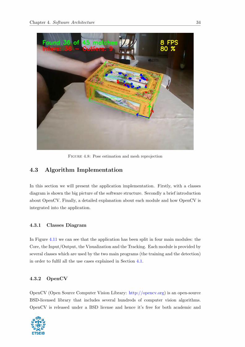
Once the camera pose is known, with a small Augmented Reality application we can
visualize the obtained results. In this case, applying the Projective Projection Model
formula (Eq. 3.1) and knowing the 3D coordinates of the object, the mesh is backpro-
jected into the image plane. In Figures 4.8 and 4.9 we can appreciate that the camera
pose is well estimated since the object mesh (in green) fits correctly with the reality.
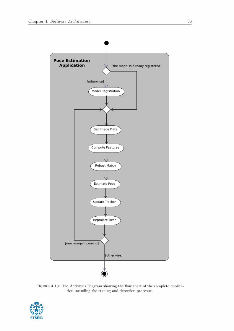
4.2 Activities Diagram
In order to visualize the application flow, an activities diagram has been designed. In the
diagram (Figure 4.10), it is possible to appreciate the two main parts of the application:
the training and detection. On the top, the training stage referred as model registration,
which must be done offline and for simplicity is represented by its main process. On
the bottom, the detection stage, which is represented with a closed loop behaviour and
where it is possible to appreciate all its use cases.
Chapter 4. Software Architecture 34
Figure 4.8: Pose estimation and mesh reprojection
4.3 Algorithm Implementation
In this section we will present the application implementation. Firstly, with a classes
diagram is shown the big picture of the software structure. Secondly a brief introduction
about OpenCV. Finally, a detailed explanation about each module and how OpenCV is
integrated into the application.
4.3.1 Classes Diagram
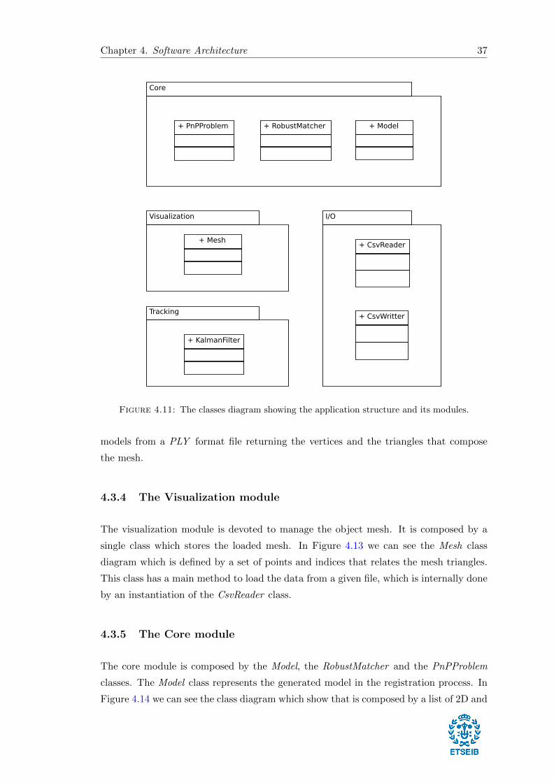
In Figure 4.11 we can see that the application has been split in four main modules: the
Core, the Input/Output, the Visualization and the Tracking. Each module is provided by
several classes which are used by the two main programs (the training and the detection)
in order to fulfil all the use cases explained in Section 4.1.
4.3.2 OpenCV
OpenCV (Open Source Computer Vision Library: http://opencv.org) is an open-source
BSD-licensed library that includes several hundreds of computer vision algorithms.
OpenCV is released under a BSD license and hence it’s free for both academic and

Chapter 4. Software Architecture 35
Figure 4.9: Pose estimation and mesh reprojection
commercial use. It has C++, C, Python and Java interfaces and supports Windows,
Linux, Mac OS, iOS and Android. OpenCV was designed for computational efficiency
and with a strong focus on real-time applications. Written in optimized C/C++, the
library can take advantage of multi-core processing. Enabled with OpenCL, it can take
advantage of the hardware acceleration of the underlying heterogeneous compute plat-
form.
OpenCV provides a module for Camera Calibration and 3D Reconstruction which has
several functions for basic multiple-view geometry algorithms, single and stereo camera
calibration, object pose estimation, stereo correspondence algorithms, and elements of
3D reconstruction. During the next section, we will see which module are used in order
to cover the application requirements.
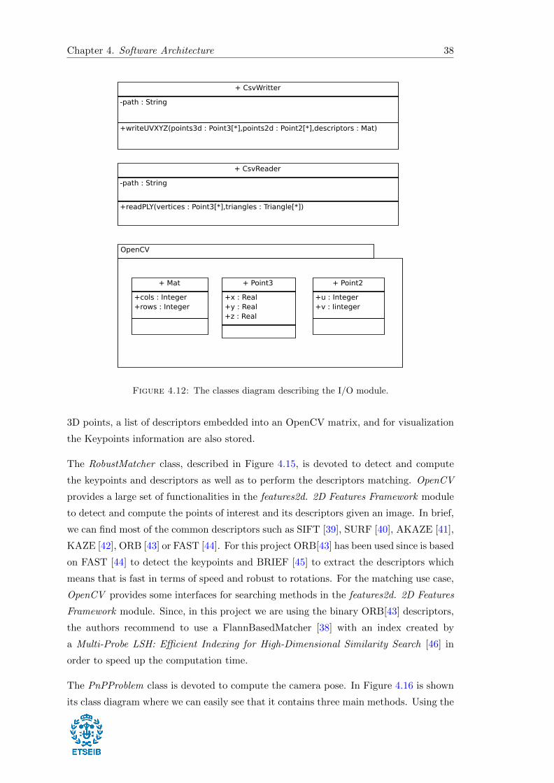
4.3.3 The Input/Output module
The Input/Output module is devoted to load and save the obtained information such
as the object mesh and the generated model files. This module contains the CsvReader
and CsvWritter classes which as their name indicate, read and write files in the CSV
format. In Figure 4.12 we can see the structure and the main methods that composes
this module. The CsvWritter is used to create the generated model file given a list of
2D-3D points and its descriptors. The CsvReader is devoted to load the 3D objects
Chapter 4. Software Architecture 36
Model Registration
[otherwise]
Get Image Data
Compute Features
Robust Match
Estimate Pose
Update Tracker
Reproject Mesh
[otherwise]
[the model is already registered]
[new image incoming]
Pose EstimationApplication
Figure 4.10: The Activities Diagram showing the flow chart of the complete applica-tion including the traning and detection processes.
Chapter 4. Software Architecture 37
Core
+ Model+ PnPProblem
Tracking
+ KalmanFilter
+ RobustMatcher
Visualization
+ Mesh
I/O
+ CsvWritter
+ CsvReader
Figure 4.11: The classes diagram showing the application structure and its modules.
models from a PLY format file returning the vertices and the triangles that compose
the mesh.
4.3.4 The Visualization module
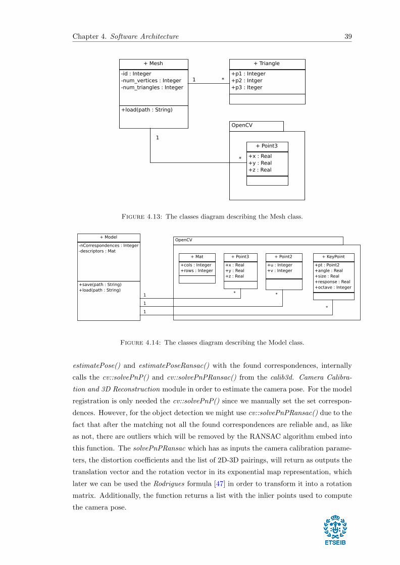
The visualization module is devoted to manage the object mesh. It is composed by a
single class which stores the loaded mesh. In Figure 4.13 we can see the Mesh class
diagram which is defined by a set of points and indices that relates the mesh triangles.
This class has a main method to load the data from a given file, which is internally done
by an instantiation of the CsvReader class.
4.3.5 The Core module
The core module is composed by the Model, the RobustMatcher and the PnPProblem
classes. The Model class represents the generated model in the registration process. In
Figure 4.14 we can see the class diagram which show that is composed by a list of 2D and
Chapter 4. Software Architecture 38
+ CsvWritter
-path : String
+writeUVXYZ(points3d : Point3[*],points2d : Point2[*],descriptors : Mat)
OpenCV
+ Mat
+cols : Integer+rows : Integer
+ Point3
+x : Real+y : Real+z : Real
+ Point2
+u : Integer+v : Iinteger
+ CsvReader
-path : String
+readPLY(vertices : Point3[*],triangles : Triangle[*])
Figure 4.12: The classes diagram describing the I/O module.
3D points, a list of descriptors embedded into an OpenCV matrix, and for visualization
the Keypoints information are also stored.
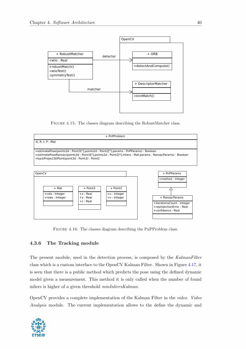
The RobustMatcher class, described in Figure 4.15, is devoted to detect and compute
the keypoints and descriptors as well as to perform the descriptors matching. OpenCV
provides a large set of functionalities in the features2d. 2D Features Framework module
to detect and compute the points of interest and its descriptors given an image. In brief,
we can find most of the common descriptors such as SIFT [39], SURF [40], AKAZE [41],
KAZE [42], ORB [43] or FAST [44]. For this project ORB[43] has been used since is based
on FAST [44] to detect the keypoints and BRIEF [45] to extract the descriptors which
means that is fast in terms of speed and robust to rotations. For the matching use case,
OpenCV provides some interfaces for searching methods in the features2d. 2D Features
Framework module. Since, in this project we are using the binary ORB[43] descriptors,
the authors recommend to use a FlannBasedMatcher [38] with an index created by
a Multi-Probe LSH: Efficient Indexing for High-Dimensional Similarity Search [46] in
order to speed up the computation time.
The PnPProblem class is devoted to compute the camera pose. In Figure 4.16 is shown
its class diagram where we can easily see that it contains three main methods. Using the
Chapter 4. Software Architecture 39
+ Mesh
-id : Integer-num_vertices : Integer-num_triangles : Integer
+load(path : String)
OpenCV
+ Point3
+x : Real+y : Real+z : Real
+ Triangle
+p1 : Integer+p2 : Intger+p3 : Iteger
1 *
1
*
Figure 4.13: The classes diagram describing the Mesh class.
+ Model
-nCorrespondences : Integer-descriptors : Mat
+save(path : String)+load(path : String)
OpenCV
+ Mat
+cols : Integer+rows : Integer
+ Point3
+x : Real+y : Real+z : Real
+ Point2
+u : Integer+v : Integer
+ KeyPoint
+pt : Point2+angle : Real+size : Real+response : Real+octave : Integer
1
*
1*
*1
Figure 4.14: The classes diagram describing the Model class.
estimatePose() and estimatePoseRansac() with the found correspondences, internally
calls the cv::solvePnP() and cv::solvePnPRansac() from the calib3d. Camera Calibra-
tion and 3D Reconstruction module in order to estimate the camera pose. For the model
registration is only needed the cv::solvePnP() since we manually set the set correspon-
dences. However, for the object detection we might use cv::solvePnPRansac() due to the
fact that after the matching not all the found correspondences are reliable and, as like
as not, there are outliers which will be removed by the RANSAC algorithm embed into
this function. The solvePnPRansac which has as inputs the camera calibration parame-
ters, the distortion coefficients and the list of 2D-3D pairings, will return as outputs the
translation vector and the rotation vector in its exponential map representation, which
later we can be used the Rodrigues formula [47] in order to transform it into a rotation
matrix. Additionally, the function returns a list with the inlier points used to compute
the camera pose.
Chapter 4. Software Architecture 40
+ RobustMatcher
-ratio : Real
+robustMatch()-ratioTest()-symmetryTest()
OpenCV
+ ORB
+detectAndCompute()
+ DescriptorMatcher
+knnMatch()
detector
matcher
Figure 4.15: The classes diagram describing the RobustMatcher class.
+ PnPProblem
-K, R, t, P : Mat
+estimatePose(points3d : Point3[*],points2d : Point2[*],params : PnPParams) : Boolean+estimatePoseRansac(points3d : Point3[*],points2d : Point2[*],inliers : Mat,params : RansacParams) : Boolean+backProject3DPoint(point3d : Point3) : Point2
OpenCV
+ Mat
+cols : Integer+rows : Integer
+ Point3
+x : Real+y : Real+z : Real
+ Point2
+u : Integer+v : Integer + RansacParams
+iterationsCount : Integer+reprojectionError : Real+confidence : Real
+ PnPParams
+method : Integer
Figure 4.16: The classes diagram describing the PnPProblem class.
4.3.6 The Tracking module
The present module, used in the detection process, is composed by the KalmanFilter
class which is a custom interface to the OpenCV Kalman Filter. Shown in Figure 4.17, it
is seen that there is a public method which predicts the pose using the defined dynamic
model given a measurement. This method it is only called when the number of found
inliers is higher of a given threshold minInliersKalman.
OpenCV provides a complete implementation of the Kalman Filter in the video. Video
Analysis module. The current implementation allows to the define the dynamic and
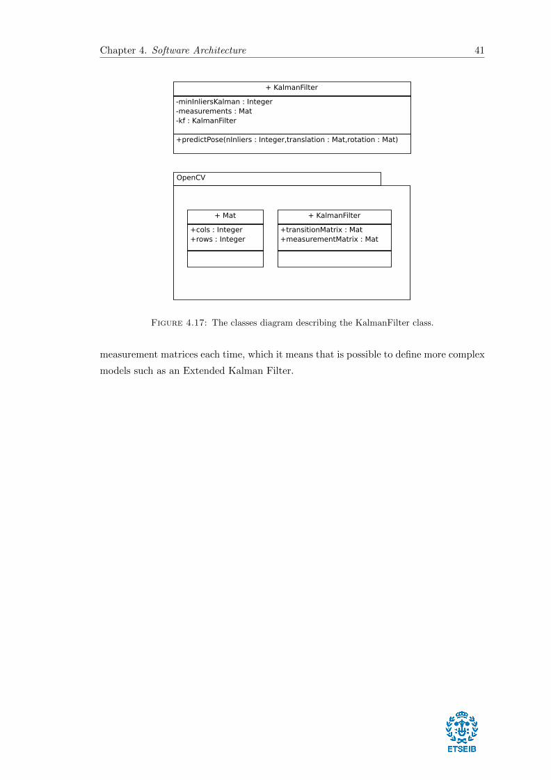
Chapter 4. Software Architecture 41
+ KalmanFilter
-minInliersKalman : Integer-measurements : Mat-kf : KalmanFilter
+predictPose(nInliers : Integer,translation : Mat,rotation : Mat)
OpenCV
+ Mat
+cols : Integer+rows : Integer
+ KalmanFilter
+transitionMatrix : Mat+measurementMatrix : Mat
Figure 4.17: The classes diagram describing the KalmanFilter class.
measurement matrices each time, which it means that is possible to define more complex
models such as an Extended Kalman Filter.

Chapter 5
Results and Contributions
In this chapter we will see the obtained results and contributions: an application for
objects pose estimation, the creation of an OpenCV tutorial and finally, the implemen-
tation and inclusion of the UPnP approach into the OpenCV libraries under the scope
of the OpenSource community.
5.1 Pose Estimation Application
The first contribution of this project is an application for pose estimation written in
C++ which is divided by two main modules: the model registration and the object
detection.
The first, registers an object extracting its 2D features and computes the 3D coordinates
of each feature given a 3D model of the object in PLY format. This module writes in
a custom made format the result of the object registration in order to be loaded by the
detection module. The detection module, loads a given object model generated by the
registration module and from a given a image sequence detects and tracks the object
reprojecting its mesh in order to visualise the obtained results.
The complete application has been included in the OpenCV repositories as a comple-
mentary resource for the tutorial which explains step by step the complete application
from the point of view of a Computer Vision developer.
43
Chapter 5. Results and Contributions 44
5.2 OpenCV Tutorial
We created an tutorial addressed to those developers interested in creating a pose esti-
mation application. The tutorial, attached in the end of this document (Appendix A),
is focused in explain step by step the code implementation of each use of case defined
in the previous sections. Moreover, the document is in the OpenCV tutorials standard
format and has been included in the new OpenCV 3.0.0 documentation [48].
5.3 UPnP Implementation
An implementation in C++ of the UPnP approach has been developed and included
in OpenCV. The source code, based on the Matlab implementation from the authors,
follows the same structure as the EPnP and can be used inside the cv::solvePnP()
function from the calib3d. Camera Calibration and 3D Reconstruction module.
5.3.1 Method validation
In order to be included into the library, the algorithm passed an unit test in terms of
accuracy in front of generated synthetic data. Explicitly, the method must guarantee
a rotation and translation error lower than 10e−3 after 1000 consecutive tests. For the
data generation, was used the OpenCV testing framework which simulates the 3D-to 2D
correspondences creating many set of points with different size uniformly distributed in
the cube [−1, 1]x[−1, 1]x[5, 10], and projected onto a [10−3, 100]x[10−3, 100] image using
a virtual calibrated camera with non squared pixels (except for UPnP). For any given
ground truth camera pose, Rtrue and ttrue and corresponding estimates R and t, the
relative rotation error was computed Erot = ‖rtrue − r‖/‖r‖ where r and rtrue are the
exponential vector representation of R and Rtrue respectively; the relative translation
vector error was computed with Etrans = ‖ttrue−t‖/‖t‖; and the error in the estimation
of the focal length was determined by Ef = ‖ftrue − f‖/f . All the errors reported in
this section correspond to the median values errors estimated over 100 experiments with
random positions of the 3D points.
In the following Figures 5.1 and 5.2 are shown the obtained results from the accuracy
test, comparing the rotation and translation errors between the different PnP methods
provided by OpenCV: ITERATIVE, P3P, EPNP, DLS and UPNP. The ITERATIVE
method, based on Levenberg-Marquardt optimization, which minimizes the reprojection
error. The P3P method, based on the paper of X.S. Gao [5], which in this case is required
exactly four object and image points. The EPNP method, based on the approach
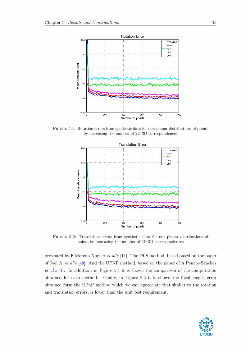
Chapter 5. Results and Contributions 45
Figure 5.1: Rotation errors from synthetic data for non-planar distributions of pointsby increasing the number of 2D-3D correspondences
Figure 5.2: Translation errors from synthetic data for non-planar distributions ofpoints by increasing the number of 2D-3D correspondences
presented by F.Moreno-Noguer et al’s [11]. The DLS method, based based on the paper
of Joel A. et al’s [49]. And the UPNP method, based on the paper of A.Penate-Sanchez
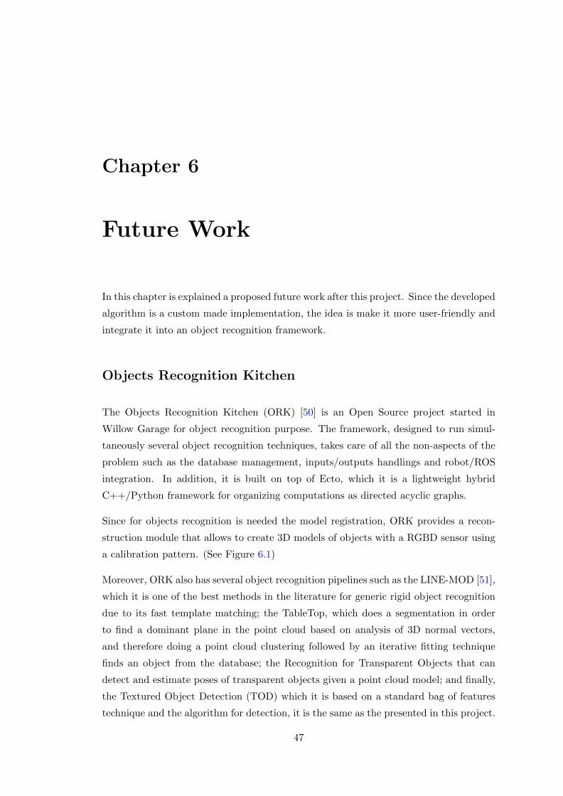
et al’s [1]. In addition, in Figure 5.4 it is shown the comparison of the computation
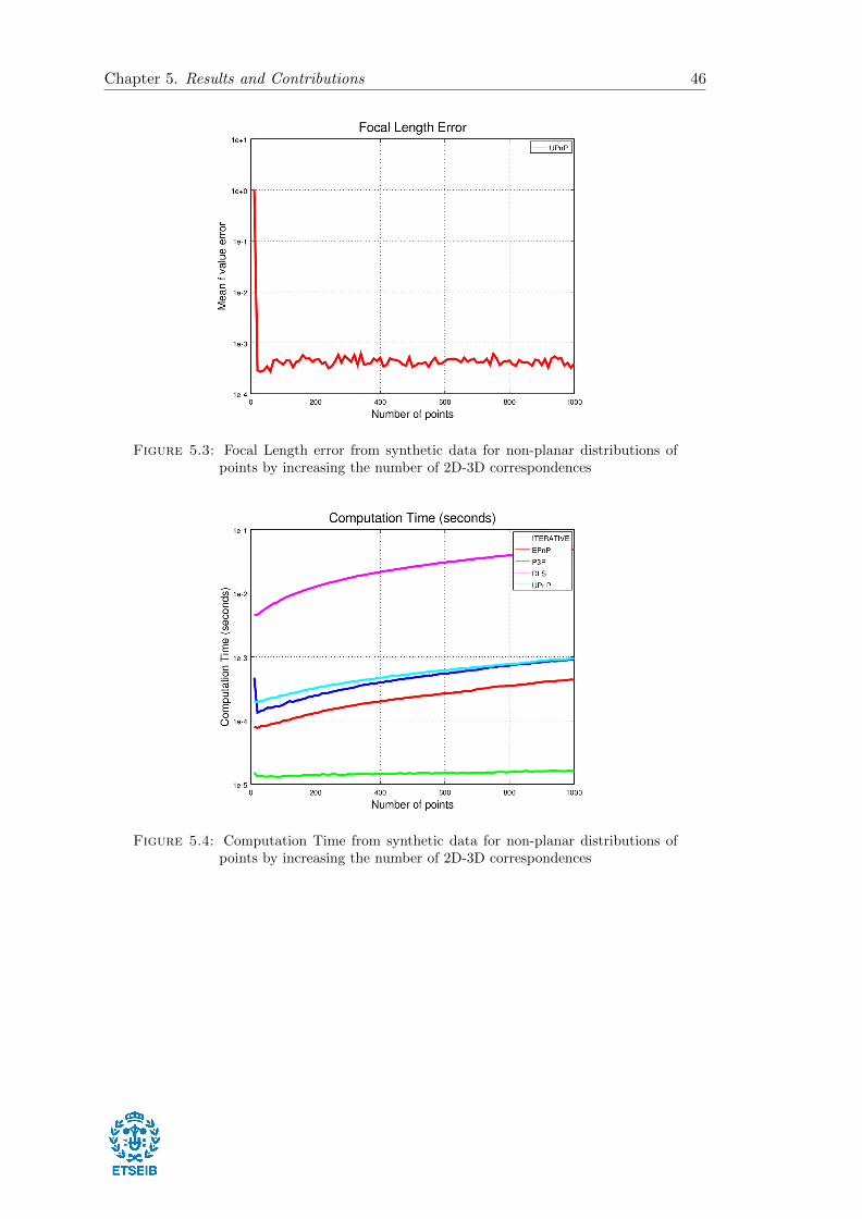
obtained for each method. Finally, in Figure 5.3 it is shown the focal length error
obtained form the UPnP method which we can appreciate that similar to the rotation
and translation errors, is lower than the unit test requirement.
Chapter 5. Results and Contributions 46
Figure 5.3: Focal Length error from synthetic data for non-planar distributions ofpoints by increasing the number of 2D-3D correspondences
Figure 5.4: Computation Time from synthetic data for non-planar distributions ofpoints by increasing the number of 2D-3D correspondences
Chapter 6
Future Work
In this chapter is explained a proposed future work after this project. Since the developed
algorithm is a custom made implementation, the idea is make it more user-friendly and
integrate it into an object recognition framework.
Objects Recognition Kitchen
The Objects Recognition Kitchen (ORK) [50] is an Open Source project started in
Willow Garage for object recognition purpose. The framework, designed to run simul-
taneously several object recognition techniques, takes care of all the non-aspects of the
problem such as the database management, inputs/outputs handlings and robot/ROS
integration. In addition, it is built on top of Ecto, which it is a lightweight hybrid
C++/Python framework for organizing computations as directed acyclic graphs.
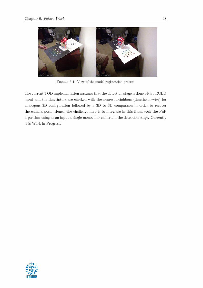
Since for objects recognition is needed the model registration, ORK provides a recon-
struction module that allows to create 3D models of objects with a RGBD sensor using
a calibration pattern. (See Figure 6.1)
Moreover, ORK also has several object recognition pipelines such as the LINE-MOD [51],
which it is one of the best methods in the literature for generic rigid object recognition
due to its fast template matching; the TableTop, which does a segmentation in order
to find a dominant plane in the point cloud based on analysis of 3D normal vectors,
and therefore doing a point cloud clustering followed by an iterative fitting technique
finds an object from the database; the Recognition for Transparent Objects that can
detect and estimate poses of transparent objects given a point cloud model; and finally,
the Textured Object Detection (TOD) which it is based on a standard bag of features
technique and the algorithm for detection, it is the same as the presented in this project.
47
Chapter 6. Future Work 48
Figure 6.1: View of the model registration process
The current TOD implementation assumes that the detection stage is done with a RGBD
input and the descriptors are checked with the nearest neighbors (descriptor-wise) for
analogous 3D configuration followed by a 3D to 3D comparison in order to recover
the camera pose. Hence, the challenge here is to integrate in this framework the PnP
algorithm using as an input a single monocular camera in the detection stage. Currently
it is Work in Progress.

Appendix A
OpenCV tutorial
49

Real Time pose estimation of a textured object
Nowadays, augmented reality is one of the top research topic in computer vision and robotics fields. The most elemental problem in augmented reality is theestimation of the camera pose respect of an object in the case of computer vision area to do later some 3D rendering or in the case of robotics obtain an object posein order to grasp it and do some manipulation. However, this is not a trivial problem to solve due to the fact that the most common issue in image processing is thecomputational cost of applying a lot of algorithms or mathematical operations for solving a problem which is basic and immediateley for humans.
GoalIn this tutorial is explained how to build a real time application to estimate the camera pose in order to track a textured object with six degrees of freedom given a 2Dimage and its 3D textured model.
The application will have the followings parts:
Read 3D textured object model and object mesh.Take input from Camera or Video.Extract ORB features and descriptors from the scene.Match scene descriptors with model descriptors using Flann matcher.Pose estimation using PnP + Ransac.Linear Kalman Filter for bad poses rejection.
TheoryIn computer vision estimate the camera pose from n 3D-to-2D point correspondences is a fundamental and well understood problem. The most general version ofthe problem requires estimating the six degrees of freedom of the pose and five calibration parameters: focal length, principal point, aspect ratio and skew. It couldbe established with a minimum of 6 correspondences, using the well known Direct Linear Transform (DLT) algorithm. There are, though, several simplifications tothe problem which turn into an extensive list of different algorithms that improve the accuracy of the DLT.
The most common simplification is to assume known calibration parameters which is the so-called Perspective-*n*-Point problem:
Problem Formulation: Given a set of correspondences between 3D points p_i expressed in a world reference frame, and their 2D projections u_i onto the image,we seek to retrieve the pose ( R and t) of the camera w.r.t. the world and the focal length f.
OpenCV provides four different approaches to solve the Perspective-*n*-Point problem which return R and t. Then, using the following formula it's possible toproject 3D points into the image plane:
s\ \left [ \beginmatrix u \\ v \\ 1 \endmatrix \right ] = \left [ \beginmatrix f_x & 0 & c_x \\ 0 & f_y & c_y \\ 0 & 0 & 1 \endmatrix \right ] \left [ \beginmatrix r_11 &r_12 & r_13 & t_1 \\ r_21 & r_22 & r_23 & t_2 \\ r_31 & r_32 & r_33 & t_3 \endmatrix \right ] \left [ \beginmatrix X \\ Y \\ Z\\ 1 \endmatrix \right ]
The complete documentation of how to manage with this equations is in Camera Calibration and 3D Reconstruction .
Source codeYou can find the source code of this tutorial in the samples/cpp/tutorial_code/calib3d/real_time_pose_estimation/ folder of the OpenCV source library.
The tutorial consists of two main programs:
1. Model registration
This applicaton is exclusive to whom don't have a 3D textured model of the object to be detected. You can use this program to create your own textured 3D
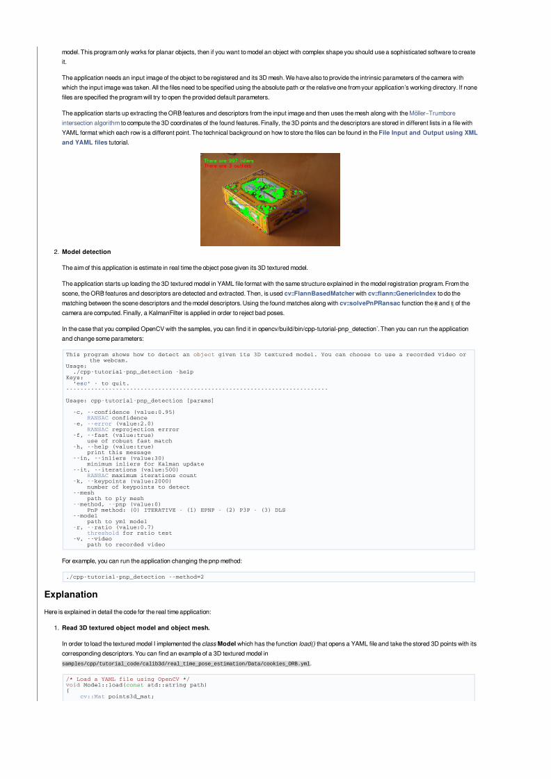
model. This program only works for planar objects, then if you want to model an object with complex shape you should use a sophisticated software to createit.
The application needs an input image of the object to be registered and its 3D mesh. We have also to provide the intrinsic parameters of the camera withwhich the input image was taken. All the files need to be specified using the absolute path or the relative one from your application’s working directory. If nonefiles are specified the program will try to open the provided default parameters.
The application starts up extracting the ORB features and descriptors from the input image and then uses the mesh along with the Möller–Trumboreintersection algorithm to compute the 3D coordinates of the found features. Finally, the 3D points and the descriptors are stored in different lists in a file withYAML format which each row is a different point. The technical background on how to store the files can be found in the File Input and Output using XMLand YAML files tutorial.
2. Model detection
The aim of this application is estimate in real time the object pose given its 3D textured model.
The application starts up loading the 3D textured model in YAML file format with the same structure explained in the model registration program. From thescene, the ORB features and descriptors are detected and extracted. Then, is used cv::FlannBasedMatcher with cv::flann::GenericIndex to do thematching between the scene descriptors and the model descriptors. Using the found matches along with cv::solvePnPRansac function the R and t of thecamera are computed. Finally, a KalmanFilter is applied in order to reject bad poses.
In the case that you compiled OpenCV with the samples, you can find it in opencv/build/bin/cpp-tutorial-pnp_detection`. Then you can run the applicationand change some parameters:
This program shows how to detect an object given its 3D textured model. You can choose to use a recorded video or the webcam.
Usage: ./cpp-tutorial-pnp_detection -helpKeys: 'esc' - to quit.--------------------------------------------------------------------------
Usage: cpp-tutorial-pnp_detection [params]
-c, --confidence (value:0.95) RANSAC confidence -e, --error (value:2.0) RANSAC reprojection errror -f, --fast (value:true) use of robust fast match -h, --help (value:true) print this message --in, --inliers (value:30) minimum inliers for Kalman update --it, --iterations (value:500) RANSAC maximum iterations count -k, --keypoints (value:2000) number of keypoints to detect --mesh path to ply mesh --method, --pnp (value:0) PnP method: (0) ITERATIVE - (1) EPNP - (2) P3P - (3) DLS --model path to yml model -r, --ratio (value:0.7) threshold for ratio test -v, --video path to recorded video
For example, you can run the application changing the pnp method:
./cpp-tutorial-pnp_detection --method=2
ExplanationHere is explained in detail the code for the real time application:
1. Read 3D textured object model and object mesh.
In order to load the textured model I implemented the class Model which has the function load() that opens a YAML file and take the stored 3D points with itscorresponding descriptors. You can find an example of a 3D textured model in samples/cpp/tutorial_code/calib3d/real_time_pose_estimation/Data/cookies_ORB.yml.
/* Load a YAML file using OpenCV */void Model::load(const std::string path) cv::Mat points3d_mat;

cv::FileStorage storage(path, cv::FileStorage::READ); storage["points_3d"] >> points3d_mat; storage["descriptors"] >> descriptors_;
points3d_mat.copyTo(list_points3d_in_);
storage.release();
In the main program the model is loaded as follows:
Model model; // instantiate Model objectmodel.load(yml_read_path); // load a 3D textured object model
In order to read the model mesh I implemented a class Mesh which has a function load() that opens a *.ply file and store the 3D points of the object and alsothe composed triangles. You can find an example of a model mesh in samples/cpp/tutorial_code/calib3d/real_time_pose_estimation/Data/box.ply.
/* Load a CSV with *.ply format */void Mesh::load(const std::string path)
// Create the reader CsvReader csvReader(path);
// Clear previous data list_vertex_.clear(); list_triangles_.clear();
// Read from .ply file csvReader.readPLY(list_vertex_, list_triangles_);
// Update mesh attributes num_vertexs_ = list_vertex_.size(); num_triangles_ = list_triangles_.size();
In the main program the mesh is loaded as follows:
Mesh mesh; // instantiate Mesh objectmesh.load(ply_read_path); // load an object mesh
You can also load different model and mesh:
./cpp-tutorial-pnp_detection --mesh=/absolute_path_to_your_mesh.ply --model=/absolute_path_to_your_model.yml
2. Take input from Camera or Video
To detect is necessary capture video. It's done loading a recorded video by passing the absolute path where it is located in your machine. In order to test theapplication you can find a recorded video in samples/cpp/tutorial_code/calib3d/real_time_pose_estimation/Data/box.mp4.
cv::VideoCapture cap; // instantiate VideoCapturecap.open(video_read_path); // open a recorded video
if(!cap.isOpened()) // check if we succeeded std::cout << "Could not open the camera device" << std::endl; return -1;
Then the algorithm is computed frame per frame:
cv::Mat frame, frame_vis;
while(cap.read(frame) && cv::waitKey(30) != 27) // capture frame until ESC is pressed
frame_vis = frame.clone(); // refresh visualisation frame
// MAIN ALGORITHM
You can also load different recorded video:
./cpp-tutorial-pnp_detection --video=/absolute_path_to_your_video.mp4
3. Extract ORB features and descriptors from the scene
The next step is to detect the scene features and extract it descriptors. For this task I implemented a class RobustMatcher which has a function forkeypoints detection and features extraction. You can find it in samples/cpp/tutorial_code/calib3d/real_time_pose_estimation/src/RobusMatcher.cpp.In your RobusMatch object you can use any of the 2D features detectors of OpenCV. In this case I used cv::ORB features because is based on cv::FAST todetect the keypoints and cv::xfeatures2d::BriefDescriptorExtractor to extract the descriptors which means that is fast and robust to rotations. You canfind more detailed information about ORB in the documentation.
The following code is how to instantiate and set the features detector and the descriptors extractor:
RobustMatcher rmatcher; // instantiate RobustMatcher
cv::FeatureDetector * detector = new cv::OrbFeatureDetector(numKeyPoints); // instatiate ORB feature detector
cv::DescriptorExtractor * extractor = new cv::OrbDescriptorExtractor(); // instatiate ORB descriptor extractor
rmatcher.setFeatureDetector(detector); // set feature detectorrmatcher.setDescriptorExtractor(extractor); // set descriptor extractor
The features and descriptors will be computed by the RobustMatcher inside the matching function.
4. Match scene descriptors with model descriptors using Flann matcher
It is the first step in our detection algorithm. The main idea is to match the scene descriptors with our model descriptors in order to know the 3D coordinates ofthe found features into the current scene.
Firstly, we have to set which matcher we want to use. In this case is used cv::FlannBasedMatcher matcher which in terms of computational cost is fasterthan the cv::BFMatcher matcher as we increase the trained collectction of features. Then, for FlannBased matcher the index created is Multi-Probe LSH:Efficient Indexing for High-Dimensional Similarity Search due to ORB descriptors are binary.
You can tune the LSH and search parameters to improve the matching efficiency:
cv::Ptr<cv::flann::IndexParams> indexParams = cv::makePtr<cv::flann::LshIndexParams>(6, 12, 1); // instantiate LSH index parameters
cv::Ptr<cv::flann::SearchParams> searchParams = cv::makePtr<cv::flann::SearchParams>(50); // instantiate flann search parameters
cv::DescriptorMatcher * matcher = new cv::FlannBasedMatcher(indexParams, searchParams); // instantiate FlannBased matcher
rmatcher.setDescriptorMatcher(matcher); // set matcher
Secondly, we have to call the matcher by using robustMatch() or fastRobustMatch() function. The difference of using this two functions is its computationalcost. The first method is slower but more robust at filtering good matches because uses two ratio test and a symmetry test. In contrast, the second method isfaster but less robust because only applies a single ratio test to the matches.
The following code is to get the model 3D points and its descriptors and then call the matcher in the main program:
// Get the MODEL INFO
std::vector<cv::Point3f> list_points3d_model = model.get_points3d(); // list with model 3D coordinatescv::Mat descriptors_model = model.get_descriptors(); // list with descriptors of each 3D
coordinate
// -- Step 1: Robust matching between model descriptors and scene descriptors
std::vector<cv::DMatch> good_matches; // to obtain the model 3D points in the scenestd::vector<cv::KeyPoint> keypoints_scene; // to obtain the 2D points of the scene
if(fast_match) rmatcher.fastRobustMatch(frame, good_matches, keypoints_scene, descriptors_model);else rmatcher.robustMatch(frame, good_matches, keypoints_scene, descriptors_model);
The following code corresponds to the robustMatch() function which belongs to the RobustMatcher class. This function uses the given image to detect thekeypoints and extract the descriptors, match using two Nearest Neighbour the extracted descriptors with the given model descriptors and vice versa. Then,a ratio test is applied to the two direction matches in order to remove these matches which its distance ratio between the first and second best match is largerthan a given threshold. Finally, a symmetry test is applied in order the remove non symmetrical matches.
void RobustMatcher::robustMatch( const cv::Mat& frame, std::vector<cv::DMatch>& good_matches, std::vector<cv::KeyPoint>& keypoints_frame, const std::vector<cv::KeyPoint>& keypoints_model, const cv::Mat&
descriptors_model )
// 1a. Detection of the ORB features this->computeKeyPoints(frame, keypoints_frame);
// 1b. Extraction of the ORB descriptors cv::Mat descriptors_frame; this->computeDescriptors(frame, keypoints_frame, descriptors_frame);
// 2. Match the two image descriptors std::vector<std::vector<cv::DMatch> > matches12, matches21;
// 2a. From image 1 to image 2 matcher_->knnMatch(descriptors_frame, descriptors_model, matches12, 2); // return 2 nearest neighbours
// 2b. From image 2 to image 1 matcher_->knnMatch(descriptors_model, descriptors_frame, matches21, 2); // return 2 nearest neighbours
// 3. Remove matches for which NN ratio is > than threshold // clean image 1 -> image 2 matches int removed1 = ratioTest(matches12); // clean image 2 -> image 1 matches int removed2 = ratioTest(matches21);
// 4. Remove non-symmetrical matches symmetryTest(matches12, matches21, good_matches);
After the matches filtering we have to subtract the 2D and 3D correspondences from the found scene keypoints and our 3D model using the obtainedDMatches vector. For more information about cv::DMatch check the documentation.
// -- Step 2: Find out the 2D/3D correspondences
std::vector<cv::Point3f> list_points3d_model_match; // container for the model 3D coordinates found in the scene
std::vector<cv::Point2f> list_points2d_scene_match; // container for the model 2D coordinates found in the scene
for(unsigned int match_index = 0; match_index < good_matches.size(); ++match_index) cv::Point3f point3d_model = list_points3d_model[ good_matches[match_index].trainIdx ]; // 3D point from
model cv::Point2f point2d_scene = keypoints_scene[ good_matches[match_index].queryIdx ].pt; // 2D point from the
scene list_points3d_model_match.push_back(point3d_model); // add 3D point list_points2d_scene_match.push_back(point2d_scene); // add 2D point
You can also change the ratio test threshold, the number of keypoints to detect as well as use or not the robust matcher:
./cpp-tutorial-pnp_detection --ratio=0.8 --keypoints=1000 --fast=false
5. Pose estimation using PnP + Ransac
Once with the 2D and 3D correspondences we have to apply a PnP algorithm in order to estimate the camera pose. The reason why we have to usecv::solvePnPRansac instead of cv::solvePnP is due to the fact that after the matching not all the found correspondences are correct and, as like as not,there are false correspondences or also called outliers. The Random Sample Consensus or Ransac is a non-deterministic iterative method which estimateparameters of a mathematical model from observed data producing an aproximate result as the number of iterations increase. After appyling Ransac all theoutliers will be eliminated to then estimate the camera pose with a certain probability to obtain a good solution.
For the camera pose estimation I have implemented a class PnPProblem. This class has 4 atributes: a given calibration matrix, the rotation matrix, thetranslation matrix and the rotation-translation matrix. The intrinsic calibration parameters of the camera which you are using to estimate the pose arenecessary. In order to obtain the parameters you can check Camera calibration with square chessboard and Camera calibration With OpenCVtutorials.
The following code is how to declare the PnPProblem class in the main program:
// Intrinsic camera parameters: UVC WEBCAM
double f = 55; // focal length in mmdouble sx = 22.3, sy = 14.9; // sensor sizedouble width = 640, height = 480; // image size
double params_WEBCAM[] = width*f/sx, // fx height*f/sy, // fy width/2, // cx height/2; // cy
PnPProblem pnp_detection(params_WEBCAM); // instantiate PnPProblem class
The following code is how the PnPProblem class initialises its atributes:
// Custom constructor given the intrinsic camera parameters
PnPProblem::PnPProblem(const double params[]) _A_matrix = cv::Mat::zeros(3, 3, CV_64FC1); // intrinsic camera parameters _A_matrix.at<double>(0, 0) = params[0]; // [ fx 0 cx ] _A_matrix.at<double>(1, 1) = params[1]; // [ 0 fy cy ] _A_matrix.at<double>(0, 2) = params[2]; // [ 0 0 1 ] _A_matrix.at<double>(1, 2) = params[3]; _A_matrix.at<double>(2, 2) = 1; _R_matrix = cv::Mat::zeros(3, 3, CV_64FC1); // rotation matrix _t_matrix = cv::Mat::zeros(3, 1, CV_64FC1); // translation matrix _P_matrix = cv::Mat::zeros(3, 4, CV_64FC1); // rotation-translation matrix
OpenCV provides four PnP methods: ITERATIVE, EPNP, P3P and DLS. Depending on the application type, the estimation method will be different. In thecase that we want to make a real time application, the more suitable methods are EPNP and P3P due to that are faster than ITERATIVE and DLS at findingan optimal solution. However, EPNP and P3P are not especially robust in front of planar surfaces and sometimes the pose estimation seems to have a mirroreffect. Therefore, in this this tutorial is used ITERATIVE method due to the object to be detected has planar surfaces.
The OpenCV Ransac implementation wants you to provide three parameters: the maximum number of iterations until stop the algorithm, the maximumallowed distance between the observed and computed point projections to consider it an inlier and the confidence to obtain a good result. You can tune theseparamaters in order to improve your algorithm performance. Increasing the number of iterations you will have a more accurate solution, but will take moretime to find a solution. Increasing the reprojection error will reduce the computation time, but your solution will be unaccurate. Decreasing the confidence yourarlgorithm will be faster, but the obtained solution will be unaccurate.
The following parameters work for this application:
// RANSAC parameters
int iterationsCount = 500; // number of Ransac iterations.float reprojectionError = 2.0; // maximum allowed distance to consider it an inlier.float confidence = 0.95; // ransac successful confidence.
The following code corresponds to the estimatePoseRANSAC() function which belongs to the PnPProblem class. This function estimates the rotation andtranslation matrix given a set of 2D/3D correspondences, the desired PnP method to use, the output inliers container and the Ransac parameters:
// Estimate the pose given a list of 2D/3D correspondences with RANSAC and the method to use
void PnPProblem::estimatePoseRANSAC( const std::vector<cv::Point3f> &list_points3d, // list with model 3D coordinates
const std::vector<cv::Point2f> &list_points2d, // list with scene 2D coordinates
int flags, cv::Mat &inliers, int iterationsCount, // PnP method; inliers container
float reprojectionError, float confidence ) // Ransac parameters cv::Mat distCoeffs = cv::Mat::zeros(4, 1, CV_64FC1); // vector of distortion coefficients cv::Mat rvec = cv::Mat::zeros(3, 1, CV_64FC1); // output rotation vector cv::Mat tvec = cv::Mat::zeros(3, 1, CV_64FC1); // output translation vector
bool useExtrinsicGuess = false; // if true the function uses the provided rvec and tvec values as // initial approximations of the rotation and translation vectors
cv::solvePnPRansac( list_points3d, list_points2d, _A_matrix, distCoeffs, rvec, tvec, useExtrinsicGuess, iterationsCount, reprojectionError, confidence, inliers, flags );
Rodrigues(rvec,_R_matrix); // converts Rotation Vector to Matrix _t_matrix = tvec; // set translation matrix
this->set_P_matrix(_R_matrix, _t_matrix); // set rotation-translation matrix
In the following code are the 3th and 4th steps of the main algorithm. The first, calling the above function and the second taking the output inliers vector fromRansac to get the 2D scene points for drawing purpose. As seen in the code we must be sure to apply Ransac if we have matches, in the other case, thefunction cv::solvePnPRansac crashes due to any OpenCV bug.
if(good_matches.size() > 0) // None matches, then RANSAC crashes
// -- Step 3: Estimate the pose using RANSAC approach pnp_detection.estimatePoseRANSAC( list_points3d_model_match, list_points2d_scene_match, pnpMethod, inliers_idx, iterationsCount, reprojectionError, confidence );
// -- Step 4: Catch the inliers keypoints to draw for(int inliers_index = 0; inliers_index < inliers_idx.rows; ++inliers_index) int n = inliers_idx.at<int>(inliers_index); // i-inlier cv::Point2f point2d = list_points2d_scene_match[n]; // i-inlier point 2D list_points2d_inliers.push_back(point2d); // add i-inlier to list
Finally, once the camera pose has been estimated we can use the R and t in order to compute the 2D projection onto the image of a given 3D point expressedin a world reference frame using the showed formula on Theory.
The following code corresponds to the backproject3DPoint() function which belongs to the PnPProblem class. The function backproject a given 3D pointexpressed in a world reference frame onto a 2D image:
// Backproject a 3D point to 2D using the estimated pose parameters
cv::Point2f PnPProblem::backproject3DPoint(const cv::Point3f &point3d) // 3D point vector [x y z 1]' cv::Mat point3d_vec = cv::Mat(4, 1, CV_64FC1); point3d_vec.at<double>(0) = point3d.x; point3d_vec.at<double>(1) = point3d.y; point3d_vec.at<double>(2) = point3d.z; point3d_vec.at<double>(3) = 1;
// 2D point vector [u v 1]' cv::Mat point2d_vec = cv::Mat(4, 1, CV_64FC1); point2d_vec = _A_matrix * _P_matrix * point3d_vec;
// Normalization of [u v]' cv::Point2f point2d; point2d.x = point2d_vec.at<double>(0) / point2d_vec.at<double>(2); point2d.y = point2d_vec.at<double>(1) / point2d_vec.at<double>(2);
return point2d;
The above function is used to compute all the 3D points of the object Mesh to show the pose of the object.
You can also change RANSAC parameters and PnP method:
./cpp-tutorial-pnp_detection --error=0.25 --confidence=0.90 --iterations=250 --method=3
6. Linear Kalman Filter for bad poses rejection
Is it common in computer vision or robotics fields that after applying detection or tracking techniques, bad results are obtained due to some sensor errors. Inorder to avoid these bad detections in this tutorial is explained how to implement a Linear Kalman Filter. The Kalman Filter will be applied after detected agiven number of inliers.
You can find more information about what Kalman Filter is. In this tutorial it's used the OpenCV implementation of the cv::KalmanFilter based on LinearKalman Filter for position and orientation tracking to set the dynamics and measurement models.
Firstly, we have to define our state vector which will have 18 states: the positional data (x,y,z) with its first and second derivatives (velocity and acceleration),then rotation is added in form of three euler angles (roll, pitch, jaw) together with their first and second derivatives (angular velocity and acceleration)
X = (x,y,z,\dot x,\dot y,\dot z,\ddot x,\ddot y,\ddot z,\psi,\theta,\phi,\dot \psi,\dot \theta,\dot \phi,\ddot \psi,\ddot \theta,\ddot \phi)^T
Secondly, we have to define the number of measuremnts which will be 6: from R and t we can extract (x,y,z) and (\psi,\theta,\phi). In addition, we have todefine the number of control actions to apply to the system which in this case will be zero. Finally, we have to define the differential time betweenmeasurements which in this case is 1/T, where T is the frame rate of the video.
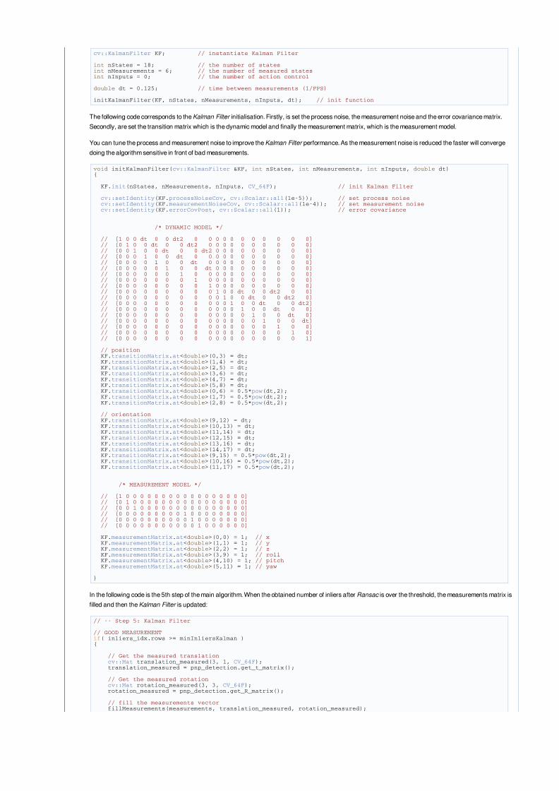
cv::KalmanFilter KF; // instantiate Kalman Filter
int nStates = 18; // the number of statesint nMeasurements = 6; // the number of measured statesint nInputs = 0; // the number of action control
double dt = 0.125; // time between measurements (1/FPS)
initKalmanFilter(KF, nStates, nMeasurements, nInputs, dt); // init function
The following code corresponds to the Kalman Filter initialisation. Firstly, is set the process noise, the measurement noise and the error covariance matrix.Secondly, are set the transition matrix which is the dynamic model and finally the measurement matrix, which is the measurement model.
You can tune the process and measurement noise to improve the Kalman Filter performance. As the measurement noise is reduced the faster will convergedoing the algorithm sensitive in front of bad measurements.
void initKalmanFilter(cv::KalmanFilter &KF, int nStates, int nMeasurements, int nInputs, double dt)
KF.init(nStates, nMeasurements, nInputs, CV_64F); // init Kalman Filter
cv::setIdentity(KF.processNoiseCov, cv::Scalar::all(1e-5)); // set process noise cv::setIdentity(KF.measurementNoiseCov, cv::Scalar::all(1e-4)); // set measurement noise cv::setIdentity(KF.errorCovPost, cv::Scalar::all(1)); // error covariance
/* DYNAMIC MODEL */
// [1 0 0 dt 0 0 dt2 0 0 0 0 0 0 0 0 0 0 0] // [0 1 0 0 dt 0 0 dt2 0 0 0 0 0 0 0 0 0 0] // [0 0 1 0 0 dt 0 0 dt2 0 0 0 0 0 0 0 0 0] // [0 0 0 1 0 0 dt 0 0 0 0 0 0 0 0 0 0 0] // [0 0 0 0 1 0 0 dt 0 0 0 0 0 0 0 0 0 0] // [0 0 0 0 0 1 0 0 dt 0 0 0 0 0 0 0 0 0] // [0 0 0 0 0 0 1 0 0 0 0 0 0 0 0 0 0 0] // [0 0 0 0 0 0 0 1 0 0 0 0 0 0 0 0 0 0] // [0 0 0 0 0 0 0 0 1 0 0 0 0 0 0 0 0 0] // [0 0 0 0 0 0 0 0 0 1 0 0 dt 0 0 dt2 0 0] // [0 0 0 0 0 0 0 0 0 0 1 0 0 dt 0 0 dt2 0] // [0 0 0 0 0 0 0 0 0 0 0 1 0 0 dt 0 0 dt2] // [0 0 0 0 0 0 0 0 0 0 0 0 1 0 0 dt 0 0] // [0 0 0 0 0 0 0 0 0 0 0 0 0 1 0 0 dt 0] // [0 0 0 0 0 0 0 0 0 0 0 0 0 0 1 0 0 dt] // [0 0 0 0 0 0 0 0 0 0 0 0 0 0 0 1 0 0] // [0 0 0 0 0 0 0 0 0 0 0 0 0 0 0 0 1 0] // [0 0 0 0 0 0 0 0 0 0 0 0 0 0 0 0 0 1]
// position KF.transitionMatrix.at<double>(0,3) = dt; KF.transitionMatrix.at<double>(1,4) = dt; KF.transitionMatrix.at<double>(2,5) = dt; KF.transitionMatrix.at<double>(3,6) = dt; KF.transitionMatrix.at<double>(4,7) = dt; KF.transitionMatrix.at<double>(5,8) = dt; KF.transitionMatrix.at<double>(0,6) = 0.5*pow(dt,2); KF.transitionMatrix.at<double>(1,7) = 0.5*pow(dt,2); KF.transitionMatrix.at<double>(2,8) = 0.5*pow(dt,2);
// orientation KF.transitionMatrix.at<double>(9,12) = dt; KF.transitionMatrix.at<double>(10,13) = dt; KF.transitionMatrix.at<double>(11,14) = dt; KF.transitionMatrix.at<double>(12,15) = dt; KF.transitionMatrix.at<double>(13,16) = dt; KF.transitionMatrix.at<double>(14,17) = dt; KF.transitionMatrix.at<double>(9,15) = 0.5*pow(dt,2); KF.transitionMatrix.at<double>(10,16) = 0.5*pow(dt,2); KF.transitionMatrix.at<double>(11,17) = 0.5*pow(dt,2);
/* MEASUREMENT MODEL */
// [1 0 0 0 0 0 0 0 0 0 0 0 0 0 0 0 0 0] // [0 1 0 0 0 0 0 0 0 0 0 0 0 0 0 0 0 0] // [0 0 1 0 0 0 0 0 0 0 0 0 0 0 0 0 0 0] // [0 0 0 0 0 0 0 0 0 1 0 0 0 0 0 0 0 0] // [0 0 0 0 0 0 0 0 0 0 1 0 0 0 0 0 0 0] // [0 0 0 0 0 0 0 0 0 0 0 1 0 0 0 0 0 0]
KF.measurementMatrix.at<double>(0,0) = 1; // x KF.measurementMatrix.at<double>(1,1) = 1; // y KF.measurementMatrix.at<double>(2,2) = 1; // z KF.measurementMatrix.at<double>(3,9) = 1; // roll KF.measurementMatrix.at<double>(4,10) = 1; // pitch KF.measurementMatrix.at<double>(5,11) = 1; // yaw
In the following code is the 5th step of the main algorithm. When the obtained number of inliers after Ransac is over the threshold, the measurements matrix isfilled and then the Kalman Filter is updated:
// -- Step 5: Kalman Filter
// GOOD MEASUREMENTif( inliers_idx.rows >= minInliersKalman )
// Get the measured translation cv::Mat translation_measured(3, 1, CV_64F); translation_measured = pnp_detection.get_t_matrix();
// Get the measured rotation cv::Mat rotation_measured(3, 3, CV_64F); rotation_measured = pnp_detection.get_R_matrix();
// fill the measurements vector fillMeasurements(measurements, translation_measured, rotation_measured);
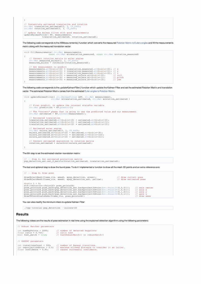
// Instantiate estimated translation and rotationcv::Mat translation_estimated(3, 1, CV_64F);cv::Mat rotation_estimated(3, 3, CV_64F);
// update the Kalman filter with good measurementsupdateKalmanFilter( KF, measurements, translation_estimated, rotation_estimated);
The following code corresponds to the fillMeasurements() function which converts the measured Rotation Matrix to Eulers angles and fill the measurementsmatrix along with the measured translation vector:
void fillMeasurements( cv::Mat &measurements, const cv::Mat &translation_measured, const cv::Mat &rotation_measured) // Convert rotation matrix to euler angles cv::Mat measured_eulers(3, 1, CV_64F); measured_eulers = rot2euler(rotation_measured);
// Set measurement to predict measurements.at<double>(0) = translation_measured.at<double>(0); // x measurements.at<double>(1) = translation_measured.at<double>(1); // y measurements.at<double>(2) = translation_measured.at<double>(2); // z measurements.at<double>(3) = measured_eulers.at<double>(0); // roll measurements.at<double>(4) = measured_eulers.at<double>(1); // pitch measurements.at<double>(5) = measured_eulers.at<double>(2); // yaw
The following code corresponds to the updateKalmanFilter() function which update the Kalman Filter and set the estimated Rotation Matrix and translationvector. The estimated Rotation Matrix comes from the estimated Euler angles to Rotation Matrix.
void updateKalmanFilter( cv::KalmanFilter &KF, cv::Mat &measurement, cv::Mat &translation_estimated, cv::Mat &rotation_estimated )
// First predict, to update the internal statePre variable cv::Mat prediction = KF.predict();
// The "correct" phase that is going to use the predicted value and our measurement cv::Mat estimated = KF.correct(measurement);
// Estimated translation translation_estimated.at<double>(0) = estimated.at<double>(0); translation_estimated.at<double>(1) = estimated.at<double>(1); translation_estimated.at<double>(2) = estimated.at<double>(2);
// Estimated euler angles cv::Mat eulers_estimated(3, 1, CV_64F); eulers_estimated.at<double>(0) = estimated.at<double>(9); eulers_estimated.at<double>(1) = estimated.at<double>(10); eulers_estimated.at<double>(2) = estimated.at<double>(11);
// Convert estimated quaternion to rotation matrix rotation_estimated = euler2rot(eulers_estimated);
The 6th step is set the estimated rotation-translation matrix:
// -- Step 6: Set estimated projection matrixpnp_detection_est.set_P_matrix(rotation_estimated, translation_estimated);
The last and optional step is draw the found pose. To do it I implemented a function to draw all the mesh 3D points and an extra reference axis:
// -- Step X: Draw pose
drawObjectMesh(frame_vis, &mesh, &pnp_detection, green); // draw current posedrawObjectMesh(frame_vis, &mesh, &pnp_detection_est, yellow); // draw estimated pose
double l = 5;std::vector<cv::Point2f> pose_points2d;pose_points2d.push_back(pnp_detection_est.backproject3DPoint(cv::Point3f(0,0,0))); // axis centerpose_points2d.push_back(pnp_detection_est.backproject3DPoint(cv::Point3f(l,0,0))); // axis xpose_points2d.push_back(pnp_detection_est.backproject3DPoint(cv::Point3f(0,l,0))); // axis ypose_points2d.push_back(pnp_detection_est.backproject3DPoint(cv::Point3f(0,0,l))); // axis zdraw3DCoordinateAxes(frame_vis, pose_points2d); // draw axes
You can also modify the minimum inliers to update Kalman Filter:
./cpp-tutorial-pnp_detection --inliers=20
ResultsThe following videos are the results of pose estimation in real time using the explained detection algorithm using the following parameters:
// Robust Matcher parameters
int numKeyPoints = 2000; // number of detected keypointsfloat ratio = 0.70f; // ratio testbool fast_match = true; // fastRobustMatch() or robustMatch()
// RANSAC parameters
int iterationsCount = 500; // number of Ransac iterations.int reprojectionError = 2.0; // maximum allowed distance to consider it an inlier.float confidence = 0.95; // ransac successful confidence.
Bibliography
[1] Adrian Penate-Sanchez, Juan Andrade-Cetto, and Francesc Moreno-Noguer. Ex-
haustive linearization for robust camera pose and focal length estimation. 99, 2013.
ISSN 0162-8828.
[2] S. Nagabhushana. Computer Vision and Image Processing. New Age Interna-
tional, 2005. ISBN 9788122416428. URL http://books.google.fr/books?id=
eSu5I9pU3rUC.
[3] Vincent Lepetit and Pascal Fua. Monocular model-based 3d tracking of rigid ob-
jects: A survey. In Foundations and Trends in Computer Graphics and Vision,
pages 1–89, 2005.
[4] R. Hartley and A. Zisserman. Multiple View Geometry in Computer Vision. Cam-
bridge University Press, 2nd edition, 2004.
[5] X.-S. Gao, X.-R. Hou, J. Tang, and H.-F. Cheng. Complete solution classification
for the perspective-three-point problem. 25(8):930–943, 2003.
[6] D. DeMenthon and L.S. Davis. Model-based object pose in 25 lines of code. 15
(1-2):123–141, 1995.
[7] R. Horaud, F. Dornaika, B.t Lamiroy, and S. Christy. Object pose: The link between
weak perspective, paraperspective, and full perspective. 22(2):173–189, 1997.
[8] C.P. Lu, G.D. Hager, and E. Mjolsness. Fast and globally convergent pose estima-
tion from video images. 22(6):610–622, 2000.
[9] A. Ansar and K. Daniilidis. Linear pose estimation from points or lines. 25(5):
578–589, 2003. ISSN 0162-8828.
[10] P.D. Fiore. Efficient linear solution of exterior orientation. 23(2):140–148, 2001.
[11] V. Lepetit, F. Moreno-Noguer, and P. Fua. EPnP: An accurate O(n) solution to
the PnP problem. 81(2):151–166, 2008.
59
Bibliography 60
[12] G. Schweighofer and A. Pinz. Globally optimal O(n) solution to the PnP problem
for general camera models. 2008.
[13] M. Bujnak, Z. Kukelova, and T. Pajdla. New efficient solution to the absolute pose
problem for camera with unknown focal length and radial distortion. In . Vol. 6492
of Lecture Notes in Computer Science, pages 11–24, 2010.
[14] M. Bujnak, Z. Kukelova, and T. Pajdla. A general solution to the P4P problem for
camera with unknown focal length. pages 1–8, 2008.
[15] Z. Kukelova, M. Bujnak, and T. Pajdla. Polynomial eigenvalue solutions to the
5-pt and 6-pt relative pose problems. pages 56.1–56.10, 2008.
[16] H. Stewenius, D. Nister, F. Kahl, and F. Schaffalitzky. A minimal solution for
relative pose with unknown focal length. pages 789–794, 2005.
[17] B. Triggs. Camera pose and calibration from 4 or 5 known 3d points. pages 278–284,
1999.
[18] M. Byrod, Z. Kukelova, K. Josephson, T. Pajdla, and K. Astrom. Fast and robust
numerical solutions to minimal problems for cameras with radial distortion. pages
1–8, 2008.
[19] K. Josephson and M. Byrod. Pose estimation with radial distortion and unknown
focal length. volume 2, pages 2419–2426, 2009.
[20] M.A. Fischler and R.C. Bolles. Random sample consensus: a paradigm for model
fitting with applications to image analysis and automated cartography. Communi-
cations of the ACM, 24(6):381–395, 1981.
[21] P. Rousseeuw and A. Leroy. Robust Regression and Outlier Detection. Wiley, 1987.
[22] T. Thang-Pham, T.J. Chin, J. Yu, and D. Sutter. The random cluster model for
robust geometric fitting. pages 710–717, 2012.
[23] K. Choi, S. Lee, and Y. Seo. A branch-and-bound algorithm for globally optimal
camera pose and focal length. 28(9):1369–1376, 2010.
[24] F. Kahl, S. Agarwal, M. Chandraker, D. Kriegman, and S. Belongie. Practical
global optimization for multiview geometry. 79(3):271–284, 2008.
[25] F. Kahl and R. Hartley. Multiple-view geometry under the L∞-norm. 30(9):1603–
1617, 2008.
[26] Ben Tordoff and David W. Murray. Guided-MLESAC: Faster Image Transform
Estimation by Using Matching Priors. 27(10):1523–1535, 2005.
Bibliography 61
[27] O. Chum and J. Matas. Matching with PROSAC - progressive sample consensus.
pages 220–226, 2005.
[28] Kai Ni, Hailin Jin, and Frank Dellaert. GroupSAC: Efficient Consensus in the
Presence of Groupings. pages 2193–2200, 2009.
[29] David Nister. Preemptive RANSAC for Live Structure and Motion Estimation.
pages 199–206, 2003.
[30] Rahul Raguram, Jan-Michael Frahm, and Marc Pollefeys. A Comparative Analysis
of RANSAC Techniques Leading to Adaptive Real-Time Random Sample Consen-
sus. pages 500–513, 2008.
[31] Tat-Jun Chin, Jin Yu, and David Suter. Accelerated Hypothesis Generation for
Multi-Structure Robust Fitting. 2010.
[32] O. Enqvist, K. Josephson, and F. Kahl. Optimal Correspondences from Pairwise
Constraints. 2009.
[33] F. Sebastian Grassia. Practical parameterization of rotations using the exponential
map. Journal of Graphics Tools, 3:29–48, 1998.
[34] Zhengyou Zhang, Rachid Deriche, Olivier Faugeras, and Quang-Tuan Luong. A
robust technique for matching two uncalibrated images through the recovery of the
unknown epipolar geometry. 1994.
[35] B. K. P Horn, H. M. Hilden, and S. Negahdaripour. Closed-form solution of absolute
orientation using orthonormal matrices. 5(7):1127–1135, 1988.
[36] James Rumbaugh, Ivar Jacobson, and Grady Booch. The Unified Modeling Lan-
guage Reference Manual. Addison-Wesley, 2 edition, 2005.
[37] Tomas Moller and Ben Trumbore. Fast, minimum storage ray-triangle intersection.
J. Graph. Tools, 2(1):21–28, October 1997. ISSN 1086-7651. doi: 10.1080/10867651.
1997.10487468. URL http://dx.doi.org/10.1080/10867651.1997.10487468.
[38] Marius Muja and David G. Lowe. Scalable nearest neighbor algorithms for high
dimensional data. Pattern Analysis and Machine Intelligence, IEEE Transactions
on, 36, 2014.
[39] David G. Lowe. Distinctive image features from scale-invariant keypoints. Int.
J. Comput. Vision, 60(2):91–110, November 2004. ISSN 0920-5691. doi: 10.
1023/B:VISI.0000029664.99615.94. URL http://dx.doi.org/10.1023/B:VISI.
0000029664.99615.94.
Bibliography 62
[40] Herbert Bay, Andreas Ess, Tinne Tuytelaars, and Luc Van Gool. Speeded-up robust
features (surf). Comput. Vis. Image Underst., 110(3):346–359, June 2008. ISSN
1077-3142. doi: 10.1016/j.cviu.2007.09.014. URL http://dx.doi.org/10.1016/
j.cviu.2007.09.014.
[41] P. F. Alcantarilla, J. Nuevo, and A. Bartoli. Fast explicit diffusion for accelerated
features in nonlinear scale spaces. 2013.
[42] P. F. Alcantarilla, A. Bartoli, and A. J. Davison. KAZE features. 2012.
[43] Ethan Rublee, Vincent Rabaud, Kurt Konolige, and Gary Bradski. Orb: An effi-
cient alternative to sift or surf. In International Conference on Computer Vision,
Barcelona, 11/2011 2011.
[44] Piotr Dollar, Ron Appel, Serge Belongie, and Pietro Perona. Fast feature pyramids
for object detection. PAMI, 2014.
[45] M. Calonder, V. Lepetit, M. Ozuysal, T. Trzcinski, C. Strecha, and P. Fua. BRIEF:
Computing a Local Binary Descriptor Very Fast. IEEE Transactions on Pattern
Analysis and Machine Intelligence, 34(7):1281–1298, 2012.
[46] Qin Lv, William Josephson, Zhe Wang, Moses Charikar, and Kai Li. Multi-Probe
LSH: Efficient Indexing for High-Dimensional Similarity Search . ACM, 2007. ISBN
978-1-59593-649-3.
[47] R.W. Brockett. Robotic manipulators and the product of exponentials formula,
volume 58 of Lecture Notes in Control and Information Sciences. Springer Berlin
Heidelberg, 1984. ISBN 978-3-540-13168-7. doi: 10.1007/BFb0031048. URL http:
//dx.doi.org/10.1007/BFb0031048.
[48] Edgar Riba. Real time pose estimation of a textured object, 2014. URL http:
//docs.opencv.org/trunk/dc/d2c/tutorial_real_time_pose.html.
[49] Joel A. Hesch and Stergios I. Roumeliotis. A direct least-squares (dls) method
for pnp. In Dimitris N. Metaxas, Long Quan, Alberto Sanfeliu, and Luc J. Van
Gool, editors, ICCV, pages 383–390. IEEE, 2011. ISBN 978-1-4577-1101-5. URL
http://dblp.uni-trier.de/db/conf/iccv/iccv2011.html#HeschR11.
[50] Objects recognition kitchen. URL http://wg-perception.github.io/object_
recognition_core/.
[51] S. Hinterstoisser, S. Holzer, C. Cagniart, S. Ilic, K. Konolige, N. Navab, and V. Lep-
etit. Multimodal templates for real-time detection of texture-less objects in heavily
cluttered scenes. 2011.