Author's Note: This is the final accepted version of the manuscript for online distribution in line with

Elsevier's 'Author Rights' policy. The following article is published as:

Wardle, S.G., Palmisano, S. & Gillam, B.J. (2014) Monocular and binocular edges enhance the

perception of stereoscopic slant. Vision Research, 100, 113-123. DOI: 10.1016/j.visres.2014.04.012

If you have subscription rights to the journal, the published version is available at

http://dx.doi.org/10.1016/j.visres.2014.04.012

Monocular and binocular edges enhance the perception of stereoscopic slant

Susan G. Wardle*a, Stephen Palmisanob, and Barbara J. Gillama

a School of Psychology, The University of New South Wales, Sydney, Australia

b School of Psychology, University of Wollongong, Wollongong, Australia

*Corresponding author. Present Address: Department of Cognitive Science, Macquarie University,

Australian Hearing Hub, 16 University Avenue, Sydney, NSW, 2109, Australia.

Email address: susan.wardle@mq.edu.au (Susan G. Wardle)

Phone: +61 2 9850 4072

Wardle, Palmisano & Gillam (2014)

2

Abstract

Gradients of absolute binocular disparity across a slanted surface are often considered

the basis for stereoscopic slant perception. However, perceived stereo slant around a

vertical axis is usually slow and significantly under-estimated for isolated surfaces.

Perceived slant is enhanced when surrounding surfaces provide a relative disparity

gradient or depth step at the edges of the slanted surface, and also in the presence of

monocular occlusion regions (sidebands). Here we investigate how different kinds of

depth information at surface edges enhance stereo slant about a vertical axis. In

Experiment 1, perceived slant decreased with increasing surface width, suggesting

that the relative disparity between the left and right edges was used to judge slant.

Adding monocular sidebands increased perceived slant for all surface widths. In

Experiment 2, observers matched the slant of surfaces that were isolated or had a

context of either monocular or binocular sidebands in the frontal plane. Both types of

sidebands significantly increased perceived slant, but the effect was greater with

binocular sidebands. These results were replicated in a second paradigm in which

observers matched the depth of two probe dots positioned in front of slanted surfaces

(Experiment 3). A large bias occurred for the surface without sidebands, yet this bias

was reduced when monocular sidebands were present, and was nearly eliminated with

binocular sidebands. Our results provide evidence for the importance of edges in

stereo slant perception, and show that depth from monocular occlusion geometry and

binocular disparity may interact to resolve complex 3D scenes.

Keywords: binocular vision, stereoscopic slant, monocular regions, 3D surface

perception, depth matching, binocular disparity

Wardle, Palmisano & Gillam (2014)

3

1. Introduction

Horizontal disparity arising from differences in perspective between the left

and right eye's views of the world gives rise to stereoscopic vision, which is an

important source of information about depth and spatial structure for humans and

other animals with overlapping visual fields. Absolute disparity of a single point is

defined as the angular deviation of its left and right eye images from corresponding

positions relative to the fixation point. However, the perceived depth of two points is

based on their relative disparity (Erkelens and Collewijn, 1985; Gogel, 1956; Gillam,

Chambers and Russo, 1988; Westheimer, 1979). Relative disparity is the difference in

angular separation between the two points in each eye's view and does not change

with fixation. For a slanted surface, absolute disparity increases across the surface as

the first spatial derivative of disparity (i.e. the disparity gradient). Although a gradient

of absolute disparity specifies stereo slant around a vertical axis, perceived slant is

often significantly underestimated compared to geometric prediction (Gillam, Flagg,

and Finlay, 1984; Pierce and Howard, 1997; van Ee and Erkelens, 1996; Mitchison

and Westheimer, 1990), and can have a long latency after stereo fusion is achieved

(Gillam et al., 1988; van Ee and Erkelens, 1996).

Gillam et al. (1988) attribute the ineffectiveness of absolute disparity in

specifying stereoscopic slant to two factors. Firstly, that relative disparity is the

critical stimulus for stereoscopic depth and secondly, that the relative disparity of

successive pairs of equally spaced points on a slanted planar surface is constant across

the surface and thus does not form a gradient. This proposal is supported by Gillam et

al.'s (1984, 1988) finding that stereo slant around a vertical axis is facilitated by

introducing a gradient of relative disparity to the slanted surface. Slant is enhanced

when a frontal plane surface is placed above the slanted surface in a "twist"

configuration (similar to the situation depicted in Figure 1a), which produces a

gradient of relative disparity along the abutting surface edges. In contrast, when the

second surface forms a "hinge" with the first (Figure 1b), abutting the slanted surface

on a side parallel to the axis of slant (Gillam and Pianta, 2005; Gillam, Blackburn and

Brooks, 2007), it does not produce a gradient of relative disparity or facilitate stereo

slant perception. This demonstrates that the presence of a “reference surface” is not

sufficient to facilitate stereoscopic slant.

Wardle, Palmisano & Gillam (2014)

4

Interestingly, stereoscopic slant is increased in a variation of the "hinge"

configuration (Figure 1c) in which the frontal plane surface is displaced in depth from

the edge of the slanted surface (Gillam et al., 2007). This supports the view that stereo

slant perception is at least partly dependent on relative disparity at surface edges –

what Gillam et al. (1988) called the “boundary mode”. However, the enhancement of

perceived slant in this case is much less than that produced by the twist configuration

(which in contrast provides a full gradient of relative disparity along the slanted

surface - Figure 1a).

Gillam and Blackburn (1998) also showed that the presence of monocular

regions at the edges of a stereoscopically slanted surface can enhance the perceived

slant. Monocular regions occur with natural binocular viewing as a result of occlusion

relationships between near and far objects in the two eyes, which produce regions of

the 3D scene that are visible to only one eye. Importantly, these monocular regions do

not introduce relative disparity, but can be seen in depth relative to a neighboring

binocular surface based on occlusion geometry (Gillam & Borsting, 1988; Nakayama

& Shimojo, 1990; Cook and Gillam, 2004; Wardle & Gillam, 2013a). The monocular

regions in Gillam and Blackburn's (1998) stimuli were regions of monocular texture

("monocular sidebands") on the left and right side of a randomly textured binocular

slanted surface. This would occur in a binocular view if a slanted surface passed

through an aperture in the frontal plane. In the example shown in Figure 2, the

monocular sidebands are only visible to the right eye. The monocular sideband on the

right is perceived to lie behind the slanted surface (hence it is occluded in the other

eye’s view), and the monocular sideband on the left is perceived as a continuation of

the slanted surface. In order to account for the latter monocular sideband being

invisible in the left eye, an illusory surface (a "phantom occluder") is perceived (see

also: Wardle and Gillam, 2013b).

The role of monocular sidebands in the enhancement of stereoscopic slant

relative to or in addition to other forms of edge information about depth has not been

investigated, and is a focus of this paper. Although a depth step due to a monocular

region is based on occlusion geometry instead of relative disparity, it may be as

effective as an equivalent binocular depth step in enhancing perceived slant. We use

surfaces with a horizontal gradient of absolute disparity (consistent with slant around

a vertical axis) to compare the effectiveness of monocular occlusion geometry and

binocular disparity at surface edges in enhancing perceived slant. We consider four

Wardle, Palmisano & Gillam (2014)

5

forms of relative depth information at the surface edges; relative disparity between

opposite edges of a single surface (Experiment 1), and three forms of relative depth

between a slanted surface and contextual surfaces. These are (a) the relative disparity

gradient between abutting surfaces separated vertically (Experiments 2 and 3), (b)

relative depth at the sides of the slanted surfaces from monocular occlusion geometry

(Experiments 1-3) and (c) relative depth between the sides of the slanted surfaces and

proximal binocular surfaces in the frontal plane (Experiments 2 and 3). In Experiment

1, we used stimuli of different widths to test whether relative disparity at opposite

sides of a single binocular surface is used to derive stereo slant. If this is the case, we

should find greater perceived slant for narrower surfaces than for wider ones with the

same disparity gradient. We also compared the effects of adding monocular sidebands

to surfaces of different widths. In Experiment 2 we compared the effects of binocular

and monocular edge information on the perception of stereo slant, using a slant-

matching task. Finally, in Experiment 3 we measured the degree to which stereo slant

is underestimated in stimuli with different forms of edge information by using a

measure of bias. To preview the results, we find that the quality and precision of edge

information relates directly to the magnitude of the perceived stereoscopic slant.

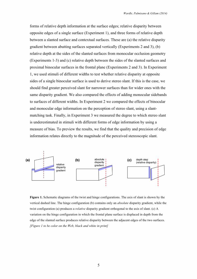
Figure 1. Schematic diagrams of the twist and hinge configurations. The axis of slant is shown by the

vertical dashed line. The hinge configuration (b) contains only an absolute disparity gradient, while the

twist configuration (a) produces a relative disparity gradient orthogonal to the axis of slant. (c) A

variation on the hinge configuration in which the frontal plane surface is displaced in depth from the

edge of the slanted surface produces relative disparity between the adjacent edges of the two surfaces.

[Figure 1 to be color on the Web, black and white in print]

Wardle, Palmisano & Gillam (2014)

6

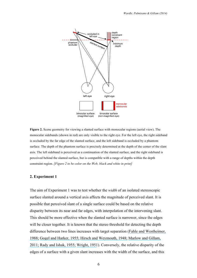
Figure 2. Scene geometry for viewing a slanted surface with monocular regions (aerial view). The

monocular sidebands (shown in red) are only visible to the right eye. For the left eye, the right sideband

is occluded by the far edge of the slanted surface, and the left sideband is occluded by a phantom

surface. The depth of the phantom surface is precisely determined at the depth of the center of the slant

axis. The left sideband is perceived as a continuation of the slanted surface, and the right sideband is

perceived behind the slanted surface, but is compatible with a range of depths within the depth

constraint region. [Figure 2 to be color on the Web, black and white in print]

2. Experiment 1

The aim of Experiment 1 was to test whether the width of an isolated stereoscopic

surface slanted around a vertical axis affects the magnitude of perceived slant. It is

possible that perceived slant of a single surface could be based on the relative

disparity between its near and far edges, with interpolation of the intervening slant.

This should be more effective when the slanted surface is narrower, since the edges

will be closer together. It is known that the stereo threshold for detecting the depth

difference between two lines increases with target separation (Fahle and Westheimer,

1988; Gogel and Harker, 1955; Hirsch and Weymouth, 1948; Marlow and Gillam,

2011; Rady and Ishak, 1955; Wright, 1951). Conversely, the relative disparity of the

edges of a surface with a given slant increases with the width of the surface, and this

Wardle, Palmisano & Gillam (2014)

7

may compensate for the disadvantage of greater separation. A further consideration is

that wider surfaces have better specified gradients of vertical disparity. Vertical

disparity is a major factor in the scaling of horizontal disparity gradients for both

distance and azimuth, and if vertical disparity is more constrained, this should lead to

more accurate estimates of surface slant for larger surfaces (Backus, Banks, van Ee

and Crowell, 1999). Experiment 1 was designed to evaluate these conflicting

predictions about the effect of surface width on stereoscopic slant. In addition,

as monocular regions increase perceived slant (Gillam & Blackburn, 1998), we

compared the effect of surface width on slant for surfaces both with and without

monocular regions to determine whether the effects are independent.

2.1 Method

2.1.1 Observers

Twelve observers naive to the experimental hypotheses participated. Observers had

normal or corrected-to-normal vision and normal stereovision as assessed by the

Stereo Titmus Test (Stereo Optical, Chicago, IL, USA). All experiments were

conducted in accordance with the ethical guidelines in the Declaration of Helsinki and

informed consent was obtained prior to participation.

2.1.2 Stimuli and Procedure

The stereoscopic stimuli were pseudo-random line patterns of even density (see

Figure 3), constructed according to the method detailed in Gillam and Blackburn

(1998). Stimuli were generated on a Pentium computer and displayed stereoscopically

via a Cambridge Research Systems D300 dual-point plotter (16-bit resolution D/A

converters) on a pair of Kikusui COS1161 X—Y oscilloscopes (P31 phosphor). The

stimuli were viewed from a distance of 70 cm through a Wheatstone stereoscope,

which presented separate images to the left and right eye. Stereoscopic slant around

the vertical axis (with either the left or right side nearer) was produced by horizontal

magnification of the texture in one eye's image, which was either 4% or 8%. These

magnifications correspond to slants of 22 and 39 deg respectively, at the 70 cm

viewing distance used. The conversion of magnification to slant (θ) is shown in

Wardle, Palmisano & Gillam (2014)

8

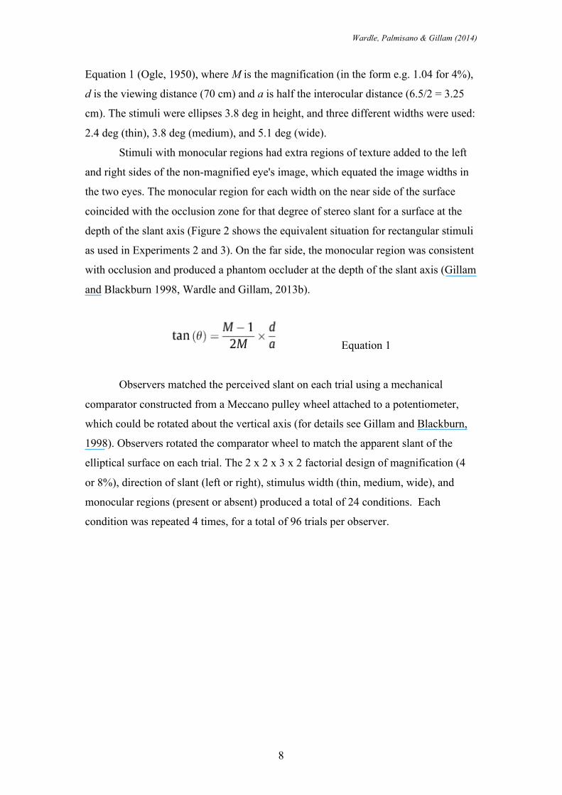
Equation 1 (Ogle, 1950), where M is the magnification (in the form e.g. 1.04 for 4%),

d is the viewing distance (70 cm) and a is half the interocular distance (6.5/2 = 3.25

cm). The stimuli were ellipses 3.8 deg in height, and three different widths were used:

2.4 deg (thin), 3.8 deg (medium), and 5.1 deg (wide).

Stimuli with monocular regions had extra regions of texture added to the left

and right sides of the non-magnified eye's image, which equated the image widths in

the two eyes. The monocular region for each width on the near side of the surface

coincided with the occlusion zone for that degree of stereo slant for a surface at the

depth of the slant axis (Figure 2 shows the equivalent situation for rectangular stimuli

as used in Experiments 2 and 3). On the far side, the monocular region was consistent

with occlusion and produced a phantom occluder at the depth of the slant axis (Gillam

and Blackburn 1998, Wardle and Gillam, 2013b).

Equation 1

Observers matched the perceived slant on each trial using a mechanical

comparator constructed from a Meccano pulley wheel attached to a potentiometer,

which could be rotated about the vertical axis (for details see Gillam and Blackburn,

1998). Observers rotated the comparator wheel to match the apparent slant of the

elliptical surface on each trial. The 2 x 2 x 3 x 2 factorial design of magnification (4

or 8%), direction of slant (left or right), stimulus width (thin, medium, wide), and

monocular regions (present or absent) produced a total of 24 conditions. Each

condition was repeated 4 times, for a total of 96 trials per observer.

Wardle, Palmisano & Gillam (2014)

9

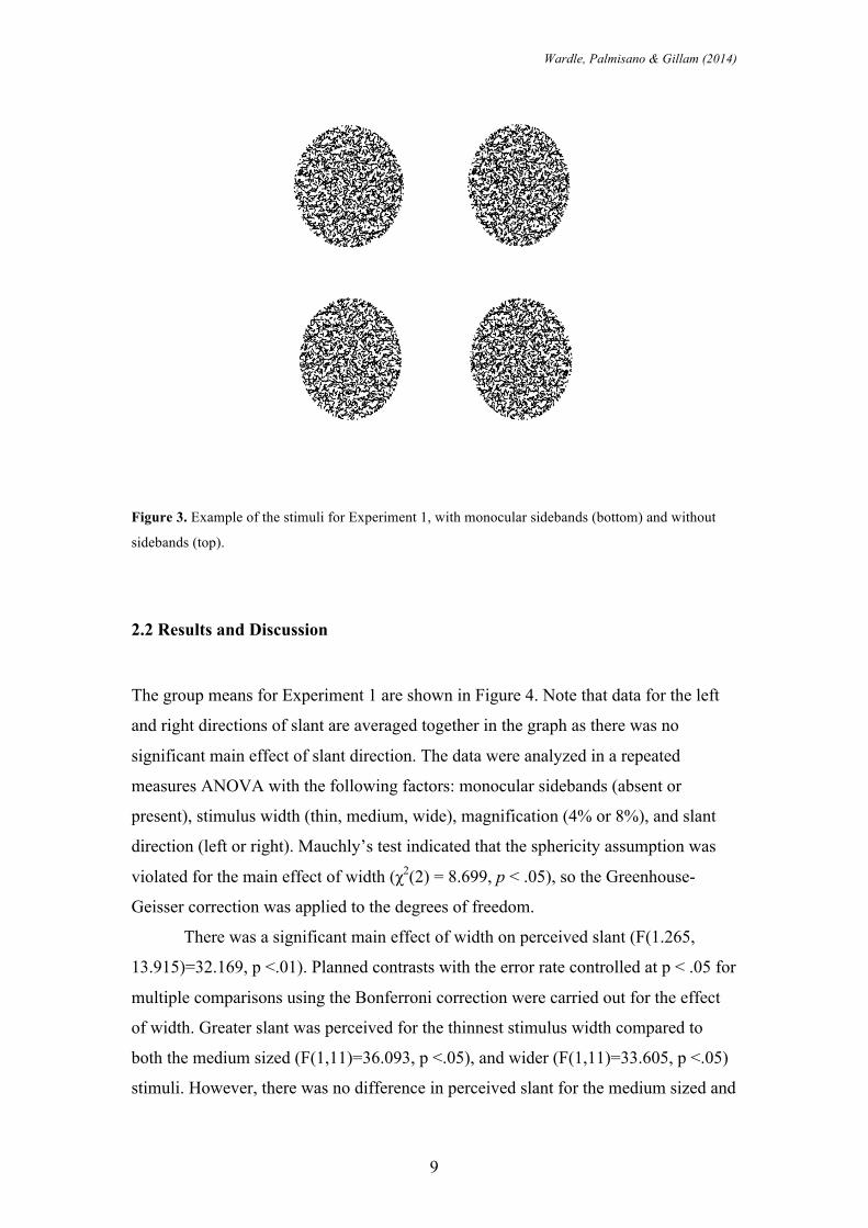
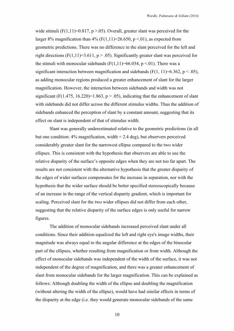
Figure 3. Example of the stimuli for Experiment 1, with monocular sidebands (bottom) and without

sidebands (top).

2.2 Results and Discussion

The group means for Experiment 1 are shown in Figure 4. Note that data for the left

and right directions of slant are averaged together in the graph as there was no

significant main effect of slant direction. The data were analyzed in a repeated

measures ANOVA with the following factors: monocular sidebands (absent or

present), stimulus width (thin, medium, wide), magnification (4% or 8%), and slant

direction (left or right). Mauchly’s test indicated that the sphericity assumption was

violated for the main effect of width (χ2(2) = 8.699, p < .05), so the Greenhouse-

Geisser correction was applied to the degrees of freedom.

There was a significant main effect of width on perceived slant (F(1.265,

13.915)=32.169, p <.01). Planned contrasts with the error rate controlled at p < .05 for

multiple comparisons using the Bonferroni correction were carried out for the effect

of width. Greater slant was perceived for the thinnest stimulus width compared to

both the medium sized (F(1,11)=36.093, p <.05), and wider (F(1,11)=33.605, p <.05)

stimuli. However, there was no difference in perceived slant for the medium sized and

Wardle, Palmisano & Gillam (2014)

10

wide stimuli (F(1,11)=0.817, p >.05). Overall, greater slant was perceived for the

larger 8% magnification than 4% (F(1,11)=26.650, p <.01), as expected from

geometric predictions. There was no difference in the slant perceived for the left and

right directions (F(1,11)=3.611, p > .05). Significantly greater slant was perceived for

the stimuli with monocular sidebands (F(1,11)=66.034, p <.01). There was a

significant interaction between magnification and sidebands (F(1, 11)=6.362, p < .05),

as adding monocular regions produced a greater enhancement of slant for the larger

magnification. However, the interaction between sidebands and width was not

significant (F(1.475, 16.220)=1.863, p > .05), indicating that the enhancement of slant

with sidebands did not differ across the different stimulus widths. Thus the addition of

sidebands enhanced the perception of slant by a constant amount, suggesting that its

effect on slant is independent of that of stimulus width.

Slant was generally underestimated relative to the geometric predictions (in all

but one condition: 4% magnification, width = 2.4 deg), but observers perceived

considerably greater slant for the narrowest ellipse compared to the two wider

ellipses. This is consistent with the hypothesis that observers are able to use the

relative disparity of the surface’s opposite edges when they are not too far apart. The

results are not consistent with the alternative hypothesis that the greater disparity of

the edges of wider surfaces compensates for the increase in separation, nor with the

hypothesis that the wider surface should be better specified stereoscopically because

of an increase in the range of the vertical disparity gradient, which is important for

scaling. Perceived slant for the two wider ellipses did not differ from each other,

suggesting that the relative disparity of the surface edges is only useful for narrow

figures.

The addition of monocular sidebands increased perceived slant under all

conditions. Since their addition equalized the left and right eye's image widths, their

magnitude was always equal to the angular difference at the edges of the binocular

part of the ellipses, whether resulting from magnification or from width. Although the

effect of monocular sidebands was independent of the width of the surface, it was not

independent of the degree of magnification, and there was a greater enhancement of

slant from monocular sidebands for the larger magnification. This can be explained as

follows: Although doubling the width of the ellipse and doubling the magnification

(without altering the width of the ellipse), would have had similar effects in terms of

the disparity at the edge (i.e. they would generate monocular sidebands of the same

Wardle, Palmisano & Gillam (2014)

11

width), edge-based depth signals in the former case would be more separated from

each other (due to the greater width of the ellipse).

In Experiments 2 and 3 we investigate the enhancement of slant from

monocular sidebands further by comparing it to equivalent binocular information at

the surface edges.

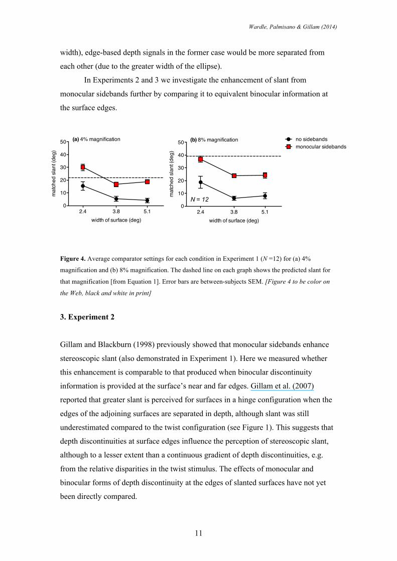
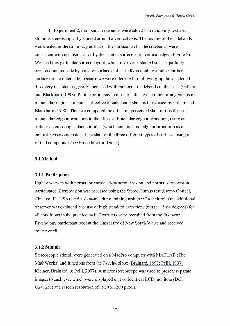
Figure 4. Average comparator settings for each condition in Experiment 1 (N =12) for (a) 4%

magnification and (b) 8% magnification. The dashed line on each graph shows the predicted slant for

that magnification [from Equation 1]. Error bars are between-subjects SEM. [Figure 4 to be color on

the Web, black and white in print]

3. Experiment 2

Gillam and Blackburn (1998) previously showed that monocular sidebands enhance

stereoscopic slant (also demonstrated in Experiment 1). Here we measured whether

this enhancement is comparable to that produced when binocular discontinuity

information is provided at the surface’s near and far edges. Gillam et al. (2007)

reported that greater slant is perceived for surfaces in a hinge configuration when the

edges of the adjoining surfaces are separated in depth, although slant was still

underestimated compared to the twist configuration (see Figure 1). This suggests that

depth discontinuities at surface edges influence the perception of stereoscopic slant,

although to a lesser extent than a continuous gradient of depth discontinuities, e.g.

from the relative disparities in the twist stimulus. The effects of monocular and

binocular forms of depth discontinuity at the edges of slanted surfaces have not yet

been directly compared.

2.4 3.8 5.10

10

20

30

40

50

width of surface (deg)

mat

ched

sla

nt (d

eg)

(a) 4% magnification

2.4 3.8 5.10

10

20

30

40

50

width of surface (deg)

mat

ched

sla

nt (d

eg)

no sidebandsmonocular sidebands

(b) 8% magnification

N = 12

Wardle, Palmisano & Gillam (2014)

12

In Experiment 2, monocular sidebands were added to a randomly-textured

stimulus stereoscopically slanted around a vertical axis. The texture of the sidebands

was created in the same way as that on the surface itself. The sidebands were

consistent with occlusion of or by the slanted surface at its vertical edges (Figure 2).

We used this particular surface layout, which involves a slanted surface partially

occluded on one side by a nearer surface and partially occluding another farther

surface on the other side, because we were interested in following-up the accidental

discovery that slant is greatly increased with monocular sidebands in this case (Gillam

and Blackburn, 1998). Pilot experiments in our lab indicate that other arrangements of

monocular regions are not as effective in enhancing slant as those used by Gillam and

Blackburn (1998). Thus we compared the effect on perceived slant of this form of

monocular edge information to the effect of binocular edge information, using an

ordinary stereoscopic slant stimulus (which contained no edge information) as a

control. Observers matched the slant of the three different types of surfaces using a

virtual comparator (see Procedure for details).

3.1 Method

3.1.1 Participants

Eight observers with normal or corrected-to-normal vision and normal stereovision

participated. Stereovision was assessed using the Stereo Titmus test (Stereo Optical,

Chicago, IL, USA), and a slant-matching training task (see Procedure). One additional

observer was excluded because of high standard deviations (range: 15-64 degrees) for

all conditions in the practice task. Observers were recruited from the first year

Psychology participant pool at the University of New South Wales and received

course credit.

3.1.2 Stimuli

Stereoscopic stimuli were generated on a MacPro computer with MATLAB (The

MathWorks) and functions from the Psychtoolbox (Brainard, 1997; Pelli, 1997;

Kleiner, Brainard, & Pelli, 2007). A mirror stereoscope was used to present separate

images to each eye, which were displayed on two identical LCD monitors (Dell

U2412M) at a screen resolution of 1920 x 1200 pixels.

Wardle, Palmisano & Gillam (2014)

13

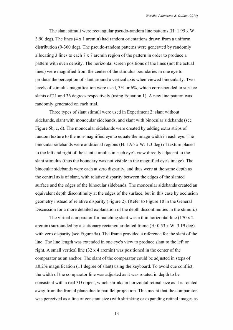
The slant stimuli were rectangular pseudo-random line patterns (H: 1.95 x W:

3.90 deg). The lines (4 x 1 arcmin) had random orientations drawn from a uniform

distribution (0-360 deg). The pseudo-random patterns were generated by randomly

allocating 3 lines to each 7 x 7 arcmin region of the pattern in order to produce a

pattern with even density. The horizontal screen positions of the lines (not the actual

lines) were magnified from the center of the stimulus boundaries in one eye to

produce the perception of slant around a vertical axis when viewed binocularly. Two

levels of stimulus magnification were used, 3% or 6%, which corresponded to surface

slants of 21 and 36 degrees respectively (using Equation 1). A new line pattern was

randomly generated on each trial.

Three types of slant stimuli were used in Experiment 2: slant without

sidebands, slant with monocular sidebands, and slant with binocular sidebands (see

Figure 5b, c, d). The monocular sidebands were created by adding extra strips of

random texture to the non-magnified eye to equate the image width in each eye. The

binocular sidebands were additional regions (H: 1.95 x W: 1.3 deg) of texture placed

to the left and right of the slant stimulus in each eye's view directly adjacent to the

slant stimulus (thus the boundary was not visible in the magnified eye's image). The

binocular sidebands were each at zero disparity, and thus were at the same depth as

the central axis of slant, with relative disparity between the edges of the slanted

surface and the edges of the binocular sidebands. The monocular sidebands created an

equivalent depth discontinuity at the edges of the surface, but in this case by occlusion

geometry instead of relative disparity (Figure 2). (Refer to Figure 10 in the General

Discussion for a more detailed explanation of the depth discontinuities in the stimuli.)

The virtual comparator for matching slant was a thin horizontal line (170 x 2

arcmin) surrounded by a stationary rectangular dotted frame (H: 0.53 x W: 3.19 deg)

with zero disparity (see Figure 5a). The frame provided a reference for the slant of the

line. The line length was extended in one eye's view to produce slant to the left or

right. A small vertical line (32 x 4 arcmin) was positioned in the center of the

comparator as an anchor. The slant of the comparator could be adjusted in steps of

±0.2% magnification (±1 degree of slant) using the keyboard. To avoid cue conflict,

the width of the comparator line was adjusted as it was rotated in depth to be

consistent with a real 3D object, which shrinks in horizontal retinal size as it is rotated

away from the frontal plane due to parallel projection. This meant that the comparator

was perceived as a line of constant size (with shrinking or expanding retinal images as

Wardle, Palmisano & Gillam (2014)

14

expected from natural viewing) rotating in depth. The comparator was placed at a

distance of 3.9 deg below the slant stimulus. A large separation between the slant

stimulus and the comparator is necessary to prevent the comparator from influencing

perceived slant.

3.1.3 Procedure

Observers viewed the stimuli through a mirror stereoscope at a distance of 84 cm.

Prior to the main experiment observers completed a practice task that involved

matching the slant of surfaces using the comparator. The stimuli used for practice

were identical to the stimuli used in the main experiment, except for the addition of

frontal-plane flankers (H: 0.98 x W: 3.90 deg) above and below the slanted surface

These formed twist configurations, which are known to increase perceived slant

(Gillam and Blackburn, 1998; Gillam, Blackburn and Brooks, 2007). Participants

adjusted the slant of the comparator using the keyboard, and pressed the space bar to

enter their response when they perceived the slant to be matched. Initially this task

was completed with feedback to give observers practice in using the comparator. The

vertical line through the central axis of the comparator turned orange when it was

matched within ±14 degrees of the stimulus's slant, and green when it was within ±1

degree. The slanted surfaces used for practice were 3, 5, or 7% magnification in the

left or right eye (corresponding to slant in the left and right directions of 21, 32, and

40 degrees). Each of the six conditions was repeated twice for a total of 12 trials with

feedback. Following the training, the observers completed the same task (4 repeats, 24

trials total) without feedback to serve as a screening test.

Observers completed the main experiment directly after the training and

practice trials. In the experiment they matched the slant of each surface using the

comparator following the same procedure as that used for the practice task. There

were 3 slant types (no sidebands, monocular sidebands, binocular sidebands), 2

magnitudes of slant (3% and 6%) and 2 directions of slant (left and right around a

vertical axis). The 12 conditions were repeated 10 times in random order and

produced a total of 120 trials. The minimum trial duration was 3s, the maximum

duration was unconstrained.

Wardle, Palmisano & Gillam (2014)

15

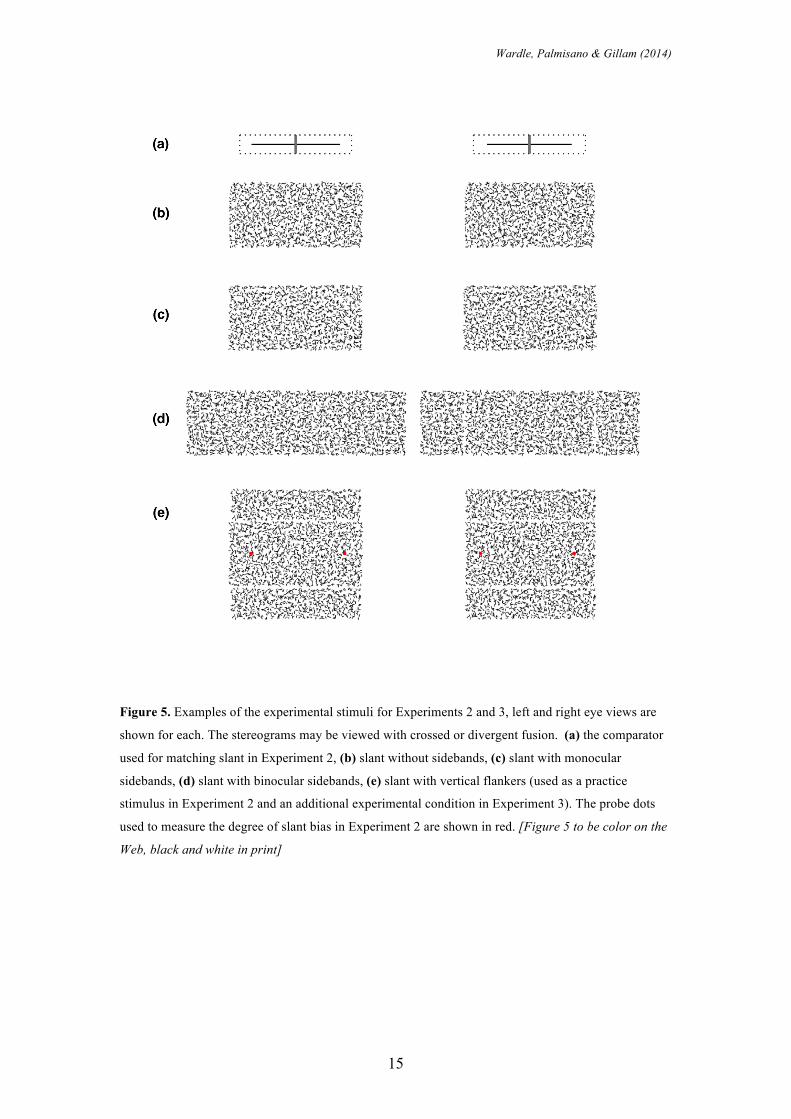
Figure 5. Examples of the experimental stimuli for Experiments 2 and 3, left and right eye views are

shown for each. The stereograms may be viewed with crossed or divergent fusion. (a) the comparator

used for matching slant in Experiment 2, (b) slant without sidebands, (c) slant with monocular

sidebands, (d) slant with binocular sidebands, (e) slant with vertical flankers (used as a practice

stimulus in Experiment 2 and an additional experimental condition in Experiment 3). The probe dots

used to measure the degree of slant bias in Experiment 2 are shown in red. [Figure 5 to be color on the

Web, black and white in print]

Wardle, Palmisano & Gillam (2014)

16

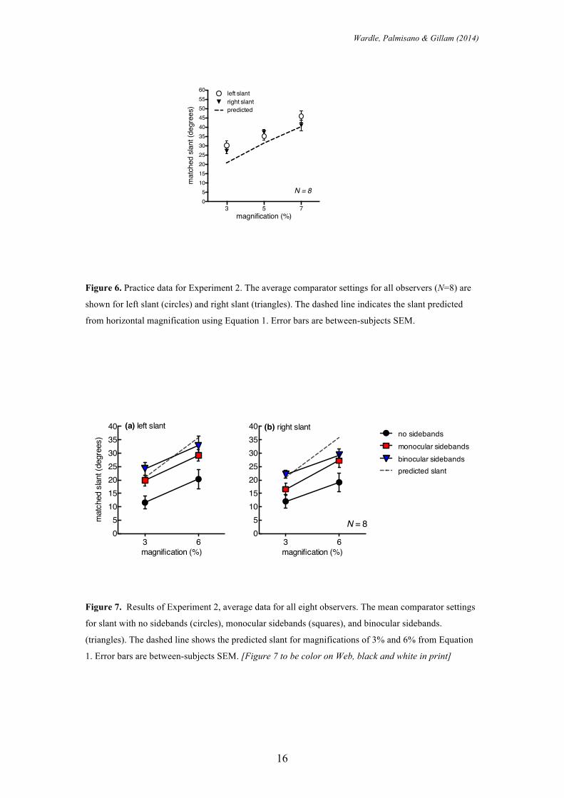
Figure 6. Practice data for Experiment 2. The average comparator settings for all observers (N=8) are

shown for left slant (circles) and right slant (triangles). The dashed line indicates the slant predicted

from horizontal magnification using Equation 1. Error bars are between-subjects SEM.

Figure 7. Results of Experiment 2, average data for all eight observers. The mean comparator settings

for slant with no sidebands (circles), monocular sidebands (squares), and binocular sidebands.

(triangles). The dashed line shows the predicted slant for magnifications of 3% and 6% from Equation

1. Error bars are between-subjects SEM. [Figure 7 to be color on Web, black and white in print]

3 605

10152025303540

magnification (%)

mat

ched

slan

t (de

gree

s)

(a) left slant

3 605

10152025303540

magnification (%)

(b) right slant

N = 8

no sidebandsmonocular sidebandsbinocular sidebandspredicted slant

3 5 705

1015202530354045505560

magnification (%)

mat

ched

sla

nt (d

egre

es)

left slant

predictedright slant

N = 8

Wardle, Palmisano & Gillam (2014)

17

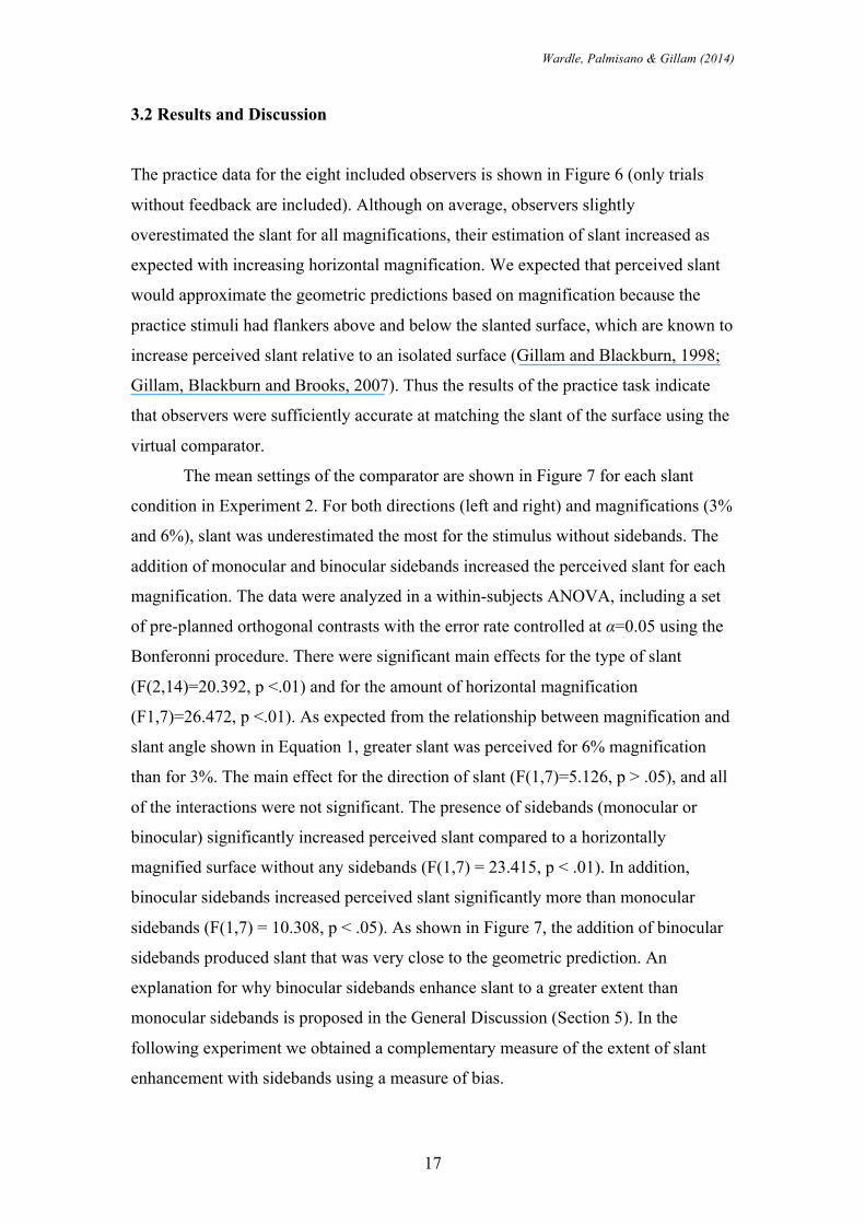
3.2 Results and Discussion

The practice data for the eight included observers is shown in Figure 6 (only trials

without feedback are included). Although on average, observers slightly

overestimated the slant for all magnifications, their estimation of slant increased as

expected with increasing horizontal magnification. We expected that perceived slant

would approximate the geometric predictions based on magnification because the

practice stimuli had flankers above and below the slanted surface, which are known to

increase perceived slant relative to an isolated surface (Gillam and Blackburn, 1998;

Gillam, Blackburn and Brooks, 2007). Thus the results of the practice task indicate

that observers were sufficiently accurate at matching the slant of the surface using the

virtual comparator.

The mean settings of the comparator are shown in Figure 7 for each slant

condition in Experiment 2. For both directions (left and right) and magnifications (3%

and 6%), slant was underestimated the most for the stimulus without sidebands. The

addition of monocular and binocular sidebands increased the perceived slant for each

magnification. The data were analyzed in a within-subjects ANOVA, including a set

of pre-planned orthogonal contrasts with the error rate controlled at α=0.05 using the

Bonferonni procedure. There were significant main effects for the type of slant

(F(2,14)=20.392, p <.01) and for the amount of horizontal magnification

(F1,7)=26.472, p <.01). As expected from the relationship between magnification and

slant angle shown in Equation 1, greater slant was perceived for 6% magnification

than for 3%. The main effect for the direction of slant (F(1,7)=5.126, p > .05), and all

of the interactions were not significant. The presence of sidebands (monocular or

binocular) significantly increased perceived slant compared to a horizontally

magnified surface without any sidebands (F(1,7) = 23.415, p < .01). In addition,

binocular sidebands increased perceived slant significantly more than monocular

sidebands (F(1,7) = 10.308, p < .05). As shown in Figure 7, the addition of binocular

sidebands produced slant that was very close to the geometric prediction. An

explanation for why binocular sidebands enhance slant to a greater extent than

monocular sidebands is proposed in the General Discussion (Section 5). In the

following experiment we obtained a complementary measure of the extent of slant

enhancement with sidebands using a measure of bias.

Wardle, Palmisano & Gillam (2014)

18

4. Experiment 3

The aim of Experiment 3 was to obtain a second, independent measure of the degree

of perceived slant with and without monocular or binocular sidebands. Two dots

positioned at the same depth in front of an isolated stereoscopically slanted surface

appear offset in depth because the slant is underestimated, while the depths of the dots

relative to the surface are perceived correctly (Mitchison and Westheimer, 1984).

When flankers are added to the top and bottom of the slanted surface (as in Figure

2e), the slant underestimation diminishes, and consequently the bias in the depth of

the probes is reduced (Gillam, Sedgwick and Marlow, 2011). Thus the degree of bias

reflects the degree to which the surface slant is underestimated. The probe bias

method may also provide a better estimate of the interpolation of depth across the

surface than the slant-matching task. In the slant-matching task, it is possible that

observers concentrated on the edges of the slanted surface while moving the

comparator. In the probe task there would be no benefit from focusing on the edges

because the probe dots are matched to each other. Here we compare the amount of

bias for slant with and without sidebands to determine the degree to which the

sidebands reduce slant underestimation.

4.1 Method

4.1.1 Participants

Eleven observers with normal or corrected-to-normal vision and normal stereovision

participated. Stereovision was assessed using the Stereo Titmus test (Stereo Optical,

Chicago, IL, USA), and a training task (see Procedure). Participants were recruited

from within the Psychology department at the University of New South Wales and

received financial reimbursement.

4.1.2 Stimuli

The experimental setup and stimuli were identical to Experiment 2, with the following

modifications. In Experiment 3 four types of slant stimulus were used (see Figure 5b,

c, d, e) : slant without sidebands, slant with monocular sidebands, slant with binocular

sidebands, and slant with binocular strips of texture above and below the slanted

surface, located at zero disparity (i.e. the same depth as the central axis of slant). This

Wardle, Palmisano & Gillam (2014)

19

stimulus was similar to the "twist" configuration, and produced a gradient of relative

disparity along the top and bottom edges of the slanted surface. This condition was

included as a control for the other slant conditions because it is known that the "twist"

configuration reduces the probe bias (Gillam, Sedgwick and Marlow, 2011). An

additional frontal plane condition was included as a baseline, in which the same

image was presented to each eye without horizontal magnification, and was perceived

as a flat surface (and thus no probe bias was expected).

4.1.3 Procedure

As in Experiment 2, observers completed a practice task before the main experiment.

The practice task involved matching the depth of two vertical black bars (H: 127 x W:

4 arcmin, horizontal separation: 0.7 deg). On each trial, the bars started at a relative

disparity between 2 - 23 arcmin. Observers adjusted the relative disparity of the bars

in steps of 0.5 arcmin using the keyboard. When the up arrow key was pressed, the

left bar moved nearer by 0.25 arcmin and the right bar moved further by 0.25 arcmin.

The direction of adjustment was reversed when the down arrow key was pressed.

When observers perceived the two bars to be matched in depth, they pressed the space

bar to initiate the next trial. Observers initially completed 12 practice trials with

feedback; the bars turned orange when within 2 arcmin of relative disparity, and green

when within 0.5 arcmin of disparity. This was followed by 24 trials without feedback.

In the main experiment observers matched the depth of two red circular probes

(diameter: 6 arcmin) positioned 7 arcmin in front of the slanted surface (when at zero

relative disparity) (see Figure 5e). The probes were horizontally separated by a

distance of 2.8 deg and their relative disparity was randomly selected between ± 4

arcmin for the start of each trial. Observers adjusted the relative depth of the probes

using the same method as in the practice task. On each trial the stimulus was

displayed for a minimum of 3 seconds, however there was no upper time limit and

observers pressed the space bar to enter their response when they perceived the probes

to be matched in depth. There were four types of slanted surface behind the probes

(no sidebands, monocular sidebands, binocular sidebands, vertical flankers), 2

magnitudes of slant (3% and 6%) and 2 directions of slant (left and right around a

vertical axis). This produced 16 conditions in a factorial design, in addition to the flat

surface condition, which served as a baseline measure. Each of the 17 conditions was

repeated 7 times in a different random order for each observer, for a total of 119 trials.

Wardle, Palmisano & Gillam (2014)

20

4.2 Results and Discussion

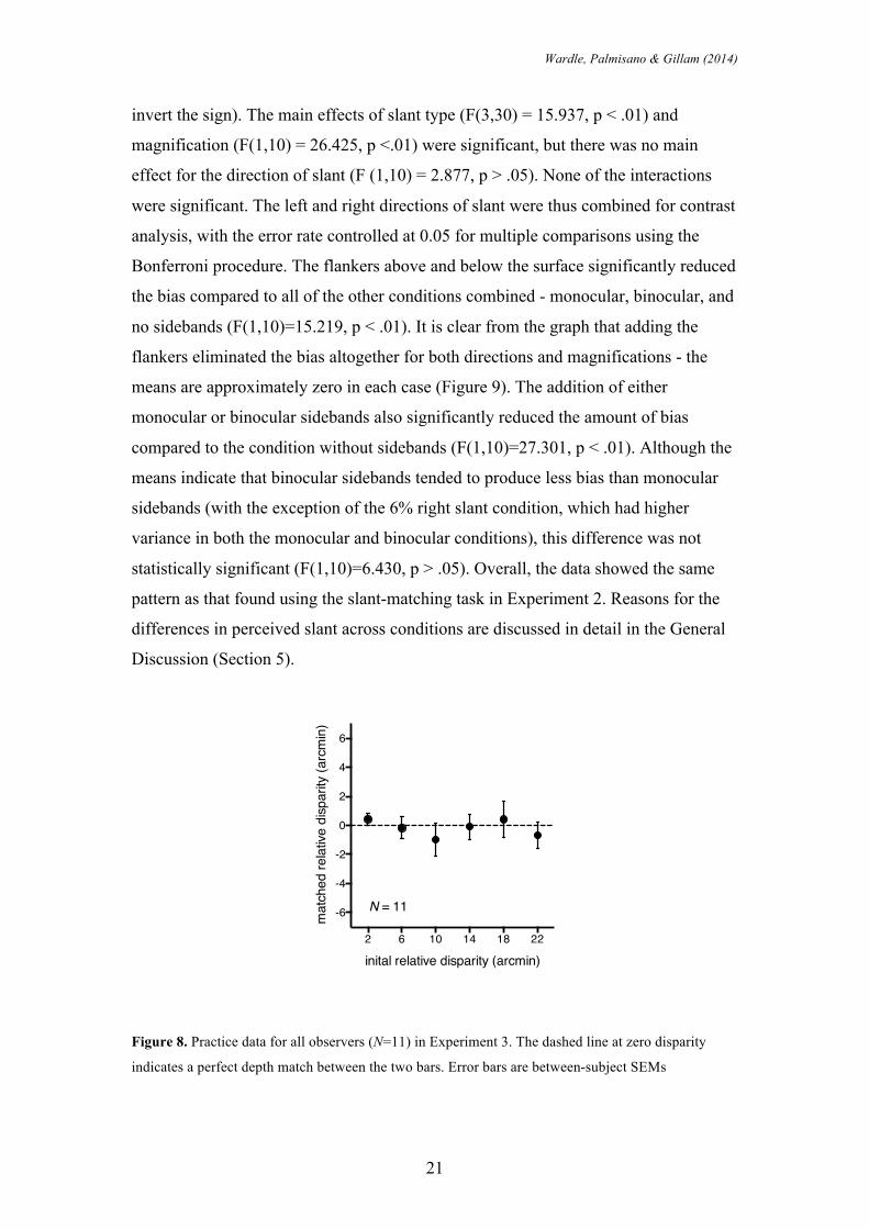
The practice data for Experiment 3 are shown in Figure 8 (only trials without

feedback are included). The means are clustered around zero disparity, confirming

that observers were able to match the depth of the two bars in the practice task from a

range of starting disparities. Note that the practice task is more difficult than the

baseline condition in Experiment 3 because there is no reference surface behind the

bars. This may explain the greater variability in the data for the practice task (Figure

8) compared to the baseline condition (Figure 9).

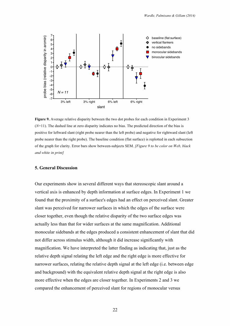
The mean probe bias for each slant condition in Experiment 3 is shown in

Figure 9. The predicted direction of the bias is coded as positive for leftward slant

(right probe perceived as nearer than left probe), and negative for rightward slant (left

probe perceived as nearer than right probe). The bias was calculated by subtracting

the matched disparity of the right probe from the matched disparity of the left probe.

The predicted direction of the bias is to perceive the probe that is further from the

surface (i.e. in front of the side of the surface which is slanted away) as nearer than

the probe that is closer to the surface.

As expected, no bias was perceived when the probes were in front of a flat

surface; the mean disparity is approximately zero (Figure 9). There was also little or

no bias for a slanted surface with flankers above and below the surface in a twist

configuration. This is predicted because slant is known not to be underestimated in

this stimulus (e.g. the practice task for Experiment 2 used this stimulus, see data in

Figure 2; also see Gillam, Blackburn and Brooks, 2007, Gillam and Blackburn, 1998;

Gillam, Sedgwick and Marlow, 2011). However, a large bias was observed for slant

without sidebands, in agreement with the slant-matching data from Experiment 2,

which showed that the slant of this surface is significantly under-estimated. When

monocular sidebands are added, a bias is still present but it is reduced in comparison

to slant without sidebands. The magnitude of bias is reduced even further when

binocular sidebands are added. Thus this pattern of results is in direct agreement with

the slant-matching data from Experiment 2. Overall, in the conditions that had a bias,

the bias was larger for the surfaces with greater slant (6% magnification).

The results were analyzed in a repeated measures ANOVA. Prior to statistical

analysis, the data was recoded so that the predicted direction of bias for left and right

slant were both positive values (the data for rightward slant was multiplied by -1 to

Wardle, Palmisano & Gillam (2014)

21

invert the sign). The main effects of slant type (F(3,30) = 15.937, p < .01) and

magnification (F(1,10) = 26.425, p <.01) were significant, but there was no main

effect for the direction of slant (F (1,10) = 2.877, p > .05). None of the interactions

were significant. The left and right directions of slant were thus combined for contrast

analysis, with the error rate controlled at 0.05 for multiple comparisons using the

Bonferroni procedure. The flankers above and below the surface significantly reduced

the bias compared to all of the other conditions combined - monocular, binocular, and

no sidebands (F(1,10)=15.219, p < .01). It is clear from the graph that adding the

flankers eliminated the bias altogether for both directions and magnifications - the

means are approximately zero in each case (Figure 9). The addition of either

monocular or binocular sidebands also significantly reduced the amount of bias

compared to the condition without sidebands (F(1,10)=27.301, p < .01). Although the

means indicate that binocular sidebands tended to produce less bias than monocular

sidebands (with the exception of the 6% right slant condition, which had higher

variance in both the monocular and binocular conditions), this difference was not

statistically significant (F(1,10)=6.430, p > .05). Overall, the data showed the same

pattern as that found using the slant-matching task in Experiment 2. Reasons for the

differences in perceived slant across conditions are discussed in detail in the General

Discussion (Section 5).

Figure 8. Practice data for all observers (N=11) in Experiment 3. The dashed line at zero disparity

indicates a perfect depth match between the two bars. Error bars are between-subject SEMs

2 6 10 14 18 22

-6

-4

-2

0

2

4

6

inital relative disparity (arcmin)

mat

ched

rela

tive

disp

arity

(arc

min

)

N = 11

Wardle, Palmisano & Gillam (2014)

22

Figure 9. Average relative disparity between the two dot probes for each condition in Experiment 3

(N=11). The dashed line at zero disparity indicates no bias. The predicted direction of the bias is

positive for leftward slant (right probe nearer than the left probe) and negative for rightward slant (left

probe nearer than the right probe). The baseline condition (flat surface) is replotted in each subsection

of the graph for clarity. Error bars show between-subjects SEM. [Figure 9 to be color on Web, black

and white in print]

5. General Discussion

Our experiments show in several different ways that stereoscopic slant around a

vertical axis is enhanced by depth information at surface edges. In Experiment 1 we

found that the proximity of a surface's edges had an effect on perceived slant. Greater

slant was perceived for narrower surfaces in which the edges of the surface were

closer together, even though the relative disparity of the two surface edges was

actually less than that for wider surfaces at the same magnification. Additional

monocular sidebands at the edges produced a consistent enhancement of slant that did

not differ across stimulus width, although it did increase significantly with

magnification. We have interpreted the latter finding as indicating that, just as the

relative depth signal relating the left edge and the right edge is more effective for

narrower surfaces, relating the relative depth signal at the left edge (i.e. between edge

and background) with the equivalent relative depth signal at the right edge is also

more effective when the edges are closer together. In Experiments 2 and 3 we

compared the enhancement of perceived slant for regions of monocular versus

3% left 3% right 6% left 6% right-7-6-5-4-3-2-101234567

slant

prob

e bi

as (r

elat

ive d

ispar

ity in

arc

min

)

N = 11

baseline (flat surface)vertical flankers

binocular sidebandsmonocular sidebandsno sidebands

Wardle, Palmisano & Gillam (2014)

23

binocular texture at the outer edges of the slanted surface. Experiment 2 demonstrated

with a slant-matching task that the magnitude of perceived slant is greater, and

Experiment 3 demonstrated that the bias in the perceived depth of two probes in front

of a slanted surface was significantly reduced when either binocular or monocular

sidebands were present. In both cases, binocular sidebands produced a greater effect

than monocular sidebands — a greater enhancement of slant (Experiment 2), and a

greater reduction in the depth bias of the probes (Experiment 3).

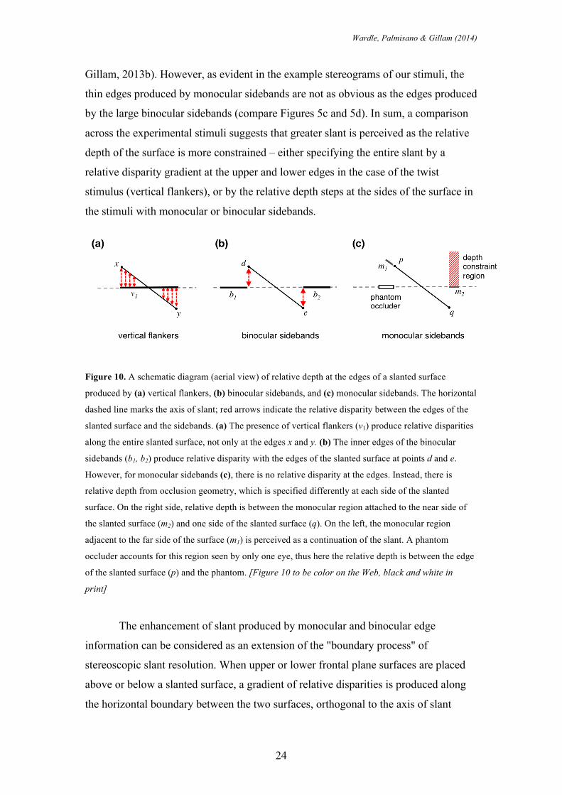
5.1 Monocular and binocular edges constrain stereoscopic slant

We suggest that the advantage afforded by binocular and monocular sidebands in the

perception of stereoscopic slant is a result of adding relative depth signals at the near

and far edges of the slanted surface (see Figure 10). The pattern of data in Experiment

2 and Experiment 3 can be related to how constrained the relative depth signals at the

edges of the slanted surface are in each case. The greatest magnitude of slant, and the

greatest reduction in the probe bias, was observed for a slanted surface with flankers

above and below the surface (a version of the "twist" stimulus). As illustrated in

Figure 10a, the change in depth of this surface is constrained across the entire surface

by the relative disparity gradient between the slanted surface and the flankers.

Binocular sidebands were the second most effective at enhancing slant, and here the

depth of the slanted surface is constrained by relative disparities at the edges of the

slanted surface and the binocular sidebands (Figure 10b). Monocular sidebands

present an entirely different situation, as the relative depth at the edges of the slanted

surface is specified by occlusion geometry instead of relative disparity. In contrast to

the precise depth specified by relative disparity, in most cases, depth from occlusion

geometry is only partially constrained1. There is also a qualitative difference in the

edges produced by binocular and monocular sidebands, as the edge on one side of the

surface with monocular sidebands is not supported by a physically present occluding

surface. However, the occlusion information is powerful enough to create a strong

phantom occluder on this side (Figure 10b). Phantom occluding surfaces arising from

monocular regions have geometrically predictable quantitative depth (Wardle and

1 Assee and Qian (2007) propose that monocular regions operate as a form of double fusion or Panum’s Limiting Case (which is a form of occlusion geometry). However, this would be an unorthodox form of Panum's Limiting Case, in which one fusion is of the outer edges of the left and right eye images and the other is of the outer edge of the narrower image in one eye and the monocularly invisible intersection of the binocular and monocular regions in the other.

Wardle, Palmisano & Gillam (2014)

24

Gillam, 2013b). However, as evident in the example stereograms of our stimuli, the

thin edges produced by monocular sidebands are not as obvious as the edges produced

by the large binocular sidebands (compare Figures 5c and 5d). In sum, a comparison

across the experimental stimuli suggests that greater slant is perceived as the relative

depth of the surface is more constrained – either specifying the entire slant by a

relative disparity gradient at the upper and lower edges in the case of the twist

stimulus (vertical flankers), or by the relative depth steps at the sides of the surface in

the stimuli with monocular or binocular sidebands.

Figure 10. A schematic diagram (aerial view) of relative depth at the edges of a slanted surface

produced by (a) vertical flankers, (b) binocular sidebands, and (c) monocular sidebands. The horizontal

dashed line marks the axis of slant; red arrows indicate the relative disparity between the edges of the

slanted surface and the sidebands. (a) The presence of vertical flankers (v1) produce relative disparities

along the entire slanted surface, not only at the edges x and y. (b) The inner edges of the binocular

sidebands (b1, b2) produce relative disparity with the edges of the slanted surface at points d and e.

However, for monocular sidebands (c), there is no relative disparity at the edges. Instead, there is

relative depth from occlusion geometry, which is specified differently at each side of the slanted

surface. On the right side, relative depth is between the monocular region attached to the near side of

the slanted surface (m2) and one side of the slanted surface (q). On the left, the monocular region

adjacent to the far side of the surface (m1) is perceived as a continuation of the slant. A phantom

occluder accounts for this region seen by only one eye, thus here the relative depth is between the edge

of the slanted surface (p) and the phantom. [Figure 10 to be color on the Web, black and white in

print]

The enhancement of slant produced by monocular and binocular edge

information can be considered as an extension of the "boundary process" of

stereoscopic slant resolution. When upper or lower frontal plane surfaces are placed

above or below a slanted surface, a gradient of relative disparities is produced along

the horizontal boundary between the two surfaces, orthogonal to the axis of slant

Wardle, Palmisano & Gillam (2014)

25

(Figure 1a). On this basis, Gillam et al. (1984) proposed two processes for slant

resolution: a "boundary" process and a "surface" process. Gillam et al. (1984) argued

that the boundary process may be more important (at least for slant around a vertical

axis), producing a faster and more veridical perception of slant based on the relative

disparity at depth discontinuities. Monocular and binocular edge information could

facilitate a variant of the boundary process, as relative depth signals are produced at

both the near and far edges of the slanted surface.

In order to understand why processes based on relative disparities at surface

boundaries improve slant, it is necessary to consider why the surface process alone

produces such poor slant, as we have confirmed in the underestimation of slant for the

isolated surface in Experiment 2, and the large probe bias for an isolated slanted

surface in Experiment 3.

5.2 Why slant around a vertical axis is poorly perceived for isolated surfaces

There are at least two possible reasons why the stereoscopic slant of an isolated

surface is underestimated. The first possibility, as mentioned in the introduction

(Section 1), relates to the difference between absolute and relative disparity.

Magnification of the entire visual field produces a gradient of absolute disparities.

However, the relative disparity between any two points at a fixed distance along the

slanted surface is a constant. Gillam et al. (1984) proposed that the "surface process"

could be based on the gradient of absolute disparity or the integration of small

identical disparity differences across the surface. The poor slant given by the surface

process could be due to the insensitivity of the visual system to absolute disparity, and

the inefficiency of integrating successive relative disparities within the surface. The

finding of Fahle and Westheimer (1988) that depth detection thresholds between two

points are elevated by adding intervening points supports the idea that the poor slant

in an isolated textured surface is the result of an integration process. The long latency

for perceiving slant around a vertical axis for isolated surfaces (Gillam et al., 1984) is

also consistent with a time-consuming integration process for resolving its slant.

The second possible reason why slant about a vertical axis may be

underestimated is that absolute disparity gradients are ambiguous with respect to slant

about that axis. Stereo slant of a given degree results in different disparity gradients at

different azimuths of the surface. Thus a surface slanted at 20 degrees (for example)

will have a different absolute disparity gradient when the surface is in front of the

Wardle, Palmisano & Gillam (2014)

26

observer compared to when it is eccentric. Conversely, the same absolute disparity

gradient specifies slants of different degrees depending on its azimuth. Mitchison and

Westheimer (1990) suggested that because of this ambiguity, horizontal disparity

gradients tend to be disregarded in favor of “salience”, a concept that can be roughly

equated with what we have called relative disparity signals2. Thus it is possible that

slant around a vertical axis is underestimated because the absolute disparity gradient

is ambiguous with respect to the slant specified and is disregarded. In the following

section we consider how a boundary process might facilitate slant in our stimuli when

there is additional monocular or binocular edge information.

5.3 Depth spreading of edge signals.

The slant of the entire surface appears to be enhanced by any of the three kinds of

edge depth steps that we have investigated (Figure 10). We assume that this

enhancement requires depth spreading from the edges to the details on the surface. In

the case of the vertical flankers (twist stimulus), the relative slant given by the

gradient of relative disparity is largely attributed to the slanted surface. This suggests

that even though the absolute disparity gradient is weak when in isolation, it

influences the allocation of the relative slant to the surface that contains the absolute

disparity gradient. Once the depth variations are assigned to the upper and lower

edges of the slanted surface, they could be transmitted vertically (parallel to the slant

axis) to all points with the same disparity. The surface appears opaque even though it

is randomly textured (with a medium density), and the depth spreading may be

subsequent to some process by which surface planarity is determined.

In the case of interpolation of the relative depth signals at the left and right

edges (from the monocular or binocular sidebands), the relative depth is also largely

attributed to the slanted surface. It appears that the relative depth signals at each end

of the surface act as "anchors" for the absolute disparity gradient. In the case of the

binocular sidebands, they provide equidistant frames against which the inner slanted

surface is seen. Although the depth of the monocular sidebands is ambiguous (Figure

2), it seems that they are also treated as equidistant frames. It is clear that anchors at

2 Since the eyes are separated horizontally, this ambiguity with respect to azimuth does not apply to slants around the horizontal axis, which may explain the well-known anisotropy in slant perception for isolated surfaces – slant around a horizontal axis is generally perceived more veridically than slant around a vertical axis. This could also be because the former contains global shear disparity whereas the latter has the less effective global compression disparity (see Gillam et al., 1988).

Wardle, Palmisano & Gillam (2014)

27

each end of a surface could resolve an ambiguous absolute disparity gradient by

pushing one side of the central surface forward, and the other side backward, relative

to the sideband surrounds. It is less obvious how end anchors would enhance the

response of a poorly registered absolute disparity gradient or enhance the integration

of identical local relative disparities across the surface. The mechanisms by which the

relative disparity at the edges combines with an absolute disparity gradient orthogonal

to the edges require further investigation.

There is a considerable literature on depth interpolation in stereopsis which

demonstrates depth spreading across regions without disparity, either in areas that are

blank in one eye and textured in the other eye (Collett, 1985; Buckley, Frisby, and

Mayhew, 1989), or across horizontal lines that are binocular but lack disparity

information (Georgeson, Yates, and Schofield, 2009). Depth interpolation also occurs

across regions of rivalrous texture between edges with disparity (Würger and Landy,

1989). Edge disparities can disambiguate how intervening ambiguous disparities are

fused (the wallpaper effect) (Mitchison and McKee, 1987). Smooth surface

reconstruction by depth interpolation occurs for sinusoidally-shaped surfaces in

random-dot stereograms which contain disparity discontinuities up to 0.3 deg (Yang

and Blake, 1995). However, none of these situations is like the one we investigate in

Experiments 2 and 3 where the surface disparities are dense, fully specified and

unambiguous, but the edge signals have a large effect on the slant resolution of the

surface.

There is already evidence that monocular sidebands can disambiguate slant in

a different context. Gillam and Blackburn (1998) measured perceived slant in "twist"

stimuli for a range of vertical separations between the two surfaces. A small amount

of slant was perceived in the frontal-parallel surface in the "twist" because the

relative-disparity gradient in the twist stimulus does not specify which of the two

surfaces is slanted. They found that adding monocular sidebands increased perceived

slant of the slanted surface and also decreased perceived slant due to contrast effects

in the frontal-parallel surface, suggesting that monocular regions resolved the

ambiguity as to which surface was slanted. Monocular regions increased slant by a

constant amount for a range of vertical separations between the slanted and frontal-

parallel surface in the twist stimulus. This is consistent with the results of Experiment

1, in which monocular regions increased perceived slant by a constant amount in

surfaces of different widths.

Wardle, Palmisano & Gillam (2014)

28

Berends, Zhang, and Schor (2003) found evidence from eye movements for

the involvement of edges in slant perception. Eye movements facilitated

discrimination of the direction of slant in a large stereoscopic surface when horizontal

disparity noise was present, but not in conditions without disparity noise. The authors

concluded that when estimates of disparity across the surface were noisy, slant

discrimination could be improved by making eye movements to the edges of the

slanted stimulus. Although the edges also contained disparity noise, their signal-to-

noise ratios were higher, as disparities were largest at the edges of the slanted surface.

Here we have shown that edges are used in resolving stereoscopic slant even in the

absence of disparity noise, and that perceived slant for isolated surfaces with only an

absolute disparity gradient is significantly underestimated. Berends et al. (2003) used

much larger stimuli than our experiments (60 x 32 compared to 1.95 x 3.90 deg) and

at a closer viewing distance (30 vs. 70 cm), which is likely to account for the

differences.

A role for depth discontinuities in stereo surface processing is further

supported by the finding of cells in area V2 of the visual cortex that respond to a

depth step in random dot stereograms (von der Heydt, Zhou and Friedman, 2000).

Some of these cells are also selective for the direction of the depth step. Although

these recordings were made using frontal-parallel surfaces (a square standing out from

a background when viewed stereoscopically), cells selective for stereoscopic depth

edges may also be involved in the perception of slant. An interesting issue highlighted

by these results, which is also acknowledged by the authors, is that the cells could be

responding to the presence of a monocular region rather than the stereoscopic edge. A

depth step in a random dot stereogram is typically accompanied by an adjacent

monocular region of texture, because some of the dots must be shifted horizontally to

simulate the conditions of a plane seen in depth against a background. Further

research will determine whether there are cells tuned specifically to monocular

regions.

5.4 Conclusion

Overall, the results show that relative depth information at the edges of a slanted

surface enhance the perception of stereoscopic slant. This occurs with the addition of

binocular regions consistent with a background and also for monocular regions that

Wardle, Palmisano & Gillam (2014)

29

naturally occur with binocular viewing of 3D scenes. The edges produced by

monocular regions have relative depth specified by occlusion geometry instead of

binocular disparity, thus the depth of these edges is less precise than binocular edges.

However, even though the depth of the edges is under-constrained, monocular regions

significantly increase perceived slant. Together the results suggest that depth

information from monocular regions and binocular disparities can interact to produce

coherent perception of slanted surfaces. Future physiological research will reveal

whether cells in visual cortex exist that are selective for the location of monocular

regions, and whether such cells underlie depth perceived from occlusion geometry.

Acknowledgements

This research was supported by Australian Research Council Discovery Grant

DP110104810 awarded to B.G. and S.P. The authors thank Shane Blackburn for

assistance in running Experiment 1.

Wardle, Palmisano & Gillam (2014)

30

References

Assee, A., & Qian, N. (2007). Solving da Vinci stereopsis with depth-edge-selective

V2 cells. Vision Research, 47, 2585–2602.

Backus, B. T., Banks, M. S., van Ee, R. & Crowell, J. A. (1999) Horizontal and

vertical disparity, eye position, and stereoscopic slant perception. Vision Research,

39, 1143-70.

Berends, E. M., Zhang, Z. L. & Schor, C. M. (2003) Eye movements facilitate stereo-

slant discrimination when horizontal disparity is noisy. Journal of Vision, 3, 780-94.

(DOI 10.1167/3.11.12)

Brainard, D. H. (1997) The Psychophysics Toolbox. Spatial Vision, 10, 433-6.

Buckley, D., Frisby, J. P. & Mayhew, J. E. W. (1989) Integration of stereo and texture

cues in the formation of discontinuities during three-dimensional surface

interpolation. Perception, 18, 563-88.

Collett, T. S. (1985) Extrapolating and interpolating surfaces in depth. Proceedings of

the Royal Society of London Series B, 224, 43-56.

van Ee, R. & Erkelens, C. (1996) Temporal aspects of binocular slant perception.

Vision Research, 36, 43-51.

Erkelens, C.J. & Collewijn, H. (1985) Motion perception during dichoptic viewing of

moving random-dot stereograms. Vision Research, 25, 583-588.

Fahle, M. & Westheimer, G. (1988) Local and global factors in disparity detection of

rows of points. Vision Research, 28, 171-8.

Georgeson, M. A., Yates, T. A., & Schofield, A. J. (2009) Depth propagation and

surface construction in 3-D vision. Vision Research, 49, 84-95.

Wardle, Palmisano & Gillam (2014)

31

Gillam, B. (2011). The influence of monocular regions on the binocular perception of

spatial layout. In L. R. Harris & M. R. M. Jenkin (Eds.), Vision in 3D environments

(pp. 46–69). New York: Cambridge University Press.

Gillam, B. J. & Blackburn, S. G. (1998) Surface separation decreases stereoscopic

slant but a monocular aperture increases it. Perception, 27, 1267-86.

Gillam, B. & Borsting, E. (1988) The role of monocular regions in stereoscopic

displays. Perception, 17, 603-8.

Gillam, B., Blackburn, S. & Brooks, K. (2007) Hinge versus twist: the effects of

'reference surfaces' and discontinuities on stereoscopic slant perception. Perception,

36, 596-616.

Gillam, B., Chambers, D. & Russo, T. (1988) Postfusional latency in stereoscopic

slant perception and the primitives of stereopsis. Journal of Experimental Psychology:

Human Perception and Performance, 14, 163-75.

Gillam, B., Flagg, T., & Finlay, D. (1984) Evidence for disparity change as the

primary stimulus for stereoscopic processing. Perception and Psychophysics, 36, 559-

64.

Gillam, B. J. & Pianta, M. J. (2005) The effect of surface placement and surface

overlap on stereo slant contrast and enhancement. Vision Research, 45, 3083-95.

Gillam, B. J., Sedgwick, H. A. & Marlow, P. (2011) Local and non-local effects on

surface-mediated stereoscopic depth. Journal of Vision, 11(6):5, 1-14. (DOI

10.1167/11.6.5)

Gogel, W. C. (1956). Relative visual direction as a factor in relative distance

perceptions. Psychological Monographs, 418, 1-19.

Wardle, Palmisano & Gillam (2014)

32

Gogel, W. C. & Harker, G. S. (1955) The effectiveness of size cues to relative

distance as a function of lateral visual separation. Journal of Experimental

Psychology, 50, 309-315.

Harris, J.M & Wilcox, L.M (2009). The role of monocularly visible regions in depth

and surface perception Vision Research, 49, 2666-2685

Hirsch M. J. & Weymouth, F. W. (1948) Distance discrimination. II. Effect on

threshold of lateral separation of the test objects' Archives of Ophthalmology, 39, 224-

231.

Howard, I.P. & Rogers, B.J. (2012) Seeing in Depth. Oxford University Press. Oxford

Kleiner, M., Brainard, D. & Pelli, D. (2007) What's new in Psychtoolbox-3?

Perception, 36 (ECVP Abstract Supplement).

Marlow, P. & Gillam, B. J. (2011) Stereopsis loses dominance over relative size as

target separation increases. Perception, 40, 1413-27.

Mitchison, G. J. & McKee, S. P. (1987) The resolution of ambiguous stereoscopic

matches by interpolation. Vision Research, 27, 285-94.

Mitchison, G. J. & Westheimer, G. (1984) The perception of depth in simple figures.

Vision Research, 24, 1063-73.

Mitchison, G. J. & Westheimer, G. (1990) "Viewing geometry and gradients of

horizontal disparity", in Vision: Coding and Efficiency Ed. C Blakemore (Cambridge:

Cambridge University Press) pp 302-309.

Nakayama, K. & Shimojo, S. (1990) da Vinci stereopsis: depth and subjective

occluding contours from unpaired image points. Vision Research, 30, 1811-25.

Ogle, K. N. 1950 Researches in binocular vision. Philadelphia: Saunders.

Wardle, Palmisano & Gillam (2014)

33

Pelli, D. G. (1997) The VideoToolbox software for visual psychophysics:

transforming numbers into movies. Spatial Vision, 10, 437-42.

Pierce, B. J. & Howard, I. P. (1997) Types of size disparity and the perception of

surface slant. Perception, 26, 1503-1517.

Rady, A. A. & Ishak, I. G. H. (1955) Relative contributions of disparity and

convergence to stereoscopic acuity. Journal of the Optical Society of America, 45,

530-534.

von der Heydt, R., Zhou, H. & Friedman, H. S. (2000) Representation of stereoscopic

edges in monkey visual cortex. Vision Research, 40, 1955-67.

Wardle, S.G., & Gillam, B.J. (2013a). Color constrains depth in da Vinci stereopsis

for camouflage but not occlusion. Journal of Experimental Psychology: Human

Perception & Performance, 39, 1525-1540. (DOI 10.1037/a0032315)

Wardle, S. G. & Gillam, B. J. (2013b) Phantom surfaces in da Vinci stereopsis.

Journal of Vision, 13(2):16, 1-14. (DOI 10.1167/13.2.16)

Westheimer, G. (1979). Cooperative neural processes involved in stereoscopic acuity.

Experimental Brain Research, 36, 585–97.

Wright, W. D. (1951) The role of convergence in stereoscopic vision. Proceedings of

the Physical Society B, 64, 289-297.

Würger, S. M. & Landy, M. S. (1989) Depth interpolation with sparse disparity cues.

Perception, 18, 39-54.

Yang, Y. & Blake, R. (1995) On the accuracy of surface reconstruction from disparity

interpolation. Vision Research, 949-60.