monitoring incremental histogram distribution for change detection in data streams

Proceedings of the Second International Workshop on

Knowledge Discovery from Sensor Data (Sensor-KDD 2008)

August 24, 2008, Las Vegas, Nevada, USA

held in conjunction with

SIGKDD'08

Workshop Chairs

Ranga Raju Vatsavai, Oak Ridge National Laboratory, TN, USA Olufemi A. Omitaomu, Oak Ridge National Laboratory, TN, USA

Joao Gama, University of Porto, Portugal Nitesh V. Chawla, University of Notre Dame, IN, USA Mohamed Medhat Gaber, Monash University, Australia

Auroop R. Ganguly, Oak Ridge National Laboratory, TN, USA

Second International Workshop on Knowledge Discovery from Sensor Data (Sensor-KDD 2008)

Wide-area sensor infrastructures, remote sensors, and wireless sensor networks, RFIDs, yield massive volumes of disparate, dynamic, and geographically distributed data. As such sensors are becoming ubiquitous, a set of broad requirements is beginning to emerge across high-priority applications including disaster preparedness and management, adaptability to climate change, national or homeland security, and the management of critical infrastructures. The raw data from sensors need to be efficiently managed and transformed to usable information through data fusion, which in turn must be converted to predictive insights via knowledge discovery, ultimately facilitating automated or human-induced tactical decisions or strategic policy based on decision sciences and decision support systems. The challenges for the knowledge discovery community are expected to be immense. On the one hand, dynamic data streams or events require real-time analysis methodologies and systems, while on the other hand centralized processing through high end computing is also required for generating offline predictive insights, which in turn can facilitate real-time analysis. Problems ranging from mitigating hurricane impacts, preparing for abrupt climate change, preventing terror attacks and monitoring improvised explosive devices require knowledge discovery solutions designed to detect and analyze anomalies, change, extremes and nonlinear processes, and departures from normal behavior. In order to be relevant to society, solutions must eventually reach end-to-end, covering the entire path from raw sensor data to real-world decisions. This workshop will bring together researchers from academia, government and the private sector to facilitate cross-disciplinary exchange of ideas in the following broad areas of knowledge discovery from sensor and sensor stream data. Offline Knowledge Discovery

1. Predictive analysis from geographically distributed and temporally spread heterogeneous data.

2. Computationally efficient approaches for mining unusual patterns, including but not limited to anomalies, outliers, extremes, nonlinear processes, and changes from massive and disparate space-time data

Online Knowledge Discovery

1. Real-time analysis of dynamic and distributed data, including streaming and event-based data

2. Mining from continuous streams of time-changing data and mining from ubiquitous data 3. Efficient algorithms to detect deviations from the normal in real-time 4. Resource-aware algorithms for distributed mining 5. Monitoring and surveillance based on a single or multiple sensor feeds

Decision and Policy Aids

1. Coordinated offline discovery and online analysis with feedback loops 2. Combination of knowledge discovery and decision scientific processes 3. Facilitation of faster and reliable tactical and strategic decisions

Sensor-KDD'08 Proceedings 1

Theory 1. Distributed data stream models 2. Theoretical frameworks for distributed stream mining

Case Studies

1. Success stories, especially about end-to-end solutions, for national or global priorities 2. Real-world problem design and knowledge discovery requirements

The first workshop was a success and attended by more seventy registered participants. This is the second workshop in this series. This year we received very high quality submissions. Each paper is reviewed by at least two program committee members. Based on the reviewers’ recommendations, we accepted seven full papers and six short papers. There is no distinction between full and short papers in term of paper length, only in presentation time. All the accepted papers will be considered for LNCS post workshop proceedings. In addition to the oral presentations of accepted papers, there will be two invited speakers – Dr. Kendra E. Moore, Program Manager, DARPA/IPTO and Prof. Jiawei Han, Department of Computer Science, University of Illinois at Urbana-Champaign. We would like to thank the SensorNet® program (the website is available at http://www.sensornet.gov) managed by the Computational Sciences and Engineering Division at the Oak Ridge National Laboratory and other collaborators. In addition, we that the SIGKDD’08 organizers, the authors of the submitted papers, and the members of the Program Committee for their respective and collective efforts to make this workshop possible. This workshop proceeding has been co-authored by UT-Battelle, LLC, under contract DE-AC05-00OR22725 with the U.S. Department of Energy. The United States Government retains, and the publisher by accepting the article for publication, acknowledges that the United States Government retains, a non-exclusive, paid-up, irrevocable, world-wide license to publish or reproduce the published form of this manuscript, or allow others to do so, for United States Government purposes. Ranga Raju Vatsavai, Oak Ridge National Laboratory, Oak Ridge, TN, USA Olufemi A. Omitaomu, Oak Ridge National Laboratory, Oak Ridge, TN, USA Joao Gama, University of Porto, Portugal Nitesh V. Chawla, University of Notre Dame, IN, USA Mohamed Medhat Gaber, Monash University, Australia Auroop R. Ganguly, Oak Ridge National Laboratory, Oak Ridge, TN, USA


Organizers Workshop Chairs Ranga Raju Vatsavai, Oak Ridge National Laboratory, Oak Ridge, TN, USA Olufemi A. Omitaomu, Oak Ridge National Laboratory, Oak Ridge, TN, USA Joao Gama, University of Porto, Portugal Nitesh V. Chawla, University of Notre Dame, IN, USA Mohamed Medhat Gaber, Monash University, Australia Auroop R. Ganguly, Oak Ridge National Laboratory, Oak Ridge, TN, USA Program Committee (in alphabetical order)

1. Michaela Black, University of Ulster, Coleraine, Northern Ireland, UK. 2. Andre Carvalho, University of Sao Paulo, Brazil. 3. Sanjay Chawla, University of Sydney. 4. Francisco Ferrer, University of Seville, Spain. 5. Ray Hickey, University of Ulster, Coleraine, Northern Ireland, UK. 6. Ralf Klinkenberg, University of Dortmund, Germany. 7. Miroslav Kubat, University Miami, FL, USA. 8. Mark Last, Ben-Gurion University, Israel. 9. Chang-Tien Lu, Virginia Tech., VA, USA. 10. Elaine Parros Machado de Sousa, University of Sao Paulo, Brazil. 11. Sameep Mehta, IBM Research, India. 12. Laurent Mignet, IBM Research, India. 13. S. Muthu Muthukrishnan, Rutgers University and AT&T Research. 14. Pedro Rodrigues, University of Porto, Portugal. 15. Josep Roure, Carnegie Mellon University, Pittsburgh, PA, USA. 16. Bernhard Seeger, University Marburg, Germany. 17. Cyrus Shahabi, University of Southern California, USA 18. Mallikarjun Shankar, Oak Ridge National Laboratory, Oak Ridge, TN, USA. 19. Alexandre Sorokine, Oak Ridge National Laboratory, Oak Ridge, TN, USA. 20. Eiko Yoneki, University of Cambridge, UK. 21. Philip S. Yu, IBM Watson Research Center, Yorktown Heights, NY, USA. 22. Nithya Vijayakumar, Cisco Systems, Inc., USA. 23. Guangzhi Qu, Oakland University, Rochester, MI, USA.

Workshop website: http://www.ornl.gov/sci/knowledgediscovery/SensorKDD-2008/


Table of Contents

Invited Speaker Bio-Sketches…...………………………….…………………………..……… 5 Spatio-Temporal Outlier Detection in Precipitation Data Elizabeth Wu, Wei Liu, and Sanjay Chawla………………………………………………….. 6 Probabilistic Analysis of a Large-Scale Urban Traffic Sensor Data Set Jon Hutchins, Alexander Ihler, and Padhraic Smyth………………………………………… 15 Monitoring Incremental Histogram Distribution for Change Detection in Data Streams Raquel Sebastiao, Joao Gama, Pedro Pereira Rodrigues, Joao Bernardes ……………… 24 Unsupervised Plan Detection with Factor Graphs George B. Davis, Jamie Olson, Kathleen M. Carley………………………………………… 33 An Adaptive Sensor Mining Framework for Pervasive Computing Applications Parisa Rashidi and Diane J. Cook……………………………………………………………… 41 Dense Pixel Visualization for Mobile Sensor Data Mining Pedro Pereira Rodrigues and Joao Gama…………………………………………………….. 50 Anomaly Detection from Sensor Data for Real-time Decisions Olufemi A. Omitaomu, Yi Fang, and Auroop R. Ganguly………………………………….... 58

Network Service Disruption upon Natural Disaster: Inference using Sensory Measurements and Human Inputs Supaporn Erjongmanee and Chuanyi Ji………………………………………………………… 67 WiFi Miner: An Online Apriori-Infrequent Based Wireless Intrusion Detection System Ahmedur Rahman, C.I. Ezeife, A.K. Aggarwal…………………………………………………. 76 Mobile Visualization for Sensory Data Stream Mining Pari Delir Haghighi, Brett Gillick, Shonali Krishnaswamy, Mohamed Medhat Gaber, Arkady Zaslavsky ……………………..…………………………………………………………… 85 Spatio-Temporal Neighborhood Discovery for Sensor Data Michael P. McGuire, Vandana P. Janeja, and Aryya Gangopadhyay ……………………... 93 Real-Time Classification of Streaming Sensor Data Shashwati Kasetty, Candice Stafford, Gregory P. Walker, Xiaoyue Wang, and Eamonn Keogh …………………………………………………………………………………….. 102 Exploiting Spatial and Data Correlations for Approximate Data Collection in Wireless Sensor Networks Chih-Chieh Hung, Wen-Chih Peng, York Shang-Hua Tsai, and Wang-Chien Lee………… 111


Invited Speaker Bio-Sketches Dr. Kendra E. Moore Program Manager DARPA / IPTO 3701 Fairfax Drive Arlington, VA 22203-1714 http://www.darpa.mil/IPTO/personnel/moore.asp Dr. Moore's research interests include automatic pattern learning and change detection in complex spatio-temporal data streams. This spans learning data representations, and activity and movement models, and adapting to changes as they occur. Dr. Moore is also interested in developing technology to understand, support, and assess peer production-based information fusion systems. Dr. Moore currently manages the Predictive Analysis for Naval Deployment Activities (PANDA) program. She also managed the Fast Connectivity for Coalition Agents Program (Fast C2AP) program, which transitioned to the US Navy's GCCS-M program in October 2007. Dr. Moore joined DARPA in 2005. Prior to joining DARPA, Dr. Moore was president and founder of Advestan, Inc., where she provided R&D consulting services to DoD customers and contractors in advanced estimation, analysis, and exploitation for large-scale information fusion applications. Before starting Advestan, Dr. Moore was the Director of Information Fusion at ALPHATECH, Inc. (now BAE Systems). She also served on the Problem-Centered Intelligence, Surveillance, and Reconnaissance (PCISR) study panel to develop recommendations for new all-source ISR architectures for a national intelligence agency. Prior to that, she developed, extended, and applied large-scale systems analysis techniques to a wide range of military command and control systems. Dr. Moore holds Ph.D. (1998) and M.S. (1989) degrees in Operations Research from Northeastern University, and M.A. (1985) and B.A., (1981) degrees in Philosophy and Religion from Columbia University and Stephens College, respectively.

Professor Jiawei Han Data Mining Group Department of Computer Science University of Illinois at Urbana-Champaign http://www.cs.uiuc.edu/~hanj Jiawei Han is a Professor in the Department of Computer Science at the University of Illinois at Urbana-Champaign. His research expertise include data mining, data warehousing, database systems, data mining from spatiotemporal data, multimedia data, stream and RFID data, social network data, and biological data. He has written over 350 journal and conference publications. He has chaired or served in over 100 program committees of international conferences and workshops, including PC co-chair of 2005 (IEEE) International Conference on Data Mining (ICDM), Americas Coordinator of 2006 International Conference on Very Large Data Bases (VLDB). He is also serving as the founding Editor-In-Chief of ACM Transactions on Knowledge Discovery from Data. He is an ACM Fellow and has received 2004 ACM SIGKDD Innovations Award and 2005 IEEE Computer Society Technical Achievement Award. His book “Data Mining: Concepts and Techniques” 2nd ed., Morgan Kaufmann, 2006) has been popularly used as a textbook worldwide.


Spatio-Temporal Outlier Detection in Precipitation Data

Elizabeth WuSchool of Information

TechnologiesThe University of Sydney

Sydney, [email protected]

Wei LiuSchool of Information



Sanjay ChawlaSchool of Information



ABSTRACTThe detection of outliers from spatio-temporal data is an im-portant task due to the increasing amount of spatio-temporaldata available and the need to understand and interpret it.Due to the limitations of current data mining techniques,new techniques to handle this data need to be developed.We propose a spatio-temporal outlier detection algorithmcalled Outstretch, which discovers the outlier movement pat-terns of the top-k spatial outliers over several time periods.The top-k spatial outliers are found using the Exact-Grid

Top-k and Approx-Grid Top-k algorithms, which are anextension of algorithms developed by Agarwal et al. [2].Since they use the Kulldorff spatial scan statistic, they arecapable of discovering all outliers, unaffected by neighbouringregions that may contain missing values. After generatingthe outlier sequences, we show one way they can be inter-preted, by comparing them to the phases of the El NinoSouthern Oscilliation (ENSO) weather phenomenon to pro-vide a meaningful analysis of the results.

Categories and Subject DescriptorsH.2.8 [Database Management]: Database Applications -Data Mining

General TermsAlgorithms

KeywordsSpatio-temporal data mining

1. INTRODUCTIONSpatio-temporal data mining is the discovery of interest-

ing spatial patterns from data over time using data min-ing techniques on spatially and temporally distributed data.One such pattern is a spatio-temporal outlier.

Permission to make digital or hard copies of all or part of this work forpersonal or classroom use is granted without fee provided that copies arenot made or distributed for profit or commercial advantage and that copiesbear this notice and the full citation on the first page. To copy otherwise, torepublish, to post on servers or to redistribute to lists, requires prior specificpermission and/or a fee.Copyright 200X ACM X-XXXXX-XX-X/XX/XX ...$5.00.

A spatio-temporal outlier is a spatio-temporal object whosethematic (non-spatial and non-temporal) attributes are sig-nificantly different from those of other objects in its spa-tial and temporal neighbourhoods. An extended discussionof the definition of a spatio-temporal outlier is provided inSection 2.

The interest in utilising spatio-temporal data mining tech-niques for the discovery of outliers in space and time hasbeen prompted by the increasing amount of spatio-temporaldata available and the need to interpret it effectively [6].The spatio-temporal outliers we discover are of interest be-cause they show particular regions which have precipitationbehaviour that is significantly different from nearby regionsover some period of time. Understanding the patterns ofsuch behaviour over several years could allow us to find rela-tionships between these regional patterns, and other weatherpatterns such as the El Nino Southern Oscillation (ENSO).Additionally, with enough historical data, we could examinethe historical behaviour of rainfall to try and predict futureextreme events, their duration, and their locations.

Another driving force behind the increasing popularity ofdata mining tools for spatio-temporal outlier detection is theinadequacies of existing methods. Traditional data miningtechniques have limitations in the discovery of outliers [10].Such algorithms can be restrictive as outliers do not fit to aspecified pattern or have a usual type of behaviour. In addi-tion, these algorithms are often computationally inefficientsince finding all the different behavioural patterns of objectsmay require more time and effort than that required to findoutliers.

The ability to discover an increased number of patternsmore accurately could enhance our understanding of manydifferent application areas. This research focuses on the fieldof Hydrology, where knowledge about the behaviour of un-usual precipitation could allow governments and individualsto better prepare for extreme events such as floods. Perform-ing data mining on geographic data forms one part of theprocess of Geographic Knowledge Discovery (GKD), whichis ‘the process of extracting information and knowledge frommassive geo-referenced databases’ [10]. Geographic datamining is the use of computational techniques and toolsto discover patterns that are distributed over geographicspace and time [11], while taking into consideration datafeatures that are specific to geographic domains [14]. Inthis study, we conduct our experiments on South Americanprecipitation data provided by the National Oceanic and At-mospheric Administration (NOAA) [9], and as such, we alsoneed to consider the geographical features of the data.


Following this, we compare our results to ENSO using theSouthern Oscillation Index (SOI), since it is believed thatthere is a teleconnection or relationship between ENSO andprecipitation. ENSO consists of two phases - El Nino and LaNina. The SOI is a measure of the strength and phase of anEl Nino or La Nina event. A prolonged negative SOI is as-sociated with an El Nino event, while a positive SOI is asso-ciated with a La Nina event. We obtained the values for theSOI from the NOAA Climate Prediction Center [12]. Thecalculation of the SOI by the NOAA is provided in greaterdetail in [17]. In South America, El Nino is associated withincreased precipitation over parts of South America, so un-derstanding the relationship between extreme precipitationevents and ENSO is an important task.

We make the following contributions in this paper:

• Extend the Exact-Grid and the more efficient Approx-

Grid algorithms from [1] to create the Exact-Grid

Top-k algorithm and the Approx-Grid Top-k algo-rithms, which find the top-k highest discrepancy re-gions, rather than only the single highest discrepancyregion.

• Develop techniques for handling missing data, and deal-ing with region selection problems encountered whenextending these algorithms to find the top-k regions.

• Extend the above algorithms to use Outstretch to findand store sequences of high discrepancy regions overtime into a tree structure.

• We provide the RecurseNodes algorithm to allow theextraction of all possible sequences and sub-sequencesfrom the Outstretch tree-structure.

• We apply Outstretch to South American precipita-tion data, to show that it is capable of finding outliersequences from the data set.

• We illustrate one way the data could be analysed bycomparing the discrepancy of regions to the SOI.

These contributions focus on assisting the Outstretch al-gorithm to find the moving paths of the most significant out-lier regions over several time periods. This makes analysis ofthe spatio-temporal nature of historical extreme events pos-sible, and could help to predict the location, duration andtiming of future extreme events. To the best of our knowl-edge, the discovery of such patterns has not previously beeninvestigated.

This paper is organised as follows. Section 2 defines anddescribes the properties of a spatio-temporal outlier. Sec-tion 3 provides an overview of related work. Section 4 de-scribes our method of discovering spatio-temporal outliers.Section 5 outlines the experimental setup and the results weachieve. A discussion of our technique and results, followedby a conclusion and suggestions for further research is givenin Section 6.

2. SPATIO-TEMPORAL OUTLIERSAn outlier can constitute different things in different ap-

plication settings, and as a result the precise definition of anoutlier is difficult to capture [13]. Spatio-temporal outlierdetection is an extension of spatial outlier detection. It aimsto find spatial outliers, but instead of just looking at a single

Figure 1: A moving region

snap shot in time, it considers the behaviour of these outliersover several time periods. Cheng and Li [5] define a spatio-temporal outlier to be a “spatial-temporal object whose the-matic attribute values are significantly different from thoseof other spatially and temporally referenced objects in itsspatial or/and temporal neighbourhoods”. Birant and Kut[3] define a spatio-temporal outlier as “an object whose non-spatial attribute value is significantly different from thoseof other objects in its spatial and temporal neighborhood”.From these definitions, Ng [13] notes two possible types ofoutliers - extreme and non-extreme. If the values under ex-amination follow a normal distribution, then extreme valuesat the tail of the distribution are classified as extreme valueoutliers. We focus on this type of outlier as they are indica-tive of extreme events.

Since a spatio-temporal outlier is a spatio-temporal ob-ject, we also need to provide a definition of a spatio-temporalobject. Theodoridis et al. [15] define a spatio-temporal ob-ject as a time-evolving spatial object whose evolution or ‘his-tory’ is represented by a set of instances (o id, si, ti), wherethe spacestamp si, is the location of object o id at times-tamp ti. According to this definition, a two dimensional re-gion is represented by a solid in three-dimensional space. Aconceptual example of a moving region is shown in Figure 1.A moving region identified from our dataset can be seen inFigure 2 in the grid whose bottom left corner identified aslongitude 10 and latitude 10.

(a) 2002 (b) 2003 (c) 2004

Figure 2: Deseasonalised Precipitation Data from

the South American NOAA Precipitation Dataset

3. RELATED WORKIn previous work, Birant and Kut [3] define two spatial

objects (S-objects) as temporal neighbors if the “values ofthese objects are observed in consecutive time units such asconsecutive days in the same year or in the same day in con-secutive years”. However, Birant and Kut regard a spatio-


temporal outlier to be a spatial outlier from a single timeperiod that is different from its immediate temporal neigh-bours. This is essentially a spatial outlier in spatio-temporaldata. Since we follow the definition of a spatio-temporal ob-ject provided by Theodoridis et al. [15], and consider that aspatio-temporal outlier may exist over more than one timeperiod. For example, in our work if there is higher than av-erage precipitation in Peru over the years 1998-2002, thenthe solid in three dimensional space is an outlier. In ex-periments conducted by Birant and Kut [3], they discover aregion in the Mediterranean Sea that is a spatial outlier in1998, where the years immediately preceeding and followingit, 1997 and 1999, contain different values for the region.While this is also considered to be an spatio-temporal out-lier by our definition, we remove the limitations imposed byBirant and Kut’s definition, and are also able to discoverspatio-temporal outliers that persist over several time peri-ods and which may move or evolve in shape and size. This isimportant as valuable outliers such as extreme events mayexist over a number of time periods.

Before moving outliers can be discovered, however, we firstneed to find the spatial outliers in each time period. To iden-tify the most significant outliers, we use a measure knownas discrepancy. One well-known method for determining thediscrepancy of spatial outliers is the spatial scan statistic,first introduced in [8]. This statistic has been applied by [1]to spatial grid data sets using an algorithm called Exact-Grid. We extend these to find the top-k outlier regions,rather than only finding the single ‘highest discrepancy’ re-gion.

The Exact-Grid algorithm finds every possible differentrectangular region in the data using four sweep lines tobound them. Once found, a well-known spatial scan statis-tic known as Kulldorff’s scan statistic is applied to give eachrectangular region a discrepancy value that indicates howdifferent it is from the rest of the dataset [2].

The Kulldorff spatial scan statistic uses two values: a mea-surement m and a baseline b. The measurement is the num-ber of incidences of an event, and the baseline is the totalpopulation at risk. For example, when finding disease out-liers, m would be the number of cases of the disease and bwould be the population at risk of catching the disease [1].

To calculate the Kulldorff scan statistic, d(m, b, R) for aregion R, we first need to find the measurement M and base-line B values for the whole dataset, where M = Σp∈Um(p)and B = Σp∈Ub(p), and U is a box enclosing the entiredataset.

We then use these global values to find m and b for the lo-

cal region R, by letting mR = Σp∈Rm(p)

Mand bR = Σp∈R

b(p)B

.Once these values have been found, all we need to do is

perform a simple substitution into the Kulldorff scan statis-tic, which is given byd(mR, bR) = mRlog(mR

bR) + (1−mR)log( 1−mR

1−bR) if mR > bR

and 0 otherwise.One of the most notable advantages of using the spatial

scan statistic is that its ability to detect outliers is unaf-fected by missing data regions. This is particularly relevantin geographical data, which often contains a large numberof missing values for regions and/or time periods.

For the Exact-Grid algorithm, one approach of dealingwith missing values was to set missing value as the averagevalue in the dataset. That would mean that the measure-ment m for the grid cell would be 0, while the baseline b for

the grid cell would become 1. However, this large baselinemeasure has an impact on the data, and causes larger gridsto be selected as high discrepancy regions due to the largerbaseline population considered to be at risk. Instead, theaproach we have adopted for each missing grid, is to set thebaseline value b, which represents the total population, tozero, as there is no population present in a missing region.In addition because the population is zero, the measurementm must be zero. This means that when we try to calculatethe spatial scan statistic, mR > bR does not hold so theresulting value is 0. As shown in the following example,zero regions are not considered as outlier regions, and so thepresence of missing values has minimal effect on the abilityof the spatial scan statistic to find outliers. In essence weare able to ignore the missing regions while still detectingvaluable and interesting outliers.

An example of the application of the Kulldorff scan statis-tic is provided in Figure 3. In this example, the maxi-mum discrepancy of the shaded area is calculated by findingM = 6, B = 16, mR = 4

6and bR = 4

16. Substituting this

into the formula gives a value of d(mR, bR) = 0.3836.

Figure 3: An example grid for calculating Kull-

dorff’s scan statistic

Previous work using the spatial scan statistic to detectspace-time clusters in point data has been done in [7]. Theyuse a pyramid with square cross sections at each time in-terval, that can either expand or contract from the start tofinish of the time interval. Candidate clusters are generatedin a biased random fashion using a randomised search algo-rithm. However, their algorithm aims to discover clustersof point data whereas our research focuses on the detectionof outliers from grid data. We have adopted the concept ofusing rectangular cross-sections at particular time periodsfrom [7] to finding outliers. However, the methods we haveused to generate the initial rectangles, and also the subse-quent rectangles are different. These changes allow us toaccommodate the discovery of outliers from data located ina spatial grid, and to find all sequences of rectangular out-liers that are stationary, move and/or change shape. Dueto the size and dimensionality of the data, finding patternswhich deviate from the normal behaviour of the dataset isa non-trivial problem. While previous methods exist to findspatial outliers in spatio-temporal data, to the best of ourknowledge, no other method exists that is capable of findingspatial outliers over more than one time period.

4. OUR APPROACHThis section describes our approach taken to discover se-

quences of spatial outliers over time. It consists of threemain steps:

1. Find the top-k outliers for each time period, using the


Exact-Grid Top-k or Approx-Grid Top-k algo-rithms.

2. Using these top-k for each time period, find all thesequences of outliers over time and store into a tree,using the Outstretch algorithm.

3. Extract all possible sequences from the tree using theRecurseNodes algorithm.

The resulting output from the above steps is a list of allsequences and subsequences of outliers found in the dataset.Each of these steps is described in the following subsections.

4.1 Exact-Grid Top-kThe Exact-Grid algorithm was proposed by Agarwal et al.

[1]. It uses 4 sweep lines to find all possible different shapedregions that are located over a grid space of size g × g. Ittakes O(g4) time to run the algorithm, since there are g4

rectangles to consider. Runtime is minimised by maintaininga count of the measurement m and baseline b values for eachrow between the left and right scan lines. By doing thisthey are able to calculate the Kulldorff discrepancy value inconstant time. Our extension to the Exact-Grid algorithm,called Exact-Grid Top-k, finds the top-k outliers for eachtime period. This is important since there may be a numberof interesting outliers present in any given time period.

Since the Exact-Grid algorithm only finds the single high-est discrepancy outlier, it did not have to take into accountoverlapping regions, as any region which had a lower dis-crepancy was simply replaced. When adding regions to thelist of top-k algorithms however, we need to consider thecase where there are overlapping regions, or else we couldend up with a list of top-k regions that lie over the samearea. This is illustrated in Figure 4(a) , where the greenregion is overlapping the blue region. The different types ofoverlap that we considered are shown in Figure 5.

(a) Two-region over-lap problem

(b) Chain overlapproblem

Figure 4: Overlap problems

However, simply eliminating the lowest discrepancy regionis not always the best solution, particularly if the regionsonly overlap slightly as this could eliminate some potentiallyinteresting outliers. Therefore, we have introduced a thresh-old parameter, so we can specify the maximum amount ofallowable overlap between regions.

Another issue is the scenario where there is a chain ofoverlaps, as shown in Figure 4(b). In this case, the dis-crepancy of the blue region is less than that of the green,and the discrepancy of the green is less than the yellow (i.e.d(blue) < d(green) < d(yellow)). If we are eliminating

(a) (b) (c)

(d) (e) (f)

(g) (h) (i)

Figure 5: Possible overlap types between two top-kregions

based on the highest discrepancy, and we find the blue re-gion first and add it to our list of top-k outliers, when wefind the green region, it will replace the blue region in thetop-k outlier list. Then, when we find the yellow region,it will replace the green region in the list of top-k outliers.This creates a chain effect, which is problematic as the blueregion may be quite different or far from the yellow regionand yet has been eliminated.

One option that was considered was to form a union be-tween the two regions. Then if the discrepancy of the unionedregion was higher, the two sub-regions would be discarded,and the union would be stored in their place in the list oftop − k. This concept is shown in figure 6. However, thiswould have decreased the efficiency of our algorithm, since itwould be more complex to search irregular shapes for over-laps.

Figure 6: The union solution to the overlap problem

Instead, to deal with the overlap problem, we chose to al-low some overlap between regions. This means we are able toinclude both spatial outliers in the top-k outlier list, whichis important because despite their overlap, they representsignificantly different locations. The amount of overlap isspecified as a percentage, and the algorithm allows the user


to vary this to the most appropriate amount for their par-ticular application domain. The procedure is described inthe following paragraphs.

The Exact-Grid Top-k algorithm finds the top-k outliersfor each time period by keeping track of the highest dis-crepancy regions as they are found. As it iterates throughall the region shapes, it may find a new region that has adiscrepancy value higher than the lowest discrepancy value(kthvalue) of the top-k regions so far. We then need to de-termine if this region should be added to the list of top-kregions. To do this we need to determine the amount ofoverlap that the new region has with regions already in thetop-k.

For any top-k region that this new candidate region over-laps with, we first calculate the percentage overlap betweenthe two regions. If it overlaps more than the percentagespecified by the parameter at input, such as 10%, then wecompare the discrepancy values of the two regions. If thenew region has a higher discrepancy value, it will replace theother region, otherwise the new region will not be added. Inthe case where the percentage overlap is below the param-eter specified maximum allowable overlap, the region willadded to the list of top-k, provided that it does not violatethe overlap condition with any of the other top-k regions.The Exact-Grid Top-k algorithm is shown in Algorithm 1.

Exact-Grid Top-k computes the overlapping region in O(k)using the subroutine in Algorithm 2, since it has to checkthe new potential top-k region against all previous regionsfor overlap. Because of this, the total time required by thealgorithm is O(g4k).

The Update Top-k subroutine calls the get overlap method,which calculates the percentage overlap between region c,the current region under examination and each of the re-gions topk in the list of top-k regions. If the overlap is lessthan 10%, the region will be added to topk and will bumpthe kth highest discrepancy region off the list. Otherwiseonly the highest discrepancy region will be kept in topk.

4.2 Approx-Grid Top-kInstead of using two horizontal lines to determine the test-

ing area, our Approx-Grid Top-k algorithm follows Agar-wal’s [1] method of approximation. That is, all the pointsinside the cells are projected onto the right sweep line. Thisis done using the same linear function as in Agarwal’s paper[1], which is:

L(mR, bR) = cos(sin(π2/8))mR − sin(sin(π2/8))bR

where R is the right sweep line. Then we find the interval ron the right sweep line which maximises the linear function.

As shown in Algorithm 3, the main difference betweenExact-Grid Top-k and Approx-Grid Top-k is their approachto creating the test rectangles from the grid. The two algo-rithms both used two vertical lines to determine the left andright edges of the test area. However, while Exact-Grid usestwo horizontal lines (line 15 and line 17 in Algorithm 1) toform the bottom and top edge, Approx-Grid Top-k projectsall points inside the two vertical lines onto the right verticalsweep line (line 6 to line 9 in Algorithm 3). By doing this,Approx-Grid Top-k reduces the maximising problem downto one-dimension. Thus, instead of two sweep lines movingfrom the bottom to the top, it simply finds the precedinginterval r which maximises the above function (line 11 inAlgorithm 3). Then the ends of this interval are used as

Algorithm 1 Exact-Grid Top-k Algorithm

Input: g ∗ g grid with values m(i, j), b(i., j), max overlapOutput: Top-k highest discrepancy regions topk—————————————————————————–

1: // Left Sweep Line2: for i = 1 to g do

3: Initialize m[y] = m(i, y), b[y] = b(i, y) for all y4: for y = 2 to g do

5: m[y]+ = m[y − 1], b[y]+ = b[y − 1]6: end for

7: // Right Sweep Line8: for j = i+1 TO g do

9: m = 0, b = 010: for y = 1 to g do

11: m+ = m(j, y), b+ = b(j, y),12: m[y]+ = m, b[y]+ = b13: end for

14: // Bottom Sweep Line15: for k = 1 to g do

16: // Top Sweep Line17: for l = k to g do

18: if k = 1 then

19: m = m[k],b = b[k]20: else

21: m = m[l] − m[k − 1],22: b = b[l] − b[k − 1]23: end if

24: if (d(m, b) > topk(k)) then

25: c=the current region,26: topk=update topk(c,topk)27: end if

28: end for

29: end for

30: end for

31: end for

the top and bottom edges of the test rectangle (line 12 in inAlgorithm 3).

The runtime of Approx-Grid Top-k is O(g3k). This in-cludes g iterations for the left sweep line, g iterations forthe right sweep line, g iterations for finding the maximizedinterval and k iterations for the update topk routine.

4.3 The Outstretch AlgorithmTo discover sequences of outliers, we developed Outstretch,

which is detailed in Algorithm 4. Outstretch takes as inputthe top-k values for each year period under analysis, and avariable r, the region stretch, which is the number of gridsto ‘stretch’ by on each side of an outlier. This is shown inFigure 7.

Figure 7: Region Stretch Size r

Outstretch then examines the top-k values of the second


Algorithm 2 Update Top-k Subroutine

Input: c, topk, max overlapOutput: Top-k highest discrepancy regions topk—————————————————————————–

1: for all tk = topk do

2: ov=get overlap(c, tk)3: if ov < max overlap then

4: add c to topk5: else

6: if dval(c)>dval(tk) then

7: replace tk with c in topk8: end if

9: end if

10: end for

to last available year periods. For all the years, each of theoutliers from the current year are examined to see if theyare framed by any of the stretched regions from the previousyear, using the function is framed. If they are, the variable‘framed’ will return true, and the item will be added to theend of the previous years child list. As a result, all possiblesequences over all years are stored into the outlier tree.

An example tree structure is shown in Figure 8. In thisexample we have found the top 4 outliers over 3 time periods.These are labelled with two numbers, the first being thetime period, the second being an identification number ofthe outlier from that time period. The algorithm stores allsingle top-k outliers from each time period, yrly topkvals,as rows in a table, where each of these rows contains theoutliers children. An example table corresponding to theexample tree in Figure 8 is given in Figure 9. From thistable we can extract the spatial outliers that persist overseveral time periods in a similar location.

Figure 8: An example outlier tree built by the Out-

stretch algorithm

The example in Figure 10 shows how a sequence of outliersover three time periods can be collected. In each diagram,the outlier is represented by the solid blue region, while thestretch region is represented by the shaded blue region. Inthis example, the stretch size r equals 1. To begin, theoutlier from the first time period is found. Then the regionis extended by the stretch size on all sides, and is searched foroutliers that are enclosed by it in the following year. If oneis found that lies completely within the stretch region, a newstretch region is generated around the new outlier. This newstretch region is then searched for outliers in the third timeperiod. This process continues until all time periods havebeen examined or there are no outliers that fall completelywithin the stretch region. As each of these outliers sequences

Algorithm 3 Approx-Grid Top-k Algorithm

Input: g × g grid with values m(i, j), b(i, j), max overlapOutput: Top-k highest discrepancy regions topk—————————————————————————–

1: // Left Sweep Line2: for i = 1 to g do

3: Initialize m[y] = m(i, y), b[y] = b(i, y) for all y4: // Right Sweep Line5: for j = i+1 TO g do

6: for y = 1 to g do

7: m[y] = m[y] + m(j, y),8: b[y] = b[y] + b(i, y)9: end for

10: // The interval that maximizes the linear function11: r = arg maxr∈R L(r),12: (yb, yt) = r13: if yb = 1 then

14: m = m[1],b = b[1]15: else

16: m = m[yt] − m[yb − 1],17: b = b[yt] − b[yb − 1]18: end if

19: if (d(m, b) > topk(k)) then

20: c=the current region,21: topk=update topk(c,topk)22: end if

23: end for

24: end for

are discovered they are stored into a tree.

Algorithm 4 Outstretch Algorithm

Input: yrly topkvals, region stretch (r), years (y)Output: outlier tree (tr)—————————————————————————–

1: for yr = 2 to y do

2: c = yrly topkvals(yr)3: for all c do

4: p = yrly topkvals(yr-1)5: for all p do

6: framed = is framed(c,p,r)7: if framed = true then

8: tr(p,len(tr(p))+1) = c9: end if

10: end for

11: end for

12: end for

The Outstretch algorithm runs in O(n3), since for each ofthe time periods available it iterates through all the top-koutliers for that period, and compares them against all theoutliers from the previous time period.

4.4 The RecurseNodes AlgorithmFrom the tree structure, all possible sequences are ex-

tracted using a simple recursive algorithm, described in Al-gorithm 5. RecurseNodes takes 4 input variables. out-lier tree contains a list of each node and its children. se-quence contains the sequence nodes so far, excluding the


Number of ChildOutlier Children List

(1,1) 1 (2,2)(1,2) 2 (2,2),(2,4)(1,3) 1 (2,1)(1,4) 1 (2,4)(2,1) 1 (3,2)(2,2) 3 (3,1),(3,2),(3,4)(2,3) 2 (3,1),(3,3)(2,4) 0(3,1) 0(3,2) 0(3,3) 0(3,4) 0

Figure 9: The outlier table corresponding to the

outlier tree shown in Figure 8

(a) Outlier att=1

(b) Outlier att=2

(c) Outlier att=3

Figure 10: Example Outstretch Algorithm Sequence

child value. child list is a list of all the children of the lastsequence item. sequence list, is a list of all the sequencesthat have been generated from the outlier tree at any pointin time. The RecurseNodes algorithm has a running timeof O(ny) where n is the total number of length-1 outliers,and y is the number of years of data and maximum possiblelength of an outlier sequence.

5. EXPERIMENTS

5.1 DataSpecial features of geographical data need to be consid-

ered when performing geographical data mining. Traditionaldata mining algorithms often assume the data to be indepen-dent and/or identically distributed [4]. These assumptionswould violate Tobler’s first law of Geography, which statesthat ‘everything is related to everything else, but near thingsare more related than distant things’ [16]. For the purposeof our experiments, we have removed some of the temporaldependencies in the data through deseasonalisation. Thisallows us to discover more interesting patterns.

Secondly, we have had to consider the effects of missingdata. In our dataset, there are a large number of missing val-ues, mostly in regions that do not lie over land masses. Oneof the advantages of using the spatial scan statistic is thatit is able to discover significant outliers despite their closeproximity to regions that contain missing data. Section 3provides further details on the techniques used to handlemissing values.

The data used in our experiments is the South Americanprecipitation data set obtained from the NOAA [9]. It is

Algorithm 5 RecurseNodes Algorithm

Inputs: outlier tree(tr), sequence(seq),child list(ch list), sequence list(seq list)Outputs: sequence list (seq list)—————————————————————————–

1: for all c in ch list do

2: new seq = seq + c3: // append new seq to the end of seq list:4: seq list(len + 1) = new seq5: //get the grandchildren:6: gchildr = tr(c)7: if size(gchild) > 0 then

8: seq list =9: RecurseNodes(tr,new seq,gchildr,seq list)

10: end if

11: end for

provided in a geoscience format, known as NetCDF. A de-scription of the data is provided in both [9] and [17]. Thedata are presented in a grid from latitude 60◦S to 15◦Nand longitude 85◦W to 35◦W . It contains daily precipi-tation values from around 7900 stations, whose values areaveraged for each grid between 1940-2006.

Before we apply our algorithms to the data it must bepre-processed. It is difficult to spot interesting patterns inraw precipitation values as rainfall patterns are seasonal, soour attention is first drawn to these seasonal patterns. Suchpatterns are not very interesting, as we are usually awareof which seasons have greater rainfall. A more interestingstatistic is the deviation of precipitation from the normalamount of precipitation expected at any particular time inthe year. Data in this form is deseasonalised, and the de-seasonalisation process is described in [17].

Once we have completed the deseasonalisation procedure,we take the average of the deseasonalised values over eachperiod, for each grid, before running either the Exact-GridTop-k or Approx-Grid Top-k algorithm, which gives a dis-crepancy value to each region.

5.2 Experimental SetupThe effectiveness of the Outstretch algorithm is evaluated

by counting the total number of spatio-temporal outliers inthe outlier tree, and the length of these outliers.

For this experiment, we set the input variables as shownin Figure 11.

Allowable Overlap is the maximum allowable size of twooverlapping regions. This means that if two regions are over-lapping by less than the percentage specified, we will notreplace the one with the lower discrepancy value with theother.

Number of top-k is the maximum number of high discrep-ancy regions that are to be found by the Exact-Grid Top-kand Approx-Grid Top-k algorithms.

Extreme Rainfall sets the threshold percentage that thedeseasonalised average rainfall must exceed to be consideredextreme. In our experiments we chose the 90th percentile ofvalues. This means that given deseasonalised average rain-fall for all regions in South America, we consider only thoseregions whose rainfall was significantly different from themean of all regions by more than 90%.

Region Stretch describes the number of grids to extend


beyond the outlier to check for outliers that are bounded byit in the subsequent time period, as shown in Figure 7.

Variable ValueAllowable Overlap 10%Number of top-k 5Extreme Rainfall 90%Region Stretch 5

Figure 11: Variable Setup

The following table in Figure 12 describes the subset ofSouth American precipitation data that we use in our ex-periments from [9].

Variable ValueNum Year Periods 10Year Range 1995-2004Grid Size 2.5◦x2.5◦

Num Latitudes 31Num Longitudes 23Total Grids 713Num Data Values 2,609,580

Figure 12: Subset of Precipitation Data Used

5.3 Experimental ResultsThe application of our algorithm to South American pre-

cipitation data involved three steps described in Section 4.The first stage of our algorithm involved finding the top-k

outliers at each time step using the Exact-Grid Top-k andApprox Grid Top-k algorithms, so we can compare the twotechniques. The results of this are shown in Figure 13, whichshow that when we set k = 5, we were able to find 5 topoutlier regions for all years using the Exact-Grid Top-k al-gorithm and usually less than 5 top outlier regions using theApprox-Grid Top-k algorithm.

Year Exact-Grid Top-k Approx-Grid Top-k1995 5 51996 5 51997 5 51998 5 51999 5 52000 5 32001 5 22002 5 32003 5 22004 5 3

Figure 13: Number of Top-k found for each year

From the second and third stages of our algorithm, wefound a total of 155 outlier sequences over 10 years whenusing the Exact-Grid Top-k algorithm and 94 outlier se-quences for the Approx-Grid Top-k algorithm. These se-quences ranged from a minimum length of 1 to a maximumlength of 10, since there are 10 year periods in our datasubset. The results of this are summarised in Figure 14.

Figure 14: Length and Number of Outliers Found

Figures 15(a) and (b) show the mean discrepancy for theoutlier sequences generated by the Exact-Grid Top-k andthe Approx-Grid Top-k algorithms respectively. The dis-crepancy is plotted at the middle year of the sequence. Forexample, given a sequence from 1999 to 2001, the mean dis-crepancy for the points in the sequence will be plotted onthe graphs as a point for the year 2000. Both graphs alsoshow the mean SOI for each year. From these graphs wecan see that during years where the SOI is negative, there isa lower discrepancy value, while positive SOI years coincidewith a higher discrepancy value. This means that during ElNino years, identifiable by prolonged negative SOI values,the outliers are less different, as indicated by their lowerdiscrepancy value, from surrounding regions as in non ElNino years.

To evaluate the computational performance of Approx-Grid Top-k and Exact-Grid Top-k, we ran both algorithmsover 1995 to 2004. This is shown in Figure 16, where we cansee that the Approx-Grid Top-k algorithm is much faster.

6. DISCUSSION AND CONCLUSIONExact-Grid Top-k and Approx-Grid Top-k algorithms are

able to find the top-k high discrepancy regions from a spa-tial grid. We have shown that Approx-Grid Top-k is ableto find a similar number of outliers from each time period,significantly faster than the Exact-Grid Top-k algorithm byapproximating the discrepancy of the outlier regions. Whilesome longer sequences could not be found by Approx-GridTop-k, shorter sequences may be able to convey the sametrend that longer sequences do. This can be seen in Figure15 where the general trend shown against the SOI is similarfor both algorithms.

We have also extended this algorithm to include the abilityto discover moving spatio-temporal outlier sequences thatchange location, shape and size, using our Outstretch algo-rithm, which stores the found sequences into a tree structure.To then extract sequences from the tree, we have providedthe RecurseNodes algorithm.

Our results demonstrate the successful application of ouralgorithm to a large precipitation data set. Given the largesize of our dataset, the time taken to run the algorithm isquite good. We have shown that our algorithm is capableof finding spatial outlier sequences and subsequences that


(a) Mean discrepancy of Exact-Grid Top-k sequences andthe mean SOI

(b) Mean discrepancy of Approx-Grid Top-k sequencesand the mean SOI

Figure 15: Relationship between discrepancy and

SOI

Exact-Grid Top-k Approx-Grid Top-k229s 35s

Figure 16: Time taken to discover the Top-k regions

over 10 years

occur over several time periods in the South American pre-cipitation data. In addition, we have shown one possibleway of interpreting the results by comparing the behaviourof the outlier regions to the El Nino and La Nina phases ofthe ENSO phenomenon.

Future work could use a similar approach to ours, but in-stead apply it to point-data. In [1], the authors providedan algorithm called Exact to discover high discrepancy re-gions in point data. Additionally, with enough historicaldata, future work could use the historical patterns we havediscovered to predict the timing, location and duration offuture events.

7. REFERENCES[1] D. Agarwal, A. McGregor, J. M. Phillips,

S. Venkatasubramanian, and Z. Zhu. Spatial ScanStatistics: Approximations and Performance Study. InKDD ’06: Proceedings of the 12th ACM SIGKDDinternational conference on Knowledge discovery and

data mining, pages 24–33, 2006.

[2] D. Agarwal, J. M. Phillips, andS. Venkatasubramanian. The Hunting of the Bump:On Maximizing Statistical Discrepancy. In Proc. 17thAnn. ACM-SIAM Symp. on Disc. Alg., pages1137–1146, January 2006.

[3] D. Birant and A. Kut. Spatio-temporal outlierdetection in large databases. In 28th InternationalConference on Information Technology Interfaces,pages 179–184, 2006.

[4] S. Chawla, S. Shekhar, W. Wu, and U. Ozesmi.Modelling Spatial Dependencies for Mining GeospatialData: An Introduction. Geographic Data Mining andKnowledge Discovery, Taylor & Francis, New York,NY, pages 131–159, 2001.

[5] T. Cheng and Z. Li. A Multiscale Approach forSpatio-Temporal Outlier Detection. Transactions inGIS, 10(2):253–263, 2006.

[6] J. Han, R. B. Altman, V. Kumar, H. Mannila, andD. Pregibon. Emerging Scientific Applications in DataMining. Communications of the ACM, 45(8):54–58,2002.

[7] V. Iyengar. On Detecting Space-Time Clusters. InProceedings of the tenth ACM SIGKDD internationalconference on Knowledge discovery and data mining,pages 587–592, Seattle, WA, 2004. ACM, New York,NY.

[8] M. Kulldorff. A Spatial Scan Statistic. Comm. inStat.: Th. and Meth., 26:1481–1496, 1997.

[9] B. Liebmann and D. Allured. Daily precipitation gridsfor south america. Bull. Amer. Meteor. Soc.,86:1567–1570, 2005.

[10] H. J. Miller. Geographic Data Mining and KnowledgeDiscovery. Wilson and A. S. Fotheringham (eds.)Handbook of Geographic Information Science, 2007.

[11] H. J. Miller and J. Han. Geographic Data Mining andKnowledge Discovery: An Overview in GeographicData Mining and Knowledge Discovery. Taylor &Francis, New York, NY, 2001.

[12] National Oceanic and Atmospheric Administration(NOAA) Climate Prediction Center. MonthlyAtmospheric & SST Indices - www.cpc.noaa.gov/data/indices [accessed: February 2, 2008].

[13] R. T. Ng. Detecting Outliers from Large Datasets inGeographic Data Mining and Knowledge Discovery.Taylor & Francis, New York, NY, 2001.

[14] S. Openshaw. Geographical Data Mining: Key DesignIssues. In Proceedings of GeoComputation ’99, 1999.

[15] Y. Theodoridis, J. R. O. Silva, and M. A. Nascimento.On the Generation of Spatiotemporal Datasets. InProceedings of the 6th International Symposium onAdvances in Spatial Databases, pages 147 – 164.Springer-Verlag, 1999.

[16] W. R. Tobler. A computer model simulation of urbangrowth in the Detroit region. Economic Geography,46(2):234–240, 1970.

[17] E. Wu and S. Chawla. Spatio-Temporal Analysis of therelationship between South American PrecipitationExtremes and the El Nino Southern Oscillation. InProceedings of the 2007 International Workshop onSpatial and Spatio-temporal Data Mining. IEEE, 2007.


Probabilistic Analysis of a Large-Scale Urban TrafficSensor Data Set

Jon HutchinsDept. of Computer Science

University of California, IrvineCA 96297-3435

[email protected]

Alexander IhlerDept. of Computer Science


[email protected]

Padhraic SmythDept. of Computer Science


[email protected]

ABSTRACTReal-world sensor time series are often significantly noisierand more difficult to work with than the relatively cleandata sets that tend to be used as the basis for experimentsin many research papers. In this paper we report on a largecase-study involving statistical data mining of over 100 mil-lion measurements from 1700 freeway traffic sensors over aperiod of seven months in Southern California. We discussthe challenges posed by the wide variety of different sensorfailures and anomalies present in the data. The volume andcomplexity of the data precludes the use of manual visu-alization or simple thresholding techniques to identify theseanomalies. We describe the application of probabilistic mod-eling and unsupervised learning techniques to this data setand illustrate how these approaches can successfully detectunderlying systematic patterns even in the presence of sub-stantial noise and missing data.

Categories and Subject DescriptorsI.5 [Pattern Recognition]: Statistical Models; I.2.6 [ArtificialIntelligence]: Learning—graphical models

General Termsprobabilistic modeling, traffic model, case study

Keywordsloop sensors, MMPP, traffic, Poisson

1. INTRODUCTIONLarge-scale sensor instrumentation is now common in a vari-ety of applications including environmental monitoring, in-dustrial automation, surveillance and security. As one exam-ple, the California Department of Transportation (Caltrans)maintains an extensive network of over 20,000 inductive loopsensors on California freeways [1, 7]. Every 30 seconds eachof these traffic sensors reports a count of the number of vehi-cles that passed over the sensor and the percentage of timethe sensor was covered by a vehicle, measurements known

as the flow and occupancy respectively. The data are con-tinuously archived, providing a potentially rich source fromwhich to extract information about urban transportationpatterns, traffic flow, accidents, and human behavior in gen-eral.

Large-scale loop sensor data of this form are well knownto transportation researchers, but have resisted systematicanalysis due to the significant challenges of dealing withnoisy real-world sensor data at this scale. Bickel et al. [1]outline some of the difficulties in a recent survey paper:

...loop data are often missing or invalid...a loopdetector can fail in various ways even when it re-ports values...Even under normal conditions, themeasurements from loop detectors are noisy...

Bad and missing samples present problems forany algorithm that uses the data for analysis...weneed to detect when data are bad and discardthem

A systematic and principled algorithm [for de-tecting faulty sensors] is hard to develop mainlydue to the size and complexity of the problem.An ideal model needs to work well with thou-sands of detectors, all with potentially unknowntypes of malfunction.

Even constructing a training set is not trivialsince there is so much data to examine and itis not always possible to be absolutely sure if thedata are correct even after careful visual inspec-tion.

Similar issues arise in many large real-world sensor systems.In particular, the presence of “bad” sensor data is a persis-tent problem—sensors are often in uncontrolled and rela-tively hostile environments, subject to a variety of unknownand unpredictable natural and human-induced changes. Re-search papers on sensor data mining and analysis often payinsufficient attention to these types of issues; for example,our previous work [4, 5] did not address sensor failures di-rectly. However, if research techniques and algorithms forsensor data mining are to be adapted and used for real-worldproblems it is essential that they can handle the challengesof such data in a robust manner.

In this paper we present a case study of applying probabilis-tic sensor modeling algorithms to a data set with 2263 loop


DEC JAN FEB MAR APR MAY JUN

0

20

40

60

80

veh c

ount

MON TUE WED THU FRI

0

20

40

60

80

veh c

ount

(a)

(b)

Figure 1: (a) A sensor that is stuck at zero for almosttwo months. (b) Five days of measurements at theend of the period of sensor failure, after which atypical pattern of low evening activity and higheractivity at morning and afternoon rush hour beginsto appear.

DEC JAN FEB MAR APR MAY JUN0

50

100

150

ve

h c

ou

nt

SAT SUN MON TUE WED THU FRI0

50

100

150

ve

h c

ou

nt

SAT SUN MON TUE WED THU FRI0

50

100

150

ve

h c

ou

nt

(a)

(b)

(c)

Figure 2: (a) A sensor with normal (periodic) ini-tial behavior, followed by large periods of missingdata and suspicious measurements. (b) A week atthe beginning of the study showing the periodic be-havior typical of traffic. (c) A week in February.Other than the missing data, these values may notappear that unusual. However, they are not consis-tent with the much clearer pattern seen in the firsttwo months. The presence of unusually large spikesof traffic, particularly late at night, also make thesemeasurements suspicious.

sensors involving over 100 million measurements, recordedover seven months in Southern California. The sensor mod-eling algorithms that we use are based on unsupervised learn-ing techniques that simultaneously learn the regular patternsof human behavior from data as well as the occurrence ofunusual events, as described in our previous work [4, 5].

The seven months of time-series data from the 2263 loopsensors contain a wide variety of anomalous behavior in-cluding “stuck at zero” failures, missing data, suspiciouslyhigh readings, and more. Figure 1 shows a sensor with a

“stuck at zero” failure, and Figure 2 shows an example of asensor with extended periods both of missing data and ofsuspicious measurements. In this paper we focus specificallyon the challenges involved in working with large numbers ofsensors having diverse characteristics. Removing bad datavia visual inspection is not feasible given the number of sen-sors and measurements, notwithstanding the fact that it canbe non-trivial for a human to visually distinguish good datafrom bad. In Figure 2, for example, the series of measure-ments between January and March might plausibly pass fordaily traffic variations if we did not know the normal con-ditions. Figure 2 also illustrates why simple thresholdingtechniques are generally inadequate, due to the large vari-ety in patterns of anomalous sensor behavior.

We begin the paper by illustrating the results of a proba-bilistic model that does not include any explicit mechanismfor handling sensor failures. As a result, the unsupervisedlearning algorithms fail to learn a pattern of normal be-havior for a large number of sensors. We introduce a rela-tively simple mechanism into the model to account for sen-sor failures, resulting in a significant increase in the numberof sensors where a true signal can be reliably detected, aswell as improved automatic identification of sensors that areso inconsistent as to be unmodelable. The remainder ofthe paper illustrates how the inferences made by the fault-tolerant model can be used for a variety of analyses, clearlydistinguishing (a) the predictable hourly, daily, and weeklyrhythms of human behavior, (b) unusual bursts of event traf-fic activity (for example, due to sporting events or traffic ac-cidents), and (c) sequences of time when the sensor is faulty.We conclude the paper with a discussion of lessons learnedfrom this case study.

2. LOOP SENSOR DATAWe focus on the flow measurements obtained from eachloop sensor, defined as the cumulative count of vehicles thatpassed over the sensor. The flow is reported and reset every30 seconds, creating a time series of count data. As shown inFigures 1 and 2, the vehicle count data is a combination of a“true” periodic component (e.g., Figure 2(b)) and a varietyof different types of failures and noise.

We collected flow measurements between November 26, 2006and July 7, 2007 for all of the entrance and exit ramps inLos Angeles and Orange County. The data were downloadedvia ftp from the PeMS database [1, 7] maintained by U.C.Berkeley in cooperation with Caltrans. Of the 2263 loopsensors, 566 sensors reported missing (no measurement re-ported) or zero values for the entire duration of the sevenmonth study. The remaining 1716 sensors reported missingmeasurements 29% of the time on average. Missing dataoccurred either when PeMS did not report a measurement(either due to a faulty detector or a faulty collection sys-tem), or when our own system was unable to access PeMS.Such measurements are explicitly flagged as missing and areknown to our model.

Aside from missing measurements and sensor failures, theperiodic structure in the data reflecting normal (predictable)driving habits of people can be further masked by periodsof unusual activity [5]; including those caused by traffic ac-cidents or large events such as concerts and sporting events.


Time t+1

��

Time t-1 Time t

ObservedMeasurement

ObservedMeasurement

ObservedMeasurement

Poisson Rate �(t-1)

Poisson Rate �(t+1)

Poisson Rate �(t)

NormalCount

NormalCount

EventCount

EventCount

EventCount

Event Event Event

NormalCount

Figure 3: Graphical model of the original approachproposed in [4, 5]. Both the event and rate variablescouple the model across time: the Markov eventprocess captures rare, persistent events, while thePoisson rate parameters are linked between similartimes (arrows not shown). For example, the rate ona particular Monday during the 3:00 to 3:05pm timeslice is linked to all other Mondays at that time.

6:00am 12:00pm 6:00pm

20

40

veh

coun

t

00.5

1

p(E

)

Figure 4: Example inference results with the modelfrom Figure 3. The blue line shows actual flow mea-surements for one sensor on one day, while the blackline is the model’s inferred rate parameters for thenormal (predictable) component of the data. Thebar plot below shows the estimated probability thatan unusual event is taking place.

Noisy measurements, missing observations, unusual eventactivity, and multiple causes of sensor failure combine tomake automated analysis of a large number of sensors quitechallenging.

3. ORIGINAL MODELIn our earlier work [5] we presented a general probabilisticmodel (hereafter referred to as the original model) that canlearn patterns of human behavior that are hidden in time se-ries of count data. The model was tested on two real-worlddata sets, and was shown to be significantly more effectivethan a baseline method at discovering both underlying re-current patterns of human behavior as well as finding andquantifying periods of unusual activity. Our original modelconsisting of two components: (a) a time-varying Poissonprocess that can account for recurrent patterns of behavior,and (b) an additional “bursty” Poisson process, modulatedby a Markov process, that accounts for unusual events.

If labeled data are available (i.e. we have prior knowledgeof the time periods when unusual events occur), then esti-mation of this model is straightforward. However, labeleddata are difficult to obtain and are likely to be only partiallyavailable even in a best-case scenario. Even with close vi-sual inspection it is not always easy to determine whetheror not event activity is present. Supervised learning (usinglabeled data) is even less feasible when applying the modelto a group of 1716 sensors.

Instead, in our earlier work [4, 5], we proposed separatingthe normal behavior and the unusual event behavior usingan unsupervised Markov modulated Poisson process [9, 10].The graphical model is shown in Figure 3. The normal (pre-dictable) component of the data is modeled using a time-varying Poisson process, and the unusual event activity ismodeled separately using a Markov chain. The event vari-able can be in one of three states: no event, positive event(indicating unusually high activity), or negative event (un-usually low activity).

In the model, the Poisson rate parameter defines how thenormal, periodic behavior counts are expected to vary, whilethe Markov chain component allows unusual events to havepersistence. If the observed measurement is far from therate parameter, or if event activity has been predicted in theprevious time slice, the probability of an event increases.

Given the model and the observed historical counts, we caninfer the unknown parameters of the model (such as therate parameters of the underlying normal traffic pattern) aswell as the values of the hidden states. Note that in addi-tion to the event state variables being connected in time,the rate parameters λ(t) are also linked (not shown in Fig-ure 3). This leads to cycles in the graphical model, makingexact inference intractable. Fortunately, there are approxi-mation algorithms that are effective in practice. We use aGibbs sampler [3] for learning the hidden parameters andhidden variables [4, 5]. The algorithm uses standard hiddenMarkov recursions with a forward inference pass followed bya backwards sampling pass for each iteration of the sam-pler. The computational complexity of the sampler is linearin the number of time slices, and empirical convergence isquite rapid (see [5] for more details).

Figure 4 shows an example of the results of the inference pro-cedure. The measured vehicle count for this particular dayfollows the model’s inferred time-varying Poisson rate for thenormal (predictable) component of the data for most of theday. In the evening, however, the observed measurementsdeviate significantly. This deviation indicates the presenceof unusual event activity and is reflected in the model’s esti-mated event probability (bottom panel). The output of themodel also includes information about the magnitude andduration of events.

The event activity in this example looks obvious given theinferred profile of normal behavior (the bold curve in Figure4); however, simultaneously identifying the normal patternand unusual event activity hidden within the measurementsis non-trivial. In our earlier work [4, 5] we found that theMarkov-modulated Poisson process was significantly moreaccurate at detecting known events than simpler baseline


Event Fraction Number of Sensors0 to 10% 91210 to 20% 38620 to 50% 26550 to 100% 153

Table 1: Original model’s fit. The study’s 1716 sen-sors are categorized using a measure of the model’sability to find a predictable periodic component inthe sensor measurements (if present). The eventfraction is defined as the fraction of time a sensor’smeasurements are classified as a positive or nega-tive event. For sensors with lower event fractions,the model has found a strong periodic componentwith fewer periods of unusual event activity.

MON TUE WED THU FRI0

0.51

Time

P(E

)

MON TUE WED THU FRI

0

20

40

60

80

veh

coun

t

Figure 5: Original model output for the sensor inFigure 1. Shown are the observed measurements(blue) for one week (the same week as Figure 1(b))along with the model’s inferred Poisson rate (black).With a long period stuck at zero, a poor model is in-ferred for normal behavior in the middle of the day.This is reflected in the event probabilities (bottom),where unusual event activity is predicted for mostof each day.

methods such as threshold-type detectors based on Poissonmodels.

4. SCALE-UP CHALLENGESAfter the initial successes described in Section 3, we wantedto test the model on a much larger network of sensors. Themodel can generally be applied to various types of sensorsthat record count data, but the loop sensor data set wasa particularly appealing choice for a case study. As men-tioned earlier, we had access to the measurements of a largeselection of loop sensors in the Southern California area. Wealso had additional information about the sensors that couldprove useful during analysis, such as their geographic loca-tion and whether each sensor was on an exit or entranceramp. In addition, there are many data analysis problemsspecific to traffic data, including accident detection, dynamicpopulation density estimation, and others. In our work wewere motivated by the challenge of extracting useful infor-mation from this large data set to provide a basic frameworkfor addressing these questions.

We applied the original model to the data from our sevenmonth study involving 1716 sensors and over 100 million

hidden variables. The model was subjected to much greaterlevels of variability than experienced in our earlier studies.Several weaknesses of the original model were identified asa result.

Table 1 shows one method for judging how well the modelfit the data. The table shows the fraction of time that themodel inferred unusual event activity for each of the sensorsduring our seven month study, i.e. the fraction of time slicesin which the event variable in Figure 3 was inferred to bein an unusual event state and are thus not explained by theperiodic component of the data.

There is reason to be suspicious when the model infers un-usual event activity for a large fraction of the time, especiallyin cases where unusual event activity is more common thannormal activity (as in the last row of the table). A review ofthe sensors where event activity was inferred over 50% of thetime revealed some weaknesses of the original model. Somesensors in this category were apparently faulty throughoutthe study. Another group of sensors recorded non-missingmeasurements for only a very small fraction of the study,which were not enough to form a good model. However,there were many sensors which appeared to have an un-derlying periodic behavior pattern that was missed by theoriginal model.

The sensor with the “stuck at zero” failure (Figure 1) is anexample of a sensor with a clear periodic pattern that theoriginal model missed. Figure 5 shows the model’s attemptto fit the data from this sensor. The model is able to learnearly morning and late night behavior, but an inaccurateprofile is inferred for normal behavior in the middle of theday. Examples such as this were observed across many othersensors, and in many cases where a poor model was inferredfor normal behavior there appeared to be long periods wherethe sensor was faulty.

We experimented with a number of modifications to themodel, including adjusting the priors on the parameters ofthe Markov process, avoiding poor initialization of the Gibbssampler which sometimes occurred when extensive periodsof failure were present, and dealing with missing data dif-ferently. These adjustments improved the performance ofthe model in some cases. But in many cases (particularly insensors with extensive periods of sensor failure) inaccurateprofiles were still inferred for normal behavior.

5. FAULT-TOLERANT MODELIt is clear from Section 4 that in order to make the originalmodel more general and robust, sensor failures should beaddressed directly instead of bundling them together withunusual event activity. We note that heuristic approachesto sensor fault detection in traffic data have been developedin prior work [2, 6], but these techniques are specific to loopdetectors and to certain types of sensor failures. Our focusin this paper is on developing an approach that can handlemore general types of faults, not only in loop sensor databut also in other sensors that measure count data.

One possible approach to solve these problems would be tomodify the model to broaden the definition of “events” toinclude sensor failures. However, sensor failures and events


Time t+1

��

Time t-1 Time t

ObservedMeasurement

ObservedMeasurement

ObservedMeasurement

Poisson Rate �(t-1)

NormalCount

Poisson Rate �(t+1)

Poisson Rate �(t)

NormalCount

NormalCount

EventCount

EventCount

EventCount

Event EventEvent

Fault Fault Fault

Figure 6: Graphical model of the fault-tolerantmethod. The fault-tolerant model is very similarto the original model (Figure 3), but with an addi-tional Markov chain added to model sensor failure.

(as we define them) tend to have quite different characteris-tic signatures. Events tend to persist for a few hours whilefailures often have a much broader range of temporal du-ration. Events also tend to be associated with a relativelysteady change (positive or negative) in count rates over theduration of the event, while failures can have significant vari-ability in count rates during the duration of the fault. Ul-timately, while there is not a crisp boundary between thesetwo types of non-normal measurements, we will show in Sec-tions 6 and 7 that both types are sufficiently different andprominent in the data to merit separate treatment.

When we detect sensor failures visually, we are in essencerecognizing extensive periods of time where the periodicstructure that we have come to expect is not present. Thisreasoning is built into a new model, defined by the graphicalmodel in Figure 6. The original model (Figure 3) has beenmodified to include an additional Markov chain for failuremodes. This failure state is a binary variable indicating thepresence or absence of a sensor failure.

If the state variable in the event chain is in an event state,the observed measurement is accounted for by both the nor-mal and event count components. If the state variable inthe fault chain is in the fault state, however, the observedmeasurement is treated as if it were missing. This allows ourmodel to ignore the faulty part of the data when inferringthe time-varying Poisson (normal) component of the data.

In a Bayesian framework, our belief about the relative du-ration of events and failures can be encoded into the priorsthat are put on the transition parameters for the two Markovchains. We expect events to be short, ranging from a fewminutes to a couple of hours; in contrast, we expect failuresto be relatively lengthy, ranging from days to months.

The modular nature of graphical models makes it possibleto extend the original model without starting from scratch.Some modifications were made to the inference calculationswhen the fault sensor process was added to the originalmodel, but learning and inference proceeds in the same gen-eral fashion as before (see [4, 5] for details). From a practicalviewpoint, relatively few changes to the software code wereneeded to extend the model to include a failure state. De-

Original Model Fault-tolerant ModelEvent Fraction Number of Sensors Number of Sensors

0 to 10% 960 128510 to 20% 375 24220 to 50% 244 11750 to 100% 137 72

Table 2: Comparison of the fraction of time in theevent state for the original and fault-tolerant mod-els. We have excluded missing data and times de-tected as faulty from the percentage calculation forboth models. While there is a slight shift to theupper rows of the table for the original model (com-pared to Table 1), we see a significantly greater shiftfor the fault-tolerant model, indicating that it hasdone a better job of inferring the true periodic struc-ture underlying the data.


0.51

P(F

)


20406080

veh

coun

t

MON TUE WED THU FRI0

20

40

60

80

veh

coun

t

Figure 7: Fault-tolerant model results for the “stuckat zero” example (refer to Figures 1 and 5 and Sec-tion 4). Shown are the raw data (top), the model’sestimate of the probability of a faulty sensor (cen-ter), and the inferred time-varying Poisson rate ofthe normal component (bottom). The model detectsthe “stuck at zero” failure, and the model’s rate fitsthe periodic signal in the data that was missed bythe original model (Figure 5).

tails of these changes are given in the Appendix.

6. EXPERIMENTAL RESULTSTable 2 gives a sense of the gains made by the fault-tolerantmodel compared to the original model. We compare thepercentage of time spent in an event state for sensors undereach model. In order to provide a fair comparison, missingmeasurements as well as measurements detected as faulty bythe fault-tolerant model were removed for both models be-fore calculating the event fraction of the remaining measure-ments predicted by each model. The fault-tolerant model isable to infer a better model of the periodic structure hid-den within the flow data. This is apparent in the shift ofsensors to the upper rows of the table where unusual activ-ity is detected less frequently and thus more of the data isexplained by the time-varying Poisson process. Of the 381sensors in the >20% range for event fraction with the origi-nal model, only 189 remain under the fault-tolerant model,a 50% reduction.



0.51

P(F

)DEC JAN FEB MAR APR MAY JUN

020406080

veh

coun

t

SUN MON TUE WED THU FRI SAT0

50

100

veh

coun

t

Figure 8: Fault-tolerant model results for the cor-rupted signal example (refer to Figure 2). The cor-rupted portion of the signal is detected (center),and the model’s inferred time-varying Poisson rate(bottom) fits the periodic signal present in the firstmonths of the study.


200

400

veh

coun

t


200

400

veh

coun

t

Figure 9: Sensor with a corrupt signal. This sensorappears to be faulty for the entire duration of ourstudy. There is no consistent periodic pattern to thesignal, and large spikes often occur in the middle ofthe night when little traffic is expected.


50

100

veh

coun

t


50

100

veh

coun

t

Figure 10: Sensor signal with no consistent periodiccomponent. There may be some periodic structurewithin a particular week (bottom panel), but thereappears to be no consistent week-to-week pattern.

Figure 7 is a plot of the same sensor as in Figures 1 and 5,where the original model was not able to find the normaltraffic behavior during the middle of the day. The fault-tolerant model was able to detect the “stuck at zero” failureat the beginning of the study and find a much more accuratemodel of normal behavior.

Figure 8 shows the performance of the fault-tolerant model

for a different type of failure. This is the same sensor shownearlier in Figure 2, where the measurements display periodicbehavior followed by a signal that appears to be corrupted.During this questionable period, the measurements are miss-ing more often than not, and unusually large spikes (many50% higher than the highest vehicle count recorded duringthe first two months of the study) at unusual times of theday are often observed when the signal returns. The fault-tolerant model can now detect the corrupted signal and alsoin effect removes the faulty measurements when inferringthe time-varying Poisson rate.

In the 50% to 100% row of the table, there are still a numberof sensors where the fault-tolerant model is not able to dis-cover a strong periodic pattern. About half of these sensorshad large portions of missing data with too few non-missingmeasurements to form a good model. Others such as seenin Figures 9 and 10, had no consistent periodic structure.Figure 9, is an example of a sensor that appears to be faultyfor the duration of our study. The measurements for thesensor in Figure 10, on the other hand, appear to have somestructure; morning rush hour with high flow, and low flowin the late evening and early morning as expected. How-ever, the magnitude of the signal seems to alter significantlyenough from week to week so that there is no consistent“normal” pattern. Even though the non-zero measurementsduring the day could perhaps be accurate measurements offlow, the unusual number of measurements of zero flow dur-ing the day along with the weekly shifts make the sensoroutput suspicious.

Before performing our large-scale analysis, we pruned somehighly suspicious sensors. With most sensors, the fault-tolerant model makes a decent fit, and can be used to parsethe corresponding time-series count data into normal, event,fault, and missing categories, and the results can be used invarious analyses. When the model gives a poor fit (Figures 9and 10 for example), the parsed data can not be trusted, andmay cause significant errors in later analysis if included. So,the outputs of such models (and the corresponding sensors)need to be excluded.

We used the information found in Table 2 to prune our sen-sor list, and limited our evaluation to the 89% of the sensorsthat predicted less than 20% unusual event activity. Theretained sensors sufficiently cover the study area of Los An-geles and Orange County, as seen in Figure 11. Removingsensors with questionable signals visually, without the useof a model, is not practical. Our model allows us to pruneaway sensors for which the model can not make any sensein an automated way.

7. LARGE-SCALE ANALYSISAfter pruning the sensor list, 1508 sensor models remain,which together have learned normal, predictable, traffic be-havior for approximately 9 million vehicle entrances and ex-its to and from the freeways of Los Angeles and OrangeCounty. During the seven month study, these models de-tected over 270,000 events and almost 13,000 periods ofsensor failure. Sensors saw unusual event activity approxi-mately once every 30 hours on average, and saw sensor fail-ure once every 26 days on average.


Figure 11: The locations of the sensors used in ourlarge-scale analysis which remain after pruning“sus-picious” sensors as described in Section 6 (top), anda road map (bottom) of our study area, Los Angelesand Orange County.

After observing almost 300,000 periods of unusual and faultyactivity, the first question we ask is: On what day of theweek and at what time of the day is it most common to seeunusual event activity? Figure 12 shows a plot of the fre-quencies of unusual events and of sensor failures as a functionof time of day and day of week. Sensor failures do not ap-pear to have much of a pattern during the day. The troughsat nighttime reflect a limitation of our fault model to detectfailures at night when there is little or no traffic. Chen etal. [2] also found it difficult to reliably detect failure eventsin loop sensor data at night and as a consequence limitedfault detection to the time-period between 5am and 10pm.

Of more interest, the frequency of unusual event activityin Figure 12 does have a strong pattern that appears pro-portional to normal traffic patterns. That is, weekdays havespikes in unusual activity that appear to correspond to morn-ing and afternoon rush hour traffic. The event pattern andthe normal traffic flow pattern are compared in Figure 13.There is a strong relationship between the two (correla-tion coefficient 0.94), although there are significant bumpsin the event activity each evening, particularly on weekendevenings, that depart from the normal flow pattern.

To explain the shape of the event fraction curve in Fig-ure 13, it is reasonable to consider two types of event ac-tivity: events correlated with flow and events independentof flow. Traffic accidents might fall into the correlated event

MON TUE WED THU FRI SAT SUN0

0.02

0.04

0.06

0.08

0.1

even

t/fau

lt fr

actio

n

Figure 12: Unusual event frequency and fault fre-quency. The thin blue line with the greater mag-nitude shows the fraction of time that events weredetected as a function of time of day, while the thickblack line shows the fraction of time that faults weredetected.

MON TUE WED THU FRI SAT SUN0

10

20

30

mea

n no

rmal

cou

nt

0

0.05

0.1

0.15

even

t fra

ctio

n

Figure 13: The event fraction (thin blue line, smallermagnitude, right y-axis) is plotted alongside themean normal vehicle flow profile (the inferred Pois-son rate averaged across the sensors) shown as thethick black line and using the left y-axis. The pro-files are similar, with a correlation coefficient of 0.94.

type, because one would expect an accident on the freewayor on an artery close to a ramp to affect traffic patterns morewhen there is already heavy traffic. Much less of a disruptionis expected if the accident occurs in the middle of the night.Traffic from large sporting events, which often occur in theevening, might fit the second type of event that is not corre-lated with traffic flow since the extra traffic is not primarilycaused by people trying to escape traffic congestion.

Also of note in Figure 13 is that the flow patterns for week-days look very similar. In Figure 14(a), the inferred time-varying Poisson rate profile for normal activity, averagedacross all 1508 sensors, for each week day are plotted ontop of each other. This figure shows that the average nor-mal traffic pattern does not vary much between Mondayand Friday. Note that in the fault-tolerant model used forthe scale up experiments, there is no information-sharing be-tween weekdays, so there is nothing in the model that wouldinfluence one weekday to look similar to another. The simi-larity is much less clear in the raw data (Figure 14(b)).

In Figure 14(a) there is also evidence of bumps occurring atregular intervals, especially in the morning and late after-noon. To investigate if the model was accurately reflecting


6:00 12:00 18:000

10

20

30

40m

ean

norm

al c

ount

6:00 12:00 18:000

10

20

30

mea

n flo

w m

easu

rem

ent

(a) (b)

Figure 14: (a) The average Poisson rate (across all sensors) for each weekday, superimposed. Althoughnothing links different weekdays, their profiles are quite similar, and the oscillation during morning andafternoon rush hour is clearly visible. (b) The mean vehicle flow rates for each weekday (average of rawmeasurements over all sensors), superimposed. The similarity in patterns is far less clear than in panel (a).

32

34

36

38

mea

n no

rmal

cou

nt

15:00 15:30 16:00 16:30 17:00 17:30 18:0018

19

20

21

22

23

mea

n flo

w m

easu

rem

ent

Figure 15: The mean normal vehicle profile (as inFigure 14) shown by the thick black line (using theleft y-axis), is plotted against the actual mean flow(light blue line, right y-axis) for Mondays between3pm and 5pm. The bumps that occur regularlyat 30-minute intervals in the model’s inferred time-varying Poisson rate are also present in the raw data.

a true behavior, we plotted the raw flow measurements foreach weekday to compare with the model prediction. Figure15 shows the plot of raw data and model profile for Monday,zoomed in on the afternoon period where the phenomenon ismore pronounced. The raw data generally follows the samepattern as the model, confirming that these oscillations arenot an artifact of the model. Interestingly, weekend daysdo not experience this behavior; and when individual rampswere examined, some showed the behavior and some did not.The peaks of the bumps appear regularly at 30 minute inter-vals. One plausible explanation [8] is that many businessesare located close to the highway, and people generally reportto work and leave work on the half hour and on the hour;the bumps are caused by people getting to work on time andleaving work.

Note that this type of discovery is not easy to make withthe raw data. In Figure 14(b), the mean flow profiles for theweekdays appear to be potentially different because eventsand failures corrupt the observed data and mask true pat-terns of normal behavior. It is not easy to see how similar

−118.18 −118.16 −118.14 −118.12 −118.1 −118.08 −118.06 −118.04 −118.02 −11834.055

34.06

34.065

34.07

34.075

34.08

34.085

16:55

−118.18 −118.16 −118.14 −118.12 −118.1 −118.08 −118.06 −118.04 −118.02 −11834.055

34.06

34.065

34.07

34.075

34.08

34.085

16:40

−118.18 −118.16 −118.14 −118.12 −118.1 −118.08 −118.06 −118.04 −118.02 −11834.055

34.06

34.065

34.07

34.075

34.08

34.085

17:25

−118.18 −118.16 −118.14 −118.12 −118.1 −118.08 −118.06 −118.04 −118.02 −11834.055

34.06

34.065

34.07

34.075

34.08

34.085

17:20

−118.18 −118.16 −118.14 −118.12 −118.1 −118.08 −118.06 −118.04 −118.02 −11834.055

34.06

34.065

34.07

34.075

34.08

34.085

16:30

34.055

34.06

34.065

34.07

34.075

34.08

34.085

18:20

−118.18 −118.16 −118.14 −118.12 −118.1 −118.08 −118.06 −118.04 −118.02 −11834.055

34.06

34.065

34.07

34.075

34.08

34.085

17:05

34.055

34.06

34.065

34.07

34.075

34.08

34.085

18:05

34.055

34.06

34.065

34.07

34.075

34.08

34.085

17:50

16:30 16:40 16:55

17:05 17:20 17:25

17:50 18:05 18:20

Figure 16: Example of a spatial event that occursalong a stretch of Interstate 10 in Los Angeles. Eachcircle is a sensor on an exit or entrance ramp. It islight colored when no unusual event activity was in-ferred by the sensor’s model over the past 5 minutes,and is darker as the estimated probability of an un-usual event (inferred by the model) increases. The9 snapshots span a nearly two hour period whereunusual activity spreads out spatially then recedes.

these daily patterns are, and the half hour bumps in commonbetween the days (Figure 15) are less likely to be spotted.An important point here is that the model (in Fig 14(a)) hasautomatically extracted a clear signal of normal behavior, asignal that is buried in the raw data (Fig 14(b)).

Lastly, we present an example of spatial analysis of themodel output. Figure 16 shows an example of a “spatialevent”. The series of plots span a two hour period beginningwith a plot of one ramp seeing unusual activity, followed byplots showing a spread of unusual activity detection. At itsheight, the unusual event activity spans a seven mile stretchof Interstate 10 in Los Angeles, which is followed by a grad-ual reduction of unusual event activity. One can imagineusing information such as this to find the extent of disrup-tion caused by an accident.


8. CONCLUSIONSWe have presented a case study of a large-scale analysis of anurban traffic sensor data set in Southern California. 100 mil-lion flow measurements from 1700 loop detectors over a pe-riod of seven months were parsed using a probabilistic modelinto normal activity, unusual event activity, and sensor fail-ure components. The model provides a useful and generalframework for systematic analysis of large noisy sensor datasets. In particular, the model was able to provide usefulinsights about an urban traffic data set that has been con-sidered difficult to analyze in the past. Future work could in-clude linking the sensors spatially, and extending the modelto detect the spatial and temporal effect of events such astraffic accidents. Other future work could include use of theoccupancy values measured by loop sensors in addition tothe flow measurements, or making use of census informationfor dynamic population estimation.

AcknowledgementsThis material is based upon work supported in part by theNational Science Foundation under Award Numbers ITR-0331707, IIS-0431085, and IIS-0083489.

9. REFERENCES[1] P. Bickel, C. Chen, J. Kwon, J. Rice, E. van Zwet, and

P. Varaiya. Measuring traffic. Statistical Science,22(4):581–597, 2007.

[2] C. Chen, J. Kwon, J. Rice, A. Skabardonis, andP. Varaiya. Detecting errors and imputing missingdata for single-loop surveillance systems.Transportation Research Record, 1855:160–167, 2003.

[3] A. Gelman. Bayesian Data Analysis. CRC Press, 2004.

[4] A. Ihler, J. Hutchins, and P. Smyth. Adaptive eventdetection with time-varying Poisson processes. InACM Int’l Conf. Knowledge Discovery and Datamining, pages 207–216, 2006.

[5] A. Ihler, J. Hutchins, and P. Smyth. Learning todetect events with Markov-modulated poissonprocesses. TKDD, 1(3), 2007.

[6] L. N. Jacobson, N. L. Nihan, and J. D. Bender.Detecting erroneous loop detector data in a freewaytraffic management system. Transportation ResearchRecord, 1287:151–166, 1990.

[7] PeMS. Freeway Performance Measurement System.http://pems.eecs.berkeley.edu/.

[8] W. Recker and J. Marca. Institute of TransportationStudies, UC Irvine, personal communication.

[9] S. Scott. Bayesian Methods and Extensions for theTwo State Markov Modulated Poisson Process. PhDthesis, Harvard University, 1998.

[10] S. Scott and P. Smyth. The Markov modulatedPoisson process and Markov Poisson cascade withapplications to web traffic data. Bayesian Statistics,7:671–680, 2003.

APPENDIXUsing the notation and inference procedure described in ourearlier work [5], we explain below the necessary modifica-tions for the fault-tolerant extension of the model.

We use a binary process f(t) to indicate the presence of afailure, i.e., f(t) = 1 if there is a sensor failure at time t, and

0 otherwise. We define the probability distribution over f(t)to be Markov in time, with transition probability matrix

Mf =

�1− f0 f0

f1 1− f1

�.

We put Beta distribution priors on f0 and f1:

f0 ∼ β(f ; aF0 , bF

0 ) f1 ∼ β(f ; aF1 , bF

1 ).

In the sampling procedure for the hidden variables giventhe parameters, the conditional joint distribution of z(t)(the event process) and f(t) is computed using a forward-backward algorithm. In the forward pass we compute p(z(t), f(t)|{N(t′), t′ ≤t}) using the likelihood functions

p(N(t)|z(t), f(t)) =8>>><>>>:P(N(t); λ(t)) z(t) = 0, f(t) = 0P

i P(N(t)− i; λ(t))NBin(i) z(t) = +1, f(t) = 0Pi P(N(t) + i; λ(t))NBin(i) z(t) = −1, f(t) = 0

U(N(t); Nmax) otherwise

where Nmax is the largest observed flow measurement andU(N(t); Nmax) is the uniform distribution over [0 . . . , Nmax].

If a failure state is not sampled (f(t) = 0), N0(t) and NE(t)are sampled as in [5]. However, if a failure state is sampled(f(t) = 1), the observed data is treated as missing.

In our previous work [5], N0(t) and NE(t) were sampledif the measurement was missing. The fault-tolerant modeldoes not sample N0(t) and NE(t) when the data is missingto avoid slow mixing of the Gibbs sampler for sensors withextensive periods of missing data.

By not sampling N0(t) for missing time slices, the time-varying Poisson rate parameter can no longer be decom-posed into day, week, and time-of-day components as in [5].Instead, a rate parameter is learned for each of the 2016unique 5-minute time periods of the week. The Poisson rateparameters have prior distributions

λi,j ∼ Γ(λ; aLi,j = 0.05, bL

i,j = 0.01)

where i takes on values {1, . . . , 7} indicating the day of theweek and j indicates the time-of-day interval {1, . . . , 288}.

We used Dirichlet priors for the rows of the Markov transi-tion matrix for the event process (Z):0@aZ

00 aZ01 aZ

02

aZ10 aZ

11 aZ12

aZ20 aZ

21 aZ22

1A =

[email protected] .0005 .0005.14 .85 .01.14 .01 .85

1A× 106

The Beta parameters for the transition matrix of the faultprocess (F ) were:�

aF0 bF

0

aF1 bF

0

�=

�.00005 .99995.0005 .9995

�× 106

Strong priors are used for the Markov transition parametersin MMPPs [9] to prevent the model from trying to explainnormal sensor noise with the Markov component. The pri-ors above ensure reasonable frequencies and durations forinferred events and faults.


Monitoring Incremental Histogram Distribution for ChangeDetection in Data Streams

Raquel SebastiãoLIAAD - INESC Porto, L.A.

and Faculty of Science,University of Porto

Rua de Ceuta, 118, 64050-190 Porto, [email protected]

João GamaLIAAD - INESC Porto, L.A.and Faculty of Economics,

University of PortoRua de Ceuta, 118, 6

4050-190 Porto, [email protected]

Pedro Pereira RodriguesLIAAD - INESC Porto, L.A.

and Faculty of Science,University of Porto

Rua de Ceuta, 118, 64050-190 Porto, [email protected]

João BernardesFaculty of Medicine, University

of Porto and INEB, PortoAlameda Prof. Hernâni

Monteiro4200 - 319 Porto, [email protected]

ABSTRACTHistograms are a common technique for density estimationand they have been widely used as a tool in exploratory dataanalysis. Learning histograms from static and stationarydata is a well known topic. Nevertheless, very few worksdiscuss this problem when we have a continuous flow of datagenerated from dynamic environments.

The scope of this paper is to detect changes from high-speed time-changing data streams. To address this problem,we construct histograms able to process examples once at therate they arrive. The main goal of this work is continuouslymaintain a histogram consistent with the current status ofthe nature. We study strategies to detect changes in thedistribution generating examples, and adapt the histogramto the most recent data by forgetting outdated data. We usethe Partition Incremental Discretization algorithm that wasdesigned to learn histograms from high-speed data streams.

We present a method to detect whenever a change in thedistribution generating examples occurs. The base idea con-sists of monitoring distributions from two different time win-dows: the reference window, reflecting the distribution ob-served in the past; and the current window which receivesthe most recent data. The current window is cumulativeand can have a fixed or an adaptive step depending on thedistance between distributions. We compared both distribu-tions using Kullback-Leibler divergence, defining a thresholdfor change detection decision based on the asymmetry of thismeasure.

We evaluated our algorithm with controlled artificial data

Permission to make digital or hard copies of all or part of this work forpersonal or classroom use is granted without fee provided that copies arenot made or distributed for profit or commercial advantage and that copiesbear this notice and the full citation on the first page. To copy otherwise, torepublish, to post on servers or to redistribute to lists, requires prior specificpermission and/or a fee.ACM SIGKDD ’08 Las Vegas, Nevada USACopyright 200X ACM X-XXXXX-XX-X/XX/XX ...$5.00.

sets and compare the proposed approach with nonparamet-ric tests. We also present results with real word data setsfrom industrial and medical domains. Those results suggestthat an adaptive window’s size exhibit high probability inchange detection and faster detection rates, with few falsepositives alarms.

KeywordsChange detection, Data streams, Machine learning, Learn-ing histograms, Monitoring data distribution, Adaptive Cu-mulative Windows

1. INTRODUCTIONNowadays, the scenario of finite stored data sets is no

longer appropriated because information is gathered assum-ing the form of transient and infinite data streams. As alarge massive amount of information is produced at a high-speed rate it is no longer possible to use algorithms whichrequire to store, in the main memory, the full historic data.In Data Streams the data elements are continuously re-ceived, treated and discarded. In this context processingtime, memory and sample size are the crucial constraintsin knowledge discovery systems [3]. Due to the exploratorynature of data and to time restrictions an exact answer maybe not required: a user may prefer a fast but approximateanswer to an exact but slow answer. Methods to deal withthese issues consist of applying synopsis techniques, such ashistograms [12, 16, 19, 27], sketches [8] and wavelets [7, 15].Histograms are one of the techniques used in data streammanagement systems to speed up range queries and selectiv-ity estimation (the proportion of tuples that satisfy a query),two illustrative examples where fast but approximate an-swers are more useful than slow and exact ones.

In the context of open-ended data streams, as we neverobserve all values of the random variable, it is not appropri-ate to use the traditional histograms to construct a graphicalrepresentation of continuous data, because they require theknowledge of all data. Thus, there is still missing algorithms


to address conveniently this issue. The Partition Incremen-tal Discretization [12, 27] and the V-Optimal Histograms[14, 16, 18] are two examples. A key characteristic of a datastream is its dynamic nature. The process generating datais not strictly stationary and evolves over time. The targetconcept may gradually change over time. Moreover, whendata is collected over time, at least for large periods of time,it is not acceptable to assume that the observations are gen-erated at random according to a stationary probability dis-tribution. Several methods in machine learning have beenproposed to deal with concept drift [11, 17, 21, 23, 27, 29,30]. Drifting concepts are often handled by time windows orweighted examples according to their age or utility. Anotherapproach to detect drift concepts is monitoring distributionson two different time windows, which monitors the evolutionof a statistical function between two distributions: from pastdata in a reference window and in a current window of themost recent data points [20, 28].

1.1 Previous workIn a previous work [28], we present a method to detect

changes in data streams. In that work, we construct his-tograms using the two layer structure of the Partition In-cremental Discretization (PiD) algorithm and address thedetection problem by monitoring distributions using a fixedwindow model. In this work, we propose a new definition ofthe number of histogram’s bins and the use of an adaptive-cumulative window model to detect changes. We also per-form studies on the distance measures and advance a dis-crepancy measure based on the asymmetry of the Kullback-Leibler Divergence (KLD). We support this decision in pre-vious results. The results of the [28] suggest that the KLDachieve faster detection rates than the other tested distancesmeasures (a measure based on entropy and the cosine dis-tance).

1.2 Motivation, challenges and paper outlineThe motivation for studying time-changing high-speed data

streams comes from the emergence of temporal applicationssuch as communications networks, web searches, financialapplications, and sensor data, which produces massive stre-ams of data. Since it is impractical to store completely inmemory all data, new algorithms are needed to process dataonline at the rate it is available. Another challenge is to cre-ate compact summaries of data streams. Histograms are infact compact representations for continuous data. They canbe used as a component in more sophisticated data miningalgorithms, like decision trees [17].

As the distribution underlying the data elements maychange over time, the development of methods to detectwhen and how the process generating the stream is evolving,is the main challenge of this study. The main contribution ofthis paper is a new method to detect changes when learninghistograms using adaptive windows. We are able to detecta time window where change has occurred. Another con-tribution is an improved technique to initialize histogramssatisfying user constraint on the admissible relative error.

The proposed method has potential use in industrial andmedical domains, namely, in monitoring biomedical signalsand production processes (respectively).

The paper is organized as follows. The next section presentsan algorithm to continuously maintain histograms over adata stream. In Section 3 we extend the algorithm for

change detection. Section 4 presents preliminary evaluationof the algorithm in benchmark datasets and real-world prob-lems. Last section concludes the paper and presents somefuture research lines.

2. HISTOGRAMSHistograms are one of the most used tools in exploratory

data analysis. They present a graphical representation ofdata, providing useful information about the distributionof a random variable. A histogram is visualized as a bargraph that shows frequency data. The basic algorithm toconstruct a histogram consists of sorting the values of therandom variable and places them into bins. Next we countthe number of data samples in each bin. The height of thebar drawn on the top of each bin is proportional to thenumber of observed values in that bin.

A histogram is defined by a set of k non-overlapping in-tervals and each interval is defined by its boundaries and afrequency count. The most used histograms are either equalwidth, where the range of observed values is divided into kintervals of equal length (∀i, j : (bi − bi−1) = (bj − bj−1)),or equal frequency, where the range of observed values is di-vided into k bins such that the counts in all bins are equal(∀i, j : (fi = fj)).

When all the data is available, there are exact algorithmsto construct histograms [26]. All these algorithms require auser defined parameter k, the number of bins. Suppose weknow the range of the random variable (domain information)and the desired number of intervals k. The algorithm toconstruct equal width histograms traverses the data once;whereas in the case of equal frequency histograms a sortoperation is required.

One of the main problems of using histograms is the def-inition of the number of intervals. A rule that has beenused is the Sturges’ rule: k = 1 + log2n, where k is thenumber of intervals and n is the number of observed datapoints. This rule has been criticized because it is implicitlyusing a binomial distribution to approximate an underlyingnormal distribution 1. Sturges rule has probably survivedbecause, for moderate values of n (less than 200) producesreasonable histograms. However, it does not work for largen. Scott gave a formula for the optimal histogram bin widthwhich asymptotically minimizes the integrated mean squareerror. Since the underlying density is usually unknown, hesuggest using the Gaussian density as a reference standard,which leads to the data-based choice for the bin width ofa × s × n−1/3, where a = 3.49 and s is the estimate of thestandard deviation.

In exploratory data analysis, histograms are used itera-tively. The user tries several histograms using different val-ues of k (the number of intervals), and choose the one thatbetter fits his purposes.

2.1 The Partition Incremental Discretization(PID)

The Partition Incremental Discretization algorithm (PiDfor short) that was designed to provide a histogram represen-

1Alternative rules for constructing histograms includeScott’s (1979) rule for the class width: k = 3.5sn−1/3 andFreedman and Diaconis’s (1981) rule for the class width:

k = 2(IQ)n−1/3 where s is the sample standard deviationand IQ is the sample interquartile range.


tation of high-speed data streams. It learns histograms usingan architecture composed by two layers. The first simplifiesand summarizes the data, the algorithm transverses the dataonce and incrementally maintains an equal-width discretiza-tion; the second layer constructs the final histogram usingonly the discretization of the first phase. The first layer isinitialized without seeing any data. As described in [12], theinput for the initialization phase is the number of intervals(that should be much larger than the desired final numberof intervals) and the range of the variable.

Consider a sample x1, x2, ... of an open-ended randomvariable with range R. In this context, and allowing to con-sider extreme values and outliers, the histogram is definedas a set of break points b1, ..., bk−1 and a set of frequencycounts f1, ..., fk−1, fk that define k intervals in the range ofthe random variable:

]−∞, b1], ]b1, b2], ..., ]bk−2, bk−1], ]bk−1,∞[.

In a histogram, all xi in a bin is represented by the cor-respondent middle point, which means that this approxima-tion error is bounded by half of the length (L) of the bin.As the first layer is composed by equal-width histogram, weobtain:

xi −mj ≤ L2

= R2k

, bj ≤ xi < bj+1 and ∀j = 1, .., k.

Considering the set of middle-break points m1, ...,mk ofthe histogram, we define the mean square error in each binas the sum of the square differences between each pointin that bin and their correspondent middle-break points:∑i (xi −mj)

2 ≤ njR2/4k2, bj ≤ xi < bj+1, ∀j = 1, .., k andnj is the number of data points in each bin. The quadraticerror (QE) is defined as the sum of this error along all bins:

QE(k) =∑kj

∑i (xi −mj)

2.

From the above equations it follows that the quadraticerror is bounded, in the worst case, by: nR2/4k2, where ndenotes the number of observed variables.

The definition of the number of intervals is one of the mainproblems of using histograms. The number of bins is directlyrelated with the quadratic error. How different would thequadratic error be if we consider just one more bin? Tostudy the evaluation of the quadratic error of a histogramwith the number of bins, we compute the following ratio,

which we refer to as the relative error: ε = QE(k)QE(k+1)

.

In order to bound the decrease of the quadratic error, wedefine the number of bins of the first layer as dependent onthe upper bound on the relative error (ε) and on the failprobability (δ):

N1 = O(1

εln

1

δ). (1)

Establishing a bound for relative error, this definition ofthe number of bins ensure that the fail probability will con-verge to zero when N1 increases. So, setting ε and δ andusing this definition we control the decrease of the quadraticerror. Figure 1 shows that the number of bins increases whenthe error decreases and the confidence increases. Figure 1(top) represents the number of bins of layer1 in function ofε and δ. The bottom figures give a projection of the numberof bins according with the variables ε and δ (respectively).

So, differing from [12] the input for the initialization phaseis a pair of parameters (that will be used to express accuracyguarantees) and the range of the variable:

Figure 1: Representation of the number of bins oflayer1. The top figure shows the dependency from εand δ and bottom figures show it according to onlyone variable.

• The upper bound on relative error ε.

• The desirable confidence level 1− δ.

• The range of the variable.

The range of the variable is only indicative. It is usedto initialize the set of breaks using an equal-width strat-egy. Each time we observe a value of the random variable,we update layer1. The update process determines the in-terval corresponding to the observed value, and incrementsthe counter of this interval. The process of updating layer1works online, performing a single scan over the data stream.It can process infinite sequences of data, processing each ex-ample in constant time and space. The second layer mergesthe set of intervals defined by the first layer. The input forthe second layer is the breaks and counters of layer1, thetype of histogram (equal-width or equal-frequency) and thedesirable final number of intervals. The algorithm for thelayer2 is very simple. For equal-width histograms, it firstcomputes the breaks of the final histogram, from the actualrange of the variable (estimated in layer1). The algorithmtraverses the vector of breaks once, adding the counters cor-responding to two consecutive breaks. For equal-frequencyhistograms, we first compute the exact number F of pointsthat should be in each final interval (from the total numberof points and the number of desired intervals). The algo-rithm traverses the vector of counters of layer1 adding thecounts of consecutive intervals till F .

The two-layer architecture divides the histogram probleminto two phases. In the first phase, the algorithm traversesthe data stream and incrementally maintains an equal-widthdiscretization. The second phase constructs the final his-togram using only the discretization of the first phase. The


computational costs of this phase can be ignored: it traversesonce the discretization obtained in the first phase. We canconstruct several histograms using different number of inter-vals and different strategies: equal-width or equal-frequency.This is the main advantage of PiD in exploratory data anal-ysis. We use PiD algorithm to create compact summaries ofdata, and along with the improvement of the number of binsdefinition, we also accomplished it with a change detectiontechnique.

3. CHANGE DETECTIONThe algorithm described in the previous section assumes

that the observations came from a stationary distribution.When data flows over time, and at least for large periods oftime, it is not acceptable to assume that the observations aregenerated at random according to a stationary probabilitydistribution. At least in complex systems and for large timeperiods, we should expect changes in the distribution of thedata.

3.1 Related WorkWhen monitoring a stream is fundamental to know if the

received data comes from the distribution observed so far. Itis necessary to perform tests in order to determine if there isa change in the underlying distribution. The null hypothesisis that the previously seen values and the current observedvalues come from the same distribution. The alternative hy-pothesis is that they are generated from different continuousdistributions.

There are several methods in machine learning to dealwith changing concepts [21, 22, 23, 30]. In general, ap-proaches to cope with concept drift can be classified intotwo categories: i) approaches that adapt a learner at regu-lar intervals without considering whether changes have reallyoccurred; ii) approaches that first detect concept changes,and next, the learner is adapted to these changes. Exam-ples of the former approaches are weighted examples andtime windows of fixed size. Weighted examples are based onthe simple idea that the importance of an example shoulddecrease with time (references about this approach can befound in [22, 24, 30]). When a time window is used, at eachtime step the learner is induced only from the examples thatare included in the window. Here, the key difficulty is howto select the appropriate window’s size: a small window canassure a fast adaptability in phases with concept changesbut in more stable phases it can affect the learner perfor-mance, while a large window would produce good and stablelearning results in stable phases but can not react quicklyto concept changes.

In the latter approaches, with the aim of detecting conceptchanges, some indicators (e.g. performance measures, prop-erties of the data, etc.) are monitored over time (see [21]for a good classification of these indicators). If during themonitoring process a concept drift is detected, some actionsto adapt the learner to these changes can be taken. Whena time window of adaptive size is used these actions usuallylead to adjusting the window’s size according to the extent ofconcept drift [21]. As a general rule, if a concept drift is de-tected the window’s size decreases; otherwise the window’ssize increases.

3.1.1 Windows modelsMost of the methods in this approach monitor the evolu-

tion of a distance function between two distributions: frompast data in a reference window and in a current window ofthe most recent data points. An example of this approach, inthe context of learning from Data Streams, has been presentby [20]. The author proposes algorithms (statistical testsbased on Chernoff bound) that examine samples drawn fromtwo probability distributions and decide whether these dis-tributions are different.

In this work, we monitor the distance between the distri-butions in two time windows: a reference window that hasa fixed size and refers to past observations and an adaptive-cumulative window that receives the actual observations andcould have a fixed or an adaptive step depending on thedistance between distributions. For both windows, we com-pute the relative frequencies: a set of empirical probabili-ties p(i) for the reference window and q(i) for the adaptive-cumulative window.

3.1.2 Adaptive-cumulative window modelIn a previous work [28] we defined the windows sizes as

dependent on the number of intervals of the layer1, beinghalf of these ones: N1

2. In this work, in order to evaluate

the influence of the number of examples required to detecta change, we defined cumulative window (the current one)using an adaptive increasing step that dependents on thedistance between data distributions. Starting with a size ofN12

, the step is incremented if the distance between data dis-tributions increases and is decremented otherwise, accordingto the following relation:

WindowStep =N1

2(1− 1

α∗ |KLD(p||q)−KLD(q||p)|), 2

(2)where α is related with the change detection threshold

(introduced further in this paper).Figure 2 shows the dependency of the window’s step on

distributions’ distance.

Figure 2: Representation of the windows’ stepwith respect to the absolute difference betweenKLD(p||q) and KLD(q||p). An illustrative exampleshowing that the window’s step decreases when theabsolute difference between distances increases.

2KLD stands for Kullback-Leibler Divergence. This measureis introduced in the next subsection.


3.2 Distance between distributions - Kullback-Leibler Divergence

Assuming that sample in the reference window has distri-bution p and that data in the current window has distribu-tion q, we use as a measure to detect whether has occurred achange in the distribution the Kullback-Leibler Divergence.

From information theory [4], the Relative Entropy is oneof the most general ways of representing the distance be-tween two distributions [10]. Contrary to the Mutual Infor-mation this measure assesses the dissimilarity between twovariables. Also known as the Kullback-Leibler (KL) distanceor divergence, it measures the distance between two proba-bility distributions and so it can be used to test for change.

Considering two discrete distributions with empirical prob-abilities p(i) and q(i), the relative entropy of p with respectto q is defined by:

KLD(p||q) =∑i p(i)log2p(i)/q(i).

The KL divergence is not a real metric since is asymmet-ric KLD(p||q) 6= KLD(q||p). Nevertheless, it satisfies manyimportant mathematical properties: is a nonnegative mea-sure, it is a convex function of p(i) and equals to zero onlyif p(i) = q(i).

Given a reference window with empirical probabilities p(i),and a sliding window with probabilities q(i): lower values ofKLD(p||q), corresponds to smaller dispersion between thedistributions of the two variables, meaning that them arecloser. A higher value of the distance represents distribu-tions that are further apart. Due to the asymmetric prop-erty, if the distributions are similar, the difference betweenKLD(p||q) and KLD(q||p) is small.

3.3 Decision RuleAccording to the distance above, we define that had oc-

curred a change in the distribution of the current windowrelatively to the reference distribution using a high quantile,the 99th percentile (or the 95th percentile, depending onthe data length), as a boundary. If the absolute differenceof the Kullback-Leibler divergence (KLD) between the dis-tributions of the reference and the current windows and theKLD between the distributions of the current and the refer-ence windows is greater than 1% (or 5%) we assign a change.If no change occurs, we maintain the reference distributionand consider more data points in the current window, andstart a new comparison. If we detect any anomalies and/ordeviations from what is expected, we can trigger an alertalarm and we clean the reference data set and initialize theprocess of search for changes. This decision rule is directlyrelated with the window’s step presented previously. FromEq. 2it is clear that the closer the distributions are to theconsidered significance level, the smaller the step will be.

4. EXPERIMENTAL EVALUATIONIn this section we evaluate our proposed technique against

statistics for nonparametric change detection. In order tocompare results we used artificial data, where we can controlthe changes in generating distributions. We also presentdetection results obtained with our method in real worlddatasets to reveal its applicability and usage.

For both kinds of datasets, the data is received at anytime producing an equal-with histogram. The number ofbins is defined according to Eq. 1, setting both the variables

ε and δ as 1% (or 5%, depending on the data length). Weconsidered that the initial data points should be used as arepresentation of data and that the number of initial pointsshould be chosen according to the number of intervals of thelayer1. So we decided that the first 10 ∗N1 data points arepart of a stabilization process and that no change occurs inthis range. For the decision rule, we established that if theabsolute difference of the KLD between the distributions ofthe reference and the current windows and the KLD betweenthe distributions of the current and the reference windowsis greater than 1% (or 5%) we assign a change.

We estimate the delay time using the number of examplesbetween the real change point and the detected point.

4.1 Controlled Experiments with Artificial DataWe compare the presented method, using a Fixed-Cumula-

tive Window Model (FCWM) and an Adaptive-CumulativeWindow Model (ACWM), with statistics for nonparametricchange detection, the two-sample Kolmogorov-Smirnov Test(KST) and the Wilcoxon Rank Sum Test (WRST).

We perform tests using data underlying Log Normal distri-butions with different parameters, we simulated changes inmean and in standard deviation (StD). Distribution changesare created as follows: we generated 10 streams with 60Kpoints each, the first and second 30K points of each streamare generated from P0 = LogN(0, 1) and P1, respectively.For changes in the mean parameter P1 = LogN(∆p, 1)and for changes in the standard deviation parameter P1 =LogN(0, 1 + ∆p), with ∆p = 0.1, .., 1. The goals of theseexperiments are:

1. Ability to Detect and React to drift.

2. Resilience to False Alarms when there is no drift, whichis not detect drift when there is no change in the targetconcept.

3. The number of examples required to detect a changeafter the occurrence of a change.

Figure 3 shows the delay time of the change detection testsusing the described artificial data, as a function of ∆p. Fordatasets with changes in the mean parameter it can be ob-served that the ACWM achieve, for all values of ∆p, betterresults than the FCWM. We can also conclude that, exceptfor small values of ∆p, the nonparametric tests outperformsthe ACWM. However, the KST and WRST, have miss de-tections for some datasets.

The WRST tests if two datasets are independent samplesfrom identical continuous distributions with equal mediansagainst the alternative hypothesis that they do not haveequal medians. The median of median of a LogNormal dis-tribution is defined as eµ. In the datasets with change in thestandard deviation parameter the mean parameter remainsthe same (µ = 0), meaning that the median is the samein all stream, so it does not make sense to use the WRSTin this kind of datasets. For the other three tests we canobserved that ACFW is the method that presents better re-sults, achieving them with less delay time and without falsealarms (the KST had 29 miss detections).

For both kinds of changes in distribution parameters, as∆p increases, one can observes that the delay time decreases,which is consistent with the design of experiments becauseas greater the ∆p the more abrupt is the created changebetween distributions.


Figure 3: Detection delay (nr. of examples) fordatasets with changes in mean and in StD parame-ters as a function of ∆p.

To evaluate the performance of the two algorithms wealso use quality metrics such as Precision and Recall. ThePrecision gives a ratio between the correct detected changesand all the detected changes and Recall is defined as a ratiobetween the correct detected changes and all the occurredchanges:

Precision = TPTP+FP

Recall = TPTP+FN

For both quality metrics, the closest to one, the betterare the results. For each detection test, we considered thesum of false alarms (TP and TN) and the sum of correctdetections (TP). For the two kinds of changes, the precisionachieved by the change detection tests were equal to one.Table 1 shows the recall achieved by the four detection tests,for all the datasets with changes in the mean and standarddeviation parameters, respectively. For each detection test,we considered the sum of false alarms (TP and TN) and thesum of correct detections (TP).

Table 1: Recall, for changes in mean and standarddeviation parameters, of the four change detectiontests.

Method Change in mean Change in StDACWM 1.00 1.00FCWM 1.00 1.00

KST 0.86 0.71WRST 0.90 -

In spite of the recall values, that suggest the use of awindow model to detect changes, we should also point outthat both nonparametric tests compare distribution of allobserved values in two different datasets. In the contextof high-speed streams, data manipulations tend to becomemore laborious. Also for nonparametric tests, the criticalvalues must be calculated for each distribution and thesevalues may not always be generated by computer software.These are two reasons why nonparametric tests work onlyfor low-dimensional data.

Comparing obtained results with ACWM and FCWM, theadvantage of using a window’s step depending on the distri-butions’ distance can be easily observed. For all datasets,the number of examples required to detect a change de-creased, allowing a faster answer and a quicker adaptationof the algorithm in drift context. The results obtained withthose datasets were very consistent and precise, supportingthe use of a window’s step depending on the distributions’distance improves the accuracy of the change detection al-gorithm.

4.2 Data and experimental setupIn order to evaluate our algorithm in real-world problems,

we considered a dataset from an industrial environment anddata sets from two different medical domains.

4.2.1 Industrial datasetTo obtain data, tests were carried out in a Kondia HS1000

machining centre equipped with a Siemens 840D open archi-tecture CNC. The blank material used for the tests was a 170mm profile of Aluminum with different hardness. The maxi-mum radial depth of cut was 4.5 mm using Sandvik end-milltools with two flutes and diameter 8, 12 and 20 mm. Testswere done with different cutting parameters, using sensorsfor registry vibration and cutting forces. A multi-componentdynamometer with an upper plate was used to measure thein-process cutting forces and piezoelectric accelerometers inthe X and Y axis for vibrations measure. A Karl Zeissmodel Surfcom 130 digital surface roughness instrument wasused to measure surface roughness.

Each record includes information on the following sevenmain variables used in a cutting process:

• Fz - feed per tooth

• Diam - tool diameter

• ae - radial depth of cut

• HB - hardness on the type of material

• Geom - tools geometry

• rpm - spindle speed

• Ra - average surface roughness

This factors was proceeding the Design of Experiment ex-plained in [9] was used for validation a Bayesian model forprediction of surface roughness. We use the sensor measureof the cutting speed on X axes to detect when a changehad occurred in the experiments. We must point out thatthe measures for each test were saved individually. Thenwe jointed 9 of them sequentially in order to have only onedataset with eight changes. The goal is to study the ef-fect of an adaptive window’s step in change detection in anindustrial problem.

Table 2 shows the obtained results and the time delay(we presented the average results for the required numberof examples to detect the 8 changes). In spite of the win-dow’s step, the algorithm detects the 8 changes, but with anadaptive window’s step (ACWM) the number of examplesrequired to detect a change decreased.

Table 2: Results, for real data, using the FCWMand ACWM.

Industrial Dataset TP FP DelayTime(average)FCWM 8 0 1760ACWM 8 0 1365

4.2.2 Medical dataset - CTGsWe have evaluated our detection algorithm on five Fetal

Cardiotocographic (CTG) problems, collected at Hospital deSao Joao, Porto. Fetal Cardiotocography is one of the mostimportant means assessment fetal well-being. CTG signals


contain information about the fetal heart rate (FHR) anduterine contractions (UC).

Five antepartum FHR with a median duration of 70.8 min(SD: 18.3) were obtained and analyzed by the SisPorto R©system. These cases corresponded to a mean gestationalage of 39.7 weeks (SD: 2.6).

The SisPorto R© system, developed at INEB (Instituto Na-cional de Engenharia Biomedica), starts the computer pro-cessing of CTG features automatically after 11 min of trac-ing acquisition and its updated every minute [1], providingestimation of FHR baseline, identifying accelerations anddecelerations and quantifying short- and long-term variabil-ity according to algorithms described in [2]. Along with thisfeatures the system also triggers alerts, such as ’Normalitycriteria met’ alert, ’Non-reassuring alerts’ and ’Very non-reassuring alerts’ (further details can be founded in [2]).However, the system usually takes about 10 min to detectthese different behaviors. In the ’Normal’ stage of FHR trac-ing can be classified according to four different patterns: A)corresponding to calm or non-eye movement (REM) sleep,B) active or rapid eye movement (REM) sleep, C) calmwakefulness and D) active wakefulness [13].

Figure 4 shows an example of the analysis of a CTG examexactly as it is produced by the SisPorto R© system. The toptracing is the FHR and the bottom the UC. The FHR base-line estimation, accelerations and decelerations and differentalerts stages also can be observed in this figure. The ’Nor-mal’ stage is represented with a green bar, the ’Suspicious’is represented with yellow and orange bars and the ’Prob-lematic’ with a red bar.

Figure 4: FHR (top) and UC (bottom) tracings.This window also includes the FHR baseline estima-tion, accelerations and decelerations and patternsclassification.

Our aim is to detect the concept changes detected by Sis-Porto, if possible faster. We applied our detection algorithmto the FHR tracings. Because the records contained few ob-servations, we set the input parameters ε and δ as 5% andfor the decision rule we established the 95th percentile asboundary.

The achieved results are consistent with the system anal-ysis and our algorithm detects the changes between the dif-ferent stages earlier than the SisPorto R© system. Furtherthan the analysis of this program, our algorithm is able todetect some changes between different patterns of the ’Nor-mal’ stage. Due to difficulty of ascertain the exact changepoints between these behaviors we could not perform a delayevaluation. However the preference of an adaptive window’sstep is again supported by detections results in this dataset.

4.2.3 Numerical high dimensional dataset: MAGICGamma Telescope Benchmark

In order to simulate a data stream with concept changes,we modified the UCI MAGIC Gamma Telescope [6], whichconsists of 19020 data points in 2 classes with 10 numer-ical (real) attributes (’fLength’, ’fWidth’, ’fSize’, ’fConc’,’fConc1’, ’fAsym’, ’fM3Long’, ’fM3Trans’, ’fAlpha’ and ’fDist’).

In order to rank the attributes’ importance, we create clas-sification trees (based on the algorithm described in [5]).We started by creating a classification tree using all the at-tributes. Then we take out the attribute that was chosenfor the split test at the root and create another classificationtree, and repeat the process until the rank is finished. We ob-tained the following ranking: ’fAlpha’, ’fLength’, ’fWidth’,’fM3Long’, ’fAsym’, ’fM3Trans’, ’fConc’, ’fSize’, ’fConc1’and ’fDist’.

For each attribute, we created a single vector composedfirst for the examples of class ’gamma’ (12332 data points)and followed by the examples of class ’hadron’ (6688 datapoints). Figure 5 shows the modified data for each attributein this dataset.

Figure 5: Data distribution of each attribute in theMAGIC Gamma Telescope dataset.

Because the data is not ’time labeled’ and to obtain resultsindependent from the examples order, for each attribute, weshuffled the examples of class ’hadron’. We repeated thisstrategy obtaining 100 sets for each attribute.

We evaluated both detection algorithms (with a fixed andadaptive cumulative window) in all datasets. Performingthe change detection test (using ACWM and FCWM) weexpected to detect changes in the top-ranked attributes,around the class change point (12332).

Both methods (ACWM and FCWM) detect the changepoint for attributes ’fLength’, ’fWidth’, ’fAsym’, ’fM3Long’and ’fM3Trans’, in all the 100 datasets of each one. Forthe rest of the attributes, none of the algorithms detectedany change point. Figure 6 shows the achieved results forthese attributes. In spite of the approximated delay time,the ACWM requires less data points to detect the changepoint for all the mentioned attributes. As expected, bothalgorithms require fewer examples to detect the change inthe top-ranked attributes, which is consistent with the treeclassification results, since the algorithm described choosesthe best attribute to split the tree.

From data characteristics one may try to explore the de-


Figure 6: Detection delay (nr. of examples) for dif-ferent attributes using the ACWM and FCWM.

tected change points. Figure 7 shows the absolute differ-ence between descriptive statistics of examples from class’gamma’ and class ’hadron’ (these values are presented aspercentage of the corresponding statistic of classe ’gamma’).The descriptive statistics shown are: mean, standard devi-ation and median. The 6 top-ranked attributes presentedhigher differences than the rest.

Figure 7: Absolute percentage difference betweendescriptive statistics of different classes.

5. CONCLUSION AND FUTURE RESEARCHIn this work we address the problem of detecting changes

when constructing histograms from time-changing high-speeddata streams. Histograms are a widely used tool in ex-ploratory analysis from static data, providing useful graphi-cal information about the distribution of a random variable.They also can be used as a component in more sophisticateddata mining algorithms, like pre-processing (discretization),Bayesian classifiers and decision trees. However, in the con-text of open-ended data there are few contributions and stillmissing algorithms to address conveniently the data repre-sentation.

The method we present here is capable to understandhow the process generating the stream is evolving; provid-ing information of a time window where changes have oc-curred and adapting the histogram representation to themost current status of nature. For both artificial and realdatasets, the results sustain that the algorithm with anadaptive window’s step is capable to faster detection rates,using fewer examples to detect changes and reaching better

performances. Finally, we must point out that our algorithmcan be applied in a large variety of data stream problems,detecting and reacting to changes using fewer examples withthe capacity of being resilient to false alarms when there areno drifts.

As a final conclusion, one can say that the results achievedso far are quite encouraging and motivating to continue thisresearch line. Improvements of this algorithm and applica-tions in more kinds of medical and industrial domains shallbe considered. The use of different synopsis techniques andthe adaptation of the proposed change detection algorithmto multivariate problems are future research steps.

6. ACKNOWLEDGMENTSThe work of Raquel Sebastiao is supported by the Por-

tuguese Foundation for Science and Technology (FCT) un-der the PhD Grant SFRH/BD/41569/2007.

The work of Pedro P. Rodrigues is supported by the Por-tuguese Foundation for Science and Technology (FCT) un-der the PhD Grant SFRH/BD/29219/2006.

The authors also thank to the financial support given bythe FEDER, the Plurianual support attributed to LIAAD,project ALES II (POSC/EIA/55340/2004).

7. REFERENCES[1] D. Ayres-de-Campos, P. Sousa, A. Costa and J.

Bernardes. Omniview-SisPorto R© 3.5 - a central fetalmonitoring station with online alerts based oncomputerized cardiotocogram+ST event analysis. J.Perinat. Med. 2008; 36 - Article in press.

[2] D. Ayres-de-Campos, J. Bernardes, A. Garrido, J.Marques-de-Sa, L. Pereira-Leite. SisPorto 2.0: aprogram for automated analysis of cardiotocograms. JMatern Fetal Med. 2000; 9:311U8.

[3] D. Barbara. Requirements for clustering data streams.SIGKDD Explorations (Special Issue on Online,Interactive and Anytime Data Mining), 3(2):23-27,2002.

[4] M. Berthold and D. Hand. Intelligent Data Analysis -An Introduction. Springer Verlag, 1999.

[5] Breiman, L., et al.. Classification and Regression Trees.Chapman & Hall, Boca Raton, 1993.

[6] R. K. Bock and P. Savicky , 2007. MAGIC GammaTelescope Benchmark.http://archive.ics.uci.edu/ml/datasets.html.

[7] M. Chabert, D. Ruiz, J-Y. Tourneret. Optimal waveletfor abrupt change detection in multiplicative noise.IEEE International Conference on Acoustics Speechand Signal Processing, pages: 1089-1092, May 2004.

[8] G. Cormode and M. Garofalakis. Sketchingprobabilistic data streams. In Proceedings of the 2007ACM SIGMOD International Conference onManagement of Data, pages:281-292, June 2007.

[9] M. Correa, M. de J. Ramırez, C. Bielza, J. Pamies, andJ.R. Alique. Prediction of surface quality usingprobabilistic models. 7th Congress of the ColombianAssociation of Automatic, Cali, Colombia, 21–24 Mar,2007. (in Spanish)

[10] T. Dasu, S. Krishnan, S. Venkatasubramanian and K.Yi. An Information-Theoretic Approach to DetectingChanges in Multi-Dimensional Data Streams. InInterface 2006 (Pasadena, CA) Report.


[11] J. Gama, P. Medas, G. Castillo and P. P. Rodrigues.Learning with Drift Detection. Advances in ArtificialIntelligence - SBIA 2004, Vol.3171 of Lecture Notes inComputer Science, pages:286-295, Sao Luiz, Maranhao,Brazil, October 2004. Springer Verlag.

[12] J. Gama and C. Pinto. Discretization from DataStreams: applications to Histograms and Data Mining.In Proceedings of the 2006 ACM Symposium on AppliedComputing, pages:662-667, 2006.

[13] H. Goncalves, J. Bernardes J, A. Paula Rocha et al.Linear and nonlinear analysis of heart rate patternsassociated with fetal behavioral states in theantepartum period. Early Human Development,83(9):585–591, 2007.

[14] S. Guha, N. Koudas and J. AndWoo. REHIST:Relative error histogram construction algorithms. InProceedings of the VLDB Conference, pages:300-311,2004.

[15] S. Guha and B. Harb. Wavelet synopsis for datastreams: minimizing non-euclidean error. InProceedings of the eleventh ACM SIGKDDInternational Conference on Knowledge Discovery inData Mining, pages:88-97, August 2005.

[16] S. Guha, N. Koudas and K. Shim. Approximation andstreaming algorithms for histogram constructionproblems. ACM Transactions on Database Systems(TODS), 31(1):396-438, 2006.

[17] G. Hulten, L. Spencer and P. Domingos. MiningTime-Changing Data Streams. ACM SIGKDD 2001. InProceedings of the Seventh ACM SIGKDDInternational Conference on Knowledge Discovery andData Mining, pages:97-106, 2001. ACM Press.

[18] H. V Jagadish, N. Koudas, S. Muthukrishnan, V.Poosala, K. C. Sevcik, and T. Suel. OptimalHistograms with Quality Guarantees. In Proc. of theVLDB Conference, pages: 275-286, 1998.

[19] P. Karras, D. Sacharidis, and N. Mamoulis ExploitingDuality in Summarization with DeterministicGuarantees. Approximating a Data Stream forQuerying and Estimation: Algorithms and PerformanceEvaluation. In Proceedings of the ACM SIGKDDInternational Conference on Knowledge Discovery andData Mining (KDD), pages:380-389, 2007.

[20] D. Kifer, S. Ben-David and J.Gehrke. Detectingchange in data streams. In VLDB 04: Proceedings ofthe 30th International Conference on Very Large DataBases, pages:180-191, 2004. Morgan KaufmannPublishers Inc.

[21] R. Klinkenberg and I. Renz. Adaptive informationfiltering: Learning in the presence of concept drifts. InLearning for Text Categorization, pages:33-40, 1998.AAAI Press.

[22] R. Klinkenberg and T. Joachims. Detecting conceptdrift with support vector machines. Proceedings ofICML-00, 17th International Conference on MachineLearning, pages 487–494, Stanford, US, 2000. MorganKaufmann Publishers.

[23] R. Klinkenberg. Learning drifting concepts: Exampleselection vs. example weighting. Intelligent DataAnalysis, 8(3):281-300, 2004.

[24] M. Maloof and R. Michalski. Selecting examples forpartial memory learning. Machine Learning, 41:27–52,

2000.

[25] T. Mendonca, A. Marcal, A. Vieira, J. Nascimento, M.Silveira, J. Marques, J. Rozeira. Comparison ofSegmentation Methods for Automatic Diagnosis ofDermoscopy Images. Proceedings of IEEE Engineeringin Medicine and Biology Society Annual Int. Conf.,EMBS 2007, Lyon, France, 2007.

[26] D.D. Pestana and S.F. Velosa. Introducao aProbabilidade e a Estatıstica. Fundacao CalousteGulbenkian, 2002.

[27] C. Pinto and J. Gama. Incremental discretization,application to data with concept drift. In Proceedings ofthe 2007 ACM Symposium on Applied Computing,pages:467-468, March 2007.

[28] R. Sebastiao and J. Gama Change Detection inLearning Histograms from Data Streams. InProceedings of Portuguese Conference on ArtificialIntelligence, Guimaraes, Portugal, December 2007.

[29] E. J. Spinosa, A. Carvalho and J. Gama. OLINDDA:A cluster-based approach for detecting novelty andconcept drift in data streams. In Proceedings of the2007 ACM Symposium on Applied Computing,pages:448-452, March 2007.

[30] G. Widmer and M. Kubat. Learning in the presence ofconcept drift and hidden contexts. Machine Learning,23:69-101, 1996.


Unsupervised Plan Detection with Factor Graphs

George B. DavisSchool of Computer ScienceCarnegie Mellon University

[email protected]

Jamie OlsonSchool of Computer ScienceCarnegie Mellon University

[email protected]

Kathleen M. CarleySchool of Computer ScienceCarnegie Mellon University

[email protected]

ABSTRACTRecognizing plans of moving agents is a natural goal formany sensor systems, with applications including roboticpathfinding, traffic control, and detection of anomalous be-havior. This paper considers plan recognition complicatedby the absence of contextual information such as labeledplans and relevant locations. Instead, we introduce 2 unsu-pervised methods to simultaneously estimate model param-eters and hidden values within a Factor graph representingagent transitions over time. We evaluate our approach byapplying it to goal prediction in a GPS dataset tracking 1074ships over 5 days in the English channel.

Categories and Subject DescriptorsI.2.6 [Artificial Intelligence]: Learning

1. INTRODUCTIONMany real world sensor networks are capable of simultane-ously tracking many agents as they navigate a space. Ex-amples include network-linked GPS devices in phones andvehicles, passive tracking mechanisms such as radar (whenpaired with technology to distinguish agent identities), andentry-point systems such as keycard and RFID scanners.(Many additional examples emerge when we consider agentsnavigating virtual spaces such as the World Wide Web, butthis paper will concentrate on focus on a physical system).As the volume and complexity of data produced by these sys-tems has grown, human monitors are increasingly dependenton algorithms that can efficiently extract relevant patternsfor their analysis.

One successful approach to pattern mining in this domainhas been to presume the existence of hidden variables whichmediate the transitions observed by sensors. For example,there may be a hidden activity that explains the time anagent spends at a certain location, or an underlying planthat explains the choice to travel from one place to another.Probabilistic relationships between hidden variables and ob-

Permission to make digital or hard copies of all or part of this work forpersonal or classroom use is granted without fee provided that copies arenot made or distributed for profit or commercial advantage and that copiesbear this notice and the full citation on the first page. To copy otherwise, torepublish, to post on servers or to redistribute to lists, requires prior specificpermission and/or a fee.SENSOR-KDD 2008, Las Vegas, Nevada, USA..

served variables can be encoded with graphical models suchas Conditional Random Fields (CRFs), which support effi-cient algorithms for inferring missing values. Previous workhave used this general approach to predict future agent ac-tions and detect surprising deviations from typical behav-ior [8]. Applications have been discussed in contexts rangingfrom robotic and human planning [2] to assistance of seniorsand disabled individuals [7].

Inference from this type of model is generally preceded bya training phase, in which model parameters are optimizedagainst a dataset for which “true” values of hidden vari-ables have been provided. In previous experiments, trainingdata were drawn from journals of experiment participants,hand-coded by human oservers, or extracted from existingdatabases (e.g. maps of known locations or obstacles). Inthis paper, we examine a case where such data would be use-ful but is unavailable. Our dataset tracks the movement of1700 merchant marine vessels servicing ports in the Englishchannel over a 5 day period. Maritime navigation is influ-enced by “soft” conventions, such as shipping lanes and way-points, rather than fixed constraints, such as roads or walls.Because some conventions differ between nationalities, com-panies, and ship types, there is no single collation that couldbe built directly into our model. The same diversity of back-grounds and conventions would make conducting a surveywith reasonable accuracy and breadth cost-prohibitive.

We believe our domain is one of many for which assumingthe existence of training data is unrealistic. Others includecovert applications where subjects cannot be polled, largescale applications where surveys would be expensive or in-accurate, and evolving environments in which training dataquickly becomes outdated. As a solution we propose and un-supervised approach to graphical models, allowing the userto exploit knowledge of the structure of hidden variables ina system without observing them - even during training.Instead, we introduce 2 algorithms that simultaneously as-signs variable values and optimizes model parameters in away that is self-consistent given the model structure. Ourmodel and algorithm are simpler than the most advancedsupervised methods, but they nonetheless give compellingresults on a goal prediction task, and serve to demonstratea variety of challenges involved in creating an unsupervisedapproach.

The rest of this paper is organized as follows. In section 2, wereview undirected graphical models of distributions, includ-


ing the relationship between our chosen representation, thefactor graph (FG), and the more commonly discussed condi-tional random field (CRF). We also review prior applicationsof CRFs to plan detection and introduce our notation anddataset. In section 3 we discuss new challenges involved inunsupervised inference and introduce our own factor graphand algorithms. In section 4, we empirically evaluate ourapproach with results regarding the intermediate variables,the goal prediction task, and convergence rates of the al-gorithm. In section 5 we summarize our contributions anddiscuss future work in this area.

2. BACKGROUND2.1 Factor GraphsWhat follows is a terse introduction to the rich topic ofundirected probabilistic graphical models (PGMs). As ourprimary goal is to introduce our notation, we refer the readerto [6] for a more thorough discussion. We restrict discussionof supervised learning and inference to a brief comparisonin section 3, when we describe our unsupervised approach.For deeper background on that topic, we defer to [12].

Consider a set X of random variables, each of which can takeone of at most n discrete states. A joint assignment to X isnotated with the integer vector ~x ∈ {Z+ ≤ n}|X|. We canparameterize the joint PMF P (X = ~x) with a vector ~w ∈ Rd

whose entries specify the probability of each combination ofvalue assignments to X. This naive representation wouldrequire d = n|X| − 1 parameters, a quantity too great tostore, fit to a dataset, or conduct inference from unless X istrivially small. The goal of a factor graph (FG) is to allowthe required number of parameters to scale better with | X |by identifying a set of functions with smaller domains whichfactorize the PMF.

Formally, a factor graph G on X can be represented by thetuple G = 〈F,D〉 where each f ∈ F is a potential function

f : Z|D(f)| → R giving the local likelihood of a vector ofvalues for the variables retrieved by the set-valued domain

function D : f ∈ F → S ⊂ X. Notating as ~xf the integervector extracting values for variable in D(f) from ~x, we canrewrite the PMF via its factorization,

P (X = ~x) =1

z

∏f∈F

f(~xf)

(1)

where z is a normalizing constant. The “graph” in fac-tor graph is the bipartite network between factors and thevariables in their domains. There is a corresponding singlemode network between variables, the Markov network for G,whose neighborhood function (which also gives the Markovblanket) is

N(x) =

⋃f∈D−1(x)

D(f)

\ x (2)

The precise relationship between the factor graph and this

Markov network is that they induce the same set of condi-tional independences,

∀x,x′∈X , x ⊥ x′ | N(x) (3)

In fact, any Markov network can be written as a factor graphin which there is one factor per variable, with domain equalto that variable plus its neighborhood. However, by break-ing a neighborhood into multiple factors, a factor graph candescribe additional structure in potential functions, yieldinga tighter bound on the number of parameters necessary. Inthe worst case, representing a factor f requires a parameter

vector ~wf with dimension n|D(f)| to enumerate potentials forall combinations of variable values in its domain. Definition(2) ensures that there exists a value k satisfying

maxf∈F|D(f)| = k ≤ max

x∈X|N(x)| , (4)

which allows us to bound the dimensionality of the full pa-rameter vector to be exponential only in k:

d =∑f∈F

n|D(f)| ≤ | F | nk (5)

Some distributions can be further abbreviated using param-eter sharing between factors. For example, most hiddenMarkov models (HMMs) apply the same set of transitionprobabilities to any pair of sequential states. To annotatethis we replace the domain function D(f) with an instanti-ation function I(f) which returns a set of variable sets, thefactor instance domains on which the factor is instantiated.Repeated instantiation of factors does not affect the numberof parameters necessary, but the PMF becomes

P (X) =1

z

∏f∈F

∏I∈I(f)

f(~dI)

(6)

In some applications, there is a clear division between the setX of hidden variables, whose values must be inferred, anda second set Y of observed variables. Better performancecan often be achieved for these cases using discriminativemodels, which represent only the conditional distributionP (X | Y ) and not relationships between observable vari-ables. Incorporating observed variables into our notationrequires no immediate adjustments, but each factor instancedomain D ∈ I(f) may now include observed variables (butmust still contain at least one hidden variable). Further-more, observed variables may be continuous so long as eachfactor involving them has a potential function with finite pa-rameterization (preferably, one compact enough to maintainthe bound in (5)).

The discriminative version of the Markov network given by(2) is known as a Conditional Random Field (CRF), andis the most common model for previous work in plan de-tection. We use factor graphs in this paper because they


generalize many other models and allow simpler notationfor our methods.

2.2 Sensor Logs and PGMsThis paper builds on a growing body of work applying PGMsto sensor logs. In our context, a sensor log is an observationset O, in which each member ~oa

t ∈ O is a vector taggedwith timestamp t and subject agent a. The vector itselfincludes all state information observed by the sensors, whichis generally spatial context such as position and speed.

Records of this form obviously record only data visible tosensors, and in so doing break into discrete observationswhat agents experience continuously. Graphical models ofsensor logs attempt to restore hidden state and continuity bylearning relationships between co-temporal and sequentialvariables. The prototypical PGM of this form is the HiddenMarkov model (HMM), which can be encoded as two-factorFG. The first factor, fS(sa

t , ~oat ) measures the likelihood of

~oat being observed if sa

t is the underlying state. The secondfactor, fT (sa

t , sat+1), measures the likelihood of transitioning

between two discrete hidden states. Work in the past decadehas built from this skeleton into more advanced models thatdiscriminate many types of hidden state and exploit a vari-ety of local information.

Ashbrook and Starner [2] fit HMMs to GPS sensor logsof users in their daily travel routines, and confirmed non-random patterns in the transition probabilities. Nguyen etal. [9][10], and later [4], developed successively more complexmodels using additional hidden layers to represent higherlevel activities (those lasting multiple observations) in a con-trolled kitchen environment. Our own work follows mostclosely on that of Liao et al., who have used CRFs [7] and hy-brid graphical models [8] to estimate activities, place types,transportation modes, goal coordinates, and occurrence ofbehavioral deviations (“novelty”) in agents navigating anurban environment.

Since neither our work nor prior models involve relation-ships or interactions between agents, the corresponding fac-tor graphs can be broken down into separate componentsfor each agent. Previous approaches have generally chosento train separate models for each agent, save for parame-ters learned off-line such as sensor error models. [7] exper-imented with making predictions for one agent based on amodel trained on another agent, with some success. Becauseour dataset has only a 5-day duration, it was necessary forus to smooth results over all agents.

Notably, there are several examples of previous work inwhich the space of hidden states is drawn from data ratherthan directly provided. In [2], GPS observations were ini-tially clustered to derive a finite state space (though theywere spot-validated by test subjects for accuracy). In [7],training data provided examples of some locations labeledwith types, but additional locations were identified by addingthem when inference suggested their existence (accordingto a hard-coded criterion). The distinction between thesemethods and the unsupervised learning we propose in thispaper is that they treat state identification as a separateclustering step specific to their model, distinct from the gen-eral purpose algorithms used during supervised training. Al-

though there are many other instances in literature of unsu-pervised learning algorithms for specific models, this paperis the first work of which we are aware discussing unsuper-vised algorithms applicable to factor graphs in general.

2.3 AIS DataFor 5 days in June 2005, a sensor network queried Auto-mated Identification System (AIS) transponders on mer-chant marine vessels navigating the English Channel. TheAutomated Identification System (AIS) is a communicationstandard for ocean vessels used by ships and ground sta-tions to coordinate shipping traffic. AIS transponders oncompliant vessels are integrated with the ship’s radio, GPS,and navigational control systems. When pinged (via broad-cast messages from other boats or ground stations), thetransponder replies with a radio packet containing ship iden-tity, current GPS coordinates, heading, speed, and variousother fields describing navigational state, destination, andmore. AIS compliance is required on ships over a certainsize by most commercial ports, making it essential for mostsizable merchant vessels operating worldwide.

In total, the sensor sweep captured movements of over 1700vessels were recorded, with activities ranging from simpleshipping lane traversals to apparently complex itinerarieswith stops at multiple ports of call. The reasons for the col-lection of the data are primarily security related. The globalshipping system plays a prominent role in a variety of terror-ist attack scenarios, both in the United States and abroad:in any country, the ports are both the most likely means ofentry for bombs and other weapons, and themselves a primeeconomic and symbolic target. In addition to being an at-tractive target, ports are currently considered unsecure –for example, it has been suggested that only 3% of shippingcontainers entering the United States are directly inspectedby customs officials. The sheer volume of commerce con-ducted via international shipping makes nave attempts atgreater security infeasible, as neither the direct costs as-sociated with detailed surveillance nor the indirect costs in-curred by reducing industry efficiency are easily absorbed. Ifautomated techniques such as those designed above can giveinsight into the behavioral patterns and structural featuresof the merchant marine population, then limited budgets forsurveillance and interdictions can be more precisely targetedto have the greatest impact on overall security. The dataunder analysis here is especially promising as it representsthe result of a relative inexpensive, passive, and consensualsurveillance effort.

In many sensor datasets, physical limitations of the sensorsare a primary source of error; for example, an error of 10min a car-installed GPS system can introduce ambiguity asto which street the car is on. In the case of AIS data, thephysical error of sensors is so small compared to the scale ofnavigation (some tankers are themselves 400m long) that asensor error model is less relevant. Instead, a primary sourceof error comes from creative utilization of user-input fieldssuch as destination and navigational status. We chose to fo-cus only on numeric fields that would be drawn directly fromnavigational computers. Even on this set, there were manycases of misconfigurations which, for example, reported 0latitude and 0 longitude for the study duration. We pre-processed to eliminate all ships with constant values for any


numeric field.

AIS responses in the original dataset were intermittent withinconsistent inter-arrival times. Although work exists re-garding the use of temporally irregular observations(e.g. [4]),we avoid these issues. Instead, we filter the data to producestreams of observations in which at least 45 minutes and atmost 180 minutes passes between observations. We also re-move ships that make fewer than 5 consecutive movements,yielding a dataset of 10935 tracks of 576 ships. We alsoremove 140 erroneous responses sent by malfunctioning orotherwise corrupted responders. Figure 1 shows the finaldataset visualized in Google Earth [1].

Figure 1: AIS sensor data from the English channel

3. METHODS3.1 Factor Graphs for AISThe trend in previous work has been to provide increasinglycomplex graphical models to incorporate additional sensordata (e.g. use of street maps in [8]) or knowledge regardingrelationship structure (e.g. modeling of activity durationby [4]). In order to concentrate on unsupervised learning,we employed the relatively simple, two-layer model shownin figure 2. The variables in our factor graph include:

Figure 2: Plan Prediction Factor Graph

• ~oat is an observed vector in R3 containing the latitude,

longitude, and speed of agent a at time t,

• sat is a discrete state variable representing the instan-

taneous state of an agent. It takes on integer values0 ≤ sa

t < ns.

• pat is a discrete plan variable capturing an internal

agent state persisting over several time periods. Ittakes on integer values 0 ≤ pa

t < np

The following factors model relationships in our graphs.

• fS(sat , ~o

at ) is a state compatibility factor which mea-

sures the likelihood of observation ~oat being generated

when within state sat . fS is implemented by maintain-

ing ns Gaussians, so that fS(c, ~oat ) is equal to the prob-

ability density at ~oat of distribution N (µc,Σc) where

the mean vectors and covariance matrices for each Gaus-sian comprise the factor parameters. To avoid overfit-ting the Gaussians corresponding to infrequently ob-served states, each one is initialized with a a meanprior drawn from a uniform distribution over the rangeof latitudes, longitudes and speeds. The prior covari-ance is the covariance matrix for the same uniformdistribution.

• fT (sat , s

at+1, p

at ) is a state transition factor which mea-

sures the likelihood of transitioning from sat to sa

t+1.This likelihood is mediated by the plan state pa

t , rep-resenting (for example) the propensity of an agent toselect a different route when targeting a different des-tination. This factor is parameterized as a likelihoodtable for all possible transitions, and is initialized witha uniform prior to ensure that a minimal probabilityremains for unobserved transitions.

• fP (pat , p

at+1) is a plan transition factor which measures

the likelihood of switching from pat to pa

t+1. Whereasthe state transition factors capture physical constraints(the need to move between continuous states), the pri-mary purpose of the plan transition factor is to modela time scale on how frequently agents are expected tochange objectives. This factor has a single parameter,the change probability, which we initialize to .2 to indi-cate an expected time scale of plans being maintainedfor approximately 5 hours (the average time-at-sea weobserved in ships that went to port). Although thisparameter (and therefore the time-scale of a plan) canbe changed during training, this initial setting plays animportant role in determining which maximal labelingwe will reach. This is discussed further in section 3.2.

3.2 Unsupervised Learning for Factor GraphsDuring supervised learning, factor parameters are generallyfound maximizing the expectation of some training set T =~t.

~w∗(~t) = argmax~w

P~w(T = ~t) (7)

Maximum likelihood estimation (MLE) can then be per-formed by finding the assignment to hidden variables X thathas maximum likelihood under factor parameters ~w∗. 1

1In most applications the training sets X and T may be dif-ferent sizes or even “shapes” in terms of relations betweenvariables. However, if a generator is provided for instantiat-ing the same factors on both sets, parameter sharing allowsus to reuse a single parameter vector.


~x∗(~w) = argmax~x

P~w∗(~t) (X = ~x) (8)

In the unsupervised case, no true values ~t are provided, pre-venting sequential learning and inference. As an alternativegoal, we seek to find an assignment satisfying the fixed pointof (7) and (8):

~x∗ = argmax~x

P~w∗(~x∗)(X = ~x) (9)

To compare the many possible solutions to (9), we introducethe self-consistency likelihood, a scoring function favoringassignments which receive high probability under their ownoptimal parameter values:

L(~x) = P~w∗(~x)(X = ~x) (10)

The global maximum of L is the fixed point with maximumself-consistency. However, finding it is challenging on sev-eral levels. First, the space of possible assignment vectorsis far too large (size n|X|) to enumerate or sample meaning-fully. Second, evaluating L(~x) is expensive: one must firstcompute the parameter values ~w∗(~x), and then the partitionconstant z for the corresponding distribution.

Algorithms for supervised inference on PGMs face the samechallenges above, and most overcome them using local searchinformed by the graphical structure. For example, the max-residual belief propagation (MRBP) algorithm maintains aset of messages corresponding to graphical ties, and incre-mentally update message values in a way that it is guaran-teed to reduce a free energy quantity. Unfortunately, thesemethods cannot be directly applied to maximize our target,L. Whereas changing the value of a variable x in a graphwith fixed factor parameters affects only local likelihoods, itcan potentially effect all factor instances used to calculateL. This is because the change may affect the optimal pa-rameter settings for all factors for which x participates in aninstance. An alternate way to describe this effect is that thedistribution P achieved by normalizing L no longer inducesthe independences given in (3) – the Markov blanket for xunder P includes all variables with which it shares a factor,not an instance.

However, we can offer a preliminary argument regarding abound on the impact of these “long range effects”. Letwf∗(~x) be the optimal parameter assignments for a singlefactor under assignments ~x, and let ~x← (x, c) be an opera-tor returning an updated assignment vector with variable xset to state c. Now consider the condition

∀x,c lim|I(f)|→∞

wf∗(~x)− wf∗(~x← (x, c)) = 0 (11)

In other words, as the number of instances of a factor grows,the incremental change to optimal parameters caused bychanging the value of a single variable approaches zero. Many

common factor parameterizations satisfy this condition, in-cluding those we use and list in section 3.1 (modulo the as-sumption that we observe all Gaussians and state transitionsa sufficient number of items). Under this condition, the ef-fect under P that changing x has on local likelihoods outsideN(x) becomes negligible as our graph becomes larger.

Armed with this intuition, we define a local search with anoperator δ : Z|X| → Z|X|, which produces a sequence of

assignment vectors following ~xi = δ( ~xi−1). If δ is such that

P~w∗(~x)(X = δ(~x)) ≥ P~w∗(~x)(X = ~x) (12)

then its fixed point must satisfy (9) as well (assuming thatit does not trivially self-cycle). In the following subsectionswe introduce two operators that satisfy this condition, buthave different properties in terms of convergence rate andsusceptibility to local maxima while maximizing L.

Asynchronous EM

One way graphical models support efficient computation isby defining marginal distributions P (x | N(x)) that canbe efficiently computer. This allows quick updates to bedesigned for Gibbs samplers and belief propagation algo-rithms [12]. Our first local search method exploits this toimprove an assignment vector incrementally by setting onevariable at a time to the value with maximum expectationunder the current state. The successor is

δA(~xt) = ~xt ←(xt, argmax

cP~w∗(~xt)

(X = ~xt ← (xt, c)

)),

(13)

where xt is drawn from a round robin schedule established inadvance. This operator is easy to implement for our graphbecause our factors support incremental updates: changingthe value of x changes only factor instances I−1(x), and eachof our factors can be readjusted to give maximum expecta-tion to a new instance assignment in constant time. Whendescribing an iteration of the algorithm we include one up-date for each variable, in order to standardize the unit ofwork by graph size. Pseudocode for an implementation ofδA can be found as Algorithm 1.

The initial assignments ~x0 are selected in the following way.First, a vector of random assignments ~x′ is established. Then,each variable is set to its maximum likelihood value withneighbor variables assigned according to ~x′ using the priorfactor parameters. This “stacking” of the initial state as-sures that initial factor parameters fully explore the rangeof possible values they can take on. In testing, we foundthat making sure that initial parameters were distributedwas essential to avoiding bad local maxima. For example,maximizing initial factor parameters against a random allo-cation vector tended to intialize all Gaussians in state fac-tors to have means near the actual mean coordinates for thedata. This initial clustering resulted in poor exploration ofthe state space, with most clusters remaining near the mapcenter even after many iterations.


Algorithm 1 ASYNCHRONOUS

~w0 ← Draws from prior~x0 ← Random allocationt← 1loop~wt ← ~wt−1

~xt ← ~xt−1

for all x ∈ X do~xt ← (~xt ← x, argmaxc P~wt

(X = ~xt ← (xt, c)

))

~wt ← argmax~w P~w(X = ~xt) (local updates)end fort← t+ 1

end loop

Algorithm 2 SYNCHRONOUS

~w0 ← Draws from priort← 0loop~xt ← MLE~w(~x) (calls MLBP)~wt+1 ← argmax~w P~w(X = ~xt)t← t+ 1

end loop

Synchronous EM

Our second operator synchronously updates all variable val-ues to a maximum likelihood estimate under the currentfactor parameters:

δS(~xt) = MLE~w∗(~xt)(X) (14)

This is analogous to a standard EM algorithm, in whichcluster assignments and cluster parameters are updated inan alternating fashion. We hypothesized that taking largersteps in the space of assignment vectors might make us lesssusceptible to local minima. However, by changing assign-ments to many variables at once, we may be less protectedby the guarantee in (11).

Pseudocode for this method is listed as Algorithm 2. Weinitialize cluster parameters with priors as we did for theasynchronous method, but it is unnecessary to initiate thefirst state as we will be using maximum likelihood beliefpropagation, which depends only on observed variables andfactor parameters. Then, at each step, we conduct inferencewith the current factor parameters using MLBP. Finally, were-optimize factor parameters to the new assignment.

3.3 Plan Projection ExperimentWe designed an experiment to simulate our system’s perfor-mance at a fundamental task: using the estimated plan ofan agent at sea to predict where it will next make port. Ourexperiment proceeds in two phases. First, we perform unsu-pervised learning on a test set representing sequences thatwould have occurred prior to some test sequences, as well ason the first potion of the test sequences themselves. Then,using the labels and factor parameters assigned during thefirst phase, we sample a distribution of future states for thetest set, in order to estimate its next stop.

To create a dataset of sequences appropriate to this task, wedeveloped the following test. First, we included only obser-vations from ships with five consecutive observations “in mo-tion” (reported velocity over 1 km / h) to eliminate a largepercentage of ships that did not move often enough to as-sist training of transition probabilities. Since our model doesnot explicitly address the duration between observations, westandardized this quantity by eliminating sequences whoseinter-observational interval was outlying (over 3 hours). Atotal of 13715 individual observations fell into sequences inthis category. Then, for the test set, we isolated the 457subsequences within the test set that consisted of routes be-ginning in motion and ending stopped, with at least 5 seg-ments in between. The criterion on test sequence length isthe only one of these filter that could not be applied withoutfull knowledge of the test set, but was necessary to ensurethat each test sequence A) was long enough for us to instan-tiate a factor graph with all factors on, and B) had a bufferbeyond this so that we would be forced to predict multiplestate transitions.

To calculate a maximum likelihood estimate for the nextportfall of a particular test ship, we appended 100 addi-tional hidden plans and states (along with associated fac-tors) to the section of the ship’s factor graph which wasoptimized during training. We then ran Gibbs a sampleron these hidden states using the factor parameters learnedduring training. Every 1000 iterations we would extract aprediction from the sampler by recording the mean positionof the first state whose expected velocity was under 1 km /h.

4. RESULTS AND ANALYSISVisual inspection of the locations and transition probabil-ities learned by our algorithm confirms that it produces acoarse but credible summary of traffic flow in the channel.Figure 3 shows one model trained with our asynchronousalgorithm and visualized using Google Earth. Vertexes areplaced at the Gaussian mean for each state, with edgesplaced between transitions with high probability under anyplan.

Figure 3: Learned plans and hidden states overlaidon AIS observations

To measure accuracy on our portfall prediction task, wecomputed the surface distance between the predicted des-tination and the actual portfall associated with each pre-diction and plotted the inverse cumulative density for this


figure as Figure 4. The curve summarizes a set of prob-ably approximately correct (PAC) bounds for the estima-tor. For example, models trained with the asynchronousalgorithm achieved accuracy under 100km 71% of the time.Synchronous models had only a 53% chance of acheiving thisaccuracy.

Figure 4: Inverse cumulative density function forerror

Another important factor in algorithm choice for probabilis-tic graphical models is time to convergence. We measuredthis by counting the number of variables updated in eachiteration of the algorithm. To minimize the impact of ran-dom starting configuration, we ran 5 trials to 20 iterationswith each algorithm, producing the mean updates and errorbars shown in figure 5.

Figure 5: Convergence rates for the two learningalgorithms

Overall, the predictions made by the model were well shortof the accuracy needed for most real world applications ofthis system. For example, if the goal was to meet the shipupon portfall, then in many parts of the English channelthere would be several potential ports within the 100km ra-dius mentioned above. However, the results do show thatasynchronous updates dominate synchronous updates in termsof both probable approximate correctness and convergencerate. We were surprised to find that after only 4 cycles ofupdates the asynchronous algorithm reached a fixed point in

most cases. In contrast, the synchronous algorithm seemedprone to cycles in which each iteration toggled significantnumber of predictions even after 20 iterations.

5. CONCLUSION AND FUTURE WORKWe presented synchronous and asynchronous expectationmaximization algorithms for unsupervised learning in factorgraphs. We used these algorithms with a factor graph inter-preting AIS data in order to simultaneously detect a map,hidden plans, and transition frequencies between plans. Toour knowledge, this was the first report applying generalpurpose unsupervised algorithms for graphical models toconduct learning with real data. We used the learned mod-els to make projections of portfalls for ships in motion. Al-though these preliminary results were not accurate enoughfor real-world application, both prediction accuracy and di-rect inspection of learned locations and transition probabil-ities suggested that a reasonable model was being inferred.Our asynchronous method significantly outperformed oursynchronous method in terms of both convergence rate andprobability of achieving high accuracy in portfall prediction.

In section 3.2 we laid out some principle objectives for unsu-pervised learning in factor graphs, which we hope can assistfuture research on this topic. In particular, we would liketo make more rigorous the argument associated with (11),so that in future work we can explore properties of the self-consistency probability P rather than focusing only on localsearch. Our appendix contains some initial work in thisdirection, as we will be exploring P as a distribution overpartitionings rather than assignment vectors.

There are many areas in which we believe our work can beextended to take advantage of recent developments in su-pervised learning on PGMs. We are particularly interestedin creating unsupervised variants of belief propagation al-gorithms, where the theory regarding convergence has ad-vanced significantly. The residual belief propagation of [5],in which messages are updated on a schedule that prioritizes“poorly fit” variables, seems especially relevant to our clus-tering application. In our experiments we saw consistentlythat some regions of the map stabilized very quickly in termsof cluster locations and transition probabilities, while oth-ers were left to slowly improve over many iterations. Theresult was that our algorithms spent significant computationconsidering updates for already stable assignments.

The primary focus of our current research is adaptation of al-gorithms for hierarchical Bayes models [11] to general factorgraphs. These models support unsupervised learning witheven fewer assumptions: the number of states for a variableclass is derived from data and a Dirichlet prior rather thanspecified in advance. The infinite hidden Markov model ofBeal et. al. [3] is especially similar in structure to our tempo-ral factor graph, and supports a Gibbs sampler to estimatemarginal probabilities in addition to a maximum likelihoodassignment.

To improve our AIS application, we are working on algo-rithms which detect significant locations with higher granu-larity. This involves both computational challenges and is-sues of insufficient data, as some regions of the map are farbetter represented than others in our dataset. Our current


experiments in this direction involve hierarchical Gaussianmixtures to allow finer grained notions of location only inareas where there is supporting data. Another importantdirection is to expand our model to include additional in-formation, such as ship class, heading, or even ownership.Doing so will give us an opportunity to examine how ouralgorithms scale with more and different types of factors.

6. ACKNOWLEDGMENTSThis work was supported in part by the National ScienceFoundation under the IGERT program (DGE-9972762) fortraining and research in CASOS, and the Office of Naval Re-search under Dynamic Network Analysis program (N00014-02-1-0973, ONR N00014-06-1-0921, ONR N00014-06-1-0104).Additional support was provided by CASOS - the Center forComputational Analysis of Social and Organizational Sys-tems at Carnegie Mellon University.

7. REFERENCES[1] Google earth. http://earth.google.com/.

[2] D. Ashbrook and T. Starner. Using gps to learnsignificant locations and predict movement acrossmultiple users. Personal Ubiquitous Comput.,7(5):275–286, 2003.

[3] M. J. Beal, Z. Ghahramani, and C. E. Rasmussen. Theinfinite hidden Markov model. In Advances in NeuralInformation Processing Systems 14. MIT Press, 2002.

[4] T. V. Duong, H. H. Bui, D. Q. Phung, andS. Venkatesh. Activity recognition and abnormalitydetection with the switching hidden semi-markovmodel. In CVPR ’05: Proceedings of the 2005 IEEEComputer Society Conference on Computer Visionand Pattern Recognition (CVPR’05) - Volume 1,pages 838–845, Washington, DC, USA, 2005. IEEEComputer Society.

[5] G. Elidan, I. McGraw, and D. Koller. Residual beliefpropagation: Informed scheduling for asynchronousmessage passing. In Proceedings of the Twenty-secondConference on Uncertainty in AI (UAI), Boston,Massachussetts, July 2006.

[6] D. Koller, N. Friedman, L. Getoor, and B. Taskar.Graphical models in a nutshell. In L. Getoor andB. Taskar, editors, Introduction to StatisticalRelational Learning. MIT Press, 2007.

[7] L. Liao, D. Fox, and H. Kautz. Extracting places andactivities from gps traces using hierarchical conditionalrandom fields. Int. J. Rob. Res., 26(1):119–134, 2007.

[8] L. Liao, D. J. Patterson, D. Fox, and H. Kautz.Learning and inferring transportation routines. Artif.Intell., 171(5-6):311–331, 2007.

[9] N. Nguyen, H. Bui, S. Venkatesh, and G. West.Recognizing and monitoring high level behaviours incomplex spatial environments. In CVPR ConferenceProceedings. IEEE International Conference onComputer Vision and Pattern Recognition (CVPR),2003.

[10] N. Nguyen, D. Phung, S. Venkatesh, and H. Bui.Learning and detecting activities from movementtrajectories using the hierarchical hidden markovmodel. In IEEE International Conference onComputer Vision and Pattern Recognition, 2005.

[11] Y. Teh, M. Jordan, M. Beal, and D. Blei. Hierarchicaldirichlet processes. Journal of the American StatisticalAssociation, 101(476):1566–1581, 2006.

[12] J. Yedida, W. Freeman, and Y. Weiss. Constructingfree-energy approximations and generalized beliefpropagation algorithms. IEEE Transactions onInformation Theory, 51(7):2282–2312, 2005.

8. APPENDIXUnsupervised learning as maximal partitioningFor any assignment vector ~x, there is a corresponding parti-tioning β(~x) which divides X into n unordered clusters, eachcorresponding to a hidden value. If we assume that factorspermit exchangeability between state indexes (which is rea-sonable, as there is no training data to justify a bias), thenthe equivalence sets induced by β are also equivalent withrespect to optimal parameters:

β(~x) = β(~x′)⇒ ~w∗(~x) = ~w∗(~x′) (15)

β-equivalence extends to whether assignment vectors satisfy(9) and the likelihood the vectors achieve under optimizedparameters. Our search for ~x∗ can therefore be reduced to asearch for β∗ = β(~x∗) ∈ B, where B is the set of all possiblepartitionings. Unfortunately, |B| (given by S(|X|, s) whereS gives Stirling’s number of the second kind) is still far toolarge to enumerate or sample meaningfully. However, a sen-sible search for assignment vectors should avoid evaluatingmultiple vectors in the same β-equivalence class.


An Adaptive Sensor Mining Framework for Pervasive Computing Applications

Parisa Rashidi Washington State University

Pullman, WA US, 99164

001-5093351786

[email protected]

Diane J. Cook Washington State University

Pullman, WA US, 99164

001-5093354985

[email protected]

Abstract Considering the wealth of sensor data in pervasive computing applications, mining sequences of sensor events brings unique challenges to the KDD community. The challenge is heightened when the underlying data source is dynamic and the patterns change. In this work, we introduce a new adaptive mining framework that detects patterns in sensor data, and more importantly, adapts to the changes in the underlying model. In our framework, the frequent and periodic patterns of data are first discovered by the Frequent and Periodic Pattern Miner (FPPM) algorithm; and then any changes in the discovered patterns over the lifetime of the system are discovered by the Pattern Adaptation Miner (PAM) algorithm, in order to adapt to the changing environment. This framework also captures vital context information present in pervasive computing applications, such as the startup triggers and temporal information. In this paper, we present a description of our mining framework and validate the approach using data collected in the CASAS smart home testbed.

Categories and Subject Descriptors H.2.8 [Database Management]: Database Applications– data mining; I.2.6 [Artificial Intelligence]: Learning– knowledge acquisition; H.4.m [Information Systems]: Information system Applications– Miscellaneous.

General Terms Algorithms, Design, Experimentation, Human Factors.

Keywords Sensor data mining, Sequential mining, Pervasive computing applications, Smart environments, Adaptation.

1. INTODUCTION With remarkable recent progress in computing power, networking equipment, sensors, and various data mining methods, we are steadily moving towards ubiquitous and pervasive computing, into a world entangled with abundant sensors and actuators. As a result, there is a wealth of sensor data that can be analyzed with the goal of identifying interesting patterns. For example, by discovering repetitive sequences (frequent or periodic), modeling their temporal constraints and learning their expected utilities, we can intelligently automate a variety of tasks such as repetitive daily tasks in homes, or assembly sequences in manufacturing floors. Mining sequences of sensor events brings unique challenges to the KDD community, and the challenge is even heightened more when the underlying data source is dynamic and the patterns change.

In this work, we introduce a new adaptive mining framework for use with pervasive computing applications, which will detect and adapt to changing patterns in the sensor data. These patterns can be expressed as a set of time ordered sequences, and discovering and adapting to the changes in such sequences can be achieved by using a sequence mining algorithm tailored to the special domain requirements of pervasive computing applications. The pervasive computing special requirements include utilizing context information such as startup triggers and temporal information, a unified framework for discovering periodic and frequent patterns, and most importantly adaptation over the lifetime of the system. Startup triggers are events that can trigger another action, e.g. a person entering a room can act as a potential startup trigger for the light in the room to be turned on. Triggers, which are absent in most traditional data mining methods, are a key data aspect in pervasive computing environments and need to be processed accordingly. At the same time, as already mentioned, discovering and adapting to the changing patterns over the lifetime of the system is a fundamental part of most pervasive computing applications. In this work, we introduce a framework to address these requirements. Providing such an adaptive framework is a significant advantage over previous sequential mining algorithms applied to pervasive computing applications, which assume the learned model is static over the lifetime of the system [1, 6, 16]. In addition, utilizing context information such as startup triggers helps to better model the complex environment.

In our framework, the frequent and periodic patterns are first discovered by the Frequent and Periodic Pattern Miner (FPPM) algorithm which discovers patterns of arbitrary length and inexact

Permission to make digital or hard copies of all or part of this work for personal or classroom use is granted without fee provided that copies are not made or distributed for profit or commercial advantage and that copies bear this notice and the full citation on the first page. To copy otherwise, or republish, to post on servers or to redistribute to lists, requires prior specific permission and/or a fee. 2nd International Workshop on Knowledge Discovery from Sensor Data (Sensor-KDD 2008), 2008, Las Vegas, Nevada, US. Copyright 2008 ACM 1-58113-000-0/00/0004…$5.00.


periods. The core component of our model, the Pattern Adaptation Miner (PAM) algorithm, detects changes in the discovered patterns over the lifetime of the system and adapts to the dynamic environment. PAM is able to detect changes autonomously or initiate the detection process by receiving feedback from the user. The startup triggers for discovered patterns are detected and updated accordingly during discovery and adaptation process. Also, the proposed mining framework is able to capture and utilize temporal information by modeling the discovered patterns in a hierarchal model called Hierarchal Activity Model (HAM).

In order to show a tangible application of our model, we evaluate it in the context of a popular pervasive computing application: smart environments. In recent years, smart environments have been a topic of interest for many researchers who have the goal of automating resident activities in order to achieve greater comfort, productivity, and energy efficiency [1, 6, 16]. A smart home uses networked sensors and controllers to try to make residents' lives more comfortable by acquiring and applying knowledge about the residents and their physical surroundings. In our discussions, we define an event as a single action such as turning on the light, while an activity is a sequence of such events, e.g. turning on the light – turning on the coffee maker, which is composed of two events. We also use the terms pattern, sequence, and activity interchangeably, depending on the context. The events can represent data generated by different sensors such as motion sensors, or by a device that is manipulated by a power-line controller, such as home appliances. Discovering how the resident performs routine activities in daily life facilitates home automation and makes it possible to customize the automation for each person. In this work we primarily consider discovering frequent and periodic activities, as automating these activities makes the environment responsive to the resident and removes the burden of repetitive tasks from the user.

In the next sections, we will describe our model in more detail. We also show the results of our experiments where we validate our approach on data generated by a synthetic data generator as well as on real data collected in a smart workplace testbed located on campus at Washington State University.

2. RELATED WORKS Despite increasing progress in pervasive computing applications and especially smart environments, the crucial issue of mining sensor data in a changing environment and maintaining an adaptive model of the environment still has not been explored in depth by the research community. An adaptive solution is especially important for smart environments, as humans often change their habits and lifestyle over time. In the smart home research community, very few adaptive solutions have been proposed, such as the simple reactive fuzzy method proposed in [15], which does not consider any complex sequential tasks, and also does not discuss how such changes can be discovered from daily activity data. In data mining community, some adaptive mining techniques have been proposed for data streams, such as the adaptive associative rule mining algorithm [9]; or methods for adapting to the memory, time or data stream rate constraints [5]. The constraint adaptive methods [5] do not consider adapting to the change in the data; in additions, mentioned works [5, 9] do not address the adaptation problem for sequence mining methods where many different aspects of a sequence can be changed over

time. We try to address the adaptation problem in smart environments by using the PAM algorithm to discover any changes in the resident’s activities data.

Another significant sensor mining requirement in some pervasive computing applications such as smart environments is detecting the contextual information that describes features of the discovered activities. Context information is valuable in order to better understand the activities and potentially automate them. In our model we will capture important context information such as startup triggers as well as temporal information including event durations, and start times. Previous sensor mining methods applied to pervasive computing applications do not deal with startup triggers’ concept systematically, and they typically do not differentiate between real sensor data (startup triggers) and actuator data (data obtained from appliances through power-line controllers). As we will see, this concept plays an important role in pervasive computing applications. In addition, other related techniques treat events in the sequence as instantaneous and ignore the conveyed temporal information. Laxman and Sastry [7] do model some temporal information, by incorporating event duration constraints into the episode description. A similar idea is proposed by Lee et al. [8], where each item in a transaction is associated with a duration time. Bettini et al. [3] place particular emphasis on the support of temporal constraints on multiple time granularities where the mining process is modeled as a pattern matching process performed by a timed finite automaton. Our work is different from these previous approaches, as we mostly focus on estimating time distributions for different time granules by utilizing combinations of local Gaussian distributions for modeling temporal information of each pattern, rather than merely considering temporal granules. Using a combination of multiple Gaussian and several temporal granules allows us to more accurately express and model duration and start times.

The basic step of our model is to first find patterns of interest, to find frequent activities, we exploit a subset of the temporal knowledge discovery field, that usually is referred to as “discovery of frequent sequences” [12], “sequence mining” [2] or “activity monitoring” [4]. In this area, the pioneering work of Agrawal to design the Aprori algorithm [2] was the starting point. Since then, there have been a number of extensions and variations on the Apriori algorithm [10]. We use a variant of the Apriori algorithm to find frequent patterns. However, in pervasive computing applications, such as smart environments, not only it is important to find frequent activities, but also those that are the most regular, occurring at predictable periods (e.g., weekly, monthly). If we ignore periodicity and only rely on frequency to discover patterns, we might discard many periodic events such as the sprinklers that go off every other morning or the weekly house cleaning. Therefore we need a unified framework that can simultaneously detect both frequent and periodic activity patterns. There are a number of earlier works that try to handle periodicity, such as the Episode Discovery (ED) algorithm [16]; however, the problem with ED and most other approaches is that they look for patterns with an exact periodicity, which is in contrast with the erratic nature of most events in the real world. Lee, et al. [8] define a period confidence for the pattern, but they require the user to specify either one or a set of desired pattern time periods. In our approach, we do not require users to specify predefined period confidence for each of the periods, as it is not realistic to force users to know in advance which time periods will be


appropriate. In addition, the periodicity of patterns for many practical applications is dynamic and change over time as internal goals or external factors change. To overcome this problem, we define two different periodicity temporal granules, to allow for the necessary flexibility in periodicity variances over two different levels. A fine grained granule is defined for hourly periods which can span several hours up to 24 hours, and a coarse grained granule is defined for daily periods which can span any arbitrary number of days. None of these periodicity granules require a period to be exact: fine grained periods provide a tolerance of up to one hour and coarse grained periods provide a tolerance of up to one day. A more detailed description of the framework is provided in the next section of the paper.

3. MODEL DESCRIPTION We assume that the input data is a sequence of individual event tuples. Each tuple is in the form <di, vi, ti> where di denotes a single data source like a motion sensor, light sensor, or appliance; vi denotes the state of the source such as on or off; and ti, denotes the occurrence time for this particular event. We assume that data is not in stream format, rather it is sent to a storage media, and the data mining process is carried out offline at regular time intervals such as weekly, or on demand as will be described later. Table 1 shows a sample of collected data.

Table 1. Sample of collected data.

Source (di) State (vi) Timestamp (ti)

Light_1 ON 05/15/2007 12:00:00

Light_2 OFF 05/15/2007 12:02:00

Motion_Sensor_1 ON 05/15/2007 12:03:00

Our FPPM algorithm, similar to the Apriori method, takes a bottom-up approach. However, unlike the Apriori algorithm, not only does it discover frequent sequences, but it also tries to find periodic sequences and their periodicity. In the first iteration, a window of size ω (initialized to 2) is passed over the data and every sequence of length equal to the window size is recorded together with its frequency and initial periodicity. Frequency is computed as the number of times the sequence occurs in the dataset, and periodicity represents the regularity of occurrence, such as every three hours or weekly. After the initial frequent and periodic sequences have been identified, FPPM incrementally builds candidates of larger size. FPPM extends sequences that made the cutoff in the previous iteration by the two events that occur before and after the current sequence instances in the data. For simplicity, we call the event right before the current sequence as its prefix, and the event right after it as its suffix. FPPM continues to increase the window size until no frequent or periodic sequences within the new window size are found or a limit on the window size is reached (if declared by user). Each discovered sequence is considered as being either periodic or frequent. At the end of the mining session, if a specific sequence is found to be both frequent and periodic, for convenience and simplicity we report it as frequent. The FPPM algorithm is used to discover the initial patterns. In order to detect the changes in the discovered patterns, PAM

provides two options. First, a fast demand-based option called explicit request allows users to highlight a number of activities to be monitored for changes. Second, a slower automatic option called smart detection automatically looks for potential changes in all patterns, based on a regular mining schedule. The explicit request mechanism detects changes in specified patterns, such that whenever a pattern is highlighted for monitoring, PAM collects data and tries to find potentially-changed versions of the specific pattern. These changes may consist of new activity start times, durations, startup triggers, periods, or structure changes (the sequence’s events and their order). Structure change is detected by finding new patterns that occur during the times that we expect the old pattern to occur. Other parameters changes are detected by finding the same structure with other different parameters (e.g., different timing or startup triggers). All changes above a given threshold will be considered as different versions of the pattern and will be shown to the user through our user interface. In addition, our smart detection mechanism automatically mines collected data at periodic intervals (e.g., every three weeks) to update the activity model. The smart detection method adapts slower than the explicit request method; however it removes the burden of specifying activities to be monitored. Figure 1 shows the overall architecture of the framework.

Figure 1. Components of our data mining framework.

3.1 Basic Frequent Pattern Finding The algorithm finds frequent patterns by visiting the data iteratively. In the first pass, the whole data is visited to calculate initial frequencies and periods, and in the next passes only a small portion of data is revisited. In the first pass, a window ω of size 2, is slid through the entire input data and every sequence of length ω, along with its frequency, f, is recorded. The frequency of each sequence refers to the number of times the sequence is encountered in the data. In order to mark a sequence as a frequent sequence, its frequency should satisfy certain conditions.

Drawing on results from information theory, we evaluate the frequency of a sequence based on its ability to compress the dataset, by replacing occurrences of the pattern with pointers to the pattern definition [11]. Calculating this compression is tricky for smart home data, as the size of the dataset may not be fixed due to varying activity levels (e.g. an active day will generate a lengthy event data stream). We compute the compression according to Equation 1, where fa represents the frequency of sequence a, t represents the input data length in hours and C represents the compression threshold. For a sequence to be considered as frequent, the following condition should hold:


Ct

fa a >∗

(1)

Previous approaches [3] have calculated the input data length in numbers of tuples, rather than in units of time, which results in making discoveries of frequent patterns dependent on the resident’s activity level. For example, if the resident has a very active day, the input data will contain more tuples and therefore the input length will take on a high value, but if resident is not active that day, the input length will have a low value. Therefore for an activity with the same frequency such as making coffee twice a day, the compression value will be dependent on the resident’s activity level. In our approach, the input length is measured in time units rather than tuples, and an activity such as making coffee twice a day will be discovered as a frequent pattern, independent of the activity level of the resident.

3.2 Basic Periodic Pattern Finding In addition to finding frequent patterns, FPPM also discovers periodic patterns. Calculating periods is a more complicated process. To calculate the period, every time a sequence is encountered, we will compute the elapsed time since its last occurrence. More precisely, if we denote the current and previous occurrence of a sequence pattern as sc and sp, and their corresponding timestamps as t(sc) and t(sp), then the distance between them is defined as t(sc) - t(sp). This distance is an initial approximation of a candidate period. To determine periodicity, as mentioned before, two different periodicity granules are considered: coarse grained and fine grained period granules. A fine grained granule is defined for hourly periods which can span several hours up to 24 hours, and a coarse grained granule is defined for daily periods which can span any arbitrary number of days. None of these periodicity granules require a period to be exact, fine grained periods provide a tolerance of up to one hour and coarse grained periods provide a tolerance of up to one day. One can claim that only a fine grained period can be sufficient to show periodicity of an activity; for example, every Sunday can be represented by a period of 7 × 24 hours instead of a coarse period of 7 days. This claim is not substantiated in practice, as taking such an approach will require the activity to happen every 7 × 24 hours with a tolerance of just 1 hour. This is not a realistic assumption, as we want to allow for more tolerance in coarse grained periods. For example, consider the scenario when a resident might watch TV every Sunday, but at different times; in this case, a fine grained period is not able to catch periodicity as its tolerance is just one hour, while a coarse grained period is easily able to catch such a periodicity as it allows for a tolerance of up to one day. The same claim can be made about other time granules, but for sake of simplicity and demonstrating the basic idea, we will just consider the two levels of temporal granules.

To construct periods, a lazy clustering method is used, such that as long as an activity's period can be matched with the previous periods (with a tolerance of one hour for fine grained, and one day for coarse grained), no new period is constructed. If the new activity has a period different than previous periods, a new period is constructed and is added to the tentative list of fine grained or coarse grained periods. In order to make sure that candidate periods are not just some transient accidental pattern, they are kept in a tentative list until they reach a confidence frequency

value. If the periodicity for a sequence is consistent a threshold number of times (e.g. 90%), the pattern is reported as periodic, and it is moved to the consolidated period list. Updating tentative and consolidated lists is performed dynamically and a period can be moved from one list to another several times. Such a schema helps to eliminate any transient periods based on current or future evidence, resulting in an adaptive evolvable mining approach. In this approach, whenever more data becomes available as a result of regularly scheduled mining sessions, the periods are revisited again, and if there is any period that does not meet periodicity criteria anymore, it will be moved from the consolidated list into the tentative list. Later if we find again more evidence that this period can be consolidated, it will be moved back into the consolidated list; this results in a more robust model that can evolve and adapt over time. In contrast to frequent pattern finding which uses a single frequency (compression) threshold for detecting all frequent sequences, we can not use a single confidence threshold for detecting all periodic sequences. Rather we need to tailor the confidence threshold to each specific periodic pattern, because the number of times that an activity occurs can vary depending on its period, making a low frequency sequence a valid periodic candidate in some cases, and a relatively high frequency sequence an invalid candidate in other cases. For example, consider a scenario where our input file contains two weeks of resident activity data and there are two periodic activities: a1 with a period of one hour and a2 with a period of 4 days. In this scenario, the number of times we expect to see a1 would be much more than a2. Therefore, a single confidence value can not work for both cases. To work around this problem, as we scan through the data we calculate and update the expected number of occurrences, E(fa), for an activity a, up to current point in data. For example, if our initial period estimate for activity a is 5 hours and so far we have scanned through 10 hours of data, we expect to see two occurrences of activity a in an ideal case. Considering the erratic nature of real-world events, not all sequences will be repeated ideally. To deal with this problem, for each new occurrence of a we check it against the following equation where fa is actual number of occurrences observed so far and ζ is a predefined threshold that determines what percentage of expected occurrences is sufficient to move a candidate periodic sequence from tentative list into consolidated list (e.g. a rigorous approach can consider it to be above 95%).

ζ>a

a

f

fE )( (2)

The predefined threshold can be different for coarse grained and fine grained periods, which we denote as ζf and ζc. In the next section, we will describe in more detail how the iterative model constructs sequences of larger sizes from the basic sequences.

3.3 Iterative Pattern Discovery After the initial frequent and periodic sequences of length two have been identified in the first iteration, the next iteration begins. In repetitive iterations, FPPM does not revisit all the data again. Instead, the algorithm attempts to extend the window by the two events before and after the discovered frequent or periodic sequence instances (as we mentioned before, the prefix and suffix) and determines if the extended sequences again satisfy the


periodicity or frequency criteria. If we denote the length of the sequence before extending as l, then the extension process might result in finding a frequent or periodic sequence of length l+1, if it has been extended by either prefix or suffix; and it might result in finding a frequent or periodic sequence of length l+2, if it has been extended by both its prefix and suffix. For example, consider Figure 2, where “BC” is a frequent pattern. Now if it is extended by its prefix (Figure 3) , then it results in another frequent pattern “ABC”. However, extending it by its suffix (Figure 4) or by both suffix and prefix (Figure 5) does not result in a frequent pattern.

Figure 2. Frequent pattern "BC"

Figure 3. Extending "BC" pattern by its prefix.

Figure 4. Extending "BC" pattern by its suffix.

Figure 5. Extending "BC" pattern by both suffix and prefix.

Incrementing the window size will be repeated until no more frequent (periodic) sequences within the new window size are found, or a limit on the window size is reached (if declared by the user). The symmetric expansion of window allows for patterns to grow both forward and backward in time, and the incremental expansion allows for discovery of variable-length patterns.

3.4 Startup Trigger Information An important notion that can be used to improve activity prediction in real world data mining applications such as smart environments is the discovery of startup triggers in sequences. Basically, a trigger is an event which causes an activity to start. A startup trigger paradigm can be compared to the event programming paradigm, in which for example a mouse click event (startup trigger) can trigger an action (such as a menu appearing). In pervasive computing and smart environments, the same paradigm applies; for example, if a person enters a dark room, it can be considered as a startup trigger for turning on the light; or as another example, running out of milk in the refrigerator can be a trigger to initiate a supermarket purchase reminder. These startup triggers will also appear in the collected data and therefore it is necessary to augment the data mining model with a trigger processing component that is able to recognize triggers, in order to facilitate automation of activities.

A trigger is typically part of an FPPM’s discovered sequence. For example, if a person turns on the light every time s/he enters the room, FPPM will discover the sequence “enter room – turn on light” from the sensor and power-line controller data. By examining this sequence, we will find out that a startup trigger is not actually part of an automated activity; rather it is a condition that starts an automated activity (in this case, turning on light).

We also can see that the startup triggers are in fact the sensor data, while automated activities represent data from actuators (power–line controllers attached to appliances). In our model, we will process the discovered sequences from FPPM in such a way that a sequence merely represents automations and only contains data from actuators, though it can have several startup triggers assigned to it. For example, the previous sequence “enter room – turn on light” will be converted to a single event sequence “turn on light” with the “enter room” triggers assigned to it. A sequence can have several triggers assigned to it. We adopt the following general policy for processing triggers:

If a trigger appears at the beginning of a sequence, it should be removed from the beginning of the sequence and be added to the list of assigned start up triggers.

If a trigger appears at the end of a sequence, it has no effect on the sequence; we simply remove it from the sequence.

If several triggers occur consecutively, we will just consider the last one, discarding the other ones.

If a trigger occurs in the middle of a sequence, we will split the sequence into two sequences and the trigger will be assigned to the second sequence (see Figure 6).

If a sequence contains more than one trigger, the above steps are repeated recursively.

Note that we assume that frequency and period would be the same for split sequences as the original sequence; but, the compression value may change as it depends on the sequence’s length. So, the compression value is computed for recently split sequences and if it does not satisfy the frequency criteria, recently split sequences will be removed from the frequent patterns’ list. Also during the sequence splitting process, sequence might reduce to one of the already existent sequences. In this case, one approach is to repeat the data mining process again to find any existing relation between these two sequences (e.g., they might have different periods). However, for the sake of simplicity and also efficiency, we do not mine the data again; rather we will choose the sequence with the highest compression value and simply discard the other.

Figure 6. A trigger causing a sequence to be split.

3.5 Temporal Information After activity structure and periods have been discovered by FPPM, the sequences will be organized in a Hierarchal Activity Model (HAM) structure, which filters out activities according to two temporal granule levels of day and hour (see Figure 7). In addition to finding frequent and periodic patterns, FPPM records duration and start times of events by processing their timestamps. These durations and start times are revisited by PAM when looking for changes. HAM captures the temporal relationships


between events in an activity by explicitly representing sequence ordering as a Markov chain [13]. Each activity will be placed in a HAM leaf node (sensor level) according to its day and time of occurrence, and will have a start time and event durations assigned to it. There have been earlier approaches to modeling durations of states in a Markov chain such as the approach by Vaseghi [14] in which state transition probabilities are conditioned on how long the current stated has been occupied. In our model, for each activity at each time node, we describe the start time and the duration of each individual event using a normal distribution that will be updated every time new data is collected. If an activity is located in different time/day nodes within the HAM model, multiple Gaussian distributions for that activity will be computed, allowing HAM to more accurately approximate the start time and duration values, by using multiple simple local normal functions that represent a more complex function.

Figure 7. Example HAM model.

3.6 Adaptation Most pervasive computing mining algorithms generate a static model, by assuming that once the desired patterns from the sensor data have been learned, no changes need to be applied to maintain the model over time. The challenge is heightened when the underlying data source is dynamic and the patterns change. In the case of smart environments, as we know, humans are likely to change their habits and activity patterns over time depending on many factors, such as social relations, seasonal and weather conditions and even emotional states. Therefore, a static model cannot serve the purpose of a long-term solution for a smart environment. Instead, we need to find a way to adapt to the changes that occur over time.

As mentioned earlier, there are two options for detecting changes in discovered patterns. The fast explicit request option allows users to highlight a number of patterns to be monitored for changes; and the smart detection option automatically looks for potential changes of all patterns, based on a regular mining schedule.

For every activity, we maintain a potential value, Q, which reflects the amount of evidence against or for an activity as being

frequent or periodic, in other words the degree to which it should be considered for automation. The potential value can be increased or decreased through a compensation effect or a decay effect, as will be described. If potential value falls below a certain activity threshold, the activity is discarded from the model, in other words it will be forgotten. Maintaining a potential value for each discovered activity can help us distinguish transient changes from long-term changes that still might be accompanied by a noise element. The potential value is increased by using the following formula:

)( rQQ ∗+= α (3)

In the above equation, r denotes the evidence value (predefined, e.g. 0.5), and ]1,0[∈α denotes the learning rate which is a small value to imply a gradual history-preserving nature of learning as there is no strong evidence or user guidance that a change is a permanent change and not a temporary one. In order to avoid infinite growth of potential, we allow value functions to grow only in the range of [-1...1]. Note that when updating the potential value, we do not differentiate between different events that comprise an activity; instead, we assign just a single value to an activity.

In addition to the compensation effect, we also employ a decay effect which subtracts a small value ε from all activities’ values at each time step θ. By applying a decay function, the value of any activity during an arbitrary time interval Δt is decreased by:

θε t

QQΔ∗

−= (4)

The decay effect allows for those activity patterns that have not been perceived over a long period of time to descend toward a vanishing value over time, or in an intuitive sense to be forgotten. This helps to adapt to changing environment in smart detection method. The effect of the decay function is compensated through compensation effect in a way that the potential value remains bounded.

3.6.1 Explicit Request In this method, whenever a pattern is highlighted to be monitored, PAM analyzes recent event data and looks for changes in the pattern, such as the pattern’s start time, durations, periods, or the pattern structure (the component events with their temporal relationships). Without loss of generality, we refer to two different categories of changes: changes that preserve the structure and changes that alter the structure.

Structure change is detected by finding new patterns that occur during the same times we expect the old pattern to occur; assuming that the start time can act as a discriminative attribute. First, PAM looks for a pattern, a, such that its start time, sa, is contained within the interval Δδ = μa ± σa, where μo and σa denote the mean and standard deviation of the original pattern’s start time distribution. These locations are marked by the algorithm in order to avoid looking at all data. PAM is looking for different patterns within these start time intervals, in which we expect to see the original pattern. It moves a sliding window of size ω (initially set to 2) over the interval and incrementally increases the window size at every iteration. The window size does not increase when no more frequent or periodic patterns of length ω can be


found. A frequent pattern can easily be extended beyond the marked point, as we require only its start time to be contained within the marked interval. This process results in finding a new pattern which may be longer, shorter, or have other different properties than the original one.

In the case where structure is preserved, we first mark all the occurrences of the original activity in the data, and based on these occurrences calculate properties such as new durations, new start times or new periods. After results from both cases have been collected, the PAM algorithm reports the list of changes that can be accepted or rejected by the user.

3.6.2 Smart Detection In the smart detection method, PAM automatically mines the data regularly to update the model and uses the decay and compensation effects to adapt to changes. This approach is slower than the explicit request method, because the changes might not be detected until the next scheduled mining session. After every mining session, the discovered patterns will include a mixture of new and previously-discovered patterns. For new patterns, we simply can add them to the model. For previously existing patterns, if the pattern shows no change, then PAM applies the compensation effect to indicate observation of more evidence for this pattern (Equation 3). However, if the pattern shows some changes, we will add the modified patterns to the model, while also preserving the original pattern, as there is no explicit evidence that this change is a permanent change. To achieve adaptation in this case, we will leave it to the compensation effect and decay functions to decide over time which version is more likely. The compensation effect will increase the value of the more frequently-observed version of the pattern while the decay function dominates for a less-observed pattern. As a result, the value of patterns that have not been observed for a long time will fall below the activity threshold; and will eventually be removed from the model. This again results in adapting to the changes in the environment.

In order to find out when a changed pattern replaces the original pattern, we can use the following analysis. If we denote the original pattern as O and the modified version of the pattern as M, then we can calculate the number of times the decay function should be applied, in order for O to be dominated by M. Assume at time ti, pattern M is discovered for the first time and its potential value is assigned an initial value of Qi

M. Also consider that the potential value for pattern O is initially Qi

O. After time ti, the decay function will periodically decrease the value of both patterns, while Qi

M also increases each time M is observed. The potential value for pattern O, Qu

O, after j applications of the decay function and at time tu, will be:

θε t

QQ Oi

Ou

Δ∗−=

(5)

We also know that in order for the original pattern to be perfectly forgotten, its value function should be below an activity threshold, i.e. Qu

O< σ. Substituting Equation 5 into QuO< σ leads to:

jQO

i <−εσ

(6)

The above inequality shows the minimum number of times that the decay function should be applied to a pattern before it’s

forgotten. At the same time, if we consider l observation due to regular mining sessions, Qi

M will be changed as following: εα jrlQQ oo

Mi

Mu −+= (7)

In order for QuM to have a value greater than the activity

threshold, we require that QuM > σ. If we consider ∆T as an

arbitrary time interval, and p as the period of regular mining (e.g. every week), then l can be defined in terms of m and ∆T, as ∆T/p. Substituting Equation 7 into Qu

M > σ and considering ∆T and p leads to:

Mi

oo

Qj

Trp

−+Δ

<εσ

α *

(8)

Equation 8 shows how frequently the old patterns will be replaced by new patterns.

4. EXPERIMENTATION Our goal is to develop a sensor mining model that unifies frequent and periodic pattern mining for pervasive computing applications. We desire that the model, as is essential for these applications, adapt to changes in those patterns over time and automatically discover startup triggers and necessary temporal information. Here we evaluate our model using synthetic and real data collected in CASAS, our smart environment testbed located at Washington State University.

4.1 FPPM Evaluation To provide a controlled validation of the FPPM algorithm, we implemented a synthetic data generator that simulates sensor events corresponding to a set of specified activities. Timings for the activities can be varied and a specified percentage of random events are interjected to give the data realism. In addition to synthetic data, to evaluate FPPM on real world data, we tested it on data obtained through sensors located in one room of the CASAS smart workplace environment. This physical test-bed is equipped with motion sensors, rug sensors, light sensors, and controllers for the lamps (Figure 8).

Motion sensor

Motion sensor

Motion sensor

Rug sensor

Motion sensor

Motion sensor

Motion sensor

Light sensor &controller




Figure 8. Testbed floor plan and sensor layout.


We initially generated one month of synthetic data that contained events for six activities. Five of the activities were event sequences of length two and the remaining activity was an event sequence of length three. One activity included an “open the door” trigger at the end and another included an “open the door” trigger in the middle of the sequence. The periods for these activities ranged from two to five hours. The devices and sensors that were simulated in this scenario were the same as those installed in WSU’s AI Lab. Details of the six simulated activities are listed here by start time, period, and components events with a duration of five minutes imposed for each event.

Table 2. Generated activities.

Start Time

Period (hourly)

Events

1 13:00 2 DoorLight ON, LeftDeskLamp ON 2 13:30 3 WhiteboardLight ON, OpenDoor 3 14:25 5 RightDeskLamp ON,

WhiteboardLight ON 4 14:55 2 LeftDeskLamp ON, OpenDoor,

RightDeskLamp ON 5 15:35 3 LeftDeskLamp ON,

WhiteboardLight ON 6 15:55 3 RightDeskLamp ON, DoorLight ON

Our expectation was that FPPM would correctly identify all six activities with their corresponding periods, triggers, start times, and durations. In fact, FPPM was able to find all of the activities with their correct periods. In addition, FPPM identified “open the door” trigger where it existed and accurately divided the sequence with a trigger in the middle into two subsequences where the trigger initiated the second subsequence. When faced with two events that are scheduled to occur at the same time, the synthetic data generator randomly picks just one of the events to simulate. Because of this design feature, the frequency of some of the detected activities was not as high as expected and thus the compression rates were lower than anticipated. For example, activity 1 had a compression rate of 6.7 instead of 8.0 and activity 5 had a compression rate of 6.0 instead of 6.6. However, in some cases the compression rates were higher than expected due to generation of similar random events. For example, split activities of activity 4 had a compression rate of 4.8 instead of 4.0. In other cases, the compression rates were as expected with minimal differences.

In addition to these synthetic data experiments, we also tested FPPM on real smart environment data. Because we needed to validate that the discovered patterns align with what we knew existed in the data, we recruited a participant to execute a simple script in the smart workplace environment. The participant moved through the environment shown in Figure 5 for about an hour, repeating the script ten times. In order to inject some randomness into the data, the participant was asked to perform random activities for about one minute in step three of the script. The script is defined as follows:

1. Turn on right desk light, wait 1 minute. 2. Turn off right desk light. 3. Perform random activities for 1 minute.

Because the testbed area was fairly small, the participant inadvertently created patterns in the random actions themselves.

In addition, the motion sensors picked up slight motions (such as hand movements) which resulted in a randomly-triggered pattern that occurred between steps 1 and 2 in the script, which FPPM then split into two subsequences. The light sensor also occasionally fired in the lab after the desk light was turned on. Despite these issues that occur in a real-world situation, FPPM was able to accurately discover the following patterns:

Right desk lamp on, Compression: 12, Trigger: Walking nearby

Right desk lamp off, Compression: 9 Left desk lamp on, Compression: 2 Right desk lamp on, Right desk lamp off, Compression: 10 Whiteboard light on, Compression: 2

The first and second patterns are the result of splitting the sequence “Right desk lamp off, Random event, Right desk lamp on” into two subsequences. The “walking” trigger is correct because after turning the light off, the participant performs a random action and heads back to the right desk to turn on the light, which usually involves walking across the room to reach the desk. The difference in compression values between the first and second sequences is due to multiple triggers from the light sensor for a single light on or light off action. The third sequence is the result of a random activity; the compression value is relatively small compared to the main script activities. The fourth sequence reflects the embedded activity, and the last sequence is a frequent activity associated with random events, again with a smaller compression value. These results support our claim that FPPM can detect patterns correctly.

4.2 PAM Evaluation In order to evaluate PAM’s ability to adapt to new patterns, we again tested it on both synthetic and real data. We hypothesize that PAM can adapt to changes in discovered patterns. To test the hypothesis, for our first experiment we created one month of synthetic data with six embedded scenarios, the same as in previous experiment with FPPM. After FPPM found corresponding activity patterns, we highlighted the third activity to be monitored for changes. We then changed the activity description in the data generator such that all event durations were set to 7 minutes, instead of 5 minutes. PAM detected the changes accordingly by finding a new duration of 6.44 minutes, which is quite close to the actual 7 minute change. The data generator does have an element of randomness, which accounts for the discrepancy between the specified and detected time change. In similar tests, PAM was also able to detect start time changes from 13:00 to 13:30, and structure changes (omission or addition).

In the next step, we tested PAM on real world data using our smart environment testbed. A volunteer participant entered the room and executed two different activities:

Turn on right lamp(1 min), perform random actions Turn on left lamp(1 min), perform random actions

The first activity was repeated 10 times over the course of two hours with random events in between. Then the participant highlighted the activity for monitoring and performed the second scripted version by changing the duration from 1 to 2 minutes. PAM detected the duration change as 1.66 minutes. The change was made to the correct parameter and in the correct direction, but did not converge on an accurate new value due to the detection of


other similar patterns with different durations. These experiments validate that PAM can successfully adapt to resident changes even in real-world data. We also found that in addition to changes in duration, AAM detected some changes in start time. This is another correct finding by AAM. As in the second dataset, we changed the duration of all events in all scenarios which resulted in a shifted start time for all scenarios, in our case 14:55 instead of original 14:25.

We also empirically validated our theoretical analysis to see how fast original patterns will be replaced by modified versions. To evaluate this, we designed an experiment in which we generated two sets of synthetic data similar to the first experiment. We then validated the adaptation capability for different decay values and different initial value function (see Figure 9). Our findings are consistent with our expectation, validating that PAM can successfully adapt to resident changes even in real-world data.

Pattern adaptation

010203040506070

0 0.1 0.2 0.3 0.4 0.5

Decay Rate

Req

uire

d de

cay

effe

ct

Analytical ResultsExperimental Results

Figure 9. Changes in decay rate.

5. CONCLUSIONS In this paper, we introduced a new adaptive mining framework to detect sequential patterns in sensor event data and to adapt to changes in the underlying model. This framework uses the FPPM algorithm to discover frequent and periodic event patterns; and FPPM is complemented by using the PAM algorithm, which detects changes in the discovered patterns. Our framework also detects startup triggers in addition to temporal information. We presented the results of our experiments on both synthetic and real data. In our ongoing work, we plan to extend the FPPM method to include discovery of parallel activities, besides detection of abrupt changes. We also intend to discover additional types of contextual information that allow the model to better generalize over discovered sequences.

6. REFERENCES [1] G.D. Abowd and E.D. Mynatt. Designing for the human

experience in smart environments. In Smart Environments: Technology, Protocols and Applications, pages 153-174, 2005.

[2] R. Agrawal and R. Srikant. Mining Sequential Patterns, Proc. 11th Int'l Conf. Data Engineering, pp. 3-14, 1995.

[3] C. Bettini, S.X. Wang, S. Jagodia, and J.-L. Lin. Discovering Frequent Event Patterns with Multiple Granularities in Time Sequences, IEEE Transactions on Knowledge and Data Engineering, vol. 10, no. 2, pp. 222-237,1998.

[4] T. Fawcett and F. Provost. Activity Monitoring: Noticing Interesting Changes in Behavior, Proc. Fifth Int'l Conf. Knowledge Discovery and Data Mining, S., pp. 53-62, 1999.

[5] Gaber, M, M., Krishnaswamy, S., and Zaslavsky, A., Adaptive Mining Techniques for Data Streams Using Algorithm Output Granularity, The Australasian Data Mining Workshop (AusDM 2003), Canberra, Australia.

[6] S. Helal, W. Mann..The Gator Tech Smart House: A programmable pervasive space. IEEE Computer, 38(3):50-60, 2005.

[7] S. Laxman and P.S. Sastry. A survey of temporal data mining, Sadhana Vol. 31, Part 2, pp. 173–198, 2006.

[8] C.H. Lee, M.-S. Chen, and C.-R. Lin. Progressive pattern miner: An efficient algorithm for mining general temporal association rules. IEEE Transactions on Knowledge and Data Engineering 15: 1004–1017, 2003.

[9] W Lin, SA Alvarez, C Ruiz - Efficient Adaptive-Support Association Rule Mining for Recommender Systems. Data Mining and Knowledge Discovery, 2002 – Springer.

[10] H. Mannila and H. Toivonen. Discovering Generalised Episodes Using Minimal Occurences, Proc. Second Int'l Conf. Knowledge Discovery and Data Mining, pp. 146-151, 1996.

[11] Rissanen, J. Modeling by shortest data description. Automatica, 14:465--471, 1978.

[12] John F. Roddick, Myra Spiliopoulou. A Survey of Temporal Knowledge Discovery Paradigms and Methods, IEEE Transactions on Knowledge and Data Engineering, vol. 14, No. 4, 2002.

[13] Sutton, R.S. On the significance of Markov decision processes . Artificial Neural Networks -- ICANN'97, pp. 273-282. Springer.

[14] S.V. Vaseghi. State duration modeling in hidden Markov models. Signal Processing, 41(1):31-41, 1995.

[15] V Vainio, A.-M., Vanhala, J. Continuous-time Fuzzy Control and Learning Methods. ISCIT 2007. October2007. Sydney, Australia.

[16] G. M. Youngblood and D. J. Cook. Data mining for hierarchical model creation. IEEE Transactions on Systems, Man, and Cybernetics, Part C, 2007.


Dense Pixel Visualization for Mobile Sensor Data Mining

Pedro Pereira RodriguesLIAAD - INESC Porto L.A.

Faculty of Sciences - University of PortoRua de Ceuta, 118 - 6 andar

4050-190 Porto - [email protected]

João GamaLIAAD - INESC Porto L.A.

Faculty of Economics - University of PortoRua de Ceuta, 118 - 6 andar

4050-190 Porto - [email protected]

ABSTRACTSensor data is usually represented by streaming time se-ries. Current state-of-the-art systems for visualization in-clude line plots and three-dimensional representations, whichmost of the time require screen resolutions that are notavailable in small transient mobile devices. Moreover, whendata presents cyclic behaviors, such as in the electricity do-main, predictive models may tend to give higher errors incertain recurrent points of time, but the human-eye is nottrained to notice this cycles in a long stream. In these con-texts, information is usually hard to extract from visual-ization. New visualization techniques may help to detectrecurrent faulty predictions. In this paper we inspect vi-sualization techniques in the scope of a real-world sensornetwork, quickly dwelling into future trends in visualizationin transient mobile devices. We propose a simple dense pixeldisplay visualization system, exploiting the benefits that itmay represent on detecting and correcting recurrent faultypredictions. A case study is also presented, where a simplecorrective strategy is studied in the context of global elec-trical load demand, exemplifying the utility of the new visu-alization method when compared with automatic detectionof recurrent errors.

Keywordsdense pixel visualization, mobile devices, sensor data

1. INTRODUCTIONSensor data is usually represented by streaming time series,which are sometimes hard to interpret, especially if visual-ization is produced in low-resolution screens usually embed-ded in small mobile devices. When applying data miningmethods to extract knowledge or to learn a given conceptfrom the sensor data series, visualizing the data mining re-sults is also an important feature for human experts. Humanexpert knowledge is most of the time difficult to include inlearning processes. Moreover, if data is not easily visualized,the experts may have even more difficulties in analyzing the

complete process.

Another key issue is the fact that these series tend to repre-sent usual physical phenomena, or human interaction withthe environment, or even human behavior, which are most ofthe times cyclic in some extent. Often, when data presentscyclic behaviors, predictive models learned for these seriesmay also tend to give higher errors in certain recurrentpoints of time. However, the human-eye is not trained tonotice these cycles in a long stream, yielding the need fornew visualization techniques.

The approach we present here is to give the human-expertthe possibility of visualizing the sensor data and the absoluteerrors of a given predictive process for a recent past period,enabling him with tools to detect recurrent periods of highererrors. Nowadays applications are being requested to answerqueries in low-resolution mobile devices [12,13]. A simplifieddense pixel approach is used in order to cope with mobileresources restrictions. After the expert detects the periodof time (hours of the day) where higher errors are recurrent,a simple technique can be used to improve the predictionin that periods in the forthcoming data, or decide on moresophisticated mining techniques for those periods.

This paper is organized as follows. Next section presentsan overview on visual data mining and how our contribu-tion relates with its different dimensions. Section 3 moti-vates the reader to sensor data produced in human-relatedenvironments, presenting the example domain of electricitydemand. Section 4 presents our main contribution, a simpledense pixel display which helps the human-expert on iden-tifying recurrent errors in long-term time series, even fromlow-resolution mobile devices. In section 5, a simple case-study is presented, where our visualization method is used todetected recurrent errors, comparing it with automatic pro-cedures in the automatic correction of following predictions.Section 6 concludes the paper with future directions.

2. VISUAL DATA MININGFor data mining to be effective, it is important to include thehuman in the data exploration process and combine the flex-ibility, creativity, and general knowledge of the human withthe enormous storage capacity and the computational powerof today’s computers [15]. Visualization techniques enablethe user to overcome major problems of automatic machinelearning methods, such as presentation and interpretationof results, lack of acceptance of the discovered findings, or


Figure 1: Real-world examples of how human behavior directly influences sensor data time patterns: highway

traffic volume [3], home water demand [18], indoor residential sound level [1] and electricity demand [6]. Not

only the evolution is cyclic but also highly correlated among different daily-life dimensions.

limited confidence in these [2]. Moreover, they represent amajor improvement in learning systems as they can com-bine human expert knowledge, human perception and hu-man reasoning, with computational power, computationaldata mining and machine learning.

Visual data mining is the task of discovering implicit, com-plex and massive but useful knowledge from large data sets,using data and/or knowledge visualization techniques basedon computer graphics [8]. The main motivation to use visualdata mining techniques is to take advantage of the humanhighly parallel processor, which combines a sophisticatedreasoning machine with a huge knowledge base, even whenthere is no 2D or 3D semantics in the data set. However, itlacks automation and induces intrinsic bias in the process.According to Keim [15], visual data mining techniques canbe classified on three orthogonal dimensions: data type to bevisualized, vizualization technique and interaction/distortiontechnique. Please see [15]for a classified overview of visual-ization techniques.

2.1 Data Type to be VisualizedData types differ mostly on the way they are structured:data with light structures, being one-dimensional (usuallytemporal, e.g. sensor data), two-dimensional (e.g. geograph-ical), or multi-dimensional (e.g. combined sensor networkdata); and data with heavy structures, such as text and hy-pertext, hierarchies and graphs, or even algorithms [15].

With respect to the problem at hands in this paper, weare addressing one-dimensional data produced by one sensorover time. Further work will focus on the integration ofvisual data mining for multi-dimensional data gathered bythe whole sensor network.

2.2 Visualization TechniqueVisualization techniques have been widely proposed for dif-ferent domains, with lots of highly sophisticated methods.From the standard 2D/3D displays (e.g. bar charts andline plots) to geometrically transformed displays (e.g. land-scapes), with high emphasis on dense pixel (e.g. recursivepattern) and stacked (e.g. treemaps) displays [15].

This is the main area of action of our work. We believethat, for mobile sensor data analysis, systems should evolvefrom the current 2D/3D standards into a simplified versionof dense pixel displays [14]. The following sections presentour proposal.

2.3 Interaction and Distortion TechniqueThese techniques empower the users with the ability to in-teract with the visualization, changing visual parameters ac-cording to current needs. They include projection, filtering,zooming, distortion and linking [15].

Our contribution in this dimension is thin. Nevertheless,since we wander along dense pixel approaches, we foreseethat future systems will enable interactive zooming and fil-tering as part of the graphical user interface, to allow theuser with different insights on the results.

3. SENSOR DATA TIME PATTERNSSensor data is usually produced at high rate, in a stream. Adata stream is an ordered sequence of instances that can beread only once or a small number of times using limited com-puting and storage capabilities [5]. These sources of data arecharacterized by being open-ended, flowing at high-speed,and generated by non stationary distributions. However,in several human-related domains, sensor data tend to fol-low certain time patterns, according to cultural habits andsociety organization. Figure 1 presents some examples ofdomains where this happens. In city surroundings, highwaytraffic volume presents usual time patterns [3]. Given itsimpact in people location, this is also related with home de-mand for resources, such as water [18] and electricity [6],andthe time pattern of hourly indoor residential sound levels [1].In these domains, not only the evolution of sensed data iscyclic, but also highly correlated among different daily-lifedimensions. In the following, we will focus on a precise sce-nario, where sensors produce data of electrical load demand.

3.1 Electricity Demand Sensor DataOne example of a sensor network where time series datastreams are of major importance to human experts is theelectricity distribution network. Electricity distribution com-panies usually set their management operators on SCADA/DMS products (Supervisory Control and Data Acquisition /Distribution Management Systems). One of their importanttasks is to forecast the electrical load (electricity demand)for a given sub-network of consumers. Load forecast is arelevant auxiliary tool for operational management of anelectricity distribution network, since it enables the identifi-cation of critical points in load evolution, allowing necessarycorrections within available time. In SCADA/DMS systems,the load forecast functionality has to estimate, on a hourlybasis, and for a near future, certain types of measures whichare representative of system’s load: active power, reactive


power and current intensity [6]. Given its practical applica-tion and strong financial implications, electricity load fore-cast has been targeted by innumerable works, mainly rely-ing on the non-linearity and generalizing capacities of neuralnetworks, which combine a cyclic factor and an autoregres-sive one to achieve good results [10].

3.2 Interpretation of Data Mining ResultsIn the context of forecasting it is relevant to present resultsin a meaningful way. Results show themselves to be of highimportance to criticize the forecasting method. In this way,a good visualization technique should present the forecastingerrors as clearly as possible, presenting relevant information.Usually, the closest period one needs to predict is the nexthour load. This way, experts may inspect errors for previ-ous predictions in a long period in the past, trying to findrecurrent errors and improve next predictions. If a good pre-dictive model is used for electrical load forecast, the error isexpected to have a normal distribution [17]. The usual errormeasure used in electricity domains is the Absolute Percent-age Error (APE) for which the mean is usually computed:

MAPE = 1n

Pn

i=1|yi−yi|

yi

. The advantage of this measure

is its easy interpretation as a percentage of the real value,which is clearer to understand than, for example, the MeanSquared Error. By analyzing the error, one can have sometype of measure on the quality of the learned model.

4. VISUALIZATION OF SENSOR DATAThe main purpose of data visualization is to gain insightabout the information space, mapping data onto graphicalfeatures, providing qualitative overview of large data sets,while searching for patterns or trends, or other artifacts indata. Data in a database or data warehouse can be viewedin various visual forms at different levels of abstraction, withdifferent combinations of attributes or dimensions [8].

A usual way of exploring data is to extract the main dimen-sions where it is observed. Another way is to extend its di-mensions. For example, n-dimensional data can be reducedinto k principal components [11] or one specific dimensionmay be separated into different components. This is espe-cially useful if high-dimensional data needs to be projectedin two or three dimensions for visualization.

Usually, in sensor operation systems, standard 2D line plotssuch as the one presented in Figure 2 are used to display thevalues of electrical load along some time interval. It is sim-ple to observe how the forecast values are distributed alongtime by looking at the same image, but a more valuable in-formation would be to inspect the error of the correspondingforecast. By analyzing the error, one can have some type ofmeasure on the quality of the learned model. However, fore-cast error, in the bottom red line, is hard to be correctlyanalyzed in such a graphic.

A special feature of these series is that the standard profilefor a week load demand is well defined [7]: five similar weekdays, followed by two weekend days. One way to find usualflaws of the forecasting process would be to analyze days sideby side instead of a continuous representation. Predictionerrors that could be recurrent to some part of the day couldbe identified more easily this way. Current state-of-the-art

Figure 2: Usually, the forecast system presents the

electrical load value and corresponding prediction

(top). The absolute percentage error is presented in

the bottom. For this plot, high-level resolutions are

needed to observe real data with reduced loss.

in visualization of electrical load is focused on interactivethree-dimensional views [16]. 3D graphics such as the onespresented in Figure 3 would increase the ability of the humanexpert to find regularities in both the data and the predictiveerror. It usually groups the days side by side, showing: thetime of the day in the xx axis, the date of the day in the yyaxis, and the value of the measured variable in the zz axis.

Figure 3: The electrical load is shown in a daily fash-

ion in three dimensions. Resolution requirements

are nearly out-of-reach for transient mobile devices.

These three-dimensional representations can be used to findregularities but might be less clear to the human eye. Graph-ics are two-dimensional and a three-dimensional representa-tion has to be flatten in some perspective, to be representedin a two-dimensional way, covering up some parts of the vi-sualization. This may, in fact, lead to some parts of theimage being impossible to see. Moreover, 3D representa-tions usually imply higher resolution requirements than 2Dplots, which limit their use in small mobile devices.

4.1 Simple Dense Pixel DisplayThe method we propose here is to use a simpler 2D approachin a representation similar to a three-dimensional graphicbut in a two-dimensional platform, creating a dense pixeldisplay. The basic idea of dense pixel techniques is to mapeach dimension value to a colored pixel and group the pixelsbelonging to each dimension into adjacent areas [14]. Thistechnique is especially relevant for time series, where datais temporally connected, usually creating multi-dimensionalvisualizations.

We create a simple dense pixel display, considering only onedimension, where the values of the measured variable aresubstituted by a color within a certain gradient. For sim-


Figure 4: Simple Dense Pixel Display: one line per

day. In this example one value is shown each 15minutes, producing a 96 × 20 pixmap, clearly within

current mobile screen standards.

plicity of this example the rainbow gradient is used wherethe warmest colors, longer wavelengths such as red, rep-resent higher values and cooler colors, shorter wavelengthssuch as blue, represent lower values. Any spectrum can beused considering the expert’s decision or taste on colors andspectres.

The arrangement of data points is directly related with thetemporal dimension, as rows represent days. Horizontally-adjacent pixels are consecutive points, while vertically-adjacentpixels are values for sensor readings at same time in consec-utive days. Figure 4 presents our simple dense pixel displayfor same data plotted in Figure 2 and left plot of Figure 3.

4.2 Recurrent Error DetectionOne motivation for visualizing data mining results is to helphuman users to find interesting regions and suitable parame-ters for further quantitative analysis. Also, this process pro-vides visual proof of the computer representations derivedfrom the mining process.

Current load forecast rates are small. Usually, the closestperiod one needs to predict is the next hour load. This way,experts may inspect errors for previous predictions in a longperiod in the past, trying to find recurrent errors in orderto improve next predictions. An automatic procedure coulddetect error peaks by evaluating extreme values in the dis-tribution of errors per period of the day, using statisticaltechniques for outlier detection [9]. From preliminary anal-ysis, this technique can, in fact, detect some errors. If theerrors occur mostly at certain times of the day, a patterncan be found and a correction can therefore be induced atthat point. Human-based approaches, however, can repre-sent higher improvements as expert knowledge can be usedto infer the recurrence of the errors.

We propose to use our plot in the analysis of recurrent er-rors. As seen on right plot of Figure 5, errors become easyto identify: as days are on horizontal lines, if a forecastmethod has a larger error at some given time, during a pe-riod, vertical areas of warmer colors become easy to spot.This translates to a recurrent fail on the predictive system,which one might correct if it occurs always in specific condi-tions. What is found to be especially useful in this approachis how simple it may become in certain cases to find erro-

neous patterns, specific periods of the day where the predic-tion error is higher than usual. As a showcase purpose, it iseasy to show if a system is mostly reliable along the day orif and where it has drawbacks. Of course, this is valid forexperts’ analysis but also to non-experts’. With a simpleobservation of the color draw, time of day and day of week,the good and bad characteristics of a system become clear.

Overall, field-working experts could benefit from these visu-alization techniques in their own mobile devices in order toinspect the behavior of sensor data. Perhaps the best way topoint out the errors would be to find the periods of the day,and the days, where the errors tend to be higher. This couldbe the most appropriate information to use when analyzingthe results of a predictive model while we try to change themodel to improve its predictions in the referred periods.

4.3 Applying Specific CorrectionsDetecting the errors in a predictive model can be done auto-matically or by humans. In the same way, correcting theseerrors by adjusting the predictor may be performed usingthese two type of procedures. Mostly, one would apply, toa certain time of the day, some corrective factor in the pre-diction. To achieve this, we would consider knowing before-hand, by using automatic or human detection, where andhow does the prediction present a larger error. In the dataanalyzed here, in just two weeks some patterns of high errorscan be found, so the correction could get some good results.

If an automatic method is unable to find a specific correc-tive factor to apply to a prediction, a human expert mightbe able to. Using specific graphics, and after finding thepatterns in the errors’ series, an acceptable and somehowreliable adjustment could be applied to the forecasted val-ues. This adjustment would benefit from the expert’s knowl-edge on the specific problem. If the spectrum of the colorsin the errors’ graphic follows the error distribution, whenthe graphics’ color becomes more and more coherent the er-rors’ peaks can be considered annulled. Still, the connectionbetween the correction and the detection of the error be-comes strong. The purpose of this work now becomes clear,because with a better error detection, corrections can getmore reliable and faster to perform even by human experts.

5. CORRECTING RECURRENT ERRORSThe main contribution of this work is to propose a sim-ple visualization strategy which helps human-experts in theanalysis of sensor data and in the detection of recurrent er-rors in predictive processes. Nevertheless, in this sectionwe present a case-study where we apply simple automaticand human-based techniques for recurrent error detectionand correction, in the context of global country electricityload demand. The idea is to give the human-expert the pos-sibility of visualizing the absolute errors for a recent pastperiod, enabling him with tools to detect recurrent periodsof higher errors. After the expert has defined the period oftime (hours of the day) where higher errors are recurrent, asimple technique can be used to improve the prediction inthat periods in the forthcoming data.

5.1 System DescriptionFor this initial testing, we are trying to predict the next-hour load demand, using a feed-forward neural network with


Figure 5: The predicted electrical load can also be shown in the same periodical fashion. More interesting is

the visualization of the absolute errors. If a forecast method has a larger error at recurrent points in time,

during a period, vertical areas of warmer colors become easy to spot. In this example, a human-expert can

easily detect at least three recurrent periods where the system is producing higher errors.

10 inputs, 4 hidden neurons (tanh-activated) and a linearoutput. The input vector for predicting time t is t minus{1, 2, 3, 4} hours and t minus {7, 14} days. As usual [6],we consider also 4 cyclic variables, for hourly and weeklyperiods (sin and cos). The choice of the networks topologyand inputs was mainly motivated by experts suggestion.

To perform a first experience on the applicability of themethod to real-world scenarios, we use a global series withthe entire load demand of the country, with four values perhour.

5.2 Detection MechanismsFirst two months are used to learn the model until it hassatisfyingly converged. Afterwards, we use three weeks (Fig-ure 5) to detect erroneous periods and apply the correctionsin the following week. We consider three different types ofdetection:

Automatic Periods are defined by looking at the distribu-tion of average errors, spotting those presenting aver-age APE above percentiles 95, 75 and 50.

Human Periods are chosen by a human expert, after seeingthe errors in the three weeks. This resulted in fourperiods: first three hours of the day, 6:00 to 9:00, 12:00to 13:00 and 16:00 to 19:00.

None All points are subject to corrective measures.

5.3 Corrective MechanismOur target function is a continuous and derivable functionover time. For these type of time series, one simple predic-tion strategy, reported elsewhere to work well, consists ofpredicting for time t the value observed at time t − k [6].Previous work with load demand data revealed that one ofthe most simple, yet effective, strategies is to use the corre-sponding value one week before (k = 168 hours) as a naıveestimate to combine with our estimate.

In this approach we do not consider error evolution or es-timates reliability. A simple strategy, where we don’t useany prior knowledge on the estimators, is to simply use theaverage of the two estimators. This way, the prediction for

a time point within a spotted period is the average betweenthe value predicted by the model (neural network) and thecorresponding real value one week before. Formally, if y isthe time series, producing l points per hour, and for time t,yt is the model’s prediction, the combined prediction is

yt = λ yt + (1 − λ) yt−k (1)

where k = 168l and λ ∈ [0, 1] is the associated weight forthe estimates (the simplest strategy would have λ = 0.5).

5.4 Comparison of Different StrategiesFor each detection strategy we vary λ from a set L of val-ues, reproducing the idea of using only the naıve estimate(λ = 0), only the model estimate (λ = 1), or weighted com-binations of these two estimates. This way, we try to assessif the definition of problematic regions by the human-expertis valuable to the forecast system. We compare the differentstrategies using the Mean Squared Error, given by:

MSE =1

n|L|

nX

i=1

X

j∈L

(yi − yij)2 (2)

where n is the size of the tested data, and yij is the pre-diction of the model with λ = j. We can also compute theMSE for a single run with fixed λ.

Left plot of Figure 6 shows MSE results with respect to λ,for all approaches. The right-most point in the plot (λ = 1)uses only the model, while left-most points (λ = 0) considercomplete naıve predictions in the chosen periods (depend-ing on the strategy). First, we should see if our model ispredicting better than the naıve. The reader can easily notethat the error is higher for the naıve approach applied to allpredictions. The fact that all plots are concave reflect theidea that the combination of the two estimates representsan improvement in the predictions. We should, however, in-spect how this combination should be done. As we increasethe weight of the naıve estimate (decreasing λ) we see thatapplying the combination to every prediction seems to out-perform the advantage of expert-defined periods. Interest-ingly, when more weight is given to this naıve estimate thanto our model’s estimate, we clearly notice that we shouldonly consider combinations in problematic periods. Auto-matic detection techniques failed to consistently lower the


Figure 6: The plots present the MSE in percentage of the original model’s MSE. Left plot presents values

with respect to λ, for all approaches: straight lines represent the application of the combined predictions

to chosen periods; circle-dashed lines represent the combination in all predictions; remaining lines represent

the application of corrections to points above percentile 95 (“+”), 75 (“/”) and 50 (“*”). The plot on the

right presents the Bias-Variance decomposition of the five strategies. Top values represent the MSE across

all values of λ, while white values within the barplot represent the percentage of the error explained by the

Bias component.

MSE, except for the percentile 50 strategy, which never-theless implies corrections in half of the predictions.

5.5 Sensitivity toλAlthough the λ parameter can be defined differently for eachapplication (and even automatically defined by online strate-gies) we also inspect how the different strategies are sensitiveto changes in this parameter. We can inspect whether thegain in the predictive MSE is due to bias or variance re-duction. We can study bias and variance in exact forms asMSE = Bias2 + V ariance, with

Bias2 =1

n

nX

i=1

(yi − yi)2 (3)

and

V ariance =1

n|L|

nX

i=1

X

j∈L

(yi − yij)2 (4)

where yi =P

j∈L yij/|L| is the average model calculated

as the average of all predictions (with different λ) for inputdata point i.

Right plot of Figure 6 plots the variation of the error fordifferent strategies. Low variance actually means that thestrategy is less sensitive to λ. It becomes clearer that au-tomatic detection techniques which take outliers into ac-count (percentiles 95 and 75), present slight (reduction be-low 20%) but robust improvements as they are less sensitiveto λ. However, they actually failed to consistently reducethe global error. The simple strategy of correcting all pre-dictions presented slightly higher reduction but at the costof high variance with respect to λ. Visual detection achievedthe best averaged result, which is nonetheless similar to theautomatic correction applied to half the predictions. How-ever, visual detection presented slightly less sensitivity toλ, being therefore more robust to include in graphical user

interfaces where the λ parameter can be arbitrarily chosen.Figure 7 presents the original and enhanced errors for thestudied week with λ = 0.5.

Right plot of Figure 6 plots the variation of the error fordifferent strategies. Low variance actually means that thestrategy is less sensitive to λ. It becomes clearer that au-tomatic detection techniques which take outliers into ac-count (percentiles 95 and 75), present slight (reduction be-low 20%) but robust improvements as they are less sensitiveto λ. However, they actually failed to consistently reducethe global error. The simple strategy of correcting all pre-dictions presented slightly higher reduction but at the costof high variance with respect to λ. Visual detection achievedthe best averaged result, which is nonetheless similar to theautomatic correction applied to half the predictions. How-ever, visual detection presented slightly less sensitivity toλ, being therefore more robust to include in graphical userinterfaces where the λ parameter can be arbitrarily cho-sen. Figure 7 presents the original and enhanced errorsfor the studied week with λ = 0.5. While strategies us-ing percentiles 95 and 75 did not deliver in reducing therecurrent high-error regions, correcting all predictions cre-ated a smoother image, with no clear high-error regions butwith greater overall error. Visually-detected and percentile50 clearly outperformed the remaining strategies, but extracare should be taken when comparing these two, given thesensitivity to λ they express. Further experiments shouldconcentrate on this result to clearly explain connections be-tween visual detection and percentile 50.

5.6 Discussion on Study ResultsWe have compared the human-based visualization detectionwith automatic detection of recurrent errors. The compari-son is done across different but simple corrective strategies.We do not seek to present this techniques as a breakthroughcorrective process, rather a simple example of how visual de-


Figure 7: Visualization of the absolute errors on test week (λ = 0.5). Top-left plot presents errors for the

original model (MSE = 100%) while top-right plot presents errors with visually detected periods (MSE =60.24%). Following plots present errors for automatic detection techniques: Per 95 (MSE = 87.58%), Per 75

(MSE = 79.71%), Per 50 (MSE = 58.67%) and All predictions (MSE = 60.93%).

tection may improve field-workers perception and supportsensors’ predictive models. We show that, in this study,not only the corrective measure should be applied only tovisually detected periods, but also that visual detection isless sensitive to parameter tuning of the corrective mech-anism than automatic detection. The fact that results ofvisually-spotted regions are quite similar to those of usingpercentile 50 could be related with the fact that human brainis trained to notice unusual patterns, hence spotting errorsabove the average, but this discussion should be taken onlyafter further tests and experiments with different data andusers. Overall, the major advantage of visual detection tech-niques is that expert knowledge is introduced in the systemas complementary information, creating possibly more rep-resentative models.

6. CONCLUDING REMARKSA human society in a given country tends to behave in a con-stant way and thus to consume resources and live accordingto similar profiles. By using visualization techniques bet-ter analysis can be performed, allowing better correctionsto usual predictive errors which we found to happen in realdata. In such financially relevant problems, such as the elec-trical consumption, every step towards more reliable predic-

tions becomes a valuable asset. In this paper we have pro-posed a simple dense pixel visualization technique for sensordata, focusing on the application domain of electrical loaddemand, which enhances the detection of recurrent periodswhere the prediction error is higher.

What is found to be especially useful in this approach ishow simple it may become in certain cases to find erroneouspatterns, specific periods of the day where the predictionerror is higher than usual. Of course, this is valid for experts’analysis but also to non-experts’. Nevertheless, these plotswere considered by electrical load forecast experts as a majorbreakthrough, since a stacked view on load forecast enhancesthe ability to inspect longer periods of data and recurrenterrors become easier to spot.

Moreover, expert knowledge is introduced in the system ascomplementary information, creating possibly better repre-sentative models. The extension of this view to the entiresensor network is still a future issue, and it could benefitfrom ambient intelligence techniques [4] since this researcharea already considers colours as an important mean of com-munication with human users. Parallel to these human-based techniques, the quality of predictive processes can alsobe enhanced by deeper sensor network comprehension tech-


niques such as sensor data clustering.

Future directions include the exhaustive validation of such arecurrent error detection technique, integrated in a graphi-cal user interface of the electrical network management sys-tem. That way, experts can directly operate on the forecastprocess, defining recurrent periods of erroneous predictions,possibly defining the set of corrective techniques they arewilling to apply to their predictions.

AcknowledgmentsThe work of Pedro P. Rodrigues is supported by the Por-tuguese Foundation for Science and Technology (FCT) un-der the PhD Grant SFRH/BD/29219/2006. The authorsthank FCT’s Plurianual financial support attributed to LI-AAD and the participation of Project ALES II under Con-tract POSC/EIA/55340/2004. Pedro P. Rodrigues is alsopartially supported by FCT through Project CALLAS un-der Contract PTDC/EIA/71462/2006. Additionally, the au-thors also wish to thank Tiago Caxias for his help on a initialversion of this work.

7. REFERENCES[1] Environmental Protection Agency. Information on

levels of environmental noise requisite to protectpublic health and welfare with an adequate margin ofsafety, March 1974. EPA/ONAC 550/9-74-004.

[2] Jesus S. Aguilar-Ruiz and Francisco J. Ferrer-Troyano.Visual data mining. The Journal of UniversalComputer Science, 11(11):1749–1751, 2005.

[3] Michael Claggett and Terry L. Miller. A methodologyfor evaluating mobile source air toxic emissions amongtransportation project alternatives. In Air Quality2006, pages 32–41, 2006.

[4] Jose L. Encarnacao. Ambient intelligence - the newparadigm for computer science and for informationtechnology. it - Information Technology, 50(1):5–6,2008.

[5] Joao Gama and Pedro Pereira Rodrigues. Data streamprocessing. In Learning from Data Streams -Processing Techniques in Sensor Networks, chapter 3,pages 25–39. Springer Verlag, 2007.

[6] Joao Gama and Pedro Pereira Rodrigues.Stream-based electricity load forecast. In Procs of the11th European Conference on Principles and Practiceof Knowledge Discovery in Databases (PKDD 2007),LNAI 4702, pages 446–453, 2007. Springer Verlag.

[7] D. Gerbec, S. Gasperic, I. Smon, and F. Gubina. Anapproach to customers daily load profiledetermination. In Power Engineering Society SummerMeeting, pages 587–591. IEEE Computer Society,2002.

[8] Jiawei Han and Micheline Kamber. Data Mining:Concepts and Techniques. Morgan Kaufmann, 2001.

[9] D. M. Hawkins. Identification of Outliers. Chapmanand Hall, 1980.

[10] H. S. Hippert, C. E. Pedreira, and R. C. Souza.Neural networks for short-term load forecasting: areview and evaluation. IEEE Transactions on PowerSystems, 16(1):44–55, 2001.

[11] H. Hotelling. Analysis of a complex of statisticalvariables into principal components. Journal ofEducational Psychology, 24, 1933.

[12] Hillol Kargupta, Ruchita Bhargava, Kun Liu, MichaelPowers, Patrick Blair, Samuel Bushra, James Dull,Kakali Sarkar, Martin Klein, Mitesh Vasa, and DavidHandy. VEDAS: A mobile and distributed datastream mining system for real-time vehicle monitoring.In Proceedings of the Fourth SIAM InternationalConference on Data Mining, 2004.

[13] Hillol Kargupta, Byung-Hoon Park, Sweta Pittie, LeiLiu, Deepali Kushraj, and Kakali Sarkar. MobiMine:Monitoring the stock market from a PDA. SIGKDDExplorations, 3(2):37–46, 2002.

[14] Daniel A. Keim. Designing pixel-oriented visualizationtechniques: Theory and applications. IEEETransactions on Visualization and ComputerGraphics, 6(1), January-March 2000.

[15] Daniel A. Keim. Information visualization and visualdata mining. IEEE Transactions on Visualization andComputer Graphics, 7(1), January-March 2002.

[16] T. J. Overbye and J. D. Weber. New methods for thevisualization of electric power system information. InProceedings of the IEEE Symposium on InformationVisualization, pages 131–16c, 2000.

[17] Pedro Rodrigues and Joao Gama. Forecast adaptationto charge transfers. WSEAS Transactions on Circuitsand Systems, 3(8):1693–1699, October 2004.

[18] Thomas M. Walski, Donald V. Chase, Dragan Savic,Walter M. Grayman, Stephen Beckwith, andEdmundo Koelle. Advanced Water DistributionModeling and Management. Haestead Press, 2003.


Anomaly Detection from Sensor Data for Real-time Decisions

Olufemi A. Omitaomu Oak Ridge National Laboratory

1 Bethel Valley Road Oak Ridge, TN 37831, USA

+1 (865) 576-7597

[email protected]

Yi Fang* Department of Computer Science

Purdue University West Lafayette, IN 47907

[email protected]

Auroop R. Ganguly** Oak Ridge National Laboratory

1 Bethel Valley Road Oak Ridge, TN 37831, USA

+1 (865) 241-1305

[email protected]

ABSTRACT The detection of unusual profiles or anomalous behavioral characteristics from multiple types of sensor data is especially complicated in security applications where the threat indicators may or may not be known in advance. Predictive modeling of massive volumes of historical data can yield insights on usual or baseline profiles, which in turn can be utilized to isolate unusual profiles when new data are observed in real-time. Thus, a two-stage knowledge discovery process is proposed, where offline approaches are utilized to design online solutions that can support real-time decisions. The profiles of the unusual, delineated in real-time, are held aside for secondary inspections, where domain knowledge may characterize these as non-threat conditions. The domain knowledge developed incrementally in this fashion, as well as embedded within the anomaly detection profile themselves at the start, can contribute to enhancing the anomaly detection process, which in turn can reduce false alarms and missed detections in real-time. The approach is illustrated in the context of ensuring safety and security of commercial trucks on the US interstate system through sensor-based anomaly detection at truck weigh stations. First, the overall problem is described in detail with an emphasis on the need to assimilate heterogeneous sensor data for risk-informed decisions in real-time. Second, a focused case study is presented with static scale data, based on prior and ongoing work in the area of situational awareness and threat detection for real-time decision support.

Categories and Subject Descriptors I.5.2 [Pattern Recognition]: Design Methodology – classifier design and evaluation, pattern analysis.

Keywords Radioactive materials, transportation security, anomaly detection.

1. INTRODUCTION The effective detection of unusual profiles or anomalous behavioral characteristics from multiple sensor data for real-time decisions is a problem in several security-related applications including truck weigh stations. At truck weigh stations, the ability to effectively detect commercial trucks that are transporting illicit radioactive materials using radiological and nuclear (RN) data is a challenge. The current strategy uses radiation portal monitor (RPM) to analyze one type of RN data called the gross count (radiation) data during the primary inspection; the gross count data measures the total radiation counts in truck cargoes. When a truck is identified as a possible security risk during this inspection, the inspection officer requests a secondary inspection and possibly a tertiary inspection. The additional inspection procedures include collecting some supplementary data such as spectroscopy data for further analyses, analyzing the cargo manifest, collecting driver’s information, and possibly conducting manual inspection. These additional procedures cause truck delays and increase the operating costs of the weigh stations. A flow chart representation of the inspection procedures are depicted in lower half of Figure 1.

Figure 1. Truck inspection flowchart at weigh station test-

beds

*This author contributed to this work while he was a post-Master student at the Oak Ridge National Laboratory. ** CORRESPONDING AUTHOR Permission to make digital or hard copies of all or part of this work for personal or classroom use is granted without fee provided that copies are not made or distributed for profit or commercial advantage and that copies bear this notice and the full citation on the first page. To copy otherwise, or republish, to post on servers or to redistribute to lists, requires prior specific permission and/or a fee. Sensor-KDD ‘08, August 24, 2008, Las Vegas, NV, USA.


Generally, the initial alarm is a false alarm and this has been attributed to several factors. Firstly, there are several legitimate cargoes, such as kitty-litter and fertilizer in commerce and medical isotopes in hospitals that contain naturally occurring radioactive material (NORM) or technologically-enhanced naturally occurring radioactive material (TENORM) respectively. These cargoes trigger alarms during the primary inspection, and constitute false alarms, even though they are generally not the target [1]. Secondly, the RPM uses plastic scintillator material (PVT), which makes it applicable to only the gross count data [2]. However, the use of only the gross count data may be insufficient to determine whether or not a vehicle is a security risk. Other problems associated with the current strategy have been discussed and investigated; for example, see [1] – [5]. Due to the high number of false alarms during the primary inspection, the essence of the secondary and tertiary inspections becomes unclear under the current strategy because they have become the common events at weigh stations.

One approach to improve on the current strategy is to use multiple sensor data such as static scale, gross count, and spectroscopy data during the primary inspection; this improvement could significantly reduce the number of false alarm during the procedure and eliminate (or drastically reduce) unnecessary truck delays as well as the costs associated with such delays during the secondary and tertiary procedures [5]. Consequently, some of the other possible sources of additional data are depicted in the upper half of Figure 1. The implementation of the improved strategy requires techniques for analyzing data from each of the sensors, a framework for combining the possible massive volume of data from these multiple sensors, a methodology for quantifying the outcomes from each sensor data in terms of security risk, and an approach to fuse these outcomes into a single global measure of risk for real-time decisions. In addition, the final decision must be available to aid the inspection officers within a few seconds because commerce cannot be interrupted or delayed beyond the normally allowed time to process a truck. These requirements motivate the generalized knowledge discovery framework and the anomaly detection approach presented in this paper.

The rest of the paper is organized as follows. A generalized knowledge discovery framework for identifying anomalous commercial trucks from multiple sensors is presented in Section 2. In Section 3, we present our anomaly detection approach for one of the sensor data – static scale data. In Section 4, we discussed the results of the application of our anomaly detection approach to simulated and benchmark data. An application of the anomaly detection approach to static scale data is presented in Section 5. A discussion of the results and some conclusions about this paper is presented in Section 6.

2. THE GENERALIZED FRAMEWORK In this section, we present our generalized framework; prior to that, we describe some of the challenges associated with anomaly detection in weigh station application and possible approaches to addressing these challenges. These approaches are the foundation for the proposed framework.

2.1 Challenges of Anomaly Detection in Weigh Station Application The ability to detect commercial trucks transporting illicit radioactive materials poses several challenges for real-time decisions. Firstly, trucks transporting illicit radioactive materials are rare; therefore, no known cases or threat indicators of anomalous trucks are available. In other words, there is an inherent difficulty in precisely defining and quantifying what constitutes anomalies. Therefore, an incremental approach for anomaly detection may be more appropriate; so that as more examples of normal and anomalous trucks become available, the anomaly detection process is enhanced. Secondly, there are several legitimate cargoes, such as fertilizer and kitty-litter in commerce and medical isotopes used in hospitals that contain NORM and TENORM respectively. It is a known fact that most of the initial alarms that are false alarms are attributed to the presence of these common cargoes in the affected trucks. This then indicates that these legitimate cargoes are readily available and easy to procure; furthermore, the high background level of some of them including kitty-litter makes them a likely material for shielding illicit radioactive materials during transportation. Hence, there is a need for a methodology for detecting anomalies with minimum false alarms and zero missed detection. This approach will enhance the overall inspection procedures by reducing the number of secondary and tertiary inspections.

Thirdly, there are several truck features that may or may not have direct relationships with the presence of illicit materials in a truck. These features include the truck sizes, truck length, license plate, and loading patterns. However, the use of these truck features along with RN data may enhance the detection process and provide useful insights for classifying the data of the existing trucks as well as the new ones. There should then be an approach for making this connection. The availability of some domain rules may be useful in this situation. Fourthly, the inspection officer must make a decision within a few seconds using all the available data because commerce cannot be interrupted or delayed beyond the normally allowed time to process a truck. The number of sensor data and the volume of data collected from trucks of various features and cargoes cannot be evaluated in real-time without disrupting commerce through unnecessary truck delays. One way to address this challenge is to perform a part of the analyses offline using all or most of the available data – offline knowledge discovery models; the statistics from the offline models can then be used in real-time models for evaluating new trucks on a daily basis. The offline mode should be maintained, updated, and/or enhanced as often as each sensor data demands.

In order to address some of these challenges, we present a generalized knowledge discovery framework that is a two-stage knowledge discovery (KD) methodology. It consists of both offline and real-time KD approaches. The offline KD approach utilizes all the truck data available based on the respective requirements of each sensor. The real-time KD approaches uses the statistics obtained during the offline KD process to determine the risk level of a new truck. The offline KD model is updated on a regular basis to guarantee consistency in the detection process.


2.2 Distributed Framework for Anomaly Detection in Weigh Stations The presented framework is a parallel configuration of N sensors as depicted in Figure 2. The framework assumes that all the sensors observe a single system-of-interest (e.g., a new truck into the weigh station) but each sensor focuses on different subset of the system (e.g., truck cargoes versus truck license plate). Each sensor has an associated offline and real-time knowledge discovery engines. The real-time knowledge discovery engines pass on their decisions to a fusion center where a global decision is reached. Let Si denote either a single observation or multiple observations at the ith sensor (i = 1,…,N). The observation Si is passed to the real-time knowledge discovery (RT-KDi) engine node to obtain the tentative local decision (LDi), which uses statistics from the offline knowledge discovery (OKDi) engine. The fusion center combines these tentative local decisions to obtain a global decision that is used to categorize new trucks using some domain rules and time-sensitive domain inputs. This framework assumes that the sensors do not communicate with each other and that there is no feedback from the fusion center or the human in the loop to any sensor. This is a modification of the popular parallel topology with fusion center used in distributed sensor stream data [e.g. 6].

Figure 2. Parallel configuration for weigh station applications The offline KD is necessary because the processing of all the trucks data usually takes time and may not be useful for real-time decision. This is a serious issue for knowledge discovery in security applications. Some of the techniques available in data mining literature include designing a faster algorithm, using a more efficient data representation, and partitioning the data [7]. In order not to delay trucks beyond the allowable time for inspection, the idea of data partitioning, which is also called incremental knowledge discovery, is the basis for this framework.

However, the data partitioning is implemented differently. For each sensor, the incremental knowledge discovery is defined as a process for maintaining the discovered patterns of the trucks passing through the weigh stations over time as more observations become available. Therefore, a two-stage knowledge discovery approach – offline and real-time knowledge discovery – is proposed. In the real-world, experts provide appropriate thresholds to obtain useful knowledge from massive data. The offline knowledge discovery engine in this framework provides such thresholds in this application with inputs from domain

experts and other security-sensitive domain rules; the real-time knowledge discovery engine uses the threshold for evaluating and classifying a new observation. The threshold is maintained as long as the model is stable; if a model drift is detected, a new threshold (or classification) is created. The operations for updating the model include checking the validity of new observations, examining the replacement of old observations with some new observations, and adding new observations to the already existing observations. Each of the model updates is aimed at reducing false alarm of the already existing observations when using it for classifying new observations. This framework is applicable to all the sensors as data requirements permit. However, the requirements for designing the respective offline KD and real-time KD engines vary from sensor to sensor. For example, the requirements for static scale data (discussed later in this paper) is to generate a lower dimension that makes a sense of the seven truck features; for spectroscopy and gross count data, the requirements include identifying the common cargoes in commerce and developing a discriminant analysis techniques; a methodology for addressing these requirements was recently developed [3], [4]. Other sensor datasets have their requirements as well. As an illustration, a case study of the framework using observations from static scale data is presented in the following sections.

3. ANOMALY DETECTION APPROACH USING STATIC SCALE DATA The truck static scale data describes vehicle attributes that may be useful for quantifying anomalous trucks in case the illicit materials are shielded using either some of the legitimate cargoes in commerce or physical objects such as a metal box. These attributes are vehicle length, vehicle weights at three locations, number of axles, vehicle speed as it approaches the primary inspection booth, and the distance of the vehicle from the sensor. One challenge with this data is the extraction of features that may be used to identify anomalies in the commercial trucks especially since none of these attributes is directly related to detecting the presence of illicit radioactive materials. However if such illicit materials are shielded using common legitimate cargoes in commerce or physical objects such as thick metal box in order to preclude the detection of any radiation source. The extra weight due to the shielding materials may affect the attributes of the truck. Furthermore, the attitude of the truck driver as the truck approaches the weigh station may also be a factor if the truck contains some illicit materials. This is under the assumption that the driver is aware of the content of his/her truck. The driver can go so slow in order to impress the inspection officers or he can go so fast in order to introduce more noise into the sensor readings. In any of these cases, the vehicle speed may then provide some useful insights. In summary, if the truck contains some illicit materials, the loading pattern, the weight pattern, or the driving pattern of the truck may not directly provide useful insights but the concomitant use of the insights from these data with the insights from other sensor data can provide more useful and effective global insights for more reliable global decisions. The use of all the static scale data attributes may not give consistent decisions. Therefore, one approach is to find a lower dimension

OKDN

RT‐KD1 RT‐KD2 RT‐KDN‐1 RT‐KDN

System‐of‐Interest

LD1 LD2 LDN‐1 LDN

S1 S2 SN‐1SN

Fusion Center

Global Domain Rules

OKD1

OKD2 OKDN‐1

…..

Time‐SensitiveDomain Inputs

….. OKDN

RT‐KD1 RT‐KD2 RT‐KDN‐1 RT‐KDN

System‐of‐Interest

LD1 LD2 LDN‐1 LDN

S1 S2 SN‐1SN

Fusion Center

Global Domain Rules

OKD1

OKD2 OKDN‐1

…..

Time‐SensitiveDomain Inputs

…..


for characterizing the truck features in such a way that the inherent classifications and differences between trucks remain unaffected.

Some approaches have been suggested for finding appropriate low-dimensional feature representations for anomaly detection problems. In particular, [8] applies PCA to build a profile of normal events, computed the chi-square statistic of new events, and generates an alarm when the chi-square statistic exceeds the threshold. The use of nonlinear manifold embedding methods such as isometric feature mapping has also been proposed [9]; an application of this approach to weigh station static scale data was also presented using data collected over four months at one of the truck weigh stations. In this paper we combine the strength of these two approaches in order to reduce or eliminate their drawbacks. Specifically, our approach applies probabilistic principal components analysis (PPCA) to build a profile of normal events using iterative approach, computes chi-square statistic of new events, and generates an alarm when the chi-square statistic exceeds the 95% threshold. For this application, we used 2-dimensional feature because it can give valuable information about the structure of the data and can be directly fed into any standard anomaly detection method [8].

3.1 Review of Techniques In this section, we review the concept of Latent variable models and discuss our proposed chi-squared statistic based anomaly detection approach.

3.1.1 Latent variable models A latent variable model is a statistical model that investigates the dependence of observed variables on a set of latent variables [10]. The most well-known latent variable model is factor analysis, which was initially developed by psychologists. Recently, it has been found that many popular multivariate statistical techniques are closely related to latent variable models. These include vector quantization, independent component analysis models (ICA), Kalman filter models and hidden Markov models (HMMs) [11]. The general latent variable model has the following form:

( ) ( ) ( )| ,p p h d= ∫x x θ θ θ (1)

where [ ]1, , T

Mx x=x … represents the observable variables and

[ ]1, , T

Pθ θ=θ … represents the latent variables. The number of

latent variables, P, is usually much less than the number of observable variables, M. In essence all latent variable models assume that x has a joint probability distribution conditional on

,θ denoted by ( )|p x θ . Based on some assumptions, we can

infer the density functions (p and h) from the known or assumed density of x in order to discover how the manifested variables depend on the latent variables. The key assumption of latent variable models is that of conditional independence; that is, the observable variables are independent of one another given the values of the latent variables. In other words, the observed

interdependence among the observable variables totally comes from their common dependence on the latent variables; once the latent variables are fixed, the behavior of the observable variables is essentially random and this can be expressed as:

( ) ( ) ( )1

| .M

ii

p h p d=

= ∏∫x θ x θ θ (2)

3.1.2 Probabilistic PCA Principal component analysis (PCA) is a widely used statistical technique in data analysis. Due to its attractiveness for linear dimension reduction problems, it has recently been expressed as a maximum likelihood solution for a generative latent variable model. This recent idea is called probabilistic PCA [12] and defined as follows:

,x x xμ ε= + +x W t (3)

where P∈ℜt are the latent variables, xW is an M P× matrix

called the factor loadings, and xε defines a noise process. In

addition, parameters such as xμ allow for non-zero means for the data. In this model, latent variables t are conventionally assumed as a standard Gaussian distribution; that is, ( ),N≈t 0 I and

xε takes an isotropic Gaussian form as ( )2,x xNε ≈ 0 σ I . The

maximum likelihood solution of xW is given as:

( )122 ,x P P x P= −W U E σ I R (4)

where PU is the matrix of the P principal eigenvectors of the

sample covariance matrix ( )( )1

1 ,N

T

x i x i xi

S x xN

μ μ=

= − −∑

P Pp

×∈ℜE is the diagonal matrix of the corresponding

eigenvalues, P Pp

×∈ℜI is the P-dimensional unit matrix, and R

is an arbitrary P P× orthogonal matrix. It can be shown that PCA is a special case of PPCA as 2 0xσ → . The probabilistic formulation of the PPCA provides additional advantages over PCA as discussed by Tipping [12]. These advantages include a principled method of handling missing values, the availability of a Bayesian framework, and a fast Expectation Maximization (EM) learning procedure.

3.1.3 Mixture of PPCA for feature reduction Given the probabilistic formulation of PCA, it is quite straightforward to construct a mixture model with probabilistic principal component analyzers, whose parameters can be determined by the EM algorithm [13]. As Tipping has shown [14], the log-likelihood of the observed data for a mixture model is given as:


( )1 1

ln | ,N K

j ji j

L p x jλ= =

⎡ ⎤= ⎢ ⎥

⎣ ⎦∑ ∑ (5)

where ( )|jp x j is a single PPCA model, jλ is the

corresponding mixing proportion with 0,jλ ≥ and 1

1K

jj

λ=

=∑

with K as the number of mixture clusters. Since there is no close form solution for maximizing likelihood for this mixture model, a tractable iterative EM algorithm has been proposed for optimizing its parameters (see Appendix). The computational complexity of the iterative EM scheme for the mixture model is ( )3O M ,

compared to ( )O MPN for PCA, and ( )2 3O MN PN+ for

isometric feature mapping (ISOMAP). Considering its computational efficiency and its ability to handle nonlinearity, the mixture model can then be regarded as a trade-off strategy between global linear models such as PCA and nonlinear manifold learning such as ISOMAP.

3.2 Chi-square statistic for anomaly detection Based on the mixture model of PPCA, we can characterize observed variables or latent variables by probability distributions. It can be shown that the observed variable x satisfies a mixture of Gaussian distributions under the mixture model as follows:

( ) ( ) ( )

( )

( ) ( ) ( )

122

1

| | ,

2

1exp ,2

M Tj j

Tj j j j

p j p j p t dt

π

σ

− −

−

=

= +

⎧ ⎫− − + −⎨ ⎬⎩ ⎭

∫x x t

W W σI

x μ W W I x μ

(6)

The chi-square statistic for a new observation is then given as:

( ) ( ) ( )1.

T Tj j j jD σ

−= − + −x μ W W I x μ (7)

If the distribution of M∈ℜx is multivariate Gaussian, the statistic is approximately chi-square distributed with M degrees of freedom ( )2

Mχ . Multivariate outliers can now simply be defined

as observations having a large squared Mahalanobis distance C. For our analyses, a 95% quantile is considered for the chi-square distribution.

3.3 The anomaly detection approach It has been shown that Gaussian distribution is a more accurate density model for one-, two-, and three-dimensional data than for higher data dimensions [9]; we monitor the low dimensional latent variables t, which satisfies isotropic Gaussian distribution. Therefore, our anomaly detection approach is summarized in the following steps:

1. Assign each observation ix a class label j based on the

maximal posterior distribution ijR computed by the EM

algorithm for the mixture model of PPCA.

2. Calculate the chi-square statistic iD for the

corresponding latent variable it given the labeled class j defined as:

.TD = t t (8)

3. Detect anomalies based on the threshold of the 95% quantile of chi-square distribution with a degree of freedom that is equal to the dimension of the latent variable t.

This approach has an implicit assumption that for each class the majority of its members are normal and only a small fraction within the class is anomalies. In some real applications, the anomalies may consist of a whole class because they are other different classes.

4. EXPERIMENTAL EVALUATIONS In this section, we evaluate the performance of our approach using synthetic and benchmark data respectively.

4.1 Simulated Data In this experiment, 100 samples each were generated from two multivariate two-dimensional Gaussian distributions as

( )1 1 1,C N μ≈ ∑ and ( )2 2 2,C N μ≈ ∑ respectively, where

[ ]1 5, 5 Tμ = − − , [ ]2 5,5 Tμ = , and 1 2

1 00 1⎡ ⎤

∑ = ∑ = ⎢ ⎥⎣ ⎦

. Two

outliers, [ ]1 5, 5 Tn = − and [ ]2 0,0 T

n = replace the first and

second observations in the first Gaussian cluster and another

outlier [ ]3 5,5 Tn = − replaces the first observation in the second

Gaussian. The data are shown in Figure 3 and the anomalies are identified with a circle. Using the proposed anomaly detection approach, Figure 4 shows the chi-square statistic for each observation and also the 95% quantile threshold. The figure shows that the observation 1, 2, and 21 are well above the threshold and thus clearly identified as anomalies. This result is consistent with our prior knowledge about these three observations.

4.2 Benchmark Data We also illustrate the performance of our proposed approach on an example introduced in [15]. This dataset includes 45 observations of fish. The input variables consist of highly correlated spectra at nine wavelengths. The single output variable is the fat concentration of the fish. The objective in this case is to identify the relationship between the spectra and the fat


concentration. The input variables are shown in Figure 5, where observation 1 and 39 – 45 are highlighted.

Figure 3. Simulated data from two dimensional Gaussian distributions with different mean and identical covariance. The circled data are the artificial anomalies.

Figure 4. Outlier detection results for the 2-D synthetic dataset by mixture of PPCA; the red line indicates the threshold of the 95% quantile of chi-square distribution with a degree of freedom of 1.

It is reported in [15] that observations 39 – 45 are outliers; by observation of the plots in Figure 5 these observations except 42 have a spectrum that apparently deviates from the majority.

Figure 6 shows the results of our approach. The plot clearly shows that observations 1, 39 – 41, and 43 – 45 are identified as outliers. Compared to our prior knowledge about the data, only observation 42 was not detected. It should be noted that in this unsupervised framework, we discard the output variable. Hubert

reported in [16] that robust PLS approach considers both the input and output information and still could not detect observation 42 as an outlier; furthermore, their approach classified observation 12 as an outlier. Compared to the previous approaches, our results are quite satisfactory.

Figure 5. Observations of the benchmark data.

Figure 6. Outlier detection results for the fish dataset by mixture of PPCA; the red line represents the 95% quantile of the chi-square distribution with a degree of freedom of 1.

5. APPLICATION TO STATIC SCALE DATA In this case study, we analyze the static scale data from the Watt Road weigh station on Interstate 40 in Knoxville. This data consists of seven features – truck lengths, truck weights at 3 locations, number of axles, vehicle speeds at the weigh station and the distance of the vehicle from the sensor; the data is collected over four months.


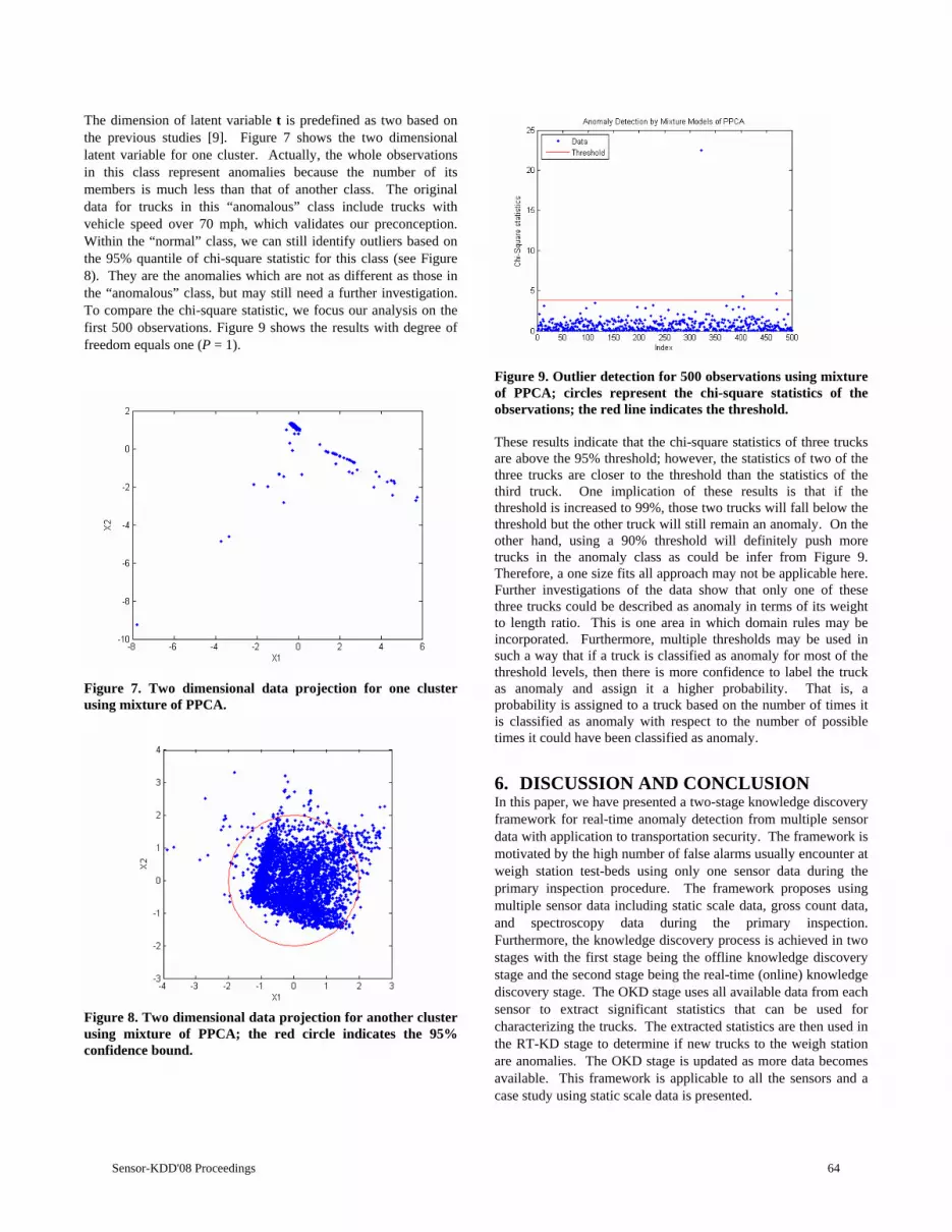
The dimension of latent variable t is predefined as two based on the previous studies [9]. Figure 7 shows the two dimensional latent variable for one cluster. Actually, the whole observations in this class represent anomalies because the number of its members is much less than that of another class. The original data for trucks in this “anomalous” class include trucks with vehicle speed over 70 mph, which validates our preconception. Within the “normal” class, we can still identify outliers based on the 95% quantile of chi-square statistic for this class (see Figure 8). They are the anomalies which are not as different as those in the “anomalous” class, but may still need a further investigation. To compare the chi-square statistic, we focus our analysis on the first 500 observations. Figure 9 shows the results with degree of freedom equals one (P = 1).

Figure 7. Two dimensional data projection for one cluster using mixture of PPCA.

Figure 8. Two dimensional data projection for another cluster using mixture of PPCA; the red circle indicates the 95% confidence bound.

Figure 9. Outlier detection for 500 observations using mixture of PPCA; circles represent the chi-square statistics of the observations; the red line indicates the threshold. These results indicate that the chi-square statistics of three trucks are above the 95% threshold; however, the statistics of two of the three trucks are closer to the threshold than the statistics of the third truck. One implication of these results is that if the threshold is increased to 99%, those two trucks will fall below the threshold but the other truck will still remain an anomaly. On the other hand, using a 90% threshold will definitely push more trucks in the anomaly class as could be infer from Figure 9. Therefore, a one size fits all approach may not be applicable here. Further investigations of the data show that only one of these three trucks could be described as anomaly in terms of its weight to length ratio. This is one area in which domain rules may be incorporated. Furthermore, multiple thresholds may be used in such a way that if a truck is classified as anomaly for most of the threshold levels, then there is more confidence to label the truck as anomaly and assign it a higher probability. That is, a probability is assigned to a truck based on the number of times it is classified as anomaly with respect to the number of possible times it could have been classified as anomaly.

6. DISCUSSION AND CONCLUSION In this paper, we have presented a two-stage knowledge discovery framework for real-time anomaly detection from multiple sensor data with application to transportation security. The framework is motivated by the high number of false alarms usually encounter at weigh station test-beds using only one sensor data during the primary inspection procedure. The framework proposes using multiple sensor data including static scale data, gross count data, and spectroscopy data during the primary inspection. Furthermore, the knowledge discovery process is achieved in two stages with the first stage being the offline knowledge discovery stage and the second stage being the real-time (online) knowledge discovery stage. The OKD stage uses all available data from each sensor to extract significant statistics that can be used for characterizing the trucks. The extracted statistics are then used in the RT-KD stage to determine if new trucks to the weigh station are anomalies. The OKD stage is updated as more data becomes available. This framework is applicable to all the sensors and a case study using static scale data is presented.


We also presented an anomaly detection approach for static scale data. The approach was tested with simulated and benchmark data; it was found to detect anomalies using limited information. Our approach also shows that the computation of mixture model of PPCA is quite efficient. Moreover, the use of EM algorithm provides a straightforward extension to the real-time computation setting. The approach also consistently identified trucks with anomalous features in all scenarios investigated.

7. ACKNOWLEDGMENT This research was funded by the Laboratory Directed Research and Development (LDRD) Program of the Oak Ridge National Laboratory (ORNL), managed by UT-Battelle, LLC, for the U.S. Department of Energy under Contract DE-AC05-00OR22725. We would like to gratefully acknowledge synergistic research activities by the SensorNet® Program managed by the Computational Sciences and Engineering Division of the Oak Ridge National Laboratory. We specifically thank the following people in the SensorNet® group: Frank DeNap, David Hill, David Feaker, Randy Walker, and Steven Saavedra. We also thank Dr. Brian Worley for his contributions to the Transportation Corridor research. We are grateful to the following scientists from ORNL who have reviewed this manuscript, either formally or informally: Mallikarjun (Arjun) Shankar, Raju Vatsavai, Randy Walker, Cy Smith, Bryan Gorman and Frank DeNap. This manuscript has been authored by UT-Battelle, LLC, under contract DE-AC05-00OR22725 with the U.S. Department of Energy. The United States Government retains, and the publisher by accepting the article for publication, acknowledges that the United States Government retains, a non-exclusive, paid-up, irrevocable, world-wide license to publish or reproduce the published form of this manuscript, or allow others to do so, for United States Government purposes.

8. REFERENCES [1] Kouzes, R.T., Ely, J.H., Geelhood, B.D., Hansen, R.R.,

Lepel, E.A., Schweppe, J.E., Siciliano, E.R., Strom, D.J., and Warner, R.A. (2003). Naturally occurring radioactive materials and medical isotopes at border crossings, IEEE Nuclear Science Symposium Conference Record, vol. 2, pp. 1448-1452.

[2] Ely, J.H., Kouzes, R.T., Geelhood, B.D., Schweppe, J.E., and Warner, R.A. (2004). Discrimination of naturally occurring radioactive material in plastic scintillator materials, IEEE Transactions on Nuclear Science, vol. 51, no. 4, pp. 1672-1676.

[3] Olufemi A. Omitaomu, Auroop R. Ganguly, Bruce W. Patton, and Vladimir A. Protopopescu (in revision). Anomaly Detection in Radiation Sensor Data with Application to Transportation Security. IEEE Transactions on Intelligent Transportation Systems.

[4] Olufemi A. Omitaomu, Auroop R. Ganguly, and Vladimir A. Protopopescu (in review). Empirical Mode Decomposition Approach for Denoising Signals. IEEE Transactions on Systems, Man, and Cybernetics: Part C.

[5] Auroop R. Ganguly, Olufemi A. Omitaomu, and Randy M. Walker (2007). Knowledge Discovery from Sensor Data for Security Applications. In J. Gama and M. Gaber (Eds.), Learning from Data Stream - Processing Techniques in Sensor Networks, 187-204. Springer, NY.

[6] Viswanathan, R. and Varshney, P.K. (1997). Distributed detection with multiple sensors: Part 1 – Fundamentals. Proceedings of the IEEE, 85, 1, 54 – 63.

[7] Provost, F. and Kolluri, V. (1999). A survey of methods for scaling up inductive algorithms. Data Mining and Knowledge Discovery, 3, 131 – 169.

[8] Ye, N. and Chen, Q. (2001). An anomaly detection technique based on a chi-square statistic for detecting intrusions into information systems, Quality and Reliability Engineering International, 17:105 – 112.

[9] Agovic, A., Banerjee, A., Ganguly, A.R., and Protopopescu, V.A. (2008). Anomaly Detection in Transportation Corridors Using Manifold Embedding. In A.R. Ganguly, J. Gama, O.A. Omitaomu, M. Gaber, and R.R. Vatsavai (Eds.), Knowledge Discovery from Sensor Data, CRC Press, (To appear).

[10] Everitt, B.S. (1984). An Introduction to Latent Variable Models, London: Chapman & Hall.

[11] Roweis, S. and Ghahramani, Z. (1999). A unifying review of linear Gaussian models, Neural Computaion, 11(2), 305 - 345.

[12] Tipping, M. E., and Bishop, C. M. (1999a). Probabilistic principal component analysis, Journal of the Royal Statistical Society B, 61, 611–622.

[13] Dempster, A., Laird, N. and Rubin, D. (1977). Maximum likelihood from incomplete data via the EM algorithm, Journal of the Royal Statistical Society, Series B, 39(1), 1-38.

[14] Tipping, M. E., and Bishop, C. M. (1999b). Mixtures of probabilistic principal component analyzers, Neural Computation, 11, 443–482.

[15] Naes, T. (1985). Multivariate calibration when the error covariance matrix is structured, Technometrics, 27, 301–311.

[16] Hubert, M., Rousseeuw, P., Verboven, S. (2002). A fast method for robust principal components with applications to chemometrics, Chemometrics and Intelligent Laboratory Systems, 60, 101–111.

9. APPENDIX The Expectation (E) step leads to the sufficient statistics which are needed to update the parameters in the M (Maximization) step. The expectations are given by:

( ) ( )12 T Tij j j j j i jσ

−= + −t I W W W x μ (9)

and

( ) 12 2 TT Tij ij j j j j ij ijσ σ

−= + +t t I W W t t (10)

Then, in the M-step, the parameters are updated by the following equations respectively:


1

1 N

j iji

RN

λ−

= ∑ (11)

( )

1

1

N

ij i j iji

j N

iji

R

R

=

=

−=∑

∑

x W tμ (12)

( )1

1 1

N NT T

j ij i j ij ij ij iji i

R R−

= =

⎡ ⎤ ⎡ ⎤= −⎢ ⎥ ⎢ ⎥⎣ ⎦ ⎣ ⎦∑ ∑W x μ t t t (13)

( )2

1

1j N

iji

QM R

σ

=

=

∑ (14)

and

( )

2

1

1

1

2

N

ij i ji

NT T

ij ij j i ji

NT T

ij ij ij j ji

R

Q R

R tr

=

=

=

⎧ ⎫− −⎪ ⎪

⎪ ⎪⎪ ⎪

= − +⎨ ⎬⎪ ⎪⎪ ⎪

⎡ ⎤⎪ ⎪⎣ ⎦⎩ ⎭

∑

∑

∑

x μ

t W x μ

t t W W

(15)

where ijR is the posterior of mixture j for producing the

observation ix and is updated at the beginning of the E step.

This EM algorithm is the same as that for a standard Gaussian mixture and similar to that of a single PPCA, except having ijR

as the local weighted term.


Network Service Disruption upon Natural Disaster:Inference Using Sensory Measurements and Human Inputs

Supaporn ErjongmaneeGeorgia Institute of Technology

Atlanta, GA [email protected]

Chuanyi JiGeorgia Institute of Technology

Atlanta, GA [email protected]

ABSTRACTNatural disasters cause large-scale network service interrup-tion which corresponds to unreachability of networks. Thisproblem relates to how networks respond under extreme con-ditions, and it is neither well-studied nor well-understood.To infer network service disruption, challenges arise, i.e.,how to use heterogeneous data that include sensory mea-surements and human inputs?

This work shows an important role of data mining and ma-chine learning in inferring large-scale network service dis-ruption upon Hurricane Katrina. We present a joint useof large-scale sensory measurements from Internet and asmall number of human inputs for effective network infer-ence. Specifically, data mining includes (a) unsupervisedlearning, i.e., clustering and feature extraction of sensorymeasurements and (b) semi-supervised learning of both sen-sory measurements and human inputs.

The approaches are evaluated on network service disruptioninduced by Hurricane Katrina at subnet level. Our resultshows that clustering reduces the spatial dimensionality by81%, and sensory measurements are temporally extracteddown to two features. The subnet statuses inferred by theclassifier derived from semi-supervised learning show inter-esting facts of network resilience and provide the spatial andthe temporal maps of network service disruption that can beused to assist disaster response and recovery.

To our understanding, this is the first work of data min-ing and machine learning using sensory measurements andhuman inputs for inference of large-scale network service dis-ruption upon a large-scale natural disaster.

Categories and Subject DescriptorsJ.2.8 [Computer Applications]: Internet Applications;H.2.8 [Database Management]: Database Application—data mining, feature extraction

1. INTRODUCTIONInternet is composed of a large number of heterogeneoussub-networks (subnets). Subnets can become unreachableafter the occurrence of natural disasters, resulting in large-scale network service disruption. To provide the reliabilityand the reachability of networks, measurements of subnetsare collected for performance and service monitoring. In ageneral setting, devices that perform data collection, e.g.,border routers, can be regarded as “sensors,” and measure-ments collected can be considered as sensory measurements.

Besides sensory measurements, this work introduces a noveluse of human inputs to aid the inference of network ser-vice disruption. Human inputs correspond to human re-ports on network outages. While sensory measurements canbe plenty, human inputs are generally available in a smallnumber. This work shows how to apply data mining and ma-chine learning to sensory measurements and human inputsto perform knowledge discovery of network service disrup-tion upon natural disasters.

1.1 Challenges and ContributionAs analytical models of network services are unavailable,sensory measurements are imperative for inferring servicedisruption. However, several challenges arise and hinder theadvance of this inference application.

The first challenge is that sensory measurements are large-scale. A monitored network generally consists of thousandsof subnets, resulting in measurements of a high spatial di-mension. For example, in this work, we consider 1009 time-series sensory measurements from 1009 subnets.

Another challenge is complex temporal patterns in sensorymeasurements. Networks exhibit unknown transient behav-iors in response to a disaster, and the corresponding mea-surements generally have bursty temporal characteristics thatare complex for inference.

The third challenge is the heterogeneity of data. In additionto sensory measurements, human inputs provide a distincttype of data. A human input is a “network-911-call” thata disaster responder makes to report network outages. Ingeneral, a report is made at a particular time instance butaftermath and delayed. Human inputs are usually availablein a small number of subnets. The other data in this workare geographic locations and network addresses of subnets.


The current state of art in inferring service disruption reliessolely on sensory measurements. Human inputs, althoughavailable, have been excluded from inference. An open issueis how to jointly use a large number of sensory measurementsand a small number of human inputs for more effective in-ference of large-scale service disruption.

This work uses offline sensory measurements and human in-puts from a large-scale natural disaster, i.e., Hurricane Kat-rina. We first provide a problem formulation in the contextof machine learning. We then apply unsupervised learn-ing, i.e., clustering and feature extraction to unlabeled datathat are time-series sensory measurements. This reducesthe spatial dimension of time-series by more than 80% andthe temporal dimension down to two features. After that,semi-supervised learning is performed by combining humaninputs with unlabeled data for inference. Because human in-puts are delayed and thus not in a usable form of labels, weshow how human inputs are converted into labeled data byindexing the unreachability pattern in time-series measure-ments. We then apply semi-supervised learning algorithm toboth labeled and unlabeled data to infer service disruption.

The main contributions of this work lie into two aspects.First is the application of data mining and machine learningto a novel networking problem, i.e., inference of large-scalenetwork service disruption upon a natural disaster. Secondis the demonstration of the need and the effectiveness oflearning from both heterogeneous sensory- and human-data.

The paper is organized as followed. The rest of Section1 presents background and heterogeneous data. Section 2provides problem formulation. Sections 3 and 4 respectivelyshow the use of unsupervised and semi-supervised learningto sensory measurements and human inputs. Results arepresented in Section 5. Section 6 discusses related works,and Section 7 concludes the paper.

1.2 Hurricane KatrinaHurricane Katrina was the most severe hurricane that floodedLouisiana, Mississippi, and Alabama in 2005 and causedlarge-scale disruption in telecommunication networks. Net-work connectivity was critical but either unavailable or un-stable experienced by disaster responders [1, 2]. There werea few public reports that showed the disaster impact to com-munications at Internet scale [3, 4] but there has not beenany study on detailed service disruption at subnet level.

1.3 Network MonitoringNetwork service disruption can be characterized as unreach-ability of subnets. This service disruption has been studiedfor day-to-day network operations [5] or by using simulationto infer large-scale network failures [6]. But the questionsarise pertaining to service disruption caused by a real large-scale natural disaster. How to remotely infer unreachablesubnets? What measurements can be used?

Sensory measurements from Internet routing infrastructurecan be used for remote monitoring and service disruption in-ference [7, 8]. Internet consists of interconnected autonomoussystems (AS), and the routing protocol among ASes is theBorder Gateway Protocol (BGP) [9]. Each AS is served byat least one Internet service provider (ISP) and is composed

B D

A C

F

E

G

p

S.A

S.B

S.C

S.F

S.G

S.D

S.E

q

Figure 1: Example of AS network.

0 1 2 3 4 5 6 7 8 9 10111213141516171819202122232425262728293031323334

−1

0

1

Time (day)

BG

P−

upda

te a

rriv

als

Figure 2: Example of time-series sensory measure-

ments. (1 = BGP announcement, -1 = BGP with-

drawal)

of one or several subnets identified by prefixes (network ad-dresses)1. In order to route traffic from one AS to a spe-cific subnet, a BGP router at each AS collects streams ofrouting messages from peering BGP routers of its neighborASes. These messages are called BGP update messages andare regarded as raw Internet sensory measurements in thiswork. Figure 1 shows the example of AS network whereX is an AS, S.X is the BGP router of AS X, and X ∈

{A,B,...,G}. AS E has two prefixes p and q. It also showsthat the BGP router S.C collects Internet sensory measure-ments from peering BGP routers S.A, S.D, and S.E.

There are two types of BGP update messages: BGP with-drawal and BGP announcement. When a subnet becomesunreachable, all BGP routers that can no longer route In-ternet traffic to this subnet send BGP withdrawals to no-tify all of their peering routers the unreachability. When asubnet becomes reachable again, there would be new BGPannouncements for this subnet. Note that besides networkservice disruption, multiple withdrawals followed by new an-nouncements can also be caused by other network events,e.g., a change of routes or routing policies. Hence, a burst

1We shall use subnet and prefix interchangeably.


of multiple withdrawals followed by new announcements isa symptom rather than a one-to-one mapping of networkservice interruption [7, 8].

BGP update messages in this work are collected and storedby Oregon Route Views [10] and are publicly-available. In2005, Oregon Route Views had about 35 geographically-distributed peering BGP routers. Oregon Route Views pro-vides about 96 files of BGP update messages available perday, and the size of each file is approximately 8 megabytes.

1.4 Large-Scale and Heterogeneous DataWe obtain the real sensory measurements and the real hu-man inputs from Hurricane Katrina. In particular, we choosesensory measurements to be BGP update messages that canprovide remote monitoring of service disruption when localmeasurements are not directly available due to the evacua-tion and the limited accessibility to the disaster area.

Geographic locations are pertinent for selecting subnets inthe disaster area to study. We identify geographic locationsof subnets from Whois database [11] and select 1009 subnetsfrom 48 ASes in the disaster area. This results in 1009 time-series sensory measurements, one per subnet. Figure 2 showsan example of time-series sensory measurements.

We choose our study duration as the Katrina interval to bebetween August 28 and September 4, 2005. Note that themandatory evacuation was announced on August 28, 2005,one day prior to the Katrina landfall (August 29, 2005, 6:00a.m., Central Daylight Time (CDT)), and most of networkdamage assessment, reported by our collaborating ISP, oc-curred within the first week after the landfall. In addition,we also select BGP update messages belong to the samesubnets but between August 1-28, 2005 for comparison; thisstudy period is called the pre-Katrina interval.

With 1009 subnets and eight-day duration, our sensory mea-surements are both spatially and temporally large-scale. Asa burst of BGP messages is a symptom rather than a one-to-one mapping of service disruption, sensory measurementsalone are insufficient to infer unreachability of all subnets.

Human inputs are reports of “this network is down”. Wecollect total 37 human inputs from two sources. The first28 human inputs are from the online message on NANOGmailing list posted by Todd Underwood from Renesys Cor-poration [4]. The other nine human inputs are network out-age reports from customers of our collaborating ISP. Humaninputs provide valuable and mostly accurate information onnetwork outage status but can be delayed from the exacttime that outage occurs. Thirty-seven human inputs areunlikely sufficient for inferring statuses for the other nearly1000 subnets. Hence, sensory measurements and human in-puts complement each other in inference of service disrup-tion.

2. PROBLEM FORMULATIONConsider an underlying network with n nodes, where a nodecorresponds to a subnet. Let Zi(t) be a binary state of nodei, Zi(t) = 1 if node i is outage (unreachable); Zi(t) = −1if node i is normal (reachable); 1 ≤ i ≤ n, and t∈[0, T ]is a time duration of interest. The state of a network is

a collection of all n states, Z(t) = {Zi(t)}n

i=1, t ∈ [0, T ],and considered to be unknown. For our case, n = 1009,and T = 8 days (August 28-September 4, 2005). Servicedisruption is defined to be the same as unreachability of anindividual subnet2.

Let X(t) ∈ Rn be an n-dimensional random vector thatcan be viewed as “response variables” corresponding to anunderlying state Z(t). Intuitively, X(t) shows symptoms ofZ(t) and is related to both outage and normal states. Aset D of m samples is assumed to be available on X(t) andconstitutes indirect observations on Z(t). Hence, D is calledunlabeled measurements. From Section 1.4, D correspondsto sensory measurements. In general, D is large-scale andinsufficient for determining an underlying network state Z(t)unless D is empowered by discriminative information.

Human inputs provide discriminative information. A set ofk human inputs are assumed to be available for a fractionof nodes, i.e., 0 ≤ k ≤ n. The simplest form of a humaninput is a symbol that takes binary values, 1 and -1, at time

t′

. Let t′

be the time that human reports the unreachabilityand t be the exact time that a network becomes unreachable.Generally, it is assumed that human reports unreachabilityof a subnet correctly3, but a report can be delayed, i.e.,

t′

> t. Thus, a human input can be regarded as a directbut delayed observation on one specific nodal state Zi(t).A set of k human inputs is Dl, where k can be small, i.e.,0 ≤ k ≪ m. In this work, we use 24 human inputs (65%) tobe training data and the other 13 for validation. Hence, forour case, k = 24, m = n − k = 985.

Problem: Given a set of unlabeled sensory measurements,D, and a set of human inputs, Dl, how to infer Z(t) fort ∈ [0, T ]?

This is an inference problem where dichotomies between out-age and normal states of subnets can be learned from sensorymeasurements and human inputs. Hence, we resort to datamining and machine learning approaches outlined below.

• We apply unsupervised learning algorithms that areclustering and feature extraction. Clustering is usedto reduce the spatial dimension of time-series sensorymeasurements. We then extract the temporal featuresfrom time-series measurements to a fewer observationsin a low-dimensional feature space and use these fea-tures as unlabeled data.

• We apply semi-supervised learning algorithm. We firstconvert human inputs to human labels by assigningdichotomies to a small number of the temporal featuresin the low-dimensional feature space. After that, alarge set of unlabeled data and a small set of labeleddata are combined to infer the statuses of subnets.

• We provide an initial understanding of network ser-vice disruption upon Hurricane Katrina and discuss

2We shall use unreachability, outage, and service disruptioninterchangeably.3Note that this is a natural assumption as human only re-ports when a network is outage.


Table 1: List of prefix subsets with (a) Geographic

location (LA = Louisiana, MS = Mississippi, AL =

Alabama) (b) Number of prefixes, and (c) Reduction

percentage

Set 1 2 3 4 5 6 7(a) LA LA LA LA LA MS AL(b) 166 53 49 115 180 232 214(c) 84.3 56.6 67.4 81.8 76.7 81.5 90.7

Table 2: Example of geographic location and time-

series pattern belong to two subnets in the same

cluster.

Sub Geographic Initial t where Durationnet Location r(t) = −1 of r(t) = −11 Hammond, LA 8/30 18:53:42 2 hrs 53 mins

9/3 23:39:09 17 mins9/4 00:25:10 10 mins

2 Hammond, LA 8/30 18:53:42 2 hrs 53 mins9/3 23:39:09 17 mins9/4 00:10:24 10 mins9/4 00:25:10 10 mins

the further use of the results and the applications infuture network study.

3. UNSUPERVISED LEARNINGWe now perform unsupervised learning to extract featuresfrom 1009 time-series sensory measurements belong to ourselected 1009 subnets. The first step is to cluster these time-series to reduce the spatial dimension. The second step is toextract temporal features from patterns in the time-series.

3.1 Spatial ClusteringFeatures can be extracted directly from time-series measure-ments of each individual subnet. However, 1009 subnets arelarge-scale, and subnets may have experienced correlatedservice disruption caused by the same disaster. Therefore,we first reduce the spatial dimension of time-series measure-ments by grouping similar time-series into clusters.

To measure the similarity of time-series from different sub-nets, we change the discrete time-series of BGP update mes-sages for a subnet i to be the continuous waveform ri(t) suchthat: when BGP announcement arrives at time t, ri(t) = 1;otherwise, for BGP withdrawal, ri(t) = −1. Consider timet, suppose two consecutive BGP updates arrive at time t1and t2, ri(t) = ri(t1) for t1 ≤ t < t2. For a subnet i withoutBGP update arrival, ri(t) = 1 for all t ∈ [0, T ].

The similarity between ri(t) and rj(t) of subnet i and subnetj is measured by the average distance d(ri(t), rj(t)), where

d(ri(t), rj(t)) = 1T

R T

t=0|ri(t) − rj(t)|dt for 1 ≤ i, j ≤ n. The

set of similarity measures, L = {d(ri(t), rj(t))}, where 1 ≤

i, j ≤ n, is used as the input for clustering.

We choose the average-linkage hierarchical clustering algo-

100

101

102

103

0

0.05

0.1

0.15

0.2

Inter−arrival time (second)

Pro

b (in

ter−

arriv

al ti

me)

inter−arrival time30 minutes

Figure 3: Empirical distribution of BGP withdrawal

inter-arrival time.

rithm since a number of clusters does not need to be pre-chosen. After clustering, we further post-process to obtaina fewer clusters by merging any two clusters if the similaritybetween them is smaller than a parameter T . The rangeof T values is varied and tested using the Davies-Bouldinindex [12] to determine cluster compactness. The suggested

values of T are between 45-90 minutes. This can also beinterpreted such that two time-series are merged into thesame cluster if their similarity measure is smaller than T .

Clustering spatially reduces 1009 time-series to 191 clusters,resulting in 81% reduction. Although, the simple hierar-chical clustering algorithm gives the reasonably good per-formance, other advanced clustering algorithms can be ap-plied to handle measurements with small similarity mea-sures. The reduction percentages are also obtained for smallerprefix sets by separating 1009 prefixes into seven subsetsbased on the customers of seven local ISPs in the disasterarea, and the reduction percentage of each subset is shownin Table 1. In details, each cluster contains the prefixesthat have a correlation coefficient of ri(t)’s between 0.9986-1.000. Table 2 shows the example of two subnets from thesame cluster. This shows that subnets from the same clus-ter have a highly similar pattern of BGP updates, and thegeographic locations belong to these subnets are similar.

3.2 Temporal Feature ExtractionBecause the resulting clusters have correlation coefficient al-most one, we randomly choose one representative prefix percluster and use this much smaller set of 191 representativeprefixes to extract temporal features of time-series.

As described in Section 1.3, a burst of multiple BGP with-drawals followed by new BGP announcements is a symptomof network service disruption. Thus, there are two featuresof this symptom. The first is a burst of withdrawals. Aburst characterizes a number of withdrawal messages thatpeering BGP routers send in a given time-duration. Thesecond is the length of an unreachable duration between thelast withdrawal of a burst and the new announcements af-ter a burst. This duration can be used to infer whether asubnet is unreachable upon a disaster or not. Thus, a burst


0 0.5 1 1.50

1

2

3

4

5

S

Tfa

il (m

inut

e)x104

(a) Unlabeled data

0 0.5 1 1.50

1

2

3

4

5

S

Tfa

il (m

inut

e)

x104

Normal labelOutage label

(b) Labeled data

Figure 4: S and Tfail of unlabeled and labeled data.

of withdrawals followed by new announcements and a suc-ceeding unreachable duration form a BGP-burst pattern.

The inference of network events from a BGP-burst patternhas been studied for day-to-day network operations [8]. Forinstance, a BGP-burst pattern with a short unreachable du-ration can be caused by a temporary service disruption, i.e.,a change of routes or routing policies, and a prefix becomesreachable soon after. However, a BGP-burst pattern with along unreachable duration is mostly caused by major servicedisruption. But questions arise: how many withdrawals areconsidered to be a burst, and how long is an unreachableduration of service disruption upon a large-scale disaster?Hence, we formally define features corresponding to a BGP-burst pattern.

Definition: Burst ratio S and unreachable duration Tfail

Let v be a time-duration in which a burst of BGP with-drawals is characterized. Let nv be a number of accumula-tive BGP withdrawals belong to a subnet that peering BGProuters send within v time-duration, and np be a number ofpeering BGP routers that could reach this subnet prior tothe Katrina interval. Note that a peering BGP router cansend more than one BGP withdrawal after a disruption.

The burst ratio is defined as S = nv

np, and S measures per-

centage of BGP withdrawals from peering BGP routers. Theunreachable duration Tfail is defined as the time period be-tween the last BGP withdrawal of a burst in v-duration andthe first new BGP announcement after a burst. Therefore,S is the spatial variable indicating how many peering BGProuters fail to reach a subnet. Tfail is the temporal variablethat characterizes an unreachable duration.

The parameter v is a time window such that if the inter-arrival time between two BGP withdrawals is larger than v

minutes, these two withdrawals are not considered to be inthe same burst. It is reported that, in day-to-day networkoperations, a burst generally lasts for 3 minutes [13] butcan be up to 15 minutes [14]. However, there was no priorresult on a burst caused by natural disasters. We derivethe empirical distribution of BGP withdrawal inter-arrivaltime after Katrina as shown in Figure 3. We select v =30 minutes that is large enough not to partition a burst.However, such a large v, a time window may include morethan one burst. This shows a disadvantage of using a fixed-size time window to locate a burst. To be more precise inlocating a burst, instead of monitoring only a number ofBGP withdrawals, we can explicitly examine the content ofevery BGP withdrawal to check subnet reachabilities.

3.3 Feature StatisticsStatistics of S and Tfail belong to time-series measurementsare collected from the Katrina interval, and the result isshown in Figures 4(a). We also collect S and Tfail statisticsfrom the pre-Katrina interval and find that there are less fea-tures with large Tfail values in the pre-Katrina than in theKatrina interval. This lack of large Tfail in the pre-Katrinainterval results in the difficulty to determine the appropriateunreachable duration of Katrina service disruption. Section4 shows how to use human inputs to derive the threshold todetermine the suitable duration of this service disruption.

4. SEMI-SUPERVISED LEARNINGWe extract 217 (S, Tfail) features from time-series measure-ments belong to 191 representative subnets; these featurescan be used as unlabeled data. Note that subnets can havemore than one (S,Tfail) feature while some subnets do nothave (S, Tfail) features at all. However, can we use delayedhuman inputs to identify a BGP-burst pattern and to obtainlabeled (S, Tfail) features? If so, sensory measurements andhuman inputs can be jointly used to infer service disruption.


12

34

56

78

910

1112

1314

15 0 0.2 0.4 0.6 0.8 1 1.2 1.4

0

0.05

0.1

ST

fail (minute)

Figure 5: Empirical probability distribution of S and

Tfail from the pre-Katrina interval.

4.1 Labeling Human InputsAs a human input can be delayed, there can be more thanone network service disruption and thus more than one BGP-burst pattern in the time-series measurements of this humaninput prior to the time of the human report. This showsthat converting a delayed human report to a human labelcan be a complex process such that which BGP-burst pat-tern, if there is more than one, exactly corresponds to aservice disruption that human reports. This work selects,for simplicity, the BGP-burst pattern immediately preced-ing a human report4. With 24 human inputs, we have 24(S, Tfail) features that are labeled with “1” (outage).

To classify subnets into two dichotomies, outage and normal,we obtain (S, Tfail) features labeled as “-1” (normal) by us-ing the pre-Katrina statistics. The assumption is made suchthat the majority of (S,Tfail) features in the pre-Katrinainterval are normal. Figure 5 shows the empirical proba-bility distribution of S and Tfail from the pre-Katrina in-terval. Small values, S < 0.1 and Tfail < 3 minutes, oc-curred with a large probability. This means that only asmall (10%) percentage of peering BGP routers send outBGP withdrawals pertaining to a prefix while the rest ofpeering BGP routers can still reach this prefix. Moreover,with small Tfail, this can be interpreted that a prefix quicklybecomes reachable after a BGP burst. Hence, prefixes withS < 0.1 and Tfail < 3 minutes are considered to be reach-able. We extract 460 features of such values and then labelthese features as normal. Figure 4(b) shows (S, Tfail) fea-tures labeled as normal and outage.

In summary, we have 217 unlabeled features, {(Si, Tfaili)}217i=1,

24 features labeled as outage {(Si, Tfaili), 1}24

i=1, 460 fea-

tures labeled as normal, {(Si, Tfaili),−1}460

i=1.

4.2 Learning Labeled and Unlabeled DataLabeled and unlabeled data have been jointly used and stud-ied in prior works as semi-supervised learning. Prior workshowed that learning with a small number of labeled data

4That is, humans are prompt in reporting a network outage.

along with unlabeled data can reduce classification errorfrom using only unlabeled data [15]. There are three ma-jor algorithms used in semi-supervised learning (see [16] andreferences in there), i.e., the generative models, the trans-ductive support vector machine, and the graph-based meth-ods. The generative models and the graph-based methodsrequire probabilistic models. Thus, these two algorithms areinfeasible because the human inputs we obtained are too fewto estimate prior probability of outages accurately. Hence,we use the transductive support vector machine (TSVM) byJoachims [17] that only relies on labeled and unlabeled data.

Our goal is to train the (S, Tfail) classifier to determinewhether prefixes are unreachable or not. To avoid over-fitting, we choose the simple semi-supervised learning thatapplies TSVM to S and to Tfail separately. The result-ing two one-dimensional linear classifiers (one for S and theother for Tfail) are used together as the two-dimensionalclassifier to infer the statuses of subnets.

Let xi be labeled data and x∗

j be unlabeled data where 1 ≤

i ≤ k, and 1 ≤ j ≤ m, xi or x∗

j is a generic variable in thealgorithm that corresponds to either S or Tfail. Let yi bethe class label for xi that is assigned as in Section 4.1, y∗

j bean unknown class label for x∗

j that is to be assigned by theclassifier, and yi, y∗

j ∈ {1,−1}. Let ξi be the so-called slackvariable of xi and ξ∗j be the slack variable of x∗

j . The use ofslack variables allows misclassified samples (see [18]).

Let w be the weight and b be the bias of a linear classifierto be obtained from minimizing

||w||2

2+ C

kX

i=1

ξi + C∗

−

X

j:y∗

j=−1

ξ∗j + C∗

+

X

j:y∗

j=+1

ξ∗j (1)

subject to

yi(w·xi + b) ≥ 1 − ξi, (2)

y∗

j (w·x∗

j + b) ≥ 1 − ξ∗j , (3)

ξi ≥ 0, ξ∗j ≥ 0 (4)

where 2||w||

is the margin width of the classifier wherePk

i=1 ξi

andPm

j=1 ξ∗j are bounds of classification error. C, C∗

− and

C∗

+ are tradeoff parameters between the margin width andthe classification error (see [17] for details).

The outputs of the algorithm are w and b; −b

wis a threshold

for either S or Tfail to determine the class labels, {y∗

j }m

j=1.

4.3 Experimental Setting and ValidationAs unlabeled data is abundant, we separate the unlabeledfeatures into 10 different subsets. Hence, 10 different classi-fiers are trained, and each training uses one separated sub-set of 21 (or 22) unlabeled features, all 24 features labeledas outage, and one subset of 30 randomly-chosen featureslabeled as normal. Other parameters used in the TSVM al-gorithm are initialized such that C = 0.1, C∗ = 0.1, andnum+ = 0.5 (these parameters are related to convergenceof the TSVM algorithm, and see [17] for details on a choiceof parameters).

Let S∗ and T ∗

fail be the thresholds such that if any prefixhas features S > S∗ and Tfail > T ∗

fail, this prefix is inferred


0 0.5 1 1.50

200

400

600

800

1000

1200

B

A

S

Tfa

il (m

inut

e)

Inferred NormalInferred Unreachable

Figure 6: Scatter plot of inferred S and Tfail. (Solid

vertical line: S = S∗, Solid horizontal line: Tfail =

T ∗

fail.) Plot only shows values of Tfail up to 1200

minutes.

as unreachable upon Katrina. Ten thresholds of S resultingfrom training 10 different classifiers are averaged to yield S∗.We follow the same process to find the value of T ∗

fail. Thisresults in S∗ = 0.6153 and T ∗

fail = 1 hour 38 minutes.

We use the rest of 13 human inputs for validation. Theresult shows that the features belong to these 13 human in-puts have S > S∗ and Tfail > T ∗

fail and thus are inferredas unreachable. The inferred unreachable statuses of thesehuman inputs are consistent to the reports that these sub-nets were outages. Hence, the values of S∗ and T ∗

fail to inferunreachable prefixes are valid.

5. INFERRED SERVICE DISRUPTIONThe thresholds learned are now used to infer service disrup-tion caused by Katrina for the other 985 subnets.

5.1 Statistics of Subnet StatusesThe decision boundaries, S = S∗ and Tfail = T ∗

fail, partitionthe feature space into two main regions shown in Figure 6:

• Outage region where S>S∗ and Tfail>T ∗

fail (upperright region in Figure 6). This region contains S andTfail belong to the inferred unreachable subnets.

• Normal region that has either S≤S∗ or Tfail≤T ∗

fail.This region contains S and Tfail belong to the inferredreachable subnets.

In normal region, there are two sub-regions marked as re-gions A and B in Figure 6. These two sub-regions containthe features that are inferred as normal but show the in-teresting characteristics of network resilience and responsesupon Hurricane Katrina.

Region A is located where S > S∗ and T≤T ∗

fail. The fea-tures in this region correspond to the prefixes that after Ka-

10 20 30 40 50 60 700

0.1

0.2

0.3

0.4

0.5

0.6

0.7

Tfail

(minute)

Pro

b(T

fail)

Pre−KatrinaKatrina

Figure 7: Empirical probability distributions of Tfail

from the pre-Katrina and the Katrina intervals.

trina, multiple peering BGP routers responded with burstyBGP withdrawals, but these prefixes only experienced briefTfail and resumed reachability soon after. The empiricalprobability distribution of Tfail, where Tfail≤T ∗

fail, presentedin Figure 7, shows that there are significantly more Tfail

with moderate values, 35-55 minutes, in the Katrina inter-val while Tfail of such values were scarce during the pre-Katrina interval5. This shows that Katrina caused networkto respond differently from day-to-day network operations.

Region B is located where S≤S∗. The features in this regioncorrespond to the prefixes that only a small number of peer-ing BGP routers responded to Katrina. Comparing among Sstatistics, we find that there are more S with values between[0.1, 0.5] in the Katrina than the pre-Katrina interval. Wealso study some corresponding prefixes and find that theseprefixes maintained the reachability statuses; hence, theremight have been parts of Internet that were not highly af-fected and responded to Katrina.

We quantify the percentages of prefixes in these four regionsas shown in Table 3. The results show that 25% of pre-fixes are inferred as outages, and there are 42% of prefixesfrom both regions A and B. With prefixes that maintainedreachabilities or responded with brief disruption duration,this provides the signs of network resilience and suggests themeaningful direction to investigate the prefixes in regions Aand B. This can result into an in-depth understanding ofnetwork resilience and responses upon a large-scale disaster.

5.2 Spatial-Temporal Damage MapsWe now obtain the spatial damage map presented in Fig-ure 8. The spatial map shows network service disruptionof different degree, based on the average disruption dura-tion of the inferred unreachable prefixes in each geographiclocation. The worst service disruption occurred at subnetsnear the coast of Louisiana. Nevertheless, our results show

5For both intervals, probabilities of Tfail >80 minutes andTfail < T ∗

fail are very small.


Figure 8: Impact degree of network service disrup-

tion. (N): Tfail<T ∗

fail, (H): T ∗

fail < Tfail < 24 hours,

and (D): Tfail≥ 24 hours.

Table 3: Percentages of prefixes in four regions.

Region Percentage of prefixesNormal 75Outage 25

A 12B 30

that not all subnets in the entire disaster area suffered fromservice disruption. This suggests that there were availablenetwork resources in the area that could have been utilizedif this information was shared among disaster responders.

We use Tfail to identify the initial time when service dis-ruption started and the duration of service disruption. Thisresults in the temporal map shown in Figure 9. The tem-poral map shows that 49.21% of service disruption occurredafter the landfall while only 5.12% occurred on August 28,2005 (the mandatory evacuation day). There were substan-tial service disruption (45.67%) occurred on August 29, 2005before the landfall, and this service disruption will be dis-cussed in a future study.

Communications are critical after disasters. The applica-tion of this work can be used in the future to infer networkservice disruption upon other disasters. The use of remotely-monitoring sensory measurements gives the advantage of theservice disruption inference when the disaster area is physi-cally inaccessible. Moreover, because ISPs do not generallydisclose information on unreachability of their service net-works, this application can be used to determine service dis-ruption across different ISPs. Furthermore, this applicationcan be further developed to use with online sensory measure-

8/29/05 8/30/05 8/31/05 9/1/050

5

10

15

20

25

30

The

dur

atio

n of

unr

each

abili

ty (

day)

The initial time of unreachability (CDT)

August 29, 2005, 6:00 a.m.

Figure 9: Initial and duration time of inferred net-

work service disruption upon Katrina. (“+” = an

inferred service disruption)

ments, and thus, it can infer service disruption in a timelyfashion to assist rescue and recovery effort after disasters.

6. RELATED WORKThere have been studies of BGP update messages related tothe widely affected network service disruption; the examplesof these studies are the September 11 attack in 2001 [19], andthe Code-Red and the Nimda worm attacks in 2003 [20].In [3], Cowie et al. presented that some disrupted networksafter Hurricane Katrina were not recovered after 10 dayshad passed. Among these studies, little has been done ondetailed study of service disruption at subnet level usingpublic available sensory measurements [3, 19]. Furthermore,human data has not been used in these prior works.

There have been studies of machine learning applicationsto BGP update messages. They were done either for day-to-day network operations or with different methods. Forexample, Andersen et al. applied the clustering algorithmto BGP update messages to infer a BGP topology [21] whileChang et al. temporally and spatially clustered ASPATHsto identify the cause of path changes [22]. Xu et al. proposedthe algorithm to infer significant BGP events by applying theprincipal component analysis (PCA) to BGP updates [8].

Semi-supervised learning has been widely studied [15, 16]and has been applied in many applications such as text clas-sification [17, 23], remote sensing [24], and image process-ing [25]. Nonetheless, semi-supervised learning has yet beenapplied in networking problem in previous studies.

7. CONCLUSIONThis work has introduced data mining and machine learningto a new networking application as inference of large-scalenetwork service disruption caused by Hurricane Katrina us-ing sensory measurements and human inputs.

We have found that data mining has played a vital role inlearning large-scale and complex sensory measurements intwo aspects. First is that clustering has reduced the spatial


dimension of sensory measurements by 81%, and feature ex-traction has reduced the temporal dimension down to twoinformative features. Second is that semi-supervised learn-ing makes use of a large number of sensory measurementsand a small number of human inputs to derive the classifierof network service disruption upon Katrina.

The results show that 25% of subnets are inferred as un-reachable. We also present the spatial and the temporaldamage maps that are practical values to disaster responseand recovery. A large fraction, i.e., 42% of prefixes are foundto be either maintained or briefly resumed reachability af-ter Katrina. This suggests the interesting directions for ob-taining a deeper understanding of network resilience andresponses under a large-scale disaster. These results wouldhave been difficult to obtain without data mining, and thisshows the usefulness of our approaches. Our application thatis based on publicly available sensory measurements can beused to remotely monitor and localize the reachable networkresources after large-scale disasters in the future.

This network application has presented challenges to theexisting data mining as well as networking approaches. Forexample, how to use data mining with a large and complexdata set in real time? How to in-depth study network re-silience in response to a large-scale disaster? These providesome of future directions for our study and motivate devel-opments of more advanced data mining applications.

8. ACKNOWLEDGEMENTSThe authors would like to thank Jere Stokely and NealeHightower for their technical help with data and comments,Cheng Guang, Derrick Dy and Phong Do for help with dataprocessing, Anwar Walid and Zesheng Chen for many helpfuldiscussions. This paper is supported by NSF SGER-Katrinaand ECS 0334759.

9. REFERENCES[1] U.S. House of Representatives. A Failure of Initiative:

Final Report of the Select Bipartisan Committee toInvestigate the Preparation for and Response toHurricane Katrina. Congressional Reports H. Rpt.109-377, Washington, D.C., 2005.

[2] K. J. Martin. Written Statement of Kevin J. Martin,Chairman Federal Communications Commission, at theHearing on Public Safety Communications from 9/11 toKatrina: Critical Public Policy Lessons, before theSubcommittee on Telecommunications and the Internet.U.S. House of Representatives, 2005.

[3] J. Cowie, A. Popescu, and T. Underwood. Impact ofHurricane Katrina on Internet Infrastructure. RenesysCorporation, 2005.

[4] T. Underwood. http://www.merit.edu/mail.archives/nanog/2005-08/msg00938.html.

[5] N. Feamster, et al. Measuring the Effects of InternetPath Faults on Reactive Routing. In Proceedings ofACM SIGMETRICS on Measurements and Modeling ofComputer, pages 126-137, 2003.

[6] A. Sahoo, K. Kant, and P. Mohapatra. Characterizationof BGP Recovery Time under Large-Scale Failures. InProceedings of IEEE International Conference onCommunications, pages 949-954, 2006.

[7] A. Feldmann, et al. Locating Internet RoutingInstabilities. ACM SIGCOMM ComputerCommunication Review, 3(4): 205-218, 2004.

[8] K. Xu, J. Chandrashekar, and Z.-L. Zhang. InferringMajor Events from BGP Update Streams. TechnicalReport 04-043, University of Minnesota, 2004.

[9] Y. Rekhter, T. Li, and S. Hares. Border GatewayProtocol 4 (RFC 1771).

[10] University of Oregon. Route Views Project.http://archive.routeviews.org.

[11] Whois Database. http://www.arin.net/whois.

[12] D. L. Davies and D. W. Bouldin. A Cluster SeparationMeasure. IEEE Transactions on Pattern Recognition andMachine Intelligence, 1(2): 224-227, 1979.

[13] C. Labovitz, G. R. Malan, and F. Jahanian. InternetRouting Instability. IEEE/ACM Transactions onNetworking, 6(5): 515-528, 1998.

[14] C. Labovitz, et al. Delayed Internet RoutingConvergence. IEEE/ACM Transactions on Networking,9(3): 293 - 306, 2001.

[15] V. Castelli and T. Cover. The Relative Value ofLabeled and Unlabeled Samples in Pattern Recognitionwith an Unknown Mixing Parameter. IEEE Transactionson Information Theory, 42(6): 2101-2117, 1996.

[16] O. Chapelle, B. Scholkopf, and A. Zien.Semi-Supervised Learning. MIT Press, 2006.

[17] T. Joachims. Transductive Inference for TextClassification using Support Vector Machines. InProceedings of International Conference on MachineLearning, pages 200-209, Bred, Slovenia, 1999.

[18] C. J. C. Burges. A Tutorial on Support VectorMachine for Pattern Recognition. Data Mining andKnowledge Discovery, 2(2): 121-167, 1998.

[19] Committee on the Internet under Crisis Conditions:Learning from September 11 National Research Council.The Internet under Crisis Conditions. The NationalAcademies Press, 2003.

[20] L. Wang, et al. Observation and Analysis of BGPBehavior under Stress. In Proceedings of ACMSIGCOMM on Internet Measurement Workshop, pages183-195, 2002.

[21] D. Andersen, et al.. Topology Inference from BGPRouting Dynamics. In Proceedings of ACM SIGCOMMInternet Measurement Workshop, pages 243-248,Marseille, France, 2002.

[22] D. F. Chang, R. Govindan, and J. Heidemann. TheTemporal and Topological Characteristics of BGP PathChanges. In Proceedings of IEEE InternationalConference on Network Protocols, pages 190-199, 2003.

[23] K. Nigam. Using Unlabeled Data to Improve TextClassification. Doctoral Thesis CMU-CS-01-126,Carnegie Mellon University, 2001.

[24] B. Shahshahani and D. Landgrebe. The Effect ofUnlabeled Samples in Reducing the Small Sample SizeProblem and Mitigating the Hughes Phenomenon. IEEETransactions on Geoscience and Remote Sensing, 32(5):1087-1095, 1994.

[25] J. Li and C. S. Chua. Transductive Inference forColor-based Particle Filter Tracking. In Proceedings ofInternational Conference Image Processing, pages III949-952, 2003.


WiFi Miner: An Online Apriori-Infrequent Based WirelessIntrus ion Detection System

Ahmedur RahmanSchool of Computer Science

University of WindsorWindsor, Ontario N9B 3P4

[email protected]

C.I. EzeifeSchool of Computer Science


[email protected]

A.K. AggarwalSchool of Computer Science


[email protected]

ABSTRACTIntrusion detection in wireless networks has become a vitalpart in wireless network security systems with wide spreaduse of Wireless Local Area Networks (WLAN). Currently,almost all devices are Wi-Fi (Wireless Fidelity) capable andcan access WLAN. This paper proposes an Intrusion De-tection System, WiFi Miner, which applies an infrequentpattern association rule mining Apriori technique to wire-less network packets captured through hardware sensors forpurposes of real time detection of intrusive or anomalouspackets. Contributions of the proposed system includes ef-fectively adapting an efficient data mining association ruletechnique to important problem of intrusion detection in awireless network environment using hardware sensors, pro-viding a solution that eliminates the need for hard-to-obtaintraining data in this environment, providing increased intru-sion detection rate and reduction of false alarms.

The proposed system, WiFi Miner solution approach isto find frequent and infrequent patterns on pre-processedwireless connection records using infrequent pattern findingApriori algorithm proposed by this paper. The proposedOnline Apriori-Infrequent algorithm improves the join andprune step of the traditional Apriori algorithm with a rulethat avoids joining itemsets not likely to produce frequentitemsets as their results, there by improving efficiency andrun times significantly. An anomaly score is assigned toeach packet (record) based on whether the record has morefrequent or infrequent patterns. Connection records withpositive anomaly scores have more infrequent patterns thanfrequent patterns and are considered anomalous packets.

KeywordsData mining, wireless intrusion, network intrusion detection,hardware sensors, infrequent patterns, no training data

1. INTRODUCTIONSecurity of computer networks has become a very cru-

.

cial issue. Traditionally, the firewall is considered as thefirst line of defense, but the unsophisticated firewall policycannot meet the requirements of some organizations, whichneed high security. Existing data mining based intrusion de-tection systems include ADAM [4], MADAMID [9], MINDS[5], DHP [10], LERAD [12], ENTROPY [18], but all thesesystems are designed for wired network environment. Inthe last few years, wireless technology has advanced rapidly,providing convenience and flexibility but few studies havebeen done on intrusion detection of wireless networks. Datamining has been applied successfully to wired network intru-sion detection since early 2000. ADAM [4] was one of theearly research that featured a system applying data miningtechniques to the problem of network intrusion detection,using association rule mining Apriori algorithm [8]. Othersystems include MADAMID and MINDS. MADAMID [9]focused on efficiency and automation of the process of net-work connection feature constructions. One limitation ofthese systems is that some of them are currently off-line buta more effective intrusion detection system should be realtime, to minimize chances of compromising network secu-rity. Another limitation in some models is that they com-pute only frequent patterns in connection records. However,many intrusions like those that embed all activities within asingle connection, do not have frequent patterns in connec-tion data. These types of intrusions might go undetectedin these models. A limitation of MINDS [5] is that it needstraining data to learn the classifier and another limitation ofMINDS is that it only analyzes the header parts of data anddoes not pay attention to payload. As a result, U2R (UserTo Root) or R2U (Root To User) attacks may go undetectedin their system.

Our studies show that current wireless IDSs are still de-pendent on training data and without prior training thesesystems cannot detect intrusions in real time and some wire-less IDS based on Association rule mining technique [11]detect intrusions only for ad-hoc network and are not appli-cable for infrastructure based WLAN. This paper proposes anetwork intrusion detection system (WiFi Miner) for wire-less environment, which uses wireless hardware sensors tocapture wireless traffic, which a newly proposed real timeand online Apriori-Infrequent based data-mining algorithmpromptly analyzes to detect new attacks. Wireless Fidelity(WiFi) is used to represent 802.11 wireless networks capableof transmitting data over short distances. Our WiFi Miner’sproposed Real-time Online Apriori-Infrequent algorithm isintroducing for the first time, the technique for analyzingincoming datasets to find infrequent patterns without any


prior training with safe data. The proposed technique candetect new types of wireless attacks efficiently with a re-duced time complexity in comparison to traditional Aprioribased systems and can flag anomalous connections in realtime on the fly.

Types of Wireless Attacks

Wireless intrusions belong to four broad categories [17], namely:(1) passive attacks, (2) active attacks, (3) man-in-the-middleattack and (4) jamming attacks. A passive attack (e.g., wardriving) occurs when someone listens to (or eavesdrops) onnetwork traffic. Armed with a wireless network adaptor thatsupports promiscuous mode, the eavesdropper can capturenetwork traffic for analysis using easily available tools, suchas Network Monitor in Microsoft products, or (Transmis-sion Control Protocol) TCPdump in Linux-based products,or AirSnort in Windows or Linux. War driving is the actof searching unsecured Wi-Fi networks by a person with aWi-Fi equipped computer. As long as somebody is sniff-ing the network packets and trying to discover some usefulinformation from gathered packets (e.g., WEP key used inthe network or available open ports), we classify these activ-ities as passive attacks. Once this information is discoveredthrough passive attacks, then hackers can launch some ac-tive attacks. Active attacks launched by hackers who accessthe network to launch these active attacks include unautho-rized access, Denial of Service (DoS) and Flooding attackslike (SYNchronized) SYN Flood attacks, and (User Data-gram Protocol) UDP Flood attacks. DoS attack attemptsto engage a host of computer resources so that these re-sources are not available to other users. DoS is an attack inwhich the attacker keeps the resource too busy or too full tohandle other legitimate requests, and thus, it denies legiti-mate users access to a machine [14]. In SYN Flood attack,the attacker sends a lot of TCP packets, where both SYNand (ACKnowledgment) ACK flags in the header are set to1 using tools like Engage Packet Builder [16]. The attacker’sIP address is fake and destination IP address is the servervictim’s address. Receiving so many packets from attackerprevents victim from accepting new legitimate requests andmay crash the victim server. Man-in-the-middle attack en-tails placing a rogue AP (Access Point) within range of wire-less stations. If the attacker knows the SSID in use by thenetwork (which is easily discoverable) and the rogue AP hasenough strength, wireless users have no way of knowing thatthey are connecting to an unauthorized AP. Because of theirundetectable nature, the only defense against rogue APs isvigilance through frequent site surveys using tools such asNetstumbler and AiroPeek, and physical security. Jammingis a special kind of DoS attack specific to wireless networks.Jamming occurs when spurious RF (Radio Frequency) fre-quencies interfere with the operation of the wireless network.Intentional and malicious jamming occurs when an attackeranalyzes the spectrum being used by wireless networks andthen transmits a powerful signal to interfere with communi-cation on the discovered frequencies. Fortunately, this kindof attack is not very common because of the expense of ac-quiring hardware capable of launching jamming attacks andit leads to a lot of time and effort being expended merely todisable communications.

1.1 Contributions and OutlineThis paper proposes a wireless intrusion detection system

called WiFi Miner, with the following two objectives:1. Eliminating the need for hard-to-get training data. Thisit does with a proposed Online Apriori-Infrequent algorithm,which does not use the confidence value parameter and doesnot create any rules, but efficiently uses only frequent andnon-frequent patterns in a record to compute an anomalyscore for the record to determine whether this record isanomalous or not on the fly.2. Real-Time Detection of Intrusions: This our system doesby integrating proprietary hardware sensors, where streamsof wireless packets (e.g., Media Access Control or MACframes ) from Access Points (AP) are promptly captured andprocessed with the proposed Online Apriori-Infrequent algo-rithm. Our proposed Real-time Online Apriori-Infrequentalgorithm improves the join and prune steps of the tradi-tional Apriori algorithm, detects frequent and infrequentpatterns in connection records, assigns anomaly scores toconnection records without generating association rules fromfrequent patterns, and increases the efficiency and run timessignificantly. The proposed system targets mostly active,passive and main-in-the-middle wireless attacks, which arenot easily detected by existing wired attacks.

Section 2 presents related work, Section 3 presents theproposed system: WiFi Miner, Section 4 describes the ex-perimental results, while section 5 concludes the paper.

2. RELATED WORKADAM [4] is a wired Apriori based network intrusion de-

tection system. First, ADAM collects normal, known fre-quent datasets through mining as training datasets. Sec-ondly, during detection, it runs an on-line algorithm to findlast frequent connections, which it compares with knownmined training normal datasets and it discards those re-cent connections which seem to be normal. With suspiciousrecords, it then uses a classifier, previously trained to clas-sify and label suspicious connections as a known type of at-tack, unknown type of attack or a false alarm. The centraltheme of MADAMID [9] approach is to apply data miningprograms to the extensively gathered audit data to com-pute models that accurately capture the actual behavior orpatterns of intrusions and normal activities. In MADAMIDthey have used association and frequent episode rule for se-quence analysis. Another research [12] presented an efficientalgorithm called LERAD (Learning Rules for Anomaly De-tection). Another important research in this field is MINDS[5], which uses a suite of data mining techniques to automati-cally detect attacks against computer networks and systems.In their research they presented two specific contributions:(1) an unsupervised anomaly detection technique that as-signs a score to each network connection that reflects howanomalous the connection is, and (2) an association patternanalysis based module that summarizes those network con-nections that are ranked highly anomalous by the anomalydetection module. An Online K-means algorithm (KMO)was used in [20], where authors analyzed network traffic datastreams collected and recorded from a WLAN system anddetected all types of attack behaviors through data miningclustering technique. The log they used is specifically forwireless traffic and they extracted these data from severalaccess points (APs). The main limitation of their approachwas that they used training data which is hard to get. An-other hybrid anomaly detection approach is proposed in [11],which uses association rule mining technique and cross fea-


Table 1: Example Database Records

TID Items1 A B D2 A C E F3 B C D F4 A B C D5 A B C E

ture mining to build normal behavior profiles of networkactivities for an individual node.

Data Mining Association Mining Related Algorithms

Association rule can be used to find correlation among itemsin a given transaction. A well-known example is marketbasket analysis, which analyzes customer buying habits byfinding associations between the different items that cus-tomers place in their shopping baskets. If most customerswho buy milk also buy bread, we can put milk and breadin the same shelf to increase sales and profit. Associationrule mining was proposed in [8], where the formal defini-tion of the problem is presented as: Let L = {i1, . . . , in}be a set of literals, called items. Let database, D be a setof transaction records, where each transaction T is a set ofitems such that T ⊆ L. Associated with each transaction isa unique identifier, called its transaction id (TID). We saythat a transaction T contains X, a set of some items in L,if X ⊆ L. An association rule is an implication of the formX → Y , where X ⊆ L, Y ⊆ L, and X ∩ Y = ∅. The ruleX → Y holds in the transaction set D with confidence c ifc% of transactions in D that contain X also contain Y. Therule X → Y has support s in the transaction set D if s%of transactions in D contain X ∪ Y . An example is shownin Table 1. Here, there are five transactions with TID 1, 2,3, 4 and 5. Rule {A} → {C} is an association rule becausewith a given minimum support of 60% or 3 out of 5 transac-tions, the 2-itemset AC which, this rule is generated from,has a support of 4/5 or 80%. The confidence for this rule is4/4=100%.

According to [8] and [1], the problem of mining associa-tion rules can be decomposed into the following two steps:1) Discovering the large itemsets or frequent patterns, i.e.,the sets of itemsets that have transaction support above apre-determined minimum supports.2) Using the large itemsets (frequent patterns) to generateassociation rules for the database that have confidence abovea pre-determined minimum confidence.

Several important association rule mining algorithms in-cluding the Apriori [8], [1], [13] and Fp-growth [7], someof which are commonly used in network intrusion detectionsystems, exist. The basic idea behind the Apriori algorithm[8], [1], is to level-wise, use shorter frequent k-itemsets (Lk)to deduce longer frequent (k+1)-itemsets (Lk+1) startingfrom candidate 1-itemsets consisting of single items in theset L defined above, until either no more frequent itemsetsor candidate itemsets can be found. Thus, the Apriori algo-rithm finds frequent k-itemsets Lk from the set of frequent(k-1)-itemsets Lk−1 using the following two main steps in-volving Joining the Lk with Lk Apriori-gen way to generatecandidate k-itemsets Ck, and secondly, pruning the Ck of

itemsets not meeting the Apriori property or not having alltheir subsets frequent in previous large itemsets. To obtainthe next frequent Lk from candidate Ck, the database hasto be scanned for support counts of all itemsets in Ck. An-other Apriori algorithm based algorithm, Signature-Aprioriis proposed in [19], which analyzes the previously known sig-natures to find the signature of related attacks quickly. Theonly limitation of their system is that it is a misuse detectionsystem and is unable to detect totally new types of attacks.

Since level-wise candidate generation as well as numer-ous scans of the database had been seen as a limitationof this approach, many optimization techniques of this ap-proach had appeared in the literature and alternative tree-based solution proposal with Frequent pattern tree growthFP-growth [6], [7] had also been used. The FP-growth ap-proach scans the database once to build the frequent headerlist, then, represents the database transaction records in de-scending order of support of the F1 list so that these frequenttransactions are used to construct the FP-tree. The FP-treeare now mined for frequent patterns recursively through con-ditional pattern base of the conditional FP-tree and suffixgrowing of the frequent patterns. Concepts of infrequentpattern computation and use of record anomaly scores com-puted from both frequent and infrequent patterns can alsobe applied with the efficient tree-based FP-tree algorithmfor association pattern mining in application domains andcould be explored in the future.

3. THE PROPOSED WIRELESS INTRUSIONDETECTION SYSTEM

Section 3.1 presents definitions relevant to the proposedWiFi Miner IDS system, section 3.2 presents the overallWiFi Miner system architecture and algorithm, section 3.3presents the Apriori-Infrequent algorithm used by the WiFiMiner system, while section 3.4 provides an example appli-cation of the Online Apriori-Infrequent algorithm.

3.1 Definitions and PropertiesThe following definitions and properties are used in the

discussion of the proposed IDS system.

Definition 3.1. A record has a maximal level of n: ifthe record, Ri, has its largest frequent itemset being an n-itemset or containing n distinct items.

Definition 3.2. A maximal level n record has a set offrequent and infrequent itemsets: consisting of all its 1-itemsets to n-itemsets that are frequent and infrequent re-spectively.

Definition 3.3. A Frequent k-itemset: is a k-itemset whichhas support greater than or equal to the given minimum sup-port with respect to the entire database stream of records.

Definition 3.4. An Infrequent k-itemset: is a k-itemsetwhich has support less than the given minimum support withrespect to the entire database stream of records and has allits subsets frequent in levels k-1 and lower. This type ofitemset is also called negative border in some work.

Definition 3.5. A maximal level n Record’s FrequentItemsets, FR: consists of the set of all its 1-itemsets to n-itemsets, which have supports greater than or equal to the


Figure 1: WiFi Miner Wireless IDS

given minimum support with respect to the entire databasestream of records.

Definition 3.6. A maximal level n Record’s InfrequentItemsets, IFR: consists of the set of all its 1-itemsets to n-itemsets, which have supports less than the given minimumsupport with respect to the entire database stream of records.All subsets of each level k Infrequent set are frequent in thelevels k - 1 and lower.

Definition 3.7. A k-itemset Anomaly Score: The anomalyscore of a level k itemset is -k if the itemset is frequent but+k if the itemset is infrequent.

Definition 3.8. A Record’s Anomaly Score: The anomalyscore of a maximal level n record is the sum of all its levels 1to n frequent and infrequent itemsets’ anomaly scores.

Proposition 3.1. A Normal/Anomalous Record Prop-erty: A normal record has more frequent than infrequentitemsets and has a negative total record anomaly score, whilean anomalous record has more infrequent than frequent item-sets and has a positive or zero total record anomaly score.

3.2 The WiFi Miner FrameworkThe proposed WiFi Miner system framework comprises

of three main modules. They are: Input Module, Prepro-cessor Module, and Anomaly Detection Module as shownin Figure 1. The proprietary Network Chemistry wirelesshardware sensors [15] first need to be properly installed andconfigured before they can be used to capture wireless net-work packets. Installing the sensors entails installing botha sensor server and sensor client software systems and log-ging on to the sensor client software console system to ini-tialize and configure the sensors. Input Module consistingof properly configured hardware sensors, collects networktraffic data from hardware wireless sensors attached to thesystem, which capture data from airwaves as most of thewireless attacks may occur before data are in wired networkand Access Points. The Preprocessor Module converts theraw data to readable format with the help of CommView forWiFi software, which is used to extract sensed data from thehardware sensor’s firebird database and saved in a .csv file(csv stands for Comma Separated Values where attributesvalues are simple text separated by commas). With Com-mView, necessary features can be extracted for analyses todetect anomalies and extracted records stored as text file areprocessed directly by our WiFi Miner system. These recordsmay also be logged into database tables for more offline pro-cessing and possible tracking of anomalous records. Thefocus of our approach is online processing, that is indepen-dent of training data. After the data are preprocessed, they

are sent to the Anomaly Detection Module, which includesthe core algorithm (Online Apriori-Infrequent) for findinginfrequent patterns or anomalies.

The proposed Online Apriori-Infrequent algorithm con-tributes by

1. Providing a mechanism for computing the anomalyscores of a record, that is based on the relative sizesand numbers of infrequent and frequent itemsets con-tained in just this record without the need for hard-to-get training data. This is based on the premise thatinfrequent itemsets are likely anomalous as is the casewith many wireless attacks.

2. Providing a smart-join mechanism that improves theAprior-gen join step and prune steps when computingcandidate itemsets, which speeds up infrequent andfrequent pattern generations.

3. Providing a mechanism that eliminates the need togenerate association rules from frequent patterns inorder to detect anomalies.

Given a record, an anomaly score is computed from all itslevel 1 to level n patterns (both frequent and non-frequentpatterns), where n is the largest number of items in themaximal frequent pattern as presented in the definitions.To compute the anomaly score of a record, each level k fre-quent pattern in the record is assigned an anomaly scoreof -k, while each level k infrequent pattern is assigned ananomaly score of +k, and the anomaly score of a record isthe sum of the anomaly scores of all its frequent and infre-quent patterns. If a record’s total anomaly score becomespositive, then, this record has more infrequent than frequentpatterns and is considered anomalous. On the other hand,if a record’s anomaly score is negative, then, the record hasmore frequent than non-frequent patterns and is considerednormal. If a record has zero anomaly score, it means ithas the same number of frequent and infrequent patterns,and for increased security, the proposed system treats sucha record as anomalous since it is safer to have a false alarmthan harmful undetected intrusion. This anomaly detectionmodule generates anomaly alerts for records with positiveanomaly scores. The simple logic behind anomaly scoreweight assignment to frequent and infrequent itemsets isthat the more the number of items in an infrequent item-set, the lower the chances of this itemset being in an arbi-trary record. Thus, the presence of an infrequent 3-itemsetis more rare than the presence of an infrequent 2-itemsetin a record. Therefore, the anomaly weights of infrequentitemsets are proportionately increased with their size levels,while those of frequent itemsets are decreased with increas-ing number of items in the itemset. For example, while aninfrequent 2-itemset like AC would have an anomaly scoreof +2, a frequent 2-itemset like AF would have anomalyscore of -2. However, an infrequent 3-itemset would have ananomaly score of +3, while a frequent 3-itemset would havean anomaly score of -3.

The WiFi Miner algorithm is presented as Algorithm 1.The proposed scheme finds anomaly/infrequent patterns with-out training classifiers offline with safe data. Instead of find-ing frequent patterns at first and then comparing these pat-terns with incoming data to detect the anomalies duringthird step, our method finds the infrequent data/anomalies


during the first step with an online Apriori-Infrequent algo-rithm, which tries to find both infrequent patterns and fre-quent patterns, improves candidate set generation schemein one step by improving the runtime complexity of Joiningand Pruning. The rest of the section describes both the On-line Apriori-Infrequent algorithm and the Anomaly scoringscheme adopted by the proposed WiFi Miner system.

Algorithm 1. (WiFi Miner: Wireless IDS)

Algorithm WiFi Miner()Input: Network connection packets (P), sensors (S),

access points (AP)Output: Anomalous connections (A)begin

While (true)(1) Capture wireless packets from AP using sensors (S)(2) Extract connection packets (P) from sensors S withCommview for WiFi software and save as .csv file(3) Call Apriori-Infrequent Algorithm with“Incoming-connection” .csv file records as inputand output anomalous records as alerts.

end

3.3 The Proposed Apriori-Infrequent AlgorithmThe goal of the Apriori-Infrequent Algorithm is to gen-

erate all frequent patterns as well as all infrequent pat-terns at every level, and be able to use this knowledge tocompute anomaly scores for records. In order to computefrequent and non-frequent itemsets efficiently, the proposedalgorithm argues that the Apriori’s method for computingcandidate (i+1)-itemsets by joining all frequent i-itemsets(Li) with themselves, if their first (i - 1) items are the sameand the first itemset comes before the second itemset in theLi list, can be improved on, with a third condition. Thethird join condition introduced by the Apriori-Infrequentalgorithm states that an itemset in the Li list will only beused to join other items in the Li list that meet the first twoconditions if this itemset’s last item (or ith item) appearsin a joinable item list called Z list, consisting of all (i-1)thitem of Li. The purpose of the Z list is to prevent aheadof time, the need to join itemsets which produce itemset re-sults that have no chance of being frequent because theirsubsets are not frequent. Such itemsets in the Apriori al-gorithm are pruned during this step but we avoid both cre-ating them in the first place, computing their subsets andpruning them. Our algorithm looks for infrequent patterns(which were frequent in the previous level but when theyare combined with some other attributes, they become in-frequent). These infrequent itemsets are similar to negativeborders [13], but is computed in a more efficient fashion inour online Apriori algorithm. This concept of fast detec-tion of infrequent pattern is useful for intrusion detectiondomain because suppose for example, in connection record,Flag ACK (ACKnowledgment) is frequent but when ACKis combined with Flag SYN (SYNchronized), it may be anattack. The formal Apriori-Infrequent algorithm is given asAlgorithm 3 and the Smart-Join technique it uses is alsogiven as Algorithm 2.

Algorithm 2. (Apriori-SmartJoin:Computing CandidateCk from Lk−1)

Algorithm Apriori-SmartJoin()Input: A list of large (k-1)-itemsets: Lk−1,

Output:A list of candidate k-itemsets: Ck,Other variables: Z-list for smart joinbegin

Ck = ∅Z = the set of all (k-2)th item in Lk−1.For each pair of itemsets M and P ∈ Lk−1 do

beginM joins with P to get itemset M ∪ P

if the following conditions are satisfied.(a) itemset M comes before itemset P in Lk−1(b) the first k-2 items in M and P (excluding justthe last item) are the same.(c) the last item (or (k-1)th item) of each itemsetin Lk−1 is joinable only if this item is in the Z listIf M and P are joinable thenCk = Ck ∪ M ∪ P

endend

Algorithm 3. (Apriori-Infrequent:Computing InfrequentPatterns)

Algorithm Apriori-Infrequent()Input: A list of candidate itemsets: C1,

minimum support count λ

Output:A list of frequent itemsets: L,Anomaly score for each record.

Other Variables:A list of Infrequent itemsets: S,begin

k = 11.Compute frequent Lk and infrequent Sk withminimum support λ from Ck.2. While (Lk 6= ∅) dobegin2.1. k = k+12.2. Compute the next candidate set Ck from Lk−1

as Lk−1 Apriori-smart join Lk−1.2.3. For each itemset in Ck do

2.3.1. Calculate all possible subsets and prune ifnot previously large.

2.4.If Ck = ∅ then break and go to step 32.5.Compute frequent Lk and infrequent Sk with

minimum support λ from Ck.2.6.Update Anomaly Score for Connection Record by callingAnomaly Score function with Lk and infrequent Sk

end3.Compute all Frequent patterns as L = L1 ∪ . . . Lk

end

Anomaly Score Calculation

The proposed WiFi Miner system is able to calculate or giveeach connection packet an anomaly score on the fly. Thisis an important step as it eliminates the need to generateassociation rules from frequent patterns as done by many ex-isting approaches in order to identify intrusions. The simpleanomaly score rule assigns a positive anomaly score of +n toevery n-itemset infrequent pattern in a record that is equalto the number of items in the infrequent pattern but as-signs a negative anomaly score of -n to a frequent patternwith n items. This rule is based on the premise that cer-tain anomalies are infrequent events that embed themselvesin frequent or normal packets. The anomaly score of eachdatabase transaction is computed in parallel with supportcounting of each level candidate set of the Apriori-Infrequentalgorithm and this utilizes the records while they are still inmemory without incurring additional I/O costs. Thus, thetotal anomaly score of a record is computed as the sum ofall the anomaly scores of this record’s itemset level 1 to level


Table 2: Database Records Anomaly Scores

TID Items Anomaly ScorePass 1 Pass 2 Final Score

1 A B D -3+0 = -3 -4+2 = -2 -52 A C E F -2+2 = 0 -2+10 = 8 +83 B C D F -3+1 = -2 -4+8 = 4 +24 A B C D -4+0 = -4 -8+4 = -4 -85 A B C E -3+1 = -2 -6+6 = 0 -2

n frequent and infrequent patterns, where n is the last non-empty level of frequent patterns for the record. A recordis declared anomalous if its total anomaly score is zero orpositive but normal if its total anomaly score is negative.

3.4 An Application of the Apriori-Infrequentand Anomaly Score

Assume that wireless network connection records werecaptured and preprocessed to produce a database transac-tion table similar to columns one and two of Table 2, withcandidate 1-items as {A, B, C, D, E, F}. In pre-processedwireless packets or records, the attributes depicted as A to Fabove would represent connection features like: connectiondate and time, source and Destination MAC address, packetsize in bytes, access point MAC address(BSSID), FrameType/Subtype, transmission rate, Client/AP sequence num-ber, signal power, access point name, source type (stationor access point), channel, etc.

Example 1: Using the WiFi Miner Apriori-Infrequent andAnomaly score counting technique, identify the anomaly oralert records from Table 2 (first two columns) if the mini-mum support threshold is 60% or 3 out of 5 transactions.

Solution 1: Applying Algorithm 3, C1 = {A:4, B:4, C:4,D:3, E:2, F:2}, and L1 = {A, B, C, D} with anomaly scoreeach of -1 and S1 = {E, F} with anomaly score each of+1. The anomaly scores of the transactions in the databasetable are computed at this level as: TID 1, ABD has ananomaly score of -1(A) -1(B) -1(D) = -3. TID 2, ACEF hasan anomaly score of -1(A) -1(C) +1(E) +1(F) = 0. Theanomaly scores of transactions 3, 4 and 5 are respectively:-2, -4, and -2. Next, we compute C2 as L1 Apriori-gen joinL1 since the Z list at this level is still empty set. Thus,C2 = {AB:3, AC:3, AD:2, BC:3, BD:3, CD:2}. L2 is com-puted as {AB, AC, BC, BD} with anomaly score of -2 each,while S2 is computed as {AD,CD} with anomaly score of +2each. The anomaly scores of the database transactions areupdated as: Tid 1 (ABD) = -3(score from previous step) -2(AB) +2(AD) -2(BD) = -5. Tid 2 (ACEF) = 0(score fromprevious step) - 2(AC) +2(AE) +2(AF) +2(CE) +2(CF)+2(EF) = +8. The rest of the anomaly scores are updatedas shown in column 3 of Table 2. During iteration 3, tocreate C3 list, the Z list is first created from L2 as item(2 -1) or the first item in each L2 itemset. Thus, Z = {A,B}. To join an L2 itemset, if the last element of the itemsetis not in the Z list, then, we should not perform the join.This means that we first reduce our L2={AB, AC, AD, BC,BD, CD} to {AB} since AC, AD, BC, BD and CD do nothave their last elements in the Z list. Thus, our C3 = {AB}

Apriori-gen join {AB} = ∅. Since C3 = ∅ as well as L3 = ∅,

Table 3: Attack Signatures Used

Attack Name Attack Signature UsedSYN Flood flag = S, dest-host = victim (same),

dest-service = vulnerable port (same)UDP Flood dst-host = victim (same),

dst-service = vulnerable port/random portPort Scanning (flag = S, src-host = attacking machine,

dst-service = vulnerable port)(flag = R, dest-host = attacking machine,src-service = dest-vulnerable port)

the algorithm ends without computing the anomaly score forthis iteration. All records with negative anomaly scores arenormal while those with positive or zero anomaly scores arealerts. The final anomaly scores of the example connectionrecords are as given in column 3 of Table 2.

4. EXPERIMENTS AND PERFORMANCEANALYSIS

To test the proposed system prototype, we installed Net-work Chemistry sensors in one PC from where we scannedall APs in ranges and selected the AP for our wireless net-work and started capturing packets from our Access Point.We created a wireless network with two other PCs whereone was the victim and another one was the attacker PC.Within 5 minutes time window we have captured around19,500 wireless packets, which were generated as a resultof some innocent activities. Then we gathered around 500anomalous packets which contained different kinds of craftedattacks like passive attacks (packets used for WEP crackingand packets used in Port scanning attack), active attacks(packets used for SYN Flood/ UDP Flood Attack), Man-In-the-Middle attack (packets used for establishing a rogueAP). Then, we launched these attacks from the attackerPC to the victim PC. Description of how we gathered theseanomalous packets is provided next. Attack signatures usedfor these attacks are summarized in Table 3.

To crack a WEP (Wired Equivalent Privacy) key, at first,we spoofed a client’s MAC address, which was known frompreviously generated innocent packets. Using this spoofedMAC address, we generated fake ARP packets and sentthese packets to the AP (Access Point) using Aireplay [3].In response to these fake ARP packets, the AP sent backreply packets, which were captured and used by Aircrack[2] to decrypt the WEP key. Our sensors captured all thesefake ARP packets and these packets were considered andgathered as anomalous packets. Attack packets for SYNFlood attack, UDP Flood attack and Port Scanning attackcan be created with tools like Engage Packet Builder [16].To gather attack packets for Man-In-the-Middle type of at-tack, we set up a rogue AP with the same SSID (Service SetIdentifier) as the legitimate one in a place nearer than thelegitimate AP. Then, using the spoofed client’s MAC ad-dress we sent de-authentication packets using Aireplay. Asa result, the targeted client is disconnected from the legiti-mate AP and is connected to the rogue AP because of thestronger signal. These de-authentication packets were cap-tured and gathered as anomalous packets. Then, we testedthese combined dataset with our system WiFi Miner to ver-


ify the detection rate and total runtime. We also testedthis input dataset with traditional Apriori based systemslike ADAM and Snort Wireless to get a comparative per-formance analysis of our WiFi Miner system with existingmostly wired IDSs.

At first, we have compared the runtime of our algorithm:Real-time Online Apriori-Infrequent Algorithm with tradi-tional Apriori algorithm concept used in ADAM and noticedan around 35% increase in execution time efficiency in ouralgorithm as shown in Figure 2. This is because we are notgenerating association rules with confidence value and alsowe have improved the join and prune sections of the algo-rithm with our Smart-Join approach. It should be statedhere that from analysis and experiments, the proposed On-line Apriori with smart join produces complete and correctfrequent and infrequent patterns as the regular Apriori al-gorithm given the same datasets.

After we collected these 500 anomalous packets, then, wetested the combined (anomalous + innocent) dataset withour system WiFi Miner to verify the detection rate and totalruntime. We also tested this input dataset with traditionalApriori based system like ADAM and Snort Wireless to get acomparative view of our system with existing ones. At first,we have compared the runtime of our algorithm: Real-timeOnline Apriori-Infrequent Algorithm with traditional Apri-ori algorithm concept used in ADAM and noticed an around35% increase in execution time efficiency in our algorithm asshown in Figure 2. This is because our WiFi Miner systemis not generating association rules with confidence value andalso has improved the join and prune sections of the Aprioritechnique with a more efficient Smart-Join approach whilestill keeping the algorithm simple. We used around 19,500innocent wireless packets along with 500 anomalous attackpackets and tested them in WiFi Miner, Snort Wireless andApriori based system in ADAM to see how many anomalouspackets get detected in all three systems. We also calculatedthe false alarms produced by each system. In our testingmodel we had 500 anomalous packets. So, after each sys-tem flags connection packets as anomalous, we verify if thatpacket belongs to the class of our 500 anomalous packets.If the packet is not an anomalous packet, then it is countedas a false alarm. The total attack detection rate and falsealarm comparative analysis of all systems is given in Table4 and Figure 3 while a more detailed analysis of their detec-tion of specific classes of attacks is provided in Table 5 andFigure 4. It can be seen from the tables that the proposedWiFi Miner system consistently detects more attacks thanboth Snort Wireless and ADAM in all categories of attacks.The proposed WiFi Miner system also records the lowestamount of false alarms.

Currently, the proposed WiFi Miner system has no mech-anism for detecting Jamming Wireless attacks. Also, if theminimum support is set too low, there may be large num-ber of frequent itemsets and fewer infrequent itemsets. As aresult, attacks may go undetected. Experiments show thatfor this wireless intrusion detection domain, a good choiceof minimum support is 60% or more. Future work shouldexplore improving efficiency of the system, handling moretypes of attacks and further reduction of false alarms.

5. CONCLUSIONS AND FUTURE WORKThis paper proposes a wireless intrusion detection system:

WiFi Miner, which uses Apriori-Infrequent based algorithm

Figure 2: Comparison of Apriori-Infrequent with

Apriori Algorithm

Table 4: Attacks Detected and False Alarm Com-

parison

Detected (Out of 500 attacks)WiFi Snort ADAMMiner Wireless

Attacks Detected 433 335 377False Alarm 180 292 248

Table 5: Specific Attacks Detected Comparisons

Detected 3 AlgorithmsWiFi Miner Snort Wireless ADAM

Passive Attacks 179 138 161(200 attacks) (89.5%) (69%) (80.5%)Active Attacks 171 145 151(200 attacks) (85.5%) (72.5%) (75.5%)Man-In-Middle 83 52 65(100 attacks) (83%) (52%) (65%)


Figure 3: Comparisons of WiFiMiner with

SnortWireless and ADAM

Figure 4: Specific Attacks Comparisons of

WiFiMiner with SnortWireless and ADAM

to detect infrequent patterns, then our algorithm designedfor Anomaly Score Calculation, assigns a score to each wire-less packet. Positive or zero anomaly score in a specificconnection record means that more infrequent/anomalouspatterns are found in that record than frequent patternswhile a negative anomaly score indicates a normal packet.We have also used proprietary Network Chemistry hard-ware sensors to capture real-time traffic in order to improveintrusion response time. Our system is different from exist-ing wireless intrusion systems, since it eliminates the needfor hard-to-get training data and detects intrusions in realtime. Also, like other existing wireless intrusion systems,it captures the packets from airwaves while wired IDSs usenet-flow data from routers. Thus, the major contribution ofour system is that it can detect anomalous packets in realtime without any training phase. We have tested our sys-tem with crafted intrusions and compared it with other twosystems and found our system to be more efficient. Anothermajor contribution is that we have introduced Smart-Join,which is an improved version of Join and Pruning steps inoriginal Apriori algorithm.

In the future, we plan to enhance our system to workwith many access points, currently it is capable of handlingwireless connection records from one access point althoughour sensors are capable of finding all APs in their ranges.We are also working towards making our system generalizedso that it can be used for both wired and wireless intrusiondetection. Other future work include applying this onlineintrusion detection system approach to other domains likeenvironment pollution monitoring systems where excessivelevels of pollution can quickly raise alerts as anomalies fromsensor captured data.

6. ACKNOWLEDGMENTSThis research was supported by the Natural Science and

Engineering Research Council (NSERC) of Canada under anoperating grant (OGP-0194134) and a University of Wind-sor grant.

7. REFERENCES[1] R. Agrawal and R. Srikant. Fast algorithms for mining

association rules in large databases. In Proceedings ofthe 20th International Conference on very LargeDatabases Santiago, Chile, pages 487–499, 1994.

[2] Aircrack. Airdump web page.http://airdump.net/papers/packet-injection-windows,2007.

[3] Aireplay. Airdump web page.http://airdump.net/papers/packet-injection-windows,2007.

[4] D. Barbara, J. Couto, S. Jadodia, and N. Wu. Adam:A testbed for exploring the use of data mining inintrusion detection. ACM SIGMOD RECORD: SpecialSelection on Data Mining for Intrusion Detection andThreat Analysis, 30(4), 2001.

[5] L. Ertoz, E. Eilertson, A. Lazarevic, P. Tan,J. Srivastava, V. Kumar, and P. Dokas. The MINDS -Minnesota Intrusion Detection System in NextGeneration Data Mining, chapter 3. MINDs, 2004.

[6] J. Han and M. Kamber. Data Mining: Concepts andTechniques. Morgan Kaufmann Publishers, New York,2000.


[7] J. Han, J. Pei, Y. Yin, and R. Mao. Mining frequentpatterns without candidate generation: Afrequent-pattern tree approach. International Journalof Data Mining and Knowledge Discovery, 8(1):53–87,Jan 2004.

[8] T. Imielinski, A. Swami, and R. Agarwal. Miningassociation rules between sets of items in largedatabases. In Proceedings of the ACM SIGMODconference on management of data, pages 207 – 216.ACM, 1993.

[9] W. Lee and S. J. Stolfo. A framework for constructingfeatures and models for intrusion detection systems.ACM Transaction on Information and SystemSecurity, 3(4):227–261, Nov. 2000.

[10] Q.-H. Li, J.-J. Xiong, and H.-B. Yang. An efficientalgorithm for frequent pattern in intrusion detection.In Proceedings of the International Conference onMachine learning and cybernatics, pages 138–142,Nov. 2003.

[11] Y. Liu, Y. Li, H. Man, and W. Jiang. A hybrid datamining anomaly detection technique in ad hocnetworks. International Journal of Wireless andMobile Computing, 2(1):37–46, 2007.

[12] V. Mahoney and P. K. Chan. Learning rules foranomaly detection of hostile network traffic. InProceedings of the Third IEEE InternationalConference on Data Mining (ICDM), pages 601 – 604.IEEE, 2003.

[13] H. Mannila and H. Toivonen. Levelwise search andborders of theories in knowledge discovery.International Journal of Data Mining and KnowledgeDiscovery, 1(3):241–258, Jan 2004.

[14] V. Marinova-Boncheva. Applying a data miningmethod for intrusion detection. In ACM InternationalConference Proceeding Series. ACM, June 2007.

[15] NetworkChemistry. Network chemistry wirelesssecurity business. http://www.networkchemistry.com,2007.

[16] E. Security. Engage security web page.http://www.engagesecurity.com, 2007.

[17] R. J. Shimonski. Wireless attacks primer. Awhitepaper published on windowssecurity.com section:Articles: Wireless security, July 2004.

[18] K. Yoshida. Entropy based intrusion detection. InProceedings of the IEEE Pacific Rim Conference onCommunications, Computers and Signal Processing,PACRIM, pages 28–30. IEEE, August 2003.

[19] H. Zhengbing, L. Zhitang, and W. Junqi. A novelintrusion detection system (nids) based on signaturesearch of data mining. In 1st international conferenceon Forensic applications and techniques intelecommunications, information, and multimedia andworkshop, January 2008.

[20] S. Zhong, T. Khoshgoftaar, and S. Nath. A clusteringapproach to wireless network intrusion detection. InProceedings of the 17th IEEE InternationalConference on Tools with Artificial Intelligence(ICTAI), pages 190–196. IEEE, 2005.


Mobile Visualization for Sensory Data Stream Mining Pari Delir Haghighi, Brett Gillick, Shonali Krishnaswamy, Mohamed Medhat Gaber, Arkady Zaslavsky

Centre for Distributed Systems and Software Engineering Monash University, Caulfield Campus

900 Dandenong Rd, Caulfield East, VIC - 3145, Australia Tel: IDD + 61 3 9903 1402, Fax: IDD + 61 3 9903 1077

{Pari.DelirHaghighi, Brett.Gillick, Shonali.Krishnaswamy, Mohamed.Gaber, Arkady.Zaslavsky}@infotech.monash.edu.au

ABSTRACT With the emergence of ubiquitous data mining and recent advances in mobile communications, there is a need for visualization techniques to enhance the user-interactions, real-time decision making and comprehension of the results of mining algorithms. In this paper we propose a novel architecture for situation-aware adaptive visualization that applies intelligent visualization techniques to data stream mining of sensory data. The proposed architecture incorporates fuzzy logic principles for modeling and reasoning about context/situations and performs gradual adaptation of data mining and visualization parameters according to the occurring situations. A prototype of the architecture is implemented and described in the paper through a real-world scenario in the area of healthcare monitoring.

Categories and Subject Descriptors H.5.2 [User Interfaces].

General Terms Design, Experimentation.

Keywords Data Stream Mining, Fuzzy logic, Context-aware, Visualization.

1. INTRODUCTION There is a range of emerging applications that use mobile devices for data analysis and processing of sensory data. Examples of such applications include mobile fieldworkers (firefighters, healthcare professionals, salespeople, police, etc.), intrusion detection and Intelligent Transportation Systems. A very significant problem in these applications is that it is imperative that the vast amounts of sensory generated data need to be processed, analyzed and displayed on mobile devices such as a PDA in a smart, cost-efficient way to leverage the benefits that this type of technology provides.

Ubiquitous Data Stream Mining (UDM) [11] is the process of analyzing data emanating from distributed and heterogeneous sources and sensors with mobile devices and has the potential to perform real-time analysis of data streams onboard resource-constrained devices. However to perform intelligent and cost-efficient analysis of data and visualization of the mining results, it is imperative for adaptation strategies to be autonomous and agile with respect to current context of the running application and to factor in contextual/situational information.

As a meta-level concept over context we define the notion of a situation that is inferred from contextual information [25]. Situation-awareness provides applications with a more general and abstract view of their environment rather than focusing on individual pieces of context. Situation-aware adaptation of data stream mining and visualization parameters enhances streaming and visualization tasks and enables continuity and consistency of the running operations.

In this paper we introduce an architecture that integrates situation-aware adaptive processing (SAAP) of data streams mining with mobile visualization (MobileVis). Situation-awareness is achieved using a Fuzzy Situation Inference (FSI) model that combines fuzzy logic principles with the Context Spaces (CS) model [25], a formal and general context modeling and reasoning approach. SAAP provides dynamic adaptation of data stream processing parameters in real-time according to the changes of context. MobileVis applies situation-aware visualization techniques to the data stream mining process in a mobile environment and enhances the ability of users to make ‘on the move’ decisions. The decision making process occurs in real-time as streamed data, which is processed by a UDM algorithm, arrives and subsequently visualized according to the current context and situation [15].

Our proposed architecture is generic and could be used in a range of applications. The prototype system that we have developed focuses on the area of mobile healthcare. Mobile health monitoring applications are recently gaining popularity among practitioners and patients as they provide a convenient and affordable way to monitor vital signs remotely and generate warnings and emergency calls. Data collected from wireless biosensors are processed and analyzed locally on a mobile device (i.e. a smart phone or a PDA) or transferred to a central server for further analysis. One of the main biosensors used for monitoring heart patients is ECG (Electrocardiogram) sensors that send ECG data as a continuous data stream to the mobile device. Real-time monitoring of heart beats and other vital signs on a mobile device provides a safe and noninvasive way for early detection of chronic diseases [22, 29].

This paper is structured as follows: Section 2 describes the architecture for situation-aware adaptive visualization. Section 3 discusses the SAAP component that provides situation-awareness and adaptation of data stream mining parameters. Section 4 describes the MobileVis (Mobile Visualization) framework. Section 5 discusses the implementation and evaluation of the architecture. Section 6 reviews the related work and finally section 7 concludes the paper and discusses the future work.


2. AN ARCHITECTURE FOR SITUATION-AWARE ADAPTIVE VISUALIZATION In this section, we introduce an architecture for situation-aware adaptive visualization of sensory data. The architecture consists of two main components as shown in Figure 1. The first component is Situation-Aware Adaptive Processing (SAAP) of data streams that consists of two engines including Fuzzy Situation Inference Engine (FSIE) and Adaptation Strategy Engine (ASE). FSIE provides situation-awareness using fuzzy logic principles and includes three subcomponents including fuzzifier, rules and situation inference. The Adaptation Strategy Engine (ASE) is responsible for adjusting data stream processing parameters according to the occurring situations. The second component of the architecture is MobileVis (Mobile Visualization), a framework which provides adaptive visualization techniques to mobile applications.

Figure 1. An Architecture for situation-aware adaptive visualization for Ubiquitous Data Mining

The next section describes the two engines of FSIE and ASE for situation-aware adaptive processing (SAAP) of sensory data.

3. SITUATION-AWARE ADAPTIVE PROCESSING (SAAP) OF DATA STREAMS 3.1 Fuzzy Situation Inference Engine (FSIE) The Fuzzy Situation Inference (FSI) model integrates fuzzy logic principles into the Context Spaces (CS) model [25]. The CS model is a formal and general context reasoning and modeling specifically developed for pervasive computing environments that addresses inaccuracies of sensory originated information. The FSI technique incorporates the CS model’s underlying theoretical basis [26] for supporting context-aware and pervasive computing environments while using fuzzy logic to model and reason about vague and uncertain situations.

Fuzziness is defined in [32] as uncertainty and vagueness related to description of the semantic meaning of events and phenomena. To enable situation-awareness in pervasive applications, it is imperative to address the issue of uncertainty [3]. The CS deals with uncertainty mainly associated with sensors’ inaccuracies. Yet there is another aspect of uncertainty in human concepts and real-world situations that needs to be represented in a context model and reflected in the results of situation reasoning. Fuzzy logic has

the benefit of representing this level of uncertainty using membership degree of values.

The FSIE consists of three subcomponents of fuzzifier, rules and situation inference that are discussed in the following subsections.

3.1.1 Fuzzifier In FSIE, crisp inputs are context attribute values such as temperature degree or light level that are obtainable by the application. Fuzzifier, as a software component, uses membership functions to map crisp inputs (i.e. context attribute values) into fuzzy sets. Prior to fuzzification, we define linguistic variables and their terms and then use a trapezoidal membership function for mapping crisp inputs into fuzzy sets.

Linguistic variables [32] are defined for each context attribute that is used in the situation reasoning process. These linguistic variables are then broken into terms or fuzzy variables. Each term of a linguistic variable is characterized by a fuzzy set. An input x is related to a fuzzy set A by a membership function µ and the relation is denoted as )(xAµ . A membership function maps the input x to a membership grade between 0 and 1 [18, 33].

3.1.2 Rules In FSIE, rules represent situations of interest and each rule consists of multiple conditions/antecedents joined with the AND operator but a condition can itself be a disjunction of conditions. An example of a FSI rule for a health-related situation considering the variables of systolic and diastolic blood pressure (SBP and DBP) and heart rate (HR) can be expressed as follows:

Rule1: if SBP is ‘high’ and DBP is ‘high’ and HR is ‘fast’ then situation is ’hypertension’

In many cases, there are certain variables that are more important than others in describing a situation. For example, low blood pressure is a strong indication of ‘hypotension’ in a person while heart rate may not be equally important. To model the importance of variables and conditions, we assign a pre-defined weight w to each condition with a value ranging between 0 and 1. The sum of weights is 1 per rule. A weight represents the importance of its assigned condition relative to other conditions in defining a situation.

3.1.3 Situation Inference To interpret a fuzzy rule we need to evaluate its antecedents and produce a single output that determines the membership degree of the consequent. We use the function maximum for the conditions joined with the OR operator; however, we apply the weighted sum function [26] to evaluate the conditions joined with the AND operator. The situation inference technique that we use to evaluate the rule and compute the confidence level in the occurrence of a situation is expressed as follows.

�=

=n

iii xwConfidence

1

)(µ

where )( ixµ denotes the membership degree of the element ix

and iw represents a weight assigned to a condition (discussed in


subsection 3.1.2). The result of ii wx )(µ represents a weighted

membership degree of ix for the condition.

Table 1 shows an example of computing the level of confidence in the occurrence of ‘hypertension’ (defined as Rule 1 in subsection 3.1.2) based on the input values of SBP, DBP and HR. Membership degree of variables are computed using a trapezoidal membership function considering the pre-defined thresholds for each variable.

Table 1. An Example of Evaluation of Rule 1

Antecedent Input Value

Weight Weighted Membership Degree

1: SBP is ‘high’ 129 mm Hg 0.35 0.9*0.35=0.315 2: DBP is ‘high’’ 93 mm Hg

0.4 0.8*0.4=0.32

3: HR is ‘fast’ 102 bpm 0.25 1*0.25=0.25 Confidence= 0.315+0.32+0.25=0.885

The result of rule evaluation is applied to the consequent and the output determines a situation’s membership degree )(x

isµ that

suggests the level of confidence in the occurrence of the situation. If the output of a rule evaluation for the ‘hypertension’ situation yields a membership degree of 0.885, we can suggest that the level of confidence in the occurrence of hypertension is 0.885. The level of confidence can be compared to a confidence threshold � between 0 and 1 (i.e. predefined by the application’s designers) to determine whether a situation is occurring [26] as follows.

εµ ≥)(xis

The output of the FSIE component consists of fuzzy situations that represent the current situation. These results are used as an input to the ASE for adjustments of data stream processing parameters. The following section describes the adaptation strategy engine.

3.2 Adaptation Strategy Engine (ASE) The Adaptation Strategy Engine (ASE) is responsible for gradual tuning and adjusting data stream processing parameters in real-time according to the results of situation inference from the FSIE. These results are multiple situations with different level of confidence.

Light weight algorithms such as LWC and RA-Cluster [12, 27] are the data stream mining algorithms that their certain parameters can be adjusted according to memory availability, battery charge or CPU utilization. These parameters control output, input or the process of the algorithm. The LWC (LightWeight Clustering) algorithm is based on the AOG (Algorithm Output Granularity) [10] approach that controls the output of the data stream mining according to the available memory. LWC considers a threshold distance measure for clustering of data. Increasing this threshold discourages forming of new clusters and in turn reduces resource consumption. We have used the concepts of AOG for situation-aware adaptation by adjusting data stream mining parameters according to the occurring situations.

To provide a fine-grained adaptation and reflecting the level of confidence of each situation in the adaptation process, we use a weighted average function for adjusting the parameter value that reflects all the results of situation inference in the adaptation of parameter values. The function format is as follows.

� �= =

=n

i

n

iijij pp

1 1

/ˆ µµ

where jp represents the set value of a parameter, iµ denotes the

membership degree of situation iS where 1�i�n and n

represents the number of pre-defined situations, and jp

represents aggregated value of the parameter. The next section discusses visualization of fuzzy situations and the output (i.e. clusters) of data stream mining.

4. MOBILEVIS (MOBILE VISUALIZATION) Creating a visualization that takes advantage of the human vision system capabilities can provide a user with insights into, and interpretation of, the data being presented [4, 21]. The use of an appropriate visualization technique gives a mobile user the ability to make ‘on the move’ decisions. A visualization which presents a user in a simple, uncluttered manner can decrease the time taken for a user to interpret data mining results. The increasing processing power and graphical capabilities of mobile devices means that visualization operations can be carried out entirely on the device. The MobileVis framework, seen in Figure 2, consists of three modules of Visualization Builder (VB), Adaptive Visualization Controller (AVC) and Graphics Abstraction Layer (GAL).

Figure 2. MobileVis framework


The visualization builder (VB) module of the framework takes as its input, the set of results generated by the UDM algorithm. The VB creates the necessary graphical components, such as text labels or lines on a chart, which are passed through the adaptive visualization controller. The adaptive visualization controller (AVC) is an autonomous process which automatically adapts the visualization to the current context/situation.

Due to the pluggable nature of the MobileVis framework, the monitoring data from SAAP and the output of data stream mining using algorithms such as LWC are used as an input to the VB component of the framework to drive the visualization. The next section discusses the implementation and evaluation of our architecture.

5. IMPLEMENTATION AND EVALUATION A prototype of the situation-aware adaptive visualization is implemented in J2ME to represent different real-world scenarios in the area of healthcare monitoring. The prototype incorporates the SAAP and MobileVis frameworks and uses the LWC algorithm for data stream mining. Figure 3 shows the results of fuzzy situation inference on the emulator. Figure 4 shows similar results on a Nokia N95 mobile phone. The figure displays the results in real-time for situations of ‘normal’, ‘Pre-Hypotension’, ‘Hypotension’, ‘Hypertension’ and ‘”Pre-Hypertension’ based on contextual information of SBP, DBP, HR and room temperature. Status bars show level of confidence and certainty in the occurrence of each situation.

The results of fuzzy situation inference are used for adaptation of the threshold parameter, which is one of the adjustable parameters of the LWC algorithm and controls the output of the data mining algorithms (i.e. clusters).

Figure 3. Fuzzy situation inference on the emulator

Figure 4. Fuzzy situation inference results on Nokia N95

The visualization of the inferred situation uses a simple image of a body which is coloured according to the threat level of the situation (See Figure 5). For the normal situation, the image is coloured green (top-left image in Figure 5), for a threat situation the image is coloured orange (top-right image in Figure 5), while in the hypertension and hypotension situations the image is coloured red (bottom-left image in Figure 5). The colour change of the image gives users an ‘at a glance’ representation of their current health situation.

Figure 5. The application window on the emulator


Each of the images containing the body image in Figure 5 shows how the current states of the monitored streams (SBP, DBP, HR, temperature) are overlaid on the image to give the user an extra level of information when they have time to take a longer look at the screen.

As well as the simple overview displayed on the main screen, the application allows the user to ‘drill down’ into each of the displayed variables. The bottom-right image in Figure 5 shows the ‘drill down’ view of the temperature information. This allows the user or doctor to get a more detailed view of each sensor’s data stream.

The top image in Figure 6 shows similar visualization on Nokia N95 mobile phone. The bottom image of the figure shows our prototype using a two-lead ECG biosensor from Alive Technologies [2] that transmits ECG signals using Bluetooth to the mobile phone. For the blood pressure and room temperature, we have used randomly generated data that simulates blood pressure and temperature fluctuations.

Figure 6. The application window on Nokia N95

Figure 7. Visualization of the output of LWC for the normal and hypertension situations respectively

Figure 7 shows the visualization of the output of data stream mining using LWC (LightWeight Clustering) algorithm that has been adjusted according to the occurring situations of ‘normal’ and ‘hypertension’ respectively. Once we have the clustering results, we can use them in different ways. Detecting changes in clusters over time can indicate an event of interest as shown in the results obtained in [13]. Another way of using the clusters is by annotating them using knowledge-based systems [16]. Having a sufficient number of clusters is crucial to accurately perform both change detection and cluster annotation. Figure 7 shows that for a healthy individual, the number of clusters is less than for a hypertension one. This leads to a similar variation in the accuracy of change detection or cluster annotation.

In the implementation of our situation-aware adaptive data stream mining we have used LWC algorithm that operates using the AOG principals and provides adaptability by adjusting the parameter of threshold distance measure according to the available memory on a device such as a PDA. The threshold determines the distance between the center of a cluster and a new incoming data record. In our evaluation, we have used the parameter of threshold for the situation-aware adaptation.

We have set the threshold value for the situation of ‘normal’ to 42, ‘pre-hypotension’ to 36, ‘hypotension’ to 26, ‘pre-hypertension’ to 18 and ‘hypertension’ to 10. For critical situations the threshold needs to be decreased and for normal situations the threshold needs to be increased. This is because these values are acceptable given a variation of 12 (i.e. 42 divided by 3) for any of the context attributes of SBP, DBP and HR has no significant impact on a healthy individual while a variation of 3 for ‘hypertension’ can be significant.

To evaluate the adaptation process closely for each situation, we have simulated a 5-day scenario for a patient that experiences fluctuations of blood pressure. The dataset used for the evaluation is drawn from uniform distribution with different ranges for each context attribute of SBP, DBP and HR. The data is generated at a rate of 30 records/minute. The rate was chosen according to the application needs.


Figure 8. Results of evaluation for situation-aware adaptation of the threshold parameter of LWC

The purpose of the evaluation is to demonstrate gradual adaptation of the distance threshold parameter in real-time and according to the level of confidence in the occurrence of situations. The results of our evaluation are presented in Figure 8. The top graph shows changes of context attribute values for each day. The bottom graph illustrates how context attribute values are mapped into fuzzy situations and how the occurring situations are used for tuning the values of the distance threshold.

Figure 8 shows as the values of SBP, DBP and HR decrease, the membership degrees of ‘hypotension’ and ‘pre-hypotension’ situations increase and as these values increase, the membership degrees of ‘hypertension’ and pre-hypertension’ increase. The figure also shows that the value of the threshold is dynamically adjusted according to the fuzziness of each situation at run-time. Decreasing the threshold value increases the number and accuracy of the output (clusters) that is required for closer monitoring of more critical situations such as hypertension. This output is passed to the next step of change detection and cluster annotation discussed earlier in this section.

To evaluate our prototype with a different parameter, we have performed a second evaluation considering the window size parameter as the adjustable parameter of LWC. We have assigned the set values for the situation of ‘normal’ as 60sec, ‘pre-hypotension’ as 45sec, ‘hypotension’ as 40sec, ‘pre-hypertension’ as 35sec and ‘hypertension’ as 30sec. Decreasing the window size parameter provides more frequent updates. This is needed when the situation is critical such as the ‘hypertension’ situation. Figure 9 shows the results of adaptation of window size. The figure illustrates gradual tuning of LWC’s window size according to the results of situation inference and membership degree of situations (i.e. level of confidence of the occurring situations).

Figure 9. Situation-Aware Adaptation of window size

6. RELATED WORK Our motivations for developing the architecture of situation-aware adaptive visualization techniques for mobile devices have led us to analyze recent publications focusing on three main research areas. These fields include ubiquitous data stream mining, context/situation modeling and reasoning using fuzzy logic, and finally visualization of data produced by data mining algorithms on mobile devices.

Data streams generated in wireless sensor networks can be processed on sensor nodes called as in-network processing [7], on a high performance computing facility at a central stationary site [17] or on mobile devices such as smart phone or PDA. Kargupta et al. [19] have developed a client/server data stream mining system called MobiMine which focuses on data stream mining applications for stock market data but the mining component is located at the server side rather than the PDA. In the Vehicle Data Stream Mining System (VEDAS) [20] the mining component is located at the PDA on-board the moving vehicle. A clustering technique has been used for analyzing and detecting the driver behavior. In [14], real-time mining of information from in-vehicle sensors to minimize driver distraction is proposed through adaptation of the instance-selection process based on changes to the data distribution. While this research recognizes the implicit need for adaptation, it is focused on intelligent sampling with little consideration for resource availability. In [30], context factors are used to filter datasets used for mining (rather than awareness of the application environment) and prune the user query to produce more accurate results. The final results are sent to a PDA but all the processing is performed on the server side.

One of the adaptive works in resource-aware data stream mining is Algorithm Output Granularity (AOG) [10] with its following works including Algorithm Input Granularity (AIG) and Algorithm Process Granularity (APG) [27] that provide adaptation of output and input streaming data and the process based on memory, battery and CPU cycles of mobile devices. However, most of these approaches have limited levels of


adaptations (mainly focusing on battery or memory) and they do not incorporate context-awareness into the ubiquitous data stream mining.

In [24], a fuzzy representation of context is introduced for adaptation of user interface application on mobile devices and the same fuzzy concept has been used in [5] for providing the user with an explicit and meaningful explanation for the system’s proactive behavior while enabling user feedback for refining adaptation rules induced from context history. Alternatively, in [6, 8] fuzzy logic is used for defining the context situations and the rules for adaptation of the policies implementing services based on their fitness degree. The concept of situational computing using fuzzy logic presented in [3] is based on pre-developed ontologies and a similarity-based situation reasoning, and the situation-aware adaptation applies to applications according to user past reactions. Ranganathan et al. [28] represent context using predicates and use probabilistic and fuzzy logic for context reasoning. Probabilistic logic is used when there is precise knowledge of event probabilities and fuzzy logic is applied when this knowledge is not available.

Review of the proposed fuzzy approaches indicates that there is a lack of a general and formal fuzzy context modeling and reasoning approach that provides support for pervasive context-aware computing scenarios. The Context Spaces (CS) model [25], that we have based our model provides a Context Spaces Algebra and heuristically-based sensor data fusion algorithms specifically developed for reasoning about context in pervasive computing environments. Our fuzzy situation inference technique combines the strengths of fuzzy logic for modeling and reasoning of imperfect context and vague situations with the CS model’s underlying theoretical basis for supporting context-aware pervasive computing scenarios.

Visualization is a useful tool in traditional data stream mining applications as it is able to represent interesting or important information to users while they are performing data mining operations manually [1, 9, 23]. The speed and volume of the data arriving at a device during data stream mining operations means that visualizing this data becomes a difficult task. In the application shown in [31] only a subset of IP addresses are able to be shown due to the limitations of standard screens. These kinds of problems increase in mobile visualization where screens are much smaller than those used with desktop data mining operations.

The MobiMine [19] application provides an example of visualization being used on a mobile device to assist users with interpretation of data mining results. However, in this system, data processing occurs on a central server with the results being sent to the user’s device for visualization. The application does not take context considerations into account.

From our review of the literature relating to mobile and context-aware visualization of ubiquitous data mining results, we have found that there is no significant work which has been done in situation-aware adaptive visualization for mobile applications.

7. CONCLUSION AND FUTURE WORK The growth and proliferation of technologies in the field of wireless networks and communication have led to emergence of diverse applications that process and analyze sensory data and

display results on mobile devices such as a smart phone. However, the real power to make a significant impact on the area of developing these applications rests not merely on deploying wireless technology but on the ability to perform real-time, intelligent analysis and visualization of the data streams that are generated by the various sensors.

In this paper we introduced an integrated architecture of situation-aware adaptive data mining and mobile visualization techniques for ubiquitous computing environments. Situation-aware adaptive processing (SAAP) of data streams provides a fuzzy approach for situation modeling and reasoning and enables situation-aware adaptation of parameters of data stream mining algorithms. The MobileVis framework provides context-aware visualization services to mobile applications. This integrated approach significantly enhances and enables a range of ubiquitous applications including mobile healthcare systems.

Since SAAP and MobileVis are integrated with resource-aware data stream mining algorithms such as LWC, they are capable to support resource-awareness. We are adding a Resource-Monitor (RM) component to our architecture that constantly reports availability of resources (i.e memory availability, battery charge or CPU utilization) to the adaptation engine. We are extending our adaptation strategies with a set of situation-aware, resource-aware and integrated adaptation strategies that consider both the results of situation inference and availability of resources in the adaptation of parameters of data stream mining algorithms.

8. REFERENCES [1] Aggarwal, C. C. 2003. A Framework for Diagnosing

Changes in Evolving Data Streams. Proceedings of the ACM SIGMOD Conference.

[2] Alive Technologies, http://www.alivetec.com

[3] Anagnostopoulos, C.B., Ntarladimas Y., and Hadjiefthymiades, S. 2007. Situational Computing: An Innovative Architecture with Imprecise Reasoning, the Journal of Systems and Software 80, 2007, 1993-2014.

[4] Burkhard, R. 2004. Learning from Architects. 2004. The Difference between Knowledge Visualization and Information Visualization, Eight International Conference on Information Visualization (London, July 2004) IV04, 519 – 524.

[5] Byun, H, and Keith, C. 2003. Supporting Proactive ‘Intelligent’ Behaviour: the Problem of Uncertainty, Proceedings of the UM03 Workshop on User Modeling for Ubiquitous Computing. (Johnstown, PA, 2003), 17–25,.

[6] Cao, J., Xing, N., Chan, a., Feng, Y., and Jin, B. 2005. Service Adaptation Using Fuzzy Theory in Context-aware Mobile Computing Middleware, In Proceedings of the 11th IEEE Conference on Embedded and Real-time Computing Systems and Applications (RTCSA’05), 2005.

[7] Chen, Y., H., Leong, H., Xu, M., Cao, J., Chan, K., Chan, A., 2006. In-network Data Processing for Wireless Sensor Networks, Proceedings of the 7th International Conference on Mobile Data Management, MDM'06.

[8] Cheung, R. 2005. An Adaptive Middleware Infrastructure Incorporating Fuzzy Logic for Mobile computing. In


Proceedings of the International Conference on Next Generation Web Services Practices, NWeSP’05.

[9] de Oliveira, M. C. F. and Levkowitz, H. (2003). From visual data exploration to visual data mining: A survey. IEEE Trans. on Visualization and Computer Graphics, 9(3), 378– 394.

[10] Gaber, M., Krishnaswamy, S., and Zaslavsky, A., 2003. Adaptive Mining Techniques for Data Streams Using Algorithm Output Granularity, The Australasian Data Mining Workshop, Held in conjunction with the 2003 Congress on Evolutionary Computation (Canberra, Australia, December 2003) Springer Verlag, Lecture Notes in Computer Science (LNCS), AusDM ’03.

[11] Gaber, M.M., Krishnaswamy, S., and Zaslavsky, A. 2004. Ubiquitous Data Stream Mining, Current Research and Future Directions Workshop Proceedings held in conjunction with The Eighth Pacific-Asia Conference on Knowledge Discovery and Data Mining (Sydney, Australia, May 26, 2004).

[12] Gaber, M., Krishnaswamy, S., and Zaslavsky, A. 2005. “On-board Mining of Data Streams in Sensor Networks”, A Book Chapter in Advanced Methods of Knowledge Discovery from Complex Data, (Eds.) S. Badhyopadhyay, U. Maulik, L. Holder and D. Cook, Springer Verlag., 2005.

[13] Gaber, M.M. and Yu, Ph. S. 2006. Detection and Classification of Changes in Evolving Data Streams. International Journal of Information Technology and Decision Making 5(4), 659-670.

[14] Galan, M., Liu, H., Torkkola, K. 2005. Intelligent Instance Selection of Data Streams for Smart Sensor Applications. SPIE Defense and Security Symposium, Intelligent Computing: Theory and Applications III. 108-119.

[15] Gillick, B., Krishnaswamy S., Gaber M., and Zaslavsky A. 2006. Visualisation of Fuzzy Classification of Data Elements in Ubiquitous Data Stream Mining. IWUC’06, 29-38.

[16] Horovitz, O., Krishnaswamy, S., Gaber, M.M. 2007. A fuzzy approach for interpretation of ubiquitous data stream clustering and its application in road safety. Intell. Data Anal. 11(1), 89-108.

[17] Hossain, A. 2002. An intelligent sensor network system coupled with statistical process model for predicting machinery health and failure, Sensors for Industry Conference.

[18] Jang, J., Sun, C., and Mizutani, E. 1997. Neuro-Fuzzy and Soft Computing: A Computational Approach to Learning and Machine Intelligence. Prentice-Hall: Upper Saddle River, NJ, 1997.

[19] Kargupta, H., Park, B., Pittie, S., Liu, L., Kushraj, D., Sarkar, K. 2002. MobiMine: Monitoring the Stock Market from a PDA. SIGKDD Explorations 3(2), 37-46.

[20] Kargupta, H., Bhargava, R., Liu, K., Powers, M., Blair, P., Bushra, S., Dull, J., Sarkar, K., Klein, M., Vasa, M., Handy, D. 2004. VEDAS: A Mobile and Distributed Data Stream Mining System for Real-Time Vehicle Monitoring. In: Proceedings of the SIAM International Data Mining Conference, SDM’04.

[21] Keim, D. A. 2002. Information visualization and visual data mining. IEEE Transactions On Visualization And Computer Graphics, 8(1), 1-8.

[22] Leijidekkers, P., and Gay, V. 2005. Personal Heart Monitoring and Rehabilitation System using Smart Phones. In Proceedings of the International Conference on Mobile Business, ICMB'05.

[23] Liu, D., Sprague, A. P., and Manne, U. 2004. JRV: an interactive tool for data mining visualization. ACM Southeast Regional Conference 2004: 442-447.

[24] Mäntyjärvi, J., and Seppanen, T. 2002. Adapting Applications in Mobile Terminals Using Fuzzy Context Information, In the Proceedings of 4th International Symposium on Mobile HCI2002, Italy, 2002, 95-107.

[25] Padovitz, A., Loke, S., and Zaslavsky, A. 2004. Towards a Theory of Context Spaces. In Proceedings of the 2nd IEEE Annual Conference on Pervasive Computing and Communications, Workshop on Context Modeling and Reasoning (Orlando, Florida, March 2004) CoMoRea’04. IEEE Computer Society.

[26] Padovitz, A., Zaslavsky, A. and Loke, S. 2006. A Unifying Model for Representing and Reasoning About Context under Uncertainty, 11th International Conference on Information Processing and Management of Uncertainty in Knowledge-Based Systems (Paris, France, July 2006) IPMU’06.

[27] Phung, N., Gaber, M., and Roehm, U. 2007. Resource-aware Distributed Online Data Mining for Wireless Sensor Networks, Proceedings of the International Workshop on Knowledge Discovery from Ubiquitous Data Streams (IWKDUDS07), in conjunction with ECML and PKDD 2007 (Warsaw, Poland, September 17, 2007).

[28] Ranganathan, A., Al-Muhtadi, J., and Campbell, R. 2004. Reasoning about Uncertain Contexts in Pervasive Computing Environments. In IEEE Pervasive Computing, 3(2), (April-June 2004), 62-70.

[29] Rubel, P., Fayn, J., Nollo, G., Assanelli, D., Li, B., Restier, L., Adami, S., Arod, S., Atoui, H., Ohlsson, M., Simon-Chautemps, L., Te´lisson, D., Malossi, C., Ziliani, G., Galassi, A., Edenbrandt, L., and Chevalier, P. 2005. Toward Personal eHealth in Cardiology: Results from the EPI-MEDICS Telemedicine Project. Journal of Electrocardiology, 2005, 38, 100-106.

[30] Vajirkar, P., Singh, S., Lee, Y. 2003. Context-Aware Data Mining Framework for Wireless Medical Application, Lecture Notes in Computer Science (LNCS), Volume 2736, Springer-Verlag. ISBN 3-540-40806-1, 381 – 391.

[31] Wegman, E., Marchette, D. 2003. On some techniques for streaming data: A case study of Inter-net packet headers, Journal of Computational and Graphical Statistics, 12(4), 893-914.

[32] Zadeh, Z. 1975. The Concept of a Linguistic Variable and Its Application to Approximate Reasoning. Information Systems, 1975, 199-249.

[33] Zimmermann, H., 1996. Fuzzy Set Theory - and Its Applications. Kluwer Academic Publishers, Norwell, Massachusetts.


Spatiotemporal Neighborhood Discovery for Sensor Data

Michael P. McGuireCenter for Urban

Environmental Research andEducation, University of

Maryland Baltimore County,1000 Hilltop Circle, Baltimore,

MD 21250, [email protected]

Vandana P. JanejaInformation Systems

Department, University ofMaryland Baltimore County„

1000 Hilltop Circle, Baltimore,MD 21250, USA

[email protected]

Aryya GangopadhyayInformation Systems

Department, University ofMaryland Baltimore County, ,1000 Hilltop Circle, Baltimore,

MD 21250, [email protected]

ABSTRACTThe focus of this paper is the discovery of spatiotemporalneighborhoods in sensor datasets where a time series of datais collected at many spatial locations. The purpose of thespatiotemporal neighborhoods is to provide regions in thedata where knowledge discovery tasks such as outlier detec-tion, can be focused. As building blocks for the spatiotempo-ral neighborhoods, we have developed a method to generatespatial neighborhoods and a method to discretize temporalintervals. These methods were tested on real life datasets in-cluding (a) sea surface temperature data from the TropicalAtmospheric Ocean Project (TAO) array in the EquatorialPacific Ocean and (b)highway sensor network data archive.We have found encouraging results which are validated byreal life phenomenon.

1. INTRODUCTIONSensors are typically used to measure a phenomenon and

result in a time series of measurements associated with aspecific location. For example environmental sensors mon-itor quality, temperature etc. in air, water or land, trafficsensors monitor congestion on highways, and comparativevacuum monitoring sensors monitor the structural stabilityof bridges. Such sensors can be considered as spatial objectsgenerating measurements over a period of time (temporal).A key to effective knowledge discovery tasks (such as out-lier detection, pattern discovery etc.) is to first identify agroup of sensors which may be characterized similarly basedon their spatial proximity and temporal measurements. Forinstance, an outlying sensor in a set of traffic sensors is onewhich is unusual with respect to its nearby sensors. Thischaracterization of similar sensors where the data is spa-tiotemporal in nature is termed as the spatiotemporal neigh-borhood. In this paper our focus is the discovery of spa-tiotemporal neighborhoods which, consists of three compo-nents:

• Defining spatial neighborhoods• Discretizing temporal intervals

Permission to make digital or hard copies of all or part of this work forpersonal or classroom use is granted without fee provided that copies arenot made or distributed for profit or commercial advantage and that copiesbear this notice and the full citation on the first page. To copy otherwise, torepublish, to post on servers or to redistribute to lists, requires prior specificpermission and/or a fee.Copyright 2008 ACM Sensor-KDD ’08, August 24, 2008, Las Vegas, NV,USA. ...$5.00.

• Combining spatial neighborhoods with temporal inter-vals to generate spatiotemporal neighborhoods.

Our notion of a spatiotemporal neighborhood is distinctfrom the traditional notions since we not only consider aspatial characterization but also a temporal characterizationto form our spatiotemporal neighborhoods.

Traditionally, spatial neighborhoods are defined as a groupof objects that are in spatial proximity to each other thathave similar non-spatial attributes [21] [6]. A particularchallenge in this research is to extend this definition to in-clude non-spatial attribute values in the formation of theneighborhoods and to account for neighborhood boundariesthat are not crisp.

If there is a vast number of measurements over a period oftime associated with each spatial object it is not feasible toanalyze every value in such a complex time series. Thus, atemporal characterization must discretize [13] a time seriesin such a way that the resulting intervals represent distincttemporal features within which knowledge discovery can befocused. Therefore, we define a temporal interval as a seg-ment of time that has similar measurement characteristics.The method to generate temporal intervals must be ableto handle the complexity that is often found in real worlddatasets. This is particularly a challenge in situations wheredivisions between intervals are not easily deduced and thenumber of temporal intervals is not known before hand.

The individual challenges of generating spatial neighbor-hoods and temporal intervals are compounded when com-bined to form spatiotemporal neighborhoods. A particularchallenge is to be able to track spatial change over time. Justas it is not feasible to analyze every value in a complex timeseries, it is even more problematic to analyze spatial pat-terns at every time step in a dataset. Because of this, a ma-jor challenge of the spatiotemporal neighborhood approachwill be to find the temporal intervals where changes in spa-tial patterns occur. This research is applicable to a numberof domains including transportation planning, climatology,meteorology, hydrology, and others. We next present twomotivating examples:

Example 1. Climatology: The TAO array [19] consistsof sensors installed on buoys positioned in the equatorialregion of the Pacific Ocean. The sensors collect a widerange of meteorological and oceanographic measurements .Sea Surface Temperature (SST) measurements are reportedevery five minutes. Over time, this results in a massive dy-namic spatiotemporal dataset. This data played an integralpart of characterizing the 1997-98 El Nino [17] and is cur-rently being used to initialize models for El Nino prediction.


There have been a number of studies which assimilate mete-orological and oceanographic data to offer a description ofthe phenomena associated with the events of the 1982-83El Nino [4] [20] and the 1997-1998 El Nino [17]. Theseanalyses show a particular importance in the spatiotemporalpatterns of meteorological variables and SST anomalies thatcharacterize El Nino events.

El Nino events are most often characterized by anoma-lously high values of SST in the eastern Pacific from 160degrees west eastward to the coast of South America. Dailyanomalies are typically calculated using a combination ofin situ and satellite measurements where the degree of theanomaly is based on the difference between the current SSTanalysis value and SST monthly climatology. This methodfinds global outliers at a relatively high spatial resolution.However, if a scientist would like to see outliers at highertemporal resolutions than the daily average, a dataset witha higher temporal frequency, such as data from the TAO /TRITON network, is needed. This data consists of a vasttime series collected at 44 sensors across the equatorial Pa-cific Ocean. The challenge from the scientist’s perspective isfirst to find the sensors in the TAO network that are proxi-mal and have similar SST measurements. To make the anal-ysis more efficient, the scientist would like to automaticallyfind areas in the data where changes to the spatial patternsare most likely to occur and focus the analysis on findinganomalies in these areas.

Example 2. Traffic Monitoring: Traffic congestion is acommon problem in urban areas. The duration and inten-sity of congestion has grown over the last 20 years [2]. Be-cause of this, transportation planners are continually devis-ing strategies to combat congestion. Many highway systemsare now employing Intelligent Transportation Systems (ITS)and have sensors which monitor traffic conditions. Thesesensors allow traffic engineers to understand the dynamicsof traffic in multiple locations on the highway network andin turn offer insight into the spatiotemporal patterns of con-gestion. There are a number of traffic control measures thatcan be employed to reduce congestion. But to arrive at anoptimal solution, traffic engineers must understand wherecongestion exists in order to determine locations to intro-duce traffic control measures. In this situation, knowingthe spatiotemporal pattern of congestion would be extremelyuseful. Furthermore knowing the spatiotemporal characteri-zation would allow the traffic engineer to identify anomaliesthat occur during peak period and off peak period hours andprovide a better understanding of the dynamics that causecongestion and result in new strategies to deal with conges-tion problems.Key Contributions: From these motivating examples wecan identify the following key contributions of our work indiscovering the spatiotemporal characterization which we re-fer to as the spatiotemporal neighborhood for complex sen-sor data.Spatial Neighborhoods: While generating spatial neigh-borhoods it is essential to find the spatial distribution ofmeasurements at individual locations in combination withthe spatial relationships between locations. One importantchallenge in identifying the spatial neighborhoods in realworld datasets is that they do not have crisp boundaries.Thus a key contribution of this work is to accommodate foroverlapping neighborhoods.Temporal Intervals: These intervals embody the concept

of neighborhoods in time (similar to spatial neighborhoodsin space). A major contribution of this work is to create un-equal width or unequal frequency intervals that are robustin the presence of outliers.Spatiotemporal Neighborhoods: There have been a num-ber of approaches in the literature which model spatiotempo-ral patterns using a graph-based approach [14] [8] [5]. How-ever, our approach is the first approach to pinpoint temporalintervals where the spatial pattern changes. In this case, itbecomes critical to accommodate the individual propertiesof spatial and temporal neighborhoods to identify points intime where the spatial pattern is most likely to change andidentify temporal patterns at many spatial locations.

In this paper we propose a method to generate spatiotem-poral neighborhoods. This is accomplished by first per-forming a spatial characterization of the data; then definingdistinct temporal intervals; and finally by defining spatialneighborhoods at each interval. We discuss experiments onreal world datasets on SST and traffic data with promisingresults in finding spatial neighborhoods and distinct tempo-ral intervals in both datasets.

The rest of the paper is organized as follows. In section 2we discuss our approach. In section 3 we outline our exper-imental results. Section 4 discusses related work and finallyin section 5 we conclude and discuss some challenges forfuture research.

2. APPROACHThe overall approach is outlined in figure 1, which com-

prises of the following distinct steps.

Spatial Neighborhood

SD & MD computation

Completely Connected Spatial

NetworkGraph Pruning

Edge Clustering

Spatial Neighborhood Generation

Temporal Discretization

Error computation

Base Interval Generation

Interval Merging



Voting

Interval Merging

Spatio-Temporal Neighborhood Generation

Spatial Neighborhood

Figure 1: Spatiotemporal Neighborhood Generation

1) Spatial Neighborhood Generation: We begin by cre-ating the spatial neighborhoods using a graph-based struc-ture derived from the relationships between the spatial nodesin terms of their spatial proximity and measurement simi-larity.2) Temporal Interval Generation: We use agglomera-tive clustering to generate temporal intervals in a time seriesdataset comprised of measurements collected at a spatialnode. For this we start with temporal intervals of a pre-set small size and merge contiguous intervals with similarwithin-interval statistics resulting in a set of unequal widthintervals representing distinct sections of the time series.3) Spatiotemporal Neighborhood Generation: Usingthese building blocks of spatial neighborhoods and tempo-ral intervals we next generate the spatiotemporal neighbor-hoods.


2.1 Spatial Neighborhood GenerationA spatial neighborhood is defined as a group of spatial

nodes that are within proximal distance of each other andexhibit similar characteristics. Before we formally defineour concept of spatial neighborhood we define some spatialprimitives:

Definition 1 (Spatial Node). Let S be a set of spa-tial nodes S = {s1, ..., sn} where each si ∈ S has a set ofcoordinates in 2D Euclidean space (six, siy) and a set of at-tributes Ai = {sia1, . . . , siam}.To define a spatial neighborhood we first consider the spatialproximity as defined by spatial relationships:

Definition 2 (Spatial Relationship). Given two spa-tial nodes (sp, sq) ∈ S a spatial relationship sr(sp, sq) existsif there exists a distance, direction or topological relationshipbetween them.For instance the spatial relationships may be qualified usinga distance relationship based on the following concept ofSpatial distance:

Definition 3 (Spatial Distance). The spatial distancesd(sp, sq) is calculated as the Euclidean distance between twospatial coordinates such that

sd =√

(spx − sqx)2 + (spy − sqy)2

In addition to the spatial relationship we also quantify thesimilarity between nodes based on the distance between themeasurement values( or the non-spatial attributes) of thespatial nodes as follows:

Definition 4 (Measurement Distance). The measure-ment distance md(sp, sq) is the Euclidean distance betweenthe set of normalized numerical attributes Ap and Aq at sp

and sq such that

md =

√√√√m∑1

(spam − sqam)2

for m attributes measured at each spatial node.We next define our notion of spatial neighborhood:

Definition 5 (Spatial neighborhood). Given a setof spatial nodes S = {s1, . . . , sn} a spatial neighborhoodspn = {sp1, . . . , spl} such that spn ⊂ S where ∀spi ∈ spnexhibits sd(spi, spj) < d, where d is a spatial distance thresh-old and md(spi, spj) < δ where δ is a measurement distancethreshold.Our spatial neighborhood method uses a graph-based struc-ture to model the data such that a spatial neighborhoodgraph SG = sg, < e > where sg is a set of nodes ∈ spn suchthat for all pair of nodes (si, sj) ∈ sg there exists an edge< ei, ej >∈ e.

In this neighborhood graph, the edges form relationshipsbetween the spatial nodes such as the spatial distance be-tween two nodes or the distance between measurements takenat two nodes. For example, this could be the distance be-tween SST measurements taken at two neighboring sensors.Figure 2 shows an illustrative example of graph-based spa-tial neighborhoods.

On the left, the measurement of spatial nodes is shownand all possible relationships between the nodes are shownas edges. The right shows three neighborhoods that areformed after applying the distance and measurement thresh-olds. Neighborhood 1 shows a contiguous group of sensorsthat are connected by being close in proximity and hav-ing similar measurement values. Neighborhoods 2 and 3,

Graph-based neighborhood

before distance and

measurement thresholds

Graph-based neighborhoods

with distance and measurement

thresholds

1

2 3

Figure 2: Graph-based Spatial Neighborhoods

while proximal to each other are divided by the measure-ment threshold. Notice the sensor that falls in the middleof neighborhood 2 and 3. This sensor is close in proxim-ity to nodes in both neighborhoods however, because of themeasurement threshold, it is more similar to the nodes inneighborhood 2.

Algorithm 1 Procedure: Graph-based Spatial Neighbor-hood GenerationRequire: A set of spatial nodes S = {s1, . . . , sn}Require: A spatial distance threshold dRequire: A measurement distance threshold δRequire: Number of clusters CEnsure: A set of spatial neighborhoods spn =

[NodeID, NeighborhoodID]//Initialize the graph and calculate pairwise euclidean distancefor i = 1 to n do

COUNT = n-ifor j = 1 to COUNT do

Add edges i,i + j to create n(n− 1)/2 edge matrixCALCULATE sd, md, and mean measurement between nodei and i + j and add to edge matrix

end forend for//Apply distance and measurement thresholds to graphSelectedEdges = edges(sd < d AND md < δ)//Cluster edges based on measurement valuesCIndex = K-Means(mean measurement,C)EdgeCluster = CONCATENATE(SelectedEdges,CIndex)//Assign nodes to neighborhoods based on CIndexfor each selected edge s do

for each cluster C doif EdgeCluster(s) = C then

Membership(s) = Nodes in EdgeCluster(s)Remove duplicate Node IDs from Membership(s)

end ifend for

end forfor each neighborhood N do

CALCULATE nq //Calculate neighborhood quality

end for

The ultimate goal of this approach is to find spatial groupsin the data that are also based on non-spatial attributes.To do this we apply clustering to the non-spatial attributesof the remaining edges. Clustering is also used because insome cases, the edges that remain after applying the d andmd thresholds do not form discrete neighborhood divisions.For example, if a node is within d of two neighborhoods andhas a md that is less than δ from a node in each neigh-borhood, this node will connect the two neighborhoods andtherefore finds non-crisp neighborhood boundaries. Cluster-ing can address this if crisp boundaries are required becauseit will assign edges to neighborhoods based on the meanmeasurement value between the two nodes. The nodes ofthe resulting clusters are then extracted to form the spatialneighborhoods. The neighborhood quality is then measuredwhere the measurement values of the nodes are compared to


the mean measurement value of the spatial neighborhood.Definition 6 (Neighborhood Quality). We use a

within-neighborhood sum of squared error (SSE)function ap-plied to the set of attributes Ai for each si to measure thespatial neighborhood quality nq such that:

nq =

n∑i=1

(siam − µspn))2/n

where siam are the attribute values for each si and µspn is themean measurement value for the entire spatial neighborhood.The nq is divided by n to normalize the value so that it canbe compared across neighborhoods of varying sizes.

The Spatial Neighborhood generation is outlined in Algo-rithm 1. The algorithm requires a set of spatial nodes andcorresponding attributes and threshold values for the spa-tial and measurement distance between spatial nodes. Thesethresholds are used as heuristics to control the relationshipsbetween spatial nodes. For example if two spatial nodes aretoo far apart but have similar measurement values, the edgewould be removed from the clustering.

2.2 Temporal Interval GenerationIn this section, we present an agglomerative approach to

generate temporal intervals from a set of temporal measure-ments. Figure 3 gives an illustrative example of this ap-proach.

0

10

20

30

40

50

60

70

80

Base Intervals

000000000000000000

Interval 3

11111111111

Interval 2

00000000000000000

Interval 1

Interval error below threshold = 0

Interval error above threshold = 1

Output Intervals

Figure 3: Agglomerative Temporal Discretization

The agglomerative approach first divides the time seriesinto a set of base equal frequency temporal intervals. Ingeneral, a temporal interval is defined as:

Definition 7 (Temporal Interval). Given a set oftemporal measurements T = {t1, . . . , tn} a temporal intervalint = {t1, . . . , tm} is a division of T such that int ⊂ T andint1 < int2, . . . , < intk, where each inti=< inti

start, intiend >

such that the size intisize = (intstart − intend).

We would like to create intervals where the size of theinterval is variable (unequal width intervals). In order tocreate such intervals we begin first with base intervals intbase

where the size intbasesize is fixed to begin with and is a user

defined parameter which largely depends on the domain andgranularity of the analysis. We calculate SSE for each baseinterval as follows:

Definition 8 (SSE). The SSE is the sum of the squareddifferences of each value within intbase from the mean of allvalues in intbase such that:

SSE =

BN∑

bn=1

dist(intbasebn − µbase

int )2

Here bn is each temporal reading in the total BN readingsfor the base interval. Then for each base interval, the SSEvalue is given a binary classification which assigns base in-tervals as having either a high or low within-interval error.The binary interval error is defined as follows:

Definition 9 (Binary Interval Error). A binary in-terval error ε = (1, 0) such that if SSE(int) > λ then ε = 1else ε = 0Here ε = 1 is a high error and ε = 0 is a low error. thiserror is applied to each intbase by using an error threshold λsuch that if SSE(int) > λ the interval is classified as 1 andif SSE(int) < λ the interval is classified as 0.

Based on the binary interval error we merge the base inter-vals into larger intervals such that consecutive groups havesimilar error classification. This results in a set of variablewidth temporal intervals defined by the within-interval er-ror. This method is flexible in that any statistical measurecan be used for within-interval error. Currently as an exam-ple, we have used SSE.

The agglomerative method is formalized in Algorithm 2.The algorithm requires as input a time series ts, a base tem-poral interval size, and a minimum error threshold λ that isused to merge intervals. The output of the algorithm is aset of variable width temporal intervals defined by columnsrepresenting the interval start, interval end, and interval er-ror.

Algorithm 2 Procedure:Temporal Interval GenerationRequire: Time series measurements ts and its instances

t1, t2, . . . , tn

where t ∈ ts and t1 < t2 < tn

Require: base temporal interval size IRequire: error threshold λEnsure: Set of variable width temporal intervals I = i1, . . . , in

where each i = start, end, error//Create base temporal intervals and calculate SSEInterval Start = 1Interval End = Interval Start + Iwhile Interval Start < length(ts) do

CALCULATE SSE for intervalend while//Apply Binary Error Classificationfor each i in I do

if interval SSE < λ thenErrorGroup(t) = 0

elseErrorGroup(t) = 1

end ifend for//Merge binary classification to create temporal intervalsfor each i in I do

if ErrorGroup(t) 6= ErrorGroup(t+1) thenAdd Interval Start and Interval End to output

end if

end for

2.3 Spatiotemporal Neighborhood GenerationSpace and time are most often analyzed separately rather

than in concert. Many applications collect vast amountsof data at spatial locations with a very high temporal fre-quency. For example, in the case of SST, it would notbe possible to comprehend 44 individual time series acrossthe equatorial Pacific Ocean. Furthermore, to look at thechange in spatial pattern at each time step would also beconfusing because it would require a large number of mapoverlays. The challenge in this case is to find the temporalintervals where the spatial neighborhoods are likely to expe-rience the most change in order to minimize the number ofspatial configurations that need to be analyzed.

In our method for spatiotemporal neighborhoods we haveincorporated both of the above approaches into an algo-rithm that generates the temporal intervals where spatialpatterns are likely to change and for each interval generates


Algorithm 3 Algorithm for Spatiotemporal Neighborhoods

Require: A set of spatial nodes S = [s1, . . . ; sn] whereeach si has a time series of measurements T and its instances[t1, t2, . . . , tn]where t ∈ T and t1 < t2 < tn

Require: A spatial distance threshold dRequire: A measurement distance threshold δRequire: A base temporal interval size IRequire: An interval error threshold λRequire: A minimum number of votes threshold mvRequire: Number of clusters CEnsure: A set of spatiotemporal neighborhoods STN = [Interval-

Start,IntervalEnd,NodeID,NeighborhoodID] //Procedure: Graph-based Spatial Neighborhood Generation //Procedure: TemporalInterval Generation //Procedure: Create spatiotemporal graphfor each t in ts do

if SUM(ErrorGroup(t))<mv thenIntervalError(t) = 0 //Apply voting function

elseIntervalError(t) = 1

end ifend forfor each interval i = 1 to number of intervals do

if IntervalError(i) 6= IntervalError(i + 1) thenAdd Interval Start and Interval End to output matrix IntIn-terest //Merge binary classification to create temporal inter-vals

end ifend for//Form spatial neighborhoods for each intervalfor each IntInterest I do

for each proximal edge p dopmd = MEAN(md) //Calculate mean md for each intervalif pmd < δ then

SelectedEdges = ProximalEdges //Apply δ to mean md ofedges at each temporal interval

end ifend for

end forfor each IntInterest I do

CIndex = K-Means(edge mean measurement value,C) //Clusteredges based on measurement valuesEdgeCluster = CONCATENATE(SelectedEdges,CIndex)

end forfor each IntInterestI do

for each selected edge s dofor each C do

if EdgeCluster(s) = C thenMembership(C) = Nodes in EdgeCluster(s) //Assignnodes to neighborhoods based on CIndexRemove duplicate values from Membership(C)

end ifCALCULATE nq //Calculate neighborhood quality

end forend for

end for

spatial neighborhoods. The combined result of this algo-rithm is a characterization of the spatiotemporal patternsin the dataset.

Because of the addition of a time series to the spatialdataset, the spatiotemporal algorithm has a number of sub-tle differences from the above approaches. The first is that along time series makes it less efficient to calculate the md andmean measurement value at the same time as sd. Thereforethreshold d is applied first and the md and mean measure-ment values are calculated only for the proximal edges.

The spatiotemporal algorithm also requires an additionalstep to deal with time series at many spatial nodes. Afterthe binary error classification is created for each time seriesat each spatial node, the time series has to be combined toform temporal intervals that can be applied to all spatialnodes. To accomplish this task, we have implemented a vot-ing function to count for each base temporal interval, thenumber of spatial nodes that have an error classification.

The voting function counts for each int the number of spa-tial nodes that have a binary error classification of 1. Thisresults in the total number of base intervals that have higherror values.

A threshold mv is then applied to the result of the vot-ing algorithm where mv represents the minimum number ofvotes for a temporal interval to be considered a high errorinterval for all spatial nodes. The application of mv con-verts the result of the voting algorithm back to a binarymatrix by giving each intvotes > mv a value of 1 and eachintvotes < mv a value of 0. These intervals are then mergedusing the same method as in the agglomerative temporal in-terval algorithm. This results in a set of temporal intervalsfor which the md and measurement values for each edge areaveraged. Once the temporal intervals are created, the δthreshold is applied to the mean md for each edge in eachinterval resulting in a selected set of edges for each tempo-ral interval. Then the edges are clustered for each intervaland the spatial nodes are assigned to their respective spatialneighborhoods. The spatiotemporal neighborhood genera-tion algorithm is presented in Algorithm 3.

3. EXPERIMENTAL RESULTSOur experimental results are organized as follows:

• Spatial Neighborhood discovery

• Temporal Interval discovery

• Spatiotemporal Neighborhood discovery

We utilized two datasets Sea Surface Temperature Dataset(SST)and Maryland Highway Taffic Dataset. We next outlinethese two datasets. Subsequently we discuss the results ob-tained in these two datasets.

3.1 DatasetsSST Data The algorithms were tested on sea surface tem-perature data from the Tropical Atmospheric Ocean Project(TAO) array in the Equatorial Pacific Ocean [19]. Thesedata consisted of measurements of sea surface temperature(SST) for 44 sensors in the Pacific Ocean where each sensorhad a time series of 1,440 data points. The format of theSST data shown in Table 1 has columns for latitude, longi-tude, data, time (GMT), and SST in degrees Celsius. The

Table 1: Sea Surface Temperature Data FormatLatitude Longitude Date Time SST(degrees C)

0 -110 20040101 000001 24.4300 -140 20040101 000001 25.5480 -155 20040101 000001 25.863... ... ... ... ...

temporal frequency of the data is 15 minutes. The SST datawas used to demonstrate methods for spatial neighborhoods,temporal intervals, and spatiotemporal neighborhoods.

Traffic Data The algorithms were also tested using aver-age traffic speed from a highway sensor network data archiveoperated by the Center for Advanced Transportation Tech-nology Laboratory at the University of Maryland, CollegePark [7]. The format of the traffic data shown in Table 2 con-sists of columns for date and time, direction, location, andaverage speed in miles per hour. The temporal frequency ofthe data is 5 minutes and consisted of approximately 2,100data points for each sensor. This data was used to testgraph-based spatial neighborhood, agglomerative temporalinterval, and spatiotemporal neighborhood algorithms.


Table 2: Average Traffic Speed Data FormatDate Time Direction Location Speed(mph)

1/2/2007 0:01 East US 50 @ Church Rd 791/2/2007 0:06 East US 50 @ Church Rd 811/2/2007 0:11 East US 50 @ Church Rd 61

... ... ... ...

3.2 Spatial Neighborhood discoveryThe graph-based spatial neighborhood algorithm was ap-

plied to both SST and traffic data. In this section the pre-liminary results of this analysis are presented.SST Data: Figure 5 shows the edge clustering of the spa-tial neighborhood for the TAO array.

(a)(b)

(c)(d)

Figure 4: Result of edge clustering for SST in theEquatorial Pacific

Validation: The resulting edge clustering is validated bythe satellite image of SST where the light regions representcooler temperatures and the dark regions represent warmertemperatures. The edges in Figure 4(a) represent coolerwater that extends from the southwestern Pacific shown inlower right part of the SST image and extends westwardalong the equator. The cluster shown in Figure 4(b) rep-resents the warm waters of the southwestern Pacific shownin the lower left part of the image. The clusters in Figure4(c) and (d) represent more moderate temperature regionsthat fall in between the extremes of clusters (a) and (b). Adepiction of the nodes colored by neighborhood is shown inFigure 5.

(a)(b)

(c)(d)

(e)

Figure 5: Graph-based neighborhoods for SST inthe Equatorial Pacific

The neighborhoods shown in Figure 5(a), (b), (c), and(d) directly reflected the result of the edge clustering andthus were also validated by the pattern of SST shown inthe satellite image background. Figure 5(e) refers to nodesthat had edges that are connected to nodes from multipleneighborhoods. These nodes represent locations where theneighborhoods overlap and, as would be expected, typicallyoccur along neighborhood boundaries. This illustrates thecontinuous nature of SST data and a major challenge todefining spatial neighborhoods in that the spatial patternsare more represented by gradual changes in SST rather thanwell defined boundaries.

The last step in the algorithm was to calculate the neigh-borhood quality using the SSE/n of the measurements takenat the nodes within the neighborhood. The neighborhoodquality for the above neighborhoods is shown in Table 3.

Table 3: Graph-based Neighborhood Quality forSST Data

Neighborhood SSE/n

(a) 0.338(b) 0.169(c) 0.286(d) 0.116

The quality values show that the within-neighborhood er-ror was relatively low and that neighborhoods (b) and (d)had less error than neighborhoods (a) and (c). This suggeststhat there is more variability in neighborhoods (a) and (c)and that the higher error values suggest that the inner spa-tial structure of the neighborhoods requires further investi-gation.Traffic Data: The graph-based approach also lends itselfwell to data that is distributed along a directional networksuch as traffic data. A few modifications had to be madeto the algorithm to find distinct neighborhoods in the net-work data. First, because the nodes and edges are prede-fined, only linear edges need to be created to successivelyconnect the nodes. To do this, the edges are sorted by theorder that they fall on the directional network so that thenodes are connected in sequential order. This removes thecomplexity of the first step in the algorithm in that a pair-wise distance function is not needed to calculate the sd, md,and mean measurement value. Also, because the edges arepredefined by a network, there is no need for thresholds toprune edges that have high spatial and measurement dis-tances. Moreover, because the nodes are connected by onlyone segment, two similar neighborhoods that are separatedby a neighborhood that is not similar are not connected andthus should be represented as separate neighborhoods. Be-cause of this, the result of the clustering algorithm had tobe post-processed to assign a new neighborhood ID to sim-ilar but unconnected edges. To do this, we looped throughthe cluster index and assigned nodes to a new neighborhoodeach time the cluster ID changed.

The algorithm was run on traffic data from 12 sensorslocated on Interstate 270 South from Frederick, Maryland tothe Washington D.C. Beltway (Interstate 495). A one monthperiod of data was used. This consisted of approximately3,000 records for each sensor. Weekends and holidays wereexcluded because we wanted the spatial neighborhoods toreflect the peak periods found in the data. Peak periods aretypically absent during weekends and holidays. Because ofthe nature of traffic patterns in terms of periods of jams andfree flow, the k-means clustering was run on the minimum,mean, and maximum speed along each edge. The resultof the algorithm and the neighborhood quality is shown inFigure 6.Validation: According to the results the I-270 corridor ischaracterized by five traffic neighborhoods. Starting in Fred-erick to the northwest, the first two neighborhoods appearto have a much lower minimum speed. This indicates thepresence of at least one very severe traffic jam. As trafficmoves to neighborhood (c), the minimum speed speeds upand continues into neighborhood (d) because the highwaygoes from two to four lanes in this area. Finally in neigh-borhood (e), the minimum speed indicates the presence of


Interstate 270

Neighborhood (a)

min - 11.95 mph

mean - 66.99 mph

max - 84.47 mph

Neighborhood (b)

min - 17.07 mph

mean - 61.19 mph

max - 85.15 mph

Neighborhood (c)

min - 29.22 mph

mean - 57.43 mph

max - 75.25 mph

Neighborhood (d)

min - 23.97 mph

mean - 64.38 mph

max - 88.78 mph

Neighborhood (e)

min - 10.53 mph

mean - 63.03 mph

max - 82 mphNeighborhood

(a)

(b)

(c)

(d)

(e)

SSE/N

9.452

1.052

13.625

1.511

0.05

Figure 6: Graph-based neighborhoods for trafficdata - I-270 south from Frederick to WashingtonBeltway

a severe traffic jam neighborhood which reflects congestionin this area caused by the Washington D.C. Beltway. Theneighborhood quality is very interesting in this example. Itshows that neighborhoods (a) and (c) are different in termsof their within-neighborhood error. This indicates that theseneighborhoods need to be investigated further to determinethe cause of this result.

3.3 Temporal Interval discoveryThe agglomerative temporal interval algorithm was tested

on both the SST and traffic datasets. For the traffic and SSTdata we used an error threshold(λ) of 1 standard deviationfrom the mean SSE for all intervals and the base intervalsize was 20.SST Data The sea surface temperature data was collectedat one sensor in the TAO array located at 0 degrees north lat-itude and 110 degrees west longitude. For this sensor, SST ismeasured every 15 minutes and in this demonstration, a 10day period was used from 01/01/2004 to 01/10/2004. Thisconsisted of approximately 1400 measurements. The resultof the agglomerative algorithm for the SST data is shown inFigure 7.

23.8

24

24.2

24.4

24.6

24.8

25

Figure 7: Agglomerative temporal intervals for SSTdata

Validation: The temporal intervals are validated by theSST time series in the figure. It is evident that the algorithmwas able to differentiate peak periods in the SST data frommore stable periods. However, it is also evident that in somecases noise in the data causes a 1-0-1 pattern in the binaryerror classification whereby the base temporal intervals areexposed.Traffic Data The traffic data was taken from the inter-section of east bound US Route 50 and Church Road inMaryland. This data consisted of average speed at 5 minuteintervals for the period of 11/03/2007 to 11/10/2007. Thesize of the dataset was approximately 2100 measurements.The intervals for the traffic data are shown in Figure 8.

35

40

45

50

55

60

65

70

75

80

(a)

Figure 8: Agglomerative temporal intervals for traf-fic data

Validation: The algorithm was extremely effective in iden-tifying periods of traffic jams and periods of free flowingtraffic. However, the algorithm was not able to isolate thetraffic jam in the interval shown in figure 8 (a). This isbecause this particular period is characterized by a slowlydecreasing average speed and thus the SSE for each intervaldoes not exceed λ.

3.4 Spatioemporal Neighborhood discoverySST Data: Due to the limitation of space we only dis-cuss the results found in SST data. We have employed thespatiotemporal neighborhood algorithm on a ten day timeseries of SST measurements for 44 sensors in the equatorialPacific Ocean, totalling 63360 observations. The objectiveof the analysis is to determine if the algorithm can allowfor the discovery of spatiotemporal patterns of sea surfacetemperature. In this section the preliminary results of thisanalysis are presented. We first discuss the temporal in-tervals, spatial neighborhoods and then the Spatiotemporalneighborhoods for some relevant intervals. The temporalintervals discovered by our approach are shown in Figure 9

24

25

26

27

28

29

30

31

1 2 3 4 5 6 7 8 9 10 11 12 13 14 15 16 17 18 19 20Intervals

Tem

pe

ratu

re (

De

gre

es

C)

Figure 9: Temporal Intervals for Time Series at allSST Measurement Locations

Validation: The algorithm divided the time series into 20temporal intervals. In Figure 9 the intervals are plotted asvertical lines on top of the SST time series for all 44 sensors.The intervals show the ability to capture the diurnal patternof the SST data by generally following the daily warming andcooling pattern that is evident in each time series. However,it can be noticed from the result that there are some sensorswhere there exists a lag in the diurnal pattern. This is likelya result of the locations being distributed across the PacificOcean and time is reported in GMT and thus there exists adelay in the warming of the water based on the rotation ofthe earth from east to west. From a data mining standpoint,where the peak SST occurs during the interval could thenbe a predictor of the longitude of the sensor location.

The next part of the algorithm created spatial neighbor-hoods for each interval. Figure 10 shows the neighborhood


quality for the four resulting neighborhoods at each tempo-ral interval.

0

0.1

0.2

0.3

0.4

0.5

0.6

0.7

1 2 3 4 5 6 7 8 9 10 11 12 13 14 15 16 17 18 19 20

Interval

SSE/n

(a)

(b)

(c)

(d)

Neighborhoods

Figure 10: Neighborhood Quality for each Interval

The neighborhood quality changes quite a bit for eachinterval with neighborhood (a) having the highest within-neighborhood error and neighborhood (b), (c), and (d) gen-erally having a low within-neighborhood error. This indi-cates that there may be more than one natural grouping inneighborhood 1 during a number of intervals. However fromintervals 9 to 13 the error in neighborhood (a) was compa-rable with neighborhoods (b), (c), and (d). This identifies achallenge in that there may not always be the same numberof neighborhoods in a dataset and furthermore, the numberof neighborhoods may not always be known a priori. Oneinteresting pattern in the graph occurs between intervals 16and 19 where the within-neighborhood error of neighbor-hood 1 goes from very high to low and back to very high.We will use these four intervals to demonstrate the resultsof the spatiotemporal neighborhoods. Figure 11 shows theneighborhoods formed for these intervals accompanied by aSST satellite image for the approximate time of the interval.

The formation of the spatiotemporal neighborhoods arevalidated by the pattern of sea surface temperature shownby the satellite image. Figure 11(a),(b),(c), and (d) showthe neighborhood formation for each time step. Neighbor-hood (a) represents the cooler temperature water comingfrom the south east part of the image. Neighborhood (b)represents the area dominated by the very warm water inthe south west part of the image, neighborhood (c) rep-resents the moderate temperature water that is wrappedaround neighborhood (a), and neighborhood (d) representsthe warmer temperatures that lie between neighborhoods(c) and (d). There are a number of locations where theneighborhoods overlap. Figure 11(e) points out the areasof overlap for each temporal interval. The overlapping areastypically take place along neighborhood boundaries wheresteep gradients of SST exist. The result also shows areaswhere change in SST occurs most. The most change occursin the western four columns of sensors. This trend is vali-dated by the satellite imagery in that it shows that this areais the boundary zone between warm water in the westernPacific and cooler water that travels along the equator.

4. RELATED WORKSpatial neighborhood formation is a key aspect to any

spatial data mining technique ( [6, 11, 12, 16, 21, 22]etc.), es-pecially outlier detection. The issue of graph based spatialoutlier detection using a single attribute has been addressedin [21]. Their definition of a neighborhood is similar to the

Interval 17

Interval 18

Interval 16

Interval 19

(a)(b)

(c)(d)

(e)

(a)(b)

(c)(d)

(a)(b)

(c)(d)

(e)

(a)(b)

(c)(d)

(e)

Figure 11: Spatiotemporal Neighborhoods for Inter-vals 16 - 19 with AVHRR Satellite SST Image

definition of neighborhood graph as in [6], which is primar-ily based on spatial relationships. However the process ofselecting the spatial predicates and identifying the spatialrelationship could be an intricate process in itself. Anotherapproach generates neighborhoods using a combination ofdistance and semantic relationships [1]. In general theseneighborhoods have crisp boundaries and do not take themeasurements from the spatial objects into account for thegeneration of the neighborhoods.

The concept of a temporal neighborhood is most closelyrelated to the literature focused on time series segmenta-tion. The purpose of which is to divide a temporal se-quence into meaningful intervals. Numerous algorithms [3,10,13,15,18] have been written to segment time series. Oneof the most common solutions to this problem applies apiecewise linear approximation using dynamic programming[3]. Three common algorithms for time series segmenta-tion are the bottom-up, top-down, and sliding window algo-rithms [13]. Another approach, Global Iterative Replace-ment (GIR), uses a greedy algorithm to gradually movebreak points to more optimal positions [10]. This approachstarts with a k-segmentation that is either equally spaced orrandom. Then the algorithm randomly selects and removesone boundary point and searches for the best place to re-place it. This is repeated until the error does not increase.Nemeth et al. (2003) [18] offer a method to segment time se-ries based on fuzzy clustering. In this approach, PCA modelsare used to test the homogeneity of the resulting segments.Most recently Lemire [15] developed a method to segmenttime series using polynomial degrees with regressor-basedcosts. These approaches primarily focus on approximating


a time series and do not result in a set of discrete temporalintervals. Furthermore, because the temporal intervals willbe generated at many spatial locations, a more simplifiedapproach is required.

There has been some work to discover spatiotemporal pat-terns in sensor data [5,8,9,14,21]. In [21] a simple definitionof a spatiotemporal neighborhood is introduced as two ormore nodes in a graph that are connected during a certainpoint in time.There have been a number of approaches thatuse graphs to represent spatiotemporal features for the pur-poses of data mining. Time-Expanded Graphs were devel-oped for the purpose of road traffic control to model traf-fic flows and solve flow problems on a network over time[14]. Building on this approach, George and Shekhar de-vised the time-aggregated graph [9]. In this approach a time-aggregated graph is a graph where at each node, a time seriesexists that represents the presence of the node at any periodin time. Spatio-Temporal Sensor Graphs (STSG) [8] extendthe concept of time-aggregated graphs to model spatiotem-poral patterns in sensor networks. The STSG approach in-cludes not only a time series for the representation of nodesbut also for the representation of edges in the graph. Thisallows for the network which connects nodes to also be dy-namic. Chan et al. [5] also use a graph representation tomine spatiotemporal patterns. In this approach, clusteringfor Spatial-Temporal Analysis of Graphs (cSTAG) is usedto mine spatiotemporal patterns in emerging graphs.

Our method is the first approach to generate spatiotem-poral neighborhoods in sensor data by combining temporalintervals with spatial neighborhoods. Also, there has yet tobe an approach to spatial neighborhoods that is based onthe ability to track relationships between spatial locationsover time.

5. CONCLUSION AND FUTURE WORKIn this paper we have proposed a novel method to identify

spatiotemporal neighborhoods using spatial neighborhoodand temporal discretization methods as building blocks. Wehave done several experiments in SST and Traffic data withpromising results validated by real life phenomenon.

In the current work we have focused on the quality of theneighborhood which has led to a tradeoff in efficiency. In ourfuture work we would like to extend this work to find highquality neighborhoods in an efficient manner. We will alsoperform extensive validation of our approach using spatialstatistics as a measure of spatial autocorrelation and studythe theoretical properties in the neighborhoods we identify.We also intend to use knowledge discovery tasks such as out-lier detection to validate the efficacy of our neighborhoods.We will also explore the identification of critical temporalintervals where most dramatic changes occur in the spatialneighborhoods.

AcknowledgementsThis article has been funded in part by the National Oceanicand Atmospheric Administration (Grants NA06OAR4310243and NA07OAR4170518). The statements, findings, con-clusions, and recommendations are those of the author(s)and do not necessarily reflect the views of the NationalOceanic and Atmospheric Administration or the Depart-ment of Commerce.

6. REFERENCES[1] N. R. Adam, V. P. Janeja, and V. Atluri.

Neighborhood based detection of anomalies in high

dimensional spatio-temporal sensor datasets. In Proc.ACM SAC, pages 576–583, New York, 2004.

[2] F. H. Administration. Traffic bottlenecks: A primerfocus on low-cost operational improvements. Technicalreport, United States Department of Transportation,2007.

[3] R. Bellman and R. Roth. Curve fitting by segmentedstraight lines. Journal of the American StatisticalAssociation, 64(327):1079–1084, 1969.

[4] M. Cane. Oceanographic events during el nino.Science, 222(4629):1189–1195, 1983.

[5] J. Chan, J. Bailey, and C. Leckie. Discovering andsummarising regions of correlated spatio-temporalchange in evolving graphs. Proc. 6th IEEE ICDM,pages 361–365, 2006.

[6] M. Ester, H. Kriegel, and J. Sander. Spatial datamining: A database approach. In 5th InternationalSymposium on Advances in Spatial Databases, pages47–66, London, UK, 1997. Springer-Verlag.

[7] C. for Advanced TransportationTechnology Laboratory. Traffic data extractionsoftware (web based).

[8] B. George, J. Kang, and S. Shekhar. Spatio-temporalsensor graphs (stsg): A sensor model for the discoveryof spatio-temporal patterns. In ACM Sensor-KDD,August 2007.

[9] B. George and S. Shekhar. Time-aggregated graphs formodeling spatio-temporal networks. Lecture Notes inComputer Science, 4231:85, 2006.

[10] J. Himberg, K. Korpiaho, H. Mannila, J. Tikanmaki,and H. Toivonen. Time series segmentation for contextrecognition in mobile devices. In ICDM, pages203–210, 2001.

[11] Y. Huang, J. Pei, , and H. Xiong. Co-location miningwith rare spatial features. Journal of GeoInformatica,10(3), 2006.

[12] Y. Huang, S. Shekhar, and H. Xiong. Discoveringcolocation patterns from spatial data sets: A generalapproach. IEEE TKDE, 16(12):1472–1485, 2004.

[13] E. Keogh and P. Smyth. A probabilistic approach tofast pattern matching in time series databases. Proc.3rd ACM KDD, pages 24–20, 1997.

[14] E. Kohler, K. Langkau, and M. Skutella.Time-expanded graphs for flow-dependent transit

times. AlgorithmsUESA, 2:599–611, 2002.[15] D. Lemire. A better alternative to piecewise linear

time series segmentation. SIAM Data Mining 2007,2007.

[16] C. Lu, D. Chen, and Y. Kou. Detecting spatialoutliers with multiple attributes. In 15th IEEEInternational Conference on Tools with ArtificialIntelligence, page 122, 2003.

[17] M. McPhaden. Genesis and evolution of the 1997-98 elnino. Science, 283:950–954, 1999.

[18] S. Nemeth, J. Abonyi, B. Feil, and P. Arva. Fuzzyclustering based segmentation of time-series, 2003.

[19] NOAA. Tropical atmosphere ocean project(http://www.pmel.noaa.gov/tao/jsdisplay/).

[20] E. Rasmusson and J. Wallace. Meteorological aspectsof the el nino/southern oscillation. Science,222(4629):1195–1202, 1983.

[21] S. Shekhar, C. Lu, and P. Zhang. Detectinggraph-based spatial outliers: algorithms andapplications (a summary of results). In 7th ACMSIG-KDD, pages 371–376, 2001.

[22] P. Sun and S. Chawla. On local spatial outliers. In 4thIEEE ICDM, pages 209–216, 2004.


Real-Time Classification of Streaming Sensor Data Shashwati Kasetty, Candice Stafford

a, Gregory P. Walker

a, Xiaoyue Wang, Eamonn Keogh

Department of Computer Science and Engineering Department of Entomology

a

University of California, Riverside Riverside, CA 92521

{kasettys, xwang, eamonn}@cs.ucr.edu, {staffc01, gregory.walker}@ucr.edu

ABSTRACT The last decade has seen a huge interest in classification of time

series. Most of this work assumes that the data resides in main

memory and is processed offline. However, recent advances in

sensor technologies require resource-efficient algorithms that can

be implemented directly on the sensors as real-time algorithms. In

this work we show how a recently introduced framework for time

series classification, time series bitmaps, can be implemented as

ultra efficient classifiers which can be updated in constant time

and space in the face of very high data arrival rates. We

demonstrate our results from a case study of an important

entomological problem, and further demonstrate the generality of

our ideas with examples from robot and cardiology data.

Categories and Subject Descriptors H.2.8 [DATABASE MANAGEMENT]: Database Applications

—Data mining

Keywords Sensor Data, Data Mining, Time Series Classification, Streaming Data, Real-time Algorithms

1. INTRODUCTION The last decade has seen a huge interest in classification of time series [12][8][14]. Most of this work assumes that the data resides in main memory and is processed offline. However recent advances in sensor technologies require resource-efficient algorithms that can be implemented directly on the sensors as real-time algorithms. In this work we show how a recently introduced framework for time series classification, time series bitmaps [14], can be implemented as ultra efficient classifiers which can be updated in constant time in the face of very high data arrival rates. Moreover, motivated by the need to be robust to concept drift, and to spot new behaviors with minimal lag, we show that our algorithm can be amnesic and is therefore able to discard outdated data as it ceases to be relevant.

In order to motivate our work and ground our algorithms we begin by presenting a concrete application in entomology which we will use as a running example in this work. However in our experiments we will consider a broader set of domains and show results from applications across various fields.

1.1 Monitoring Insects in Real Time In the arid to semi-arid regions of North America, the beet leafhopper (Circulifer tenellus), shown in Figure 1, is the only known vector (carrier) of curly top virus, which causes major economic losses in a number of crops including sugarbeet,

tomato, and beans [7]. In order to mitigate these financial losses, entomologists at the University of California, Riverside are attempting to model and understand the behavior of this insect [19].

Figure 1: left) The insect of interest. right) Because of the

circulatory nature of the insects feeding behavior, it can

carry disease from plant to plant

It is known that the insects feed by sucking sap from living plants, much like the mosquito sucks blood from mammals and birds. In order to understand the insect’s behaviors, entomologists can glue a thin wire to the insect’s back, complete the circuit through a host plant and then measure fluctuations in voltage level to create an Electrical Penetration Graph (EPG) as shown in Figure 2.

Figure 2: A schematic diagram showing the apparatus

used to record insect behavior

This method of recording the insect’s behavior appears to be capturing useful information. That is to say, skilled entomologists have been able to correlate various behaviors they have observed by directly watching the insects, with simultaneously recorded time series. However the abundance of such data opens a plethora of questions, including:

• Can we automatically classify the insect’s behavior into the

correct class? Can we detect when the beet leafhopper is in

the non-ingestion pathway phase, the phloem ingestion

phase, the xylem and mesophyll ingestion phase, or the non-

probing phase when it is resting on the leaf surface?

Being able to detect these phases automatically would save many hours of time spent by entomologists to analyze the EPGs manually. This could open avenues for detecting new behaviors

plant membrane

Beet Leafhopper

(Circulifer tenellus)

salivary glands

stylet salivary canal

stylet food canal

plant membrane

stylet

voltage source

input resistor

V

0 50 100 150 200 0

10

20

to soil near plant

to insect conductive glue

voltage reading


that entomologists have not been able to model thus far. Detecting these patterns in real-time could also eliminate the need for storing large amounts of sensor data to process and analyze at a later time. To be truly real-time, the scheme must be algorithmically time and space efficient in order to deal with the high data rates sensed by the sensors. It should be able to detect patterns in data as the data is sensed.

We propose to tackle this problem using Time Series Bitmaps (TSB) [14]. In essence TSBs are a compact summary or signature of a signal. While TSB’s have been shown to be useful for time series classification in the past [14][13], the fundamental contribution of this work is to show that we can maintain TSBs in constant time, allowing us to deal with very high rate data.

We defer a detailed discussion of TSBs until Section 3; however,

Figure 3 gives a visual intuition of them, and their utility.

Figure 3: Three traces of insect behavior clustered using

time series bitmaps. The square matrices are raw counts.

The bitmaps correspond to these raw counts scaled

between 0 and 256 then mapped to a colormap. Note that

the y-axis values are relative, not absolute, voltage values.

The raw signals have information extracted from them regarding the frequencies of short “sub-patterns”. These raw counts of sub-patterns are recorded in a square matrix, and the Euclidean distance between these matrices can effectively capture the similarity of the signals, which can then be used as an input into classification, clustering and anomaly detection algorithms [13][14]. While it is not necessary for classification algorithms, we can optionally map the values in the matrices to a colormap to allow human subjective interpretation of similarity, and higher level interpretation of the data.

Time Series Bitmaps require only a small amount of memory to store the values of the square matrix. Since these square matrices are updated in real-time, the amount of memory needed is a small constant. Furthermore, as we shall show, the operations on these matrices are also done in constant time.

The rest of the paper is organized as follows. Section 2 describes background and related work in this field. In Section 3, we provide a review of SAX and TSBs. In Section 4, we describe our algorithm in detail. Section 5 contains results from experiments. Section 6 briefly describes future work in this area. Section 7 contains the conclusion.

2. BACKGROUND AND RELATED WORK To the best of our knowledge, the proposed method of maintaining Time Series Bitmaps (TSBs) in constant time and space per update is novel. Work has been done towards deploying algorithms on sensors that use the Symbolic Aggregate Approximation (SAX) representation [22][17], and as we shall see, SAX is a subroutine in TSBs, however, neither of the two works uses TSBs.

TSBs are aggregated representations of time series. Another aggregation scheme is presented in [15], where data maps are created that represent the sensory data as well as temporal and spatial details associated with a given segment of data. However, these data maps are not analyzed in real-time, but deposited at sink nodes that are more powerful for pattern analysis.

In [21], the authors introduce an anomaly detection program using TSBs and SAX. However, the authors do not update the TSBs in constant time, but recalculate them from scratch for every TSB. In our work, we introduce a way to maintain these TSBs in constant time without having to recalculate them from scratch, saving time that makes our algorithm truly real-time. Moreover, we tackle the problem of classification, while [21] provides an algorithm for anomaly detection.

Finally, there are dozens of papers on maintaining various statistics on streaming, see [4] and the references therein. However none of these works address the task maintaining a class prediction in constant time per update.

3. A REVIEW OF SAX/BITMAPS For concreteness we begin with a review of the time series bitmap representation. For ease of exposition, we begin with an apparent digression: How can we summarize long DNA strings in constant space?

Consider a DNA string, which is a sequence of symbols drawn from the alphabet {A, C, G, T}. DNA strings can be very long. For example the human mitochondrial DNA has 16,571 such symbols, beginning with GATCACAGGTCTATCACCC… and ending with …ACATCACGATG. Given the great length of DNA strings a natural question is how can we summarize them in a compact representation? One approach would be to map a DNA sequence to a matrix of four cells based on the frequencies of each of the four possible base pairs. This produces a numeric summary; we can then further map the observed frequencies to a linear colormap to produce a visual summary as shown in Figure 4.

pathway

352 200 128 228

144 32 180 121

138 148 36 82

462 197 167 385

0 50 100 150 200

3350

250

3050

3250

2950

3150

342 345 269 372

77 19 265 80

92 135 89 136

158 218 87 316

325 298 162 366

79 9 226 96

77 73 117 125

299 263 129 356

2800

2000

2400

1800

2200

2600

phloem

1600

600

1200

400

800

1400

0 50 100 150 200 250

1000

0 50 100 150 200 250

phloem


Figure 4: i) The four DNA base pairs arranged in a 2 by 2

grid. ii) The observed frequencies of each letter can be

indexed to a colormap as shown in iii.

Note that in this case the arrangement of the four letters is arbitrary, and that the choice of colormap is also arbitrary.

We begin by assigning each letter a unique key value, k:

A → 0 C → 1 G → 2 T → 3

We can control the desired number of features by choosing l, the length of the DNA words. Each word has an index for the location of each symbol, for clarity we can show them explicitly as subscripts. For example, the first word with l = 4 extracted from the human mitochondrial DNA is GOA1T2C3. So in this example we would say k0 is G, k1 = A, k2 = T and kl = C.

To map a word to a bitmap we can use the following equation to find its row and column values:

11

0

1

0

1 2)2(,2mod)2( −−−

=

−

=

−−−∗=∗= ∑∑

nll

n n

l

n

nlnl

n divkrowkcol

Figure 5 shows the mapping for l = 1, 2 and (part of) 3.

Figure 5: The mapping of DNA words of l = 1, 2 and 3.

(The colors of the text are just to allow visualization of the

mapping).

If one examines the mapping in Figure 5, one can get a hint as to why a bitmap for a given species might be self-similar across different scales. For example note that for any value of l, the top column consists only of permutations of A and C, and that the two diagonals consist of permutations of A and T, or G and C. Similar remarks apply for other rows and columns.

In the rest of this paper, we use the alphabet {a,b,c,d} and we choose to use bitmaps of size 4x4 or l = 2. Figure 6 below was created using this alphabet, and a different colormap than the DNA example. The icons shown here were generated from a subsequence of a non-probing behavior waveform of the beet leafhopper. Refer to section 4 for details on each beet leafhopper behavior.

Figure 6: The icons created for a subsequence of a non-

probing behavior waveform for the beet leafhopper at

every level from l = 1 to 3.

Having shown how we can convert DNA into a bitmap, in the

next section we show how we can convert real-valued time series

into pseudo DNA, to allow us to avail of bitmaps when dealing

with sensors.

3.1 Converting Time Series to Symbols While there are at least 200 techniques in the literature for converting real valued time series into discrete symbols [1], the SAX technique of Lin et. al. is unique and ideally suited for our purposes [16]. The SAX representation is created by taking a real valued signal and dividing it into equal sized sections. The mean value of each section is then calculated. This produces a reduced dimensionality piecewise constant approximation of the data. This representation is then discretized in such a manner as to produce a word with approximately equi-probable symbols. Figure 7 shows the first 64 data points of the phloem phase waveform in the bottom of Figure 3 after converting it to a discrete string.

Figure 7: A real valued time series being discretized into

the SAX word accbaddccdbabbbb.

Note that because we can use SAX to convert time series into a symbolic string with four characters, we can then trivially avail of any algorithms defined for DNA, including the bitmaps introduced in the last section.

SAX was first introduced in [16], and since then it has been used to represent time series in many different domains including automated detection and identification of various species of birds through audio signals [9], and analysis of human motion [2], telemedicine and motion capture analyses.

4. OUR ALGORITHM IN CONTEXT We demonstrate our results on a case study for an important entomological problem, and then further demonstrate the generality of our ideas with examples from robot and cardiology data.

Our algorithm uses SAX (Symbolic Aggregate Approximation), a symbolic representation for time series data [10], to summarize sensor data to a representation that takes up much less space, yet captures a signature of the local (in time) behavior of the time series. We further compact the data by aggregating the SAX representations of segments of data to create a square matrix of fixed length or Time Series Bitmaps (TSBs) [14][13].

We introduce novel ways to maintain these TSBs in constant time. These optimizations make our algorithm run significantly faster, use very little space, and produce more accurate results, while being amnesic and using the most recent and relevant data to detect patterns and anomalies in real-time. With these

l = 1 l = 2 l = 3

10 20 30 40 50 60 -3 -2 -1 0 1 2 3

0

d c b a

C A

T G 0.2 0.4 0.

6 0.8 1.0 0

f(A) = 0.308 f(C) = 0.313 f(G) = 0.121 f(T) = 0.246

Homo sapiens

i ii iii

C A

T G

C A

T G 0.2 0.4 0.

6 0.8 1.0 0 0.2 0.4 0.6 0.8 1.0

AA AC CA CC

AG AT CG CT

GA GC TA TC

GG GT TG TT

A C

G T

AAA AAC ACA

AAG AAT ACG

AGA AGC

AGG

l = 1 l = 2 l = 3

AA AC CA CC

AG AT CG CT

GA GC TA TC

GG GT TG TT

A C

G T

AAA AAC ACA

AAG AAT ACG

AGA AGC

AGG

AA AC CA CC

AG AT CG CT

GA GC TA TC

GG GT TG TT

AA AC CA CCAA AC CA CC

AG AT CG CTAG AT CG CT

GA GC TA TCGA GC TA TC

GG GT TG TTGG GT TG TT

A C

G T

A C

G T

AAA AAC ACA

AAG AAT ACG

AGA AGC

AGG

l = 1 l = 2 l = 3


improvements in time and space requirements, this algorithm can be easily ported to low-power devices and deployed in sensor networks in a variety of fields.

4.1 Entomology Case Study As noted in Section 1.1, entomologists are studying the behavior of beet leafhopper (Circulifer tenellus) by gluing a thin wire to the insect’s back, completing the circuit through a host plant and then measuring fluctuations in voltage level to create an Electrical Penetration Graph (EPG). This method of recording the insect’s behavior appears to be capturing useful information. Skilled entomologists have been able to correlate various behaviors they have observed by directly watching the insects, with simultaneously recorded time series. However, the entomologists have been victims of their own success. They now have many gigabytes of archival data, and more interestingly from our perspective, they have a need for real-time analyses. For example, suppose an entomologist has a theory that the presence of carbon dioxide can suppress a particular rarely seen but important insect behavior. In order prove this theory, the entomologist must wait until the behavior begins, then increase the concentration of carbon dioxide and observe the results. If we can successfully classify the behavior in question automatically, we can conduct experiments with hundreds of insects in parallel, if we cannot automate the classification of the behavior, we are condemned to assigning one entomologist to watch each insect – an untenable bottleneck. Before giving details of our algorithm in Section 4.2, we will provide some examples and illustrations of the types of behaviors of interest.

4.1.1 Characteristic Behaviors to Classify The beet leafhopper’s behavior can be grouped into 3 phases of feeding behavior and 1 phase of non-probing or resting behavior, making this a classification problem of 4 classes. There are several other behaviors of the beet leafhopper which have not yet been identified, and we will exclude these from our experiments. The original measurements were made in terms of voltage. However, only the relative values matter, so no meaning should be attached to the absolute values of the plots. Note that we have made an effort to find particularly clean and representative data for the figures. In general the data is very complex and noisy.

4.1.1.1 Class 1 - Pathway There is no ingestion in this phase but it is believed that it occurs prior to other ingestion behaviors. During the initial stages of feeding, pathway waveforms are produced. There are several variations of pathway phase waveforms, each of which have varied characteristics. One variation of pathway is quite similar to phloem ingestion and non-probing behavior in that it is characterized by low amplitude fluctuations, which makes this variation difficult to classify. In our work, we will consider all the variations together as 1 general pathway phase behavior. An example pathway phase waveform is shown in Figure 8.

Figure 8: A Pathway Phase Waveform

4.1.1.2 Class 2 – Phloem Ingestion In this phase, the beet leafhopper is seen to be ingesting phloem sap. The waveforms in this phase are known to have low amplitude fluctuation and occur at low voltage levels. There are varied behaviors among phloem ingestion phase waveforms; however, in this work we only classify the general phloem ingestion phase which encompasses all sub-behaviors. An example phloem ingestion phase waveform is shown in Figure 9. Note that this particular waveform has characteristic reoccurring “spikes”, but the mean value can wander up and down in a very similar manner to the wandering baseline effect in cardiology [3]. This drift of the mean value has no biological meaning, neither in cardiology nor here. However, as we shall see, this wandering baseline effect can seriously degrade the performance of many classic time series classification techniques.

Figure 9: A Phloem Ingestion Phase Waveform

4.1.1.3 Class 3 – Xylem / Mesophyll Ingestion In this phase, the beet leafhopper is seen to be ingesting xylem sap. Occasionally, it is seen to be ingesting mesophyll sap. However, the waveforms of the two are indistinguishable. For entomologists, this phase is easiest to recognize since visually the waveform has very characteristic and typical features. The voltage fluctuation has high amplitude and a very regular repetition rate. An example xylem / mesophyll ingestion waveform is shown in Figure 10.

Figure 10: A Xylem / Mesophyll Ingestion Waveform

4.1.1.4 Class 4 – Non-Probing / Resting In this phase, the beet leafhopper is resting on the surface of the leaf. Sometimes the beet leafhopper may move around, and the insect’s walking and grooming behaviors can cause large

3000

4000

3500

3500

2000

50 100 150 200

1.91

1.88

1.90

1.87

1.89

1.86

X 104

50 100 150 200

5000

4850

4950

4800

4900

4750

50 100 150 200


fluctuations in voltage level. Usually, when the insect is resting, the fluctuation levels are low and somewhat flat. An example non-probing phase waveform is shown in Figure 11.

Figure 11: A Non-Probing / Resting Ingestion Waveform

4.1.2 Classification in Real-time With the abundance of data available, it becomes impractical and time consuming for a human to analyze and classify each of these behaviors visually. If we can automatically classify this behavior using an efficient classification algorithm, it could save many hours of the entomologists’ time. The benefits multiply if the behaviors can be captured in real-time as they occur, without having to record many hours of data for offline processing later.

Our algorithm is able to handle this data despite it being erratic and unpredictable, which is the case with most sensor data. We outline and describe our algorithm below, and in Section 5, we show results from experiments in which we consider streaming data, and classify the behavior that is occurring in real-time.

4.2 Maintaining TSBs in Constant Time While SAX [10] forms the basis of our algorithm and we use TSBs [14] to aggregate the raw data, the novel contribution of our work is the way we maintain the TSBs in constant time, enabling tremendous improvement in the input rate we can handle, as well as opening up the possibility of creating an efficient classifier that can be deployed in low-power devices. These improvements allow us to process data at a high rate, while still classifying and producing results in real-time.

Because long streams of data kept in memory will become outdated and meaningless after some time, and must be discarded periodically, our algorithm is amnesic, maintaining a certain constant amount of history of data at all times. This is especially useful when there is a continuous stream of data in which there are transitions from one class to another. Our algorithm can capture these changes since the classifier is not washed out by hours of outdated data that is not relevant to the current state. Furthermore, by choosing an appropriate window length it can capture these changes with minimal lag. The pseudocode for maintaining TSBs in constant time and classifying them is outlined in Table 1.

Table 1: Maintaining TSBs in Constant Time

1

2

3

4

5

6

7

8

9

10

11

12

13

14

15

16

17

18

19

20

21

22

23

24

25

26

27

28

Function classifyTSBs(N,n,a,historySize)

historyBuffer[historySize][n] // Holds SAX words

curTimeSeries[N] // Holds current sliding window

curTSB[a times a] = 0 // Initialize curTSB to 0s

input = getInput()

while curTimeSeries.size() < N and input != EOF:

curTimeSeries.append(input)

input = getInput()

curSAXWord = sax(curTimeSeries,N,n,a) // Alphabet size a

incrementTSB(curTSB,curSAXWord)

historyBuffer.append(curSAXWord)

while historyBuffer.size() < historySize and input != EOF:

curTimeSeries.pop() // Pop() removes oldest element


curSAXWord = sax(curTimeSeries,N,n,a)


historyBuffer.append(curSAXWord)

input = getInput()

classify(curTSB) // Classifies TSB after history collected

while input != EOF:

curTimeSeries.pop()


curSAXWord = sax(curTimeSeries,N,n,a)

removedWord = historyBuffer.pop() // Remove oldest word

decrementTSB(curTSB,removeWord)

historyBuffer.append(curSAXWord) // Append newest word


classify(curTSB) // Classifies TSB after each new input

input = getInput()

The input parameters to this algorithm are the 3 SAX parameters of N, n and a, along with the historySize parameter. The algorithm begins by creating two circular arrays that will hold the current data being processed and stored (lines 1-2). The curTSB array of size a times a will hold the Time Series Bitmap counts.

The curTimeSeries array (line 2) holds the current sliding window of data that will be converted to a SAX word. The SAX parameters that we use in the beef leafhopper problem are N=32 and n=16. This corresponds to a sliding window size of 32 data points that will be converted to a SAX word of 16 characters. These parameters are fixed constants in our algorithm but can be changed for other applications if necessary, although fine-tuning parameters too much could lead to a problem of overfitting the data [12]. The alphabet size we use is a=4 (lines 8, 14, 22) in order to produce a square time series bitmap of size 4x4 stored here as an array of size 16 (line 3).

The historyBuffer (line 1) is a two dimensional array that will hold the most recent SAX words in it. The number of SAX words it holds is specified by historySize. We have fixed this to be 200 in our implementation for the beet leafhopper. We estimated this by visually inspecting graphs and noticing that it is a large enough timeframe of data to indicate the type of behavior being exhibited. If more points are needed to classify, the historySize can be increased. Conversely, if less points are needed or if memory is severely scarce, the historySize can be decreased. We have refrained from fine tuning this parameter to prevent overfitting but our experiments suggest that we can obtain good results over a relatively large range of values [12].

Initially, the two buffers need to be filled as long as there is input. This is done in the first two while loops. Every time the

50

20

40

10

30

0

50 100 150 200


curTimeSeries buffer is filled, it needs to be converted to a SAX word, and curTSB needs to be updated by incrementing the appropriate positions. Once the historyBuffer is filled, we can proceed with real-time classification. The first TSB representing the initial historyBuffer is classified (line 18). Then for each new input, the TSB is computed and classified (line 27). The classifier we use is one nearest neighbor with Euclidean distance between the TSBs as the distance measure [14].

4.2.1 Optimizations in Time and Space The optimizations we propose to save time and space arise from the observation that a new TSB need not be created for each new input. We can update the TSB by removing the oldest SAX word in historyBuffer, decrementing the appropriate fields in the TSB for the removed word, appending the newest word to the historyBuffer, and updating the TSB by incrementing its fields for the new word. Similarly, curTimeSeries need not be refilled each time there is a new input. The oldest value in curTimeSeries can be removed and the new input can be added. Note that in the implementation, curTimeSeries and historyBuffer need to be circular arrays in order to perform updates in constant time. Figure 12 illustrates lines 19-28.

Figure 12: Maintaining TSBs in Constant Time

Figure 12 shows the status of the historyBuffer before and after a new input is processed. The new input mapped to the SAX word accabaddaaabbaca, takes the place of the oldest SAX word in the circular array historyBuffer, which in this case is the word abaacadccbabbbaa. This change needs to be reflected in the array curTSB. Figure 12 shows the status of the curTSB after the change. The appropriate values of the substring counts for the substrings in the SAX word being removed need to be decremented. Then, the values need to be incremented for the substrings of the new SAX word added.

4.2.2 A Special Case – Standard Deviation 0 Theoretically, the sum curTSB should remain the same after the oldest SAX word in removed and the new SAX word is inserted into the historyBuffer. This is because the two words have the same length which means that they have the same number of 2-letter substrings. However, practically, the sum might decrease.

This happens when the standard deviation of the values in curTimeSeries is 0. For real valued time series a standard deviation of zero clearly corresponds to a system failure of some kind, for example a broken wire. Our algorithm simply ignores such data.

4.2.3 Training the Classifier To classify a given segment of data into a particular class, we need to create reference TSBs. After preprocessing the data and performing the necessary conversions of format to plain ASCII text, we proceed to convert the streams of data to bitmaps using the same algorithm as in Table 1, and store these bitmaps in a file.

We could use all the annotated data as training data, however this has two problems. First, the sheer volume of data would make both the time and space complexity of nearest neighbor classification untenable. Second, the training data is noisy and complex and it may have mislabeled sections. Our solution is to do data editing, also known as prototype selection, condensation, etc [18]. In essence, our idea is to cluster the data and choose a small number of cluster centers as prototypes for the dominant class in that cluster.

We begin by randomly sampling the data to reduce the training set size while still maintaining the original distribution of the data. Once we have randomly sampled, we can cluster the data to find good representative models for each class to use in the classification. Since the Time Series Bitmap is an aggregation of time series subsequences, it is necessary that the bitmaps be randomly selected to avoid the problems that arise with clustering time series subsequences [11]. We proceed to cluster the bitmaps by using KMeans. The best centroids (i.e the ones that have the purest class labels) are computed for each class and these centroids make up the final training classifiers that are provided to the real-time algorithm in Table 1. The pseudocode for finding the training TSBs for each class X is presented in Table 2.

Table 2: Finding Training TSBs for Each Class

1

2

3

4

5

6

7

8

9

10

11

12

13

14

15

16

17

18

19

Function findOptimalClusters(TSBsClassX)

TSBsClassX = minMaxNormalize(TSBsClassX)

distances[99] // Sums of distances to nearest centroid

centroidLists[99] // Array of lists of centroids

for k = 2 : 100 // k is the number of clusters

[clusters,sumd] = kmeans(TSBsClassX,k)

minDist = sum(sumd)

minClusters = clusters

for i = 2 : 5 // Running kmeans on a given k 5 times

[clusters,sumd] = kmeans(TSBsClassX,k)

if sum(sumd) < minDist

minDist = sum(sumd)

minClusters = clusters

distances.append(minDist) // Best distances

centroidLists.append(clusters) // Best centroid lists

for i = 1 : 98 // Stops when change in distance is < 1%

curDist = distances[i]

if(curDist – distances[i+1]) / curDist < 0.01

return i,centroidLists[i]

return null,null

Before beginning the KMeans clustering, we first normalize the data using min-max normalization, in which every TSB is scaled to be between 0 and 255 (line 1). For this part of the algorithm, it would suffice to scale between 0 and 1, but since the TSBs could potentially be mapped to a colormap for visualization, it is more

abaacadccbabbbaa

badbaaabdsbabdba

abdbaaaaacccddbb

acabdddsbabcbbbb

.

.

.

.

.

.

accabaddaaabbaca

badbaaabdsbabdba

abdbaaaaacccddbb

acabdddsbabcbbbb

.

.

.

.

.

.

→

22 89

179 25

170 108

70 203

197 28

151 32

101 130

239 90

22 89

178 25

169 107

69 203

194 26

151 32

99 128

238 89

23 89

178 26

171 107

70 203

196 27

151 32

101 130

240 90 → →

original decremented incremented


suitable to scale it between 0 and 255. The results would be the same regardless of which scaling is used as long as the data is min-max normalized.

Cluster sizes from 2 to 100 are tested (lines 4-14), and each test is run 5 times (lines 8-12). For each cluster size, the resulting centroids from the best test run are recorded (lines 11-14). The best test run is the one in which the sum of the distances from each instance to the nearest centroid is the lowest. The next step is to find the best number of clusters. Although the sum of the distance to the nearest centroid will decrease monotonically as the number of clusters increases, the distance change becomes negligible after some time. It is more efficient to choose fewer number of clusters since it reduces the size of the final training set created from the centroids of these clusters. To find the best cluster size, we compute the difference in distance sum between two consecutive cluster sizes starting from cluster size 2, and terminate the search when this difference is less than 1% (lines 17-18). The best cluster size and the corresponding centroids for that cluster size are returned.

There may be rare cases when the algorithm does not find such a cluster size, and in that case the return values would be null. In such a case, the difference threshold of 1% can be increased, and the algorithm can be run again.

5. EXPERIMENTAL RESULTS In this section we describe detailed results from the beet leafhopper problem, and in order to hint at the generality of our work, we briefly present results from experiments on robot and cardiology datasets. To aid easy replication of our work, we have placed all data at: http://acmserver.cs.ucr.edu/~skasetty/classifier.

5.1 Beet Leafhopper Behavior Dataset The classification results of the beet leafhopper behavior problem largely agree with expectations. Our algorithm classifies classes known to be easy with high accuracy, and does reasonably well on more difficult classes. The results are presented in Table 3.

Table 3: Classification Accuracies

Beet Leafhopper Problem

Class Accuracy # of TSBs

Pathway 42.56% 610,538

Phloem 64.93% 1,241,560

Xylem/Mesophyll 71.94% 1,432,586

Non-Probing 95.03% 412,130

Overall 67.31% 3,696,814

Default (Overall) 38.75% 3,696,814

It is important to note that we classified all 3,696,814 examples available, without throwing out the difficult or noisy cases.

As described in Section 4, the pathway phase behavior has several variations, and in our classification, we grouped all of these sub-behaviors together as a single pathway phase behavior. The waveforms of these sub-behaviors vary quite a bit, so it is expected that the classification accuracy may not be as high as the other classes. Similarly, the phloem ingestion phase behavior has several varieties, and we grouped these together as well. However, the phloem phase behavior is classified correctly 64.93% of the time, which is much higher than the phloem phase accuracy of 42.56%.

The xylem/mesophyll ingestion phase is easiest for entomologists to detect, and as expected, our classifier mirrors this, classifying accurately 71.94% of the data. The non-probing behavior is clearly different from the other three behaviors, because the insect is simply resting on the leaf, moving around or grooming during this phase. As expected, it was easiest to detect this behavior, with a classification accuracy of 95.03%.

We compared our algorithm with several competitors, including the following using the min-max normalized time series subsequences: Euclidean distance [11], the distance between the energy of the two Fourier coefficients with the maximum magnitude [6], the distance between the energy of the first 10 Fourier coefficients [6], and the difference in variance. We made every effort to find the best possible settings for competitors that have parameters.

Due to the slow running times of the other algorithms, we reduced the size of the test set by randomly selecting 1% of the testing data from each class. Since the training data was smaller (with 15,015 instances), we selected 10% of this data randomly to create the new training set. The results of all the classes together are presented in Table 4.

Table 4: Accuracy Comparison

Beet Leafhopper Problem (All Classes Together)

Classifier Accuracy

Default Rate 38.75%

TSBs with KMeans 68.94%

Euclidean Distance 41.84%

distFFT with maxMag 41.59%

distFFT with firstCoeff 42.41%

Variance Distance 40.65%

It is clear that overall, across all classes, our algorithm performs much better than the other algorithms we tested it against. It beats the second best algorithm by more than 26%. The distribution of the 4 classes in the test set is not equal. After sampling 1% from each class, we have 6,105 instances for pathway, 12,416 instances for phloem ingestion, 14,326 instances for xylem or mesophyll ingestion and 4,121 instances for non-probing. Therefore, the default classification rate is 38.75%. Clearly, the other algorithms are only marginally better than default. Our algorithm beats the default rate by more than 30%.

We used this downsampled data on our algorithm to create the confusion matrix in Figure 13.

Test Class

Pathway Phloem Xylem /

Mesophyll

Non-

Probing

Pathway 34.37% 12.22% 18.74% 2.84%

Phloem 23.54% 72.72% 6.76% 2.81%

Xylem /

Mesophyll 6.96% 4.55% 73.12% 0.07% P

redicted Class

Non-

Probing 35.14% 10.51% 1.39% 94.27%

Figure 13: Confusion matrix showing test class versus

predicted class


The diagonal shows the accuracy of our classifier on each class. The pathway phase is the only behavior our algorithm does not accurately classify above the default rate. The rest of the classes classify well above the default rate.

This confusion matrix illuminates several complexities and characteristics of this dataset that make classifying it particularly challenging. It is interesting to note that very rarely is a class misclassified as the xylem / mesophyll ingestion behavior. This is because the xylem / mesophyll ingestion phase has a very distinct waveform characterized by constant repetition and high voltage fluctuations as we described in Section 4.

The pathway waveforms are particularly difficult to model, and therefore, difficult to classify correctly due to the high variations in the sub-behaviors of this class. They are misclassified at a very high rate as non-probing or phloem ingestion. This is because there is a particular variation of pathway that has the low amplitude voltage fluctuation characteristic of non-probing (during resting) and phloem ingestion waveforms, and this variation of pathway is the most frequent in our dataset.

It is natural that the non-probing or resting behavior waveforms classify correctly at a very high percentage (94.27% in this case) since the other behaviors are all related to feeding. Although pathway waveforms are some times misclassified as non-probing behavior, the converse is not true. We attribute this to the low number of variations within the non-probing behavior class. The algorithm only needs to model two types of waveforms for this class. The waveforms are somewhat flat with low voltage fluctuations when the insect is resting, and high fluctuations are typical when the insect is grooming. On the other hand, the pathway class has four distinct sub-behaviors making it much more difficult to model. Moreover, as mentioned above, the most confusing variation of pathway waveforms is the most frequent variation in our dataset.

The data used to generate the results in Figure 13 follow a similar overall trend as the results in Table 3 generated from running our algorithm on a test set 100 times as large and a training set 10 times as large. The larger the dataset, the more difficult it is to classify due to the unpredictable and erratic behavior in sensor data. Here, we can see that our algorithm scales well and maintains accuracy rates overall as the dataset grows in size.

5.2 Robot Dataset To illustrate the generality of our algorithm, we have run additional experiments on different datasets using a similar setup and procedure as for the beet leafhopper behavior classification problem. The same parameters were used as well.

The Sony AIBO is a small quadruped robot that comes equipped with a tri-axial accelerometer. We obtained accelerometer data for the AIBO moving on various surfaces: on a field, on a lab carpet and on cement [20]. We applied our algorithm to this dataset to see if it could detect which surface the robot was moving on for a given waveform. Like the beet leafhopper dataset, we passed the streams of data for each surface to generate the TSBs, ran the training algorithm in Table 2 on randomly sampled TSBs from the training data streams, and classified the TSBs using the one nearest neighbor algorithm with Euclidean distance between the TSBs as the distance measure. Table 5 shows the results.

Table 5: Classification Results from Robot Dataset

Accuracy

Default Rate across 3 classes 38.42%

X-Axis Data across 3 classes 73.36%

Y-Axis Data across 3 classes 60.84%

Z-Axis Data across 3 classes 62.97%

Like the beet leafhopper dataset, the distribution of the number of data points in each class of the robot accelerometer dataset is also unequal. The default accuracy rate was calculated to be 38.42%. For all three, the x-axis, y-axis and z-axis acceleration data, our algorithm clearly beats the default rate, with the x-axis data being most easy to classify.

5.3 Cardiology Dataset In this experiment, we used two time series of heartbeat data from two different individuals (www.physionet.org). These two heartbeat time series clearly look different if examined visually. We tested our algorithm on this data to see how well it performs. In this case, the number of data points is equal in the two classes. Therefore, default classification accuracy is 50%. Our algorithm was able to get an accuracy rate of 97.29%. This is a relatively easy dataset to classify compared to the robot and beet leafhopper datasets.

Since it is easy to visualize, we use this dataset to illustrate how our algorithm classifies streaming sensor data in real-time. We concatenated together one subsequence taken from each of the two heartbeat waveforms to create one single stream of data. We then run our algorithm on this stream, and the resulting classification labels it produces are captured. Figure 14 shows the visualization of our algorithm in action.

Figure 14: Visualization of our algorithm running in real-

time. Person 1 data is indicated in blue and Person 2 data

is indicated in red. The labels produced by our classifier

are shown in black. The y-axis of the heartbeat data

stream is meaningless since the data has been repositioned

and resized for better visualization.

As described in section 4, we store 200 SAX words in the historyBuffer and convert 32 raw data points to a single SAX word. This means that the first classification does not occur till 200+32-1 = 231 points after the data begins streaming. During the first 230 points, the historyBuffer is still being populated, therefore, no classification occurs. There is a delay of 230 data points before the window of SAX words in the historyBuffer contains words entirely from the current class. Therefore, the lag period in the transition from one class to the next is 230 data points. Figure 14 illustrates this lag.

200 1800 1400 1000 600

Person 2

Person 1


6. FUTURE WORK There are several applications for our algorithm. We have shown that TSBs can be maintained in constant time and space, and can be highly accurate classifiers. In the near future, we intend to deploy this algorithm on a wireless sensor network to monitor buildings, running it in real-time on the hardware. We intend to explore how our algorithm performs in a distributed environment.

7. CONCLUSION In this work, we have introduced a novel way to update Time Series Bitmaps in constant time. We have demonstrated that an amnesic algorithm like the one we propose can accurately detect complicated patterns in the erratic sensor data from an important entomological problem. Our algorithm is fast and accurate, and optimized for space. We have also described the wide range of applications for our algorithm by demonstrating its effectiveness in classifying robot and cardiology data.

8. ACKNOWLEDGEMENTS Thanks to David C. Keith, Martin Gawecki, Anoop Mathur,

Kyriakos Karenos, Dr. Vana Kalogeraki, Dragomir Yankov and

Dr. Michail Vlachos. Further thanks to Dr. Manuela Veloso and

Douglas Vail for donating the robotic data.

9. REFERENCES [1] J. Almeida, J. Carrico, A. Maretzek, P. Noble, and M.

Fletcher. Analysis of genomic sequences by Chaos Game

Representation. In Bioinformatics, 17(5):429-37, 2001.

[2] V. Bhatkar, R. Pilkar, J. Skufca, C. Storey, and C. Robinson. Time-series-bitmap based approach to analyze human

postural control and movement detection strategies during

small anterior perturbations. ASEE, St. Lawrence Section

Conference, 2006.

[3] L. Burattini, W. Zareba, and R. Burattini, Automatic detection of microvolt T-wave alternans in Holter recordings:

effect of baseline wandering. Biomedical Signal Processing

and Control 1(2), pp. 162-168, 2006.

[4] M. Datar, A. Gionis, P. Indyk, R. Motwani. Maintaining Stream Statistics over Sliding Windows. In Proc. SIAM-

ACM Symp. on Discrete Algorithms, pp. 635-644, 2002.

[5] C. Daw, C. Finney, and E. Tracy. A review of symbolic analysis of experimental data. In Review of Scientific

Instruments, volume 74, no. 2, pages 915-930, 2003.

[6] G. Janacek, A. Bagnall, and M. Powell. A likelihood ratio distance measure for the similarity between the Fourier

transform of time series. PAKDD, 2005.

[7] S. Kaffka, B. Wintermantel, M. Burk, and G. Peterson. Protecting high-yielding sugarbeet varieties from loss to

curly top, 2000. http://sugarbeet.ucdavis.edu/Notes/Nov00a.htm

[8] K. Kalpakis, D. Gada, and V. Puttagunta. Distance measures for effective clustering of ARIMA time-series. In Proc. of the

1st IEEE International Conference on Data Mining, 2001.

[9] E. Kasten, P. McKinley, and S. Gage. Automated Ensemble Extraction and Analysis of Acoustic Data Streams. ICDCS

Systems Workshops, 2007.

[10] E. Keogh, J. Lin, and A. Fu. HOT SAX: Efficiently finding the most unusual time series subsequence. In Proc. of the 5th

IEEE International Conference on Data Mining, pp. 226-

233, 2005.

[11] E. Keogh, J. Lin, and W. Truppel. Clustering of Time Series Subsequences is Meaningless: Implications for Past and

Future Research. In Proc. of the 3rd IEEE International

Conference on Data Mining, pp. 115-122, 2003.

[12] E. Keogh, S. Lonardi, and C. Ratanamahatana. Towards Parameter-Free Data Mining. In Proc. of the 10th ACM

SIGKDD International Conference on Knowledge Discovery

and Data Mining, 2004.

[13] E. Keogh, L. Wei, X. Xi, S. Lonardi, J. Shieh, and S. Sirowy. Intelligent icons: Integrating lite-weight data mining and

visualization into GUI operating systems. ICDM, 2006.

[14] N. Kumar, N. Lolla, E. Keogh, S. Lonardi, C.A. Ratanamahatana, and L. Wei. Time-series bitmaps: A

practical visualization tool for working with large time series

databases. In Proc. of SIAM International Conference on

Data Mining (SDM ’05), 2005.

[15] M. Li, Y. Liu, and L. Chen. Non-threshold based event detection for 3D environment monitoring in sensor networks.

ICDCS, 2007.

[16] J. Lin, E. Keogh, S. Lonardi, and B. Chiu. A symbolic representation of time series, with implications for streaming

algorithms. In Proc. of the 8th ACM SIGMOD Workshop on

Research Issues in Data Mining and Knowledge Discovery,

2003.

[17] D. Minnen, T. Starner, I. Essa, and C. Isbell. Discovering characteristic actions from on-body sensor data. 10th

International Symposium on Wearable Computer, 2006.

[18] E. Pekalska, R. Duin, and P. Paclik. Prototype selection for dissimilarity-based classifiers. Pattern Recognition, Vol. 39,

No.2, pages 189-208, 2006.

[19] C. Stafford and G. Walker. Characterization and correlation of DC electrical penetration graph waveforms with feeding

behavior of beet leafhopper (Homoptera: Cicadellidae).

Under submission, 2008.

[20] D. Vail and M. Veloso. Learning from accelerometer data on a legged robot. In Proc. of the 5th IFAC/EURON Symposium

on Intelligent Autonomous Vehicles, 2004.

[21] L. Wei, N. Kumar, V. Lolla, E. Keogh, S. Lonardi, and C. Ratanamahatana. Assumption-Free Anomaly Detection in

Time Series. In Proc. of the 17th International Scientific and

Statistical Database Management Conference, pp. 237-240,

2005.

[22] M. Zoumboulakis and G. Roussos. Escalation: Complex event detection in wireless sensor networks. In Proc. of 2nd

European Conference on Smart Sensing and Context, 2007.


Exploiting Spatial and Data Correlations for ApproximateData Collection in Wireless Sensor Networks

Chih-Chieh Hung Wen-Chih Peng York Shang-Hua TsaiNational Chiao Tung University

Hsinchu, Taiwan, ROC{hungcc, wcpeng, tsaish}@cs.nctu.edu.tw

Wang-Chien LeeThe Pennsylvania State University

State College, PA 16801, [email protected]

ABSTRACTSensor nodes with similar readings can be grouped such thatonly readings from representative nodes need to be reported.However, efficiently identifying the sensor groups and theirrepresentative nodes is a very challenging task. In this pa-per, we propose an algorithm, namely DCglobal, to deter-mine a set of representative nodes that have high energylevels and wide data coverage ranges, where a data cover-age range of a sensor node is the set of sensor nodes whosereading vectors are very close to the sensor node. Further-more, a maintenance mechanism is proposed to dynamicallyselect alternative representative nodes when the representa-tive nodes have less energy or representative nodes can nolonger capture spatial correlation within their data cover-age ranges. Through experimental studies on both synthe-sis and real datasets, we found that DCglobal is able toeffectively and efficiently provide approximate data collec-tion while prolonging the network lifetime.

Keywords:Approximate data collection, wireless sensor net-works, spatial and data correlation.

1. INTRODUCTIONRecent advances in micro-sensing MEMS and wireless com-

munication technologies have motivated the development ofwireless sensor networks (WSN). Due to the form factor,sensor nodes are typically powered by small batteries. Asa result, a major research issue in wireless sensor networkis how to extend the network lifetime of WSN. To addressthis issue, various energy-saving techniques have been pro-posed in the literature [2][4][5][9][11][13]. Some argue thatit is sufficient to support approximate data collection bytolerant certain error in readings from sensor nodes [4][9].Moreover, sensor nodes nearby are usually expected to have

Permission to make digital or hard copies of all or part of this work forpersonal or classroom use is granted without fee provided that copies arenot made or distributed for profit or commercial advantage and that copiesbear this notice and the full citation on the first page. To copy otherwise, torepublish, to post on servers or to redistribute to lists, requires prior specificpermission and/or a fee.Copyright 200X ACM X-XXXXX-XX-X/XX/XX ...$5.00.

similar readings due to their spatial correlation. Hence, aset of representative sensor nodes (denoted as r-nodes) canbe used to approximate the readings of a monitored region.By rotating the role of representative nodes, the networklifetime of WSN can be extended.

Some research efforts have been elaborated on exploitingspatial and data correlation for approximate data collections[7][9]. Explicitly, to capture similar reading results from spa-tial correlation between sensor nodes, clustering techniquescan be used. A distance function in the data space of sensorreadings can be used to model the similarity between read-ings of two sensor nodes. The smaller a distance betweentwo readings, the more similar they are. Meanwhile, sensornodes located spatially close to each other can be identi-fied by their communication connectivity. Given a specifieddistance threshold, nearby sensor nodes with similar read-ings are grouped. In [7], the authors proposed a snapshotquery in which only the r-nodes need to report their read-ings. However, in [7], only one hop neighbor are involvedin the similarity calculation. Moreover, in [9], the authorsproposed to cluster sensor nodes nearby and formulated theproblem as a CLIQUE-COVER problem, where a clique inthe communication graph refers a group of sensor nodes hav-ing strong data and spatial correlation1. For example, Fig-ure 1 shows a graph that models the connectivity (represent-ing closeness) and readings of sensor nodes in the network.Assume that the Manhattan distance (i.e., the absolute dif-ference value in their sensing readings) is used as the sim-ilarity function and an error threshold is 0.5. As shown inFigure 1(a), the number of r-nodes under snapshot queriesis 6 (i.e., the black nodes are r-nodes). In addition, it can beseen in Figure 1(b), there are eight disjoint cliques coveringthe whole set of vertices in the graph. Consequently, r-nodeswill be used to sample the readings in the network.

In this paper, we argue that selecting r-nodes by solvinga SET-COVER problem can further reduce the number ofselected r-nodes and thus extend the network lifetime. TheSET-COVER problem is defined as follows:

SET-COVER Problem: Given a graph G = (V, E) anda set S = {S1, S2, ..., Sn}, where Si ⊆ V for each i, find

1Given a graph G = (V, E), find the minimal number of

disjoint cliques {C1, C2, ..., Ck} such that⋃k

i=1 Ci = V .


A

25.2

B

25.5

C

26.1

D

26.1

E25.5 F

26

G

26.1

H

I

24.5

J

25.4

K

25.6

L

26.7

M

N

24.9

O

24.5

P

24.5

Q

24.5

R S

26.7

27.3

26.6 26.9

(a)

A

25.2

B

25.5

C

26.1

D

26.1

E25.5 F

26

G

26.1

H

I

24.5

J

25.4

K

25.6

L

26.7

M

N

24.9

O

24.5

P

24.5

Q

24.5

R S

26.7

27.3

26.6 26.9

(b)

A B C D

E F G H

I J K L M

N O P Q R S

S1

S2

S3

S5

S4

S7S6

(c)

Figure 1: An illustrative example: (a)Snapshot, (b)CLIQUE-COVER and (c) SET-COVER

the subset of S, denoted as T , with minimal cardinality suchthat

⋃t∈T t = V .

In a SET-COVER problem, given a graph and a set ofsubsets of vertices, the goal is to find a minimal number ofsubsets to cover all vertices in the graph. By formulatingour problem into a SET-COVER problem, we select one r-node for each subset of nodes in the sensor network. Asshown in Figure 1(c), there are seven given sets S1, S2, ...,and S7. We can select S1, S2, S3, and S4 (with A, F, Nand S as r-nodes, respectively) to cover the whole verticesin the graph. As the wireless sensor network can be easilymodeled as a connectivity graph, the main challenge is toobtain a proper input set S, which is the basic for solvingSET-COVER problem, to select r-nodes.

To address this issue, we exploit a notion of data cover-age range for each sensor node. The data coverage range ofa sensor node si is the set of sensor nodes which are con-nected via a sequence of one-hop neighbors with readingssimilar to si’s (governed by a threshold value ε). Each sen-

sor node in data coverage range of a sensor node si is saidto be data-covered by si. For the rest of this paper, weuse the term ”cover” in short to represent the term ”data-cover”. To conserve energy, as few r-nodes should be se-lected as possible such that the union set of their data cov-erage ranges covers the whole sensor nodes. Following theexample in Figure 1 by using Manhattan distance as thesimilarity function with an error threshold being 0.5, it canbe observed that the data coverage ranges of A, F, N, andS are {A,B,E,J,K}, {B,C,D,E,F,G,K}, {I,J,N,O,P,Q} and{H,L,M,R,S}, respectively. If nodes A, F, N and S are se-lected as r-nodes, all readings of other sensor nodes couldbe represented/approximated by these four sensor nodes.For example, since sensor node E is covered by sensor nodeA, the sensing reading of sensor node E (i.e., 25.5) can beapproximated by reading of sensor node A (i.e., 25.2). Fur-thermore, the union set of their data coverage ranges coversthe whole sensor nodes. As such, the network lifetime canbe extended since only four sensor nodes are reported theirreadings and the error between the readings obtained andthe ground truth is tolerable.

Nevertheless, to realize the proposed idea, several designissues need to be addressed. First, the data coverage rangeof each sensor node needs to be derived. Second, in or-der to extend network lifetime, the selected r-nodes shouldalso have abundant energy and large data coverage ranges.Third, an effective maintenance mechanism needs to be inplace to adapt to the energy budgets of nodes and the dy-namics of sensor readings. It is a non-trivial task to select asubstitutable r-node because sensor nodes in the data cov-erage range of the original r-nodes do not necessarily covereach other. For example, as shown in Figure 1(c), both nodeM and node R are within the data coverage range of nodeS, but they do not cover each other. Similar to many priorworks [8][9], we assume that sensor nodes send all sensorreadings to the sink for analysis. Given a pre-specified errorthreshold and a set of sensor nodes with their readings, wepropose DCglobal (Standing for Data Coverage with globalinformation) to determine a set of r-nodes to maximize net-work lifetime in WSN. In algorithm DCglobal, by takingboth sensing readings and energy levels of all sensor nodescollected from WSN into account, the sink will select a setof r-nodes which cover all sensor nodes and maximize thenetwork lifetime. Specifically, algorithm DCglobal is ableto derive a set of representative nodes with high availabilityof energy and wide data coverage ranges. Furthermore, themaintenance mechanism we proposed for DCglobal dynam-ically select substitutes for r-nodes when r-nodes run low onenergy or r-nodes no longer capture the correlations withintheir data coverage ranges. Experiments based on both syn-thesis and real datasets show that the proposed DCglobalsignificantly outperforms previous works in terms of extend-ing the network lifetime of WSN.

The rest of this paper is organized as follows. Relatedworks are discussed in Section 2. Preliminaries are given inSection 3. In Section 4, we develop DCglobal to select r-nodes for WSN. Performance studies are conducted in Sec-tion 5. This paper concludes with Section 6.

2. RELATED WORKSThere is a number of researches on data collection in

WSN. These works can be roughly classified into three cat-egories. In the first category, in-network data aggregation is


performed for data collection [11][13], which uses a routingtree to partially aggregate measurements (e.g., MAX, MIN)on their way to their destination such that the amount oftransmitted data is reduced. However, these works preserveenergy only on some specified operations. In the second cat-egory, approximate data collection is performed by buildingprobabilistic models [3][4]. The authors in [3] explored amodel-driven architecture in which a centralized probabilis-tic model is used to estimate the readings of sensor nodes bygenerating an observation plan to collect appropriate read-ings of sensor nodes. Also, the authors of [4] exploitedspatial correlation for approximate data collection, wherea replicated dynamic probabilistic model is built for eachclique to minimize the communication from sensor nodes tothe sink. However, in these works, users must define a prob-abilistic model to fit collected readings. It is hard to definewhen sensor nodes are deployed in an unfamiliar environ-ment. In the last category, approximation data collectionis performed without building probabilistic models [7][9]. In[7], by utilizing spatial correlation, the author derived an ex-tension of declarative query in sensor networks, called snap-shot queries. The snapshot queries can be answered througha data-driven approach by using a linear regression model topredict the readings of 1-hop neighbors. The authors in [9]proposed an algorithm, named as EEDC, that is executedin a centralized server. Based on spatial correlation, EEDCpartitions sensor nodes into disjoint cliques such that sen-sor nodes in the same clique have similar surveillance timeseries. Round-robin scheduling has been employed to shareworkload of data collection. In our paper, we exploit dataand spatial correlation for approximate data collection. Tothe best of our knowledge, this is the first work to formulatea SET-COVER problem to achieve energy saving in supportof approximate data collection.

3. PRELIMINARIESTo model spatial correlation among sensor nodes, we first

define the reading behaviors of sensor nodes and then thesimilarity between two reading behaviors of sensor nodes.Thus, we have the following definitions:

Definition 1. Reading Vector: Assume that the read-ings of a sensor node si consists of a series of readings ina sliding window `. The readings vector of si is −→vi (t) =<xi(t− `+1), xi(t− `+2), ..., xi(t) >, where xi(t) is the read-ing sensed by si at the time t.

Clearly, the readings of a sensor node within a sliding win-dow is represented as a reading vector. Therefore, we candefine the similarity of two sensor nodes in terms of dis-tance of their reading vectors. There are a lot of existingdistance functions, such as Euclidean distance, cosine dis-tance and so on, which are usually application specific andtask dependent [6]. To simplify our discussions, we employthe Manhattan distance (i.e., d(si, sj) = |−→vi (t) − −→vj (t)|) inthe following examples.

Given a distance function between two sensor nodes, wecan formally define data coverage range as follows:

Definition 2. Data Coverage Range: Given an errorthreshold ε, the data coverage range of sensor node si, de-noted as Ci, is the set of sensor nodes such that sensor nodesj in Ci if and only if there exists a sequence of sensor nodes

< si = s0, s1, ..., sk = sj > for k ≥ 0, st directly communi-cates with st+1 and d(si, st) ≤ ε for 0 ≤ t ≤ k − 1.

For example, in Figure 1(b), suppose ε to be 0.5. E isin the data coverage range of sensor node A because thereexists a sequence of sensor node < A, B, E > such that Acan communicate with B and B can communicate with E.In addition, d(A, B) = 0.3 ≤ 0.5, and d(A, E) = 0.3 ≤ 0.5.Consequently, the data coverage range of sensor node A is{A, B, E, J, K}.

To analyze the guideline for r-nodes selection to extendnetwork lifetime, it is necessary to derive a network lifetimemodel. Here, the same concept in [1] is used for modeling.Let G = (V, E) be the communication graph of a WSN, S bethe set of sensor nodes, Ei be the energy level of sensor nodesi, and Ni be the set of neighbor sensor nodes of sensor nodesi. Assume that the transmission energy required for sensornode si to transmit an information unit to its neighboringsensor node sj is pij . To indicate whether sensor node si andsj involve into data collection or not, Iij(k) is defined as theindication random variable, where Iij(k) = 1 if si transmitsan information to sj when involving into data collection ofthe kth time. Otherwise, Iij(k) = 0.

Following the notation above, given the frequency for datacollection f , the lifetime of a sensor node si , T (i), is givenby Ei∑f

k=1∑

j∈Nipij×Iij(k)

. In addition to the energy level of

sensor node si, the main factor affecting the lifetime of a sen-sor node is how many transmission during data collection.When involving a lot of transmission for data collection (i.e.,there are a lot of k such that Iij(k) = 1), a sensor node willsoon exhaust its energy and thus its lifetime will be short.The network lifetime is defined as the length of time un-til the first sensor node runs out its battery. Based on thedefinitions above, the problem of selecting r-nodes can beformulated as follows:

Problem: Let the error threshold for data collection beε and data collection frequency be f . Given a set of sensornode S = {s1, s2, ..., sn} with the associated data cover-age range {C1, C2, ..., Cn} and energy level of each sensornode: {E1, E2..., En}2, find the set of r-nodes R ⊆ S tomaximize the network lifetime of WSN under the constraint⋃

si∈R Ci = S.

Intuitively, the size of R will significantly affect the life-time because only r-nodes have to report their readings.Moreover, to extend the network lifetime, the sensor nodeswith higher energy levels should have higher priority to be-come r-nodes. Thus, a strategy for selecting r-nodes is togive high priority to the sensor nodes with high energy lev-els.

4. DCGLOBAL: ALGORITHM FOR DETER-MINING R-NODES WITH GLOBAL IN-FORMATION

In Section 4.1, we propose algorithm DCglobal to select r-nodes for extending network lifetime. The sink first requiressensor nodes to report their readings and energy levels. Oncecollecting global information at the sink, DCglobal is able todetermine the set of r-nodes. Then, the sink broadcasts the

2In this paper, we discretize remaining energy into levels.


information of r-nodes to each sensor node in the network.Correspondingly, our maintenance mechanism is developedin Section 4.2.

4.1 Design of DCglobalAfter collecting readings and energy levels from sensor

nodes, the sink has energy levels of sensor nodes as E ={E1, E2, ..., En}. In addition, since the sink owns the topol-ogy of the network and readings of sensor nodes, it is straight-forward to compute data coverage range of sensor nodes asC = {C1, C2, ..., Cn} by the definition above. Given C andE as inputs, algorithm DCglobal can then determine r-nodesin the network. In a nutshell, DCglobal sorts sensor nodesin descending order of energy level and data coverage rangeof each sensor node. The higher order a sensor node is,more energy or larger data coverage range a sensor nodehas. Then, DCglobal can select r-nodes iteratively by theorders of sensor nodes until the union set of data coverageranges of r-nodes covers all sensor nodes.

To rank sensor nodes, we first define a partial order rela-tion ¹EnC (Energy and Coverage) between two sensor nodesas follows:

Definition 3. Partial Order Relation ¹EnC: LetS = {s1, ... , sn} be the set of sensor nodes, the data cov-erage range of si is Ci and the energy level of si is Ei. Apartial order relation ¹EnC is a binary relation over S × S.For all si, sj ∈ S, si ¹EnC sj if and only if Ei < Ej or(Ei = Ej and Ci ⊆ Cj).

The philosophy of the partial order relation ¹EnC is toassign priorities to sensor nodes. Since our goal is to extendnetwork lifetime, which refers the period of time till the firstsensor node dies, sensor nodes are ranked based on their en-ergy first and use their data coverage ranges as a tie-breaker.More specifically, in partial order relation ¹EnC , two sensornodes are related if one of them is inferior to the other sen-sor node according to the energy level and the data coveragerange. In ¹EnC , the maximal sensor node is referred to thesensor node that no other sensor node could be inferior to.

Algorithm 1 DCglobal

Input: S, the set of sensor nodes; C, Data coverage ranges;E, Energy levels;

Output: R, the set of r-nodes1: P ← partial ordered set built by ¹EnC using C and E;2: S′ ← S3: R ← φ4: while S′ 6= φ do5: begin6: s ← the maximal sensor node in P ;7: for each sensor node j ∈ Ci do8: begin9: Remove j from S′;

10: Remove all elements related to j in P ;11: Remove j from M for other sensor nodes;12: end13: Add s into R;14: Remove all elements related to s in P ;15: end16: Return R

There are two properties about¹EnC to be clarified. First,

one sensor node si may not be inferior to another sensornode sj when their energy levels are the same and the datacoverage range of one sensor node does not cover the other’sdata coverage range. In other words, si and sj cannot betotally replaced by each other when selecting r-nodes. Thus,sensor nodes which are not inferior to each other have thesame priority to become r-nodes. Second, the partial orderrelation ¹EnC ranks sensor nodes according to their energylevels first. It is possible that the maximal sensor nodes mayown smaller data coverage ranges than other sensor nodesand thus the number of r-nodes may increase. However,since r-nodes in each round may most likely consume moreenergy than sensor nodes which are not r-nodes, the sensornodes with boarder data coverage ranges and more energywill become maximal sensor nodes in the following rounds.Thus, based on ¹EnC , the number of r-nodes is minimized.

An illustrative example of DCglobal is shown in Figure2(b), where the number above a sensor node represents theenergy level of this sensor node, black sensor nodes are r-nodes, and white sensor nodes are covered by r-nodes. Toillustrate this example, assume that the length of readingvector is 1, the values of readings are the same as Figure1(b) and the error threshold ε is set to 0.5. The runningprocedure is shown in Figure 2(a), where R is the set ofselected r-nodes and sequences in P are sensor nodes listedin a decreasing order in terms of ¹EnC . Sensors with higherorder have higher priority to become r-nodes. Those sensornodes in the same bucket are not inferior to each other andthus own the same priority to become r-nodes. In the firstround, as shown in Figure 2(b), sensor node N is selected asa r-node since N is the maximal sensor node in P . Then, Plist is updated in that N and sensor nodes covered by N areremoved from the list. In the second round, sensor node A isselected as a r-node because A is the maximal sensor nodein P . In a similar way, sensor node F and S are selectedto be r-nodes. When r-nodes selected are able to cover thewhole set of sensor node, DCglobal terminates. As a result,the set of r-node R is {N, A, F, S} in this example.

4.2 Maintenance MechanismHere we describe our design of the maintenance mecha-

nism for DCglobal. The maintenance mechanism substitutesthose r-nodes that run low on energy and those that no morerepresent nodes in their data coverage ranges. Since r-nodesmay likely consume more energy than sensor nodes whichare not r-nodes. Thus, to extend network lifetime, r-nodesshould be substituted by those sensor nodes with more en-ergy. On the other hand, a r-node remains valid only if itcan cover all sensor nodes in its data coverage. Each r-nodeshould be valid in each time slot. With time passing by,however, some r-nodes may no longer cover sensor nodes intheir own data coverage ranges. In this case, r-nodes shouldbe re-selected to represent the readings of the whole networkprecisely.

The operation of our maintenance mechanism hybrids re-active and proactive approaches to address the two issues.First, the sink periodically collects readings and energy lev-els of sensor nodes to update the data coverage ranges Cand energy levels E of sensor nodes for every ` time slots.According to the information of sensor nodes, updated datacoverage ranges are compared with the previous data cov-erage ranges to make sure which r-nodes are valid. On theother hand, during the periodical maintenance periods, the


N, (A,F,S), (L,H), (B,C,G,M,O,P,Q,R), (D,I), E, J, K1

2

3

4

N

S, (L,H), (M,R) N,A,F,S

(F,S), (L,H), (C,G,M,R), D, K N,A,F

(A,F,S), (L,H), (B,C,G,M,R), D, E, K N,A

P list R

(a)

A

8

B

7

C

7

D

6

E

5 8

G

7

H

I

6

J

5

K

3

L

8

M

9

O

7

P

7

Q

7

N

F

R S

8

7

7 8

(b)

Figure 2: An illustrative example: (a) running pro-cedure and (b) results

sink does not collect information from the network. Thus,every sensor node in the network should keep monitoring thevariation of the environment. Specifically, every sensor nodesi maintains its current reading vector −→vi (t) at the currenttime t and the reading vector −→vi (tp) at the time tp whenannounced by its r-node. Once discovering the distance be-tween −→vi (t) and −→vi (tp) larger than ε, a sensor node si willnotify its r-node. The r-node asks each sensor node in itsdata coverage range to send their reading vectors at time tp

to the sink. Thus, the sink can verify whether the r-nodeis valid or not. Depending on the validity of an r-node, thedifferent maintenance operations will be executed as follows.

Finding substituting r-nodes

For a valid r-node, it still represents the sensor nodes in itsdata coverage range. However, if the energy level of a valid r-node is one level lower than the previous energy level (whenit became a r-node), this r-node should be substituted. Notethat if the data coverage ranges of r-nodes to be replaced areadjacent to each other, we can select substitutes for theser-nodes at the same time in order to reduce the number ofsubstituting r-nodes. To simplify our discussion, a valid r-node needed to be replaced is abbreviated as a valid r-nodefor the rest of this paper.

Here, we discuss a notion of Shared Representative Neigh-bor (abbreviated as SRN). The SRN represents the numberof common sensor nodes covered by a sensor node and a r-node. For example, in Figure 1(b), E can cover {A,B,E,F,J,K}and F can cover {B,C,D,E,F,G,K}. The SRN between E andF is 1 since B is the common sensor node covered by E and F(note that the SRN between E and F does not count E and Fthemselves). The SRN measures the degree of data coveragerange overlapping between a sensor node and a r-node. If asensor node has a large SRN value to a r-node, their datacoverage ranges are highly overlapping. Intuitively, the sen-sor node with high SRN to a r-node is suitable for replacingthe r-node and thus assigned to substitute a r-node.

To exploit SRN in selection of substituting r-nodes, a DC

A

7

B7

C

7

D

6

E5

G

K

F

3

7

7

(a)

51

31

3

3

1

1

A

7

B7

C

7

D

6

E5

G

K

F

3

7

7

(b)

Figure 3: An illustrative example: (a) DC graph (b)SRN graph

graph is constructed to reflect the data coverage of sensornodes in adjacent data coverage ranges of valid r-nodes. ADC graph is defined as follows:

Definition 4. DC Graph: Let {s1, s2, ..., sm} be thevalid r-nodes with their data coverage ranges adjacent toeach other. The DC graph for {s1, s2, ..., sm} is a graphGDC = (VDC , EDC), where VDC =

⋃mi=1 Ci and (si, sj) ∈

EDC if si covers sj.

Following the example in Figure 2(b), suppose that validr-nodes needed to be replaced are A and F, where their en-ergy levels are reduced to level 7. The corresponding DCgraph is shown as Figure 3(a). Once obtaining a DC graph,we can construct the SRN graph for valid r-nodes with ad-jacent data coverage ranges:

Definition 5. SRN Graph: Let {s1, s2, ..., sm} be thevalid r-nodes with their data coverage ranges adjacent toeach other. The SRN graph for {s1, s2, ..., sm} is defined tobe a weighted graph GSRN = (VSRN , ESRN ), where VSRN =⋃m

i=1 Ci and (si, s) ∈ ESRN with weight w if s has w com-mon neighbors with a r-node si in the DC Graph GDC .

For example, as shown the DC graph in Figure 3(a), sensornode K has five common neighbors, (i.e., B, C, D, E, andG), to the valid r-node F. Thus, there is an edge (F, K)with weight 5 in the SRN graph. In a similar way, thecorresponding SRN graph can be constructed as shown inFigure 3(b).

Based on the SRN graph and the energy levels of sensornodes, the substituting r-node(s) can be selected as follows:among the sensor nodes with the highest energy levels, thesensor node with the largest total weight of each edge con-nected to it in the SRN graph is selected to be the substitut-ing r-node. Then, sensor nodes covered by it are removedfrom the DC graph. This step is repeated until the DCgraph is empty.

For example, in Figure 3(b), among the sensors with thehighest energy level 7, G owns the largest SRN value 3,


Round VDC r-nodes

1 A,B,C,D,E,F,G,K Φ2 A,B,E G3 Φ G,B

Table 1: An execution scenario of selecting substi-tuting r-nodes

which is larger than SRN value of B (i.e., 1+1=2). There-fore, G is selected to be the substituting r-node and C, D,F, G, and K are removed from the DC graph. In the nextround, B is selected to be the substituting r-node and re-moved from the DC graph. The procedure terminates sincethe DC graph is empty. The whole procedure is shown inTable 1.

Determining new r-nodes

Since the environment may change, some of r-nodes becomeinvalid because sensor nodes in their data coverage rangeshould be covered by new r-nodes. In this case, the sink firstchecks whether any sensor node can be covered by existingr-nodes or not. If so, sensor nodes are assigned to the datacoverage range of some existing r-nodes. For those sensornodes that cannot be covered by existing r-nodes, the sinkexecutes localized DCglobal for them.

5. PERFORMANCE EVALUATIONIn this section, our experiments are conducted by both

synthesis dataset and real dataset. In both datasets, wecompare our proposed DCglobal with EEDC [9], snapshot[7] and Naive (no clustering).

5.1 DatasetsFor synthesis datset, we randomly deploy 1, 000 sensor

nodes in a [0 . . . 1000) × [0 . . . 1000) area (the unit - me-ters) and the sink is at (0, 0). Following the transmissionrange of mica2 [14], each sensor node is set to be 100 meters.Twenty events are placed in the field in uniform distribution;the initial value of events are normal distribution N(25◦C,1◦C). To make the reading more volatile, the value changes[−1 . . . 1]◦C follow a normal distribution every 20 time units.The reading of a sensor node at time t is the weighted av-erage of all events at time t. The weight of an event isthe inverse of the square of the distance between the sensornode and the event. We submit 1, 000 range queries withrange 100m× 100m at random in time interval [0 . . . 2000].The lifetime of each sensor node is set to be able to trans-mit 1, 000 messages. The error threshold is 3 and the win-dow size is 50 time units. All experiments are preformed1, 000 times and the result is the average performance. Inreal dataset, we use the publicly available Intel Lab dataset[10] that consists 54 sensor nodes which measure various at-tributes. We use light attribute from this dataset. In thisdataset, due to missing readings and asymmetric commu-nication between two sensor nodes, we fill missing readingsby previous readings and consider two sensor nodes to beconnected if the probability of packet loss is less than 50%.All experimental results are the average performance fromreadings of ten days from this dataset.

5.2 Network Lifetime

0

200

400

600

800

1000

1200

1400

500 1000 1500 2000 2500 3000

Net

wor

k Li

fetim

e

frequency

"DCglobal""EEDC"

"Snapshot""Naive"

(a)

0

100

200

300

400

500

600

700

500 1000 1500 2000 2500 3000

Net

wor

k Li

fetim

e

frequency

"DCglobal""EEDC"

"Snapshot""Naive"

(b)

Figure 4: Network lifetime over the numberof queries varied under (a)synthesis and (b)realdatasets

We first investigate the network lifetime of DCglobal, Snap-shot, EEDC, and the Naive scheme (no clustering). Figure4(a) and Figure 4(b) depict the network lifetime by varyingthe number of queries. Snapshot builds a linear regressionprediction model to estimate the reading of sensor node’s aone-hop neighbors and select one-hop cluster head. EEDCis a centralized algorithm that find all cliques in the networkbase on both connectivity and data coverage in each clique.In each clique, cluster head is selected in round-robin. Notethat the network lifetime is the time when the first sensornode depletes its energy. For synthesis dataset, Figure 4(a)shows that the network lifetime of DCglobal is much longerthan other algorithms. From real dataset, as the numberof queries increases, DCglobal has longer network lifetimethan other approaches. By considering both data coveragesize and remaining energy of each sensor node, DCglobal ex-tends the network lifetime by 66% in both datasets, showingthe effectiveness of DCglobal.

5.3 Impact of Error ThresholdsDCglobal selects r-nodes to report their reading for ap-

proximate data collection. Thus, the error threshold willhas an impact on the network lifetime as well. For syn-


400

600

800

1000

1200

1400

1600

1800

2000

0.2 0.4 0.6 0.8 1 1.2 1.4 1.6 1.8 2

Net

wor

k Li

fetim

e

Error Threshold

"DCglobal""EEDC"

"snapshot"

(a)

0

100

200

300

400

500

600

700

0.5 1 1.5 2 2.5 3 3.5 4

Net

wor

k Li

fetim

e

Error Threshold

"DCglobal""EEDC"

"Snapshot"

(b)

Figure 5: Network lifetime over variant errorthreshold under (a)synthesis and (b)real datasets

thesis dataset, Figure 5(a) shows that the network lifetimeincreases when the error threshold increases. This is be-cause that when the error threshold is loose, the numberof r-nodes will decrease and thus the network lifetime isextended. On the other hand, for real data, Figure 5(b) in-dicates that the lifetime for DCglobal increases when errorthreshold increases. In this case, the lifetime of EEDC andSnapshot do not increase significantly. Note that when theerror threshold is between 0.5 to 2, the trend of the lifetimeis not significant for EEDC and DCglobal. However, whenthe error threshold exceeds to 2.5, the trend of all algorithmsis stable. Thus, in this environment, a reasonable guess toerror threshold is around 2.5.

5.4 Environmental VariationFinally, we evaluate the performance of these algorithms

under environmental changes. To control the environmentalvariation, we use synthesis data only to show the results.In Figure 6(a) and 6(b), the impact of varied environmentsis shown for each algorithm by differing the event readingchanging interval, from unstable to stable. DCglobal per-forms well, resulting longer network lifetime whether theenvironment is unstable or stable. We can see that the life-time of other algorithms do not change too much. How-

0

500

1000

1500

2000

2500

5 10 15 20 25 30 35 40 45 50

Net

wor

k Li

fetim

e

Environment Change Frequency

"DCglobal""EEDC"

"Snapshot""Naive"

(a)

0

50

100

150

200

5 10 15 20 25 30 35 40 45 50

Num

ber

of R

-nod

es

Environment Change Frequency

"DCglobal""EEDC"

"Snapshot"

(b)

Figure 6: (a) Network lifetime under the environ-mental change (b) Number of r-nodes over variantenvironment change frequency

ever, DCglobal can extend the network lifetime when theenvironment becomes stable. Also, it can be seen that thenumber of r-nodes selected by DCglobal is less than EEDCand Snapshot. It also supports our claim that DCglobal,an algorithm based on solving a SET-COVER problem, iseffective to reduce the number of r-nodes. Thus, we can con-clude that DCglobal can adapt to dynamically environmentchanging.

6. CONCLUSIONSIn this paper, we addressed the problem of selecting a set

of r-nodes for approximate data collection in WSN. Specifi-cally, we argued that the number of r-nodes can be reducedby solving a SET-COVER problem. Moreover, by exploit-ing spatial and data correlation, data coverage range of eachsensor is determined. By taking energy level and data cov-erage range of each sensor node into account, DCglobal canfurther reduce the number of r-nodes, thereby extending thenetwork lifetime. In addition, the maintenance mechanismfor DCglobal was proposed to efficiently select substitutingr-nodes for r-nodes with less energy and to reflect the changeof environments. Experimental results on both synthesisand real datasets show that DCglobal is able to significantly


extend the network lifetime and outperform prior works.

AcknowledgementWen-Chih Peng was supported in part by the National Sci-ence Council, Project No. NSC 95-2221-E-009-061-MY3 andby Taiwan MoE ATU Program. Wang-Chien Lee was sup-ported in part by the National Science Foundation underGrant no. IIS-0328881, IIS-0534343 and CNS-0626709.

7. REFERENCES[1] J.-H. Chang and L. Tassiulas. Energy conserving

routing in wireless ad-hoc networks. In Proc. of IEEEINFOCOM, pages 22–31, 2000.

[2] C. fan Hsin and M. Liu. Network coverage using lowduty-cycled sensors: random & coordinated sleepalgorithms. In Proc. of IPSN, pages 433–442, 2004.

[3] A. Deshpande, C. Guestrin, S. Madden, J. M.Hellerstein, and W. Hong. Model-driven dataacquisition in sensor networks. In Proc. of VLDB,pages 588–599, 2004.

[4] D. Chu, A. Deshpande, J. M. Hellerstein, andW. Hong. Approximate data collection in sensornetworks using probabilistic models. In Proc. ofICDE, pages 48–59, 2006.

[5] C. Guestrin, P. Bodık, R. Thibaux, M. A. Paskin, andS. Madden. Distributed regression: an efficientframework for modeling sensor network data. In Proc.of IPSN, pages 1–10, 2004.

[6] H. V. Jagadish, A. O. Mendelzon, and T. Milo.Similarity-based queries. In Proc. of ACM PODS,pages 36–45, 1995.

[7] Y. Kotidis. Snapshot queries: Towards data-centricsensor networks. In Proc. of ICDE, pages 131–142,2005.

[8] L. Krishnamurthy et al. Design and deployment ofindustrial sensor networks: experiences from asemiconductor plant and the north sea. In Proc. ofACM SenSys, pages 64–75, 2005.

[9] C. Liu, K. Wu, and J. Pei. A dynamic clustering andscheduling approach to energy saving in datacollection from wireless sensor networks. In Proc. ofIEEE SECON, pages 374–385, 2005.

[10] S. Madden. Intel Lab Data 2004.http://berkeley.intel-research.net/labdata.

[11] S. Madden, M. J. Franklin, J. M. Hellerstein, andW. Hong. Tag: A tiny aggregation service for ad-hocsensor networks. In Proc. of OSDI, 2002.

[12] A. Meka and A. K. Singh. Distributed spatialclustering in sensor networks. In Proc. of EDBT,pages 980–1000, 2006.

[13] Y. Yao and J. Gehrke. The cougar approach toin-network query processing in sensor networks.SIGMOD Record, 31(3):9–18, 2002.

[14] Crossbow Technology Co. Mica2 Datasheet.http://www.xbow.com.


monitoring incremental histogram distribution for change detection in data streams

Documents