Models for fuel droplet heating and evaporation: Comparative analysis

S.S. Sazhin *, T. Kristyadi, W.A. Abdelghaffar, M.R. Heikal

Faculty of Science and Engineering, School of Engineering, University of Brighton, Cockcroft Building, Brighton BN2 4GJ, UK

Received 5 January 2006; received in revised form 16 February 2006; accepted 17 February 2006

Available online 21 March 2006

Abstract

The results of comparative analysis of liquid and gas phase models for fuel droplets heating and evaporation, suitable for implementation into

computational fluid dynamics (CFD) codes, are presented. Among liquid phase models, the analysis is focused on the model based on the

assumption that the liquid thermal conductivity is infinitely large, and the so-called effective thermal conductivity model. Seven gas phase models

are compared. These are six semi-theoretical models based on various assumptions and a model based merely on the approximation of

experimental data. It is pointed out that the gas phase model, taking into account the finite thickness of the thermal boundary layer around the

droplet, predicts the evaporation time closest to the one based on the approximation of experimental data. In most cases, the droplet evaporation

time depends strongly on the choice of the gas phase model. The droplet surface temperature at the initial stage of heating and evaporation does

not practically depend on the choice of the gas phase model, while the dependence of this temperature on the choice of the liquid phase model is

strong. The direct comparison of the predictions of various gas models, with available experimental data referring to droplet heating and

evaporation without break-up, leads to inconclusive results. The comparison of predictions of various liquid and gas phase models with the

experimentally observed total ignition delay of n-heptane droplets without break-up, has shown that this delay depends strongly on the choice of

the liquid phase model, but practically does not depend on the choice of the gas phase model. In the presence of droplet break-up processes, the

evaporation time and the total ignition delay depend strongly on the choice of both gas and liquid phase models.

q 2006 Elsevier Ltd. All rights reserved.

Keywords: Droplet heating; Conduction; Radiation

1. Introduction

The importance of the development of accurate and

computer efficient models, describing fuel droplet heating

and evaporation in engineering and environmental appli-

cations, is widely recognised [1–11]. In most of these

applications, the processes of droplet heating and evaporation

have to be modelled alongside the effects of turbulence,

combustion, droplet break-up and related phenomena in

complex three-dimensional enclosures [12–15]. This has led

to a situation where finding a compromise between the

complexity of the models and their computational efficiency

becomes the essential precondition for successful modelling.

In [16–27] simplified models for droplet heating and

evaporation have been developed. In these models, sophisti-

cated underlying physics was described using relatively

simple mathematical tools. Some of these models, including

0016-2361/$ - see front matter q 2006 Elsevier Ltd. All rights reserved.

doi:10.1016/j.fuel.2006.02.012

* Corresponding author. Tel.: C44 1273 642677; fax: C44 1273 642301.

E-mail address: s.sazhin@brighton.ac.uk (S.S. Sazhin).

those taking into account the effects of the temperature

gradient inside droplets, recirculation inside them and their

radiative heating, were implemented into numerical codes

focused on simulating droplet convective and radiative

heating, evaporation and the ignition of fuel vapour/air

mixture [28,29].

In [28], the results of implementation of the analytical

solutions of the heat conduction equation inside the droplets,

for constant convection heat transfer coefficient h, into a

numerical code were reported. This code was then applied to

the numerical modelling of fuel droplet heating and evapor-

ation in conditions relevant to diesel engines, but without

taking into account the effects of droplet break-up. This

approach was shown to be more CPU effective and accurate

than the approach based on the numerical solution of the

discretised heat conduction equation inside the droplet, and

more accurate than the solution based on the parabolic

temperature profile model. The relatively small contribution

of thermal radiation to droplet heating and evaporation allowed

the authors to take it into account using a simplified model,

which does not consider the variation of radiation absorption

inside droplets (this result is similar to the one reported in

[26,27]).

Fuel 85 (2006) 1613–1630

www.fuelfirst.com

Nomenclature

a coefficient introduced in Eq. (8) (m-b)

b coefficient introduced in Eq. (8)

BF dimensionless number introduced in Eq. (20)

BM Spalding mass number

BT Spalding heat transfer number

c specific heat capacity (J/(kg K))

D binary diffusion coefficient (m2/s)

F function introduced in Eqs. (15) and (16)

h convective heat transfer coefficient (W/(m2 K))

hm mass transfer coefficient (m/s)

h0 parameter introduced in Eq. (7)

k thermal conductivity (W/(m K))

L specific heat of evaporation (J/kg)

Le Lewes number

m mass (kg)

M molar mass (kg/kmol)

Nu Nusselt number

qn coefficient introduced in Eq. (7)

Qc power supplied to a droplet (W)

QL power spent on droplet (W)

p pressure (Pa)

pn coefficient introduced in Eq. (7)

P(R) normalized thermal radiation power absorbed in a

droplet (K/s)~P parameter introduced in Eq. (7)

Ped Peclet number

Pr Prandtl number

R distance from the centre of the droplet (m)

Re Reynolds number

Sc Schmidt number

Sh Sherwood number

t time (s)

T temperature (K)~T parameter introduced in Eq. (7)

vn function introduced in Eq. (7)

X molar fraction

Y mass fraction

Greek symbols

3/kB parameter used in Eq. (B5) (K)

2 parameter introduced in Eq. (12)

k thermal diffusivity (m2/s) or parameter introduced

in Equation (7)

qR radiation temperature (K)

ln eigen values introduced in Eq. (7)

m0 parameter introduced in Eq. (7)

v kinematic viscosity (m2/s)

r density (kg/m3)

s minimal distance between molecules (A) or Stefan-

Boltzmann constant (W/m2K4))

ss surface tension (N/m)

Fij function introduced in Eq. (B3)

c keff/klU collision integral

Subscripts

a air

c centre

cr critical

d droplet

eff effective

ext external

f film zone

F fuel vapour

g gas

l liquid

mix mixture

p constant pressure

s surface

0 initial or non-evaporating

N far from the droplet

Superscripts

– average

w normalized

S.S. Sazhin et al. / Fuel 85 (2006) 1613–16301614

The model described in [28] was further developed in [29].

In the latter paper, the effects of the temperature gradient inside

fuel droplets on droplet evaporation, break-up and the ignition

of fuel vapour/air mixture were investigated based on a zero-

dimensional code. This code took into account the coupling

between the liquid and gas phases and described the

autoignition process based on the eight step chain branching

reaction scheme. The effect of the temperature gradient inside

droplets was investigated by comparing the ‘effective thermal

conductivity’ (ETC) model (see [16]) and the ‘infinite thermal

conductivity’ (ITC) model, both of which were implemented

into the zero-dimensional code. It was pointed out that in the

absence of break-up, the influence of the temperature gradient

inside droplets on droplet evaporation at realistic diesel engine

conditions was generally small (less than about 5%). In the

presence of the break-up process, however, the temperature

gradient inside the droplets led to a significant decrease in

evaporation time. The effect of the temperature gradient inside

droplets led to a noticeable decrease in the total ignition delay,

even in the absence of break-up. In the presence of break-up

this effect was shown to be significant, leading to more than a

halving of the total ignition delay. It was recommended that the

effect of the temperature gradient inside the droplets is taken

into account in computational fluid dynamics codes describing

droplet break-up and evaporation processes, and the ignition of

the evaporated fuel/air mixture.

Although the results reported in [28,29] have clearly

demonstrated the usefulness of the new numerical model for

droplet heating, based on the analytical solution of the heat

conduction equation inside a droplet, a number of important

S.S. Sazhin et al. / Fuel 85 (2006) 1613–1630 1615

questions still remained unanswered. Firstly, the comparison of

accuracy and CPU efficiency of the new model and the one

based on the numerical solution of the discretised heat

conduction equation inside the droplet, was performed under

the assumption that gas parameters are fixed (non-coupled

solution). Secondly, the predictions of the new model were

studied based on one of the simplest models for the gas phase.

The sensitivity of the results to the choice of the gas phase

model were not investigated.

The main objective of this paper is to extend further the

analysis reported in [28,29] with a view of clarifying the above

mentioned two issues. Namely, the performance of the new

model, developed in [28,29], will be investigated taking into

account the coupling of liquid and gas phases, and using

various models for the gas phase. The models used in the

analysis are discussed in Section 2. The results of the analysis

are presented and discussed in Section 3. The main conclusions

of this study are summarised in Section 4.

2. Models

During the heating and evaporation of droplets, the

processes in liquid and gas phases are closely linked in

general. This has been demonstrated by coupled solutions of

the heat conduction equation in these phases for stationary,

spherical and non-evaporating droplets [30–32]. However, the

generalisation of this type of solutions to the case of moving,

evaporating droplets in a realistic environment, modelled by

computational fluid dynamics (CFD) codes, seems not to be

feasible at the moment. Fortunately, in many practical

applications, including those in diesel engines, the diffusivity

of gas phase is substantially (more than an order of magnitude)

larger than that of a liquid phase [11]. This allows us to

separate the processes of these phases, taking into account that

gas adjusts to changing parameters much quicker than liquid.

The problem of heat transfer from gas to liquid using the same

assumptions as in [30–32], except that the surface temperature

of droplets was fixed, was solved by a number of authors,

including [33–35]. As follows from this solution, initially, the

heat transfer coefficient from gas to droplets is infinitely high,

but it approaches the steady state value rather rapidly. If this

initial stage (a few ms in the case of diesel fuel droplets heating[35]) is ignored then it can be assumed that the heating of

droplets by the gas phase can be described in terms of a steady-

state heat transfer coefficient. This assumption, universally

used in CFD codes (e.g. KIVA, PHOENICS, VECTIS,

FLUENT), is considered to be valid in our analysis as well.

This will allow us to consider steady-state gas phase models,

and assume that all transient processes take place in the liquid

phase only. In what follows, liquid and gas phase models are

considered separately.

2.1. Liquid phase models

Following [9] the liquid phase models of droplet heating can

be subdivided into the following groups in order of ascending

complexity: (1) models based on the assumption that the

droplet surface temperature is uniform and does not change

with time; (2) models based on the assumption that there is no

temperature gradient inside droplets (infinite thermal conduc-

tivity (ITC) of liquid); (3) models taking into account finite

liquid thermal conductivity, but not the re-circulation inside

droplets (conduction limit); (4) models taking into account

both finite liquid thermal conductivity and the re-circulation

inside droplets via the introduction of a correction factor to the

liquid thermal conductivity (effective thermal conductivity

(ETC) models); (5) models describing the re-circulation inside

droplets in terms of vortex dynamics (vortex models); (6)

models based on the full solution of the Navier–Stokes

equation.

The first group allows the reduction of the dimension of the

system via the complete elimination of the equation for droplet

temperature. This appears to be particularly attractive for the

analytical studies of droplet evaporation and the thermal

ignition of fuel vapour/air mixture (see, e.g. [36–39]). This

group of models, however, appears to be too simplistic for most

practically important applications. Groups (5) and (6) have not

been used and are not expected to be used in most applications,

including computational fluid dynamics (CFD) codes, in the

foreseeable future due to their complexity. These models are

widely used for the validation of more basic models of droplet

heating, or for in-depth understanding of the underlying

physical processes (e.g. [16,26,27,40–42]). The focus of our

analysis will be on groups (2)–(4), as these are the ones which

are actually used in most practical applications, including CFD

codes, or their incorporation in them is feasible.

For the second group of models (no temperature gradient

inside droplets) the droplet temperature can be found from the

energy balance equation

4

3pR3

drlcldTddt

Z 4pR2dhðTgKTdÞ; (1)

where Rd is the droplet radius, rl and cl are liquid density and

specific heat capacity, respectively, Tg and Td are ambient gas

and droplet temperatures, respectively, t is time, h is the

convection heat transfer coefficient. Approximations for h

depend on the processes in the gas phase, as discussed in

Section 2.2. Eq. (1) merely indicates that all the heat supplied

from gas to droplet is spent on raising the temperature of the

droplet. It has a straightforward solution

Td Z Tg C ðTd0KTgÞexp K3ht

clrlRd

� �; (2)

where Td(tZ0)ZTd0.

Eq. (1) and its solution (2) are widely used in various

applications. Eq. (1) was used to determine experimentally the

heat transferred by convection to droplets [43]. Solution (2) is

widely used in most CFD codes. The application of this model

is sometimes justified by the fact that liquid thermal

conductivity is much higher than that of gas. However, the

main parameter, which controls droplet transient heating is not

its conductivity, but its diffusivity. As mentioned earlier, in the

case of diesel engine sprays, the diffusivity for liquid is more

S.S. Sazhin et al. / Fuel 85 (2006) 1613–16301616

than an order of magnitude less than that for gas. This raises the

question of whether the second group of models is applicable to

modelling transient fuel droplet heating in these engines. The

only reasonable way to answer this question is to consider the

third group of models, which take into account the effect of

finite liquid thermal conductivity.

If the liquid thermal conductivity is not infinitely large then

the effects of temperature gradient inside droplets needs to be

taken into account. As the first approximation, we can ignore

effects of convection and consider the conduction limit (group

3). Assuming that droplet heating is spherically symmetric, the

transient heat conduction equation inside droplets can be

written as [44–46]

vT

vtZ kl

v2T

vR2C

2

R

vT

vR

� �CPðRÞ; (3)

where klZkl/(clrl) is the liquid thermal diffusivity, kl is the

liquid thermal conductivity, TZT(R,t) is the droplet tempera-

ture, R is the distance from the centre of the droplet and P(R) is

the normalised power generated in unit volume inside the

droplet due to thermal radiation (in K/s). cl, rl and kl are

assumed to be constant for the analytical solution of Eq. (3).

Their variations with temperature and time are accounted for

when the analytical solution of this equation is incorporated

into the numerical code [28,29].

Assuming that the droplet is heated by convection from the

surrounding gas, and cooled due to evaporation, the energy

balance equation at the droplet surface can be written as

hðTgKTsÞZKrlL _Rd CklvT

vRRZRd

;�� (4)

where hZh(t) is the convection heat transfer coefficient (time

dependent in the general case), Ts is the droplet’s surface

temperature, L is the specific heat of evaporation. We took into

account that _Rd!0. Eq. (4) can be considered as a boundary

condition for Eq. (3) at RZRd. This needs to be complemented

by the boundary condition at RZ0: vT/vRjRZ0Z0 and the

initial condition: T(tZ0)ZT0(R). Eq. (4) can be rearranged to

TeffKTs Zklh

vT

vRjRZRd

; (5)

where TeffZTgC ðrlL _Rd=hÞ. Eq. (5) allows the generalisation

of the solution obtained for non-evaporating droplets to the

case when droplet evaporation is taken into account.

The value of _Rd is controlled by fuel vapour diffusion from

the droplet surface. It can be found from the equation [16]

_md Z 4pR2d_Rdrl Z 2p �rgDFaRdSh0lnð1CBMÞ; (6)

where �rg is the average gas (mixture of air and fuel

vapour) density, DFa is the binary diffusion coefficient of

fuel vapour in air (see Appendices A and B), Sh0h2hmRd/

DFa is the Sherwood number of non-evaporating droplets,

hm is the mass transfer coefficient. BMZ ðYfsKYNÞ=ð1KYfsÞ

is the Spalding mass number, Yfs and YfN is the mass

fraction of vapour near the droplet surface and at large

distances from the droplet, respectively. They are

calculated from the Clausius-Clapeyron equation as

discussed in [28]. Approximations for Sh0 depend on the

modelling or approximations of the processes in the gas

phase. These will be discussed in Section 2.2.

In the case when h(t)ZhZconst, the solution of Eq. (3) with

RdZconst and the corresponding boundary and initial

conditions, as discussed above, can be presented as [25]

TðR; tÞZRd

R

XNnZ1

pn

kl2nCexpKkl2nt

� �qnK

pn

kl2n

� ��

Ksin ln

kvnk2l2n

m0ð0ÞexpKkl2nt� �

Ksin ln

kvnk2l2n

ðt0

dm0ðtÞ

dt

!expKkl2nðtKtÞ� �

dt

�sinðlnR=RdÞCTeffðtÞ;

(7)

where

m0ðtÞZhTeffðtÞRd

kl; h0 Z ðhRd=klÞK1;

kvnk2 Z

1

21C

h0

h20 Cl2n

� �; kZ

kl

clrlR2d

;

pn Z1

Rdkvnk2

ðRd

0

~PðRÞvnðRÞdR;

qn Z1

Rdkvnk2

ðRd

0

~T0ðRÞvnðRÞdR;

~PðRÞZRPðRÞ=ðclrlRdÞ; ~T0ðRÞZRT0ðRÞ=Rd;

vnðRÞZ sinðlnR=RdÞ ðnZ 1;2;.Þ;

a set of positive eigenvalues ln numbered in ascending order

(nZ1,2,.) is found from the solution of the following

equation

l cos lCh0sin lZ 0:

If T0(R) is twice differentiable, then the series in (7)

converges absolutely and uniformly for all tR0 and R2[0,Rd].

In the limiting case when m0Zconst, P(R)Z0 and kl/NEq. (7) reduces to Eq. (2) [47]. In [25], this solution was

generalised to the case of almost constant h. In the case of

arbitrary h the original differential Eq. (3) was reduced to the

Volterra integral equation of the second kind. These results,

however, were shown to be of limited practical importance

[28]. They will not be discussed.

In the model originally discussed in [28] the dependence of

P on R was taken into account using the approximation

suggested in [20]. However, it was shown that using this model

for P(R) leads to very small improvement of the accuracy of the

prediction when compared with the simplified model in which

only the integral absorption of thermal radiation in the droplet

S.S. Sazhin et al. / Fuel 85 (2006) 1613–1630 1617

was taken into account (cf. [27,28]). In the latter model P(R)

was approximated as [17,21]

PðRÞZ 3!106asRbK1dðmmÞq

4R=ðclrlÞ; (8)

where qR is the radiation temperature, Rd(mm) is the droplet

radius in mm, a and b are polynomials of radiation temperature

(quadratic functions in the first approximation). The

expressions for these coefficients for a typical automotive

diesel fuel (low sulphur ESSO AF1313 diesel fuel) in the range

of radiation temperatures 1000–3000 K were used in our

analysis [20]. qR is equal to the external temperature in the case

of optically thin gas. In the case of optically thick gas it can be

assumed that qR is equal to the gas temperature in the vicinity

of the droplet. Since the CPU requirement for the model based

on Eq. (8) is more than an order of magnitude smaller than in

the case of the model taking into account the dependence of P

on R, Expression (8) is recommended for practical applications

[28,29].

The liquid finite thermal conductivity model (group 3) can

be generalised to take into account the internal recirculation

inside droplets. This can be achieved by replacing the thermal

conductivity of liquid kl by the so-called effective thermal

conductivity keffZckl, where the coefficient c varies from

about 1 (at droplet Peclet number PedZRedPrd!10) to 2.72 (at

PedO500). It can be approximated as [16]

cZ 1:86C0:86 tanh½2:225 log10ðPed=30Þ�:

The values of transport coefficients in Ped are taken for liquid

fuel. The relative velocity of droplets and their diameters are

used for calculation of Red. This model belongs to group 4 in

the earlier presented classification. It can predict the droplet

average surface temperature, but not the distribution of

temperature inside droplets. In our case, however, we are

primarily interested in the accurate prediction of the former

temperature, which controls droplet evaporation. Hence, the

applicability of this model can be justified. This liquid phase

model essentially allows us to use solution (7) not only for

stationary droplets, for which it was originally derived, but for

the moving droplets as well.

In practical applications we do not need to know all the

details of distribution of temperature inside droplets as

predicted by Eq. (7). The key parameters needed for us are

the surface temperature Ts and the average temperature as

predicted by equation:

�T Z3

R3d

ðRd

0

R2TðRÞdR (9)

Eq. (1) can be formally rewritten for �T if h is replaced by h*

found from the modified Nusselt number

Nu� h2h�Rd

kgZNu

TgKTs

TgK �TZ

2hRd

kg

TgKTs

TgK �T: (10)

In the general case, this approach has limited practical

importance as we would still need to use solution (7) to link

Ts and �T . It can, however, be useful if we are able to find a

reasonable simplification of this solution. A number of possible

simplifications have been suggested [18,48]. Following [18]

we approximate this solution by the parabolic function

TðR;tÞZ TcðtÞC ½TsðtÞKTcðtÞ�R

Rd

� �2

; (11)

where Ts and Tc are the temperature on the droplet surface (RZRd) and at the droplet centre (RZ0), respectively. Approxi-

mation (11) is obviously not valid at the very beginning of the

heating process when TZTc in most of the droplet, but the

contribution from this range of time can be ignored in most

practical applications. Presentation (11) allows us to find the

relation between Ts and �T in the form [18]

Ts Z�T C0:2zTg

1C0:2z; (12)

where zZNu

2

kg

kl:

Eq. (12) in combination with Eq. (10) allows us to apply the

solution of Eq. (1) to the general problem of droplet heating in

the presence of temperature gradient in them. This model was

called the parabolic temperature profile model [18]. This

approach is certainly less accurate than the one based on

solution (7), but its CPU requirements are comparable with

those needed for group 2 of liquid phase models (see solution

(2)).

The practical application of the models described above

depends of the choice of the approximations for Sh0 and Nu.

These will follow from the analysis of gas phase models

discussed in Section 2.2.

2.2. Gas phase models

In the simplest models for droplet heating and evaporation,

it was assumed that the concentration of vapour is so small that

its contribution to the heating process (superheat) can be

ignored. This would allow us to assume that BM/0 in Eq. (6),

and would lead to considerable simplification of this equation

and the corresponding expression for Nu. This approach is

widely used in the analytical studies of the process (e.g. [36–

39]), but not in practical engineering applications.

The simplest model of droplet heating and evaporation in

which the effect of superheat is taken into account leads to the

following approximations for Sh0 and Nu [6,49]

Sh0 h2hmRd=DFa Z 2ð1C0:3Re1=2d Sc1=3d Þ; (13)

NuZ 2lnð1CBMÞ

BM

1C0:3Re1=2d Pr1=3d

� ; (14)

where RedZ2RdjvdKvgj= �ng, ScdZ �ng=DFa and PrdZ �cpg �mg= �kgare Reynolds, Schmidt and Prandtl numbers of the moving

droplets, respectively, vd and vg are droplet and gas velocities,

�ng and �mg are average gas kinematic and dynamic viscosities,

�cpg and �kg are average gas specific heat capacity at constant

S.S. Sazhin et al. / Fuel 85 (2006) 1613–16301618

pressure and thermal conductivity; the temperature dependence

of all parameters is taken into account.

This model was used in [28,29], and in the following

analysis it is referred to as Model 0.

A more rigorous analysis of the problem is based of the

replacement of BM in Eq. (14) by the Spalding heat transfer

number BT defined as [9]

BT ZcpFðTgKTsÞ

Leff;

where LeffZLC ðQL= _mdÞ, QL is the power spent on droplet

heating, cpF is the specific heat capacity of fuel vapour.

The model based on Eq. (13) and the modified Eq. (14) (BM

is replaced by BT) is referred to as Model 1.

Further improvement of the models led to the introduction

of corrections due to the finite thicknesses of the mass and

thermal boundary layers. This led to the following expressions

for for Sh0 and Nu [9]:

Sh0 Z 2 1C0:3Re1=2d Sc1=3d

FðBMÞ

� �; (15)

NuZ 2lnð1CBTÞ

BT

1C0:3Re1=2d Pr1=3d

FðBTÞ

� �; (16)

where

FðBM;TÞZ ð1CBM;TÞ0:7 lnð1CBM;TÞ

BM;T

:

The model based on Eqs. (15) and (16) is referred to as

Model 2. Model 1 can be considered as the limiting case of

Model 2 when F(BM)ZF(BT)Z1

Although both Models 1 and 2 are widely used in practical

application, there have been some doubts regarding the

accuracy of their approximation of the dependence of Sh0and Nu on Re, Pr and Sc. Abramzon and Sirignano [16]

suggested an alternative expressions for Sh0 and Nu:

Sh0 Z 2 1Cð1CRedScdÞ

1=3max 1;Re0:077d

� �K1

2FðBMÞ

� �; (17)

NuZ 2lnð1CBTÞ

BT

1Cð1CRedPrdÞ

1=3max½1;Re0:077d �K1

2FðBTÞ

� �:

(18)

The model based on Eqs. (17) and (18) is referred to as

Model 4. Model 3 is referred to as the limiting case of Model 4

when F(BM)ZF(BT)Z1.

The model based on Eqs. (15) and (16) but with 0.3 replaced

by 0.276 is referred to as Model 5. This value of the coefficient

was recommended by some authors as discussed in [9].

The models discussed so far are based on the combination of

fitting experimental data and theoretical analysis of the

processes (semi-theoretical models). An alternative approach

is based on finding suitable correlations which are inferred

merely from the analysis of experimental data. These

correlations were presented in the form [40]:

Sh0 Z 21

lnð1CBMÞ

1C0:435Re1=2d Sc1=3d

ð1CBMÞ0:7

� �; (19)

NuZ2C0:57 Re1=2d Pr1=3d

ð1CBFÞ0:7

; (20)

where in the absence of thermal radiation BF is defined as:

BF ZcpFðTgKTsÞ

L1K

QL

Qc

� �;

Qc is heat rate supplied to the droplet by convection. Note

that in the original definition of BF the effect of thermal

radiation was incorporated [40]. This will not be done in the

paper to get consistency with other models. The model based

on Eqs. (19) and (20) will be referred to as Model 6.

Note that Eqs. (19) and (20) were obtained for a limited

range of parameters. For example, Eq. (19) was obtained for

20%Red%2000 and Eq. (20) was obtained for 24%Red%1974

and 0.07%BF%2.79 [11]. These equations can be used outside

this range of parameters, although in this case their accuracy

and reliability become uncertain.

All other models used in our analysis (cooling of gas,

exchange of momenta, droplet break-up and the autoignition of

the fuel vapour/air mixture) are the same as used in [29]. In the

analysis of gas cooling the values of Nu are divided by ln(1CBM)/BM in the case of Models 0, by ln(1CBT)/BT for Models

1–5, and by 1/(1CBF)0.7 in the case of Model 6.

In Models 0–5 the values of transport coefficient were taken

at the temperature:

Tref Z Tg CTgKTs

3

and using the following mass fraction of fuel:

YFðrefÞ Z YFs CYFNKYFs

3:

For Model 6 these values were taken for film zone where

temperature and fuel vapour mass fraction are defined as:

Tf Z ðTg CTsÞ=2

and

Yf Z ðYFs CYFNÞ=2:

The only exception is the value of density used for the

definition of Re. In Model 6 it was taken equal to that of the

ambient gas.

3. Results

3.1. Monodisperse spray: effect of gas phase models

This section is focused on the investigation of the effects of

the choice of a gas phase model on fuel droplet heating and

evaporation. The break-up processes and chemical reactions in

the gas phase are ignored at this stage. The temperature

gradient inside droplets and recirculation in them are taken into

account based on the effective thermal conductivity (ETC)

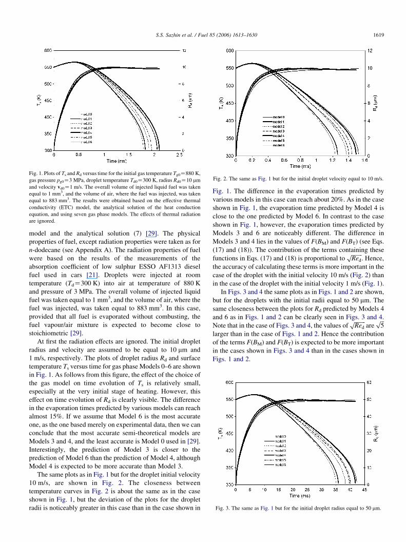
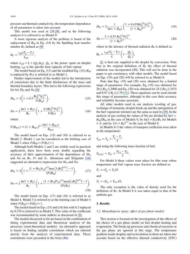
Fig. 2. The same as Fig. 1 but for the initial droplet velocity equal to 10 m/s.

Fig. 3. The same as Fig. 1 but for the initial droplet radius equal to 50 mm.

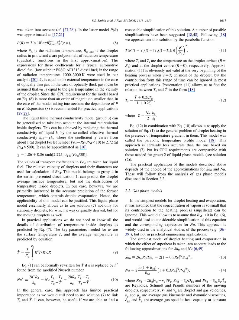
Fig. 1. Plots of Ts and Rd versus time for the initial gas temperature Tg0Z880 K,

gas pressure pg0Z3 MPa, droplet temperature Td0Z300 K, radius Rd0Z10 mm

and velocity vd0Z1 m/s. The overall volume of injected liquid fuel was taken

equal to 1 mm3, and the volume of air, where the fuel was injected, was taken

equal to 883 mm3. The results were obtained based on the effective thermal

conductivity (ETC) model, the analytical solution of the heat conduction

equation, and using seven gas phase models. The effects of thermal radiation

are ignored.

S.S. Sazhin et al. / Fuel 85 (2006) 1613–1630 1619

model and the analytical solution (7) [29]. The physical

properties of fuel, except radiation properties were taken as for

n-dodecane (see Appendix A). The radiation properties of fuel

were based on the results of the measurements of the

absorption coefficient of low sulphur ESSO AF1313 diesel

fuel used in cars [21]. Droplets were injected at room

temperature (TdZ300 K) into air at temperature of 880 K

and pressure of 3 MPa. The overall volume of injected liquid

fuel was taken equal to 1 mm3, and the volume of air, where the

fuel was injected, was taken equal to 883 mm3. In this case,

provided that all fuel is evaporated without combusting, the

fuel vapour/air mixture is expected to become close to

stoichiometric [29].

At first the radiation effects are ignored. The initial droplet

radius and velocity are assumed to be equal to 10 mm and

1 m/s, respectively. The plots of droplet radius Rd and surface

temperature Ts versus time for gas phase Models 0–6 are shown

in Fig. 1. As follows from this figure, the effect of the choice of

the gas model on time evolution of Ts is relatively small,

especially at the very initial stage of heating. However, this

effect on time evolution of Rd is clearly visible. The difference

in the evaporation times predicted by various models can reach

almost 15%. If we assume that Model 6 is the most accurate

one, as the one based merely on experimental data, then we can

conclude that the most accurate semi-theoretical models are

Models 3 and 4, and the least accurate is Model 0 used in [29].

Interestingly, the prediction of Model 3 is closer to the

prediction of Model 6 than the prediction of Model 4, although

Model 4 is expected to be more accurate than Model 3.

The same plots as in Fig. 1 but for the droplet initial velocity

10 m/s, are shown in Fig. 2. The closeness between

temperature curves in Fig. 2 is about the same as in the case

shown in Fig. 1, but the deviation of the plots for the droplet

radii is noticeably greater in this case than in the case shown in

Fig. 1. The difference in the evaporation times predicted by

various models in this case can reach about 20%. As in the case

shown in Fig. 1, the evaporation time predicted by Model 4 is

close to the one predicted by Model 6. In contrast to the case

shown in Fig. 1, however, the evaporation times predicted by

Models 3 and 6 are noticeably different. The difference in

Models 3 and 4 lies in the values of F(BM) and F(BT) (see Eqs.

(17) and (18)). The contribution of the terms containing these

functions in Eqs. (17) and (18) is proportional toffiffiffiffiffiffiffiffiRed

p. Hence,

the accuracy of calculating these terms is more important in the

case of the droplet with the initial velocity 10 m/s (Fig. 2) than

in the case of the droplet with the initial velocity 1 m/s (Fig. 1).

In Figs. 3 and 4 the same plots as in Figs. 1 and 2 are shown,

but for the droplets with the initial radii equal to 50 mm. The

same closeness between the plots for Rd predicted by Models 4

and 6 as in Figs. 1 and 2 can be clearly seen in Figs. 3 and 4.

Note that in the case of Figs. 3 and 4, the values offfiffiffiffiffiffiffiffiRed

pare

ffiffiffi5

p

larger than in the case of Figs. 1 and 2. Hence the contribution

of the terms F(BM) and F(BT) is expected to be more important

in the cases shown in Figs. 3 and 4 than in the cases shown in

Figs. 1 and 2.

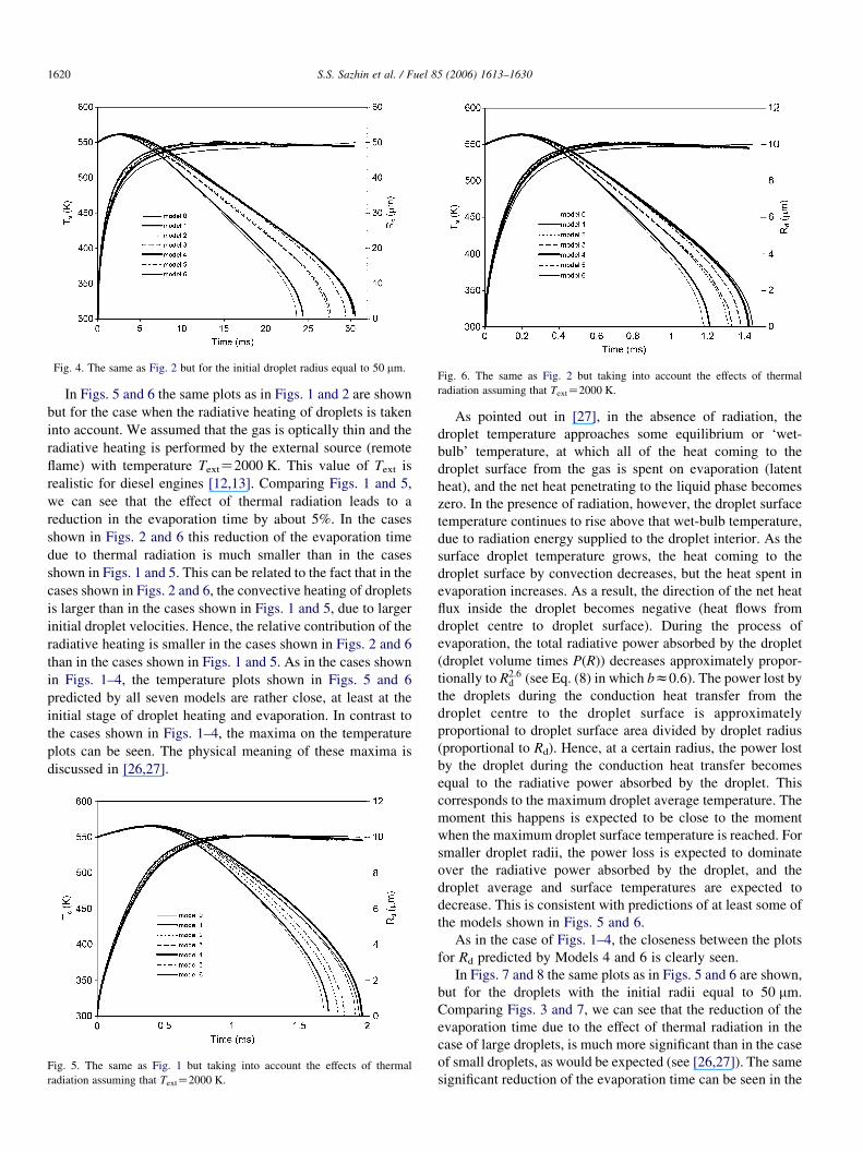
Fig. 4. The same as Fig. 2 but for the initial droplet radius equal to 50 mm.Fig. 6. The same as Fig. 2 but taking into account the effects of thermal

radiation assuming that TextZ2000 K.

S.S. Sazhin et al. / Fuel 85 (2006) 1613–16301620

In Figs. 5 and 6 the same plots as in Figs. 1 and 2 are shown

but for the case when the radiative heating of droplets is taken

into account. We assumed that the gas is optically thin and the

radiative heating is performed by the external source (remote

flame) with temperature TextZ2000 K. This value of Text is

realistic for diesel engines [12,13]. Comparing Figs. 1 and 5,

we can see that the effect of thermal radiation leads to a

reduction in the evaporation time by about 5%. In the cases

shown in Figs. 2 and 6 this reduction of the evaporation time

due to thermal radiation is much smaller than in the cases

shown in Figs. 1 and 5. This can be related to the fact that in the

cases shown in Figs. 2 and 6, the convective heating of droplets

is larger than in the cases shown in Figs. 1 and 5, due to larger

initial droplet velocities. Hence, the relative contribution of the

radiative heating is smaller in the cases shown in Figs. 2 and 6

than in the cases shown in Figs. 1 and 5. As in the cases shown

in Figs. 1–4, the temperature plots shown in Figs. 5 and 6

predicted by all seven models are rather close, at least at the

initial stage of droplet heating and evaporation. In contrast to

the cases shown in Figs. 1–4, the maxima on the temperature

plots can be seen. The physical meaning of these maxima is

discussed in [26,27].

Fig. 5. The same as Fig. 1 but taking into account the effects of thermal

radiation assuming that TextZ2000 K.

As pointed out in [27], in the absence of radiation, the

droplet temperature approaches some equilibrium or ‘wet-

bulb’ temperature, at which all of the heat coming to the

droplet surface from the gas is spent on evaporation (latent

heat), and the net heat penetrating to the liquid phase becomes

zero. In the presence of radiation, however, the droplet surface

temperature continues to rise above that wet-bulb temperature,

due to radiation energy supplied to the droplet interior. As the

surface droplet temperature grows, the heat coming to the

droplet surface by convection decreases, but the heat spent in

evaporation increases. As a result, the direction of the net heat

flux inside the droplet becomes negative (heat flows from

droplet centre to droplet surface). During the process of

evaporation, the total radiative power absorbed by the droplet

(droplet volume times P(R)) decreases approximately propor-

tionally to R2:6d (see Eq. (8) in which bz0.6). The power lost by

the droplets during the conduction heat transfer from the

droplet centre to the droplet surface is approximately

proportional to droplet surface area divided by droplet radius

(proportional to Rd). Hence, at a certain radius, the power lost

by the droplet during the conduction heat transfer becomes

equal to the radiative power absorbed by the droplet. This

corresponds to the maximum droplet average temperature. The

moment this happens is expected to be close to the moment

when the maximum droplet surface temperature is reached. For

smaller droplet radii, the power loss is expected to dominate

over the radiative power absorbed by the droplet, and the

droplet average and surface temperatures are expected to

decrease. This is consistent with predictions of at least some of

the models shown in Figs. 5 and 6.

As in the case of Figs. 1–4, the closeness between the plots

for Rd predicted by Models 4 and 6 is clearly seen.

In Figs. 7 and 8 the same plots as in Figs. 5 and 6 are shown,

but for the droplets with the initial radii equal to 50 mm.

Comparing Figs. 3 and 7, we can see that the reduction of the

evaporation time due to the effect of thermal radiation in the

case of large droplets, is much more significant than in the case

of small droplets, as would be expected (see [26,27]). The same

significant reduction of the evaporation time can be seen in the

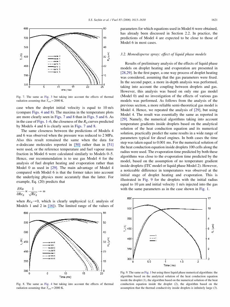
Fig. 7. The same as Fig. 3 but taking into account the effects of thermal

radiation assuming that TextZ2000 K.

S.S. Sazhin et al. / Fuel 85 (2006) 1613–1630 1621

case when the droplet initial velocity is equal to 10 m/s

(compare Figs. 4 and 8). The maxima in the temperature plots

are more clearly seen in Figs. 7 and 8 than in Figs. 5 and 6. As

in the case of Figs. 1–6, the closeness of the Rd curves predicted

by Models 4 and 6 is clearly seen in Figs. 7 and 8.

The same closeness between the predictions of Models 4

and 6 was observed when the pressure was reduced to 2 MPa.

Also this result remained the same when the data for

n-dodecane molecules reported in [50] rather than in [51]

were used, or the reference temperature and fuel vapour mass

fraction in Model 6 were calculated similarly to Models 0–5.

Hence, our recommendation is to use gas Model 4 for the

analysis of fuel droplet heating and evaporation rather than

Model 0 as used in [29]. The main advantage of Model 4

compared with Model 6 is that the former takes into account

the underlying physics more accurately than the latter. For

example, Eq. (20) predicts that

vNu

vRedf

1ffiffiffiffiffiffiffiffiRed

p /N

when Red/0, which is clearly unphysical (c.f. analysis of

Models 1 and 2 in [16]). The limited range of the values of

Fig. 8. The same as Fig. 4 but taking into account the effects of thermal

radiation assuming that TextZ2000 K.

parameters for which equations used in Model 6 were obtained,

has already been discussed in Section 2.2. In practice, the

predictions of Model 4 are expected to be close to those of

Model 6 in most cases.

3.2. Monodisperse spray: effect of liquid phase models

Results of preliminary analysis of the effects of liquid phase

models on droplet heating and evaporation are presented in

[28,29]. In the first paper, a one way process of droplet heating

was considered, assuming that the gas parameters were fixed.

In the second paper, a more in-depth analysis was performed,

taking into account the coupling between droplets and gas.

However, this analysis was based on only one gas model

(Model 0) and no investigation of the effects of various gas

models was performed. As follows from the analysis of the

previous section, a more reliable semi-theoretical gas model is

Model 4. Hence, we repeated the analysis of [29], but using

Model 4. The result was essentially the same as reported in

[29]. Namely, the numerical algorithms taking into account

temperature gradients inside droplets based on the analytical

solution of the heat conduction equation and its numerical

solution, practically predict the same results in a wide range of

parameters typical for diesel engines. In both cases the time

step was taken equal to 0.001 ms. For the numerical solution of

the heat conduction equation inside droplets 100 cells along the

radius were used. The evaporation time predicted by both these

algorithms was close to the evaporation time predicted by the

model, based on the assumption of no temperature gradient

inside droplets (ITC model or liquid phase Model 2). However,

a noticeable difference in temperatures was observed at the

initial stage of droplet heating and evaporation. This is

illustrated in Fig. 9 for the droplets with the initial radius

equal to 10 mm and initial velocity 1 m/s injected into the gas

with the same parameters as in the case shown in Fig. 1.

Fig. 9. The same as Fig. 1 but using three liquid phase numerical algorithms: the

algorithm based on the analytical solution of the heat conduction equation

inside the droplet (1), the algorithm based on the numerical solution of the heat

conduction equation inside the droplet (2), the algorithm based on the

assumption that the thermal conductivity inside droplets is infinitely large (3).

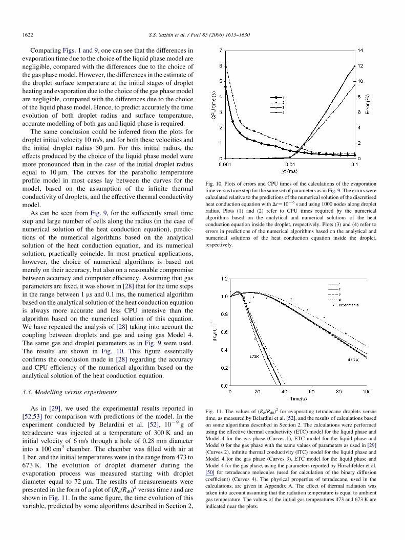
Fig. 11. The values of (Rd/Rd0)2 for evaporating tetradecane droplets versus

time, as measured by Belardini et al. [52], and the results of calculations based

on some algorithms described in Section 2. The calculations were performed

using the effective thermal conductivity (ETC) model for the liquid phase and

Model 4 for the gas phase (Curves 1), ETC model for the liquid phase and

Model 0 for the gas phase with the same values of parameters as used in [29]

(Curves 2), infinite thermal conductivity (ITC) model for the liquid phase and

Model 4 for the gas phase (Curves 3), ETC model for the liquid phase and

Model 4 for the gas phase, using the parameters reported by Hirschfelder et al.

[50] for tetradecane molecules (used for calculation of the binary diffusion

coefficient) (Curves 4). The physical properties of tetradecane, used in the

calculations, are given in Appendix A. The effect of thermal radiation was

taken into account assuming that the radiation temperature is equal to ambient

gas temperature. The values of the initial gas temperatures 473 and 673 K are

indicated near the plots.

Fig. 10. Plots of errors and CPU times of the calculations of the evaporation

time versus time step for the same set of parameters as in Fig. 9. The errors were

calculated relative to the predictions of the numerical solution of the discretised

heat conduction equation with DtZ10K6 s and using 1000 nodes along droplet

radius. Plots (1) and (2) refer to CPU times required by the numerical

algorithms based on the analytical and numerical solutions of the heat

conduction equation inside the droplet, respectively. Plots (3) and (4) refer to

errors in predictions of the numerical algorithms based on the analytical and

numerical solutions of the heat conduction equation inside the droplet,

respectively.

S.S. Sazhin et al. / Fuel 85 (2006) 1613–16301622

Comparing Figs. 1 and 9, one can see that the differences in

evaporation time due to the choice of the liquid phase model are

negligible, compared with the differences due to the choice of

the gas phase model. However, the differences in the estimate of

the droplet surface temperature at the initial stages of droplet

heating and evaporation due to the choice of the gas phasemodel

are negligible, compared with the differences due to the choice

of the liquid phase model. Hence, to predict accurately the time

evolution of both droplet radius and surface temperature,

accurate modelling of both gas and liquid phase is required.

The same conclusion could be inferred from the plots for

droplet initial velocity 10 m/s, and for both these velocities and

the initial droplet radius 50 mm. For this initial radius, the

effects produced by the choice of the liquid phase model were

more pronounced than in the case of the initial droplet radius

equal to 10 mm. The curves for the parabolic temperature

profile model in most cases lay between the curves for the

model, based on the assumption of the infinite thermal

conductivity of droplets, and the effective thermal conductivity

model.

As can be seen from Fig. 9, for the sufficiently small time

step and large number of cells along the radius (in the case of

numerical solution of the heat conduction equation), predic-

tions of the numerical algorithms based on the analytical

solution of the heat conduction equation, and its numerical

solution, practically coincide. In most practical applications,

however, the choice of numerical algorithms is based not

merely on their accuracy, but also on a reasonable compromise

between accuracy and computer efficiency. Assuming that gas

parameters are fixed, it was shown in [28] that for the time steps

in the range between 1 ms and 0.1 ms, the numerical algorithm

based on the analytical solution of the heat conduction equation

is always more accurate and less CPU intensive than the

algorithm based on the numerical solution of this equation.

We have repeated the analysis of [28] taking into account the

coupling between droplets and gas and using gas Model 4.

The same gas and droplet parameters as in Fig. 9 were used.

The results are shown in Fig. 10. This figure essentially

confirms the conclusion made in [28] regarding the accuracy

and CPU efficiency of the numerical algorithm based on the

analytical solution of the heat conduction equation.

3.3. Modelling versus experiments

As in [29], we used the experimental results reported in

[52,53] for comparison with predictions of the model. In the

experiment conducted by Belardini et al. [52], 10K9 g of

tetradecane was injected at a temperature of 300 K and an

initial velocity of 6 m/s through a hole of 0.28 mm diameter

into a 100 cm3 chamber. The chamber was filled with air at

1 bar, and the initial temperatures were in the range from 473 to

673 K. The evolution of droplet diameter during the

evaporation process was measured starting with droplet

diameter equal to 72 mm. The results of measurements were

presented in the form of a plot of (Rd/Rd0)2 versus time t and are

shown in Fig. 11. In the same figure, the time evolution of this

variable, predicted by some algorithms described in Section 2,

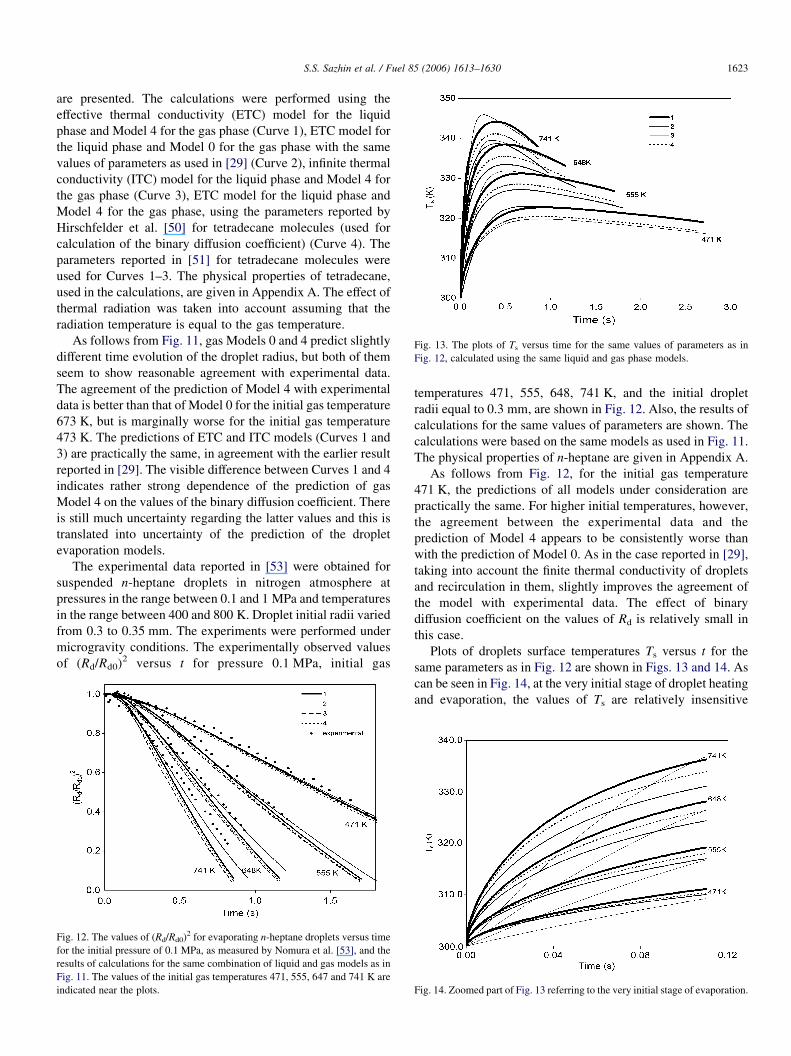
Fig. 13. The plots of Ts versus time for the same values of parameters as in

Fig. 12, calculated using the same liquid and gas phase models.

S.S. Sazhin et al. / Fuel 85 (2006) 1613–1630 1623

are presented. The calculations were performed using the

effective thermal conductivity (ETC) model for the liquid

phase and Model 4 for the gas phase (Curve 1), ETC model for

the liquid phase and Model 0 for the gas phase with the same

values of parameters as used in [29] (Curve 2), infinite thermal

conductivity (ITC) model for the liquid phase and Model 4 for

the gas phase (Curve 3), ETC model for the liquid phase and

Model 4 for the gas phase, using the parameters reported by

Hirschfelder et al. [50] for tetradecane molecules (used for

calculation of the binary diffusion coefficient) (Curve 4). The

parameters reported in [51] for tetradecane molecules were

used for Curves 1–3. The physical properties of tetradecane,

used in the calculations, are given in Appendix A. The effect of

thermal radiation was taken into account assuming that the

radiation temperature is equal to the gas temperature.

As follows from Fig. 11, gas Models 0 and 4 predict slightly

different time evolution of the droplet radius, but both of them

seem to show reasonable agreement with experimental data.

The agreement of the prediction of Model 4 with experimental

data is better than that of Model 0 for the initial gas temperature

673 K, but is marginally worse for the initial gas temperature

473 K. The predictions of ETC and ITC models (Curves 1 and

3) are practically the same, in agreement with the earlier result

reported in [29]. The visible difference between Curves 1 and 4

indicates rather strong dependence of the prediction of gas

Model 4 on the values of the binary diffusion coefficient. There

is still much uncertainty regarding the latter values and this is

translated into uncertainty of the prediction of the droplet

evaporation models.

The experimental data reported in [53] were obtained for

suspended n-heptane droplets in nitrogen atmosphere at

pressures in the range between 0.1 and 1 MPa and temperatures

in the range between 400 and 800 K. Droplet initial radii varied

from 0.3 to 0.35 mm. The experiments were performed under

microgravity conditions. The experimentally observed values

of (Rd/Rd0)2 versus t for pressure 0.1 MPa, initial gas

Fig. 12. The values of (Rd/Rd0)2 for evaporating n-heptane droplets versus time

for the initial pressure of 0.1 MPa, as measured by Nomura et al. [53], and the

results of calculations for the same combination of liquid and gas models as in

Fig. 11. The values of the initial gas temperatures 471, 555, 647 and 741 K are

indicated near the plots.

temperatures 471, 555, 648, 741 K, and the initial droplet

radii equal to 0.3 mm, are shown in Fig. 12. Also, the results of

calculations for the same values of parameters are shown. The

calculations were based on the same models as used in Fig. 11.

The physical properties of n-heptane are given in Appendix A.

As follows from Fig. 12, for the initial gas temperature

471 K, the predictions of all models under consideration are

practically the same. For higher initial temperatures, however,

the agreement between the experimental data and the

prediction of Model 4 appears to be consistently worse than

with the prediction of Model 0. As in the case reported in [29],

taking into account the finite thermal conductivity of droplets

and recirculation in them, slightly improves the agreement of

the model with experimental data. The effect of binary

diffusion coefficient on the values of Rd is relatively small in

this case.

Plots of droplets surface temperatures Ts versus t for the

same parameters as in Fig. 12 are shown in Figs. 13 and 14. As

can be seen in Fig. 14, at the very initial stage of droplet heating

and evaporation, the values of Ts are relatively insensitive

Fig. 14. Zoomed part of Fig. 13 referring to the very initial stage of evaporation.

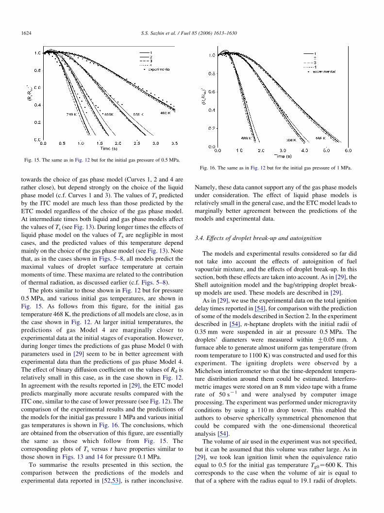
Fig. 15. The same as in Fig. 12 but for the initial gas pressure of 0.5 MPa.

Fig. 16. The same as in Fig. 12 but for the initial gas pressure of 1 MPa.

S.S. Sazhin et al. / Fuel 85 (2006) 1613–16301624

towards the choice of gas phase model (Curves 1, 2 and 4 are

rather close), but depend strongly on the choice of the liquid

phase model (c.f. Curves 1 and 3). The values of Ts predicted

by the ITC model are much less than those predicted by the

ETC model regardless of the choice of the gas phase model.

At intermediate times both liquid and gas phase models affect

the values of Ts (see Fig. 13). During longer times the effects of

liquid phase model on the values of Ts are negligible in most

cases, and the predicted values of this temperature depend

mainly on the choice of the gas phase model (see Fig. 13). Note

that, as in the cases shown in Figs. 5–8, all models predict the

maximal values of droplet surface temperature at certain

moments of time. These maxima are related to the contribution

of thermal radiation, as discussed earlier (c.f. Figs. 5–8).

The plots similar to those shown in Fig. 12 but for pressure

0.5 MPa, and various initial gas temperatures, are shown in

Fig. 15. As follows from this figure, for the initial gas

temperature 468 K, the predictions of all models are close, as in

the case shown in Fig. 12. At larger initial temperatures, the

predictions of gas Model 4 are marginally closer to

experimental data at the initial stages of evaporation. However,

during longer times the predictions of gas phase Model 0 with

parameters used in [29] seem to be in better agreement with

experimental data than the predictions of gas phase Model 4.

The effect of binary diffusion coefficient on the values of Rd is

relatively small in this case, as in the case shown in Fig. 12.

In agreement with the results reported in [29], the ETC model

predicts marginally more accurate results compared with the

ITC one, similar to the case of lower pressure (see Fig. 12). The

comparison of the experimental results and the predictions of

the models for the initial gas pressure 1 MPa and various initial

gas temperatures is shown in Fig. 16. The conclusions, which

are obtained from the observation of this figure, are essentially

the same as those which follow from Fig. 15. The

corresponding plots of Ts versus t have properties similar to

those shown in Figs. 13 and 14 for pressure 0.1 MPa.

To summarise the results presented in this section, the

comparison between the predictions of the models and

experimental data reported in [52,53], is rather inconclusive.

Namely, these data cannot support any of the gas phase models

under consideration. The effect of liquid phase models is

relatively small in the general case, and the ETC model leads to

marginally better agreement between the predictions of the

models and experimental data.

3.4. Effects of droplet break-up and autoignition

The models and experimental results considered so far did

not take into account the effects of autoignition of fuel

vapour/air mixture, and the effects of droplet break-up. In this

section, both these effects are taken into account. As in [29], the

Shell autoignition model and the bag/stripping droplet break-

up models are used. These models are described in [29].

As in [29], we use the experimental data on the total ignition

delay times reported in [54], for comparison with the prediction

of some of the models described in Section 2. In the experiment

described in [54], n-heptane droplets with the initial radii of

0.35 mm were suspended in air at pressure 0.5 MPa. The

droplets’ diameters were measured within G0.05 mm. A

furnace able to generate almost uniform gas temperature (from

room temperature to 1100 K) was constructed and used for this

experiment. The igniting droplets were observed by a

Michelson interferometer so that the time-dependent tempera-

ture distribution around them could be estimated. Interfero-

metric images were stored on an 8 mm video tape with a frame

rate of 50 sK1 and were analysed by computer image

processing. The experiment was performed under microgravity

conditions by using a 110 m drop tower. This enabled the

authors to observe spherically symmetrical phenomenon that

could be compared with the one-dimensional theoretical

analysis [54].

The volume of air used in the experiment was not specified,

but it can be assumed that this volume was rather large. As in

[29], we took lean ignition limit when the equivalence ratio

equal to 0.5 for the initial gas temperature Tg0Z600 K. This

corresponds to the case when the volume of air is equal to

that of a sphere with the radius equal to 19.1 radii of droplets.

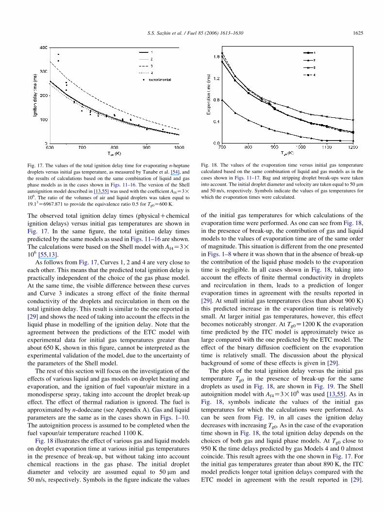
Fig. 17. The values of the total ignition delay time for evaporating n-heptane

droplets versus initial gas temperature, as measured by Tanabe et al. [54], and

the results of calculations based on the same combination of liquid and gas

phase models as in the cases shown in Figs. 11–16. The version of the Shell

autoignition model described in [13,55] was used with the coefficient Af4Z3!

106. The ratio of the volumes of air and liquid droplets was taken equal to

19.13Z6967.871 to provide the equivalence ratio 0.5 for Tg0Z600 K.

Fig. 18. The values of the evaporation time versus initial gas temperature

calculated based on the same combination of liquid and gas models as in the

cases shown in Figs. 11–17. Bag and stripping droplet break-ups were taken

into account. The initial droplet diameter and velocity are taken equal to 50 mm

and 50 m/s, respectively. Symbols indicate the values of gas temperatures for

which the evaporation times were calculated.

S.S. Sazhin et al. / Fuel 85 (2006) 1613–1630 1625

The observed total ignition delay times (physicalCchemical

ignition delays) versus initial gas temperatures are shown in

Fig. 17. In the same figure, the total ignition delay times

predicted by the same models as used in Figs. 11–16 are shown.

The calculations were based on the Shell model with Af4Z3!106 [55,13].

As follows from Fig. 17, Curves 1, 2 and 4 are very close to

each other. This means that the predicted total ignition delay is

practically independent of the choice of the gas phase model.

At the same time, the visible difference between these curves

and Curve 3 indicates a strong effect of the finite thermal

conductivity of the droplets and recirculation in them on the

total ignition delay. This result is similar to the one reported in

[29] and shows the need of taking into account the effects in the

liquid phase in modelling of the ignition delay. Note that the

agreement between the predictions of the ETC model with

experimental data for initial gas temperatures greater than

about 650 K, shown in this figure, cannot be interpreted as the

experimental validation of the model, due to the uncertainty of

the parameters of the Shell model.

The rest of this section will focus on the investigation of the

effects of various liquid and gas models on droplet heating and

evaporation, and the ignition of fuel vapour/air mixture in a

monodisperse spray, taking into account the droplet break-up

effect. The effect of thermal radiation is ignored. The fuel is

approximated by n-dodecane (see Appendix A). Gas and liquid

parameters are the same as in the cases shown in Figs. 1–10.

The autoignition process is assumed to be completed when the

fuel vapour/air temperature reached 1100 K.

Fig. 18 illustrates the effect of various gas and liquid models

on droplet evaporation time at various initial gas temperatures

in the presence of break-up, but without taking into account

chemical reactions in the gas phase. The initial droplet

diameter and velocity are assumed equal to 50 mm and

50 m/s, respectively. Symbols in the figure indicate the values

of the initial gas temperatures for which calculations of the

evaporation time were performed. As one can see from Fig. 18,

in the presence of break-up, the contribution of gas and liquid

models to the values of evaporation time are of the same order

of magnitude. This situation is different from the one presented

in Figs. 1–8 where it was shown that in the absence of break-up

the contribution of the liquid phase models to the evaporation

time is negligible. In all cases shown in Fig. 18, taking into

account the effects of finite thermal conductivity in droplets

and recirculation in them, leads to a prediction of longer

evaporation times in agreement with the results reported in

[29]. At small initial gas temperatures (less than about 900 K)

this predicted increase in the evaporation time is relatively

small. At larger initial gas temperatures, however, this effect

becomes noticeably stronger. At Tg0Z1200 K the evaporation

time predicted by the ITC model is approximately twice as

large compared with the one predicted by the ETC model. The

effect of the binary diffusion coefficient on the evaporation

time is relatively small. The discussion about the physical

background of some of these effects is given in [29].

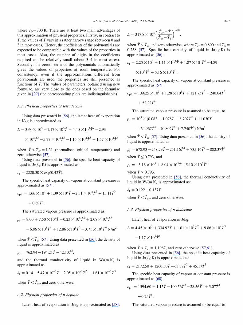
The plots of the total ignition delay versus the initial gas

temperature Tg0 in the presence of break-up for the same

droplets as used in Fig. 18, are shown in Fig. 19. The Shell

autoignition model with Af4Z3!106 was used [13,55]. As in

Fig. 18, symbols indicate the values of the initial gas

temperatures for which the calculations were performed. As

can be seen from Fig. 19, in all cases the ignition delay

decreases with increasing Tg0. As in the case of the evaporation

time shown in Fig. 18, the total ignition delay depends on the

choices of both gas and liquid phase models. At Tg0 close to

950 K the time delays predicted by gas Models 4 and 0 almost

coincide. This result agrees with the one shown in Fig. 17. For

the initial gas temperatures greater than about 890 K, the ITC

model predicts longer total ignition delays compared with the

ETC model in agreement with the result reported in [29].

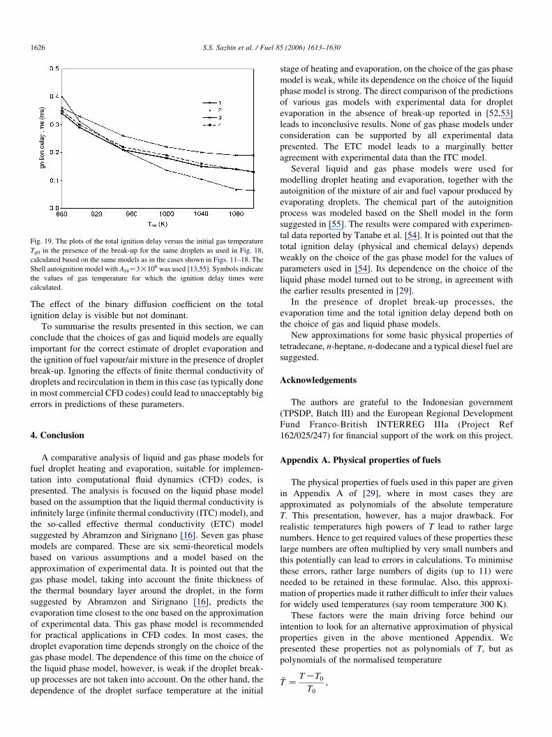
Fig. 19. The plots of the total ignition delay versus the initial gas temperature

Tg0 in the presence of the break-up for the same droplets as used in Fig. 18,

calculated based on the same models as in the cases shown in Figs. 11–18. The

Shell autoignition model with Af4Z3!106 was used [13,55]. Symbols indicate

the values of gas temperature for which the ignition delay times were

calculated.

S.S. Sazhin et al. / Fuel 85 (2006) 1613–16301626

The effect of the binary diffusion coefficient on the total

ignition delay is visible but not dominant.

To summarise the results presented in this section, we can

conclude that the choices of gas and liquid models are equally

important for the correct estimate of droplet evaporation and

the ignition of fuel vapour/air mixture in the presence of droplet

break-up. Ignoring the effects of finite thermal conductivity of

droplets and recirculation in them in this case (as typically done

in most commercial CFD codes) could lead to unacceptably big

errors in predictions of these parameters.

4. Conclusion

A comparative analysis of liquid and gas phase models for

fuel droplet heating and evaporation, suitable for implemen-

tation into computational fluid dynamics (CFD) codes, is

presented. The analysis is focused on the liquid phase model

based on the assumption that the liquid thermal conductivity is

infinitely large (infinite thermal conductivity (ITC) model), and

the so-called effective thermal conductivity (ETC) model

suggested by Abramzon and Sirignano [16]. Seven gas phase

models are compared. These are six semi-theoretical models

based on various assumptions and a model based on the

approximation of experimental data. It is pointed out that the

gas phase model, taking into account the finite thickness of

the thermal boundary layer around the droplet, in the form

suggested by Abramzon and Sirignano [16], predicts the

evaporation time closest to the one based on the approximation

of experimental data. This gas phase model is recommended

for practical applications in CFD codes. In most cases, the

droplet evaporation time depends strongly on the choice of the

gas phase model. The dependence of this time on the choice of

the liquid phase model, however, is weak if the droplet break-

up processes are not taken into account. On the other hand, the

dependence of the droplet surface temperature at the initial

stage of heating and evaporation, on the choice of the gas phase

model is weak, while its dependence on the choice of the liquid

phase model is strong. The direct comparison of the predictions

of various gas models with experimental data for droplet

evaporation in the absence of break-up reported in [52,53]

leads to inconclusive results. None of gas phase models under

consideration can be supported by all experimental data

presented. The ETC model leads to a marginally better

agreement with experimental data than the ITC model.

Several liquid and gas phase models were used for

modelling droplet heating and evaporation, together with the

autoignition of the mixture of air and fuel vapour produced by

evaporating droplets. The chemical part of the autoignition

process was modeled based on the Shell model in the form

suggested in [55]. The results were compared with experimen-

tal data reported by Tanabe et al. [54]. It is pointed out that the

total ignition delay (physical and chemical delays) depends

weakly on the choice of the gas phase model for the values of

parameters used in [54]. Its dependence on the choice of the

liquid phase model turned out to be strong, in agreement with

the earlier results presented in [29].

In the presence of droplet break-up processes, the

evaporation time and the total ignition delay depend both on

the choice of gas and liquid phase models.

New approximations for some basic physical properties of

tetradecane, n-heptane, n-dodecane and a typical diesel fuel are

suggested.

Acknowledgements

The authors are grateful to the Indonesian government

(TPSDP, Batch III) and the European Regional Development

Fund Franco-British INTERREG IIIa (Project Ref

162/025/247) for financial support of the work on this project.

Appendix A. Physical properties of fuels

The physical properties of fuels used in this paper are given

in Appendix A of [29], where in most cases they are

approximated as polynomials of the absolute temperature

T. This presentation, however, has a major drawback. For

realistic temperatures high powers of T lead to rather large

numbers. Hence to get required values of these properties these

large numbers are often multiplied by very small numbers and

this potentially can lead to errors in calculations. To minimise

these errors, rather large numbers of digits (up to 11) were

needed to be retained in these formulae. Also, this approxi-

mation of properties made it rather difficult to infer their values

for widely used temperatures (say room temperature 300 K).

These factors were the main driving force behind our

intention to look for an alternative approximation of physical

properties given in the above mentioned Appendix. We

presented these properties not as polynomials of T, but as

polynomials of the normalised temperature

~T ZTKT0T0

;

S.S. Sazhin et al. / Fuel 85 (2006) 1613–1630 1627

where T0Z300 K. There are at least two main advantages of

this approximation of physical properties. Firstly, in contrast to

T, the values of ~T vary in a rather narrow range (between 0 and

3 in most cases). Hence, the coefficients of the polynomials are

expected to be comparable with the values of the properties in

most cases. Also, the number of digits in the coefficients

required can be relatively small (about 3–4 in most cases).

Secondly, the zeroth term of the polynomials automatically

gives the values of properties at room temperature. For

consistency, even if the approximations different from

polynomials are used, the properties are still presented as

functions of ~T . The values of parameters, obtained using new

formulae, are very close to the ones based on the formulae

given in [29] (the corresponding plots are indistinguishable).

A.1. Physical properties of tetradecane

Using data presented in [56], the latent heat of evaporation

in J/kg is approximated as

LZ 3:60!105K1:17!105 ~T C4:40!103 ~T2K2:93

!104 ~T3K5:77!104 ~T

4K1:15!104 ~T

5C1:57!104 ~T

6

when ~T! ~TcrZ1:31 (normalised critical temperature) and

zero otherwise [57].

Using data presented in [56], the specific heat capacity of

liquid in J/(kg K) is approximated as:

cl Z 2220:30!expð0:42 ~TÞ:

The specific heat capacity of vapour at constant pressure is

approximated as [57]:

cpF Z 1:66!103 C1:39!102 ~TK2:51!102 ~T2C15:11 ~T

3

C0:69 ~T4:

The saturated vapour pressure is approximated as:

ps Z 9:00C7:50!102 ~TK0:23!105 ~T2C2:08!105 ~T

3

K6:86!105 ~T4C12:86!105 ~T

5K3:71!105 ~T

6N=m2

when ~T! ~Tcr [57]. Using data presented in [56], the density of

liquid is approximated as

rl Z 762:94K194:21 ~TK42:13 ~T2;

and the thermal conductivity of liquid in W/(m K) is

approximated as

kl Z 0:14K5:47!10K2 ~TK2:05!10K2 ~T2C1:61!10K2 ~T

3

when ~T! ~Tcr, and zero otherwise.

A.2. Physical properties of n-heptane

Latent heat of evaporation in J/kg is approximated as [58]:

LZ 317:8!103~TcrK ~T~TcrK ~Tb

� �0:38

;

when ~T! ~Tcr and zero otherwise, where ~TcrZ0:800 and ~TbZ0:238 [57]. Specific heat capacity of liquid in J/(kg K) is

approximated as [56]:

cl Z 2:25!103 C1:11!103 ~T C1:87!103 ~T2K4:89

!103 ~T3C5:16!103 ~T

4:

The specific heat capacity of vapour at constant pressure is

approximated as [57]:

cpF Z 1:6625!103 C1:28!103 ~T C121:75 ~T2K240:64 ~T

3

C52:22 ~T4:

The saturated vapour pressure is assumed to be equal to

ps Z 105!ð0:082C1:078 ~T C8:707 ~T2C11:030 ~T

3

C64:967 ~T4K40:802 ~T

5C7:740 ~T

6Þ N=m2

when ~T! ~Tcr [57]. Using data presented in [56], the density of

liquid is approximated as

rl Z 678:93K248:73 ~TK251:16 ~T2C735:16 ~T

3K882:37 ~T

4

when ~T%0:793, and

rl ZK3:16!105 C8:04!105 ~TK5:10!105 ~T2

when ~TO0:793.

Using data presented in [56], the thermal conductivity of

liquid in W/(m K) is approximated as:

kl Z 0:122K0:137 ~T

when ~T! ~Tcr, and zero otherwise.

A.3. Physical properties of n-dodecane

Latent heat of evaporation in J/kg:

LZ 4:45!105 C334:92 ~T C1:01!105 ~T2C9:86!104 ~T

3

K1:17!105 ~T4

when ~T! ~TcrZ1:1967, and zero otherwise [57,61].

Using data presented in [56], the specific heat capacity of

liquid in J/(kg K) is approximated as:

cl Z 2172:50C1260:50 ~TK63:38 ~T2C45:17 ~T

3:

The specific heat capacity of vapour at constant pressure is

approximated as [60]:

cpF Z 1594:60C1:15 ~TK100:56 ~T2K28:56 ~T

3C5:07 ~T

4

K0:25 ~T5:

The saturated vapour pressure is assumed to be equal to

S.S. Sazhin et al. / Fuel 85 (2006) 1613–16301628

ps Z 6894:76!exp½12:13K3743:84=ð300 ~T C207Þ�

when ~T! ~TcrZ1:1967. The density of liquid is approximated

as [59]

rl Z 744:96K230:42 ~T C40:90 ~T2K88:70 ~T

3:

The thermal conductivity of liquid n-dodecane and liquid

diesel fuel in W/(m K) was used in the table form (see Table 1

[57]).

The surface tension is approximated as [60]:

ss Z 0:0528 1K~TC1

~Tcr C1

� �0:121

:

0:267

67% ~T!0:667

67% ~T!1:067

67% ~T! ~Tcr

A.4. Physical properties of diesel fuel

In this section a compilation of physical properties of a

‘typical’ diesel fuel is given. These are expected to differ

slightly from any particular diesel fuel.

Latent heat of evaporation in J/kg is approximated as [58]:

LZ 254!103~TcrK ~T~TcrK ~Tb

� �0:38

;

when ~T! ~TcrZ1:419, and zero otherwise, where ~TbZ0:788.

The specific heat capacity of liquid in J/(kg K) is

approximated as [60]:

cl Z 1896:60C1366:20 ~TK266:40 ~T2:

The specific heat capacity of vapour at constant pressure is

approximated as equal to that of n-dodecane [60]. The

saturated vapour pressure is assumed to be equal to [58]:

ps Z

1000!exp½8:59K2591:52=ð300 ~T C257Þ� when ~T!

1000!exp½14:06K4436:10=ð300 ~T C257Þ� when 0:2

1000!exp½12:93K3922:51=ð300 ~T C257Þ� when 0:6

1000!exp½16:20K5810:82=ð300 ~T C257Þ� when 1:0

8>>>>><>>>>>:

The density of liquid is approximated as [59]:

rl Z 840=½0:201 ~T C1:008�:

The thermal conductivity of liquid in W/(m K) is presented

in Table 1 of [57]

The surface tension is approximated as [60]:

ss Z 0:059 1K~TC1

~Tcr C1

� �0:121

:

Appendix B. Physical properties of a mixture of fuel

vapour and air

Density and specific heat capacity of the mixture are

calculated using the following simple formulae:

rmix Zpmix

RmixTmix

; (B1)

cp mix Z ð1KYFÞcpa CYFcpF; (B2)

where pmix, Rmix and Tmix are the pressure, gas constant, and

temperature of the mixture of fuel vapour and air, YF is the mass

fraction of fuel vapour, subscripts a and F refer to air and fuel

vapour, respectively.

Dynamic viscosity of the mixture is calculated from the

following general semi-empirical formula [49]:

mmix ZXNiZ1

XimiPNjZ1

XjFij

; (B3)

where

Fij Z1ffiffiffi8

p 1CMi

Mj

� �K1=2

1Cmi

mj

� �1=2 Mj

Mi

� �1=4� �2;

Xi are molar fractions of species i, Mi are molar masses (kg/

kmol), the summation is performed over all N species.

Similarly, the thermal conductivity of the mixture is

calculated from the following general semi-empirical formula

[49,62]:

kmix ZXNiZ1

XikiPNiZ1

XjFij

; (B4)

where Fij is the same as in Eq. (B3).

The binary diffusion coefficient was estimated using the

following equation [49]:

DFa Z 1:8583!10K7

ffiffiffiffiffiffiffiffiffiffiffiffiffiffiffiffiffiffiffiffiffiffiffiffiffiffiffiffiffiffiffiT3

1

MF

C1

Ma

� �s1

psFaUFaðT *Þ; (B5)

where DFa is in m2/s, p is in atm (1 atmZ0.101 MPa), T is in K,

sFaZ0.5(sFCsa) is the minimal distance between molecules

in A (1 AZ10K10 m), UFa is the collision integral, the value of

which depends on the normalised temperature T*ZTkB/3, kB is

the Boltzmann constant, 3Zffiffiffiffiffiffiffiffi3F3a

p.

The values of sa and 3a/kB can be obtained from Table E.1 in

[49]: saZ3.617 A, 3a/kBZ97.0 K. There is some controversy

regarding the values of these parameters for various fuels. The

values sF (in A) and 3F/kB (in K) for tetradecane, n-heptane and

n-dodecane reported by Hirschfelder et al. [50] and Paredes

et al. [51] are shown in this table:

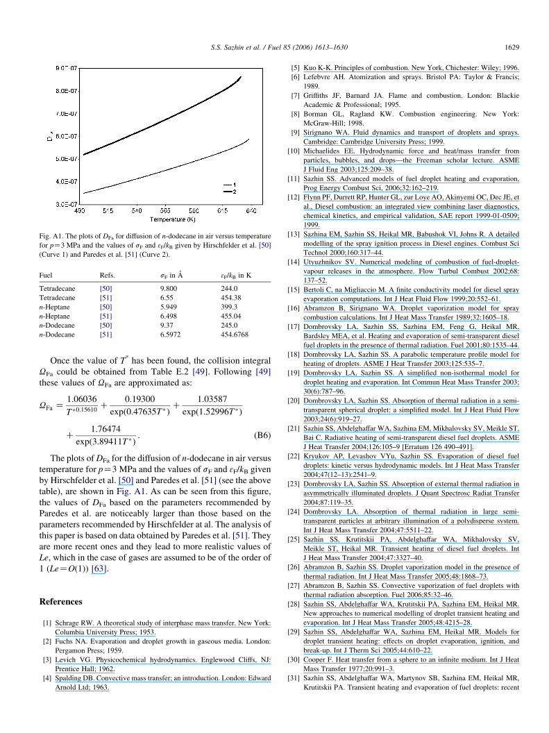
Fig. A1. The plots of DFa for diffusion of n-dodecane in air versus temperature

for pZ3 MPa and the values of sF and 3F/kB given by Hirschfelder et al. [50]

(Curve 1) and Paredes et al. [51] (Curve 2).

S.S. Sazhin et al. / Fuel 85 (2006) 1613–1630 1629

Fuel Refs. sF in A 3F/kB in K

Tetradecane [50] 9.800 244.0

Tetradecane [51] 6.55 454.38

n-Heptane [50] 5.949 399.3

n-Heptane [51] 6.498 455.04

n-Dodecane [50] 9.37 245.0

n-Dodecane [51] 6.5972 454.6768

Once the value of T* has been found, the collision integral

UFa could be obtained from Table E.2 [49]. Following [49]

these values of UFa are approximated as:

UFa Z1:06036

T *0:15610C

0:19300

expð0:47635T *ÞC

1:03587

expð1:52996T *Þ

C1:76474

expð3:89411T *Þ: (B6)

The plots ofDFa for the diffusion of n-dodecane in air versus

temperature for pZ3 MPa and the values of sF and 3F/kB given

by Hirschfelder et al. [50] and Paredes et al. [51] (see the above

table), are shown in Fig. A1. As can be seen from this figure,

the values of DFa based on the parameters recommended by

Paredes et al. are noticeably larger than those based on the

parameters recommended by Hirschfelder at al. The analysis of

this paper is based on data obtained by Paredes et al. [51]. They

are more recent ones and they lead to more realistic values of

Le, which in the case of gases are assumed to be of the order of

1 (LeZO(1)) [63].

References

[1] Schrage RW. A theoretical study of interphase mass transfer. New York:

Columbia University Press; 1953.

[2] Fuchs NA. Evaporation and droplet growth in gaseous media. London:

Pergamon Press; 1959.

[3] Levich VG. Physicochemical hydrodynamics. Englewood Cliffs, NJ:

Prentice Hall; 1962.

[4] Spalding DB. Convective mass transfer; an introduction. London: Edward

Arnold Ltd; 1963.

[5] Kuo K-K. Principles of combustion. New York, Chichester: Wiley; 1996.

[6] Lefebvre AH. Atomization and sprays. Bristol PA: Taylor & Francis;

1989.

[7] Griffiths JF, Barnard JA. Flame and combustion. London: Blackie

Academic & Professional; 1995.

[8] Borman GL, Ragland KW. Combustion engineering. New York:

McGraw-Hill; 1998.

[9] Sirignano WA. Fluid dynamics and transport of droplets and sprays.

Cambridge: Cambridge University Press; 1999.

[10] Michaelides EE. Hydrodynamic force and heat/mass transfer from

particles, bubbles, and drops—the Freeman scholar lecture. ASME

J Fluid Eng 2003;125:209–38.

[11] Sazhin SS. Advanced models of fuel droplet heating and evaporation,

Prog Energy Combust Sci, 2006;32:162–219.

[12] Flynn PF, Durrett RP, Hunter GL, zur Loye AO, Akinyemi OC, Dec JE, et

al., Diesel combustion: an integrated view combining laser diagnostics,

chemical kinetics, and empirical validation, SAE report 1999-01-0509;

1999.

[13] Sazhina EM, Sazhin SS, Heikal MR, Babushok VI, Johns R. A detailed

modelling of the spray ignition process in Diesel engines. Combust Sci

Technol 2000;160:317–44.

[14] Utyuzhnikov SV. Numerical modeling of combustion of fuel-droplet-

vapour releases in the atmosphere. Flow Turbul Combust 2002;68:

137–52.

[15] Bertoli C, na Migliaccio M. A finite conductivity model for diesel spray

evaporation computations. Int J Heat Fluid Flow 1999;20:552–61.

[16] Abramzon B, Sirignano WA. Droplet vaporization model for spray

combustion calculations. Int J Heat Mass Transfer 1989;32:1605–18.

[17] Dombrovsky LA, Sazhin SS, Sazhina EM, Feng G, Heikal MR,

Bardsley MEA, et al. Heating and evaporation of semi-transparent diesel

fuel droplets in the presence of thermal radiation. Fuel 2001;80:1535–44.

[18] Dombrovsky LA, Sazhin SS. A parabolic temperature profile model for

heating of droplets. ASME J Heat Transfer 2003;125:535–7.

[19] Dombrovsky LA, Sazhin SS. A simplified non-isothermal model for

droplet heating and evaporation. Int Commun Heat Mass Transfer 2003;

30(6):787–96.

[20] Dombrovsky LA, Sazhin SS. Absorption of thermal radiation in a semi-

transparent spherical droplet: a simplified model. Int J Heat Fluid Flow

2003;24(6):919–27.

[21] Sazhin SS, Abdelghaffar WA, Sazhina EM, Mikhalovsky SV, Meikle ST,

Bai C. Radiative heating of semi-transparent diesel fuel droplets. ASME

J Heat Transfer 2004;126:105–9 [Erratum 126 490–491].

[22] Kryukov AP, Levashov VYu, Sazhin SS. Evaporation of diesel fuel

droplets: kinetic versus hydrodynamic models. Int J Heat Mass Transfer

2004;47(12–13):2541–9.

[23] Dombrovsky LA, Sazhin SS. Absorption of external thermal radiation in

asymmetrically illuminated droplets. J Quant Spectrosc Radiat Transfer

2004;87:119–35.

[24] Dombrovsky LA. Absorption of thermal radiation in large semi-

transparent particles at arbitrary illumination of a polydisperse system.

Int J Heat Mass Transfer 2004;47:5511–22.

[25] Sazhin SS, Krutitskii PA, Abdelghaffar WA, Mikhalovsky SV,

Meikle ST, Heikal MR. Transient heating of diesel fuel droplets. Int

J Heat Mass Transfer 2004;47:3327–40.

[26] Abramzon B, Sazhin SS. Droplet vaporization model in the presence of

thermal radiation. Int J Heat Mass Transfer 2005;48:1868–73.

[27] Abramzon B, Sazhin SS. Convective vaporization of fuel droplets with

thermal radiation absorption. Fuel 2006;85:32–46.

[28] Sazhin SS, Abdelghaffar WA, Krutitskii PA, Sazhina EM, Heikal MR.

New approaches to numerical modelling of droplet transient heating and

evaporation. Int J Heat Mass Transfer 2005;48:4215–28.

[29] Sazhin SS, Abdelghaffar WA, Sazhina EM, Heikal MR. Models for

droplet transient heating: effects on droplet evaporation, ignition, and

break-up. Int J Therm Sci 2005;44:610–22.

[30] Cooper F. Heat transfer from a sphere to an infinite medium. Int J Heat

Mass Transfer 1977;20:991–3.

[31] Sazhin SS, Abdelghaffar WA, Martynov SB, Sazhina EM, Heikal MR,

Krutitskii PA. Transient heating and evaporation of fuel droplets: recent

S.S. Sazhin et al. / Fuel 85 (2006) 1613–16301630

results and unsolved problems. In: Proceedings of fifth international

symposium on multiphase flow, heat mass transfer and energy conversion,

Xi’an, China; 3–6 July 2005. (CD-ROM).

[32] Sazhin SS, Krutitskii PA, Martynov SB, Mason D, Heikal MR, Sazhina

EM. Transient heating of a semitransparent droplet. In: Proceedings of

HEFAT2005 (fourth International Conference on Heat Transfer, Fluid

Mechanics and Thermodynamics), Cairo, Egypt; 2005; Paper number:

SS1.

[33] Todes OM. Quasi-stationary regimes of mass and heat transfer between a

spherical body and ambient medium. In: Fedoseev VA, editor. Problems

of evaporation, combustion and gas dynamics in disperse systems.

Proceedings of the sixths conference on evaporation, combustion and gas

dynamics in disperse systems (October 1966). Odessa: Odessa University

Publishing House; 1968. p. 151–9 [in Russian].

[34] Feng Z-G, Michaelides EE. Unsteady heat transfer from a sphere at small

Peclet numbers. ASME J Fluids Eng 1996;118:96–102.

[35] Sazhin SS, Goldshtein V, Heikal MR. A transient formulation of

Newton’s cooling law for spherical bodies. ASME J Heat Transfer

2001;123:63–4.

[36] Goldfarb I, Gol’dshtein V, Kuzmenko G, Greenberg JB. On thermal

explosion of a cool spray in a hot gas. Proceedings of the 27th

international symposium on combustion (Colorado, USA), vol. 2. 1998, p.

2367–74.

[37] Goldfarb I, Gol’dshtein V, Kuzmenko G, Sazhin SS. Thermal radiation

effect on thermal explosion in gas containing fuel droplets. Combust

Theory Modell 1999;3:769–87.

[38] Sazhin SS, Feng G, Heikal MR, Goldfarb I, Goldshtein V, Kuzmenko G.

Thermal ignition analysis of a monodisperse spray with radiation.

Combust Flame 2001;124:684–701.

[39] Bykov V, Goldfarb I, Gol’dshtein V, Greenberg JB. Thermal explosion in

a hot gas mixture with fuel droplets: a two reactants model. Combust

Theory Modell 2002;6:1–21.

[40] Haywood RJ, Nafziger R, Renksizbulut M. A detailed examination of gas

and liquid transient processes in convection and evaporation. ASME

J Heat Transfer 1989;111:495–502.

[41] Chiang CH, Raju MS, Sirignano WA. Numerical analysis of convecting,

vaporizing fuel droplet with variable properties. Int J Heat Mass Transfer

1992;35:1307–24.

[42] Polyanin AD, Kutepov AM, Vyazmin AV, Kazenin DA. Hydrodynamics,

mass and heat transfer in chemical engineering. London: Taylor &

Francis; 2002 p. 149–214.

[43] Castanet G, Lavieille P, Lemoine F, Lebouche M, Atthasit A, Biscos Y,

et al. Energetic budget on an evaporating monodisperse droplet stream

using combined optical methods. Evaluation of the convective heat

transfer. Int J Heat Mass Transfer 2002;45:5053–67.

[44] Carslaw HS, Jaeger JC. Conduction of heat in solids. Oxford: Clarendon

Press; 1986.

[45] Luikov AV. Analytical heat transfer theory. London: Academic Press;

1968.

[46] Kartashov EM. Analytical methods in the heat transfer theory in solids.

Moscow: Vysshaya Shkola; 2001 [in Russian].

[47] Sazhin SS, Krutitskii PA. A conduction model for transient heating of fuel

droplets. In: Begehre HGW, Gilbert RP, Wong MW, editors. Progress in

Analysis. Proceedings of the third international ISAAC (International

Society for Analysis, Applications and Computations) congress (August

20–25, 2001, Berlin), vol. II. Singapore: World Scientific; 2003. p. 1231–

9.

[48] Zeng Y, Lee CF. A preferential vaporization model for multicomponent

droplets and sprays. Atomization Sprays 2002;12:163–86.

[49] Bird RB, Stewart EW, Lightfoot EN. Transport phenomena. 2nd ed. New

York: Wiley; 2002.

[50] Hirschfelder JO, Curtiss CF, Bird RB. Molecular theory of gases and

liquids. 4th ed. New York: Wiley; 1967.

[51] Paredes MLL, Nobrega R, Tavares FW. A completely analytical equation

of state for mixture of square-well chain fluid of variable well width. XIX

inter American congress of chemical engineering, Agios de Sao Pedro,

Brazil; 24–27 September 2000, paper No. 396.

[52] Belardini P, Bertoli C, Lazzaro M, Massoli P. Single droplet evaporation

rate: experimental and numerical investigations, Proceedings of the

second international conference on fluid-mechanics, combustion, emis-

sions and reliability in reciprocating engines, Capri, Italy; 1992, p. 265–

70.

[53] Nomura H, Ujiie Y, Rath HJ, Sato J, Kono M. Experimental study on

high-pressure droplet evaporation using microgravity conditions. Twenty

sixth Symposium (International) on Combustion. The Combustion

Institute; 1996, p. 1267–73.

[54] Tanabe M, Kono M, Sato J, Koenig J, Eigenbrod C, Dinkelacker F, et al.

Two stage ignition of n-heptane isolated droplets. Combust Sci Technol

1995;108:103–19.

[55] Sazhina EM, Sazhin SS, Heikal MR, Marooney C. The Shell autoignition

model: application to gasoline and Diesel fuels. Fuel 1999;78(4):

389–401.

[56] Maxwell JB. Data book on hydrocarbons: application to process

engineering. New York: D. van Nostrand Company, INC.; 1950.

[57] Poling BE, Prausnitz JM, O’Connell J. The properties of gases and

liquids. New York: McGraw-Hill; 2000.

[58] Chin JS, Lefebvre AH. The role of the heat-up period in fuel drop

evaporation. Int J Turbo Jet Eng 1985;2:315–25.

[59] Handbook of Aviation Fuel Properties, SAE CRC Technical report no.

530; 1984.

[60] Durret RP, Oren DC, Ferguson CR. A multidimensional data set for diesel

combustion model validation: I. initial conditions, pressure history and

spray shapes, SAE Technical report 872087; 1987.

[61] Borman GL, Johnson JH. Unsteady vaporization histories and trajectories

of fuel drops injected into swirling air, SAE Technical report 620271;

1962.

[62] Mason EA, Saxena CS. Approximate formula for the thermal

conductivity of gas mixtures. Phys Fluids 1958;1:361–9.

[63] Harstad K, Bellan J. The Lewis number under supercritical conditions. Int

J Heat Mass Transfer 1999;42:961–70.