1

Australian Agricultural and Resource Economics Society (AARES)

National conference

2010

Modelling riparian buffers for water quality enhancement in the

Karapiro catchment

Thiagarajah Ramilan, Frank Scrimgeour and Dan Marsh

Department of Economics, the University of Waikato

New Zealand

2

Abstract

The use of riparian land buffers is widely promoted as a method of mitigating the

effects of sediment and nutrient runoff from intensive land use in New Zealand.

Farmers receive advice and financial assistance from Regional Councils for activities

such as establishment and planting of riparian buffers, but funding is limited.

The effect of buffers on water quality goals varies across land types so the optimum

size of riparian buffer width varies across farms. We build a stylised model to

determine the optimum buffer width and apply it to the Karapiro catchment. The

model can easily be extended to model salinity removal, conservation reserve

programmes, establishing wetlands and carbon sequestration.

1. Introduction

Nonpoint source water pollution is increasingly a focal point for efforts to reduce

water quality impairments. Two major strategies used to manage nonpoint pollution

are source reduction and interception (Ribaudo, Heimlich, Claassen, & Peters, 2001).

Source reduction strategies induce changes in the way nutrients are managed on the

farm. Interception strategies such as riparian buffers involve filtering out nutrient flow

from surface and sub-surface farm discharges before they reach surface waters.

Riparian buffers generally encompass vegetative strips of land that extend alongside

the streams, rivers and bank of lakes and are effective in intercepting and removing

nutrients, sediment, organic matter, and other environmental benefits they provide,

including improved terrestrial and aquatic habitat, flood control, stream bank

stabilization and esthetics (Qiu, Prato, & Boehm, 2006). Riparian buffers remove e to

nitrogen by stock exclusion; filtering the surface runoff; vegetative uptake and

biological denitrification (Martin, Kaushik, Trevors, & Whitely, 1999). These are

used for nitrogen abatement in many studies (Ribaudo, et al., 2001; Tanner, Nguyen,

& Sukias, 2005).

Riparian buffer strips have played an important role in Waikato regional council’s

voluntary programmes to improve water quality and funds and advice made available

to farmers under the ‘Clean Streams’ project of the Ministry for the Environment

3

(2003). The establishment of riparian buffers are costly and funding is limited.

However not all land affect water quality goals in the same way. To facilitate the

decision making process, a stylised model for a riparian buffer is developed and

applied to the virtual population of farms in the Karapiro catchment. The reminder of

the paper is structured as follows. A review of literature on the efficiency of riparian

buffer strips presented first. This literature review is followed by a brief overview of

the Karapiro catchment. The model

 

2. Farm nitrogen and riparian efficiency 

The estimation of farm nitrogen delivery to water bodies is a complicated issue for

variety of reasons. First, it requires estimation of nitrogen discharge, which depends

on land use and geophysical properties. The term nitrogen discharge reflects the

nitrogen lost from the farm through leaching and runoff. In pastoral systems nitrogen

discharge is calculated by the amount of nitrogen applied in fertiliser, farm dairy

effluent, urine and dung by grazing animals depending on soil type and porosity,

topography and rainfall. Disaggregating nitrogen discharge into runoff and leaching is

problematic as very little information is available to distinguish surface and

subsurface flows (Thomas, Ledgard, & Francis, 2005). Delivery of discharged

nitrogen to a water body depends on the distance, hydrology and terrain features of

flow pathway. The effectiveness of a buffer will depend upon its ability to intercept

nitrogen in its various forms travelling along surface and subsurface pathways.

According to the scientific literature nitrogen removal efficiency of riparian buffers

can be quite variable. Philippe & Hill (2006) cited many US studies in which nitrate

removal efficiency from sub surface flow varies from 90 to 44 percent. Gilliam,

Parsons, & Mikkelsen (1997) reported that buffer zones are capable of removing 50-

90 percent sediment associated nitrogen from surface run off and subsurface flows

depending on the hydrology. Parkyn (2004) cited Fennessy & Cronk (1997) and

Gilliam (1994), who claimed greater than 90% reduction in sub surface nitrogen by

forested riparian buffers. This may be due to nitrogen uptake by deep tree roots and

denitrification. A study by Williamson, Smith, & Cooper (1996) revealed that the

riparian margins were capable of reducing particulate nitrogen by 26 percent. A recent

report prepared for the “Water programme of action” by Agribusiness group et al

4

(2007) stated that buffer strips are capable of removing 7% of total nitrogen

discharge (4% by filtering and 3% by stock exclusion). Bedard-Haughn, Tate, &

Kessel (2004) reported buffer effectiveness for nitrogen removal as follows; 8 meter

buffer 28% and 16 meter buffer by 42%.

Lowrance et al (1997) reported that from surface flow 73% of nitrogen is removed by

a 9.1 m buffer strip and 54% removed by a 4.6 m buffer strip of dense vegetation. In

general, the steeper and longer the slope that feeds into the waterway, the wider the

riparian buffer needs to be. Collier et al (1995) recommended 1-3 meters width for

gently rolling slope and 5-10 meters width for steeper slopes. Stace & Fulton (2003)

considered 5-10 meters width riparian margin along the lake margin for riparian

protection works in the Rotorua catchment. Fencing of riparian margins reportedly

has the potential of removing 90% of nitrogen from surface flow by means of

enhancing the microbial action (Environment Waikato, 2004). Some claim lower

efficiency as nitrate rich ground water tends to flow under the riparian zones and

discharge directly to streams. For instance the key nitrate pathway with porous pumice

soils in the central North Island of New Zealand is vertical, down to groundwater. So the

nitrate predominantly bypasses riparian vegetation (Howard-Williams & Pickmere,

1999). Wilcock et al (2006) reported that intercepting surface or subsurface nitrogen

flow was inadequate as most of the nitrogen loss is through drainage. Therefore

determining overall buffer effectiveness requires an understanding of the attenuation

efficiency with respect to nutrients washed into the buffer and quantification of the

nutrient load that bypasses the buffer (Parkyn, 2004). Generalisation of these cited

performances are used later in empirical analysis.

3. Overview of the study area

The Karapiro cathment is located to the north of Hamilton in New Zealand, It

includes the middle part of the Waikato River catchment from the Karapiro dam to

Lake Arapuni, plus contributing tributaries. The catchment is bisected by the main

stem of the Waikato River. It is approximately ises approximately 151,678 hectares,

with an annual average precipitation of 1200-1600 mm/year. It has considerable

spatial variability in terms of physiographic parameters such as topography and soil

type. Land use in the catchment is predominantly pastoral, with dairying as the major

5

pastoral farming activity. Dairy farming in New Zealand is an intensive form of land

use, often involving high stocking rates and fertiliser application rates which generate

elevated concentrations of nitrogen in water. Dairying is considered to contribute

considerably to the problem of nitrogen discharge to water bodies (Ledgard, De Klein,

Crush, & Thorrold, 2000).

4. The model Farm nitrogen discharge is assumed to depend on stocking rate, nitrogen fertiliser

application, soil type, topography and length of riparian margin (equation 1). Where,

Si is the vector of stocking rate, Ni is the vector of synthetic nitrogen application. iθ is

the vector of geo physical parameters such as soil type and topography.

),,( iiii NSfZ θ= (1)

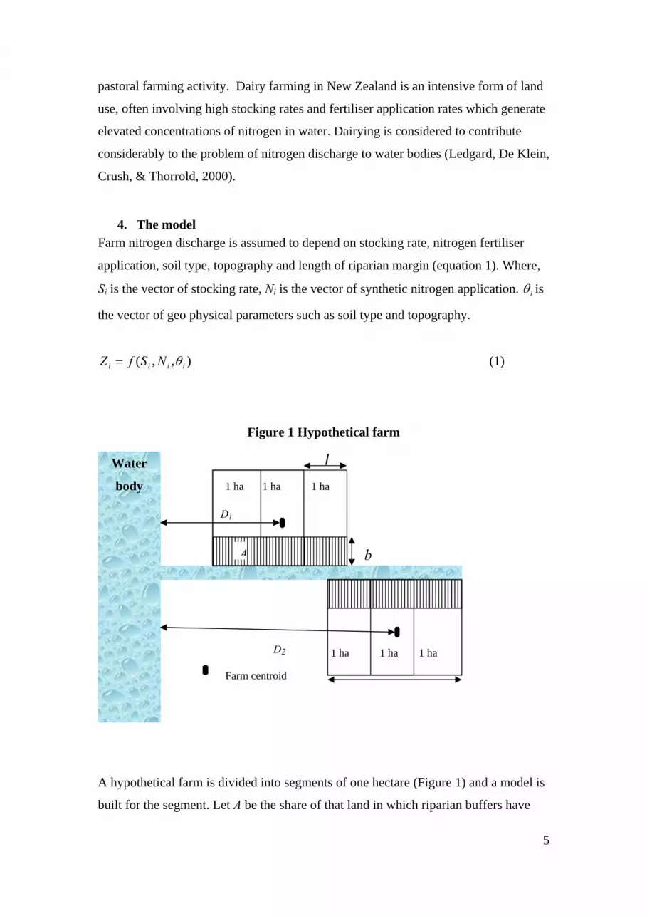
Figure 1 Hypothetical farm

A hypothetical farm is divided into segments of one hectare (Figure 1) and a model is

built for the segment. Let A be the share of that land in which riparian buffers have

Water

body

D1

D2

Farm centroid

l

b

1 ha

A

1 ha 1 ha

1 ha 1 ha 1 ha

6

been established. The extent of riparian buffer depends on length of stream margins

and topography of the land. It is assumed that buffers start at the stream or river’s

border and extend continuously outward away from the banks symmetrically on both

sides of river or stream1. A riparian buffer of extent A is assumed to have constant

width b throughout its length l. In the absence of consistent experimental findings on

the surface/subsurface flow of nitrogen and filtering ability, the following

assumptions are made. Surface and subsurface flow component of nitrogen discharge

is denoted by ϕi, which is assumed to be 25% of farm nitrogen discharged (Zi ) plus a

maximum 25% of Zi depending on the normalised2 value of riparian length per ha3 in

each farm (equation 2). The remaining 50% is lost through leaching.

∫∫ +=%25

0

25.0 iii

MaxL

li ZZLϕ (2)

Riparian buffers are assumed to be capable of removing a maximum of 80% of the

sub surface/surface flow nitrogen. Thus up to 40% of nitrogen discharged is

intercepted. The intercepting ability of a riparian buffer has been modelled by

adapting the functional form used by Lankoski, Lichtenberg, & Ollikainen (2008a).

This functional form is modified by using parameters and specifications from New

Zealand based experimental studies (equation 3).

)*1.01( βϕ ijii bq −= (3)

The maximum recommended buffer width is 5 m for gently rolling landscape and

10m for steeper landscapes. So maximum buffer width is assumed to be 7m.

Topographic differences are not explicitly considered in this analysis of nitrogen

removal efficiency within the buffer strip. However topographic differences are taken

into account when estimating the nitrogen discharges entering the buffer strip. Further

1 Width (b) of the riparian buffer is assumed to be constant for a particular farm type. Therefore the

extent of buffer A translates into the width b of the buffer at that location. 2 Riparian length is divided by maximum of riparian length per ha (404.6 km/ha) 3 It is assumed that runoff and animal contribution are positively related to the riparian length per ha as

it exposes more water to surface flow as well as increases probability for stock crossing.

7

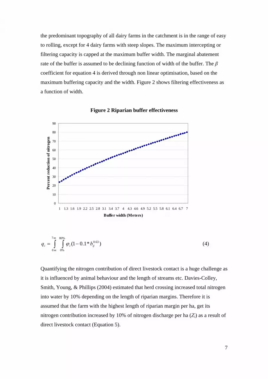
the predominant topography of all dairy farms in the catchment is in the range of easy

to rolling, except for 4 dairy farms with steep slopes. The maximum intercepting or

filtering capacity is capped at the maximum buffer width. The marginal abatement

rate of the buffer is assumed to be declining function of width of the buffer. The β

coefficient for equation 4 is derived through non linear optimisation, based on the

maximum buffering capacity and the width. Figure 2 shows filtering effectiveness as

a function of width.

Figure 2 Riparian buffer effectiveness

0

10

20

30

40

50

60

70

80

90

1 1.3 1.6 1.9 2.2 2.5 2.8 3.1 3.4 3.7 4 4.3 4.6 4.9 5.2 5.5 5.8 6.1 6.4 6.7 7

Buffer width (Meters)

Perc

ent r

educ

tion

of n

itrog

en

)*1.01( 63.07

0

%80

%0iji

m

mi bq −= ∫ ∫ ϕ (4)

Quantifying the nitrogen contribution of direct livestock contact is a huge challenge as

it is influenced by animal behaviour and the length of streams etc. Davies-Colley,

Smith, Young, & Phillips (2004) estimated that herd crossing increased total nitrogen

into water by 10% depending on the length of riparian margins. Therefore it is

assumed that the farm with the highest length of riparian margin per ha, get its

nitrogen contribution increased by 10% of nitrogen discharge per ha (Zi) as a result of

direct livestock contact (Equation 5).

8

∫∫=%10

%0

. ii

LMax

li ZLS (5)

Riparian buffers are assumed to be capable of completely stopping the direct livestock

nitrogen component. Therefore total abatement from riparian buffers can be modelled

as follows (Equation 6)

iiijiiji Szblb ++ )()*1.0( 63.0ϕ (6)

Nitrogen decay function

In order to model the amount of nitrogen received from the farm to the water body

with simplicity and no loss of generality, farms along the single tributary, draining

into the water body are considered. The proportion of nitrogen removed or retained in

the flow path to the main stem of the water body is assumed to be a function of

distance. The functional form and parameters proposed for this decay function by

Skop & Sorensen (1998) were adopted for this study (Equation 7). The rationale for

adopting this functional form is that the longer the distance it takes to transport to the

water body the more nitrate can be removed by denitrification or retained by

accumulation in biomass or sediment. These parameters are constant per unit distance.

The decay process (retention /removal) includes processes that occurred from the time

when nitrogen is discharged until it appears in the main stem of the water body. It is

assumed only leached nitrogen is subject to the decay process. This is consistent with

empirical application of Skop and Sorensen (1998).

iD

i PZ )1(5.0 − (7)

In equation 7, iDyp )1( − , denotes the fraction of nitrogen not retained or removed

from each kg of nitrogen discharged through leaching. P indicates the probability of

nitrogen detention, which is 0.00085 according to Skop and Sorensen (1998). Di is the

distance from the main stem of the water body to the farm centroid4 in km.

4 Centroid is a polygon’s mean center which is based on the weighted average of its x and y coordinates.

9

The total amount of nitrogen potentially delivered to the water body from each farm

can be modelled as follows (Equation 8).

)(])1(5.0[ iiiiiF

i vSqSP i ++−++−=ℜ ϕ (8)

vi is nitrogen discharge averted as a result of converting land into riparian buffers. It

equates to the total area of the strip multiplied by the discharge rates. For

computational convenience the nitrogen discharge from land converted into strip is

assumed to be 0. The total amount of nitrogen reaching the main stem of the water

body can be defined as follows.

∑ℜ=ℜI

iiT i= 1, 2………I farms (9)

Damage function

The environmental damage cost depends on biological and economic parameters such

as habitat degradation and commercial and recreational interests. Water pollution may

affect both local residents and the general public living outside the catchment as

people derive utility from the amenities and services that the water ecosystem

provides. These amenities and services may include good drinking water, scenic lake

views, fishing and other recreational opportunities such as water sporting. Water

pollution may also causes ecosystem damages that are not fully internalised by local

residents. For instance time lags with gradual accumulation of pollutant, impair the

ecosystem, but only generates tangible decline in amenities once it crosses a

threshold.

Most of the bio-economic modeling studies relating to cost aspects of environmental

change and account only for on-farm impacts. Typically these studies consider the

costs of reduced production and additional expenditure to adopt abatement measures

(Bennett, 2005). Modelling the damage function is a complex task. The damage

function of nitrogen discharges can be estimated by means of the value of averting

expenditure and or non market valuation. The averting expenditure valuation method

10

estimates the costs of corresponding nitrogen reduction such as at municipal water

treatment facility. With the non market valuation method the value changes in the

quality of water is assessed through estimated willingness to pay. The choice

modelling approach is commonly used to elicit monetary values. For instance

Mallawaarachchi and Quiggin (2001) used choice-modeling-derived estimates of the

values of different types of remnant vegetation with farm profit estimates in bio-

economic modeling.

Since there is little information available on damage costs of nitrogen discharges in

the New Zealand context, parameter estimates used by Martinez & Albiac (2006) are

adapted as a starting value to model damage function. They used a value equivalent to

NZ $ 2.50 as a cost to remove kg of nitrogen from water using a discontinuous

tertiary biological denitrification treatment. In order to have an increasing function to

reflect the cost of environmental damage, the damage function has been approximated

by an exponential function of nitrogen delivered to the water body (Equation 10).

Total economic damage E (DF) is a function of nitrogen delivered to the water body.

D (0)=0, D’ (TR)=>0, D’’ (TR)=>0. The parameter lambda is the unit emission cost

of nitrogen discharge and is set equal to the cost of removing a kg of nitrogen from

water. λ =2.5. However it does not account for economic damage resulted from

nitrogen discharges from other dimensions other than the perspective of quality

drinking water. k is assumed to be 1.2 . A similar functional form has been used by

Suter, Vossler, Poe, & Segerson (2008) to model damage cost. They assumed k is

equal to 1.5.

k

iDFE )()( ℜ= λ (10)

Optimum buffer width

Nitrogen received by the main stem of the river is assumed to be affected by land use

intensity, land quality and distance, which together determine the effective width of

riparian buffer (Figure 3).

11

Figure 3 Social and private optimum

The private optimum is based on profit maximising behaviour of producers. The

social optimum is derived by incorporating negative externalities associated with

environmental damage. The social optimum involves choosing the riparian buffer

width (bij) and level of changes at intensive margin. The cost of riparian buffers

equals forgone farm income due to land retirement plus the annualised cost of

establishment and maintenance of the buffer.

Nitrogen has been treated as an assimilative pollutant (Tietenberg, 2006b). Therefore

the social optimum of dairy farming is modelled in this paper in a static context.

Nitrogen discharge has also previously been treated as a static problem (Lankoski,

Lichtenberg, & Ollikainen, 2008a).

The cost of achieving reductions in nitrogen delivered can vary because of differences

in production and pollution potential resulting from variations in geophysical factors

and other factors affecting productivity such as management. Dairy farm production

can be modelled as a function of nitrogen discharge (Ramilan, 2008). To estimate

nitrogen discharges, farm choice of nitrogen fertiliser, stocking rate and feed are

Distance from the main water body

Improvement in land quality

Water surface

Forest

Privately

optimal riparian

buffer= 0

Farm land

Farm land use intensity

Socially optimal

riparian buffer

12

considered. Dairy profit function is assumed to be increasing and concave with f `>0

and f ``<0.

[ ] )()1(),( iiiijiii

I

iDFElcblZPfAMax −−−∑ θ (11)

s.t ∑ ℜ=ℜI

ii T

5. Empirical analysis

A virtual population of farms generated using spatial micro-simulation is used for

empirical analysis (described in detail on the chapter 4 (Ramilan, 2008)). Besides the

soil and topographic features and intensity of production, the location of farm and

farm exposure to the streams influence the delivery of nitrogen discharged to surface

water. Stream length within each farm boundary is estimated using the River

Environment Classification (REC) data base. The minimum distance between each

farm and the main stem of the river is calculated by estimating the distance between

the Centeroid of each farm polygon to the main stem of the water body. This distance

is used to calculate the decay function specified in the equation 7. Figure 4 displays

the distribution of farm riparian margins and farm Centeroids.

Figure 4 Farm riparian margins and centeroids

13

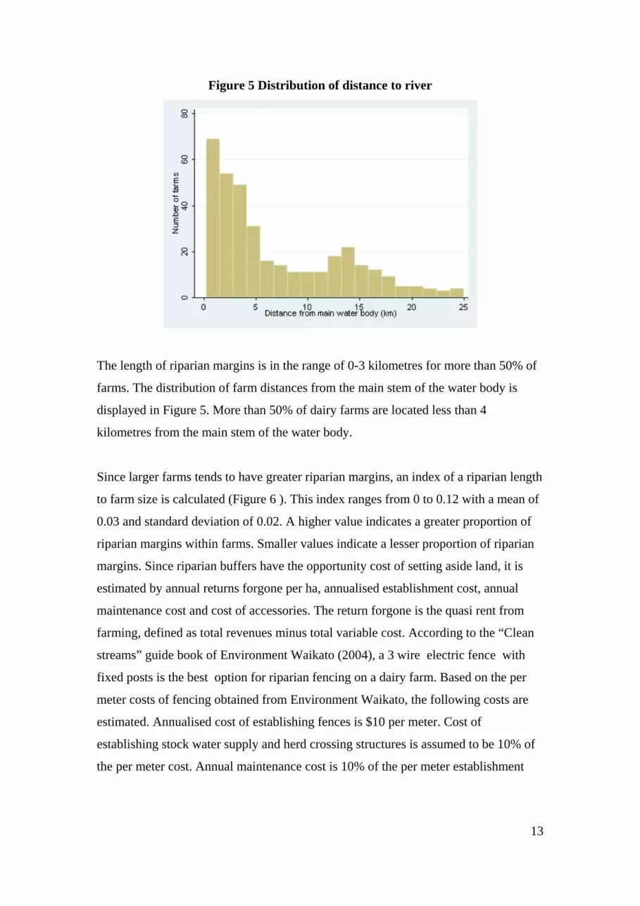
Figure 5 Distribution of distance to river

The length of riparian margins is in the range of 0-3 kilometres for more than 50% of

farms. The distribution of farm distances from the main stem of the water body is

displayed in Figure 5. More than 50% of dairy farms are located less than 4

kilometres from the main stem of the water body.

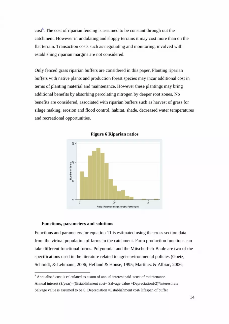
Since larger farms tends to have greater riparian margins, an index of a riparian length

to farm size is calculated (Figure 6 ). This index ranges from 0 to 0.12 with a mean of

0.03 and standard deviation of 0.02. A higher value indicates a greater proportion of

riparian margins within farms. Smaller values indicate a lesser proportion of riparian

margins. Since riparian buffers have the opportunity cost of setting aside land, it is

estimated by annual returns forgone per ha, annualised establishment cost, annual

maintenance cost and cost of accessories. The return forgone is the quasi rent from

farming, defined as total revenues minus total variable cost. According to the “Clean

streams” guide book of Environment Waikato (2004), a 3 wire electric fence with

fixed posts is the best option for riparian fencing on a dairy farm. Based on the per

meter costs of fencing obtained from Environment Waikato, the following costs are

estimated. Annualised cost of establishing fences is $10 per meter. Cost of

establishing stock water supply and herd crossing structures is assumed to be 10% of

the per meter cost. Annual maintenance cost is 10% of the per meter establishment

14

cost5. The cost of riparian fencing is assumed to be constant through out the

catchment. However in undulating and sloppy terrains it may cost more than on the

flat terrain. Transaction costs such as negotiating and monitoring, involved with

establishing riparian margins are not considered.

Only fenced grass riparian buffers are considered in this paper. Planting riparian

buffers with native plants and production forest species may incur additional cost in

terms of planting material and maintenance. However these plantings may bring

additional benefits by absorbing percolating nitrogen by deeper root zones. No

benefits are considered, associated with riparian buffers such as harvest of grass for

silage making, erosion and flood control, habitat, shade, decreased water temperatures

and recreational opportunities.

Figure 6 Riparian ratios

Functions, parameters and solutions

Functions and parameters for equation 11 is estimated using the cross section data

from the virtual population of farms in the catchment. Farm production functions can

take different functional forms. Polynomial and the Mitscherlich-Baule are two of the

specifications used in the literature related to agri-environmental policies (Goetz,

Schmidt, & Lehmann, 2006; Hefland & House, 1995; Martinez & Albiac, 2006; 5 Annualised cost is calculated as a sum of annual interest paid +cost of maintenance.

Annual interest ($/year)=((Establishment cost+ Salvage value +Depreciation)/2)*interest rate

Salvage value is assumed to be 0. Depreciation =Establishment cost/ lifespan of buffer

15

Sumelius, Grgic, Mesic, & Franic, 2005). The Mitscherlich- Baule functional form

has an attractive biological property of growth plateau beyond the input threshold.

The parameters of this function are estimated using the nonlinear regression

procedure in Stata version 10 (StataCorp., 2007). However, this specification quite

frequently presents convergence problems in optimisation (Martinez & Albiac, 2006).

In order to avoid potential difficulties in obtaining numerical solutions, particularly

for the policies emphasizing changes at the intensive margin, the quadratic function is

also estimated. A quadratic functional form presents a maximum yield level, although

it lacks the property of a growth plateau. The empirical functional form derived here

differs distinctly from the approaches of Martinez et al and Goetz et al, as it is in

terms of nitrogen discharge rather than nitrogen fertiliser use. Table 1 presents the

functional forms and estimation results for the Mitscherlich- Baule and quadratic

response functions in terms of nitrogen discharge per ha (Z). Y is milksolids produced

per ha

Table 1 Functional form and parameters

Functional form Mitscherlich- Baule Quadratic

Parameters )1( iZeY δβα −−= 2ZZY δβα ++=

α 2696 (1.96) 258.39 (2.38)

β 0.923 (39.35) 20.91 (4.02)

δ 0.010 (1.21) -0.058

Adj R2 0.95 0.42

*Statistics in parentheses are t statistics.

Average farm profit derived from catchment farms is 1.65 dollars per kg of

milksolids. Livestock contribution is a binary choice variable because in the presence

of fencing, the animal contribution is 0 regardless of the buffer width. However in

order to avoid the complexities in modelling it is treated as a part of runoff.

The maximisation problem stated in the equation 11 is solved by optimizing each

farm individually to derive maximum farm returns and optimum riparian buffer width.

It resulted in 3,620 serial optimisations for 10 scenarios. This serial optimisation

process was automated by developing a macro using visual basic applications, which

16

activated Excel’s built in solver. In another scenario the optimisation is implemented

for varying nitrogen delivery levels without the riparian buffers to quantify the

economic impact of changes at intensive margin.

6. Results and discussion 

Without any agri environmental policy, profit maximising farms will ignore the

damages from ambient pollution and maximise profits. Farms undertake no abatement

effort, because expected damage is not considered. It results in no riparian buffers.

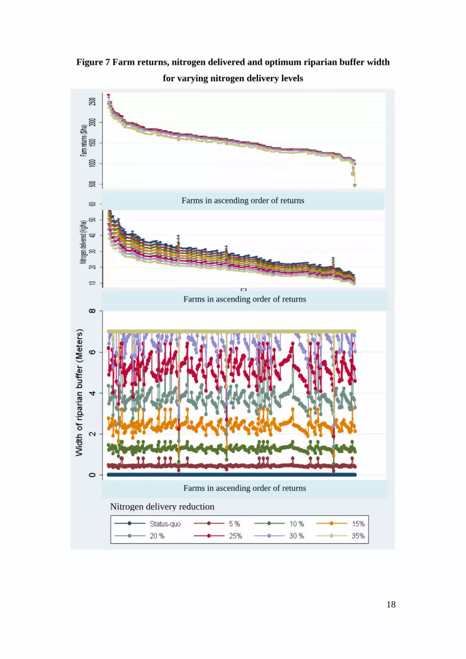
Figure 7 illustrates the pattern of changes in farm profit, optimum riparian width and

nitrogen delivered into the water body for every dairy farm in the catchment.

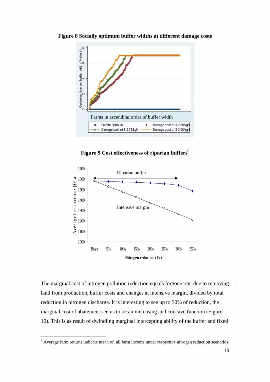
Figure 8 shows the pattern of increase in the optimum width of riparian buffer, when

the damage cost is varied. Higher environmental damage results in greater width,

maximum specified width of buffer become optimum for more farms. Results indicate

that the farm returns vary between 7-10% depending on the level of nitrogen

reduction required to achieve the social optimum, which is determined by the damage

cost. Simulation results for different scenarios are displayed in 2.

17

Table 2 Simulation results

Scenarios Average buffer

size/farm (m2)

Average returns /farm

($)

Nitrogen delivered

(kg)

Private optimum 0 179,370 1,185,169

Social optimum at a

damage cost of

$2.50 KgN 14,287 165,244 888,421

$2.75 KgN 16,022 164,121 871,728

$3.00 KgN 17,555 163,014 858,283

Reduction of

nitrogen delivery by

5 % 1,429 178,787 1,125,356

10 % 4,155 178,360 1,066,487

15 % 7,713 177,802 1,006,992

20 % 11,926 177,140 926,529

25 % 16,692 176,393 888,803

30 % 21,720 174,803 829,618

35 % 23,498 168,039 770,360

When nitrogen delivered to the water body is parametrically restricted the farming

intensity remained unchanged until a 30% reduction (no changes at intensive margin).

Given the assumption of nitrogen retention ability it indicates, riparian buffers are

capable of reducing nitrogen discharges up to 30%. Beyond 30%, the reduction

requires changes at the intensive margin. However riparian buffers are very cost

effective when compared to changes at the intensive margin as the impact on average

farm returns are less (Figure 9). Therefore it is rational to use riparian buffers

complementary to changes at the intensive margin, when higher levels of reduction

are required. In addition the cost of compliance monitoring associated with the

riparian margin is reportedly less because of its visibility and difficulties associated

with reversibility (Lankoski, Lichtenberg, & Ollikainen, 2008a).

18

Figure 7 Farm returns, nitrogen delivered and optimum riparian buffer width

for varying nitrogen delivery levels

Farms in ascending order of returns

Farms in ascending order of returns

Nitrogen delivery reduction

Farms in ascending order of returns

19

Figure 8 Socially optimum buffer widths at different damage costs

Figure 9 Cost effectiveness of riparian buffers6

The marginal cost of nitrogen pollution reduction equals forgone rent due to removing

land from production, buffer costs and changes at intensive margin, divided by total

reduction in nitrogen discharge. It is interesting to see up to 30% of reduction, the

marginal cost of abatement seems to be an increasing and concave function (Figure

10). This is as result of dwindling marginal intercepting ability of the buffer and fixed

6 Average farm returns indicate mean of all farm income under respective nitrogen reduction scenarios

1000

1100

1200

1300

1400

1500

1600

1700

Base 5% 10% 15% 20% 25% 30% 35%

Nitrogen reduction (% )

Ave

rage

farm

ret

urns

($/h

a)

Riparian buffer

Intensive margin

Farms in ascending order of buffer width

20

fencing cost. Marginal abatement cost tremendously increases when abatement is

achieved by changes at the intensive margin. Variations in marginal abatement cost

draws attention towards possible implementation of emission trading schemes, which

may be politically palatable as it includes potential compensation to farms. Socially

optimum nitrogen reduction levels can be a basis to determine target levels of

nitrogen reduction in potential trading programmes. The total number of discharge

permits can be equal to the social optimum measured in terms of nitrogen delivered to

the main water body.

Figure 10 Marginal cost of abatement

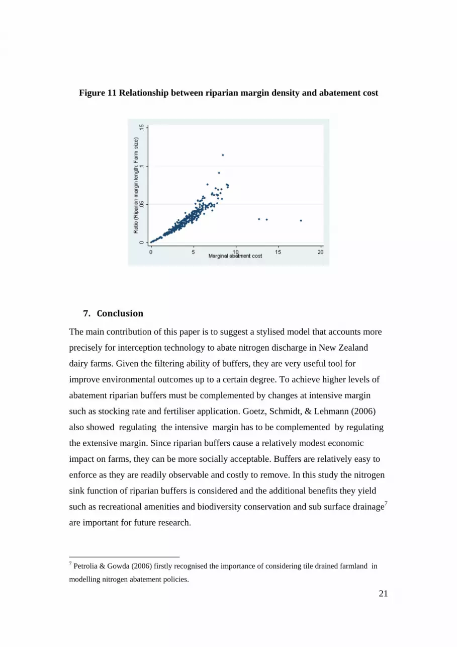
The relationship between riparian ratios (higher ratios indicate greater the length of

riparian margins per unit area) and the marginal cost of abatement at 5 % reduction in

nitrogen delivery is explored (Figure 11). It seems that the cost of abatement is lesser

in farms with a lower ratio. It is some what consistent with the findings of Bontems,

Rotillon, & Turpin (2005), who stated that in France large farms had better ability to

adopt land conservation practices. Perhaps farms with a lower ratio can adopt higher

buffer widths.

0

10

20

30

40

50

60

5% 10% 15% 20% 25% 30% 35%

Scenarios

Cost

($/k

g)

21

Figure 11 Relationship between riparian margin density and abatement cost

 

7. Conclusion 

The main contribution of this paper is to suggest a stylised model that accounts more

precisely for interception technology to abate nitrogen discharge in New Zealand

dairy farms. Given the filtering ability of buffers, they are very useful tool for

improve environmental outcomes up to a certain degree. To achieve higher levels of

abatement riparian buffers must be complemented by changes at intensive margin

such as stocking rate and fertiliser application. Goetz, Schmidt, & Lehmann (2006)

also showed regulating the intensive margin has to be complemented by regulating

the extensive margin. Since riparian buffers cause a relatively modest economic

impact on farms, they can be more socially acceptable. Buffers are relatively easy to

enforce as they are readily observable and costly to remove. In this study the nitrogen

sink function of riparian buffers is considered and the additional benefits they yield

such as recreational amenities and biodiversity conservation and sub surface drainage7

are important for future research.

7 Petrolia & Gowda (2006) firstly recognised the importance of considering tile drained farmland in

modelling nitrogen abatement policies.

22

The stylised model would also be enhanced by more reliable region specific estimates

of buffering capacity and localised estimates of nitrogen decay and damage cost

parameters.

The framework can easily be modified to apply for land retirement schemes or

conservation reserve programmes or establishing wetlands. The natural extension of

this model is to incorporate forest buffers and capture the carbon sequestration

capacity, which likely to enhance nutrient abatement efficiency and economic

viability.

References

Agribusiness Group, Agresearch, NIWA, Crop and Food, & Aqualinc. (2007). Impact of Management Changes on Farm Profitability and Environmental Outcomes. Christchurch.

Bedard-Haughn, A., Tate, K. W., & Kessel, C. (2004). Using nitrogen-15 to quantify vegetative buffer effectiveness for sequestering nitrogen in runoff. Journal of Environmental Quality, 33, 2252-2262.

Bennett, J. (2005). Australasian environmental economics: contributions, conflicts and 'cop-outs'. The Australian Journal of Agricultural and Resource Economics, 49(3), 243-261.

Bontems, P., Rotillon, G., & Turpin, N. (2005). Self-Selecting Agri-environmental policies with an application to the Don watershed. [10.1007/s10640-004-7593-3]. Environmental and Resource Economics, 31(3), 275-301.

Collier, K. J., Davies-Colley, R. J., Rutherford, J. C., Smith, C. M., & Williamson, R. B. (1995). Managing Riparian Zones : a contribution to protecting New Zealand's rivers and streams. Wellington: Department of Conservation.

Davies-Colley, R. J., Smith, R. A., Young, R., & Phillips, C. J. (2004). Water quality impact of dairy cow herd crossing a stream. New Zealand Journal of Marine and Freshwater Research, 38, 596-576.

Environment Waikato. (2004). Clean Streams- A Guide to Managing Waterways on Waikato Farms Hamilton.

Fennessy, M. S., & Cronk, J. K. (1997). The effectiveness and restoration potential of riparian ectones for the management of nonpoint source pollution, particularly nitrate. Critical Reviews in Environmental Science and Technology, 27, 285-317.

Gilliam, J. W. (1994). Riparian wetlands and water quality. Journal of Environmental Quality, 23(3), 896-900.

Gilliam, J. W., Parsons, J. E., & Mikkelsen, R. L. (1997). Nitrogen dynamics and buffer zones. In N. E. Haycok (Ed.), Buffer zones : their process and potential in water protection. Quest Environmental (pp. 54-61). UK: Harpenden.

Goetz, R. U., Schmidt, H., & Lehmann, B. (2006). Determining the economic gains from regulation at the extensive and intensive margins. European Review of Agricultural Economics, 33(1), 1-30.

23

Hefland, G. E., & House, B. W. (1995). Regulating nonpoint source pollution under heterogeneous conditions. American Journal of Agricultural Economics, 77(4), 1024-1032.

Howard-Williams, C. C., & Pickmere, S. (1999). Nutrient and vegetation changes in a retired pasture stream. Recent changes in the context of a long-term dataset. Science for Conservation 114. Wellington.: Department of Conservation.

Lankoski, J., Lichtenberg, E., & Ollikainen, M. (2008a). Agri-Environmental Program Compliance in a Heterogeneous Landscape, WP 08-05. College Park: Department of Agricultural and Resource Economics, The University of Maryland.

Lankoski, J., Lichtenberg, E., & Ollikainen, M. (2008b). Point/nonpoint effluent trading with spatial heterogeneity. American Journal of Agricultural Economics 1-15. DOI: 10.1111/1467-8276.1208.01172.x.

Ledgard, S. F., De Klein, C. A. M., Crush, J. R., & Thorrold, B. S. (2000). Dairy farming, nitrogen losses and nitrate-sensitive areas. Proceedings of the New Zealand Society of Animal Production 60 6, 256-260.

Lowrance, R., Altier, L. S., Newbold, J. D., Schnabel, R. R., Groffman, P. M., Denver, J. M., et al. (1997). Water Quality Functions of Riparian Forest Buffers in Chesapeake Bay Watersheds. Environmental Management, 21(5), 687-712.

Martin, T. L., Kaushik, N. K., Trevors, J. T., & Whitely, H. R. (1999). Review : denitrification in temperate climate riparian zones. Water, Air and Soil Pollution, 111(1-4), 171-186.

Martinez, Y., & Albiac, J. (2006). Nitrate pollution control under soil heterogeneity. Land Use Policy, 23(4), 521-532.

Ministry for the Environment. (2003). Dairying and Clean Streams Accord. Wellington.

Parkyn, S. (2004). Review of Riparian Buffer Zone Effectiveness, Technical Paper No: 2004/05. Wellington: Ministry of Agriculture and Forestry.

Petrolia, D. R., & Gowda, P. H. (2006). Missing the boat: Midwest farm drainage and Gulf of Mexico hypoxia. Review of Agricultural Economics, 28(2), 240-253.

Philippe, G. V., & Hill, A. R. (2006). A landscape based approach to estimate riparian hydrological and nitrate removal functions. Journal of the American Water Resources Association, 42(4), 1099.

Qiu, Z., Prato, T., & Boehm, G. (2006). Economic valuation of riparian buffer and open space in a suburban watershed. Journal of American Water Resources Association, 42, 1583-1596.

Ramilan, T. (2008). Improving Water Quality through Environmental Policies and Farm Management: an Environmental Economics Analysis of Dairy Farming in Karapiro Catchment. Economics, PhD,Thesis, Department of Economics, University of Waikato, New Zealand.

Ribaudo, M. O., Heimlich, R., Claassen, R., & Peters, M. (2001). Least- cost management of nonpoint source pollution: source reduction verses interception strategies for controlling nitrogen loss in the Mississippi Basin. Ecological Economics, 37(2), 183-197.

Skop, E., & Sorensen, P. B. (1998). GIS-based modelling of solute fluxes at the catchment scale: a case study of the agricultural contribution to the riverine nitrogen loading in the Vejle Fjord catchment, Denmark. Ecological Modelling, 106(2-3), 291-310.

24

Stace, C., & Fulton, V. (2003). Riparian protection in the Rotorua lake catchment. In N. E. Miller (Ed.), Practical Management for Good Lake Water Quality. Rotorua: Lake Water Quality Society and the Royal Society of New Zealand.

StataCorp. (2007). Stata Statistical Software: Release 10: College Station, TX: StataCorp LP. .

Sumelius, J., Grgic, Z., Mesic, M., & Franic, R. (2005). Marginal abatement costs for reducing leaching of nitrates in Croatian farming systems. Agricultural and Food Science, 14(3), 293-309.

Suter, J. F., Vossler, C. A., Poe, G. L., & Segerson, K. (2008). Experiments on damage-based ambient taxes for nonpoint source polluters. American Journal of Agricultural Economics, 90(1), 86-102.

Tanner, C. C., Nguyen, M. L., & Sukias, J. P. S. (2005). Nutrient removal by a constructed wetland treating subsurface drainage from grazed dairy pasture. Agriculture, Ecosystems & Environment, 105(1-2), 145-162.

Thomas, S., Ledgard, S., & Francis, G. (2005). Improving estimates of nitrate leaching for quantifying New Zealand’s indirect nitrous oxide emissions. Nutrient Cycling in Agroecosystems, 73(2), 213-226.

Tietenberg, T. H. (2006b). Emissions Trading: Principles and Practice (2nd ed.). Washington, DC: Resources for the Future.

Wilcock, R. J., Monaghan, R. M., Quinn, J. M., Cambell, A. M., Thorrold, B. S., Duncan, M. J., et al. (2006). Land-use impacts and water quality targets in the intensive dairying catchment of the Toenepi stream, New Zealand. New Zealand Journal of Marine and Freshwater Research, 40, 123-140.

Williamson, R. B., Smith, C. M., & Cooper, A. B. (1996). Watershed riparian management and its benefits to a Eutrophic lake. Journal of Water Resources Planning and Management, 122(1), 24-32.