robust scheduling on a single machine using time buffers
TRANSCRIPT

Manuskripte
aus den
Instituten fur Betriebswirtschaftslehre
der Universitat Kiel
Draft Version
Robust Scheduling on a Single Machine using Time Buffers
Dirk Briskorn1,3,∗, Joseph Leung2, Michael Pinedo3
September 2008
1: Christian-Albrechts-Universitat zu KielInstitut fur Betriebswirtschaftslehre
Olshausenstr. 40, 24098 Kiel, Germanyhttp://www.bwl.uni-kiel.de/bwlinstitute/Prod
2: Department of Computer ScienceNew Jersey Institute of Technology
University Heights, Newark, NJ 07102, USAhttp://web.njit.edu/∼leung/
3: Stern School of BusinessNew York University
44 West 4th Street, New York, NY 10012, USAhttp://www.stern.nyu.edu/∼mpinedo
∗: supported by a fellowship within the Postdoc-Programof the German Academic Exchange Service (DAAD)

Abstract
This paper studies the allocation of buffer times in a single machine environment.Buffer times are a common tool to protect the schedule against disruptions such asmachine failures. We introduce new classes of robust machine scheduling problems. Foran arbitrary scheduling problem 1|β|γ, prmt 6∈ β, we obtain three corresponding robustproblems: maximize overall (weighted) buffer time while ensuring a given schedule’sperformance (regarding γ), optimize the schedule’s performance (regarding γ) whileensuring a given minimum overall (weighted) buffer time, and finding the trade offcurve regarding both objectives.
We outline the relationships between the different classes of problems and the corre-sponding underlying problem. Furthermore, we analyze the robust counterparts of threefundamental problems.
Keywords: Single machine scheduling, robustness, buffer time allocation
1 Introduction
In recent years robust optimization has attained more and more attention. While there arelots of formal definitions of robust solutions to an optimization problem (and still there seemsnot to be one single approach) the basic idea can be put in an abstract way like this: Finda feasible solution to the optimization problem at hand that is not necessarily optimal butremains feasible and has a good performance if parameter values of the problem change.Depending on the specific problem the changes of parameters may be restricted to a givendomain or to a subset of parameters. Furthermore, it may depend on the underlying problemto which extent the focus is on solutions that remain feasible or solutions that have goodperformance, respectively. Usually, a solution is called solution-robust if it remains feasible forcertain changes in the problem’s parameters. If, even more, the solutions performance doesnot change for certain changes, the solution is called quality-robust.There are several reasons why robust solutions may be important. Data used in the opti-mization problem may be uncertain. Hence, while solving the problem we cannot consider theproblem that turns out to be the challenge (or at least there is no guarantee that we do so).Moreover, realization of the solutions derived from the optimization problem may be uncertainand, thus, the realization may differ from the plan derived from the optimization problem. Inboth cases it adds considerably to the predictability of the result of the real world process ifour solution is robust.A vast amount of literature on robust optimization can be found, see Ben-Tal and Nemirovski[3, 4] and Kouvelis and Yu [15] for overviews. Most approaches of robust optimization belongto one of the following classes as proposed by Davenport and Beck [10]: First, redundancybased approaches aim at protecting solutions against uncertainty by using less resources ortime slots than are available. In case of disruptions this surplus can be used to follow theactual plan. Second, probabilistic approaches are based on the analysis of probability and theextension of disruptions providing a tool to evaluate solutions’ robustness. Third, contingentsolution approaches come up with a set of solutions being alternatives chosen – and possiblybeing switched in between – during execution.Robust machine scheduling has been considered in several papers, see Aytug et al. [2] for arecent survey. Daniels and Kouvelis [9] propose an approach based on worst-case analysis.Daniels and Carrillo [8] consider the problem to find the schedule that reaches a given perfor-mance (minimization of flow-time) with the maximum likelihood under uncertain processing
1

times. Kouvelis et al. [16] consider a two-machine flow shop where processing times are uncer-tain and the makespan should be minimized. These approaches are scenario based and aim atminimizing the regret of choosing a specific schedule caused by an other schedule performingbetter for a certain scenario.Goren and Sabuncuoglu [11], Herroelen and Leus [13], Leon et al. [19], Leus and Herroelen[20, 21], Mehta and Uzsoy [22], and Wu et al. [26] employ probabilistic analysis to constructpredictive schedules. Predictiveness here means that the expected deviation of the realizedschedule to the intended one is minimized. The deviation is measured either in the schedule’sperformance or in the schedule’s specification (e.g. start times of jobs).Briand et al. [6] consider 1|ri|Lmax and find a set of solutions of equal performance whichallow to switch from one solution to an other while processing. Therefore, it is possible toadapt the schedule to be executed online.A specific redundancy based approach to protect schedules against disruptions is to insert timebuffers between jobs. More specifically, a buffer between two jobs protects the start time ofthe latter job (and, therefore, its finishing time) against delays of the finishing time of theformer one. Time buffer allocation has been studied in the context of project scheduling (e.g.in Al-Fawzan and Haouari [1], Kobylanski and Kuchta [14], Shi et al. [24], and Van de Vonderet al. [25]) as well as in the context of machine scheduling (e.g. in Leus and Herroelen [21]).Leus and Herroelen [21] discuss the problem to allocate buffer such that the sum of weightedexpected deviation of start times is minimum when the makespan (and, therefore, the overallbuffer time) is limited.In this paper we consider a similar concept. However, we consider the minimum (weighted)buffer inserted between a pair of consecutive jobs on a single machine. The insertion ofbuffer times affects two opposed properties of the schedule. We reasonably assume thatrobustness is increasing if the inserted buffers are larger. However, the schedules performance(e.g. makespan) may then worsen. Informal speaking, this gives us two types of optimizationproblems:
• Given a required robustness (measured as minimum (weighted) buffer time) what is thebest performance we can reach?
• Given a requirement for the schedule’s performance what is the maximum robustness(hence the maximum minimum (weighted) buffer time) we can reach?
The remainder of the paper is organized as follows. In Section 2 we formalize a frameworkconcerning buffer allocation for one machine problems. Section 3 focuses on performanceoptimization if a certain degree of robustness is required. The results obtained here are usedin the following Section 4 as a tool box to obtain results for robustness maximization if acertain performance is required. We conclude the paper with a summary of our insights andan overview of future directions for research.
2 Problem Specification
In what follows we restrict ourselves to single machine environments without preemption ofjobs. We consider robust counterparts of machine scheduling problems that can be clas-sified according to the well-known notation introduced by Graham et al. [12] as 1|β|γ,β ⊂ {prec, ri, pi = 1, pj = p, di}, γ ∈ {fmax,
∑
Ci,∑
wiCi,∑
Ti,∑
wiTi,∑
Ui,∑
wiUi}.For a given schedule σ of n jobs let σ(l), 1 ≤ l ≤ n, denote the job in the lth position. Wedefine the buffer time bi related to job i = σ(l), 1 ≤ l ≤ n − 1, as the amount of machine
2

idle time between jobs i and σ(l + 1). Hence bσ(l) = Cσ(l+1) −Cσ(l) − pσ(l+1), 1 ≤ l ≤ n− 1.Furthermore, bσ(n) := 0.The main idea of a buffer time bi between job i and its successor is to protect the starting timeof i’s successor. If completion of i is delayed by p+
i for whatever reason, then the starting timeof its successor is not affected if p+
i ≤ bi. If p+i > bi then the successor cannot start on time
but still its starting time is delayed less than it would be without a buffer. Hence, time buffersare convenient because they do not only provide a certain degree of quality-robustness but firstand foremost the robustness of each single starting time is enhanced. This may be importantif we think of a single machine embedded in an JIT-environment, for example, where tools ormaterial to process jobs are delivered right on time.We propose three surrogate measures for robustness that have to be maximized:
• the minimum buffer time of schedule σ that is defined as Bmσ = min1≤l<n bσ(l),
• the minimum relative buffer time of schedule σ that is defined as Bpσ =
min1≤l<n
(
bσ(l)/pσ(l)
)
, and
• the minimum weighted buffer time of schedule σ that is defined as Bwσ =
min1≤l<n
(
bσ(l)/wbσ(l)
)
.
Each buffer protects the following jobs from disruption. Considering the minimum buffer timeas a robustness measure is motivated by the idea to balance the degree of protection fromdisruption by the preceding job. If we can assume that the probabilities of jobs to be finishedlater than expected as well as the amount of delay are similar, then this minimum buffer timeseems to be an appropriate surrogate measure of robustness.Minimum relative buffer time is motivated by the assumption that the protection for thefollowing job should be correlated with the processing time of the actual job. There may betwo reasons for that. First, we may assume that procedures required to process jobs are moreor less homogeneous and mainly differ in the amount of time necessary. Then, the risk ofmalfunctions at each point of time may be quite the same. However, a job that is processedfor a longer period of time bears a higher risk of failure during its processing. Second, if weassume that procedures of jobs differ reasonably, then more complicated procedures (leadingto larger processing times) may entail a higher probability of malfunction. In both cases it isappropriate to postulate a fixed relation between processing times and corresponding buffer asa surrogate measure.In order to consider the individual risk for each job we propose a minimum weighted buffertime. Here, a buffer weight wb
i is associated with each job i giving the planner an idea of howthe buffers of different jobs should be related to each other. Of course, as by setting wb
i = 1or wb
i = pi we can cover both cases mentioned above.In each case no protection is necessary for disruptions caused by the last job and, hence, weexclude this job from the robustness measures. We want to emphasize that we are awareof the fact that the proposed measures seem to be methodically inferior to several otherproposals in literature. However, the simplicity of the concept may imply opportunities to solvecorresponding optimization problems while for many other robustness measures optimizationproblems are intractable even for the most simplest settings.Moreover, the buffer insertion can be seen as an application of the robustness concept inBertsimas and Sim [5] to machine scheduling. Bertsimas and Sim [5] consider robust solutionsto a linear program. They assume that an interval for each parameter is known where itsactual value is randomnly drawn from. Informally speaking, for given protection parameter Γk
3

for constraint k, the authors consider the set Sk of Γk parameters having the worst impact onfeasibility of a solution if they deviate from the expected value. The authors then formulatethe problem to find the optimal solutions that is feasible even if for each constraint k eachparameter in Sk differs from the expected value to a maximum amount.Although we cannot formulate most scheduling problems as a linear optimization problem wecan apply this idea. Consider the following set of constraints where si and Si is the startingtime and the successor, respectively, of job i:
si + pi ≤ sSi∀i
Since we have only one parameter in each constraint there is no choice to be made whichparameter affects feasibility of a solution most. Suppose that the realization of pi is drawnfrom the interval [pi− p−i , pi + p+
i ] where p is the expected value. Then, obviously, pi + p+i is
the worst case regarding feasibility of a solution. To protect the solution against this case wehave to choose sSi
≥ si + pi + p+i . Note that this can be seen as inserting buffer time bi ≥ p+
i
to protect the start time of job Si.There is an other buffer time related surrogate measure for robustness of a schedule that hasbeen mentioned in the literature, e.g. Al-Fawzan and Haouari [1], namely the sum of all buffertimes. However, in accordance with the reasoning in Kobylanski and Kuchta [14] we refuseto follow this idea. If we consider total buffer time as a robustness measure, the distributionof total buffer time on single buffers is not concerned. Hence, a schedule having only a singlebuffer before the last job is considered as robust as a schedule where the same amount of totalbuffer time is evenly distributed on buffers between each pair of consecutive jobs. However,in the first schedule no job but the last one is protected against disruptions by preceding oneswhile in the second schedule each job is protected (to a certain amount).
5 10 15 20 25
b1 b2 b3i = 1 i = 2 i = 3 i = 4
Figure 1: Schedule σ with Time Buffers
Figure 1 presents an arbitrary schedule σ of 4 jobs. Job 4 is scheduled last. We observe thatBm
σ = 2 since min1≤l<n bσ(l) = min{2, 4, 6} = 2. Furthermore, Bpσ = 1 since
min1≤l<n
bσ(l)
pσ(l)= min
{
1,4
3,6
4
}
= 1.
To illustrate Bwσ let us assume that buffer weights wb
1 = 1, wb2 = 5, and wb
3 = 6 are given.Then, Bp
σ = 0.8 since
min1≤l≤n
bσ(l)
wbσ(l)
= min {2, 0.8, 1} = 0.8.
For a given scheduling problem 1|β|γ we define SmB , Sp
B, and SwB as the subsets of feasible
schedules such that if and only if σ ∈ SmB , σ ∈ Sp
B, and σ ∈ SwB we have Bm
σ ≥ B, Bpσ ≥ B,
and Bwσ ≥ B, respectively. Additionally, we introduce Sγ
γ as the subset of feasible jobs suchthat if and only σ ∈ Sγ
γ the objective value of σ does not exceed γ.
4
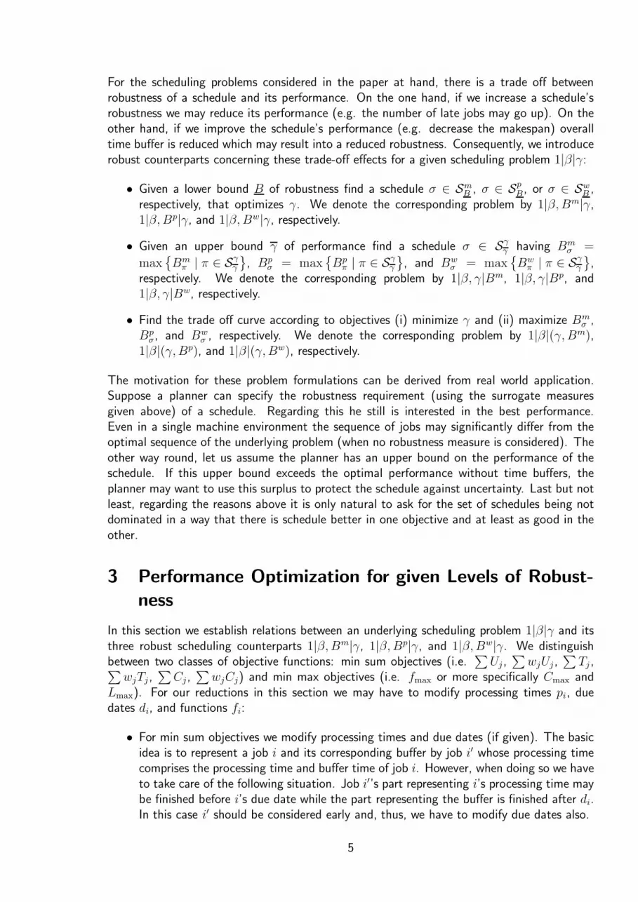
For the scheduling problems considered in the paper at hand, there is a trade off betweenrobustness of a schedule and its performance. On the one hand, if we increase a schedule’srobustness we may reduce its performance (e.g. the number of late jobs may go up). On theother hand, if we improve the schedule’s performance (e.g. decrease the makespan) overalltime buffer is reduced which may result into a reduced robustness. Consequently, we introducerobust counterparts concerning these trade-off effects for a given scheduling problem 1|β|γ:
• Given a lower bound B of robustness find a schedule σ ∈ SmB , σ ∈ Sp
B, or σ ∈ SwB ,
respectively, that optimizes γ. We denote the corresponding problem by 1|β, Bm|γ,1|β, Bp|γ, and 1|β, Bw|γ, respectively.
• Given an upper bound γ of performance find a schedule σ ∈ Sγγ having Bm
σ =
max{
Bmπ | π ∈ S
γγ
}
, Bpσ = max
{
Bpπ | π ∈ S
γγ
}
, and Bwσ = max
{
Bwπ | π ∈ S
γγ
}
,respectively. We denote the corresponding problem by 1|β, γ|Bm, 1|β, γ|Bp, and1|β, γ|Bw, respectively.
• Find the trade off curve according to objectives (i) minimize γ and (ii) maximize Bmσ ,
Bpσ, and Bw
σ , respectively. We denote the corresponding problem by 1|β|(γ, Bm),1|β|(γ, Bp), and 1|β|(γ, Bw), respectively.
The motivation for these problem formulations can be derived from real world application.Suppose a planner can specify the robustness requirement (using the surrogate measuresgiven above) of a schedule. Regarding this he still is interested in the best performance.Even in a single machine environment the sequence of jobs may significantly differ from theoptimal sequence of the underlying problem (when no robustness measure is considered). Theother way round, let us assume the planner has an upper bound on the performance of theschedule. If this upper bound exceeds the optimal performance without time buffers, theplanner may want to use this surplus to protect the schedule against uncertainty. Last but notleast, regarding the reasons above it is only natural to ask for the set of schedules being notdominated in a way that there is schedule better in one objective and at least as good in theother.
3 Performance Optimization for given Levels of Robust-
ness
In this section we establish relations between an underlying scheduling problem 1|β|γ and itsthree robust scheduling counterparts 1|β, Bm|γ, 1|β, Bp|γ, and 1|β, Bw|γ. We distinguishbetween two classes of objective functions: min sum objectives (i.e.
∑
Uj ,∑
wjUj ,∑
Tj ,∑
wjTj ,∑
Cj,∑
wjCj) and min max objectives (i.e. fmax or more specifically Cmax andLmax). For our reductions in this section we may have to modify processing times pi, duedates di, and functions fi:
• For min sum objectives we modify processing times and due dates (if given). The basicidea is to represent a job i and its corresponding buffer by job i′ whose processing timecomprises the processing time and buffer time of job i. However, when doing so we haveto take care of the following situation. Job i′’s part representing i’s processing time maybe finished before i’s due date while the part representing the buffer is finished after di.In this case i′ should be considered early and, thus, we have to modify due dates also.
5

• For min max objectives we do the same modifications as mentioned above. Additionally,we have to consider function fi. Function fi is a function of job i’s completion timeand, moreover, i’s due date may be involved. So, in the first case we have to ensure thatfi′(Ci′) = fi(Ci′− (pi′−pi)) and in the second case fi′(Ci′, di′) = fi(Ci′− (pi′−pi), di)must hold. Basically, this says that the functions values for i and i′ for the same startingpoints have to be the same.
5 10 15 20 25
σp b1 b2 b3 b4i = 1 i = 2 i = 3 i = 4
σm b1 b2 b3 b4i = 1 i = 2 i = 3 i = 4
σ i = 1 i = 2 i = 3 i = 4
Figure 2: Sketch of reduction technique
Figure 2 presents three schedules that are related to one another. Schedule σ is the solutionto an underlying scheduling problem having no time buffers. Schedule σm represents thecorresponging solution to the robust counterpart considering minimum buffer time. In thiscase Bm = 1. Schedule σp represents the corresponging solution to the robust counterpartconsidering minimum relative buffer time (Bm = 0.75).First, to provide some intuition for the basic technique used in all proofs in this sectionwe determine as an example the complexity status of 1|pj = p; rj; B
m|∑
Tj and 1|pj =p; rj; B
w|∑
Tj . Afterwards, we give proofs for more general results.
Lemma 1. 1|pj = p; rj ; Bw|
∑
Tj is strongly NP -hard.
Proof. We prove the complexity of 1|pi = p; ri; Bw|
∑
Ti by reduction from 1|ri|∑
Ti which,as a generalization of 1|ri|Lmax, is known to be strongly NP -hard.For a given instance P of 1|ri|
∑
Tj we construct an instance P w as follows. We retain allparameters but pi and di and set p′i = p′ = minj{pj} as well as d′
i = di − pi + p′. Note thatwe obtain identical processing times. Furthermore, we set wb
i = (pi − p′)/p′ and Bw = 1.We find an optimal solution σ to P from σw to P w as follows. We set Ci = C ′
i − p′ + pi.First, we obeserve that σ is feasible to P . Let i be an arbitrary job that is not scheduled lastand let s(i) be i’s immediate successor. Then,
Cs(i) − Ci = C ′s(i) − p′ + ps(i) − C ′
i + p′ − pi
≥ C ′i + p′wb
iBw + p′ − p′ + ps(i) − C ′
i + p′ − pi (1)
= pi − p′ + ps(i) + p′ − pi = ps(i)
Suppose there is a better schedule σw for P w. We construct a better schedule σ for P bysetting C ′
i = Ci + p′ − pi. For corresponding solutions for P w and P objective values areidentical since
6

Ci − di = C ′i − p′ + pi − d′
i − pi + p′ = C ′i − d′
i.
Hence, σ is better than σ and σ can therefore not be optimal.
In the following, we use the reduction techniques to determine relationships between underlyingproblems and their robust counterparts in a setting that is more general than the one inLemma 1.
Theorem 1. Problems 1|β, Bm|γ and 1|β, Bp|γ are equivalent even if Bm > 0 and Bp > 0.
Proof. The proof is done in two steps: First, we reduce 1|β, Bm|γ to 1|β, Bp|γ and we dothe reverse afterwards. We distinguish between two cases.
• Case (i): Processing times are arbitrary, that is β ∩ {pi = p, pi = 1} = ∅.
• Case (ii): Processing times of all jobs are equal, that is {pi = p} ∈ β or {pi = 1} ∈ β.
Let P m be an arbitrary instance of 1|β, Bm|γ. We construct an instance P p of 1|β, Bp|γ asfollows. We preserve all problem’s characteristics but pi, di, and fi, i ∈ {1, . . . , n}. In case(i) we set p′i = (pi + Bm)/2, d′
i = di + (Bm − pi)/2, f ′i(C
′i, d
′i) = fi(C
′i − (Bm − pi)/2, di),
and Bp = 1. In case (ii) we set p′ = p, d′i = di, and f ′
i = fi as well as Bp = (Bm)/p.We derive a solution σm to P m from an optimal solution σp to P p by setting Ci = C ′
i+p′i−Bm
in case (i) and Ci = C ′i in case (ii).
Note that in case (i) we have b′i/p′i ≥ Bp
σp = 1 for each i 6= σp(n) while in case (ii) we haveb′i/p
′i ≥ Bp
σp = Bm/pi for each i 6= σp(n). Now we can see that solution σm is feasible to P m.Let i be an arbitrary job that is not scheduled last and let s(i) be i’s immediate successor.In case (i),
Cs(i) − Ci = C ′s(i) + p′s(i) −Bm − C ′
i − p′i + Bm
≥ C ′i + p′i + p′s(i) + p′s(j) − C ′
i − p′i (2)
= 2p′s(i) = ps(i) + Bm
while in case (ii),
Cs(i) − Ci = C ′s(i) − C ′
i
≥ C ′i + pi
Bm
pi
+ ps(i) − C ′i (3)
= ps(i) + Bm.
Furthermore, in case (i)
Ci − di = C ′i + p′i −Bm − d′
i +Bm − pi
2
= C ′i +
pi + Bm
2−Bm − d′
i +Bm − pi
2(4)
= C ′i − d′
i
while, trivially, Ci−di = C ′i−d′
i in case (ii). Note that lateness Ci−di may concern feasibilityor performance. So, feasibility of σm is given. If the γ performance is based on lateness,
7

obviously the performances of σm and σp are identical. The same holds for general fmax dueto the modification of fi. Finally, if γ ∈ {
∑
Ci,∑
wiCi}, solutions σm and σp have objectivevalues that differ by a constant that does not depend on the solutions, that is
γ(σp) =∑
j
wjC′j
=∑
j
wjCj −∑
j
(p′j −Bm)wj (5)
= γ(σm)−∑
j
(p′j − Bm)wj
in case (i) and γ(σp) =∑
j wjC′j =
∑
j wjCj = γ(σm) otherwise.Suppose there is a solution σm that is better than σm. Then, we can construct a feasiblesolution σp by letting C ′
j = Cj − p′j + Bm in case (i) and C ′j = Cj otherwise. Using (2), (3),
(4), and (5) it is easy to show that σp is better than σp.Now, let P p be an arbitrary instance of 1|β, Bp|γ. We construct an instance P m of 1|β, Bm|γas follows. We preserve all problem’s characteristics but pi, di, and fi, i ∈ {1, . . . , n}. Incase (i), we set Bm = mini {pi}, p′i = pi (1 + Bp) − Bm, d′
i = di + piBp − Bm, and
f ′i(C
′i, d
′i) = fi(C
′i + Bm − piB
p, di). In case (ii), we set p′ = p, d′i = di, and f ′
i = fi as wellas Bp = Bm/p.We derive a solution σp to P p from an optimal solution σm to P m by setting Ci = C ′
i +Bm−piB
p in case (i) and Ci = C ′i otherwise. Based on the same arithmetics as in (2), (3), (4),
and (5) it is easy to show that σp must be optimal for P p.
Theorem 2. If processing times are not restricted to unit processing times, then problems1|β|γ, 1|β, Bm|γ and 1|β, Bp|γ are equivalent even if Bm > 0 and Bp > 0.
For proofs to Theorems 2 to 5 we only give reductions. All arithmetics to prove feasibility andoptimality are analogous to (2), (3), (4), and (5). Regarding Theorem 1 we restrict ourselvesto show that 1|β|γ and 1|β, Bm|γ are equivalent to prove Theorem 2.
Proof. First, we reduce 1|β, Bm|γ to 1|β|γ. Let P m be an arbitrary instance of 1|β, Bm|γ. Weconstruct an instance P of 1|β|γ as follows. We preserve all problem’s characteristics but pi, di,and fi, i ∈ {1, . . . , n}. We set p′i = pi +Bm, d′
i = di +Bm, and f ′i(C
′i, d
′i) = fi(C
′i−Bm, di).
We derive a solution σm to P m from an optimal solution σ to P by setting Ci = C ′i − Bm.
Now, we reduce 1|β|γ to 1|β, Bm|γ. Let P be an arbitrary instance of 1|β|γ. We constructan instance P m of 1|β, Bm|γ as follows. We preserve all problem’s characteristics but pi,di, and fi, i ∈ {1, . . . , n}. We set Bm = (mini pi)/2, p′i = pi − Bm, d′
i = di − Bm, andf ′
i(C′i, d
′i) = fi(C
′i + Bm, di). We derive a solution σ to P from an optimal solution σm to
P m by setting Ci = C ′i + Bm.
Theorem 3. If pi = 1, then problems 1|β, Bp|γ, 1|β, Bm|γ, and 1|β ′|γ are equivalent whenβ ′ restricts all processing times to be equal (but not necessarily unit).
Proof. The reduction of 1|β, Bm|γ to 1|β ′|γ is analogous to the one in the proof of Theorem 2.Note that p′j = p holds for all processing times. The reduction of 1|β ′|γ to 1|β, Bm|γ is doneas follows. If p < 1, then we can multiply all processing times and – if considered – duedates and release dates by a constant k such that kp ≥ 1. Then, we set Bm = p − 1,p′i = p−Bm = 1, d′
i = di −Bm, and f ′i(C
′i, d
′i) = fi(C
′i + Bm, di).
8

Theorem 4. If processing times are arbitrary, then problems 1|β|γ, 1|β, Bm|γ, 1|β, Bp|γ, and1|β, Bw|γ are equivalent even if Bm > 0 and Bp > 0.
Regarding Theorem 2 we restrict ourselves to show that 1|β|γ and 1|β, Bw|γ are equivalent.
Proof. First, we reduce 1|β, Bw|γ to 1|β|γ. Let P w be an arbitrary instance of 1|β, Bw|γ.We construct an instance P of 1|β|γ as follows. We preserve all problem’s characteristics butpi, di, and fi, i ∈ {1, . . . , n}. We set p′i = pi(1 + wb
i ), d′i = di + piw
bi , and f ′
i(C′i, d
′i) =
fi(C′i − piw
bi , di). We derive a solution σw to P w from an optimal solution σ to P by setting
Ci = C ′i − piw
bi .
Note that 1|β, Bw|γ is a generalization of 1|β, Bp|γ. Due to Theorem 2 1|β|γ can be reducedto 1|β, Bw|γ.
Theorem 5. If pi = p, then problems 1|β, Bw|γ and 1|β ′|γ are equivalent even if Bw > 0when β ′ implies arbitrary processing times.
Proof. First, we reduce 1|β, Bw|γ to 1|β ′|γ in analogy to the reduction in the proof to Theo-rem 4.Now, we reduce 1|β ′|γ to 1|β, Bw|γ. Let P be an arbitrary instance of 1|β ′|γ. We construct aninstance P w of 1|β, Bw|γ as follows. We preserve all problem’s characteristics but pi, di, andfi, i ∈ {1, . . . , n}. We set p′i = (mini{pi})/2, wb
i = (pi − p′i)/p′i, Bm = 1, d′
i = di − pi + p′i,and f ′
i(C′i, d
′i) = fi(C
′i + pi − p′i, di). Note that we have no restriction for pi. We derive a
solution σ to P from an optimal solution σm to P m by setting Ci = C ′i − p′i + pi.
Remark 1. Using the techniques employed above it is easy to see that 1|β, Bw|γ and1|β ′, Bw|γ when β and β ′ imply pj = 1 and pj = p are equivalent.
Summarizing Theorems 1 to 5, we can provide strong results for the computational complexityof the robust counterparts of the single machine scheduling problem 1|β|γ when the robustnessis given.
• 1|β, Bm|γ, 1|β, Bp|γ, and 1|β|γ are equivalent unless pj = 1
• 1|β, Bm|γ, 1|β, Bp|γ, and 1|β ′|γ are equivalent for β implying unit processing times andβ ′ implying equal (but not necessarily unit) processing times
• 1|β, Bm|γ, 1|β, Bp|γ, 1|β, Bw|γ, and 1|β|γ are equivalent unless {pj = p} ∈ β
• 1|β, Bm|γ, 1|β, Bp|γ, 1|β, Bp|γ, and 1|β ′|γ are equivalent for {pj = p} ∈ β andβ ′ = β \ {pi = p}
Figure 3 illustrates the reducability of the classes of problems considered in this section.Each node represents the class of problems specified by the structure of processing timescorresponding to the column and the robustness measure corresponding to the row. Notethat 1|β|γ represents the underlying problem. The label at each arrow outlines the Theoremproviding the relationship represented by the arrow. Here, “Gen.” and “Rem. 1” refer toa trivial generalization and Remark 1, respectively. The dashed lines partition the problemclasses into three equivalence classes.Hence, in most cases if the underlying problem is known to be solvable in polynomial time,we can solve the robust counterpart where robustness is given using the algorithms for theunderlying problem. This, does not hold in general for underlying problems where processingtimes are restricted. In particular,
9

1|β|γ
1|β, Bm|γ
1|β, Bp|γ
1|β, Bw|γ
pj = 1 pj = p pj
1
2
1
2
1
4
5
Rem. 1
3
Gen.
Gen.
Figure 3: Equivalence Graph
1. 1|prec; pi = p; ri|Lmax,
2. 1|prec; pi = p; ri|∑
Cj ,
3. 1|pi = p; ri|∑
wjCj,
4. 1|pi = p; ri|∑
wjUj , and
5. 1|pi = p; ri|∑
Tj
are polynomially solvable, see Brucker [7]. However,
1. 1|prec; pi = p; ri; Bw|Lmax,
2. 1|prec; pi = p; ri; Bw|
∑
Cj,
3. 1|pi = p; ri; Bw|
∑
wjCj ,
4. 1|pi = p; ri; Bw|
∑
wjUj , and
5. 1|pi = p; ri; Bw|
∑
Tj
are equivalent to the corresponding problems with arbitrary processing times that are knownto be strongly NP -hard, see Brucker [7].
4 Robustness Optimization for a required Performance
Level
In this section we consider the three robust counterparts 1|β, γ|Bm, 1|β, γ|Bp, and 1|β, γ|Bw.The main issue is here that the order of jobs is not fixed but depends on the degree of robustnessas we can illustrate with a rather simple example.
10
5 10 15 20 25
σ1 b1 b2b3i = 1 i = 2i = 3 i = 4
σ0.5 b1 b2 b3i = 1 i = 2 i = 3 i = 4
σ0 i = 1 i = 2 i = 3 i = 4
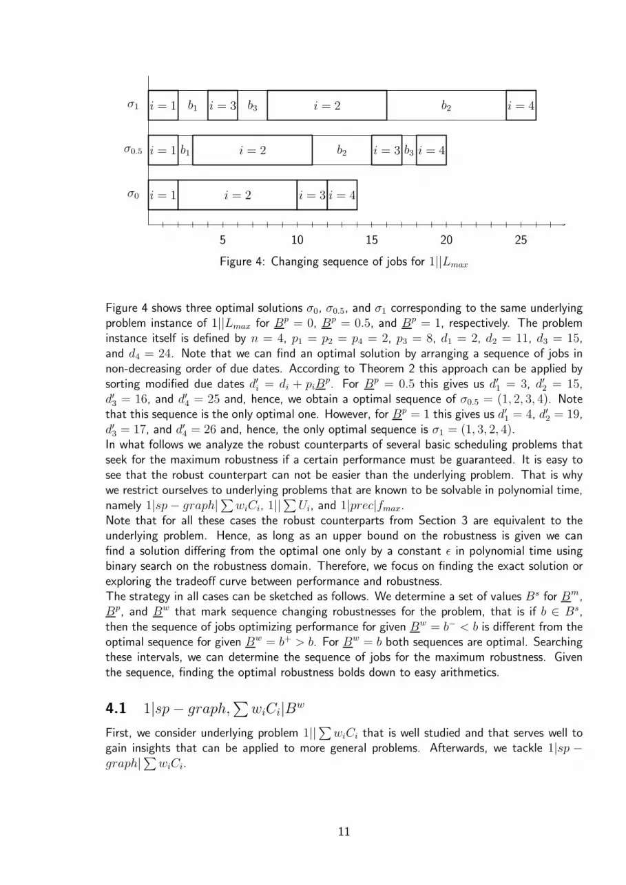
Figure 4: Changing sequence of jobs for 1||Lmax
Figure 4 shows three optimal solutions σ0, σ0.5, and σ1 corresponding to the same underlyingproblem instance of 1||Lmax for Bp = 0, Bp = 0.5, and Bp = 1, respectively. The probleminstance itself is defined by n = 4, p1 = p2 = p4 = 2, p3 = 8, d1 = 2, d2 = 11, d3 = 15,and d4 = 24. Note that we can find an optimal solution by arranging a sequence of jobs innon-decreasing order of due dates. According to Theorem 2 this approach can be applied bysorting modified due dates d′
i = di + piBp. For Bp = 0.5 this gives us d′
1 = 3, d′2 = 15,
d′3 = 16, and d′
4 = 25 and, hence, we obtain a optimal sequence of σ0.5 = (1, 2, 3, 4). Notethat this sequence is the only optimal one. However, for Bp = 1 this gives us d′
1 = 4, d′2 = 19,
d′3 = 17, and d′
4 = 26 and, hence, the only optimal sequence is σ1 = (1, 3, 2, 4).In what follows we analyze the robust counterparts of several basic scheduling problems thatseek for the maximum robustness if a certain performance must be guaranteed. It is easy tosee that the robust counterpart can not be easier than the underlying problem. That is whywe restrict ourselves to underlying problems that are known to be solvable in polynomial time,namely 1|sp− graph|
∑
wiCi, 1||∑
Ui, and 1|prec|fmax.Note that for all these cases the robust counterparts from Section 3 are equivalent to theunderlying problem. Hence, as long as an upper bound on the robustness is given we canfind a solution differing from the optimal one only by a constant ǫ in polynomial time usingbinary search on the robustness domain. Therefore, we focus on finding the exact solution orexploring the tradeoff curve between performance and robustness.The strategy in all cases can be sketched as follows. We determine a set of values Bs for Bm,Bp, and Bw that mark sequence changing robustnesses for the problem, that is if b ∈ Bs,then the sequence of jobs optimizing performance for given Bw = b− < b is different from theoptimal sequence for given Bw = b+ > b. For Bw = b both sequences are optimal. Searchingthese intervals, we can determine the sequence of jobs for the maximum robustness. Giventhe sequence, finding the optimal robustness bolds down to easy arithmetics.
4.1 1|sp− graph,∑
wiCi|Bw
First, we consider underlying problem 1||∑
wiCi that is well studied and that serves well togain insights that can be applied to more general problems. Afterwards, we tackle 1|sp −graph|
∑
wiCi.
11

4.1.1 1|∑
wiCi|Bw
It is well known that an optimal solution to this problem can be found by sorting jobs in non-increasing order of pi/wi. Regarding Theorem 4, 1|Bw|
∑
wiCi can be solved by reducing itto 1||
∑
wiCi where processing times are defined as p′i = pi + wbiB
w. Thus, we derive theoptimal order of jobs for given robusteness by sorting (pi + wb
iBw)/wi. Furthermore, we can
see the optimal performance as a non-decreasing function of the required robustness.We determine
Bs =
{
b | b =piwj − pjwi
wiwbj − wjwb
i
> 0, i < j
}
and sort this set according to non-decreasing values. Note that |Bs| ∈ O(n2). Let bk,k ∈ 1, . . . , |Bs| be the kth value in Bs. Applying binary search on Bs, we can find the smallestvalue bk∗ in Bs such that the optimal solution value to 1|Bw|
∑
wiCi with Bw = bk∗ exceedsγ. Then, the sequence of jobs corresponding to the interval [bk∗−1, bk∗ ] is the sequence ofjobs for maximum robustness. For a given sequence σ of jobs we can determine the maximumrobustness as a function of γ:
Bw(γ, σ) =γ −
∑
i wi
∑
j≤i pj∑
i wi
∑
j<i wbj
(we assume that jobs are numbered according to σ). The computational complexity of thisprocedure is O(n2 log n).Instead of finding the optimal robustness for a specific given γ we may be interested in findingthe trade off curve between robustness and total weighted completion time. In the following,we give an algorithm to find the tradeoff curve represented by function Bw(γ). The procedureresembles the one described above except for Bs being searched sequentially.
Algorithm 1
1. find and sort Bs
2. find the optimal sequence σ for 1||∑
wiCi and corresponding optimal solution value v∗0
3. in [0, v∗0[ the tradeoff curve is not defined
4. for k = 1, . . . , |Bs|
(a) find the optimal solution value v∗k for 1|Bw|
∑
wiCi where Bw = bk
(b) in [v∗k−1, v
∗k[ the tradeoff curve is given by linear function Bw(γ) = Bw(γ, σ)
(c) modify σ by switching the jobs bk corresponds to
(d) k ← k + 1
5. in [b|Bs|,∞[ the tradeoff curve is given by linear function Bw(γ) = Bw(γ, σ)
Obviously, the algorithm finds all optimal sequences and, therefore, the whole tradeoff curvein O(n2 log n). The complexity is not higher than the one for solving 1|Bw|
∑
wiCi becausein both cases sorting Bs takes the most effort.In order to illustrate the connection between we give the following example. Let us supposewe have a set of jobs I = {1, 2, 3}. We have pi = i and wi = 1 for each 1 ≤ i ≤ 3, and
12

b
b
b
b
b
b
10 11 12 13 14 15 16 17 18 19 20 21 22 23 24 250
0.15
0.30
0.45
0.60
0.75
0.90
1.05
1.20
1.35
1.50
Bw
γ
Figure 5: Trade Off Curve for 1||(∑
Ci, Bw)
wb1 = 3.5, wb
2 = 1.5 and wb3 = 0.5. We then have Bs = {0.5, 2/3, 1}. Figure 5 illustrates the
the graph corresponding to the trade off curve as the solid line. Break points are dotted andcorrespond to jobs 1 and 2, jobs 1 and 3, and jobs 2 and 3 switching in the optimal sequence.Note that the trade off curve is piecewise linear and convex which can also be observed fromthe formal expression of Bw(γ). Due to the definition of Bs jobs i′ and j′, pi′/wi′ < pj′/wj′,can switch positions in the optimal sequence only if wi′w
bj′ −wj′w
bi′ < 0. Let σ and σ′ be the
sequences before and after the switch. Then,
n∑
i=1
wσ′(i)
i−1∑
j=1
wbσ′(j) −
n∑
i=1
wσ(i)
i−1∑
j=1
wbσ(j) = wi′w
bj′ − wj′w
bi′ < 0.
Note that for special case 1|Bp|∑
wiCi we have Bs = ∅ which means that each optimalsequence of jobs for Bp = 0 is optimal for each Bp > 0. Hence, in this case finding thetardeoff curve can be done in O(n logn).
4.1.2 1|sp− graph,∑
wiCi|Bw
First, we give a brief overview of the algorithm for 1|sp−graph|∑
wiCi by Lawler [18]. For agiven problem the algorithm does a series of comparisons of values pi/wi. However, the exactvalues are of no importance as far as sequencing is concerned since it only decides which oftwo values is larger. In each iteration the algorithm may form a composite job (i, j) from twojobs i and j that is defined by p(i,j) = pi + pj and w(i,j) = wi + wj. This is why, in contrastto Section 4.1.1, it is not sufficient to consider
Bs =
{
b | b =piwj − pjwi
wiwbj − wjwb
i
> 0, i < j
}
to find all values of Bw leading to changing optimal sequences.
13

We pick up the example of Section 4.1.1 and add a single precedence constraint requiringthat 2 cannot precede 1. Considering the decomposition tree we can see that 2 follows 1immediately in each optimal sequence. Therefore, only optimal sequences are σ1 = (1, 2, 3)and σ2 = (3, 1, 2). It turns out that σ1 = (1, 2, 3) provides a better schedule for Bw < 0.75and that σ2 = (1, 2, 3) provides a better schedule for Bw > 0.75. However, 0.75 6∈ Bs. InFigure 5 we represent the corresponding trade off curve as dashed line. Note that in the firstsection both trade off curves are identical due to identical optimal sequences. However, incontrast to Section 4.1.1 jobs 1 and 2 can not switch and from this point both trade off curvesare different.The reason for this effect is that composite job (i, j) replaces simple jobs i and j whenever itis decided that j follows i immediately. In our case, (1, 2) replaces 1 and 2. Then, comparing
p1 + wb1B
w + p2 + wb2B
w
w1 + w2
top3 + wb
3Bw
w3
gives the result that 3 should precede (1, 2) for Bw > 0.5. An extension of Bs covering allsequence changing robustnesses could be defined as
B′s =
{
b | b =pI′wI′′ − pI′′wI′
wI′wbI′′ − wI′′wb
I′
> 0, I ′, I ′′ ⊂ I
}
where pI′ =∑
i∈I′ pi, wI′ =∑
i∈I′ wi, and wbI′ =
∑
i∈I′ wbi . However, since |B′s| ∈ O(22n)
we can not sort it in polynomial time.Taking this into account, our algorithm works in a stepwise manner mimicking the algorithmby Lawler [18]. We determine Bs,1 which is identical to Bs in Section 4.1.1 and sort this setaccording to non-decreasing values. After having determined b1
k∗ (analogue to bk∗) we obtaina unique ordering of values
pi + wbib
1k∗−1
wi
, i ∈ I1 = I
which allows us to execute at least one step of the algorithm by Lawler [18]. As soon as acomposite job (i, j) is created, we have to consider the modified set of jobs I2 = I1 \ {i, j}∪{(i, j)} starting the procedure all over again. More specifically, the algorithm can be given asfollows.
Algorithm 2
1. I1 ← I
2. for k ← 1
3. repeat
(a) find and sort Bs,k according to Ik
(b) find bkk∗ using binary search on Bs,k and the algorithm by Lawler [18]
(c) having a unique ordering of jobs in Ik execute one step of the algorithm by Lawler[18]
(d) if no composite job is created go to Step 3c
(e) if a composite job is created obtain set of jobs Ik+1 by adding the composite joband dropping all jobs being contained in the composite job from Ik
14

(f) if only one node is left in the decomposition tree go to Step 4
(g) k ← k + 1
4. extract optimal sequence σ from the remaining job
5. obtain maximum robustness as Bw(γ, σ)
Note that determining Bs,l, l > 1, takes less effort than determining Bs,1. Since we restrictourselves to robustness values within [bl−1
k∗−1, bl−1k∗ [ we consider
Bs,2 =
{
b | bl−1k∗−1 ≤ b =
p(i,j)w′i − p′iw(i,j)
w(i,j)w′bi − w′
iwb(i,j)
< bl−1k∗ , i′ ∈ I1 \ {i, j}
}
and obtain |Bs,l| ∈ O(n).Correctness of our algorithm follows from correctness of the algorithm for 1|sp−graph|
∑
wiCi
and the fact that sequencing is based only on elementary steps of deciding which of two valuespi/wi and pi/wi is larger.Computational complexity of our algorithm can be determined as follows. Finding and sortingBs,1 takes O(n2 log n). Employing binary search and the algorithm by Lawler [18] to find b1
k∗
costs O(n log2 n). Since |Bs,l| ∈ O(n), l > 1, computational effort to determine and sort Bs,l
in following iterations is O(n log n). Furthermore, finding blk∗ costs O(n log2 n) again. Since
we have no more than n iterations overall complexity is O(n2 log2 n).Note, that analogue to Section 4.1.1 the optimal sequence of jobs does not change dependingon Bp. To see this, consider two disjoint subsets of jobs I1 and I2. Corresponding compositejobs have
∑
i∈I1 p′i∑
i∈I1 wi
and
∑
i∈I2 p′i∑
i∈I2 wi
which translates to
∑
i∈I1 pi(1 + Bp)∑
i∈I1 wi
and
∑
i∈I2 pi(1 + Bp)∑
i∈I2 wi
regarding the reduction of the robust problem to the underlying problem. Hence,
∑
i∈I1 pi(1 + Bp)∑
i∈I1 wi
<
∑
i∈I2 pi(1 + Bp)∑
i∈I2 wi
if and only if
∑
i∈I1 pi∑
i∈I1 wi
<
∑
i∈I2 pi∑
i∈I2 wi
.
Therefore, we can determine the tradeoff curve trivially by finding the only optimal sequencein O(n logn).
4.2 1|∑
Ui|Bw
In this section we first develop properties of optimal solution. Then, algorithms for 1|∑
Ui|Bm
and 1|∑
Ui|Bw are proposed.
Lemma 2. In an optimal solution to 1|∑
Ui|Bw the number of late jobs is exactly γ.
15

Proof. First, we show that in an optimal schedule there is at least one tight job. Let a schedulebe given such that all early jobs are scheduled before the first late job and let jobs be numberedaccording to this schedule. Suppose no job in the set of early jobs Ie is tight in schedule σ.Then, we can increase Bw
σ by
mini∈Ie
di − Ci∑
j<i wbj
> 0
which means that σ is not optimal.Now, let assume we have a schedule σ with less than γ late jobs and i is the first tightjob. Moving i to the end of schedule we can start each following job pi time units earlier.Considering the above, we increase Bw
σ and, therefore, σ has not been optimal.
4.2.1 1|∑
Ui|Bm
Note that the problem is not bounded for γ = n or γ = n − 1 and there is a job i havingpi ≤ di. For γ ≤ n−2, Lemma 2 enables us to develop the following algorithm for 1|
∑
Ui|Bm.
Since there is at least one tight job among exactly n− γ early jobs in an optimal schedule σthere are up to n − γ − 1 buffers before the first tight job that determines Bm. Hence, themaximum robustness is
Bm ∈
{
di
k| i ∈ I, k ∈ {1, . . . , n− γ − 1}
}
.
Assuming that processing times as well as due dates are integer w. l. o. g., we obtain integertotal buffer before the first tight job. Multiplying processing times and due dates by Πn−γ−1
k=2 kwe obtain an integer maximum robustness as optimal solution to 1|
∑
Ui|Bm. Hence, we can
apply binary search on{
1, . . . , maxi diΠn−γ−1k=2 k
}
to find maximum robustness. Note that
log(maxi
diΠn−γ−1k=2 k) = O(n logn).
Considering, that we have to solve the underlying problem 1||∑
Ui in each step which takesO(n log n) we obtain overall complexity of O(n2 log2 n).
4.2.2 1|∑
Ui|Bw
As for 1|∑
Ui|Bm, the problem is not bounded for γ = n or γ = n − 1 and there is a
job i having pi ≤ di. For all other cases we propose an algorithm using the known solutionalgorithm for the underlying problem 1||
∑
Ui in an iterative procedure. The basic idea ofthe following algorithm is to focus on a set Bs such that we can find an interval [bk∗−1, bk∗ ],bk∗−1, bk∗ ∈ Bs, of robustness values containing the optimal solution value and providing aunique ordering of modified processing times and due dates for all Bw ∈ [bk∗−1, bk∗ ].We consider the set
Bs =
{
b | b =piwj − pjwi
wiwbj − wjw
bi
> 0, i, j ∈ I
}
∪
{
b | b =diwj − djwi
wiwbj − wjw
bi
> 0, i, j ∈ I
}
.
We can find the smallest value bk∗ in Bs such that the optimal solution value to 1|Bw|∑
wiCi
with Bw = bk∗ exceeds γ using binary search. This can be done in O(n2 log n) time since|Bs| ∈ O(n2). The order of non-decreasing modified processing times p′i = pi + bwb
i and
16

non-decreasing modified due dates d′i = di + bwb
i (breaking ties according to non-decreasingwb
i ) gives two total orders of the set of jobs for the optimal solution. Note that the algorithmby Moore [23] is based on steps dependent on the comparison of processing times or due datesonly.The basic idea of our algorithm is as follows. Based on the current solution (and, hence, givensequence of early jobs) for a given Bw we enlarge robustness as much as possible without oneof the early jobs violating its due date. Let jobs be numbered according to non-decreasing duedates and let Ie be the set of early jobs. Then, the maximum amount b+ by which robustnesscan be increased without the current sequence of early jobs getting infeasible is
b+ = mini∈Ie
d′i − Ci
∑
j∈Ie,j<i wbj
.
If we set Bw = Bw + b+ at least one job i ∈ Ie will be tight. If we further increase robustnessby ǫ, according to the procedure by Moore [23] a job j = arg maxj∈Ie,j≤i will be chosen to belate. Note that this does not mean that necessarily the number of late jobs goes up.In the following we first specify the algorithm and afterwards provide a proof of correctness.
Algorithm 3
1. find b using binary search on Bs
2. solve problem 1|Bw|∑
Ui, Bw = b
3. repeat until the optimal solution has more than γ tardy jobs
(a) find b+
(b) b← b + b+ + ǫ
(c) solve problem 1|Bw|∑
Ui, Bw = b
Let σ and σ′ be the sequences of jobs before Step 3b and after Step 3c. Let j be the jobhaving largest processing time p′j among those jobs being on time and scheduled before tightjob i. In the following we neglect the subschedule of late jobs and assume that late jobs arescheduled after the last early job. Jobs in Ie be numbered according to non-decreasing duedates.
Lemma 3. If k is the position of j in σ, then σ(k) < σ′(k) and σ(k′) = σ′(k′) for eachk′ < k.
Proof. Since the order of modified processing times and modified due dates is identical, thealgorithm by Moore [23] processes identically for the first σ(k) − 1 jobs. To see that, notethat if for a subset I ′ the largest due date (corresponding to job i′ ∈ I ′) was violated beforeStep 3b, then the same subset violates the largest due date again after Step 3c.
∑
i∈I′
(
p′i + wbi b
+)
>∑
i∈I′
p′i + wbi′b
+
> d′i′ + wb
i′b+
Furthermore, let I t,l ⊂ {1, . . . , σ(k)} be the subset of jobs chosen to be tardy in iteration l ofthe algorithm until σ(k) is scheduled. Since the order of modified processing times does notchange we obtain I t,l ⊆ I t,l+1. The Lemma follows.
17

Theorem 6. The algorithm terminates after no more than O(n3) iterations.
Proof. Let jobs be numbered according to non-decreasing due dates. Consider a string ofbinary values indicating that job i is early in iteration l if and only if the corresponding bitequals 1. Note that the number of ones can never be increased during our algorithm. RegardingLemma 3, the fact that in the solution given by the algorithm by Moore [23] early jobs aresorted according to non-decreasing due dates, and the unique order of due dates, we cansketch the behaviour of the bstring like this: For each number of tardy jobs the number ofzeroes is fixed. The zeroes may go from left to right in the string which cannot take morethan n2 steps. So, the overall number of steps is n3.
Regarding Theorem 6 and the fact that we apply the algorithm of Moore [23] in each iter-ation we obtain a computational complexity of O(n4 log n) to find the optimal solution to1|
∑
Ui|Bw. To find the trade off curve we have to search Bs sequentially. This cummulates
in run time complexity of
O(n2 · n4 log n) = O(n6 log n).
This curve is defined only for γ ∈ {0, . . . , n − 2} and gives the highest b that allowes for acertain number n− γ of early jobs.
4.3 1|prec, fmax|Bw
In this section we consider robust counterparts of problem 1|prec|fmax that is known to besolvable in O(n2), see Lawler [17]. First, we focus on the special cases 1|prec|Cmax and1|prec|Lmax. Afterwards, we consider a more general case where fi is an arbitrary non-decreasing function in Ci. The basic idea is to employ algorithms known for the underlyingproblem in a procedure searching the domain of B.
4.3.1 1|prec, Cmax|Bw and 1|prec, Lmax|B
w
Obviously, an arbitrary sequence of jobs (as long as precedence constraints are not vio-lated) gives an optimal solution for 1|prec|Cmax. The reduction of 1|prec, Bw|Cmax to1|prec, Bw|fmax as proposed in Section 3 leads to p′i = pi + wb
iBw and f ′
i(C′i) = fi(C
′i −
wbiB
w) = C ′i−wb
iBw. The makespan (according to modified processing times) in the reduced
problem is∑
i p′i but due to the modification of fi jobs may be differently suitable to be chosen
as the last job. An intuitive explanation is that the buffer corresponding to the last job doesnot contribute to the makespan and should be, therefore, chosen as large as possible.It is easy to see that chosing job
i∗ = arg maxi∈I
{
wbi | (i, j) 6∈ E ∀j 6= i
}
as the last job provides an optimal solution for 1|prec, Cmax|Bw. This implies that the choice
is arbitrary for 1|prec, Cmax|Bm. Note in both cases the optimal sequence of jobs does not
depend on Bw. Furthermore, we do not even need to find the optimal sequence of jobs tofind the trade off curve. The curve is given as a function
Bw(γ) =γ −
∑
i∈I pi∑
i∈I,i6=i∗ wbi
which means the trade off curve (that is linear in this case) can be found O(n).
18

For 1|prec|Lmax we again refer to the reduction of 1|prec, Bw|fmax to 1|prec|fmax as proposedin Section 3 leading to a modification. We obtain p′i = pi + wb
iBw and f ′
i(C′i, d
′i) = fi(C
′i −
wbiB
w, d′i−wb
iBw) = C ′
i−d′i. Therefore, we can apply a modification of the well known earliest
due date rule: We choose the job having largest modified due date among those having nosuccessor to be the last job. In order to solve 1|prec, Lmax|B
w we consider set of robustnessvalues
Bs =
{
b | b =di − dj
wbj − wb
i
> 0, i, j ∈ I
}
.
Applying binary search to find the b∗ ∈ Bs that is the smallest value such that 1|prec, Bw|Lmax
with Bw = b∗ leads to an objective value exceeding γ. This gives us the order of modified duedates for the optimal value of Bw and, hence, enables us to apply the modified due date rule.This takes takes O(n2 log n) time since |Bs| ∈ O(n2). After finding the optimal sequence σwe can compute the maximum robustness as
min1≤i≤n
{
γ + dσ(i) −∑
j≤i pσ(j)∑
j<i wbσ(j)
}
in linear time. Hence, overall computational complexity is O(n2 log n).Of course, by sequential search of Bs we can find all optimal sequences in O(n3 log n). Notethat there may be several break points of the trade off curve for a given sequence σ since thetight job
i∗ = arg min1≤i≤n
{
γ + dσ(i) −∑
j≤i pσ(j)∑
j<i wbσ(j)
}
may change. It is easy to see that if i∗ is the tight job for γ and j∗ is the tight job forγ′ > γ and both optimal sequences are identical, then j ≥ i. Hence, the tight job for a givensequence of jobs cannot change more than n− 1 times. Since finding the next tight job is inO(n) finding the whole trade off curve is in O(n5 log n).The trade off curve Bw(γ, σ, i∗) for given sequence of jobs σ and tight job i∗ is linear andspecified by
Bw(γ, σ, i∗) =γ + dσ(i∗) −
∑
j≤i∗ pσ(j)∑
j<i∗ wbσ(j)
.
Since for given sequence σ each tight job for larger γ cannot be a predecessor of i∗ in σ, wecan see that the trade off curve for σ is concave.However, as we illustrate with an example the trade off curve may not be concave in general.Consider 3 jobs specified by p1 = p2 = p3 = 1, wb
1 = wb3 = 1, wb
2 = 2, d1 = 1, d2 = 2, andd3 = 5. We observe that job 1 can be scheduled first in each schedule since d′
1 ≤ min{d′2, d
′3}.
Job 2 precedes and follows job 3 if B < 3 and if B > 3, respectively. Note that B = 3corresponds to γ = 7. Since Lmax cannot be negative (due to job 1) Bw(γ) is defined forγ ≥ 0.We observe that job 2 is tight for γ ∈ [0, 1] while job 3 is tight for γ ∈ [1, 7]. Note that jobs 2and 3 switch at B = 3 and γ = 7, respectively. For B ≥ 3 and γ ≥ 7 job 2 is tight resultinginto a break point at the switch point, see Figure 6. Clearly, Bw(γ) is neither concave norconvex. However, Bw(γ) is concave for both optimal sequences corrseponding to intervals[0, 7] and [7,∞[.
19

b
b
b
0 1 2 3 4 5 6 7 8 9 10 11 12 13 14 150
0.51.01.52.02.53.03.54.04.55.05.56.06.57.0
Bw
γ
Figure 6: Trade Off Curve for 1||(Lmax, Bw)
4.3.2 1|prec, fmax|Bw
Here we consider the more general case where the only restriction on fi is that it is non-decreasing function in completion time. Here, we distinguish two cases regarding fi.
Theorem 7. If finding max {C | f−1(C) ≤ γ} is NP -hard, then 1|prec, fmax|Bm,
1|prec, fmax|Bp, and 1|prec, fmax|B
w are NP -hard also.
Proof. We can reduce the problem to find max {C | f−1(C) ≤ γ} to 1|prec, fmax|Bm as
follows. Let the number of jobs be 2. Consider both jobs having unit processing time andfunctions fi(C) = fj(C) = f(C−2). The maximum buffer size b between both jobs will obvi-ously lead to the second job being finished exactly at max {C | f−1(C) ≤ γ}+2. Subtractingoverall processing time of 2, we obtain Bm
σ = max {C | f−1(C) ≤ γ} as value of optimalschedule σ. The proof can be done analogously for 1|prec, fmax|B
p and 1|prec, fmax|Bw.
Theorem 8. If finding max {C | f−1(C) ≤ γ} can be done in polynomial time, then1|prec, fmax|B
m, 1|prec, fmax|Bp, and 1|prec, fmax|B
w can be solved in polynomial time.
Proof. We reduce 1|prec, fmax|Bm, 1|prec, fmax|B
p, and 1|prec, fmax|Bw to
1|prec, Lmax|Bm, 1|prec, Lmax|B
p, and 1|prec, Lmax|Bw, respectively. Obviously
dγi = max
{
Ci | f−1i (Ci) ≤ γ
}
gives a due date for job i. Given an instance P of1|prec, fmax|B
w we create an instance P ′ of 1|prec, Lmax|Bw as follows:
• n′ = n
• p′i = pi
• d′i = dγ
i
• γ = 0
20

It is easy to see, that the optimal solution to P ′ provides an optimal solution to P .
Consequently, the computational complexity of 1|prec, fmax|Bm and 1|prec, fmax|B
w isO(C(dγ
i ) + n log n) and O(C(dγi ) + n2 log n), respectively, where C(dγ
i ) gives the comu-tational complexity to find max {C | f−1(C) ≤ γ}. Corresponding trade off curves can befound in O(C(dγ
i ) + n log n) and O(C(dγi ) + n3 log n).
5 Conclusions and Outlook
In this paper we propose three surrogate measures for robustness of a schedule on a singlemachine based on time buffers between jobs. We introduce a generic robustness counterpartfor classic single machine scheduling problems and obtain a robust decision problem and threerobust optimization problems corresponding to each classic single machine scheduling problem.While being reasonable our robustness concept has the advantage over other concepts in theliterature that we do not loose polynomiality of classic problems when considering the robustcounterpart in general. In particular, for the problem to minimize the objective function whileproviding a certain robustness level we show exactly in which cases we loose polynomialty. Forthe problem to maximize robustness while not exceeding a certain objective value we show forthree problems exemplarily that we can obtain polynomial algorithms. Also trade off curves forminimizing the objective value and maximizing the robustness are found in polynomial time.For future research we can think of several variations and extensions of the concept provided inthe paper at hand. First, incontrast to jobs being related with the following buffer each job maybe related to the preceding buffer. This can be motivated by requiring a certain protection levelfor each job which is implemented by the preceding job. Furthermore, combinations of bothconcepts are possible. Second, the size or importance, respectively, of a buffer may depend onits position in the sequence. Of course the probability of interruptions before a specific positionis higher for positions being located towards the end of the schedule and, hence, buffers atthe end should be larger than at the beginning tendentially. Third, probabilistic analysis canbe employed to derive the size of a specific buffer. Fourth, the concept proposed here can beextended to the case with more than one machine.
References
[1] M. Al-Fawzan and M. Haouari. Executing production schedules in the face of uncertain-ties: A review and some future directions. International Journal of Production Economics,96:175–187, 2005.
[2] H. Aytug, M. Lawely, K. McKay, S. Mohan, and R. Uzsoy. Executing production schedulesin the face of uncertainties: A review and some future directions. European Journal ofOperational Research, 161(1):86–110, 2005.
[3] A. Ben-Tal and A. Nemirovski. Robust optimization methodology and applications.Mathematical Programming, Series B, 92:453–480, 2002.
[4] A. Ben-Tal and A. Nemirovski. Selected topics in robust convex optimization. Mathe-matical Programming, Series B, 112:125–158, 2008.
[5] D. Bertsimas and M. Sim. The price of robustness. Operations Research, 52(1):3553,2004.
21

[6] C. Briand, H. T. La, and J. Erschler. A Robust Approach for the Single Machine Problem.Journal of Scheduling, 10:209–221, 2007.
[7] P. Brucker. Scheduling Algorithms. Springer, Berlin, 2004.
[8] R. L. Daniels and J. E. Carrillo. β-robust scheduling for single-machine systems withuncertain processing times. IIE Transactions, 29:977–985, 1997.
[9] R. L. Daniels and P. Kouvelis. Robust Scheduling to Hedge Against Processing TimeUncertainty in Single-stage Production. Management Science, 41(2), 1995.
[10] A. J. Davenport and J. C. Beck. A Survey of Techniques for Scheduling with Uncertainty.Working Paper, 2000.
[11] S. Goren and I. Sabuncuoglu. Robustness and stability measures for scheduling: single-machine environment. IIE Transactions, 40:66 83, 2008.
[12] R. L. Graham, E. L. Lawler, J. K. Lenstra, and A. H. G. Rinnooy Kan. Optimisation andapproximation in deterministic sequencing and scheduling: A survey. Annals of DiscreteMathematics, 5:236–287, 1979.
[13] W. Herroelen and R. Leus. The construction of stable project baseline schedules. Euro-pean Journal of Operational Research, 156(3):550–565, 2004.
[14] P. Kobylanski and D. Kuchta. A note on the paper by M. A. Al-Fawzan and M. Haouariabout a bi-objective problem for robust resource-constrained project scheduling. Interna-tional Journal of Production Economics, 107:496–501, 2007.
[15] P. Kouvelis and G. Yu. Robust Discrete Optimization and Its Applications. KluwerAcademic Publishers, 1997.
[16] P. Kouvelis, R. L. Daniels, and G. Vairaktarakis. Robust Scheduling of a Two-MachineFlow Shop with Uncertain Processing Times. IIE Transactions, 2000.
[17] E. Lawler. Optimal Sequencing of a Single Machine subject to Precedence Constraints.Management Science, 19:544–546, 1973.
[18] E. Lawler. Sequencing Jobs to Minimize Total Weighted Completion Time Subject ToPrecedence Constraints. Annals of Discrete Mathematics, 2:75–90, 1978.
[19] V. J. Leon, S. D. Wu, and R. H. Storer. Robustness Measures and Robust Schedulingfor Job Jobs. IIE Transactions, 26(5):32–43, 1994.
[20] R. Leus and W. Herroelen. The Complexity of Machine Scheduling for Stability with aSingle Disrupted Job. OR Letters, 33:151–156, 2005.
[21] R. Leus and W. Herroelen. Scheduling for stability in single-machine production systems.Journal of Scheduling, 10(3):223–235, 2007.
[22] S. V. Mehta and R. Uzsoy. Predictable scheduling of a single machine subject to break-downs. International Journal of Computer-Integrated Manufacturing, 12:15–38, 1999.
[23] J. M. Moore. An n Job, One Machine Sequencing Algorithm for Minimizing the Numberof Late Jobs. Management Science, 15(1):102–109, 1968.
22

[24] Z. Shi, E. Jeannot, and J. J. Dongarra. Robust task scheduling in non-deterministic het-erogeneous computing systems. In IEEE International Conference on Cluster Computing,2006.
[25] S. Van de Vonder, E. Demeulemeester, W. Herroelen, and R. Leus. The Use of Buffersin Project Management: The Trade-Off between Stability and Makespan. InternationalJournal of Production Economics, 2005.
[26] S. D. Wu, E. Byeon, and R. H. Storer. A graph-theoretic decomposition of the job shopscheduling problem to achieve scheduling robustness. Operations Research, 47:113–124,1999.
23