modeling unsaturated flow in absorbent swelling porous media: part 2. numerical simulation

Transp Porous Med (2010) 83:437–464DOI 10.1007/s11242-009-9454-6

Modeling Unsaturated Flow in Absorbent SwellingPorous Media: Part 1. Theory

Hans-Jörg G. Diersch · Volker Clausnitzer · Volodymyr Myrnyy ·Rodrigo Rosati · Mattias Schmidt · Holger Beruda ·Bruno J. Ehrnsperger · Raffaele Virgilio

Received: 10 March 2009 / Accepted: 14 July 2009 / Published online: 13 August 2009© Springer Science+Business Media B.V. 2009

Abstract The flow and deformation processes in swelling porous media are modeled forabsorbent hygiene products (e.g., diapers, wipes, papers etc.). The first part of the articlederives the fundamental equations for the hysteretic unsaturated flow, liquid absorption, andlarge deformation. The final set of model equations consists of balance equations of mobileand absorbed (immobile) liquid combined with a series of constitutive relationships. Theresulting equation system is strongly nonlinear and requires advanced numerical strategiesfor solving. The second part of the article focuses on numerical solution and presents simu-lation results for 2D and 3D applications.

Keywords Unsaturated flow · Absorbent gelling material · Swelling porous media ·Capillary hysteresis · Diaper core flow modeling

List of Symbols

Roman LettersAp Solid–liquid interface area per REV, L2

Ap, total Maximum solid–liquid interface area per REV, L2

asl(sl) Saturation-dependent fraction of the solid–liquid interface area, 1a Solid displacement direction vector, 1

H.-J. G. Diersch (B) · V. Clausnitzer · V. MyrnyyDHI-Wasy GmbH, Waltersdorfer Str. 105, Berlin 12526, Germanye-mail: [email protected]

R. Rosati · M. Schmidt · H. Beruda · B. J. EhrnspergerProcter & Gamble Service GmbH, Sulzbacher Str. 40, Schwalbach am Taunus 65824, Germany

R. VirgilioProcter & Gamble Services Company SA, Temselaan 100, Strombeek-Bever 1853, Belgium

123

438 H.-J. G. Diersch et al.

ai Direction vector at node i , 1ai Spatial components of a, 1B Thickness, LC Stiffness tensor, M L−1 T−2

C Intrinsic concentration, M L−3

C Bulk concentration, M L−3

Ca Pore constant, L−1

D/Dt Material derivative, T−1

d Strain vector, 1ds Volumetric solid strain, 1e = −g/|g|, Gravitational unit vector, 1f External supply or functionG Geometry constant, 1g Gravity vector, L T−2

g = |g|, Gravitational acceleration, L T−2

H Surface tension head, L2

I Identity tensor, 1J s Jacobian of solid domain, volume dilatation function, 1j Diffusive (nonadvective) flux vector, M L−2 T−1

K Hydraulic conductivity tensor, L T−1

k Permeability tensor, L2

kr Relative permeability, 1k+ Reaction rate constant, M−1L T−1

L Gradient operator, L−1

L Differential operator, ML−3 T−1

lsi Side lengths of a small solid cuboid, LM Molar mass, Mm Unit tensor, 1m Mass, Mm VG curve fitting parameter, 1ms

2 AGM x-load, 1ms

2 = (ms2 max − ms

2)/ms2 max, Normalized AGM x-load, 1

ms2 max Maximum AGM x-load, 1

n Pore size distribution index, 1p Pressure, M L−1 T−2

Q Mass supply, M L−3 T−1

q Volumetric Darcy flux, L T−1

R Chemical reaction term, M L−3 T−1

R Radius, Lr Pore radius or distance, Ls Saturation, 1u Solid displacement vector, placement transformation function, Lu Scalar solid displacement norm, LV REV volume, L3

Vp Pore volume, L3

v Velocity vector, L T−1

x Eulerian spatial coordinates, Lxi Components of x, L

123

Modeling Unsaturated Flow in Absorbent Swelling Porous Media 439

Greek Lettersα VG curve fitting parameter, L−1

�s Closed boundary of solid control space �s, L2

γ Liquid compressibility, M−1 L T2

γ = γρl0g, Specific liquid compressibility, L−1

γi j Shear strain component, 1�z Vertical extent, Lδ Exponential fitting parameter, 1

δi j ={

1, i = j0, i �= j

Kronecker delta

ε Porosity, void space, 1εα Volume fraction of α-phase, 1μ Dynamic viscosity, M L−1 T−1

ρ Density or intrinsic concentration, M L−3

σ Solid stress tensor, M L−1 T−2

σ ∗ Liquid surface tension, ML−2 T−2

τ AGM reaction (speed) rate constant, T−1

φl, φs Deformation (sink/source) terms for liquid and solid, respectively, T−1, M L−1 T−1

ψ l Pressure head of liquid phase l, L�s Control space of porous solid or domain, L3

ωk Mass fraction of species k, 1ω Reaction rate modifier, 1∇ Nabla (vector) operator (= grad), L−1

∇i = ∂/∂xi , Partial differentiation with respect to xi

SubscriptsAGMraw Available AGM in reactionAGMconsumed Consumed AGM in reactionAGM AGMc Capillarye Effective or elementalH2O WaterI Material Lagrangian coordinate, ranging from 1 to 3i , j Spatial Eulerian coordinate, ranging from 1 to 3, or nodal indicesk Species indicatorL → S AGM absorbed liquid0 Reference, initial or dryp Porer Residual, reactive or relative

Superscriptsα Phase indicatorD Number of space dimensiong Gas phasel Liquid phase

123


s Solid phaseT Transpose

AbbreviationsAGM Absorbent gelling materialCM Inert carrier materialREV Representative elementary volumeRHS Right-hand sideSAP Superabsorbent polymerVG van Genuchten[. . .] Chemical activity, molar bulk concentration() · () Vector dot (scalar) product()⊗ () Tensor (dyadic) product

1 Introduction

Industry has been growing interest in using absorbent gelling material (AGM) for hygieneproducts such as diapers, wipes, pads, and tissue papers. AGM-containing products havesignificantly improved properties with respect to an extreme increase in storage capacity touptake liquid at a high speed. AGM represents a granulate powder with particles rangingfrom 45 to 850µm. AGM also known as superabsorbent polymer (SAP) as, for example,it can absorb about 30 times of its own weight of urine, whereas cellulose can only absorbabout four times of its own weight. In using AGM, it is possible to design, for instance,thinner diapers at improved leakage and dryness performance (move from 100% pulp coresto about 30% pulp cores today). Those designs are ingenious combinations of different thinlayers consisting of fiber material blended with or without AGM. Acquisition patches anddistribution layers which do not contain AGM are used to uptake, distribute, and partitionliquid. Within the layered structure the moving liquid is directed to a storage core, whichforms a blend of AGM and cellulose fibers. It is crucial that the storage core remains suit-ably permeable during the temporal absorption process to transport liquid within the layer.Absorption causes a significant swelling of the storage core in time. Within the swollen bed,a gel blocking has to be avoided, which would essentially slow down or even stop the liquiduptake. The objective is to control the swelling process in maintaining a high permeabilityof an AGM-containing storage core. It requires modeling of absorption processes in hetero-geneous, partially saturated, largely deforming fibrous porous media in an extended form.

Traditionally, deformable porous media have been extensively studied for natural geo-logic structures in soil and rock mechanics of subsurface systems. Typical applications havereferred to soil consolidation and land subsidence, slope or embankment stability, structurefoundation, and subsurface storage (see e.g., Lewis and Schrefler 1998; Bai and Elsworth2000; Kolditz 2002). In most cases, linear elasticity has been assumed; however, there werealso extensions to poroelastoplasticity, poroviscoelasticity, and poroviscoplasticity (Coussy1995). These theoretical principles developed for construction and geologic materials can betaken as fundamental basis for the present deformable fibrous media; however, the complexityof the absorbing large-deformation processes requires extensions with respect to constitu-tive relations, fast reaction dependency, hysteretic influences, and control of porous structureswelling.

123


This article is the first of two parts. It presents a rigorous theoretical development of thebasic equations governing the liquid dynamics and solid deformation for AGM swellingporous media under isothermal conditions. The article covers fundamental balance equa-tions and constitutive relationships for hysteretic unsaturated flow, liquid absorption, andlarge deformation of fiber material. In the second part, the numerical strategy for solvingthe coupled set of AGM model equations is described. The numerical computations are per-formed by the FEFLOW finite-element flow simulator (DHI-WASY 2008) which has beenextended for unsaturated AGM flow processes. Computations refer to swelling geometriesin 2D and 3D applications. Modeling results are given for laboratory experiments and diapersimulations.

2 Theoretical Development of Flow in AGM Cores

2.1 Multiphase System and Volume Fraction Concept

The isothermal unsaturated flow in AGM cores is considered as a three-phase system con-sisting of a solid phase s, a gas (air) phase g, and a mobil liquid phase l, which forms aporous medium (e.g., Bear and Bachmat 1991; Coussy 1995; De Boer 2000; Pinder and Gray2008). We introduce the phase indicator (α= s, g, l). (Note that the used symbols are sum-marized in List of Symbols.) Such a porous medium occupies a control space of porous solid�s ⊂ �D , which is bounded by the solid surface �s in an actual placement, where D is thenumber of space dimension (2 or 3). The control space changes in time due to the deformation(swelling or shrinkage) of the porous medium. This solid control space is occupied by thedifferent α-phases. Note that the boundary �s is a material surface for the solid phase s and anon-material surface for the liquid l and gas g phases, i.e., fluids can enter or leave the solidcontrol space �s through �s (Coussy 1995; De Boer 2000).

Each point of the control space�s is considered to be the centroid of a representative ele-mentary volume (REV) or average volume element V . This volume V is considered invariantin time. The phases α have the partial volumes V α in the REV volume V . Accordingly, wecan define the volume fraction of the α-phase εα as

εα = V α

V= V α∑

α V α. (1)

From (1) the identity results∑α

εα = 1. (2)

In addition, we prefer the following definitions for the two fluid phases l, g, and for the solidphase s (α = l,s,g):

εl = εsl εg = εsg εs = 1 − ε (3)

with

sl + sg = 1 0 ≤ sl ≤ 1 0 ≤ sg ≤ 1 (4)

where ε is the porosity (void space), and s is a saturation referring to the dynamic liquid l,and the stagnant gas g phases.

123


Furthermore, each phase α represents a molecular mixture of several identifiable chemicalspecies (components) k. We introduce the density of the species k as ραk

ραk = mαk

V α(5)

and the mass fraction

ωαk = ραk

ρα(6)

of the α-phase, where mαk is the mass of species k in the α-phase, and ρα is the density of

the α-phase given by

ρα = mα

V α= 1

V α

∑k

mαk =

∑k

ραk (α = s, l, g). (7)

We note that ραk represents an intrinsic concentration of the kth species in the α-phase (massof species per unit volume of phase), which is commonly used for species in a fluid phase,viz.,

Cαk = ραk (α = l, g). (8)

In contrast, a bulk concentration of the kth species in the solid phase s will be defined as

Csk = ms

k

V= εsρs

k . (9)

2.2 Kinematic Equations

The volume fraction concept formulated in the reference state at initial time t = t0 can bederived from the corresponding expressions in the actual placement of the deformable con-trol space of porous solid �s. In the reference placement, the porous medium occupies thecontrol space�s

o at initial time. Each spatial point x of the actual placement is simultaneouslyoccupied by material points Xα of all α phases at the time t . If the motion of the α-phasesis understood as a chronological succession of placements uα , then for the spatial positionof the material points, which can be identified with the reference position vector Xα at timet = t0, the following relation holds at time t (e.g., Coussy 1995; De Boer 2000)

x = uα(Xα, t), (10)

which represents the Lagrangian or material description of motion. The existence of a func-tion inverse to (10) leads to the Eulerian description of motion, viz.,

Xα = (uα)−1(x, t). (11)

In order to have this mapping continuous and bijective at all times, the Jacobian Jα of thistransformation must be non-zero and strictly positive, i.e.,

Jα = det(Grad uα) > 0, (12)

where

Grad uα = ∂x∂Xα

= uαiI = ∂xi

∂X Iα (i, I = 1, 2, 3) (13)

123


represents the deformation gradient tensor of the phase α. Note that the index i identifies thespatial Eulerian coordinates and the index I denotes the material Lagrangian coordinates.The inverse of (13) is given by

(Grad uα)−1 = grad Xα = ∇Xα = ∂Xα

∂x= uαIi = ∂X Iα

∂xi(i, I = 1, 2, 3). (14)

With the deformation (swelling or shrinkage) of the porous matrix, there will be a “differ-ential” change of the control space �s of the porous solid. This can be expressed by theJacobian of the deformed and the reference (non-deformed) solid volumes:

J s = �s(x, t)

�s0(X

s, 0). (15)

Apparently, the Jacobian can also be considered as a volume-dilation function of the poroussolid s, which is developed further below.

The purpose of an Eulerian formulation is to describe the kinematics of deformation inde-pendently of any reference configuration. Thus, the velocity of the solid phase is defined asthe material time rate of change of its motion:

vs = ∂us(Xs, t)

∂t

∣∣∣∣Xs

= vs(x, t), (16)

where |Xs indicates that Xs is held constant. By use of (12), (13), (14), and (16), it can beproven that:

dJ s

dt= J s(∇ · vs). (17)

In a more general approach, the divergence of the solid velocity ∇ · vs can be expressed bythe solid strain ds or solid displacements us as follows (Lewis and Schrefler 1998)

∇ · vs = mT ∂ds

∂t= mTL

∂us

∂t, (18)

where m is the specific unit tensor

mT = [1, 1, 1, 0, 0, 0] (19)

(superscript T is the transpose) and L is the symmetric gradient operator

L =

⎡⎢⎢⎢⎢⎢⎢⎣

∇1 0 00 ∇2 00 0 ∇3

∇2 ∇1 00 ∇3 ∇2

∇3 0 ∇1

⎤⎥⎥⎥⎥⎥⎥⎦, (20)

where ∇1 = ∂/∂x1, ∇2 = ∂/∂x2, and ∇3 = ∂/∂x3. Strain and displacement are related bythe following relationship with denoted matrix operations:

ds︸︷︷︸[6×1]

= L︸︷︷︸[6×3]

us︸︷︷︸[3×1]

, (21)

where

ds = [ds

1, ds2, ds

3, γs12, γ

s23, γ

s31

]T, (22)

123


where dsi and γ s

i j denote the normal strain components and the shear strain components ofthe solid, respectively.

2.3 Balance Equations

2.3.1 Mass Conservation

The mass conservation of chemical species k in the α-phase system can be concisely writtenin the following general form (e.g., Pinder and Gray 2008):

Lαkωαk = ∂

∂t(εαραωαk )+ ∇ · (εαραvαωαk )+ ∇ · jαk = Rk + Qα

k , (23)

where Lαk is the operator defined by (23), vα is the barycentric velocity vector of the α-phase,jαk = jαk (v

α, ωαk ) is the nonadvective species flux vector accounting for dispersive and dif-fusive transport, Rk is a general reaction term incorporating homogeneous (intra-phase) andheterogeneous (inter-phase) reactions, Qα

k is a bulk solute mass source term incorporatingboth internal and external transfers, and k is the species indicator.

The mass balance for each phase α is obtained by summing (23) over all species k, viz.,

∑k

(Lαkωαk ) = ∂

∂t(εαρα)+ ∇ · (εαραvα) = Qα (24)

with the identities ∑α

εα = 1,∑

k

ωαk = 1,

∑k

jαk = 0,∑

k

Rk = 0(25)

and the definition ∑k

Qαk = Qα. (26)

In general, if a species k exists in more than one phaseα, for instance, the species is exchangedbetween liquid l and the solid phase s in an absorption process, and we assume that k doesnot exist in the gas phase g, then the transport equations (23) have to be summed over allphases α

∑α

(Lαkωαk ) = ∂

∂t(εlρlωl

k + εsρsωsk)+ ∇ · (εlρlvlωl

k)+ ∇ · (εsρsvsωsk)+ ∇ · jl

k

= Rk + Qk, (27)

where

Qk = Qlk + Qs

k (28)

introduces a bulk mass source term. Note that in (27) the nonadvective species flux in thesolid phase does not exist.

2.3.2 Momentum Conservation

Neglecting the inertial terms in the momentum balance and assuming slow movements ofthe deformable porous medium, the following momentum equations hold:

123


Liquid phase l

εl(vl − vs) = −klrkμl (∇ pl − ρlg) (29)

representing the well-known Darcy equation written for deformable porous media, where klr

is the relative permeability, k is the liquid-independent (saturated) permeability tensor of theporous medium, μl is the dynamic viscosity of the liquid, pl is the liquid pressure, and g isthe gravity vector.Solid phase s

εsρsg + ∇ · σ s = 0, (30)

where σ s is the stress tensor of the solid.Gas phase gThe gas phase g is assumed stagnant, i.e.,

εg(vg − vs) ≡ 0. (31)

Accordingly, there is no need to consider the momentum balance for the gas phase since vg

is immediately known from (31) if the solid velocity is known because vg = vs.

2.3.3 Species Assumptions

(a) We consider only one chemical component (k = 1) in each phase l and s. Accordingly,the dispersive mass fluxes jαk do not exist anymore

jαk ≡ 0 ∀α (32)

and the mass density and mass fraction can be simplified as

ραωαk = ραk = ρα ∀α. (33)

For the liquid phase, the density ρl is regarded as a function of pressure pl

ρl = ρl(pl). (34)

The total differential yields then

dρl =(

1

ρl

∂ρl

∂pl

)ρldpl = γρldpl, (35)

where γ is the liquid compressibility. If we assume that γ is constant, then we canexpress the equation of state for the liquid density in a linearly approximated form,viz.,

ρl = ρl0eγ (p

l−pl0) ≈ ρl

0[1 + γ (pl − pl0)], (36)

where ρl0 and pl

0 are reference values for the density and the pressure of the liquidphase, respectively.

(b) Source terms Qαk should not exist:

Qαk ≡ 0 ∀α. (37)

123


2.3.4 Simplified Balance Equations

Introducing the volumetric flux density for the liquid phase l according to

ql = εl(vl − vs) (38)

and using the assumptions from (32) to (37) as well as the definitions (3), the mass balanceequations (23) lead to the following expression (for the sake of simplicity, the species indi-cator k is dropped):Liquid phase l

∂

∂t(εsl)+ εslγ

∂pl

∂t+ ∇ · ql + ∇ · (εlvs) = Rl

ρl0

. (39)

Equation 39 is rewritten in the following form:

ε∂sl

∂t+ εslγ

∂pl

∂t+ ∇ · ql = Rl

ρl0

− slε(∇ · vs)− sl ∂ε

∂t− φl(vs), (40)

where φl(vs) represents an additional deformation term for the deformable porous mediumwhich is given by

φl(vs) = vs · ∇(εsl). (41)

Note that the evaluation of the RHS of (40) will require the knowledge of the solidvelocity vs.Solid phase s

∂

∂t(εsρs)+ ∇ · (εsρsvs) = Rs. (42)

When using (16), Eq. 42 can be written in the form:

∂

∂t(εsρs)+ εsρs(∇ · vs) = Rs − ∂us

∂t· ∇(εsρs). (43)

The solid displacements us can be determined by using the solid momentum balance state-ment (30), where the solid stress σ s can be developed such as

σ s = Cds = CLus (44)

in which C represents a stiffness tensor. Inserting (44), the solid momentum equation (30)takes the form:

(LTCL)us = −εsρsg (45)

and this can be used to determine the solid-displacement vector us.

123


2.3.5 Summarized Balance Equations and Reductions

From the above, we can now summarize the following four balance equations:

ε∂sl

∂t+ εslγ

∂pl

∂t+ ∇ · ql = Rl

ρl0


∂t− φl(vs)

ql = −klrkμl (∇ pl − ρlg) (46)

∂

∂t(εsρs)+ εsρs(∇ · vs) = Rs − ∂us

∂t· ∇(εsρs)

(LTCL)us = −εsρsg

to compute an appropriately chosen set of primary variables, e.g., pl, ql, ρs, and us. Note,however, the choice of the actual primary variables will be made further below.

When it may be possible to express explicitly the solid strain ds as a function of theswelling solid volume �s in such a form as

Lus = ds(�s) (47)

then the set of balance equations (46) can be significantly simplified,

ε∂sl

∂t+ εslγ

∂pl

∂t− ∇ ·

[kl

rkμl (∇ pl − ρlg)

]= Rl

ρl0


∂t− φl(us)

∂

∂t(εsρs)+ εsρs(∇ · vs) = Rs − φs(us) (48)

Lus = ds(�s)

with the deformation terms

φl(us) = ∂us

∂t· ∇(εsl),

φs(us) = ∂us

∂t· ∇(εsρs), (49)

where only three primary variables remain, e.g., pl, ρs, and us. The use of (47) in contrastto (45) implies that we assume a stress-free deformation, which means that there is alwaysa free swelling process due to chemical reactions (cf. Coussy 1995). The first equation of(48) can be recognized as a generalized Richards-type flow equation describing the liquidmovement in unsaturated porous media extended to absorbing and swelling materials.

In the above equations (48), further expressions for the chemical reactions and constitutiverelations are required, particularly for ε, Rl, Rs, sl, ds, kl

r , and k, to close the equation system,which are discussed in the following.

2.4 Closure of Equation System

2.4.1 The AGM x-Load ms2 Relation

In AGM cores, the solid mass in the REV with a constant volume V consists of three con-stituents (species)

ms = msCM + ms

AGM + msL→S,

V s = V sCM + V s

AGM + V sL→S,

(50)

123


where the subscripts CM, AGM, L → S denote inert carrier material (e.g., airfelt, polymers,fibers), AGM, and liquid that went into (absorbed onto) the AGM, respectively, ms corre-sponds to the solid mass, and V s is the solid volume. Bulk concentrations Cs

CM, CsAGM, and

CsL→S for CM, AGM, and the sorbed liquid, respectively, are given by

CsCM = ms

CM

V, Cs

AGM = msAGM

V, Cs

L→S = msL→S

V. (51)

It can be assumed that the constituents CM and AGM are mass-conservative with respect tothe time-varying solid space of the control space�s. The specific form of mass conservationfor these two species simply reads

∫�s

CsCMdV =

∫�s

0

CsCM0

dV,

∫�s

CsAGMdV =

∫�s

0

CsAGM0

dV, (52)

where CsCM0

and CsAGM0

are the concentrations of CM and AGM, respectively, per reference(initial) volume �s

0. The mass of absorbed liquid within the control space �s changes withtime; however, no absorbed liquid will cross the boundary �s of the control space. Thus, atany time,

∫�s

CsL→SdV =

∫�s

0

CsL→S0

dV, (53)

where CsL→S0

is the concentration of absorbed liquid per reference (initial) bulk volume�s0.

Using the Jacobian of the deformed and of the reference (undeformed, initial) volumesaccording to (15), one obtains

∫�s

0

(CsCM0

− CsCM J s)dV = 0,

∫�s

0

(CsAGM0

− CsAGM J s)dV = 0, (54)

∫�s

0

(CsL→S0

− CsL→S J s)dV = 0.

It follows that

CsCM = 1

J s CsCM0

, CsAGM = 1

J s CsAGM0

, CsL→S = 1

J s CsL→S0

(55)

and, substituting into (51)

msCM = 1

J s CsCM0

V, msAGM = 1

J s CsAGM0

V, msL→S = 1

J s CsL→S0

V,

V sCM = 1

J s

CsCM0ρs

CM0V, V s

AGM = 1J s

CsAGM0ρs

AGM0V, V s

L→S = 1J s

CsL→S0ρs

H2OV .

(56)

123


In AGM experiments, the property ms2 is measured, termed as AGM x-load, which is defined

by mass of sorbed liquid per mass of AGM

ms2 = ms

L→S

msAGM

. (57)

Substituting (56) into (57), it follows that

CsL→S0

= ms2Cs

AGM0. (58)

Since msL→S = ms

AGMms2 from (57) and V s

L→S = msL→Sρs

H2O, the relation (50) yields

ms = V

J s [CsCM0

+ CsAGM0

(1 + ms2)],

V s = V

J s

[Cs

CM0

ρsCM0

+ CsAGM0

ρsAGM0

(1 + ms

2

ρsAGM0

ρsH2O

)]. (59)

Recalling εs = V s/V and ρs = ms/V , we obtain from (59)

εs = 1

J s

[Cs

CM0

ρsCM0

+ CsAGM0

ρsAGM0

(1 + ms

2

ρsAGM0

ρsH2O

)](60)

and

εsρs = ms

V= 1

J s [CsCM0

+ CsAGM0

(1 + ms2)]. (61)

Thus, there is simply

∂(εsρs J s)

∂ms2

= CsAGM0

. (62)

Defining the initial solid fraction εs0 ≡ εs(ms

2 = 0) and noting that J s(ms2 = 0) = 1,

evaluating (60) at ms2 = 0 gives

εs0 = Cs

CM0

ρsCM0

+ CsAGM0

ρsAGM0

, (63)

which can be used to substitute CsCM0

/ρsCM0

in (60) according to

εs = 1

J s

(εs

0 + ms2

CsAGM0

ρsH2O

). (64)

2.4.2 Porosity ε

It is found in AGM experiments that the porosity (void space) ε is a function of the AGMx-load ms

2. Good fits have been attained for the following empirical expression:

ε = ε(ms2) = 2εmax

1 + (ms2εscale + 1)εexp

(65)

123


with given fitting parameters εmax, εscale, and εexp. The derivation of the solid fraction εs

with respect to the AGM x-load ms2 yields the following relation:

∂εs

∂ms2

= 2εmaxεscaleεexp(ms2εscale + 1)εexp−1

[1 + (ms2εscale + 1)εexp ]2 . (66)

2.4.3 The Volume Dilatation Function J s

With εs = 1 − ε independently defined as a function of ms2, the volume dilatation J s of the

porous solid can be directly expressed as a function of ms2 in using Eq. 64, viz.,

J s(ms2) = 1

εs(ms2)

(εs

0 + ms2

CsAGM0

ρsH2O

). (67)

The derivation of J s (67) with respect to the AGM x-load ms2 results

∂ J s

∂ms2

= 1

εs

(Cs

AGM0

ρsH2O

− J s ∂εs

∂ms2

). (68)

2.4.4 Solid Density ρs

In using the relationships (60) and (61), the solid density ρs can be explicitly expressed as afunction of the AGM x-load ms

2:

ρs = CsCM0

+ CsAGM0

(1 + ms2)

CsCM0ρs

CM0+ Cs

AGM0ρs

AGM0

(1 + ms

2

ρsAGM0ρs

H2O

) . (69)

Its derivation with respect to ms2 leads to

∂ρs

∂ms2

=Cs

AGM0

[Cs

CM0

(1

ρsCM0

− 1ρs

H2O

)+ Cs

AGM0

(1

ρsAGM0

− 1ρs

H2O

)][

CsCM0ρs

CM0+ Cs

AGM0

(1

ρsAGM0

+ ms2

ρsH2O

)]2 . (70)

Since typically ρsCM0

> ρsH2O and ρs

AGM0> ρs

H2O, the derivative ∂ρs/∂ms2 is always negative.

2.4.5 Chemical Reactions Rs, Rl

The liquid transfer between the dynamic liquid phase l and the AGM of the solid phase s canbe modeled as nonequilibrium (kinetic) sorption process in the following form:

excess[H2O(l)] + [AGMraw(s)] absorption k+−−−−−−−→ [H2OL→S(s)] + [AGMconsumed(s)] (71)

with the rate constant k+, the liquid concentration [H2O(l)], the available reacting AGM solidconcentration [AGMraw(s)], the consumed AGM solid concentration [AGMconsumed(s)], andthe sorbed liquid concentration in the solid [H2OL→S(s)]. The square bracket symbol [...]refers to the chemical activity, i.e., molar bulk concentrations.

This reaction is spatially limited to the liquid–solid interface and, consequently, the rateof the (forward) reaction depends on the density of the reactants at the fluid–solid phase

123


interface and on the extent of the phase interface. Invoking the Langmuir assumption ofmutually independent sorption sites, the rate dependence is linear with respect to each of thetwo densities and to the interface extent:

vr ∝{

density of H2O(l)at phase interface

}{density of AGMraw(s)at phase interface

}{interface area perbulk volume

}, (72)

where vr is a reaction velocity with respect to the sorbed liquid concentration

vr = ∂

∂t[H2OL→S(s)]. (73)

Then, the reaction rates Rs and Rl for the bulk concentration of liquid mass can then bewritten as follows:

Rs = vr MH2O,

Rl = −Rs. (74)

where MH2O is the molar mass of the liquid.We will assume that the entire raw (unconsumed) AGM is exposed to the pore space and

thus, at full liquid saturation, accessible to the liquid. This assumption is confirmed by exper-iment inasmuch as essentially the entire AGM is shown to absorb water. If all of the raw AGMis always present at the solid–void–space interface, the rate-affecting density of raw AGMat the interface is proportional to its bulk concentration, [AGMraw(s)]. Furthermore, for aliquid species, the species (reactant) density at the phase interface is the same as the speciesmass concentration within the liquid phase. For pure liquid-phase water, this is simply ρl

H2O.

The area (per bulk volume) of the liquid–solid interface is a function of liquid saturation sl.The shape of this function is specific to a given porous medium and depends on the pore-sizedistribution and the pore geometry. Introducing asl(sl) as a saturation-dependent fraction ofa maximum interface area per REV, Ap, total, we arrive at

vr = k+ρlH2O[AGMraw(s)]asl(sl)Ap, total. (75)

At any given time, the total molar concentration of AGM absorption sites at a given locationis subjected to the following equilibrium condition:

[AGMraw(s)] + [AGMconsumed(s)] = [AGM(s)]. (76)

In addition, every consumed absorption site corresponds to one absorbed molecule ofH2OL→S(s), i.e.,

[AGMconsumed(s)] = [H2OL→S(s)]. (77)

Substituting now,

vr = k+ρlH2O([AGM(s)] − [AGMconsumed(s)])asl(sl)Ap, total,

vr = k+ρlH2O[AGM(s)]

(1 − [AGMconsumed(s)]

[AGM(s)])

asl(sl)Ap, total, (78)


(1 − [H2OL→S(s)]

[AGM(s)])

asl(sl)Ap, total.

With ms2 = ms

L→Sms

AGM, it follows that ms

2 = CsL→S

CsAGM

.

123


Substituting molar concentrations, CX = [X ]MX , with MX denoting the mass of1 mole X ,

ms2 = [H2OL→S(s)]MH2O

[AGM(s)]MAGM. (79)

(Note that MAGM specifies the mass of AGM corresponding to one mol of absorption sites.)When AGM has been fully consumed in the reaction (“loaded”), no AGMraw remains so that

[AGM(s)]min = 0,

[AGMconsumed(s)]max = [H2OL→S(s)]max = [AGM(s)], (80)

ms2 max = [H2OL→S(s)]MH2O

[AGM(s)]MAGM= [AGM(s)]MH2O

[AGM(s)]MAGM= MH2O

MAGM(81)

and, substituting in (78)


(1 − ms

2

ms2 max

)asl(sl)Ap, total. (82)

Written with bulk concentrations, (82) yields

vr = k+ρlH2O

CsAGM

MAGMms

2 asl(sl) Ap, total, (83)

where

ms2 = ms

2 max − ms2

ms2 max

. (84)

Since from (55), CsAGM = 1

J s CsAGM0

, one gets

vr = k+ρlH2O

1

MAGM

CsAGM0

J s ms2 asl(sl) Ap, total. (85)

Finally, the reaction rates Rs and Rl for the bulk reactions (74) leads to the following expres-sions:

Rs = τCs

AGM0

J s ms2 asl(sl),

Rl = −Rs (86)

introducing the specific AGM reaction constant

τ = k+ρlH2O

MH2O

MAGMAp, total. (87)

In (86), asl(sl) is a specific area of the solid–liquid interface. A physical interpretation of thisarea function leads to the following expression, which is derived in Appendix:

asl(s(sle)) = 1 − e−αexp s

1 − e−αexp(88)

with

s(sle) = sl

e − sle, threshold

1 − sle, threshold

, (89)

123


where sle is the effective liquid saturation given by

sle = sl − sl

r

sls − sl

r(90)

and slr and sl

s correspond to the residual and maximum saturations of the liquid, respectively.In (89) sl

e, threshold represents an effective-saturation threshold slightly greater than zero thatis used to numerically control the AGM uptake starting from a dry medium.

2.4.6 Capillary Pressure–Liquid Saturation Relations sl

Assuming that the liquid phase is the wetting phase, the relationship between the quantity ofa wetting liquid l and the nonwetting gas g in the void space ε is recorded by the capillarypressure pc, for which constitutive relationships are required. In general, it is assumed thatpc only depends on the liquid saturation sl

pc = pg − pl = pc(sl). (91)

Typical empirical relations are given by the van Genuchten (VG) expression1

sle = sl − sl

r

sls − sl

r=⎧⎨⎩

1

[1 + |αψ l|n]mψ l < 0

1 ψ l ≥ 0(92)

with the pressure head ψ l of the liquid

ψ l = −pc

ρl0g

= pl

ρl0g

(assuming pg ≡ 0), (93)

where α, n, and m are the VG-fitting parameters possessing hysteretic dependencies, andg is the gravitational acceleration. The assumption in (93) in accordance with the hydro-static condition of the air (31) implies that gravity effects of air phase are negligible |ψ l| �|ρg�z/ρl| ≈ O(10−5m). The VG parameters are dependent on the porosity ε, which is afunction of ms

2 according to (65). Hence, we have to consider that the VG parameters α, n,and m should be potentially dependent on ms

2. However, it was found that only α is requiredto develop on ms

2. Good fits could be attained by using the following empirical relationshipfor the VG α-parameter:

α = α(ms2) =

⎧⎨⎩αmax ms

2 ≤ ms2, threshold

αmax

[1 + αscale(ms2 − ms

2, threshold)]αexpms

2 > ms2, threshold

, (94)

1 The first derivative of the saturation s with respect to the pressure head ψ is given by (dropping superscriptl for convenience)

∂s

∂ψ= mnα(αψ)n−1

[1 + (αψ)n ]m+1 (ss − sr).

The second derivative of s reads

∂2s

∂ψ2 = −{(m + 1)mn2α2(αψ)2n−2

[1 + (αψ)n ]m+2 + m(1 − n)nα2(αψ)n−2

[1 + (αψ)n ]m+1

}(ss − sr).

As it can be seen, s is continuously differentiable at ψ = 0 if n ≥ 1. However, if 1 < n < 2, then s is notLipschitz continuously differentiable, and the second derivative of s is infinite at ψ = 0. Only for n ≥ 2, asecond derivative exists at ψ = 0.

123


where

αmax ={αmax,wetting

∂ψ l

∂t > 0

αmax,drying∂ψ l

∂t < 0, (95)

where αmax = α(ms2 = 0). The derivative of α with respect to ms

2 results

∂α

∂ms2

=⎧⎨⎩

0 ms2 ≤ ms

2, threshold

− αmaxαscaleαexp


2, threshold)]αexp+1 ms2 > ms

2, threshold. (96)

Thus, the derivative of the liquid saturation sl with respect to ms2 is then

∂sl

∂ms2

= ∂sl

∂α

∂α

∂ms2

= (sls − sl

r)ψlnm(αψ l)n−1

[1 + (αψ l)n]m+1

∂α

∂ms2

(97)

= − (sls − sl

r)ψlnm[α(ms

2)ψl]n−1

{1 + [α(ms2)ψ

l]n}m+1

αmaxαscaleαexp


2, threshold)]αexp+1 .

2.4.7 Permeabilities klr , k

The relative permeability of the liquid phase is dependent on the liquid saturation. For thepresent analysis, an exponential expression in the following form is preferred:

klr(s

l) = (se)δ, (98)

where the exponent δ serves as a fitting parameter. We note that (98) represents an indepen-dent relationship with an additional free parameter δ. It has been found more appropriate forfitting the experimental data in contrast to the classic VG model, which is restricted by theMualem assumption with m = 1 − 1/n.

The saturated permeability k is considered as dependent on the AGM x-load ms2 as

k = k(ms2). (99)

A relationship has been developed and implemented that provides sufficient flexibility inmodeling permeability as an isotropic material k = kI at full pore-space saturation k versusAGM-load ms

2, viz.,

k(ms2) = kbase[1 + kcoeff exp(kexpcoeff ms

2) sin(2πksincoeff ms2 + ksinphase)], (100)

where kbase, kcoeff , kexpcoeff , ksincoeff , and ksinphase correspond to empirical parameters.

2.4.8 Solid Strain ds

The relation between the solid displacement us = (us1, us

2, us3) and the solid strain ds is given

by (21), where us1, us

2, and us3 correspond to the components of the displacement vector us

in the principal coordinate directions. For the present class of AGM problems, shear effects(γ s

12, γ s23, γ s

31) will be considered negligible so that

ds(ms2) = [ds

1(ms2), ds

2(ms2), ds

3(ms2), 0, 0, 0]T, (101)

while (21) simplifies to

∂usi

∂xi= ds

i (i = 1, 2, 3). (102)

123


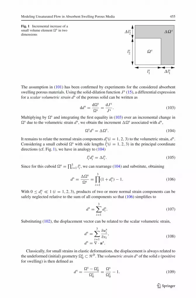
Fig. 1 Incremental increase of asmall volume element �s in twodimensions

Ω s

ΔΩ sΔ ls2

ls2

ls1 Δ ls

1

The assumption in (101) has been confirmed by experiments for the considered absorbentswelling porous materials. Using the solid-dilation function J s (15), a differential expressionfor a scalar volumetric strain ds of the porous solid can be written as

dds = d�s

�s = dJ s

J s . (103)

Multiplying by �s and integrating the first equality in (103) over an incremental change in�s due to the volumetric strain ds, we obtain the increment ��s associated with ds,

�sds = ��s. (104)

It remains to relate the normal strain components dsi (i = 1, 2, 3) to the volumetric strain, ds.

Considering a small cuboid �s with side lengths lsi (i = 1, 2, 3) in the principal coordinate

directions (cf. Fig. 1), we have in analogy to (104)

lsi ds

i = �lsi . (105)

Since for this cuboid �s = ∏3i=1 ls

i , we can rearrange (104) and substitute, obtaining

ds = ��s

�s =3∏

i=1

(1 + dsi )− 1. (106)

With 0 ≤ dsi � 1 (i = 1, 2, 3), products of two or more normal strain components can be

safely neglected relative to the sum of all components so that (106) simplifies to

ds =3∑

i=1

dsi . (107)

Substituting (102), the displacement vector can be related to the scalar volumetric strain,

ds =3∑

i=1

∂usi

∂xi,

ds = ∇ · us.

(108)

Classically, for small strains in elastic deformations, the displacement is always related tothe undeformed (initial) geometry�s

0 ⊂ �D . The volumetric strain ds of the solid s (positivefor swelling) is then defined as

ds = �s −�s0

�s0

= �s

�s0

− 1. (109)

123


Because the displacements for AGM problems are large, a relation of this form is insuffi-cient. Typically, AGM-containing media can swell ten times and more related to the initial(unswollen) structure. For those large-deformation problems (Lewis and Schrefler 1998), thegeometry has to be incremented numerically so that the solid volume �s

n ⊂ �D at a giventime stage tn can serve as reference for the step from n to n + 1, where n denotes the timeplane:

dsn+1 = �s

n+1 −�sn

�sn

= �sn+1

�sn

− 1 (110)

written for the new time plane n + 1 valid in the t ∈ (0, T ) temporal domain, where �sn =

�s(tn) ⊂ �D is the solid volume at the last time stage, �sn+1 = �s(tn+1) ⊂ �D is the solid

volume at the new (current) time stage, T is the final solution time, and ds0 ≡ 0 at initial time

t = t0. Note that ds tends toward zero as the geometry ceases to change.The scalar solid strain ds

n+1 (110) can be expressed by the solid dilation function J s (15),

dsn+1 = J s

n+1

J sn

− 1, (111)

which can be analytically evaluated using (67). Thus, the solid strain becomes directly afunction of the AGM x-load ms

2,

dsn+1(m

s2) = J s(ms

2(n+1))

J s(ms2(n))

− 1, (112)

where ms2(n+1) = ms

2(tn+1) and ms2(n) = ms

2(tn) are the AGM x-loads computed at the currentand previous time stages, respectively.

3 Final Model Equations

3.1 Choice of Suited Primary Variables

In a numerical approach, we have to solve the set of balance equations (48) with the aboveconstitutive relationships for appropriately chosen primary variables. The following werefound suitable for AGM simulations:

1. The Richards equation is solved for the pressure head ψ l = pl/(ρl0g).

2. The solid mass conservation equation is solved for the concentration of absorbed liquidper reference (initial) bulk volume Cs

L→S0.

3. The solid strain equation is solved for the solid displacement us.

With known ψ l, CsL→S0

, and us, all secondary variables can be evaluated, such as sl, ql, vs,ε, ρs, etc.

3.1.1 Reformations of Balance Terms

Solid phase sIn (48), the terms connected with the divergence of the solid velocity ∇ · vs can be simplifiedby substituting (17) with (68) according to

∇ · vs = 1

J s

dJ s

dt= 1

J s

∂ J s

∂ms2

∂ms2

∂t= 1

εs

(1

J s

CsAGM0

ρsH2O

− ∂εs

∂ms2

)∂ms

2

∂t. (113)

123


Furthermore, we can take into account (17) and (62) to simplify the following terms

∂

∂t(εsρs)+ εsρs(∇ · vs) = ∂

∂t(εsρs)+ 1

J s

dJ s

dt(εsρs)

= ∂(εsρs)

∂ms2

∂ms2

∂t+ 1

J s

∂ J s

∂ms2

∂ms2

∂t(εsρs)

= 1

J s

∂(εsρs J s)

∂ms2

∂ms2

∂t= Cs

AGM0

J s

∂ms2

∂t. (114)

Noting that CsAGM0

is stationary, we found from (59),

∂CsL→S0

∂t= Cs

AGM0

∂ms2

∂t(115)

so that (114) can be further simplified

∂

∂t(εsρs)+ εsρs(∇ · vs) = 1

J s

∂CsL→S0

∂t. (116)

This result can be used to develop the final form of the balance equation for the solid phase s

∂

∂t(εsρs)+ εsρs(∇ · vs) = Rs − φs(us),

1

J s

∂CsL→S0

∂t= Rs − φs(us), (117)

∂CsL→S0

∂t= τ asl(sl

e)ms2Cs

AGM0− J sφs(us).

Liquid phase lThe balance equation of the liquid phase l results then in

ε∂sl

∂t+ εslγ

∂ψ l

∂t+ ∇ · ql = Rl

ρl0


∂t− φl(us)

= − Rl

ρl0

− slε

J s

∂ J s

∂ms2

∂ms2

∂t− sl ∂ε

∂ms2

∂ms2

∂t− φl(us)

= −[

1

ρl0

CsAGM0

J s + sl(∂ε

∂ms2

+ ε

J s

∂ J s

∂ms2

)]∂ms

2

∂t

− 1

ρl0

φs(us)− φl(us). (118)

The liquid saturation sl is a function of ψ l and ms2 according to the dependencies appearing

in (92) and (94):

sl = sl(ψ l, α(ms2)). (119)

We can develop the storage term of (118) according to

ε∂sl

∂t= ε

∂sl(ψ l)

∂t+ ε

∂sl

∂ms2

∂ms2

∂t, (120)

123


where the derivative ∂sl/∂ms2 is given by (97). The form (120) is used in FEFLOW, where

the derivative for the pressure-dependent saturation function sl(ψ l)with respect toψ l is per-formed internally in dependence on the actually used approximation scheme of the Richardsequation with the possible alternates of the mixed formulation or standard formulation. Inthis study, the mixed formulation is always preferred, which provides mass-conservative andaccurate solutions (for more details, see part 2 of this article).

3.1.2 Summarized Formulation

In choosing ψ l, CsL→S0

, and us as the primary variables, we find the final working equationswritten in the following form:

ε∂sl(ψ l)

∂t+ εslγ

∂ψ l

∂t− ∇ · [kl

rK(∇ψ l + e)] = −[

1

ρl0

CsAGM0

J s + ε∂sl

∂ms2

+ sl(∂ε

∂ms2

+ ε

J s

∂ J s

∂ms2

)]∂ms

2

∂t− 1

ρl0

φs(us)− φl(us), (121)

∂CsL→S0

∂t= τ asl(s(sl

e))ms2Cs

AGM0− J sφs(us),

∇ · us = ds.

Note that AGM x-load ms2 can be directly computed from Cs

L→S0by using the definition

(58) ms2 = Cs

L→S0/Cs

AGM0. Note further that in (121), the gravitational unit vector e is used

according to g = −ge. Furthermore, a specific liquid compressibility is defined as γ = γρl0g.

In addition to (121) we have the following constitutive relations:

sle = sl − sl

r

sls − sl

r={

1[1+|α(ms

2)ψl|n ]m ψ l < 0

1 ψ l ≥ 0,

α(ms2) = αmax

(1 + ms2αscale)

αexp, αmax =

{αmax,wetting

∂ψ l

∂t > 0

αmax,drying∂ψ l

∂t < 0,

klr = (sl

e)δ,

K = kρl0g

μl = KbaseI[1 + kcoeff exp(kexpcoeff ms2) sin(2πksincoeff ms

2 + ksinphase)],

Kbase = kbaseρl0g

μl , ms2 = ms

2 max − ms2

ms2 max

,


1 − e−αexp, s(sl

e) = sle − sl

e, threshold


,

ε = 2εmax

1+(ms2εscale+1)εexp

,∂εs

∂ms2

= 2εmaxεscaleεexp(ms2εscale+1)εexp−1

[1+(ms2εscale+1)εexp ]2 , (122)

εs0 = Cs

CM0

ρsCM0

+ CsAGM0

ρsAGM0

, εmax = 1 − εs0,

∂sl

∂ms2

= − (sls − sl

r)ψlnm[α(ms

2)ψl]n−1

{1 + [α(ms2)ψ

l]n}m+1

αmaxαscaleαexp


2, threshold)]αexp+1 ,

123


J s = 1

1 − ε

(εs

0 + ms2

CsAGM0

ρsH2O

),

∂ J s

∂ms2

= 1

1 − ε

(Cs

AGM0

ρsH2O

− J s ∂εs

∂ms2

),

ds = J sn+1

J sn

− 1,

φl(us) = ∂us

∂t· ∇(εsl),

φs(us) = ∂us

∂t· ∇(εsρs),

ms2 = Cs

L→S0

CsAGM0

,

where the saturation of the liquid phase sl appears as a secondary variable, which is derivedfrom the VG capillary–pressure relationship (92) at known pressure head ψ l.

The deformation terms φl(us) and φs(us) of (121) and (122) are negligible if the productresulting from the solid velocity ∂us/∂t and the gradient of the saturation sl as well as thegradient of the AGM x-load ms

2 remains small relative to the other balance terms. This is truein typical applications because the major displacement direction us is often widely perpen-dicular to the gradient of the AGM x-load ∇ms

2 and the gradient of the saturation ∇sl. In allsubsequent applications, these deformation terms will be neglected.

4 Large Deformation Control

The solid displacement us is computed from the hyperbolic differential equation ∇ ·us = ds,where the scalar solid strain ds is a function of the volume dilatation J s and therefore afunction of the AGM x-load ms

2. The displacement vector us can be decomposed into a scalardisplacement norm us and a displacement-direction vector as of unit size,

us = usas = us[as1, as

2, as3]T (123)

so that

∇ · us = as · ∇us + us∇ · as. (124)

The second term on the RHS will be zero for a homogeneous displacement direction, i.e., ifall points of the domain move in the same direction. This term can be safely neglected if therestriction

as · ∇us � us∇ · as (125)

is satisfied.

Proof A geometric constraint on the curvature of the domain can be developed using an ide-alized domain of thickness B and spherical inner (�s

1) and outer (�s2) surfaces, both centered

at the origin (see Fig. 2). Let R denote the radius of the outer surface. The inner surface is thefixed domain boundary and the swelling-direction vector field as(x) is given by as

i = xi/r ,where

r =√√√√ D∑

i=1

x2i (126)

123


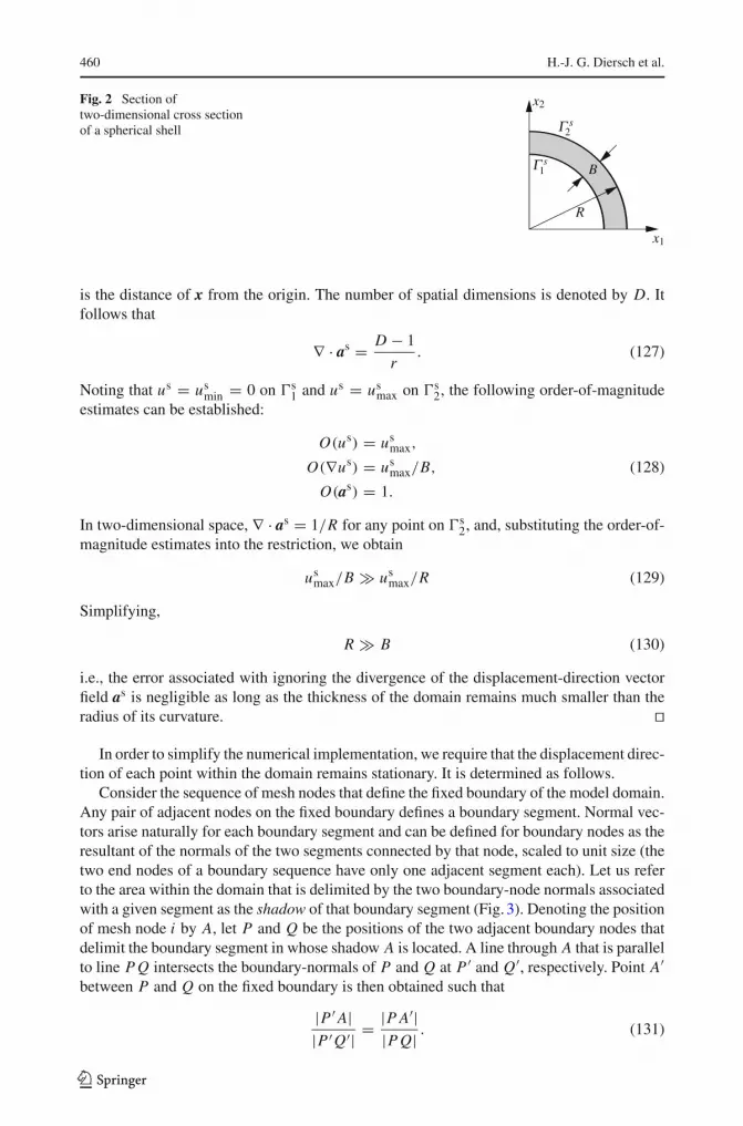
Fig. 2 Section oftwo-dimensional cross sectionof a spherical shell

x1

x2

Γ s1

Γ s2

B

R

is the distance of x from the origin. The number of spatial dimensions is denoted by D. Itfollows that

∇ · as = D − 1

r. (127)

Noting that us = usmin = 0 on �s

1 and us = usmax on �s

2, the following order-of-magnitudeestimates can be established:

O(us) = usmax,

O(∇us) = usmax/B, (128)

O(as) = 1.

In two-dimensional space, ∇ · as = 1/R for any point on �s2, and, substituting the order-of-

magnitude estimates into the restriction, we obtain

usmax/B � us

max/R (129)

Simplifying,

R � B (130)

i.e., the error associated with ignoring the divergence of the displacement-direction vectorfield as is negligible as long as the thickness of the domain remains much smaller than theradius of its curvature. ��

In order to simplify the numerical implementation, we require that the displacement direc-tion of each point within the domain remains stationary. It is determined as follows.

Consider the sequence of mesh nodes that define the fixed boundary of the model domain.Any pair of adjacent nodes on the fixed boundary defines a boundary segment. Normal vec-tors arise naturally for each boundary segment and can be defined for boundary nodes as theresultant of the normals of the two segments connected by that node, scaled to unit size (thetwo end nodes of a boundary sequence have only one adjacent segment each). Let us referto the area within the domain that is delimited by the two boundary-node normals associatedwith a given segment as the shadow of that boundary segment (Fig. 3). Denoting the positionof mesh node i by A, let P and Q be the positions of the two adjacent boundary nodes thatdelimit the boundary segment in whose shadow A is located. A line through A that is parallelto line P Q intersects the boundary-normals of P and Q at P ′ and Q′, respectively. Point A′between P and Q on the fixed boundary is then obtained such that

|P ′ A||P ′Q′| = |P A′|

|P Q| . (131)

123


Fig. 3 Determining the nodal displacement direction in 2D

Line A′ A defines the stationary displacement direction asi for node i . A crossing of nodal

displacement paths, which would lead to ill-defined mesh geometry, is completely preventedif the fixed boundary has no concave parts. Concave boundary sections are acceptable if thefinal (maximum) displacement is less than the distance at which the first crossover betweenneighboring nodes would occur. This condition is expected to be met in many practicalapplications.

As ds depends on ms2, the following equation must be solved at each time stage:

(as · ∇us(n+1)) = ds

n+1 = J sn+1

J sn

− 1 = J s(ms2(n+1))

J s(ms2(n))

− 1. (132)

The RHS of (132) is obtained directly by evaluating the Jacobian J s at the current (n + 1)and previous (n) time stages via equation (67) (or in (122)).

5 Conclusions

The theoretical basis for modeling the fluid movement in variably saturated and free-swelling AGM-containing porous structures has been derived. The resulting set of equa-tions includes a generalized Richards equation, an equation for the solid-mass conservationwith kinetic reaction term, and a relationship for the solid strain. The system of equationsmust be closed by multiple constitutive relations that include rather complex expressions andmake the system highly nonlinear. The final equations (121)–(122) can be numerically solvedfor the liquid-phase pressure headψ l, the absorbed liquid Cs

L→S0, and the solid displacement

us. With known ψ l, CsL→S0

, and us, secondary variables such as the AGM x-load ms2, the

liquid-phase saturation sl, the Darcy flux ql, or the porosity ε, can be computed.The swelling AGM structures are modeled as a large-scale deformation problem with

accumulating discrete spatial movements over finite time intervals. The deformation processis assumed stress-free and possesses a free-swelling dynamics. This must require a mov-ing-mesh strategy which incrementally updates two- or three-dimensional model domains

123


based directly on the current spatial distribution of the solid displacement us. The numericalsolution strategy will be described in the second part of this article.

Appendix: Derivation of The Saturation-Dependent Fraction of the Solid–Liquid Inter-face Area asl(sl)

It appears reasonable to assume that the ratio between the volume Vp and solid–interface areaAp of a pore of radius r is proportional to r , viz.,

Vp(r)

Ap(r)∝ r or Ap(r) = G

1

rVp(r), (133)

where G is a geometry constant. For capillaries, G = 2. Moreover, the capillary pressureheadψ l associated with a given pore size r is related to liquid surface tension σ ∗ and wettingangle and can be typically described by an inverse function of r ,

ψ l(r) = H1

r, (134)

where, for capillaries and a zero wetting angle, the constant H is equal to 2σ ∗ρlg

. Replacing 1r

in Ap(r) of (133), it results

Ap(ψl) = G

Hψ lVp(ψ

l). (135)

Considering a group of pores within an REV subject to a capillary pressureψ l, the combinedvolume of pores filled with liquid is given by

Vp, filled(ψl) =

ψ l∫ξ=−∞

Vp(ξ)dξ, (136)

while the corresponding total solid–liquid interface area within the REV is given by

Ap, filled(ψl) =

ψ l∫ξ=−∞

G

HξVp(ξ)dξ. (137)

The maximum possible values for Vp and Ap are those at full pore-space saturation,

Vp, total = Vp(0) =0∫

ψ l=−∞Vp(ψ

l)dψ l (138)

and

Ap, total = Ap(0) =0∫

ψ l=−∞

G

Hψ lVp(ψ

l)dψ l, (139)

respectively. Liquid saturation of the pore space sl is given by

sl(ψ l) = Vp, filled(ψl)

Vp, total(140)

123


so that

dsl

dψ l = Vp(ψl)

Vp, total. (141)

The shape of dsl/dψ l can be typically considered as known; it can often be obtained analyt-ically from the empirical sl(ψ l) model chosen (e.g., van Genuchten). For the fraction asl ofmaximum possible solid–liquid interface within the REV, the analogous expressions are

asl(ψ l) = Ap, filled(ψl)

Ap, total(142)

and

dasl

dψ l =GHψ

lVp(ψl)

Ap, total. (143)

Replacing Vp(ψl) by using (141)

dasl

dψ l =GHψ

l dsl

dψ l Vp, total

Ap, total(144)

and rearranging as

dasl

dψ l = Caψl dsl

dψ l , (145)

where all the constants have been combined into the parameter Ca, the re-integration of (145)yields

asl(ψ l)=ψ l∫

ξ =−∞Caξ

dsl

dψ l dξ. (146)

The integral (146) cannot be generally expressed analytically but is easily evaluated numer-ically. The parameter Ca can be obtained by noting that asl(0) = 1, so that

Ca = 1∫ 0ψ l =−∞ ψ l dsl

dψ l dψ l(147)

and accordingly

asl(ψ l)=∫ ψ l

ξ = −∞ ξ dsl

dψ l dξ∫ 0ψ l = −∞ ψ l dsl

dψ l dψ l(148)

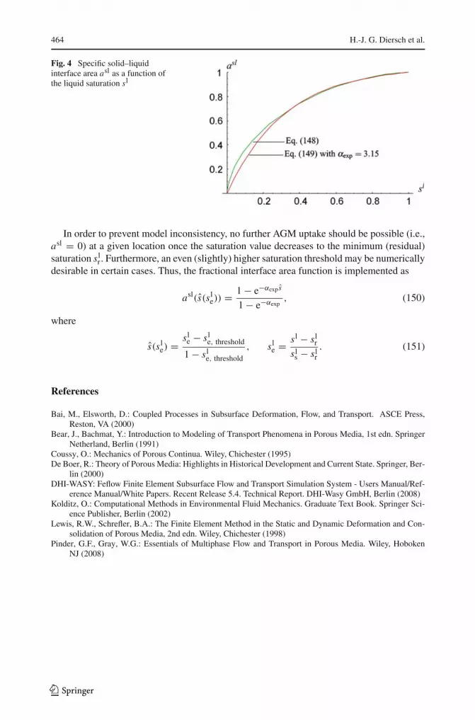
Plotting numerically evaluated asl(ψ l) versus sl(ψ l) results in a functional shape asl(sl)

resembling an exponential function. Shown in Fig. 4 is a plot (in green color) of asl(ψ l)

versus sl(ψ l) using the VG parameters given earlier and the empirical fit,

asl(sl) = 1 − e−αexpsl

1 − e−αexp(149)

in red.

123


Fig. 4 Specific solid–liquidinterface area asl as a function ofthe liquid saturation sl

In order to prevent model inconsistency, no further AGM uptake should be possible (i.e.,asl = 0) at a given location once the saturation value decreases to the minimum (residual)saturation sl

r . Furthermore, an even (slightly) higher saturation threshold may be numericallydesirable in certain cases. Thus, the fractional interface area function is implemented as


1 − e−αexp, (150)

where

s(sle) = sl

e − sle, threshold


, sle = sl − sl

r

sls − sl

r. (151)

References

Bai, M., Elsworth, D.: Coupled Processes in Subsurface Deformation, Flow, and Transport. ASCE Press,Reston, VA (2000)

Bear, J., Bachmat, Y.: Introduction to Modeling of Transport Phenomena in Porous Media, 1st edn. SpringerNetherland, Berlin (1991)

Coussy, O.: Mechanics of Porous Continua. Wiley, Chichester (1995)De Boer, R.: Theory of Porous Media: Highlights in Historical Development and Current State. Springer, Ber-

lin (2000)DHI-WASY: Feflow Finite Element Subsurface Flow and Transport Simulation System - Users Manual/Ref-

erence Manual/White Papers. Recent Release 5.4. Technical Report. DHI-Wasy GmbH, Berlin (2008)Kolditz, O.: Computational Methods in Environmental Fluid Mechanics. Graduate Text Book. Springer Sci-

ence Publisher, Berlin (2002)Lewis, R.W., Schrefler, B.A.: The Finite Element Method in the Static and Dynamic Deformation and Con-

solidation of Porous Media, 2nd edn. Wiley, Chichester (1998)Pinder, G.F., Gray, W.G.: Essentials of Multiphase Flow and Transport in Porous Media. Wiley, Hoboken

NJ (2008)

123

modeling unsaturated flow in absorbent swelling porous media: part 2. numerical simulation

Documents