macroscopic equations for flow in unsaturated porous media
TRANSCRIPT
Macroscopic Equations for Flow in
Unsaturated Porous Media
Promotoren: Prof. dr. ir. A. Leijnse,
hoogleraar grondwaterkwaliteit,
Wageningen Universiteit
Prof. dr. ir. P. A. Troch,
hoogleraar hydrologie en kwantitatief waterbeheer,
Wageningen Universiteit
Samenstelling Promotiecommissie:
Prof. J. P. du Plessis, Stellenbosch University, South Africa
Prof. W. G. Gray, University of North Carolina, USA
Prof. S. M. Hassanizadeh, Technische Universiteit Delft
Prof. dr. ir. R. A. Feddes, Wageningen Universiteit
Marc Rene Hoffmann
Macroscopic Equations for Flow in
Unsaturated Porous Media
Proefschrift
ter verkrijging van de graad van doctor
op gezag van de rector magnificus
van Wageningen Universiteit,
prof. dr. ir. L. Speelman,
in het openbaar te verdedigen
op woensdag 24 september 2003
des namiddags te vier uur in de Aula.

Hoffmann, M. R.
Macroscopic Equations for Flow in Unsaturated Porous Media.
Dissertation Wageningen Universiteit, Wageningen 2003
ISBN 90-5808-893-6
Copyright c© Marc R. Hoffmann, 2003.
Abstract
Hoffmann, M.R., 2003. Macroscopic Equations for Flow in Unsaturated Porous
Media. Dissertation, Wageningen University, The Netherlands.
This dissertation describes averaging of microscale flow equations to obtain
a consistent description of liquid flow in unsaturated porous media on the
macroscale. It introduces a new method of averaging the pressure term and a
unit cell model capable of describing unsaturated flow.
Starting from the description of liquid flow through individual pores, a macro-
scopic equation for flow of a liquid in a porous medium in the presence of a
gas is derived. The flow is directly influenced by phase interfaces, i.e. solid-
liquid or gas-liquid. By including these pore scale phenomena in a continuum
description of fluid transport in porous media, equations for liquid flow on the
macroscale are obtained.
The unit cell model is based on a simplified geometric representation of a
porous medium. It allows for the modeling of the important characteristics of
a porous medium for unsaturated flow.
Through the use of volume averaging and direct integration macroscale mo-
mentum and mass balance equations are derived from the microscale momen-
tum and mass balance equations, resulting in a novel form of the macroscale
pressure term. The macroscale flow of liquids in unsaturated porous media
can be written proportional to a driving force, which is proportional to the
difference of the inverse area averaged liquid pressures across an averaging vol-
ume. In principle the flow is driven by gradients in liquid pressure, but due to
the nonlinear coupling between capillary forces and liquid pressure the driving
force becomes nonlinear.
Two dynamic terms were derived by simplifying the flow dynamics in a porous
medium. They remain to be tested quantitatively and still have considerable
uncertainty concerning their exact form and/or magnitude.
Comparison of the newly proposed macroscale equations with the Buckingham-
Darcy equation shows that, using reasonable assumptions, the newly proposed
macroscale equations can be written in a form similar to the Buckingham-
Darcy equation. The newly proposed macroscale equations are compared to
an experiment and satisfactory agreement between experiment and calcula-
tions was observed.
keywords: momentum balance, nonlocal equations, porous media, upscaling,
unsaturated flow, volume averaging.

.
Contents
Nomenclature 1
1 Introduction 5
1.1 What is it about? . . . . . . . . . . . . . . . . . . . . . . . . . . 5
1.2 Problem Description . . . . . . . . . . . . . . . . . . . . . . . . 5
1.3 Relevance . . . . . . . . . . . . . . . . . . . . . . . . . . . . . . 7
1.4 Objectives and Approach . . . . . . . . . . . . . . . . . . . . . 8
1.5 Outline of Dissertation . . . . . . . . . . . . . . . . . . . . . . . 9
2 Overview and Review 11
2.1 Introduction . . . . . . . . . . . . . . . . . . . . . . . . . . . . . 11
2.1.1 Definition of a porous medium . . . . . . . . . . . . . . 11
2.1.2 History . . . . . . . . . . . . . . . . . . . . . . . . . . . 13
2.2 Flow at the Pore Scale . . . . . . . . . . . . . . . . . . . . . . . 15
2.2.1 Single-phase flow . . . . . . . . . . . . . . . . . . . . . . 15
2.2.2 Two-phase flow . . . . . . . . . . . . . . . . . . . . . . . 16
2.3 Upscaling to the Continuum Scale . . . . . . . . . . . . . . . . 25
2.3.1 Space averaging theories . . . . . . . . . . . . . . . . . . 27
2.3.2 Resulting theories . . . . . . . . . . . . . . . . . . . . . 30
vii
viii CONTENTS
3 Development of a Mathematical Model 33
3.1 Introduction . . . . . . . . . . . . . . . . . . . . . . . . . . . . . 33
3.2 Assumptions . . . . . . . . . . . . . . . . . . . . . . . . . . . . 33
3.2.1 Assumptions regarding the fluids . . . . . . . . . . . . . 34
3.2.2 Assumptions regarding the porous medium . . . . . . . 35
3.2.3 Assumptions regarding flow and capillarity . . . . . . . 35
3.2.4 Assumptions not made . . . . . . . . . . . . . . . . . . . 36
3.3 The Basic Interstitial Equations . . . . . . . . . . . . . . . . . . 37
3.4 Volume Averaging . . . . . . . . . . . . . . . . . . . . . . . . . 38
3.4.1 Averaging of the mass balance equation . . . . . . . . . 39
3.4.2 Averaging of the momentum balance equation . . . . . 40
3.4.3 Averaging of the boundary conditions . . . . . . . . . . 43
3.4.4 The combined averaged equations . . . . . . . . . . . . 44
4 Closure Model 45
4.1 Introduction . . . . . . . . . . . . . . . . . . . . . . . . . . . . . 45
4.2 Description of the RUC . . . . . . . . . . . . . . . . . . . . . . 45
4.2.1 Topology and geometry . . . . . . . . . . . . . . . . . . 46
4.2.2 Geometrical properties . . . . . . . . . . . . . . . . . . . 47
4.3 Capillary Pressure Relationship . . . . . . . . . . . . . . . . . . 49
4.3.1 Geometry of liquid inside a corner . . . . . . . . . . . . 50
4.4 Flow Models . . . . . . . . . . . . . . . . . . . . . . . . . . . . 52
4.4.1 Single-phase flow . . . . . . . . . . . . . . . . . . . . . . 53
4.4.2 Two-phase flow . . . . . . . . . . . . . . . . . . . . . . . 55
4.5 Velocity Relations . . . . . . . . . . . . . . . . . . . . . . . . . 58
CONTENTS ix
5 Closure Modeling 61
5.1 Closure of the Divergence Term . . . . . . . . . . . . . . . . . . 61
5.2 Closure of the Viscous Term . . . . . . . . . . . . . . . . . . . . 63
5.2.1 The solid-liquid interfacial area term . . . . . . . . . . . 63
5.2.2 The gas-liquid interfacial area term . . . . . . . . . . . . 65
5.3 Closure of the Pressure Term . . . . . . . . . . . . . . . . . . . 68
5.4 Boundary and Initial Conditions . . . . . . . . . . . . . . . . . 70
5.5 The Total Averaged Equations . . . . . . . . . . . . . . . . . . 70
5.6 Discussion . . . . . . . . . . . . . . . . . . . . . . . . . . . . . . 72
6 Comparison Buckingham-Darcy 75
6.1 Introduction . . . . . . . . . . . . . . . . . . . . . . . . . . . . . 75
6.2 Order of Magnitude Analysis . . . . . . . . . . . . . . . . . . . 75
6.3 Further Analysis . . . . . . . . . . . . . . . . . . . . . . . . . . 77
6.3.1 Stationary solution . . . . . . . . . . . . . . . . . . . . . 80
6.3.2 Comparison of the averaged pressure term . . . . . . . . 83
6.3.3 Estimation of hydraulic conductivity . . . . . . . . . . . 84
6.3.4 Comparison of the dynamic terms . . . . . . . . . . . . 85
6.4 Comparison with Experiment . . . . . . . . . . . . . . . . . . . 89
6.4.1 Description of experiment . . . . . . . . . . . . . . . . . 89
6.4.2 Calculations . . . . . . . . . . . . . . . . . . . . . . . . . 90
6.4.3 Calculation results . . . . . . . . . . . . . . . . . . . . . 92
7 Discussion 95
7.1 Discussion . . . . . . . . . . . . . . . . . . . . . . . . . . . . . . 95
7.1.1 Pressure term . . . . . . . . . . . . . . . . . . . . . . . . 96
7.1.2 Dynamic terms . . . . . . . . . . . . . . . . . . . . . . . 97
7.1.3 Representative Unit Cell model . . . . . . . . . . . . . . 98
7.1.4 Constitutive relations . . . . . . . . . . . . . . . . . . . 99
7.2 Recommendations and Possible Extensions . . . . . . . . . . . 100
7.3 Conclusions . . . . . . . . . . . . . . . . . . . . . . . . . . . . . 101
x CONTENTS
A Volume Averaged Pressure Term 103
Summary 105
Samenvatting 107
Bibliography 110
Nawoord 121
Curriculum Vitae 123
Nomenclature
symbol description
a fraction characterising pore opening (–)
A area (m2)
A area in pore (corner) occupied by fluid (m2)
A(h) adsorptive component in AYL (eq. (2.19)) (m2/s2)
Ac liquid area in corner, perpendicular to flow (m2)
Ap pore area normal to flow (m2)
Asvl Hamacker constant, for quartz sand −1.9 ∗ 10−19 (J)
b factor characterising if pore is open (2), or closed (1) (–)
Bo Bond number, (eq. (2.11)) (–)
c1,2,3,4 factors defined by equations (5.46), (5.47), (5.48), (5.49) (–)
C factor depending on x, curvature (1/m); positive for an in-
terface concave outward from the liquid
Ca Capillary number, (eq. (2.37)) (–)
Cc capillary component in eq. (2.19) (m2/s2)
d microscopic characteristic length (RUC) (m)
f Fanning friction factor for fully developed flow (–)
f function describing geometric components, (eq. (4.40)) (–)
f function f(x, t) in eq. (3.12)
F conductance factor (–)
Fv conductance factor two-phase flow 1.7 (–)
g gravity acceleration (m/s2)
G Gibbs partial specific free energy (J)
h hydraulic head, film thickness in AYL equation (m)
H slit spacing, characteristic height of liquid in corner (m)
i index number (–)
j number of corners in RUC (–)
kD saturated hydraulic conductivity (m/s)
kr relative hydraulic conductivity (–)
Kn Knudsen number (–)
1
2 NOMENCLATURE
symbol description
lg flow length in RUC (m)
lp penetration length in Lucas-Washburn equation (eq. (2.4))
(m)
L characteristic length (m)
L length (m)
nl liquid saturation (–)
N macroscopic unit vector (–)
Nl characteristic liquid saturation (–)
p pressure (kg/ms2)
pc capillary pressure (kg/ms2)
plc critical pressure drainage for liquid (kg/ms2)
P generic Pressure (kg/ms2)
P wetted perimeter (m)
q volumetric flow rate (m3/s)
r radius of curvature of gas-liquid interface (m)
rc critical radius of curvature of gas-liquid interface during
drainage (m)
rh hydraulic radius (m)
ri critical radius of curvature of gas-liquid interface during imhi-
bition (m)
R1, R2 principal radii of curved surface (m)
Re Reynolds number (–)
S surface (m2)
s unit vector tangent to surface (–)
S saturation (m3/m3)
t time (s)
T characteristic time (s)
U characteristic velocity (m/s)
v velocity (m/s)
v velocity (m/s)
Vl volume of liquid in averaging volume (m3)
Vp volume of pores in averaging volume (m3)
Vs volume of solid in averaging volume (m3)
V0 volume of averaging volume (m3)
w velocity of surface (m/s)
x, y, z space coordinates (m)
α half opening angle of corner (rad)
γ surface (interfacial) tension at interface (kg/s2)
ε porosity (m3/m3), Vp/V0
NOMENCLATURE 3
symbol description
θ contact angle liquid - solid (rad)
µ dynamic viscosity (kg/ms)
ν unit normal vector on S (–)
ρ density (kg/m3)
τ proportionality factor in dynamic term (kg/ms)
τSsl cross-sectional average wall shear stress (kg/ms2)
Ψ generalized variable
〈 〉 average of quantity over volume of RUC, except when super-
script given˙( ) deviation from mean
| | magnitude
subscripts:
0 boundary of RUC (averaged quantity, entrance)
1 boundary of RUC (averaged quantity, exit)
D as subscript for specific discharge, also “Darcy” velocity
a air
c mean inside corner
d dynamic
f fluid (gas or liquid)
g gas
l liquid
m mean
p mean inside pore
s solid, static
tot total
w water
Vector notation follows Bird et al. (1960).

4
1 Introduction
This dissertation describes averaging of the microscale flow equations to obtain
a consistent description of liquid flow in unsaturated porous media on the
macroscale. It introduces a new method of averaging the pressure term and a
unit cell model capable of describing unsaturated flow.
1.1 What is it about?
This dissertation is about unsaturated flow in porous media. More specifically
it is about mathematical modeling of two-phase flow through rigid porous
media. The two phases considered are a wetting liquid and a gas. In practice
one can think of a sandy soil partially saturated with water, partially with
air. Strictly speaking, the flow of the liquid phase is treated as single-phase
flow in the presence of an inviscid gas phase. However, the gas phase directly
influences the liquid flow through surface forces and the resulting flow is called
two-phase flow or unsaturated flow in this dissertation.
Starting from the description of fluid flow through individual pores, an equa-
tion for flow of a liquid in a porous medium in the presence of a gas is derived.
This flow is directly influenced by phase interfaces e.g. solid-liquid or gas-liquid.
By explicitly including these pore scale phenomena in a continuum description
of fluid transport in porous media, a consistent theoretical description of fluid
flow on the macroscale is obtained.
1.2 Problem Description
Groundwater flow, flow in lungs, flow inside the catalytic converter of a car
and wind blowing through a forest are all examples of flow in porous media.
5
6 CHAPTER 1. INTRODUCTION
Examples where two-phase flow plays an important role are drainage and irri-
gation of agricultural lands, groundwater pollution, nuclear waste storage, oil
and gas winning, and the drying of food materials.
Current equations describing fluid transport in porous media are based on
(semi)empirical equations derived in the 19th century (Darcy, 1856) for single-
phase flow and in the 20th century for multi-phase flow (Buckingham, 1907;
Washburn, 1921; Richards, 1931; Buckley and Leverett, 1942). The current
standard equations used in soil physics are called the Buckingham-Darcy equa-
tion and Richards equation. These equations try to describe the “average”
behavior of a mixture of a porous medium and one or more fluids. They have
since then been put on a firm basis by theoretical investigations of Hubbert
(1956), Anderson and Jackson (1967), Whitaker (1966, 1969), Slattery (1967,
1969), and Gray and Hassanizadeh (1991a). The theoretical work by Whitaker
(1977) confirmed the general nature of Richards equation, if considerable as-
sumptions are made. Theoretical work of Gray and Hassanizadeh (1991a),
and experimental work of Aleman et al. (1989) and Grant and Salehzadeh
(1996) showed that there is still a considerable gap between the theory and
experiments, and Richards equation. The main problems lie in the nature of
the average capillary or liquid pressure and the interplay between the param-
eterization of constitutive relations and the average liquid pressure. These
difficulties are in part due to the averaged nature of Richards equation. Av-
eraging smoothes discontinuities, leading to smoothed macroscale equations.
Another difficulty arises when Richards equation is applied in practice. In
order to find a solution, constitutive relations are needed between water con-
tent and pressure head, and relative hydraulic conductivity and water content.
At very low water contents, often unrealistic solutions are obtained due to
the form of the constitutive relations used (Fuentes et al., 1992). Due to the
nonlinear character of Richard’s equation only a limited number of analytical
solutions are known. Usually one resorts to numerical solution techniques,
which normally involve discretisation and integration. In mathematical terms
Richards equation is a partial differential equation that is defined with local
point support, but in physical terms Richards equation is seen as a description
on the cm scale. These interpretations somewhat conflict when discretisa-
tion is applied (Nitsche and Brenner, 1989, p. 240). This is due to the fact
that when discretisation is applied, always interpolation is needed. In practice
this interpolation is different from the assumptions made in deriving Richards
equation. For example the constitutive relations commonly used are based on
the assumption of gradient independence.
At the end of the last millennium Gray and Hassanizadeh (1991a), and Has-
1.3. RELEVANCE 7
sanizadeh and Gray (1997, 1993) proposed more general, theoretically obtained
equations to describe multi-phase flow in porous media. These equations were
derived by volume averaging and thermodynamics. Volume averaging has
been used in the last decennia, mostly for single-phase flow in porous media,
although examples of multi-phase flow are described in Bear and Bensabat
(1989) and Hassanizadeh and Gray (1997). Despite enormous theoretical de-
velopments, practical applications of volume averaging have been limited due
to the so called closure problem. A closure problem, or closure, refers to a step
in volume averaging where terms containing microscale variables are expressed
in terms containing macroscale variables. Different possibilities exist to solve
this closure problem: numerical methods (Quintard and Whitaker, 1990), ap-
proximations based on empirical equations (Whitaker, 1980) and analytical so-
lutions for Representative Unit Cells (RUC’s) (du Plessis and Masliyah, 1988;
du Plessis and Diedericks, 1997). The difficulty in applying the volume aver-
aging theory lies in the development of a practical solvable closure problem.
Volume averaging starts with a description of fluid flow on the pore or mi-
croscale. Through the averaging process we replace the microscale variables by
macroscale variables, for example we change from the description of the actual
liquid configuration in pore to the average liquid content on the macroscale.
The term scale refers to a ”typical”measurement scale. A spatial scale is a
representative length unit through which we want to describe flow. The mag-
nitude is usually the diameter of an averaging volume. On the microscale or
pore-scale this would be tenth of mm, on the macroscale or continuum scale
cm’s. It is also possible that the term scale refers to a typical time unit which
captures the characteristics of the flow.
1.3 Relevance
Flow in porous media is difficult to be accurately modeled quantitatively.
Richards equation can give good results, but needs constitutive relations.
These are usually empirically based and require extensive calibration (van
Genuchten, 1980; Pullan, 1990). The parameters needed in the calibration
are amongst others: capillary pressure and pressure gradient, volumetric flow,
liquid content, irreducible liquid content, and temperature (Bachmann et al.,
2002). In practice it is usually too demanding to measure all these parameters.
In the model introduced in this dissertation no constitutive relations per se are
used, but a description of flow in terms of physical parameters of the porous
8 CHAPTER 1. INTRODUCTION
medium and the fluids. These parameters are amongst others: viscosity, poros-
ity, and interfacial tensions. The concept of a Representative Unit Cell (RUC)
implicitly replaces part of the constitutive relations, because it defines the ge-
ometry of the pore space. The newly derived mathematical model can be used
in drainage modeling and in the following applications where the Buckingham-
Darcy or Richards equation are not directly applicable, e.g. gravity free flow
of fluids in porous media in space for plant growth (Scovazzo et al., 2001),
(inverse) determination of structural porous media properties from fluid flow
measurements (Montillet et al., 1992; Roberts and Knackstedt, 1996). Note
that these properties depend on the specific porous medium model chosen.
In their present form the newly derived equations are not suited for infiltration
models, for the description of fingering flow, for flow of non-Newtonian fluids,
and for flow with drag along the fluid-fluid interfaces. The model can be
extended to include additional processes like vapor diffusion, heat transport,
and electrical conductivity, by directly averaging these processes with the aid
of the RUC approach.
1.4 Objectives and Approach
The objective of this dissertation is to develop a macroscopic model for the
movement of a wetting liquid in a rigid porous medium in the presence of a gas
phase. This dissertation uses the method of spatial averaging to change scales
in the description of flow in porous media. The starting point is a description
of the fluid flow on the pore- or microscale. By coarsening the description of
the microscale, solid and fluid phases start to form a continuum. This new
imaginary continuum has all the properties of the small scale system on ”aver-
age”. The averaged properties are derived through a closure method based on
the Representative Unit Cell (RUC) concept developed by professor J. P. du
Plessis (du Plessis and Masliyah, 1988). It is extended to allow unsaturated
flow, and phase interfaces are explicitly included.
By making different choices in the volume averaging procedure, a different
form of the equations than the traditional one (Whitaker, 1986b) is obtained.
The work presented in this dissertation introduces:
1. A new way of handling the liquid pressure term.
2. A unit cell model for unsaturated flow.
1.5. OUTLINE OF DISSERTATION 9
1.5 Outline of Dissertation
Chapter 2 gives an overview of the historical development of the study of flow
and transport in porous media. Chapter 3 describes the method of spatial
averaging as used in this dissertation, and states the basic equations, assump-
tions and conditions. In chapter 4 a geometric model for a porous medium is
developed together with the pore scale flow equations. The results of chapters
3 and 4 are used in chapter 5 to derive averaged equations that describe un-
saturated flow in porous media. A comparison of the newly derived equations
with the Buckingham-Darcy equation and an experiment is given in chapter 6.
Chapter 7 contains an overall discussion, recommendations and conclusions.

10
2 Overview and Review
This chapter provides an overview and gives a historical perspective of the
study of flow in porous media. Single-phase and two-phase flow at the pore
scale are described, basic equations are introduced, and concepts of the differ-
ent flow mechanisms are explained. Thereafter different methods for upscaling
to a continuum description of flow in porous media are introduced and the
basics of volume averaging are explained.
2.1 Introduction
Flow in porous media plays an important role in many areas of science and
engineering. Examples of the application of porous media flow phenomena are
as diverse as flow in human lungs or flow due to solidification in the mushy
zone of liquid metals. Table 2.1 lists other areas where flow in porous media
plays an important role. The description of the behavior of fluids in porous
media is based on knowledge gained in studying these fluids in pure form. Flow
and transport phenomena are described analogous to the movement of pure
fluids without the presence of a porous medium. The presence of a permeable
solid influences these phenomena significantly. The individual description of
the movement of the fluid phases and their interaction with the solid phase
is modeled by an upscaled porous media flow equation. The concept of up-
scaling from small to large scales is widely used in physics. Statistical physics
translates the description of individual molecules into a continuum description
of different phases, which in turn is translated by volume averaging into a
continuum porous medium description.
2.1.1 Definition of a porous medium
The definition of a porous medium used in this dissertation is based on the
objective of describing flow in porous media. A porous medium is a heteroge-
11
12 CHAPTER 2. OVERVIEW AND REVIEW
Hydrology Groundwater flow, salt water intrusion
into coastal aquifers, soil remediation
Agriculture Irrigation, drainage, contaminant
movement in soils, soil-less cultures
Geology Petroleum reservoir engineering, geo-
thermal energy
Chemical engineering Packed bed rectors, filtration, fuel cells,
drying of granular materials
Mechanical engineering Solar cell design, wicked heat pipes,
heat exchangers, porous gas burners
Industrial materials Rubber foam, glass fiber mats, con-
crete, brick manufacturing
Table 2.1: Areas where flow in porous media plays an important role.
neous system consisting of a rigid and stationary solid matrix and fluid filled
voids. The solid matrix or phase is always continuous and fully connected.
A phase is considered a homogeneous portion of a system, which is separated
from other such portions by a definitive boundary, called an interface. The
size of the voids or pores is large enough such that the contained fluids can be
treated as a continuum. On the other hand, they are small enough that the
interface between different fluids is not significantly affected by gravity.
The topology of the solid phase determines if the porous medium is permeable,
i.e. if fluid can flow through it, and the geometry determines the resistance
to flown and therefore the permeability. The most important influence of
the geometry on the permeability is through the interfacial or surface area
between the solid phase and the fluid phase. The topology and geometry also
determine if a porous medium is isotropic, i.e. all parameters are independent
of orientation, or anisotropic if the parameters depend on orientation. In multi-
phase flow the geometry and surface characteristics of the solid phase determine
the fluid distribution in the pores, as does the interaction between the fluids.
A porous medium is homogeneous if its average properties are independent
of location, and heterogeneous if they depend on location. An example of a
porous medium is sand. Sand is an unconsolidated porous medium, and the
grains have predominantly point contact. Because of the irregular and angular
nature of sand grains, many wedge-like crevices are present. An important
quantitative aspect is the surface area of the sand grains exposed to the fluid.
It determines the amount of water which can be held by capillary forces against
the action of gravity and influences the degree of permeability.
2.1. INTRODUCTION 13
The fluid phase
The fluid phase occupying the voids can be heterogeneous in itself, consist-
ing of any number of miscible or immiscible fluids. If a specific fluid phase is
connected, continuous flow is possible. If the specific fluid phase is not con-
nected, it can still have bulk movement in ganglia or drops. For single-phase
flow the movement of a Newtonian fluid is described. For two-phase immisci-
ble flow, a viscous Newtonian wetting liquid together with a non-viscous gas
are described. In practice these would be water and air. Other fluid phase
compositions are not considered in this dissertation.
2.1.2 History
One of the first successful attempts to describe flow through porous media was
by the French engineer Henry Darcy (Darcy, 1856). He was a civil engineer
responsible for the drinking water supply of the city of Dijon. The drinking
water was cleaned by percolation through sand columns. Darcy wanted to
know the relation between specific discharge and head gradient in the sand
columns. He found the following relation, commonly called Darcy’s law, by
experiment and written in modern notation:
vD = −kD∆h
∆x(2.1)
with vD the specific discharge, kD the hydraulic conductivity, x a space coor-
dinate and h the hydraulic head. This equation has formed the basis for nearly
all models describing the creeping flow of fluids through porous media up to
the end of the 1960’s, when it was also derived theoretically (Hubbert, 1956)
and alternative models were proposed (Bear and Bachmat, 1990, p. 122, 161).
In Darcy’s law, the head drop is entirely due to viscous dissipation, induced by
the solid-liquid interface. This implies that Darcy’s law becomes invalid when
inertial effects play a role, or when the solid surface area (porosity) becomes
very small (large) (Carman, 1956).
A major contribution to the description of flow in unsaturated soils was made
by Buckingham (1907). He introduced a flux law for the movement of water
in unsaturated soils, which is a modification of Darcy’s law:
vD = −kDkr(S)∂h
∂x(2.2)
14 CHAPTER 2. OVERVIEW AND REVIEW
with S = S(h) the liquid saturation, and kr(S) the relative hydraulic conduc-
tivity.
Richards (1931) combined the Buckingham flux law together with the mass
balance equation (Richards equation):
∂εS(h)
∂t= −∇ · [kDkr(S)∇h] (2.3)
with ε the porosity. The above two equations form the basis for most of the
current studies of flow in unsaturated soils. In order to solve these equations
constitutive relations between kr and S, and S and h are necessary. The con-
stitutive relations in Richards equation are commonly described by empirical
parametric formulas, for example the formulas of Leverett (1941) and Corey
(1994) from petroleum engineering, and the formulas of van Genuchten (1980)
and Pullan (1990) from agricultural engineering. They contain fitting param-
eters which are calibrated by experiments.
Lucas (1918) and Washburn (1921) described the kinetics of wetting in capil-
laries by the following equation:
v(t) =∂
∂tlp(t) =
rγgl cos θ
4µl lp(t)(2.4)
with v(t) the penetration velocity , r the radius of the capillary, γgl the in-
terfacial tension between gas and liquid, θ the contact angle between liquid
and solid, µl the liquid viscosity, and lp(t) the penetration length of the liquid.
This equation can be directly integrated, yielding:
lp(t)2 =
γglr cos θ
2µlt (2.5)
It describes the translation of the gas-liquid interface as it penetrates a cap-
illary porous solid. Washburn (1921) applied this equation to charcoal as an
example of a porous medium. It is one of the few equations which explicitly
takes into account the kinetics of the wetting fluid movement. In this disser-
tation the kinetics of wetting fluid movement are taken into account in the
closure modeling.
In 1956 Miller and Miller were the first researchers to describe explicitly the
different force balances at micro- and macroscales in a porous medium. They
derived similarity scaling laws based on capillary forces (surface tension) and
2.2. FLOW AT THE PORE SCALE 15
characteristic length scales. Morrow (1970) extended the description of two-
phase flow by thermodynamic considerations, i.e. by taking into account pore
level gas-fluid-solid configurations and interfacial energies.
This short account of the historical developments shows a continuous improve-
ment made in the modeling of flow through porous media. In the next section
the different flow mechanisms are explained and more recent developments
included. Additional background information can be found in the excellent
reviews of Hilfer (1996), and Adler and Brenner (1988).
2.2 Flow at the Pore Scale
Flow at the pore scale is governed by the specific geometry of the solid phase,
which determines the boundary with the fluid phases. This boundary exerts
a viscous drag on a moving fluid. If multiple fluid phases are present, their
interaction gives rise to a phenomenon called capillarity. Capillarity is a man-
ifestation of the interaction between the fluids and the solid, and the cohesion
in the fluids, called surface tension. This overview mainly deals with quasi
steady flow at the pore scale, which can still give rise to unsteady phenomena
at the continuum scale.
2.2.1 Single-phase flow
In single-phase flow, one fluid phase is present in the voids of the porous
medium. When the fluid starts moving, friction develops at the fluid solid
interface and inside the fluid. For an incompressible Newtonian fluid with no
other body forces than gravity, motion is described by the momentum balance
equations (Navier-Stokes equations) (Bird et al., 1960; Fourie, 2000):
ρ
(
∂v
∂t+∇ · (vv)
)
= −∇p+ µ∇2v + ρg (2.6)
with ρ the density, v the velocity, t time, p the pressure, µ the dynamic vis-
cosity, and g the gravitational acceleration. Together with the mass balance
equation (Bird et al., 1960):
∇ · (ρv) = 0 (2.7)
16 CHAPTER 2. OVERVIEW AND REVIEW
which for incompressible flow becomes:
∇ · v = 0 (2.8)
a consistent set of equations with variables p and v is obtained. This system
of equations describes the temporal and spatial evolution of the fluid move-
ment. It is still under-determined without initial and boundary conditions.
Initial conditions are the starting configuration of the fluid at t = t0, and the
boundary conditions describe the space-time boundaries of the flow domain.
Assuming steady state flow, the boundary conditions reduce to a specification
of the interfacial conditions at the fluid-solid interface and the fluid entrances
and exits. The boundary condition at the fluid-solid interface is:
B.C. v(x, t) = 0 at fluid-solid interface (2.9)
The above boundary condition is called a no-slip condition. It is appropriate
if the Knudsen number Kn = d/λ0 > 10, with λ0 the molecular mean free
path length and d a characteristic distance (Helmig, 1997, p. 86). For low
values of the Reynolds number, i.e. slow viscous flow at low Reynolds numbers,
equations (2.6) reduce to (Hilfer and Øren, 1996):
− ρg +∇p = µ∇2v (2.10)
These equations are called the Stokes equations and model slow viscous domi-
nated flow in the pores of a porous medium. It is important to recognize that
the absolute pressure level p plays no role in equations (2.6) and (2.10) because
of incompressibility. Only differences in pressure affect the fluid flow. This im-
plies that flow at a high pressure level in deep groundwater is exactly the
same than flow at an atmospheric pressure level, if the same pressure gradient
applies.
2.2.2 Two-phase flow
Two-phase flow in porous media is in effect flow in a three-phase system:
the solid phase and two fluid phases. Moving interfaces in two-phase flow
will give rise to effects not observed in single-phase flow. The interaction
between the different fluids and the solid surface at the pore scale determines
the fluid distribution and behavior (Buckingham, 1907). If the cohesive forces
in the fluids are larger than the adhesive forces between the fluids, they form
2.2. FLOW AT THE PORE SCALE 17
a sharp interface and are immiscible (Dracos, 1991). An example are water
and air (possibly including water vapor), or oil and water. Miscible fluids, for
example, are alcohol and water. The concept of miscibility depends on the
thermodynamic state of the fluids. The examples given here are for standard
conditions in soils 1.
At the pore, scale surface forces usually play a much more important role than
gravity (through the density of the fluids). For example, for air and water, the
Bond number related to the density difference is:
Bo =gravitational force
surface tension force=
(ρw − ρa)gL2
γwa≈ 10−2 (2.11)
with γwa ≈ 10−2 kg/s2 the interfacial tension between water and air, L ≈ 10−4
m the pore characteristic length scale, and ρw ≈ 103 kg/m3, ρa ≈ 1 kg/m3,
the densities of water and air respectively. Gravitational and surface tension
forces become comparable in magnitude in pores of approximately cm size.
Due to the strong influence of surface forces, the fluid distribution is directly
influenced by the fluid volume through the fluid surface area.
Surface Tension
The geometry of the interface between two fluids is determined by interfacial
(surface) tension. This tension is defined as the amount of energy that is
required to create a unit area of surface. It can also be seen as a force per unit
length acting along an arbitrary line on the interface. The interfacial tension
acts tangentially to the interface and minimizes the amount of interface, if no
other forces prevent this (Pellicer et al., 1995). It is formally defined as the
change of Helmholtz free energy per change in unit area Ai of the interface at
constant temperature, volume and chemical composition (Sherwood, 1971). In
this dissertation the interfacial tension is treated as constant. The interfacial
tension gives rise to a difference in pressure across the interface at equilibrium
(Pellicer et al., 1995):
∆p = pg − pl = γgldAi
dVl(2.12)
with pg the gas phase pressure, pl the liquid phase pressure and Vl the liquid
volume. It can also be expressed as (Young-Laplace equation) (de Gennes,
1Air phase at atmospheric pressure, temperature ≈ 10− 20◦C
18 CHAPTER 2. OVERVIEW AND REVIEW
1985):
∆p = γgl
(
1
R1+
1
R2
)
= γglC (2.13)
with R1 and R2 the principal radii of the curved surface and C the curvature
of the interface, which is positive for an interface concave outward from the
liquid.
Wettability
When three phases are in contact with each other, they are separated by
interfaces between each two phases and by contact lines where the three phases
meet. If one of the surfaces is static (the solid surface) we can write (Pellicer
et al., 1995):
cos θ =γsg − γsl
γgl(2.14)
which is called Young’s equation and defines the contact angle θ. The smaller
the contact angle, the larger the area of the solid surface wetted by a constant
volume of fluid. If the contact angle goes to zero, the wetting fluid will tend
to cover the surface of the solid completely. In soils most surfaces are rough,
and an apparent contact angle develops (de Gennes, 1985), and θ is used
to denote this apparent contact angle. A moving liquid will exhibit contact
angle hysteresis, depending on direction and velocity with respect to the solid
surface (de Gennes, 1985). Receding contact angles are usually smaller than
advancing contact angles. If the solid surface is rough, jumps of the contact
line can occur, causing sudden interface stretching and contraction. This is
due to the ”pinning” of the contact line (de Gennes, 1985). The interaction
between the wetting state and the fluid-fluid interfacial tension results in a
specific fluid configuration inside a pore.
Capillary Pressure
Capillary pressure is a term with different usage. Sometimes it is strictly
related to interfacial tension (Mason and Morrow, 1991), sometimes it denotes
a general potential driving transport processes (Nitao and Bear, 1996). In soil
science water is usually assumed to be the wetting fluid and at lower pressure
2.2. FLOW AT THE PORE SCALE 19
than atmospheric pressure. The standard definition for capillary pressure in
soil science is:
pc = pnon wetting − pwetting = pg − pl (2.15)
The non-wetting pressure is chosen as reference level and arbitrarily set to
zero:
pnon wetting = 0 (2.16)
which implies that:
pc = −pl (2.17)
and, using equation (2.13):
pl = −γgl(1
R1+
1
R2) (2.18)
The above definition of a pressure reference level implies that pl can become
negative. This does not imply that absolute negative pressures exist, but that
pl is negative compared to pg = 0. In soils, the liquid pressure at low water
contents is usually measured by comparing the soil to some other material
at a given potential (Koorevaar et al., 1983). In effect these “capillary pres-
sure” measurements are thus potential measurements. These are often highly
negative, below the bubbling pressure of pure water. The picture of capillary
pressure as being a water pressure is highly simplified and not justifiable on
physical grounds (Gray and Hassanizadeh, 1991a). It is possible to use pc as a
measure of the energy state of soil water, and so include effects of electrostatic
forces and other not directly specified influences (Nitao and Bear, 1996). If the
radius of the gas-liquid interface is calculated by using equation (2.13) from the
average ∆p on the macroscale, the result is highly questionable, if this radius is
to represent the true radius of the gas-liquid interface (Gray and Hassanizadeh,
1991a). In order to overcome the difficulties related to the bubbling pressure
of water, pc can be defined as composed of a capillary component Cc(C) and
an adsorptive component A(h). The adsorptive component accounts for water
held by the solid porous medium matrix, usually in thin films, covering the
solid phase. The geometry of these films follows the outer surface of the solid
phase, and as such these films can be concave or convex. The Young-Laplace
equation does not apply to these films. Written in terms of constant partial
20 CHAPTER 2. OVERVIEW AND REVIEW
specific Gibbs free energy, G, the Augmented Young-Laplace equation (AYL),
which extends equation (2.13) by considering the gas-liquid interface as a liq-
uid vapor interface and including adsorption effects (Nitao and Bear, 1996;
Tuller et al., 1999), can be written as:
G = A(h) + Cc(C) (2.19)
or in terms of capillary pressure:
pc = ρl [A(h) + Cc(C)] (2.20)
where h is the thickness of the adsorbed film. Cc(C) can be expressed as
(Tuller et al., 1999):
Cc(C) =γglρl
(1
R1+
1
R2) cos θ (2.21)
and A(h) as:
A(h) =Asvl
6πρlh3(2.22)
with Asvl the Hamacker constant, a material property, and h the thickness of
the liquid film. In principle the Hamacker constant is “constant” only for flat
surfaces, but here it is used for order of magnitude estimation only. It can
then be treated as a constant even if the surfaces are not perfectly flat. If the
dimensionless ratio of the terms on the left hand side of equation (2.20) is of
order 1, they are equally important. This ratio can be expressed as:
A(h)
Cc(C)=
adsorption term
capillary term
=Asvl
6πh3γgl(1R1
+ 1R2
) cos θ(2.23)
Assuming that limR2→∞, i.e. the capillary meniscus is curved only due to R1,
and θ = 0. In that case the terms are equally important if:
1 ≈ AsvlR16πh3γgl
h ≈ (10−19 R1)1/3 m2/3 (2.24)
2.2. FLOW AT THE PORE SCALE 21
�
�
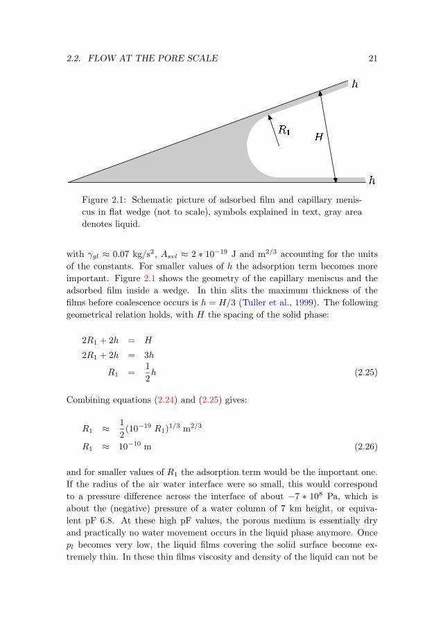
����
Figure 2.1: Schematic picture of adsorbed film and capillary menis-
cus in flat wedge (not to scale), symbols explained in text, gray area
denotes liquid.
with γgl ≈ 0.07 kg/s2, Asvl ≈ 2 ∗ 10−19 J and m2/3 accounting for the units
of the constants. For smaller values of h the adsorption term becomes more
important. Figure 2.1 shows the geometry of the capillary meniscus and the
adsorbed film inside a wedge. In thin slits the maximum thickness of the
films before coalescence occurs is h = H/3 (Tuller et al., 1999). The following
geometrical relation holds, with H the spacing of the solid phase:
2R1 + 2h = H
2R1 + 2h = 3h
R1 =1
2h (2.25)
Combining equations (2.24) and (2.25) gives:
R1 ≈ 1
2(10−19 R1)
1/3 m2/3
R1 ≈ 10−10 m (2.26)
and for smaller values of R1 the adsorption term would be the important one.
If the radius of the air water interface were so small, this would correspond
to a pressure difference across the interface of about −7 ∗ 108 Pa, which is
about the (negative) pressure of a water column of 7 km height, or equiva-
lent pF 6.8. At these high pF values, the porous medium is essentially dry
and practically no water movement occurs in the liquid phase anymore. Once
pl becomes very low, the liquid films covering the solid surface become ex-
tremely thin. In these thin films viscosity and density of the liquid can not be
22 CHAPTER 2. OVERVIEW AND REVIEW
assumed constant any more (Gray and Hassanizadeh, 1991a; Tuller and Or,
2001, p. 261). The liquid viscosity and density then depend on the distance to
the solid surface. This plays a role only in films thinner than 10−8 m (Tuller
and Or, 2001). These effects can play an important role in fine textured soils,
but are relative unimportant in sands (Tuller and Or, 2001) with their specific
surface areas in the order of 104 m2/m3 (Hilfer, 1996). The amount of water
held by adsorptive forces in sands at the above limit can be easily estimated
as 10−10 m ∗ 104m2/m3 ≈ 10−6m3/m3, which is indeed negligible for most
practical purposes. The same conclusions can be drawn from capillary rise
and drainage, and from flow in capillary groove experiments. Hence in these
cases capillary bound water is more important than water bound by adsorptive
forces (Lago and Araujo, 2001; Romero and Yost, 1996).
In conclusion, the assumption is justified that most water at low capillary
pressure is held by capillary forces in sandy soils, and that these capillary
forces are the major phenomena in determining the flow of liquid, in contrast
to adsorptive forces that play only a minor role. From now on the adsorptive
forces as such are not longer directly considered in this dissertation and it is
assumed that practically all water is held by capillary forces.
In the last few paragraphs the contribution of the vapor phase on the liquid
equilibrium was not considered (as is in the reminder of this dissertation). It
should be kept in mind that mass transport through the vapor phase in very
dry soils is more important than liquid flow. This subject would warrant at
least another few years of research. However the movement of liquid in very
dry soils is not further considered here.
Flow at the Pore Scale
The equations describing two-phase flow at the pore scale are very similar
to the single-phase flow equations. The major difference is that two fluids
are present and hence two momentum and mass balances need to be solved.
Additionally the interfacial conditions between the two fluid phases need to be
specified. The momentum balances (eqs. (2.6)) become:
ρg
(
∂vg∂t
+∇ · (vgvg))
= −∇pg + µg∇2vg + ρgg (2.27)
ρl
(
∂vl∂t
+∇ · (vlvl))
= −∇pl + µl∇2vl + ρlg (2.28)
2.2. FLOW AT THE PORE SCALE 23
with subscript g for the gas phase and l for the liquid phase. They are aug-
mented by the mass balance equations:
∇ · (ρgvg) = 0 (2.29)
∇ · (ρlvl) = 0 (2.30)
with boundary conditions:
B.C.1 vg = 0 at gas-solid interface (2.31)
B.C.2 vl = 0 at solid-liquid interface (2.32)
B.C.3 vg = vl at gas-liquid interface (2.33)
B.C.4 (pl − pg)(x, t) = −γglC(x, t) at gas-liquid interface (2.34)
B.C.1 and B.C.2 are the standard no-slip boundary conditions for the fluid-
solid interface. B.C.3 states that there is no mass transfer across the gas-liquid
interface. B.C.4 describes the pressure jump condition across the gas-liquid
interface. This expression is a simplified form of the full stress balance at
the gas-liquid interface (Hilfer, 1996). If the dynamics of the interface need
to be taken into account, explicit balance equations can be derived (Gray and
Hassanizadeh, 1991b). Additionally the boundary conditions at the entries and
exits of the fluid domain need to be described. The above equations contain a
self contradiction: B.C.1 and B.C.2 state no-slip at the solid interface. If the
contact line between gas, liquid and solid moves, it must slip along the solid
interface. This contradiction is not important in the following description of
two-phase flow (Hilfer, 1996; Dussan V., 1979; de Gennes, 1985). Here the
assumption is made that a thin, quasi stationary liquid film covers the solid
at all times, and so the singularity at the contact line is removed.
It is a common assumption that the gas phase has atmospheric pressure every-
where and that the influence of gravity on the gas phase is negligible (Koore-
vaar et al., 1983). This implies that all gradients in the gas phase vanish:
∇pg = 0 (2.35)
A second common assumption is that the gas phase has “infinite” mobility,
i.e. µg = 0 (Bear, 1988). This implies that there is no viscous coupling at the
gas-liquid interface (and hence the simple form of B.C.4). In any case, due to
the high viscosity contrast of water and air (µw ≈ 1 × 10⁻³, µa ≈ 2 × 10⁻⁵),
24 CHAPTER 2. OVERVIEW AND REVIEW
viscous coupling only plays a role in high-speed flows. Capillary equilibrium,
i.e. quasi static capillary forces can be assumed if (Dracos, 1991):
∣
∣
∣
∣
(µl − µg)U
γgl
∣
∣
∣
∣
¿ 1 (2.36)
with U a characteristic velocity. The above term is a modified capillary num-
ber (Ca), related to the viscosity contrast. The common definition for Ca is
(Probstein, 1989):
Ca =viscous force
surface tension force=
µU
γ(2.37)
With the given assumptions, equations (2.27) essentially vanish, and equations
(2.28) can be used without direct reference to equation (2.27). Using dimen-
sional analysis and scaling arguments similar to single-phase flow (Hilfer and
Øren, 1996), equations (2.28) reduce to:
− ρlg +∇pl = µl∇2vl (2.38)
whereby slow, viscous dominated low Reynolds number flow is assumed. As
with single-phase flow this can be described as purely viscous, creeping flow.
When the volume of liquid becomes small, it will tend to cover the solid with
thin films. Because the flow resistance in thin films scales with approximately
the film thickness to the power three (Bird et al., 1960), liquid movement
becomes slower and slower as the thickness approaches zero. There are sev-
eral examples in the literature which solve two-phase flow at the pore scale.
Payatakes et al. (1973) and Saez et al. (1986) use a periodically constricted
pore model. Their model allows capillary effects to play only a small role,
because their model is essentially two-dimensional. As they use the model also
for high-speed flows, where capillarity is of less importance, their assumptions
are reasonable. Ruan and Illangasekare (1999) developed a liquid flow model
applicable to sandy soils based on a sheet flow model. Their model is based
on quasi-spherical unit cells and allows a variety of flow phenomena to be
modeled. A drawback of their approach is that no closed-form relationship for
saturation-capillary pressure dependence is given. Tuller (Tuller and Or, 2001)
used a combination of polygonal pores and slits to describe flow together with
capillary and adsorption phenomena. The great advantage of their model is
the accurate representation of adsorption, but the flow model is quite primitive
in terms of the geometrical representation of the pore space. In effect their
model is a two-dimensional model.
2.3. UPSCALING TO THE CONTINUUM SCALE 25
2.3 Upscaling to the Continuum Scale
The change of scale from the pore or microscale to the continuum or macroscale
changes the form of the flow equations. For single-phase and multi-phase flow
different techniques and assumptions are used that lead to different forms of
the governing equations. An important quality of the upscaled equations is
whether they are local or nonlocal (Cushman, 1990a). Local equations have a
mathematical structure similar to the Navier-Stokes equations (eqs. 2.6) and
depend on local point values only. Nonlocal equations also depend on long
range interactions. Most theories describing flow in porous media use local
equations. Notable exceptions are so called ”pressure drop” correlations used
in chemical engineering (Brodkey and Hershey, 1988), and the original form of
Darcy’s law (Darcy, 1856). These equations are nonlocal, because they depend
on an external pressure drop directly. Central to the local versus nonlocal
distinction is the definition of so called point values. The definition of what a
mathematical point and a physical point in the upscaled equations is, is given
by Nitsche and Brenner (1989, p. 240): ”a ’point’ at the microscale does not
strictly represent a mathematical point; instead, it has meaning only beyond
a much smaller intermediate size (characteristic of the mesoscale), which is
nevertheless so much greater than the pore scale that the macroscopic ’point’
contains an appreciable, indeed representative, portion of the microstructure”.
The ’volume’ associated with the macroscopic point is called a Representative
Elementary Volume (REV).
The term upscaling is used in many contexts. Here it is used to denote an
operation that describes a spatial transformation from the pore scale to the
continuum scale or macroscale . At the continuum scale new parameters enter
the flow equations and replace small-scale descriptions. On the macroscale the
detailed description of interfaces and spatial distributions disappears and is
replaced by macroscale parameters. Going from the pore to the continuum
scale results in a loss of information (Cushman, 1990b). This lost information
is commonly replaced by implicit (du Plessis and Masliyah, 1988; du Plessis,
1997)) or explicit constitutive relations (Bear and Bachmat, 1990). There are
different methods for the upscaling process: heuristic and empirically based
methods, stochastic methods, methods based on homogenization, mixture the-
ories and space averaging theories.
These upscaling methods have the following definitions in common. Porosity
is defined as:
ε =VpV0
(2.39)
26 CHAPTER 2. OVERVIEW AND REVIEW
with Vp the pore volume and V0 the averaging volume. The liquid saturation
nl is defined as:
nl =VlVp
(2.40)
with Vl the volume of the liquid phase in V0. The following constraints apply:
Vs + Vp = V0 (2.41)
Vl + Vg = Vp (2.42)
nl + ng = 1 (2.43)
with the subscript s indicating the solid phase and Vs the volume of the solid
phase in V0.In the following sections the main upscaling approaches are listed.
Heuristics and empirical descriptions, and stochastic methods
Heuristics and empirical descriptions are based on the direct description of
experiments (van Genuchten, 1980), or an extension of Darcy’s equation to
two-phase flow (Richards, 1931). Modern methods use pore network modeling
(Hassanizadeh et al., 2001) to obtain upscaled flow equations and/or parame-
ters for constitutive relations, based on physical or computer models.
Stochastic upscaling methods are not often used in flow in porous media. Their
main application area lies in transport theories, e.g. solute transport (Cush-
man, 1990a).
Homogenization
A third class of upscaling techniques is based on the method of homogenization.
”A more descriptive name of this method is ’an asymptotic method for the
study of periodic media’.” (Ene, 1990). Homogenization deals with multi-
scale systems, i.e. systems in which the different scales are clearly separated.
It is based on the study of periodic solutions of partial differential equations
and the asymptotic behavior of these as the period tends to zero. The method
is restricted to problems with periodic boundary conditions and structures.
Due to these restrictions the method cannot be applied directly to multi-phase
flow (Pride and Flekkøy, 1999), although attempts have been made (Hornung,
1997).
2.3. UPSCALING TO THE CONTINUUM SCALE 27
Mixture theories
Mixture theories are based on ”mixing” of the description of different phases
in a multi-phase medium. They were applied in the context of flow in porous
media by Bowen (1984) and Wang and Beckermann (1993). Mixture theories
result in simpler upscaled equations than the homogenization method or spa-
tial averaging, because they do not describe the movement of the different fluid
phases in porous media separately, but lumped (Bowen, 1984). A disadvan-
tage is that the information regarding a specific phase is lost and that certain
pore level phenomena (phase discontinuities, counter-current flow) can not be
described easily.
2.3.1 Space averaging theories
Space averaging theories are widely used in the upscaling of processes in porous
media (Nitsche and Brenner, 1989). Space averaging is called volume averaging
if the averaging is carried out over a three-dimensional volume. This volume
is called a Representative Elementary Volume (REV). The basis of volume
averaging in porous media was derived by Whitaker (1966, 1967, 1969), An-
derson and Jackson (1967), Slattery (1967, 1969), Gray (1975), and Blake
and Garg (1976). Later contributions and extensions were made by: Has-
sanizadeh and Gray (1979a,b, 1980), Tosun and Willis (1980), Narasimhan
(1980b), Drew (1983), Whitaker (1985), Crapiste et al. (1986), and Bear and
Bachmat (1990). Basically, volume averaging is a very simple technique, based
on the mean value theorem for integrals. It states that for a given function
f(x), a unique average value 〈f〉 can be determined. On the other hand, a
given average value 〈f〉 can be the result of averaging different functions f(x).
Volume averaging considers two types of averages, the phase average, defined
by:
〈Ψ〉 =
∫
V0
ΨdV∫
V0
1dV =1
V0
∫
V0
Ψ dV (2.44)
with Ψ a generalized variable, and the intrinsic phase average defined by:
〈Ψ〉i =
∫
Vi
ΨdV∫
Vi
1 dV =1
Vi
∫
Vi
Ψ dV (2.45)
28 CHAPTER 2. OVERVIEW AND REVIEW
with Vi the volume of phase i. The intrinsic phase average is defined as an
average in a specific phase i. In the above two formulas, the angular brackets
〈 〉 denote the average defined by the integrals. The intrinsic phase average
is commonly used to describe the liquid pressure, as this pressure is defined
inside the liquid phase only and not inside the whole averaging volume.
The microscale transport equations contain spatial and time derivatives. In
order to average the spatial derivatives, the need arises to interchange differ-
entiation with spatial integration. The resulting theorem is called the spatial
averaging theorem (Anderson and Jackson, 1967; Whitaker, 1967; Slattery,
1967; Gray, 1975; Gray and Lee, 1977). For a general variable (Gray et al.,
1993):
〈∇Ψ〉 = ∇〈Ψ〉+ 1
V0
∫
SΨ
νΨ dS (2.46)
with SΨ the surface of the averaging volume occupied by Ψ, and ν an outward
unit normal vector on SΨ. The above implies for the divergence operation:
〈∇ ·Ψ〉 = ∇ · 〈Ψ〉+ 1
V0
∫
SΨ
ν ·Ψ dS (2.47)
Gray (1975) introduced a consistent decomposition of the average value of a
variable in the local value and the local deviations from the spatial average:
〈Ψ〉 = Ψ− Ψ (2.48)
whereby the dot denotes the deviations from the average. This decompo-
sition together with the spatial averaging theorem makes it possible to de-
rive macroscale equations in a mathematically well defined and traceable way
(Diedericks, 1999, p. 29). These averaging theorems, although mathematically
well defined for any (continuous) function, are physically meaningful only for
additive functions. Additive functions are those which measure the extent or
amount of a given property in the system (Sherwood, 1971).
Hassanizadeh and Gray (1979a) proposed a set of four criteria, which should,
in their view, be satisfied in the averaging process. These criteria are based
on physical reasoning and try to ensure consistent and physically meaningful
macroscale equations:
2.3. UPSCALING TO THE CONTINUUM SCALE 29
criterion I When an averaging operation involves integration, the integrand
multiplied by the infinitesimal element of integration must be an additive quan-
tity.
Several authors violate this criterion and obtain physically questionable macro-
scopic balances (Kowalski, 2000; Hager and Whitaker, 2000, 2002a,b; Hsu and
Cheng, 1988; Pride and Flekkøy, 1999), see also Narasimhan (1980a) and the
response by W. G. Gray in Narasimhan (1980a). Hager and Whitaker (2002b)
showed that in certain situations this criterion can be relaxed. If the integrand,
written as a linear combination with a capacity function, is additive, then also
non additive quantities can be the directly averaged.
criterion II The macroscopic quantities shall exactly account for the total
amount of the corresponding microscopic quantity.
In effect criterion II is a balance statement, and could be paraphrased as: The
“large” is “the sum of all small parts”.
criterion III The primitive concept of a physical quantity, as first introduced
into the classical continuum mechanics, must be preserved by proper definition
of the macroscopic quantities.
Hassanizadeh and Gray (1979a) give an example for this criterion: “..., heat
is a mode of transfer of energy through a boundary different from work. The
definition of macroscopic heat flux must also be a mode of energy transfer
different from macroscopic work.”
criterion IV The average value of a microscopic quantity must be the same
function that is most widely observed and measured in a field situation or in
the laboratory.
Criterion IV is not based on physical reasoning, but on practical considera-
tions. The question arises what exactly should be considered the “most widely
observed and measured” quantity (see also the discussion about tensiometers
in sect. 3.4.2).
In their work Hassanizadeh and Gray (1979a) and Gray and Hassanizadeh
(1991b) show that volume integrals of quantities such as pressure, which are
defined per unit area, can be transformed into area integrals. This is of special
importance in multi-phase flow, where the area integrals are often evaluated
over the fluid-fluid interfaces (Bear and Bachmat, 1990).
30 CHAPTER 2. OVERVIEW AND REVIEW
Closure
After volume averaging of the microscopic equations, the resulting macroscopic
equations still contain microscopic quantities, usually in the form of integrals of
microscale terms (Whitaker, 1980; Crapiste et al., 1986). The approximation
of these integrals in terms of macroscopic quantities is called closure. Different
methods can be found in the literature:
• Numerical methods: Quintard and Whitaker (1990, 1994), Fourie (2000).
• Empirical methods: Whitaker (1980), Bear (1988).
• Units cell concepts: du Plessis and Masliyah (1988, 1991), du Plessis and
Roos (1994), Hsu and Cheng (1988), Diedericks and du Plessis (1997),
Smit and du Plessis (2000), Hoffmann (2000b).
Here the unit cell concept is used. Up to now this concept has been applied
mainly to single-phase flow, and the application to multi-phase flow devel-
oped here extends this concept to the use in unsaturated flow. The work
presented here is parallel to the work of Hassanizadeh and Gray (1980). They
use thermodynamic relationships to constrain the closure problem while this
work directly approximates the closure problem.
2.3.2 Resulting theories
Once the flow description retains to the macroscale, a different terminology
is applied to the description of this flow. From experiments we know that at
different liquid saturations, different flow paths for the liquid exist. At low
capillary pressures the liquid preferentially occupies the smaller pores and cor-
ners in the porous medium. The liquid permeability is then determined by the
connectivity of the liquid phase and the amount of contact surface with the
solid. Different authors put forward flow models describing unsaturated flow.
Buckingham (1907) formulates his theory analogous to thermal and electrical
conduction. Whitaker (1986b) uses an analogy to Darcy’s law, and derives an
equation similar to Richards equation, assuming static contact lines and us-
ing order of magnitude analysis. Bear and Nitao (1993) derive a macroscopic
flux law including thermal effects and thermodynamic relations for three fluid
phases. Recently Pride and Flekkøy (1999) derived a macroscopic flux law in
the fixed contact line regime. Hassanizadeh and Gray (1997) criticize most
2.3. UPSCALING TO THE CONTINUUM SCALE 31
models for apparent paradoxes and propose general relations based on ther-
modynamic relationships. The results of all these authors reflect their choices
during the averaging process. The derived macroscopic flux laws are often
similar, but it is not clear which one is more generally applicable in practical
calculations of unsaturated flow. Most of the proposed macroscopic equations
disregard time dependence or dynamics in the momentum balance and intro-
duce no dependence on average gradients.

32
3 Development of a Mathematical
Model for Flow in Unsaturated Porous
Media
3.1 Introduction
This chapter describes the development of upscaled unsaturated flow equations
in porous media. In chapter 2 an overview of the different approaches to
volume averaging was given. From now on this dissertation is mainly concerned
with liquid movement. The gas phase is still assumed to be present and to
influence the liquid behavior, but is not described explicitly any more. The
main assumptions are listed in section 3.2. In section 3.3 the starting equations
on the pore scale and the boundary and initial conditions are stated. These
equations are volume averaged and the closure problem is developed in section
3.4. In chapter 4, a geometrical model for a Representative Unit Cell (RUC)
is described and analyzed and a method to solve the two-phase flow problem
inside an RUC is proposed.
The approach taken in here is based on the closure scheme developed by
du Plessis and Masliyah (1988). This scheme is augmented with additional
boundary conditions which are introduced due to fluid-fluid interfaces. Previ-
ous applications of du Plessis and co-workers described high Reynolds number
flow in porous media (du Plessis, 1994, 1992) and flow in granular porous media
(du Plessis and Masliyah, 1991; Knackstedt and du Plessis, 1996).
3.2 Assumptions
In this section the assumptions underlying the development of the unsaturated
flow model are stated formally. These assumptions are sometimes stated in
33
34 CHAPTER 3. DEVELOPMENT OF A MATHEMATICAL MODEL
the literature (Pride and Flekkøy, 1999), but more often they are implicitly
assumed (Whitaker, 1986b, 1980). It may seem that these assumptions are
too restrictive or too many, but they are less than the (implicit) assumptions
commonly made (Whitaker, 1986b). If additional assumptions are made during
the derivation of the equations, they will be clearly stated.
3.2.1 Assumptions regarding the fluids
Assumption 1 The fluids are incompressible and the density ρ is constant.
Incompressibility and constant density are reasonable for flow in unsaturated
soils, provided pressure variations are not too large. As this work is mainly
concerned with capillary held water, these variations are relatively small. Close
to a solid surface the variation of density of the liquid phase is relatively large,
but it is assumed that the liquid bound by adhesive forces does not contribute
to the flow.
Assumption 2 The viscosity µ is constant.
This assumption is common in the soil physics literature (Koorevaar et al.,
1983), but was questioned by Gray and Hassanizadeh (1991a). In sandy soils
it is justified, because only a small fraction of the liquid is held by adsorptive
surface forces close to the solid grains. In this small fraction density and
viscosity are not constant, but this fraction does not significantly contribute
to liquid flow (see sec. 2.2.2).
Assumption 3 The fluids exert no interfacial drag on each other.
Because the viscosity ratio between liquid and gas is very high (sec. 2.2.2), the
gas phase can be assumed to exert virtually no drag on the solid phase:
Assumption 4 The individual fluid phases remain continuous at all times.
Sometimes this continuity is through a thin film, which essentially allows no
flow.
The above assumption is made in order to remove the discontinuity at the con-
tact line between solid, liquid and gas. The assumption is reasonable, because
solid surfaces are covered by a thin film of liquid, which often is deposited by
vapor.
3.2. ASSUMPTIONS 35
Assumption 5 The gas phase is assumed to be at constant, atmospheric pres-
sure.
This assumption is identical to the gas phase pressure assumption made in
deriving Richards equation (Bear, 1988).
3.2.2 Assumptions regarding the porous medium
Assumption 6 The porous medium is non-oriented or isotropic in the sense
that there is no natural direction associated with the pore structure inside an
averaging volume.
Unconsolidated porous media are often isotropic within a specific layer. Due
to natural deposition and sedimentation patterns, a layered porous medium
is not isotropic. Here it is assumed that modeling takes place within such an
isotropic layer.
Assumption 7 The solid phase is fixed in space and time.
The solid phase is assumed to be incompressible and not moving relative to a
fixed reference frame.
Assumption 8 The porous medium is homogeneous on the averaging scale.
This assumption implies that there are no macroscopic boundaries inside an
averaging volume, and that there is no change of medium.
3.2.3 Assumptions regarding flow and capillarity
Assumption 9 The flow is essentially inertia free (see section 2.2.2) and the
liquid flow is governed by equations (2.38).
Assumption 10 The flow is isothermal, and thermal effects on the surface
tension, as described in e.g. Grant and Salehzadeh (1996), play no role.
Assumption 11 During and after drainage of the wetting liquid a thin liquid
film is left covering the solid surface. This implies an effective receding contact
angle θ = 0.
36 CHAPTER 3. DEVELOPMENT OF A MATHEMATICAL MODEL
Assumption 12 Contact lines between liquid, gas, and solid can move. This
movement is assumed to be relatively smooth.
The last assumption requires some explanation. Haines (1927) already showed
that, due to capillary forces and the geometry of the solid phase, rapid contact
line movement can occur in soils and lead to ”pressure jumps”. These pressure
jumps are of very small duration (Morrow, 1970), and are assumed to average
out in an averaging volume. Assumption 4 already stated that the solid surface
is always covered with a thin liquid film. Given this assumption, the present
assumption could be read as: contact lines between capillary held liquid, gas,
and solid covered with a thin liquid film can move.
Assumption 13 Gravity forces are small compared to capillary forces at the
pore scale.
The basis of this assumption was discussed in section 2.2.2.
Assumption 14 The profile of capillary pressure inside a pore perpendicular
to the flow is not directly influenced by the flow (sec. 2.2.2, eq. 2.36).
This assumption leads to a Poiseuille like description of the microscale flow in
the pores.
Assumption 15 Only movement of liquid held by capillary forces contributes
to flow, liquid held by adsorptive forces is essentially immobile.
The above assumption was explained in section 2.2.2.
3.2.4 Assumptions not made
It is also important to list some assumptions not made here, but that are
common in the volume averaging literature on two-phase porous media flows:
1. There are no assumptions about the pressure gradients inside the averag-
ing volume (in contrast with Aleman et al. (1989); Whitaker (1986a), see
also Pride and Flekkøy (1999)), except the standard volume averaging
length scale requirements (Crapiste et al., 1986). These state: micro-
scopic length scale ¿ radius of averaging volume ¿ macroscopic length
scale.
3.3. THE BASIC INTERSTITIAL EQUATIONS 37
2. No assumptions are made regarding the saturation gradient inside an
averaging volume, except the length scale constraints imposed by volume
averaging (Crapiste et al., 1986).
3. Dynamic effects are allowed in the macroscopic momentum balance and
not neglected as in Whitaker (1986b).
3.3 The Basic Interstitial Equations
At the pore or microscopic scale the momentum balance is described by the
Stokes equations (assumption 9). A pore can be occupied by air and water
simultaneously. The presence of a phase interface (air - water) and the geo-
metric configuration of the solid influence the configuration of the fluid phases
and their dynamic behavior (see section 2.2.2). The pressure is also influenced
by the phase interfaces. A jump in pressure across the interface, refereed to
as capillary pressure, is generated. The pressure is directly influenced by the
three-phase contact line of the solid, liquid, and gas.
For the liquid phase, the microscopic momentum balance equations (2.38) are:
−ρlg +∇pl = µl∇2vl
They are augmented by the mass balance equation (2.30):
∇ · (ρlvl) = 0
And with ρl = constant, this can be written as:
∇ · vl = 0 (3.1)
with boundary conditions (similar to equations (2.31)):
B.C.1 vl = 0 at solid-liquid interface (3.2)
B.C.2 vg = vl at gas-liquid interface (3.3)
B.C.3 pl(x) = −γglC at gas-liquid interface (3.4)
B.C.4 pl = pl0,1 at entrances and exits
of averaging volume
(3.5)
with C denoting the curvature of the gas-liquid interface and pl0,1 the entry
and exit liquid pressure of an averaging volume.
38 CHAPTER 3. DEVELOPMENT OF A MATHEMATICAL MODEL
Although the flow equations on the microscale are quasi-steady, due to the
boundary conditions, the flow can be unsteady. Formally:
pl0,1 = pl0,1(x, y, z, t) (3.6)
vl,g = vl,g(x, y, z, t) (3.7)
C = C(x, y, z, t) (3.8)
This dependence on the time evolution of the boundary conditions influences
the solution of the closure problem directly and gives rise to dynamic effects
in the volume averaged flow equations.
3.4 Volume Averaging
In section 2.3 volume averaging was explained. Due to the specific nature
of the two-phase flow problem certain averaging identities are worked out in
detail. Equations (3.1) and (2.38) are averaged term by term, using volume
averaging rules and theorems from vector integral calculus.
In the literature several examples exist of the use of volume averaging in a
porous medium with constant volume fractions of fluids inside an averaging
volume (see chapter 2). Averaging with variable fluid fractions is not common
and introduces extra terms in the averaged equations which are similar to the
case when the porosity varies (Ma and Ruth, 1993; Kaviany, 1995). Interfaces
between the different phases are taken into account and are modeled in the
closure approximation. This closure approximation circumvents the use of
constitutive equations, which conventionally parameterize for phase interface
effects (Whitaker, 1986b).
Here the boundary conditions are averaged also. This is necessary to keep the
volume averaged equations compatible with the boundary conditions. Many
workers do not directly consider the boundary conditions (Gray and Has-
sanizadeh, 1991a; Narasimhan, 1980b), or recognize their importance but ig-
nore them in the averaging process (Whitaker, 1986b; Crapiste et al., 1986).
The averaging of boundary conditions is sometimes used in pore network mod-
eling (Dahle et al., 2002) and in unit cell concepts (Ma and Ruth, 1993). The
direct averaging of the boundary conditions as part of the volume averaging
helps in making the volume averaged equations applicable to practical sit-
uations. If the boundary conditions are not in an averaged form they are
incompatible with the averaged equations.
3.4. VOLUME AVERAGING 39
3.4.1 Averaging of the mass balance equation
In contrast with single-phase flow, the mass balance equation has a different
macroscopic form than the microscopic one. This is due to the change of fluid
contents caused by the divergence of the macroscopic flow. This section follows
closely Whitaker (1980, 1986b). Starting with equation (3.1), averaging the
right hand side gives:
〈0〉 = 0 (3.9)
The flow is incompressible (assumption 3.2.1), and the average of the left hand
side is given by:
〈∇ · vl〉 = ∇ · 〈vl〉+1
V0
∫
S
ν · vl dS
= ∇ · 〈vl〉+1
V0
∫
Ssl
ν · vl dS +1
V0
∫
Sgl
ν · vl dS (3.10)
= ∇ · 〈vl〉+1
V0
∫
Sgl
ν · vl dS (3.11)
where Sgl is the gas-liquid interfacial area and Ssl is the solid-liquid interfacial
area. Because the solid-liquid interface is fixed in space, surface integrals
normal to the solid-liquid interface which in the integrand explicitly contains
the fluid velocity, are zero (eq. (3.2)). By making use of the transport theorem
(Gray et al., 1993, p. 136, eq. 7.4):
∫
V
∂f
∂t
∣
∣
∣
∣
x
dV =d
dt
∫
V
f dV −∫
S
ν ·wf dS (3.12)
where w is the velocity of the interface. Setting f = 1, V = nlVp (volume of
fluid):
∫
(nlVp)
∂1
∂t
∣
∣
∣
∣
x
d(nlVp) =d
dt
∫
(nlVp)
1 d(nlVp)−∫
S
ν ·w1 dS
0 =∂nlVp∂t
−∫
Ssl
ν ·w dS −∫
Sgl
ν ·w dS (3.13)
40 CHAPTER 3. DEVELOPMENT OF A MATHEMATICAL MODEL
0 =∂nlVp∂t
−∫
Sgl
ν ·w dS
0 =∂εnl∂t− 1
V0
∫
Sgl
ν ·w dS (3.14)
with ε the porosity. Adding equation (3.14) to equation (3.11):
〈∇ · vl〉 = ∇ · 〈vl〉+1
V0
∫
Sgl
ν · (vl −w) dS +∂εnl∂t
(3.15)
Assuming no mass transport over the gas-liquid interface (immiscible) requires
that vl −w = 0 or vl = w, so that the above equation reduces to:
〈∇ · vl〉 = ∇ · 〈vl〉+∂εnl∂t
(3.16)
This equation contains the time derivative of the liquid content. The time
dependence enters the equation due to the time dependence of the microscopic
boundary conditions, i.e. the movement of the gas-liquid interface, resulting in
the non-zero divergence of the average velocity.
3.4.2 Averaging of the momentum balance equation
Like the mass balance equation, the momentum balance (eq. (2.38)) is averaged
term by term.
Averaging of the body-force term
The components of the body force term are constant, and their treatment in
volume averaged form is similar to the microscopic form (Whitaker, 1986b):
〈−ρlg〉 = − 1
V0
∫
V0
ρlg dV (3.17)
〈−ρlg〉 = − 1
V0
∫
Vl
ρlg dV +
∫
V0−Vl
ρlg dV
(3.18)
3.4. VOLUME AVERAGING 41
Because ρl is zero in V0 − Vl, i.e. the volume not occupied by the liquid:
〈−ρlg〉 = − 1
V0
∫
Vl
ρlg dV (3.19)
〈−ρlg〉 = −VlV0ρlg (3.20)
〈−ρlg〉 = −εnlρlg (3.21)
Averaging of the pressure term
The pressure term contains the liquid pressure gradient. It is the most prob-
lematic term in the averaging process. Different researchers treat this term in
completely different manners (Whitaker, 1986b; Hassanizadeh and Gray, 1993;
Hassanizadeh et al., 2002; Dahle et al., 2002). As described in chapter 2, the
pressure is used to describe the capillary component of the liquid potential and
it is assumed that this drives the flow and is responsible for the bulk liquid
phase movement. The treatment is based on an incompressible liquid. No
macroscopic volume average form for the phase average pressure is proposed.
Instead a nonlocal formulation is developed in chapter 5. It is based on an
areal averaged pressure. In essence, the pressure gradient term is part of the
closure problem, and in this chapter simply written in integral form:
〈∇pl〉 =1
V0
∫
V0
∇pl dV (3.22)
Treatment of the gradient of the liquid pressure as part of the closure prob-
lem is not common, and the question arises why the more common treatment
of the pressure as a volume averaged quantity as in Whitaker (1986b), or a
thermodynamics based approach as in Hassanizadeh and Gray (1997) is not
used. In appendix A the traditional method of averaging the liquid pressure
term is worked out. The major problem with this method is that there are
no instruments measuring a volume averaged pressure. All instruments (e.g.
tensiometers) measure a force per unit area, i.e. pressure averaged over a rep-
resentative area. A tensiometer measures the areal averaged pressure around
its circumference. This measurement includes the effect of gravity on the mea-
surement, but this effect is small when the tensiometer is small. A similar
reasoning can be applied to a multi-step outflow experiment in a pressure cell.
Here the boundary conditions are applied on ceramic plates, which cover the
42 CHAPTER 3. DEVELOPMENT OF A MATHEMATICAL MODEL
entrance and exit of the porous medium, and thus apply a uniform areal aver-
aged liquid pressure. Here the gradient of the volume average pressure is not
used at the boundaries of the porous medium, and on the macroscopic scale
no volume average pressure needs to be defined (criterion IV, p. 29). Instead
of the gradient of the volume averaged liquid pressure used in the traditional
equations, the average of the pressure term is expressed here as a nonlocal
term, which can be called the “volume average difference of the area averaged
liquid pressure”. The treatment of measurements and calculations for flow in-
side a porous medium is further developed in chapters 5 and 6. Aleman et al.
(1989) in effect use the pressure at the boundaries of an averaging volume to
define a volume averaged liquid pressure. As such their treatment is similar to
the one used here, but they make the additional simplifying assumption that
no pressure gradient inside of the averaging volume exists. As shown earlier,
this leads to the following paradox: Flow is due to a pressure gradient, and
if there is flow inside an averaging volume, there must be a pressure gradient.
But in order to conduct the volume averaging it is assumed that there is no
pressure gradient, and this implies no liquid flow.
Averaging of the viscous term
The viscous term is averaged in a similar way as described by du Plessis and
Diedericks (1997) and Whitaker (1986b). The major difference in the deriva-
tion is due to the influence of the time dependent gas-liquid boundary:
〈µl∇2vl〉 = 〈µl∇ · (∇vl)〉
= µl∇ · 〈∇vl〉+µlV0
∫
Sslg
ν · (∇vl) dS
= µl∇ ·
∇〈vl〉+
1
V0
∫
Sslg
νvl dS
+
µlV0
∫
Sslg
ν · (∇vl) dS
= µl∇2〈vl〉+µlV0
∇ ·
∫
Sslg
νvl dS +
∫
Sslg
ν · (∇vl) dS
(3.23)
Using the vector identity (Bird et al., 1960, eq. A.3-14):
∇2〈vl〉 = ∇(∇ · 〈vl〉)−∇× (∇× 〈vl〉)
3.4. VOLUME AVERAGING 43
the above equation can be written as:
〈µl∇2vl〉 = µl [∇(∇ · 〈vl〉)−∇× (∇× 〈vl〉)]
+µlV0
∇ ·
∫
Sslg
νvl dS +
∫
Sslg
ν · (∇vl) dS
(3.24)
This form of the volume averaged viscous term will be further used in the
closure. It should be noted that the macroscopic velocity 〈vl〉 is non-zero if
the liquid content inside an averaging volume changes due to inflow, even if
there is no outflow or vice versa (Pride and Flekkøy, 1999). The term µl∇2〈vl〉is usually called the Brinkman term (Brinkman, 1947, 1949; Kaviany, 1995).
3.4.3 Averaging of the boundary conditions
In order to keep the boundary conditions (eqs. (3.2), (3.3), (3.4), and (3.5))
compatible with the volume averaged equations, they too need to be averaged.
The boundary conditions internal in an averaging volume have no analog on
the macroscopic scale, and thus do not arise on this scale. They are accounted
for in the closure. In effect only equations (3.5) exist on the macroscale, sup-
plemented by other macroscale boundary conditions (see sec. 5.4). Equation
(3.5) needs to be compatible with the averaged pressure gradient term, and as
such is area averaged over the entrances and exits of an averaging volume:
〈pl|0〉 =1
S0
∫
S0
p0 dS
= p0 (3.25)
〈pl|1〉 =1
S1
∫
S1
p1 dS
= p1 (3.26)
with the following definitions:
p1,0 =1
Sexit, entry
∫
Sexit, entry
pl dS (3.27)
That is, p1,0 is the area averaged pressure at the exit c.q. entrance.
44 CHAPTER 3. DEVELOPMENT OF A MATHEMATICAL MODEL
3.4.4 The combined averaged equations
The combined averaged mass balance equation becomes (eqs. (3.16), (3.9)):
∇ · 〈vl〉 = −∂εnl∂t
(3.28)
The volume averaged momentum balance equations are obtained by combining
equations (3.21), (3.22) and (3.24):
−εnlρlg + µl [−∇(∇ · 〈vl〉) +∇× (∇× 〈vl〉)]
=µlV0∇ ·
∫
Sslg
νvl dS +µlV0
∫
Sslg
ν · (∇vl) dS −1
V0
∫
V0
∇pl dV (3.29)
These are the upscaled momentum balance equations valid at the macroscale.
The terms on the left hand side only contain macroscopic variables, whereas the
terms on the right hand side contain microscopic variables inside the integrals.
These terms represent the closure problem. In chapter 5 these equations are
further analyzed. The averaged boundary conditions are given by p0 and p1.
4 Closure Model
4.1 Introduction
This chapter describes the development of a Representative Unit Cell (RUC)
model for the closure of the volume averaged equations derived in chapter 3,
and the proposed solution for the local flow equations. In sections 4.2 and
4.3 the geometrical RUC model together with the capillary pressure model is
explained. An RUC is similar to a Representative Elementary Volume (REV)
in the sense that it is a three dimensional averaging volume, but the concept
of an RUC also entails a detailed geometrical description. This description is
to imagine a typical porous medium configuration in which the flow processes
are modeled. The RUC should not be equated with a portion of a real porous
medium, because not all features of a real porous medium are modeled. Its
“average” behavior is assumed to mimic the behavior of a real porous medium.
The emphasis is on those features which directly influence the flow processes
on average. The RUC needs to accommodate the topology, geometry and
capillary pressure relationship of a porous medium. As shown in chapter 2,
capillarity plays a major role in unsaturated flow. The geometry of the RUC is
expressed in terms of the macroscopic parameters porosity, ε, and the critical
radius for drainage, rc. Additionally three RUC parameters, a, b, and j, will
be defined. In sections 4.4 and 4.5 the microscopic momentum equations are
solved, based on a Poiseuille type flow model. The solution is then used in the
closure of equations (3.29).
4.2 Description of the RUC
The RUC is made of a cubic unit cell. In this chapter no explicit relations
are given for the stacking of RUC’s, as we are concerned only with the local
flow problem here. du Plessis and Diedericks (1997) show that for a vari-
ety of RUC configurations in single-phase flow, maximum staggering is the
45
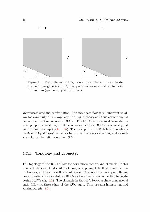
46 CHAPTER 4. CLOSURE MODEL
�����
���
�
���
��� �
���
�
���
Figure 4.1: Two different RUC’s, frontal view; dashed lines indicate
opening to neighboring RUC; gray parts denote solid and white parts
denote pore (symbols explained in text).
appropriate stacking configuration. For two-phase flow it is important to al-
low for continuity of the capillary held liquid phase, and thus corners should
be assumed continuous across RUC’s. The RUC’s are assumed to model an
isotropic porous medium, i.e. the configuration of the RUC’s does not depend
on direction (assumption 6, p. 35). The concept of an RUC is based on what a
particle of liquid “sees” while flowing through a porous medium, and as such
is similar to the definition of an REV.
4.2.1 Topology and geometry
The topology of the RUC allows for continuous corners and channels. If this
were not the case, fluid could not flow, or capillary held fluid would be dis-
continuous, and two-phase flow would cease. To allow for a variety of different
porous media to be modeled, an RUC can have open areas connecting to neigh-
boring RUC’s (fig. 4.1). The channels in the RUC follow a three-dimensional
path, following three edges of the RUC cube. They are non-intersecting and
continuous (fig. 4.2).
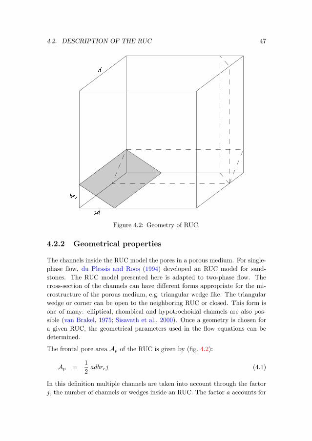
4.2. DESCRIPTION OF THE RUC 47
�����
���
�
Figure 4.2: Geometry of RUC.
4.2.2 Geometrical properties
The channels inside the RUC model the pores in a porous medium. For single-
phase flow, du Plessis and Roos (1994) developed an RUC model for sand-
stones. The RUC model presented here is adapted to two-phase flow. The
cross-section of the channels can have different forms appropriate for the mi-
crostructure of the porous medium, e.g. triangular wedge like. The triangular
wedge or corner can be open to the neighboring RUC or closed. This form is
one of many: elliptical, rhombical and hypotrochoidal channels are also pos-
sible (van Brakel, 1975; Sisavath et al., 2000). Once a geometry is chosen for
a given RUC, the geometrical parameters used in the flow equations can be
determined.
The frontal pore area Ap of the RUC is given by (fig. 4.2):
Ap =1
2adbrcj (4.1)
In this definition multiple channels are taken into account through the factor
j, the number of channels or wedges inside an RUC. The factor a accounts for
48 CHAPTER 4. CLOSURE MODEL
the base length of the wedge relative to d, the RUC dimension. If the RUC
channel is closed b = 2, or if open b = 1 (fig. 4.1). The critical radius for
drainage (explained in section 4.3) is given by rc.
The saturated “wetted” perimeter of a single pore corner is defined as:
Pp = ad+ (a2d2 + b2r2c )1/2 (4.2)
and the saturated wetted perimeter of an RUC is:
P =
{
j(ad+ (a2d2 + b2r2c )1/2) : if b = 2
j(a2d2 + b2r2c )1/2 : if b = 1
(4.3)
Through trigonometric relations tanα and sinα are defined by:
tan(α) =rcad
(4.4)
sin(α) =rc
(r2c + a2d2)1/2(4.5)
with α the half opening angle of the wedge. The pore volume Vp is defined
from the RUC geometry as:
Vp = 3dAp −j
3(a2d2brc + b2r2cad) (4.6)
= Ap(3d−2
3(ad+ brc)) (4.7)
As an approximation the flow length lg inside the RUC is computed by re-
quiring that the pore volume is equal to the frontal pore area times the flow
length:
Vp = lgAp (4.8)
lg =VpAp
(4.9)
=2εd2
abrcj(4.10)
using the relation Vp = εd3 and equation (4.1). The above definition of lg does
not take into account changes in volumetric flow inside the different corners,
4.3. CAPILLARY PRESSURE RELATIONSHIP 49
but is based on the ratio of the volume of a straight channel to the curved one
inside the RUC.
Taking together equations (4.1), (4.6) and Vp = εd3:
d =brc12ε
(
(a2j2(2a− 9)2 − 48ajε)1/2 + aj(9− 2a))
(4.11)
In the above development rc and ε are taken as the main structural parameters
of the porous medium. These parameters in turn define the magnitude of the
parameters d and α, together with a, b and j. With these, the geometry
of an RUC is completely defined. The parameters rc and ε are regarded as
macroscopic parameters of the porous medium, and are directly measurable
on the macroscopic scale.
4.3 Capillary Pressure Relationship
The relation between the pressure difference between the fluids and the liquid
saturation is modeled similar to Mason and Morrow (1991), using the Mayer
and Stowe-Princen (MSP) method (Princen, 1969a,b, 1970). The relationship
does not take into account the effects of short range adhesion forces, but could
be modified accordingly with the Augmented Young-Laplace equation (see
section 2.2.2).
If a non-wetting fluid enters a pore filled with a wetting fluid, an interface
between the two fluids is formed. This interface is called a main terminal
meniscus (MTM). As soon as the two principal radii of the meniscus have
the same magnitude, the non-wetting fluid enters the capillary. This radius is
called the critical radius for drainage, rc. During imhibition, when a wetting
fluid fills a capillary, a possibly different critical radius corresponds to complete
filling of the capillary with the wetting fluid. This radius corresponds to the
situation that the liquid from the separate corners starts to touch each other.
Both critical radii depend on the contact angle and the specific geometry of
the pore. For the modeling of the capillary pressure saturation relationship,
channel curvature in the longitudinal direction is not taken into account. The
critical radius for drainage is expressed as:
rc = −γglplc
(4.12)
In this expression assumption 11 (p. 35) was used, which implies that the con-
tact angle θ = 0. The critical liquid pressure for drainage plc is similar to
50 CHAPTER 4. CLOSURE MODEL
the air entry pressure in traditional soil physics modeling. Equation (4.12)
is written without the factor 2 in the Young-Laplace equation for a spherical
interface. This corresponds to R2 =∞ in equation (2.18). Effectively it is as-
sumed that the gas liquid interface is approximately cylindrical at r = rc inside
a pore, and that at gas entry, the pore drains abruptly. The use of equation
(4.12) allows rc to be calculated from the air entry pressure of a desaturation
experiment. Thus rc is defined based on a macroscopic measurement and as
such a macroscopic measurable parameter. In effect, rc denotes some kind of
“average” critical radius for drainage.
4.3.1 Geometry of liquid inside a corner
In this section basic equations for the wetting fluid (liquid) inside a corner of a
pore are derived. The following equations are derived for a single corner only
(fig. 4.3) and still have to be assembled for the particular RUC in question.
The fluid configuration has to obey the Concus-Finn conditions (Weislogel and
Lichter, 1998) in order to yield a stable interface:
θ <π
2− α (4.13)
with θ the contact angle and α the half opening angle of the corner. This con-
dition states that liquid forms a stable interface only in certain combinations
of corner opening half angle and contact angle. The length of the solid-liquid
interface inside a corner is defined by (see fig. 4.3):
Lsl =2r cos(θ + α)
sin(α)(4.14)
and with θ = 0:
Lsl =2
tan(α)r (4.15)
= fLslr (4.16)
Similarly, Lgl is defined as:
Lgl = (π − 2α− 2θ)r (4.17)
and with θ = 0:
Lgl = (π − 2α)r (4.18)
= fLglr (4.19)
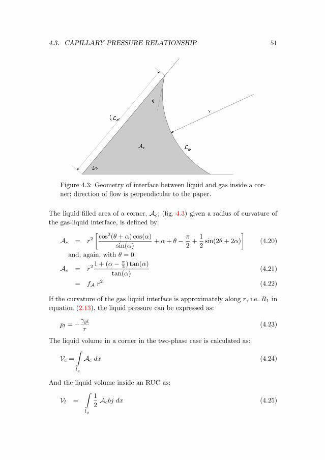
4.3. CAPILLARY PRESSURE RELATIONSHIP 51
���
������
��
�
���
Figure 4.3: Geometry of interface between liquid and gas inside a cor-
ner; direction of flow is perpendicular to the paper.
The liquid filled area of a corner, Ac, (fig. 4.3) given a radius of curvature of
the gas-liquid interface, is defined by:
Ac = r2[
cos2(θ + α) cos(α)
sin(α)+ α+ θ − π
2+
1
2sin(2θ + 2α)
]
(4.20)
and, again, with θ = 0:
Ac = r21 + (α− π
2 ) tan(α)
tan(α)(4.21)
= fA r2 (4.22)
If the curvature of the gas liquid interface is approximately along r, i.e. R1 in
equation (2.13), the liquid pressure can be expressed as:
pl = −γglr
(4.23)
The liquid volume in a corner in the two-phase case is calculated as:
Vc =∫
lg
Ac dx (4.24)
And the liquid volume inside an RUC as:
Vl =
∫
lg
1
2Acbj dx (4.25)
52 CHAPTER 4. CLOSURE MODEL
=1
2bjVc (4.26)
The above definitions define the geometry related variables for an RUC. They
will be used in the solution of the local RUC flow model in section 4.4 and in
chapter 5 for the closure.
4.4 Flow Models
In order to find an approximate analytical solution for the closure problem,
the resistance to flow in the RUC channels needs to be specified. Single-phase
flow in micro channels was studied by e.g. MacLaine-Cross (1969), Ayyaswamy
et al. (1974), Sisavath et al. (2000, 2001), Thompson and Fogler (1997), and
Patzek and Kristensen (2001). The standard monograph on the subject is
Shah and London (1978). Common to these approaches is the assumption
of Stokes flow, which leads to a Poiseuille flow regime inside the channel for
fully developed flow (Romero and Yost, 1996; Weislogel and Lichter, 1998). In
two-phase flow in micro channels, the liquid is in part in contact with the solid
surface, and in part with another fluid phase. Here the other fluid phase is a gas
(air), which exerts no shear stress on the liquid (Ma et al., 1994; Hilfer, 1996).
For slow flows, as studied here, the velocity profile is nearly instantaneously
fully developed (Weislogel and Lichter, 1998), and curvature effects along the
corner are not significant. This assumption introduces negligible error if the
flow length is larger than 2−3 times the hydraulic radius (Ruth and Ma, 1993).
How can such a simple flow model reflect the flow in porous media, where the
pores are not smooth and converging-diverging? Erickson et al. (2002) showed
by numerical calculations that the basic flow mechanism in capillary pressure
driven flow does not change qualitatively in converging-diverging pores in an
average sense. What does change are the values of some parameters, but
the dynamics stay the same. Borhan and Rungta (1993) showed, by using a
semi-analytic model for flow between periodically corrugated plates, that the
flow equations can be scaled to the standard dynamic ones, but with another
characteristic capillary penetration time. Lago and Araujo (2001) and Staples
and Shaffer (2002), by experiments and by a morphological porous medium
model, showed that these dynamics also hold in porous media. Lago and
Araujo (2001) also observed the typical algebraic behavior of the capillary
velocity against time. As slow, continuous flow is assumed, contact line pinning
is assumed to play no significant role. Pinning is mostly important near the
imhibition threshold, but there is no direct evidence that it is important in
4.4. FLOW MODELS 53
corner flow (Schaffer and Wong, 2000). Lago and Araujo (2001) showed that
pinning has influence in packings of glass beads, but that no such behavior can
be observed in sandstones. It is assumed that this has to do with the micro
structure of the pores in packings of glass beads. In these the wetting fluid has
no continuous corners for flow, but instead has to follow converging-diverging
flow paths. In sandstones the flow paths are more wedge like, as is assumed
here. Weislogel and Lichter (1998) state that because the flow in a corner is
predominantly parallel to the contact line, the normal velocity perpendicular
to the contact line is small, and the discontinuity in the velocity at the contact
line is not significantly influencing the flow (see assumption 12, p. 36).
Rewriting the momentum balance equations (eqs. 2.10) as (Shah and London,
1978):
∇2vl =1
µ∇pl (4.27)
and:
∇2vl = constant (4.28)
i.e. fully developed flow. Under the assumption of Poiseuille flow this leads to
(Panton, 1984):
vp,c = −Fp,c
µlAc
∂pl∂x
(4.29)
with Fp,c a resistance factor and the average pore or corner velocity defined
as:
vp,c =1
Ac
∫
Ac
vl dA (4.30)
4.4.1 Single-phase flow
For single-phase flow, the magnitude of vp does not change in axial direction.
Fp is a constant, as is the pressure drop. Commonly the resistance factor for
laminar flow in pipes is expressed as the product of the Fanning friction factor
f and the Reynolds number Re (Shah and London, 1978):
fRe = constant (4.31)
54 CHAPTER 4. CLOSURE MODEL
The definition of the Reynolds number for flow in the pores is:
Re = ρl |vp|4rhµl
(4.32)
The Fanning friction factor is given by (Ma et al., 1994; Shah and London,
1978):
f =2rh
ρl|vp|2∂pl∂x
(4.33)
Combining equations (4.32) and (4.33) gives:
fRe =8r2h
µl |vp|∂pl∂x
(4.34)
with the hydraulic radius rh of a cross section of the pores inside an RUC
defined by:
rh =Ap
Pp(4.35)
Combined, the above equations define the following equation for single phase
flow in a pore:
vp = − 8r2hµl fRe
∂pl∂x
(4.36)
By comparing equations (4.29) and (4.36), the relation between fRe and F can
be obtained:
Fp =8
fRe
r2hAp
(4.37)
Numerical values for fRe are given in Shah and London (1978) for different
pore geometries.
4.4. FLOW MODELS 55
4.4.2 Two-phase flow
Capillary driven two-phase flow in a corner is described by a Poiseuille type
equation, similar to a nonlinear diffusion equation (Dong and Chatzis, 1995;
Romero and Yost, 1996; Weislogel and Lichter, 1998). This nonlinear partial
differential equation is similar to the foam drainage equation (Verbist et al.,
1996). In principle it can be transformed to an ordinary differential equation by
a similarity transformation (Mayer et al., 1983). Weislogel and Lichter (1998)
list classes of solutions for this equation with given boundary conditions. For
instance, for a constant pressure boundary condition the speed of the advanc-
ing meniscus is proportional to√t. There are no general analytical solutions
available for arbitrary initial and boundary conditions, but the dynamics were
studied for a variety of conditions by Weislogel and Lichter (1998), Weislogel
(2001), and Romero and Yost (1996). Solutions were established for planar
and non-planar corner geometries. Apart from a solution for the dynamics of
this equation, an approximation for the resistance factor is also required. The
derivation of the resistance factors for two-phase flow in corners was studied
by Ayyaswamy et al. (1974). Ransohoff and Radke (1988) used finite element
calculations to derive the resistance factor. Zhou et al. (1997) developed an-
alytical correlations, but their correlations can deviate substantially from the
true solution. Weislogel and Lichter (1998) developed the method used here,
by scaling of the flow equations. The corner flow problem is also widely studied
in heat transfer in micro channels, e.g. in electronics cooling. These solutions
are usually not applicable, because due to forced convection the shear stress
at the gas-liquid interface is not negligible (Suh et al., 2001).
The general geometry of the flow is shown in figure 4.4. The governing equation
(4.27) can be rewritten as:
∂pl∂x
= µl
(
∂2
∂y2vl +
∂2
∂z2vl
)
(4.38)
Scaling by x∗ = x/L, y∗ = y/H, z∗ = z/(H tan(α)), v∗ = vl/v, and P ∗ =
fHpl/γgl (with starred quantities denoting dimensionless quantities), yields:
γglHfL
∂P ∗
∂x∗= µlv
(
1
H2 tan2(α)
∂2v∗
∂y∗2+
1
H2
∂2v∗
∂z∗2
)
(4.39)
with L a characteristic length scale along the pore, H a characteristic height
of the liquid, α the half opening angle of the wedge, v a characteristic velocity,
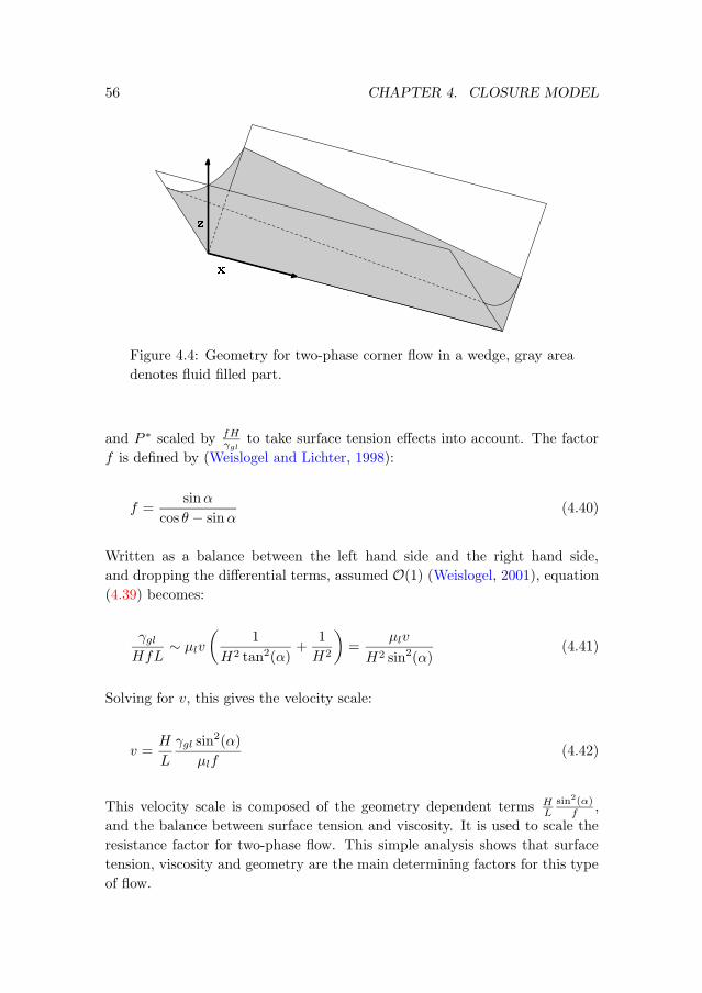
56 CHAPTER 4. CLOSURE MODEL
�
�
Figure 4.4: Geometry for two-phase corner flow in a wedge, gray area
denotes fluid filled part.
and P ∗ scaled by fHγgl
to take surface tension effects into account. The factor
f is defined by (Weislogel and Lichter, 1998):
f =sinα
cos θ − sinα(4.40)
Written as a balance between the left hand side and the right hand side,
and dropping the differential terms, assumed O(1) (Weislogel, 2001), equation
(4.39) becomes:
γglHfL
∼ µlv
(
1
H2 tan2(α)+
1
H2
)
=µlv
H2 sin2(α)(4.41)
Solving for v, this gives the velocity scale:
v =H
L
γgl sin2(α)
µlf(4.42)
This velocity scale is composed of the geometry dependent terms HLsin2(α)
f ,
and the balance between surface tension and viscosity. It is used to scale the
resistance factor for two-phase flow. This simple analysis shows that surface
tension, viscosity and geometry are the main determining factors for this type
of flow.
4.4. FLOW MODELS 57
Two-phase flow model
In this section the flow model for two-phase flow is developed. The model
takes into account the change of liquid area available for flow along a pore
coupled to the change of capillary pressure. The mass balance equation for
quasi one-dimensional flow along a corner can be written as (Dong and Chatzis,
1995):
∂
∂xqc(x, t) = −
∂
∂tAc(x, t) (4.43)
with qc(x, t) = vcAc, the volumetric corner discharge.
The scaling factor of equation (4.42) is based on a two-dimensional flow de-
scription. In order to use it in the quasi one-dimensional Poiseuille equa-
tion (eq. (4.29)), it is adapted resulting in a dimensionless resistance factor
Fvsin2(α)f2fA
. Substituting this resistance factor in the flow equation (eq. (4.29)),
the flow equation for a corner becomes:
vc = −Fv
µl
sin2(α)
f2fAAc
∂pl∂x
(4.44)
for Poiseuille type flow (Weislogel and Lichter, 1998). Fv is a dimensionless
constant, defined as in Weislogel and Lichter (1998):
Fv = 1.6 ... 1.8 ≈ 1.7 (4.45)
Equation (4.44) is a scaled form of equation (4.29). The resistance factor Fc
for two-phase flow from equation (4.29) can then be written as:
Fc = Fvsin2(α)
f2fA(4.46)
In steady state, equation (4.43) becomes ∂∂xqc(x, t) = 0 and can be analytically
integrated together with equation (4.44). This leads to an expression of the
liquid area in a corner:
Ac(x) = (A3/20 + x
(A3/21 −A
3/20 )
lg)2/3 (4.47)
where the subscripts 0 and 1 denote the entrance and exit of the corner. The
above equation can be integrated along the corners in a RUC, yielding an
58 CHAPTER 4. CLOSURE MODEL
expression for the volume of liquid, expressed in terms of liquid entrance and
exit pressure. Using equation (4.25):
Vl =3bjfAγ2gllg(p
−51 − p−50 )
10(p−31 − p−30 )(4.48)
whereby equations (4.22) and (4.23) are used to express Ac in terms of pl.
With the definition of nl = Vl/Vp (eq. (2.40)):
nl =3bjfAγ2gllg(p
40 + p1p
30 + p20p
21 + p0p
31 + p41)
10Vp(p20 + p0p1 + p21)p20p21
(4.49)
The above expression for nl will be used in chapter 6 in the calculations of the
quasi steady momentum balance. If p0 = p1 = pla:
nl =bjfAγ2gllg
2Vppla2 (4.50)
In the closure (ch. 5), the following definition for the cross sectional average
shear stress for a corner is used (Shah and London, 1978; Ma et al., 1994):
τSsl(x) = −∂pl∂x
Ac
Lsl(4.51)
4.5 Velocity Relations
The flow model introduced in the last section describes the flow inside a pore.
Due to the tortuosity of the liquid flow, the pore length average velocity is not
equal to the volume averaged velocity (du Plessis and Masliyah, 1988). Figure
4.5 schematically shows this in 2-D. In order to have a certain volumetric
discharge through the RUC, the microscale or pore velocity needs to be larger
than the macroscale or volume average velocity. The following definitions are
used to express the pore or corner average velocity in the volume average
velocity:
vca =1
lg
∫
lg
vc dx (4.52)
vD = 〈vl〉 =εnldbj
2lgvca (4.53)
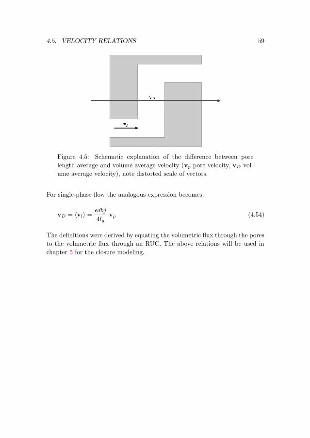
4.5. VELOCITY RELATIONS 59
���
���
Figure 4.5: Schematic explanation of the difference between pore
length average and volume average velocity (vp pore velocity, vD vol-
ume average velocity), note distorted scale of vectors.
For single-phase flow the analogous expression becomes:
vD = 〈vl〉 =εdbj
4lgvp (4.54)
The definitions were derived by equating the volumetric flux through the pores
to the volumetric flux through an RUC. The above relations will be used in
chapter 5 for the closure modeling.

60
5 Closure Modeling
In chapter 3 the averaged equations were derived. Chapter 4 describes an RUC
model, in which the microscopic flow processes are modeled. In this chapter
equations (3.28) and (3.29) will be combined with the results from chapter
4. The closure problem in these equations, i.e. the integrals still containing
microscopic quantities, will be solved and the microscopic quantities will be
replaced by macroscopic quantities. Boundary and initial conditions are stated
and the equations are formulated to be compatible with these conditions. For
the solution of the closure problem, the quasi one-dimensional flow modeling
inside the pores, adopted in chapter 4, implies that the RUC is aligned with
vD. In chapter 6 the equations will be further analyzed.
In equations (3.29), three integral terms still contain microscopic parameters:
µlV0∇ ·
∫
Sslg
νvl dS +µlV0
∫
Sslg
ν · (∇vl) dS −1
V0
∫
V0
∇pl dV (5.1)
These terms are called: the divergence term, the viscous term and the pressure
term. In the following sections these are reformulated term by term.
5.1 Closure of the Divergence Term
The divergence term models the influence of the flow on the gas-liquid inter-
face. Whitaker (1986a,b) incorrectly stated that this term was zero, because
he assumed a no-slip condition at the gas-liquid interface. Bousquet-Melou
et al. (2002) derived a simplified closure for the divergence term for solidifica-
tion problems. Their closure was based on a quasi no-slip condition, and the
development followed here results in a similar macroscopic term as derived by
Bousquet-Melou et al. (2002), although the specifics of the closure are different.
In order to approximate the divergence term, the liquid velocity is split into
61
62 CHAPTER 5. CLOSURE MODELING
a part normal to the gas-liquid interface and a part tangent to the interface
(Chen et al., 2000):
vl = vlνν + vlss (5.2)
with s a unit vector tangent to the interface. The divergence term becomes:
µlV0∇ ·
∫
Sslg
νvl dS =µlV0∇ ·
∫
Sslg
ν(vlνν + vlss) dS (5.3)
The magnitude of vlν is much smaller than the magnitude of vls , because the
flow is mainly tangent to the interface in the length direction of a corner. If
the above products were written differently, the two tensors νν and νs would
arise directly. The components of both tensors are usually of the same order
of magnitude. Assuming that vlss can be modeled by vca, and dropping the
smaller term containing vlν :
µlV0∇ ·
∫
Sslg
νvl dS ≈ µlV0∇ ·
∫
Sslg
νvca dS (5.4)
Probably vca in the above equation is an overestimation of the magnitude,
because the integral is over the total solid-liquid-gas interface, and velocity at
the solid-liquid interface is zero. The integral in equation (5.4) can be directly
solved by taking vca out of the integral, because it is already an averaged
quantity:
µlV0∇ ·
∫
Sslg
νvl dS ≈ µlV0∇ ·
∫
Sslg
ν dS vca (5.5)
Using the volume averaging rule (Crapiste et al., 1986):
1
V0
∫
Ssgl
ν dS = −∇(εnl) (5.6)
equation 5.5 becomes:
µlV0∇ ·
∫
Sslg
νvl dS ≈ −µl∇ · (∇(εnl) vca) (5.7)
5.2. CLOSURE OF THE VISCOUS TERM 63
Using equation (4.53):
µlV0∇ ·
∫
Sslg
νvl dS ≈ −2µllgdbj∇ · [(∇nl)
1
nlvD] (5.8)
In this derivation only the larger term in the integral was taken into account.
There is considerable uncertainty if the above derivation is accurate, but dur-
ing the order of magnitude analysis in section 6.2, it will be shown that the
divergence term is small and is not expected to influence the flow significantly.
If the smaller term containing vlν was retained, a dynamic term would result
(see also section 5.2.2). Equation (5.8) is similar to one of the closure terms
derived by Bousquet-Melou et al. (2002) and Goyeau et al. (1997).
5.2 Closure of the Viscous Term
The viscous term describes the viscous dissipation inside the pore due to the
flow of liquid and the momentum change due to the change of gas-liquid in-
terfacial area:
µlV0
∫
Sslg
ν · (∇vl) dS =µlV0
∫
Ssl
ν · (∇vl) dS +µlV0
∫
Sgl
ν · (∇vl) dS (5.9)
The integral over the solid-liquid interfacial area and the integral over the gas-
liquid interfacial area in equation (5.9) are treated separately in the following
sections. All shear stress acts along the solid-liquid interface, as no shear stress
is assumed to act on the gas-liquid interface (eqs. (3.3), (3.4)) (Suh et al., 2001).
However due to the change of gas-liquid surface area and liquid volume, the
gas-liquid surface area term is non-zero.
5.2.1 The solid-liquid interfacial area term
The microscopic Poiseuille flow model from section 4.4.2 is used here to derive
a volume averaged expression for the momentum dissipated through friction
along the surface of the solid phase inside the RUC:
µlV0
∫
Ssl
ν · (∇vl) dS =µlV0
∫
Ssl
∂vl∂ν
dS
=µlV0
∫
lg
∫
Lsl
∂vl∂ν
dL dxc (5.10)
64 CHAPTER 5. CLOSURE MODELING
whereby ∂∂ν is the directional derivative in the direction of ν with dimension
length−1. With τsl = − 1Lsl
∫
Lsl
µ ∂∂νvl dL (Shah and London, 1978):
µlV0
∫
Ssl
ν · (∇vl) dS = − 1
V0
∫
lg
τslLsl dxc
using equations (4.51), (4.29), (4.52) and (4.53):
µlV0
∫
Ssl
ν · (∇vl) dS = − 1
V0
∫
lg
− ∂pl∂xcAc dxc
= − µlFV0
∫
lg
vc dxc
= − µllgFV0
vca
= −2µll
2g
εnldFV0bjvD (5.11)
For two-phase flow equation (5.11) with equation (4.46) becomes:
µlV0
∫
Ssl
ν · (∇vl) dS = −2µl f
2 fA l2g
εnl d Fv sin2(α) V0bj
vD (5.12)
And for single-phase flow the above equation with equations (4.37) and (4.54)
becomes:
µlV0
∫
Ssl
ν · (∇vl) dS = −µl fRe Ap l2g2ε d r2h V0bj
vD (5.13)
The form of the solid-liquid interfacial area term for single-phase flow in
equation (5.13) is different from the expression developed by du Plessis and
Masliyah (1988). They choose to express this term directly as a function of
wetted solid surface area, and not in terms of the hydraulic radius as in equa-
tion (5.13). In principle these two formulations are compatible and can be
expressed in each other. Here the choice is for the hydraulic radius form,
because it connects better with the two-phase form of the equations.
5.2. CLOSURE OF THE VISCOUS TERM 65
5.2.2 The gas-liquid interfacial area term
The gas-liquid interfacial area term describes the change of momentum due to
the change of gas-liquid surface area during unsteady flow. In most descriptions
of unsaturated flow this term is ignored (Whitaker, 1986b). Pride and Flekkøy
(1999) described the influence of the change of interfacial area on unsaturated
flow in the fixed contact line regime, and concluded that it is highly nonlinear.
Kralchevsky et al. (1994) derived expressions for the situation of no shear
stress along the interface and normal motion to the interface. The boundary
conditions at the interface used here (eqs. (3.3), (3.4)) are relative simple
compared to the full stress balance (Hilfer, 1996). If the surface tension was
space dependent or surfactants were assumed to be present at the interface,
different boundary conditions would result (Lopez and Hirsa, 1998). Analog
to the solid-liquid term (eq. (5.10):
µlV0
∫
Sgl
ν · (∇vl) dS =µlV0
∫
Sgl
∂vl∂ν
dS (5.14)
Using the decomposition of the velocity in the surface (eq. (5.2)):
µlV0
∫
Sgl
ν · (∇vl) dS =µlV0
∫
Sgl
∂
∂ν(vlνν + vlss) dS
=µlV0
∫
Sgl
∂
∂ν(vlνν) +
∂
∂ν(vlss) dS (5.15)
The two terms in the integral cancel for a stationary interface. However, if a
surfactant was present, this would not necessarily be the case (Bisperink, 1997;
Lopez and Hirsa, 1998). For a non-stationary interface undergoing dilatation
it is assumed that the dilatation is mainly in the direction of ν and that ν
is (nearly) perpendicular to the length direction of the corner. Dropping the
second term because of the last assumption:
µlV0
∫
Sgl
ν · (∇vl) dS ≈ µlV0
∫
Sgl
∂
∂ν(vlνν) dS
≈ µlV0
∫
lg
∫
Lgl
∂
∂ν(vlνν) dL dxc (5.16)
The factor vlν is related to the change of the radius of the gas-liquid interface
(Chen et al., 2000). It describes a “source of surface area” due to normal
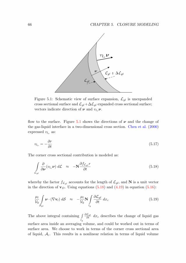
66 CHAPTER 5. CLOSURE MODELING
� �������������
�����
������
Figure 5.1: Schematic view of surface expansion, Lgl is unexpanded
cross sectional surface and Lgl+∆Lgl expanded cross sectional surface;
vectors indicate direction of ν and vlνν.
flow to the surface. Figure 5.1 shows the directions of ν and the change of
the gas-liquid interface in a two-dimensional cross section. Chen et al. (2000)
expressed vlν as:
vlν = −∂r
∂t(5.17)
The corner cross sectional contribution is modeled as:
∫
Lgl
∂
∂ν(vlνν) dL ≈ −N∂fLgl
r
∂t(5.18)
whereby the factor fLglaccounts for the length of Lgl, and N is a unit vector
in the direction of vD. Using equations (5.18) and (4.19) in equation (5.16):
µlV0
∫
Sgl
ν · (∇vl) dS ≈ − µlV0N
∫
lg
∂Lgl∂t
dxc (5.19)
The above integral containing∫
lg
∂Lgl
∂t dxc describes the change of liquid gas
surface area inside an averaging volume, and could be worked out in terms of
surface area. We choose to work in terms of the corner cross sectional area
of liquid, Ac. This results in a nonlinear relation in terms of liquid volume
5.2. CLOSURE OF THE VISCOUS TERM 67
(see eq. 4.24). The advantage is that no surface area is introduced in the
macroscopic equations. If it were introduced, surface area would be another
variable to be specified and measured (criterion IV, p. 29). Expressing Lgl inAc (eqs. (4.19), (4.22)) and simplifying:
µlV0
∫
Sgl
ν · (∇vl) dS ≈ − µlV0N
∫
lg
fLgl√fA
∂√Ac
∂tdxc (5.20)
Ac is split in an average part and the deviations (analogous to eq. (2.48), but
in one dimension along the pore only):
Ac = 〈Ac〉+ Ac (5.21)
After substitution of equation (5.21), equation (5.20) becomes:
µlV0
∫
Sgl
ν · (∇vl) dS ≈ − µlV0N
∫
lg
fLgl√fA
∂√
〈Ac〉+ Ac
∂tdxc (5.22)
Changing temporal differentiation and spatial integration, because lg is inde-
pendent of time:
µlV0
∫
Sgl
ν · (∇vl) dS ≈ − µlV0N
fLgl√fA
∂
∂t
∫
lg
√
〈Ac〉+ Ac dxc (5.23)
Expanding the square root term in a series:
µlV0
∫
Sgl
ν · (∇vl) dS
≈ − µlV0N
fLgl√fA
∂
∂t
√
〈Ac〉∫
lg
(1 +1
2
Ac
〈Ac〉− 1
8
A2c〈Ac〉2
+ . . .) dxc
(5.24)
Integrating the first two terms:
µlV0
∫
Sgl
ν · (∇vl) dS
≈ − µlV0N
fLgl√fA
∂
∂t
√
〈Ac〉
lg + 0 +
∫
lg
(−1
8
A2c〈Ac〉2
+ . . .) dxc
(5.25)
68 CHAPTER 5. CLOSURE MODELING
Dropping higher order terms, which in essence is a linearization:
µlV0
∫
Sgl
ν · (∇vl) dS ≈ − µlV0N
fLgl√fA
∂
∂t
[
√
〈Ac〉lg]
(5.26)
Using 〈Ac〉 = 2Vl/(lgbj):
µlV0
∫
Sgl
ν · (∇vl) dS ≈ − µlV0N
fLgl√fA
∂
∂t
[√
2Vllgbj
lg
]
(5.27)
Using eqs. (2.39) and (2.40):
µlV0
∫
Sgl
ν · (∇vl) dS ≈ − µlV0N
fLgl√fA
∂
∂t
[√
2εnlV0lgbj
]
≈ − µl√2V0
NfLgl√fA
√
V0√
lg1√
εnlbj
∂εnl∂t
(5.28)
As a result of the above closure, the left hand side of equation (5.9), combining
equations (5.12), and (5.28) becomes:
µlV0
∫
Sslg
ν · (∇vl) dS = −2µl f
2 fA l2g
εnl d Fv sin2(α) V0bj
vD
−N µl√2V0
fLgl√fA
√
V0√
lg1√
εnlbj
∂εnl∂t
(5.29)
These terms model the viscous effects in two-phase flow. The first term is due
to the shear stress along the solid-liquid surface and the second term describes
effects due to surface dilatation in unsteady flow.
5.3 Closure of the Pressure Term
In this section the liquid pressure term (eq. 3.22) is rewritten using the RUC
model from chapter 4. The liquid pressure is defined in the liquid only, and as
5.3. CLOSURE OF THE PRESSURE TERM 69
such averaging is done in the liquid phase:
〈∇pl〉l =1
Vl
∫
Vl
∇pl dV (5.30)
=1
Vl
∫
lg
∫
Ac
Nlgd
∂pl∂xc
dS dxc (5.31)
withN a unit vector. A change of coordinate system in the direction of the cor-
ner was done. This change of coordinate system in a corner was approximated
by:
∇pl =∂xc∂x
∂pl∂xc≈ N
∆xc∆x
∂pl∂xc
= Nlgd
∂pl∂xc
(5.32)
whereby the gradient is in the direction along the pore and ∂xc∂x is the Jacobian.
Due to the assumptions made, pl is constant at any cross section in a pore,
and can be directly integrated over Ac:
〈∇pl〉l = NlgVld
∫
lg
Ac∂pl∂xc
dxc (5.33)
Using eqs. (4.22) and (4.23):
〈∇pl〉l = NfAγ2gllg
Vld
∫
lg
1
p2l
∂pl∂xc
dxc (5.34)
= NfAγ2gllg
Vld
∫
lg
−∂p−1l∂xc
dxc (5.35)
The above expression can be directly integrated along the length direction of
the corner:
〈∇pl〉l = −NfAγ2gllg
Vld(1
p1− 1
p0) (5.36)
This expression is further used for the liquid pressure term. It can be written
in more familiar notation as:
〈∇pl〉l = NfAγ2gllg
Vl1
p0p1
p1 − p0d
(5.37)
70 CHAPTER 5. CLOSURE MODELING
In order to be compatible with the rest of the momentum balance, the ex-
pression for the liquid pressure term needs to be written in a form which is
valid over V0 and not only Vl. Use is made of the volume averaging rule
〈Ψ〉 = εnl〈Ψ〉i (Crapiste et al., 1986). The above equation was averaged along
one corner. In order to assemble it for the RUC model, taking into account
the number of pores in an RUC, j, and factor b:
1
V0
∫
V0
∇pl dV = −NεnlfAγ2gllgbj
2Vld(1
p1− 1
p0) (5.38)
5.4 Boundary and Initial Conditions on the
Macroscale
The boundary conditions which arise for the pressure on the macroscale are
simply p0 and p1. The time dependent terms entering the closure also re-
quire additional initial conditions, which have no analog in the traditional
Buckingham-Darcy type equations. The boundary and initial conditions are
given by:
nl(t = t0) = n0l (5.39)
nl(x = x0, x1) = nlx0,1(5.40)
p0,1(t) = p0,1 (5.41)
vD(x = x0, x1) = vDx0,1(5.42)
5.5 The Total Averaged Equations
In this section the combined averaged equations are given in their final form.
These equations are valid on the macroscopic scale and contain only macro-
scopic variables. In this form they are further analyzed and used in chapter
6. Rewriting equation (3.28) using equation (4.53) gives the macroscopic mass
balance equation:
∇ · vD = −∂εnl∂t
(5.43)
5.5. THE TOTAL AVERAGED EQUATIONS 71
The momentum balance equation (eq. (3.29)) becomes, using equations (4.53),
(5.8), (5.29), (5.38) and (5.8):
−εnlρlg + µl [−∇(∇ · vD) +∇× (∇× vD)]
−εnlfAγ2gllgbj
2VldN(
1
p1− 1
p0) = −
2µl f2 fA l2g
εnl d Fv sin2(α) V0bj
vD
− µl√2V0
fLgl√fA
√
V0√
lg1√
εnlbjN
∂εnl∂t
−2µllgdbj
∇ · [(∇nl)1
nlvD] (5.44)
The above equations contain microscopic geometric parameters. These can be
eliminated by using the RUC relations from chapter 4. Using a simpler form
with:
−εnlρlg + µl [−∇(∇ · vD) +∇× (∇× vD)]
−c1 N(1
p1− 1
p0)
= −c2
nlvD −
c3
n1/2l
N∂εnl∂t− c4 ∇ · [(∇nl)
1
nlvD] (5.45)
With c1, c2, c3 and c4 given by:
c1 =fAγ2gllgbj
2d4(5.46)
c2 =2µl f
2 fA l2g
ε d4 Fv sin2(α) bj
(5.47)
c3 =µlfLgl
l1/2g√
2d3/2f1/2A ε1/2b1/2j1/2
(5.48)
c4 =2µllgdbj
(5.49)
The mass balance (eq. (5.43)) could be used to further rewrite equation (5.45),
and terms containing ∂εnl∂t would arise. This is not done here in order to
facilitate the analysis in chapter 6. Equations (5.45) will be further analyzed in
chapter 6, where they are compared to the Buckingham-Darcy type equations
and to an experiment.
72 CHAPTER 5. CLOSURE MODELING
For single-phase flow and standard averaging of the pressure term (du Plessis
and Diedericks, 1997), the momentum balance becomes:
− ερlg + ε∇〈pl〉l + µl∇× (∇× vD) = −µl fRe Ap l2g2ε d4 r2hbj
vD (5.50)
whereby it is assumed that in single-phase flow an average liquid pressure is
defined.
There are still microscopic geometric parameters left in the averaged momen-
tum equations: a, b, j. The handling of these will be explained in chapter 6.
The parameters f , fA, lg, d, sinα, and fLglare determined using the expres-
sions from chapter 4, using the macroscopic parameters ε and rc or plc.
5.6 Discussion
Starting from the pore scale equations (eqs. (2.38)), and using the assumptions
of section 3.2, macroscale equations were derived. The main assumptions were:
relative slow flow with no inertial effects, quasi steady-state flow at the pore
scale, no dynamic contact line effects, and capillarity as the main driving force.
The equations were written with the fraction of liquid inside the pores, nl, as
a main variable. Macroscopic surface area was expressed in terms of nl also,
yielding equations (5.45). The pressure term was directly integrated and N
was added to express the direction of the macroscopic pressure gradient. In
essence this integration was along one space dimension only. The main dif-
ference between equations (5.45) and the traditional Buckingham-Darcy type
equations is in the pressure term. Due to the direct integration of the micro-
scopic pressure gradient, no macroscopic pressure gradient arises directly. The
integrated pressure term is not really an volume averaged term, but a macro-
scopic term describing the influence of a difference in liquid pressure across an
RUC. The other terms in equations (5.45) are volume averaged terms, com-
parable to the traditional equations and volume averaging work by Whitaker
(1986b). The integrated pressure term is a nonlocal term, in contrast with the
traditional equations, and depends on the averaging length scale through the
distance between p0 and p1. No factor like the conductivity arises directly, but
instead factors arising from the RUC model account for the conductivity. If p0(or p1) tend to become very negative, flow still can occur and is driven by the
other less negative pressure. In the traditional equations, the gradient of liquid
pressure would then tend to become very large, and the conductivity would
5.6. DISCUSSION 73
tend to become extremely small, resulting in a behavior of the equations crit-
ically dependent on the conductivity parameterization (Fuentes et al., 1992).
The proposed equations also contain dynamic terms which were derived using
closure assumptions. These are not present in the traditional equations, and
are often modeled heuristically (Stauffer, 1977). Due to the exactly defined
RUC, the order of magnitude of these macroscopic terms can be estimated
(sec. 6.3.4).

74
6 Comparison of the Macroscale
Equations with the Buckingham-Darcy
Equation
6.1 Introduction
The goal of this chapter is to analyze and compare the equations derived
in chapter 5 with the traditional Buckingham-Darcy (BD) type equations and
the dynamic capillary pressure model used by Hassanizadeh et al. (2002). Fur-
thermore a numerical comparison will be made with an experiment by Stauffer
(1977). First an order of magnitude analysis is conducted on equations (5.45),
followed by analytical approximations to compare the structure of these equa-
tions to the BD approach. Then a numerical simulation of an experiment is
done on the basis of a data set from Stauffer (1977). In this chapter analysis
is only conducted with respect to drainage, implying a contact angle θ = 0
(assumption 11, p. 35).
6.2 Order of Magnitude Analysis of the Aver-
aged Equation
Equations (5.45) are the full macroscale equations for the momentum balance
in unsaturated flow. In this section they are made dimensionless using the
notation in table 6.1. Because nl is already dimensionless, n∗l is defined as a
place-holder of O(1). p1 and p0 are not variables in the momentum balance
equations. They are treated as “constant” boundary conditions, and written as
P and P +∆P . Using the above notation yields for the mass balance equation
(eq. 5.43):
εNl
T
∂n∗l∂t∗
= −V
L
∂v∗
∂x∗(6.1)
75
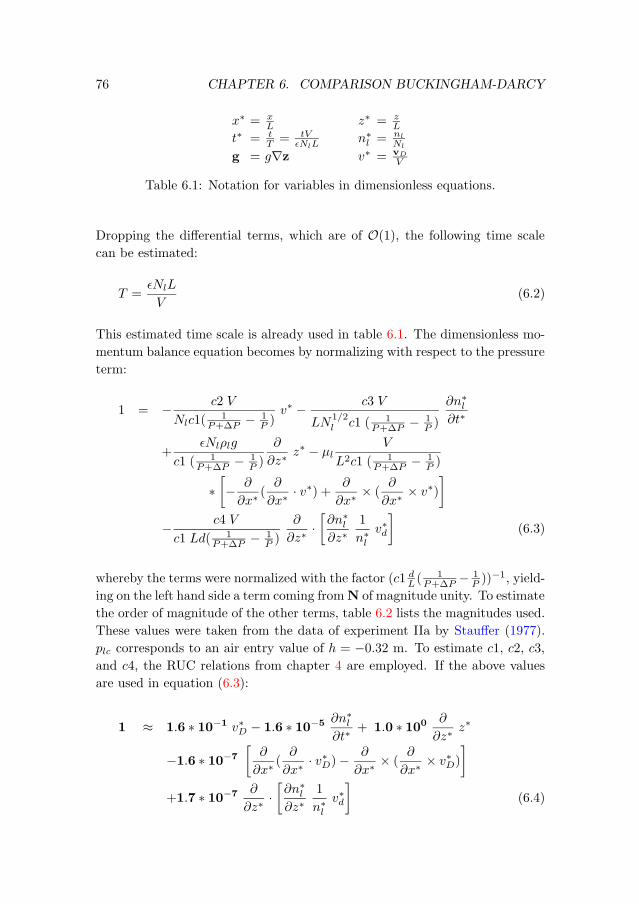
76 CHAPTER 6. COMPARISON BUCKINGHAM-DARCY
x∗ = xL z∗ = z
L
t∗ = tT = tV
εNlLn∗l = nl
Nl
g = g∇z v∗ = vDV
Table 6.1: Notation for variables in dimensionless equations.
Dropping the differential terms, which are of O(1), the following time scale
can be estimated:
T =εNlL
V(6.2)
This estimated time scale is already used in table 6.1. The dimensionless mo-
mentum balance equation becomes by normalizing with respect to the pressure
term:
1 = − c2 V
Nlc1(1
P+∆P − 1P )
v∗ − c3 V
LN1/2l c1 ( 1
P+∆P − 1P )
∂n∗l∂t∗
+εNlρlg
c1 ( 1P+∆P − 1
P )
∂
∂z∗z∗ − µl
V
L2c1 ( 1P+∆P − 1
P )
∗[
− ∂
∂x∗(
∂
∂x∗· v∗) + ∂
∂x∗× (
∂
∂x∗× v∗)
]
− c4 V
c1 Ld( 1P+∆P − 1
P )
∂
∂z∗·[
∂n∗l∂z∗
1
n∗lv∗d
]
(6.3)
whereby the terms were normalized with the factor (c1 dL (
1P+∆P − 1
P ))−1, yield-
ing on the left hand side a term coming fromN of magnitude unity. To estimate
the order of magnitude of the other terms, table 6.2 lists the magnitudes used.
These values were taken from the data of experiment IIa by Stauffer (1977).
plc corresponds to an air entry value of h = −0.32 m. To estimate c1, c2, c3,
and c4, the RUC relations from chapter 4 are employed. If the above values
are used in equation (6.3):
1 ≈ 1.6 ∗ 10−1 v∗D − 1.6 ∗ 10−5 ∂n∗l∂t∗
+ 1.0 ∗ 100 ∂
∂z∗z∗
−1.6 ∗ 10−7
[
∂
∂x∗(
∂
∂x∗· v∗D)−
∂
∂x∗× (
∂
∂x∗× v∗D)
]
+1.7 ∗ 10−7 ∂
∂z∗·[
∂n∗l∂z∗
1
n∗lv∗d
]
(6.4)
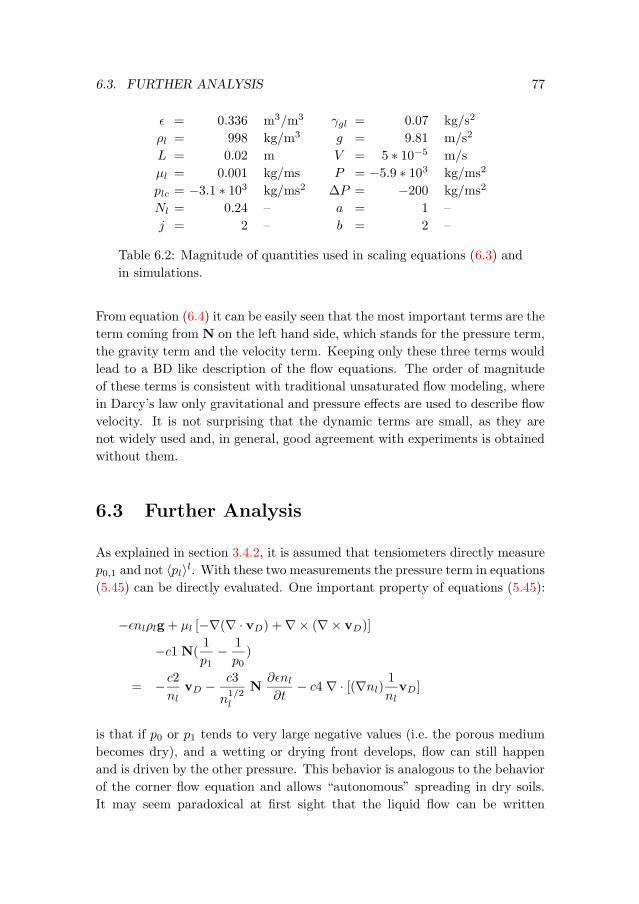
6.3. FURTHER ANALYSIS 77
ε = 0.336 m3/m3 γgl = 0.07 kg/s2
ρl = 998 kg/m3 g = 9.81 m/s2
L = 0.02 m V = 5 ∗ 10−5 m/s
µl = 0.001 kg/ms P = −5.9 ∗ 103 kg/ms2
plc = −3.1 ∗ 103 kg/ms2 ∆P = −200 kg/ms2
Nl = 0.24 – a = 1 –
j = 2 – b = 2 –
Table 6.2: Magnitude of quantities used in scaling equations (6.3) and
in simulations.
From equation (6.4) it can be easily seen that the most important terms are the
term coming from N on the left hand side, which stands for the pressure term,
the gravity term and the velocity term. Keeping only these three terms would
lead to a BD like description of the flow equations. The order of magnitude
of these terms is consistent with traditional unsaturated flow modeling, where
in Darcy’s law only gravitational and pressure effects are used to describe flow
velocity. It is not surprising that the dynamic terms are small, as they are
not widely used and, in general, good agreement with experiments is obtained
without them.
6.3 Further Analysis
As explained in section 3.4.2, it is assumed that tensiometers directly measure
p0,1 and not 〈pl〉l. With these two measurements the pressure term in equations
(5.45) can be directly evaluated. One important property of equations (5.45):
−εnlρlg + µl [−∇(∇ · vD) +∇× (∇× vD)]
−c1 N(1
p1− 1
p0)
= −c2
nlvD −
c3
n1/2l
N∂εnl∂t− c4 ∇ · [(∇nl)
1
nlvD]
is that if p0 or p1 tends to very large negative values (i.e. the porous medium
becomes dry), and a wetting or drying front develops, flow can still happen
and is driven by the other pressure. This behavior is analogous to the behavior
of the corner flow equation and allows “autonomous” spreading in dry soils.
It may seem paradoxical at first sight that the liquid flow can be written
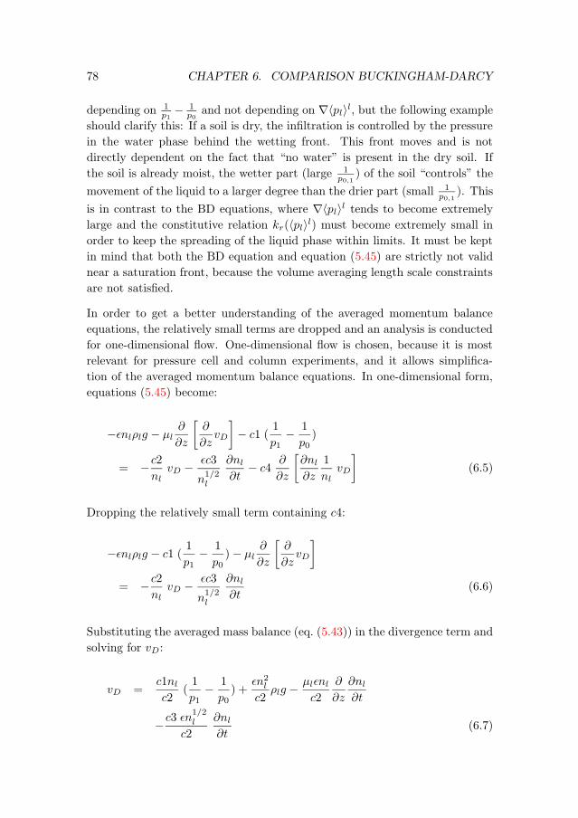
78 CHAPTER 6. COMPARISON BUCKINGHAM-DARCY
depending on 1p1− 1
p0and not depending on ∇〈pl〉l, but the following example
should clarify this: If a soil is dry, the infiltration is controlled by the pressure
in the water phase behind the wetting front. This front moves and is not
directly dependent on the fact that “no water” is present in the dry soil. If
the soil is already moist, the wetter part (large 1p0,1
) of the soil “controls” the
movement of the liquid to a larger degree than the drier part (small 1p0,1
). This
is in contrast to the BD equations, where ∇〈pl〉l tends to become extremely
large and the constitutive relation kr(〈pl〉l) must become extremely small in
order to keep the spreading of the liquid phase within limits. It must be kept
in mind that both the BD equation and equation (5.45) are strictly not valid
near a saturation front, because the volume averaging length scale constraints
are not satisfied.
In order to get a better understanding of the averaged momentum balance
equations, the relatively small terms are dropped and an analysis is conducted
for one-dimensional flow. One-dimensional flow is chosen, because it is most
relevant for pressure cell and column experiments, and it allows simplifica-
tion of the averaged momentum balance equations. In one-dimensional form,
equations (5.45) become:
−εnlρlg − µl∂
∂z
[
∂
∂zvD
]
− c1 (1
p1− 1
p0)
= −c2
nlvD −
εc3
n1/2l
∂nl∂t− c4
∂
∂z
[
∂nl∂z
1
nlvD
]
(6.5)
Dropping the relatively small term containing c4:
−εnlρlg − c1 (1
p1− 1
p0)− µl
∂
∂z
[
∂
∂zvD
]
= −c2
nlvD −
εc3
n1/2l
∂nl∂t
(6.6)
Substituting the averaged mass balance (eq. (5.43)) in the divergence term and
solving for vD:
vD =c1nlc2
(1
p1− 1
p0) +
εn2lc2
ρlg −µlεnlc2
∂
∂z
∂nl∂t
−c3 εn1/2l
c2
∂nl∂t
(6.7)
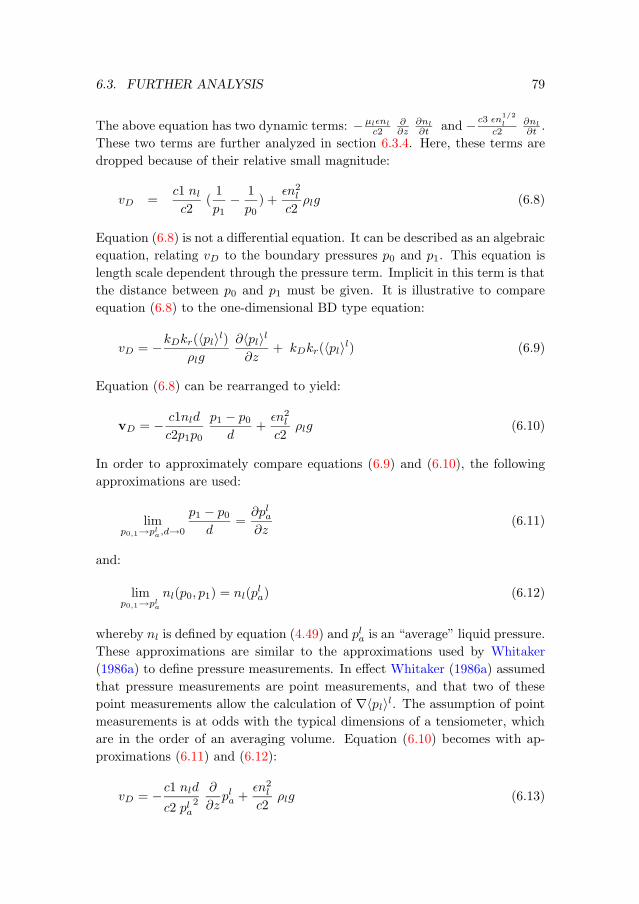
6.3. FURTHER ANALYSIS 79
The above equation has two dynamic terms: −µlεnlc2
∂∂z
∂nl∂t and − c3 εn
1/2
l
c2∂nl∂t .
These two terms are further analyzed in section 6.3.4. Here, these terms are
dropped because of their relative small magnitude:
vD =c1 nlc2
(1
p1− 1
p0) +
εn2lc2
ρlg (6.8)
Equation (6.8) is not a differential equation. It can be described as an algebraic
equation, relating vD to the boundary pressures p0 and p1. This equation is
length scale dependent through the pressure term. Implicit in this term is that
the distance between p0 and p1 must be given. It is illustrative to compare
equation (6.8) to the one-dimensional BD type equation:
vD = −kDkr(〈pl〉l)ρlg
∂〈pl〉l∂z
+ kDkr(〈pl〉l) (6.9)
Equation (6.8) can be rearranged to yield:
vD = − c1nld
c2p1p0
p1 − p0d
+εn2lc2
ρlg (6.10)
In order to approximately compare equations (6.9) and (6.10), the following
approximations are used:
limp0,1→pla,d→0
p1 − p0d
=∂pla∂z
(6.11)
and:
limp0,1→pla
nl(p0, p1) = nl(pla) (6.12)
whereby nl is defined by equation (4.49) and pla is an “average” liquid pressure.
These approximations are similar to the approximations used by Whitaker
(1986a) to define pressure measurements. In effect Whitaker (1986a) assumed
that pressure measurements are point measurements, and that two of these
point measurements allow the calculation of ∇〈pl〉l. The assumption of point
measurements is at odds with the typical dimensions of a tensiometer, which
are in the order of an averaging volume. Equation (6.10) becomes with ap-
proximations (6.11) and (6.12):
vD = −c1 nld
c2 pla2
∂
∂zpla +
εn2lc2
ρlg (6.13)
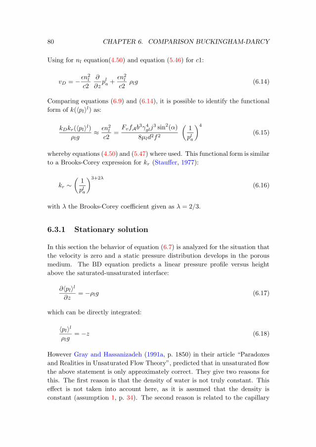
80 CHAPTER 6. COMPARISON BUCKINGHAM-DARCY
Using for nl equation(4.50) and equation (5.46) for c1:
vD = − εn2lc2
∂
∂zpla +
εn2lc2
ρlg (6.14)
Comparing equations (6.9) and (6.14), it is possible to identify the functional
form of k(〈pl〉l) as:
kDkr(〈pl〉l)ρlg
≈ εn2lc2
=FvfAb3γ4glj
3 sin2(α)
8µld2f2
(
1
pla
)4
(6.15)
whereby equations (4.50) and (5.47) where used. This functional form is similar
to a Brooks-Corey expression for kr (Stauffer, 1977):
kr ∼(
1
pla
)3+2λ
(6.16)
with λ the Brooks-Corey coefficient given as λ = 2/3.
6.3.1 Stationary solution
In this section the behavior of equation (6.7) is analyzed for the situation that
the velocity is zero and a static pressure distribution develops in the porous
medium. The BD equation predicts a linear pressure profile versus height
above the saturated-unsaturated interface:
∂〈pl〉l∂z
= −ρlg (6.17)
which can be directly integrated:
〈pl〉lρlg
= −z (6.18)
However Gray and Hassanizadeh (1991a, p. 1850) in their article “Paradoxes
and Realities in Unsaturated Flow Theory”, predicted that in unsaturated flow
the above statement is only approximately correct. They give two reasons for
this. The first reason is that the density of water is not truly constant. This
effect is not taken into account here, as it is assumed that the density is
constant (assumption 1, p. 34). The second reason is related to the capillary
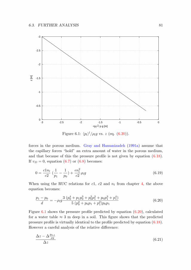
6.3. FURTHER ANALYSIS 81
-3
-2.5
-2
-1.5
-1
-0.5
0-3 -2.5 -2 -1.5 -1 -0.5 0
z [m
]
<pl>l/ ρ g [m]
Figure 6.1: 〈pl〉l/ρlg vs. z (eq. (6.20)).
forces in the porous medium. Gray and Hassanizadeh (1991a) assume that
the capillary forces “hold” an extra amount of water in the porous medium,
and that because of this the pressure profile is not given by equation (6.18).
If vD = 0, equation (6.7) or (6.8) becomes:
0 =c1nlc2
(1
p1− 1
p0) +
εn2lc2
ρlg (6.19)
When using the RUC relations for c1, c2 and nl from chapter 4, the above
equation becomes:
p1 − p0d
= −ρlg3 (p40 + p1p
30 + p20p
21 + p0p
31 + p41)
5 (p20 + p0p1 + p21)p0p1(6.20)
Figure 6.1 shows the pressure profile predicted by equation (6.20), calculated
for a water table ≈ 3 m deep in a soil. This figure shows that the predicted
pressure profile is virtually identical to the profile predicted by equation (6.18).
However a careful analysis of the relative difference:
∆z −∆p0,1
ρg
∆z(6.21)
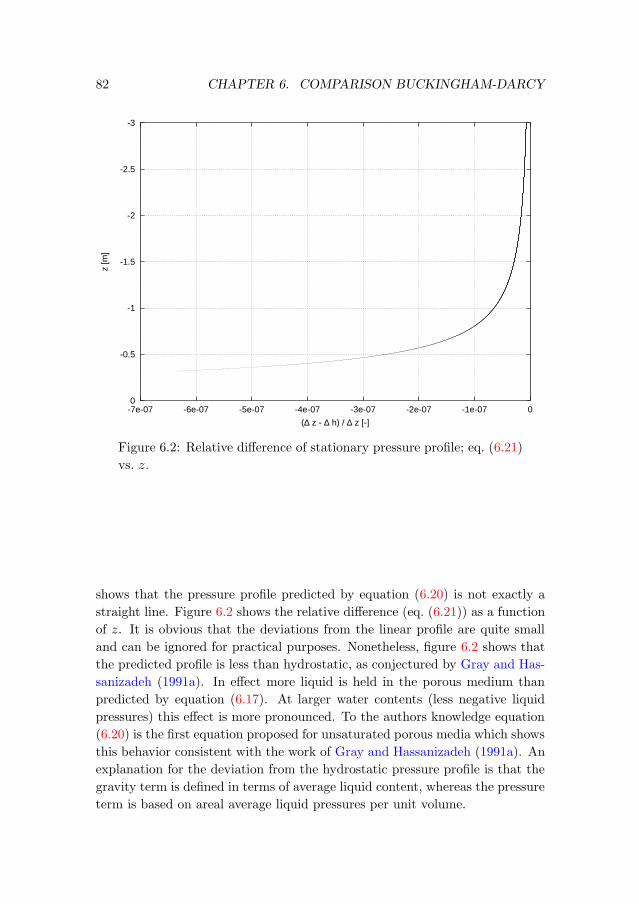
82 CHAPTER 6. COMPARISON BUCKINGHAM-DARCY
-3
-2.5
-2
-1.5
-1
-0.5
0-7e-07 -6e-07 -5e-07 -4e-07 -3e-07 -2e-07 -1e-07 0
z [m
]
(∆ z - ∆ h) / ∆ z [-]
Figure 6.2: Relative difference of stationary pressure profile; eq. (6.21)
vs. z.
shows that the pressure profile predicted by equation (6.20) is not exactly a
straight line. Figure 6.2 shows the relative difference (eq. (6.21)) as a function
of z. It is obvious that the deviations from the linear profile are quite small
and can be ignored for practical purposes. Nonetheless, figure 6.2 shows that
the predicted profile is less than hydrostatic, as conjectured by Gray and Has-
sanizadeh (1991a). In effect more liquid is held in the porous medium than
predicted by equation (6.17). At larger water contents (less negative liquid
pressures) this effect is more pronounced. To the authors knowledge equation
(6.20) is the first equation proposed for unsaturated porous media which shows
this behavior consistent with the work of Gray and Hassanizadeh (1991a). An
explanation for the deviation from the hydrostatic pressure profile is that the
gravity term is defined in terms of average liquid content, whereas the pressure
term is based on areal average liquid pressures per unit volume.
6.3. FURTHER ANALYSIS 83
6.3.2 Comparison of the averaged pressure term
As shown in appendix A, using the traditional averaging of the pressure term
yields (Whitaker, 1986b):
〈∇pl〉 = εnl∇〈pl〉l
or in one-dimensional form:
〈∂pl∂z〉 = εnl
∂
∂z〈pl〉l (6.22)
The averaged pressure terms in equation (6.22) and equation (6.7) can be
compared directly:
εnl∂
∂z〈pl〉l : −c1( 1
p1− 1
p0) (6.23)
:c1d
p0p1
p1 − p0d
(6.24)
Using equations (4.50) and (5.46), and approximations (6.11) and (6.12):
εnl∂
∂z〈pl〉l : εnl
∂
∂zpla (6.25)
The above relation shows that the traditional averaging of the pressure term
is similar to the method introduced here, if approximations (6.11) and (6.12)
are used. If during the development of the averaged pressure term in section
5.3 it was assumed that the sum of all corner liquid areas Acs is independent
of liquid pressure, the following averaging would result:
〈∇pl〉l =1
Vl
∫
Vl
∇pl dV
=1
Vl
∫
lg
∫
Acs
Nlgd
∂pl∂xc
dS dxc
= NlgdVl
∫
lg
Acs∂pl∂xc
dxc
= NAcslgVl
p1 − p0d
= Np1 − p0
d(6.26)
84 CHAPTER 6. COMPARISON BUCKINGHAM-DARCY
whereby equation (5.32) was used and Acs is defined analogous to equa-
tion (4.8) as Acs = Vllg. For one-dimensional flow, equation (6.22) on the
left hand side and equation (6.26) on the right hand side:
∂
∂z〈pl〉l :
p1 − p0d
(6.27)
If the fluid area Acs is constant along the corners in an RUC, the geometric
transformation multiplierlgd directly cancels and does not enter the averaged
equations as in the averaging of the pressure term in section 5.3 for unsaturated
flow (Ma and Ruth, 1993).
The factorlgd in the nonlocal form of the pressure term is similar to the aeros-
ity factor proposed by Ma and Ruth (1993). If change in cross-sectional liquid
area had not been taken into account during the averaging, the newly proposed
result would be even more like the traditional averaged pressure term, how-
ever, with the important difference that the newly proposed term is nonlocal,
whereas the traditional term is local.
6.3.3 Estimation of the saturated hydraulic conductivity
The RUC geometric relations developed in chapter 4 allow a direct estimation
of the saturated hydraulic conductivity. It can be evaluated using equation
5.50 as:
kd =2ε2d4r2hbjρg
µlfReApl2g(6.28)
fRe is given in Shah and London (1978) as:
fRe ≈ 12.3 (6.29)
Using the values from table 6.2, and the RUC relations from chapter 4:
kd = 1.3 ∗ 10−4m/s (6.30)
This value can be directly compared to the average value measured by Stauffer
(1977) for his experiment II as 2.1∗10−4 m/s. The simple RUC and flow model
of chapter 4 together with the closure for saturated flow in section 5.2 provides
an estimate of kD only using the macroscopic variables ε, plc, and the properties
µl, ρl, g, and an estimate of fRe from Shah and London (1978). The estimate
of kD is quite accurate, considered that only ε and plc were used as porous
medium parameters. This estimate compares in accuracy with more standard
methods (Carman, 1956).
6.3. FURTHER ANALYSIS 85
6.3.4 Comparison of the dynamic terms with Stauffer’s
model
Equation (6.7) contains two time dynamic terms: one with the divergence of
the velocity, and the other with the derivative of the liquid content. Both
originate from the microscopic viscous term. Most two-phase flow equations
have no or one dynamic term. In his dissertation Stauffer (1977) proposed a
model for a dynamic capillary pressure. This dynamic model was proposed
in order to model rapid changes in water content in his experiments. He
conjectured that the pressure in the Buckingham-Darcy equation is a dynamic
pressure and that it can be expressed as:
〈pc〉ld − 〈pc〉ls = −τ∂nl∂t
(6.31)
whereby subscript d indicates a dynamic pressure and subscript s indicates a
static pressure and τ a dimensionless proportionality factor. In terms of the
liquid pressure:
〈pl〉ld − 〈pl〉ls = τ∂nl∂t
(6.32)
with 〈pl〉ls the static volume average liquid pressure and 〈pl〉ld the dynamic
volume average liquid pressure. Stauffer (1977) indicated that τ could depend
on water content, but did not elaborate further on this. The term ∂nl∂t is also
called a capillary relaxation factor. If equation (6.32) is used in the standard
BD equation (eq. (6.9)):
vD = −kDkr(〈pl〉ld)ρlg
[
∂
∂z〈pl〉ls +
∂
∂z
(
τ∂nl∂t
)]
+ kDkr(〈pl〉ld) (6.33)
The dynamic term was introduced ad hoc in Stauffer’s dissertation, although
he tried to find physical explanations in terms of dynamic contact angles (see
Stauffer, 1977, p. 130). It is shown here that a dynamic term of the same
form as the second term on the right hand side of equation (6.33) can be
directly derived from the Brinkman term (Brinkman, 1947, 1949) without the
introduction of a dynamic pressure. In section 3.4.2, the viscous term was
averaged, yielding a sum of terms, containing µl∇2〈vl〉. In the beginning of
section 6.3 (p. 78) this term was rewritten for one-dimensional flow together
with the mass balance as:
− µlεnlc2
∂
∂z
∂nl∂t
(6.34)
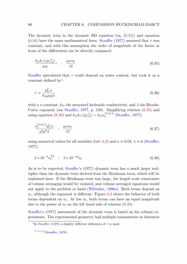
86 CHAPTER 6. COMPARISON BUCKINGHAM-DARCY
The dynamic term in the dynamic BD equation (eq. (6.33)) and equation
(6.34) have the same mathematical form. Stauffer (1977) assumed that τ was
constant, and with this assumption the order of magnitude of the factor in
front of the differential can be directly compared:
kDkr(〈pl〉ld)ρlg
τ :µlεnlc2
(6.35)
Stauffer speculated that τ could depend on water content, but took it as a
constant defined by1:
τ =p2lcα
kDρlgλ(6.36)
with α a constant, kD the saturated hydraulic conductivity, and λ the Brooks-
Corey exponent (see Stauffer, 1977, p. 128). Simplifying relation (6.35) and
using equation (6.36) and kDkr(〈pl〉ld) = kDn3+2/λl (Stauffer, 1977):
n3+2/λl p2lcα
ρ2l g2λ
:µlεnlc2
(6.37)
using numerical values for all variables (tab. 6.2) and α ≈ 0.03, λ ≈ 6 (Stauffer,
1977):
5 ∗ 10−4n313
l : 5 ∗ 10−10nl (6.38)
As is to be expected, Stauffer’s (1977) dynamic term has a much larger mul-
tiplier than the dynamic term derived from the Brinkman term, which will be
explained later. If the Brinkman term was large, the length scale constraints
of volume averaging would be violated, and volume averaged equations would
not apply to the problem at hand (Whitaker, 1986a). Both terms depend on
nl, although the exponent is different. Figure 6.3 shows the behavior of both
terms dependent on nl. At low nl, both terms can have an equal magnitude
due to the power of nl on the left hand side of relation (6.38).
Stauffer’s (1977) assessment of the dynamic term is based on his column ex-
periments. The experimental geometry had multiple tensiometers at distances
1In Stauffer (1978) a slightly different definition of τ is used:
τ = ε τ(Stauffer, 1978)
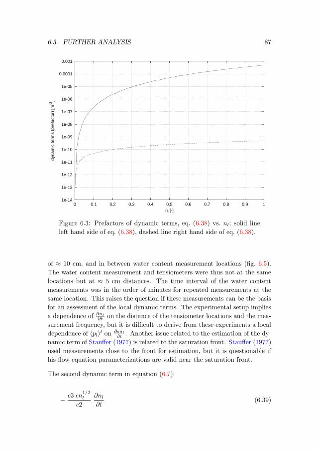
6.3. FURTHER ANALYSIS 87
1e-14
1e-13
1e-12
1e-11
1e-10
1e-09
1e-08
1e-07
1e-06
1e-05
0.0001
0.001
0 0.1 0.2 0.3 0.4 0.5 0.6 0.7 0.8 0.9 1
dyna
mic
term
s (p
refa
ctor
) [m
-2]
nl [-]
Figure 6.3: Prefactors of dynamic terms, eq. (6.38) vs. nl; solid line
left hand side of eq. (6.38), dashed line right hand side of eq. (6.38).
of ≈ 10 cm, and in between water content measurement locations (fig. 6.5).
The water content measurement and tensiometers were thus not at the same
locations but at ≈ 5 cm distances. The time interval of the water content
measurements was in the order of minutes for repeated measurements at the
same location. This raises the question if these measurements can be the basis
for an assessment of the local dynamic terms. The experimental setup implies
a dependence of ∂nl∂t on the distance of the tensiometer locations and the mea-
surement frequency, but it is difficult to derive from these experiments a local
dependence of 〈pl〉l on ∂εnl∂t . Another issue related to the estimation of the dy-
namic term of Stauffer (1977) is related to the saturation front. Stauffer (1977)
used measurements close to the front for estimation, but it is questionable if
his flow equation parameterizations are valid near the saturation front.
The second dynamic term in equation (6.7):
− c3 εn1/2l
c2
∂nl∂t
(6.39)
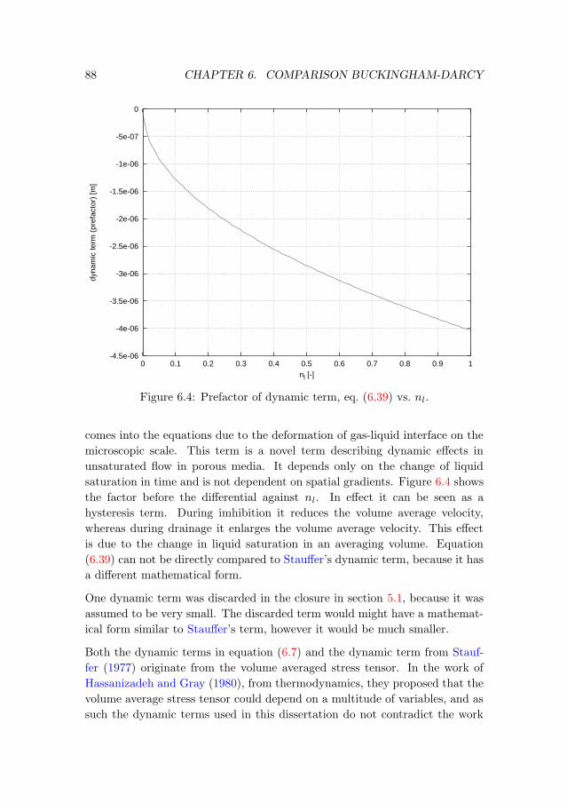
88 CHAPTER 6. COMPARISON BUCKINGHAM-DARCY
-4.5e-06
-4e-06
-3.5e-06
-3e-06
-2.5e-06
-2e-06
-1.5e-06
-1e-06
-5e-07
0
0 0.1 0.2 0.3 0.4 0.5 0.6 0.7 0.8 0.9 1
dyna
mic
term
(pr
efac
tor)
[m]
nl [-]
Figure 6.4: Prefactor of dynamic term, eq. (6.39) vs. nl.
comes into the equations due to the deformation of gas-liquid interface on the
microscopic scale. This term is a novel term describing dynamic effects in
unsaturated flow in porous media. It depends only on the change of liquid
saturation in time and is not dependent on spatial gradients. Figure 6.4 shows
the factor before the differential against nl. In effect it can be seen as a
hysteresis term. During imhibition it reduces the volume average velocity,
whereas during drainage it enlarges the volume average velocity. This effect
is due to the change in liquid saturation in an averaging volume. Equation
(6.39) can not be directly compared to Stauffer’s dynamic term, because it has
a different mathematical form.
One dynamic term was discarded in the closure in section 5.1, because it was
assumed to be very small. The discarded term would might have a mathemat-
ical form similar to Stauffer’s term, however it would be much smaller.
Both the dynamic terms in equation (6.7) and the dynamic term from Stauf-
fer (1977) originate from the volume averaged stress tensor. In the work of
Hassanizadeh and Gray (1980), from thermodynamics, they proposed that the
volume average stress tensor could depend on a multitude of variables, and as
such the dynamic terms used in this dissertation do not contradict the work
6.4. COMPARISON WITH EXPERIMENT 89
of Hassanizadeh and Gray (1980). It is not expected that the dynamic terms
normally play an important role in flow in unsaturated porous media, however
near a saturation front these terms could become important.
6.4 Comparison with Experiment
After the analytical analysis in the previous sections, in this section the nu-
merical solution of equation (6.8) is compared to an experiment by Stauffer
(1977). Equation (6.8) is chosen because it does not contain the dynamic terms
and the other comparably small term. If a numerical solution of equation (6.7)
with the dynamic terms was the goal, a relation between p0,1 and nl had to
be found, whereby nl = nl(p0,1(t), t). In section 4.4.2 an expression for nl(eq. (4.49)) was found, based on quasi-steady flow in a corner. In principle a
dynamic expression for nl could be found, but this would make the local flow
model much more involved. As the order of magnitude analysis in section 6.2
already indicated, it is not expected that dynamic terms play an important
role in unsaturated flow as studied here. This is the reason why a quasi-steady
calculation procedure is used. Stauffer (1977) used the same experiment to
estimate his proposed dynamic term (see section 6.3.4 for a discussion).
6.4.1 Description of experiment
The porous medium employed by Stauffer is unconsolidated sand with an aver-
age porosity of 0.336. The mean particle diameter of the sand is approximately
3 ∗ 10−4 m. It is assumed that the liquid (water) is completely wetting the
sand and that the contact angle θ = 0. The experimental unit consists of a
vertical sand column in a cylinder of diameter 0.045 m and length 0.638 m.
At the top of the column there is no liquid inflow or outflow and atmospheric
pressure, while the bottom of the column drains in a reservoir with a constant
level. Figure 6.5 shows schematically the geometry of the experiment.
To conduct an experiment, the sand column is completely saturated and then
allowed to drain freely. The liquid pressure is measured with tensiometers
along the column and water content is measured with a gamma ray absorption
technique. Additionally the air pressure is measured throughout the column
in order to detect effects of pressure variation in the gas phase and its possible
influence on the liquid movement. The outflow is collected and weighted on
a digital scale. Here the data from experiment IIa are used to compare with
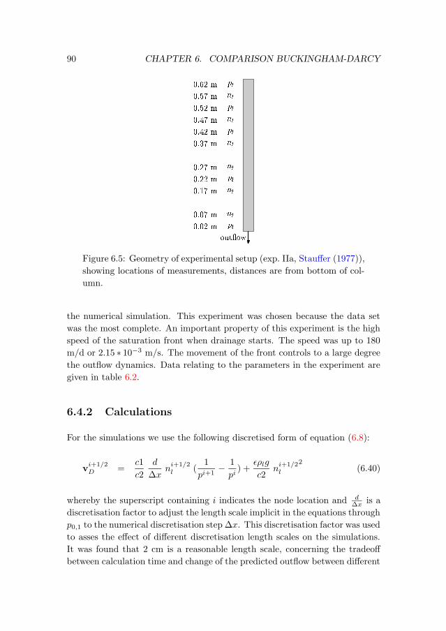
90 CHAPTER 6. COMPARISON BUCKINGHAM-DARCY
���
���
���
���
� �
� �
���
���
���
���
� �
��� ���
��� ���
��� � ��
��� ���
��� ���
��� ���
��� ����
��� ���
��� ���
��� � ��
��� ���
� ���������
Figure 6.5: Geometry of experimental setup (exp. IIa, Stauffer (1977)),
showing locations of measurements, distances are from bottom of col-
umn.
the numerical simulation. This experiment was chosen because the data set
was the most complete. An important property of this experiment is the high
speed of the saturation front when drainage starts. The speed was up to 180
m/d or 2.15 ∗ 10−3 m/s. The movement of the front controls to a large degree
the outflow dynamics. Data relating to the parameters in the experiment are
given in table 6.2.
6.4.2 Calculations
For the simulations we use the following discretised form of equation (6.8):
vi+1/2D =
c1
c2
d
∆xni+1/2l (
1
pi+1− 1
pi) +
ερlg
c2ni+1/2l
2(6.40)
whereby the superscript containing i indicates the node location and d∆x is a
discretisation factor to adjust the length scale implicit in the equations through
p0,1 to the numerical discretisation step ∆x. This discretisation factor was used
to asses the effect of different discretisation length scales on the simulations.
It was found that 2 cm is a reasonable length scale, concerning the tradeoff
between calculation time and change of the predicted outflow between different
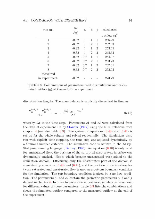
6.4. COMPARISON WITH EXPERIMENT 91
run nr.plcρlg
a b j calculated
outflow (g)
1 -0.32 1 1 1 266.29
2 -0.32 1 2 1 252.63
3 -0.32 1 1 2 253.65
4 -0.32 1 2 2 245.52
5 -0.32 0.7 1 1 284.07
6 -0.32 0.7 2 1 263.73
7 -0.32 0.7 1 2 267.01
8 -0.32 0.7 2 2 252.02
measured
in experiment: -0.32 - - - 273.79
Table 6.3: Combinations of parameters used in simulations and calcu-
lated outflow (g) at the end of the experiment.
discretisation lengths. The mass balance is explicitly discretised in time as:
vi+1/2D − vi−1/2D
∆x= −εnl
it+∆t − nlt
∆t
i
(6.41)
whereby ∆t is the time step. Parameters c1 and c2 were calculated from
the data of experiment IIa by Stauffer (1977) using the RUC relations from
chapter 4 (see also table 6.3). The system of equations (6.40) and (6.41) is
set up for the whole column and solved sequentially. The simulations were
run with explicit time stepping, the time step was adjusted dynamically by
a Courant number criterion. The simulation code is written in the XLisp-
Stat programming language (Tierney, 1990). As equation (6.40) is only valid
for unsaturated flow, the position of the saturated-unsaturated interface was
dynamically tracked. Nodes which became unsaturated were added to the
simulation domain. Effectively, only the unsaturated part of the domain is
simulated by equations (6.40) and (6.41), and the position of the interface be-
tween saturated and unsaturated flow is used as a bottom boundary condition
for the simulation. The top boundary condition is given by a no-flow condi-
tion. The parameters c1 and c2 contain the geometric parameters a, b and j
defined in chapter 4. In order to asses their importance, simulations were done
for different values of these parameters. Table 6.3 lists the combinations and
shows the simulated outflow compared to the measured outflow at the end of
the experiment.
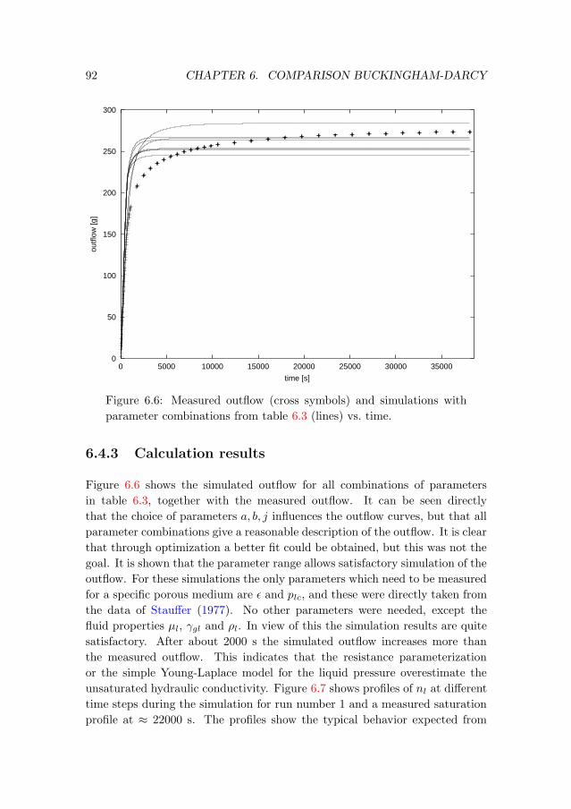
92 CHAPTER 6. COMPARISON BUCKINGHAM-DARCY
0
50
100
150
200
250
300
0 5000 10000 15000 20000 25000 30000 35000
outfl
ow [g
]
time [s]
Figure 6.6: Measured outflow (cross symbols) and simulations with
parameter combinations from table 6.3 (lines) vs. time.
6.4.3 Calculation results
Figure 6.6 shows the simulated outflow for all combinations of parameters
in table 6.3, together with the measured outflow. It can be seen directly
that the choice of parameters a, b, j influences the outflow curves, but that all
parameter combinations give a reasonable description of the outflow. It is clear
that through optimization a better fit could be obtained, but this was not the
goal. It is shown that the parameter range allows satisfactory simulation of the
outflow. For these simulations the only parameters which need to be measured
for a specific porous medium are ε and plc, and these were directly taken from
the data of Stauffer (1977). No other parameters were needed, except the
fluid properties µl, γgl and ρl. In view of this the simulation results are quite
satisfactory. After about 2000 s the simulated outflow increases more than
the measured outflow. This indicates that the resistance parameterization
or the simple Young-Laplace model for the liquid pressure overestimate the
unsaturated hydraulic conductivity. Figure 6.7 shows profiles of nl at different
time steps during the simulation for run number 1 and a measured saturation
profile at ≈ 22000 s. The profiles show the typical behavior expected from
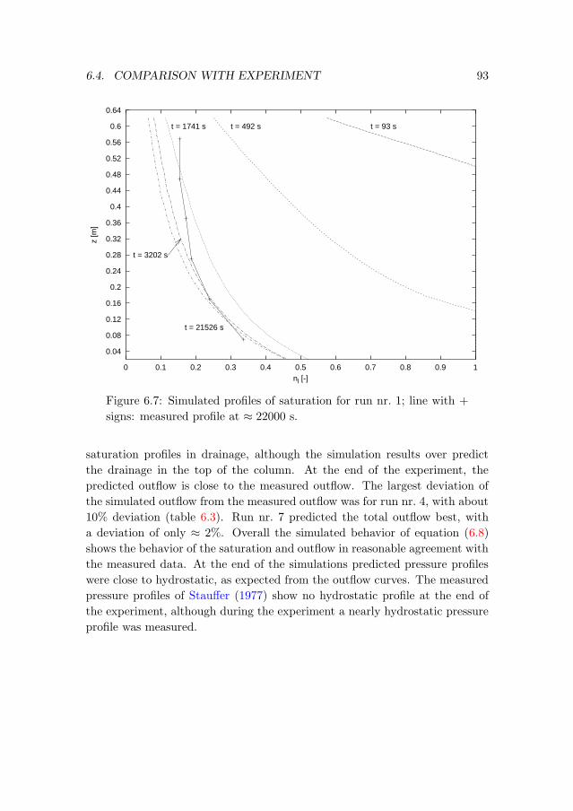
6.4. COMPARISON WITH EXPERIMENT 93
0.04
0.08
0.12
0.16
0.2
0.24
0.28
0.32
0.36
0.4
0.44
0.48
0.52
0.56
0.6
0.64
0 0.1 0.2 0.3 0.4 0.5 0.6 0.7 0.8 0.9 1
z [m
]
nl [-]
t = 93 st = 492 st = 1741 s
t = 3202 s
t = 21526 s
Figure 6.7: Simulated profiles of saturation for run nr. 1; line with +
signs: measured profile at ≈ 22000 s.
saturation profiles in drainage, although the simulation results over predict
the drainage in the top of the column. At the end of the experiment, the
predicted outflow is close to the measured outflow. The largest deviation of
the simulated outflow from the measured outflow was for run nr. 4, with about
10% deviation (table 6.3). Run nr. 7 predicted the total outflow best, with
a deviation of only ≈ 2%. Overall the simulated behavior of equation (6.8)
shows the behavior of the saturation and outflow in reasonable agreement with
the measured data. At the end of the simulations predicted pressure profiles
were close to hydrostatic, as expected from the outflow curves. The measured
pressure profiles of Stauffer (1977) show no hydrostatic profile at the end of
the experiment, although during the experiment a nearly hydrostatic pressure
profile was measured.

94
7 Discussion, Recommendations and
Conclusions
In this chapter a discussion of equations (5.45) and the mass balance equation
(5.43) derived in chapter 5 is given. Together with the comparison in chapter
6, strengths and weaknesses of the above equations are discussed. First the
general properties and the averaged pressure term are discussed, followed by
a discussion of the dynamic terms. Then the drawbacks are explained and
recommendations for possible extensions are given. Finally recommendations
and general conclusions will be stated.
7.1 Discussion
In section 5.5 equations (5.45) were proposed as the averaged momentum bal-
ance equations on the macroscale. These equations differ from the traditional
volume averaged equations in the pressure term, the dynamic terms and in
the form chosen for the Brinkman term. In chapter 6 these were simplified
to one-dimensional form (eq. (6.5)) and relatively small terms were neglected.
The resulting equation (6.8) was compared to the traditional Buckingham-
Darcy equation and to an experiment. The simplified one-dimensional form of
the averaged equations (6.8) is in an algebraic equation. This is the result of
the direct integration of the pressure term and effectively removes the spatial
derivative from this term. The fact that the momentum balance equations
become nonlocal is caused by the direct effect of the boundary conditions on
the flow. A similar effect of the boundary conditions is also observed in up-
scaling from the core to larger scales, e.g. in renormalization calculations in
unsaturated flow (Hoffmann, 2000a). The relation between liquid saturation
and boundary pressures was established for quasi-steady flow only, which im-
plies that the combination of equations (5.45)and (4.49) can only be solved
for quasi-steady flow. The volume averaged mass balance equation derived in
95
96 CHAPTER 7. DISCUSSION
this dissertation is identical to the traditional volume averaged mass balance
equation.
Naturally the question arises: Can the averaged momentum balance equations
be called ”truly”volume averaged equations? Two views are possible:
• Yes, because each term in the equations is averaged over an averaging
volume.
• No, because the averaged pressure term contains area averaged pres-
sures. These quantities are therefor not truly volume averaged quanti-
ties. Moreover this term is nonlocal and length scale dependent. In the
traditional equations the length scale does not enter directly into the
equations.
Another point of discussion is whether equations (5.45) are truly three-dimen-
sional equations. The mathematical notation is in three-dimensional vector
form, but the pressure term and one dynamic term were averaged along a
corner inside a Representative Unit Cell along one dimension only. On the
macroscale these terms contain a unit vector, which is a notational help in
making these terms three-dimensional.
7.1.1 Pressure term
As already explained in chapter 6, the pressure term has a different form than
the traditional volume averaged pressure term. This is the main difference
between equations (5.45) and the traditional volume averaged equations. The
precise form of this difference is due to the interpretation of the pressure mea-
surement made by tensiometers and in pressure cells. Hassanizadeh and Gray
(1979a) state that “The average value of a microscopic quantity must be the
same function that is most widely observed and measured in a field situation
or in the laboratory” (Criterion IV (p. 29)). Here the pressure measurement
is interpreted as an area average measurement and not a volume average mea-
surement. If this interpretation is valid, the principle of areal averaging of the
pressure term developed in section 5.3 is valid. The areal averaging directly
uses equation (4.23) to express liquid area in liquid pressure. This is a simplifi-
cation of reality. A better representation of the relation between liquid area in
a corner and liquid pressure could improve the averaged pressure term greatly.
Extensions could include a more realistic pore geometry, taking into account
surface roughness, or using a relation derived from measurements. In effect
7.1. DISCUSSION 97
the relation between liquid area in a corner and and liquid pressure could be
seen as a constitutive relation.
The form of the averaged pressure term shows that the flow of liquid in unsat-
urated porous media can be written proportional to 1p1− 1
p0. In principle the
flow is still driven by the gradients in liquid pressure, but due to the nonlinear
coupling between capillary forces and liquid pressure gradient, the apparent
driving force is proportional to 1p1− 1
p0. This form reduces the need to in-
troduce the highly nonlinear kr(〈pl〉l) relationship (eqs. (6.15) and (6.16))
which is used in the traditional models for flow in unsaturated porous media.
A related property is that the difference 1p1− 1
p0becomes smaller as p0,1 be-
come more negative, i.e. the porous medium becomes drier. This reduces the
effective driving force for flow and accounts for part of the nonlinearities in
unsaturated flow.
The result obtained by averaging the pressure term is similar to the result that
would be obtained with the ”control volume method”used in fluid mechanics
(Panton, 1984). In this method the forces acting on a control volume are
calculated by summing the forces around the perimeter surface of the control
volume. In effect a similar method has been used by Hassanizadeh et al. (2002)
in their pore network simulation model. They calculated the areal average
liquid pressure at the entry and exit planes of their pore network and related
this to the volume average static capillary pressure. Hassanizadeh et al. (2002,
p. 50) state: ”a natural definition of the macroscopic capillary pressure is given
by the pressure difference associated with the boundary fluid reservoirs”. The
result is a nonlocal definition of the capillary pressure term, which depends
on the averaging length scale (the pore network length scale). In their work
Hassanizadeh et al. (2002) apparently did not directly take into account the
length scale dependence of their nonlocal definition of capillary pressure.
The nonlocal pressure definition avoids the need to presuppose that liquid flow
is driven by the gradient of the average liquid pressure (Whitaker, 1986b).
By its definition the pressure term of section 5.3 represents a static liquid
pressure, although the pressure at the entry and exit planes can depend on
time. The areal average pressure definition avoids the need to use a dynamic
liquid pressure to account for dynamic effects.
7.1.2 Dynamic terms
The two dynamic terms in equation (5.45) containing ∂εnl∂t describe the effect
of volume averaging on the flow dynamics. On the microscale equations (2.38)
98 CHAPTER 7. DISCUSSION
describe steady flow, but due to a change in liquid saturation in the averaging
volume, the dynamic terms directly enter the macroscopic mass and momen-
tum balance equations. In the momentum balance equations these terms orig-
inate from the microscopic viscous term and they act as a ”momentum sink”.
The first dynamic term µε ∂∂x
∂nl∂t is part of the macroscopic Brinkman term.
As shown in the order of magnitude analysis in section 6.2, it is relatively small
and not expected to influence flow in unsaturated porous media significantly.
The remarkable property of this term is that it has the same mathematical
form as the dynamic term proposed by Stauffer (1977), as shown in section
6.3.4.
The second dynamic term ε c3
n1/2
l
∂nl∂t does not depend on the spatial derivative,
but on the temporal derivative only. It was derived from the surface dilatation
through direct integration and linearisation in section 5.2. It is a novel term
in the momentum balance for two-phase flow. Basically it describes the effect
of advection of liquid into the averaging volume and damps the dynamics. It
could be interpreted as a hysteresis term. This hysteresis is then only due
to the flow dynamics and has nothing to do with the traditional hysteresis
effect which is explained in terms of the ink bottle effect and contact angle
hysteresis. The interesting aspect is that the factor ε c3
n1/2
l
becomes large as nl
becomes small. But at small nl,∂nl∂t is small, except near a steep wetting front.
Such a steep wetting fronts can be observed during infiltration of water into
a dry soil. But near such a steep wetting front the volume averaging length
scale constraints are not valid and thus the averaged equations are not valid.
However it must be remarked that the form of the second dynamic term is
based on assumptions and as such is not the result of a strict mathematical
derivation.
In section 6.4 the dynamic terms were not included in the simulations because
they are relatively small. An improved dynamic closure incooperating the
dynamic terms in the relationship nl(p0, p1, t) would be needed to do this.
However it is expected that the total influence of the dynamic terms is not
important in unsaturated flow in sand-like porous media. These terms could
play a role close to a wetting front, but then the volume averaging length scale
constraints are not satisfied.
7.1.3 Representative Unit Cell model
The RUC model proposed in chapter 4 encompasses a concrete geometric spec-
ification, in contrast to the abstract Representative Elementary Volume (REV)
7.1. DISCUSSION 99
model. The geometric specification allows the development of a microscale flow
model and avoids the need to parameterize the closure relations as is done in
the traditional volume averaging procedure. Both the REV and RUC are an
abstraction of a real porous medium. The flow model used in the RUC is
based on a Poiseuille assumption and simplifies the description of the flow.
It uses a resistance factor and a scaling proposed by Weislogel and Lichter
(1998). Although the geometric specification of the RUC is relative simple,
apparently the wedge like corner geometry captures the most important geom-
etry and topology related aspects of a real porous medium (sand). With this,
unsaturated flow can be modeled, needing only the porosity and the air entry
value as porous medium parameters. The microscopic geometric parameters
a, b and j influence the flow dynamics and there is no direct way to determine
them a priori. They could be used as tuning parameters, together with the
constant resistance factor Fv. As shown in chapter 6, the exact choice of a, b
and j influences the flow dynamics, but the total outflow predicted is relative
insensitive to their precise value.
7.1.4 Constitutive relations
In the Buckingham-Darcy (BD) equation two constitutive relations are needed
to describe the relations between relative hydraulic conductivity and liquid
saturation kr(S) or volume average pressure kr(〈pl〉l), and volume average
pressure and saturation S(〈pl〉l). Equations (5.45) or (6.8) have no direct ana-
log to kr(S) or kr(〈pl〉l). In effect during the averaging of the pressure term
the two-dimensional Young-Laplace equation (eq. 4.23) served as a constitu-
tive relation. Together with the averaging of the viscous term an analog to
the kr(〈pl〉l) relation was proposed in chapter 6 (eq. 6.15). The use of the
two-dimensional Young-Laplace equation is a simplification. The constitutive
relation S(〈pl〉l) was implicitly accounted for through the use of the Young-
Laplace equation for liquid area in a corner. This proposed relation is only
valid for unsaturated flow, and the switching to saturated flow is discontinu-
ous. When solving the BD equation together with the volume averaged mass
balance a related difficulty arises. In this case the constitutive relation S(〈pl〉l)needs to be inverted to 〈pl〉l(S). This relation is not unique for S = 1, and dif-
ficulties arise in determining exactly the location of the saturated-unsaturated
interface in a porous medium. The relation between liquid saturation and the
boundary pressures (eq. (4.49)) could be seen as a constitutive relation. How-
ever it is based on the microscopic flow model of section 4.4.2 and as such a
direct result of averaging.
100 CHAPTER 7. DISCUSSION
7.2 Recommendations and Possible Extensions
The first recommendation is to test the averaged momentum equations with
other data sets. In chapter 6 simulations were done for one experiment, and
reasonable agreement between simulations and measured values was obtained.
Additional tests could show whether the developed model is capable of simu-
lating unsaturated flow in a wide range of sand-like porous media.
In the averaging process from microscale to macroscale several simplifications
were made. A number of these simplifications are addressed here and some
new possible extensions are suggested:
1. The relation between corner liquid area Ac and averaged pressure p0,1is based on the Young-Laplace equation. This simple relation could be
replaced by a more realistic parameterization, either based on a rela-
tion accounting for more physics through introducing adhesive forces
and surface roughness, or a more realistic pore geometry. This exten-
sion is relatively easy to implement in the current flow model, because it
would modify only the pressure term and the microscale flow model.
2. At low saturations, vapor diffusion plays an important role in the move-
ment of the liquid phase through evaporation and condensation. In order
to take this effect into account, an equation for the movement of the liq-
uid vapor should be introduced and coupled to the momentum and mass
balance equations. This extension implies that the averaging needs to
be redone, as no transport across the gas-liquid interface was assumed.
Additionally momentum and mass balance equations would arise for the
vapor and gas phase, making the total transport model much more com-
plicated.
3. The Representative Unit Cell (RUC) model is an abstraction of reality.
It appears that the RUC model covers the most important geometry
related aspects of a simple porous medium (sand). Extensions could
include taking into account channel curvature in the flow model. A
non-planar corner geometry could improve the modeling of the corner
liquid area and pressure relation. In principle the RUC model could
be extended much more and made more complicated. But this would
contradict the goal of the RUC model in using it as a simple model for
a porous medium.
4. Through the volume averaging procedure, dynamic terms were intro-
duced in the mass and momentum balance equations. All spatial vari-
7.3. CONCLUSIONS 101
ables are spatially averaged, but the time dependent terms depend on
a ”microscopic”time scale. Temporal averaging of the equations could
result in an improved modeling of the dynamic terms and a temporal
scale better fitting the spatial scale (Ishii, 1975). This process of com-
bining temporal and spatial averaging gives rise to new closure problems
and raises the issue of the commutativity of the two different averaging
processes (Pedras and de Lemos, 2000). An extension in this direction
would involve substantial theoretical work.
5. It would be interesting to directly compare the RUC model to pore net-
work modeling simulations. Moreover, the corner flow model developed
in chapter 4 could be used in advanced pore network models with an-
gular pores for a more realistic porous medium representation than the
circular tube models commonly employed in pore network modeling.
7.3 Conclusions
− Through the use of volume averaging and direct integration macroscopic
momentum and mass balance equations were derived from the micro-
scopic momentum and mass balance equations. As a result a novel form
of the macroscopic pressure term is proposed.
− The apparent driving force for liquid flow in unsaturated porous media
is 1p1− 1
p0. This is a result of the nonlinear coupling between capillary
forces and liquid pressure gradient.
− A geometric representation of a porous medium (sand) called a Repre-
sentative Unit Cell model was developed and used in the closure problem
generated by the volume averaging. The simple RUC model appears to
be capable of modeling the important characteristics of a porous medium
for unsaturated flow.
− In this work two dynamic terms were derived by simplifications of the
flow dynamics in an RUC. They remain to be tested quantitatively and
still have considerable uncertainty concerning their exact form and/or
magnitude.
− Comparison of the newly proposed equations with the Buckingham-
Darcy equation shows that, using reasonable assumptions, the newly
102 CHAPTER 7. DISCUSSION
proposed equations can be written in a form similar to the Buckingham-
Darcy equation. However the newly proposed equations are nonlocal and
have an apparent nonlinear driving force.
− A numerical solution of the newly proposed equations was compared to
an outflow experiment and satisfactory agreement between experiment
and calculations was observed.
A Traditional Form of the Volume
Averaged Pressure Term
In this appendix the traditional form of the volume averaged pressure term
(Whitaker, 1986a,b; Ma and Ruth, 1993) is presented. As stated in chapters
3 and 5, the liquid pressure is averaged over the liquid phase only, as the
macroscopic pressure measurement is an intrinsic liquid phase measurement.
The derivation of Ma and Ruth (1993) is followed, adjusted for the two-phase
case:
〈∇pl〉l =1
Vl
∫
Vl
∇pldV (A.1)
= ∇〈pl〉l +1
Vl
∫
Sslg
ν pl dS (A.2)
= ∇〈pl〉l +1
εnlV0
∫
Sslg
νpl dS +〈pl〉lεnl∇(εnl) (A.3)
whereby the integral containing pl was rewritten using equation 2.2 in Ma and
Ruth (1993). The integral term in the above equation is normally assumed to
be small and dropped:
= ∇〈pl〉l +〈pl〉lεnl∇(εnl) (A.4)
The last term in the above equation is a Brinkman (1949, 1947) like term,
and required to be small in order to satisfy the volume averaging length scale
constraints. It is proportional to 〈pl〉l, and this requires an absolute definition
of pressure. A relative definition of liquid pressure, as adopted in chapter
2 of this dissertation is not possible. If this was done, it would depend on
103
104 APPENDIX A. VOLUME AVERAGED PRESSURE TERM
the chosen pressure reference level. Dropping the term and using the volume
averaging rule (Crapiste et al., 1986) 〈Ψ〉 = εnl〈Ψ〉i:
〈∇pl〉 = εnl∇〈pl〉l (A.5)
Equation (A.5) is used in most volume averaging descriptions of unsaturated
flow.
Summary
This dissertation describes modeling of unsaturated flow in porous media. The
fluid phases considered are a wetting liquid and a gas. In practice one can think
of a sandy soil, partially saturated with water, partially with air.
Starting from the description of fluid flow through individual pores, an equa-
tion for flow of a liquid in a porous medium in the presence of a gas is derived.
This flow is directly influenced by phase interfaces, e.g. solid-liquid or gas-
liquid. By explicitly including these pore scale phenomena in a continuum
description of fluid transport in porous media, a consistent theoretical descrip-
tion of fluid flow on the macroscale is obtained.
Chapter 2 provides an overview and gives a historical perspective of the study
of flow in porous media. Single-phase and two-phase flow at the pore scale are
described, basic equations introduced, and concepts of the different flow mech-
anisms explained. Thereafter different methods for upscaling to a continuum
description of flow in porous media are introduced and the basics of volume
averaging explained.
Chapter 3 describes the development of upscaled unsaturated flow equations
in porous media. The main assumptions are listed and the starting equations
on the pore scale and the boundary and initial conditions are stated. These
equations are volume averaged and the closure problem is developed. The ap-
proach taken here is based on the closure scheme developed by du Plessis and
Masliyah (1988), augmented with additional boundary conditions which are
introduced due to fluid-fluid interfaces.
Chapter 4 describes the development of a Representative Unit Cell (RUC)
model for the closure of the volume averaged equations derived in chapter 3.
In chapter 5 the volume averaged equations derived in chapter 3 are com-
bined with the results from chapter 4. The closure problem in these equations
is solved and microscopic quantities are replaced by macroscopic quantities.
Boundary and initial conditions are stated and the equations are formulated
to be compatible with these conditions.
Chapter 6 analyzes and compares the equations derived in chapter 5 with the
105
106 SUMMARY
traditional Buckingham-Darcy (BD) type equations and the dynamic capillary
pressure model used by Hassanizadeh et al. (2002). Furthermore a numerical
comparison is made with an experiment by Stauffer (1977).
In chapter 7 a discussion of the upscaled equations is given. Together with
the comparison in chapter 6, strengths and weaknesses of the above equations
are discussed. First the general properties and the averaged pressure term are
discussed, followed by a discussion of the dynamic terms. Then the drawbacks
are explained and recommendations for possible extensions are given.
The main recommendations are: a) To test the averaged momentum equations
with other data sets; b) To improve the relation between corner liquid area
and averaged pressure; c) To include vapor diffusion at low saturations; d) To
improve the Representative Unit Cell (RUC) model; e) To include temporal
averaging in the upscaling procedure; f) To directly compare the RUC model
to pore network modeling simulations.
The main results are: a) Macroscopic momentum and mass balance equations
were derived from the microscopic momentum and mass balance equations;
b) The apparent driving force for liquid flow in unsaturated porous media is1p1− 1
p0. This is a result of the nonlinear coupling between capillary forces and
liquid pressure gradient; c) A geometric representation of a porous medium
(sand) called a Representative Unit Cell model was developed and used in the
closure problem generated by the volume averaging. The simple RUC model
appears to be capable of modeling the important characteristics of a porous
medium for unsaturated flow; d) Two dynamic terms were derived by simpli-
fications of the flow dynamics in an RUC. They remain to be tested quantita-
tively; e) Comparison of the newly proposed equations with the Buckingham-
Darcy equation shows that, using reasonable assumptions, the newly proposed
equations can be written in a form similar to the Buckingham-Darcy equation.
However the newly proposed equations are nonlocal and have an apparent
nonlinear driving force; f) Comparison of the newly proposed equations to
an outflow experiment shows satisfactory agreement between experiment and
calculations.
Samenvatting
Dit proefschrift beschrijft het modelleren van onverzadigde stroming in po-
reuze media. De beschreven vloeistoffen zijn een benattende vloeistof en een
gas. In de praktijk kan men denken aan zand, gedeeltelijk verzadigd met wa-
ter, gedeeltelijk verzadigd met lucht.
Uitgaande van de beschrijving van vloeistofstroming door individuele porien,
wordt een vergelijking voor de stroming van een vloeistof in de aanwezigheid
van een gas afgeleid. Deze stroming wordt mede bepaald door grensvlakken,
bijvoorbeeld vast-vloeibaar of gas-vloeibaar. Door expliciet deze porieschaal
verschijnselen in een continuum beschrijving van vloeistof stroming door po-
reuze media mee te nemen, wordt een consistente theoretische beschrijving op
de macroschaal verkregen.
Hoofdstuk 2 geeft een overzicht en een korte geschiedenis van het onderzoek
naar stroming in poreuze media. Een- en twee-fase stroming op porieschaal
wordt beschreven, de basis vergelijkingen worden geıntroduceerd, en de con-
cepten van de verschillende stromingsmechanismen worden verklaard. Daarna
worden verschillende methodes voor het opschalen naar een continuum be-
schrijving van vloeistof stroming in poreuze media beschreven evenals de ba-
sismethode van volume middeling.
Hoofdstuk 3 beschrijft de ontwikkeling van nieuwe opgeschaalde onverzadigde
stromingsvergelijkingen in poreuze media. De hoofdaannames worden beschre-
ven en de initiele en randvoorwaarden worden vastgesteld. Deze nieuwe verge-
lijkingen worden volume gemiddeld en het sluitingsprobleem wordt ontwikkeld.
De benadering die hier gekozen is, is gebaseerd op het sluitingsschema zoals
ontwikkeld door du Plessis and Masliyah (1988), aangevuld met additionele
randvoorwaarden door de aanwezigheid van vloeistof-vloeistof grensvlakken.
Hoofdstuk 4 beschrijft de ontwikkeling van een “Representative Unit Cell
(RUC)” model voor de sluiting van de volume gemiddelde vergelijkingen, af-
geleid in hoofdstuk 3.
In hoofdstuk 5 worden de volume gemiddelde vergelijkingen van hoofdstuk
3 samengevoegd met de resultaten van hoofdstuk 4. Het sluitingsprobleem
107
108 SAMENVATTING
in deze vergelijkingen wordt opgelost en microscopische grootheden worden
vervangen door macroscopische grootheden. Rand- en initiele voorwaarden
worden opgesteld, en de vergelijkingen worden compatibel met deze geformu-
leerd.
Hoofdstuk 6 analyseert en vergelijkt de vergelijkingen afgeleid in hoofdstuk 5
met de traditionele Buckingham-Darcy (BD) type vergelijkingen en het dyna-
mische capillaire druk model zoals gebruikt door Hassanizadeh et al. (2002).
Verder wordt een numerieke oplossing van de vergelijkingen vergeleken met
een experiment van Stauffer (1977).
In hoofdstuk 7 wordt een discussie van de opgeschaalde vergelijkingen gegeven.
Samen met de uitkomsten van hoofdstuk 6, worden sterkte en zwakte punten
van de bovengenoemde vergelijkingen besproken. Eerst worden de algemene
eigenschappen en de gemiddelde drukterm besproken, gevolgd door een discus-
sie van de dynamische termen. Daarna worden mogelijke nadelen verklaard en
aanbevelingen voor mogelijke uitbreidingen gegeven.
De belangrijkste aanbevelingen zijn: a) Het testen van de gemiddelde mo-
mentum vergelijkingen met andere data sets; b) Het verbeteren van de relatie
tussen corner liquid area en gemiddelde druk; c) Het meenemen van waterdamp
diffusie bij lage verzadigingen; d) Het verbeteren van het “Representative Unit
Cell” (RUC) model; e) Het toevoegen van tijdmiddeling in de opschalings-
procedure; f) Het direct vergelijken van het RUC model met porie netwerk
modellen.
De belangrijkste resultaten zijn: a) Macroscopische momentum en massa ba-
lans vergelijkingen zijn afgeleid van microscopische momentum en massa balans
vergelijkingen; b) De schijnbaar veroorzakende kracht for vloeistof stroming in
onverzadigde poreuze media is 1p1− 1
p0. Dit is het gevolg van de niet-lineaire
koppeling tussen capilaire krachten en de drukgradient in de vloeistof; c) Een
geometrische representatie van een poreus medium (zand), genoemd “Repre-
sentative Unit Cell” model is ontwikkeld en gebruikt in het sluitingsprobleem
bij de volume middeling. Het eenvoudige RUC model lijkt goed in staat de
belangrijke eigenschappen van een poreus medium voor onverzadigde stroming
te modelleren; d) Twee dynamische termen zijn afgeleid door vereenvoudigin-
gen van de stromingsdynamica in een RUC. Deze moeten nog kwantitatief
getest worden; e) Een vergelijking van de nieuw voorgestelde vergelijkingen
met de Buckingham-Darcy vergelijking laat zien, dat gebruik makende van
redelijke aannames, de nieuw voorgestelde vergelijkingen in een vorm kunnen
worden geschreven, die lijkt op de Buckingham-Darcy vergelijking. Echter, de
nieuw voorgestelde vergelijkingen zijn niet lokaal en hebben een schijnbaar niet
lineaire veroorzakende kracht; f) Vergelijking van de nieuw voorgestelde ver-
gelijkingen met een uitstroom experiment laat redelijke overeenkomst tussen

109
experiment en berekeningen zien.

110
Bibliography
Adler, P. M. and Brenner, H., 1988. Multiphase flow in porous media. Ann. Rev.Fluid Mech., 20:35 – 59.
Aleman, M. A., Ramamohan, T. R., and Slattery, J. C., 1989. The difference betweenstedy-state and unsteady-state relative permeabilities. Transport in Porous Media,4(5):449 – 493.
Anderson, T. B. and Jackson, R., 1967. A fluid mechanical description of fluidizedbeds. Ind. & Eng. Chem. Fund., 6(4):527 – 539.
Ayyaswamy, P. S., Catton, I., and Edwards, D. K., 1974. Capillary flow in triangulargrooves. Trans. ASME, Journal of Applied Mechanics, pp. 332 – 336.
Bachmann, J., Horton, R., Grant, S. A., and van der Ploeg, R. R., 2002. Temperaturedependence of water retention curves for wettable and water-repellent soils. SoilSci. Soc. Amer. J., 66(1):44 – 52.
Bear, J., 1988. Dynamics of Fluids in Porous Media. Dover, Mineola, N.Y. ISBN0-486-65675-6.
Bear, J. and Bachmat, Y., 1990. Introduction to Modelling of Transport Phenomenain Porous Media, volume 4 of Theory and Applications of Transport in PorousMedia series. Kluwer Academic Publishers, Dordrecht, The Netherlands. ISBN0-7923-0557-4.
Bear, J. and Bensabat, J., 1989. Advective fluxes in multiphase porous media undernonisothermal conditions. Transport in Porous Media, 4(5):423 – 448.
Bear, J. and Nitao, J. J., 1993. Infiltration and contaminant transport in the vadosezone (nonisothermal); part 1: Conceptual and mathematical models. TechnicalReport UCRL-JC-111742 pt 1 PREPRINT, Lawrence Livermore National Labo-ratory, USA. This paper was prepared for submittal to Water Resources Research,but never appeared.
Bird, R. B., Stewart, W. E., and Lightfoot, E. N., 1960. Transport Phenomena.Wiley, New York.
Bisperink, C. G. J., 1997. The Influence of Spreading Particles on the Stability of ThinLiquid Films. Ph.D. thesis, Wageningen Agricultural University, Wageningen, TheNetherlands.
Blake, T. R. and Garg, S. K., 1976. On the species transport equation for flow inporous media. Water Resources Research, 12(4):748 – 750.
Borhan, A. and Rungta, K. K., 1993. Lucas-Washburn kinetics for capillary penetra-tion between periodically corrugated plates. J. of Colloid and Interface Science,155(2):438 – 443.
111
112 BIBLIOGRAPHY
Bousquet-Melou, P., Goyeau, B., Quintard, M., Fichot, F., and Gobin, D., 2002. Av-erage momentum equation for interdendritic flow in a solidifying columnar mushyzone. Int. J. of Heat and Mass Transfer, 45(17):3651 – 3665.
Bowen, R. M., 1984. Porous media model formulations by the theory of mixtures. InJ. Bear and M. Y. Corapcioglu, editors, Fundamentals of Transport Phenomena inPorous Media, volume 82 of NATO Advanced Study Institutes series, pp. 63 – 119.Martinus Nijhoff Publishers, Dordrecht, The Netherlands. ISBN 90-247-2982-3.
Brinkman, H. C., 1947. A calculation of the viscous force exerted by a flowing fluidon a dense swarm of particles. Appl. Sci. Res., A 1:27 – 34.
Brinkman, H. C., 1949. Problems of fluid flow through swarms of particles andthrough macromolecules in solution. Research (London), 2:190 – 194.
Brodkey, R. S. and Hershey, H. S., 1988. Transport Phenomena - A Unified Approach.McGraw-Hill Chemical Engineering Series. McGraw-Hill, New York. ISBN 0-07-100152-2.
Buckingham, E., 1907. Studies on the movement of soil moisture. Bulletin 38,U. S. Department of Agriculture – Bureau of Soils, Washington.
Buckley, S. E. and Leverett, M. C., 1942. Mechanism of fluid displacement in sands.Trans. American Institute of Mining Engineers, 146:107 – 116.
Carman, P. C., 1956. Flow of Gases Through Porous Media. Butterworths, London.
Chen, K. P., Saric, W., and Stone, H., 2000. On the deviatoric normal stress on aslip surface. Physics of Fluids, 12(12):3280 – 3281.
Corey, A. T., 1994. Mechanics of Inmiscible Fluids in Porous Media. Water ResourcesPublications, Fort Collins, Colorado, third edition. ISBN 0-918334-83-7. Revisededition of: Mechanics of Heterogeneous Fluids in Porous Media.
Crapiste, G. H., Rotstein, E., and Whitaker, S., 1986. A general closure scheme forthe method of volume averaging. Chemical Engineering Science, 41(2):227 – 235.
Cushman, J. H., editor, 1990a. Dynamics of Fluids in Hierarchical Porous Media.Academic Press, London. ISBN 0-12-200260-1.
Cushman, J. H., 1990b. An introduction to hierarchical porous media. In J. H.Cushman, editor, Dynamics of Fluids in Hierarchical Porous Media, chapter I, pp.1 – 6. Academic Press, London. ISBN 0-12-200260-1.
Dahle, H. K., Celia, M. A., Hassanizadeh, S. M., and Hvistendahl Karlsen, K., 2002.A total pressure-saturation formulation of two-phase flow incorporating dynamiceffects in the capillary-pressure-saturation relationship. In S. M. Hassanizadeh,R. J. Schotting, W. G. Gray, and G. F. Pinder, editors, Computational Methodsin Water Resources, Volume 2, number 47 in Developments in Water Science, pp.1067 – 1074. Elsevier, Amsterdam.
Darcy, H., 1856. Les Fontaines Publiques de la Ville de Dijon. Victor Dalmont,Paris.
de Gennes, P. G., 1985. Wetting: Statics and dynamics. Reviews of Modern Physics,57(3):827 – 863.
Diedericks, G. P. J., 1999. Pore-Scale Modelling of Transport Phenomena in Ho-mogeneous Porous Media. Ph.D. thesis, University of Stellenbosch, Stellenbosch,South Africa.
Diedericks, G. P. J. and du Plessis, J. P., 1997. Modelling of flow through homoge-neous foams. Mathematical Engineering in Industry, 6(2):133 – 154.
BIBLIOGRAPHY 113
Dong, M. and Chatzis, I., 1995. The imhibition and flow of a wetting liquid along thecorners of a square capillary tube. J. of Colloid and Interface Science, 172(2):278– 288.
Dracos, T., 1991. Multiphase flow in porous media. In J. Bear and J.-M. Buchlin,editors, Modelling and Applications of Transport Phenomena in Porous Media,volume 5 of Theory and Applications of Transport in Porous Media, lecture seriespresented at the von Karman Institute for Fluid Dynamics, Rhode-Saint-Genese,Belgium, nov. 30 - dec. 4, 1987 ch. 2, pp. 195 – 220. Kluwer, Dordrecht. ISBN0-7923-1443-3.
Drew, D. A., 1983. Mathematical modeling of two phase flow. Ann. Rev. of FluidMech., 15:261 – 291.
du Plessis, J. P., 1992. High reynolds number flow through granular porous media. InT. F. Russel, R. E. Ewing, C. A. Brebbia, and G. F. Pinder, editors, ComputationalMethods in Water Resources IX, volume 2 Math. Mod. in Water Resources, pp.180 – 186. Proc. of the ninth Int. Conf. on Comp. Meth. in Water Res., heldat the Univ. of Colorado, Denver, USA, June, 1992, Computational MechanicsPublications, Southampton, Boston. ISBN 1-85312-198-3.
du Plessis, J. P., 1994. Analytical quantification of coefficients in the Ergun equationfor fluid friction in a packed bed. Transport in Porous Media, 16(2):189 – 207.
du Plessis, J. P., editor, 1997. Fluid Transport in Porous Media, volume 13 of Ad-vances in Fluid Mechanics. Computational Mechanics Publications, Southampton.ISBN 1-85312-429-X.
du Plessis, J. P. and Diedericks, G. P. J., 1997. Pore-scale modelling of interstitialtransport phenomena. In P. du Plessis, editor, Fluid Transport in Porous Media,volume 13 of Advances in Fluid Mechanics, chapter 2, pp. 61 – 104. ComputationalMechanics Publications. ISBN 1-85312-429-X.
du Plessis, J. P. and Masliyah, J. H., 1988. Mathematical modelling of flow throughconsolidated isotropic porous media. Transport in Porous Media, 3(2):145 – 161.
du Plessis, J. P. and Masliyah, J. H., 1991. Flow through isotropic granular porousmedia. Transport in Porous Media, 6(3):207 – 221.
du Plessis, J. P. and Roos, L. I., 1994. Predicting the hydrodynamic perme-ability of sandstone with a pore-scale model. Journal of Geophysical Research,99(B10):19,771 – 19,776.
Dussan V., E. B., 1979. On the spreading of liquids on solid surfaces: Static anddynamic contact lines. Ann. Rev. Fluid Mech., 11:371 – 400.
Ene, H. I., 1990. Application of the homogenization method to transport in porousmedia. In J. H. Cushman, editor, Dynamics of Fluids in Hierarchical PorousMedia, chapter VIII, pp. 223 – 241. Academic Press, London. ISBN 0-12-200260-1.
Erickson, D., Li, D., and Park, C. B., 2002. Numerical simulation of capillary-drivenflows in nonuniform cross-sectional capillaries. J. of Colloid and Interface Science,250(2):422 – 430.
Fourie, J. G., 2000. The Mathematical Modelling of Heat Transfer and Fluid Flowin Cellular Metallic Foams. Ph.D. thesis, University of Stellenbosch, Stellenbosch,South Africa.
Fuentes, C., Haverkamp, R., and Parlange, J.-Y., 1992. Parameter constraints onclosed-form soilwater relationships. J. of Hydrology, 134(1 - 4):117 – 142.
114 BIBLIOGRAPHY
Goyeau, B., Benihaddadene, T., Gobin, D., and Quintard, M., 1997. Averaged mo-mentum equation for flow through a nonhomogenenous (sic) structure. Transportin Porous Media, 28(1):19 – 50.
Grant, S. A. and Salehzadeh, A., 1996. Calculation of temperature effects on wettingcoefficients of porous solids and their capillary pressure functions. Water ResourcesResearch, 32(2):261 – 270.
Gray, W. G., 1975. A derivation of the equations for multi-phase transport. Chem.Eng. Sci., 30(3):229 – 233.
Gray, W. G. and Hassanizadeh, S. M., 1991a. Paradoxes and realities in unsaturatedflow theory. Water Resources Research, 27(8):1847 – 1854.
Gray, W. G. and Hassanizadeh, S. M., 1991b. Unsaturated flow theory includinginterfacial phenomena. Water Resources Research, 27(8):1855 – 1863.
Gray, W. G. and Lee, P. C. Y., 1977. On the theorems for local volume averaging ofmultiphase systems. Int. J. Multiphase Flow, 3:333 – 340.
Gray, W. G., Leijnse, A., Kolar, R. L., and Blain, C. A., 1993. Mathematical Toolsfor Changing Spatial Scales in the Analysis of Physical Systems. CRC Press, BocaRaton. ISBN 0-8493-8934-8.
Hager, J. and Whitaker, S., 2000. Vapor-liquid jump conditions within a porousmedium: Results for mass and energy. Transport in Porous Media, 40(1):73 – 111.
Hager, J. andWhitaker, S., 2002a. Reply to the comment by S. J. Kowalski. Transportin Porous Media, 46(1):103 – 105.
Hager, J. and Whitaker, S., 2002b. The thermodynamic significance of the localvolume averaged temperature. Transport in Porous Media, 46(1):19 – 35.
Haines, W. B., 1927. Studies in the physical properties of soils – iv a further con-tribution to the theory of capillary phenomena in soil. J. of Agricultural Science,17:264 – 290.
Hassanizadeh, M. and Gray, W. G., 1979a. General conservation equations for multi-phase systems: 1. averaging procedure. Advances in Water Resources, 2(3):131 –144.
Hassanizadeh, M. and Gray, W. G., 1979b. General conservation equations for multi-phase systems: 2. mass, momenta, energy, and entropy equations. Advances inWater Resources, 2(4):191 – 203.
Hassanizadeh, M. and Gray, W. G., 1980. General conservation equations for multi-phase systems: 3. constitutive theory for porous media flow. Advances in WaterResources, 3(1):25 – 40.
Hassanizadeh, S. M., Celia, M. A., and Dahle, H. K., 2002. Dynamic effect inthe capillary pressure-saturation relationship and its impacts on unsaturated flow.Vadose Zone Journal, 1(1):38 – 57.
Hassanizadeh, S. M. and Gray, W. G., 1993. Thermodynamic basis of capillarypressure in porous media. Water Resources Research, 29(10):3389 – 3405.
Hassanizadeh, S. M. and Gray, W. G., 1997. Recent advances in theories of two-phase flow in porous media. In P. du Plessis, editor, Fluid Transport in PorousMedia, volume 13 of Advances in Fluid Mechanics, chapter 3, pp. 104 – 160.Computational Mechanics Publications. ISBN 1-85312-429-X.
Hassanizadeh, S. M., Miller, C. T., and Parlange, M. B., editors, 2001. Advances inWater Resources – Special Issue Pore Scale Modeling, volume 24. Elsevier.
BIBLIOGRAPHY 115
Helmig, R., 1997. Multiphase Flow and Transport Processes in the Subsurface – aContribution to the Modeling of Hydrosystems. Springer, Berlin. ISBN 3-540-62703-0.
Hilfer, R., 1996. Transport and Relaxation Phenomena in Porous Media. Advancesin Chemical Physics, 92:299 – 424.
Hilfer, R. and Øren, P. E., 1996. Dimensional Analysis of Pore Scale and Field ScaleImmiscible Displacement. Transport in Porous Media, 22(1):53 – 72.
Hoffmann, M. R., 2000a. Fast real space renormalization for two-phase porous mediaflow. In J. M. Crolet, editor, Computational Methods for Flow and Transportin Porous Media, volume 17 of Theory and Applications of Transport in PorousMedia, pp. 83 – 91. Kluwer, Dordrecht. ISBN 0-7923-6263-2.
Hoffmann, M. R., 2000b. Volume averaged equations for two-phase flow in porousmedia. In L. R. Bently, J. F. Sykes, C. A. Brebbia, and C. F. Pinder, editors,Computational Methods in Water Resources XII, volume 1, pp. 225 – 230. Balkema,Dordrecht. ISBN 90-5809-125-4.
Hornung, U., editor, 1997. Homogenization and Porous Media, volume 6 of Interdis-ciplinary Applied Mathematics. Springer Verlag. ISBN 0-387-94786-8.
Hsu, C. T. and Cheng, P., 1988. Closure schemes of the macroscopic energy equationfor convective heat transfer in porous media. Int. Comm. Heat Mass Transfer,15:689 – 703.
Hubbert, M. K., 1956. Darcy law and the field equations for the flow of undergroundfluids. Trans. Am. Inst. Metal. Eng., 207:222 – 239.
Ishii, M., 1975. Thermo-Fluid Dynamic Theory of Two-Phase Flow. Eyrolles, Paris.
Kaviany, M., 1995. Principles of Heat Transfer in Porous Media. Mechanical Engi-neering Series. Springer, New York, second edition. ISBN 0-387-94550-4.
Knackstedt, M. A. and du Plessis, J. P., 1996. Simple Permeability Model for NaturalGranular Media. Geophysical Research Letters, 23(13):1609 – 1612.
Koorevaar, P., Menelik, G., and Dirksen, C., 1983. Elements of Soil Physics. De-velopments in Soil Science (13). Elsevier, Amsterdam, third edition. ISBN 0-444-42242-0.
Kowalski, S. J., 2000. Comment on ’vapor-liquid jump conditions within a porousmedium: Results for mass and energy’ by J. Hager and S. Whitaker. Transport inPorous Media, 40(1):113.
Kralchevsky, P. A., Eriksson, J. C., and Ljunggren, S., 1994. Theory of curvedinterfaces and membranes: Mechanical and themodynamical approaches. Adv. inColloid and Interface Science, 48:19 – 59.
Lago, M. and Araujo, M., 2001. Capillary rise in porous media. J. of Colloid andInterface Science, 234(1):35 –43.
Leverett, M. C., 1941. Capillary behaviour in porous solids. Trans. American Insti-tute of Mining Engineers, 142:152 – 169.
Lopez, J. M. and Hirsa, A., 1998. Direct determination of the dependence of the sur-face shear and dilatational viscosities on the thermodynamic state of the interface:Theoretical foundations. J. of Colloid and Interface Science, 206(1):231 – 239.
Lucas, R., 1918. Ueber das Zeitgesetz des kapillaren Aufstiegs von Flussigkeiten.Kolloid-Zeitschrift, 23(1):15 – 22.
Ma, H. and Ruth, D. W., 1993. The microscopic analysis of high Forchheimer numberflow in porous media. Transport in Porous Media, 13(2):139 – 160.
116 BIBLIOGRAPHY
Ma, H. B., Peterson, G. P., and Lu, X. J., 1994. The influence of vapour-liquidinteractions on the liquid pressure drop in triangular microgrooves. Int. J. HeatMass Transfer, 37(15):2211 – 2219.
MacLaine-Cross, I. L., 1969. An approximate method for calculating heat transferand pressure drop in ducts with laminar flow. J. of Heat Transfer (Trans. ASME),91:171 – 173.
Mason, G. and Morrow, N. R., 1991. Capillary behaviour of a Perfectly Wetting Liq-uid in Irregular Triangular Tubes. J. of Colloid and Interface Science, 141(1):262– 274.
Mayer, F. J., McGrath, J. F., and Steele, J. W., 1983. A class of similarity solutionsfor the nonlinear thermal conduction problem. J. Phys. A: Math. Gen., 16:3393 –3400.
Miller, E. E. and Miller, R. D., 1956. Physical Theory for Capillary Flow Phenomena.Journal of Applied Physics, 27(4):324 – 332.
Montillet, A., Comiti, J., and Legrand, J., 1992. Determination of structural param-eters of metallic foams from permeametry measurements. J. of Materials Science,27:4460 – 4464.
Morrow, N. R., 1970. Physics and thermodynamics of capillary action in porousmedia. Industrial and Engineering Chemistry, 62(6):32 – 56.
Narasimhan, T. N., 1980a. Letters to the editor: On ‘general conservation equationsfor multiphase systems: 1. averaging procedure’ by M. Hassanizadeh and W. G.Gray. Advances in Water Resources, 3:143 – 144.
Narasimhan, T. N., 1980b. A note on volume averaging. Advances in Water Re-sources, 3:135 – 139.
Nitao, J. J. and Bear, J., 1996. Potentials and their role in transport in porousmedia. Water Resources Research, 32(2):225 – 250.
Nitsche, L. C. and Brenner, H., 1989. Eulerian kinematics of flow through spatiallyperiodic models of porous media. Arch. Rational Mech. Anal., 107:225 – 292.
Panton, R. L., 1984. Incompressible Flow. John Wiley & Sons, Inc., New York. ISBN0-471-89765-5.
Patzek, T. W. and Kristensen, J. G., 2001. Shape factor correlations of hydraulicconductance in noncircular capillaries II. two-phase creeping flow. J. of Colloidand Interface Science, 236(2):305 – 317.
Payatakes, A. C., Tien, C., and Turian, R. M., 1973. A new model for granular porousmedia: Part I. Model formulation. American Institute of Chemical EngineersJournal, 19(1):58 – 67.
Pedras, M. H. J. and de Lemos, M. J. S., 2000. On the definition of turbulent kineticenergy for flow in porous media. Int. Comm. Heat Mass Transfer, 27(2):211 – 220.
Pellicer, J., Manzanares, J. A., and Mafe, 1995. The physical description of ele-mentary description of elemantary surface phenomena: Thermodynamics versusmechanics. American J. of Physics, 63(6):542 – 547.
Pride, S. R. and Flekkøy, E. G., 1999. Two-phase flow through porous media in thefixed-contact-line regime. Physical Review E, 60(4):4285 – 4299.
Princen, H. M., 1969a. Capillary phenomena in assemblies of parallel cylinders; I.Capillary rise between two cylinders. J. of Colloid and Interface Science, 30(1):69– 75.
BIBLIOGRAPHY 117
Princen, H. M., 1969b. Capillary phenomena in assemblies of parallel cylinders; II.Capillary rise in systems with more than two cylinders. J. of Colloid and InterfaceScience, 30(3):359 – 371.
Princen, H. M., 1970. Capillary phenomena in assemblies of parallel cylinders; III.Liquid columns between horizontal parallel cylinders. J. of Colloid and InterfaceScience, 34(2):171 – 184.
Probstein, R. F., 1989. Physicochemical Hydrodynamics: An Introduction. Butter-worths, Stoneham, MA.
Pullan, A. J., 1990. The quasilinear approximation for unsaturated porous mediaflow. Water Resources Research, 26(6):1219 – 1234.
Quintard, M. and Whitaker, S., 1990. Two-Phase Flow in Heterogeneous PorousMedia II: Numerical Experiments for Flow Perpendicular to a Stratified System.Transport in Porous Media, 5(5):429 – 472.
Quintard, M. and Whitaker, S., 1994. Two-phase flow in heterogeneous porous mediaV: Geometrical results for two-dimensional systems. Transport in Porous Media,15(2):183 – 196.
Ransohoff, T. C. and Radke, E., 1988. Laminar flow of a wetting liquid along thecorners of a predominantly gas-occupied noncircular pore. Journal of Colloid andInterface Science, 121(2):392 – 401.
Richards, L. A., 1931. Capillary conduction of liquids through porous medium.Physics, 1:318 – 333.
Roberts, A. P. and Knackstedt, M. A., 1996. Structure-property correlations in modelcomposite materials. Physical Review E, 54(3):2313 – 2328.
Romero, L. A. and Yost, F. G., 1996. Flow in an open channel capillary. J. FluidMech., 322:109 – 129.
Ruan, H. and Illangasekare, T. H., 1999. Estimation of relative hydraulic conductivitybased on a sheet flow model. J. of Hydrology, 219(1 - 2):83 – 93.
Ruth, D. W. and Ma, H., 1993. Numerical analysis of viscous, incompressible flowin a diverging-converging ruc. Transport in Porous Media, 13(2):161 – 177.
Saez, A. E., Carbonell, R. G., and Levec, J., 1986. The hydrodynamics of tricklingflow in packed beds; part I: Conduit models. American Institute of ChemicalEngineers Journal, 32(3):353 – 368.
Schaffer, E. and Wong, P., 2000. Contact line dynamics near the pinning threshold:A capillary rise and fall experiment. Physical Review E, 61(5):5257 – 5277.
Scovazzo, P., Illangasekare, T. H., Hoehn, A., and Todd, P., 2001. Modeling of two-phase flow in membranes and porous media in microgravity as applied to plantirrigation in space. Water Resources Research, 37(5):1231 – 1243.
Shah, R. K. and London, A. L., 1978. Laminar Flow Forced Convection in Ducts –A Source Book for Compact Heat Exchanger Analytical Data, volume Supplement1 of Advances in Heat Transfer. Academic Press, New York. ISBN 0-12-020051-1.
Sherwood, D., 1971. Introductory Chemical Thermodynamics. Longman, London.ISBN 0582 44208 7.
Sisavath, S., Jing, X. D., and Zimmerman, R. W., 2000. Effect of pore shape on thehydraulic conductivity of pores in sedimentary rocks. Physics and Chemistry ofthe Earth (A), 25(2):163–168.
118 BIBLIOGRAPHY
Sisavath, S., Jing, X. D., and Zimmerman, R. W., 2001. Laminar flow throughirregularly-shaped pores in sedimentary rocks. Transport in Porous Media,45(1):41 – 62.
Slattery, J. C., 1967. Flow of viscoelastic fluids through porous media. AIChE J.,13(6):1066 – 1071.
Slattery, J. C., 1969. Single-phase flow through porous media. AIChE J., 15(6):866– 872.
Smit, G. J. F. and du Plessis, J. P., 2000. Pore-scale modelling of peculiarities ofnon-newtonian flow in porous media. In Proceedings of NHTC’00, 34th NationalHeat Transfer Conference Pittsburgh, Pennsylvania August 20-22, 2000, pp. 1 – 8.ASME. Published on CDROM.
Staples, T. L. and Shaffer, D. A., 2002. Wicking flow in irregular capillaries. Colloidsand Surfaces A, 204(1 – 3):239 – 250.
Stauffer, F., 1977. Einfluss der Kapillaren Zone auf Instationaere Drainagevor-gaenge. Diss. ETH Nr. 5931, Eidgenoessische Technische Hochschule Zuerich,Zuerich, Switzerland.
Stauffer, F., 1978. Time dependence of the relations between capillary pressure, wa-ter content and conductivity during drainage of porous media. In Proceedings ofthe International IAHR Symposium on Scale Effects in Porous Media, Thessano-liki, Greece, Aug. 27 – Sep. 1, 1978, pp. 3.35 – 3.52. International Association ofHydraulic Engineering and Research (IAHR), Madrid, Spain.
Suh, J.-S., Greif, R., and Grigoropoulos, C. P., 2001. Friction in micro-channel flowsof a liquid and vapor in trapezoidal and sinusoidal grooves. Int. J. Heat MassTransfer, 44(16):3101 – 3109.
Thompson, K. E. and Fogler, H. S., 1997. Modeling flow in disordered packed bedsfrom pore-scale fluid mechanics. AIChE J., 43(6):1377 – 1389.
Tierney, L., 1990. Lisp-Stat: An Object-Oriented Environment for Statistical Com-puting and Dynamic Graphics. John Wiley & Sons, New York. ISBN 0-471-50916-7.
Tosun, I. and Willis, M. S., 1980. Generalized proof of the modified averaging theo-rem. Chem. Eng. Sci., 35:1462 – 1463.
Tuller, M. and Or, D., 2001. Hydraulic conductivity of variably saturated porousmedia: Film and corner flow in angular pore space. Water Resources Research,37(5):1257 – 1276.
Tuller, M., Or, D., and Dudley, L. M., 1999. Adsorption and capillary condensationin porous media: Liquid retention and interfacial configurations in angular pores.Water Resources Research, 35(7):1949 – 1964.
van Brakel, J., 1975. Pore Space Models for Transport Phenomena in Porous Media.Review and Evaluation with Special Emphasis on Capillary Liquid Transport.Powder Technology, 11:205 – 236.
van Genuchten, M. T., 1980. A Closed-form Equation for Predicting the HydraulicConductivity of Unsaturated Soils. Soil Sci. Soc. Amer. J., 44:892 – 898.
Verbist, G., Weaire, D., and Kraynik, A. M., 1996. The foam drainage equation.J. Phys.: Condens. Matter, 8(21):3715 – 3731.
Wang, C.-Y. and Beckermann, C., 1993. A two-phase mixture model of liquid-gasflow and heat transfer in capillary porous media – I. Formulation. Int. J. HeatMass Transfer, 36(11):2747 – 2758.
BIBLIOGRAPHY 119
Washburn, E. W., 1921. The Dynamics of Capillary Flow. Physical Review, SecondSeries, 17(3):273 – 283.
Weislogel, M. M., 2001. Capillary flow in interior corners: The infinite column.Physics of Fluids, 13(11):3101 – 3107.
Weislogel, M. M. and Lichter, S., 1998. Capillary flow in an interior corner. J. ofFluid Mechanics, 373:349 – 378.
Whitaker, S., 1966. The equations of motion in porous media. Chem. Eng. Sci.,21:291 – 300.
Whitaker, S., 1967. Diffusion and dispersion in porous media. AIChE J., 13(3):420– 427.
Whitaker, S., 1969. Advances in theory of fluid motion in porous media. Ind. & Eng.Chem., 61(12):14 – 28.
Whitaker, S., 1977. Simultaneous heat, mass, and momentum transfer in porousmedia: A theory of drying. Advances in Heat Transfer, 13:119 – 203.
Whitaker, S., 1980. Heat and Mass Transfer in Granular Porous Media. In A. S. Mu-jumdar, editor, Advances in Drying, volume 1, chapter 2, pp. 23 – 61. Hemisphere,Washington. ISBN 0-89116-185-6.
Whitaker, S., 1985. A simple geometrical derivation of the spatial averaging theorem.Chemical Engineering Education, 19:18 – 52.
Whitaker, S., 1986a. Flow in porous media I: A theoretical derivation of Darcy’s law.Transport in Porous Media, 1(1):3 – 25.
Whitaker, S., 1986b. Flow in porous media II: The governing equations for immisci-ble, two-phase flow. Transport in Porous Media, 1(2):105 – 125.
Zhou, D., Blunt, M., and Orr, Jr., F. M., 1997. Hydrocarbon drainage along cornersof noncircular capillaries. J. of Colloid and Interface Science, 187(1):11 – 21.

120
Nawoord
Met veel plezier heb ik de afgelopen jaren bij Wageningen Universiteit gewerkt.
Onderzoek is leuk, en het werken op een universiteit bevalt mij goed. Bij het
tot stand komen van dit proefschrift waren veel mensen belangrijk, hetzij door
mijn constante vragen te beantwoorden hetzij door organisatorisch te helpen.
Ten eerste wil ik Toon Leijnse, mijn promotor, bedanken. Toon, je hebt mij
veel geholpen doordat ik altijd met jou kon praten en je altijd begreep waar
ik het over had. Ook jouw ervaring als onderzoeker en persoon was waardevol
gedurende dit onderzoek.
Verder wil ik Reinder Feddes bedanken voor het mogelijk maken van dit on-
derzoek. Na mijn terugkeer uit Grenoble heb jij geregeld dat ik dit onderzoek
bij de vakgroep kon doen.
Peter Troch, mijn copromotor, heeft mij de mogelijkheid geboden in een aan-
stelling als onderzoeker, naast mijn officiele werk, verder te werken aan mijn
proefschrift.
Tijdens een congres in Frankrijk leerde ik Prieur du Plessis kennen. Hij ver-
telde een boeiend verhaal over zijn RUC modellen, en direct ontstond er de
gedachte een keer op bezoek in Stellenbosch te gaan. Tijdens mijn verblijf
in Stellenbosch werd ik gastvrij ontvangen en kon gebruik maken van de fa-
ciliteiten van het Departement Toegepaste Wiskunde van de Universiteit van
Stellenbosch. Ook de collegas van Prieur: Francois, Hardus, Linda en Mare-
tha, en zijn familie zorgden voor een plezierig verblijf. Prieur, bedankt voor
de discussies over ’volume averaging’ en de braai.
When I was visiting the University of Notre Dame to meet Toon, Bill Gray
and his wife Genny offered a friendly welcome and a home to stay during the
visit.
De groep onderzoekers in Delft, waar ik vaak contact mee heb: Majid, Ruud,
Marco, Saskia, Cor, Hans, Anke Jannie en Twan, zorgde voor een stroom
nieuwe ideeen en kritiek op mijn onderzoek.
En op de vakgroep natuurlijk Annemarie en Henny, die mij bij alle vragen kon-
den helpen. In de bibliotheek hielpen vooral Magda en Lenie bij het vergaren
121
van literatuur.
Tenslotte waren de collega’s van de gang naast de hydraulicahal natuurlijk heel
belangrijk: ten eerste Lies en Paul, de paranimfen, die altijd open stonden voor
vragen en ideeen; maar ook Annemiek, Ben, Remko, Margje, Rafal, Wubbo,
Anton en Jan.
Laura en Kaai hielpen mij het onderzoek te relativeren. Laura, bedankt voor
alles wat je hebt gedaan.
Marc
122
Curriculum Vitae
Marc Rene Hoffmann was born on October 27th 1967 in Aachen, Germany. In
1989 he started the study “Bodem, Water, Atmosfeer” (“Soil, Water, Atmo-
sphere”) at Wageningen Agricultural University (now Wageningen University).
He graduated in 1994 with the degree of ir. with distinction. His two main
thesis works were in the areas of meteorology and soil physics. After a short
period as a consulting engineer, he obtained a scholarship to do research in soil
physics at the university “Joseph Fourier” in Grenoble, France. In September
1996 he started the research described in this dissertation at the department
of water resources, Wageningen University.
Currently Marc is doing research and supervising students in hydraulics related
subjects, including flow in porous media and ecohydraulics, at Wageningen
University.
123