Modeling Parallel and Distributed Systems with Finite Workloads

Ahmed M. Mohamed, Lester Lipsky and Reda Ammar

{ahmed, lester, reda@engr.uconn.edu} Dept. of Computer Science and Engineering

University of Connecticut, Storrs, CT 06269, USA Tel: 860-486-0559, Fax:860-486-4817

ABSTRACT

In studying or designing parallel and distributed systems one should have available a robust analytical model

that includes the major parameters that determines the system performance. Jackson networks have been very successful

in modeling parallel and distributed systems. However, the ability of Jackson networks to predict performance with

system changes remains an open question, since they do not apply to systems where there are population size constraints.

Also, the product-form solution of Jackson networks assumes steady state and exponential service centers or certain

specialized queueing disciplines. In this paper, we present a transient model for Jackson networks that is applicable to

any population size and any finite workload (no new arrivals). Using several Erlangian and Hyperexponential

distributions we show to what extent the exponential distribution can be used to approximate other distributions and

transient systems with finite workloads. When the number of tasks to be executed is large enough, the model approaches

the product-form solution (steady state solution). We also, study the case where the nonexponential servers have

queueing (Jackson networks can’t be applied). Finally, we show how to use the model to analyze the performance of

parallel and distributed systems.

Key Words: Analytical Modeling, Performance Prediction, Queueing Models, Jackson Networks and Transient Analysis.

1. INTRODUCTION

It is often assumed that tasks in parallel systems are independent and run independently using separate hardware

(e.g. Fork/Join type applications). In this case the problem is reduced to an order statistics problem [5,20,21,22,23].

However, in many applications tasks must interact through shared resources (e.g. shared data, communication channels).

Hence, order statistics analysis is not adequate and one must apply more general models. We used the product-form

solution for Jackson networks in [14,15] to model clusters of workstations. This model is satisfactory if the steady state

region is much larger than the transient and draining regions (i.e. if the number of tasks is much greater than the number

of workstations) and the exponential distribution is accepted as an approximation to the application service time.

However, if this is not the case, the transient model should be employed.

It has been shown by Leland et al [11] that the distribution of the CPU times at BELLCORE are power tail

(PT). Also, Corrvella [6], Lipsky [12], Hatem [9] and others, found that file sizes stored on disks and even page sizes are

PT. If these observations are correct, then performance modeling based on exponential distribution is not adequate.

In a previous work, we developed a transient model for Jackson networks using exponential distribution as the

applications service distribution [16]. In this paper we introduce a transient model to study the transient behavior of

Jackson networks for other distributions (e.g., Erlangian and Hyperexponential). The model is applicable to any

population size. When the number of tasks to be executed is large enough, the model approaches the product-form

solution (steady state solution). We study two cases, first when the nonexponential servers have no queueing (dedicated

servers, like local CPU’s and disks) then when they have queueing (shared servers like shared disks and the

communication network). We also show how to use the model to analyze the performance of parallel and distributed

systems. The model, we present includes the major performance parameters that affect the performance of parallel and

distributed systems. More parameters always can be added to the basic model (e.g., scheduling overhead, multitasking,

….) if needed. In our analysis, we use the linear algebraic queueing theory (LAQT) approach. All the necessary

background needed can be found in Chapter 6 of [13]. The rest of the paper is organized as follows: In Section 2, we

give a brief background on Jackson networks. A brief theoretical background on LAQT is presented in Section 3. In

Section 4, we introduce our transient model. In Section 5, we show how to use the model to analyze the performance of

different configurations of parallel and distributed systems. In Section 6, we show some of our results.

2. BACKGROUND

Since the early 1970s, networks of queues have been studied and applied to numerous areas in computer

modeling with a high degree of success. General exponential queueing network models were first solved by Jackson

[10] and by Gordon et al [8] who showed that certain classes of steady state queueing networks with any number of

service centers could be solved using a product-form (PF) solution. A substantial contribution was made by Buzen [3,4]

who showed that the ominous-looking formulas were computationally manageable. Basket et al [18]

summarized under what generalizations the PF solution could be used (e.g., processor sharing, multiple classes, etc).

Thereafter, the performance analysis of queueing networks began to be considered as a research field of its own.

We used the product form solution of Jackson networks to analyze the performance of clusters of workstations [14]. This

model is designed to include the major architecture parameters that affect the performance of clusters of workstations.

The model then was used to develop an efficient data allocation algorithms [15]. Then we [16] developed a transient

model for Jackson networks and showed to what extent the steady state model can be used. However, there is a

computational problem in attempting to use this model for large systems. An approximation to the transient model using

the steady state solution was presented to overcome such problems when dealing with large systems [17].

3. THEORETICAL BACKGROUND

In the following section, we introduce some definitions that are important for our analysis. A complete description can be

found in [13].

3.1 Definitions

- Matrices used if only one task in the system

S is a system consisting of a set of service centers. The service rate of each server is exponential.

Ξ is the set of all internal states of S.

p is the entrance row vector where pi is the probability that upon entering S, a task goes to server i.

q’ is exit column vector where qi is the probability of leaving the system when service completed at server i.

M is the completion rate matrix whose diagonal elements are the completion rates of the individual servers.

P is the transition matrix where Pij is the probability that a task goes from server i to server j when service is completed

at i.

B is the service rate matrix, B = M (I – P).

τ’ is a column vector where τi is the mean time until a task leaves S, given that it started at server i.

V is the service time matrix where Vij is the mean time a task spends at j from the time it first visits i until it leaves the

system. V = B-1

ε’ is a column vector all of whose components are ones.

- Matrices used if K > 1 tasks in the system

Ξk is the set of all internal states of S when there are k active tasks there. There are D(k) such states.

Mk is the completion rate matrix where [Mk]ii the service rate of leaving state i. The rest of the elements are zeros.

Pk is the transition matrix where [Pk]ij i,j ∈ Ξk, is the probability that the system goes from state i to state j when service

is completed while the system in state i.

Qk is the exit matrix where [Qk]ij is the probability of a task leaving S when the system was in state i∈ Ξk, leaves the

system in state j ∈ Ξk-1.

Rk entrance matrix where [Rk]ij is the probability that a customer upon entering S finding it in state i ∈ Ξk-1 goes to server

that puts the system in state j ∈ Ξk.

τ’k is a column vector of dimension D(k) where [τk]i is the mean time until a customer leaves S, given that the system

started in state i ∈ Ξk.

3.2 Matrix Representation of Distribution Functions

Every distribution function can be approximated closely as needed by some m-dimensional vector-matrix pair

< p, B > in the following way. The PDF is given by

F(t) =: Pr(X ≤ t) = 1 – p exp (-t B) ε’

Where p ε’ = 1. The matrix function exp(-t B) is defined by its Taylor expansion. Any m x m matrix X when multiplied

from the left by a row m-vector and from the right by an m-column vector, yields a scalar. Since this function appears

often in LAQT, it’s been defined in Chapter 3 of [13],

Ψ[X] := p X ε’

So, F(t) is a scalar function of t. It follows that the pdf is given by,

b(t) = dt

tdF )( = p exp (-t B) B ε’ = Ψ[ exp (-t B) B]

and the reliability function is given by

R(t) := Pr(X > t) = 1 – F(t)= p exp(-tB)ε’=Ψ[exp (-t B)]

It can also be shown that,

E(Tn) = n! Ψ[Vn]

For more detailed description please see [13].

4. THE TRANSIENT MODEL

Suppose we have a computer system made up of K workstations and we wish to compute a job made of N tasks

where N > K. The first K tasks are assigned to the system and the rest are queued up waiting for service. Once a task

finishes it is immediately replaced by another task from the execution queue. Assume that the system initially opens up

and K tasks flow in. The first task enters and puts the system in state p ∈ Ξ1.The second task enters and takes the system

from that state to state pR2 ∈ Ξ2 and so on. The state of the system after the Kth task enters is:

pK = pR2 R3 ……… RK

It can be shown that the time until the first task finishes and leaves the system is [19],

τ’K = MK-1

ε’K + PK τ’K

τ’K = (IK – PK)-1 MK-1 ε’K = VK ε’K

The mean time until someone leaves is equal to the sum of two terms; the time until a change in the system status

happens, [1/[MK]ii = (MK-1 ε’K)i], and if the event is not a departure the system goes to another state, [PK], and leaves

from there. The mean time is given by,

tK = pK VK ε’K = Ψ[ VK]

How long does it take for the next task to finish?. There are two possibilities, either N = K (number of tasks is equal to

the number of workstations) or N > K.

4.1 Case 1. (N = K)

The case when N < K is ignored here because if N < K we run the application in a smaller size cluster where N = K. First,

we define the matrix Yk where [Yk]ij is the probability that the S will be in state j ∈ Ξk-1 immediately

after a departure, given that the system was in state i ∈ Ξk and no other customers have entered. Yk can be obtained from

the following argument. When an event occurs in S, either someone leaves, [Qk], or the internal state of the system

changes, [Pk], and eventually somebody leaves, [Yk].

Yk = Qk + Pk Yk

Yk =(Ik – Pk)-1Qk = (Ik – Pk)-1 Mk

-1 MkQk =Vk Mk Qk 1≤ k ≤ K

We then consider how long it takes for the second task to finish after the first one left.

pk Yk (Vk-1 ε’k-1 ) = pk Yk (τ’k-1)

Where, [pk]i is the probability that the system was in state i when the epoch (epoch is the time between two successive

departure) began.

This means, after the first task leaves, the system is in state pkYk with k – 1, tasks. The second task takes (τ’k-1) to leave

next. The time between the second and third departure is,

pk Yk Yk-1 (Vk-2 ε’k-2 ) = pk Yk Yk-1 (τ’k-2)

and so on. In general the mean time to finish executing all of the N tasks is given by,

E(T) = pK [τ’K + YK τ’K-1 + ….. + YK YK-1… Y1τ’1]

4.2 Case 2. (N > K)

The first K tasks are assigned to the system and the rest are queued up waiting for service. When a task, out of

the first K tasks, leaves the system, another one immediately takes its place, putting the system in state

YK RK = VK MK QK RK

The mean time until the second task finishes is given by,

pK YK RK (VK ε’K) = pK YK RK (τ’K)

Now, another tasks enters the system, putting the system in state,

YK RK YK RK = (VK MK QK RK)2

The mean time until the third task finishes is given by,

pK (YK RK)2 (VK ε’K) = pK (YK RK)2 (τ’K)

Eventually we will reach case one again, where there will be only K tasks remaining but with here with initial

state pK (YK RK)N-K. In general, the mean time to finish executing all the N tasks is,

E(T) = pK [ (Y∑−

=

KN

i 0K RK)i] (τ’K) + pK (YKRK)N-KYK [τ’K + YK τK-1 + YKYK-1τ’K-2 + ….. + YK YK-1… Y1τ’1]

Each term of the above equation helps describe the transient behavior. When i is small, the term (YK RK)i gives different

values for different values of i which gives different departure times for different epochs. Once i becomes large the term

becomes constant which gives, the steady state solution for Jackson networks. Once the number of tasks remaining

becomes less than the number of processors, we have different values of k (k < K) for different system sizes, which leads

to the other transient region (draining region).

5. MODELING PARALLEL AND DISTRIBUTED SYSTEMS

In studying or designing parallel and distributed systems [1,2,7] one should have available a robust analytical

model that includes the major parameters that determine the system performance. The success of a performance model

is dependent on how accurately the model matches the system and more importantly what insights does it provide for

performance analysis. The major parameters we are modeling include communication contention, geometry

configurations, time needed to access different resources and data distribution. Such a model is useful to get a basic

understanding of how the system performs. More details can always be added to the basic model like scheduler

overheads, multitasking and task dependencies.

5.1 Application Model

The target parallel application can be considered to be a set of independent, identically distributed (iid) tasks,

where each task is made up of a sequence of requests for CPU, local data and remote data. The tasks are queued up (if N

> K), and the first K tasks are assigned to the system. When a task is finished, it is immediately replaced by another task

in the queue. The set of active tasks can communicate with each other by exchanging data from each other's disks. But

we assume that tasks take the most recent updated data. The tasks run in parallel, but they must queue for service when

they wish to access the same device.

Each task consists of a finite number of instructions, either I/O instructions or CPU instructions. Therefore, the

execution of the task consists of phases of computation, then I/O then computation, etc, until finished. We assume that

during an I/O phase the task cannot start a new computational phase (no CPU-I/O overlap). Assume that T is the random

variable that represents the running time of a task if it is alone in the system. Then, the mean execution time E(T) for a

task can be divided into three components: T1, T2 and T3,

E(T1) is the expected time needed to execute non-I/O instructions locally (local CPU time).

E(T2) is the expected time needed to execute I/O instructions locally (local disk time)

E(T3) is the expected time needed to execute I/O instructions (remote disk time)

As in [14,15], we use the following parameters to represent the above components.

X = E(T1) + E(T2), C * X = E(T1),

(1 – C) * X = E(T2), Y = E(T3).

C is the fraction of local time that the task spends at the local CPU.

So based on the above parameters we can write T as:

E(T) = C * X + ( 1 – C ) * X + Y.

The performance model uses these parameters to calculate the effect of contention on the system performance.

5.2 System Model

It is assumed that the computer system consists of a network of workstations under the control of a single

scheduling mechanism [2,7]. The communication time is modeled according to a probability distribution.

Two different architectures are considered:

1- Centralized Data Storage. In this model there is a central storage and all of the workstations will contact this central

storage when they request global data.

2- Distributed Data Storage. Here, the required global data is distributed among all of the workstations.

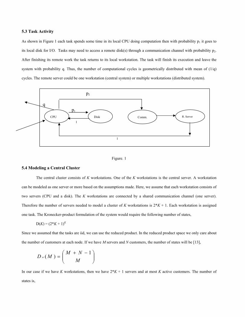
5.3 Task Activity

As shown in Figure 1 each task spends some time in its local CPU doing computation then with probability p1 it goes to

its local disk for I/O. Tasks may need to access a remote disk(s) through a communication channel with probability p2.

After finishing its remote work the task returns to its local workstation. The task will finish its execution and leave the

system with probability q. Thus, the number of computational cycles is geometrically distributed with mean of (1/q)

cycles. The remote server could be one workstation (central system) or multiple workstations (distributed system).

p2 q p1

1

1

CPU Disk Comm. R. Server

Figure. 1

5.4 Modeling a Central Cluster

The central cluster consists of K workstations. One of the K workstations is the central server. A workstation

can be modeled as one server or more based on the assumptions made. Here, we assume that each workstation consists of

two servers (CPU and a disk). The K workstations are connected by a shared communication channel (one server).

Therefore the number of servers needed to model a cluster of K workstations is 2*K + 1. Each workstation is assigned

one task. The Kronecker-product formulation of the system would require the following number of states,

D(K) = (2*K + 1)K

Since we assumed that the tasks are iid, we can use the reduced product. In the reduced product space we only care about

the number of customers at each node. If we have M servers and N customers, the number of states will be [13],

−+=

MNM

MD RP

1)(

In our case if we have K workstations, then we have 2*K + 1 servers and at most K active customers. The number of

states is,

+=

kkK

kD RP

*2)( , 1≤ k ≤ K

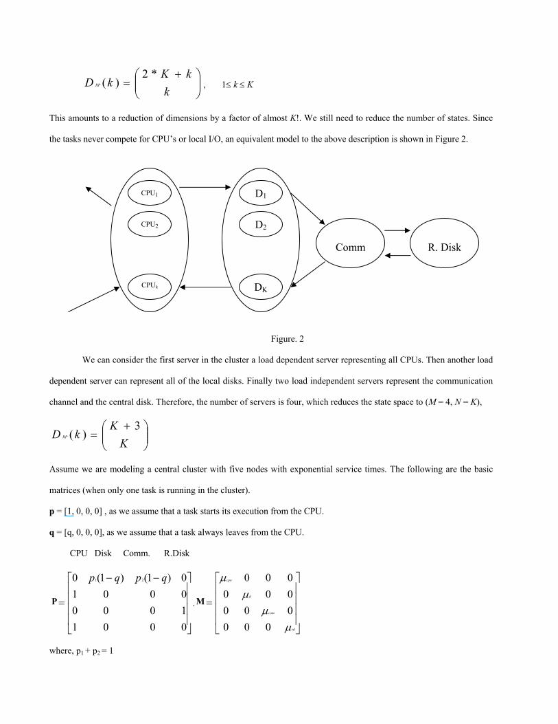
This amounts to a reduction of dimensions by a factor of almost K!. We still need to reduce the number of states. Since

the tasks never compete for CPU’s or local I/O, an equivalent model to the above description is shown in Figure 2.

CPU1

CPU2

CPUk

D1

D2

DK

Comm

R. Disk

Figure. 2

We can consider the first server in the cluster a load dependent server representing all CPUs. Then another load

dependent server can represent all of the local disks. Finally two load independent servers represent the communication

channel and the central disk. Therefore, the number of servers is four, which reduces the state space to (M = 4, N = K),

+=

KK

kD RP

3)(

Assume we are modeling a central cluster with five nodes with exponential service times. The following are the basic

matrices (when only one task is running in the cluster).

p = [1, 0, 0, 0] , as we assume that a task starts its execution from the CPU.

q = [q, 0, 0, 0], as we assume that a task always leaves from the CPU.

CPU Disk Comm. R.Disk

P

−−

=

0001100000010)1()1(0 21 qpqp

, M

=

rd

com

d

cpu

µµ

µµ

000000000000

where, p1 + p2 = 1

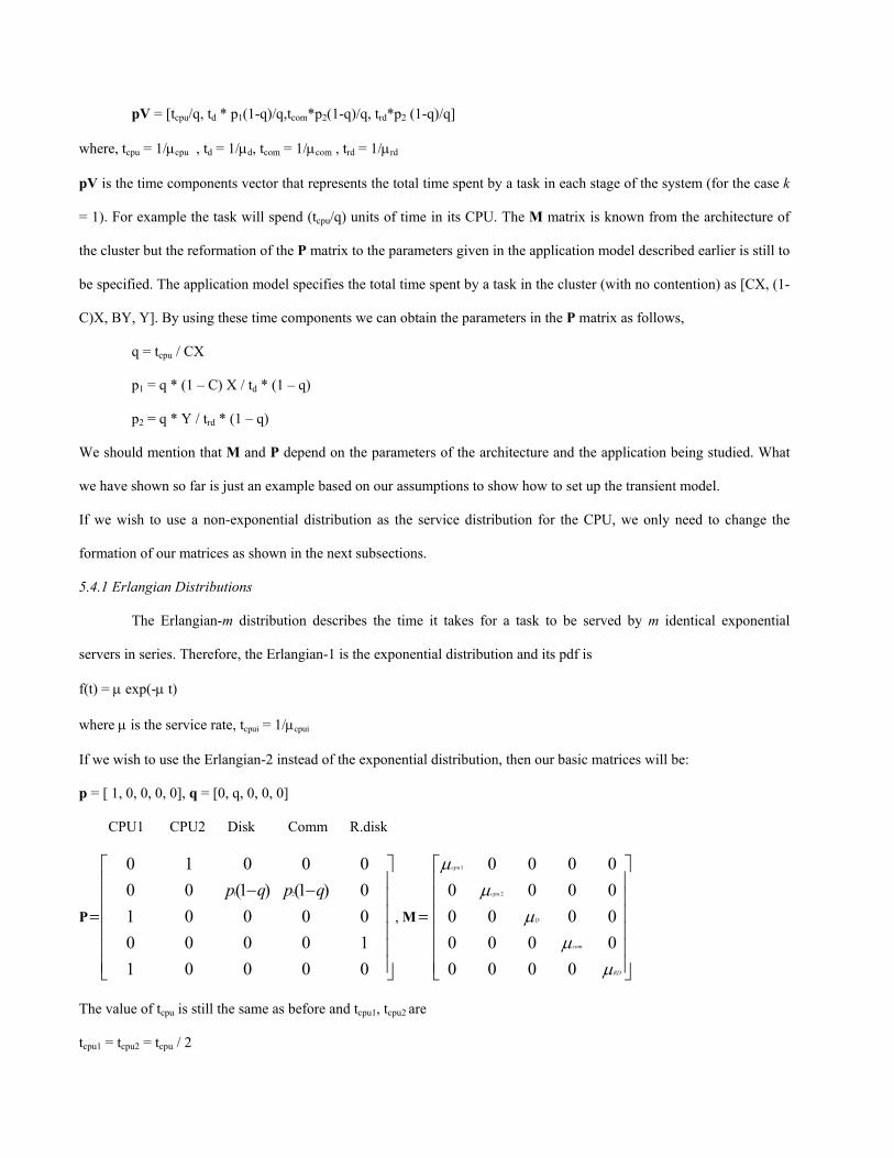
pV = [tcpu/q, td * p1(1-q)/q,tcom*p2(1-q)/q, trd*p2 (1-q)/q]

where, tcpu = 1/µcpu , td = 1/µd, tcom = 1/µcom , trd = 1/µrd

pV is the time components vector that represents the total time spent by a task in each stage of the system (for the case k

= 1). For example the task will spend (tcpu/q) units of time in its CPU. The M matrix is known from the architecture of

the cluster but the reformation of the P matrix to the parameters given in the application model described earlier is still to

be specified. The application model specifies the total time spent by a task in the cluster (with no contention) as [CX, (1-

C)X, BY, Y]. By using these time components we can obtain the parameters in the P matrix as follows,

q = tcpu / CX

p1 = q * (1 – C) X / td * (1 – q)

p2 = q * Y / trd * (1 – q)

We should mention that M and P depend on the parameters of the architecture and the application being studied. What

we have shown so far is just an example based on our assumptions to show how to set up the transient model.

If we wish to use a non-exponential distribution as the service distribution for the CPU, we only need to change the

formation of our matrices as shown in the next subsections.

5.4.1 Erlangian Distributions

The Erlangian-m distribution describes the time it takes for a task to be served by m identical exponential

servers in series. Therefore, the Erlangian-1 is the exponential distribution and its pdf is

f(t) = µ exp(-µ t)

where µ is the service rate, tcpui = 1/µcpui

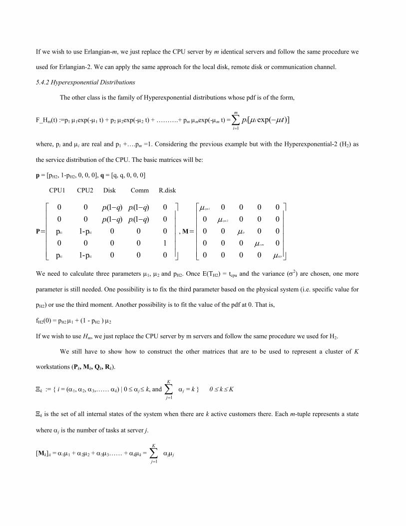
If we wish to use the Erlangian-2 instead of the exponential distribution, then our basic matrices will be:

p = [ 1, 0, 0, 0, 0], q = [0, q, 0, 0, 0]

CPU1 CPU2 Disk Comm R.disk

P= , M

−−

0000110000000010)1()1(0000010

21 qpqp

=

RD

com

D

cpu

cpu

µµ

µµ

µ

00000000000000000000

2

1

The value of tcpu is still the same as before and tcpu1, tcpu2 are

tcpu1 = tcpu2 = tcpu / 2

If we wish to use Erlangian-m, we just replace the CPU server by m identical servers and follow the same procedure we

used for Erlangian-2. We can apply the same approach for the local disk, remote disk or communication channel.

5.4.2 Hyperexponential Distributions

The other class is the family of Hyperexponential distributions whose pdf is of the form,

F_Hm(t) :=p1 µ1exp(-µ1 t) + p2 µ2exp(-µ2 t) + ……….+ pm µmexp(-µm t) =∑ )]exp([1

tpm

i

iii

=

−µµ

where, pi and µi are real and p1 +….pm =1. Considering the previous example but with the Hyperexponential-2 (H2) as

the service distribution of the CPU. The basic matrices will be:

p = [pH2, 1-pH2, 0, 0, 0], q = [q, q, 0, 0, 0]

CPU1 CPU2 Disk Comm R.disk

P= , M

−−−−

000p-1p10000000p-1p0)1()1(000)1()1(00

H2H2

H2H2

21

21

qpqpqpqp

=

RD

com

D

cpu

cpu

µµ

µµ

µ

00000000000000000000

2

1

We need to calculate three parameters µ1, µ2 and pH2. Once E(TH2) = tcpu and the variance (σ2) are chosen, one more

parameter is still needed. One possibility is to fix the third parameter based on the physical system (i.e. specific value for

pH2) or use the third moment. Another possibility is to fit the value of the pdf at 0. That is,

fH2(0) = pH2 µ1 + (1 - pH2 ) µ2

If we wish to use Hm, we just replace the CPU server by m servers and follow the same procedure we used for H2.

We still have to show how to construct the other matrices that are to be used to represent a cluster of K

workstations (Pk, Mk, Qk, Rk).

Ξk := { i = (α1, α2, α3,…… αk) | 0 ≤ αj ≤ k, and ∑ α=

K

j 1j = k } 0 ≤ k ≤ K

Ξk is the set of all internal states of the system when there are k active customers there. Each m-tuple represents a state

where αj is the number of tasks at server j.

[Mk]ii = α1µ1 + α2µ2 + α3µ3…… + αkµk = α∑=

K

j 1jµj

[Pk]ii := 0, unless [(i) – (j)] has exactly two nonzero elements, one with the value 1 and the other is –1. This means that

only one task can move at a time. Let αa be the number of customers in the server where the task left and αb is the

number of customers in the server where the task went. Then,

[Pk]ij = [P]ab iik

aa

M ][µα

[Rk]ij = 0, unless [(j) – (i)] has exactly one nonzero element and that element would have the value 1. Let a be the

component that is not zero.

[Rk]ij = pa

[Qk]ij = 0, unless [(i) – (j)] has exactly one nonzero element and that element would have the value 1. Let a be the

component that is not zero.

[Qk]ij = iik

aaa

Mq][

µα

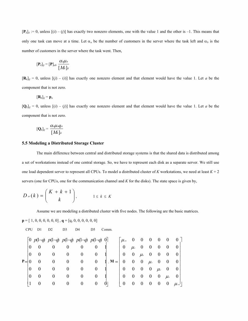
5.5 Modeling a Distributed Storage Cluster

The main difference between central and distributed storage systems is that the shared data is distributed among

a set of workstations instead of one central storage. So, we have to represent each disk as a separate server. We still use

one load dependent server to represent all CPUs. To model a distributed cluster of K workstations, we need at least K + 2

servers (one for CPUs, one for the communication channel and K for the disks). The state space is given by,

++=

kkK

kD RP

1)( , 1 ≤ k ≤ K

Assume we are modeling a distributed cluster with five nodes. The following are the basic matrices.

p = [ 1, 0, 0, 0, 0, 0, 0] , q = [q, 0, 0, 0, 0, 0, 0]

CPU D1 D2 D3 D4 D5 Comm.

P=

−−−−−

0000001100000010000001000000100000010000000)1()1()1()1()1(0 54321 qpqpqpqpqp

, M

=

com

d

d

d

d

d

cpu

µµ

µµ

µµ

µ

000000000000000000000000000000000000000000

where, 11∑=

=K

iip

V = (I – P)-1 M-1

pV=[tcpu/q,td*p1(1-q)/q,td*p2(1-q)/q,td*p3(1-q)/q,td*p4(1-q)/q, td*p5(1-q)/q, tcom *(1-q)/q]

As before, pV is the vector that represents the total time spent by a task in each stage of the system. Again, the

M matrix is known from the architecture of the cluster but the P matrix is constructed by using the application model.

Since the shared data is distributed according to a specific data allocation algorithm, the time component spent in each

node would be known (Yi is the time spent remotely on node i). If it is not known, we can assume that the shared data

has been distributed uniformly. As in the central case, we use these values to construct the P matrix.

q = tcpu / CX

p1 = q * Y1 / td1 * (1 – q), p2 = q * Y1 / td2 * (1 – q), p3 = q * Y1 / td3 * (1 – q)

p4 = q * Y1 / td4 * (1 – q), p5 = q * Y1 / td5 * (1 – q)

If we wish to use a non-exponential distribution, we just follow the same procedure as before. The other matrices, (Pk,

Mk, Qk, Rk), are constructed exactly the same way as described in section 5.4.

6. RESULTS

In this section, we show some of the results that can be obtained from the model. First, we show the different

performance regions (transient, steady state and draining). Then, we demonstrate the effect of the distribution on the

steady state value of the system. Finally, we study the effect of the service distribution and the performance region on

some of the performance metrics (speedup and execution time prediction).

We assume a parallel application consisting of 30 tasks (N = 30). We chose N = 30 to be able to see the transient and

draining regions clearly. Once the steady state is reached, adding more tasks will only increase the steady state region.

The average execution time per task is 12 units of time (E(T) = 12). The application is running on a 5-workstation and an

8-workstation clusters. To show the effect of the performance region on the accuracy of performance measures, we

increase the number of tasks to 100 and compare with the case of 30. The results we show are for central cluster.

6.1 Shared Servers with Non-Exponential Service Times

We assume that the shared server (remote disk) is the non-exponential server while the dedicated servers are

exponential servers. In this case Jackson networks models can not be applied but our model can be applied.

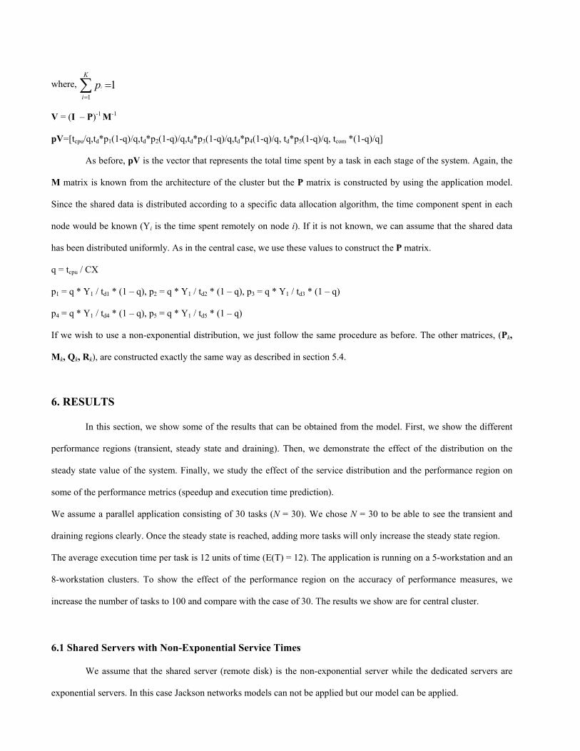
6.1.1 Performance Behavior

In Figures 3,4, we show how the performance behavior of an application changes if we assume different service

distributions. As mentioned earlier, there are three different regions in the performance characteristic of any system, the

transient region, the steady state region and the draining region starts.

0 5 10 15 20 25 30100

101

102Inter-departure Tim e, K = 5

Task Order

t

E xpH2, C2 = 10H2, C2 = 50

Figure 3. 30-task application running on a 5-workstations central cluster.

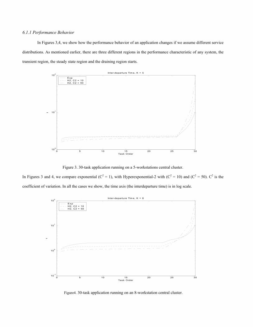
In Figures 3 and 4, we compare exponential (C2 = 1), with Hyperexponential-2 with (C2 = 10) and (C2 = 50). C2 is the

coefficient of variation. In all the cases we show, the time axis (the interdeparture time) is in log scale.

0 5 10 15 20 25 3010-1

100

101

102Inter-departure Tim e, K = 8

Task Order

t

E xpH2, C2 = 10H2, C2 = 50

Figure4. 30-task application running on an 8-workstation central cluster.

6.1.2 Steady State

The steady state value of the system depends on the system size and the service distribution. In pervious work,

we showed that to reach steady state, the number of tasks to be executed must be much greater than the number of nodes

in the system. In Figure 5, we show how the steady state of the system changes with changing the distribution. The

steady state interdeparture time can be calculated by:

tSS = pSS VK ε’K

where pSS can be obtained from:

pSS VK RK = pSS and pSS ε’K = 1

10 20 30 40 50 60 70 80 90 1000

0.5

1

1.5

2

2.5

3

3.5

4

4.5

5Steady State Interdeparture Time, K = 8

C2

t

No ContentionContention

Figure 5. Steady state interdeparture time for a cluster of 8 workstations. Two cases are considered when the shared server under a heavy load and light load.

It is interesting to know that the steady state value of the system is not always increasing with increasing C2 but it

reaches a minimum value then it increases again. The minimum value of the steady state depends on the system and

application configurations. In case of no-contention, the service distribution does not have any effect on the steady state

of the system. The reason is that there is no queueing in this case.

6.1.3 Performance Prediction

One of the main objectives of having a performance model is to be able to predict the running time of the target

application. In most of the cases, the exponential distribution is assumed. As we mentioned earlier, it has been shown

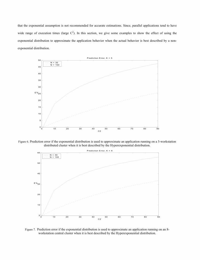
that the exponential assumption is not recommended for accurate estimations. Since, parallel applications tend to have

wide range of execution times (large C2). In this section, we give some examples to show the effect of using the

exponential distribution to approximate the application behavior when the actual behavior is best described by a non-

exponential distribution.

0 10 20 30 40 50 60 70 80 900

5

10

15

20

25

30

35

40

45

50P redic tion E rror, K = 5

C2

E %

N = 30N = 100

Figure 6. Prediction error if the exponential distribution is used to approximate an application running on a 5-workstation distributed cluster when it is best described by the Hyperexponential distribution.

0 10 20 30 40 50 60 70 80 900

10

20

30

40

50

60P redic t ion E rror, K = 8

C2

E %

N = 30N = 100

Figure 7. Prediction error if the exponential distribution is used to approximate an application running on an 8-workstation central cluster when it is best described by the Hyperexponential distribution.

In Figure 6 and 7, we calculate the percentage error of the application, if the exponential distribution is assumed. The

percentage error is calculated as :

E = app

appapp

act

act

TETETE

)()()( exp−

* 100 ,

where,

E(Tact)app is the total execution time of the parallel application with the correct distribution.

E(Texp)app is the total execution time of the parallel application if the exponential distribution is assumed.

Our results indicate that the exponential distribution fails to approximate distributions with large C2. In Figures 6 and 7,

we see that the error exceeds 20 % if C2=10. The percentage error always increases with increasing C2.

6.1.4 Speedup

One of the reasons we use parallel systems is to speed up the computation. It is always important to know the value of

the speedup that your computing resources can provide. We found that one of the common problems is that the actual

speedup is less than the expected speedup from the available resources. Our results show that there are three reasons.

Obviously the first reason is contention. The second reason is the operating region (i.e., steady state or transient).

0 10 20 30 40 50 60 70 80 900

0.5

1

1.5

2

2.5

3

3.5

4S ys tem S peedup, K = 5

C2

S P

N = 30N = 100

Figure 8. The effect of service distribution on the system speedup.

In Figures 8 and 9, we use the same application but with different number of tasks (30, 100) and calculate the speedup

for different C2. In the case of 20 tasks, the transient region dominates. Then we increased the number of tasks to 100 in

order for the steady state region to dominate. It is clear that, if the system is working in the transient region, the speedup

is much less than if the system is working in the steady state region. This behavior can be explained if we return to

Figures 3 and 4 and notice the effect of the transient and draining regions explained earlier.

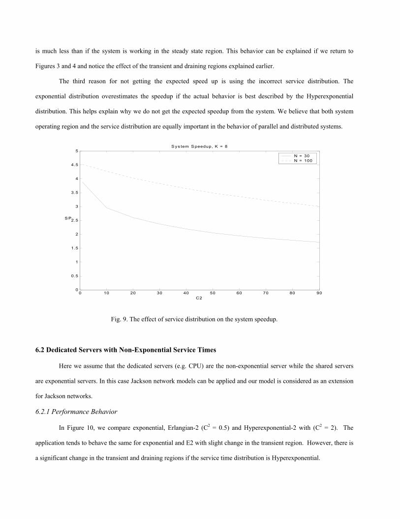
The third reason for not getting the expected speed up is using the incorrect service distribution. The

exponential distribution overestimates the speedup if the actual behavior is best described by the Hyperexponential

distribution. This helps explain why we do not get the expected speedup from the system. We believe that both system

operating region and the service distribution are equally important in the behavior of parallel and distributed systems.

0 10 20 30 40 50 60 70 80 900

0.5

1

1.5

2

2.5

3

3.5

4

4.5

5S ys tem S peedup, K = 8

C2

S P

N = 30N = 100

Fig. 9. The effect of service distribution on the system speedup.

6.2 Dedicated Servers with Non-Exponential Service Times

Here we assume that the dedicated servers (e.g. CPU) are the non-exponential server while the shared servers

are exponential servers. In this case Jackson network models can be applied and our model is considered as an extension

for Jackson networks.

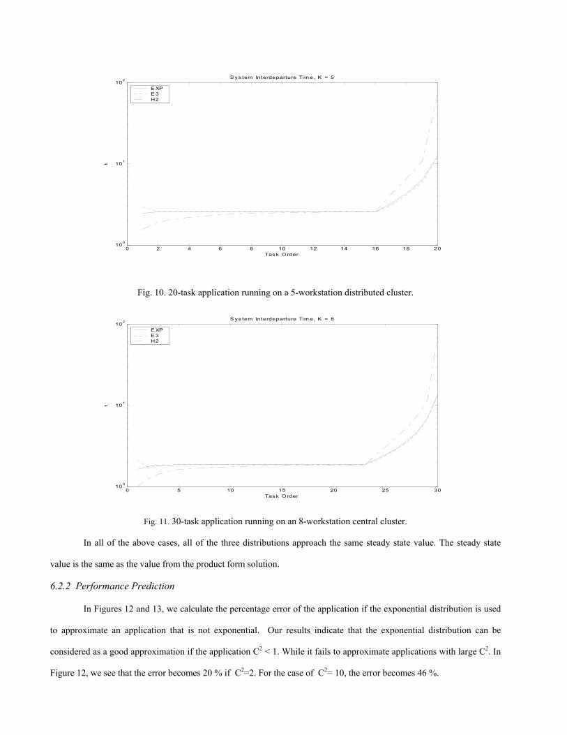
6.2.1 Performance Behavior

In Figure 10, we compare exponential, Erlangian-2 (C2 = 0.5) and Hyperexponential-2 with (C2 = 2). The

application tends to behave the same for exponential and E2 with slight change in the transient region. However, there is

a significant change in the transient and draining regions if the service time distribution is Hyperexponential.

0 2 4 6 8 10 12 14 16 18 20100

101

102S ys tem Interdeparture Tim e, K = 5

Task Order

t

E XPE 3H2

Fig. 10. 20-task application running on a 5-workstation distributed cluster.

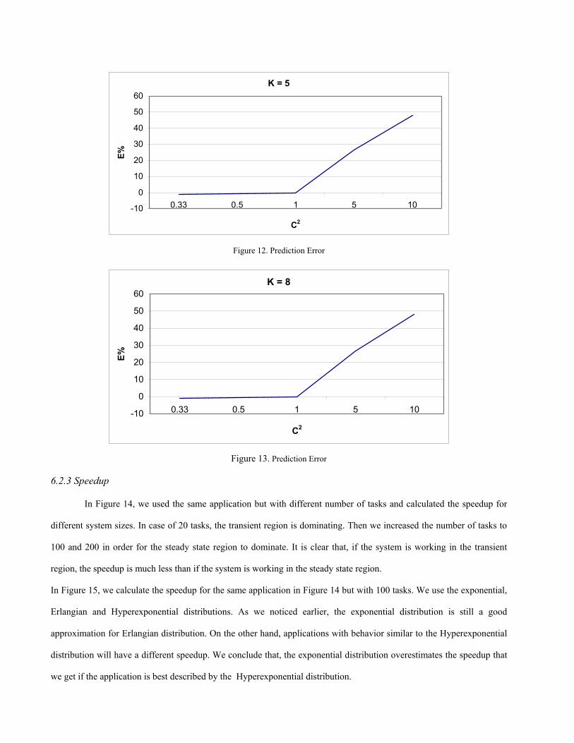
0 5 10 15 20 25 30100

101

102S ys tem Interdeparture Tim e, K = 8

Task Order

t

E XPE 3H2

Fig. 11. 30-task application running on an 8-workstation central cluster.

In all of the above cases, all of the three distributions approach the same steady state value. The steady state

value is the same as the value from the product form solution.

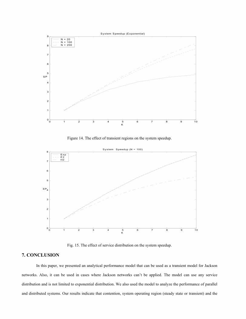
6.2.2 Performance Prediction

In Figures 12 and 13, we calculate the percentage error of the application if the exponential distribution is used

to approximate an application that is not exponential. Our results indicate that the exponential distribution can be

considered as a good approximation if the application C2 < 1. While it fails to approximate applications with large C2. In

Figure 12, we see that the error becomes 20 % if C2=2. For the case of C2= 10, the error becomes 46 %.

K = 5

-10

0

10

20

30

40

50

60

0.33 0.5 1 5 10

C2

E%

Figure 12. Prediction Error

K = 8

-10

0

10

20

30

40

50

60

0.33 0.5 1 5 10

C2

E%

Figure 13. Prediction Error

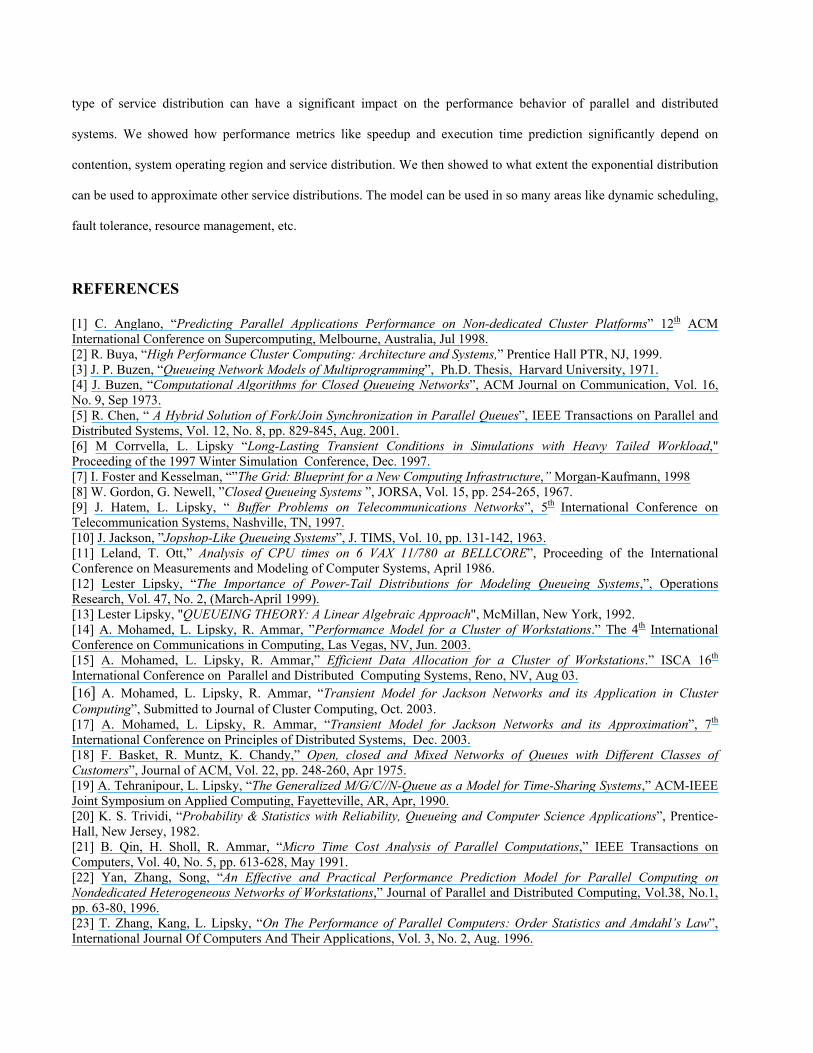
6.2.3 Speedup

In Figure 14, we used the same application but with different number of tasks and calculated the speedup for

different system sizes. In case of 20 tasks, the transient region is dominating. Then we increased the number of tasks to

100 and 200 in order for the steady state region to dominate. It is clear that, if the system is working in the transient

region, the speedup is much less than if the system is working in the steady state region.

In Figure 15, we calculate the speedup for the same application in Figure 14 but with 100 tasks. We use the exponential,

Erlangian and Hyperexponential distributions. As we noticed earlier, the exponential distribution is still a good

approximation for Erlangian distribution. On the other hand, applications with behavior similar to the Hyperexponential

distribution will have a different speedup. We conclude that, the exponential distribution overestimates the speedup that

we get if the application is best described by the Hyperexponential distribution.

0 1 2 3 4 5 6 7 8 9 100

1

2

3

4

5

6

7

8

9S y s tem S peedup (E xponential)

K

S P

N = 20N = 100N = 200

Figure 14. The effect of transient regions on the system speedup.

0 1 2 3 4 5 6 7 8 9 100

1

2

3

4

5

6

7

8S ys tem S peedup (N = 100)

K

S P

E xpE 2H2

Fig. 15. The effect of service distribution on the system speedup.

7. CONCLUSION

In this paper, we presented an analytical performance model that can be used as a transient model for Jackson

networks. Also, it can be used in cases where Jackson networks can’t be applied. The model can use any service

distribution and is not limited to exponential distribution. We also used the model to analyze the performance of parallel

and distributed systems. Our results indicate that contention, system operating region (steady state or transient) and the

type of service distribution can have a significant impact on the performance behavior of parallel and distributed

systems. We showed how performance metrics like speedup and execution time prediction significantly depend on

contention, system operating region and service distribution. We then showed to what extent the exponential distribution

can be used to approximate other service distributions. The model can be used in so many areas like dynamic scheduling,

fault tolerance, resource management, etc.

REFERENCES

[1] C. Anglano, “Predicting Parallel Applications Performance on Non-dedicated Cluster Platforms” 12th ACM International Conference on Supercomputing, Melbourne, Australia, Jul 1998. [2] R. Buya, “High Performance Cluster Computing: Architecture and Systems,” Prentice Hall PTR, NJ, 1999. [3] J. P. Buzen, “Queueing Network Models of Multiprogramming”, Ph.D. Thesis, Harvard University, 1971. [4] J. Buzen, “Computational Algorithms for Closed Queueing Networks”, ACM Journal on Communication, Vol. 16, No. 9, Sep 1973. [5] R. Chen, “ A Hybrid Solution of Fork/Join Synchronization in Parallel Queues”, IEEE Transactions on Parallel and Distributed Systems, Vol. 12, No. 8, pp. 829-845, Aug. 2001. [6] M Corrvella, L. Lipsky “Long-Lasting Transient Conditions in Simulations with Heavy Tailed Workload," Proceeding of the 1997 Winter Simulation Conference, Dec. 1997. [7] I. Foster and Kesselman, “”The Grid: Blueprint for a New Computing Infrastructure,” Morgan-Kaufmann, 1998 [8] W. Gordon, G. Newell, ”Closed Queueing Systems ”, JORSA, Vol. 15, pp. 254-265, 1967. [9] J. Hatem, L. Lipsky, “ Buffer Problems on Telecommunications Networks”, 5th International Conference on Telecommunication Systems, Nashville, TN, 1997. [10] J. Jackson, ”Jopshop-Like Queueing Systems”, J. TIMS, Vol. 10, pp. 131-142, 1963. [11] Leland, T. Ott,” Analysis of CPU times on 6 VAX 11/780 at BELLCORE”, Proceeding of the International Conference on Measurements and Modeling of Computer Systems, April 1986. [12] Lester Lipsky, “The Importance of Power-Tail Distributions for Modeling Queueing Systems,”, Operations Research, Vol. 47, No. 2, (March-April 1999). [13] Lester Lipsky, "QUEUEING THEORY: A Linear Algebraic Approach", McMillan, New York, 1992. [14] A. Mohamed, L. Lipsky, R. Ammar, ”Performance Model for a Cluster of Workstations.” The 4th International Conference on Communications in Computing, Las Vegas, NV, Jun. 2003. [15] A. Mohamed, L. Lipsky, R. Ammar,” Efficient Data Allocation for a Cluster of Workstations.” ISCA 16th International Conference on Parallel and Distributed Computing Systems, Reno, NV, Aug 03. [16] A. Mohamed, L. Lipsky, R. Ammar, “Transient Model for Jackson Networks and its Application in Cluster Computing”, Submitted to Journal of Cluster Computing, Oct. 2003. [17] A. Mohamed, L. Lipsky, R. Ammar, “Transient Model for Jackson Networks and its Approximation”, 7th International Conference on Principles of Distributed Systems, Dec. 2003. [18] F. Basket, R. Muntz, K. Chandy,” Open, closed and Mixed Networks of Queues with Different Classes of Customers”, Journal of ACM, Vol. 22, pp. 248-260, Apr 1975. [19] A. Tehranipour, L. Lipsky, “The Generalized M/G/C//N-Queue as a Model for Time-Sharing Systems,” ACM-IEEE Joint Symposium on Applied Computing, Fayetteville, AR, Apr, 1990. [20] K. S. Trividi, “Probability & Statistics with Reliability, Queueing and Computer Science Applications”, Prentice-Hall, New Jersey, 1982. [21] B. Qin, H. Sholl, R. Ammar, “Micro Time Cost Analysis of Parallel Computations,” IEEE Transactions on Computers, Vol. 40, No. 5, pp. 613-628, May 1991. [22] Yan, Zhang, Song, “An Effective and Practical Performance Prediction Model for Parallel Computing on Nondedicated Heterogeneous Networks of Workstations,” Journal of Parallel and Distributed Computing, Vol.38, No.1, pp. 63-80, 1996. [23] T. Zhang, Kang, L. Lipsky, “On The Performance of Parallel Computers: Order Statistics and Amdahl’s Law”, International Journal Of Computers And Their Applications, Vol. 3, No. 2, Aug. 1996.