modeling fire occurrence at the city scale - mdpi

International Journal of

Environmental Research

and Public Health

Article

Modeling Fire Occurrence at the City Scale:A Comparison between Geographically WeightedRegression and Global Linear Regression

Chao Song 1, Mei-Po Kwan 2,3 and Jiping Zhu 1,*1 State Key Laboratory of Fire Science, University of Science and Technology of China, Hefei 230026, China;

[email protected] Department of Geography and Geographic Information Science, University of Illinois at

Urbana-Champaign, 255 Computing Applications Building, MC-150, 605 E Springfield Ave.,Champaign, IL 61820, USA; [email protected]

3 Department of Human Geography and Spatial Planning, Faculty of Geosciences, Utrecht University,P.O. Box 80125, 3508 TC Utrecht, The Netherlands

* Correspondence: [email protected]; Tel.: +86-551-63606453

Academic Editor: Jason K. LevyReceived: 12 February 2017; Accepted: 5 April 2017; Published: 8 April 2017

Abstract: An increasing number of fires are occurring with the rapid development of cities, resultingin increased risk for human beings and the environment. This study compares geographicallyweighted regression-based models, including geographically weighted regression (GWR) andgeographically and temporally weighted regression (GTWR), which integrates spatial and temporaleffects and global linear regression models (LM) for modeling fire risk at the city scale. The resultsshow that the road density and the spatial distribution of enterprises have the strongest influenceson fire risk, which implies that we should focus on areas where roads and enterprises are denselyclustered. In addition, locations with a large number of enterprises have fewer fire ignition records,probably because of strict management and prevention measures. A changing number of significantvariables across space indicate that heterogeneity mainly exists in the northern and eastern rural andsuburban areas of Hefei city, where human-related facilities or road construction are only clustered inthe city sub-centers. GTWR can capture small changes in the spatiotemporal heterogeneity of thevariables while GWR and LM cannot. An approach that integrates space and time enables us to betterunderstand the dynamic changes in fire risk. Thus governments can use the results to manage firesafety at the city scale.

Keywords: GTWR; GWR; heterogeneity; space and time; global linear regression; fire risk

1. Introduction

Fire is a natural phenomenon that occurs worldwide in complex environments. Fire presents agreat threat to people and the natural environment and scientists are aware of the necessity to managefire risk. An example is the big fire that occurred in Chicago in 1871 when flying debris obscuredthe sky and Chicago was overcome by fire. To date, it is still a challenge for scientists to explain theoccurrence and spread of natural fires, and it is even more difficult to predict fires. Fires have beenstudied in many regions around the world [1–5], such as in Spain [6,7] and many other countries [8].However, few studies have examined fire risk at the city scale and its influence on the environmentrequires further studies. Worldwide, it is widely known that human activities play an importantrole in fire risk [9–12]. Dense urban population in urban areas and related hidden sources of hazardssuch as electrical installations and power lines may lead to the occurrence of fires as described inprevious studies [13,14]. Places with a high population density such as markets and residential areas

Int. J. Environ. Res. Public Health 2017, 14, 396; doi:10.3390/ijerph14040396 www.mdpi.com/journal/ijerph

http://www.mdpi.com/journal/ijerph

http://www.mdpi.com

http://www.mdpi.com/journal/ijerph

Int. J. Environ. Res. Public Health 2017, 14, 396 2 of 23

are especially vulnerable to high levels of fire risk. In addition, other factors such as road density,distance to water bodies, average temperature, precipitation, relative humidity, wind speed, slope, andaspect, which can be summarized as socioeconomic, climate and topographic predictors, were foundto be associated with fire risk [7,13,15].

Several studies have adopted global linear regression models (LM) to study fire risk [15,16].However, because of the relationship between fire risk and its influencing factors that may vary overspace, which is referred to as spatial heterogeneity, LM, including ordinary least squares (OLS) models,may not be adequate for examining the spatially varying relationship between multiple predictorsand fire occurrence. This limitation is mostly due to the constant coefficients in LM. Geographicallyweighted regression (GWR) has been widely used to take into account the spatial heterogeneity becauseof the unique characteristics of the model. GWR allows the regression coefficients to vary for individuallocations, capturing the effects of non-stationarity and revealing variations in the importance of thevariables across the study area. The use of GWR focuses particularly on data analysis and interpretationrather than prediction [8,16,17]. Aside from the popular spatially varied coefficient model, GWR wasextended further and geographically and temporally weighted regression (GTWR) was developed todeal with both spatial and temporal non-stationarity [17]. GWR-based models are not just designed forimproving model fitness; rather they facilitate the spatiotemporal exploration of natural phenomena.

GTWR integrates both temporal and spatial information in the weight matrices to capture spatialand temporal heterogeneity simultaneously [17,18]. The approach has been used in models of houseprices and land use change [17–19]. The statistical performance of the GTWR is better than that of theGWR and the OLS in terms of goodness-of-fit. It is a well-known fact that fire risk is a phenomenonthat changes over space and time [11,20–22]. The frequency of fire and its ignition locations showspatiotemporal dependence such as clustering, lagging and seasonal trends. Therefore, the existing firemodels could be improved by incorporating temporal effects by integrating both spatial and temporalinformation in the weighting matrices [17,18,23]. Therefore, we aim to use GTWR to discover thepotential rules for fire risk and to compare the approach with GWR and LM.

Before developing a GWR or GTWR model, the first task is to select variables and to fit an LM byadopting the OLS method for the purpose of comparison. The process of selecting variables is complexand different criteria or approaches may be used for different models, such as the Akaike informationcriterion (AIC), Bayesian information criterion (BIC), cross validation (CV), stepwise regression, andmean squared errors (MSE) reduction [15,24,25]. Further, an accuracy assessment of predictive spatialmodels needs to account for spatial autocorrelation. However, little attention has been paid to theinfluence arising from the presence of spatial autocorrelation in geospatial data and residuals, whichmay result in overfitting or underestimation [26]. By using spatial cross validation and bootstrapstrategies, spatial prediction errors in the resampling-based accuracy assessment can be improvedand the bias caused by residual spatial autocorrelation (RSA) can be corrected [26,27]. R statisticalsoftware and the packages “spgwr”, “sperrorest”, and “caret” have been used to calibrate the spatialcross validation (SCV) process and thus the resampling-based variable importance and predictionerror across data folds can be achieved [26,28]. Therefore, it is necessary to first select variables byusing SCV before using the variable in a further regression model.

This study compares geographically weighted regression-based models (including GWR andGTWR, which integrates spatial and temporal effect) and LM for modeling fire risk at the city scale.We use historical fire records and related datasets for Hefei city in China to undertake the comparativeanalysis. The study is divided into three tasks. First, SCV and CV are separately employed andcompared in order to obtain the importance of the variables and then the relatively important predictorsare selected after multicollinearity test. We also compare SCV and CV and identify the specificdifferences between them. Second, we adopt the selected variables from the previous step and fitthe OLS model using the “caret” package in the R software. The significance level and the relativeimportance of the variables in the OLS model are quantified and the non-significant variables areremoved. Third, we use the significant variables to fit a GWR model and visualize the local coefficients,


the local significance of the coefficients and the residual distribution. GTWR is then employed andthe fitness of the three models is summarized, along with a semivariogram analysis of residuals indifferent time periods. In this study, we adopted the original GTWR model created by Huang [18].Therefore, the other improved GTWR models are not examined in the study.

The study shows that by using advanced GIS and spatial statistical methods along with detailedhistorical datasets of fire ignition, it is possible to build valid and meaningful models to explain firerisk. We can use them to improve the management of fire risk and safety in urban areas as well as inthe natural environment.

2. Materials and Methods

2.1. Study Area

The study area is in Hefei city, which is located in the middle of Anhui Province in China. Thecity comprises a total area of around 7029 km2 and had a population of about five million prior to 2010.The land use in Hefei in 2005 and 2010 is shown in Figure 1. The data set with a spatial resolution of300 m is provided by the Database of Global Change Parameters, Chinese Academy of Sciences [29].


and visualize the local coefficients, the local significance of the coefficients and the residual

distribution. GTWR is then employed and the fitness of the three models is summarized, along with

a semivariogram analysis of residuals in different time periods. In this study, we adopted the

original GTWR model created by Huang [18]. Therefore, the other improved GTWR models are not

examined in the study.

The study shows that by using advanced GIS and spatial statistical methods along with detailed

historical datasets of fire ignition, it is possible to build valid and meaningful models to explain fire

risk. We can use them to improve the management of fire risk and safety in urban areas as well as in

the natural environment.

2. Materials and Methods

2.1. Study Area

The study area is in Hefei city, which is located in the middle of Anhui Province in China. The

city comprises a total area of around 7029 km2 and had a population of about five million prior to

2010. The land use in Hefei in 2005 and 2010 is shown in Figure 1. The data set with a spatial

resolution of 300 m is provided by the Database of Global Change Parameters, Chinese Academy of

Sciences [29].

Figure 1. Land use in Hefei city in 2005 and 2010.

Although the study area is small relative to previous studies, there still exists considerable

diversity in its socioeconomic, climate, topographic, and other attributes. In previous studies,

researchers mainly adopted complex socioeconomic factors for fire occurrence and fire risk, which

include population density, population structure, road density, slope, and other factors. These

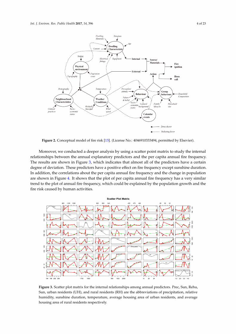
factors play important roles in fire occurrence, as shown in Figure 2, which is a conceptual summary

of various fire risk factors and was developed by Corcoran et al. [13].

2.2. Dependent Variable and Preliminary Analysis for Infrastructure Fire Frequency

A dataset of fire records for the period of 2002–2010 in Hefei was obtained from the Fire Bureau

in Anhui Province, China. The contained information includes the time of occurrence, event type,

location, event damage, and fire-fighting time. A total of 12,629 historical infrastructure fire fighting

records were extracted. The annual demographic and climate records including population,

precipitation (Prec), relative humidity (Rehu), sunshine duration (Sun), temperature (Temp), GDP,

and the average housing area of urban residents (UH) and rural residents (RH) in Hefei were

provided by the statistical bureau of Anhui Province (http://www.ahtjj.gov.cn/tjj/web/index.jsp).

Figure 1. Land use in Hefei city in 2005 and 2010.

Although the study area is small relative to previous studies, there still exists considerablediversity in its socioeconomic, climate, topographic, and other attributes. In previous studies,researchers mainly adopted complex socioeconomic factors for fire occurrence and fire risk, whichinclude population density, population structure, road density, slope, and other factors. These factorsplay important roles in fire occurrence, as shown in Figure 2, which is a conceptual summary of variousfire risk factors and was developed by Corcoran et al. [13].

2.2. Dependent Variable and Preliminary Analysis for Infrastructure Fire Frequency

A dataset of fire records for the period of 2002–2010 in Hefei was obtained from the Fire Bureau inAnhui Province, China. The contained information includes the time of occurrence, event type, location,event damage, and fire-fighting time. A total of 12,629 historical infrastructure fire fighting recordswere extracted. The annual demographic and climate records including population, precipitation(Prec), relative humidity (Rehu), sunshine duration (Sun), temperature (Temp), GDP, and the averagehousing area of urban residents (UH) and rural residents (RH) in Hefei were provided by the statisticalbureau of Anhui Province (http://www.ahtjj.gov.cn/tjj/web/index.jsp).

http://www.ahtjj.gov.cn/tjj/web/index.jsp

Int. J. Environ. Res. Public Health 2017, 14, 396 4 of 23Int. J. Environ. Res. Public Health 2017, 14, 396 4 of 22

Figure 2. Conceptual model of fire risk [13]. (License No.: 4046910333494, permitted by Elsevier)

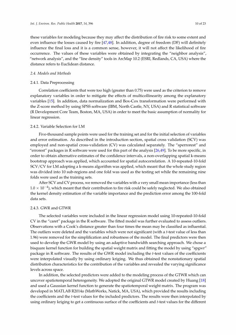
Moreover, we conducted a deeper analysis by using a scatter point matrix to study the internal

relationships between the annual explanatory predictors and the per capita annual fire frequency.

The results are shown in Figure 3, which indicates that almost all of the predictors have a certain

degree of deviation. These predictors have a positive effect on fire frequency except sunshine

duration. In addition, the correlations about the per capita annual fire frequency and the change in

population are shown in Figure 4. It shows that the plot of per capita annual fire frequency has a

very similar trend to the plot of annual fire frequency, which could be explained by the population

growth and the fire risk caused by human activities.

Figure 3. Scatter plot matrix for the internal relationships among annual predictors. Prec, Sun, Rehu,

Sun, urban residents (UH), and rural residents (RH) are the abbreviations of precipitation, relative

humidity, sunshine duration, temperature, average housing area of urban residents, and average

housing area of rural residents respectively.

Figure 2. Conceptual model of fire risk [13]. (License No.: 4046910333494, permitted by Elsevier).

Moreover, we conducted a deeper analysis by using a scatter point matrix to study the internalrelationships between the annual explanatory predictors and the per capita annual fire frequency.The results are shown in Figure 3, which indicates that almost all of the predictors have a certaindegree of deviation. These predictors have a positive effect on fire frequency except sunshine duration.In addition, the correlations about the per capita annual fire frequency and the change in populationare shown in Figure 4. It shows that the plot of per capita annual fire frequency has a very similartrend to the plot of annual fire frequency, which could be explained by the population growth and thefire risk caused by human activities.


Figure 2. Conceptual model of fire risk [13]. (License No.: 4046910333494, permitted by Elsevier)

Moreover, we conducted a deeper analysis by using a scatter point matrix to study the internal

relationships between the annual explanatory predictors and the per capita annual fire frequency.

The results are shown in Figure 3, which indicates that almost all of the predictors have a certain

degree of deviation. These predictors have a positive effect on fire frequency except sunshine

duration. In addition, the correlations about the per capita annual fire frequency and the change in

population are shown in Figure 4. It shows that the plot of per capita annual fire frequency has a

very similar trend to the plot of annual fire frequency, which could be explained by the population

growth and the fire risk caused by human activities.

Figure 3. Scatter plot matrix for the internal relationships among annual predictors. Prec, Sun, Rehu,

Sun, urban residents (UH), and rural residents (RH) are the abbreviations of precipitation, relative

humidity, sunshine duration, temperature, average housing area of urban residents, and average

housing area of rural residents respectively.

Figure 3. Scatter plot matrix for the internal relationships among annual predictors. Prec, Sun, Rehu,Sun, urban residents (UH), and rural residents (RH) are the abbreviations of precipitation, relativehumidity, sunshine duration, temperature, average housing area of urban residents, and averagehousing area of rural residents respectively.



Moreover, Figure 4 shows that in the latest years, fire frequency per capita has decreased more

than fire frequency. Table 1 also shows that human-caused fires play an important role in explaining

ignitions and places of interest (POI), and areas, where population is clustered, represent the main

potential causes of fire risk, evidenced by the high proportion of fire occurring in those places, with

the exception of fires associated with chemical industries, traffic, and electrical appliances.

Figure 4. Annual summaries for fire records (2002–2010) and the relationship with population

growth.

Table 1. Statistical summary for fire categories.

Category Number Proportion

Population-clustered places (hotel, school, market, etc.) 2993 0.502941

Other 967 0.162494

Traffic-related 938 0.157621

Important buildings (warehouse, gas stations, etc.) 566 0.09511

Electricity 256 0.043018

High-rise buildings 109 0.018316

Chemical industries 88 0.014787

Underground buildings 34 0.005713

In order to make comparisons between GTWR and other models, we divided the entire time

period of nine years into five temporal periods of nearly 22 months each. Thus, we could obtain the

spatial distribution of the fire ignition points for different time periods. The spatial distribution of

fire ignition points is shown in Figure 5 The response variable, called average fire density, was

derived using the kernel density method, which turns discrete points in a study area into a

continuous density surface to minimize the uncertainty and mistakes in the ignition records [15].

Fire density is defined in this study as the ignition frequency in one grid cell (occurrence number per

period per km2).

A spatial resolution of 1 km × 1 km and a fixed bandwidth of 5 km were used as a rule of thumb

after comparing several different bandwidth values (from 1 km to 10 km) [6]. Water bodies and

similar land cover types where fire cannot occur were excluded from the analysis. The resulting base

grid had 6985 cells covering the entire study area excluding water bodies. The centers of the pixels

were used as the initial sample points. In order to mitigate the effect of spatial autocorrelation, rather

than using all 6985 grids, 1000 sample points distributed randomly in space were selected for each

time period, thus, 5000 sample points in total were used in the process of training the model. In

addition, 500 samples dispersed spatially were used as validation samples across the five time

periods.

Figure 4. Annual summaries for fire records (2002–2010) and the relationship with population growth.

Moreover, Figure 4 shows that in the latest years, fire frequency per capita has decreased morethan fire frequency. Table 1 also shows that human-caused fires play an important role in explainingignitions and places of interest (POI), and areas, where population is clustered, represent the mainpotential causes of fire risk, evidenced by the high proportion of fire occurring in those places, withthe exception of fires associated with chemical industries, traffic, and electrical appliances.

Table 1. Statistical summary for fire categories.

Category Number Proportion

Population-clustered places (hotel, school, market, etc.) 2993 0.502941Other 967 0.162494Traffic-related 938 0.157621Important buildings (warehouse, gas stations, etc.) 566 0.09511Electricity 256 0.043018High-rise buildings 109 0.018316Chemical industries 88 0.014787Underground buildings 34 0.005713

In order to make comparisons between GTWR and other models, we divided the entire timeperiod of nine years into five temporal periods of nearly 22 months each. Thus, we could obtain thespatial distribution of the fire ignition points for different time periods. The spatial distribution of fireignition points is shown in Figure 5 The response variable, called average fire density, was derivedusing the kernel density method, which turns discrete points in a study area into a continuous densitysurface to minimize the uncertainty and mistakes in the ignition records [15]. Fire density is defined inthis study as the ignition frequency in one grid cell (occurrence number per period per km2).


Figure 5. Ignition points between 2002 and 2010, divided into five time periods.

2.3. Explanatory Variables: Selection and Pre-Processing

A total of 25 explanatory variables covering a variety of socioeconomic attributes were

extracted from the databases [13,30–34]. These variables consider the influence of socioeconomic

conditions on fire occurrence, as well as the influence of climate and topographic conditions. These

explanatory variables were derived from the previous literature and several new variables

consisting of the spatial distribution of buildings were selected for the modeling process of

infrastructure fire occurrence. These explanatory variables are shown in Table 2. Some variables,

including static and dynamic variables, are illustrated in Figure 6. It should be noted that the

uncertain geographic context problem (UGCoP) could affect the reallocation of fire risk

spatiotemporally because of the dynamic change of socioeconomic attributes in urban areas [35].

This highlights the reason for the need of spatiotemporal models. All the explanatory variables were

resampled to a resolution of 1 km × 1 km to achieve the same resolution as that of the fire density.

Table 2. Candidate explanatory variables.

Variable Name Code Data Source Resolution/Unit

Elevation DEM

The data set is provided by

Geospatial Data Cloud site,

Computer Network Information

Center, Chinese Academy of

Sciences (http://www.gscloud.cn)

30 m

Slope SLOPE Calculated by ArcGis 10.2 surface

analysis tool 30 m

Aspect ASPECT The same as SLOPE 30 m

Topographic Position Index POSITION The same as DEM 30 m

Terrain Ruggedness Index TRI The same as DEM 30 m

Shaded relief SHADE The same as SLOPE 30 m

Normalized Difference Vegetation Index NDVI The same as DEM 500 m

Yearly average maximum surface

temperature TEMMAX The same as DEM 1 km

Yearly average minimum surface

temperature TEMMIN The same as DEM 1 km

Figure 5. Ignition points between 2002 and 2010, divided into five time periods.

A spatial resolution of 1 km × 1 km and a fixed bandwidth of 5 km were used as a rule of thumbafter comparing several different bandwidth values (from 1 km to 10 km) [6]. Water bodies and similarland cover types where fire cannot occur were excluded from the analysis. The resulting base grid had6985 cells covering the entire study area excluding water bodies. The centers of the pixels were used asthe initial sample points. In order to mitigate the effect of spatial autocorrelation, rather than using all6985 grids, 1000 sample points distributed randomly in space were selected for each time period, thus,5000 sample points in total were used in the process of training the model. In addition, 500 samplesdispersed spatially were used as validation samples across the five time periods.

2.3. Explanatory Variables: Selection and Pre-Processing

A total of 25 explanatory variables covering a variety of socioeconomic attributes were extractedfrom the databases [13,30–34]. These variables consider the influence of socioeconomic conditionson fire occurrence, as well as the influence of climate and topographic conditions. These explanatoryvariables were derived from the previous literature and several new variables consisting of the spatialdistribution of buildings were selected for the modeling process of infrastructure fire occurrence.These explanatory variables are shown in Table 2. Some variables, including static and dynamicvariables, are illustrated in Figure 6. It should be noted that the uncertain geographic context problem(UGCoP) could affect the reallocation of fire risk spatiotemporally because of the dynamic change ofsocioeconomic attributes in urban areas [35]. This highlights the reason for the need of spatiotemporalmodels. All the explanatory variables were resampled to a resolution of 1 km × 1 km to achieve thesame resolution as that of the fire density.


Table 2. Candidate explanatory variables.

Variable Name Code Data Source Resolution/Unit

Elevation DEM

The data set is provided by Geospatial DataCloud site, Computer Network InformationCenter, Chinese Academy of Sciences(http://www.gscloud.cn)

30 m

Slope SLOPE Calculated by ArcGis 10.2surface analysis tool 30 m

Aspect ASPECT The same as SLOPE 30 m

Topographic Position Index POSITION The same as DEM 30 m

Terrain Ruggedness Index TRI The same as DEM 30 m

Shaded relief SHADE The same as SLOPE 30 m

Normalized DifferenceVegetation Index NDVI The same as DEM 500 m

Yearly average maximumsurface temperature TEMMAX The same as DEM 1 km

Yearly average minimumsurface temperature TEMMIN The same as DEM 1 km

Yearly average meansurface temperature TEMAVE The same as DEM 1 km

Population POPULATION GPWv4, NASA Socioeconomic Data andApplications Center (SEDAC) [36] 1 km

Line density of roads LINEProduct Specification of EarthData Pacifica (Beijing) Co., Ltd.(http://www.geoknowledge.com.cn)

1 km

Kernel density ofresidential points RESIDENT The same as LINE 1 km

Kernel density ofmarket points MARKET The same as LINE 1 km

Kernel density ofhotel points HOTEL The same as LINE 1 km

Kernel density of schools,universities, etc. EDU The same as LINE 1 km

Kernel density ofenterprise points ENTERPRISE The same as LINE 1 km

Value of 11 for landcover- Post-flooding orirrigated croplands

LAND11

The data set is provided by Databaseof Global Change Parameters,Chinese Academy of Sciences.(http://globalchange.nsdc.cn)

300 m

Value of 14 for land cover-Rainfed croplands LAND14 The same as LAND11 300 m

Value of 20 and 30 forland cover- Mosaiccropland/vegetation

LAND2030 The same as LAND11 300 m

Value of 190 for land cover-Artificial surfaces andassociated areas

LAND190 The same as LAND11 300 m

The other valuesof land cover LANDOTHER The same as LAND11 300 m

Distance to water bodies DW The same as LINE and calculated byArcMap 10.2 spatial analysis toolbox m

Distance to fire stations DF The same as DW m

Distance to roads DR The same as DW m

DEM: digital elevation model.

http://www.gscloud.cn

http://www.geoknowledge.com.cn

http://globalchange.nsdc.cn



Yearly average mean surface temperature TEMAVE The same as DEM 1 km

Population POPULATION

GPWv4, NASA Socioeconomic Data

and Applications Center (SEDAC)

[36]

1 km

Line density of roads LINE

Product Specification of Earth Data

Pacifica (Beijing) Co., Ltd.

(http://www.geoknowledge.com.cn)

1 km

Kernel density of residential points RESIDENT The same as LINE 1 km

Kernel density of market points MARKET The same as LINE 1 km

Kernel density of hotel points HOTEL The same as LINE 1 km

Kernel density of schools, universities, etc. EDU The same as LINE 1 km

Kernel density of enterprise points ENTERPRISE The same as LINE 1 km

Value of 11 for land cover- Post-flooding or

irrigated croplands LAND11

The data set is provided by Database

of Global Change Parameters,

Chinese Academy of Sciences.

(http://globalchange.nsdc.cn)

300 m

Value of 14 for land cover- Rainfed

croplands LAND14 The same as LAND11 300 m

Value of 20 and 30 for land cover- Mosaic

cropland/vegetation LAND2030 The same as LAND11 300 m

Value of 190 for land cover- Artificial

surfaces and associated areas LAND190 The same as LAND11 300 m

The other values of land cover LANDOTHER The same as LAND11 300 m

Distance to water bodies DW The same as LINE and calculated by

ArcMap 10.2 spatial analysis toolbox m

Distance to fire stations DF The same as DW m

Distance to roads DR The same as DW m

DEM: digital elevation model.

Figure 6. Illustration of explanatory variables. Figure 6. Illustration of explanatory variables.

2.3.1. Topography

Topographic features affect the spatial patterns, the composition, and the flammability ofvegetation in addition to influencing local climatic conditions [7,8,31,37–40]. The elevation for Hefeicity was obtained from the MODIS Global Digital Terrain Model (GDTM) 30-m resolution digitalelevation model (DEM) dataset [41]. All topographic variables were resampled to 1 km by using the“resample” tool in ArcGIS 10.2. Areas of low elevation are more likely chosen for developing humansettlements and thus capture the density of buildings. POSITION and SHADE were calculated basedon the DEM dataset using the platform of the Computer Network Information Center at the ChineseAcademy of Sciences, as shown in Table 2. Slope, aspect and terrain ruggedness index were calculatedusing the ArcGIS 10.2 (ESRI, Redlands, CA, USA) surface analysis tool and aspect was converted toa numeric variable with a range between −1 and 1 by using the aspect index based on the cosinefunction as shown in Equation (1) [42]:

Aspect index = − cos(θ × 2 × π/360) (1)

The proportion of the different topographic classes in each grid cell was then retrieved by usingthe “extract-multi-values-to-points” tool in ArcGIS 10.2. In total, six variables were obtained.

2.3.2. Land Cover and NDVI

Different land cover types may reflect different sources that characterize the nature of fire [8,16].As different land cover types reflect the potential area of human activities, it is important to payattention to their distribution. Since previous studies have found a strong association between landcover types and fire occurrence [7,43], this study also considered the proportion of different land cover


types that occurred at different time periods of the study (from 2002 to 2010). Land cover types whoseproportion was too small (below 1%) or whose relevance to infrastructure fire was not high wereexcluded such as forest and grassland. The land cover types irrigated croplands, rain-fed croplands,mosaic cropland/vegetation, and artificial surfaces and associated areas were extracted from the landuse map for the following analysis. The categories of land use type were converted into dummyvariables, which facilitated the quantitative analysis as shown in Table 2. In order to diminish the effectof collinearity, LANDOTHER was excluded as the control group so it would not be in the model. Thenormalized difference vegetation index (NDVI) was used as the vegetation index for further analysis.Monthly MODND1D NDVI data was downloaded with a resolution of 500 m by using the platform ofthe Computer Network Information Center at the Chinese Academy of Sciences, as shown in Table 2.NDVI reflects the fuel greenness and the amount of actively growing vegetation in one grid cell [3].The spatial distribution of NDVI for each time period was obtained by using “raster calculator” tool inArcGIS 10.2, with which the layers of monthly NDVI were superimposed and averaged accordingly.Areas with a low value of NDVI likely indicate a higher cover of buildings than vegetation, suggestingwhere there is much greater likelihood of infrastructure fire occurrence.

2.3.3. Temperature

The analysis includes three main climate variables: average surface temperature, maximumsurface temperature, and minimum surface temperature (from 2002 to 2010). The temperature-relatedvariables has the similar characteristics of spatial distribution in terms of the heat island effect, whichcan indicate the area where is the city center. The source of the original input dataset was the dailyMOD11A1 data (version 5 with tile data) and we obtained the temperature variables by extracting themonthly MODIS synthetic products in China from the Computer Network Information Center at theChinese Academy of Sciences (http://www.gscloud.cn). Afterwards, the average value of temperaturein each time period was further processed by using the “raster calculator” tool in ArcGIS 10.2 thus wecould get the value of temperature in each grid cell.

2.3.4. Spatial Distribution of Population and Human Activities

Human activity is strongly related to fire occurrence [1,7,44–46]. The locations where humanactivities occur and where humans concentrate such as markets or hotels are also the locations of morefrequent fires [13]. The spatial distribution of the population and the POIs such as business enterprises,educational facilities, residential areas, markets and hotels were included in this study. These types ofPOIs were seldom included in past studies of fire occurrence, which may lead to misleading results.

The geographic location and details about the POIs were obtained from EarthData Pacifica(Beijing) Co., Ltd. (http://www.geoknowledge.com.cn). A kernel density estimation with a fixedbandwidth was chosen to derive density surfaces for the other predictor variables including businessenterprises, educational facilities, residential areas, markets, and hotels. The optimal fixed bandwidthwas obtained by comparing a series of values from 5 km to 10 km, resulting in choosing 5 km for POIsexcept for hotels and educational facilities, where a bandwidth of 7 km was used.

Based on the method used for the Gridded Population of the World (version 4) for the estimationof human population density, we assigned population values to 30 arc-second (1 km) grid cells for 2000,2005, and 2010 [36]. In detail, the population in period 2 can be obtained by interpolating the valueof 2000 and 2005, and so on. The population density grids were derived by dividing the populationcount grids by the land area grids. The pixel values represent persons per square kilometer for theaverage distribution of the population in different temporal periods.

2.3.5. Other Variables

In addition to the socioeconomic variables described above, the analysis also included othervariables such as the distance from the ignition points to roads, the distance to water bodies, thedistance to fire stations, and the line density of roads defined as road length per unit area. We chose


http://www.geoknowledge.com.cn


these variables for modeling because they may affect the distribution of fire risk to some extent andeven influence the losses caused by fire [47,48]. In addition, degree of freedom (DF) will definitelyinfluence the final loss and it is a common sense, however, it will not affect the likelihood of fireoccurrence. The values of these variables were obtained by integrating the “neighbor analysis”,“network analysis”, and the “line density” tools in ArcMap 10.2 (ESRI, Redlands, CA, USA) where thedistance refers to Euclidean distance.

2.4. Models and Methods

2.4.1. Data Preprocessing

Correlation coefficients that were too high (greater than 0.75) were used as the criterion to removeexplanatory variables in order to mitigate the effects of multicollinearity among the explanatoryvariables [15]. In addition, data normalization and Box-Cox transformation were performed withthe Z-score method by using SPSS software (IBM, North Castle, NY, USA) and R statistical software(R Development Core Team, Boston, MA, USA) in order to meet the basic assumption of normality forlinear regression.

2.4.2. Variable Selection for LM

Five-thousand sample points were used for the training set and for the initial selection of variablesand error estimation. As described in the introduction section, spatial cross validation (SCV) wasemployed and non-spatial cross-validation (CV) was calculated separately. The “sperrorest” and“errorest” packages in R software were used for this part of the analysis [26,49]. To be more specific, inorder to obtain alternative estimates of the confidence intervals, a non-overlapping spatial k-meansbootstrap approach was applied, which accounted for spatial autocorrelation. A 10-repeated-10-foldSCV/CV for LM adopting a k-means algorithm was applied, which meant that the whole study regionwas divided into 10 sub-regions and one fold was used as the testing set while the remaining ninefolds were used as the training sets.

After SCV and CV process, we removed the variables with a very small mean importance (less than1.0 × 10−4), which meant that their contribution to fire risk could be safely neglected. We also obtainedthe kernel density estimation of the variable importance and the prediction error among the 100-folddata sets.

2.4.3. GWR and GTWR

The selected variables were included in the linear regression model using 10-repeated-10-foldCV in the “caret” package in the R software. The fitted model was further evaluated to assess outliers.Observations with a Cook’s distance greater than four times the mean may be classified as influential.The outliers were deleted and the variables which were not significant (with a t-test value of less than1.96) were removed for the simplification and robustness of the model. The final predictors were thenused to develop the GWR model by using an adaptive bandwidth searching approach. We chose abisquare kernel function for building the spatial weight matrix and fitting the model by using “spgwr”package in R software. The results of the GWR model including the t-test values of the coefficientswere interpolated visually by using ordinary kriging. We thus obtained the nonstationary spatialdistribution characteristics for the contribution of the variables and revealed the varying significancelevels across space.

In addition, the selected predictors were added to the modeling process of the GTWR which canuncover spatiotemporal heterogeneity. We adopted the original GTWR model created by Huang [18]and used a Gaussian kernel function to generate the spatiotemporal weight matrix. The program wasdeveloped in MATLAB R2014a (MathWorks, Natick, MA, USA), which provided the results includingthe coefficients and the t-test values for the included predictors. The results were then interpolated byusing ordinary kriging to get a continuous surface of the coefficients and t-test values for the different


time periods. Meanwhile, the goodness-of-fit was compared among the three models (LM, GWR, andGTWR). Based on the residual sum of squares (RSS) and the coefficient of determination (R-squared),we can compare the statistical performance of the GWR and GTWR models [18]. The variables mightexhibit non-stationarity if the inter-quartile range (25% and 75% quartiles) of the GWR parameters isgreater than ±1 standard deviation (SD) of the equivalent global OLS parameters [16]. This test wasdescribed in the following section.

In view of residual spatial autocorrelation (RSA), if no autocorrelation remained in the residualsof the regression models, the spatial pattern observed in the dependent variable could be explainedby the spatial pattern observed in the predictors [15,27]. The residuals were obtained separately forthe different periods. In order to analyze the explanatory power with regard to the spatial structure,semivariograms of the residuals with the function of distance were derived from the different modelsand these residuals were visualized with different colors to examine the heterogeneity and unstableperformance of the models.

Furthermore, in order to investigate the potential regularity that influences the dynamic change offire occurrence in different temporal periods, we standardized the change of the predictors for the gridcells of the training sets. Considering the characteristics of dynamic change for socio-economic andinfrastructural predictors across temporal periods, we analyzed the correlation between the changes infire density and the variable predictors, which can reflect the sensitivity and explain the reasons forchanges in fire density over time. Moreover, the number of significant variables in the different spatiallocations was evaluated for the five time periods.

2.4.4. Model Validation

Models were validated by using an independent dataset. Five-hundred sample points were usedto compare the fitness among the three models and the RSS was calculated. The coefficient values ofthe predictors for the validation points were obtained by extraction from the continuous surface inArcGIS 10.2. By comparing the models’ predictive accuracy for fire risk analysis, we will be able tochoose a relatively robust model for fire prevention and better understand the dynamics of fire.

3. Results

3.1. Results of the Variables Selection for the LM

All the variables were investigated and the fire density obtained by using the kernel density wasconverted by using a natural logarithm transformation. The variables ENTERPRISE, EDU, HOTEL,RESIDENT, and MARKET were converted by using a Box-Cox transformation when the value of λ

was −0.5. All of the independent variables were then standardized. After the collinearity analysisthat examined the correlations among the independent variables, LAND11, HOTEL, LANDOTHERand EDU were excluded from the modeling process. Further, we obtained the correlations among thepredictor variables and visualized the results using the “corrgram” package in R studio (Figure 7).As shown in Figure 7, we reordered on the rows and columns of the matrix (made by principalcomponent method) in order to have similar variables with related patterns together. We obtained thevariance inflation factor (VIF) values of these variables except for the five dummy variables for theland use types. There was no VIF value greater than 5, indicating that there exists no multicollinearityamong the variables. The remaining independent explanatory variables were included in the initialSCV and CV training processes.



3. Results

3.1. Results of the Variables Selection for the LM

All the variables were investigated and the fire density obtained by using the kernel density

was converted by using a natural logarithm transformation. The variables ENTERPRISE, EDU,

HOTEL, RESIDENT, and MARKET were converted by using a Box-Cox transformation when the

value of λ was −0.5. All of the independent variables were then standardized. After the collinearity

analysis that examined the correlations among the independent variables, LAND11, HOTEL,

LANDOTHER and EDU were excluded from the modeling process. Further, we obtained the

correlations among the predictor variables and visualized the results using the “corrgram” package

in R studio (Figure 7). As shown in Figure 7, we reordered on the rows and columns of the matrix

(made by principal component method) in order to have similar variables with related patterns

together. We obtained the variance inflation factor (VIF) values of these variables except for the five

dummy variables for the land use types. There was no VIF value greater than 5, indicating that there

exists no multicollinearity among the variables. The remaining independent explanatory variables

were included in the initial SCV and CV training processes.

Figure 7. Correlogram of the explanatory variables. Red indicates a negative correlation and blue

indicates a positive correlation. The larger the covered area in the fan diagram, the greater the

absolute correlation value is.

Using global linear regression as the training model, estimates of the prediction error and

variable importance were obtained as shown in Table 3. The resampling-based prediction error

results across the 100-fold dataset are plotted in Figure 8, which indicates that the contribution to fire

risk for each independent variable varies in the different sub training sets because the importance

value is not constant. Furthermore, the difference between the absolute value of the prediction error

is less for the SCV in the training set and the testing set than for the CV models. The figure also

indicates that the prediction error in both training set and testing set for the SCV model is more

dispersive while the prediction error is more gathered for the CV model, which may reflect that the

prediction deviation is not normal for the CV. However, the mean importance for some variables

changes considerably for different sub-regions, especially for LINE, RESIDENT, and NDVI, whose

contribution to fire risk become negative in the random resampling process of the CV model. The

results produced by the CV model may be unreliable because they are contrary to the

common-sense knowledge that infrastructure fires - are often clustered in densely populated areas.

Figure 7. Correlogram of the explanatory variables. Red indicates a negative correlation and blueindicates a positive correlation. The larger the covered area in the fan diagram, the greater the absolutecorrelation value is.

Using global linear regression as the training model, estimates of the prediction error and variableimportance were obtained as shown in Table 3. The resampling-based prediction error results acrossthe 100-fold dataset are plotted in Figure 8, which indicates that the contribution to fire risk for eachindependent variable varies in the different sub training sets because the importance value is notconstant. Furthermore, the difference between the absolute value of the prediction error is less for theSCV in the training set and the testing set than for the CV models. The figure also indicates that theprediction error in both training set and testing set for the SCV model is more dispersive while theprediction error is more gathered for the CV model, which may reflect that the prediction deviationis not normal for the CV. However, the mean importance for some variables changes considerablyfor different sub-regions, especially for LINE, RESIDENT, and NDVI, whose contribution to fire riskbecome negative in the random resampling process of the CV model. The results produced by the CVmodel may be unreliable because they are contrary to the common-sense knowledge that infrastructurefires - are often clustered in densely populated areas.

As Table 3 shows, ENTERPRISE and LINE, which are closely related to human activities, werethe most important variables influencing the value of fire risk. According to the results of the SCVmodel, POSITION, ASPECT, DR, DF, SHADE, TEMMAX, TRI, DW, and TEMMIN were removedbecause of their small importance values. The remaining 12 variables were used in the following LMtraining process. We infer that the distance to fire stations has little correlation with the probabilityof fire ignition, which means that the spatial distribution of the fire stations for improving responseefficiency does not affect the occurrence of fires, though the fire stations should be located in areaswith a high demand for service. In addition, some of the topographic predictors have little influenceon fire risk such as SHADE, and those variables were deleted because of their low average value ofvariable importance.


Table 3. Results of SCV and CV for linear regression.

IndicatorsLM

SCV CV

Mean of Train.error −0.371 −0.450Mean of Test.error −0.426 −0.446Mean Imp of LINE 6.30 × 10−3 −1.79 × 10−3

Mean Imp of POPULATION 6.03 × 10−3 1.11 × 10−4

Mean Imp of LAND2030 2.55 × 10−3 3.39 × 10−3

Mean Imp of RESIDENT 2.10 × 10−3 −1.37 × 10−4

Mean Imp of LAND190 1.39 × 10−3 3.85 × 10−3

Mean Imp of LAND14 1.07 × 10−3 −6.83 × 10−3

Mean Imp of POSITION 5.72 × 10−4 −9.51 × 10−4

Mean Imp of ASPECT 4.11 × 10−4 1.14 × 10−3

Mean Imp of DR 3.60 × 10−4 4.15 × 10−4

Mean Imp of SHADE 1.80 × 10−4 −2.17 × 10−4

Mean Imp of TEMMAX 1.60 × 10−5 −1.65 × 10−3

Mean Imp of TRI −8.20 × 10−4 −5.48 × 10−4

Mean Imp of DW −9.61 × 10−4 2.61 × 10−4

Mean Imp of DF −1.10 × 10−3 3.85 × 10−2

Mean Imp of SLOPE −1.65 × 10−3 6.41 × 10−3

Mean Imp of TEMAVE −1.87 × 10−3 6.65 × 10−3

Mean Imp of TEMMIN −6.32 × 10−3 1.79 × 10−2

Mean Imp of MARKET −9.41 × 10−3 1.22 × 10−3

Mean Imp of DEM −9.81 × 10−3 −7.00 × 10−4

Mean Imp of NDVI −1.01 × 10−2 1.25 × 10−2

Mean Imp of ENTERPRISE −4.53 × 10−2 −3.43 × 10−3

“Imp” means the mean importance of variables. The underlined and italic values represent a negative effect towardsthe response variable while normal text represents a positive effect.


Table 3. Results of SCV and CV for linear regression.

Indicators LM

SCV CV

Mean of Train.error −0.371 −0.450

Mean of Test.error −0.426 −0.446

Mean Imp of LINE 6.30×10−3 −1.79×10−3

Mean Imp of POPULATION 6.03×10−3 1.11×10−4

Mean Imp of LAND2030 2.55×10−3 3.39×10−3

Mean Imp of RESIDENT 2.10×10−3 −1.37×10−4

Mean Imp of LAND190 1.39×10−3 3.85×10−3

Mean Imp of LAND14 1.07×10−3 −6.83×10−3

Mean Imp of POSITION 5.72×10−4 −9.51×10−4

Mean Imp of ASPECT 4.11×10−4 1.14×10−3

Mean Imp of DR 3.60×10−4 4.15×10−4

Mean Imp of SHADE 1.80×10−4 −2.17×10−4

Mean Imp of TEMMAX 1.60×10−5 −1.65×10−3

Mean Imp of TRI −8.20×10−4 −5.48×10−4

Mean Imp of DW −9.61×10−4 2.61×10−4

Mean Imp of DF −1.10×10−3 3.85×10−2

Mean Imp of SLOPE −1.65×10−3 6.41×10−3

Mean Imp of TEMAVE −1.87×10−3 6.65×10−3

Mean Imp of TEMMIN −6.32×10−3 1.79×10−2

Mean Imp of MARKET −9.41×10−3 1.22×10−3

Mean Imp of DEM −9.81×10−3 −7.00×10−4

Mean Imp of NDVI −1.01×10−2 1.25×10−2

Mean Imp of ENTERPRISE −4.53×10−2 −3.43×10−3

“Imp” means the mean importance of variables. The underlined and italic values represent a

negative effect towards the response variable while normal text represents a positive effect.

Figure 8. Kernel density plot for prediction error produced by SCV and CV. The small circles

represent each data subset created from bootstrap.

As Table 3 shows, ENTERPRISE and LINE, which are closely related to human activities, were

the most important variables influencing the value of fire risk. According to the results of the SCV

model, POSITION, ASPECT, DR, DF, SHADE, TEMMAX, TRI, DW, and TEMMIN were removed

because of their small importance values. The remaining 12 variables were used in the following LM

training process. We infer that the distance to fire stations has little correlation with the probability

Figure 8. Kernel density plot for prediction error produced by SCV and CV. The small circles representeach data subset created from bootstrap.


3.2. Results of the LM and the GWR-Based Model

The remaining 12 variables were first used in the training process for the LM after the featureselection of the SCV. The regression results after the diagnosis of outliers in the LM results are shownin Table 4. LINE, ENTERPRISE, DEM, NDVI, LAND2030, TEMAVE, and SLOPE were significant andwere included. Meanwhile, the adjusted R-squared in the LM was 0.2385 and the RSS was 3801.229.The degree of freedom (DF) in the LM was 4992. Both LINE and ENTERPRISE are important forthe modeling of fire risk but their effect is opposite to each other. The higher the road density, thehigher the density of fire is. However, the places where enterprises are clustered have a low firedensity, because these locations are under a strict risk control management, leading to relatively scarceoccurrence of fire risk.

Table 4. Statistical summary of the LM.

Explanatory Variables Coefficient (C) Std. Error t Value Pr (>|t|)

Intercept 0.00001 0.01234 −0.001 0.9995LINE 0.12850 0.01465 8.771 <2.0 × 10−16 ***

ENTERPRISE −0.32200 0.01581 −20.364 <2.0 × 10−16 ***DEM −0.07834 0.01360 −5.759 0.000001 ***NDVI −0.07091 0.01416 −5.007 <2.0 × 10−16 ***

LAND2030 −0.02292 0.01262 −1.816 0.0694 †TEMAVE 0.07167 0.01326 5.404 0.000001 ***

SLOPE −0.02595 0.01324 −1.960 0.0500 †

“***” means the significance is at the level of 0.001 and “†” means the significance is at the level of 0.1.

Using the same data, the GWR and GTWR models were also tested and the results are reportedin Table 5. “C” is the coefficient value of the LM, “Std. Error” is the standard error of the LMvariable coefficients, ”-“ represents no value, and the bold text indicates the corresponding variable issignificantly non-stationary or one of the quantile values is bigger than “C ± Std. Error”. The adaptivebandwidth was chosen as 0.374 and 0.242 for the GWR and GTWR models respectively, which meantthe selected sample points were weighted for the local least squares process. The results indicatedthat local models based on the GWR had a better fit than the LM. The summary results show that theGTWR model has a better fit than the GWR model and the change in the local significance level occurswhen the weight matrix is obtained from two to three dimensions.

Table 5. Statistical summary of the GWR and GTWR models.

ExplanatoryVariables

GWR GTWR

Quantile (25%, 75%) C ± Std. Error Quantile (25%, 75%) C ± Std. Error

Intercept (−0.0100, 0.2175) (−0.0123, 0.0123) - -LINE (0.0862, 0.5346) (0.1139, 0.1432) (−0.0070, 1.4744) (0.1139, 0.1432)ENTERPRISE (−0.3433, −0.2143) (−0.3378, −0.3062) (−1.7656, 0.4415) (−0.3378, −0.3062)DEM (−0.1752, −0.0248) (−0.0919, −0.0647) (−0.2915, 0.2071) (−0.0919, −0.0647)NDVI (−0.1225, 0.0117) (−0.0851, −0.0568) (−0.1230, 0.1369) (−0.0851, −0.0568)LAND2030 (−0.0462, −0.0013) (−0.0355, −0.0103) (−0.1097, 0.1554) (−0.0355, −0.0103)TEMAVE (0.0308, 0.0949) (−0.0584, 0.0849) (−0.1026, 0.3715) (0.0584,0.0849)SLOPE (−0.0422, 0.0092) (−0.0392, −0.0127) (−0.1376, 0.0880) (−0.0392, −0.0127)

R squared 0.2837 0.8705RSS 3403.22 646.52

RSSimprovement GWR vs. LM: −398.01 GTWR vs. LM: −3154.71 GTWR vs. GWR: −2756.70

“C” is the coefficient value of LM. “Std. Error” is the standard error of LM variable coefficients; “-” represents novalue and the bold texts indicate that the corresponding variables are significantly non-stationary.

As seen in Table 5, all of the predictors except the intercept term are significant non-stationaryvariables in the GWR and GTWR models. However, the quantile range of predictors is different for the


GTWR and GWR models. It is worth noting that the absolute values of the upper and lower limit ofthe coefficients are greater in the GTWR than in the GWR model. This reflects the need to consider thedistribution of the selected predictors as a dynamic spatiotemporal parameter in predicting fire riskand the importance of considering the contribution of the time dimension to the fit of the model.

Additional details about the distribution and varying significance of the coefficients for the GTWRmodel across space-time are shown in Figures 9 and 10. By taking the periods 1, 3, and 5 as an example,the varying distribution of the coefficients and the correspondent t-test values (at the significance levelsof 0.01 and 0.05) are somewhat different for the three periods. We created graphs of ENTERPRISE,LINE, and DEM (a, b, and c) as an example because of limited page space. For each predictor, thecoefficient and the t-test value change over time. In addition, heterogeneity exists both in space andtime as the varied parameter values in Figures 9 and 10 indicate.

The dark areas of ENTERPRISE and LINE indicate a positive effect mainly in some northern andnortheastern regions of the city and this may uncover strong spatial variability. Therefore, we candetermine the areas with different significance level, allowing us to make dynamic decisions to preventfire occurrence.


Table 5. Statistical summary of the GWR and GTWR models.

Explanatory Variables GWR GTWR

Quantile (25%, 75%) C ± Std. Error Quantile (25%, 75%) C ± Std. Error

Intercept (−0.0100, 0.2175) (−0.0123, 0.0123) - -

LINE (0.0862, 0.5346) (0.1139, 0.1432) (−0.0070, 1.4744) (0.1139, 0.1432)

ENTERPRISE (−0.3433, −0.2143) (−0.3378, −0.3062) (−1.7656, 0.4415) (−0.3378, −0.3062)

DEM (−0.1752, −0.0248) (−0.0919, −0.0647) (−0.2915, 0.2071) (−0.0919, −0.0647)

NDVI (−0.1225, 0.0117) (−0.0851, −0.0568) (−0.1230, 0.1369) (−0.0851, −0.0568)

LAND2030 (−0.0462, −0.0013) (−0.0355, −0.0103) (−0.1097, 0.1554) (−0.0355, −0.0103)

TEMAVE (0.0308, 0.0949) (−0.0584, 0.0849) (−0.1026, 0.3715) (0.0584,0.0849)

SLOPE (−0.0422,0.0092) (−0.0392, −0.0127) (−0.1376,0.0880) (−0.0392, −0.0127)

R squared 0.2837 0.8705

RSS 3403.22 646.52

RSS improvement GWR vs. LM: −398.01 GTWR vs. LM: −3154.71 GTWR vs. GWR: −2756.70

“C” is the coefficient value of LM. “Std. Error” is the standard error of LM variable coefficients; “-”

represents no value and the bold texts indicate that the corresponding variables are significantly

non-stationary.

Figure 9. Distribution of the coefficients for GTWR in different periods at the resolution of 100 m.

The letters (a–c) represent ENTERPRISE, LINE, and DEM respectively. Figure 9. Distribution of the coefficients for GTWR in different periods at the resolution of 100 m.The letters (a–c) represent ENTERPRISE, LINE, and DEM respectively.


Figure 10. t-test values of the coefficients for GTWR in different periods at the resolution of 100 m.

The letters (a–c) represent ENTERPRISE, LINE, and DEM respectively. The darker of the color, the

more significant the coefficient is. White means the variable is not significant within that region,

black indicates the variable is at the significance level of 0.01, and dark gray indicates a significance

level of 0.05 (t-test value is 2.58 and 1.96 respectively).

The dark areas of ENTERPRISE and LINE indicate a positive effect mainly in some northern

and northeastern regions of the city and this may uncover strong spatial variability. Therefore, we

can determine the areas with different significance level, allowing us to make dynamic decisions to

prevent fire occurrence.

3.3. Test of Spatial Autocorrelation for Residuals

The spatial distribution of the residuals was tested by using semivariograms and taking period

1, 3 and 5 as an illustration (Figure 11). As for GWR and LM, the semivariograms indicate a spatial

autocorrelation for the residuals of the dependent variable with a spatial lag of up to nearly 12 km;

the semivariance remains rather steady up to 100 km, beyond which it increases again to some

extent. This is good proof that the various spatial clustering patterns change at different spatial

scales. The GTWR model showed lower values of semivariance than the other two models, and

exhibited a flat semivariance line for the entire distance, as indicated by the fit curve in Figure 11.

The results show a strong ability of the GTWR model for explaining the spatial structure. The

distribution of the residuals for all time periods is shown in Figure 12, which indicates that the

residuals in the GTWR model are mostly generated outside the center of the city. In addition, the

spatial shape and scope of the distribution of the residuals are different for the five time periods.

Figure 10. t-test values of the coefficients for GTWR in different periods at the resolution of 100 m.The letters (a–c) represent ENTERPRISE, LINE, and DEM respectively. The darker of the color, themore significant the coefficient is. White means the variable is not significant within that region, blackindicates the variable is at the significance level of 0.01, and dark gray indicates a significance level of0.05 (t-test value is 2.58 and 1.96 respectively).

3.3. Test of Spatial Autocorrelation for Residuals

The spatial distribution of the residuals was tested by using semivariograms and taking period1, 3 and 5 as an illustration (Figure 11). As for GWR and LM, the semivariograms indicate a spatialautocorrelation for the residuals of the dependent variable with a spatial lag of up to nearly 12 km;the semivariance remains rather steady up to 100 km, beyond which it increases again to someextent. This is good proof that the various spatial clustering patterns change at different spatial scales.The GTWR model showed lower values of semivariance than the other two models, and exhibiteda flat semivariance line for the entire distance, as indicated by the fit curve in Figure 11. The resultsshow a strong ability of the GTWR model for explaining the spatial structure. The distribution of theresiduals for all time periods is shown in Figure 12, which indicates that the residuals in the GTWRmodel are mostly generated outside the center of the city. In addition, the spatial shape and scope ofthe distribution of the residuals are different for the five time periods.


Figure 11. Semivariograms of the three models (LM in red, GWR in green and GTWR in black; the

blue curve is the fitting plot).

Figure 12. Spatial distribution of the residuals for GTWR.

Figure 11. Semivariograms of the three models (LM in red, GWR in green and GTWR in black; the bluecurve is the fitting plot).


Figure 11. Semivariograms of the three models (LM in red, GWR in green and GTWR in black; the

blue curve is the fitting plot).

Figure 12. Spatial distribution of the residuals for GTWR. Figure 12. Spatial distribution of the residuals for GTWR.


3.4. Assessment of Independent Validation for the Models

An independent validation was applied initially to the 500 sample points across the differenttime periods. Afterward, only 491 of these 500 sample points were used in the validation process aftereliminating the points without effective values. The final GWR and GTWR models and their relatedpredictor coefficient values were extracted and the RSS were obtained as shown in Table 6. The GTWRmodel proved more robust in the independent validation because it’s the model that has the lowestRSS value, which indicates that for our dataset, the GTWR model is assumed the best prediction model.The results for the RSS are nearly identical for the GWR (571.516) as for the LM (570.207).

Table 6. Statistical comparison among the three models (accounting for the RSS).

Time PeriodModel

LM GWR GTWR

1 567.517 567.919 507.7092 573.082 574.668 506.1013 569.504 570.852 507.2634 575.697 572.586 508.2245 565.234 571.556 510.529

RSS Average value 570.207 571.516 507.965

Although statistical performance varies between the different time periods and considering thedifferences in the fitting mechanism of the GTWR and GWR models, we may infer that the GTWRmodel performs best not only in the training sets but also in the independent validation sets. Previousresearch has shown that GTWR was statistically the best among LM, GWR, and GTWR [17,18] and ourresults provide further evidence of this.

3.5. Heterogeneity of the Variable Significance Level

The number of variables which are significant at different levels is unevenly distributed in spaceand time. As shown in Figure 13, we observed that for the GTWR model in different time periods, thenumber of variables with different significance levels (0.01 and 0.05) varied across the entire city.


3.4. Assessment of Independent Validation for the Models

An independent validation was applied initially to the 500 sample points across the different

time periods. Afterward, only 491 of these 500 sample points were used in the validation process

after eliminating the points without effective values. The final GWR and GTWR models and their

related predictor coefficient values were extracted and the RSS were obtained as shown in Table 6.

The GTWR model proved more robust in the independent validation because it’s the model that has

the lowest RSS value, which indicates that for our dataset, the GTWR model is assumed the best

prediction model. The results for the RSS are nearly identical for the GWR (571.516) as for the LM

(570.207).

Table 6. Statistical comparison among the three models (accounting for the RSS).

Time Period Model

LM GWR GTWR

1 567.517 567.919 507.709

2 573.082 574.668 506.101

3 569.504 570.852 507.263

4 575.697 572.586 508.224

5 565.234 571.556 510.529

RSS Average value 570.207 571.516 507.965

Although statistical performance varies between the different time periods and considering the

differences in the fitting mechanism of the GTWR and GWR models, we may infer that the GTWR

model performs best not only in the training sets but also in the independent validation sets.

Previous research has shown that GTWR was statistically the best among LM, GWR, and GTWR

[17,18] and our results provide further evidence of this.

3.5. Heterogeneity of the Variable Significance Level

The number of variables which are significant at different levels is unevenly distributed in

space and time. As shown in Figure 13, we observed that for the GTWR model in different time

periods, the number of variables with different significance levels (0.01 and 0.05) varied across the

entire city.

Figure 13. Number of variables with different significance levels for GTWR.

Meanwhile, the figure indicates that all seven variables are significant in the center area, which

has the densest population while the number of significant variables changes hierarchically in some

Figure 13. Number of variables with different significance levels for GTWR.


Meanwhile, the figure indicates that all seven variables are significant in the center area, whichhas the densest population while the number of significant variables changes hierarchically in somenorthern and eastern regions. The results show that the heterogeneity mainly exists in rural areaswhere human-related facilities or road construction are only clustered in the sub-centers. GTWR candetect imperceptible changes and this finding illustrates the advantage of GTWR when compared toGWR and LM.

3.6. Spatiotemporal Changes in Fire Density

We studied the causes of the spatiotemporal changes in fire occurrence at the city scale. The sevenpredictors chosen by the models were not constant all the time and LINE and ENTERPRISE were themost important variables. Therefore, the changes in value of the grid cells of LINE and ENTERPRISEwere calculated by subtraction from period 1 to period 2, etc., for all periods. The changes in valuewere standardized and thus a correlation coefficient between the change of variable and the changeof fire density was obtained (Figure 14). As indicated in Figure 14, although ENTERPRISE is themost important variable in the GTWR model, the variable which influences the change in fire densitytemporally is varying. ENTERPRISE influences the change in fire density more than LINE prior toperiod 2, close to the year of 2005. LINE plays a more important role than ENTERPRISE after period 3,which can be probably explained by the expansion of the urban region and the changes in the shape ofthe city. An increasing number of buildings and infrastructure have been constructed in the newlybuilt area, called the city sub-center, and a dense road network and related supporting facilities havebeen developed. The improvement in access by the population will indirectly contribute to the growthof fire occurrence. On the other hand, by implementing technology to control fire risk in enterprises,the frequency of fire is less than before. Moreover, with the increase in land costs in urban areas, anincreasing number of enterprises have moved to the suburbs and as the population will also increasein these areas, more sub-centers of fire risk will develop.


northern and eastern regions. The results show that the heterogeneity mainly exists in rural areas

where human-related facilities or road construction are only clustered in the sub-centers. GTWR can

detect imperceptible changes and this finding illustrates the advantage of GTWR when compared to

GWR and LM.

3.6. Spatiotemporal Changes in Fire Density

We studied the causes of the spatiotemporal changes in fire occurrence at the city scale. The

seven predictors chosen by the models were not constant all the time and LINE and ENTERPRISE

were the most important variables. Therefore, the changes in value of the grid cells of LINE and

ENTERPRISE were calculated by subtraction from period 1 to period 2, etc., for all periods. The

changes in value were standardized and thus a correlation coefficient between the change of

variable and the change of fire density was obtained (Figure 14). As indicated in Figure 14, although

ENTERPRISE is the most important variable in the GTWR model, the variable which influences the

change in fire density temporally is varying. ENTERPRISE influences the change in fire density

more than LINE prior to period 2, close to the year of 2005. LINE plays a more important role than

ENTERPRISE after period 3, which can be probably explained by the expansion of the urban region

and the changes in the shape of the city. An increasing number of buildings and infrastructure have

been constructed in the newly built area, called the city sub-center, and a dense road network and

related supporting facilities have been developed. The improvement in access by the population will

indirectly contribute to the growth of fire occurrence. On the other hand, by implementing

technology to control fire risk in enterprises, the frequency of fire is less than before. Moreover, with

the increase in land costs in urban areas, an increasing number of enterprises have moved to the

suburbs and as the population will also increase in these areas, more sub-centers of fire risk will

develop.

Figure 14. Histogram plot of the correlation between the change of predictors and the change of fire

density.

4. Conclusions

In this study, we first performed a spatial cross validation for a linear regression model and

compared its results with a stochastic cross validation. The contribution to fire risk by variables

varied in different sub training sets and we infer that this kind of nonstationary situation also

existed across space and that SCV could reduce the prediction error. The results also showed that

the variables LINE and ENTERPRISE were the most important variables for modeling fire risk,

although their effects on fire risk were opposite to each other. Further, the results indicated that

road density and the population distribution had the most positive influence on fire risk, which

implies that we should pay more attention to locations where roads and people are densely

Figure 14. Histogram plot of the correlation between the change of predictors and the change offire density.

4. Conclusions

In this study, we first performed a spatial cross validation for a linear regression model andcompared its results with a stochastic cross validation. The contribution to fire risk by variables variedin different sub training sets and we infer that this kind of nonstationary situation also existed acrossspace and that SCV could reduce the prediction error. The results also showed that the variables


LINE and ENTERPRISE were the most important variables for modeling fire risk, although theireffects on fire risk were opposite to each other. Further, the results indicated that road densityand the population distribution had the most positive influence on fire risk, which implies that weshould pay more attention to locations where roads and people are densely clustered. The resultsalso showed that areas with a large number of enterprises had fewer fire ignition records, probablybecause of strict fire management and prevention measures. Infrastructure fire risk was commonlyclustered in areas with dense population and increased human activities, which was in line with thecommon-sense knowledge.

The study compared LM, GWR, and GTWR by using the variables with a high mean importancevalue, which were used in the modeling process for fire risk at the city scale. LINE, ENTERPRISE,DEM, SLOPE, LAND2030, and TEMAVE which were all significant were employed in the LM first.The results showed that constant coefficient models like LM did not predict fire risk accurately andcould not reveal the spatiotemporal heterogeneity. The statistical results highlighted the weakness ofthe LM considering the low R-squared value.

With regard to GWR-based methods, the statistical performance improved when comparedto OLS and the GTWR was the best model. The R-squared values were 0.2385, 0.2837, and 0.8705for OLS, GWR and GTWR respectively as shown in Table 5. More details on the distribution andvarying significance of the coefficients for GTWR across space-time were illustrated and the varyingdistribution of the coefficients together with the correspondent t-test values (at the significance level of0.01 and 0.05) changed to some extent for the different periods.

With regard to the spatial distribution of the residuals, the semivariograms indicated spatialautocorrelation for GWR and LM up to a 12-km lag, with a relatively steady semivariance up to 100 km,beyond which it increased again to some extent. This is good proof that the various spatial clusteringpatterns changed at different spatial scales. The GTWR model showed lower values of semivariancethan the GWR and the LM, as well as a flat semivariance line for the entire distance. The resultsshowed the strong ability of GTWR to explain the spatial structure.

For the validation process, GTWR proved more robust because the model had the lowest RSSvalue, which indicates that for our dataset, the GTWR is the best of the fitted regression models.In addition, a deeper exploration of the GWR revealed the heterogeneity to some extent, althoughthe gap between GWR and GTWR was significant. The results indicate that all seven selectedvariables are significant in the center areas which have the densest population while the numberof significant variables changed hierarchically in some northern and eastern regions. The results showthat the heterogeneity mainly exists in suburban and rural areas where human-related facilities orroad construction are only clustered in some sub-centers of a city. GTWR can capture small changeswhile GWR cannot. This finding further illustrated the advantage of GTWR when compared to GWRand LM.

In addition, an in-depth analysis of the relationship between the change in predictors and thechange in fire density was conducted. The results show that the variable that influences the changein fire density temporally is varying. This can be probably explained by the expansion of the urbanregion and the changes in the shape of the city. In addition, an increasing number of buildings andinfrastructures have been constructed in the newly built area and the improvement in access bythe population will indirectly contribute to the growth of fire occurrence. On the other hand, byimplementing technology to control the fire risk in enterprises, the frequency of fire is less than before.Moreover, more sub-centers of fire risk will develop.

The findings in this paper reveal the advantages of using GTWR for explaining fire riskspatiotemporally. This approach, which integrates space and time, enables us to understand thedynamic change in fire risk. Further, we can also make accurate predictions by using the variables thathave a high correlation with fire risk in city areas. Therefore, we can determine the areas with differentsignificance levels, allowing us to make dynamic decisions to prevent fire occurrence. An additional


finding of this study was that the calculation of the bandwidth used in GTWR will also influence theresults and this aspect should be studied further in the future.

Acknowledgments: The authors are grateful for financial support from China Scholarship Council. Thiswork was also sponsored by the National Key Research and Development Plan (Grant No. 2016YFC0800600,2016YFC0800100) and the Fundamental Research Funds for the Central Universities of China (Grant No.WK2320000033, WK2320000036). The authors are also grateful for the Fire Bureau of Anhui Province, China, fromwhom researchers can obtain the historical fire records. This work was also supported in part by the NationalNatural Science Foundation of China (grant number 41529101) and by the grant 1-ZE24 (Project of StrategicImportance) from the Hong Kong Polytechnic University.

Author Contributions: As regards to the authors, Chao Song did the majority of the work and wrote this paper,Mei-Po Kwan offered valuable suggestions from the view of geography and English polishing, Jiping Zhu isthe corresponding author offering financial assistance, valuable suggestions from the view of fire science anddata source.

Conflicts of Interest: The authors declare no conflict of interest. The funding sponsors had no role in the designof the study; in the collection, analyses, or interpretation of data; in the writing of the manuscript, and in thedecision to publish the results.

References

1. Guo, F.; Su, Z.; Wang, G.; Sun, L.; Lin, F.; Liu, A. Wildfire ignition in the forests of southeast China: Identifyingdrivers and spatial distribution to predict wildfire likelihood. Appl. Geogr. 2016, 66, 12–21. [CrossRef]

2. Wu, Z.; He, H.S.; Yang, J.; Liang, Y. Defining fire environment zones in the boreal forests of northeasternChina. Sci. Total Environ. 2015, 518–519, 106–116. [CrossRef] [PubMed]

3. Zhang, H.; Qi, P.; Guo, G. Improvement of fire danger modelling with geographically weighted logisticmodel. Int. J. Wildland Fire 2014, 23, 1130–1146. [CrossRef]

4. Serra, L.; Juan, P.; Varga, D.; Mateu, J.; Saez, M. Spatial pattern modelling of wildfires in Catalonia, Spain2004–2008. Environ. Model. Softw. 2013, 40, 235–244. [CrossRef]

5. Chang, Y.; Zhu, Z.; Bu, R.; Chen, H.; Feng, Y.; Li, Y.; Hu, Y.; Wang, Z. Predicting fire occurrence patterns withlogistic regression in Heilongjiang Province, China. Landsc. Ecol. 2013, 28, 1989–2004. [CrossRef]

6. Vilar, L.; Woolford, D.G.; Martell, D.L.; Martn, M.P. A model for predicting human-caused wildfire occurrencein the region of Madrid, Spain. Int. J. Wildland Fire 2010, 19, 325–337. [CrossRef]

7. Rodrigues, M.; de la Riva, J.; Fotheringham, S. Modeling the spatial variation of the explanatory factors ofhuman-caused wildfires in Spain using geographically weighted logistic regression. Appl. Geogr. 2014, 48,52–63. [CrossRef]

8. Oliveira, S.; Pereira, J.M.C.; San-Miguel-Ayanz, J.; Lourenço, L. Exploring the spatial patterns of fire densityin southern Europe using geographically weighted regression. Appl. Geogr. 2014, 51, 143–157. [CrossRef]

9. Rodrigues, M.; de la Riva, J. An insight into machine-learning algorithms to model human-caused wildfireoccurrence. Environ. Model. Softw. 2014, 57, 192–201. [CrossRef]

10. Corcoran, J.; Higgs, G. Special issue on spatial analytical approaches in urban fire management. Fire Saf. J.2013, 62, 1–2. [CrossRef]

11. Leone, V.; Lovreglio, R.; Martín, M.P.; Martínez, J.; Vilar, L. Human factors of fire occurrencein the Mediterranean. In Earth Observation of Wildland Fires in Mediterranean Ecosystems; Springer:Berlin/Heidelberg, Germany, 2009; pp. 149–170.

12. Romero-Calcerrada, R.; Novillo, C.J.; Millington, J.D.A.; Gomez-Jimenez, I. Gis analysis of spatial patterns ofhuman-caused wildfire ignition risk in the SW of Madrid (Central Spain). Landsc. Ecol. 2008, 23, 341–354.[CrossRef]

13. Jennings, C.R. Social and economic characteristics as determinants of residential fire risk in urbanneighborhoods: A review of the literature. Fire Saf. J. 2013, 62, 13–19. [CrossRef]

14. Price, O.; Bradstock, R. Countervailing effects of urbanization and vegetation extent on fire frequency onthe wildland urban interface: Disentangling fuel and ignition effects. Landsc. Urban Plan. 2014, 130, 81–88.[CrossRef]

15. Oliveira, S.; Oehler, F.; San-Miguel-Ayanz, J.; Camia, A.; Pereira, J.M.C. Modeling spatial patterns of fireoccurrence in Mediterranean Europe using multiple regression and random forest. For. Ecol. Manag. 2012,275, 117–129. [CrossRef]

http://dx.doi.org/10.1016/j.apgeog.2015.11.014

http://dx.doi.org/10.1016/j.scitotenv.2015.02.063

http://www.ncbi.nlm.nih.gov/pubmed/25747370

http://dx.doi.org/10.1071/WF13195

http://dx.doi.org/10.1016/j.envsoft.2012.09.014

http://dx.doi.org/10.1007/s10980-013-9935-4




http://dx.doi.org/10.1016/j.envsoft.2014.03.003

http://dx.doi.org/10.1016/j.firesaf.2013.11.001

http://dx.doi.org/10.1007/s10980-008-9190-2


http://dx.doi.org/10.1016/j.landurbplan.2014.06.013

http://dx.doi.org/10.1016/j.foreco.2012.03.003


16. Martínez-Fernández, J.; Chuvieco, E.; Koutsias, N. Modelling long-term fire occurrence factors in Spain byaccounting for local variations with geographically weighted regression. Nat. Hazards Earth Syst. Sci. 2013,13, 311–327. [CrossRef]

17. Fotheringham, A.S.; Crespo, R.; Yao, J. Geographical and temporal weighted regression (GTWR). Geogr. Anal.2015, 47, 431–452. [CrossRef]

18. Huang, B.; Wu, B.; Barry, M. Geographically and temporally weighted regression for modelingspatio-temporal variation in house prices. Int. J. Geogr. Inf. Sci. 2010, 24, 383–401. [CrossRef]

19. Wrenn, D.H.; Sam, A.G. Geographically and temporally weighted likelihood regression: Exploring thespatiotemporal determinants of land use change. Reg. Sci. Urban Econ. 2014, 44, 60–74. [CrossRef]

20. Corcoran, J.; Higgs, G.; Higginson, A. Fire incidence in metropolitan areas: A comparative study of Brisbane(Australia) and Cardiff (United Kingdom). Appl. Geogr. 2011, 31, 65–75. [CrossRef]

21. Asgary, A.; Ghaffari, A.; Levy, J. Spatial and temporal analyses of structural fire incidents and their causes:A case of Toronto, Canada. Fire Saf. J. 2010, 45, 44–57. [CrossRef]

22. Bai, Y.; Wu, L.; Qin, K.; Zhang, Y.; Shen, Y.; Zhou, Y. A geographically and temporally weighted regressionmodel for ground-level PM2.5 estimation from satellite-derived 500 m resolution AOD. Remote Sens. 2016, 8,262. [CrossRef]

23. Tobler, W.R. A computer movie simulating urban growth in the Detroit region. Econ. Geogr. 1970, 46, 234–240.[CrossRef]

24. Grömping, U. Variable importance assessment in regression: Linear regression versus random forest.Am. Stat. 2009, 63, 308–319. [CrossRef]

25. Grömping, U. Relative importance for linear regression in R: The package relaimpo. J. Stat. Softw. 2006, 17,1–27. [CrossRef]

26. Brenning, A. Spatial cross-validation and bootstrap for the assessment of prediction rules in remote sensing:The R package sperrorest. In Proceedings of the 2012 International Geoscience and Remote SensingSymposium (IGARSS), Munich, Germany, 22–27 July 2012; pp. 5372–5375.

27. Le Rest, K.; Pinaud, D.; Monestiez, P.; Chadoeuf, J.; Bretagnolle, V. Spatial leave-one-out cross-validation forvariable selection in the presence of spatial autocorrelation. Glob. Ecol. Biogeogr. 2014, 23, 811–820. [CrossRef]

28. Team, R.C. R: A Language and Environment for Statistical Computing; R Foundation for Statistical Computing:Vienna, Austria, 2013.

29. Database of Global Change Parameters, Chinese Academy of Sciences. Available online: http://globalchange.nsdc.cn (accessed on 15 September 2015).

30. Mourão, P.R.; Martinho, V.D. The choices of the fire—Debating socioeconomic determinants of the firesobserved at Portuguese municipalities. For. Policy Econ. 2014, 43, 29–40. [CrossRef]

31. Romero-Calcerrada, R.; Barrio-Parra, F.; Millington, J.D.A.; Novillo, C.J. Spatial modelling of socioeconomicdata to understand patterns of human-caused wildfire ignition risk in the SW of Madrid (Central Spain).Ecol. Model. 2010, 221, 34–45. [CrossRef]

32. Sebastián-López, A.; Salvador-Civil, R.; Gonzalo-Jiménez, J.; SanMiguel-Ayanz, J. Integration ofsocio-economic and environmental variables for modelling long-term fire danger in Southern Europe.Eur. J. For. Res. 2008, 127, 149–163. [CrossRef]

33. Butry, D.T. Economic performance of residential fire sprinkler systems. Fire Technol. 2008, 45, 117–143.[CrossRef]

34. Almeida, A.F.; Moura, P.V. The relationship of forest fires to agro-forestry and socio-economic parameters inPortugal. Int. J. Wildland Fire 1992, 2, 37–40. [CrossRef]

35. Kwan, M.-P. The uncertain geographic context problem. Ann. Assoc. Am. Geogr. 2012, 102, 958–968.[CrossRef]

36. Center for International Earth Science Information Network-CIESIN-Columbia University. Gridded Populationof the World, Version 4 (GPWV4): Population Density; NASA Socioeconomic Data and Applications Center(SEDAC): Palisades, NY, USA, 2015.

37. Tian, X.; Zhao, F.; Shu, L.; Wang, M. Distribution characteristics and the influence factors of forest fires inChina. For. Ecol. Manag. 2013, 310, 460–467. [CrossRef]

38. Pierce, A.D.; Farris, C.A.; Taylor, A.H. Use of random forests for modeling and mapping forest canopy fuelsfor fire behavior analysis in Lassen Volcanic National Park, California, USA. For. Ecol. Manag. 2012, 279,77–89. [CrossRef]

http://dx.doi.org/10.5194/nhess-13-311-2013

http://dx.doi.org/10.1111/gean.12071

http://dx.doi.org/10.1080/13658810802672469

http://dx.doi.org/10.1016/j.regsciurbeco.2013.10.005



http://dx.doi.org/10.3390/rs8030262

http://dx.doi.org/10.2307/143141

http://dx.doi.org/10.1198/tast.2009.08199

http://dx.doi.org/10.18637/jss.v017.i01

http://dx.doi.org/10.1111/geb.12161



http://dx.doi.org/10.1016/j.forpol.2014.01.007

http://dx.doi.org/10.1016/j.ecolmodel.2009.08.008

http://dx.doi.org/10.1007/s10342-007-0191-5

http://dx.doi.org/10.1007/s10694-008-0054-8


http://dx.doi.org/10.1080/00045608.2012.687349




39. Catry, F.X.; Rego, F.C.; Bação, F.L.; Moreira, F. Modeling and mapping wildfire ignition risk in Portugal. Int. J.Wildland Fire 2009, 18, 921–931. [CrossRef]

40. Lozano, F.J.; Suárez-Seoane, S.; Kelly, M.; Luis, E. A multi-scale approach for modeling fire occurrenceprobability using satellite data and classification trees: A case study in a mountainous Mediterranean region.Remote Sens. Environ. 2008, 112, 708–719. [CrossRef]

41. Geospatial Data Cloud. Available online: http://www.gscloud.cn (accessed on 21 September 2015).42. Wu, Z.; He, H.S.; Yang, J.; Liu, Z.; Liang, Y. Relative effects of climatic and local factors on fire occurrence in

boreal forest landscapes of northeastern China. Sci. Total Environ. 2014, 493, 472–480. [CrossRef] [PubMed]43. Luo, R.; Dong, Y.; Gan, M.; Li, D.; Niu, S.; Oliver, A.; Wang, K.; Luo, Y. Global analysis of influencing forces

of fire activity: The threshold relationships between vegetation and fire. Life Sci. J. 2013, 10, 15–24.44. Slavkovikj, V.; Verstockt, S.; Van Hoecke, S.; Van de Walle, R. Review of wildfire detection using social media.

Fire Saf. J. 2014, 68, 109–118. [CrossRef]45. Ager, A.A.; Preisler, H.K.; Arca, B.; Spano, D.; Salis, M. Wildfire risk estimation in the Mediterranean area.

Environmetrics 2014, 25, 384–396. [CrossRef]46. Fuentes-Santos, I.; Marey-Perez, M.F.; Gonzalez-Manteiga, W. Forest fire spatial pattern analysis in Galicia

(NW Spain). J. Environ. Manag. 2013, 128, 30–42. [CrossRef] [PubMed]47. Lu, L.; Peng, C.; Zhu, J.; Satoh, K.; Wang, D.; Wang, Y. Correlation between fire attendance time and burned

area based on fire statistical data of Japan and China. Fire Technol. 2013, 50, 851–872. [CrossRef]48. Wang, D.; Lu, L.; Zhu, J.; Yao, J.; Wang, Y.; Liao, G. Study on correlation between fire fighting time and fire

loss in urban building based on statistical data. J. Civ. Eng. Manag. 2016, 22, 874–881. [CrossRef]49. Brenning, A.; Schwinn, M.; Ruiz-Páez, A.P.; Muenchow, J. Landslide susceptibility near highways is increased

by 1 order of magnitude in the Andes of Southern Ecuador, Loja Province. Nat. Hazards Earth Syst. Sci. 2015,15, 45–57. [CrossRef]

© 2017 by the authors. Licensee MDPI, Basel, Switzerland. This article is an open accessarticle distributed under the terms and conditions of the Creative Commons Attribution(CC BY) license (http://creativecommons.org/licenses/by/4.0/).


http://dx.doi.org/10.1016/j.rse.2007.06.006


http://dx.doi.org/10.1016/j.scitotenv.2014.06.011



http://dx.doi.org/10.1002/env.2269

http://dx.doi.org/10.1016/j.jenvman.2013.04.020


http://dx.doi.org/10.1007/s10694-012-0306-5

http://dx.doi.org/10.3846/13923730.2014.914101

http://dx.doi.org/10.5194/nhess-15-45-2015

http://creativecommons.org/

http://creativecommons.org/licenses/by/4.0/.

modeling fire occurrence at the city scale - mdpi

Documents