modeling bicycle facility operation: a cellular automaton approach
TRANSCRIPT

Modeling Bicycle Facility Operation:
a Cellular Automaton Approach
Gregory Gould Department of Civil and Environmental Engineering
& Institute of Transportation Studies University of California
1 Shields Ave, Davis, CA, 95616 Phone: (603) 781-1929 Fax: (530) 752-7872 [email protected]
Alex Karner
Department of Civil and Environmental Engineering & Institute of Transportation Studies
University of California 1 Shields Ave, Davis, CA, 95616
Phone: (530) 752-0586 Fax: (530) 752-7872 [email protected]

Abstract State-of-the-art methods for the safe and efficient design of bicycle facilities are based on
difficult to collect data and potentially dubious assumptions regarding cyclist behavior.
Simulation models could offer a way forward, but existing bicycling models in the academic
literature have not been validated using actual data. This paper attempts to address both of these
shortcomings simultaneously by conducting a field study to obtain real-world bicycle data and
implementing a simulation using a multilane and inhomogeneous cellular automata model to
reproduce the observations. The resulting model is found to emulate field conditions while
possibly under-predicting bike path capacity. The analysis indicates that the model's potential as
for planning could be high given additional work on the underlying model specification and the
collection of additional data.
Given current concerns surrounding regional air pollution, climate change and urban congestion,
this research is timely. If we begin to see more substantial mode shifting to non-motorized
modes, this and similar models could become standard tools in the city or regional planner's
toolkit.
After a discussion of the context in which this research is being conducted, we review the
relevant literature on bicycle facility design and bicycle traffic operation, before summarizing the
real-world data collection methods and results. The simulation model is then presented along
with results and discussion comparing the modeled to observed data. We conclude with
suggestions for future work in data collection and model development.
1
Introduction Traffic engineers typically concern themselves with designing intersections and roads which are
safe and which provide a sufficient level of service (LOS) to users. For highways, LOS is ranked
from A to F (best to worst) according to its volume to capacity (v/c) ratio as defined in the
Highway Capacity Manual (TRB 2000b). The capacity of a highway is the point at which a
marginal increase in vehicle density results in decreasing traffic flow rates and corresponds to
LOS E. The relationships between highway traffic flow, density, and speed are well understood
through observation, models and simulations (see, e.g., Gartner, Messer et al. 2001). The
understanding of the relationship between these basic traffic quantities and the physical highway
environment is essential to the traffic engineer in building properly designed highways.
When it comes to designing bicycle facilities, namely shared-use “bicycle”1
Given rising concern over regional air quality and climate change which are both linked to motor
vehicle use, bicycling may become an increasingly attractive alternative to driving.
paths and bike lanes,
comparatively much less is known about the relationships between the basic traffic quantities
mentioned above. Until fairly recently, most bicycle paths were designed as two lane, two-way
facilities using some basic and arbitrary assumptions about the width required for safe bicycle
travel. This approach does not allow for designing bicycle paths based on projected or observed
bicycle demand, speed or other important factors. Given the lack of knowledge about bicycle
operation, several studies have been conducted with the goal of quantifying the relationships
between flow, density and speed, and several methods have been proposed to measure bicycle
path LOS.
2 The latter
set of concerns stems from the burning of fossil fuels to provide transportation energy resulting
in the emission of the greenhouse gas carbon dioxide,3
1 Which typically carry at least pedestrian in addition to bicycle flow, although there are shared use paths for bicycles and mopeds (not pedestrians) in the Netherlands (Botma and Papendrecht 1991). 2 There are substantial cultural barriers to overcome before the potential of the bicycle can be fully realized, however. The Secretary of Transportation, Mary Peters, in a recent television interview on the Public Broadcasting Station stated that, “there's about probably[sic] some 10 percent to 20 percent of the current spending [derived from gas tax revenue] that is going to projects that really are not transportation…Some of that money is being spent on…bike paths [and] trails” (emphasis mine). See http://tinyurl.com/2mxmzm for the complete transcript. 3 Other greenhouse gases and air pollutants are also created, but carbon dioxide represents the largest proportion.
the primary driver of climate change
(IPCC 2007) whose magnitude is substantial and growing. The potential to use bicycles and

2
other non-motorized modes for climate change mitigation has long been recognized. In a report
for the World Bank written in 1992, Replogle (1992) observes that without policy support,
nonmotorized vehicular travel will decline precipitously in major Asian cities with disastrous
climate change effects. It appears instead that many countries, but most notably China, have
pressed ahead with motorization goals according to recent disaggregate international vehicle
ownership forecasts presented by Dargay et al. (2007). They project an 11 percent annual
average growth rate for vehicle ownership in China from 2002 to 2030. This is clear evidence
that Replogle’s (1992) advice was not heeded.
The attractiveness of the bicycle increases further when combining these concerns with urban
congestion issues. If cycling is to become a significant mode of transportation, it will have to be
accompanied by an increase in the quality and quantity of bicycle infrastructure. As an example,
Kingham et al. (2001) surveyed United Kingdom commuters about what factors would drive a
mode shift to bicycle from automobile. They found that improved infrastructure, security and
safety combined with residential locations closer to work could effect this change. At least one of
these components—improved infrastructure—will invariably be measured using some form of
LOS. If provided at an appropriate level, the desired changes in land use could be achieved as a
result.
In the near- to medium-term, with mode share dominated by motor vehicles, the focus of most
construction and transportation funding is likely to remain on highways and related
infrastructure. Therefore, research into the optimal design and operation of bicycle facilities is a
timely venture since the bicycle facilities that we operate and design today under limited budgets
will influence the perception of bicycling as a viable form of transportation tomorrow. Limited
funding should not be wasted on overbuilt bicycle facilities, nor should that funding go to
projects which provide such a poor LOS that users are unnecessarily inconvenienced or
endangered.
In this paper we discuss the relationships and differences between vehicular flow on highways
and bicycle traffic flow on shared-use paths. We review the historical and current literature
covering bicycle traffic flow theory and how it is used in determining the LOS and the design

3
widths of bike paths. We find that available data and data collection methods present problems in
bicycle traffic research caused by the difficulty of observing potentially important bicycle traffic
parameters (such as the number of passings and delayed passings) and the relative infrequency of
paths which receive a high volume of bike traffic, thus limiting opportunities to observe the full
range of traffic conditions. Given these difficulties, we propose the use of a Cellular Automata
simulation model to study some aspects of bicycle operation on a bike path which are difficult to
do otherwise. We collect bicycle traffic data from the University of California, Davis (UC Davis)
campus at three locations with different path widths and traffic characteristics at high flow times
to compare with simulation results.
Literature Review Bicycle traffic theory is not as advanced as highway traffic theory and has not received nearly as
much attention (Botma and Papendrecht 1991). Further, “significant research is required in
almost all areas” (Taylor and Davis 1999, p. 108) of bicycle traffic including traffic flow,
intersection control, capacity and LOS, modeling and geometric design of cycling facilities.
However, numerous studies on bicycle operation and path design have been conducted over the
past 40 years. Most of the early studies were conducted in Europe where bicycling as a form of
transportation (rather than recreation) makes up a larger mode share (Pucher, Komanoff et al.
1999). In the United States early studies were conducted around college campuses where
dedicated bicycle facilities exist and bicycles make up a large portion of mode share.
The objective of most early bicycle traffic studies was to determine the optimal bike path or lane
width, while others were conducted to assess safety, the impact of bicycles on vehicle traffic
flow, and capacity of intersections (see Taylor and Davis 1999 for a review). However, our
current research is only interested with operation of dedicated bicycle and pedestrian facilities so
we will not mention these other studies further, unless they contribute additional information.
An early study of bicycle operation for the City of Davis, California and the University of
California (Smith 1972) was conducted to determine the adequacy of then-current bicycle
facilities and to plan for future bicycle facilities. The study begins with an overview of the state
of knowledge of bicycle traffic theory at the time, which comes entirely from earlier European

4
research. The study reports that based on German design standards, which were the de facto
standards at the time, a cyclist requires a minimum four foot travel lane due to the fact that a
bicycle can not travel in a perfectly straight line and that a bicycle path or lane should then be at
least twice this width to allow for passing. A review of the earlier European studies, summarized
in a plot, also finds that bike path capacities are approximately 235 bikes/hr/ft, but vary across
the studies. These two findings were the main pieces of information used to design many of the
bike paths and lanes which exist in Davis today.
Given the lack of bicycle traffic theory at the time, and the increasing popularity of bicycles in
the United States, a comprehensive study was conducted by Miller and Ramey (1975) at the
University of California, Davis for the DeLeuw, Cather and Company (the company was
previously commissioned by the University and City to conducted the initial bicycle flow study
mentioned above). The report found that then-current standards for bicycle facility design were
based on European standards which vary widely across country and study and had not been
validated for conditions in the United States. Further, they found that the then-current design
standards did not consider LOS, how the user perceives the quality of the facility. The
researchers proposed a new approach to bicycle facility analysis based on the LOS paradigm for
Highways (HRB 1965) which grades a facility from A to F (best to worst) based on v/c ratios.
The v/c ratios are assumed to be correlated to a user’s perception of the quality of service
provided by a highway facility which depends on highway conditions including travel time,
speed, safety and freedom to maneuver. In order to use this approach the relationship between
flow and density is required. This requires the determination of the fundamental diagram of
bicycle traffic.
To determine the fundamental diagram of bicycle operation Miller and Ramey (1975) used a
radar gun to measure speed, and counted bicycle flow on a selection of bicycle paths around
Davis and the American River path in Sacramento. They then determined density using the well
known relationship between the three parameters and the path width as shown in equation 1.
(1) widthuqk
⋅=
where:

5
q = flow (bikes/hr)
u = average speed (mph)
k = density (bikes/ft2)
width = path width (ft)
A summary of Miller and Ramey’s (1975) findings which were summarized in a report by
Homburger (1976) are shown in Figure 1.
Figure 1: Fundamental diagram for bicycle flow
The results, as indicated by the plot, contradict the earlier estimate of bicycle path capacity of
235 bikes/hr/ft and appears to indicate that capacity is somewhere above 700 bikes/hr/ft. The
authors find, based on fitting a polynomial function to the data, that capacity is reached at 792
bikes/hr/ft.
An alternative approach to characterize bicycle flow relationships was undertaken by Navin
(1994) who analyzed cyclists under experimental conditions. Children (aged 11-14) were
recruited from elementary schools and were filmed while riding on a 2.5 m wide ovular track
behind a lead cyclist. Different groups were selected, each at a different lead cyclist speed. Data
collection included speeds of cyclists (compared to the pacesetter to ensure that stability had
been achieved) and density measured as the sum of bicycles entirely and partially on the
observed area, divided by the area of the section. Flow was counted as the number of bikes
passing a point per unit time. Turning radii and grade effects on speed were also observed. Navin
(1994) concludes that the maximum flow achievable on a 2.5m wide bike path is 10,000 bikes/h,
Q-K Plot Adapted form Miller and Ramey (1975) and Homburger (1976)
0
100
200
300
400
500
600
700
800
0 0.005 0.01 0.015 0.02 0.025
Density (bikes/ft2)
Flow
(bik
es/h
r/ft)

6
or 1220 bikes/hr/ft, somewhat higher than the previous estimate likely due to the orderly manner
in which the experiment was conducted.
For validation of his experimental results, Navin (1994) utilizes data from Botma and
Papendrecht (1991) who studied bicycle traffic operations on a mixed use bike path (bicycles and
mopeds) under real-world conditions using a specially designed mat containing detectors capable
of measuring moments of passage and lateral positions of cycles. No location where capacity
was reached could be found and mean speed was found to be independent of path width, and
speed measurements followed a normal distribution. Using a definition of capacity based on an
extrapolation of the volume-density ratio, they find an approximate capacity of 6000 bikes/hr on
a 250cm wide bike lane, or 732 bikes/hr/ft while noting that “this value is only an indication of
the order of magnitude of bicycle path capacity” (p. 68) since it is not clear that their data
follows a quadratic relationship, but they still proceed to fit one to it. Alternately, they define
capacity as reached when all cyclists are “nonfree” or constrained to follow a bike in front of
them instead of proceeding at their desired speed. Using a decomposition of bikes into free and
nonfree based on previously defined methods for automobiles, they determined that capacity
varied between 1170 and 1400 bikes/hr/ft largely in agreement with Navin (1994).
To determine LOS, Miller and Ramey (1975) divided the area under the curve in Figure 1 to the
left of the critical density (found to be 0.024 bikes/ft2) into six sections and assigned them the
familiar A – F grades. LOS A was chosen to be the area where free flow speeds were observed,
with the other grades being assigned based on v/c ratios reported for Highway traffic in the 1965
Highway Capacity Manual (HRB 1965). Based on this data, and findings that flow-density
relationships are not linear with path width, minimum path widths can be determined to meet
each level of service (see Smith 1976, Table 32 for an example of minimum path width
determination).
Navin (1994) defines LOS to “reflect riding comfort and freedom to move laterally” (p. 34). As
such, he proposes LOS based on the free area surrounding a bicycle which he breaks into three
zones representing shrinking distances to the reference cyclist: circulation, comfort and collision.

7
In LOS A, no zones overlap whereas in LOS F, collisions are eminent. The author then
calculates v/c ratios for each LOS, returning to similar conclusions as above.
The LOS approaches proposed above never caught on, and most paths were constructed based on
guidelines provided by AASHTO’s “Guide for the Development of Bicycle Facilities,” the latest
edition of which was published in 1999 (AASHTO 1999). Earlier editions form the basis of the
1985 Highway Capacity Manual’s bicycle recommendations (TRB 1985). The AASHTO guide
recommends a 10 foot wide bike path and under expectations of high usage up to 14 foot wide
bike paths. These guidelines appear to be based on earlier research indicating that a cyclist
requires a minimum of four feet per lane, so that a two lane bicycle path (two direction bike
paths) should be at least eight feet wide. An extra two feet are added to accommodate service
vehicles and allow some extra room for passing.
Nearly two decades after the first LOS approach was proposed, Botma (1995) and Allen et al.
(1998) proposed a new LOS approach based on the idea of hindrance. Botma’s (1995) idea was
that the quality of a bicycle path trip was based on how constrained a cyclist’s movements are.
This is similar to the ideas of Miller and Ramey (1975) and that of the LOS used for highways in
the Highway Capacity Manual (TRB 2000b) but differs in that Botma (1995) does not assume
density is the most important factor in determining hindrance. Instead, he proposes that the
number of passing and meeting (meeting a cyclist traveling in the opposite direction) events are
better proxy of hindrance and hence of LOS. This may be a better measure of LOS due to several
important differences between bicycle facility operation and highway operation. The first is that
not all cyclists attempt to travel at the same maximum speed. Slow cyclists often impede faster
cyclists as the faster cyclist must wait for an opportunity to pass. Each acceleration to pass a
slower cyclist adds to the fatigue and delay of the faster cyclist. The second is that bicycle paths
are often in reality “mixed-use” paths which also serve pedestrians and other non-motorized
vehicles which impede the cyclist.
Both papers (Botma 1995; Allen, Rouphail et al. 1998) provide similar methods for estimating
the number of passing and meeting events based on some assumptions about bicycle operation
and the path. The major assumption are that slow cyclists do not impede faster cyclists, the path

8
only contains two lanes, meeting events provide 50 percent less hindrance then passing events
and that cyclist speed is normally distributed. The first two assumptions severely limit the
usefulness of the proposed methods since cyclists do not actually travel in lanes and a planner
may want to design a bicycle path with more than two lanes. The second assumption, that slower
cyclists do not impede faster cyclists, is plainly unrealistic and likely to be important.
Additionally, the third assumption is based solely on the opinion of the researchers. However, at
least one study (Virkler and Balasubramanian 1998) found that the proposed methods did a good
job at predicting meeting and passing events.
As in previous cases, LOS is assigned a grade from A-F with A being fewer passing and meeting
events and F being many. The most current Highway Capacity Manual (TRB 2000a) adopts this
methodology as its recommendation for determining the LOS of a bicycle path. In the 2000
Highway Capacity Manual, the formulas presented to determine passing and meeting events
include an additional assumption that the mean speed of bicycle traffic is 11.2 mph with a
standard deviation of 1.9 mph. No guidance is provided on how to incorporate knowledge of
different average speeds.
Due to the above mentioned limitations a new study, the most recent available, “Evaluation of
Safety, Design, and Operation of Shared Use Paths” (Hummer, Rouphail et al. 2006) has
suggested a new method of determining LOS and bike path width. The study’s stated goals are
to produce an objective measure of bicycle facility LOS which is verified with actual field data,
including cyclist’s opinions, and is easy to implement with readily available or easy to collect
data. The proposed method extends the methods of Botma (1995) and Allen et al.(1998) to
account for passive passing events, delayed passing events, and variable path width. Passive
passing events occur from the point of view of the cyclist being passed. Delayed passing events
are those that a faster cyclist wishes to make, but must wait for a suitable opportunity.
In order to determine an objective LOS measure, cyclists were surveyed about their opinions of
the quality of service provided by bike paths of different designs and under different traffic
conditions. This was accomplished by showing a group of 105 respondents, mostly from local
bicycle user groups, 36 one minute video clips of bike paths of different designs and traffic

9
conditions and then asking them to rate on a five-point scale their assessment of the adequacy of
lateral and longitudinal separation, ability to pass and their over all opinion of quality of service.
The results were then analyzed to obtain a regression equation which relates the respondent
perceptions of the quality of service to the physical attributes and traffic condition of the
displayed paths.
The resulting equation is able to determine a LOS score between one and five based on the
number of weighted events (active and passive passing and meeting), the path width and whether
or not the path has a center line. However, the survey instrument was not able to capture user
perception of delayed passing events because they would be impossible to observe in the 60
second video clips. Accordingly, a correction factor was added based on the judgment of the
researchers which reduced the LOS score in proportion to the number of delayed passing events.
The resulting LOS was assigned the usual A-F grades, with a LOS score of three defining the
boundary between LOS C and D.
To make practical use of this method, an engineer or planner must know the number of active,
passive and delayed passing events to determine the LOS or, based on a desired LOS, to
determine the proper path width. However, these metrics are extremely difficult to measure in
the field. The study by Hummer et al. (2006) used a floating bicycle observer method, complete
with onboard video, speed and audio recording devices. Additionally, if a new path is being
designed, the engineer or planner needs a method to estimate the required variables. Hummer et
al. (2006) developed a model to estimate the required variables given the path width, whether or
not there is a center line, flow rate and mode split (ratio of cyclists to pedestrians). The model
estimates the number of events that a cyclist traveling at the average speed (12.5 mph) would
experience.
While the method proposed by Hummer et al. (2006) expands and improves on the earlier
hindrance methods, it still relies on assumption of average speed and speed distribution, assumes
a 50/50 directional split in flow and relies on a complicated probabilistic model to estimate the
required variables. The validity of the survey technique to determine user perception of bicycle
operational quality is also subject to question—the use of bicycle club members instead of a

10
more representative cyclist or general populations sample has likely biased their results. Slower
cyclists or cyclists with different objectives may value path attributes differently. A LOS
measure dependent on such an unrepresentative segment of the population cannot be justified for
use in a nation wide design standard.
While simulation models cannot tell us anything about a user’s perception of bicycle facility
quality, they could provide insight into how various parameters, including cyclist behavior, can
impact facility operation. Field data, especially potentially important variables such as passing
and delayed passing, can be difficult to observe. Additionally, field observations are limited to
the conditions that exist today. For example, we rarely observe congested bicycle facilities and
are limited to studying bike paths that are no more than 20 feet wide. Simulation models can help
fill in the gaps and explore alterative designs. For these reasons, we propose a simulation model
to aid in bicycle facility design. The remainder of this paper describes the bike flow data
collected on the UC Davis campus and our attempts to reproduce key features of the data using
simulation modeling.
Methods: UC Davis data collection The UC Davis campus provides a good environment for the study of bicycle operation due to a
large network of shared-use bike paths and dedicated lanes, and the popularity of using bicycles
for non-recreational purposes. Bicycle traffic data was collected between November 30, 2007
and December 5, 2007 at three locations on campus during peak traffic conditions. The sites
were chosen based on the following criteria:
• High bike flows
• Designated bike paths with minimal pedestrian and motor vehicle cross traffic
• Far enough from intersections or other obstacles which could impede traffic
The bicycle paths and data collection sites (red boxes) are shown in the images below.

11
Figure 2: Site 1 – Bird’s eye view, Russell
Figure 3: Site 1 - Ground level view, Russell

12
Figure 4: Site 2 – Bird’s eye view, Bio
Figure 5: Site 2 - Ground level view, Bio

13
Figure 6: Site 3 – Bird’s eye view, Arc
Figure 7: Site 3 - Ground level view, Arc

14
The Russell and Arc sites typify the larger style bicycle paths around the campus while the Bio
site typifies a narrower style path. Each of the bicycle paths in this study has a yellow center line
and a fairly straight sampled section. The Arc path is concrete while the Russell and Bio paths
are asphalt. The Russell and Arc sites are largely used for traveling from residential areas to the
campus core, resulting in heavy morning traffic flows and relatively little pedestrian traffic. The
Bio site is closer to the campus core located near a number of large lecture halls and experiences
heavy traffic between courses. The Bio site also has a fair number of pedestrians, though many
choose to walk on a dirt track on the side of the path to avoid bicycles (see Figure 8).
Figure 8: Dirt pedestrian track at Bio site
The details of the data collection sites and times are provided in Table 1 below. The peak flow
periods were short, lasting only 10 to 15 minutes, and usually occurred just before the hour
during morning commutes and during class changes. Traffic during other time periods was
generally much lower. Accordingly, we chose to record during peak periods.

15
Table 1: Data collection site details
Data Collection
Site Date Time Length Path Width Sample Area Length
Russell 12/5/2007 8:45am 16min 9.6 ft (east) / 7.75 ft (west) 30ft
Bio 11/30/2007 11:45am 14min 12 ft 19.5 ft
Bio 12/3/2007 8:40am 24min 12 ft 19.5 ft
Arc 11/30/2007 8:45am 12min 20 ft 20ft
Bicycle traffic data was collected using a hi-definition digital video camera (Sony HDR-SR1)
mounted on a tripod along the side of each path providing a perpendicular view of same. At each
site we moved the camera as far back from the path as possible to maximize observation area.
This area is shown in Table 1 as the Sample Area Length. Reference lines were placed across
each path using pink duct tape or ribbon to clearly mark the sample area.
The bicycle traffic videos were then downloaded onto PC workstations and analyzed using
Media Player Classic v6.4.9.0 video playback software.4
4 http://sourceforge.net/projects/guliverkli
This software allowed us to set discrete
time intervals for observation. From the videos, bicycle flow and density and pedestrian flow
were recorded in each direction. Flow was recorded by counting the number of bicycles or
pedestrians entering the sample area during 30 second intervals and then dividing by the path
width. Unlike highway traffic flow which is reported in flow per lane, bicycle paths do not have
lanes and so flows are reported per unit of path width. For directional flows, the path width was
assumed to be the distance from the center line to the edge and for combined flows the width of
the entire path. This assumption was made based on our observations that bicycles generally
observed the center line, keeping to its right side. The corresponding density was recorded in one
second time steps by counting the number of bicycles or pedestrians within the sample area at a
point in time and then dividing by the sample area. Similar to the flow calculation, the area for
directional density was assumed to be the distance from the centerline to the edge multiplied by
the sample area length. The average density over 30 seconds was then estimated by averaging 30
density observations. Speed data was not collected due to the labor intensity involved with hand
clocking (using a stopwatch to time bicycles cross a known distance) and that our small sample

16
width areas are not ideally suited for such measurements (a larger distance would provide more
accurate average speed measurement).
Results and discussion: UC Davis data collection The plots in Figure 9 show the 30 second counts and cumulative counts of bikes at two of the
sites. The Russell site is not displayed because it was counted differently. At the Russell site the
flows moved in platoons due to a signalized intersection upstream of the data collection area. To
reduce the burden of the bicycle counting and density estimation steps we only took
measurements of the platoons ignoring the flow in-between them. However, the trends displayed
in Figure 9 and Figure 10 describe the traffic patterns observed at the Russell site.
Figure 9: 30 second bike counts and cumulative bike counts
The plots in Figure 9 show that bicycle flows were variable, most notably at the Arc site were the
affect of the up stream traffic signal that impacted the Russell site can still be noticed. The plots
also indicate that peak flows only lasted several minutes and that at each site we observed
between 250 and 300 bikes.
The flow-density relationships at each site are shown in Figure 10. The blue points indicate
traffic moving to the right and green points to the left. At each site, for each direction, flow was
positively correlated to density, indicating that at no time did we observe densities above
capacity. Fitting a line thought the combined right and left moving traffic observations and
finding the slope provides an estimate of the average speed and is also displayed in Figure 10.
Flow Time Series Plot
0
5
10
15
20
25
0 2 4 6 8 10 12 14 16 18
Time (minutes)
Flow
(bik
es/3
0 se
cond
s)
Bio 11/30/2007 (Right)
Bio 12/3/2007 (Left)
Arc (right)
Cumulative Flow
0
50
100
150
200
250
300
350
400
0 2 4 6 8 10 12 14 16 18
Time (minutes)
Cum
ulat
ive
Coun
t of B
ikes
Bio 11/30/2007ArcBio 12/3/2007

17
Figure 10: Flow-density plots and average speed estimates
The estimated average speeds are close to those reported in the literature (Miller and Ramey
1975; Homburger 1976; Smith 1976; Allen, Rouphail et al. 1998) though they vary across the
three sites and appear to increase with increasing path width.
Methods: simulation modeling Cellular automata (CA) models are widely used across many disciplines to explore interactions
between agents that possess a finite set of changeable characteristics. CA models are discrete
since the interactions occur on a grid of finite size and number of locations (cells). Such models
have recently seen increasing academic attention particularly in physics, mathematics and
computer science.5
5 Indeed, a query for “cellular automaton or cellular automata” returns slightly over 6000 results with 54% published in 2001 or later.
The application of a CA approach to traffic flow was proposed by Nagel and
Schreckenberg (1992) who modeled a single-lane under free flow and congestion conditions.
Russel
y = 51543x
0
100
200
300
400
500
600
0 0.002 0.004 0.006 0.008 0.01 0.012
Density (bikes/ft2)
Flow
(bik
es/h
r/ft)
RightLeftCombinedLinear (Combined)
Arc
y = 58979x
0
50
100
150
200
250
300
0 0.0005 0.001 0.0015 0.002 0.0025 0.003 0.0035 0.004 0.0045
Density (bikes/ft2)
Flow
(bik
es/h
r/ft)
RightLeftCombinedLinear (Combined)
Bio
y = 45732x
0
50
100
150
200
250
300
350
400
0 0.001 0.002 0.003 0.004 0.005 0.006 0.007 0.008 0.009 0.01
Density (bikes/ft2)
Flow
(bik
es/h
r/ft)
RightLeftCombinedLinear (Combined)
Site Slope
Average
Speed (mph)
Russell 51543 9.8
Arc 58979 11.2
Bio 45732 8.7

18
In a CA model for traffic flow, each cell represents a discrete section of the roadway of a
specified distance. In any given time step, that cell may either be occupied, or not. An iteration
of the model begins by updating all speeds in the network. If the speed of a vehicle is less than
the limit and the distance to the next vehicle is greater than the current speed plus one, it is
incremented. If the space between the current vehicle and the next is greater than the current
vehicle’s speed, it decelerates to the distance between vehicles minus one. Since human beings
do not operate deterministically, and we are attempting to model human behavior, a random
element is then imposed—if a certain (usually) small probability threshold is exceeded, then the
current vehicle reduces its speed by one. This property keeps the system from quickly entering a
deterministic state (Nagel and Schreckenberg 1992). Finally, the positions of all vehicles are
updated based on their speeds, and the model is iterated again until the desired number of time
periods has been modeled.
The utility of CA models for traffic flow stems from the shortcomings of existing models. Traffic
flows can be investigated at a variety of levels ranging from the most aggregate (traditional four
step travel demand models) to the most disaggregate (microscopic simulation models). However,
it is difficult, costly and sometimes impossible or meaningless to extract macro-level traffic
characteristics from micro-level models and vise versa (Benjaafar, Dooley et al. 1997). CA
methods can explicitly include individual driver behavior, extend to multi-lane cases, and are
relatively simple and cheap in terms of computing time and effort required (Benjaafar, Dooley et
al. 1997). The results of many CA model runs can be aggregated to study the macro-level traffic
characteristics of a given roadway including plots of the fundamental diagram, traffic
characteristic-time, and space-time (trajectory) plots.
Several parameters must be specified for CA model implementation. For traffic flow these
include length of roadway, cell length (vehicle length since they must be equal as a cell can
either be occupied or not), speed limit (in miles/hour or cells/update time), and the time
increment under study.
Due to the simplicity of the CA model, research on its implementation under various conditions
has been extensive. Of particular relevance to the present study, recent attempts have included

19
models which are purported to represent bicycle flow (see, e.g., Jiang, Jia et al. 2004; Jia, Li et
al. 2007). These models are not CA in the strictest sense—they are multi-value CA models in the
sense that each cell may be occupied by a number of vehicles greater than one. In both example
papers, the maximum number of bicycles occupying a given cell is four. They also introduce
inhomogeneous vehicle fleets to account for the differences in speeds observed between cyclists
of different ability, age and equipment. Two maximum speeds were used: two cells/update for
fast bicycles, and one cell/update for slow bicycles. Neither model was empirically validated
using actual bicycle data which makes their relevance to bicycle planning applications highly
questionable. Additionally, we argue that the additional utility gained by switching to a multi-
value CA model may outweighed by the additional model complexity introduced. For these
reasons, this paper implements a multi-lane inhomogeneous CA model to investigate bicycle
flow characteristics on a one mile loop with varying parameter values. We utilized Matlab
R2006a (The MathWorks Inc. 2006) for model implementation. The model parameters are
discussed below.
The approach taken here is shown to be computationally simple while providing rich behavioral
data for comparison to the empirical results described above. It is expected that this tool could be
used to determine LOS measures for new bike path construction.6
The extension of the single lane CA to the two lane case was originally proposed by Rickert et
al. (1996). The algorithm described below borrows from their work. It involves much the same
logic as the single lane case with several exceptions. Before the acceleration step, both lanes are
examined to evaluate lane changing opportunities. Irrespective of the lane changing rule
employed,
7
6 Of course, without accurately forecasted bike travel demand, these models will not produce reliable results. The travel demand modeling of bicycles is an interesting field substantially overlapping the study of transportation and land use interactions. The interested reader is referred to Cervero and Kockelman (1997) for a discussion of how the built environment can affect the generation of non-motorized trips and to Porter et al. (1999) for an overview of pedestrian and bicycle forecasting issues. 7 To be discussed further below.
the action of changing lanes is taken to be strictly parallel in the sense that every
vehicle decides simultaneously at the beginning of each time step whether to change lanes. This
ensures that no vehicles are favored in the lane changing process, and that nothing changes in
between time steps that would affect the resultant outcome. Unfortunately, this adds to the

20
computational burden, since many operations could be rolled into one if sequential updates were
instead used.
The actual implementation of the multilane case takes the form of several if statements combined
with functions which are capable of looking forward and backwards in the opposite lane. The
case of three or more lanes would require many additional statements and added complexity
(Daoudia and Moussa 2003). For our initial lane changing rule we implemented the following
conditions which must all be true in order for a vehicle to change lanes, following Rickert et al.
(1996):
• The gap in the current lane to the next vehicle is less than or equal to some desired
threshold, x (nextVeh <= x)
• The gap ahead in the next lane is greater than or equal to some desired threshold, xo
which may or may not be equal to x (nextVehO >= xo)
• Looking backwards, the closest vehicle is sufficiently far away (backDist >= y)
• A random number is less than the probability of lane change (rand < pLane)
The relevant quantities are illustrated in Figure 11. Rickert et al. (1996) note that the omission of
the final condition leads to rapid lane changing behavior if all vehicles are initially located in the
same lane and density is relatively high. This is because of parallel updating. Since they all look
ahead and see a gap smaller than desirable, they all decide to change lanes. The same thing
happens in the next time step and the process repeats ad infinitum. However, reducing the
probability of lane changing to 0.5 from 1.0 reduces the number of these “ping-pong” changes by
a factor of five (Rickert, Nagel et al. 1996). In any case, the random properties of the CA model
are what make it interesting from a behavioral perspective; the extension of this idea to lane
changing behavior is no exception. As an additional mitigation measure, all vehicles were
initially randomly distributed across the two lanes with speed equal to zero to ensure that no
steady state patterns would form upon model initialization.

21
Figure 11: Illustration indicating relevant quantities for lane changing rule, adapted from Knopse et al. (2002) Note: Shaded cells are occupied by vehicles i = vehicle for which we are determining lane changing quantities backDist = distance from the present vehicle to the closest vehicle opposite the direction of travel in the opposite lane nextVehO = distance from the present vehicle to the closest vehicle in the direction of travel in the opposite lane nextVeh = distance from the present vehicle to the closest vehicle in the direction of travel in the same lane
Parameters The value of undertaking a modeling exercise in this case lies in the calibration of the model
results to the observed data. To this end, there are several parameters which were held constant
across model runs as they reflect more or less physically constant values as observed in the
literature. These are listed along with their assigned values in Table 2. Above a certain value, the
length of roadway considered should not affect model results, as long as there is sufficient
distance for the bicycles to reach a steady state. Preliminary testing revealed that one mile was an
appropriate length. Using seven feet as the cell length is justified in combination with the
maximum speeds used for slow and fast vehicles. Average cycling speeds reported in the
literature, as discussed above all fall around 12 mph which translates approximately to 2.5 cells/s
given a 7 foot cell length. Similarly, faster bicycles seldom travel faster than 15 mph, or
approximately 3 cells/s. Given these observations, we choose speeds of 2 (9.5 mph) and 3 cells/s
for slow and fast cyclists respectively. Our observations also indicated that bicycle speed was
relatively constant with little probability of random slowdowns, save for the occasional cellular
phone using bicyclist.

22
Table 2: Constant parameters Parameter Value Length of road 1 mile Length of cell 7 feet Max speed 1 3 cells/s Max speed 2 2 cells/s Slowdown probability 0.1 Symmetry No
Other model parameters were varied since they were expected to have a significant effect on the
results. These are listed in Table 3. Table 3: Variable parameters
Parameter Values Look back distance 0, 1 Probability of lane change 0, 0.7, 0.9, 1 Proportion of slow vehicles 0.25, 0.5, 0.75
The lane changing rule as currently described gives no preference to occupying either lane. That
is to say that once a vehicle is traveling in either lane, they stay there until another vehicle in that
lane appears as though it will slow them down. This condition is known as symmetry and is not
how cyclists behave. Instead, they attempt to overtake slower vehicles and then shift back to a
position in front of the vehicle just passed. Thus, even though there are no ‘lanes’ per se, cyclists
behave as if there is one lane for passing, and one lane for through traffic, especially on narrow
lanes such as that at the Bio site. To implement the asymmetric condition in the model, the first
lane changing rule is omitted when determining desirability of lane change from the left lane to
the right hand lane. This means that a vehicle in the left hand lane need not be obstructed by a
vehicle in front, but will try to get back into the right hand lane at the earliest opportunity.
Following the absence of symmetry from cyclist behavior, the third lane changing rule involving
the look-back threshold was altered between low values. Since the consequences of obstructing
another cyclist are low compared to the obstruction of an automobile, the threshold must be set
much lower than for the vehicle case to emulate actual cycling behavior.
Finally, the proportion of slow vehicles was varied. Since we did not measure speed distributions
in the field, we have only obtained average values for platoons of flow lasting 30 seconds. It is
not possible to observe relative proportions from the video recordings.

23
Results and discussion: simulation modeling Seven scenarios of the model were run varying over the parameters described in Table 3. Each
model run is defined in Table 4.
Table 4: Scenario definitions
Scenario Probability of Lane Change
Proportion of Slow Bikes Look Back
Run 1 0.9 0.5 No Run 2 0.9 0.25 No Run 3 0.9 0.75 No Run 4 1 0.5 No Run 5 0.7 0.5 No Run 6 0 0.5 No Run 7 0.9 0.5 Yes (1 cell)
For each run the usual plots were created: flow-density (Q-K), speed-density (U-K) and speed-
flow (U-Q), along with plots of the amount of lane changing across densities.
Flow and speed were calculated for each lane using the boundary method, which is analogous to
a set of two loop detectors on a highway. In our case the boundary was the interface between two
neighboring cells. If a vehicle had a velocity of 1 cell/second at cell i and time t, it passed though
the boundary between cell i and cell i+1 by time t+1 second. Similarly, a vehicle with a velocity
of 2 cells/second at cell i-1 at time t also passed though the boundary between cell i and cell i+1
by time t+1second, and a vehicle with no velocity in cell i at time t did not pass though the
boundary. The traffic simulation was broken into 30 second observation periods (which
corresponded to the observation periods used in our field data collection) during which boundary
observations were accumulated and averaged. Average velocities were estimated using a
harmonic average to generate a space-mean speed.
Density could be estimated using its relationship with the calculated flow and speed above;
however, since we can not observe bikes with a velocity of zero crossing the boundary these
bikes would not be reflected in the estimate. This turns out to be an increasingly important
consideration at high densities when many bikes have velocities of zero. Alternatively, density
was estimated at the cell to the left of the boundary used above. If a bike was present the density
was unity, otherwise it was zero. The observed densities over a 30 second period were summed
and averaged.
24
The flow and density for each lane were then added together to obtain the density for the bike
path. The average speed of the bike path was computed using a harmonic average of the average
speed from each lane. The results were than standardized for comparison to our field data and the
literature. Flow was converted from bikes/hr to bike/hr/ft by dividing by eight feet based on the
assumption that each “lane” in our CA model was four feet wide. This follows from the
literature, where bikes lanes are often assumed to be four feet wide. Density was converted from
bikes/mile to bikes/ft2 by diving by the area of the bike path, again assuming that each lane was
four feet wide. Speed was reported in miles per hour and is assumed to not be a function of the
bike path width.
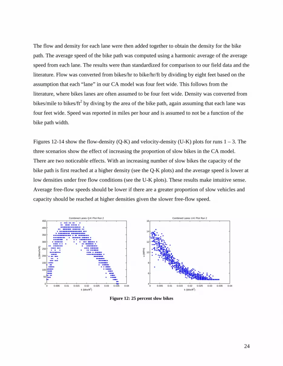
Figures 12-14 show the flow-density (Q-K) and velocity-density (U-K) plots for runs 1 – 3. The
three scenarios show the effect of increasing the proportion of slow bikes in the CA model.
There are two noticeable effects. With an increasing number of slow bikes the capacity of the
bike path is first reached at a higher density (see the Q-K plots) and the average speed is lower at
low densities under free flow conditions (see the U-K plots). These results make intuitive sense.
Average free-flow speeds should be lower if there are a greater proportion of slow vehicles and
capacity should be reached at higher densities given the slower free-flow speed.
Figure 12: 25 percent slow bikes
0 0.005 0.01 0.015 0.02 0.025 0.03 0.035 0.040
50
100
150
200
250
300
350
400
450
k (bike/ft2)
q (b
ike/
hr/ft
)
Combined Lanes Q-K Plot Run 2
0 0.005 0.01 0.015 0.02 0.025 0.03 0.035 0.044
6
8
10
12
14
16
k (bike/ft2)
u (M
PH
)
Combined Lanes U-K Plot Run 2
25
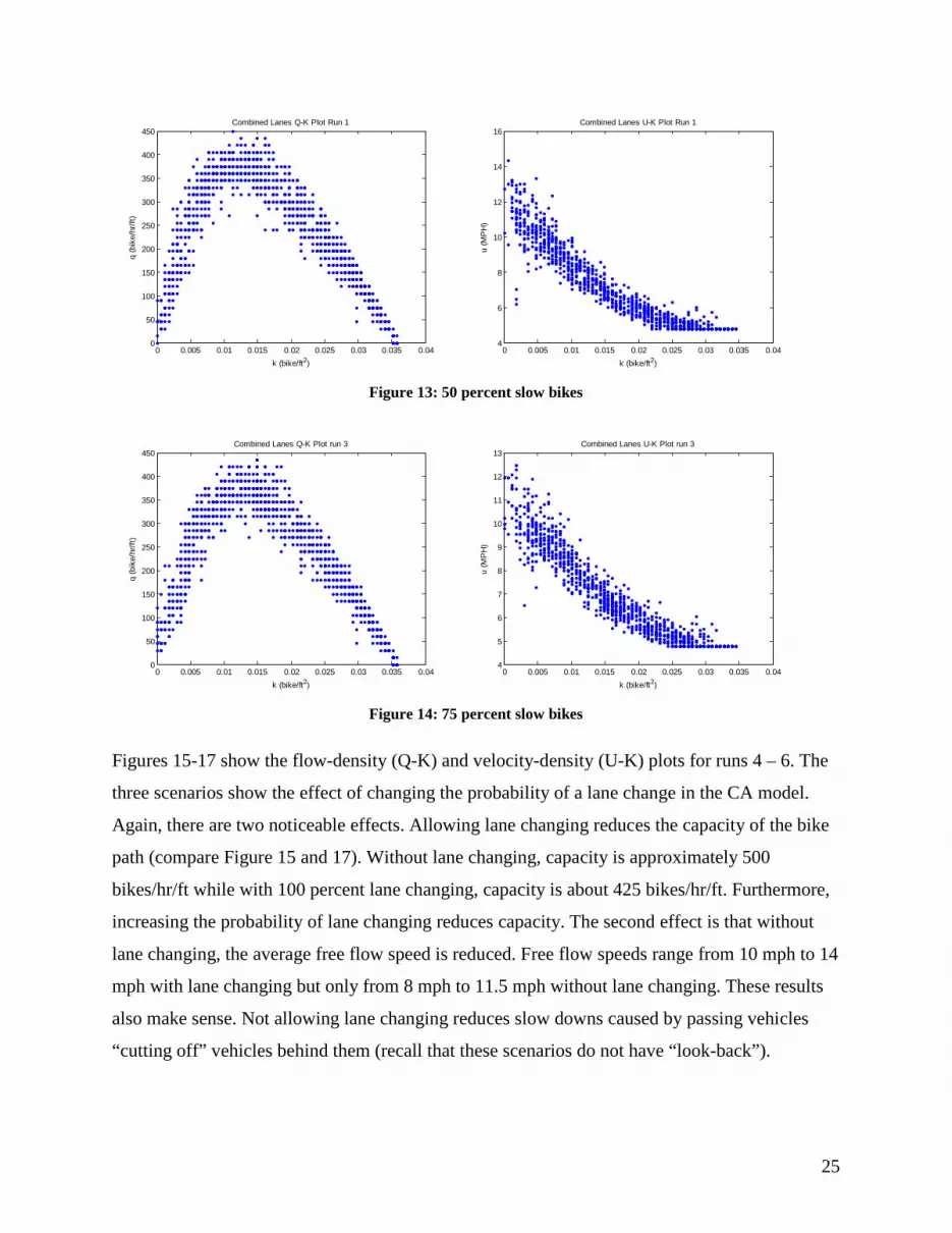
Figure 13: 50 percent slow bikes
Figure 14: 75 percent slow bikes
Figures 15-17 show the flow-density (Q-K) and velocity-density (U-K) plots for runs 4 – 6. The
three scenarios show the effect of changing the probability of a lane change in the CA model.
Again, there are two noticeable effects. Allowing lane changing reduces the capacity of the bike
path (compare Figure 15 and 17). Without lane changing, capacity is approximately 500
bikes/hr/ft while with 100 percent lane changing, capacity is about 425 bikes/hr/ft. Furthermore,
increasing the probability of lane changing reduces capacity. The second effect is that without
lane changing, the average free flow speed is reduced. Free flow speeds range from 10 mph to 14
mph with lane changing but only from 8 mph to 11.5 mph without lane changing. These results
also make sense. Not allowing lane changing reduces slow downs caused by passing vehicles
“cutting off” vehicles behind them (recall that these scenarios do not have “look-back”).
0 0.005 0.01 0.015 0.02 0.025 0.03 0.035 0.040
50
100
150
200
250
300
350
400
450
k (bike/ft2)
q (b
ike/
hr/ft
)Combined Lanes Q-K Plot Run 1
0 0.005 0.01 0.015 0.02 0.025 0.03 0.035 0.044
6
8
10
12
14
16
k (bike/ft2)
u (M
PH
)
Combined Lanes U-K Plot Run 1
0 0.005 0.01 0.015 0.02 0.025 0.03 0.035 0.040
50
100
150
200
250
300
350
400
450
k (bike/ft2)
q (b
ike/
hr/ft
)
Combined Lanes Q-K Plot run 3
0 0.005 0.01 0.015 0.02 0.025 0.03 0.035 0.044
5
6
7
8
9
10
11
12
13
k (bike/ft2)
u (M
PH
)
Combined Lanes U-K Plot run 3

26
Additionally, by not allowing passing, the speeds of faster vehicles are limited by the slower
moving vehicles.
Figure 15: 0 percent probability of lane change
Figure 16: 70 percent probability of lane change
Figure 17: 100 percent probability of lane change
0 0.005 0.01 0.015 0.02 0.025 0.03 0.035 0.040
50
100
150
200
250
300
350
400
450
500
k (bike/ft2)
q (b
ike/
hr/ft
)
Combined Lanes Q-K Plot Run 6
0 0.005 0.01 0.015 0.02 0.025 0.03 0.035 0.044
5
6
7
8
9
10
11
12
13
k (bike/ft2)
u (M
PH
)
Combined Lanes U-K Plot Run 6
0 0.005 0.01 0.015 0.02 0.025 0.03 0.035 0.040
50
100
150
200
250
300
350
400
450
k (bike/ft2)
q (b
ike/
hr/ft
)
Combined Lanes Q-K Plot Run 5
0 0.005 0.01 0.015 0.02 0.025 0.03 0.035 0.044
6
8
10
12
14
16
k (bike/ft2)
u (M
PH
)
Combined Lanes U-K Plot Run 5
0 0.005 0.01 0.015 0.02 0.025 0.03 0.035 0.040
50
100
150
200
250
300
350
400
450
k (bike/ft2)
q (b
ike/
hr/ft
)
Combined Lanes Q-K Plot run 4
0 0.005 0.01 0.015 0.02 0.025 0.03 0.035 0.044
5
6
7
8
9
10
11
12
13
14
k (bike/ft2)
u (M
PH
)
Combined Lanes U-K Plot run 4

27
The last scenario, examining the effect of look-back, is displayed in Figure 18. The effect of
allowing cyclists to “look-back” one cell (7 feet) before changing lanes allows both a high flow
rate (just over 500 bikes/hr/lane) and maintenance of free flow speeds. The higher flow rate and
speed is achieved since cyclists reduce the amount of slow downs caused by “cutting off” other
cyclists and may maintain their desired free-flow speeds as long as they have a one cell gap in
the left lane to move into.
Figure 18: One cell look-back
In addition to looking at the usual traffic measures, we also look at lane changing behavior.
Ideally, we would measure the actual number of passing and delayed passings in order to derive
LOS as defined in Hummer et al. (2006) or the 2000 Highway Capacity Manual (TRB 2000a).
While the data do exist to do this from the model output, additional computational effort would
be required to extract the data, which we leave to future work at this time. However, the amount
of lane changing indicates how the model is performing and provides an alternative (yet closely
related) measure of hindrance. The frequency with which cyclists change lanes is related to their
dissatisfaction with the performance of their current lane, so a greater amount of lane changing
indicates greater hindrance. Additionally, as densities increase, passing opportunities decrease
and delayed lane changes occur, a second form of hindrance. While we do not directly observe
delayed lane changes, we do observe the drop in the amount of lane changing as densities
increase.
0 0.005 0.01 0.015 0.02 0.025 0.03 0.035 0.040
100
200
300
400
500
600
k (bike/ft2)
q (b
ike/
hr/ft
)
Combined Lanes Q-K Plot run 7
0 0.005 0.01 0.015 0.02 0.025 0.03 0.035 0.044
5
6
7
8
9
10
11
12
13
14
k (bike/ft2)
u (M
PH
)
Combined Lanes U-K Plot run 7

28
Lane changes are observed from a matrix which records when a lane change is made in the CA
network matrix. Lane changes are observed at the cell to the left of the boundary used to
observed speed and flow. Similar to the method used to observed density the lane change
observations are summed and averaged over a 30 second time window. The reported number of
lane changes per hour therefore represents the number of bikes engaged in a lane change at the
boundary.
The plots of lane changes over density in Figure 19 show the effect of different proportions of
slow moving vehicles on lane changing frequency. The plots are basically the same, indicating
that the proportion of slow moving vehicles does not greatly influence the amount of lane
changing. The plots in Figure 19 also show that the amount of lane changing increases with
increasing density until around 0.025 bikes/ft2. At this density, which corresponds to the point at
which speeds are severely reduced and many vehicles are stopped (see Figure 12), the amount of
lane changing drops off sharply. This is caused by the inability to switch lanes because of
occupancy by another vehicle, indicating that traffic conditions are likely to be just as bad in the
other lane.
Figure 19: Lane changing with 25 (left) and 75 (right) percent slow moving bikes
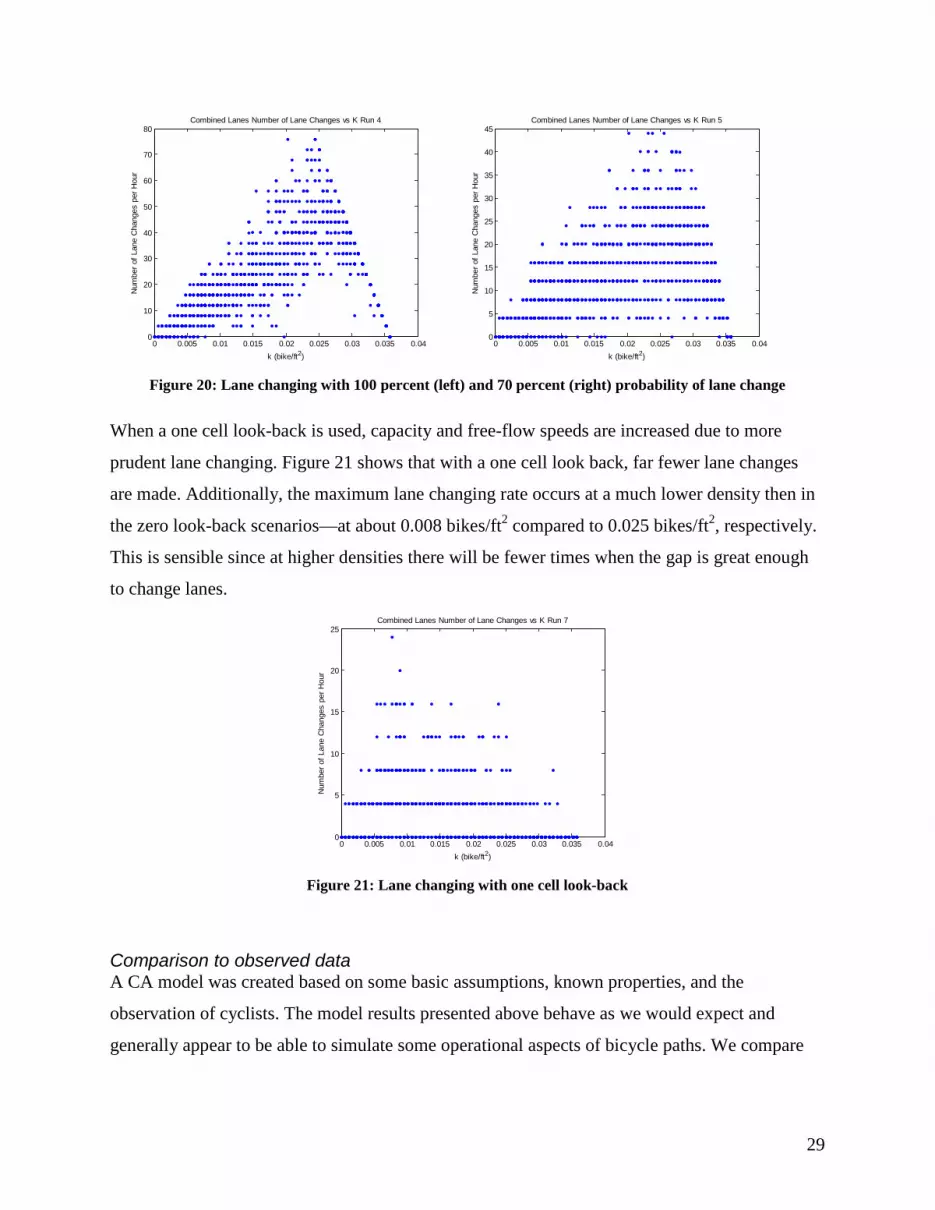
Figure 20 shows the impact of varying the probability of lane change parameter. As would be
expected, the amount of lane changing increases when this parameter is increased. With a 100
percent probability of lane changing (every time a lane change would be beneficial, a lane
change is made) a maximum lane changing rate of almost 80 lane changes per hour is observed.
0 0.005 0.01 0.015 0.02 0.025 0.03 0.035 0.040
10
20
30
40
50
60
k (bike/ft2)
Num
ber o
f Lan
e C
hang
es p
er H
our
Combined Lanes Number of Lane Changes vs K Run 2
0 0.005 0.01 0.015 0.02 0.025 0.03 0.035 0.040
10
20
30
40
50
60
k (bike/ft2)
Num
ber o
f Lan
e C
hang
es p
er H
our
Combined Lanes Number of Lane Changes vs K Run 3
29
Figure 20: Lane changing with 100 percent (left) and 70 percent (right) probability of lane change
When a one cell look-back is used, capacity and free-flow speeds are increased due to more
prudent lane changing. Figure 21 shows that with a one cell look back, far fewer lane changes
are made. Additionally, the maximum lane changing rate occurs at a much lower density then in
the zero look-back scenarios—at about 0.008 bikes/ft2 compared to 0.025 bikes/ft2, respectively.
This is sensible since at higher densities there will be fewer times when the gap is great enough
to change lanes.
Figure 21: Lane changing with one cell look-back
Comparison to observed data A CA model was created based on some basic assumptions, known properties, and the
observation of cyclists. The model results presented above behave as we would expect and
generally appear to be able to simulate some operational aspects of bicycle paths. We compare
0 0.005 0.01 0.015 0.02 0.025 0.03 0.035 0.040
10
20
30
40
50
60
70
80
k (bike/ft2)
Num
ber o
f Lan
e C
hang
es p
er H
our
Combined Lanes Number of Lane Changes vs K Run 4
0 0.005 0.01 0.015 0.02 0.025 0.03 0.035 0.040
5
10
15
20
25
30
35
40
45
k (bike/ft2)
Num
ber o
f Lan
e C
hang
es p
er H
our
Combined Lanes Number of Lane Changes vs K Run 5
0 0.005 0.01 0.015 0.02 0.025 0.03 0.035 0.040
5
10
15
20
25
k (bike/ft2)
Num
ber o
f Lan
e C
hang
es p
er H
our
Combined Lanes Number of Lane Changes vs K Run 7

30
two scenarios from the CA model which produced the two most distinct fundamental diagrams,
Run 1 and Run 7, with plots of our field data. These are shown in Figure 22.
Figure 22: Field data and simulation fundamental diagram comparison
The field data closely matches both simulation results, completely falling within the range of
values produced by the simulation. The Russell and Arc site data appear to more closely match
the Run 7 scenario while the Bio site data matches more closely to the Run 1 scenario. The
modeled capacities (maximum flow) also fall within the lower range of bike path capacities
reported in the literature which were previously mentioned. While these results do support our
argument that CA models can be used to model cyclist behavior, they do not offer concrete
proof. To validate and calibrate our model will requires more field data over a larger range of
densities, and collection of additional types of data such as speed distribution and lane changing
(or passing). Limitations presented by the time frame of this project and available equipment to
reduce the labor intensity of the data collection effort precluded us from collecting these data.
Russel
0
100
200
300
400
500
600
0 0.005 0.01 0.015 0.02 0.025 0.03 0.035 0.04
Density (bikes/ft2)
Flow
(bik
es/h
r/ft)
RightRun 1 CA ModelRun 7 CA Model
Bio
0
100
200
300
400
500
600
0 0.005 0.01 0.015 0.02 0.025 0.03 0.035 0.04
Density (bikes/ft2)
Flow
(bik
es/h
r/ft)
RightLeftRun 1 CA ModelRun 7 CA Model
Arc
0
100
200
300
400
500
600
0 0.005 0.01 0.015 0.02 0.025 0.03 0.035 0.04
Density (bikes/ft2)
Flow
(bik
es/h
r/ft)
RightLeftRun 1 CA ModelRun 7 CA Model

31
Given the lack of validation, the CA model with lane changing still appears suited to the task. By
varying the look-back distance we can observe a change in bike path capacity. We observe from
the field that many cyclists (at least at UC Davis) do not look back, cutting off other cyclists and
thus creating slow downs. The model gives us a way to explore how a cyclist education program
could help improve bike path operation by increasing look-back. Additionally, by increasing the
proportion of fast cyclists we can observe that capacity is reached at a lower density. This feature
is important to model how bicycle paths should be designed for different types of users. These
are just two examples, but they demonstrate how the model is sensitive to parameters that are
known to effect bicycle path operation.
Future work The CA model presented in this paper has shown good agreement with observed data. However,
it models a critical density which is at the low end of those observed in the literature (see Allen,
Rouphail et al. 1998 and above discussion). This is likely due to the model update rules. Recall:
if the space between the current vehicle and the next is greater than the current vehicle’s speed, it
decelerates to the distance between vehicles minus one. This means that closely packed vehicles
all traveling at equal speeds are not possible given the current model configuration. While this
rule applies to automobile flow, it may not adequately capture bicyclist behavior at high
densities. Future simulations will include varied update rules allowing for the formation of
tightly packed, high speed platoons. This will push up the critical density and thus maximum
flow. It will also lend more confidence to the capacity predictions output by the model which are
undoubtedly already a vast improvement over fitting a polynomial expression to data with a
dubious fit.
The effect of lane width will also have to be further investigated. As the model currently
functions, there is no influence of lane width—in calculating densities on an area basis, we have
simply assumed that we more closely modeled a narrow path (Bio) since on that path, bicycles
traveled in mostly a two-lane configuration and could not extend far beyond that. However, the
model outputs could simply be scaled by an arbitrary lane width. A more realistic approach
would introduce friction factors that increase as lane width narrows. These would introduce
lateral interactions in addition to parallel ones within the CA model structure. Under this

32
framework, a passing cyclist could slow down the cyclist that was passed which could have the
effect of causing slowdowns.
An additional extension closely related to the above would be the addition of multiple lanes to
allow for the modeling of wider bike paths. As noted above, for the case of automobiles, this has
been attempted by Daoudia and Moussa (2003) and could be relatively easily applied to the
present case of bicycles. The influence of cross traffic could also be considered in a bidirectional
framework such as that proposed for vehicular traffic by Simon and Gutowitz (1998). While they
only considered the case of a two-lane highway, we would necessarily have to consider more
complex interactions since bicycle flows necessarily in multiple ‘lanes’ in one direction.
Finally, the technological methods of our empirical data collection could be vastly improved.
Manually counting vehicles was tedious. Automated detectors similar to those used for
automobile traffic would be an improvement, as would methods of collecting speeds using a
radar gun, for example. This would allow validation of the flow and density measurements which
could be extracted from detectors.
Conclusions We have presented the first empirically validated, multilane, inhomogeneous CA model for
bicycle flow in the literature. It was found to accurately model the fundamental diagram of
bicycle flow while possibly underestimating bicycle lane capacity due to the CA update rules.
With additional research, this could become an invaluable planning tool for use by city and
regional planners in concert with enhanced bicycle trip forecasting methods. With the national
and global issues of climate change, air pollution and urban congestion combined with crumbling
national infrastructure, the time for planning for adequate bicycle facilities is now.

33
References AASHTO (1999). Guide for the Development of Bicycle Facilities. Washington D.C.
Allen, D., N. Rouphail, J. Hummer and J. Milazzo (1998). "Operational Analysis of Uninterrupted Bicycle Facilities." Transportation Research Record 1636(-1): 29-36.
Benjaafar, S., K. Dooley and W. Setyawan (1997). Cellular Automata for Traffic Flow Modeling. Minneapolis, MN, University of Minnesota, Department of Mechanical Engineering, CTS97-09.
Botma, H. (1995). "METHOD TO DETERMINE LEVEL OF SERVICE FOR BICYCLE PATHS AND PEDESTRIAN-BICYCLE PATHS." Transportation Research Record(1502): 38-44.
Botma, H. and H. Papendrecht (1991). "Traffic operation of bicycle traffic." Transportation Research Record 1320: 65-72.
Cervero, R. and K. Kockelman (1997). "Travel demand and the 3Ds: Density, diversity, and design." Transportation Research Part D: Transport and Environment 2(3): 199-219.
Daoudia, A. K. and N. Moussa (2003). "Numerical simulations of a three-lane traffic model using cellular automata." Chinese Journal of Physics 41(6): 671-681.
Dargay, J., D. Gately and M. Sommer (2007). "Vehicle Ownership and Income Growth, Worldwide: 1960-2030." The Energy Journal 28(4): 143-170.
Gartner, N., C. J. Messer and A. K. Rathi, Eds. (2001). Traffic Flow Theory: A State-of-the-Art Report, Oak Ridge National Laboratory, Transportation Research Board and US Department of Transportation.
Homburger, W. S. (1976). Capacity of Bus Routes, and of Pedestrain and Bicycle Facilities. Institute of Transportation Studies, University of California, Berkeley.
HRB (1965). Highway Capacity Manual 1965. Washington D.C., National Research Council.
Hummer, J. E., N. M. Rouphail, J. L. Toole, R. S. Patten, R. J. Schneider, J. S. Green, R. G. Hughes and S. J. Fain (2006). Evaluation of Saftey, Design, and Operation of Shared-Use Paths - Final Report. FHWA.
IPCC (2007). Contribution of working group I to the fourth assessment report of the Intergovernmental Panel on Climate Change: summary for policymakers.
Jia, B., X. G. Li, R. Jiang and Z. Y. Gao (2007). "Multi-value cellular automata model for mixed bicycle flow." European Physical Journal B 56(3): 247-252.
Jiang, R., B. Jia and Q. S. Wu (2004). "Stochastic multi-value cellular automata models for bicycle flow." Journal of Physics A: Mathematical and General 37(6): 2063-2072.

34
Kingham, S., J. Dickinson and S. Copsey (2001). "Travelling to work: will people move out of their cars." Transport Policy 8(2): 151-160.
Knospe, W., L. Santen, A. Schadschneider and M. Schreckenberg (2002). "A realistic two-lane traffic model for highway traffic." Journal of Physics A: Mathematical and General 35(15): 3369-3388.
Miller, R. E. and M. R. Ramey (1975). Width Requirements for Bikeways: A level of Service Approach. Department of Civil and Environmental Engineering, University of California, Davis.
Nagel, K. and M. Schreckenberg (1992). "A cellular automaton model for freeway traffic." Journal De Physique I 2(12): 2221-2229.
Navin, F. P. (1994). "Bicycle traffic flow characteristics: experimental results and comparisons." ITE Journal 64(3): 31-36.
Porter, C., J. Suhrbier and W. Schwartz (1999). "Forecasting Bicycle and Pedestrian Travel: State of the Practice and Research Needs." Transportation Research Record 1674: 94-101.
Pucher, J., C. Komanoff and P. Schimek (1999). "Bicycling renaissance in North America?: Recent trends and alternative policies to promote bicycling." Transportation Research Part A: Policy and Practice 33(7-8): 625-654.
Replogle, M. (1992). Non-Motorized Vehicles in Asian Cities. Washington, D.C., World Bank, Technical Paper Number 162.
Rickert, M., K. Nagel, M. Schreckenberg and A. Latour (1996). "Two lane traffic simulations using cellular automata." Physica A: Statistical and Theoretical Physics 231(4): 534-550.
Simon, P. M. and H. A. Gutowitz (1998). "Cellular automaton model for bidirectional traffic." Physical Review E 57(2): 2441-2444.
Smith, D. T. (1972). City of Davis, University of California, Bicycle Circulation and Saftey Study. San Francisco, CA, De Leuw, Cather & Company.
Smith, D. T. (1976). Safety and Location Criteria for Bicycle Facilities. Washington, D.C., Federal Highway Administration, FHWA-RD-75-112.
Taylor, D. and W. Davis (1999). "Review of Basic Research in Bicycle Traffic Science, Traffic Operations, and Facility Design." Transportation Research Record 1674: 102-110.
The MathWorks Inc. (2006). Matlab: the Language of Technical Computing.
TRB (1985). Highway Capacity Manual 1985. Washington D.C., National Research Council.

35
TRB (2000a). Chapter 19 - Bicycles. in Highway Capacity Manual 2000. Washington, D.C., National Research Council.
TRB (2000b). Highway Capacity Manual 2000. Washington D.C., National Research Council.
Virkler, M. and R. Balasubramanian (1998). "Flow Characteristics on Shared Hiking/Biking/Jogging Trails." Transportation Research Record 1502.