automorphisms of transition graphs for a linear cellular automaton

Automorphisms of transition graphs for a linear

cellular automaton

Edward J. Powley and Susan Stepney

Department of Computer Science, University of York, UK

Abstract. A cellular automaton (CA) is a discrete dynamical system,and the transition graph is a representation of the CA’s phase space.Automorphisms of the transition graph correspond to symmetries of thephase space; studying how the total number of automorphisms varieswith the number of cells on which the CA operates yields a (partial)classification of the space of CA rules according to their dynamical be-haviour.In the general case, to find the number of automorphisms we must iterateover the entire transition graph; thus the time complexity is exponentialwith respect to the number of cells. However, if the CA is linear, the tran-sition graph has properties which allow the number of automorphismsto be computed much more efficiently. In this paper, we investigate thenumbers of automorphisms for a particular linear CA, elementary rule90. We observe a relationship between the number of automorphisms anda number theoretical function, the suborder function.

1 Introduction

A cellular automaton (CA) consists of a finite nonempty set of states, a discretelattice of cells, and a local update rule which maps deterministically the stateof a cell and its neighbours at time t to the state of that cell at time t + 1. Aconfiguration of a CA is an assignment of a state to each cell. The local updaterule extends to a global map, a function from configurations to configurations,in the natural way.

The transition graph of a CA is a directed graph whose vertices are theconfigurations of the CA, and whose edges are determined by the global map.There is an edge from vertex r to vertex s if and only if the global map sendsconfiguration r to configuration s. The transition graph is a representation of theoverall structure of the phase space of the CA: in particular, the automorphisms(self-isomorphisms or “symmetries”) of the transition graph are, in a sense, thesymmetries of the CA’s dynamics [1]. Examples of transition graphs are shownin Figs. 1 and 2.

In [1], we investigate how numbers of automorphisms vary with the numberN of cells on which the CA operates (Fig. 3). For the majority of CA rules, thereseems to be a linear relationship between the number of automorphisms and eeN

.

56 Powley and Stepney

33 copies 1 copy

Fig. 1. Transition graph for rule 90 on 11 cells.

60 copies 4 copies 6 copies

Fig. 2. Transition graph for rule 90 on 12 cells.

However, we identify two classes of CAs for which this linear correspondence doesnot seem to hold. One of these classes consists almost entirely of linear CAs (CAswhose local update rule is a linear function), and is characterised by the “zig-zag”pattern depicted in Fig. 4 (a). In this paper, we investigate this pattern moreclosely.

As is the case with many other classes of system, linear CAs submit muchmore readily to analysis than their non-linear counterparts. Indeed, the oper-ation of a linear CA is simply repeated convolution of a configuration with afixed sequence corresponding to the rule, which in turn is equivalent to repeatedmultiplication in a finite ring of polynomials. Martin et al [2] use this fact tostudy linear CAs, and succeed in proving several results about one linear CAin particular (elementary rule 90, in Wolfram’s terminology [3]). We use theseresults to derive an algorithm, dramatically more efficient than the general al-

Automorphisms of transition graphs for a linear CA 57

Fig. 3. Plot of log10 log10 A(f, N) (where A(f, N) is the number of automor-phisms) against N , for 6 ≤ N ≤ 16 and for all 88 essentially different ECArules. From [1].

gorithm described in [1], for computing the number of automorphisms for thetransition graphs of rule 90.

We argue, but do not prove, that the “zig-zag” oscillations in the number ofautomorphisms for rule 90 on N cells correspond to the oscillations of a numbertheoretical function known as the suborder function.

2 Linear CAs and polynomials

We restrict our attention to finite one-dimensional CAs, i.e. we take the latticeto be ZN (the cyclic group of integers modulo N). This lattice has periodicboundary condition, in that we consider cell N − 1 to be adjacent to cell 0. Theneighbourhood is specified in terms of its radius r, so that the neighbours ofcell i are cells i − r, . . . , i + r. We further restrict our attention to CAs whosestate set is also a cyclic group, say Zk. Thus the local update rule is a functionf : Z

2r+1k → Zk, which extends to a global map F : Z

Nk → Z

Nk .

Such a CA is said to be linear if the local update rule is a linear function;that is, if there exist constants λ−r, . . . , λr such that

f(x−r, . . . , xr) = λ−rx−r + · · ·+ λrxr , (1)

where the operations of addition and multiplication are the usual operations ofmodular arithmetic.

Martin et al [2] study linear CAs by means of polynomials. Denote by RNk

the set of polynomials with coefficients over Zk of degree at most N − 1. We


Fig. 4. As Fig. 3, but for 6 ≤ N ≤ 17, and showing the two classes of ECAswhich do not exhibit a linear relationship between numbers of automorphismsand eeN

. From [1].

can define addition and multiplication in RNk similarly to the usual arithmetic

of polynomials, but setting xN = 1 (so in effect, powers are computed moduloN). Under these operations, RN

k is a ring.Let f be a local update rule of the form of Equation 1. We associate with f

the polynomial Tf in RNk defined by

Tf(x) = λ−rxr + · · ·+ λrx

−r . (2)

Furthermore, we associate with a configuration s = a0a1 . . . aN−1 ∈ ZNk the

polynomialAs(x) = a0 + a1x + · · ·+ aN−1x

N−1 . (3)

Then the polynomial associated with the configuration F (s) is simply Tf(x)As(x).In other words, repeated application of the global map F corresponds to repeatedmultiplication by the polynomial Tf(x).

2.1 Rule 90

Let r = 1 and k = 2, and consider f : Z32 → Z2 defined by

f(x−1, x0, x1) = x−1 + x1 . (4)

Since r = 1 and k = 2, this is an example of an elementary cellular automaton.According to Wolfram’s numbering scheme [3], f is rule 90. The polynomialcorresponding to f is

Tf (x) = x + x−1 . (5)


Remark 2.1. Let F be the global map for rule 90 on N cells. Choose an initialconfiguration s0, and let

st = F ◦ · · · ◦ F︸︷︷︸

t occurrences

(s0) . (6)

Then at most O(log t) polynomial multiplications are required to compute st.

Proof. It suffices to show that the polynomial (Tf (x))t can be written as a prod-

uct of at most O(log t) polynomials, where each term in this product is eitherknown or computable in constant time.

Since we are working with coefficients over Z2, we have

(x + x−1

)2k

= x2k

+ x−2k

(7)

for all nonnegative integers k. Thus if t is a power of 2, st can be computed bymultiplication with xt + x−t.

If t is not a power of 2, it can nevertheless be written as a sum of ⌈log2 t⌉ orfewer powers of 2 (i.e. in binary notation). If

t = 2i1 + · · ·+ 2il , (8)

then(x + x−1

)t=(x + x−1

)2i1

. . .(x + x−1

)2il

. (9)

The product on the right-hand side involves no more than ⌈log2 t⌉ terms, eachof which can be determined in constant time via Equation 7. ⊓⊔

2.2 Cycle lengths and the suborder function

For positive integers n and k, the (multiplicative) suborder function sordn(k) isdefined [2] by

sordn(k) =

{

min{j > 0 : kj ≡ ±1 mod n

}if such a j exists

0 otherwise .(10)

Note that sordn(k) 6= 0 if and only if n and k are relatively prime. In particular,if k = 2 then sordn(2) is nonzero if n is odd and zero if n is even. The suborderfunction sordn(2) is plotted in Fig. 5.

If n is odd, then we have

log2 n ≤ sordn(2) ≤ n− 1

2. (11)

The set of values of n for which the upper bound is achieved is a subset of theprimes.

Let ΠN denote the length of the cycle reached by rule 90 from an initialconfiguration which assigns state 1 to a single cell and state 0 to the remainder.


Fig. 5. Plot of the suborder function sordn(2) against n, for 3 ≤ n ≤ 200.

Due to rule 90’s linearity, all cycle lengths must be factors of ΠN . Furthermore,Martin et al [2] show that

ΠN =

1 if N is a power of 22ΠN/2 if N is even but not a power of 2a factor of 2sordN (2) − 1 if N is odd .

(12)

3 Counting automorphisms of transition graphs

Definition 3.1. Consider a CA whose set of configurations is C and whoseglobal map is F . The transition graph for this CA is the directed graph withvertex set C and edge set

{(s, F (s)) : s ∈ C} . (13)

Every vertex in a transition graph has out-degree 1. This forces the graphto have a “circles of trees” topology: the graph consists of a number of disjointcycles, with a (possibly single-vertex) tree rooted at each vertex in each cycle.

The basins of the transition graph are its disjoint components: each basinconsists of exactly one cycle, along with the trees rooted on that cycle.

Examples of transition graphs are shown in Figs. 1 and 2.

Definition 3.2. Consider a directed graph with vertex set V and edge set E.An automorphism on this graph is an isomorphism from the graph to itself; inother words, a bijection α : V → V such that

(x, y) ∈ E ⇐⇒ (α(x), α(y)) ∈ E . (14)


Denote by A(f, N) the number of automorphisms in the transition graph forthe CA with local rule f on N cells.

In [1] we describe an algorithm for computing the number of automorphismsfor a transition graph. This algorithm works by exploiting the recursive structureof the transition graph. For instance, consider a tree, rooted at vertex r, such thatthe “children” of r are vertices c1, . . . , ck. Then the number of automorphisms inthe tree is the product of the numbers of automorphisms for each subtree rootedat a ci, multiplied with the number of permutations of c1, . . . , ck which preservethe isomorphism classes of the subtrees.

Transition graphs for linear CAs have further structure to be exploited:

Lemma 3.1 ([2, Lemma 3.3]). In a transition graph for a linear CA, the treesrooted at the vertices in the cycles form a single isomorphism class.

Thus two basins are isomorphic if and only if their cycles have the samelength. Cycles of different lengths can occur within a transition graph, so thebasins do not necessarily form a single isomorphism class. To find the isomor-phism classes, it is necessary (and sufficient) to find the lengths and multiplicitiesof the cycles. Martin et al [2] give an algorithm for this in rule 90, and it seemsreasonable to expect that similar algorithms exist for other linear CAs.

The following results characterise the structure of the trees themselves forrule 90 on N cells:

Theorem 3.1 ([2, Theorem 3.3]). If N is odd, all trees in the transition graphconsist of a single edge.

Theorem 3.2 ([2, Theorem 3.4]). If N is even, all trees in the transitiongraph have the following properties:

1. The distance from the root vertex to every leaf vertex is

1

2max

{2j : 2j|N

}; (15)

2. The root vertex has in-degree 3;3. Every non-root non-leaf vertex has in-degree 4.

These theorems are illustrated in Figs. 1 and 2.If N is odd, clearly the only automorphism on each tree is the identity. How

many automorphisms does each tree possess if N is even? The following resultis an application of [1, Lemma 1].

Lemma 3.2. Consider a tree of depth D > 1, whose root vertex v has in-degree3 and with all other vertices having in-degree 4. The number of automorphismsfor this tree is

A(v) = 2422(D−1)

/4 . (16)

Proof. See Appendix 7. ⊓⊔


The following theorem is our main result, and follows directly from Lemma 3.2above and Lemma 2 and Theorem 2 in [1].

Theorem 3.3. Suppose that, for some value of N , the distinct cycle lengths inrule 90 are l1, . . . , lk, and there are mi cycles of length li. Let

AT =

{

1 if N is odd

242N−2

/42N−D2(N)

if N is even ,(17)

whereD2(N) = max

{2j : 2j|N

}. (18)

Then

A(90, N) =

(k∏

i=1

mi! · lmi

i

)

·AT . (19)


Thus if the lis and mis are known, the number of automorphisms can easilybe calculated. The following corollary illustrates a particularly straightforwardspecial case:

Corollary 3.1. If N is a power of 2, then

A(90, N) = 242N−2

/4 . (20)


4 Computational results

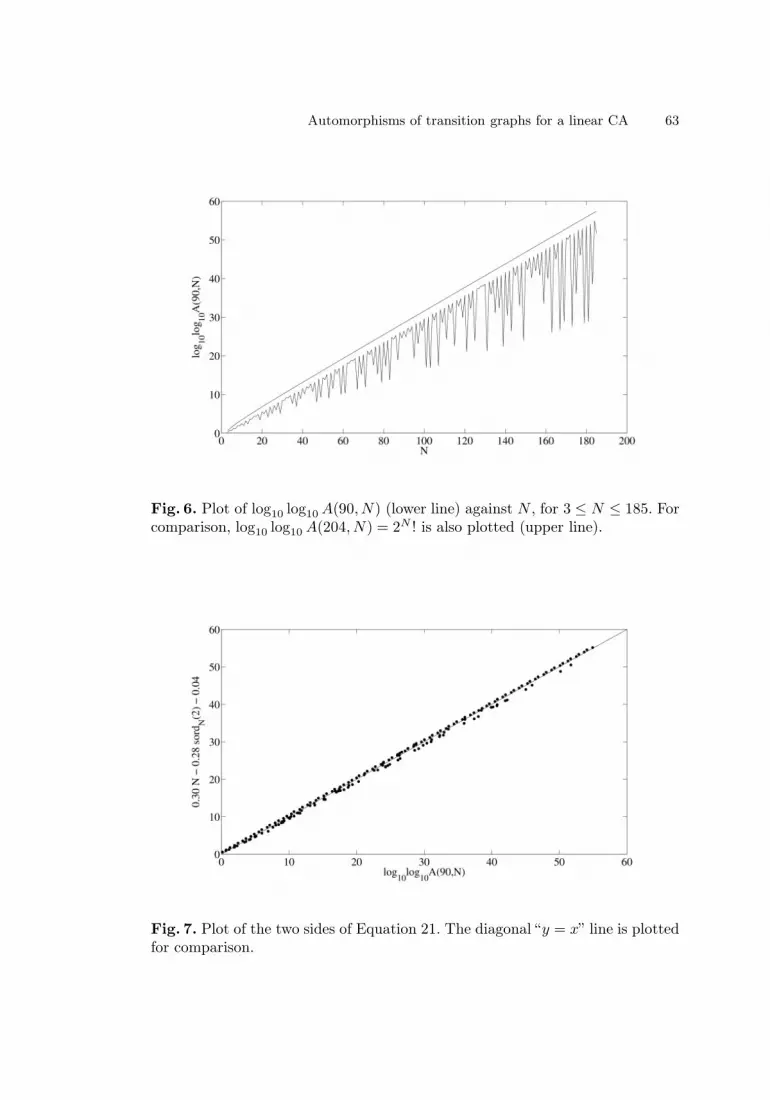
Martin et al [2] provide cycle lengths and multiplicities for 3 ≤ N ≤ 40, aswell as an algorithm for computing the lengths and multiplicities for larger N .Using these in conjunction with Theorem 3.3, we are able to compute values ofA(90, N) for N much larger than by the general method described in [1]. Someresults are shown in Fig. 6.

Compare Fig. 6 with the suborder function sordN (2) plotted in Fig. 5. Inparticular, observe that peaks in one seem to correspond with troughs in theother. Indeed, it can be verified numerically that we have an approximate linearrelationship:

log10 log10 A(90, N) ≈ 0.30N − 0.28 sordN (2)− 0.04 . (21)

Figure 7 plots the two sides of Equation 21, and Fig. 8 plots the differencebetween them against N . Although the correlation is not exact, note that thereare no outliers. Also note that the difference between the two sides, and hencethe error in this approximation, seems to increase (albeit slowly) with N .


Fig. 6. Plot of log10 log10 A(90, N) (lower line) against N , for 3 ≤ N ≤ 185. Forcomparison, log10 log10 A(204, N) = 2N ! is also plotted (upper line).

Fig. 7. Plot of the two sides of Equation 21. The diagonal “y = x” line is plottedfor comparison.


Fig. 8. Plot of the difference between the two sides of Equation 21 against N .

5 Conclusion

Previously [1] we computed numbers of automorphisms for all 88 essentiallydifferent ECAs. Implementing the “brute force” method described therein on acurrent desktop PC, we find that N = 17 is the practical limit of what can becomputed in a reasonable length of time. Furthermore, the exponential complex-ity of the computation means that an increase in computational resources wouldnot significantly increase this limit. In contrast, rule 90 has properties whichallow for a much more efficient algorithm. On the same desktop PC, we areable to count automorphisms for N ≤ 185, and for many (though increasinglyuncommon) cases beyond, with ease.

However, it seems plausible that there exists an even simpler expressionfor the number of automorphisms in rule 90, and that the suborder functionsordN (2) dominates this expression. The suborder function relates to rule 90since, if N is odd, all cycle lengths must divide 2sordN (2) − 1. It is not clear whythe expression

∏

i

mi! · lmi

i , (22)

where the lis are the cycle lengths and the mis are their respective multiplicities,should be so strongly correlated with this common multiple of the lis. We plan toinvestigate this further, and to determine whether this approximate correlationdoes indeed indicate the existence of a simpler exact expression for A(90, N).

It is reasonable to expect that other linear rules admit a similar approach tothat applied here. Indeed, Martin et al [2] generalise some (but not all) of their


results beyond rule 90. We intend to use these more general results to extendour methods to the other linear ECAs, and to other linear CAs in general.

However, these methods almost certainly do not apply to nonlinear CAs:the analogy with finite rings of polynomials is crucial to this work, but thisanalogy only holds for linear CAs. Thus this work demonstrates (if yet anotherdemonstration were needed!) the ease of analysis and computation for linear CAsas compared to their nonlinear counterparts.

Acknowledgment

This work is funded by an EPSRC DTA award.

6 Appendix

7 Proofs

7.1 Proof of Lemma 3.2

Let ui be any vertex at depth i in the tree, so v = u0 and uD is a leaf. Then by[1, Lemma 1], noting that the children of ui form a single isomorphism class, wehave

A(v) = A(u0) = 3!A(u1)3 (23)

A(u1) = 4!A(u2)4 (24)

...

A(uD−1) = 4!A(uD)4 (25)

A(uD) = 1 . (26)

Thus

A(v) = 3! (4!(4!(. . . (1)4 . . . )4)4)3︸︷︷︸

D−1 occurrences of 4!

(27)

= 3!× 4!3 × 4!3×4 × · · · × 4!3×4D−2

(28)

= 3!× 4!3∑

D−2

i=04i

. (29)

It can be shown that, for any positive integers n and k,

n∑

i=0

ki =kn+1 − 1

k − 1. (30)


Thus

A(v) = 3!× 4!3∑

D−2

i=04i

(31)

= 3!× 4!3×(4D−1−1)/3 (32)

=3!

4!× 4!4

D−1

(33)

= 2422(D−1)

/4 (34)

as required. ⊓⊔

7.2 Proof of Theorem 3.3

[1, Theorem 2] states that

A(90, N) =

∏

I∈{Bi}/∼=

|I|!

k∏

i=1

A(Bi)mi

. (35)

By [2, Lemma 3.3], all of the trees rooted at vertices in cycles are isomorphic.Thus two basins are isomorphic if and only if they have the same cycle length,and so we have

∏

I∈{Bi}/∼=

|I|! =

k∏

i=1

mi! . (36)

Now let A(Bi) be the number of automorphisms for a basin whose cycle lengthis li. By [1, Lemma 2], we have

A(Bi) =liq

li∏

j=1

A(vj) . (37)

But all of the trees are isomorphic, so q = 1 and thus

A(Bi) = liA(v)li , (38)

where A(v) is the number of automorphisms in a tree. Substituting into Equa-tion 35 we have

A(90, N) =

(k∏

i=1

mi!

)(k∏

i=1

(liA(v)li )mi

)

(39)

=

k∏

i=1

(mi! · lmi

i · A(v)limi)

(40)

=

(k∏

i=1

mi! · lmi

i

)

·A(v)∑

k

i=1limi . (41)


It now suffices to show that

A(v)∑

k

i=1limi = AT (42)

with AT as defined in Equation 17.If N is odd, [2, Theorem 3.3] states that all trees consist of a single edge.

Thus A(v) = 1, and so A(v)∑

k

i=1limi = 1 = AT , regardless of the values of limi.

Suppose that N is even. By [2, Theorem 3.4], all trees are of the form de-scribed in Lemma 3.2, with D = D2(N)/2. Thus we have

A(v) = 242D2(N)−2

/4 . (43)

Now,∑k

i=1 limi is simply the number of configurations which occur in cycles,and thus, by a corollary to [2, Theorem 3.4], is given by

k∑

i=1

limi = 2N−D2(N) . (44)

Hence

A(v)∑

k

i=1limi = 242D2(N)−2×2N−D2(N)

/42N−D2(N)

(45)

= 242D2(N)−2+N−D2(N)

/42N−D2(N)

(46)

= 242N−2

/42N−D2(N)

(47)

= AT (48)

as required. ⊓⊔

7.3 Proof of Corollary 3.1

If N is a power of 2 then D2(N) = N , so

AT = 242N−2

/4 (49)

Furthermore, by [2, Lemmas 3.4 and 3.5], the only possible cycle length is 1; by[2, Lemma 3.7], there is only one such cycle. Thus

A(90, N) =(1! · 11

)· AT (50)

= AT (51)

= 242N−2

/4 (52)

as required. ⊓⊔


References

[1] Powley, E., Stepney, S.: Automorphisms of transition graphs for elementary cel-lular automata. In: proceedings of Automata 2007: 13th International Workshopon Cellular Automata. (2008) To appear in Journal of Cellular Automata.

[2] Martin, O., Odlyzko, A.M., Wolfram, S.: Algebraic properties of cellular au-tomata. Communications in Mathematical Physics 93 (1984) 219–258.

[3] Wolfram, S.: Statistical mechanics of cellular automata. Reviews of ModernPhysics 55(3) (1983) 601–644.

automorphisms of transition graphs for a linear cellular automaton

Documents