Modeling and Uncertainty Analysis of Groundwater

Level Using Six Evolutionary Optimization

Algorithms Hybridized with ANFIS, SVM, and ANN

Akram Seifi 1,*, Mohammad Ehteram 2, Vijay P. Singh 3 and Amir Mosavi 4,*

1 Department of Water Science & Engineering, Vali-e-Asr University of Rafsanjan, Rafsanjan, Iran 2 Department of Water Engineering and Hydraulic Structures, Faculty of Civil Engineering, Semnan

University, Semnan 35131-19111, Iran. 3 Department of Biological and Agricultural Engineering & Zachry Department of Civil Engineering Texas

A&M University College Station, Texas, TX 77843-2117, USA; vsingh@tamu.edu 4 Institute of Structural Mechanics, Bauhaus-Universität Weimar, 99423 Weimar, Germany.

* Correspondence: a.seifi@vru.ac.ir, amir.mosavi@uni-weimar.de

Abstract: In the present study, six meta-heuristic schemes are hybridized with artificial neural

network (ANN), adaptive neuro-fuzzy interface system (ANFIS), and support vector machine

(SVM), to predict monthly groundwater level (GWL), evaluate uncertainty analysis of predictions

and spatial variation analysis. The six schemes, including grasshopper optimization algorithm

(GOA), cat swarm optimization (CSO), weed algorithm (WA), genetic algorithm (GA), krill

algorithm (KA), and particle swarm optimization (PSO), were used to hybridize for improving the

performance of ANN, SVM, and ANFIS models. Groundwater level (GWL) data of Ardebil plain

(Iran) for a period of 144 months were selected to evaluate the hybrid models. The pre-processing

technique of principal component analysis (PCA) was applied to reduce input combinations from

monthly time series up to 12-month prediction intervals. The results showed that the ANFIS-GOA

was superior to the other hybrid models for predicting GWL in the first piezometer (RMSE:1.21,

MAE:0.878, NSE:0.93, PBIAS:0.15, R2:0.93), second piezometer (RMSE:1.22, MAE:0.881, NSE:0.92,

PBIAS:0.17, R2:0.94), and third piezometer (RMSE:1.23, MAE:0.911, NSE:0.91, PBIAS:0.19, R2:0.94) in

the testing stage. The performance of hybrid models with optimization algorithms was far better

than that of classical ANN, ANFIS, and SVM models without hybridization. The percent of

improvements in the ANFIS-GOA versus standalone ANFIS in piezometer 10 were 14.4%, 3%,

17.8%, and 181% for RMSE, MAE, NSE, and PBIAS in training stage and 40.7%, 55%, 25%, and 132%

in testing stage, respectively. The improvements for piezometer 6 in train step were 15%, 4%, 13%,

and 208% and in test step were 33%, 44.6%, 16.3%, and 173%, respectively, that clearly confirm the

superiority of developed hybridization schemes in GWL modelling. Uncertainty analysis showed

that ANFIS-GOA and SVM had, respectively, the best and worst performances among other models.

In general, GOA enhanced the accuracy of the ANFIS, ANN, and SVM models.

Keywords: Groundwater; artificial intelligence; hydrologic model; groundwater level prediction;

machine learning; principal component analysis; spatiotemporal variation; uncertainty analysis;

hydroinformatics; support vector machine; big data; artificial neural network

1. Introduction

One of the most important sources of water supply for industrial, drinking, and irrigation

purposes is groundwater (GW). GW has a significant role in economic development, environmental

management, and ecosystem sustainability [1,2]. However, in recent years undue exploitation has

caused a tremendous pressure on GW resources, resulting in GW crisis [3]. As a result, the GW level

(GWL) in different regions of the world has been decreasing rapidly. Further, widespread pollution

of surface water is severely affecting GW. A decrease in GWL can also be caused by climate factors

and can lead to a number of eco-environmental problems [4]. For proper water resources

management, particularly effective utilization and sustainable management of groundwater

resources, accurate and reliable prediction of GWL is essential [5,6]. Thus, it is necessary to predict

the Ardebil groundwater level for water resources management. Mathematical models incorporating

GW dynamics are applied to predict GWL for optimizing groundwater use, optimal management,

and development of conservation plans [5,7]. Since such models are costly, time-consuming, and

data-intensive, their use in practice is limited because of data-scarcity [8,9]. In such cases, when

geological and hydro-geological data are insufficient, soft computing models become an attractive

option [10]. Artificial neural network (ANN), adaptive neuro-fuzzy interface (ANFIS), genetic

programming (GP), support vector machine (SVM), and decision tree models are among the

important soft computing models that are suited for modeling dynamic and uncertain nonlinear

systems [7].

Recently, soft computing models have been widely used worldwide to predict GWL. Jalal

Kameli et al. [11] evaluated neuro-fuzzy (NF) and ANN models to estimate GWL using rainfall, air

temperature, and GWLs in neighboring wells, and showed that the NF model performed better than

the ANN model. Identifying the lag time of time series for observed rainfall by correlation analysis,

Trichakis et al. [12] used the ANN model to predict GWL and found the ANN model to be useful to

model Karst aquifers that are difficult to simulate using numerical models. Using evaporation,

rainfall, and water levels in observation levels as input, Fallah-Mehdipour et al. [13] applied the

ANFIS and genetic programming models for predicting GWL and showed that GP decreased the

value of mean root square error (RMSE) compared to the RMSE by the ANFIS. Moosavi et al. [14]

evaluated the ANN, ANFIS-wavelet, and ANN-wavelet models and showed that predicted GWL

was more accurate for 1 and 2 months ahead than for 3 and 4 months ahead. Predicting GWL in the

Bastam plain by ANFIS and ANN models in Emamgholizadeh et al. [15] study confirmed that if the

water shortage of the aquifer remained equal to the pumping rate of water from wells, the minimum

reduction of GWL occurred. Suryanarayana et al. [16] proposed a hybrid model integrating the SVM

model with the wavelet transform and indicated that the SVM-wavelet model was more accurate in

predicting GWL. Using rainfall, pan evaporation, and river stage as input, Mohanty et al. [17]

indicated that the ANN model was better using shorter lead times for GWL predictions than the

larger lead times. Yoon et al. [18] demonstrated that the SVM model was superior to the ANN model

in predicting GWL. Zho et al. [19] found that the wavelet-SVM model was better than the wavelet-

ANN model for modelling GWL. Comparing ANN and autoregressive integrated moving average

(ARIMA), Choubin and Malekian [20] showed that the ARIMA model was more accurate than ANN

in modelling GWL. Das et al. [21] found ANFIS to be better than ANN for predicting GWL.

Literature review shows that although soft computing models are capable for predicting

groundwater level, they have weaknesses and uncertainties [22]. The ANN models have different

parameters, such as weight connections, bias, and need training algorithms to fine-tune their

parameters. ANFIS and SVM models have nonlinear and linear parameters and use different kinds

of training algorithms, such as backpropagation algorithm, descent gradient method, etc. However,

the standard training algorithms have two major defects: slow convergence and getting trapped in

local optima [22]. Recently, nature-based optimization algorithms have been developed for finding

the appropriate values of model parameters to improve ANN, ANFIS, and SVM models. Jalalkamali

and Jalalkamali [23] applied a hybrid model of ANN and genetic algorithm (ANN-GA) to find the

best number of neutrons for the hidden layer and predict GWL in an individual well. Mathur [24]

applied hybrid SVM-PSO (particle swarm optimization) model for predicting GWL in Rentachintala

region of Andhra Pradesh, India, where optimal parameters of SVM were determined using PSO.

Results showed that SVM-PSO was more accurate than the ANN, ANFIS, and ARMA models.

Hosseini et al. [25] hybridized ANN and ant colony optimization (ACO) to predict the GWL in

Shabestar plain, Iran, and found that the hybrid ANN-ACO model reduced overtraining errors. Zare

and Koch [26] demonstrated that the hybridized wavelet-ANFIS model was superior in modelling

GWL to other regression models. Balavalikar et al. [27] found that the hybrid ANN-PSO model was

better in predicting monthly GWL of Udupi district, India, than the classical ANN model.

Malekzadeh et al. [28] evaluated ANN, wavelet extreme machine learning (WEML), SVM, wavelet-

SVM, and wavelet-ANN for predicting GWL, and concluded that WEML was more accurate. These

studies reveal that hybrid models are more accurate and efficient than single models in predicting

GWL and it is inferred from these studies that meta-heuristic optimization algorithms are superior

to the classical ones, but require uncertainty analysis for artificial intelligence models.

New hybrid intelligent optimization models can be regarded as appropriate alternative methods

with an acceptable range of error for predicting GWL. Among the nature-inspired optimization

algorithms, the grasshopper optimization algorithm (GOA) is a novel and robust meta-heuristic

method that mimics the swarming behavior of grasshoppers in nature. The GOA is a multi-solution-

based algorithm during the optimization process to avoid higher local optima and has high

convergence ability toward the optimum [29]. It has different functions than other optimization

algorithms that enable it to find the best optimal solution in the search space with high probability.

Therefore, this algorithm escapes from local optima and finds the global optimum in the search space.

This capability is considered as an advantage of GOA [30] and as reason for the selection of GOA for

the current study. Several researchers used GOA for monthly river flow [31], soil compression

coefficient [32], coefficients of sediment rating curve [33], and concrete slump [34], but the uncertainty

analysis and GWL modeling has not yet been studied.

These models have some drawbacks in the previous studies that are addressed in the current

paper. These models are robust tools for modeling many of the nonlinear hydrologic processes such

as rainfall-runoff, stream flow, and ground-water level. Despite the wide application of soft

computing models, few studies have investigated the capability of novel optimization algorithms,

such as GOA integrated with typical predictive methods, for GWL prediction, uncertainty evaluation,

and spatial variation modeling. The main problem in developing these models is the using of an

appropriate training procedure. Especially, AI tend to be very data intensive in training stage, and

there appears to be no established methodology for design and successful implementation of training

procedure and error minimizations. Therefore, there are still some questions about AI tools that must

be further studied, and important aspects such as local trapping, uncertainty analysis of results,

uncertainty due to meta-heuristic optimization algorithms in training, spatial changes modelling

with hybrid models must be explored further. Based on the best knowledge of the authors, no

published papers exist that evaluate the uncertainty of different meta-heuristic optimizations for

groundwater level prediction in hybridization with ANN, ANFIS, and SVM. The main contribution

and novelty of the present study is comparative uncertainty analysis of the novel hybrid models,

spatial changes modelling by considering PCA as appropriate input selection in regard to uncertainty

results. Despite the wide application of soft computing models, few studies have investigated the

capability of novel optimization algorithms, such as GOA integrated with typical predictive methods,

for GWL prediction, uncertainty evaluation, and spatial variation modeling. The state-of-art models,

including ANN, ANFIS, and SVM, have been employed to predict GWL, but these models are easily

trapped in local optima and often need longer training times. Hence, the main contribution of this

study is to develop and to assess the applicability of hybrid ANFIS-GOA, SVM-GOA, and ANN-

GOA models for predicting monthly GWL and uncertainty of results in Ardabil basin in Iran.

Application of GOA method integrated with ANN, ANFIS, and SVM models is useful to search the

best numerical weights of neurons and bias values. The other objectives of this paper were to (1)

compare the GOA with different optimization algorithms of particle swarm (PSO), weed algorithm

(WA), cat algorithm (CA), and genetic algorithm (GA); (2) evaluate the uncertainty of the hybridized

models for predicting monthly GWL; (3) use principal component analysis to select the appropriate

input combinations from time-series data up to 12-month lag; (4) modeling spatial variation of GWL

by using hybrid intelligence models results in geospatial analysis.

2. Materials and Methods

2.1. Case Study and Data

The Ardebil plain, with the area of 990 km2, is located in the northwest of Iran between latitudes

38′3° and 38′27 and the longitudes of 47′55° and 48′20° (Figure 1). The average annual rainfall is 304

mm. The hottest month in this plain is May and the driest month is July. The average annual

temperature is 9 °C. In Ardebil plain, groundwater supplies water for drinking, agricultural, and

industrial purposes. There is a negative balance of about 550 million m3 in the Ardebil aquifer. The

GWL decreases by 20–30 cm per year, which is the fastest decline. The Ardebil plain has 89 villages,

that use groundwater for agricultural uses. The current condition of the GWL in the Ardebil plain

has negative impacts on the farmers as its main users. In this study, the following parameters were

used as the input to the hybrid ANN, ANFIS, and SVM models. Then, the principal component

analysis was used to select the best input combination up to 12-month lag.

𝐻(𝑡) = 𝑓[𝐻(𝑡 − 1), 𝐻(𝑡 − 2), 𝐻(𝑡 − 3), . . . . . 𝐻(𝑡 − 12)] (1)

where, 𝐻(𝑡) is the GWL at month t, 𝐻(𝑡 − 1) is the 1-month lagged H, 𝐻(𝑡 − 2) is the 2-month

lagged H, 𝐻(𝑡 − 3) is the 3-month lagged H, and 𝐻(𝑡 − 12) is the 12-month lagged H. The data of

140 months (2000 (January)–2012 (September)) were selected for the current study. A total of 20% of

the data set was used for testing, and 80% of the data set was used for the training, that were selected

randomly. Nine observed wells (wells 6, 9, 10, 24, 11, 4, 7, 8, and 1) were used to provide the

spatiotemporal variation of GWL for different months. Each piezometer had 140 monthly data points.

The measurements were made one time during each month.

Figure 1. Location of Ardebil Plain as the case study.

2.2. ANFIS Model

The ANFIS model uses fuzzy interface systems which use fuzzy if-then rules to construct a

predictive model. The ANFIS model has been widely used for predicting rainfall [33], temperature

[34], runoff [35], evaporation [36], and sediment load [37]. Figure 1 shows the structure of the ANFIS

model in the framework of the study. The square nodes and circle nodes show the adaptive and fixed

nodes, respectively. The ANFIS model has five layers [38]. (1) The inputs are fuzzified in the first

layer whose nodes are constant. The membership grade of inputs is the output of the first layer:

𝑜𝑖1 = 𝑢𝐴𝑖(𝑥), 𝑖 = 1,2. .

𝑜𝑖1 = 𝑢𝐵𝑖−2

(𝑦), 𝑖 = 3,4, .. (2)

where, 𝑜𝑖1 is the output of the first layer, 𝑢𝐴𝑖(𝑥) and 𝑢𝐵𝑖−2

(𝑦) are the fuzzy membership functions

for the fuzzy set Ai and Bi-2, respectively. The bell-shaped member function is selected for the current

study due to its smoothness and concise notation:

𝑢𝐴𝑖(𝑥) =

1

1 + [(𝑥 − 𝑐𝑖

𝑎𝑖)

2

]𝑏𝑖

, 𝑖 = 1,2, .. (3)

where a, b, and c are the premise parameters (training algorithms obtain these parameters).

(2) The nodes of the second layer are labelled with M, which shows that they carry out a simple

multiplier function. The fuzzy strengths 𝜔𝑖 of each rule are the output of the second layer:

𝑜𝑖2 = 𝜔𝑖 = 𝑢𝐴𝑖

(𝑥)𝑢𝐵𝑖(𝑦), 𝑖 = 1,2. ., (4)

(3) The nodes of the third layer are also fixed. The fuzzy strengths from the previous layer are

normalized in the third layer. The sum of weight functions is used to compute the normalization

factor. The normalized fuzzy strengths are the output of the third layer:

𝑜𝑖3 = �̄�𝑖 =

𝜔𝑖

∑ 𝜔𝑖2𝑖=1

(5)

(4) The nodes of the fourth layer are adaptive and its outputs are computed as:

𝑜𝑖4 = �̄�𝑖𝑧𝑖 = �̄�𝑖(𝑝𝑖 + 𝑞𝑖𝑦 + 𝑟𝑖), 𝑖 = 1,2. ., (6)

where, pi, qi, and ri are the consequent parameters.

(5) The output in the fifth layer is labelled with S. A fixed node is observed in this layer. This

layer computes the total summation of all the incoming signals:

𝑜𝑖5 = 𝑧 = ∑ �̄�𝑖𝑧𝑖

2

𝑖=1

=∑ 𝜔𝑖𝑧𝑖

2𝑖=1

∑ 𝜔𝑖2𝑖=1

(7)

In the classical training approach, a combination of the least square and gradient descent

methods is commonly used as a hybrid learning algorithm to adjust the parameters of the ANFIS

model. The consequent parameters of ANFIS model are updated by applying the least square method

in the forward pass. Additionally, in the backward pass, the gradient descent method is used for

updating the premise parameters. In the hybridized schemes, tuning and adjusting the consequent

and premise parameters are determined by the optimization algorithms as the hybrid training

scheme.

2.3. ANN Model

The artificial neural network uses behavioral patterns to provide a framework for modeling

mechanisms. It consists of three layers: input, hidden, and output layers, and includes the processing

units named neurons which are arranged in several layers [39]. The connection weights link the

neurons of preceding layers to the neurons of the following layers. The output of the middle layer

(hidden layer) is used as the input to the following layer. The input data is received by the input

layer, while the last layer generates the final output of the ANN model. The middle layers receive

and transmit the input data to the connected nodes in the following layers. The weighted sum of

inputs is used by the hidden neurons to produce the intermediate output. The ANN model uses the

activation functions to compute the outputs of the hidden and output neurons. It uses the bias values

to set the output along with the weighted sum of inputs to the neuron. The process of ANN modelling

has two major levels: (1) preparing the network structure, and (2) adjustment of the weights of

connections. The literature review indicates that the backpropagation training algorithm is wildly

used in different fields, such as water engineering [40]. First, the output of the ANN model is obtained

as a response of the ANN model. In the next level, the error between observed and estimated values

is minimized to find the weights of the model. If the output is different from the observed value, the

modification of weights and biases will start to decrease the error values. However, the

backpropagation algorithm has a slow convergence rate and to overcome its inherent weakness the

meta-heuristic optimization algorithms are used in the present study. Figure 1 shows the structure of

the ANN model and its hybridization with intelligence algorithms.

2.4. SVM Model

The SVM model has been widely used for predicting solar radiation [41], rainfall [42], landslides

[43], and drought [44]. In the SVM model, the input data are divided into testing and training

samples. The selected input vector (training sample) is mapped into a high-dimensional feature

space. Then, the optimal decision function is generated [44]. Equation (7) shows the regression

estimation function of the SVM model:

𝑓(𝑥) = 𝑊𝑇𝜙(𝑥) + 𝑏 (8)

where, 𝜙(𝑥) is the nonlinear mapping function for mapping sample data (x) into an m-dimensional

feature vector, b is the bias, and 𝑊𝑇 is the weight vector of the independent function. 𝑊𝑇 and b are

computed by minimizing the following function:

𝐷(𝑓) =1

2‖𝑤‖2 +

𝐶

𝑛∑𝑅𝜀[𝑦𝑗, 𝑓(𝑥𝑗)]

𝑛

𝑗=1

(9)

where, D(f) is the generalized optimal function, ‖𝑤‖2 is the complexity of the model, C is the penalty

parameter, and 𝑅𝜀 is the error control function of 휀. Thus, the optimization problem is defined as

follows:

𝑚𝑖𝑛 𝑄 (𝑊, 𝜉) =1

2‖𝑊‖2 + 𝐶 ∑𝜉𝑗 + 𝜉𝑗

𝑛

𝑛

𝑗=1

𝑊𝑇𝜙(𝑥𝑗) + 𝑏 − 𝑦𝑗 ≤ 휀 + 𝜉𝑗

𝑦𝑗 − 𝑊𝑇𝜙(𝑥𝑗) − 𝑏 ≤ 휀 + 𝜉∗𝑗

𝜉𝑗 ≥ 0, 𝜉∗𝑗≥ 0, 𝑗 = 1,2, . . , 𝑛

(10)

where, 𝜉𝑗 and 𝜉∗𝑗 are the relation factors. Adjusting the partial derivatives of W, b, 𝜉𝑗, and 𝜉∗

𝑗 to 0

and using the Lagrangian equation, an optimization problem can be formulated as follows:

𝐿(𝑊, 𝑎, 𝑏, 휀, 𝑦) = 𝑚𝑖𝑛1

2∑(𝑎𝑟 − 𝑎𝑟

∗)𝑇𝐻𝑟,𝑗∗

𝑛

𝑗=1

𝑎𝑟 − 𝑎𝑟∗ + 휀 ∑(𝑎𝑟 − 𝑎𝑟

∗)

𝑛

𝑗=1

+ ∑𝑦𝑟(𝑎𝑟 − 𝑎𝑟∗)

𝑛

𝑗=1

∑(𝑎𝑟 − 𝑎𝑟∗)

𝑛

𝑟=1

= 0, (0 ≤ 𝑎𝑟 , 𝑎𝑟∗ ≤ 𝐶)

𝐻𝑟,𝑗 = 𝐾(𝑥, 𝑥𝑗) = 𝜙(𝑥𝑟)𝑇𝜙(𝑥𝑗), (𝑟 = 1,2, . . , 𝑛)

(11)

where, 𝐾(𝑥, 𝑥𝑗) is the kernel function. The most popular kernel function is the radial basis function:

𝐾(𝑥, 𝑥𝑗) = 𝑒𝑥𝑝 (−|𝑥 − 𝑥𝑗|

2

2𝛾2) (12)

where, 𝛾 is the radial basis function parameter. The SVM based model uses the grid search algorithm

(GS) to find the optimal value of parameters C and 𝛾 . Specifically, a set of initial values is chosen for

both parameters 𝛾 and C. To select 𝛾 and C using cross-validation, the available data are divided

into k subsets. One subset is regarded as testing data and then assessed using the remaining k-1

training subsets. Then, the cross-validation error is computed using the split error for the SVM model

using different values of C and 𝛾 . Various combination of parameters C and 𝛾 are evaluated and

the one yielding the lowest cross-validation error is chosen and used to train the SVM model for the

whole dataset. The structure of the SVM model is shown in Figure 2.

Figure 2. Developed methodology framework for modeling groundwater level time series.

2.5. Optimization Algorithms

2.5.1. Grasshoppers Optimization Algorithm (GOA)

Soft computing models

ANFIS ANN SVM

Training model

Calculate

training accuracy

Ground water level data from three piezometers

Meeting stop

criteria? Optimal model

Yes

No Updating positions Is it the optimal solution?

No

Optimal results Yes

GWL

Optimization

algorithms

GOA CSO WA GA KA PSO

Calculate the fitness function Initialize population

Time series for 12 months lagged:

Reduction number of inputs using PCA

Grasshoppers are regarded as pests because they damage agricultural crops. They are a group

of insects that can generate large insect swarms. The mathematical function to investigate the

swarming behavior of grasshoppers is demonstrated with the following equation [45]:

𝑋𝑖 = 𝑆𝑖 + 𝐺𝑖 + 𝐴𝑖 (13)

where, 𝑋𝑖 is the position of the ith grasshopper, 𝑆𝑖 is the classical interaction, 𝐺𝑖 is the gravity force

on the ith grasshopper, and 𝐴𝑖 is the wind advection. The classical interaction is simulated as follows:

𝑆𝑖 = ∑𝑠(𝑑𝑖𝑗)

𝑁

𝑗=1

�̂�𝑖𝑗 (14)

where, dij is the distance between the ith and jth grasshoppers, and s is a function for the definition of

the strength of social forces.

𝑑𝑖𝑗 = |𝑥𝑖 − 𝑥𝑗|

�̂�𝑖𝑗 =𝑥𝑗 − 𝑥𝑖

𝑑𝑖𝑗

(15)

The function s is computed as follows:

𝑠(𝑟) = 𝑓𝑒−𝑟𝑙 − 𝑒−𝑟 (16)

where, f is the intensity of attraction, and l is the attractive length scale. The distance between

grasshoppers ranges between 0 and 15. Repulsion is observed in the interval [0 2.079]. The

grasshoppers enter the comfort zone if they are far from 2.079 units from other grasshoppers. G

component is computed as follows:

𝐺𝑖 = −𝑔�̂�𝑔 (17)

where, g is the gravitational constant and �̂�𝑔 is a unity vector towards the center of the earth. The A

parameter is computed as follows:

𝐴𝑖 = 𝑢�̂�𝑤 (18)

where, u is a constant drift and �̂�𝑤 is a unit vector in the direction of the wind. Finally, the new

position of a grasshopper is computed using its common position, the food source position, and the

position of all other grasshoppers:

𝑋𝑖 = ∑ 𝑠(|𝑥𝑗 − 𝑥𝑖|)

𝑁

𝑗=1𝑗≠𝑖

𝑥𝑗 − 𝑥𝑖

𝑑𝑖𝑗

− 𝑔�̂�𝑔 + 𝑢�̂�𝑤 (19)

where, N is the number of grasshoppers. However, Equation (18) cannot be directly used for

optimization because grasshoppers do not converge to a specified point. Thus, a corrected equation

is used to update the grasshopper’s position:

𝑋𝑖𝑑 = 𝑐

[

∑𝑐𝑢𝑏𝑑 − 𝑙𝑏𝑑

2𝑠(|𝑥𝑗

𝑑 − 𝑥𝑖𝑑|)

𝑥𝑗 − 𝑥𝑖

𝑑𝑖𝑗

𝑁

𝑗=1𝑗≠𝑖 ]

+ �̂�𝑑 (20)

where, 𝑢𝑏 is the upper bound; 𝑙𝑏𝑑 is the lower bound; �̂�𝑑 is the value of the Dth dimension in the

target space (optimal solution found so far); and c is a decreasing coefficient to shrink the comfort

zone, repulsion zone, and attraction zone. Figure 2 shows the flowchart of GOA.

2.5.2. Weed Algorithm (WA)

Weeds have a very adaptive nature that converts them to undesirable plants in agriculture.

Figure 3 shows the flowchart of the WA algorithm [46]. The WA starts with initializing a random

population of weeds in the search space. A predefined number of weeds are randomly distributed

over the entire dimensional space, indicated as a solution space. The fitness of weeds is assessed by

considering its fitness function to optimize the problem. Each agent of the current population can

produce some seeds via a predefined region considering its own location. In this way, the number of

produced seeds relies on its fitness function in the population regarding the best and worst solutions,

as observed in Figure 3. The number of seeds is computed as follows [46]:

𝑁𝑢𝑚𝑏𝑒𝑟(𝑜𝑓)𝑠𝑒𝑒𝑑(𝑎𝑟𝑜𝑢𝑛𝑑)𝑤𝑒𝑒𝑑𝑖 =𝐹𝑖 − 𝐹𝑤𝑜𝑟𝑠𝑡

𝐹𝑏𝑒𝑠𝑡 − 𝐹𝑤𝑜𝑟𝑠𝑡

(𝑆𝑚𝑖𝑛𝑚𝑎𝑥 + 𝑆𝑚𝑖𝑛) (21)

where, 𝐹𝑤𝑜𝑟𝑠𝑡 is the worst fitness function, 𝐹𝑏𝑒𝑠𝑡 is the best fitness function, 𝑆𝑚𝑖𝑛 is the minimum

number of seeds, 𝑆𝑚𝑎𝑥 is the maximum number of seeds, and 𝐹𝑖 is ith fitness function. The

distribution of seeds is random over the search space and is based on the standard deviation 𝜎𝑖 and

zero mean. The standard deviation of the distribution of seeds varies as follows:

𝜎𝑐𝑢𝑟 =(𝑖𝑡𝑒𝑟𝑚𝑎𝑥()

𝑛)

(𝑖𝑡𝑒𝑟𝑚𝑎𝑥()𝑛)(𝜎𝑖𝑛𝑖𝑡 − 𝜎𝑓𝑖𝑛𝑎𝑙) + 𝜎𝑓𝑖𝑛𝑎𝑙

(22)

where, 𝑖𝑡𝑒𝑟𝑚𝑎𝑥 is the maximum number of iterations, 𝜎𝑐𝑢𝑟 is the standard deviation at the current

iteration, 𝜎𝑓𝑖𝑛𝑎𝑙 is the final value of standard deviation, 𝜎𝑖𝑛𝑖𝑡 is the predefined initial value of

standard deviation, and n is the nonlinear modulation index. Seeds are produced by each weed and

then are distributed over the space. The competitive exclusion is the final level in the WA. If a weed

does not generate seeds, it will be extinct. If all the weeds generate seeds, the number of weeds

increases exponentially. Therefore, the number of seeds is limited to the maximum value (Pmax). The

weeds with better fitness function are allowed to reproduce. Weeds with worse fitness function are

removed (see figure 4).

Figure 3. The flowchart of grasshopper optimization algorithm (GOA) [30].

1: Objective function f(x), x = (x1, x2, ..…, xdim), dim= no. of dimensions

2: Generate initial population of n grasshoppers xi= (i=1, 2, ….., n)

3: Calculate fitness of each grasshopper

4: T = the best search agent

5: while stopping criteria not met do

6: Update c1 using equation (20)

7: for each grasshopper gh in population do

8: Normalize the distances between grasshoppers in [1,4]

9: Update the position of the grosshopers by Eq. (19)

10: If required, update bounds of gh

11: end for

12: If there is a better solution, update T

13: end while

14: Output the T.

Figure 4. The flowchart of weed algorithm (WA) [46].

2.5.3. Cat Swarm Optimization (CSO)

Recently, CSO has gained popularity among other optimization algorithms because of its

exploration ability and is widely used in different fields, such as wireless sensor networks [47],

robotics [48], data clustering [49], and dynamic multi-objective algorithms [50]. Chu et al. (2006)

introduced the cat swarm algorithm [51]. Figure 5 shows the flowchart of CSO. The CSO uses hunting

and resting skills for optimization. First, the initial population of cats is initialized randomly. The

seeking mode and tracing mode are two important operation modes in the CSO model. The seeking

mode demonstrates the resting ability of cats which change their position and remain alert. This mode

is regarded as a local search for the solutions. The seeking memory pool (SMP), the seeking range of

selected dimension (SRD), and counts of dimension to change (CDS) affect the cat’s behavior. The

number of duplicate cats is denoted by SMP. CDC shows that the dimensions are to be mutated and

SRD denotes change value of chosen dimensions. In the seeking mode, most of the cat’s time is in the

resting time, even though they remain alert [52]. The seeking mode includes the following levels:

• Generate replicas of the cats as per SMP.

• The position of each copy is updated as follows:

Define the solution

Number of

iterations >

itmax?

Yes

No

Start

Initialize a population of weeds

within the solution space

Evaluate the fitness of each

weed and rank the population

Reproduce new seeds based on the rank of the population

Number of

weeds > Pmax?

Evaluate the fitness of new

weeds and rank the population

Disperse the new seeds over

the solution space

Eliminate

weeds

with

Weeds

with the

best fitness

Stop

Yes

No

𝑥𝑘,𝑑 = [(1 + (2 × 𝑟𝑎𝑛𝑑 − 1) ∗ 𝑆𝑅𝐷) ∗ 𝑥𝑗,𝑑 ← 𝑖𝑓(𝐷) ∈ 𝑁

𝑥𝑗,𝑑 ← 𝑜𝑡ℎ𝑒𝑟𝑤𝑖𝑠𝑒] (23)

where, 𝑥𝑘,𝑑 is the position of the kth cat in the dth dimension (new position of the cat), 𝑟𝑎𝑛𝑑 is the

random number, N is the number of cats, D is the number of dimensions, and 𝑥𝑗,𝑑 is the position of

jth cat in the d dimension (old position of the cat).

• Compute the objective function for all copies and choose the best objective function value (xbest)

of the cat.

• Substitute xj,p with the best cat if the xbest is better than xj,p in terms of the objective function value.

The hunting skill of cats is represented by the tracing mode. Cats trace the objectives with high

energy by changing their locations with their own velocities. The velocity is updated as follows:

𝑣𝑗,𝑑,𝑛𝑒𝑤 = 𝜔 × 𝑣𝑗,𝑑 + 𝑟1 × 𝑐1 × (𝑥𝑏𝑒𝑠𝑡,𝑑 − 𝑥𝑗,𝑑) (24)

where, 𝜔 is the inertia weight, 𝑐1 is a constant, and 𝑣𝑗,𝑑 is the velocity of jth cat in the d dimension,

and 𝑣𝑗,𝑑,𝑛𝑒𝑤 is the new velocity of the jth cat. The position of cats in the tracing mode is updated as

follows:

𝑥𝑗,𝑑 = 𝑥𝑗,𝑑 + 𝑣𝑗𝑑 (25)

where, 𝑥𝑗,𝑑,𝑛𝑒𝑤 is the jth position of the kth cat in the dth dimension (new position of the cat).

Figure 5. Flowchart of cat swarm optimization (CSO) for the optimization problems [49].

2.5.4. Particle Swarm Optimization (PSO)

Create N cats

Yes

No

Start

Initialize the position

and the flag of very cat

Calculate the

probability value

(parameter t)

Evaluate the cats according to the

fitness function and keep the

position of cat, which has the best

fitness value

Terminate?

Re-pick number of cats and

set them into tracing mode

according to MR, and set

the other into seeking mode

Apply Catk into

tracing mode

process

Stop

Yes

No

Catk is in the

seeking

mode?

Apply Catk into

seeking mode

process

Moving

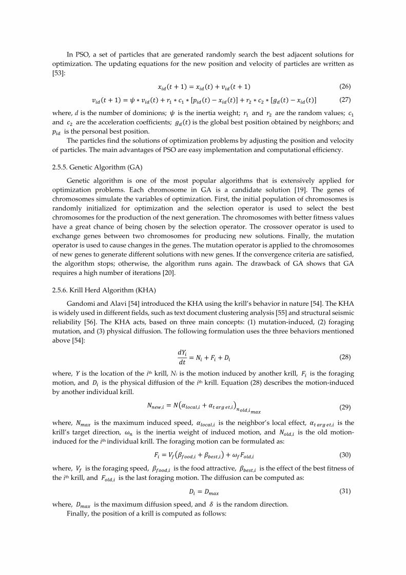
In PSO, a set of particles that are generated randomly search the best adjacent solutions for

optimization. The updating equations for the new position and velocity of particles are written as

[53]:

𝑥𝑖𝑑(𝑡 + 1) = 𝑥𝑖𝑑(𝑡) + 𝑣𝑖𝑑(𝑡 + 1) (26)

𝑣𝑖𝑑(𝑡 + 1) = 𝜓 ∗ 𝑣𝑖𝑑(𝑡) + 𝑟1 ∗ 𝑐1 ∗ [𝑝𝑖𝑑(𝑡) − 𝑥𝑖𝑑(𝑡)] + 𝑟2 ∗ 𝑐2 ∗ [𝑔𝑑(𝑡) − 𝑥𝑖𝑑(𝑡)] (27)

where, d is the number of dominions; 𝜓 is the inertia weight; 𝑟1 and 𝑟2 are the random values; 𝑐1

and 𝑐2 are the acceleration coefficients; 𝑔𝑑(𝑡) is the global best position obtained by neighbors; and

𝑝𝑖𝑑 is the personal best position.

The particles find the solutions of optimization problems by adjusting the position and velocity

of particles. The main advantages of PSO are easy implementation and computational efficiency.

2.5.5. Genetic Algorithm (GA)

Genetic algorithm is one of the most popular algorithms that is extensively applied for

optimization problems. Each chromosome in GA is a candidate solution [19]. The genes of

chromosomes simulate the variables of optimization. First, the initial population of chromosomes is

randomly initialized for optimization and the selection operator is used to select the best

chromosomes for the production of the next generation. The chromosomes with better fitness values

have a great chance of being chosen by the selection operator. The crossover operator is used to

exchange genes between two chromosomes for producing new solutions. Finally, the mutation

operator is used to cause changes in the genes. The mutation operator is applied to the chromosomes

of new genes to generate different solutions with new genes. If the convergence criteria are satisfied,

the algorithm stops; otherwise, the algorithm runs again. The drawback of GA shows that GA

requires a high number of iterations [20].

2.5.6. Krill Herd Algorithm (KHA)

Gandomi and Alavi [54] introduced the KHA using the krill’s behavior in nature [54]. The KHA

is widely used in different fields, such as text document clustering analysis [55] and structural seismic

reliability [56]. The KHA acts, based on three main concepts: (1) mutation-induced, (2) foraging

mutation, and (3) physical diffusion. The following formulation uses the three behaviors mentioned

above [54]:

𝑑𝑌𝑖

𝑑𝑡= 𝑁𝑖 + 𝐹𝑖 + 𝐷𝑖 (28)

where, 𝑌 is the location of the ith krill, Ni is the motion induced by another krill, 𝐹𝑖 is the foraging

motion, and 𝐷𝑖 is the physical diffusion of the ith krill. Equation (28) describes the motion-induced

by another individual krill.

𝑁𝑛𝑒𝑤,𝑖 = 𝑁(𝛼𝑙𝑜𝑐𝑎𝑙,𝑖 + 𝛼𝑡 𝑎𝑟𝑔 𝑒𝑡,𝑖)𝑛𝑜𝑙𝑑,𝑖𝑚𝑎𝑥

(29)

where, 𝑁𝑚𝑎𝑥 is the maximum induced speed, 𝛼𝑙𝑜𝑐𝑎𝑙,𝑖 is the neighbor’s local effect, 𝛼𝑡 𝑎𝑟𝑔 𝑒𝑡,𝑖 is the

krill’s target direction, 𝜔𝑛 is the inertia weight of induced motion, and 𝑁𝑜𝑙𝑑,𝑖 is the old motion-

induced for the ith individual krill. The foraging motion can be formulated as:

𝐹𝑖 = 𝑉𝑓(𝛽𝑓𝑜𝑜𝑑,𝑖 + 𝛽𝑏𝑒𝑠𝑡,𝑖) + 𝜔𝑓𝐹𝑜𝑙𝑑,𝑖 (30)

where, 𝑉𝑓 is the foraging speed, 𝛽𝑓𝑜𝑜𝑑,𝑖 is the food attractive, 𝛽𝑏𝑒𝑠𝑡,𝑖 is the effect of the best fitness of

the ith krill, and 𝐹𝑜𝑙𝑑,𝑖 is the last foraging motion. The diffusion can be computed as:

𝐷𝑖 = 𝐷𝑚𝑎𝑥 (31)

where, 𝐷𝑚𝑎𝑥 is the maximum diffusion speed, and 𝛿 is the random direction.

Finally, the position of a krill is computed as follows:

𝑋𝑛𝑒𝑤,𝑖 = 𝑋𝑜𝑙𝑑,𝑖 + 𝛥𝑡𝑑𝑋𝑖

𝑑𝑡 (32)

where, 𝑋𝑛𝑒𝑤,𝑖 is the value of the next individual krill location, and 𝑋𝑜𝑙𝑑,𝑖 represents the current

position of solution number I, and 𝛥𝑡 is the essential constant. Figure 5 shows the flowchart of the

krill algorithm.

2.6. Principal Component Analysis (PCA)

PCA is a statistical orthogonal transformation to obtain a set of values of linearly uncorrelated

(principal components) from a set of observations. When the user has the number of inputs but he

cannot identify the appropriate inputs, the PCA is used to reduce the number of inputs. The final

data set should be able to demonstrate most of the variance of the original input data by creating a

variable reduction [57]. PCA can be explained, based on the following equation [57]:

𝑍𝑖 = 𝑎𝑖1 + 𝑎𝑖2+. . . +𝑎𝑖𝑝𝑥𝑝 (33)

where, 𝑍𝑖 shows the principal component, 𝑎𝑖𝑝 is the related eigenvector, and xi is the input variable.

The information is obtained by solving Equation (34):

|𝑅 − 𝜆𝐼| = 0 (34)

where, 𝑅 is the variance-covariance matrix, I is the unit matrix, and 𝜆 is the eigenvalues.

2.7. Taguchi Model

The random parameters of optimization algorithms are the most important parameters affecting

the outputs of the optimization algorithms. Thus, determining the appropriate values of random

parameters is necessary to construct the optimization models. The Taguchi model is widely used to

design different parameters of different experiments or experimental models. First, the initial level is

determined for each of the random parameters in the optimization algorithms. In the Taguchi

method, parameters are classified into two groups: (1) controllable, and (2) uncontrollable (noise). In

the Taguchi model, each parameter combination that has a higher S (signal)/N (noise) ratio is

regarded as the best combination [58].

𝑆/𝑁 = −10 𝑙𝑜𝑔 (1

𝑛∑ 𝑌𝑖

2

𝑛

𝑖=1

) (35)

where, n is the number of data, and 𝑌𝑖 is the fitness function that is obtained by the Taguchi model.

For example, consider the PSO algorithm with four parameters and three levels. When the population

size is at level 1, the acceleration coefficient is tested at levels 1, 2, 3, and 4. Similarly, the inertia

coefficient is tested at levels 1, 2, 3, and 4.

2.8. Hybrid ANN, ANFIS, and SVM Models with Optimization Algorithms

The optimization algorithms can be used as a robust training algorithm for the ANN models.

The process starts with the initialization of a group of random agents (particles, chromosomes, krill,

grasshoppers, weeds, or cats). The position of agents represents the ANN weights and biases.

Following this level, using the initial biases and weights (i.e., the initial position of agents), the hybrid

ANN-optimization algorithms are trained, and the error between the observed and estimated value

is calculated. At each iteration, the calculated error is decreased by the updating of agent locations.

The model procedure in ANFIS-optimization algorithm models starts with the initialization of a

set of agents (particles, chromosomes, krill, grasshoppers, weeds, or cats) and continues with the

random choice of agents and finally adjusts a location for each agent. First, the ANFIS model is

trained. Then, the consequent and premise parameters are optimized by the optimization algorithms.

The root mean square error (RMSE) is defined as an objective function. The aim of optimization

algorithms is to minimize the objective function value with finding the appropriate values of

consequent and premise parameters.

In SVM, the C parameter and kernel function parameters have significant effects on the accuracy

of the SVM. The random population of agents (particles, chromosomes, krill, grasshoppers, weeds,

or cats) are initialized for training the SVM parameters. The RMSE is defined as an objective function.

The aim of hybrid SVM-optimization algorithm models is to minimize model errors. Figure 2 shows

the developed framework of hybrid ANN, ANFIS, and SVM-optimization models for modeling

groundwater level.

Thus, the model parameters are considered as decision variables for optimization algorithms.

The optimization algorithms aim to minimize the error function to find the optimal value of model

parameters. The PCA selects the appropriate input combinations. Then the hybrid and standalone

models uses the input combinations to forecast GEWL. The models uses the optimized model

parameters to accurately forecast monthly GWL.

2.9. Uncertainty Analysis of Soft Computing Models

The input data and the inability of model structure are the sources of uncertainty. In this

research, an integrated framework is developed to simultaneously evaluate the input data and model

structure.

Input data uncertainty

The combined Bayesian uncertainty was used to compute the uncertainty contributed by input

data. The input error model was used to account for the uncertainty of input data [59]:

( )2

, , ~ ,a t t mH KH K N m s= (366

)

where, ,a tH : the adjusted groundwater level (GWL),

tH : the observed GWL, t: the given month, K:

the normally distributed random, m: mean, and m : variance. For each soft computing model, m

and m were added to the system. A dynamically dimensioned search was used to find the value

of m: mean and m : variance as defined by [59].

Mode Structure Uncertainty

Bayesian model average (BMA) is used for model uncertainty. The posterior model probability

and averaging over the best models were used to estimate the uncertainty of the models. The

weighted average prediction of quantity of target variable is computed as follows [59]:

1

k

j k jk jk

H F eb=

= +å (37)

where, Fj: the point prediction of each model, ej: noise, k : the weight vector of model, H: n

observation of GWL, k: number of models, and j: number of observations. For accurate application of

BMA model, the standard deviation of normal probability distribution functions and weights should

be estimated accurately. The log-likelihood function is used to calculate the weights and standard

deviation as follows [59]:

( ) ( )2

2

21 1

1 1, | , log exp

22

n k

BMA BMA k k j jki k

k

L F H H Fb s b sps

-

= =

ì üé ùï ï= - -ê úí ý

ê úï ïë ûî þå å (38)

where, BMA : maximum likelihood Bayesian weight. Markov Chain Monte Carlo (MCMC)

simulations are used to compute the log-likelihood function. The integrated framework is defined as

follows:

1- A number of models are selected to simulate the GWL.

2- The prior probability is assigned to each model.

3- An error input model is defined.

4- The posterior distribution of input error models and model parameters are obtained.

5- A predetermined number of GWLs for each model is provided using probabilistic parameter

estimations obtained from level 2 to level 4.

6- The variance and weight of models are estimated.

7- The weights for ensemble members of models are summed to compute the weight models.

8- To the experimental soft computing models. The following indices were used to quantify the

uncertainty of models:

𝑝 =1

𝑛𝑐𝑜𝑢𝑛𝑡[𝐻|𝑋𝐿 ≤ 𝐻 ≤ 𝑋𝑈] (39)

𝑑 =�̄�𝑥

𝜎𝑥

�̄�𝑥 =1

𝑘∑(𝑋𝑈 − 𝑋𝐿)

𝑘

𝑙=1

(40)

9- where k is the number of observed data, 𝑋𝑈 is the upper bound of data, 𝑋𝐿 is the lower bound

of data, 𝜎𝑥 is standard deviation, p is bracketed by 95% of predicted uncertainties, d is the

distance between the upper and lower bounds, and �̄�𝑥 is the average distance between the

upper and lower bounds [59,60].

2.10. Statistical Indices for Evaluation of Different Models

In this study, the following indices were used to evaluate the performance of models:

Root mean square error:

𝑅𝑀𝑆𝐸 = √1

𝑁∑((𝐻0(𝑡)) − (𝐻𝑠(𝑡)))

2𝑛

𝑡=1

(371

)

Mean absolute error:

𝑀𝐴𝐸 =1

𝑁∑|𝐻0(𝑡) − 𝐻𝑠(𝑡)|

1

𝑡=1

2

(42)

Nash Sutcliffe efficiency:

𝑁𝑆𝐸 = 1 −∑ |𝐻𝑠(𝑡) − 𝐻0(𝑡)|

2𝑛𝑖=1

∑ |𝐻𝑠 − �̄�0(𝑡)|2𝑛

𝑖=1

(43)

Percent bias (PBIAS):

𝑃𝐵𝐼𝐴𝑆 = [∑ (𝐻𝑠(𝑡) − 𝐻0(𝑡))

2𝑛𝑖=1

∑ (𝐻𝑜𝑡)2𝑛

𝑖=1

] (44)

where, N is the number of data, H0 is the observed value, and Ps is the predicted value.

RMSE and MAE show a good match between observed data and estimated values when it equals

0. The NSE shows a good match between the observed values and estimated values when it equals 1.

The best value of PBIAS is zero.

3. Results and Discussion

3.1. Inputs Selection by PCA

In this study, 12 input variables (H(t-1), …., H(t-12)) were considered to select the input lag times

of monthly GWL. As presented in the flowchart and framework of the current study in Figure 1, the

first step of the model developments is the appropriate selection of time lags for GWL modelling by

PCA analysis. Table 1 shows the variance contribution rate for PCAs as the principal component

loadings. There are the loadings of 12 principal components versus 12 input lag times of GWL. The

first four PCs variance summed up a contribution of 91%, among which the first PC variance had a

contribution of 48% loadings. It was observed that the inputs H(t-1), H (t-2), H (t-3), H (t-4), and H (t-

5) had higher factor loading in comparison with other inputs of the PCs. Thus, the first four PCs were

selected for the hybrid soft computing models which included inputs H(t-1), H (t-2), H (t-3), H (t-4),

and H (t-5) because of their higher loading factor. This loading analysis of variables reduced the raw

initial input parameter numbers from 12 to 5, that decrease the model development efforts. The

coefficients of more 0.75 are significant for Eigen value verifications [60].

Table 1. Principal component loadings.

PC 1 2 3 4 5 6 7 8 9 10 11 12

H (t-1) 0.98 0.95 0.93 0.90 0.89 0.88 0.88 0.86 0.75 0.62 0.52 0.45

H (t-2) 0.84 0.82 0.88 0.86 0.85 0.84 0.85 0.82 0.62 0.60 0.51 0.44

H (t-3) 0.83 0.81 0.80 0.77 0.74 0.72 0.84 0.80 0.61 0.55 0.43 0.40

H (t-4) 0.82 0.80 0.78 0.76 0.75 074 0.83 0.78 0.60 0.54 0.39 0.37

H (t-5) 0.81 0.79 0.76 0.75 0.72 0.71 0.82 0.79 0.55 0.51 0.38 0.35

H (t-6) 0.73 0.67 0.74 0.73 0.71 0.70 0.80 0.77 0.54 0.50 0.37 0.34

H (t-7) 0.62 0.55 0.72 0.70 0.65 0.64 0.76 0.75 0.53 0.47 0.33 0.30

H (t-8) 0.61 0.50 0.71 0.69 0.54 0.52 0.65 0.64 0.51 0.46 0.30 0.29

H (t-9) 0.54 0.54 0.70 0.65 0.42 0.64 0.54 0.52 0.50 0.45 0.29 0.25

H (t-10) 0.42 0.42 0.69 0.66 0.41 0.62 0.45 0.44 0.49 0.42 0.28 0.26

H (t-11) 0.42 0.42 0.55 0.54 0.40 0.55 0.42 0.40 0.47 0.41 0.27 0.24

H (t-12) 0.40 0.40 0.45 0.43 0.38 0.52 0.40 0.38 0.46 0.38 0.25 0.23

Eigen value 5.78 3.22 1.12 0.90 0.6 0.27 0.05 0.03 0.02 0.003 0.003 0.03

Cumulative

variance 48% 74% 84% 91% 96% 99 99.5 99.7 99.99 99.99 99.99 100%

3.2. Selection of Random Parameters by the Taguchi Model

The Taguchi model was used to find the value of random parameters rather than the classical

trial and error methods. Table 2 shows the computed signal-to-noise (S/N) ratio for each random

parameter in the optimization module of the hybrid training of ANFIS. Each parameter had four

levels and the best level of each parameter is selected based on the S/N values. The S/N ratio was

computed for each level of parameters. The best value of parameters had the highest S/N rate. For

example, sensitivity analysis for different values of GOA parameters was done, as shown in Table 2.

The results indicated that the population size = 300 had the highest value of S/N. Thus, the optimal

size of population was 300. The maximum S/N ratio for parameter l was 1.23. Thus, the optimal value

of parameter l was 1.5. The maximum S/N ratio for parameter f was 1.14. Thus, the optimal value of

parameter f was 0.5.

Table 2. Results of Taguchi model for a: GOA, b: particle swarm optimization (PSO), c: genetic

algorithm (GA), d: WA, e: CSO, and f: krill algorithm.

(a)

Population size S/N l S/N f S/N

100 1.05 0.5 1.07 0.1 1.09

200 1.15 1 1.19 0.3 1.12

300 1.20 1.5 1.23 0.5 1.14

400 1.02 2 1.18 0.7 1.10

(b)

Population size S/N c1 S/N c2 S/N S/N

100 1.25 1.6 1.20 1.6 1.21 0.3 1.19

200 1.29 1.8 1.27 1.8 1.25 0.50 1.18

300 1.23 2.0 1.26 2.0 1.23 0.70 1.17

400 1.20 2.2 1.22 2.2 1.25 0.90 1.24

(c)

Population size S/N Mutation probability S/N Crossover rate S/N

100 1.18 0.01 1.16 1.6 1.21

200 1.20 0.03 1.17 1.8 1.25

300 1.21 0.05 1.20 2.0 1.23

400 1.17 0.07 1.19 2.2 1.25

(d)

Pmax S/N n S/N

50 1.12 1 1.14

100 1.23 2 1.17

150 1.19 3 1.18

200 1.17 4 1.19

(e)

Population size S/N SMP S/N MR S/N

100 1.11 5 1.10 0.10 1.12

200 1.24 10 1.15 0.30 1.16

300 1.17 15 1.17 0.50 1.18

400 1.15 20 1.21 0.70 1.20

(f)

Population size S/N Vf S/N Nmax S/N

100 1.10 0.005 1.12 0.02 1.14

200 1.12 0.010 1.15 0.04 1.17

300 1.14 0.015 1.17 0.06 1.12

400 1.16 0.020 1.14 0.08 1.21

3.3. Results of Hybrid ANN, ANFIS, and SVM Models

In this section, the results of developed hybrid models are presented and compared with each

other and with the usual ANFIS, ANN, and SVM models. These models are hybridized with GOA,

CSO, KA, WA, PSO, and GA meta-heuristic optimization algorithms. The results of models in three

piezometers of 6, 9, and 10 as shown in Figure 6, are presented and discussed. These piezometers

were selected as samples to evaluate the ability of new hybrid models.

Figure 6. The flowchart of the krill algorithm [54].

• piezometer 6

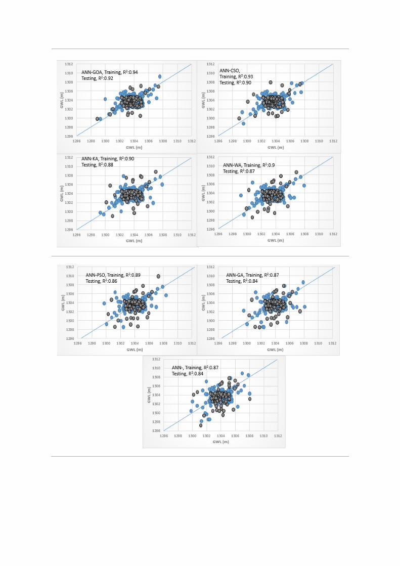
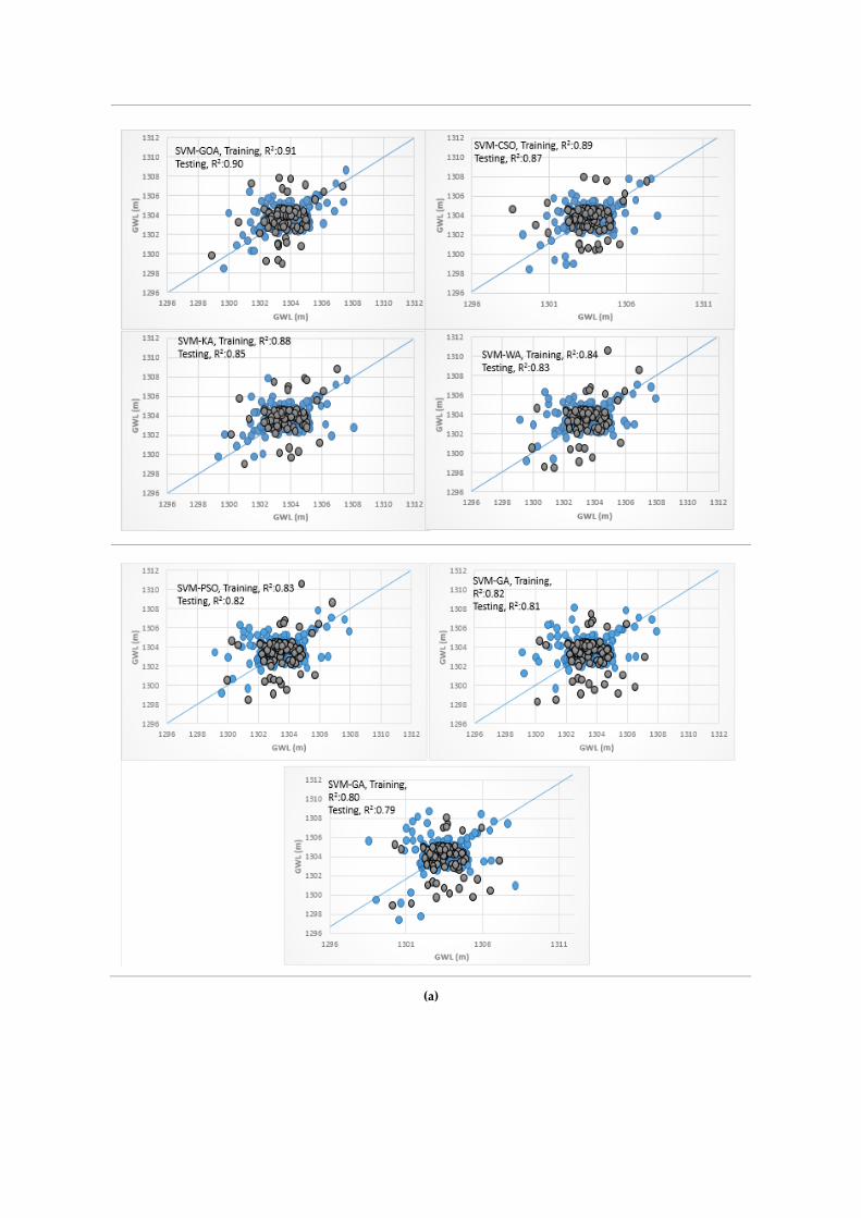
Table 3 and Figure 7a show the results of hybrid optimized and standalone soft computing

models for piezometer 6. Results indicated that ANFIS-GOA was the most accurate model and is

selected as the optimum model that was verified by a value of RMSE = 1.12 m, MAE = 0.812 m, NSE

= 0.95, and PBIAS = 0.12 for the training level. For the testing phase assessed with the ANFIS-GOA,

results indicated a value of RMSE: 1.21 m, MAE: 0.878 m, NSE: 0.93, and PBIAS: 0.15 which reflected

better performance in comparison to other models. From Table 3, results indicated that the SVM

model with the higher values of RMSE, MAE, and PBIAS and lower values of NSE was the worst

model among other models. Among the hybrid ANN models, the ANN-GOA outperformed the

ANN-CSO, ANN-GA, ANN-PSO, ANN-WA, and ANN-KA models with the best values for RMSE =

1.21 m, MAE = 0.878 m, NSE = 0.93, PBIAS = 0.15 in the test stage. The ability of GA was lower than

that of CSO, PSO, WA, and KA because of higher values of RMSE, MAE, and PBIAS and lower values

of NSE in train and test steps as presented in Table 3. Among SVM models, the hybrid SVM-GOA

was observed to have the lowest value of NSE and the highest values of RMSE, MAE, and PBIAS. It

was important to mention that the standalone SVM, ANN, and ANFIS had worse performance than

hybrid ANN, SVM, and ANFIS models that indicates the superiority of hybridization in model

developments. Among PSO, CSO, GA, KA, and WA, the CSO had better results than the other

optimization algorithms. The general results showed that ANFSI model was superior to the SVM and

ANN models. Additionally, the ANN model had lower values of RMSE and MAE than did the SVM

model. Additionally, the results of ANFIS-GOA as the best model in piezometer 6 in comparison with

standalone ANFIS shows that meta-heuristic hybridizations improved the model performances in

train and test steps. The percent of RMSE, MAE, NSE, and PBIAS improvements by ANFIS-GOA in

train step were 15%, 4%, 13%, and 208% and these values for the test steps of ANFIS-GOA are 33%,

44.6%, 16.3%, and 173%, respectively, that clearly confirm the superiority of developed hybridization

schemes in GWL modelling. Additionally, in Figure 7a, the scatter plots of training and testing steps

visualize the performance of ANFIS-GOA compared to the other models. Furthermore, simulations

coincide very well with the observed values and all of the data points concentrated over the y = x line

with R2 = 0.93. Furthermore, this figure shows that other hybridized models such as CSO, PSO, KA,

WA, GA, and standalone ANFIS have less accuracy in high and low values of GWL, while the ANFIS-

GOA over all of low to high values of GWL performed accurately in regard to the observations.

Begin

Step 1: Initialization. Set the generation counter G=1; initialize the population P of

NP krill

individuals randomly; set the foraging speed Vf, the maximum diffusion speed

Dmax,

and the maximum induced speed Nmax.

Step 2: While the termination criteria is not satisfied or G<Gmax do

Sort the population/krill from best to worst.

for i=1:NP (all krill) do

Perform the following motion calculation.

Motion induced by the presence of other individuals

Foraging motion

Physical diffusion

Implement the genetic operators.

Update the krill individual position in the search space.

Evaluate each krill individual according to its position.

end for i

Sort the population/krill from best to worst and find the current best.

G=G+1.

Step 3: end while

Step 4: Post-processing the results and visualization.

End.

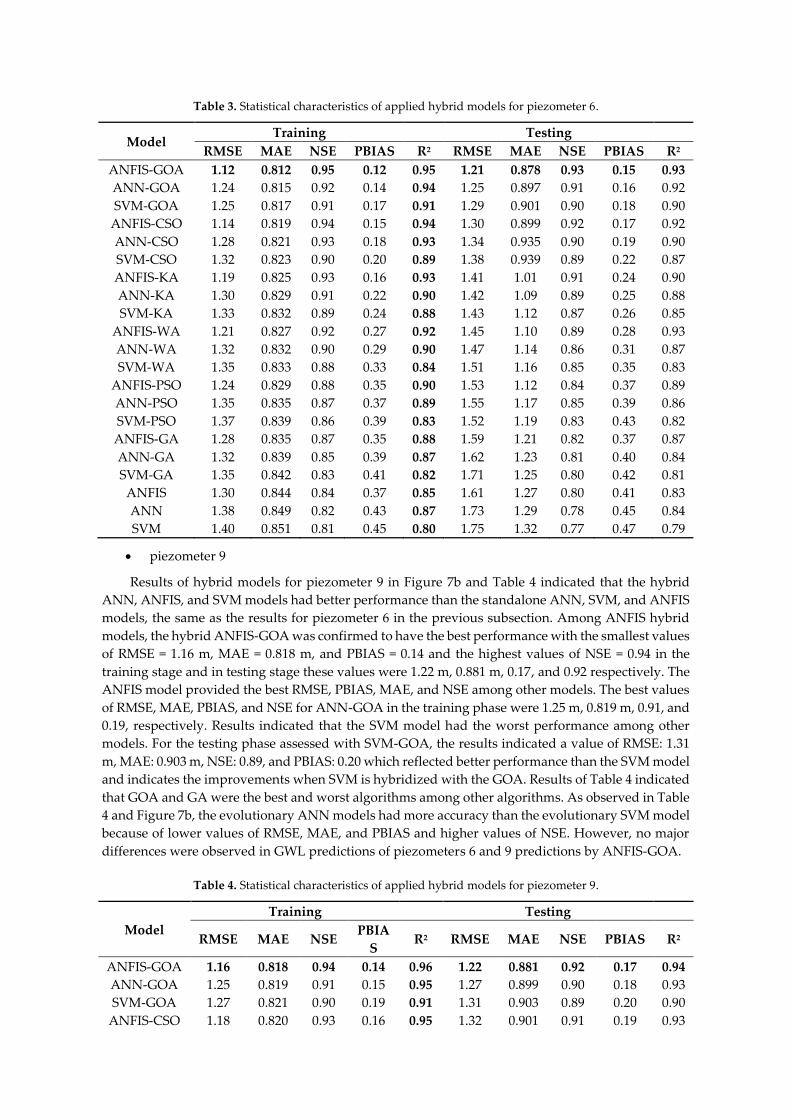
Table 3. Statistical characteristics of applied hybrid models for piezometer 6.

Model Training Testing

RMSE MAE NSE PBIAS R2 RMSE MAE NSE PBIAS R2

ANFIS-GOA 1.12 0.812 0.95 0.12 0.95 1.21 0.878 0.93 0.15 0.93

ANN-GOA 1.24 0.815 0.92 0.14 0.94 1.25 0.897 0.91 0.16 0.92

SVM-GOA 1.25 0.817 0.91 0.17 0.91 1.29 0.901 0.90 0.18 0.90

ANFIS-CSO 1.14 0.819 0.94 0.15 0.94 1.30 0.899 0.92 0.17 0.92

ANN-CSO 1.28 0.821 0.93 0.18 0.93 1.34 0.935 0.90 0.19 0.90

SVM-CSO 1.32 0.823 0.90 0.20 0.89 1.38 0.939 0.89 0.22 0.87

ANFIS-KA 1.19 0.825 0.93 0.16 0.93 1.41 1.01 0.91 0.24 0.90

ANN-KA 1.30 0.829 0.91 0.22 0.90 1.42 1.09 0.89 0.25 0.88

SVM-KA 1.33 0.832 0.89 0.24 0.88 1.43 1.12 0.87 0.26 0.85

ANFIS-WA 1.21 0.827 0.92 0.27 0.92 1.45 1.10 0.89 0.28 0.93

ANN-WA 1.32 0.832 0.90 0.29 0.90 1.47 1.14 0.86 0.31 0.87

SVM-WA 1.35 0.833 0.88 0.33 0.84 1.51 1.16 0.85 0.35 0.83

ANFIS-PSO 1.24 0.829 0.88 0.35 0.90 1.53 1.12 0.84 0.37 0.89

ANN-PSO 1.35 0.835 0.87 0.37 0.89 1.55 1.17 0.85 0.39 0.86

SVM-PSO 1.37 0.839 0.86 0.39 0.83 1.52 1.19 0.83 0.43 0.82

ANFIS-GA 1.28 0.835 0.87 0.35 0.88 1.59 1.21 0.82 0.37 0.87

ANN-GA 1.32 0.839 0.85 0.39 0.87 1.62 1.23 0.81 0.40 0.84

SVM-GA 1.35 0.842 0.83 0.41 0.82 1.71 1.25 0.80 0.42 0.81

ANFIS 1.30 0.844 0.84 0.37 0.85 1.61 1.27 0.80 0.41 0.83

ANN 1.38 0.849 0.82 0.43 0.87 1.73 1.29 0.78 0.45 0.84

SVM 1.40 0.851 0.81 0.45 0.80 1.75 1.32 0.77 0.47 0.79

• piezometer 9

Results of hybrid models for piezometer 9 in Figure 7b and Table 4 indicated that the hybrid

ANN, ANFIS, and SVM models had better performance than the standalone ANN, SVM, and ANFIS

models, the same as the results for piezometer 6 in the previous subsection. Among ANFIS hybrid

models, the hybrid ANFIS-GOA was confirmed to have the best performance with the smallest values

of RMSE = 1.16 m, MAE = 0.818 m, and PBIAS = 0.14 and the highest values of NSE = 0.94 in the

training stage and in testing stage these values were 1.22 m, 0.881 m, 0.17, and 0.92 respectively. The

ANFIS model provided the best RMSE, PBIAS, MAE, and NSE among other models. The best values

of RMSE, MAE, PBIAS, and NSE for ANN-GOA in the training phase were 1.25 m, 0.819 m, 0.91, and

0.19, respectively. Results indicated that the SVM model had the worst performance among other

models. For the testing phase assessed with SVM-GOA, the results indicated a value of RMSE: 1.31

m, MAE: 0.903 m, NSE: 0.89, and PBIAS: 0.20 which reflected better performance than the SVM model

and indicates the improvements when SVM is hybridized with the GOA. Results of Table 4 indicated

that GOA and GA were the best and worst algorithms among other algorithms. As observed in Table

4 and Figure 7b, the evolutionary ANN models had more accuracy than the evolutionary SVM model

because of lower values of RMSE, MAE, and PBIAS and higher values of NSE. However, no major

differences were observed in GWL predictions of piezometers 6 and 9 predictions by ANFIS-GOA.

Table 4. Statistical characteristics of applied hybrid models for piezometer 9.

Model

Training Testing

RMSE MAE NSE PBIA

S R2 RMSE MAE NSE PBIAS R2

ANFIS-GOA 1.16 0.818 0.94 0.14 0.96 1.22 0.881 0.92 0.17 0.94

ANN-GOA 1.25 0.819 0.91 0.15 0.95 1.27 0.899 0.90 0.18 0.93

SVM-GOA 1.27 0.821 0.90 0.19 0.91 1.31 0.903 0.89 0.20 0.90

ANFIS-CSO 1.18 0.820 0.93 0.16 0.95 1.32 0.901 0.91 0.19 0.93

ANN-CSO 1.29 0.823 0.92 0.19 0.94 1.36 0.938 0.88 0.18 0.92

SVM-CSO 1.33 0.825 0.91 0.22 0.89 1.39 0.940 0.87 0.20 0.88

ANFIS-KA 1.20 0.827 0.92 0.18 0.94 1.34 1.05 0.90 0.22 0.92

ANN-KA 1.31 0.831 0.90 0.23 0.91 1.44 1.10 0.86 0.23 0.90

SVM-KA 1.35 0.833 0.88 0.25 0.87 1.45 1.14 0.85 0.27 0.86

ANFIS-WA 1.22 0.829 0.91 0.28 0.91 1.49 1.12 0.83 0.29 0.90

ANN-WA 1.36 0.834 0.89 0.30 0.89 1.51 1.15 0.82 0.32 0.88

SVM-WA 1.38 0.835 0.87 0.34 0.86 1.53 1.17 0.83 0.37 0.85

ANFIS-PSO 1.27 0.831 0.86 0.36 0.87 1.55 1.19 0.81 0.39 0.86

ANN-PSO 1.39 0.837 0.85 0.38 0.87 1.57 1.23 0.80 0.40 0.85

SVM-PSO 1.40 0.840 0.84 0.40 0.85 1.59 1.25 0.83 0.45 0.84

ANFIS-GA 1.29 0.839 0.83 0.39 0.85 1.61 1.28 0.80 0.39 0.84

ANN-GA 1.42 0.840 0.82 0.40 0.86 1.63 1.29 0.79 0.42 0.84

SVM-GA 1.43 0.843 0.81 0.42 0.82 1.69 1.32 0.77 0.43 0.81

ANFIS 1.33 0.845 0.82 0.39 0.84 1.71 1.39 0.79 0.42 0.83

ANN 1.44 0.851 0.80 0.44 0.85 1.76 1.40 0.77 0.47 0.83

SVM 1.45 0.852 0.79 0.47 0.81 1.77 1.43 0.76 0.49 0.78

• piezometer 10

Here the results of models in piezometer 10 are evaluated. As observed in Table 5, results

indicated that the ANFIS-GOA was better in terms of minimizing RMSE, MAE, and PBIAS than the

other models. ANFIS-GOA reduced RMSE error by 7.01% and 7.04% compared to ANN-GOA and

SVM-GOA, respectively. The standalone ANFIS, ANN, and SVM models provided worse results

than the hybrid models. The SVM model provided the worst performance among other models. The

NSE of ANFIS-GOA, ANFIS-CSO, ANFIS-KA, ANFIS-WA, ANFIS-PSO, and ANFIS-GA was 0.91,

0.90, 0.89, 0.79, and 0.75, respectively. GA had the worst performance among other algorithms. As is

shown in Table 5, the error in the estimated GWL by using GA was more than that of PSO, KA, WA,

GA, CSO, and GOA. Overall, the percent of improvements in the ANFIS-GOA versus standalone

ANFIS in piezometer 6 were 14.4%, 3%, 17.8%, and 181% for RMSE, MAE, NSE, and PBIAS in training

stage and 40.7%, 55%, 25%, and 132% in testing stage, respectively. These values again confirm that

all of the hybridized models performed more accurately than the stand-alone models and indicate

the generality of hybridizing Taguchi with training procedure compared to the classical standalone

models.

Table 5. Statistical characteristics of applied hybrid models for piezometer 10.

Model Training Testing

RMSE MAE NSE PBIAS R2 RMSE MAE NSE PBIAS R2

ANFIS-GOA 1.18 0.819 0.93 0.16 0.96 1.23 0.911 0.91 0.19 0.94

ANN-GOA 1.27 0.821 0.90 0.17 0.95 1.28 0.921 0.90 0.20 0.94

SVM-GOA 1.29 0.823 0.89 0.20 0.89 1.32 0.925 0.87 0.21 0.88

ANFIS-CSO 1.20 0.822 0.92 0.17 0.95 1.34 0.914 0.90 0.22 0.93

ANN-CSO 1.31 0.824 0.91 0.20 0.92 1.37 0.926 0.87 0.23 0.90

SVM-CSO 1.35 0.827 0.90 0.23 0.87 1.40 0.930 0.86 0.25 0.86

ANFIS-KA 1.22 0.829 0.89 0.19 0.94 1.41 1.10 0.89 0.24 0.91

ANN-KA 1.33 0.833 0.87 0.24 0.89 1.43 1.12 0.85 0.26 0.88

SVM-KA 1.37 0.835 0.86 0.27 0.85 1.47 1.17 0.84 0.28 0.84

ANFIS-WA 1.24 0.837 0.90 0.29 0.90 1.50 1.14 0.82 0.30 0.89

ANN-WA 1.37 0.839 0.88 0.31 0.88 1.52 1.16 0.81 0.33 0.87

SVM-WA 1.39 0.840 0.86 0.35 0.84 1.54 1.18 0.80 0.38 0.82

ANFIS-PSO 1.29 0.838 0.85 0.37 0.89 1.56 1.20 0.79 0.40 0.87

ANN-PSO 1.40 0.842 0.84 0.39 0.87 1.58 1.25 0.78 0.41 0.86

SVM-PSO 1.41 0.844 0.83 0.41 0.83 1.60 1.27 0.77 0.43 0.81

ANFIS-GA 1.31 0.839 0.82 0.42 0.86 1.62 1.29 0.76 0.42 0.85

ANN-GA 1.44 0.845 0.81 0.43 0.88 1.65 1.32 0.75 0.44 0.85

SVM-GA 1.45 0.847 0.80 0.44 0.82 1.71 1.33 0.74 0.45 0.80

ANFIS 1.35 0.849 0.79 0.45 0.85 1.73 1.41 0.73 0.44 0.84

ANN 1.45 0.853 0.78 0.47 0.85 1.77 1.42 0.72 0.49 0.82

SVM 1.47 0.855 0.77 0.49 0.8 1.78 1.45 0.70 0.50 0.79

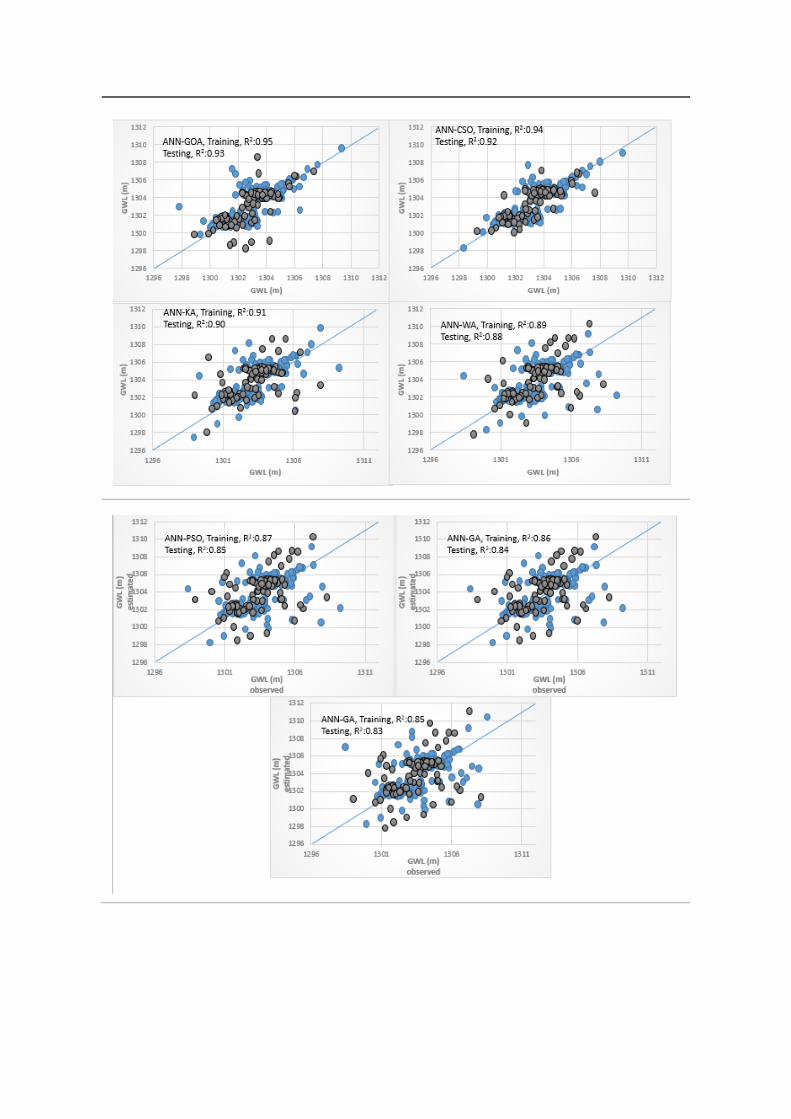
3.4. Analysis of Scatterplots of Soft Computing Models

• piezometer 6

Scatterplots for the soft computing models are provided in Figure 7a for the training and testing

phases. It is clear that the hybrid ANFIS-GOA predictions were much closer to the measured data in

the testing and training phases with a higher coefficient of determination. This result indicated a

better correlation and a larger degree of statistical match between measured and predicted data of

ANFIS-GOA relative to the other hybrid ANN and SVM models. The R2 values were found to vary

in the range of 0.84–0.94 and 0.79–0.91 for the ANN (hybrid ANN models and based ANN model)

and SVM models (hybrid SVM models and based SVM model), respectively. The SVM model had

the lowest R2 among other models. Additionally, the ANFIS-GA, ANN-GA, and SVM-GA models

had the lowest R2 among other hybrid ANFIS, ANN, and SVM models. There is a weak agreement

between the lower and higher values of the actual and estimated GWLs in this scatter plots of

piezometer 6, unlike the ANFIS-GOA results.

• piezometer 9

As observed in Figure 7b, the R2 values of testing phase were 0.94, 0.93, 0.92, 0.90, 0.86, 0.84, and

0.83 for ANFIS-GOA, ANFIS-CSO, ANFIS-KA, ANFIS-WA, ANFIS-PSO, ANFIS-GA, and ANFIS

model, respectively. GOA had a better performance than other optimization algorithms. The outputs

indicated that all hybrid optimized ANFIS, ANN, and SVM models outperformed the standalone

ANFIS, ANN, and SVM models. As the results in Table 4 show incorporating the Taguchi and GOA

in ANFIS training enhanced the R2 values 13% in comparison with the standalone ANFIS and in all

of the developed models the hybridized meta-heuristic models outperformed the single standalone

models.

• Piezometer 10

The results of Figure 7c indicated that the ANFIS-GOA and SVM models produced the best and

the worst results, respectively. It is clear that developed hybrid ANFIS-GOA model forecasting of

GWL was less scattered and closer to the straight line of 1:1 than those the other models and it shows

impressive results in regard to the other models. For training and testing phases, GA had a worse

performance than CSO, PSO, KA, WA, and GOA because of the lower values of R2. The standalone

ANFIS model had the worst performance among the ANFIS-GOA, ANFIS-CSO, ANFIS-WA, ANFIS-

PSO, ANFIS-GA, and ANFIS-KA models. The ANFIS-GOA model with R2 = 0.94 as is presented in

Table 5, the values of GWL simulated by the ANFIS-GOA are almost equal to the observed values of

GWL. The linear fit of the forecasted GWL and measured GWL results have a high correlation

coefficient that is very close to 1.00 (R2 =0 .97) and a perfect correlation coefficient (R2 value) of 0.94,

confirmed that the simulation model has provided a very good prediction of the observed values of

GWL. Additionally, 94% of the observed GWL values accurately fit the hybrid ANFIS-GOA model

predictions.

(a)

(b)

(c)

Figure 7. The scatter plots of exanimated soft computing models for predicting groundwater level

(GWL), (a) piezometer 6, (b) piezometer 9, and (c) piezometer 10.

3.5. Uncertainty Analysis of Soft Computing Models

As stated in the aims of the current study, the uncertainty analysis of hybrid intelligence models

is another major contribution and novelty of the present study. The same as the previous subsections,

in this section the results of uncertainty analysis of hybrid models in selected three piezometers are

provided and comparative evaluation between different hybrid models are presented. The hybrids

of ANFIS, SVM, and ANN models with GOA, WA, KA, PSO, and GA are joined with the non-

parametric Monte-Carlo Simulations (MCSs) to quantify the uncertainty of developed models in

GWL simulations. The probability of model predictions in MCSs is considered as a degree of

uncertainty of model results and demonstrates the probabilities in the GWL forecasting bands that

enclosed the observed GWL inside these bounds of probability.

• Piezometer 6

In the trained hybrid models, the uncertainty in the model trained parameters and weights is

the major source of uncertainty in model results. Here the effects of uncertainty in trained,

optimization, and determination of parameters, and weights of intelligence developed hybrid models

for piezometer 6 are presented. For training and testing stage, the uncertainty of the models results

in piezometer 6 are provided in Figure 8a and in Table 6. The uncertainty results are quantified by

the two indices of p and d and visualized by the uncertainty bounds of 95%. At first, the values of p

show how many of the observed GWL values in the training and testing stages are positioned inside

the 95% confidence bounds. Secondly, the d-factor as the measure of deviations should be small also.

Figure 8 indicated that the highest and lowest d was obtained for SVM and ANFIS-GOA, respectively.

Based on p and d indices, CSO had better performance than PSO, GA, KA, and WA. Results indicated

that the standalone ANN, ANFIS, and SVM models had higher d and lower p than hybrid ANFIS,

ANN, and SVM models that indicate higher uncertainty in the standalone model results. The overall

comparison of the results indicated that the ANN model outperformed the SVM model. The d values

of uncertainties of models in Table 6 show that in all of developed models for GWL the d value is

lower than 1, that proves the superior tight bounds of developed models. The best results are derived

by the ANFIS-GOA with d = 012 and p = 0.94 indicates that developed model 95% of observations are

covered by the uncertainty bounds. The desired values for p in model uncertainty analysis have

values greater than 80% [49].

• Piezometer 9

As presented in Table 6 and in Figure 8b, SVM-GOA and SVM had the lowest and highest d

among SVM models. According to Table 6, GOA outperformed CSO and KA, but both algorithms

were better than GA, PSO, and WA. The p-value of the standalone ANFIS model was increased by

the optimization algorithms. GA provided lower performance in the optimization of ANN with p

equal to 0.83 and d equal to 0.24, compared to WA, GOA, PSO, KA, CSO, and WA.

Again, the comparisons confirm the superiority of ANFIS-GOA in uncertainty verifications that

have p = 0.94 and d = 0.16. As confirmed by these values of p in all of the developed models, all of

them are satisfactory and the major part of GWL simulations are enclosed by the 95% prediction

interval based on model prediction in Monte Carlo simulations. However, the d values that measure

the average distance from upper and lower limits of prediction interval, for the ANFIS-GOA models

are significantly and considerably smaller than those of all of the other models. In general, the benefits

of ANFIS-GOA models over the other models is two-fold. At first, the GOA based models provide a

more accurate prediction of GWL with fewer errors. Secondly, the confidence interval of ANFIS-GOA

model results is much narrower and yet encloses almost the greatest percent of observation in MCSs.

• Piezometer 10

From Table 6, it was observed that ANFIS-GOA yielded the most dominant performance among

other models. The weakest model in the optimization of the ANFIS model was ANFIS-GA with a p

of 0.82 and d of 0.20. The ANN model provided better performance than the SVM model. The

corresponding performance values of the SVM-GA model had p of 0.79 and d of 0.30. The standalone

SVM model had the worst performance among other models.

However, general results indicated that the ANFIS-GOA has the best performance among other

models. Figure 9 shows the coefficient of variation for different optimization algorithms. ANFIS-

GOA had a lower coefficient of variation than other models and optimization algorithms. The worst

results were for GA. In general, there are three main sources that generate the uncertainty of model

outputs: the first one is the data and knowledge uncertainty, the second one is the parametric

uncertainty due to unknown model parameters, and the third one is the structural uncertainty due

to physical complexity of phenomena. The main contribution of the current paper is the uncertainty

analysis of hybrid models prediction of GWL in the form of parametric uncertainty due to regulatory

parameters and weights produced in the training stage of models.

Table 6. The results of uncertainty of soft computing models.

Model Piezometer 6 Piezometer 9 Piezometer 10

p d p d p d

ANFIS-GOA 0.94 0.14 0.94 0.16 0.95 0.17

ANN-GOA 0.93 0.16 0.91 0.17 0.93 0.19

SVM-GOA 0.86 0.23 0.86 0.20 0.89 0.27

ANFIS-CSO 0.93 0.15 0.93 0.15 0.92 0.17

ANN-CSO 0.91 0.19 0.92 0.21 0.91 0.20

SVM-CSO 0.84 0.21 0.88 0.23 0.88 0.29

ANFIS-KA 0.90 0.15 0.92 0.17 0.89 0.18

ANN-KA 0.89 0.20 0.87 0.19 0.87 0.21

SVM-KA 0.86 0.21 0.89 0.19 0.86 0.29

ANFIS-WA 0.90 0.19 0.89 0.19 0.85 0.18

ANN-WA 0.86 0.23 0.84 0.24 0.84 0.19

SVM-WA 0.89 0.27 0.85 0.25 0.83 0.29

ANFIS-PSO 0.89 0.21 0.86 0.19 0.84 0.19

ANN-PSO 0.84 0.25 0.85 0.20 0.82 0.21

SVM-PSO 0.84 0.27 0.84 0.24 0.81 0.31

ANFIS-GA 0.87 0.20 0.83 0.24 0.82 0.20

ANN-GA 0.84 0.27 0.86 0.25 0.80 0.25

SVM-GA 0.80 0.32 0.89 0.29 0.79 0.30

ANFIS 0.85 0.20 0.87 0.24 0.78 0.20

ANN 0.82 0.28 0.83 0.24 0.77 0.27

SVM 0.80 0.35 0.82 0.29 0.76 0.33

(a)

(b)

(c)

Figure 8. Computed uncertainty bound for piezometer 6; (a) ANFIS, (b) ANN, (c) SVM.

3.6. Spatiotemporal Variation of GWL

The previous section indicated that the GOA improved the performance of ANN, ANFIS, and

SVM models. The results indicated that the GOA had better performance than other optimization

algorithms. As shown in Figure 9, the hybrid GOA models (ANFIS-GOA, ANN-GOA, and SVM-

GOA) have low variation coefficients in modeling.

Most literature reviews revealed only a few quantity comparisons. Furthermore, they did not

include the spatiotemporal variation of GWL. In this section, the latitude, longitude, H(t-1), H (t-2),

H (t-3), H (t-4), and H (t-5), hydraulic conductivity (HC), and specific yield of nine observed wells

(well 6, 9, 10, 24, 11, 4, 7, 8, and 1) were used to provide the spatiotemporal variation of GWL for

different months. The Ardebil plain is a heterogeneous aquifer. Thus, the hydraulic conductivity and

specific yield spatially vary in the Ardebil plain. HC is a measure of a material’s capacity to transmit

water. The specific yield is defined as the ratio of the volume of water that an aquifer will yield by

gravity to the total volume of the aquifer. A pumping test method was used to obtain the value of the

hydraulic conductivity and specific yield. Figure 10 shows the measured hydraulic conductivity and

specific yield for the Ardebil plain. In this section, the ANFIS, ANN, and SVM models with the best

algorithm (GOA) were used to provide the spatiotemporal variation of GWL. The difference between

estimated GWL models and observed GWL was computed for all months of years. The RMSE was

used as an error function to compare the estimated data with the observed data. From Figure 11, it

was clear that the ANFIS-GOA provided more accurate estimation than ANN-GOA and SVM-GOA.

It was clear that the RMSE of ANFIS-GOA varied from white (1.2 m) to dark blue (2.2), while the

RMSE of ANN-GOA and SVM-GOA varied from 1.7 (yellow) to 2.7 m (light green). Thus, results

indicated that ANFIS-GOA has higher accuracy for the heterogeneous aquifers. The heterogeneous

aquifers are considered as complex hydraulic systems because their hydraulic parameters vary

spatially and temporally. Additionally, the climate parameters, such as temperature and rainfall, can

increase the complexity of prediction of GWL for heterogeneous aquifers.

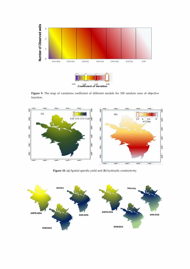
Figure 9. The map of variations coefficient of different models for 100 random runs of objective

function.

Figure 10. (a) Spatial specific yield and (b) hydraulic conductivity.

Figure 11. The spatial and temporal variation of GWL.

4. Conclusions

In this study, the ANFIS, ANN, and SVM models were used to predict groundwater level. The

GOA, CSO, GA, PSO, WA, and KA were used to fine-tune and integrate with the ANN, SVM, and

ANFIS models. Three piezometers (6, 9, and 10) in the Ardebil plain were considered as a case study

for the GWL investigation. The input combinations of time series (up to 12-month lag) were reduced

using principal component analysis (PCA). For the testing phase and piezometer 6 ANFIS-GOA

indicated a value of RMSE: 1.21, MAE: 0.878, NSE: 0.93, and PBIAS: 0.15 which reflected better

performance than the other models. The R2 values were found to vary in the range of 0.84–0.94 and

0.79–0.91 for the ANN (hybrid ANN models and based ANN model) and SVM models (hybrid SVM

models and based SVM model), respectively. The results indicated that the SVM model had the

lowest R2 among other models. It was observed that the ANFIS-GOA yielded the most dominant

performance among other models. From uncertainty analysis, the weakest model in the optimization

of the ANFIS model was ANFIS-GA with a p = 0.87 and d = 0.21. However, general results indicated

that the ANFIS-GOA had better performance than other models. Additionally, the results of

spatiotemporal variations maps of GWL showed that ANFIS-GOA has high accuracy for the

heterogeneous Ardebil aquifer. Future studies can evaluate the accuracy of these models under

climate change conditions. The climate parameters such as temperature and rainfall can be simulated

for future periods. Then, these parameters can be used as input to the models to simulate GWL for

the future periods.

Author Contributions: Conceptualization, A.S., and M.E.; methodology, A.S., and M.E.; writing—review and

editing, A.S., M.E., V.P.S., and A.M..; validation; A.M., A.S., and M.E.; supervision, V.P.S.; Funding acquisition,

A.M. All authors have read and agreed to the published version of the manuscript.

Funding: This work is supported by the Hungarian State and the European Union under the EFOP-3.6.1-16-

2016-00010 project and the 2017-1.3.1-VKE-2017-00025 project.

Conflicts of Interest: The authors declare no conflict of interest.

Acknowledgments: Support of the Hungarian State and the European Union under the EFOP-3.6.1-16-2016-

00010 project and the 2017-1.3.1-VKE-2017-00025 project is acknowledged. We also acknowledge the support of

the German Research Foundation (DFG) and the Bauhaus-Universität Weimar within the Open-Access

Publishing Programme.

References

1. Sattari, M. T.; Mirabbasi, R.; Sushab, R. S.; Abraham, J. Prediction of Groundwater Level in Ardebil Plain

Using Support Vector Regression and M5 Tree Model. Groundwater 2018.

https://doi.org/10.1111/gwat.12620.Jeong,

2. J.; Park, E. Comparative applications of data-driven models representing water table fluctuations. J. Hydrol.

2019, 572, 261–273, doi:10.1016/j.jhydrol.2019.02.051.

3. Alizamir, M.; Kisi, O.; Zounemat-Kermani, M. Modelling long-term groundwater fluctuations by extreme

learning machine using hydro-climatic data. Hydrol. Sci. J. 2018, 63, 63–73,

doi:10.1080/02626667.2017.1410891.

4. Yoon, H.; Kim, Y.; Lee, S.H.; Ha, K. Influence of the range of data on the performance of ANN-and SVM-

based time series models for reproducing groundwater level observations. Acque Sotter. Ital. J. Groundwater.

2019, doi:10.7343/as-2019-376.

5. Mohanty, S.; Jha, M.K.; Kumar, A.; Sudheer, K.P. Artificial neural network modeling for groundwater level

forecasting in a river island of eastern India. Water Resour. Manag. 2010, 24, 1845–1865, doi:10.1007/s11269-

009-9527-x.

6. Natarajan, N.; Sudheer, C. Groundwater level forecasting using soft computing techniques. Neural Comput.

Appl. 2019, 1–18, doi:10.1007/s00521-019-04234-5.

7. Lee, S.; Lee, K.K.; Yoon, H. Using artificial neural network models for groundwater level forecasting and

assessment of the relative impacts of influencing factors. Hydrogeol. J. 2019, 27, 567–579, doi:10.1007/s10040-

018-1866-3.

8. Khan, U.T.; Valeo, C. Dissolved oxygen prediction using a possibility theory based fuzzy neural network.

Hydrol. Earth Syst. Sci. 2016, 20, 2267–2293, doi:10.5194/hess-20-2267-2016.

9. Jeihouni, E.; Eslamian, S.; Mohammadi, M.; Zareian, M.J. Simulation of groundwater level fluctuations in

response to main climate parameters using a wavelet–ANN hybrid technique for the Shabestar Plain, Iran.

Environ. Earth Sci. 2019, 78, 293, doi:10.1007/s12665-019-8283-3.

10. Alian, S.; Mayer, A.; Maclean, A.; Watkins, D.; Mirchi, A. Spatiotemporal Dimensions of Water Stress

Accounting: Incorporating Groundwater–Surface Water Interactions and Ecological Thresholds. Environ.

Sci. Technol. 2019, 53, 2316–2323, doi:10.1021/acs.est.8b04804.

11. Jalalkamali, A.; Sedghi, H.; Manshouri, M. Monthly groundwater level prediction using ANN and neuro-

fuzzy models: A case study on Kerman plain, Iran. J. Hydroinformatics. 2010, 13, 867–876,

doi:10.2166/hydro.2010.034.

12. Trichakis, I.C.; Nikolos, I.K.; Karatzas, G.P. Artificial neural network (ANN) based modeling for karstic

groundwater level simulation. Water Resour. Manag. 2011, 25, 1143–1152, doi:10.1007/s11269-010-9628-6.

13. Fallah-Mehdipour, E.; Haddad, O.B.; Mariño, M.A. Prediction and simulation of monthly groundwater

levels by genetic programming. J Hydro-Environment. Res. 2013, 7, 253–260, doi:10.1016/j.jher.2013.03.005.

14. Moosavi, V.; Vafakhah, M.; Shirmohammadi, B.; Behnia, N. A wavelet-ANFIS hybrid model for

groundwater level forecasting for different prediction periods. Water Resour. Manag. 2013, 27, 1301–1321,

doi:10.1007/s11269-012-0239-2.

15. Emamgholizadeh, S.; Moslemi, K.; Karami, G. Prediction the Groundwater Level of Bastam Plain (Iran) by

Artificial Neural Network (ANN) and Adaptive Neuro-Fuzzy Inference System (ANFIS). Water Resour.

Manag. 2014, 28, 5433–5446, doi:10.1007/s11269-014-0810-0.

16. Suryanarayana, C.; Sudheer, C.; Mahammood, V.; Panigrahi, B.K. An integrated wavelet-support vector

machine for groundwater level prediction in Visakhapatnam, India. Neurocomputing. 2014, 145, 324–335,

doi:10.1016/j.neucom.2014.05.026.

17. Mohanty, S.; Jha, M.K.; Raul, S.K.; Panda, R.K.; Sudheer, K.P. Using artificial neural network approach for

simultaneous forecasting of weekly groundwater levels at multiple sites. Water Resour. Manag. 2015, 29,

5521–5532, doi:10.1007/s11269-015-1132-6.

18. Yoon, H.; Hyun, Y.; Ha, K.; Lee, K.K.; Kim, G.B. A method to improve the stability and accuracy of ANN-

and SVM-based time series models for long-term groundwater level predictions. Comput. Geosci. 2016, 90,

144–155, doi:10.1016/j.cageo.2016.03.002.

19. Zhou, T.; Wang, F.; Yang, Z. Comparative analysis of ANN and SVM models combined with wavelet

preprocess for groundwater depth prediction. Water 2017, 9, 781, doi:10.3390/w9100781.

20. Choubin, B.; Malekian, A. Combined gamma and M-test-based ANN and ARIMA models for groundwater

fluctuation forecasting in semiarid regions. Environ. Earth Sci. 2017, 76, 538, doi:10.1007/s12665-017-6870-8.

21. Das, U.K.; Roy, P.; Ghose, D.K. Modeling water table depth using adaptive Neuro-Fuzzy Inference System.

ISH J. Hydraul. Eng. 2019, 25, 291–297, doi:10.1080/09715010.2017.1420497.

22. Hadipour, A.; Khoshand, A.; Rahimi, K.; Kamalan, H.R. Groundwater Level Forecasting by Application of

Artificial Neural Network Approach: A Case Study in Qom Plain, Iran. J. Hydrosci. Environ. 2019, 3, 30–34,

doi:10.22111/jhe.2019.4972.

23. Jalalkamali, A.; Jalalkamali, N. Groundwater modeling using hybrid of artificial neural network with

genetic algorithm. Afr. J. Agric. Res. 2011, 6, 5775–5784, doi:10.5897/AJAR11.1892.

24. Mathur, S. Groundwater level forecasting using SVM-PSO. Int. J. Hydrol. Sci. Technol. 2012, 2, 202–218,

doi:10.1504/IJHST.2012.047432.

25. Hosseini, Z.; Gharechelou, S.; Nakhaei, M.; Gharechelou, S. Optimal design of BP algorithm by ACO R

model for groundwater-level forecasting: A case study on Shabestar plain, Iran. Arab. J. Geosci. 2016, 9, 436,

doi:10.1007/s12517-016-2454-2.

26. Zare, M.; Koch, M. Groundwater level fluctuations simulation and prediction by ANFIS-and hybrid

Wavelet-ANFIS/Fuzzy C-Means (FCM) clustering models: Application to the Miandarband plain. J. Hydro-

Environ. Res. 2018, 18, 63–76, doi:10.1016/j.jher.2017.11.004.

27. Balavalikar, S.; Nayak, P.; Shenoy, N.; Nayak, K. Particle swarm optimization based artificial neural

network model for forecasting groundwater level in Udupi district. In Proceedings of the AIP Conference; AIP

Elsevier. New York. USA: 2018. doi:10.1063/1.5031983.

28. Malekzadeh, M.; Kardar, S.; Saeb, K.; Shabanlou, S.; Taghavi, L. A Novel Approach for Prediction of

Monthly Ground Water Level Using a Hybrid Wavelet and Non-Tuned Self-Adaptive Machine Learning

Model. Water Resour. Manag. 2019, 33, 1609–1628, doi:10.1007/s11269-019-2193-8.

29. Mirjalili, S.Z.; Mirjalili, S.; Saremi, S.; Faris, H.; Aljarah, I. Grasshopper optimization algorithm for multi-

objective optimization problems. Appl. Intell. 2018, 48, 805–820, doi:10.1007/s10489-017-1019-8.

30. Arora, S.; Anand, P. Chaotic Grasshopper Optimization Algorithm for Global Optimization.

Neural Comput. Appl. 2019. https://doi.org/10.1007/s00521-018-3343-2.

31. Alizadeh, Z.; Yazdi, J.; Kim, J.; Al-Shamiri, A. Assessment of Machine Learning Techniques for Monthly

Flow Prediction. Water 2018, 10, 1676, doi:10.3390/w10111676.

32. Moayedi, H.; Gör, M.; Lyu, Z.; Bui, D.T. Herding Behaviors of Grasshopper and Harris hawk for

Hybridizing the Neural Network in Predicting the Soil Compression Coefficient. Meas. J. Int. Meas. Confed.

2019a, 107389, doi:10.1016/j.measurement.2019.107389.

33. Gampa, S.R.; Jasthi, K.; Goli, P.; Das, D.; Bansal, R.C. Grasshopper optimization algorithm based two stage

fuzzy multiobjective approach for optimum sizing and placement of distributed generations, shunt

capacitors and electric vehicle charging stations. J. Energy Storage. 2020, 27, 101117,

doi:10.1016/j.est.2019.101117.

34. Moayedi, H.; Kalantar, B.; Foong, L.K.; Tien Bui, D.; Motevalli, A. Application of three metaheuristic

techniques in simulation of concrete slump. Appl. Sci. 2019b, 9, 4340, doi:10.3390/app9204340.

35. Kumar, A.; Kumar, P.; Singh, V.K. Evaluating Different Machine Learning Models for Runoff and

Suspended Sediment Simulation. Water Resour. Manag. 2019, 33, 1217–1231, doi:10.1007/s11269-018-2178-z.

36. Khosravi, K.; Daggupati, P.; Alami, M.T.; Awadh, S.M.; Ghareb, M.I.; Panahi, M.; ThaiPham, B.; Rezaei, F.;

Qi, C.; Yaseen, Z.M. Meteorological data mining and hybrid data-intelligence models for reference

evaporation simulation: A case study in Iraq. Comput. Electron. Agric. 2019, 167, 105041,

doi:10.1016/j.compag.2019.105041.

37. Kisi, O.; Yaseen, Z.M. The potential of hybrid evolutionary fuzzy intelligence model for suspended

sediment concentration prediction. Catena 2019, 174, 11–23, doi:10.1016/j.catena.2018.10.047.

38. Dubdub, I.; Rushd, S.; AlYaari, M.; Ahmed, E. Application of Artificial Neural Network to Model the

Pressure Losses in the Water-Assisted Pipeline Transportation of Heavy Oil. Proceedings of the SPE Middle

East Oil and Gas Show and Conference. Soc. Pet. Eng. 2019, doi:10.2118/194742-MS.

39. Moghaddam, H.K.; Moghaddam, H.K.; Kivi, Z.R.; Bahreinimotlagh, M.; Alizadeh, M.J. Developing

comparative mathematic models, BN and ANN for forecasting of groundwater levels. Groundw. Sustain.

Dev. 2019, 100237, doi:10.1016/j.gsd.2019.100237.

40. Fan, J.; Wang, X.; Wu, L.; Zhou, H.; Zhang, F.; Yu, X.; Lu, X.; Xiang, Y. Comparison of Support Vector

Machine and Extreme Gradient Boosting for predicting daily global solar radiation using temperature and

precipitation in humid subtropical climates: A case study in China. Energy Convers. Manag. 2018, 164, 102–

111, doi:10.1016/j.enconman.2018.02.087.

41. Pour, S.H.; Shahid, S.; Chung, E.S.; Wang, X.J. Model output statistics downscaling using support vector

machine for the projection of spatial and temporal changes in rainfall of Bangladesh. Atmos. Res. 2018, 213,

149–162, doi:10.1016/j.atmosres.2018.06.006.

42. Pham, B.T.; Bui, D.T.; Prakash, I. Bagging based Support Vector Machines for spatial prediction of

landslides. Environ. Earth Sci. 2018, 77, 146, doi:10.1007/s12665-018-7268-y.

43. Deo, R.C.; Salcedo-Sanz, S.; Carro-Calvo, L.; Saavedra-Moreno, B. Drought prediction with standardized

precipitation and evapotranspiration index and support vector regression models. In Integrating Disaster

Science and Management, 1st ed.; Elsevier: Amsterdam, The Netherlands, 2018; pp. 151–174.

doi:10.1016/B978-0-12-812056-9.00010-5.

44. Mafarja, M.; Aljarah, I.; Faris, H.; Hammouri, A.I.; Ala’M, A.Z.; Mirjalili, S. Binary grasshopper optimisation

algorithm approaches for feature selection problems. Expert Syst. Appl. 2019, 117, 267–286,

doi:10.1016/j.eswa.2018.09.015.

45. Mehrabian, A.R.; Lucas, C. A novel numerical optimization algorithm inspired from weed colonization.

Ecol. Inform. 2006, 1, 355–366, doi:10.1016/j.ecoinf.2006.07.003.

46. Chandirasekaran, D.; Jayabarathi, T. Cat swarm algorithm in wireless sensor networks for optimized

cluster head selection: A real time approach. Cluster Comput. 2019, 22, 11351–11361, doi:10.1007/s10586-017-

1392-4.

47. Karpenko, A.P.; Leshchev, I.A. Advanced Cat Swarm Optimization Algorithm in Group Robotics Problem.

Procedia Comput. Sci. 2019, 150, 95–101, doi:10.1016/j.procs.2019.02.020.

48. Ramezani, F. Solving Data Clustering Problems using Chaos Embedded Cat Swarm Optimization. J. Adv.

Comput. Res. 2019, 10, 1–10.

49. Orouskhani, M.; Shi, D. Fuzzy adaptive cat swarm algorithm and Borda method for solving dynamic multi‐

objective problems. Expert Syst. 2018, 35, e12286, doi:10.1111/exsy.12286.

50. Pradhan, P.M.; Panda, G. Solving multiobjective problems using cat swarm optimization. Expert Syst. Appl.

2012, 39, 2956–2964, doi:10.1016/j.eswa.2011.08.157.

51. Chu, S.C.; Tsai, P.W.; Pan, J.S. Cat swarm optimization. In Proceedings of the Pacific Rim International

Conference on Artificial Intelligence; Springer: Berlin/Heidelberg, Germany, 2006; pp. 854–858.

doi:10.1007/11801603_94.

52. Saha, S.K.; Ghoshal, S.P.; Kar, R.; Mandal, D. Cat swarm optimization algorithm for optimal linear phase

FIR filter design. ISA Trans. 2013, 52, 781–794, doi:10.1016/j.isatra.2013.07.009.

53. Kennedy, J.; Eberhart, R.C. A discrete binary version of the particle swarm algorithm. Proceedings of 1997

IEEE International conference on systems, man, and cybernetics. Comput. Cybern. Simul. IEEE 1997, 4104–

4108, doi:10.1109/icsmc.1997.637339.

54. Wang, G. G.; Gandomi, A. H.; Alavi, A. H.; Gong, D. A Comprehensive Review of Krill Herd

Algorithm: Variants, Hybrids and Applications. Artif. Intell. Rev. 2019.

https://doi.org/10.1007/s10462-017-9559-1. 55. Abualigah, L.M.; Khader, A.T.; Hanandeh, E.S. A combination of objective functions and hybrid Krill herd

algorithm for text document clustering analysis. Eng. Appl. Artif. Intell. 2018, 73, 111–125,

doi:10.1016/j.engappai.2018.05.003.

56. Asteris, P.G.; Nozhati, S.; Nikoo, M.; Cavaleri, L.; Nikoo, M. Krill herd algorithm-based neural network in

structural seismic reliability evaluation. Mech. Adv. Mater. Struct. 2019, 26, 1146–1153,

doi:10.1080/15376494.2018.1430874.

57. Lu, C.; Feng, J.; Liu, W.; Lin, Z.; Yan, S. Tensor robust principal component analysis with a new tensor

nuclear norm. IEEE Trans. Pattern Anal. Mach. Intell. 2019, doi:10.1109/TPAMI.2019.2891760.

58. Priyadarshi, D.; Paul, K.K. Optimisation of biodiesel production using Taguchi model. Waste Biomass Valori.

2019, 10, 1547–1559, doi:10.1007/s12649-017-0158-9.

59. Yen, H.; Wang, X.; Fontane, D.G.; Harmel, R.D.; Arabi, M. A Framework for Propagation of Uncertainty

Contributed by Parameterization, Input Data, Model Structure, and Calibration/Validation Data in

Watershed Modeling. Environ. Model. Softw. 2014, doi:10.1016/j.envsoft.2014.01.004.

60. Youcai, Z.; Sheng, H. Pollution Characteristics of Industrial Construction and Demolition Waste. In

Pollution Control and Resource Recovery; 2017; USA, New York. doi:10.1016/b978-0-12-811754-5.00004-x.