1

Journal of Hazardous Materials, 197, 285-293, 2011 doi: 10.1016/j.jhazmat.2011.09.086

MODELLING AND SIMULATION OF DENSE CLOUD

DISPERSION IN URBAN AREAS BY MEANS OF COMPUTATIONAL FLUID DYNAMICS

F. Scargiali, F. Grisafi, A. Busciglio and A. Brucato

Dipartimento di Ingegneria Chimica, Gestionale, Informatica e Meccanica Università degli Studi di Palermo

ABSTRACT The formation of toxic heavy clouds as a result of sudden accidental releases from

mobile containers, such as road tankers or railway tank cars, may occur inside urban

areas so the problem arises of their consequences evaluation.

Due to the semi-confined nature of the dispersion site simplified models may often be

inappropriate.

As an alternative, Computational Fluid Dynamics (CFD) has the potential to provide

realistic simulations even for geometrically complex scenarios since the heavy gas

dispersion process is described by basic conservation equations with a reduced number

of approximations.

In the present work a commercial general purpose CFD code (CFX 4.4 by Ansys® ) is

employed for the simulation of dense cloud dispersion in urban areas. The simulation

strategy proposed involves a stationary pre-release flow field simulation followed by a

dynamic after-release flow and concentration field simulations.

In order to try a generalization of results, the computational domain is modelled as a

simple network of straight roads with regularly distributed blocks mimicking the

buildings. Results show that the presence of buildings lower concentration maxima and

enlarge the side spread of the cloud. Dispersion dynamics is also found to be strongly

affected by the quantity of heavy-gas released.

Keywords: Heavy Clouds; Urban Canopy; CFD; Dispersion modeling; complex terrain.

Corresponding author: Alberto Brucato, e-mail: brucato@unipa.it, tel. +3909123863716, fax +390917025020, Dipartimento di Ingegneria Chimica, Gestionale, Informatica e Meccanica, Viale delle Scienze, Ed.6, 90128 Palermo

2

1. INTRODUCTION

Heavy clouds are gaseous mixtures of air and hazardous materials characterized

by a density larger than the environment. The dispersion dynamics of such negatively

buoyant mixtures can be quite different from that of neutrally or positively buoyant

mixtures, depending on the initial cloud Richardson number Ri0, as gravity keeps them

close to the ground where the threat to human safety is highest. Ri0 is dependent on the

initial cloud mass or the mass flux, the relative density excess of the cloud, the

representative size of the cloud, and the ambient wind speed.

Quantitative risk analysis for loss prevention purposes demands successful

simulation of possible accidental events, which is usually carried out by means of

simplified empirical models. For example the so called “box-models” developed in the

past (SLAB, DEGADIS) are widely used in risk analysis procedures [1, 2]. Although

they show satisfactory agreement with available field observations at several sites,

including some with obstacles [3] these models would have problems in areas with large

terrain obstacles especially when the irregular topography of the site plays an important

role [4, 5, and 6]. This is the case of toxic heavy cloud formation inside urban areas, as a

result of sudden accidental releases from mobile containers, such as road tankers or

railway tank cars.

In this field, Computational Fluid Dynamics (CFD) may provide the answer as it

allows the simulation of complex physical processes by describing heat and mass

transport phenomena with fully developed mathematical models. CFD simulations of

pollutant dispersions in the atmospheric boundary layer (ABL) have been carried out in

the past using the k-turbulence model with encouraging results both for neutrally

buoyant pollutants [7] and for heavy gas dispersion processes [8, 9, 10]. Koopman and

Ermak [11] reported a comprehensive review of the methodologies available to describe

3

the dispersion of liquefied natural gas (LNG) in the ABL and stated that “Navier-

Stokes models provide the most complete description of the flow and dispersion of cold,

denser than air cloud in the atmosphere and are well suited for ... dispersion simulations

over complex terrain”.

As concerns gas dispersions in confined or semi-confined areas, CFD tools have been

largely applied to describe neutrally buoyant pollutant dispersions inside urban

canopies, using both RANS [12, 13, 14, 15] and Large Eddy Simulations [16, 17], or to

assess a building canopy model for urban climate planning [18, 19, 20].

CFD techniques were also used to model the release and mixing process of a dense gas

within buildings using RANS [5, 6, 21, 22, 23] and LES [16, 23]. Results showed

reasonable agreement with flow field and gas dispersion experimental data, confirming

that CFD may be an effective tool for understanding wind flow and tracer dispersion in

urban areas.

The aim of the present work is that of setting up a CFD based simulation

strategy for modeling dense (as well as neutrally buoyant) cloud dispersion in urban

environments. The simulation strategy proposed involves a stationary pre-release flow

field simulation followed by a dynamic after-release flow and concentration field

simulations.

In order to generalize the results, the computational domain was modelled as a

simple network of straight roads with regularly distributed blocks mimicking the

buildings. Influence of building fractional area coverage and normalized height, wind

velocity and release quantity on the dispersion phenomenon, was also investigated.

4

2 NUMERICAL SIMULATION

For all numerical simulations of the present work, advantage was taken from the use

of the commercial CFD code CFX-4.4 by Ansys® .

2.1 Basic equations and buoyancy treatment

The simulation runs solve the Reynolds-averaged mass, momentum and scalar transport

equations. If the k- model [24] is used for turbulence, these can be written as:

U

t (1)

gUUU U

U

T

tpt (2)

YDY

t

Y 2

Y

t

U

(3)

The turbulent kinematic viscosity t is obtained from the Prandtl-Kolmogorov equation:

2

tk

C (4)

where k (turbulent kinetic energy) and (its dissipation rate) are computed by solving

appropriate transport equations:

5

k

k

t GGkDt

kD

(5)

k

CGCGk

CDt

D 2

2k31t

(6)

Here, k and ε are turbulent Prandtl numbers for k and ε, respectively.

G is the turbulence production terms due to shear:

TtG UUU ; (7)

whereas Gk is the turbulence production term associated with buoyancy. In the present

case density gradients are practically entirely related to concentration gradients, as

thermal gradients contribution is negligible in the relatively short (200 m) domain

height. The relevant generation term was therefore computed as:

YggG ak

t

k

tk

(8)

where = (Y-a)/a is a density coefficient due to concentration, Y and a being the

densities of the dense gas and background fluid, respectively.

The parameter values used in all simulations are the “consensus” values for k-

model:

C = 0.09; C1 = 1.44; C2 = 1.92; C3 = 0.50; k = 1.0; = 1.3

6

The so called weakly compressible approximation (CFX 4.4 User Manual) was adopted

for the buoyancy treatment instead of the simpler Boussinesq approximation employed

elsewhere [8], in view of the strong density gradients in the proximities of the dense

plume. The main hypothesis behind this approximation is that density variations are

related only to the mean molecular weight and/or temperature changes in the fluid,

while density is assumed to be independent of the pressure field. Density is in practice

expressed by the following equation of state:

RT

MP wref (8)

Hence a constant reference pressure is assumed for the estimation of fluid density; as a

consequence, no sound waves are possible (i.e. sound speed is infinite). The reference

pressure Pref was always set at 1 atm in the present case.

The dense gas dispersion model here adopted has already been validated [25] by

comparison with literature experimental data. The simulations there performed

concerned the experiments carried out by Ayrault et al. [26], involving either neutrally

buoyant or heavy continuous plume releases in an atmospheric wind tunnel. Simulations

were found to correctly predict the switch from the Gaussian profile characterizing

neutrally buoyant dispersions (Fig. 1a) and the bi-modal pattern experimentally

observed with negatively buoyant plumes (Fig. 1b) over a detection line placed 100 mm

downstream a transverse solid fence obstacle 30mm high. The latter feature of the

concentration field is related the appearance of two counter-rotating vortexes (Fig. 1c)

generated by density gradient gravitational effects that are not found in the case of

neutral release. The good agreement between simulation results and experiment can

7

clearly be regarded as a confirmation of the overall soundness of the model here

adopted.

3 SIMULATION STRATEGY

3.1 Simulation Strategy and Computational Details

The computational domain was modelled as a simple network of straight roads with

regular blocks mimicking the buildings. The release point was placed in the middle of a

crossing, as depicted in Fig. 2.

Buildings height, width, and face to face distance were varied in order to assess their

influence on the dispersion process. The total computational grid encompassed about

700 000 cells to guarantee a fine discretization between the buildings. In the vertical

direction, grid cells were clustered close to the ground, to improve discretization where

needed.

The simulation of each release event was conducted in two steps: (i) the first step was

devoted to the generation of the flow field before the release, while the second step (ii)

dealt with the after-release heavy cloud dispersion, as detailed in the next two sections.

3.2 Before-Release Flow Field Simulation (BRFFS)

Having split the simulation in two steps, the stationary pre-release flow field was

conveniently computed by carrying out a “steady-state” simulation, with large savings

of CPU time with respect to a dynamic simulation carried on until steady state

convergence. Moreover the simulated system consisted of an indefinitely wide network

of buildings separated by straight roads. As such the physical system considered is

characterized by periodicities along both roads directions. As a consequence, in order to

obtain the before-release flow field in the indefinitely wide buildings network,

8

simulations could be limited to a much smaller domain surrounding a single building,

by suitably imposing periodic boundary conditions on all four lateral vertical planes, as

depicted in Fig. 2. The computational grid adopted encompassed 26x26x45 = 30426

cells and is reported in Fig. 3. A constant wind speed (7 m/s in most cases) was

imposed at the top boundary of the domain, 200 m above ground level.

In this way the pre-release turbulent flow field obtained does include the mechanical

turbulence generation due to terrain geometry while turbulence generation/suppression

effects by thermal gradients (related to air stability classes) are not considered. In

practice the simulations performed concern stable atmospheric boundary layer (ABL)

conditions. As a matter of fact, mechanical turbulence generation should be expected to

be the major turbulence source at the investigated system scales, while the (larger scale)

turbulence generated by thermal gradients inside the (much higher) ABL can be

expected to be less important.

An examples of vector plot obtained on a vertical plane across the buildings is reported

in Figs. 4 where the presence of a flow recirculation vortex between subsequent

buildings is evident.

Pre-release flow field simulation results were quantitatively compared with

experimental data available in the literature [27]. In Figs. 5 a-b experimental vertical

profiles of normalised horizontal velocity (Ux) obtained behind a building (point A in

the figure) and in the gap between buildings (point B in the figure) are compared with

the relevant simulation results. As it can be seen, the simulated before-release flow-field

(solid lines), is in good agreement with experiment (symbols) with a maximum standard

deviation of 6%. This implies that the computational options here adopted are adequate

for the present simulation purposes.

3.3 Cloud Release and Dispersion Simulation (CRDS)

9

After the release, the presence of the heavy cloud is bound to significantly affect the

local flow field (as witnessed by Fig. 1), and this changes in time while cloud size,

shape and concentration change, due to convection and dispersion phenomena. As a

consequence the flow field undergoes a time dynamics, which has to be accounted for if

realistic simulations are to be carried out. To this end fully time dependent flow field

simulations were carried out in conjunction with cloud scalar transport simulations.

In practice the flow, pressure and turbulence fields predicted in the first step of the

simulation strategy around the generic building, were imposed as initial conditions

around each of the 24 buildings of the new computational domain (see Fig.1). At the

upstream vertical boundary the relevant velocities and turbulence quantities computed

in the first step were adopted as stationary inlet conditions.

At the two lateral vertical sides of the domain, symmetry conditions were specified,

which constrained the bulk flow to be parallel to the lateral boundaries at the locations.

At the upper surface of the domain, quite far away from ground level, a symmetry

condition was also specified, to ensure that velocity stayed horizontal throughout the

simulation and that all quantities had zero gradients across the boundary.

All the above boundary conditions derive in practice from the reasonable assumption

that boundaries were sufficiently far away from the cloud region for possible boundary

condition oversimplifications to negligibly affect simulation results.

Finally, no-slip conditions were imposed at all bottom and building walls, while at the

downstream boundary a “mass flow” boundary condition was specified, which fixes the

total mass outflow to be the same as that entering the domain from all sources.

The flow field simulations of the after-release cloud dispersion process were carried out

in transient conditions until the gas cloud had exited the computational domain. The

time step was chosen in such a way that in all cells a Courant number (defined as the

ratio between simulation time step and the fluid flight time over the cell) smaller than

10

one was obtained. The differentiation scheme adopted was the (mainly second order)

hybrid up-wind for all computed quantities.

The eleven test cases analyzed are listed in Table 1. Buildings height (H), width (W),

and face to face distance (S), were varied from run to run in order to evaluate the

influence of these parameters on the dispersion phenomenon (cases 1 – 5). Two further

scenarios, simulated only for comparison purposes, regarded the assumption of flat

terrain (case 6) and the release of a neutrally-buoyant gas (case 11).

For the cloud dispersion simulations a certain amount of chlorine was assumed

to be suddenly released inside the computational domain. In most cases, the

instantaneous quantity of chlorine released was assumed to be about 90 kg. In order to

assess the influence of released quantity on dispersion dynamics, also the cases of ten

times smaller (case 7) and larger (case 8) releases were considered. In all cases the

release point was assumed to be placed in the middle of the crossing at zero meters

above ground.

Strong simplifications were made as regards the simulation of the complex

physicochemical phenomena involved in the initial seconds of the release, as jet

dispersion, temperature variations, presence of liquid drops, etc. were neglected. In

practice, the entire quantity released was assumed to immediately assume the

temperature and velocity of air in the cells of emission (as obtained in the first step of

the simulation work). In the base case (Case 1 in Table 1) it was assumed that the

release resulted in instantaneously filling a volume of 4m*4m*2m (x, y, z directions

respectively) so resulting in a release of 90.7 kg of chlorine. For the larger release case

(Case 8) it was assumed that the volume entirely filled was 8m*8m*5m (x,y,z directions

respectively) hence resulting in a release of 907 kg of chlorine, while for the smaller

release case (Case 7), it was assumed that a volume of 2m*4m*1m (1x2x1 cells in the

x,y,z directions respectively) was filled with a gas mixture containing 61 % wt of

11

chlorine, hence resulting in a release of 9.02 kg of chlorine. The above simplifications

were considered acceptable in the present work especially in view of the simulation runs

purpose, i.e. studying the influence of buildings and streets geometry on heavy gas

dispersion dynamics in urban environment.

Finally the influence of wind velocity on the heavy cloud dispersion dynamics was

analysed in cases 9 and 10 where a wind speed of respectively 3.5 m/s and 14 m/s at

200 m above ground was imposed.

4 RESULTS AND DISCUSSION

4.1 Heavy-gas dispersion: influence of geometrical parameters

The simulation results obtained for the base case (Case 1 in Table 1) are reported in Fig.

6 as three-dimensional views of chlorine concentration isosurfaces at 15, 60 and 180

seconds after the release. The outer isosurface (coloured in blue) refers to a chlorine

concentration in air of 10 ppm wt. This surface may be regarded as a safe external cloud

boundary in view of the reference concentration of about 25 ppm wt, which is currently

considered as "Immediately Dangerous to Life or Health" (IDLH) by the NIOSH [28].

Two other isosurfaces (visible in lighter green and red colours), corresponding to 100

and 1000 ppm wt, are represented inside the cloud boundary to highlight the width of

strongly affected areas as well as the intensity of gradients in the proximity of cloud

boundary.

As it can be seen, shortly after the release (Fig. 6 a), the cloud has a flat and rounded

shape, as it is typical of heavy clouds. After the first minute (Fig. 6 b) while the higher

concentration isosurface (1000 ppm) has already reached the third street crossing, part

of the cloud is still trapped between the first buildings, where the presence of

12

recirculation vortices slows down cloud dispersion. After three minutes (Fig. 6 c), the

cloud core has already passed through the computational domain, though zones with a

chlorine concentration higher than the IDLH are still present in side streets.

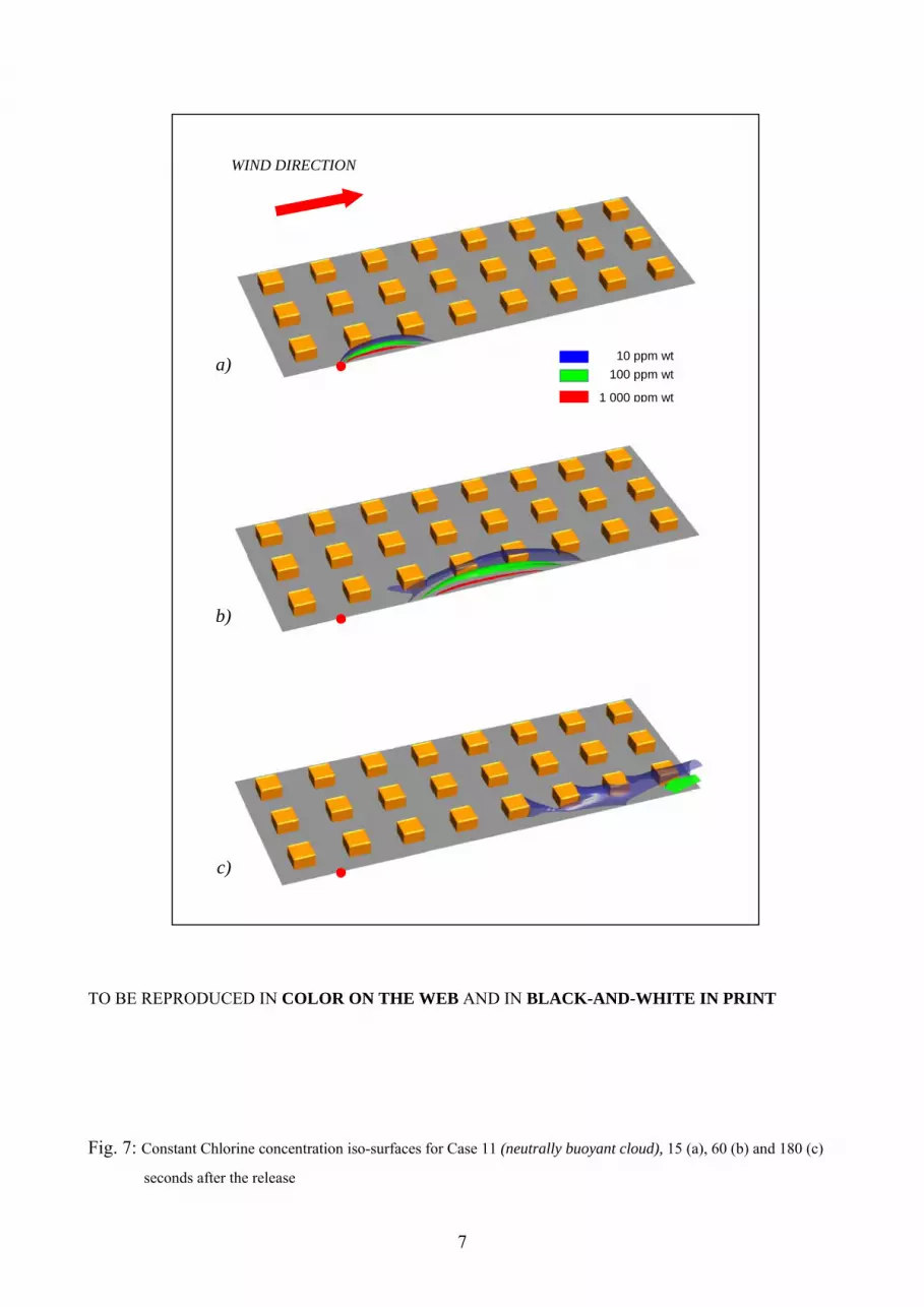
For comparison purposes, the dispersion of a neutrally buoyant cloud (Case 11) is

presented in Figs. 7 a-c. All computational parameters were set identical to “Case 1”,

with the exception of cloud density, which was imposed to be the same as that of

surrounding air. As it can be seen the simulated dispersion process is rather different

from that reported in Figs. 6 a-c, which confirms the importance of buoyancy effects for

the dispersions under investigation. In particular the isodense cloud has a more regular

shape and the presence of buildings has a lower influence on cloud dispersion process,

leaving the cloud freer to move along wind direction (Compare figures 6b and 7b). Also

the cloud moves faster and after 3 minutes the cloud has almost completely left the

computational domain (Fig. 7c).

The influence of buildings height is shown in Figs. 8 a-d, where cloud boundaries 30

seconds after the release, are shown for flat terrain and three different building heights

(Cases 6, 2, 1 and 3 respectively). The ratio between buildings height (H) and buildings

width (W) is used as non-dimensional parameter. As it can be seen, in the case of flat

terrain the cloud is flatter and longer and it is moving faster than in the other cases along

the wind direction. The buildings presence clearly induces larger vertical and lateral

dispersions, also slowing down the cloud.

In order to get a quantitative appreciation of the diverse dispersion conditions, in Fig. 9

maxima of the chlorine mass fraction on the ground are reported versus downwind

distance (for the same cases already shown (Cases 1, 2, 3 and 6)). For each location

downwind the release point, the value reported here is the highest ground-level chlorine

mass fraction experienced by that location during the entire dispersion process. In

practice, each curve reported in Fig. 9 may be regarded as the envelope of all

13

instantaneous spatial distributions of the ground-level chlorine mass fraction

distributions. It is possible to observe that the Cmax achieved at the various distances

decreases when buildings height increases, which is clearly a consequence of the

vertical dispersion induced by the buildings. It is worth noting that the first two curves,

pertaining to flat terrain and 6 m high buildings do practically coincide, which implies

that in order for the building dispersive effects to become important, a minimum

building height is needed. Notably, the same chlorine concentration maximum is

achieved for the two cases at different times after the release, as it can be inferred by

comparing Fig. 8 and Fig. 9.

From what proceeds it may be stated that, using a flat terrain simplified model may be

appropriate for relatively short houses and will result into conservative estimates in the

case of taller buildings. On the other hand, a flat terrain simplified model would never

be able to highlight the presence of dangerous concentration of heavy gas in lateral

streets.

The results obtained when varying the building fractional area coverage “f”:

2

2

SW

Wf

(9)

are reported in Fig. 10, where the maximum concentrations reached at fixed times after

the release are reported as a function of the relevant distances downstream the release

point for the flat terrain case (f=0), case 1 (f=0.15), case 4 (f=0.09) and case 5 (f=0.21).

The effect of buildings is again that of increasing cloud lateral spread while the distance

between buildings gets shorter. This effect contributes to faster dispersion, as it can be

appreciated in Fig. 11.

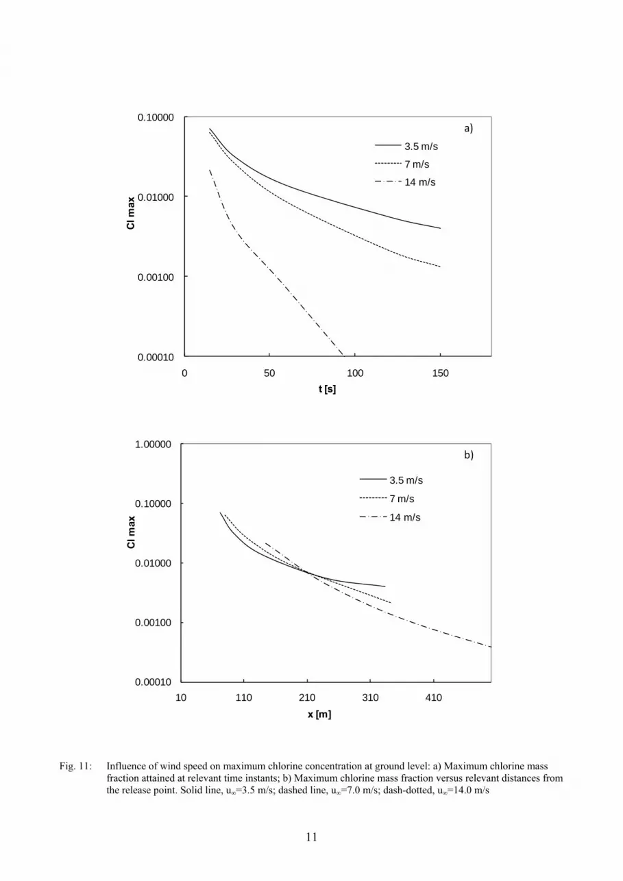
4.2 Influence of wind speed

14

Cases 9 and 10 of Table.1 regarded the same geometrical conditions and released

quantity as in the base case, but different wind speeds 200 m above ground level (3.5

and 14 m/s respectively). Of course, heavy cloud advancing velocity increases when

wind speed increases, and the maximum concentration reached at the given times

strongly decreases as wind speed is increased, as shown in Fig. 11 a, due to the larger

distance travelled by the cloud. It is worth noting that if one reports maximum chlorine

concentrations at ground level versus the relevant distances from the release point

(Fig.11 b) the three curves tend to collapse on a single line, which implies that the

dispersion phenomena occurring are mainly based on convective effects. These are

related to average velocities, which are essentially proportional to the forcing wind. As

a consequence a faster forcing speed substantially results in the same sequence of

pictures, but occurring at a faster pace.

4.3 Influence of released gas quantity

The characteristic behaviour of heavy clouds and their tendency to stratification during

the dispersion process strictly depends on cloud mixture density. As cloud density

decreases when air is mixed in, buoyancy effects decrease until cloud density becomes

practically equal to environment density. For this reason, though starting from the same

initial concentration, a larger quantity of mass released may be expected to experience a

slower dilution than a small quantity so maintaining a “negatively buoyant” behaviour

for a longer time. In Fig. 12 a, b and c three different chlorine concentration contours on

the ground, normalized with respect to the amount released are plotted 30 seconds after

the release, for the same geometry parameters and wind speed. For comparison

purposes, in Fig. 12 d normalised concentration contours for a “neutrally buoyant” gas

release are reported. The three dense gas releases differ only in the total released mass

(9, 90, and 900 kg) and are otherwise identical. If the released gas were neutrally

15

buoyant, its mass fraction would be a purely passively advected scalar; its spatial

distribution would be strictly proportional to the total quantity released and the three

normalised contours reported in Fig. 12 a, b and c would exhibit exactly the same

shape.

Actually, the normalised contours are significantly different from each other,

especially for the largest release (Fig. 12 c, 900 kg) where the lateral dispersion of the

cloud is much higher than in the other cases, with the cloud reaching also the nearby

parallel street while the vertical dispersion is lower. Notably, the concentration

maximum (innermost circle in Figs.12), that lays on the symmetry axis in the case of a

neutrally buoyant release (Fig.12 d), is never on the symmetry axis for the heavy

releases (thus implying bimodal concentration profiles similar to that in Fig. 1 b), with

the displacement from the symmetry axis increasing while the amount released

increases. It is worth noting that the smaller heavy gas release of 9 kg (Fig. 12 a)

behaves almost as a neutrally buoyant cloud as it is possible to appreciate by comparing

Figs. 12 a and 12 d.

The above results show that it is not possible to perform a simulation with a

reference amount released and then to extend the results obtained to all possible

scenarios by simply setting a constant concentration-multiplier proportional to the

amount released. This makes any quantitative generalization of results very hard if not

impossible. On the other hand, results from the present study should help getting a

perception of the sensitivity of dispersion features to the main parameters affecting the

dispersion, and highlighting the differences that should be expected from the much

simpler case of heavy releases over a flat terrain, for which simple models are available

in the literature.

16

5 CONCLUSIONS

A two-step simulation procedure for the dense cloud dispersion able to exploit general

purpose CFD codes has been developed and applied to a simplified geometry

mimicking an infinitely wide urban canopy. The main novelty of the proposed

simulation strategy lies on the fact that simulations were carried out in two steps.

The first step, Before-release flow field simulation (BRFFS), was aimed at

computing the stationary flow and turbulence fields existing before the release. To this

end a suitable three-dimensional generalised “box” representing a generic building

surrounded by straight roads inside the urban area was numerically simulated while

imposing steady-state conditions. The before-release flow fields obtained were found to

be in good agreement with literature experimental data.

In the second step, Cloud Release and Dispersion Simulation (CRDS), the

dispersion of a heavy cloud (chlorine gas) released inside the computational domain

was simulated with proper boundary conditions as assessed in the first step. Also, a

suitable scalar transport equation was added to the purely thermo-fluid-dynamics

equations and the so called “weakly compressible” approximation was adopted to

account for the density effects associated with gas concentration.

Results confirm that the presence of buildings reduces maximum ground

concentrations while enlarging the affected area interested. Due to the larger negative

buoyancy effects, increasing the amount of heavy-gas released slows down the cloud

and increases (normalized) maximum concentrations and lateral spread of the cloud.

The approach proposed in this work may be employed to help setting up and

validating simplified dispersion models by providing the information needed to asses

the dependence of heuristic model parameters on the main geometric features of urban

areas.

17

18

NOMENCLATURE

BRFFS Before Release Flow Field Simulation

C1 parameter in k-model (Eqn. 6), dimensionless

C2 parameter in k-model (Eqn. 6), dimensionless

C3 parameter in k-model (Eqn. 6), dimensionless

C constant in k-model (Eqn. 4), dimensionless

CRDS Cloud Release and Dispersion Simulation

D molecular diffusivity of chlorine in air, m2 s-1

G turbulence production due to viscous forces, J m-3

Gk turbulence production due to buoyancy forces, J m-3

H buildings height, m

IDLH concentration “Immediately Dangerous to Life or Health”, ppm

Pref reference pressure, Pa

R ideal gas constant, Pa m3 K-1 kmol-1

S buildings face to face distance, m

T temperature, K

U vector of velocity field, m s-1

U∞ wind velocity at 200 m above ground level, m s-1

UH wind velocity at top building height (H), m s-1

Ux wind velocity along wind direction (x), m s-1

W buildings width, m

Mw mean molecular weight of the gas mixture, kg kmol-1

Y chlorine mass fraction, dimensionless

f building fractional area coverage, dimensionless

g acceleration gravity, m s-2

19

k turbulent kinetic energy, m2 s-2

p pressure, N m-2

x distance from the release point, m

Greek symbols

dissipation of turbulent kinetic energy, m2 s-2

viscosity, Pa s

T turbulent viscosity, Pa s

kinematic viscosity, m2 s-1

t turbulent kinematic viscosity, m2 s-1

fluid density, kg m-3

Y dense gas density, kg m-3

a background fluid density, kg m-3

k kmodel parameters, dimensionless

kmodel parameters, dimensionless

Y turbulent Schmidt number, dimensionless

20

REFERENCES

[1] S.R. Hanna and D. Strimaitis, Workbook of test cases for vapour cloud source

dispersion models, Center for Chemical Process Safety, AIChE, New York, 1989.

[2] F. Rigas, M. Konstandinidou, P. Centola, G.T. Reggio, Safety analysis and risk

assessment in a new pesticide production line, J. Loss Prev. Process Ind., 16 (2003)

103-109.

[3] R. S. Hanna, J. C. Chang, Use of the Kit Fox field data to analyze dense gas

dispersion modelling issues, Atmos. Environ., 35, (2001) 2231-2242.

[4] N.J.Duijm, B. Carissimo, A. Mercer, C. Bartholomè and H. Giesbrecht,

Development and test of an evaluation protocol for heavy gas dispersion models, J.

Hazard. Mater., 56 (1997) 273-285

[5] M.A. McBride, M.D. Reeves, M.D. Vanderheyden, Lea C.J., Zhou X.X., Use of

Advanced Techniques to Model the Dispersion of Chlorine in Complex Terrain,

Trans IChemE, Part B, Process Saf. Environ. Protect., 79 (B2) (2001) 89-102.

[6] S. Sklavounos, F. Rigas, Simulation of Coyote series trials-Part I: CFD estimation

of non-isothermal LNG releases and comparison with box-model predictions,

Chem. Eng. Sci., 61 (2006) 1434-1443.

[7] A. Huser, P.J. Nilsen, H. Skatun, Application of k- model to the ABL: Pollution in

complex terrain, J. Wind Eng. Ind. Aerodyn., 67 & 68 (1997) 425-436.

[8] F. Scargiali, E. Di Rienzo, M. Ciofalo, F. Grisafi, A. Brucato, Heavy gas dispersion

modelling over a topographically complex mesoscale: a CFD based approach,

Trans IChemE, Part B, Process Saf. Environ. Protect., 83 (B3) (2005) 242-256

[9] I.V. Kovalets, V.S. Maderich, Numerical Simulation of Interaction of the Heavy

Gas Cloud with the Atmospheric Surface Layer, Environ. Fluid. Mech., 6 (2006)

313-340.

[10] A. Luketa-Hanlin, R.P. Koopman, D.L. Ermak, On the application of

computational fluid dynamics codes for liquefied natural gas dispersion, J. Hazard.

Mater., 140 (2007) 504-517.

[11] P. R. Koopman, D. L. Ermak, Lessons learned from LNG safety research, J.

Hazard. Mater., 140 (2007) 412-428.

21

[12] J.J. Baik, J.J. Kim, On the escape of pollutants from urban street canyons, Atmos.

Environ., 36, (2002) 527-536.

[13] M. Schatzmann, B. Leitl, Validation and application of obstacle-resolving urban

dispersion models, Atmos. Environ., 36 (2002) 4811- 4821.

[14] J.J. Kim, J. J. Baik, Effects of inflow turbulence intensity on flow and pollutant

dispersion in an urban street canyon, J. Wind Eng. Ind. Aerodyn., 91 (2003) 309-

329.

[15] I.R. Cowan, I.P. Castro, A.G. Robins, Numerical considerations for simulations of

flow and dispersion around buildings, J. Wind Eng., 67 & 68 (1997) 535-545.

[16] A. Walton, A.Y.S. Cheng, Large-eddy simulation of pollution dispersion in an

urban street canyon-Part II: idealised canyon simulation, Atmos. Environ., 36

(2002) 3615-3627.

[17] R.F. Shi, Z.S. Cui, Z.S. Wang, Z.S. Xu, Z.S. Zhang, Large eddy simulation of wind

field and plume dispersion in building array, Atmos. Environ, 42 (2008) 1083-1097

[18] Y. Ashie, V. T. Ca, T. Asaeda, Building canopy model for the analysis of urban

climate, Atmos. Environ., 81 (1999) 237-248.

[19] E.R. Marciotto, A.P. Oliveira, S.R. Hanna, Modelling study of the aspect ratio

influence on urban canopy energy fluxes with a modified wall-canyon energy

budget scheme, Build. Environ., 45 (2010) 2497-2505.

[20] Memon R.A., Leung D.Y.C., Liu C.H., Effects of building aspect ratio and wind

speed on air temperature in urban-like street canyons, Build. Environ., 45 (2010)

176-188.

[21] S. Gilham, D.M. Deaves, P. Woodburn, Mitigation of dense gas releases within

buildings: validation of CFD modelling, J. Hazard. Mater., 71 (2000) 193-218

[22] S. Sklavounos, F. Rigas, Validation of turbulence models in heavy gas dispersion

over obstacles, J. Hazard. Mater., A108 (2004) 9-20.

[23] S.R. Hanna, M.J. Brown, F.E. Camelli, S.T. Chan, W.J. Coirier, O.R. Hansen, A.H.

Huber, S. Kim, R.M. Reynolds, Detailed simulations of atmospheric flow and

dispersion in downtown Manhattan, Bull American Meteorol. Soc., 12 (2006) 1713-

1726.

[24] B.E. Launder and D.B. Spalding, The numerical computation of turbulent flows,

Comp. Meth. Eng., 3 (1974) 269-289

22

[25] F. Scargiali, F. Grisafi, G. Micale, A. Brucato, CFD simulation of dense plumes in

an atmospheric wind tunnel, Proc. LP 2004, 31 May – 3 June 2004, Praha, Czech

Republic, ISBN 80-02-01574-6, (2004) 3137-3142.

[26] M. Ayrault, S. Simoëns, P. Méjean, Negative buoyancy effects on the dispersion of

continuous gas plumes downwind solid obstacles”, J. Hazard. Mater., 57 (1998)

79-103.

[27] S.R. Hanna, S. Tehranian, B. Carissimo, R.W. Macdonald, R. Lohner, Comparison

of model simulations with observations of mean flow and turbulence within simple

arrays, Atmos. Environ., 36 (2002) 5067-5079.

[28] U.S. National Institute for Occupational Safety and Health, NIOSH pocket guide to

chemical hazards, J.J. Keller and Associates, Inc., USA, 1997.

ACKNOWLEDGMENTS

This research work was carried out under financial support by University of Palermo.

23

FIGURES CAPTIONS

Fig. 1: Simulation and experiment for the release of continuous plumes: a) neutrally

buoyant plume (env=1); b,c) dense plume (env=2); a,b): horizontal mean

concentration profiles on a transversal line 0.5 m downwind the release point:

symbols: experimental data by Ayrault et al [26]); solid lines: CFD simulation

results [25]; c) dense plume vector plot over a vertical-transversal plane 0.1 m

downwind the release point [25].

Fig. 2: Sketch of the computational domain. The box represents the computational

domain used for the “Before Release Flow Field Simulations” (BRFFS).

Fig. 3: Computational domain for the “Before Release Flow-Field Simulations”

(BRFFS)

Fig. 4: Vector plot on a vertical plane, across a building and parallel to wind direction

(all vectors sharing the same size in order to highlight flow structure)

Fig. 5: Vertical profiles of normalized velocity (Ux/UHx) in the wake a), and in the gap

b): experimental data; - model data

Fig. 6 Constant chlorine concentration isosurfaces for Case 1 (base case), 15 (a), 60

(b) and 180 (c) seconds after the release

Fig. 7: Constant chlorine concentration isosurfaces for Case 11 (neutrally buoyant

cloud), 15 (a), 60 (b) and 180 (c) seconds after the release

Fig. 8: Constant chlorine concentration isosurfaces for different building heights (H),

30 seconds after the release: a) flat terrain (Case 6); b) H=6 m (Case 2); c)

H=12 m (Case 1); d) H = 24 m (Case 3)

Fig. 9: Influence of normalized buildings height on the maximum concentrations

achieved versus relevant distances from the release point

Fig. 10: Influence of buildings fractional area coverage on the maximum chlorine

concentrations achieved versus relevant distances from the release point

Fig. 11: Influence of wind speed on maximum chlorine concentration at ground level:

a) Maximum chlorine mass fraction attained at relevant time instants; b)

Maximum chlorine mass fraction versus relevant distances from the release

point. Solid line, u∞=3.5 m/s; dashed line, u∞=7.0 m/s; dash-dotted, u∞=14.0

m/s

Fig. 12: a), b), c): Chlorine normalised contours 30 seconds after the release. Quantity

released: a) 9 kg; b) 90 kg; c) 900 kg; chlorine contours: a) 0.1, 10, 100,

24

1000, ppm wt; b) 1, 10,100, 1000, 10 000 ppm wt; c) 10, 100, 1000, 100 000

ppm wt, innermost circle: location of chlorine maximum concentration.

d) Neutrally buoyant gas normalised contours 30 seconds after the release.

Quantity released: 90 kg; contours: 1, 10,100, 1000, 10 000 ppm wt. Grey

circle: location of chlorine maximum concentration

Table 1: Cases analysed

1

Table 1: Cases analysed

Case Quantity released

[kg]

Initial cloud size [m3]

env H [m] S [m] W [m] U∞ [m/s]

[200 m height]

H/W f %

fract. area

coverage

1 (Base) 90.7 34 2.45 12 32 20 7.0 0.6 15

2 90.7 34 2.45 6 32 20 7.0 0.3 15

3 90.7 34 2.45 24 32 20 7.0 1.2 15

4 90.7 34 2.45 12 48 20 7.0 0.6 9

5 90.7 34 2.45 12 24 20 7.0 0.6 21

6 (Flat terrain) 90.7 34 2.45 0 ∞ 0 7.0 0 0

7 9.02 3.4 2.45 12 32 20 7.0 0.6 15

8 907 344 2.45 12 32 20 7.0 0.6 15

9 90.7 34 2.45 12 32 20 3.5 0.6 15

10 90.7 34 2.45 12 32 20 14.0 0.6 15

11 (neutrally-buoyant cloud) 90.7 34 1 12 32 20 7.0 0.6 15

1

Fig. 1: Simulation and experiment for the release of continuous plumes: a) neutrally buoyant plume (ρ/ρenv=1); b,c) dense plume

(ρ/ρenv=2); a,b): horizontal mean concentration profiles on a transversal line 0.5 m downwind the release point: symbols:

experimental data by Ayrault et al [27]); solid lines: CFD simulation results [26]; c) dense plume vector plot over a

vertical-transversal plane 0.1 m downwind the release point [26].

0,0

0,2

0,4

0,6

0,8

1,0

-400 -200 0 200 400y (mm)

C/C

max

a)

0,0

0,2

0,4

0,6

0,8

1,0

-400 -200 0 200 400

y (mm)

C/C

max

b)

c)

2

Fig. 2: Sketch of the computational domain for chlorine release. The box represents the computational domain used for the “before release flow field simulations”(BRFFS).

U∞

B A

x

y

z

WIND DIRECTION

RELEASE POINT U∞= 7 m/s at 200 m

3

Fig. 3: Computational domain for the “Before Release Flow-Field Simulations” (BRFFS)

4

Fig 4: Vector plot on a vertical plane across a building and parallel to wind direction (all vectors sharing the same

size in order to highlight flow structure)

x

z

WIND DIRECTION

5

0

1

2

3

4

5

6

-0.2 0 0.2 0.4 0.6 0.8 1 1.2

Ux/UHx

z/H

A

a)

0

1

2

3

4

5

6

-0.2 0 0.2 0.4 0.6 0.8 1 1.2Ux/UHx

z/H B

b)

Fig. 5: Vertical profiles of normalised velocity (Ux/UHx) in the wake a), and in the gap b): • experimental data; - model

data.

6

TO BE REPRODUCED IN COLOR ON THE WEB AND IN BLACK-AND-WHITE IN PRINT

Fig. 6: Constant Chlorine concentration iso-surfaces for case 1 (base case), 15 (a), 60 (b) and 180 (c) seconds after the

release

RELEASE POINT

10 ppm wt

100 ppm wt

1 000 ppm wt

WIND DIRECTION

a)

b)

c)

7

TO BE REPRODUCED IN COLOR ON THE WEB AND IN BLACK-AND-WHITE IN PRINT Fig. 7: Constant Chlorine concentration iso-surfaces for Case 11 (neutrally buoyant cloud), 15 (a), 60 (b) and 180 (c)

seconds after the release

10 ppm wt

100 ppm wt

1 000 ppm wt

WIND DIRECTION

a)

b)

c)

8

TO BE REPRODUCED IN COLOR ON THE WEB AND IN BLACK-AND-WHITE IN PRINT Fig. 8: Constant Chlorine concentration iso-surfaces for different building heights (H), 30 seconds after the release:

a) H/W=0 (Case 6); b) H/W=0.3 m (Case 2); c) H/W=0.6 m (Case 1); d) H/W = 1.2 m (Case 3)

WIND DIRECTION

10 ppm wt

100 ppm wt

1 000 ppm wt

RELEASE POINT

a)

b)

c)

d)

9

0.0001

0.0010

0.0100

0.1000

0 100 200 300 400 500

Cl m

ax

x [m]

H/W= 0

H/W = 0.3

H/W = 0.6

H/W = 1.2

Fig. 9: Influence of normalized buildings height (H/W) on the maximum concentrations achieved versus relevant distances from the release point

10

0.0001

0.0010

0.0100

0.1000

0 100 200 300 400 500

Cl m

ax

x (m)

f = 0f= 9 %f = 15 %f = 21 %

Fig. 10: Influence of buildings fractional area coverage on the maximum chlorine concentrations achieved versus relevant distances from the release point

11

0.00010

0.00100

0.01000

0.10000

0 50 100 150

Cl m

ax

t [s]

3.5 m/s

7 m/s

14 m/s

a)

0.00010

0.00100

0.01000

0.10000

1.00000

10 110 210 310 410

Cl m

ax

x [m]

3.5 m/s

7 m/s

14 m/s

b)

Fig. 11: Influence of wind speed on maximum chlorine concentration at ground level: a) Maximum chlorine mass

fraction attained at relevant time instants; b) Maximum chlorine mass fraction versus relevant distances from the release point. Solid line, u∞=3.5 m/s; dashed line, u∞=7.0 m/s; dash-dotted, u∞=14.0 m/s

12

Fig. 12: a), b), c): Chlorine normalised contours 30 seconds after the release. Quantity released: a) 9 kg; b) 90 kg; c)

900 kg; chlorine contours: a) 0.1, 10, 100, 1000, ppm wt; b) 1, 10,100, 1000, 10 000 ppm wt; c) 10, 100, 1000, 100 000 ppm wt; innermost circles: location of chlorine maximum concentration. d) Neutrally buoyant gas normalised contours 30 seconds after the release. Quantity released: 90 kg; contours:

1, 10,100, 1000, 10 000 ppm wt