Pergamon Atmospherw Enmronment Vol 29, No 16, pp 2075-2087, 1995 Copynght © 1995 Elsewer Setence Ltd

Pnnted m Great Bntam All rtghts reserved 1352-2310/95 $9 50 + 000

1352-2310(94)00244-4

DEVELOPMENT OF DENSE GAS DISPERSION MODEL FOR EMERGENCY PREPAREDNESS

M A N J U M O H A N , T. S. P A N W A R and M. P. S I N G H Centre for Atmospheric Soences, Indian Institute of Technology, Hauz Khas,

New Delhi 110016, India

(Ftrst received 10 February 1993 and in final form 8 May 1994)

Abstract--Mathematical models are recognized as important tools for providing quantitative assessment of the consequences of the aeodental release of hazardous materials. In several accidental release situations, denser-than-air vapour clouds are formed which exhibit dispersion behavlour markedly different from that observed for passive atmospheric pollutants. The present work undertakes the development and validation of conceptually simple and computationally efficient dense gas dispersion models which could be used for emergency response. Here, IIT Heavy Gas Models I and II have been developed for instantaneous and continuous releases, respectively, of dense toxic materials in the atmosphere. Sensitivity tests have been performed to determine the various empirical coefficaents which are found to be quite different than those used in the earlier studies. Particular emphasis has been laid on model validation by comparing their performance against relevant field trial data (Thorney Island, Burro Series and Maplin Sands Trials) as well as with other models. On the basis of statistical evaluation, a good performance of the model has been established. The performance of the IIT Heavy Gas Model is close to the model showing the best performancc amongst 11-14 other models developed in various countries. Using the IIT Heavy Gas Model, the Safe disl ance/vulnerable zones can be easily estimated for different meteorological and release condi- tions for the; storage of various hazardous chemicals.

Key word index: Gravity slumping, air entrainment, cloud heating, sensitivity analysis, model validation, statistical evaluation, vulnerable zones.

1. INTRODUCTION

The increasing use of hazardous toxic substances and the associated potential risk warrant development of practical and well-tested mathematical models for es- timating vulnerable zones in relation to their acci- dental release in the atmosphere. In many of the accidental release situations, denser-than-air clouds are formed. The negative buoyancy modifies the dis- persion of a toxic gas cloud and its modelling requires an approach different from a positively buoyant or a passive gas cloud as it tends to hug the ground and does not readily (disperse. Gravity driven flow and stable stratification are the key factors making dense gases behave differently when released into the atmo- sphere (Hunt et al, 1983).

The models which give the most physically com- plete description of dense gas dispersion are those that are based on the three-dimensional, time-dependent conservation equations Examples of this type of model include FEM3, SIGMET, MARIAH, and ZEPHYR (Ermak et al., 1987). At the intermediate level of completeness and complexity are the sim- ilarity type models. These type of models use simplifi- ed forms of the conservation equations that are obtained by averaging the cloud properties over

the cross wind plane. Quasi-three-dimensional solu- tions are obtained by using similarity profiles, i.e, by assuming a cross wind profile for the concentration and other cloud properties. Examples of this type of model include SLAB, HEGADAS, and DEGADIS. At the simplest level are the modified Gaussian plume models. These models are usually used to simulate continuous releases and employ a variety of modifica- tions to include the effects of dense gas dispersion within the Gaussian plume model for trace gas re- leases (Ermak et al., 1987).

The intermediate class of models for heavy gas release and dispersion has been identified by a variety of names. Wheatly and Webber (1984) used the term "box models", Blackmore et al. (1982) "Slab models", and Havens (1982) "box (top-hat profile) models". The results from these type of models have proved in the past as the important ingredients for effective contingency planning, in-crisis remedial action and other decision measures. Hence the present work undertakes the development and validation of reasonably simple op- erational heavy gas dispersion model which could be used for emergency response. The model is essentially a numerical box type of model which includes all the basic features tenable to dense gas dispersion in a real- istic manner. In order to verify the accuracy of various

2075

2076 M . M O H A N et al

input parameters and empirical coefficients, sensitiv- ity tests have been performed through several model simulations using the field data. The most essential part of the model development effort is to test the model against observed data as well as with other models already available for this purpose. In this regard, rigorous statistical tests have been performed which indicate a good model performance. Being computatlonally efficient, these models are well suited for emergency response purposes.

One of the important aspects in these models is the appropnate transition from dense gas to passive phase. Often, matching of various parameters before and after transition lacks strong physical foundation. For example, in case of catastrophic/instantaneous release of toxic materials, appropriate dispersion parameters after transition are not available. There- fore, normally one resorts to the use of dispersion parameters which are tenable for continuous releases upto distances of 1 km from the source and for an averaging time varying 10-30 min. In the present work, an attempt has been made to incorporate formula- tion based on turbulent energy density and cloud dimensions after transition to the passive phase. Al- though it requires more in-depth study, it ensures continuity of the various parameters after the transition phase and gives more realistic results.

2. M O D E L F O R M U L A T I O N

The model developed is a numerical box model where governing equations take into account the rel- evant physical processes associated with dense gas dispersion, namely, gravitational slumping, entrain- ment of air, cloud heating, and finally, transition to the passive phase. The model consists of two versions; while IIT Heavy Gas Model-I is valid for instan- taneous releases, l iT Heavy Gas Model-II is suitable for continuous releases of dense gases. The governing model equations are solved numerically using forward finite difference scheme for IIT Heavy Gas Model-I and the Runge--Kutta method for IIT Heavy Gas Model-II. The models have been developed taking into account the work carried out earlier by Kaiser and Walker (1978), Cox and Carpenter (1979), Britter and McQuaid (1988), Van Ulden (1974), Britter and Griffiths (1982), Jagger (1983), Singh et al. (1991), and several other workers. Cloud geometry is considered to be cylindrical in the case of instantaneous release and rectangular in the case of continuous release in the conventional manner. The main input parameters to the mathematical model for dispersion calculations are the emission rates and the relevant meteorological parameters. Numerical solution of the equations evaluates the cloud characteristics, i.e. radius (length in the case of continuous release), height, density, temperature and amount of air entrained at each time step. An appropriate treatment for the cloud disper-

sion parameters is made after transition to the passive phase. The concentration distribution is assumed to be Gaussian in nature.

2.1. Dense gas dispersion model for instantaneous re- lease of toxic materials: IIT Heavy Gas Model-I

The instantaneous release model described here is concerned mainly with the rapid releases of large quantities of toxic gases to the atmosphere and is thus intended to model "puff" releases. The characteristic features of dense gas dispersion included in the model are as follows.

(a) Gravitational slumping. Assuming that the puff is in the form of a cylinder of height h and radius R, the velocity of the edge of the cloud is adequately described by the liquid column analogy (Cox and Carpenter, 1979; Eidsvik, 1980; Fay, 1983; Hanna and Drivas, 1987; McQuaid, 1987):

dR ,,[" , Ap'~ 1/2 - -~=t~gn-~ ; (1)

where t is the time after slumping has started, g is the acceleration due to gravity, p is the density within the cylinder and Ap = p - p , , p, being the density of ambi- ent air and K is a constant.

(b) Entrainment of air. Air is presumed to be en- trained both at the edges and at the top of the cloud. Although some of the models consider only top en- trainment based on Van Ulden's Dutch Freon experi- ments, in the present model we have considered both top and edge entrainment based on our model simula- tions and studies.

The rate at which air is entrained into the cloud is given by (Cox and Carpenter, 1979; Hanna and Drivas, 1987; McQuaid, 1987):

dR dM'= P'(nR 2) U" + a* 2nRh p" (2)

where a* is a parameter which controls the rate of edge entrainment of air. U, is the top entrainment velocity which is a function of Richardson number Ri and the longitudinal turbulence velocity U~.

The entrainment velocity Uc depends on U~ and Ri as follows:

U e = or' U I R ! - 1 (2a)

where

(gl,) Ap (2b) R,= U"" ~ p'-~.

Equation (2a) is valid when U, <~ U~. Here Um is the longitudinal turbulence velocity which is propor- tional to the friction velocity U . with the constant of proportionality being 3.0 (very unstable, category A-B weather), 2.4 (neutral, category C-D weather) or 1.6 (very stable, category E-F weather). ~' is an en- trainment constant and Is is the turbulence length scale which is a function of the height above the ground and of stability. An expression for l, as a func-

Dense gas dispersion model 2077

tion of h is given by Taylor et al. (1970) as

l, = 5.88 h ° 4s.

(c) Cloud heatinff. Since there is a temperature dif- ference between the ground and the airborne vapour, it is necessary to consider the mechanisms by which the cloud can absorb heat.

The rate of change of temperature of the cloud including the effect of the entrained air is given by

dMa Ce=ATa +0rR2) Q¢ dT dt

(3) dt M. C~ + MCp

where C~ is the specific heat capacity of the toxic material and M is its mass (Kaiser and Walker, 1978). Here, Q~ is the rate of heating of the cloud due to the turbulent natural convection and forced convection. It depends on the temperature difference between the ground and the cloud and on various thermodynamic properties of the material (McAdams, 1954; Fryer and Kaiser, 1979). Cp~ and M~ are the specific heat capa- city and mass of the entrained air, respectively.

Thus, equations (1)-(3) form a set of three coupled linear differential equations which may be solved nu- merically for the independent variables R, M= and T.

(d) Transition to the passive phase. Sooner or later the cloud of dispersing gas becomes so dilute that the atmospheric turbulence takes over. The criteria used to determine when this transition occurs are as fol- lows.

(i) In the case of radius, the atmospheric turbu- lence is taken to dominate the spread when dR/dt has decreased so that

Co=FApghl'/2 (4) L P = J

where C is a constant that depends on the weather category. C takes on the values 0.22, 0.16, 0.11, 0.08, 0.06 and 0.04 in category A, B,C, D, E, and F weather, respectively.

For the case of growth of height, Cox and Roe (1977) indicate that U~ has a limiting value approxim- ately equal to hi, so that this can be used as a transition criterion, i.e.

U, = U1 (5)

When both the above conditions are satisfied, transition is made to the passive phase.

(ii) The density difference Ap is also calculated and if Ap<0.001 Kgm -3, it is assumed that the plume becomes passive even if equations (4) and (5) are not satisfied.

Based on the above discussion, the governing equa- tions of the model are solved numerically to obtain the cloud growth aad the other relevant parameters as a function of time. The above-mentioned system of equations provides us with R, h, M=, T, and V at each time step. In this manner, the cloud dimensions and other relevant parameters are determined.

(e) Concentration within the puff. It is assumed that the material is distributed in a Gaussian fashion. It may be argued that the assumption of a Gaussian profile is not consistent with the simultaneous as- sumption that gravity driven slumping is important where a top-hat profile could be assumed to be more realistic. However, a comparison of the hazard range based on average centreline concentration shows little difference in the prediction (Kaiser and Walker, 1978; Davidson, 1986) and hence for all practical purposes it is appropriate to assume Gaussian distribution.

The radius R and height h are taken to define the 10% edge oftbe cloud which is a conventional assump- tion. So, the standard deviations of the cloud in the lateral and vertical directions are given by ay = R/2.14 and a~=h/2.14 for all values of x. After transition of the cloud to the passive phase, cloud dimensions are taken as (Van Ulden, 1974; Eidsvik, 1980):

R = RT + 2 U , ( t - iT) (6)

h = hT + ~1U,(t-- tT) (7)

where ~tl is a coefficient for vertical entrainment with a value of 0.4; RT and hT are the radius and height at the time of transition iT; U, is the friction velocity due to mechanical turbulence and is related to the mean wind speed by U, = (7[7 where C is a "surface drag constant" that depends on the weather category. These are based on the equations derived from the criterion of Van Ulden (1974) that at the end of the slumping phase turbulence energy density equals the mean potential energy density and on equation (1) (Ontario Ministry of Environment, 1983). Moreover, cloud dimensions in the above form ensure smooth- ness of dispersion parameters when transition to the passive phase occurs. Also, most of the dispersion parameters cited in the literature are valid only for continuous releases and are not strictly applicable to instantaneous release situations. Although it calls for a more in-depth study, but at present the disper- sion parameters based on cloud dimensions given by equations (6) and (7) seem to be physically more appropriate.

2.2 Dense oas dlspersion model for continuous release of tomc materials: I IT Heavy Gas Model-lI

This section is concerned with the development of a dispersion model for the continuous release of dense toxic materials. Based on experimental evidence, a rectangular source geometry is considered appropri- ate for continuous releases. The plume can be thought to consist of a number of rectangular elements or "puffs" emerging from the source at regular time inter- vals. The model follows the development of these puffs at a series of downwind points. These puffs are im- mediately assumed to advect with the ambient wind. The plume also slumps due to the action of gravity and is allowed to entrain air through its sides and top surface. A considerable simplification is obtained by allowing the plume to slump only in the lateral direc- tion. With advectlon downwind, the cloud gains

2078 M. MOHAN et al

buoyancy by entraining air and if the cloud is cold, by absorbing heat from the ground. Eventually the plume begins to disperse in a passive manner through the action of atmospheric turbulence. In order to follow the dispersion processes down to low concen- trations, especially important for toxic gases, a virtual source passive dispersion model is fitted to the slump- ing plume.

The equations used for the development of the continuous release model (IIT Heavy Gas Model-II) are based on the work carried out earlier by Cox and Carpenter (1979), Jagger (1983), Wheatley et al. (1987), etc. The equations are similar in form to the ones used for the instantaneous release model with due consid- eration being given for a changed shape of the gas cloud, i.e. rectangular instead of cylindrical. All the basic phenomena associated with dense gas disper- sion, namely, gravity slumping, entrainment of air, cloud heating and transition to the passive phase are properly accounted for.

The brief description of the model equations used m IIT Heavy Gas Model-II is given below:

(a) Mass, density and volume equations for the plume. For a steady plume entraining air, the mass of a small plume element, width 2L, density Pc and height h, at a distance x from the source is

M(x)=Ma+Ms=2L(x)h(x)p~(x)dx (8)

M1 a + ~,1~ = 2L(x)h(x)Pc (x) Uc(x) (9)

(I= 2L(x) h(x) U,(x) (10)

U c = dx/dt (11)

pc = (.,~7/, + .~/s)/b (12)

v=TcJ~la + Tcl('ls. (13) paT. psTs

(b) Gravity slumpinff.

dL --d-~ = k(o'h)l/2

o ' = o ( p c - p,)/pa

(14)

(15)

dL k f 9'I)" ]1/2 ~xx- L2LU2J ' (16)

(c) Entrainment of air.

dM, dL - - = 2hdxpa~x ~ + 2LdxpaU~ (17)

dt

dl(4~ _ p, l?oq dL + 2Lp.U.. (18)

dx L dx

(d) Cloud heatino.

dTc 1

dx = IVl a C p, + Kt s C ps

[ ( T , - - T c ) C ~ - ~ + 2 L Q c 1. (19)

(e) Criteria for transmon to the passive phase. (i) The rate of lateral growth of the plume due to atmospheric turbulence must be greater than that due to gravity spreading, i.e. dw/dx > dL/dx where w is the half-width of a Gaussian plume. Additionally the rela- tion Ue > U1 must be satisfied. (ii) The plume is also considered to be passive when the density difference between the cloud and the surrounding air has be- come less than some arbitrarily chosen small value. In the present case, this value is taken as 0.001 kg m -3.

(f) Concentration wtthin the plume.

C(x,y,z) = Msexp[ -- y2/2a2(x)] exp[ -- z2/2tr~(x)]

and

(20)

C(x, O, O) = ~18 [hey(x) a~(x) Uc]" (21)

Here additional symbols/notations used in this model are as follows:

Ma, Ms the gaseous mass fluxes pertaining to air and toxic substance, respectively

12 the gaseous volume flux d downwind distance travelled by the gas

cloud in dt time Uc velocity of gas cloud Pa density of entrained air Pc density of gas cloud pg density of toxic substance (gas) Ta temperature of entrained air or ambient

temperature Tg temperature of ground surface Tc temperature of gas cloud Cpa specific heat capacity of entramed air Cps specific heat capacity of the toxic mater-

ial (gas).

Similar to the instantaneous case, here also the concentration profile is taken to be Gaussian. The dispersion parameters ~y and a= before transition are given by L/2.14 and h/2.14, respectively. After transition, the dispersion parameters are calculated using the Briggs Urban Formulation.

The initial conditions of the passive phase are de- fined using continuity of plume height, h t, and half- width, Lt, at the transition point. For proper match- ing of ay and ¢r~ values at the transition point, two separate virtual sources are used, one for lateral plume spread and another for height variation. The position of these virtual sources are determined by performing successive iterations.

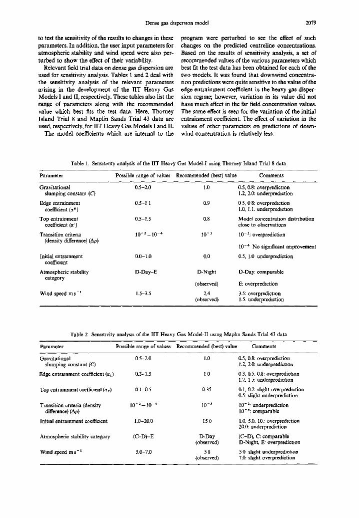
2.3. Sensitivity analysis

Sensitivity analysis is performed to determine the importance of various parameters on the model out- put. The various entrainment coefficients and tran- sition criteria values used in the model were perturbed

Dense gas dlspersmn model 2079

to test the sensitivity of the results to changes in these parameters. In addition, the user input parameters for atmospheric stability and wind speed were also per- turbed to show the effect of their variability.

Relevant field trial data on dense gas dispersion are used for sensitivity analysis. Tables 1 and 2 deal with the sensitivity analysis of the relevant parameters arising in the development of the l i T Heavy Gas Models I and II, respectively. These tables also list the range of parameters along with the recommended value which best fits the test data. Here, Thorney Island Trial 8 and Maplin Sands Trial 43 data are used, respectively, for l i T Heavy Gas Models I and II.

The model coefficients which are internal to the

program were perturbed to see the effect of such changes on the predicted centreline concentrations. Based on the results of sensitivity analysis, a set of recommended values of the various parameters which best fit the test data has been obtained for each of the two models. It was found that downwind concentra- tion predictions were quite sensitive to the value of the edge entrainment coefficient in the heavy gas disper- sion regime; however, variation in its value did not have much effect in the far field concentration values. The same effect is seen for the variation of the initial entrainment coefficient. The effect of variation in the values of other parameters on predictions of down- wind concentration is relatively less.

Table 1. Sensmvlty analysis of the IIT Heavy Gas Modem using Thorney Island Trial 8 data

Parameter Possible range of values Recommended (best) value Comments

Gravitational 0.5-2.0 1.0 slumping constanl (C)

Edge entrainment 0.5-1 1 0.9 coefficient (~*)

Top entrainment 0.5-1.5 0.8 coefficient (~')

Transition criterm 10- 2_ 10- 4 10- 3 (density difference',)(Ap)

Initial entrainment 0.0-1.0 0.0 coefficient

Atmospheric stability D-Day-E D-Night category

(observed)

Wind speed m s- 1 1.5-3.5 2.4 (observed)

Table 2 Sensmvity analysis of the IIT Heavy Gas Model-II usmg Maphn Sands Trial 43 data

Parameter Possible range of values Recommended (best) value Comments

0.5, 0.8: overpredictaon 1.2, 2.0: underpredaction

0 5, 0 8: overprechction 1.0, 1.1. underpredletaon

Model concentraUon distribution close to observations

10-2: overprediction

10 -4 No sigmficant tmprovement

0.5, 1.0 underprediction

D-Day: comparable

E: overpredlction

3.5: overpredictlon 1.5. underpredlction

Gravitational 0 5-2.0 slumping constant (C)

Edge entrainment coefficient (~1) 0.3-1.5

Top entrainment coefficient (~2) 0 1-0.5

Transition criteria (density 10- 2 _ 10- 4 difference) (Ap)

Initial entrainment coefficient 1.0-20.0

Atmospheric stability category (C-D)-E

Wind speed m s- ~ 5.0-7.0

1.0 0.5, 0.8: overprediction 1.2, 2 0: underpredictlon

1 0 0 3, 0.5, 0.8: overpredietlon 1.2, 1 5: underpredlction

0.35 0.1, 0.2' shght-overpredlction 0.5: slight underpredietion

10- s 10- 2. underprediction 10-4: comparable

15 0 1.0, 5.0, 10.: overpredletion 20.0: underprediction

D-Day (C-D), C: comparable (observed) D-Night, E' overpredictlon

5 8 5 0 shght underpredlctlon (observed) 7.0: shght overpredietion

2080 M. MOHAN et al.

3. MODEL VALIDATION

The comparison of model predictions with appro- priate field experiments is a crucml requirement for assessing the performance of the model. The instan- taneous version of the present model is validated by considering the Thorney Island field trials (Freon +N2) while the continuous version considers the Maplin Sands (LNG and LPG) and Burro Series (LNG) trials. For the purpose of model validation, the observed maximum concentration is compared with the model predicted centreline maximum concentra- tion at several downwind distances.

3.1. Thorney Island Field Tmals

The heavy gas dispersion trials at Thorney Island (U.K.) were undertaken by the Health and Safety Executive during 1982-1984 (McQuaid, 1985). They involved large instantaneous isothermal dense gas

(Freon+N2) releases from a collapsible tent-like structure. For the validation of IIT Heavy Gas Model-l, we would be focusing on the Phase I trials (McQuaid, 1985; McQuaid and Roebuck, 1985; Hanna et al., 1991; Havens and Spicer, 1985) of these experiments.

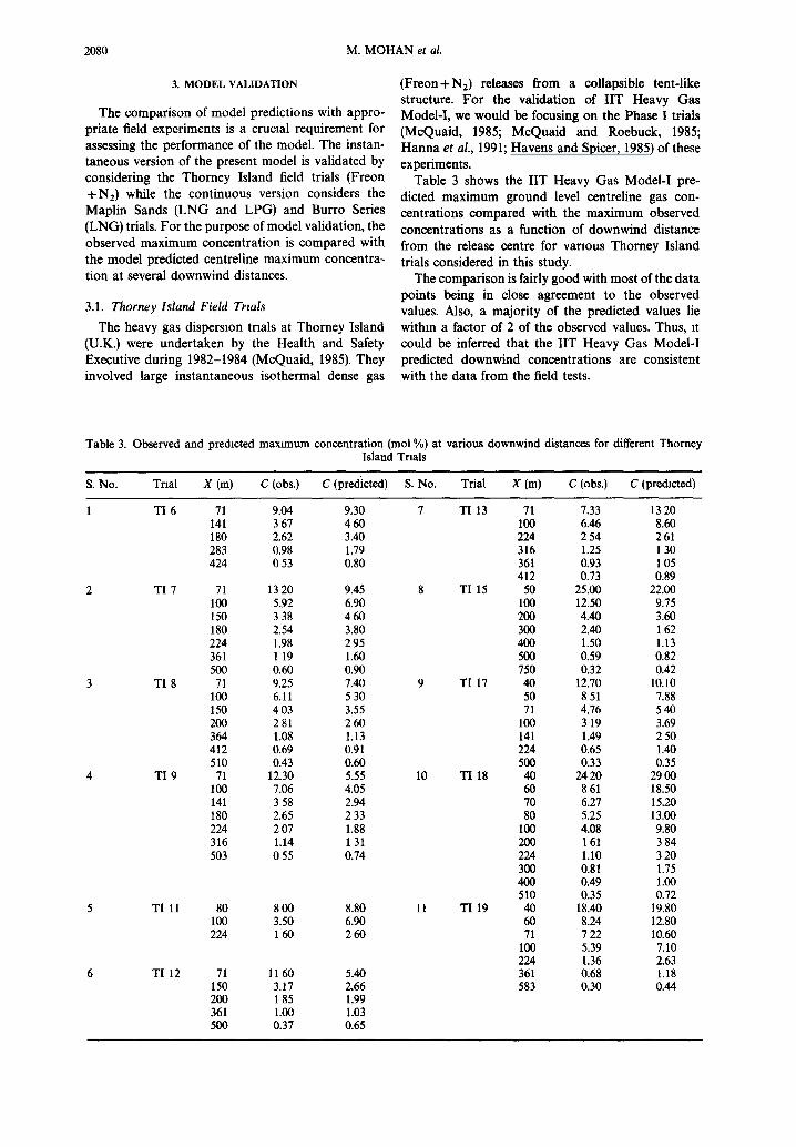
Table 3 shows the l iT Heavy Gas Model-I pre- dicted maximum ground level centreline gas con- centrations compared with the maximum observed concentrations as a function of downwind distance from the release centre for various Thorney Island trials considered in this study.

The comparison is fairly good with most of the data points being in close agreement to the observed values. Also, a majority of the predicted values lie within a factor of 2 of the observed values. Thus, It could be inferred that the l iT Heavy Gas Model-I predicted downwind concentrations are consistent with the data from the field tests.

Table 3. Observed and predicted maximum concentration (mol %) at various downwind distances for different Thorney Island Trials

S. No. Tnal X (m) C (obs.) C (predicted) S. No. Trial X (m) C (obs.) C (predicted)

1 TI 6 71 9.04 9.30 7 TI 13 71 7.33 13 20 141 3 67 4 60 100 6.46 8.60 180 2.62 3.40 224 2 54 2 61 283 0.98 1.79 316 1.25 1 30 424 0 53 0.80 361 0.93 1 05

412 0.73 0.89 2 TI 7 71 13 20 9.45 8 TI 15 50 25.00 22.00

100 5.92 6.90 100 12.50 9.75 150 3 38 4 60 200 4.40 3.60 180 2.54 3.80 300 2.40 1 62 224 1.98 2 95 400 1.50 1.13 361 1 19 1.60 500 0.59 0.82 500 0.60 0.90 750 0.32 0.42

3 TI 8 71 9.25 7.40 9 TI 17 40 12.70 10.10 100 6.11 5 30 50 8 51 7.88 150 4 03 3.55 71 4.76 5 40 200 2 81 2 60 100 3 19 3.69 364 1.08 1.13 141 1.49 2 50 412 0.69 0.91 224 0.65 1.40 510 0.43 0.60 500 0.33 0.35

4 TI 9 71 12.30 5.55 10 TI 18 40 24 20 29 00 100 7.06 4.05 60 8 61 18.50 141 3 58 2.94 70 6.27 15.20 180 2.65 2 33 80 5.25 13.00 224 2 07 1.88 I00 4.08 9.80 316 1.14 1 31 200 1 61 3 84 503 0 55 0.74 224 1.10 3 20

300 0.81 1.75 400 0.49 1.00 510 0.35 0.72

5 TI 11 80 800 8.80 11 TI 19 40 18.40 19.80 100 3.50 6.90 60 8.24 12.80 224 1 60 2 60 71 7 22 10.60

100 5.39 7.10 224 1.36 2.63

6 TI 12 71 11 60 5.40 361 0.68 1.18 150 3.17 2.66 583 0.30 0.44 200 1 85 1.99 361 1.00 1.03 500 0.37 0.65

Dense gas dispersion model 2081

3.2. Burro Series Field Trials

The Burro Series of tests were sponsored by the U.S. DOE and conducted by Lawrence Livermore National Laboratory (LLNL) and Naval Weapons Center (NWC) personnel at China Lake, California in 1980 to determine the transport and dispersion of vapour from spills of liquefied natural gas (LNG) on water. Good data on dispersion over land under a variety of meteorological conditions was obtained (Hanna et al., 1991; Havens and Spicer, 1985; Koop- man et al., 1982).

Table 4 shows the IIT Heavy Gas Model-II pre- dicted maximum groundlevel centreline gas concen- trations compared with the maximum observed concentrations as a function of downwind distance for various Burro Series Trials considered in this study. It may be noted that raajority of the predicted values lie within a factor of 2 of the observed values. Hence, the IIT Heavy Gas Model-II predicts downwind concen- trations consistent with the field data from Burro Series Trials.

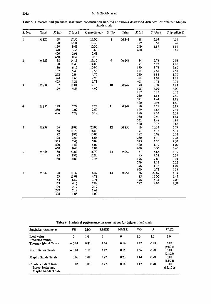
3.3 Maplin Sands Field Trials

The dispersion and combustion trials sponsored by Shell and conducted at Maplin Sands, U.K., in 1980 (Koopman etal., 1989; Puttock et al., 1982; Hanna et al., 1991) involved the release of liquefied natural gas

Table 4. Observed and predicted maximum concentration (tool %) at various downwind distances for different Burro

Senes Trials

S No. Trial X(m) C(observed) C(predicted)

1 B3 57 22.40 16.50 140 8.99 9.36 400 0.80 2.37 800 0.40 0.08

2 134 57 17.70 18.30 140 7.16 9.82 400 2.44 1.92 800 0 27 0.06

3 B5 57 19.04 18.40 140 9 60 10.80 400 2.42 2.78 800 0.41 0.12

4 B6 57 17.94 18.20 140 6.28 10.10 400 2.79 2.14

5 B7 57 17.94 18.80 140 7.13 12.20 400 3.86 4.13 800 0.80 1.06

6 B8 140 16.49 4.68 400 4.25 2.38 800 1.93 1.49

7 B9 57 10.00 16.60 140 10.60 11.10 400 3.96 5.31 800 1.40 2.37

(LNG) and refrigerated liquid propane (LPG) onto the surface of the sea.

Table 5 shows the IIT Heavy Gas Model-II pre- dicted maximum ground level centreline gas concen- trations compared with the maximum observed concentrations (Hanna et al., 1991; Havens and Spicer, 1985) as a function of downwind distance from the release centre for various Maplin Sands trials considered in this study. Here again, the comparison is fairly good with most of the data points being in close agreement to the observed values. Also, a major- ity of the predicted values lie within a factor of 2 of the observed values. It is observed that the IIT Heavy Gas Model-II predicted downwind concentrations are consistent with the field data from Maplin Sands Trials. This will be further substantiated by the results from statistical analysis presented in the following section.

3.4. Statistical Model Evaluation

The statistical methodology provides a straightfor- ward assessment of the model performance by using simple performance measures. The performance measures give an idea of the discrepancy between predictions and observations. For each experimental programme, maximum (centreline) concentrations predicted by each model will be compared to the observed maximum value at distances where measurements were taken. The performance measures used in the statistical evaluation include determina- tion of the fractional bias (FB), geometric mean bias (MG) and geometric mean variance (VG) which are defined as follows:

F B = -(0 - ,Yp 0.5(go + ~?p)

MG = exp (In Xo - In Xp)

VG = exp [(In Xo- In Xp) 2]

where Xo is an observed quantity, Xp is the corres- ponding modelled quantity, and an overbar indicates an average. In addition, root mean square error (RMSE), normalized mean square error (NMSE), cor- relation coelliclent (R), and fraction within a factor of two (FAC 2) are also calculated.

The values for the various performance measures for different field trials are summarized in Table 6. The values of the various statistical parameters indi- cate a good performance of the IIT Heavy Gas Model for both Instantaneous and Continuous releases of dense gases.

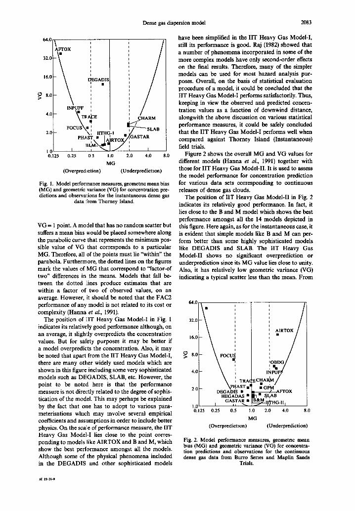
Figure 1 shows the overall geometric mean bias, MG, and geometric variance, VG, values for different models (Hanna et al., 1991) together with those for IIT Heavy Gas Model-I which is used here to assess the model performance for concentration prediction for the Thorney Island (Instantaneous release) data set.

Here, in Fig. 1, a "perfect" model compared against observations would be placed at the M G = 1 and

2082

Table 5. Observed and

M. MOHAN e t al.

predicted maximum concentration (mol %) at vanous downwind distances for different Maphn Sands trials

S. No. Trial X(m) C (obs.) C (predicted) S. No. Trial X(m) C (obs) C (predicted)

1 MS27 58 17.50 17.00 8 MS43 88 5.65 4.54 90 12.31 13.30 129 3.51 3.47

130 9.49 10.30 249 1.89 1 84 320 3.56 3.60 400 0 75 0.87 400 2.91 2.41 650 0.57 0.13

2 MS29 58 14.15 19.10 9 MS46 34 9.76 7 95 90 11.43 14.80 91 5.72 4 80

130 6.19 1090 130 3 76 3.60 182 5.43 7.55 182 2 61 2.57 252 2.04 4.70 250 1 85 1.70 324 1.65 2.96 322 1.67 1 13 403 1.35 1.73 401 0 72 0.74

3 MS34 87 11.81 12.10 10 MS47 90 8.09 4.94 179 4.55 4.92 128 4.02 4.00

4 MS35 129 7.74 7.73 11 MS49 250 3.07 2.52 406 2.28 0.18

5 MS39 36 19.00 20.00 12 MS50 58 11.70 16.50 92 9.00 13.00

175 3.00 8.66 325 2.40 5.08 400 1.60 4.04 650 0.60 2.03

6 MS56 58 23.00 16.70 13 MS52 92 8.00 12.80

180 4.00 7.26

7 MS42 28 11.32 6.49 14 MS54 53 11.09 4.78 83 6.67 3.71

123 4.15 2.88 179 2.17 2.19 247 2.18 1.67 398 1.05 1.02

182 3.13 3.12 250 1.55 2.40 321 1.44 1.88 400 0.95 1.46

90 7.21 3.89 129 4.67 2.94 180 4 35 2.14 250 2.50 1.44 322 1.48 0.99 400 0 76 0.68

59 10.33 6 79 93 5 71 5.31

182 3.08 3.14 250 1 70 2 21 325 1.20 1 53 400 1.19 1 09 650 0.50 0.40

61 5.63 6.79 95 3.38 5.34

178 2.60 3.24 249 1.12 2.22 398 1.18 1 09 650 0.75 0 38

56 22 69 4.39 85 12 00 3.45

178 5 34 2.08 247 4 95 1.59

Table 6. Statistical performance measure values for different field trials

Statistical parameter FB MG RMSE NMSE VG R FAC2

Ideal value 0 1.0 0 0 1.0 1.0 1.0 Predicted values Thorney Island Trials - 0 14 0.81 2.76 0.16 1.22 0.88 0 83

(59/71) Burro Series Trials -0.02 1.12 3.27 0.11 1.56 0.88 0.81

(21/26) Maplin Sands Trials 0.06 1.08 3.27 0.23 1.44 0.78 0.83

(62/75) Combined data from 0.03 1.07 3.27 0.18 1.47 0.78 0.82

Burro Series and (83/101) Mapfin Sands Trials

Dense gas dispersion model 2083

64.0

32.0

16.0

rO 8.0 >

~AFTOX

INPUFF 4.C --

2"0 I

10 0.125

EIEGADIS

FOCUS\• I ,I--7:-.___ SLAB ~ X ' , nTHG-I • [ /

PHAST • [ AIRTOXU/GASTAR

I ) ~ , I

0.25 0 5 1.0 2.0 4.0 MG

(Overpred letion) (Underpredictlon)

8.0

Fig. 1. Model performance measures, geometnc mean bias (MG) and geometric variance (VG) for concentration pre- dictions and observations for the instantaneous dense gas

data from Thorney Island.

VG = 1 point. A model that has no random scatter but suffers a mean bias would be placed somewhere along the parabolic curve that represents the minimum pos- sible value of VG that corresponds to a particular MG. Therefore, all of the points must lie "within" the parabola. Furthermore, the dotted lines on the figures mark the values of MG that correspond to "factor-of two" differences in the means. Models that fall be- tween the dotted :lines produce estimates that are within a factor of two of observed values, on an average. However, it should be noted that the FAC2 performance of any model is not related to its cost or complexity (Hanna et al., 1991).

The position of ][IT Heavy Gas Model-I in Fig. 1 indicates its relatively good performance although, on an average, it slighdy overpredicts the concentration values. But for satety purposes it may be better if a model overpredicts the concentration. Also, it may be noted that apart from the IIT Heavy Gas ModeM, there are many other widely used models which are shown in this figure including some very sophisticated models such as DEGADIS, SLAB, etc. However, the point to be noted here is that the performance measure is not directly related to the degree of sophis- tication of the model. This may perhaps be explained by the fact that one has to adopt to various para- meterisations which may revolve several empirical coefficients and assumptions in order to include better physics. On the sca'~[e of performance measure, the IIT Heavy Gas Model-I lies close to the point corres- ponding to models like AIRTOX and B and M, which show the best performance amongst all the models. Although some of the physical phenomena included in the DEGADIS and other sophisticated models

have been simplified in the IIT Heavy Gas Model-I, still its performance is good. Raj (1982) showed that a number of phenomena incorporated in some of the more complex models have only second-order effects on the final results. Therefore, many of the simpler models can be used for most hazard analysis pur- poses. Overall, on the basis of statistical evaluation procedure of a model, it could be concluded that the IIT Heavy Gas Modem performs satisfactorily. Thus, keeping in view the observed and predicted concen- tration values as a function of downwind distance, alongwith the above discussion on various statistical performance measures, it could be safely concluded that the IIT Heavy Gas Model-I performs well when compared against Thorney Island (Instantaneous) field trials.

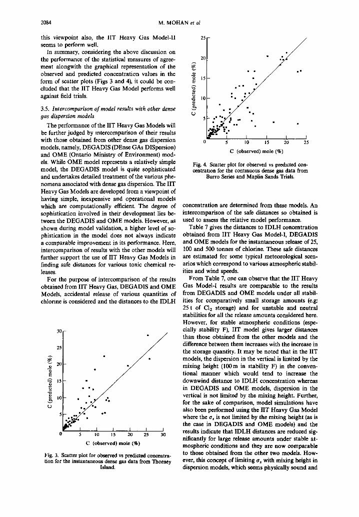
Figure 2 shows the overall M G and VG values for different models (Hanna et al., 1991) together with those for IIT Heavy Gas Model-II. It is used to assess the model performance for concentration prediction for various data sets corresponding to continuous releases of dense gas clouds.

The position of IIT Heavy Gas Model-II in Fig. 2 indicates its relatively good performance. In fact, it lies close to the B and M model which shows the best performance amongst all the 14 models depicted in this figure. Here again, as for the instantaneous case, it is evident that simple models like B and M can per- form better than some highly sophisticated models like DEGADIS and SLAB. The IIT Heavy Gas Model-II shows no significant overprediction or underprediction since its M G value lies close to unity. Also, it has relatively low geometric variance (VG) indicating a typical scatter less than the mean. From

64.0

32.0

16.0

>~ 8.0

4.0

2 0 - D E G A D I S •

H E G A D A S • G A S T A R •

1 .0 ~ - - 0 . 1 2 5

• GPM ) _---.----4--A FTOX

- SLAB

0.25 0.5 1.0 2.0 4.0 8.0

MG (Overpredictlon) (Underprediction)

Fig. 2. Model performance measures, geometnc mean bias (MG) and geometric variance (VG) for concentra- tion predictions and observations for the continuous dense gas data from Burro Series and Maplin Sands

Trials.

AE 29-16-H

2084 M. M O H A N et al

this viewpoint also, the IIT Heavy Gas Model-II seems to perform well.

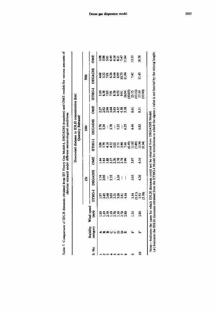
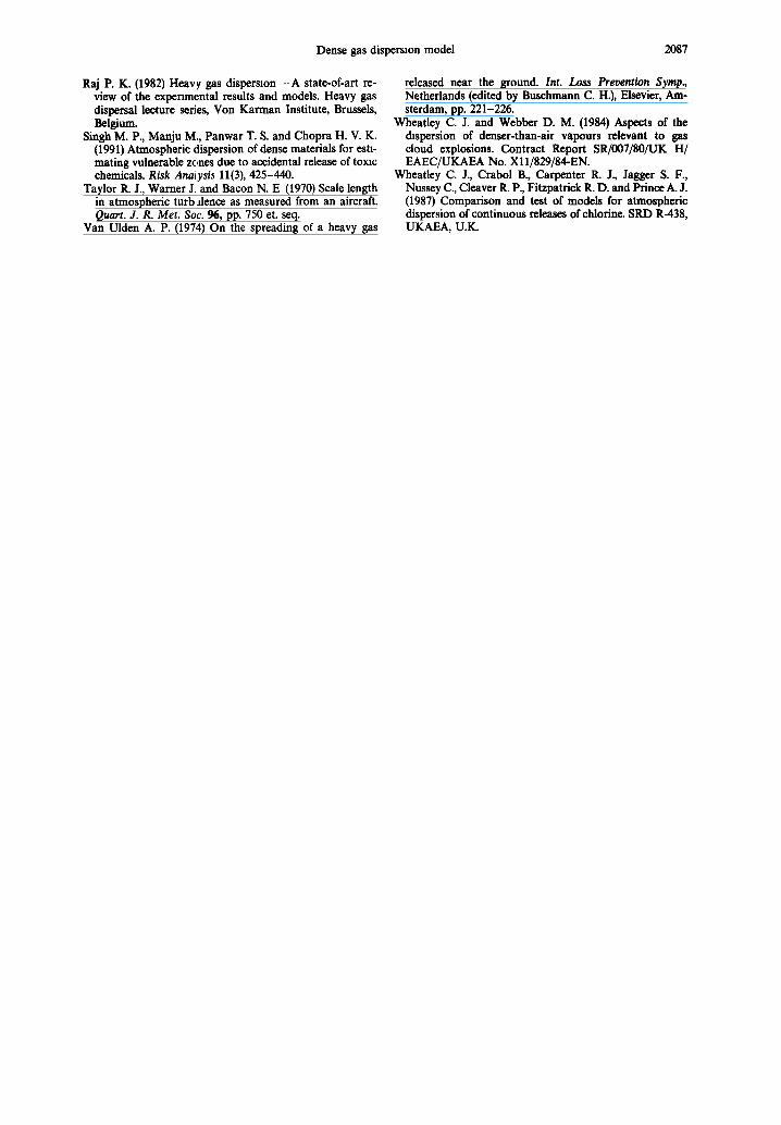
In summary, considering the above discussion on the performance of the statistical measures of agree- ment alongwith the graphical representation of the observed and predicted concentration values in the form of scatter plots (Figs 3 and 4), it could be con- cluded that the IIT Heavy Gas Model performs well against field trials.

3.5. Intercomparison of model results with other dense oas dispersion models

The performance of the IIT Heavy Gas Models will be further judged by mtercomparison of their results with those obtained from other dense gas dispersion models, namely, DEGADIS (DEnse GAs DISpersion) and • M E (Ontario Ministry of Environment) mod- els. While • M E model represents a relatively simple model, the DEGADIS model is quite sophisticated and undertakes detailed treatment of the various phe- nomena associated with dense gas dispersion. The IIT Heavy Gas Models are developed from a viewpoint of having simple, inexpensive and operational models which are computationally efficient. The degree of sophistication involved in their development lies be- tween the DEGADIS and • M E models. However, as shown during model validation, a higher level of so- phistication in the model does not always indicate a comparable improvement in its performance. Here, intercomparison of results with the other models will further support the use of IIT Heavy Gas Models in finding safe distances for various toxic chemical re- leases.

For the purpose of intercomparison of the results obtained from liT Heavy Gas, DEGADIS and OME Models, accidental release of various quantities of chlonne is considered and the distances to the IDLH

30

25

20 O E

to

5

• • • m~

n i •m

we m • o •

I I I I I I 5 I0 15 20 25 30

C (observed) mole (%)

Fig. 3. Scatter plot for observed vs predicted concentra- tion for the instantaneous dense gas data from Thorney

Island.

O

&

25

20

15

l0

• f f a s

a s s •

• w a

• a •

, , , " ,

5 10 15 20 25

C (observed) mole (%)

Fig. 4. Scatter plot for observed vs predicted con- centratlon for the contmuous dense gas data from

Burro Series and Maplin Sands Trials.

concentration are determined from these models. An intercomparison of the safe distances so obtained is used to assess the relative model performance.

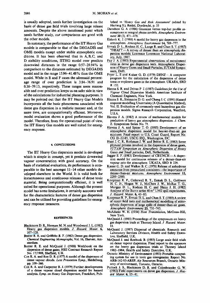
Table 7 gives the distances to IDLH concentration obtained from IIT Heavy Gas Model-I, DEGADIS and • M E models for the instantaneous release of 25, 100 and 500 tonnes of chlorine. These safe distances are estimated for some typical meteorological scen- arios which correspond to various atmospheric stabil- ities and wind speeds.

From Table 7, one can observe that the IIT Heavy Gas MOdeM results are comparable to the results from DEGADIS and • M E models under all stabil- ities for comparatively small storage amounts (e.g: 25 t of C12 storage) and for unstable and neutral stabilities for all the release amounts considered here. However, for stable atmospheric conditions (espe- cially stability F), IIT model gives larger distances than those obtained from the other models and the difference between them increases with the increase in the storage quantity. It may be noted that in the IIT models, the dispersion in the vertical is limited by the mixing height (100m in stability F) in the conven- tional manner which would tend to increase the downwind distance to IDLH concentration whereas in DEGADIS and • M E models, dispersion in the vertical is not limited by the mixing height. Further, for the sake of comparison, model simulations have also been performed using the IIT Heavy Gas Model where the ~z is not limited by the mixing height (as is the case in DEGADIS and • M E models) and the results indicate that IDLH distances are reduced sig- nificantly for large release amounts under stable at- mospheric conditions and they are now comparable to those obtained from the other two models. How- ever, this concept of limiting az with mixing height in dispersion models, which seems physically sound and

Tab

le 7

. C

ompa

riso

n o

f ID

LH

dis

tanc

es o

btai

ned

from

IIT

Hea

vy G

as M

odel

-I, D

EG

AD

IS (

tran

sien

t) a

nd O

ME

mod

els

for

vari

ous

amo

un

ts o

f ch

lori

ne r

elea

sed

unde

r di

ffer

ent m

eteo

rolo

gica

l con

diti

ons

Dow

nwin

d di

stan

ce t

o ID

LH

con

cent

rati

on (k

m)

Qua

ntit

y R

elea

sed

25t

100t

SO

Ot

Sta

bili

ty

Win

d sp

eed

S. N

o.

cate

gory

(m

/s)

IIT

HG

-I

DE

GA

DIS

O

ME

II

TH

G-I

D

EG

AD

IS

OM

E

IIT

HG

-I

DE

GA

DIS

O

ME

g

1 A

1.

19

1.97

2

B

1.19

2.

45

3 B

2.

70

2.66

4

C

1.19

3.

03

5 C

2.

70

3.21

6

D

1.19

3.

68

7 D

2.

70

3.81

8

E

2.80

4.

16

9 F

1.35

5.

34

(5.1

1)

10

F 2.

80

5.93

(5

.38)

1.74

1.

44

3.06

2.

76

2.27

5.

10

4.68

3.

88

2.05

1.

84

3.79

3.

24

2.92

6.

38

5.52

5.

06

--

1.88

4.

18

--

2.96

7.

05

7.01

5.

01

2.35

2.

27

4.72

3.

70

3.64

7.

91

6.36

6.

44

--

2.30

5.

01

--

3.63

8.

38

8.44

6.

16

3.24

2.

78

5.71

5.

22

4.52

9.

52

8.95

8.

21

--

2.78

5.

90

--

4.38

9.

91

10.7

3 7.

47

--

2.99

7.

48

6.25

5.

30

16.9

4 11

.84

11.8

4 (6

.49)

(1

0.85

) 3.

03

3.97

11

.05

4.46

6.

61

25.7

5 7.

42

13.5

5 (7

.89)

(1

3.12

) 4.

26

4.16

11

.96

6.83

8.

31

27.1

9 11

.45

18.5

8 (8

.34)

(1

3.90

)

=o

O

No

te:-

-In

dic

ates

the

case

s fo

r w

hich

ID

LH

dis

tanc

es c

ould

no

t be

obt

aine

d fr

om D

EG

AD

IS M

odel

. (#

) In

dica

tes

the

IDL

H d

ista

nces

obt

aine

d fr

om th

e II

TH

G-I

Mod

el f

or s

imul

atio

ns m

whi

ch th

e si

gma-

z va

lue

is n

ot

hmlt

ed b

y th

e m

ixin

g he

ight

.

Ix3

2086 M. MOHAN et al.

is usually adopted, needs further investigation on the basis of dense gas field trials involving large release amounts. Despite the above mentioned point which needs further study, our comparisons are good with the other models.

In summary, the performance of the l iT Heavy Gas models is comparable to that of the DEGADIS and OME models except under stable atmospheric con- ditions. It has been observed that in A, B,C, and D stability conditions, IITHG model over predicts downwind distances in the range 0.57-28.94% in comparison to the distances estimated by DEGADIS model and in the range 15.96-41.48% than the OME model. While in E and F cases the aforesaid percent- age range of over prediction is 3.84-76.91 and 0.36-39.13, respectively. These ranges seem reason- able and over prediction keeps us on safer side in view of the calculations for industrial planning purposes. It may be pointed out that the l iT Heavy Gas Models incorporate all the basic phenomena associated with dense gas dispersion in a realistic manner and, at the same time, are computationally efficient. Moreover, model evaluation shows a good performance of the model. Therefore, from the operational point of view, the l iT Heavy Gas models are well suited for emerg- ency response.

4. CONCLUSIONS

The IIT Heavy Gas dispersion model is developed which is simple in concept, yet it predicts downwind vapour concentration with good accuracy. On the basis of statistical evaluation, its performance is com- parable to the best amongst 11-14 other models de- veloped elsewhere in the World. It is valid both for instantaneous and continuous releases of dense toxic material. Being computationaily efficient, it is well suited for operational purposes. Although the present model has some limitations, it certainly accounts well for the characteristic features of dense gas dispersion and can be utilized for providing guidelines for emerg- ency response measures.

REFERENCES

Blackmore D. R., Herman M. N. and Woodward J. L. (1982) Heavy gas dispersion models. J. Hazard. Mater. 6, 107-128.

Bntter R. E. and Griffiths R. F. (1982) Dense gas dispersion. Chemical Engineering Monographs; Vol. 16, Elsevier, Am- sterdam.

Bntter R. E. and McQuaid J. (1988) Workbook on the dispersion of dense gases. HSE Contract Research Report No. 17/1988, Sheffield, U.K.

Cox R. A. and Roe D. R. (1977) A model of the dispersion of dense vapour clouds. Loss Prevention Symp., Heidelberg, pp. 359-366.

Cox R. A. and Carpenter R. J. (1979) Further developments of a dense vapour cloud dispersion model for hazard analysis. Syrup. on Heavy Gas Dispersion, Frankfurt, Pub-

hshed m "Heavy Gas and R~sk Assessment' (edited by Hartwlg S.), Reidel, Dordrecht, p. 55

Davldson G. A (1986) Gaussian versus top-hat profile as- sumptions m integral plume models. Atmospheric Environ- ment 20 (3), 471-478.

Eidsvlk K. J. (1980) A model for heavy gas dispersion in the atmosphere. Atmosphertc Environment 14, 769-777.

Ermak D L., Rodean H. C., Lange R. and Chan S. T. (1987) "DRAFT--A survey of denser than air atmospheric dis- persion models; Lawrence Llvermore National Laborat- ory, July, 1987.

Fay J A. (1983) Experimental observations of entrainment rates in dense gas dispersion tests. Atmospheric Disper- sion of Heavy Gases and Small Particles, IUTAM Sympo- smm, Delft.

Fryer L. S and Kaiser G. D. (1979) DENZ--A computer program for the calculation of the dispersion of dense toxic or exploswe gases in the atmosphere. UKAEA, SRD R 152.

Hanna S. R. and Drivas P J. (1987) Guidelines for the Use of Vapour Cloud Dispersion Models. American Institute of Chemical Engineers, New York.

Hanna S R., StrimaltlS D. G. and Chang J. C (1991) Hazard response modelhng Uncertainty (,4, Quantitative Method), Vol. II; Evaluation of commonly-used hazardous gas dis- persion models. Sigma Research Corporation, Westford, U.S.A.

Havens J A. (1982) A review of mathematical models for pre&ction of heavy gas atmosphenc dispersion. J. Chem. E. Symposium Series No. 71.

Havens J. A. and Spicer T. O. (1985) Development of an atmospheric dispersion model for heavier-than-air gas mixtures. Final report to U.S. Coast Guard, Report No. CG-D--22-85, USCG HQ., Waslungton, DC.

Hunt J. C. R., Rothman J. W. and Britter R. E. (1983) Some physical process involved in the dispersion of dense gases, IUTAM Symposium on Atmospheric Dispersion of Heavy Gases and Small particles, Deft, Netherlands.

Jagger S. F. (1983) Development of CRUNCH--A disper- sion model for continuous releases of a denser-than-air vapour into the atmosphere. UKAEA, SRD R 229.

Kmser G. D. and Walker B. C. (1978) Release of anhydrous ammoma from pressurized containers--the importance of denser-than-air mixtures. Atmospherzc Environment 12, 2289-2300.

Koopman R. P., Cederwall R. T., Ermak D. L., Goldwlre H. C. Jr., Hogan W. J., McClure J. W., McRae T. G., Morgan D. L., Rodean H. C. and Shinn J. H. (1982) Analysis of the Burro series 40 m 3 LNG spill experiments. J. Hazard. Mater. 6, 43-83.

Koopman R. P., Ermak D. L. and Chan S. T. (1989) A review of recent field tests and mathematical modelling of atmo- spheric dispersion of large spills of denser-than-air gases. Atmospheric Environment 23, 731-745.

McAdams W. H. (1954) Heat Transmission, McGraw-Hill, New York.

McQuaid J. (1985) Proceedings of the sympusmm on heavy gas dispersion tnals at Thorney Island. J Hazard. Mater. 11.

McQuaid J. (1987) Dispersal of chemicals. Research and Laboratory Services Division, Health and Safety Execu- tive, Sheffield, U.K.

McQuald J. and Roebuck B. (1985) Large scale field trials on dense vapour dispersion. Final report to the sponsors on the heavy gas dispersion trials at Thomey Island 1982-1984, Health and Safety Executive, U.K.

Ontario Ministry of Environment (1983) Portable comput- ing system for use in toxic gas emergoneies. Report No. ARB-162-83-ARSP, Air Resources Branch, Ontario Min- istry of environment, Toronto, Ontario.

Puttock J. S., Blackmore D. R. and Cotenbrander G. W. (1982) Field expertments on dense gas dispersion. J. Haz- ard Mater. 6, 13-41.

Dense gas dispersion model 2087

Raj P. K. (1982) Heavy gas disperslon--A state-of-art re- view of the experimental results and models. Heavy gas dispersal lecture series, Von Karraan Institute, Brussels, l~lgium.

Singh M. P., Manju M., Panwar T. S. and Chopra H. V. K. (1991) Atmospheric dispersion of dense materials for esti- mating vulnerable zones due to accidental release of toxic chemicals. Risk Analysis 11(3), 425-440.

Taylor R..I., Warner J. and Bacon N. E (1970) Scale length in atmospheric turbulence as measured from an aircraft. Quart. J. R. Met. Soc. 96, pp. 750 et. seq.

Van Ulden A. P. (1974) On the spreading of a heavy gas

released near the ground. Int. Loss Prevention Symp., Netherlands (edited by Buschmann C. H.), EIs¢vier, Am- sterdam, pp. 221-226.

Wheatley C. J. and Webbcr D. M. (1984) Aspects of the d~spersion of denser-than-air vapours relevant to gas cloud explosions. Contract Report SR/007/80/UK H/ EAEC/UKAEA No. X11/829/84-EN.

Wheatley C. J., Crabol B., Carpenter R. J., Jagger S. F., Nussey C., Cleaver R. P., Fitzpatrick R. D. and Prince A. J. (1987) Comparison and test of models for atmospheric dispersion of continuous releases of chlorine. SRD R-438, UKAEA, U.K.