modeling adaptive decision-making of farmer: an integrated
TRANSCRIPT
i
Modeling adaptive decision-making of farmer: An integrated
economic and management model, with an application to
smallholders in India
Modélisation des décisions adaptatives de l’agriculteur : Un modèle
économique et décisionnel intégré, avec un cas d’étude en Inde
Marion Robert
PhD Manuscript

iii
ABSTRACT
This thesis develops and discusses farmers’ decision-making modeling approaches for representing the
adaptation of farming to global changes and water policies: their effects on agricultural economics and
practices and water resources comprise critical information for decision makers. After a summary, six
articles are presented.
The first article reviews bio-economic and bio-decision models, in which strategic and tactical decisions
are included in dynamic adaptive and expectation-based processes, in 40 literature articles.
The second article describes the case-study and presents a typology of Indian farmers from a survey
including 684 farms in Berambadi, an agricultural watershed in South India.
The third article presents a step-by-step approach that combines decision-making analysis with a
modeling approach inspired by cognitive sciences and software-development methods. This
methodology bridges the gap between field observations and the design of the decision model. It is a
useful tool to guide modelers in building decision model in farming system.
The fourth article describes the conceptual model NAMASTE, which was conceived to represents
farmers adaptation processes under uncertainty. Since NAMASTE was designed in an extreme case of
highly vulnerable agriculture, its generic framework and formalisms can be used to conceptually
represent many other farm production systems.
The fifth article investigates the role of water management policies on groundwater resource depletion
under climate change conditions. We built a stochastic dynamic programming farm model. The model
reproduced decision on irrigation investment and cropping system made each year with the concern of
future impacts on water availability for irrigation.
The sixth article describes the NAMASTE dynamic simulation model developed to model farming
systems for evaluation and test of water management policies.
Key-words: farmers’ decision-making, farm typology, conceptual model, stochastic programming,
water management policies, climate change, Berambadi watershed.

v
RESUME EN FRANÇAIS
Cette thèse développe et discute une approche de modélisation des processus de décision des agriculteurs
qui prend en compte l'adaptation des pratiques aux changements globaux et aux politiques de l'eau. En
effet ces changements ont des effets sur l'économie et les pratiques agricoles ainsi que sur les ressources
en eau et sont des informations essentielles pour la prise de décision. Après un synoptique de thèse, six
articles sont présentés.
Le premier article est une revue de littérature d’une quarantaine d’articles sur les modèles bio-
économiques et bio-décisionnels, dans laquelle les processus d’adaptation sont inclus dans les décisions
stratégiques et tactiques.
Le deuxième article décrit le cas d’étude et présente une typologie des agriculteurs indiens déterminée
à partir de 684 enquêtes d’exploitations agricoles dans le bassin versant agricole du Berambadi, au sud-
ouest de l’Inde.
Le troisième article présente une méthodologie qui combine l'analyse des processus de décision avec
une approche de modélisation inspirée des sciences cognitives et des méthodes de développement
informatique. Cette méthodologie permet le passage entre les observations de terrain et la conception
du modèle de décision. Il s’agit d’un outil utile pour les modélisateurs qui les guide dans la construction
de modèles de décision pour les systèmes agricoles.
Le quatrième article décrit le modèle conceptuel NAMASTE, conçu pour représenter les processus
adaptatifs de décision des agriculteurs dans un environnement incertain. Puisque NAMASTE a été conçu
dans un cas extrême d'agriculture très vulnérable, son cadre et ses formalismes génériques peuvent être
utilisés pour représenter conceptuellement de nombreux autres systèmes de production agricole.
Le cinquième article étudie le rôle des politiques de gestion de l'eau sur la baisse des ressources en eau
souterraine dans des conditions de changement climatique. Nous avons construit un modèle agricole de
programmation dynamique stochastique. Le modèle reproduit les décisions annuelles d'investissement
en irrigation et de choix de systèmes de cultures réalisées avec le souci des impacts futurs sur la
disponibilité de l'eau pour l'irrigation.
Le sixième article décrit le modèle dynamique de simulation NAMASTE développé pour l'évaluation
et le test de politiques de l’eau sur les processus de décision des agriculteurs et la nappe phréatique.
Mots-clés: processus de décision des agriculteurs ; typologie des exploitations agricoles ; modèle
conceptuel ; programmation stochastique dynamique ; politiques de gestion de l'eau ; changement
climatique ; bassin versant du Berambadi.


vii
PREFACE
I chose to present my thesis in an original way. As my written restitution is based on six articles either
submitted or close to be submitted, and as it could be quite tedious to read and reread the article
introductions that globally deal with the same theme (the one of my thesis), I chose to make a synoptic
document of the thesis. This document of forty pages, gives in one hand the major advances (key
messages found in the articles), and in the other hand deals with the introduction, the research approach
and discussion-perspectives on the work that I conducted in depth. The reader can thus have an overview
of the work done and go, if necessary, read the different articles. I also chose to provide a number of
appendixes which could not be added to the articles but which can help understanding methodological
items that could also be used by other researchers.


ix
ACKNOWLEDGEMENTS
I would like to begin by first thanking my PhD advisors, Dr. Jacques-Eric Bergez and Dr. Alban Thomas,
for their trust, guidance and shrewd advice all along the thesis. Thank you very much for your time and
availability despite your overbooked schedules and responsibilities. Your organization and confidence
have kept me on schedule for the entire duration of this project. I am also very thankful to Jacques-Eric
for following me up and encouraging me every day.
I would also like to thank my steering committee members Dr. Delphine Leenhardt, Dr. Aude Ridier,
Dr. Alexandre Joannon, Dr. Victor Picheny, Dr. Stephan Couture, Dr. Arnaud Reynaud and Dr. Laurent
Ruiz for their commitment, ideas and encouraging remarks.
I would also like to thank my PhD defense committee members Dr. Ken Giller, Dr. Florence Jacquet,
Dr. Benoît Dedieu and Dr. Thierry Lamaze for participating to the defense and evaluation of my work,
and for their interesting insights on it.
There are many people unnamed who have given me great support, both academically and emotionally,
and I will forever be indebted to all of them. This represents a time and opportunity in my life that I will
always cherish and surely reflect on as the true beginning of my professional endeavors.
I would like to thank all my colleagues, with whom I have worked for the last three years and who have
contributed to the development of my reasoning. I would like to thank specifically the co-authors of the
articles that are the basis of this thesis: Jacques-Eric Bergez, Alban Thomas, Laurent Ruiz, Muddu
Sekhar, Shrinivas Badiger, Hélène Raynal, Delphine Leenhardt, Magali Willaume, Jérôme Dury, Olivier
Thérond, Pierre Casel, Eric Casellas, Patrick Chabrier and Alexandre Joannon.
I would also like to thank Eric and Pierre for their great job in the model computer implementation.
Thank you so much for your patience and adaptation to my poor knowledge in IT.
Special thanks go to my colleagues from INRA, and particularly to the PhD students of the office B205
and to my Indian friends Buvi, Divya, Amit and Sreelash. Particular thanks to Ariane, Charlotte and
André for their support and advice; and to Céline for the moments of relaxation.
I am also grateful to my friends Alice and Marie for their insightful advice and discussions.
Thank you to Michelle and Michael Corson and my sister for proof reading the English version on
several parts of this document.
Warm thanks go to my parents for believing in my project.
Last and not least, loving thanks to Tony for his support and patience during evenings, week-ends and
vacations, during my bad and good moods and for his technical support with C.

xi
LIST OF PUBLICATIONS
Published or submitted to peer-reviewed journals
1*Robert, M, Hu, W., Nielsen, M.K., Stowe, C.J. (2015) Attitudes towards implementation of
surveillance-based parasite control on Kentucky Thoroughbred farm – current strategies, awareness and
willingness-to-pay, Equine Veterinary Journal, Vol. 47 (6), doi: 10.1111/evj.12344
1*Robert, M., Stowe, C.J. (2016) Ready to Run: Price determinants of Thoroughbred from two-year-
olds in training sales, Applied Economics incorporating Applied Financial Economics, Vol. 48, doi:
10.1080/00036846.2016.1164817
Robert, M., Dury, J., Thomas, A., Therond, O., Sekhar, M., Badiger, S., Ruiz, L., Bergez, J.E. (2016)
CMFDM a methodology to guide the design of a conceptual model of farmers’ decision-making
processes, Agricultural Systems, Vol. 148, p 86-94, doi: 10.1016/j.agsy.2016.07.010
Robert, M., Thomas, A., Sekhar, M., Badiger, S., Ruiz, L., Raynal, H., & Bergez, J. E. (2016). Adaptive
and dynamic decision-making processes: A conceptual model of production systems on Indian farms.
Agricultural Systems, doi : 10.1016/j.agsy.2016.08.001
Robert, M., Thomas, A., Bergez, J.E. (2016) Integrating adaptative processes in farming decision-
making models – a review, Agronomy for Sustainable Development, doi: 10.1007/s13593-016-0402-x
Robert, M., Thomas, A., Sekhar, M., Badiger, S., Ruiz, L., Willaume, M., Leenhardt, D., Bergez, J.E.
(2016) Typology of farming systems for modeling water management issues in the semi-arid tropics
(Berambadi watershed, India), Water (under review)
Robert, M., Bergez, J.E., Thomas A (2016) Stochastic dynamic programming approach to analyze
adaptation to climate change - application to groundwater irrigation in India, European Journal of
Operational Research (submitted)
Robert, M., Thomas, A., Sekhar, M., Raynal, H., Casellas, E., Casel, P., Chabier, P., Joannon, A. &
Bergez, J. E (2016) NAMASTE: a dynamic model for water management at the farm level integrating
strategic, tactical and operational decisions, Environmental Modelling & Software (submitted)
1 * Corresponds to publications that are not connected to the work presented in this thesis.

xii
Abstracts and proceedings
Robert, M., Thomas, A., Bergez, J.E. (2015) Modeling Adaptive Decision-Making of Farmer: an
Integrated Economic and Management Model, with an Application to Smallholders in India In: the 5th
International Symposium for farming Systems Design (FSD) ‘Multi-functional Farming systems in a
changing world, 5th-10th September 2015, Montpellier, France
Robert, M., Thomas, A., Bergez, J.E. (2016) CMFDM: A methodology to guide the design of a
conceptual model of farmers’ decision-making processes. In: the 8th International Congress on
Environmental Modeling and Software Society (iEMSs), 12th-14th July 2016, Toulouse, France
Robert, M., Thomas, A., Bergez, J.E. (2016) NAMASTE: A dynamic integrated model for simulating
farm practices under groundwater scarcity in semi-arid region of India In: the 14th Congress on
European Society of Agronomy (ESA), 5th-9th September 2016, Edinburgh, Scotland
Additional scientific contributions
Member of the scientific committee of the Ecole Chercheurs « Approches interdisciplinaires de la
modélisation des agroécosystèmes » that will be hold the 7th-10th March 2017.
xiii
CONTENTS
Introduction – Synthesis Chapter ........................................................................................................ 1
1.1. General introduction ..................................................................................................................... 2
1.1.1. Today’s and tomorrow’s challenges for the agriculture .................................................. 2
1.1.2. Designing farming systems ............................................................................................. 3
1.1.3. Agricultural production systems and complex systems................................................... 4
1.1.4. Global challenges in designing agricultural production systems .................................... 7
1.2. Thesis project ............................................................................................................................... 7
1.2.1. Research context .............................................................................................................. 7
1.2.2. Thesis objectives ........................................................................................................... 11
1.3. Thesis proceedings ..................................................................................................................... 16
1.4. Thesis results .............................................................................................................................. 17
1.4.1. Literature review on adaptation in decision models ...................................................... 17
1.4.2. The Berambadi watershed ............................................................................................. 19
1.4.3. A methodology to guide the design of a conceptual model of farmers’ decision-making
processes ....................................................................................................................................... 20
1.4.4. The conceptual model NAMASTE ............................................................................... 22
1.4.5. Strategic decisions on investments and cropping systems modeled with a stochastic
dynamic programming approach ................................................................................................... 24
1.4.6. The computer model NAMASTE ................................................................................. 26
1.5. Discussions and prospects .......................................................................................................... 28
1.5.1. Review on the thesis results .......................................................................................... 28
1.5.2. From the demonstration prototype to the production model ......................................... 29
1.5.3. Verification and validation ............................................................................................ 33
1.5.4. A decision model for the AICHA project ...................................................................... 37
1.6. Conclusion .................................................................................................................................. 42
Processes of adaptation in farm decision-making models- A review .............................................. 44
2.1. Introduction ................................................................................................................................ 46
2.2. Background on modeling decisions in agricultural economics and agronomy .......................... 48
2.3. Method ....................................................................................................................................... 49
2.4. Formalisms to manage adaptive decision-making processes ..................................................... 50
2.4.1. Formalisms in proactive adaptation processes .............................................................. 51
2.4.2. Formalisms in reactive adaptation processes ................................................................. 52
2.5. Modeling adaptive decision-making processes in farming systems ........................................... 54
2.5.1. Adaptations and strategic decisions for the entire farm................................................. 54
2.5.2. Adaptation and tactic decisions ..................................................................................... 55
xiv
2.5.3. Sequential adaptation of strategic and tactical decisions ............................................... 57
2.6. Discussion .................................................................................................................................. 58
2.6.1. Adaptation: reactive or proactive process? .................................................................... 58
2.6.2. Decision-making processes: multiple stages and sequential decisions ......................... 59
2.6.3. What about social sciences? .......................................................................................... 59
2.6.4. Uncertainty and dynamic properties .............................................................................. 60
2.7. Conclusion .................................................................................................................................. 61
Acknowledgements ........................................................................................................................... 62
Table caption ..................................................................................................................................... 63
Figure caption .................................................................................................................................... 65
Farm typology in the Berambadi watershed (India): farming systems are determined by farm size
and access to groundwater .................................................................................................................. 70
3.1. Introduction ................................................................................................................................ 72
3.2. Materials and methods ................................................................................................................ 73
3.2.1. Case study: Hydrological and morphological description of the watershed ................. 73
3.2.2. Survey design and sampling .......................................................................................... 74
3.2.3. Analysis method ............................................................................................................ 75
3.3. Variability and spatialization of farm characteristics and practices ........................................... 76
3.3.1. Farm structure ................................................................................................................ 76
3.3.2. Farm practices ............................................................................................................... 78
3.3.3. Water management for irrigation .................................................................................. 79
3.3.4. Economic performances of the farm ............................................................................. 80
3.4. Typology of farms in the Berambadi watershed ........................................................................ 81
3.4.1. Characteristics of farm typology ................................................................................... 81
3.4.2. Characteristics of the farm types ................................................................................... 82
3.5. Discussion .................................................................................................................................. 83
3.6. Conclusion .................................................................................................................................. 86
Acknowledgements ........................................................................................................................... 87
Table caption ..................................................................................................................................... 88
Figure caption .................................................................................................................................... 90
CMFDM: A methodology to guide the design of a conceptual model of farmers’ decision-making
processes ............................................................................................................................................... 98
4.1. Introduction .............................................................................................................................. 100
4.2. Founding principles of the methodology .................................................................................. 100
4.3. The CMFDM methodology ...................................................................................................... 102
4.3.1. Step 1: problem definition ........................................................................................... 102
4.3.2. Step 2: case study selection ......................................................................................... 102
xv
4.3.3. Step 3: data collection and analysis of individual case studies ................................... 102
4.3.4. Step 4: the generic conceptual model .......................................................................... 103
4.4. Methodology implementation in a case study .......................................................................... 104
4.4.1. Step 1: problem definition ........................................................................................... 104
4.4.2. Step 2: case study selection ......................................................................................... 104
4.4.3. Step 3: data collection and analysis of individual case studies ................................... 105
4.4.4. Step 4: the generic conceptual model .......................................................................... 108
4.5. Discussion - Conclusion ...................................................................................................... 110
Acknowledgements ......................................................................................................................... 112
Figure caption .................................................................................................................................. 113
Adaptive and dynamic decision-making processes: A conceptual model of production systems on
Indian farms ....................................................................................................................................... 121
5.1. Introduction ......................................................................................................................... 123
5.2. Modeling processes ............................................................................................................. 124
5.2.1. Indian case study ......................................................................................................... 124
5.2.2. Modeling steps ............................................................................................................ 125
5.2.3. Conceptual validation .................................................................................................. 127
5.3. A conceptual model of production systems on Indian farms .............................................. 128
5.3.1. What should be modeled ............................................................................................. 128
5.3.2. Modeling in NAMASTE ............................................................................................. 131
5.3.3. Description of the other systems in the model ............................................................ 140
5.4. Discussion ........................................................................................................................... 143
5.5. Conclusion ........................................................................................................................... 145
Acknowledgements ......................................................................................................................... 146
Table caption ................................................................................................................................... 147
Figure caption .................................................................................................................................. 148
A stochastic dynamic programming approach to analyze adaptation to climate change -
application to groundwater irrigation in India ............................................................................... 155
6.1. Introduction ......................................................................................................................... 157
6.2. Literature review on long-term farmer decisions under uncertainty ................................... 158
6.3. Methods ............................................................................................................................... 160
6.3.1. The farmer’s production problem ................................................................................ 160
6.3.2. Data ............................................................................................................................. 164
6.4. Simulations and results ........................................................................................................ 165
6.4.1. Scenarios ..................................................................................................................... 165
6.4.2. Results ......................................................................................................................... 167
6.5. Discussion ........................................................................................................................... 169
xvi
6.6. Conclusion ........................................................................................................................... 171
Acknowledgements ......................................................................................................................... 173
Table caption ................................................................................................................................... 174
Figure caption .................................................................................................................................. 178
NAMASTE: a dynamic model for water management at the farm level integrating strategic,
tactical and operational decisions .................................................................................................... 185
7.1. Introduction ......................................................................................................................... 187
7.2. Materials and methods ......................................................................................................... 188
7.2.1. Conceptual modelling .................................................................................................. 188
7.2.2. RECORD: a modeling and simulation computer platform .......................................... 189
7.3. Description of the farming system model ........................................................................... 191
7.3.1. Models used to build the farming system model ......................................................... 191
7.3.2. Model structure ............................................................................................................ 193
7.3.3. Dynamic functioning ................................................................................................... 193
7.4. Application case: the NAMASTE simulation model .......................................................... 194
7.4.1. Coupling the farming system model to the hydrological model.................................. 194
7.4.2. NAMASTE simulaton ................................................................................................. 195
7.4.3. Calibration and validation ........................................................................................... 196
7.4.4. Simulation results ........................................................................................................ 197
7.5. Discussion ........................................................................................................................... 199
7.6. Conclusion ........................................................................................................................... 201
Acknowledgements ......................................................................................................................... 202
Figure caption .................................................................................................................................. 203
Bibliography ...................................................................................................................................... 213
Appendix ............................................................................................................................................ 239
Appendix 1: Thesis sequence of events........................................................................................... 241
Appendix 2: Data used in NAMASTE development ...................................................................... 244
Appendix 3: Conceptual model and Ontology ................................................................................ 298
Appendix 4: Economic model - Model equations .......................................................................... 304
Appendix 5: Economic model - Yield estimations and climatic expectations ................................ 306
Appendix 6: Operational decision and modeling ............................................................................ 312
Appendix 7: Coupled model – a village with two farms ................................................................. 322
xvii
LIST OF ACRONYMS
ACCAF: Adaptation to Climate Change of Agriculture and Forest
AICHA: Adaptation of Irrigated Agriculture to Climate Change
AMBHAS: Assimilation of Multi-satellite data at Berambadi watershed for Hydrology And land
Surface experiment
BDI: Belief-Desire-Intention
CEFIPRA: Centre for the Promotion of Advanced Research
CETIOM: Centre Technique Interprofessionnel des Oléagineux Métropolitains
CMFDM: Conceptual Modeling of the Farmer agent underlying Decision-Making processes
CRASH: Crop Rotation and Allocation Simulator using Heuristics
CTA: Cognitive-Task Analysis
DP: Dynamic programming
DSP: discrete stochastic programming
EDT: Doctoral School of the University of Toulouse
INRA: French National Institute of Agronomy
NAMASTE: Numerical Assessments with Models of Agricultural Systems integrating Techniques and
Economics
NDM: Naturalistic decision making
RECORD: Renovation and COORDination of agro-ecosystem modeling
STICS: Simulateur multidisciplinaire pour les cultures standard
UML: Unified Modelling Language

Chapter 1 Marion Robert
1
Chapter 1
Introduction – Synthesis Chapter
Chapter 1 Marion Robert
2
1.1. GENERAL INTRODUCTION
1.1.1. Today’s and tomorrow’s challenges for the agriculture
Agriculture is facing many challenges both in terms of productivity and revenue and in terms of
environmental and health impacts. Agriculture must thus face a demand for increasing production
regarding quantity, quality, accessibility and availability to secure food production and improve product
quality to cope the needs of the world’s growing population (Meynard et al. 2012; Hertel 2015;
McKenzie and Williams 2015). The FAO (Food and Agriculture Organization of the United Nations)
estimates that global agricultural production must increase by nearly 60% from 2005/2007 to 2050 to
meet the food demand of the estimated 9 billion people by 2050 while ensuring fair incomes for farmers
(FAO 2012). Increasing agricultural productivity is all the more important to face the increasing
competition for land, water and investment between urban, agricultural and industrial sectors (FAO
2011).
However, increasing agricultural productivity must be made within a framework of environmental and
health constraints. First it should consider limiting the impact on the environment, by reducing the
impacts on water and aquatic environments (nitrate, pesticide, drug residue pollutions through leaching
and runoff), on air (nitrous oxide, methane, ammonia and other greenhouse gas) and finally on soil (soil
structural discontinuity, compacted areas, risk of leaching and erosion, decline in soil biodiversity). It
should also consider limiting habitat modification to encourage and maintain biodiversity. Second,
agricultural productivity should take into account the scarcity of resources mobilized by agricultural
production such as water resources, phosphorus and fossil energy (particularly for the production of
nitrogen fertilization) (FAO 2011; Brown et al. 2015).
These agricultural challenges also have to be considered within the known context of climate change.
Under climate change conditions, warmer temperatures, changes of rainfall patterns and increased
frequency of extreme weather are expected to occur. The global mean temperature expected by the end
of this century could be 1.8° to 4.0°C warmer than at the end of the previous century within an uneven
pattern across the globe. Climate change could lead to extreme climatic events, such as increased
intensity and frequency of hot and cold days, storms, cyclones, droughts and flooding (Anwar et al.
2013). Climate change alters weather conditions and thus has direct, biophysical effects on agricultural
production and would negatively affects crop yields and livestock (Nelson et al. 2014). Sea-level rises
will increase the risk of flooding of agricultural land in coastal regions. Changes in rainfall patterns may
support the growth of weeds, pests and diseases (Lapeyre de Bellaire and al. 2016).
Chapter 1 Marion Robert
3
1.1.2. Designing farming systems
Facing the aforementioned challenges, conventional farming systems have their limitations and a
particular attention is made on the dynamics of innovations likely to consider and resolve the former
issues (Novak 2008). In a broad sense, innovation is seen as the action of "transforming a discovery on
a technique, a product or a conception of social relationship into new practices" (Alter 2000).
In agronomy, innovation is generally defined as a process which promotes the introduction of new
changes and leading to its spread and its recognition through applications cases (INRA Sens 2008;
Klerkx et al. 2010). Innovation requires a design process based on scientific and / or empirical
knowledge. The design process is conducted by agricultural and development research institutes in close
collaboration with farmers to address their needs, their constraints and their knowledge on agricultural
production systems (Le Gal et al. 2011).
Two ways of designing systems are distinguished: i) the rule-based design aims at gradually improving
existing technologies and systems, based on predefined objectives and standardized evaluation
processes (Meynard et al. 2012); ii) the innovative design is built to meet completely new expectations
initially undetermined but getting more and more specific as the exploration process takes shape
(Meynard et al. 2012; Lefèvre et al. 2014). In an uncertain and changing environment, traditional rule-
based analytical frameworks are challenged. The adaptable design approaches that take into account
varying objectives, skills and modes of validation and do not need to be specified in advance may be
preferable (Meynard et al. 2012).
Different tools and methods have already been developed to address the issue of farming system designs.
Loyce and Wery (2006) classified them into three groups: (i) diagnosis (e.g. Doré et al. 1997) allows to
understand and evaluate agricultural systems from field measurements and surveys, (ii) prototyping (e.g.
Vereijken 1997) consists in designing a limited number of systems based on expert-knowledge, in
testing and evaluating them, and in adapting the prototypes; (iii) model and simulation based approaches
(e.g. Romera et al. 2004) where the model allows to design a simplified representation of a real system
and the simulation allows to change the state of the system in order to understand and evaluate its
behavior.
Given the complexity of the agricultural production systems, simulation modeling is a commonly used
tool for the design and the evaluation of innovative agricultural production systems (Bergez et al. 2010).
Indeed, systemic modeling and dynamic simulations appear to be powerful tools to represent the
dynamic interactions between biological and technical processes at different time and space scales and
to assess and quantify the performances of a variety of alternative systems for a diversity of production
contexts (Bergez et al. 2013).
Chapter 1 Marion Robert
4
1.1.3. Agricultural production systems and complex systems
Definition and organization of farming systems
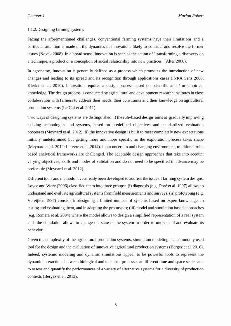
An agricultural production system is defined as a complex system of resources, technical activities,
biological processes and decisional processes that aims at meeting farm production objectives by
producing agricultural goods (Tristan et al. 2011). The agricultural production system is a complex
matrix of interdependent items that are partially controlled by the farm manager or the farm household
subjected to a socio-economic and climatic external environment (Figure 1.1).
Dury et al. (2013) identified five categories of objectives that drive decisional processes within farming
systems: 1) financial like maintain, secure, increase or maximize farm income, 2) workload by
decreasing, minimizing, maintaining or spreading working hours, 3) farm status considering the future
of the farm, 4) technical aspects on crop management techniques, 5) environmental aspects with
reasoning on biodiversity and pollution.
Decisional processes aim at developing a resource management strategy that transforms land, capital,
labor resources into agricultural products taking into consideration infrastructure and intuitional
constraints such as equipment, storage and transportation, marketing facilities and farm credits. This
transformation is the result of farmer’s short-term technical activities on the farm. The farmer mobilizes
knowledge to make decisions based on know-how, skills and specific observations made previously on
his production system.
Agricultural production system may be composed of several production sub-systems with specific
production objectives. Three main production subsystems are identified in Coléno et al., (2005): crop
production, animal production and transformation unit. These sub-systems are interrelated since the end
product and wastes of one sub-system may be used as inputs in others (Figure 1.1).
Chapter 1 Marion Robert
5
Figure 1.1 : Agricultural production system organized into three integrated production subsystems (from Coléno et al. 2005).
Management of farming system
The farmer dynamically plans and coordinates his technical activities on his farm at different time and
space scales. However agricultural production systems are facing new challenges due to a constantly
changing global environment that is a source of risk and uncertainty, and in which past experience is not
sufficient to gauge the odds of a future negative event. Concerning risk, farmers are exposed to
production risk mostly due to climate and pest conditions, to market risk that impact input and output
prices, and institutional risk through agricultural, environmental and sanitary regulations (Hardaker
2004). Farmers may also face uncertainty due to rare events affecting, e.g. labor, production capital
stock, and extreme climatic conditions, which add difficulties to the production of agricultural goods
and calls for re-evaluating current production practices. To remain competitive, farmers have no choice
but to adapt and adjust their daily management practices (Hémidy et al. 1996; Hardaker 2004; Darnhofer
et al. 2010; Dury 2011).
Based on his past experience and on forecasts on weather and market prices, the famer can anticipate
some events and production conditions. Thus he is able to plan several management options to face these
different production conditions. However, given the limitations of human cognition to anticipate the
Chapter 1 Marion Robert
6
future, everything cannot be anticipated (Chavas 2012). The farmer must therefore be able to establish
a reflexive analysis on the observations he made on his environment in order to instantly review his
initial management plan and if necessary his production objectives. The farmer's decision-making
process is therefore a dynamic sequence of planning, observation, reflection, adaptation, implementation
as technical activities and learning processes (Risbey et al. 1999; Le Gal et al. 2011). This variable and
uncertain production context justifies why a management plan repeated over several years won’t give
the same production results and why different management plans may lead to the same production
results. Farmer’s decision-making is a continuous process in time and space. Farmers make decisions
based on his visibility and expectations on the production context that impact his management on the
long-, medium- or short-term. Decisions may affect the whole agricultural production system, a
production sub-system or even smaller spatial unit such as the plot (Cerf and Sebillotte 1988; Papy et
al. 1988; Osman 2010). For instance, investing in equipments, in buildings or in lands are decisions that
reflect a willingness to expand or modernize the farm. These decisions have long-term consequences
because 1) loans are often over several years, 2) the farm structure and infrastructures are changed for
the coming years (life duration of a tractor, building, etc.). However, decisions on selecting varieties and
crop management techniques have an impact on the short term and at a local scale corresponding to the
production season and the plot. Finally, deciding to delay the sowing, to extend the water turns or to
apply pesticide treatment will have an immediate effect on the biophysical system because these
decisions correspond to technical activities executed on each plot.
Specificities of irrigated farming systems
A production system is considered as irrigated when water supply other than rainfall is provided on one
or several plots. The irrigation water is pumped from a water point and distributed to the fields through
appropriate water transport infrastructure. In irrigated production systems, crops benefit from both the
contribution of rainfall and irrigation water to cover their water needs. Irrigation is an effective
management tool against the variability and uncertainty of rainfall events. The irrigation water can come
from surface water fed by the rainfall runoff like streams, rivers, ponds, lakes and dams. Irrigation water
can also come from the aquifer that is fed by the rainfall drained into the ground. The deep aquifers are
located between two impermeable layers leading to slow recharge compared to surface water reservoirs.
Irrigation water can come from different sources considered as collective when multiple users are
identified or individual. Except for individual rainfall reservoirs, the other sources of irrigation are often
subject to conflicts and management issues (Gleick 1993; Wolf 2007). Conflicts over rivers between
upstream and downstream users are commonly seen as the upstream pumping will impact the
downstream flow (Chokkakula 2015). On a reservoir, tensions appear when pumping exceeds the
rainfall recharge from run-off particularly in drought conditions (Rajasekaram and Nandalal 2005). For
groundwater, pumping may exceed rainfall recharge. Moreover, lateral flows conduct the water table
Chapter 1 Marion Robert
7
level to rebalance so that intensive pumping by one farmer impacts the yield of the neighbor’s borewell
(Janakarajan 1999).
1.1.4. Global challenges in designing agricultural production systems
The production of knowledge on agricultural production system is an important issue while designing
such system. Several types of knowledge have to be produced to understand the complexity of systems:
1) knowledge on the system structure to understand its organization and composition; 2) knowledge on
internal processes e.g. decision processes, biophysical processes; and 3) knowledge on inputs and
outputs to understand the exchanges of information and matters within the system and with the external
environment as well as the impact of an entity on another entity (how climate change impacts on farmers’
decision making processes). The use of appropriate tools to collect and organize knowledge is important
to ensure the quality of the knowledge production process.
Another challenge in designing agricultural production systems is to properly define the limits of the
system to be designed. Agricultural production systems are too complex to be entirely designed as they
are. The level of specificities and details to be considered depend on the initial research question.
Designing agricultural production systems requires considering the time and space scales at which
processes should be represented. Some processes may occur at several time and space scales (e.g.
decision processes), others are specific to only one scale (e.g. sowing is made a defined date on a defined
plot). An interesting issue in designing systems is to be able to upscale or downscale a representation.
1.2. THESIS PROJECT
1.2.1. Research context
The Indian agriculture
India is the most populous country in the world after China. India has 17.5% of the global population
with 1.26 billion people in 2015. The growth rate of its population was 1.2% in 2014. A third of the
Indian population (212 million) is undernourished and lives below the extreme poverty line (Central
Intelligence Agency 2016). Famine and poverty remain a major obstacle to the country development.
India is the world’s fourth-ranking agricultural power. In 2014, Indian agriculture accounted for 17.8%
of GDP and employed 49.7% of the workforce. India has an important agricultural area of over 190
million hectares of which 37% is irrigated. Climatic gradient, topographic and soil diversity allow a
wide range of crops (India Brand Equity Foundation 2016). The main agricultural products are wheat,
millet, rice, corn, sugarcane, tea, potato, cotton. Productivity and yields have risen sharply since the
1950s after the Green Revolution with the development of irrigation, the use of high-yield seeds and
Chapter 1 Marion Robert
8
fertilizers and the availability of bank loans. However, subsistence farming is still dominant in India
today. Farm households grow on small plots and crops are partly self-consumed (Dorin and Landy
2002). Indian farms have an average size of 1.5 hectares. This fragmentation of holdings is inheritance
of the land reform made in 1947 after the Independence from the British that had the aim to redistribute
land to poor farmers by restricting the size of the landed property (Chandra 2000). This fragmentation
contributes to the low mechanization of farming where animal traction and manual labor are still
dominant in Indian agriculture.
Three seasons regulate the farm cropping system: i) kharif (June to September) which corresponds to
the South-West monsoon season, when almost all the cropping area is cultivated, either exclusively
rainfed or with complementary irrigation; ii) rabi (October to January), the North-East monsoon season
or winter season, when most of the plots where irrigation is possible are cultivated; and iii) Summer
(February to May), the hot and dry season, when only few irrigated plots are cultivated. Despite the
development of irrigation promoted by the Green Revolution, two-thirds of Indian agricultural
production are still heavily dependent on the monsoon and are produced in kharif. Investments in
infrastructure are also limited. Storage and conservation facilities of agricultural products are lacking in
the rural area of the country and cause huge losses of up to 40% of crops for fruits and vegetables (Dorin
and Landy 2002). After harvest, farmers are compelled to sell immediately their products and often at
low prices. The lack of maintenance of irrigation canals and wells are causing the loss of over a third of
transported water (Aubriot 2013). In this context of increasing population and industrial development,
conflicts over the water resource use are increasing (Chokkakula 2015).
The Green Revolution also led to the main problems that the agricultural sector is facing today. The
intensification of agricultural production with the massive use of fertilizers and pesticides heavily
distorted the soil and led to a soil depletion with significant loss of nutrients (Dorin and Landy 2002).
The intensive drilling and the development of submersible pumps caused a significant drop in the natural
groundwater resources (Aubriot 2013). Climate change and rising temperatures are also encouraging
intensifying irrigation. This intensification of practices and input uses increased the production cost of
farmers who had to heavily borrow money. In addition, farmers still greatly rely on local merchants and
wholesalers who push them to sell at low prices. Therefore, farmers are subject to multiple pressures
that led some to desperate situations and even suicide. In recent years, the farmers' suicide rate has
terribly increased (Mishra 2007). In 2014, the number of suicides has been estimated at 12 360, taking
into account the population of farm owners and farm workers (National Crime Reports Bureau 2015).
The AICHA project
In the context of climate change and of agriculture increasingly relying on groundwater irrigation, it is
crucial to develop reliable methods for sustainability assessment of current and alternative agricultural
Chapter 1 Marion Robert
9
systems. The multi-disciplinary Indo-French research project AICHA (Adaptation of Irrigated
Agriculture to Climate Change) (2013-2017) has aimed to develop an integrated model (in agronomy,
hydrogeology and economics) to simulate interactions between agriculture, hydrology and economics
and to evaluate scenarios of the evolution of climate, agricultural systems and water management
policies.
The AICHA project is supported by the Indo-French Centre for the Promotion of Advanced Research
(CEFIPRA), and the INRA flagship program on Adaptation to Climate Change of Agriculture and Forest
(ACCAF),and includes researchers from the Indian Institute of Sciences (IISc), the Indo-French Cell on
Water Science (IFCWS), Ashoka Trust for Research in Ecology and the Environment (ATREE), the
French National Center of Scientific Research (CNRS) (UMR COSTEL) and the French National
Institute for Agricultural Research (INRA) (UMR SAS, UMR LERNA, UMR AGIR, UMR EMMAH,
UR RECORD).
The Berambadi watershed situated in the south west of India, with an area of 84 km², is an ideal site for
this project. The Berambadi watershed is small enough to allow fine monitoring and large enough to
include a large part of the variability of agricultural systems. It has been developed as a research
observatory since 2002 by the Indo-French Cell of the Water Science Cell (LMI IFCWS − IISc/IRD) in
Bangalore. It belongs to the Kabini river basin (about 7000 km², southwest of Karnataka), which is a
tributary of the Kaveri River basin.
Due to the rain shadow of the Western Ghats on the South West monsoon rains, the Kabini basin exhibits
a steep rainfall gradient, from the humid zone in the west with more than 5000 mm of rain per year to
the semi-arid zone in the East with less than 700 mm of rain per year. The Berambadi watershed being
in towards the East of the Kabini, its climate is tropical sub-humid (aridity index P/PET of 0.7) with a
rainfall of 800 mm/year and PET of 1100 mm on average (Sekhar et al. 2016). A moderate East-West
rainfall gradient is observed at the scale of the watershed, with around 900mm rainfall per year upstream
(West) and less than 700mm rainfall per year downstream (East).
For the past 50 years the climate variability has intensified in this region (Jogesh & Dubash 2014).
Predictions for 2030 announced an increase in temperature of 1.8 to 2.2 ° C, associated with lower
annual rainfall especially during the monsoon (Jogesh & Dubash 2014). For a region such as southern
India whose farm production heavily depends on monsoon and winter months, climate change will have
severe repercussions on natural resources and on the agricultural economy.
Black soil (Vertisols and Vertic intergrades), red soil (Ferrasols and Chromic Lusivols) and
rocky/weathered soil are the main soil types in the area and are representative soil types for
granitic/gnessic lithology found in South India. These are representative of the soil types for
granitic/gnessic lithology found in South India (Barbiéro et al. 2007). The hard rock aquifer is composed
Chapter 1 Marion Robert
10
of fissured granite underlain by a 5-20 m layer of weathered material. Groundwater transmissivity and
borewell yields decrease with water table depth (Maréchal et al. 2010).
During centuries, the traditional system of “tanks” has been efficiently used to extend the cropping
season with the water stored during monsoon (Dorin and Landy 2002). However, poor maintenance of
the water tanks and increasing silt deposition decreased its efficiency over time. At the Indian
independence from the British in 1947, Prime Minister Jawaharlal Nehru decided that developing
agriculture would be the priority of the country. He promoted huge irrigation projects based on the
construction of large dams. This fundamentally altered the demand for irrigation in the Cauvery
watershed and shifted the focus from not only using water flowing into the sea but also to dividing water
resources (Pani 2009). The significance of this technological change was intensified by the growing
demand for water. In the rural economy, the Green Revolution strategy that started in the 1960s was
based on high yield seeds, chemical fertilizers and irrigated agriculture, which meant increasing the
demand for water. The development of submersible pump technology in the 1990s resulted in a dramatic
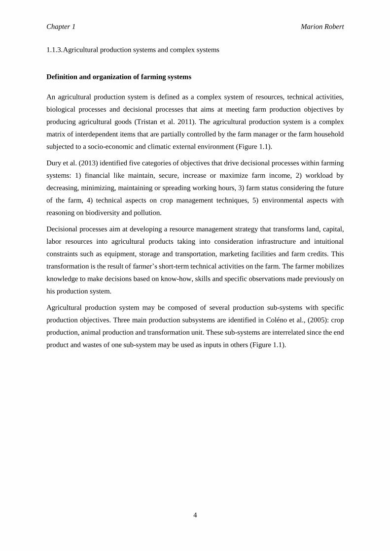
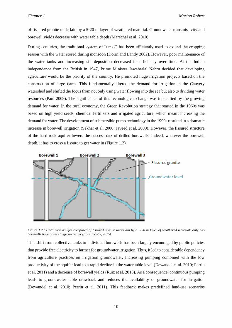
increase in borewell irrigation (Sekhar et al. 2006; Javeed et al. 2009). However, the fissured structure
of the hard rock aquifer lowers the success ratz of drilled borewells. Indeed, whatever the borewell
depth, it has to cross a fissure to get water in (Figure 1.2).
Figure 1.2 : Hard rock aquifer composed of fissured granite underlain by a 5-20 m layer of weathered material: only two
borewells have access to groundwater (from Jacoby, 2015).
This shift from collective tanks to individual borewells has been largely encouraged by public policies
that provide free electricity to farmer for groundwater irrigation. Thus, it led to considerable dependency
from agriculture practices on irrigation groundwater. Increasing pumping combined with the low
productivity of the aquifer lead to a rapid decline in the water table level (Dewandel et al. 2010; Perrin
et al. 2011) and a decrease of borewell yields (Ruiz et al. 2015). As a consequence, continuous pumping
leads to groundwater table drawback and reduces the availability of groundwater for irrigation
(Dewandel et al. 2010; Perrin et al. 2011). This feedback makes predefined land-use scenarios
Chapter 1 Marion Robert
11
unrealistic, since farmers need to adapt their actions continually according to groundwater availability
(Ruiz et al. 2015).
The main originality of the project lies on its multidisciplinary approach that combines on the one hand
the economic impacts on agricultural production and on the hydrological regime and on the other hand
the feedback effects of the hydro-climatic-economic impact on farming practices, on land use and on
agricultural productivity. The project involves several scientific issues. It aims at developing an
integrated eco-agro-hydrological model able to take into account the direct effects of agricultural
practices on water resources and the feedback effects by considering the adaptive behavior of farmer to
climate change, resource availability and market development. This integrated modeling approach also
answers the question of optimal water resource management in a context of increasing scarcity. It also
deals with the issue of distribution of water resources and agricultural land in the context of climate
change. The AICHA project analyzes scientific questions such as:
• modeling the hydrological transfers and their relationship with agricultural practices
• coupling of economic models with agronomic simulators
• testing alternative scenarios of water resource management policies at the watershed scale.
1.2.2. Thesis objectives
Agricultural production systems are facing new challenges due to an ever changing global environment
that is a source of risk and uncertainty. To adapt to these environmental changes, farmers must adjust
their management strategies and remain competitive while also satisfying societal preferences for
sustainable food systems. Representing and modeling farmers’ decision-making processes by including
adaptation is therefore an important challenge for the agricultural research community. Three issues are
at the core of this research:
Represent farmers’ decision-making and adaptation processes
What are the engaged processes in farmers’ decision-making?
Farmers’ decision-making processes are a combination of decision stages: i) the strategic decision
stage, with a long-term effect (years to decades) on whole-farm organization (e.g., decisions about
equipment investment, infrastructure development or farm expansion); ii) the tactical decision stage,
with a medium-term effect (several months or seasons) on the farm cropping system and its resource
management; and iii) the operational decision stage, with a short-term effect restricted to specific
plots and describing daily adjustments to crop management practices (Risbey et al. 1999; Le Gal et
al. 2011). Some models focus on one particular type of decision – mainly strategic (Barbier and
Bergeron 1999; Berge and Ittersum 2000; Hyytiäinen et al. 2011) or operational (Martin-Clouaire
Chapter 1 Marion Robert
12
and Rellier 2006; Merot et al. 2008; Martin et al. 2011a; Aurbacher et al. 2013; Moore et al. 2014).
Some others model two decision levels – strategic and tactical (Trebeck and Hardaker 1972; Adesina
1991; Mosnier et al. 2009) or strategic and operational (Navarrete and Bail 2007; Dury 2011;
Taillandier et al. 2012a; Gaudou and Sibertin-Blanc 2013). However, to the best of our knowledge,
the scientific literature does not offer models that include a decision model with the three decision
stages within the same model.
How can we integrate adaptive behaviors in farmers’ decision-making processes?
In the early 1980s, Petit developed the theory of the “farmer’s adaptive behavior” and claimed that
farmers have a permanent capacity for adaptation (Petit 1978). Adaptation refers to adjustments in
agricultural systems in response to actual or expected stimuli through changes in practices, processes
and structures and their effects or impacts on moderating potential modifications and benefiting
from new opportunities (Grothmann and Patt 2003; Smit and Wandel 2006). Another important
concept in the scientific literature on adaptation is the concept of adaptive capacity or capability
(Darnhofer 2014). This refers to the capacity of the system to resist evolving hazards and stresses
(Ingrand et al. 2009; Dedieu and Ingrand 2010) and it is the degree to which the system can adjust
its practices, processes and structures to moderate or offset damages created by a given change in
its environment (Brooks and Adger 2005; Martin 2015). For authors in the early 1980s such as Petit
(1978) and Lev and Campbell (1987), adaptation is seen as the capacity to challenge a set of
systematic and permanent disturbances. Moreover, decision-makers integrate long-term
considerations when dealing with short term changes in production. Both claims lead to the notion
of a permanent need to keep adaptation capability under uncertainty. Holling (2001) proposed a
general framework to represent the dynamics of a socio-ecological system based on both ideas
above, in which dynamics are represented as a sequence of “adaptive cycles”, each affected by
disturbances. Depending on whether the latter are moderate or not, farmers may have to reconfigure
the system, but if such redesigning fails, then the production system collapses. Adaptive behaviors
in farming systems have been considered (modeled) in bio-economic and bio-decision approaches.
Formalisms describing proactive behavior and anticipation decision-making processes and
formalisms representing reactive adaptation decision-making processes are used to model farmers’
decision-making processes in farming systems. There is a need to include adaptation and
anticipation to uncertain events in modeling approaches of the decision-making process.
How can we represent interactions between different dimensions of decision-making processes?
Some of the most common dimensions in adaptation research on individual behavior refer to the
timing and the temporal and spatial scopes of adaptation (Smit et al. 1999; Grothmann and Patt
2003). The first dimension distinguishes proactive versus reactive adaptations. Proactive adaptation
refers to anticipated adjustment, which is the capacity to anticipate a shock (change that can disturb
Chapter 1 Marion Robert
13
farmers’ decision-making processes); it is also called anticipatory or ex-ante adaptation. Reactive
adaptation is associated with adaptation performed after a shock; it is also called responsive or ex-
post adaptation (Attonaty et al. 1999; Brooks and Adger 2005; Smit and Wandel 2006). The
temporal scope distinguishes strategic adaptations from tactical adaptations, the former referring to
the capacity to adapt in the long term (years), while the latter are mainly instantaneous short-term
adjustments (seasonal to daily) (Risbey et al. 1999; Le Gal et al. 2011). The spatial scope of
adaptation opposes localized adaptation versus widespread adaptation. In a farm production context,
localized adaptations are often at the plot scale, while widespread ones concern the entire farm.
Temporal and spatial scopes are easily considered in farmers’ decision-making processes; however,
incorporating the timing scope of farmers’ adaptive behavior is a growing challenge when designing
farming systems.
Conceive a flexible and resilient agricultural production system
How can we design agricultural production systems from field observations?
The agricultural research community has a particular interest in modeling farming systems to
simulate opportunities for adaptation that ensure flexibility and resilience of farming systems. To
account for actors and their actions in the environment, it is essential to precisely represent their
decision-making processes. Some methods have been developed to describe farmers’ decision-
making processes such as the “model for actions” (Aubry et al. 1998a), rule-based models (Bergez
et al. 2006; Donatelli et al. 2006) and activity-based models (Clouaire and Rellier 2009; Martin et
al. 2013). However none precisely specifies the process between farmers’ decision-making and the
modeling activity. There is no clear guiding framework explaining how to proceed from field studies
to designing a model.
Which representation should be used in conceptual modeling of farming systems?
A conceptual model is a non-software description of a computer simulation model. It is the bridge
between the real system and a computer model (Robinson 2008) and therefore requires
simplification and abstraction (Robinson 2010). We identified three main ideas in the scientific
literature that are interesting to consider when modeling a farming system: i) a systemic
representation is relevant (Martin et al. 2011b; Tanure et al. 2013), ii) dynamic processes bring the
farming system to life (Bellman 1954; Mjelde 1986; Cerf and Sebillotte 1988; Papy et al. 1988;
Osman 2010), and iii) farmers’ decision-making processes are flexible and adaptive over time and
space (Grothmann and Patt 2003; Smit and Wandel 2006; Darnhofer 2014). However, to the best of
our knowledge, there is no representation of farming systems that integrates these three aspects into
a conceptual model.
Chapter 1 Marion Robert
14
How should the conceptual representation of farming system be implemented for computerized
simulation?
Conceptual modeling is followed by software implementation that codes the conceptual results. In
the past decade, several conceptual generic frameworks have been proposed for farm systems
modeling (Bergez et al. 2013). To overcome problems which arise when building, simulating and
reusing models (Reynolds and Acock 1997; Acock et al. 1999), generic computing platforms have
been created to propose model repositories to facilitate their use and re-use (e.g. CropSyst (Van
Evert and Campbell 1994) or ICASA (Bouma and Jones 2001)). The RECORD integrated modeling
platform gathers, links and provides models and companion tools to answer new agricultural
questions (Bergez et al. 2013). Coupling models representing the different entities of our agricultural
production system should be facilitated by the use of such platform.
Consider a context of water scarcity and climate change
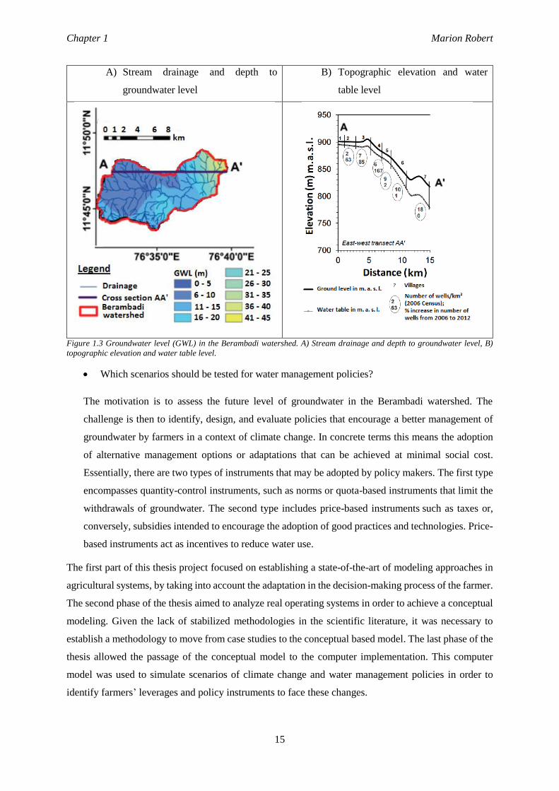
How can we account for the effect of groundwater level on farming practices and simulate the
retro-action of farming practices and in particular irrigation, on the variability of the aquifer?
In the Berambadi watershed, groundwater transmissivity and borewell yields decrease with water
table depth (Maréchal et al. 2010). As a consequence, continuous pumping leads to severe water
table drawdowns especially in hard rock aquifers and reduces the availability of groundwater for
irrigation (Dewandel et al. 2010; Perrin et al. 2011). This feedback makes predefined land-use
scenarios unrealistic, since farmers need to adapt their actions continually according to groundwater
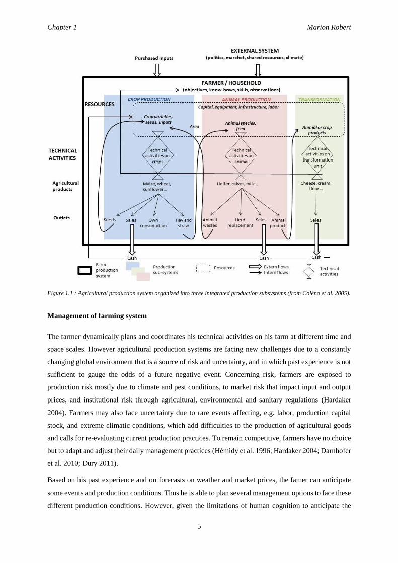
availability (Ruiz et al. 2015). Water table levels display a pattern that is atypical in hydrology:
valley regions have deeper groundwater table levels than topographically higher zones. Thus, an
unusual groundwater level gradient is observed; with a shallow groundwater table upstream and
deep groundwater table downstream (Figure 1.3). This pattern results from intensive groundwater
pumping since the early 1990s in villages located in the valley (where soils were more fertile)
(Sekhar et al. 2011). Low costs of pumping water and subsidies for irrigation equipments
encouraged farmers to drill even more borewells (Shah et al. 2009). This dramatic evolution is
closely linked to the spatial distribution of soil type and groundwater availability, as well as farming
practices, access to the market, new agricultural technologies and technical know-how, and
government aid (Sekhar et al. 2011). Modeling how farmer practices depend on groundwater
availability and how the global impact of pumping, farming practices and climate change impact on
groundwater variability is important to understand the retro-action dynamic between practices and
natural resource in particular.
Chapter 1 Marion Robert
15
A) Stream drainage and depth to
groundwater level
B) Topographic elevation and water
table level
Figure 1.3 Groundwater level (GWL) in the Berambadi watershed. A) Stream drainage and depth to groundwater level, B)
topographic elevation and water table level.
Which scenarios should be tested for water management policies?
The motivation is to assess the future level of groundwater in the Berambadi watershed. The
challenge is then to identify, design, and evaluate policies that encourage a better management of
groundwater by farmers in a context of climate change. In concrete terms this means the adoption
of alternative management options or adaptations that can be achieved at minimal social cost.
Essentially, there are two types of instruments that may be adopted by policy makers. The first type
encompasses quantity-control instruments, such as norms or quota-based instruments that limit the
withdrawals of groundwater. The second type includes price-based instruments such as taxes or,
conversely, subsidies intended to encourage the adoption of good practices and technologies. Price-
based instruments act as incentives to reduce water use.
The first part of this thesis project focused on establishing a state-of-the-art of modeling approaches in
agricultural systems, by taking into account the adaptation in the decision-making process of the farmer.
The second phase of the thesis aimed to analyze real operating systems in order to achieve a conceptual
modeling. Given the lack of stabilized methodologies in the scientific literature, it was necessary to
establish a methodology to move from case studies to the conceptual based model. The last phase of the
thesis allowed the passage of the conceptual model to the computer implementation. This computer
model was used to simulate scenarios of climate change and water management policies in order to
identify farmers’ leverages and policy instruments to face these changes.

Chapter 1 Marion Robert
16
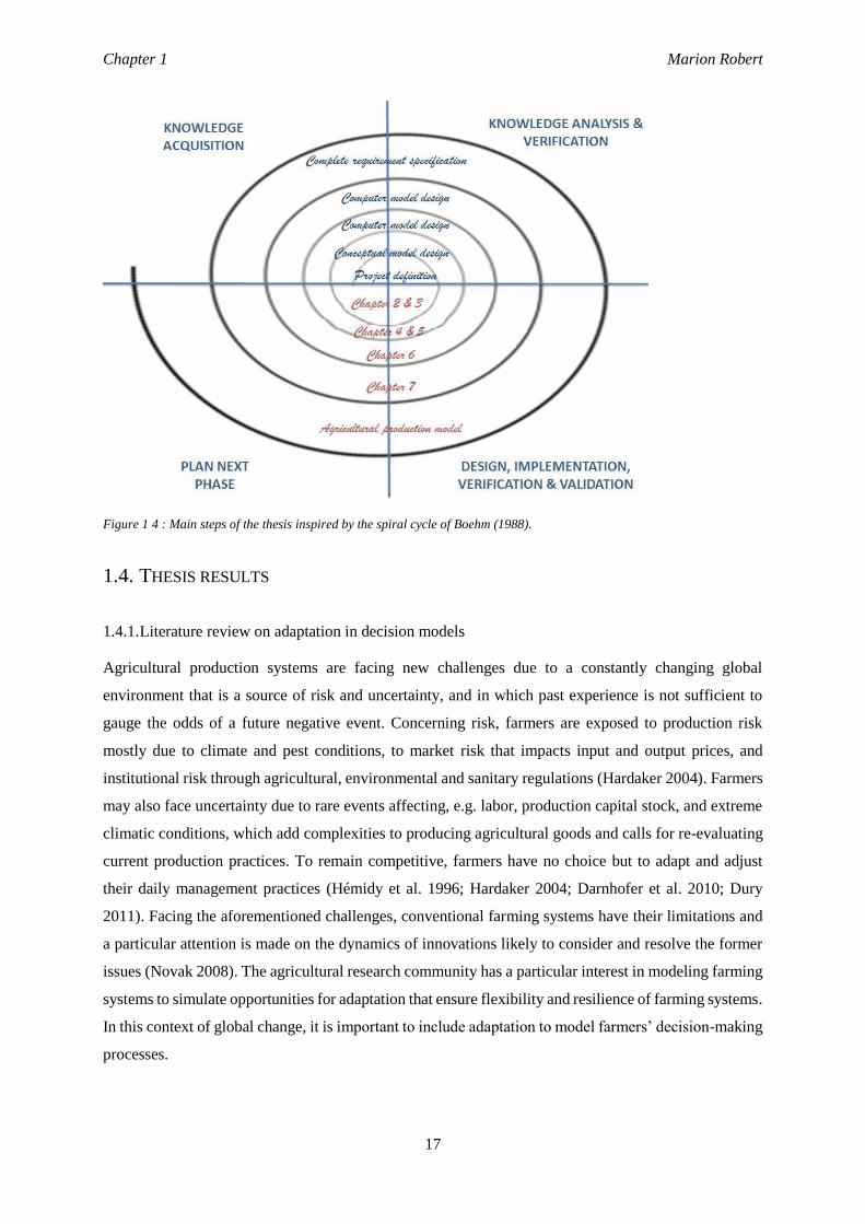
1.3. THESIS PROCEEDINGS
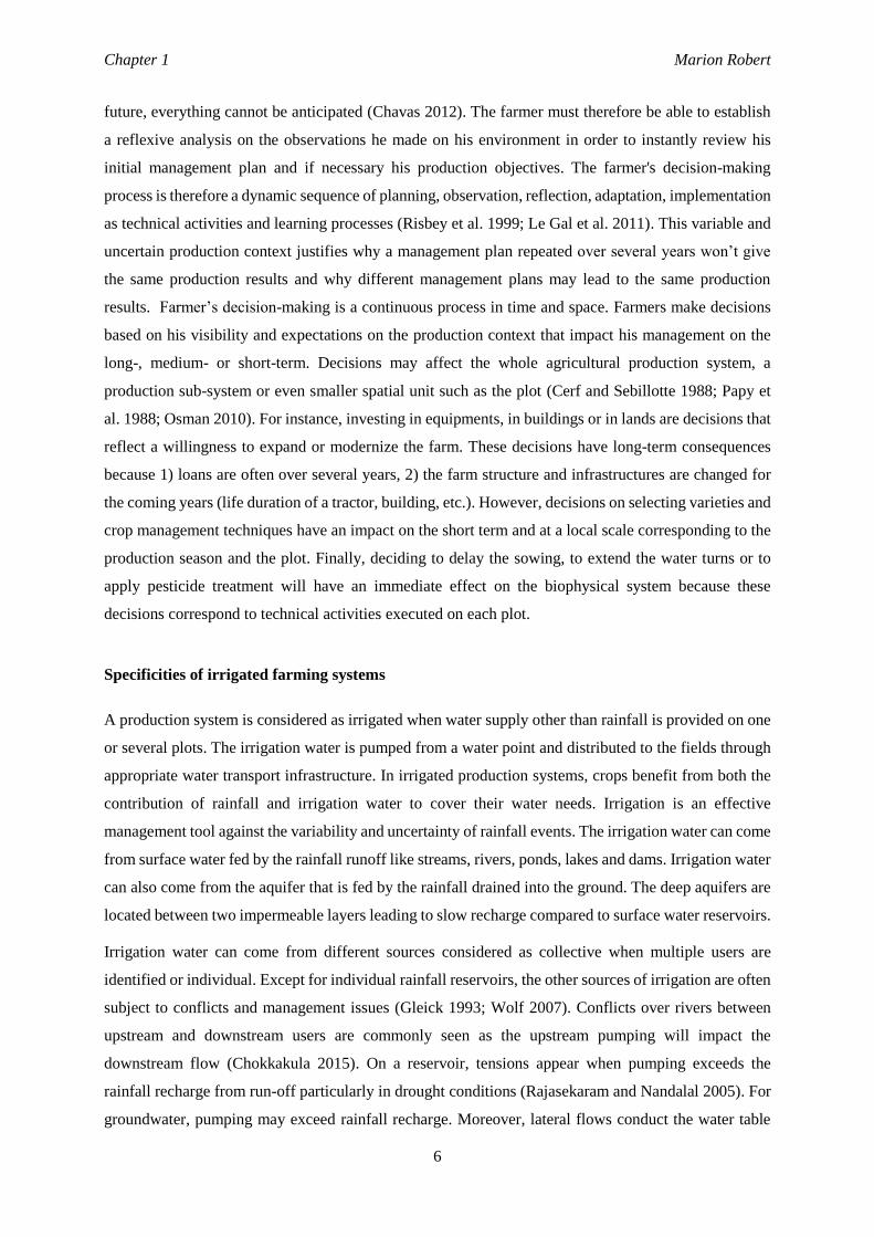
The main steps of the thesis can be summarized by the spiral cycle for the development of expert systems
of Boehm (1988). The development of the simulation model NAMASTE (Figure 1.4) began with the
expression of the needs formulated by the AICHA project to agree on what should be done in the model.
An analysis of these needs helped formulating the project definition. Following the literature review
(Chapter 2) and familiarization with the Berambadi basin (Chapter 3), we considered that the analysis
and modeling of agricultural production systems in uncertain environment require taking into account
the whole process of farmers’ decisions in integrating the different temporal and spatial scales of
decision making.
The conceptual model design formalizes the problem and chooses the functional specifications of the
simulation model using a conceptual framework (Chapter 4 and 5). The farm was formalized with three
entities (the decision-making system, the operating system and the biophysical system 3.4). The
decision-making system has been described with the beliefs, desires, intentions formalism (BDI). The
conceptual model was formulated in UML graphics to facilitate understanding between researchers,
modelers, IT professionals and stakeholders of the project.
Conceptual modeling is followed by the computer implementation of the model on a simulation
platform. Software development is done by coding the results of the design and functionality of the
model highlighted in the previous steps. A first computer approach provides the economic decision
model. A second computer approach adds the operation decision model coupled to the whole system.
Chapter 1 Marion Robert
17
Figure 1 4 : Main steps of the thesis inspired by the spiral cycle of Boehm (1988).
1.4. THESIS RESULTS
1.4.1. Literature review on adaptation in decision models
Agricultural production systems are facing new challenges due to a constantly changing global
environment that is a source of risk and uncertainty, and in which past experience is not sufficient to
gauge the odds of a future negative event. Concerning risk, farmers are exposed to production risk
mostly due to climate and pest conditions, to market risk that impacts input and output prices, and
institutional risk through agricultural, environmental and sanitary regulations (Hardaker 2004). Farmers
may also face uncertainty due to rare events affecting, e.g. labor, production capital stock, and extreme
climatic conditions, which add complexities to producing agricultural goods and calls for re-evaluating
current production practices. To remain competitive, farmers have no choice but to adapt and adjust
their daily management practices (Hémidy et al. 1996; Hardaker 2004; Darnhofer et al. 2010; Dury
2011). Facing the aforementioned challenges, conventional farming systems have their limitations and
a particular attention is made on the dynamics of innovations likely to consider and resolve the former
issues (Novak 2008). The agricultural research community has a particular interest in modeling farming
systems to simulate opportunities for adaptation that ensure flexibility and resilience of farming systems.
In this context of global change, it is important to include adaptation to model farmers’ decision-making
processes.
Chapter 1 Marion Robert
18
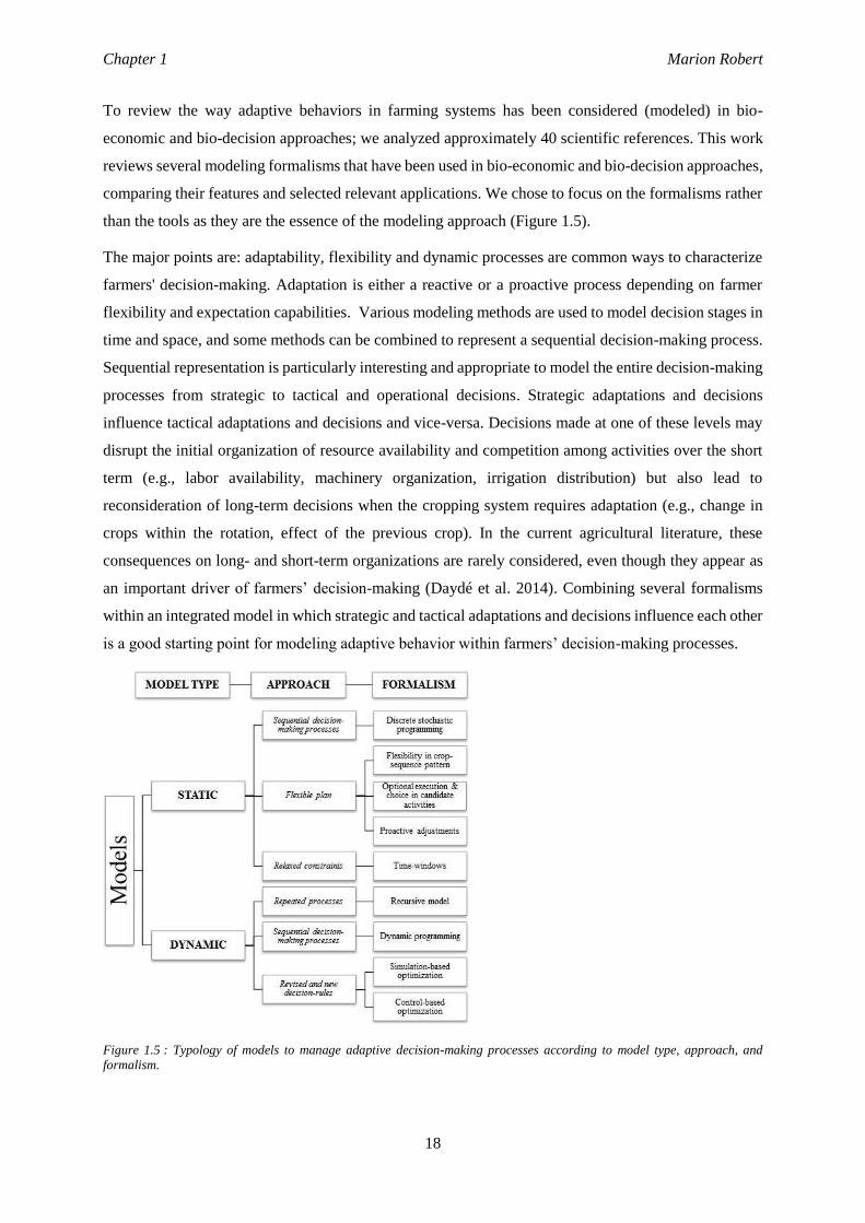
To review the way adaptive behaviors in farming systems has been considered (modeled) in bio-
economic and bio-decision approaches; we analyzed approximately 40 scientific references. This work
reviews several modeling formalisms that have been used in bio-economic and bio-decision approaches,
comparing their features and selected relevant applications. We chose to focus on the formalisms rather
than the tools as they are the essence of the modeling approach (Figure 1.5).
The major points are: adaptability, flexibility and dynamic processes are common ways to characterize
farmers' decision-making. Adaptation is either a reactive or a proactive process depending on farmer
flexibility and expectation capabilities. Various modeling methods are used to model decision stages in
time and space, and some methods can be combined to represent a sequential decision-making process.
Sequential representation is particularly interesting and appropriate to model the entire decision-making
processes from strategic to tactical and operational decisions. Strategic adaptations and decisions
influence tactical adaptations and decisions and vice-versa. Decisions made at one of these levels may
disrupt the initial organization of resource availability and competition among activities over the short
term (e.g., labor availability, machinery organization, irrigation distribution) but also lead to
reconsideration of long-term decisions when the cropping system requires adaptation (e.g., change in
crops within the rotation, effect of the previous crop). In the current agricultural literature, these
consequences on long- and short-term organizations are rarely considered, even though they appear as
an important driver of farmers’ decision-making (Daydé et al. 2014). Combining several formalisms
within an integrated model in which strategic and tactical adaptations and decisions influence each other
is a good starting point for modeling adaptive behavior within farmers’ decision-making processes.
Figure 1.5 : Typology of models to manage adaptive decision-making processes according to model type, approach, and
formalism.
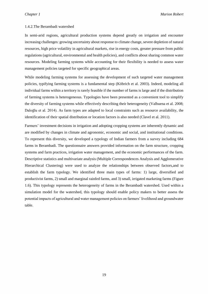
Chapter 1 Marion Robert
19
1.4.2. The Berambadi watershed
In semi-arid regions, agricultural production systems depend greatly on irrigation and encounter
increasing challenges: growing uncertainty about response to climate change, severe depletion of natural
resources, high price volatility in agricultural markets, rise in energy costs, greater pressure from public
regulations (agricultural, environmental and health policies), and conflicts about sharing common water
resources. Modeling farming systems while accounting for their flexibility is needed to assess water
management policies targeted for specific geographical areas.
While modeling farming systems for assessing the development of such targeted water management
policies, typifying farming systems is a fundamental step (Köbrich et al. 2003). Indeed, modeling all
individual farms within a territory is rarely feasible if the number of farms is large and if the distribution
of farming systems is heterogeneous. Typologies have been presented as a convenient tool to simplify
the diversity of farming systems while effectively describing their heterogeneity (Valbuena et al. 2008;
Daloğlu et al. 2014). As farm types are adapted to local constraints such as resource availability, the
identification of their spatial distribution or location factors is also needed (Clavel et al. 2011).
Farmers’ investment decisions in irrigation and adopting cropping systems are inherently dynamic and
are modified by changes in climate and agronomic, economic and social, and institutional conditions.
To represent this diversity, we developed a typology of Indian farmers from a survey including 684
farms in Berambadi. The questionnaire answers provided information on the farm structure, cropping
systems and farm practices, irrigation water management, and the economic performances of the farm.
Descriptive statistics and multivariate analysis (Multiple Correspondences Analysis and Agglomerative
Hierarchical Clustering) were used to analyze the relationships between observed factors,and to
establish the farm typology. We identified three main types of farms: 1) large, diversified and
productivist farms, 2) small and marginal rainfed farms, and 3) small, irrigated marketing farms (Figure
1.6). This typology represents the heterogeneity of farms in the Berambadi watershed. Used within a
simulation model for the watershed, this typology should enable policy makers to better assess the
potential impacts of agricultural and water management policies on farmers’ livelihood and groundwater
table.
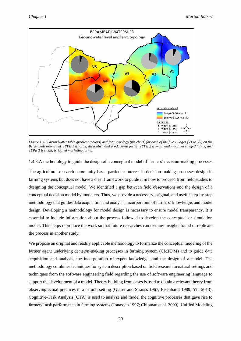
Chapter 1 Marion Robert
20
Figure 1. 6: Groundwater table gradient (colors) and farm typology (pir chart) for each of the five villages (V1 to V5) on the
Berambadi watershed. TYPE 1 is large, diversified and productivist farms; TYPE 2 is small and marginal rainfed farms; and
TYPE 3 is small, irrigated marketing farms.
1.4.3. A methodology to guide the design of a conceptual model of farmers’ decision-making processes
The agricultural research community has a particular interest in decision-making processes design in
farming systems but does not have a clear framework to guide it in how to proceed from field studies to
designing the conceptual model. We identified a gap between field observations and the design of a
conceptual decision model by modelers. Thus, we provide a necessary, original, and useful step-by-step
methodology that guides data acquisition and analysis, incorporation of farmers’ knowledge, and model
design. Developing a methodology for model design is necessary to ensure model transparency. It is
essential to include information about the process followed to develop the conceptual or simulation
model. This helps reproduce the work so that future researches can test any insights found or replicate
the process in another study.
We propose an original and readily applicable methodology to formalize the conceptual modeling of the
farmer agent underlying decision-making processes in farming system (CMFDM) and to guide data
acquisition and analysis, the incorporation of expert knowledge, and the design of a model. The
methodology combines techniques for system description based on field research in natural settings and
techniques from the software engineering field regarding the use of software engineering language to
support the development of a model. Theory building from cases is used to obtain a relevant theory from
observing actual practices in a natural setting (Glaser and Strauss 1967; Eisenhardt 1989; Yin 2013).
Cognitive-Task Analysis (CTA) is used to analyze and model the cognitive processes that gave rise to
farmers’ task performance in farming systems (Jonassen 1997; Chipman et al. 2000). Unified Modeling
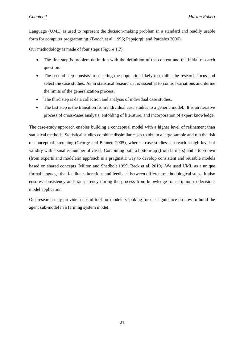
Chapter 1 Marion Robert
21
Language (UML) is used to represent the decision-making problem in a standard and readily usable
form for computer programming (Booch et al. 1996; Papajorgji and Pardalos 2006).
Our methodology is made of four steps (Figure 1.7):
The first step is problem definition with the definition of the context and the initial research
question.
The second step consists in selecting the population likely to exhibit the research focus and
select the case studies. As in statistical research, it is essential to control variations and define
the limits of the generalization process.
The third step is data collection and analysis of individual case studies.
The last step is the transition from individual case studies to a generic model. It is an iterative
process of cross-cases analysis, enfolding of literature, and incorporation of expert knowledge.
The case-study approach enables building a conceptual model with a higher level of refinement than
statistical methods. Statistical studies combine dissimilar cases to obtain a large sample and run the risk
of conceptual stretching (George and Bennett 2005), whereas case studies can reach a high level of
validity with a smaller number of cases. Combining both a bottom-up (from farmers) and a top-down
(from experts and modelers) approach is a pragmatic way to develop consistent and reusable models
based on shared concepts (Milton and Shadbolt 1999; Beck et al. 2010). We used UML as a unique
formal language that facilitates iterations and feedback between different methodological steps. It also
ensures consistency and transparency during the process from knowledge transcription to decision-
model application.
Our research may provide a useful tool for modelers looking for clear guidance on how to build the
agent sub-model in a farming system model.
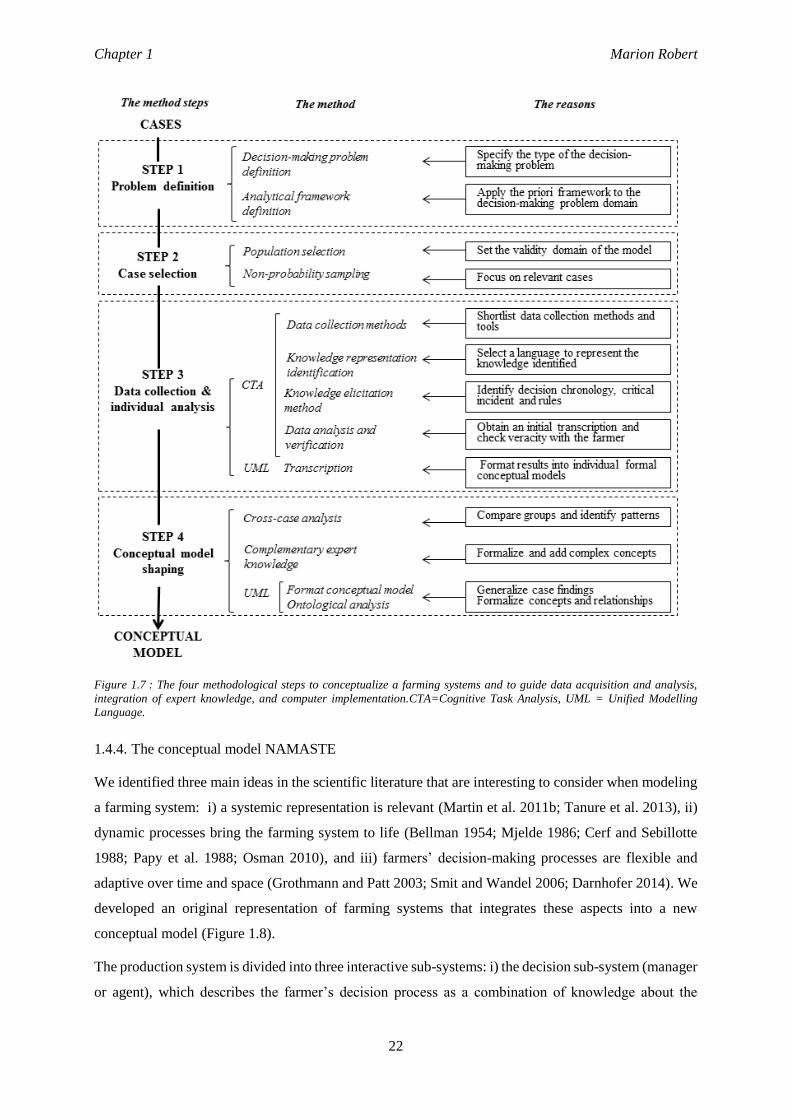
Chapter 1 Marion Robert
22
Figure 1.7 : The four methodological steps to conceptualize a farming systems and to guide data acquisition and analysis,
integration of expert knowledge, and computer implementation.CTA=Cognitive Task Analysis, UML = Unified Modelling
Language.
1.4.4. The conceptual model NAMASTE
We identified three main ideas in the scientific literature that are interesting to consider when modeling
a farming system: i) a systemic representation is relevant (Martin et al. 2011b; Tanure et al. 2013), ii)
dynamic processes bring the farming system to life (Bellman 1954; Mjelde 1986; Cerf and Sebillotte
1988; Papy et al. 1988; Osman 2010), and iii) farmers’ decision-making processes are flexible and
adaptive over time and space (Grothmann and Patt 2003; Smit and Wandel 2006; Darnhofer 2014). We
developed an original representation of farming systems that integrates these aspects into a new
conceptual model (Figure 1.8).
The production system is divided into three interactive sub-systems: i) the decision sub-system (manager
or agent), which describes the farmer’s decision process as a combination of knowledge about the
Chapter 1 Marion Robert
23
system, objectives, and decisions; ii) the operating sub-system (technical system), which translates the
decision orders into action execution and dynamics of farm resources; and, iii) the biophysical sub-
system, which describes interactions between physical and biological items, in particular the relations
between ground water, soil, and plant growth and development (Clouaire and Rellier 2009; Le Gal et al.
2010; Dury 2011; Akplogan 2013). We considered farmers as cognitive agents able to think, memorize,
analyze, predict and learn to face future events and plan their actions (Le Bars et al. 2005). We used the
as Belief-Desire-Intention (BDI) framework to represent this cognitive agents (Bratman 1987a; Rao and
Georgeff 1991).
One original feature of our model is the decision sub-model that covers three stages of decisions and
adaptations:
Each year, farmers decide whether to invest in irrigation equipment (e.g. dig a new borewell,
get a new pump) to optimize their profit. They also select the corresponding cropping system
and associated crop management operations (e.g. land preparation, sowing, fertilization,
irrigation, harvest) that will ensure the best income for their long-term climatic and price
expectations. This decision stage has a long-term effect on the entire farm due to the long
duration of loans and equipment life.
Each season, farmers make a decision that will have a medium-term effect on the entire season
and establishes the cropping system adopted for the season. Farmers integrate new observed
knowledge about climate and prices so that the cropping system initially selected at the
beginning of the year may no longer best optimize their income. They review their crop selection
and match the best practices to obtain the best cropping system for the known farming
conditions.
From the cropping system selected at the beginning of the season, farmers decide and adjust
their daily crop operations in each plot depending on climate conditions and resource
constraints. This decision stage covers the entire season at a daily time step
To model three stages of decision, we combined economic, decision-rule, and activity-based models.
Sequential representation is particularly interesting and appropriate to model the entire decision-making
processes from strategic to tactical and operational decision (Risbey et al. 1999; Le Gal et al. 2011).
Another original feature is the integrated dynamic interaction of different sub-systems that build the
farm production system.
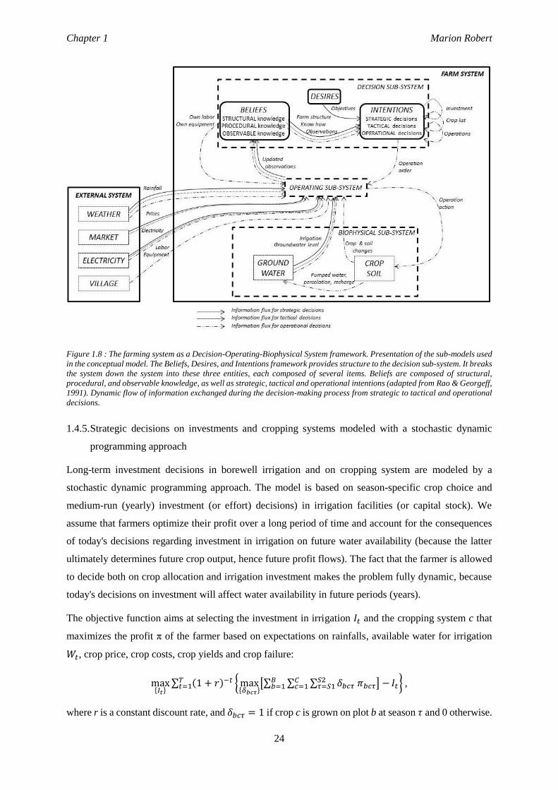
Chapter 1 Marion Robert
24
Figure 1.8 : The farming system as a Decision-Operating-Biophysical System framework. Presentation of the sub-models used
in the conceptual model. The Beliefs, Desires, and Intentions framework provides structure to the decision sub-system. It breaks
the system down the system into these three entities, each composed of several items. Beliefs are composed of structural,
procedural, and observable knowledge, as well as strategic, tactical and operational intentions (adapted from Rao & Georgeff,
1991). Dynamic flow of information exchanged during the decision-making process from strategic to tactical and operational
decisions.
1.4.5. Strategic decisions on investments and cropping systems modeled with a stochastic dynamic
programming approach
Long-term investment decisions in borewell irrigation and on cropping system are modeled by a
stochastic dynamic programming approach. The model is based on season-specific crop choice and
medium-run (yearly) investment (or effort) decisions) in irrigation facilities (or capital stock). We
assume that farmers optimize their profit over a long period of time and account for the consequences
of today's decisions regarding investment in irrigation on future water availability (because the latter
ultimately determines future crop output, hence future profit flows). The fact that the farmer is allowed
to decide both on crop allocation and irrigation investment makes the problem fully dynamic, because
today's decisions on investment will affect water availability in future periods (years).
The objective function aims at selecting the investment in irrigation 𝐼𝑡 and the cropping system c that
maximizes the profit π of the farmer based on expectations on rainfalls, available water for irrigation
𝑊𝑡, crop price, crop costs, crop yields and crop failure:
max{𝐼𝑡}
∑ (1 + 𝑟)−𝑡𝑇𝑡=1 { max
{𝛿𝑏𝑐𝜏}[∑ ∑ ∑ 𝛿𝑏𝑐𝜏 𝜋𝑏𝑐𝜏
𝑆2𝜏=𝑆1
𝐶𝑐=1
𝐵𝑏=1 ] − 𝐼𝑡} ,
where r is a constant discount rate, and 𝛿𝑏𝑐𝜏 = 1 if crop c is grown on plot b at season 𝜏 and 0 otherwise.
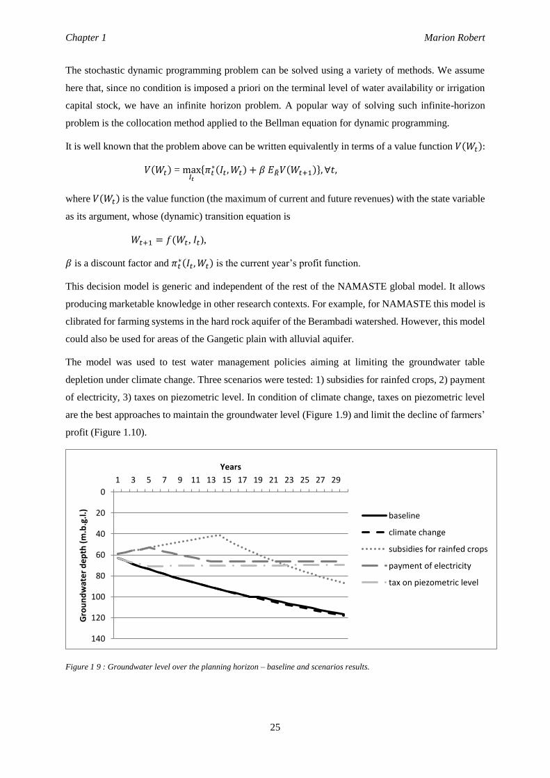
Chapter 1 Marion Robert
25
The stochastic dynamic programming problem can be solved using a variety of methods. We assume
here that, since no condition is imposed a priori on the terminal level of water availability or irrigation
capital stock, we have an infinite horizon problem. A popular way of solving such infinite-horizon
problem is the collocation method applied to the Bellman equation for dynamic programming.
It is well known that the problem above can be written equivalently in terms of a value function 𝑉(𝑊𝑡):
𝑉(𝑊𝑡) = max𝐼𝑡
{𝜋𝑡∗(𝐼𝑡, 𝑊𝑡) + 𝛽 𝐸��𝑉(𝑊𝑡+1)}, ∀𝑡,
where 𝑉(𝑊𝑡) is the value function (the maximum of current and future revenues) with the state variable
as its argument, whose (dynamic) transition equation is
𝑊𝑡+1 = 𝑓(𝑊𝑡, 𝐼𝑡),
𝛽 is a discount factor and 𝜋𝑡∗(𝐼𝑡, 𝑊𝑡) is the current year’s profit function.
This decision model is generic and independent of the rest of the NAMASTE global model. It allows
producing marketable knowledge in other research contexts. For example, for NAMASTE this model is
clibrated for farming systems in the hard rock aquifer of the Berambadi watershed. However, this model
could also be used for areas of the Gangetic plain with alluvial aquifer.
The model was used to test water management policies aiming at limiting the groundwater table
depletion under climate change. Three scenarios were tested: 1) subsidies for rainfed crops, 2) payment
of electricity, 3) taxes on piezometric level. In condition of climate change, taxes on piezometric level
are the best approaches to maintain the groundwater level (Figure 1.9) and limit the decline of farmers’
profit (Figure 1.10).
Figure 1 9 : Groundwater level over the planning horizon – baseline and scenarios results.
0
20
40
60
80
100
120
140
1 3 5 7 9 11 13 15 17 19 21 23 25 27 29
Gro
un
dw
ate
r d
ep
th (
m.b
.g.l
.)
Years
baseline
climate change
subsidies for rainfed crops
payment of electricity
tax on piezometric level
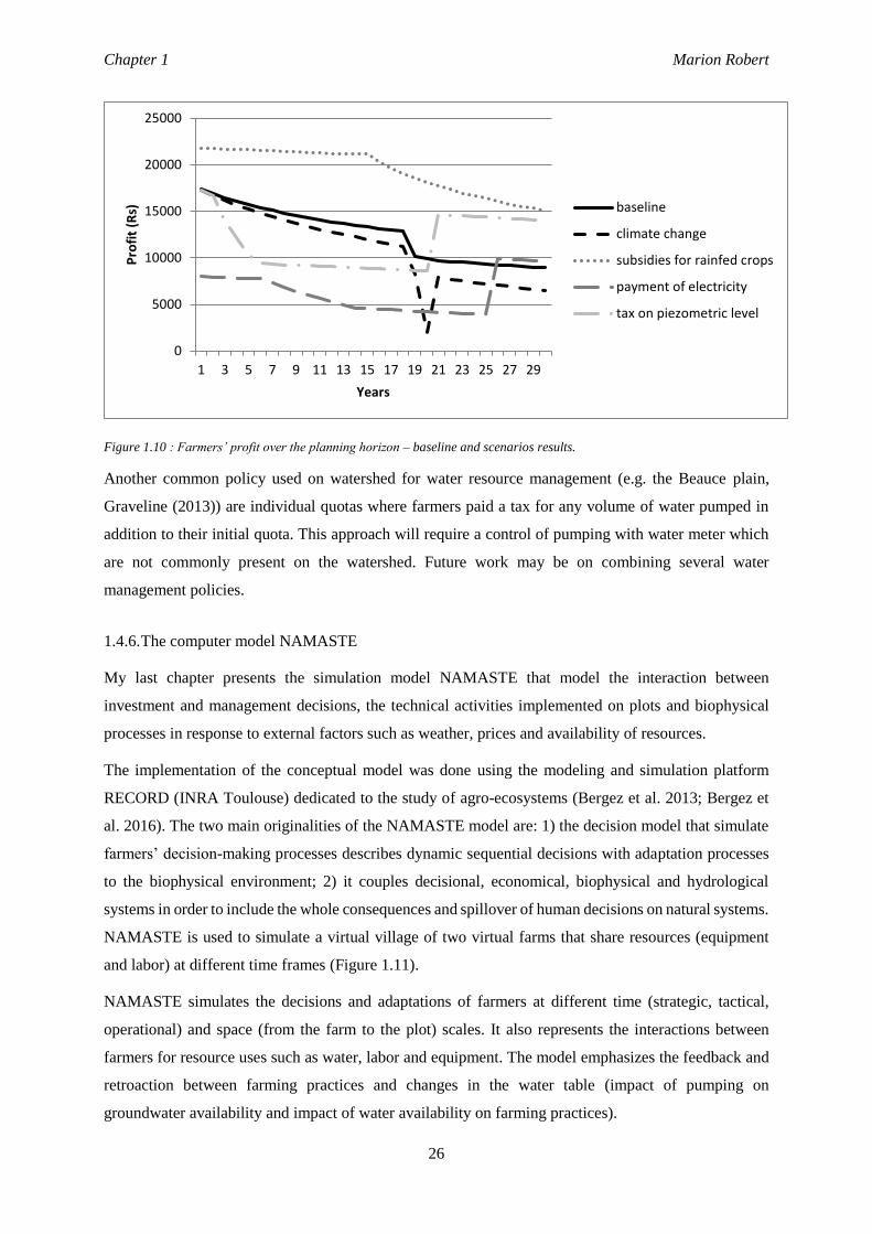
Chapter 1 Marion Robert
26
Figure 1.10 : Farmers’ profit over the planning horizon – baseline and scenarios results.
Another common policy used on watershed for water resource management (e.g. the Beauce plain,
Graveline (2013)) are individual quotas where farmers paid a tax for any volume of water pumped in
addition to their initial quota. This approach will require a control of pumping with water meter which
are not commonly present on the watershed. Future work may be on combining several water
management policies.
1.4.6. The computer model NAMASTE
My last chapter presents the simulation model NAMASTE that model the interaction between
investment and management decisions, the technical activities implemented on plots and biophysical
processes in response to external factors such as weather, prices and availability of resources.
The implementation of the conceptual model was done using the modeling and simulation platform
RECORD (INRA Toulouse) dedicated to the study of agro-ecosystems (Bergez et al. 2013; Bergez et
al. 2016). The two main originalities of the NAMASTE model are: 1) the decision model that simulate
farmers’ decision-making processes describes dynamic sequential decisions with adaptation processes
to the biophysical environment; 2) it couples decisional, economical, biophysical and hydrological
systems in order to include the whole consequences and spillover of human decisions on natural systems.
NAMASTE is used to simulate a virtual village of two virtual farms that share resources (equipment
and labor) at different time frames (Figure 1.11).
NAMASTE simulates the decisions and adaptations of farmers at different time (strategic, tactical,
operational) and space (from the farm to the plot) scales. It also represents the interactions between
farmers for resource uses such as water, labor and equipment. The model emphasizes the feedback and
retroaction between farming practices and changes in the water table (impact of pumping on
groundwater availability and impact of water availability on farming practices).
0
5000
10000
15000
20000
25000
1 3 5 7 9 11 13 15 17 19 21 23 25 27 29
Pro
fit
(Rs)
Years
baseline
climate change
subsidies for rainfed crops
payment of electricity
tax on piezometric level
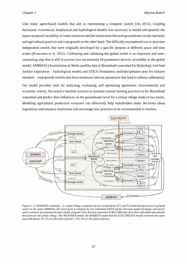
Chapter 1 Marion Robert
27
Like many agent-based models that aim in representing a complete system (An 2012), coupling
decisional, economical, biophysical and hydrological models was necessary to model and quantify the
spatio-temporal variability of water resources and the interactions between groundwater on the one hand,
and agricultural practices and crop growth on the other hand. The difficulty encountered was to associate
independent models that were originally developed for a specific purpose at different space and time
scales (Kraucunas et al. 2015). Calibrating and validating the global model is an important and time-
consuming step that is still in process (we encountered 94 parameters directly accessible in the global
model, AMBHAS (Assimilation of Multi-satellite data at Berambadi watershed for Hydrology And land
Surface experiment – hydrological model) and STICS (Simulateur multidisciplinaire pour les cultures
standard – crop growth model) also have numerous internal parameters that lead to tedious calibration).
Our model provides tools for analyzing, evaluating, and optimizing agronomic, environmental and
economic criteria. We tested a baseline scenario to simulate current farming practices in the Berambadi
watershed and predict their influences on the groundwater level for a virtual village made of two farms.
Modeling agricultural production scenarios can effectively help stakeholders make decisions about
regulations and resource restrictions and encourage new practices to be recommended to farmers.
Figure 1.11 NAMASTE simulator - a virtual village composed of two virtual farms (F1 and F2) both having access to ground
water on the same AMBHAS cell. Each farm is simulate by two individual DEVS atomic decision model (strategic and tactic)
and a common operational decision model using the VLE decision extension of RECORD that describes individual operational
decisions for the whole village. The WEATHER model, the MARKET model and the ELECTRICITY model constrain the same
way both farms. P1, P2 are the plots of farm 1. P3, P4 are the plots of farm2.
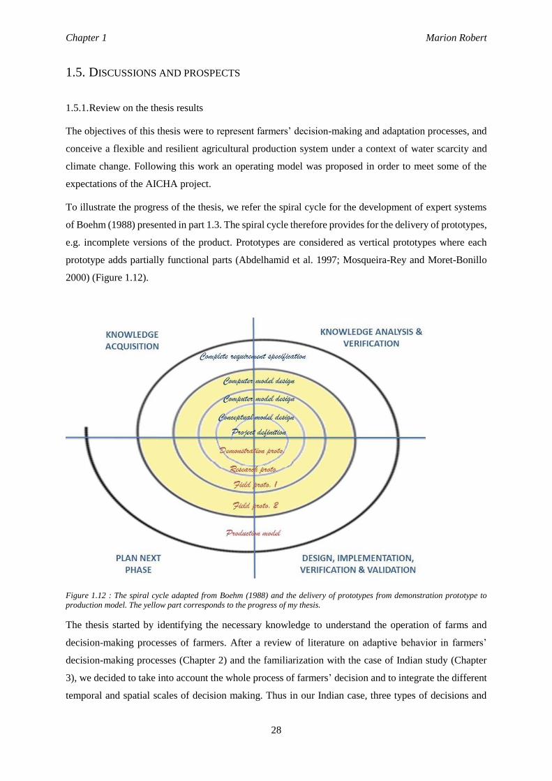
Chapter 1 Marion Robert
28
1.5. DISCUSSIONS AND PROSPECTS
1.5.1. Review on the thesis results
The objectives of this thesis were to represent farmers’ decision-making and adaptation processes, and
conceive a flexible and resilient agricultural production system under a context of water scarcity and
climate change. Following this work an operating model was proposed in order to meet some of the
expectations of the AICHA project.
To illustrate the progress of the thesis, we refer the spiral cycle for the development of expert systems
of Boehm (1988) presented in part 1.3. The spiral cycle therefore provides for the delivery of prototypes,
e.g. incomplete versions of the product. Prototypes are considered as vertical prototypes where each
prototype adds partially functional parts (Abdelhamid et al. 1997; Mosqueira-Rey and Moret-Bonillo
2000) (Figure 1.12).
Figure 1.12 : The spiral cycle adapted from Boehm (1988) and the delivery of prototypes from demonstration prototype to
production model. The yellow part corresponds to the progress of my thesis.
The thesis started by identifying the necessary knowledge to understand the operation of farms and
decision-making processes of farmers. After a review of literature on adaptive behavior in farmers’
decision-making processes (Chapter 2) and the familiarization with the case of Indian study (Chapter
3), we decided to take into account the whole process of farmers’ decision and to integrate the different
temporal and spatial scales of decision making. Thus in our Indian case, three types of decisions and
Chapter 1 Marion Robert
29
various adaptation options have been identified taking place at three different levels (strategic, tactical
and operational). These functional specifications led to a first demonstration prototype.
Then it was important to have the tools to organize and to integrate farming system knowledge into the
production system design process. I set up a step-by-step methodology (Chapter 4), to move from case
studies to a conceptual model. This conceptual model was used as research prototype. It precisely
defined the processes I wanted to take into account to meet the thesis objectives and AICHA project
expectations. The conceptual model presented in this thesis (Chapter 5) focused on the description and
definition of the decision model in interaction with other models of the operating system and external
system. This research prototype must be clear and understandable by all. The conceptual model is based
on an ontology that provides a common vocabulary for all individuals involved in the project
(researchers, modelers and experts). This allowed to discuss the model and to validate the model by the
majority of participants of the AICHA project. This research prototype was the basis for the computer
implementation of the model on the RECORD simulation platform. A first field prototype provides the
economic decision model. A second field prototype adds the operation decision model coupled to the
whole system. Functional tests have validated first each entity of the model independently before
validating the entire model. The final field prototype that I obtained corresponded to a computer model
useful to run scenarios of climate change, agricultural policy and resources scarcity and to identify the
levers used by farmers to cope with these changes in a qualitative point of view. Improvements and
deepening will be needed later to reach the production model that will meet the expectations of AICHA
project.
1.5.2. From the demonstration prototype to the production model
Selecting the biophysical model
In farm systems, decisions are translated into technical operations impacting the biophysical system.
These decisions are dependent on farmer’s observations on the state of the biophysical system. Thus in
NAMASTE, strategic and tactical decisions rely on crop yields while operational decisions depend on
soil conditions, crop stage and germination rate. Technical operations impacting on the biophysical
system are soil preparation, sowing, fertilization, irrigation and harvesting. Two major types of crop
simulation models are often used: 1) empirical or statistical models that consider relationship between
yields and components of yields with climate and environmental settings as correlation equation or
regression ; and 2) the mechanistic or functional models that describe both the relationships and
mechanisms between soil-plant systems, and climate decision (Basso et al. 2013). To simulate daily and
dynamically plant growth, use of water and crop management operations, we selected the mechanistic
model STICS to be coupled with our decision model (Brisson et al. 1998).
Chapter 1 Marion Robert
30
Three main limitations are identified:
1) Even if STICS is meant to be a generic crop model able to simulate several types of crops, its
calibration is difficult and brings a significant amount of uncertainty concerning the validity of
the model.
2) STICS does not take into account biotic processes such as pests, diseases and weeds that have
a significant impact on plant growth (Bergez et al. 2010).
3) Crop rotation is not directly considered in STICS. The crop model must be coupled with a crop
rotation model that loads a simulation unit for each new cultural plan launched by the decision
model.
The simplest alternative would be to consider the yield and the water used as the only parameters to be
considered in the decision, instead of simulating the dynamic aspect of the model. This approach is
acceptable for the strategic and tactical decisions as they are based on an expected average yield and
average production costs. However it is not acceptable for operational decisions because the conditions
of the technical operations depend on these dynamic crop settings. In this case, only the rain and the
availability of resources should constrain the decision to run a technical operation. Other simplified
functional models and calibrated for Indian crops exist as AquaCrop FAO (Raes et al. 2011) but are
based on a single process e.g. the water balance and exclude other environmental outputs e.g. nitrogen
and carbon footprints and the biotic and abiotic stresses affecting yields.
The decision model: an integrated model?
The sequential representation is particularly suited to represent the whole decision making process from
strategic decisions to tactical and operational decisions (Cerf and Sebillotte 1988; Papy et al. 1988;
Osman 2010). The strategic decisions influence the tactical and operational decisions and vice versa
disrupting the availability of resources and generating competition between activities in the short term
but also by challenging rotations and crop sequences (Daydé et al. 2014). The description of these
processes requires the development of a decision model at three levels built like we proposed in
NAMASTE. However, the current model does not fully describe this integration. Starting from
independently developed models, there remains some work regarding the coupling of the different levels
of decisions to make the global model dynamically integrated.
Strategic and tactic decisions are based on farmer’s expectations on events, occurrences, levels of certain
variables and parameters affecting decisions. Each new piece of information received may impact
farmers’ expectations and makes them reconsider and review their expectations. For instance, the
strategic decision model is mainly based on climate, market prices, production costs and yields
expectations. Through learning and appropriation processes of observed information, farmers review
their expectations by integrating it to their own knowledge database. This implies that observed
Chapter 1 Marion Robert
31
information at operational level are dynamically transferred to the farmer's knowledge database and
integrated into the algorithm that formulates farmer’s expectations. For example, in our strategic
decision model the farmer refers to probabilities of occurrence of year more or less rainy set by the last
40 years of climate data. Running the operational decision model with new climate data is not going to
change the probabilities of occurrence at the strategic level. The model should dynamically integrate the
new information in its formalism to compute these probabilities of occurrence. Bayesian approaches are
commonly used for the revision of parameters in dynamic systems (Stengel 1986). Concerning yields,
a higher level of integration could be expected between economic and operational models and between
tactical and operational models. At the strategic level, yields are currently estimated from simple
production functions depending on level of irrigation and are calibrated for several climate occurrences.
Given the use of a functional crop model for the operational level it is unfortunate that we did not to
include it in the upper levels to obtain yields. Thus each loop testing crop profits should use the
operational level over many representative years to obtain an average yield which would include the
intra- seasonal variability of rainfalls.
The decision model: a generic model?
In order to model the different types of farms identified in Chapter 3, some parameters of the NAMASTE
model must be made more generic and flexible. A critical point is the possible change of number of
plots of a farm within a planning horizon. Indeed, changing the number of plots should automatically
change the structure of the strategic and tactic models in terms of possible iterations and crop
combinations. It should also change the operational model by adding plots (or STICS models) and
linking them to the operating system and the corresponding decision model.
Another issue that deals with the possible change of number of plots is the management of the soil
characteristics from year to year. Soil status is simulated by the STICS models. Right now, we consider
that at each simulation the hydrological and mineral state of the soil is re-initiated to the initial
conditions. However, technical practices and crop types impact on soil status. When plot sizes and plot
number are fixed, it is easy to take in consideration these year-to-year impacts. However, when plots are
changing, it becomes difficult to know from which STICS model should the values come from.
Also calibration of new crops will allow better describing farm types depending on rainfed and irrigated
conditions or on crop objectives of sale or self-consumption. For now, it is the irrigated farms with cash
crops that are the best addressed in NAMASTE.
Finally, the generic characteristic of the structure and formalisms used in this model depend on the ease
to use it in other cases studies. The systemic representation is suitable for any type of farm system where
the farm is considered made of a decision component in interaction with a biophysical component under
variable and uncertain environment conditions. The structure and sequential representation of the
Chapter 1 Marion Robert
32
farmers’ decision-making processes is also generic and reusable in other contexts. Other combinations
of strategic / tactical / operational decisions can be described with this approach. However, the
adaptation to other case studies requests a facility on the instruction of new decision rules and
constraints. With today’ model, these adaptations are possible but require precise documentation on the
steps and methodologies to implement.
Improvements and deepening for the NAMASTE model
Climate scenarios and water management policies have been tested during my thesis. However many
improvements in the computer implementation are possible and could not be done during my PhD for
lack of time. First to reconsider the points made in the previous paragraph, farm structure and
initialization parameters are not fully scalable. Later on, the model will be able to dynamically create
one or more farms from an input file.
Second, the technical management practices (ITK) are described in csv files, read by an R script that
turns them into plan files mobilized by the RECORD decision plugin. For the same crop, several ITK
are possible depending on the intensification of practices in terms of fertilization and irrigation.
Howeverr, given the current model architecture, each ITK is also specific to the operation through the
resources (labor and equipment) to be mobilized for the execution of technical operations. Thus there
are currently nearly 100 plan files (5 x 10 crop intensification practices x 2 farms) to load at the
beginning of each simulation which dramatically slows down the simulation process. Subsequently, the
plan file creation should be dynamic so that plan files are not specific to farms (in terms of resources)
and that only those mobilized for the simulation are loaded in the simulator.
The duration of technical activities is also a point on which modeling time should be spent. So far, the
simulator considers that each activity takes place in one day and systematically releases resources for
the next day. However, certain activities such as sowing, weeding and harvesting can take place over
several days depending on the availability of the workforce. Subsequently, the operating system should
be able to set the duration of a technical activity depending on the resource needs and on the available
resources. It should also maintain the mobilization of resources during the whole activity duration.
To deal with the issue on soil state and plot changes, one solution may be to sub-divide a farm into
smaller-sized sub-plots. Then a plot will be a combination of sub-plots and will have several STICS
models running independently to simulate a crop growth.
Moreover, the management of alternative crops at a sowing or germination failures does not allow to
reuse the initial rotation as the replacement crop is added to the rotation, which implies that the rotation
is modified and subsequently integrates the alternative crops. However a rotation is assumed to be fixed.
Even if adjustments are possible during rotation they should not be maintained for the next rotation. The
management of the rotation is done at two levels: 1) at the decision level, 2) at the biophysical level.
Chapter 1 Marion Robert
33
The problem lies in the biophysical system. The rotator is a model in charge to load the subsequent
simulation unit (USM) for the STICS model. At the beginning of the simulation, the same crop list is
provided to the decision model and the rotator. When the replacement crop is introduced, the rotator
receives an alert from the decision model to inform him about the replacement of one culture by another.
The rotator will then insert this new crop in its crop list but is not able to identify this new crop as a
temporary crop.
Finally, the setting of the model makes it difficult to test alternative scenarios in terms of new practices
and policies. Indeed, the setting of crops under STICS is tedious and requires a lot of field data.
Integrating new ITK requires describing new decision rules, new predicates, and new constraints. Add
a new policy requires changing the script and the parameter files of the strategic and tactic model.
1.5.3. Verification and validation
Verification and validation in the model development process
Each prototypes developed during the development cycle of the agricultural production system is
followed by verification and validation phases to obtain a valid simulation model (Borenstein 1998;
Sargent 2013; Augusiak et al. 2014) (Figure 1.13). Conceptual validation follows the development of
the conceptual model (or research prototype) and this process is repeated until the conceptual model is
sufficient to meet the objectives of the initial problem and its modeling. The verification of the computer
models ensures that the computer models (field prototype 1 and 2) are correctly implemented in relation
to the conceptual model. Finally the operational validation is conducted on the computer model to
determine if the outputs of the simulation are adequate for simulation purposes. For each step, data
validation ensures the adequacy of the data to build the model, to evaluate the model, to test the
simulation model.
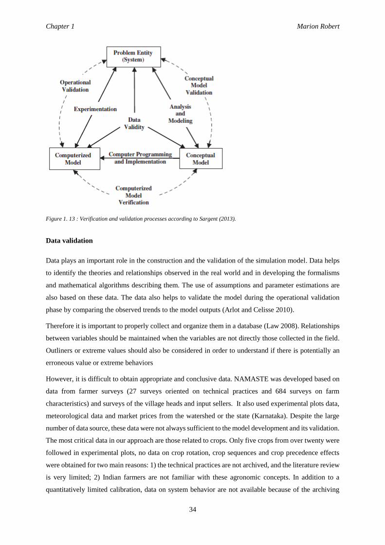
Chapter 1 Marion Robert
34
Figure 1. 13 : Verification and validation processes according to Sargent (2013).
Data validation
Data plays an important role in the construction and the validation of the simulation model. Data helps
to identify the theories and relationships observed in the real world and in developing the formalisms
and mathematical algorithms describing them. The use of assumptions and parameter estimations are
also based on these data. The data also helps to validate the model during the operational validation
phase by comparing the observed trends to the model outputs (Arlot and Celisse 2010).
Therefore it is important to properly collect and organize them in a database (Law 2008). Relationships
between variables should be maintained when the variables are not directly those collected in the field.
Outliners or extreme values should also be considered in order to understand if there is potentially an
erroneous value or extreme behaviors
However, it is difficult to obtain appropriate and conclusive data. NAMASTE was developed based on
data from farmer surveys (27 surveys oriented on technical practices and 684 surveys on farm
characteristics) and surveys of the village heads and input sellers. It also used experimental plots data,
meteorological data and market prices from the watershed or the state (Karnataka). Despite the large
number of data source, these data were not always sufficient to the model development and its validation.
The most critical data in our approach are those related to crops. Only five crops from over twenty were
followed in experimental plots, no data on crop rotation, crop sequences and crop precedence effects
were obtained for two main reasons: 1) the technical practices are not archived, and the literature review
is very limited; 2) Indian farmers are not familiar with these agronomic concepts. In addition to a
quantitatively limited calibration, data on system behavior are not available because of the archiving
Chapter 1 Marion Robert
35
problem of the technical activities and crop choices made from one year to another. This limitation
reconsiders the reliability of the model and its calibration. Today NAMASTE is considered qualitatively
acceptable but will need further calibration and assessments to be considered quantitatively
representative.
Conceptual validation
Conceptual validation is essential to ensure that the assumptions, theories and simplifications used to
build the conceptual model are sufficiently accurate and relevant to meet the stakeholders’ requirements
and the objectives of the study (Costal et al. 1996; Borenstein 1998; Liu et al. 2011). To validate the
conceptual model, we used: i) face validation that consists in asking experts and knowledgeable
individuals about the study objectives to evaluate the conceptual model and determine whether it is
correct and reasonable for the study purpose; and ii) traces techniques that consists in tracking entities
through each sub-model and the overall model to determine whether the model’s logic and the necessary
accuracy are maintained (Robinson 2010; Sargent 2010; Robinson 2014). Conceptual validation is
inherently an informal process referring to subjective and human judgement.
Each sub-model and the overall model must be evaluated to determine if they are reasonable and correct.
First, we applied White-Box validation to the sub-models to determine whether each constituent part of
the conceptual model represents the real world with sufficient accuracy to meet the study objectives
(Robinson 2014). Each sub-system was validated by experts in the associated research field. Both
experts and modelers were essential to build the decision sub-model. Modelers ensure that decision
processes are appropriately designed into the chosen framework and formalisms. Indian agronomic
researchers validated the decision rules for crop management and adaption. We also asked Indian
researchers from the research project to participate to the validation of each sub-model as main
stakeholders on the project and to certify the representation and data used to build the external system.
Second, we applied Black-Box validation to the overall model to determine whether the model provide
a sufficiently accurate representation of the real world for the intended purpose of the study (Robinson
2014). The entire system was validated by experts on the different sub-systems, modelers and the Indian
researchers. They worked on the consistency between inputs and outputs of each sub-system to ensure
rational interactions between systems. Specification of each sub-model was circulated among those who
have a detailed knowledge of the system. They shared feedbacks on whether the model was relevant by
determining if the appropriate details and aggregate relationships were used for the model’s intended
purpose.
Basically, the conceptual validation used in NAMASTE involves a subjective process based on informal
intuitive human judgment. Conceptual validation is essential to reduce the risk of distortions and errors
on further model development steps; however conceptual validation is not enough to the validation of
Chapter 1 Marion Robert
36
the final production model. It must be supported by mathematical validation and statistical validation
approaches during the next steps of model development.
Computer model verification
The verification of the computer model ensures that its implementation matches the expectations of the
conceptual model. Simulation models are often large computer models that can be the subject of
computer bugs or coding errors. The verification therefore ensures the absence of coding errors and
verifies that the simulation language used has been properly implemented in computer programming
(Borenstein 1998).
We used two basic approaches for the verification of NAMASTE: the static approach and the dynamic
approach. The first approach leads to include anti-bugs and unitary tests all along the code that locally
checks locally the program. The second one consists of running the program in different conditions and
analyzes the outputs to ensure the proper behavior of the model and to reveal possible implementation
errors.
However, we should consider that errors identified during the computer model verification may be due
to the conceptual model itself, to the computer program with coding errors or non-optimization of the
programming language or to the data used in the dynamic approach (Whitner and Balci 1986).
Operational validation
The operational validation determines whether the behavior of the final simulation model has the
required accuracy to meet the expectations and primary research objectives (Kleijnen 1995). The
operational validation uses the developed simulation model, which implies that any malfunction can
come from what has been developed in the preceding steps of model development, as well as from the
assumptions, the theories or the data (Refsgaard and Knudsen 1996).
The operational validation can be done objectively by comparing the behavior of the simulation model
outputs to the observed system or other models with statistical tests or subjectively without statistical
test (Sargent 2013).
The first objective validation approach uses hypothesis tests to compare means, variances and
distributions between output variables and the observed system or other already validated models. The
second objective validation approach uses confidence intervals based on means and standard deviations
for each set of data obtained from system observations.
In NAMASTE, operational validation was mainly conducted subjectively. The first subjective validation
approach uses graphical comparison between simulation results and observed system such as box plots,
histograms and graphs that describe variables behavior. The second approach of subjective validation
Chapter 1 Marion Robert
37
explores the simulation model behavior by analyzing the outputs of the simulation model. This
exploration was done qualitatively by defining whether the directions and the magnitudes of the output
variables are acceptable. Subjective validation may also be done quantitatively by precisely analyzing
the directions and magnitudes of these variables. We used sensibility analyses to examine the behavior
of the NAMASTE model.
1.5.4. A decision model for the AICHA project
Scaling up an agricultural production model
Upscaling from the farm level to catchment, regional and national level is a common approach in
studying system behavior and dynamics such as farm adaptation to climate change (Gibbons et al. 2010),
land use and land cover change to climate change (Rounsevell et al. 2014), ecosystem changes to biotic
and abiotic processes (Nash et al. 2014). Peters et al. (2007) identified three domains of scales: 1) “fine”
at the scale of an individual; 2) “intermediate” at the scale of groups of individuals and, 3) “broad” at
the scale of large spatial extents such as landscape, region and the whole globe.
The appropriate scale is defined by the question or hypothesis of research and often requires the
upscaling or downscaling of existing models (Gibbons et al. 2010). We consider the problem of
upscaling from the perspective of modeling the retro-action of farmers’ adaptation to climatic change
and groundwater evolution. We emphasize upscaling from the farm level to the catchment level. The
underlying scale is the farm level where farmers’ decision making occurs and resources are allocated.
To study the global impact and retro-action of groundwater evolution and climate change on farmers’
practices we upscale the farm model developed during this thesis.
Two main methods of upscaling can be used: 1) simple model replication of the farm models for each
unit (farms) modeled; 2) model aggregation. The first approach is computationally intensive and requires
sufficient data and knowledge of farmers’ characteristics for the farm model specification and
calibration (Rounsevell et al. 2014). We will use the aggregation approach by globally representing all
individual farmers and classifying them according to a limited number of clearly defined decision-
making strategies, following the typology proposed in Chapter 3.
The aggregation or upscaling challenge is to determine which fine-scale details actually matter at
intermediate or broad scales. Research questions are different depending on the scale. At the farm scale,
we focused on decision-making processes of farmers and their adaptation to uncertain changes (e.g.
climate, resource availability). At the watershed scale the issue is to look at the effect of decision making
on groundwater table rather than the process of decision making itself and to consider interactions
between individuals for shared resources. At the watershed scale, relative trends become more important
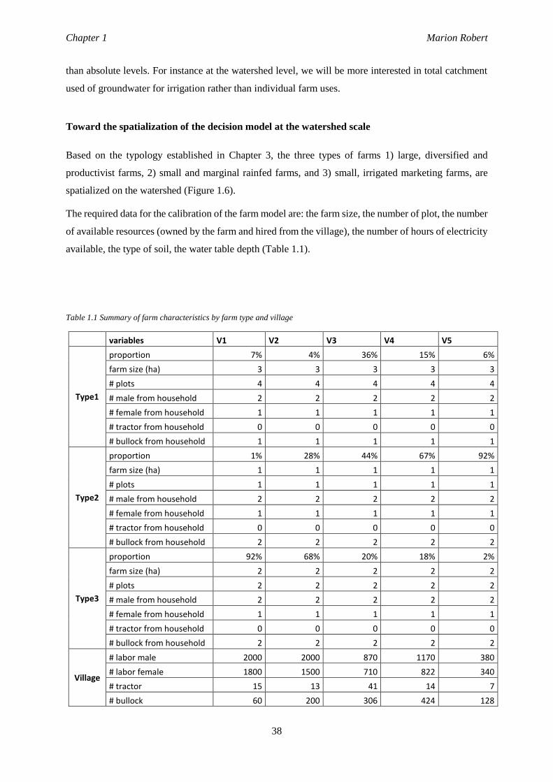
Chapter 1 Marion Robert
38
than absolute levels. For instance at the watershed level, we will be more interested in total catchment
used of groundwater for irrigation rather than individual farm uses.
Toward the spatialization of the decision model at the watershed scale
Based on the typology established in Chapter 3, the three types of farms 1) large, diversified and
productivist farms, 2) small and marginal rainfed farms, and 3) small, irrigated marketing farms, are
spatialized on the watershed (Figure 1.6).
The required data for the calibration of the farm model are: the farm size, the number of plot, the number
of available resources (owned by the farm and hired from the village), the number of hours of electricity
available, the type of soil, the water table depth (Table 1.1).
Table 1.1 Summary of farm characteristics by farm type and village
variables V1 V2 V3 V4 V5
Type1
proportion 7% 4% 36% 15% 6%
farm size (ha) 3 3 3 3 3
# plots 4 4 4 4 4
# male from household 2 2 2 2 2
# female from household 1 1 1 1 1
# tractor from household 0 0 0 0 0
# bullock from household 1 1 1 1 1
Type2
proportion 1% 28% 44% 67% 92%
farm size (ha) 1 1 1 1 1
# plots 1 1 1 1 1
# male from household 2 2 2 2 2
# female from household 1 1 1 1 1
# tractor from household 0 0 0 0 0
# bullock from household 2 2 2 2 2
Type3
proportion 92% 68% 20% 18% 2%
farm size (ha) 2 2 2 2 2
# plots 2 2 2 2 2
# male from household 2 2 2 2 2
# female from household 1 1 1 1 1
# tractor from household 0 0 0 0 0
# bullock from household 2 2 2 2 2
Village
# labor male 2000 2000 870 1170 380
# labor female 1800 1500 710 822 340
# tractor 15 13 41 14 7
# bullock 60 200 306 424 128
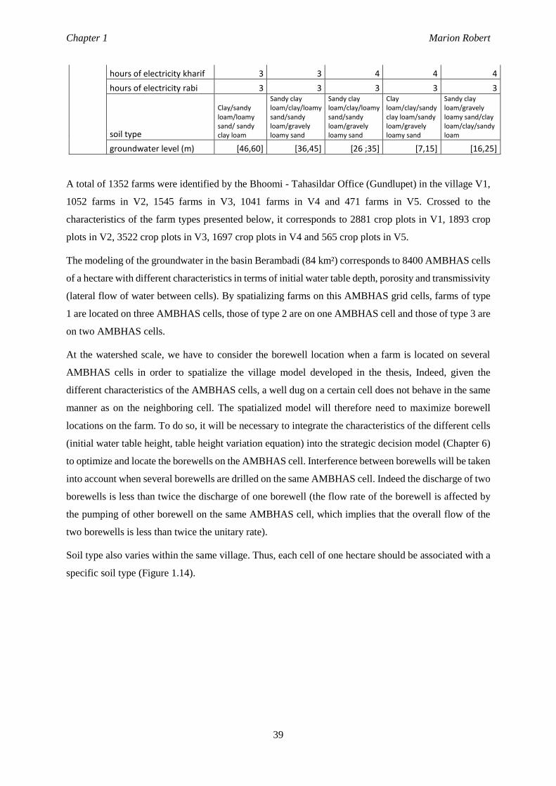
Chapter 1 Marion Robert
39
hours of electricity kharif 3 3 4 4 4
hours of electricity rabi 3 3 3 3 3
soil type
Clay/sandy loam/loamy sand/ sandy clay loam
Sandy clay loam/clay/loamy sand/sandy loam/gravely loamy sand
Sandy clay loam/clay/loamy sand/sandy loam/gravely loamy sand
Clay loam/clay/sandy clay loam/sandy loam/gravely loamy sand
Sandy clay loam/gravely loamy sand/clay loam/clay/sandy loam
groundwater level (m) [46,60] [36,45] [26 ;35] [7,15] [16,25]
A total of 1352 farms were identified by the Bhoomi - Tahasildar Office (Gundlupet) in the village V1,
1052 farms in V2, 1545 farms in V3, 1041 farms in V4 and 471 farms in V5. Crossed to the
characteristics of the farm types presented below, it corresponds to 2881 crop plots in V1, 1893 crop
plots in V2, 3522 crop plots in V3, 1697 crop plots in V4 and 565 crop plots in V5.
The modeling of the groundwater in the basin Berambadi (84 km²) corresponds to 8400 AMBHAS cells
of a hectare with different characteristics in terms of initial water table depth, porosity and transmissivity
(lateral flow of water between cells). By spatializing farms on this AMBHAS grid cells, farms of type
1 are located on three AMBHAS cells, those of type 2 are on one AMBHAS cell and those of type 3 are
on two AMBHAS cells.
At the watershed scale, we have to consider the borewell location when a farm is located on several
AMBHAS cells in order to spatialize the village model developed in the thesis, Indeed, given the
different characteristics of the AMBHAS cells, a well dug on a certain cell does not behave in the same
manner as on the neighboring cell. The spatialized model will therefore need to maximize borewell
locations on the farm. To do so, it will be necessary to integrate the characteristics of the different cells
(initial water table height, table height variation equation) into the strategic decision model (Chapter 6)
to optimize and locate the borewells on the AMBHAS cell. Interference between borewells will be taken
into account when several borewells are drilled on the same AMBHAS cell. Indeed the discharge of two
borewells is less than twice the discharge of one borewell (the flow rate of the borewell is affected by
the pumping of other borewell on the same AMBHAS cell, which implies that the overall flow of the
two borewells is less than twice the unitary rate).
Soil type also varies within the same village. Thus, each cell of one hectare should be associated with a
specific soil type (Figure 1.14).
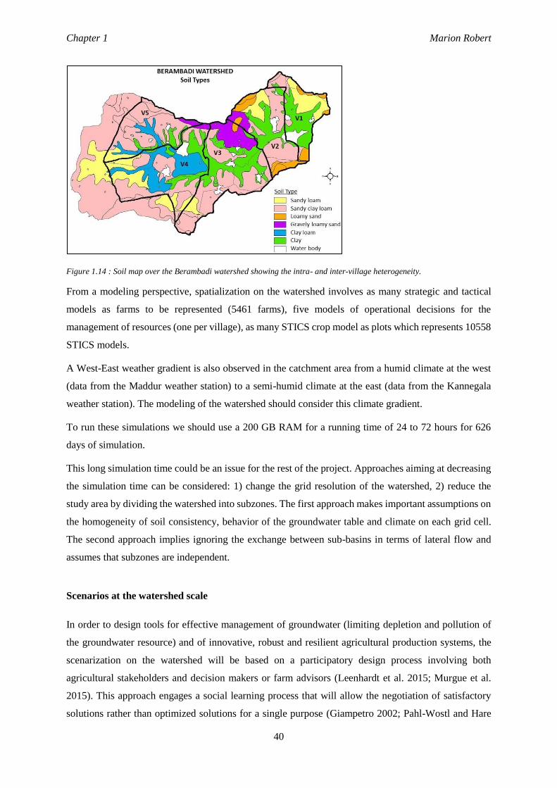
Chapter 1 Marion Robert
40
Figure 1.14 : Soil map over the Berambadi watershed showing the intra- and inter-village heterogeneity.
From a modeling perspective, spatialization on the watershed involves as many strategic and tactical
models as farms to be represented (5461 farms), five models of operational decisions for the
management of resources (one per village), as many STICS crop model as plots which represents 10558
STICS models.
A West-East weather gradient is also observed in the catchment area from a humid climate at the west
(data from the Maddur weather station) to a semi-humid climate at the east (data from the Kannegala
weather station). The modeling of the watershed should consider this climate gradient.
To run these simulations we should use a 200 GB RAM for a running time of 24 to 72 hours for 626
days of simulation.
This long simulation time could be an issue for the rest of the project. Approaches aiming at decreasing
the simulation time can be considered: 1) change the grid resolution of the watershed, 2) reduce the
study area by dividing the watershed into subzones. The first approach makes important assumptions on
the homogeneity of soil consistency, behavior of the groundwater table and climate on each grid cell.
The second approach implies ignoring the exchange between sub-basins in terms of lateral flow and
assumes that subzones are independent.
Scenarios at the watershed scale
In order to design tools for effective management of groundwater (limiting depletion and pollution of
the groundwater resource) and of innovative, robust and resilient agricultural production systems, the
scenarization on the watershed will be based on a participatory design process involving both
agricultural stakeholders and decision makers or farm advisors (Leenhardt et al. 2015; Murgue et al.
2015). This approach engages a social learning process that will allow the negotiation of satisfactory
solutions rather than optimized solutions for a single purpose (Giampetro 2002; Pahl-Wostl and Hare
Chapter 1 Marion Robert
41
2004; Newig et al. 2008; Sterk et al. 2009). The challenge will be to get participants to express as clearly
as possible their views on possible changes at the catchment scale in order to identify the concepts and
objectives for evaluation. This evaluation of scenarios will be made by running the simulation model
for each proposed scenario. It will allow seeing the effects of these possible changes on the quantitative
and qualitative evolution of groundwater on the Berambadi watershed.
Possible scenarii based on my thesis work are:
Climate change scenario: a report published by the Bangalore Climate Change Initiative -
Karnataka (BCCI-K) in 2011 predicts a decline of 1.85% of annual rainfall and a rise of 1.96°C
in average temperatures associated with higher drought frequency in the district Chamaraja
Najar between 2021 and 2050.
Crop subsidies: rainfed cropping systems may be encouraged by the establishment of subsidies
to cover the risks incurred without the support of irrigation. Crops such as pulses (lentils,
chickpeas) which are the basis of Indian food have been neglected these last years in favor of
more lucrative cash crops. Between 2015 and 2016, India imported 5.8 million tonnes of pulses
mainly produced in Africa. Subsidies encouraging local production of pulses can also be
considered.
Piezometric taxation: this global tax evolving with the decline of the groundwater table, impacts
all irrigating farmers on the same water table regardless of pumping intensity. It can be a good
policy to limit groundwater extraction.
Electricity management: even if the access to electricity is limited to few hours per day on the
watershed, free electricity does not limit over-consumption behaviors. Charging electricity
could makes farmers aware of resource depletion.
Irrigation quota: quotas are a fairly common practice in water management policies (Graveline
2013), however they require that each borewell / pump is equipped with a water meter.
Collecting rainfall for irrigation: the use of water retention basin (ponds) is an ancient technique
in the watershed that was abandoned in favor of individual pumping. Subsidies for the
establishment or upgrading of the status of individual or collective ponds can encourage the
collection and use of rainwater for irrigation.
Collection of rainfall water for direct recharge of the aquifer: collected rainfall water (runoff
from roofs, retention pond) could be conducted to the old open wells for the direct recharge of
the aquifer.
Chapter 1 Marion Robert
42
1.6. CONCLUSION
The objectives of this thesis were to represent farmers’ decision-making and adaptation processes, and
conceive a flexible and resilient agricultural production system under a context of water scarcity and
climate change.
We provided a necessary, original, and useful step-by-step methodology that guides data acquisition and
analysis, incorporation of farmers’ knowledge, and model design.
We identified three main ideas in the scientific literature that are interesting to consider when modeling
a farming system: i) a systemic representation is relevant, ii) dynamic processes bring the farming
system to life (Bellman 1954; Mjelde 1986; Cerf and Sebillotte 1988; Aubry et al. 1998a; Osman 2010),
(Bellman 1954; Mjelde 1986; Cerf and Sebillotte 1988; Papy et al. 1988; Osman 2010)(Bellman 1954;
Mjelde 1986; Cerf and Sebillotte 1988; Papy et al. 1988; Osman 2010)(Bellman 1954; Mjelde 1986;
Cerf and Sebillotte 1988; Papy et al. 1988; Osman 2010)and iii) farmers’ decision-making processes are
flexible and adaptive over time and space (Grothmann and Patt 2003; Smit and Wandel 2006; Darnhofer
2014)(Grothmann and Patt 2003; Smit and Wandel 2006; Darnhofer 2014)(Grothmann and Patt 2003;
Smit and Wandel 2006; Darnhofer 2014)(Grothmann and Patt 2003; Smit and Wandel 2006; Darnhofer
2014). We developed an original representation of farming systems that integrates these aspects into a
new conceptual model.
NAMASTE simulates the decisions of farmers in different time (strategic, tactical, operational) and
space (from the farm to the plot) scales. It represents the interactions between farmers for resource uses
such as water, labor and equipment. The model also emphasizes the feedback and retroaction between
farming practices and changes in the water table (e.g. pumping impact on groundwater availability,
water availability impact on farming practices).
The model was initially developed to address critical issues of groundwater depletion and farming
practices in a watershed in southwestern India. Its structure, frameworks and formalisms can be used in
other agricultural contexts. Our application focused on water management in semi-arid agricultural
systems, but it can also be applied to other farming systems to confirm the re-usability and applicability
of the framework.
For the AICHA project, we proposed a farm model that will be useful for future upscaling at the
watershed scale.

Chapter 2 Marion Robert
44
Chapter 2
Processes of adaptation in farm
decision-making models- A review
Marion Robert1,*, Alban Thomas2, Jacques-Eric Bergez1
¹ INRA, Université Fédérale de Toulouse, UMR 1248 AGIR, F-31326 Castanet-Tolosan, France
² Toulouse School of Economics, INRA, University of Toulouse, F-31000 Toulouse, France
*: Corresponding author, Tel: +33 (0)5 61 28 50 30. E-mail: [email protected]
Accepted for publication in Agronomy for Sustainable Development
Review Article
Doi: 10.1007/s13593-016-0402-x
Quote: Robert, Thomas, A., & Bergez, J. E. (2016). Processes of adaptation in farm decision-making
models – A review. Agronomy for Sustainable Development.
Chapter 2 Marion Robert
45
Agricultural production systems should evolve fast to cope with risks induced by climate change.
Farmers should adapt their management strategies to stay competitive and satisfy the societal demand
for sustainable food systems. It is therefore important to understand decision-making processes used by
farmers for adaptation. Processes of adaptation are in particular addressed by bio-economic and bio-
decision models.
Here we review bio-economic and bio-decision models, in which strategic and tactical decisions are
included in dynamic adaptive and expectation-based processes, in 40 literature articles. The major points
are: adaptability, flexibility and dynamic processes are common ways to characterize farmers' decision-
making. Adaptation is either a reactive or a proactive process depending on farmer flexibility and
expectation capabilities. Various modeling methods are used to model decision stages in time and space,
and some methods can be combined to represent a sequential decision-making process.
Keywords: farmers’ decision-making, bio-economic model, bio-decision model, uncertainty, adaptation
Chapter 2 Marion Robert
46
2.1. INTRODUCTION
Agricultural production systems are facing new challenges due to a constantly changing global
environment that is a source of risk and uncertainty, and in which past experience is not sufficient to
gauge the odds of a future negative event. Concerning risk, farmers are exposed to production risk
mostly due to climate and pest conditions, to market risk that impact input and output prices, and
institutional risk through agricultural, environmental and sanitary regulations (Hardaker 2004). Farmers
may also face uncertainty due to rare events affecting, e.g. labor, production capital stock, and extreme
climatic conditions, which add difficulties to producing agricultural goods and calls for re-evaluating
current production practices. To remain competitive, farmers have no choice but to adapt and adjust
their daily management practices (Hémidy et al. 1996; Hardaker 2004; Darnhofer et al. 2010; Dury
2011) (Figure 2.1). In the early 1980s, Petit developed the theory of the “farmer’s adaptive behavior”
and claimed that farmers have a permanent capacity for adaptation (Petit 1978). Adaptation refers to
adjustments in agricultural systems in response to actual or expected stimuli through changes in
practices, processes and structures and their effects or impacts on moderating potential modifications
and benefiting from new opportunities (Grothmann and Patt 2003; Smit and Wandel 2006). Another
important concept in the scientific literature on adaptation is the concept of adaptive capacity or
capability (Darnhofer 2014). This refers to the capacity of the system to resist evolving hazards and
stresses (Ingrand et al. 2009; Dedieu and Ingrand 2010) and it is the degree to which the system can
adjust its practices, processes and structures to moderate or offset damages created by a given change in
its environment (Brooks and Adger 2005; Martin 2015). For authors in the early 1980s such as Petit
(1978) and Lev and Campbell (1987), adaptation is seen as the capacity to challenge a set of systematic
and permanent disturbances. Moreover, agents integrate long-term considerations when dealing with
short term changes in production. Both claims lead to the notion of a permanent need to keep adaptation
capability under uncertainty. Holling (2001) proposed a general framework to represent the dynamics
of a socio-ecological system based on both ideas above, in which dynamics are represented as a sequence
of “adaptive cycles”, each affected by disturbances. Depending on whether the latter are moderate or
not, farmers may have to reconfigure the system, but if such redesigning fails, then the production
system collapses.
Some of the most common dimensions in adaptation research on individual behavior refer to the timing
and the temporal and spatial scopes of adaptation (Smit et al. 1999; Grothmann and Patt 2003). The first
dimension distinguishes proactive vs. reactive adaptation. Proactive adaptation refers to anticipated
adjustment, which is the capacity to anticipate a shock (change that can disturb farmers’ decision-
making processes); it is also called anticipatory or ex-ante adaptation. Reactive adaptation is associate
with adaptation performed after a shock; it is also called responsive or ex-post adaptation (Attonaty et
al. 1999; Brooks and Adger 2005; Smit and Wandel 2006). The temporal scope distinguishes strategic
Chapter 2 Marion Robert
47
adaptations from tactical adaptations, the former referring to the capacity to adapt in the long term
(years), while the latter are mainly instantaneous short-term adjustments (seasonal to daily) (Risbey et
al. 1999; Le Gal et al. 2011). The spatial scope of adaptation opposes localized adaptation versus
widespread adaptation. In a farm production context, localized adaptations are often at the plot scale,
while widespread adaptation concerns the entire farm. Temporal and spatial scopes of adaptation are
easily considered in farmers’ decision-making processes; however, incorporating the timing scope of
farmers’ adaptive behavior is a growing challenge when designing farming systems.
System modeling and simulation are interesting approaches to designing farming systems which allow
limiting the time and cost constraints (Rossing et al. 1997; Romera et al. 2004; Bergez et al. 2010)
encountered in other approaches, such as diagnosis (Doré et al. 1997), systemic experimentation
(Mueller et al. 2002) and prototyping (Vereijken 1997). Modeling adaptation to uncertainty when
representing farmers’ practices and decision-making processes has been addressed in bio-economic and
bio-decision approaches (or management models) and addressed at different temporal and spatial scales.
The aim of this paper is to review the way adaptive behaviors in farming systems has been considered
(modeled) in bio-economic and bio-decision approaches. This work reviews several modeling
formalisms that have been used in bio-economic and bio-decision approaches, comparing their features
and selected relevant applications. We chose to focus on the formalisms rather than the tools as they are
the essence of the modeling approach.
Approximately 40 scientific references on this topic were found in the agricultural economics and
agronomy literature. This paper reviews approaches used to model farmers’ adaptive behaviors when
they encounter uncertainty in specific stages of, or throughout, the decision-making process. There is a
vast literature on technology adoption in agriculture, which can be considered a form of adaptation, but
which we do not consider here, to focus on farmer decisions for a given production technology. After
presenting some background on modeling decisions in agricultural economics and agronomy and the
methodology used, we present formalisms describing proactive behavior and anticipation decision-
making processes and formalisms for representing reactive adaptation decision-making processes. Then
we illustrate the use of such formalisms in papers on modeling farmers’ decision-making processes in
farming systems. Finally, we discuss the need to include adaptation and anticipation to uncertain events
in modeling approaches of the decision-making process and discuss adaptive processes in other
domains.
Chapter 2 Marion Robert
48
2.2. BACKGROUND ON MODELING DECISIONS IN AGRICULTURAL ECONOMICS AND
AGRONOMY
Two main fields dominate decision-making approaches in farm management: agricultural economics
(with bio-economic models) and agronomy (with bio-decision models) (Pearson et al. 2011).
Agricultural economists are typically interested in the analysis of year-to-year strategical (sometimes
tactical) decisions originating from long-term strategies (e.g., investment and technical orientation). In
contrast, agronomists focus more on day-to-day farm management described in tactical decisions. The
differences in temporal scale are due to the specific objective of each approach. For economists, the
objective is to efficiently use scarce resources by optimizing the configuration and allocation of farm
resources given farmers’ objectives and constraints in a certain production context. For agronomists, it
is to organize farm practices to ensure farm production from a biophysical context (Martin et al. 2013).
Agronomists identify relevant activities for a given production objective, their interdependency, what
preconditions are needed to execute them and how they should be organized in time and space. Both
bio-economic and bio-decision models represent farmers’ adaptive behavior.
Bio-economic models integrate both biophysical and economic components (Knowler 2002; Flichman
2011). In this approach, equations describing a farmer’s resource-management decisions are combined
with those representing inputs to and outputs from agricultural activities (Janssen and van Ittersum
2007). The main goal of farm-resource allocation in time and space is to improve economic performance
of farming systems, usually along with environmental performance. Bio-economic models indicate the
optimal management behavior to adopt by describing agricultural activities. Agricultural activities are
characterized by an enterprise and a production technology used to manage the activity. Technical
coefficients represent relations between inputs and outputs by stating the amount of inputs needed to
achieve a certain amount of outputs (e.g., matrix of input-output coefficients, see Janssen and van
Ittersum 2007). Many farm-management decisions can be formulated as a multistage decision-making
process in which farmer decision-making is characterized by a sequence of decisions made to meet
farmer objectives. The time periods that divide the decision-making process are called stages and
represent the moments when decisions must be made. Decision making is thus represented as a dynamic
and sustained process in time (Bellman 1954; Mjelde 1986; Osman 2010). This means that at each stage,
technical coefficients are updated to proceed to the next round of optimization. Three major
mathematical programming techniques are commonly used to analyze and solve models of decision
under uncertainty: recursive models, dynamic stochastic programming, and dynamic programming (see
Miranda and Fackler 2004). Agricultural economic approaches usually assume an idealized situation for
decision, in which the farmer has clearly expressed goals from the beginning and knows all the relevant
alternatives and their consequences. Since the farmer’s rationality is considered to be complete, it is
feasible to use the paradigm of utility maximization (Chavas et al. 2010). Simon (1950) criticized this
Chapter 2 Marion Robert
49
assumption of full rationality and claimed that decision-makers do not look for the best decision but for
a satisfying one given the amount of information available. This gave rise to the concept of bounded
and adaptive rationality (Simon 1950; Cyert and March 1963), in which the rationality of decision-
makers is limited by the information available, cognitive limitations of their minds and the finite timing
of the decision. In bounded rationality, farmers tend to look for satisfactory rather than utility
maximization when making relevant decisions (Kulik and Baker, 2008). From complete or bounded
rationality, all bio-economic approaches are characterized by the common feature of computing a certain
utility value for available options and then selecting the one with the best or satisfactory value. In applied
agricultural economics, stochastic production models are more and more commonly used to represent
the sequential production decisions by farmers, by specifying the production technology through a series
of operational steps involving production inputs. These inputs have often the dual purpose of controlling
crop yield or cattle output level on the one hand, and controlling production risk on the other (Burt 1993;
Maatman et al. 2002; Ritten et al. 2010). Furthermore, sequential production decisions with risk and
uncertainty can also be specified in a dynamic framework, to account for intertemporal substitutability
between inputs (Fafchamps 1993). Dynamic programming models have been used as guidance tools in
policy analysis and to help farmers identify irrigation strategies (Bryant et al. 1993).
Biophysical models have been investigated since the 1970s, but the difficulty in transferring simulation
results to farmers and extension agents led researchers to investigate farmers’ management practices
closely and develop bio-decision models (Bergez et al. 2010). A decision model, also known as a
decision-making process model or farm-management model, comes from on-farm observations and
extensive studies of farmers’ management practices. These studies, which show that farmers’ technical
decisions are planned, led to the “model for action” concept (Matthews et al. 2002), in which decision-
making processes are represented as a sequence of technical acts. Rules that describe these technical
acts are organized in a decision schedule that considers sequential, iterative and adaptive processes of
decisions (Aubry et al. 1998). In the 1990s, combined approaches represented farming systems as bio-
decision models that link the biophysical component to a decisional component based on a set of
decision rules (Aubry et al. 1998b; Attonaty et al. 1999; Bergez et al. 2006; Bergez et al. 2010). Bio-
decision models describe the appropriate farm-management practice to adopt as a set of decision rules
that drives the farmer’s actions over time (e.g., a vector returning a value for each time step of the
simulation). Bio-decision models are designed (proactive) adaptations to possible but anticipated
changes. By reviewing the decision rules, these models also describe the farmer’s reactive behavior.
2.3. METHOD
To achieve the above goal, a collection of articles was assembled through three steps. The first step was
a search on Google Scholar using the following combination of keywords: Topic = ((decision-making
Chapter 2 Marion Robert
50
processes) or (decision model) or (knowledge-based model) or (object-oriented model) or (operational
model)) AND Topic = ((bio-economics or agricultural economics) or (agronomy or bio-decision)) AND
Topic = ((adaptation) or (uncertainty) or (risk)). The first topic defines the tool of interest: only work
using decision-making modeling (as this is the focus of this paper). Given that different authors use
slightly different phrasings, the present paper incorporated the most-commonly used alternative terms
such as knowledge-based model, object-oriented model, and operational model. The second topic
restricts the search to be within the domains of bio-economics and agronomy. The third topic reflects
the major interest of this paper, which relates to farmer adaptations facing uncertain events. This paper
did not use “AND” to connect the parts within topics because this is too restrictive and many relevant
papers are filtered out.
The second step was a classification of formalisms referring to the timing scopes of the adaptation. We
retained the timing dimension as the main criteria for the results description in our paper. The timing
dimension is an interesting aspect of adaptation to consider when modeling adaptation in farmers’
decision-making processes. Proactive processes concern the ability to anticipate future and external
shocks affecting farming outcomes and to plan corresponding adjustments. In this case, adaptations
processes are time-invariant and formalisms describing static processes are the most appropriate since
they describe processes that do not depend explicitly on time. Reactive processes describe the farmer’s
capacity to react to a shock. In this case, adaptation concerns the ability to update the representation of
a shock and perform adaptations without any anticipation. In this case adaptation processes are time-
dependent and formalisms describing dynamic processes are the most appropriate since they describe
processes that depend explicitly on time (Figure 2.2). Section 4 presents these results.
The third step was a classification of articles related to farm management in agricultural economics and
agronomy referring to the temporal and spatial scopes of the adaptation. This last step aimed at
illustrating the use of the different formalisms presented in the fourth section to model adaptation within
farmer decision-making processes. This section is not supposed to be exhaustive but to provide examples
of use in farming system literature. Section 5 presents these results.
2.4. FORMALISMS TO MANAGE ADAPTIVE DECISION-MAKING PROCESSES
This section aims at listing formalisms used to manage adaptive decision-making processes in both bio-
economic and bio-decision models. Various formalisms are available to describe adaptive decision-
making processes. Adaptation processes can be time-invariant when it is planned beforehand with a
decision tree, alternative and optional paths and relaxed constraints to decision processes. Adaptation
processes can be time-varying when it is reactive to a shock with dynamic internal changes of the
decision process via recursive decision, sequential decision or reviewed rules. We distinguish proactive
or anticipated processes to reactive processes. Six formalisms were included in this review.
Chapter 2 Marion Robert
51
2.4.1. Formalisms in proactive adaptation processes
In proactive or anticipated decision processes, adaptation consists in the iterative interpretation of a
flexible plan built beforehand. The flexibility of this anticipatory specification that allows for adaptation
is obtained by the ability to use alternative paths, optional paths or by relaxing constraints that condition
a decision.
Anticipated shocks in sequential decision-making processes
When decision-making process is assumed to be a succession of decisions to make, it follows that
farmers are able to integrate new information about the environment at each stage and adapt to possible
changes occurring between two stages. Farmers are able to anticipate all possible states of the shock
(change) to which they will have to react. In 1968, Cocks stated that discrete stochastic programming
(DSP) could provide solutions to sequential decision problems (Cocks 1968). DSP processes sequential
decision-making problems in discrete time within a finite time horizon in which knowledge about
random events changes over time (Rae 1971; Apland and Hauer 1993). During each stage, decisions are
made to address risks. One refers to “embedded risk” when decisions can be divided between those
initially made and those made at a later stage, once an uncertain event has occurred (Trebeck and
Hardaker 1972; Hardaker 2004). The sequential and stochastic framework of the DSP can be represented
as a decision tree in which nodes describe the decision stages and branches describe anticipated shocks.
Considering two stages of decision, the decision-maker makes an initial decision (𝑢1) with uncertain
knowledge of the future. After one of the states of nature of the uncertain event occurs (k), the decision-
maker will adjust by making another decision (𝑢2𝑘) in the second stage, which depends on the initial
decision and the state of nature k of the event. Models can become extremely large when numerous
states of nature are considered; this “curse of dimensionality” is the main limitation of these models
(Trebeck and Hardaker 1972; Hardaker 2004).
Flexible plan with optional paths and interchangeable activities
In manufacturing, proactive scheduling is well-suited to build protection against uncertain events into a
baseline schedule (Herroelen and Leus 2004; Darnhofer and Bellon 2008). Alternative paths are
considered and choices are made at the operational level while executing the plan. This type of structure
has been used in agriculture as well, with flexible plans that enable decision-makers to anticipate shocks.
Considering possible shocks that may occur, substitutable components, interchangeable partial plans,
and optional executions are identified and introduced into the nominal plan. Depending on the context,
a decision is made to perform an optional activity or to select an alternative activity or partial plan
(Clouaire and Rellier 2009). Thus, two different sequences of events would most likely lead to
performing two different plans. Some activities may be cancelled in one case but not in the other
Chapter 2 Marion Robert
52
depending on whether they are optional or subject to a context-dependent choice (Bralts et al. 1993;
Castellazzi et al. 2008; Dury et al. 2010; Castellazzi et al. 2010).
Relaxed constraints on executing activities
Management operations on biophysical entities are characterized by a timing of actions depending on
their current states. The concept of bounded rationality, presented earlier, highlights the need to obtain
satisfactory results instead of optimal ones. Following the same idea, Kemp and Michalk (2007)point
out that “farmers can manage more successfully over a range than continually chasing optimum or
maximum values”. In practice, one can easily identify an ideal time window in which to execute an
activity that is preferable or desirable based on production objectives instead of setting a specific
execution date in advance (Shaffer and Brodahl 1998b; Aubry et al. 1998b; Taillandier et al. 2012b).
Timing flexibility helps in managing uncontrollable factors.
2.4.2. Formalisms in reactive adaptation processes
In reactive decision processes, adaptation consists in the ability to perform decisions without any
anticipation by integrating gradually new information. Reactivity is obtained by multi-stage and
sequential decision processes and the integration of new information or the set-up of unanticipated path
within forehand plan.
Gradual adaptation in a repeated process
The recursive method was originally developed by Day (1961) to describe gradual adaptation to changes
in exogenous parameters after observing an adjustment between a real situation and an optimal situation
obtained after optimization (Blanco-Fonseca et al. 2011). Recursive models explicitly represent multiple
decision stages and optimize each one; the outcome of stage n is used to reinitialize the parameters of
stage n+1. These models consist of a sequence of mathematical programming problems in which each
sub-problem depends on the results of the previous sub-problems (Day 1961; Day 2005; Janssen and
van Ittersum 2007; Blanco-Fonseca et al. 2011). In each sub-problem, dynamic variables are re-
initialized and take the optimal values obtained in the previous sub-problem. Exogenous changes (e.g.,
rainfall, market prices) are updated at each optimization step. For instance, the endogenous feedback
mechanism for a resource (e.g., production input or natural resource) between sub-periods is represented
with a first-order linear difference equation: 𝑅𝑡 = 𝐴𝑡−1G𝑋𝑡−1∗ + Y𝑅𝑡−1 + 𝐶𝑡,where the resource level of
period t (𝑅𝑡 ) depends on the optimal decisions (𝑋𝑡−1∗ ) and resource level at t-1 (𝑅𝑡−1) and on exogenous
variables (𝐶𝑡). The Bayesian approach is the most natural one for updating parameters in a dynamic
system, given incoming period-dependent information. Starting with an initial prior probability for the
statistical distribution of model parameters, sample information is used to update the latter in an efficient
Chapter 2 Marion Robert
53
and fairly general way (Stengel 1986). The Bayesian approach to learning in dynamic systems is a
special but important case of closed-loop models, in which a feedback loop regulates the system as
follows: depending on the (intermediate) observed state of the system, the control variable (the input) is
automatically adjusted to provide path correction as a function of model performance in the previous
period.
Adaptation in sequential decision-making processes
In the 1950s, Bellman presented the theory of dynamic programming (DP) to emphasize the sequential
decision-making approach. Within a given stage, the decision-making process is characterized by a
specific status corresponding to the values of state variables. In general, this method aims to transform
a complex problem into a sequence of simpler problems whose solutions are optimal and lead to an
optimal solution of the initial complex model. It is based on the principle of optimality, in which “an
optimal policy has the property that whatever the initial state and decisions are, the remaining decisions
must constitute an optimal policy with regard to the state resulting from the first decisions” (Bellman
1954). DP explicitly considers that a decision made in one stage may affect the state of the decision-
making process in all subsequent stages. State-transition equations are necessary to link the current stage
to its successive or previous stage, depending on whether one uses a forward or backward DP approach,
respectively. In the Bellman assumptions (backward DP), recursion occurs from the future to the present,
and the past is considered only for the initial condition. In forward DP, stage numbering is consistent
with real time. The optimization problem defined at each stage can result in the application of a wide
variety of techniques, such as linear programming (Yaron and Dinar 1982) and parametric linear
programming (Stoecker et al. 1985). Stochastic DP is a direct extension of the framework described
above, and efficient numerical techniques are now available to solve such models, even though the curse
of dimensionality may remain an issue (Miranda and Fackler 2004).
Reactive plan with revised and new decision rules
An alternative to optimization is to represent decision-making processes as a sequence of technical
operation organized through a set of decision rules. This plan is reactive when rules are revised or newly
introduced after a shock. Revision is possible with simulation-based optimization, in which the rule
structure is known and the algorithm looks for optimal indicator values or thresholds. It generates a new
set of indicator thresholds to test at each new simulation loop (Nguyen et al. 2014). For small discrete
domains, the complete enumeration method can be used, whereas when the optimization domain is very
large and a complete enumeration search is no longer possible, heuristic search methods are considered,
such as local searching and branching methods. Search methods start from a candidate solution and
randomly move to a neighboring solution by applying local changes until a solution considered as
Chapter 2 Marion Robert
54
optimal is found or a time limit has passed. Metaheuristic searches using genetic algorithms, Tabu
searches and simulated annealing algorithms are commonly used (Nguyen et al. 2014). Control-based
optimization is used to add new rules to the plan. In this case, the rule structure is unknown, and the
algorithm optimizes the rule’s structure and optimal indicator values or thresholds. Crop-management
decisions can be modeled as a Markov control problem when the distribution of variable 𝑋𝑖+1 depends
only on the current state 𝑋𝑖 and on decision 𝐷𝑖 that was applied at stage i. The decision-making process
is divided into a sequence of N decision stages. It is defined by a set of possible states s, a set of possible
decisions d, probabilities describing the transitions between successive states and an objective function
(sum of expected returns) to be maximized. In a Markov control problem, a trajectory is defined as the
result of choosing an initial state s and applying a decision d for each subsequent state. The DSP and
DP methods provide optimal solutions for Markov control problems. Control-based optimization and
metaheuristic searches are used when the optimization domain is very large and a complete enumeration
search is no longer possible.
2.5. MODELING ADAPTIVE DECISION-MAKING PROCESSES IN FARMING SYSTEMS
This section aims at illustrating the use of formalisms to manage adaptive decision-making processes in
farming systems both in bio-economic and bio-decision models. Around 40 papers using the six
formalisms on adaptation have been found. We distinguish strategic adaptation at the farm level, tactic
adaptation at the farm and plot scale and strategic and tactic adaptation both at the farm and plot scale.
2.5.1. Adaptations and strategic decisions for the entire farm
Strategic decisions aim to build a long-term plan to achieve farmer production goals depending on
available resources and farm structure. For instance, this plan can be represented in a model by a
cropping plan that selects the crops grown on the entire farm, their surface area and their allocation
within the farmland. It also offers long-term production organization, such as considering equipment
acquisition and crop rotations. In the long-term, uncertain events such market price changes, climate
events and sudden resource restrictions are difficult to predict, and farmers must be reactive and adapt
their strategic plans.
Barbier and Bergeron (1999) used the recursive process to address price uncertainty in crop and animal
production systems; the selling strategy for the herd and cropping pattern were adapted each year to deal
with price uncertainty and policy intervention over 20 years. Similarly, Heidhues (1966) used a recursive
approach to study the adaptation of investment and sales decisions to changes in crop prices due to
policy measures. Domptail and Nuppenau (2010) adjusted in a recursive process herd size and the
purchase of supplemental fodder once a year depending on the available biomass that depended directly
on rainfall. In a study of a dairy-beef-sheep farm in Northern Ireland, Wallace and Moss (2002)
Chapter 2 Marion Robert
55
examined the effect of possible breakdowns due to bovine spongiform encephalopathy on animal-sale
and machinery-investment decisions over a seven-year period with linear programming and a recursive
process.
Thus, in the operation research literature, adaptation of a strategic decision is considered a dynamic
process that should be modeled via a formalism describing a reactive adaptation processes (Table 2.1).
2.5.2. Adaptation and tactic decisions
Adaptation for the agricultural season and the farm
At the seasonal scale, adaptations can include reviewing and adapting the farm’s selling and buying
strategy, changing management techniques, reviewing the crop varieties grown to adapt the cropping
system and deciding the best response to changes and new information obtained about the production
context at the strategic level, such as climate (Table 2.1).
DSP was used to describe farmers’ anticipation and planning of sequential decision stages to adapt to
an embedded risk such as rainfall. In a cattle farm decision-making model, Trebeck and Hardaker (1972)
represented adjustment in feed, herd size and selling strategy in response to rainfall that impacted pasture
production according to a discrete distribution with “good”, “medium”, or “poor” outcomes. After
deciding about land allocation, rotation sequence, livestock structure and feed source, Kingwell et al.
(1993) considered that wheat-sheep farmers in western Australia have two stages of adjustment to
rainfall in spring and summer: reorganizing grazing practices and adjusting animal feed rations. In a
two-stage model, Jacquet and Pluvinage (1997) adjusted the fodder or grazing of the herd and quantities
of products sold in the summer depending on the rainfall observed in the spring; they also considered
reviewing crop purposes and the use of crops as grain to satisfy animal-feed requirements. Ritten et al.
(2010) used a dynamic stochastic programming approach to analyze optimal stocking rates facing
climate uncertainty for a stocker operation in central Wyoming. The focus was on profit maximization
decisions on stocking rate based on an extended approach of predator-prey relationship under climate
change scenarios. The results suggested that producers can improve financial returns by adapting their
stocking decisions with updated expectations on standing forage and precipitation. Burt (1993) used
dynamic stochastic programming to derive sequential decisions on feed rations in function of animal
weight and accommodate seasonal price variation; he also considered decision on selling animals by
reviewing the critical weight at which to sell a batch of animals. In the model developed by Adesina
(1991), initial cropping patterns are chosen to maximize farmer profit. After observing low or adequate
rainfall, farmers can make adjustment decisions about whether to continue crops planted in the first
stage, to plant more crops, or to apply fertilizer. After harvesting, farmers follow risk-management
strategies to manage crop yields to fulfill household consumption and income objectives. They may
Chapter 2 Marion Robert
56
purchase grain or sell livestock to obtain more income and cover household needs. To minimize deficits
in various nutrients in an African household, Maatman et al. (2002) built a model in which decisions
about late sowing and weeding intensity are decided after observing a second rainfall in the cropping
season.
Adaptation of the cropping system was also described using flexible plans for crop rotations. Crops were
identified to enable farmers to adapt to certain conditions. Multiple mathematical approaches were used
to model flexible crop rotations: Detlefsen and Jensen (2007) used a network flow, Castellazzi et al.
(2008) regarded a rotation as a Markov chain represented by a stochastic matrix, and Dury (2011) used
a weighted constraint-satisfaction-problem formalism to combine both spatial and temporal aspects of
crop allocation.
Adaptation of daily activities at the plot scale
Daily adaptations concern crop operations that depend on resource availability, rainfall events and task
priority. An operation can be cancelled, delayed, replaced by another or added depending on the farming
circumstances (Table 2.1).
Flexible plans with optional paths and interchangeable activities are commonly used to describe the
proactive behavior farmers employ to manage adaptation at a daily scale. This flexibility strategy was
used to model the adaptive management of intercropping in vineyards (Ripoche et al. 2011); grassland-
based beef systems (Martin et al. 2011b); and whole-farm modeling of a dairy, pig and crop farm
(Chardon et al. 2012). For instance, in a grassland-based beef system, the beef production level that was
initially considered in the farm management objectives might be reviewed in case of drought, and
decided a voluntary underfeeding of the cattle (Martin et al. 2011b). McKinion et al. (1989) applied
optimization techniques to analyze previous runs and hypothesize potentially superior schedules for
irrigation decision on cotton crop. Rodriguez et al. (2011) defined plasticity in farm management as the
results of flexible and opportunistic management rules operating in a highly variable environment. The
model examines all paths and selects the highest ranking path.
Daily adaptations were also represented with timing flexibility to help manage uncontrollable factors.
For instance, the cutting operation in the haymaking process is monitored by a time window, and
opening predicates such as minimum harvestable yield and a specific physiological stage ensure a
balance between harvest quality and quantity (Martin et al. 2011a). The beginning of grazing activity
depends on a time range and activation rules that ensure a certain level of biomass availability (Cros et
al. 1999). Shaffer and Brodahl (1998) structured planting and pesticide application event time windows
as the outer-most constraint for this event for corn and wheat. Crespo et al. (2011) used time-window to
insert some flexibility to the sowing of southern African maize.
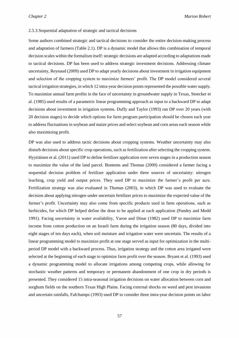
Chapter 2 Marion Robert
57
2.5.3. Sequential adaptation of strategic and tactical decisions
Some authors combined strategic and tactical decisions to consider the entire decision-making process
and adaptation of farmers (Table 2.1). DP is a dynamic model that allows this combination of temporal
decision scales within the formalism itself: strategic decisions are adapted according to adaptations made
to tactical decisions. DP has been used to address strategic investment decisions. Addressing climate
uncertainty, Reynaud (2009) used DP to adapt yearly decisions about investment in irrigation equipment
and selection of the cropping system to maximize farmers’ profit. The DP model considered several
tactical irrigation strategies, in which 12 intra-year decision points represented the possible water supply.
To maximize annual farm profits in the face of uncertainty in groundwater supply in Texas, Stoecker et
al. (1985) used results of a parametric linear programming approach as input to a backward DP to adapt
decisions about investment in irrigation systems. Duffy and Taylor (1993) ran DP over 20 years (with
20 decision stages) to decide which options for farm program participation should be chosen each year
to address fluctuations in soybean and maize prices and select soybean and corn areas each season while
also maximizing profit.
DP was also used to address tactic decisions about cropping systems. Weather uncertainty may also
disturb decisions about specific crop operations, such as fertilization after selecting the cropping system.
Hyytiäinen et al. (2011) used DP to define fertilizer application over seven stages in a production season
to maximize the value of the land parcel. Bontems and Thomas (2000) considered a farmer facing a
sequential decision problem of fertilizer application under three sources of uncertainty: nitrogen
leaching, crop yield and output prices. They used DP to maximize the farmer’s profit per acre.
Fertilization strategy was also evaluated in Thomas (2003), in which DP was used to evaluate the
decision about applying nitrogen under uncertain fertilizer prices to maximize the expected value of the
farmer’s profit. Uncertainty may also come from specific products used in farm operations, such as
herbicides, for which DP helped define the dose to be applied at each application (Pandey and Medd
1991). Facing uncertainty in water availability, Yaron and Dinar (1982) used DP to maximize farm
income from cotton production on an Israeli farm during the irrigation season (80 days, divided into
eight stages of ten days each), when soil moisture and irrigation water were uncertain. The results of a
linear programming model to maximize profit at one stage served as input for optimization in the multi-
period DP model with a backward process. Thus, irrigation strategy and the cotton area irrigated were
selected at the beginning of each stage to optimize farm profit over the season. Bryant et al. (1993) used
a dynamic programming model to allocate irrigations among competing crops, while allowing for
stochastic weather patterns and temporary or permanent abandonment of one crop in dry periods is
presented. They considered 15 intra-seasonal irrigation decisions on water allocation between corn and
sorghum fields on the southern Texas High Plains. Facing external shocks on weed and pest invasions
and uncertain rainfalls, Fafchamps (1993) used DP to consider three intra-year decision points on labor
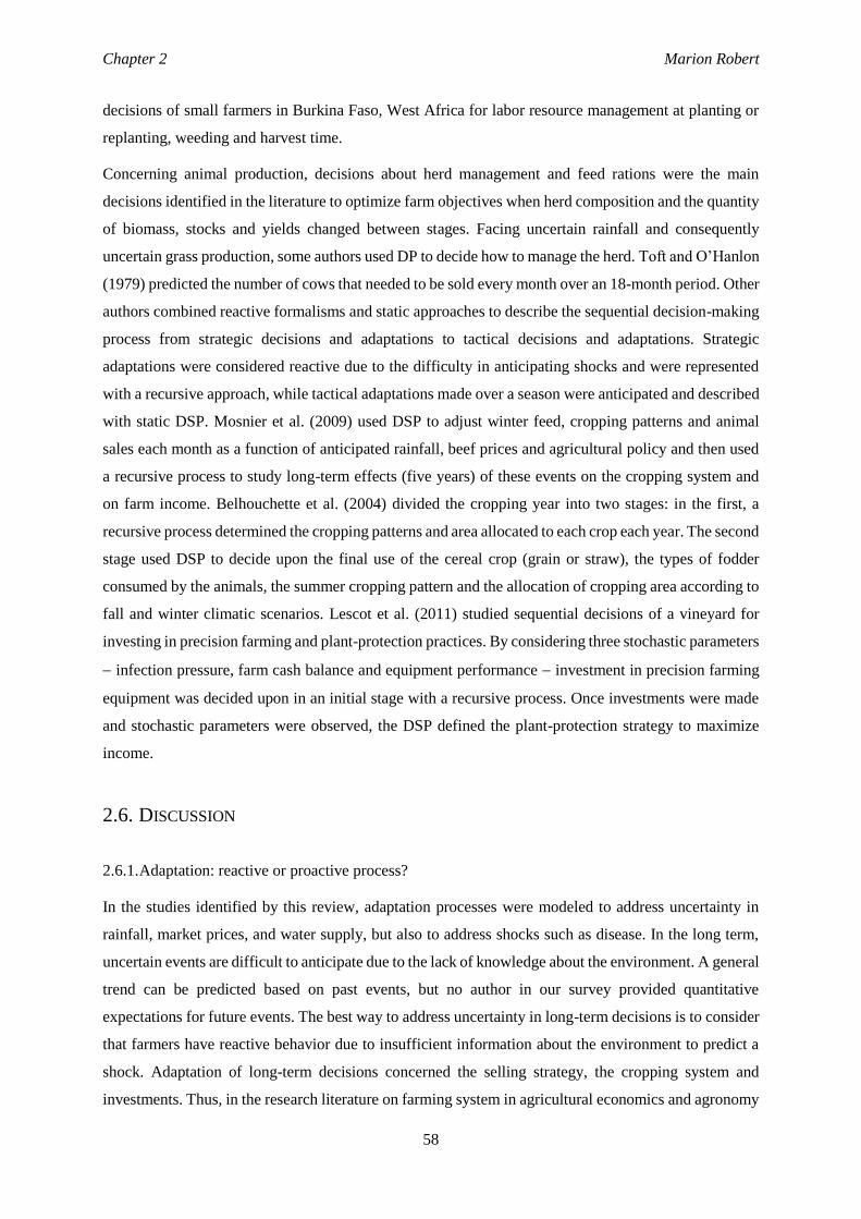
Chapter 2 Marion Robert
58
decisions of small farmers in Burkina Faso, West Africa for labor resource management at planting or
replanting, weeding and harvest time.
Concerning animal production, decisions about herd management and feed rations were the main
decisions identified in the literature to optimize farm objectives when herd composition and the quantity
of biomass, stocks and yields changed between stages. Facing uncertain rainfall and consequently
uncertain grass production, some authors used DP to decide how to manage the herd. Toft and O’Hanlon
(1979) predicted the number of cows that needed to be sold every month over an 18-month period. Other
authors combined reactive formalisms and static approaches to describe the sequential decision-making
process from strategic decisions and adaptations to tactical decisions and adaptations. Strategic
adaptations were considered reactive due to the difficulty in anticipating shocks and were represented
with a recursive approach, while tactical adaptations made over a season were anticipated and described
with static DSP. Mosnier et al. (2009) used DSP to adjust winter feed, cropping patterns and animal
sales each month as a function of anticipated rainfall, beef prices and agricultural policy and then used
a recursive process to study long-term effects (five years) of these events on the cropping system and
on farm income. Belhouchette et al. (2004) divided the cropping year into two stages: in the first, a
recursive process determined the cropping patterns and area allocated to each crop each year. The second
stage used DSP to decide upon the final use of the cereal crop (grain or straw), the types of fodder
consumed by the animals, the summer cropping pattern and the allocation of cropping area according to
fall and winter climatic scenarios. Lescot et al. (2011) studied sequential decisions of a vineyard for
investing in precision farming and plant-protection practices. By considering three stochastic parameters
infection pressure, farm cash balance and equipment performance investment in precision farming
equipment was decided upon in an initial stage with a recursive process. Once investments were made
and stochastic parameters were observed, the DSP defined the plant-protection strategy to maximize
income.
2.6. DISCUSSION
2.6.1. Adaptation: reactive or proactive process?
In the studies identified by this review, adaptation processes were modeled to address uncertainty in
rainfall, market prices, and water supply, but also to address shocks such as disease. In the long term,
uncertain events are difficult to anticipate due to the lack of knowledge about the environment. A general
trend can be predicted based on past events, but no author in our survey provided quantitative
expectations for future events. The best way to address uncertainty in long-term decisions is to consider
that farmers have reactive behavior due to insufficient information about the environment to predict a
shock. Adaptation of long-term decisions concerned the selling strategy, the cropping system and
investments. Thus, in the research literature on farming system in agricultural economics and agronomy
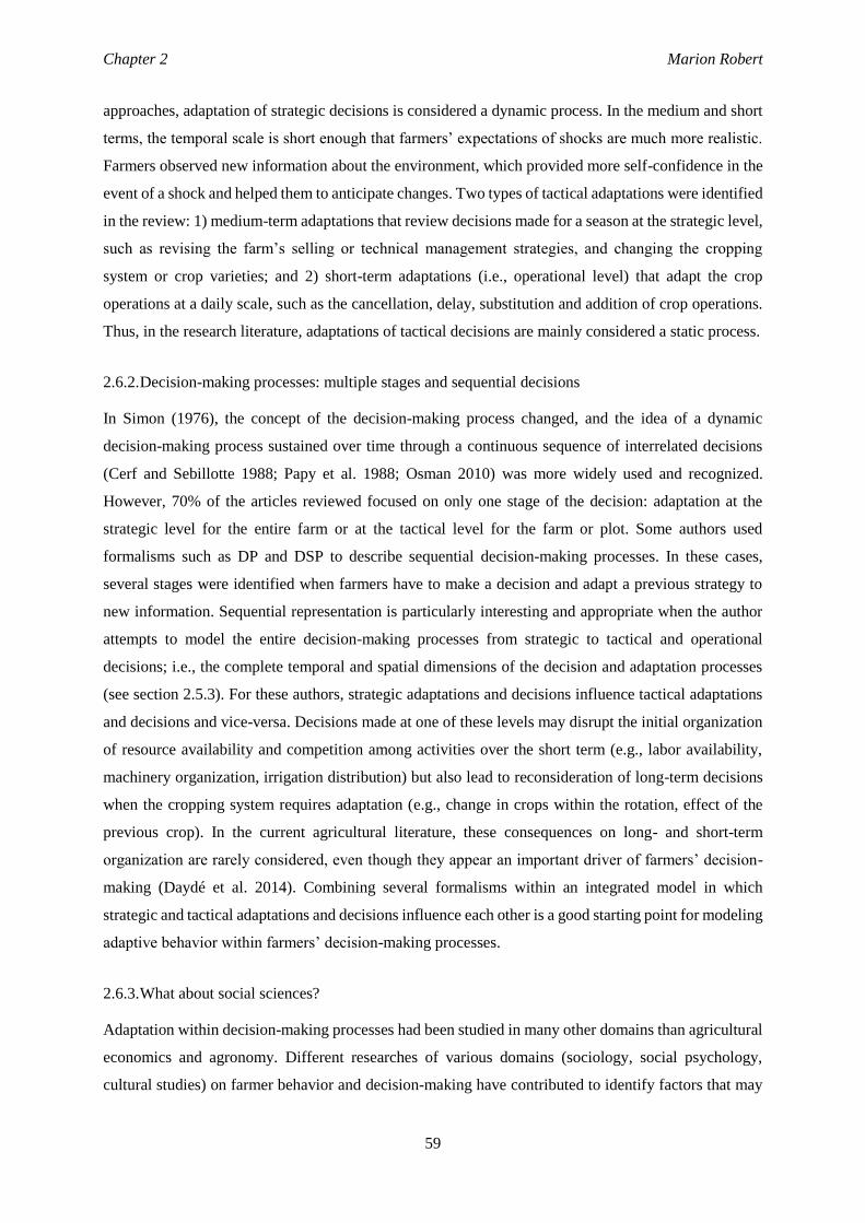
Chapter 2 Marion Robert
59
approaches, adaptation of strategic decisions is considered a dynamic process. In the medium and short
terms, the temporal scale is short enough that farmers’ expectations of shocks are much more realistic.
Farmers observed new information about the environment, which provided more self-confidence in the
event of a shock and helped them to anticipate changes. Two types of tactical adaptations were identified
in the review: 1) medium-term adaptations that review decisions made for a season at the strategic level,
such as revising the farm’s selling or technical management strategies, and changing the cropping
system or crop varieties; and 2) short-term adaptations (i.e., operational level) that adapt the crop
operations at a daily scale, such as the cancellation, delay, substitution and addition of crop operations.
Thus, in the research literature, adaptations of tactical decisions are mainly considered a static process.
2.6.2. Decision-making processes: multiple stages and sequential decisions
In Simon (1976), the concept of the decision-making process changed, and the idea of a dynamic
decision-making process sustained over time through a continuous sequence of interrelated decisions
(Cerf and Sebillotte 1988; Papy et al. 1988; Osman 2010) was more widely used and recognized.
However, 70% of the articles reviewed focused on only one stage of the decision: adaptation at the
strategic level for the entire farm or at the tactical level for the farm or plot. Some authors used
formalisms such as DP and DSP to describe sequential decision-making processes. In these cases,
several stages were identified when farmers have to make a decision and adapt a previous strategy to
new information. Sequential representation is particularly interesting and appropriate when the author
attempts to model the entire decision-making processes from strategic to tactical and operational
decisions; i.e., the complete temporal and spatial dimensions of the decision and adaptation processes
(see section 2.5.3). For these authors, strategic adaptations and decisions influence tactical adaptations
and decisions and vice-versa. Decisions made at one of these levels may disrupt the initial organization
of resource availability and competition among activities over the short term (e.g., labor availability,
machinery organization, irrigation distribution) but also lead to reconsideration of long-term decisions
when the cropping system requires adaptation (e.g., change in crops within the rotation, effect of the
previous crop). In the current agricultural literature, these consequences on long- and short-term
organization are rarely considered, even though they appear an important driver of farmers’ decision-
making (Daydé et al. 2014). Combining several formalisms within an integrated model in which
strategic and tactical adaptations and decisions influence each other is a good starting point for modeling
adaptive behavior within farmers’ decision-making processes.
2.6.3. What about social sciences?
Adaptation within decision-making processes had been studied in many other domains than agricultural
economics and agronomy. Different researches of various domains (sociology, social psychology,
cultural studies) on farmer behavior and decision-making have contributed to identify factors that may
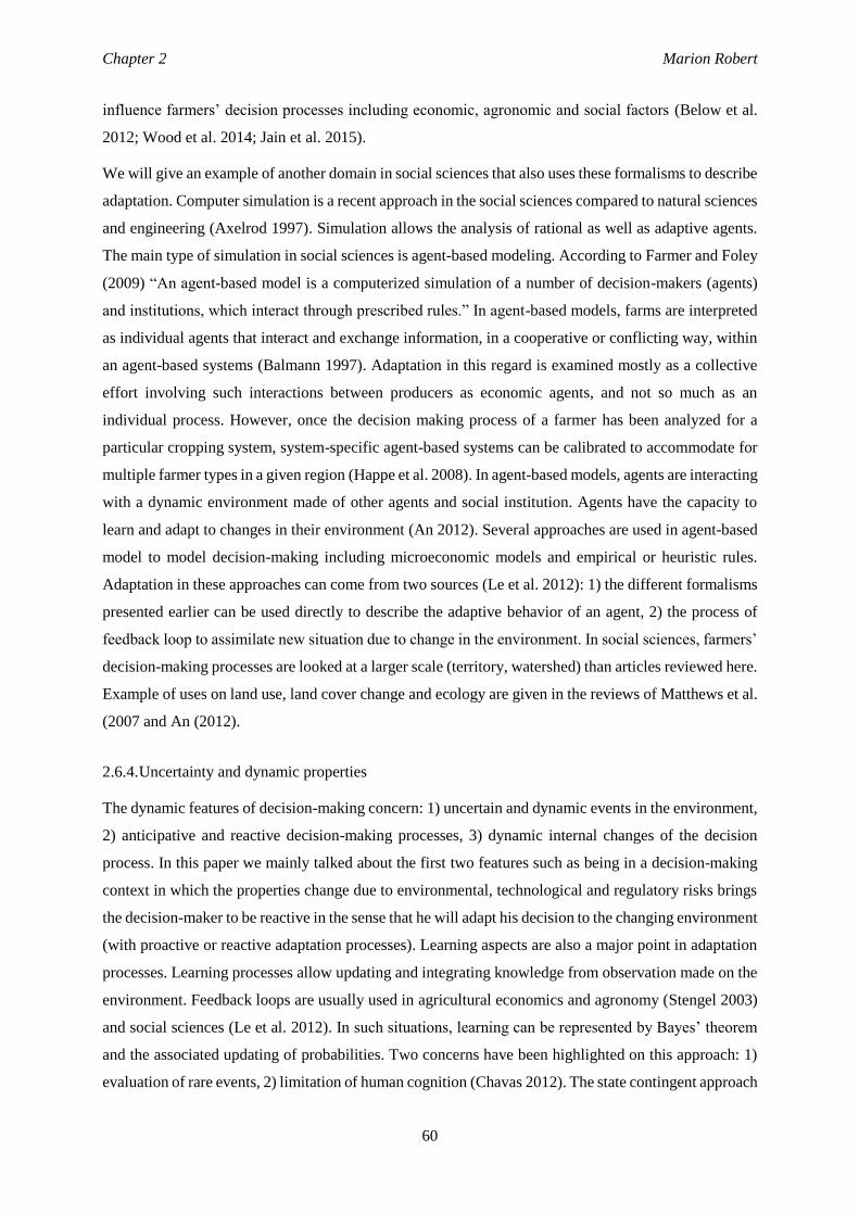
Chapter 2 Marion Robert
60
influence farmers’ decision processes including economic, agronomic and social factors (Below et al.
2012; Wood et al. 2014; Jain et al. 2015).
We will give an example of another domain in social sciences that also uses these formalisms to describe
adaptation. Computer simulation is a recent approach in the social sciences compared to natural sciences
and engineering (Axelrod 1997). Simulation allows the analysis of rational as well as adaptive agents.
The main type of simulation in social sciences is agent-based modeling. According to Farmer and Foley
(2009) “An agent-based model is a computerized simulation of a number of decision-makers (agents)
and institutions, which interact through prescribed rules.” In agent-based models, farms are interpreted
as individual agents that interact and exchange information, in a cooperative or conflicting way, within
an agent-based systems (Balmann 1997). Adaptation in this regard is examined mostly as a collective
effort involving such interactions between producers as economic agents, and not so much as an
individual process. However, once the decision making process of a farmer has been analyzed for a
particular cropping system, system-specific agent-based systems can be calibrated to accommodate for
multiple farmer types in a given region (Happe et al. 2008). In agent-based models, agents are interacting
with a dynamic environment made of other agents and social institution. Agents have the capacity to
learn and adapt to changes in their environment (An 2012). Several approaches are used in agent-based
model to model decision-making including microeconomic models and empirical or heuristic rules.
Adaptation in these approaches can come from two sources (Le et al. 2012): 1) the different formalisms
presented earlier can be used directly to describe the adaptive behavior of an agent, 2) the process of
feedback loop to assimilate new situation due to change in the environment. In social sciences, farmers’
decision-making processes are looked at a larger scale (territory, watershed) than articles reviewed here.
Example of uses on land use, land cover change and ecology are given in the reviews of Matthews et al.
(2007 and An (2012).
2.6.4. Uncertainty and dynamic properties
The dynamic features of decision-making concern: 1) uncertain and dynamic events in the environment,
2) anticipative and reactive decision-making processes, 3) dynamic internal changes of the decision
process. In this paper we mainly talked about the first two features such as being in a decision-making
context in which the properties change due to environmental, technological and regulatory risks brings
the decision-maker to be reactive in the sense that he will adapt his decision to the changing environment
(with proactive or reactive adaptation processes). Learning aspects are also a major point in adaptation
processes. Learning processes allow updating and integrating knowledge from observation made on the
environment. Feedback loops are usually used in agricultural economics and agronomy (Stengel 2003)
and social sciences (Le et al. 2012). In such situations, learning can be represented by Bayes’ theorem
and the associated updating of probabilities. Two concerns have been highlighted on this approach: 1)
evaluation of rare events, 2) limitation of human cognition (Chavas 2012). The state contingent approach
Chapter 2 Marion Robert
61
presented by Chambers and Quiggin (2000; 2002) can provide a framework to investigate economic
behavior under uncertainty without probability assessments. According to this framework, agricultural
production under uncertainty can be represented by differentiating outputs according to the
corresponding state of nature. This yields a more general framework than conventional approaches of
production under uncertainty, while providing more realistic and tractable representations of production
problems (Chambers and Quiggin 2002). These authors use state-contingent representations of
production technologies to provide theoretical properties of producer decisions under uncertainty,
although empirical applications still remain difficult to implement (see O’Donnell and Griffiths 2006
for a discussion on empirical aspects of the state-contingent approach). Other learning process
approaches are used in artificial intelligence such as reinforcement learning and neuro-DP (Bertsekas
and Tsitsiklis 1995; Pack Kaelbling et al. 1996).
2.7. CONCLUSION
A farm decision-making problem should be modeled within an integrative modeling framework that
includes sequential aspects of the decision-making process and the adaptive capability and reactivity of
farmers to address changes in their environment. Rethinking farm planning as a decision-making
process, in which decisions are made continuously and sequentially over time to react to new available
information, and in which the farmer is able to build a flexible plan to anticipate certain changes in the
environment, is important to more closely simulate reality. Coupling optimization formalisms and
planning appears to be an interesting approach to represent the combination of several temporal and
spatial scales in models.

Chapter 2 Marion Robert
62
ACKNOWLEDGEMENTS
This research work was funded by the Indo-French Centre for the Promotion of Advanced Research
(CEFIPRA), the INRA flagship program on Adaptation to Climate Change of Agriculture and Forest
(ACCAF) and the Doctoral School of the University of Toulouse. We sincerely thank Stéphane Couture
and Aude Ridier for helpful comments.
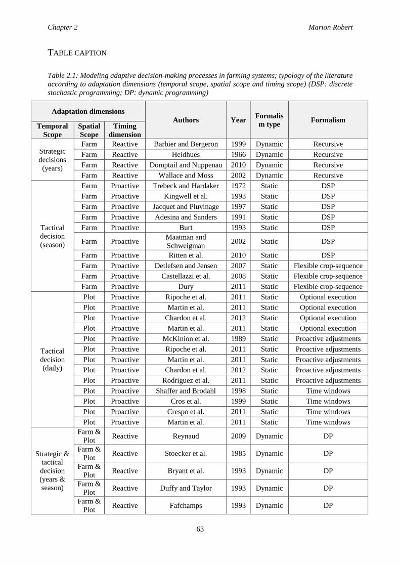
Chapter 2 Marion Robert
63
TABLE CAPTION
Table 2.1: Modeling adaptive decision-making processes in farming systems; typology of the literature
according to adaptation dimensions (temporal scope, spatial scope and timing scope) (DSP: discrete
stochastic programming; DP: dynamic programming)
Adaptation dimensions
Authors Year Formalis
m type Formalism
Temporal
Scope
Spatial
Scope
Timing
dimension
Strategic
decisions
(years)
Farm Reactive Barbier and Bergeron 1999 Dynamic Recursive
Farm Reactive Heidhues 1966 Dynamic Recursive
Farm Reactive Domptail and Nuppenau 2010 Dynamic Recursive
Farm Reactive Wallace and Moss 2002 Dynamic Recursive
Tactical
decision
(season)
Farm Proactive Trebeck and Hardaker 1972 Static DSP
Farm Proactive Kingwell et al. 1993 Static DSP
Farm Proactive Jacquet and Pluvinage 1997 Static DSP
Farm Proactive Adesina and Sanders 1991 Static DSP
Farm Proactive Burt 1993 Static DSP
Farm Proactive Maatman and
Schweigman 2002 Static DSP
Farm Proactive Ritten et al. 2010 Static DSP
Farm Proactive Detlefsen and Jensen 2007 Static Flexible crop-sequence
Farm Proactive Castellazzi et al. 2008 Static Flexible crop-sequence
Farm Proactive Dury 2011 Static Flexible crop-sequence
Tactical
decision
(daily)
Plot Proactive Ripoche et al. 2011 Static Optional execution
Plot Proactive Martin et al. 2011 Static Optional execution
Plot Proactive Chardon et al. 2012 Static Optional execution
Plot Proactive Martin et al. 2011 Static Optional execution
Plot Proactive McKinion et al. 1989 Static Proactive adjustments
Plot Proactive Ripoche et al. 2011 Static Proactive adjustments
Plot Proactive Martin et al. 2011 Static Proactive adjustments
Plot Proactive Chardon et al. 2012 Static Proactive adjustments
Plot Proactive Rodriguez et al. 2011 Static Proactive adjustments
Plot Proactive Shaffer and Brodahl 1998 Static Time windows
Plot Proactive Cros et al. 1999 Static Time windows
Plot Proactive Crespo et al. 2011 Static Time windows
Plot Proactive Martin et al. 2011 Static Time windows
Strategic &
tactical
decision
(years &
season)
Farm &
Plot Reactive Reynaud 2009 Dynamic DP
Farm &
Plot Reactive Stoecker et al. 1985 Dynamic DP
Farm &
Plot Reactive Bryant et al. 1993 Dynamic DP
Farm &
Plot Reactive Duffy and Taylor 1993 Dynamic DP
Farm &
Plot Reactive Fafchamps 1993 Dynamic DP
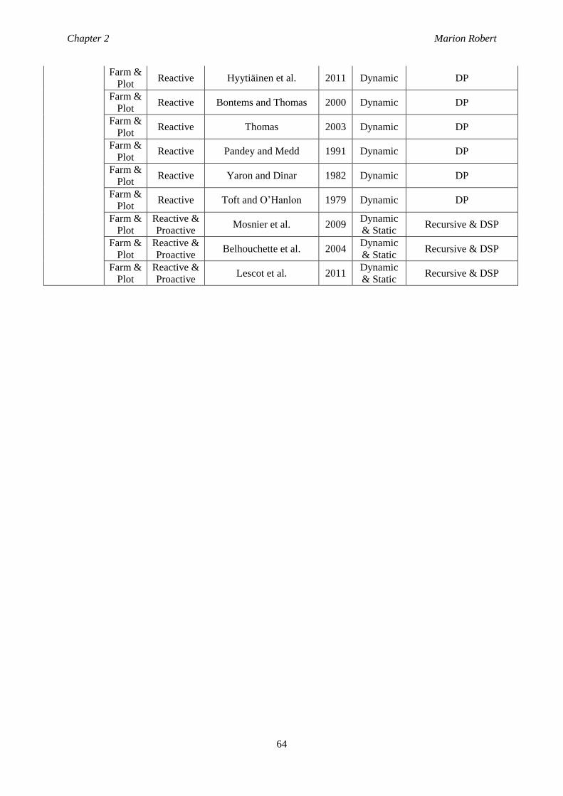
Chapter 2 Marion Robert
64
Farm &
Plot Reactive Hyytiäinen et al. 2011 Dynamic DP
Farm &
Plot Reactive Bontems and Thomas 2000 Dynamic DP
Farm &
Plot Reactive Thomas 2003 Dynamic DP
Farm &
Plot Reactive Pandey and Medd 1991 Dynamic DP
Farm &
Plot Reactive Yaron and Dinar 1982 Dynamic DP
Farm &
Plot Reactive Toft and O’Hanlon 1979 Dynamic DP
Farm &
Plot
Reactive &
Proactive Mosnier et al. 2009
Dynamic
& Static Recursive & DSP
Farm &
Plot
Reactive &
Proactive Belhouchette et al. 2004
Dynamic
& Static Recursive & DSP
Farm &
Plot
Reactive &
Proactive Lescot et al. 2011
Dynamic
& Static Recursive & DSP

Chapter 2 Marion Robert
65
FIGURE CAPTION
Figure 2.1: Adaptation of maize outputs after drought condition. At the beginning of the season, the
farmer aims at growing maize for grain production. Due to dry conditions and low grass growth, the
farmer has to use forage stocks to feed the herd, so that the stocks decrease. To maintain the stocks, the
farmer has to adapt and change his crop orientation to maize silage.
FigureFigure 2.2: Typology of models to manage adaptive decision-making processes according to
model type, approach, and formalism.
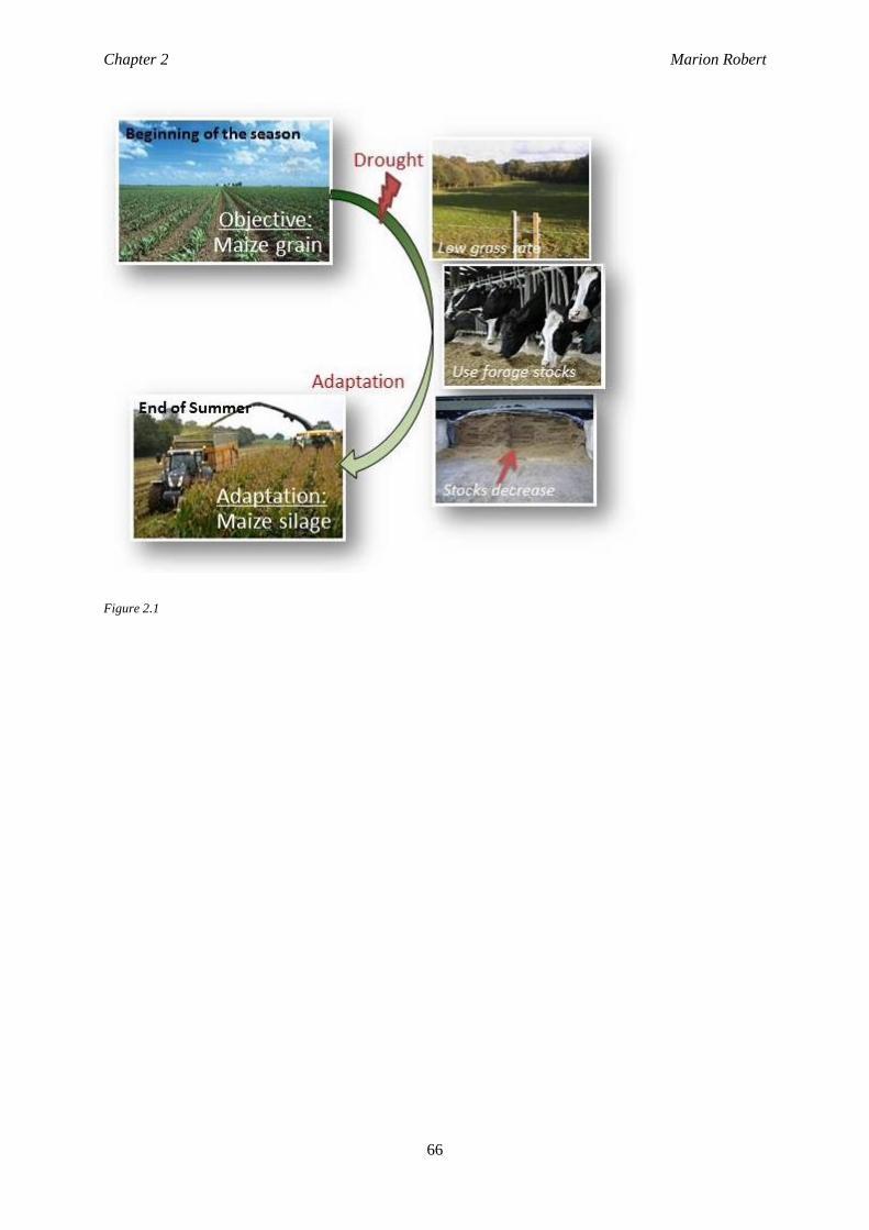
Chapter 2 Marion Robert
66
Figure 2.1
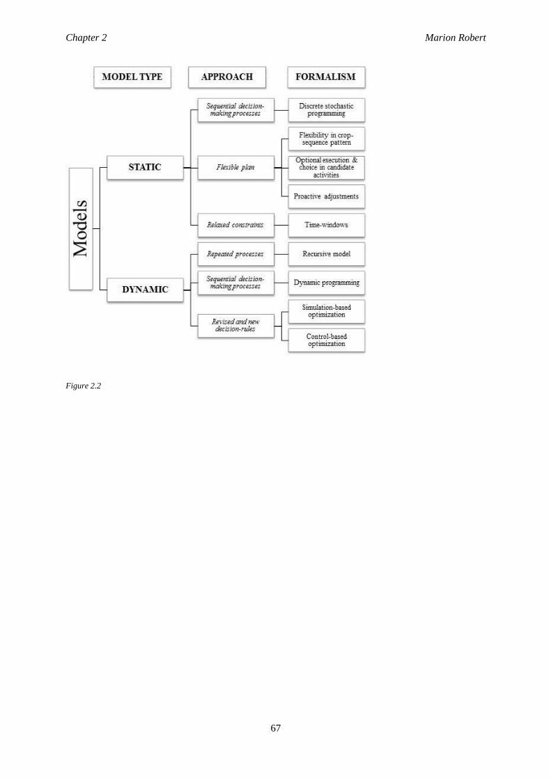
Chapter 2 Marion Robert
67
Figure 2.2


Chapter 3 Marion Robert
70
Chapter 3
Farm typology in the Berambadi
watershed (India): farming systems are
determined by farm size and access to
groundwater
Marion Robert∗1, Alban Thomas2, Muddu Sekhar3,6, Shrinivas Badiger4, Laurent Ruiz5,6, Magali
Willaume1, Delphine Leenhardt1 and Jacques-Eric Bergez1 1
AGIR, Université de Toulouse, INPT-ENSAT, INRA, F-31326 Castanet-Tolosan, France
2INRA, Toulouse School of Economics, UMR 1415 TSE-R, F-31000 Toulouse, France
3Indian Institute of Sciences, Department of Civil Engineering, Bangalore 560012, India
4ATREE, Bangalore 560064, India
5INRA, Agrocampus, UMR 1069 SAS, F-35042 Rennes, France
6Indo-French Cell of Water Sciences, IRD-IISc, Bangalore, India
∗ Corresponding author: ([email protected])
Accepted fo publication in Water
Scientific paper
Doi: 10.3390/w9010051
Quote: Robert, Thomas, A., Sekhar, M., Badiger, S., Ruiz, L., Willaume, M., Leenhardt, D. & Bergez,
J. E. (2017). Fram Typology in the Berambadi Watershed (India): Farming Systems Are Determined by
Farm Size and access to Groundwater. Water. 9 (1), 51.
Chapter 3 Marion Robert
71
Farmers’ production decisions and agricultural practices directly and indirectly influence the quantity
and quality of natural resources, some being depleted common resources such as groundwater.
Representing farming systems while accounting for their flexibility is needed to evaluate targeted,
regional water management policies. Farmers’ decisions regarding investing in irrigation and adopting
cropping systems are inherently dynamic and must adapt to changes in climate and agronomic, economic
and social, and institutional, conditions. To represent this diversity, we developed a typology of Indian
farmers from a survey of 684 farms in Berambadi, an agricultural watershed in southern India (state of
Karnataka). The survey provided information on farm structure, the cropping system and farm practices,
water management for irrigation, and economic performances of the farm. Descriptive statistics and
multivariate analysis (Multiple Correspondence Analysis and Agglomerative Hierarchical Clustering)
were used to analyze relationships between observed factors and establish the farm typology. We
identified three main types of farms: 1) large diversified and productivist farms, 2) small and marginal
rainfed farms, and 3) small irrigated marketing farms. This typology represents the heterogeneity of
farms in the Berambadi watershed. Used within a simulation model of the watershed, this typology
should enable policy makers to better assess potential impacts of agricultural and water management
policies on farmers’ livelihood and the groundwater table.
Keywords: farm typology, Multiple Correspondence Analysis, Agglomerative Hierarchical Clustering,
Berambadi watershed
Chapter 3 Marion Robert
72
3.1. INTRODUCTION
In semi-arid regions, agricultural production systems depend greatly on irrigation and encounter
increasing challenges: growing uncertainty about how to respond to climate change, severe depletion of
natural resources, high volatility in market prices, rises in energy costs, greater pressure from public
regulations (agricultural, environmental, and health policies), and conflicts about sharing communal
water resources (Ragab and Prudhomme 2002). Policies to improve agricultural water use efficiency are
often found to be inefficient when there are designed without taking into account the whole system,
including farmer’s choices, as shown for example by Fishman, Devineni, and Raman (2015) in the case
of irrigation technologies. Modeling farming systems at regional scale is a relevant approach to assess
“ex-ante” targeted water management policies (Valverde et al. 2015; Graveline 2016). However, as
modeling all individual farms within a region is usually not feasible, such approaches requires building
a farm typology (Köbrich et al. 2003) representing in a simplified way the existing diversity of farming
systems while accounting to the possible differential response of farm types to management policies.
A typology is an artificial way to define different homogeneous groups, categories or types based on
specific criteria in order to organize reality from a viewpoint relevant to the objectives of the model
(Duvernoy 2000; Andersen et al. 2007; Valbuena et al. 2008). Typologies are a convenient tool to
simplify the diversity of farming systems while effectively describing their heterogeneity (Poussin et al.
2008; Valbuena et al. 2008; Daloğlu et al. 2014). Since farm types are adapted to local restrictions such
as resource availability, it is also necessary to identify their spatial distribution or location factors (Clavel
et al. 2011).
Building such typologies is particularly challenging in the case of India. During the “green revolution”
that started in the 1970s, development of irrigation was mostly concentrated in the command area of
dams, and the construction of large dams has been promoted (Pani 2009). Later, the development of
submersible pump technology in the 1990s resulted in a dramatic increase of the irrigated agricultural
area (Sekhar et al. 2006; Javeed et al. 2009). This shift from collective ponds (Dorin and Landy 2002;
Chandrasekaran et al. 2009) to individual borewells has been largely encouraged by public policies that
provide farmers free electricity for groundwater irrigation (Shah et al. 2012). This shift caused
agricultural practices to depend heavily on irrigation from groundwater (Aubriot 2013) and induced a
well-identified “groundwater crisis” with tremendous impacts on water resources and ecosystems.
Today, millions of small farms (less than one hectare, on average) owning individual borewells, with
great diversity in practices and strategies (Sekhar et al. 2011) are spread in areas where only rainfed
agriculture was possible few years ago. In such a context, modeling and quantifying spatio-temporal
variability in water resources and interactions among groundwater, agricultural practices and crop
Chapter 3 Marion Robert
73
growth, which is an essential component of integrated and comprehensive water resource management,
is a challenge (Venot et al. 2010; Ruiz et al. 2015).
In this article, we generate a typology of farms and spatialize farm types in the Berambadi watershed
(84 km²), located in Southern India. This site was selected because it is small enough for accurate
monitoring and large enough to include a large portion of the variability in agricultural systems within
the region. Identifying and understanding variability in farm characteristics and farming practices on the
watershed, based on farmer surveys, provide us relevant criteria for proposing possible scenarios of
farming system evolution in the watershed, that could be later simulated in watershed models.
3.2. MATERIALS AND METHODS
3.2.1. Case study: Hydrological and morphological description of the watershed
Berambadi (11°43'00” to 11°48'00" N, 76° 31'00" to 76° 40'00" E) is an 84 km² watershed located in
southwestern India. It belongs to the South Gundal basin, 816 km2, part of the Kabini River basin
(approximately 7000 km², southwestern Karnataka state), which is a tributary of the Kaveri River basin
(Figure 3.1). Biophysical variables have been intensively monitored since 2009 in the Berambadi
watershed, under the Environmental Research Observatory ORE BVET (http://bvet.obs-mip.fr/en) and
the AMBHAS observatory (Sekhar et al. 2016; Tomer et al. 2015, www.ambhas.com).
Due to the rain shadow of the Western Ghats during the southwestern monsoon rains, the Kabini basin
exhibits a steep rainfall gradient, from a humid zone in the west with more than 5000 mm of rain per
year to a semi-arid zone in the east with less than 700 mm of rain per year. Since the Berambadi
watershed is located in the eastern Kabini basin, its climate is tropical sub-humid (aridity index P/PET
of 0.7), with rainfall of 800 mm/year and PET of 1100 mm per year, on average (Sekhar et al. 2016). A
moderate east-west rainfall gradient is observed at the watershed scale, with approximately 900 mm
rainfall per year upstream (west) and less than 700 mm rainfall per year downstream (east). Three
seasons regulate the cropping systems: 1) kharif (June to September), which is the southwestern
monsoon season, when almost all plots are cultivated and are either exclusively rainfed or have
supplemental irrigation; 2) rabi (October to January), the northeasten monsoon or winter season, when
most of the plots where irrigation is possible are cultivated; and 3) summer (February to May), the hot
and dry season, when only few irrigated plots are cultivated.
Black soil (Vertisols and Vertic intergrades), red soil (Ferrasols and Chromic Lusivols) and
rocky/weathered soil are the main soil types in the area and represent the granitic/gnessic lithology found
in southern India (Barbiéro et al. 2007). The hard-rock aquifer is composed of fissured granite underlain
by a 5-20 m layer of weathered material. Groundwater transmissivity and borewell yields decrease with
groundwater table depth (Maréchal et al. 2010). As a consequence, continuous pumping causing
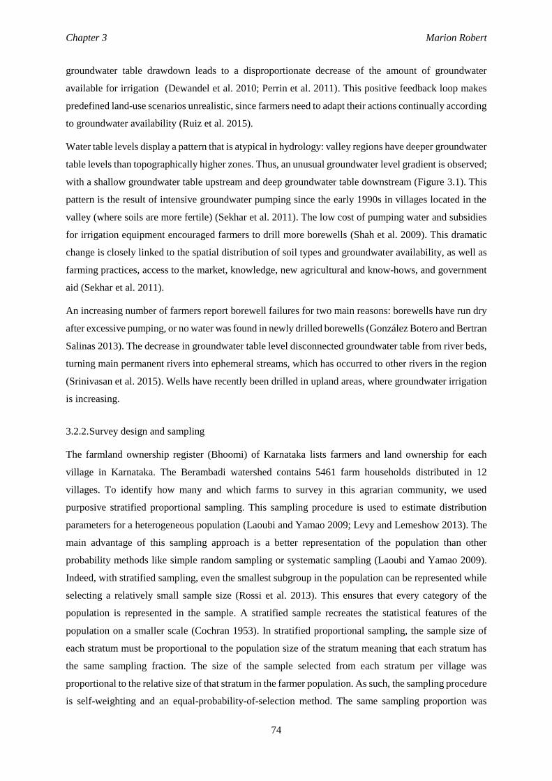
Chapter 3 Marion Robert
74
groundwater table drawdown leads to a disproportionate decrease of the amount of groundwater
available for irrigation (Dewandel et al. 2010; Perrin et al. 2011). This positive feedback loop makes
predefined land-use scenarios unrealistic, since farmers need to adapt their actions continually according
to groundwater availability (Ruiz et al. 2015).
Water table levels display a pattern that is atypical in hydrology: valley regions have deeper groundwater
table levels than topographically higher zones. Thus, an unusual groundwater level gradient is observed;
with a shallow groundwater table upstream and deep groundwater table downstream (Figure 3.1). This
pattern is the result of intensive groundwater pumping since the early 1990s in villages located in the
valley (where soils are more fertile) (Sekhar et al. 2011). The low cost of pumping water and subsidies
for irrigation equipment encouraged farmers to drill more borewells (Shah et al. 2009). This dramatic
change is closely linked to the spatial distribution of soil types and groundwater availability, as well as
farming practices, access to the market, knowledge, new agricultural and know-hows, and government
aid (Sekhar et al. 2011).
An increasing number of farmers report borewell failures for two main reasons: borewells have run dry
after excessive pumping, or no water was found in newly drilled borewells (González Botero and Bertran
Salinas 2013). The decrease in groundwater table level disconnected groundwater table from river beds,
turning main permanent rivers into ephemeral streams, which has occurred to other rivers in the region
(Srinivasan et al. 2015). Wells have recently been drilled in upland areas, where groundwater irrigation
is increasing.
3.2.2. Survey design and sampling
The farmland ownership register (Bhoomi) of Karnataka lists farmers and land ownership for each
village in Karnataka. The Berambadi watershed contains 5461 farm households distributed in 12
villages. To identify how many and which farms to survey in this agrarian community, we used
purposive stratified proportional sampling. This sampling procedure is used to estimate distribution
parameters for a heterogeneous population (Laoubi and Yamao 2009; Levy and Lemeshow 2013). The
main advantage of this sampling approach is a better representation of the population than other
probability methods like simple random sampling or systematic sampling (Laoubi and Yamao 2009).
Indeed, with stratified sampling, even the smallest subgroup in the population can be represented while
selecting a relatively small sample size (Rossi et al. 2013). This ensures that every category of the
population is represented in the sample. A stratified sample recreates the statistical features of the
population on a smaller scale (Cochran 1953). In stratified proportional sampling, the sample size of
each stratum must be proportional to the population size of the stratum meaning that each stratum has
the same sampling fraction. The size of the sample selected from each stratum per village was
proportional to the relative size of that stratum in the farmer population. As such, the sampling procedure
is self-weighting and an equal-probability-of-selection method. The same sampling proportion was
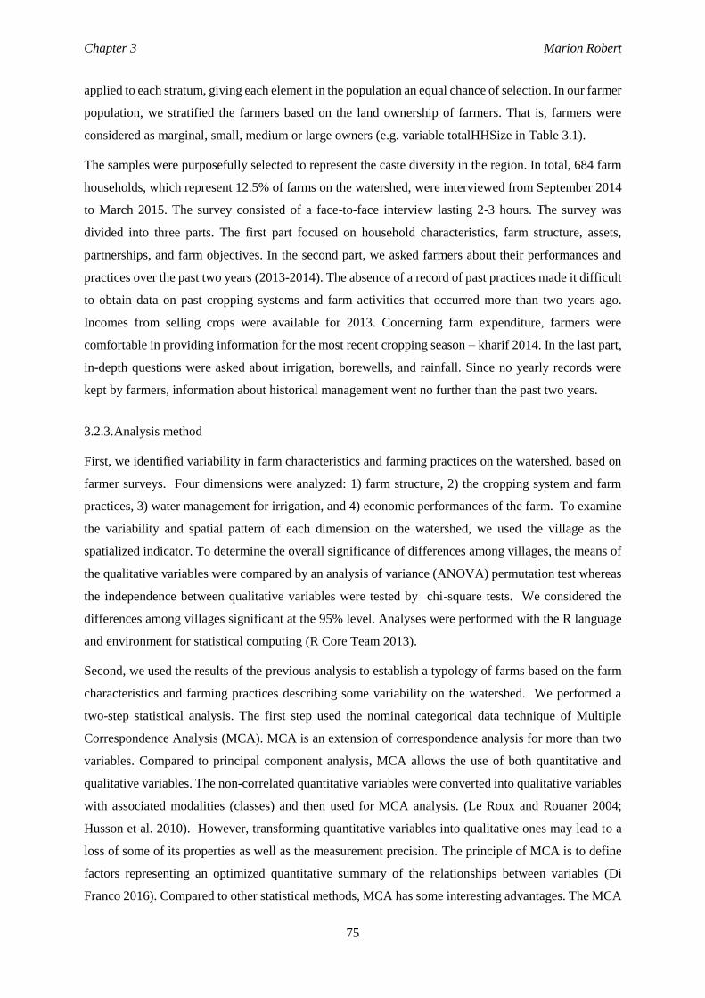
Chapter 3 Marion Robert
75
applied to each stratum, giving each element in the population an equal chance of selection. In our farmer
population, we stratified the farmers based on the land ownership of farmers. That is, farmers were
considered as marginal, small, medium or large owners (e.g. variable totalHHSize in Table 3.1).
The samples were purposefully selected to represent the caste diversity in the region. In total, 684 farm
households, which represent 12.5% of farms on the watershed, were interviewed from September 2014
to March 2015. The survey consisted of a face-to-face interview lasting 2-3 hours. The survey was
divided into three parts. The first part focused on household characteristics, farm structure, assets,
partnerships, and farm objectives. In the second part, we asked farmers about their performances and
practices over the past two years (2013-2014). The absence of a record of past practices made it difficult
to obtain data on past cropping systems and farm activities that occurred more than two years ago.
Incomes from selling crops were available for 2013. Concerning farm expenditure, farmers were
comfortable in providing information for the most recent cropping season – kharif 2014. In the last part,
in-depth questions were asked about irrigation, borewells, and rainfall. Since no yearly records were
kept by farmers, information about historical management went no further than the past two years.
3.2.3. Analysis method
First, we identified variability in farm characteristics and farming practices on the watershed, based on
farmer surveys. Four dimensions were analyzed: 1) farm structure, 2) the cropping system and farm
practices, 3) water management for irrigation, and 4) economic performances of the farm. To examine
the variability and spatial pattern of each dimension on the watershed, we used the village as the
spatialized indicator. To determine the overall significance of differences among villages, the means of
the qualitative variables were compared by an analysis of variance (ANOVA) permutation test whereas
the independence between qualitative variables were tested by chi-square tests. We considered the
differences among villages significant at the 95% level. Analyses were performed with the R language
and environment for statistical computing (R Core Team 2013).
Second, we used the results of the previous analysis to establish a typology of farms based on the farm
characteristics and farming practices describing some variability on the watershed. We performed a
two-step statistical analysis. The first step used the nominal categorical data technique of Multiple
Correspondence Analysis (MCA). MCA is an extension of correspondence analysis for more than two
variables. Compared to principal component analysis, MCA allows the use of both quantitative and
qualitative variables. The non-correlated quantitative variables were converted into qualitative variables
with associated modalities (classes) and then used for MCA analysis. (Le Roux and Rouaner 2004;
Husson et al. 2010). However, transforming quantitative variables into qualitative ones may lead to a
loss of some of its properties as well as the measurement precision. The principle of MCA is to define
factors representing an optimized quantitative summary of the relationships between variables (Di
Franco 2016). Compared to other statistical methods, MCA has some interesting advantages. The MCA
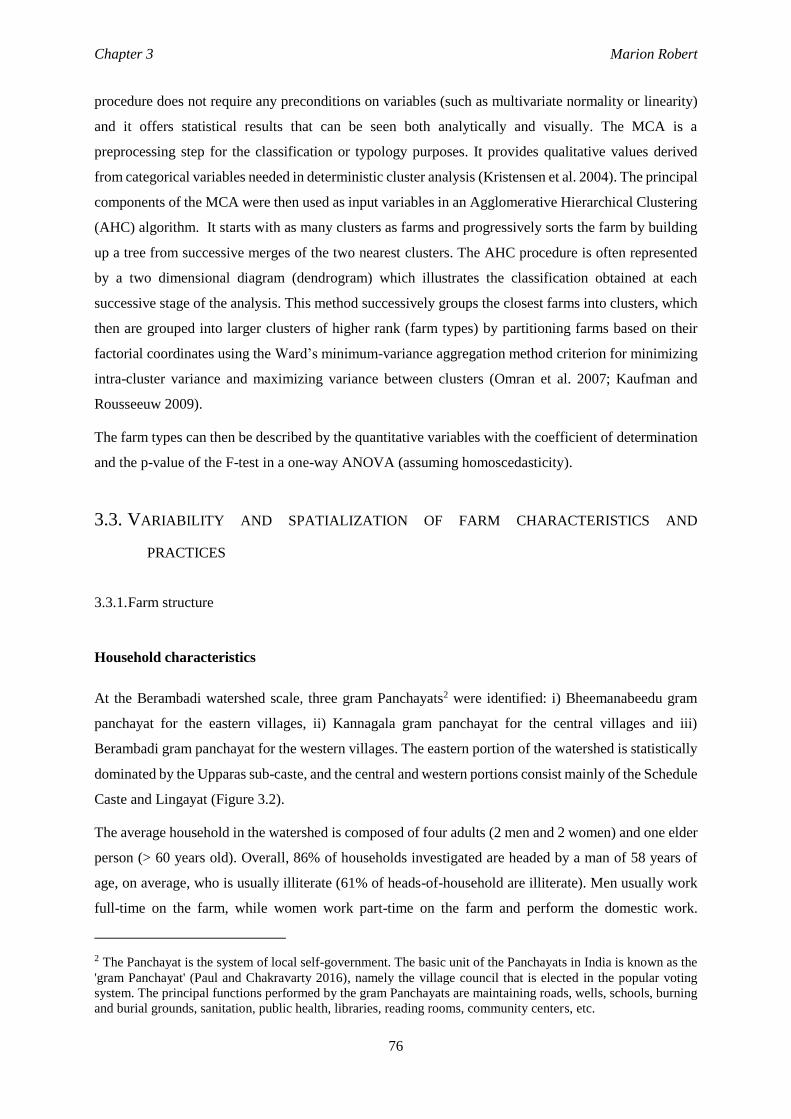
Chapter 3 Marion Robert
76
procedure does not require any preconditions on variables (such as multivariate normality or linearity)
and it offers statistical results that can be seen both analytically and visually. The MCA is a
preprocessing step for the classification or typology purposes. It provides qualitative values derived
from categorical variables needed in deterministic cluster analysis (Kristensen et al. 2004). The principal
components of the MCA were then used as input variables in an Agglomerative Hierarchical Clustering
(AHC) algorithm. It starts with as many clusters as farms and progressively sorts the farm by building
up a tree from successive merges of the two nearest clusters. The AHC procedure is often represented
by a two dimensional diagram (dendrogram) which illustrates the classification obtained at each
successive stage of the analysis. This method successively groups the closest farms into clusters, which
then are grouped into larger clusters of higher rank (farm types) by partitioning farms based on their
factorial coordinates using the Ward’s minimum-variance aggregation method criterion for minimizing
intra-cluster variance and maximizing variance between clusters (Omran et al. 2007; Kaufman and
Rousseeuw 2009).
The farm types can then be described by the quantitative variables with the coefficient of determination
and the p-value of the F-test in a one-way ANOVA (assuming homoscedasticity).
3.3. VARIABILITY AND SPATIALIZATION OF FARM CHARACTERISTICS AND
PRACTICES
3.3.1. Farm structure
Household characteristics
At the Berambadi watershed scale, three gram Panchayats2 were identified: i) Bheemanabeedu gram
panchayat for the eastern villages, ii) Kannagala gram panchayat for the central villages and iii)
Berambadi gram panchayat for the western villages. The eastern portion of the watershed is statistically
dominated by the Upparas sub-caste, and the central and western portions consist mainly of the Schedule
Caste and Lingayat (Figure 3.2).
The average household in the watershed is composed of four adults (2 men and 2 women) and one elder
person (> 60 years old). Overall, 86% of households investigated are headed by a man of 58 years of
age, on average, who is usually illiterate (61% of heads-of-household are illiterate). Men usually work
full-time on the farm, while women work part-time on the farm and perform the domestic work.
2 The Panchayat is the system of local self-government. The basic unit of the Panchayats in India is known as the
'gram Panchayat' (Paul and Chakravarty 2016), namely the village council that is elected in the popular voting
system. The principal functions performed by the gram Panchayats are maintaining roads, wells, schools, burning
and burial grounds, sanitation, public health, libraries, reading rooms, community centers, etc.
Chapter 3 Marion Robert
77
Agricultural labor is a secondary occupation for 16% of the interviewed population. Few people migrate
to work in other places during rabi season (people migrate in only 4% of households). Households in
the Berambadi gram panchayat are statistically smaller, with three adult members and one elderly
person. A larger percentage of farmers are better educated in the Kannegala gram panchayat, and over
50% attended at least pre-primary school (vs. 20% in the rest of the watershed) (Figure 3.2).
Land holding
Average farm size in the watershed is 1.2 hectares and varies from 0.01-9.3 hectares. Most farms are
small (48% have 0.8-2 hectares) or marginal (32% have < 0.8 hectares). Only 17% of farms have more
than 2 hectares, while 3% have more than 4 hectares. Farmers own their farmland. A field with adjacent
agricultural plots cultivated by the same farmer is called a “jeminu”. A farm can comprise several
“jeminus”, which may or may not be located nearby each other; they can even be located in different
villages. Overall, 45% of farmers have only one jeminu, while 26% have 2, 13% have 3 and 16% have
more than 3. The entire jeminu can be dedicated to one crop each season (54%) or divided into several
crop plots (31% with 2 crop plots, 14% with 3-5 crop plots). On average, a crop plot is 0.4 hectare but
varies from 0.01-2.4 hectares.
Land holding is variable on the watershed. Statistically, more marginal farms (< 0.8 ha) exist in the
Beemanabeedu gram panchayat (42%, vs. 23% in the rest of the watershed), where farms are more
fragmented (80% of farms in the Beemanabeedu gram panchayat have more than 1 jeminus vs. 55% in
the rest of the watershed). Farms in the Berambadi gram panchayat are less diversified: 80% cultivate
only one plot with one crop (vs. 60% in the rest of the watershed) (Figure 3.2).
Livestock and equipment
Even though livestock production is usually a secondary activity, farmers have animals for traction,
milk, meat and breeding. To represent the livestock intensity we built a coefficient of Tropical Livestock
Unit (TLU) where cows, oxens, buffalos, and bulls are 1 TLU and sheep and goats equal 0.2 TLU
(Meyer 2016). Farmers have an average of 2 TLU.
The traditional equipment for soil operations is based on animal traction. Motorization recently spread,
and plowing with a tractor now commonly supplements the traditional animal work. However, tractors
are expensive, and most farmers (94%) prefer to rent from a tractor owner in the village rather than
obtaining a loan to buy one. Farmers use oxen, bulls and buffalos along with a plow (96% use a plow
and 87% own one). Farmers who own animals for traction usually have only one pair of animals. A
pesticide sprayer is the most common equipment used for farming operations in the Berambadi
watershed (88% use a sprayer and 61% own one). Seeders, weeders and rotovators are rarely owned or
Chapter 3 Marion Robert
78
used in the watershed. Seeding, fertilizing, weeding and harvesting are usually performed manually and
do not require specific equipment.
Equipment use varies spatially across the watershed. The percentage of farmers owning buffalos is
statistically the highest in the Kannegala and Berambadi gram panchayats. Statistically, a pesticide
sprayer is owned mainly by farmers in the Beemanabeedu and Berambadi gram panchayats. Livestock
ownership varies statistically across the watershed: more than 50% of farmers own at least 2 TLU in the
Kannegala and Berambadi gram panchayats, while 20% of farmers own at least TLU in the
Beemanabeedu gram panchayat (Figure 3.2).
Labor
Because many technical operations are manual, farming practices are highly labor-intensive. Only two
farmers employ permanent workers; they hire workers on a daily basis or based on crop-operation
contracts. Women typically perform sowing, weeding and harvesting, and men typically perform soil
preparation, fertilization, pesticide treatment and irrigation. In 2013 and 2014, 40 male workers and 84
female workers were hired on average per hectare for the cropping season. No significant spatial
variability was found in labor per hectare across the watershed.
3.3.2. Farm practices
Input use
The amount of input purchased per unit of cultivated area decreases on a northwest-southeast gradient.
Villages from the Berambadi gram panchayat have higher expenses for pesticides (3750 Rs/hectare) and
chemical fertilizers (6250 Rs/hectare). The percentage of farms that do not use manure is also
statistically higher (40-80%) in villages from the Berambadi gram panchayat, which reinforces
dependency on chemical inputs. While the purchase of pesticides strongly decreases along this gradient
(reaching only 750 Rs/hectare in the Beemanabeedu gram panchayat), the decrease in the purchase of
chemical fertilizer is lower (from 6250 to 4500 Rs/hectare) (Figure 3.2).
Crop yield performances
Crop yields vary greatly among fields. However, high-input villages from Berambadi gram panchayat
and low-input villages from Beemanabeedu gram panchayat have particularly low yields (< 2.5
t/hectare, on average, for rainfed sorghum, or irrigated maize). Villages in the Kannegala gram
panchayat have statistically better results, (> 2.5 t/hectare, on average and up to 10 t/hectare for for the
same crops) (Figure 3.2). In villages from the Kannegala and Berambadi gram panchayats, more than
Chapter 3 Marion Robert
79
30 and 35% of farming areas are grown for subsistence whereas only 5% of the farming areas of villages
from the Beemanabeedu gram panchayat are grown for subsistence.
3.3.3. Water management for irrigation
Access to irrigation
Overall, 59% of farms have access to irrigation. Irrigated farms have on average more jeminus than non-
irrigated farms: 32% of irrigated farms vs. 63% of non-irrigated farms have only one jeminu. Farms
with only one jeminu are mainly rainfed (58%), while 73% of farms with more than one jeminu are
irrigated. For 63% of irrigated farms, all the jeminus have access to irrigation. All the surveyed farms
with access to irrigation directly use groundwater on their fields or temporarily store it in individual
farm ponds. We observed only a few cases of exchange or sale of water between farmers. Statistically,
more irrigated farms exist in the Beemanabeedu gram panchayat, where they represent approximately
80% of the farms.
Borewells
The first borewells in the watershed were drilled in the 1970s, and borewell drilling has increased
dramatically since the mid-1990s. In our sample, 31 borewells were drilled before 1995, and 470
borewells were drilled after 1995. In the 1970s and 1980s, most borewells were drilled in the
Beemanabeedu and Kannegala gram panchayats, while in the Berambadi gram panchayat well drilling
occurred mainly in the 2000s. In addition to the increasing number of borewells, technology has allowed
drilling deeper wells. The maximum depth of wells drilled before 1995 was 150 m, while 15% of the
borewells drilled from 1995-2010 were deeper than 150 m. Among the 214 borewells drilled after 2010,
25% were deeper than 150 m, with the deepest reaching 250 m.
From the survey sample of 1192 borewells, 33% were working at the time of the survey, while 58% had
failed (i.e. produced no water), and 9% had been temporarily stopped since 2013. No relation was found
between the depth of a borewell and whether it worked, had been stopped or had failed. There are as
many farms with at least one no working borewell as farms on which all borewells work (115 and 105
farms, respectively, of the 245 farms that had drilled at least one borewell). Overall, 49 farms (7%) that
attempted to drill borewells never got groundwater for irrigation.
Figure 3.3 summarizes the spatial distribution of irrigated farms and their borewell characteristics within
the watershed. Each farm has drilled approximately 3 borewells in the Beemanabeedu gram panchayat
vs. less than one in the Berambadi gram panchayat, which is consistent with irrigated farms being located
predominantly in the Beemanabeedu gram panchayat villages. However, borewell failure has occurred
predominantly in the Beemanabeedu gram panchayat villages (more than 65% of borewells drilled in
Chapter 3 Marion Robert
80
the Beemanabeedu gram panchayat villages have failed, vs. 53% in the Kannegala gram panchayat
villages, and 35% in Berambadi gram panchayat villages), which results in a relatively uniform number
of working borewells per farm within the watershed.
Pumps and access to electricity
Farmers use electric pumps, mostly of 7.5 horse power (HP). Farmers who need electricity, i.e. those
with at least one working borewell, have approximately 3-4 hours of electricity per day during kharif
and 2-3 hours per day during rabi, with on average 2-4 power outages per day. The duration of electricity
supply during kharif is statistically higher in the Kannegala gram panchayat villages, where 69% of
farms have more than 4 hours of power per day. Electricity is usually available less than 4 hours per day
in the rest of the watershed (Figure 3.2).
Farm ponds
Farm ponds are shallow ponds in which farmers store pumped water for distribution throughout the day,
especially during power outages at critical times. It takes 2-9 hours to fill a farm pond. Approximately
290 individual farm ponds exist on the surveyed farms, and only 36% of farms have one. No relationship
was found between farm pond ownership and location on the watershed.
Irrigation methods
Among irrigated farms, 81% use only one irrigation method. Furrow irrigation is by far the most
common method (75% of irrigated farms), mainly as the only irrigation method (58%), and more rarely
is used in combination with a sprinkler or drip (17%). Among alternative methods of irrigation,
sprinklers (17% of the jeminus) are used more often than drip irrigation (3% of the jeminus) or flood
irrigation (2% of the jeminus). Sprinkler irrigation statistically occurs more in the Beemanabeedu gram
panchayat villages (37-78% of jeminus, depending on the village), while the Berambadi gram panchayat
villages almost exclusively used furrow irrigation (94% of jeminus) (Figure 3.2).
3.3.4. Economic performances of the farm
Investment in farm structure
Considering investments in equipment and livestock, farmers owned an average of 4500 Rs/hectare of
equipment 18,670 Rs/TLU of livestock at the time of the survey. On average in 2013-2014, farmers hire
22,100 Rs/hectare of labor each cropping season, with male wages fixed at 250 Rs/day and female labor
at 150 Rs/day. The only clear statistical difference in investment in farm structure is the livestock
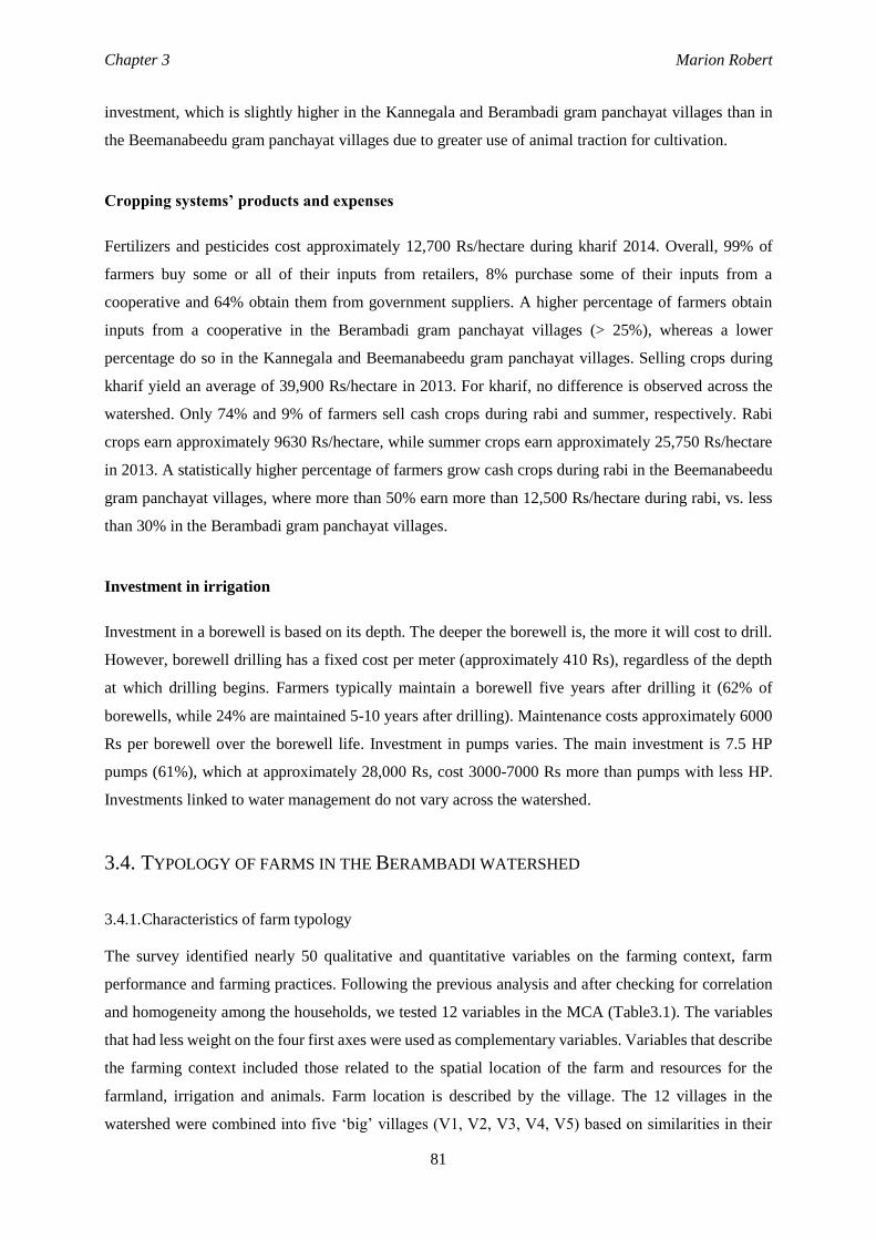
Chapter 3 Marion Robert
81
investment, which is slightly higher in the Kannegala and Berambadi gram panchayat villages than in
the Beemanabeedu gram panchayat villages due to greater use of animal traction for cultivation.
Cropping systems’ products and expenses
Fertilizers and pesticides cost approximately 12,700 Rs/hectare during kharif 2014. Overall, 99% of
farmers buy some or all of their inputs from retailers, 8% purchase some of their inputs from a
cooperative and 64% obtain them from government suppliers. A higher percentage of farmers obtain
inputs from a cooperative in the Berambadi gram panchayat villages (> 25%), whereas a lower
percentage do so in the Kannegala and Beemanabeedu gram panchayat villages. Selling crops during
kharif yield an average of 39,900 Rs/hectare in 2013. For kharif, no difference is observed across the
watershed. Only 74% and 9% of farmers sell cash crops during rabi and summer, respectively. Rabi
crops earn approximately 9630 Rs/hectare, while summer crops earn approximately 25,750 Rs/hectare
in 2013. A statistically higher percentage of farmers grow cash crops during rabi in the Beemanabeedu
gram panchayat villages, where more than 50% earn more than 12,500 Rs/hectare during rabi, vs. less
than 30% in the Berambadi gram panchayat villages.
Investment in irrigation
Investment in a borewell is based on its depth. The deeper the borewell is, the more it will cost to drill.
However, borewell drilling has a fixed cost per meter (approximately 410 Rs), regardless of the depth
at which drilling begins. Farmers typically maintain a borewell five years after drilling it (62% of
borewells, while 24% are maintained 5-10 years after drilling). Maintenance costs approximately 6000
Rs per borewell over the borewell life. Investment in pumps varies. The main investment is 7.5 HP
pumps (61%), which at approximately 28,000 Rs, cost 3000-7000 Rs more than pumps with less HP.
Investments linked to water management do not vary across the watershed.
3.4. TYPOLOGY OF FARMS IN THE BERAMBADI WATERSHED
3.4.1. Characteristics of farm typology
The survey identified nearly 50 qualitative and quantitative variables on the farming context, farm
performance and farming practices. Following the previous analysis and after checking for correlation
and homogeneity among the households, we tested 12 variables in the MCA (Table3.1). The variables
that had less weight on the four first axes were used as complementary variables. Variables that describe
the farming context included those related to the spatial location of the farm and resources for the
farmland, irrigation and animals. Farm location is described by the village. The 12 villages in the
watershed were combined into five ‘big’ villages (V1, V2, V3, V4, V5) based on similarities in their
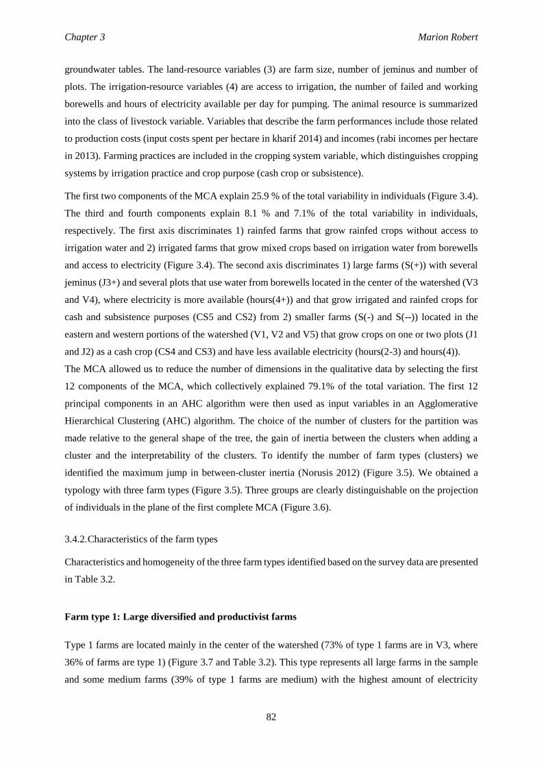
Chapter 3 Marion Robert
82
groundwater tables. The land-resource variables (3) are farm size, number of jeminus and number of
plots. The irrigation-resource variables (4) are access to irrigation, the number of failed and working
borewells and hours of electricity available per day for pumping. The animal resource is summarized
into the class of livestock variable. Variables that describe the farm performances include those related
to production costs (input costs spent per hectare in kharif 2014) and incomes (rabi incomes per hectare
in 2013). Farming practices are included in the cropping system variable, which distinguishes cropping
systems by irrigation practice and crop purpose (cash crop or subsistence).
The first two components of the MCA explain 25.9 % of the total variability in individuals (Figure 3.4).
The third and fourth components explain 8.1 % and 7.1% of the total variability in individuals,
respectively. The first axis discriminates 1) rainfed farms that grow rainfed crops without access to
irrigation water and 2) irrigated farms that grow mixed crops based on irrigation water from borewells
and access to electricity (Figure 3.4). The second axis discriminates 1) large farms (S(+)) with several
jeminus (J3+) and several plots that use water from borewells located in the center of the watershed (V3
and V4), where electricity is more available (hours(4+)) and that grow irrigated and rainfed crops for
cash and subsistence purposes (CS5 and CS2) from 2) smaller farms (S(-) and S(--)) located in the
eastern and western portions of the watershed (V1, V2 and V5) that grow crops on one or two plots (J1
and J2) as a cash crop (CS4 and CS3) and have less available electricity (hours(2-3) and hours(4)).
The MCA allowed us to reduce the number of dimensions in the qualitative data by selecting the first
12 components of the MCA, which collectively explained 79.1% of the total variation. The first 12
principal components in an AHC algorithm were then used as input variables in an Agglomerative
Hierarchical Clustering (AHC) algorithm. The choice of the number of clusters for the partition was
made relative to the general shape of the tree, the gain of inertia between the clusters when adding a
cluster and the interpretability of the clusters. To identify the number of farm types (clusters) we
identified the maximum jump in between-cluster inertia (Norusis 2012) (Figure 3.5). We obtained a
typology with three farm types (Figure 3.5). Three groups are clearly distinguishable on the projection
of individuals in the plane of the first complete MCA (Figure 3.6).
3.4.2. Characteristics of the farm types
Characteristics and homogeneity of the three farm types identified based on the survey data are presented
in Table 3.2.
Farm type 1: Large diversified and productivist farms
Type 1 farms are located mainly in the center of the watershed (73% of type 1 farms are in V3, where
36% of farms are type 1) (Figure 3.7 and Table 3.2). This type represents all large farms in the sample
and some medium farms (39% of type 1 farms are medium) with the highest amount of electricity

Chapter 3 Marion Robert
83
available for pumping (56% of type 1 farms have > 4 hours per day). Overall, 56% of type 1 farms have
more than 2 hectares of land. These large farms are often composed of several jeminus where farmers
can easily cultivate several plots. Nearly all type 1 farms have the same water access. Overall, 97% of
these farms are irrigated from one or more borewells. However, access to groundwater for irrigation is
risky and costly; 64% of these farms also experienced borewell. Overall, 88% of these farms graze
livestock to provide animal traction and manure. Input costs and income from selling cash crops are
diversified in this farm type. Farming practices are diversified, with cropping systems that mix irrigated
and rainfed crops grown as cash crops or for subsistence (53% in CS5) or as cash crops only (19% in
CS3 and CS4).
Farm type 2: Small and marginal rainfed farms
Type 2 includes marginal and small rainfed farms located in the central (39% of type 2 farms are in V3)
and western portions of the watershed (45% of type 2 farms are in V4 and V5) (Figure 3.7 and Table
3.2). More than 90% of these farms have less than 2 hectares on one jeminu and operate on 1-2 plots.
They have no access to irrigation, and few have ever attempted to drill a borewell. Due to the absence
of irrigation, it is difficult to grow crops during rabi (62% earned < 37,000 Rs/hectare in 2013). These
small farms have the lowest farming expenditures (64% invested < 7,400 Rs/hectare in fertilizers and
pesticides during kharif in 2014). While 65% grow only cash crops, the other 35% grow also subsistence
crops to cover household needs.
Farm type 3: Small irrigable marketing farms
Type 3 consists of small irrigated farms located in the eastern portion of the watershed (72% are in V1
and V2) (Figure 3.7 and Table 3.2). Overall, 85% of type 3 farms have less 2 hectares on one jeminu
and operate on 1-2 plots. Farmers have at least one borewell, and 67% have experienced a failed
borewell. Electricity for pumping is less available in this portion of the watershed than in the center
(type 1). In general, farmers have medium to large expenses balanced by medium to large incomes from
selling crops. Cropping systems are diversified by mixing irrigated and rainfed crops, but all production
is reserved for cash crops (91% of farms in CS3 and CS4).
3.5. DISCUSSION
Irrigation technology developed after 1995 greatly influenced groundwater table depletion in the
Berambadi watershed. In addition to this technological development, expected future change in regional
climate might lead to higher evapotranspiration which could result in decrease of groundwater recharge.
To preserve the depth of the groundwater table and minimize its depletion due to agricultural practices,
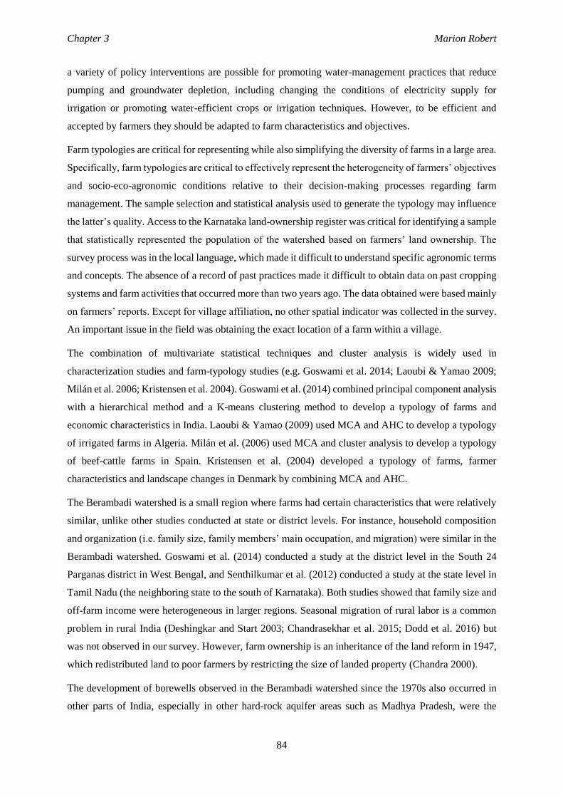
Chapter 3 Marion Robert
84
a variety of policy interventions are possible for promoting water-management practices that reduce
pumping and groundwater depletion, including changing the conditions of electricity supply for
irrigation or promoting water-efficient crops or irrigation techniques. However, to be efficient and
accepted by farmers they should be adapted to farm characteristics and objectives.
Farm typologies are critical for representing while also simplifying the diversity of farms in a large area.
Specifically, farm typologies are critical to effectively represent the heterogeneity of farmers’ objectives
and socio-eco-agronomic conditions relative to their decision-making processes regarding farm
management. The sample selection and statistical analysis used to generate the typology may influence
the latter’s quality. Access to the Karnataka land-ownership register was critical for identifying a sample
that statistically represented the population of the watershed based on farmers’ land ownership. The
survey process was in the local language, which made it difficult to understand specific agronomic terms
and concepts. The absence of a record of past practices made it difficult to obtain data on past cropping
systems and farm activities that occurred more than two years ago. The data obtained were based mainly
on farmers’ reports. Except for village affiliation, no other spatial indicator was collected in the survey.
An important issue in the field was obtaining the exact location of a farm within a village.
The combination of multivariate statistical techniques and cluster analysis is widely used in
characterization studies and farm-typology studies (e.g. Goswami et al. 2014; Laoubi & Yamao 2009;
Milán et al. 2006; Kristensen et al. 2004). Goswami et al. (2014) combined principal component analysis
with a hierarchical method and a K-means clustering method to develop a typology of farms and
economic characteristics in India. Laoubi & Yamao (2009) used MCA and AHC to develop a typology
of irrigated farms in Algeria. Milán et al. (2006) used MCA and cluster analysis to develop a typology
of beef-cattle farms in Spain. Kristensen et al. (2004) developed a typology of farms, farmer
characteristics and landscape changes in Denmark by combining MCA and AHC.
The Berambadi watershed is a small region where farms had certain characteristics that were relatively
similar, unlike other studies conducted at state or district levels. For instance, household composition
and organization (i.e. family size, family members’ main occupation, and migration) were similar in the
Berambadi watershed. Goswami et al. (2014) conducted a study at the district level in the South 24
Parganas district in West Bengal, and Senthilkumar et al. (2012) conducted a study at the state level in
Tamil Nadu (the neighboring state to the south of Karnataka). Both studies showed that family size and
off-farm income were heterogeneous in larger regions. Seasonal migration of rural labor is a common
problem in rural India (Deshingkar and Start 2003; Chandrasekhar et al. 2015; Dodd et al. 2016) but
was not observed in our survey. However, farm ownership is an inheritance of the land reform in 1947,
which redistributed land to poor farmers by restricting the size of landed property (Chandra 2000).
The development of borewells observed in the Berambadi watershed since the 1970s also occurred in
other parts of India, especially in other hard-rock aquifer areas such as Madhya Pradesh, were the
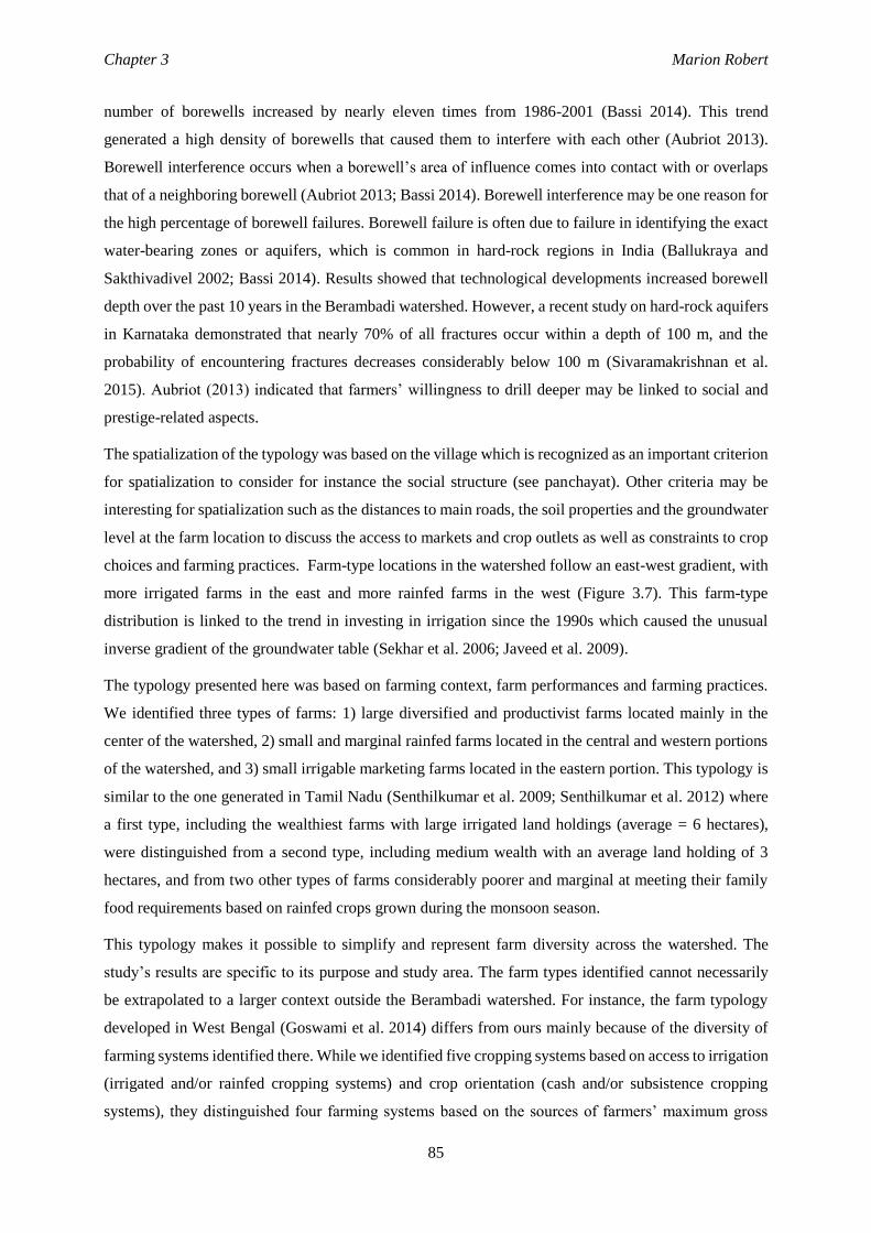
Chapter 3 Marion Robert
85
number of borewells increased by nearly eleven times from 1986-2001 (Bassi 2014). This trend
generated a high density of borewells that caused them to interfere with each other (Aubriot 2013).
Borewell interference occurs when a borewell’s area of influence comes into contact with or overlaps
that of a neighboring borewell (Aubriot 2013; Bassi 2014). Borewell interference may be one reason for
the high percentage of borewell failures. Borewell failure is often due to failure in identifying the exact
water-bearing zones or aquifers, which is common in hard-rock regions in India (Ballukraya and
Sakthivadivel 2002; Bassi 2014). Results showed that technological developments increased borewell
depth over the past 10 years in the Berambadi watershed. However, a recent study on hard-rock aquifers
in Karnataka demonstrated that nearly 70% of all fractures occur within a depth of 100 m, and the
probability of encountering fractures decreases considerably below 100 m (Sivaramakrishnan et al.
2015). Aubriot (2013) indicated that farmers’ willingness to drill deeper may be linked to social and
prestige-related aspects.
The spatialization of the typology was based on the village which is recognized as an important criterion
for spatialization to consider for instance the social structure (see panchayat). Other criteria may be
interesting for spatialization such as the distances to main roads, the soil properties and the groundwater
level at the farm location to discuss the access to markets and crop outlets as well as constraints to crop
choices and farming practices. Farm-type locations in the watershed follow an east-west gradient, with
more irrigated farms in the east and more rainfed farms in the west (Figure 3.7). This farm-type
distribution is linked to the trend in investing in irrigation since the 1990s which caused the unusual
inverse gradient of the groundwater table (Sekhar et al. 2006; Javeed et al. 2009).
The typology presented here was based on farming context, farm performances and farming practices.
We identified three types of farms: 1) large diversified and productivist farms located mainly in the
center of the watershed, 2) small and marginal rainfed farms located in the central and western portions
of the watershed, and 3) small irrigable marketing farms located in the eastern portion. This typology is
similar to the one generated in Tamil Nadu (Senthilkumar et al. 2009; Senthilkumar et al. 2012) where
a first type, including the wealthiest farms with large irrigated land holdings (average = 6 hectares),
were distinguished from a second type, including medium wealth with an average land holding of 3
hectares, and from two other types of farms considerably poorer and marginal at meeting their family
food requirements based on rainfed crops grown during the monsoon season.
This typology makes it possible to simplify and represent farm diversity across the watershed. The
study’s results are specific to its purpose and study area. The farm types identified cannot necessarily
be extrapolated to a larger context outside the Berambadi watershed. For instance, the farm typology
developed in West Bengal (Goswami et al. 2014) differs from ours mainly because of the diversity of
farming systems identified there. While we identified five cropping systems based on access to irrigation
(irrigated and/or rainfed cropping systems) and crop orientation (cash and/or subsistence cropping
systems), they distinguished four farming systems based on the sources of farmers’ maximum gross
Chapter 3 Marion Robert
86
income. These included rice, vegetables, fish and off-farm based farming systems. However, the two-
step method combining MCA and AHC is subject to generalization for even larger regions (Kristensen
et al. 2004; Milán et al. 2006; Laoubi and Yamao 2009; Goswami et al. 2014).
This study predicts two scenarios for the watershed: 1) farmers, especially on small, irrigated marketing
farms and large productivist irrigated farms, may continue to maximize profits by producing high water-
demanding crops and cash crops; and 2) irrigation technology may continue to spread toward the western
portion of the watershed and convert small rainfed farms into small irrigable marketing farms.
Simulation models may help determining whether these scenarios may be sustainable in terms of
groundwater depletion and farmers’ incomes.
3.6. CONCLUSION
The typology presented here should enable policy makers to better assess the potential influence of
agricultural and water-management policies on farmers’ livelihoods and the groundwater table. The
typology can be used in simulation models to predict impacts of climate change, specifically higher
evapotranspiration, on farming practices and the groundwater level. Such simulation models are useful
to test policies aiming to slow groundwater-table depletion and limit income risks due to crop failure.
For example, simulation models could explore policies to maintain small rainfed farms (e.g. subsidizing
rainfed crops, especially subsistence crops such as pulses) or policies to encourage farmers to adopt
better water management in cropping systems, (e.g. decreasing the area of crops that consume large
amounts of water, such as banana, sugar cane and turmeric, or modifying electricity availability or
subsidizing drip irrigation or less water consuming crops or varieties).

Chapter 3 Marion Robert
87
ACKNOWLEDGEMENTS
This study was part the multidisciplinary Indo-French research project AICHA (Adaptation of Irrigated
Agriculture to Climate Change 4700-W1) funded by the Indo-French Centre for the Promotion of
Advanced Research (CEFIPRA), the INRA flagship program on Adaptation to Climate Change of
Agriculture and Forest (ACCAF), the Doctoral School of the University of Toulouse (EDT) and ORE
BVET (http://bvet.obs-mip.fr). We are grateful to all the experts, farmers, and trainees who helped
implement the method. We are also very grateful for the help and hard work of the field team. Particular
thoughts go to Jarayma and his family, to whom we convey my sincere condolences.
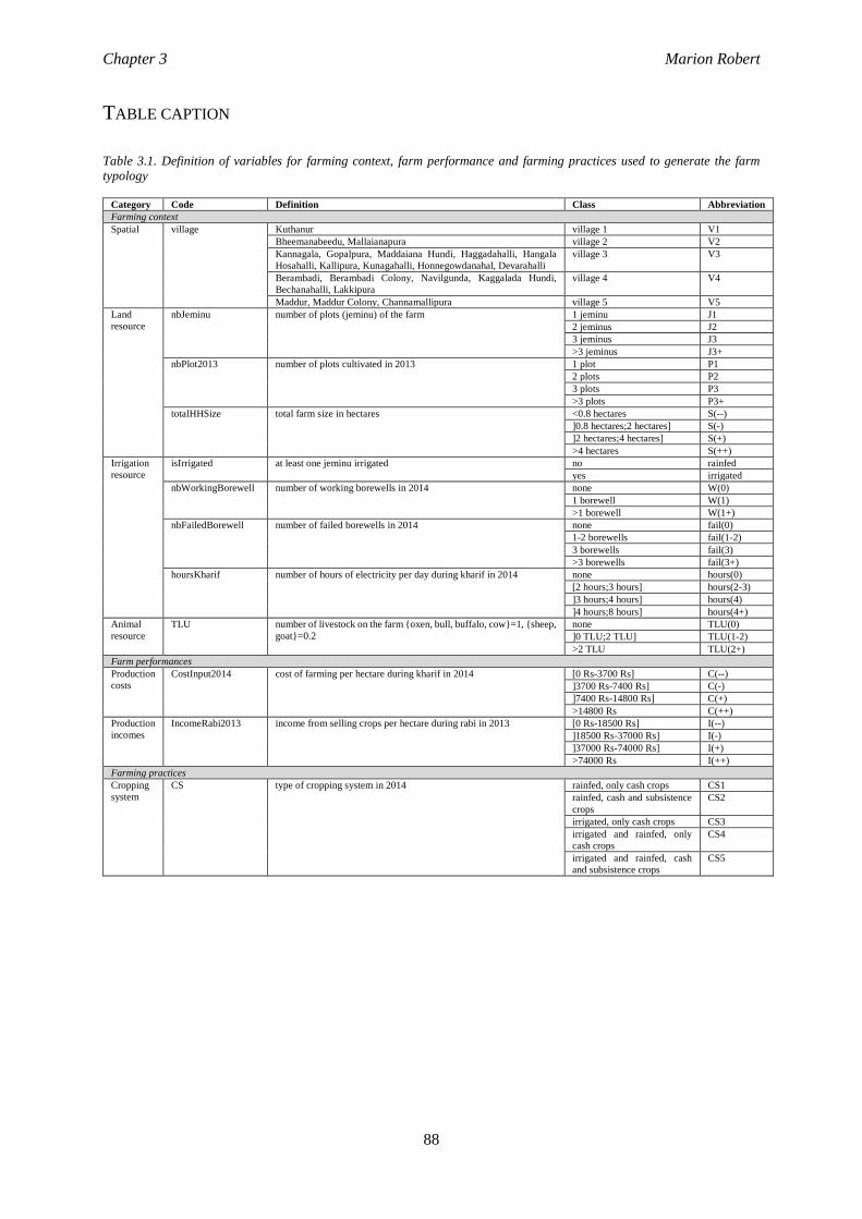
Chapter 3 Marion Robert
88
TABLE CAPTION
Table 3.1. Definition of variables for farming context, farm performance and farming practices used to generate the farm
typology
Category Code Definition Class Abbreviation
Farming context
Spatial village Kuthanur village 1 V1
Bheemanabeedu, Mallaianapura village 2 V2
Kannagala, Gopalpura, Maddaiana Hundi, Haggadahalli, Hangala
Hosahalli, Kallipura, Kunagahalli, Honnegowdanahal, Devarahalli
village 3 V3
Berambadi, Berambadi Colony, Navilgunda, Kaggalada Hundi,
Bechanahalli, Lakkipura
village 4 V4
Maddur, Maddur Colony, Channamallipura village 5 V5
Land
resource
nbJeminu number of plots (jeminu) of the farm 1 jeminu J1
2 jeminus J2
3 jeminus J3
>3 jeminus J3+
nbPlot2013 number of plots cultivated in 2013 1 plot P1
2 plots P2
3 plots P3
>3 plots P3+
totalHHSize total farm size in hectares <0.8 hectares S(--)
]0.8 hectares;2 hectares] S(-)
]2 hectares;4 hectares] S(+)
>4 hectares S(++)
Irrigation
resource
isIrrigated at least one jeminu irrigated no rainfed
yes irrigated
nbWorkingBorewell number of working borewells in 2014 none W(0)
1 borewell W(1)
>1 borewell W(1+)
nbFailedBorewell number of failed borewells in 2014 none fail(0)
1-2 borewells fail(1-2)
3 borewells fail(3)
>3 borewells fail(3+)
hoursKharif number of hours of electricity per day during kharif in 2014 none hours(0)
[2 hours;3 hours] hours(2-3)
]3 hours;4 hours] hours(4)
]4 hours;8 hours] hours(4+)
Animal
resource
TLU number of livestock on the farm {oxen, bull, buffalo, cow}=1, {sheep,
goat}=0.2
none TLU(0)
]0 TLU;2 TLU] TLU(1-2)
>2 TLU TLU(2+)
Farm performances
Production
costs
CostInput2014 cost of farming per hectare during kharif in 2014 [0 Rs-3700 Rs] C(--)
]3700 Rs-7400 Rs] C(-)
]7400 Rs-14800 Rs] C(+)
>14800 Rs C(++)
Production
incomes
IncomeRabi2013 income from selling crops per hectare during rabi in 2013 [0 Rs-18500 Rs] I(--)
]18500 Rs-37000 Rs] I(-)
]37000 Rs-74000 Rs] I(+)
>74000 Rs I(++)
Farming practices
Cropping
system
CS type of cropping system in 2014 rainfed, only cash crops CS1
rainfed, cash and subsistence
crops
CS2
irrigated, only cash crops CS3
irrigated and rainfed, only
cash crops
CS4
irrigated and rainfed, cash
and subsistence crops
CS5
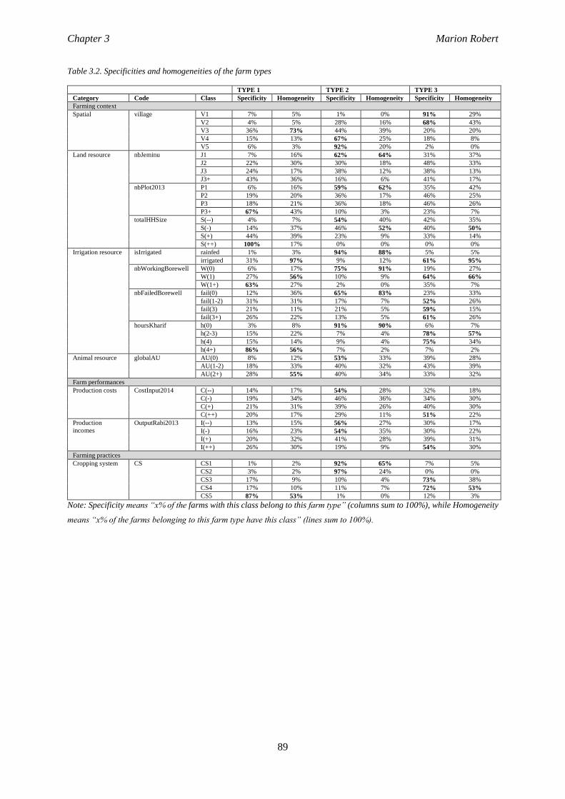
Chapter 3 Marion Robert
89
Table 3.2. Specificities and homogeneities of the farm types
TYPE 1 TYPE 2 TYPE 3
Category Code Class Specificity Homogeneity Specificity Homogeneity Specificity Homogeneity
Farming context
Spatial village V1 7% 5% 1% 0% 91% 29%
V2 4% 5% 28% 16% 68% 43%
V3 36% 73% 44% 39% 20% 20%
V4 15% 13% 67% 25% 18% 8%
V5 6% 3% 92% 20% 2% 0%
Land resource nbJeminu J1 7% 16% 62% 64% 31% 37%
J2 22% 30% 30% 18% 48% 33%
J3 24% 17% 38% 12% 38% 13%
J3+ 43% 36% 16% 6% 41% 17%
nbPlot2013 P1 6% 16% 59% 62% 35% 42%
P2 19% 20% 36% 17% 46% 25%
P3 18% 21% 36% 18% 46% 26%
P3+ 67% 43% 10% 3% 23% 7%
totalHHSize S(--) 4% 7% 54% 40% 42% 35%
S(-) 14% 37% 46% 52% 40% 50%
S(+) 44% 39% 23% 9% 33% 14%
S(++) 100% 17% 0% 0% 0% 0%
Irrigation resource isIrrigated rainfed 1% 3% 94% 88% 5% 5%
irrigated 31% 97% 9% 12% 61% 95%
nbWorkingBorewell W(0) 6% 17% 75% 91% 19% 27%
W(1) 27% 56% 10% 9% 64% 66%
W(1+) 63% 27% 2% 0% 35% 7%
nbFailedBorewell fail(0) 12% 36% 65% 83% 23% 33%
fail(1-2) 31% 31% 17% 7% 52% 26%
fail(3) 21% 11% 21% 5% 59% 15%
fail(3+) 26% 22% 13% 5% 61% 26%
hoursKharif h(0) 3% 8% 91% 90% 6% 7%
h(2-3) 15% 22% 7% 4% 78% 57%
h(4) 15% 14% 9% 4% 75% 34%
h(4+) 86% 56% 7% 2% 7% 2%
Animal resource globalAU AU(0) 8% 12% 53% 33% 39% 28%
AU(1-2) 18% 33% 40% 32% 43% 39%
AU(2+) 28% 55% 40% 34% 33% 32%
Farm performances
Production costs CostInput2014 C(--) 14% 17% 54% 28% 32% 18%
C(-) 19% 34% 46% 36% 34% 30%
C(+) 21% 31% 39% 26% 40% 30%
C(++) 20% 17% 29% 11% 51% 22%
Production
incomes
OutputRabi2013 I(--) 13% 15% 56% 27% 30% 17%
I(-) 16% 23% 54% 35% 30% 22%
I(+) 20% 32% 41% 28% 39% 31%
I(++) 26% 30% 19% 9% 54% 30%
Farming practices
Cropping system CS CS1 1% 2% 92% 65% 7% 5%
CS2 3% 2% 97% 24% 0% 0%
CS3 17% 9% 10% 4% 73% 38%
CS4 17% 10% 11% 7% 72% 53%
CS5 87% 53% 1% 0% 12% 3%
Note: Specificity means “x% of the farms with this class belong to this farm type” (columns sum to 100%), while Homogeneity
means “x% of the farms belonging to this farm type have this class” (lines sum to 100%).
Chapter 3 Marion Robert
90
FIGURE CAPTION
Figure 3.1. Location of the case study. The Berambadi watershed belongs to the South Gundal watershed located
in southern Karnataka state. GW is the ground water level below ground (m). The GW level comes from
extrapolation of data measured on 600 disused borewells at the end of 2012 monsoon.
Figure 3.2. Spatialization of statistically different farm characteristics on the watershed. Black lines refer to gram
panchayat borders, grey lines refer to village borders, green area describes the forest.
Figure 3.3. Distribution of irrigated farms and number of borewells per farm on the watershed. The maps present
for the 12 villages 1) the distribution of irrigated farms, 2) the average number of borewells drilled per farm, 3)
the average number of working borewells per farm and 4) the average number of failed borewells per farm.
Figure 3.4. A) Projection of the variables used to generate the farm typology in the plane of the first two
factors of Multiple Correspondence Analysis (MCA); B) Projection of the class of variables used to
generate the farm typology in the plane of the first two factors of the MCA. Variables and class are
described in Table 3.1..
Figure 3.5. Dendrogram of individuals from Agglomerative Hierarchical Clustering performed on the first 12
components of the Multiple Correspondence Analysis. Type 1 are large, diversified and productivist farms. Type
2 are small, marginal rainfed farms. Types 3 are small, irrigable marketing farms. Using the first 12 principal
components in an AHC algorithm, we obtained a typology with three farm types (red line). Jump in between-
cluster inertia is represented in the right corner.
Figure 3.6. Individuals of the three farm types projected on the plane of the first two dimensions of the Multiple
Correspondence Analysis. Type 1 are large, diversified and productivist farms. Types 2 are small, marginal rainfed
farms. Type 3 are small, irrigable marketing farms.
Figure 3.7. Groundwater table gradient (colors) and farm typology (pie chart) for each of the five villages (V1 to
V5) on the Berambadi watershed. Type 1 are large, diversified and productivist farms. Type 2 are small, marginal
rainfed farms. Type 3 are small, irrigable marketing farms. Grey lines refer to the borders of the 12 villages, green
area describes the forest. The ground water level was obtained using disused borewells and mesured at the end of
2012 monsoon (NB: no borewell was monitored in the forest and close by the forest leading to a partial map of
ground water level).
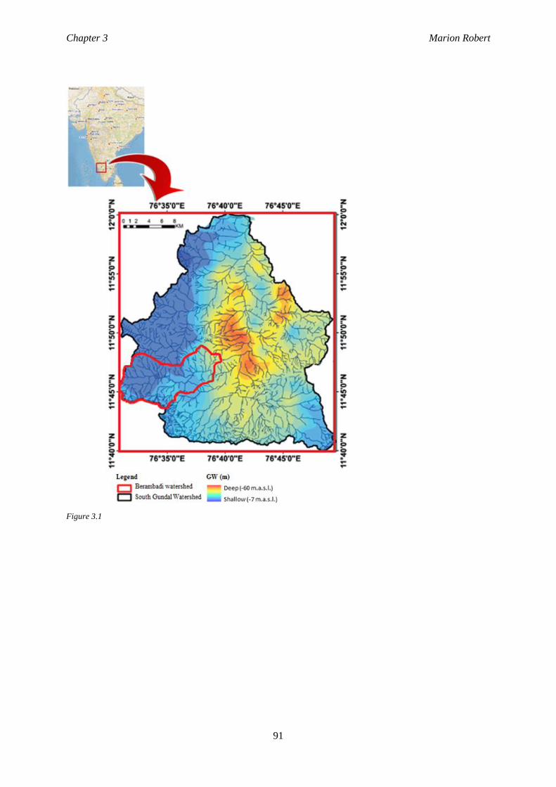
Chapter 3 Marion Robert
91
Figure 3.1
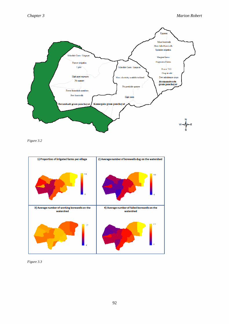
Chapter 3 Marion Robert
92
Figure 3.2
Figure 3.3
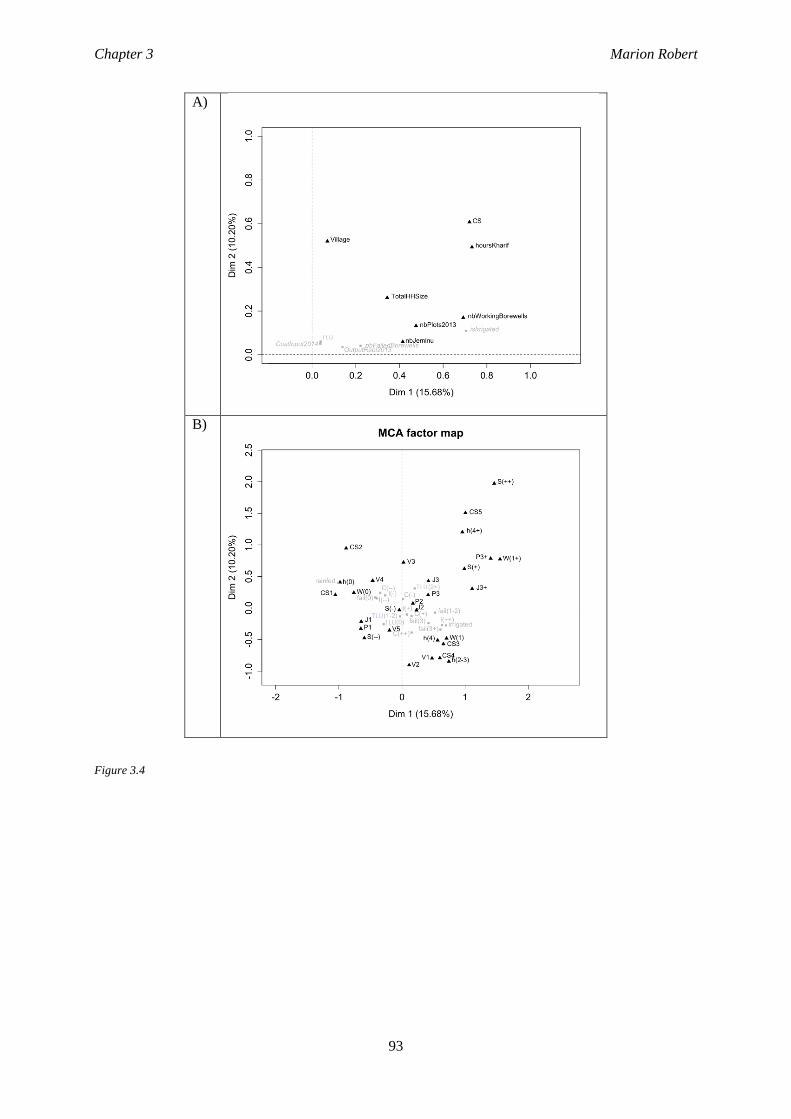
Chapter 3 Marion Robert
93
A)
B)
Figure 3.4
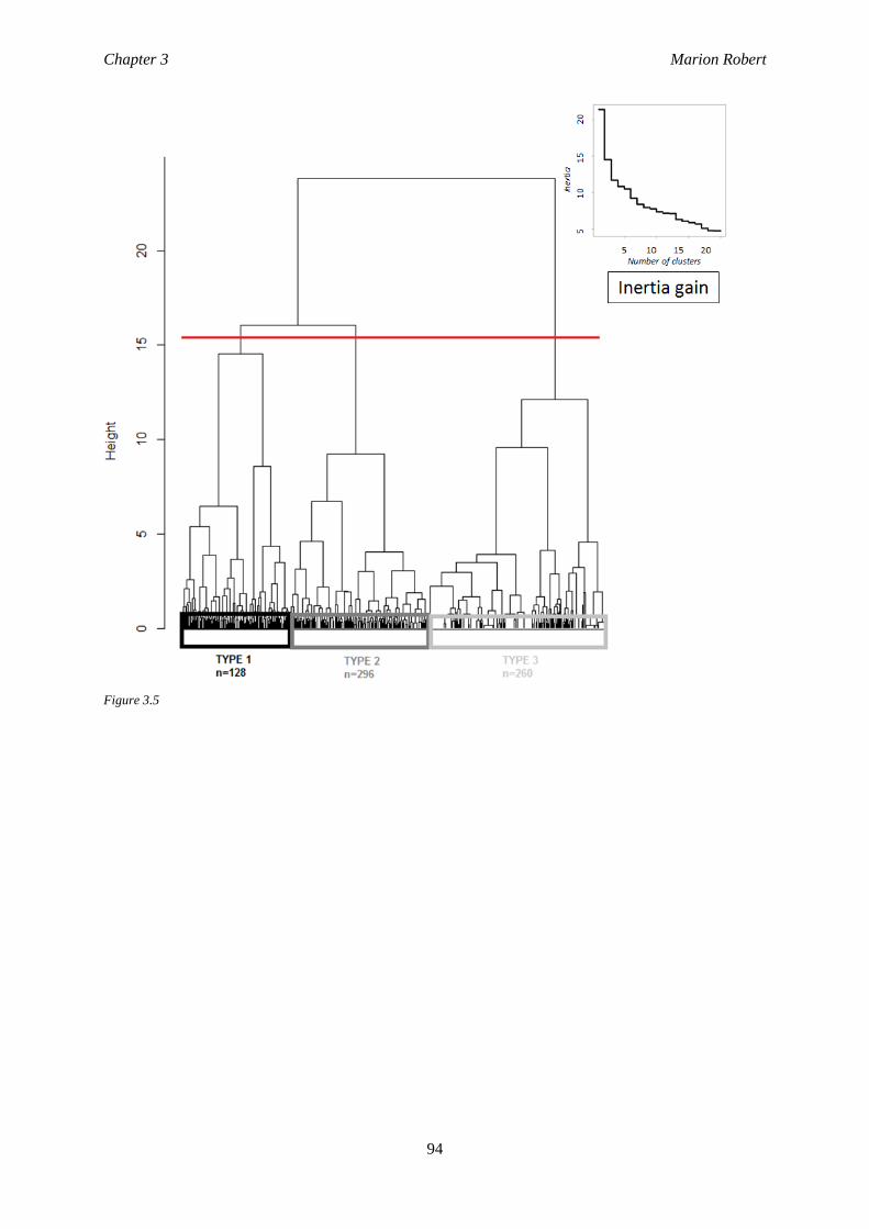
Chapter 3 Marion Robert
94
Figure 3.5
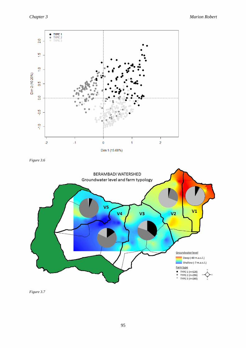
Chapter 3 Marion Robert
95
Figure 3.6
Figure 3.7


Chapter 4 Marion Robert
98
Chapter 4
CMFDM: A methodology to guide the
design of a conceptual model of
farmers’ decision-making processes
Marion Robert1,*, Jérôme Dury1, Alban Thomas2, Olivier Therond1, Muddu Sekhar3
, Shrini Badiger4
,
Laurent Ruiz5
& Jacques-Eric Bergez1
¹ AGIR, Université de Toulouse, INPT, INP-PURPAN, INRA, 31320, Castanet Tolosan, France
² INRA, Toulouse School of Economics, UMR 1081 LERNA, F-31000 Toulouse, France 3
IISC, Department of Civil Engineering, Bangalore 560012, India 4
ATREE, Bangalore 560 064, India 5
INRA, UMR 1069 SAS, F-35042 Rennes, France
*: Corresponding author, Tel: +33 (0)5 61 28 50 30. E-mail: [email protected]
Published in Agricultural Systems
Short Communication
Doi: 10.1016/j.agsy.2016.07.010
Quote: Robert, M., Dury, J., Thomas, A., Therond, O., Sekhar, M., Badiger, S., Ruiz, L. & Bergez, J. E.
(2016). CMFDM: A methodology to guide the design of a conceptual model of farmers' decision-making
processes. Agricultural Systems, 148, 86-94.
Chapter 4 Marion Robert
99
The agricultural research community offers languages and approaches to model farmers’ decision-
making processes but does not often clearly detail the steps necessary to build an agent model underlying
farmers’ decision-making processes. We propose an original and readily applicable methodology for
modelers to guide data acquisition and analysis, incorporate expert knowledge, and conceptualize
decision-making processes in farming systems using a software engineering language to support the
development of the model. We propose a step-by-step approach that combines decision-making analysis
with a modeling approach inspired by cognitive sciences and software-development methods. The
methodology starts with case-based analysis to study and determine the complexity of decision-making
processes and provide tools to obtain a generic and conceptual model of the decisional agent in the
studied farming system. A generic farm representation and decision diagrams are obtained from cross-
case analysis and are modeled with Unified Modeling Language. We applied the methodology to a
research question on water management in an emerging country (India). Our methodology bridges the
gap between field observations and the design of the decision model. It is a useful tool to guide modelers
in building decision model in farming system.
Keywords: decision modeling, farming systems, water management, case-based analysis, cognitive task
analysis, UML
Chapter 4 Marion Robert
100
4.1. INTRODUCTION
The agricultural research community has a particular interest in modeling farming systems to simulate
opportunities for adaptation that ensure flexibility and resilience of farming systems. To account for actors
and their actions in the environment, it is essential to precisely represent their decision-making processes.
Some methods have been developed to describe farmers’ decision-making processes such as the “model for
actions” (Aubry et al. 1998a), rule-based models (Bergez et al. 2006; Donatelli et al. 2006) and activity-
based models (Clouaire and Rellier 2009; Martin et al. 2013). However none specifies precisely the process
between farmers’ decision-making and the modeling activity. In the real world, people do not exhibit
optimal behavior like that described in well-structured and controlled experimental settings. One major
contribution of the naturalistic decision making (NDM) community is in describing how people make
decisions in real-world settings (Klein 2008). NDM starts with field research. NDM asserts that the structure
and content of decision-making processes are defined by the organization of the domain in which the
decision maker is acting (Zsambok and Klein 2014). It is therefore pointless to develop a decision model
without a detailed understanding and formal representation of the relationship between the knowledge
farmers have in a specific domain and the decisions they make. Building a conceptual model is a standard
step in model development. It describes the model without programming language and facilitates
communication between modelers and analysts. However, these conceptual representations are often
oriented towards a computerized implementation of the model. Consequently, they do not detail the structure
of the system and how it functions (Lamanda et al. 2012).
The objective of our paper is to propose an original and readily applicable methodology to formalize the
conceptual modeling of the farmer agent underlying decision-making processes in farming system
(CMFDM) and to guide data acquisition and analysis, the incorporation of expert knowledge, and the design
of a model. The methodology combines techniques for system description based on field research in natural
settings and techniques from the software engineering field regarding the use of software engineering
language to support the development of a model. Our research may provide a useful tool for modelers
looking for clear guidance on how to build the agent sub-model in a farming system model.
4.2. FOUNDING PRINCIPLES OF THE METHODOLOGY
Our conceptual modeling of farmers’ decision-making processes in farming system methodology
(CMFDM) is based on three founding principles: 1) Theory building from cases is used to obtain a relevant
theory from observing actual practices in a natural setting (Glaser and Strauss 1967; Eisenhardt 1989; Yin
Chapter 4 Marion Robert
101
2013). Theory building from case studies is a research process using qualitative and quantitative methods
to gather data from one or more case studies in a single natural setting, considering contextual and time
aspects of the current phenomenon studied without any experimental control or manipulation (Meredith
1998). The use of case studies is the basis for developing the theoretical constructs and propositions from
empirical evidence. Theory is emergent in the sense that it develops from cross-case analysis and the
recognition of patterns of relationship within and across cases. Theory building is a recursive cycling process
among the case data, the emerging theory and the literature. The first part of the process is inductive going
from cases to new theory while the second part of the process is deductive seeking to test the theory
previously build with another set of data (Carroll and Swatman 2000; Carlile and Christensen 2005;
Eisenhardt and Graebner 2007). The process is totally iterative since it constantly involves backward and
forward iterations between case comparison, and theory implementation. Grounded theory research, case
researches according to Yin (1994) and Eisenhardt (1989) are well established empirical methodologies for
theory building from case (Steenhuis and Bruijn 2006) ; 2) Cognitive-Task Analysis (CTA) is used to
analyze and model the cognitive processes that gave rise to farmers’ task performance in farming systems
(Jonassen 1997; Chipman et al. 2000). CTA provides information about knowledge, cognitive processes,
and goal structures needed to solve complex problems and perform tasks (Zsambok and Klein 2014). With
the help of CTA, the analyst looks at the system from the perspective of the person performing the task. An
important part of the analysis is tracking past critical events that shape a person’s feelings or expectations
about the task (Schraagen et al. 2000). CTA includes a step to map the different tasks, identify the critical
decision points and cluster, link and prioritize them and characterize the strategy used to face them (Klein
1989). CTA has a wide and varied pool of methods among which the most frequently used are structured
interviews, verbal protocol analysis (‘think-aloud’ protocols, retrospective verbal protocols), and critical
decision methods (Klein 1989) ; 3) Unified Modelling Language (UML) is used to represent the decision-
making problem in a standard and readily usable form for computer programming (Booch et al. 1996;
Papajorgji and Pardalos 2006). UML is a standardized object-oriented modeling language in the software
engineering field (Booch et al. 1996; Papajorgji and Pardalos 2006).UML is an efficient way to transcribe
and abstract information for modeling purposes due to its similarity to knowledge objects (Milton and
Kazmierczak 2006). UML has been used as ontology language (Cranefield and Purvis 1999; Pinet et al.
2009). Classes, concepts and relationships are defined and form a common vocabulary for analysts, and
modelers who need to share information on the domain (Beck et al. 2010). The ontology is a “formal explicit
specification of a shared conceptualization” (Gruber 1993). The visual representation of UML graphs
facilitates the design process of the ontology.
Chapter 4 Marion Robert
102
Based on these three founding principles, we defined a standardized methodology aiming at guiding the
translation of selected case-study observations into a conceptual representation of a generic decision model
of the farming system. It is organized into four steps that are combined in an iterative process (Figure 4.1).
4.3. THE CMFDM METHODOLOGY
4.3.1. Step 1: problem definition
The first step is problem definition. Ideally, the theory building from cases research should start without any
theory or hypothesis to test under consideration. However, it is truly impossible to reach this ideal but it is
important to attempt to approach it in order to avoid bias and limits in the findings because of preordained
theoretical perspectives. Thus, the definition of the context and the initial research question is important in
theory building from cases to not become overwhelmed by the volume of data. Moreover, a priori
framework can be designed to shape the initial design of the theory building research that can potentially
specify some important variables identified in the literature but it should be done by avoiding any
consideration of relationship between variables or hypothesis.
4.3.2. Step 2: case study selection
The second step is the selection of case studies. As in statistical researches, selecting the population likely
to exhibit the research focus is essential to control variations and define the limits of the generalization
process. The appropriate population is characterized by satisfying criteria for the research question defined
earlier. However the sampling of cases from the appropriate population is particular and is based on a
theoretical sampling approach driven by the search for diversity instead of a statistical search for
representativeness (Glaser and Strauss 1967; Eisenhardt and Graebner 2007). Case studies may be selected
to replicate previous cases, extend the emergent theory, or fill theoretical categories. Random selection is
not advised given the limited number of cases studied, but selection of extreme cases or polar types is
preferred.
4.3.3. Step 3: data collection and analysis of individual case studies
The third step is data collection and analysis of individual case studies based on CTA and UML. Five sub-
steps are followed. First, based on the prior definition of the context, the initial research question and the
framework potentially advanced in STEP 1, the analyst is able to shortlist multiple data collection methods
and tools that can be both qualitative and quantitative. Tools used are usually interviews, surveys,
observations, document analysis and standard quantitative measure like questionnaires. Using multiple data
Chapter 4 Marion Robert
103
collection method presents two main advantages: 1) it makes possible the triangulation between collected
data providing stronger evidences of theory constructs and hypothesis; 2) it overlaps data analysis and allows
the analyst to take advantage of flexible data collection and to make adjustment during this process. These
adjustments ensures some flexibility and arises new data collection opportunities to probe emergent themes
or new theoretical insights in order to understand each individual case as much deep as possible. Secondly,
based on the prior definition of the context, the initial research question and the framework potentially
advanced in STEP 1, appropriate UML representations for the important variables identified in the literature
are selected among the list of UML structural and behavioral diagrams. This step ensures that the
representation maps directly to the information reached by a specific data collection method and provides
direction and order to identify sub-variables and relationship between variables. Thirdly, data is collected
in the field. In one hand, data collection is dedicated to become more familiar with the individual context
by identifying specific characteristics of individual environment and the sequence of activities or tasks
realized by each individual. This information are obtained from document analysis and direct interaction
with the farmer through survey and questionnaire that help identifying farmer’s knowledge on the farming
context. On the other hand, data collection aims at capturing the cognitive processes set up to realize tasks.
In this purpose, critical decision method (Klein, 1989) is used as a knowledge-elicitation method to collect
farmer’s knowledge and identify critical incidents that disrupt farming management and allow adaptive
behavior elicitation. Data collection is emergent in theory building from cases. That means what the analyst
learns from the data collected from one individual case often is used to determine subsequent data collection.
Fourthly, individual cases are analyzed and verified. An initial transcription using UML representation is
made of the information collected and then presented to the concerned farmer for verification, refinement,
and revision during a second meeting. This ensures that representation of a task and the underlying cognitive
components are sufficiently complete and accurate to format into a formal individual conceptual model.
Finally, verified individual conceptual model on farmers’ knowledge and cognitive processes are formally
represented with UML diagrams. This step allows the unique pattern of each case to emerge before
generalizing patterns across cases.
4.3.4. Step 4: the generic conceptual model
The last step is the transition from individual case studies to a generic model. It is an iterative process of
cross-cases analysis, enfolding of literature, and incorporation of expert knowledge. One way to do the
cross-cases analysis is to list similarities and differences between individual analysis and UML graphs.
Another way is by selecting dimensions and to compare cases related to these dimensions. Concepts and
relationship between variables emerge from cross-cases analysis shaping hypothesis and theories. It is
essential to compare the emergent results from cross-cases analysis with the extant literature in order to
Chapter 4 Marion Robert
104
improve the theory validity and enlarge its generalizability. Relationship and concepts that are replicated
across most or all of the cases or at least validated by the literature are retained to ensure robustness and
generalizability. Experts and modelers are also used to strengthen development of the generic model by
formulating and adding more complex and meta concepts. It leads to the addition of abstract classes that are
not usually used by farmers. In that respect, the generalization of classes is an important process in object
oriented modeling (Papajorgji and Pardalos 2006). The generic conceptual model is formatted with the UML
graphs and leads to an ontological analysis that formalizes and efficiently specifies concepts and
relationships among these concepts.
4.4. METHODOLOGY IMPLEMENTATION IN A CASE STUDY
4.4.1. Step 1: problem definition
We applied the methodology to farming systems in the context of irrigation water management under water
scarcity. We chose to focus the application of our methodology on the conceptual representation of a farmer.
We consider farmers as cognitive agents able to think, memorize, analyze, predict, and learn to manage
future events and plan their actions (Le Bars et al. 2005). In artificial intelligence and cognitive sciences,
cognitive agents have been commonly represented as Belief-Desire-Intention (BDI) agents (Bratman 1987b;
Rao and Georgeff 1991). The concept of Belief represents the farmer’s knowledge of the system. Desires
are the objectives or satisfying goals of the farmer. Intentions are actions plan to achieve the farmer’s
objectives (Desires). The BDI framework is founded on the well-known theory of rational action in humans.
BDI agents are considered as having an incomplete view of their environment. We used the BDI to structure
the formal knowledge produced by the CMFDM. Our conceptual representation of a farmer included the
knowledge on the farm structure and on the decision-making processes and adaptations. Contrary to
normative approaches, BDI is a practical reasoning representation used to simulate bounded rationality and
is an intuitive representation of the human decision-making process. Compared to fully rational approaches,
its descriptive capacity enables the representation of decision processes that are the closest to reality. To
provide the BDI structure, we agree with Rider (2012) that cognitive task analysis is an efficient transition
between farmers’ decision processes in the real world and its representation.
4.4.2. Step 2: case study selection
CMFDM was applied, inter alia, on water management of small farm holders in an emerging country (India).
In the Berambadi watershed (Karnataka state, southern India), farmers are facing increasing temperatures,
unpredictable rainfall, and groundwater depletion. Agriculture depends greatly on rainfall and access to
Chapter 4 Marion Robert
105
irrigation. While groundwater access is nearly free and limited only by the availability of electricity, many
farmers encounter dry and temporarily non-functioning borewells. Water table levels display a non-standard
pattern, hydrogeologically speaking; valley regions have deeper groundwater levels than topographically
higher zones. Thus an unusual groundwater level gradient is observed with shallow water in the upstream
and deep water in the downstream. Farms are really small, less than one hectare, with mainly manual and
animal traction work capacity. Farms are composed of jeminus (plots) subdivided into beles (crop plots)
that change from year to year. The cropping system is organized around three seasons: i) the rainy season,
when most of the crop is grown (kharif); ii) the winter season, when mainly irrigated crops are grown (rabi);
and iii) the dry season, when little cultivation occurs (summer). Monsoon rainfall is a key determinant for
crop choice. Crops may be under contract, directly sold to agents or markets, or are for subsistence. Farmers
are highly in debt due to investing in irrigation systems. Government subsidies greatly reduce the price of
chemical fertilizers and provide affordable inputs. The methodology was used to identify farmers’
knowledge and crop management decisions in a context of changes in rainfall and groundwater level. The
main concern was to understand and model the adaptation processes of the farmers who face these changes.
The population was local crop farmers on the watershed. The farmer population is characterized by the
following criteria: location, farm size, and access to irrigation. We interviewed 27 farmers from 10 villages
spread across the Berambadi watershed selected to have farms from all over the watershed in area where
the water table is really deep or really shallow and in transitional zone. We selected very big farms as well
as very small farms that could be irrigated or rainfed.
4.4.3. Step 3: data collection and analysis of individual case studies
Firstly we shortlisted the data collection methods and tools to use for our case study in India. Document
analysis on farming context on the watershed, at the state level or at the country level was important to get
familiar with the Indian field prior to the survey stage. We reviewed the literature on crop management
practices, irrigation practices, water issues, water management, and market and climate trends in Karnataka.
We met with extension service agents and researchers to gather general and specific information about the
watershed. The survey process was based on a questionnaire to frame the interview process and to get
quantitative measures shared by all survey done. We constructed a questionnaire based on the three parts of
the BDI: 1) the farmers’ beliefs (farm structures and characteristics), It focused on household characteristics,
the farm structure, assets, and partnerships, In-depth questions were asked about irrigation, borewells, and
rainfall; 2) the farmers’ desires (objectives and cropping pattern). We asked farmers about their objectives
and crop production over the past three years. Since no records were kept from year to year, information
about historical management went no further than three years in the past; 3) the farmers’ intentions
(decisions and adaptations). It aimed to reveal the farmers’ actions, reactions and adaptations to different
Chapter 4 Marion Robert
106
events. We questioned farmers about how they foresee their cropping-plan and asked them to describe the
sequence of decisions concerning cropping-plan decisions made the year before sowing. At this stage,
farmers usually describe a general decision plan for optimum conditions. Comparing this plan to the past
cropping system showed that crops actually grown can differ from the given cropping system. We
encouraged farmers to point out events that make them change their cropping system. To depict farmers’
practices and support the cognitive elicitation process, we used a timeline chart on which the farmers placed
stickers to represent farm activities and decision timing. The farmers indicated when specific events
occurred and explained what was done to address them. The survey process also combines extensive maps
and direct observations. Cadastral maps and district maps were used to mediate the farm data collection
process at the watershed scale. We realized direct observation and took notes on physical farm
characteristics like plot organization, building and borewell locations, distance to roads, etc. After details
about household organization, farm assets, and farm marketing position, we asked farmers about their
objectives and crop production over the past three years. We mediated this step by extensive use of farm
maps.
Secondly, we selected UML representations for the collected data. Structural diagram are appropriate to
represent the static aspect of the system. We used object diagrams for the representation of the farm
structure. Behavioral diagrams basically capture the dynamic aspect of a system. We used activity diagrams
to represent the decision-making processes, sequence diagrams to represent the interaction and flow of
information exchanged between the diverse entities of the farming system, use case diagram to represent
the relationships among the functionalities and their internal/external actors like farmers’ partnership,
relationships with sellers and buyers.
Thirdly, data was collected in the field. A preliminary test of the questionnaire showed that farmers were
not responsive to open-ended questions. Since interviewers were not researchers or farmers, we limited
open-ended questions with multiple-choice questions that included ranking preferences. Specific terms for
agronomic concepts such as “crop sequence”, “crop rotation”, and “previous-crop effect” were avoided and
addressed using examples. We avoided controversial questions about potential costs and water or electricity
fees. Beyond the questionnaire, the survey data collection process was adapted to each farmer depending on
previous interviews, on farmer’s answer, and on observations made. Thus questions were added to look
deeper into some farmer’s answers or to react to field observations. For instance, when unexpected crops
were mentioned while asking for the crops grown in 2012, 2013 and 2014, the interviewer asked for
complementary explanation to justify the farmer’s crops choice made during these years. Also the
interviewer added references to other interviews while talking to the farmer to ask the farmer’s opinion on
Chapter 4 Marion Robert
107
why he is behaving differently. For instance he asked why a certain farmer was not growing any sunflower
when most of the other farmers interviewed are.
Fourthly, we build an initial transcription of the knowledge collected and returned to ask farmers to verify,
refine, confirm and revise our preliminary results and emerging rules. This helped to introduce actions that
are obvious to farmers, such as growing sorghum depending on family grain stocks and not officially
including it in a crop rotation.
Finally, individual conceptual model on farmers’ knowledge and cognitive processes are formally
represented with UML diagrams. To illustrate individual conceptual models, we focus in this part on 1) the
representation and structure of the knowledge of the farmer with object diagrams; 2) the representation of
the decision-making processes with activity diagrams.
1) The farmer described the farm as a structure using four or five types of resources: land, labor, equipment,
livestock and, water (for irrigated farms). To illustrate the method, we focus on farmland representation.
We constructed individual object diagrams that depict farmers’ representation of their farmland
organization. Two examples include:
For Indian farmer In1 (Figure 4.2A), land organization differed between seasons in a fully rainfed
system. The number and size of plots changed from kharif to rabi due to high dependency on rainfall
in winter. Part of the land was more fertile due to application of tank-bed silt two years previously.
The farmer preferred to grow cash crops on the fertile land and subsistence crops on the less-fertile
part.
For Indian farmer In2, farmland (20 acres) was divided into two jeminus (Figure 4.2B). The
management differed on each jeminu. One was irrigated, and the other was fully rainfed. He grew
cash crops on the irrigated jeminu and preferred subsistence crops on the rainfed one. His land
organization during rabi was less sensitive to rainfall since water from a borewell enabled crop
growth during that season.
2) Concerning the decision-making processes of farmers, our analysis revealed that drought and water
restrictions, market prices, access to contracts, and delay in rainfall or monsoons in India were critical
incidents that push farmers to adapt. We asked them to explicitly describe alternative decisions that are
made when these changes occur. We identified two typical adaptation phases. At the beginning of the season
before any crop operations occur, farmers observe changes in the environment that lead them to adapt some
or all of the cropping system. After starting land preparation, the farmer may change a crop at the plot scale.
Le Gal et al. (2011) and Risbey et al. (1999) described the first level of intra-annual decisions as “tactical”
and daily decisions as “operational”. We offer an example on an Indian farmer:
Chapter 4 Marion Robert
108
Indian farmer In2 adapted his cropping system based on borewell yield, sunflower market prices,
and sorghum family grain stocks (Figure 4.3). During kharif, he set the irrigated area for long-term
crops (turmeric) and short-term crops (garlic) based on observing his borewell and estimating how
much water it would provide. In the case of a deep water table, the farmer replaced crops having
high water requirements with cash crops having low water requirements. In rainfed conditions,
sunflower price and sorghum family grain stocks influenced the area planted in sunflower. For rabi,
the farmer decided to cultivate or fallow his land based on borewell yield and expected rainfall.
4.4.4. Step 4: the generic conceptual model
For the Indian case study, we built a generic decision model. We compared individual analysis and graphs
to each other, referred to the literature, and asked experts and modelers to participate in the model
development.
We selected the following dimensions to highlight patterns in terms of similarities or differences between
cases: irrigation access, farm size, number of jeminu, village, and cash crop production. At this stage,
irrigation access clearly shows differences in land managements between fully rainfed farms and irrigable
farms. Kharif is the main cropping season to cultivate in the watershed. We focused on kharif cropping
systems to identify similarities between farms. Rainfed farmers are small to marginal farms going from 0.12
hectares to 2 hectares. We observed two behaviors: growing only crop to sell or growing also subsistence
crops. Cross-case in the irrigable farms highlights three types of farms: farms fully irrigated and growing
only cash crops, farms growing cash crops in irrigated and rainfed conditions, and farms growing cash and
subsistence crops in irrigated and rainfed conditions.
Concerning the representation of farm structure knowledge, the individual analysis from step 3 highlights
concepts used by farmers to organize their land and define their cropping system (Figure 4.4). Concepts
mentioned by most or all the Indian farmers were “season”, “soil fertility”, “jeminu”, “crop type”,
“irrigability” and “bele” (see farmers In1 and In2). One also talked about “ownership” saying he had
different practices on owned land and on rented land and another about “temporary plot” by having a jeminu
located in the Berambadi tank that is usable only when the water level in the tank is low enough. We did
not retain the last two concepts that were not relevant for the other farmers. We complemented the bottom-
up incorporation from farmers with top-down incorporation from experts and modelers. Modelers and
experts used abstract classes to summarize concepts. We generalized the concepts “Season”, “Soil”,
“Jeminu”, into TemporalUnit, BiophysicalUnit, and PhysicalUnit, respectively. The “bele” is considered
as the ManagementUnit where crop practices are effective. “Irrigability” and “crop type” were included
Chapter 4 Marion Robert
109
with the ManagementUnit. Farmers can develop several cropping systems with different crop management
practices, which we called CropManagementBlock.
Concerning the representation of decision-making processes and adaptation, we aim at getting generic
decision frame for each group; we crossed individual tactic decision UML activity diagrams (Figure 4.3) to
build a generic model (Figure 4.5). For instance, we focus on Indian farmers growing cash and self-
consumption crops under irrigated and rainfed conditions.
All farmers mentioned borewell yield as the primary factor that could change their cropping system and
cause them to reassess their irrigable area and long-term and short-term irrigated crops. Market prices and
available water for irrigation may influence their crop choice at the beginning of each season. Management
of the rainfed land depends on sorghum and finger millet stocks, and prices. Half of the farmers also
mentioned that the farm location from a local market or a main road influenced their crop choice. They
explained that they have higher chance to get contracts on beetroots or cabbages when their farm is along a
main road. Half of them also considered marigold contracts offered by marigold the cropping season which
ensure minimum revenue. An important part of farmers also mentioned rainfall expectations or monsoon
expectation as a condition for selecting rainfed crops. Deep root crops are favored when rainfalls are
expected to be low. Two farmers mentioned religious festivals as a motivation for growing watermelon and
one mentioned possible swaps of subsistence crops with his neighbor to justify not selecting sorghum crop.
We did not retain the last two concepts that were not relevant for the other farmers. We complemented the
bottom-up incorporation from farmers with top-down incorporation from experts and modelers. Irrigated
crops are classified in either long-term (11-month to three-year) and high water- demanding crops (turmeric,
sugar cane and banana), short-term crops (less than 11 months) with high water requirements (garlic and
onion), or short-term crops with low water requirements (watermelon, beetroot, cabbage and other
vegetables) (Figure 4.5). Rainfed crops are for selling (sunflower, marigold, horse gram, and groundnut) or
for subsistence (sorghum and finger millet). The generic decision frame of Indian farmers growing cash and
self-consumption crops under irrigated and rainfed conditions (Figure 4.5) consider first the borewell yield
to estimate the proportion of irrigated and rainfed land. Then for the irrigated plots, water is distributed to
the different crop types identified by the experts and modelers. Farm location and market prices are the next
levels to select irrigated crops. Concerning rainfed crops, grain stock status determines whether the farmer
will grow subsistence crops. Then marigold contracts and market prices control the rainfed crop choice.
Farmers look at crop prices proposed by marigold companies while selecting their rainfed crops which is
the only crops with prices fixed at the beginning of season.
The methodology also provided generic plans for crop-management decisions and adaptations at sowing
and germination times to allow farmers to adapt in case of the inability to sow or low germination.

Chapter 4 Marion Robert
110
4.5. DISCUSSION - CONCLUSION
The agricultural research community has a particular interest in decision-making processes design in
farming systems but does not have a clear framework to guide it in how to proceed from field studies to
designing the conceptual model. We identified a gap between field observations and the design of a
conceptual decision model by modelers. In this article, we provided a necessary, original, and useful step-
by-step methodology that guides data acquisition and analysis, incorporation of farmers’ knowledge, and
model design. Developing a methodology for model design was necessary to ensure model transparency. It
is essential to include information about the process followed to develop the conceptual or simulation model.
This helps reproduce the work so that future researches can test any insights found or replicate the process
in another study.
We offered an original methodology that combines several widely used frameworks to elicit and represent
a cognitive agent behaving in interaction with its environment to go toward computer modeling. Our
methodology belongs to the range of qualitative methodologies that aim at understanding a particular
phenomenon from the perspective of those experiencing it (Ryan and Bernard 2000). Similarly to the
ethnographic decision modeling, our methodology aims at studying behavior and practices in a natural
setting using triangulation of the multiple data collection approaches. However, the step-by-step
methodology proposed by Gladwin (1989) aims to not generate theories from cases but to understand
farmers’ behavior from a cultural perspective in terms of patterns of learned and shared behavior and beliefs
of a particular social, ethnic, or age group. Thus in ethnographic decision modeling focus is usually made
on one particular aspect of the reality setting rather than the whole context.
The case-study approach enables building a conceptual model with a higher level of refinement than
statistical methods. Statistical studies combine dissimilar cases to obtain a large sample and run the risk of
conceptual stretching (George and Bennett 2005), whereas case studies can reach a high level of validity
with a smaller number of cases. Case studies help to obtain a relevant theory from observing actual practices.
In fully understanding the nature and complexity of the decision-making process, it helps to answer the why
rather than just the what and how. Combining both a bottom-up (from farmers) and a top-down (from experts
and modelers) approach is a pragmatic way to develop consistent and reusable models based on shared
concepts (Milton and Shadbolt 1999; Beck et al. 2010). The sampling of case studies is an important step in
the methodology; the diversity criteria must be supported by existing literature. The intervention of external
experts during the generalization process is also an important methodological element to prevent an
overflow of too many case-specific details. CTA enables farmers to express their knowledge in its most
natural and intuitive form – their spoken language (Rider 2012). However, the use of knowledge-acquisition
techniques to elicit farmers’ representations is not straightforward and is time-consuming (Hoffman and
Chapter 4 Marion Robert
111
Lintern 2006). The need for direct observations and the use of multiple methods and tools add difficulties
to the methodology. The selection of cases is essential to the approach but can lead to selection bias. The
researcher must not select cases that promote a favored hypothesis or exclude cases that conflict with initial
theories.
To model farmers and their perspective of the world it is important to consider farmers’ representation of
their environment, their objectives and their intentions and decisions to achieve the desire state. Both
farmers’ knowledge and decisions have to be modeled within a generic decision models.
Unlike ethnographic decision modeling that predicts behavioral choices under specific circumstances
displayed in decision trees (Gladwin 1989; Ryan and Bernard 2006), decision tables (Mathews and Hill
1990) or a set of rules in the form of if-then statements (Ryan and Martinez 1996), our methodology
considers also farmers’ knowledge and representation using a unique and formal language. Like Becu et al.
(2003), we argue that the use of the formal language UML is an effective way to transcribe and abstract
information for modeling purposes because of the similarity between knowledge objects and UML methods
(Milton and Shadbolt 1999). We could have used other tools since UML was not initially used for ontology
development, like the ontology web language (Lacy 2005). However, UML has a rapidly growing
community with strong support and has already been successfully tested for ontology building (Kogut et al.
2002). We used UML as a unique formal language that facilitates iterations and feedback between different
methodological steps. It also ensures consistency and transparency during the process from knowledge
transcription to decision-model application. We used UML instead of cognitive maps (Mackenzie et al.
2006; Voinov and Bousquet 2010) or decision trees for knowledge and dynamic decision representation
because UML represents the decision-making problem in a standard and readily usable form for computer
programming. It enables efficient programming and data storage while limiting distortions between the
conceptual and computer models due to programming constraints (Papajorgji and Pardalos 2006).
This methodology was successfully used to design a conceptual model for the simulation model CRASH
(Crop Rotation and Allocation Simulator using Heuristics) to plan, simulate and analyze cropping-plan
decision- making at the farm scale in France (Dury 2011) and the decision model NAMASTE (Numerical
Assessments with Models of Agricultural Systems integrating Techniques and Economics), which simulates
Indian farmers’ decision-making processes at tactical and operational levels (Robert et al. 2015; Robert et
al. (Under Review)).

Chapter 4 Marion Robert
112
ACKNOWLEDGEMENTS
This research was funded by INRA, Arvalis-institut du vegetal, and CETIOM (for the French study) and
the Indo-French Centre for the Promotion of Advanced Research (CEFIPRA), the Adaptation au
Changement Climatique de l'Agriculture et de la Forêt (ACCAF) and the Doctoral School of the University
of Toulouse (EDT) (for the Indian study). We are grateful to all the experts, farmers, and trainees who
helped implement the methodology. A special thanks to Iswar Patil for his help with the Indian case study.
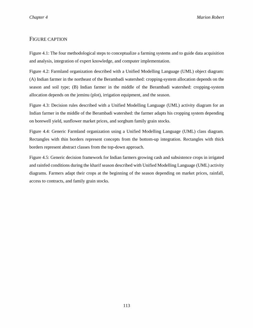
Chapter 4 Marion Robert
113
FIGURE CAPTION
Figure 4.1: The four methodological steps to conceptualize a farming systems and to guide data acquisition
and analysis, integration of expert knowledge, and computer implementation.
Figure 4.2: Farmland organization described with a Unified Modelling Language (UML) object diagram:
(A) Indian farmer in the northeast of the Berambadi watershed: cropping-system allocation depends on the
season and soil type; (B) Indian farmer in the middle of the Berambadi watershed: cropping-system
allocation depends on the jeminu (plot), irrigation equipment, and the season.
Figure 4.3: Decision rules described with a Unified Modelling Language (UML) activity diagram for an
Indian farmer in the middle of the Berambadi watershed: the farmer adapts his cropping system depending
on borewell yield, sunflower market prices, and sorghum family grain stocks.
Figure 4.4: Generic Farmland organization using a Unified Modelling Language (UML) class diagram.
Rectangles with thin borders represent concepts from the bottom-up integration. Rectangles with thick
borders represent abstract classes from the top-down approach.
Figure 4.5: Generic decision framework for Indian farmers growing cash and subsistence crops in irrigated
and rainfed conditions during the kharif season described with Unified Modelling Language (UML) activity
diagrams. Farmers adapt their crops at the beginning of the season depending on market prices, rainfall,
access to contracts, and family grain stocks.
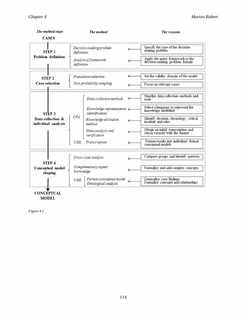
Chapter 4 Marion Robert
114
Figure 4.1
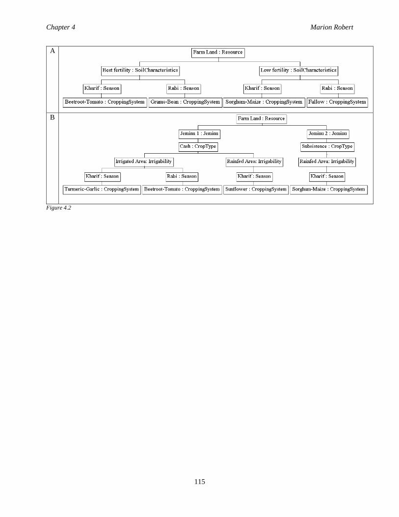
Chapter 4 Marion Robert
115
A
B
Figure 4.2
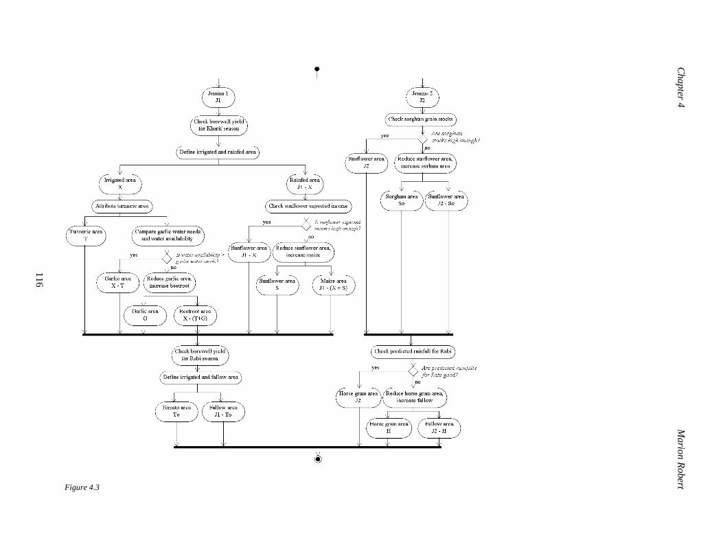
116
Ch
ap
ter 4
Mario
n R
obert
Figure 4.3
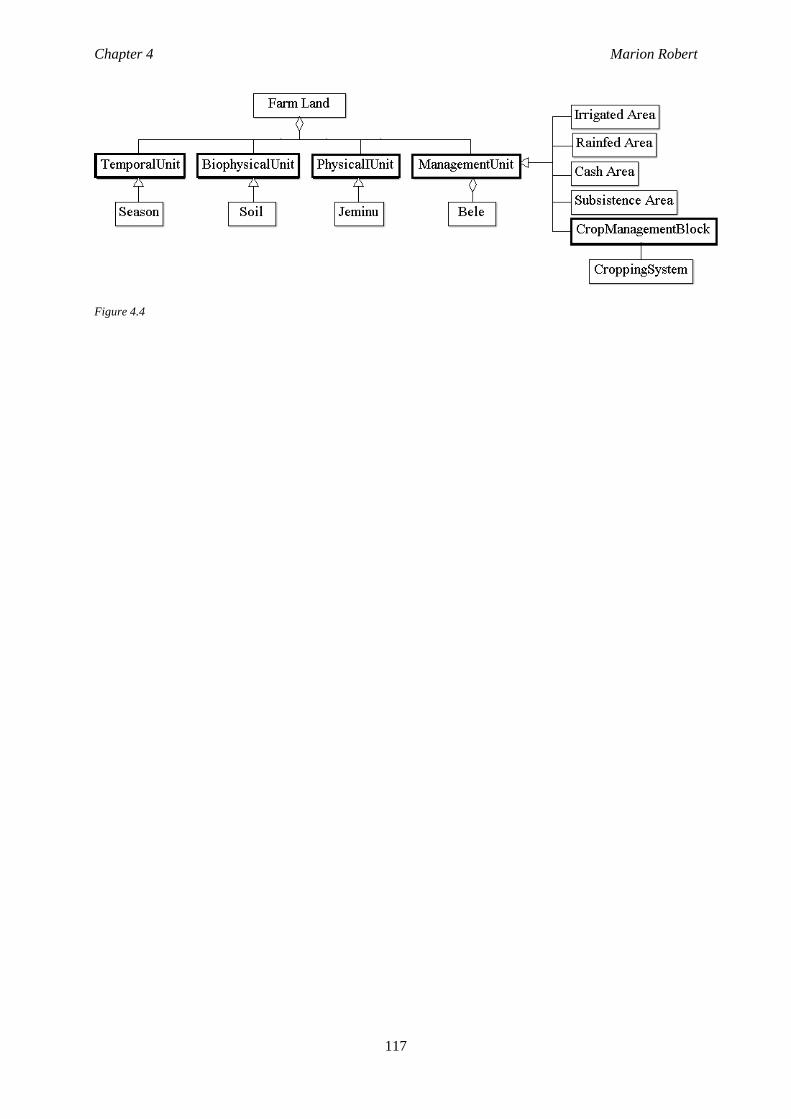
Chapter 4 Marion Robert
117
Ch
ap
ter 4
Mario
n R
obert
Figure 4.4
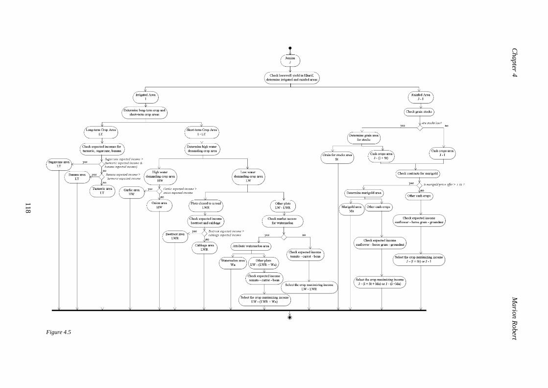
Chapter 4
M
ario
n R
obert
118
Figure 4.5


Chapter 5 Marion Robert
121
Chapter 5
Adaptive and dynamic decision-
making processes: A conceptual model
of production systems on Indian farms
Marion Robert∗1, Alban Thomas2, Muddu Sekhar3,7, Shrinivas Badiger4, Laurent Ruiz5,7, Hélène
Raynal6and Jacques-Eric Bergez1
1AGIR, Université de Toulouse, INPT, INP-PURPAN, INRA, 31320, Castanet-Tolosan, France
2INRA, Toulouse School of Economics, UMR 1081 LERNA, F-31000 Toulouse, France
3Indian Institute of Sciences, Department of Civil Engineering, Bangalore 560012, India
4ATREE, Bangalore 560 064, India
5INRA, UMR 1069 SAS, F-35042 Rennes, France
6INRA, UR 0875 MIAT, F-31326 Castanet-Tolosan, France
7Indo-French Cell of Water Sciences, IRD-IISc, Bangalore, India
∗ Corresponding author: ([email protected])
Published in Agricultural Systems
Scientific paper
Doi: 10.1016/j.agsy.2016.08.001
Quote: Robert, M., Thomas, A., Sekhar, M., Badiger, S., Ruiz, L., Raynal, H., & Bergez, J. E. (2016).
Adaptive and dynamic decision-making processes: A conceptual model of production systems on Indian
farms. Agricultural Systems.
Chapter 5 Marion Robert
122
Farming systems are complex structures with several dimensions interacting in a dynamic and
continuous manner around farmers’ management strategies. This complexity peaks in semi-arid regions
of India, where small farms encounter a highly competitive environment for markets and resources,
especially unreliable access to water from rainfall and irrigation. To represent such strategies, we
propose the conceptual model NAMASTE, which was conceived and based on data collected in the
Berambadi watershed in southern India. The most relevant and novel aspects of NAMASTE are i) the
system-based representation of farm production systems, ii) the description of dynamic processes
through management flexibility and adaptation, and iii) the representation of steps in farmers’ decision-
making processes at various temporal and spatial scales. Since NAMASTE was designed in an extreme
case of highly vulnerable agriculture, its generic framework and formalisms can be used to conceptually
represent many other farm production systems.
Keywords: conceptual model, farmer decision-making process, system-based representation,
adaptation, irrigation.
Chapter 5 Marion Robert
123
5.1. INTRODUCTION
Modeling farming systems and how these systems change and adapt to external changes and
opportunities is particularly interesting for the agricultural research community to better assess their
flexibility and resiliency. A variety of conceptual representations have been developed to represent
decision-making processes with diverse levels of complexity in the system (plot to farm) and the
adaptation process (from days to years). Examples include the “model for actions” at the cropping
system level and mainly for tactical adaptation (Cerf and Sebillotte 1988; Aubry et al. 1998a), rule-
based models (Bergez et al. 2006; Moore et al. 2014; Snow et al. 2014; Holzworth et al. 2015) and
activity-based models (Clouaire and Rellier 2009; Martin et al. 2013).
Farmers’ decision-making processes, planned at three different temporal and spatial scales, are a
combination of decision stages: i) the strategic decision stage, with a long-term effect (years to decades)
on whole-farm organization (e.g., decisions about equipment investment, infrastructure development or
farm expansion); ii) the tactical decision stage, with a medium-term effect (several months or seasons)
on the farm cropping system and its resource management; and iii) the operational decision stage, with
a short-term effect restricted to specific plots and describing daily adjustments to crop management
practices (Risbey et al. 1999; Le Gal et al. 2011). Some models focus on one particular type of decision
– mainly strategic (Barbier and Bergeron 1999; Berge and Ittersum 2000; Hyytiäinen et al. 2011) or
operational (Martin-Clouaire and Rellier 2006; Merot et al. 2008; Martin et al. 2011a; Aurbacher et al.
2013; Moore et al. 2014). Others model two decision levels – strategic and tactical (Trebeck and
Hardaker 1972; Adesina 1991; Mosnier et al. 2009) or strategic and operational (Navarrete and Bail
2007; Dury 2011; Taillandier et al. 2012a; Gaudou and Sibertin-Blanc 2013). However, to the best of
our knowledge, the scientific literature does not offer models that include a decision model with the
three decision stages within the same model. To understand the ability and possibility to adapt farming
systems, it is essential to consider the entire decision-making process. Ignoring one decision stage can
bias evaluation of the impact of changes on a farm production system and miss possible options for
farming system adaptation.
In semi-arid regions, agricultural production systems depend greatly on irrigation and encounter
increasing challenges: growing uncertainty about how to respond to climate change, severe depletion of
natural resources, high volatility in market prices, rise in energy costs, and greater pressure from public
regulations (agricultural, environmental, and health policies). In the Deccan Plateau in India, the
development of submersible pump technology in the 1990s resulted in a dramatic increase in borewell
irrigation (Sekhar et al. 2006; Javeed et al. 2009). However, the low productivity of the aquifer
(Dewandel et al. 2010; Perrin et al. 2011) and a rapid decline in the water table level led to decreasing
borewell yields (Ruiz et al. 2015), which means that groundwater-irrigated agriculture still largely
depends on rainfall. Climate variability has increased over the last 50 years in this region (Jogesh and
Chapter 5 Marion Robert
124
Dubash 2014). Predictions indicate a 1.8-2.2 °C increase in temperature by 2030, and southwestern
regions of Karnataka are projected to suffer from a decrease in annual rainfall, especially during the
monsoon season (Jogesh and Dubash 2014). For a region that largely depends on monsoon patterns and
winter months to maintain agricultural production, any shift in climatic conditions would have a severe
impact on natural resources and the economy. This highly complex and competitive environment
requires farmers to continuously adapt their farming system and management practices (Hardaker 2004),
and it is a place where explicitly considering the three stages of farmer decisions is critical to accurately
represent production systems.
The objective of this article is to introduce the conceptual model NAMASTE (Numerical Assessments
with Models of Agricultural Systems integrating Techniques and Economics) and detail the explicit
integration of the three decision stages: strategic, tactical and operational. A conceptual model is a non-
software description of a computer simulation model. It is the bridge between the real system and a
computer model (Robinson 2008) and therefore requires simplification and abstraction (Robinson
2010). NAMASTE is well suited to agricultural systems in semi-arid regions highly dependent on
irrigation. One original feature of our model is the decision sub-model that covers three stages of
decisions and adaptations. Another original feature is the integrated dynamic interaction of different
sub-systems that build the farm production system. We first present the methodology used to build the
conceptual model. Then, we outline the decision sub-system and its interactions with the biophysical
sub-system and the external system. We discuss the key modeling choices and present several insights
on how to move from the conceptual model to a computer simulation model.
5.2. MODELING PROCESSES
5.2.1. Indian case study
The design of the conceptual model was based on data collected in the Berambadi watershed (11°43'00”
to 11°48'00" N, 76° 31'00" to 76° 40'00" E) in southern India, where biophysical variables have been
intensively monitored since 2009 under the Environmental Research Observatory ORE BVET. Since
2013, the multi-disciplinary Indo-French project CEFIPRA (Centre for the Promotion of Advanced
Research) AICHA (Adaptation of Irrigated Agriculture to Climate Change) has aimed to develop an
integrated model to simulate interactions between agriculture, hydrology and economics and to evaluate
scenarios of the evolution of climate, agricultural systems and water management policies at the
watershed scale. The Berambadi watershed (84 km²) belongs to the Kabini River basin, which is part of
the South Gundal River basin (816 km²) (southwest of Karnataka). Its climate is dominated by a
monsoon regime that generates a strong rainfall gradient with decadal trends, strong inter-annual
variability and recurrent droughts (Ruiz et al. 2015). Three seasons regulate the farm cropping system:
i) kharif (June to September), the rainy season (monsoon), when most of the cropping area is cultivated;
Chapter 5 Marion Robert
125
ii) rabi (October to January), the winter season, when most irrigated plots are cultivated; and iii) summer
(February to May), the hot and dry season, when only few plots are cultivated.
On average, farm size in the Berambadi watershed is 3.6 acres. 47% of the household on the watershed
have water access for irrigation. In kharif, crops mainly grown in rainfed condition are sorghum, maize,
sunflower, marigold, and in irrigated conditions are turmeric, onion, garlic, and banana. 20% of the
cropping area is dedicated to subsistence crops such as sorghum, millet and pulses. In rabi, mainly maize,
horse gram and vegetables are grown in irrigated conditions. In summer almost 90% of the crop land is
fallow land.
The hard rock aquifer is composed of fissured granite underlain by a 5-20 m layer of weathered material.
Hydraulic conductivity and borewell yields decrease with water table depth. As a consequence,
continuous pumping leads to groundwater table drawback and reduces the availability of groundwater
for irrigation. This feedback makes predefined land-use scenarios unrealistic, since farmers need to
adapt their actions continually according to groundwater availability. In addition, water table levels
display a non-standard pattern, hydrogeologically speaking; valley regions have deeper groundwater
levels than topographically higher zones (Figure 5.2). This pattern results from intensive groundwater
pumping since the early 1990s in villages located in the valley (Sekhar et al. 2011) that disconnected
groundwater from streams, which now run dry most of the year. Low costs of pumping water and
subsidies for irrigation equipment encouraged farmers to drill even more borewells. This dramatic
evolution is closely linked to the spatial distribution of soil type and groundwater availability, as well
as farming practices, access to the market, knowledge, new technologies and government aid (Sekhar et
al. 2011). An increasing number of farmers report well failures and give two reasons for this: either
wells have run dry after excessive pumping, or no water was found in newly drilled borewells (González
Botero and Bertran Salinas 2013).
The NAMASTE model aims at simulating farmers’ adaptation to climate change, water table depletion,
economic context and agrarian changes such as government subsidies. Its hierarchical structure is
described in Figure 5.1.
5.2.2. Modeling steps
To build the conceptual model we followed a three-step method:
Step 1: We identified events, concepts and knowledge that are relevant to the conceptual model.
Knowledge acquisition helps to understand and describe the real system. We surveyed farmers
in the watershed in 2014 and 2015. The first survey targeted 27 farmers to obtain detailed data
about their practices, in particular their decisions and the process of adapting their decisions.
The second survey targeted 680 farmers and obtained broad data about farm characteristics and
social, economic and agronomic environment. This survey led to a typology of farmers on the
Chapter 5 Marion Robert
126
watershed based on biophysical factors (e.g. farm location, soil type, ground water
accessibility), on economic factors (e.g. farm size, labor, equipment), on social factors (e.g.
castes, family structure, education, off-farm job) (details are found in Robert et al. (in Prep.)).
We surveyed seed retailers and Panchayats (village leaders) to learn about recommended crop
management practices and village organization. Additionally, 52 experimental plots were
monitored over three years, which provided observed quantitative data about crop production
and crop management. These data helped supplement the verbal information provided by
farmers during surveys. Meteorological data were obtained from a meteorological station and
water gauges installed on the watershed. Prices and costs were obtained from farmers and from
official district data from the Indian Ministry of Agriculture and Cooperation (Directorate of
Economics and Statistics) and the National Informatics Center (Agricultural Census Division).
Step 2: We used the case study CMFDM method (standing for Conceptual Modeling of the Farmer agent
underlying Decision-Making processes) (Robert et al. 2016a) to identify system components
and the interactions between them that structure and organize farming processes in a coherent
systemic representation. CMFDM underpins the development of a conceptual model by
combining both a bottom-up from empirical data by observing actual practices in a natural
setting and a top-down from experts and modelers. It uses multiple data collection which makes
possible the triangulation between collected data providing stronger evidences of theory
constructs and hypothesis. Case study method provides a deep understanding of the complex
processes used in decision-making processes. Two main systems were identified: i) a farming
system, which is complex and composed of interacting or interdependent sub-systems (mainly,
decision and biophysical sub-systems), themselves made up of interacting and interdependent
entities; and ii) an external system, which is a set of independent entities that describe uncertain
and uncontrolled events that influence the production process.
Step 3: We selected the formalisms and frameworks to simulate the target processes. To facilitate the
design and coding of the computer model that follows the conceptual model, selected
formalisms and frameworks were implemented in the French National Institute of Agronomy
(INRA) RECORD (Renovation and COORDination of agro-ecosystem modeling) modeling and
simulation software platform within a multidisciplinary approach (e.g. agronomy, soil science,
bioclimatology, epidemiology, management science, statistics, applied mathematics and
computer science) (Bergez et al. 2013).
The first framework described the systemic representation of the farm production system (Figure
5.3). The production system is divided into three interactive sub-systems: i) the decision sub-
system (manager or agent), which describes the farmer’s decision process as a combination of
knowledge about the system, objectives, and decisions; ii) the operating sub-system (technical
system), which translates the decision orders into action execution and dynamics of farm
Chapter 5 Marion Robert
127
resources; and, iii) the biophysical sub-system, which describes interactions between physical
and biological elements, in particular the relations between ground water, soil, and plant growth
and development (Clouaire and Rellier 2009; Le Gal et al. 2010; Dury 2011; Akplogan 2013).
The farming system interacts with an external system that simulates pressure and conditions in
the farming environment such as rainfall (WEATHER) and market prices (MARKET), and
specifically in an Indian context, such as electricity service (ELECTRICITY) and the village
source of labor and equipment (VILLAGE).
The second framework aimed to organize the decision sub-system (Figure 5.3). We considered
farmers as cognitive agents able to think, memorize, analyze, predict and learn to face future
events and plan their actions (Le Bars et al. 2005). In artificial intelligence and cognitive
sciences, cognitive agents are commonly represented as Belief-Desire-Intention (BDI) agents
(Bratman 1987a; Rao and Georgeff 1991). “Belief” represents the agent’s knowledge of the
system. We considered that farmers have three types of knowledge (Beliefs). The first two are
structural knowledge, concerning farm structure, its organization and its characteristic resources
(e.g., land, labor, equipment, and water), and procedural knowledge, concerning farmers’ know-
how about farming. With experience, farmers have a basis for deciding and planning their
actions. In our approach, procedural knowledge corresponds to the plan library of Georgeff’s
Procedural Reasoning System (Rao and Georgeff 1991). The third type is observed knowledge,
describing the data that farmers obtain by observing and monitoring changes in the farming
environment (e.g., field observations, market monitoring, weather predictions, opportunities to
hire labor and rent equipment). “Desires” represents the farmer’s objectives or satisfying goals.
The 27 interviewed Indian farmers of the first survey asserted they manage their farms to
maximize profits and improve their financial situation by selling cash crops. Optimizing crop
production can encourage farmers to improve or invest in irrigation systems. They face a
delicate tradeoff among investing in a borewell, adopting new technologies to increase income
with a more productive cropping system, accumulating debts, and risking system failures.
“Intentions” represents the farmer’s plans for actions to achieve objectives (Desires) by knowing
the status of the system (Beliefs). “Intentions” are the decisions farmers must make at strategic,
tactical and operational stages.
5.2.3. Conceptual validation
Conceptual validation is essential to ensure that the assumptions, theories and simplifications used to
build the conceptual model are sufficiently accurate and relevant to to meet the stakeholders’
requirements and the objectives of the study (Costal et al. 1996; Borenstein 1998; Liu et al. 2011). To
validate the conceptual model, we used: i) face validation that consists in asking experts and individuals
knowledgeable about the study objectives to evaluate the conceptual model and determine whether it is
Chapter 5 Marion Robert
128
correct and reasonable for the study purpose; and ii) traces techniques that consists in tracking of entities
through each sub-model and the overall model to determine whether the model’s logic and the necessary
accuracy maintained (Robinson 2010; Sargent 2010; Robinson 2014). Conceptual validation is
inherently an informal process referring to subjective and human judgement.
Each sub-model and the overall model must be evaluated to determine if they are reasonable and correct.
First, we applied White-Box validation to the sub-models to determine whether each constituent part of
the conceptual model represents the real world with sufficient accuracy to meet the study objectives
(Robinson 2014). Each sub-system was validated by experts in the associated research field. Experts
and modelers were essential for building the decision sub-model. Modelers ensure that decision
processes are appropriately designed into the chosen framework and formalisms. Indian agronomic
researchers validated the decision rules for crop management and adaption. We also asked Indian
researchers from the research project to participate to the validation of each sub-model as main
stakeholders on the project and to certify the representation and data used to build the external system.
Second, we applied Black-Box validation to the overall model to determine whether the model provide
a sufficiently accurate representation of the real world for the intended purpose of the study (Robinson
2014). The entire system was validated by experts on the different sub-systems, modelers and the Indian
researchers. They worked on the consistency between inputs and outputs of each sub-system to ensure
rational interactions between systems. Specifications of each sub-model were circulated among those
who have a detailed knowledge of the system. They shared feedbacks on whether the model was
appropriate by determining if the appropriate detail and aggregate relationships were used for the
model’s intended purpose.
Finally, information-technology engineers from the RECORD platform verified the feasibility of the
model for future computer implementation. Once the conceptual model will be implemented under the
modeling and simulation RECORD platform, the validation of the conceptual model will also be
expanded with model simulation validation technique.
5.3. A CONCEPTUAL MODEL OF PRODUCTION SYSTEMS ON INDIAN FARMS
5.3.1. What should be modeled
Three major decisions to represent
We identified three major technical decisions that need to be represented in the model.
Type 1: Investing in access to irrigation is essential to expect increase farm irrigation capacity and
improve farm productivity. However, it is expensive, and farmers must consider if it is worth
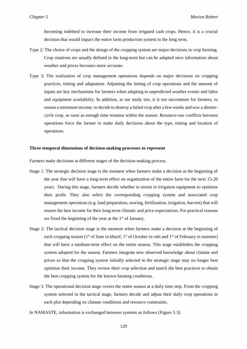
Chapter 5 Marion Robert
129
becoming indebted to increase their income from irrigated cash crops. Hence, it is a crucial
decision that would impact the entire farm production system in the long term.
Type 2: The choice of crops and the design of the cropping system are major decisions in crop farming.
Crop rotations are usually defined in the long-term but can be adapted once information about
weather and prices becomes more accurate.
Type 3: The realization of crop management operations depends on major decisions on cropping
practices, timing and adaptation. Adjusting the timing of crop operations and the amount of
inputs are key mechanisms for farmers when adapting to unpredicted weather events and labor
and equipment availability. In addition, at our study site, it is not uncommon for farmers, to
ensure a minimum income, to decide to destroy a failed crop after a few weeks and sow a shorter-
cycle crop, as soon as enough time remains within the season. Resource-use conflicts between
operations force the farmer to make daily decisions about the type, timing and location of
operations.
Three temporal dimensions of decision-making processes to represent
Farmers make decisions at different stages of the decision-making process.
Stage 1: The strategic decision stage is the moment when farmers make a decision at the beginning of
the year that will have a long-term effect on organization of the entire farm for the next 15-20
years. During this stage, farmers decide whether to invest in irrigation equipment to optimize
their profit. They also select the corresponding cropping system and associated crop
management operations (e.g. land preparation, sowing, fertilization, irrigation, harvest) that will
ensure the best income for their long-term climatic and price expectations. For practical reasons
we fixed the beginning of the year at the 1st of January.
Stage 2: The tactical decision stage is the moment when farmers make a decision at the beginning of
each cropping season (1st of June in kharif, 1st of October in rabi and 1st of February in summer)
that will have a medium-term effect on the entire season. This stage establishes the cropping
system adopted for the season. Farmers integrate new observed knowledge about climate and
prices so that the cropping system initially selected in the strategic stage may no longer best
optimize their income. They review their crop selection and match the best practices to obtain
the best cropping system for the known farming conditions.
Stage 3: The operational decision stage covers the entire season at a daily time step. From the cropping
system selected in the tactical stage, farmers decide and adjust their daily crop operations in
each plot depending on climate conditions and resource constraints.
In NAMASTE, information is exchanged between systems as follows (Figure 5.3):
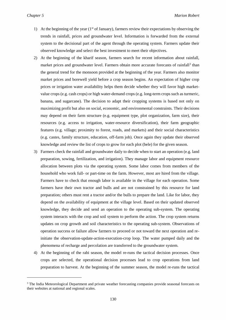
Chapter 5 Marion Robert
130
1) At the beginning of the year (1st of January), farmers review their expectations by observing the
trends in rainfall, prices and groundwater level. Information is forwarded from the external
system to the decisional part of the agent through the operating system. Farmers update their
observed knowledge and select the best investment to meet their objectives.
2) At the beginning of the kharif season, farmers search for recent information about rainfall,
market prices and groundwater level. Farmers obtain more accurate forecasts of rainfall3 than
the general trend for the monsoon provided at the beginning of the year. Farmers also monitor
market prices and borewell yield before a crop season begins. An expectation of higher crop
prices or irrigation water availability helps them decide whether they will favor high market-
value crops (e.g. cash crops) or high water-demand crops (e.g. long-term crops such as turmeric,
banana, and sugarcane). The decision to adapt their cropping systems is based not only on
maximizing profit but also on social, economic, and environmental constraints. Their decisions
may depend on their farm structure (e.g. equipment type, plot organization, farm size), their
resources (e.g. access to irrigation, water-resource diversification), their farm geographic
features (e.g. village; proximity to forest, roads, and markets) and their social characteristics
(e.g. castes, family structure, education, off-farm job). Once again they update their observed
knowledge and review the list of crops to grow for each plot (bele) for the given season.
3) Farmers check the rainfall and groundwater daily to decide when to start an operation (e.g. land
preparation, sowing, fertilization, and irrigation). They manage labor and equipment resource
allocation between plots via the operating system. Some labor comes from members of the
household who work full- or part-time on the farm. However, most are hired from the village.
Farmers have to check that enough labor is available in the village for each operation. Some
farmers have their own tractor and bulls and are not constrained by this resource for land
preparation; others must rent a tractor and/or the bulls to prepare the land. Like for labor, they
depend on the availability of equipment at the village level. Based on their updated observed
knowledge, they decide and send an operation to the operating sub-system. The operating
system interacts with the crop and soil system to perform the action. The crop system returns
updates on crop growth and soil characteristics to the operating sub-system. Observations of
operation success or failure allow farmers to proceed or not toward the next operation and re-
initiate the observation-update-action-execution-crop loop. The water pumped daily and the
phenomena of recharge and percolation are transferred to the groundwater system.
4) At the beginning of the rabi season, the model re-runs the tactical decision processes. Once
crops are selected, the operational decision processes lead to crop operations from land
preparation to harvest. At the beginning of the summer season, the model re-runs the tactical
3 The India Meteorological Department and private weather forecasting companies provide seasonal forecasts on
their websites at national and regional scales.
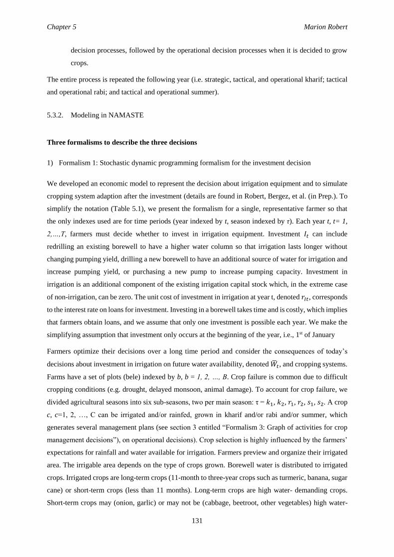
Chapter 5 Marion Robert
131
decision processes, followed by the operational decision processes when it is decided to grow
crops.
The entire process is repeated the following year (i.e. strategic, tactical, and operational kharif; tactical
and operational rabi; and tactical and operational summer).
5.3.2. Modeling in NAMASTE
Three formalisms to describe the three decisions
1) Formalism 1: Stochastic dynamic programming formalism for the investment decision
We developed an economic model to represent the decision about irrigation equipment and to simulate
cropping system adaption after the investment (details are found in Robert, Bergez, et al. (in Prep.). To
simplify the notation (Table 5.1), we present the formalism for a single, representative farmer so that
the only indexes used are for time periods (year indexed by t, season indexed by τ). Each year t, t= 1,
2,…,T, farmers must decide whether to invest in irrigation equipment. Investment 𝐼𝑡 can include
redrilling an existing borewell to have a higher water column so that irrigation lasts longer without
changing pumping yield, drilling a new borewell to have an additional source of water for irrigation and
increase pumping yield, or purchasing a new pump to increase pumping capacity. Investment in
irrigation is an additional component of the existing irrigation capital stock which, in the extreme case
of non-irrigation, can be zero. The unit cost of investment in irrigation at year t, denoted 𝑟𝐼𝑡, corresponds
to the interest rate on loans for investment. Investing in a borewell takes time and is costly, which implies
that farmers obtain loans, and we assume that only one investment is possible each year. We make the
simplifying assumption that investment only occurs at the beginning of the year, i.e., 1st of January
Farmers optimize their decisions over a long time period and consider the consequences of today’s
decisions about investment in irrigation on future water availability, denoted ��𝑡, and cropping systems.
Farms have a set of plots (bele) indexed by b, b = 1, 2, …, B. Crop failure is common due to difficult
cropping conditions (e.g. drought, delayed monsoon, animal damage). To account for crop failure, we
divided agricultural seasons into six sub-seasons, two per main season: τ = 𝑘1, 𝑘2, 𝑟1, 𝑟2, 𝑠1, 𝑠2. A crop
c, c=1, 2, …, C can be irrigated and/or rainfed, grown in kharif and/or rabi and/or summer, which
generates several management plans (see section 3 entitled “Formalism 3: Graph of activities for crop
management decisions”), on operational decisions). Crop selection is highly influenced by the farmers’
expectations for rainfall and water available for irrigation. Farmers preview and organize their irrigated
area. The irrigable area depends on the type of crops grown. Borewell water is distributed to irrigated
crops. Irrigated crops are long-term crops (11-month to three-year crops such as turmeric, banana, sugar
cane) or short-term crops (less than 11 months). Long-term crops are high water- demanding crops.
Short-term crops may (onion, garlic) or may not be (cabbage, beetroot, other vegetables) high water-
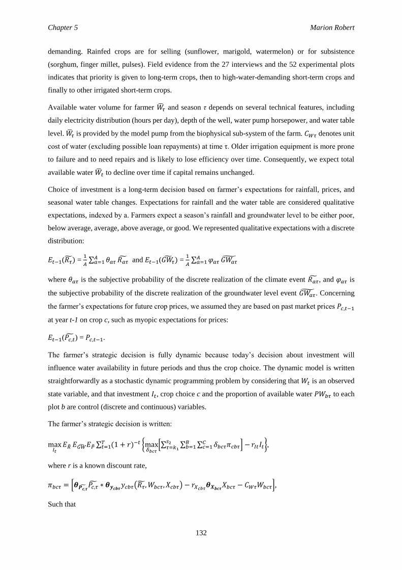
Chapter 5 Marion Robert
132
demanding. Rainfed crops are for selling (sunflower, marigold, watermelon) or for subsistence
(sorghum, finger millet, pulses). Field evidence from the 27 interviews and the 52 experimental plots
indicates that priority is given to long-term crops, then to high-water-demanding short-term crops and
finally to other irrigated short-term crops.
Available water volume for farmer ��𝜏 and season τ depends on several technical features, including
daily electricity distribution (hours per day), depth of the well, water pump horsepower, and water table
level. ��𝜏 is provided by the model pump from the biophysical sub-system of the farm. 𝐶𝑊𝜏 denotes unit
cost of water (excluding possible loan repayments) at time τ. Older irrigation equipment is more prone
to failure and to need repairs and is likely to lose efficiency over time. Consequently, we expect total
available water ��𝑡 to decline over time if capital remains unchanged.
Choice of investment is a long-term decision based on farmer’s expectations for rainfall, prices, and
seasonal water table changes. Expectations for rainfall and the water table are considered qualitative
expectations, indexed by a. Farmers expect a season’s rainfall and groundwater level to be either poor,
below average, average, above average, or good. We represented qualitative expectations with a discrete
distribution:
𝐸𝑡−1(𝑅��) = 1
𝐴 ∑ 𝜃𝑎𝜏
𝐴𝑎=1 𝑅𝑎�� and 𝐸𝑡−1(𝐺𝑊𝜏
) = 1
𝐴 ∑ 𝜑𝑎𝜏
𝐴𝑎=1 𝐺𝑊𝑎��
where 𝜃𝑎𝜏 is the subjective probability of the discrete realization of the climate event 𝑅𝑎��, and 𝜑𝑎𝜏 is
the subjective probability of the discrete realization of the groundwater level event 𝐺𝑊𝑎��. Concerning
the farmer’s expectations for future crop prices, we assumed they are based on past market prices 𝑃𝑐,𝑡−1
at year t-1 on crop c, such as myopic expectations for prices:
𝐸𝑡−1(𝑃𝑐,��) = 𝑃𝑐,𝑡−1.
The farmer’s strategic decision is fully dynamic because today’s decision about investment will
influence water availability in future periods and thus the crop choice. The dynamic model is written
straightforwardly as a stochastic dynamic programming problem by considering that 𝑊𝑡 is an observed
state variable, and that investment 𝐼𝑡, crop choice c and the proportion of available water 𝑃𝑊𝑏𝜏 to each
plot b are control (discrete and continuous) variables.
The farmer’s strategic decision is written:
max𝐼𝑡
𝐸�� 𝐸𝐺��𝐸�� ∑ (1 + 𝑟)−𝑡𝑇𝑡=1 {max
𝛿𝑏𝑐𝜏
[∑ ∑ ∑ 𝛿𝑏𝑐𝜏𝜋𝑐𝑏𝜏𝐶𝑐=1
𝐵𝑏=1
𝑠2𝜏=𝑘1
] − 𝑟𝐼𝑡𝐼𝑡},
where r is a known discount rate,
𝜋𝑏𝑐𝜏 = [𝜽𝑷𝒄,��𝑃𝑐,�� ∗ 𝜽𝒚𝒄𝒃𝝉
𝑦𝑐𝑏𝜏(𝑅��, 𝑊𝑏𝑐𝜏, 𝑋𝑐𝑏𝜏) − 𝑟𝑋𝑐𝑏𝜏𝜽𝑿𝒃𝒄𝝉
𝑋𝑏𝑐𝜏 − 𝐶𝑊𝜏𝑊𝑏𝑐𝜏],
Such that
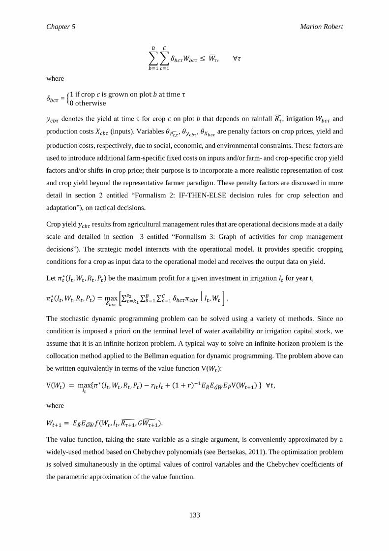
Chapter 5 Marion Robert
133
∑ ∑ 𝛿𝑏𝑐𝜏𝑊𝑏𝑐𝜏
𝐶
𝑐=1
𝐵
𝑏=1
≤ ��𝜏 , ∀𝜏
where
𝛿𝑏𝑐𝜏 = {1 if crop 𝑐 is grown on plot 𝑏 at time τ0 otherwise
𝑦𝑐𝑏𝜏 denotes the yield at time τ for crop c on plot b that depends on rainfall 𝑅��, irrigation 𝑊𝑏𝑐𝜏 and
production costs 𝑋𝑐𝑏𝜏 (inputs). Variables 𝜃𝑃𝑐,��, 𝜃𝑦𝑐𝑏𝜏
, 𝜃𝑋𝑏𝑐𝜏 are penalty factors on crop prices, yield and
production costs, respectively, due to social, economic, and environmental constraints. These factors are
used to introduce additional farm-specific fixed costs on inputs and/or farm- and crop-specific crop yield
factors and/or shifts in crop price; their purpose is to incorporate a more realistic representation of cost
and crop yield beyond the representative farmer paradigm. These penalty factors are discussed in more
detail in section 2 entitled “Formalism 2: IF-THEN-ELSE decision rules for crop selection and
adaptation”), on tactical decisions.
Crop yield 𝑦𝑐𝑏𝜏 results from agricultural management rules that are operational decisions made at a daily
scale and detailed in section 3 entitled “Formalism 3: Graph of activities for crop management
decisions”). The strategic model interacts with the operational model. It provides specific cropping
conditions for a crop as input data to the operational model and receives the output data on yield.
Let 𝜋𝑡∗(𝐼𝑡, 𝑊𝑡 , 𝑅𝑡 , 𝑃𝑡) be the maximum profit for a given investment in irrigation 𝐼𝑡 for year t,
𝜋𝑡∗(𝐼𝑡, 𝑊𝑡 , 𝑅𝑡 , 𝑃𝑡) = max
𝛿𝑏𝑐𝜏
[∑ ∑ ∑ 𝛿𝑏𝑐𝜏𝜋𝑐𝑏𝜏 𝐼𝑡, 𝑊𝑡 𝐶𝑐=1
𝐵𝑏=1
𝑠2𝜏=𝑘1
] .
The stochastic dynamic programming problem can be solved using a variety of methods. Since no
condition is imposed a priori on the terminal level of water availability or irrigation capital stock, we
assume that it is an infinite horizon problem. A typical way to solve an infinite-horizon problem is the
collocation method applied to the Bellman equation for dynamic programming. The problem above can
be written equivalently in terms of the value function V(𝑊𝑡):
V(𝑊𝑡) = max𝐼𝑡
{𝜋∗(𝐼𝑡, 𝑊𝑡 , 𝑅𝑡, 𝑃𝑡) − 𝑟𝐼𝑡𝐼𝑡 + (1 + 𝑟)−1𝐸��𝐸𝐺��𝐸��V(𝑊𝑡+1) } ∀𝑡,
where
𝑊𝑡+1 = 𝐸��𝐸𝐺��𝑓(𝑊𝑡 , 𝐼𝑡, 𝑅𝜏+1, 𝐺𝑊𝜏+1) .
The value function, taking the state variable as a single argument, is conveniently approximated by a
widely-used method based on Chebychev polynomials (see Bertsekas, 2011). The optimization problem
is solved simultaneously in the optimal values of control variables and the Chebychev coefficients of
the parametric approximation of the value function.
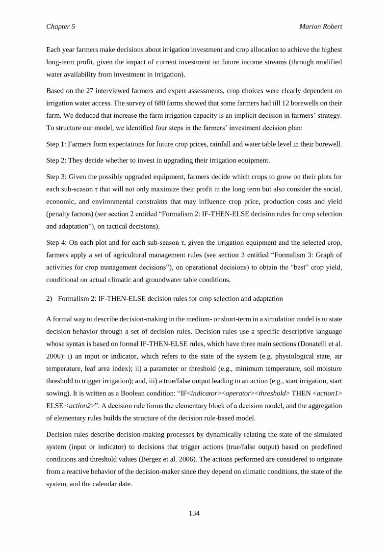
Chapter 5 Marion Robert
134
Each year farmers make decisions about irrigation investment and crop allocation to achieve the highest
long-term profit, given the impact of current investment on future income streams (through modified
water availability from investment in irrigation).
Based on the 27 interviewed farmers and expert assessments, crop choices were clearly dependent on
irrigation water access. The survey of 680 farms showed that some farmers had till 12 borewells on their
farm. We deduced that increase the farm irrigation capacity is an implicit decision in farmers’ strategy.
To structure our model, we identified four steps in the farmers’ investment decision plan:
Step 1: Farmers form expectations for future crop prices, rainfall and water table level in their borewell.
Step 2: They decide whether to invest in upgrading their irrigation equipment.
Step 3: Given the possibly upgraded equipment, farmers decide which crops to grow on their plots for
each sub-season τ that will not only maximize their profit in the long term but also consider the social,
economic, and environmental constraints that may influence crop price, production costs and yield
(penalty factors) (see section 2 entitled “Formalism 2: IF-THEN-ELSE decision rules for crop selection
and adaptation”), on tactical decisions).
Step 4: On each plot and for each sub-season τ, given the irrigation equipment and the selected crop,
farmers apply a set of agricultural management rules (see section 3 entitled “Formalism 3: Graph of
activities for crop management decisions”), on operational decisions) to obtain the “best” crop yield,
conditional on actual climatic and groundwater table conditions.
2) Formalism 2: IF-THEN-ELSE decision rules for crop selection and adaptation
A formal way to describe decision-making in the medium- or short-term in a simulation model is to state
decision behavior through a set of decision rules. Decision rules use a specific descriptive language
whose syntax is based on formal IF-THEN-ELSE rules, which have three main sections (Donatelli et al.
2006): i) an input or indicator, which refers to the state of the system (e.g. physiological state, air
temperature, leaf area index); ii) a parameter or threshold (e.g., minimum temperature, soil moisture
threshold to trigger irrigation); and, iii) a true/false output leading to an action (e.g., start irrigation, start
sowing). It is written as a Boolean condition: “IF<indicator><operator><threshold> THEN <action1>
ELSE <action2>”. A decision rule forms the elementary block of a decision model, and the aggregation
of elementary rules builds the structure of the decision rule-based model.
Decision rules describe decision-making processes by dynamically relating the state of the simulated
system (input or indicator) to decisions that trigger actions (true/false output) based on predefined
conditions and threshold values (Bergez et al. 2006). The actions performed are considered to originate
from a reactive behavior of the decision-maker since they depend on climatic conditions, the state of the
system, and the calendar date.
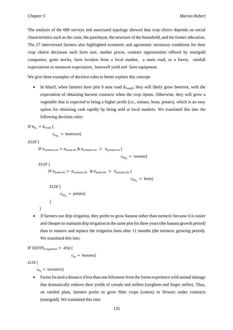
Chapter 5 Marion Robert
135
The analysis of the 680 surveys and associated typology showed that crop choice depends on social
characteristics such as the caste, the panchayat, the structure of the household, and the farmer education.
The 27 interviewed farmers also highlighted economic and agronomic necessary conditions for their
crop choice decisions such farm size, market prices, contract opportunities offered by marigold
companies, grain stocks, farm location from a local market, a main road, or a forest, rainfall
expectations or monsoon expectation, borewell yield and farm equipment.
We give three examples of decision rules to better explain this concept:
In kharif, when farmers have plot b near road 𝑏𝑟𝑜𝑎𝑑, they will likely grow beetroot, with the
expectation of obtaining harvest contracts when the crop ripens. Otherwise, they will grow a
vegetable that is expected to bring a higher profit (i.e., tomato, bean, potato), which is an easy
option for obtaining cash rapidly by being sold at local markets. We translated this into the
following decision rules:
IF 𝑏𝐾1= 𝑏𝑟𝑜𝑎𝑑 {
𝑐𝑏𝐾1= beetroot}
𝐸𝐿𝑆𝐸 {
IF 𝜋𝑡𝑜𝑚𝑎𝑡𝑜 𝑏𝜏 > 𝜋𝑏𝑒𝑎𝑛 𝑏𝜏 & 𝜋𝑡𝑜𝑚𝑎𝑡𝑜 𝑏𝜏 > 𝜋𝑝𝑜𝑡𝑎𝑡𝑜 𝑏𝜏 {
𝑐𝑏𝐾1= tomato}
𝐸𝐿𝑆𝐸 {
IF 𝜋𝑏𝑒𝑎𝑛 𝑏𝜏 > 𝜋𝑡𝑜𝑚𝑎𝑡𝑜 𝑏𝜏 & 𝜋𝑏𝑒𝑎𝑛 𝑏𝜏 > 𝜋𝑝𝑜𝑡𝑎𝑡𝑜 𝑏𝜏 {
𝑐𝑏𝐾1= bean}
𝐸𝐿𝑆𝐸 {
𝑐𝑏𝐾1= potato}
}
}
If farmers use drip irrigation, they prefer to grow banana rather than turmeric because it is easier
and cheaper to maintain drip irrigation in the same plot for three years (the banana growth period)
than to remove and replace the irrigation lines after 11 months (the turmeric growing period).
We translated this into:
IF 𝐸𝑄𝑈𝐼𝑃𝑖𝑟𝑟𝑖𝑔𝑎𝑡𝑖𝑜𝑛 = drip {
𝑐𝑏𝜏= banana}
𝐸𝐿𝑆𝐸 {
𝑐𝑏𝜏= turmeric}
Farms located a distance d less than one kilometer from the forest experience wild animal damage
that dramatically reduces their yields of cereals and millets (sorghum and finger millet). Thus,
on rainfed plots, farmers prefer to grow fiber crops (cotton) or flowers under contracts
(marigold). We translated this into:
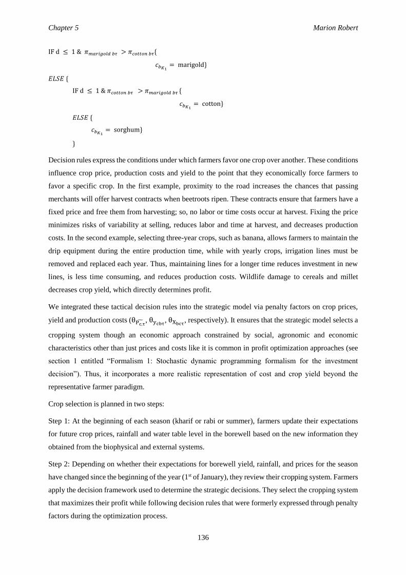
Chapter 5 Marion Robert
136
IF d ≤ 1 & 𝜋𝑚𝑎𝑟𝑖𝑔𝑜𝑙𝑑 𝑏𝜏 > 𝜋𝑐𝑜𝑡𝑡𝑜𝑛 𝑏𝜏{
𝑐𝑏𝐾1= marigold}
𝐸𝐿𝑆𝐸 {
IF d ≤ 1 & 𝜋𝑐𝑜𝑡𝑡𝑜𝑛 𝑏𝜏 > 𝜋𝑚𝑎𝑟𝑖𝑔𝑜𝑙𝑑 𝑏𝜏 {
𝑐𝑏𝐾1= cotton}
𝐸𝐿𝑆𝐸 {
𝑐𝑏𝐾1= sorghum}
}
Decision rules express the conditions under which farmers favor one crop over another. These conditions
influence crop price, production costs and yield to the point that they economically force farmers to
favor a specific crop. In the first example, proximity to the road increases the chances that passing
merchants will offer harvest contracts when beetroots ripen. These contracts ensure that farmers have a
fixed price and free them from harvesting; so, no labor or time costs occur at harvest. Fixing the price
minimizes risks of variability at selling, reduces labor and time at harvest, and decreases production
costs. In the second example, selecting three-year crops, such as banana, allows farmers to maintain the
drip equipment during the entire production time, while with yearly crops, irrigation lines must be
removed and replaced each year. Thus, maintaining lines for a longer time reduces investment in new
lines, is less time consuming, and reduces production costs. Wildlife damage to cereals and millet
decreases crop yield, which directly determines profit.
We integrated these tactical decision rules into the strategic model via penalty factors on crop prices,
yield and production costs (θPc,τ, θycbτ
, θXbcτ, respectively). It ensures that the strategic model selects a
cropping system though an economic approach constrained by social, agronomic and economic
characteristics other than just prices and costs like it is common in profit optimization approaches (see
section 1 entitled “Formalism 1: Stochastic dynamic programming formalism for the investment
decision”). Thus, it incorporates a more realistic representation of cost and crop yield beyond the
representative farmer paradigm.
Crop selection is planned in two steps:
Step 1: At the beginning of each season (kharif or rabi or summer), farmers update their expectations
for future crop prices, rainfall and water table level in the borewell based on the new information they
obtained from the biophysical and external systems.
Step 2: Depending on whether their expectations for borewell yield, rainfall, and prices for the season
have changed since the beginning of the year (1st of January), they review their cropping system. Farmers
apply the decision framework used to determine the strategic decisions. They select the cropping system
that maximizes their profit while following decision rules that were formerly expressed through penalty
factors during the optimization process.
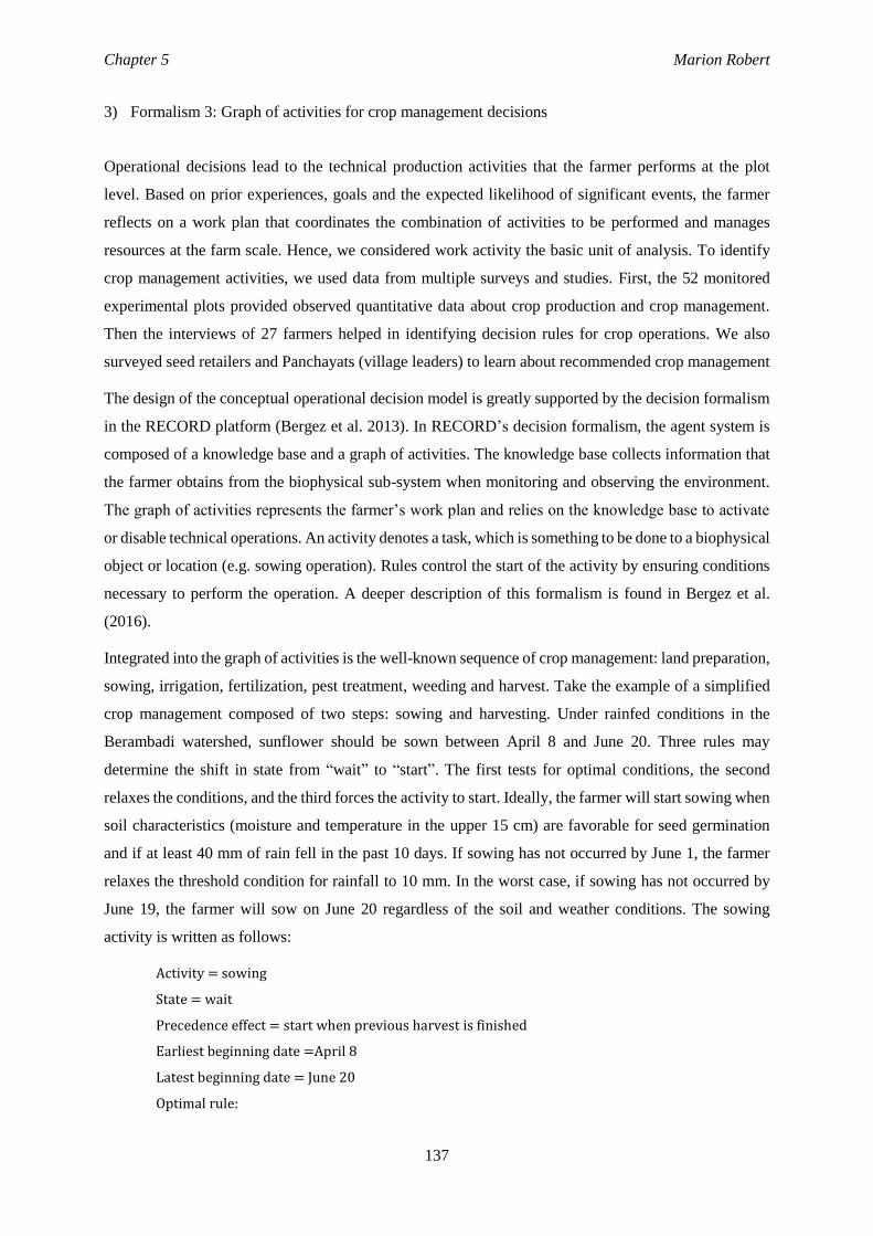
Chapter 5 Marion Robert
137
3) Formalism 3: Graph of activities for crop management decisions
Operational decisions lead to the technical production activities that the farmer performs at the plot
level. Based on prior experiences, goals and the expected likelihood of significant events, the farmer
reflects on a work plan that coordinates the combination of activities to be performed and manages
resources at the farm scale. Hence, we considered work activity the basic unit of analysis. To identify
crop management activities, we used data from multiple surveys and studies. First, the 52 monitored
experimental plots provided observed quantitative data about crop production and crop management.
Then the interviews of 27 farmers helped in identifying decision rules for crop operations. We also
surveyed seed retailers and Panchayats (village leaders) to learn about recommended crop management
The design of the conceptual operational decision model is greatly supported by the decision formalism
in the RECORD platform (Bergez et al. 2013). In RECORD’s decision formalism, the agent system is
composed of a knowledge base and a graph of activities. The knowledge base collects information that
the farmer obtains from the biophysical sub-system when monitoring and observing the environment.
The graph of activities represents the farmer’s work plan and relies on the knowledge base to activate
or disable technical operations. An activity denotes a task, which is something to be done to a biophysical
object or location (e.g. sowing operation). Rules control the start of the activity by ensuring conditions
necessary to perform the operation. A deeper description of this formalism is found in Bergez et al.
(2016).
Integrated into the graph of activities is the well-known sequence of crop management: land preparation,
sowing, irrigation, fertilization, pest treatment, weeding and harvest. Take the example of a simplified
crop management composed of two steps: sowing and harvesting. Under rainfed conditions in the
Berambadi watershed, sunflower should be sown between April 8 and June 20. Three rules may
determine the shift in state from “wait” to “start”. The first tests for optimal conditions, the second
relaxes the conditions, and the third forces the activity to start. Ideally, the farmer will start sowing when
soil characteristics (moisture and temperature in the upper 15 cm) are favorable for seed germination
and if at least 40 mm of rain fell in the past 10 days. If sowing has not occurred by June 1, the farmer
relaxes the threshold condition for rainfall to 10 mm. In the worst case, if sowing has not occurred by
June 19, the farmer will sow on June 20 regardless of the soil and weather conditions. The sowing
activity is written as follows:
Activity = sowing
State = wait
Precedence effect = start when previous harvest is finished
Earliest beginning date =April 8
Latest beginning date = June 20
Optimal rule:
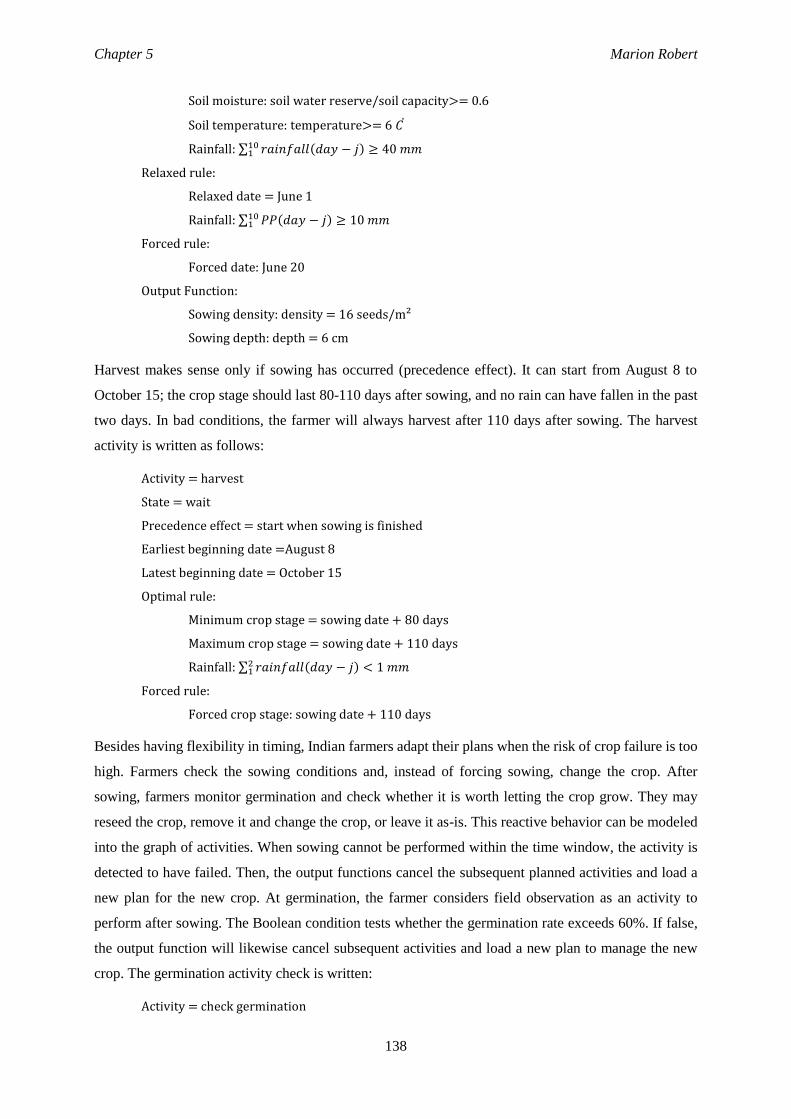
Chapter 5 Marion Robert
138
Soil moisture: soil water reserve/soil capacity>= 0.6
Soil temperature: temperature>= 6 𝐶
Rainfall: ∑ 𝑟𝑎𝑖𝑛𝑓𝑎𝑙𝑙(𝑑𝑎𝑦 − 𝑗) ≥ 40 𝑚𝑚101
Relaxed rule:
Relaxed date = June 1
Rainfall: ∑ 𝑃𝑃(𝑑𝑎𝑦 − 𝑗) ≥ 10 𝑚𝑚101
Forced rule:
Forced date: June 20
Output Function:
Sowing density: density = 16 seeds/m²
Sowing depth: depth = 6 cm
Harvest makes sense only if sowing has occurred (precedence effect). It can start from August 8 to
October 15; the crop stage should last 80-110 days after sowing, and no rain can have fallen in the past
two days. In bad conditions, the farmer will always harvest after 110 days after sowing. The harvest
activity is written as follows:
Activity = harvest
State = wait
Precedence effect = start when sowing is finished
Earliest beginning date =August 8
Latest beginning date = October 15
Optimal rule:
Minimum crop stage = sowing date + 80 days
Maximum crop stage = sowing date + 110 days
Rainfall: ∑ 𝑟𝑎𝑖𝑛𝑓𝑎𝑙𝑙(𝑑𝑎𝑦 − 𝑗) < 1 𝑚𝑚21
Forced rule:
Forced crop stage: sowing date + 110 days
Besides having flexibility in timing, Indian farmers adapt their plans when the risk of crop failure is too
high. Farmers check the sowing conditions and, instead of forcing sowing, change the crop. After
sowing, farmers monitor germination and check whether it is worth letting the crop grow. They may
reseed the crop, remove it and change the crop, or leave it as-is. This reactive behavior can be modeled
into the graph of activities. When sowing cannot be performed within the time window, the activity is
detected to have failed. Then, the output functions cancel the subsequent planned activities and load a
new plan for the new crop. At germination, the farmer considers field observation as an activity to
perform after sowing. The Boolean condition tests whether the germination rate exceeds 60%. If false,
the output function will likewise cancel subsequent activities and load a new plan to manage the new
crop. The germination activity check is written:
Activity = check germination
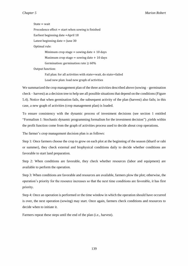
Chapter 5 Marion Robert
139
State = wait
Precedence effect = start when sowing is finished
Earliest beginning date =April 18
Latest beginning date = June 30
Optimal rule:
Minimum crop stage = sowing date + 10 days
Maximum crop stage = sowing date + 10 days
Germination: germination rate ≥ 60%
Output function:
Fail plan: for all activities with state=wait, do state=failed
Load new plan: load new graph of activities
We summarized the crop management plan of the three activities described above (sowing – germination
check – harvest) as a decision tree to help see all possible situations that depend on the conditions (Figure
5.4). Notice that when germination fails, the subsequent activity of the plan (harvest) also fails; in this
case, a new graph of activities (crop management plan) is loaded.
To ensure consistency with the dynamic process of investment decisions (see section 1 entitled
“Formalism 1: Stochastic dynamic programming formalism for the investment decision”) ,yields within
the profit function come from the graph of activities process used to decide about crop operations.
The farmer’s crop management decision plan is as follows:
Step 1: Once farmers choose the crop to grow on each plot at the beginning of the season (kharif or rabi
or summer), they check external and biophysical conditions daily to decide whether conditions are
favorable to start land preparation.
Step 2: When conditions are favorable, they check whether resources (labor and equipment) are
available to perform the operation.
Step 3: When conditions are favorable and resources are available, farmers plow the plot; otherwise, the
operation’s priority for the resource increases so that the next time conditions are favorable, it has first
priority.
Step 4: Once an operation is performed or the time window in which the operation should have occurred
is over, the next operation (sowing) may start. Once again, farmers check conditions and resources to
decide when to initiate it.
Farmers repeat these steps until the end of the plan (i.e., harvest).
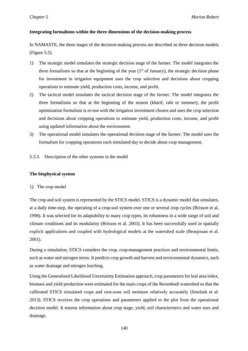
Chapter 5 Marion Robert
140
Integrating formalisms within the three dimensions of the decision-making process
In NAMASTE, the three stages of the decision-making process are described as three decision models
(Figure 5.5).
1) The strategic model simulates the strategic decision stage of the farmer. The model integrates the
three formalisms so that at the beginning of the year (1st of January), the strategic decision phase
for investment in irrigation equipment uses the crop selection and decisions about cropping
operations to estimate yield, production costs, income, and profit.
2) The tactical model simulates the tactical decision stage of the farmer. The model integrates the
three formalisms so that at the beginning of the season (kharif, rabi or summer), the profit
optimization formalism is re-run with the irrigation investment chosen and uses the crop selection
and decisions about cropping operations to estimate yield, production costs, income, and profit
using updated information about the environment.
3) The operational model simulates the operational decision stage of the farmer. The model uses the
formalism for cropping operations each simulated day to decide about crop management.
5.3.3. Description of the other systems in the model
The biophysical system
1) The crop model
The crop and soil system is represented by the STICS model. STICS is a dynamic model that simulates,
at a daily time-step, the operating of a crop-soil system over one or several crop cycles (Brisson et al.
1998). It was selected for its adaptability to many crop types, its robustness in a wide range of soil and
climate conditions and its modularity (Brisson et al. 2003). It has been successfully used in spatially
explicit applications and coupled with hydrological models at the watershed scale (Beaujouan et al.
2001).
During a simulation, STICS considers the crop, crop-management practices and environmental limits,
such as water and nitrogen stress. It predicts crop growth and harvest and environmental dynamics, such
as water drainage and nitrogen leaching.
Using the Generalized Likelihood Uncertainty Estimation approach, crop parameters for leaf area index,
biomass and yield production were estimated for the main crops of the Berambadi watershed so that the
calibrated STICS simulated crops and root-zone soil moisture relatively accurately (Sreelash et al.
2013). STICS receives the crop operations and parameters applied to the plot from the operational
decision model. It returns information about crop stage, yield, soil characteristics and water uses and
drainage.
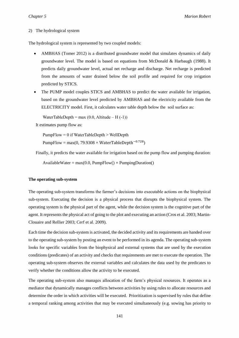
Chapter 5 Marion Robert
141
2) The hydrological system
The hydrological system is represented by two coupled models:
AMBHAS (Tomer 2012) is a distributed groundwater model that simulates dynamics of daily
groundwater level. The model is based on equations from McDonald & Harbaugh (1988). It
predicts daily groundwater level, actual net recharge and discharge. Net recharge is predicted
from the amounts of water drained below the soil profile and required for crop irrigation
predicted by STICS.
The PUMP model couples STICS and AMBHAS to predict the water available for irrigation,
based on the groundwater level predicted by AMBHAS and the electricity available from the
ELECTRICITY model. First, it calculates water table depth below the soil surface as:
WaterTableDepth = max (0.0, Altitude – H (-1))
It estimates pump flow as:
PumpFlow = 0 if WaterTableDepth > WellDepth
PumpFlow = max(0, 79.9308 × WaterTableDepth−0.728)
Finally, it predicts the water available for irrigation based on the pump flow and pumping duration:
AvailableWater = max(0.0, PumpFlow() × PumpingDuration()
The operating sub-system
The operating sub-system transforms the farmer’s decisions into executable actions on the biophysical
sub-system. Executing the decision is a physical process that disrupts the biophysical system. The
operating system is the physical part of the agent, while the decision system is the cognitive part of the
agent. It represents the physical act of going to the plot and executing an action (Cros et al. 2003; Martin-
Clouaire and Rellier 2003; Cerf et al. 2009).
Each time the decision sub-system is activated, the decided activity and its requirements are handed over
to the operating sub-system by posting an event to be performed in its agenda. The operating sub-system
looks for specific variables from the biophysical and external systems that are used by the execution
conditions (predicates) of an activity and checks that requirements are met to execute the operation. The
operating sub-system observes the external variables and calculates the data used by the predicates to
verify whether the conditions allow the activity to be executed.
The operating sub-system also manages allocation of the farm’s physical resources. It operates as a
mediator that dynamically manages conflicts between activities by using rules to allocate resources and
determine the order in which activities will be executed. Prioritization is supervised by rules that define
a temporal ranking among activities that may be executed simultaneously (e.g. sowing has priority to
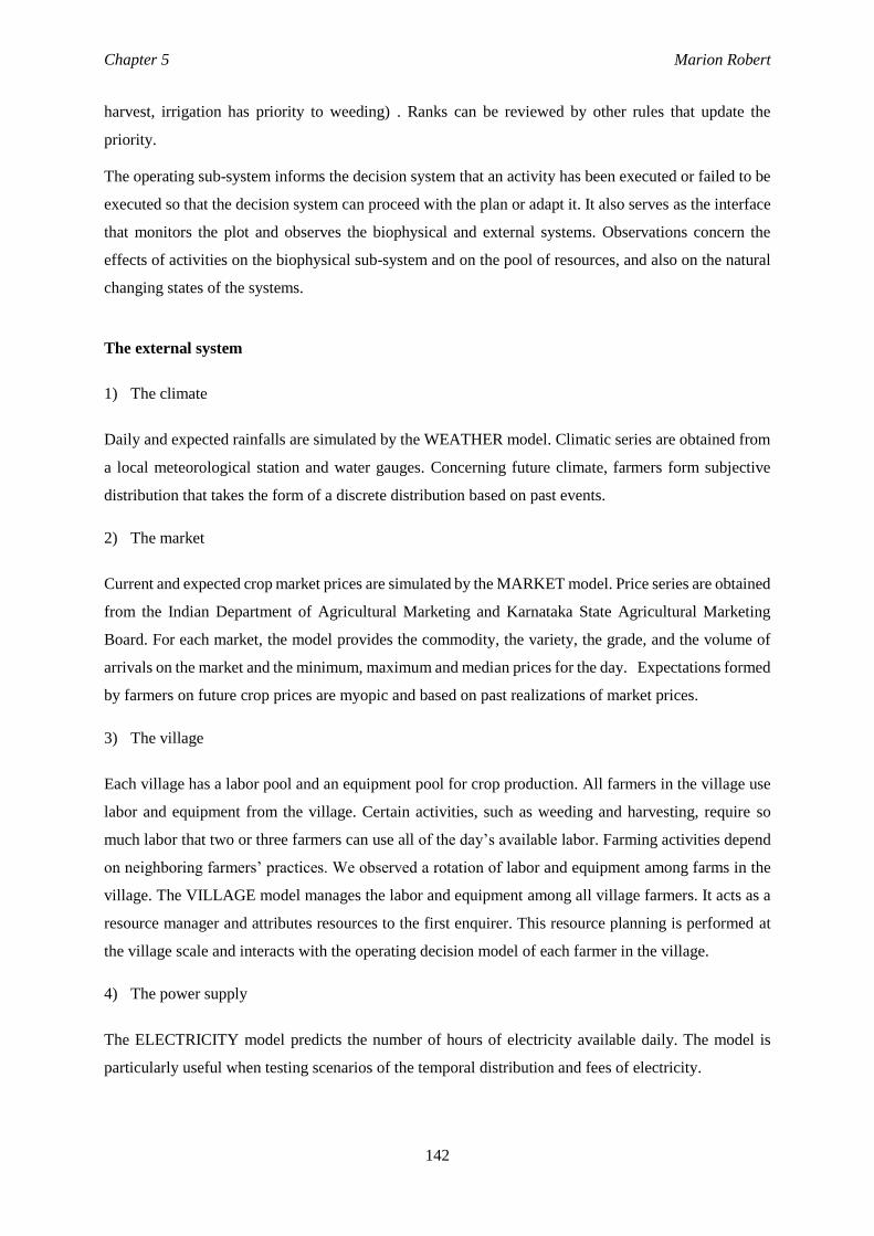
Chapter 5 Marion Robert
142
harvest, irrigation has priority to weeding) . Ranks can be reviewed by other rules that update the
priority.
The operating sub-system informs the decision system that an activity has been executed or failed to be
executed so that the decision system can proceed with the plan or adapt it. It also serves as the interface
that monitors the plot and observes the biophysical and external systems. Observations concern the
effects of activities on the biophysical sub-system and on the pool of resources, and also on the natural
changing states of the systems.
The external system
1) The climate
Daily and expected rainfalls are simulated by the WEATHER model. Climatic series are obtained from
a local meteorological station and water gauges. Concerning future climate, farmers form subjective
distribution that takes the form of a discrete distribution based on past events.
2) The market
Current and expected crop market prices are simulated by the MARKET model. Price series are obtained
from the Indian Department of Agricultural Marketing and Karnataka State Agricultural Marketing
Board. For each market, the model provides the commodity, the variety, the grade, and the volume of
arrivals on the market and the minimum, maximum and median prices for the day. Expectations formed
by farmers on future crop prices are myopic and based on past realizations of market prices.
3) The village
Each village has a labor pool and an equipment pool for crop production. All farmers in the village use
labor and equipment from the village. Certain activities, such as weeding and harvesting, require so
much labor that two or three farmers can use all of the day’s available labor. Farming activities depend
on neighboring farmers’ practices. We observed a rotation of labor and equipment among farms in the
village. The VILLAGE model manages the labor and equipment among all village farmers. It acts as a
resource manager and attributes resources to the first enquirer. This resource planning is performed at
the village scale and interacts with the operating decision model of each farmer in the village.
4) The power supply
The ELECTRICITY model predicts the number of hours of electricity available daily. The model is
particularly useful when testing scenarios of the temporal distribution and fees of electricity.
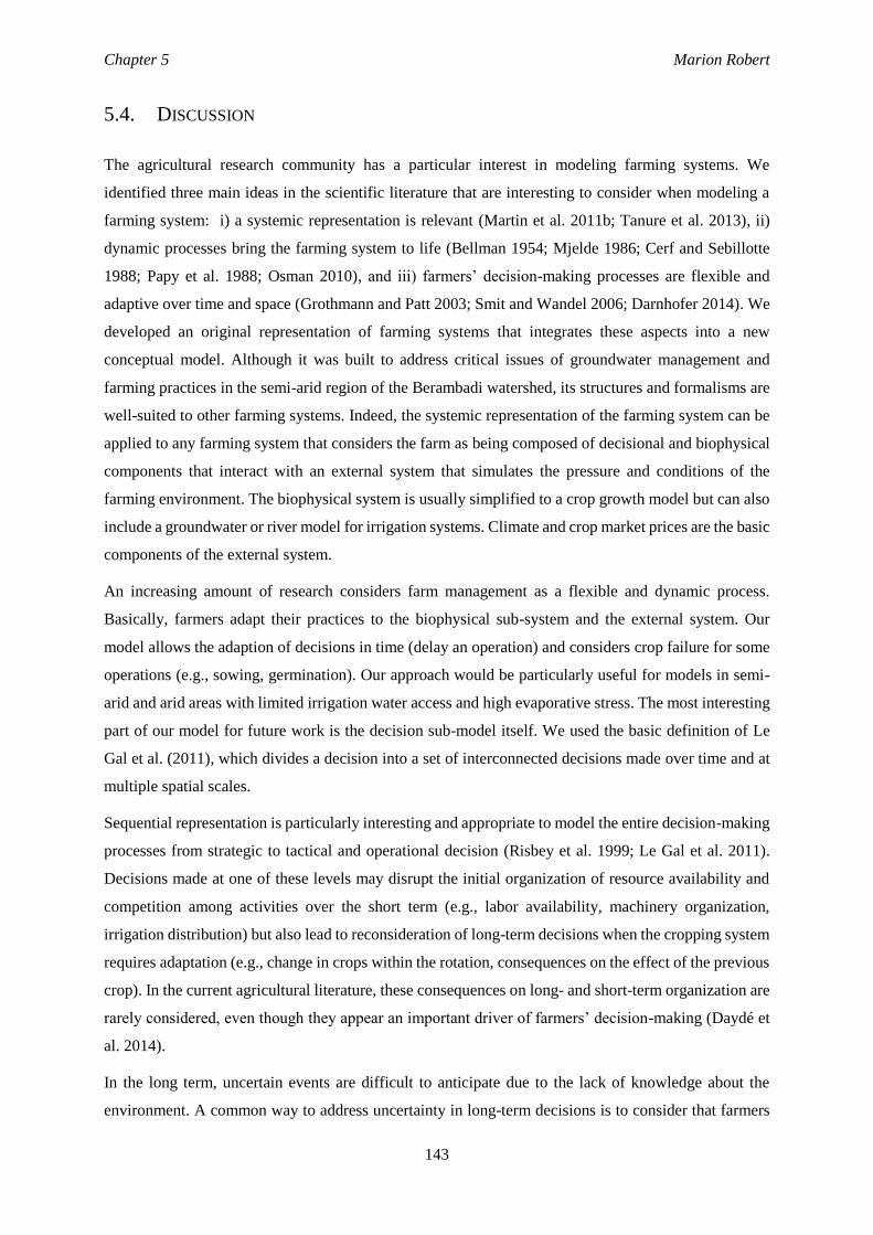
Chapter 5 Marion Robert
143
5.4. DISCUSSION
The agricultural research community has a particular interest in modeling farming systems. We
identified three main ideas in the scientific literature that are interesting to consider when modeling a
farming system: i) a systemic representation is relevant (Martin et al. 2011b; Tanure et al. 2013), ii)
dynamic processes bring the farming system to life (Bellman 1954; Mjelde 1986; Cerf and Sebillotte
1988; Papy et al. 1988; Osman 2010), and iii) farmers’ decision-making processes are flexible and
adaptive over time and space (Grothmann and Patt 2003; Smit and Wandel 2006; Darnhofer 2014). We
developed an original representation of farming systems that integrates these aspects into a new
conceptual model. Although it was built to address critical issues of groundwater management and
farming practices in the semi-arid region of the Berambadi watershed, its structures and formalisms are
well-suited to other farming systems. Indeed, the systemic representation of the farming system can be
applied to any farming system that considers the farm as being composed of decisional and biophysical
components that interact with an external system that simulates the pressure and conditions of the
farming environment. The biophysical system is usually simplified to a crop growth model but can also
include a groundwater or river model for irrigation systems. Climate and crop market prices are the basic
components of the external system.
An increasing amount of research considers farm management as a flexible and dynamic process.
Basically, farmers adapt their practices to the biophysical sub-system and the external system. Our
model allows the adaption of decisions in time (delay an operation) and considers crop failure for some
operations (e.g., sowing, germination). Our approach would be particularly useful for models in semi-
arid and arid areas with limited irrigation water access and high evaporative stress. The most interesting
part of our model for future work is the decision sub-model itself. We used the basic definition of Le
Gal et al. (2011), which divides a decision into a set of interconnected decisions made over time and at
multiple spatial scales.
Sequential representation is particularly interesting and appropriate to model the entire decision-making
processes from strategic to tactical and operational decision (Risbey et al. 1999; Le Gal et al. 2011).
Decisions made at one of these levels may disrupt the initial organization of resource availability and
competition among activities over the short term (e.g., labor availability, machinery organization,
irrigation distribution) but also lead to reconsideration of long-term decisions when the cropping system
requires adaptation (e.g., change in crops within the rotation, consequences on the effect of the previous
crop). In the current agricultural literature, these consequences on long- and short-term organization are
rarely considered, even though they appear an important driver of farmers’ decision-making (Daydé et
al. 2014).
In the long term, uncertain events are difficult to anticipate due to the lack of knowledge about the
environment. A common way to address uncertainty in long-term decisions is to consider that farmers
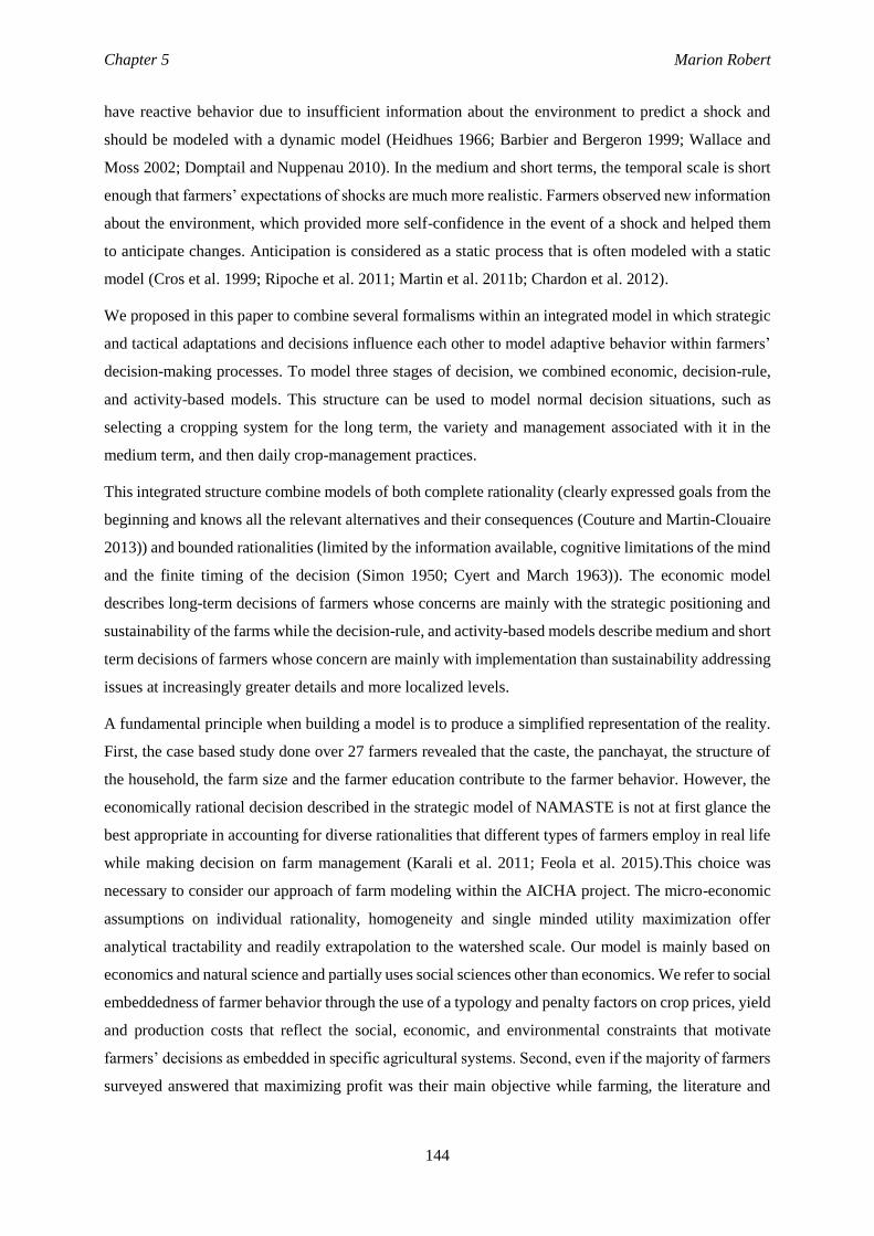
Chapter 5 Marion Robert
144
have reactive behavior due to insufficient information about the environment to predict a shock and
should be modeled with a dynamic model (Heidhues 1966; Barbier and Bergeron 1999; Wallace and
Moss 2002; Domptail and Nuppenau 2010). In the medium and short terms, the temporal scale is short
enough that farmers’ expectations of shocks are much more realistic. Farmers observed new information
about the environment, which provided more self-confidence in the event of a shock and helped them
to anticipate changes. Anticipation is considered as a static process that is often modeled with a static
model (Cros et al. 1999; Ripoche et al. 2011; Martin et al. 2011b; Chardon et al. 2012).
We proposed in this paper to combine several formalisms within an integrated model in which strategic
and tactical adaptations and decisions influence each other to model adaptive behavior within farmers’
decision-making processes. To model three stages of decision, we combined economic, decision-rule,
and activity-based models. This structure can be used to model normal decision situations, such as
selecting a cropping system for the long term, the variety and management associated with it in the
medium term, and then daily crop-management practices.
This integrated structure combine models of both complete rationality (clearly expressed goals from the
beginning and knows all the relevant alternatives and their consequences (Couture and Martin-Clouaire
2013)) and bounded rationalities (limited by the information available, cognitive limitations of the mind
and the finite timing of the decision (Simon 1950; Cyert and March 1963)). The economic model
describes long-term decisions of farmers whose concerns are mainly with the strategic positioning and
sustainability of the farms while the decision-rule, and activity-based models describe medium and short
term decisions of farmers whose concern are mainly with implementation than sustainability addressing
issues at increasingly greater details and more localized levels.
A fundamental principle when building a model is to produce a simplified representation of the reality.
First, the case based study done over 27 farmers revealed that the caste, the panchayat, the structure of
the household, the farm size and the farmer education contribute to the farmer behavior. However, the
economically rational decision described in the strategic model of NAMASTE is not at first glance the
best appropriate in accounting for diverse rationalities that different types of farmers employ in real life
while making decision on farm management (Karali et al. 2011; Feola et al. 2015).This choice was
necessary to consider our approach of farm modeling within the AICHA project. The micro-economic
assumptions on individual rationality, homogeneity and single minded utility maximization offer
analytical tractability and readily extrapolation to the watershed scale. Our model is mainly based on
economics and natural science and partially uses social sciences other than economics. We refer to social
embeddedness of farmer behavior through the use of a typology and penalty factors on crop prices, yield
and production costs that reflect the social, economic, and environmental constraints that motivate
farmers’ decisions as embedded in specific agricultural systems. Second, even if the majority of farmers
surveyed answered that maximizing profit was their main objective while farming, the literature and
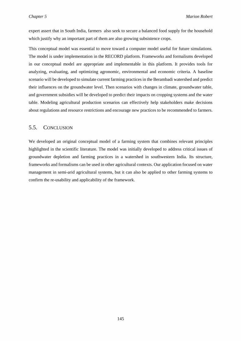
Chapter 5 Marion Robert
145
expert assert that in South India, farmers also seek to secure a balanced food supply for the household
which justify why an important part of them are also growing subsistence crops.
This conceptual model was essential to move toward a computer model useful for future simulations.
The model is under implementation in the RECORD platform. Frameworks and formalisms developed
in our conceptual model are appropriate and implementable in this platform. It provides tools for
analyzing, evaluating, and optimizing agronomic, environmental and economic criteria. A baseline
scenario will be developed to simulate current farming practices in the Berambadi watershed and predict
their influences on the groundwater level. Then scenarios with changes in climate, groundwater table,
and government subsidies will be developed to predict their impacts on cropping systems and the water
table. Modeling agricultural production scenarios can effectively help stakeholders make decisions
about regulations and resource restrictions and encourage new practices to be recommended to farmers.
5.5. CONCLUSION
We developed an original conceptual model of a farming system that combines relevant principles
highlighted in the scientific literature. The model was initially developed to address critical issues of
groundwater depletion and farming practices in a watershed in southwestern India. Its structure,
frameworks and formalisms can be used in other agricultural contexts. Our application focused on water
management in semi-arid agricultural systems, but it can also be applied to other farming systems to
confirm the re-usability and applicability of the framework.

Chapter 5 Marion Robert
146
ACKNOWLEDGEMENTS
This study was funded by the Indo-French Centre for the Promotion of Advanced Research (CEFIPRA),
the INRA flagship program on Adaptation to Climate Change of Agriculture and Forest (ACCAF) and
the Doctoral School of the University of Toulouse (EDT) and ORE BVET (http://bvet.obs-mip.fr). We
are grateful to all the experts, farmers, and trainees who helped implement the methodology. A special
thanks to Iswar Patil and the survey conductors for their help with the survey.

Chapter 5 Marion Robert
147
TABLE CAPTION
Table 5.1: Definitions of symbols in section 0
Symbol Definition
t Year
τ Season
𝐼𝑡 Investment in irrigation equipment
𝑟𝐼𝑡 Unit cost of investment in irrigation
��𝑡 Water available for irrigation
b Bele
c Crop
𝐶𝑊𝜏 Unit cost of water
𝑅𝑎�� Climate event (rainfall)
𝐺𝑊𝑎�� Groundwater level
𝑃𝑐,�� Crop prices
𝑃𝑊𝑏𝜏 Proportion of water available to each plot
r Discount rate
𝜋𝑏𝑐𝜏 Profit
𝑦𝑐𝑏𝜏 Crop yield
𝑋𝑐𝑏𝜏 Production costs
𝜃𝑃𝑐,�� Penalty factors on crop prices
𝜃𝑦𝑐𝑏𝜏 Penalty factors on yield
𝜃𝑋𝑏𝑐𝜏 Penalty factors on production costs
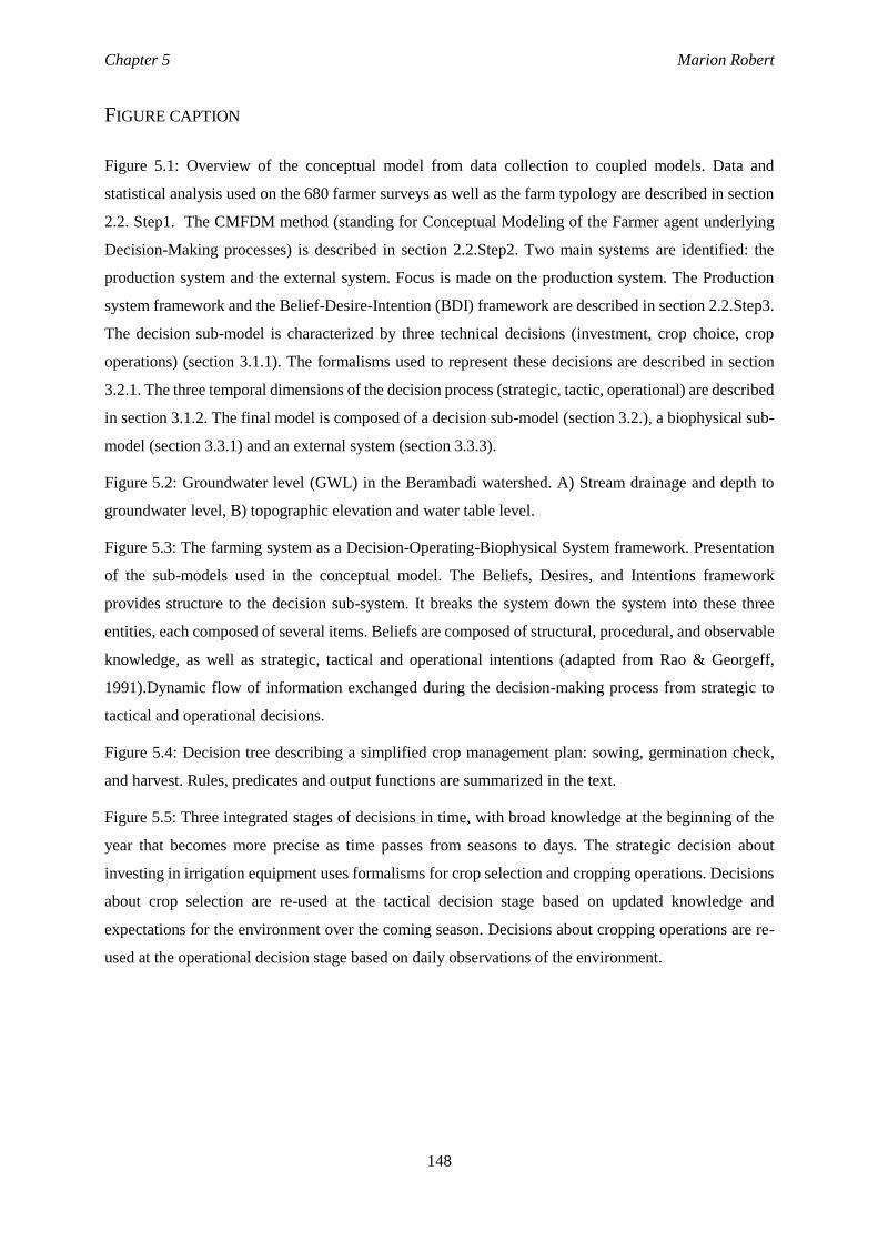
Chapter 5 Marion Robert
148
FIGURE CAPTION
Figure 5.1: Overview of the conceptual model from data collection to coupled models. Data and
statistical analysis used on the 680 farmer surveys as well as the farm typology are described in section
2.2. Step1. The CMFDM method (standing for Conceptual Modeling of the Farmer agent underlying
Decision-Making processes) is described in section 2.2.Step2. Two main systems are identified: the
production system and the external system. Focus is made on the production system. The Production
system framework and the Belief-Desire-Intention (BDI) framework are described in section 2.2.Step3.
The decision sub-model is characterized by three technical decisions (investment, crop choice, crop
operations) (section 3.1.1). The formalisms used to represent these decisions are described in section
3.2.1. The three temporal dimensions of the decision process (strategic, tactic, operational) are described
in section 3.1.2. The final model is composed of a decision sub-model (section 3.2.), a biophysical sub-
model (section 3.3.1) and an external system (section 3.3.3).
Figure 5.2: Groundwater level (GWL) in the Berambadi watershed. A) Stream drainage and depth to
groundwater level, B) topographic elevation and water table level.
Figure 5.3: The farming system as a Decision-Operating-Biophysical System framework. Presentation
of the sub-models used in the conceptual model. The Beliefs, Desires, and Intentions framework
provides structure to the decision sub-system. It breaks the system down the system into these three
entities, each composed of several items. Beliefs are composed of structural, procedural, and observable
knowledge, as well as strategic, tactical and operational intentions (adapted from Rao & Georgeff,
1991).Dynamic flow of information exchanged during the decision-making process from strategic to
tactical and operational decisions.
Figure 5.4: Decision tree describing a simplified crop management plan: sowing, germination check,
and harvest. Rules, predicates and output functions are summarized in the text.
Figure 5.5: Three integrated stages of decisions in time, with broad knowledge at the beginning of the
year that becomes more precise as time passes from seasons to days. The strategic decision about
investing in irrigation equipment uses formalisms for crop selection and cropping operations. Decisions
about crop selection are re-used at the tactical decision stage based on updated knowledge and
expectations for the environment over the coming season. Decisions about cropping operations are re-
used at the operational decision stage based on daily observations of the environment.
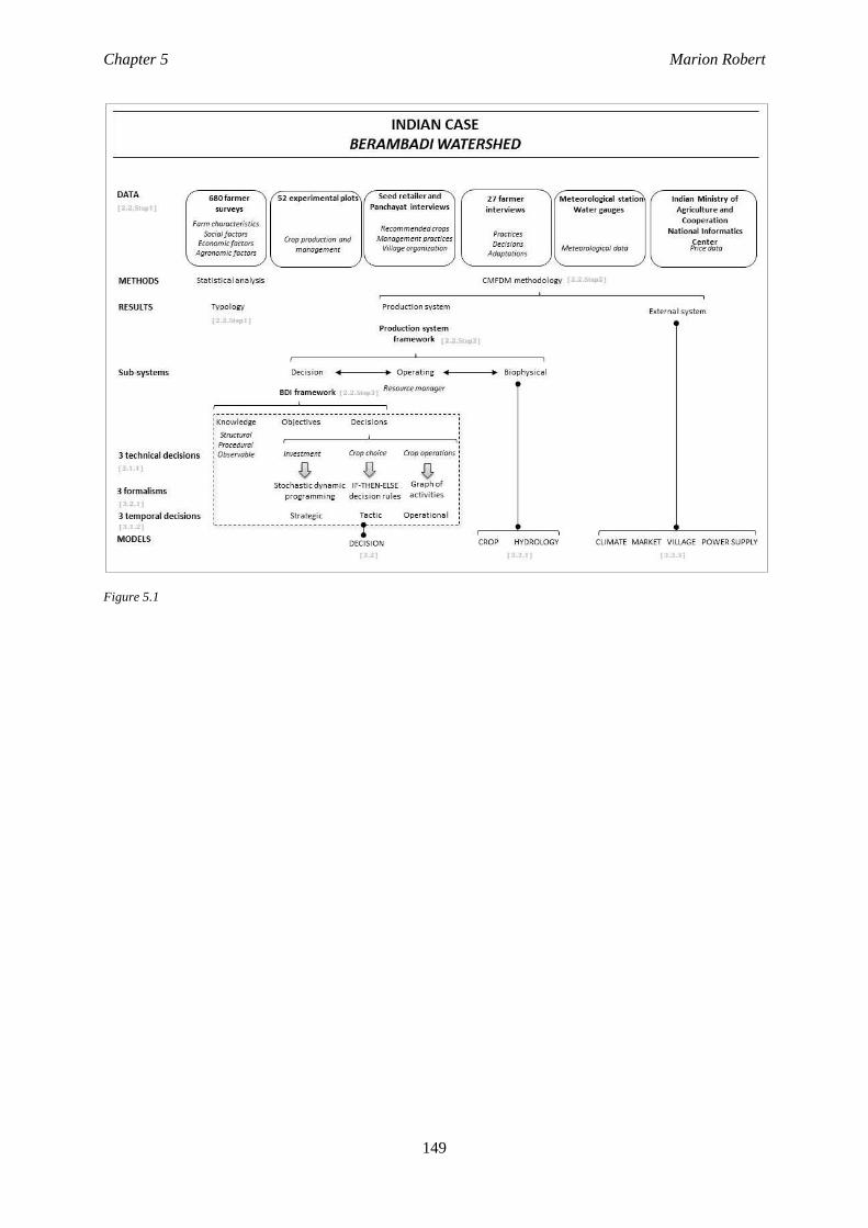
Chapter 5 Marion Robert
149
Figure 5.1
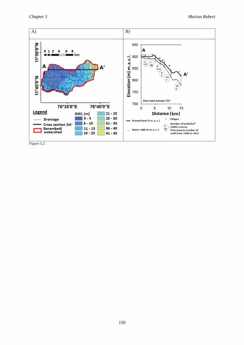
Chapter 5 Marion Robert
150
A) B)
Figure 5.2
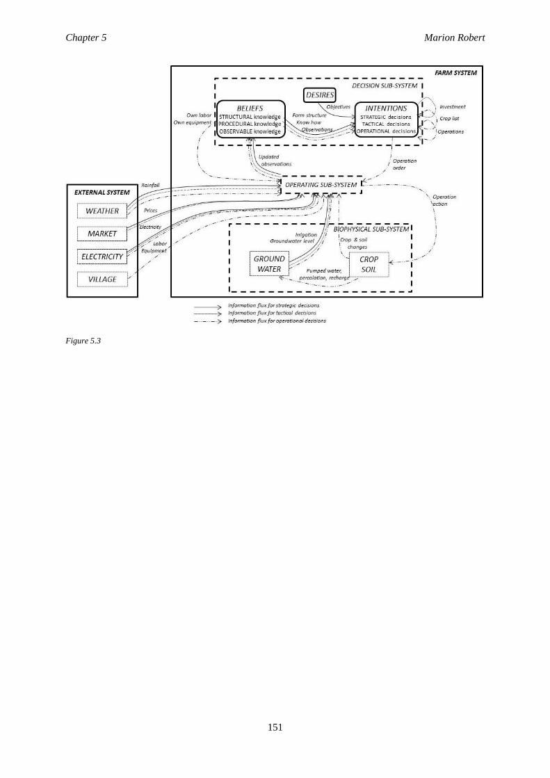
Chapter 5 Marion Robert
151
Figure 5.3
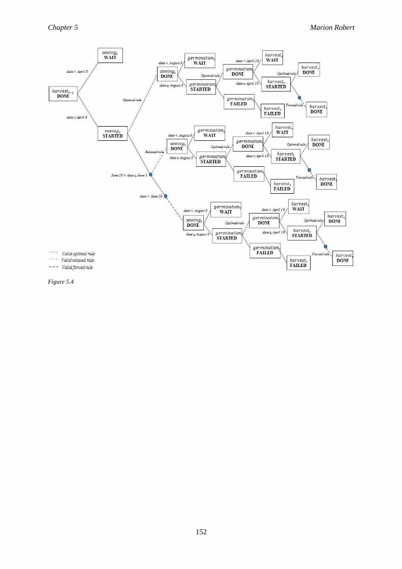
Chapter 5 Marion Robert
152
Figure 5.4
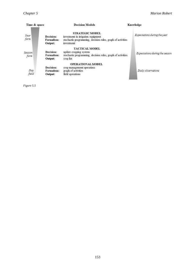
Chapter 5 Marion Robert
153
Figure 5.5

Chapter 6 Marion Robert
155
Chapter 6
A stochastic dynamic programming
approach to analyze adaptation to
climate change - application to
groundwater irrigation in India
Marion Robert∗1, Jacques-Eric Bergez1 and Alban Thomas2
1 AGIR, Université Fédérale de Toulouse, INRA, INPT, F-31326 Castanet-Tolosan, France
2Toulouse School of Economics, INRA, University of Toulouse, F-31000 Toulouse, France
∗ Corresponding author: ([email protected])
Submitted to European Journal of Operational Research
Scientific paper
Version: 05 December 2016
Chapter 6 Marion Robert
156
Agricultural sustainability under climate change is a major challenge in semi-arid countries, mainly due
to rare or depleted water resources. This article explores short- and long-term consequences of farmers’
adaptation decisions about groundwater resources under several climate change scenarios. We modeled
farmer decisions about crop choice, investment in irrigation and water application rates using a
stochastic dynamic programming model with discrete time and control variables. We also investigated
the performance of water management policies for groundwater resource depletion, and considered
adaptive farmer decisions about irrigation and crop systems. Several sources of risk were considered:
rainfall average and variability, crop market prices, crop yield and borewell failure. Policy simulations
were performed with a calibrated version of the stochastic dynamic model, using data from a field survey
in the Berambadi watershed, Karnataka state, southern India. The most relevant and novel aspects of
our model are i) the consideration of investment decisions about irrigation over a long-term horizon, ii)
the consideration of several water management policies, iii) the detailed description of farmers’ water
practices and representation of crop choice based on the agricultural season.
Keywords: (D) OR in agriculture; (I) Stochastic programming; (D) OR in environment and climate
change; (D) Strategic planning; (B) Scenarios.
Chapter 6 Marion Robert
157
6.1. INTRODUCTION
Climate change is a significant challenge for sustainable agricultural production in the coming decades,
especially since global food demand is expected to double by the year 2050. Predictions of climate
change impacts indicate a reduction in most crop yields under both irrigated and rainfed conditions, an
increase in weeds, diseases and pests and changes in crop development and pollination periods (Kahil
et al. 2015).
Agricultural systems in semi-arid areas depend greatly on irrigation and encounter increasing challenges
due to climate change (e.g. growing uncertainty about the performance of strategies for adapting to
climate change, severe depletion of natural resources), high volatility in crop market prices, rises in
energy costs and greater pressure from public regulations (e.g. agricultural, environmental and health
policies). In the Deccan Plateau in India, aided by state policy that subsidizes electricity and improved
irrigation technology (e.g. new drilling and submersible pump techniques), the countryside has
witnessed the proliferation of individual, electrical pump-driven borewells that abstract water from
underground aquifers (Sekhar et al. 2006; Javeed et al. 2009). This led to claims of a “democratization
of irrigation”, with smallholder farmers accessing irrigation water (Taylor 2013). However, the low
productivity of the aquifer (Dewandel et al. 2010; Perrin et al. 2011) and a rapid decline in the
groundwater table level led to decreasing borewell yields (Ruiz et al. 2015), implying that
(groundwater)-irrigated agriculture still largely depends on rainfall. Climate variability has increased
over the last 50 years in this region (Jogesh and Dubash 2014); predictions indicate a 1.8-2.2°C increase
in temperature by 2030, and southwestern regions of Karnataka state (southern India) are projected to
experience a decrease in annual rainfall, especially during the monsoon season (Jogesh and Dubash
2014). For a region that largely depends on monsoon patterns and winter months to maintain agricultural
production, any shift in climate conditions would have a severe impact on natural resources and the
economy. Over the past two decades, agrarian India has been in the midst of a considerable crisis,
manifested by increasing levels of indebtedness and most tragically exemplified by the wave of farmer
suicides that have plagued the countryside of the Deccan Plateau in particular. The need to cope with
upcoming debt payments induces farmers to shift towards irrigated cash crops, and gaining control over
water access is central to maintain household sustainability. Accessing groundwater may be a solution
to provide water for crops on a more regular basis, but this solution must also consider social and cultural
aspects of farmer indebtedness, including a new temporal horizon for debt repayment and accounting
for the risk of failed wells (Taylor 2013).
In this article, we model adaptive decisions of farmers facing climate change: long-term decisions about
investment in borewell irrigation and short-term decisions about cropping systems and the irrigation
water application rate for crops. We use a stochastic dynamic model of farmers’ decisions to test socio-
economic and water management policies under several climate change scenarios. Various policies are
Chapter 6 Marion Robert
158
considered (i.e. subsidizing rainfed crops, reforming subsidized energy for irrigation, a water charge
indexed to ambient groundwater level), and their impacts on farmer profit and groundwater level are
compared. Each scenario is considered along with a climate change scenario to evaluate the potential of
each policy to mitigate the climate’s impact on groundwater level.
6.2. LITERATURE REVIEW ON LONG-TERM FARMER DECISIONS UNDER
UNCERTAINTY
Several fields in the literature have discussed models of farmers’ decisions under risk and uncertainty,
including irrigation management, ranging from environmental and resource economics to applications
of operational research to hydrological issues. Krishnamurthy (2016) presented a theory that clarifies
the properties of water management models under risk and uncertainty. Sekhri (2014) explored
implications of groundwater irrigation on poverty in rural India using a detailed survey of agricultural
wells.
It is essential to consider risk and uncertainty when representing irrigation management and cropping
system decisions because of the uncertain nature of water availability for irrigation and crop yield
resulting from climate conditions. Iglesias & Garrote (2015) provided a literature review on agricultural
adaptation to climate change in Europe that describes the possible drivers of adaptation and policy
implications.
Two main approaches are distinguished in the agricultural economics literature (Robert et al. 2016b).
First, in stochastic programming, uncertainty and risk are incorporated as non-embedded risk into the
objective function, i.e., in prices, yields and revenues, or in constraints, to represent stochastic resource
availability (McCarl et al. 1999; Briner and Finger 2013; Graveline 2016). Second, in discrete stochastic
programming, uncertainty and risk are incorporated as embedded risks, including both risk anticipation
and adjustments, which allows for recourse in the decision.
In stochastic programming, the main advantage of incorporating risk is to consider stochastic variables
such as prices, yields, borewell recharge and water availability for irrigation, which are all related to
uncertain weather. In this way, relationships between farm production variables and climate are better
considered and represented in models. Fernandez et al. (2016) used stochastic programming to model
economic impacts of changes in water availability in small-scale agriculture in the Vergara River Basin,
Chile. They applied a calibration method for risk programming models with mean-variance model
specification developed by Petsakos & Rozakis (2015) to include risk in the objective function of
agricultural models. Blanco-Gutierrez et al. (2013) used a risk-based economic optimization model and
a hydrologic water management simulation model to model a vulnerable drought-prone agro-ecological
area in the Middle Guadiana River Basin, Spain. Similarly, Foster et al. (2014) predicted optimal
irrigation strategies under variable levels of groundwater supply for irrigated maize production in the
Chapter 6 Marion Robert
159
Texas High Plains region of the United States, and assessed the limits of existing models for predicting
farmers’ land and groundwater use decisions.
In discrete stochastic programming, the decision problem is broken down into several decision stages in
which new information is available. It can be represented by decision trees. The typical case treated with
discrete stochastic programming is cropping pattern planning under weather and/or water uncertainty.
For instance, McCarl et al. (1999), Mejías et al. (2004) and Connor et al. (2009) defined an initial stage
that models the choice of long-term capital investments that remain fixed for several years regardless of
annual stochastic variations (water allocation and water price). The second stage addresses short-term
(annual) decisions, such as water application rates and land for crops or fallow.
The use of dynamic programming to represent and solve water, nutrient or animal feed management
problems in agriculture has a long history. Burt (1993) considered an expected present value problem
and from dynamic programming generated a set of sequential decision rules for optimal feed rations and
marketed animal weights. Randomness in input and output prices was considered, and properties of the
stochastic model were examined for two cases of model application: infinite sequence and single batch.
However, no empirical application was presented. Bryant et al. (1993) used a dynamic programming
model to explore allocation of irrigation among crops under random climate conditions. During dry
periods, a crop can be abandoned temporarily or permanently. Intra-seasonal irrigation rules were
considered for maize and sorghum in the Texas High Plains. These authors also used a crop simulator
to “simplify” decision rules for crop choice and irrigation application rates. Only two plots of fixed size
were set, and a fixed irrigation volume was allocated to only one crop.
Ritten et al. (2010) developed a stochastic dynamic programming model for purposes similar to those
of Burt (1993), i.e., to solve for optimal stocking rates under climate change. More precisely, they
considered farmers’ decisions when rainfall is unknown before the start of the growing season. Farmers
maximized the current net value of their land, and the (random) dynamic state variable was vegetation
density. When climate scenarios were introduced profitability decreased as rainfall variability increased
compared to the baseline climate.
Maatman et al. (2002) also considered a stochastic programming model to represent farmers' sequential
decisions in response to changes in expected rainfall and introduced a food security condition into the
problem. More precisely, the farmer’s objective was to minimize nutrient deficits at the household level
and during several periods (i.e. beginning of the growing season, later in the the growing season and
after harvesting). They presented one of the first examples in the literature of application of stochastic
programming with an explicit subsistence strategy for farmers and adaptation to climate change in an
intra-seasonal setting. The method, two-stage stochastic models and multiple-recourse models differed,
however, from nonlinear stochastic dynamic programming, and no investment decisions in irrigation
were considered.
Chapter 6 Marion Robert
160
In the present article, we combine several features of the models discussed above into a model that
describes farmer decision rules for groundwater irrigation in more detail, with southern India as an
empirical application. Specifically, we consider climate scenarios allowing for changes in rainfall
distribution and farmer long-term decisions about investment in irrigation, short-term intra-seasonal
decisions about crops and plot size, and water application rates. We developed a dynamic stochastic
programming model to study these multiple decisions and improve description of the variety of
adaptation pathways to climate change.
6.3. METHODS
6.3.1. The farmer’s production problem
We consider a representative farmer who makes decisions about irrigation and crop choice, and
considers consequences of his current decisions on future water availability (because the latter ultimately
determines future crop output, hence future profits). Our framework is based on a bio-economic model
with season-specific crop choice and an annual investment decision about irrigation strategies.
The multiple stages of the farmer decision-making process are described as follows:
At the beginning of the planning horizon, the farmer forms an expectation about several random
variables: future climate, future market prices for crops and groundwater availability (for irrigation).
At the beginning of the year, the farmer decides whether or not to invest in irrigation, or to rely on
rainfall for the coming year.
At the beginning of each growing season, the farmer decides which crops to grow on the farm and
the associated land area for each plot (plot size varies).
For each growing season, the farmer decides the irrigation-water application rate for each crop,
given total water availability and observed rainfall.
For each growing season, given the irrigation equipment and selected crops, the farmer follows a
set of irrigation rules to obtain the “best” crop yield, conditional on actual climate conditions. Given
the irrigation equipment, selected crops and irrigation practices, the farmer selects the plot size so
the most profitable crop is grown on a larger area than less profitable crops. In particular, when a
dry climate is expected, farmers are likely to grow multiple crops to diversify the risk of crop failure.
The farmer’s objective is to select the sequence of investment in irrigation equipment and season-
specific crops that maximize the discounted stream of future revenue across the planning horizon based
on expectations on rainfall, available water for irrigation, crop prices, crop costs, crop yields and crop
failure.
Farmers maximize seasonal profit as a function of crop choice, plot size and water application rate for
each crop (which is a percentage of total available water). Once investment in irrigation and crop choice
Chapter 6 Marion Robert
161
decisions are made, water input for crops is determined by combining irrigation from groundwater and
rainfall. More precisely, water availability (from expected rainfall and expected groundwater level)
triggers the decision to grow particular crops and, during the agricultural season, farmers adjust water
for plant needs on a daily (or weekly) basis. The adjustment is made according to agronomic “rules”,
and input or output prices and other economic variables are assumed not to influence these decisions.
However, the marginal cost of irrigation water may still depend upon the amount of water abstracted
(excluding irrigation investment cost). The farmer makes decisions about crop allocation and irrigation
investment, which makes the problem fully dynamic because today's investment decisions will affect
water availability in the future. We denote the planning horizon by T (years).
Formal representation of the problem is as follows. The representative farmer has B plots, on which C
crops can be planted. Crops can be grown during two cropping seasons (the season index is τ, with τ =
S1, S2) of duration 𝑆𝑒𝑎𝑠𝑜𝑛1𝑙𝑒𝑛𝑔𝑡ℎ and 𝑆𝑒𝑎𝑠𝑜𝑛2𝑙𝑒𝑛𝑔𝑡ℎ, respectively. Farmer decisions depend on, among
other things, expected rainfall, which is distributed according to a discrete distribution of five profiles
(poor, below average, average, above average or good). Each rainfall regime is associated with an
average, season-specific rainfall level denoted 𝑟𝑎𝑖𝑛𝑆1 and 𝑟𝑎𝑖𝑛𝑆2, respectively, and the probability of
occurrence of each rainfall regime at the beginning of each year is denoted 𝑝𝑟𝑆1 and 𝑝𝑟𝑆2, respectively.
The farmer’s annual decisions about investment in irrigation include the decision to drill a new borewell,
the well’s depth (𝑊𝐸𝐿𝐿𝑑𝑒𝑝𝑡ℎ) and the power of the (electrical) pump (HP). Assuming the farmer
benefits from a m-year loan with a fixed interest rate of r%, the annual investment cost is
𝐼𝑡 = (1 + 𝑟) (1
𝑚) (𝐶𝑂𝑆𝑇𝑤𝑒𝑙𝑙 + 𝐶𝑂𝑆𝑇𝑝𝑢𝑚𝑝) + 𝐶𝑂𝑆𝑇𝑚𝑎𝑖𝑛𝑡𝑒𝑛𝑎𝑛𝑐𝑒, (1)
where 𝐶𝑂𝑆𝑇𝑤𝑒𝑙𝑙, 𝐶𝑂𝑆𝑇𝑝𝑢𝑚𝑝 and 𝐶𝑂𝑆𝑇𝑚𝑎𝑖𝑛𝑡𝑒𝑛𝑎𝑛𝑐𝑒 are the costs of borewell construction, purchasing
the electrical pump and annual borewell maintenance, respectively.
In hard rock aquifers, drilling a borewell is risky because of possible failure when the borewell does not
reach a water fissure. 𝐹𝐴𝐼𝐿𝑤𝑒𝑙𝑙 denotes the probability of borewell failure (implying that investment in
borewell irrigation may well exceed the construction cost of a single borewell); the actual construction
cost for an operating borewell (𝐶𝑂𝑆𝑇𝑤𝑒𝑙𝑙) is inflated by 𝐹𝐴𝐼𝐿𝑤𝑒𝑙𝑙 and is a function of borewell depth
(𝑊𝐸𝐿𝐿𝑑𝑒𝑝𝑡ℎ).
The irrigation capacity of the farm also depends on the depth of the groundwater table (𝑊𝑇𝑑𝑒𝑝𝑡ℎ) and
the time available for pumping (hours of electricity available per day in the first season, 𝑃𝑜𝑤𝑒𝑟_𝑑𝑎𝑦𝑆1,
and the second season, 𝑃𝑜𝑤𝑒𝑟_𝑑𝑎𝑦𝑆2). The flow rate (FR) of the well provides the maximum water
abstraction capacity of the irrigation system and is defined as follows:
𝐹𝑅 = ℎ(𝐻𝑃, 𝑊𝑇𝑑𝑒𝑝𝑡ℎ, 𝑊𝐸𝐿𝐿𝑑𝑒𝑝𝑡ℎ) > 0 if 𝑊𝐸𝐿𝐿𝑑𝑒𝑝𝑡ℎ > 𝑊𝑇𝑑𝑒𝑝𝑡ℎ,
0 otherwise. (2)
Chapter 6 Marion Robert
162
The flow rate is considered the state variable of our dynamic model, in which it is denoted W. W is both
dynamic and stochastic because it depends on borewell yield, the rainfall recharge factor and
depreciation of irrigation capital stock (with a factor of 𝑅𝐴𝑇𝐸𝑑𝑒𝑝𝑟𝑒𝑐𝑖𝑎𝑡𝑖𝑜𝑛).
The expected water available for irrigation in the first and second seasons (��𝑆1 and ��𝑆2 ) is determined
from the flow rate, daily power supply available for pumping (𝑃𝑜𝑤𝑒𝑟_𝑑𝑎𝑦𝑆1 and 𝑃𝑜𝑤𝑒𝑟_𝑑𝑎𝑦𝑆2) and
the number of days per season (𝑆𝑒𝑎𝑠𝑜𝑛1𝑙𝑒𝑛𝑔𝑡ℎ and 𝑆𝑒𝑎𝑠𝑜𝑛2𝑙𝑒𝑛𝑔𝑡ℎ):
��𝑆1 = 𝑊×𝑃𝑜𝑤𝑒𝑟_𝑑𝑎𝑦𝑆1×𝑆𝑒𝑎𝑠𝑜𝑛1𝑙𝑒𝑛𝑔𝑡ℎ
and ��𝑆2 = 𝑊×𝑃𝑜𝑤𝑒𝑟_𝑑𝑎𝑦𝑆2×𝑆𝑒𝑎𝑠𝑜𝑛2𝑙𝑒𝑛𝑔𝑡ℎ (3)
Therefore, total irrigation capacity expected for the year is �� = ��𝑆1 + ��𝑆2 and is distributed among
plots according to a season-specific vector 𝑅𝐴𝑇𝐸𝑖𝑟𝑟𝑖𝑔𝑎𝑡𝑖𝑜𝑛. The cost of pumping groundwater to irrigate
crops (𝐶𝑂𝑆𝑇𝑝𝑢𝑚𝑝𝑖𝑛𝑔) depends on the number of hours of pumping (𝐻𝑂𝑈𝑅𝑆𝑖𝑟𝑟𝑖𝑔𝑎𝑡𝑖𝑜𝑛), the electric
power used (𝑃𝑂𝑊𝐸𝑅𝑖𝑟𝑟𝑖𝑔𝑎𝑡𝑖𝑜𝑛) and the cost of electricity (𝐶𝑂𝑆𝑇𝑒𝑙𝑒𝑐𝑡𝑟𝑖𝑐𝑖𝑡𝑦):
𝐶𝑂𝑆𝑇𝑝𝑢𝑚𝑝𝑖𝑛𝑔 = 𝐻𝑂𝑈𝑅𝑆𝑖𝑟𝑟𝑖𝑔𝑎𝑡𝑖𝑜𝑛 × 𝑃𝑂𝑊𝐸𝑅𝑖𝑟𝑟𝑖𝑔𝑎𝑡𝑖𝑜𝑛 × 𝐶𝑂𝑆𝑇𝑒𝑙𝑒𝑐𝑡𝑟𝑖𝑐𝑖𝑡𝑦, (4)
Where 𝐻𝑂𝑈𝑅𝑆𝑖𝑟𝑟𝑖𝑔𝑎𝑡𝑖𝑜𝑛 = (𝑃𝑜𝑤𝑒𝑟_𝑑𝑎𝑦𝑆1×𝑆𝑒𝑎𝑠𝑜𝑛1𝑙𝑒𝑛𝑔𝑡ℎ + 𝑃𝑜𝑤𝑒𝑟_𝑑𝑎𝑦𝑆2×𝑆𝑒𝑎𝑠𝑜𝑛2𝑙𝑒𝑛𝑔𝑡ℎ)×
𝑅𝐴𝑇𝐸𝑖𝑟𝑟𝑖𝑔𝑎𝑡𝑖𝑜𝑛.
Regarding the choice of the cropping system and irrigation practices, crops can be irrigated or rainfed
or both, may be grown during both seasons or only during the monsoon season and can be short-term
(only one season) or long-term (over two seasons) crops. When selecting crops, the farmer estimates the
chance of crop failure (𝑅𝐴𝑇𝐸𝑓𝑎𝑖𝑙𝑢𝑟𝑒) and plans to grow another crop (c_replace) if the first crop fails.
For a given irrigation capital stock, crop choice and irrigation practices are decided by comparing crop-
specific and season-specific expected profits, with the expectation considered among the five rainfall
regimes mentioned previously. 𝜋𝑏𝑐𝜏.denotes expected profit from crop c in season 𝜏 on plot b, and we
approximate 𝜋𝑏𝑐𝜏 as:
𝜋𝑏𝑐𝜏 ≅ ∑ 𝑝𝑟𝜏,𝑖[
5
𝑖=1
(1 − 𝑅𝐴𝑇𝐸𝑓𝑎𝑖𝑙𝑢𝑟𝑒)[𝑃𝑅𝐼𝐶𝐸𝑐𝜏(��𝜏)𝑌𝐼𝐸𝐿𝐷𝑏𝑐𝜏(��𝜏, 𝑊𝑏𝑐𝜏)× 𝑆𝐼𝑍𝐸𝑝𝑙𝑜𝑡 − 𝐶𝑂𝑆𝑇𝑐
− 𝐶𝑂𝑆𝑇𝑝𝑢𝑚𝑝𝑖𝑛𝑔]
+ (𝑅𝐴𝑇𝐸𝑓𝑎𝑖𝑙𝑢𝑟𝑒) [𝑃𝑅𝐼𝐶𝐸𝑐𝑟𝑒𝑝𝑙𝑎𝑐𝑒,𝜏(��𝜏)𝑌𝐼𝐸𝐿𝐷𝑏,𝑐𝑟𝑒𝑝𝑙𝑎𝑐𝑒,𝜏 (��𝜏, 𝑊𝑏,𝑐𝑟𝑒𝑝𝑙𝑎𝑐𝑒,𝜏) 𝑆𝐼𝑍𝐸𝑝𝑙𝑜𝑡 − 𝐶𝑂𝑆𝑇𝑐𝑟𝑒𝑝𝑙𝑎𝑐𝑒
−𝐶𝑂𝑆𝑇𝑐 − 𝐶𝑂𝑆𝑇𝑝𝑢𝑚𝑝𝑖𝑛𝑔
],
(5)
where ��𝜏 denotes random rainfall in season 𝜏, crop yield (𝑌𝐼𝐸𝐿𝐷𝑏𝑐𝜏) and crop price (𝑃𝑅𝐼𝐶𝐸𝑐𝜏) are
stochastic variables that depend on rainfall, 𝑊𝑏𝑐𝜏 is irrigation water applied to crop c, and 𝑆𝐼𝑍𝐸𝑝𝑙𝑜𝑡 is
the size of the plot (fixed or adjusted by the farmer). Because we focus on irrigation, we consider other
Chapter 6 Marion Robert
163
crop management practices (e.g. fertilizer, seed, labor) as constant; thus, crop cost 𝐶𝑂𝑆𝑇𝑐 is a fixed
parameter. Expected profit among rainfall regimes is approximated as the average profit earned during
the five rainfall regimes, weighted by their probabilities of occurrence at the beginning of each year
(vectors 𝑝𝑟𝐾 and 𝑝𝑟𝑅). We assume crop yield is a quadratic function of irrigation water distributed to
the crop, which is the minimum between total available water for the crop (𝑅𝐴𝑇𝐸𝑖𝑟𝑟𝑖𝑔𝑎𝑡𝑖𝑜𝑛 ×��𝑆1 for
the first season and 𝑅𝐴𝑇𝐸𝑖𝑟𝑟𝑖𝑔𝑎𝑡𝑖𝑜𝑛×��𝑆2 for the second season) and the optimal amount of water the
crop needs to reach optimal yield (𝐼𝑟𝑟𝑖𝑐).
For crop c (dropping indexes b and 𝜏 for the sake of simplicity):
𝑌𝐼𝐸𝐿𝐷𝑐(��, 𝑊) = 𝑎𝑐 + 𝑏𝑐 min[(𝑅𝐴𝑇𝐸𝑖𝑟𝑟𝑖𝑔𝑎𝑡𝑖𝑜𝑛,𝑐 (��)×��𝑆1 , 𝐼𝑟𝑟𝑖𝑐 (��)]
+ 𝑑𝑐 min[𝑅𝐴𝑇𝐸𝑖𝑟𝑟𝑖𝑔𝑎𝑡𝑖𝑜𝑛,𝑐 (��)×��𝑆1 , 𝐼𝑟𝑟𝑖𝑐 (��)],2 (6)
where 𝑅𝐴𝑇𝐸𝑖𝑟𝑟𝑖𝑔𝑎𝑡𝑖𝑜𝑛,𝑐 ∈ [0,1], ∀𝑐, 𝑐 = 1, … , 𝐶.
Because crop price in local markets is likely to depend on climate conditions beyond the farmer’s control
(because farmers are “price takers”), we assume that crop price is determined from a reference price
(𝑅𝐸𝐹𝑐) multiplied by crop price elasticity with respect to rainfall. Hence, price decreases by a factor of
α when rainfall shifts to the next rainfall regime, and the random price for crop c under rainfall regime
𝑖, 𝑖 = 1, … ,5 is
𝑃𝑅𝐼𝐶𝐸𝑐 = 𝑅𝐸𝐹𝑐× 𝛼𝑖. (7)
The farmer’s problem over the T years of the planning horizon is
max{𝐼𝑡}
∑ (1 + 𝑟)−𝑡𝑇𝑡=1 { max
{𝛿𝑏𝑐𝜏}[∑ ∑ ∑ 𝛿𝑏𝑐𝜏 𝜋𝑏𝑐𝜏
𝑆2𝜏=𝑆1
𝐶𝑐=1
𝐵𝑏=1 ] − 𝐼𝑡} , (8)
where r is a constant discount rate, and 𝛿𝑏𝑐𝜏 = 1 if crop c is grown on plot b in season 𝜏 (otherwise 0).
We assume that since no a priori condition is imposed on the terminal level of water availability or
irrigation capital stock, we have an infinite-horizon problem. To solve this stochastic dynamic
programming problem, the Bellman approach is commonly used in the literature (Bertsekas 2011). To
simplify notation, we denote 𝜋𝑡∗(𝐼𝑡, 𝑊𝑡) as the profit obtained in year t from optimal control variables
for problem (8), with year-dependent state variable 𝑊𝑡 and control variable 𝐼𝑡. Note that optimal control
variables that are season-specific, i.e., crop choice, irrigation application rate and plot size, are implicitly
assumed with this notation. The maximization problem is thus equivalently expressed as the following
Bellman equation for time period t:
𝑉(𝑊𝑡) = max𝐼𝑡
{𝜋𝑡∗(𝐼𝑡, 𝑊𝑡) + 𝛽 𝐸��𝑉(𝑊𝑡+1)}, ∀𝑡, (9)
where 𝑉(𝑊𝑡) is the value function (the maximum of current and future revenues) with the state variable
as its argument, whose (dynamic) transition equation is
Chapter 6 Marion Robert
164
𝑊𝑡+1 = 𝑓(𝑊𝑡, 𝐼𝑡), (10)
𝛽 is a discount factor and 𝜋𝑡∗(𝐼𝑡, 𝑊𝑡) is the current year’s profit function.
A popular way of solving such infinite-horizon problems is a colocation method (e.g., Bertsekas (2011)
and Miranda & Fackler (2004)) applied to Equation (9). The unknown value function is approximated
through contraction mapping involving Chebyshev polynomials whose associated coefficients are
solved iteratively from a value-function colocation technique. If the order of Chebyshev polynomials
for approximating the value function is p, we form the following system of p equations with p unknowns
evaluated for a given value of the state variable, 𝑊𝑝:
∑ 𝑐𝑝Φ𝑝(𝑊𝑝) = max {𝜋∗(𝐼, 𝑊𝑝) + 𝛽𝐸�� ∑ 𝑐𝑝Φ𝑝[𝑓(𝑊𝑝)]𝑃𝑝=1 }𝑃
𝑝=1 , 𝑝 = 1, … , 𝑃, (11)
where Φ𝑝 and 𝑐𝑝 is the Chebyshev polynomial of order p and its associated coefficient (to be evaluated),
respectively. In the system above, we drop reference to a particular sequence of years (t and t+1) because
we are looking to approximate the value function at the steady state. For this reason, the maximization
problem is considered for any pair of subsequent values of the state variable, 𝑊𝑝 and 𝑊′ = 𝑓(𝑊𝑝). The
algorithm for solving the problem above starts by selecting a series of p approximation points (the
Chebyshev nodes) for which optimal controls are calculated. Given optimal values of the control
variables, the Chebyshev coefficients are updated in an intermediate stage, and the process continues
until convergence in both optimal control values and Chebyshev coefficients.
6.3.2. Data
The model is applied to a representative farmer from the Berambadi watershed in Karnataka, India, who
specializes in arable crops, with turmeric, sunflower, marigold, sorghum and maize as major crops
grown on two plots. The Berambadi watershed (84 km²) belongs to the Kabini River Basin, which is
part of the South Gundal River Basin (816 km²) (southwestern Karnataka). Its climate is dominated by
a monsoon regime that generates a strong rainfall gradient with decadal trends, strong inter-annual
variability and recurrent droughts (Ruiz et al. 2015). Three seasons regulate the farm cropping system:
i) kharif (June to September), the rainy season (monsoon), when most of the cropping area is cultivated;
ii) rabi (October to January), the winter season, when most irrigated plots are cultivated; and iii) summer
(February to May), the hot and dry season without cultivation.
During kharif, farmers cultivate sunflower, marigold, and maize in rainfed or irrigated conditions and
sorghum in rainfed conditions. They also plant irrigated turmeric during this season and harvest it at the
end of the next season (rabi). During rabi, farmers grow irrigated maize. If a crop fails during kharif,
farmers try to grow maize as a replacement crop to ensure a minimum revenue for the season.
The hard rock aquifer is composed of fissured granite underlain by a 5-20 meter layer of weathered
material. In these conditions, using pumps with more horse power is not a solution to increase the amount
Chapter 6 Marion Robert
165
of irrigation water, due to the low lateral recharge rate, nor is drilling deeper borewells, since this
depends on the structure of the fissured granite. In the Berambadi watershed, electricity for irrigation is
fully subsidized except for an annual fixed charge of approximately 330 Rs per horse power. Therefore,
the marginal cost of power supply for irrigation can be considered 0, even though there are some
maintenance costs (discussed above).
Most data were collected from farmer surveys, while some variables were quantified using values from
official Indian reports. We surveyed farmers in the watershed in 2014 and 2015. The first survey targeted
27 farmers to obtain detailed data about their practices, in particular their decisions and the process of
adapting their decisions. The second survey targeted 680 farmers and obtained general data about farm
characteristics and farmers’ social, economic and agronomic environment. Data from this survey were
used to generate a typology of farmers on the watershed based on biophysical factors (e.g. farm location,
soil type, ground water accessibility), economic factors (e.g. farm size, labor, equipment), and social
factors (e.g. caste, family structure, education, off-farm employment). Additionally, 52 experimental
plots were monitored over three years, which provided observed quantitative data about crop production
and management. These data supplemented the verbal information farmers provided during surveys.
Meteorological data were obtained from a meteorological station and water gauges installed on the
watershed. Prices and costs were obtained from farmers and from official district data from the Indian
Ministry of Agriculture and Cooperation (Directorate of Economics and Statistics) and the National
Informatics Center (Agricultural Census Division). Several values from the surveys were used to
calibrate model parameters (Table 1).
6.4. SIMULATIONS AND RESULTS
6.4.1. Scenarios
To evaluate impacts of scenarios of changes in climate and water management policies on farmers’
decisions at the farm scale, several simulations are performed over a planning horizon of 30 years
(assumed to be the average lifetime of a borewell).
Baseline scenario
In the baseline scenario, parameters describing the climate, crop marketing conditions (prices and costs)
and water pumping conditions (hours of electricity, cost of pumping) are set to average values obtained
from farmer surveys.
Chapter 6 Marion Robert
166
Climate change scenarios
Scenario 1 describes the cropping system under climate change conditions in which drier weather (less
rainfall) would occur more often. We introduce three additional parameters: 1) 𝑠ℎ𝑖𝑓𝑡𝑃𝐸𝑅𝐶 describes the
additional weight associated with the rain regimes, in percentage; 2) 𝑠ℎ𝑖𝑓𝑡𝑇𝑌𝑃𝐸 indicates more weight
on the drier rain regimes when it is equal to two or on the wetter rain regimes when it is equal to one;
and 3) 𝑠ℎ𝑖𝑓𝑡𝑂𝐶𝐶𝑈 indicates more weight on the first two rain regimes of a given type when it is equal to
2 or to the first rain regime when it is equal to 1. In all climate change scenarios, we assumed that the
proportions of both low and below-average rain regimes would increase by 1% each year ( and the
proportions of the other rain regimes would decrease by (1-[(pr(poor)*1.01)+pr(below
average)*1.01)])/(pr(average)+pr(above average)+pr(good)). This would increase the chance of drier
rain regimes by 30% after 30 years of simulation (Table 2).
Water management policy scenario: subsidized rainfed crops
Scenario 2 describes the cropping system under climate change conditions and a water management
policy that aims to limit groundwater abstraction by encouraging farmers to grow crops under rainfed
conditions. The policy provides a subsidy to farmers for each unit of land managed under rainfed
conditions. Seven levels of subsidies 𝑟𝑎𝑖𝑛𝑓𝑒𝑑𝑆𝑈𝐵𝑆 are tested every 1000 Rs/ha from 1000-7000 Rs/ha,
associated only with rainfed crops (Table 2).
Water management policy scenario: subsidized energy supply
Scenario 3 describes the cropping system under climate change conditions and a water management
policy which aims to limit groundwater abstraction by establishing a user fee for supplying electricity
to farmers. The policy sets a user fee for electricity for agricultural purposes. Five levels of fee
𝑒𝑙𝑒𝑐𝑡𝑟𝑖𝑐𝑖𝑡𝑦𝐹𝐸𝐸 are tested every 0.50 Rs/kWh from 0.50-3.50 Rs/kWh (Table 2).
Water management policy scenario: water charge based on groundwater level
Scenario 4 describes the cropping system under climate change conditions and a water management
policy that aims to limit groundwater abstraction by establishing an ambient tax on farmers (Segerson
1988; Graveline 2013) based on groundwater level. The policy specifies an ambient water charge based
on measured groundwater level, and all farmers located on the same aquifer will have the same tax,
regardless of their individual water abstraction. Groundwater level is impacted by total water use of the
shared aquifer. The annual tax is applicable when groundwater level has decreased by more than 10%
Chapter 6 Marion Robert
167
from its initial depth (at the beginning of the planning horizon) and has decreased between the beginning
and the end of the given year. In these conditions, the ambient tax 𝑊𝑇𝑇𝐴𝑋 is proportional to groundwater
depletion when the latter exceeds 𝑊𝑇𝐷𝐸𝐶𝑅𝐸𝐴𝑆𝐸 = 10%. Nine tax levels are tested every 100 Rs/% from
200-1000 Rs/% (Table 2).
6.4.2. Results
The dynamic stochastic problem program described in Equation (11) is solved with p=10 as the order
of Chebychev polynomials and approximation nodes. The convolution converged in 111 iterations and
took 64 minutes and 47 seconds on a 2 GHz desktop computer. The criterion for convergence is that the
sum of squared errors between polynomial coefficients of two consecutive iterations must be less than
0.0001.
The simulation results depend greatly on the validity and quality of the input assumptions and data. The
model’s predictions should be considered more as trends rather than absolute values.
Baseline scenario
Under the baseline scenario (Figure 6.1), the farmer invests in a borewell during the first year of
simulation. Investing in a borewell allows him to switch from rainfed marigold to irrigated sunflower
and turmeric in kharif and from rainfed maize to irrigated maize in rabi. The total amount of pumped
water allowed by the borewell flow rate is used each year. The deeper the groundwater table, the lower
the pump flow, which requires the farmer to reconsider plot and water allocation between sunflower and
turmeric. In the 19th year, the water in the first borewell becomes extremely low due to the low flow
rate, and the farmer has to decrease the area of turmeric in favor of sunflower, which decreases profits.
The first borewell becomes dry after 20 years of pumping. To maintain this irrigated system, the farmer
has no choice but to invest in a second borewell, deeper than the first, at the beginning of the 21st year.
Groundwater level decreases from 60 to 116 m.b.g.l. during the planning horizon. Increasing
groundwater depth by 56 m over 30 years is an extremely severe scenario.
Scenario1 : Climate change scenario
Under the climate change scenario, the farmer’s investment behavior is similar to that in the baseline
scenario, except that the first borewell becomes dry at the end of the 19th year of pumping, prompting
the farmer to drill a second borewell in the 20th year (one year earlier than in the baseline scenario)
(Figure 6.2). The 20th year is disastrous for the farmer because his first borewell is dry and he still has
one year of loan repayment left for it, in addition to the new loan obtained for the second borewell. With
a higher probability of a dry weather, expected groundwater recharge decreases, prompting the farmer
to reduce the area of turmeric in favor of sunflower earlier than in the baseline scenario. Profits are thus
Chapter 6 Marion Robert
168
lower in this scenario. The groundwater level decreases from 60 to 118 m.b.g.l. during the planning
horizon. As in the baseline case, increasing groundwater depth by 58 m over 30 years is an extremely
severe scenario.
Scenario2: Climate change and subsidized rainfed crops
For subsidies up to 3000 Rs/ha, farmer behavior is similar to that in the climate change scenario without
a water management policy (Figure 6.3). The farmer invests in a borewell the first year to grow irrigated
turmeric and sunflower in kharif. In the 19th year, instead of growing both turmeric and sunflower, the
farmer grows only irrigated sunflower, providing one additional year of pumping (compared to the
climate-change-only scenario) before the borewell dries up. Instead of drilling a second borewell, the
farmer benefits from the subsidy by growing rainfed marigold. Receiving the subsidy is more profitable
than investing in a new borewell. Annual profit in each of the last ten years ranges from 8400-15,900
Rs/ha with a subsidy of 1000 Rs/ha of rainfed land, compared to 6400-7900 Rs/ha under the climate
change scenario without a water management policy. From 4000-6000 Rs/ha, irrigated sunflower is
replaced by rainfed marigold. All available water is used on turmeric until the 19th year. From there,
water use goes from 70 to 65 percent of available water in kharif but stops in rabi season, corresponding
to the volume of water recharge from rainfall in kharif and rabi. As a result, the borewell is not even dry
after 30 years of pumping. This scenario leads to a depletion of 40 m of groundwater table height after
the 30-year planning horizon. For a subsidy of 7000 Rs/ha of rainfed crops, the farmer postpones the
decision to invest in a borewell until the 15th year. In that year, the groundwater table reaches 45 m.b.g.l.,
with 15 m of recharge from rainfall. The groundwater table is high enough to grow turmeric on three-
quarters of the land under optimal cropping conditions, and profit from the crop will cover drilling of
the borewell and even ensure extra revenue in the first year of investment. Unfortunately, pumping
influences groundwater level faster than recharge from rainfall, and water for irrigation rapidly
decreases, pushing the farmer to decrease the area of turmeric. Finally, with a subsidy of 7000 Rs/ha,
groundwater depth increases by only 27 m after 30 years, and with a subsidy of 8000 Rs/ha, the farmer
does not drill a borewell.
Scenario 3: Climate change and power supply fees
When electricity costs 0.50 Rs/kWh, farmers invest in a borewell the first year to irrigate a cropping
system consisting of turmeric and sunflower as much as possible during kharif (Figure 6.4). Pumping
at this rate causes the borewell to dry up after 25 years, after which the farmer grows only sunflower
and pumps only an amount of water equal to the recharge from rainfall. When electricity costs 1.00-1.50
Rs/kWh, farmers drill borewells in the first year and grow maize during rabi under rainfed conditions to
use all water during kharif for turmeric and sunflower. At 2.00 Rs/kWh, farmer behavior is similar to
Chapter 6 Marion Robert
169
that at 1.00-1.50 Rs/kWh, except farmers begin to grow only sunflower in the 19th year and only irrigate
as much as the recharge to maintain the borewell level at 82 m.b.g.l. From 2.50 Rs/kWh, farmers delay
investing in a borewell, which leads to groundwater table recharge from rainfall. At 2.50 Rs/kWh, a
borewell is drilled in the 6th year, and the groundwater level is maintained at 66 m.b.g.l. from the 14th
year, with the farmer growing only sunflower with an amount of water equal to the recharge from
rainfall. At 3.00 Rs/kWh, a borewell is drilled in the 14th year, and the groundwater level is maintained
at 48 m.b.g.l. from the 18th year. At 3.50 Rs/kWh, the borewell is dug in the 21st year, and the
groundwater level is maintained at 36 m.b.g.l.
Electricity cost influences profit greatly as soon as farmers invest in a borewell. Farmers first stop
irrigating during rabi and then begin to decrease irrigation during kharif to use only part of their pumping
capacity.
Scenario 4: Climate change and water charge based on groundwater level
Since groundwater level is allowed to decrease slightly, the first decision a famer makes is to drill a
borewell in the first year (Figure 6.5). As long as the groundwater level does not fall “too much”,
growing irrigated crops is profitable. Once the 10% threshold is reached, the farmer decreases water
abstraction until he pumps only the equivalent of recharge from rainfall during kharif,and stops pumping
during rabi so that the groundwater level no longer declines. When this occurs, only irrigated sunflower
is planted. For instance, with a water tax at 200 Rs per percentage of groundwater depletion below 10%,
the farmer will pump from the borewell until it falls to 79 m.b.g.l. in the 9th year, yielding a maximum
tax of approximately 4330 Rs/year. After this year, the farmer changes the cropping system from
turmeric-sunflower to sunflower-sunflower, irrigating with a volume equal to borewell recharge. At 600
Rs/%, the threshold becomes 70 m.b.g.l. in the 6th year, which yields a maximum tax of 4600 Rs/year.
At 1000 Rs/%, the farmer grows only sunflower starting in the 5th year so that water in the borewell does
not decrease below 68 m.b.g.l., which yields a maximum tax of 3330 Rs/year.
6.5. DISCUSSION
Uncertainty and risk significantly influence farmers’ decisions and should be considered when modeling
decision-making processes in farming systems. In agricultural economics, two main modeling
approaches treat risk and uncertainty as factors either non-embedded in stochastic programming or
embedded in discrete stochastic programming. In the present study, a dynamic stochastic programming
model with recursive programming was built to study decisions about investment in borewell irrigation
and about cropping systems under climate risk.
Chapter 6 Marion Robert
170
The model tested water management policies aiming at limiting groundwater table depletion. Given
hypothesis and simplifications used to describe our representative Indian farmer, it showed that under
climate change, a tax on the ambient groundwater level could be an appropriate approach to stabilize
groundwater level and limit a decline in farmers’ profits. Another common policy in watersheds to
manage water resources (e.g., the Beauce plain in France (Graveline, 2013)) is an individual quota policy
in which farmers pay a fixed charge for any water pumped beyond their initial quota. This approach
requires using water meters to monitor the volume of water pumped, which is costly.
This study adds to the literature on irrigation management and agricultural adaptation to climate change
in semi-arid countries involving a dynamic bio-economic representation of farmer decisions under
climate change in a dynamic setting. First, we consider investment decisions about irrigation over a
long-term horizon, which is similar to the horizon for impacts of climate change and therefore relevant.
This helps assess expected impacts of specific climate scenarios (average rainfall intensity and rainfall
distribution) and benefits of long-term decisions about irrigation infrastructure, while using the same
bio-economic decision model for crop choice and irrigation water application rate. Second, we consider
several policies that provide farmers with incentives to manage water abstraction in an optimal manner.
Third, we combine climate and economic scenarios to explore the robustness of farmer adaptation
strategies to changes in the outlook of agricultural markets. Fourth, the description of farmers’ water
practices (including borewell characteristics and water application rate) is as detailed as the
representation of crop choice based on the agricultural season. Most references in the literature focus on
only one of these two dimensions. This accurate description of farmer behavior allows us to explore a
wider range of adaptation strategies in response to climate or market events. Our decision model
encompasses a significant range of possible farmer decisions, especially during agricultural seasons
within a year, in a way that better represents options available to Indian farmers for adapting to climate
change. Because our representation of agricultural production technology using groundwater irrigation
is more detailed than that of most articles in the literature, it is able to capture implications of farmer
decisions for revenue and the groundwater level more accurately. More precisely, the flexibility of the
production model, in which plot size, crop choice, crop succession and irrigation application rate can be
optimized, is expected to provide a more realistic representation of the sensitivity of farmer revenues to
market prices and policy instruments. It is well known (e.g., Chavas, 2012) that, according to the Le
Chatelier-Samuelson principle, the sensitivity of an agent’s decisions to external pressures is higher if
more degrees of freedom exist (for instance, more control variables) (Samuelson 1961). In its more
popular version, this principle states that elasticity of input demand or output supply is lower in the
short-term, when all technological dimensions are fixed, than in the long-term, when decisions can
include production technology. When models represent production technology as less flexible than it
really is, they are likely to under-estimate sensitivity to prices or policy instruments. For instance, when
crop choice and plot size are decision variables, an increase in access cost to irrigation is likely to require
Chapter 6 Marion Robert
171
more adaptation by the farmer than when crop systems are fixed. Additionally, a farmer may be more
sensitive to changes in irrigation cost in the long-term, when irrigation capital becomes a control
variable, than in the short-term, when only season-specific decisions are feasible. Representing more
decision variables is necessary to better evaluate impacts of changes in market variables and the
performance of policy instruments that influence farmers’ decisions.
There are several caveats to our analysis. First, the generic nature of the bio-economic and groundwater
irrigation model is limited due to the need to calibrate many agricultural and hydrological parameters.
Even the representation of irrigation technology is based on hard rock fractured aquifers, and the list of
possible crops is also specific to the watershed considered in our case study. The simulations yield
solutions that depend greatly on the validity and quality of the input assumptions and data. The model’s
predictions should be considered more as trends rather than absolute values. However, the structure of
the bio-economic model may be used for a wide range of agricultural settings, as long as decisions about
crop choice and irrigation are of similar nature, and provided that the model can be calibrated with
survey and/or technical data. Second, the model was built to be applicable to other settings and research
on investment decisions that influence future decisions about farm management. An important issue
regarding farmers’ decisions that the model does not address is the importance of subsistence crops.
These crops are not grown to be sold but to be consumed by the household. Their cultivation depends
on household needs and current stocks of grain. One way to address this limitation is to allocate one plot
to a subsistence crop (sorghum), the size of whose plot will be optimized to fill the stock for the coming
year. Another possibility is to estimate the cost of buying all subsistence grain at the market to cover
family needs and ensure that the farm has enough capital to purchase it each season and each year. Third,
we restricted farmers’ risk and uncertainty preferences to risk neutrality and non-ambiguity. Farmers
are assumed to maximize expected profit based on decision variables in the long- and short-terms, but
they are not risk averse and therefore do not adapt production strategies to hedge against production or
price risks. Extending our model by considering the expected-utility framework or prospect theory to
avoid limitations of the expected-utility framework (e.g., Bocquého, Jacquet, & Reynaud (2013)) is
certainly feasible, provided risk preferences can be inferred from field surveys or the literature (Ridier,
Chaib, & Roussy, 2016).
6.6. CONCLUSION
We developed an original dynamic stochastic programming model with recursive programming to study
decisions about investment in borewell irrigation and about cropping systems under climate risk. We
used the model to test socio-economic and water management policies under climate change scenarios.
The model was initially developed to address critical issues surrounding groundwater depletion and

Chapter 6 Marion Robert
172
farming practices in a watershed in southwestern India. Its structure can be used in other agricultural
settings.

Chapter 6 Marion Robert
173
ACKNOWLEDGEMENTS
This research was funded by the Indo-French Centre for the Promotion of Advanced Research
(CEFIPRA), the INRA flagship program on Adaptation to Climate Change of Agriculture and Forest
(ACCAF) and the Doctoral School of the University of Toulouse (EDT). We are grateful to all the
experts, farmers, and trainees who helped collect the data. A special thanks to Tony Raveneau and Ronan
Trepos for their help with computer implementation.
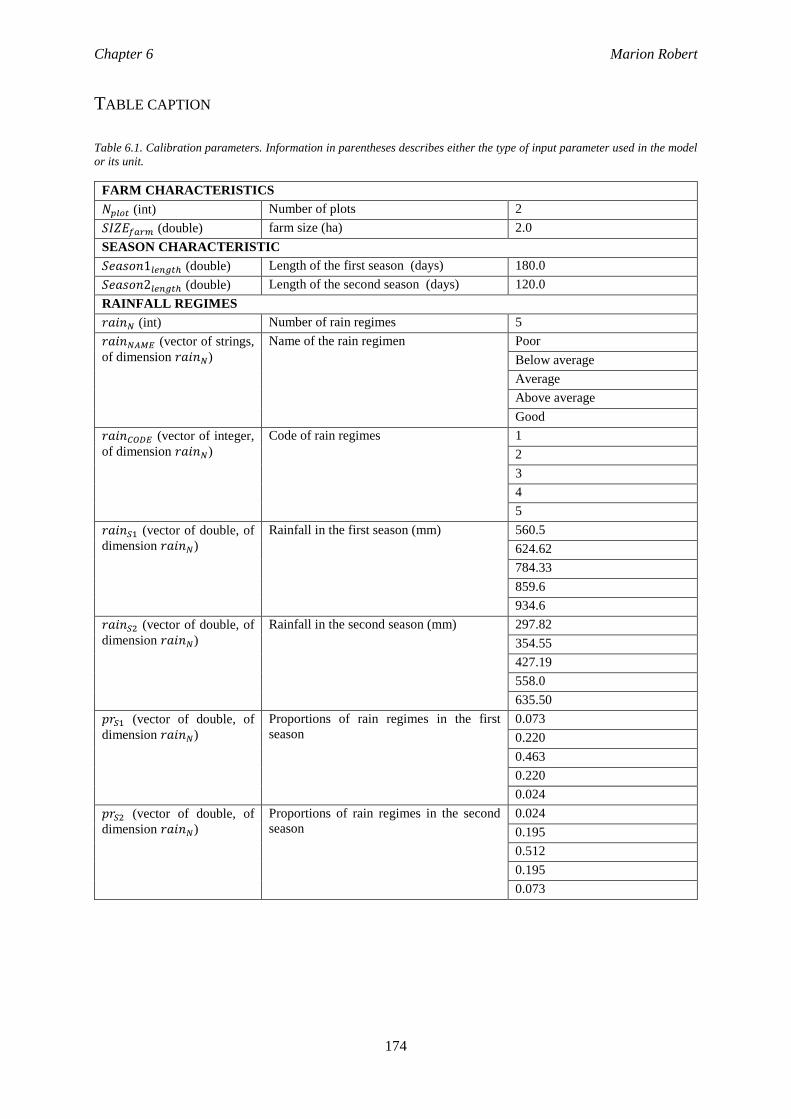
Chapter 6 Marion Robert
174
TABLE CAPTION
Table 6.1. Calibration parameters. Information in parentheses describes either the type of input parameter used in the model
or its unit.
FARM CHARACTERISTICS
𝑁𝑝𝑙𝑜𝑡 (int) Number of plots 2
𝑆𝐼𝑍𝐸𝑓𝑎𝑟𝑚 (double) farm size (ha) 2.0
SEASON CHARACTERISTIC
𝑆𝑒𝑎𝑠𝑜𝑛1𝑙𝑒𝑛𝑔𝑡ℎ (double) Length of the first season (days) 180.0
𝑆𝑒𝑎𝑠𝑜𝑛2𝑙𝑒𝑛𝑔𝑡ℎ (double) Length of the second season (days) 120.0
RAINFALL REGIMES
𝑟𝑎𝑖𝑛𝑁 (int) Number of rain regimes 5
𝑟𝑎𝑖𝑛𝑁𝐴𝑀𝐸 (vector of strings,
of dimension 𝑟𝑎𝑖𝑛𝑁)
Name of the rain regimen Poor
Below average
Average
Above average
Good
𝑟𝑎𝑖𝑛𝐶𝑂𝐷𝐸 (vector of integer,
of dimension 𝑟𝑎𝑖𝑛𝑁)
Code of rain regimes 1
2
3
4
5
𝑟𝑎𝑖𝑛𝑆1 (vector of double, of
dimension 𝑟𝑎𝑖𝑛𝑁)
Rainfall in the first season (mm) 560.5
624.62
784.33
859.6
934.6
𝑟𝑎𝑖𝑛𝑆2 (vector of double, of
dimension 𝑟𝑎𝑖𝑛𝑁)
Rainfall in the second season (mm) 297.82
354.55
427.19
558.0
635.50
𝑝𝑟𝑆1 (vector of double, of
dimension 𝑟𝑎𝑖𝑛𝑁)
Proportions of rain regimes in the first
season
0.073
0.220
0.463
0.220
0.024
𝑝𝑟𝑆2 (vector of double, of
dimension 𝑟𝑎𝑖𝑛𝑁)
Proportions of rain regimes in the second
season
0.024
0.195
0.512
0.195
0.073
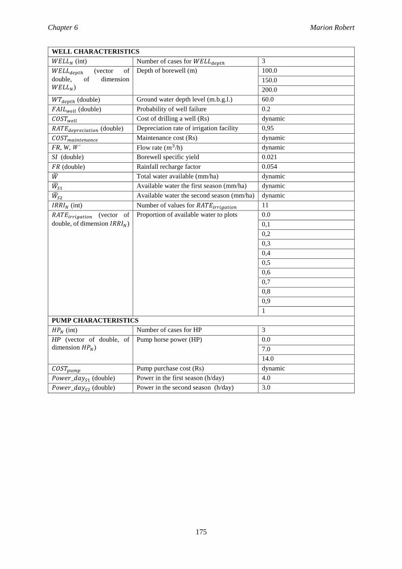
Chapter 6 Marion Robert
175
WELL CHARACTERISTICS
𝑊𝐸𝐿𝐿𝑁 (int) Number of cases for 𝑊𝐸𝐿𝐿𝑑𝑒𝑝𝑡ℎ 3
𝑊𝐸𝐿𝐿𝑑𝑒𝑝𝑡ℎ (vector of
double, of dimension
𝑊𝐸𝐿𝐿𝑁)
Depth of borewell (m) 100.0
150.0
200.0
𝑊𝑇𝑑𝑒𝑝𝑡ℎ (double) Ground water depth level (m.b.g.l.) 60.0
𝐹𝐴𝐼𝐿𝑤𝑒𝑙𝑙 (double) Probability of well failure 0.2
𝐶𝑂𝑆𝑇𝑤𝑒𝑙𝑙 Cost of drilling a well (Rs) dynamic
𝑅𝐴𝑇𝐸𝑑𝑒𝑝𝑟𝑒𝑐𝑖𝑎𝑡𝑖𝑜𝑛 (double) Depreciation rate of irrigation facility 0,95
𝐶𝑂𝑆𝑇𝑚𝑎𝑖𝑛𝑡𝑒𝑛𝑎𝑛𝑐𝑒 Maintenance cost (Rs) dynamic
FR, W, W’ Flow rate (𝑚3/h) dynamic
SI (double) Borewell specific yield 0.021
𝐹𝑅 (double) Rainfall recharge factor 0.054
�� Total water available (mm/ha) dynamic
��𝑆1 Available water the first season (mm/ha) dynamic
��𝑆2 Available water the second season (mm/ha) dynamic
𝐼𝑅𝑅𝐼𝑁 (int) Number of values for 𝑅𝐴𝑇𝐸𝑖𝑟𝑟𝑖𝑔𝑎𝑡𝑖𝑜𝑛 11
𝑅𝐴𝑇𝐸𝑖𝑟𝑟𝑖𝑔𝑎𝑡𝑖𝑜𝑛 (vector of
double, of dimension 𝐼𝑅𝑅𝐼𝑁)
Proportion of available water to plots 0.0
0,1
0,2
0,3
0,4
0,5
0,6
0,7
0,8
0,9
1
PUMP CHARACTERISTICS
𝐻𝑃𝑁 (int) Number of cases for HP 3
HP (vector of double, of
dimension 𝐻𝑃𝑁)
Pump horse power (HP) 0.0
7.0
14.0
𝐶𝑂𝑆𝑇𝑝𝑢𝑚𝑝 Pump purchase cost (Rs) dynamic
𝑃𝑜𝑤𝑒𝑟_𝑑𝑎𝑦𝑆1 (double) Power in the first season (h/day) 4.0
𝑃𝑜𝑤𝑒𝑟_𝑑𝑎𝑦𝑆2 (double) Power in the second season (h/day) 3.0
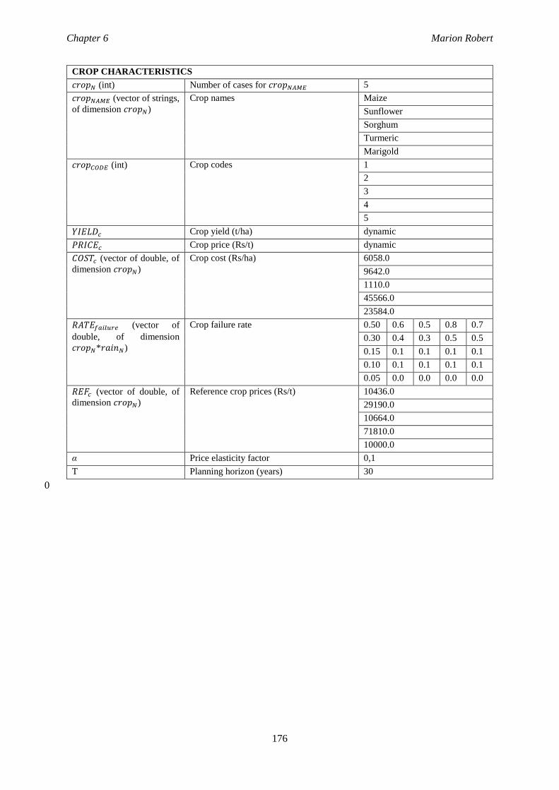
Chapter 6 Marion Robert
176
CROP CHARACTERISTICS
𝑐𝑟𝑜𝑝𝑁 (int) Number of cases for 𝑐𝑟𝑜𝑝𝑁𝐴𝑀𝐸 5
𝑐𝑟𝑜𝑝𝑁𝐴𝑀𝐸 (vector of strings,
of dimension 𝑐𝑟𝑜𝑝𝑁)
Crop names Maize
Sunflower
Sorghum
Turmeric
Marigold
𝑐𝑟𝑜𝑝𝐶𝑂𝐷𝐸 (int) Crop codes 1
2
3
4
5
𝑌𝐼𝐸𝐿𝐷𝑐 Crop yield (t/ha) dynamic
𝑃𝑅𝐼𝐶𝐸𝑐 Crop price (Rs/t) dynamic
𝐶𝑂𝑆𝑇𝑐 (vector of double, of
dimension 𝑐𝑟𝑜𝑝𝑁)
Crop cost (Rs/ha) 6058.0
9642.0
1110.0
45566.0
23584.0
𝑅𝐴𝑇𝐸𝑓𝑎𝑖𝑙𝑢𝑟𝑒 (vector of
double, of dimension
𝑐𝑟𝑜𝑝𝑁*𝑟𝑎𝑖𝑛𝑁)
Crop failure rate 0.50 0.6
0
0.5
0
0.8
0
0.7
0 0.30 0.4
0
0.3
0
0.5
0
0.5
0 0.15 0.1
5
0.1
5
0.1
5
0.1
5 0.10 0.1
0
0.1
0
0.1
0
0.1
0 0.05 0.0
5
0.0
5
0.0
5
0.0
5 𝑅𝐸𝐹𝑐 (vector of double, of
dimension 𝑐𝑟𝑜𝑝𝑁)
Reference crop prices (Rs/t) 10436.0
29190.0
10664.0
71810.0
10000.0
α Price elasticity factor 0,1
T Planning horizon (years) 30
0
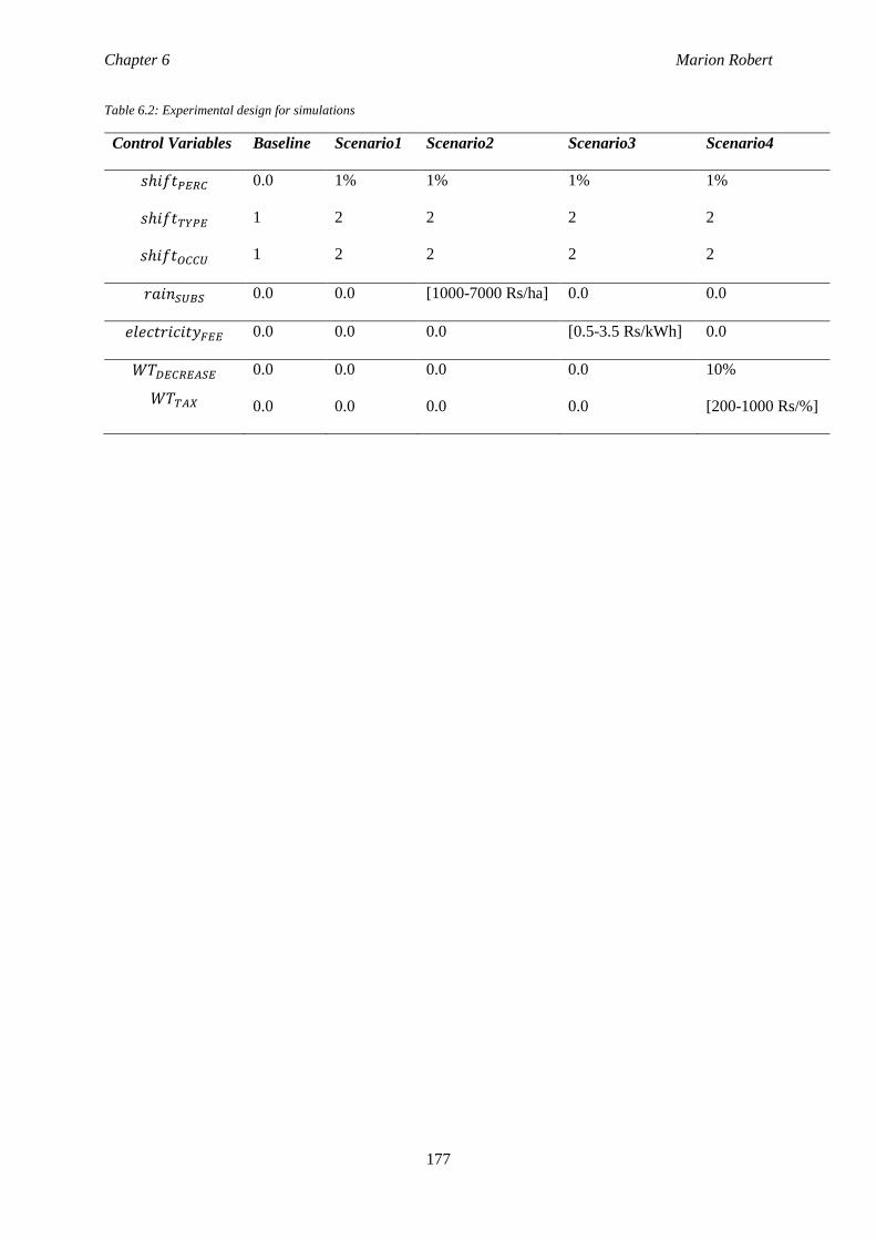
Chapter 6 Marion Robert
177
Ch
ap
ter 6
Mario
n R
obert
Table 6.2: Experimental design for simulations
Control Variables Baseline Scenario1 Scenario2 Scenario3 Scenario4
𝑠ℎ𝑖𝑓𝑡𝑃𝐸𝑅𝐶
𝑠ℎ𝑖𝑓𝑡𝑇𝑌𝑃𝐸
𝑠ℎ𝑖𝑓𝑡𝑂𝐶𝐶𝑈
0.0
1
1
1%
2
2
1%
2
2
1%
2
2
1%
2
2
𝑟𝑎𝑖𝑛𝑆𝑈𝐵𝑆 0.0 0.0 [1000-7000 Rs/ha] 0.0 0.0
𝑒𝑙𝑒𝑐𝑡𝑟𝑖𝑐𝑖𝑡𝑦𝐹𝐸𝐸 0.0 0.0 0.0 [0.5-3.5 Rs/kWh] 0.0
𝑊𝑇𝐷𝐸𝐶𝑅𝐸𝐴𝑆𝐸
𝑊𝑇𝑇𝐴𝑋
0.0
0.0
0.0
0.0
0.0
0.0
0.0
0.0
10%
[200-1000 Rs/%]
Chapter 6 Marion Robert
178
Ch
ap
ter 6
Mario
n R
obert
FIGURE CAPTION
Figure 6.1: Baseline scenario over the planning horizon (30 years): A) groundwater level, B) farmer
profit and C) relative crop area in kharif (irrigated maize replaces irrigated sunflower in rabi) (blue
columns indicate investment years).
Figure 6.2: Climate change scenario: A) groundwater level, B) farmer profit and C) relative crop area
in kharif (irrigated maize replaces irrigated sunflower in rabi) (blue columns indicate investment
years).
Figure 6.3: Climate change and subsidized rainfed crops scenario: A) groundwater level, B) farmer
profit, C) relative crop area in kharif for 7,000 Rs of subsidies D) relative crop area in kharif for
4,000 Rs of subsidies and E) relative crop area in kharif for 1,000 Rs of subsidies (irrigated maize
replaces irrigated sunflower in rabi) (blue columns indicate investment years).
Figure 6.4: Climate change and power supply fee scenario: A) groundwater level, B) farmer profit, C)
relative crop area in kharif for 3.50 Rs/kWh of fee D) relative crop area in kharif for 2.00 Rs/kWh
of fee and E) relative crop area in kharif for 0.50 Rs/kWh of fee (irrigated maize replaces irrigated
sunflower in rabi) (blue columns indicate investment years).
Figure 6.5: Climate change and water tax based on groundwater level: A) groundwater level, B) farmer
profit, C) relative crop area in kharif for 1000 Rs/% of tax D) relative crop area in kharif for 600
Rs/% of tax and E) relative crop area in kharif for 200 Rs/% of tax (irrigated maize replaces
irrigated sunflower in rabi) (blue columns indicate investment years).
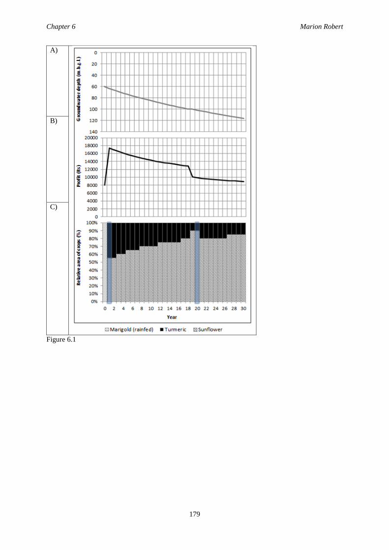
Chapter 6 Marion Robert
179
Ch
ap
ter 6
Mario
n R
obert
A)
B)
C)
Figure 6.1
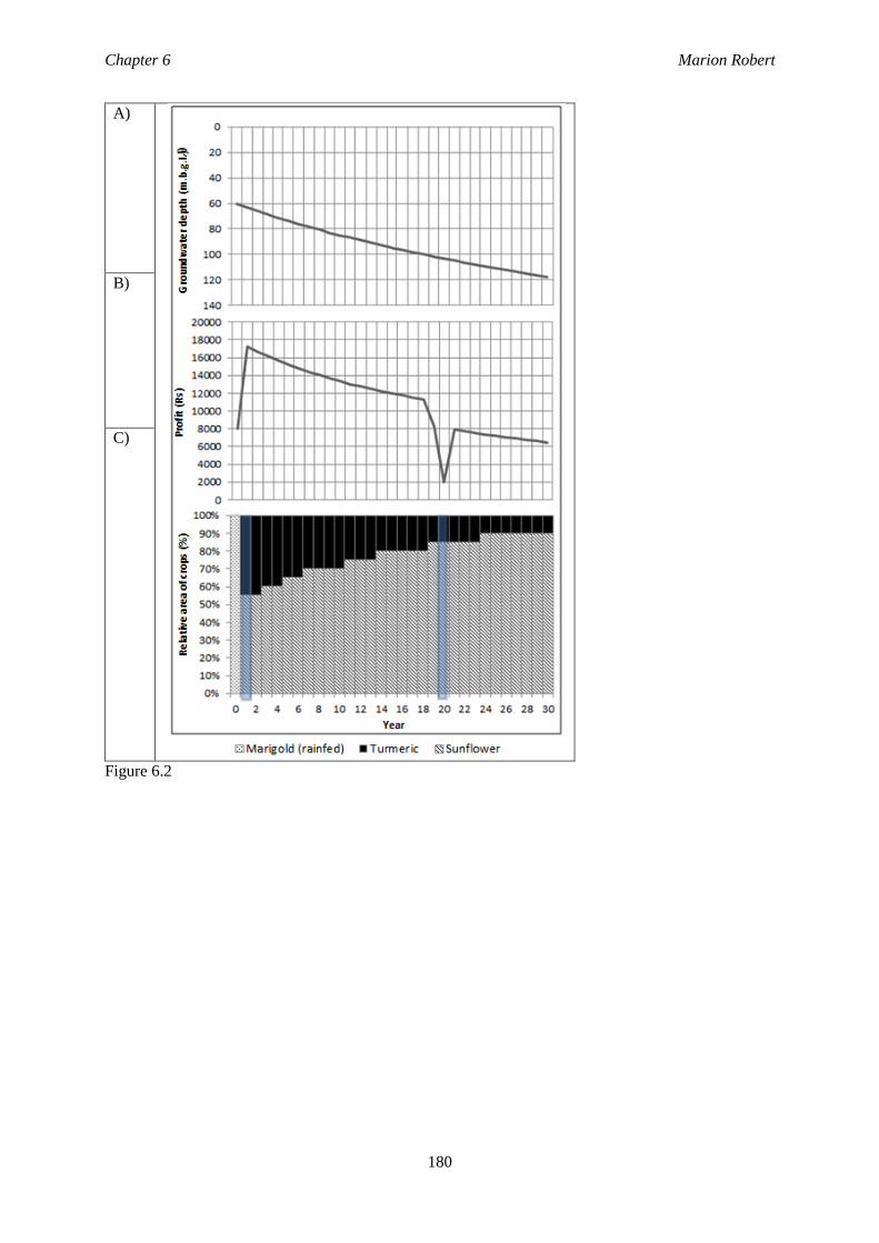
Chapter 6 Marion Robert
180
Ch
ap
ter 6
Mario
n R
obert
A)
B)
C)
Figure 6.2
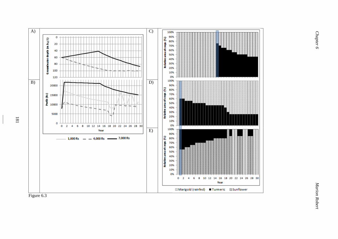
Chapter 6
M
ario
n R
obert
181
A)
C)
B)
D)
E)
Figure 6.3
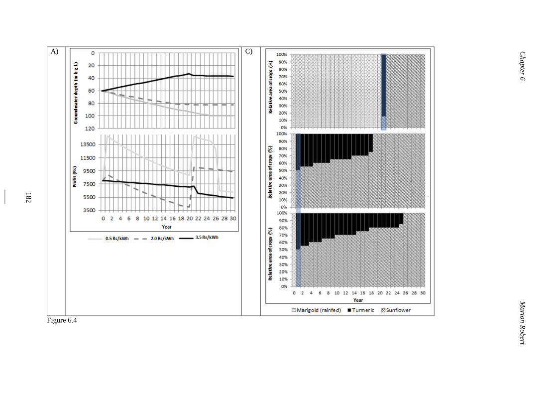
Chapter 6
M
ario
n R
obert
182
A)
C)
Figure 6.4
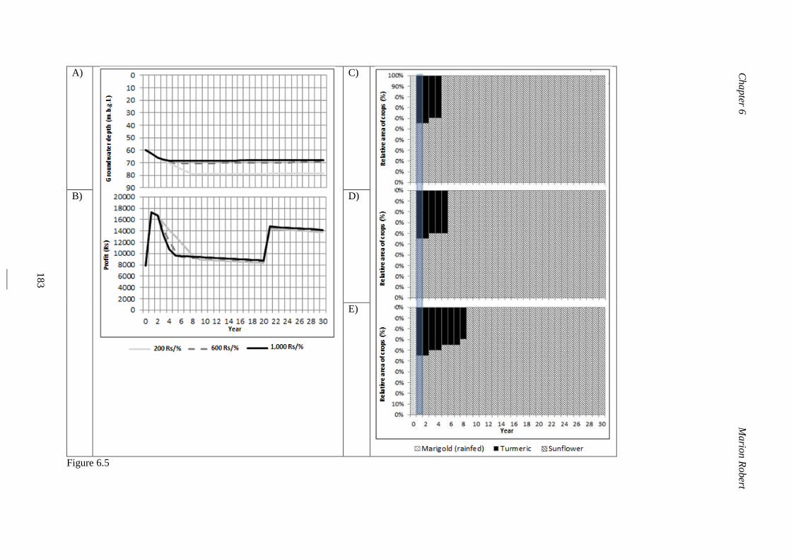
Chapter 6
M
ario
n R
obert
183
A)
C)
B)
D)
E)
Figure 6.5

Chapter 7 Marion Robert
185
Chapter 7
NAMASTE: a dynamic model for
water management at the farm level
integrating strategic, tactical and
operational decisions
Marion Robert∗1, Alban Thomas2, Muddu Sekhar3,4, Hélène Raynal5, Éric Casellas5, Pierre Casel1,
Patrick Chabrier5, Alexandre Joannon6 and Jacques-Éric Bergez1
1 INRA, Université Fédérale de Toulouse, UMR 1248 AGIR, F-31326 Castanet-Tolosan, France
2INRA, Toulouse School of Economics, UMR 1081 LERNA, F-31000 Toulouse, France
3Indian Institute of Sciences, Department of Civil Engineering, Bangalore 560012, India
4Indo-French Cell of Water Sciences, IRD-IISc, Bangalore, India
5INRA, UR 0875 MIAT, F-31326 Castanet-Tolosan, France
6INRA, UR 0980 SAD-PAYSAGE, F-35042 Rennes, France
Submitted to Environmental Modelling & Software
Scientific paper
Version: January 3rd, 2017
∗ Corresponding author: ([email protected])
Chapter 7 Marion Robert
186
Ch
ap
ter 7
Mario
n R
obert
Farming systems are complex and have several dimensions that interact in a dynamic and continuous
manner depending on farmers’ management strategies. This complexity peaks in Indian semi-arid
regions, where small farms encounter a highly competitive environment for markets and resources,
especially unreliable access to water from rainfall and irrigation. NAMASTE, a dynamic computer
model for water management at the farm level, was developed to reproduce interactions between
decisions (investment and technical) and processes (resource management and biophysical) under
scenarios of climate-change, socio-economic and water-management policies. The most relevant and
novel aspects are i) system-based representation of farming systems, ii) description of dynamic
processes via management flexibility and adaptation, iii) representation of farmers’ decision-making
processes at multiple temporal and spatial scales, iv) management of shared resources. NAMASTE’s
ability to simulate farmers’ adaptive decision-making processes is illustrated by simulating a virtual
Indian village composed of two virtual farms with access to groundwater.
Keywords: farmer’s decision-making process, adaptation, modeling, climate change, water management
policy
Chapter 7 Marion Robert
187
Ch
ap
ter 7
Mario
n R
obert
7.1. INTRODUCTION
Agriculture faces many challenges regarding its productivity, revenue and environmental and health
impacts, challenges that must be considered within the known context of climate change. Agriculture
also faces demands to increase the quantity, quality, accessibility and availability of production to secure
food production and improve product quality to address needs of the world’s growing population
(Meynard et al. 2012; Hertel 2015; McKenzie and Williams 2015). Agricultural productivity must
increase within a framework of environmental and health concerns. To do so, agriculture should
decrease its environmental impacts on water, air, soil and aquatic environments and consider the scarcity
of resources such as water, phosphorus and fossil fuels (especially for production of nitrogen fertilizers)
(FAO 2011; Brown et al. 2015). Under climate change, warmer temperatures, changes in rainfall
patterns and increased frequency of extreme weather are expected to occur. Consequently, it has direct,
biophysical effects on agricultural production and can negatively affect crop yields and livestock
(Nelson et al. 2014). Rising sea-level will increase risks of flooding of agricultural land in coastal
regions, while changes in rainfall patterns could increase growth of weeds, pests and diseases (De
Lapeyre de Bellaire et al. 2016).
On the Deccan Plateau in India, the countryside has witnessed the proliferation of individual, electrical
pump-driven borewells that abstract water from underground aquifers (Sekhar et al. 2006; Javeed et al.
2009). The low productivity of the aquifer (Dewandel et al. 2010; Perrin et al. 2011) and a rapid decline
in the water table level has decreased borewell yields (Ruiz et al. 2015), indicating that (groundwater)
irrigated agriculture still largely depends on rainfall. For a region that depends largely on monsoon and
winter rainfall to maintain agricultural production, any shift in climate would have a severe impact on
natural resources and the economy. Drilling borewells to gain control over water access is crucial to
maintain household sustainability; however, it also entails the risk of failed borewells and intractable
debts (Taylor 2013).
Modeling and quantifying spatio-temporal variability in water resources and interactions among
groundwater, agricultural practices and crop growth is an essential component of integrated and
comprehensive water resource management (Ruiz et al. 2015). Simulating scenarios of climate change
and water management policies is an essential tool to identify mechanisms that farmers can use and
policies that can be implemented to address these challenges (White et al. 2015). In these modeling and
simulation approaches, farmers’ decision-making processes should be considered to assess how
agricultural production systems change and adapt to external changes and opportunities. Farm
management requires farmers to make a set of interconnected and successive decisions over time and at
multiple spatial scales (Risbey et al. 1999; Le Gal et al. 2011). In the long term, farmers decide on
possible investments and marketing strategies to select or adapt to best fulfill their objectives. Decisions
about cropping systems also impact the farm. Decisions about crop rotation and allocation are
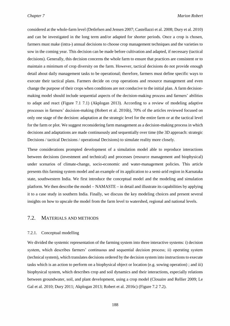
Chapter 7 Marion Robert
188
Ch
ap
ter 7
Mario
n R
obert
considered at the whole-farm level (Detlefsen and Jensen 2007; Castellazzi et al. 2008; Dury et al. 2010)
and can be investigated in the long term and/or adapted for shorter periods. Once a crop is chosen,
farmers must make (intra-) annual decisions to choose crop management techniques and the varieties to
sow in the coming year. This decision can be made before cultivation and adapted, if necessary (tactical
decisions). Generally, this decision concerns the whole farm to ensure that practices are consistent or to
maintain a minimum of crop diversity on the farm. However, tactical decisions do not provide enough
detail about daily management tasks to be operational; therefore, farmers must define specific ways to
execute their tactical plans. Farmers decide on crop operations and resource management and even
change the purpose of their crops when conditions are not conducive to the initial plan. A farm decision-
making model should include sequential aspects of the decision-making process and farmers’ abilities
to adapt and react (Figure 7.1 7.1) (Akplogan 2013). According to a review of modeling adaptive
processes in farmers’ decision-making (Robert et al. 2016b), 70% of the articles reviewed focused on
only one stage of the decision: adaptation at the strategic level for the entire farm or at the tactical level
for the farm or plot. We suggest reconsidering farm management as a decision-making process in which
decisions and adaptations are made continuously and sequentially over time (the 3D approach: strategic
Decisions / tactical Decisions / operational Decisions) to simulate reality more closely.
These considerations prompted development of a simulation model able to reproduce interactions
between decisions (investment and technical) and processes (resource management and biophysical)
under scenarios of climate-change, socio-economic and water-management policies. This article
presents this farming system model and an example of its application to a semi-arid region in Karnataka
state, southwestern India. We first introduce the conceptual model and the modeling and simulation
platform. We then describe the model NAMASTE in detail and illustrate its capabilities by applying
it to a case study in southern India. Finally, we discuss the key modeling choices and present several
insights on how to upscale the model from the farm level to watershed, regional and national levels.
7.2. MATERIALS AND METHODS
7.2.1. Conceptual modelling
We divided the systemic representation of the farming system into three interactive systems: i) decision
system, which describes farmers’ continuous and sequential decision process; ii) operating system
(technical system), which translates decisions ordered by the decision system into instructions to execute
tasks which is an action to perform on a biophysical object or location (e.g. sowing operation) ; and iii)
biophysical system, which describes crop and soil dynamics and their interactions, especially relations
between groundwater, soil, and plant development, using a crop model (Clouaire and Rellier 2009; Le
Gal et al. 2010; Dury 2011; Akplogan 2013; Robert et al. 2016c) (Figure 7.2 7.2).
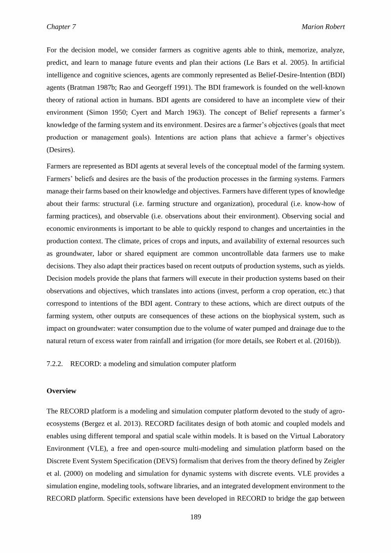
Chapter 7 Marion Robert
189
Ch
ap
ter 7
Mario
n R
obert
For the decision model, we consider farmers as cognitive agents able to think, memorize, analyze,
predict, and learn to manage future events and plan their actions (Le Bars et al. 2005). In artificial
intelligence and cognitive sciences, agents are commonly represented as Belief-Desire-Intention (BDI)
agents (Bratman 1987b; Rao and Georgeff 1991). The BDI framework is founded on the well-known
theory of rational action in humans. BDI agents are considered to have an incomplete view of their
environment (Simon 1950; Cyert and March 1963). The concept of Belief represents a farmer’s
knowledge of the farming system and its environment. Desires are a farmer’s objectives (goals that meet
production or management goals). Intentions are action plans that achieve a farmer’s objectives
(Desires).
Farmers are represented as BDI agents at several levels of the conceptual model of the farming system.
Farmers’ beliefs and desires are the basis of the production processes in the farming systems. Farmers
manage their farms based on their knowledge and objectives. Farmers have different types of knowledge
about their farms: structural (i.e. farming structure and organization), procedural (i.e. know-how of
farming practices), and observable (i.e. observations about their environment). Observing social and
economic environments is important to be able to quickly respond to changes and uncertainties in the
production context. The climate, prices of crops and inputs, and availability of external resources such
as groundwater, labor or shared equipment are common uncontrollable data farmers use to make
decisions. They also adapt their practices based on recent outputs of production systems, such as yields.
Decision models provide the plans that farmers will execute in their production systems based on their
observations and objectives, which translates into actions (invest, perform a crop operation, etc.) that
correspond to intentions of the BDI agent. Contrary to these actions, which are direct outputs of the
farming system, other outputs are consequences of these actions on the biophysical system, such as
impact on groundwater: water consumption due to the volume of water pumped and drainage due to the
natural return of excess water from rainfall and irrigation (for more details, see Robert et al. (2016b)).
7.2.2. RECORD: a modeling and simulation computer platform
Overview
The RECORD platform is a modeling and simulation computer platform devoted to the study of agro-
ecosystems (Bergez et al. 2013). RECORD facilitates design of both atomic and coupled models and
enables using different temporal and spatial scale within models. It is based on the Virtual Laboratory
Environment (VLE), a free and open-source multi-modeling and simulation platform based on the
Discrete Event System Specification (DEVS) formalism that derives from the theory defined by Zeigler
et al. (2000) on modeling and simulation for dynamic systems with discrete events. VLE provides a
simulation engine, modeling tools, software libraries, and an integrated development environment to the
RECORD platform. Specific extensions have been developed in RECORD to bridge the gap between
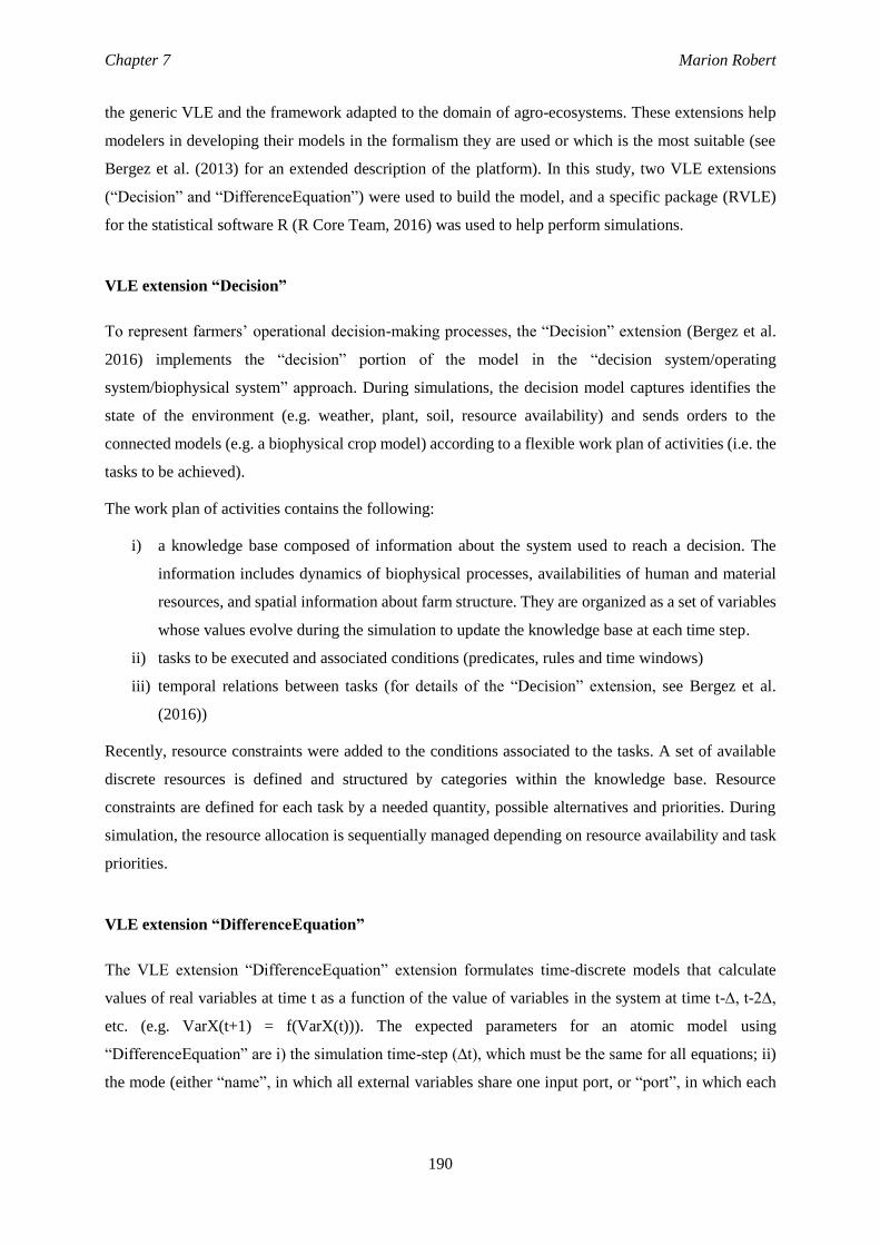
Chapter 7 Marion Robert
190
Ch
ap
ter 7
Mario
n R
obert
the generic VLE and the framework adapted to the domain of agro-ecosystems. These extensions help
modelers in developing their models in the formalism they are used or which is the most suitable (see
Bergez et al. (2013) for an extended description of the platform). In this study, two VLE extensions
(“Decision” and “DifferenceEquation”) were used to build the model, and a specific package (RVLE)
for the statistical software R (R Core Team, 2016) was used to help perform simulations.
VLE extension “Decision”
To represent farmers’ operational decision-making processes, the “Decision” extension (Bergez et al.
2016) implements the “decision” portion of the model in the “decision system/operating
system/biophysical system” approach. During simulations, the decision model captures identifies the
state of the environment (e.g. weather, plant, soil, resource availability) and sends orders to the
connected models (e.g. a biophysical crop model) according to a flexible work plan of activities (i.e. the
tasks to be achieved).
The work plan of activities contains the following:
i) a knowledge base composed of information about the system used to reach a decision. The
information includes dynamics of biophysical processes, availabilities of human and material
resources, and spatial information about farm structure. They are organized as a set of variables
whose values evolve during the simulation to update the knowledge base at each time step.
ii) tasks to be executed and associated conditions (predicates, rules and time windows)
iii) temporal relations between tasks (for details of the “Decision” extension, see Bergez et al.
(2016))
Recently, resource constraints were added to the conditions associated to the tasks. A set of available
discrete resources is defined and structured by categories within the knowledge base. Resource
constraints are defined for each task by a needed quantity, possible alternatives and priorities. During
simulation, the resource allocation is sequentially managed depending on resource availability and task
priorities.
VLE extension “DifferenceEquation”
The VLE extension “DifferenceEquation” extension formulates time-discrete models that calculate
values of real variables at time t as a function of the value of variables in the system at time t-∆, t-2∆,
etc. (e.g. VarX(t+1) = f(VarX(t))). The expected parameters for an atomic model using
“DifferenceEquation” are i) the simulation time-step (∆t), which must be the same for all equations; ii)
the mode (either “name”, in which all external variables share one input port, or “port”, in which each
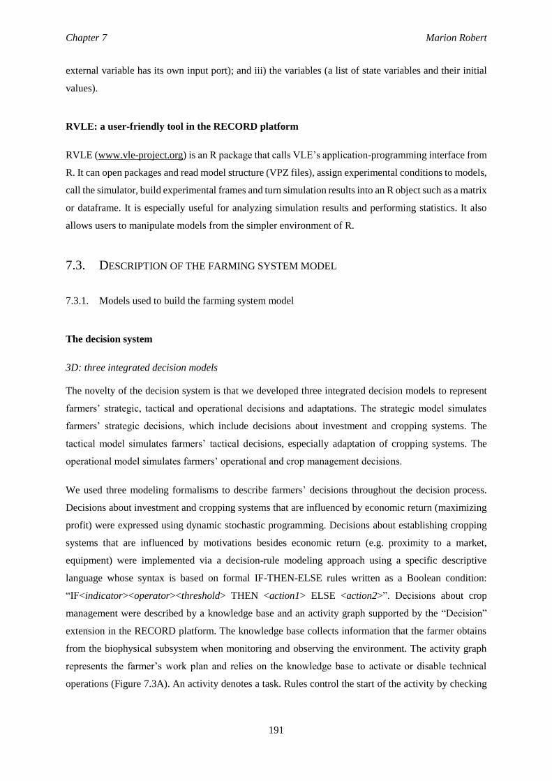
Chapter 7 Marion Robert
191
Ch
ap
ter 7
Mario
n R
obert
external variable has its own input port); and iii) the variables (a list of state variables and their initial
values).
RVLE: a user-friendly tool in the RECORD platform
RVLE (www.vle-project.org) is an R package that calls VLE’s application-programming interface from
R. It can open packages and read model structure (VPZ files), assign experimental conditions to models,
call the simulator, build experimental frames and turn simulation results into an R object such as a matrix
or dataframe. It is especially useful for analyzing simulation results and performing statistics. It also
allows users to manipulate models from the simpler environment of R.
7.3. DESCRIPTION OF THE FARMING SYSTEM MODEL
7.3.1. Models used to build the farming system model
The decision system
3D: three integrated decision models
The novelty of the decision system is that we developed three integrated decision models to represent
farmers’ strategic, tactical and operational decisions and adaptations. The strategic model simulates
farmers’ strategic decisions, which include decisions about investment and cropping systems. The
tactical model simulates farmers’ tactical decisions, especially adaptation of cropping systems. The
operational model simulates farmers’ operational and crop management decisions.
We used three modeling formalisms to describe farmers’ decisions throughout the decision process.
Decisions about investment and cropping systems that are influenced by economic return (maximizing
profit) were expressed using dynamic stochastic programming. Decisions about establishing cropping
systems that are influenced by motivations besides economic return (e.g. proximity to a market,
equipment) were implemented via a decision-rule modeling approach using a specific descriptive
language whose syntax is based on formal IF-THEN-ELSE rules written as a Boolean condition:
“IF<indicator><operator><threshold> THEN <action1> ELSE <action2>”. Decisions about crop
management were described by a knowledge base and an activity graph supported by the “Decision”
extension in the RECORD platform. The knowledge base collects information that the farmer obtains
from the biophysical subsystem when monitoring and observing the environment. The activity graph
represents the farmer’s work plan and relies on the knowledge base to activate or disable technical
operations (Figure 7.3A). An activity denotes a task. Rules control the start of the activity by checking
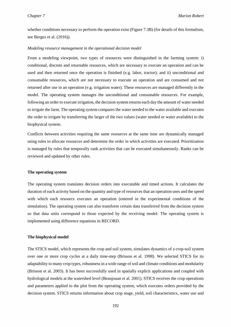
Chapter 7 Marion Robert
192
Ch
ap
ter 7
Mario
n R
obert
whether conditions necessary to perform the operation exist (Figure 7.3B) (for details of this formalism,
see Bergez et al. (2016)).
Modeling resource management in the operational decision model
From a modeling viewpoint, two types of resources were distinguished in the farming system: i)
conditional, discrete and returnable resources, which are necessary to execute an operation and can be
used and then returned once the operation is finished (e.g. labor, tractor); and ii) unconditional and
consumable resources, which are not necessary to execute an operation and are consumed and not
returned after use in an operation (e.g. irrigation water). These resources are managed differently in the
model. The operating system manages the unconditional and consumable resources. For example,
following an order to execute irrigation, the decision system returns each day the amount of water needed
to irrigate the farm. The operating system compares the water needed to the water available and executes
the order to irrigate by transferring the larger of the two values (water needed or water available) to the
biophysical system.
Conflicts between activities requiring the same resources at the same time are dynamically managed
using rules to allocate resources and determine the order in which activities are executed. Prioritization
is managed by rules that temporally rank activities that can be executed simultaneously. Ranks can be
reviewed and updated by other rules.
The operating system
The operating system translates decision orders into executable and timed actions. It calculates the
duration of each activity based on the quantity and type of resources that an operation uses and the speed
with which each resource executes an operation (entered in the experimental conditions of the
simulation). The operating system can also transform certain data transferred from the decision system
so that data units correspond to those expected by the receiving model. The operating system is
implemented using difference equations in RECORD.
The biophysical model
The STICS model, which represents the crop and soil system, simulates dynamics of a crop-soil system
over one or more crop cycles at a daily time-step (Brisson et al. 1998). We selected STICS for its
adaptability to many crop types, robustness in a wide range of soil and climate conditions and modularity
(Brisson et al. 2003). It has been successfully used in spatially explicit applications and coupled with
hydrological models at the watershed level (Beaujouan et al. 2001). STICS receives the crop operations
and parameters applied to the plot from the operating system, which executes orders provided by the
decision system. STICS returns information about crop stage, yield, soil characteristics, water use and
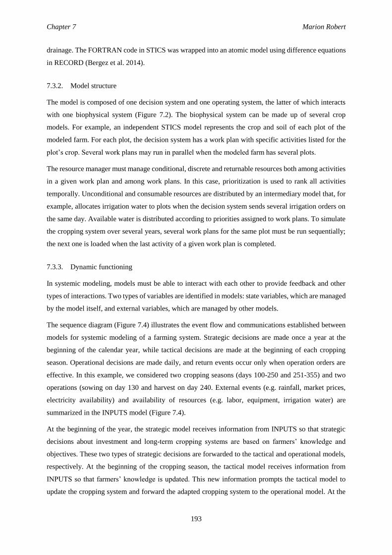
Chapter 7 Marion Robert
193
Ch
ap
ter 7
Mario
n R
obert
drainage. The FORTRAN code in STICS was wrapped into an atomic model using difference equations
in RECORD (Bergez et al. 2014).
7.3.2. Model structure
The model is composed of one decision system and one operating system, the latter of which interacts
with one biophysical system (Figure 7.2). The biophysical system can be made up of several crop
models. For example, an independent STICS model represents the crop and soil of each plot of the
modeled farm. For each plot, the decision system has a work plan with specific activities listed for the
plot’s crop. Several work plans may run in parallel when the modeled farm has several plots.
The resource manager must manage conditional, discrete and returnable resources both among activities
in a given work plan and among work plans. In this case, prioritization is used to rank all activities
temporally. Unconditional and consumable resources are distributed by an intermediary model that, for
example, allocates irrigation water to plots when the decision system sends several irrigation orders on
the same day. Available water is distributed according to priorities assigned to work plans. To simulate
the cropping system over several years, several work plans for the same plot must be run sequentially;
the next one is loaded when the last activity of a given work plan is completed.
7.3.3. Dynamic functioning
In systemic modeling, models must be able to interact with each other to provide feedback and other
types of interactions. Two types of variables are identified in models: state variables, which are managed
by the model itself, and external variables, which are managed by other models.
The sequence diagram (Figure 7.4) illustrates the event flow and communications established between
models for systemic modeling of a farming system. Strategic decisions are made once a year at the
beginning of the calendar year, while tactical decisions are made at the beginning of each cropping
season. Operational decisions are made daily, and return events occur only when operation orders are
effective. In this example, we considered two cropping seasons (days 100-250 and 251-355) and two
operations (sowing on day 130 and harvest on day 240. External events (e.g. rainfall, market prices,
electricity availability) and availability of resources (e.g. labor, equipment, irrigation water) are
summarized in the INPUTS model (Figure 7.4).
At the beginning of the year, the strategic model receives information from INPUTS so that strategic
decisions about investment and long-term cropping systems are based on farmers’ knowledge and
objectives. These two types of strategic decisions are forwarded to the tactical and operational models,
respectively. At the beginning of the cropping season, the tactical model receives information from
INPUTS so that farmers’ knowledge is updated. This new information prompts the tactical model to
update the cropping system and forward the adapted cropping system to the operational model. At the
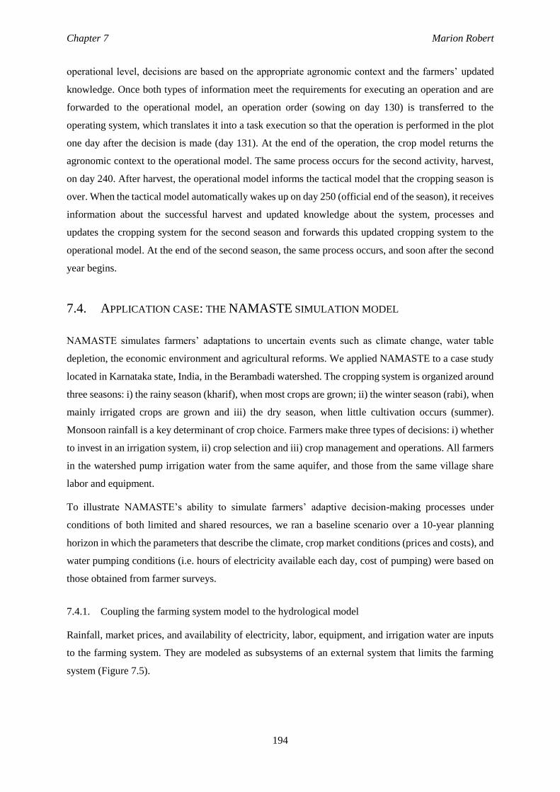
Chapter 7 Marion Robert
194
Ch
ap
ter 7
Mario
n R
obert
operational level, decisions are based on the appropriate agronomic context and the farmers’ updated
knowledge. Once both types of information meet the requirements for executing an operation and are
forwarded to the operational model, an operation order (sowing on day 130) is transferred to the
operating system, which translates it into a task execution so that the operation is performed in the plot
one day after the decision is made (day 131). At the end of the operation, the crop model returns the
agronomic context to the operational model. The same process occurs for the second activity, harvest,
on day 240. After harvest, the operational model informs the tactical model that the cropping season is
over. When the tactical model automatically wakes up on day 250 (official end of the season), it receives
information about the successful harvest and updated knowledge about the system, processes and
updates the cropping system for the second season and forwards this updated cropping system to the
operational model. At the end of the second season, the same process occurs, and soon after the second
year begins.
7.4. APPLICATION CASE: THE NAMASTE SIMULATION MODEL
NAMASTE simulates farmers’ adaptations to uncertain events such as climate change, water table
depletion, the economic environment and agricultural reforms. We applied NAMASTE to a case study
located in Karnataka state, India, in the Berambadi watershed. The cropping system is organized around
three seasons: i) the rainy season (kharif), when most crops are grown; ii) the winter season (rabi), when
mainly irrigated crops are grown and iii) the dry season, when little cultivation occurs (summer).
Monsoon rainfall is a key determinant of crop choice. Farmers make three types of decisions: i) whether
to invest in an irrigation system, ii) crop selection and iii) crop management and operations. All farmers
in the watershed pump irrigation water from the same aquifer, and those from the same village share
labor and equipment.
To illustrate NAMASTE’s ability to simulate farmers’ adaptive decision-making processes under
conditions of both limited and shared resources, we ran a baseline scenario over a 10-year planning
horizon in which the parameters that describe the climate, crop market conditions (prices and costs), and
water pumping conditions (i.e. hours of electricity available each day, cost of pumping) were based on
those obtained from farmer surveys.
7.4.1. Coupling the farming system model to the hydrological model
Rainfall, market prices, and availability of electricity, labor, equipment, and irrigation water are inputs
to the farming system. They are modeled as subsystems of an external system that limits the farming
system (Figure 7.5).
Chapter 7 Marion Robert
195
Ch
ap
ter 7
Mario
n R
obert
Hydrological sub-system
AMBHAS (Tomer 2012) is a spatially explicit groundwater model that simulates dynamics of daily
groundwater level based on equations from McDonald & Harbaugh (1988). It predicts daily groundwater
level, actual net recharge and discharge. Net recharge is predicted from the amount of water drained
below the soil profile and required for crop irrigation predicted by STICS for a 1 ha cell. The PYTHON
code in AMBHAS was wrapped into an atomic model using difference equations in RECORD.
Climate, market and power supply sub-systems
The WEATHER model simulates expected and actual rainfall each day. The MARKET model simulates
expected and actual crop market prices. The ELECTRICITY model simulates the number of hours of
electricity available each day. These sub-models are implemented in an atomic model using difference
equations in RECORD.
7.4.2. NAMASTE simulaton
When resources are shared, interactions are important to an individual farmer’s decision-making
process. To integrate resource constraints into the farming system model, our experimental model
simulates a virtual village composed of two virtual farms that have access to groundwater in the same
AMBHAS cell of 3 ha (Figure 7.5). The first farmer manages 1 ha of land organized into two crop plots
and owns one bullock for cropping operations; the second manages 2 ha of land organized into two crop
plots and owns two bullocks. Neither farmer owns a tractor. On each farm, both the farmer and his wife
work. Both farms can hire labor and rent equipment from the village (i.e. 110 female laborers, 90 male
laborers, 4 bullocks, 1 tractor). Because a borewell can be drilled on each plot, this NAMASTE
simulation consisted of four borewell models. During simulation, the strategic decision model may
change the parameters for pump horsepower and well depth. The net recharge (water drained minus
water pumped) returned to the AMBHAS cell is calculated by an intermediate model that calculates the
difference between total drainage and pumping flows of all plots.
NAMASTE simulation of two farms in one village proceeds as follows. Each farm is simulated by a
decision system, which includes strategic, tactical and operational decision models. NAMASTE
considers farm characteristics (e.g. number of plots, soil type, amount of labor and equipment), crop
management files and initial farm status as initial conditions. The operational decision model manages
the village’s labor and equipment that is used for crop production. It functions as a resource manager
and attributes resources to the first enquirer. The operational model interacts with the operating system,
while the biophysical system has as many STICS models as there are plots in the village. The external
system (i.e. WEATHER, MARKET and ELECTRICITY models) constrains both farms in the same
Chapter 7 Marion Robert
196
Ch
ap
ter 7
Mario
n R
obert
way, and we assume that farmers’ individual or combined decisions do not influence it. The same
AMBHAS cell simulates the irrigation water available to both farms.
At the beginning of the year, in the strategic model, each farmer makes decisions about investment and
the cropping system for the next ten years independent of other farm decisions. Investment in a borewell
determines parameters of the borewell model for each plot. At the beginning of the cropping season, in
the tactical model, each farmer independently updates the cropping system based on new information
on prices, rainfall and groundwater level. This updated cropping system is then entered into the
operational model, which defines the crop rotation and the management of each crop. The operational
model determines when conditions necessary for crop operations are met and requests resources from
its resource manager. Farmers’ practices interact at this level, which means that one farmer’s crop
operations may be restricted by the other’s when both need labor and equipment at the same time.
Irrigation water may also be a source of conflict between farmers, since the water that one farmer
withdraws from the aquifer is no longer available to the other (Figure 7.5).
7.4.3. Calibration and validation
The model was calibrated with data from two farm surveys conducted in the Berambadi watershed.
Farmers on the watershed were surveyed in 2014 and 2015. The first survey targeted 27 farmers to
obtain detailed data about their practices, especially their decisions and how they adapted them. The
second survey targeted 684 farmers to obtain broad data on farm characteristics and the social, economic
and agronomic environments. This survey enabled creation of a typology of farmers on the watershed
based on biophysical factors (e.g. farm location, soil type, groundwater accessibility), economic factors
(e.g. farm size, labor, equipment) and social factors (e.g. castes, family structure, education, off-farm
job) (for more details, see Robert et al. (submitted)). We surveyed seed retailers and village leaders
(panchayats) to learn about recommended crop management practices and village organization.
Additionally, 52 experimental plots were monitored over three years, which provided empirical data on
crop production and management. These data helped supplement the verbal information that farmers
provided during surveys. Meteorological data were obtained from a meteorological station and water
gauges installed on the watershed. Prices and costs were obtained from farmers and official district data
from the Indian Ministry of Agriculture and Cooperation (Directorate of Economics and Statistics) and
the National Informatics Center (Agricultural Census Division).
The model was validated using computerized model verification and operational validation.
Computerized model verification checks whether the computer implementation corresponds to the
conceptual model representation (Whitner and Balci 1986; Sargent 2013). It verifies that the computer
code has no coding errors or computer bugs and that the simulation language is implemented well. We
used two main approaches for computerized model verification: i) static, which tests the main script at
multiple points, allowing for local checks during encoding, and ii) dynamic, which executes the script
Chapter 7 Marion Robert
197
Ch
ap
ter 7
Mario
n R
obert
with several sets of data and experimental conditions to verify the accuracy of outputs. In contrast,
operational validation checks whether the behavior of the final simulation model is accurate enough to
fulfill the research objectives. The model was validated mainly by subjectively exploring its behavior
(Sargent 2013). First, we graphically compared model predictions to observed data, verifying that
predicted yields lay within the ranges of observed yields in the watershed. We also qualitatively analyzed
model behavior, verifying that predicted variables moved in the same directions as observed variables.
For example, we verified that crop choice, management and yield correctly responded to climate
variations; that investment in irrigation corresponded to economic and climate environments; and that
the groundwater table correctly responded to rainfall and irrigation.
7.4.4. Simulation results
Sequential decision making and adaptation at different temporal and spatial scales
To illustrate decision processes and adaptations, we describe the sequential decision-making processes
the first farmer followed to cultivate 1 ha of land (Figure 7.6). At the beginning of the 10-year planning
horizon, the farmer has expectations for the future climate (i.e. percentage chances that a year will have
good, above-average, average, below-average or poor rainfall). Farmers’ expectations for the climate
influence those for socio-economic and hydrological conditions (crop prices and groundwater level,
respectively). Based on these expectations, the farmer plans long-term investment (e.g. adding a
borewell) associated with an optimal cropping system choice (first column, Figure 7.6). At the tactical
level, the farmer knows what kind of climate to expect (i.e. average rainfall) but is uncertain about the
seasonal distribution of rainfall throughout the year. The farmer observes the groundwater level (H) at
the beginning of each year (initially 60 m.b.g.l.; simulated observations in later years come from the
operational decision model) and has expectations for how it will change throughout the year (i.e.
expected H). The farmer reviews the cropping system decision (second column, Figure 7.6) and begins
daily crop operations (operational decisions) (third column, Figure 7.6).
The farmer can adapt crops and/or practices when conditions are not suitable. In the fourth year, which
had below-average rainfall, the farmer adapted crop choice at the tactical level. The farmer, knowing
that low rainfall during the cropping season impacts rainfed crops in particular and observing a
groundwater level much higher (12.4 m higher) than expected at the beginning of the planning horizon,
changed 0.1 ha of rainfed marigold to irrigated sunflower (to go with the 0.9 ha of irrigated tumeric).
In the third year, which had above-average rainfall, the farmer adapted crop choice at the operational
level. The farmer planned to grow 0.9 ha of turmeric and 0.1 ha of marigold. Both crops have similar
sowing windows (30 March1 May) and conditions (rules): soil moisture must be low enough to bear
loads (rule: < 75% of field capacity) but high enough for seeds to germinate (rule: > 60% of field
Chapter 7 Marion Robert
198
Ch
ap
ter 7
Mario
n R
obert
capacity) and rain must not be forecast for two consecutive days (since sowing can last two days) (rule:
total expected rainfall for two consecutive days must not exceed 5 mm). Five days in April (6, 7, 8, 9
and 11) had acceptable soil moisture (60-75% of field capacity), but April’s high rainfall (147 mm)
prevented sowing. Because sowing turmeric and marigold was not possible, the farmer had to review
the cropping plan and sow only maize, which has a wider sowing window (April -June).
In the sixth year, which had above-average rainfall, the farmer adapted practices at the operational level.
Unlike in the third year, turmeric and sunflower could be sown in April; however, frequent rainfall
events after sowing decreased the number of irrigation events planned for turmeric. Four planned
irrigation events were cancelled because irrigation rules recommend irrigating when total rainfall during
the past three days is < 50 mm and < 5 mm of rainfall is expected in the next two days.
Tactical and operational adaptations influenced the groundwater level and the farmer’s profit (Figure
7.7). Due to generally adequate rainfall during the planning horizon (except the 4th, 9th and 10th years),
pumping was lower and recharge was higher than predicted at the strategic level. Thus, the groundwater
level did not decrease as much as expected, and the borewell did not go dry during the planning horizon.
Concerning profit, rainfall induced economically disastrous years (i.e. 3rd and 9th years), by preventing
the farmer’s initial cropping system plan and requiring maize to be sown, or highly profitable years (i.e.
the 6th year), by being above average and well distributed during crop growth. In at least one year (i.e.
the 10th) irrigation was able to compensate for the below-average rainfall and provide a profit.
Resource management: between scarcity and sharing
NAMASTE considers situations in which resources may be limited because they are scarce and limited
and/or used by another farmer. In these conditions, farmers adapt their daily practices, delaying crop
operations until resources become available. Competition for resources can be internal, when operations
occur at the same time in two plots of the same farm, or external, when competition due to another
farmer’s practices.
To illustrate resource management in NAMASTE, we describe management of village resources (female
and male labor, a tractor and bullocks) in the first year of the planning horizon (Figure 7.8). The first
farmer planned to grow turmeric on 0.9 ha with 16 irrigation events and rainfed marigold on 0.1 ha. The
second farmer planned to grow turmeric on 1.6 ha with 12 irrigation events and rainfed marigold on 0.4
ha. Three types of resource conflicts were observed (Figure 7.8):
i) Conflicts over use of the tractor to plow land. Turmeric and marigold plots must be plowed
during the same window (1-23 March) and according to the same conditions (rules). Since
turmeric has a higher priority index than marigold, the resource manager allocates the tractor to
the turmeric plots first (e.g. the first tractor plowing occurs on 10-11 March for turmeric plots
and 15-16 March for marigold plots). Between turmeric plots, the resource is randomly
Chapter 7 Marion Robert
199
Ch
ap
ter 7
Mario
n R
obert
attributed. For example, for turmeric, the first tractor plowing occurs on March 10th on farm 1
and March 11th on farm 2 and the second tractor plowing occurs on March 20th on farm 1 and
on March 21st on farm 2.
ii) Conflicts over use of female labor to weed turmeric (10 April5 September). Since both
turmeric plots were sown on 13 April, they had the same time windows for weeding events (10-
35, 55-65, 85-95 and 115-125 days after sowing). For each weeding event, the first farmer
needed 21 male and 52 female laborers, and the second farmer needed 36 male and 91 female
laborers. Since the village had only 110 female laborers, both farmers could not weed their plots
at the same time. The resource is randomly attributed.
iii) Conflicts over use of both female and male labor to harvest turmeric. The first farmer needed
49 male and 58 female laborers, and the second farmer needed 87 male and 103 female laborers
to harvest their turmeric plots. Since both female and male labor was limited, one of the farmers
had to delay harvest.
7.5. DISCUSSION
Understanding farmers’ decision-making processes and relationships with the biophysical system is
necessary to understand farming system complexity at multiple scales. NAMASTE is a simulation
model able to reproduce interactions between decisions (investment and technical) and processes
(resource management and biophysical) under scenarios of climate-change, socio-economic and water-
management policies. The model has two main innovations: i) its decision model simulates farmers’
decision-making processes by describing dynamic sequential decisions via adaptation to the biophysical
environment and ii) it couples decisional, economic, biophysical and hydrological systems to predict
effects and spillover of human decisions on natural systems.
Research increasingly considers farm management as a flexible and dynamic process. In recent
agricultural literature, however, consequences on long- and short-term farm organization are rarely
considered, even though they appear to influence farmers’ decision-making greatly (Daydé et al. 2014).
We used the basic definition of Le Gal et al. (2011), which divides a decision into a set of interconnected
decisions made over time and at multiple spatial scales. Sequential and dynamic representation is
particularly useful and appropriate for modeling entire processes for making strategic, tactical and
operational decisions (Risbey et al. 1999; Le Gal et al. 2011).
Like many agent-based models that represent a complete system (An 2012), coupling decisional,
economic, biophysical and hydrological models was necessary to model and quantify spatio-temporal
variability in water resources and interactions among groundwater, agricultural practices and crop
growth. One difficulty in modeling these processes is combining independent models that were
originally developed for specific purposes at different spatial and temporal scales (Kraucunas et al.
Chapter 7 Marion Robert
200
Ch
ap
ter 7
Mario
n R
obert
2015). The biophysical model used in NAMASTE was developed to simulate fixed practices such as
sowing, irrigation and harvest on one plot for one cropping season. The hydrological model simulates
groundwater dynamics of a large territory. The decision model describes farmers’ decisions and
practices on their farms. Meaningful model integration requires consistency in the underlying system
boundaries, assumptions and scale of analysis of these diverse models in the global model. As Kling et
al. (2016) suggested, it is necessary to develop “bridge” models that convert outputs of one model into
inputs of another. This approach enables models to be connected at different scales and to operate
together by downscaling outputs from global to local models (e.g. AMBHAS) and by upscaling outputs
from local to global models (e.g. decision and biophysical models). This can ensure that component
models are manageable and provide outputs at both local and global scales (Hibbard and Janetos 2013).
In this study, operational validation was performed mainly by subjectively and qualitatively exploring
model behavior (Sargent 2013). We developed a simulation model able to reproduce interactions
between decisions (investment and technical) and processes (resource management and biophysical)
under scenarios of climate-change, socio-economic and water-management policies. Nonetheless,
quantitative simulation results for the Berambadi case study still have high uncertainty. Calibrating and
validating the global model is an important and time-consuming step that is still underway (94
parameters are directly accessible in the global model, and AMBHAS and STICS have many internal
parameters that require tedious calibration).
Upscaling from the farm level to watershed, regional and national levels is a common approach for
studying system behavior and dynamics, such as farm adaptations to climate change (Gibbons et al.
2010), land use and land cover changes in response to climate change (Rounsevell et al. 2014) and
ecosystem changes in response to biotic and abiotic processes (Nash et al. 2014). Peters et al. (2007)
identified three types of scales: “fine” (one individual), “intermediate” (groups of individuals) and
“broad” (large spatial extents such as the landscape, region and planet). The appropriate scale is defined
by the research question or hypothesis and often requires upscaling or downscaling existing models
(Gibbons et al. 2010). We consider the upscaling issue from the perspective of modeling consequences
of farmers’ adaptations to changes in climate and groundwater. The challenge of aggregation or
upscaling is to determine which fine-scale details matter most at intermediate or broad scales. Research
questions differ according to the scale. At the farm scale, we focused on farmers’ decision-making
processes and their adaptation to uncertain changes (e.g. climate and resource availability). The
watershed level requires exploring the influence of decision making on the groundwater table rather
than the process of decision making itself and to consider interactions between individuals for shared
resources. At the watershed level, relative trends are more important than absolute values. For example,
at the watershed level we are more interested in the total amount of groundwater used for irrigation in
the watershed than on individual farms.
Chapter 7 Marion Robert
201
Ch
ap
ter 7
Mario
n R
obert
Our model provides tools to analyze, evaluate, and optimize agronomic, environmental and economic
criteria. We tested the model with a baseline scenario to simulate current farming practices in the
Berambadi watershed and predict influence of the latter on groundwater level in a virtual village
composed of two farms. Modeling agricultural production scenarios can help stakeholders make
decisions about regulations and resource restrictions and encourage new practices to recommend to
farmers.
7.6. CONCLUSION
We developed an original simulation model of a farming system that combines relevant principles
highlighted in the scientific literature. The model was initially developed to address critical issues of
groundwater depletion and farming practices in a watershed in southwestern India. Its structure,
frameworks and formalisms can be applied to other agricultural contexts. Our application focused on
water management in semi-arid agricultural systems, but the model can also be applied to other farming
systems to confirm the reusability and robustness of the framework.

Chapter 7 Marion Robert
202
Ch
ap
ter 7
Mario
n R
obert
ACKNOWLEDGEMENTS
This study was funded by the Indo-French Centre for the Promotion of Advanced Research (CEFIPRA),
the INRA flagship program on Adaptation of Agriculture and Forests to Climate Change (AAFCC), the
Doctoral School of the University of Toulouse (EDT) and the Observatory for Environment Research
“Experimental Tropical Watersheds” (ORE BVET, http://bvet.obs-mip.fr). We are grateful to all the
experts, farmers, survey takers and trainees who helped implement the method. We give special thanks
to Tony Raveneau for his help with the computer implementation.
Chapter 7 Marion Robert
203
Ch
ap
ter 7
Mario
n R
obert
FIGURE CAPTION
Figure 7.1. Representation of farmers’ decision-making processes at multiple temporal and spatial
scales, indicating processes to adjust farm management to the farm environment.
Figure 7.2. Conceptual representation of the farming system based on integration of three systems.
Based on knowledge, farmers make decisions that the operating system translates into executable
actions. These actions modify the state of the biophysical system. Specific outputs for irrigation
management provide information about water consumption and natural drainage of groundwater.
Figure 7.3. A) Activity plan of the sequence of sorghum operations created with the decision extension.
B) Rules and associated predicates for the activity plan of the sequence of sorghum operations.
Figure 7.4. Sequence diagram of the event flow in systemic modeling of the farming system. We
considered two cropping seasons (days 100-250 and 251-355) and two operations (sowing order on day
130 and harvest order on day 240. O.S. = operating system, LT = long-term
Figure 7.5. NAMASTE model: a virtual village composed of two virtual farms (F1 and F2), each having
access to ground water on the same AMBHAS cell. Each farm is simulated by two individual DEVS
atomic decision model (strategic and tactic) and a common operational decision model using the VLE
decision extension of RECORD that describes individual operational decisions for the whole village.
The WEATHER model, the MARKET model and the ELECTRICITY model constrain the same way
both farms. Farm 1 contains two plots P1 and P2, Farm 2 contains two plots P1 and P2. GW =
groundwater, HP = horsepower
Figure 7.6. Decisions and adaptations of one farmer during the 10-year planning horizon (each line
describes one year). The first column describes the farmer’s strategic decisions about investment in
irrigation. The second column describes the farmer’s tactical decisions and adaptations at the beginning
of each year after observing the weather and the groundwater level. The third column describes the
farmer’s operational decisions about and adaptations to crop choice and irrigation after observing daily
rainfall. Numbers in brackets indicate the number of irrigation events for each crop. CS = cropping
system, π = profit, Rs = Indian rupees, H = groundwater level, m.b.g.l. = meters below ground level.
Figure 7.7. Groundwater level and profit of one farmer during the 10-year planning horizon –
comparison of expected values at the strategic level (optimal profit and expected groundwater level from
strategic decisions) and final values at the operational level. H = groundwater level, m.b.g.l. = meters
below ground level, Rs = Indian rupees (bleu drops describe rainfall types: 1 drop is poor rainfall, 2
drops is below-average rainfall, 3 drops is average rainfall, 4 drops is above-average rainfall, 5 drops is
good rainfall).
Figure 7.8. Resource management in a village composed of two farms – example of available (in %)
village resources (female and male labor, bullocks and tractor) during the first year of the planning

Chapter 7 Marion Robert
204
Ch
ap
ter 7
Mario
n R
obert
horizon. Three conflicts are identified (1, 2, 3). Activities of one farm were postponed when resource
conflicts occurred.
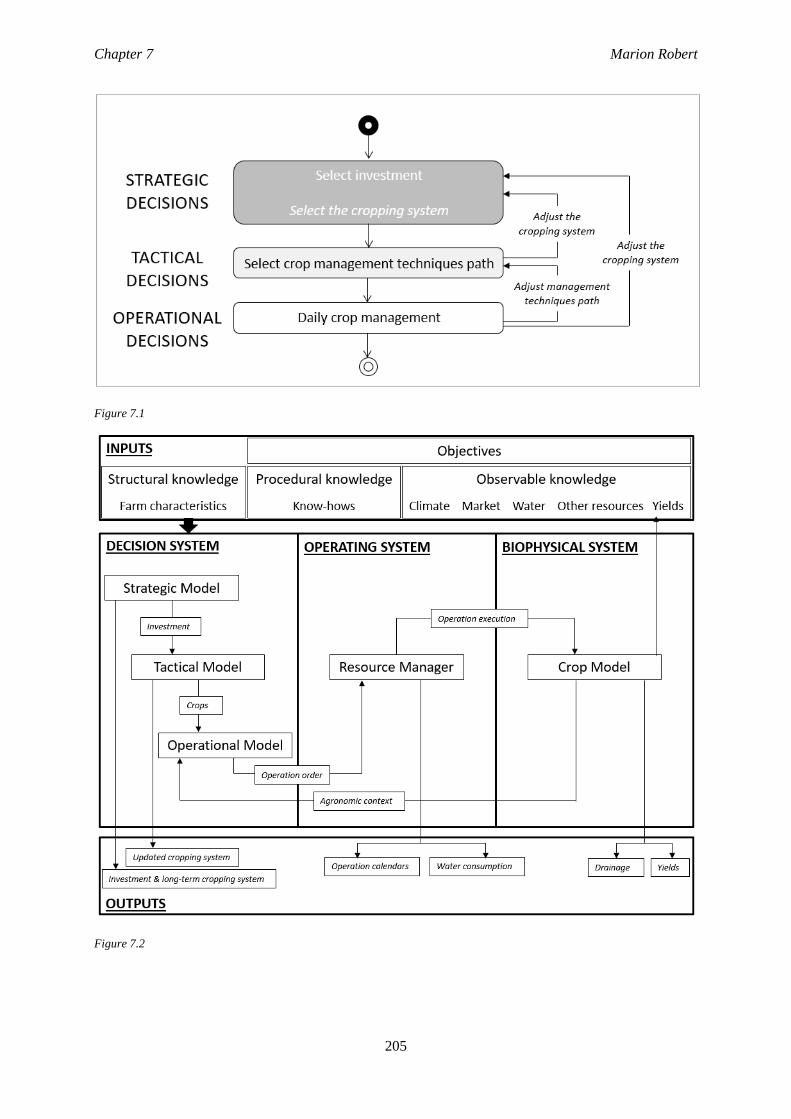
Chapter 7 Marion Robert
205
Ch
ap
ter 7
Mario
n R
obert
Figure 7.1
Figure 7.2
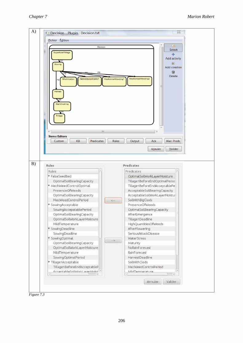
Chapter 7 Marion Robert
206
Ch
ap
ter 7
Mario
n R
obert
A)
B)
Figure 7.3
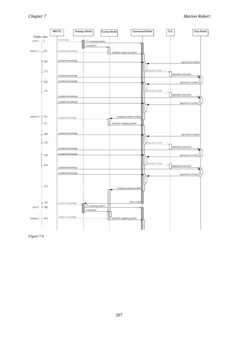
Chapter 7 Marion Robert
207
Ch
ap
ter 7
Mario
n R
obert
Figure 7.4
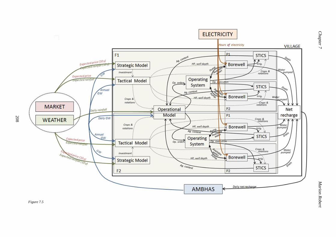
Chapter 7
M
ario
n R
obert
208
Figure 7.5
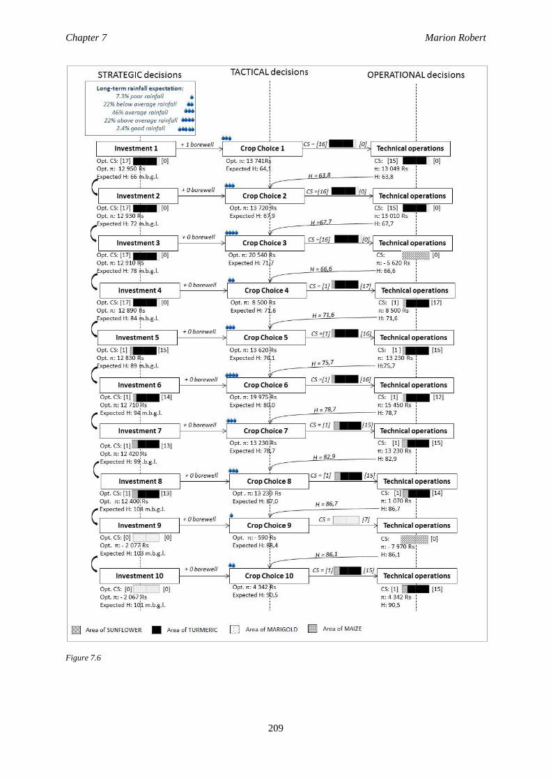
Chapter 7 Marion Robert
209
Ch
ap
ter 7
Mario
n R
obert
Figure 7.6
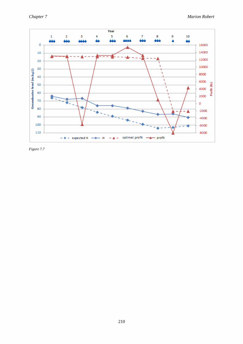
Chapter 7 Marion Robert
210
Ch
ap
ter 7
Mario
n R
obert
Figure 7.7
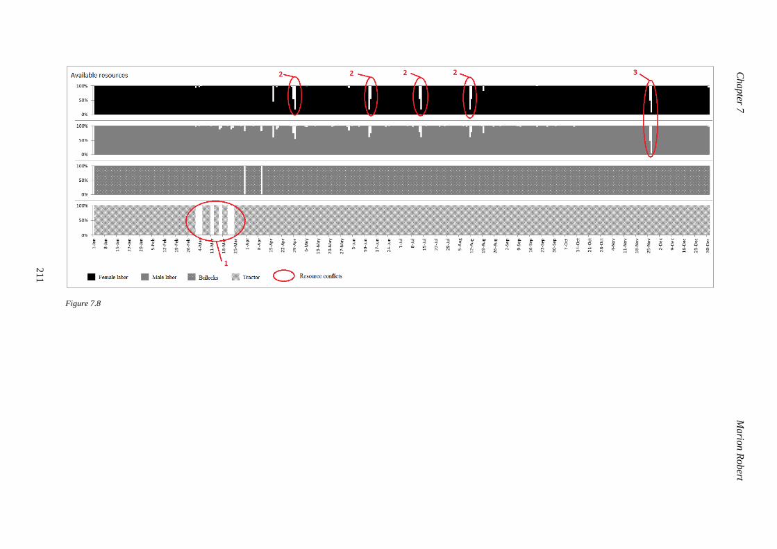
Chapter 7
M
ario
n R
obert
211
Figure 7.8


Bibliography Marion Robert
213
Bibliography
Bibliography Marion Robert
214
Abdelhamid Y, Hassan H, Rafea A (1997) A Proposed Methodology For Expert System Engineering.
In: 5th International conference on artificial intelligence applications. Egyptians Computer
Society, Cairo, Egypt,
Acock B, Pachepsky YA, Mironenko E V., et al (1999) Guics. Agronomy Journal 91:657. doi:
10.2134/agronj1999.914657x
Adesina A (1991) Peasant farmer behavior and cereal technologies: Stochastic programming analysis
in Niger. Agricultural Economics 5:21–38. doi: 10.1016/0169-5150(91)90034-I
Akplogan M (2013) Approche modulaire pour la planification continue - Application à la conduite des
systèmes de culture. Université de Toulouse
Alter N (2000) L’innovation ordinaire.
An L (2012) Modeling human decisions in coupled human and natural systems: Review of agent-based
models. Ecological Modelling 229:25–36. doi: 10.1016/j.ecolmodel.2011.07.010
Andersen E, Elbersen B, Godeschalk F, Verhoog D (2007) Farm management indicators and farm
typologies as a basis for assessments in a changing policy environment. Journal of Environmental
Management 82:353–362. doi: 10.1016/j.jenvman.2006.04.021
Anwar MR, Liu DL, Macadam I, Kelly G (2013) Adapting agriculture to climate change: a review.
Theoretical and Applied Climatology 113:225–245. doi: 10.1007/s00704-012-0780-1
Apland J, Hauer G (1993) Discrete stochastic programming: Concepts, examples and a review of
empirical applications. Minnesota
Arlot S, Celisse A (2010) A survey of cross-validation procedures for model selection. Statistics Surveys
4:40–79. doi: 10.1214/09-SS054
Attonaty J-M, Chatelin M-H, Garcia F (1999) Interactive simulation modeling in farm decision-making.
Computers and Electronics in Agriculture 22:157–170. doi: 10.1016/S0168-1699(99)00015-0
Aubriot O (2013) Tank and Well Irrigation Crisis, Concept Pu. New Delhi
Aubry C, Papy F, Capillon A (1998a) Modelling decision-making processes for annual crop
management. Agricultural Systems 56:45–65.
Aubry C, Papy F, Capillon A (1998b) Modelling decision-making processes for annual crop
management. Agricultural Systems 56:45–65. doi: 10.1016/S0308-521X(97)00034-6
Augusiak J, Van den Brink PJ, Grimm V (2014) Merging validation and evaluation of ecological models
to “evaludation”: A review of terminology and a practical approach. Ecological Modelling
280:117–128. doi: 10.1016/j.ecolmodel.2013.11.009
Bibliography Marion Robert
215
Aurbacher J, Parker PS, Sanchez GAC, et al (2013) Influence of climate change on short term
management of field crops–A modelling approach. Agricultural Systems 119:44–57.
Axelrod R (1997) Advancing the art of simulation in the social sciences. In: Simulating social
phenomena, Springer B. pp 21–40
Ballukraya PN, Sakthivadivel R (2002) Over-exploitation and artificial recharging of hard-rock aquifers
of South India: Issues and options. In: IWMI-TATA Water Policy Research Program Annual
Partners’ Meeting. Vallabh Vidyanagar, Gujarat, India, p 14
Balmann A (1997) Farm-based modelling of regional structural change: A cellular automata approach.
European Review of Agricultural Economics 24:85–108.
Barbier B, Bergeron G (1999) Impact of policy interventions on land management in Honduras: results
of a bioeconomic model. Agricultural Systems 60:1–16. doi: 10.1016/S0308-521X(99)00015-3
Barbiéro L, Parate HR, Descloitres M, et al (2007) Using a structural approach to identify relationships
between soil and erosion in a semi-humid forested area, South India. CATENA 70:313–329. doi:
10.1016/j.catena.2006.10.013
Bassi N (2014) Assessing potential of water rights and energy pricing in making groundwater use for
irrigation sustainable in India. Water Policy 16:442–453.
Basso B, Cammarano D, Carfagna E (2013) Review of Crop Yield Forecasting Methods and Early
Warning Systems. In: Proceedings of the First Meeting of the Scientific Advisory Committee of
the Global Strategy to Improve Agricultural and Rural Statistics. FAO, Rome, Italy, p 18
Beaujouan V, Durand P, Ruiz L (2001) Modelling the effect of the spatial distribution of agricultural
practices on nitrogen fluxes in rural catchments. Ecological Modelling 137:93–105. doi:
10.1016/S0304-3800(00)00435-X
Beck H, Morgan K, Jung Y, et al (2010) Ontology-based simulation in agricultural systems modeling.
Agricultural Systems 103:463–477.
Becu N, Bousquet F, Barreteau O (2003) A methodology for eliciting and modelling stakeholders’
representations with agent based modelling. In: Multi-Agent-Based Simulation III, Springer B. pp
131–148
Belhouchette H, Blanco M, Flichman G (2004) Targeting sustainability of agricultural systems in the
Cebalat watershed in Northern Tunisia : An economic perspective using a recursive stochastic
model. In: Conference TA (ed) European Association of Environmental and Resource Economics.
Budapest, Hungary, pp 1–12
Bellman R (1954) The theory of dynamic programming. Bulletin of the American Mathematical Society
60:503–516. doi: 10.1090/S0002-9904-1954-09848-8
Bibliography Marion Robert
216
Below TB, Mutabazi KD, Kirschke D, et al (2012) Can farmers’ adaptation to climate change be
explained by socio-economic household-level variables? Global Environmental Change 22:223–
235. doi: 10.1016/j.gloenvcha.2011.11.012
Berge H Ten, Ittersum M Van (2000) Farming options for The Netherlands explored by multi-objective
modelling. European Journal of Agronomy 13:263–277.
Bergez J, Garcia F, Wallach D (2006) Representing and optimizing management decisions with crop
models. In: Working with Dynamic Crop Models: Evaluation, Analysis, Parameterization, and
Applications, Elsevier. pp 173–207
Bergez JE, Chabrier P, Gary C, et al (2013) An open platform to build, evaluate and simulate integrated
models of farming and agro-ecosystems. Environmental Modelling & Software 39:39–49. doi:
10.1016/j.envsoft.2012.03.011
Bergez JE, Colbach N, Crespo O, et al (2010) Designing crop management systems by simulation.
European Journal of Agronomy 32:3–9. doi: 10.1016/j.eja.2009.06.001
Bergez J-E, Raynal H, Joannon A, et al (2016) A new plug-in under RECORD to link biophysical and
decision models for crop management. Agronomy for Sustainable Development 36:19. doi:
10.1007/s13593-016-0357-y
Bergez JE, Raynal H, Launay M, et al (2014) Evolution of the STICS crop model to tackle new
environmental issues: New formalisms and integration in the modelling and simulation platform
RECORD. Environmental Modelling & Software 62:370–384. doi: 10.1016/j.envsoft.2014.07.010
Bertsekas DP (2011) Dynamic programming and optimal control 3rd edition, volume II, MA: Athena.
Belmont
Bertsekas DP, Tsitsiklis JN (1995) Neuro-dynamic programming: an overview. In: Proceedings of the
34th IEEE Conference on Decision and Control. New Orleans, pp 560–564
Blanco-Fonseca M, Flichman G, Belhouchette H (2011) Dynamic optimization problems: different
resolution methods regarding agriculture and natural resource economics. In: Bio-Economic
Models applied to Agricultural Systems, Springer N. pp 29–57
Blanco-Gutiérrez I, Varela-Ortega C, Purkey DR (2013) Integrated assessment of policy interventions
for promoting sustainable irrigation in semi-arid environments: A hydro-economic modeling
approach. Journal of Environmental Management 128:144–160. doi:
10.1016/j.jenvman.2013.04.037
Bocquého G, Jacquet F, Reynaud A (2013) Reversal and magnitude effects in long-term time
preferences: Results from a field experiment. Economics Letters 120:108–111. doi:
10.1016/j.econlet.2013.04.006
Bibliography Marion Robert
217
Boehm BW (1988) A Spiral Model of Software Development and Enhancement. Computer 21:61–72.
Bontems P, Thomas A (2000) Information Value and Risk Premium in Agricultural Production: The
Case of Split Nitrogen Application for Corn. American Journal of Agricultural Economics 82:59–
70. doi: 10.1111/0002-9092.00006
Booch G, Rumbaugh J, Jacobson I (1996) The unified modeling language for object-oriented
development. Rational Software Corporation
Borenstein D (1998) Towards a practical method to validate decision support systems. Decision Support
Systems 23:227–239.
Bouma J, Jones J. (2001) An international collaborative network for agricultural systems applications
(ICASA). Agricultural Systems 70:355–368. doi: 10.1016/S0308-521X(01)00051-8
Bralts VF, Driscoll MA, Shayya WH, Cao L (1993) An expert system for the hydraulic analysis of
microirrigation systems. Computers and Electronics in Agriculture 9:275–287. doi: 10.1016/0168-
1699(93)90046-4
Bratman M (1987a) Intention, plans, and practical reason, Harvard Un. Cambridge, MA
Bratman M (1987b) Intention, Plans, and Practical Reason. Center for the Study of Language and
Information
Briner S, Finger R (2013) The effect of price and production risks on optimal farm plans in Swiss dairy
production considering 2 different milk quota systems. Journal of Dairy Sciences 96:2234–2246.
Brisson N, Gary C, Justes E, et al (2003) An overview of the crop model stics. European Journal of
Agronomy 18:309–332. doi: 10.1016/S1161-0301(02)00110-7
Brisson N, Mary B, Ripoche D, et al (1998) STICS: a generic model for the simulation of crops and
their water and nitrogen balances. I. Theory and parameterization applied to wheat and corn.
Agronomie 18:311–346. doi: 10.1051/agro:19980501
Brooks N, Adger WN (2005) Assessing and enhancing adaptive capacity. In: Lim B, Spanger-Siegfried
E (eds) Adaptation Policy Frameworks for Climate Change: developing Strategies, Policies and
Mesures. Cambridge University Press, pp 165–182
Brown CM, Lund JR, Cai X, et al (2015) The future of water resources systems analysis: Toward a
scientific framework for sustainable water management. Water Resources Research 51:6110–
6124. doi: 10.1002/2015WR017114
Bryant KJ, Mjelde JW, Lacewell RD (1993) An intraseasonal dynamic optimization model to allocate
irrigation water between crops. American Journal of Agricultural Economics 75:1021. doi:
10.2307/1243989
Bibliography Marion Robert
218
Burt OR (1993) Decision rules for the dynamic animal feeding problem. American Journal of
Agricultural Economics 75:190. doi: 10.2307/1242967
Carlile P, Christensen C (2005) The cycles of theory building in management research. Boston
University-School of Management
Carroll J, Swatman P (2000) Structured-case: a methodological framework for building theory in
information systems research. European Journal of Information Systems 9:235–242.
Castellazzi M, Matthews J, Angevin F, et al (2010) Simulation scenarios of spatio-temporal arrangement
of crops at the landscape scale. Environmental Modelling & Software 25:1881–1889. doi:
10.1016/j.envsoft.2010.04.006
Castellazzi M, Wood G, Burgess P, et al (2008) A systematic representation of crop rotations.
Agricultural Systems 97:26–33. doi: 10.1016/j.agsy.2007.10.006
Central Intelligence Agency (2016) South Asia: India. In: The world Factbook.
https://www.cia.gov/library/publications/resources/the-world-factbook/geos/in.html. Accessed 13
Oct 2016
Cerf M, Faverdin P, Garcia F (2009) Formalisation de l’interaction entre processus décisionnels et
processus biophysiques. In: Update Sciences & Technologies. pp 28–40
Cerf M, Sebillotte M (1988) Le concept de modèle général et la prise de décision dans la conduite d’une
culture. Comptes Rendus de l’Académie d’Agriculture de France 4:71–80.
Chambers RG, Quiggin J (2000) Uncertainty, Production, Choice and Agency: The State-Contingent
Approach, Cambridge. New York
Chambers RG, Quiggin J (2002) The State-Contingent Properties of Stochastic Production Functions.
American Journal of Agricultural Economics 84:513–526. doi: 10.1111/1467-8276.00314
Chandra B (2000) India after Independance: 1947-2000, Penguin UK.
Chandrasekaran K, Devarajulu S, Kuppannan P (2009) Farmers’ Willingness to Pay for Irrigation
Water: A Case of Tank Irrigation Systems in South India. Water 1:5–18. doi: 10.3390/w1010005
Chandrasekhar S, Das M, Sharma A (2015) Short-term Migration and Consumption Expenditure of
Households in Rural India. Oxford Development Studies 43:105–122. doi:
10.1080/13600818.2014.964194
Chardon X, Rigolot C, Baratte C, et al (2012) MELODIE: a whole-farm model to study the dynamics
of nutrients in dairy and pig farms with crops. Animal 6:1711–1721. doi:
10.1017/S1751731112000687
Chavas J-P (2012) On learning and the economics of firm efficiency: a state-contingent approach.
Bibliography Marion Robert
219
Journal of Productivity Analysis 38:53–62. doi: 10.1007/s11123-012-0268-0
Chavas J-P, Chambers RG, Pope RD (2010) Production Economics and Farm Management: a Century
of Contributions. American Journal of Agricultural Economics 92:356–375. doi:
10.1093/ajae/aaq004
Chipman S, Schraagen J, Shalin V (2000) Introduction to cognitive task analysis. Cognitive Task
Analysis 3–23.
Chokkakula S (2015) The Political Geographies of Interstate Water Disputes in India. University of
Washington
Clavel L, Soudais J, Baudet D, Leenhardt D (2011) Integrating expert knowledge and quantitative
information for mapping cropping systems. Land Use Policy 28:57–65. doi:
10.1016/j.landusepol.2010.05.001
Clouaire RM, Rellier JP (2009) Modelling and simulating work practices in agriculture. International
Journal of Metadata, Semantics and Ontologies 4:42. doi: 10.1504/IJMSO.2009.026253
Cochran W (1953) Sampling techniques, John Wiley.
Cocks KD (1968) Discrete Stochastic Programming. Management Science 15:72–79. doi:
10.1287/mnsc.15.1.72
Coléno FC, Duru M, Theau JP (2005) A Method to Analyse Decision-making Processes for Land Use
Management in Livestock Farming. International Journal of Agricultural Sustainability 3:69–78.
doi: 10.1080/14735903.2005.9684745
Connor J, Schwabe K, King D, et al (2009) Impacts of climate change on lower Murray irrigation.
Australian Journal of Agricultural and Resource Economics 53:437–456. doi: 10.1111/j.1467-
8489.2009.00460.x
Costal D, Teniente E, Urpi T, Farré C (1996) Handling Conceptual Model Validation by Planning. In:
International Conference on Advanced Information Systems Engineering. Springer Berlin
Heidelberg, pp 255–271
Couture S, Martin-Clouaire R (2013) Towards a better understanding of operational decision making in
agricultural production systems. In: Fourth International Symposium for Farming Systems Design.
Lanzhou, China, p 2
Cranefield S, Purvis M (1999) UML as an ontology modelling language. University of Otago, Dunedin
Crespo O, Hachigonta S, Tadross M (2011) Sensitivity of southern African maize yields to the definition
of sowing dekad in a changing climate. Climatic Change 106:267–283. doi: 10.1007/s10584-010-
9924-4
Bibliography Marion Robert
220
Cros MJ, Duru M, Garcia F, Martin-Clouaire R (1999) A DSS for rotational grazing management :
simulating both the biophysical and decision making processes. In: MODSIM99. Hamilton, NZ,
pp 759–764
Cros MJ, Garcia F, Martin-Clouaire R, Rellier JP (2003) Modelling management operation in
agricultural production simulator.
Cyert R, March J (1963) A behavioral theory of the firm. Englewood, Cliffs, NJ
Daloğlu I, Nassauer JI, Riolo RL, Scavia D (2014) Development of a farmer typology of agricultural
conservation behavior in the American Corn Belt. Agricultural Systems 129:93–102. doi:
10.1016/j.agsy.2014.05.007
Darnhofer I (2014) Resilience and why it matters for farm management. European Review of
Agricultural Economics 41:461–484. doi: 10.1093/erae/jbu012
Darnhofer I, Bellon S (2008) Adaptive farming systems–A position paper. In: 8th European IFSA
Symposium. Clermont-Ferrand (France), pp 339–351
Darnhofer I, Bellon S, Dedieu B, Milestad R (2010) Adaptiveness to enhance the sustainability of
farming systems. A review. Agronomy for Sustainable Development 30:545–555. doi:
10.1051/agro/2009053
Day R (1961) Recursive programming and supply prediction. In: Heady EO, Baker CB, Diesslin HG,
et al. (eds) Agricultural Supply Functions - estimating techniques and interpretation. Ames, Iowa:
Iowa State University Press, Ames, Iowa, pp 108–125
Day R (2005) Microeconomic Foundations for Macroeconomic Structure. Los Angeles
Daydé C, Couture S, Garcia F, Martin-Clouaire R (2014) Investigating operational decision-making in
agriculture. In: Ames D, Quinn N, Rizzoli A (eds) International Environmental Modelling and
Software Society. San Diego, CA, pp 1–8
De Lapeyre de Bellaire L, Bachelier B, Dorel M, et al (2016) Conception des systèmes de culture et
intensification écologique. In: Développement durable et filières tropicales, Editions Q. pp 125–
138
Dedieu B, Ingrand S (2010) Incertitude et adaptation: cadres théoriques et application à l’analyse de la
dynamique des systèmes d’élevage. Productions animales 23:81–90.
Deshingkar P, Start D (2003) Seasonal Migration for Livelihoods in India: Coping, Accumulation and
Exclusion. London
Detlefsen NK, Jensen AL (2007) Modelling optimal crop sequences using network flows. Agricultural
Systems 94:566–572. doi: 10.1016/j.agsy.2007.02.002
Bibliography Marion Robert
221
Dewandel B, Perrin J, Ahmed S, et al (2010) Development of a tool for managing groundwater resources
in semi-arid hard rock regions: application to a rural watershed in South India. Hydrological
Processes 24:2784–2797. doi: 10.1002/hyp.7696
Di Franco G (2016) Multiple correspondence analysis: one only or several techniques? Quality &
Quantity 50:1299–1315. doi: 10.1007/s11135-015-0206-0
Dodd W, Humphries S, Patel K, et al (2016) Determinants of temporary labour migration in southern
India. Asian Population Studies 12:294–311. doi: 10.1080/17441730.2016.1207929
Domptail S, Nuppenau E-A (2010) The role of uncertainty and expectations in modeling (range)land
use strategies: An application of dynamic optimization modeling with recursion. Ecological
Economics 69:2475–2485. doi: 10.1016/j.ecolecon.2010.07.024
Donatelli M, Evert F Van, Guardo A Di (2006) A component to simulate agricultural management. In:
IEMSs Congress. Vermont, USA,
Doré T, Sebillotte M, Meynard J (1997) A diagnostic method for assessing regional variations in crop
yield. Agricultural Systems 54:169–188. doi: 10.1016/S0308-521X(96)00084-4
Dorin B, Landy F (2002) Agriculture et alimentation de l’Inde - les vertes années (1947-2001), INRA
Editi. Paris
Duffy PA, Taylor CR (1993) Long-term planning on a corn-soybean farm: A dynamic programming
analysis. Agricultural Systems 42:57–71. doi: 10.1016/0308-521X(93)90068-D
Dury J (2011) The cropping-plan decision-making : a farm level modelling and simulation approach.
Institut National Polytechnique de Toulouse
Dury J, Garcia F, Reynaud A, et al (2010) Modelling the complexity of the cropping plan decision-
making. In: International Environmental Modelling and Software Society. iEMSs, Ottawa,
Canada, pp 1–8
Dury J, Garcia F, Reynaud A, Bergez J-E (2013) Cropping-plan decision-making on irrigated crop
farms: A spatio-temporal analysis. European Journal of Agronomy 50:1–10. doi:
10.1016/j.eja.2013.04.008
Duvernoy I (2000) Use of a land cover model to identify farm types in the Misiones agrarian frontier
(Argentina). Agricultural Systems 64:137–149. doi: 10.1016/S0308-521X(00)00019-6
Eisenhardt K (1989) Building theories from case study research. Academy of Management Review
14:532–550.
Eisenhardt K, Graebner M (2007) Theory building from cases: Opportunities and challenges. Academy
of Management Journal 50:25–32.
Bibliography Marion Robert
222
Fafchamps M (1993) Sequential Labor Decisions Under Uncertainty: An Estimable Household Model
of West-African Farmers. Econometrica 61:1173. doi: 10.2307/2951497
FAO (2011) The state of the world’s land and water resources for food and agriculture (SOLAW) –
Managing systems at risk, Food and A. Rome and Earthscan, London
Farmer JD, Foley D (2009) The economy needs agent-based modelling. Nature 460:685–686.
Feola G, Lerner AM, Jain M, et al (2015) researching farmer behaviour in climate change adaptation
and sustainable agriculture: Lessons learned from five case studies. Journal of Rural Studies
39:74–84.
Fernández FJ, Ponce RD, Blanco M, et al (2016) Water Variability and the Economic Impacts on Small-
Scale Farmers. A Farm Risk-Based Integrated Modelling Approach. Water Resources
Management 30:1357–1373. doi: 10.1007/s11269-016-1227-8
Fishman R, Devineni N, Raman S (2015) Can improved agricultural water use efficiency save India’s
groundwater? Environmental Research Letters 10:84022. doi: 10.1088/1748-9326/10/8/084022
Flichman G (2011) Bio-Economic Models applied to Agricultural Systems, Springer. Springer
Netherlands, Dordrecht
Foster T, Brozović N, Butler AP (2014) Modeling irrigation behavior in groundwater systems. Water
Resources Research 50:6370–6389. doi: 10.1002/2014WR015620
Gaudou B, Sibertin-Blanc C (2013) The maelia multi-agent platform for integrated assessment of low-
water management issues. In: International Worshop on Multi-Agent-Based Simulation-MABS. p
85
George A, Bennett A (2005) Case studies and theory development in the social sciences. MIT Press
Giampetro M (2002) Complexity and Scales: The Challenge for Integrated Assessment. Integrated
Assessment 3:247–265. doi: 10.1076/iaij.3.2.247.13568
Gibbons JM, Wood ATA, Craigon J, et al (2010) Semi-automatic reduction and upscaling of large
models: A farm management example. Ecological Modelling 221:590–598. doi:
10.1016/j.ecolmodel.2009.11.006
Gladwin CH (1989) Ethnographic Decision Tree Modelling. SAGE Publications, Beverly Hills
Glaser B, Strauss A (1967) The discovery grounded theory: strategies for qualitative inquiry. Aldine,
New York
Gleick PH (1993) Water and Conflict: Fresh Water Resources and International Security. International
Security 18:79. doi: 10.2307/2539033
González Botero D, Bertran Salinas A (2013) Assessing farmers’ vulnerability to climate change: a case
Bibliography Marion Robert
223
study in Karnataka, India. Universitat Autonoma de Barcelone
Goswami R, Chatterjee S, Prasad B (2014) Farm types and their economic characterization in complex
agro-ecosystems for informed extension intervention: study from coastal West Bengal, India.
Agricultural and Food Economics 2:5. doi: 10.1186/s40100-014-0005-2
Graveline N (2013) Agricultures’ adaptation to water management policies and global change : the
interest of economic programming models. AgoParis Tech
Graveline N (2016) Economic calibrated models for water allocation in agricultural production: A
review. Environmental Modelling & Software 81:12–25. doi: 10.1016/j.envsoft.2016.03.004
Grothmann T, Patt A (2003) Adaptive capacity and human cognition. In: Meeting of the Global
Environmental Change Research Community. Montreal, Canada, pp 1–19
Gruber T (1993) What is an Ontology. Stanford University’s Knowledge Sharing Technology Project
Happe K, Balmann A, Kellermann K, Sahrbacher C (2008) Does structure matter? The impact of
switching the agricultural policy regime on farm structures. Journal of Economic Behavior &
Organization 67:431–444. doi: 10.1016/j.jebo.2006.10.009
Hardaker J (2004) Coping with risk in agriculture, Cabi. CABI, Wallingford
Heidhues T (1966) A Recursive Programming Model of Farm Growth in Northern Germany. Journal of
Farm Economics 48:668. doi: 10.2307/1236868
Hémidy L, Boiteux J, Cartel H (1996) Aide à la décision et accompagnement stratégique : l’exp érience
du CDER de la Marne. In: Communication pour le colloque INRA/ Pour la terre et les Hommes,
50 ans de recherches à l’INRA. Laon, pp 33–51
Herroelen W, Leus R (2004) Robust and reactive project scheduling: a review and classification of
procedures. International Journal of Production Research 42:1599–1620. doi:
10.1080/00207540310001638055
Hertel TW (2015) The challenges of sustainably feeding a growing planet. Food Security 7:185–198.
doi: 10.1007/s12571-015-0440-2
Hibbard KA, Janetos AC (2013) The regional nature of global challenges: a need and strategy for
integrated regional modeling. Climatic Change 118:565–577. doi: 10.1007/s10584-012-0674-3
Hoffman R, Lintern G (2006) Eliciting and representing the knowledge of experts. Cambridge
Handbook of Expertise and Expert Performances 203–222.
Holling CS (2001) Understanding the Complexity of Economic, Ecological, and Social Systems.
Ecosystems 4:390–405. doi: 10.1007/s10021-001-0101-5
Holzworth DP, Snow V, Janssen S, et al (2015) Agricultural production systems modelling and
Bibliography Marion Robert
224
software: Current status and future prospects.
Husson F, Lê S, Pagès J (2010) Exploratory multivariate analysis by example using R, CRC Press.
Hyytiäinen K, Niemi JK, Koikkalainen K, et al (2011) Adaptive optimization of crop production and
nitrogen leaching abatement under yield uncertainty. Agricultural Systems 104:634–644.
Iglesias A, Garrote L (2015) Adaptation strategies for agricultural water management under climate
change in Europe. Agricultural Water Management 155:113–124. doi:
10.1016/j.agwat.2015.03.014
India Brand Equity Foundation (2016) Growth in Agriculture. In: Indian Agriculture industry: an
overview. http://www.ibef.org/industry/agriculture-india.aspx. Accessed 13 Oct 2016
Ingrand S, Astigarraga L, Chia E, et al (2009) Développer les propriétés de flexibilité des systèmes de
production agricole en situation d’incertitude: pour une durabilité qui dure... In: 13ème Journées
de la Recherche Cunicole. Le Mans, France, pp 1–9
INRA Sens (2008) Processus d’innovation. Sciences en Société
Jacoby H (2015) WELL-FARE ECONOMICS OF GROUNDWATER DEVELOPMENT.
Jacquet F, Pluvinage J (1997) Climatic uncertainty and farm policy: A discrete stochastic programming
model for cereal-livestock farms in Glgeria. Agricultural Systems 53:387–407. doi: 10.1016/0308-
521X(95)00076-H
Jain M, Naeem S, Orlove B, et al (2015) Understanding the causes and consequences of differential
decision-making in adaptation research: Adapting to a delayed monsoon onset in Gujarat, India.
Global Environmental Change 31:98–109. doi: 10.1016/j.gloenvcha.2014.12.008
Janakarajan S (1999) Conflicts over the invisible resource in Tamil Nadu. In: Moench M, Caspari E,
Dixit A (eds) Rethinking the mosaic - Investigations into Local Water Management. Nepal Water
Conservation Foundation and the Institute for Social and Environmental Transition, Colorado,
USA, p 315
Janssen S, van Ittersum MK (2007) Assessing farm innovations and responses to policies: A review of
bio-economic farm models. Agricultural Systems 94:622–636. doi: 10.1016/j.agsy.2007.03.001
Javeed Y, Sekhar M, Bandyopadhyay S, Mangiarotti S (2009) EOF and SSA analyses of hydrological
time series to assess climatic variability and land-use effects: a case study in the Kabini River basin
of South India. IAHS-AISH publication 167–177.
Jogesh A, Dubash NK (2014) Mainstreaming climate change in state development planning: An analysis
of Karnataka’s Action Plan on Climate Change. New Delhi
Jonassen DH (1997) Instructional design models for well-structured and III-structured problem-solving
Bibliography Marion Robert
225
learning outcomes. Educational Technology Research and Development 45:65–94.
Kahil MT, Connor JD, Albiac J (2015) A stochastic model of irrigation adaption to climate change in
southern Europe. In: 21st Annual Conference of the European Association of Environmental and
Resource Economists. Helsinki, p 21
Karali E, Rounsevell MDA, Doherty R (2011) Integrating the diversity of farmers’ decisions into studies
of rural land-use change. Procedia Environmental Sciences 6:136–145. doi:
10.1016/j.proenv.2011.05.014
Kaufman L, Rousseeuw PJ (2009) Finding Groups in Data: An Introduction to Cluster Analysis, John
Wiley.
Kemp D, Michalk D (2007) Towards sustainable grassland and livestock management. The Journal of
Agricultural Science 145:543–564.
Kingwell RS, Pannell DJ, Robinson SD (1993) Tactical responses to seasonal conditions in whole-farm
planning in Western Australia. Agricultural Economics 8:211–226. doi: 10.1016/0169-
5150(93)90015-5
Kleijnen JPC (1995) Verification and validation of simulation models. European Journal of Operational
Research 82:145–162. doi: 10.1016/0377-2217(94)00016-6
Klein G (2008) Naturalistic Decision Making. The Journal of Human Factors and Ergonomics Society
50:456–460.
Klein G (1989) Critical decision method for eliciting knowledge. Systems, Man and Cybernetics, IEEE
Transactions 19:462–472.
Klerkx L, Aarts N, Leeuwis C (2010) Adaptive management in agricultural innovation systems: The
interactions between innovation networks and their environment. Agricultural Systems 103:390–
400. doi: 10.1016/j.agsy.2010.03.012
Kling C, Arritt R, Calhoun G, et al (2016) Research needs and challenges in the FEW system: Coupling
economic models with agronomic, hydrologic, and bioenergy models for sustainable food, energy,
and water systems. Ames, Iowa
Knowler D (2002) A Review of Selected Bioeconomic Models with Environmental Influences in
Fisheries. Journal of Bioeconomics 4:163–181. doi: 10.1023/A:1021151809501
Köbrich C, Rehman T, Khan M (2003) Typification of farming systems for constructing representative
farm models: two illustrations of the application of multi-variate analyses in Chile and Pakistan.
Agricultural Systems 76:141–157. doi: 10.1016/S0308-521X(02)00013-6
Kogut P, Cranefield S, Hart L (2002) UML for ontology development. The Knowledge Engineering
Review 17:61–64.
Bibliography Marion Robert
226
Kraucunas I, Clarke L, Dirks J, et al (2015) Investigating the nexus of climate, energy, water, and land
at decision-relevant scales: the Platform for Regional Integrated Modeling and Analysis (PRIMA).
Climatic Change 129:573–588. doi: 10.1007/s10584-014-1064-9
Krishnamurthy CKB (2016) Optimal management of groundwater under uncertainty: A unified
approach. Environmental and Resource Economics. doi: 10.1007/s10640-015-9989-7
Kristensen LS, Thenail C, Kristensen SP (2004) Landscape changes in agrarian landscapes in the 1990s:
the interaction between farmers and the farmed landscape. A case study from Jutland, Denmark.
Journal of Environmental Management 71:231–244. doi: 10.1016/j.jenvman.2004.03.003
Lacy LW (2005) OWL: representing information using the Web Ontology Language. Trafford
Publishing
Lamanda N, Roux S, Delmotte S, et al (2012) A protocol for the conceptualisation of an agro-ecosystem
to guide data acquisition and analysis and expert knowledge integration. European Journal of
Agronomy 38:104–116.
Laoubi K, Yamao M (2009) A typology of irrigated farms as a tool for sustainable agricultural
development in irrigation schemes. International Journal of Social Economics 36:813–831. doi:
10.1108/03068290910967091
Law AM (2008) How to build valid and credible simulation models. In: Mason SJ, Hill RR, Monch L,
et al. (eds) Proceedings of the 2008 Winter Simulation Conference.
Le QB, Seidl R, Scholz RW (2012) Feedback loops and types of adaptation in the modelling of land-
use decisions in an agent-based simulation. Environmental Modelling & Software 27–28:83–96.
doi: 10.1016/j.envsoft.2011.09.002
Le Bars M, Chatelin M, Attonaty J (2005) Raisonnement procédural dans un modèle de simulation de
la gestion d’un bassin versant. In: CABM-HEMA SMAGET. Lyon,
Le Gal P, Dugué P, Faure G, Novak S (2011) How does research address the design of innovative
agricultural production systems at the farm level? A review. Agricultural Systems 104:714–728.
doi: 10.1016/j.agsy.2011.07.007
Le Gal P, Merot A, Moulin C, et al (2010) A modelling framework to support farmers in designing
agricultural production systems. Environmental Modelling & Software 25:258–268. doi:
10.1016/j.envsoft.2008.12.013
Le Roux B, Rouaner H (2004) Geometric Data Analysis: From Correspondence Analysis to Structured
Data Analysis, Springer S.
Leenhardt D, Murgue C, Therond O (2015) Une approche agroécologique de la gestion quantitative de
l’eau en zone de déficit chronique. Innovations Agronomiques 43:57–70.
Bibliography Marion Robert
227
Lefèvre V, Capitaine M, Peigné J, Roger-Estrade J (2014) Farmers and agronomists design new
biological agricultural practices for organic cropping systems in France. Agronomy for Sustainable
Development 34:623–632. doi: 10.1007/s13593-013-0177-2
Lescot JM, Rousset S, Souville G (2011) Assessing investment in precision farming for reducing
pesticide use in French viticulture. In: EAAE 2011 Congress: Change and Uncertainty Challenges
for Agriculture, Food and Natural Resources. Zurich, Switzerland, pp 1–19
Lev L, Campbell DJ (1987) The temporal dimension in farming systems research: the importance of
maintaining flexibility under conditions of uncertainty. Journal of Rural Studies 3:123–132. doi:
10.1016/0743-0167(87)90028-3
Levy PS, Lemeshow S (2013) Sampling of Populations: Methods and Applications, John Wiley.
Liu J, Yu Y, Zhang L, Nie C (2011) An Overview of Conceptual Model for Simulation and Its
Validation. Procedia Engineering 24:152–158. doi: 10.1016/j.proeng.2011.11.2618
Loyce C, Wery J (2006) Les outils des agronomes pour l’évaluation et la conception de systèmes de
culture. In: L’agronomie aujourd’hui, synthèses, Quae. Versailles, France, pp 77–95
Maatman A, Schweigman C, Ruijs A, van Der Vlerk MH (2002) Modeling farmers’ response to
uncertain rainfall in Burkina Faso: A stochastic programming approach. Operations Research
50:399–414. doi: 10.1287/opre.50.3.399.7749
Mackenzie A, Pidd M, Rooksby J (2006) Wisdom, decision support and paradigms of decision making.
European Journal of Operational Research 170:156–171.
Maréchal J-C, Vouillamoz J-M, Mohan Kumar MS, Dewandel B (2010) Estimating aquifer thickness
using multiple pumping tests. Hydrogeology Journal 18:1787–1796. doi: 10.1007/s10040-010-
0664-3
Martin G (2015) A conceptual framework to support adaptation of farming systems–Development and
application with Forage Rummy. Agricultural Systems 132:52–61. doi:
10.1016/j.agsy.2014.08.013
Martin G, Martin-Clouaire R, Duru M (2013) Farming system design to feed the changing world. A
review. Agronomy for Sustainable Development 33:131–149. doi: 10.1007/s13593-011-0075-4
Martin G, Martin-Clouaire R, Rellier JP, Duru M (2011a) A simulation framework for the design of
grassland-based beef-cattle farms. Environmental Modelling & Software 26:371–385. doi:
10.1016/j.envsoft.2010.10.002
Martin G, Martin-Clouaire R, Rellier JP, Duru M (2011b) A conceptual model of grassland-based beef
systems. International Journal of Agricultural and environmental Information systems 2:20–39.
doi: 10.4018/jaeis.2011010102
Bibliography Marion Robert
228
Martin-Clouaire R, Rellier J (2006) Représentation et interprétation de plans de production flexibles -
Google Search. In: Actes des Journées Francophones sur la Planification, la décision et
l’Apprentissage pour la Conduite de Systèmes (JFPDA). Toulouse,
Martin-Clouaire R, Rellier JP (2003) A conceptualization of farm mangement strategy. In: Efita-03.
Debrecen, Hungary, pp 719–726
Mathews HF, Hill C (1990) Applying cognitive decision theory to the study of regional patterns of
illness treatment choice. American Anthropologist 91:155–170.
Matthews R, Gilbert N, Roach A (2007) Agent-based land-use models: a review of applications.
Landscape … 22:1447–1459.
Matthews R, Stephens W, Hess T, et al (2002) Applications of crop/soil simulation models in tropical
agricultural systems. Advances in Agronomy 76:31–124. doi: 10.1016/S0065-2113(02)76003-3
McCarl BA, Dillon CR, Keplinger KO, Williams RL (1999) Limiting pumping from the Edwards
Aquifer: An economic investigation of proposals, water markets, and spring flow guarantees.
Water Resources Research 35:1257–1268. doi: 10.1029/1998WR900116
McDonald MG, Harbaugh AW (1988) A modular three-dimensional finite-difference ground-water
flow model. U.S. Geological Survey, Denvers
McKenzie FC, Williams J (2015) Sustainable food production: constraints, challenges and choices by
2050. Food Security 7:221–233. doi: 10.1007/s12571-015-0441-1
McKinion JM, Baker DN, Whisler FD, Lambert JR (1989) Application of the GOSSYM/COMAX
system to cotton crop management. Agricultural Systems 31:55–65. doi: 10.1016/0308-
521X(89)90012-7
Mejías P, Varela-Ortega C, Flichman G (2004) Integrating agricultural policies and water policies under
water supply and climate uncertainty. Water Resources Research 40:n/a-n/a. doi:
10.1029/2003WR002877
Meredith J (1998) Building operations management theory through case and field research. Journal of
Operations Management 16:441–454.
Merot A, Bergez J, Capillon A, Wery J (2008) Analysing farming practices to develop a numerical,
operational model of farmers’ decision-making processes: An irrigated hay cropping system in
France. Agricultural Systems 98:108–118.
Meyer C (2016) Dictionnaire des Sciences Animales. In: Montpellier, France , CIRAD. http://dico-
sciences-animales.cirad.fr/. Accessed 27 Sep 2016
Meynard JM, Dedieu B, Bos AB (2012) Re-design and co-design of farming systems. An overview of
methods and practices. In: Farming Systems Research into the 21th century: The new dynamic,
Bibliography Marion Robert
229
Springer N. pp 405–429
Milán MJ, Bartolomé J, Quintanilla R, et al (2006) Structural characterisation and typology of beef cattle
farms of Spanish wooded rangelands (dehesas). Livestock Science 99:197–209. doi:
10.1016/j.livprodsci.2005.06.012
Milton N, Shadbolt N (1999) Towards a knowledge technology for knowledge management.
International Journal of Human-Computer Studies 51:615–641.
Milton S, Kazmierczak E (2006) Ontology as meta-theory: A perspective. Scandinavian Journal of
Information Systems 18:5.
Miranda MJ, Fackler PL (2004) Applied computational economics and finance, MIT Press.
Mishra S (2007) Risks, Farmers’ Suicides and Agrarian Crisis in India: Is There A Way Out? Mumbay,
India
Mjelde JW (1986) Dynamic programming model of the corn production decision process with stochastic
climate forecasts. University of Illinois
Moore AD, Holzworth DP, Herrmann NI, et al (2014) Modelling the manager: representing rule-based
management in farming systems simulation models. Environmental Modelling & Software
62:399–410.
Mosnier C, Agabriel J, Lherm M, Reynaud A (2009) A dynamic bio-economic model to simulate
optimal adjustments of suckler cow farm management to production and market shocks in France.
Agricultural Systems 102:77–88. doi: 10.1016/j.agsy.2009.07.003
Mosqueira-Rey E, Moret-Bonillo V (2000) Validation of intelligent systems: a critical study and a tool.
Expert Systems with Applications 18:1–16.
Mueller JP, Barbercheck ME, Bell M, et al (2002) Development and implementation of a long-term
agricultural systems study: challenges and opportunities. Hort Technology 12:362–368.
Murgue C, Therond O, Leenhardt D (2015) Toward integrated water and agricultural land management:
Participatory design of agricultural landscapes. Land Use Policy 45:52–63. doi:
10.1016/j.landusepol.2015.01.011
Nash KL, Allen CR, Angeler DG, et al (2014) Discontinuities, cross-scale patterns, and the organization
of ecosystems. Ecology 95:654–667. doi: 10.1890/13-1315.1
National Crime Reports Bureau (2015) Accidental Death and Suicides in India. In: ADSI Report Annual
– 2014.
Navarrete M, Bail M Le (2007) SALADPLAN: a model of the decision-making process in lettuce and
endive cropping. Agronomy for sustainable development 27:209–221.
Bibliography Marion Robert
230
Nelson GC, Valin H, Sands RD, et al (2014) Climate change effects on agriculture: Economic responses
to biophysical shocks. Proceedings of the National Academy of Sciences 111:3274–3279. doi:
10.1073/pnas.1222465110
Newig J, Haberl H, Pahl-Wostl C, Rothman DS (2008) Formalised and Non-Formalised Methods in
Resource Management—Knowledge and Social Learning in Participatory Processes: An
Introduction. Systemic Practice and Action Research 21:381–387. doi: 10.1007/s11213-008-9112-
x
Nguyen AT, Reiter S, Rigo P (2014) A review on simulation-based optimization methods applied to
building performance analysis. Applied Energy 113:1043–1058. doi:
10.1016/j.apenergy.2013.08.061
Norusis M (2012) Cluster analysis. In: IBM SPSS Statistics 19 Statistical Procedures Companion. pp
361–391
Novak S (2008) Méthodes de conception de systèmes de production innovants à l’échelle de
l’exploitation agricole.
O’Donnell CJ, Griffiths WE (2006) Estimating State-Contingent Production Frontiers. American
Journal of Agricultural Economics 88:249–266. doi: 10.1111/j.1467-8276.2006.00851.x
Omran M, Engelbrecht A, Salman A (2007) An overview of clustering methods. Intelligent Data
Analysis 11:583–605.
Osman M (2010) Controlling uncertainty: a review of human behavior in complex dynamic
environments. Psychological Bulletin 136:65. doi: 10.1037/a0017815
Pack Kaelbling L, Littman M, Moore A (1996) Reinforcement Learning: a survey. Journal of Artificial
Intelligence Research 4:237–285.
Pahl-Wostl C, Hare M (2004) Processes of social learning in integrated resources management. Journal
of Community & Applied Social Psychology 14:193–206. doi: 10.1002/casp.774
Pandey S, Medd RW (1991) A stochastic dynamic programming framework for weed control decision
making: An application to Avena fatua L. Agricultural Economics 6:115–128.
Pani N (2009) Institutions that cannot manage change: a Gandhian perspective on the Cauvery dispute
in South India. Water Alternatives 2:315–327.
Papajorgji P, Pardalos P (2006) Software engineering techniques applied to agricultural systems,
Springer S. Incorporated
Papy F, Attonaty J, Laporte C, Soler L (1988) Work organization simulation as a basis for farm
management advice (equipment and manpower, levels against climatic variability). Agricultural
systems 27:295–314.
Bibliography Marion Robert
231
Paul S, Chakravarty R (2016) Constraints in Role Performance of Gram Panchayat in Agriculture and
Dairy Farming. Indian Research Journal of Extension Education 9:29–31.
Pearson LJ, Nelson R, Crimp S, Langridge J (2011) Interpretive review of conceptual frameworks and
research models that inform Australia’s agricultural vulnerability to climate change.
Environmental Modelling & Software 26:113–123. doi: 10.1016/j.envsoft.2010.07.001
Perrin J, Ahmed S, Hunkeler D (2011) The effects of geological heterogeneities and piezometric
fluctuations on groundwater flow and chemistry in a hard-rock aquifer, southern India.
Hydrogeology Journal 19:1189–1201. doi: 10.1007/s10040-011-0745-y
Peters DPC, Bestelmeyer BT, Turner MG (2007) Cross–Scale Interactions and Changing Pattern–
Process Relationships: Consequences for System Dynamics. Ecosystems 10:790–796. doi:
10.1007/s10021-007-9055-6
Petit M (1978) The farm household complex as an adaptive system. Proceedings of the 4
Forschungscolloquium des Lehrstuhls für Wirtschaftslehre des Landbaus 78:57–70.
Petsakos A, Rozakis S (2015) Calibration of agricultural risk programming models. European Journal
of Operational Research 242:536–545. doi: Calibration of agricultural risk programming models
Pinet F, Roussey C, Brun T, Vigier F (2009) The Use of UML as a Tool for the Formalisation of
Standards and the Design of Ontologies in Agriculture. Springer
Poussin JC, Imache A, Beji R, et al (2008) Exploring regional irrigation water demand using typologies
of farms and production units: An example from Tunisia. Agricultural Water Management 95:973–
983. doi: 10.1016/j.agwat.2008.04.001
R Core Team (2013) R: A language and environment for statistical computing. 409.
Rae A (1971) An empirical application and evaluation of discrete stochastic programming in farm
management. American Journal of Agricultural Economics 53:625–638. doi: 10.2307/1237827
Raes D, Steduto P, Hsiao TC, Fereres E (2011) Reference manual AquaCrop, FAO.
Ragab R, Prudhomme C (2002) SW—Soil and Water. Biosystems Engineering 81:3–34. doi:
10.1006/bioe.2001.0013
Rajasekaram V, Nandalal KD (2005) Decision Support System for Reservoir Water Management
Conflict Resolution. Journal of Water Resources Planning and Management 131:410–419. doi:
10.1061/(ASCE)0733-9496(2005)131:6(410)
Rao A, Georgeff M (1991) Modeling rational agents within a BDI-architecture. In: Second International
Conference on Principles of Knowledge Representation and Reasoning. KR91, pp 473–484
Refsgaard JC, Knudsen J (1996) Operational Validation and Intercomparison of Different Types of
Bibliography Marion Robert
232
Hydrological Models. Water Resources Research 32:2189–2202. doi: 10.1029/96WR00896
Reynaud A (2009) Adaptation à court et à long terme de l’agriculture au risque de sécheresse: une
approche par couplage de modèles biophysiques et économiques. Revue d’Etudes en Agriculture
et Environnement 90:121–154.
Reynolds JF, Acock B (1997) Modularity and genericness in plant and ecosystem models. Ecological
Modelling 94:7–16. doi: 10.1016/S0304-3800(96)01924-2
Rider CES (2012) Methodology for eliciting, encoding and simulating human decision making
behaviour. University of Edinburgh
Ridier A, Chaib K, Roussy C (2016) A Dynamic Stochastic Programming model of crop rotation choice
to test the adoption of long rotation under price and production risks. European Journal of
Operational Research 252:270–279. doi: 10.1016/j.ejor.2015.12.025
Ripoche A, Rellier JP, Martin-Clouaire R, et al (2011) Modelling adaptive management of intercropping
in vineyards to satisfy agronomic and environmental performances under Mediterranean climate.
Environmental Modelling & Software 26:1467–1480. doi: 10.1016/j.envsoft.2011.08.003
Risbey J, Kandlikar M, Dowlatabadi H, Graetz D (1999) Scale, context, and decision making in
agricultural adaptation to climate variability and change. Mitigation and Adaptation Strategies for
Global Change 4:137–165. doi: 10.1023/A:1009636607038
Ritten JP, Frasier WM, Bastian CT, Gray ST (2010) Optimal rangeland stocking decisions under
stochastic and climate-impacted weather. American Journal of Agricultural Economics 92:1242–
1255. doi: 10.1093/ajae/aaq052
Robert M, Bergez JE, Thomas A Economic analysis of groundwater irrigation: A stochastic dynamic
programming appraoch, with an application to smallholders in India.
Robert M, Dury J, Thomas A, et al (2016a) CMFDM: A methodology to guide the design of a conceptual
model of farmers’ decision-making processes. Agricultural Systems 148:86–94. doi:
10.1016/j.agsy.2016.07.010
Robert M, Thomas A, Bergez JE (2015) Modelling Adaptive Decision-Making of Farmer: an Integrated
Economic and Management Model, with an Application to Smallholders in India - Recherche
Google. In: Gritti ES, Wery J (eds) 5th International Symposium for Farming Systems Design.
Montpellier, pp 431–432
Robert M, Thomas A, Bergez J-E (2016b) Processes of adaptation in farm decision-making models. A
review. Agronomy for Sustainable Development 36:64. doi: 10.1007/s13593-016-0402-x
Robert M, Thomas A, Sekhar M, et al Farming systems and water management issues in the Berambadi
watershed.
Bibliography Marion Robert
233
Robert M, Thomas A, Sekhar M, et al (2016c) Adaptive and dynamic decision-making processes: A
conceptual model of production systems on Indian farms. Agricultural Systems 13. doi:
10.1016/j.agsy.2016.08.001
Robinson S (2008) Conceptual modelling for simulation Part I: definition and requirements. Journal of
the operational research society 59:278–290.
Robinson S (2010) Conceptual modelling: Who needs it. SCS M&S Magazine 2:1–7.
Robinson S (2014) Simulation: the practice of model development and use, John Wiley.
Rodriguez D, DeVoil P, Power B, et al (2011) The intrinsic plasticity of farm businesses and their
resilience to change. An Australian example. Field Crops Research 124:157–170. doi:
10.1016/j.fcr.2011.02.012
Romera AJ, Morris ST, Hodgson J, et al (2004) A model for simulating rule-based management of cow–
calf systems. Computers and Electronics in Agriculture 42:67–86. doi: 10.1016/S0168-
1699(03)00118-2
Rossi P, Wright J, Anderson A (2013) Handbook of Survey Research Quantitative Studies in Social
Relations, Academic P.
Rossing W, Meynard J, Ittersum M Van (1997) Model-based explorations to support development of
sustainable farming systems: case studies from France and the Netherlands. Developments in Crop
… 25:339–351.
Rounsevell MDA, Arneth A, Alexander P, et al (2014) Towards decision-based global land use models
for improved understanding of the Earth system. Earth System Dynamics 5:117–137. doi:
10.5194/esd-5-117-2014
Ruiz L, Sekhar M, Thomas A, et al (2015) Adaptation of irrigated agriculture to climate change: trans-
disciplinary modelling of a watershed in South India. In: Hydrological Sciences and Water
Security: Past, Present and Future (Proceedings of the 11th Kovacs Colloquium, Paris, France,
June 2014). IAHS Publ., p 2
Ryan GW, Bernard HR (2000) Data management and analysis methods. In: Handbook of Qualitative
Research, 2nd edn. SAGE Publications, pp 769–802
Ryan GW, Bernard HR (2006) Testing an ethnographic decision tree model on a national sample:
Recycling beverage cans. Human Organization 65:103–114.
Ryan GW, Martinez H (1996) Can we predict what mothers do? Modelinf childwood diarrhea in rural
Mexico. Human Organizations 55:47–57.
Samuelson P (1961) Foundations of Economic Analysis, Harvard Un. Cambridges, MA, USA
Bibliography Marion Robert
234
Sargent RG (2010) Verification and validation of simulation models. In: Johansson B, Jain S, Montoya-
Torres J, et al. (eds) Proceedings of the 2010 Winter Simulation Conference. pp 130–143
Sargent RG (2013) Verification and validation of simulation models. Journal of Simulation 7:12–24.
doi: 10.1057/jos.2012.20
Schraagen J, Chipman SF, Shalin VL (2000) Cognitive task analysis, Psycology. Lawrence Erlbaum
Associates, London
Segerson K (1988) Uncertainty and incentives for nonpoint pollution control. Journal of Environmental
Economics and Management 15:87–98. doi: 10.1016/0095-0696(88)90030-7
Sekhar M, Javeed Y, Bandyopadhyay S, et al (2011) Groundwater management practices and emerging
challenges: Lessons from a case study in the Karnataka State of South India. In: Press C (ed)
Groundwater Management Practices. p 436
Sekhar M, Rasmi SN, Javeed Y, et al (2006) Modelling the groundwater dynamics in a semi-arid hard
rock aquifer influenced by boundary fluxes, spatial and temporal variability in pumping/recharge.
Advances in Geosciences 4:173–181. doi: 10.1142/9789812707208_0022
Sekhar M, Riotte J, Ruiz L, et al (2016) Influences of Climate and Agriculture on Water and
Biogeochemical Cycles: Kabini Critical Zone Observatory. Proceedings of the Indian National
Science Academy. doi: 10.16943/ptinsa/2016/48488
Sekhri S (2014) Wells, water, and welfare: The impact of access to groundwater on rural poverty and
conflict. American Economic Journal: Applied Economics 6:76–102. doi: 10.1257/app.6.3.76
Senthilkumar K, Bindraban PS, de Boer W, et al (2009) Characterising rice-based farming systems to
identify opportunities for adopting water efficient cultivation methods in Tamil Nadu, India.
Agricultural Water Management 96:1851–1860. doi: 10.1016/j.agwat.2009.08.007
Senthilkumar K, Bindraban PS, de Ridder N, et al (2012) Impact of policies designed to enhance
efficiency of water and nutrients on farm households varying in resource endowments in south
India. NJAS - Wageningen Journal of Life Sciences 59:41–52. doi: 10.1016/j.njas.2012.01.002
Shaffer M., Brodahl M. (1998a) Rule-based management for simulation in agricultural decision support
systems. Computers and Electronics in Agriculture 21:135–152. doi: 10.1016/S0168-
1699(98)00031-3
Shaffer M, Brodahl M (1998b) Rule-based management for simulation in agricultural decision support
systems. Computers and Electronics in Agriculture 21:135–152.
Shah T, Giordano M, Mukherji A (2012) Political economy of the energy-groundwater nexus in India:
exploring issues and assessing policy options. Hydrogeology Journal 20:995–1006. doi:
10.1007/s10040-011-0816-0
Bibliography Marion Robert
235
Shah T, Ul Hassan M, Khattak MZ, et al (2009) Is Irrigation Water Free? A Reality Check in the Indo-
Gangetic Basin. World Development 37:422–434. doi: 10.1016/j.worlddev.2008.05.008
Simon H (1950) Administrative behavior. American Journal of Nursing 50:46–47. doi:
10.1097/00000446-195002000-00071
Sivaramakrishnan J, Asokan A, Sooryanarayana KR, et al (2015) Occurrence of Ground Water in Hard
Rock Under Distinct Geological Setup. Aquatic Procedia 4:706–712. doi:
10.1016/j.aqpro.2015.02.091
Smit B, Burton I, Klein RJ, Street R (1999) The science of adaptation: a framework for assessment.
Mitigation and Adaptation Strategies for Global Change 4:199–213.
Smit B, Wandel J (2006) Adaptation, adaptive capacity and vulnerability. Global Environmental Change
16:282–292. doi: 10.1016/j.gloenvcha.2006.03.008
Snow VO, Rotz CA, Moore AD, et al (2014) The challenges–and some solutions–to process-based
modelling of grazed agricultural systems. Environmental Modelling & Software 62:420–436.
Sreelash K, Sekhar M, Ruiz L, et al (2013) Improved modeling of groundwater recharge in agricultural
watersheds using a combination of crop model and remote sensing. Journal of the Indian Institute
of Science 93:189–207.
Srinivasan V, Thompson S, Madhyastha K, et al (2015) Why is the Arkavathy River drying? A multiple-
hypothesis approach in a data-scarce region. Hydrology and Earth System Sciences 19:1905–1917.
doi: 10.5194/hess-19-1905-2015
Steenhuis H, Bruijn E (2006) Building theories from case study research: the progressive case study.
Stengel M (2003) Introduction to graphical Models, hidden Markov models and Bayesian networks.
DeToyohashi University of Technology
Stengel RT (1986) Stochastic Optimal Control, John Wiley.
Sterk B, Leeuwis C, van Ittersum MK (2009) Land use models in complex societal problem solving:
Plug and play or networking? Environmental Modelling & Software 24:165–172. doi:
10.1016/j.envsoft.2008.07.001
Stoecker AL, Seidmann A, Lloyd GS (1985) A linear dynamic programming approach to irrigation
system management with depleting groundwater. Management Science 31:422–434. doi:
10.1287/mnsc.31.4.422
Taillandier P, Therond O, Gaudou B (2012a) A new BDI agent architecture based on the belief theory.
Application to the modelling of cropping plan decision-making. In: International Environmental
Modelling and Software Society. Leipzig, Germany,
Bibliography Marion Robert
236
Taillandier P, Therond O, Gaudou B (2012b) Une architecture d’agent BDI basée sur la théorie des
fonctions de croyance : application à la simulation du comportement des agriculteurs. In: Journée
Francophones sur les Systèmes Multi-Agents 2012. Honfleur, France, pp 107–116
Tanure S, Nabinger C, Becker JL (2013) Bioeconomic model of decision support system for farm
management. Part I: Systemic conceptual modeling. Agricultural Systems 115:104–116.
Taylor M (2013) Liquid Debts: credit, groundwater and the social ecology of agrarian distress in Andhra
Pradesh, India. Third World Quarterly 34:691–709. doi: 10.1080/01436597.2013.786291
Thomas A (2003) A dynamic model of on-farm integrated nitrogen management. European Review of
Agricultural Economics 30:439–460. doi: 10.1093/erae/30.4.439
Toft H, O’Hanlon P (1979) A dynamic programming model for on-farm decision making in a drought.
Review of Marketing and Agricultural Economics 47:5–16.
Tomer S, Al Bitar A, Sekhar M, et al (2015) Retrieval and Multi-scale Validation of Soil Moisture from
Multi-temporal SAR Data in a Semi-Arid Tropical Region. Remote Sensing 7:8128–8153. doi:
10.3390/rs70608128
Tomer SK (2012) Soil moisture modelling and assimilation in experimental plots of South India. Indian
Institute of Science
Trebeck DB, Hardaker JB (1972) The integrated use of simulation and stochastic programming for
whole farm planning under risk. Australian Journal of Agricultural and Resource Economics
16:115–126. doi: 10.1111/j.1467-8489.1972.tb00095.x
Tristan D, Cassedane X, Even MA, Vert J (2011) Fiche-variable: Systèmes de production et itinéraires
techniques agricoles.
Valbuena D, Verburg PH, Bregt AK (2008) A method to define a typology for agent-based analysis in
regional land-use research. Agriculture, Ecosystems & Environment 128:27–36. doi:
10.1016/j.agee.2008.04.015
Valverde P, de Carvalho M, Serralheiro R, et al (2015) Climate change impacts on rainfed agriculture
in the Guadiana river basin (Portugal). Agricultural Water Management 150:35–45. doi:
10.1016/j.agwat.2014.11.008
Van Evert FK, Campbell GS (1994) CropSyst: A Collection of Object-Oriented Simulation Models of
Agricultural Systems. Agronomy Journal 86:325. doi:
10.2134/agronj1994.00021962008600020022x
Venot J-P, Reddy VR, Umapathy D (2010) Coping with drought in irrigated South India: Farmers’
adjustments in Nagarjuna Sagar. Agricultural Water Management 97:1434–1442. doi:
10.1016/j.agwat.2010.04.009
Bibliography Marion Robert
237
Vereijken P (1997) A methodical way of prototyping integrated and ecological arable farming systems
(I/EAFS) in interaction with pilot farms. European Journal of Agronomy 7:235–250.
Voinov A, Bousquet F (2010) Modelling with stakeholders. Environmental Modelling & Software
25:1268–1281.
Wallace MT, Moss JE (2002) Farmer Decision-Making with Conflicting Goals: A Recursive Strategic
Programming Analysis. Journal of Agricultural Economics 53:82–100. doi: 10.1111/j.1477-
9552.2002.tb00007.x
White DD, Wutich AY, Larson KL, Lant T (2015) Water management decision makers’ evaluations of
uncertainty in a decision support system: the case of WaterSim in the Decision Theater. Journal of
Environmental Planning and Management 58:616–630. doi: 10.1080/09640568.2013.875892
Whitner RB, Balci O (1986) Guidelines for selecting and using simulation model verification
techniques. In: MacNair EA, Musselman KJ, Heidelberger P (eds) Winter Simulation Conference.
Piscataway, NJ, pp 559–568
Wolf AT (2007) Shared Waters: Conflict and Cooperation. Annual Review of Environment and
Resources 32:241–269. doi: 10.1146/annurev.energy.32.041006.101434
Wood SA, Jina AS, Jain M, et al (2014) Smallholder farmer cropping decisions related to climate
variability across multiple regions. Global Environmental Change 25:163–172. doi:
10.1016/j.gloenvcha.2013.12.011
Yaron D, Dinar A (1982) Optimal allocation of farm irrigation water during peak seasons. American
Journal of Agricultural Economics 64:681–689. doi: 10.2307/1240577
Yin R (1994) Case study research: Design and methods, Thousand O. Sage Publishing, CA
Yin R (2013) Case study research: Design and methods. SAGE Publications
Zsambok CE, Klein G (2014) Naturalistic decision making. Lawrence Erlbaum Associates

Appendix Marion Robert
239
Appendix


Appen
dix 1
M
ario
n R
obert
241
APPENDIX 1: THESIS SEQUENCE OF EVENTS
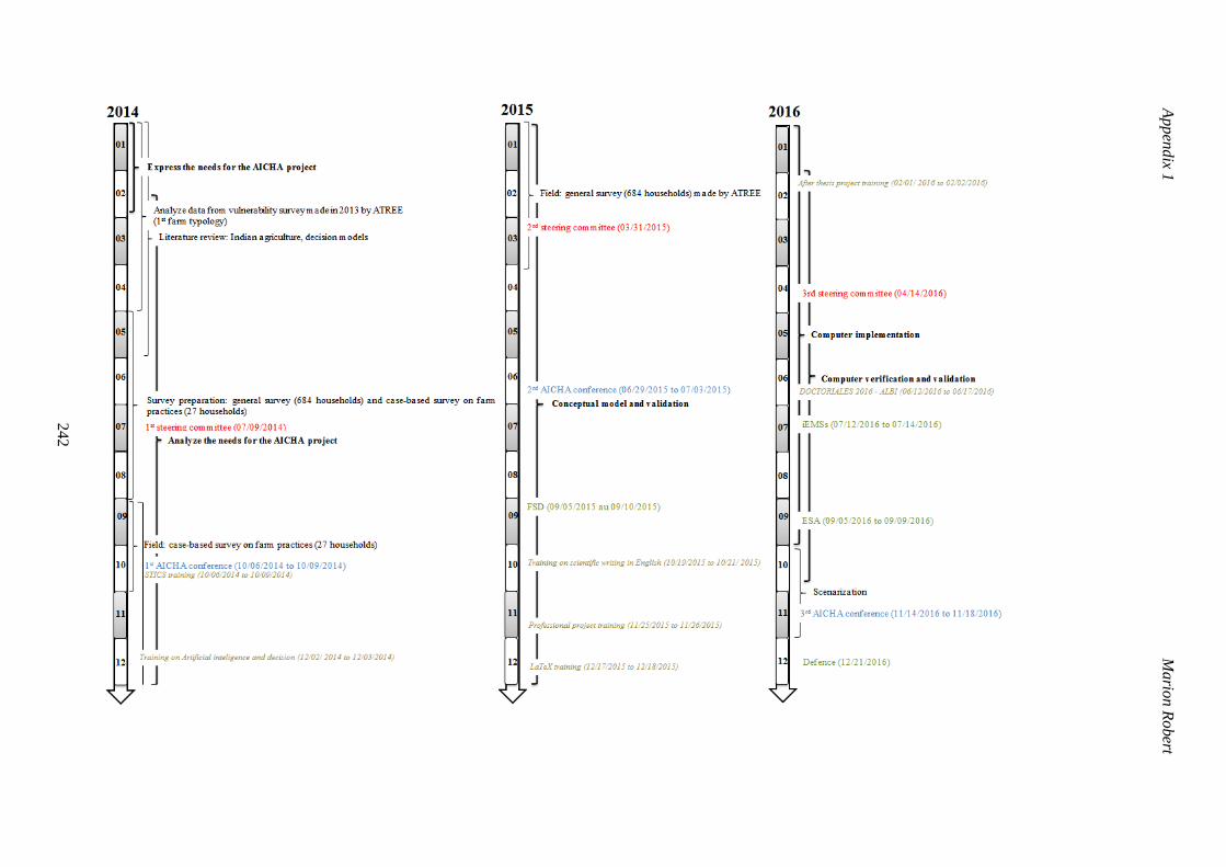
Appen
dix 1
M
ario
n R
obert
242

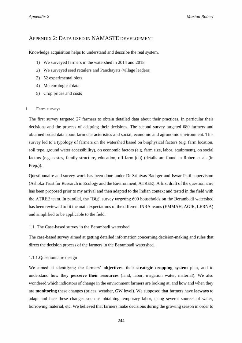
Appendix 2 Marion Robert
244
APPENDIX 2: DATA USED IN NAMASTE DEVELOPMENT
Knowledge acquisition helps to understand and describe the real system.
1) We surveyed farmers in the watershed in 2014 and 2015.
2) We surveyed seed retailers and Panchayats (village leaders)
3) 52 experimental plots
4) Meteorological data
5) Crop prices and costs
1. Farm surveys
The first survey targeted 27 farmers to obtain detailed data about their practices, in particular their
decisions and the process of adapting their decisions. The second survey targeted 680 farmers and
obtained broad data about farm characteristics and social, economic and agronomic environment. This
survey led to a typology of farmers on the watershed based on biophysical factors (e.g. farm location,
soil type, ground water accessibility), on economic factors (e.g. farm size, labor, equipment), on social
factors (e.g. castes, family structure, education, off-farm job) (details are found in Robert et al. (in
Prep.)).
Questionnaire and survey work has been done under Dr Srinivas Badiger and Iswar Patil supervision
(Ashoka Trust for Research in Ecology and the Environment, ATREE). A first draft of the questionnaire
has been proposed prior to my arrival and then adapted to the Indian context and tested in the field with
the ATREE team. In parallel, the “Big” survey targeting 600 households on the Berambadi watershed
has been reviewed to fit the main expectations of the different INRA teams (EMMAH, AGIR, LERNA)
and simplified to be applicable to the field.
1.1. The Case-based survey in the Berambadi watershed
The case-based survey aimed at getting detailed information concerning decision-making and rules that
direct the decision process of the farmers in the Berambadi watershed.
1.1.1. Questionnaire design
We aimed at identifying the farmers’ objectives, their strategic cropping system plan, and to
understand how they perceive their resources (land, labor, irrigation water, material). We also
wondered which indicators of change in the environment farmers are looking at, and how and when they
are monitoring these changes (prices, weather, GW level). We supposed that farmers have leeways to
adapt and face these changes such as obtaining temporary labor, using several sources of water,
borrowing material, etc. We believed that farmers make decisions during the growing season in order to
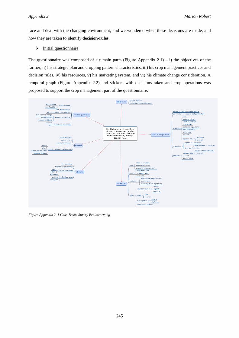
Appendix 2 Marion Robert
245
face and deal with the changing environment, and we wondered when these decisions are made, and
how they are taken to identify decision-rules.
Initial questionnaire
The questionnaire was composed of six main parts (Figure Appendix 2.1) – i) the objectives of the
farmer, ii) his strategic plan and cropping pattern characteristics, iii) his crop management practices and
decision rules, iv) his resources, v) his marketing system, and vi) his climate change consideration. A
temporal graph (Figure Appendix 2.2) and stickers with decisions taken and crop operations was
proposed to support the crop management part of the questionnaire.
Figure Appendix 2. 1 Case-Based Survey Brainstorming
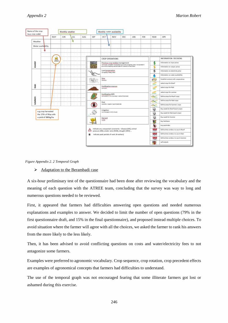
Appendix 2 Marion Robert
246
Adaptation to the Berambadi case
A six-hour preliminary test of the questionnaire had been done after reviewing the vocabulary and the
meaning of each question with the ATREE team, concluding that the survey was way to long and
numerous questions needed to be reviewed.
First, it appeared that farmers had difficulties answering open questions and needed numerous
explanations and examples to answer. We decided to limit the number of open questions (79% in the
first questionnaire draft, and 15% in the final questionnaire), and proposed instead multiple choices. To
avoid situation where the farmer will agree with all the choices, we asked the farmer to rank his answers
from the more likely to the less likely.
Then, it has been advised to avoid conflicting questions on costs and water/electricity fees to not
antagonize some farmers.
Examples were preferred to agronomic vocabulary. Crop sequence, crop rotation, crop precedent effects
are examples of agronomical concepts that farmers had difficulties to understand.
The use of the temporal graph was not encouraged fearing that some illiterate farmers got lost or
ashamed during this exercise.
Figure Appendix 2. 2 Temporal Graph
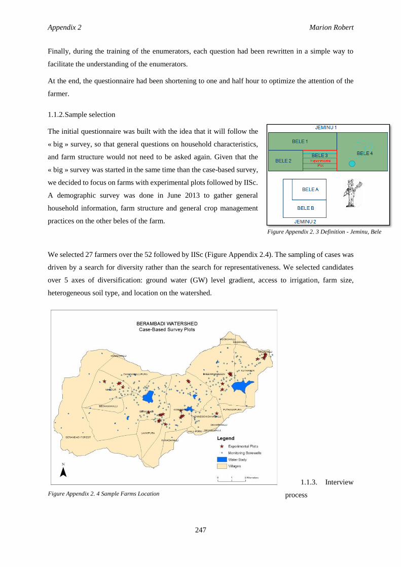
Appendix 2 Marion Robert
247
Finally, during the training of the enumerators, each question had been rewritten in a simple way to
facilitate the understanding of the enumerators.
At the end, the questionnaire had been shortening to one and half hour to optimize the attention of the
farmer.
1.1.2. Sample selection
The initial questionnaire was built with the idea that it will follow the
« big » survey, so that general questions on household characteristics,
and farm structure would not need to be asked again. Given that the
« big » survey was started in the same time than the case-based survey,
we decided to focus on farms with experimental plots followed by IISc.
A demographic survey was done in June 2013 to gather general
household information, farm structure and general crop management
practices on the other beles of the farm.
We selected 27 farmers over the 52 followed by IISc (Figure Appendix 2.4). The sampling of cases was
driven by a search for diversity rather than the search for representativeness. We selected candidates
over 5 axes of diversification: ground water (GW) level gradient, access to irrigation, farm size,
heterogeneous soil type, and location on the watershed.
1.1.3. Interview
process
Figure Appendix 2. 3 Definition - Jeminu, Bele
Figure Appendix 2. 4 Sample Farms Location
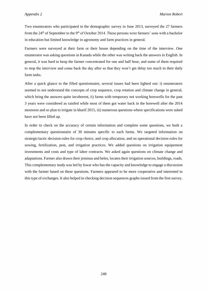
Appendix 2 Marion Robert
248
Two enumerators who participated in the demographic survey in June 2013, surveyed the 27 farmers
from the 24th of September to the 9th of October 2014. These persons were farmers’ sons with a bachelor
in education but limited knowledge in agronomy and farm practices in general.
Farmers were surveyed at their farm or their house depending on the time of the interview. One
enumerator was asking questions in Kanada while the other was writing back the answers in English. In
general, it was hard to keep the farmer concentrated for one and half hour, and some of them required
to stop the interview and come back the day after so that they won’t get delay too much in their daily
farm tasks.
After a quick glance to the filled questionnaire, several issues had been lighted out: i) enumerators
seemed to not understand the concepts of crop sequence, crop rotation and climate change in general,
which bring the answers quite incoherent, ii) farms with temporary not working borewells for the past
3 years were considered as rainfed while most of them got water back in the borewell after the 2014
monsoon and so plan to irrigate in kharif 2015, iii) numerous questions where specifications were asked
have not been filled up.
In order to check on the accuracy of certain information and complete some questions, we built a
complementary questionnaire of 30 minutes specific to each farms. We targeted information on
strategic/tactic decision-rules for crop choice, and crop allocation, and on operational decision-rules for
sowing, fertilization, pest, and irrigation practices. We added questions on irrigation equipement
investments and costs and type of labor contracts. We asked again questions on climate change and
adaptations. Farmer also drawn their jeminus and beles, locates their irrigation sources, buildings, roads.
This complementary study was led by Iswar who has the capacity and knowledge to engage a discussion
with the farmer based on these questions. Farmers appeared to be more cooperative and interested in
this type of exchanges. It also helped in checking decision sequences graphs issued from the first survey.

CASE-BASED SURVEY
249
The aim of the project is to develop scenarios of water consumption by agriculture in changing climate. It is therefore necessary to understand farming practices that impact water use
Start the interview by describing the purpose of the survey: for academic research only, accurate answers
are important and gratefully acknowledged, etc.
We are going to ask you some questions about your farm, the way you organise your production, the
source of information you use, and about yourself and the family members involved in production. All
is which will be treated confidentially.
1. Basic Information
Date
Plot number
Name of Village
Panchayat Name
Name of household head
Caste
Religion
Farming Experience
2. Household Information:
2.1. General information
Name
Relatio
n with
HH
head*
Gender
Age
in
years
Educatio
n
Occupation** Members
fulltime
work in
own farm
Members
temporarily
work in own
farm Primary Secondary
* Head=1, Wife/Husband=2, Son/Daughter=3, Grandchild=4, Father/Mother=5, Sister/Brother=6,
Niece/Nephew=7,Uncle/Aunt=8, Son/Daughter-In-Law=9,Father/Mother-In-Law=10, Brother/Sister-
In-Law=11, Grandparent=12, others=13
** Own agriculture work=1, Agriculture labour=2, Petty business=3, Dairy farming=4, Plantation
worker=5, NTFP collecting=6, Livestock grazing=7, Factory worker=8, Pension earner (social
security/Job pension)=9, Rural crafts (carpentry, blacksmith, pottery, weaving, goldsmith, basket
making, leather work, etc.)=10, Government job=11, Commission agent=12, Contractor=13, Quarry
worker=14, Bee keeper=15, Student=16, Domestic work (cleaning, cooking, water fetching, child care,
fire making, washing clothes, etc) =17, Driver=18, Not working (Children/Aged/physical disable/illness
etc.)=19, Mason= 20, Other=21 (specify)
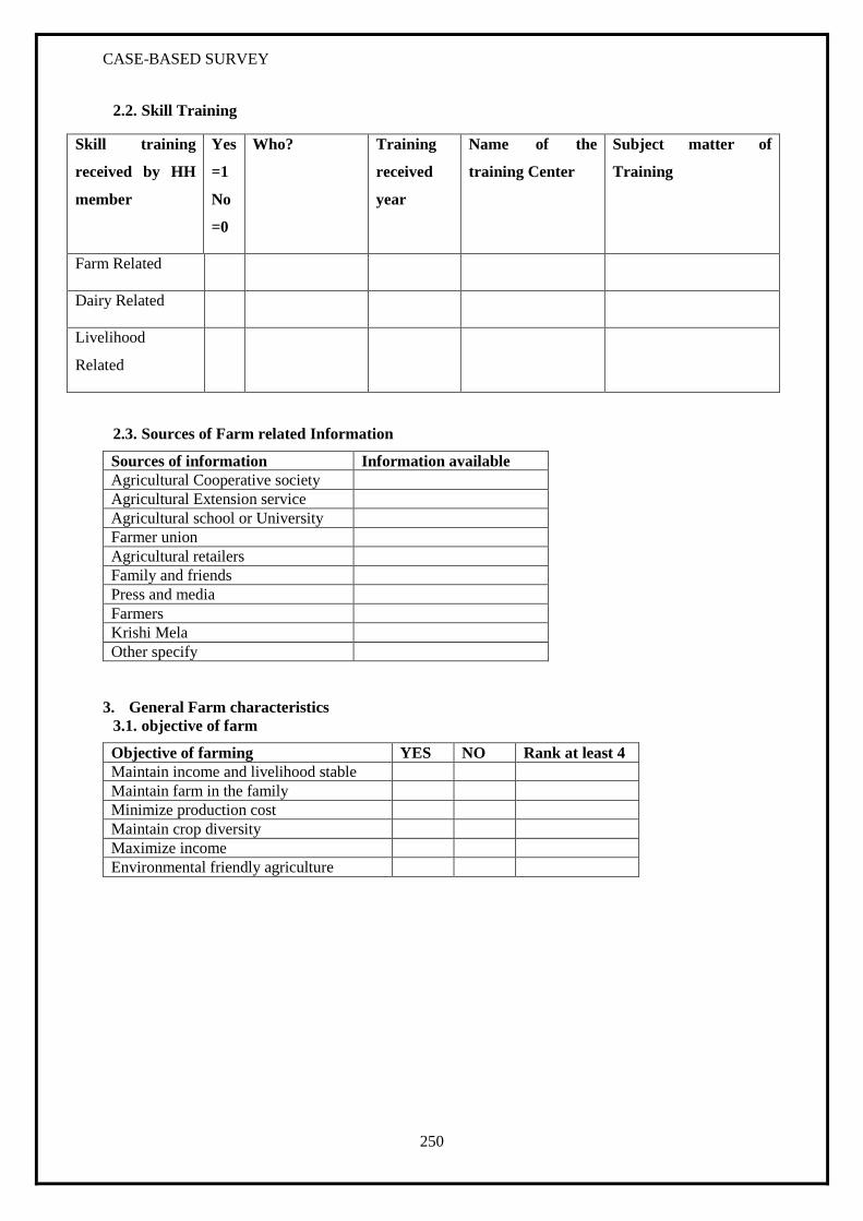
CASE-BASED SURVEY
250
2.2. Skill Training
Skill training
received by HH
member
Yes
=1
No
=0
Who? Training
received
year
Name of the
training Center
Subject matter of
Training
Farm Related
Dairy Related
Livelihood
Related
2.3. Sources of Farm related Information
Sources of information Information available
Agricultural Cooperative society
Agricultural Extension service
Agricultural school or University
Farmer union
Agricultural retailers
Family and friends
Press and media
Farmers
Krishi Mela
Other specify
3. General Farm characteristics
3.1. objective of farm
Objective of farming YES NO Rank at least 4
Maintain income and livelihood stable
Maintain farm in the family
Minimize production cost
Maintain crop diversity
Maximize income
Environmental friendly agriculture

CASE-BASED SURVEY
251
3.2. Specific Farm Characteristics:
3.3. Manpower
Inform the number of labor needed in kharif 2014:
Activity wise Labour use Number of
Own Labour
Number of Hired
Labour
Number of
Permanent
labour
No of
Mutual
Labour
Wage Paid(Average)
Male female Male Female
Land Preparation
Sowing
Weeding
Manure Application
Fertilizer Application
Harvest
Threshing
a. Number of farms in different
location and location identity
FARM 1
FARM 2
b. Farm Size (in acre)
c. Farm ownership
e. From how many years do you
operate the farms
g. Farm soil type
h. Farm Buildings Type
h.1. No of buildings
h.2. Year of farm building
constructed
i. Farm distance from your home in
Km
j. Is farm has irrigation source?
k. ownership of irrigation
source(Own/Joint/Neighbor/Govern
ment)
l. Irrigation method of each farm
m. Do you have farm pond/Farm
tank?
n. Water Source for Pond/farm tank
o. How many hours it take to fill? -

CASE-BASED SURVEY
252
Inform the number of labor needed in rabi 2013:
Activity wise Labour
use
Number of
Own
Labour
Number of
Hired Labour
Number
of
Permane
nt labour
No of
mutual
labour
Wage
Paid(Average)
Male female
Male Female
Land Preparation
Sowing
Weeding
Manure Application
Fertilizer
Application
Harvest
Threshing
3.4. Farm assets
Material type Number of
equipment
Owned=1
rent=2
Person using it
Tractor
Tractor and implements
Bullocks and implements
Wooden plough
Iron plough
Seeder
Weeder
Pesticide sprayer
Wheel barrow
Treshing machine
Organic manure pit
3.5. Livestock Information:
Type* Number Present value Reasons for keeping**
- - - -
*Bulls=1, oxen=2, cow=3, buffalo=4, sheep=5, goat=6, poultry=8, pig=9
**own cultivation/Hiring out=1, manure=2, fuel (cooking) =3, milk=4, meat=5, egg=6

CASE-BASED SURVEY
253
3.5.1. How do you manage manure from cattle?
□ Use on land
□ Give or sell to others
□ Fuel (cooking)
□ Others (be specific)
4. Decision rules
4.1. For the choice of your crops
4.1.1. How do you choose your crops?
(give 4 reasons and order)
□ Crop choice is made according to water availability
□ Crop choice depends on input costs
□ The market for the crop is more accessible/crop easier to sell
□ The price you expect is the leading factor
□ You are familiar with growing these crops
□ Crop choice depends on labour available (minimize working hours?)
□ Suit to soil
□ High yield
□ Other (be specific
4.1.2. What are the crops usually grow for self-use purpose and cash purpose?
4.1.3. What is the usual crop sequence that you follow (e.g. Marigold – Maize – Marigold
– Maize) in kharif? In rabi?
Need base crops Crop name Percentage
cash crops
Self-consumption crops
Crop sequence (KHARIF)
RAINFED plots
IRRIGATED plots
Crop sequence (RABI)
RAINFED plots
IRRIGATED plots
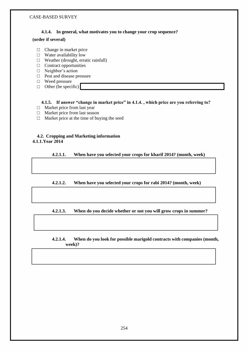
CASE-BASED SURVEY
254
4.1.4. In general, what motivates you to change your crop sequence?
(order if several)
□ Change in market price
□ Water availability low
□ Weather (drought, erratic rainfall)
□ Contract opportunities
□ Neighbor’s action
□ Pest and disease pressure
□ Weed pressure
□ Other (be specific)
4.1.5. If answer “change in market price” in 4.1.4. , which price are you referring to?
□ Market price from last year
□ Market price from last season
□ Market price at the time of buying the seed
4.2. Cropping and Marketing information
4.1.1. Year 2014
4.2.1.1. When have you selected your crops for kharif 2014? (month, week)
4.2.1.2. When have you selected your crops for rabi 2014? (month, week)
4.2.1.3. When do you decide whether or not you will grow crops in summer?
4.2.1.4. When do you look for possible marigold contracts with companies (month,
week)?
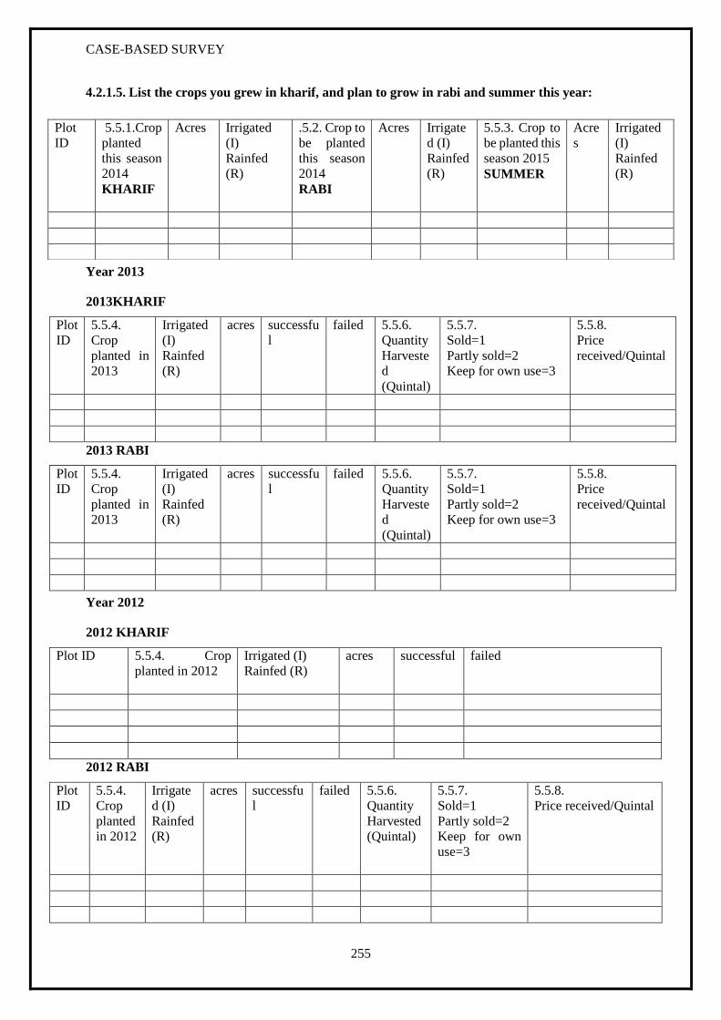
CASE-BASED SURVEY
255
4.2.1.5. List the crops you grew in kharif, and plan to grow in rabi and summer this year:
Year 2013
2013KHARIF
Plot
ID
5.5.4.
Crop
planted in
2013
Irrigated
(I)
Rainfed
(R)
acres successfu
l
failed 5.5.6.
Quantity
Harveste
d
(Quintal)
5.5.7.
Sold=1
Partly sold=2
Keep for own use=3
5.5.8.
Price
received/Quintal
2013 RABI
Plot
ID
5.5.4.
Crop
planted in
2013
Irrigated
(I)
Rainfed
(R)
acres successfu
l
failed 5.5.6.
Quantity
Harveste
d
(Quintal)
5.5.7.
Sold=1
Partly sold=2
Keep for own use=3
5.5.8.
Price
received/Quintal
Year 2012
2012 KHARIF
Plot ID 5.5.4. Crop
planted in 2012
Irrigated (I)
Rainfed (R)
acres successful failed
2012 RABI
Plot
ID
5.5.4.
Crop
planted
in 2012
Irrigate
d (I)
Rainfed
(R)
acres successfu
l
failed 5.5.6.
Quantity
Harvested
(Quintal)
5.5.7.
Sold=1
Partly sold=2
Keep for own
use=3
5.5.8.
Price received/Quintal
Plot
ID
5.5.1.Crop
planted
this season
2014
KHARIF
Acres Irrigated
(I)
Rainfed
(R)
.5.2. Crop to
be planted
this season
2014
RABI
Acres Irrigate
d (I)
Rainfed
(R)
5.5.3. Crop to
be planted this
season 2015
SUMMER
Acre
s
Irrigated
(I)
Rainfed
(R)
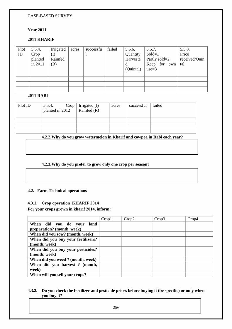
CASE-BASED SURVEY
256
Year 2011
2011 KHARIF
Plot
ID
5.5.4.
Crop
planted
in 2011
Irrigated
(I)
Rainfed
(R)
acres successfu
l
failed 5.5.6.
Quantity
Harveste
d
(Quintal)
5.5.7.
Sold=1
Partly sold=2
Keep for own
use=3
5.5.8.
Price
received/Quin
tal
2011 RABI
Plot ID 5.5.4. Crop
planted in 2012
Irrigated (I)
Rainfed (R)
acres successful failed
4.2.2. Why do you grow watermelon in Kharif and cowpea in Rabi each year?
4.2.3. Why do you prefer to grow only one crop per season?
4.2. Farm Technical operations
4.3.1. Crop operation KHARIF 2014
For your crops grown in kharif 2014, inform:
Crop1 Crop2 Crop3 Crop4
When did you do your land
preparation? (month, week)
When did you sow? (month, week)
When did you buy your fertilizers?
(month, week)
When did you buy your pesticides?
(month, week)
When did you weed ? (month, week)
When did you harvest ? (month,
week)
When will you sell your crops?
4.3.2. Do you check the fertilizer and pesticide prices before buying it (be specific) or only when
you buy it?

CASE-BASED SURVEY
257
4.3.3. Do the pesticide and fertilizer prices influence your choice of crops?
4.3.4. Crop constraints Found in KHARIF 2014
Crop name Type of constraint
Seed
defect
Late
sowing
Delayed
rain
Heavy
rain
Long
dry spell
weed Disease Pests Animal
Pressure
a.
b.
c.
d.
4.3.5. What have you done to face these crop constraints (see 4.3.4.)?
Crop name Action done to face crop constraints
a.
b.
c.
d.
4.3.6. At which time in kharif do you have the most amount of work to do? Why? in which order
do you deal with your crops?
Time in kharif 2013 YES / NO Crops priority order:
Land Preparation YES / NO
Sowing YES / NO
Weeding YES / NO
Manure Application YES / NO
Fertilizer Application YES / NO
Harvest YES / NO
Threshing YES / NO
4.3.7. Crop operation RABI 2013
For your crops grown in rabi 2013, inform:
Crop1 Crop2 Crop3 Crop4
When did you do your land preparation?
(month, week)
When did you sow? (month, week)
When did you buy your fertilizers? (month,
week)
When did you buy your pesticides? (month,
week)
When did you weed ? (month, week)
When did you harvest ? (month, week)
When will you sell your crops?

CASE-BASED SURVEY
258
4.3.8. Crop constraints Found in RABI 2013
Crop name Type of constraint
Seed
defect
Late
sowing
Delayed
rain
Heavy
rain
Long
dry spell
weed Disease Pests Animal
Pressure
a.
b.
c.
d.
4.3.8.1. What have you done to face these crop constraints (see 4.3.8.)?
Crop name Action done to face crop constraints
a.
b.
c.
d.
4.3.9. At which time in Rabi do you have the most amount of work to do? Why? in which order
do you deal with your crops?
Time in Rabi 2013 YES / NO Crops priority order:
Land Preparation YES / NO
Sowing YES / NO
Weeding YES / NO
Manure Application YES / NO
Fertilizer Application YES / NO
Harvest YES / NO
Threshing YES / NO
4.4. Concerning the location of the crops on the plot
From kharif 2013 to kharif 2014, precise which crop was grown in kharif 2013 at this place?
plot Crop kharif 2013 Crop kharif 2014
From Kharif 2014 to Rabi 2014 precise which crop will be plant in Rabi 2014 at this place?
plot Crop kharif 2014 Crop rabi 2014

CASE-BASED SURVEY
259
4.5. Concerning the soil quality of your crop plots:
Do you have some crop plots: YES / NO Which crops to do like to grow on it?
More fertile YES / NO
Less fertile YES / NO
Close to tank/stream YES / NO
In coconut garden YES / NO
In tree shadow plots YES / NO
4.6. Concerning the location of your crops:
Do you prefer grow certain crop: YES / NO Which crops to do like to
grow on it?
Why?
Closer to the road YES / NO
Closer to the house YES / NO
4.7. For your land preparation
4.7.1. How do you determine when to start land preparation?
□ Same month/week every year (if so which month/week)
□ After the start of first rain? (if so how many days after first rain)
□ Based on groundwater availability (ground water level)
□ Other
4.7.2. What is the gap (no of days) between harvest of kharif and sowing in rabi?
4.8. For your irrigation system
4.8.1. How do you determine when to irrigate?
□ Fixed interval (once in a week or once in 10 days)
□ Soil humidity inferior to
□ Take in consideration the groundwater level
□ Physical aspect of the plant
□ No rain for days
□ You follow the manufacturer’s recommendations (specify his name)
□ You follow the agricultural technician advice (specify his name)
4.8.2. How do you organize the distribution of water among the different fields? (how do you
define which field get irrigated first, second...)
□ all the fields are irrigated the same day, the same way
□ rotate irrigation between fields depending on the stage of the plant
□ irrigate fields where the plant seems to need water
4.8.3. How do you determine the amount of water you apply?
□ Same amount of irrigation for all crops
□ Based on crop water requirement
□ Based on crop type (commercial, self-consumption)
□ Based on crop duration
□ Based on water holding capacity of the soil
□ Based on expected income crops

CASE-BASED SURVEY
260
4.8.4. What crops have the highest irrigation priority?
□ crop more sensitive to drought (list the crops……………………………………….……..)
□ higher expected income (list the crops……………………………………………………..)
□ crops for self-consumption (list the crops…….……………………………………………)
4.8.5. What do you do if the water available in the borewell is decreasing and not enough to
irrigate the whole irrigated land?
□ Change frequency (be specific)
□ Change quantity (be specific)
□ Borrow water resource from a neighbor
□ Change irrigation techniques (be specific)
□ Stop irrigating
□ Other (be specific)
4.9. For your fertiliser operations
4.9.1. Do you apply manure?
Crop kharif 2014 Crop rabi 2013
Yes / No Yes / No
Yes / No Yes / No
Yes / No Yes / No
Yes / No Yes / No
4.9.2. How do you allocate farm manure to the different crops in kharif and rabi season?
□ Equally distributed
□ Depending on crop needs
□ Depending on crop giving higher expected income
□ Other (be specific)
4.9.3. Do you apply chemical fertilizer to each field? YES / NO
4.9.4. Do you adapt these applications to your soil characteristics? YES / NO
4.9.5. How do you determine the quantities and number of fertilization applications?
□ It depends on the market price of fertilizer
□ It depends on the availability of farm yard manure
□ You follow the agricultural department advice(specify the name)
□ You follow the manufacturer’s recommendations (specify the name)
□ You decide based on your past experience
□ Other (be specific)
4.9.6. What crops have the highest fertilization priority? Why?
priority crop reasons
1
2
3
4

CASE-BASED SURVEY
261
4.10. For your pesticide operations
4.10.1. How do you determine the quantities and number of pesticide applications?
□ You decide based on your past experience
□ You follow the agricultural technician advice (specify his name)
□ You follow the manufacturer’s recommendations (specify his name)
□ Decide based disease type
4.10.2. When do you decide to treat?
□ do a systematic treatment (specify when, and plant stage)
□ treat only if pest attack
4.11. What would you do if you were unable to sow the planned crop in time (e.g. because of
erratic rains, late monsoon)?
□ grow the next season crop (specify which one)
□ grow a shorter season crop (specify which one)
□ make a temporary fallow
□ other (be specific)
4.12. What would you do if the crop does not come up well?
□ Resow the same crop
□ grow a shorter season crop (specify which one)
□ keep it like it is
□ make a temporary fallow
□ other (be specific)
4.13. Residue management
□ Not Managing
□ Burn in the filed/Through out of field
□ De-composting in the field
□ Use for fuel
□ Others
4.14. Does late or early monsoon influence your choice of crop to grow in kharif? YES / NO
4.15. In kharif, if the monsoon has been delayed, do you:
□ Reduce your soil preparation
□ Increase seed density
□ Change crops for the season (specify which ones)
□ Select short duration and resistant varieties
4.16. In rabi, if the rain in kharif has been good and the water level in the borewell is high, do you:
□ Grow additional short duration cash crops (specify which ones)
□ Increase the area of the higher expected income crops (specify % area increase)
□ Don’t change your usual crop sequence
4.17. In Rabi, if the rain in Kharif has been poor and the water level in the borewell is low, do you:
□ Grow only less water requirement crops (specify which ones)

CASE-BASED SURVEY
262
□ Do Fallow
□ Grow only higher expected income crops (specify which ones)
□ Don’t change your usual crop sequence
□ Select short duration and resistant varieties
5. Perception / ressources / contraints
5.1. Market system and agro food chain
5.1.1. Where do you get your inputs (seeds, fertilizers, pesticides)?
inputs Retailer/cooperative/company/government agro shop (give name if possible)
seeds
fertilizers
pesticides
5.1.2. Where do you sell your crops?
crops
Cooperative
Marketing board(specify name)
Local market
Local agent
Company
Others (specify)
5.2. Water
5.2.1. Borewell information
Sl
No.
Farm
location
Number
Borewell
installed
year
Total
depth of
borewell
Working/Fail/yet
to start
When was
bore well
failed
Motor
fitted/Motor
not fitted
Pump HP
1
2
3
5.2.2. How many hours during the day is power supplied to your farm:
Total Hours …………. in kharif,
Total hours…………..in rabi
Total hours ………….in summer
5.2.3. Does your access to water limit the area that you cultivate in any season of the year? YES / NO
5.2.4.Does irrigation water availability affect your decision about the type of crop grown?YES/NO
5.2.5. what will you do if your borewell fails?
□ Buy water v

CASE-BASED SURVEY
263
□ Increase tank and rain water storage
□ Change your crop choice (specify which crops to stop, new crops)
□ Changes in irrigation system (changes in equipment)
□ Get crop insurance
□ Dig a deepper well
□ Other (be specific)
5.2.6. Do you buy water? YES/NO (if yes, from who?)
5.3. Climate
5.3.5. Have you heard of climate change? YES / NO
5.3.6. Have you identified current changes in climate? YES / NO
5.3.7. What are the main climatic risks you have already encountered?
Climatic risks kharif / rabi year Number of days Adaptation code*
Flood kharif / rabi
Drough kharif / rabi
Delayed monsoon kharif / rabi
Wind kharif / rabi
High temperature kharif / rabi
Low temperature kharif / rabi
Rainy season end sooner kharif / rabi
Less rain kharif / rabi
In a climate change scenario, the conditions would be warmer, with less rainfall in Kharif and
more dry spell in Rabi.
5.3.8. What would you change in your farming practices to face climate change?
Changes crops YES / NO
Select more resistant varieties YES / NO
Change sowing dates YES / NO
Do more intercropping crops YES / NO
Plant shade trees YES / NO
Change your irrigation equipment YES / NO
Migrate to other area YES / NO
Get crop insurances YES / NO
Diversify your crops (grow more crops but on smaller area) YES / NO
1.2. The global survey in the Berambadi watershed
* Change in crop variety=1, Decrease irrigation=2, Increase irrigation=3, Form pond construct=4, Dig new borewell=5, Stop
irrigation=6, Reduce livestock=7, Keep improved livestock=8, Migration to other area=9, Lease out land=10, Purchase
water=11, Plant shade trees=12, Change sowing time=13, Others=14 (specify)
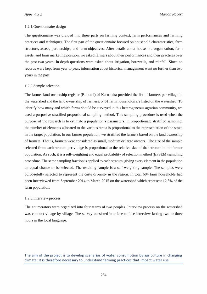
Appendix 2 Marion Robert
264
1.2.1. Questionnaire design
The questionnaire was divided into three parts on farming context, farm performances and farming
practices and techniques. The first part of the questionnaire focused on household characteristics, farm
structure, assets, partnerships, and farm objectives. After details about household organization, farm
assets, and farm marketing position, we asked farmers about their performances and their practices over
the past two years. In-depth questions were asked about irrigation, borewells, and rainfall. Since no
records were kept from year to year, information about historical management went no further than two
years in the past.
1.2.2. Sample selection
The farmer land ownership register (Bhoomi) of Karnataka provided the list of farmers per village in
the watershed and the land ownership of farmers. 5461 farm households are listed on the watershed. To
identify how many and which farms should be surveyed in this heterogeneous agrarian community, we
used a purposive stratified proportional sampling method. This sampling procedure is used when the
purpose of the research is to estimate a population’s parameters. In proportionate stratified sampling,
the number of elements allocated to the various strata is proportional to the representation of the strata
in the target population. In our farmer population, we stratified the farmers based on the land ownership
of farmers. That is, farmers were considered as small, medium or large owners. The size of the sample
selected from each stratum per village is proportional to the relative size of that stratum in the farmer
population. As such, it is a self-weighting and equal probability of selection method (EPSEM) sampling
procedure. The same sampling fraction is applied to each stratum, giving every element in the population
an equal chance to be selected. The resulting sample is a self-weighting sample. The samples were
purposefully selected to represent the caste diversity in the region. In total 684 farm households had
been interviewed from September 2014 to March 2015 on the watershed which represent 12.5% of the
farm population.
1.2.3. Interview process
The enumerators were organized into four teams of two peoples. Interview process on the watershed
was conduct village by village. The survey consisted in a face-to-face interview lasting two to three
hours in the local language.
The aim of the project is to develop scenarios of water consumption by agriculture in changing climate. It is therefore necessary to understand farming practices that impact water use

GLOBAL FARM SURVEY
265
Start the interview by describing the purpose of the survey: for academic research only, accurate
answers are important and gratefully acknowledged, etc.
We are going to ask you some questions about your farm, the way you organise your production,
the source of information you use, and about yourself and the family members involved in
production. All is which will be treated confidentially.
1. Basic Information
1. Name of Village______________________
2. Panchayat Name__________________________
3. Household Number ______________________
4. Name of household head ________________________
5. Respondent Name_______________________________
6. Caste_________________________________
6. Interviewer ____________________________________
7. Date_________________
8. Interview start time _____________ Interview End time___________
2. Household Information:
2.1 How many members presently residing in the home? _______

GLOBAL FARM SURVEY
266
Sl.
Name
Relation
with
HH
head
Gender
Age
in
years*
Education
Occupation** Training
on farm
activities
Training
on dairy
activities
Income
form
off-
farm
activity Primary Secondary
1
2
3
4
5
6
7
8
9
10
* For a child below one year code is 0
Relationship code:
Head=1, Wife/Husband=2, Son/Daughter=3, Grandchild=4, Father/Mother=5, Sister/Brother=6,
Niece/Nephew=7,Uncle/Aunt=8, Son/Daughter-In-Law=9,Father/Mother-In-Law=10, Brother/Sister-In-
Law=11, Grandparent=12, others=13
Education code:
Illiterate=1, Read and write=2, Pre-Primary School (1-5)=3, Upper primary (6-8)=4, High School (9-10)=5,
PUC - (11-12), Diploma Course=6, Graduation=7, Post-Graduation and above=8, Technical Degree (medical,
engineering, agriculture, etc.)=9, Other professional courses (TCH/Bed/Med)=10
**Occupation code:
Own agriculture work=1, Agriculture labour=2, Petty business=3, Dairy farming=4, Plantation worker=5, NTFP
collecting=6, Livestock grazing=7, Factory worker=8, Pension earner (social security/Job pension)=9, Rural crafts
(carpentry, blacksmith, pottery, weaving, goldsmith, basket making, leather work, etc.)=10, Government job=11,
Commission agent=12, Contractor=13, Quarry worker=14, Bee keeper=15, Student=16, Domestic work (cleaning,
cooking, water fetching, child care, fire making, washing clothes, etc) =17, Driver=18, Not working
(Children/Aged/physical disable/illness etc.)=19, Mason= 20, Other=21 (specify)
2.2. Manpower
1. How many family members work permanently on the farm, including yourself? ________
Persons
2. How many family members work temporary on the farm, including yourself? _______
Persons

GLOBAL FARM SURVEY
267
3. Do you have permanently workers (that are not family members) on your farm? Yes/No.
If yes, number of ______Persons
4. Did you hire temporary workers on the farm during the last year? Yes/No. if yes, number of
________persons
5. At what wage were they paid/day Male Worker Rs._______Day Female worker
Rs.__________Day
6. Were you helped by neighbours during the last season? Yes/No. if yes number
of___________ Persons and Number of days helped_________
7. How many family members working as agriculture labours(2013)?________________
8. Approximate labour work days in a week
1. kharif :
2. rabi :
3. summer :
9. Number of month work days in a Season
1. kharif :
2. rabi :
3. summer :
10. Any of your family members temporarily migrating (2013)? Yes/No
If yes,
1. Period of migration______________
2. Place of Migration_________________
3. Nature of work did during migration________________
4. Total net savings from Migration_____________________
2.3. Skill Manpower
1. Did you or member of your family receive any training on farm activities? Yes/NO if yes,
Number of days/week/month/years of training taken--------------
1. a. Date of the last training____________
2. Did you or member of your family receive any training on dairy activities? Yes/NO if yes,
Number of days/week/month/years of training taken---------------

GLOBAL FARM SURVEY
268
2. a. Date of the last training ____________
3. What institution was in charge of the training?
3.1 Farm Related 3.2 Dairy related
a. Agricultural University a. Agricultural University
b. Agriculture department b. NGO
c. Horticulture department c. Milk co-operative societies
d. NGO d. others
e. Farm companies
f. Farm co-operative societies
g. Others
4. Did the training include
1. Land preparation
2. Crop choice
3. Fertiliser use
4. Irrigation
5. Seed management and selection
6. Extreme weather management
7. Others, specify ………………..
5. Did you find the training useful 0. No
1. Yes
If no, specify ……………………………………………………………………………….
6. Integration in farmer networks and source of information
a. Are you part of a farmer network? 0. No
1. Farmer union (identify it)
2. Cooperative (name it and locate it)
3. Other, specify
b. What are your main sources of information? 0. No information needed

GLOBAL FARM SURVEY
269
1. Cooperative (name it and locate it)
2. Extension services (name and locate it)
3. Agricultural school or institute (name it
and locate it)
4. Farmer union (name it and locate it)
5. Agricultural retailers (name and locate
it)
6. Family and friends
7. Other farmers
8. Press and media
9. Other, specify …………………………
c. Formal institutional membership network
1) Member in SHG Y/N M/F Number of persons _________
2) Member in Dairy Farm Y/N M/F Number of persons _________
3) Member in SDMC Y/N M/F Number of persons _________
4) Member in JFPM Y/N M/F Number of persons _________
5) Member in JSYS (TWUA) Y/N M/F Number of persons _________
6) Member in NREGP Y/N M/F Number of persons__________
7) Any other membership (specify) ________________________________________
d. informal institutions Networks
1. farmer-to-farmer extension Yes/No
2. Number of Close Farmers________
e.Trust Index
1. “Most farmers who live in this village can be trusted.”
a. Do trust = 1
b. Do not trust =0
2. Do you think over the last few years this level of trust has gotten better, gotten worse, or stayed about
the same?
a. Better =2
b. The same= 1
c. Worse=0
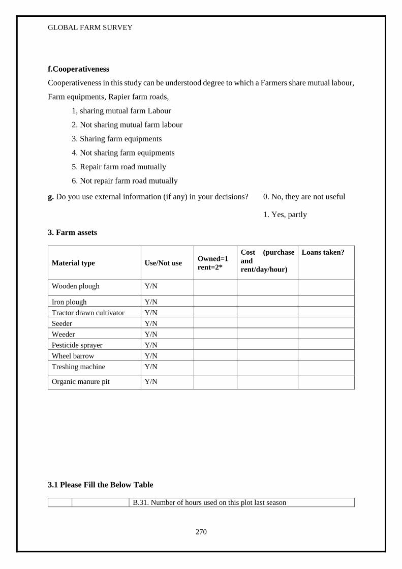
GLOBAL FARM SURVEY
270
f.Cooperativeness
Cooperativeness in this study can be understood degree to which a Farmers share mutual labour,
Farm equipments, Rapier farm roads,
1, sharing mutual farm Labour
2. Not sharing mutual farm labour
3. Sharing farm equipments
4. Not sharing farm equipments
5. Repair farm road mutually
6. Not repair farm road mutually
g. Do you use external information (if any) in your decisions? 0. No, they are not useful
1. Yes, partly
3. Farm assets
Material type Use/Not use Owned=1
rent=2*
Cost (purchase
and
rent/day/hour)
Loans taken?
Wooden plough Y/N
Iron plough Y/N
Tractor drawn cultivator Y/N
Seeder Y/N
Weeder Y/N
Pesticide sprayer Y/N
Wheel barrow Y/N
Treshing machine Y/N
Organic manure pit Y/N
3.1 Please Fill the Below Table
B.31. Number of hours used on this plot last season

GLOBAL FARM SURVEY
271
Plot
ID
B.30.
Tractor/bullock
used on this plot
0. None
1. own tractor
2.rented tractor
3. owned
bullock
4. rented
Bullock
1. For tilling
For spraying
manure,
fertilizers,
pesticides
3. For
carrying
harvest
4. For other
5. Total
4. Livestock Information:
Type* Number Present value Reasons for keeping** Income per year(2013)
1.
2.
3.
4.
5.
6.
7. *Bulls=1, oxen=2, cow=3, buffalo=4, sheep=5, goat=6, poultry=8, pig=9
**own cultivation/Hiring out=1, manure=2, fuel (cooking) =3, milk=4, meat=5, egg=6
4. A. How do you manage manure from cattle?
0. No particular management
1. Use on land
2. Give or sell to others
3. Fuel (cooking)
4. B. Did our cattle stock change since last year?
0. No
1. Increased: ……… animals
2. Decreased: … …animals
5. General Farm Characteristics:
1. Do you have Farm Land? Yes No
2. In how many places your farm lands located? (Including lease in/Share cropping land-
_________
3. Total Rainfed land__________ (Acre)
4. Total irrigated land_________ (Acre)
5.1. Specific Farm Characteristics:

GLOBAL FARM SURVEY
272
a. Number of farms in
different location and
location identity
One( ) Two ( ) Three ( ) Four ( )
b. Farm Size (in acre)
c. Farm ownership Own/Lease /Share
Own/Lease/ Share Own/Lease /Share Own/Lease/ Share
d. Source of ownership of your own farm
Parents/Purchase/Gift/Government
Parents/Purchase/Gift/Government
Parents/Purchase/Gift/Government
Parents/Purchase/Gift/Government
e. From how many years
do you operate the farms
f. Is there any change in
farm size over the last five
years
Increase/Decrease/Same Increase/Decrease/Same Increase/Decrease/Sam
e
Increase/Decrease/Sam
e
If yes, How many acres? If yes, How many acres? If yes, How many acres? If yes, How many acres?
g. Farm soil type
h. Farm Buildings
Farmhous
e
Pump
house
Farmhous
e
Pump
house
Farmhou
se
Pump
house
Farmhou
se
Pump
house
h.1. No of buildings One/two/
three
One/two/
three
One/two/
three
One/two/
three
One/two/
three
One/two/
three
One/two/
three
One/two/
three
h.2. Recently constructed
farm building (mention
year)
h.3. Oldest farm building(mention year)
i. Farm distance from your home in Km
j. Is farm has irrigation source?
Yes/No Yes/No Yes/No Yes/No
k. ownership of irrigation
source(Own/Joint/Neighbor/Government)
l. Irrigation method of each
farm
Flood/Furrow/Sprinkler/
drip
Flood/Furrow/Sprinkler/
drip
Flood/Furrow/Sprinkler
/drip
Flood/Furrow/Sprinkler
/drip
m. Do you have farm
pond/Farm tank?
Yes/No Yes/No Yes/No Yes/No
n. Water Source for
Pond/farm tank
Own well/Rainwater Own well/Rainwater Own well/Rainwater Own well/Rainwater
o. How many hours it take to fill?

GLOBAL FARM SURVEY
273
5.2 What changes made in farm investments, farm size and crop pattern from past 5
years? And why?
a. Machinery investment?
b. Livestock investments?
c. Irrigation investment and uses?
d. Other infrastructure investments?
e. Changes in land preparation?
f. Introduction of new crops? Stop others? (e.g. Marigold)
g. Increase or decrease cropping land area?
5.3 General objective of farm
5.3. A. What would you say the general objective of your farm is
1. Earn a livelihood for my family
2. Maintain the farm in the family
3. I prefer farming to any other activity
5.3. B. Would you say your farm has an adequate size? 1. Farm is too small
2. Farm is Medium
3. Farm is too big
5.4 Crop management
a. Do you follow a crop pattern defined over several years? Y/N
If yes, which one:.........
b. Which crops do you try to grow each year and why?
Cash crops:
Self-consumption crops:
5.5 Cropping and Marketing information
Year 2014
Plot
ID
5.5.1.Crop
planted this
season 2014
KHARIF
Crop code
(see
appendix)
Acres 5.5.2. Crop to
be planted this
season 2014
RABI
Crop code (see
appendix)
Acres 5.5.3. Crop to be planted
this season 2015
SUMMER
Crop code (see appendix)
Acres
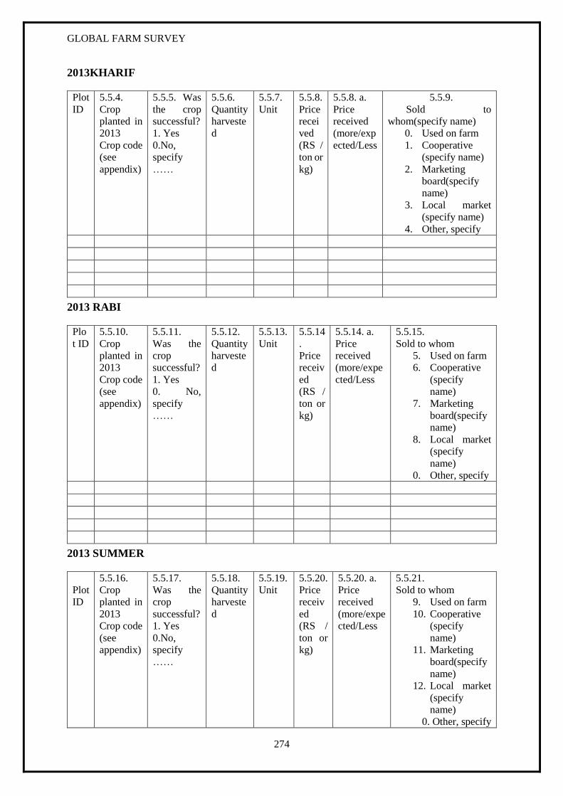
GLOBAL FARM SURVEY
274
2013KHARIF
Plot
ID
5.5.4.
Crop
planted in
2013
Crop code
(see
appendix)
5.5.5. Was
the crop
successful?
1. Yes
0.No,
specify
……
5.5.6.
Quantity
harveste
d
5.5.7.
Unit
5.5.8.
Price
recei
ved
(RS /
ton or
kg)
5.5.8. a.
Price
received
(more/exp
ected/Less
5.5.9.
Sold to
whom(specify name)
0. Used on farm
1. Cooperative
(specify name)
2. Marketing
board(specify
name)
3. Local market
(specify name)
4. Other, specify
2013 RABI
Plo
t ID
5.5.10.
Crop
planted in
2013
Crop code
(see
appendix)
5.5.11.
Was the
crop
successful?
1. Yes
0. No,
specify
……
5.5.12.
Quantity
harveste
d
5.5.13.
Unit
5.5.14
.
Price
receiv
ed
(RS /
ton or
kg)
5.5.14. a.
Price
received
(more/expe
cted/Less
5.5.15.
Sold to whom
5. Used on farm
6. Cooperative
(specify
name)
7. Marketing
board(specify
name)
8. Local market
(specify
name)
0. Other, specify
2013 SUMMER
Plot
ID
5.5.16.
Crop
planted in
2013
Crop code
(see
appendix)
5.5.17.
Was the
crop
successful?
1. Yes
0.No,
specify
……
5.5.18.
Quantity
harveste
d
5.5.19.
Unit
5.5.20.
Price
receiv
ed
(RS /
ton or
kg)
5.5.20. a.
Price
received
(more/expe
cted/Less
5.5.21.
Sold to whom
9. Used on farm
10. Cooperative
(specify
name)
11. Marketing
board(specify
name)
12. Local market
(specify
name)
0. Other, specify
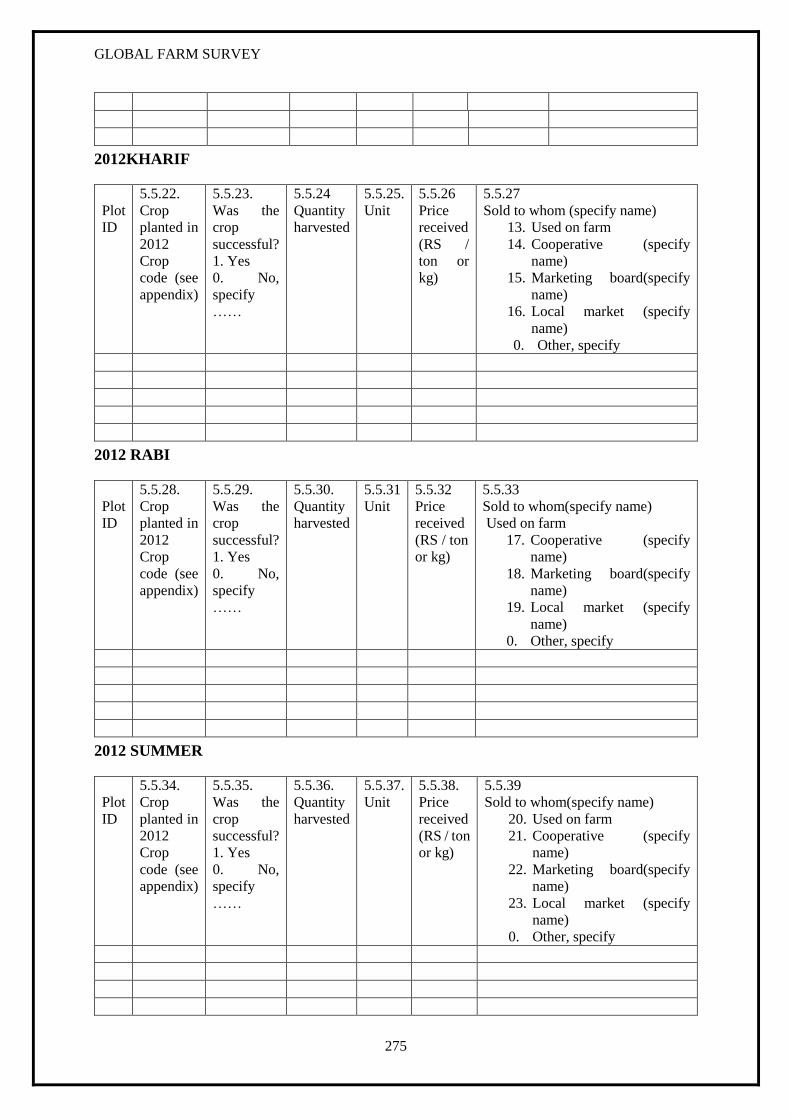
GLOBAL FARM SURVEY
275
2012KHARIF
Plot
ID
5.5.22.
Crop
planted in
2012
Crop
code (see
appendix)
5.5.23.
Was the
crop
successful?
1. Yes
0. No,
specify
……
5.5.24
Quantity
harvested
5.5.25.
Unit
5.5.26
Price
received
(RS /
ton or
kg)
5.5.27
Sold to whom (specify name)
13. Used on farm
14. Cooperative (specify
name)
15. Marketing board(specify
name)
16. Local market (specify
name)
0. Other, specify
2012 RABI
Plot
ID
5.5.28.
Crop
planted in
2012
Crop
code (see
appendix)
5.5.29.
Was the
crop
successful?
1. Yes
0. No,
specify
……
5.5.30.
Quantity
harvested
5.5.31
Unit
5.5.32
Price
received
(RS / ton
or kg)
5.5.33
Sold to whom(specify name)
Used on farm
17. Cooperative (specify
name)
18. Marketing board(specify
name)
19. Local market (specify
name)
0. Other, specify
2012 SUMMER
Plot
ID
5.5.34.
Crop
planted in
2012
Crop
code (see
appendix)
5.5.35.
Was the
crop
successful?
1. Yes
0. No,
specify
……
5.5.36.
Quantity
harvested
5.5.37.
Unit
5.5.38.
Price
received
(RS / ton
or kg)
5.5.39
Sold to whom(specify name)
20. Used on farm
21. Cooperative (specify
name)
22. Marketing board(specify
name)
23. Local market (specify
name)
0. Other, specify
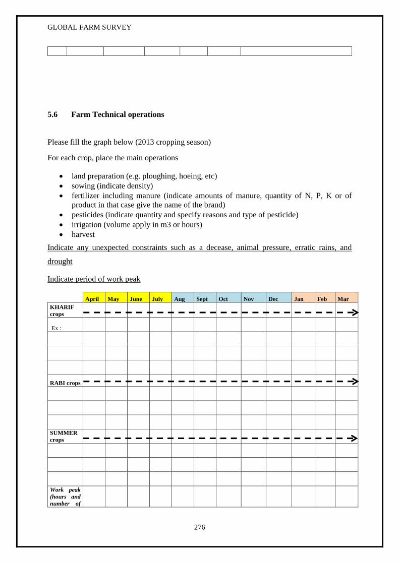
GLOBAL FARM SURVEY
276
5.6 Farm Technical operations
Please fill the graph below (2013 cropping season)
For each crop, place the main operations
land preparation (e.g. ploughing, hoeing, etc)
sowing (indicate density)
fertilizer including manure (indicate amounts of manure, quantity of N, P, K or of
product in that case give the name of the brand)
pesticides (indicate quantity and specify reasons and type of pesticide)
irrigation (volume apply in m3 or hours)
harvest
Indicate any unexpected constraints such as a decease, animal pressure, erratic rains, and
drought
Indicate period of work peak
April May June July Aug Sept Oct Nov Dec Jan Feb Mar
KHARIF
crops
Ex :
RABI crops
SUMMER
crops
Work peak
(hours and
number of
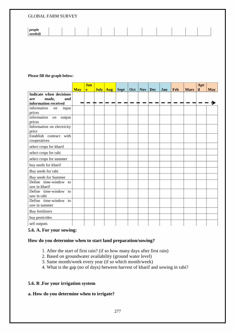
GLOBAL FARM SURVEY
277
people
needed)
Please fill the graph below:
5.6. A. For your sowing:
How do you determine when to start land preparation/sowing?
1. After the start of first rain? (if so how many days after first rain)
2. Based on groundwater availability (ground water level)
3. Same month/week every year (if so which month/week)
4. What is the gap (no of days) between harvest of kharif and sowing in rabi?
5.6. B .For your irrigation system
a. How do you determine when to irrigate?
May
Jun
e July Aug Sept Oct Nov Dec Jan Feb Mars
Apr
il May
Indicate when decisions
are made, and
information received
information on input
prices
information on output
prices
Information on electricity
price
Establish contract with
cooperatives
select crops for kharif
select crops for rabi
select crops for summer
buy seeds for kharif
Buy seeds for rabi
Buy seeds for Summer
Define time-window to
saw in kharif
Define time-window to
saw in rabi
Define time-window to
saw in summer
Buy fertilizers
buy pesticides
sell outputs
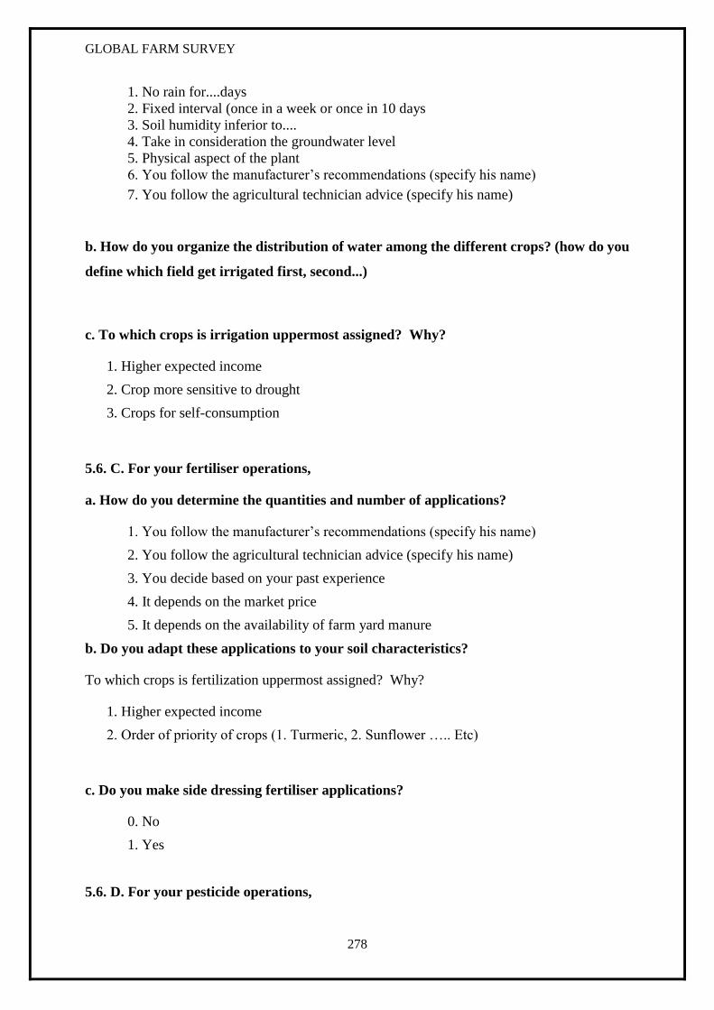
GLOBAL FARM SURVEY
278
1. No rain for....days
2. Fixed interval (once in a week or once in 10 days
3. Soil humidity inferior to....
4. Take in consideration the groundwater level
5. Physical aspect of the plant
6. You follow the manufacturer’s recommendations (specify his name)
7. You follow the agricultural technician advice (specify his name)
b. How do you organize the distribution of water among the different crops? (how do you
define which field get irrigated first, second...)
c. To which crops is irrigation uppermost assigned? Why?
1. Higher expected income
2. Crop more sensitive to drought
3. Crops for self-consumption
5.6. C. For your fertiliser operations,
a. How do you determine the quantities and number of applications?
1. You follow the manufacturer’s recommendations (specify his name)
2. You follow the agricultural technician advice (specify his name)
3. You decide based on your past experience
4. It depends on the market price
5. It depends on the availability of farm yard manure
b. Do you adapt these applications to your soil characteristics?
To which crops is fertilization uppermost assigned? Why?
1. Higher expected income
2. Order of priority of crops (1. Turmeric, 2. Sunflower ….. Etc)
c. Do you make side dressing fertiliser applications?
0. No
1. Yes
5.6. D. For your pesticide operations,

GLOBAL FARM SURVEY
279
a. How do you determine the quantities and number of applications?
1. You follow the manufacturer’s recommendations (specify his name)
2. You follow the agricultural technician advice (specify his name)
3. You decide based on your past experience
4. Decide based decease type
b. For your fertiliser and pesticide operations, do you decide according to the aspect of
leaves, soil… 0. No
1. Yes
c. How do you manage pest?
1. Spraying pesticide
2. Planting pest control plants
3. Early sowing crops (mature before pest attack starts)
4. Removing decease plants
5. Not taken any action
5.6. E. For the choice of your crops (rank here)
1. The price you expect is the leading factor (max profit, secure profit, repay loan
(ST/LT), children’s education?)
2. The market for the crop is more accessible/crop easier to sell
3. You are used to grow these crops
4. Crop choice is made according to water availability
5. Crop choice depends on input costs
6. Crop choice depends on labour available (minimize working hours?)
7. To meet household food grain needs
8. To produce livestock grain
9. Need for diversification
5.6. F. For the choice of the plots where to grow the wanted crops (rank here)
. 1. Proximity to roads
2. Irrigable characteristic of the plot
3. Soil characteristics
4. Passed crop
5. Use to grow this crop at a certain place
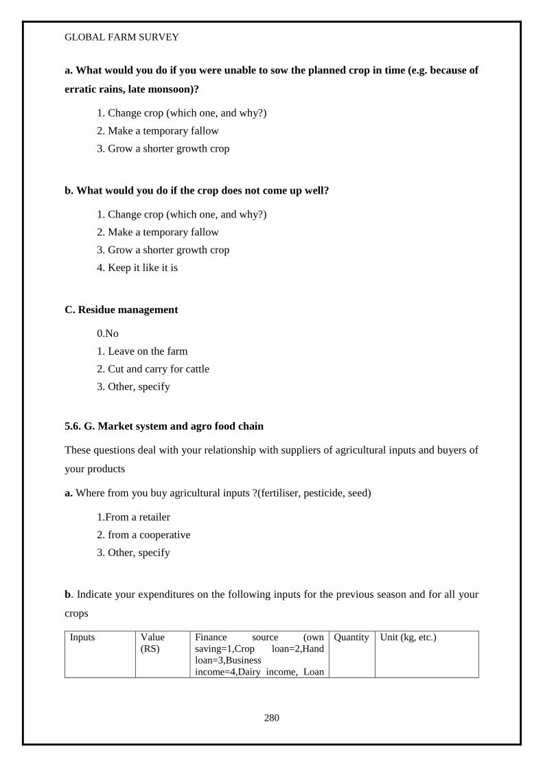
GLOBAL FARM SURVEY
280
a. What would you do if you were unable to sow the planned crop in time (e.g. because of
erratic rains, late monsoon)?
1. Change crop (which one, and why?)
2. Make a temporary fallow
3. Grow a shorter growth crop
b. What would you do if the crop does not come up well?
1. Change crop (which one, and why?)
2. Make a temporary fallow
3. Grow a shorter growth crop
4. Keep it like it is
C. Residue management
0.No
1. Leave on the farm
2. Cut and carry for cattle
3. Other, specify
5.6. G. Market system and agro food chain
These questions deal with your relationship with suppliers of agricultural inputs and buyers of
your products
a. Where from you buy agricultural inputs ?(fertiliser, pesticide, seed)
1.From a retailer
2. from a cooperative
3. Other, specify
b. Indicate your expenditures on the following inputs for the previous season and for all your
crops
Inputs Value
(RS)
Finance source (own
saving=1,Crop loan=2,Hand
loan=3,Business
income=4,Dairy income, Loan
Quantity Unit (kg, etc.)
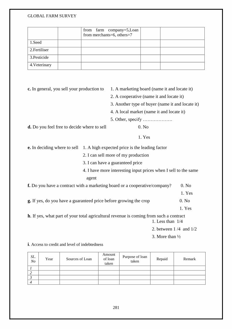
GLOBAL FARM SURVEY
281
from farm company=5,Loan
from merchants=6, others=7
1.Seed
2.Fertiliser
3.Pesticide
4.Veterinary
c. In general, you sell your production to 1. A marketing board (name it and locate it)
2. A cooperative (name it and locate it)
3. Another type of buyer (name it and locate it)
4. A local market (name it and locate it)
5. Other, specify ……………….
d. Do you feel free to decide where to sell 0. No
1. Yes
e. In deciding where to sell 1. A high expected price is the leading factor
2. I can sell more of my production
3. I can have a guaranteed price
4. I have more interesting input prices when I sell to the same
agent
f. Do you have a contract with a marketing board or a cooperative/company? 0. No
1. Yes
g. If yes, do you have a guaranteed price before growing the crop 0. No
1. Yes
h. If yes, what part of your total agricultural revenue is coming from such a contract
1. Less than 1/4
2. between 1 /4 and 1/2
3. More than ½
i. Access to credit and level of indebtedness
SL.
No Year Sources of Loan
Amount
of loan
taken
Purpose of loan
taken Repaid Remark
1
2
3
4
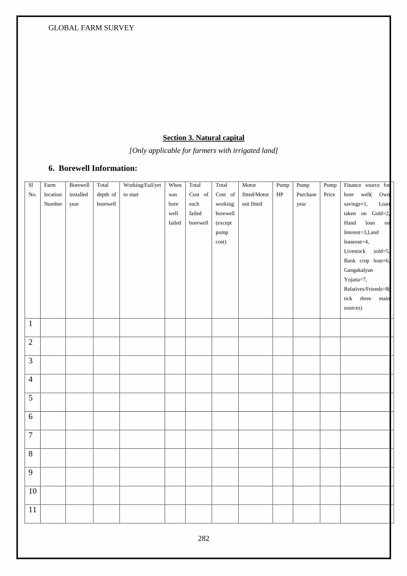
GLOBAL FARM SURVEY
282
Section 3. Natural capital
[Only applicable for farmers with irrigated land]
6. Borewell Information:
Sl
No.
Farm
location
Number
Borewell
installed
year
Total
depth of
borewell
Working/Fail/yet
to start
When
was
bore
well
failed
Total
Cost of
each
failed
borewell
Total
Cost of
working
borewell
(except
pump
cost)
Motor
fitted/Motor
not fitted
Pump
HP
Pump
Purchase
year
Pump
Price
Finance source for
bore well( Own
savings=1, Loan
taken on Gold=2,
Hand loan on
Interest=3,Land
leaseout=4,
Livestock sold=5,
Bank crop loan=6,
Gangakalyan
Yojana=7,
Relatives/Friends=8(
tick three main
sources)
1
2
3
4
5
6
7
8
9
10
11

GLOBAL FARM SURVEY
283
12
13
14
15
6. A. When was the last repair made? _______________________________
6. B. What kind of repair made? ____________________________________
6. C. How much money spent for repair? _____________________________
6.2. Factors that force farmer to go for multiple borewells/Re-bored/digging new borewell
1, Capable to manage financial Burden- Yes/No
2. Misleading by local water diviner/Borewell agents/Friends and relatives - Yes/No
3. Gut feeling of farmers that he certainly getting water/god shake- Yes/No
4. Less aware/No awareness of geological condition of the area- Yes/No
5. Deeper borewell may be getting water--- Yes/No
6. Want to irrigate more crop area/to bring rainfed land into irrigation ---Yes/No
7. Neighboring farmers owning multiple borewells-------Yes/No
8. Want grow more commercial crops----Yes/No
9. Limited hour supply of electricity hence one borewell not sufficient for irrigation—Yes/No
10. Low water in existing borewell/other problem in existing borewells (not deep, Boulders etc)
Yes/No
6.3. Farmer’s satisfaction over working borewells:
Working
Borewells
Satisfied Not Satisfied Some how ok Reason for not satisfied( Low discharge=1,
Frequent Repair=2, Stop working in
summer=3, water quality not good=4, Motor
burn frequently=5, Problem in bore hole=6,
Low pump capacity=7( tick three main
reasons)
1
2
3

GLOBAL FARM SURVEY
284
4
5
6
6.3. A. How many hours during the day is power supplied to your farm:
Total Hours …………. in kharif
Total hours………. in rabi/summer
6.3. B. How many time power shut down during specified time of three phase power supply?
_________
6.3. C. Does your access to water limit the area that you cultivate in any season of the year?
Yes/No
If yes, how much area really limits among total irrigable area(2013)? In
1. Kharif :
2. Rabi :
3. Summer :
6.3. D. Does irrigation water availability affect your decision the type of crop you grow?
Yes/No
If yes, which crop you give the priority?
1. ______________
2. ______________
3. ______________
6.4. E. If Irrigation water availability not affects your decision of crop selection, which crops
give the priority?
1. ______________
2. ______________
3. ______________
7. Possible adaptations/leeway to face Climate Change
To be asked necessarily after characterization of current practices (otherwise risk of bias)
To be discussed: Open or multiple choice questions ? (Proposal: open question, but possible
answers "a priori" are proposed in dotted boxes: if the farmer has no idea, propose a list of
these possible choices)
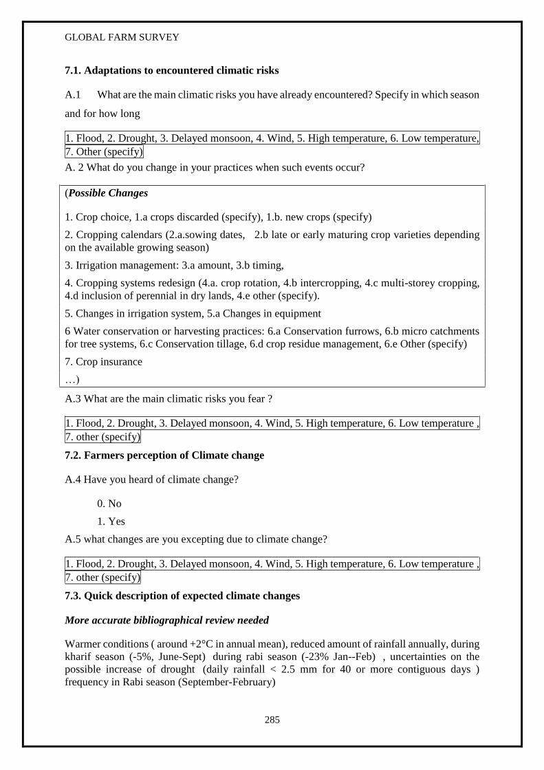
GLOBAL FARM SURVEY
285
7.1. Adaptations to encountered climatic risks
A.1 What are the main climatic risks you have already encountered? Specify in which season
and for how long
1. Flood, 2. Drought, 3. Delayed monsoon, 4. Wind, 5. High temperature, 6. Low temperature,
7. Other (specify)
A. 2 What do you change in your practices when such events occur?
(Possible Changes
1. Crop choice, 1.a crops discarded (specify), 1.b. new crops (specify)
2. Cropping calendars (2.a.sowing dates, 2.b late or early maturing crop varieties depending
on the available growing season)
3. Irrigation management: 3.a amount, 3.b timing,
4. Cropping systems redesign (4.a. crop rotation, 4.b intercropping, 4.c multi-storey cropping,
4.d inclusion of perennial in dry lands, 4.e other (specify).
5. Changes in irrigation system, 5.a Changes in equipment
6 Water conservation or harvesting practices: 6.a Conservation furrows, 6.b micro catchments
for tree systems, 6.c Conservation tillage, 6.d crop residue management, 6.e Other (specify)
7. Crop insurance
…)
A.3 What are the main climatic risks you fear ?
1. Flood, 2. Drought, 3. Delayed monsoon, 4. Wind, 5. High temperature, 6. Low temperature ,
7. other (specify)
7.2. Farmers perception of Climate change
A.4 Have you heard of climate change?
0. No
1. Yes
A.5 what changes are you excepting due to climate change?
1. Flood, 2. Drought, 3. Delayed monsoon, 4. Wind, 5. High temperature, 6. Low temperature ,
7. other (specify)
7.3. Quick description of expected climate changes
More accurate bibliographical review needed
Warmer conditions ( around +2°C in annual mean), reduced amount of rainfall annually, during
kharif season (-5%, June-Sept) during rabi season (-23% Jan--Feb) , uncertainties on the
possible increase of drought (daily rainfall < 2.5 mm for 40 or more contiguous days )
frequency in Rabi season (September-February)
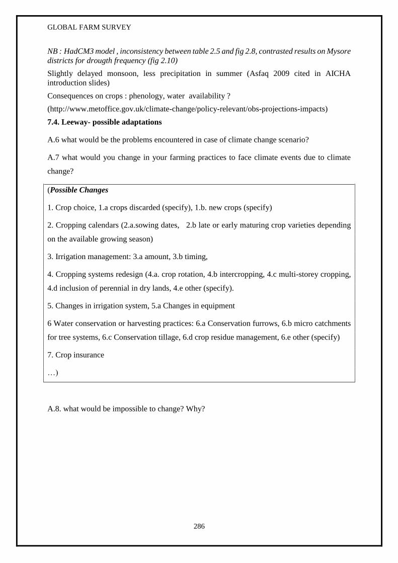
GLOBAL FARM SURVEY
286
NB : HadCM3 model , inconsistency between table 2.5 and fig 2.8, contrasted results on Mysore
districts for drougth frequency (fig 2.10)
Slightly delayed monsoon, less precipitation in summer (Asfaq 2009 cited in AICHA
introduction slides)
Consequences on crops : phenology, water availability ?
(http://www.metoffice.gov.uk/climate-change/policy-relevant/obs-projections-impacts)
7.4. Leeway- possible adaptations
A.6 what would be the problems encountered in case of climate change scenario?
A.7 what would you change in your farming practices to face climate events due to climate
change?
(Possible Changes
1. Crop choice, 1.a crops discarded (specify), 1.b. new crops (specify)
2. Cropping calendars (2.a.sowing dates, 2.b late or early maturing crop varieties depending
on the available growing season)
3. Irrigation management: 3.a amount, 3.b timing,
4. Cropping systems redesign (4.a. crop rotation, 4.b intercropping, 4.c multi-storey cropping,
4.d inclusion of perennial in dry lands, 4.e other (specify).
5. Changes in irrigation system, 5.a Changes in equipment
6 Water conservation or harvesting practices: 6.a Conservation furrows, 6.b micro catchments
for tree systems, 6.c Conservation tillage, 6.d crop residue management, 6.e other (specify)
7. Crop insurance
…)
A.8. what would be impossible to change? Why?

GLOBAL FARM SURVEY
287
Appendix 1: crop codes
1 Marygold
2 Horsegram
3 Turmeric
4 Onion
5 Watermelon
6 Beetroot
7 Maize
8 Jowar
9 Ginger
10 tsinees
11 Ragi
12 Sunflower
13 Coconut
14 Vegetables
15 Beans
16 Benise
17 Tomato
18 Carrot
19 Bengalgram
20 Banana
21 Cotton
22 Cowpeas
23 Redgram
24 Cabbage
25 Chilly
26 Garlic
27 Paddy
28 Potato
29 Sugarcane
30 Castrot
31 Groundnut
32 Brizal
33 Arese
34 Feildnet

Appendix 2 Marion Robert
288
2. Retailers and panchayat surveys
We surveyed seed retailers and Panchayats (village leaders) to learn about recommended crop
management practices and village organization.
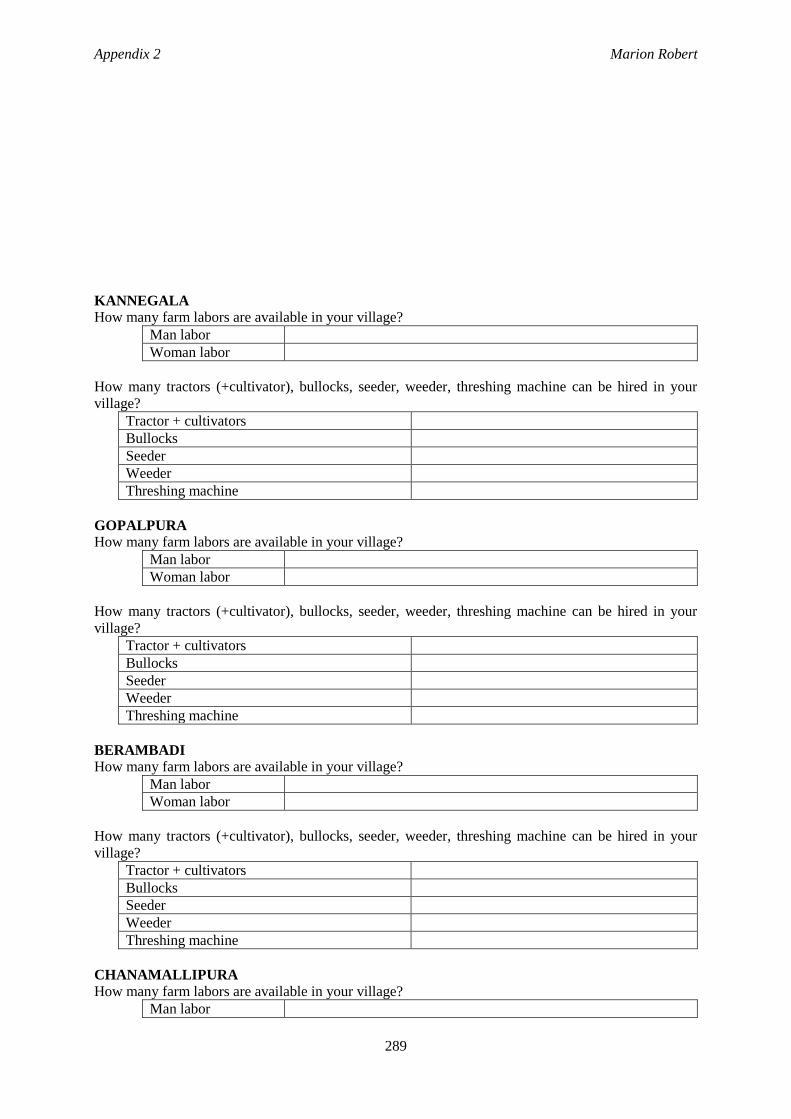
Appendix 2 Marion Robert
289
KANNEGALA
How many farm labors are available in your village?
Man labor
Woman labor
How many tractors (+cultivator), bullocks, seeder, weeder, threshing machine can be hired in your
village?
Tractor + cultivators
Bullocks
Seeder
Weeder
Threshing machine
GOPALPURA
How many farm labors are available in your village?
Man labor
Woman labor
How many tractors (+cultivator), bullocks, seeder, weeder, threshing machine can be hired in your
village?
Tractor + cultivators
Bullocks
Seeder
Weeder
Threshing machine
BERAMBADI
How many farm labors are available in your village?
Man labor
Woman labor
How many tractors (+cultivator), bullocks, seeder, weeder, threshing machine can be hired in your
village?
Tractor + cultivators
Bullocks
Seeder
Weeder
Threshing machine
CHANAMALLIPURA
How many farm labors are available in your village?
Man labor

GENERAL QUESTIONS TO PANCHAYAT
290
Woman labor
How many tractors (+cultivator), bullocks, seeder, weeder, threshing machine can be hired in your
village?
Tractor + cultivators
Bullocks
Seeder
Weeder
Threshing machine
MADDUR
How many farm labors are available in your village?
Man labor
Woman labor
How many tractors (+cultivator), bullocks, seeder, weeder, threshing machine can be hired in your
village?
Tractor + cultivators
Bullocks
Seeder
Weeder
Threshing machine
MADDUR COLONY
How many farm labors are available in your village?
Man labor
Woman labor
How many tractors (+cultivator), bullocks, seeder, weeder, threshing machine can be hired in your
village?
Tractor + cultivators
Bullocks
Seeder
Weeder
Threshing machine
BECHANAHALLI
How many farm labors are available in your village?
Man labor
Woman labor
How many tractors (+cultivator), bullocks, seeder, weeder, threshing machine can be hired in your
village?
Tractor + cultivators
Bullocks
Seeder
Weeder
Threshing machine
CHANNAMALLIPURA
How many farm labors are available in your village?
Man labor

GENERAL QUESTIONS TO PANCHAYAT
291
Woman labor
How many tractors (+cultivator), bullocks, seeder, weeder, threshing machine can be hired in your
village?
Tractor + cultivators
Bullocks
Seeder
Weeder
Threshing machine
LAKKIPURA
How many farm labors are available in your village?
Man labor
Woman labor
How many tractors (+cultivator), bullocks, seeder, weeder, threshing machine can be hired in your
village?
Tractor + cultivators
Bullocks
Seeder
Weeder
Threshing machine
KUNAGAHALLI
How many farm labors are available in your village?
Man labor
Woman labor
How many tractors (+cultivator), bullocks, seeder, weeder, threshing machine can be hired in your
village?
Tractor + cultivators
Bullocks
Seeder
Weeder
Threshing machine
KALLIPURA
How many farm labors are available in your village?
Man labor
Woman labor
How many tractors (+cultivator), bullocks, seeder, weeder, threshing machine can be hired in your
village?
Tractor + cultivators
Bullocks
Seeder
Weeder
Threshing machine
HONNEGOWDANAHALLI
How many farm labors are available in your village?
Man labor

GENERAL QUESTIONS TO PANCHAYAT
292
Woman labor
How many tractors (+cultivator), bullocks, seeder, weeder, threshing machine can be hired in your
village?
Tractor + cultivators
Bullocks
Seeder
Weeder
Threshing machine
BEEMANABEEDHU
How many farm labors are available in your village?
Man labor
Woman labor
How many tractors (+cultivator), bullocks, seeder, weeder, threshing machine can be hired in your
village?
Tractor + cultivators
Bullocks
Seeder
Weeder
Threshing machine
KUTHANUR
How many farm labors are available in your village?
Man labor
Woman labor
How many tractors (+cultivator), bullocks, seeder, weeder, threshing machine can be hired in your
village?
Tractor + cultivators
Bullocks
Seeder
Weeder
Threshing machine
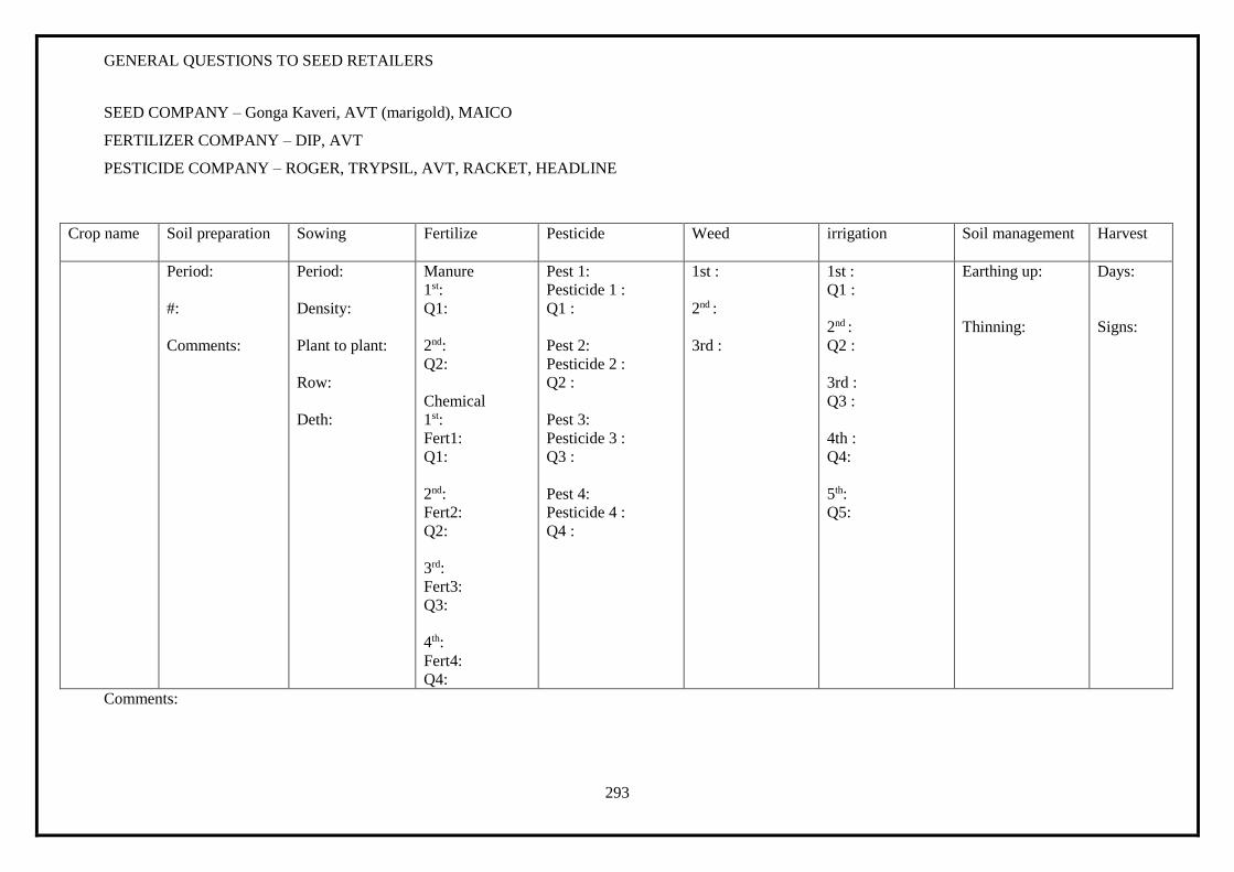
GENERAL QUESTIONS TO SEED RETAILERS
293
SEED COMPANY – Gonga Kaveri, AVT (marigold), MAICO
FERTILIZER COMPANY – DIP, AVT
PESTICIDE COMPANY – ROGER, TRYPSIL, AVT, RACKET, HEADLINE
Crop name Soil preparation Sowing
Fertilize Pesticide Weed irrigation Soil management Harvest
Period:
#:
Comments:
Period:
Density:
Plant to plant:
Row:
Deth:
Manure
1st:
Q1:
2nd:
Q2:
Chemical
1st:
Fert1:
Q1:
2nd:
Fert2:
Q2:
3rd:
Fert3:
Q3:
4th:
Fert4:
Q4:
Pest 1:
Pesticide 1 :
Q1 :
Pest 2:
Pesticide 2 :
Q2 :
Pest 3:
Pesticide 3 :
Q3 :
Pest 4:
Pesticide 4 :
Q4 :
1st :
2nd :
3rd :
1st :
Q1 :
2nd :
Q2 :
3rd :
Q3 :
4th :
Q4:
5th:
Q5:
Earthing up:
Thinning:
Days:
Signs:
Comments:
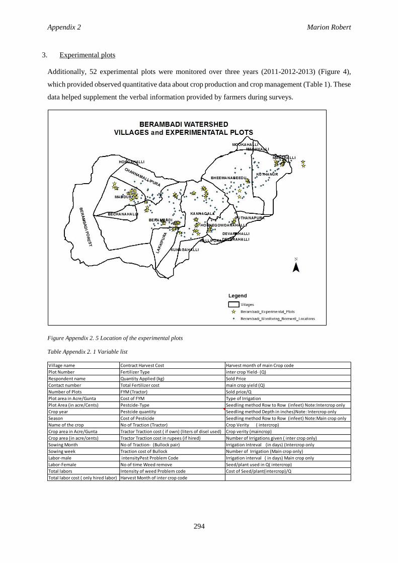
Appendix 2 Marion Robert
294
3. Experimental plots
Additionally, 52 experimental plots were monitored over three years (2011-2012-2013) (Figure 4),
which provided observed quantitative data about crop production and crop management (Table 1). These
data helped supplement the verbal information provided by farmers during surveys.
Figure Appendix 2. 5 Location of the experimental plots
Table Appendix 2. 1 Variable list
Village name Contract Harvest Cost Harvest month of main Crop code
Plot Number Fertilizer Type inter crop Yield- (Q)
Respondent name Quantity Applied (kg) Sold Price
Contact number Total Fertilizer cost main crop yield (Q)
Number of Plots FYM (Tractor) Sold price/Q
Plot area in Acre/Gunta Cost of FYM Type of Irrigation
Plot Area (in acre/Cents) Pestcide-Type Seedling method Row to Row (infeet) Note:Intercrop only
Crop year Pestcide quantity Seedling method Depth in inches)Note: Intercrop only
Season Cost of Pesticide Seedling method Row to Row (infeet) Note:Main crop only
Name of the crop No of Traction (Tractor) Crop Verity ( intercrop)
Crop area in Acre/Gunta Tractor Traction cost ( if own) (liters of disel used) Crop verity (maincrop)
Crop area (in acre/cents) Tractor Traction cost in rupees (if hired) Number of Irrigations given ( inter crop only)
Sowing Month No of Traction- (Bullock pair) Irrigation Intreval (in days) (Intercrop only
Sowing week Traction cost of Bullock Number of Irrigation (Main crop only)
Labor-male intensityPest Problem Code Irrigation interval ( in days) Main crop only
Labor-Female No of time Weed remove Seed/plant used in Q( intercrop)
Total labors Intensity of weed Problem code Cost of Seed/plant(intercrop)/Q
Total labor cost ( only hired labor) Harvest Month of inter crop code

Appendix 2 Marion Robert
295
4. Meteorological data
Meteorological data were obtained from a meteorological station and water gauges installed on the
watershed.
5. Price and cost data
Prices and costs were obtained from farmers and from official district data from the Indian Ministry of
Agriculture and Cooperation (Directorate of Economics and Statistics) and the National Informatics
Center (Agricultural Census Division).


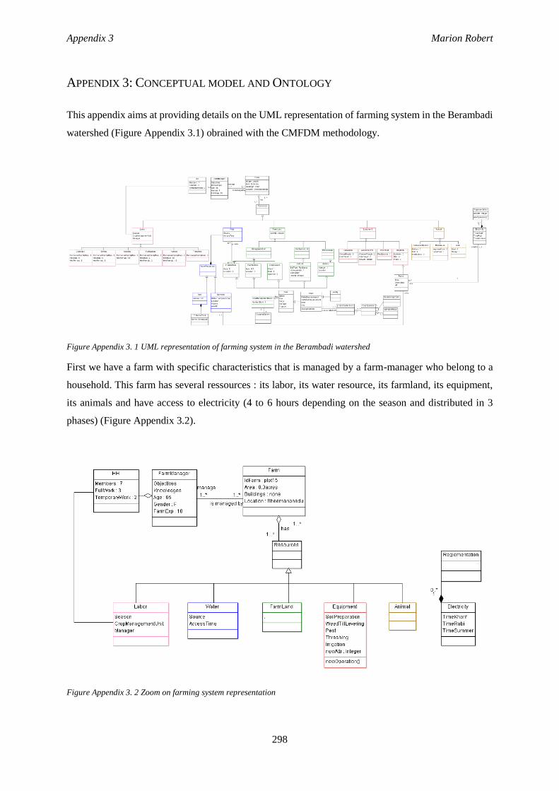
Appendix 3 Marion Robert
298
APPENDIX 3: CONCEPTUAL MODEL AND ONTOLOGY
This appendix aims at providing details on the UML representation of farming system in the Berambadi
watershed (Figure Appendix 3.1) obrained with the CMFDM methodology.
Figure Appendix 3. 1 UML representation of farming system in the Berambadi watershed
First we have a farm with specific characteristics that is managed by a farm-manager who belong to a
household. This farm has several ressources : its labor, its water resource, its farmland, its equipment,
its animals and have access to electricity (4 to 6 hours depending on the season and distributed in 3
phases) (Figure Appendix 3.2).
Figure Appendix 3. 2 Zoom on farming system representation
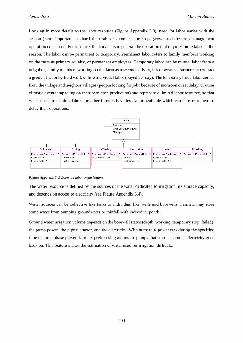
Appendix 3 Marion Robert
299
Looking in more details to the labor resource (Figure Appendix 3.3), need for labor varies with the
season (more important in kharif than rabi or summer), the crops grown and the crop management
operation concerned. For instance, the harvest is in general the operation that requires more labor in the
season. The labor can be permanent or temporary. Permanent labor refers to family members working
on the farm as primary activity, or permanent employees. Temporary labor can be mutual labor from a
neighbor, family members working on the farm as a second activity, hired persons. Farmer can contract
a group of labor by field work or hire individual labor (payed per day). The temporary hired labor comes
from the village and neighbor villages (people looking for jobs because of monsoon onset delay, or other
climatic events impacting on their own crop production) and represent a limited labor resource, so that
when one farmer hires labor, the other farmers have less labor available which can constrain them to
delay their operations.
Figure Appendix 3. 3 Zoom on labor organization.
The water resource is defined by the sources of the water dedicated to irrigation, its storage capacity,
and depends on access to electricity (see Figure Appendix 3.4).
Water sources can be collective like tanks or individual like wells and borewells. Farmers may store
some water from pumping groundwater or rainfall with individual ponds.
Ground water irrigation volume depends on the borewell status (depth, working, temporary stop, failed),
the pump power, the pipe diameter, and the electricity. With numerous power cuts during the specified
time of three phase power, farmers prefer using automatic pumps that start as soon as electricity goes
back on. This feature makes the estimation of water used for irrigation difficult..
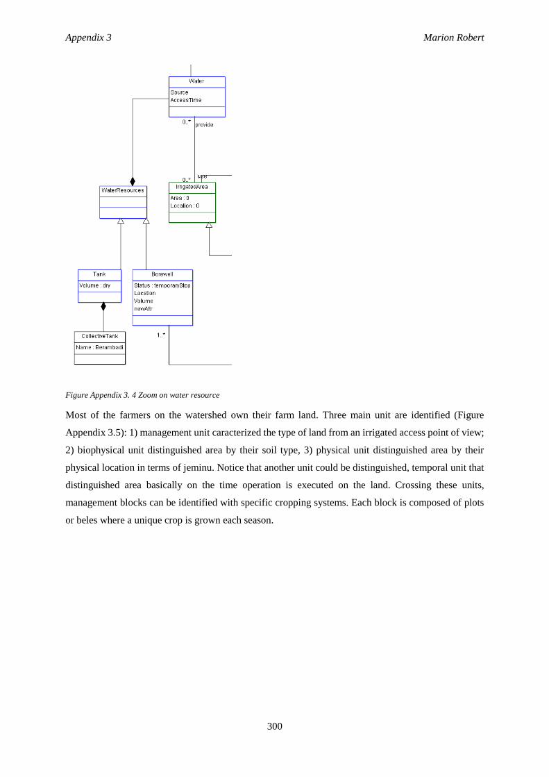
Appendix 3 Marion Robert
300
Figure Appendix 3. 4 Zoom on water resource
Most of the farmers on the watershed own their farm land. Three main unit are identified (Figure
Appendix 3.5): 1) management unit caracterized the type of land from an irrigated access point of view;
2) biophysical unit distinguished area by their soil type, 3) physical unit distinguished area by their
physical location in terms of jeminu. Notice that another unit could be distinguished, temporal unit that
distinguished area basically on the time operation is executed on the land. Crossing these units,
management blocks can be identified with specific cropping systems. Each block is composed of plots
or beles where a unique crop is grown each season.
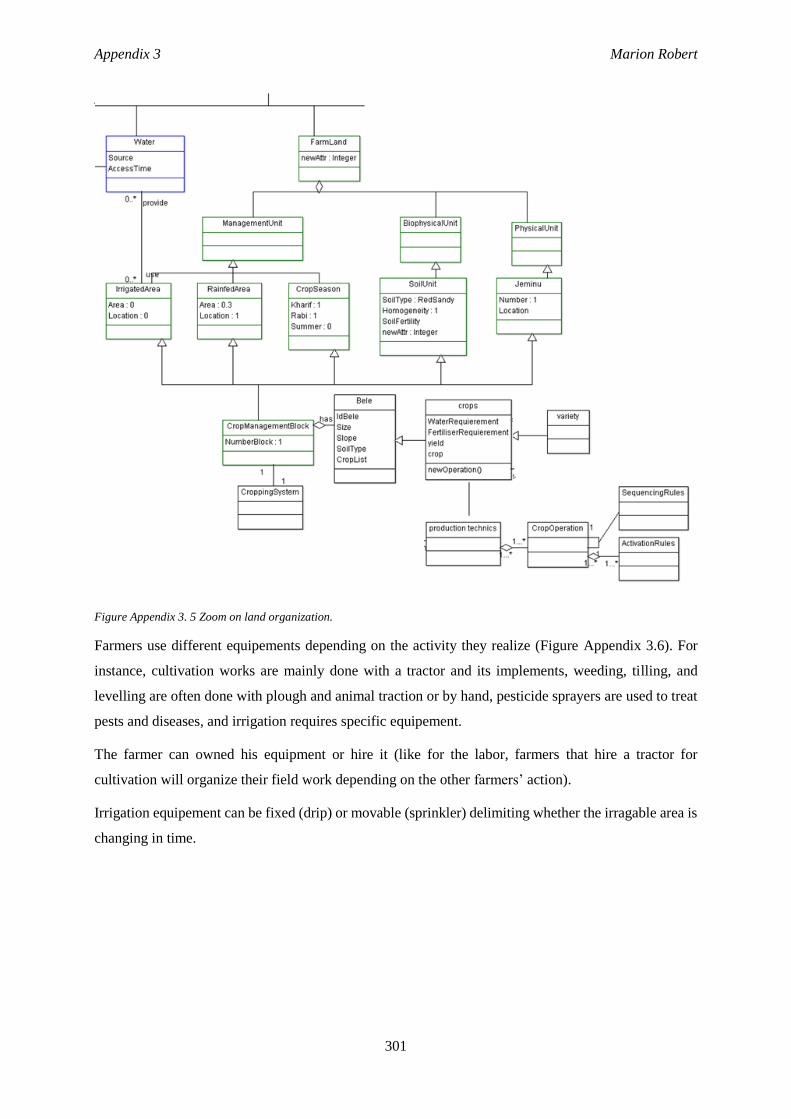
Appendix 3 Marion Robert
301
Figure Appendix 3. 5 Zoom on land organization.
Farmers use different equipements depending on the activity they realize (Figure Appendix 3.6). For
instance, cultivation works are mainly done with a tractor and its implements, weeding, tilling, and
levelling are often done with plough and animal traction or by hand, pesticide sprayers are used to treat
pests and diseases, and irrigation requires specific equipement.
The farmer can owned his equipment or hire it (like for the labor, farmers that hire a tractor for
cultivation will organize their field work depending on the other farmers’ action).
Irrigation equipement can be fixed (drip) or movable (sprinkler) delimiting whether the irragable area is
changing in time.
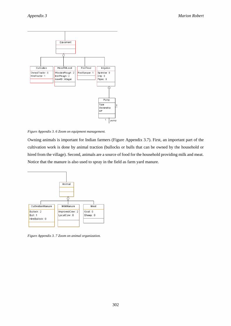
Appendix 3 Marion Robert
302
Figure Appendix 3. 6 Zoom on equipment management.
Owning animals is important for Indian farmers (Figure Appendix 3.7). First, an important part of the
cultivation work is done by animal traction (bullocks or bulls that can be owned by the household or
hired from the village). Second, animals are a source of food for the household providing milk and meat.
Notice that the manure is also used to spray in the field as farm yard manure.
Figure Appendix 3. 7 Zoom on animal organization.

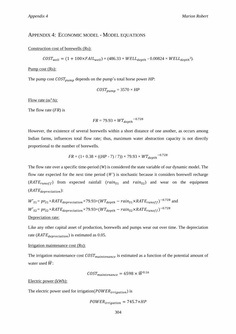
Appendix 4 Marion Robert
304
APPENDIX 4: ECONOMIC MODEL - MODEL EQUATIONS
Construction cost of borewells (Rs):
𝐶𝑂𝑆𝑇𝑤𝑒𝑙𝑙 = (1 + 100×𝐹𝐴𝐼𝐿𝑤𝑒𝑙𝑙) × (486.33 × 𝑊𝐸𝐿𝐿𝑑𝑒𝑝𝑡ℎ - 0.00824 × 𝑊𝐸𝐿𝐿𝑑𝑒𝑝𝑡ℎ²).
Pump cost (Rs):
The pump cost 𝐶𝑂𝑆𝑇𝑝𝑢𝑚𝑝 depends on the pump’s total horse power HP:
𝐶𝑂𝑆𝑇𝑝𝑢𝑚𝑝 = 3570 × HP
Flow rate (m3/h):
The flow rate (FR) is
FR = 79.93 × 𝑊𝑇𝑑𝑒𝑝𝑡ℎ−0.728
However, the existence of several borewells within a short distance of one another, as occurs among
Indian farms, influences total flow rate; thus, maximum water abstraction capacity is not directly
proportional to the number of borewells.
FR = (1+ 0.38 × ((HP - 7) / 7)) × 79.93 × 𝑊𝑇𝑑𝑒𝑝𝑡ℎ−0.728
The flow rate over a specific time-period (W) is considered the state variable of our dynamic model. The
flow rate expected for the next time period (W’) is stochastic because it considers borewell recharge
(𝑅𝐴𝑇𝐸𝑟𝑢𝑛𝑜𝑓𝑓) from expected rainfall (𝑟𝑎𝑖𝑛𝑆1 and 𝑟𝑎𝑖𝑛𝑆2) and wear on the equipment
(𝑅𝐴𝑇𝐸𝑑𝑒𝑝𝑟𝑒𝑐𝑖𝑎𝑡𝑖𝑜𝑛):
𝑊′𝑆1= 𝑝𝑟𝑆1×𝑅𝐴𝑇𝐸𝑑𝑒𝑝𝑟𝑒𝑐𝑖𝑎𝑡𝑖𝑜𝑛×79.93×(𝑊𝑇𝑑𝑒𝑝𝑡ℎ − 𝑟𝑎𝑖𝑛𝑆1×𝑅𝐴𝑇𝐸𝑟𝑢𝑛𝑜𝑓𝑓)−0.728 and
𝑊′𝑆2= 𝑝𝑟𝑆2×𝑅𝐴𝑇𝐸𝑑𝑒𝑝𝑟𝑒𝑐𝑖𝑎𝑡𝑖𝑜𝑛×79.93×(𝑊𝑇𝑑𝑒𝑝𝑡ℎ − 𝑟𝑎𝑖𝑛𝑆2×𝑅𝐴𝑇𝐸𝑟𝑢𝑛𝑜𝑓𝑓)−0.728
Depreciation rate:
Like any other capital asset of production, borewells and pumps wear out over time. The depreciation
rate (𝑅𝐴𝑇𝐸𝑑𝑒𝑝𝑟𝑒𝑐𝑖𝑎𝑡𝑖𝑜𝑛) is estimated as 0.05.
Irrigation maintenance cost (Rs):
The irrigation maintenance cost 𝐶𝑂𝑆𝑇𝑚𝑎𝑖𝑛𝑡𝑒𝑛𝑎𝑛𝑐𝑒 is estimated as a function of the potential amount of
water used ��:
𝐶𝑂𝑆𝑇𝑚𝑎𝑖𝑛𝑡𝑒𝑛𝑎𝑛𝑐𝑒 = 6598 × ��0.16
Electric power (kWh):
The electric power used for irrigation(𝑃𝑂𝑊𝐸𝑅𝑖𝑟𝑟𝑖𝑔𝑎𝑡𝑖𝑜𝑛) is
𝑃𝑂𝑊𝐸𝑅𝑖𝑟𝑟𝑖𝑔𝑎𝑡𝑖𝑜𝑛 = 745.7×𝐻𝑃

Appendix 5 Marion Robert
306
APPENDIX 5: ECONOMIC MODEL - YIELD ESTIMATIONS AND CLIMATIC
EXPECTATIONS
1. Objective
The economic model uses yields to estimate the income from selling crops within the profit function
depending on farmers’ expectations on climate for the coming seasons. We aim at providing a yield
matrix where yields depend on climate, irrigation and fertilization intensification. This matrix is an input
to the economic model.
Five crops are used:
Kharif: sunflower, marigold, sorghum, maize
Rabi: maize
Kharif and Rabi: turmeric
Six soils are used:
soil11: loamy sand
soil12: sandy loam
soil13: gravely loamy sand
soil14: sandy clay loam
soil15: clay loam
soil16: clay
2. Climatic expectations
Based on the five crops and the season and cropping duration of each crop type, we need to estimate
total rainfalls in kharif (110-250 Julian days), rabi (240-400 Julian days) and for the year (kharif and
rabi, 110-360 Julian days).
NB: time windows for the rainfalls are the minimum and maximum Julian days obtain from the STICS
files that were calibrated and used by Avignon team and for the pump model calibration.
We used the climatic serial of Maddur enter in RECORD. Daily rainfalls are provided from 1973 to
2013. Kharif and rabi rainfalls are approximate by lognormal function (kharif: meanlog=6.181978,
sdlog=0.2735082; rabi: meanlog=5.714544, sdlog=0.3949741) and the “year” is approximate by a
normal function (mean=811.2707, sd=185.8911).
Years can be considered poor, below average, average, above average, good (Table Appendix 4.1).
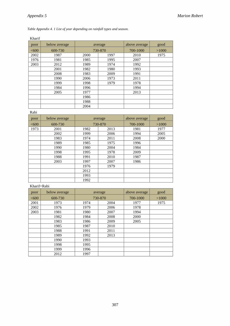
Appendix 5 Marion Robert
307
Table Appendix 4. 1 List of year depending on rainfall types and season.
Kharif
poor below average average above average good
<600 600-730 730-870 700-1000 >1000
2002 1987 2000 1997 2010 1975
1976 1981 1985 1995 2007 2003 2012 1989 1974 1992
2001 1982 1980 1993
2008 1983 2009 1991
1990 2006 1973 2011
1999 1998 1979 1978
1984 1996 1994
2005 1977 2013
1986
1988
2004
Rabi
poor below average average above average good
<600 600-730 730-870 700-1000 >1000
1973 2001 1982 2013 1981 1977
2002 1999 2006 1994 2005
1983 1974 2011 2008 2000
1989 1985 1975 1996
1990 1980 2004 1984
1998 1995 1978 2009
1988 1991 2010 1987
2003 1997 2007 1986
1976 1979
2012
1993
1992
Kharif+Rabi
poor below average average above average good
<600 600-730 730-870 700-1000 >1000
2001 1973 1974 2004 1977 1975
2002 1976 1979 2006 1978 2003 1981 1980 2007 1994
1982 1984 2008 2000
1983 1986 2009 2005
1985 1987 2010
1988 1991 2011
1989 1992 2013
1990 1993
1998 1995
1999 1996
2012 1997
Appendix 5 Marion Robert
308
3. Yield expectations
Irrigation can be optimal, 75%, 50% 25% or none.
Based on experimental plots, we fixed irrigation dose to 15mm.
3.1. Optimal irrigation
Optimal irrigation is estimated by the automatic irrigation on STICS.
STICS automatically calculates water inputs so as to satisfy water requirements at the level of the
RATIOL parameter (water stress index): the model triggers irrigation each time the stomatal stress index
(SWFAC) is less than RATIOL. Irrigation amounts (AIRG) are then calculated so as to replenish the
soil water reserve (HUR) to field capacity (HUCC) down to the rooting front (ZRAC) without exceeding
the maximum dose authorized by the irrigation system (DOSIMX). Irrigation is applied only if AIRG >
DOSEIRRIGMIN (the minimal dose allowed to do an irrigation). We force irrigation dose to be 15mm
(DOSIMX = DOSEIRRIGMIN = 15). At the time of sowing, irrigation is provided if it has no rained,
to enable germination. Irrigation at sowing is 15mm (IRRLEV) or less depending on soil water reserve.
STICS optimal irrigation provides the optimal number of irrigation and associated doses. The overall
volume of water provided to the plant by irrigation is the sum of all irrigations during crop growth.
Since STICS is supposed to cover the plant water need, the yield function is expected to be uniform for
all climates (see graphs below for soil11). The marigold is not uniform for soil 11, over 430mm of
rainfall, it seems like the marigold yield is decreasing. Marigold is sensitive to water logging, in rainy
season, well internal drainage is important. For the other crops, not having a uniform function can be
explained by abundant rainfalls happening when the crop do not need much water.
3.2. Non-optimal irrigations: 75%, 50%, 25%
Each year, STICS optimal irrigation gave the number of irrigation and total irrigation volume 𝑉𝑜𝑝𝑡
provided to the plant. We can deduce non-optimal irrigations as:
𝑉75% = 0.75*𝑉𝑜𝑝𝑡 and #irrigation = 𝑉75% / 15mm
𝑉50% = 0.50*𝑉𝑜𝑝𝑡 and #irrigation = 𝑉50% / 15mm
𝑉25% = 0.25*𝑉𝑜𝑝𝑡 and #irrigation = 𝑉25% / 15mm
To estimate yields from non-optimal irrigations, we use a decision model coupled with STICS and a
climate model. The decision model describes simple management practices with time of sowing and
harvest fixed. Number of irrigation and fertilization doses depends on the intensification of the
management practices. 108 management practices (ITK) are identified. Crossing with the 6 soils, 5 crops
and 5 types of climate, we obtained 960 simulations to run with the simulator "decision/STICS/climate".
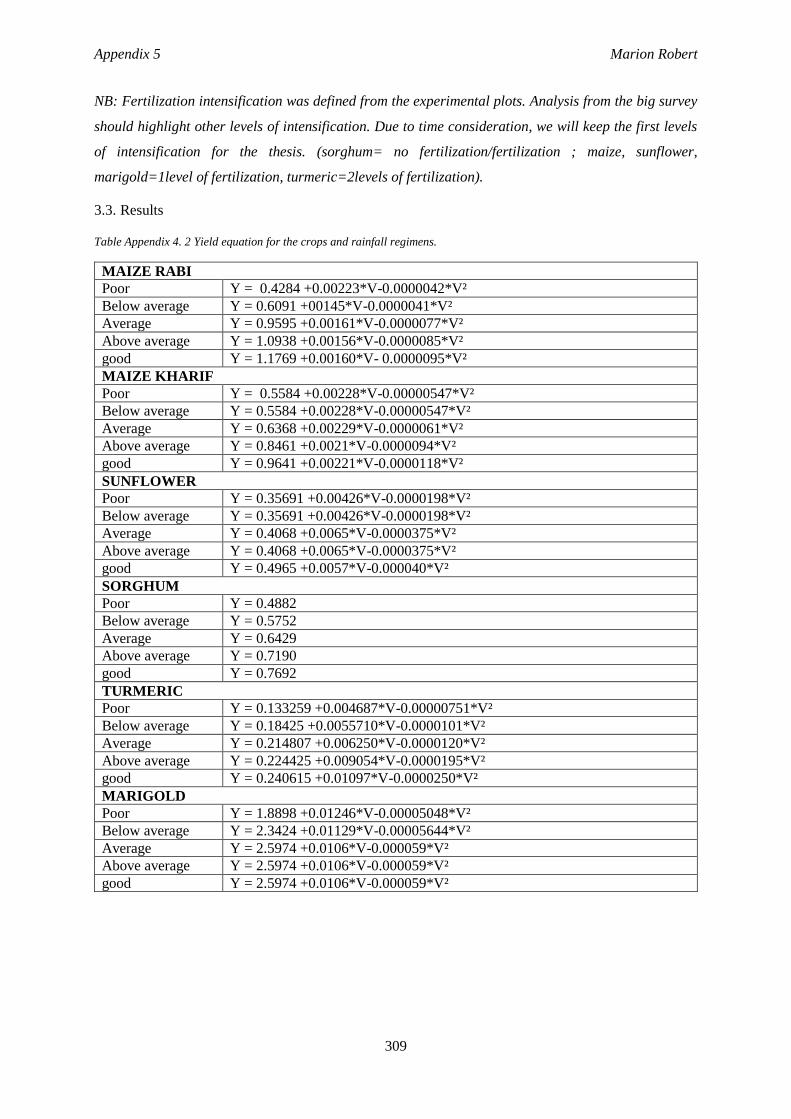
Appendix 5 Marion Robert
309
NB: Fertilization intensification was defined from the experimental plots. Analysis from the big survey
should highlight other levels of intensification. Due to time consideration, we will keep the first levels
of intensification for the thesis. (sorghum= no fertilization/fertilization ; maize, sunflower,
marigold=1level of fertilization, turmeric=2levels of fertilization).
3.3. Results
Table Appendix 4. 2 Yield equation for the crops and rainfall regimens.
MAIZE RABI
Poor Y = 0.4284 +0.00223*V-0.0000042*V²
Below average Y = 0.6091 +00145*V-0.0000041*V²
Average Y = 0.9595 +0.00161*V-0.0000077*V²
Above average Y = 1.0938 +0.00156*V-0.0000085*V²
good Y = 1.1769 +0.00160*V- 0.0000095*V²
MAIZE KHARIF
Poor Y = 0.5584 +0.00228*V-0.00000547*V²
Below average Y = 0.5584 +0.00228*V-0.00000547*V²
Average Y = 0.6368 +0.00229*V-0.0000061*V²
Above average Y = 0.8461 +0.0021*V-0.0000094*V²
good Y = 0.9641 +0.00221*V-0.0000118*V²
SUNFLOWER
Poor Y = 0.35691 +0.00426*V-0.0000198*V²
Below average Y = 0.35691 +0.00426*V-0.0000198*V²
Average Y = 0.4068 +0.0065*V-0.0000375*V²
Above average Y = 0.4068 +0.0065*V-0.0000375*V²
good Y = 0.4965 +0.0057*V-0.000040*V²
SORGHUM
Poor Y = 0.4882
Below average Y = 0.5752
Average Y = 0.6429
Above average Y = 0.7190
good Y = 0.7692
TURMERIC
Poor Y = 0.133259 +0.004687*V-0.00000751*V²
Below average Y = 0.18425 +0.0055710*V-0.0000101*V²
Average Y = 0.214807 +0.006250*V-0.0000120*V²
Above average Y = 0.224425 +0.009054*V-0.0000195*V²
good Y = 0.240615 +0.01097*V-0.0000250*V²
MARIGOLD
Poor Y = 1.8898 +0.01246*V-0.00005048*V²
Below average Y = 2.3424 +0.01129*V-0.00005644*V²
Average Y = 2.5974 +0.0106*V-0.000059*V²
Above average Y = 2.5974 +0.0106*V-0.000059*V²
good Y = 2.5974 +0.0106*V-0.000059*V²


Appendix 6 Marion Robert
312
APPENDIX 6: OPERATIONAL DECISION AND MODELING
The agent sub-system represents an activity plan that is the different technical operations to be
performed and consists of a graph of tasks and relations between tasks. Formally, the activity plan is a
direct multi-graph without loop (G=(V, E)), where V represents the tasks and E the links or relations
between the tasks. The tasks are defined as tuples:
Preconditions represent the requirements for executing task. Preconditions are a set of predicate
functions, each of which queries the knowledge base. An example can be: “Did it rain in the last three
days?” This function returns TRUE or FALSE. If all predicates are TRUE, then the preconditions are
valid.
Status describes the current phase of the task as one of the following: {WAITED, STARTED, ENDED,
FINISHED, or FAILED}.
Time windows represent the earliest and latest starting and ending dates.
Links represent relations between two tasks. A link can be valid or invalid according to the status of the
source and target tasks. Like tasks, links are defined as tuples:
– Types represent the relation between tasks i and j. A type can be one of the following: {SiSj,FiSj,FiFj},
indicating
whether one task must start (S) or finish(F) before the other.
– Time lag window defines the time lag in the relation between tasks, for example, ensuring that task j
can start
after two units of time after the end of task i.
A crop management decision model is then defined by(i) a set of variable members of KB and associated
facts (update functions); (ii) tasks and associated predicates, rules, and time windows; and (iii) temporal
relations between tasks.
A knowledge base (KB) contains all information about the system that the farmer can use to reach a
decision: dynamics of the state variables, state of the resources, and also spatial information about farm
structure using geographic information system (GIS) (Dury 2011). Observations received by the
decision model update the KB using functions called“facts.”
Appendix 6 Marion Robert
313
1. Management operation description
Twelve activities are identified:
1- FYM
This activity describes the farmer applying farm yard manure to his field. Manure is applied before any
land preparation work at the beginning of the cropping season, after the first rains. Farm yard manure
application requests the load capacity of the soil good enough to allow the tractor to pass in the field.
Dose is measured in tractor load/ac (will be convert into T/ha).
2- Tractor plough campaign
After applying farm yard manure, the farmer will start his land preparation. Most of the farmer who do
not have a tractor will hire one. We suppose in our model that at least one tractor plough (and at max 3
tractor plough) is done. Tractor plough may be repeated several times depending on the soil structure
and the cost of it. We suppose that farmer will repeat their tractor ploughing until they reach an optimal
soil structure (to be determine in term of STICS variables (da(30cm) for instance) and
optimal/acceptable threshold). In the decision model, tractor plough is described as a tractor ploughing
campaign. The decision model inform the Operating System that the campaign has start and it is the
Operating System that determine if ploughing should be done depending on soil structure. Tractor
ploughing is done after rainfall when the load capacity is good and the soil humidity enough high for
the plough to go deep enough.
3- Bullock plough campaign
If the soil structure need for the crop (deep roots or superficial roots) is not good enough, then farmers
practice more land preparation by animal traction and wooden or iron plough. Once again we suppose
that all farmers can do bullock ploughing with their own bullocks or by hiring some. Bullock ploughing
may not be done if the soil structure is good enough for sowing. In the other case, farmers can pass up
to 3 times the bullocks. In the decision model, tractor plough is described as a bullock ploughing
campaign. The decision model inform the Operating System that the campaign has start and it is the
Operating System that determine if ploughing should be done depending on soil structure. Animal
ploughing is done after rainfall when the load capacity is good and the soil humidity enough high for
the plough to go deep enough.
4- Sowing
Once the soil structure is reached for sowing, farmers prepare the furrows and the seed bed. Crop species
and variety had been selected at the beginning of the season (in our model we suppose they use only one
variety). Advices on plant-to-plant and row-to-row space are obtained from websites, as well as depth
of the seedling. Surveys provide weight of seeds sown for 1 acre. To get the sowing density from surveys
we need to know the weight of one seed so that we can deduce the number of plant per hectare. Or we
Appendix 6 Marion Robert
314
can use the website recommendation to deduce the variable density plants/ha. Sowing is done when
humidity is apparent in at least 6inch of soil. We need to translate this information into STICS variable,
maybe with HUM for a soil layer of 15cm. Most of sowing has to be done in clement temperature. Some
crops need several days without rain after sowing (e.g. beetroot). If the conditions for sowing are not
met, then the farmer adapts and can change crop or fallow his land (dynamically load a new plan or fail
the rest of the plan).
5- Sowing check point
Farmers check the sowing possibility. When the sowing could not be done in time because of
unsatisfactory conditions, they will sow another crop.
6- Germination check point
Farmers check the crop germination. When the germination rate is lower than an optimal value, they
may resow the same crop, remove and sow another crop or keep it like this. Germination is favorable
when no stress is encountered the first month of plant growth. We consider the hydric and nitrogen
stress.
7- 7- 8- Fertilization_N, Fertilization_P, Fertilization_K
Amount of fertilizer was provided in all 3 surveys (big surveys, 27 surveys and experimental plot
surveys). From the name of the fertilizer we were able to deduce the N, P, K quantity applied on plots.
Information on time and crop stage of application was only provided for rainfed experimental plots. We
crossed this information with crop management practices advised on the web. We defined 3 levels of
fertilization intensification based on nitrogen application: high fertilization, low fertilization, none
(value kgN/ha). Nitrogen fertilization may be applied in 1, 2 or 3 times. Phosphate and potassium
fertilization are depending on soil type. We suppose in our model that P and K fertilization is applied
only once as basal application. Fertilization is done at specific crop stage and no rainfall for 2days after
application is preferred in optimal conditions. The fertilization operation has a fixed number of
applications for each crop. Thus it may be better to have an activity for each application (for example:
fertilization at sowing, fertilization at 25 days)
8- Irrigation campaign
In surveys, irrigation was described as a number of irrigation given per crops and an interval between
two irrigations. In case of rainfall in the coming days, irrigation is supposed to be cancelled for this time.
Volume applied at irrigation is not clearly expressed by the farmers. It seems like when they have
electricity, the electric pump activate and pump from the borewell until the electricity shut down. When
they have a tank, they will pump and store water directly to the tank, then will irrigate from the tank.
Two possibilities: 1- we suppose they pump water all time long they have electricity, 2- we fixed a soil
humidity threshold for which they stop pumping even if they still have electricity. As the model is a 1
Appendix 6 Marion Robert
315
day time step, we do not care about the different electricity time shift happening during the day.
Concerning tank storage, two possibilities: 1- farmers distribute all their water during the day (in this
case the tank do not need to be modeled in the model), 2- water can be stored until the next irrigation
period, the pumping is then reduce due to the water volume already available in the tank (in this case,
we need to model the tank (evaporation, recharge with rain, and get information on size and storage
capacity). A campaign of irrigation is initiated and the operating system starts the irrigation if the rainfall
conditions, the interval and the number of time of application are respected.
9- 11- Pest treatment and weeding campaigns
Pest treatment and weeding is applied only when farmers estimate those pests and weeds are threatening
their crops. In the surveys, pest and weed pressure are quantified as “no problem”, “low”, “medium”,
and “high”. Pest and weed are not managed into the STICS model. A pest and weed model will be
created to send a pressure value to the decision model. We will use a function modeling pest and weed
pressure increasing with time and going back to zero when pesticide or weeding are done by the farmer.
In the decision model, the activities will be pest and weed campaigns where several operations can be
done. The decision model informs the Operating System that the campaign has started, and it is the
Operating system that will decide when to act depending on the pressure rate provided by the pest and
weed models.
10- Harvest
Farmers harvest their crops when it reaches an optimal stage of maturity. When the harvest is done over
several days, then the farmer need to be sure that it won’t rain. Some crops have sequential harvest
(marigold, sunflower, cotton, beans, chili, tomato...), for STICS (simulate a crop plot at the same stage)
we will consider that harvest is done only in one time for all crops.
2. Activities, rules, predicates and the decision plugin of RECORD
We use the plugin decision within the RECORD platform. Before going to RECORD, we need to
clearly express different part of the decision: activities, activity parameters, activity time windows,
rules and predicates, activities precedence relations and effects (Bergez et al. 2016).
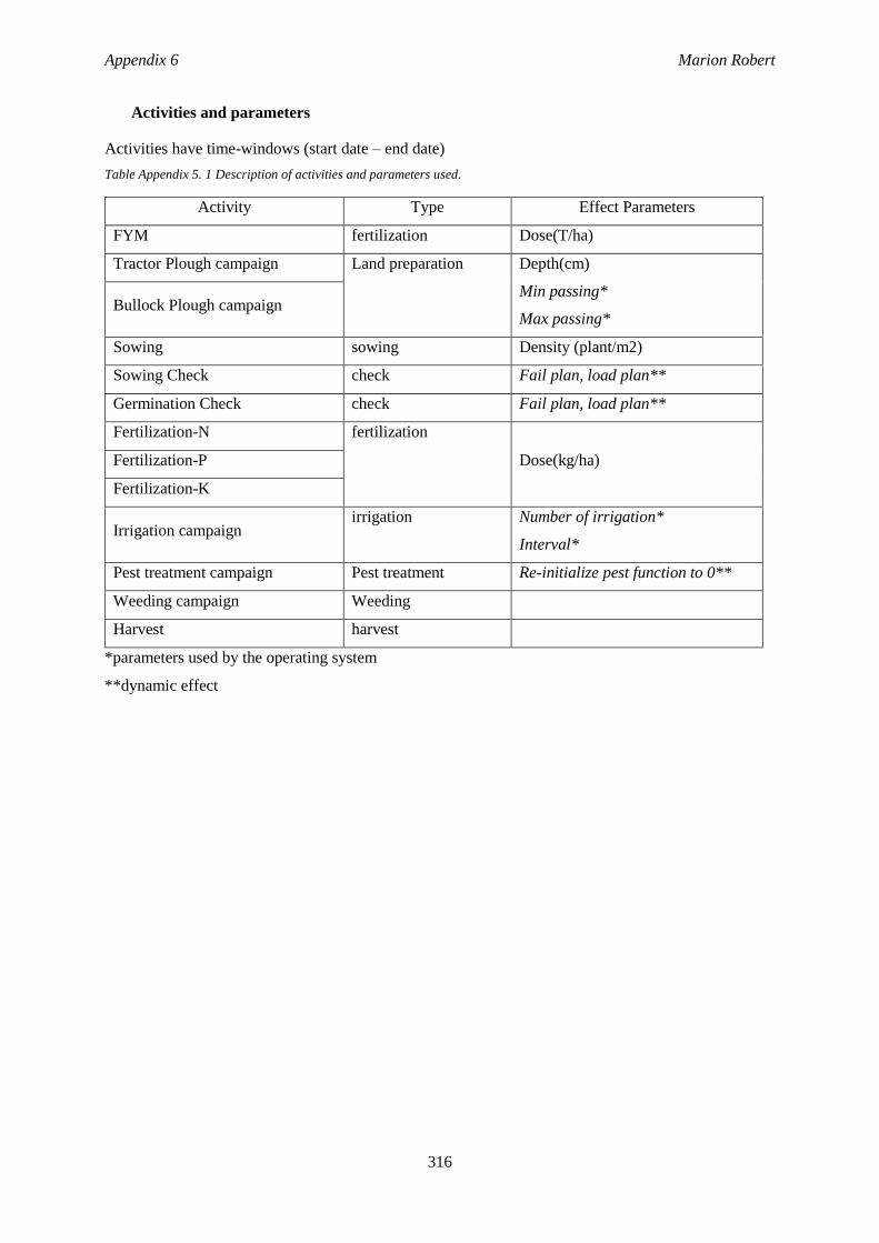
Appendix 6 Marion Robert
316
Activities and parameters
Activities have time-windows (start date – end date)
Table Appendix 5. 1 Description of activities and parameters used.
Activity Type Effect Parameters
FYM fertilization Dose(T/ha)
Tractor Plough campaign Land preparation Depth(cm)
Min passing*
Max passing* Bullock Plough campaign
Sowing sowing Density (plant/m2)
Sowing Check check Fail plan, load plan**
Germination Check check Fail plan, load plan**
Fertilization-N fertilization
Dose(kg/ha) Fertilization-P
Fertilization-K
Irrigation campaign irrigation Number of irrigation*
Interval*
Pest treatment campaign Pest treatment Re-initialize pest function to 0**
Weeding campaign Weeding
Harvest harvest
*parameters used by the operating system
**dynamic effect
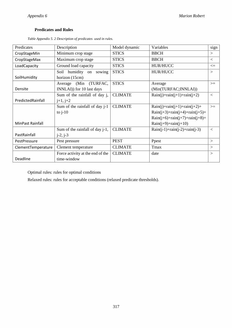
Appendix 6 Marion Robert
317
Predicates and Rules
Table Appendix 5. 2 Description of predicates used in rules.
Predicates Description Model dynamic Variables sign
CropStageMin Minimum crop stage STICS BBCH >
CropStageMax Maximum crop stage STICS BBCH <
LoadCapacity Ground load capacity STICS HUR/HUCC <=
SoilHumidity
Soil humidity on sowing
horizon (15cm)
STICS HUR/HUCC >
Densite
Average (Min (TURFAC,
INNLAI)) for 10 last days
STICS Average
(Min(TURFAC;INNLAI))
>=
PredictedRainfall
Sum of the rainfall of day j,
j+1, j+2
CLIMATE Rain(j)+rain(j+1)+rain(j+2) <
MinPast Rainfall
Sum of the rainfall of day j-1
to j-10
CLIMATE Rain(j)+rain(j+1)+rain(j+2)+
Rain(j+3)+rain(j+4)+rain(j+5)+
Rain(j+6)+rain(j+7)+rain(j+8)+
Rain(j+9)+rain(j+10)
>=
PastRainfall
Sum of the rainfall of day j-1,
j-2, j-3
CLIMATE Rain(j-1)+rain(j-2)+rain(j-3) <
PestPressure Pest pressure PEST Ppest >
ClementTemperature Clement temperature CLIMATE Tmax >
Deadline
Force activity at the end of the
time-window
CLIMATE date >
Optimal rules: rules for optimal conditions
Relaxed rules: rules for acceptable conditions (relaxed predicate thresholds).

Appendix 6 Marion Robert
318
Table Appendix 5. 3 Description of rules used by activities.
Activity Rules Predicates
FYM
Optimal/acceptable rule
Load capacity
PastRainfall
Deadline rule Deadline
Tractor Plough campaign
Optimal/acceptable rule
Load capacity
SoilHumidity
Deadline rule Deadline
Bullock Plough campaign
Optimal/acceptable rule
Load capacity
SoilHumidity
Deadline rule Deadline
Sowing
Optimal/acceptable rule
Load capacity
SoilHumidity MinPastRainfall PredictedRainfall ClementTemperature
Deadline rule Deadline
Germination Check
Optimal/acceptable rule
CropStageMin
CropStageMax
densite
Deadline rule Deadline
Fertilization-N
Optimal/acceptable rule
CropStageMin
CropStageMax
PredictedRainfall
Deadline rule Deadline
Fertilization-P
Optimal/acceptable rule
CropStageMin
CropStageMax
PredictedRainfall
Deadline rule Deadline
Fertilization-K
Optimal/acceptable rule
CropStageMin
CropStageMax
PredictedRainfall
Deadline rule Deadline
Irrigation campaign
Optimal/acceptable rule
CropStageMin
CropStageMax
PredictedRainfall
PastRainfall Deadline rule Deadline
Pest treatment campaign
Optimal/acceptable rule
PredictedRainfall
PestPressure
Deadline rule Deadline
Weeding campaign
Optimal/acceptable rule
CropStageMin
CropStageMax
PredictedRainfall
Deadline rule Deadline
Harvest
Optimal/acceptable rule
CropStageMin
CropStageMax
PredictedRainfall
Deadline rule Deadline
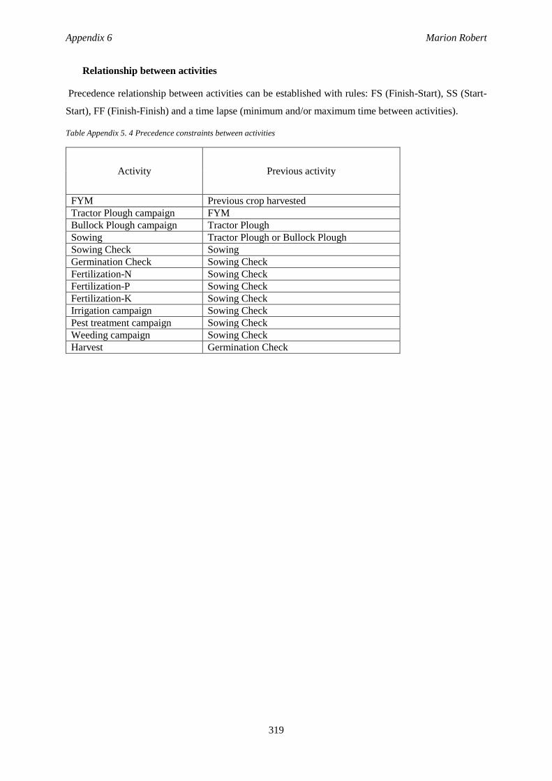
Appendix 6 Marion Robert
319
Relationship between activities
Precedence relationship between activities can be established with rules: FS (Finish-Start), SS (Start-
Start), FF (Finish-Finish) and a time lapse (minimum and/or maximum time between activities).
Table Appendix 5. 4 Precedence constraints between activities
Activity Previous activity
FYM Previous crop harvested
Tractor Plough campaign FYM
Bullock Plough campaign Tractor Plough
Sowing Tractor Plough or Bullock Plough
Sowing Check Sowing
Germination Check Sowing Check
Fertilization-N Sowing Check
Fertilization-P Sowing Check
Fertilization-K Sowing Check
Irrigation campaign Sowing Check
Pest treatment campaign Sowing Check
Weeding campaign Sowing Check
Harvest Germination Check
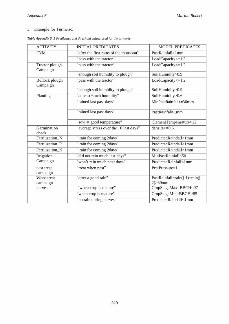
Appendix 6 Marion Robert
320
3. Example for Turmeric:
Table Appendix 5. 5 Predicates and threshold values used for the turmeric.
ACTIVITY INITIAL PREDICATES MODEL PREDICATES
FYM "after the first rains of the monsoon" PastRainfall>1mm
"pass with the tractor" LoadCapacity<=1.2
Tractor plough
Campaign
"pass with the tractor" LoadCapacity<=1.2
"enough soil humidity to plough" SoilHumidity>0.9
Bullock plough
Campaign
"pass with the tractor" LoadCapacity<=1.2
"enough soil humidity to plough" SoilHumidity>0.9
Planting "at least 6inch humidity" SoilHumidity>0.6
"rained last past days" MinPastRainfall<=30mm
"rained last past days" PastRainfall>1mm
"sow at good temperature" ClementTempenrature>12
Germination
check
"average stress over the 10 last days” densite>=0.5
Fertilization_N " rain for coming 2days" PredictedRaindall>1mm
Fertilization_P " rain for coming 2days" PredictedRaindall>1mm
Fertilization_K " rain for coming 2days" PredictedRaindall>1mm
Irrigation
Campaign
"did not rain much last days" MinPastRainfall<50
"won’t rain much next days" PredictedRainfall<1mm
pest treat
campaign
"treat when pest” PestPressure=1
Weed treat
campaign
"after a good rain" PastRainfall=rain(j-1)+rain(j-
2)>30mm
harvest "when crop is mature" CropStageMax=BBCH<97
"when crop is mature" CropStageMin=BBCH>85
"no rain during harvest" PredictedRaindall<1mm

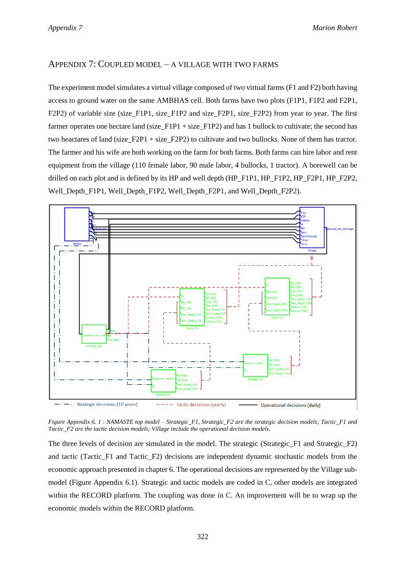
Appendix 7 Marion Robert
322
APPENDIX 7: COUPLED MODEL – A VILLAGE WITH TWO FARMS
The experiment model simulates a virtual village composed of two virtual farms (F1 and F2) both having
access to ground water on the same AMBHAS cell. Both farms have two plots (F1P1, F1P2 and F2P1,
F2P2) of variable size (size_F1P1, size_F1P2 and size_F2P1, size_F2P2) from year to year. The first
farmer operates one hectare land (size_F1P1 + size_F1P2) and has 1 bullock to cultivate; the second has
two heactares of land (size_F2P1 + size_F2P2) to cultivate and two bullocks. None of them has tractor.
The farmer and his wife are both working on the farm for both farms. Both farms can hire labor and rent
equipment from the village (110 female labor, 90 male labor, 4 bullocks, 1 tractor). A borewell can be
drilled on each plot and is defined by its HP and well depth (HP_F1P1, HP_F1P2, HP_F2P1, HP_F2P2,
Well_Depth_F1P1, Well_Depth_F1P2, Well_Depth_F2P1, and Well_Depth_F2P2).
Figure Appendix 6. 1 : NAMASTE top model – Strategic_F1, Strategic_F2 are the strategic decision models; Tactic_F1 and
Tactic_F2 are the tactic decision models; Village include the operational decision models.
The three levels of decision are simulated in the model. The strategic (Strategic_F1 and Strategic_F2)
and tactic (Tactic_F1 and Tactic_F2) decisions are independent dynamic stochastic models from the
economic approach presented in chapter 6. The operational decisions are represented by the Village sub-
model (Figure Appendix 6.1). Strategic and tactic models are coded in C, other models are integrated
within the RECORD platform. The coupling was done in C. An improvement will be to wrap up the
economic models within the RECORD platform.
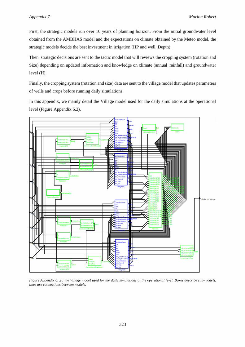
Appendix 7 Marion Robert
323
First, the strategic models run over 10 years of planning horizon. From the initial groundwater level
obtained from the AMBHAS model and the expectations on climate obtained by the Meteo model, the
strategic models decide the best investment in irrigation (HP and well_Depth).
Then, strategic decisions are sent to the tactic model that will reviews the cropping system (rotation and
Size) depending on updated information and knowledge on climate (annual_rainfall) and groundwater
level (H).
Finally, the cropping system (rotation and size) data are sent to the village model that updates parameters
of wells and crops before running daily simulations.
In this appendix, we mainly detail the Village model used for the daily simulations at the operational
level (Figure Appendix 6.2).
Figure Appendix 6. 2 : the Village model used for the daily simulations at the operational level. Boxes describe sub-models,
lines are connections between models.
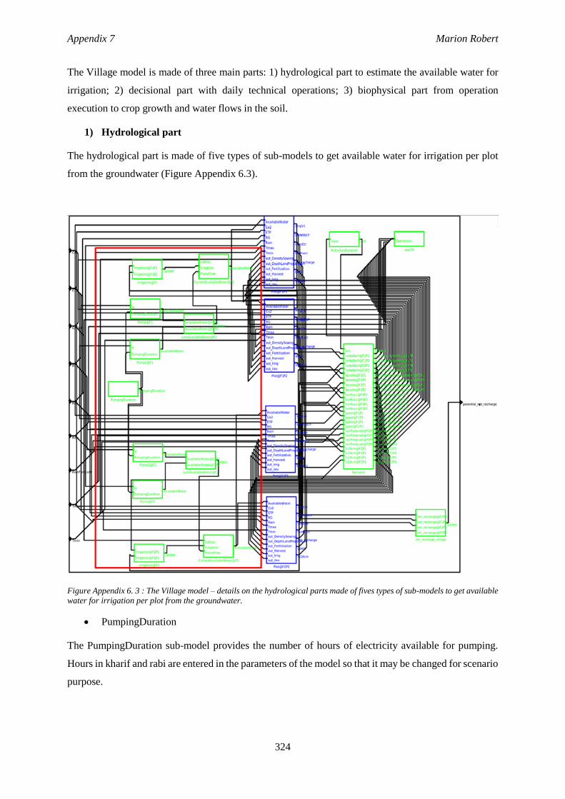
Appendix 7 Marion Robert
324
The Village model is made of three main parts: 1) hydrological part to estimate the available water for
irrigation; 2) decisional part with daily technical operations; 3) biophysical part from operation
execution to crop growth and water flows in the soil.
1) Hydrological part
The hydrological part is made of five types of sub-models to get available water for irrigation per plot
from the groundwater (Figure Appendix 6.3).
Figure Appendix 6. 3 : The Village model – details on the hydrological parts made of fives types of sub-models to get available
water for irrigation per plot from the groundwater.
PumpingDuration
The PumpingDuration sub-model provides the number of hours of electricity available for pumping.
Hours in kharif and rabi are entered in the parameters of the model so that it may be changed for scenario
purpose.
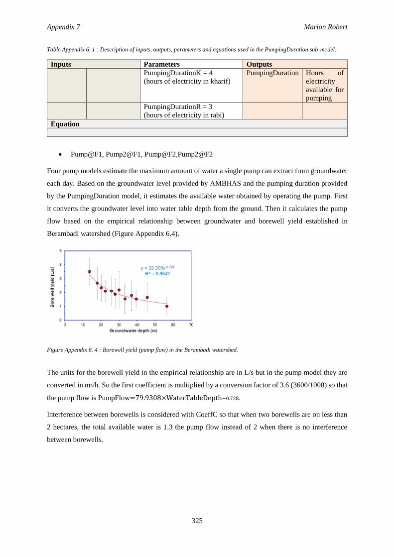
Appendix 7 Marion Robert
325
Table Appendix 6. 1 : Description of inputs, outputs, parameters and equations used in the PumpingDuration sub-model.
Inputs Parameters Outputs
PumpingDurationK = 4
(hours of electricity in kharif)
PumpingDuration Hours of
electricity
available for
pumping
PumpingDurationR = 3
(hours of electricity in rabi)
Equation
Pump@F1, Pump2@F1, Pump@F2,Pump2@F2
Four pump models estimate the maximum amount of water a single pump can extract from groundwater
each day. Based on the groundwater level provided by AMBHAS and the pumping duration provided
by the PumpingDuration model, it estimates the available water obtained by operating the pump. First
it converts the groundwater level into water table depth from the ground. Then it calculates the pump
flow based on the empirical relationship between groundwater and borewell yield established in
Berambadi watershed (Figure Appendix 6.4).
Figure Appendix 6. 4 : Borewell yield (pump flow) in the Berambadi watershed.
The units for the borewell yield in the empirical relationship are in L/s but in the pump model they are
converted in m3/h. So the first coefficient is multiplied by a conversion factor of 3.6 (3600/1000) so that
the pump flow is PumpFlow=79.9308×WaterTableDepth−0.728.
Interference between borewells is considered with CoeffC so that when two borewells are on less than
2 hectares, the total available water is 1.3 the pump flow instead of 2 when there is no interference
between borewells.
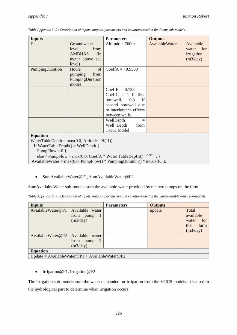
Appendix 7 Marion Robert
326
Table Appendix 6. 2 : Description of inputs, outputs, parameters and equations used in the Pump sub-models.
Inputs Parameters Outputs
H Groundwater
level from
AMBHAS (in
meter above sea
level)
Altitude = 700m AvailableWater Available
water for
irrigation
(m3/day)
PumpingDuration Hours of
pumping from
PumpingDuration
model
CoeffA = 79.9308
CoeffB = -0.728
CoeffC = 1 if first
borewell, 0.3 if
second borewell due
to interference effects
between wells.
WellDepth =
Well_Depth from
Tactic Model
Equation
WaterTableDepth = max(0.0, Altitude - H(-1));
If WaterTableDepth() > WellDepth {
PumpFlow = 0 };
else { PumpFlow = max(0.0, CoeffA * WaterTableDepth() CoeffB ; }
AvailableWater = max(0.0, PumpFlow() * PumpingDuration() * mCoeffC );
SumAvailableWater@F1, SumAvailableWater@F2
SumAvailableWater sub-models sum the available water provided by the two pumps on the farm.
Table Appendix 6. 3 : Description of inputs, outputs, parameters and equations used in the SumAvailableWater sub-models.
Inputs Parameters Outputs
AvailableWater@P1 Available water
from pump 1
(m3/day)
update Total
available
water for
the farm
(m3/day)
AvailableWater@P2 Available water
from pump 2
(m3/day)
Equation
Update = AvailableWater@P1 + AvailableWater@P2
Irrigation@F1, Irrigation@F2
The Irrigation sub-models sum the water demanded for irrigation from the STICS models. It is used in
the hydrological part to determine when irrigation occurs.
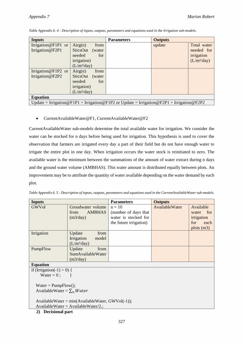
Appendix 7 Marion Robert
327
Table Appendix 6. 4 : Description of inputs, outputs, parameters and equations used in the Irrigation sub-models.
Inputs Parameters Outputs
Irrigation@F1P1 or
Irrigation@F2P1
Airg(n) from
SticsOut (water
needed for
irrigation)
(L/m²/day)
update Total water
needed for
irrigation
(L/m²/day)
Irrigation@F1P2 or
Irrigation@F2P2
Airg(n) from
SticsOut (water
needed for
irrigation)
(L/m²/day)
Equation
Update = Irrigation@F1P1 + Irrigation@F1P2 or Update = Irrigation@F2P1 + Irrigation@F2P2
CurrentAvailableWater@F1, CurrentAvailableWater@F2
CurrentAvailableWater sub-models determine the total available water for irrigation. We consider the
water can be stocked for n days before being used for irrigation. This hypothesis is used to cover the
observation that farmers are irrigated every day a part of their field but do not have enough water to
irrigate the entire plot in one day. When irrigation occurs the water stock is reinitiated to zero. The
available water is the minimum between the summations of the amount of water extract during n days
and the ground water volume (AMBHAS). This water amount is distributed equally between plots. An
improvement may be to attribute the quantity of water available depending on the water demand by each
plot.
Table Appendix 6. 5 : Description of inputs, outputs, parameters and equations used in the CurrentAvailableWater sub-models.
Inputs Parameters Outputs
GWVol Groudwater volume
from AMBHAS
(m3/day)
n = 10
(number of days that
water is stocked for
the future irrigation)
AvailableWater Available
water for
irrigation
for each
plots (m3)
Irrigation Update from
Irrigation model
(L/m²/day)
PumpFlow Update from
SumAvailableWater
(m3/day)
Equation
if (Irrigation(-1) > 0) {
Water = 0 ; }
Water = PumpFlow();
AvailableWater = ∑ 𝑊𝑎𝑡𝑒𝑟𝑛
AvailableWater = min(AvailableWater, GWVol(-1));
AvailableWater = AvailableWater/2.;
2) Decisional part
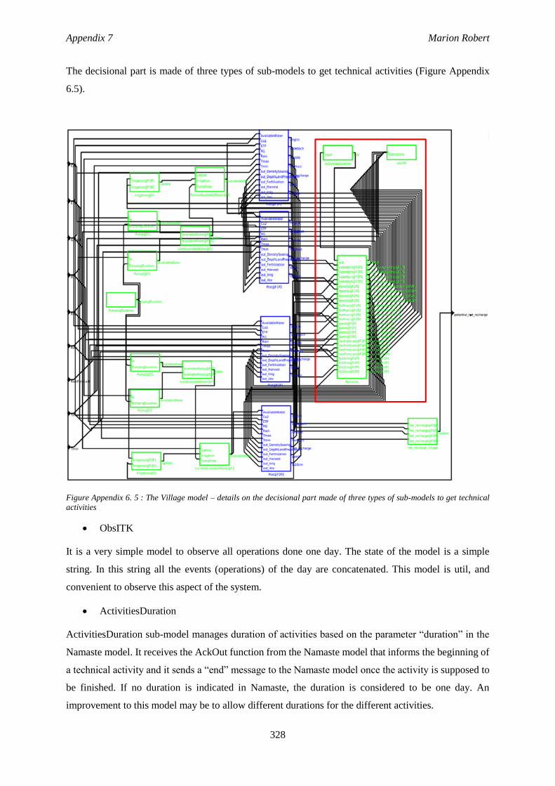
Appendix 7 Marion Robert
328
The decisional part is made of three types of sub-models to get technical activities (Figure Appendix
6.5).
Figure Appendix 6. 5 : The Village model – details on the decisional part made of three types of sub-models to get technical
activities
ObsITK
It is a very simple model to observe all operations done one day. The state of the model is a simple
string. In this string all the events (operations) of the day are concatenated. This model is util, and
convenient to observe this aspect of the system.
ActivitiesDuration
ActivitiesDuration sub-model manages duration of activities based on the parameter “duration” in the
Namaste model. It receives the AckOut function from the Namaste model that informs the beginning of
a technical activity and it sends a “end” message to the Namaste model once the activity is supposed to
be finished. If no duration is indicated in Namaste, the duration is considered to be one day. An
improvement to this model may be to allow different durations for the different activities.
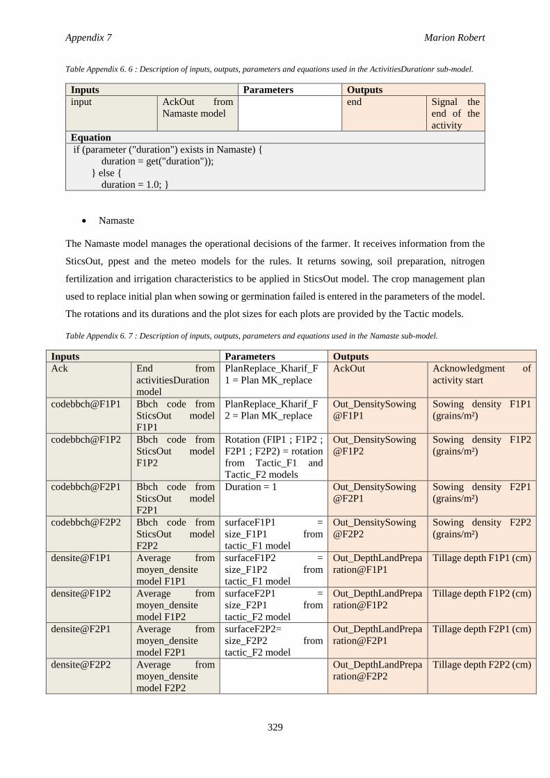
Appendix 7 Marion Robert
329
Table Appendix 6. 6 : Description of inputs, outputs, parameters and equations used in the ActivitiesDurationr sub-model.
Inputs Parameters Outputs
input AckOut from
Namaste model
end Signal the
end of the
activity
Equation
if (parameter ("duration") exists in Namaste) {
duration = get("duration"));
} else {
duration = 1.0; }
Namaste
The Namaste model manages the operational decisions of the farmer. It receives information from the
SticsOut, ppest and the meteo models for the rules. It returns sowing, soil preparation, nitrogen
fertilization and irrigation characteristics to be applied in SticsOut model. The crop management plan
used to replace initial plan when sowing or germination failed is entered in the parameters of the model.
The rotations and its durations and the plot sizes for each plots are provided by the Tactic models.
Table Appendix 6. 7 : Description of inputs, outputs, parameters and equations used in the Namaste sub-model.
Inputs Parameters Outputs
Ack End from
activitiesDuration
model
PlanReplace_Kharif_F
1 = Plan MK_replace
AckOut Acknowledgment of
activity start
codebbch@F1P1 Bbch code from
SticsOut model
F1P1
PlanReplace_Kharif_F
2 = Plan MK_replace
Out_DensitySowing
@F1P1
Sowing density F1P1
(grains/m²)
codebbch@F1P2 Bbch code from
SticsOut model
F1P2
Rotation (FIP1 ; F1P2 ;
F2P1 ; F2P2) = rotation
from Tactic_F1 and
Tactic_F2 models
Out_DensitySowing
@F1P2
Sowing density F1P2
(grains/m²)
codebbch@F2P1 Bbch code from
SticsOut model
F2P1
Duration = 1 Out_DensitySowing
@F2P1
Sowing density F2P1
(grains/m²)
codebbch@F2P2 Bbch code from
SticsOut model
F2P2
surfaceF1P1 =
size_F1P1 from
tactic_F1 model
Out_DensitySowing
@F2P2
Sowing density F2P2
(grains/m²)
densite@F1P1 Average from
moyen_densite
model F1P1
surfaceF1P2 =
size_F1P2 from
tactic_F1 model
Out_DepthLandPrepa
ration@F1P1
Tillage depth F1P1 (cm)
densite@F1P2 Average from
moyen_densite
model F1P2
surfaceF2P1 =
size_F2P1 from
tactic_F2 model
Out_DepthLandPrepa
ration@F1P2
Tillage depth F1P2 (cm)
densite@F2P1 Average from
moyen_densite
model F2P1
surfaceF2P2=
size_F2P2 from
tactic_F2 model
Out_DepthLandPrepa
ration@F2P1
Tillage depth F2P1 (cm)
densite@F2P2 Average from
moyen_densite
model F2P2
Out_DepthLandPrepa
ration@F2P2
Tillage depth F2P2 (cm)
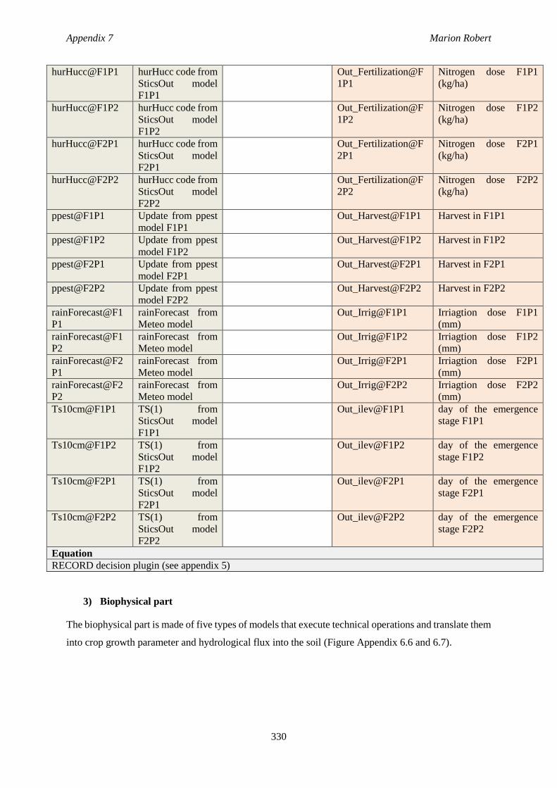
Appendix 7 Marion Robert
330
hurHucc@F1P1 hurHucc code from
SticsOut model
F1P1
Out_Fertilization@F
1P1
Nitrogen dose F1P1
(kg/ha)
hurHucc@F1P2 hurHucc code from
SticsOut model
F1P2
Out_Fertilization@F
1P2
Nitrogen dose F1P2
(kg/ha)
hurHucc@F2P1 hurHucc code from
SticsOut model
F2P1
Out_Fertilization@F
2P1
Nitrogen dose F2P1
(kg/ha)
hurHucc@F2P2 hurHucc code from
SticsOut model
F2P2
Out_Fertilization@F
2P2
Nitrogen dose F2P2
(kg/ha)
ppest@F1P1 Update from ppest
model F1P1
Out_Harvest@F1P1 Harvest in F1P1
ppest@F1P2 Update from ppest
model F1P2
Out_Harvest@F1P2 Harvest in F1P2
ppest@F2P1 Update from ppest
model F2P1
Out_Harvest@F2P1 Harvest in F2P1
ppest@F2P2 Update from ppest
model F2P2
Out_Harvest@F2P2 Harvest in F2P2
rainForecast@F1
P1
rainForecast from
Meteo model
Out_Irrig@F1P1 Irriagtion dose F1P1
(mm)
rainForecast@F1
P2
rainForecast from
Meteo model
Out_Irrig@F1P2 Irriagtion dose F1P2
(mm)
rainForecast@F2
P1
rainForecast from
Meteo model
Out_Irrig@F2P1 Irriagtion dose F2P1
(mm)
rainForecast@F2
P2
rainForecast from
Meteo model
Out_Irrig@F2P2 Irriagtion dose F2P2
(mm)
Ts10cm@F1P1 TS(1) from
SticsOut model
F1P1
Out_ilev@F1P1 day of the emergence
stage F1P1
Ts10cm@F1P2 TS(1) from
SticsOut model
F1P2
Out_ilev@F1P2 day of the emergence
stage F1P2
Ts10cm@F2P1 TS(1) from
SticsOut model
F2P1
Out_ilev@F2P1 day of the emergence
stage F2P1
Ts10cm@F2P2 TS(1) from
SticsOut model
F2P2
Out_ilev@F2P2 day of the emergence
stage F2P2
Equation
RECORD decision plugin (see appendix 5)
3) Biophysical part
The biophysical part is made of five types of models that execute technical operations and translate them
into crop growth parameter and hydrological flux into the soil (Figure Appendix 6.6 and 6.7).
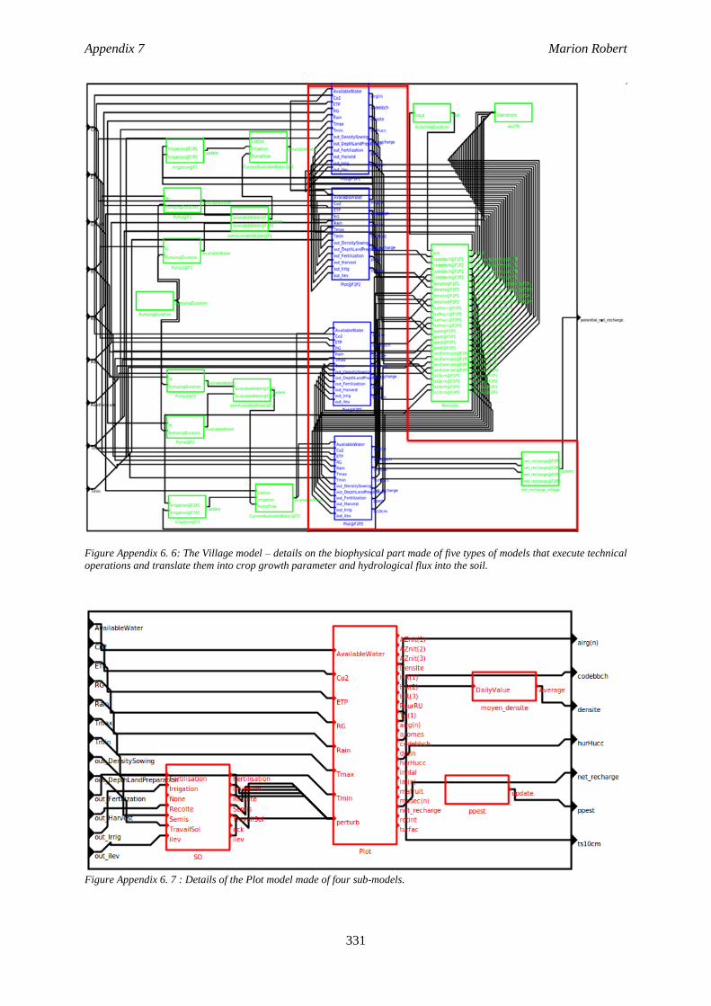
Appendix 7 Marion Robert
331
Figure Appendix 6. 6: The Village model – details on the biophysical part made of five types of models that execute technical
operations and translate them into crop growth parameter and hydrological flux into the soil.
Figure Appendix 6. 7 : Details of the Plot model made of four sub-models.
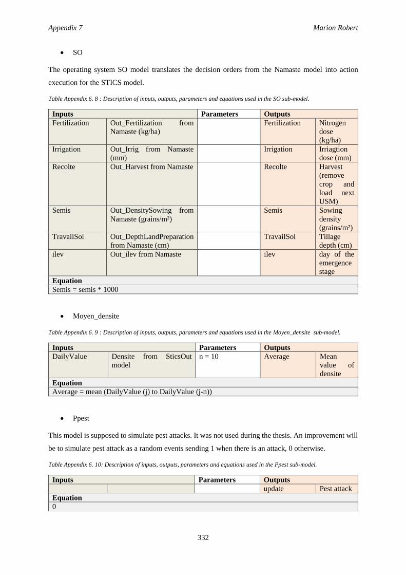
Appendix 7 Marion Robert
332
SO
The operating system SO model translates the decision orders from the Namaste model into action
execution for the STICS model.
Table Appendix 6. 8 : Description of inputs, outputs, parameters and equations used in the SO sub-model.
Inputs Parameters Outputs
Fertilization Out_Fertilization from
Namaste (kg/ha)
Fertilization Nitrogen
dose
(kg/ha)
Irrigation Out_Irrig from Namaste
(mm)
Irrigation Irriagtion
dose (mm)
Recolte Out_Harvest from Namaste Recolte Harvest
(remove
crop and
load next
USM)
Semis Out_DensitySowing from
Namaste (grains/m²)
Semis Sowing
density
(grains/m²)
TravailSol Out_DepthLandPreparation
from Namaste (cm)
TravailSol Tillage
depth (cm)
ilev Out_ilev from Namaste ilev day of the
emergence
stage
Equation
Semis = semis * 1000
Moyen_densite
Table Appendix 6. 9 : Description of inputs, outputs, parameters and equations used in the Moyen_densite sub-model.
Inputs Parameters Outputs
DailyValue Densite from SticsOut
model
n = 10 Average Mean
value of
densite
Equation
Average = mean (DailyValue (j) to DailyValue (j-n))
Ppest
This model is supposed to simulate pest attacks. It was not used during the thesis. An improvement will
be to simulate pest attack as a random events sending 1 when there is an attack, 0 otherwise.
Table Appendix 6. 10: Description of inputs, outputs, parameters and equations used in the Ppest sub-model.
Inputs Parameters Outputs
update Pest attack
Equation
0
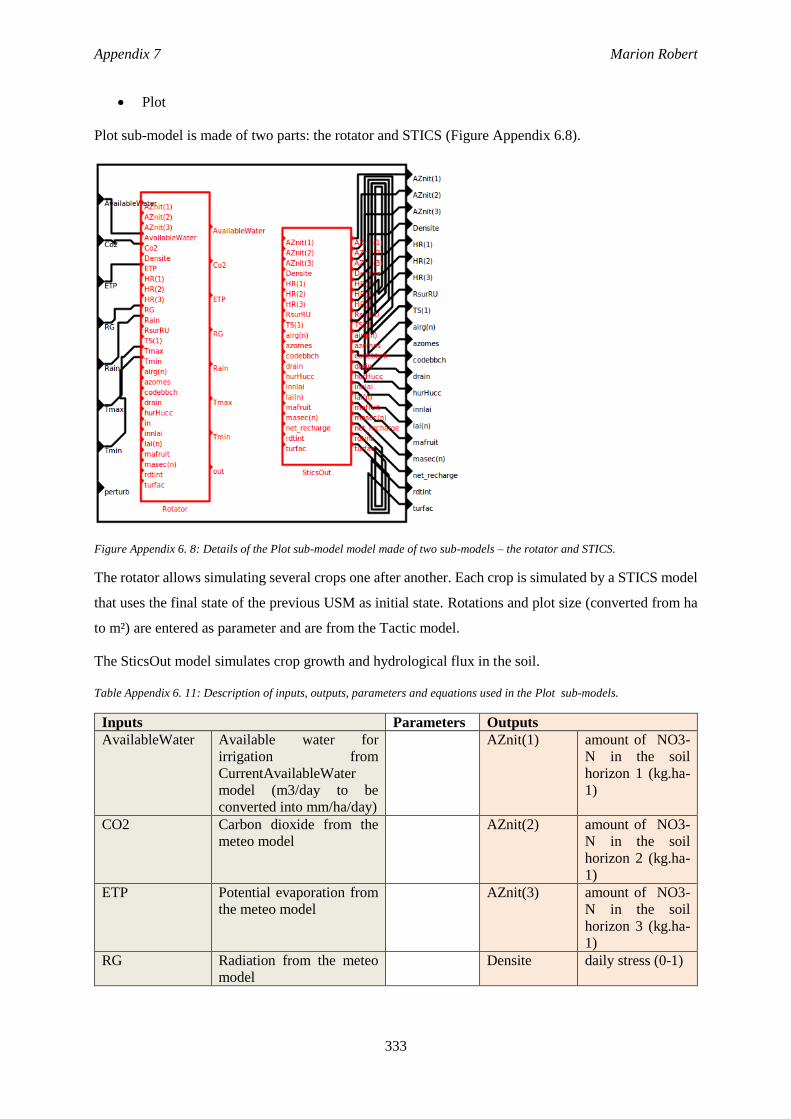
Appendix 7 Marion Robert
333
Plot
Plot sub-model is made of two parts: the rotator and STICS (Figure Appendix 6.8).
Figure Appendix 6. 8: Details of the Plot sub-model model made of two sub-models – the rotator and STICS.
The rotator allows simulating several crops one after another. Each crop is simulated by a STICS model
that uses the final state of the previous USM as initial state. Rotations and plot size (converted from ha
to m²) are entered as parameter and are from the Tactic model.
The SticsOut model simulates crop growth and hydrological flux in the soil.
Table Appendix 6. 11: Description of inputs, outputs, parameters and equations used in the Plot sub-models.
Inputs Parameters Outputs
AvailableWater Available water for
irrigation from
CurrentAvailableWater
model (m3/day to be
converted into mm/ha/day)
AZnit(1) amount of NO3-
N in the soil
horizon 1 (kg.ha-
1)
CO2 Carbon dioxide from the
meteo model
AZnit(2) amount of NO3-
N in the soil
horizon 2 (kg.ha-
1)
ETP Potential evaporation from
the meteo model
AZnit(3) amount of NO3-
N in the soil
horizon 3 (kg.ha-
1)
RG Radiation from the meteo
model
Densite daily stress (0-1)
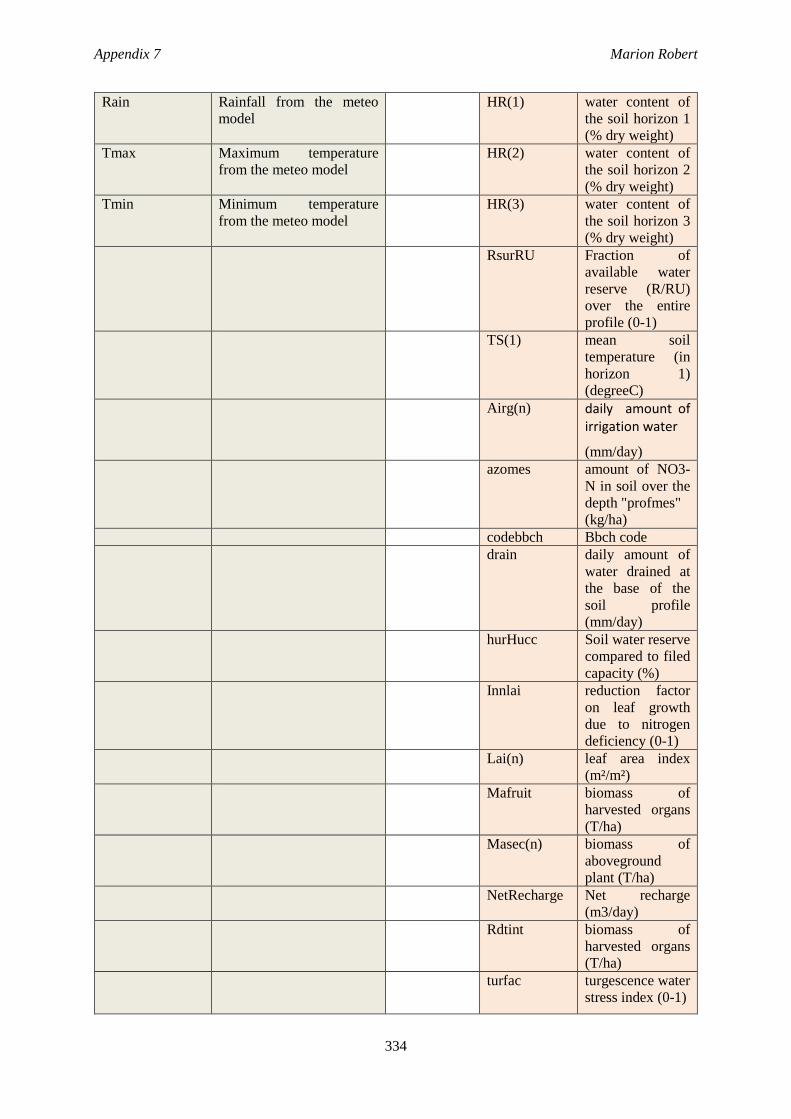
Appendix 7 Marion Robert
334
Rain Rainfall from the meteo
model
HR(1) water content of
the soil horizon 1
(% dry weight)
Tmax Maximum temperature
from the meteo model
HR(2) water content of
the soil horizon 2
(% dry weight)
Tmin Minimum temperature
from the meteo model
HR(3) water content of
the soil horizon 3
(% dry weight)
RsurRU Fraction of
available water
reserve (R/RU)
over the entire
profile (0-1)
TS(1) mean soil
temperature (in
horizon 1)
(degreeC)
Airg(n) daily amount of irrigation water
(mm/day)
azomes amount of NO3-
N in soil over the
depth "profmes"
(kg/ha)
codebbch Bbch code
drain daily amount of
water drained at
the base of the
soil profile
(mm/day)
hurHucc Soil water reserve
compared to filed
capacity (%)
Innlai reduction factor
on leaf growth
due to nitrogen
deficiency (0-1)
Lai(n) leaf area index
(m²/m²)
Mafruit biomass of
harvested organs
(T/ha)
Masec(n) biomass of
aboveground
plant (T/ha)
NetRecharge Net recharge
(m3/day)
Rdtint biomass of
harvested organs
(T/ha)
turfac turgescence water
stress index (0-1)
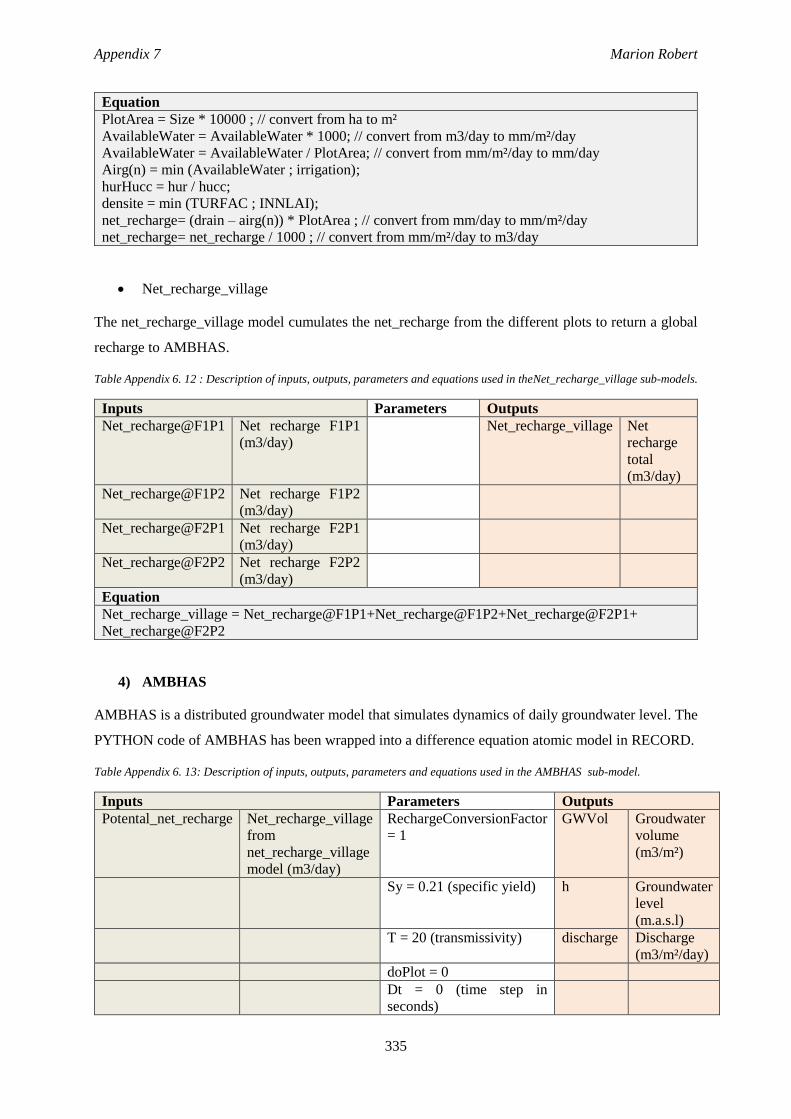
Appendix 7 Marion Robert
335
Equation
PlotArea = Size * 10000 ; // convert from ha to m²
AvailableWater = AvailableWater * 1000; // convert from m3/day to mm/m²/day
AvailableWater = AvailableWater / PlotArea; // convert from mm/m²/day to mm/day
Airg(n) = min (AvailableWater ; irrigation);
hurHucc = hur / hucc;
densite = min (TURFAC ; INNLAI);
net_recharge= (drain – airg(n)) * PlotArea ; // convert from mm/day to mm/m²/day
net_recharge= net_recharge / 1000 ; // convert from mm/m²/day to m3/day
Net_recharge_village
The net_recharge_village model cumulates the net_recharge from the different plots to return a global
recharge to AMBHAS.
Table Appendix 6. 12 : Description of inputs, outputs, parameters and equations used in theNet_recharge_village sub-models.
Inputs Parameters Outputs
Net_recharge@F1P1 Net recharge F1P1
(m3/day)
Net_recharge_village Net
recharge
total
(m3/day)
Net_recharge@F1P2 Net recharge F1P2
(m3/day)
Net_recharge@F2P1 Net recharge F2P1
(m3/day)
Net_recharge@F2P2 Net recharge F2P2
(m3/day)
Equation
Net_recharge_village = Net_recharge@F1P1+Net_recharge@F1P2+Net_recharge@F2P1+
Net_recharge@F2P2
4) AMBHAS
AMBHAS is a distributed groundwater model that simulates dynamics of daily groundwater level. The
PYTHON code of AMBHAS has been wrapped into a difference equation atomic model in RECORD.
Table Appendix 6. 13: Description of inputs, outputs, parameters and equations used in the AMBHAS sub-model.
Inputs Parameters Outputs
Potental_net_recharge Net_recharge_village
from
net_recharge_village
model (m3/day)
RechargeConversionFactor
= 1
GWVol Groudwater
volume
(m3/m²)
Sy = 0.21 (specific yield) h Groundwater
level
(m.a.s.l)
T = 20 (transmissivity) discharge Discharge
(m3/m²/day)
doPlot = 0
Dt = 0 (time step in
seconds)
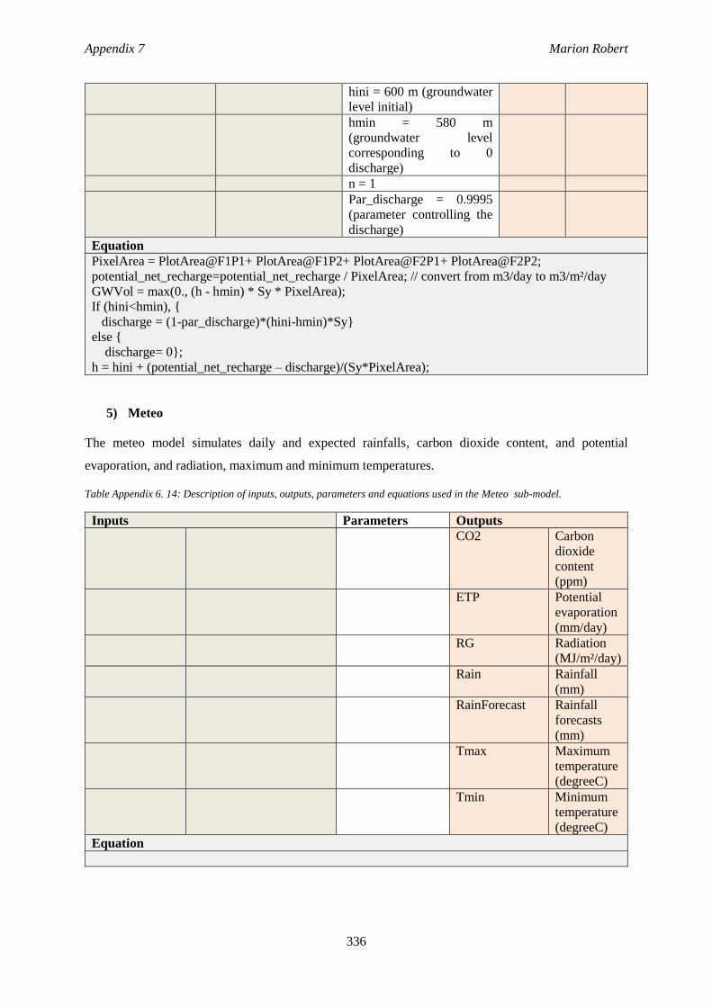
Appendix 7 Marion Robert
336
hini = 600 m (groundwater
level initial)
hmin = 580 m
(groundwater level
corresponding to 0
discharge)
n = 1
Par_discharge = 0.9995
(parameter controlling the
discharge)
Equation
PixelArea = PlotArea@F1P1+ PlotArea@F1P2+ PlotArea@F2P1+ PlotArea@F2P2;
potential_net_recharge=potential_net_recharge / PixelArea; // convert from m3/day to m3/m²/day
GWVol = max(0., (h - hmin) * Sy * PixelArea);
If (hini<hmin), {
discharge = (1-par_discharge)*(hini-hmin)*Sy}
else {
discharge= 0};
h = hini + (potential_net_recharge – discharge)/(Sy*PixelArea);
5) Meteo
The meteo model simulates daily and expected rainfalls, carbon dioxide content, and potential
evaporation, and radiation, maximum and minimum temperatures.
Table Appendix 6. 14: Description of inputs, outputs, parameters and equations used in the Meteo sub-model.
Inputs Parameters Outputs
CO2 Carbon
dioxide
content
(ppm)
ETP Potential
evaporation
(mm/day)
RG Radiation
(MJ/m²/day)
Rain Rainfall
(mm)
RainForecast Rainfall
forecasts
(mm)
Tmax Maximum
temperature
(degreeC)
Tmin Minimum
temperature
(degreeC)
Equation

Modélisation des décisions adaptatives de l’agriculteur : Un modèle économique et décisionnel
intégré, avec un cas d’étude en Inde
Dans les régions semi-arides, les systèmes de production agricole dépendent fortement de l'irrigation et
font face à des difficultés croissantes (épuisement des ressources naturelles, forte volatilité des prix du
marché, hausse des coûts de l'énergie, incertitude sur les changements climatiques). Modéliser ces
systèmes agricoles et la façon dont ils s’adaptent est important pour les décideurs politiques afin de
mieux évaluer leur flexibilité et leur résilience. Pour comprendre la capacité des systèmes agricoles à
s’adapter, il est essentiel de considérer l'ensemble du processus de décision : des décisions sur le long-
terme à l’échelle de l’exploitation aux décisions de court-terme à l’échelle de la parcelle. Pour ce faire,
cette thèse conçoit un système de production agricole adaptable dans un contexte de diminution de l'eau
et de changement climatique. Elle fournit une méthodologie guidant l'acquisition de données, leur
analyse et la conception de modèle. Elle présente le modèle de simulation NAMASTE représentant les
décisions des agriculteurs, les interactions entre agriculteurs pour l'utilisation des ressources communes
et met l'accent sur la rétroaction entre pratiques agricoles et évolution de la nappe phréatique. Le modèle
a été initialement développé pour résoudre les problèmes critiques de baisse des eaux souterraines liés
aux pratiques agricoles dans un bassin versant du sud-ouest de l'Inde. Sa structure, ses cadres
conceptuels et ses formalismes peuvent être utilisés dans d'autres contextes agricoles.
MOTS-CLES : processus de décision; typologie; modèle conceptuel ; programmation stochastique
dynamique ; politiques de gestion de l'eau ; changement climatique ; bassin versant du Berambadi.
Modeling adaptive decision-making of farmer: An integrated economic and management model,
with an application to smallholders in India
In semi-arid regions, agricultural production systems depend greatly on irrigation and encounter
increasing challenges (depletion of natural resources, high volatility in market prices, rise in energy
costs, growing uncertainty about climate change). Modeling farming systems and how these systems
change and adapt to these challenges is particularly interesting for policy makers to better assess their
flexibility and resiliency. To understand the ability of farming systems to adapt, it is essential to consider
the entire decision-making process: from long-term decisions at the farm scale to short-term decisions
at the plot level. To this end, the thesis conceives a flexible and resilient agricultural production system
under a context of water scarcity and climate change. It provides a step-by-step methodology that guides
data acquisition and analysis and model design. It proposes a simulation model NAMASTE that
simulates the farmers’ decisions in different time and space scales, represents the interactions between
farmers for resource uses and emphasizes the feedback and retroaction between farming practices and
changes in the water table. The model was initially developed to address critical issues of groundwater
depletion and farming practices in a watershed in southwestern India. Its structure, frameworks and
formalisms can be used in other agricultural contexts.
KEYWORDS: farmers’ decision-making, farm typology, conceptual model, stochastic dynamic
programming, water management policies, climate change, Berambadi watershed.
LIEU ET DATE DE SOUTENANCE: Centre INRA Toulouse, le 21 décembre 2016
DISCIPLINE ADMINISTRATIVE : Agrosystèmes, Ecosystèmes et Environnement
AUTEUR : Marion Robert
DIRECTEURS DE THESE : Jacques-Eric Bergez et Alban Thomas
LABORATOIRE D’ACCEUIL : UMR AGIR 1248 INRA/INP-ENSAT, Toulouse