the feed | farmer mac

The FeedFarmer Mac’s Quarterly Perspective on Agriculture

Spring 2017

The Feed is a publication produced by the Federal Agricultural Mortgage Corporation (“Farmer Mac”), which distributes this publication directly. The information and opinions contained herein have been compiled or arrived at from sources believed to be reliable, but no representation or warranty, express or implied, by Farmer Mac is made as to the accuracy, completeness, timeliness, or correctness of the information, opinions, or the sources from which they were derived. The information and opinions contained herein are here for general information purposes only and have been provided with the understanding that the authors and publishers are not herein engaged in rendering investment, legal, accounting, tax, or other professional advice or services. This publication may include “forward-looking statements,” which include all projections, forecasts, or expectations of future performance or results, as well as statements or expressions of opinions. No reliance should be placed on any forward-looking statements expressed in this publication. Farmer Mac specifically disclaims any liability for any errors, inaccuracies, or omissions in this publication and for any loss or damage, however arising, that may result from the use of or reliance by any person upon any information or opinions contained herein. Such information and opinions are subject to change at any time without notice, and nothing contained in this pub-lication is intended as an offer or solicitation with respect to the purchase or sale of any security, including any Farmer Mac security. Unless stated otherwise, all views expressed herein represent Farmer Mac’s opinion. From time to time, The Feed features articles or reports from authors unaffiliated with Farmer Mac, and the views and opinions expressed in these articles or reports do not necessarily reflect those of Farmer Mac. This document may not be reproduced, distributed, or published, in whole or in part, for any purposes, without the prior written consent of Farmer Mac. All copyrights are reserved.

Farmer Mac is a vital part of the agricultural credit markets and was created to increase access to and reduce the cost of capital for the benefit of American agricultural and rural communities. As the nation’s premier secondary market for agricultural credit, we provide financial solutions to a broad spectrum of the agricultural community, including agricultural lenders, agribusinesses, and other institutions that can benefit from access to flexible, low-cost financing and risk management tools. Farmer Mac‘s customers benefit from our low cost of funds, low overhead costs, and high operational efficiency. In fact, we are often able to provide the lowest cost of borrowing to agricultural and rural borrowers. For more than a quarter-century, Farmer Mac has been delivering the capital and commitment rural America deserves.

Table of Contents

A Message from Curt Covington . . . . . . . . . . . . . . .2

Production and Market Price Map . . . . . . . . . . . . .2

Special: Farm Bankruptcies . . . . . . . . . . . . . . . . . . .3

Farm Labor Expense and Immigration . . . . . . . . . .5

Farm Income . . . . . . . . . . . . . . . . . . . . . . . . . . . . . .7

Weather . . . . . . . . . . . . . . . . . . . . . . . . . . . . . . . . . . .9

California Water Policy Update . . . . . . . . . . . . . .10

Crops . . . . . . . . . . . . . . . . . . . . . . . . . . . . . . . . . . . .11

Dairy . . . . . . . . . . . . . . . . . . . . . . . . . . . . . . . . . . . .13

Livestock . . . . . . . . . . . . . . . . . . . . . . . . . . . . . . . . .14

Analysts Corner: Farm Income Prediction . . . . . .15

Resources . . . . . . . . . . . . . . . . . . . . . . . . . . . . . . . .17

About the Authors . . . . . . . . . . . . . . . . . . . . . . . . .18

ABOUT THE FEEDThe Feed is a quarterly economic outlook for current events and market conditions within agriculture. The report is broad-based, covers multiple regions and commodities and incorporates data and analysis from numerous sources to present a mosaic of the leading industry information, with a focus on the latest information from the United States Department of Agriculture and their Economic Research Service. There are several regularly included sections like weather and major industry segments, but the authors rotate through other industries and topics as they become relevant in the seasonal agricultural cycle. Where the report adds value to readers is through its unique synthesis of these multiple sources into a single succinct report. Please enjoy.

ABOUT FARMER MAC

Contacts

To subscribe to The Feed,

please visit:

www .farmermac .com/thefeed

For media inquiries:

Megan Pelaez

Director – Communications

MPelaez@farmermac .com | 202 .872 .5689

For business inquiries:

Patrick Kerrigan

Vice President -- Business Development

PKerrigan@farmermac .com | 202 .872 .5560

Follow Farmer Mac:

@FarmerMacNews

@FarmerMacNews

Follow the author:

@JacksonTakach

https://www.farmermac.com/thefeed/

mailto:[email protected]

mailto:[email protected]

https://twitter.com/farmermacnews/

https://www.facebook.com/farmermacnews/

https://twitter.com/jacksontakach

A MESSAGE FROM CURT COVINGTON

The Feed - Spring 2017 2

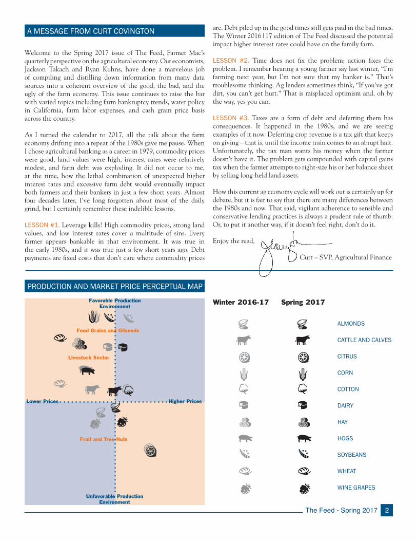
Lower Prices Higher Prices

Favorable ProductionEnvironment

Unfavorable ProductionEnvironment

Fruit and Tree Nuts

Feed Grains and Oilseeds

Livestock Sector

Welcome to the Spring 2017 issue of The Feed, Farmer Mac’s quarterly perspective on the agricultural economy. Our economists, Jackson Takach and Ryan Kuhns, have done a marvelous job of compiling and distilling down information from many data sources into a coherent overview of the good, the bad, and the ugly of the farm economy. This issue continues to raise the bar with varied topics including farm bankruptcy trends, water policy in California, farm labor expenses, and cash grain price basis across the country.

As I turned the calendar to 2017, all the talk about the farm economy drifting into a repeat of the 1980s gave me pause. When I chose agricultural banking as a career in 1979, commodity prices were good, land values were high, interest rates were relatively modest, and farm debt was exploding. It did not occur to me, at the time, how the lethal combination of unexpected higher interest rates and excessive farm debt would eventually impact both farmers and their bankers in just a few short years. Almost four decades later, I’ve long forgotten about most of the daily grind, but I certainly remember these indelible lessons.

LESSON #1. Leverage kills! High commodity prices, strong land values, and low interest rates cover a multitude of sins. Every farmer appears bankable in that environment. It was true in the early 1980s, and it was true just a few short years ago. Debt payments are fixed costs that don’t care where commodity prices

are. Debt piled up in the good times still gets paid in the bad times. The Winter 2016|17 edition of The Feed discussed the potential impact higher interest rates could have on the family farm.

LESSON #2. Time does not fix the problem; action fixes the problem. I remember hearing a young farmer say last winter, “I’m farming next year, but I’m not sure that my banker is.” That’s troublesome thinking. Ag lenders sometimes think, “If you’ve got dirt, you can’t get hurt.” That is misplaced optimism and, oh by the way, yes you can.

LESSON #3. Taxes are a form of debt and deferring them has consequences. It happened in the 1980s, and we are seeing examples of it now. Deferring crop revenue is a tax gift that keeps on giving – that is, until the income train comes to an abrupt halt. Unfortunately, the tax man wants his money when the farmer doesn’t have it. The problem gets compounded with capital gains tax when the farmer attempts to right-size his or her balance sheet by selling long-held land assets.

How this current ag economy cycle will work out is certainly up for debate, but it is fair to say that there are many differences between the 1980s and now. That said, vigilant adherence to sensible and conservative lending practices is always a prudent rule of thumb. Or, to put it another way, if it doesn’t feel right, don’t do it.

Enjoy the read,

Curt – SVP, Agricultural Finance

ALMONDS

CATTLE AND CALVES

CITRUS

CORN

COTTON

DAIRY

HAY

HOGS

SOYBEANS

WHEAT

WINE GRAPES

Winter 2016-17 Spring 2017

PRODUCTION AND MARKET PRICE PERCEPTUAL MAP

3 The Feed - Spring 2017

Key Highlights

Farmers may select from a variety of chapters in the U .S . Bankruptcy Code to file for bankruptcy,

but Chapter 12 is specifically designed for farmers and fishers to reduce their financial burden while

continuing operations .

Farm bankruptcy rates (i .e ., Chapter 12 filings) have remained relatively low during the last

decade, but the agricultural downturn during the last three years has resulted in a small uptick in

farm bankruptcy rates .

While there is considerable variation across the U .S ., farm bankruptcy rates remain low and stable

for several Midwest states .

SPECIAL REPORT: TRENDS IN FARM BANKRUPTCIES (resource 1)

FARM BANKRUPTCIES OVER TIME. When a business files for bankruptcy, it is generally perceived as a sign of financial stress. Filing for bankruptcy may ultimately lead to the cessation of operations, although this is not a certainty and there are many instances of businesses successfully using a bankruptcy filing to reduce their financial burden and continue operations. There are various forms of bankruptcy available to businesses -- Chapters 7, 11, and 13 are available to all types of businesses, not just farms. For farms, there is an additional option in the U.S. Bankruptcy Code (Chapter 12) that can be utilized in times of financial stress, which is not available to other businesses. A major advantage of this form of bankruptcy for farmers is that they can continue farming while they restructure their debt.

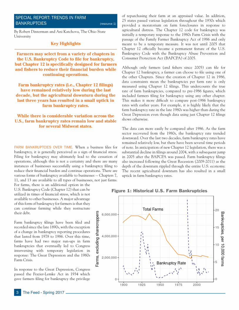
Farm bankruptcy filings have been filed and recorded since the late 1890s, with the exception of a change in bankruptcy reporting procedures that lasted from 1978 to 1986. Over this time, farms have had two major run-ups in farm bankruptcies that eventually led to Congress intervening with temporary legislation in response: The Great Depression and the 1980s Farm Crisis. In response to the Great Depression, Congress passed the Frazier-Lemke Act in 1934 which gave farmers filing for bankruptcy the privilege

By Robert Dinterman and Ani Katchova, The Ohio State University

of repurchasing their farm at an appraised value. In addition, 25 states passed various legislation throughout the 1930s which provided a moratorium on farm foreclosures in response to agricultural distress. The Chapter 12 code for bankruptcy was initially a temporary response to the 1980s Farm Crisis with the passage of the Family Farmer Bankruptcy Act of 1986 and only meant to be a temporary measure. It was not until 2005 that Chapter 12 officially became a permanent fixture of the U.S. Bankruptcy Code with the Bankruptcy Abuse Prevention and Consumer Protection Act (BAPCPA) of 2005.

Although only farmers (and fishers since 2005) can file for Chapter 12 bankruptcy, a farmer can choose to file using one of the other Chapters. Since the creation of Chapter 12 in 1986, data constraints mean the bankruptcies per farm rate is only measured using Chapter 12 filings. This undercounts the true rate of farm bankruptcies, compared to pre-1986 figures, which included farmers filing for bankruptcy using any other chapter. This makes it more difficult to compare post-1986 bankruptcy rates with earlier years. For example, it is highly likely that the farm bankruptcy rate in the late 1980s was higher than during the Great Depression even though data using just Chapter 12 filings shows otherwise.

The data can more easily be compared after 1986. As the farm sector recovered from the 1980s, the bankruptcy rate trended downward. Over the last two decades, farm bankruptcy rates have remained relatively low, but there have been several time periods of note. In anticipation of new Chapter 12 legislation, there was a substantial decline in filings around 2004, with a subsequent jump in 2005 after the BAPCPA was passed. Farm bankruptcy filings also increased following the Great Recession (2009-2011) as the depth of the downturn rippled through the entire U.S. economy. The recent agricultural downturn has also resulted in a small uptick in farm bankruptcy rates.

Figure 1: Historical U.S. Farm Bankruptcies


FARM BANKRUPTCIES ACROSS THE UNITED STATES. Since October 1996, there have been 10,292 Chapter 12 bankruptcies filed within the United States according to the U.S. Court System’s Judicial Business Table F-2, which also tracks district level filings. A U.S. federal court district is a sub-state level court territory, and although most states only have one district, the number of federal court districts in a state generally increases with state population. The three states which have four districts were the top three states by population in the 2010 Census (California, New York, and Texas).

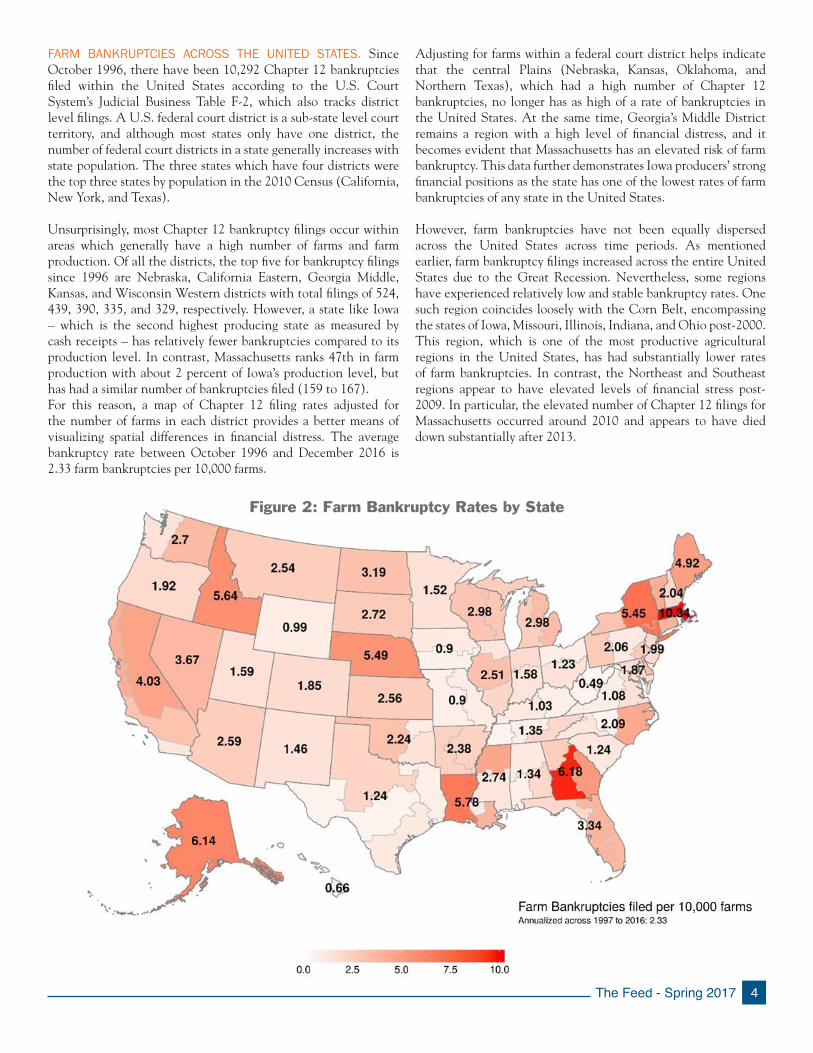
Unsurprisingly, most Chapter 12 bankruptcy filings occur within areas which generally have a high number of farms and farm production. Of all the districts, the top five for bankruptcy filings since 1996 are Nebraska, California Eastern, Georgia Middle, Kansas, and Wisconsin Western districts with total filings of 524, 439, 390, 335, and 329, respectively. However, a state like Iowa – which is the second highest producing state as measured by cash receipts – has relatively fewer bankruptcies compared to its production level. In contrast, Massachusetts ranks 47th in farm production with about 2 percent of Iowa’s production level, but has had a similar number of bankruptcies filed (159 to 167).For this reason, a map of Chapter 12 filing rates adjusted for the number of farms in each district provides a better means of visualizing spatial differences in financial distress. The average bankruptcy rate between October 1996 and December 2016 is 2.33 farm bankruptcies per 10,000 farms.

Adjusting for farms within a federal court district helps indicate that the central Plains (Nebraska, Kansas, Oklahoma, and Northern Texas), which had a high number of Chapter 12 bankruptcies, no longer has as high of a rate of bankruptcies in the United States. At the same time, Georgia’s Middle District remains a region with a high level of financial distress, and it becomes evident that Massachusetts has an elevated risk of farm bankruptcy. This data further demonstrates Iowa producers’ strong financial positions as the state has one of the lowest rates of farm bankruptcies of any state in the United States.

However, farm bankruptcies have not been equally dispersed across the United States across time periods. As mentioned earlier, farm bankruptcy filings increased across the entire United States due to the Great Recession. Nevertheless, some regions have experienced relatively low and stable bankruptcy rates. One such region coincides loosely with the Corn Belt, encompassing the states of Iowa, Missouri, Illinois, Indiana, and Ohio post-2000. This region, which is one of the most productive agricultural regions in the United States, has had substantially lower rates of farm bankruptcies. In contrast, the Northeast and Southeast regions appear to have elevated levels of financial stress post-2009. In particular, the elevated number of Chapter 12 filings for Massachusetts occurred around 2010 and appears to have died down substantially after 2013.

Figure 2: Farm Bankruptcy Rates by State


FARM LABOR EXPENSE AND IMMIGRATION POLICY IMPLICATIONS (resource 2, 3, 4, 5, 6, 7)

Key Highlights

Labor represents approximately 12 percent of all farm expenses, but labor costs vary by region and

production type .

Increases in farm labor costs have outpaced both inflation and non-farm wage growth .

Nearly half of farm laborers (46 percent) are unauthorized to work in the U .S .

The recent Presidential campaign has thrust U.S. immigration policy into the spotlight. While the political focus has often been on border security, labor is a key input to U.S. agriculture, and changes to immigration policy have the potential to affect the sector greatly. The importance of farm labor and its interconnection with immigration policy is receiving increased interest. Shortly after former Georgia Governor Sonny Perdue was appointed as Secretary of Agriculture last month, the Trump administration placed Secretary Perdue in charge of a task force to investigate ways to promote agricultural and rural prosperity. Secretary Perdue has acknowledged that President Trump has asked him to investigate ways to improve the existing farm-worker guest visa programs. Senate Democrats have also recently introduced the Agricultural Worker Program Act, which would help protect undocumented farmworkers from deportation and provide eligibility for authorized worker status over time. These measures come at a time when many farmers are already noticing the effect of labor shortage and multiple news outlets have covered the interconnectivity of immigration and the ongoing farm labor shortage.

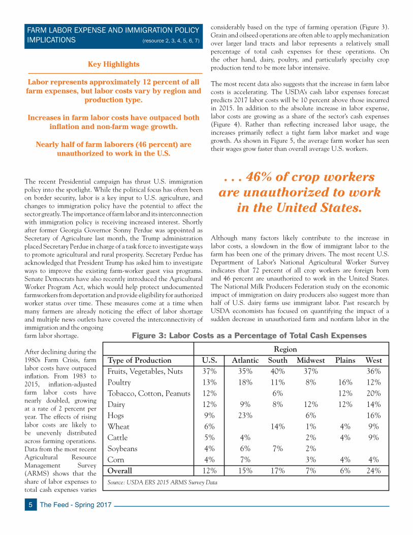
After declining during the 1980s Farm Crisis, farm labor costs have outpaced inflation. From 1983 to 2015, inflation-adjusted farm labor costs have nearly doubled, growing at a rate of 2 percent per year. The effects of rising labor costs are likely to be unevenly distributed across farming operations. Data from the most recent Agricultural Resource Management Survey (ARMS) shows that the share of labor expenses to total cash expenses varies

considerably based on the type of farming operation (Figure 3). Grain and oilseed operations are often able to apply mechanization over larger land tracts and labor represents a relatively small percentage of total cash expenses for these operations. On the other hand, dairy, poultry, and particularly specialty crop production tend to be more labor intensive.

The most recent data also suggests that the increase in farm labor costs is accelerating. The USDA’s cash labor expenses forecast predicts 2017 labor costs will be 10 percent above those incurred in 2015. In addition to the absolute increase in labor expense, labor costs are growing as a share of the sector’s cash expenses (Figure 4). Rather than reflecting increased labor usage, the increases primarily reflect a tight farm labor market and wage growth. As shown in Figure 5, the average farm worker has seen their wages grow faster than overall average U.S. workers.

Although many factors likely contribute to the increase in labor costs, a slowdown in the flow of immigrant labor to the farm has been one of the primary drivers. The most recent U.S. Department of Labor’s National Agricultural Worker Survey indicates that 72 percent of all crop workers are foreign born and 46 percent are unauthorized to work in the United States. The National Milk Producers Federation study on the economic impact of immigration on dairy producers also suggest more than half of U.S. dairy farms use immigrant labor. Past research by USDA economists has focused on quantifying the impact of a sudden decrease in unauthorized farm and nonfarm labor in the

Figure 3: Labor Costs as a Percentage of Total Cash Expenses

RegionType of Production U.S. Atlantic South Midwest Plains WestFruits, Vegetables, Nuts 37% 35% 40% 37% 36%Poultry 13% 18% 11% 8% 16% 12%Tobacco, Cotton, Peanuts 12% 6% 12% 20%Dairy 12% 9% 8% 12% 12% 14%Hogs 9% 23% 6% 16%Wheat 6% 14% 1% 4% 9%Cattle 5% 4% 2% 4% 9%Soybeans 4% 6% 7% 2% Corn 4% 7% 3% 4% 4%Overall 12% 15% 17% 7% 6% 24%Source: USDA ERS 2015 ARMS Survey Data

. . . 46% of crop workers are unauthorized to work

in the United States.


9

The most recent data also suggests that the increase in farm labor costs is accelerating. The USDA’s cash labor expenses forecast predicts 2017 labor costs will be 10 percent above those incurred in 2015. In addition to the absolute increase in labor expense, labor costs are growing as a share of the sector’s cash expenses (Figure 4). Rather than reflecting increased labor usage, the increases primarily reflect a tight farm labor market and wage growth. As shown in Figure 5, the average farm worker has seen their wages grow faster than overall average U.S. workers.

Figure 4: Farm Labor Expenses and Percentage of Total Expenses

Figure 5: Percentage Increase in Wages from 2007 to 2016 by Labor Type

0%

2%

4%

6%

8%

10%

12%

14%

0

5

10

15

20

25

30

35

1980 1986 1992 1998 2004 2010 2016

Percent$ Billion

Farm Labor Expenses

Labor Expenses

Total Cash Expenses

37.8%33.6%

25.8%

Crop Workers Animals/ProductsWorkers

All U.S. Workers

Agricultural WorkersSource: Bureau of Labor Statistics, Quarterly Census of Employment and Wages

37.8%33.6%

25.8%

Crop Workers Animals/ProductsWorkers

All U.S. Workers

Agricultural WorkersSource: Bureau of Labor Statistics, Quarterly Census of Employment and Wages

Figure 5: Percent Increase in Wages from 2007 to 2016 by Labor Type

Figure 4: Farm Labor Expenses and Percent of Total Expenses

agricultural sector. While their research does not assume a policy cause, their model simulates a sudden reduction of 5.8 million people from the unauthorized labor force and estimates the impact on agricultural employment, wages, output, and exports over a fifteen-year horizon.

The USDA simulation assumes unauthorized foreign workers compete with U.S. born and authorized foreign workers for jobs in the farm and nonfarm economy. As the supply of unauthorized labor dwindled, farmers would face higher wage rates to compete for remaining workers and, in some cases, labor shortfalls could force farmers to cut back on production. At the end of the fifteen-year simulation horizon, the number of unauthorized farmworkers would decline by more than one-third in response to a sudden, substantial decline of undocumented workers in the U.S. The number of U.S. born and authorized foreign workers would increase as higher wages entice workers to enter the agricultural sector. However, the net effect could be a 3.4 to 5.5 percent decline in farm workers, and farm wages that are 3.9 to 9.9 percent higher.

With fewer workers and higher labor costs, the USDA’s simulation suggests that the amount of U.S. agricultural output and exports would likely decline in the long-run. While not included in the model, these conditions would also likely place downward pressure on producer profitability. Consistent with their greater reliance on labor, the simulation found that fruit, tree nut, vegetable, and nursery farming operations would experience larger impacts. The result was that the output of these operations could decline by 2.0 to 5.4 percent, while exports could fall 2.5 to 9.3 percent over a 15-year horizon.

Even if immigration policy remains substantially unchanged, worker shortages and higher labor costs are likely to increase, which will lead to changes on the farm. In response to higher costs, farmers may cut back on the production of labor-intensive commodities for capital-intensive ones. Past experiences also suggest that farmers are likely to increase their use of labor-saving technologies. Several previously labor-intensive commodities, including raisins, baby leaf lettuce, and tomatoes, have already trended toward mechanization. Emerging technologies like robotic milking parlors, drones, and self-driving tractors all have the potential to greatly reduce the need for labor in the long run. However, in the short run, labor remains a key input in production agriculture and tight farm labor markets are likely to continue.


FARM INCOME (resource 8, 9)

Key Highlights

Net farm income to decline again in 2017 but at a declining rate .

Net cash income to increase as producers liquidate some of their 2016 crop held in storage .

University of Missouri’s Food and Agriculture Policy Research Institute (FAPRI) projections show

farm profitability could rebound in the next ten years, although at lower levels than the recent

farm boom .

After three years of declining income, market participants are eager to learn more about the state of the agricultural economy. The market received several new data points on the likely path of the agricultural economy during first quarter 2017. The United States Department of Agriculture (USDA) released its first forecast of 2017’s farm income level in February, while the University of Missouri’s FAPRI released its 10-year baseline projections in early-March. Both data points suggest that the farm economy may stabilize in 2017, while FAPRI’s data also suggests the potential for moderate improvements in the longer-term farm income outlook.

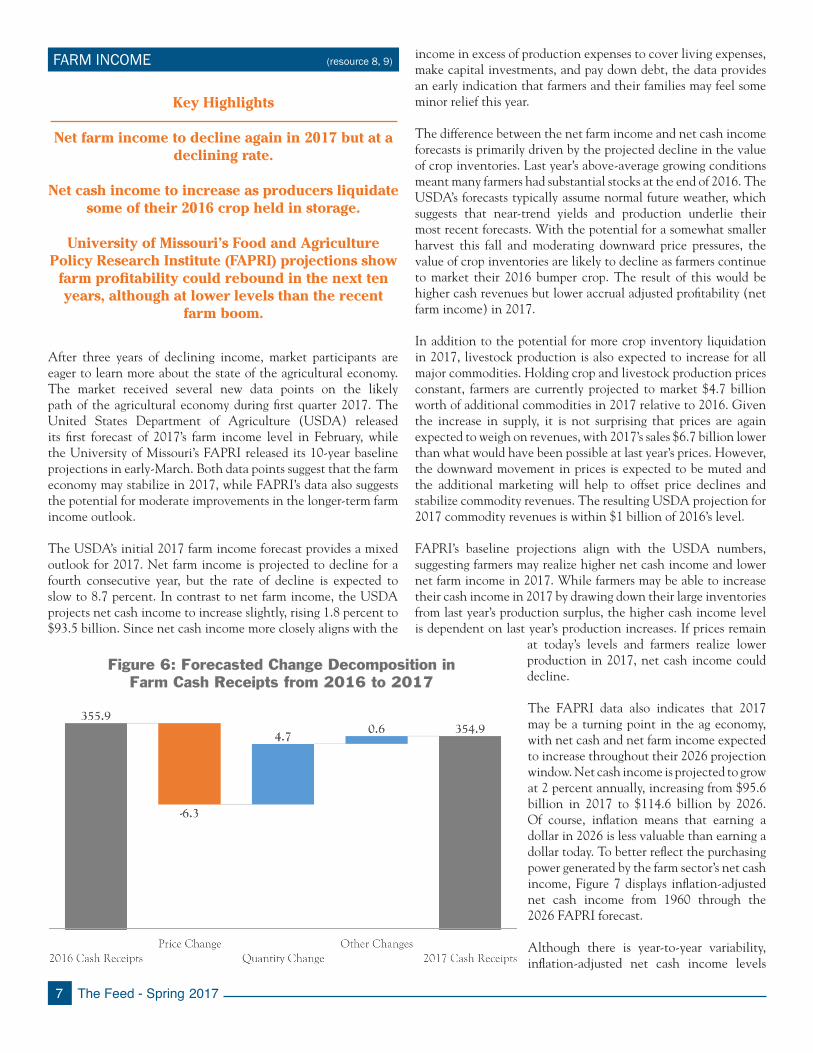
The USDA’s initial 2017 farm income forecast provides a mixed outlook for 2017. Net farm income is projected to decline for a fourth consecutive year, but the rate of decline is expected to slow to 8.7 percent. In contrast to net farm income, the USDA projects net cash income to increase slightly, rising 1.8 percent to $93.5 billion. Since net cash income more closely aligns with the

income in excess of production expenses to cover living expenses, make capital investments, and pay down debt, the data provides an early indication that farmers and their families may feel some minor relief this year.

The difference between the net farm income and net cash income forecasts is primarily driven by the projected decline in the value of crop inventories. Last year’s above-average growing conditions meant many farmers had substantial stocks at the end of 2016. The USDA’s forecasts typically assume normal future weather, which suggests that near-trend yields and production underlie their most recent forecasts. With the potential for a somewhat smaller harvest this fall and moderating downward price pressures, the value of crop inventories are likely to decline as farmers continue to market their 2016 bumper crop. The result of this would be higher cash revenues but lower accrual adjusted profitability (net farm income) in 2017.

In addition to the potential for more crop inventory liquidation in 2017, livestock production is also expected to increase for all major commodities. Holding crop and livestock production prices constant, farmers are currently projected to market $4.7 billion worth of additional commodities in 2017 relative to 2016. Given the increase in supply, it is not surprising that prices are again expected to weigh on revenues, with 2017’s sales $6.7 billion lower than what would have been possible at last year’s prices. However, the downward movement in prices is expected to be muted and the additional marketing will help to offset price declines and stabilize commodity revenues. The resulting USDA projection for 2017 commodity revenues is within $1 billion of 2016’s level. FAPRI’s baseline projections align with the USDA numbers, suggesting farmers may realize higher net cash income and lower net farm income in 2017. While farmers may be able to increase their cash income in 2017 by drawing down their large inventories from last year’s production surplus, the higher cash income level is dependent on last year’s production increases. If prices remain

at today’s levels and farmers realize lower production in 2017, net cash income could decline.

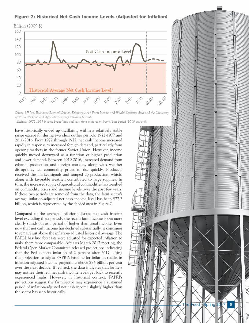
The FAPRI data also indicates that 2017 may be a turning point in the ag economy, with net cash and net farm income expected to increase throughout their 2026 projection window. Net cash income is projected to grow at 2 percent annually, increasing from $95.6 billion in 2017 to $114.6 billion by 2026. Of course, inflation means that earning a dollar in 2026 is less valuable than earning a dollar today. To better reflect the purchasing power generated by the farm sector’s net cash income, Figure 7 displays inflation-adjusted net cash income from 1960 through the 2026 FAPRI forecast.

Although there is year-to-year variability, inflation-adjusted net cash income levels

Figure 6: Forecasted Change Decomposition in Farm Cash Receipts from 2016 to 2017


have historically ended up oscillating within a relatively stable range except for during two clear outlier periods: 1972-1977 and 2010-2016. From 1972 through 1977, net cash income increased rapidly in response to increased foreign demand, particularly from opening markets in the former Soviet Union. However, income quickly moved downward as a function of higher production and lower demand. Between 2010-2016, increased demand from ethanol production and foreign markets, along with weather disruptions, led commodity prices to rise quickly. Producers received the market signals and ramped up production, which, along with favorable weather, contributed to large supplies. In turn, the increased supply of agricultural commodities has weighed on commodity prices and income levels over the past few years. If these two periods are removed from the data, the farm sector’s average inflation-adjusted net cash income level has been $77.2 billion, which is represented by the shaded area in Figure 7. Compared to the average, inflation-adjusted net cash income level excluding these periods, the recent farm income boom more clearly stands out as a period of higher than usual income. Even now that net cash income has declined substantially, it continues to remain just above the inflation-adjusted historical average. The FAPRI baseline forecasts were adjusted for expected inflation to make them more comparable. After its March 2017 meeting, the Federal Open Market Committee released projections indicating that the Fed expects inflation of 2 percent after 2017. Using this projection to adjust FAPRI’s baseline for inflation results in inflation-adjusted income projections above $84 billion per year over the next decade. If realized, the data indicates that farmers may not see their real net cash income levels get back to recently experienced highs. However, in historical context, FAPRI’s projections suggest the farm sector may experience a sustained period of inflation-adjusted net cash income slightly higher than the sector has seen historically.

Figure 7: Historical Net Cash Income Levels (Adjusted for Inflation)

L

L

S

SL

S

L

SL

S

S

SLS

SLS

S

L

L

SLL

SL

SLS

SLS

S

S

The Drought Monitor focuses on broad-scale conditions. Local conditions may vary. See accompanying text summary for forecast statements.

Shttp://droughtmonitor.unl.edu/

U.S. Drought Monitor May 23, 2017Valid 8 a.m. EDT

(Released Thursday, May. 25, 2017)

Intensity:D0 Abnormally DryD1 Moderate DroughtD2 Severe DroughtD3 Extreme DroughtD4 Exceptional Drought

Author:Brad Rippey

Drought Impact Types:

S = Short-Term, typically less than 6 months (e.g. agriculture, grasslands)

L = Long-Term, typically greater than 6 months (e.g. hydrology, ecology)

Delineates dominant impacts

U.S. Department of Agriculture


Key Highlights

Another favorable growing season is likely for the Midwest .

A moderate El Niño has developed in the Pacific Ocean over the spring, though impacts from this

pattern may not materialize until late summer, and even then, the most likely impact will be on the

tropical cyclone season in the Atlantic basin .

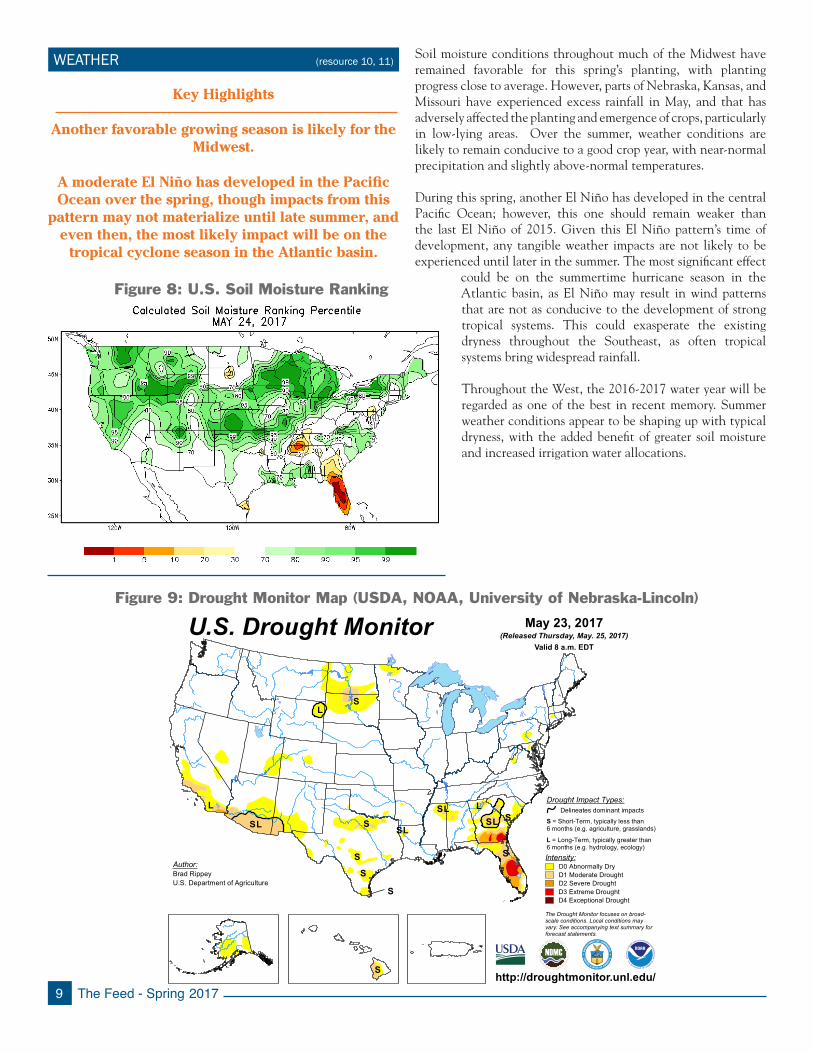
WEATHER (resource 10, 11) Soil moisture conditions throughout much of the Midwest have remained favorable for this spring’s planting, with planting progress close to average. However, parts of Nebraska, Kansas, and Missouri have experienced excess rainfall in May, and that has adversely affected the planting and emergence of crops, particularly in low-lying areas. Over the summer, weather conditions are likely to remain conducive to a good crop year, with near-normal precipitation and slightly above-normal temperatures.

During this spring, another El Niño has developed in the central Pacific Ocean; however, this one should remain weaker than the last El Niño of 2015. Given this El Niño pattern’s time of development, any tangible weather impacts are not likely to be experienced until later in the summer. The most significant effect

could be on the summertime hurricane season in the Atlantic basin, as El Niño may result in wind patterns that are not as conducive to the development of strong tropical systems. This could exasperate the existing dryness throughout the Southeast, as often tropical systems bring widespread rainfall.

Throughout the West, the 2016-2017 water year will be regarded as one of the best in recent memory. Summer weather conditions appear to be shaping up with typical dryness, with the added benefit of greater soil moisture and increased irrigation water allocations.

Figure 9: Drought Monitor Map (USDA, NOAA, University of Nebraska-Lincoln)

Figure 8: U.S. Soil Moisture Ranking


CALIFORNIA WATER POLICY UPDATE (resource 12, 13)

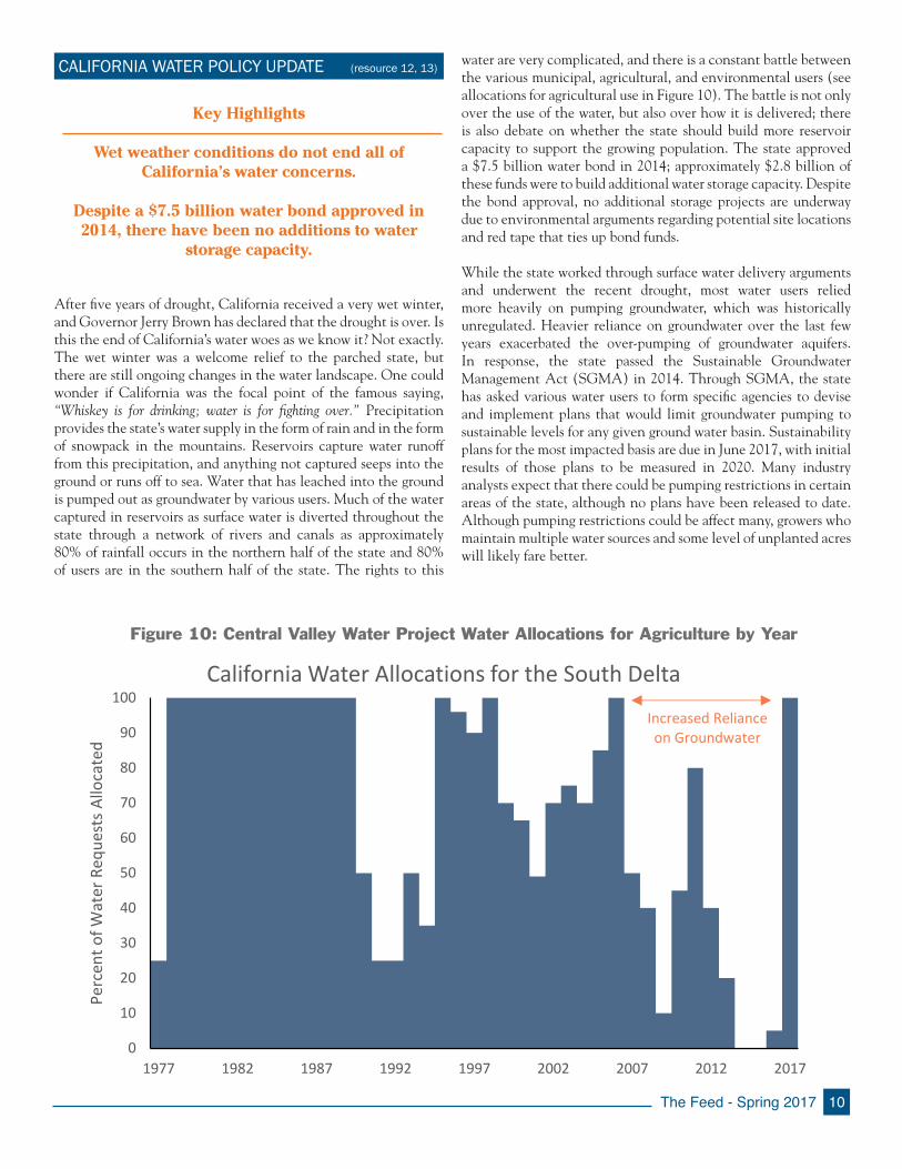
After five years of drought, California received a very wet winter, and Governor Jerry Brown has declared that the drought is over. Is this the end of California’s water woes as we know it? Not exactly. The wet winter was a welcome relief to the parched state, but there are still ongoing changes in the water landscape. One could wonder if California was the focal point of the famous saying, “Whiskey is for drinking; water is for fighting over.” Precipitation provides the state’s water supply in the form of rain and in the form of snowpack in the mountains. Reservoirs capture water runoff from this precipitation, and anything not captured seeps into the ground or runs off to sea. Water that has leached into the ground is pumped out as groundwater by various users. Much of the water captured in reservoirs as surface water is diverted throughout the state through a network of rivers and canals as approximately 80% of rainfall occurs in the northern half of the state and 80% of users are in the southern half of the state. The rights to this

Key Highlights

Wet weather conditions do not end all of California’s water concerns .

Despite a $7 .5 billion water bond approved in 2014, there have been no additions to water

storage capacity .

Figure 10: Central Valley Water Project Water Allocations for Agriculture by Year

water are very complicated, and there is a constant battle between the various municipal, agricultural, and environmental users (see allocations for agricultural use in Figure 10). The battle is not only over the use of the water, but also over how it is delivered; there is also debate on whether the state should build more reservoir capacity to support the growing population. The state approved a $7.5 billion water bond in 2014; approximately $2.8 billion of these funds were to build additional water storage capacity. Despite the bond approval, no additional storage projects are underway due to environmental arguments regarding potential site locations and red tape that ties up bond funds.

While the state worked through surface water delivery arguments and underwent the recent drought, most water users relied more heavily on pumping groundwater, which was historically unregulated. Heavier reliance on groundwater over the last few years exacerbated the over-pumping of groundwater aquifers. In response, the state passed the Sustainable Groundwater Management Act (SGMA) in 2014. Through SGMA, the state has asked various water users to form specific agencies to devise and implement plans that would limit groundwater pumping to sustainable levels for any given ground water basin. Sustainability plans for the most impacted basis are due in June 2017, with initial results of those plans to be measured in 2020. Many industry analysts expect that there could be pumping restrictions in certain areas of the state, although no plans have been released to date. Although pumping restrictions could be affect many, growers who maintain multiple water sources and some level of unplanted acres will likely fare better.

0

10

20

30

40

50

60

70

80

90

100

1977 1982 1987 1992 1997 2002 2007 2012 2017

Perc

ent o

f Wat

er R

eque

sts A

lloca

ted

California Water Allocations for the South Delta

Increased Reliance on Groundwater


CROPS (resource 14, 15, 16)

Excess supply continues to plague the global grain complex. U.S. corn production has set records in each of the last four years, and U.S. soybean production has set records for each of the last three years. While U.S. wheat production is down in recent years, global production is booming, with record crops in each of the last

nine years, largely due to more area planted and better growing conditions in Russia. Global ending stocks of corn, soybeans, and wheat are at all-time highs in 2017. Since 2012, corn and soybean supplies have increased by 64 and 74 percent, respectively. The sizable corn and soybean crops in Brazil and Argentina are a primary source of supply growth in 2017, and the March 2017 USDA prospective plantings report shows a 7 percent increase in soybean acres this year. Corn and wheat acreage in the U.S. is expected to decline in 2017, which could help alleviate some of the excess supply issues for these two commodities later this year. Late spring snow in the western plains caused significant damage to the winter wheat crop, and that too could help alleviate some supply issues this year.

Strong demand has partially offset the effects of the grain glut. Corn-based ethanol production in the U.S. continues to climb, driven largely by exports to Brazil. High sugar prices have made U.S. ethanol more competitive compared to South American, sugar-based ethanol. Growing demand for protein has led to a growing number of animals on feed, increasing the demand for grain for feed. The index for grain-consuming animal units in the U.S. is up 3.6 percent since 2012. Cheap, abundant corn is crowding out usage of other feed grains like wheat and sorghum,

Key Highlights

Record corn, soybean, and global wheat supplies continue to depress commodity prices .

Demand for grains is a bright spot, with strong ethanol production and more grain-consuming

animal units .

University of Missouri FAPRI forecasts a 2017 national corn price of $3 .60, a national soybean

price of $9 .57, and a national wheat price of $4 .44 .

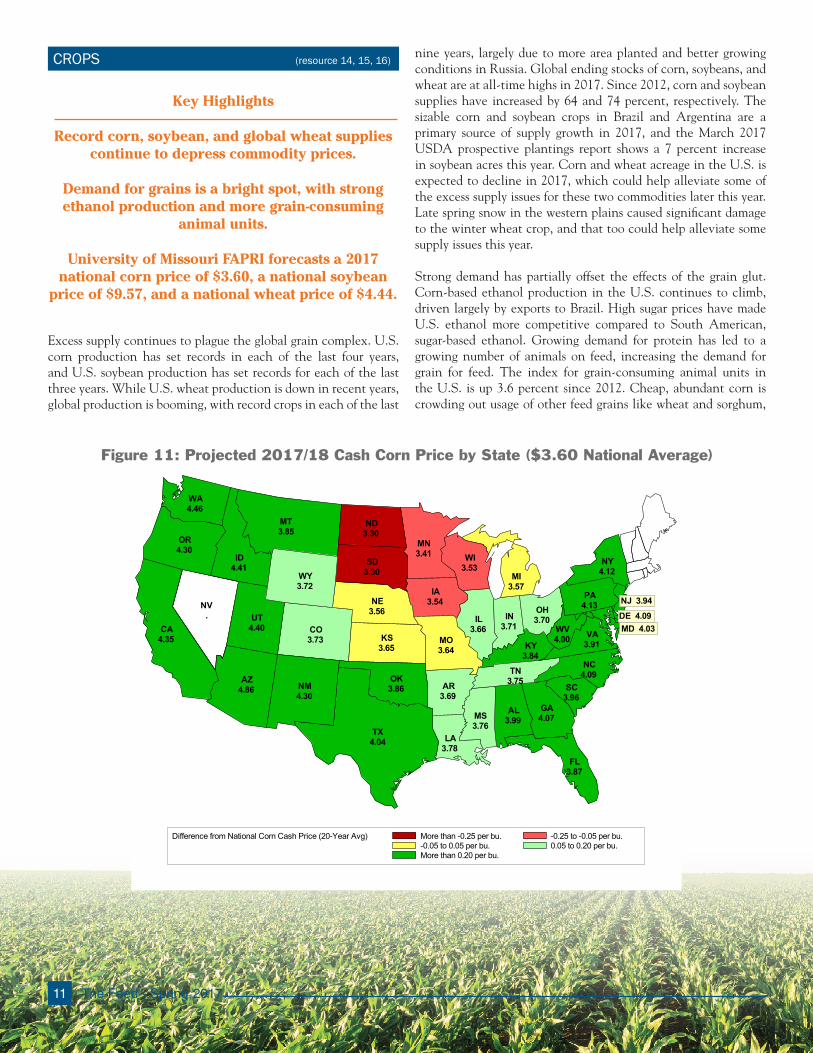
Figure 11: Projected 2017/18 Cash Corn Price by State ($3.60 National Average)

08:50 Thursday, May 25, 2017 108:50 Thursday, May 25, 2017 1

20-Year Average Corn Basis to National Average Farm Price

Difference from National Corn Cash Price (20-Year Avg) More than -0.25 per bu. -0.25 to -0.05 per bu.-0.05 to 0.05 per bu. 0.05 to 0.20 per bu.More than 0.20 per bu.

AL3.99

AZ4.86 AR

3.69

CA4.35

CO3.73

DE 4.09

FL3.87

GA4.07

ID4.41

IL3.66

IN3.71

IA3.54

KS3.65 KY

3.84

LA3.78

MD 4.03

MI3.57

MN3.41

MS3.76

MO3.64

MT3.85

NE3.56NV

.NJ 3.94

NM4.30

NY4.12

NC4.09

ND3.30

OH3.70

OK3.86

OR4.30

PA4.13

SC3.96

SD3.30

TN3.75

TX4.04

UT4.40

VA3.91

WA4.46

WV4.00

WI3.53

WY3.72


for which demand is down in 2017. Soy products continue to find favor in consumers, particularly for soybean oil products in Asia. Through the end of February, soybean exports to China are up 4 percent in 2017. Growth in global per capita wheat disappearance lags both corn and soybeans, likely a result of consumer preferences (i.e., the popularity of the gluten-free diet) and the inability of wheat use as a biofuel feedstock.

Through the first quarter of 2017, grain prices have adjusted to market dynamics. Higher-than-expected soybean production caused a November futures contract price decline of more than $0.70 per bushel in March. Corn futures contracts have been relatively stable, dipping $0.15 per bushel in March before recovering in April on news of a decline in expected acres planted. Wheat prices moved higher in February on lower planting expectations, dropped in March and early April on good weather conditions, and rallied again in early May as Midwestern storms reduced crop quality and yield expectations. The USDA will release its first 2017-18 commodity price projections in May, but the University of Missouri’s FAPRI has released national average cash price forecasts for this year’s crop: corn at $3.60 per bushel, soybeans at $9.57 per bushel, and wheat at $4.44 per bushel.

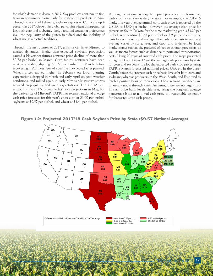
Although a national average farm price projection is informative, cash crop prices vary widely by state. For example, the 2015-16 marketing year average annual corn cash price is reported by the USDA as $3.40 per bushel; however, the average cash price for growers in South Dakota for the same marketing year is $3.20 per bushel, representing $0.20 per bushel or 5.9 percent cash price basis below the national average. The cash price basis to national average varies by state, year, and crop, and is driven by local market forces such as the presence of feed or ethanol processors, as well as macro factors such as distance to ports and transportation costs. Using 20 years of surveyed cash prices, the maps presented in Figure 11 and Figure 12 use the average cash price basis by state for corn and soybeans to plot the expected cash crop prices using FAPRI’s March forecasted national prices. Growers in the upper Cornbelt face the steepest cash price basis levels for both corn and soybeans, whereas producers in the West, South, and East tend to fetch a positive basis on their crops. These regional variances are relatively stable through time. Assuming there are no large shifts in cash price basis levels this year, using the long-run average percentage basis to national cash price is a reasonable estimator for forecasted state cash prices.

Figure 12: Projected 2017/18 Cash Soybean Price by State ($9.57 National Average)

08:50 Thursday, May 25, 2017 208:50 Thursday, May 25, 2017 2

20-Year Average Soybean Basis to National Average Farm Price

Difference from National Soybean Cash Price (20-Year Avg) More than -0.25 per bu. -0.25 to -0.05 per bu.-0.05 to 0.05 per bu. 0.05 to 0.20 per bu.More than 0.20 per bu.

AL9.86

AZ. AR

9.69

CA.

CO.

DE 9.68

FL9.11

GA9.79

ID.

IL9.80

IN9.73

IA9.57

KS9.39 KY

9.81

LA9.73

MD 9.57

MI9.50

MN9.40

MS9.64

MO9.59

MT.

NE9.29NV

.NJ 9.43

NM.

NY9.53

NC9.54

ND9.08

OH9.69

OK9.36

OR.

PA9.58

SC9.63

SD9.13

TN9.69

TX9.16

UT.

VA9.51

WA.

WV9.59

WI9.39

WY.


DAIRY (resource 8, 17, 18, 19, 20)

Key Highlights

U .S . milk and dairy product supplies are up and increasing during 2017 .

A new Canadian dairy policy took effect, cutting demand for U .S . ultrafiltered milk across the bor-

der and sparking a new U .S .-Canada dairy dispute .

The outlook for milk prices in 2017 has weakened in April, but prices should still far exceed levels

experienced in 2016 .

-10

-5

0

5

10

15

20

25

30

Cos

t/V

alue

per

Cw

t Pr

oduc

ed

Gross Profit Feed Costs Total Direct Costs Class III Milk Price

Feed Cost Only

Total Cost (incl. taxes, labor, etc.)

Monthly Class III Price

Source: USDA ERS National Milk Cost of Production Estimates

U.S. dairy production has been off to a quick start in 2017. Dairy producers began the year with a dairy cattle inventory of 9.35 million head, the largest herd since 1996. Production on a per-cow basis is up 2 percent in 2017, and through February, national milk production was up 1 percent over 2016 levels, led by big increases in New Mexico and Texas. Butter production fell in the early months of 2017, but cheese and dry milk production increased significantly. For most dairy products, February ending stocks have increased significantly over 2016 levels.

Globally, production in the early months of 2017 is down due primarily to reductions in the European Union, Australia, and Argentina. Dutch dairy operations will sell or cull an estimated 160,000 dairy cows in 2017 to comply with the European Commission phosphate emissions regulations. Australian producers culled more than 100,000 dairy cows last year because of high beef prices, and the herd reduction has led to lower total

output in 2017. Argentinian production has been beset by floods in 2016 and again in 2017, and the primary producer, SanCor, continues to struggle financially. However, New Zealand milk production is increasing in 2017 with better pasture conditions and processing plant capacity growth by Fonterra.

While still positive, demand drivers for dairy products have weakened in first quarter 2017. Domestic demand for butter and cheese pulled back in February, and stocks of both are accumulating rapidly. Global demand, and thus exports, remain strong in early 2017, particularly for non-fat dry milk exports to Mexico. Trade relations with Canada have been strained since April due to a change in Canadian dairy policies closing a loophole in NAFTA that made the sale of U.S. ultrafiltered milk to Canadian processors duty-free. In early April, one processor in Wisconsin canceled many of its buy-side contracts, surprising as many as 75 dairy producers with a letter announcing the cancellation effective May 1. The canceled contracts affect an estimated one million pounds of milk production per day, just over 1 percent of Wisconsin daily milk production. The decline in demand had a noticeable effect on dairy product prices as well as dairy cow prices in March and April.

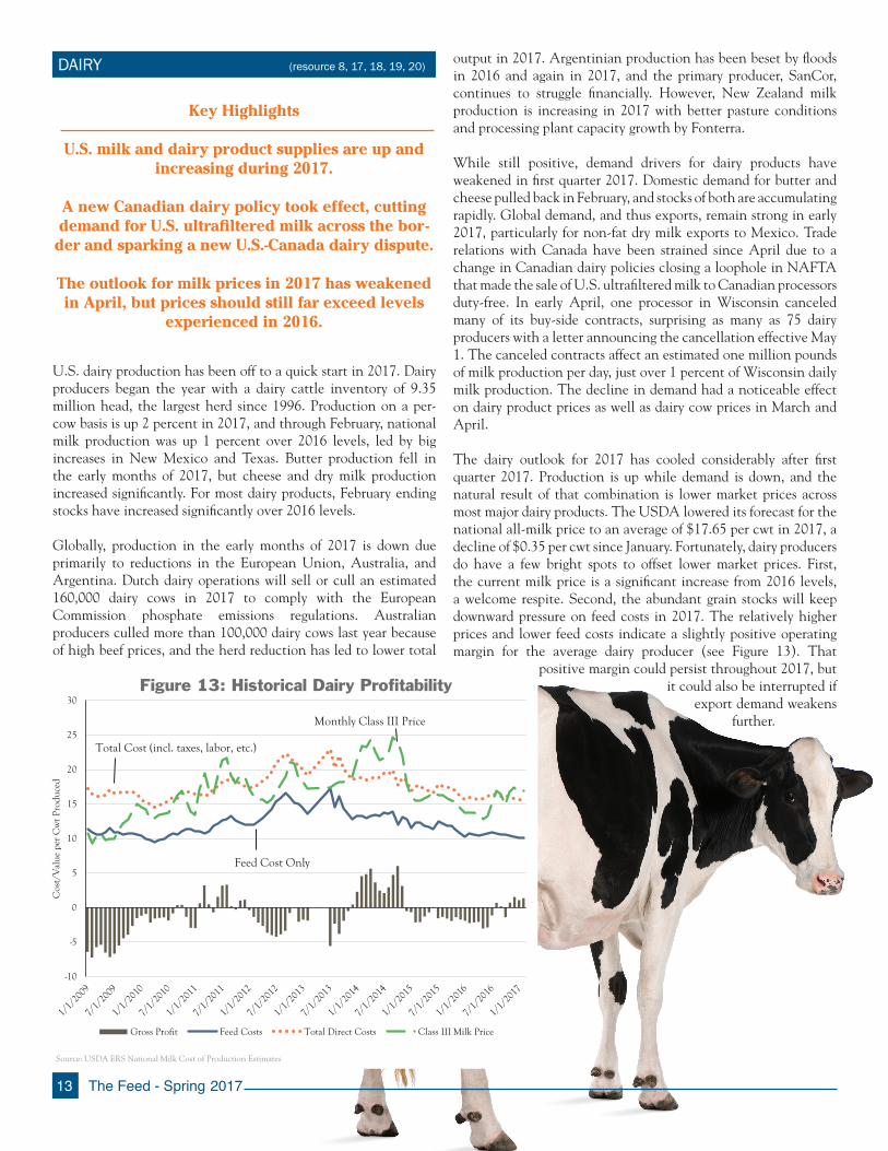
The dairy outlook for 2017 has cooled considerably after first quarter 2017. Production is up while demand is down, and the natural result of that combination is lower market prices across most major dairy products. The USDA lowered its forecast for the national all-milk price to an average of $17.65 per cwt in 2017, a decline of $0.35 per cwt since January. Fortunately, dairy producers do have a few bright spots to offset lower market prices. First, the current milk price is a significant increase from 2016 levels, a welcome respite. Second, the abundant grain stocks will keep downward pressure on feed costs in 2017. The relatively higher prices and lower feed costs indicate a slightly positive operating margin for the average dairy producer (see Figure 13). That

positive margin could persist throughout 2017, but it could also be interrupted if

export demand weakens further.

Figure 13: Historical Dairy Profitability


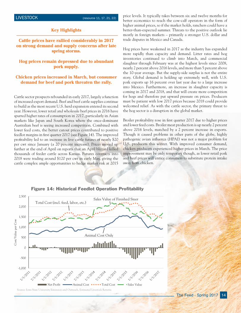
LIVESTOCK (resource 11, 17, 21, 22)

Cattle sector prospects rebounded in early 2017, largely a function of increased export demand. Beef and beef cattle supplies continue to build as the most recent U.S. herd expansion entered its second year. However, lower retail and wholesale beef prices in 2016 have spurred higher rates of consumption in 2017, particularly in Asian markets like Japan and South Korea where the once-dominant Australian beef is seeing increased competition. Combined with lower feed costs, the better cutout prices contributed to positive feedlot margins in first quarter 2017 (see Figure 14). The improved profitability led to an increase in live cattle futures of nearly $20 per cwt since January (a 20 percent increase). Prices moved up further at the end of April on reports that an April blizzard killed thousands of feeder cattle across Kansas. Futures contracts into 2018 were trading around $120 per cwt in early May, giving the cattle complex ample opportunities to hedge market risk at 2015

Key Highlights

Cattle prices have rallied considerably in 2017 on strong demand and supply concerns after late

spring storms .

Hog prices remain depressed due to abundant pork supply .

Chicken prices increased in March, but consumer demand for beef and pork threaten the rally .

price levels. It typically takes between six and twelve months for better economics to reach the cow-calf operators in the form of higher animal prices, so if the market holds, ranchers could have a better-than-expected summer. Threats to the positive outlook lie mostly in foreign markets – primarily a stronger U.S. dollar and trade disputes in Mexico and Canada. Hog prices have weakened in 2017 as the industry has expanded more rapidly than capacity and demand. Litter rates and hog inventories continued to climb into March, and commercial slaughter through February was at the highest levels since 2008, nearly 2 percent above 2016 levels, and more than 5 percent above the 10-year average. But the supply-side surplus is not the entire story. Global demand is holding up extremely well, with U.S. pork exports up 16 percent over last year due to a large increase into Mexico. Furthermore, an increase in slaughter capacity is coming in 2017 and 2018, and that will create more competition for hogs and therefore put upward pressure on prices. Producers must be patient with low 2017 prices because 2018 could provide welcomed relief. As with the cattle sector, the primary threat to the hog sector is a disruption in the global market.

Broiler profitability rose in first quarter 2017 due to higher prices and lower feed costs. Broiler meat production is up nearly 2 percent above 2016 levels, matched by a 2 percent increase in exports. Though it caused problems in other parts of the globe, highly pathogenic avian influenza (HPAI) was not a major problem for U.S. producers this winter. With improved consumer demand, chicken producers experienced higher prices in March. The price improvement may be only temporary though, as lower retail pork and beef prices will entice consumers to substitute protein intake away from chicken.

-1,000

-500

0

500

1,000

1,500

2,000

2,500

Cos

t/V

alue

per

Cow

Net Profit Animal Cost Total Cost Sales Value

Animal Cost Only

Total Cost (incl. feed, labor, etc.)Sales Value of Finished Steer

Source: Iowa State University Extension and Outreach, Estimated Livestock Returns

Figure 14: Historical Feedlot Operation Profitability


ANALYSTS CORNER: USDA FEBRUARY FARMINCOME PREDICTION PERSPECTIVE (resource 8, 23, 24)

Key Highlights

USDA February net cash income forecasts tend to be conservative, averaging 12 .6 percent lower

than the final historical estimate .

The USDA forecasts for net farm income tend to be more accurate than for net cash income, with an

average forecast variance of 8 .3 percent below the final historical estimate .

USDA February estimates accurately predict directional change in the agricultural economy,

particularly for economic downturns .

RESULTS. Forecasting a complex, multifaceted economic series is an incredibly challenging undertaking, and is one that the USDA takes on several times per year in issuing its farm income projections. Following the USDA’s $16.7 billion upward revision in farm income last August, there has been increased interest in the movement of these income forecasts as the market unfolds throughout the year. Although the USDA does not publish a dataset for past forecasts, The Feed’s authors have compiled a dataset of previous USDA forecasts from historical publications and internet archives going back to 2000. Because the USDA’s release of its first 2017 income forecast was noted earlier in this issue of The Feed, this article will provide some perspective on the historical accuracy of the USDA’s initial February net cash income (NCI) and net farm income (NFI) projections for the year.

An analysis of the data supports a similar conclusion to research conducted by University of Illinois economists, who found that the

USDA’s February NFI projection has frequently under-predicted the actual level of net farm income by about 6 percent on average from 1975 through 2015. The USDA’s February NCI projection has similarly under-predicted actual levels. Statistical tests of the USDA’s 2000-2015 February NCI and NFI projections suggest that both income measures tend to be conservative, as well as provide an estimate of the typical range of the average percentage forecast error for each series. Specifically, the USDA’s 2000-2015 February NCI forecast under-predicted actual NCI by roughly 12.6 percent, while the NFI forecast under-predicted actual NFI by 8.3 percent. If past trends hold, the NCI and NFI forecasts would be expected to be revised upward as more is learned about conditions in the ag economy in 2017. If past variances hold in 2017, the USDA may revise final NCI and NFI levels in future releases to between $100 and $114 billion and $64 to $73 billion, respectively.

In addition to the size of forecasting variance, another important element of forecasting accuracy is the ability to predict turning points in the ag economy. The USDA’s February forecast has correctly predicted directional changes in NCI in two-thirds of such instances, while correctly predicting swings in NFI in three-quarters of such instances. However, the USDA February forecasts were less likely to predict rising income levels (identifying just under 50 percent of the cases where either NCI or NFI increased). Given the tendency of conservative projections, it is not surprising that forecasts for both series can accurately detect downturns in the ag economy as the USDA identified 100 percent of observed declines in either series.

Although the USDA’s farm income forecasts are often referenced with an air of certainty, it is important to remember forecasting is an enterprise inherently fraught with uncertainty. What may have seemed likely at the time a forecast was made could later seem wholly unlikely given shifts in agricultural commodity markets. Whether USDA’s February income forecasts tend to under-predict actual income levels due to conservative assumptions or rapid changes in the ag economy through the year, these forecasts prepare market participants for potential downside risk, even if it is not fully realized.


Figure 15: Net Cash Income and Net Farm Income Forecast Variance, 2000-2015

-20.0

-10.0

0.0

10.0

20.0

30.0

40.0

50.0Percent

Net cash income Net farm income

METHODOLOGY. Typically, it would be straightforward to compare the compiled dataset of NCI and NFI forecasts to the NCI and NFI estimates currently published by USDA for the same years. However, the currently published estimates of prior year data include adjustments, which changed historical income levels relative to the information available when the USDA released the forecasts. Failing to account for these revisions would change the perceived accuracy of the original forecasts. For example, USDA’s February forecast for 2013 NCI showed a decline of 8.3 percent relative to the 2011 estimate data available when the forecast was made. After the initial forecast was made, data from the 2012 Census of Agriculture became available and the 2011 NCI estimate was revised downward. Because of the downward revision

in the 2011 NCI estimate, the USDA’s February forecast for 2013 NCI appears to suggest the USDA had expected a small increase in NCI, even though it had originally predicted that NCI would decline. To correct for these types of revisions, the USDA’s original forecasts were adjusted to reflect revisions to historical farm income data.

To provide a common scale, Figure 15 presents the calculated forecast variance from the USDA’s NCI and NFI forecasts as a percentage of the February 2017 release value for each historical year. Because a positive forecast error signals a February forecast that was lower than the realized official estimate, the data suggests that the USDA’s initial February income projections for both series tend to be too low.

Over the 16 years of forecasts from 2000 to 2015, the USDA’s initial NCI projection under-predicted the actual outcome 14 times, while its NFI forecast was too low 11 times.

The largest overprediction for either series occurred in 2008, a period of heightened uncertainty. These forecasts were made during a period when there was uncertain but expected upward pressure on commodity prices from the Renewable Fuels Standard and the depth of the Great Recession was still largely unexpected. Given the uncertainty over which effect would dominate the change in farm income, it is understandable that the USDA forecast failed to foresee the drop in farm commodity prices.

The information and opinions or conclusions contained herein have been compiled or arrived at from the following sources and references:

1 U.S. Court System Judicial Business Reports (http://www.uscourts.gov/statistics/table/f-2/judicial-business)

2 USDA, ERS Farm Labor Topic Page (https://www.ers.usda.gov/amber-waves/2012/june/immigration-policy/)

3 ERS Report --The Potential Impact of Changes in Immigra-tion Policy on U.S. Agricultura and the Market for Hired Farm Labor (https://www.ers.usda.gov/publications/pub-de-tails/?pubid=44983)

4 ERS Report -- The U.S. Produce Industry and Labor (https://www.ers.usda.gov/publications/pub-details/?pubid=44766)

5 National Milk Producers Federation Study: The Economic Impact of Immigration on U.S. Dairy Farms (http://www.nmpf.org/files/file/NMPF%20Immigration%20Survey%20Web.pdf)

6 U.S. Department of Labor National Agricultural Work-ers Survey Data (https://www.doleta.gov/agworker/naws.cfm#d-tables)

7 Bureau of Labor Statistics Quarterly Census of Employment and Wages (https://www.bls.gov/cew/)

8 USDA ERS Farm Income and Wealth Statistics (http://www.ers.usda.gov/data-products/farm-income-and-wealth-statis-tics.aspx)

9 University of Missouri Food and Agricultural Policy Re-search Institute 2017 U.S. Baseline Briefing Book (https://www.fapri.missouri.edu/publication/2017-u-s-baseline-brief-ing-book/)

10 National Drought Mitigation Center’s Drought Monitor (UNL/NOAA; http://droughtmonitor.unl.edu/)

RESOURCES 11 NOAA Weather Prediction Center (http://www.wpc.ncep.noaa.gov/)

12 U.S. Bureau of Reclamation Central Valley Water Project (https://www.usbr.gov/mp/cvp-water/)

13 NOAA Weather Prediction Center (http://www.wpc.ncep.noaa.gov/)

14 USDA Office of the Chief Economist – World Agricultural Supply and Demand Estimates Reports (http://www.usda.gov/oce/commodity/wasde/)

15 USDA Economic Research Service Feed Outlooks (http://www.ers.usda.gov/publications/fds-feed-outlook.aspx)

16 USDA National Agricultural Statistics Service QuickStats Database (https://quickstats.nass.usda.gov/)

17 University of Wisconsin – Understanding Dairy Markets (http://future.aae.wisc.edu/)

18 U.S. Dairy Export Council (http://www.usdec.org/)

19 Eurostat (http://ec.europa.eu/eurostat/data/database)

20 USDA Economic Research Service Livestock, Dairy, and Poultry Outlook (http://www.ers.usda.gov/publications/ldpm-livestock,-dairy,-and-poultry-outlook/.aspx)

21 Iowa State University Extension (http://www2.econ.iastate.edu/estimated-returns/)

22 USDA Meat Price Spreads (http://www.ers.usda.gov/da-ta-products/meat-price-spreads.aspx)

23 Todd Kuethe, Todd Hubbs, and Dwight Sanders (2017) “Assessing the Accuracy of USDA’s Net Farm Income Fore-cast” Proceedings of the NCC-134 Conference on Applied Commodity Price Analysis, Forecasting, and Market Risk Management, St. Louis, MO.

24 Internet Archive Wayback Machine, multiple historical USDA sites (https://archive.org/web/)


Co-Author - Jackson Takach, Farmer Mac’s Director of Economic & Financial Research, is a Kentucky native whose strong ties to agriculture began while growing up in the small farming town of Scottsville. He has since dedicated a career to agricultural finance where he can combine his passion for rural America with his natural curiosity of the world and his strong (and perhaps unrealistic) desire to explain how we interact within it. He

joined the Farmer Mac team in 2005, and has worked in the research, credit, and underwriting departments. Today, his focus at Farmer Mac currently includes quantitative analysis of credit, interest rate, and other market-based risks, as well as monitoring conditions of the agricultural economy, operational information systems analysis, and statistical programming. He holds a Bachelor’s degree in economics from Centre College, a Master’s degree in agricultural economics from Purdue University, and a Master’s of Business Administration from Indiana University’s Kelley School of Business. He has also been a CFA Charterholder since 2012.

Co-Author - Ryan Kuhns is an Economist who joined the Farmer Mac team in 2016. Prior to joining Farmer Mac, Ryan was an Economist with the USDA, Economic Research Service, where he forecast farm sector income and researched topics related to agricultural finance. His passion for agriculture developed from his time at USDA and frequent exploration of rural America. At Farmer Mac, he gets to focus that passion

on analyzing the agricultural economic environment, developing quantitative credit risk models, and statistical programming. Ryan has a bachelor’s degree in economics from Bucknell University, a Master’s degree in economics from Georgia State University, and Certificate in Forecasting through Johns Hopkins University and the International Institute of Forecasters.

Contributing Author - Curt Covington, Farmer Mac’s SVP, Agricultural Finance leads the company’s business development efforts in the Farm & Ranch and USDA Guarantees business segments, in addition to overseeing the company’s credit administration and underwriting functions. Curt’s passion for rural America developed at a young age on his family’s grape and tree nut farm in Selma, California. His extensive experience in ag

lending spans over three decades. In addition to his role at Farmer Mac, Curt is a respected leader in the agricultural mortgage industry and is actively involved in leadership roles within industry trade groups. He is the present chairman of the RMA Agricultural Lending Committee. Curt also serves as co-chair and manages two agricultural Lender programs: The Agricultural Lending Institute, a joint venture with California State University, Fresno, and The Agricultural Banking Institute of the Americas, a joint venture with Universidad del Pacifico, in Peru. Curt studied finance at the University of Southern California and earned a Masters in Agribusiness from Santa Clara University.

ABOUT THE AUTHORS Contributing Author - Brian Brinch joined Farmer Mac in 2000 as a Financial Research Associate. Since then, he has held various roles within the Financial Research department and in 2014, was promoted to VP, Financial Planning and Analysis, where he now leads the team responsible for the development of Farmer Mac’s financial projections and plans, as well as the data analytics used to analyze the company’s loan

portfolios. Brian follows agricultural and rural utility industry trends and risks while he oversees the company’s stress testing and capital plans. Brian received both his undergraduate degree in meteorology and his master’s in Agriculture and Applied Economics from Penn State University. He is a CFA Charterholder and FRM Certified.

Contributing Author – Danny Odom is Farmer Mac’s Director of Institutional Credit. Danny administers underwriting for the company’s credit exposure to financial institutions and investment companies and manages agented credits in the traditional ag space. Prior to joining Farmer Mac, he held underwriting and portfolio/underwriting management positions at one of the nation’s largest commercial bank lenders to

agriculture. Danny serves on the board of the California Ag Lender’s Society. He graduated from California State University, Fresno with his Bachelor’s in Agricultural Business.

Contributing Author - Ani Katchova is Associate Professor and Farm Income Enhancement Chair in the Department of Agricultural, Environmental, and Development Economics at The Ohio State University. She chairs the Farm Income Enhancement Program and manages a research team of post doctorates and graduate research assistants to conduct research and outreach on U.S. agricultural economics

issues. Her research has been published in leading journals such as the American Journal of Agricultural Economics, Applied Economic Perspectives and Policy, Agricultural Finance Review, and Agribusiness.

Contributing Author - Robert Dinterman is a Postdoctoral Researcher in Agribusiness within the Department of Agricultural, Environmental, and Development Economics at The Ohio State University. His current research topics includes beginning farmers and ranchers, farmland values, farm composition, farm financial condition, and other farm and agribusiness related topics.


1999 K Street, N.W. Fourth Floor Washington, DC 20006Phone: 800.879.3276 Fax: 800.999.1814 www.farmermac.com

Issue No. 7

Corporate Stewardship I Unparalleled Service I Innovative Thinking I Collegial Collaboration

Unrelenting Excellence I Absolute Integrity I Passion for Rural America I One Farmer Mac

the feed | farmer mac

Documents