JOURNAL OF APPLIED ECONOMETRICSJ. Appl. Econ. 16: 563–576 (2001)DOI: 10.1002/jae.623

MODEL UNCERTAINTY IN CROSS-COUNTRY GROWTHREGRESSIONS

CARMEN FERNANDEZ,a EDUARDO LEYb* AND MARK F. J. STEELc

a School of Mathematics and Statistics, University of Saint Andrews, UKb IMF Institute, International Monetary Fund, Washington, DC, USA

c Institute of Mathematics and Statistics, University of Kent at Canterbury, UK

SUMMARYWe investigate the issue of model uncertainty in cross-country growth regressions using Bayesian ModelAveraging (BMA). We find that the posterior probability is spread widely among many models, suggestingthe superiority of BMA over choosing any single model. Out-of-sample predictive results support this claim.In contrast to Levine and Renelt (1992), our results broadly support the more ‘optimistic’ conclusion of Sala-i-Martin (1997b), namely that some variables are important regressors for explaining cross-country growthpatterns. However, care should be taken in the methodology employed. The approach proposed here is firmlygrounded in statistical theory and immediately leads to posterior and predictive inference. Copyright 2001John Wiley & Sons, Ltd.

1. INTRODUCTION

Many empirical studies of the growth of countries attempt to identify the factors explaining thedifferences in growth rates by regressing observed GDP growth on a host of country characteristicsthat could possibly affect growth. This line of research was heavily influenced by Kormendi andMeguire (1985) and Barro (1991). Excellent recent surveys of these cross-section studies and theirrole in the broader context of economic growth theory are provided in Durlauf and Quah (1999)and Temple (1999). A more specific discussion of various approaches to model uncertainty in thiscontext can be found in Temple (2000) and Brock and Durlauf (2000). The latter paper advocatesa decision-theoretic approach to policy-relevant empirical analysis.

In this paper we focus on cross-country growth regressions and attempt to shed further lighton the importance of such models for empirical growth research. Prompted by the proliferation ofpossible explanatory variables in such regressions and the relative absence of guidance fromeconomic theory as to which variables to include, Levine and Renelt (1992) investigate the‘robustness’ of the results from such linear regression models. They use a variant of the Extreme-Bounds Analysis introduced in Leamer (1983, 1985) and conclude that very few regressors passthe extreme-bounds test. In response to this rather negative finding, Sala-i-Martin (1997b) employsa less severe test for the importance of explanatory variables in growth regressions, the aim being‘to assign some level of confidence to each of the variables’1 rather than to classify them as robust

* Correspondence to: Eduardo Ley, International Monetary Fund, 700 19 Street NW, Washington DC 20431, USA.1 For each variable, he denotes the level of confidence by CDF(0) and defines it as the maximum of the probability massto the left and the right of zero for a (Normal) distribution centred at the estimated value of the regression coefficient andwith the corresponding estimated variance. He deals with model uncertainty by running many different regressions andeither computing CDF(0) based on the averages of the estimated means and variances (approach 1), or redefining CDF(0)

Copyright 2001 John Wiley & Sons, Ltd. Received 16 March 2000Revised 22 January 2001

564 C. FERNANDEZ, E. LEY AND M. F. J. STEEL

versus non-robust. On the basis of his methodology, Sala-i-Martin (1997b) identifies a relativelylarge number of variables as important for growth regression.

Here we set out to investigate this issue in a formal statistical framework that explicitly allowsfor the specification uncertainty described above. In particular, a Bayesian framework allows usto deal with both model and parameter uncertainty in a straightforward and formal way. Wealso consider an extremely large set of possible models by allowing for any subset of up to 41regressors to be included in the model. This means we have a set of 241 D 2.2 ð 1012 (over twotrillion!) different models to deal with. Novel Markov chain Monte Carlo (MCMC) techniques areadopted to solve this numerical problem, using the so-called Markov chain Monte Carlo ModelComposition �MC3� sampler, first used in Madigan and York (1995).

Our findings are based on the same data as those of Sala-i-Martin2 and broadly support themore ‘optimistic’ conclusion of Sala-i-Martin (1997b), namely that some variables are importantregressors for explaining cross-country growth patterns. However, the variables we identify asmost useful for growth regression differ somewhat from his results. More importantly, we donot advocate selecting a subset of the regressors, but we use Bayesian Model Averaging, whereall inference is averaged over models, using the corresponding posterior model probabilities asweights. It is important to point out that our methodology allows us to go substantially further thanthe previous studies, in that we provide a clear interpretation of our results and a formal statisticalbasis for inference on parameters and out-of-sample prediction. Finally, let us briefly mention thatthis paper is solely intended to investigate a novel methodology to tackle the issues of modeluncertainty and inference in cross-country growth regressions, based on the Normal linear model.We do not attempt to address here the myriad other interesting topics, such as convergence ofcountries, data quality or any further issues of model specification.

2. THE MODEL AND THE METHODOLOGY

Following the analyses in Levine and Renelt (1992) and Sala-i-Martin (1997b) as well as thetradition in the growth regression literature, we will consider linear regression models where GDPgrowth for n countries, grouped in a vector y , is regressed on an intercept, say ˛, and a numberof explanatory variables chosen from a set of k variables in a matrix Z of dimension n ð k.Throughout, we assume that rank ��n : Z� D k C 1, where �n is an n-dimensional vector of 1’s,and define ˇ as the full k-dimensional vector of regression coefficients.

Whereas Levine and Renelt and Sala-i-Martin restrict the set of regressors to always containcertain key variables and then allow for four3 other variables to be added, we shall allow for anysubset of the variables in Z to appear in the model. This results in 2k possible models, which willthus be characterized by the selection of regressors. We denote by Mj the model with regressorsgrouped in Zj, leading to

y D ˛�n C Zjˇj C ε �1�

as the average of the CDF(0)’s resulting from the various regressions (approach 2). In both cases, the averaging overmodels is either done uniformly or with weights proportional to the likelihoods. See also our footnote 14 in this context.Regressors leading to CDF(0) > 0.95 are classified as ‘significant’.2 We thank Xavier Sala-i-Martin for making his data publicly available at his website. The data are also available at thisjournal’s website.3 Levine and Renelt (1992) consider one up to four added regressors, Sala-i-Martin (1997a,b) restricts the analysis toexactly four extra regressors.

Copyright 2001 John Wiley & Sons, Ltd. J. Appl. Econ. 16: 563–576 (2001)

MODEL UNCERTAINTY IN GROWTH REGRESSIONS 565

where ˇj 2 <kj �0 � kj � k� groups the relevant regression coefficients and 2 <C is a scaleparameter. In line with most of the literature in this area (see e.g. Mitchell and Beauchamp, 1988,and Raftery, Madigan and Hoeting, 1997), exclusion of a regressor means that the correspondingelement of ˇ is zero. Thus, we are always conditioning on the full set of regressors Z. Finally,we shall assume that ε follows an n-dimensional Normal distribution with zero mean and identitycovariance matrix.

In our Bayesian framework, we need to complete the above sampling model with a priordistribution for the parameters in Mj, namely ˛, ˇj and . In the context of model uncertainty,it is acknowledged that the choice of this distribution can have a substantial impact on posteriormodel probabilities (see e.g. Kass and Raftery, 1995, and George, 1999). Raftery et al. (1997) usea ‘weakly-informative’ prior which is data-dependent. Here we follow Fernandez, Ley and Steel(2001) who, on the basis of theoretical results and extensive simulations, propose a ‘benchmark’prior distribution that has little influence on posterior inference and predictive results and is, thus,recommended for the common situation in which incorporating substantive prior information intothe analysis is not possible or desirable. In particular, they propose to use improper noninformativepriors for the parameters that are common to all models, namely ˛ and , and a g-prior structurefor ˇj. This corresponds to the product of

p�˛, � / �1 �2�

andp�ˇjj˛, ,Mj� D f

kjN �ˇjj0, 2�gZ0

jZj��1� �3�

where fqN�wjm,V� denotes the density function of a q-dimensional Normal distribution on w with

mean m and covariance matrix V. Fernandez et al. (2001) investigate many possible choices forg in equation (3) and conclude that taking g D 1/maxfn, k2g leads to reasonable results. Finally,the k � kj components of ˇ which do not appear in Mj are exactly equal to zero. Note that inequation (2) we have assumed a common prior for across the different models. This is a usualpractice in the literature (e.g. Mitchell and Beauchamp, 1988; Raftery et al., 1997) and does notseem unreasonable since, by always conditioning on the full set of regressors, keeps the samemeaning (namely the residual standard deviation of y given Z ) across models. The distributionin equation (2) is the standard non-informative prior for location and scale parameters, and is theonly one that is invariant under location and scale transformations (such as induced by a changein the units of measurement). As Fernandez et al. (2001) show, the prior in equations (2) and (3)has convenient properties (marginal likelihoods can be computed analytically) while leading tosatisfactory results from a posterior and predictive point of view.

So far, we have described the sampling and prior setting under model Mj. As already mentioned,a key aspect of the problem is the uncertainty about the choice of regressors—i.e. modeluncertainty. This means that we also need to specify a prior distribution over the space M ofall 2k possible models:

P�Mj� D pj, j D 1, . . . , 2k, with pj > 0 and2k∑

jD1

pj D 1 �4�

In our empirical application, we will take pj D 2�k so that we have a Uniform distribution on themodel space. This implies that the prior probability of including a regressor is 1/2, independentlyof the other regressors included in the model. This is a standard choice in the absence of prior

Copyright 2001 John Wiley & Sons, Ltd. J. Appl. Econ. 16: 563–576 (2001)

566 C. FERNANDEZ, E. LEY AND M. F. J. STEEL

information but other choices—e.g. downweighing models with a large number of regressors—arecertainly possible. See Chipman (1996) for priors that allow for dependence between regressors.

The Bayesian paradigm now automatically deals with model uncertainty, since the posteriordistribution of any quantity of interest, say , is an average of the posterior distributions of thatquantity under each of the models with weights given by the posterior model probabilities. Thus

Pjy D2k∑

jD1

Pjy,MjP�Mjjy� �5�

Note that, by making appropriate choices of , this formula gives the posterior distribution ofparameters such as the regression coefficients or the predictive distribution that allows to forecastfuture or missing observables. The marginal posterior probability of including a certain variableis simply the sum of the posterior probabilities of all models that contain this regressor. Theprocedure described in equation (5), which is typically referred to as Bayesian Model Averaging(BMA), immediately follows from the rules of probability theory—see e.g. Leamer (1978).

We now turn to the issue of how to compute Pjy in equation (5). The posterior distributionof under model Mj, Pjy,Mj , is typically of standard form (the following sections mention thisdistribution for several choices of ). The additional burden due to model uncertainty is havingto compute the posterior model probabilities, which are given by

P�Mjjy� D ly�Mj�pj

2k∑hD1

ly�Mh�ph

�6�

where ly�Mj�, the marginal likelihood of model Mj, is obtained as

ly�Mj� D∫

p�yj˛, ˇj, ,Mj�p�˛, �p�ˇjj˛, ,Mj� d˛ dˇj d �7�

with p�yj˛, ˇj, ,Mj� the sampling model corresponding to equation (1) and p�˛, � andp�ˇjj˛, ,Mj� the priors defined in equations (2) and (3), respectively. Fernandez et al. (2001)show that for the Bayesian model in (1)–(4) the marginal likelihood can be computed analytically.In the somewhat simplifying case where, without loss of generality, the regressors are demeaned,such that �0nZ D 0, and defining Xj D ��n : Zj�, y D �0ny/n and MXj D In � Xj�X0

jXj��1X0j, they

obtain

ly�Mj� /(

g

g C 1

)kj/2 ( 1

g C 1y0MXjy C g

g C 1�y � y�n�

0�y � y�n�

)��n�1�/2

�8�

Since marginal likelihoods can be computed analytically, the same holds for the posterior modelprobabilities, given in equation (6), and the distribution described in equation (5).

In practice, however, computing the relevant posterior or predictive distribution throughequations (5), (6) and (8) is hampered by the very large amount of terms involved in the sums. Inour application, we have k D 41 possible regressors, and we would thus need to calculate posteriorprobabilities for each of the 241 D 2.2 ð 1012 models and average the required distributions over allthese models. Exhaustive evaluation of all these terms is computationally prohibitive. Even usingfast updating schemes, such as that proposed by Smith and Kohn (1996), in combination with the

Copyright 2001 John Wiley & Sons, Ltd. J. Appl. Econ. 16: 563–576 (2001)

MODEL UNCERTAINTY IN GROWTH REGRESSIONS 567

Gray code order, computations become practically infeasible when k is larger than approximately25 (George and McCulloch, 1997).4 In order to substantially reduce the computational effort, weshall approximate the posterior distribution on the model space M by simulating a sample fromit, applying the MC3 methodology of Madigan and York (1995). This consists in a Metropolisalgorithm—see e.g. Tierney (1994) and Chib and Greenberg (1996)—to generate drawings througha Markov chain on M which has the posterior model distribution as its stationary distribution.The sampler works as follows. Given that the chain is currently at model Ms, a new modelMj is proposed randomly through a Uniform distribution on the space containing Ms, and allmodels with either one regressor more or one regressor less than Ms. The chain moves to Mj

with probability p D minf1, [ly�Mj�pj]/[ly�Ms�ps]g and remains at Ms with probability 1 � p.Raftery et al. (1997) and Fernandez et al. (2001) use MC3 methods in the context of the linearregression model.

In the implementation of MC3, we shall take advantage of the fact that marginal likelihoods canbe computed analytically through equation (8). Thus, we shall use the chain to merely indicatewhich models should be taken into account in computing the sums in equations (5) and (6)—i.e.to identify the models with high posterior probability. For the set of models visited by the chain,posterior probabilities will be computed through appropriate normalization of ly�Mj�pj. This ideawas called ‘window estimation’ in Clyde, Desimone and Parmigiani (1996) and was denoted by‘Bayesian Random Search’ in Lee (1996). In addition, Fernandez et al. (2001) propose to usethis as a convenient diagnostic aid for assessing the performance of the chain. A high positivecorrelation between posterior model probabilities based on the empirical frequencies of visits inthe chain, on the one hand, and the exact marginal likelihoods, on the other, suggests that the chainhas reached its equilibrium distribution. Of course, the chain will not cover the entire model spacesince this would require sampling all 241 models, an impossible task as we already mentioned.Thus, the sample will not constitute, as such, a perfect replica of the posterior model distribution.Rather, the objective of sampling methods in this context is to explore the model space in order tocapture the models with higher posterior probability (George and McCulloch, 1997). Nevertheless,our efficient implementation (see footnote 13) allows us to cover a high percentage of the posteriormass and, thus, to also characterize a very substantial amount of the variability inherent in theposterior distribution.

3. POSTERIOR RESULTS

We take the same data as used and described in Sala-i-Martin (1997b), covering 140 countries, forwhich average per capita GDP growth was computed over the period 1960–1992. Sala-i-Martinstarts with the model in (1) and a large set of 62 variables that could serve as regressors.5 He then

4 The largest computational burden lies on the evaluation of the marginal likelihood of each model. In the context of ourapplication and without use of fast updating schemes or Gray code ordering, an estimate of the average rate at which wecan compute ly�Mj� is over 36,000 per minute of CPU time (on a state-of-the-art Sun Ultra-2 with two 296MHz CPUs,512Mb of RAM and 3.0Gb of swap space running under Solaris 2.6), which would imply that exhaustive evaluationwould approximately take 115 years. Even if fast updating algorithms and ordering schemes can be found that reducethis by a factor k D 41 (as suggested in George and McCulloch, 1997), this is still prohibitive. In addition, storing andmanipulating the results—e.g. to compute predictive and posterior densities for regression coefficients—seems totallyunfeasible with current computing technology.5 This set of possible regressors does not include the investment share of GDP, which was included in Levine and Renelt(1992) as a variable always retained in the regressions. However, they comment that then the only channel through

Copyright 2001 John Wiley & Sons, Ltd. J. Appl. Econ. 16: 563–576 (2001)

568 C. FERNANDEZ, E. LEY AND M. F. J. STEEL

restricts his analysis to those models where three specific variables are always included (these arethe level of GDP, life expectancy and primary school enrollment rate, all for 1960) and, for eachof the remaining 59 variables, he adds that variable and all possible triplets of the other 58. Hefinally computes6 CDF(0) for that regressor as the weighted average of the resulting CDF(0)’s toconclude that 22 of the 59 variables are ‘significant’, in that CDF(0) is larger than 0.95. Thus, inall he considers 455,126 different models,7 which we will denote by Ms.

We shall undertake our analysis on the basis of the following set of regressors. First, we takethe 25 variables that Sala-i-Martin (1997b) flagged as being important (his three retained variablesand the 22 variables in his Table 1, page 181). We have available n D 72 observations for allthese regressors. We then add to this set all regressors that do not entail a loss in the number ofobservations. Thus, we keep n D 72 observations which allows us to expand the set of regressorsto a total of k D 41 possible variables. Z will be the 72 ð 41 design matrix corresponding to thesevariables (transformed by subtracting the mean. so that �0nZ D 0), and we shall allow for any subsetof these 41 regressors, leading to a total set of 241 D 2.2 ð 1012 models under consideration in M.Since we do not start from the full set of 62 variables, we do not cover all models in Ms. On theother hand, since we allow for any combination of regressors, our model space is of much largersize than Ms. Clearly, we cover the subset of Ms that corresponds to the 41 regressors consideredhere. This intersection between M and Ms consists of 73,815 models and will be denoted by MI

in the sequel. In view of the fact that MI contains all models in Ms using Sala-i-Martin’s (1997b)favoured regressors, we would certainly expect that a relatively large fraction of the posterior massin Ms is concentrated in MI.

To analyse these data, we use the Bayesian model in equations (1)–(4) with a Uniform prioron model probabilities, i.e. pj D 2�k in (4). Since n < k2, we shall take g D 1/k2 in the prior in(3). Given the size of M we would expect to need a fairly large amount of drawings of the MC3

sampler to adequately identify the high posterior probability models. We shall report results froma run with 2 million recorded drawings after a burn-in of 1 million discarded drawings, leadingto a correlation coefficient between visit frequencies and posterior probabilities based on (8) of0.993. The results based on a different run with 500,000 drawings after a mere 100,000 burn-in drawings are very close indeed. In particular, the best 76 models (those with posterior massabove 0.1%) are exactly the same in both runs. Many more runs, started from randomly drawnpoints in model space and leading to virtually identical results, confirmed the good behaviour ofthe sampler. More formally, we can estimate the total posterior model probability visited by thechain following George and McCulloch (1997), by comparing visit frequencies and the aggregatemarginal likelihood for a predetermined subset of models. Basing such an estimate on the bestmodels visited in a short run, we estimate the model probability covered by the reported chainto be 70%, which is quite reasonable in view of the fact that we only visit about one in every15 million models.8

which other variables can affect growth is the efficiency of resource allocation. Sala-i-Martin (1997a) finds that includinginvestment share in all regressions does not critically alter the conclusions with respect to those of Sala-i-Martin (1997b).6 Approach 2 described in his footnote 1. He comments that levels of significance found using approach 1 in footnote 1were virtually identical. However, see our discussion at the end of this section.7 Note that the (almost) 2 million regressions in the title of his paper result from counting each model four times, sincehe distinguishes between identical models according to whether a variable is being “tested” or merely added in the triplet(see also his footnote 3).8 In order to put this covered probability estimate in perspective, we have to consider the trade-off between accuracy andcomputing effort. If we run a longer chain of 5 million draws, after a 1 million burn-in, we visit about twice as many

Copyright 2001 John Wiley & Sons, Ltd. J. Appl. Econ. 16: 563–576 (2001)

MODEL UNCERTAINTY IN GROWTH REGRESSIONS 569

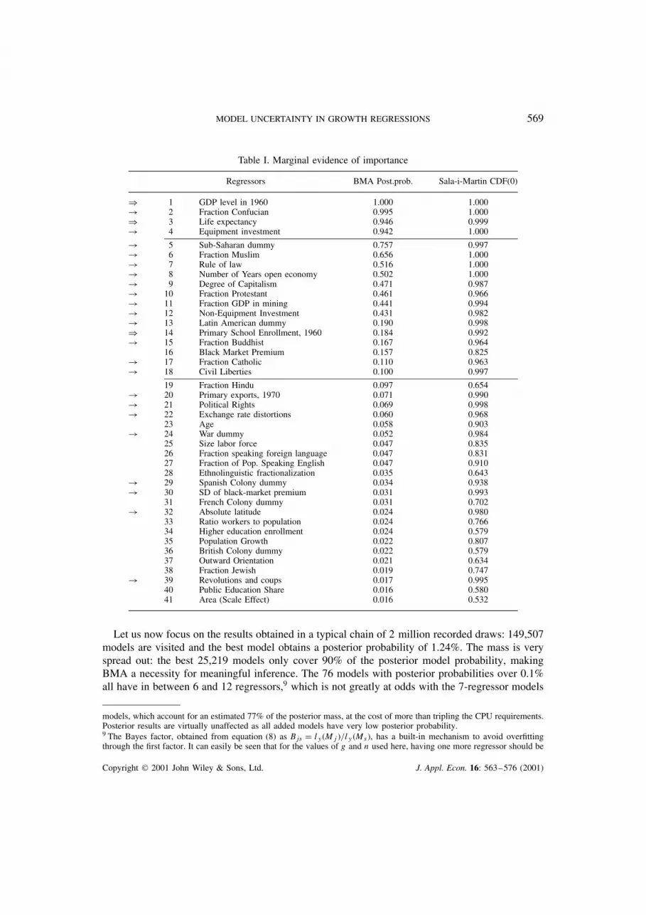
Table I. Marginal evidence of importance

Regressors BMA Post.prob. Sala-i-Martin CDF(0)

) 1 GDP level in 1960 1.000 1.000! 2 Fraction Confucian 0.995 1.000) 3 Life expectancy 0.946 0.999! 4 Equipment investment 0.942 1.000

! 5 Sub-Saharan dummy 0.757 0.997! 6 Fraction Muslim 0.656 1.000! 7 Rule of law 0.516 1.000! 8 Number of Years open economy 0.502 1.000! 9 Degree of Capitalism 0.471 0.987! 10 Fraction Protestant 0.461 0.966! 11 Fraction GDP in mining 0.441 0.994! 12 Non-Equipment Investment 0.431 0.982! 13 Latin American dummy 0.190 0.998) 14 Primary School Enrollment, 1960 0.184 0.992! 15 Fraction Buddhist 0.167 0.964

16 Black Market Premium 0.157 0.825! 17 Fraction Catholic 0.110 0.963! 18 Civil Liberties 0.100 0.997

19 Fraction Hindu 0.097 0.654! 20 Primary exports, 1970 0.071 0.990! 21 Political Rights 0.069 0.998! 22 Exchange rate distortions 0.060 0.968

23 Age 0.058 0.903! 24 War dummy 0.052 0.984

25 Size labor force 0.047 0.83526 Fraction speaking foreign language 0.047 0.83127 Fraction of Pop. Speaking English 0.047 0.91028 Ethnolinguistic fractionalization 0.035 0.643

! 29 Spanish Colony dummy 0.034 0.938! 30 SD of black-market premium 0.031 0.993

31 French Colony dummy 0.031 0.702! 32 Absolute latitude 0.024 0.980

33 Ratio workers to population 0.024 0.76634 Higher education enrollment 0.024 0.57935 Population Growth 0.022 0.80736 British Colony dummy 0.022 0.57937 Outward Orientation 0.021 0.63438 Fraction Jewish 0.019 0.747

! 39 Revolutions and coups 0.017 0.99540 Public Education Share 0.016 0.58041 Area (Scale Effect) 0.016 0.532

Let us now focus on the results obtained in a typical chain of 2 million recorded draws: 149,507models are visited and the best model obtains a posterior probability of 1.24%. The mass is veryspread out: the best 25,219 models only cover 90% of the posterior model probability, makingBMA a necessity for meaningful inference. The 76 models with posterior probabilities over 0.1%all have in between 6 and 12 regressors,9 which is not greatly at odds with the 7-regressor models

models, which account for an estimated 77% of the posterior mass, at the cost of more than tripling the CPU requirements.Posterior results are virtually unaffected as all added models have very low posterior probability.9 The Bayes factor, obtained from equation (8) as Bjs D ly�Mj�/ly�Ms�, has a built-in mechanism to avoid overfittingthrough the first factor. It can easily be seen that for the values of g and n used here, having one more regressor should be

Copyright 2001 John Wiley & Sons, Ltd. J. Appl. Econ. 16: 563–576 (2001)

570 C. FERNANDEZ, E. LEY AND M. F. J. STEEL

in MS. Indeed, MI, the intersection of M and MS, is allocated 0.38% posterior probability, whichis 112,832 times the prior mass.10 So there is a small but non-negligible amount of support for theclass of models chosen by Sala-i-Martin, and the best model in MI receives a posterior probabilityof 0.30%.

Marginal posterior probabilities of including each of the 41 regressors CDF(0) that were atthe basis of the findings of Sala-i-Martin (1997b). An arrow in front of a regressor identifies the22 important regressors of Sala-i-Martin (1997b, Table 1) and regressors with double arrows arethe ones he always retained in the models. Starting with the latter three, it is clear that GDPin 1960 and (to a lesser degree) life expectancy can indeed be retained without many problems,but that is not the case for primary school enrollment. The 22 regressors that Sala-i-Martin flagsas important have posterior probabilities of inclusion ranging from as low as 1.7% to 100.0%.Nevertheless, the Spearman rank correlation coefficient between CDF(0) and marginal posteriorinclusion probabilities is 0.94.

Of course, this is only a small part of the information provided by BMA, which really providesa joint posterior distribution of all possible 41 regression coefficients, consisting of both discrete(at zero, when a regressor is excluded) and continuous parts. Among other things, it will provideinformation on which combinations of regressors are likely to occur, avoiding models with highlycollinear regressors. For example, Civil liberties and Political rights are the two variables with thehighest pairwise correlation in the sample: it is 0.96. Thus, it is quite likely that if one of thesevariables is included in a model, the other will not be needed, as it captures more or less the sameinformation. Indeed, the posterior probability of including both these variables is 0.1%, which ismuch smaller than the product of the marginal inclusion probabilities (about 0.7%).

Thus, the marginal importance of regressors derived from our methodology does not lead tothe same results as found in Sala-i-Martin (1997b), but the results are not too dissimilar either.However, there are a number of crucial differences. First, BMA addresses the issue of probabilitiesof models, not just of individual regressors, and thus provides a much richer type of informationthan simply that indicated by Table I. In addition, an important difference is that we have acoherent statistical framework in which inference can be based on all models, averaged with theirposterior probabilities. So there is no need for us to choose a particular model or discard any ofthe regressors. As we shall see in the next section, using BMA rather than choosing one particularmodel is quite beneficial for prediction. In contrast, there is no formal inferential or modellingrecipe attached to the conclusions in Sala-i-Martin. Does one adopt a model with all importantregressors included at the same time or with a subset of four of those? If model averaging is theimplicit message, it is unclear how to implement this outside the Bayesian paradigm.

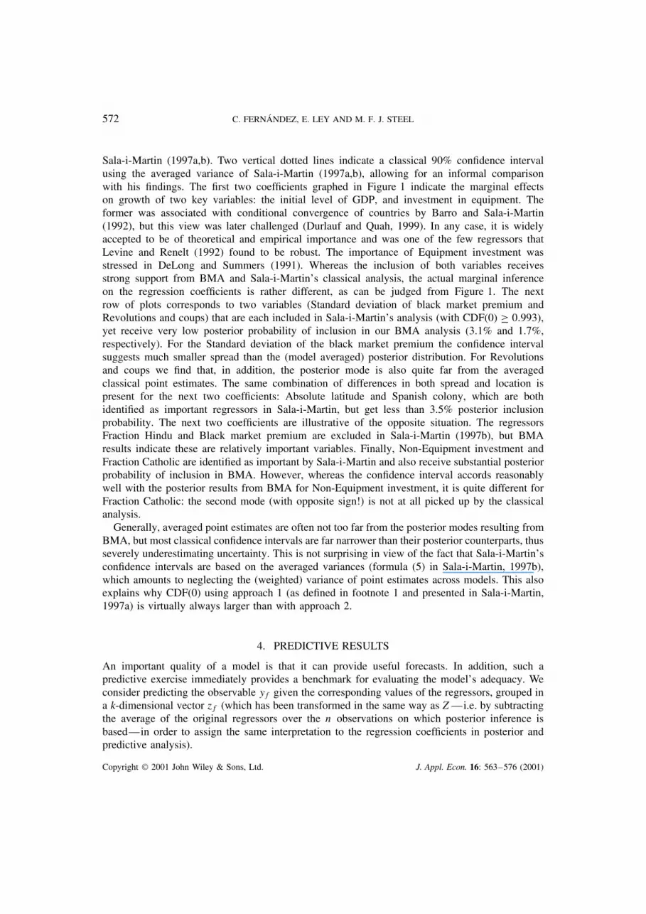
Figure 1 graphically presents the marginal posterior distribution of some regression coefficients.A gauge on top of the graphs indicates (in black) the posterior probability of inclusion of thecorresponding regressor (thus revealing the same information as in Table I). The density ineach of the graphs describes the posterior distribution of the regression coefficient given thatthe corresponding variable is included in the regression. Each of these densities is itself a mixtureas in equation (5) over the Student-t posteriors for each model that includes that particularregressor. A dashed vertical line indicates the averaged point estimate presented in Table I of

offset by a decrease in the sum of squared residuals of about 10% in order to have a unitary Bayes factor. For asymptoticlinks between our Bayes factors and various classical model selection criteria, see Fernandez et al. (2001).10 For comparison, the posterior probability of the best 73,815 models (the same number of models as in MI) multipliesthe corresponding prior probability by about 29.5 million.

Copyright 2001 John Wiley & Sons, Ltd. J. Appl. Econ. 16: 563–576 (2001)

MODEL UNCERTAINTY IN GROWTH REGRESSIONS 571

200

150

100

50

0

20000

15000

10000

5000

0

3000

2500

2000

1500

1000

500

0

15

10

5

0

15

12.5

10

7.5

5

2.5

0−0.05 0 0.05 0.1 0.15 0.2 −0.03 −0.02 −0.01 0

7060

50

40

3020

100

0.01 0.02

−0.04 −0.03 −0.02 −0.01

70

60

50

40

30

20

10

0

80

60

40

20

0

60

8

6

4

2

00 0.1 0.2 0.3 0.4 0.5

50

40

30

20

10

0

0.010 0.02

−0.03 −0.02 −0.01 0 0.01 0.02 0.03

−0.15 −0.1 −0.05 0 0.05

Nonequipment Investment Fraction Catholic

Black-Market Premium

Spanish Colony

Revolutions and Coups

0.1 0.15

−0.025 −0.02

−0.0001

−0.0004 −0.0002 0 0.0002 0.0004

−0.00005 0 0.00005

−0.015

S.D. of Black-Market premium

Absolute Latitude

Fraction Hindu

GDP Level in 1960 Investment Equipment

−0.01 −0.005 0

−0.02 −0.01 0.010 0.02

Figure 1. Posterior densities of selected coefficients

Copyright 2001 John Wiley & Sons, Ltd. J. Appl. Econ. 16: 563–576 (2001)

572 C. FERNANDEZ, E. LEY AND M. F. J. STEEL

Sala-i-Martin (1997a,b). Two vertical dotted lines indicate a classical 90% confidence intervalusing the averaged variance of Sala-i-Martin (1997a,b), allowing for an informal comparisonwith his findings. The first two coefficients graphed in Figure 1 indicate the marginal effectson growth of two key variables: the initial level of GDP, and investment in equipment. Theformer was associated with conditional convergence of countries by Barro and Sala-i-Martin(1992), but this view was later challenged (Durlauf and Quah, 1999). In any case, it is widelyaccepted to be of theoretical and empirical importance and was one of the few regressors thatLevine and Renelt (1992) found to be robust. The importance of Equipment investment wasstressed in DeLong and Summers (1991). Whereas the inclusion of both variables receivesstrong support from BMA and Sala-i-Martin’s classical analysis, the actual marginal inferenceon the regression coefficients is rather different, as can be judged from Figure 1. The nextrow of plots corresponds to two variables (Standard deviation of black market premium andRevolutions and coups) that are each included in Sala-i-Martin’s analysis (with CDF(0) ½ 0.993),yet receive very low posterior probability of inclusion in our BMA analysis (3.1% and 1.7%,respectively). For the Standard deviation of the black market premium the confidence intervalsuggests much smaller spread than the (model averaged) posterior distribution. For Revolutionsand coups we find that, in addition, the posterior mode is also quite far from the averagedclassical point estimates. The same combination of differences in both spread and location ispresent for the next two coefficients: Absolute latitude and Spanish colony, which are bothidentified as important regressors in Sala-i-Martin, but get less than 3.5% posterior inclusionprobability. The next two coefficients are illustrative of the opposite situation. The regressorsFraction Hindu and Black market premium are excluded in Sala-i-Martin (1997b), but BMAresults indicate these are relatively important variables. Finally, Non-Equipment investment andFraction Catholic are identified as important by Sala-i-Martin and also receive substantial posteriorprobability of inclusion in BMA. However, whereas the confidence interval accords reasonablywell with the posterior results from BMA for Non-Equipment investment, it is quite different forFraction Catholic: the second mode (with opposite sign!) is not at all picked up by the classicalanalysis.

Generally, averaged point estimates are often not too far from the posterior modes resulting fromBMA, but most classical confidence intervals are far narrower than their posterior counterparts, thusseverely underestimating uncertainty. This is not surprising in view of the fact that Sala-i-Martin’sconfidence intervals are based on the averaged variances (formula (5) in Sala-i-Martin, 1997b),which amounts to neglecting the (weighted) variance of point estimates across models. This alsoexplains why CDF(0) using approach 1 (as defined in footnote 1 and presented in Sala-i-Martin,1997a) is virtually always larger than with approach 2.

4. PREDICTIVE RESULTS

An important quality of a model is that it can provide useful forecasts. In addition, such apredictive exercise immediately provides a benchmark for evaluating the model’s adequacy. Weconsider predicting the observable yf given the corresponding values of the regressors, grouped ina k-dimensional vector zf (which has been transformed in the same way as Z —i.e. by subtractingthe average of the original regressors over the n observations on which posterior inference isbased—in order to assign the same interpretation to the regression coefficients in posterior andpredictive analysis).

Copyright 2001 John Wiley & Sons, Ltd. J. Appl. Econ. 16: 563–576 (2001)

MODEL UNCERTAINTY IN GROWTH REGRESSIONS 573

Prediction naturally fits in the Bayesian paradigm as all parameters can be integrated out,formally taking parameter uncertainty into account. If we also wish to deal with model uncertainty,BMA as in equation (5) provides us with the formal mechanism, and we can characterize theout-of-sample predictive distribution of yf by

p�yfjy� D2k∑

jD1

fS

(yf

∣∣∣∣ n � 1, y C 1

g C 1z0f,jˇ

Łj,

n � 1

dŁj

ð{

1 C 1

nC 1

g C 1z0f,j�Z

0jZj�

�1zf,j

}�1)

P�Mjjy��9�

where fS�xj', b, a� denotes the p.d.f. of a univariate Student-t distribution with ' degrees offreedom, location b (the mean if ' > 1) and precision a (with variance '/fa�' � 2�g provided' > 2) evaluated at x. In addition, zf,j groups the j elements of zf corresponding to the regressorsin Mj, ˇŁ

j D �Z0jZj��1Z0

jy and

dŁj D 1

g C 1y0MXjy C g

g C 1�y � y�n�

0�y � y�n� �10�

We shall now split the sample into n observations on which we base our posterior inferenceand q observations which we retain in order to check the predictive accuracy of the model. Asa formal criterion, we shall use the log predictive score (LPS ), introduced by Good (1952). It isa strictly proper scoring rule, in the sense that it induces the forecaster to be honest in divulginghis predictive distribution. For f D n C 1, . . . , n C q—i.e. for each country in the predictionsample—we base our measure on the predictive density evaluated in these retained observationsynC1, . . . , ynCq, namely:

LPS D �1

q

nCq∑fDnC1

lnp�yfjy� �11�

The smaller LPS is, the better the model does in forecasting the prediction sample. Interpretingvalues for LPS can perhaps be facilitated by considering that in the case of i.i.d. sampling, LPSapproximates an integral that equals the sum of the Kullback–Leibler divergence between theactual sampling density and the predictive density in equation (9) and the entropy of the samplingdistribution (Fernandez et al., 2001). So LPS captures uncertainty due to a lack of fit plus theinherent sampling uncertainty, and does not distinguish between these two. Here we are necessarilyfaced with a different zf for every forecasted observation (corresponding to a specific country), sowe are not strictly in the context of observations that are generated by the same distribution. Still,we think the above interpretation may shed some light on the calibration and comparison of LPSvalues. If, for the sake of argument, we assume that we fit the sampling distribution perfectly, thenLPS approximates entropy alone. In the context of a Normal sampling model with fixed standarddeviation Ł, this latter entropy can then be translated into a value for Ł, using the fact that entropyequals ln� Ł

p2+e�. Thus, a known Normal sampling distribution with fixed Ł would induce the

same inherent predictive uncertainty as measured by LPS , if we choose Ł D exp�LPS�/p

2+e.Of course, as a direct consequence, a difference in LPS of, say, 0.1, corresponds to about a 10%difference in values for Ł.

We shall use LPS to compare four different regression strategies: the BMA approach, leading toequation (9), the best model—i.e. the one with the highest posterior probability—in M, the best

Copyright 2001 John Wiley & Sons, Ltd. J. Appl. Econ. 16: 563–576 (2001)

574 C. FERNANDEZ, E. LEY AND M. F. J. STEEL

Table II. Predictive Performance

Number of times LPS

Best Worst Beaten by null Min Mean Max

BMA 9 0 2 �3.470 �2.977 �2.408Best model in M 0 8 12 �3.370 �2.316 �1.268Best model in MI 8 0 4 �3.460 �2.838 �1.341Full model 3 8 12 �3.266 �2.261 �0.940Null model 0 4 . . . �2.850 �2.560 �1.853

model in MI, and the full model with all k regressors. As a benchmark for the importance of growthregression, we also include LPS for the ‘null model’, i.e. the model with only the intercept where noindividual country characteristics are used. We would expect this model to reproduce the marginalgrowth distribution (without conditioning on regressors) pretty well. As the sample standarddeviation of growth is 0.01813, we could then roughly expect LPS values for the null modelaround the entropy value corresponding to Ł D 0.01813, which is �2.591. For the regressionmodels, we would hope that they predict better, since they use the information in the regressors,and this should ideally be reflected in a smaller LPS or a conditional Ł value under 0.01813.

The partition of the sample into the inference and the prediction sample is done randomly,by assigning observations to the inference sample with probability 0.75. The results of twentydifferent partitions are summarized in Table II. Besides numerical summaries of the LPS values,we also indicate how often the model is beaten by the trivial null model, and how often the modelperforms best and worst. The following key characteristics emerge: the null model performs in afairly conservative fashion and its mean LPS is very close to what we expected on the basis of thesample standard deviation. The full model and the best model in M are beaten by the benchmarknull model in over half the cases, and clearly perform worst of the regression models. The bestmodel in MI does quite a bit better and generally improves a lot on the null model, but cansometimes lead to very bad predictions (the maximum value of LPS corresponds to Ł D 0.0633,3.5 times that of the sample). In contrast, the BMA approach never leads us far astray: it is onlybeaten by the null model twice and the largest value of LPS corresponds to Ł D 0.0218 (and thisoccurs in a case where it actually outperforms all other models by a large margin). It performsbest most frequently and the best prediction it produced corresponds to Ł D 0.0075 which is onlyabout 40% of the sample standard deviation. The mean LPS value for the BMA model correspondsto Ł D 0.0123, i.e. a reduction of the sample standard deviation by about a third.

The fact that BMA does so much better than simply taking the best model is compellingevidence supporting the use of formal model averaging rather than the selection of any givenmodel. Interestingly, the best model in MI does better than the best model in M (which containsMI). This underlines that the highest posterior probability on the basis of the inference sampledoes not necessarily lead to the best predictions in the prediction sample. In addition, MI isrestricted to those models that include the three regressors always retained by Sala-i-Martin ontheory grounds. This extra information (although not always supported by the data) may help inpredicting.11

11 Of course, this relative success of the best model in MI has no immediate bearing on the predictive performance of aclassical analysis.

Copyright 2001 John Wiley & Sons, Ltd. J. Appl. Econ. 16: 563–576 (2001)

MODEL UNCERTAINTY IN GROWTH REGRESSIONS 575

In summary, the use of regression models with BMA results in a considerable predictiveimprovement over the null model, thus clearly suggesting that growth regression is not a futileexercise, although care should be taken in the methodology adopted.

5. DISCUSSION

The value of growth regression in cross-country analysis has been illustrated in the predictiveexercise in the previous section. We agree with Sala-i-Martin (1997b) that some regressors can beidentified as useful explanatory variables for growth in a linear regression model, but we advocatea formal treatment of model (and parameter) uncertainty. In our methodology the marginal impor-tance of an explanatory variable does not necessarily imply anything about the size or sign of theregression coefficient in a set of models, but is based entirely on the posterior probabilities of mod-els containing that regressor. In addition, we go one step further and provide a practical and theoret-ically sound method for inference, both posterior and predictive, using Bayesian Model Averaging(BMA). From the huge spread of the posterior mass in model space and the predictive advantageof BMA, it is clear that model averaging is recommended when dealing with growth regression.

Our Bayesian paradigm provides us with a formal framework to implement this model averaging,and recent Markov chain Monte Carlo (MCMC) methods are shown to be very powerful indeed.Despite the huge model space (with 2.2 trillion models), we obtain very reliable results withoutan inordinate amount of computational effort.12

The analysis in Sala-i-Martin (1997b) is not Bayesian and thus no formal model averaging canoccur, even though he considers weighing with the integrated likelihood.13 In addition, the latteranalysis evaluates all models and is thus necessarily restricted to a rather small set of models,MS, which seems not to receive that much empirical support from the data. Even though we finda roughly similar set of variables that can be classified as ‘important’ for growth regressions, acrucial additional advantage is that our results are immediately interpretable in terms of modelprobabilities and all inference can easily be conducted in a purely formal fashion by BMA. It isnot clear to us what to make of the recommendations in Sala-i-Martin (1997b): should the appliedresearcher use all the regressors identified as important or mix over the corresponding models inMS? However, the latter would have to be without proper theoretical foundation or guidance if aclassical statistical framework is adopted.

In our view, the treatment of a very large model set, such as M, in a theoretically sound andempirically practical fashion requires BMA and MCMC methods. In addition, this methodologyprovides a clear and precise interpretation of the results, and immediately leads to posterior andpredictive inference.

ACKNOWLEDGEMENTS

We greatly benefited from useful comments from co-editor Steven Durlauf, Ed Leamer, JonTemple, an anonymous referee, and participants at seminars at the Fundacion de Estudios deEconomıa Aplicada (Madrid), the Inter-American Development Bank, the International Monetary

12 The reported chain took about 2 23 hours of CPU time on a fast Sun Ultra-2 with two 296MHz CPUs, 512Mb of RAM

and 3.0Gb of swap space running under Solaris 2.6. Our programs are coded in Fortran 77 and are available at thisjournal’s website.13 Sala-i-Martin (1997a,b) do not specify what this integrated likelihood is; as there is no prior to integrate with, this mayrefer to the maximized likelihood, which is proportional to �y0MXjy�

�n/2 for Mj.

Copyright 2001 John Wiley & Sons, Ltd. J. Appl. Econ. 16: 563–576 (2001)

576 C. FERNANDEZ, E. LEY AND M. F. J. STEEL

Fund, Heriot-Watt University, the University of Kent at Canterbury, the University of Southampton,and the 1999 European Economic Association Meetings at Santiago de Compostela. Part ofthis research was conducted while Carmen Fernandez was at the Department of Mathematics,University of Bristol, and Mark Steel at the Department of Economics, University of Edinburgh.

REFERENCES

Barro RJ. 1991. Economic growth in a cross section of countries. Quarterly Journal of Economics 106:407–444.

Barro RJ, Sala-i-Martin XX. 1992. Convergence. Journal of Political Economy 100: 223–251.Brock WA, Durlauf SN. 2000. Growth economics and reality. Working Paper 8041, National Bureau of

Economic Research, Cambridge, Massachusetts.Chib S, Greenberg E. 1996. Markov chain Monte Carlo simulation methods in econometrics. Econometric

Theory 12: 409–431.Chipman H. 1996. Bayesian variable selection with related predictors. Canadian Journal of Statistics 24:

27–36.Clyde M, Desimone H, Parmigiani G. 1996. Prediction via orthogonalized model mixing. Journal of the

American Statistical Association 91: 1197–1208.DeLong JB, Summers L. 1991. Equipment investment and economic growth. Quarterly Journal of Economics

106: 445–502.Durlauf SN, Quah DT. 1999. The new empirics of economic growth. In Handbook of Macroeconomics

(Vol. IA), Taylor JB, Woodford M (eds). North-Holland: Amsterdam; 231–304.Fernandez C, Ley E, Steel MFJ. 2001. Benchmark priors for Bayesian model averaging. Journal of Econo-

metrics 100: 381–427.George EI. 1999. Bayesian model selection. In Encyclopedia of Statistical Sciences Update (Vol. 3), Kotz S,

Read C, Banks DL (eds). Wiley: New York; 39–46.George EI, McCulloch RE. 1997. Approaches for Bayesian variable selection. Statistica Sinica 7: 339–373.Good IJ. 1952. Rational decisions. Journal of the Royal Statistical Society, B 14: 107–114.Kass RE, Raftery AE. 1995. Bayes factors. Journal of the American Statistical Association 90: 773–795.Kormendi R, Meguire P. 1985. Macroeconomic determinants of growth, cross-country evidence. Journal of

Monetary Economics 16: 141–163.Leamer EE. 1978. Specification Searches: Ad Hoc Inference with Nonexperimental Data. Wiley: New York.Leamer EE. 1983. Let’s take the con out of econometrics. American Economic Review 73: 31–43.Leamer EE. 1985. Sensitivity analyses would help. American Economic Review 75: 308–313.Lee H. 1996. Model selection for consumer loan application data. Dept of Statistics Working Paper No. 650,

Carnegie-Mellon University.Levine R, Renelt D. 1992. A sensitivity analysis of cross-country growth regressions. American Economic

Review 82: 942–963.Madigan D, York J. 1995. Bayesian graphical models for discrete data. International Statistical Review 63:

215–232.Mitchell TJ, Beauchamp JJ. 1988. Bayesian variable selection in linear regression. Journal of the American

Statistical Association 83: 1023–1036 (with discussion).Raftery AE, Madigan D, Hoeting JA. 1997. Bayesian model averaging for linear regression models. Journal

of the American Statistical Association 92: 179–191.Sala-i-Martin XX. 1997a. I just ran four million regressions. Mimeo, Columbia University.Sala-i-Martin XX. 1997b. I just ran two million regressions. American Economic Review 87: 178–183.Smith M, Kohn R. 1996. Nonparametric regression using Bayesian variable selection. Journal of Economet-

rics 75: 317–343.Temple J. 1999. The new growth evidence. Journal of Economic Literature 37: 112–156.Temple J. 2000. Growth regressions and what the textbooks don’t tell you. Bulletin of Economic Research

52: 181–205.Tierney L. 1994. Markov chains for exploring posterior distributions. Annals of Statistics 22: 1701–1762

(with discussion).

Copyright 2001 John Wiley & Sons, Ltd. J. Appl. Econ. 16: 563–576 (2001)