model reduction for dynamical systems with quadratic output

INTERNATIONAL JOURNAL FOR NUMERICAL METHODS IN ENGINEERINGInt. J. Numer. Meth. Engng 2012; 91:229–248Published online 5 June 2012 in Wiley Online Library (wileyonlinelibrary.com). DOI: 10.1002/nme.4255

Model reduction for dynamical systems with quadratic output

R. Van Beeumen1,*,†, K. Van Nimmen2,3, G. Lombaert2 and K. Meerbergen1

1Department of Computer Science, Katholieke Universiteit Leuven, Heverlee, Belgium2Department of Civil Engineering, Katholieke Universiteit Leuven, Heverlee, Belgium

3Department of Industrial Engineering, Katholieke Hogeschool Sint-Lieven, Ghent, Belgium

SUMMARY

Finite element models for structures and vibrations often lead to second order dynamical systems with largesparse matrices. For large-scale finite element models, the computation of the frequency response functionand the structural response to dynamic loads may present a considerable computational cost. Padé via Krylovmethods are widely used and are appreciated projection-based model reduction techniques for linear dynam-ical systems with linear output. This paper extends the framework of the Krylov methods to systems witha quadratic output arising in linear quadratic optimal control or random vibration problems. Three differenttwo-sided model reduction approaches are formulated based on the Krylov methods. For all methods, thecontrol (or right) Krylov space is the same. The difference between the approaches lies, thus, in the choice ofthe observation (or left) Krylov space. The algorithms and theory are developed for the particularly impor-tant case of structural damping. We also give numerical examples for large-scale systems corresponding tothe forced vibration of a simply supported plate and of an existing footbridge. In this case, a block form ofthe Padé via Krylov method is used. Copyright © 2012 John Wiley & Sons, Ltd.

Received 27 April 2011; Revised 28 October 2011; Accepted 17 November 2011

KEY WORDS: model reduction; quadratic output; Arnoldi method; modal superposition; recycling

1. INTRODUCTION

In structural dynamics and vibro-acoustics, frequent use is made of finite element (FE) modelsto design and analyze structures subjected to dynamic loading. For large-scale FE models, thecomputation of the frequency response function and the structural response to dynamic loads maypresent a considerable computational cost. Efficient evaluation of the frequency response functionis extremely important in reducing computation time of parametric studies, see [1]. Several methodshave been developed for efficient evaluation. Among the most widely used methods is the modelorder reduction (MOR) through modal superposition. In this case, a Galerkin projection is performedon a reduced basis consisting of a subset of the eigenvectors of the generalized eigenvalue problemassociated with the stiffness and mass matrix of the FE model of the structure. This method is partic-ularly efficient in low-frequency range where the modal density is small and the structural responseis dominated by a few global modes. The reduction does not come without a price, however, asa high number of modes may be required to obtain a good approximation, and the computation ofthese modes may be quite expensive, particularly for a large FE model. Furthermore, it is not alwayseasy to select the modes that should be included in the reduced basis.

Other methods, which have shown to be extremely useful, are related to the Ritz vector technique[2, 3]. This is a Krylov subspace method, which is also known as Padé via Krylov [4–7]. The sys-tem’s output is approximated by a low degree rational polynomial such that the first derivatives at the

*Correspondence to: R. Van Beeumen, Departement of Computer Science, Katholieke Universiteit Leuven,Celestijnenlaan 200A, 3001 Heverlee, Belgium.

†E-mail: [email protected]

Copyright © 2012 John Wiley & Sons, Ltd.

230 R. VAN BEEUMEN ET AL.

origin (also called moments) correspond with the exact output function. Padé via Krylov methods aretherefore also called moment matching methods. Krylov methods have been used successfully forthe computation of frequency response functions with proportional [8] and nonproportional damp-ing [5,9–14]. An extensive overview of model reduction methods with a large number of referencesare found in recent books by Antoulas [15] and Benner et al. [16].

The aforementioned methods allow for an efficient model reduction when a linear output is con-sidered, that is, a linear combination of the components of the state vector or, in a finite elementcontext, the vector that collects the DOF of the model. In many cases, however, the response quanti-ties of interest correspond to a quadratic system output, that is, the product in the time or frequencydomain of components of the state vector or the vector that collects the degrees of freedom of thesystem. Examples include linear quadratic optimal control problems, problems of random vibrationwhere the second order response statistics, due to stochastic excitation [17], are computed, as wellas all problems where response quantities related to energy or power are considered.

In the present paper, model reduction is considered for linear dynamical systems that have struc-tural damping with quadratic output. The classical approach is to rewrite the governing equationsof a system with quadratic output as an equivalent linear system with multiple outputs [18]. Inthis way, any method for model reduction of linear systems for multiple outputs can be used.In the present paper, we present two improvements to this idea. First, we reuse (or recycle [19–21])the eigenmodes computed from the control Krylov space derived from the excitation. We, thereby,use the fact that a system with structural damping has the same eigenmodes as the undamped system.The excited modes are reused to improve the construction of the left (or observation) Krylov spaces.This is a mix between moment matching and modal superposition. Second, we propose an alter-native selection of the output vectors in order to obtain more matching moments for the quadraticoutput. These methods can be used for models in the frequency domain and in the time domain.

The outline of this paper is as follows. In Section 2, we give the problem formulation and discussfour different situations where quadratic outputs arise. We also review how reduced models forstructural damping can be obtained. In Section 3, we review the notion of Padé via Krylov meth-ods for linear systems and the concepts of moments and moment matching. We revisit the idea ofrecycling for one-sided methods and introduce recycling for two-sided Krylov methods for modelswith structural damping. In Section 4, we propose new methods for model reduction by Padé viaKrylov for systems with a quadratic output. First, we discuss the use of recycling eigenmodes in themodel reduction method of an equivalent linear system with multiple outputs [18], which we callELMOR in this paper. We then present an improvement of the ELMOR method, which we denoteby decomposition free ELMOR (DF-ELMOR) method. Finally, we present the quadratic momentmatching (QMM) method, which tries to match as many moments of the quadratic output functionas possible for a given order of the reduced model. Section 5 illustrates the numerical methods fortwo structural dynamical problems with a quadratic output. We illustrate the power of recycling forMOR and compare the three new two-sided methods with each other and with the one-sided method.We formulate the main conclusions in Section 6.

Throughout the paper, we denote by AT the matrix transpose and by A� its Hermitian transpose.The complex conjugate of a is denoted by a. The Euclidean inner product of two vectors, x and y,is denoted by y�x, and the induced 2-norm is denoted by kxk. The M norm kxkM is defined asthe norm corresponding to the M inner product

px�Mx. Dependence on the variable s is always

explicitly denoted, for example x.s/. The vector ej is a vector of zeroes, except at position j whereit has a unit value.

2. PROBLEM FORMULATION

Let us first consider a dynamical system with a quadratic output in the frequency domain:

QD²..1C i�/K �!2M/x.!/D f u.!/

y.!/D x�.!/Sx.!/, (1)

Copyright © 2012 John Wiley & Sons, Ltd. Int. J. Numer. Meth. Engng 2012; 91:229–248DOI: 10.1002/nme

MODEL REDUCTION FOR DYNAMICAL SYSTEMS WITH QUADRATIC OUTPUT 231

where K and M 2 Rn�n are the stiffness matrix and the mass matrix, respectively; f 2 Rn; � isthe structural (proportional) damping factor; S 2 Rn�n is a symmetric rank r matrix with r � n;x.!/ 2Cn is the displacement vector; u.!/ 2C is the system’s input; and y.!/ 2C is the output.When the equation of motion is obtained by means of the finite element method, the vector x.!/collects the degrees of freedom of the model. Note that ! 2 � is the frequency, where � is thefrequency range or frequency interval of interest. Throughout the paper, we assume the mass matrixM is symmetric positive definite and the stiffness matrix K is symmetric and nonsingular. If thelatter condition would not hold, we assume there is a � 2 R such that K � �2M is nonsingular.Therefore, we can suppose, without loss of generality, that � D 0.

In the following, a number of problems are discussed where the quadratic output is considered tomotivate the development of tailored MOR methods. First, a weighted square output of the followingform is considered:

y.!/D

rXjD1

jwj e�j x.!/j

2

where r is the total number of outputs considered andwj the weights. The ouput y.!/ can be writtenas in the system (1) by constructing a diagonal matrix S with weights wj on the elements corre-sponding to the selected output components and zeroes elsewhere. This form of output allows thecomputation of the spatial average of a displacement or velocity field over a given surface as illus-trated by the numerical examples in §5. This is also useful in many other problems, for example, inestimating the total radiated sound power in problems of vibro-acoustics.

Second, the calculation of the auto power spectral density (PSD) function of the response in arandom vibration problem is considered. The output y.!/ is now computed as follows:

y.!/D Sjj .!/D e�jNZ.!/�1fSu.!/f

TZ.!/�1ej

with Z.!/D .1C i�/K �!2M and Su.!/, a scalar that represents the real-valued auto PSD func-tion of the excitation u.!/. This problem can be reformulated as in (1) by choosing u.!/D

pSu.!/

and S , a diagonal matrix with a unit value at the element .j , j / corresponding to the selected outputcomponent and zeroes elsewhere. This case can be generalized to an output representing the averageof the auto PSD function of multiple components in a way similar to the first example. When thecross power spectral density function of two output components i and j is considered, the outputy.!/ becomes

y.!/D Sij .!/D e�iNZ.!/�1fSu.!/f

TZ.!/�1ej

and can be formulated as in (1) by choosing u.!/ DpSu.!/ and S , a matrix with a unit value at

the element .i , j / and zeroes elsewhere. In this case, the matrix S is nonsymmetric, and the meth-ods proposed in the following can not be used. In the particular case where no structural damping ispresent, however, the cross PSD function Sij is real, and an alternative symmetric matrix S 0 can bedefined by rewriting the output as y.!/D 1

2x�.!/.S C S�/x.!/.

Third, let us consider a system with a quadratic output in the time domain:

QD²M Rx.t/CKx.t/D f u.t/

y.t/D xT .t/Sx.t/. (2)

Note that the output y.t/ in the system (2) does not represent the Fourier transform of the out-put y.!/ in the system (1) as in the case of a linear output. A quadratic output y.t/ of the formxT .t/Sx.t/ is encountered when the root mean square (RMS) value of the output component xj .t/is considered:

RMSj D1

T

Z T

0

x2j .t/dt .

The output y.t/D x2j .t/ can be rewritten as y.t/D xT .t/Sx.t/with S , a diagonal matrix havinga unit value at the element .j , j / and zeroes elsewhere.



A last application arises in the optimal control of a linear quadratic regulator where an objectivefunction of the following form is minimized:

1

2

Z t1

t0

�xT .t/Sx.t/C uT .t/Ru.t/

�dt

where, again, a reduced model for quadratic output may significantly increase the computationalefficiency.

In the case of structural damping, we rewrite the system (1) as

QD².K � sM/x.s/D f Qu.s/

y.s/D x�.s/Sx.s/,, (3)

where s D !2=.1C i�/ and Qu D 1=.1C i�/u. The variable s will be used throughout the paperinstead of !.

All methods we describe next build a reduced model of the form

OQD². OK � s OM/ Ox.s/D Of u.s/

Oy.s/D Ox�.s/ OS Ox.s/(4)

where OK D W �KV , OM D W �MV , OS D V �SV , and Of D W �f and V ,W 2 Rn�k . Note thatwhenW ¤ V , OK and OM are, in general, nonsymmetric. The matrix V is determined from a momentmatching Krylov space that uses f and is independent of S . The choice of V guarantees that y.s/and Oy.s/match the k moments, regardless the choice ofW . In the paper, we discuss various alterna-tives for W such that y.s/ and Oy.s/ match more than k moments. We compare these methods withthe case where W D V , leading to symmetric OK and OM . We call this a one-sided Krylov methodbecause W needs not to be computed.

3. LINEAR MODELS WITH MULTIPLE OUTPUTS

In this section, we review the Padé via Krylov method for linear systems with multiple outputs. Weexploit the symmetry of K and M , and the positive-definite character of M . We also discuss theidea of recycling in the case of multiple outputs.

3.1. Moment matching via Lanczos’ method

Consider the linear system with single input u.s/ and multiple outputs y.s/ (SIMO)

LD².K � sM/x.s/D f u.s/

y.s/D H�x.s/, (5)

where K,M 2 Rn�n, f 2 Rn, H 2 Rn�p , x.s/ 2 Cn is the state, u.s/ 2 C is the input, andy.s/ 2Cp is the output. The number of states n is called the dimension or order of the system L.

We first introduce the notion of a Krylov space. Let ADK�1M and b DK�1f . Then, we definea Krylov space of dimension k by

Kk.A, b/D span°b,Ab,A2b, � � � ,Ak�1b

±. (6)

When K and M are symmetric and M is positive definite, the Krylov space in (6) is usuallybuilt by the Lanczos method [22]. Note, therefore, that K�1M is self-adjoint with respect to theM inner product. Algorithm 1 describes how an M -orthogonal basis Vk D Œv1, v2, � � � , vk� can beconstructed.

Next to Vk , the method also computes Tk D V �k MK�1MVk as a by-product of the orthogonal-

ization process. The matrix Tk is symmetric and tridiagonal. We will not use Tk for model reductionbut for computing the eigenvalues of

KuD �Mu (7)



which is the undamped generalized eigenvalue problem [23]. We will use this eigendecomposi-tion for recycling eigenvectors in §3.2. The Lanczos method can also be applied to a block ofvectors B 2 Rn�r in a similar way, which corresponds to the case where multiple right-handsides are considered. See [23] for the implementation details. The initial block B should first beM -orthogonalized by the Gram–Schmidt method. Important to mention is that the Gram–Schmidtorthogonalization should be improved by re-orthogonalization for reasons of numerical stability.This often produces more accurate results [24].

In the context of MOR, we build a model that uses the input vector f as well as the output matrixH . In order to do so, we build two Krylov spaces, one with f and one with H :

Vk WKk.K�1M ,K�1f /D span°K�1f , .K�1M/K�1f , � � � , .K�1M/k�1K�1f

±(8)

Wk WKk.K�1M ,K�1H/D span°K�1H , .K�1M/K�1H , � � � , .K�1M/`�1K�1H

±(9)

where ` and k are chosen such that k D `p and p is the number of columns ofH . A reduced modelis defined as

OLD². OK � s OM/ Ox.s/D Of u.s/

Oy.s/D OH� Ox.s/, (10)

with OKDW �kKVk , OMDW �

kMVk , OfDW �

kf , and OHDV �

kH . The model is ‘good’ when

ky.s/ � Oy.s/k is small, in some sense. The key property of the Krylov methods is that they leadto moment matching. The moments of y.s/ are obtained by developing y.s/ in a Taylor series as

y.s/D

1XjD0

Yj sj

where Yj is called the j th moment of y.s/. We assume that the power series converges. It can beshown that the moments are YjDH�.K�1M/jK�1f for j D 0, 1, 2, : : :. The relation with theLanczos algorithm is given by Theorem 1, which relies on the following lemmas.

Lemma 1Let the columns of Vk span the Krylov space Kk.K�1M ,K�1f /. Let Wk be such thatOKDW �

kKVk is invertible. Let XjD.K�1M/jK�1f be the j th moment of x.s/ for system

(5). Similarly, define OXjD. OK�1 OM/j OK�1 Of for the reduced system (10). Then, XjDVk OXj forj D 0, : : : , k � 1.

ProofWe prove the lemma by using the property that all Xj for j D 0, : : : , k � 1 lie in the Krylov spaceKk.K�1M ,K�1f /. See also [7, 24].



Let j D 0. Because X0 lies in the Krylov space, there exists a ´0 such that X0 DK�1f D Vk´0.Then, by multiplying on the left by K and W �

kand by using the definitions of OM and OK, we have

K�1f D Vk´0

W �k f DW�k KVk´0

Of D OK´0,

from which follows ´0 D OX0 and, thus, X0 D Vk OX0.Assume j > 0 and that Xj�1 D Vk OXj�1. Then, because Xj lies in the Krylov space, there exists

a ´j such that Xj D Vk´j . Hence, we find, similar to the case where j D 0,

K�1MXj�1 D Vk´jW �k M.Vk

OXj�1/DW �k KVk´jOM OXj�1 D OK´j ,

from which ´j D OXj and, thus, Xj D Vk OXj . This proves the lemma. �

Lemma 2Let the columns of Wk span the Krylov space Kk.K�1M ,K�1H/. Let Vk and Wk be, such thatOKDW �

kKVk is invertible. LetZjD.K�1M/jK�1H . Similarly, we define OZjD. OK�� OM �/j OK�� OH .

Then, Zj DWk OZj for j D 0, : : : , `� 1.

ProofThe proof follows from Lemma 1, where the role of Vk andWk is interchanged. We, therefore, havetransposes for OK and OM . �

Theorem 1Given the reduced model defined by the system of equations (10), let OYj be the j th moment of Oy.s/.Then, OYj D Yj for j D 0, : : : , kC `� 1.

ProofSee [7, 15, 25, 26] for moment matching in Krylov methods. We prove the theorem for the presentcase, where K and M are symmetric and M is positive definite.

The j th moments Yj and OYj are, respectively,

Yj DH�.K�1M/jK�1f

OYj D OH�. OK�1 OM/j OK�1 Of .

Following Lemma 1, we have

.K�1M/jK�1f D Vk OXj for j D 0, : : : , k � 1.

Similarly, by Lemma 2, we have

H�.K�1M/iK�1 D OH�. OK�1 OM/i OK�1W �k for i D 0, : : : , `� 1.

Hence, we find for j D 0, : : : , k � 1,

Yj DH�.K�1M/jK�1f

DH�Vk OXjD OH� OXj D OYj .



For i D 0, : : : , `� 1, we have

YkCi DH�.K�1M/i .K�1M/.K�1M/k�1K�1f

D�OH�. OK�1 OM/i OK�1W �k

�M�Vk. OK

�1 OM/k�1 OK�1 Of�

D OH�. OK�1 OM/kCi OK�1 Of D OYkCi .

This proves the theorem. �

By Theorem 1, the output of the reduced order model (10) is a Padé approximation of the outputof model (5).

3.2. Connection with modal superposition and recycling

Modal superposition is often the desired method for model reduction, provided it is cheap to com-pute the modes. Let .�j ,'j / for j D 1, : : : ,n be the eigenvalues and eigenmodes of the generalizedeigenvalue problem (7). The system’s output can be written as

y.s/D

nXjD1

.H�'j /.'�j f /

�j � su.s/.

Now, the k lowest eigenfrequencies and modes .�j ,'j / for j D 1, : : : , k can be computed withthe Lanczos method, as follows. Let Tk D V �kMK

�1MVk be computed with the Lanczos methodfor building Vk , and let

Tk´j D �j´j j D 1, : : : , k (11)

be the eigenpairs of Tk . Then, we call O'j D Vk´j a Ritz vector and O�j D ��1j a Ritz value ofthe generalized eigenvalue problem (7). Typically, the lowest modes are well approximated by themethod. The computed eigenpairs can be used to approximate the output

Oy.s/D

kXjD1

.H� O'j /. O'�j f /

O�j � su.s/. (12)

Recycling is studied in the literature for one-sided methods, that is, methods for fast computationof the state vector x.s/ [20, 21]. This technique was previously proposed to speed up Krylov-basedmodel reduction methods [19, 21]. In this paper, we use recycling also for two-sided methods. Theoutput of (5) is decomposed as

y.s/D yR.s/C yL.s/,

where yR.s/ is computed through modal superposition (12). This can be done very cheaply becausethe Ritz values and the Ritz vectors are computed from Tk which is a by-product of the orthog-onalization process of the Lanczos method for constructing the Krylov space (8). Let us nowassume that �1, � � � ,�q are the eigenfrequencies in the frequency range of interest � and are usedin the modal superposition for the computation of yR.s/. It this case, it has been observed [20, 21]that the computation of yL.s/ requires only very few Lanczos iterations. This is due to the fact thatvertical asymptotes of y.s/ are all contained by yR.s/, whereas yL.s/ is a smooth function in thefrequency range of the recycled modes. Outside this frequency range, yL.s/ has vertical asymptotescorresponding to the poles that are not recycled. Decomposing the computation of the output iscalled frequency sweeping in [20] and recycling of eigenmodes in [21].

This methodology is illustrated for a 20-DOF chain-like spring-mass model, fixed at the bottomspring end and free at the top twentieth mass. The masses are considered to be the same for alllinks in the chain; a uniform stiffness distribution is chosen along the chain. The ratio of the springstiffness to the mass of a link is chosen to be 1. A structural damping ratio of 1 % is assumed. Thestructure is subjected to an impulse excitation of the unit magnitude at the top mass of the model.



Assume the eigenpairs .�j ,'j / for j D 1, : : : , 5 are given. Figure 1 shows that the modulus of therecycled part yR.s/ contains all peaks of the modulus of the total response in the frequency rangeof the recycled modes (0–0.2 Hz). The modulus of the remaining part, yL.s/, is very smooth in thisfrequency range. This is a typical result of recycling. For approximating yL.s/, only a few iterationsof the Lanczos method are required.

The fact that the Lanczos method can be used to compute eigenvalues and eigenvectors allows usto compute the reduced model more efficiently. This is called recycling, as we now explain.

Theorem 2Let Uq D Œ'1, � � � ,'q� and �q D diag.Œ�1, � � � ,�q�/. We can decompose the output of (5) into twoindependent terms

yR.s/DH�Uq.ƒq � sI /

�1U �q f u.s/

yL.s/DH�.I �UqU

�qM/.K � sM/�1.I �MUqU

�q /f u.s/

where y.s/D yR.s/C yL.s/.

ProofThe external force f can be decomposed into two components: fRDMUqU

�q f and fLD.I �

MUqU�q /f . The corresponding state vectors are the solutions of the following problems:

.K � sM/xR.s/D fRu.s/, (13)

.K � sM/xL.s/D fLu.s/. (14)

Because the columns of Uq are eigenvectors of the generalized eigenvalue problem (7), we havexR.s/D Uq´R.s/, and (13) can be rewritten as

.K � sM/Uq´R.s/D fRu.s/,

.MUqƒq � sMUq/´R.s/DMUqU�q f u.s/,

.ƒq � sI /´R.s/D U�q f u.s/,

(15)

where we used KUq D MUqƒq and U �qMUq D I , respectively. Multiplying (14) on the left byU �q , we have

.U �q K � sU�qM/xL.s/D .U

�q �U

�qMUqU

�q /f u.s/,

.ƒqU�qM � sU

�qM/xL.s/D 0,

.ƒq � sI /U�qMxL.s/D 0,

Figure 1. Modulus of the total response y (solid line), modulus of yR (dotted line), and modulus of yL(dashed line) in the frequency range of interest �.



or

U �qMxL.s/D 0. (16)

On the basis of (15) and (16), the output can be decomposed into two components:

yR.s/DH�xR.s/DH

�Uq.ƒq � sI /�1U �q f u.s/,

yL.s/DH�xL.s/DH

�.I �UqU�qM/xL.s/

DH�.I �UqU�qM/.K � sM/�1.I �MUqU

�q /f u.s/.

This proves the theorem. �

By Theorem 2, the reduced order model OL (10) is now constructed as follows. We compute Vkfrom the Krylov space (8). For the construction of Wk , we work in two steps. First, we compute Oƒqand OUq from Vk . Second, we defineWk D

hOUq , OWk�q

i, where OWk�q is the basis of Lanczos vectors

of the space

Kk�q.K�1M ,K�1HL/D span°K�1HL, .K�1M/K�1HL, � � � , .K�1M/`�1K�1HL

±

with HL D .I �MUqU�q /H and k � q D p`.

The output yL.s/ matches the k � q C ` moments. Note that in this case, less moments for y.s/and Oy.s/ are matched than in the case without recycling. However, by recycling, the approxima-tion of y.s/ may be more accurate because yL.s/ is smooth and, therefore, needs less moments tobe matched.

In rare occasions, the Lanczos method breaks down when constructing (8). This happens when,in Algorithm 1, Avj is a linear combination of v1, : : : , vj . In this case, the columns of Vj span aninvariant subspace, and all j Ritz vectors are exact eigenvectors of A. The state vector x.s/ from (5)is then computed exactly by the Lanczos method. Hence, also y.s/ is computed exactly, regardlessthe choice of Wk for which W �

kVk is nonsingular.

4. PADÉ VIA KRYLOV METHODS FOR QUADRATIC OUTPUT

In this section, we explain how model reduction for linear SIMO systems can be used to construct areduced model for cases where the output is quadratic.

Consider the linear system (3) with a quadratic output where K, M , and f are defined as before,and S 2 Cn�n is a rank r matrix with r � n. The quadratic output function uses the state vec-tor x.s/, which is a large vector of dimension n. The goal is to replace this system with the lowerorder system (4), where OKDW �

kKVk , OMDW �

kMVk , OSDV �

kSVk , and OfDW �

kf . Similar to the

linear case, we obtain this reduced system by replacing x.s/DVk Ox.s/ in (3) and by multiplyingthe state equation of (3) on the left by W �

k. Here, we assume Vk ,Wk 2 Rn�k with k � n. The

matrix Vk is determined in the same way as in §3. Following Lemma 1, x.s/ and Vk Ox.s/ matchthe first k moments. Therefore, y.s/ and Oy.s/ match k moments as well for any Wk with W �

kKVk

nonsingular. The goal is now to choose Wk , such that more moments of y.s/ are matched.Let us first consider the following situation as an introduction to this problem. Let S be a

rank one symmetric positive definite matrix, written as S D cc� with c 2 Rn. Then, y.s/ D.x�.s/c/.c�x.s//D jc�x.s/j2. This suggests choosing Wk following (9) with H D c, such that 2kmoments of c�x.s/ are matched. This guarantees that the 2k moments of y.s/ and Oy.s/ are matchedas well. This idea is now further explored.

4.1. An equivalent linear system with multiple outputs

We first rewrite the system with quadratic output (3) as a linear system with r outputs. The quadraticoutput function is then rewritten as a quadratic function of r variables.



Consider the eigendecomposition S D LDL� with L 2 Rn�r and D, an r � r diagonal matrix.Then, the output can be written as y.s/D ´�.s/D´.s/, where ´.s/ 2Cr is the output of

LQ D

².K � sM/x.s/ D f u.s/

´.s/ D L�x.s/. (17)

This is a linear SIMO system, and a reduced model for this system with output O.s/ isobtained as explained before. The approximation of the quadratic output is then computed asOy.s/ D O�.s/D O.s/. We call this method the equivalent linear multiple output method, whichwe denote by ELMO. The different steps are summarized in Algorithm 2. Assuming that k is amultiple of r , Vk and Wk are built with k and k=r Krylov iterations, respectively. Because (17) is alinear system, we can use the concepts of recycling which was discussed before.

Let Zj denote the moments of ´.s/. Now, by identifying the powers of s in the Taylor series ofy.s/D ´�.s/D´.s/, the moments of y.s/ are defined as

Yj DjXiD0

Yi ,j�i , (18)

where Yi ,j D Z�i DZj are called the partial moments of y.s/. Note also that Yj ,i D Yi ,j . FollowingTheorem 1, kC k=r moments of ´.s/ and O.s/ are matched: Zj D OZj , for j D 0, : : : , kC k=r � 1and so are the partial moments Yi ,j for i , j D 0, : : : , k C k=r � 1. This also corresponds to amatching of kC k=r moments between y.s/ and Oy.s/.

As discussed in §3.2, recycling can also be combined with the ELMO method. We denote thisELMO with recycling as ELMOR. Algorithm 3 gives the different steps.

4.2. The decomposition free ELMO method

A drawback of the ELMO method is that a decomposition of S in the form LDL� is required.Often, S has a special structure that allows the fast computation of this decomposition. In somecases, however, such a decomposition may not be easy to obtain. The following method is thereforeproposed as the decomposition free ELMO, denoted by DF-ELMO.

First, we write the partial moments of y.s/ as Yi ,j D X �i SXj . The following lemma forms thekey theory for the DF-ELMO method.



Lemma 3Let the columns of Vk span Kk.K�1M ,K�1f /, and let the columns of Wk spanKk.K�1M ,K�1H/, where H 2 Rn�h, such that Range.H/ D Range.SX /, where X DŒX0,X1, � � � ,Xk�1�. Then,

Yi ,j D OYi ,j for

8<:i , j D 0, : : : , k � 1i D k, : : : , kC `� 1, j D 0, : : : , k � 1i D 0, : : : , k � 1, j D k, : : : , kC `� 1

.

Note that h6max.r , k/.

ProofFrom Lemma 1, we have Xj D Vk OXj , such that

Yi ,j D X �i SXj D OX �i V �k SVk OXj D OYi ,j , for i , j D 0, : : : , k � 1.

The Krylov spaces Kk.K�1M ,K�1f / and Kk.K�1M ,K�1H/ are, respectively, the right andleft Krylov spaces for the linear system

LD².K � sM/x.s/D f u.s/

y?.s/D H�x.s/

.

The reduced model using Vk and Wk becomes

OLD². OK � s OM/ Ox.s/D Of u.s/

Oy?.s/D OH� Ox.s/,

where OH D V �kH 2 Rk�h, such that Range. OH/ D Range. OS OX /, where OX D Œ OX0, OX1, � � � , OXk�1�.

As a result, there is a ti 2Rh, such that

SXj DHtj and OS OXj D OHtj for j D 0, : : : , k � 1. (19)

We note that SXj D SVk OXj , and so V �kSXj D OS OXj . Following Theorem 1, the first k C `

moments of y?.s/ and Oy?.s/ match:

H�Xj D OH� OXj , for j D 0, : : : , kC `� 1.

Following (19), we deduce that

Yi ,j D X �i SXj D OX �i OS OXj D OYi ,j , for j D 0, : : : , kC `� 1, i D 0, : : : , k � 1

which, together with Yi ,j D Yj ,i , proves the lemma. �

In the DF-ELMO method, we do not decompose S but match the partial moments Yi ,j , i , j D0, : : : , k � 1 and i D k, : : : , k C ` � 1, j D 0, : : : , k � 1. A graphical representation is given inFigure 2(a). From Lemma 3, it follows that we have to construct Wk from Kk.K�1M ,K�1H/ tomatch those partial moments. Note that this Krylov space operates on the vectors K�1SXj , wherewe would like to avoid the computation of the moments Xj . Because Xj is a linear combination ofthe first j C 1 columns of Vk , we, therefore, build Wk from Kk.K�1M ,K�1SVk/. Note also thatthe rank of SVk is bounded by the rank r of S and k, and therefore, this method should not be moreexpensive than the ELMO method.

The different steps of the DF-ELMO method are summarized in Algorithm 4. FollowingLemma 3, this method matches k C ` the moments between y.s/ and Oy.s/. So, all moments Yjand OYj for j D 0, : : : , kC `� 1 are matched.



Figure 2. The partial moments Yi ,j matched by (a) the decomposition free ELMO (DF-ELMO) methodand (b) the quadratic moment matching (QMM) method: moments matched because of Vk (bullets) and

moments matched because of Wk (stars).

A note is in order about recycling. Because the output is quadratic, we cannot simply apply amodal decomposition of the output function. However, we can use the alternative linear system, asin §4.1. For the DF-ELMOR method, the equivalent linear system is

LQ D

².K � sM/x.s/ D f u.s/

´.s/ D V �kSx.s/

,

where the output matrixHDSVk and the output is then computed as y.s/D Ox�.s/´.s/. Algorithm 5gives the different steps of the DF-ELMOR method.

4.3. Quadratic moment matching method

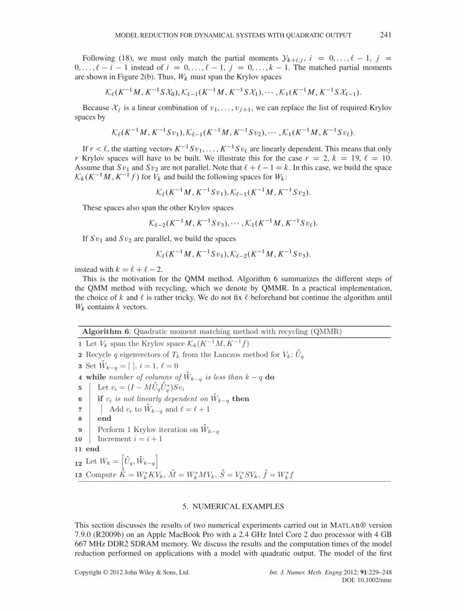
An important conclusion from the analysis of the previous method is that too many partial momentsare matched for matching k C ` moments of y.s/. It is sufficient to match only the partialmoments below the dashed antidiagonal in Figure 2. Moreover, it is possible that we could increase` slightly by not matching unnecessary partial moments. This is the idea of the quadratic momentmatching method, which we denote by QMM.



Following (18), we must only match the partial moments YkCi ,j , i D 0, : : : , ` � 1, j D0, : : : , ` � i � 1 instead of i D 0, : : : , ` � 1, j D 0, : : : , k � 1. The matched partial momentsare shown in Figure 2(b). Thus, Wk must span the Krylov spaces

K`.K�1M ,K�1SX0/,K`�1.K�1M ,K�1SX1/, � � � ,K1.K�1M ,K�1SX`�1/.

Because Xj is a linear combination of v1, : : : , vjC1, we can replace the list of required Krylovspaces by

K`.K�1M ,K�1Sv1/,K`�1.K�1M ,K�1Sv2/, � � � ,K1.K�1M ,K�1Sv`/.

If r < `, the starting vectors K�1Sv1, : : : ,K�1Sv` are linearly dependent. This means that onlyr Krylov spaces will have to be built. We illustrate this for the case r D 2, k D 19, ` D 10.Assume that Sv1 and Sv2 are not parallel. Note that `C `� 1D k. In this case, we build the spaceKk.K�1M ,K�1f / for Vk and build the following spaces for Wk :

K`.K�1M ,K�1Sv1/,K`�1.K�1M ,K�1Sv2/.

These spaces also span the other Krylov spaces

K`�2.K�1M ,K�1Sv3/, � � � ,K1.K�1M ,K�1Sv`/.

If Sv1 and Sv2 are parallel, we build the spaces

K`.K�1M ,K�1Sv1/,K`�2.K�1M ,K�1Sv3/.

instead with k D `C `� 2.This is the motivation for the QMM method. Algorithm 6 summarizes the different steps of

the QMM method with recycling, which we denote by QMMR. In a practical implementation,the choice of k and ` is rather tricky. We do not fix ` beforehand but continue the algorithm untilWk contains k vectors.

5. NUMERICAL EXAMPLES

This section discusses the results of two numerical experiments carried out in MATLAB® version7.9.0 (R2009b) on an Apple MacBook Pro with a 2.4 GHz Intel Core 2 duo processor with 4 GB667 MHz DDR2 SDRAM memory. We discuss the results and the computation times of the modelreduction performed on applications with a model with quadratic output. The model of the first



application arises from the analysis of a simply supported plate and the second one from the anal-ysis of an existing footbridge. These models are approximated by the different methods developedin §4. The relative errors of the approximated outputs are given, and the computational efforts ofthe proposed methods are compared. We also illustrate the power of recycling for the MOR ofdynamical systems with a quadratic output. Finally, the different methods are compared with thesingle-sided method, where Wk D Vk .

5.1. Simply supported plate

In this application, we consider a simply supported plate representing a concrete floor [27]. Thedimensions of the plate are 10� 10� 0.3 m (Figure 3). The Young’s modulus, Poisson’s ratio, pro-portional damping ratio, and density are 30 GPa, 0.3, 0.1, and 2500 kg/m3, respectively. For thediscretization of the plate, we use a regular mesh of 100� 100 discrete Kirchoff triangular (DKT)shell elements [28]. This leads to a system with a total number of 29799 DOFs. The excitationis a point load at the center of the floor. The matrix S computes the mean square value ofthe displacement in four points selected around the point of excitation. This leads to a positivesemidefinite matrix S of rank 4 and the model Q defined by (1) with � D 0.1.

Figure 4 shows the modulus of the quadratic output and the relative error for the outputs of thereduced models of order k D 32, 36, 40 obtained with the ELMO, DF-ELMO, and QMM methods.We observe that the DF-ELMO method always gives a better approximation of the output than theELMO method. Furthermore, the QMM method still improves the approximation.

The corresponding computation times for different orders k of the reduced models are given inTable I(a). These timings include the construction of the reduced models as well as the evaluationin 200 frequency points (n! D 200). However, as we will discuss further, the time required for theevaluation is negligible to the time required for the construction of these reduced models. Table I(b)shows that the computation times for the three proposed methods are similar for the same orderk. Also, note that the computation times for the model reduction methods scale linearly with theorder k of the reduced model. The construction of the reduced model is decomposed into (1) thesparse factorization of K; next, (2) the sparse backward solves with these factors, a matrix vectormultiplication with M and the Gram–Schmidt orthogonalization in each iteration of the Lanczosmethod. We have a similar cost for the left Krylov space. Then, (3) there are additional costs for thecomputation of OM , OK, OS , and Of . We observed that for this problem, more than 80 % of the timewas spent in the k Krylov steps, which explains the linear cost in k.

In Table I(b), the computation times for the evaluation of the large-scale model and for the reducedmodel of order k D 40 obtained with QMM are given. We note that the computation time forthe large-scale model scales linearly with the number of evaluation points n! . On the other hand,Table I(b) also shows that the extra evaluation time of the reduced model in more frequency pointsn! is almost negligible. Comparing the computation time to evaluate the large-scale model and thecomputation time to compute and evaluate the reduced model by the QMM method of order k D 40shows that the computational cost was reduced by a factor of 2.5 up to more than 200. This illustratesthe importance of model reduction for systems with a quadratic output.

It is also important to notice that the Krylov subspaces are built using real arithmetic. This isbecause all matrices and vectors involved are real. However, the direct approach has to factor a

Figure 3. Supported plate with excitation f and observation points.



0 200 400 600 800 1000 1200 1400 1600 1800 2000 0 200 400 600 800 1000 1200 1400 1600 1800 2000

0 200 400 600 800 1000 1200 1400 1600 1800 2000

10−4

10−6

10−8

10−10

10−12

10−14

10−4

10−2

100

10−6

10−8

10−10

10−12

10−14

10−4

10−2

100

10−6

10−8

10−10

10−12

10−140 200 400 600 800 1000 1200 1400 1600 1800 2000

10−4

10−2

100

10−6

10−8

10−10

10−12

10−14

Figure 4. Modulus of the quadratic output and relative errors for the outputs of the reduced models of orderk D 32, 36, 40 obtained through the equivalent linear system with multiple outputs method (ELMO, solidline), the decomposition free ELMO method (DF-ELMO, dashed line), and the quadratic moment matching

method (QMM, dashed-dotted line).

Table I. Computation times for the quadratic output of the supported plate: (a) with model order reductionfor different orders k and (b) with and without model order reduction for different numbers of frequency

points, n! .

large-scale complex matrix, which is expensive both in time as in storage. The reduced model isevaluated for a complex value of s, but because it is small, this cost is not high.

The computational cost of all the methods is primarily determined by the Krylov iterations. Themethods without recycling need k Krylov iterations for the computation of Vk , and need k=r Kryloviterations, with a block size of r , for the computation of Wk . On the other hand, the methods withrecycling need k iterations for the computation of Vk but need only .k�q/=r iterations, with a blocksize of r , for Wk . The additional computational cost due to the extraction of the q-recycled modesis negligible because it only requires an eigenvalue decomposition of the small-scale tridiagonalmatrix Tk .



0 200 400 600 800 1000 1200 1400 1600 1800 2000

10−4

10−2

100

10−6

10−8

10−10

10−12

10−14

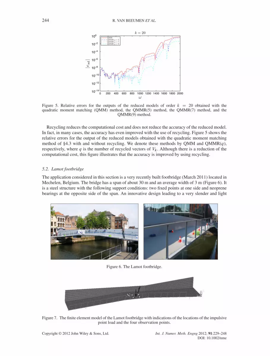
Figure 5. Relative errors for the outputs of the reduced models of order k D 20 obtained with thequadratic moment matching (QMM) method, the QMMR(5) method, the QMMR(7) method, and the

QMMR(9) method.

Recycling reduces the computational cost and does not reduce the accuracy of the reduced model.In fact, in many cases, the accuracy has even improved with the use of recycling. Figure 5 shows therelative errors for the output of the reduced models obtained with the quadratic moment matchingmethod of §4.3 with and without recycling. We denote these methods by QMM and QMMR(q),respectively, where q is the number of recycled vectors of Vk . Although there is a reduction of thecomputational cost, this figure illustrates that the accuracy is improved by using recycling.

5.2. Lamot footbridge

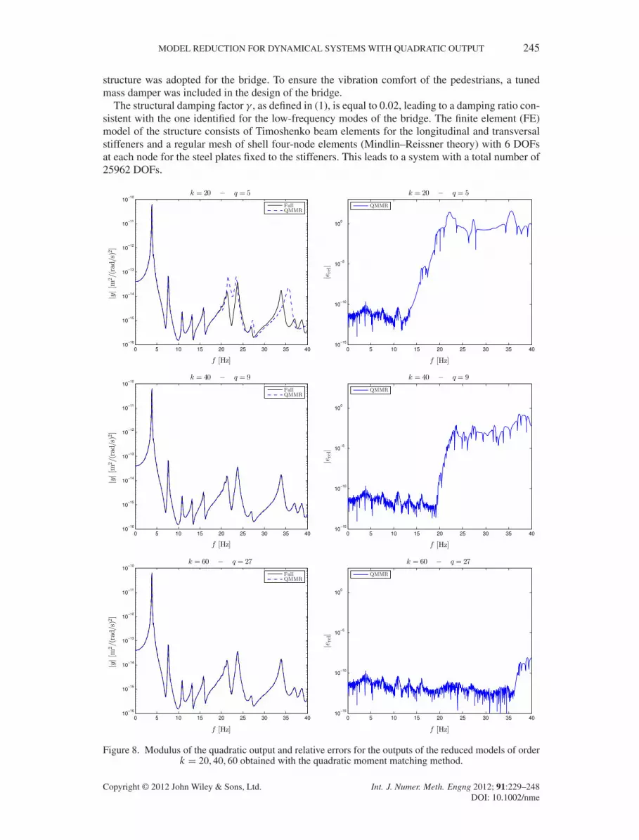
The application considered in this section is a very recently built footbridge (March 2011) located inMechelen, Belgium. The bridge has a span of about 30 m and an average width of 3 m (Figure 6). Itis a steel structure with the following support conditions: two fixed points at one side and neoprenebearings at the opposite side of the span. An innovative design leading to a very slender and light

Figure 6. The Lamot footbridge.

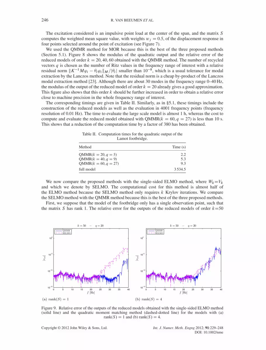
Figure 7. The finite element model of the Lamot footbridge with indications of the locations of the impulsivepoint load and the four observation points.



structure was adopted for the bridge. To ensure the vibration comfort of the pedestrians, a tunedmass damper was included in the design of the bridge.

The structural damping factor � , as defined in (1), is equal to 0.02, leading to a damping ratio con-sistent with the one identified for the low-frequency modes of the bridge. The finite element (FE)model of the structure consists of Timoshenko beam elements for the longitudinal and transversalstiffeners and a regular mesh of shell four-node elements (Mindlin–Reissner theory) with 6 DOFsat each node for the steel plates fixed to the stiffeners. This leads to a system with a total number of25962 DOFs.

Figure 8. Modulus of the quadratic output and relative errors for the outputs of the reduced models of orderk D 20, 40, 60 obtained with the quadratic moment matching method.



The excitation considered is an impulsive point load at the center of the span, and the matrix Scomputes the weighted mean square value, with weights wj D 0.5, of the displacement response infour points selected around the point of excitation (see Figure 7).

We used the QMMR method for MOR because this is the best of the three proposed methods(Section 5.1). Figure 8 shows the modulus of the quadratic output and the relative error of thereduced models of order k D 20, 40, 60 obtained with the QMMR method. The number of recycledvectors q is chosen as the number of Ritz values in the frequency range of interest with a relativeresidual norm kK�1M'i � �i'ikM=j�i j smaller than 10�8, which is a usual tolerance for modalextraction by the Lanczos method. Note that the residual norm is a cheap by-product of the Lanczosmodal extraction method [23]. Although there are about 30 modes in the frequency range 0–40 Hz,the modulus of the output of the reduced model of order k D 20 already gives a good approximation.This figure also shows that this order k should be further increased in order to obtain a relative errorclose to machine precision in the whole frequency range of interest.

The corresponding timings are given in Table II. Similarly, as in §5.1, these timings include theconstruction of the reduced models as well as the evaluation in 4001 frequency points (frequencyresolution of 0.01 Hz). The time to evaluate the large scale model is almost 1 h, whereas the cost tocompute and evaluate the reduced model obtained with QMMR(k D 60, q D 27) is less than 10 s.This shows that a reduction of the computation time by a factor of 380 has been obtained.

Table II. Computation times for the quadratic output of theLamot footbridge.

Method Time (s)

QMMR(k D 20, q D 5) 2.2QMMR(k D 40, q D 9) 5.3QMMR(k D 60, q D 27) 9.3

full model 3 534.5

We now compare the proposed methods with the single-sided ELMO method, where WkDVkand which we denote by SELMO. The computational cost for this method is almost half ofthe ELMO method because the SELMO method only requires k Krylov iterations. We comparethe SELMO method with the QMMR method because this is the best of the three proposed methods.

First, we suppose that the model of the footbridge only has a single observation point, such thatthe matrix S has rank 1. The relative error for the outputs of the reduced models of order kD50

Figure 9. Relative error of the outputs of the reduced models obtained with the single-sided ELMO method(solid line) and the quadratic moment matching method (dashed-dotted line) for the models with (a)

rank(S/D 1 and (b) rank(S/D 4.



is shown in Figure 9(a). In this figure, we observe that the QMMR method gives a much betterapproximation of the quadratic output than the SELMO method.

Second, we apply the SELMO and QMMR methods for the case where four observation pointsare considered and, thus, with a matrix S of rank 4. The corresponding relative error for the outputsof the reduced models of order k D 50 is shown in Figure 9(b). In this case, the QMMR and SELMOmethods produce approximations of the quadratic output of almost the same accuracy. This is dueto the fact that, in the case rank.S/ > 1, a smaller number of Krylov iterations is performed bythe QMMR method for the construction ofWk . Because of the smaller number of Krylov iterations,less moments are matched by QMMR.

Therefore, we can conclude that the higher the rank of S , the less additional moments are matchedby the two-sided methods (e.g. QMMR) compared to the single-sided method (SELMO). Thus, thetwo-sided methods are most suitable for problems with an S matrix of rank 1, as confirmed by theresults in Figure 9.

6. CONCLUSIONS

The general framework of the Krylov methods is extended to systems with a quadratic output. Threetwo-sided methods are proposed where the control (or right) Krylov space is the same. The differ-ence between the methods lies in the choice of the observation (or left) Krylov space. First, theELMO method writes the SISO system with a quadratic output as a linear SIMO system and usesthis system to construct the matrices Vk and Wk . Second, the DF-ELMO method avoids the decom-position of the matrix S for the construction of the reduced model. Third, the QMM method tries tomatch, as much as possible, moments between the outputs of the large-scale and the reduced system.With the use of recycling, the proposed methods try to combine the strength of modal superpositionand Padé via Krylov methods.

The numerical experiments show that the proposed model reduction methods lead to a significantreduction of the computation time required for the evaluation of systems with a quadratic output.We observed no benefit in using two-sided MOR methods when the rank of S is larger than one. Thealgorithms require a large number of parameters, such as k, q, and `. Note that ` is chosen automat-ically in Algorithm 6. The value of recycled modes, q, is chosen as the number of Ritz values in thefrequency range with small residual norm, as was illustrated in §5.2. As a result, the only remainingparameter to be chosen by the user is the number of vectors, k.

ACKNOWLEDGEMENTS

This paper presents research results of the Belgian Network DYSCO (Dynamical Systems, Control, andOptimization), funded by the Interuniversity Attraction Poles Programme, initiated by the Belgian StateScience Policy Office. The research is also partially funded by the Research Council K.U.Leuven grantsPFV/10/002 (Optimization in Engineering Center, OPTEC) and OT/10/038 (Multiparameter model orderreduction and its applications).

The authors would like to thank the following industrial partners for their important contribution to thestudy of the vibration response of the footbridge: Waterwegen en Zeekanaal NV, Emotec / Emergo-Group,Herbosch-Kiere, and the Flemish Government - Department of Mobility and Public Works âAS DivisionSteel Structures. We are particularly grateful for the information they have provided and the permission toperform vibration measurements, enabling the thorough study of the dynamic behavior of the footbridge.The scientific responsibility rests with its author(s).

We are grateful to the two anonymous referees, whose comments have improved the content andpresentation of the paper.

REFERENCES

1. Amsallem D, Cortial J, Carlberg K, Farhat C. A method for interpolating on manifolds structural dynamicsreduced-order models. International Journal of Numerical Methods in Engineering 2009; 80:1241–1258.

2. Wilson EL, Yuan MW, Dickens JM. Dynamic analysis by direct superposition of Ritz vectors. EarthquakeEngineering and Structural Dynamics 1982; 10:813–821.

3. Ibrahimbegovic HC, Chen EL, Wilson EL, Taylor RL. Ritz method for dynamic analysis of large discrete linearsystems with non-proportional damping. Earthquake Engineering and Structural Dynamics 1990; 19:877–889.



4. Feldman P, Freund RW. Efficient linear circuit analysis by Padé approximation via the Lanczos process. IEEETransactions on Computer-Aided Design of Integrated Circuits and Systems 1995; CAD–14:639–649.

5. Grimme E, Sorensen D, Van Dooren P. Model reduction of state space systems via an implicitly restarted Lanczosmethod. Numerical Algorithms 1996; 12:1–31.

6. Bai Z, Ye Q. Error estimation of the Padé approximation of transfer functions via the Lanczos process. ETNA 1998;7:1–17.

7. Bai Z, Freund RW. A partial Padé-via-Lanczos method for reduced-order modeling. Linear Algebra and itsApplications 2001; 332–334:139–164.

8. Meerbergen K. Fast frequency response computation for Rayleigh damping. International Journal of NumericalMethods in Engineering 2008; 73(1):96–106.

9. Simoncini V, Perotti F. On the numerical solution of .�2AC�BCC/x D b and application to structural dynamics.SIAM Journal on Scientific Computing 2002; 23(6):1875–1897.

10. Simoncini V. Linear systems with a quadratic parameter and application to structural dynamics. In Iterative meth-ods in scientific computation iv, Vol. 5, Kincaid DR, Elster A (eds), IMACS Series in Computational and AppliedMathematics. Elsevier Science Publishers B. V.: Amsterdam, The Netherlands, The Netherlands, 1999; 451–461.

11. Gallivan K, Grimme E, Van Dooren P. A rational Lanczos algorithm for model reduction. Numerical Algorithms1996; 12:33–63.

12. Kuzuoglu M, Mittra R. Finite element solution of electromagnetic problems over a wide frequency range via thePadé approximation. Computer Methods in Applied Mechanics and Engineering 1997; 169:263–277.

13. Malhotra M, Pinsky PM. Efficient computation of multi-frequency far-field solutions of the Helmholtz equation usingPadé approximation. Journal of Computational Acoustics 2000; 8(1):223–240.

14. Bai Z, Su Y. Dimension reduction of second-order dynamical systems via a second-order Arnoldi method. SIAMJournal on Matrix Analysis and Applications 2005; 26(5):1692–1709.

15. Antoulas A. Approximation of Large-Scale Dynamical Systems. SIAM: Philadelphia, PA, USA, 2005.16. Benner P, Mehrmann V, Sorensen D (eds). Dimension Reduction of Large-Scale Systems. Springer-Verlag: Berlin,

Heidelberg, 2005.17. Lutes L, Sarkani S. Random Vibrations: Analysis of Structural and Mechanical Systems. Elsevier Butterworth-

Heinemann: Oxford, UK, 2004.18. Saak J. Efficient numerical solution of large scale algebraic matrix equations in PDE control and model order

reduction. PhDThesis, University of Chemnitz, 2009.19. Bennighof JK, Kaplan MF. Frequency sweep analysis using multi-level substructuring, global modes and iteration.

Proceedings of 39th AIAA/ASME/ASCE/AHS Structures, Structural Dynamics and Materials Conference, 1998.20. Ko JH, Bai Z. High-frequency response analysis via algebraic substructuring. International Journal of Numerical

Methods in Engineering 2008; 76(3):295–313.21. Meerbergen K, Bai Z. The Lanczos method for parameterized symmetric linear systems with multiple right-hand

sides. SIAM Journal on Matrix Analysis and Applications 2010; 31(4):1642–1662. DOI: 10.1137/08073144X. URLhttp://link.aip.org/link/?SML/31/1642/1.

22. Lanczos C. An iteration method for the solution of the eigenvalue problem of linear differential and integral operators.Journal of Research of the National Bureau of Standards 1950; 45:255–282.

23. Grimes RG, Lewis JG, Simon HD. A shifted block Lanczos algorithm for solving sparse symmetric generalizedeigenproblems. SIAM Journal on Matrix Analysis and Applications 1994; 15:228–272.

24. Meerbergen K. The solution of parametrized symmetric linear systems. SIAM Journal on Matrix Analysis andApplications 2002; 24(4):1038–1059. DOI: http://dx.doi.org/10.1137/S0895479800380386.

25. Boley DL. Krylov space methods on state-space control models. Circuits Systems Signal Process 1994; 13:733–758.26. Salimbahrami B, Lohmann B. Krylov subspace methods in linear model order reduction: introduction and invariance

properties. Technical Report, Institute of Automation, University of Bremen, 2002. URL http://www.rt.mw.tum.de/salimbahrami/Invariance.pdf.

27. Yue Y, Meerbergen K. Using Krylov-Padé model order reduction for accelerating design optimization of struc-tures and vibrations in the frequency domain. International Journal of Numerical Methods in Engineering 2012;90:1207–1232.

28. Calladine CR. Theory of Shell Structures. Cambridge University Press: Cambridge, 1989.


model reduction for dynamical systems with quadratic output

Documents