linear-quadratic jump-diffusion modeling

Mathematical Finance, Vol. 17, No. 4 (October 2007), 575–598

LINEAR-QUADRATIC JUMP-DIFFUSION MODELING

PENG CHENG

Barclays Capital and Swiss Finance Institute

OLIVIER SCAILLET

HEC, Universite de Geneve and Swiss Finance Institute

We aim at accommodating the existing affine jump-diffusion and quadratic modelsunder the same roof, namely the linear-quadratic jump-diffusion (LQJD) class. Wegive a complete characterization of the dynamics of this class by stating explicitlythe structural constraints, as well as the admissibility conditions. This allows us tocarry out a specification analysis for the three-factor LQJD models. We compute thestandard transform of the state vector relevant to asset pricing up to a system ofordinary differential equations. We show that the LQJD class can be embedded into theaffine class using an augmented state vector. This establishes a one-to-one equivalencerelationship between both classes in terms of transform analysis.

KEY WORDS: linear-quadratic models, affine models, jump-diffusions, standard transform, optionpricing

1. INTRODUCTION

Current research using jump-diffusion processes relies mostly on two classes of models:the affine jump-diffusion (AJD) class in the sense of, for example, Duffie and Kan (1996)and Duffie, Pan, and Singleton (2000), and the quadratic Gaussian (QG) class in thesense of, for example, Ahn, Dittmar, and Gallant (2002) and Leippold and Wu (2002).The popularity of both classes rests not only in their modeling flexibility, but also in theirtechnical tractability in deriving the standard transform of the state vector,1 defined inDuffie, Pan, and Singleton (2000), for option and bond pricing. Filipovic (2002) provesthat the maximal consistent order of a separable, polynomial model is two. Naturally,one would wonder whether the AJD and the QG models exhaust the set of models with

1 Duffie, Pan, and Singleton (2000) also define the extended transform of the state vector. The solutionprocedure is the same as that of the standard transform, and will not be discussed in this paper.

We would like to thank the Editor, Dilip Madan, and the two anonymous referees for constructive criticismand comments. We also thank P. Collin-Dufresne, J. Detemple, G. Dhaene, D. Duffie, J.D. Fermanian, S.Galluccio, C. Gourieroux, A. Kaul, M. Musiela, and R. Stulz for many stimulating discussions. We havereceived fruitful comments from participants at the FAME doctoral workshop, AFFI meeting 2003, ESEM2003, EFA 2003, and finance seminars at Imperial College, BNP Paribas, Zurich, Lugano, and CREST(Paris). The authors received support by the Swiss National Science Foundation through the NationalCenter of Competence Research (NCCR): Financial Valuation and Risk Management. The first author alsoreceived a Doctoral Research Grant from International Centre FAME for completing the project. Part ofthis research was done when the second author was visiting THEMA and IRES.

Manuscript received March 2005; final revision received January 2007.Address correspondence to Olivier Scaillet, HEC, Universite de Geneve and Swiss Finance Institute, 102

Bd. Carl Vogt, CH - 1211, Switzerland; e-mail: [email protected].

C© 2007 The Authors. Journal compilation C© 2007 Blackwell Publishing Inc., 350 Main St., Malden, MA 02148,USA, and 9600 Garsington Road, Oxford OX4 2DQ, UK.

575

576 P. CHENG AND O. SCAILLET

tractable solutions for the transform, or a maximal flexible, polynomial model is yet tobe found.

We find the existing AJD and QG classes, as they are currently specified, both belongto a more general, quadratic framework, which will be established in this paper. Withinthis framework, the state vector is constructed from a jump-diffusion vector, which isrestricted to linear form only, and a pure diffusion vector, which enters both the linearand the quadratic forms. We detail the minimal sufficient conditions for an admissiblestate vector, as well as the structural constraints for obtaining the standard transform, asan exponential quadratic function. We call this structure linear-quadratic (LQ) to reflectits construction, and such a process linear-quadratic jump-diffusion (LQJD). By Filipovic(2002), the LQJD class is, in fact, the maximal flexible dynamic structure for a separable,quadratic model with tractable transforms of the underlying process.

The LQJD framework, as a generalization of the AJD and QG classes, joins theirmodeling flexibility together. An AJD model, while capable of capturing jumps, is in-herently linear and may not capture nonlinearity in the underlying process adequately.See Ait-Sahalia (1996), Ahn and Gao (1999), and Dai and Singleton (2000) for evidenceon nonlinearity in interest rates and swap yield curves, respectively. Moreover, Dai andSingleton (2000) and Backus, Foresi, Mozumda, and Wu (2001) point out that the fit-ting performance of an AJD model can be significantly improved only at the cost ofintroducing negative correlations among the state variables, and thus losing positivityof the underlying, e.g., interest rates. The QG class seems to be a neat solution to theseproblems. Examples can be found in Ahn, Dittmar, and Gallant (2002) and Leippoldand Wu (2003) on the term structure of interest rates, and Leippold and Wu (2007) ona multi-currency framework. However, a consistent QG model does not permit jumps(Chen, Bayraktar, and Poor 2005). An LQJD model, in contrast, would accommodatethese important features, that is, nonlinearity, jumps, positivity of the underlying process,under the same roof.

An additional, striking feature of the LQJD state vector, in comparison to the pureAJD and QG state vectors, is its nonlinear specifications for the drift, the diffusion, andthe market price of risk. For example, let µP and µQ be the drift vectors under the twoequivalent probability measures P and Q. If the underlying process is either AJD or QGunder both measures, the quantity µP − µQ would only admit an affine specification(see Dai and Singleton 2003). Under the LQJD framework, however, µP − µQ can beLQ in the state vector. This is a marked improvement over the AJD and QG models. Inparticular, an investigation of nonlinearity in the market price of risk as suggested by Pan(2002), which is not possible in the AJD or QG framework, is now feasible.

Despite the additional modeling flexibility, the LQJD class is still as tractable as theQG and the AJD classes. Like Duffie, Pan, and Singleton (2000), we derive the transformsof the LQJD process up to a system of ordinary differential equations (ODEs), which wediscover to be a system of non-symmetric Riccati differential equations (RDEs). Resultsfrom the literature of RDEs (i.e., Radon’s lemma) suggest that the initial value problemfor an RDE system that we have to solve in the LQJD setting is (locally) equivalent tothe one for a linear system. Hence, there is a standard routine for solving the differentialsystem.

A further finding, resulting from the solution scheme of the LQJD standard transform,is the valuation equivalence between linear-quadratic and affine models. Intuitively, bya simple change-of-variables technique, a quadratic form aX2 + bX + c in X can bereplaced by aZ + bX + c, which is now affine in an augmented, constrained vector (X , Z).We prove that the system of ODEs obtained for a LQJD process is identical to that for its

LINEAR-QUADRATIC JUMP-DIFFUSION MODELING 577

augmented affine version, hence an LQJD model can in fact be rewritten as a constrainedAJD model. This, together with the fact that the AJD class is nested in the LQJD class,establishes a one-to-one relationship between the two classes of models in terms of theirtransforms. In other words, the set of LQJD models that is absolutely distinct from(augmented) AJD models is empty when considering asset pricing by transform analysis.

However, while the augmented LQ model is affine in the sense of Duffie, Pan, andSingleton (2000), it may not fit into the affine specifications of Dai and Singleton (2000).We show, with an example, that the causes of the problem are the presence of the quadraticfactors and their deterministic relationship with the augmented factors. Therefore, theequivalence between LQJD and AJD models stated here concerns the valuation side oftheir transforms only.

The relationship between tractable affine and quadratic models has drawn little researchattention until recently. See, for example, Pan and Wu (2005) and Chen, Filipovic, andPoor (2004), where special quadratic term structure models with affine equivalence aregiven. See also Gourieroux and Sufana (2003), who are aware of such equivalence in astudy of Wishart autoregressive processes in discrete time. However, without a unifiedground on which this problem can be examined, the affine and the quadratic classes areeasily, and indeed commonly taken as two separate sets. The LQJD framework providessuch a unified ground, and we consider our finding a valuable theoretical contributionto the debate of affine versus quadratic classes.

The rewriting of an LQJD to its affine equivalence also permits analyses done pre-viously for the AJD class to be carried out for the LQJD class. One example is Collin-Dufresne, Goldstein, and Jones (2003), in which a three-factor maximal affine term struc-ture model with stochastic volatility is studied. Their technique of rotating latent statevariables into observables is similarly applicable in the LQJD setting. We can also con-duct a specification analysis for an LQJD model in a similar manner to that in Daiand Singleton (2000). In particular, in the paper, we give the sufficient conditions for anLQJD specification to be admissible, and provide the maximal flexible specifications forthree-factor LQJD models.

To the best of our knowledge, the first piece of work that coins the term LQJD isPiazzesi (2001) in interest rate modeling.2 The paper initiates the issue of includingjumps with quadratic arrival intensity for pricing bonds in the quadratic class, and fulfilsthe task by constructing the state vector from two parts: one being pure Gaussian–Markov without jumps, and the other being square-root process with jumps. The driftand the covariance matrices are still affine in the state vector. Clearly, the state vector inPiazzesi (2001) is an AJD vector and a QG vector knitted together, and the possibility ofintegrating nonlinearity in the drift of the linear vector is not dealt with. We believe thatthis specification of the state vector is not rich enough to render the model an extensionfully capable of integrating the modeling strengths of both classes in one.

We are also aware that Liu (2007) proposes some state vector dynamics fairly akin toours. While Liu’s analysis is oriented toward solving optimal dynamic portfolio selectionproblems, ours aims at pricing issues via transform analysis. Consequently, we are ableto prove that the AJD class is more general than conventionally thought, and is actuallyequivalent to the LQJD class. In contrast, Liu (2007) still treats the affine class as anon-trivial subset of the LQJD class. Furthermore, the specification of Liu (2007) (hisequation [11]) is not fully compatible with our LQJD setting. In particular, the thirdinequality of his equation (11) does not allow for a proper solution for the transforms.

2 A published version of this paper is Piazzesi (2004), where the term LQJD is dropped


The rest of the paper is structured as follows. Section 2 describes the specification ofthe LQJD framework and the structural constraints. Section 3 discusses the admissibilityconditions and carries out a specification analysis of the LQJD model. Section 4 computesthe standard transform and shows the link and the equivalence between the LQJD andAJD classes in terms of their transforms. A discussion of option pricing via transformanalysis in the LQJD setting is also included. Section 5 concludes. Technical details arecollected in the Appendices. Further details, explanations, and references, as well as anumerical application of LQJD modeling to stochastic volatility, can also be found in theextended version of this paper, Cheng and Scaillet (2002).

2. THE LQJD SETTINGS

In this section, we provide a general definition of the LQJD state vector and its standardtransform. We write down the partial-integro differential equation (PIDE) that must besatisfied by the standard transform, and discuss the structural constraints on the statevector such that the PIDE can be solved up to the solution of a system of ODEs. It turnsout that a LQJD process admits a nonlinear drift and a nonlinear diffusion, which is amarked improvement over the pure AJD and QG classes.

The complete solution to the standard transform, however, will be presented after adiscussion of admissibility conditions in Section 3.

2.1. The LQJD State Vector and Its Standard Transform

The n-dimension, cadlag state vector Xt is drawn from some state space D, and followsthe stochastic differential equation (SDE):

dXt = µ(Xt, t) dt + σ (Xt, t) dW t + dJt,(2.1)

where

(i) Wt is a standard n◦-dimension Brownian motion vector;(ii) Jt is a pure jump process with independent increments dJt, whose size distri-

butions and arrival intensities are given by � (dy, t) and λ(Xt, t), respectively;(iii) (E,F, P) is the usual probability space with (W , J)-augmented filtration (Ft)t≥0,

meaning that

– F0 contains all the P-null sets of F ;– the filtration F is right-continuous.

See, for example, Protter (2004).For identification, we require that n ≥ n◦. Moreover, we assume that µ, σ , �, and λ

satisfy the regularity conditions that guarantee a unique solution to (2.1) for every X0.In the LQJD setting, the drift matrix µ(Xt, t), the covariance matrix �(Xt, t) =

σ (Xt, t)σ (Xt, t)�, and the jump arrival intensity λ(Xt, t) are all LQ in the state vectorby construction. That is, each entry of µ, �, and λ is of the following form

κ(Xt, t) = 12

X��κ(t)Xt + bκ(t)� Xt + cκ(t),(2.2)

where the superscript� denotes matrix transpose, and the coefficient matrix �κ is blockdiagonal with the following representation


�κ =(

Aκ 0

0 0

),(2.3)

with Aκ being symmetric. Note that the dimension of Aκ depends on the number of statevariables that enters the quadratic forms of µ, �, and λ. We can now partition the statevector Xt and the coefficient vector bκ accordingly as

X =(

Xt

X¯ t

), bκ =

(kκ

lκ

),(2.4)

and rewrite (2.2) as

κ(X, t) = lκ(t)�X¯ t︸︷︷︸

(linear part)

+ 12

X�t Aκ(t)Xt + kκ(t)�Xt + cκ(t)︸︷︷︸

(quadratic part)

,(2.5)

hence the name “linear-quadratic.”The standard transform of a state vector Xt is defined, in general, as

φ(g; Xt, t, T ) = Et

[exp

(−

∫ T

tR(Xs, s) ds

)eg(XT ,T )

],(2.6)

where Et[·] = E[· |Ft] is the expectation conditional on information up to t: Ft, t ≤ T <

∞. If the process �(Xt, t), defined as

�(Xt, t) = exp(

−∫ t

0R(Xs, s) ds

)eg(Xt,t),(2.7)

is a martingale, then the standard transform can be solved as

φ(g; Xt, t, T ) = eg(Xt,t) Et[�(XT, T )]�(Xt, t)

= eg(Xt,t).

This implies that g(Xt, t) satisfies the following PIDE:

LEMMA 2.1 If the technical integrability conditions hold and the function g(x, t) satisfiesthe following PIDE (the Cauchy problem)

R = ∂g∂t

+ µ� ∂g∂x

+ 12

tr

[(∂2g∂x2

+ ∂g∂x

(∂g∂x

)�)�

]+ λ(θ − 1),(2.8)

where θ = ∫D

eg(x+y,t)−g(x,t)�(x, dy, t), then �t is a martingale.

Proof. See Appendix A.

Given the result in Filipovic (2002) that the maximal consistent order of a separable,polynomial model is two, we take both g(Xt, t) and R(Xt, t) as LQ functions in Xt.

We use LQqm(n) to denote an n-factor LQJD model where the first q members of the

state vector Xt appear at least once in a quadratic form (i.e., Xt has dimension q), andm members of X

¯ t appear in either λ or �. Without loss of generality, we assume these mfactors are the first m members of X

¯ t. Hence, for an LQqm(n) model,

g(X, t) = l(t)�X¯ t + 1

2X�

t A(t)Xt + k(t)�Xt + c(t),


where A is symmetric with rank q. Clearly, the LQJD model reduces to a QG model whenq = n, and to an AJD model (such as the Am[n] model of Dai and Singleton (2000) withjumps) when q = 0. By reference to these two classes, the variables X and X

¯are named

quadratic and affine vectors, respectively.

2.2. The Structural Constraints

For both g(Xt, t) and R(Xt, t) to be LQ in Xt, an LQqm(n) model must satisfy the

following structural constraints (see Appendix B.1 for more details):

[SC1] The first q entries of the jump component J are zeros.

That is, jumps are restricted to the affine vector X¯

only. This comes from λ, g, and Rbeing all LQ functions by definition, which, together with (2.8), implies that θ is in factindependent of x. The minimal constraint for this to hold true is that the first q entriesof the jump size distribution is zero.

[SC2] The drift matrix of Xt is

µ(Xt, t) =(

µ(Xt, t)

µ¯

(Xt, X¯ t, t)

)n×1

.

In particular

(a) The drift matrix of the quadratic vector X, µ(Xt, t), is only an affine functionof X;

(b) The drift matrix of the affine vector X¯, µ

¯(Xt, X

¯ t, t), is LQ in X (i.e., affinein X

¯and quadratic in X ).

The restriction that µ(Xt, t) is an affine function of X only could be justified heuristi-cally as follows. By definition, X

¯should remain in linear terms only. If µ were an affine

function of X¯

as well, it would bring powers of X¯

to two as the quadratic vector X passthrough the quadratic terms. Constraint [SC2](a) looks quite restrictive, because it doesnot allow linking members of X

¯with X through the drift of X. For instance, if X

¯is the

logarithm of stock price and X is the state vector describing the dynamics of stock pricevolatility, it is indeed desirable to let the logarithm of the stock price X

¯play a “feedback”

role on the volatility state vector X. Constraint [SC2](a) rules out the possibility of havingthis type of “feedback” effect through the drift of X in the LQJD setting. However, wecan still model this effect through the correlation structure of X.

In comparison to an AJD process, the affine vector X¯

in the LQJD framework has anonlinear component that is generated by a quadratic form of the quadratic vector X. Asalready mentioned, we believe that the incorporated nonlinearity is a marked improve-ment from the pure AJD and QG classes. In particular, the quantity µP − µQ, where P

and Q are two equivalent probability measures, is LQ in the state vector in the LQJDsetting. In contrast, as pointed out by Dai and Singleton (2003), both the AJD and QGclasses admit only affine specifications for µP − µQ. Apparently, such restriction preventsan investigation of nonlinear specification, as suggested in Pan (2002).


[SC3] The covariance matrix of Xt is

�(Xt, t) =(

�(t) �(Xt, t)

�(Xt, t)� �¯

(Xt, X¯ t, t)

)n×n

.

In particular

(a) the covariance matrix of the quadratic vector X, �(t), is deterministic in t;(b) the covariance matrix of the affine vector X

¯, �

¯(Xt, X

¯ t, t) , is LQ in X (i.e.,affine in X

¯and quadratic in X);

(c) from (a) and (b), the covariance matrix between X¯

and X, �(Xt, t), isaffine in X only.

Constraint [SC3](b) differs from the usual practice in affine modeling, which restrictsσ to be square-root affine in the state vector. (see, for example, Dai and Singleton 2000).However, it is the covariance matrix �, not σ itself, that matters for solving PIDE (2.8).(see Duffie, Pan, and Singleton 2000). Moreover, restrictions on σ would in fact excludean important group of models, which distinguish themselves from the square-root affinemodels by carrying sign information in σ .

Also note that option pricing models based on a quadratic specification for σ of thestock price as in Rady (1997) are not embedded in the LQJD class. This is because thelogarithm of the stock price is usually a member of the affine vector X

¯, and as such it is

excluded from any quadratic forms in the LQJD setting by construction.There are only a small number of LQJD models existing in the current literature that

are distinct from the pure AJD or QG models. The more distant ones include Stein andStein (1991), which is LQ1

0(2) with � = 0 and λ = 0 (i.e., no jumps), and Schobel andZhu (1999), which is an extension of Stein and Stein (1991) with � �= 0. The more recentones include Piazzesi (2001) and (2004), which are LQ1

1(4) with µ¯

being only affine inthe state vector. Santa-Clara and Yan (2005) propose an LQ2

0(3) model for modelingstock market index with stochastic volatility and jumps. It corresponds, in our notation,to Xt = (X1t X2t)�, which models the instantaneous volatility (Vt = X2

1t) and the jumpintensity (λt = X2

2t), together with X¯ t = (X3t), which is the logarithm of the stock price.

The drift and the covariance matrices for this LQ20(3) model are, respectively,

µt =

kµ1 X1t + cµ1

kµ2 X2t + cµ2

12 X�

t Aµ3 Xt + cµ3

, �t =

c11 c12 k13 X1t

. c22 k23 X1t

. . X21t

,(2.9)

where k and c’s are constants, and Aµ3 is a constant, 2 × 2 diagonal matrix.We will use the Santa-Clara and Yan (2005) model as a running example, and show

that it is not the maximal flexible model in the LQ20(3) class. In the next section, we will

discuss the LQJD admissibility conditions and the relevant specification analysis, whichaddress the issue of maximal flexible models.

3. ADMISSIBILITY CONDITIONS AND SPECIFICATION ANALYSIS

In addition to the structural constraints which are necessary conditions for obtaininga tractable transform, we also need admissibility conditions that guarantee a positivejump intensity λ and a positive semi-definite covariance matrix �, such that a solution


to SDE (2.1) exists and is unique. The structural constraints and the admissibility con-ditions allow us to extend the classification scheme and specification analysis of Daiand Singleton (2000) to the LQJD setting. Specifically, an n-factor LQJD model withq quadratic factors can be classified into n − q + 1 subfamilies (indexed by m), and themaximal flexible LQq

m(n) model can be identified accordingly. We illustrate such analysiswith three-factor LQJD models.

In a pure affine diffusion setting, Gourieroux and Sufana (2006) points out that theanalysis of Dai and Singleton (2000) provides sufficient but not necessary conditions,and excludes some admissible, nonlinear state space. Their analysis, however, involvesthe study of the dynamics of � and its determinant on the boundary of the state space,which will become extremely involved when the number of factors inceases. We will stillfollow the recipe provided by Dai and Singleton (2000), and leave the Gourieroux andSufana (2006) type of analysis for n-factor models in a jump-diffusion setting for futureresearch. However, our results on the equivalence relationship between LQJD and AJDclasses, and in particular the rewriting of an LQJD model as its AJD equivalence (seeSection 4.2 below), actually provides examples mentioned in Gourieroux and Sufana(2006), which do not fit into the standard Dai and Singleton (2000) classification.

3.1. Admissibility Conditions

For an LQJD process to be admissible, its jump intensity λ should be positive andits covariance matrix � should be positive semi-definite. When q = n, an LQq

m(n) modelreduces to a QG model and no admissibility conditions are needed. When q = 0, theLQJD model becomes an AJD model, and the admissibility conditions, as well as thecorresponding specification analysis, have been detailed in Dai and Singleton (2000). Foran LQq

m(n) model with 0 < q < n, we have

[AC1] Up to invariant transforms defined in Dai and Singleton (2000), the covariancematrix of the first m factors of the affine vector X

¯ t is diagonal, with the ith

diagonal term linear in Xq+i,t, the ith factor of X¯ t

The invariant transforms of Dai and Singleton (2000) are applicable to the first mfactors of X

¯ t, because they only appear in affine terms by definition, and their diffusionsdo not contain any quadratic terms. [AC1] ensures that when Xq+i,t, i ≤ m, reaches zero,its diffusion also becomes zero and Xq+i,t is locally deterministic. In the presentation wehave applied the invariant transforms to get rid of the constant term in the diffusion ofXq+i,t, so that we can discuss its drift separately. In effect, imposing [AC1] is equivalentto representing Xq+i,t in a canonical form as discussed in Dai and Singleton (2000).

At zero boundary, Xq+i,t should have a positive drift. Recall that the drift of Xq+i,t hasthe following specification:

µq+i (X, t) = lµq+i (t)�X

¯ t + 12

X�t Aµq+i (t)Xt + kµq+i (t)

�Xt + cµq+i (t)︸︷︷︸(quadratic part)

.(3.1)

To guarantee a positive µq+i when Xq+i,t is at its zero boundary, we must have

[AC2] The jth entry of lµq+i is zero when j > m, and non-negative when j ≤ m and j �= i.[AC3] The quadratic part of (3.1) is non-negative, that is,


(a) Aµq+i is positive semi-definite;(b) kµq+i belongs to the column space of Aµq+i ;(c) cµq+i ≥ 1

2 k�µq+i

A+µq+i

kµq+i , where the superscript+ denotes the Moore-Penrose, or generalized inverse of a matrix (e.g., when a matrix A is non-singular, A+ = A−1).

The admissibility conditions above closely resemble the ones of an AJD model. Inparticular, [AC1] corresponds to conditions C2 and C3 in Dai and Singleton (2000), and[AC2] and [AC3] to conditions C1, C4, and C5. See Appendix B of Dai and Singleton(2000).

If Xq+i,t has a jump component, its jump size must be non-negative. Specifically

[AC4] For all i ≤ m, the jump size distribution of Xq+i,t has support on R+ ∪ {0} .

Finally, we need the volatilities of the last n − q − m factors of X¯ t (i.e., Xq+m+i,t where

i ≤ n − q − m), as well as members of the jump intensity vector λ, to be non-negative.Let ϑ denote either �q+m+i,q+m+i where i ≤ n − q − m, or a member of λ . Note that ϑ isLQ in the state vector and can be represented as

ϑ(X, t) = lϑ (t)�X¯ t + 1

2X�

t Aϑ (t)Xt + kϑ (t)�Xt + cϑ (t)︸︷︷︸(quadratic part)

.(3.2)

We have

[AC5] The jth entry of lϑ is zero when j > m (by definition), and non-negative whenj ≤ m.

[AC6] The quadratic part of (3.2) is non-negative.

There is no need to discuss the specifications of the off-diagonal terms of � because theycan be constructed by applying structural constraint [SC3] and admissibility conditions[AC5]–[AC6].

3.2. Specification Analysis of Three-Factor LQJD Models

The structural constraints and admissibility conditions allow us to carry out a spec-ification analysis of the LQJD models that identifies the maximal dynamic structurefor a given number of factors. We concentrate on the three-factor LQJD models, thatis, LQq

m(3). As mentioned above, the cases of q = 0 and q = 3 have already been studiedin the AJD and QG literature, respectively. Hence, we will only consider q = 1 and q = 2.

From the previous subsection we know that an LQqm(n) family can be further classified

into n − q + 1 subfamilies. For n = 3 and q = 1, 2, this results in five subfamilies of LQJDmodels. For each subfamily, we consider the maximal flexible structure for the drift andthe covariance matrices. We will not discuss the structure of the jump intensity matrix,for it very much resembles that of the drift matrix.

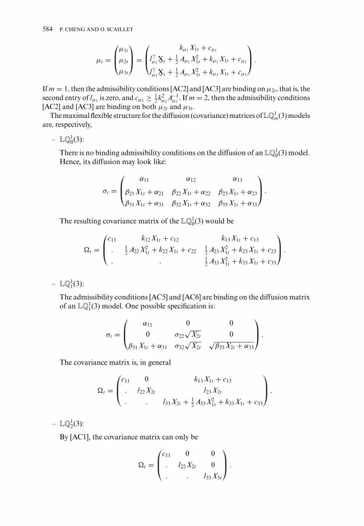
3.2.1. The Maximal LQ1m(3) Models. For an LQ1

m(3) model, Xt = (X1t) and X¯ t =

(X2t X3t)�. The maximal flexible structure for the drift of all LQ1m(3) models can be

represented as


µt =

µ1t

µ2t

µ3t

=

kµ1 X1t + cµ1

l�µ2X¯ t + 1

2 Aµ2 X21t + kµ2 X1t + cµ2

l�µ3X¯ t + 1

2 Aµ3 X21t + kµ3 X1t + cµ3

.

If m = 1, then the admissibility conditions [AC2] and [AC3] are binding on µ2t, that is, thesecond entry of lµ2 is zero, and cµ2 ≥ 1

2 k2µ2

A−1µ2

. If m = 2, then the admissibility conditions[AC2] and [AC3] are binding on both µ2t and µ3t.

The maximal flexible structure for the diffusion (covariance) matrices of LQ1m(3) models

are, respectively,

– LQ10(3):

There is no binding admissibility conditions on the diffusion of an LQ10(3) model.

Hence, its diffusion may look like:

σt =

α11 α12 α13

β21 X1t + α21 β22 X1t + α22 β23 X1t + α23

β31 X1t + α31 β32 X1t + α32 β33 X1t + α33

.

The resulting covariance matrix of the LQ10(3) would be

�t =

c11 k12 X1t + c12 k13 X1t + c13

. 12 A22 X2

1t + k22 X1t + c2212 A23 X2

1t + k23 X1t + c23

. . 12 A33 X2

1t + k33 X1t + c33

.

– LQ11(3):

The admissibility conditions [AC5] and [AC6] are binding on the diffusion matrixof an LQ1

1(3) model. One possible specification is:

σt =

α11 0 0

0 σ22√

X2t 0

β31 X1t + α31 σ32√

X2t√

β33 X2t + α33

.

The covariance matrix is, in general

�t =

c11 0 k13 X1t + c13

. l22 X2t l23 X2t

. . l33 X2t + 12 A33 X2

1t + k33 X1t + c33

.

– LQ12(3):

By [AC1], the covariance matrix can only be

�t =

c11 0 0

. l22 X2t 0

. . l33 X3t

.


This corresponds to the diffusion matrix

σt = ±

α11 0 0

0 σ22√

X2t 0

0 0 σ33√

X3t

.

Note that regardless of the sign of σt, the covariance is identical, as well as theresulting standard transform.

Similar to the AJD class, as more affine variables enter the specification of the diffusionmatrix, the structure of �t becomes increasingly restrictive.

3.2.2. The Maximal LQ2m(3) Models. For an LQ2

m(3) model, Xt = (X1t X2t)�

and X¯ t = (X3t). The maximal flexible structure for the drift of all LQ2

m(3) models can berepresented as:

µt =

µ1t

µ2t

µ3t

=

k�µ1

Xt + cµ1

k�µ2

Xt + cµ2

lµ3 X¯ t + 1

2 X�t Aµ3 Xt + k�

µ3Xt + cµ3

.

If m = 1, the admissibility condition [AC3] is binding on µ3t, that is, cµ3 ≥ 12 k�

µ3A+

µ3kµ3 .

The maximal flexible structure for the diffusion (covariance) matrices of LQ2m(3) models

are, respectively,

– LQ20(3):

There is no binding admissibility conditions on the diffusion of an LQ20(3) model.

Hence, its diffusion may look like:

σt =

α11 α12 α13

α21 α22 α23

β�31Xt + α31 β�

32Xt + α32 β�33Xt + α33

.

The resulting covariance matrix of the LQ20(3) would be

�t =

c11 c12 k13 X1t + c13

. c22 k23 X1t + c23

. . 12 X�

t A33Xt + k�33Xt + c33

.

In Section 2 we presented the Santa-Clara and Yan (2005) model (Equation [2.9]),which is an LQ2

0(3). By comparing the drift and the covariance matrices with themaximal flexible specifications of an LQ2

0(3) model above, we see that the Santa-Clara and Yan (2005) model is not maximal flexible, since it sets the second entryof kµ1 , the first entry of kµ2 , kµ3 , c13, c23, c33, and k33 to zero, and

Aµ3 =(

1 0

0 1

), A33 =

(1 0

0 0

).


– LQ21(3):

The structure of LQ21(3) is less flexible than that of LQ2

0(3) in that the admissibilitycondition [AC1] becomes binding. The maximal flexible diffusion of LQ2

1(3) is:

σt = ±

α11 α12 0

α21 α22 0

σ33√

X3t

,

and the corresponding covariance matrix is

�t =

c11 c12 0

. c22 0

. . k33 X3t

.

4. SOLUTION TO THE STANDARD TRANSFORM AND THEEQUIVALENCE BETWEEN LQJD AND AJD CLASSES

Provided that the structural constraints and the admissibility conditions are satisfied, wecan derive the solution of the standard transform as an exponential LQ function. A veryimportant result of this section is the equivalence relationship between the LQJD andthe AJD classes in terms of their transforms. That is, an LQJD process can actually bereformulated as a constrained AJD process.

4.1. Solution to the Standard Transform

Recall that the solution to the standard transform is

φ(g; Xt, t, T ) = eg(Xt,t),

provided that the LQ function g(x, t) satisfies the PIDE (2.8) in Lemma 2.1:

R = ∂g∂t

+ µ� ∂g∂x

+ 12

tr

[(∂2g∂x2

+ ∂g∂x

(∂g∂x

)�)�

]+ λ(θ − 1),

where θ (x, t) = ∫D

eg(x+y,t)−g(x,t)�(x, dy, t), and R and λ are both LQ functions, that is,for κ = R and λ, κ(x, t) = 1

2 x��κ(t)x + bκ(t)�x + cκ(t). We may solve the PIDE up toa system of ODEs using the method of undetermined coefficients. To achieve this, firstnote that the drift µ(x, t) and the covariance matrix �(x, t) of the state vector can bewritten as

µ = 12

(In ⊗ x�)

Ax + Bx + C,

� = 12

(In ⊗ x�)

A(In ⊗ x) + B(In ⊗ x) + C,

where ⊗ is the Kronecker product operator, In is an n-dimensional identity matrix, andthe coefficient matrices (A B C) and (A B C) satisfy the structural and admissibility


constraints. For example, µ and � of the Santa-Clara and Yan (2005) model can berepresented with

A =

03×3

03×3

�µ3

, with �µ3 =

(Aµ3 02×1

01×2 0

);

A =

03×3 03×3 03×3

03×3 03×3 03×3

03×3 03×3 �33

, with �33 =

1 0 0

0 0 0

0 0 0

;

B =

01×3 01×3 B13

01×3 01×3 B23

B31 B32 01×3

, with Bi j = (

ki j 0 0)

;

and

B =

kµ1 0 0

0 kµ2 0

0 0 0

; C =

cµ1

cµ2

cµ3

; C =

c11 c12 0

c12 c22 0

0 0 0

.

We have the following proposition:

PROPOSITION 4.1. Suppose that the technical integrability conditions hold, and that theLQ function g(x, t) = 1

2 x��(t)x + b(t)�x + c(t) with terminal condition g(x, T ) = g(x),admits a unique solution through the following system of ODEs:

−dbdt

= bλ(θ − 1) − bR + bµ + 12

b�,(4.1)

−d�

dt= �λ(θ − 1) − �R + �µ + 1

2��,(4.2)

−dcdt

= cλ(θ − 1) − cR + cµ + 12

c� + 12

tr [A�],(4.3)

where

�µ = Aᵀ (b ⊗ In) + 2B��,

bµ = �C + B�b,

cµ = C�b,

(4.4)

and

�� = 2�C� + 4�B(b ⊗ In) + (b� ⊗ In

)A(b ⊗ In),

b� = 2�Cb + (b� ⊗ In

)B�b,

c� = bᵀCb.

(4.5)

Then the solution to the standard transform φ(g; Xt, t, T), defined by (2.6), is

φ(g; Xt, t, T ) = eg(Xt,t).


Proof. See Appendix B.2.

One may have observed that ODE (4.2) is a system of non-symmetric matrix Riccatidifferential equations (RDE), which takes the form:

ddτ

� = M21(τ ) + M22(τ )� − � M11(τ ) − � M12(τ )�.(4.6)

Take the specifications of the Santa-Clara and Yan (2005) model as an example. Themodel is LQ2

0(3), so we only have to consider the ODE for the leading diagonal block, A,of �. Moreover, AR = 0, θ is calculated from a log-normal distribution, and

Aλ =(

1 0

0 0

).

Using the (A B C) and (A B C) matrices of the Santa-Clara and Yan (2005) modelpresented above, we have

ddτ

A = M21(τ ) + M22(τ )A− AM11(τ ) − AM12(τ )A,

where

M21(τ ) = Aλ(θ − 1) + Aµ3 b3 +(

b23 0

0 0

),

and

M22(τ ) = 2

(kµ1 0

0 kµ2

), M11(τ ) = −2

(k13b3 0

k23b3 0

), M12(τ ) = −

(c11 c12

c12 c22

),

with b3 being the 3rd entry of b in ODE (4.1). In fact, the ODE of b can also be writtenin the form of (4.6).

A standard solution procedure, called Radon’s lemma, exists for such systems:

THEOREM 4.1 (Radon’s lemma)Let:

M(τ ) =(

M11(τ ) M12(τ )

M21(τ ) M22(τ )

).

If Y (τ ) = (Q(τ )�P(τ )�)� is, on some interval U ⊂ R, a solution of the linear system

ddτ

Y(τ ) = M(τ )Y(τ ),(4.7)

such that det Q(τ ) �= 0 for τ ∈ U, then:

� (τ ) = P(τ )Q(τ )−1

is a solution of (4.6); in particular, � (τ0) = P(τ0)Q(τ0)−1.

By Radon’s lemma, the initial value problem for a matrix RDE system that we have tosolve in the LQJD setting is (locally) equivalent to an initial value problem for the linearsystem defined in (4.7). Since standard procedures exist for solving linear systems ofODEs such as (4.7), the added computational burden is limited. For instance, in solvingfor the standard transform of the Santa-Clara and Yan (2005) model, one may apply


Radon’s lemma to obtain b and �. c is then obtained by integrating the right-hand sideof (4.3).

We make no further efforts on the discussion about the existence and uniqueness ofthe solutions of RDE systems. First, there does not exist a general theory on these issuesfor matrix Riccati systems (see Freiling 2002). This implies that such discussions must becase specific. Second, all models for financial applications are simple enough to admitunique solutions. For further details on RDE systems, see, for instance, Freiling (2002)and the references therein.

Finally, we note that some authors tend to call all quadratic matrix differential equa-tions matrix RDEs. However, not all quadratic differential equations can be representedin a form similar to (4.6). Previous studies on AJD and QG models have mentioned thatthe resulting ODE systems are Riccati equations, but none of them has clarified theirviews on this point.

4.2. The Equivalence between LQJD and AJD Models

While it is straightforward to recognize AJD class as a subset of the LQJD class, itmight come as a surprise that the LQJD class can in fact be accommodated in the AJDclass. Indeed, by introducing some pseudo-factors to replace the quadratic terms, one mayreformulate an LQJD model as a constrained AJD model. This reformulation leads toa one-to-one equivalence relationship between LQJD and AJD classes in terms of theirtransforms.

To see this, first note that all quadratic terms are affine in elements of X X�. Therefore,we introduce the vector Z of pseudo-factors, which is defined as

Z = v [XX�],

where v is the vector-half operator. This operator, also denoted by vech, stacks the lowerelements of a square matrix into a vector. Hence, v [XX�] only collects the distinct elementsof the symmetric matrix XX�.

Note that the drift of the quadratic vector X is affine in X, and the covariance matrixis deterministic. Hence, the drift of Z is affine in (Z� X�)�, and the covariance of Z isaffine in X. We can now rephrase the LQJD setting in terms of the augmented state vector

Xa =

Z

X

X¯

.(4.8)

Using notations from Duffie, Pan, and Singleton (2000), we have

d Xa = µa(Xat

)dt + σ a(Xa

t

)dW t + dJa

t ,(4.9)

where

µa = K1 Xa + K0,

�a = H1(IN+n ⊗ Xa

) + H0.

The above expressions show that all terms in the LQJD setting can be represented asaffine forms of Xa, which means that LQJD and AJD classes are in fact nested within


each other. We further have an equivalence relationship between the LQJD and AJDclasses in terms of their standard transforms:

PROPOSITION 4.2. The standard transform of an n-factor LQJD model with an m-dimension, quadratic vector X is equal to the standard transform of a constrained,(N+n)-factor, N = q(q + 1)/2, affine model of Duffie, Pan, and Singleton (2000), wherethe state vector is augmented by an additional N × 1 pseudo state vector Z = v [XX�]with Z0 = v [X0 X�

0 ].

Proof. Applying the results from the LQJD setting and the results from the AJDsetting, respectively, to X and Xa and their transforms. This leads to two sets of ODEs,which can be shown to be equivalent3 . �

The Santa-Clara and Yan (2005) model is again well suited as an example here. Forsimplicity, we suppress the jump component, so that the model becomes LQ1

0(2):

µt =(

kµ1 X1t + cµ1

12 Aµ3 X2

1t + cµ3

), �t =

(c11 k13 X1t

. X21t

).(4.10)

We introduce the pseudo state vector, which consists of the instantaneous variance, Vt,of the stock price logarithm st:

Zt = Vt = X21t.

Note that the augmented state vector is Xt = (Vt X1t st)� and �t is affine in both Vt andX1t, corresponding to an A2(3) model. We write the augmented drift µa

t and covariance�a

t alongside the maximal flexible drift µAt and covariance �A

t of an A2(3) model ( Xt =(VA

t XA1t XA

2t)�, where VA

t and XA1t enter the diffusion term)

µat =

2kµ1 2cµ1 0

0 kµ1 012 Aµ3 0 0

Vt

X1t

st

+

c11

cµ1

cµ3

,

µAt =

k11 k12 0

k21 k22 0

k31 k32 k33

Vt

X1t

X2t

+

θ1

θ2

θ3

,

and

�at =

4c11Vt 2c11 X1t 2k13Vt

. c11 k13 X1t

. . Vt

, �A

t =

β11VAt 0 β13VA

t

. β22 XA1t β23 XA

1t

. . β33VAt + β33 XA

1t + α33

.

The most obvious difference is that in the augmented LQ10(2) model Vt = X2

1t, whereX1t follows a Gaussian process, but in the A2(3) model VA

t and XA1t are distinct square-root

processes. Moreover, the drift µAt has to satisfy the constraints

k12 ≥ 0, θ1 ≥ 0, k21 ≥ 0, θ2 ≥ 0,

3 For a more detailed proof, please refer to the extended version of this paper, Cheng and Scaillet (2002).


while µat satisfies a different set of constraints, equivalent to relaxing the constraints on

(k12 θ1 k21 θ2), but imposing k21 = k32 = k33 = 0, which is unnecessary, and

k11 = 2k22, k12 = 2θ2,

due to the deterministic relationship Vt = X21t.

The constraints imposed on �At and �a

t are also different. For �At :

β11 > 0, β22 > 0, β33 > 0, β33 > 0, α33 > 0.

For �at , β22 = β33 = α33 = 0, which is unnecessary. However, it allows correlation be-

tween Vt and X1t (the correlation is ±1, depending on the sign of X1t), while VAt and XA

1thave zero correlation. It is also interesting to look at the (2, 3)th term of the covariancematrices. In the reduced Santa-Clara and Yan (2005) model, this term is closely linked tothe correlation between the volatility factor X1t and the logarithm of the stock price st.One may observe that in the LQJD model, the correlation actually depends on the signof X1t, while in the affine model A2(3) the correlation is either positive or negative, butnever shift signs.

In summary, while an LQ model can be rewritten as an affine model by augmentingthe state vector, it may not fit into an affine class defined by Dai and Singleton (2000).This is due to the presence of the Gaussian factors, for example, X1t = ±√

Vt, whichare particular to the quadratic models. The equivalence relationship stated here is, there-fore, on the valuation side. Put it differently, while an LQJD model can be solved usingtechniques normally applied to AJD models, it extends the modeling flexibility of affinemodels to the nonlinear territory. This is evidenced by the discussion of the correlationterms above.

Proposition 4.2 is a strong result, for the quadratic class has always been taken to bea separate group from the affine class in asset pricing methodology. We have just shownthat this perception is not valid. Indeed, the proposition above concerns a full valua-tion equivalence, that is, the numerical schemes necessary for computing the transformswill deliver exactly the same results. A straightforward consequence of Proposition 4.2is that the analysis techniques of affine models also become applicable to LQJD mod-els. An example is Collin-Dufresne, Goldstein, and Jones (2003), in which a three-factormaximal affine term structure model with stochastic volatility is studied. Their tech-nique of rotating latent state variables into observables is similarly applicable in theLQJD setting. Moreover, the reformulation can be done in an automatic way throughmatrix algebra manipulations and easily implemented in a symbolic calculus package(see the extended version of this paper, Cheng and Scaillet (2002), for a fully workedexample).

Further note that the technique of change of variables, which we use to derive thevaluation equivalence between AJD and LQJD models, does not apply for general struc-tures of the state vector. This equivalence is really due to the presence of LQ structures atevery step of the identification procedure. For example, the change of variables techniquebreaks down in the Hull and White (1987) model, where the instantaneous variance isthe exponential of the volatility factor.

4.3. The LQJD Dynamics under the Risk-Neutral Measure

It is well known that option prices are not derived from the data-generating processunder the historical (objective) measure P, but from some risk-adjusted process under an


equivalent measure Q. Therefore, for pricing purpose, one needs to know the specificationof the state-price density, ξt, which is defined in the LQJD framework as

ξ (Xt, t) = exp(

−∫ t

0RP(Xs, s) ds

)egξ (Xt,t),(4.11)

where

gξ (Xt, t) = 12

X�t �ξ (t)Xt + b�

ξ (t)Xt + cξ (t),

satisfies PIDE (2.8). Without loss of generality, we assume ξ (X0, 0) = 1, which givesthe initial condition for the PIDE. By Lemma 2.1, ξ (Xt, t) is a positive P-martingale.Furthermore, by restricting ξ (Xt, t) to be exponential LQ in Xt, we have ensured that thestructure of the state vector remains LQJD under the new measure Q.

The equivalent martingale measure Q is defined via

dQ

dP

∣∣∣∣t= ξ (XT, T )

ξ (Xt, t).(4.12)

Let

WQt = WP

t −∫ t

0σ (Xs, s)�[�ξ (s)Xs + bξ (s)] ds.(4.13)

The following Lemma, which is similar to Lemma 2 in Appendix C of Duffie, Pan, andSingleton (2000), states that ξ (Xt, t)W Q is a P local martingale. It then follows that W Q

is a standard Brownian Motion under Q.

LEMMA 4.2 ξ (Xt, t)W Q is a P-martingale, provided that all technical integrability con-ditions are satisfied.

Proof. See Appendix C.

Moreover, let N be the jump-counting process with intensity λP(Xt, t) under P

and λQ(Xt, t) under Q. Define

MQ = NPt −

∫ t

0θ (lξ )λP(Xs, s) ds.(4.14)

Since jumps are restricted to affine variables X¯

only, results from Duffie, Pan, andSingleton (2000) concerning jumps are directly applicable in the LQJD setting. Specif-ically, by Lemma 3 in Appendix C of Duffie, Pan, and Singleton (2000), and providedthat the technical integrability conditions are satisfied, ξ (Xt, t)MQ is a P -martingale. Itfollows that MQ is a compensated jump-counting process under Q.

The structure of the state vector under the measure Q is now

dXt = µQ(Xt, t) dt + σ (Xt, t) dWQt + dJQ

t ,(4.15)

with the drift being

µQ(Xt, t) = µP(Xt, t) + �(Xt, t)[�ξ (t)Xt + bξ (t)],(4.16)

and the jump intensity being


λQ(Xt, t) = θ (lξ )λP(Xt, t).(4.17)

The diffusion part remains unchanged.One may now easily infer from (4.15) the market price of risk relative to the Q

drift µQ(Xt, t). In particular, the quantity µQ − µP is LQ in the state vector Xt. Incontrast, �ξ (t) is zero in an AJD model, and � is independent of Xt in a QG model.Consequently, µQ − µP is only affine in both latter cases.

Since the state-price density is obtained explicitly, one may estimate jointly the objectiveand the risk-neutral measures in the LQJD settings and extract information content fromthe option markets. An analysis of this kind can be found, for instance, in Chernov andGhysels (2000) and Pan (2002).

Given the dynamics of the state vector under the risk-neutral measure Q, option pric-ing via transform analysis is then straightforward. (see, for example, Duffie, Pan, andSingleton (2000), Carr and Madan (1999), and Lewis (2000).

5. CONCLUSION

We have generalized the transform analysis methods existing for the AJD and QG classesto the LQJD clase. We present in detail the characterization of the LQJD structure, derivethe structural restrictions and the admissibility conditions, and carry out a specificationanalysis for the three-factor LQJD models. We solve the standard transform up to asystem of ODEs, which is identified as a system of non-symmetric Riccati differentialequations with standard solution routines. Finally, we prove that an LQJD model can beconverted to an AJD model by introducing a vector of pseudo factors. The notion is quiteintuitive, but has never been demonstrated in full generality before. This is a strong result,for researchers have always taken affine and quadratic models as two separate classes,whereas we show that the set of the quadratic models that is absolutely distinct from theaffine class is actually empty in terms of asset pricing by transform analysis.

The LQJD model also provides the theoretical basis for future research on nonlinearspecifications of the market price of risk, as well as its estimation using joint observationsof prices and options. Such study with affine models has already been carried out by, forinstance, Chernov and Ghysels (2000) and Pan (2002). Since the LQJD framework is veryflexible, selecting an appropriate model is of great concern. We leave this issue for futureresearch.

APPENDIX A

Proof of Lemma 2.1. By Ito’s lemma for semi-martingales, we have

�t = �0 +∫ t

0D�s ds +

∫ t

0ηs dW s + Jt,

where the infinitesimal operator D is defined as

D f (x, t) = ∂ f∂t

(x, t) + µ(x)�∂ f∂x

(x, t) + 12

tr[�(x)

∂2 f∂x2

(x, t)]

+ λ(x, t)∫

D

[ f (x + y, t) − f (x, t)]�(x, dy, t),


and

ηt =(

∂�t

∂x

)�σt,

Jt =∑

0<τ (i )≤t

(�τ (i ) − �τ (i )−

) −∫ t

0γs ds,

with τ (i) denoting the ith jump time of X , and

γt = λ(x, t)∫

D

[�(x + y, t) − �(x, t)]�(x, dy, t).

Suppose the following technical integrability conditions hold

(i ) E0[|�T|] < ∞;

(i i ) E0

[(∫ T

0ηsη

ᵀs ds

)1/2]

< ∞;

(i i i ) E0

[∫ T

0|γs | ds

]< ∞.

By integrability condition (i i ),∫ t

0 ηsdW s is a martingale. Furthermore, Jt is a martingaleas well. This is because

E0

[ ∑0<τ (i )≤t

(�τ (i ) − �τ (i )−

)] = E0

[ ∑0<τ (i )≤t

Eτ (i )−[�τ (i ) − �τ (i )−

]]

= E0

[ ∑0<τ (i )≤t

�τ (i )− (θτ (i ) − 1)

]

= E0

[ ∑0<τ (i )≤t

∫ τ (i )

τ (i )−�u(θu − 1) dNu

]

= E0

[∫ t

0�u(θu − 1) dNu

]

= E0

[∫ t

0�u(θu − 1)λu du

]

= E0

[∫ t

0γu du

],

where the last but one equality is due to the fact that the jump-counting process Nt hasintensity λt, and the last equality is by definition of γt. By integrability condition (iii), wehave

E0[Jt] = E0

[ ∑0<τ (i )≤t

(�τ (i ) − �τ (i )−

) −∫ t

0γu du

].

= 0.

Hence, Jt is a martingale.The PIDE is obtained by computing D�t, setting it to zero, and dividing through the

resulting equation by �t(�= 0).


APPENDIX B. STRUCTURAL CONSTRAINTS AND ODES

Appendix B gives details on the derivation of the structural constraints underlying theLQJD modeling, as well as the computations leading to the ODEs of Proposition 4.1.They both rely on the PIDE of Lemma 2.1:

R = ∂g∂t

+ µ� ∂g∂x

+ 12

tr

[(∂2g∂x2

+ ∂g∂x

(∂g∂x

)�)�

]+ λ(θ − 1),

where all terms should be LQ in x.

B.1. Justification of the Structural Constraints

Structural constraint [SC1] on the jump components is justified as follows. Note thatthe ODEs are identified by imposing D�t ≡ 0 . The last component in D�t is

λ(x, t)∫

D

[�(x + y, t) − �(x, t)]�(x, dy, t)

= �(x, t)λ(x, t)∫

D

exp(

12

x��(t)y + 12

y��(t)x + 12

y��(t)y + b(t)�y)

�(dy, t).

Since �(x, t) can be cancelled throughout D�(x, t) = 0, and since we want the remainingterms all be LQ functions for identification, it is necessary that the integral term in theabove equation be independent of x. Given the structure of �(t) imposed by (2.3), theminimal restriction on y is then [SC1], namely its first q entries are zeros.

For [SC2] and [SC3], note that the right hand side of the PIDE above contains thefollowing two quantities

(i) µ� ∂g∂x ;

(ii) tr [ ∂g∂x ( ∂g

∂x )��], where g(x, t) = 12 x��(t)x + b(t)�x + c(t).

(i) and (ii) depend on µ and �, respectively, and must be LQ in x to permit the use ofthe method of undetermined coefficients.

We start by making no assumptions on µ and �. First, we stack µ as

µ =

12 x��µ1 x + b�

µ1x + cµ1

...12 x��µn x + b�

µnx + cµn

n×1

.

Let

A =

�µ1

...

�µn

n2×n

, B =

b�µ1

...

b�µn

n×n

, C =

cµ1

...

cµn

n×1

,

then µ can be compactly written as

µ = 12

(In ⊗ x�)

Ax + Bx + C.


Note that ∂g∂x = �x + b. For µ� ∂g

∂x to be LQ in x, we must have[(In ⊗ x�)

Ax]�

�x = 0,

which leads to �µi ≡ 0, for all i = 1, 2, . . . , m. This justifies [SC2].Similarly, we can write � as

� = 12

(In ⊗ x�)

A(In ⊗ x) + B(In ⊗ x) + C.

For tr [ ∂g∂x ( ∂g

∂x )��] to be LQ in x, first note that

tr

[∂g∂x

(∂g∂x

)��

]=

(∂g∂x

)��

∂g∂x

.

Hence, we need

x��(In ⊗ x�)

A(In ⊗ x)�x = 0,

x��B(In ⊗ x)�x = 0,

which yields [SC3].

B.2. Obtaining the ODEs (Proof of Proposition 4.1)

From above, we can compute

µ� ∂g∂x

= 12

x��µx + bᵀµx + cµ,

where (�µbµcµ) are given by (4.4), and

tr

[∂g∂x

(∂g∂x

)��

]= 1

2x��x + b�

�x + c�,

where (��b�c�) are given by (4.5).Moreover,

∂2g∂x2

= � =(

Am×m 0

0 0

),

and by [SC3](a), the leading m × m block, �, of � is deterministic in t. Hence:

tr[

∂2g∂x2

�

]= tr [A�],

and is deterministic in t as well.Knowing that both R and λ are LQ functions of x, i.e., for κ = R, λ,

κ(x, t) = 12

x��κ(t)x + bκ(t)�x + cκ(t),

we can easily apply the method of undetermined coefficients and obtain the ODEs inProposition 4.1.


APPENDIX C

Proof of Lemma 4.1. By Ito’s formula, for 0 ≤ s ≤ t ≤ T ,

ξtWQ

t = ξs W Qs +

∫ t

sW Q

u dξu +∫ t

sξu−dW Q

u +∫ t

sd〈ξ, W Q〉c

u

= ξs W Qs +

∫ t

sW Q

u dξu +∫ t

sξu−

(dWP

u − σ (Xu, u)�[�ξ (u)Xu + bξ (u)] du)

+∫ t

sξuσ (Xu, u)�[�ξ (u)Xu + bξ (u)] du

= ξs W Qs +

∫ t

sW Q

u dξu +∫ t

sξu−dWP

u ,

where ξt stands for ξ (Xt, t), and 〈ξ, W Q〉c denotes the continuous part of 〈ξ, W Q〉.Since W P and ξ are both P-martingales,

∫ t0 W Q

u dξu and∫ t

0 ξu−dWPu , t ≥ 0, are P-

martingales as well. Hence ξtWQ

t is a P-martingale.

REFERENCES

AHN, D-H., R. F. DITTMAR, and A. R. GALLANT (2002): Quadratic Term Structure Models:Theory and Evidence, Rev. Financ Stud. 15, 243–288.

AHN, D-H., and B. GAO (1999): A Parametric Nonlinear Model of Term Structure Dynamics,Rev. Financ. Stud. 12, 721–762.

AIT-SAHALIA, Y. (1996): Testing Continuous-Time Models of the Spot Interest Rate, Rev. Financ.Stud. 9, 385–426.

BACKUS, D., S. FORESI, A. MOZUMDAR, and L. WU (2001): Predictable Changes in Yields andForward Rates, J. Financ. Econ. 59, 281–311.

CARR, P., and D. B. MADAN (1999): Option Valuation Using the Fast Fourier Transform, J.Comput. Finance 2, 61–73.

CHEN, L., E. BAYRAKTAR, and H. V. POOR (2005): Consistency Problems for Jump-DiffusionModels, Appl. Math. Finance 12(2), 101–119.

CHEN, L., D. FILIPOVIC, and H. V. POOR (2004): Quadratic Term Structure Models for Risk-freeand Defaultable Rates, Math. Finance 14, 515–536.

CHENG, P., and O. SCAILLET (2002): Linear-Quadratic Jump-Diffusion Modeling with Applica-tion to Stochastic Volatility, FAME working paper series, No. 67.

CHERNOV, M., and E. GHYSELS (2000): A Study Towards a Unified Approach to the JointEstimation of Objective and Risk Neutral Measures for the Purpose of Options Valuation, J.Financ. Econ. 56, 407–458.

COLLIN-DUFRESNE, P., B. GOLDSTEIN, and C. JONES (2003): Identification and Estimation ofmaximal affine term structure models: an application to stochastic volatility, Working paper,Carnegie Mellon University.

DAI, Q., and K. J. SINGLETON (2000): Specification Analysis of Affine Term Structure Models,J. Finance 55, 1943–1978.

DAI, Q., and K. J. SINGLETON (2003): Term Structure Dynamics in Theory and Reality, Rev.Financ. Stud. 16, 631–678.

DUFFIE, D., and R. KAN (1996): A Yield-Factor Model of Interest Rates, Math. Finance 6,379–406.


DUFFIE, D., J. PAN, and K. SINGLETON (2000): Transform Analysis and Asset Pricing for AffineJump-Diffusions, Econometrica 68, 1343–1376.

FILIPOVIC, D. (2002): Separable Term Structures and the Maximal Degree Problem, Math. Fi-nance 12, 341–349.

FREILING, G. (2002): A Survey of Nonsymmetric Riccati Equations, Linear Algebra and ItsApplications 243–270.

GOURIEROUX, C., and R. SUFANA (2003): Wishart Quadratic Term Structure Models, Workingpaper, CREST.

GOURIEROUX, C., and R. SUFANA (2006): A Classification of Two-Factor Affine Diffusion TermStructure Models, J. Financ. Econometrics 4, 31–52.

HULL, J., and A. WHITE (1987): The Pricing of Options on Assets with Stochastic Volatilities, J.Finance 42, 281–300.

LEWIS, A. L. (2000): Option Valuation under Stochastic Volatility with Mathematica Code, FinancePress, USA.

LEIPPOLD, M., and L. WU (2002): Asset Pricing under the Quadratic Class, J. Financ. Quant.Anal. 37, 271–295.

LEIPPOLD, M., and L. WU (2003): Design and Estimation of Quadratic Term Structure Models,European Finance Rev. 7, 47–73.

LEIPPOLD, M., and L. WU (2007): Design and Estimation of Multi-Currency Quadratic Models,Rev. Finance 11(2), 167–207.

LIU, J. (2007): Portfolio Selection in Stochastic Environments, Review of Financial Studies 20(1),1–39.

PIAZZESI, M. (2001): An Econometric Model of the Yield Curve with Macroeconomic JumpEffects, NBER Working Paper 8246.

PIAZZESI, M. (2004): Bond Yields and the Federal Reserve, J. Political Economy 113, 311–344.

PAN, J. (2002): The Jump-Risk Premia Implicit in Options: Evidence from an Integrated Time-series Study, J. Financ. Econ. 63, 3–50.

PAN, E., and L. WU (2005): Taking Positive Interest Rates Seriously, Advances in QuantitativeAnalysis of Finance and Accounting 4, Chapter 14.

PROTTER, P. E. (2004): Stochastic Integration and Differential Equations. Springer.

RADY, S. (1997): Option Pricing in the Presence of Natural Boundaries and a Quadratic DiffusionTerm, Finance and Stochastics 1, 331–344.

SANTA-CLARA, P., and S. YAN (2005): Crashes, Volatility, and the Equity Premium: Lessons fromS& P 500 Options, Working Paper, UCLA.

SCHOBEL, R., and J. ZHU (1999): Stochastic Volatility with an Ornstein-Uhlenbeck Process: AnExtension, European Finance Rev. 3, 23–46.

STEIN, E. M., and J. C., STEIN (1991): Stock Price Distributions with Stochastic Volatility: AnAnalytic Approach, Review of Financial Studies 4, 727–752.

linear-quadratic jump-diffusion modeling

Documents