ORIGINAL ARTICLE

Mischaracterising density dependence biases estimated effectsof coloured covariates on population dynamics

Andreas Linden • Mike S. Fowler • Niclas Jonzen

Received: 25 March 2012 / Accepted: 29 August 2012 / Published online: 13 November 2012

� The Society of Population Ecology and Springer Japan 2012

Abstract Environmental effects on population growth

are often quantified by coupling environmental covariates

with population time series, using statistical models that

make particular assumptions about the shape of density

dependence. We hypothesized that faulty assumptions

about the shape of density dependence can bias estimated

effect sizes of temporally autocorrelated covariates. We

investigated the presence of bias using Monte Carlo sim-

ulations based on three common per capita growth func-

tions with distinct density dependent forms (h-Ricker,

Ricker and Gompertz), autocorrelated (coloured) ‘known’

environmental covariates and uncorrelated (white)

‘unknown’ noise. Faulty assumptions about the shape of

density dependence, combined with overcompensatory

intrinsic population dynamics, can lead to strongly biased

estimated effects of coloured covariates, associated with

lower confidence interval coverage. Effects of negatively

autocorrelated (blue) environmental covariates are

overestimated, while those of positively autocorrelated

(red) covariates can be underestimated, generally to a les-

ser extent. Prewhitening the focal environmental covariate

effectively reduces the bias, at the expense of the estimate

precision. Fitting models with flexible shapes of density

dependence can also reduce bias, but increases model

complexity and potentially introduces other problems of

parameter identifiability. Model selection is a good option

if an appropriate model is included in the set of candidate

models. Under the specific and identifiable circumstances

with high risk of bias, we recommend prewhitening or

careful modelling of the shape of density dependence.

Keywords Autoregressive models � Environmental

forcing � Prewhitening � Statistical inference � Theta-Ricker

model � Time series

Introduction

Environmental forcing is recognized as an important

determinant of population fluctuations, in combination with

intrinsic factors, such as density dependence and popula-

tion structure (Turchin 1995, 1999). Statistical identifica-

tion of important environmental variables affecting

population growth, and the quantification of such envi-

ronmental effects, are crucial research questions in popu-

lation ecology (Stenseth et al. 2002; Ruokolainen et al.

2009; Knape and de Valpine 2011), including its applica-

tions to e.g., conservation, pest control, fisheries and

wildlife management. For example, rainfall has important

positive effects on hunted populations of ducks in North

America (Johnson and Grier 1988) and on red kangaroo in

Australia (McCarthy 1996), which needs to be accounted

for when making management decisions.

Electronic supplementary material The online version of thisarticle (doi:10.1007/s10144-012-0347-0) contains supplementarymaterial, which is available to authorized users.

A. Linden (&)

Department of Biology, Centre for Ecological and Evolutionary

Synthesis, University of Oslo, P.O. Box 1066, Blindern,

0316 Oslo, Norway

e-mail: andreas.linden@iki.fi

M. S. Fowler

Population Ecology Group, Institut Mediterrani d’Estudis

Avancats (UIB–CSIC), Miquel Marques 21,

07190 Esporles, Spain

N. Jonzen

Department of Biology (Theoretical Population Ecology and

Evolution Group), Lund University, Ecology Building,

SE-223 62 Lund, Sweden

123

Popul Ecol (2013) 55:183–192

DOI 10.1007/s10144-012-0347-0

Historically the cross-correlation between environmental

variables and population density was used to detect envi-

ronmental effects, but that approach easily generates mis-

leading results (e.g., Royama 1981, 1992; Ranta et al. 2000;

Kaitala and Ranta 2001; Lundberg et al. 2002). The most

common modern approach is to fit simple phenomenolog-

ical models of population growth, including density

dependence, environmental covariates and possibly inter-

actions between those two, to time series of population

counts or density (e.g., Stenseth et al. 2002; Brannstrom and

Sumpter 2006; Knape and de Valpine 2011). Despite the

risk of oversimplification, this approach can be seen as a

step towards better estimates of a more quantitative nature.

Analyses of autocorrelated (coloured) population time

series are associated with a number of complexities,

potentially leading to spurious statistical relationships and/

or bias (Chatfield 2004; Ripa and Ives 2007; Linden and

Knape 2009). It should be emphasized that because eco-

logical time series are often short (Cazelles 2004), so are

the covariates used. Hence, even if the underlying envi-

ronmental process described by the covariate is uncorre-

lated over long time-scales, it is not uncommon that the

selected covariate has a temporal structure over shorter

temporal periods (Ruokolainen et al. 2009). Density

dependence is often modelled assuming some rather simple

functional relationship between density and population

growth (e.g., Berryman and Turchin 2001; Jonzen et al.

2002). If the estimated strength of density dependence is

biased, e.g., by ignoring observation error in population

density, the estimates of autocorrelated environmental

effects can also become biased (Linden and Knape 2009).

We hypothesize that similar bias could arise due to poor

approximation of the intrinsic population dynamic struc-

ture, e.g., the wrong shape of density dependent feedback.

Here we use a simulation approach to study whether

statistical estimates of environmental effect sizes on pop-

ulation growth are trustworthy when the true shape of

density dependence is unknown or poorly approximated.

We focus on the accuracy and precision of point estimates

for the estimated environmental effects, as well as the

confidence interval coverage. We also assess whether

identified bias can be reduced with prewhitening and/or a

flexible approach to modelling the shape of density

dependence. We highlight situations where common

practice would lead to biased estimates of environmental

effects, and discuss how existing statistical procedures can

be implemented to minimize the identified risk of bias.

Methods

To investigate the estimated effect sizes of environmental

covariates, we simulated time series data according to

stochastic generalizations of three well known, discrete

time population growth models (see section ‘Population

growth models and data simulation’ below). We varied the

strength of density compensation across a wide range of

return rates (TR) and incorporated an autocorrelated (col-

oured) stochastic environmental variable. We then applied

three statistical models (each corresponding to a specific

population model) to the data generated by each population

model, to estimate the effect sizes of the environmental

variable of interest (see section ‘Statistical estimation of

the environmental effect’ below). This approach was based

on the assumption that researchers generally do not have

perfect knowledge of the underlying processes driving

intrinsic dynamics in natural populations. Previous work

has considered systems including observation error, cou-

pled only with the correct form of density dependence

(Linden and Knape 2009), demonstrating the presence of

bias when observation error is ignored. We only considered

process error models in this study, i.e., we assumed prefect

knowledge about population density (no observation error),

to simplify the analysis and avoid overlap with that study.

Population growth models and data simulation

We simulated time series data using models of the general

form

Ntþ1 ¼ Nt exp f Ntð Þ þ bWt þ ut½ � ð1Þ

where Nt is population density at time t, f (Nt) is a density

dependent function of per capita growth that maps

expected changes in population density over consecutive

time steps, and Wt is a known, potentially autocorrelated

(coloured) environmental variable with effect size b (the

focus of this study). The term ut represents unknown

environmental variation and is i.i.d. normally distributed

(white) with zero mean and variance r2. To initiate pop-

ulations, we drew N1 from a uniform random distribution

with limits [0, 2], i.e., with a maximum of twice the

equilibrium density, N* = 1. We simulated the population

dynamics for 130 and 200 time steps, discarding the first

100 time steps in both cases to avoid transient effects due

to initial densities, using the final 30 and 100 steps (29 and

99 transitions in population size), respectively, for further

analysis.

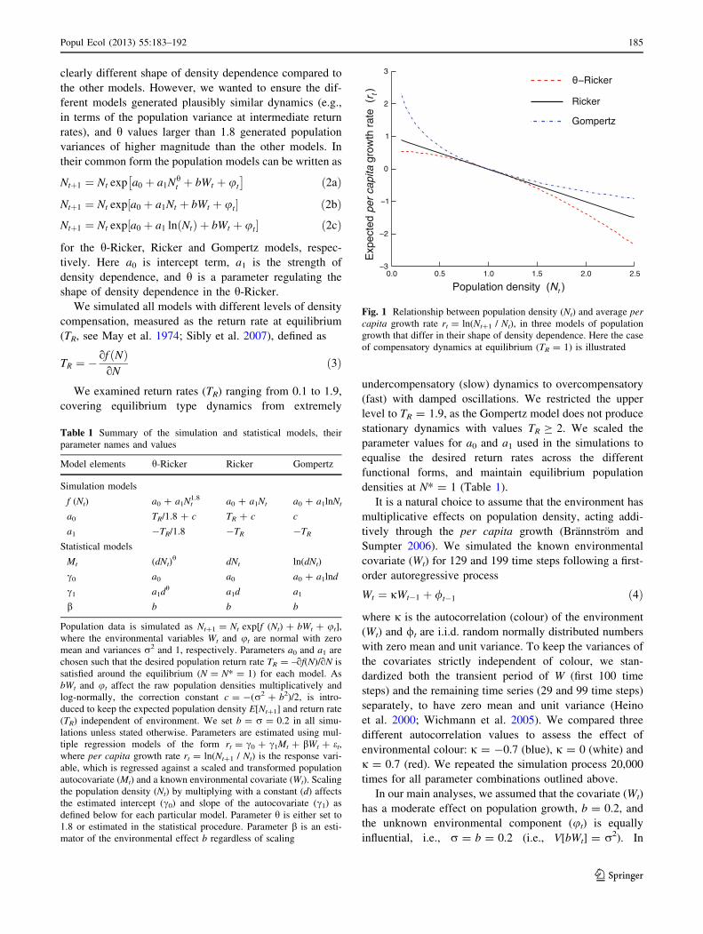
The per capita growth functions f (Nt) investigated here

(Table 1) are generalizations of (1) the h-Ricker model

with the parameter h fixed to 1.8; (2) the Ricker model; and

(3) the Gompertz model; (Gilpin and Ayala 1973; Ricker

1954; Gompertz 1825, respectively). These models differ

here only in their shape of density dependence, showing

concave, linear and convex relationships of density to per

capita growth rate (Fig. 1). As such, the choice of

parameter h = 1.8 is somewhat arbitrary, but represents a

184 Popul Ecol (2013) 55:183–192

123

clearly different shape of density dependence compared to

the other models. However, we wanted to ensure the dif-

ferent models generated plausibly similar dynamics (e.g.,

in terms of the population variance at intermediate return

rates), and h values larger than 1.8 generated population

variances of higher magnitude than the other models. In

their common form the population models can be written as

Ntþ1 ¼ Nt exp a0 þ a1Nht þ bWt þ ut

� �ð2aÞ

Ntþ1 ¼ Nt exp a0 þ a1Nt þ bWt þ ut½ � ð2bÞNtþ1 ¼ Nt exp a0 þ a1 ln Ntð Þ þ bWt þ ut½ � ð2cÞ

for the h-Ricker, Ricker and Gompertz models, respec-

tively. Here a0 is intercept term, a1 is the strength of

density dependence, and h is a parameter regulating the

shape of density dependence in the h-Ricker.

We simulated all models with different levels of density

compensation, measured as the return rate at equilibrium

(TR, see May et al. 1974; Sibly et al. 2007), defined as

TR ¼ �of Nð ÞoN

ð3Þ

We examined return rates (TR) ranging from 0.1 to 1.9,

covering equilibrium type dynamics from extremely

undercompensatory (slow) dynamics to overcompensatory

(fast) with damped oscillations. We restricted the upper

level to TR = 1.9, as the Gompertz model does not produce

stationary dynamics with values TR C 2. We scaled the

parameter values for a0 and a1 used in the simulations to

equalise the desired return rates across the different

functional forms, and maintain equilibrium population

densities at N* = 1 (Table 1).

It is a natural choice to assume that the environment has

multiplicative effects on population density, acting addi-

tively through the per capita growth (Brannstrom and

Sumpter 2006). We simulated the known environmental

covariate (Wt) for 129 and 199 time steps following a first-

order autoregressive process

Wt ¼ jWt�1 þ /t�1 ð4Þ

where j is the autocorrelation (colour) of the environment

(Wt) and /t are i.i.d. random normally distributed numbers

with zero mean and unit variance. To keep the variances of

the covariates strictly independent of colour, we stan-

dardized both the transient period of W (first 100 time

steps) and the remaining time series (29 and 99 time steps)

separately, to have zero mean and unit variance (Heino

et al. 2000; Wichmann et al. 2005). We compared three

different autocorrelation values to assess the effect of

environmental colour: j = -0.7 (blue), j = 0 (white) and

j = 0.7 (red). We repeated the simulation process 20,000

times for all parameter combinations outlined above.

In our main analyses, we assumed that the covariate (Wt)

has a moderate effect on population growth, b = 0.2, and

the unknown environmental component (ut) is equally

influential, i.e., r = b = 0.2 (i.e., V[bWt] = r2). In

Table 1 Summary of the simulation and statistical models, their

parameter names and values

Model elements h-Ricker Ricker Gompertz

Simulation models

f (Nt) a0 ? a1Nt1.8 a0 ? a1Nt a0 ? a1lnNt

a0 TR/1.8 ? c TR ? c c

a1 -TR/1.8 -TR -TR

Statistical models

Mt (dNt)h dNt ln(dNt)

c0 a0 a0 a0 ? a1lnd

c1 a1dh a1d a1

b b b b

Population data is simulated as Nt?1 = Nt exp[f (Nt) ? bWt ? ut],

where the environmental variables Wt and ut are normal with zero

mean and variances r2 and 1, respectively. Parameters a0 and a1 are

chosen such that the desired population return rate TR = –qf(N)/qN is

satisfied around the equilibrium (N = N* = 1) for each model. As

bWt and ut affect the raw population densities multiplicatively and

log-normally, the correction constant c = -(r2 ? b2)/2, is intro-

duced to keep the expected population density E[Nt?1] and return rate

(TR) independent of environment. We set b = r = 0.2 in all simu-

lations unless stated otherwise. Parameters are estimated using mul-

tiple regression models of the form rt = c0 ? c1Mt ? bWt ? et,

where per capita growth rate rt = ln(Nt?1 / Nt) is the response vari-

able, which is regressed against a scaled and transformed population

autocovariate (Mt) and a known environmental covariate (Wt). Scaling

the population density (Nt) by multiplying with a constant (d) affects

the estimated intercept (c0) and slope of the autocovariate (c1) as

defined below for each particular model. Parameter h is either set to

1.8 or estimated in the statistical procedure. Parameter b is an esti-

mator of the environmental effect b regardless of scaling

Fig. 1 Relationship between population density (Nt) and average percapita growth rate rt = ln(Nt?1 / Nt), in three models of population

growth that differ in their shape of density dependence. Here the case

of compensatory dynamics at equilibrium (TR = 1) is illustrated

Popul Ecol (2013) 55:183–192 185

123

addition, we investigated bias with different values for

parameters b and r, in the range 0.05–0.5, fixing the other

parameter (b or r) as 0.2. This was done by simulating data

with under- and overcompensatory Ricker dynamics

(TR = 0.2, 1.8) with statistical estimation based on Gom-

pertz-type density dependence—two of the most com-

monly used approaches (see Table 1). As the magnitude of

bias is likely to be proportional to b, we presented the

relative bias in the estimate (b) here as (b - b)/b. These

results were based on 100,000 replicates.

Statistical estimation of the environmental effect

For each replicated simulation we estimated the environ-

mental effect (b) using linear multiple regression of the

general form

rt ¼ c0 þ c1Mt þ bWt þ et ð5Þ

where the realized per capita growth rate rt = ln(Nt?1/Nt)

was the response variable, while an autocovariate Mt and the

known environmental variable Wt were used as explanatory

variables. The autocovariate varied between the models,

being Mt = (dNt)1.8 in the h-Ricker, Mt = dNt in Ricker and

Mt = ln(dNt) in Gompertz. Here d is the inverse of the

sample mean of the portion of the time series used in the

regression (d = n/P

Nt; n = 29 or 99). This scaling proce-

dure was carried out to avoid numerical problems in the

fitting process, which can occasionally be present under

extreme return rates. Multiplying the population density by a

constant (d) does not alter the response variable (rt), and the

least squares solution using a scaled autocovariate still gives

the maximum likelihood estimator of b (denoted as b) for

each of the given models. However, some of the other

parameters of the models are affected by the scaling in a

manner depending on the particular model used. A summary

of the correspondence between the parameters in the simu-

lation model (Eqs. 2a, 2b, 2c) and the regression models used

for statistical estimation (Eq. 5), including consequences of

scaling, is given in Table 1.

We also fitted the h-Ricker model, with parameter h free

to be estimated (Table 1) as an example of a model with a

flexible shape of density dependence. The two first simu-

lation models represent special cases of this, with h = 1.8

and h = 1, respectively. However, the Gompertz model is

an example of a structurally different model, which can be

approximated by the free h-Ricker model (with expected

estimates of 0 \ h\ 1) to reduce possible bias. Fitting the

h-Ricker model can be viewed as a separable non-linear

least squares problem (Ruhe and Wedin 1980), which can

be solved with ordinary least squares, conditionally on the

parameter h. We used a one-dimensional golden section

search over parameter h, coupled with ordinary least

squares regression estimation of the other parameters.

Finally, the analysis was repeated with a prewhitened

version of the environmental covariate, to investigate

whether this approach reduces any bias. Prewhitening is a

collective name for methods employed to remove auto-

correlation from time series, and is typically applied to

reduce or avoid problems in time series analyses arising

from autocorrelation (Chatfield 2004). The prewhitened

covariate we used was represented by the residuals from a

first order autoregression fitted to the covariate (Wt as the

response variable, Wt-1 as the explanatory variable, for

only those time steps included in the statistical analyses,

t C 101).

We assessed accuracy (the possible bias) and precision

(the consistency of the estimation procedure) of the envi-

ronmental effect estimates (b) by examining their means

± the standard deviations under the different simulated

conditions. We calculated the 95 % confidence interval

coverage, i.e., how often the estimated confidence intervals

actually contain the true value used to generate the data,

based on profile likelihoods (e.g., Hilborn and Mangel

1997), as one minus the rejection rate of a likelihood ratio

test, with the true value as the null hypothesis. As a rough

measure of model fit we used the coefficient of determi-

nation (R2), which here also equals the proportion of var-

iance in the per capita growth between consecutive years

ln(Nt?1/Nt) explained by the model. Among the models

with fixed shape of density dependence, and hence equal

number of estimated parameters, ranking models by R2 is

equivalent to ranking by information theoretical model

selection criteria. Therefore, we did not explicitly compare

models using model selection methods.

Results

When the model used for statistical estimation corre-

sponded to the simulation model that generated the data,

the estimated effect size of the known environmental

covariate (b) was unbiased, precise, and had trustworthy

confidence intervals (results not shown). In populations

with undercompensatory dynamics (TR \ 1), with equal

strengths of known and unknown environmental variation

(b = r = 0.2), the estimation properties of b were gen-

erally very good under all combinations of simulated and

fitted models we examined [Figs. 2, 3, and Fig. S1 in

Electronic Supplementary Material (ESM)]. Varying the

autocorrelation (colour; j) of the known environmental

covariate (Wt) did not qualitatively change this aspect of

the results.

With overcompensatory population dynamics (TR [ 1),

faulty assumptions about the underlying form of density

dependence did affect statistical estimates of environmental

effects. For negatively autocorrelated (blue) environments, b

186 Popul Ecol (2013) 55:183–192

123

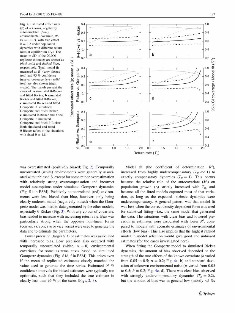
was overestimated (positively biased; Fig. 2). Temporally

uncorrelated (white) environments were generally associ-

ated with unbiased b, except for some minor overestimation

with relatively strong overcompensation and incorrect

model assumptions under simulated Gompertz dynamics

(Fig. S1 in ESM). Positively autocorrelated (red) environ-

ments were less biased than blue, however, only being

clearly underestimated (negatively biased) when the Gom-

pertz model was fitted to data generated by the other models,

especially h-Ricker (Fig. 3). With any colour of covariate,

bias tended to increase with increasing return rate. Bias was

particularly strong when the opposite non-linear forms

(convex vs. concave or vice versa) were used to generate the

data and to estimate the parameters.

Lower precision (larger SD) of estimates was associated

with increased bias. Low precision also occurred with

temporally uncorrelated (white, j = 0) environmental

covariates for some extreme cases based on simulated

Gompertz dynamics (Fig. S1d, f in ESM). This arises even

if the mean of replicated estimates closely matched the

value used to generate the time series. Estimated 95 %

confidence intervals for biased estimates were typically too

optimistic, such that they included the true estimate in

clearly less than 95 % of the cases (Figs. 2, 3).

Model fit (the coefficient of determination, R2),

increased from highly undercompensatory (TR \\ 1) to

exactly compensatory dynamics (TR = 1). This occurs

because the relative role of the autocovariate (Mt) on

population growth (rt) strictly increased with TR, and

because all the fitted models captured most of that varia-

tion, as long as the expected intrinsic dynamics were

undercompensatory. A general pattern was that model fit

was best when the correct density dependent form was used

for statistical fitting—i.e., the same model that generated

the data. The situations with clear bias and lowered pre-

cision in estimates were associated with lower R2, com-

pared to models with accurate estimates of environmental

effects (low bias). This also implies that the highest ranked

model in model selection would give good and unbiased

estimates (for the cases investigated here).

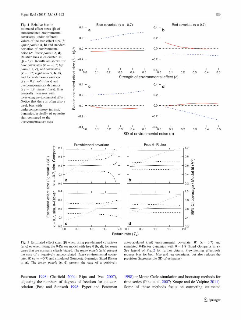
When fitting the Gompertz model to simulated Ricker

dynamics, the amount of bias observed depended on the

strength of the true effects of the known covariate (b varied

from 0.05 to 0.5; r = 0.2; Fig. 4a, b) and standard devi-

ation of unknown environmental noise (r varied from 0.05

to 0.5; b = 0.2; Fig. 4c, d). There was clear bias observed

with strongly undercompensatory dynamics (TR = 0.2),

but the amount of bias was in general low (mostly \5 %;

a b

c d

e f

Fig. 2 Estimated effect sizes

(b) of a known, negatively

autocorrelated (blue)

environmental covariate, Wt

(j = -0.7), with true effect

b = 0.2 under population

dynamics with different return

rates at equilibrium (TR). The

mean ± SD of the 20,000

replicate estimates are shown as

black solid and dashed lines,

respectively. Total model fit

measured as R2 (grey dashedline) and 95 % confidence

interval coverage (grey solidline) are also shown (right

y-axis). The panels present the

cases of: a simulated h-Ricker

and fitted Ricker, b simulated

Ricker and fitted h-Ricker,

c simulated Ricker and fitted

Gompertz, d simulated

Gompertz and fitted Ricker,

e simulated h-Ricker and fitted

Gompertz, f simulated

Gompertz and fitted h-Ricker.

Both simulated and fitted

h-Ricker refers to the situations

with fixed h = 1.8

Popul Ecol (2013) 55:183–192 187

123

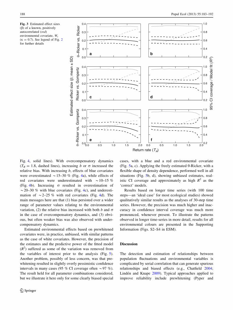
Fig. 4, solid lines). With overcompensatory dynamics

(TR = 1.8, dashed lines), increasing b or r increased the

relative bias. With increasing b, effects of blue covariates

were overestimated *15–30 % (Fig. 4a), while effects of

red covariates were underestimated with *10–15 %

(Fig. 4b). Increasing r resulted in overestimation of

*20–30 % with blue covariates (Fig. 4c), and underesti-

mation of *2–25 % with red covariates (Fig. 4d). The

main messages here are that (1) bias persisted over a wider

range of parameter values relating to the environmental

variation, (2) the relative bias increased with both b and rin the case of overcompensatory dynamics, and (3) obvi-

ous, but often weaker bias was also observed with under-

compensatory dynamics.

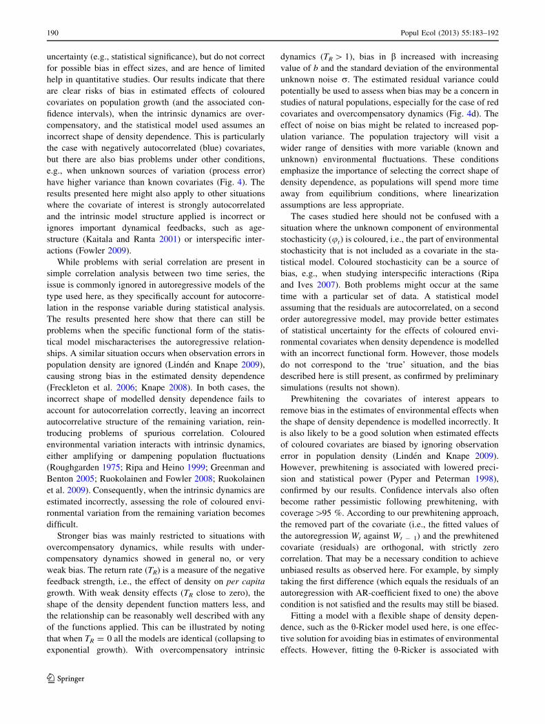
Estimated environmental effects based on prewhitened

covariates were, in practice, unbiased, with similar patterns

as the case of white covariates. However, the precision of

the estimates and the predictive power of the fitted model

(R2) suffered as some of the variation was removed from

the variables of interest prior to the analysis (Fig. 5).

Another problem, possibly of less concern, was that pre-

whitening resulted in slightly overly pessimistic confidence

intervals in many cases (95 % CI coverage often *97 %).

The result held for all parameter combinations considered,

but we illustrate it here only for some clearly biased special

cases, with a blue and a red environmental covariate

(Fig. 5a, c). Applying the freely estimated h-Ricker, with a

flexible shape of density dependence, performed well in all

situations (Fig. 5b, d), showing unbiased estimates, real-

istic CI coverage and approximately as high R2 as the

‘correct’ models.

Results based on longer time series (with 100 time

steps—an ‘ideal case’ for most ecological studies) showed

qualitatively similar results as the analyses of 30-step time

series. However, the precision was much higher and inac-

curacy in confidence interval coverage was much more

pronounced, whenever present. To illustrate the patterns

observed in longer time-series in more detail, results for all

environmental colours are presented in the Supporting

Information (Figs. S2–S4 in ESM).

Discussion

The detection and estimation of relationships between

population fluctuations and environmental variables is

complicated by serial correlation that can generate spurious

relationships and biased effects (e.g., Chatfield 2004;

Linden and Knape 2009). Typical approaches applied to

improve reliability include prewhitening (Pyper and

a b

c d

e f

Fig. 3 Estimated effect sizes

(b) of a known, positively

autocorrelated (red)

environmental covariate, Wt

(j = 0.7). See legend of Fig. 2

for further details

188 Popul Ecol (2013) 55:183–192

123

Peterman 1998; Chatfield 2004; Ripa and Ives 2007),

adjusting the numbers of degrees of freedom for autocor-

relation (Post and Stenseth 1998; Pyper and Peterman

1998) or Monte Carlo simulation and bootstrap methods for

time series (Piha et al. 2007; Knape and de Valpine 2011).

Some of these methods focus on correcting estimated

a b

c d

Fig. 4 Relative bias in

estimated effect sizes (b) of

autocorrelated environmental

covariates, under different

values of the true effect size (b;

upper panels, a, b) and standard

deviation of environmental

noise (r; lower panels, c, d).

Relative bias is calculated as

(b – b)/b. Results are shown for

blue covariates (j = –0.7; leftpanels, a, c), red covariates

(j = 0.7; right panels, b, d),

and for undercompensatory-

(TR = 0.2; solid lines) and

overcompensatory dynamics

(TR = 1.8; dashed lines). Bias

generally increases with

increasing environmental effect.

Notice that there is often also a

weak bias with

undercompensatory intrinsic

dynamics, typically of opposite

sign compared to the

overcompensatory case

a b

c d

Fig. 5 Estimated effect sizes (b) when using prewhitened covariates

(a, c) or when fitting the h-Ricker model with free h (b, d), for some

cases that are normally clearly biased. The upper panels (a, b) present

the case of a negatively autocorrelated (blue) environmental covar-

iate, Wt (j = -0.7) and simulated Gompertz dynamics (fitted Ricker

in a). The lower panels (c, d) present the case of a positively

autocorrelated (red) environmental covariate, Wt (j = 0.7) and

simulated h-Ricker dynamics with h = 1.8 (fitted Gompertz in c).

See legend of Fig. 2 for further details. Prewhitening effectively

reduces bias for both blue and red covariates, but also reduces the

precision (increases the SD of estimates)

Popul Ecol (2013) 55:183–192 189

123

uncertainty (e.g., statistical significance), but do not correct

for possible bias in effect sizes, and are hence of limited

help in quantitative studies. Our results indicate that there

are clear risks of bias in estimated effects of coloured

covariates on population growth (and the associated con-

fidence intervals), when the intrinsic dynamics are over-

compensatory, and the statistical model used assumes an

incorrect shape of density dependence. This is particularly

the case with negatively autocorrelated (blue) covariates,

but there are also bias problems under other conditions,

e.g., when unknown sources of variation (process error)

have higher variance than known covariates (Fig. 4). The

results presented here might also apply to other situations

where the covariate of interest is strongly autocorrelated

and the intrinsic model structure applied is incorrect or

ignores important dynamical feedbacks, such as age-

structure (Kaitala and Ranta 2001) or interspecific inter-

actions (Fowler 2009).

While problems with serial correlation are present in

simple correlation analysis between two time series, the

issue is commonly ignored in autoregressive models of the

type used here, as they specifically account for autocorre-

lation in the response variable during statistical analysis.

The results presented here show that there can still be

problems when the specific functional form of the statis-

tical model mischaracterises the autoregressive relation-

ships. A similar situation occurs when observation errors in

population density are ignored (Linden and Knape 2009),

causing strong bias in the estimated density dependence

(Freckleton et al. 2006; Knape 2008). In both cases, the

incorrect shape of modelled density dependence fails to

account for autocorrelation correctly, leaving an incorrect

autocorrelative structure of the remaining variation, rein-

troducing problems of spurious correlation. Coloured

environmental variation interacts with intrinsic dynamics,

either amplifying or dampening population fluctuations

(Roughgarden 1975; Ripa and Heino 1999; Greenman and

Benton 2005; Ruokolainen and Fowler 2008; Ruokolainen

et al. 2009). Consequently, when the intrinsic dynamics are

estimated incorrectly, assessing the role of coloured envi-

ronmental variation from the remaining variation becomes

difficult.

Stronger bias was mainly restricted to situations with

overcompensatory dynamics, while results with under-

compensatory dynamics showed in general no, or very

weak bias. The return rate (TR) is a measure of the negative

feedback strength, i.e., the effect of density on per capita

growth. With weak density effects (TR close to zero), the

shape of the density dependent function matters less, and

the relationship can be reasonably well described with any

of the functions applied. This can be illustrated by noting

that when TR = 0 all the models are identical (collapsing to

exponential growth). With overcompensatory intrinsic

dynamics (TR [ 1), bias in b increased with increasing

value of b and the standard deviation of the environmental

unknown noise r. The estimated residual variance could

potentially be used to assess when bias may be a concern in

studies of natural populations, especially for the case of red

covariates and overcompensatory dynamics (Fig. 4d). The

effect of noise on bias might be related to increased pop-

ulation variance. The population trajectory will visit a

wider range of densities with more variable (known and

unknown) environmental fluctuations. These conditions

emphasize the importance of selecting the correct shape of

density dependence, as populations will spend more time

away from equilibrium conditions, where linearization

assumptions are less appropriate.

The cases studied here should not be confused with a

situation where the unknown component of environmental

stochasticity (ut) is coloured, i.e., the part of environmental

stochasticity that is not included as a covariate in the sta-

tistical model. Coloured stochasticity can be a source of

bias, e.g., when studying interspecific interactions (Ripa

and Ives 2007). Both problems might occur at the same

time with a particular set of data. A statistical model

assuming that the residuals are autocorrelated, on a second

order autoregressive model, may provide better estimates

of statistical uncertainty for the effects of coloured envi-

ronmental covariates when density dependence is modelled

with an incorrect functional form. However, those models

do not correspond to the ‘true’ situation, and the bias

described here is still present, as confirmed by preliminary

simulations (results not shown).

Prewhitening the covariates of interest appears to

remove bias in the estimates of environmental effects when

the shape of density dependence is modelled incorrectly. It

is also likely to be a good solution when estimated effects

of coloured covariates are biased by ignoring observation

error in population density (Linden and Knape 2009).

However, prewhitening is associated with lowered preci-

sion and statistical power (Pyper and Peterman 1998),

confirmed by our results. Confidence intervals also often

become rather pessimistic following prewhitening, with

coverage[95 %. According to our prewhitening approach,

the removed part of the covariate (i.e., the fitted values of

the autoregression Wt against Wt - 1) and the prewhitened

covariate (residuals) are orthogonal, with strictly zero

correlation. That may be a necessary condition to achieve

unbiased results as observed here. For example, by simply

taking the first difference (which equals the residuals of an

autoregression with AR-coefficient fixed to one) the above

condition is not satisfied and the results may still be biased.

Fitting a model with a flexible shape of density depen-

dence, such as the h-Ricker model used here, is one effec-

tive solution for avoiding bias in estimates of environmental

effects. However, fitting the h-Ricker is associated with

190 Popul Ecol (2013) 55:183–192

123

severe problems of parameter identifiability in some cases

(Polansky et al. 2009; Clark et al. 2010), and can be mis-

leading for research questions relating to the shape of the

density dependent response. When population dynamics are

concentrated to the region close to equilibrium, the joint

likelihood of parameter h and the intrinsic growth rate (a0

here, often referred to as r) is correlated, forming a shallow

ridge (Polansky et al. 2009; Clark et al. 2010). Increasing

the strength of process noise reduces the problems of

identifiability (Clark et al. 2010). Populations visit a wider

range of their phase space, highlighting non-linear behav-

iours away form the equilibrium and increasing accuracy

and confidence in parameter estimates. Whenever these

kinds of models are applied, any conclusions should be

based on careful consideration of all plausible parameter

combinations in the h - r parameter space, e.g., as deter-

mined by the profile likelihood (Polansky et al. 2009).

Another approach is to apply model selection or multi-

model inference on a set of competing models with different

shapes of density dependence (van de Meer et al. 2000;

Williams et al. 2004; Brook and Bradshaw 2006). We

showed that high R2 is associated with unbiased estimates of

environmental effects (and reliable confidence intervals),

suggesting that this approach would work, but the risk

remains that none of the candidate models considered is

sufficient. Further, model selection between different shapes

of density dependence is similar to fitting the h-Ricker with

several arbitrarily fixed values for h, and is hence likely to be

associated with similar identifiability problems as the h-

Ricker model. Nevertheless, advocating several of the fitted

models, independently or using multimodel inference, might

offer more robust conclusions. In contrast to prewhitening

covariates, neither a flexible shape of density dependence,

nor model selection will reduce bias in the environmental

effect associated with sampling and observation error in

population density (Linden and Knape 2009).

Our results show that biased estimated effects of envi-

ronmental variables are mainly of concern when coloured

covariates are coupled with an incorrect shape of density

dependence and overcompensatory intrinsic population

dynamics. The relevance of weak bias, also present with

undercompensatory dynamics, depends on the area of

application. Bias is associated with rather specific and

somewhat recognizable conditions, which is good news for

ecologists analysing natural time series. Strongly over-

compensatory and complex single species dynamics have

been suggested to be fairly uncommon (or at least, hard to

identify) in nature (Zimmer 1999; Shelton and Mangel

2011), although by no means exclusively absent (Ellner

and Turchin 1995; Turchin 1995, 2003; Bjørnstad and

Grenfell 2001; Ives et al. 2008). Sibly et al. (2007, their

Fig. S3) demonstrate a wide range of return rates estimated

from natural populations, with approximately half showing

overcompensating patterns (TR [ 1), suggesting that

overcompensatory dynamics might be more common than

previously thought, even within the region of stable equi-

librium dynamics. These estimates remain tentative how-

ever, as Sibly et al. (2007) did not account for observation

error, nor include specific environmental covariates. Fur-

ther, terrestrial environmental variables, and commonly

used climate indices (such as the North Atlantic Oscilla-

tion) are seldom strongly autocorrelated, while marine

variables are often reddened (Vasseur and Yodzis 2004). It

is important to keep in mind that problems of bias can arise

whenever the relevant (sampled) environmental and pop-

ulation time series data appear strongly coloured (espe-

cially blue) and overcompensatory, respectively, even if

that does not reflect the long-term behaviour of the

underlying processes. It is therefore the sample autocor-

relation that is of primary importance—which makes

identifying the risk more manageable. Short time series can

show strong autocorrelation simply by chance.

In conclusion, we recommend caution when working

with covariates showing strong sample autocorrelation.

This is particularly true for negatively autocorrelated

covariates coupled with overcompensatory intrinsic popu-

lation dynamics. Severe bias was typically associated with

a lowered model fit. Hence, the conventional wisdom of

not making strong inference based on a poor model fit to

data (in all aspects) remains valid and should be a guiding

principle in applied population biology. Prewhitening the

covariates, model selection and multimodel inference of

different shapes of density dependence, and models that are

flexible in describing the intrinsic population dynamics can

all be used to reduce bias in such situations. Each of these

approaches are associated with their own problems, should

be chosen carefully, and should preferably not be applied

in cases where not needed.

Acknowledgments The work was funded by the Academy of Fin-

land (AL; grant ref. 135682), MSF received support from the Spanish

Ministry of Science (grant ref. CGL2006-04325/BOS). NJ was

financially supported by the Swedish Research Council (grant ref.

2009-5155).

References

Berryman A, Turchin P (2001) Identifying the density-dependent

structure underlying ecological time series. Oikos 92:265–270

Bjørnstad ON, Grenfell BT (2001) Noisy clockwork: time series

analysis of population fluctuations in animals. Science

293:638–643

Brannstrom A, Sumpter DJT (2006) Stochastic analogues of deter-

ministic single-species population models. Theor Popul Biol

69:442–451

Brook BW, Bradshaw CJA (2006) Strength of evidence for density

dependence in abundance time series of 1198 species. Ecology

87:1445–1451

Popul Ecol (2013) 55:183–192 191

123

Cazelles B (2004) Symbolic dynamics for identifying similarity

between rhythms of ecological time series. Ecol Lett 7:755–763

Chatfield C (2004) The analysis of time series—an introduction, 6th

edn. Chapman & Hall, London

Clark F, Brook BW, Delean S, Akcakaya HR, Bradshaw CJA (2010)

The h-logistic is unreliable for modelling most census data. Meth

Ecol Evol 1:253–262

Ellner S, Turchin P (1995) Chaos in a noisy world: new methods and

evidence from time-series analysis. Am Nat 145:343–375

Fowler MS (2009) Increasing community size and connectance can

increase stability in competitive communities. J Theor Biol

258:179–188

Freckleton RP, Watkinson AR, Green RE, Sutherland WJ (2006)

Census error and the detection of density dependence. J Anim

Ecol 75:837–851

Gilpin ME, Ayala FJ (1973) Global models of growth and compe-

tition. Proc Natl Acad Sci USA 70:3590–3593

Gompertz B (1825) On the nature of the function expressive of the

law of human mortality, and on a new mode of determining the

value of life contingencies. Philos Trans R Soc B-Biol Sci

115:513–585

Greenman JV, Benton TG (2005) The frequency spectrum of

structured discrete time population models: its properties and

their ecological implications. Oikos 110:369–389

Heino M, Ripa J, Kaitala V (2000) Extinction risk under coloured

environmental noise. Ecography 23:177–184

Hilborn R, Mangel M (1997) The ecological detective: confronting

models with data. Princeton University Press, Princeton

Ives AR, Einarsson A, Jansen VAA, Gardarsson A (2008) High-

amplitude fluctuations and alternative dynamical states of

midges in Lake Myvatn. Nature 452:84–87

Johnson DH, Grier JW (1988) Determinants of breeding distributions

of ducks. Wildl Monogr 100:1–37

Jonzen N, Hedenstrom A, Hjort C, Lindstrom A, Lundberg P,

Andersson A (2002) Climate patterns and the stochastic

dynamics of migratory birds. Oikos 97:329–336

Kaitala V, Ranta E (2001) Is the impact of environmental noise

visible in the dynamics of age-structured populations? Proc R

Soc B 268:1769–1774

Knape J (2008) Estimability of density dependence in models of time

series data. Ecology 89:2994–3000

Knape J, de Valpine P (2011) Effects of weather and climate on the

dynamics of animal population time series. Proc R Soc B

278:985–992

Linden A, Knape J (2009) Estimating environmental effects on

population dynamics: consequences of observation error. Oikos

118:675–680

Lundberg P, Ripa J, Kaitala V, Ranta E (2002) Visibility of

demography-modulating noise in population dynamics. Oikos

96:379–382

May RM, Conway GR, Hassell MP, Southwood TRE (1974) Time

delays, density-dependence and single-species oscillations.

J Anim Ecol 43:747–770

McCarthy MA (1996) Red kangaroo (Macropus rufus) dynamics:

effects of rainfall, density dependence, harvesting and environ-

mental stochasticity. J Appl Ecol 33:45–53

Piha M, Linden A, Pakkala T, Tiainen J (2007) Linking weather and

habitat to population dynamics of a migratory farmland song-

bird. Ann Zool Fenn 44:20–34

Polansky L, de Valpine P, Lloyd-Smith JO, Getz WM (2009)

Likelihood ridges and multimodality in population growth rate

models. Ecology 90:2313–2320

Post E, Stenseth NC (1998) Large-scale climatic fluctuation and

population dynamics of moose and whitetailed deer. J Anim Ecol

67:537–543

Pyper BJ, Peterman RM (1998) Comparison of methods to account

for autocorrelation in correlation analyses of fish data. Can J Fish

Aquat Sci 55:2127–2140

Ranta E, Lundberg P, Kaitala V, Laakso J (2000) Visibility of the

environmental noise modulating population dynamics. Proc R

Soc B 267:1851–1856

Ricker WE (1954) Stock and recruitment. J Fish Res Board Can

11:559–623

Ripa J, Heino M (1999) Linear analysis solves two puzzles in

population dynamics: the route to extintion and extinction in

coloured environments. Ecol Lett 2:219–222

Ripa J, Ives A (2007) Interaction assessment in correlated and

autocorrelated environments. In: Vasseur DA, McCann KS (eds)

The impact of environmental variability on ecological systems.

Springer, The Netherlands, pp 111–131

Roughgarden J (1975) A simple model for population dynamics in

stochastic environments. Am Nat 109:713–736

Royama T (1981) Fundamental concepts and methodology for the

analysis of animal population dynamics, with particular refer-

ence to univoltine species. Ecol Monogr 51:473–493

Royama T (1992) Analytical population dynamics, 1st edn. Chapman

& Hall, London

Ruhe A, Wedin PA (1980) Algorithms for separable nonlinear least

squares problems. Siam Rev 22:318–337

Ruokolainen L, Fowler MS (2008) Community extinction patterns in

coloured environments. Proc R Soc B 275:1175–1183

Ruokolainen L, Linden A, Kaitala V, Fowler MS (2009) Ecological

and evolutionary dynamics under coloured environmental var-

iation. Trends Ecol Evol 24:555–563

Shelton AO, Mangel M (2011) Fluctuation of fish population and the

magnifying effects of fishing. Proc Natl Acad Sci USA

108:7075–7080

Sibly RM, Barker D, Hone J, Pagel M (2007) On the stability of

populations of mammals, birds, fish and insects. Ecol Lett

10:970–976

Stenseth NC, Mysterud A, Ottersen G, Hurrell JW, Chan K-S, Lima

M (2002) Ecological effects of climate fluctuations. Science

297:1292–1296

Turchin P (1995) Population regulation: old arguments and a new

synthesis. In: Capuccino N, Price PW (eds) Population dynam-

ics: new approaches and synthesis, 1st edn. Academic Press, San

Diego, pp 19–40

Turchin P (1999) Population regulation: a synthetic view. Oikos

84:153–159

Turchin P (2003) Complex population dynamics: a theoretical/

empirical synthesis. Princeton University Press, Princeton

van de Meer J, Beukma JJ, Dekker R (2000) Population dynamics of

two marine polychaetes: the relative role of density dependence,

predation and winter conditions. ICES J Mar Sci 57:1488–1494

Vasseur DA, Yodzis P (2004) The color of environmental noise.

Ecology 85:1146–1152

Wichmann MC, Johst K, Schwager M, Blasius B, Jeltsch F (2005)

Extinction risk, coloured noise and the scaling of variance. Theor

Popul Biol 68:29–40

Williams ID, van de Meer J, Dekker R, Beukema JJ, Holmes SP

(2004) Exploring interactions among intertidal macrozoobenthos

of the Dutch Wadden Sea using population growth models. J Sea

Res 52:307–319

Zimmer C (1999) Life after chaos. Science 284:83–86

192 Popul Ecol (2013) 55:183–192

123