gambling biases - tilburg university

Bachelor’s Thesis Tilburg University

Gambling Biases

Applied to investment decisions

Philippe Weusten

228617

Supervisor: Dr. P.S. Dalton

Date: 31 May 2012

7.813 words

Index

1. Introduction

1.1 Research Problem

1.2 Structure

2. Theory

2.1 The Hot Hand

2.2 The Gambler’s Fallacy

2.3 The House Money Effect

2.4 Preference Reversal

3. Literature

3.1 The Hot Hand




4. Analysis

4.1 The Hot Hand




5. Conclusion

References

Chapter 1 Introduction

According to the book “Nudge” by Thaler and Sunstein (2009) people who gamble in casinos

are willing to take more risks with their new winnings. They gamble more with this newly obtained

money than with their own money. Furthermore Thaler and Sunstein claim that this does not only

hold for gamblers, but this effect is also present with people who never gamble. Investors are willing

to take bigger risks when their previous investments have paid off. Reading this particular part of

Nudge raises a couple of questions. Both gambling and investing involve decision making under

uncertainty and risk-taking. However, there are some substantial differences between gambling in a

casino and investing. When people go to a casino, they go to have a good time. They reserve a

certain amount of money for gambling and they expect to lose some of this money. A “fun-factor” is

involved in gambling; people can derive utility from the gambling experience. Gambling more with

their winnings can be a part of this fun-factor. Investors on the other hand have to make their living

from investing their money; they want to get a high as possible profit. The fun-factor is absent for

investors. But according to Thaler and Sunstein both gamblers and investors face some similar effects

that affect their risk-taking behavior. This seems contradictory because investors are not influenced

by the fun-factor. Therefore it is interesting to investigate to what extent investors and gamblers face

the same biases. Obviously taking more risks with winnings, ceteris paribus, is not rational; the

circumstances and probabilities do not change (especially not in a casino). Excessive risk-taking is one

of the causes of the financial crises the Western countries have faced in recent years and that they

are still facing. This makes research about risk-taking behavior even interesting for governments.

Maybe by providing some small nudges excessive risk-taking can be constrained up to some level.

What can we learn from behavior in casino’s that can help us to understand investment decisions?

More factors that can explain irrational risk-taking behavior from the field of behavioral economics

will have to be considered. That is what will be studied in this thesis.

1.1 Research Problem

In this thesis, connections between risk-taking behavior in gambling and investment decision

making will be investigated. There are some inconsistencies in the behavior of gamblers and perhaps

they can be applied to investors as well in order to explain their risk-taking behavior. Investors as

well as gamblers do not always act rationally when making decisions; this is the most important

similarity. In what way they are irrational will be analyzed in this thesis. What can be learned about

investment decisions by looking at the behavior of gamblers? This leads to the following research

question:

Do investors have the same irrationalities that gamblers have in their risk-taking behavior?

In this study the existing literature about these factors will be investigated first, and in the end it will

be linked to investors. This requires the following sub-question:

What factors cause gamblers to be irrational in their risk-taking behavior?

1.2 Structure

The second chapter will focus on placing the problem in a theoretical perspective. The

different behavioral factors that can explain irrational risk-taking for gamblers will be introduced and

explained in concept. Then in the third chapter the evidence that these factors really exist will have

to be provided. The existing literature about these factors will be studied. Scientific proof for the

existence of the discussed factors for gamblers will be sought-after. In the fourth chapter the

literature that investigates the existence of the particular factors for investors will be addressed.

Finally it will be examine whether there is a connection, and to what degree this connection exists.

Finally all findings will be analyzed to come up with a conclusion and sound answers to the research

questions in chapter five.

Chapter 2 Theory

In this chapter the factors that can explain irrational risk-taking by gamblers and investors

will be introduced and explained. Excessive risk-taking is often caused by a false interpretation of

probabilities, overconfidence or misplaced optimism. Four important biases will be discussed in this

chapter: the hot hand, the gamblers’ fallacy, the house money effect and preference reversal. The

theoretical background will be explained in this chapter, so that in the next chapter it can be

investigated if there is really any scientific proof that these biases really exist for gamblers.

2.1 The Hot Hand

The hot hand (sometimes called streak-shooting) is a phenomenon that is also used often in

sports, the most obvious example being basketball. When a basketball player has scored a few

baskets in a row people believe that the probability that the player will score his next shot is greater.

If a player has scored his past few shots in a row he is believed to have a ‘hot hand’. Sports

announcers will say things like ‘This player is on fire!’. This will heighten basketball fans’ belief in the

hot hand. Gilovich, Vallone and Tversky (1985) show in their paper that there is “no positive

correlation between successive shots.” By studying shooting records of the Philedelphia 76ers, free-

throw records of the Boston Celtics and a controlled shooting experiment with Cornell’s varsity

players they prove that the hot hand is a misperception of chance in random sequences; a myth

embraced by basketball fans.

This sports phenomenon however can be translated to gambling. Sundali and Croson (2006)

define the hot hand more generally as “a belief in positive auto-correlation of a non-correlated

random sequence of outcomes like winning or losing.” Explained in a simple way this would mean

that if someone would flip a ‘fair’ coin three times in a row, and guesses the outcome (heads or tails)

right all three times, the person would believe his probability to guess the outcome of the next flip

right to be greater than 50 percent. He believes that he has a ‘hot hand’ and will be more likely to

guess correctly.

The opposite of the hot hand in gambling is called “stock of luck” by Sundali and Croson. This

would mean a belief in negative auto-correlation of a non-correlated random sequence of outcomes

like winning or losing. A person would believe himself to be less likely to guess right after three

successful guesses. With stock of luck people believe that they have a limited amount of luck, and

when this amount is depleted they are less likely to win in following bets. Both the hot hand and

stock of luck can influence gamblers decisions.

As an explanation for the hot hand Sundali and Croson relate it to the ‘illusion of

control’ as described by Langer (1975). This illusion of control describes that people (false) believe

that they can control outcomes that are random.

Summing up, people who believe in the hot hand will increase their bets after a series of

wins (and decrease after a series of losses) and people who believe in stock of luck will decrease their

bets after a series of wins and (and increase after a series of losses).


The gambler’s fallacy is closely related to the hot hand, but differs on one very important

point. As described by Sundali and Croson (2006) the gambler’s fallacy “is a belief in negative

autocorrelation of a non-autocorrelated random sequence of outcomes like coin flips. “ Simply

explained this means that if a player would flip a ‘fair’ coin three times in a row and observes three

times heads, his subjective probability of seeing another heads drops below 50 percent. He believes

the outcome of the next flip is more likely to be tails.

As well as the hot hand, also the gambler’s fallacy has an opposite this is called the ‘hot

outcome’. This means the belief in positive autocorrelation of a non-autocorrelated random

sequence of outcomes like coin flips. People who believe in the hot outcome think the probability of

heads after three times heads is greater than 50 percent.

According to all this, people will bet less money on the outcome that has been observed in

previous rounds if they believe in the gambler’s fallacy, but more if they believe in the hot outcome.

It is important to distinguish that the gambler’s fallacy and the hot hand are not just each

other’s opposites. The gambler’s fallacy concerns the outcomes of a random process (like heads or

tails with a coin flip or the number of eyes shown after a throw of dice) and the hot hand is about the

outcome of the bet of an individual (like winning or losing). If coin flipping is considered, tn the

gambler’s fallacy / hot outcome the coin is ‘hot’ or not, but in the hot hand / stock of luck the person

is ‘hot’ or not. This will lead to different betting patterns. The studies about whether or not these two

phenomena really occur with gamblers will be discussed in chapter 3.


The third factor, that can affect decision making for gamblers as well as investors is the

house money effect as first described by Thaler and Johnson (1990). They state that decision makers

are influenced by outcomes of previous decisions. From this Thaler and Johnson derive the house

money effect. The term house money effect comes from casinos. To understand this, first he

phenomenon of mental accounting has to be understood. Thaler and Sunstein (2009) define mental

accounting as “adopting internal control systems.” Mental accounting is the system that is used to

evaluate, regulate and process budgets. Gamblers in casinos also use mental accounting. Often they

have an initial budget of their own money, say 1000 dollars. With this budget they are willing to take

a certain amount of risk. If they win money by gambling, for example 200 dollars, they refer to these

200 dollars as house money. To this house money they assign another (higher) risk limit than to their

initial own budget. This is a clear example of mental accounting. The house money means that

people are willing to take more risks if they have won money on previous occasions. This house

money effect differs from the hot hand and the gambler’s fallacy in the way that it does not really

affect people’s perceived probabilities, but more the willingness to take risks, coming from mental

accounting.

The house money effect also has an opposite, namely break-even effects. This is the effect

that people are more inclined to seek possibilities to break even if they have suffered losses on

previous occasions. Here loss aversion shows up. This also comes from the self control mechanism

that is mental accounting.

Barberis, Huang and Santos (2001) present a model that can explain the house money effect.

They introduce loss aversion over financial wealth fluctuations and the effect of prior outcomes in an

asset pricing framework. In this model agents can choose between a risk-free asset that pays a

certain interest rate and a risky asset (stock) that pays an uncertain amount of dividend.

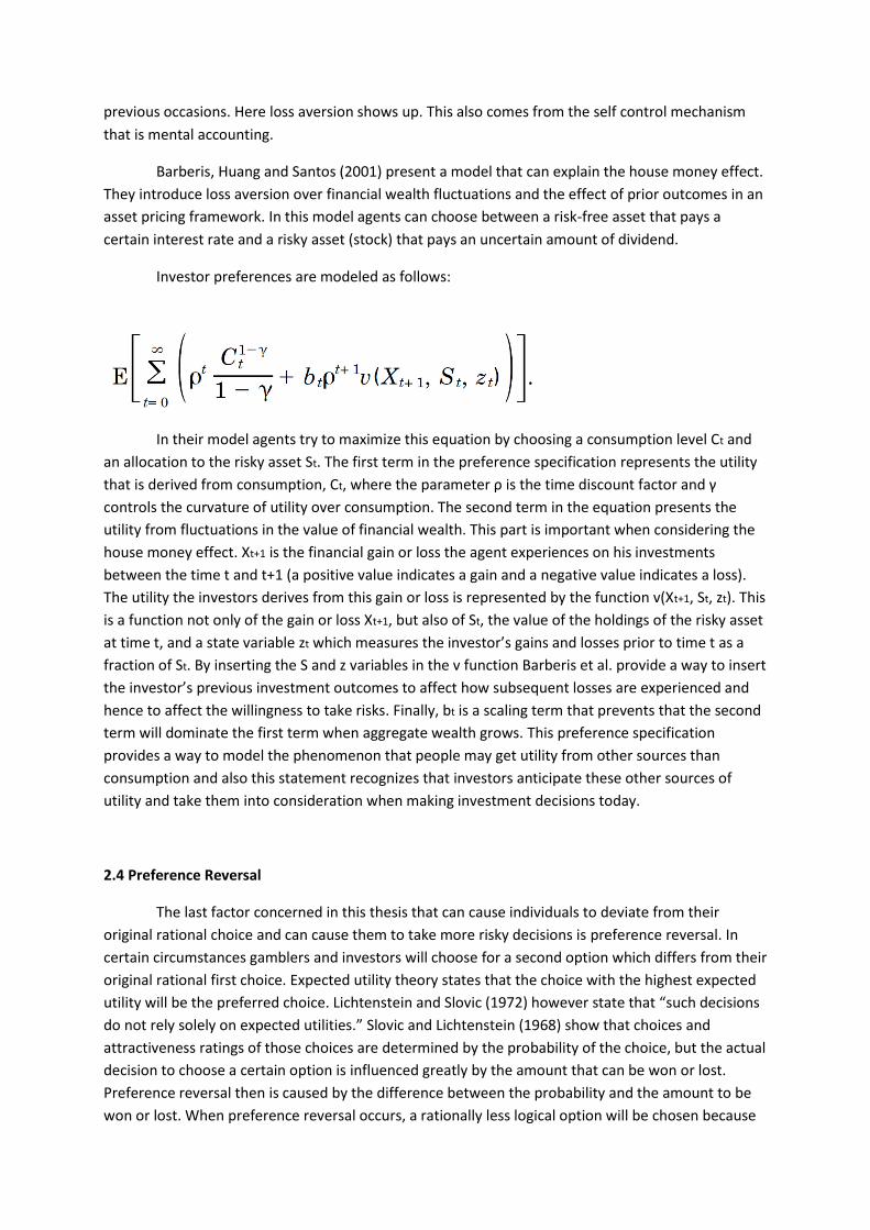
Investor preferences are modeled as follows:

In their model agents try to maximize this equation by choosing a consumption level Ct and

an allocation to the risky asset St. The first term in the preference specification represents the utility

that is derived from consumption, Ct, where the parameter ρ is the time discount factor and γ

controls the curvature of utility over consumption. The second term in the equation presents the

utility from fluctuations in the value of financial wealth. This part is important when considering the

house money effect. Xt+1 is the financial gain or loss the agent experiences on his investments

between the time t and t+1 (a positive value indicates a gain and a negative value indicates a loss).

The utility the investors derives from this gain or loss is represented by the function v(Xt+1, St, zt). This

is a function not only of the gain or loss Xt+1, but also of St, the value of the holdings of the risky asset

at time t, and a state variable zt which measures the investor’s gains and losses prior to time t as a

fraction of St. By inserting the S and z variables in the v function Barberis et al. provide a way to insert

the investor’s previous investment outcomes to affect how subsequent losses are experienced and

hence to affect the willingness to take risks. Finally, bt is a scaling term that prevents that the second

term will dominate the first term when aggregate wealth grows. This preference specification

provides a way to model the phenomenon that people may get utility from other sources than

consumption and also this statement recognizes that investors anticipate these other sources of

utility and take them into consideration when making investment decisions today.


The last factor concerned in this thesis that can cause individuals to deviate from their

original rational choice and can cause them to take more risky decisions is preference reversal. In

certain circumstances gamblers and investors will choose for a second option which differs from their

original rational first choice. Expected utility theory states that the choice with the highest expected

utility will be the preferred choice. Lichtenstein and Slovic (1972) however state that “such decisions

do not rely solely on expected utilities.” Slovic and Lichtenstein (1968) show that choices and

attractiveness ratings of those choices are determined by the probability of the choice, but the actual

decision to choose a certain option is influenced greatly by the amount that can be won or lost.

Preference reversal then is caused by the difference between the probability and the amount to be

won or lost. When preference reversal occurs, a rationally less logical option will be chosen because

the amount to be won or lost is greater. The amount that can be won or lost becomes the primary

determinant of choice, whilst originally the probability that an option actually will happen was the

initial primary determinant. To maintain the original rational option requires a great deal of self-

control.

This concludes chapter 2, the theoretical introduction of the factors that explain risk-taking

behavior by gamblers and investors. In the next chapter data will be gathered in order to prove the

existence of these four biases.

Chapter 3 Literature

This chapter will provide scientific papers that will investigate the existence of the biases

described in the previous chapter. Above all this will be a literature study. Scientific papers about the

particular factors will studied. The methods that are used and the results that are found will be

presented in the course of this chapter. First the hot hand will be addressed, then the gambler’s

fallacy, followed by the house money effect and preference reversal.

3.1 The hot hand

The term hot hand, as mentioned in the previous chapter, originally comes from basketball.

Gilovich, Vallone and Tversky (1985) looked for empirical evidence for the existence of the hot hand

in basketball. Both fans and professional basketball players believe that the chance of hitting a basket

is greater following a hit than following a miss. Gilovich et al. investigated both free throws of the

Boston Celtics and field goals of the Philadelphia 76ers. However, they found that the outcomes of

attempts were mostly independent of the outcome of the previous attempt. Also they found that the

frequency of streaks of hits in players’ records were not greater than the frequency predicted by a

binomial model that assumes a constant hit rate. Finally they conducted a controlled experiment

with the varsity players of Cornell University. For this experiment they had 14 men and 12 women, to

shoot from a distance from where their hit percentage was expected to be about 50 percent. Each

player had to take 100 shots, from different positions at the same distance. Players received a

financial reimbursement for their participation, the amount of money they received was determined

by how accurately they shot and how accurately the predicted their own hits and misses. Also for this

experiment Gilovich et al. found no significant correlation between shots. So, according to this

research there is no proof that the hot hand exists in basketball. This thesis however focuses on the

hot hand in gambling and investing.

Chau and Phillips (1995) investigated how blackjack players deviate from optimal play and

how their risk-taking behavior varies. They were questioned if people followed probabilistic theories.

Probabilistic theories assume people to be rational; to operate on numerical odds. Twelve

undergraduate students of the University of Hong Kong played computer blackjack for money. From

examining the behavior of these students Chau and Phillips found that long-term probabilities are

not sufficient to explain risk-taking behavior. “Players were sensitive to short-term fluctuations in

odds and recent outcomes, as well as to their control over skill-relevant factors.” From this Chau and

Phillips derive that their results do not support probabilistic models of risk-taking behavior; the

players did not always act rationally based on numerical odds. There is slight evidence for the hot

hand though. People who believe in the hot hand also do not act rationally on numerical odds. Chau

en Philips claim that the players were sensitive to recent outcomes, which is equal what the hot hand

is; bet more if one has won in the precious occasion. Players take the immediate outcomes as an

indication of their current luck. Players were found to increase their bets after a win and decrease

their bet after a loss.

Burns and Corpus (2004) also took a look at streaks and the choices of people. They had a

group of 195 students from the Michigan State University to participate in their study. The main

focus of this research was on the randomness of streaks. In different scenarios the participants had

to estimate the percentage of chance that the next event would be a continuation of the streak and

indicate how random they thought the outcomes were. The results Burns and Corpus found show

that participants were more likely to continue a streak when it was implied that the events were

generated by a nonrandom process. This makes sense when the hot hand is considered: if people

believe in the hot hand, they estimate the degree of randomness not accurately. It does not matter

how random or nonrandom the events actually are, but on how random/nonrandom the events are

judged to be by the participants. This also applies to the hot hand.

Croson and Sundali (2005) present results from real life casinos, using videotapes to examine

biases such as the hot hand in a naturalistic setting. The data come from the roulette tables in a

casino in Reno. To analyze if players’ behavior is consistent with hot hand beliefs Croson and Sundali

analyze if the players bet on more or fewer numbers in response to previous losses and wins. 80

percent of their subjects quit after losing on a spin while only 20 percent quit after winning. This part

is consistent with hot hand beliefs. From their data Croson and Sundali even made a regression to

calculate number of bets on a certain spin, when the result of the previous spin is known. The

regression involves an indicator valuable that states if the person has won or lost on the previous

spin, the number of bets on the previous spin and the number of bets on the very first spin as a

control for individual differences. The results of this regression Croson and Sundali created show that

winning a bet in trial t – 1 significantly increases the number of bets placed in trial t. This is consistent

with the hot hand bias.

Sundali and Croson (2006) also found a connection between the hot hand and the gambler’s

fallacy; this and other literature about the gambler’s fallacy will be addressed in the following

paragraph.

3.2 The gambler’s fallacy

The first paper that will be discussed regarding the gambler’s fallacy is the one from

Clotfelter and Cook (1991). They study state lotteries in order to test theories in risk-taking behavior

and decision-making under uncertainty. People who play in lotteries have several ways of picking

their numbers. They often pick their children’s birthdays, their own address numbers, their favorite

sportsman’s uniform number etc. For example in the state Maryland there was a three-digit betting

lottery. In this game the numbers 333 and 777 were picked nine times the average rate. Clotfelter

and Cook also detected the gambler’s fallacy in lottery play. In the Maryland three-digit game, the

amount bet on a number the day after it was hit dropped by a fourth and even dropped further to

about half its previous level on the second day. This effect especially occurs in lotteries with a fixed-

payout system: in Maryland a fixed amount 500 dollars on any winning bet was offered. Other

lotteries in other states used a pari-mutuel system for their number payouts. In this system less

money can be won by betting on the very popular numbers. This way players will spread their bets

more uniformly. Clottfelter and Cook found a flatter distribution of bets across all numbers in the

pari-mutuel system than in the fixed payout system.

The study by Chau and Phillips (1995), also mentioned in the previous paragraph about the

hot hand, addresses the gambler’s fallacy as well. Similar to the hot hand, players who are subject to

the gambler’s fallacy take into account the previous outcomes; they do not only act rationally on

long-term probabilities. Also players were found to have a self-serving bias; they attributed

successful outcomes to their own abilities and unsuccessful outcomes to bad luck, even though the

chances of winning or losing were predetermined. Players overestimate the degree of control they

had over the game. Finally Chau and Phillips state that we might have to change the criteria for

rationality in order deal with different systems of reasoning. One of these systems of reasoning can

possibly intend there is the gambler’s fallacy (and also the hot hand).

Terrel and Farmer (1996) present empirical data from the Woodlands Greyhound Park. Here

people can bet on dog and horse races. They present observed patterns of returns based upon a

model that divides bettors into two groups: one group that invests very little time and effort to

assess probabilities of outcomes and the other group that invests a lot of time and effort. They also

take into account information costs in their model. The gambler’s fallacy in this context would mean

that people estimate the chances of a dog that has won the previous race, to be lower in the current

race. Terrel and Farmer see slight evidence that this happens in dog race betting. The degree to

which the gambler’s fallacy is present in these circumstances varies between the two groups of

bettors. The pleasure gamblers (the ones that do not invest much effort and time) are more affected

by the gambler’s fallacy because they might base their bets more on superstition, because they do

not devote their time too much to acquiring the true probabilities of events. For the bettors that do

invest lots of time and effort the evidence for the gambler’s fallacy is much scarcer.

The research of Burns and Corpus (2004) as discussed before also addresses the gambler’s

fallacy. This research focuses on when people are inclined to continue a streak. They saw that the

participants had ‘a strong bias toward behavior consistent with the gambler’s fallacy’. After that they

list some of the factors that can explain why the gambler’s fallacy is so strong. The first is people

applying a law of small numbers. The representativeness heuristic causes people to believe that

every segment of a random sequence should reflect the true proportion. So a streak of one particular

event should and soon and be evened out by other events. Another explanation mentioned here is

that a bias to go against streaks would be successful when event are generated randomly but

without replacement (for example picking a card from a card deck and then throwing it away). The

gambler’s fallacy can be seen as an overgeneralization of this strategy when apply it to other

circumstances. A last explanation why the gambler’s fallacy can be so strong is that in some

situations that people call random they still believe in a “luck” factor, that produces nonrandom

outcomes. The experiment of Burns and Corpus does not distinguish between these different

possible explanations, but it does provide evidence that the randomness of an event may play a role

in people’s beliefs in the gambler’s fallacy.

Croson and Sundali’s study (2005) of the roulette tables also investigates the gambler’s

fallacy. The same data that were used to analyze hot hand beliefs are used for the gambler’s fallacy.

For this part Croson and Sundali focus on outside bets in roulette (Odd/Even, Red/Black, Low/High).

A bet is classified to be consistent with the gambler’s fallacy if it bets against a streak of length n.

Where a streak of length n is just the number of times a popular outcome has occurred consecutively

in the past. In the figure below Croson and Sundali show the bets that are classified as gambler’s

fallacy bets in black. The figure shows the findings of Croson and Sundali about betting streaks.

Source: Croson and Sundali (2005)

On the horizontal axis n, the length of the streak is shown. So for example of the 130 bets

that were placed after a streak of length three, 52 percent were gambler’s fallacy bets. From this

table it can be concluded that the longer the streak, the more consistent the behavior of gamblers

will be with the gambler’s fallacy. Especially for streaks of length 5, and 6 and above the results are

significant.

In the next paper of Sundali and Croson (2006) use their data from the previous study

(Croson and Sundali (2005)) to establish a connection between the hot hand and the gambler’s

fallacy. First identifying the two biases within a given individual and then examining their within-

person correlation, they find a positive and significant correlation between the hot hand and the

gambler’s fallacy across individuals. They place all players in categories, being a hot hand, stock of

luck, hot outcome or gambler’s fallacy player. After this they analyzed and found that players who

act consistently with the gambler’s fallacy (betting on numbers that have not appeared previously),

are more likely to show behavior consistent with the hot hand (increasing the number of bets after

they had won.) As an opposite of this, players that act consistently with the hot outcome (betting on

numbers that have often appeared previously) are found to be more likely to show behavior

consistent with the stock of luck bias (decreasing the number of bets after a win). Sundali and Croson

propose locus of control as an explanation for these findings. Locus of control is defined as “a belief

about whether the outcomes of our actions are contingent on what we do (internal locus of control)

or on events outside our personal control (external control orientation)”. A person with internal locus

of control attributes outcomes to personal effort and decision, whereas a person with external locus

of control attributes the same outcomes to chance and other external factors. Applied to gambling, a

person with internal locus of control will attribute the wins he made to personal decisions and skill. If

a player with internal locus of control has won because of skill he thinks these gambling skills will

lead to more wins. This explains the strategy of betting more after wins, exercising hot hand

behavior. These kinds of players do not believe in randomness; they believe that the outcomes are

controlled by some process that can be learned by the use of skill. A win for these players serves as a

validation that he has learned the pattern and this confidence will cause him to bet more on the next

gamble. According to Croson and Sundali “The most plausible cognitive explanation for her supposed

pattern-detecting skill is representativeness, which explains why she bets consistently with the

gambler’s fallacy.” This way Croson and Sundali suggest the explanation that the internal locus of

control causes both hot hand and gambler’s fallacy beliefs.

3.3 The house money effect

Thaler and Johnson (1990) investigate the effects of prior gains and losses on subsequent

risky choices. They state that after a gain, subsequent losses that are smaller than the original gain

can be integrated with the original gain, which decreases the effect of loss-aversion and increases

risk-seeking. Gamblers are less concerned losing their gains than losing their own money. In the

experiment investigating the house money effect posed by Thaler and Johnson they found that 77

percent of the participants were more risk-seeking after a gain. On the other hand they find evidence

for break-even effects: prior losses will lead to less risk-seeking in subsequent events. This is caused

by the change of reference point: the amount of own money is decreased. Thaler and Johnson

suggest that both these effects (break even and house money) can be explained by a change of

mood. Players who win on the first occasion become in a good mood, while players who experience

an initial loss become in a negative mood. The mood can affect risk-taking behavior strongly, as

shown by Isen, Means, Patrick and Nowicki (1982). Secondly Thaler and Johnson pose that the initial

loss can cause a stock of luck effect; gamblers think it is not their lucky day and that their actual

chance of winning is lower than the real probability. Similar to this a prior gain can cause a hot hand

effect.

The house money effect is also considered shortly by Croson and Sundali (2006). When

explaining the hot hand they state that the house money effect can be a false cause of the hot hand.

People bet on more numbers because they get richer, they have won house money. They do not bet

on more numbers because they are personally more likely to win.

Other papers that are available about the house money effect mainly digress about the

effects on investment decisions, rather than on casino gambling situations. Therefore these papers

will be addressed in the next chapter.


Lichtenstein and Slovic (1971) did three experiments investigating preference reversal. In

each experiment the participants were given the choice between the P-bet (the bet with the highest

probability) and the $-bet (the bet with the highest payoff). After this they were given the

opportunity to bid for the other bet. In all three experiments the participants frequently chose one of

the two bets initially and subsequently bid more for the bet they did not choose. This demonstrates

preference reversal. Across the three experiments the frequency of the reversals somewhat varied,

but the frequency was always greater than could be explained by individual unreliability alone.

Lichtenstein and Slovic explain this preference reversal by changes in the decision processes that

underlie bids and choices. Information processing happens differently for bids than for choices. For

choices there is no natural starting point (as the participants need not pay for the initial choice). But

for the bidding there is: the starting point is the amount to be won. The amount to win therefore

dominates bids but not choices

Rachlin and Green (1972) conducted an experiment about preference reversal on pigeons. In

this study they wanted to test self-control, also for gamblers (and investors) a very important

attribute. The pigeons were first offered a choice (Choice Y) between a small, immediate award

(immediate 2 second exposure to grain) and a larger reward (4 seconds exposure to grain with a

delay of 4 seconds). In this event the pigeons preferred the small immediate reward. But when

offered a different choice (Choice X) between 1: a delay of T seconds followed by Choice Y or 2: a

delay of T seconds followed by the large reward only the choice of the pigeons depended on T. When

T was small, the pigeons chose for Choice Y, (followed by choosing the small reward) and when T was

large the pigeons chose the large reward only. So as T increases preference reversal occurs. The

preference for the large delayed alternative depicts a certain degree of commitment to a given

choice. This can also apply to humans when making saving decisions or gamblers committing to a

certain gambling pattern. Such commitment can be seen as a way of exercising self-control.

In the next chapter ways to link the gambling biases that were discussed to investment

decisions will be searched for in the available academic literature.

Chapter 4 Analysis

In this part the four biases that have been discussed before will be linked to investment

decisions. Scientific papers discussing the biases on investors will be studied.

4.1 The Hot Hand

When applied to investment decisions, the hot hand bias would mean that an investor would

expect himself to make a profit with a new investment decision when previous investments had paid

off. In this situation the investor would be very confident about his own judgment of investment

decisions. On the other hand if an investor believes in stock of luck he will expect to lose money with

a new investment if the previous investments had paid off. Therefore he will not invest in new risky

choices after a streak of successful investments.

Shefrin and Statman (1985) investigate the feature of aversion to loss realization. A

theoretical framework of this behavior pattern is developed. The concerns the general disposition

investors have to sell winners too early and hold losers too long. In other words investors are often

inclined to sell assets that earn them profits too early (the asset could earn more profit if held longer)

and to keep assets that make losses too long (the asset makes more losses over time, while the

investor hopes it will become profitable). One of the factors that can explain this is the tendency

people have to seek pride and avoid regret; people are embarrassed to admit they made a loss. In

the second part of their research Shefrin and Statman provide empirical evidence for the patterns of

loss and gain realization. They are concerned about the time that passes between the point when an

investor buys a stock and the point when he sells it. The main interest here is whether investors time

the realization of their losses differently from the realization of their gains. From the evidence they

collected Shefrin and Statman conclude that the disposition to sell winning stocks and hold losing

stocks shows up in real financial markets and not only in laboratory experiments. Investors use less

time to realize their wins and more to realize their losses.

Applying this paper to the hot hand theory would suggest evidence for stock of luck beliefs;

the opposite of the hot hand. After winning on a certain stock, people believe that their amount of

luck is depleted and sell the stock. On the other hand they keep losing stocks because they believe

they should get ‘lucky’ soon because they have had bad luck on recent occasions.

Odean (1998) investigates the disposition effect as well. For his study he obtained the trading

records for 10.000 accounts from January 1987 to December 1993 at a large discount brokerage

house. These accounts were randomly selected from all active accounts (with at least one

transaction). In total 162.948 trades were recorded in the given period. Accounts that were closed

during the time slot were not replaced; therefore the data may have some kind survivorship bias in

favor of the more successful investors. Odean, like Shefrin and Statman (1985) focuses on whether

investors sell their winning stocks too early and hold their losing stocks too long. Odean puts the

question if investors realize their wins earlier than their losses. As an illustration of the findings of

Odean the graph below shows the ratio of the proportion of the gains realized (PGR) to the

proportion of losses realized (PLR) for each month. The gains and the losses are aggregated across all

accounts in the data set and over the entire time span.

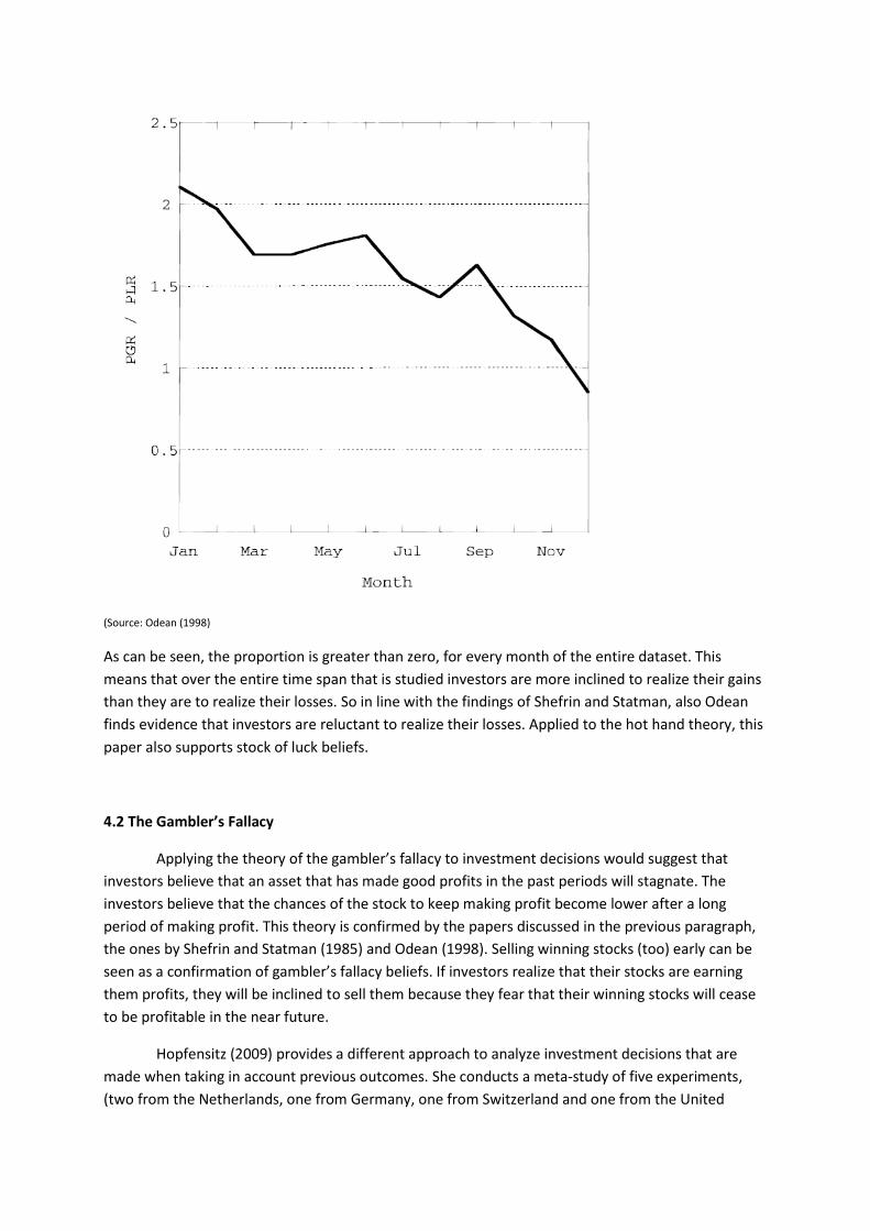
(Source: Odean (1998)

As can be seen, the proportion is greater than zero, for every month of the entire dataset. This

means that over the entire time span that is studied investors are more inclined to realize their gains

than they are to realize their losses. So in line with the findings of Shefrin and Statman, also Odean

finds evidence that investors are reluctant to realize their losses. Applied to the hot hand theory, this

paper also supports stock of luck beliefs.


Applying the theory of the gambler’s fallacy to investment decisions would suggest that

investors believe that an asset that has made good profits in the past periods will stagnate. The

investors believe that the chances of the stock to keep making profit become lower after a long

period of making profit. This theory is confirmed by the papers discussed in the previous paragraph,

the ones by Shefrin and Statman (1985) and Odean (1998). Selling winning stocks (too) early can be

seen as a confirmation of gambler’s fallacy beliefs. If investors realize that their stocks are earning

them profits, they will be inclined to sell them because they fear that their winning stocks will cease

to be profitable in the near future.

Hopfensitz (2009) provides a different approach to analyze investment decisions that are

made when taking in account previous outcomes. She conducts a meta-study of five experiments,

(two from the Netherlands, one from Germany, one from Switzerland and one from the United

States) all varying in number of participants and number of rounds) providing the participants with

an investment task. The participants each had to make a decision on how to divide their available

points between a safe and a risky project. The expected value of the safe project was one point per

invested point, the expected value of the risky project was 1.17. The earnings from previous rounds

could not be used in the next round (which is why this study cannot be used when addressing the

house money effect later). The maximum amount of points therefore stayed constant throughout all

rounds in the study. When analyzing the investment behavior across all rounds it is observed that the

participants display signs of the gambler’s fallacy. When having won in the last or second to last

round the overall tendency is to invest less in the following round. In this sense this paper also

provides proof for existence of the gambler’s fallacy.


The house money effect applied to investment decisions is very easily explained. If investors

have gained profits from the investments they did with their own money, mental accounting causes

that they do not see their profits as their own money. Therefore they are willing to take more risks

with their profits.

Liu, Tsai Wang and Zhu (2006) study the Taiwan Futures Exchange (TAIFEX) in order to find

evidence for the house money effect. For their research Liu et al. obtained trading data from the

TAIFEX for 753 trading days between December 2001 and December 2004. The options from the

TAIFEX have become very popular financial products from 2003 on. In 2003 the TAIFEX options were

ranked fourth among all the index options in the world and second in Asia in terms of numbers of

traded lots. What Liu et al. basically did was look at the relation between trading outcomes in the

morning and risk-taking in afternoon trading for 21 professional traders. This way they offer analysis

on the shortest period possible, providing a ‘clean’ context to investigate the influence of previous

outcomes on subsequent behavior. During a very short period other factors are less likely to affect

investors’ behavior than during longer periods. In gambling subsequent betting rounds appear within

a short period of time as well. An illustration of their many findings is shown in the figure below.

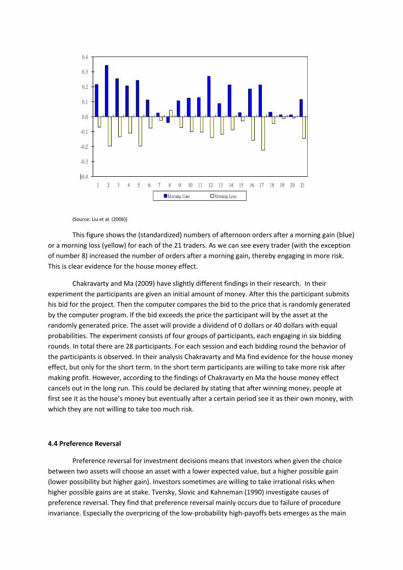
(Source: Liu et al. (2006))

This figure shows the (standardized) numbers of afternoon orders after a morning gain (blue)

or a morning loss (yellow) for each of the 21 traders. As we can see every trader (with the exception

of number 8) increased the number of orders after a morning gain, thereby engaging in more risk.

This is clear evidence for the house money effect.

Chakravarty and Ma (2009) have slightly different findings in their research. In their

experiment the participants are given an initial amount of money. After this the participant submits

his bid for the project. Then the computer compares the bid to the price that is randomly generated

by the computer program. If the bid exceeds the price the participant will by the asset at the

randomly generated price. The asset will provide a dividend of 0 dollars or 40 dollars with equal

probabilities. The experiment consists of four groups of participants, each engaging in six bidding

rounds. In total there are 28 participants. For each session and each bidding round the behavior of

the participants is observed. In their analysis Chakravarty and Ma find evidence for the house money

effect, but only for the short term. In the short term participants are willing to take more risk after

making profit. However, according to the findings of Chakravarty en Ma the house money effect

cancels out in the long run. This could be declared by stating that after winning money, people at

first see it as the house’s money but eventually after a certain period see it as their own money, with

which they are not willing to take too much risk.


Preference reversal for investment decisions means that investors when given the choice

between two assets will choose an asset with a lower expected value, but a higher possible gain

(lower possibility but higher gain). Investors sometimes are willing to take irrational risks when

higher possible gains are at stake. Tversky, Slovic and Kahneman (1990) investigate causes of

preference reversal. They find that preference reversal mainly occurs due to failure of procedure

invariance. Especially the overpricing of the low-probability high-payoffs bets emerges as the main

cause of preference reversal. Tversky, Slovic and Kahneman interpret the overpricing of long shots as

“an effect of scale compatibility: because the prices and the payoffs are expressed in the same units,

payoffs are weighted more heavily in pricing than in choice. “ The possible winnings are considered

more important than the probabilities.

Cox and Grether (1996) conducted experiments on preference reversal and found that in

different circumstances preference reversal happens on different levels. They observe the preference

reversal phenomenon strongly on the short term in a market setting. For this market setting they use

a second price auction. In this type of auction the highest bidder wins, but only pays the price the

second-highest bid. This gives bidders the incentive to bid their true value. However, Cox and Grether

find that after five repetitions of the auction the bids of the subjects are in general consistent with

their choices and the preference reversal phenomenon disappears.

Chapter 5 Conclusion

In this thesis the existing literature about gambling fallacies has been studied in order to

come up with an answer to the research question: ‘Do investors have the same irrationalities that

gamblers have in their risk-taking behavior?’

In order to get to an answer to this question the sub question ‘What factors cause gamblers

to be irrational in their risk-taking behavior?’ was posed. First in chapter 2 four biases or fallacies that

occur in gambling were introduced: the hot hand, the gambler’s fallacy, the house money effect and

preference reversal. Then in chapter 3, evidence for the existence of these four biases in gambling

was sought after in the existing literature.

First the hot hand; Chau and Philips (1995) found evidence for the hot hand in blackjack,

Burns and Corpus (2001) found evidence for the hot hand when outcomes are believed to be

generated by a nonrandom process and Croson and Sundali (2005) found evidence for the hot hand

in roulette. From these three papers it can be concluded that the hot hand actually exists in

gambling. Second the gambler’s fallacy; Clotfelter and Cook (1991) detect the gambler’s fallacy in

lottery play, Chau and Philips find proof for gambler’s fallacy beliefs when players experience bad

luck and Burns and Corpus as well as Croson and Sundali find data that prove both the existence of

the hot hand and the gambler’s fallacy. This is explained by the locus of control as described by

Sundali and Croson (2006). Then the house money effect; Thaler and Johnson (1990) find prove for

the house money effect explained by a change of mood. Croson and Sundali also state that the house

money effect can be a false cause of the hot hand. Finally preference reversal; Lichtenstein and Slovic

(1971) as well as Rachlin and Green (1972) find evidence for the existence of preference reversal.

From all these papers it can be concluded that all four biases do exist in gambling. To answer the sub

question: the hot hand, the gambler’s fallacy, the house money effect and preference reversal all

cause gamblers to be irrational in their risk taking behavior.

In chapter 4 the literature for existence of the four gambling fallacies for investors was

studied. The question is whether investors are subject to the same biases than gamblers. Addressing

the hot hand both Shefrin and Statman (1985) and Odean (1998) find no evidence for the hot hand in

investing. On the contrary; they find evidence for stock of luck beliefs, in the disposition to sell

winning stocks and hold losing stocks. Therefore the hot hand for investors has not been proved in

this thesis. In line with this reasoning, one can state that these Shefrin and Statman and Odean

provide proof for the gambler’s fallacy. Also Hopfensitz (2009) provides data that supporting the

existence of the gambler’s fallacy for investors. Liu et al. (2006) provide evidence for the house

money effect on the stock Taiwan Futures exchange. Chakravarty and Ma (2009) also support the

house money effect, but only in the short run. The same holds for the findings of Cox and Grether

(1996) on preference reversal: it cancels out in the long run. Tversky et al. (1990) however support

the existence of preference reversal. Summing up, all four fallacies that are present for gamblers can

affect investors as well, although the degree to which investors are influenced by these fallacies

differs. Investors are affected most by the gambling fallacy, followed by the house money effect and

preference reversal and they are less affected by the hot hand. Future research should focus on

finding empirical evidence for real-world existence of the four biases. The gambling biases are mostly

confirmed in laboratory studies, but real hard evidence supporting the existence of the biases in the

world of investors is scarce.

References

Barberis, N., Huang, M. & Santos, T. (2001), Prospect Theory and Asset Prices. The Quarterly

Journal of Economics, 116, (1), 1-53.

Burns, B. & Corpus, B. (2004), Randomness and inductions from streaks: “Gambler’s fallacy”

versus “hot hand”. Psychonomic Bulletin & Review, 11, (1), 179-184.

Chakravarty, S. & Ma, Y. (2009), A Reexamination of the House Money Effect: Rational

Behavior or Irrational Exuberance? Working Paper Purdue Universit, West Lafayette.

Chau, A. & Phillips, J. (1995), Effects of Perceived Control upon Wagering and Attributions in Computer Blackjack. The Journal of General Psychology, 122, (3), 253-269. Clotfelter, C. & Cook, P. (1991), Lotteries in the Real World. Journal of Risk and Uncertainty, 4, (3), 227-232. Cox, J. & Grether, D. (1996), The preference reversal phenomenon: Response mode, markets and incentives. Economic Theory, 7, 381-405. Croson, R. & Sundali, J. (2005), The Gambler’s Fallacy and the Hot Hand: Empirical Data from Casino’s. The Journal of Risk and Uncertainty, 30, (3), 195-209. Gilovich, T., Vallone R., & Tversky, A. (1985), The Hot Hand in Basketball: On the Misperception of Random Sequences. Cognitive Psychology, 17, 295-314. Grether, D. & Plott, C. (1979), Economic Theory of Choice and the Preference Reversal Phenomenon. The American Economic Review, 69, (4), 623-638. Hopfensitz, A. (2009), Previous outcomes and reference dependence: A meta study of repeated investment tasks with and without restricted feedback. MPRA Working Paper No. 16096

Isen, A. M., B. Means, R. Patrick & G.P. Nowicki, (1982) “Positive Affect and Decision Making” In M.S. Clark & Fiske (Eds). Affect and Cognition, Erlbaum, Hillsdale, NJ. Lichtenstein, S. & Slovic, P. (1971), Reversals of Preference between bids and choices in gambling decisions. Journal of Expirimental Psychology, 89, (1), 46-55. Liu, Y., Tsai, C., Wang, M. & Zhu, N. (2006), House Money Effect: Evidence from Market Makers at Taiwan Futures Exchange. Working paper. University of California, Davis and National Chengchi University. Odean, T. (1998), Are Investors Reluctant to Realize Their Losses? The Journal of Finance, 53, (5), 1775-1797. Rachlin, H. & Green, L. (1972), Commitment, Choice and Self-control. Journal of the Experimental Analysis of Behavior, 17, (1), 15-22. Shefrin, H. & Statman, M. (1985), The Disposition to Sell Winners Too Early and Ride Losers Too Long: Theory and Evidence. The Journal of Finance, 40, (3), 777-790.

Sundali, J. & Croson, R. (2006), Biases in casino betting: The hot hand and the gambler’s fallacy. Judgment and Decision Making, 1, (1), 1-12. Terrel, D. & Farmer, A. (1996), Optimal Betting and Efficiency in Parimutuel Betting Markets with Information Costs. The Economic Journal, 107, (437), 846-868. Thaler, R. & Johnson, E. (1990), Gambling with the house money and trying to break even: The effects of prior outcomes to risky choice. Management Science, 36, (6), 643-660. Thaler, R. & Sunstein, C. (2009), Nudge. London; Penguin Books

Tversky, A., Slovic P., & Kahneman, D. (1990), The Causes of Preference Reversal. The

American Economic Review, 80, (1), 204-217.

Tversky, A. & Thaler, R. (1990), Anomalies: Preference Reversals. The Journal of Economic

Perspectives, 4, (2), 201-211.

Weber, M. & Zuchel, H. (2001), How Do Prior Outcomes Affect Ricky Choice? Further

Evidence on the House-Money Effect and Escalation of Commitment. Working Paper, Universität

Mannheim

gambling biases - tilburg university

Documents