extinction risk, coloured noise and the scaling of variance
TRANSCRIPT
1
Extinction risk, coloured noise and the scaling of variance
Matthias C. Wichmann1, * Karin Johst2
Monika Schwager3
Bernd Blasius4 Florian Jeltsch3
1) CEH Dorset, Winfrith Tech. Centre, Winfrith Newburgh, Dorchester, Dorset, DT2 8ZD, UK 2) UFZ Centre for Environmental Research, Department of Ecological Modelling, Permoser Str. 15, D-04318 Leipzig, Germany 3) University of Potsdam, Department of Biochemistry and Biology, Plant Ecology and Nature Conservation, Maulbeerallee 2, D-14469 Potsdam, Germany 4) University of Potsdam, Department of Physics, Nonlinear Dynamics, Am Neuen Palais 10, D-14469 Potsdam, Germany *) corresponding author, e-mail: <[email protected]>, Phone: ++44 1305 213583, Fax: ++44 1305 213600,
Running head: Extinction risk and coloured noise
2
ABSTRACT
The impact of temporally correlated fluctuating environments (coloured noise) on the
extinction risk of populations has become a main focus in theoretical population ecology. In
this study we particularly focus on the extinction risk in strongly correlated environments. 5
Here, we found that, in contrast to moderate autocorrelation, the extinction risk was highly
dependent on the process of noise generation, in particular on the method of variance scaling.
Such scaling is commonly applied to avoid variance-driven biases when comparing the
extinction risk under white and coloured noise. We show that for strong auto-correlation
often-used scaling techniques lead to a high variability in the variances of the resulting time 10
series and thus to deviations in the subsequent extinction risk. Therefore, we present an
alternative scaling method that always delivers the target variance, even in the case of strong
autocorrelation. In contrast to earlier techniques, our very intuitive method is not bound to
auto-regressive processes but can be applied to all types of coloured noises. We strongly
recommend our method to generate time series when the target of interest is the effect of 15
noise colour on extinction risk not obscured by any variance effects.
Key words: environmental noise, noise colour, auto-correlation, population dynamics,
extinction risk, variance scaling
3
INTRODUCTION 20
Research into theoretical population ecology has focused on factors impacting populations’
performance and hence their extinction risk. On the one hand, these factors include all the
parameters characteristic to the system (e.g. birth rate, mortality, intra-specific competition,
carrying capacity) yielding the population’s growth rate and competition mode. On the other
hand, these factors are subject to variations in time – often-called noise – occurring as 25
demographic noise (intrinsic to the population) and environmental noise (extrinsic to the
population). While demographic noise is regarded as temporally uncorrelated (white noise),
environmental noise is known to be often auto-correlated to various degrees (Steele, 1985;
Pimm and Redfearn, 1988; Lande, 1993; Halley, 1996).
There are at least four descriptive attributes of time series of environmental noise affecting 30
corresponding population dynamics: (1) the mean, (2) variance, (3) the frequency distribution
of values and (4) noise colour, i.e. temporal auto-correlation. The effects of the first two
attributes, the mean and variance, have been studied extensively during the past (e.g. Goel and
Richter-Dyn, 1974; Roughgarden, 1975; Tuljapurkar, 1989; Lande, 1993; Foley, 1994; Wissel
et al., 1994). The third attribute, frequency distribution, remains insufficiently studied and has 35
not been primarily addressed by any publications. Recent research has focused on the fourth
attribute, i.e. the colour of environmental noise, and complex relationships have been found
between noise colour, underlying population dynamics and extinction risk by several authors
(Roughgarden, 1975; Ripa and Lundberg, 1996; Johst and Wissel, 1997; Petchey et al., 1997;
Kaitala et al., 1997a; b; Heino, 1998; Halley and Kunin, 1999; Cuddington and Yodzis, 1999; 40
Ripa and Heino, 1999; Ripa and Lundberg, 2000). All these studies emphasized the
importance of considering the colour of environmental noise in studies of population
dynamics and extinction risk.
In this paper we investigate the effects of temporally correlated fluctuating environments on
population dynamics. While auto-correlation has been found to cause severe effects on the 45
dynamics and extinction risk of populations (e.g. Ripa and Lundberg, 1996), the noise
generating process is particularly important when studying the effects of strong auto-
correlation (Heino et al., 2000). Cuddington and Yodzis (1999) investigated the effects on
population dynamics where underlying environmental noise is best described as 1/fb noises.
However, results of these authors may not apply when the underlying environmental noise 50
can be better described by auto-regressive processes. Such auto-regressive processes have
been frequently used to study population dynamics and extinctions risk in fluctuating

4
environments (Ripa and Lundberg, 1996; Johst and Wissel, 1997; Petchey et al., 1997; 2000;
Kaitala et al., 1997a; b; Heino, 1998; Ripa and Heino, 1999; Ripa and Lundberg, 2000;
Wichmann et al., 2003a; b). 55
Therefore, we study the impact of auto-regressive environmental noise on population
dynamics and the resulting extinction risk. We compare various procedures to generate
coloured noise putting emphasis on highly autocorrelated environments. Here, we evidence
the impact of the noise generating process on the estimated extinction risk and the according
biological implications. In particular, we reveal that, depending on the method of scaling the 60
variance, differences in the subsequent extinction risk arise. We then propose an alternative
method of generating coloured noise with specific target variance. This method is very simple
to handle when assessing extinction risk. It is particularly appropriate for the generation of
strongly correlated noise of any type.
5
EXTINCTION RISK IN AUTOCORRELATED ENVIRONMENTS 65
Background
Populations are always under the influence of noisy environments. Such environmental noise
has important effects on population dynamics as it has long been recognised by ecologists. In
particular, it is common knowledge that deterministically growing populations can be driven
to extinction by environmental noise. In general, the actual risk of population extinction is 70
increasing with the strength of environmental noise. This has been studied by numerous
authors (Goel and Richter-Dyn, 1974; Roughgarden, 1975; May and Oster, 1976; Mode and
Jacobsen, 1987; Tuljapurkar, 1989; Lande, 1993; Morales, 1999).
Usually, in these studies non-correlated noise has been used. However, in practice
environmental noise is autocorrelated, i.e. coloured (Steele, 1985; Lawton, 1988; Pimm and 75
Redfarn, 1988; Halley, 1996). Hence, the danger of using white noise instead of red noise for
projections of extinction risk has been highlighted (e.g. Morales, 1999). Consequently, the
issue of calculating the extinction risk in auto-correlated environments has been targeted by
numerous earlier studies. However, while some of these studies suggest decreased extinction
risk in coloured environments (e.g. Ripa and Lundberg, 1996; Heino et al., 2000) other 80
studies found increased extinction risk (e.g. Mode and Jacobsen, 1987; Foley, 1994; Johst and
Wissel, 1997; Wichmann et al., 2003b). Cuddington and Yodzis (1999), as well as Morales
(1999) suggest that these contradicting results might be driven by different structures of the
noise generation process.
Therefore, in this section we compare the extinction risk in auto-correlated environments for 85
various types of the generating auto-regressive process (AR1). In a later section the technical
differences and biological appropriateness among these types of generation are discussed in
more detail and we finally recommend a practical alternative.
Methods to calculate the extinction risk
For all calculations of extinction risk, we use a well-known model of population dynamics, 90
the Maynard Smith-Slatkin model (Maynard Smith and Slatkin, 1973; May and Oster, 1976;
Bellows, 1981):
( )b
t
t
tt
KNR
RNN
⎟⎟⎠
⎞⎜⎜⎝
⎛−+
=+
*11
*1 [Equation 1]
6
where N describes the population size at time steps t and t+1, respectively. R is the growth
rate, Kt is the carrying capacity at time step t and b is a competition parameter controlling the 95
dynamic behaviour of the model (compare Petchey et al., 1997). We chose this model since it
was found to be particularly flexible, broadly applicable and well capable to describe a wide
range of data (Bellows, 1981).
We studied the extinction risk for short time scales of 50 time steps and longer time scales of
1,000 time steps. For our simulations we chose a parameter set of Kmean=100, R=4.5 and 100
b=1.0. Demographic noise was included by letting Nt+1 be an integer number Zt drawn from a
Poisson distribution with the deterministic expectation for Nt+1 as its mean, i.e. Nt+1 = Zt(Nt+1)
(Petchey et al., 1997). Environmental noise was generated according to the temporally
correlated fluctuating quantity, Φt, with
11 ++ ∗+Φ∗=Φ ttt εβα . [Equation 2] 105
Here, εt is a random number drawn from a normal distribution with unit variance and zero
mean, β is a scaling parameter that sets the overall variance of the time series and the initial
value is arbitrarily set to zero, Φ0=0. Note, that auto-correlation coefficient α > 0 corresponds
to positive temporal correlations (“red noise”). We varied α in steps of 0.05 between 0.00 and
0.95 but we also studied α=0.99. Standard deviation σ was also varied (σ=25; 30; 35; 40; 45) 110
using the factor β in Eq.(2). The variance, σ2, was then rescaled according to different
approaches resulting in various guises of the AR1 process.
According to the length of population time series we used two different commonly applied
approaches of variance rescaling. When generating long time series for 1,000 population time
steps (Fig.1a) we followed Ripa and Lundberg (1996) (compare Eq.4 below) but for short 115
time series of 50 time steps we rescaled variances according to Heino et al. (2000) (compare
Eq.5 below). For both, short and long time series, we also used an alternative approach of
variance correction, which will be presented in detail in the technical section of this paper
(Eq.6 below).
The resulting time series of environmental noise had an additive effect on the mean carrying 120
capacity K, i.e. Kt = Kmean + Φt. In the case of Kt<0 we set Kt=0 in order to avoid artificially
negative values for carrying capacity. The rules of this model are very close to those of earlier
investigations which used the Ricker equation instead of the Maynard Smith-Slatkin model
(Ripa and Lundberg, 1996; Petchey et al., 1997; Cuddington and Yodzis, 1999; Heino et al.,
2000). 125
7
Results on extinction risk
With our calculations of extinction risk we were able to reproduce the results of earlier studies
when using conventional scaling methods (Ripa and Lundberg, 1996 and Heino et al. 2000;
for example compare Fig.1a and Fig.1d, with Fig.4c and 3b in Heino et al., 2000,
respectively). This agreement underlines that the deviations in extinction risk highlighted in 130
Fig.1c and f are due to different rescaling techniques but not to the usage of deviating models
of population dynamics.
Fig.1 shows the calculated extinction risks for commonly applied rescaling methods (Fig.1a,
d)and an alternative method presented here (Fig.1b, e) on two different time scales based on
10,000 repeated simulation runs. In particular, Fig.1c and f evidence that both methods 135
produce consistent results for small and intermediate auto-correlation but different results for
high auto-correlation.
Note that these results in principle maintain when assuming T=1,000 to be a “short” time
series and replacing the approach by Ripa and Lundberg (1996) by the more cumbersome
approach of Heino et al. (2000). It remains, however, indistinct why extinction risk on 140
different time scales is driven in different directions (Fig.1c,f). We conclude that, concerning
the resulting extinction risks, (1) the choice of the rescaling method does not matter for
moderate auto-correlation but (2) this choice obviously becomes very important for strongly
auto-correlated environmental noise (Fig.1c,f).
Therefore, in the following main part of this paper we review alternative methods of variance 145
rescaling. In particular, we point out limitations of commonly applied methods and we
evidence the variability in autocorrelated time series. We then introduce a practical
alternative.
8
THE ISSUE OF GENERATING COLOURED NOISE
Usually, when investigating the effects of noise colour on extinction risk, one is faced with 150
the problem to generate random time series with given colour. Therefore, an original time
series of white noise is dyed, i.e. the temporal correlation of environmental fluctuations is
modified in order to study the resulting effects on population dynamics. For this purpose a
AR1 process (Eq.2) is often used to generate the temporally correlated fluctuating quantity, Φt
(alternatively cf. Cuddington & Yodzis 1999). Note, that in Eq.(2) a possible bias by 155
initialising Φ0=0. is customary removed by omitting an initial transient of Φ. The time series
of an environmental parameter, for example the carrying capacity K, then is calculated as Kt =
K0+Φt with K0 being the desired average.
When modifying the colour of time series according to Eq.(2), however, a problem arises: As
the standard deviation of the AR1-process (Eq.2) is given by 160
21 αβσ−
= , [Equation 3]
modifications in the degree of auto-correlation, α, always entail a change in variance σ2 of Φ
(Roughgarden, 1975; Chatfield, 1984; Ripa and Lundberg, 1996). Since |α|<1 Eq.(3) implies
that this variance is always larger than the variance of the underlying white noise, σ2>β2.
Thus, one faces the problem that “the effects of change in colour will be masked by the 165
effects of [changing] variance” (Heino et al., 2000, p. 178). Hence, various techniques have
been developed to rescale the time series depending on the auto-correlation parameter α such
that the red noise of different α and white noise can be compared on the basis of the same
variance (Chatfield, 1984; Heino et al., 2000).
However, as we show these scaling techniques are very intricate and can lead to ambiguous 170
results, in particular for strong auto-correlation (Fig.1). In our study we explore new
approaches for tackling these problems in order to avoid variance-induced biases when
calculating the extinction risk of populations in coloured environments. This includes a novel
alternative to the current practice of generating dyed time series.

9
SCALING TO EXPECTED VARIANCE 175
Scaling to expected asymptotic variance
As pointed out in the introduction problems arise by the generation of coloured time series
since the variance of the time series resulting from the AR1-process depends on the
autocorrelation parameter α (Eq.3). Those problems can be circumvented by rescaling Φt and
choosing an appropriate value of the free parameter β in Eq.(2). Many authors (Roughgarden, 180
1975; Foley, 1994; Ripa and Lundberg, 1996; Petchey et al., 1997; Cuddington and Yodzis,
1999 and others) used a factor that scales the coloured noise to the desired asymptotic
variance σ∞2 depending on the auto-correlation coefficient α
21)( ασαββ −=≡ ∞ . [Equation 4]
Note that Eq.(4) corrects the variance as it is expected to result from the AR1 process (Eq.2). 185
Scaling to expected variance over a certain time scale T
When studying Eq.(4), Heino et al. (2000) pointed out that the expected variance, σT2, of short
coloured time series of finite length T may deviate from the asymptotic variance, σ∞2, i.e.
from the expected variance of an infinitely long time series. These findings confirm with our
simulation results in Fig.2 and Fig.3. Fig.2a shows that this deviation decreases with 190
increasing T (compare also dash/double dot lines in Fig.3). This problem that the expected
value of the variance increases with the length of the time series is a feature common to all
coloured time series (Pimm and Redfearn, 1988; Lawton, 1988).
Heino et al. (2000) discussed this problem intensively, and suggested that the length of the
time series be taken into account when rescaling the variance. These authors call for scaling to 195
the expected variance of the time horizon T over which the extinction risk is to be assessed.
Starting an AR1 process from its mean value, they suggest to vary the scaling factor β
depending on time series length T:
( )22
22
2
)1()21)(1(
122
)1)(1(,
αααα
ααααασαββ
−−+−
+−
−++−
−−=≡
TT
TT TTTT .[Equation 5]
σT2 is now the target variance of a time series of length T. Note that Eq.(5) approaches Eq.(4) 200
in the limit of large T.
10
Limitations
To summarize, for the correction of variance two solutions have been proposed: either to
rescale to the asymptotic variance (e.g. Eq.4, e.g. Ripa and Lundberg, 1996) or to rescale to
the expected variance at a certain time scale T (e.g. Eq.5, Heino et al., 2000). 205
The first alternative has the advantage to keep calculations simple, as well as leaving the
rescaling independent from time series length, T (Tab.2). However, Eq.(4) bears problems for
short time series. In particular, Heino et al. (2000) call for scaling to the expected asymptotic
variance only if long-term properties of noise are likely to be important for extinction risk.
Moreover, the first alternative is restricted to those types of noise with finite variance. In 210
contrast, 1/fb noise (where the variance increases with time according to a power law) does
not have finite variance when time approaches infinity (Halley, 1996). Therefore scaling to
the asymptotic variance is not applicable for such noise types.
These problems can be overcome by the second approach of rescaling the variance for a
certain length of a time series. Thus, Eq.(5) can also be used for short sample length. 215
Furthermore, the second alternative points yet in another direction as, in principle, it allows
for variance correction even when the asymptotic variance does not exist (e.g. 1/fb noise).
However, we want to stress that also Eq.(5) is not unproblematic because the final time of the
simulated population dynamics has to be fixed, i.e.β≡β(T). This is only partly a problem when
investigating the extinction risk P0(T) at a certain time T. Though, when focusing on the 220
Mean Time to Extinction (Grimm and Wissel, 2004) the extinction risk for different time
horizons T has to be calculated (Wissel et al., 1994; Johst and Wissel, 1997; Wichmann et al.,
2003a; b). Then, the question remains to which T the variance should be scaled. Also Eq.(4) is
not satisfactory solving this problem as, here, the underlying assumption is that time series
length equals infinity (T=∞). 225
Moreover, we claim at least two more problems of both approaches that in principle cannot be
solved by either Eq.(4) or Eq.(5). First, both scaling methods are specifically attached to the
AR1-process and in this sense, they are not valid in a general case. For any other process of
noise generation it becomes necessary to replace Eq.(4) and (5) by a cumbersome derivation
of expected variances. (For example Eq.5 has to be replaced by a different formula if initial 230
transients of time series are omitted; see Heino et al., 2000). Second, Eq.(4) and Eq.(5) both
rescale to the expected variance but do not consider variability in the actual variance. The
latter point is explained in more detail in the following paragraph.
11
Tab. 2 provides an overview on the different rescaling methods and their benefits.
Variability of variance 235
In this section we highlight the difference between the expected variance of a noisy process
and the actual variance of a given time series. Actual variance we understand as the variance
of a time series which results from an individual simulation run with a given realisation of
random numbers. This has to be distinguished carefully from the expected variance which is
defined as the average variance in a large number of repeated simulation runs. In our 240
simulations we found that for strong auto-correlation there can be considerable deviations
between the actual and the expected variance.
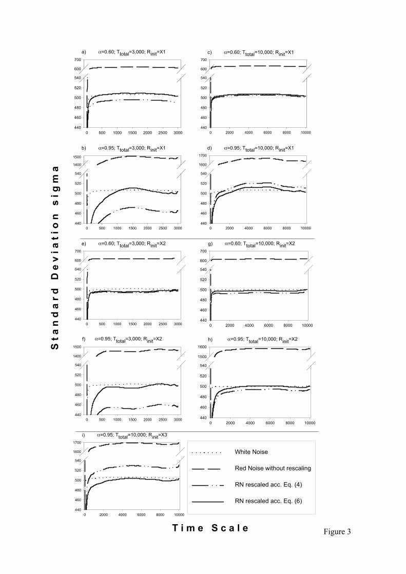
This is demonstrated for example in Fig.3 which reveals that the variances (standard
deviations) of single time series produced by Eq.(4) can be either reduced (Figs.3a,b,f,h) or
elevated (Figs.3d,i) depending on the underlying random number series. Similar results 245
appear in the alternative scaling scheme for small but fixed sample lengths (Eq.5) as
evidenced in Fig.4 In summary, for large α the actual variance of single time series scatters
largely around the expected variance.
To explore this case more systematically in Fig.2 we generated an entire set of time series, Φi,
by repeated simulations of the un-scaled AR1 process (Eq.2). For each time series, i, a 250
different realisation of random numbers was used and we calculated the actual standard
deviation σi(T,α). The ensemble average <σi> then gives an estimate for the expected variance
(Fig.2a, b). In contrast, the standard deviation of the variances in the ensemble of time series,
std(σi), is a measure for the variability of the actual variance (Fig.2c,d).
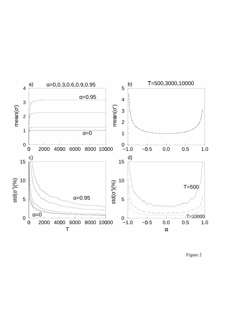
In agreement with earlier studies we found that the expected variance <σi> increases with the 255
absolute value of the auto-correlation parameter α (Fig.2a, b). However, our simulations
reveal a surprising variability of the actual variances in the ensemble of time series over the
whole parameter range. This variability decreases with increasing sample length, T (Fig.2c)
but increases dramatically with the absolute value of α (Fig.2d).
If the autocorrelation is small we can rapidly reduce this variability by increasing the length 260
of the time series (Fig.2c: α=0). This confirms with the common wisdom that from single
short time series it is hard or even impossible to draw conclusions on general features. In
contrast, for sufficiently long time series variability essentially plays no role and individual
simulation runs give a valid representation for the whole ensemble. To measure this effect
quantitatively in our simulation runs we determine the critical sample length, Tmin, beyond 265
12
which the variability drops below the significance level and plays no longer a significant role
(Tab.1). For white noise we found a relatively short length of Tmin=200 (p=0.05).
This behaviour, i.e. Tmin, changes totally when the time series are coloured (Tab.1). Most
important, we observe that for strong auto-correlation the variability of variances is
maintained even for much larger sample lengths (Fig.2c: α=0.95). In particular, we find a 270
critical sample length of Tmin=423 if α=0.6 but much larger Tmin=3,900 for α=0.95. This
reveals that, for example with α=0.95, even a large sample of T=3,000 does not exceed
corresponding Tmin and that consequently the variability evidenced in Fig.2c may cause
significantly different variances among time series realisations (p=0.05). Looking from yet
another angle: when the auto-correlation parameter approaches limiting values (α 1; α -1) 275
the variability of variances is dramatically elevated (Fig.2d). To summarize, samples with a
length of several thousand time steps that are representative for white noise must be seen as
insufficient, i.e. too short, to be representative for strong auto-correlation.
Studies on extinction risk typically assess time scales which vary from several decades to
several thousand, but sometimes can reach ten thousand time steps depending on the system, 280
the species and objectives of the study (e.g Shaffer, 1981). Correspondingly, the critical
sample length Tmin can easily reach or exceed time scales of population extinction as found in
our simulations for stronger auto-correlation (Tab.1). This suggests that the variability of
variances can indeed play a role when estimating the risk of extinction for biological
populations in an auto-correlated environment (compare Fig.1). 285
We conclude that the variability of variances, as shown in Fig.2, must be taken into account
when rescaling the variance of auto-correlated time series. Recall that the currently applied
schemes (e.g. Eq.4, 5) rescale the time series according to the expected variance while, at
least for large α, the actual variance of a particular time series may considerably deviate from
this value. As these deviations depend on the explicit random number realisation (Fig.3) they, 290
in principle, cannot be removed by scaling to the expected variance. As a result, even when
using rescaling schemes Eq.(3) and (4), the extinction risk calculated for strong auto-
correlation might be influenced by biases in the variance.
To overcome these problems we suggest to remove random deviations in variances by
rescaling according to the actual variance. In the following we present an alternative method 295
of rescaling the variances of coloured noise which tackles all major problems pointed out
here: (1) dealing with short sample lengths, T, (2) overcoming restriction to the AR1-process
and, (3) taking the variability of the actual variance in repeated simulation runs into account.
13
SCALING TO THE ACTUAL VARIANCE
Below we present a simple but practical method in order to generate coloured time series of a 300
given variance even for large auto-correlation parameters, α. In contrast to the current
practice of coupling the AR1 process (Eq.2) with rescaling β to the expected variance (Eq.4
and 5), we here suggest to scale to the actual variance. This means to run the AR1 process in a
first step without any rescaling and then, in a second, step to readapt the variance to the value
of the original time series of white noise. 305
A very easy and intuitive way of determining the rescaling factor, c, yielding the target
variance is to measure the ratio in variances of the auto-correlated but un-scaled time series
and the original driving white noise
RNT
WNTTcc_
_),(σσ
α =≡ . [Equation 6]
Here, σT_WN is the actual standard deviation of the original white noise time series with 310
sample length T and σT_RN is the actual standard deviation for un-scaled red noise. This yields
the scaling factor c that might be regarded as equivalent to the term square root of (1-α2) in
Eq.(4) and (5). Here, however, the new scaling factor c is applied separately from the
generating AR1-process. Note, that for the unlikely case of c > 1.0 the variance would
increase, while for the expected case of c < 1.0 the variance will decrease during the rescaling 315
process.
When scaling to infinity the variability in variances disappears. Therefore, in the limit when T
approaches ∞, σT_WN and σT_RN turn into their asymptotic variances, σ∞_WN and σ∞_RN,
respectively. This immediately leads to
21lim α−=∞→ cT [Equation 7] 320
which corresponds to the well known result from Eq.(4).
Post AR1–rescaling of environmental parameters can easily be done by multiplying the
distance of each data point from the time series mean by the rescaling factor c and changing
data values accordingly
( )Φ−Φ=Φ tt c** [Equation 8] 325
14
Here, Φt refers to the time series of the AR1-process (Eq.2) before applying any variance
correction, Φ is the actual average of this time series. Finally, *tΦ gives the value for the
new, rescaled time series.
We want to emphasize that in the rescaling process Eq.(6) the variability of the red noise time
series is not totally removed. Only the additional variability, which is artificially caused 330
during the dying scheme, is taken out. In contrast, the “natural” variability of the driving
white noise, i.e. the variability which does not depend on the dying process, is maintained. As
a result when scaling to “infinity”, i.e. very long environmental time series, our method
results in variances which are very close to that desired for white noise (Fig.3). Here under
moderate auto-correlation our method can reproduce the results of Eq.(4) (e.g. Fig.3c,e). 335
However, for large auto-correlation parameters α Eq.(6) leads to variances (standard
deviations) much closer to the desired one (of white noise) than those produced by Eq.(4)
(e.g. Fig.3b,f,h).
15
DISCUSSION
In this study we investigate the extinction risk of populations exposed to temporally 340
correlated fluctuating environments (coloured noise). First, we compare the results for
different types of the process generating environmental noise. We found the subsequent
extinction risk to be biased by the method of variance scaling with most severe impacts
occurring for strongly autocorrelated environments (Fig.1). We then, secondly, discuss the
limitations of commonly used scaling techniques and reveal several problems, in particular 345
the high variability in variances of strongly auto-correlated time series (Fig.2c,d).
Consequentially, we present a new method (Eq.6) that overcomes these problems. Compared
to commonly used methods our approach harbours various advantages as summarized in
Tab.2.
350
Applicability of rescaling to the actual variance
The main advantage of our method (Eq.6) compared to conventional methods (Eq.4, 5) is the
ability to take the variability in variances into account. Hence, our approach enables us to
properly rescale variances in strongly auto-correlated time series. Moreover, like the
specifically designed Eq.5 our new approach (Eq.6) is able to overcome the problems that go 355
together with short sample lengths (Fig.4; compare Heino et al., 2000). In contrast to
conventional methods, Eq.(6) is not attached to a particular noise generating process but is
applied after noise generation. Thus, our method can be applied to any noise type including
ARn-processes and 1/fb-noise. Moreover, it can even be applied to coloured time series where
the underlying process of noise generation remains completely unknown. 360
An additional advantage of our method is that it reproduces white noise variance more
reliably than the methods currently used (Eq. 4 and 5). It meets the initial aim by providing a
way of generating coloured noise not only for slight and moderate, but also for strong auto-
correlation with a given variance. Another advantage of this method is its straightforward
practicality. It is very intuitive to measure a deviation in variance and to correct it 365
accordingly, making our method very easy to grasp.
Our method of variance rescaling was applied to coloured noise generated by an AR1-process.
From a statistical point of view, however, post AR1 rescaling might bear a shortcoming
because the rescaling process depends on the realisation of the random numbers. This implies 370
16
that different noisy time series are essentially generated by an AR1-process (Eq.2) using
different values of β. Thus, one could argue that the stochastic process by which the red noise
time series are generated is not constant. This is somewhat problematic because ad hoc it is
not clear in which way different auto-correlated time series can be compared.
A closely related point of criticism would be that deviations of the actual from the expected 375
variance are subject to stochasticity and thus they should not be removed. Here, the crucial
question is whether the variability of variances must be seen as an artefact of the AR1 process
or if it is inherent to auto-correlation in nature. If the first case is valid this supports our
method, the latter case would speak against its application in population biology. However, on
the current state of knowledge and heading for the aim to investigate the effects of auto-380
correlation while keeping the variance constant we here recommend to rescale according to
the actual rather than the expected variance.
From yet another point of view one might argue that using the actual instead of the expected
variance of the time series, as we do here, is subject of a particular assumption, i.e. the
assumption of a more predictable future. Then, evidently, this assumption leads to different 385
results than the assumptions underlying the existing methods for rescaled variances (Figs.3,
4), as well as for the subsequent extinction risk (Fig.1). Thus, one might argue what the more
reliable assumption is. We here claim that when systematically studying and modifying one
parameter (e.g. auto-correlation) other conditions (e.g. variance) should be kept constant.
Rescaling according to the actual variance, as we suggest, retains the variances of the original 390
driving white noise time series and thus it explicitly gives respect to stochastic variability in
variances as found in white noise (compare Fig.4). Hence, our method of rescaling to the
actual variances provides a simple and consistent way of tackling the problems discussed
here.
If instead re-scaling to the expected variances is used, then our results on the variability of 395
variances point out that for large α individual simulation runs have no meaning. Therefore, an
optimal strategy could be to support the conventional scaling with a very large number of
simulation runs and then to study the statistical properties of the resulting distributions of
noise variances and calculated extinction times. Such an approach is not necessary with our
method. 400
We are aware that the problems claimed for the actual variance of time series also hold for
further “attributes” of time series, such as the mean and levels of auto-correlation, which may
randomly deviate from the expected value for short sample sizes. Accordingly to variances, in
17
this study we preferred the actual to the expected mean value (Eq.8) while the object of
modification, i.e. autocorrelation may be exactly measured in the resulting time series. 405
However, one should also bear in mind that the characterisation of a time series using such
descriptive attributes (e.g. mean, variance, autocorrelation) will always be imperfect. Even the
sum of all known descriptive attributes can never completely describe a time series.
Consequently, one may always find differences in the estimated extinction risk resulting from
different time series with identical (but imperfect) descriptive attributes. 410

18
CONCLUSION
This manuscript contributes to the growing evidence that appropriate generation of coloured
time series is not unproblematic and poses several problems in population ecology and the
assessment of extinction risk. Heino et al. (2000) claimed differences in the impact of noise 415
colour on extinction risk among various studies (e.g. higher extinction risk due to coloured
noise: Mode and Jacobsen, 1987; Foley, 1994; Johst and Wissel, 1997; Roughgarden, 1975;
Wichmann et al., 2003a; b; but lower extinction risk under coloured noise: Roughgarden,
1975; Ripa and Lundberg, 1996) and suggest that the reason can be found in different scaling
practices of the variance of the coloured time series. Other authors stress the importance of 420
density regulation on the results, i.e. whether there is undercompensatory or
overcompensatory density dependence (Petchey et al., 1997; Cuddington and Yodzis, 1999;
Petchey, 2000). It should also be borne in mind that the impact of coloured noise on
extinction risk depends not only on the noise colour itself but also on its relation to the time
scale of population growth (growth rate) of the species considered (Johst and Wissel, 1997). 425
Furthermore, the results may significantly differ when 1/fb noises are used instead of an AR1
process to generate the dyed time series (Cuddington and Yodzis, 1999). Morales (1999)
suggests that the noise effects on population extinction depend on model structure. The latter
point is in particular accordance with the findings of this paper.
The suggestions for scaling the coloured time series made here can help to deal with the 430
problems discussed above. In particular, we present a very simple and consistent procedure to
generate time series with given colour and variance even for strong temporal auto-correlation.
Compared to earlier studies, this method harbours two major advantages: (1) the variability in
variances is reduced, and (2) this method is not restricted to the AR1-process but can be
applied independently of the type of noise generation. While the latter point favours the 435
general applicability of this method the first point enables us to compare the extinction risk
P0(T) of populations experiencing different colours of environmental noise on the basis of the
same variance. Accordingly, we have shown that omitting variability in variances alters the
calculated extinction risk particularly under strongly correlated noise. The method proposed
here may help increase our understanding of the impact of coloured environmental noise on 440
extinction risk.

19
Acknowledgements
We are grateful to Christian Wissel and Kirk A. Moloney for encouraging our work on
coloured environmental noise, to Juergen Groeneveld and Udo Schwarz for helpful
discussions, and to Mikko Heino and Alan M. Hastings for comments on an earlier version of 445
this manuscript. This work was partly funded by the German Academic Exchange Service
(“DAAD Doktorandenstipendium im Rahmen von HSP III”), the German Volkswagen-
Stiftung and the German Ministry of Science (BMBF) in the framework of BIOTA South
Africa (01LC0024).
450
References
Bellows, T. S., 1981. The descriptive properties of some models for density dependence. J. Anim. Ecol. 50, 139-
156.
Chatfield, C., 1984. The analysis of time series. Chapman and Hall, London, New York.
Cuddington, K. M., Yodzis, P., 1999. Black noise and population persistence. Proc. R. Soc. Lond. B 266, 969-455 973.
Foley, P., 1994. Predicting extinction times from environmental stochasticity and carrying capacity. Conserv.
Biol. 8, 124-137.
Goel, N. S., Richter-Dyn, N., 1974. Population growth and extinction. In: Goel, N. S., Richter-Dyn, N.(Eds.),
Stochastic models in biology. Academic Press, New York, pp. 73-91. 460
Grimm, V., Wissel, C., 2004. The intrinsic mean time to extinction: a unifying approach to analyzing persistence
and viability of populations. Oikos 105, 501-511.
Halley, J. M., 1996. Ecology, evolution and 1/f-noise. Trends Ecol. Evol. 11, 33-37.
Halley, J. M., Kunin, V. E., 1999 Extinction risk and the 1/f family of noise models. Theor. Popul. Biol. 56, 215-
230. 465
Heino, M., 1998. Noise colour, synchrony and extinctions in spatially structured populations. Oikos 83, 368-375.
Heino, M., Ripa, J., Kaitala, V., 2000. Extinction risk under coloured environmental noise. Ecography 23, 177-
184.
Johst, K., Wissel, C., 1997. Extinction Risk in a temporally correlated fluctuating environment. Theor. Popul.
Biol. 52, 91-100. 470
Kaitala, V., Lundberg, P., Ripa, J., Ylikarjula, J., 1997a. Red, blue and green: Dyeing population dynamics.
Annales Zoologici Fennici 34, 217-228.
Kaitala, V., Ylikarjula, J., Ranta, E., Lundberg, P., 1997b. Population dynamics and the colour of environmental
noise. Proc. R. Soc. Lond. B 264, 943-948.
20
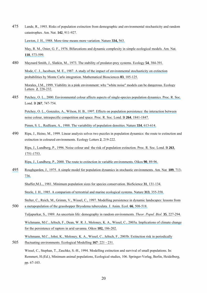
Lande, R., 1993. Risks of population extinction from demographic and environmental stochasticity and random 475 catastrophes. Am. Nat. 142, 911-927.
Lawton, J. H., 1988. More time means more variation. Nature 334, 563.
May, R. M., Oster, G. F., 1976. Bifurcations and dynamic complexity in simple ecological models. Am. Nat.
110, 573-599.
Maynard Smith, J., Slatkin, M., 1973. The stability of predator-prey systems. Ecology 54, 384-391. 480
Mode, C. J., Jacobsen, M. E., 1987. A study of the impact of environmental stochasticity on extinction
probabilities by Monte Carlo integration. Mathematical Biosciences 83, 105-125.
Morales, J.M., 1999. Viability in a pink environment: why "white noise" models can be dangerous. Ecology Letters 2, 228-232.
Petchey, O. L., 2000. Environmental colour affects aspects of single-species population dynamics. Proc. R. Soc. 485 Lond. B 267, 747-754.
Petchey, O. L., Gonzales, A., Wilson, H. B., 1997. Effects on population persistence: the interaction between
noise colour, intraspecific competition and space. Proc. R. Soc. Lond. B 264, 1841-1847.
Pimm, S. L., Redfearn, A., 1988. The variability of population densities. Nature 334, 613-614.
Ripa, J., Heino, M., 1999. Linear analysis solves two puzzles in population dynamics: the route to extinction and 490 extinction in coloured environments. Ecology Letters 2, 219-222.
Ripa, J., Lundberg, P., 1996. Noise colour and the risk of population extinction. Proc. R. Soc. Lond. B 263,
1751-1753.
Ripa, J., Lundberg, P., 2000. The route to extinction in variable environments. Oikos 90, 89-96.
Roughgarden, J., 1975. A simple model for population dynamics in stochastic environments. Am. Nat. 109, 713-495 736.
Shaffer,M.L., 1981. Minimum population sizes for species conservation. BioScience 31, 131-134.
Steele, J. H., 1985. A comparism of terrestrial and marine ecological systems. Nature 313, 355-358.
Stelter, C., Reich, M., Grimm, V., Wissel, C., 1997. Modelling persistence in dynamic landscapes: lessons from
a metapopulation of the grasshopper Bryodema tuberculata. J. Anim. Ecol. 66, 508-518. 500
Tuljapurkar, S., 1989. An uncertain life: demography in random environments. Theor. Popul. Biol. 35, 227-294.
Wichmann, M.C., Jeltsch, F., Dean, W. R. J., Moloney, K. A., Wissel, C., 2003a. Implications of climate change
for the persistence of raptors in arid savanna. Oikos 102, 186-202.
Wichmann, M.C., Johst, K., Moloney, K. A., Wissel, C., Jeltsch, F., 2003b. Extinction risk in periodically
fluctuating environments. Ecological Modelling 167: 221 - 231. 505
Wissel, C., Stephan, T., Zaschke, S.-H., 1994. Modelling extinction and survival of small populations. In:
Remmert, H.(Ed.), Minimum animal populations, Ecological studies, 106. Springer-Verlag, Berlin, Heidelberg,
pp. 67-103.
21
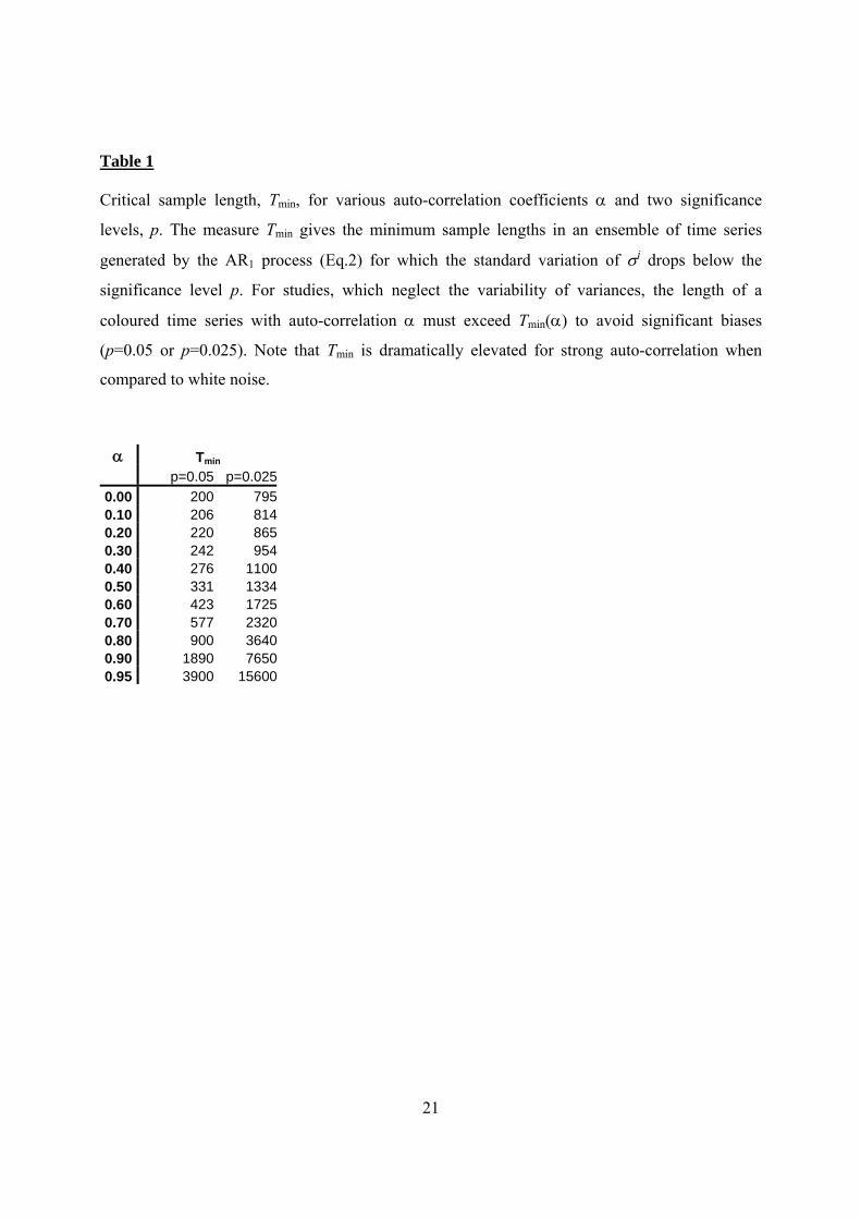
Table 1
Critical sample length, Tmin, for various auto-correlation coefficients α and two significance
levels, p. The measure Tmin gives the minimum sample lengths in an ensemble of time series
generated by the AR1 process (Eq.2) for which the standard variation of σi drops below the
significance level p. For studies, which neglect the variability of variances, the length of a
coloured time series with auto-correlation α must exceed Tmin(α) to avoid significant biases
(p=0.05 or p=0.025). Note that Tmin is dramatically elevated for strong auto-correlation when
compared to white noise.
α Tmin p=0.05 p=0.025
0.00 200 7950.10 206 8140.20 220 8650.30 242 9540.40 276 11000.50 331 13340.60 423 17250.70 577 23200.80 900 36400.90 1890 76500.95 3900 15600
22
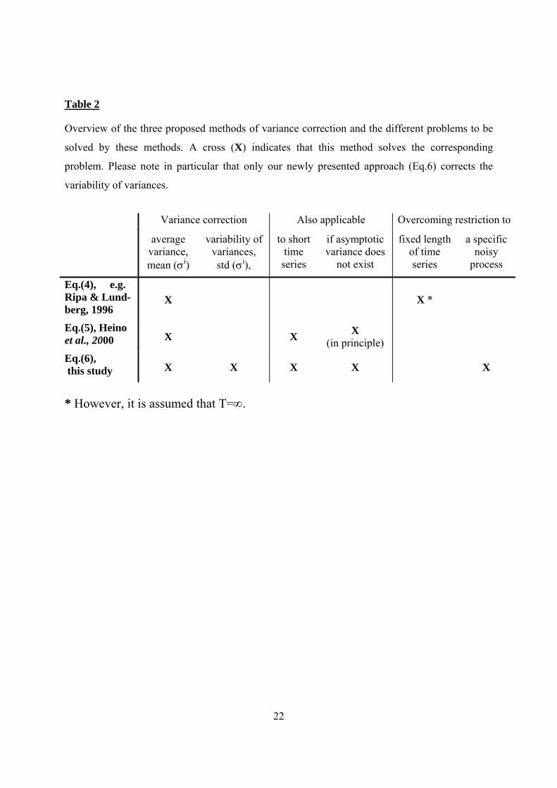
Table 2
Overview of the three proposed methods of variance correction and the different problems to be
solved by these methods. A cross (X) indicates that this method solves the corresponding
problem. Please note in particular that only our newly presented approach (Eq.6) corrects the
variability of variances.
Variance correction Also applicable Overcoming restriction to
average variance, mean (σi)
variability of variances, std (σi),
to short time
series
if asymptotic variance does
not exist
fixed length of time series
a specific noisy
process
Eq.(4), e.g. Ripa & Lund-berg, 1996
X X *
Eq.(5), Heino et al., 2000 X X X
(in principle)
Eq.(6), this study X X X X X
* However, it is assumed that T=∞.
23
Figure Captions
Figure 1:
Extinction risk is plotted versus auto-correlation coefficient α (bottom axis) when coloured noise,
Φt, has been created by various techniques. Extinction risks were assessed on two different time
scales: after 1,000 time steps (a-c) and after 50 time steps (d-f). The results are compared for
different methods of rescaling the variance in dyed time series: the commonly used methods (a,
d) and the method to be introduced in this study (b, e). Additionally, the absolute differences
between the resulting extinction risks of the compared approaches (a-b and d-e, respectively) are
shown (c, f). Various line styles represent varying standard deviation from σ=25 (solid line) to
σ=45 (dotted line).
24
Figure 2:
Variability of the standard deviation σi(T,α) in an ensemble of 200 coloured time series generated
by the AR1 process (Eq.2). Plotted are the ensemble average of the standard deviation, mean(σi)
(top), and the standard deviation of σi in percentage of the ensemble mean, std(σi) (bottom), in
dependence on the time series length T (left) and auto-correlation parameter α (right). No
additional scaling has been performed. Note, that there is a high variability in variances for large
auto-correlation parameters (d) which maintains when applying Eq.(4) or Eq.(5) but is eliminated
by Eq.(6).
25
Figure 3:
Standard deviation σ (left axis) of time series created by various techniques versus the length of
time series fragments (bottom axis). We took a time series of constant length (Ttotal=3,000, left,
and 10,000, right). In order to calculate σ we average over all samples of fragments of smaller
lengths T. The number of realisations yielding <σ> for a given T is Ttotal-T+1. Accordingly, on
right plots σ is averaged over a larger number of samples when compared to the same time scale
value on left plots. The underlying assumption is to use time series fragments drawn randomly
from a long time series to perform repeats in the simulation of extinction risk (by contrast see
Fig.4). The standard deviations σ of coloured noise are shown without scaling (dashed line),
scaling according to Eq.(4) (dash/double-dot line) and scaling according to Eq.(6) (solid line).
The standard deviation of white noise is given as a reference (dotted line). Plots are shown for
two different random number initialisations (Rinit=X1: a–d and Rinit=X2: e–h) and for two different
time series lengths (Ttotal=3,000: a, b, e, f and Ttotal=10,000: c, d, g, h). The auto-correlation
parameters are α = 0.60 (a, c, e, g) and α = 0.95 (b, d, f, h). Additionally, a third random number
initialisation (Rinit=X3: i) is shown for α = 0.95 and 10,000 time steps that produces variances
larger than white noise variance.
26
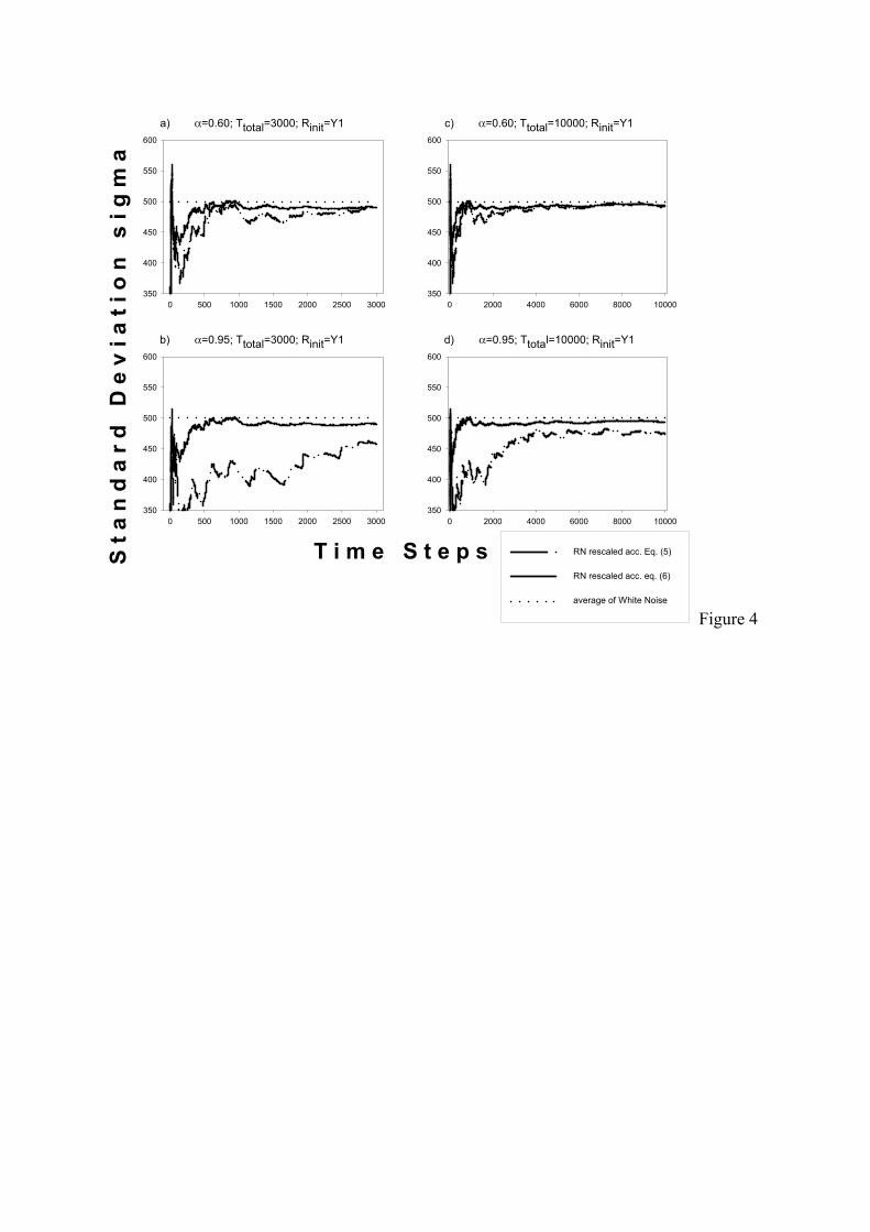
Figure 4:
Standard deviation σ (left axis) of time series created by various techniques versus the length of a
particular time series (bottom axis). Note that in contrast to Fig.3, σ is calculated from just one
particular time series fragment (from time step 1 to time step left axis value) yielding the
fluctuations in the plot, i.e. only one realisation, here. Therefore, left and right plots show
identical data but the left plot gives a smaller scale on bottom axis. The standard deviations of
coloured noise are shown for scaling according to Eq.(5) (dash/double dot line) and scaling
according to Eq.(6) (solid line), the latter yielding exactly the same curve as desired (e.g. white
noise (T)). Additionally, the asymptotic standard deviation of white noise is given as a further
reference (dotted line). Like in Fig.3, two different maximum lengths of the time series (3,000: a,
b and 10,000: c, d) and two degrees of auto-correlation (α = 0.60: a, c, and α = 0.95: b, d) are
shown while random number initialisation remains constant (Rinit=Y1).

Rescaled acc. eq. (4)
0.0 0.2 0.4 0.6 0.8 1.0Extin
ctio
n ris
k in
100
0 ge
nera
tions
0.0
0.2
0.4
0.6
0.8
1.0
sigma 25 sigma 30 sigma 35 sigma 40 sigma 45
Rescaled acc. eq. (6)
0.0 0.2 0.4 0.6 0.8 1.00.0
0.2
0.4
0.6
0.8
1.0
Difference between a) and b)
0.0 0.2 0.4 0.6 0.8 1.0-0.3
-0.2
-0.1
0.0
0.1
0.2
0.3
Rescaled acc. eq. (5)
0.0 0.2 0.4 0.6 0.8 1.0Extin
ctio
n ris
k in
50
gene
ratio
ns
0.0
0.2
0.4
0.6
Rescaled acc. eq. (6)
auto-correlation coefficient
0.0 0.2 0.4 0.6 0.8 1.00.0
0.2
0.4
0.6
Difference between d) and e)
0.0 0.2 0.4 0.6 0.8 1.0-0.3
-0.2
-0.1
0.0
0.1
0.2
0.3
a) b) c)
d) e) f)
Figure 1
(this study)
(Heino et al., 2000)
(e.g. Ripa & Lundberg, 1996)
(this study)
0�
2000 4000�
6000 8000 10000� 0
1
2
3
4
mea
n(�
σi)
0�
2000 4000�
6000 8000 10000�
T
0
5
10
15
std(
σ i )(%
)
−1.0 −0.5�
0.0 0.5 1.0 0
1
2
3
4
5
mea
n(�σi )
−1.0 −0.5�
0.0 0.5 1.0α�
0
5
10
15
std(
σ i (%)
�
α=0,0.3,0.6,0.9,0.95 T=500,3000,10000�
a) b)
c) d)
α=0.95
α=0
α=0.95
α=0
Figure 2
T=10000
T=500
a) α=0.60; Ttotal=3,000; Rinit=X1
0 500 1000 1500 2000 2500 3000
S t a
n d
a r
d D
e v
i a
t i o
n
s i g
m a
440
460
480
500
520
540
600
700
b) α=0.95; Ttotal=3,000; Rinit=X1
0 500 1000 1500 2000 2500 3000440
460
480
500
520
540
1400
1500
c) α=0.60; Ttotal=10,000; Rinit=X1
0 2000 4000 6000 8000 10000440
460
480
500
520
540
600
700
d) α=0.95; Ttotal=10,000; Rinit=X1
0 2000 4000 6000 8000 10000440
460
480
500
520
540
1600
1700
e) α=0.60; Ttotal=3,000; Rinit=X2
0 500 1000 1500 2000 2500 3000440
460
480
500
520
540
600
700
f) α=0.95; Ttotal=3,000; Rinit=X2
0 500 1000 1500 2000 2500 3000440
460
480
500
520
540
1400
1500
g) α=0.60; Ttotal=10,000; Rinit=X2
0 2000 4000 6000 8000 10000440
460
480
500
520
540
600
700
h) α=0.95; Ttotal=10,000; Rinit=X2
0 2000 4000 6000 8000 10000440
460
480
500
520
540
1500
1600
i) α=0.95; Ttotal=10,000; Rinit=X3
T i m e S c a l e0 2000 4000 6000 8000 10000
440
460
480
500
520
540
1600
1700
White Noise
Red Noise without rescaling
RN rescaled acc. Eq. (4)
RN rescaled acc. Eq. (6)
Figure 3
a) α=0.60; Ttotal=3000; Rinit=Y1
0 500 1000 1500 2000 2500 3000
S t a
n d
a r
d D
e v
i a
t i o
n
s i g
m a
350
400
450
500
550
600
b) α=0.95; Ttotal=3000; Rinit=Y1
0 500 1000 1500 2000 2500 3000350
400
450
500
550
600
c) α=0.60; Ttotal=10000; Rinit=Y1
0 2000 4000 6000 8000 10000350
400
450
500
550
600
d) α=0.95; Ttotal=10000; Rinit=Y1
T i m e S t e p s0 2000 4000 6000 8000 10000
350
400
450
500
550
600
RN rescaled acc. Eq. (5)
RN rescaled acc. eq. (6)
average of White Noise
Figure 4