Jackknife Estimation of Sampling Variance of Ratio Estimators in Complex Samples: Bias and the Coefficient of Variation

June 2006 RR-06-19

ResearchReport

Andreas Oranje

Research & Development

Jackknife Estimation of Sampling Variance of Ratio Estimators in Complex Samples:

Bias and the Coefficient of Variation

Andreas Oranje

ETS, Princeton, NJ

June 2006

As part of its educational and social mission and in fulfilling the organization's nonprofit charter

and bylaws, ETS has and continues to learn from and also to lead research that furthers

educational and measurement research to advance quality and equity in education and assessment

for all users of the organization's products and services.

ETS Research Reports provide preliminary and limited dissemination of ETS research prior to

publication. To obtain a PDF or a print copy of a report, please visit:

http://www.ets.org/research/contact.html

Copyright © 2006 by Educational Testing Service. All rights reserved.

ETS and the ETS logo are registered trademarks of Educational Testing Service (ETS).

Abstract

A multitude of methods has been proposed to estimate the sampling variance of ratio estimates in

complex samples (Wolter, 1985). Hansen and Tepping (1985) studied some of those variance

estimators and found that a high coefficient of variation (CV) of the denominator of a ratio

estimate is indicative of a biased estimate of the standard error of a ratio estimate. Using the

same populations, Kovar (1985) and Kovar, Rao, and Wu (1988) repeated the research and

showed that the relation between a high CV and bias in standard errors is weak. In light of these

conflicting findings, this study uses substantially different populations and design choices taken

from the National Assessment of Educational Progress (NAEP) to further investigate the

relationship between bias, the CV, and the number of strata, which has also been found to be an

indicator of bias (Burke & Rust, 1995). It is found that the CV is a relatively weak indicator of

bias, showing poor power properties. Suggestions are made to improve upon statistical

suppression rules related to the CV and number of replicate strata.

Key words: Complex sample variance estimation, coefficient of variation, jackknife repeated

replication, National Assessment of Educational Progress

i

Acknowledgments

The work reported herein was supported under the Contract Award No. ED-02-CO-0023 from

the National Center for Education Statistics (NCES), within the Institute of Education Sciences

(IES) of the U.S. Department of Education. The NCES project officer is Arnold Goldstein.

The author would like to thank the NAEP Design and Analysis Committee, in particular

Lynne Stokes, Betsy Becker, Johnny Blair, and Tej Pandey for their many helpful comments

about the design and analysis of this study. Also, the author would like to thank Keith Rust of

Westat for his help with the interpretation of the results. Finally, many ETS colleagues have

contributed to this work, in particular Henry Braun on the design and John Donoghue on the

interpretation and presentation of results.

ii

Introduction

The sampling variance of estimators in complex samples can be estimated by several

approaches (Wolter, 1985; Kovar, Ghangurde, Germain, Lee, & Gray, 1985), often classified

into two categories: resampling methods and model-based methods. Resampling methods

include jackknife, bootstrap, and numerous variants thereof (e.g., Efron & Tibshirani, 1993;

Kovar, 1985; Rao & Wu, 1988). These are widely used in population, economic, and educational

surveys, balancing the cost of computer-intensive methods against accuracy. Model-based

methods usually stem from Taylor series approximations in complex samples, although textbook

formulas based on normal and student t approximations for simple random samples fall into this

category as well.

Two decades ago Hansen and Tepping (1985) conducted a simulation study to compare

variance estimates of ratios using one variant of each method listed above and the complex

sampling design of the National Assessment of Educational Progress (NAEP) at that time. They

compared the half jackknife repeated replication (half-JRR) method to a Taylor series

approximation (Woodruff, 1971). M.H. Hansen and B. Tepping (1985) reported two major

findings. First, their Taylor series estimator often over- and underestimated the true variance,

especially compared to their JRR estimator. Second, over- and underestimation occurred most

often and most severely for estimates where the coefficient of variation (CV) of the denominator

was relatively large and, therefore, they concluded. “None of the estimators appear to be useful

for values of the coefficient of variation larger than .2” (p. 3).

A ratio estimate for two observed variables x and y

ˆ yRx

= (1)

is often used for estimating totals or means when an auxiliary variable is available (Cochran, 1977,

p.150). In the case of NAEP and Hansen’s and Tepping’s study (Hansen & Tepping, 1985), a

weighted mean of some proficiency variable z is estimated, which is a ratio estimate, and, in this

case, a Horvitz-Thompson estimator (Cochran, 1977, p. 259). The weights are computed as the

inverse of the probability of a unit being selected into the sample. Hence, a mean,

1

ˆi i

i

ii

w zz

w=∑∑

, (2)

is estimated for i units in the sample with weights w. In NAEP and similar large-scale

assessments such as the Trends in International Mathematics and Science Study (TIMSS) and the

National Adult Assessments of Literacy (NAAL), z is a measure of proficiency computed based

on student responses to cognitive items and conditioned on many background variables such as

gender and race/ethnicity. The values are computed from an imputation model and are

distributed as a mixture of normal distributions. A detailed treatment of this method and model

can be found in Mislevy (1984, 1985). While the imputation model is important in determining

measurement variation, this study will focus solely on sampling variation, which accounts for

around 90% to 95% of the variation in NAEP.

Percent estimates have a similar ratio estimator form as means, using an indicator

function I instead of z to classify units into the subgroup of interest:

ˆi i

i

ii

w Ip

w=∑∑

. (3)

I can indicate a gender or race/ethnicity group, but also whether the average imputed value of a

student is within a defined level of performance. Subsequently, the percentage of students in the

sample who perform at or above a certain level can be computed.

The CV of an observed variable x (Cochran, 1977, p. 162)

( ) ( )22x

Var xCV

x= (4)

or relative standard error provides an upper bound of the relative bias of the ratio estimator. The

CV is equal to the relative bias of the ratio estimator if the correlation between the numerator and

denominator is 1. In most large-scale assessments the correlation between on the one hand the

weights and on the other hand the product of the weights and a proficiency measure z or

indicator function I, is close to zero. Hansen and Tepping (1985) derived the relationship

between the CV and the bias in the standard error of a ratio estimate empirically from two-way

2

plots of the ratio of the variance estimate and the true variance with the CV. In their case, the

true variance was determined by the mean squared error (MSE) from many samples.

Subsequently, histograms were constructed placing the bias in bins for large and small CV.

About 30 populations were used in their study, and the variance across 32 strata as well as the

correlation (.3, .5, and .8) between the numerator and the denominator were manipulated. Their

conclusion was based on the fact that 6 of 12 estimates obtained from sampling from populations

with a CV larger than 20% showed severe bias (up to three times the expected standard error)

while no substantial bias was found for any of the estimates obtained from sampling from

populations with a CV smaller than 20%. The limited number of populations chosen for this

study may have driven this conclusion. Nevertheless, in a large-scale survey such as NAEP,

results with a CV exceeding 20% are suppressed (reports in 2005) or a warning is issued to the

reader (reports before 2005).

Kovar (1985) extended the work of Hansen and Tepping (1985) by including regression

and correlation estimators and adding more variance estimation methods, such as the bootstrap,

while using the same populations. An extension of this work also appeared in Kovar et al.

(1988), where, in addition to samples of size 2 per replicate stratum, samples of size 5 were also

used and, furthermore, nonlinear statistics such as quantiles were included. In both studies

comparable results for the JRR and sample-based Taylor series were found, though a model-

based variant of the Taylor series did perform substantially worse. However, in contrast to

Hansen and Tepping (1985), Kovar et al. (1988, p. 35) limited themselves to cautious statements

about the relationship between the CV and the variance estimation bias, stating that for higher

CVs, differences between methods become more pronounced.

Besides the CV, other characteristics related to the number of primary sampling units

have also been shown to affect the bias of variance estimates. Burke and Rust (1995) show that

the relation of sampling error to sample size is far from monotone and rather unpredictable.

Furthermore, they studied cases where estimates are based on between 2 and 30 primary

sampling units out of 105 in a real data population. They show that at least 6 units are necessary

to be able to make valid inferences using the jackknife procedure. The major obstacle resulting in

a loss of reliability of a variance estimator has to do with to what extent the true degrees of

freedom is close to the number of primary sampling units and how large it is. However,

estimating the degrees of freedom is difficult (see also Johnson & Rust, 1993).

3

Complex samples such as NAEP, TIMSS, or NAAL generally use a stratified multistage

probability sampling design. At the first stage, primary sampling units (PSUs) are sampled

within strata (based on geographic characteristics) with probability relative to size, and schools

are sampled within those geographically determined PSUs, also with probability relative to size.

At the second stage, a simple random sample of students is drawn in each sampled school for the

appropriate ages or grades of the assessment. A distinction is made between certainty and

noncertainty schools: Certainty schools are sampled from a PSU that is included in the sample

with certainty. Noncertainty schools are sampled from a PSU that is sampled from all

noncertainty PSUs on the sampling frame. A PSU becomes a certainty PSU if there are relatively

many schools in the PSU on the sampling frame and, therefore, can be considered an essential

part of the sample.

A general formula for variance estimation in a stratified sample that is sampled with

replacement is (e.g. Cochran, 1977, Theorem 5.3):

22 h

stratified hh h

sV Wn

=∑ (5)

with Wh the weight of stratum h, nh the sample size in each stratum, and sh the standard deviation

in each stratum. In the leave-out-many or half-JRR method, a group of similar units (e.g.,

schools, pair of PSUs) is assigned to a replicate or pseudo stratum r and, subsequently, to one of

two units in the stratum (i.e., a pair) that will each have approximate size nh/2. One unit is

selected at random in each replicate stratum. Then, for one replicate stratum at a time, the student

sampling weights of the selected unit in that replicate stratum are doubled while the weights in

the complement1 unit are set to zero. A ratio estimate is computed for this modified sample and

compared with the original estimate. This is repeated for each replicate stratum, squaring and

then summing the result. Formula (5) then simplifies to

( 2ˆ ˆJackknife r

r

V R= −∑ )R̂ (6)

where is the ratio estimate based on the student sampling weights of replicate stratum r in

which n

ˆrR

h student sampling weights are modified to either 0 or 2 times their original value. This

simplification is possible because an average is taken over all replicates and over all sampling

4

units in the stratum. However, it should be noted that it is assumed that sampling fractions are

deemed negligible (Cochran, 1977, p. 93, Corollary 1). In other words, if the difference in

weights between the members in a pair is substantial, additional bias is introduced. The selection

of a nh/2 sample occurs mostly by assigning PSUs to one of the units of a pair (i.e., a replicate

stratum) based on stratifying characteristics such as median income or state assessment results

where available.

Some practical observations should be made regarding the CV in combination with the

JRR method as described above. First of all, the CV has a maximum of 1. This is easily shown

by the following. Suppose there are R replicate strata, then each replicate estimate of the sample

size contains R-1 strata that are simply added and one stratum where approximately half the units

are doubled and added to the other strata and the other half is discarded. At the extremes, two

situations can occur: Either the units that are doubled have no weight at all, or the units that are

doubled carry all the weight from that stratum. Suppose the total weighted sample size is W+, the

sum of weights in a stratum is denoted Wr, and the stratum of interest is denoted r*, then the

estimated sample size based on that stratum is

**

2r rr r

W W W W++ = +∑ *r (7)

or

**

rr r

W W W+= −∑ r

r⎞⎟

(8)

and, therefore, the difference between the total sample size and the stratum is at most Wr*.

Hence, the numerator of the CV is at the extremes the sum of the squared sum of weights in each

stratum obeying the basic inequality:

22( ) r

R RVar W W W⎛≤ ≤ ⎜

⎝ ⎠∑ ∑ (9)

Therefore, the numerator cannot exceed the denominator in the CV formula. Furthermore, if for

every replicate stratum the students only appear in one of the variance units, equation (9) can be

extended to:

5

2

21 1

rR

rR

W

RW

≤⎛ ⎞⎜ ⎟⎝ ⎠

∑

∑≤ , (10)

denoting the square of the lower and upper bounds of the CV. The left part of this inequality

turns into an equality if . A case where this situation has a substantial

probability of occurring is when there are very few students in a subgroup and those students are

clustered in a few schools. It is expected that in these cases the jackknife estimates are

underestimating the true variation since the replicate strata do not represent the variation in the

sample completely.

, for all ,i jW W i j=

Hansen and Tepping (1985) and Kovar et al. (1988) used 32 replicate strata in their

studies with, predominantly, 2 units per stratum. Although this strategy is sufficient to compare

estimators for the overall mean and total (sample) statistics, two special, partly overlapping

situations often occur where variance estimation might be especially problematic:

1. If the subgroup of interest resides in few strata (e.g., only certain geographical areas).

2. If the subgroup of interest not only occurs in few strata, but is also sparse and clustered

within those strata (e.g., Native Americans in Montana).

Obviously, the design of Hansen and Tepping (1985) needs to be extended to provide an

answer to: For which cases is variance estimation problematic and how can problematic

estimation be detected? Generally, a suppression rule is used for these situations. For example,

NAEP suppresses statistics that are based on students from less than five replicate strata

(Johnson & Rust, 1993; Burke & Rust, 1995).

In the following, characteristics of the current NAEP sampling and analysis design

(Allen, Donoghue, & Schoeps, 2001) are described as an example of a stratified complex sample.

The NAEP population is made up of primary strata (e.g., states) and for every primary stratum a

separate stratified sample is drawn. In each primary stratum, usually 100 or more schools are

sampled with inverse probability relative to size and stratified on several characteristics such as

metropolitan statistical area status and denomination. Subsequently, the sampled schools are

serpentine-ordered based on school location (urban to rural) and minority classifications and

within cells on median household income or achievement scores (from state assessments),

6

assuring that neighboring cells are most similar. Schools are then assigned to one of two possible

variance units in a pair for each of 62 replicate strata following this order. On average, in each

school a random sample of 20 to 25 students is drawn. A distinction is made between certainty

and noncertainty schools: Certainty schools are sampled in the sample if they appear in a

certainty-cluster, usually an area that represents a major part of the students in the primary

stratum and is part of the sample with certainty. All the other schools are noncertainty schools. In

noncertainty schools, schools are assigned to the variance units of the replicate strata as

described above, while in certainty schools students are assigned to the variance units of the

replicate strata. The ordering of students in certainty schools is usually by appearance on the

administration roster, which is essentially by subject assessed and then alphabetical by last name.

Weights for students are computed based on the inverse probability of inclusion in the

sample from the sampling frame and adjusted for nonresponse. Because the total student

population between primary strata can be very different in size, a lot of variation in weights

between schools can also be found between primary strata. In addition, because a simple random

sample is drawn within schools while schools themselves are drawn with probability relative to

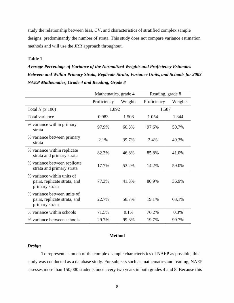
size, most of the variation is between schools and not between students. Table 1 shows the

relative percentages of within and between sums of squares aggregated at several levels of

sampling for the weights and proficiency estimates of the NAEP 2003 mathematics, grade 4 and

reading, grade 8 samples. The table shows that almost all variance of the sampling weights

occurs between schools. About half the variance can be found between states (primary strata),

while the assignment of schools and students to certain replicate strata and units accounts for the

other half. It should be noted, though, that the occurrence of certainty schools and of multiple

schools in one of the units of a pair still results in substantial within-units variance compared to

between-schools variance. For proficiency, most of the variance occurs within schools.

From the description above, it is clear that current NAEP designs are quite different from

the design that Hansen and Tepping (1985) used in their study. Also, it was noted that there are

some conflicting findings in the literature on the relation of bias and the CV and that the number

of strata could be a crucial factor especially when comparing specific student groups. Therefore,

this study has two objectives. The first is to resolve the discrepancies between the findings on the

relation of bias and CV in the studies of Hansen and Tepping, Kovar (1985), and Kovar et al.

(1988) by introducing current NAEP designs, statistics, and data. The second objective is to

7

study the relationship between bias, CV, and characteristics of stratified complex sample

designs, predominantly the number of strata. This study does not compare variance estimation

methods and will use the JRR approach throughout.

Table 1

Average Percentage of Variance of the Normalized Weights and Proficiency Estimates

Between and Within Primary Strata, Replicate Strata, Variance Units, and Schools for 2003

NAEP Mathematics, Grade 4 and Reading, Grade 8

Mathematics, grade 4 Reading, grade 8

Proficiency Weights Proficiency Weights

Total N (x 100) 1,892 1,587 Total variance 0.983 1.508 1.054 1.344

% variance within primary strata 97.9% 60.3% 97.6% 50.7%

% variance between primary strata 2.1% 39.7% 2.4% 49.3%

% variance within replicate strata and primary strata 82.3% 46.8% 85.8% 41.0%

% variance between replicate strata and primary strata 17.7% 53.2% 14.2% 59.0%

% variance within units of pairs, replicate strata, and primary strata

77.3% 41.3% 80.9% 36.9%

% variance between units of pairs, replicate strata, and primary strata

22.7% 58.7% 19.1% 63.1%

% variance within schools 71.5% 0.1% 76.2% 0.3% % variance between schools 29.7% 99.8% 19.7% 99.7%

Method

Design

To represent as much of the complex sample characteristics of NAEP as possible, this

study was conducted as a database study. For subjects such as mathematics and reading, NAEP

assesses more than 150,000 students once every two years in both grades 4 and 8. Because this

8

study is interested in relatively small sample sizes, the full NAEP samples can serve as the

population and small samples can be drawn from this database. In this study two populations

have been used: 2003 NAEP reading, grade 8 and 2003 NAEP mathematics, grade 4.

First, stratified samples were drawn, based on 62 replicate strata and 2 variance units per

stratum as assigned originally in NAEP. Five sample sizes were created drawing 1 through 5

students from each variance unit from each replicate stratum. Therefore, the total number of

students in each sample was at a minimum of 124 (62 x 2 x 1) and at a maximum of 620 (62 x 2

x 5). Although this represents at most .4% of the population, samples were drawn with

replacement to further ensure relative independence between samples. Furthermore, 100 samples

were drawn to compute the average bias, and 100 repetitions were conducted to study the

distribution of bias. Therefore, in total 10,000 samples were drawn for each subject. Definitions

of bias and stability will be given in the following sections.

Besides overall estimates of student group means and sample size totals, specific cases of

clustering are studied. In NAEP, small race/ethnicity groups, such as Native Americans/Alaskan

Natives, are often clustered in only a few schools. A race/ethnicity by gender table is created for

each sample and average score and totals estimates are computed for each of the cells. The

race/ethnicity variable in this study has the following categories: White, Black, Hispanic,

Asian/Pacific Islander, Native American/Alaskan Native, and Other.

Clustering

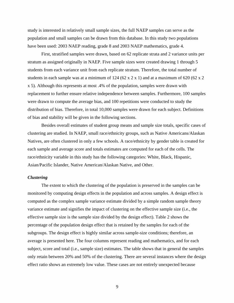
The extent to which the clustering of the population is preserved in the samples can be

monitored by computing design effects in the population and across samples. A design effect is

computed as the complex sample variance estimate divided by a simple random sample theory

variance estimate and signifies the impact of clustering on the effective sample size (i.e., the

effective sample size is the sample size divided by the design effect). Table 2 shows the

percentage of the population design effect that is retained by the samples for each of the

subgroups. The design effect is highly similar across sample-size conditions; therefore, an

average is presented here. The four columns represent reading and mathematics, and for each

subject, score and total (i.e., sample size) estimates. The table shows that in general the samples

only retain between 20% and 50% of the clustering. There are several instances where the design

effect ratio shows an extremely low value. These cases are not entirely unexpected because

9

variance estimation based on few replicates is notoriously problematic (Burke & Rust, 1995).

Therefore, erratic percentages can be attributed to poor estimation rather than poor sampling.

Table 2

Percentage of Population Design Effects Retained by the Samples in the Study for Reading

and Mathematics and for Scale Score and Total Estimates

Reading Mathematics Score Total Score Total

White 48% 38% 55% 24% Black 51% 29% 56% 23% Hispanic 65% 45% 82% 25% Asian 32% 30% 32% 26% Native American 17% 33% 8% 11%

Male

Other 42% 17% 41% 46%

White 43% 40% 71% 24% Black 49% 27% 46% 22% Hispanic 72% 41% 61% 30% Asian 28% 37% 53% 37% Native American 16% 33% 40% 20%

Female

Other 25% 50% 41% 49%

Variation

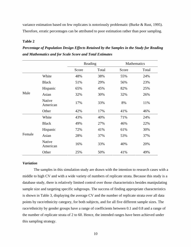
The samples in this simulation study are drawn with the intention to research cases with a

middle to high CV and with a wide variety of numbers of replicate strata. Because this study is a

database study, there is relatively limited control over those characteristics besides manipulating

sample size and targeting specific subgroups. The success of finding appropriate characteristics

is shown in Table 3, displaying the average CV and the number of replicate strata over all data

points by race/ethnicity category, for both subjects, and for all five different sample sizes. The

race/ethnicity by gender groups have a range of coefficients between 0.1 and 0.8 and a range of

the number of replicate strata of 2 to 60. Hence, the intended ranges have been achieved under

this sampling strategy.

10

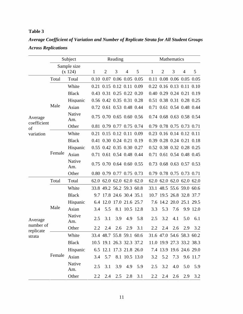
Table 3

Average Coefficient of Variation and Number of Replicate Strata for All Student Groups

Across Replications

Subject Reading Mathematics

Sample size

(x 124) 1 2 3 4 5 1 2 3 4 5 Total Total 0.10 0.07 0.06 0.05 0.05 0.11 0.08 0.06 0.05 0.05

White 0.21 0.15 0.12 0.11 0.09 0.22 0.16 0.13 0.11 0.10Black 0.43 0.31 0.25 0.22 0.20 0.40 0.29 0.24 0.21 0.19Hispanic 0.56 0.42 0.35 0.31 0.28 0.51 0.38 0.31 0.28 0.25Asian 0.72 0.61 0.53 0.48 0.44 0.71 0.61 0.54 0.48 0.44Native Am. 0.75 0.70 0.65 0.60 0.56 0.74 0.68 0.63 0.58 0.54

Male

Other 0.81 0.79 0.77 0.75 0.74 0.79 0.78 0.75 0.73 0.71White 0.21 0.15 0.12 0.11 0.09 0.23 0.16 0.14 0.12 0.11Black 0.41 0.30 0.24 0.21 0.19 0.39 0.28 0.24 0.21 0.18Hispanic 0.55 0.42 0.35 0.30 0.27 0.52 0.38 0.32 0.28 0.25Asian 0.71 0.61 0.54 0.48 0.44 0.71 0.61 0.54 0.48 0.45Native Am. 0.75 0.70 0.64 0.60 0.55 0.73 0.68 0.63 0.57 0.53

Average coefficient of variation

Female

Other 0.80 0.79 0.77 0.75 0.73 0.79 0.78 0.75 0.73 0.71Total Total 62.0 62.0 62.0 62.0 62.0 62.0 62.0 62.0 62.0 62.0

White 33.8 49.2 56.2 59.3 60.8 33.1 48.5 55.6 59.0 60.6Black 9.7 17.8 24.6 30.4 35.1 10.7 19.5 26.8 32.8 37.7Hispanic 6.4 12.0 17.0 21.6 25.7 7.6 14.2 20.0 25.1 29.5Asian 3.4 5.5 8.1 10.5 12.8 3.3 5.3 7.6 9.9 12.0Native Am. 2.5 3.1 3.9 4.9 5.8 2.5 3.2 4.1 5.0 6.1

Male

Other 2.2 2.4 2.6 2.9 3.1 2.2 2.4 2.6 2.9 3.2White 33.4 48.7 55.8 59.1 60.6 31.6 47.0 54.6 58.3 60.2Black 10.5 19.1 26.3 32.3 37.2 11.0 19.9 27.3 33.2 38.3Hispanic 6.5 12.1 17.3 21.8 26.0 7.4 13.9 19.6 24.6 29.0Asian 3.4 5.7 8.1 10.5 13.0 3.2 5.2 7.3 9.6 11.7Native Am. 2.5 3.1 3.9 4.9 5.9 2.5 3.2 4.0 5.0 5.9

Average number of replicate strata

Female

Other 2.2 2.4 2.5 2.8 3.1 2.2 2.4 2.6 2.9 3.2

11

Evaluation

The most desirable characteristic in variance estimators is that they be close to the truth.

Because the simulation design is highly complex, an empirical MSE is computed to represent

truth following the design of Kovar (1985). One thousand samples are drawn under the exact

same conditions as the study samples, and the average squared difference from the expected or

true value is taken,

( )( )1000 2

1

ˆ

1000

ss

R E RMSE =

−=∑

(11)

to be the MSE. The bias as percentage of the MSE is computed for each statistic. Also, an

absolute percentage bias is given to discuss patterns of bias.

In practice, decision rules are enforced based on the CV and the number of replicate

strata, to notify the reader whether an estimate of variation is suspect or not. In this study, the

outcome of these rules can be represented as Type I and Type II error rates, being the probability

of flagging an estimate for a high CV or few replicate strata, while the estimate is unbiased, and

the probability of not flagging an estimate for a high CV or few replicate strata, while the

estimate is biased. In the statistical literature, estimators are usually considered to be biased if

they deviate from the true value by 5% to 10%. For the CV, 5% intervals are used running

between 10% and 100%. Generally, estimates with a CV less than 10% are considered to be of

reasonably low variability, while estimates above 20% are considered severe cases. For the

number of replicate strata, cutpoints from 1 through 60 are used where generally estimates based

on less than 5 strata are considered severe cases. Subsequently, these error rates are shown as

receiver operating curves plotting (1 – Type II) error or power against the Type I error. The idea

is that the further the curve is from the diagonal, the better the power is relative to Type I error.

Availability

The sampling approach in this study does not allow for direct manipulation of the

proportion of each of the race/ethnicity groups in each sample. Therefore, some of the smaller

groups may not always be included and may yield empty cells. Subsequently, not all statistics are

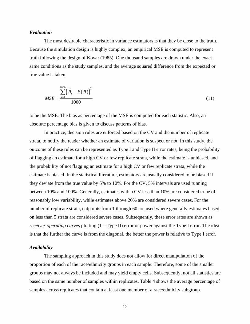
based on the same number of samples within replicates. Table 4 shows the average percentage of

samples across replicates that contain at least one member of a race/ethnicity subgroup.

12

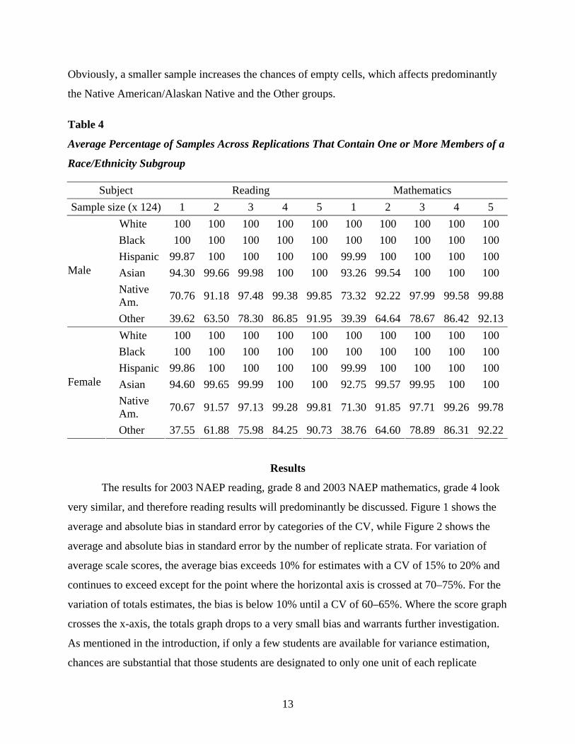
Obviously, a smaller sample increases the chances of empty cells, which affects predominantly

the Native American/Alaskan Native and the Other groups.

Table 4

Average Percentage of Samples Across Replications That Contain One or More Members of a

Race/Ethnicity Subgroup

Subject Reading Mathematics Sample size (x 124) 1 2 3 4 5 1 2 3 4 5

White 100 100 100 100 100 100 100 100 100 100 Black 100 100 100 100 100 100 100 100 100 100 Hispanic 99.87 100 100 100 100 99.99 100 100 100 100 Asian 94.30 99.66 99.98 100 100 93.26 99.54 100 100 100 Native Am. 70.76 91.18 97.48 99.38 99.85 73.32 92.22 97.99 99.58 99.88

Male

Other 39.62 63.50 78.30 86.85 91.95 39.39 64.64 78.67 86.42 92.13White 100 100 100 100 100 100 100 100 100 100 Black 100 100 100 100 100 100 100 100 100 100 Hispanic 99.86 100 100 100 100 99.99 100 100 100 100 Asian 94.60 99.65 99.99 100 100 92.75 99.57 99.95 100 100 Native Am. 70.67 91.57 97.13 99.28 99.81 71.30 91.85 97.71 99.26 99.78

Female

Other 37.55 61.88 75.98 84.25 90.73 38.76 64.60 78.89 86.31 92.22

Results

The results for 2003 NAEP reading, grade 8 and 2003 NAEP mathematics, grade 4 look

very similar, and therefore reading results will predominantly be discussed. Figure 1 shows the

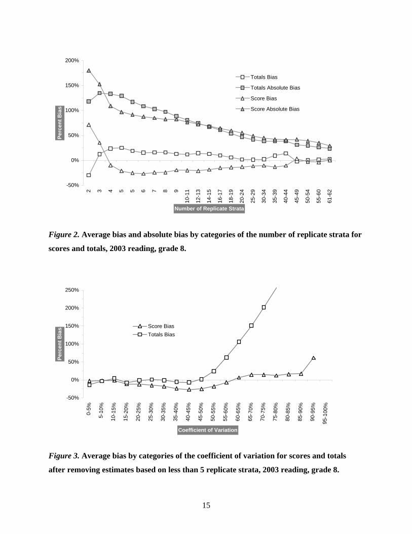
average and absolute bias in standard error by categories of the CV, while Figure 2 shows the

average and absolute bias in standard error by the number of replicate strata. For variation of

average scale scores, the average bias exceeds 10% for estimates with a CV of 15% to 20% and

continues to exceed except for the point where the horizontal axis is crossed at 70–75%. For the

variation of totals estimates, the bias is below 10% until a CV of 60–65%. Where the score graph

crosses the x-axis, the totals graph drops to a very small bias and warrants further investigation.

As mentioned in the introduction, if only a few students are available for variance estimation,

chances are substantial that those students are designated to only one unit of each replicate

13

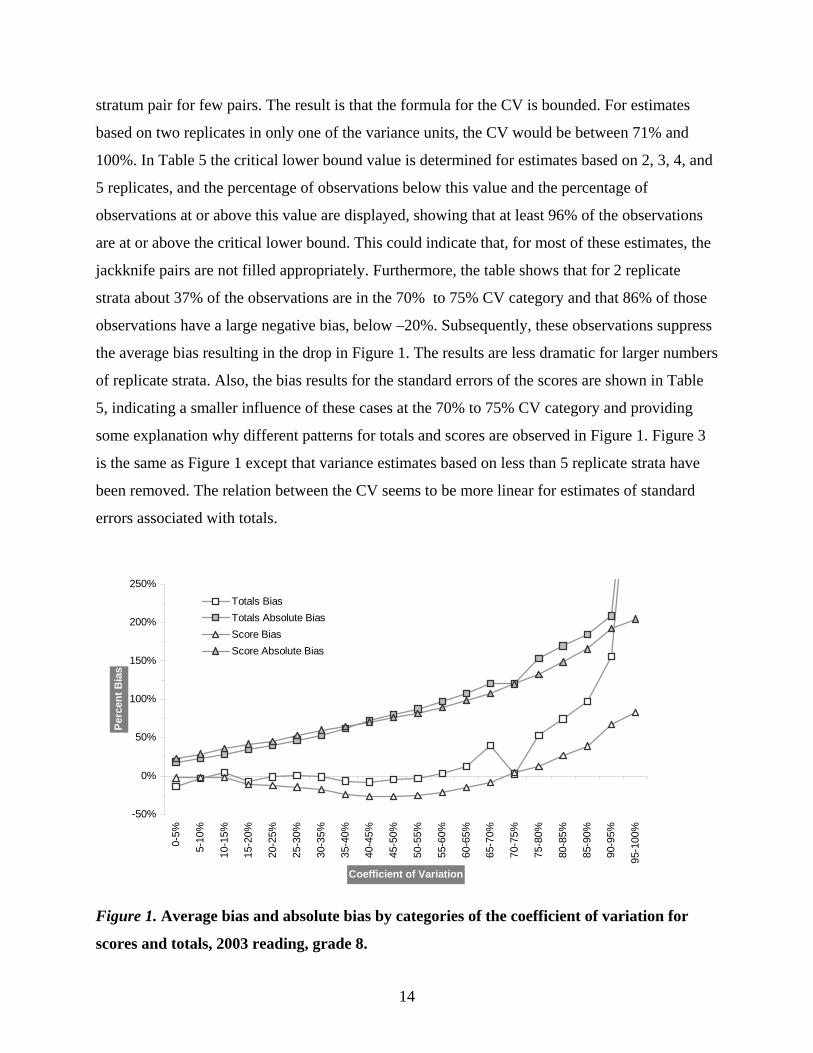
stratum pair for few pairs. The result is that the formula for the CV is bounded. For estimates

based on two replicates in only one of the variance units, the CV would be between 71% and

100%. In Table 5 the critical lower bound value is determined for estimates based on 2, 3, 4, and

5 replicates, and the percentage of observations below this value and the percentage of

observations at or above this value are displayed, showing that at least 96% of the observations

are at or above the critical lower bound. This could indicate that, for most of these estimates, the

jackknife pairs are not filled appropriately. Furthermore, the table shows that for 2 replicate

strata about 37% of the observations are in the 70% to 75% CV category and that 86% of those

observations have a large negative bias, below –20%. Subsequently, these observations suppress

the average bias resulting in the drop in Figure 1. The results are less dramatic for larger numbers

of replicate strata. Also, the bias results for the standard errors of the scores are shown in Table

5, indicating a smaller influence of these cases at the 70% to 75% CV category and providing

some explanation why different patterns for totals and scores are observed in Figure 1. Figure 3

is the same as Figure 1 except that variance estimates based on less than 5 replicate strata have

been removed. The relation between the CV seems to be more linear for estimates of standard

errors associated with totals.

-50%

0%

50%

100%

150%

200%

250%

0-5%

5-10

%

10-1

5%

15-2

0%

20-2

5%

25-3

0%

30-3

5%

35-4

0%

40-4

5%

45-5

0%

50-5

5%

55-6

0%

60-6

5%

65-7

0%

70-7

5%

75-8

0%

80-8

5%

85-9

0%

90-9

5%

95-1

00%

Coefficient of Variation

Perc

ent B

ias

Totals BiasTotals Absolute BiasScore BiasScore Absolute Bias

Figure 1. Average bias and absolute bias by categories of the coefficient of variation for

scores and totals, 2003 reading, grade 8.

14

-50%

0%

50%

100%

150%

200%

2 3 4 5 5 6 7 8 9

10-1

1

12-1

3

14-1

5

16-1

7

18-1

9

20-2

4

25-2

9

30-3

4

35-3

9

40-4

4

45-4

9

50-5

4

55-6

0

61-6

2

Number of Replicate Strata

Perc

ent B

ias

Totals Bias

Totals Absolute Bias

Score Bias

Score Absolute Bias

Figure 2. Average bias and absolute bias by categories of the number of replicate strata for

scores and totals, 2003 reading, grade 8.

-50%

0%

50%

100%

150%

200%

250%

0-5%

5-10

%

10-1

5%

15-2

0%

20-2

5%

25-3

0%

30-3

5%

35-4

0%

40-4

5%

45-5

0%

50-5

5%

55-6

0%

60-6

5%

65-7

0%

70-7

5%

75-8

0%

80-8

5%

85-9

0%

90-9

5%

95-1

00%

Coefficient of Variation

Perc

ent B

ias Score Bias

Totals Bias

Figure 3. Average bias by categories of the coefficient of variation for scores and totals

after removing estimates based on less than 5 replicate strata, 2003 reading, grade 8.

15

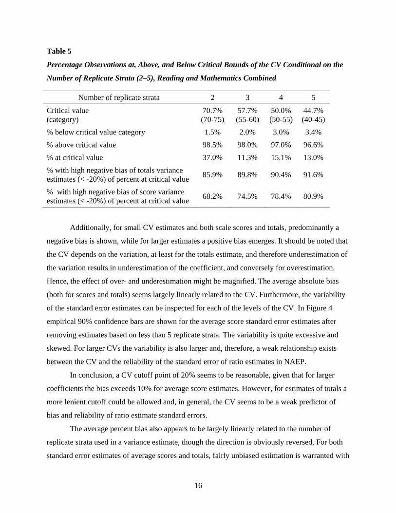
Table 5

Percentage Observations at, Above, and Below Critical Bounds of the CV Conditional on the

Number of Replicate Strata (2–5), Reading and Mathematics Combined

Number of replicate strata 2 3 4 5

Critical value (category)

70.7% (70-75)

57.7% (55-60)

50.0% (50-55)

44.7% (40-45)

% below critical value category 1.5% 2.0% 3.0% 3.4% % above critical value 98.5% 98.0% 97.0% 96.6% % at critical value 37.0% 11.3% 15.1% 13.0% % with high negative bias of totals variance estimates (< -20%) of percent at critical value 85.9% 89.8% 90.4% 91.6%

% with high negative bias of score variance estimates (< -20%) of percent at critical value 68.2% 74.5% 78.4% 80.9%

Additionally, for small CV estimates and both scale scores and totals, predominantly a

negative bias is shown, while for larger estimates a positive bias emerges. It should be noted that

the CV depends on the variation, at least for the totals estimate, and therefore underestimation of

the variation results in underestimation of the coefficient, and conversely for overestimation.

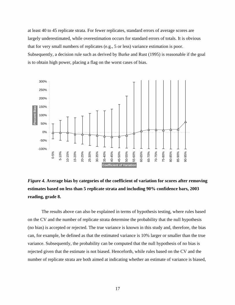
Hence, the effect of over- and underestimation might be magnified. The average absolute bias

(both for scores and totals) seems largely linearly related to the CV. Furthermore, the variability

of the standard error estimates can be inspected for each of the levels of the CV. In Figure 4

empirical 90% confidence bars are shown for the average score standard error estimates after

removing estimates based on less than 5 replicate strata. The variability is quite excessive and

skewed. For larger CVs the variability is also larger and, therefore, a weak relationship exists

between the CV and the reliability of the standard error of ratio estimates in NAEP.

In conclusion, a CV cutoff point of 20% seems to be reasonable, given that for larger

coefficients the bias exceeds 10% for average score estimates. However, for estimates of totals a

more lenient cutoff could be allowed and, in general, the CV seems to be a weak predictor of

bias and reliability of ratio estimate standard errors.

The average percent bias also appears to be largely linearly related to the number of

replicate strata used in a variance estimate, though the direction is obviously reversed. For both

standard error estimates of average scores and totals, fairly unbiased estimation is warranted with

16

at least 40 to 45 replicate strata. For fewer replicates, standard errors of average scores are

largely underestimated, while overestimation occurs for standard errors of totals. It is obvious

that for very small numbers of replicates (e.g., 5 or less) variance estimation is poor.

Subsequently, a decision rule such as derived by Burke and Rust (1995) is reasonable if the goal

is to obtain high power, placing a flag on the worst cases of bias.

-100%

-50%

0%

50%

100%

150%

200%

250%

300%

0-5%

5-10

%

10-1

5%

15-2

0%

20-2

5%

25-3

0%

30-3

5%

35-4

0%

40-4

5%

45-5

0%

50-5

5%

55-6

0%

60-6

5%

65-7

0%

70-7

5%

75-8

0%

80-8

5%

85-9

0%

90-9

5%

Coefficient of Variation

Perc

ent B

ias

Figure 4. Average bias by categories of the coefficient of variation for scores after removing

estimates based on less than 5 replicate strata and including 90% confidence bars, 2003

reading, grade 8.

The results above can also be explained in terms of hypothesis testing, where rules based

on the CV and the number of replicate strata determine the probability that the null hypothesis

(no bias) is accepted or rejected. The true variance is known in this study and, therefore, the bias

can, for example, be defined as that the estimated variance is 10% larger or smaller than the true

variance. Subsequently, the probability can be computed that the null hypothesis of no bias is

rejected given that the estimate is not biased. Henceforth, while rules based on the CV and the

number of replicate strata are both aimed at indicating whether an estimate of variance is biased,

17

both also appear to result in different decisions: The CV rule can be characterized as minimizing

Type I errors, while the number of replicate strata rule maximizes power.

Receiver Operating Characteristic Curve (ROC)

To further explore Type I and II probabilities, receiver operating characteristic curves

(ROCs) were constructed and displayed in Figure 5 for the CV and in Figure 6 for the number of

replicate strata. The focus will be on standard errors of average scale score estimates. Although

the totals estimates ROCs are slightly different from the average scale ROCs, commensurate

with the plots in Figures 1 and 2, the difference in probabilities between the two rules is highly

similar. The results are averaged across mathematics and reading.

0%

10%

20%

30%

40%

50%

60%

70%

80%

90%

100%

0% 10% 20% 30% 40% 50% 60% 70% 80% 90% 100%

Type I error

1- T

ype

II er

ror

50%30%20%10%x=y line

30%

20%

10%

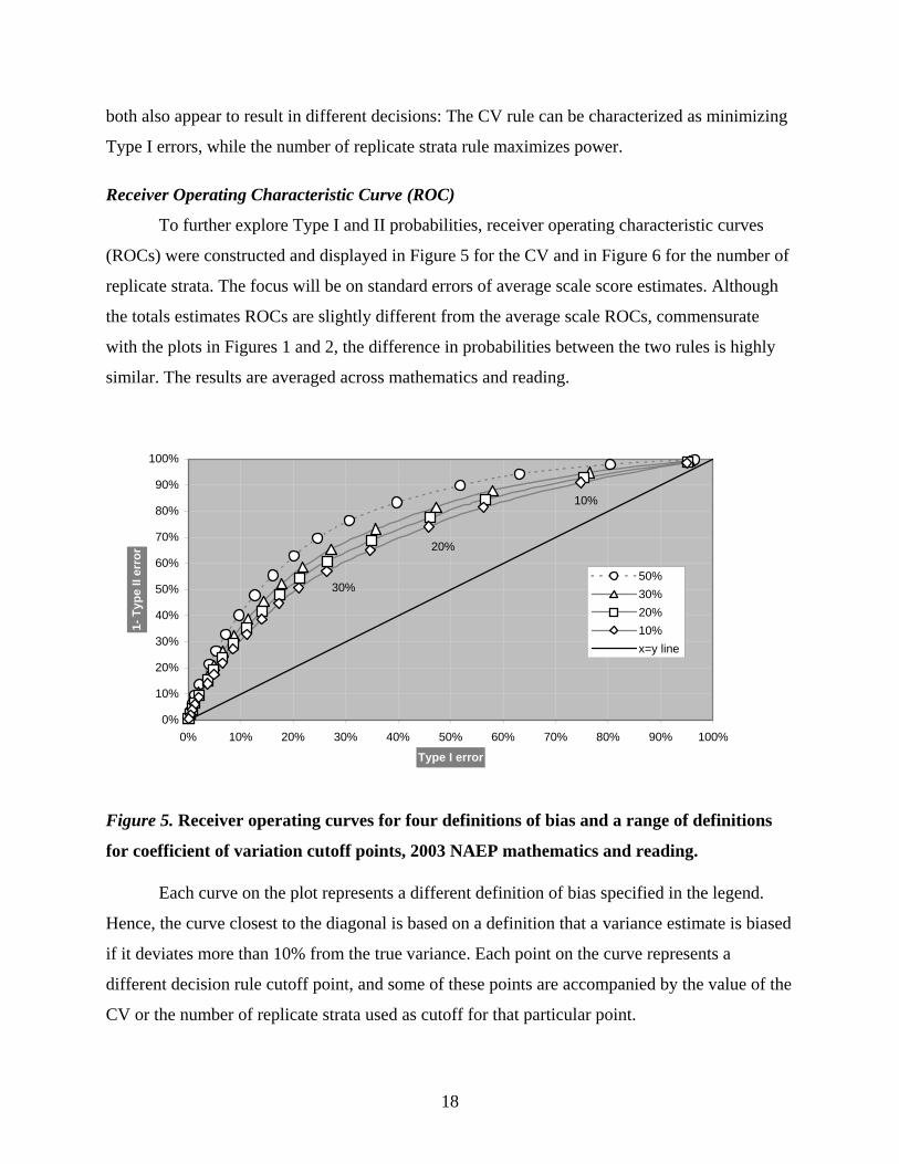
Figure 5. Receiver operating curves for four definitions of bias and a range of definitions

for coefficient of variation cutoff points, 2003 NAEP mathematics and reading.

Each curve on the plot represents a different definition of bias specified in the legend.

Hence, the curve closest to the diagonal is based on a definition that a variance estimate is biased

if it deviates more than 10% from the true variance. Each point on the curve represents a

different decision rule cutoff point, and some of these points are accompanied by the value of the

CV or the number of replicate strata used as cutoff for that particular point.

18

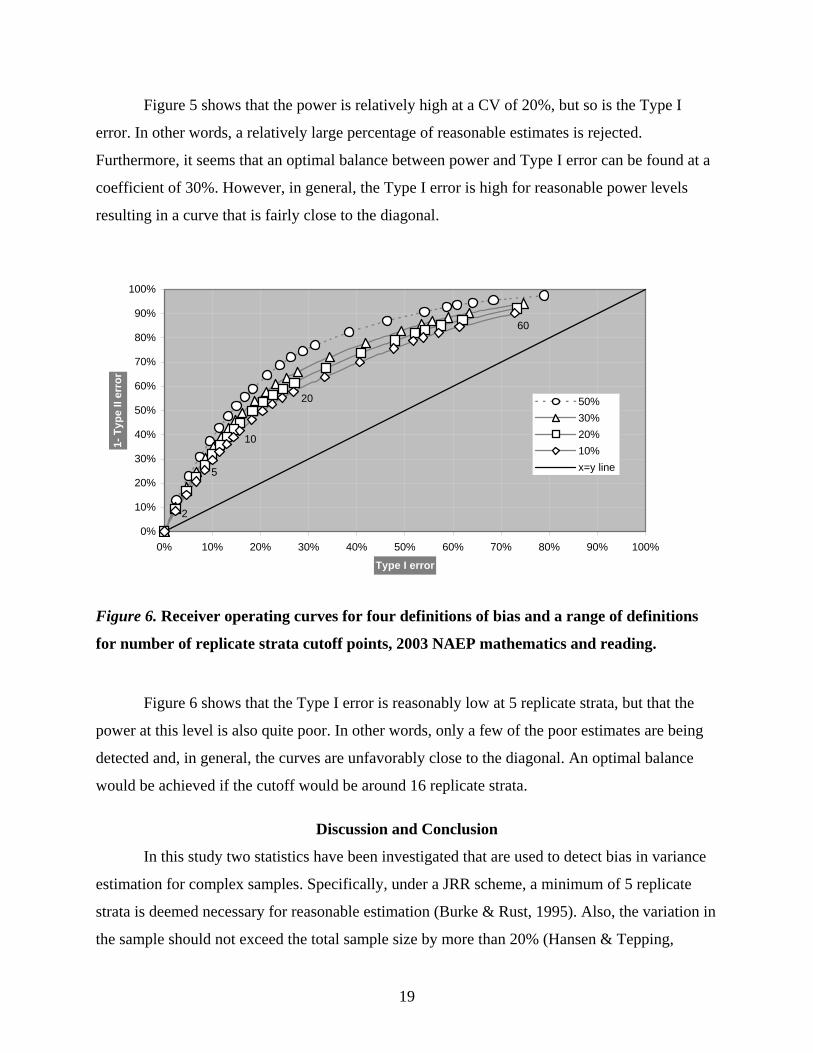
Figure 5 shows that the power is relatively high at a CV of 20%, but so is the Type I

error. In other words, a relatively large percentage of reasonable estimates is rejected.

Furthermore, it seems that an optimal balance between power and Type I error can be found at a

coefficient of 30%. However, in general, the Type I error is high for reasonable power levels

resulting in a curve that is fairly close to the diagonal.

0%

10%

20%

30%

40%

50%

60%

70%

80%

90%

100%

0% 10% 20% 30% 40% 50% 60% 70% 80% 90% 100%

Type I error

1- T

ype

II er

ror

50%30%20%10%x=y line

60

5

2

10

20

Figure 6. Receiver operating curves for four definitions of bias and a range of definitions

for number of replicate strata cutoff points, 2003 NAEP mathematics and reading.

Figure 6 shows that the Type I error is reasonably low at 5 replicate strata, but that the

power at this level is also quite poor. In other words, only a few of the poor estimates are being

detected and, in general, the curves are unfavorably close to the diagonal. An optimal balance

would be achieved if the cutoff would be around 16 replicate strata.

Discussion and Conclusion

In this study two statistics have been investigated that are used to detect bias in variance

estimation for complex samples. Specifically, under a JRR scheme, a minimum of 5 replicate

strata is deemed necessary for reasonable estimation (Burke & Rust, 1995). Also, the variation in

the sample should not exceed the total sample size by more than 20% (Hansen & Tepping,

19

1985). With respect to the latter indicator, some controversy has been documented (e.g., Kovar et

al., 1988) questioning the validity of this rule.

By drawing records from a large-scale assessment database, a quasi-simulation study was

conducted to investigate the relation between bias and the two indicators of bias. The results

show that the rule of 5 is quite liberal and predominantly aimed at removing the worst estimates.

On the other hand, the CV rule is more conservative and predominantly aimed at removing cases

that could be biased, yielding a relatively high power.

While it is in several ways problematic to make strong inferences about how these results

translate to an operational setting, tentative conclusions can be drawn from these results. The

most important one is that it seems that these rules are quite poor predictors of bias. While a 20%

cutoff for the CV appeared reasonable in terms of bias, this cutoff is problematic in terms of

committing Type I errors. The same is true for the number of replicate strata. While 5 seems an

appropriate cutoff for detecting severe bias, this rule is problematic in terms of Type II error.

Hence, it is questionable to what extent these rules are useful. At best, an exorbitantly high CV

may indicate consistently that the reliability of the standard error estimate is jeopardized and a

minimum to the number of replicates may serve as a stopgap measure. It should be noted that the

limited design of this study may present a somewhat biased picture because estimates based on

few replicates were largely limited to very small sample sizes. In sum, the findings show that

these predictors of bias are somewhat weak and, therefore, in practice it remains highly uncertain

whether estimates are biased in relatively small samples.

There is little question that it is important to alert readers about those cases where it is

undeniably clear that the jackknife estimate does not yield appropriate results. It might be fruitful

to defer to an alternative variance estimator in those cases, although the comparisons of Kovar et

al. (1985, 1988) indicate that it is quite likely that alternative estimators will simultaneously do

poorly. One option that is used by the Census Bureau (2002) is to use design effects of relatively

large groups for small groups assuming the clustering is equivalent. The effects would be

multiplied by a simple random sample estimate for groups where a stratified complex sample

estimate is known to be inappropriate. In any case, the conclusion could simply be that the

sample or, in some cases, the population does not allow for these inferences. For cases where it is

uncertain whether the variance estimation is biased, some options could be considered.

20

First and most obvious, a better predictor or combination of predictors should be sought.

Since the degrees of freedom themselves are difficult to accurately determine in a complex

sample, indirect indicators, as the CV is, might still provide the most feasible option to detecting

a low reliability of the standard error estimate. Among others, candidates are those related to the

intraclass correlation and the variability of variance across clusters, schools, or replicates.

Furthermore, a better predictor or combination could be focused on the inference and not so

much on the variance estimate in isolation. The idea is that biased variance estimates could be

permitted if the effect on a t- or z-statistic is relatively small and/or not meaningful in terms of

the results a program publishes.

Finally, this study is solely focused on the statistical properties of jackknife variance

estimates in a large-scale survey setting. However, there are several practical issues and

questions related to these statistical properties that should be considered and explored in

concurrence. First, to what extent are flagging results indicative that the purpose of the survey is

not fulfilled, and is the level of flagging decreasing across time? Second, to what extent should

problematic estimates be removed from the results instead of issuing a warning to the user? How

sample-dependent are these rules? For example, are there special samples where different rules

should be applied?

21

References

Allen, N., Donoghue, J. R., & Schoeps, T. (2001). The NAEP 1998 technical report.

Washington, DC: National Center for Education Statistics.

Burke, J., & Rust, K. (1995, August). On the performance of jackknife variance estimation for

systematic samples with small numbers of primary sampling units. Paper presented at the

Joint Statistical Meetings, Orlando, FL.

Census Bureau. (2002). Design and methodology. Washington, DC: Author.

Cochran, W.G. (1977). Sampling techniques. New York: John Wiley & Sons.

Efron, B., & Tibshirani, R.J. (1993). An introduction to the bootstrap (Monographs on Statistics

and Applied Probability No. 57). Boca Raton, FL: Chapman & Hall.

Hansen, M. H., & Tepping, B. (1985). Note to professor N. J. K. Rao. Unpublished manuscript.

Johnson, E.G., & Rust, K.F. (1993). Effective degrees of freedom for variance estimates

from a complex sample survey. Paper presented at the 1993 annual meeting of the

American Statistical Association, San Francisco.

Kovar, J. (1985). Variance estimation of nonlinear statistics in stratified samples (Working

Paper No. BSMD 85–052E). Ottawa, Canada: Statistics Canada.

Kovar, J., Ghangurde, P., Germain, M.-F., Lee, H., & Gray, G. (1985). Variance estimation in

sample surveys (Working paper No. BSMD 85–49). Ottawa, Canada: Statistics Canada.

Kovar, J.G., Rao, J.N.K., & Wu, C.F.J. (1988). Bootstrap and other methods to measure error in

survey estimates. The Canadian Journal of Statistics, 16, 25–45.

Mislevy, R.J. (1984). Estimating latent distributions. Psychometrika, 49(3), 359–381

Mislevy, R.J. (1985). Estimation of latent group effects. Journal of the American Statistical

Association, 80(392), 993–997.

Rao, J.N.K., & Wu, C.F.J. (1988). Resampling inference with complex survey data. Journal of

the American Statistical Association, 83(401), 231–241.

Wolter, K.M. (1985). Introduction to variance estimation. New York: Springer.

Woodruff, R.S. (1971). A simple method for approximating the variance of a complicated

estimate. Journal of the American Statistical Association, 66(334), 411–414.

22

Note

1 Although a JRR-half is used in this study, a JRR-complement can be computed by doubling

the weights of the observations in the variance units that were not selected in the JRR-half and

setting the weights of the observations that were selected in the JRR-half to zero. Both

estimates have been computed initially and a correlation across all estimates between the CV

greater than 0.999 and a correlation of 0.75 between the bias of the proficiency estimates were

found. Therefore, no further attention has been devoted to the JRR-complement.

23